Embed Size (px)
Citation preview
Measures of Variability
Measures of Variability
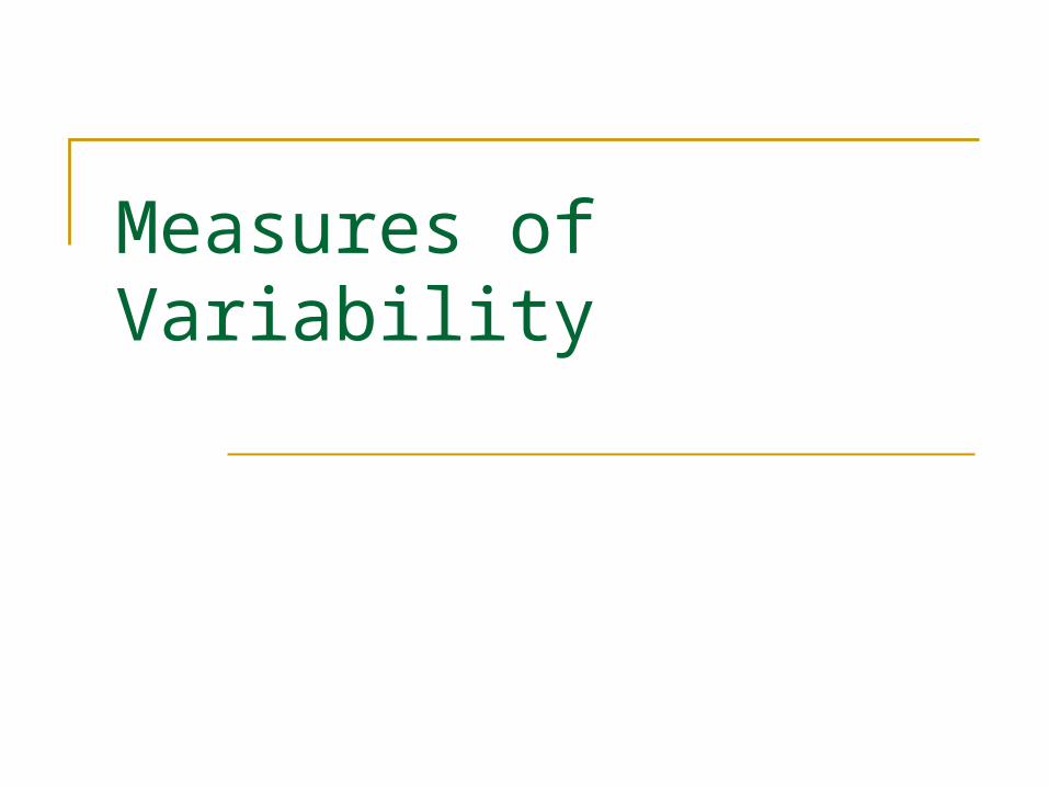
Why are measures of variability important? Why not just stick with the mean? Ratings of attractiveness (out of 10) – Mean = 5
Everyone rated you a 5 (low variability) What could we conclude about attractiveness from this?
People’s ratings fell into a range from 1 – 10, that averaged a 5 (high variability) What could we conclude about attractiveness from this?
Measures of Variability
Measures of Variability Range Interquartile Range Average Deviation Variance Standard Deviation
Measures of Variability
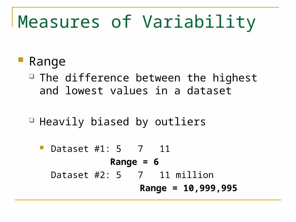
Range The difference between the highest and lowest
values in a dataset
Heavily biased by outliers
Dataset #1: 5 7 11
Range = 6
Dataset #2: 5 7 11 million
Range = 10,999,995
Measures of Variability
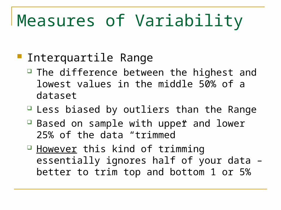
Interquartile Range The difference between the highest and lowest
values in the middle 50% of a dataset Less biased by outliers than the Range Based on sample with upper and lower 25% of the
data “trimmed” However this kind of trimming essentially ignores
half of your data – better to trim top and bottom 1 or 5%
Measures of Variability
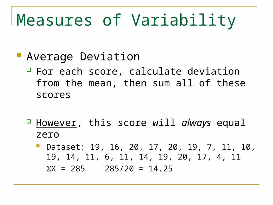
Average Deviation For each score, calculate deviation from the
mean, then sum all of these scores
However, this score will always equal zero Dataset: 19, 16, 20, 17, 20, 19, 7, 11, 10, 19, 14, 11, 6,
11, 14, 19, 20, 17, 4, 11
X = 285 285/20 = 14.25
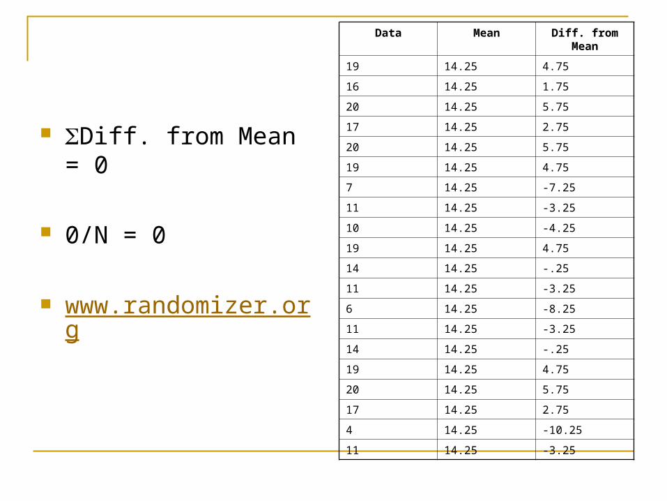
Diff. from Mean = 0
0/N = 0
www.randomizer.org
Data Mean Diff. from Mean
19 14.25 4.75
16 14.25 1.75
20 14.25 5.75
17 14.25 2.75
20 14.25 5.75
19 14.25 4.75
7 14.25 -7.25
11 14.25 -3.25
10 14.25 -4.25
19 14.25 4.75
14 14.25 -.25
11 14.25 -3.25
6 14.25 -8.25
11 14.25 -3.25
14 14.25 -.25
19 14.25 4.75
20 14.25 5.75
17 14.25 2.75
4 14.25 -10.25
11 14.25 -3.25
Measures of Variability
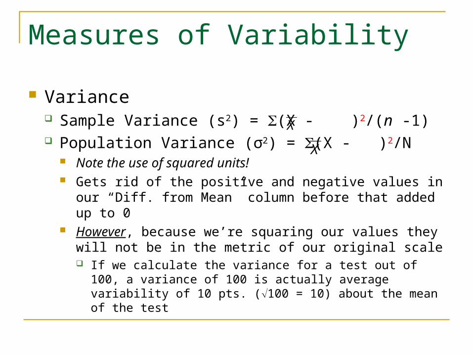
Variance Sample Variance (s2) = (X - )2/(n -1) Population Variance (σ2) = (X - )2/N
Note the use of squared units! Gets rid of the positive and negative values in our “Diff.
from Mean” column before that added up to 0 However, because we’re squaring our values they will
not be in the metric of our original scale If we calculate the variance for a test out of 100, a variance
of 100 is actually average variability of 10 pts. (100 = 10) about the mean of the test
X
X
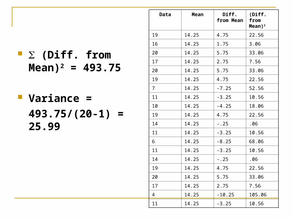
(Diff. from Mean)2 = 493.75
Variance =
493.75/(20-1) = 25.99
Data Mean Diff. from Mean
(Diff. from Mean)2
19 14.25 4.75 22.56
16 14.25 1.75 3.06
20 14.25 5.75 33.06
17 14.25 2.75 7.56
20 14.25 5.75 33.06
19 14.25 4.75 22.56
7 14.25 -7.25 52.56
11 14.25 -3.25 10.56
10 14.25 -4.25 18.06
19 14.25 4.75 22.56
14 14.25 -.25 .06
11 14.25 -3.25 10.56
6 14.25 -8.25 68.06
11 14.25 -3.25 10.56
14 14.25 -.25 .06
19 14.25 4.75 22.56
20 14.25 5.75 33.06
17 14.25 2.75 7.56
4 14.25 -10.25 105.06
11 14.25 -3.25 10.56
Measures of Variability
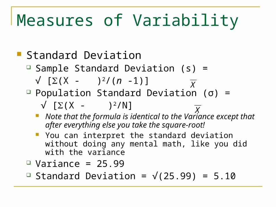
Standard Deviation Sample Standard Deviation (s) =
√ [(X - )2/(n -1)] Population Standard Deviation (σ) =
√ [(X - )2/N] Note that the formula is identical to the Variance except
that after everything else you take the square-root! You can interpret the standard deviation without doing
any mental math, like you did with the variance Variance = 25.99 Standard Deviation = √(25.99) = 5.10
X
X
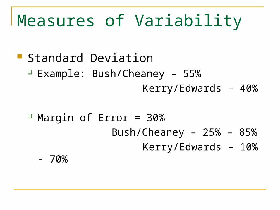
Measures of Variability
Standard Deviation Example: Bush/Cheaney – 55%
Kerry/Edwards – 40%
Margin of Error = 30%
Bush/Cheaney – 25% – 85%
Kerry/Edwards – 10% - 70%
Computational Formula for Variability Definitional Formula
designed more to illustrate how the formula relates to the concept it underlies
Computational Formula identical to the definitional formula, but different in
form allows you to compute your variable with less
effort particularly useful with large datasets
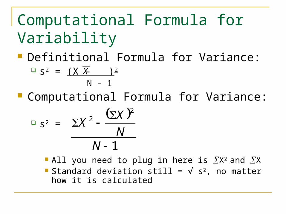
Computational Formula for Variability Definitional Formula for Variance:
s2 = (X – )2
N – 1
Computational Formula for Variance:
s2 =
All you need to plug in here is X2 and X Standard deviation still = √ s2, no matter how it is
calculated
X
1
22
NN
XX
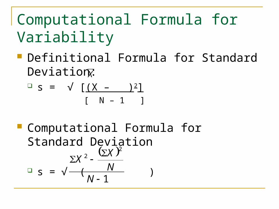
Computational Formula for Variability Definitional Formula for Standard Deviation:
s = √ [(X – )2] [ N – 1 ]
Computational Formula for Standard Deviation
s = √ ( )
X
1
22
NN
XX
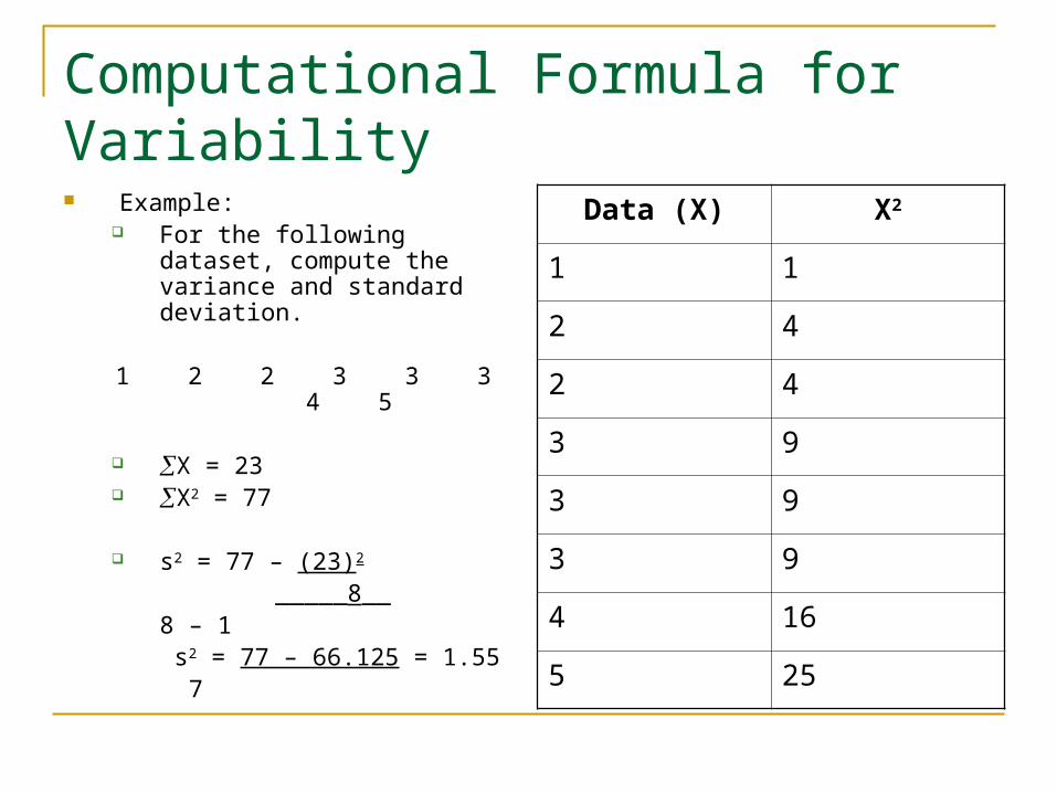
Computational Formula for Variability Example:
For the following dataset, compute the variance and standard deviation.
1 2 2 3 3 3 4 5
X = 23 X2 = 77
s2 = 77 – (23)2
_____8__8 – 1
s2 = 77 – 66.125 = 1.55 7
Data (X) X2
1 1
2 4
2 4
3 9
3 9
3 9
4 16
5 25
Measures of Variability
What do you think will happen to the standard deviation if we add a constant (say 4) to all of our scores?
What if we multiply all the scores by a constant?
Measures of Variability
Characteristics of the Standard Deviation Adding a constant to each score will not alter the
standard deviation i.e. add 3 to all scores in a sample and your s will remain
unchanged Let’s say our scores originally ranged from 1 – 10
Add 5 to all scores, the new data ranges from 6 – 15 In both cases the range is 9
Measures of Variability
However, multiplying or dividing each score by a constant causes the s to be similarly multiplied or divided by that constant (and s2 by the square of the constant) i.e. divide each score by 2 and your s will decrease from
10 to 5 in multiplication, higher numbers increase more than
lower ones do, increasing the distance between the highest and lowest score, which increases the variability i.e. 2 x 5 = 10 – difference of 8 pts.
5 x 5 = 25 – difference of 20 pts.
Measures of Variability
Characteristics of the Standard Deviation Generally, the larger the dataset, the smaller the
range/standard deviation More scores = more clustering in the middle –
REMEMBER: more central scores are more likely to occur
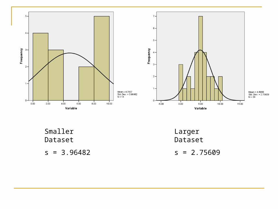
Smaller Dataset
s = 3.96482
Larger Dataset
s = 2.75609

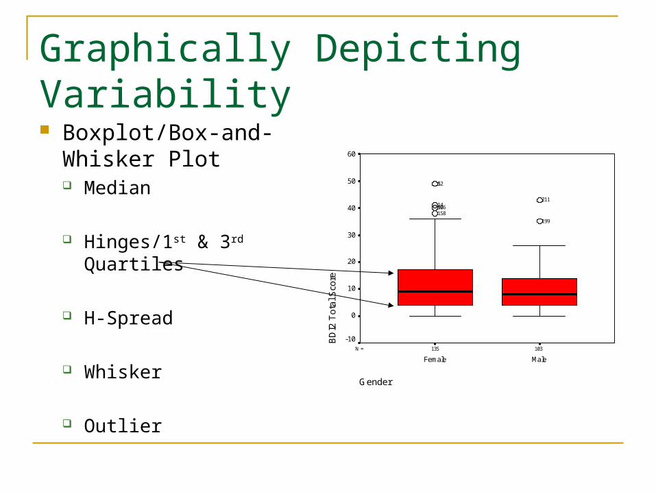
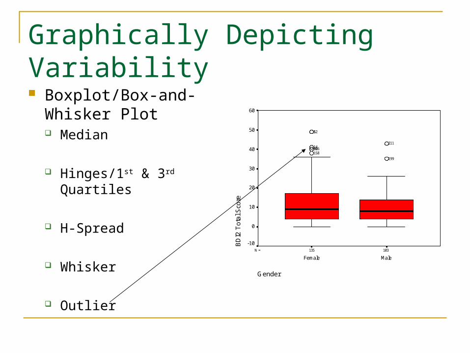
Graphically Depicting Variability Boxplot/Box-and-
Whisker Plot Median
Hinges/1st & 3rd Quartiles
H-Spread
Whisker
Outlier
103135N =
Gender
MaleFemale
BD
I2 T
ota
l Sco
re
60
50
40
30
20
10
0
-10
199
211
1581669214
521
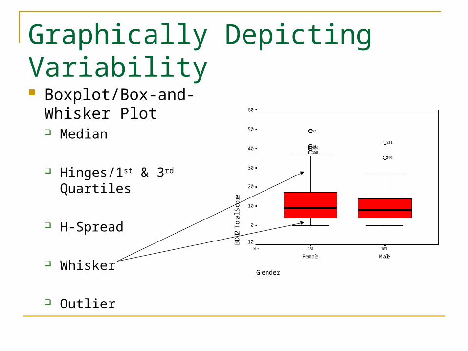
Graphically Depicting Variability Boxplot/Box-and-
Whisker Plot Median
Hinges/1st & 3rd Quartiles
H-Spread
Whisker
Outlier
103135N =
Gender
MaleFemale
BD
I2 T
ota
l Sco
re
60
50
40
30
20
10
0
-10
199
211
1581669214
521

Graphically Depicting Variability Boxplot/Box-and-
Whisker Plot Median
Hinges/1st & 3rd Quartiles
H-Spread
Whisker
Outlier
103135N =
Gender
MaleFemale
BD
I2 T
ota
l Sco
re
60
50
40
30
20
10
0
-10
199
211
1581669214
521
{
Graphically Depicting Variability Boxplot/Box-and-
Whisker Plot Median
Hinges/1st & 3rd Quartiles
H-Spread
Whisker
Outlier
103135N =
Gender
MaleFemale
BD
I2 T
ota
l Sco
re
60
50
40
30
20
10
0
-10
199
211
1581669214
521
Graphically Depicting Variability Boxplot/Box-and-
Whisker Plot Median
Hinges/1st & 3rd Quartiles
H-Spread
Whisker
Outlier
103135N =
Gender
MaleFemale
BD
I2 T
ota
l Sco
re
60
50
40
30
20
10
0
-10
199
211
1581669214
521
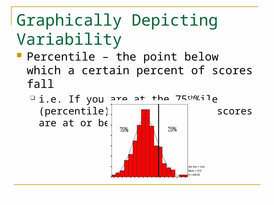
Graphically Depicting Variability Percentile – the point below which a certain
percent of scores fall i.e. If you are at the 75th%ile (percentile), then
75% of the scores are at or below your score
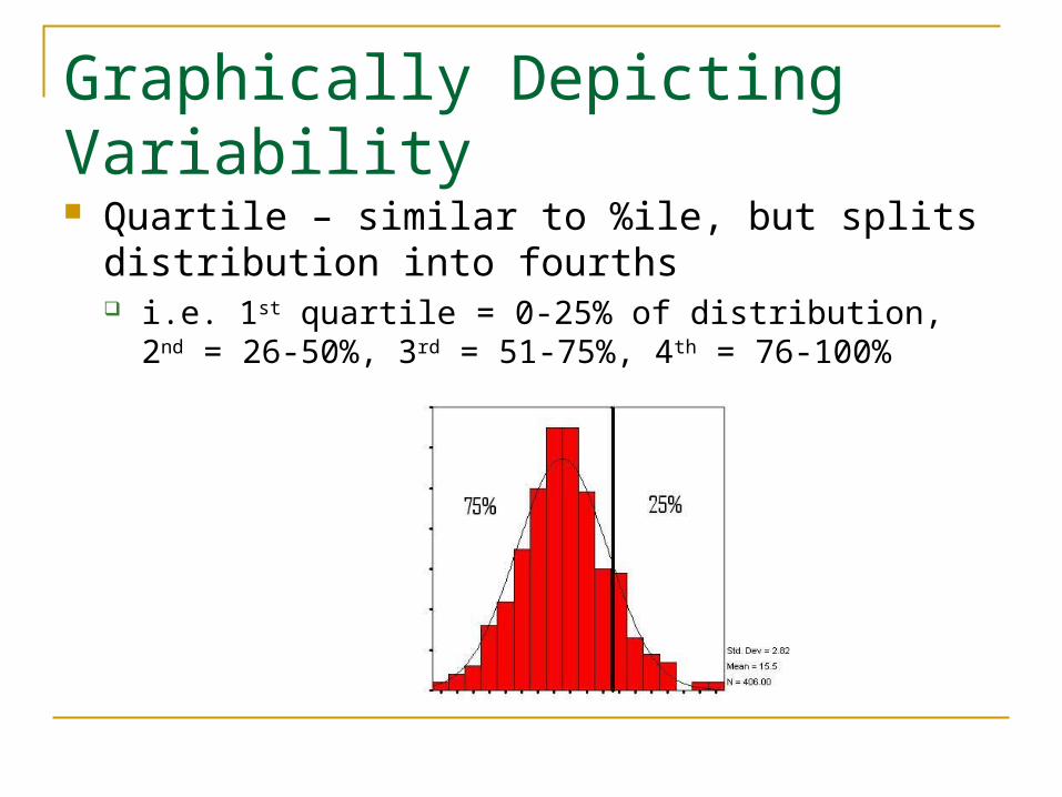
Graphically Depicting Variability Quartile – similar to %ile, but splits distribution into
fourths i.e. 1st quartile = 0-25% of distribution, 2nd = 26-50%, 3rd =
51-75%, 4th = 76-100%
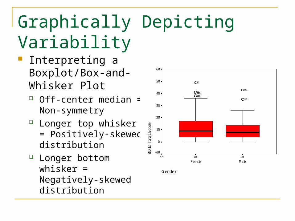
Graphically Depicting Variability Interpreting a
Boxplot/Box-and-Whisker Plot Off-center median = Non-
symmetry Longer top whisker =
Positively-skewed distribution
Longer bottom whisker = Negatively-skewed distribution
103135N =
Gender
MaleFemale
BD
I2 T
ota
l Sco
re
60
50
40
30
20
10
0
-10
199
211
1581669214
521
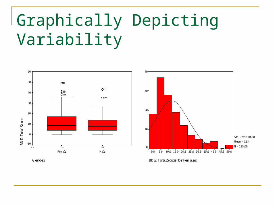
Graphically Depicting Variability
BDI2 Total Score for Females
50.045.040.035.030.025.020.015.010.05.00.0
40
30
20
10
0
Std. Dev = 10.80
Mean = 12.4
N = 135.00103135N =
Gender
MaleFemale
BD
I2 T
ota
l Sco
re
60
50
40
30
20
10
0
-10
199
211
1581669214
521
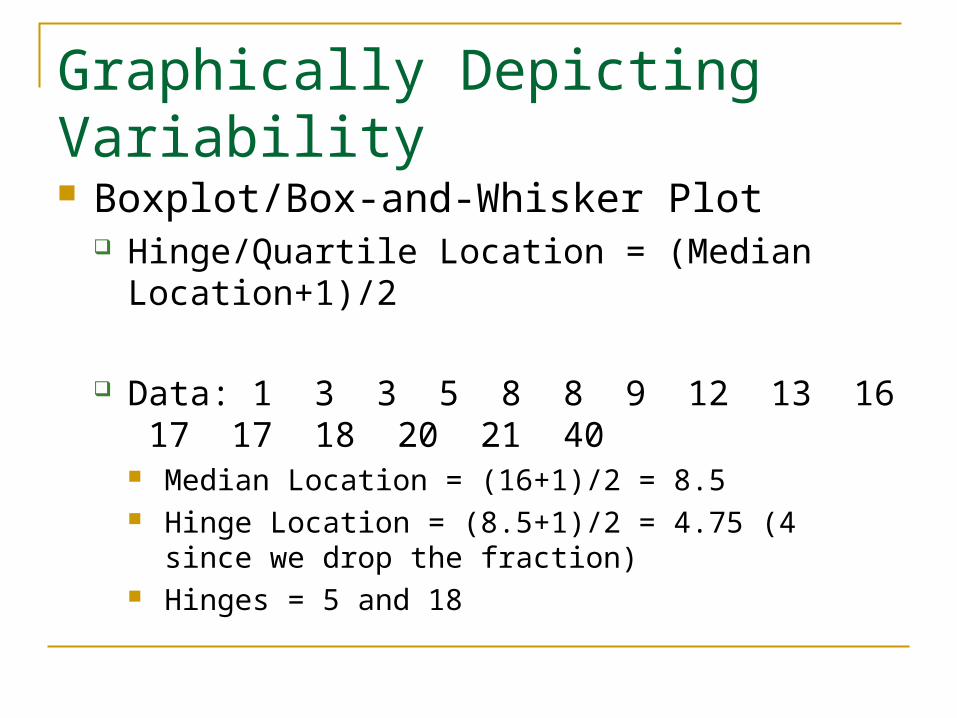
Graphically Depicting Variability Boxplot/Box-and-Whisker Plot
Hinge/Quartile Location = (Median Location+1)/2
Data: 1 3 3 5 8 8 9 12 13 16 17 17 18 20 21 40 Median Location = (16+1)/2 = 8.5 Hinge Location = (8.5+1)/2 = 4.75 (4 since we drop the
fraction) Hinges = 5 and 18
Graphically Depicting Variability
H-Spread = Upper Hinge – Lower Hinge H-Spread = 18-5 = 13
Whisker = H-Spread x 1.5 Since the whisker always ends at an actual data point, if we,
say calculated the whisker to end at a value of 12, but the data only has a 10 and a 15, we would end the whisker at the 10.
Whiskers = 12x1.5 = 19.5Lower whisker from 5 to 1Higher whisker from 18 to 21
Outliers Value of 40 extends beyond upper whisker
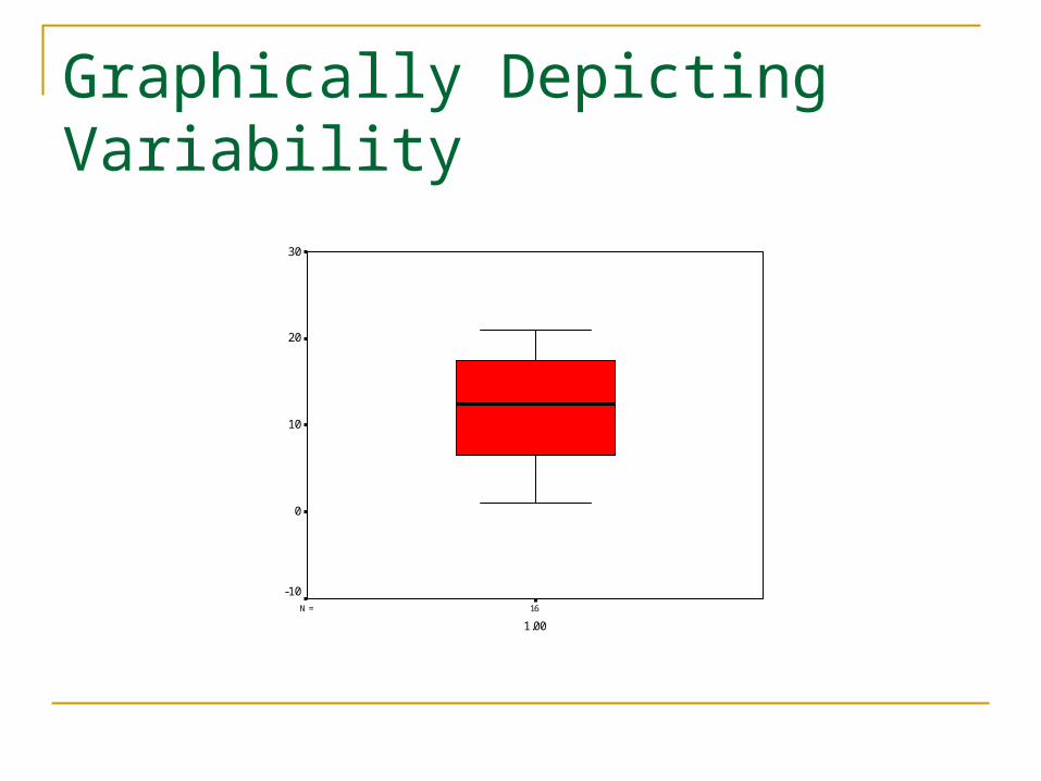
Graphically Depicting Variability
16N =
1.00
30
20
10
0
-10
![Measures of Variability for Graphical Models · Measures of Structure Variability Measures of Structure Variability All of these measures can be rescaled to vary in the [0;1] interval](https://img.pdfslide.us/doc/110x75/5fca5b8d790dd006415e4823/measures-of-variability-for-graphical-models-measures-of-structure-variability-measures.jpg)