Measures of variability: understanding the complexity of natural phenomena

In addition to knowing where the center of the distribution is, it is often helpful to know the degree to which individual values cluster around the center (or perhaps don’t)

This is known as variability, and it is the very thing we are attempting to understand

If human behavior was a constant, we’d have no need to study it. The fact that we see complexity in behavior means that there is some aspect of it that we don’t understand, something about that varies, for the individual over time, across individuals, across groups of individuals etc.

Complexity reflects uncertainty about the phenomenon of interest, and our ability to predict behavior is a reflection of the amount of variability we can account for

The following are simple statistics that can give us an idea of the complexity of the variable we’re trying to study.

There are various measures of variability, the most straightforward being the range of the sample:◦ Highest value minus lowest value

While range provides a good first pass at variance, it is not the best measure because:◦ It is calculated from only 2 points of data (poor

sufficiency)◦ Those two values are the most extreme in the

sample (no resistance)◦ Can change dramatically from sample to sample

(poor efficiency)

Range based on percentiles. Data can be ordered and then, much like we did

for the median as the 50th percentile (also known as the second quartile or Q2), we now look for numbers corresponding to the 25th and 75th percentile (Q1 and Q3)

Q3- Q1 gives us the interquartile range

Note that by only concerning oneself this middle 50% of scores, extreme scores will not affect this measure of variability

On the other hand, it still is not that sufficient relative to other measures

Another approach to estimating variance is to directly measure the degree to which individual data points differ from the mean and then average those deviations.

However, if we try to do this with real data, the result will always be zero

One way to get around the problem with the average deviation is to use the absolute value of the differences, instead of the differences themselves.

The absolute value of some number is just the number without any sign:◦ For Example: |-3| = 3

This will provide us with the mean absolute deviation

Although the mean absolute deviation is an acceptable measure of variability, the most commonly used measure is variance (denoted s2 for a sample and 2 for a population) and its square root termed the standard deviation (denoted s for a sample and for a population)

The computation of variance is also based on the basic notion of the average deviation however, instead of getting around the “zero problem” by using absolute deviations (as in MAD), it is eliminating by squaring the differences from the mean.◦ Specifically:

22

1

( )

1

ni

xi

X Xs

N

Variance sometimes difficult to interpret on its own as it is in squared units of the original scale values◦ What we’d like is something that’s on the same

scale as the original variable. Standard deviation is just the square root of

the variance, and gets our measure of variability back to the original scale units.

It represents the typical score deviation from the mean

If the variable is normally distributed, a rule of thumb is that:

s = R/6

This will be more clear when we talk about the normal distribution and its properties, but the idea is that roughly 99% of the data falls between 3 SD above and below the mean.

Using a robust measure of variability can be quite easy and will revolve around deviations from the median instead of the mean

Once our deviations from the median, we take the absolute value of the deviations, order them, and take the median of those

This in turn could serve as a robust means to find a univariate outlier1

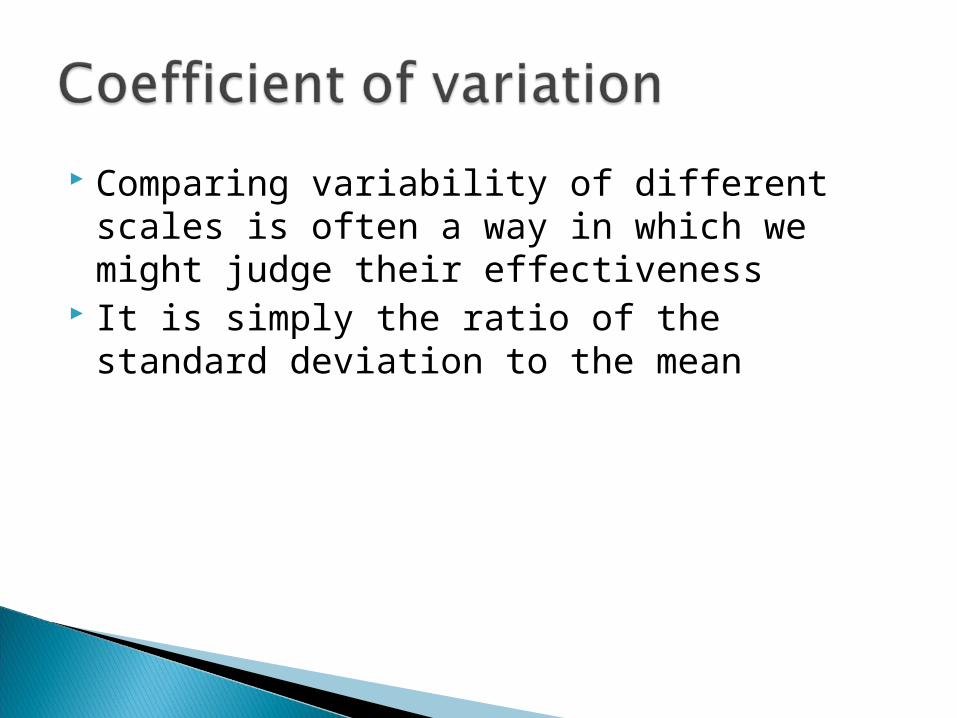
Comparing variability of different scales is often a way in which we might judge their effectiveness

It is simply the ratio of the standard deviation to the mean

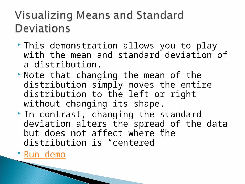
This demonstration allows you to play with the mean and standard deviation of a distribution.

Note that changing the mean of the distribution simply moves the entire distribution to the left or right without changing its shape.

In contrast, changing the standard deviation alters the spread of the data but does not affect where the distribution is “centered”

Run demo