Measures of between-cluster variability in cluster randomized trials with binary outcomes

STATISTICS IN MEDICINEStatist. Med. 2009; 28:1739–1751Published online 19 April 2009 in Wiley InterScience(www.interscience.wiley.com) DOI: 10.1002/sim.3582

Measures of between-cluster variability in cluster randomized trialswith binary outcomes

Andrew Thomson∗,†, Richard Hayes and Simon Cousens

Department of Epidemiology and Population Health, London School of Hygiene and Tropical Medicine,Keppel Street, London WC1E 7HT, U.K.

SUMMARY

Cluster randomized trials (CRTs) are increasingly used to evaluate the effectiveness of health-care inter-ventions. A key feature of CRTs is that the observations on individuals within clusters are correlated asa result of between-cluster variability. Sample size formulae exist which account for such correlations,but they make different assumptions regarding the between-cluster variability in the intervention arm ofa trial, resulting in different sample size estimates. We explore the relationship for binary outcome databetween two common measures of between-cluster variability: k, the coefficient of variation and �, theintracluster correlation coefficient. We then assess how the assumptions of constant k or � across treatmentarms correspond to different assumptions about intervention effects. We assess implications for samplesize estimation and present a simple solution to the problems outlined. Copyright q 2009 John Wiley &Sons, Ltd.

KEY WORDS: cluster randomized trials; sample size; binary outcomes

1. INTRODUCTION

Cluster randomized trials (CRTs) are increasingly used to evaluate the effectiveness of health-careinterventions [1–4]. It is widely understood that the individuals within a cluster tend to be moresimilar to each other than they are to the individuals in another cluster. This phenomenon of within-cluster correlation or, equivalently, between-cluster variation must be taken into account in thedesign and analysis of CRTs. When the outcome is dichotomous, there are two common measuresof the phenomenon that have been used in sample size formulae: the coefficient of variation, k,used in the formula of Hayes and Bennett [5], and the intracluster correlation coefficient, �, usedin the formula of Donner and Klar [6]. In designing a CRT one needs an estimate of one of these

∗Correspondence to: Andrew Thomson, Department of Epidemiology and Population Health, London School ofHygiene and Tropical Medicine, Keppel Street, London WC1E 7HT, U.K.

†E-mail: [email protected]

Received 30 November 2007Copyright q 2009 John Wiley & Sons, Ltd. Accepted 30 January 2009

1740 A. THOMSON, R. HAYES AND S. COUSENS

measures among control clusters. Such an estimate may be obtained from expert opinion, previouspublished values or a pilot study.

In our experience, there is often confusion among CRT investigators about the relationshipbetween these two measures. We have been unable to find published accounts of this relationshipor of the implications of this for the design and analysis of CRTs. Our main aim in this paper is toprovide a clear exposition of these issues, illustrated by numerical examples based on parametervalues typical of those seen in such trials. These issues are of considerable practical importancesince, as we shall see, inappropriate assumptions regarding k or �, or their constancy acrosstreatment arms, may result in trials that are either inadequately powered or unnecessarily large.

We begin by describing the relationship between k and �, and then explore how assumptions ofconstant k or constant � across the arms of a trial correspond to different assumptions about theeffect of the intervention. We show, for example, that constancy of k across study arms occurs ifthe intervention reduces or increases the risk of an outcome by a constant factor in each cluster.We go on to compare the two alternative sample size formulae, based on k and �. We show thatthese are special cases of a more general formula, the main difference being the assumed between-cluster variance in the intervention arm and investigate the implications of different assumptionsfor sample size calculations. We note that the assumption of constancy of k across study arms isnot invariant to the re-parameterization of ‘success’ as ‘failure’, and outline a suggested practicalapproach to sample size calculation that avoids some of the limitations of current approaches.

Attention is restricted in this paper to CRTs with an unmatched design and two treatment arms.We do not consider other designs, such as matched or stratified trials, which have different, althoughrelated, sample size formulae. Neither do we consider the implications of these issues for theanalysis of CRTs, although we note that different analytical methods make different assumptionsabout between-cluster variation in the intervention arm.

2. THE RELATIONSHIP BETWEEN k, � AND INTERVENTION EFFECTS

2.1. Introduction

In this section, we derive the relationship between the different methods of between-cluster vari-ability. We show that, except under special conditions, if k is constant across study arms then �will not be, and vice versa. We then consider how constancy of k or � relates to assumptionsregarding constancy of intervention effects on different scales. A numerical example is providedto illustrate these different assumptions.

2.2. The relationship between k and �

Let � j be the true risk in cluster j in one arm of a CRT, where we shall use the term risk to denotethe probability of the binary outcome of interest. We assume that the � j come from a distributionwith E(� j )=� and variance Var(� j ).

The intracluster correlation coefficient � is given by

�= Var(� j )

�(1−�)

Copyright q 2009 John Wiley & Sons, Ltd. Statist. Med. 2009; 28:1739–1751DOI: 10.1002/sim

MEASURES OF BETWEEN-CLUSTER VARIABILITY 1741

The coefficient of variation k is given by

k= SD(� j )

�and squaring this yields k2= Var(� j )

�2

Making Var(� j ) the subject of both these equations, we see that

��(1−�)=k2�2 and thus �=k2(

�

1−�

)

Surprisingly, we have not seen the relationship between these two measures stated explicitlyelsewhere.

We now introduce an extra subscript to denote the two arms of a CRT, which have differentexpected values �i and may have different variances Var(�i j ), where i=0 denotes the control armand i=1 denotes the intervention arm. The values of k2 in the control and intervention arms aregiven by

Var(�0 j )

�20and

Var(�1 j )

�21

respectively. If we assume k is constant across arms, it follows that

Var(�1 j )= Var(�0 j )�21�20

(1)

Similarly, the values of � in the control and intervention arms are

Var(�0 j )

�0(1−�0)and

Var(�1 j )

�1(1−�1)

and if we assume � is constant across arms then

Var(�1 j )= Var(�0 j )�1(1−�1)

�0(1−�0)(2)

It is clear that the assumption of common k across arms results, in general, in a different estimateof Var(�1 j ) from that implied by the assumption of common �. We note from equations (1) and(2) that the ratio of these estimates of Var(�1 j ) is given by

�1(1−�0)

�0(1−�1)

Thus, we have equality only when the true odds ratio is 1, corresponding to no intervention effect.As the intervention effect increases, so too does the ratio of the variances.

2.3. The relationship with intervention effects

2.3.1. Introduction. In this section, we ask ‘what is the effect on the variance in the interventionarm if the intervention has a fixed effect on a certain scale?’ We then see how this relates tothe assumptions of constant k or constant � across arms of the trial by comparing the relation-ship between Var(�1 j ) and Var(�0 j ) derived from the fixed effect assumption with equations (1)



and (2). Let h(.) be the link function that relates the cluster-level risk, �i j , to a linear combi-nation of covariates. In general, if we ignore covariates other than the intervention effect, themodel can be specified as h(�i j )=�+�i j xi j +ui j , where ui j is a random effect with mean 0 thatrepresents between-cluster variability, xi j is a covariate taking the value i and �i j represents theintervention effect.

Three link functions are commonly used, the identity, log and logit links, and these correspondto fixed effects on different scales. In the j th cluster in the intervention arm, the value of h(�1 j ) inthe absence of intervention is given by h(�1 j )=�+u1 j . If the intervention effect is fixed, we canwrite h(�1 j )=�+�+u1 j . If the clusters are randomly allocated to the intervention and controlarms, it follows that Var(u0 j )=Var(u1 j ) and thus Var(h(�0 j ))=Var(h(�1 j )).

We now explore the implications of fixed intervention effects using each of the three linkfunctions. On all three scales, if �=0 then both k and � will always be constant across arms, sowe now assume that � �=0.

2.3.2. Identity link. If h is the identity link, �i j =�+�xi j +ui j , and � represents the risk differ-ence, (�1−�0). If this is a fixed effect, then it is easy to see that Var(�0 j )=Var(�1 j ). With thisassumption, it is clear from equations (1) and (2) that k is never constant across arms and � isonly constant in the special case �0=1−�1.

2.3.3. Log link. If h is the log link, log(�i j )=�+�xi j +ui j , and we note that �i =E(�i j )=E[exp(�+�xi j +ui j )=exp(�+�xi j )E[exp(ui j )]]. Since randomization ensures that u0 j and u1 jhave the same distribution, it follows that with a fixed intervention effect on the log scale, e� repre-sents the risk ratio (�1/�0). Furthermore, Var(�0 j )=Var(e�+u0 j ) and Var(�1 j )=Var(e�+�+u1 j ),which we can re-write as e2�Var(e�+u1 j ). It follows that Var(�1 j )=e2�Var(�0 j ), and substitutinge� =(�1/�0) we obtain

Var(�1 j )= Var(�0 j )�21�20

This is identical to equation (1), and thus k will be the same in each arm of the trial if and onlyif the intervention reduces risk by the same percentage in all clusters. It follows that � will differbetween the trial arms under this assumption.

2.3.4. Logit link. The situation is more complex if h is the logit link:

log

(�i j

1−�i j

)=�+�xi j +ui j

Then � represents the cluster-specific log odds ratio and e� is the cluster-specific odds ratio. Wecan also define the population average or marginal odds ratio as

�1(1−�0)

�0(1−�1)

It is well known that no closed-form solution exists for integrating out the random effect on thelogit scale [7], and so the population average odds ratio cannot be written down as a functionof � and �. The cluster-specific and population average odds ratios are different parameters andformulae exist which approximate the relationship between them [8, 9].



If we make the simplifying assumption that they are approximately the same, which they willbe if the risk or the between-cluster variability is small, we can use a first-order Taylor seriesexpansion that gives Var(�i j )≈Var(logit(�i j ))�2i (1−�i )2. If the intervention effect is fixed on theodds ratio scale, it follows that

Var(�0 j )

�20(1−�0)2≈ Var(�1 j )

�21(1−�1)2

Re-arranging gives

Var(�1 j )≈ Var(�0 j )�21(1−�1)2

�20(1−�0)2

and comparison with equation (1) indicates that k will only be approximately constant across armsif the outcome is rare. This is intuitively obvious as the risk ratio will approximate the odds ratioin this case. As for the risk difference, � is constant only in the special case �0=1−�1. We stressthat this is only an approximation, and does not consider the fixed odds ratio further, as there maybe many cases where this approximation does not hold.

It is important to note that if the intervention effect is constant on one scale then it is notconstant on any other scale.

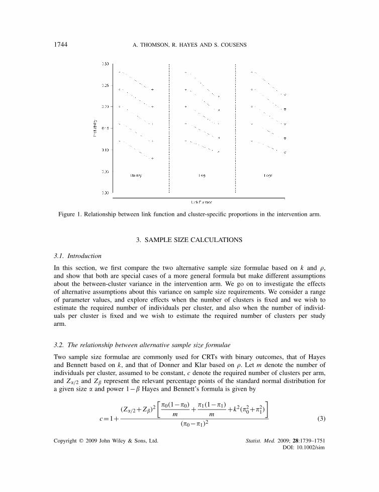
2.3.5. An illustration. Consider a set of five clusters with known true risks 0.12, 0.16, 0.20, 0.24and 0.28, with a mean of 0.2. As we know the true risks, we can specify the size of the randomeffect for each cluster on each scale. Suppose that the intervention reduces the mean value to 0.16.This corresponds to a risk difference of 0.04, and a risk ratio of 0.8.

The calculation of the odds ratio is more complex. As we know the values of the randomeffects, we can calculate the value of the cluster-specific odds ratio that gives a mean risk in theintervention arm of 0.16. If the clusters have the same size then the population averaged odds ratiois given by

0.16×0.8

0.84×0.2=0.762

which is very close to the cluster-specific odds ratio, and thus our approximation is reasonable.This is due to the relatively small between-cluster variability in this example.

Figure 1 shows the resulting risks in the five clusters after the intervention has been applied,assuming a fixed intervention effect using the identity, log and logit link functions.

We first note that the dotted line showing the intervention effect on the cluster with initial risk0.20 has the same gradient for log and identity link functions. For the identity link, all lines areparallel as the effect of the intervention is to shift all risks by a fixed absolute amount. For thelog link, the gradient is steepest for high initial risks and less steep for small risks. It is clear thatin this example the between-cluster variability in risk following intervention is larger assuming afixed risk difference than for a fixed risk ratio. Assuming that the odds ratio is fixed results inan estimate of between-cluster variability in the intervention arm that is intermediate between theother two values. The gradient is steepest for the highest prevalence, decreases as the prevalencedecreases, and always lies between the gradients for the log link and identity link.



Figure 1. Relationship between link function and cluster-specific proportions in the intervention arm.

3. SAMPLE SIZE CALCULATIONS

3.1. Introduction

In this section, we first compare the two alternative sample size formulae based on k and �,and show that both are special cases of a more general formula but make different assumptionsabout the between-cluster variance in the intervention arm. We go on to investigate the effectsof alternative assumptions about this variance on sample size requirements. We consider a rangeof parameter values, and explore effects when the number of clusters is fixed and we wish toestimate the required number of individuals per cluster, and also when the number of individ-uals per cluster is fixed and we wish to estimate the required number of clusters per studyarm.

3.2. The relationship between alternative sample size formulae

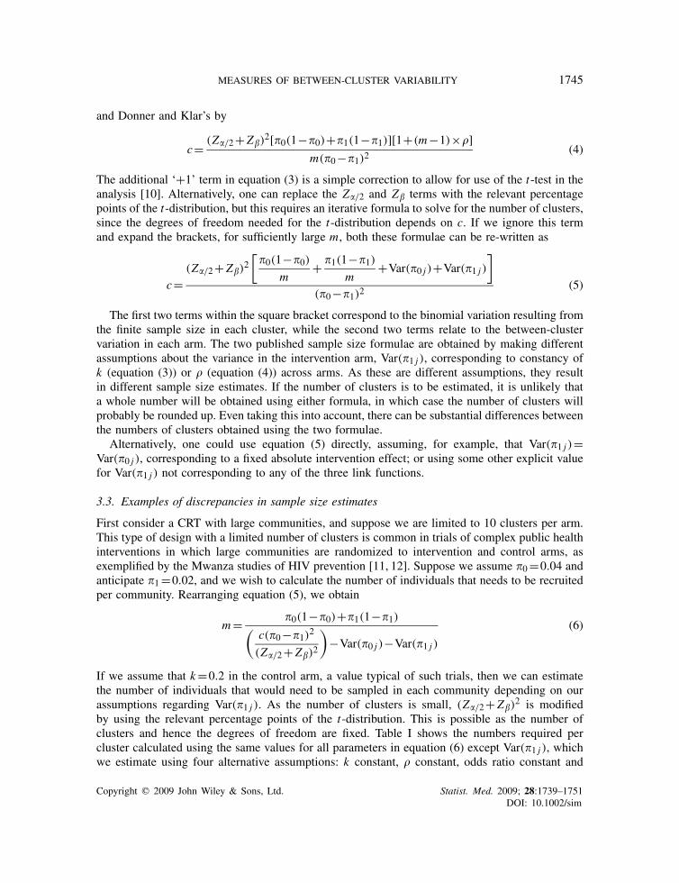
Two sample size formulae are commonly used for CRTs with binary outcomes, that of Hayesand Bennett based on k, and that of Donner and Klar based on �. Let m denote the number ofindividuals per cluster, assumed to be constant, c denote the required number of clusters per arm,and Z�/2 and Z� represent the relevant percentage points of the standard normal distribution fora given size � and power 1−� Hayes and Bennett’s formula is given by

c=1+(Z�/2+Z�)

2[�0(1−�0)

m+ �1(1−�1)

m+k2(�20+�21)

]

(�0−�1)2(3)



and Donner and Klar’s by

c= (Z�/2+Z�)2[�0(1−�0)+�1(1−�1)][1+(m−1)×�]

m(�0−�1)2(4)

The additional ‘+1’ term in equation (3) is a simple correction to allow for use of the t-test in theanalysis [10]. Alternatively, one can replace the Z�/2 and Z� terms with the relevant percentagepoints of the t-distribution, but this requires an iterative formula to solve for the number of clusters,since the degrees of freedom needed for the t-distribution depends on c. If we ignore this termand expand the brackets, for sufficiently large m, both these formulae can be re-written as

c=(Z�/2+Z�)

2[�0(1−�0)

m+ �1(1−�1)

m+Var(�0 j )+Var(�1 j )

]

(�0−�1)2(5)

The first two terms within the square bracket correspond to the binomial variation resulting fromthe finite sample size in each cluster, while the second two terms relate to the between-clustervariation in each arm. The two published sample size formulae are obtained by making differentassumptions about the variance in the intervention arm, Var(�1 j ), corresponding to constancy ofk (equation (3)) or � (equation (4)) across arms. As these are different assumptions, they resultin different sample size estimates. If the number of clusters is to be estimated, it is unlikely thata whole number will be obtained using either formula, in which case the number of clusters willprobably be rounded up. Even taking this into account, there can be substantial differences betweenthe numbers of clusters obtained using the two formulae.

Alternatively, one could use equation (5) directly, assuming, for example, that Var(�1 j )=Var(�0 j ), corresponding to a fixed absolute intervention effect; or using some other explicit valuefor Var(�1 j ) not corresponding to any of the three link functions.

3.3. Examples of discrepancies in sample size estimates

First consider a CRT with large communities, and suppose we are limited to 10 clusters per arm.This type of design with a limited number of clusters is common in trials of complex public healthinterventions in which large communities are randomized to intervention and control arms, asexemplified by the Mwanza studies of HIV prevention [11, 12]. Suppose we assume �0=0.04 andanticipate �1=0.02, and we wish to calculate the number of individuals that needs to be recruitedper community. Rearranging equation (5), we obtain

m= �0(1−�0)+�1(1−�1)(c(�0−�1)2

(Z�/2+Z�)2

)−Var(�0 j )−Var(�1 j )

(6)

If we assume that k=0.2 in the control arm, a value typical of such trials, then we can estimatethe number of individuals that would need to be sampled in each community depending on ourassumptions regarding Var(�1 j ). As the number of clusters is small, (Z�/2+Z�)

2 is modifiedby using the relevant percentage points of the t-distribution. This is possible as the number ofclusters and hence the degrees of freedom are fixed. Table I shows the numbers required percluster calculated using the same values for all parameters in equation (6) except Var(�1 j ), whichwe estimate using four alternative assumptions: k constant, � constant, odds ratio constant and



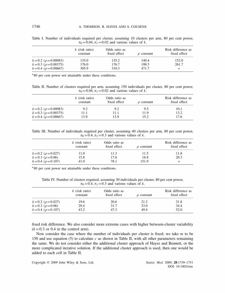
Table I. Number of individuals required per cluster, assuming 10 clusters per arm, 80 per cent power,�0=0.04,�1=0.02 and various values of k.

k (risk ratio) Odds ratio as Risk difference asconstant fixed effect � constant fixed effect

k=0.2 (�=0.00083) 135.0 135.2 140.4 152.0k=0.3 (�=0.00375) 176.0 176.7 198.5 261.7k=0.4 (�=0.00667) 305.9 310.3 471.7 ∗∗80 per cent power not attainable under these conditions.

Table II. Number of clusters required per arm, assuming 150 individuals per cluster, 80 per cent power,�0=0.04,�1=0.02 and various values of k.


k=0.2 (�=0.00083) 9.2 9.2 9.5 10.1k=0.3 (�=0.00375) 11.1 11.1 11.9 13.2k=0.4 (�=0.00667) 13.9 13.9 15.2 17.6

Table III. Number of individuals required per cluster, assuming 40 clusters per arm, 80 per cent power,�0=0.4,�1=0.3 and various values of k.


k=0.2 (�=0.027) 11.0 11.3 11.5 11.8k=0.3 (�=0.06) 15.8 17.6 18.8 20.3k=0.4 (�=0.107) 41.0 78.1 151.9 ∗∗80 per cent power not attainable under these conditions.

Table IV. Number of clusters required, assuming 30 individuals per cluster, 80 per cent power,�0=0.4,�1=0.3 and various values of k.


k=0.2 (�=0.027) 19.6 20.6 21.2 21.8k=0.3 (�=0.06) 29.4 31.7 33.0 34.4k=0.4 (�=0.107) 43.2 47.3 49.4 52.0

fixed risk difference. We also consider more extreme cases with higher between-cluster variability(k=0.3 or 0.4 in the control arm).

Now consider the case where the number of individuals per cluster is fixed; we take m to be150 and use equation (5) to calculate c as shown in Table II, with all other parameters remainingthe same. We do not consider either the additional cluster approach of Hayes and Bennett, or themore complicated iterative solution. If the additional cluster approach is used, then one would beadded to each cell in Table II.



Now consider a CRT in which there is a larger number of small clusters. Suppose that we arelimited to 40 clusters per arm, with �0=0.4 and �1=0.3, much higher risks than in the previousexample. This reflects parameters that one might see in a CRT in a primary-care setting based onrandomization of health practices. Table III shows the number of individuals required per cluster,while Table IV shows the number of clusters required per arm if we are restricted to 30 individualsper cluster.

Tables I and II demonstrate the substantial differences in sample size that can arise fromour different assumptions regarding between-cluster variability. As the between-cluster variabilityincreases, the disparity between the measures increases. This is to be expected as, in the absence ofbetween-cluster variability, all assumptions will give the same sample size. The difference appearsmore extreme when one wishes to estimate the number of subjects per cluster for a fixed numberof clusters. One explanation for this is that in equation (6), Var(�i j ) is in the denominator whereasin equation (5) it is in the numerator. For a fixed number of clusters, it is the magnitude of Var(�i j )relative to

c(�0−�1)2

(Z�/2+Z�)2

that affects sample size, whereas for a fixed cluster size it is its magnitude relative to

�0(1−�0)

m+ �1(1−�1)

m

In Table I, with k=0.3, the assumption of common � as opposed to common k results in anincrease in the trial size of 13 per cent, whereas for k=0.4 it is 54 per cent larger. In this latter case,assuming � is constant would result in a significant waste of resources if, in reality, k is constant,and could make certain trials appear unfeasible. These tables also demonstrate that differencesoccur regardless of the total sample size required.

The values of k are chosen to be the same throughout Tables I–IV, and it is of note that thevalues of � differ markedly between those in Tables I and II, and those in Tables III and IV. Thisclearly illustrates the point that the relationship between these two measures of between-clustervariability is heavily influenced by the baseline risk �0.

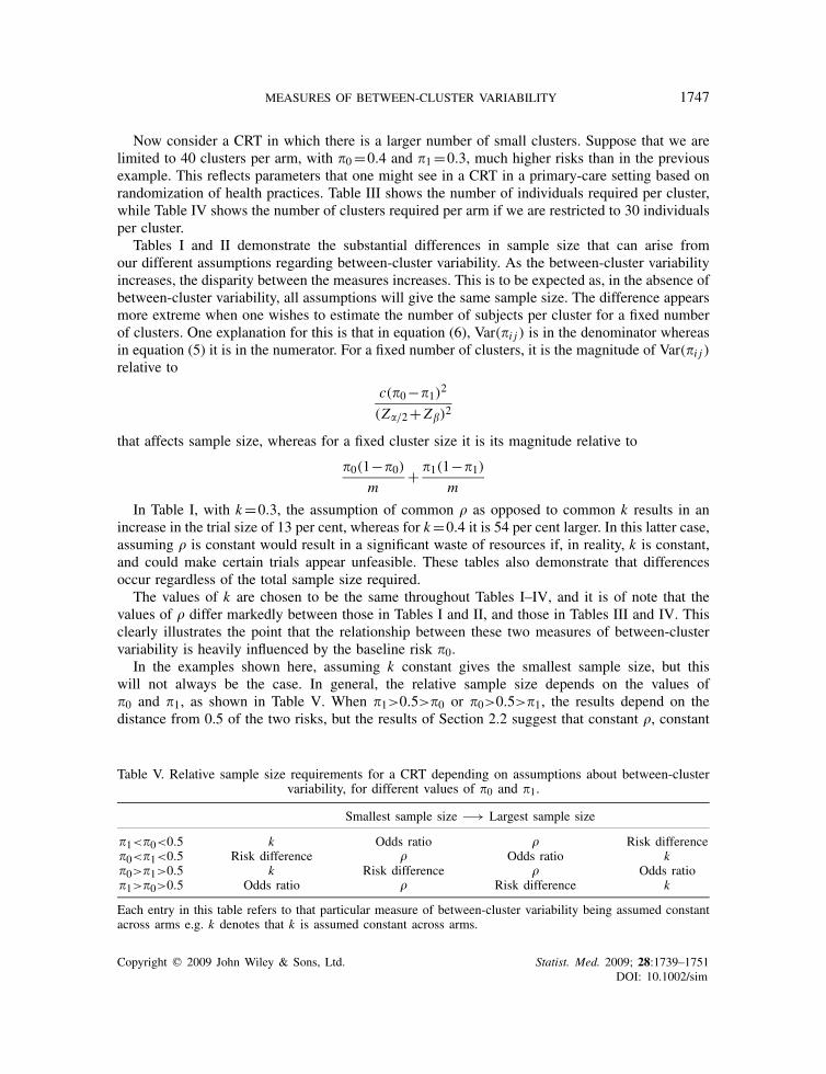
In the examples shown here, assuming k constant gives the smallest sample size, but thiswill not always be the case. In general, the relative sample size depends on the values of�0 and �1, as shown in Table V. When �1>0.5>�0 or �0>0.5>�1, the results depend on thedistance from 0.5 of the two risks, but the results of Section 2.2 suggest that constant �, constant

Table V. Relative sample size requirements for a CRT depending on assumptions about between-clustervariability, for different values of �0 and �1.

Smallest sample size −→ Largest sample size

�1<�0<0.5 k Odds ratio � Risk difference�0<�1<0.5 Risk difference � Odds ratio k�0>�1>0.5 k Risk difference � Odds ratio�1>�0>0.5 Odds ratio � Risk difference k

Each entry in this table refers to that particular measure of between-cluster variability being assumed constantacross arms e.g. k denotes that k is assumed constant across arms.



odds ratio and constant risk difference will give similar results, with constant k giving differentresults.

Table V also highlights a possible disadvantage of using k. Consider a CRT where �1<�0<0.5.If we re-parameterize a success as a failure and vice versa then �1>�0>0.5, corresponding to thefirst and fourth rows of Table V, respectively. Given that the data are unchanged, we would expectthe sample size estimates to be the same. For constant � and risk difference, the sample size isinvariant under this transformation but for k this is not the case; constant k now requires the largestsample size when previously it was the smallest. This point is discussed further in Section 4.

It has been hypothesized for some time that the values of � are likely to be smaller, the furtherthe risk � is from 0.5, and a recent review of published empirical estimates of � suggests that thismay indeed be the case [2]. A non-null intervention effect implies different risks in the two studyarms, and thus it is likely that the values of � will also differ. This, together with the lack of a clearepidemiological interpretation of constant � in terms of constancy of intervention effects, callsinto question the use of sample size formulae based on this assumption. In contrast, k will alwaysbe constant if the intervention effect can be assumed to have a fixed effect on the ratio scale. Thismay not always be the case, and it would be informative to examine empirical data from CRTsto investigate how often this assumption holds. A potential advantage of using � in sample sizecalculations is that it provides a simple estimate of the design effect, 1+(m−1)�; the other measuresdo not provide such a simple expression for this parameter. Moreover, if the investigator has noa priori information concerning the scale on which the intervention effect is likely to work, Table Vsuggests that constant � may provide a trade-off between an under-powered design and a waste ofresources.

4. FURTHER ISSUES REGARDING SAMPLE SIZE FORMULAE

4.1. Assuming k constant is not invertible

Consider a trial with a given �0 and Var(�0 j ) where

�1= �0a

for some value a. If we assume k is constant, then

Var(�1 j )

�21= Var(�0 j )

�20

and substitution yields

Var(�1 j )= Var(�0 j )

a2(7)

If we re-parameterize a success as a failure, by letting �∗0=1−�0 and �∗

1=1−�1, then we arestill modelling the same process and clearly Var(�i j )=Var(�∗

i j ) for i=0,1. In the control arm,k is now given by

Var(�∗0 j )

(�∗0)

2



which, unless �0=0.5, will be a different value. This in itself is not necessarily a problem.However, it should be noted that under this re-parameterization, the assumption of constant kyields a different estimate of Var(�∗

1 j ) and hence Var(�1 j )

Var(�∗1 j )

(�∗1)

2= Var(�∗

0 j )

(�∗0)

2and thus

Var(�1 j )

(1−�1)2= Var(�0 j )

(1−�0)2

Substituting in �1 = �0a

yields Var(�1 j )=Var(�0 j )

(1− �0

a

)2(1−�0)2

(8)

In the presence of an intervention effect (a �=1), equations (7) and (8) provide different estimatesof Var(�1 j ).

As an example, suppose �0=0.4, �1=0.3 and k=0.2 in the control arm. Thus, Var(�0 j )=0.0064. The assumption of common k yields Var(�1 j )=0.0036. If we now re-parameterize interms of �∗

i , then k in the control arm is given by 0.08/0.6=0.133 and k in the intervention armis given by 0.06/0.7=0.0857. Thus, not only does k take a different value but the assumption ofconstant k does not hold under the re-parameterization.

It may sometimes be appropriate to re-parameterize if �0>0.5 and the intervention is expectedto increase the risk of interest. Assuming k is constant implies that the risk is increased by aconstant factor, but this may not be possible for some clusters since risks cannot exceed unity.One can always halve the risk, but not always double it. The assumptions of constant � or fixedrisk difference do not suffer from this disadvantage.

4.2. A practical approach

We have seen in previous sections that the assumption of constant � has no epidemiologicaljustification, while the assumption of constant k may not always be appropriate and suffers froman invertability problem. Given the limitations in these assumptions, we suggest an alternativeapproach. We propose using equation (5) directly and give a practical example as to how thismight be done.

Consider a trial where, in the control clusters, it is estimated that there is a mean probability �0of 0.2, and that this ranges across clusters from approximately 0.1–0.3. We can assume that thiscorresponds to approximately 4 standard deviations, and thus SD(�0 j )=(0.3−0.1)/4=0.05, andthus Var(�0 j )=2.5×10−4. It should be noted that under this assumption, k=0.25 and �=0.0156.

Now suppose that, in the intervention arm, the mean prevalence �1 is reduced to 0.1, and thatit will range between 0.04 and 0.16. Again we assume that this corresponds to approximately4 standard deviations, and thus SD(�1 j )=(0.16−0.04)/4=0.03, and Var(�1 j )=9×10−4. Againwe can calculate k = 0.3 and �=0.01. We substitute the exact values into equation (5), to obtain therequired sample size. If we are estimating the number of clusters, and this is small (less than 15)then we recommend the addition of an extra cluster to compensate for this.

Judgement about the likely range of risks in the intervention arm may be informed by ourprevious discussion of how Var(�i j ) depends on constancy of intervention effects on the absolute,log or logit scales. We may also wish to increase the assumed variance in the intervention arm toallow for the possibility that intervention effects may vary between clusters.



5. DISCUSSION

There are two common approaches to measuring between-cluster variability in cluster randomizedtrials (CRTs) with binary outcomes. These are the coefficient of variation k, and the intraclustercorrelation coefficient, �. For a given risk, �, these are related by the formula

�=k2(

�

1−�

)

Practical experience suggests that field epidemiologists may find k easier to use and interpret,since the coefficient of variation (the standard deviation expressed relative to the mean) is a familiarconcept used in many branches of medicine, whereas few find the intracluster correlation coefficientas an intuitive measure.

It may be helpful to consider why we have these two different measures. When the outcomeis continuous, � may be a more appropriate measure of between-cluster variability. Knowledgeof � is sufficient to correct for clustering in a sample size calculation, but knowledge of k isnot: a measure of within-cluster variability is also necessary, while � already encompasses this.Conversely, when the outcome is a person-time rate, k is readily defined, but � is not since thereis no clearly defined unit of observation when working with a person-time denominator. The needfor convenient sample size formulae for both types of outcome explains the existence of these twoalternative approaches, both of which are easily adapted for use with binary data.

As we have seen, both formulae are the special cases of a more general sample size formula thatexplicitly involves the between-cluster variance in the intervention arm. Assumptions of constant� or constant k across study arms result in different estimates of this variance, leading to differentsample size estimates. We have shown that the difference between them is greatest when between-cluster variability is high. The effect also appears to be more pronounced when estimating thenumber of individuals required when the number of clusters is fixed.

Given these differences, we recommend that investigators should use the general form of thesample size formula and give careful consideration to suitable choice of value for Var(�1 j ), thebetween-cluster variation in risk in the intervention arm. While the assumption that the interventionhas a fixed relative effect in each cluster, corresponding to constancy of k across study arms, maysometimes be appropriate, this will not always be the case. It may be advisable to compute a rangeof sample size estimates, based on different assumptions about the intervention effect, to helpinform the final choice of sample size. If these are similar, this will provide some reassurance thatthe trial will be adequately powered. If empirical estimates of between-cluster variance in eachstudy arm were routinely reported in CRTs, compilation of such estimates would help to guide thedesign of future studies.

In this paper, we have only considered unmatched trials. Matched or stratified designs may beappropriate in order to reduce between-cluster variability. Given that the differences between thesample size formulae are greatest when between-cluster variability is substantial, the differencebetween the two methods may be less for matched and stratified trials. However, some authorshave cautioned against this approach as the reduction in variability may be outweighed by the lossof degrees of freedom in the analysis [13].

A lot of work has looked at the fact that different models estimate different parameters [7, 8, 14],yet little appears to have gone into the discussion of the assumptions made by these methodsregarding the variances in each arm. Further work is needed to look at the consequences of thedifferent assumptions, in terms of the robustness of these models.



Different analytical methods make different assumptions regarding the between-cluster variancein the two study arms. These methods include generalized estimating equations, random effectslogistic regression, beta-binomial regression, adjusted �2 methods and simpler methods such as thet-test. While much previous work has focused on the different parameters estimated by differentmodels [7, 8, 14], further work is needed to explore the consequences of the different varianceassumptions for the robustness of these methods.

Although cluster randomization has become an increasingly common design for the evaluation ofhealth interventions, there is still some confusion regarding measures of between-cluster variability.By clearly defining the relationship between the two most common measures, we aimed to alleviatethis confusion. When designing a CRT, the likely effect of the intervention should be taken intoaccount when estimating the between-cluster variability in the intervention arm. Researchers shouldalso be aware of the assumptions behind their analytical approaches, which may or may not beappropriate under certain conditions.

REFERENCES

1. Bland JM. Cluster randomised trials in the medical literature: two bibliometric surveys. BMC Medical ResearchMethodology 2004; 4:21.

2. Campbell MK, Fayers PM, Grimshaw JM. Determinants of the intracluster correlation coefficient in clusterrandomized trials: the case of implementation research. Clinical Trials 2005; 2(2):99–107.

3. Isaakidis P, Ioannidis JP. Evaluation of cluster randomized controlled trials in sub-Saharan Africa. AmericanJournal of Epidemiology 2003; 158(9):921–926.

4. Eldridge SM, Ashby D, Feder GS, Rudnicka AR, Ukoumunne OC. Lessons for cluster randomized trials in thetwenty-first century: a systematic review of trials in primary care. Clinical Trials 2004; 1(1):80–90.

5. Hayes RJ, Bennett S. Simple sample size calculation for cluster-randomized trials. International Journal ofEpidemiology 1999; 28(2):319–326.

6. Donner A, Klar N. Design and Analysis of Cluster Randomization Trials in Health Research. Hodder: London,2000.

7. Ten Have TR, Ratcliffe SJ, Reboussin BA, Miller ME. Deviations from the population-averaged versus cluster-specific relationship for clustered binary data. Statistical Methods in Medical Research 2004; 13:3–16.

8. Neuhaus JM. Statistical methods for longitudinal and clustered designs with binary responses. Statistical Methodsin Medical Research 1992; 1(3):249–273.

9. Zeger SL, Liang KY, Albert PS. Models for longitudinal data: a generalized estimating equation approach.Biometrics 1988; 44(4):1049–1060.

10. Snedecor W, Cochran W. Statistical Methods. Iowa State University Press: Ames, 1967; 113.11. Grosskurth H, Mosha F, Todd J, Mwijarubi E, Klokke A, Senkoro K, Mayaud P, Changalucha J, Nicoll A,

ka-Gina G, Newell J, Mugeye K, Mabey D, Hayes R. Impact of improved treatment of sexually transmitteddiseases on HIV infection in rural Tanzania: randomised controlled trial. The Lancet 1995; 346(8974):530–536.

12. Hayes RJ, Changalucha J, Ross DA, Gavyole A, Todd J, Obasi AI, Plummer ML, Wight D, Mabey DC,Grosskurth H. The MEMA kwa Vijana project: design of a community randomised trial of an innovativeadolescent sexual health intervention in rural Tanzania. Contemporary Clinical Trials 2005; 26(4):430–442.

13. Klar N, Donner A. The merits of matching in community intervention trials: a cautionary tale. Statistics inMedicine 1997; 16(15):1753–1764.

14. Bellamy SL, Gibberd R, Hancock L, Howley P, Kennedy B, Klar N, Lipsitz S, Ryan L. Analysis of dichotomousoutcome data for community intervention studies. Statistical Methods in Medical Research 2000; 9(2):135–159.


Documents

Measures of between-cluster variability in cluster randomized trials with binary outcomes