Embed Size (px)
Citation preview

NTIA Report 93-301 NOAA Special Report
MEASUREMENTS OF WIND PROFILER EMC CHARACTERISTICS
Daniel Law Frank Sanders
Gary Patrick Michael Richmond
U.S. DEPARTMENT OF COMMERCE Ronald H. Brown, Secretary
Larry Irving, Assistant Secretary
for Communications and Information and Administrator, National Telecommunications
and Information Administration
MARCH 1994


iii
ABSTRACT
This report provides the results of measurements that were conducted on a 404.37 MHz wind profiler located in Platteville, Colorado. These measurements included: radiated spectra (both high and low mode), radiated harmonic and subharmonic power measurements, characterization of the antenna frequency response, determination of the radiated antenna gain values near ground level, susceptibility of profiler performance to interference from selected emission waveforms, and the effects on a typical land mobile/amateur operation from wind profiler emissions. In addition, the report presents a detailed wind profiler system description including operations/functions, system hardware, digital signal processing, as well as an analytical estimation of the interference effects on profiler performance. The information contained within this report can serve as an aid in conducting electromagnetic compatibility (EMC) analysis to determine compatibility between wind profilers and other systems.
KEY WORDS
Wind Profiler Characteristics Wind Profiler Interference Susceptibility
Wind Profiler Radars Wind Profiler Radiated Measurements
Wind Profiler System Description

iv

v
PRODUCT DISCLAIMER
Measurement and radio equipment are mentioned in this report to adequately explain the wind profiler system and the measurement procedures. In no case does such identification imply recommendation or endorsement by the National Telecommunications and Information Administration or National Oceanic and Atmospheric Administration, nor does it imply that the equipment identified is necessarily the best available for these applications.

vi
vii
CONTENTS Subsection Page
SECTION 1 INTRODUCTION
1.1 BACKGROUND ...................................................................................................................... 1 1.2 OBJECTIVES.......................................................................................................................... 2 1.3 APPROACH ............................................................................................................................ 3
SECTION 2 WIND PROFILER SYSTEMS
2.1 INTRODUCTION .................................................................................................................... 5 2.2 GENERAL OPERATION AND FUNCTION ............................................................................ 5 2.3 SYSTEM DESCRIPTION........................................................................................................ 5 2.4 SYSTEM TIMING/WAVEFORMS ........................................................................................... 9 Oblique High ..................................................................................................................... 9 Oblique Low ...................................................................................................................... 9 Vertical High...................................................................................................................... 9 Vertical Low....................................................................................................................... 9 2.5 PROFILER SYSTEM HARDWARE ...................................................................................... 10 Frequency Generator ...................................................................................................... 10 RF Power Amplifier ......................................................................................................... 10 Antenna .......................................................................................................................... 10 Receiver .......................................................................................................................... 12 Receiver RF Assembly.................................................................................................... 13 Receiver IF Assembly ..................................................................................................... 13 Receiver A/D Assembly .................................................................................................. 13 2.6 DIGITAL SIGNAL PROCESSING (PROFILER) ................................................................... 14 Profiler Hub Processing .................................................................................................. 16 Consensus Averaging ..................................................................................................... 16 Wind Calculation ............................................................................................................. 17
SECTION 3 INTERFERENCE TO PROFILERS
3.1 INTRODUCTION .................................................................................................................. 19 3.2 COHERENT INTERFERENCE............................................................................................. 19 3.3 INCOHERENT INTERFERENCE (NOISE)........................................................................... 19 3.4 SYSTEM NOISE TEMPERATURE....................................................................................... 20 3.5 SYSTEM FREQUENCY RESPONSE................................................................................... 22 3.6 SYSTEM POST-PROCESSING NOISE POWER ................................................................ 24 3.7 MINIMUM DETECTABLE SIGNAL POWER ........................................................................ 24 3.8 INTERFERENCE ANALYSIS ............................................................................................... 26
viii
CONTENTS continued
Subsection Page
SECTION 3 INTERFERENCE TO PROFILERS
continued
On-Tune FM....................................................................................................................27 Off-Tune FM.................................................................................................................... 28 On-Tune Non-FM Radar ................................................................................................. 28 Off-Tune Non-FM Radar ................................................................................................. 29 On-Tune Chirped Radar.................................................................................................. 29 Off-Tune Chirped Radar.................................................................................................. 30 Effect of Range-Doppler Processing............................................................................... 30
SECTION 4 WIND PROFILER MEASUREMENTS
4.1 INTRODUCTION .................................................................................................................. 31 4.2 EMISSION SPECTRUM MEASUREMENTS........................................................................ 31 4.3 HARMONIC AND SUBHARMONIC RADIATED POWER MEASUREMENTS..................... 33 4.4 ANTENNA SELECTIVITY MEASUREMENTS ..................................................................... 37 4.5 ANTENNA GAIN MEASUREMENTS.................................................................................... 38 Antenna Gain Calculations.............................................................................................. 42 4.6 WIND PROFILER INTERFERENCE SUSCEPTIBILITY TESTS.......................................... 45 On-Tune CW Signal Injection.......................................................................................... 48 Results of On-Tune CW Signal Injection......................................................................... 49 Off-Tune CW Signal Injection.......................................................................................... 49 Results of Off-Tune CW Signal Injection......................................................................... 49 On-Tune FM Signal Injection .......................................................................................... 49 Results of On-Tune FM Signal Injection ......................................................................... 51 Off-Tune FM Signal Injection .......................................................................................... 51 Results of Off-Tune FM Signal Injection ......................................................................... 51 Non-FMed, On-Tune Pulsed Signal Injection (“continuous” source)............................... 51 Results of Non-FMed, On-Tune, Pulsed Signal Injection (“continuous” source) ...................................................................................................... 53 Non-FMed, On-Tune, Pulsed Signal Injection (“intermittent” source) ............................. 53 Results of Non-FMed, On-Tune, Pulsed Signal Injection (“intermittent” source)...................................................................................................... 54 Non-FMed, Off-Tune, Pulsed Signal Injection (both “continuous” and “intermittent” sources) ................................................................ 54 Results of Non-FMed, Off-Tune, Pulsed Signal Injection (both “continuous” and “intermittent” sources) ................................................................ 54
ix
CONTENTS continued
Subsection Page
SECTION 4 WIND PROFILER MEASUREMENTS
continued Chirped, On-Tune, Pulsed Signal Injection (“continuous”) .............................................. 54 Results of Chirped, On-Tune Signal Injection (“continuous”) .......................................... 55 Chirped, On-Tune Signal Injection (“intermittent”)........................................................... 55 Results of Chirped, On-Tune Signal Injection (“intermittent”).......................................... 56 Chirped, Off-Tune Pulsed Signal Injection ...................................................................... 56 4.7 EFFECTS FROM WIND PROFILER EMISSIONS ON LAND MOBILE/AMATEUR OPERATIONS ..................................................................................... 57 On-Tune Test ..................................................................................................................57 Off-Tune Test .................................................................................................................. 57 Summary......................................................................................................................... 57
SECTION 5 SUMMARY AND CONCLUSIONS
5.1 SUMMARY .......................................................................................................................... 59 5.2 CONCLUSIONS.................................................................................................................... 60
LIST OF FIGURES Figure
2-1 Wind profiler artist conception........................................................................................... 6 2-2 Wind profiler block diagram............................................................................................... 7 2-3 Profiler receiver block diagram........................................................................................ 12 2-4 Frequency response of IF filters...................................................................................... 14 2-5 Profiler Doppler spectrum ............................................................................................... 16 3-1 Oblique high mode TDA frequency response (± 300 Hz)................................................ 23 3-2 Oblique high mode frequency response (± 7000 Hz)...................................................... 23 3-3 Oblique high mode frequency response ......................................................................... 25 3-4 Oblique low mode frequency response........................................................................... 25 3-5 On-Tune FM interference................................................................................................ 27 4-1 Radiated spectrum measurement schematic .................................................................. 34 4-2 Platteville short-pulse radiated spectrum envelope......................................................... 35 4-3 Platteville long-pulse radiated spectrum envelope.......................................................... 35 4-4 Radiated harmonic measurement schematic .................................................................. 36 4-5 Antenna characteristics, 390-410 MHz ........................................................................... 39
x
CONTENTS continued
Subsection Page
LIST OF FIGURES continued
4-6 Antenna characteristics, 100-1100 MHz ......................................................................... 39 4-7 Antenna pattern measurement schematic ...................................................................... 41 4-8 Platteville ground-level antenna pattern (east mode)...................................................... 43 4-9 Platteville ground-level antenna pattern (north mode) .................................................... 43 4-10 Platteville ground-level antenna pattern (vertical mode) ................................................. 44 4-11 Platteville ground-level antenna pattern (decibel average of E, N and V)....................... 44 4-12 Interference injection schematic...................................................................................... 46 4-13 CW signal spectrum ........................................................................................................50 4-14 FM spectrum ................................................................................................................... 50 4-15 Non-FMed pulse spectrum, 1 ms/pulse, 300 pps............................................................ 52 4-16 Non-FMed pulse spectrum, 10 ms/pulse, 300 pps.......................................................... 52 4-17 Chirped pulse spectrum, 5 MHz FM, 10 ms/pulse, 300 pps............................................ 55
LIST OF TABLES Table 2-1 Profiler Characteristics ...................................................................................................... 8 2-2 RF Power Amplifier Characteristics ................................................................................ 11 2-3 Profiler Antenna Characteristics...................................................................................... 11 2-4 Receiver Characteristics ................................................................................................. 13 3-1 Signal Processing Characteristics................................................................................... 26 4-1 Harmonic and Subharmonic level (dBc) for the Platteville Wind Profiler Radar......................................................................................................... 37 4-2 Sample of Antenna Pattern Data Points ......................................................................... 41 4-3 Interference Test Results: 3-dB Profiler System Noise Level Increase........................... 56 5-1 Interference Thresholds Resulting in 3-dB Increase in Profiler’s System Noise Level ......................................................................................... 61 LIST OF REFERENCES.......................................................... 63
1
SECTION 1 INTRODUCTION
1.1 BACKGROUND
Wind profiler radar systems provide hourly (or more frequent) wind speed and direction values as a function of altitude. The primary role for wind profilers is in weather observation and forecasting; however, other applications have been identified, including severe wind condition warnings, flight planning, space shuttle support, and pollution studies (acid rain and volcanic ash). Currently, wind speed and direction are determined by the National Weather Service (NWS)a and other agencies by tracking the flight path of radiosondes, which also provide information on temperature, barometric pressure, and relative humidity in the atmosphere along their flight paths. Radiosondes are expendable and are usually released twice daily. Although wind profilers are not direct replacements for radiosondes, they will provide regular, more frequent wind observations.
Wind profiler operations to date have been for experimental purposes at several
research facilities. In addition, the National Oceanic and Atmospheric Administration (NOAA)a currently operates a demonstration network of 31 wind profilers and plans a national network of 100–200 units. Other Government [i.e., Department of Defense (DOD)] and non- Government wind profiler users are expected.
A concern about wind profiler operations is the selection of appropriate operating frequency bands. Atmospheric propagation characteristics require that wind profiler systems operate in the 50–1000 MHz range. Currently, three frequency ranges are of particular interest: around 50 MHz, 200–500 MHz, and around 900 MHz, each of which best accommodates a particular application. Since the NOAA plans a 200–500 MHz national wind profiler network, efforts to accommodate wind profilers have focused on that band.
No single frequency band is presently available to accommodate the 200–500 MHz
type wind profiler operations for all users, Government and non-Government. Furthermore, the selection of any frequency band must take into account any potential international effect. For example, the wind profiler developed for NOAA at 404.37 MHz may be sold by its manufacturer to other countries, where conscientious attempts to protect operations such as COSPAS (COsmicheskaya Sistyema Poiska Avariynych-Russian Federation acronym for Space System for Search of Distressed Vessels) and SARSAT (Search And Rescue Satellite-Aided Tracking system) operating in the 406-406.1 MHz band may not be made. In addition, a frequency band selected solely on the basis of national usage may not be suitable for international usage, and thus national trade may be adversely affected. As a result, the Interdepartment Radio Advisory Committee (IRAC) requested that the National Telecommunications and Information Administration (NTIA)a conduct an assessment of the 216–225 MHz, 400.15–406 MHz, and 420–450 MHz bands to assist in determining the appropriate part of the spectrum for midfrequency (200–500 MHz) wind profiler radar operations.
a Agencies within the United States Department of Commerce (DOC).
2
Section 1 Introduction
The requested study was completed by NTIA.1 The study recommended that the 440–450 MHz band be considered for long-term wind profiler operations. It was noted that only limited wind profiler measurements had been conducted, and additional measurements would aid in verifying some of the assumptions made in the NTIA study. The test plan for these measurements was coordinated with NTIA's Institute for Telecommunication Sciences (ITS), NOAA, and various IRAC agencies.
The measurements were conducted on the Unisys wind profiler in Platteville, Colorado,
operating on 404.37 MHz. It is assumed that the characteristics associated with the 404.37-MHz profiler would remain the same for profilers in the 200–500 MHz range, independent of any new frequency chosen.
1.2 OBJECTIVES The objectives of the measurements on the Unisys wind profiler are as follows: 1. Determine the radiated short-pulse and long-pulse emission spectra of the wind
profiler; 2. Determine the amplitudes of the wind profiler's radiated harmonics and
subharmonics relative to the center frequency amplitude; 3. Determine any filter characteristics associated with the antenna; 4. Determine the gain of the profiler antenna at ground level relative to an isotropic
antenna; 5. Determine the susceptibility of the profiler to various waveforms that represent
typical systems operating in the 440–450 MHz band; and 6. Determine the effects of wind profiler emissions on a receiver that would
represent typical land mobile/amateur operations.
1 Patrick, G. and Richmond, M. (1991), Assessment of Bands for Wind Profiler
Accommodation (216–225, 400.15–406, and 420–450 MHz Bands), NTIA Report 91-280, September 1991.
3
Section 1 Introduction 1.3 APPROACH
To meet the above objectives, a preliminary measurement plan was developed and coordinated between NTIA/ITS, NOAA, and various IRAC agencies.2 The plan was implemented in a series of measurements and tests on the profiler at Platteville, Colorado, in 1991. _______________________
2 NTIA/ITS, RSMS Measurement Plan on the Unisys wind profiler, May 1991.

5
SECTION 2 WIND PROFILER SYSTEMS
2.1 INTRODUCTION
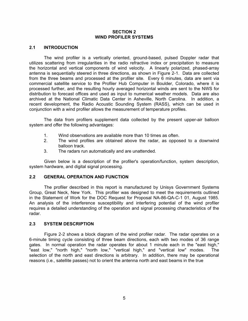
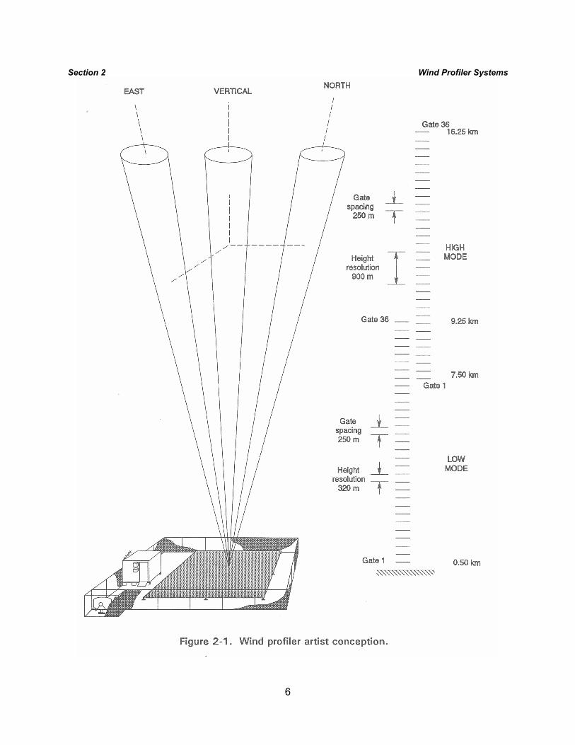
The wind profiler is a vertically oriented, ground-based, pulsed Doppler radar that utilizes scattering from irregularities in the radio refractive index or precipitation to measure the horizontal and vertical components of wind velocity. A linearly polarized, phased-array antenna is sequentially steered in three directions, as shown in Figure 2-1. Data are collected from the three beams and processed at the profiler site. Every 6 minutes, data are sent via commercial satellite service to the Profiler Hub Computer in Boulder, Colorado, where it is processed further, and the resulting hourly averaged horizontal winds are sent to the NWS for distribution to forecast offices and used as input to numerical weather models. Data are also archived at the National Climatic Data Center in Asheville, North Carolina. In addition, a recent development, the Radio Acoustic Sounding System (RASS), which can be used in conjunction with a wind profiler allows the measurement of temperature profiles.
The data from profilers supplement data collected by the present upper-air balloon
system and offer the following advantages:
1. Wind observations are available more than 10 times as often. 2. The wind profiles are obtained above the radar, as opposed to a downwind
balloon track. 3. The radars run automatically and are unattended.
Given below is a description of the profiler's operation/function, system description, system hardware, and digital signal processing.
2.2 GENERAL OPERATION AND FUNCTION
The profiler described in this report is manufactured by Unisys Government Systems Group, Great Neck, New York. This profiler was designed to meet the requirements outlined in the Statement of Work for the DOC Request for Proposal NA-86-QA-C-1 01, August 1985. An analysis of the interference susceptibility and interfering potential of the wind profiler requires a detailed understanding of the operation and signal processing characteristics of the radar.
2.3 SYSTEM DESCRIPTION
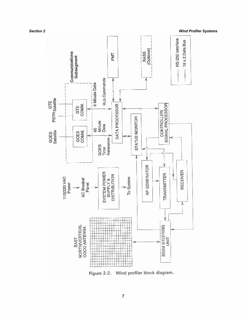
Figure 2-2 shows a block diagram of the wind profiler radar. The radar operates on a 6-minute timing cycle consisting of three beam directions, each with two modes of 36 range gates. In normal operation the radar operates for about 1 minute each in the "east high," "east low," "north high," "north low," "vertical high," and "vertical low" modes. The selection of the north and east directions is arbitrary. In addition, there may be operational reasons (i.e., satellite passes) not to orient the antenna north and east beams in the true
6
Section 2 Wind Profiler Systems
7
Section 2 Wind Profiler Systems
8
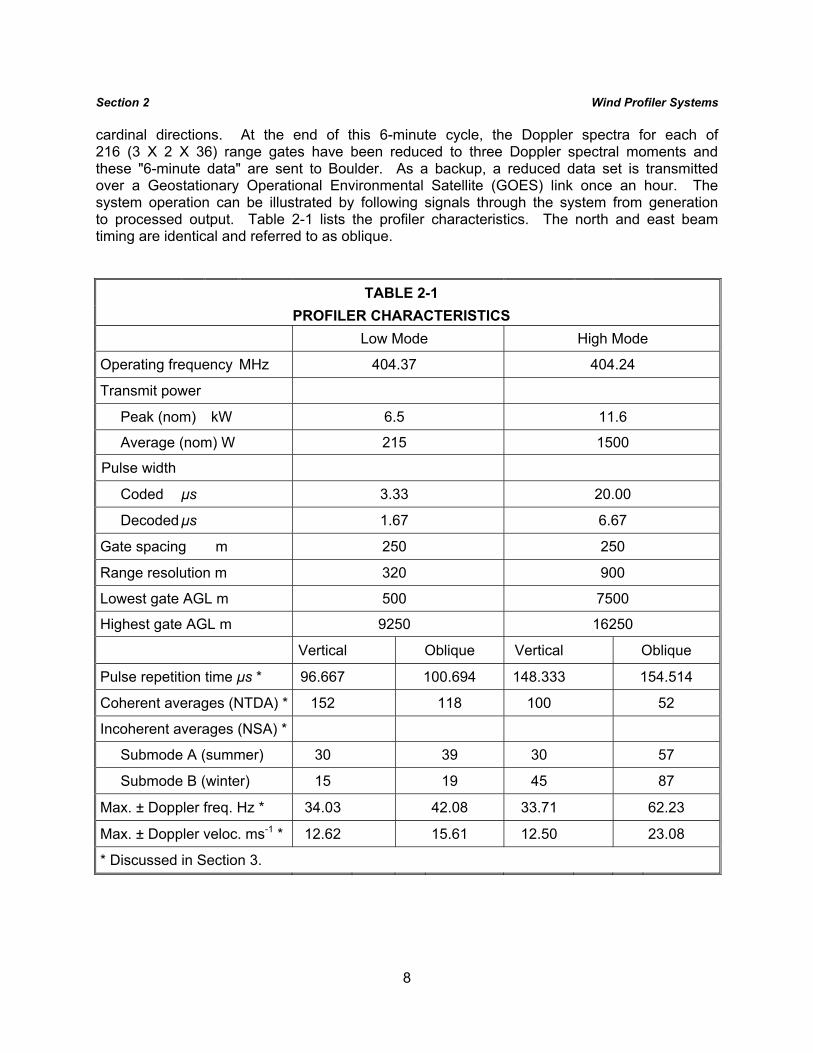
Section 2 Wind Profiler Systems cardinal directions. At the end of this 6-minute cycle, the Doppler spectra for each of 216 (3 X 2 X 36) range gates have been reduced to three Doppler spectral moments and these "6-minute data" are sent to Boulder. As a backup, a reduced data set is transmitted over a Geostationary Operational Environmental Satellite (GOES) link once an hour. The system operation can be illustrated by following signals through the system from generation to processed output. Table 2-1 lists the profiler characteristics. The north and east beam timing are identical and referred to as oblique. TABLE 2-1 PROFILER CHARACTERISTICS Low Mode High Mode
Operating frequency MHz 404.37 404.24
Transmit power
Peak (nom) kW 6.5 11.6
Average (nom) W 215 1500
Pulse width
Coded µs 3.33 20.00
Decoded µs 1.67 6.67
Gate spacing m 250 250
Range resolution m 320 900
Lowest gate AGL m 500 7500
Highest gate AGL m 9250 16250
Vertical Oblique Vertical Oblique
Pulse repetition time µs * 96.667 100.694 148.333 154.514
Coherent averages (NTDA) * 152 118 100 52
Incoherent averages (NSA) *
Submode A (summer) 30 39 30 57
Submode B (winter) 15 19 45 87
Max. ± Doppler freq. Hz * 34.03 42.08 33.71 62.23
Max. ± Doppler veloc. ms-1 * 12.62 15.61 12.50 23.08
* Discussed in Section 3.
9
Section 2 Wind Profiler Systems 2.4 SYSTEM TIMING WAVEFORMS
The controller/signal processor generates the system timing and the differential logic signals for the frequency generator to form the transmitter excitation. The timing is derived from a 14.4-MHz crystal oscillator, which is accurate and stable enough to meet the timing specifications. The four different operating modes are listed in Table 2-1.
Oblique High
In the oblique high mode, the signal processor generates a pulse of 20 µs made up of three 6.67-µs “chips,” resulting in a pulse compression ratio of 3:1. The complementary code set
A = + + + B = + - + C = + + - , where + indicates a 0° phase shift and - indicates a 180° phase shift, is transmitted in the sequence C, A, C, B, C, A, C, B,... with a pulse repetition time (PRT) of 154.514 µs. Beginning at a height 017.5 km, 36 samples are taken 1.7361 µs apart, which, considering the 73.7° beam elevation angle, corresponds to a vertical spacing of 249.95 m. The last sample is taken at 16.25 km above ground level (AGL). Oblique Low
The oblique low mode uses a pulse duration of 3.33-µs consisting of two 1.67-µs chips, for a pulse compression of 2:1. The complementary code set
A = + + B = + - is transmitted in the sequence A, B, A, B, A, B,... with a PRT of 100.694 µs. The 36 samples are taken as above, at 1.7361-µs (249.95-m) intervals from 0.5 to 9.25 km AGL. Vertical High
The vertical high mode uses the same pulse duration and pulse coding as the oblique high mode. The PRT is 143.333 µs and the 36 samples are taken at 1.667-µs intervals, which, with the vertical beam orientation, corresponds to 250-m spacing from 7.5 to 16.25 km AGL.
Vertical Low
The vertical low mode uses the same pulse duration and pulse coding as the oblique low mode. The PRT is 96.667 µs and the 36 samples are spaced 250-m from 0.5 to 9.25 km AGL.
Additional timing requirements of the controller/signal processor are discussed in
Section 2.6 on signal processing.
10
Section 2 Wind Profiler Systems 2.5 PROFILER SYSTEM HARDWARE Frequency Generator
The frequency generator contains two independent, low-noise, temperature-controlled, crystal oscillators. The local oscillator (LO) at 374.22 MHz ± 0.005% and the coherent oscillator (COHO) at 30 MHz ± 0.005% are mixed and pulse modulated to form the transmitter excitation at +12 dBm. In addition to the phase coded pulses, successive radar pulses are pseudorandomly phase shifted using a sequence of length 64, so the separation between spectral lines is PRF/64, not PRF. This additional encoding is used to reduce range-ambiguous returns. To accomplish this function, the LO is phase shifted from pulse to pulse by a 3-bit phase shifter under control of the signal processor. The COHO is biphase modulated with the pulse code, then filtered by a 30.3-MHz surface acoustic wave (SAW) device that performs a minimum-shift keying (MSK) modulation which reduces the transmitted spectrum sidelobe levels at the expense of range resolution. As a result of the MSK pulse coding, the high-mode radiated spectrum is asymmetric with its peak at 404.24 MHz and the low-mode spectrum is symmetric with its center at 404.37 MHz.
The pulse-to-pulse, phase-shifted LO and unmodulated COHO signals, at a level of +15 dBm, are also sent to the receiver, providing the coherence between transmitted and received signals.
RF Power Amplifier
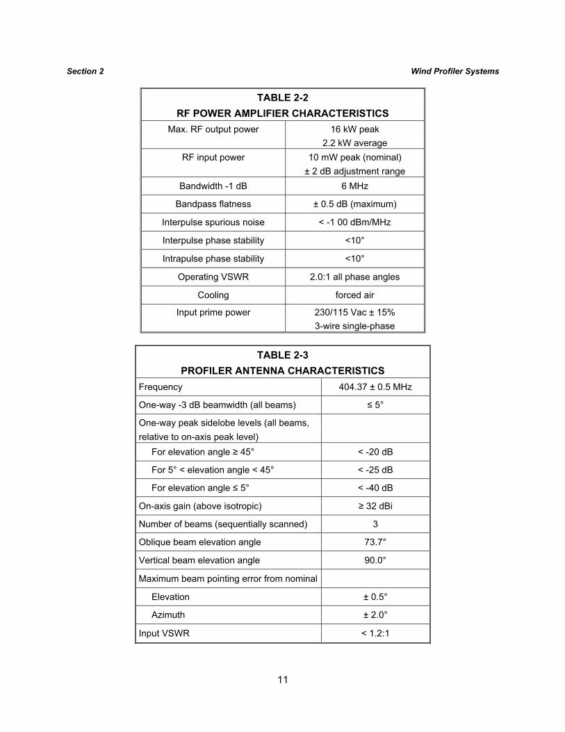
The radio frequency (RF) power amplifier accepts the low-level (10 mW) signal from the frequency generator and amplifies it for transmission. It consists of a redundant driver amplifier, which amplifies the signal to about 80 W, and a solid-state power amplifier consisting of 16 modules operating in parallel, each of which is capable of 1.2 kW peak output. Table 2-2 lists the power amplifier characteristics. The amplifier is typically run at an average power level of 1.5 kW average (11.6 kW peak) in the high modes and about 215 W average (6.5 kW peak) in the low modes.
Antenna
The profiler employs a coaxial-collinear (COCO) antenna for both transmission and reception. The antenna characteristics are listed in Table 2-3. Individual COCO elements are constructed from low-loss coaxial cable whose inner and outer conductors are exchanged every one-half wavelength inside the cable. The radiation characteristic of the COCO element is similar to feeding an equivalent number of collinear dipoles with equal amplitude and phase. The advantage is that the COCO elements require only one feed point as opposed to feeding the individual dipoles. One disadvantage is that each "dipole" in the row cannot be phased individually. This limitation is overcome by employing two orthogonal arrays with individual rows of elements that are phased to generate a beam broadside to the element axis. The profiler uses one array for the north and vertical beams, and the superimposed, orthogonal array for the east beam. The COCO elements are positioned about one-quarter wavelength above a metal mesh ground plane, and the resulting square arrays have a physical aperture of 100 m2. For reliability reasons, all the beam steering switches are inside the equipment shelter.
11
Section 2 Wind Profiler Systems
TABLE 2-2 RF POWER AMPLIFIER CHARACTERISTICS
Max. RF output power 16 kW peak 2.2 kW average
RF input power 10 mW peak (nominal) ± 2 dB adjustment range
Bandwidth -1 dB 6 MHz
Bandpass flatness ± 0.5 dB (maximum)
Interpulse spurious noise < -1 00 dBm/MHz
Interpulse phase stability <10°
Intrapulse phase stability <10°
Operating VSWR 2.0:1 all phase angles
Cooling forced air
Input prime power 230/115 Vac ± 15% 3-wire single-phase
TABLE 2-3
PROFILER ANTENNA CHARACTERISTICS Frequency 404.37 ± 0.5 MHz
One-way -3 dB beamwidth (all beams) ≤ 5°
One-way peak sidelobe levels (all beams, relative to on-axis peak level) For elevation angle ≥ 45° < -20 dB
For 5° < elevation angle < 45° < -25 dB
For elevation angle ≤ 5° < -40 dB
On-axis gain (above isotropic) ≥ 32 dBi
Number of beams (sequentially scanned) 3
Oblique beam elevation angle 73.7°
Vertical beam elevation angle 90.0°
Maximum beam pointing error from nominal
Elevation ± 0.5°
Azimuth ± 2.0°
Input VSWR < 1.2:1
12
Section 2 Wind Profiler Systems Receiver
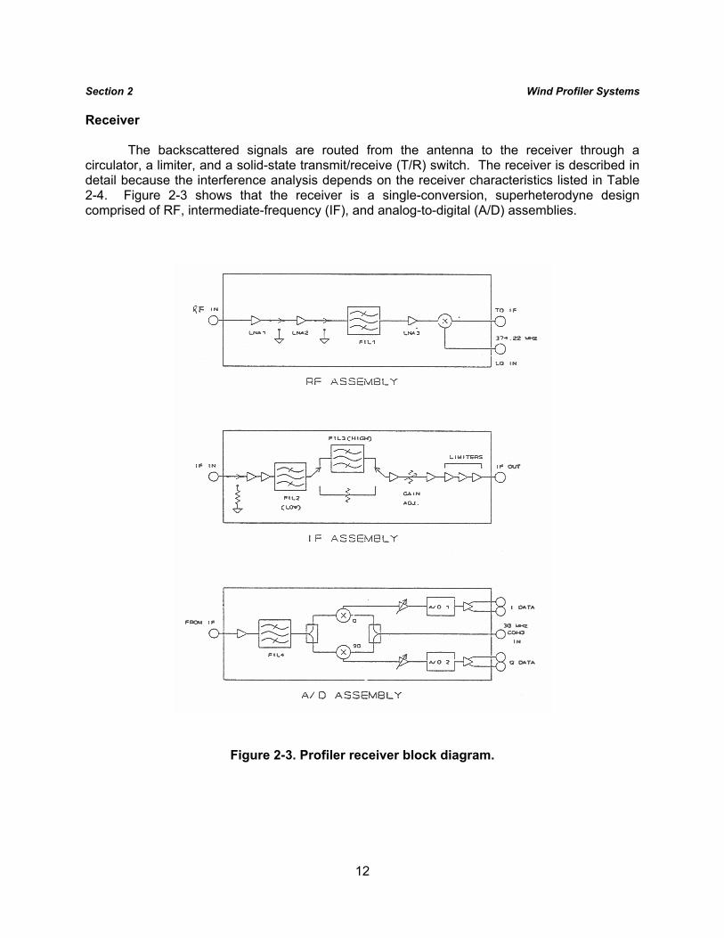
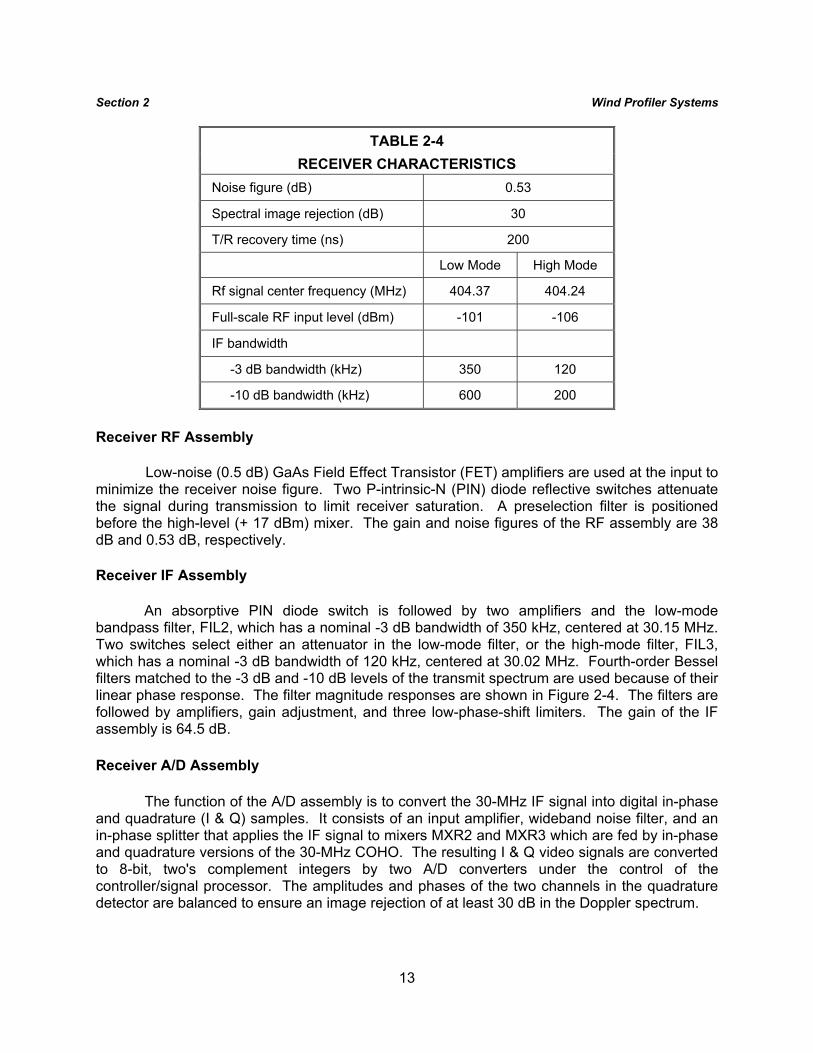
The backscattered signals are routed from the antenna to the receiver through a circulator, a limiter, and a solid-state transmit/receive (T/R) switch. The receiver is described in detail because the interference analysis depends on the receiver characteristics listed in Table 2-4. Figure 2-3 shows that the receiver is a single-conversion, superheterodyne design comprised of RF, intermediate-frequency (IF), and analog-to-digital (A/D) assemblies.
Figure 2-3. Profiler receiver block diagram.
13
Section 2 Wind Profiler Systems
TABLE 2-4 RECEIVER CHARACTERISTICS
Noise figure (dB) 0.53
Spectral image rejection (dB) 30
T/R recovery time (ns) 200
Low Mode High Mode
Rf signal center frequency (MHz) 404.37 404.24
Full-scale RF input level (dBm) -101 -106
IF bandwidth
-3 dB bandwidth (kHz) 350 120
-10 dB bandwidth (kHz) 600 200
Receiver RF Assembly
Low-noise (0.5 dB) GaAs Field Effect Transistor (FET) amplifiers are used at the input to minimize the receiver noise figure. Two P-intrinsic-N (PIN) diode reflective switches attenuate the signal during transmission to limit receiver saturation. A preselection filter is positioned before the high-level (+ 17 dBm) mixer. The gain and noise figures of the RF assembly are 38 dB and 0.53 dB, respectively.
Receiver IF Assembly
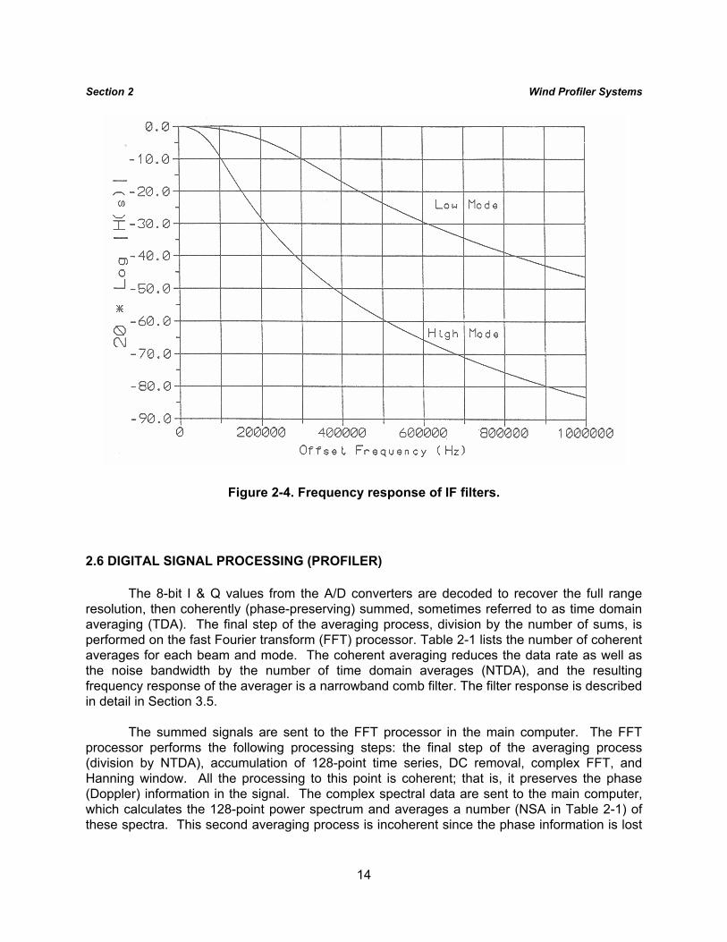
An absorptive PIN diode switch is followed by two amplifiers and the low-mode bandpass filter, FIL2, which has a nominal -3 dB bandwidth of 350 kHz, centered at 30.15 MHz. Two switches select either an attenuator in the low-mode filter, or the high-mode filter, FIL3, which has a nominal -3 dB bandwidth of 120 kHz, centered at 30.02 MHz. Fourth-order Bessel filters matched to the -3 dB and -10 dB levels of the transmit spectrum are used because of their linear phase response. The filter magnitude responses are shown in Figure 2-4. The filters are followed by amplifiers, gain adjustment, and three low-phase-shift limiters. The gain of the IF assembly is 64.5 dB.
Receiver A/D Assembly
The function of the A/D assembly is to convert the 30-MHz IF signal into digital in-phase and quadrature (I & Q) samples. It consists of an input amplifier, wideband noise filter, and an in-phase splitter that applies the IF signal to mixers MXR2 and MXR3 which are fed by in-phase and quadrature versions of the 30-MHz COHO. The resulting I & Q video signals are converted to 8-bit, two's complement integers by two A/D converters under the control of the controller/signal processor. The amplitudes and phases of the two channels in the quadrature detector are balanced to ensure an image rejection of at least 30 dB in the Doppler spectrum.
14
Section 2 Wind Profiler Systems
Figure 2-4. Frequency response of IF filters. 2.6 DIGITAL SIGNAL PROCESSING (PROFILER)
The 8-bit I & Q values from the A/D converters are decoded to recover the full range resolution, then coherently (phase-preserving) summed, sometimes referred to as time domain averaging (TDA). The final step of the averaging process, division by the number of sums, is performed on the fast Fourier transform (FFT) processor. Table 2-1 lists the number of coherent averages for each beam and mode. The coherent averaging reduces the data rate as well as the noise bandwidth by the number of time domain averages (NTDA), and the resulting frequency response of the averager is a narrowband comb filter. The filter response is described in detail in Section 3.5.
The summed signals are sent to the FFT processor in the main computer. The FFT
processor performs the following processing steps: the final step of the averaging process (division by NTDA), accumulation of 128-point time series, DC removal, complex FFT, and Hanning window. All the processing to this point is coherent; that is, it preserves the phase (Doppler) information in the signal. The complex spectral data are sent to the main computer, which calculates the 128-point power spectrum and averages a number (NSA in Table 2-1) of these spectra. This second averaging process is incoherent since the phase information is lost
15
Section 2 Wind Profiler Systems in the calculation of the power spectrum. The signal-to-noise ratio (SIN) increases linearly with coherent averaging time or the coherence time of the signal, whichever is less, and the signal detectability is improved by an amount equal to the square root of the number of incoherent averages. The total dwell time (in seconds) in any beam mode is ))()()(( NSANFFTNTDAPRTtdwell = , (1) where tdwell = the dwell time (s) NFFT = the number of FFT points (128) NSA = the number of (incoherent) spectral averages.
Using the values from Table 2-1, it is seen that the nominal dwell time for each beam in submode A is close to 1 minute. In submode B, the winter mode, the profiler spends more time in the high modes than in the low modes. This submode B is not currently in operational use.
The data processor removes ground clutter by replacing frequency components close to
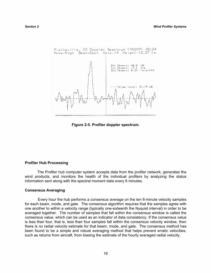
zero Doppler with values interpolated from neighboring points. At this point, the received spectra are ready for moment estimation, which consists of four main steps. The first step is to calculate the mean noise level using an objective algorithm.3 Once the noise level is determined, the algorithm scans for the peak in the spectrum using a five-point running average. This average is used to distinguish narrow noise peaks from the (presumably) wider atmospheric return. Once the peak is determined, the atmospheric signal is defined as that part of the original (unsmoothed) spectrum from the peak down to the noise level. Then the zeroth moment, representing the signal power; the first moment, representing the mean Doppler velocity; and the second moment, representing the velocity variance, are calculated. Figure 2-5 shows an actual Doppler spectrum with the noise level, the zeroth, first, and second spectral moments indicated. The three spectral moments for each beam, mode, and range gate are the raw data that are sent to Boulder every 6 minutes. The normal data message is approximately 3000 bytes.
3 Hildebrand, P.H. and Sekhon, R.S., Objective Determination of the Noise Level in
Doppler Spectra, Journal of Applied Meteorology, No. 13, October 1974.
16
Section 2 Wind Profiler Systems
Figure 2-5. Profiler doppler spectrum. Profiler Hub Processing
The Profiler hub computer system accepts data from the profiler network, generates the wind products, and monitors the health of the individual profilers by analyzing the status information sent along with the spectral moment data every 6 minutes.
Consensus Averaging
Every hour the hub performs a consensus average on the ten 6-minute velocity samples for each beam, mode, and gate. The consensus algorithm requires that the samples agree with one another to within a velocity range (typically one-sixteenth the Nyquist interval) in order to be averaged together. The number of samples that fall within the consensus window is called the consensus value, which can be used as an indicator of data consistency. If the consensus value is less than four, that is, less than four samples fall within the consensus velocity window, then there is no radial velocity estimate for that beam, mode, and gate. The consensus method has been found to be a simple and robust averaging method that helps prevent erratic velocities, such as returns from aircraft, from biasing the estimate of the hourly averaged radial velocity.
17
Section 2 Wind Profiler Systems Wind Calculation
For each of the 36 heights in the low and high modes, the horizontal wind is calculated from the consensus-averaged radial velocities from the three beams. If the radial velocity from any of the three beams is missing due to lack of consensus, the horizontal wind is not calculated. Missing winds are not interpolated or extrapolated. As an indicator of the quality of this wind calculation, one may ask, “What is the probability of a wind estimate in the absence of any signal?" Assuming uniformly distributed random velocities (as is the case for no systematic biases), the consensus average will generate a radial velocity with a probability of 0.0676 (6.76%). Since velocity estimates are required for all three beams, the probability of an erroneous wind estimate is 0.0003, or (0.03%).
In practice, one needs to be more concerned with systematic sources of error, such as
low-level signals emitted from the radar itself that are coupled in through the antenna, or ground clutter signals that are too wide or too strong to be handled by the clutter removal processing.
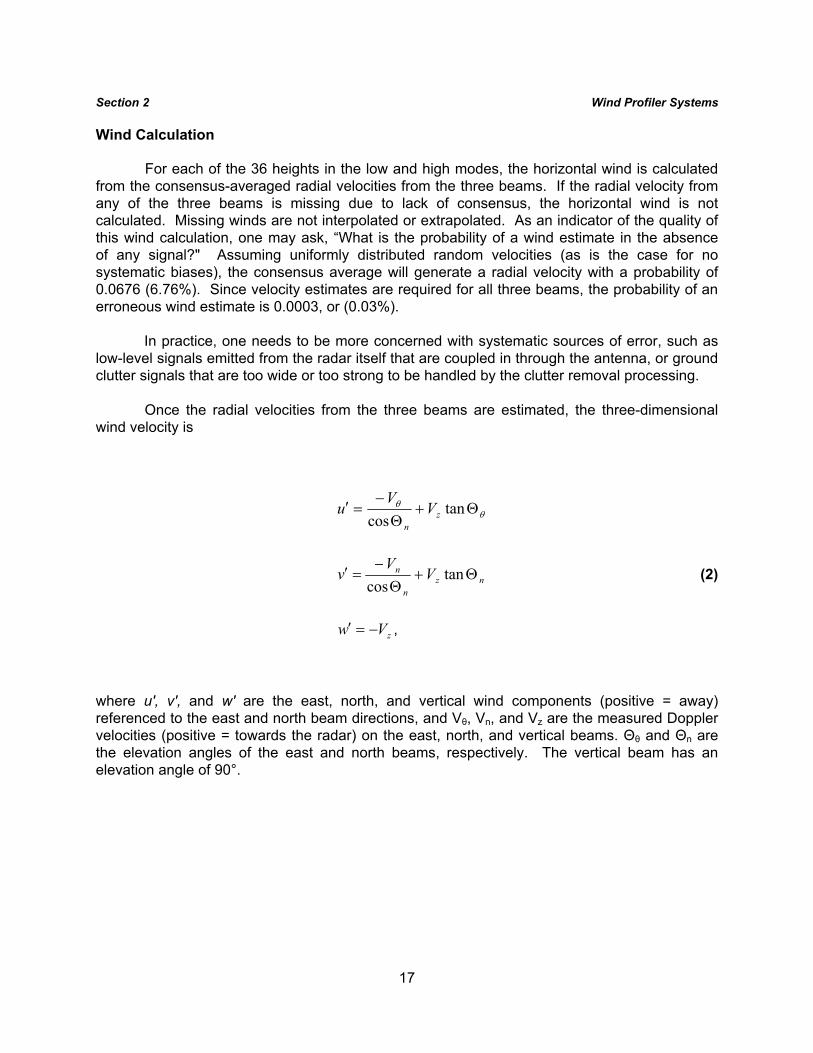
Once the radial velocities from the three beams are estimated, the three-dimensional
wind velocity is
θθ Θ+Θ
−=′ tan
cos zn
VV
u
nzn
n VV
v Θ+Θ
−=′ tan
cos (2)
zVw −=′ , where u′, v′, and w′ are the east, north, and vertical wind components (positive = away) referenced to the east and north beam directions, and Vθ, Vn, and Vz are the measured Doppler velocities (positive = towards the radar) on the east, north, and vertical beams. Θθ and Θn are the elevation angles of the east and north beams, respectively. The vertical beam has an elevation angle of 90°.
18
Section 2 Wind Profiler Systems
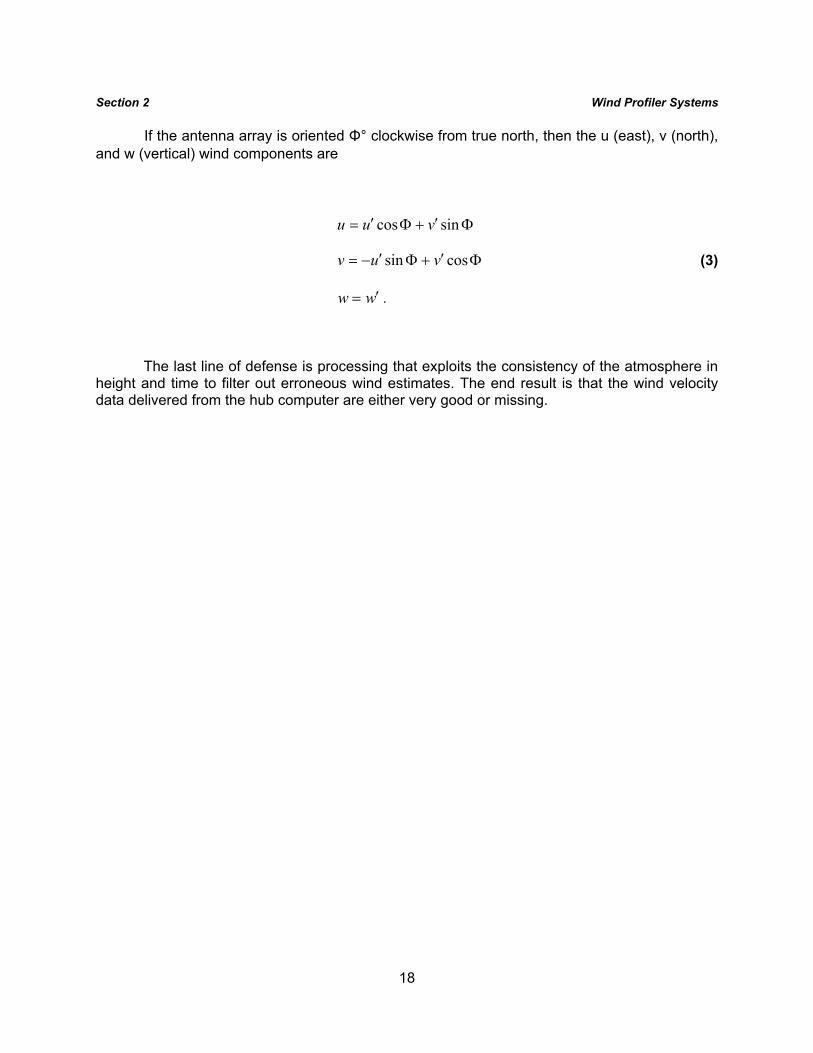
If the antenna array is oriented Φ° clockwise from true north, then the u (east), v (north), and w (vertical) wind components are
Φ′+Φ′= sincos vuu Φ′+Φ′−= cossin vuv (3) ww ′= .
The last line of defense is processing that exploits the consistency of the atmosphere in height and time to filter out erroneous wind estimates. The end result is that the wind velocity data delivered from the hub computer are either very good or missing.
19
SECTION 3 INTERFERENCE TO PROFILERS
3.1 INTRODUCTION
Given the information in Section 2, the effect of interference on profiler performance can be estimated. This requires a characterization of the interfering source in terms of its power level, distance, frequency spectrum, time dependence, etc. Sources of interference fall into two general categories: coherent and incoherent.
This section discusses coherent and incoherent interference, system noise temperature,
system frequency response, system noise power, and minimum detectable signal power. In addition, an interference analysis discussion is provided on the effects of frequency modulation (FM) and pulse type emissions on the wind profiler.
3.2 COHERENT INTERFERENCE
Coherent interference is potentially the most disruptive to profiler operation. This is because, by definition, a coherent interfering signal will be interpreted by the profiler as a valid signal in its Doppler spectrum. If the interfering signal is larger than the atmospheric return, it will be selected in the spectral moment calculations. If the signal frequency remained stable over the 1-minute dwell time for a beam and mode, it would be reported as the estimate of the radial velocity for that time period. Further, if the signal remained stable over a 1-hour period, then the erroneous Doppler velocity would pass consensus and form an erroneous indication of wind velocity.
Fortunately, the profiler has some built-in immunity to external stable signal sources. As
explained in Section 2.5, the profiler controller/processor applies a pseudorandom phase shift sequence in order to reduce range-ambiguous returns. Since the phase-shifted signal is used to generate both the transmitted pulse and the receiver LO, the radar maintains internal coherence throughout the averaging process. External stable signals, such as ground returns from distances greater than the PRT-determined unambiguous range, are reduced in the averaging process. One other effect of this phase shift is to "whiten" any external, stable (CW) sources of interference. For an external system to remain truly coherent, it would have to detect the phase of the profiler pulse and shift its phase accordingly. Short of a sophisticated and intentional jamming effort, the probability of a truly coherent interfering signal is very small. The phase code cancellation is not perfect. On average, it provides about 20 dB of reduction. The effect of the pseudorandom coding is to place even highly stable real-world signals, such as data or voice FM signals, into the second category of interference.
3.3 INCOHERENT INTERFERENCE (NOISE)
Any interfering signal that is whitened by the phase code or any source of broadband noise will raise the system noise level, thereby degrading the system S/N. The effect of the added noise on profiler operation is to reduce the height coverage of the radar. However, it must be emphasized that there is no simple rule that can be used to determine that on any particular day a particular noise level increase will decrease the height coverage by some value.
20
Section 3 Interference To Profilers The reason is the high dynamic range of the turbulence that accounts for the profiler radar returns. The turbulence structure parameter, Cn
2, may vary by 20 dB daily and 20 dB annually. The profilers have been designed with enough sensitivity to provide their designed height coverage most of the time. However, due to the variable nature of the returns there will be times when the profiler is unable to measure the winds at certain heights. At other times, the signals from all heights are strong enough that a S/N degradation on the order of 3 dB may not result in any loss of wind velocity measurements, although the uncertainty of the wind estimates may increase.
Based on analysis from years of profiler data, there has emerged a simple rule of thumb for the decrease in Cn
2 versus height.4 It is generally accepted that it falls off at 1 to 2 dB per kilometer in the atmosphere above the boundary layer, which is typically 1 km. Therefore, one may state that, on average, an increase of x dB of system noise will result in about x/2 to x km loss in profiler height coverage. The lost wind data may not be at the highest gates since the lowest atmospheric turbulence sometimes occurs in layers that are sampled by the middle group of range gates. For example, the uniform winds in the jet stream at about 12 km altitude often lack the turbulence required to produce strong profiler radar returns. Under these conditions, the profiler may be operating at the limits of its signal detection capability. Any degradation in the S/N would result in lost wind estimates for the center of the jet stream while the enhanced turbulence above and below the jet stream would allow for normal wind measurements.
For the purposes of this analysis, we calculate the interference levels necessary to
degrade the profiler system S/N by nearly 1 dB. An interference power level equal to 0.25 of the system noise power corresponds to an interference-to-noise ratio (I/N) of -6 dB which results in nearly 1 dB S/N degradation. We do not claim that this is an acceptable level of interference. Under some atmospheric conditions this level of interference could degrade the profiler height coverage from 0.5 to 1 km and may not be acceptable to the owner of the profiler. However, given the techniques outlined here and using a suitable model for propagation loss, one may calculate interference levels or separation distances for various interference sources for an assumed I/N.
3.4 SYSTEM NOISE TEMPERATURE
The profiler system operating temperature in degrees Kelvin, referenced to the antenna terminals, is5
4 Nastrom, G.D., Gage, K.S., Ecklund, S.L., Variability of Turbulence, 4--20km, in
Colorado and Alaska from MST Radar Observations, J. Geophys. Res. Vol. 91, 1986. 5 Skolnik, H.I., Radar Handbook, 1970, McGraw-Hill, Inc.
21
Section 3 Interference To Profilers
( ) rlltla
taa
gtg
gsky
sys TllTl
Tl
TTT
T
T +−+⎟⎟⎠
⎞⎜⎜⎝
⎛−+
+⎟⎟⎠
⎞⎜⎜⎝
⎛−
= 111
1
, (4)
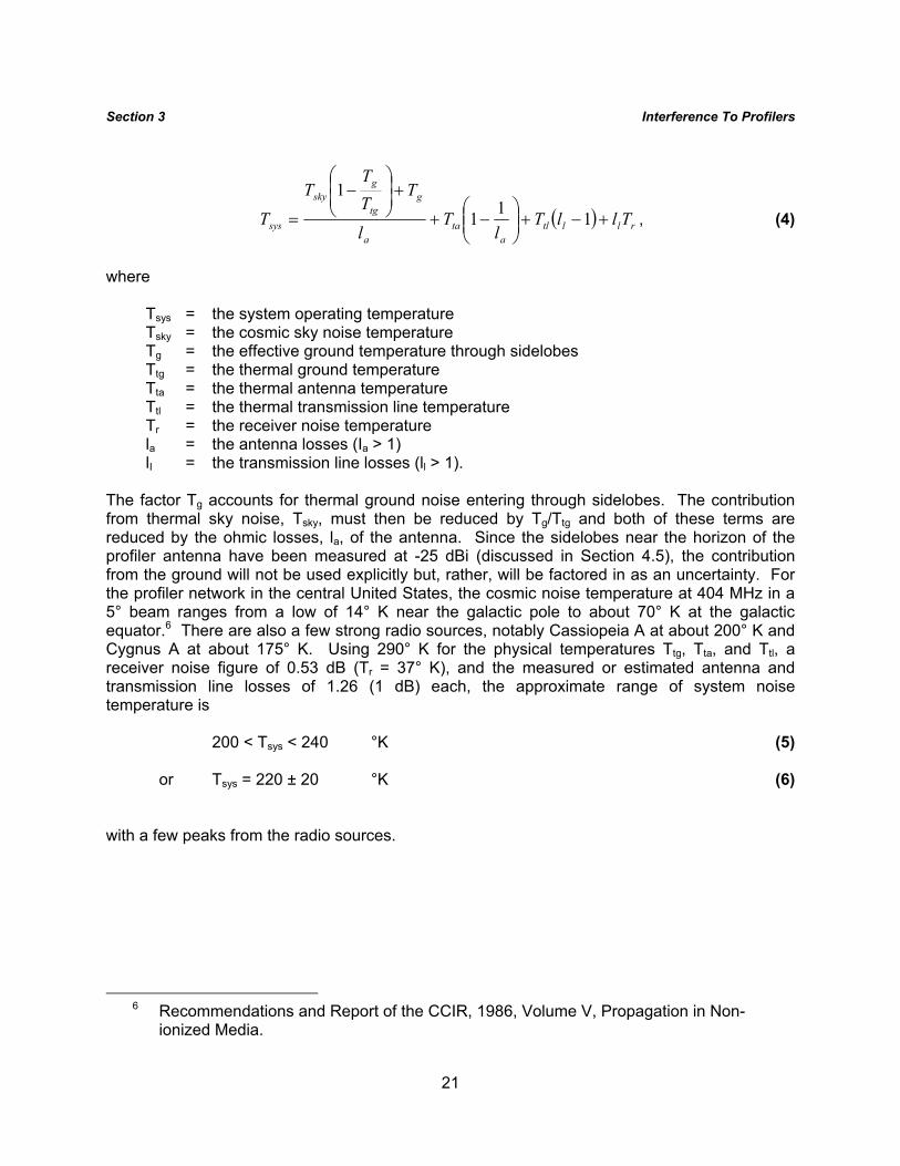
where Tsys = the system operating temperature Tsky = the cosmic sky noise temperature Tg = the effective ground temperature through sidelobes Ttg = the thermal ground temperature Tta = the thermal antenna temperature Ttl = the thermal transmission line temperature Tr = the receiver noise temperature la = the antenna losses (Ia > 1) lI = the transmission line losses (ll > 1). The factor Tg accounts for thermal ground noise entering through sidelobes. The contribution from thermal sky noise, Tsky, must then be reduced by Tg/Ttg and both of these terms are reduced by the ohmic losses, la, of the antenna. Since the sidelobes near the horizon of the profiler antenna have been measured at -25 dBi (discussed in Section 4.5), the contribution from the ground will not be used explicitly but, rather, will be factored in as an uncertainty. For the profiler network in the central United States, the cosmic noise temperature at 404 MHz in a 5° beam ranges from a low of 14° K near the galactic pole to about 70° K at the galactic equator.6 There are also a few strong radio sources, notably Cassiopeia A at about 200° K and Cygnus A at about 175° K. Using 290° K for the physical temperatures Ttg, Tta, and Ttl, a receiver noise figure of 0.53 dB (Tr = 37° K), and the measured or estimated antenna and transmission line losses of 1.26 (1 dB) each, the approximate range of system noise temperature is 200 < Tsys < 240 °K (5) or Tsys = 220 ± 20 °K (6) with a few peaks from the radio sources.
6 Recommendations and Report of the CCIR, 1986, Volume V, Propagation in Non-
ionized Media.
22
Section 3 Interference To Profilers 3.5 SYSTEM FREQUENCY RESPONSE
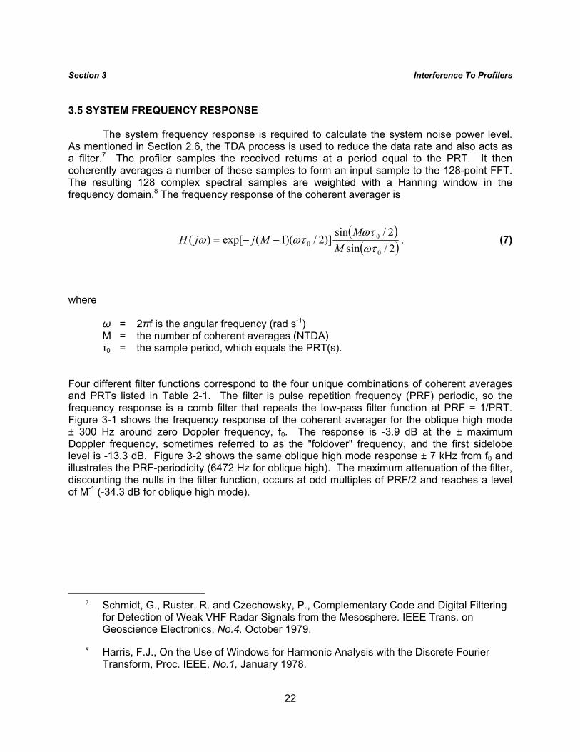
The system frequency response is required to calculate the system noise power level. As mentioned in Section 2.6, the TDA process is used to reduce the data rate and also acts as a filter.7 The profiler samples the received returns at a period equal to the PRT. It then coherently averages a number of these samples to form an input sample to the 128-point FFT. The resulting 128 complex spectral samples are weighted with a Hanning window in the frequency domain.8 The frequency response of the coherent averager is
( )( )2/sin
2/sin)]2/)(1(exp[)(
0
00 ωτ
ωτωτω
MM
MjjH −−= , (7)
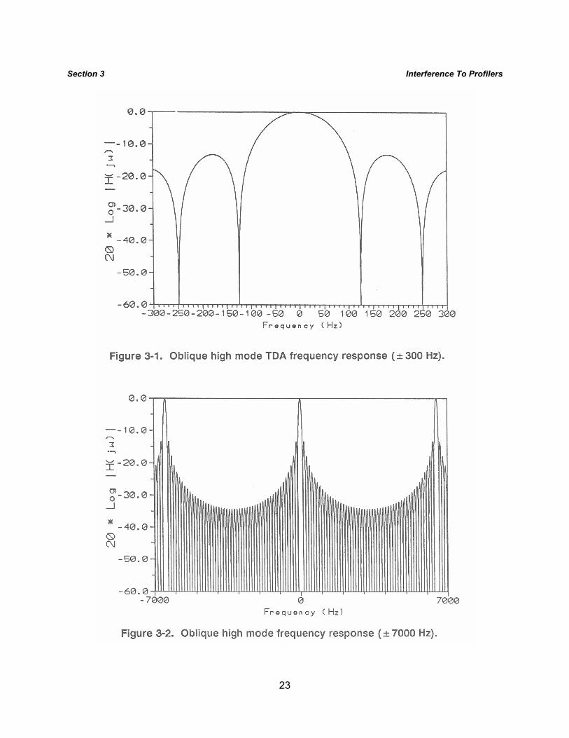
where ω = 2πf is the angular frequency (rad s-1) M = the number of coherent averages (NTDA) τ0 = the sample period, which equals the PRT(s). Four different filter functions correspond to the four unique combinations of coherent averages and PRTs listed in Table 2-1. The filter is pulse repetition frequency (PRF) periodic, so the frequency response is a comb filter that repeats the low-pass filter function at PRF = 1/PRT. Figure 3-1 shows the frequency response of the coherent averager for the oblique high mode ± 300 Hz around zero Doppler frequency, f0. The response is -3.9 dB at the ± maximum Doppler frequency, sometimes referred to as the "foldover" frequency, and the first sidelobe level is -13.3 dB. Figure 3-2 shows the same oblique high mode response ± 7 kHz from f0 and illustrates the PRF-periodicity (6472 Hz for oblique high). The maximum attenuation of the filter, discounting the nulls in the filter function, occurs at odd multiples of PRF/2 and reaches a level of M-1 (-34.3 dB for oblique high mode).
7 Schmidt, G., Ruster, R. and Czechowsky, P., Complementary Code and Digital Filtering
for Detection of Weak VHF Radar Signals from the Mesosphere. IEEE Trans. on Geoscience Electronics, No.4, October 1979.
8 Harris, F.J., On the Use of Windows for Harmonic Analysis with the Discrete Fourier
Transform, Proc. IEEE, No.1, January 1978.
23
Section 3 Interference To Profilers
24
Section 3 Interference To Profilers
The Nyquist interval for the Doppler spectrum is (τ0 M)-1, which is PRF/M. Figure 3-2 illustrates that the coherent averager reduces the noise bandwidth by an amount proportional to the number of coherent averages. The corresponding statistical explanation is that coherently averaging a signal in the presence of noise improves the S/N by an amount equal to the number of averages (provided the signal maintains coherence over the averaging period).
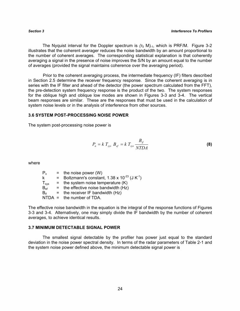
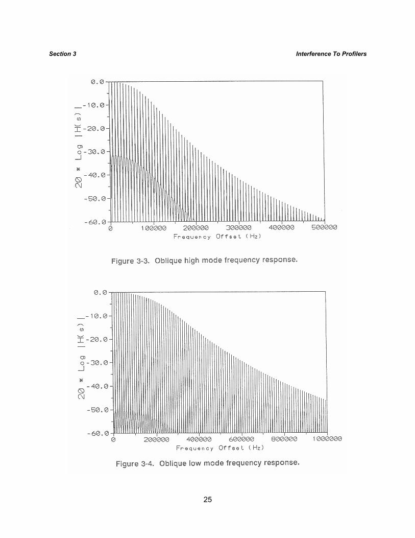
Prior to the coherent averaging process, the intermediate frequency (IF) filters described
in Section 2.5 determine the receiver frequency response. Since the coherent averaging is in series with the IF filter and ahead of the detector (the power spectrum calculated from the FFT), the pre-detection system frequency response is the product of the two. The system responses for the oblique high and oblique low modes are shown in Figures 3-3 and 3-4. The vertical beam responses are similar. These are the responses that must be used in the calculation of system noise levels or in the analysis of interference from other sources.
3.6 SYSTEM POST-PROCESSING NOISE POWER The system post-processing noise power is
NTDAB
TkBTkP ifsysefsysn == (8)
where Pn = the noise power (W) k = Boltzmann's constant, 1.38 x 10⁻²³ (J K-1) Tsys = the system noise temperature (K) Bef = the effective noise bandwidth (Hz) Bif = the receiver IF bandwidth (Hz) NTDA = the number of TDA. The effective noise bandwidth in the equation is the integral of the response functions of Figures 3-3 and 3-4. Alternatively, one may simply divide the IF bandwidth by the number of coherent averages, to achieve identical results. 3.7 MINIMUM DETECTABLE SIGNAL POWER
The smallest signal detectable by the profiler has power just equal to the standard deviation in the noise power spectral density. In terms of the radar parameters of Table 2-1 and the system noise power defined above, the minimum detectable signal power is
25
Section 3 Interference To Profilers
26
Section 3 Interference To Profilers
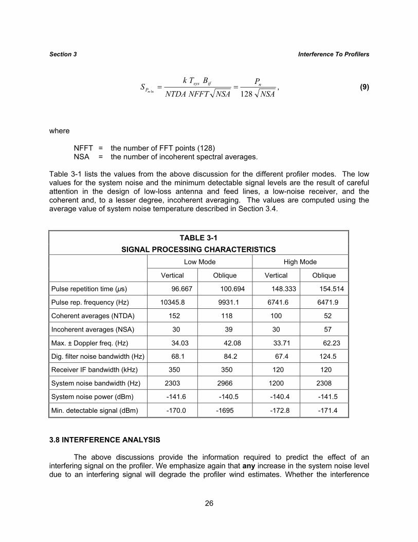
NSAP
NSANFFTNTDA
BTkS nifsysPm 128ln
== , (9)
where NFFT = the number of FFT points (128) NSA = the number of incoherent spectral averages. Table 3-1 lists the values from the above discussion for the different profiler modes. The low values for the system noise and the minimum detectable signal levels are the result of careful attention in the design of low-loss antenna and feed lines, a low-noise receiver, and the coherent and, to a lesser degree, incoherent averaging. The values are computed using the average value of system noise temperature described in Section 3.4.
TABLE 3-1 SIGNAL PROCESSING CHARACTERISTICS
Low Mode High Mode
Vertical Oblique Vertical Oblique
Pulse repetition time (µs) 96.667 100.694 148.333 154.514
Pulse rep. frequency (Hz) 10345.8 9931.1 6741.6 6471.9
Coherent averages (NTDA) 152 118 100 52
Incoherent averages (NSA) 30 39 30 57
Max. ± Doppler freq. (Hz) 34.03 42.08 33.71 62.23
Dig. filter noise bandwidth (Hz) 68.1 84.2 67.4 124.5
Receiver IF bandwidth (kHz) 350 350 120 120
System noise bandwidth (Hz) 2303 2966 1200 2308
System noise power (dBm) -141.6 -140.5 -140.4 -141.5
Min. detectable signal (dBm) -170.0 -1695 -172.8 -171.4
3.8 INTERFERENCE ANALYSIS
The above discussions provide the information required to predict the effect of an interfering signal on the profiler. We emphasize again that any increase in the system noise level due to an interfering signal will degrade the profiler wind estimates. Whether the interference
27
Section 3 Interference To Profilers results in lost profiler height coverage depends on the highly variable atmospheric signals and cannot be determined a priori. However, using the 1-2 dB per kilometer rule of thumb discussed in Section 3.3, one can estimate the loss of height coverage for a particular interference level. We analyze the interference level referenced to the receiver input for typical FM and pulsed type interference since these types of signals are representative of systems operating in the band. On-Tune FM
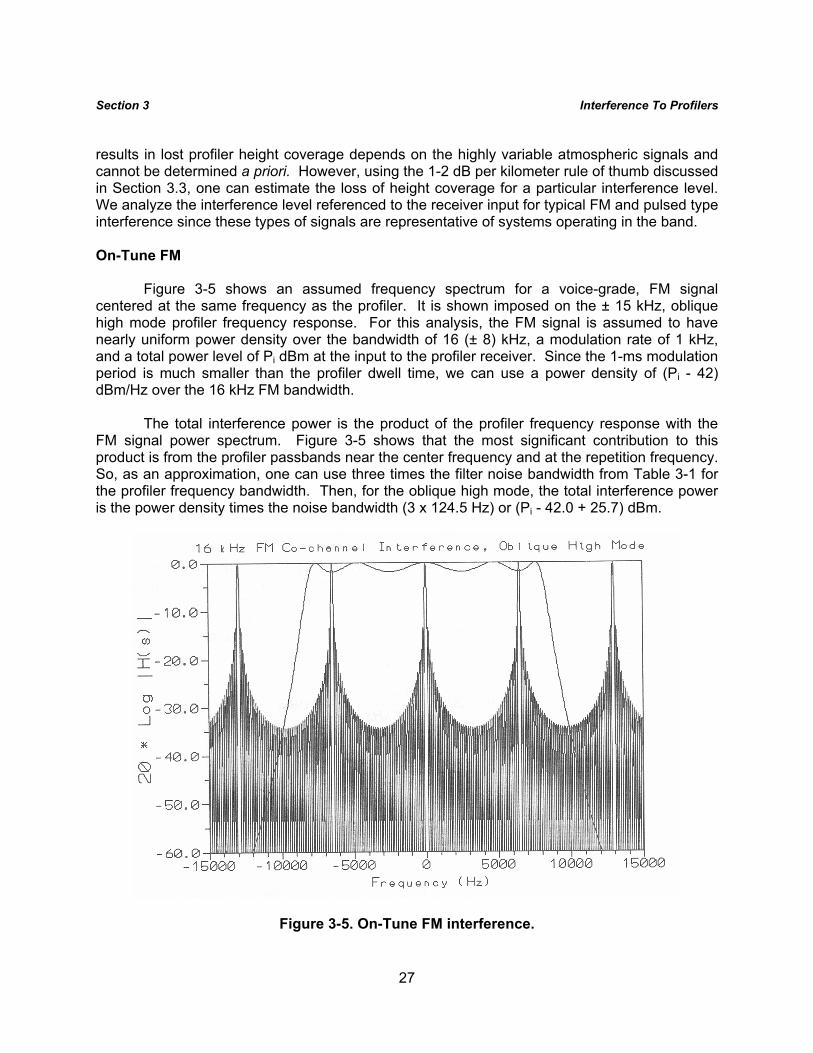
Figure 3-5 shows an assumed frequency spectrum for a voice-grade, FM signal centered at the same frequency as the profiler. It is shown imposed on the ± 15 kHz, oblique high mode profiler frequency response. For this analysis, the FM signal is assumed to have nearly uniform power density over the bandwidth of 16 (± 8) kHz, a modulation rate of 1 kHz, and a total power level of Pi dBm at the input to the profiler receiver. Since the 1-ms modulation period is much smaller than the profiler dwell time, we can use a power density of (Pi - 42) dBm/Hz over the 16 kHz FM bandwidth.
The total interference power is the product of the profiler frequency response with the
FM signal power spectrum. Figure 3-5 shows that the most significant contribution to this product is from the profiler passbands near the center frequency and at the repetition frequency. So, as an approximation, one can use three times the filter noise bandwidth from Table 3-1 for the profiler frequency bandwidth. Then, for the oblique high mode, the total interference power is the power density times the noise bandwidth (3 x 124.5 Hz) or (Pi - 42.0 + 25.7) dBm.
Figure 3-5. On-Tune FM interference.
28
Section 3 Interference To Profilers
Using the system noise levels for the four modes in Table 3-1, the average FM power levels required for an I/N of -6 dB are calculated using the following formula [(system noise power (dBm)) + 16.3 - 6]
oblique high -131.2 dBm oblique low -130.2 dBm vertical high -130.1 dBm vertical low -131.2 dBm. Off-Tune FM
If the same FM signal operated at a center frequency 1 MHz away from the profiler center frequency, Figure 2-4 shows that the low-mode and high-mode IF filters provide more than 45 dB and 80 dB of rejection, respectively. Therefore, interference signal levels at the receiver input of -85 dBm for the low mode, and -55 dBm for the high mode are required for an I/N of -6 dB. This type of off-tune analysis is limited to power levels that do not force any stage of the receiver prior to the limiters into nonlinear operation.
On-Tune Non-FM Radar
The wind profiler receiver is susceptible to two forms of interference. The first interference mechanism affects the limiter diodes described in Section 2.5 and shown in the IF section of Figure 2-3. The limiters saturate at a receiver input power level of -106 and -101 dBm for the high and low mode, respectively, for signals in the IF pass band.
For the simple pulsed radar case, we assume a 1-µs pulse width (PW) and a pulse
repetition frequency (PRF) of 300 Hz (PRT = 3.33 ms). The transmit spectrum of the radar has lines spaced at 300 Hz enveloped by a sinc function with a first-null bandwidth of ± 1 MHz. Since the interfering pulse has a nominal (3 dB) bandwidth of 1 MHz which is larger than the IF bandwidth of the profiler, the peak interference power levels at the receiver input required to activate the limiters are
dBmkHzMHz 88
1201log20106 −≈⎟⎟
⎠
⎞⎜⎜⎝
⎛+− (10)
for the high mode, and
dBmkHzMHz 92
3501log20101 −≈⎟⎟
⎠
⎞⎜⎜⎝
⎛+− (11 )
for the low mode. If the interference power exceeds these levels, the wind profiler receiver will
29
Section 3 Interference To Profilers experience gain compression resulting in a decrease in the desired signal level. If the desired signal level is at a minimum level, the loss of signal due to gain compression could result in performance degradation of the wind profiler. The gain compression would occur for the time duration of the interfering signal plus any time associated with the recovery time of the limiter circuitry. However, the duty cycle of this event should be relatively small for typical radar signals representing operations in the 420-450 MHz band.
The second interference mechanism affects the detection process of the wind profiler receiver. When the interference adds noise to the receiver it affects the signal processing by reducing the signal-to-noise ratio in the detection circuitry. The interference power that is of concern to the detection process is limited (by the above mentioned limiters) to -88 dBm for the high mode and -92 dBm for the low mode. These peak power levels correspond to average powers of -123 and -127 dBm, respectively. If we assume that all of the average is confined to the 2-MHz first-null bandwidth and multiply this spectrum with the profiler frequency response (shown in Figures 3-3 and 3-4), we find that the total interfering power levels seen by the profiler are:
oblique high -149 dBm oblique low -152 dBm vertical high -152 dBm vertical low -153 dBm. Since these levels are about 10 dB below the system noise power for each mode, we would expect about 0.5 dB increase in noise and little significant interference to the profiler.
These results show that, for an interfering radar with the above assumed characteristics, interference power levels below -88 dBm for the high mode and -92 dBm for the low mode will have a minimum impact on the wind profiler detection process. At interference power levels above these values, the wind profiler receiver could experience gain compression effects. However, as explained later, the range-doppler processing capabilities of the wind profiler receiver should offer a considerable degree of immunity to low duty cycle interference such as that from radars operating in the 420-450 MHz band. Thus, the gain compression effects will probably not cause degradation until the threshold levels (-88 and -92 dBm) are exceeded by a considerable margin.
Off-Tune Non-FM Radar
As in the FM case above, the additional protection provided by the IF filters decreases the interference power by 45 and 80 dB for the low and high modes when the interfering radar is tuned 1 MHz off the profiler center frequency.
On-Tune Chirped Radar
We assume an interfering radar employs a 5-MHz chirped pulse width of 10 µs and a pulse repetition frequency of 300 Hz (PRT = 3.33 ms). The transmit spectrum could have a ± 2.5 MHz bandwidth. As in the case of non-FM radar above, the profiler receiver limiters could
30
Section 3 Interference To Profilers saturate and gain compression occur. The peak interference power levels that could result in initiation of limiting are -74 dBm for the high mode and -78 dBm for the low mode. At these levels, the average interference power levels in the noise filter would be oblique high -132 dBm oblique low -135 dBm vertical high -135 dBm vertical low -136 dBm. These levels are 5 to 9 dB above the system noise levels for each mode, so we would expect the effect of the interfering radar to be detectable. Off-Tune Chirped Radar
Since the interference of the co-channel radar described above is 5 to 9 dB above the system noise, we would expect that an adjacent channel chirped radar that is off-tuned sufficiently to realize 15 to 20 dB of frequency rejection due to the IF filters (see Figure 2-4) would not degrade the profiler detection process. That is, if the chirped bandwidth (± 2.5 MHz) is off-tuned by at least 500 kHz (i.e., a frequency difference of 3 MHz between the center frequency of the radar spectrum and the profiler tuned frequency), the radar signal would be sufficiently attenuated to protect the detection process. However, as above, peak power levels in an adjacent band large enough to saturate the limiters could cause interference.
Effect of Range-Doppler Processing
By considering the nature of interfering signals in the time domain, we discover that profilers enjoy a considerable degree of immunity from low duty cycle interference such as the radars described above. Since the profiler separates the returned signals in range and processes returns from thousands of pulses to obtain the Doppler information, it is unlikely that an interfering pulsed radar will maintain sufficient time or frequency coherence to interfere with a particular range-Doppler bin. For low duty cycle (e.g., < 1.0 %) pulsed interference, interfering signal levels of 50 dB above the receiver noise level can be suppressed due to range-Doppler processing.
31
SECTION 4 WIND PROFILER MEASUREMENTS
4.1 INTRODUCTION
The following measurements were conducted on the Unisys wind profiler system at Platteville, Colorado:
1. Profiler short-pulse and long-pulse radiated emission spectra; 2. Profiler radiated harmonic and subharmonic amplitudes relative to the center
frequency amplitude; 3. Filter characteristics associated with the profiler’s antenna; 4. Horizontal gain of the profiler antenna at ground level relative to an isotropic
antenna; 5. Susceptibility of the profiler to various waveforms that represent typical systems
operating in the 440-450 MHz band; and 6. Effects of profiler emissions on a typical receiver that is representative of land
mobile/amateur operations. The procedures and results for each of these measurements are described below. 4.2 EMISSION SPECTRUM MEASUREMENTS
The wind profiler radar operates in two range modes: low altitude and high altitude. The profiler pulses are phase coded. The high-mode pulse width is 20 µs, broken into three phase chips of 6.67 µs each, and the low-mode pulse width is 3.3 µs broken into two phase chips of 1.67 µs each.
The wind profiler radar operates in both a low-altitude mode and a high-altitude mode on
each of three beams (east, north, and vertical), for a total of six radiation modes. Normally, the wind profiler radar operates in each beam mode for 1 minute and switches through all six modes in 6 minutes. The wind profiler radar's mode progression, using a nomenclature where H and L stand for high and low, respectively, and E, N, and V stand for east, north, and vertical, respectively, is HE, LE, HN, LN, HV, LV. This means that the transmitter changes pulse widths once every minute, and likewise the profiler's radiated spectrum changes once every minute. If a measurement is to be made on a single radiated mode, then either that measurement must be made in less than one minute, or the profiler must be taken out of normal operation and locked into a single mode for the duration of the measurement.
A wideband spectrum measurement of the profiler was required in both pulse modes.
It was initially assumed that operating a spectrum analyzer with a peak-hold detector in a maximum-hold mode while sweeping across the frequency band of interest would suffice for this
32
Section 4 Wind Profiler Measurements measurement. However, such a technique was determined to be inadequate for our measurements. The spectrum of primary interest for the profiler extends from 385 to 425 MHz, and within this range the amplitude of the profiler's emissions can be expected to vary by as much as 110 dB. The instantaneous dynamic range of a spectrum analyzer will typically be only about 60-70 dB. Thus, a swept measurement across the entire band will result either in saturation of the spectrum analyzer at the profiler's center frequency, or in loss of the profiler's spectrum in the measurement system's thermal noise across parts of the band.
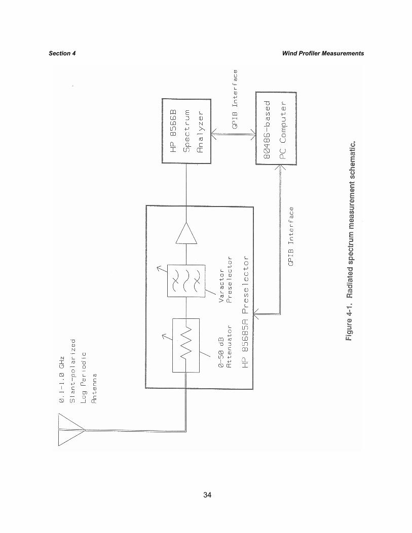
To overcome this limitation, a 0-50 dB RF attenuator was installed ahead of the spectrum analyzer as part of a Hewlett Packard 85685A preselector. Such an attenuator can extend the available dynamic range by 50 dB, for a total available measurement dynamic range of 110 dB. The HP 85685A also provided varactor preselection for the measurement system. The drawback of this arrangement is that the attenuation must be varied as a function of the frequency being measured. This means that a measurement of the profiler's spectrum cannot be performed in a swept-frequency analyzer mode. Rather, the spectrum analyzer must be tuned to a frequency, the attenuation must be adjusted at that frequency, and then the emission amplitude can be measured at that frequency. Then, the entire process must be repeated at the next frequency of interest. This means that the spectrum analyzer must be stepped, not swept, in frequency across the band to be measured. To ensure that all energy in the emission spectrum is convolved in the measurement bandwidth, the increment of each step must be less than or equal to the measurement bandwidth.
The optimum theoretical measurement bandwidth for this project would be approximately
1/compressed pulse width. (An accurate peak power measurement at the center frequency cannot be made in a bandwidth narrower than this; if a measurement is made with a bandwidth wider than this, the measured peak power amplitude will be accurate, but the sideband amplitudes will increase relative to the center-frequency amplitude.) Thus, for the high-altitude (long pulse) mode, the measurement bandwidth should be close to 1/τ = 1/6.67 X 10-6 = 150 kHz, and the optimum bandwidth for the low-altitude (short pulse) mode measurement would be 1/τ = 1/1.67 x 10-6 = 600 kHz. The nearest available measurement bandwidths in the spectrum analyzer were 100 and 300 kHz for the two modes.
Given that these are the measurement bandwidths, the step sizes for frequency tuning
in these measurements must be equal to or less than 100 and 300 kHz for the high and low profiler modes, respectively. This means that, for complete coverage of the 385-425 MHz band, the high and low modes have to be measured in 400 steps and 133 steps, respectively. Allowing 0.1 seconds per measurement step, plus overhead time for analyzer tuning, etc., means that the high and low modes can be measured across the band in 3 minutes and 1 minute, respectively. But the profiler switches directional beams and pulse widths once every minute. This means that a broad dynamic range measurement over the frequency band of interest cannot be performed when the profiler is in its normal mode of operation. As a result, the measurements require that wind profiler personnel lock the profiler into a single beam direction and pulse width for the duration of the measurement. (This is what was done at Platteville, where the profiler was locked into the high and low east beam modes.) The absolute power measured at the center frequency will vary as a function of beam mode and the position of the measurement system in the beam,
33
Section 4 Wind Profiler Measurements but the profiler's relative emission spectrum (amplitudes at sideband frequencies relative to the main beam level) does not depend on the beam mode or position of the measurement system.
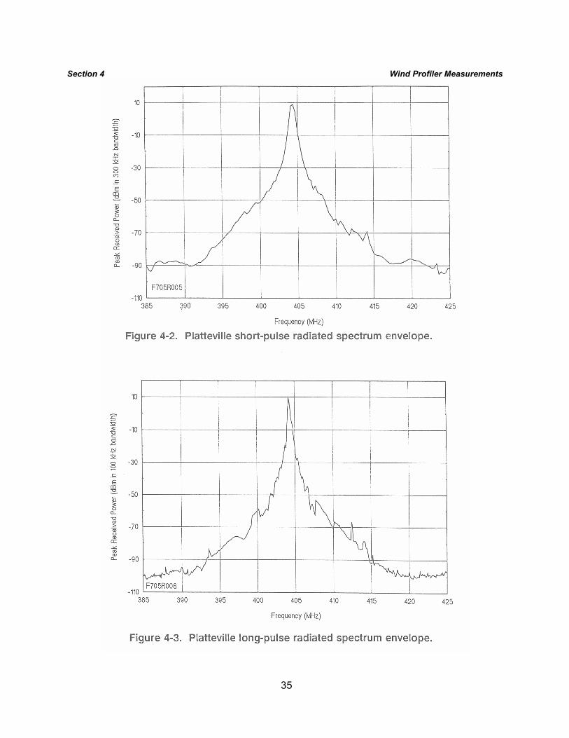
Figure 4-1 shows the schematic measurement arrangement for the radiated profiler spectrum measurement. Because of the emitter's low duty cycle, peak detection was used for the measurements. The measurement was made repeatedly, and the resulting spectra were highly repeatable. Figures 4-2 and 4-3 show the envelope of the short-pulse and long-pulse radiated spectra that were measured. The slightly "rough" features in the spectrum near 412-414 MHz were verified as belonging to the profiler, and were not emissions from other sources. The actual radiated spectra have lines within the envelope with a spacing of PRF/64.
4.3 HARMONIC AND SUBHARMONIC RADIATED POWER MEASUREMENTS
Measurements of the profiler's harmonic and subharmonic power levels relative to the fundamental were performed. The first three radiated harmonic levels and the first radiated subharmonic level were compared to the power received at the center frequency. The level of a harmonic relative to the center frequency level will not depend on the profiler's beam mode.
The measurement arrangement is shown in Figure 4-4. Improperly filtered measurement
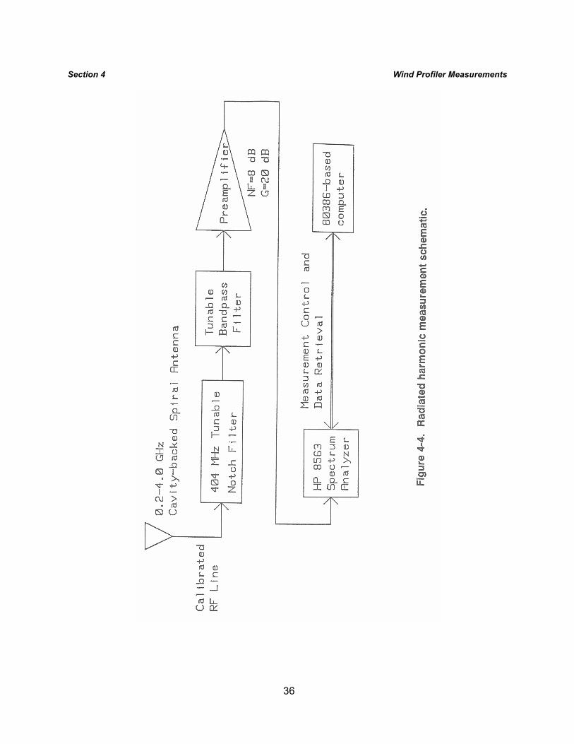
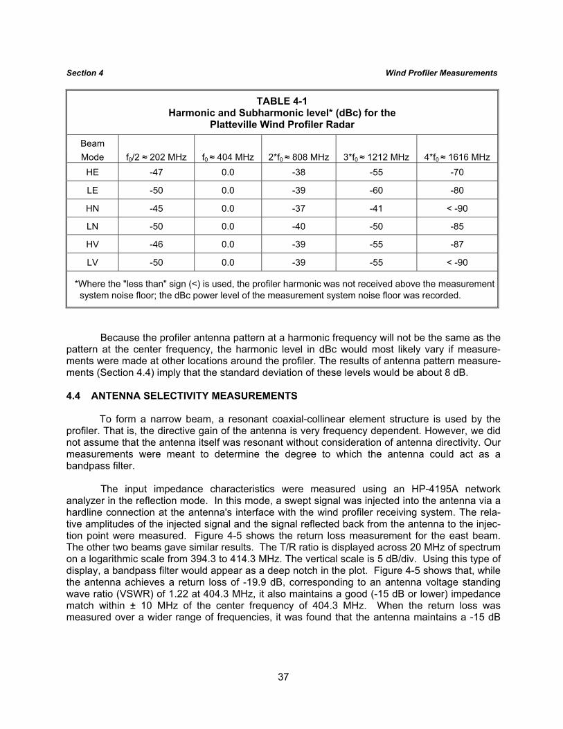
systems can generate false harmonics. To eliminate this problem, a notch filter tuned to the profiler's center frequency was used ahead of the spectrum analyzer. The notch was used for all measurements except, of course, the measurement of the profiler's fundamental frequency emission. A noise diode calibration was performed through the notch, the RF line, and the spectrum analyzer. A bandwidth wider than the profiler emission bandwidth must be used for this type of measurement. A 300-kHz bandwidth was used for these measurements. The measurement system noise figure was 8 dB, and the preamp gain was 25 dB. The calibration factors are included in the results of this measurement, summarized in Table 4-1.
The profiler emissions at the center frequency were typically measured at about -10 to
-20 dBm at the input to the spectrum analyzer. The center frequency power observed varied with the beam mode, both because the profiler's actual power varies between high mode and low mode and also because the profiler's antenna pattern changes with beam direction. The decibels relative to carrier amplitude (dBc) values recorded at the harmonics represent the "average" reading interpreted from the changing spectrum analyzer display; actual power levels were observed to vary by about ± 3 dB while measurements were in progress. Wind profiler measurements showed that subharmonic (202 MHz) and second (808 MHz) and third harmonic (1212 MHz) emissions were in the range of 37 to 60 dB down from the fundamental. Fourth harmonic (1616 MHz) levels were at least 70 dB down from the fundamental.
Subsequently, additional harmonic and subharmonic measurements were made at
several locations around the Unisys profiler. These measurements were conducted to determine if significant variability in received power could occur as a function of location. The results of measurements indicated that no significant variability existed (± 3 dB) as a function of location.
34
Section 4 Wind Profiler Measurements
35
Section 4 Wind Profiler Measurements
36
Section 4 Wind Profiler Measurements
37
Section 4 Wind Profiler Measurements
TABLE 4-1 Harmonic and Subharmonic level* (dBc) for the
Platteville Wind Profiler Radar
Beam Mode f0/2 ≈ 202 MHz f0 ≈ 404 MHz 2*f0 ≈ 808 MHz 3*f0 ≈ 1212 MHz 4*f0 ≈ 1616 MHz
HE -47 0.0 -38 -55 -70
LE -50 0.0 -39 -60 -80
HN -45 0.0 -37 -41 < -90
LN -50 0.0 -40 -50 -85
HV -46 0.0 -39 -55 -87
LV -50 0.0 -39 -55 < -90
*Where the "less than" sign (<) is used, the profiler harmonic was not received above the measurement system noise floor; the dBc power level of the measurement system noise floor was recorded.
Because the profiler antenna pattern at a harmonic frequency will not be the same as the pattern at the center frequency, the harmonic level in dBc would most likely vary if measure-ments were made at other locations around the profiler. The results of antenna pattern measure-ments (Section 4.4) imply that the standard deviation of these levels would be about 8 dB.
4.4 ANTENNA SELECTIVITY MEASUREMENTS
To form a narrow beam, a resonant coaxial-collinear element structure is used by the profiler. That is, the directive gain of the antenna is very frequency dependent. However, we did not assume that the antenna itself was resonant without consideration of antenna directivity. Our measurements were meant to determine the degree to which the antenna could act as a bandpass filter.
The input impedance characteristics were measured using an HP-4195A network
analyzer in the reflection mode. In this mode, a swept signal was injected into the antenna via a hardline connection at the antenna's interface with the wind profiler receiving system. The rela-tive amplitudes of the injected signal and the signal reflected back from the antenna to the injec-tion point were measured. Figure 4-5 shows the return loss measurement for the east beam. The other two beams gave similar results. The T/R ratio is displayed across 20 MHz of spectrum on a logarithmic scale from 394.3 to 414.3 MHz. The vertical scale is 5 dB/div. Using this type of display, a bandpass filter would appear as a deep notch in the plot. Figure 4-5 shows that, while the antenna achieves a return loss of -19.9 dB, corresponding to an antenna voltage standing wave ratio (VSWR) of 1.22 at 404.3 MHz, it also maintains a good (-15 dB or lower) impedance match within ± 10 MHz of the center frequency of 404.3 MHz. When the return loss was measured over a wider range of frequencies, it was found that the antenna maintains a -15 dB
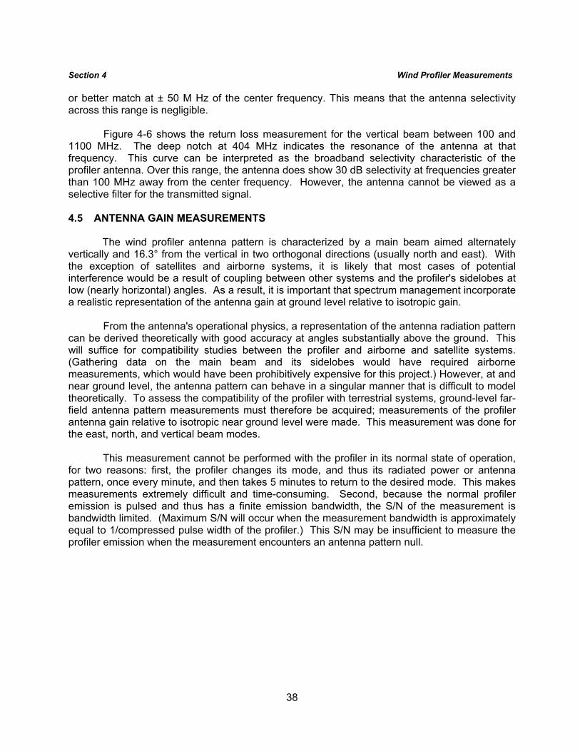
38
Section 4 Wind Profiler Measurements or better match at ± 50 M Hz of the center frequency. This means that the antenna selectivity across this range is negligible.
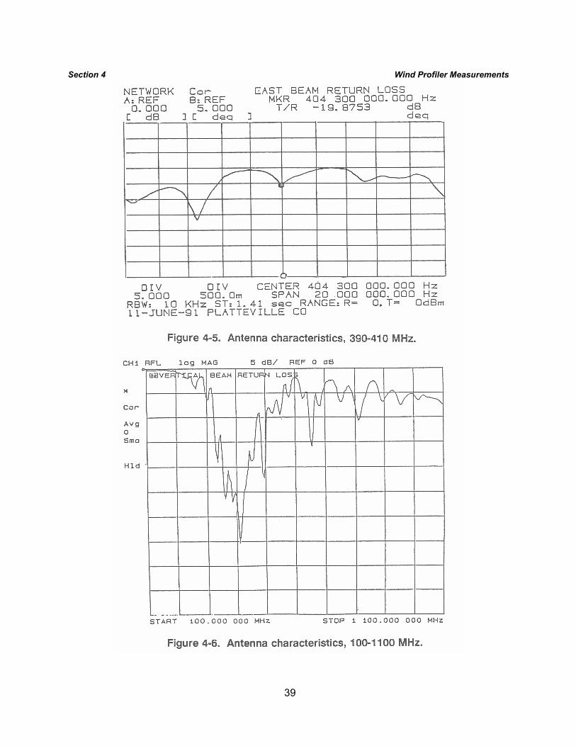
Figure 4-6 shows the return loss measurement for the vertical beam between 100 and 1100 MHz. The deep notch at 404 MHz indicates the resonance of the antenna at that frequency. This curve can be interpreted as the broadband selectivity characteristic of the profiler antenna. Over this range, the antenna does show 30 dB selectivity at frequencies greater than 100 MHz away from the center frequency. However, the antenna cannot be viewed as a selective filter for the transmitted signal.
4.5 ANTENNA GAIN MEASUREMENTS
The wind profiler antenna pattern is characterized by a main beam aimed alternately vertically and 16.3° from the vertical in two orthogonal directions (usually north and east). With the exception of satellites and airborne systems, it is likely that most cases of potential interference would be a result of coupling between other systems and the profiler's sidelobes at low (nearly horizontal) angles. As a result, it is important that spectrum management incorporate a realistic representation of the antenna gain at ground level relative to isotropic gain.
From the antenna's operational physics, a representation of the antenna radiation pattern
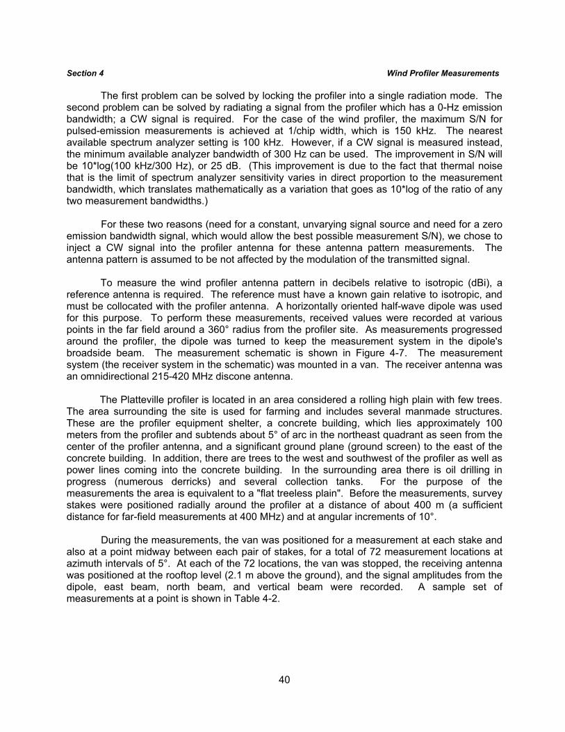
can be derived theoretically with good accuracy at angles substantially above the ground. This will suffice for compatibility studies between the profiler and airborne and satellite systems. (Gathering data on the main beam and its sidelobes would have required airborne measurements, which would have been prohibitively expensive for this project.) However, at and near ground level, the antenna pattern can behave in a singular manner that is difficult to model theoretically. To assess the compatibility of the profiler with terrestrial systems, ground-level far-field antenna pattern measurements must therefore be acquired; measurements of the profiler antenna gain relative to isotropic near ground level were made. This measurement was done for the east, north, and vertical beam modes.
This measurement cannot be performed with the profiler in its normal state of operation,
for two reasons: first, the profiler changes its mode, and thus its radiated power or antenna pattern, once every minute, and then takes 5 minutes to return to the desired mode. This makes measurements extremely difficult and time-consuming. Second, because the normal profiler emission is pulsed and thus has a finite emission bandwidth, the S/N of the measurement is bandwidth limited. (Maximum S/N will occur when the measurement bandwidth is approximately equal to 1/compressed pulse width of the profiler.) This S/N may be insufficient to measure the profiler emission when the measurement encounters an antenna pattern null.
39
Section 4 Wind Profiler Measurements
40
Section 4 Wind Profiler Measurements
The first problem can be solved by locking the profiler into a single radiation mode. The second problem can be solved by radiating a signal from the profiler which has a 0-Hz emission bandwidth; a CW signal is required. For the case of the wind profiler, the maximum S/N for pulsed-emission measurements is achieved at 1/chip width, which is 150 kHz. The nearest available spectrum analyzer setting is 100 kHz. However, if a CW signal is measured instead, the minimum available analyzer bandwidth of 300 Hz can be used. The improvement in S/N will be 10*log(100 kHz/300 Hz), or 25 dB. (This improvement is due to the fact that thermal noise that is the limit of spectrum analyzer sensitivity varies in direct proportion to the measurement bandwidth, which translates mathematically as a variation that goes as 10*log of the ratio of any two measurement bandwidths.)
For these two reasons (need for a constant, unvarying signal source and need for a zero
emission bandwidth signal, which would allow the best possible measurement S/N), we chose to inject a CW signal into the profiler antenna for these antenna pattern measurements. The antenna pattern is assumed to be not affected by the modulation of the transmitted signal.
To measure the wind profiler antenna pattern in decibels relative to isotropic (dBi), a
reference antenna is required. The reference must have a known gain relative to isotropic, and must be collocated with the profiler antenna. A horizontally oriented half-wave dipole was used for this purpose. To perform these measurements, received values were recorded at various points in the far field around a 360° radius from the profiler site. As measurements progressed around the profiler, the dipole was turned to keep the measurement system in the dipole's broadside beam. The measurement schematic is shown in Figure 4-7. The measurement system (the receiver system in the schematic) was mounted in a van. The receiver antenna was an omnidirectional 215-420 MHz discone antenna.
The Platteville profiler is located in an area considered a rolling high plain with few trees. The area surrounding the site is used for farming and includes several manmade structures. These are the profiler equipment shelter, a concrete building, which lies approximately 100 meters from the profiler and subtends about 5° of arc in the northeast quadrant as seen from the center of the profiler antenna, and a significant ground plane (ground screen) to the east of the concrete building. In addition, there are trees to the west and southwest of the profiler as well as power lines coming into the concrete building. In the surrounding area there is oil drilling in progress (numerous derricks) and several collection tanks. For the purpose of the measurements the area is equivalent to a "flat treeless plain". Before the measurements, survey stakes were positioned radially around the profiler at a distance of about 400 m (a sufficient distance for far-field measurements at 400 MHz) and at angular increments of 10°.
During the measurements, the van was positioned for a measurement at each stake and also at a point midway between each pair of stakes, for a total of 72 measurement locations at azimuth intervals of 5°. At each of the 72 locations, the van was stopped, the receiving antenna was positioned at the rooftop level (2.1 m above the ground), and the signal amplitudes from the dipole, east beam, north beam, and vertical beam were recorded. A sample set of measurements at a point is shown in Table 4-2.
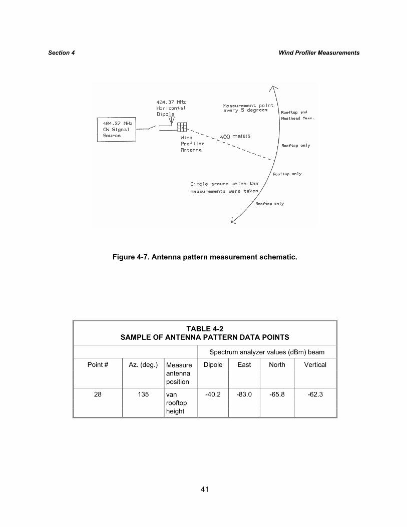
41
Section 4 Wind Profiler Measurements
Figure 4-7. Antenna pattern measurement schematic.
TABLE 4-2 SAMPLE OF ANTENNA PATTERN DATA POINTS
Spectrum analyzer values (dBm) beam
Point # Az. (deg.) Dipole East North Vertical
Measure antenna position
28 135 -40.2 -83.0 -65.8 -62.3
van rooftop height
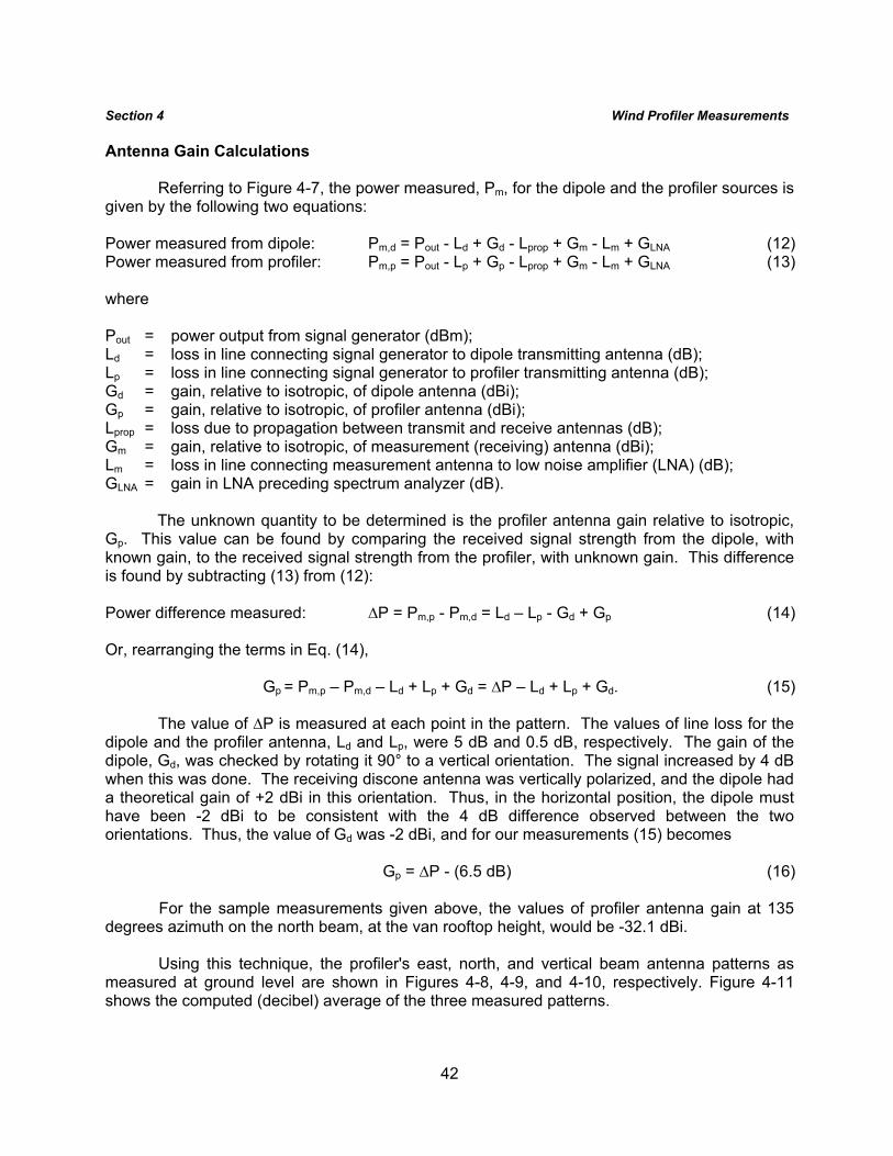
42
Section 4 Wind Profiler Measurements Antenna Gain Calculations
Referring to Figure 4-7, the power measured, Pm, for the dipole and the profiler sources is given by the following two equations:
Power measured from dipole: Pm,d = Pout - Ld + Gd - Lprop + Gm - Lm + GLNA (12) Power measured from profiler: Pm,p = Pout - Lp + Gp - Lprop + Gm - Lm + GLNA (13) where Pout = power output from signal generator (dBm); Ld = loss in line connecting signal generator to dipole transmitting antenna (dB); Lp = loss in line connecting signal generator to profiler transmitting antenna (dB); Gd = gain, relative to isotropic, of dipole antenna (dBi); Gp = gain, relative to isotropic, of profiler antenna (dBi); Lprop = loss due to propagation between transmit and receive antennas (dB); Gm = gain, relative to isotropic, of measurement (receiving) antenna (dBi); Lm = loss in line connecting measurement antenna to low noise amplifier (LNA) (dB); GLNA = gain in LNA preceding spectrum analyzer (dB).
The unknown quantity to be determined is the profiler antenna gain relative to isotropic, Gp. This value can be found by comparing the received signal strength from the dipole, with known gain, to the received signal strength from the profiler, with unknown gain. This difference is found by subtracting (13) from (12): Power difference measured: ∆P = Pm,p - Pm,d = Ld – Lp - Gd + Gp (14) Or, rearranging the terms in Eq. (14), Gp = Pm,p – Pm,d – Ld + Lp + Gd = ∆P – Ld + Lp + Gd. (15)
The value of ∆P is measured at each point in the pattern. The values of line loss for the dipole and the profiler antenna, Ld and Lp, were 5 dB and 0.5 dB, respectively. The gain of the dipole, Gd, was checked by rotating it 90° to a vertical orientation. The signal increased by 4 dB when this was done. The receiving discone antenna was vertically polarized, and the dipole had a theoretical gain of +2 dBi in this orientation. Thus, in the horizontal position, the dipole must have been -2 dBi to be consistent with the 4 dB difference observed between the two orientations. Thus, the value of Gd was -2 dBi, and for our measurements (15) becomes
Gp = ∆P - (6.5 dB) (16)
For the sample measurements given above, the values of profiler antenna gain at 135 degrees azimuth on the north beam, at the van rooftop height, would be -32.1 dBi.
Using this technique, the profiler's east, north, and vertical beam antenna patterns as
measured at ground level are shown in Figures 4-8, 4-9, and 4-10, respectively. Figure 4-11 shows the computed (decibel) average of the three measured patterns.
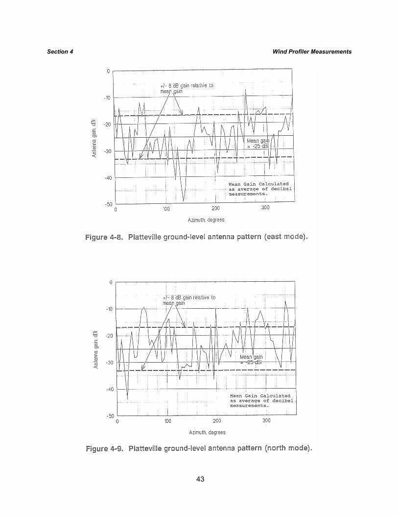
43
Section 4 Wind Profiler Measurements
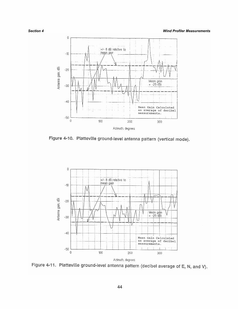
44
Section 4 Wind Profiler Measurements
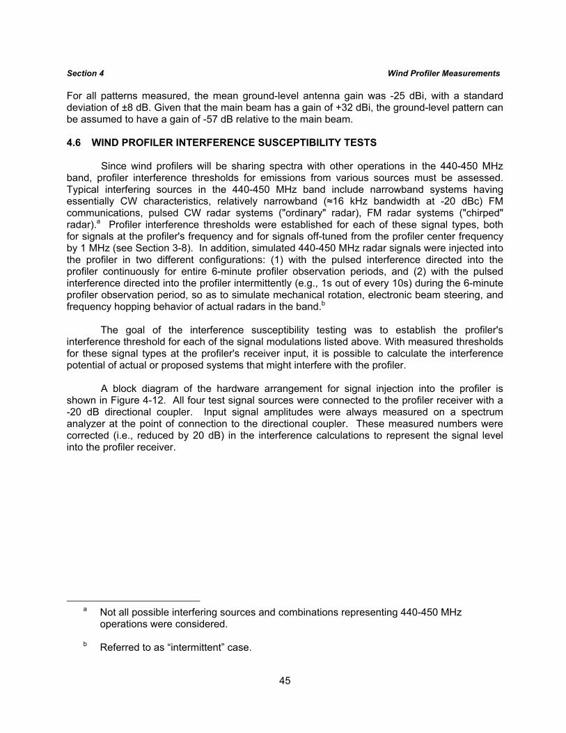
45
Section 4 Wind Profiler Measurements For all patterns measured, the mean ground-level antenna gain was -25 dBi, with a standard deviation of ±8 dB. Given that the main beam has a gain of +32 dBi, the ground-level pattern can be assumed to have a gain of -57 dB relative to the main beam. 4.6 WIND PROFILER INTERFERENCE SUSCEPTIBILITY TESTS
Since wind profilers will be sharing spectra with other operations in the 440-450 MHz band, profiler interference thresholds for emissions from various sources must be assessed. Typical interfering sources in the 440-450 MHz band include narrowband systems having essentially CW characteristics, relatively narrowband (≈16 kHz bandwidth at -20 dBc) FM communications, pulsed CW radar systems ("ordinary" radar), FM radar systems ("chirped" radar).a Profiler interference thresholds were established for each of these signal types, both for signals at the profiler's frequency and for signals off-tuned from the profiler center frequency by 1 MHz (see Section 3-8). In addition, simulated 440-450 MHz radar signals were injected into the profiler in two different configurations: (1) with the pulsed interference directed into the profiler continuously for entire 6-minute profiler observation periods, and (2) with the pulsed interference directed into the profiler intermittently (e.g., 1s out of every 10s) during the 6-minute profiler observation period, so as to simulate mechanical rotation, electronic beam steering, and frequency hopping behavior of actual radars in the band.b
The goal of the interference susceptibility testing was to establish the profiler's
interference threshold for each of the signal modulations listed above. With measured thresholds for these signal types at the profiler's receiver input, it is possible to calculate the interference potential of actual or proposed systems that might interfere with the profiler.
A block diagram of the hardware arrangement for signal injection into the profiler is
shown in Figure 4-12. All four test signal sources were connected to the profiler receiver with a -20 dB directional coupler. Input signal amplitudes were always measured on a spectrum analyzer at the point of connection to the directional coupler. These measured numbers were corrected (i.e., reduced by 20 dB) in the interference calculations to represent the signal level into the profiler receiver.
a Not all possible interfering sources and combinations representing 440-450 MHz
operations were considered. b Referred to as “intermittent” case.
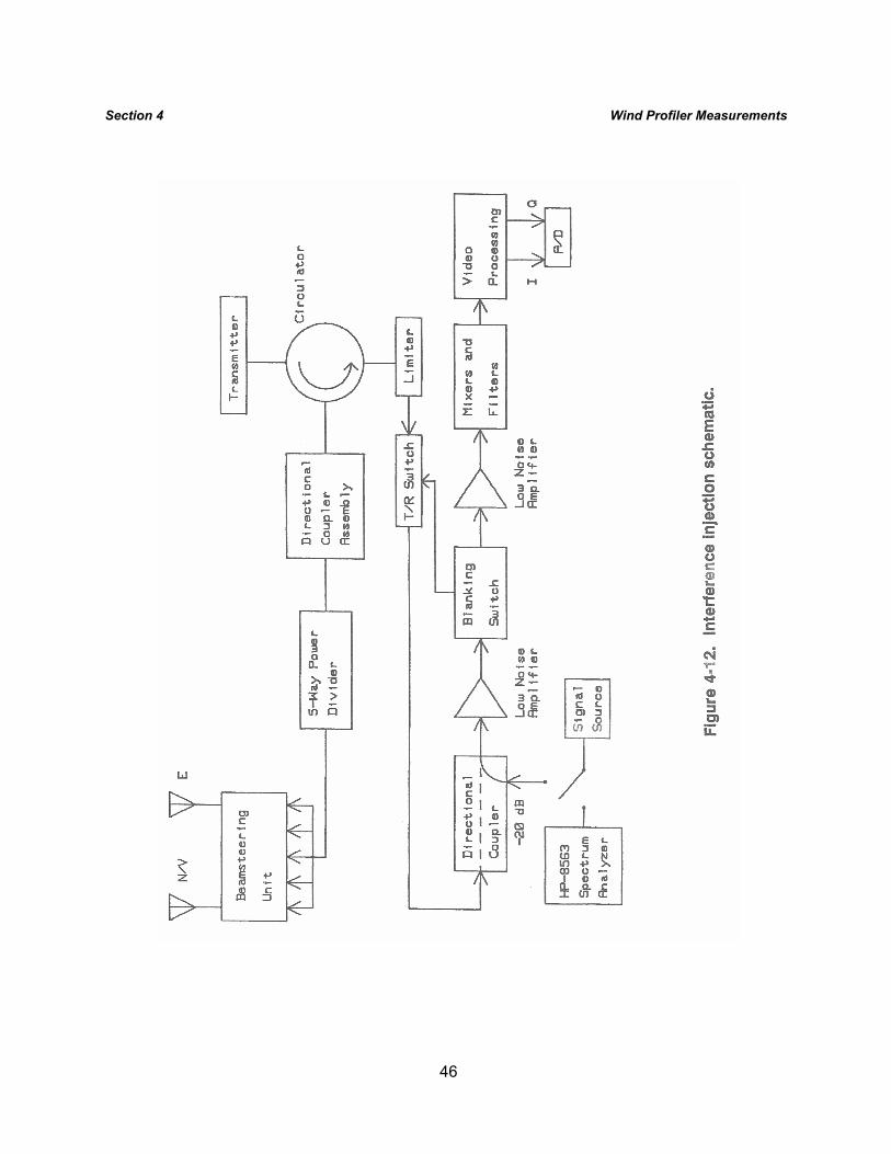
46
Section 4 Wind Profiler Measurements
47
Section 4 Wind Profiler Measurements
The question of how to assess the effects of the injected "interference" to the profiler is nontrivial, as described in Section 3. The profiler is an integrating device, and it requires six 1-minute integrations to produce a single atmospheric observation. In addition, the observations are the result not only of hardware processing, but also of software processing. The profiler's software is as integral to the system as the hardware, and any realistic assessment of the profiler's susceptibility to interference must take into account the software's algorithmic response as well as the hardware response. Potentially interfering signals that are seen prominently in the profiler's first IF, for example, can be eliminated by subsequent digital signal processing (DSP) to that section (software). If the mitigating effects of DSP are ignored, a grossly pessimistic estimate of the profiler's susceptibility to interference would result.
In addition to the filtering effect of DSP, the coherence of a potentially interfering signal
would be expected to affect interference thresholds. The profiler, as a coherent processor, can be expected to be much more susceptible to coherent interference than to noncoherent interference, although it is difficult to assess beyond that generalization, a priori, the effects of an interfering signal on the profiler's processing algorithms.
Interference thresholds would be expected to correlate with the interfering signal power
and duty cycle, regardless of the interfering signal's spectrum. Since a single profiler observation requires six 1-minute integrations, the percentage of time that an interfering signal is present during a minute will correlate with interference potential.
The profiler's design makes it impractical to perform interference measurements on the
profiler component by component. The only realistic way to perform interference testing is to treat the profiler (hardware and software combined) as a black-box, input-versus-output system. The effects on 6-minute observations must be related to known input amplitudes of a given interfering signal. This is achieved most effectively by running the profiler in a normal mode, collecting one or two atmospheric observations as baseline data, and then injecting the interfering signal via a directional coupler. The results of the observations made under the two different conditions (interference ON versus interference OFF) can then be compared. Diagnostic software output is used for the comparison, as described more fully below.
When this testing is performed, significant sources of variation will remain (and are
inherent) in the interference thresholds that are measured. The reason is that the atmosphere is itself highly variable, and the quality of profiler returns thus varies from altitude-to-altitude, from day-to-day, and from season to season. In effect, the wind profiler radar's S/N varies as a function of altitude and time, and thus so too will the interference threshold levels. Even if sufficient time and money were available to run interference tests for months or years and to look at all range gates while tests were in progress, the results would still be, at best, statistical guidelines for the effects of various interference levels. The tests that were actually performed could not be conducted over all range gates and over extensive time intervals, but rather were limited to sets of 6-minute observations of specific range gates made available by the diagnostic software.
Observations were repeated on different days, and no significant differences were noted
for any test signal as a function of time. Only the upper range gates in the high and low profiler
48
Section 4 Wind Profiler Measurements modes were observed, as these normally have the lowest S/N and thus are the most susceptible to interference effects. The repeatability of the test results and the conservatism of range gates selection lead us to believe that (1) the results represent typical profiler operating conditions, and thus the measured interference thresholds can be used by spectrum managers to assess this profiler's compatibility with other systems, and (2) additional useful information would probably not be generated by more extended testing intervals with our test procedures.
An important issue in this testing is to define interference for the profiler, and to determine what level of interference effect in the profiler is then considered to be a problem. Although it is obvious that any level of degradation is undesirable, it is also true that wind profiler operations can proceed with some finite level of effective degradation to the profiler. But how much degradation? Degradation effects can be observed as an effective increase in the profiler's system noise level, and this phenomenon first affects the range gates with the lowest S/N. (Generally, the upper range gates have the lowest S/N; therefore interference effects will usually be observed first in the upper range gates of high and low profiler modes.)
Interference was defined for the purposes of these tests to be a consistently discernible
increase in profiler system noise due to the injection of an interfering signal into the profiler receiver. The minimum discernible increase was found to be approximately 3 dB based on observations of a single 6-minute data period. Therefore, for testing purposes, 3 dB was used as the threshold for observation of interference. We do not claim that this is an acceptable interference level for profiler operations but, only that it was the limit of our testing capability. The results of the tests are summarized in Table 4-3, given at the end of this section on page 56.
On-Tune CW Signal Injection
A frequency domain impulse at the radar center frequency was required for this test. The signal source, an HP-8640B signal generator, was tuned to the profiler's center frequency. The profiler and injected frequencies were made coincident by simultaneously observing the profiler spectrum and the signal generator output on a spectrum analyzer, and tuning the interfering signal until the two signals were coincident on the analyzer display. The coincidence was also checked by observing the interfering signal on an oscilloscope attached to the first profiler IF, and tuning the signal until the observed interference effects were maximized. Because an interfering signal would not be expected to be phase locked to the profiler, the test signal was not phase locked to the profiler. Observation of the oscilloscope diagnostic indicated that the signal drifted in and out of coherence with the profiler a few times every minute, on a random basis. Accidental coherence would typically last a few seconds at a time.
Because of the inherently high spectrum analyzer noise figure, the amplitude of the
interfering signal was checked on a spectrum analyzer at a much higher level than would be used for the tests. A vernier on the signal generator was used to bring the indicated output level into agreement with the measured level. Then, as the level was reduced in 10 dB steps to the amplitude of the injection tests, the signal was observed on the analyzer to also drop in 10 dB steps. The signal level used for the interference tests was too low to be observed on the
49
Section 4 Wind Profiler Measurements spectrum analyzer (which has a 30-dB noise figure), but was inferred to be accurately indicated by the (now calibrated) signal generator indicator. Because a CW signal is an impulse in the frequency domain and thus has zero spectral width (to within the stability of the source oscillator), any measured spectrum of the signal will indicate only the frequency domain impulse response of the measuring device, as shown in Figure 4-13. Results of On-Tune CW Signal Injection
This test indicated a barely detectable increase (about 1 dB) in the profiler noise level when the interfering signal input level, corrected for the directional coupler factor, was -140 dBm. At -135 dBm, an increase of approximately 3 dB in the profiler's system noise level was observed. At -125 dBm input, all atmospheric signals in the high mode were lost. For this test, the threshold input level of -135 dBm held for a full 6-minute observation cycle should be considered a worst-case scenario. If the signal were present for a fraction of that time, then the threshold level would be higher. If the signal were present only for a few seconds out of each minute, as might be the case for actual interfering signals, then it is doubtful that any input level, no matter how high, would noticeably degrade the profiler's performance as long as the receiver is not driven into saturation.
Off-Tune CW Signal Injection
The same test as above was performed, but with the interfering signal off-tuned from the profiler by 1 MHz.
Results of Off-Tune CW Signal Injection
The CW signal was increased in amplitude to -70 dBm, and no effect was seen by the profiler. Higher levels were not attempted because of concern about possible damage to the profiler receiver's RF front end. The interference threshold (Table 4-3) exceeds -70 dBm, even when the signal is present throughout the profiler observation; as before, the threshold would be even higher if the signal were present for a percentage of that period.
On-Tune FM Signal Injection
A wind profiler radar might operate in the proximity of FM communication transmitters. A 16-kHz FMCW test signal with a 1 kHz modulation tone was used. Actual voice modulation, as a random modulation input, should have no more effect on the profiler, and probably less effect, than the modulation used in these tests. The same techniques were used to tune this signal and to check its amplitude as were used for the CW signal. The measured spectrum of the signal is shown in Figure 4-14. The signal was present throughout the profiler's observation period of 6 minutes (i.e., 100% duty cycle for 6 minutes); a lower interference duty cycle would have yielded a higher interference threshold.
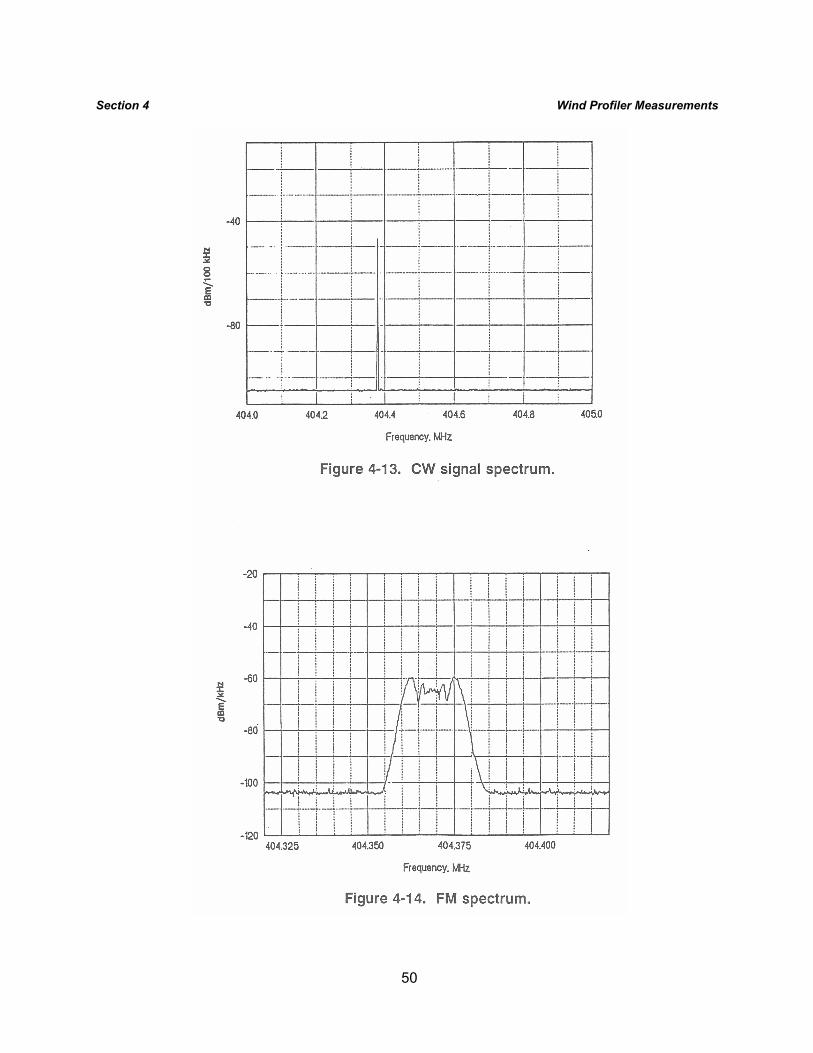
50
Section 4 Wind Profiler Measurements
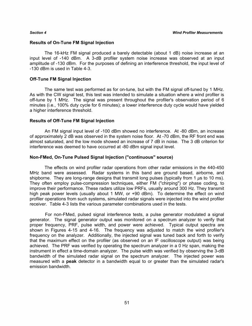
51
Section 4 Wind Profiler Measurements Results of On-Tune FM Signal Injection
The 16-kHz FM signal produced a barely detectable (about 1 dB) noise increase at an input level of -140 dBm. A 3-dB profiler system noise increase was observed at an input amplitude of -130 dBm. For the purposes of defining an interference threshold, the input level of -130 dBm is used in Table 4-3.
Off-Tune FM Signal Injection
The same test was performed as for on-tune, but with the FM signal off-tuned by 1 MHz. As with the CW signal test, this test was intended to simulate a situation where a wind profiler is off-tune by 1 MHz. The signal was present throughout the profiler's observation period of 6 minutes (i.e., 100% duty cycle for 6 minutes); a lower interference duty cycle would have yielded a higher interference threshold.
Results of Off-Tune FM Signal Injection
An FM signal input level of -100 dBm showed no interference. At -80 dBm, an increase of approximately 2 dB was observed in the system noise floor. At -70 dBm, the RF front end was almost saturated, and the low mode showed an increase of 7 dB in noise. The 3 dB criterion for interference was deemed to have occurred at -80 dBm signal input level.
Non-FMed, On-Tune Pulsed Signal Injection ("continuous" source)
The effects on wind profiler radar operations from other radar emissions in the 440-450 MHz band were assessed. Radar systems in this band are ground based, airborne, and shipborne. They are long-range designs that transmit long pulses (typically from 1 µs to 10 ms). They often employ pulse-compression techniques, either FM ("chirping") or phase coding, to improve their performance. These radars utilize low PRFs, usually around 300 Hz. They transmit high peak power levels (usually about 1 MW, or +90 dBm). To determine the effect on wind profiler operations from such systems, simulated radar signals were injected into the wind profiler receiver. Table 4-3 lists the various parameter combinations used in the tests.
For non-FMed, pulsed signal interference tests, a pulse generator modulated a signal
generator. The signal generator output was monitored on a spectrum analyzer to verify that proper frequency, PRF, pulse width, and power were achieved. Typical output spectra are shown in Figures 4-15 and 4-16. The frequency was adjusted to match the wind profiler's frequency on the analyzer. Additionally, the injected signal was tuned back and forth to verify that the maximum effect on the profiler (as observed on an IF oscilloscope output) was being achieved. The PRF was verified by operating the spectrum analyzer in a 0 Hz span, making the instrument in effect a time-domain analyzer. The pulse width was verified by observing the 3-dB bandwidth of the simulated radar signal on the spectrum analyzer. The injected power was measured with a peak detector in a bandwidth equal to or greater than the simulated radar's emission bandwidth.
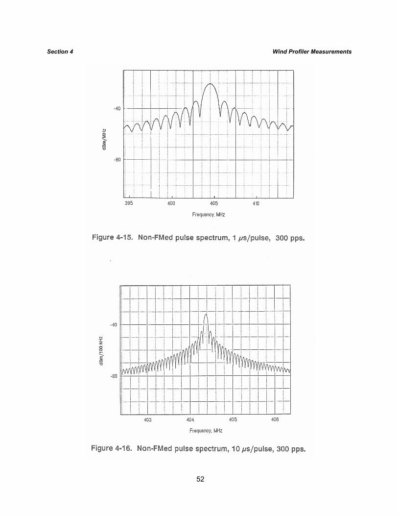
52
Section 4 Wind Profiler Measurements
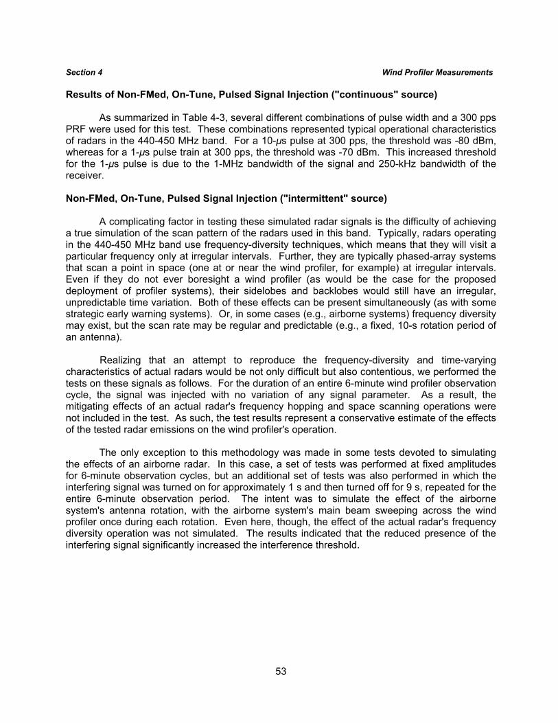
53
Section 4 Wind Profiler Measurements Results of Non-FMed, On-Tune, Pulsed Signal Injection ("continuous" source)
As summarized in Table 4-3, several different combinations of pulse width and a 300 pps PRF were used for this test. These combinations represented typical operational characteristics of radars in the 440-450 MHz band. For a 10-µs pulse at 300 pps, the threshold was -80 dBm, whereas for a 1-µs pulse train at 300 pps, the threshold was -70 dBm. This increased threshold for the 1-µs pulse is due to the 1-MHz bandwidth of the signal and 250-kHz bandwidth of the receiver.
Non-FMed, On-Tune, Pulsed Signal Injection ("intermittent" source)
A complicating factor in testing these simulated radar signals is the difficulty of achieving a true simulation of the scan pattern of the radars used in this band. Typically, radars operating in the 440-450 MHz band use frequency-diversity techniques, which means that they will visit a particular frequency only at irregular intervals. Further, they are typically phased-array systems that scan a point in space (one at or near the wind profiler, for example) at irregular intervals. Even if they do not ever boresight a wind profiler (as would be the case for the proposed deployment of profiler systems), their sidelobes and backlobes would still have an irregular, unpredictable time variation. Both of these effects can be present simultaneously (as with some strategic early warning systems). Or, in some cases (e.g., airborne systems) frequency diversity may exist, but the scan rate may be regular and predictable (e.g., a fixed, 10-s rotation period of an antenna).
Realizing that an attempt to reproduce the frequency-diversity and time-varying
characteristics of actual radars would be not only difficult but also contentious, we performed the tests on these signals as follows. For the duration of an entire 6-minute wind profiler observation cycle, the signal was injected with no variation of any signal parameter. As a result, the mitigating effects of an actual radar's frequency hopping and space scanning operations were not included in the test. As such, the test results represent a conservative estimate of the effects of the tested radar emissions on the wind profiler's operation.
The only exception to this methodology was made in some tests devoted to simulating
the effects of an airborne radar. In this case, a set of tests was performed at fixed amplitudes for 6-minute observation cycles, but an additional set of tests was also performed in which the interfering signal was turned on for approximately 1 s and then turned off for 9 s, repeated for the entire 6-minute observation period. The intent was to simulate the effect of the airborne system's antenna rotation, with the airborne system's main beam sweeping across the wind profiler once during each rotation. Even here, though, the effect of the actual radar's frequency diversity operation was not simulated. The results indicated that the reduced presence of the interfering signal significantly increased the interference threshold.
54
Section 4 Wind Profiler Measurements
The end result of these tests was to test the wind profiler against non-FMed, pulsed signals in modes that represent a more continuous interference pattern than would be expected from systems actually being operated or anticipated in the 440-450 MHz band. As such, we regard the results of these tests as highly conservative from the standpoint of assessing interference thresholds for the wind profiler.
Results of Non-FMed, On-Tune, Pulsed Signal Injection ("intermittent" source)
The intermittent nature of these signals results in interference thresholds that exceeded -70 dBm at the input to the profiler receiver, as summarized in Table 4-3.
Non-FMed, Off-Tune, Pulsed Signal Injection (both "continuous" and "intermittent" sources)
The same test was performed as described for the non-FMed, on-tune test except the interfering source was off-tuned by 1 MHz.
Results of Non-FMed, Off-Tune, Pulsed Signal Injection (both "continuous" and "intermittent" sources)
Tuning the radar signals off-tune by 1 MHz resulted in an interference threshold in excess of -70 dBm at the input to the profiler receiver, as given in Table 4-3.
Chirped, On-Tune, Pulsed Signal Injection ("continuous")
Most of the comments made above for non-FMed signal injection apply for the chirped signal tests. The only difference between these test modes is the modulation of the pulses. For these tests, the pulses were linearly swept across frequency ranges that simulated actual chirped radar operations. An example spectrum of one of the injected signals is shown in Figure 4-17. Radars in this band typically chirp across a range of 5 or 6 MHz in a period of about 13 µs.
As with the non-FMed pulses, it may be assumed that the real radar pulses are phase
code modulated. This modulation was not simulated; unless the phase coding should be coherent with the wind profiler, it should have no additional interference effect. Such coherence would never be expected to occur.
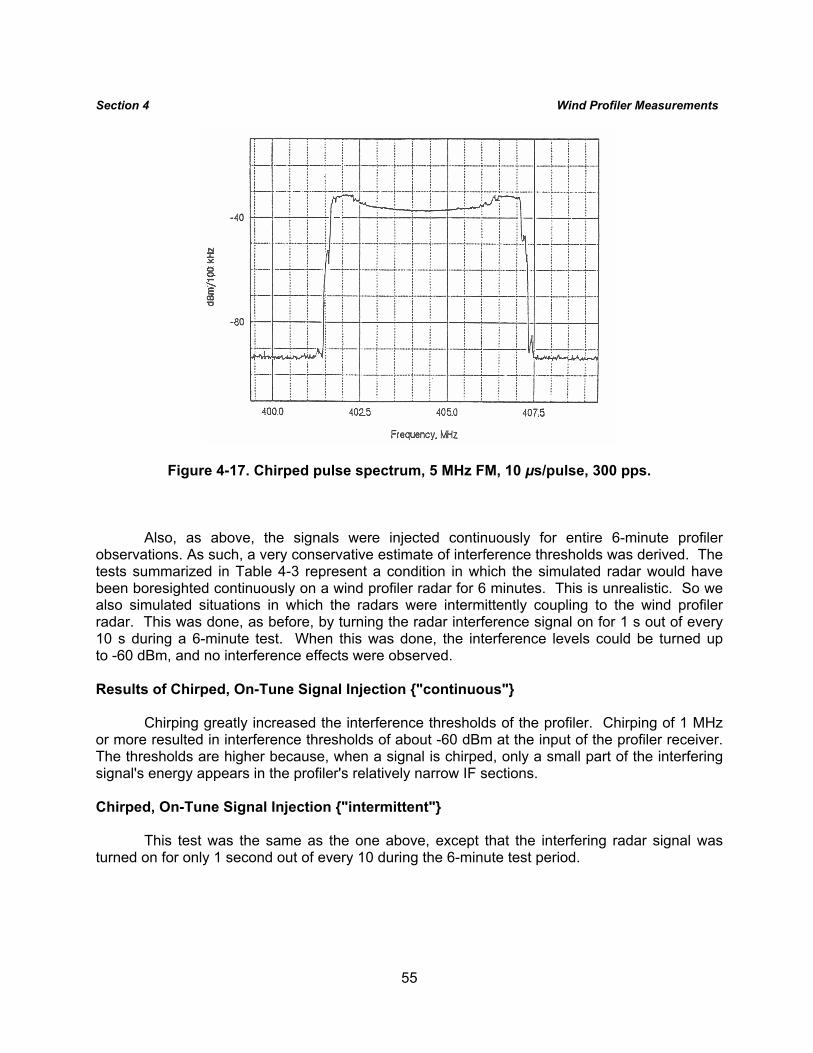
55
Section 4 Wind Profiler Measurements
Figure 4-17. Chirped pulse spectrum, 5 MHz FM, 10 µs/pulse, 300 pps.
Also, as above, the signals were injected continuously for entire 6-minute profiler observations. As such, a very conservative estimate of interference thresholds was derived. The tests summarized in Table 4-3 represent a condition in which the simulated radar would have been boresighted continuously on a wind profiler radar for 6 minutes. This is unrealistic. So we also simulated situations in which the radars were intermittently coupling to the wind profiler radar. This was done, as before, by turning the radar interference signal on for 1 s out of every 10 s during a 6-minute test. When this was done, the interference levels could be turned up to -60 dBm, and no interference effects were observed.
Results of Chirped, On-Tune Signal Injection {"continuous"}
Chirping greatly increased the interference thresholds of the profiler. Chirping of 1 MHz or more resulted in interference thresholds of about -60 dBm at the input of the profiler receiver. The thresholds are higher because, when a signal is chirped, only a small part of the interfering signal's energy appears in the profiler's relatively narrow IF sections.
Chirped, On-Tune Signal Injection {"intermittent"}
This test was the same as the one above, except that the interfering radar signal was turned on for only 1 second out of every 10 during the 6-minute test period.
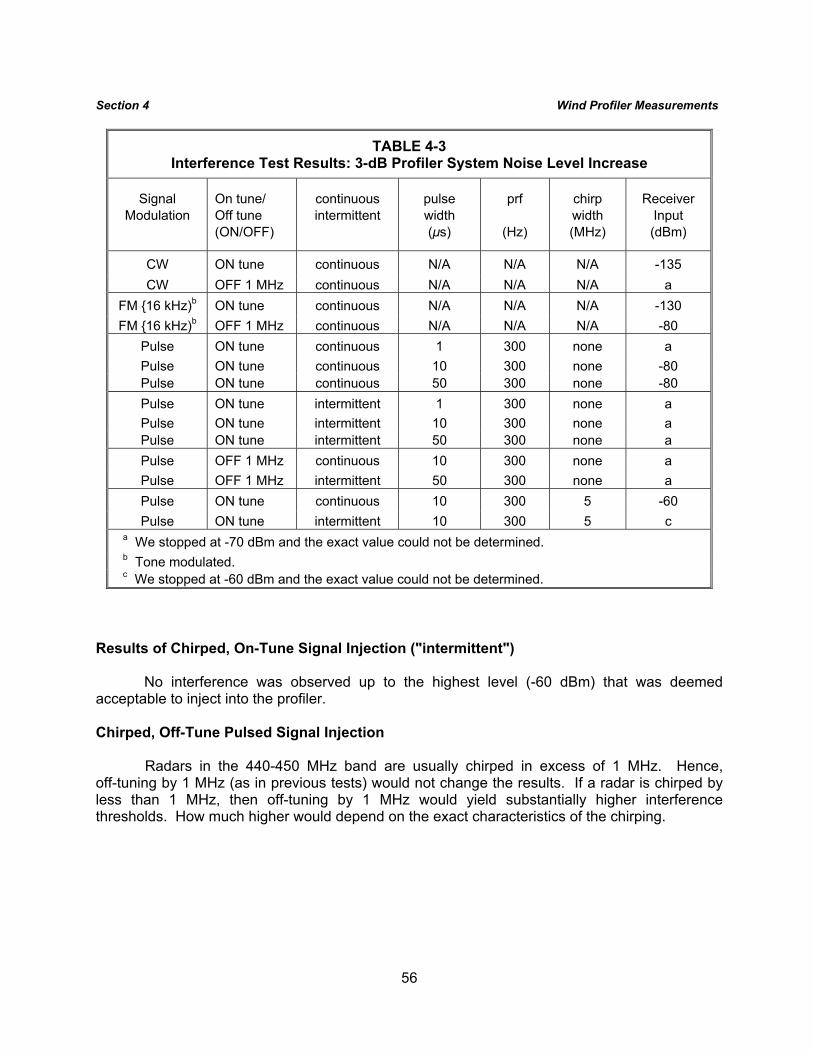
56
Section 4 Wind Profiler Measurements
TABLE 4-3 Interference Test Results: 3-dB Profiler System Noise Level Increase
Signal Modulation
On tune/ Off tune (ON/OFF)
continuous intermittent
pulse width (µs)
prf
(Hz)
chirp width (MHz)
Receiver Input (dBm)
CW ON tune continuous N/A N/A N/A -135 CW OFF 1 MHz continuous N/A N/A N/A a
FM {16 kHz)b ON tune continuous N/A N/A N/A -130 FM {16 kHz)b OFF 1 MHz continuous N/A N/A N/A -80
Pulse ON tune continuous 1 300 none a Pulse ON tune continuous 10 300 none -80 Pulse ON tune continuous 50 300 none -80 Pulse ON tune intermittent 1 300 none a Pulse ON tune intermittent 10 300 none a Pulse ON tune intermittent 50 300 none a Pulse OFF 1 MHz continuous 10 300 none a Pulse OFF 1 MHz intermittent 50 300 none a Pulse ON tune continuous 10 300 5 -60 Pulse ON tune intermittent 10 300 5 c
a We stopped at -70 dBm and the exact value could not be determined. b Tone modulated. c We stopped at -60 dBm and the exact value could not be determined.
Results of Chirped, On-Tune Signal Injection ("intermittent")
No interference was observed up to the highest level (-60 dBm) that was deemed acceptable to inject into the profiler.
Chirped, Off-Tune Pulsed Signal Injection
Radars in the 440-450 MHz band are usually chirped in excess of 1 MHz. Hence, off-tuning by 1 MHz (as in previous tests) would not change the results. If a radar is chirped by less than 1 MHz, then off-tuning by 1 MHz would yield substantially higher interference thresholds. How much higher would depend on the exact characteristics of the chirping.
57
Section 4 Wind Profiler Measurements 4.7 EFFECTS FROM WIND PROFILER EMISSIONS ON LAND MOBILE/AMATEUR OPERATIONS
Since wind profilers will coexist with land mobile/amateur operations, the possibility of interference from wind profiler emissions was assessed, both on-tune and off-tuned by 1 MHz.
The receiver chosen for these tests was an ICOM RG-7000. The device has a noise
figure of about 15 dB which is typical of such receivers. The receiver bandwidth is selectable; for our tests a 10-kHz bandwidth was selected as being representative of the typical bandwidth employed in actual operations.
On-Tune Test
An ICOM receiver was placed in a van, and a vertically polarized omnidirectional, 220-420 MHz discone antenna was mounted at rooftop level (approximately 2.1 m above the ground). The receiver was tuned to the profiler's center frequency, and a manual adjustment and built-in signal meter were used to "peak up" the receiver on the profiler emission. Both FM and AM demodulations were tested.
The van was driven along one radial away from the profiler, and the test continued until
the profiler signal was lost in the receiver's internally generated noise. Although AM demodulation received the signal at a slightly longer distance than FM demodulation, both tests lost the profiler signal at a distance of approximately 1.6 km. This test was repeated several weeks later, and the same result was obtained.
Off-Tune Test
This test was identical to the test above, except that the receiver was tuned 1 MHz above the wind profiler frequency. In this case, the maximum distance at which the signal from the profiler was received out of the ICOM noise floor was about 1.1 km.
Summary
The ICOM receiver tests indicate that emissions from this wind profiler would pose no appreciable concern for existing mobile stations, even if those operations were on-tune to the profiler.
59
SECTION 5 SUMMARY AND CONCLUSIONS
5.1 SUMMARY
The measurements given in this report were conducted on the Unisys wind profiler located in Platteville, Colorado, operating on the frequency 404.37 MHz.
In assessing the effect of potentially interfering signals on wind profiler performance, we
examined various characteristics such as the type of interfering signal modulation, percentage of time within each minute that the interfering signal is exposed to the profiler, duty cycle, pulse width and PRF (if applicable) of the interfering signal. In addition, although the performance of profilers may vary as a function of design type, the Unisys design that was tested is considered to be representative of current 400 MHz wind profiler radar technology.
It is important to note that a profiler system, as a coherent processor, experiences the
highest susceptibility to interfering signals when such signals are on frequency and coherent with the profiler. If the interfering signals are either off-tune or are not coherent, then the profiler's susceptibility is substantially reduced. If a signal is present only a small percentage of time within each minute, then the susceptibility is also substantially reduced. For example, in cases where an interfering radar signal was simulated continuously versus a simulation with intermittent signals (in which the interference occurred for 1 s out of every 10 s), an increased interference threshold was observed.
Potentially interfering signals also affect the profiler less if their spectral density is spread
over a larger portion of spectrum, resulting in lower total interfering power in the profiler's passband. This is expected theoretically, and was confirmed by the measurements. This means, again, that an on-tune FM signal will affect the profiler less than an on-tune CW signal with the same power. And, as noted, the coherence or lack thereof of an interfering signal has a large effect on profiler susceptibility.
Off-tuning any signal has the effect of substantially reducing the profiler susceptibility to
interference and as a result we were not able to observe interference to the profiler with non-chirped signals tuned 1 MHz off the profiler's center frequency.
Other factors are important in reducing profiler susceptibility to interference. The
presence of a limiter and range-Doppler processing in the profiler receiver system would significantly lower the susceptibility to low duty cycle interference (e.g., < 1.0%). Also, siting considerations have an impact on a profiler operation. Having locations in remote areas with a minimum of urban development will present fewer possibilities for the occurrence of interfering signals. Terrain that acts in a shielding fashion could also reduce interference from (or to) ground-based systems.
The results of tests made by injecting signals into the profiler receiver can be sum-
marized as follows. Coherent interference can be a potential problem for a wind profiler, but it is not expected that any signal will be coherent with a profiler. Pulsed signals can produce notice-able interference levels if the pulsed input simulates a continuously boresighted radar. However,
60
Section 5 Summary and Conclusions interference susceptibility levels are substantially higher when realistic radar operations in the 440-450 MHz band are simulated (i.e., when the interfering radar signal is injected into the profiler for 1 s out of every 10). Interference from radars increases in severity as pulse widths lengthen or if pulse repetition frequencies are increased. The wider the chirp range of a radar, the less severe the interference potential, given other factors remaining equal.
It is noted that factors such as wind profiler characteristics, performance requirements, and interference susceptibility may vary depending on the function or mission of the profiler.
5.2 CONCLUSIONS 1. Emission spectrum measurements conducted on a Unisys wind profiler (both high and
low mode) are shown in Figures 4-2 and 4-3, respectively. These spectra are asymmetrical about the carrier and show good spectrum conservation, due to factors such as MSK coding and solid-state transmitters.
2. Wind profiler measurements showed that subharmonic (202 MHz) and second (808 MHz)
and third harmonic (1212 MHz) emissions (Table 4-1) were in the range of 37 to 60 dB down from the fundamental. Fourth harmonic (1616 MHz) levels were at least 70 dB down from the fundamental.
3. Profiler antenna selectivity characteristics (Figures 4-5 and 4-6) will not improve profiler
resistance to interference from systems tuned to within ±10 MHz of the profiler frequency, but would probably improve compatibility (by providing about 30 dB of rejection) for systems tuned more than 100 MHz from the profiler center frequency.
4. The average gain (computed in decibels) of the wind profiler antenna at ground level near
the profiler horizon (Figure 4-11) was measured to be -25 dBi (±8 dB standard deviation). The low profiler sidelobe levels will enhance profiler compatibility with other systems.
5. Table 5-1 gives the range of interference threshold levels that resulted in a 3-dB
degradation in profiler S/N for four types of signals that represent typical operations in the 440-450 MHz band. The 3-dB criterion was selected due to the limitation of the measurement setup and may not be an acceptable level of interference for profiler performance.
6. In tests conducted with an ICOM RG-7000 (intended to represent a typical land
mobile/amateur receiver), emissions from the wind profiler were not discernible above the receiver's internally generated noise at distances exceeding 1.6 km along a single radial when the receiver was tuned to the profiler center frequency. The receiving system utilized a vertically polarized omnidirectional discone antenna at a height of 2.1 m above ground level. Terrain, vegetation, and structural blocking were minimal. These results, coupled with the remote siting envisioned for (200-500 MHz) profiler systems, indicate that profiler operations should be compatible with most land mobile/amateur operations.

61
Section 5 Summary and Conclusions
TABLE 5-1 INTERFERENCE THRESHOLDS RESULTING IN
3-dB INCREASE IN PROFILER'S SYSTEM NOISE LEVEL
Type of signala
On-Tune (dBm at Rx input)
1 MHz Off-Tune (dBm at Rx input)
CW -135 b
16 kHz FMc -130 to -135 -80 to -85
Pulsed
-80 continuous signal injection
intermittent signal injectionb continuous and
intermittent signal injectionb
Chirpd
-60 continuous
intermittente f
a For pulse and chirp signals, the receiver inputs levels are peak values. b The measurements stopped at -70 dBm and the exact value could not be determined. c Tone modulated. d Based on selected input signals, see Section 4.6. e The measurements stopped at -60 dBm and the exact value could not be determined. f Assumed same as cochannel chirp results.


63
LIST OF REFERENCES Harris, F.J., On the Use of Windows for Harmonic Analysis with the Discrete Fourier Transform,
Proc. IEEE, No.1, January 1978. Hildebrand, P.H. and Sekhon, R.S., Objective Determination of the Noise Level in Doppler
Spectra, Journal of Applied Meteorology, No. 13, October 1974. Nastrom, G.D., Gage, KS., Ecklund, S.L., Variability of Turbulence, 4--20 km, in Colorado and
Alaska from MST Radar Observations, J. Geophys, Res. No. 91, 1986. NTIA/ITS, RSMS Measurement Plan on the Unisys wind profiler, May 1991. Patrick, G., Richmond, M. (1991), Assessment of Bands for Wind Profiler Accommodation
(216-225, 400.15-406, and 420-450 MHz Bands), NTIA Report 91-280, September 1991, U.S. Department of Commerce, National Telecommunications and Information Administration, Washington, D.C.
Recommendations and Report of the CCIR, 1986, Volume V, Propagation in Non-ionized Media. Schmidt, G., Ruster, R. and Czechowsky, P., Complementary Code and Digital Filtering for
Detection of Weak VHF Radar Signals from the Mesosphere. IEEE Trans. on Geoscience Electronics, No. 4, October 1979.
Skolnik, H.J., Radar Handbook, 1970, McGraw-Hill, Inc.