MEASUREMENTS OF THE THERMAL EXPANSION AND HEAT

CAPACITY OF METALS BY ELECTROMAGNETIC

LEVITATION

Except where reference is made to the work of others, the work described in this thesis is

my own or was done in collaboration with my advisory committee. This thesis does not include proprietary or classified information.

Baojian Guo

Certificate of Approval: Jeffrey W. Fergus Ruel. A. Overfelt, Chair Associate Professor Professor Materials Engineering Materials Engineering Zhongyang Cheng Stephen L. McFarland Assistant Professor Acting Dean Materials Engineering Graduate School

MEASUREMENTS OF THE THERMAL EXPANSION AND HEAT

CAPACITY OF METALS BY ELECTROMAGNETIC

LEVITATION

Baojian Guo

A Thesis

Submitted to

the Graduate Faculty of

Auburn University

in Partial Fulfillment of the

Requirements for the

Degree of

Master of Science

Auburn, Alabama August 7, 2006

iii

MEASUREMENTS OF THE THERMAL EXPANSION AND HEAT

CAPACITY OF METALS BY ELECTROMAGNETIC

LEVITATION

Baojian Guo

Permission is granted to Auburn University to make copies of this thesis at its discretion, upon request of individuals or institutions and at their expense.

The author reserves all publication rights.

Signature of Author

Date of Graduation

iv

VITA

Baojian Guo, son of Liangcai Guo and Feng Xu, was born on January 30, 1977 in

Jining, P. R. China. He attended Zhejiang University, Hangzhou, China from September

1996 and obtained a B.S. degree in Mechanical Engineering in 2000. After one years

working for Air Conditioner Division, Midea Co., LTD, Shunde, China, he entered Auburn

University pursuing his graduate studies in Materials Engineering in January 2002.

v

THESIS ABSTRACT

MEASUREMENTS OF THE THERMAL EXPANSION AND HEAT

CAPACITY OF METALS BY ELECTROMAGNETIC

LEVITATION

Baojian Guo Master of Science, August 7, 2006

(B.S. in M.E., Zhejiang University, Hongzhou, P.R.China, 2000)

92 Typed Pages

Directed by Ruel A. Overfelt

Electromagnetic levitation is a very useful non-contact melting technique that

can be exploited for measurements of thermophysical properties of many reactive metals

and alloys. This study focused on thermal expansion and heat capacity measurements

based on digital image processing and the modulated power method using the

electromagnetic levitation technique (EML). An improved pixel threshold method was

developed for accurate determination of the thermal expansion of an axisymmetrically

levitated droplet. The modulated power method, originally proposed by Fecht and

Johnson (1991), was exploited for measuring the heat capacity of metals in the

temperature range of around 1300 to 1800 K. Moffats uncertainty estimation procedure

(Moffat, 1998) was used to theoretically analyze the various contributions to the

vi

experimental uncertainty. A numerical model was developed to examine the sample

modulated movement and non-uniform temperature distribution effects during the

modulated heating process. The experimental work used different materials including

nickel, titanium, zirconium and nickel-based superalloy IN718. The experiments were

performed with the electromagnetic levitator of Auburn University.

vii

ACKNOWLEDGMENTS

The author would like to express my grateful appreciation to Dr. Ruel A.

Overfelt, whose academic guidance, mentorship, support and patience were invaluable

during the entire course of this research. The experience of studying, working with him

will have an enormous impact for the career path of the author.

The author would like to thank Dr. Deming Wang for his important suggestions

and help throughout the course of this project.

The author also wants to thank my committee members: Dr. Fergus and Dr.

Cheng for providing unconditional support and valuable suggestions.

Sincere appreciation is expressed to my research group members, George

Teodorescu and Rui Shao, for their support and friendship over the years.

Finally, I would like to thank my wife and my parents and other family members

for their love and understanding. It is their constant support, which makes this thesis

possible.

viii

Style manual or journal used: Auburn University manuals and guides for the preparation

of theses and dissertations

Computer Software used: MS Word 2003, MS Excel 2003 and SigmaPlot 8.0

ix

TABLE OF CONTENTS

LIST OF TABLES..........................................................................................................xi

LIST OF FIGURES.......................................................................................................xii

1. INTRODUCTION ....................................................................................................1

2. LITERATURE REVIEW..........................................................................................5

2.1. Thermal Expansion Measurement by Image Processing.................................5

2.2. Specific Heat Measurement by Modulated Power Method............................7

3. EXPERIMENT PROCEDURES AND ANALYTICAL TECHNIQUES..................10

3.1. Electromagnetic Levitation Apparatus .........................................................10

3.2. Sample Image Acquisition and Processing...................................................13

3.3. Modulated Power Method: Control and Data Acquisition ............................21

3.4. Numerical Model of Modulated Power Method ..........................................26

3.4.1. Analysis of Sample Movement due to Modulated Power ...................26

3.4.2. Analysis of Internal Temperature Field ..............................................28

4. RESULTS AND DISCUSSION.................................................................................32

4.1. Sample Movement Effects...........................................................................32

4.2. Thermal Expansion of Molten Nickel and Nickel-Based Alloy IN713 ........34

4.3. Modulated Power Specific Heat Measurements ..........................................39

5. CONCLUSIONS.......................................................................................................50

6. SUGGESTIONS FOR FUTURE RESEARCH..........................................................52

x

REFERENCES..............................................................................................................53

APPENDICES...............................................................................................................59

A. THE SOURCE CODE FOR THERMAL EXPANSION MEASUREMENT ..............59

B. THE SOURCE CODE FOR NUMERICAL MODEL OF MODULATED

POWER METHOD. . 67

C. THE SOURCE CODE FOR ANALYSIS OF TEMPERATURE DATA .....................76

xi

LIST OF TABLES

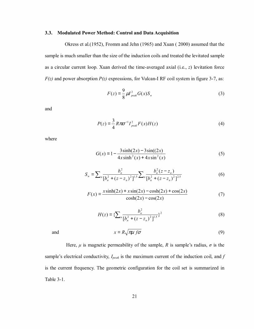
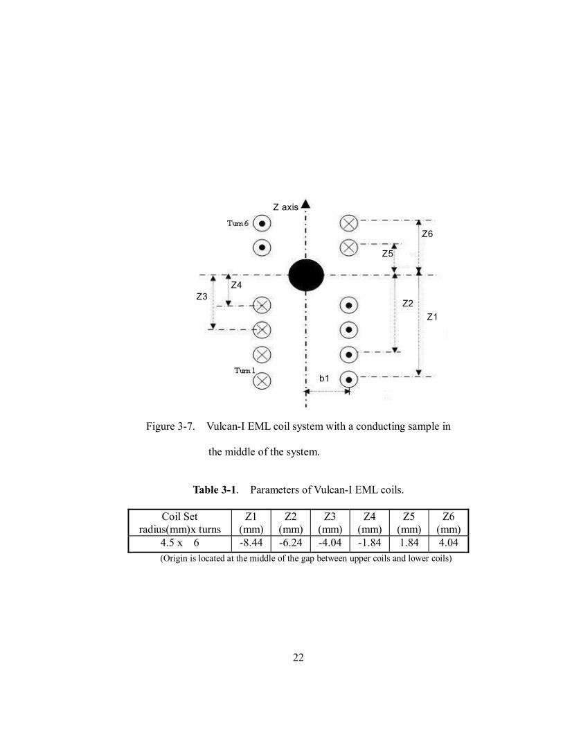
Table 3-1. Parameters of Vulcan-I EML coils . ..........................................................22

Table 3-2. Thermophysical properties of liquid nickel samples at the melting

temperature of 1728 K . ............................................................................29

Table 4-1. AISI E52100 steel composition (wt %).....................................................34

Table 4-2. Nickel-based superalloy IN713 composition (wt %). ................................39

Table 4-3. Uncertainty Estimates of the Nickel Specific Heat Measurement using

the EML Modulated Power Method. ........................................................47

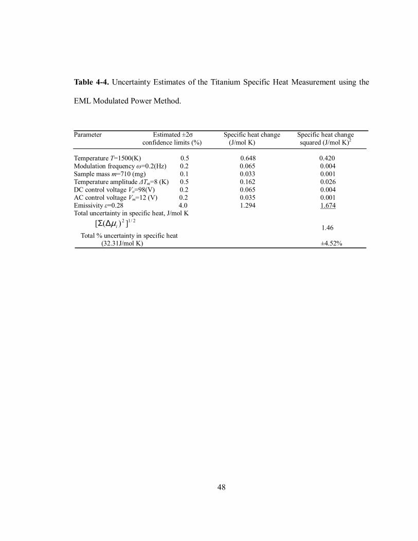
Table 4-4. Uncertainty Estimates of the Titanium Specific Heat Measurement

using the EML Modulated Power Method. ...............................................48

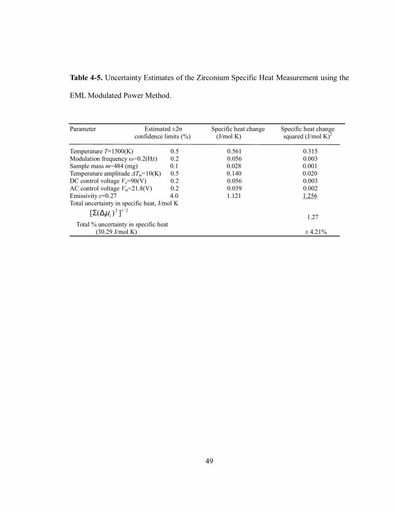
Table 4-5. Uncertainty Estimates of the Zirconium Specific Heat Measurement

using the EML Modulated Power Method. ...............................................49

xii

LIST OF FIGURES

Figure 1-1. Schematic sketch of the electromagnetic induction coils with a

conducting sample in the middle of the system. ..................................... 3

Figure 2-1. Radial intensity gradient profile along a levitated droplet. ...................... 8

Figure 3-1. Electromagnetic levitator of Auburn University. ..................................... 11

Figure 3-2. Functional diagram of experimental setup. .............................................12

Figure 3-3. Temperature measurement comparison between pyrometer and

thermocouple. ........................................................................................14

Figure 3-4. A levitated spherical solid nickel sample at 1295 oC. ..............................16

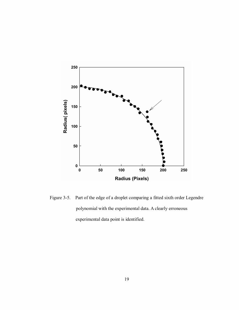
Figure 3-5. Part of the edge of a droplet comparing a fitted sixth order Legendre

polynomial with the experimental data. 19

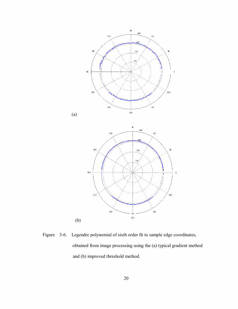
Figure 3-6. Legendre polynomial of sixth order fit to sample edge coordinates

obtained from image processing using the (a) typical gradient method

and (b) improved threshold method. .......................................................20

Figure 3-7. Vulcan-I EML coil system with a conducting sample in the middle of

the system . 22

Figure 3-8. Schematic diagram of modulated heating power method.........................24

Figure 3-9. Calculated EM force exerted on the levitated sample along axial

direction (z-axis). ...................................................................................27

xiii

Figure 3-10. (a) Spherical coordinates used in the numerical modeling.

(b) Schematic showing the assumed volumetric heating..........................30

Figure 4-1. (a) The peak coil current (lower trace) and resultant sample position

response (upper trace). (b) Comparison of dynamic temperature

response of the sample for motionless and moving sample cases.

ω= 0.2 Hz, Io=122 A, ∆Io=3 A, Im=10 A..................................................33

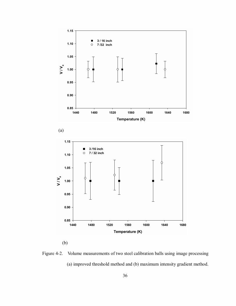
Figure 4-2. Volume measurements of two steel calibration balls using image

processing (a) improved threshold method and (b) maximum intensity

gradient method......................................................................................36

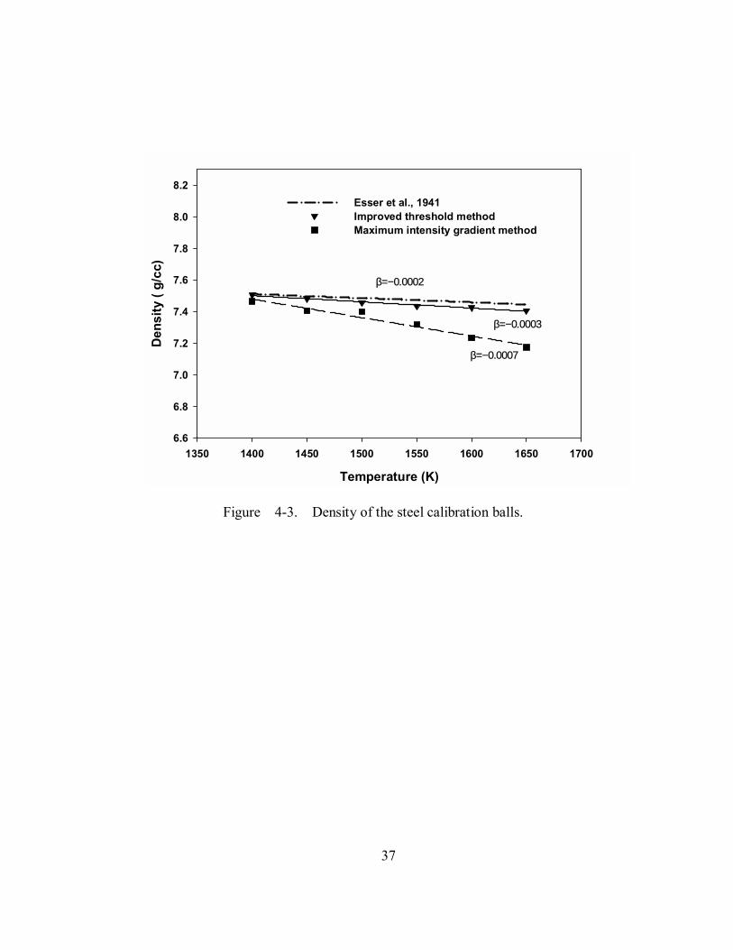
Figure 4-3. Density of the steel calibration balls........................................................37

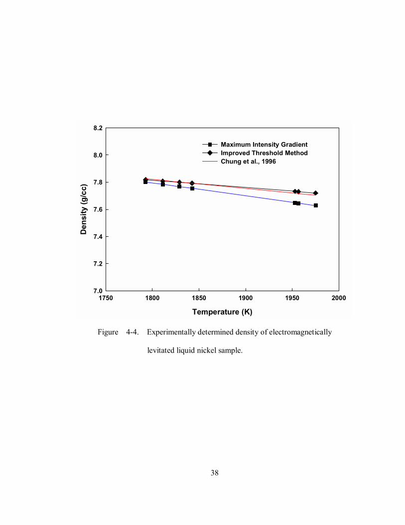
Figure 4-4. Experimentally determined density of electromagnetically levitated

liquid nickel samples..............................................................................38

Figure 4-5. Experimentally determined density of electromagnetically levitated

molten IN713. ........................................................................................41

Figure 4-6. Conductive heat loss through the suspension wire and its effect on

heat capacity calculation. ....................................................................... 42

Figure 4-7. Heat capacity of nickel: present work and data reported in the literature..44

Figure 4-8. Heat capacity of titanium: present work and data reported in the

literature. ....... 45

Figure 4-9. Heat capacity of zirconium: present work and data reported in the

literature.................................................................................................46

1

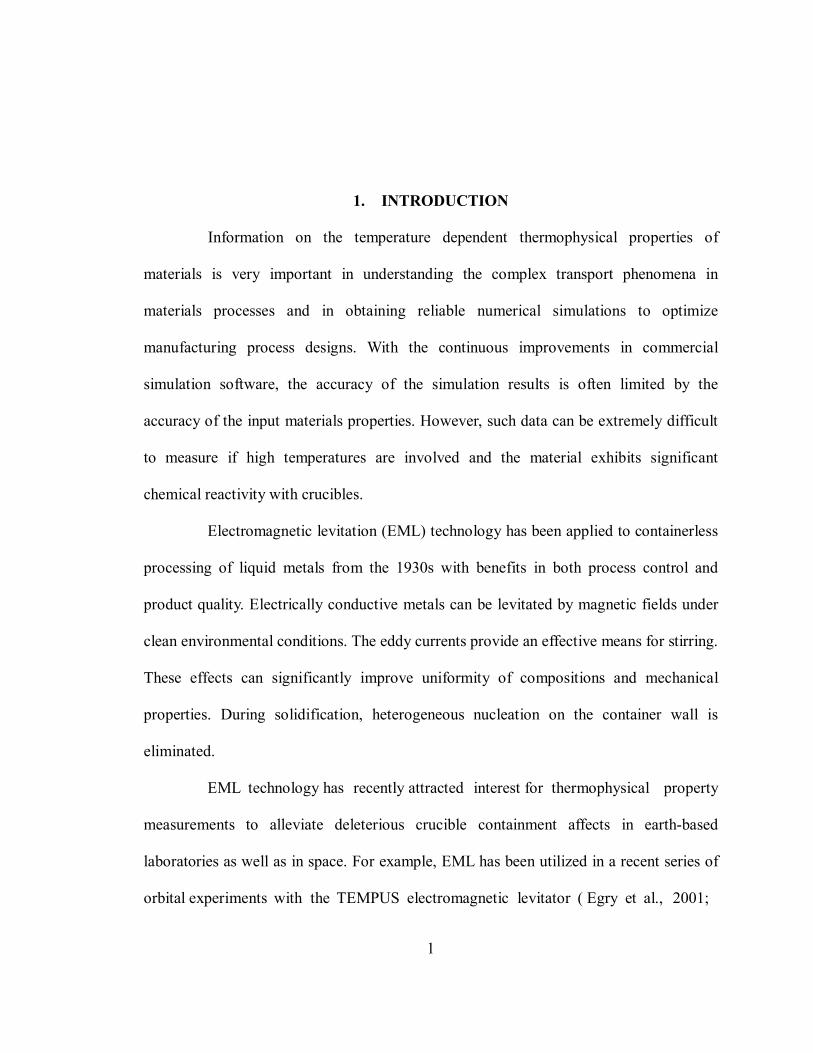
1. INTRODUCTION

Information on the temperature dependent thermophysical properties of

materials is very important in understanding the complex transport phenomena in

materials processes and in obtaining reliable numerical simulations to optimize

manufacturing process designs. With the continuous improvements in commercial

simulation software, the accuracy of the simulation results is often limited by the

accuracy of the input materials properties. However, such data can be extremely difficult

to measure if high temperatures are involved and the material exhibits significant

chemical reactivity with crucibles.

Electromagnetic levitation (EML) technology has been applied to containerless

processing of liquid metals from the 1930s with benefits in both process control and

product quality. Electrically conductive metals can be levitated by magnetic fields under

clean environmental conditions. The eddy currents provide an effective means for stirring.

These effects can significantly improve uniformity of compositions and mechanical

properties. During solidification, heterogeneous nucleation on the container wall is

eliminated.

EML technology has recently attracted interest for thermophysical property

measurements to alleviate deleterious crucible containment affects in earth-based

laboratories as well as in space. For example, EML has been utilized in a recent series of

orbital experiments with the TEMPUS electromagnetic levitator ( Egry et al., 2001;

2

Wunderlich et al., 2001).

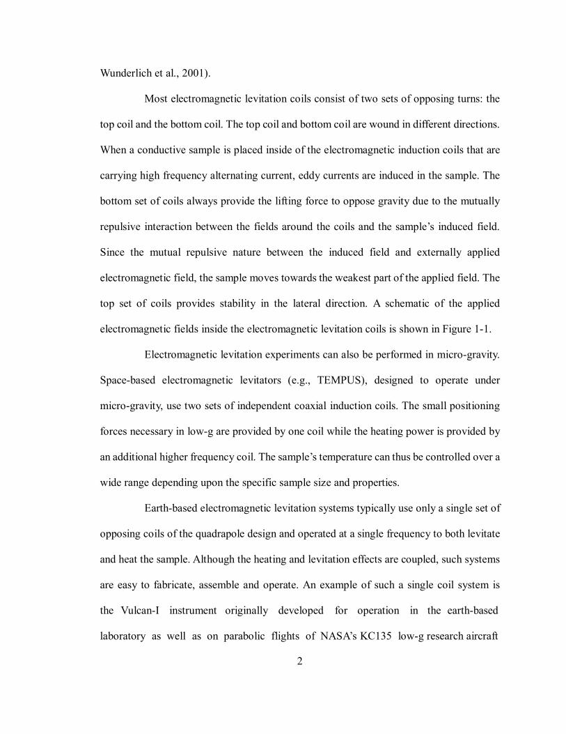
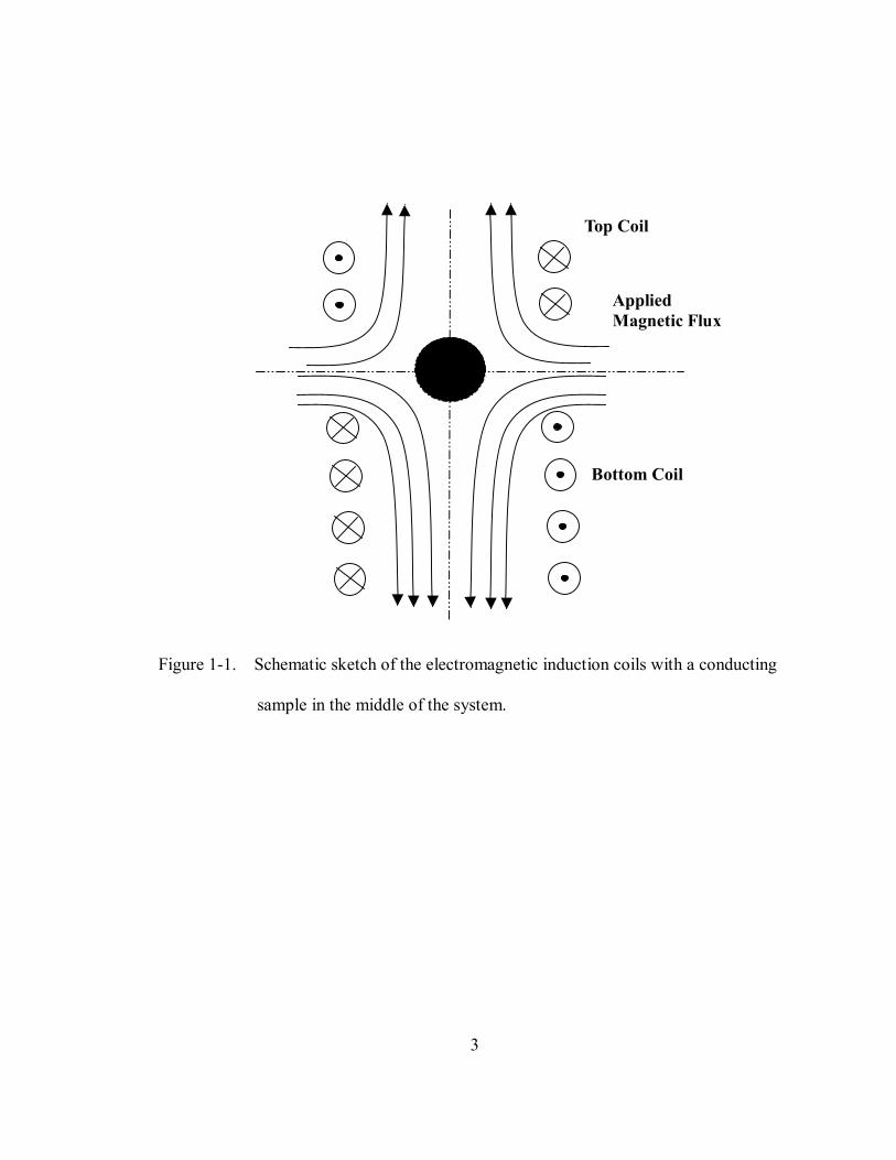
Most electromagnetic levitation coils consist of two sets of opposing turns: the

top coil and the bottom coil. The top coil and bottom coil are wound in different directions.

When a conductive sample is placed inside of the electromagnetic induction coils that are

carrying high frequency alternating current, eddy currents are induced in the sample. The

bottom set of coils always provide the lifting force to oppose gravity due to the mutually

repulsive interaction between the fields around the coils and the samples induced field.

Since the mutual repulsive nature between the induced field and externally applied

electromagnetic field, the sample moves towards the weakest part of the applied field. The

top set of coils provides stability in the lateral direction. A schematic of the applied

electromagnetic fields inside the electromagnetic levitation coils is shown in Figure 1-1.

Electromagnetic levitation experiments can also be performed in micro-gravity.

Space-based electromagnetic levitators (e.g., TEMPUS), designed to operate under

micro-gravity, use two sets of independent coaxial induction coils. The small positioning

forces necessary in low-g are provided by one coil while the heating power is provided by

an additional higher frequency coil. The samples temperature can thus be controlled over a

wide range depending upon the specific sample size and properties.

Earth-based electromagnetic levitation systems typically use only a single set of

opposing coils of the quadrapole design and operated at a single frequency to both levitate

and heat the sample. Although the heating and levitation effects are coupled, such systems

are easy to fabricate, assemble and operate. An example of such a single coil system is

the Vulcan-I instrument originally developed for operation in the earth-based

laboratory as well as on parabolic flights of NASAs KC135 low-g research aircraft

3

Figure 1-1. Schematic sketch of the electromagnetic induction coils with a conducting

sample in the middle of the system.

Top Coil

Bottom Coil

Applied Magnetic Flux

4

(Chen and Overfelt, 1998; Wang et al., 2003).

A very promising feature of EML is its potential for measuring several important

thermophysical properties on a single levitated sample over a large temperature range. The

absence of crucibles eliminates reactions with the melt and high levels of undercooling can

also be reached. Such applications require sophisticated non-contact diagnostics such as

two-color pyrometry for temperature measurement and high-speed video analysis for

characterizing the sample motion. The thermophysical properties of typical interest are

surface tension, density and thermal expansion, emissivity, specific and latent heats,

thermal conductivity and electrical conductivity. Reviews of theoretical and experimental

work in this area are given by Herlach et al. (1993) , Egry et al.(1993) and Bakhtiyarov and

Overfelt (2002; 2003).

More recently, high-temperature electrostatic levitation (HTESL) has been

developed at NASAs Jet Propulsion Laboratory (Chung et al., 1996) . HTESL charges a

sample and then uses electrostatic repulsive forces to levitate and position the charged

sample. A separate optical power system (laser, focused lamp, etc.) is needed to heat the

sample. HTESL systems are inherently unstable and require complex monitoring and

control systems for reliable operation. Nevertheless, HTESL can be applied to electrical

non-conducting materials as well as conductive materials.

This study intended to develop a new digital image processing method to

accurately measure the thermal expansion of levitated solid and molten metals and to

implement the modulated power method of specific heat measurement on different sizes of

solid samples. In addition, a numerical model was developed to examine the heat transfer

phenomena and examine the uncertainty in the heat capacity measurements.

5

2. LITERATURE REVIEW

2.1 . Thermal Expansion Measurement by Image Processing

Thermal expansion is an important thermophysical property in materials science.

Since direct physical contact is avoided in EML, standard push rod dilatometry cannot be

applied for measurements of thermal expansion. Sample images taken with precise optical

systems are required to characterize the sample sizes and evaluate thermal expansion

effects. When a sample is levitated and heated by an induction coil, the volumes of

symmetrical samples can be determined from side view images. However careful coil

design and fabrication is required to establish stable heating and levitation conditions

necessary for symmetrical molten droplets in typical earth-based EML laboratories.

In previous work (El-Mehairy and Ward, 1963), electromagnetically levitated

samples were photographed from the side using high speed film cameras. A photographic

enlarger was then used to achieve the necessary resolution for density measurements. The

edges of the samples for each image were determined by hand, and the volumes were then

obtained as a body of revolution from the edge profiles. This is a very inefficient method

and also inevitably involved random errors caused by each individual experimenter. The

modern development of CCD (charged-couple device) cameras and digital image

processing technique enable electromagnetically levitated sample images to be

automatically recorded and the recorded images analyzed using digital image processing

6

technique.

The key issue of accurate volume measurement is precise and repeatable

detection of the droplet edge in the images. An edge is defined as the boundary between

two regions with relatively distinct gray-level properties. Most edge detection algorithms

are based on the computation of a local gradient operator where the edge is at the location

of the maximum intensity gradient. Because of the intrinsic sensitivity of taking derivatives

from experimental data, the gradient method is very sensitive to noise and has demanding

requirements for picture quality (Gonzalez and Wintz, 1987; Jain, 1989). Several

researchers in electromagnetic levitation have adopted first-order derivative gradient

operators to determine the sample edge from image data (Brillo and Egry, 2003; Chung et

al., 1996; Damaschke et al., 1998; Gorges et al., 1996; Racz and Egry, 1995).These

techniques detected the edge by searching for the maximum intensity gradient along radial

vectors of each picture. Second-order derivative operators have also been reported (Racz

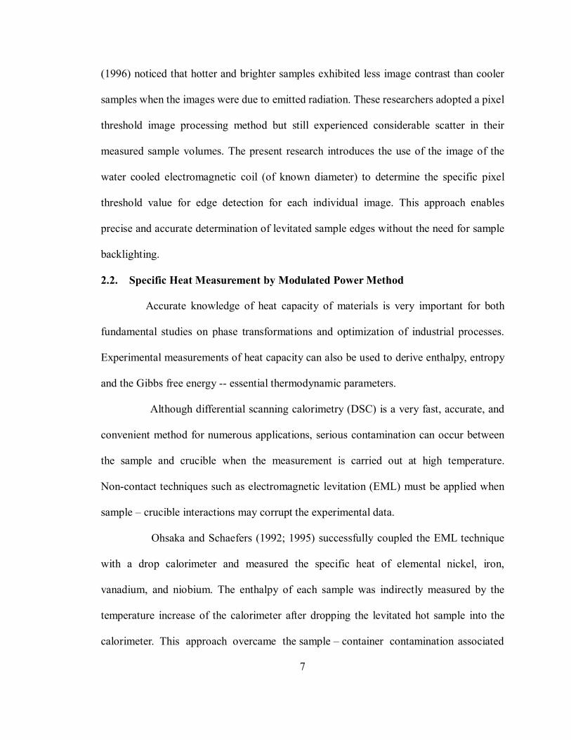
and Egry, 1995). Figure 2-1 shows a typical intensity gradient profile along a levitated

sample radial direction. Figure 2-1 (a) is the intensity first-order derivative profile and

figure 2-1 (b) is the intensity second-order derivative profile. However, as noted above,

gradient methods have strict requirements on picture quality and thus backlighting

techniques have been adopted to reduce pixel blooming in CCDs and improve contrast

(Brillo and Egry, 2003; Chung et al., 1996; Damaschke et al., 1998). Pixel blooming occurs

when a pixels electrical charge exceeds the CCD pixels storage limit and then the

electrical charge overflows to neighboring pixels.

A robust alternative approach to analysis of noisy images involves threshold

methods (Gonzalez and Wintz, 1987; Jain, 1989). Racz and Egry (1995) and Gorges et al

7

(1996) noticed that hotter and brighter samples exhibited less image contrast than cooler

samples when the images were due to emitted radiation. These researchers adopted a pixel

threshold image processing method but still experienced considerable scatter in their

measured sample volumes. The present research introduces the use of the image of the

water cooled electromagnetic coil (of known diameter) to determine the specific pixel

threshold value for edge detection for each individual image. This approach enables

precise and accurate determination of levitated sample edges without the need for sample

backlighting.

2.2. Specific Heat Measurement by Modulated Power Method

Accurate knowledge of heat capacity of materials is very important for both

fundamental studies on phase transformations and optimization of industrial processes.

Experimental measurements of heat capacity can also be used to derive enthalpy, entropy

and the Gibbs free energy -- essential thermodynamic parameters.

Although differential scanning calorimetry (DSC) is a very fast, accurate, and

convenient method for numerous applications, serious contamination can occur between

the sample and crucible when the measurement is carried out at high temperature.

Non-contact techniques such as electromagnetic levitation (EML) must be applied when

sample crucible interactions may corrupt the experimental data.

Ohsaka and Schaefers (1992; 1995) successfully coupled the EML technique

with a drop calorimeter and measured the specific heat of elemental nickel, iron,

vanadium, and niobium. The enthalpy of each sample was indirectly measured by the

temperature increase of the calorimeter after dropping the levitated hot sample into the

calorimeter. This approach overcame the sample container contamination associated

8

Pixel 0 50 100 150 200 250 300 350

Firs

t-ord

er d

eriv

ativ

e

0

5

10

15

20

25

30

35

(a)

Pixel

0 50 100 150 200 250 300 350

Seco

nd-o

rder

der

ivat

ive

-30

-20

-10

0

10

20

30

(b)

Figure 2-1. Radial intensity gradient profile along a levitated droplet.

(a) First-order derivative profile. (b) Second-order derivative profile.

9

with conventional calorimeters. However, it introduced significant experimental

complexity and only allowed a single point measurement of enthalpy with each sample

processed. In the pioneering modulated power experiments (Bachmann et al., 1972;

Sullivan and Seidel, 1968), heat capacity measurement was performed at low

temperatures with a small sample (1-500mg) and in which a silicon chip was used as the

sample holder. Fecht and Johnson (1991) and their colleagues (Fecht and Wunderlich,

1994; Wunderlich et al., 1993; Wunderlich et al., 2000; Wunderlich et al., 2001;

Wunderlich and Fecht, 1993; Wunderlich and Fecht, 1996; Wunderlich et al., 1997)

applied the modulated power method to the electromagnetic heating and levitation

technique. In this application, the electromagnetically heated and levitated sample is

exposed to a slowly varying sinusoidally-modulated heating power. The temperature

response of the levitated sample slightly lagged behind the imposed power profile with a

time constant that depended upon the thermal inertia of the sample. By proper choice of

the modulation frequency, the transient effects of external and internal thermal

relaxations can be ignored with errors of only approximately 1% (Fecht and Johnson,

1991). The unknown specific heat can then be calculated if the samples emissive

properties are known. The electromagnetic levitation technique (Egry et al., 1993;

Wroughton et al., 1952) combined with the modulation power method is an excellent

experimental technique that allows containerless heat capacity measurements on

electrically conductive samples.

10

3. EXPERIMENT PROCEDURES AND ANALYTICAL TECHNIQUES

3.1 . Electromagnetic Levitation Apparatus

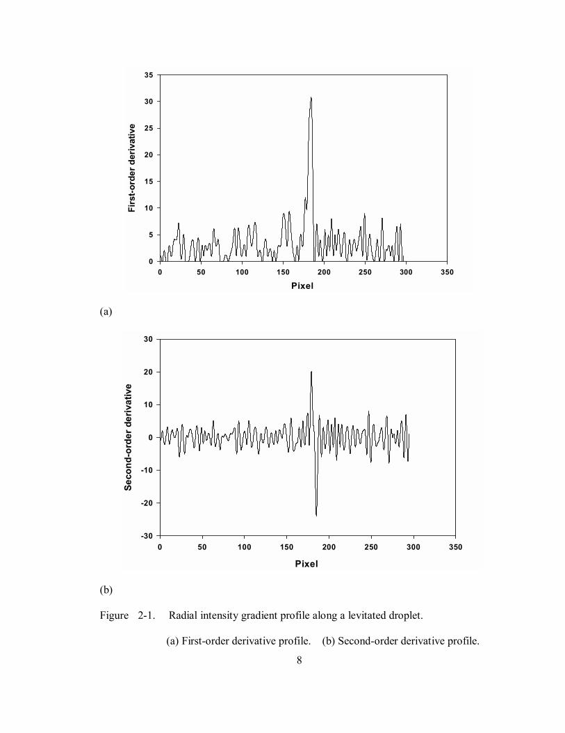
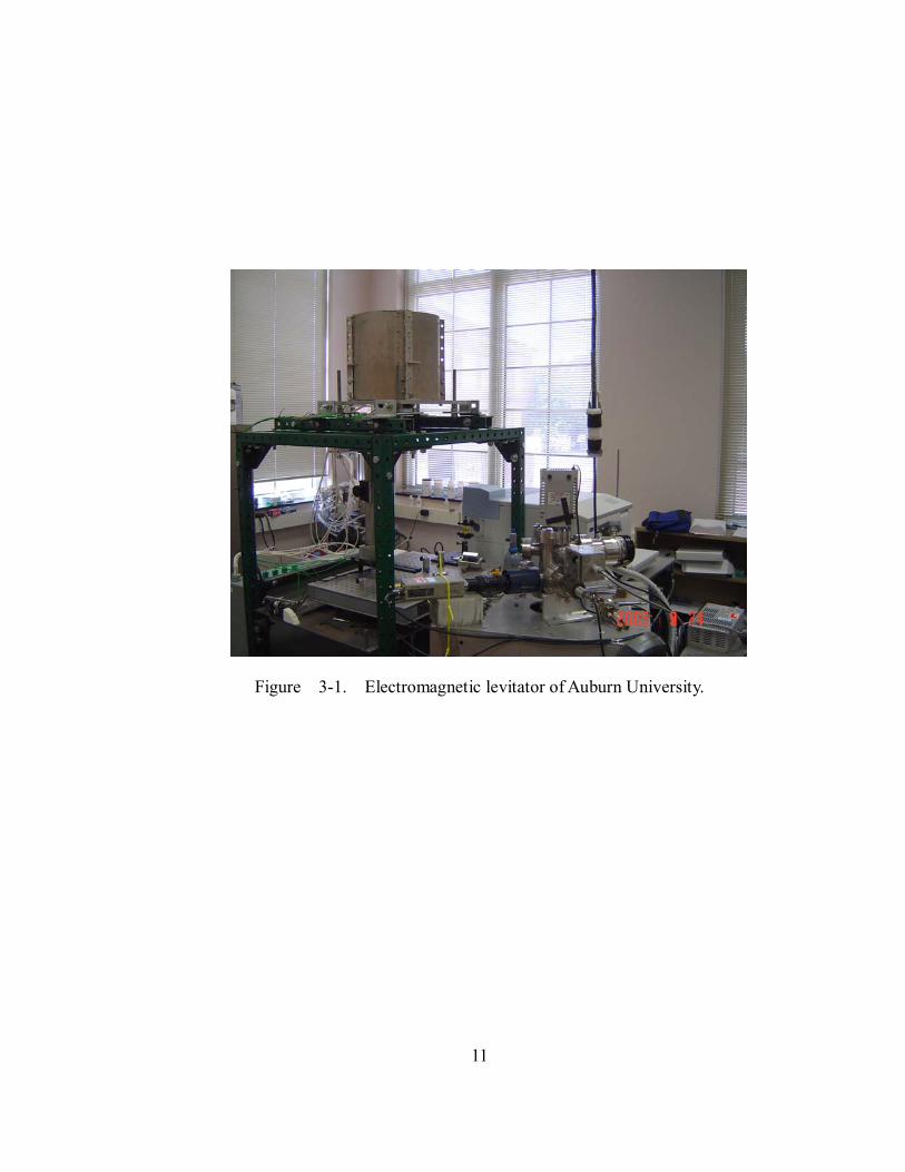
A key part of the electromagnetic levitator at Auburn University (Figure 3-1.) is

the induction coil housed in a vacuum chamber (10-6 torr) pumped by a turbomolecular

pump. A sample handler with a rotational sample selector allows up to 8 samples to be

processed without opening the vacuum chamber. A commercial 1 kW RF power supply is

used to provide a high frequency alternating current of approximately 175 amps at 280 kHz

to the induction coil. The induction coil was configured to impose a quadrupole positioning

field to keep the sample approximately in the middle of the coil. One of the advantages of

the quadrapole design is that the system is very simple, easy to make with high degree of

symmetry and exhibits a stably levitated sample.

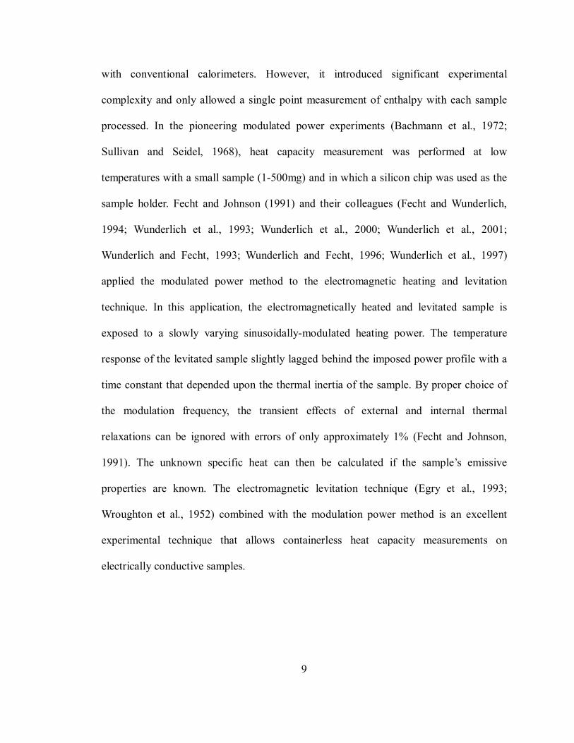
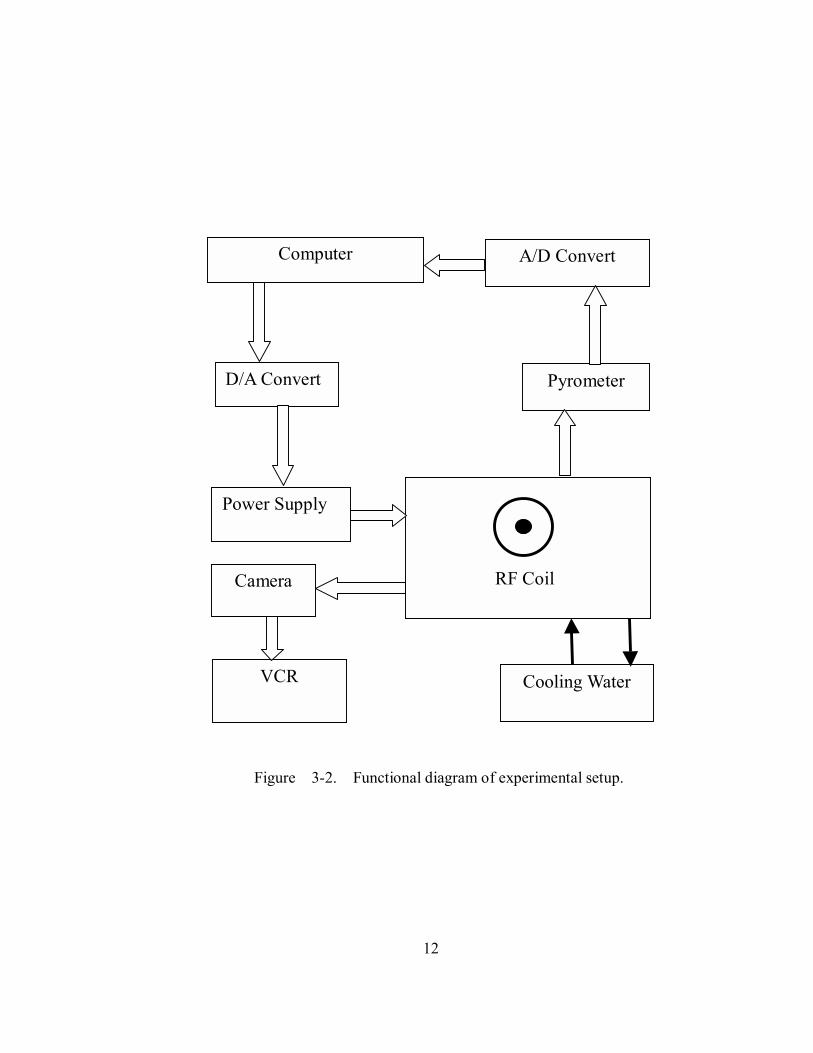
The RF power supply is controlled by a computer and D/A converter using

RS232 Serial Interfaces. The power supply control signal is composed of a DC component

and an AC component. A functional diagram of the experimental setup is shown in figure

3-2.

11

Figure 3-1. Electromagnetic levitator of Auburn University.

12

Figure 3-2. Functional diagram of experimental setup.

Computer

D/A Convert

Power Supply

RF Coil

Pyrometer

A/D Convert

Cooling Water

Camera

VCR

13

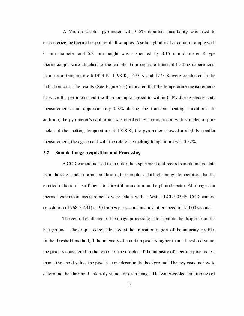
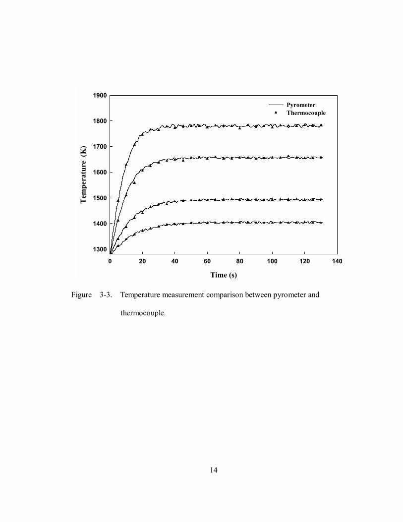
A Micron 2-color pyrometer with 0.5% reported uncertainty was used to

characterize the thermal response of all samples. A solid cylindrical zirconium sample with

6 mm diameter and 6.2 mm height was suspended by 0.15 mm diameter R-type

thermocouple wire attached to the sample. Four separate transient heating experiments

from room temperature to1423 K, 1498 K, 1673 K and 1773 K were conducted in the

induction coil. The results (See Figure 3-3) indicated that the temperature measurements

between the pyrometer and the thermocouple agreed to within 0.4% during steady state

measurements and approximately 0.8% during the transient heating conditions. In

addition, the pyrometers calibration was checked by a comparison with samples of pure

nickel at the melting temperature of 1728 K, the pyrometer showed a slightly smaller

measurement, the agreement with the reference melting temperature was 0.52%.

3.2 . Sample Image Acquisition and Processing

A CCD camera is used to monitor the experiment and record sample image data

from the side. Under normal conditions, the sample is at a high enough temperature that the

emitted radiation is sufficient for direct illumination on the photodetector. All images for

thermal expansion measurements were taken with a Watec LCL-903HS CCD camera

(resolution of 768 X 494) at 30 frames per second and a shutter speed of 1/1000 second.

The central challenge of the image processing is to separate the droplet from the

background. The droplet edge is located at the transition region of the intensity profile.

In the threshold method, if the intensity of a certain pixel is higher than a threshold value,

the pixel is considered in the region of the droplet. If the intensity of a certain pixel is less

than a threshold value, the pixel is considered in the background. The key issue is how to

determine the threshold intensity value for each image. The water-cooled coil tubing (of

14

Time (s)

0 20 40 60 80 100 120 140

Tem

pera

ture

(K

)

1300

1400

1500

1600

1700

1800

1900PyrometerThermocouple

Figure 3-3. Temperature measurement comparison between pyrometer and

thermocouple.

15

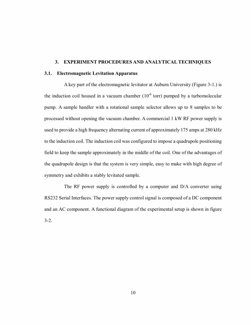
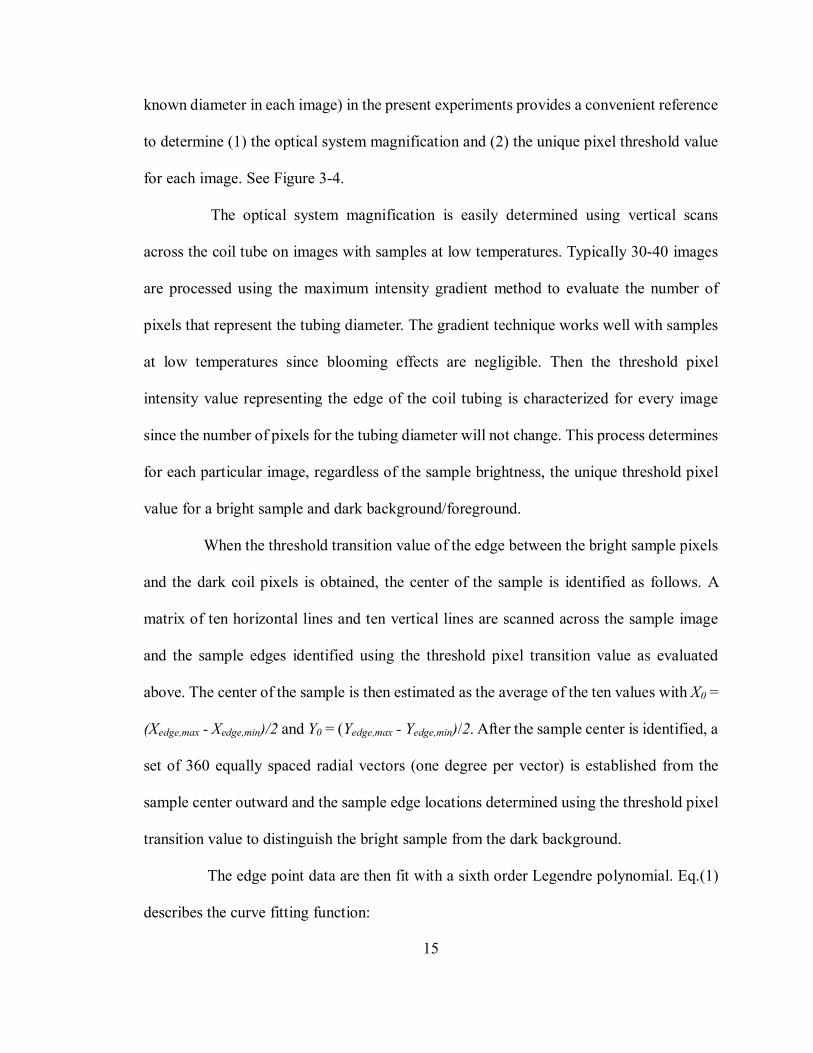
known diameter in each image) in the present experiments provides a convenient reference

to determine (1) the optical system magnification and (2) the unique pixel threshold value

for each image. See Figure 3-4.

The optical system magnification is easily determined using vertical scans

across the coil tube on images with samples at low temperatures. Typically 30-40 images

are processed using the maximum intensity gradient method to evaluate the number of

pixels that represent the tubing diameter. The gradient technique works well with samples

at low temperatures since blooming effects are negligible. Then the threshold pixel

intensity value representing the edge of the coil tubing is characterized for every image

since the number of pixels for the tubing diameter will not change. This process determines

for each particular image, regardless of the sample brightness, the unique threshold pixel

value for a bright sample and dark background/foreground.

When the threshold transition value of the edge between the bright sample pixels

and the dark coil pixels is obtained, the center of the sample is identified as follows. A

matrix of ten horizontal lines and ten vertical lines are scanned across the sample image

and the sample edges identified using the threshold pixel transition value as evaluated

above. The center of the sample is then estimated as the average of the ten values with X0 =

(Xedge,max - Xedge,min)/2 and Y0 = (Yedge,max - Yedge,min)/2. After the sample center is identified, a

set of 360 equally spaced radial vectors (one degree per vector) is established from the

sample center outward and the sample edge locations determined using the threshold pixel

transition value to distinguish the bright sample from the dark background.

The edge point data are then fit with a sixth order Legendre polynomial. Eq.(1)

describes the curve fitting function:

16

Figure 3-4. A levitated spherical solid nickel sample at 1295 oC.

Note the horizontal coil blocking part of the image.

17

))(cos()(6

0

θθ ∑=

=j

jjfit PaR (1)

where Pj(cos(θ)) are the Legendre polynomials and aj are the polynomial coefficients. The

curve fitting is implemented with a standard least-squares procedure. The curve fitting

procedure provides a complete definition of the samples edge even though the coil blocks

part of the sample image. In addition, the curve fitting procedure actually improves upon

the one-pixel resolution of the image.

Since surface tension ensures a molten samples surface remains relatively

smooth, large deviations in a droplets edge data are not physically possible. A typical set

of edge data and the fitted polynomial are shown in figure 3-5. The data point marked by

the arrow is clearly an outlier and should not be used in the edge determination procedure.

The fitting residuals between the locations of the experimental data points and the fitted

curve are examined and all edge points with a residual greater than 2σ are discounted and

eliminated from the experimental data set. After the outliers are removed, the data are then

fit again with a new sixth order Legendre polynomial.

Figure 3-6 shows a comparison of curve fits after the droplet edge data were

determined by the typical maximum intensity gradient method and the improved threshold

method as outlined above. The improved threshold method provides much better

agreement with the experimental data. The improved threshold method was also found to

be a more accurate approach, as will be discussed later in the experiment results section.

Assuming that the sample is axisymetric, the droplet volume can then be

calculated as a body of revolution from the smooth curve as

18

∫=π

θθθπ

0

)(3)(3

2 dSinRV (2)

Once the volume is determined, the density is easily calculated if the sample

mass is known. In the present experiments, the mass of the each sample was carefully

evaluated before and after the experiment and evaporation was assumed to occur linearly

with time while the sample was molten. The value of dV/dT for molten metals is of the

order of 10-4 g cm-3 K-1. The error analysis of Racz and Egry (Racz and Egry, 1995) show

that edge location using pixel interpolation combined with Legendre polynomial fitting

enable theoretical volume uncertainties of ∆V/V ~ 10-4.

19

Radius (Pixels)

0 50 100 150 200 250

Rad

ius(

pix

els)

0

50

100

150

200

250

Figure 3-5. Part of the edge of a droplet comparing a fitted sixth order Legendre

polynomial with the experimental data. A clearly erroneous

experimental data point is identified.

20

(a)

(b)

Figure 3-6. Legendre polynomial of sixth order fit to sample edge coordinates,

obtained from image processing using the (a) typical gradient method

and (b) improved threshold method.

21

3.3. Modulated Power Method: Control and Data Acquisition

Okress et al.(1952), Fromm and Jehn (1965) and Xuan ( 2000) assumed that the

sample is much smaller than the size of the induction coils and treated the levitated sample

as a circular current loop. Xuan derived the time-averaged axial (i.e., z) levitation force

F(z) and power absorption P(z) expressions, for Vulcan-I RF coil system in figure 3-7, as:

npeak SxGIzF )(89)( 2µ= (3)

and

)()(43)( 21 zHxFIRzP peak

−= πσ (4)

where

)(sin4)(sinh4

)2sin((3)2sinh(31)( 22 xxxxxxxG

+−−= (5)

∑∑ −+−

−+=

nnn

nnn

nn

nn zzb

zzbzzb

bS 5.222

2

5.122

2

])([)(

])([ (6)

)2cos()2cosh(

)2cos()2cosh()2sin()2sinh()(xx

xxxxxxxF−

+−+= (7)

25.122

2

])([

)( ∑ −+=

nnn

n

zzbb

zH (8)

and σπµ fRx = (9)

Here, µ is magnetic permeability of the sample, R is samples radius, σ is the

samples electrical conductivity, Ipeak is the maximum current of the induction coil, and f

is the current frequency. The geometric configuration for the coil set is summarized in

Table 3-1.

22

Z1Z2

Z3Z4

Z5

Z6

b1

Z axis

Figure 3-7. Vulcan-I EML coil system with a conducting sample in

the middle of the system.

Table 3-1. Parameters of Vulcan-I EML coils.

Coil Set

radius(mm)x turns Z1

(mm) Z2

(mm) Z3

(mm) Z4

(mm) Z5

(mm) Z6

(mm) 4.5 x 6 -8.44 -6.24 -4.04 -1.84 1.84 4.04

(Origin is located at the middle of the gap between upper coils and lower coils)

23

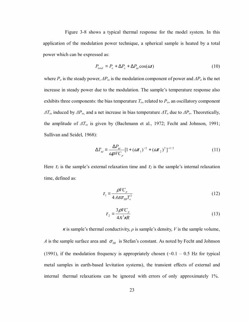
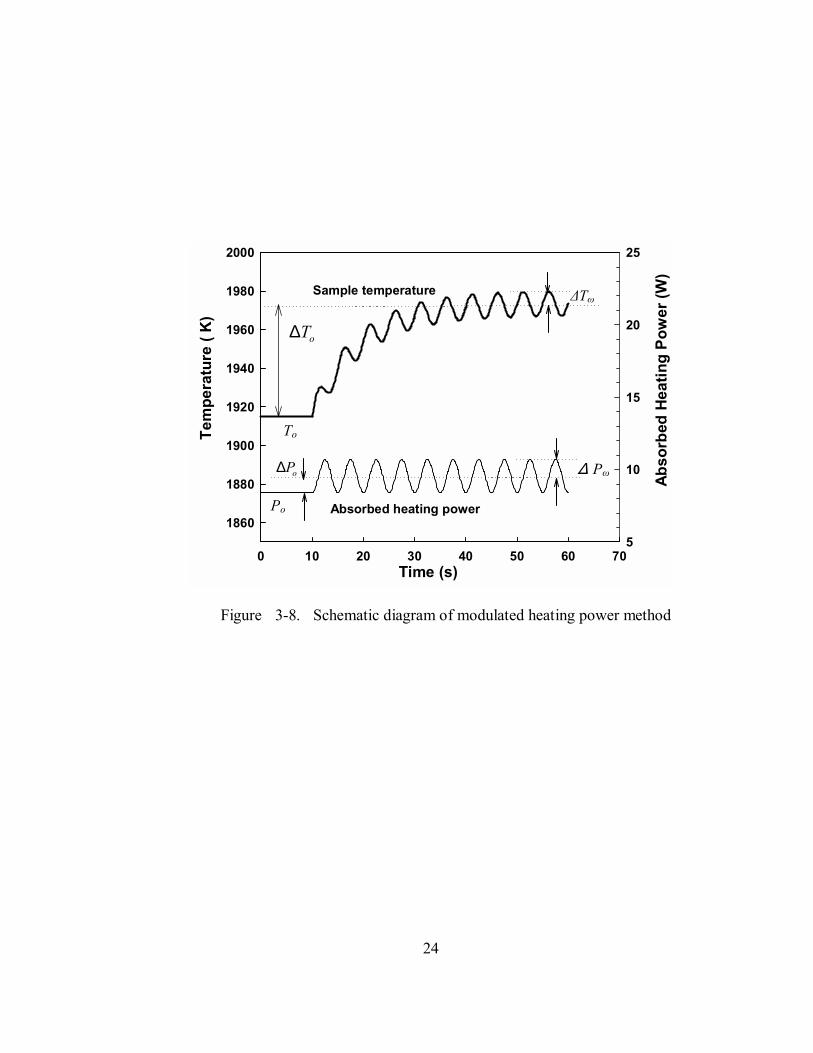
Figure 3-8 shows a typical thermal response for the model system. In this

application of the modulation power technique, a spherical sample is heated by a total

power which can be expressed as:

)cos( tPPPP oototal ωω∆+∆+= (10)

where Po is the steady power, ∆Pω is the modulation component of power and ∆Po is the net

increase in steady power due to the modulation. The samples temperature response also

exhibits three components: the bias temperature To, related to Po, an oscillatory component

∆Tω induced by ∆Pω, and a net increase in bias temperature ∆To due to ∆Po. Theoretically,

the amplitude of ∆Tω is given by (Bachmann et al., 1972; Fecht and Johnson, 1991;

Sullivan and Seidel, 1968):

2/122

21 ])()(1[ −− ++

∆=∆ ωτωτ

ωρω

ωpVC

PT (11)

Here τ1 is the samples external relaxation time and τ2 is the samples internal relaxation

time, defined as:

31 4 oSB

p

TAVCεσ

ρτ = (12)

RVC p

κπρ

τ 32 43

= (13)

κ is samples thermal conductivity, ρ is samples density, V is the sample volume,

A is the sample surface area and SBσ is Stefans constant. As noted by Fecht and Johnson

(1991), if the modulation frequency is appropriately chosen (~0.1 0.5 Hz for typical

metal samples in earth-based levitation systems), the transient effects of external and

internal thermal relaxations can be ignored with errors of only approximately 1%.

24

Time (s)0 10 20 30 40 50 60 70

Tem

pera

ture

( K

)

1860

1880

1900

1920

1940

1960

1980

2000

5

10

15

20

25

oT∆

∆Tω

To

Po

Δ Pω oP∆

Abso

rbed

Hea

ting

Pow

er (W

)

Sample temperature

Absorbed heating power

Figure 3-8. Schematic diagram of modulated heating power method

25

Thus Eq.(11) reduces to:

pVC

PT

ωρω

ω∆

=∆ (14)

A control voltage is applied to the power supply of the RF system, and the current in the

electromagnetic coil can be represented as:

)cos()( tIItI mopeak ω+= (15)

Substituting Eq.(15) in Eq.(4), the total power can be formulated as:

)2cos()cos( 2 tPtPPPP oototal ωω ωω ∆+∆+∆+= (16)

where, )()(43 21 zHxFIRP oo

−= πσ (17)

)()(83 21 zHxFIRP mo

−=∆ πσ (18)

)()(23 1 zHxFIIRP mo

−=∆ πσω (19)

and oPP ∆=∆ ω2 (20)

At steady state in vacuum, the input power Po is just balanced by the radiative

heat losses. When the coil current is modulated, the bulk sample temperature will rise by

∆To due to the increase ∆Po in average absorbed power as shown in figure 3-8. Although

the temperature signal should theoretically contain a 2ω frequency component, this

component is <1% due to Im<<Io. Determination of the specific heat from Eq. (14) requires

knowledge of the power modulation amplitude ∆Pω from the samples temperature

response. For a motionless sample, ∆Pω can be estimated from Po as:

oo

m PII

P2

=∆ ω (21)

26

where Po is experimentally obtained using the Stefan-Boltzmann law:

][ 44envoSBo TTAP −= εσ (22)

in which Tenv is surrounding environment temperature.

3.4. Numerical Model of Modulated Power Method

3.4.1. Analysis of Sample Movement due to Modulated Power

In the presence of modulation current in the form of Eq.(15), the total

levitation force can be expressed by Eq.(23) when neglecting the 2ω frequency

component.

)cos( tFFFF oototal ωω∆+∆+= (23)

where:

noo SxGIF )(89 2µ= (24)

nmo SxGIF )(169 2µ=∆ (25)

nmo SxGIIF )(49 µω =∆ (26)

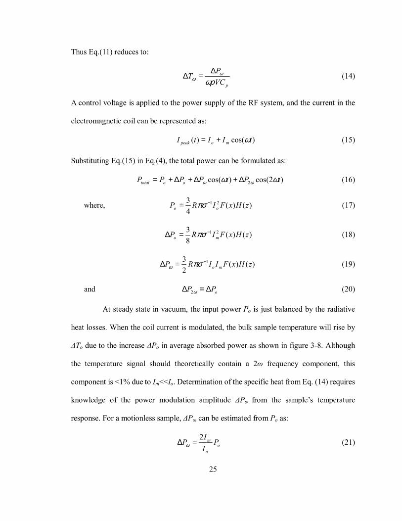
With knowledge of the time-averaged levitation force and modulated current

form, mathematical expressions can be quickly developed for analyzing the samples

oscillatory motion. Figure 3-9 shows a typical theoretical levitation profile on a nickel

sample in the coil design used in the current experiments. The equilibrium levitation

position is indicated by the arrow. When the sample deviates from its equilibrium position,

a restoring force proportional to the displacement is exerted on the sample. Therefore, a

simple spring mass system can be used to describe the oscillatory motion of levitated

samples.

27

Position of the sample (mm)

-20 -10 0 10 20

Levi

tatio

n Fo

rce

/ (Vo

lum

e x

g )

(g

/cc)

-20

-15

-10

-5

0

5

10

15

20

Lower turnsUpper turnsNet levitation force

EML coil range

Figure 3-9. Calculated EM force exerted on the levitated sample along axial

direction (z-axis). Coil Current (peak): 130A, Frequency: 200 KHz.

The equilibrium position corresponding to the sample density is indicated

28

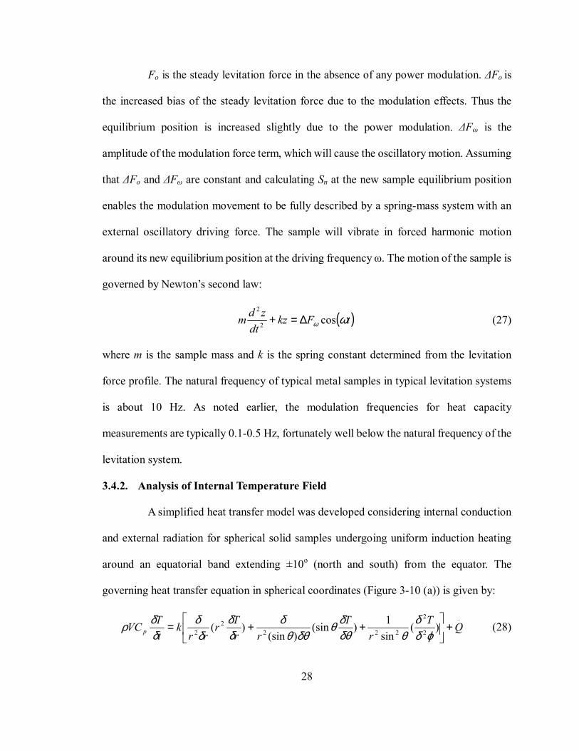
Fo is the steady levitation force in the absence of any power modulation. ∆Fo is

the increased bias of the steady levitation force due to the modulation effects. Thus the

equilibrium position is increased slightly due to the power modulation. ∆Fω is the

amplitude of the modulation force term, which will cause the oscillatory motion. Assuming

that ∆Fo and ∆Fω are constant and calculating Sn at the new sample equilibrium position

enables the modulation movement to be fully described by a spring-mass system with an

external oscillatory driving force. The sample will vibrate in forced harmonic motion

around its new equilibrium position at the driving frequency ω. The motion of the sample is

governed by Newtons second law:

( )tFkzdt

zdm ωω cos2

2

∆=+ (27)

where m is the sample mass and k is the spring constant determined from the levitation

force profile. The natural frequency of typical metal samples in typical levitation systems

is about 10 Hz. As noted earlier, the modulation frequencies for heat capacity

measurements are typically 0.1-0.5 Hz, fortunately well below the natural frequency of the

levitation system.

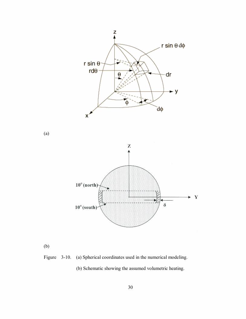
3.4.2. Analysis of Internal Temperature Field

A simplified heat transfer model was developed considering internal conduction

and external radiation for spherical solid samples undergoing uniform induction heating

around an equatorial band extending ±10o (north and south) from the equator. The

governing heat transfer equation in spherical coordinates (Figure 3-10 (a)) is given by:

.

2

2

2222

2 )(sin1)(sin

)(sin)( QT

rT

rrTr

rrk

tTVC p +

++=

ϕδδ

θδθδθ

δθθδ

δδ

δδ

δδρ (28)

29

where the heat generation term .

Q only existed in the inductively heated region. The

penetration depth of induction heating is given by:

0

2ωσµ

δ = (29)

Figure 3-10 (b) is the schematic showing the simplified heating assumed. Table 3-2 lists the

thermophysical properties of liquid nickel used for the heat transfer analysis. The sample

size investigated was 4 mm diameter.

Table 3-2. Thermophysical properties of liquid nickel samples at the melting

temperature of 1728 K (Brandes and Brook, 1992) .

Parameters Value Unit

density (ρ)

emissivity (ε)

specific heat (Cp)

thermal conductivity (k)

electrical conductivity (σ)

saturated pressure (Ps)

7.905

0.22

620

76

5·106

0.0029

g cm-3

J kg-1k-1

wm-1k-1

(Ωm)-1

torr

30

(a)

(b)

Figure 3-10. (a) Spherical coordinates used in the numerical modeling.

(b) Schematic showing the assumed volumetric heating.

31

The electromagnetic heating power was assumed to be uniformly distributed in a

shell volume region defined by the sample surface (latitudes from 10° north to 10° south)

and the penetration depth. Electromagnetic levitation systems typically operate at 100-500

kHz. Thus for this analysis of the modulated power method using frequencies of 0.1-0.5

Hz, the induced heating currents can be assumed to instantaneously rise to their peak

values. The radiation heat losses were linearized as:

)( 1 envlrarad TTAhq −= + (30)

with ))(( 22envlenvlSBra TTTTh ++= εσ (31)

where, the subscripts l, and l+1 denote the times t and t+∆t.

32

4. RESULTS AND DISCUSSION

4.1 . Sample Movement Effects

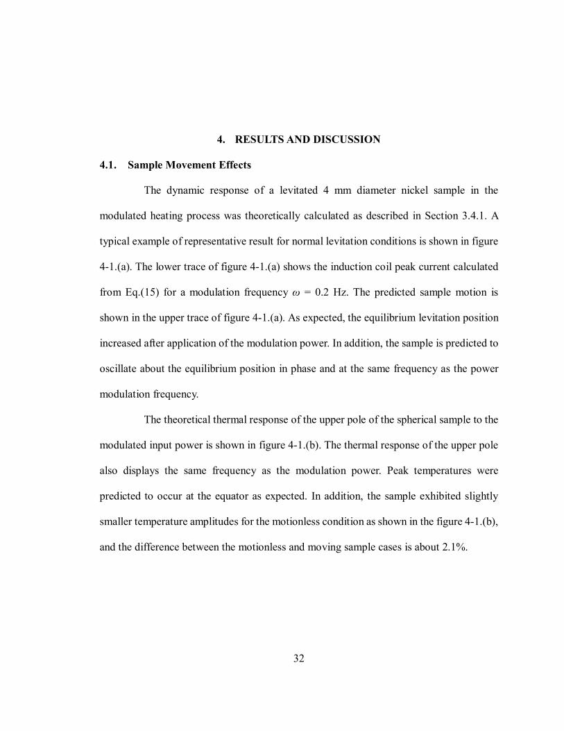
The dynamic response of a levitated 4 mm diameter nickel sample in the

modulated heating process was theoretically calculated as described in Section 3.4.1. A

typical example of representative result for normal levitation conditions is shown in figure

4-1.(a). The lower trace of figure 4-1.(a) shows the induction coil peak current calculated

from Eq.(15) for a modulation frequency ω = 0.2 Hz. The predicted sample motion is

shown in the upper trace of figure 4-1.(a). As expected, the equilibrium levitation position

increased after application of the modulation power. In addition, the sample is predicted to

oscillate about the equilibrium position in phase and at the same frequency as the power

modulation frequency.

The theoretical thermal response of the upper pole of the spherical sample to the

modulated input power is shown in figure 4-1.(b). The thermal response of the upper pole

also displays the same frequency as the modulation power. Peak temperatures were

predicted to occur at the equator as expected. In addition, the sample exhibited slightly

smaller temperature amplitudes for the motionless condition as shown in the figure 4-1.(b),

and the difference between the motionless and moving sample cases is about 2.1%.

33

Time (s)

0 10 20 30 40 50 60

Posi

tion

(mm

)

-1.4

-1.2

-1.0

-0.8

-0.6

-0.4

-0.2

0.0

0.2

Cur

rent

(A)

110

120

130

140

150

PositionCurrent

Time (s)

0 10 20 30 40 50 60

Tem

pera

ture

( K)

1890

1895

1900

1905

1910

1915

1920

Modulation movement consideredNo modulation movement assumption

(a)

(b)

Figure 4-1. (a) The peak coil current (lower trace) and resultant sample position

response (upper trace). (b) Comparison of dynamic temperature response

of the sample for motionless and moving sample cases. ω= 0.2 Hz, Io=122

A, ∆Io=3 A, Im=10 A.

34

4.2. Thermal Expansion of Molten Nickel and Nickel-Based Alloy IN713

In order to test the accuracy of the present image processing technique, two

different diameter steel calibration balls (AISI E52100) were electromagnetically heated,

and the images were recorded from the video camera and analyzed for their volumes. The

composition of AISI E52100 steel is summarized in Table 4-1.

Table 4-1. AISI E52100 steel composition (wt %).

Element C Cr Fe Mn P S Si

E52100 0.98-1.1 1.45 97 0.35 Max 0.025 Max 0.025 0.23

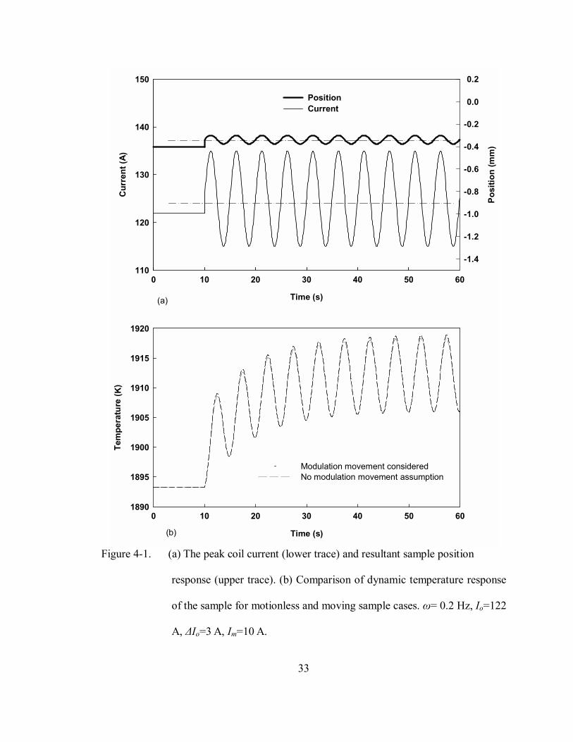
The normalized volumes (value divided by the average value) are shown in

figure 4-2. Figure 4-2(a) shows the volume measurements using the improved threshold

method, and figure 4-2 (b) shows the volume measurements using the maximum intensity

gradient method. The result shows that the improved threshold method exhibits a smaller

standard deviation in terms of volume determination. The difference in these two methods

arises mainly from the blooming effect, which generated a noisy contour for the heated,

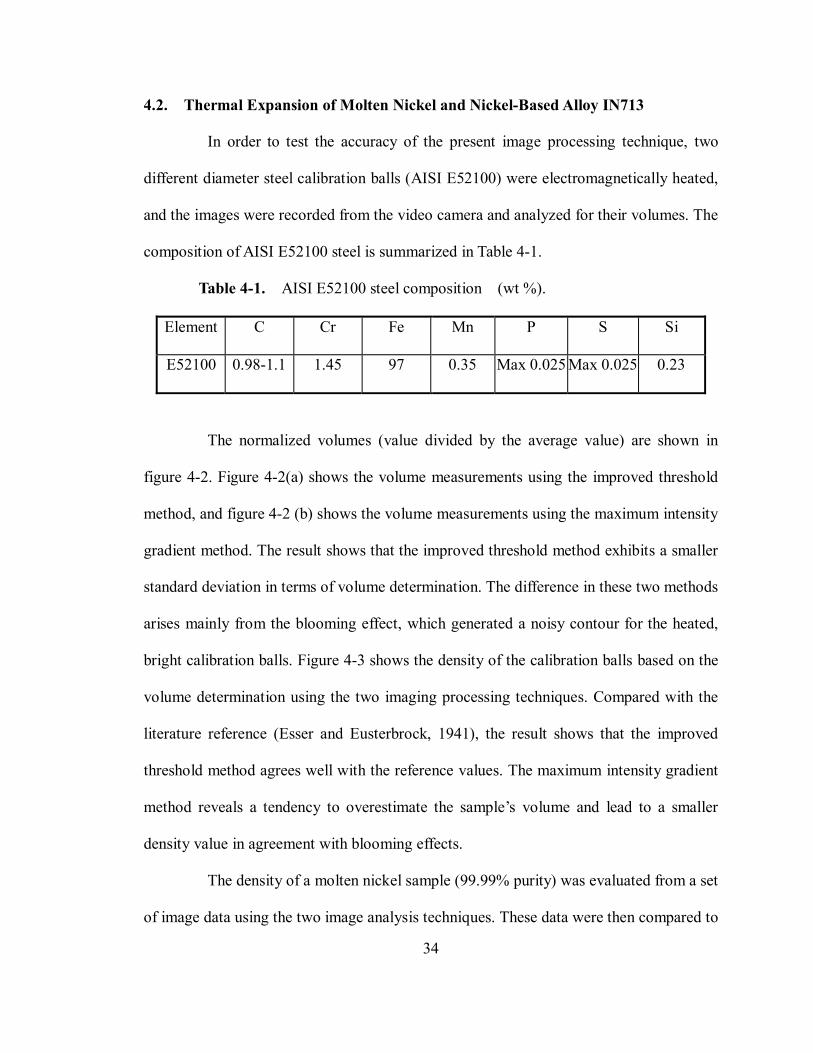
bright calibration balls. Figure 4-3 shows the density of the calibration balls based on the

volume determination using the two imaging processing techniques. Compared with the

literature reference (Esser and Eusterbrock, 1941), the result shows that the improved

threshold method agrees well with the reference values. The maximum intensity gradient

method reveals a tendency to overestimate the samples volume and lead to a smaller

density value in agreement with blooming effects.

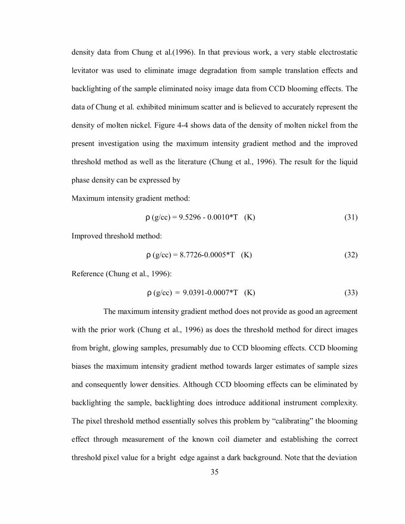
The density of a molten nickel sample (99.99% purity) was evaluated from a set

of image data using the two image analysis techniques. These data were then compared to

35

density data from Chung et al.(1996). In that previous work, a very stable electrostatic

levitator was used to eliminate image degradation from sample translation effects and

backlighting of the sample eliminated noisy image data from CCD blooming effects. The

data of Chung et al. exhibited minimum scatter and is believed to accurately represent the

density of molten nickel. Figure 4-4 shows data of the density of molten nickel from the

present investigation using the maximum intensity gradient method and the improved

threshold method as well as the literature (Chung et al., 1996). The result for the liquid

phase density can be expressed by

Maximum intensity gradient method:

ρ (g/cc) = 9.5296 - 0.0010*T (K) (31)

Improved threshold method:

ρ (g/cc) = 8.7726-0.0005*T (K) (32)

Reference (Chung et al., 1996):

ρ (g/cc) = 9.0391-0.0007*T (K) (33)

The maximum intensity gradient method does not provide as good an agreement

with the prior work (Chung et al., 1996) as does the threshold method for direct images

from bright, glowing samples, presumably due to CCD blooming effects. CCD blooming

biases the maximum intensity gradient method towards larger estimates of sample sizes

and consequently lower densities. Although CCD blooming effects can be eliminated by

backlighting the sample, backlighting does introduce additional instrument complexity.

The pixel threshold method essentially solves this problem by calibrating the blooming

effect through measurement of the known coil diameter and establishing the correct

threshold pixel value for a bright edge against a dark background. Note that the deviation

36

Temperature (K)

1440 1480 1520 1560 1600 1640 1680

V / V

a

0.85

0.90

0.95

1.00

1.05

1.10

1.15

3 / 16 inch 7 /32 inch

(a)

Temperature (K)

1440 1480 1520 1560 1600 1640 1680

V / V

a

0.85

0.90

0.95

1.00

1.05

1.10

1.15

3 /16 inch7 / 32 inch

(b)

Figure 4-2. Volume measurements of two steel calibration balls using image processing

(a) improved threshold method and (b) maximum intensity gradient method.

37

Temperature (K)

1350 1400 1450 1500 1550 1600 1650 1700

Den

sity

( g/

cc)

6.6

6.8

7.0

7.2

7.4

7.6

7.8

8.0

8.2Esser et al., 1941Improved threshold methodMaximum intensity gradient method

β=−0.0002

β=−0.0003

β=−0.0007

Figure 4-3. Density of the steel calibration balls.

38

Temperature (K)

1750 1800 1850 1900 1950 2000

Den

sity

(g/c

c)

7.0

7.2

7.4

7.6

7.8

8.0

8.2

Maximum Intensity GradientImproved Threshold MethodChung et al., 1996

Figure 4-4. Experimentally determined density of electromagnetically

levitated liquid nickel sample.

39

of the maximum gradient method increases as the temperature of the nickel sample

increases, presumably due to increased CCD blooming from the brighter samples.

Commercial nickel-based superalloy IN713 is widely used in demanding

applications due to the alloys excellent high temperature strength. The composition of this

alloy is shown in Table 4-2.

Table 4-2. Nickel-based superalloy IN713 composition (wt %).

Element C Cr Mo Fe Ti Al Co Nb

IN713 0.13 13.89 4.0 0.2 0.9 6.0 0.15 2.0

Unfortunately electromagnetic levitation of such alloys is difficult because the

electrical conductivities are low and the densities are high. Successful levitation and

melting of the alloy was achieved after several different coil designs were tested. Volumes

of the samples were estimated using the image threshold technique. The sample masses

were measured before and after the experiments and the sample mass during the

measurements estimated assuming constant evaporation rates while each sample was

molten. The measured density of IN713 in liquid state with 95% prediction interval of the

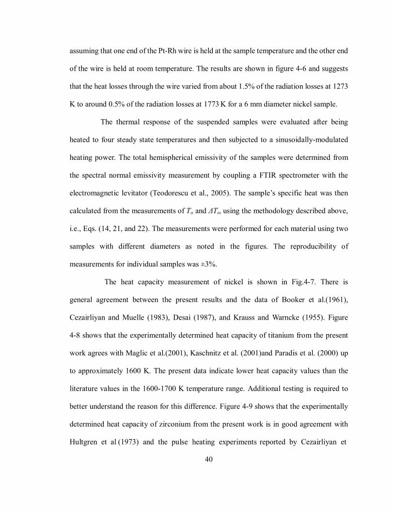
regression line is shown in Figure 4-5.

4.3. Modulated Power Specific Heat Measurements

Modulation heating and cooling experiments were performed with solid nickel,

titanium and zirconium samples in the temperature range of 1300 K to 1800 K. The

samples were suspended in the center of the induction coil with a very small 0.15 mm

diameter Pt (87%)-Rh (13%) wire.

A simple conduction model of the heat losses through the wire was developed by

40

assuming that one end of the Pt-Rh wire is held at the sample temperature and the other end

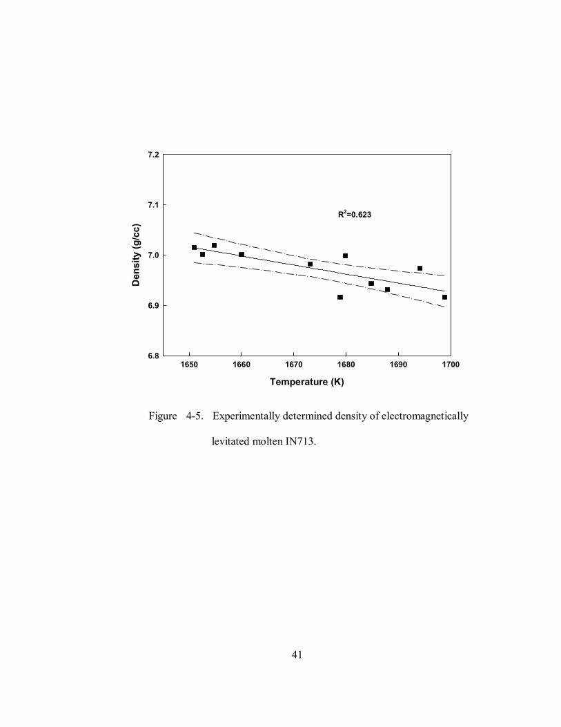
of the wire is held at room temperature. The results are shown in figure 4-6 and suggests

that the heat losses through the wire varied from about 1.5% of the radiation losses at 1273

K to around 0.5% of the radiation losses at 1773 K for a 6 mm diameter nickel sample.

The thermal response of the suspended samples were evaluated after being

heated to four steady state temperatures and then subjected to a sinusoidally-modulated

heating power. The total hemispherical emissivity of the samples were determined from

the spectral normal emissivity measurement by coupling a FTIR spectrometer with the

electromagnetic levitator (Teodorescu et al., 2005). The samples specific heat was then

calculated from the measurements of To and ∆Tω using the methodology described above,

i.e., Eqs. (14, 21, and 22). The measurements were performed for each material using two

samples with different diameters as noted in the figures. The reproducibility of

measurements for individual samples was ±3%.

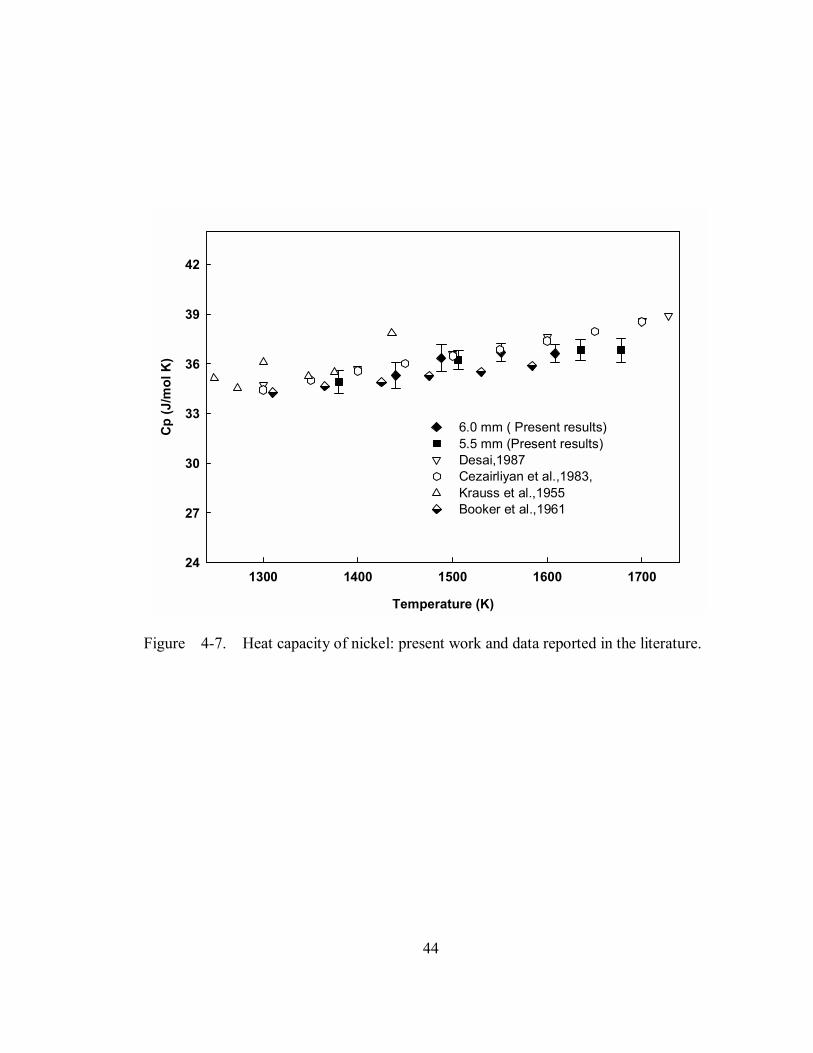
The heat capacity measurement of nickel is shown in Fig.4-7. There is

general agreement between the present results and the data of Booker et al.(1961),

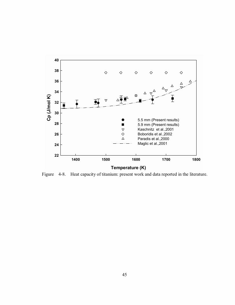
Cezairliyan and Muelle (1983), Desai (1987), and Krauss and Warncke (1955). Figure

4-8 shows that the experimentally determined heat capacity of titanium from the present

work agrees with Maglic et al.(2001), Kaschnitz et al. (2001)and Paradis et al. (2000) up

to approximately 1600 K. The present data indicate lower heat capacity values than the

literature values in the 1600-1700 K temperature range. Additional testing is required to

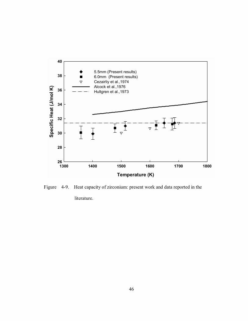
better understand the reason for this difference. Figure 4-9 shows that the experimentally

determined heat capacity of zirconium from the present work is in good agreement with

Hultgren et al (1973) and the pulse heating experiments reported by Cezairliyan et

41

Temperature (K)

1650 1660 1670 1680 1690 1700

Den

sity

(g/c

c)

6.8

6.9

7.0

7.1

7.2

R2=0.623

Figure 4-5. Experimentally determined density of electromagnetically

levitated molten IN713.

42

Temperature (K)

1400 1600 1800 2000

Con

duct

ive

heat

loss

/ R

adia

tive

heat

loss

(%)

0.0

0.2

0.4

0.6

0.8

1.0

1.2

1.4

1.6

Spec

ific

heat

mea

sreu

men

t err

or (%

)

0.0

0.1

0.2

0.3

0.4

0.5

Conductive heat loss Cp measurement error

Figure 4-6. Conductive heat loss through the suspension wire and its effect on

heat capacity calculation.

43

al.(1974). Alcock et al. (1976) reported slightly higher values of the heat capacity as well

as greater temperature dependence.

The least-squares fit polynomial functions that represent the results for heat

capacity for nickel, titanium and zirconium in the measured temperature range are:

Nickel: (1380 ≤ T ≤ 1678)

3-82-4 102.923-101.050T0.109-61.885 TTCp ××××+×= (34)

Titanium: (1361 ≤ T ≤ 1721) 3-82-4 10194.2101.112-T0.19075.767 TTCp ××+×××+= (35)

Zirconium: (1359 ≤ T ≤1686)

3-82-4 10341.3101.442T0.201-121.315 TTCp ××−××+×= (36)

where Cp is in J · mol -1 · K-1, and T is in K. In the computation of heat capacity, the

atomic weights of nickel, titanium and zirconium were taken as 58.693, 47.880 and

91.224, respectively.

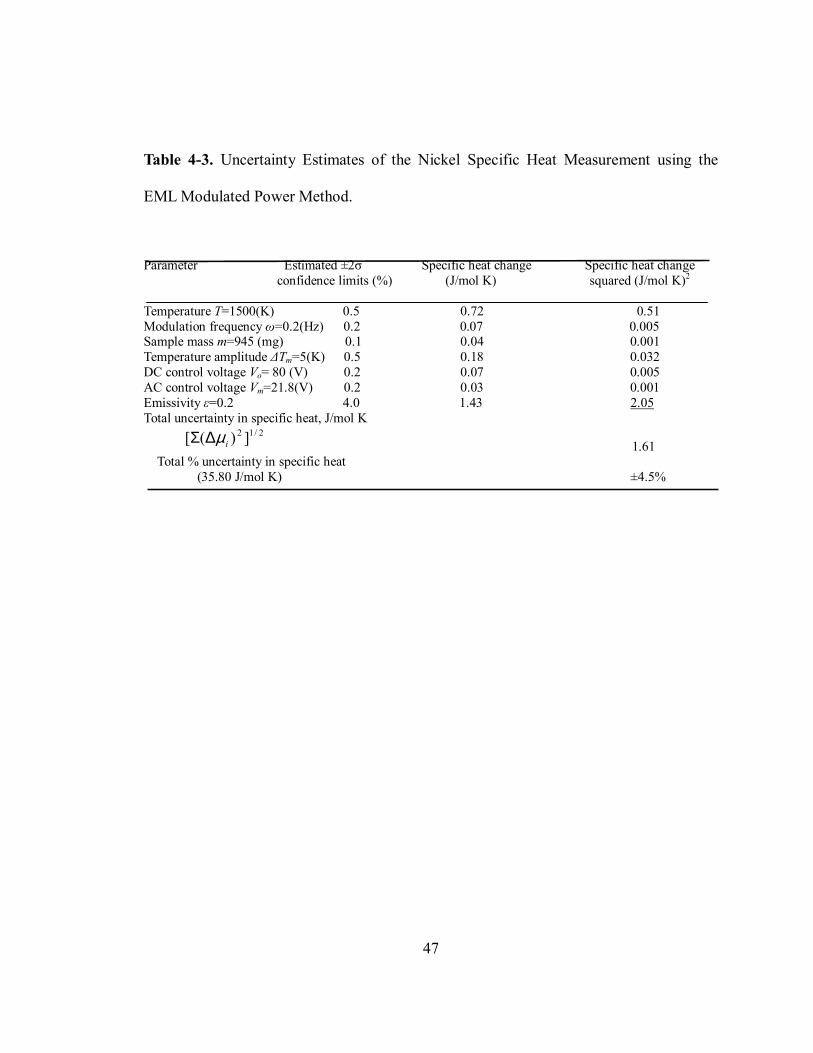
Moffats uncertainty estimation procedure (Moffat, 1998) was used to

theoretically analyze the various contributions to the experimental uncertainty. The

results of these calculations are shown in Table 4-3, 4-4, and 4-5. The total estimated

uncertainty (95% confidence limits) is approximately 4.5 % for a typical specific heat

measurement.

The largest contributor to the uncertainty in specific heat measurement was the

uncertainty in emissivity (primarily due to the ±0.5% uncertainty in temperature

measurement of the noncontact pyrometer). Improvements in the accuracy of the

temperature characterization are possible on measurements of solid samples of pure

elements evaluated incrementally just below and just above the melting temperature.

44

Temperature (K)

1300 1400 1500 1600 1700

Cp

(J/m

ol K

)

24

27

30

33

36

39

42

6.0 mm ( Present results)5.5 mm (Present results)Desai,1987Cezairliyan et al.,1983, Krauss et al.,1955Booker et al.,1961

Figure 4-7. Heat capacity of nickel: present work and data reported in the literature.

45

Temperature (K)

1400 1500 1600 1700 1800

Cp

(J/m

ol K

)

22

24

26

28

30

32

34

36

38

40

5.5 mm (Present results)5.9 mm (Present results)Kaschnitz et al.,2001Boboridis et al.,2002Paradis et al.,2000Maglic et al.,2001

Figure 4-8. Heat capacity of titanium: present work and data reported in the literature.

46

Temperature (K)

1300 1400 1500 1600 1700 1800

Spec

ific

Hea

t (J/

mol

K)

26

28

30

32

34

36

38

40

5.5mm (Present results)6.0mm (Present results)Cezairliy et al.,1974Alcock et al.,1976Hultgren et al.,1973

Figure 4-9. Heat capacity of zirconium: present work and data reported in the

literature.

47

Table 4-3. Uncertainty Estimates of the Nickel Specific Heat Measurement using the

EML Modulated Power Method.

Parameter Estimated ±2σ Specific heat change Specific heat change confidence limits (%) (J/mol K) squared (J/mol K)2 Temperature T=1500(K) 0.5 0.72 0.51 Modulation frequency ω=0.2(Hz) 0.2 0.07 0.005 Sample mass m=945 (mg) 0.1 0.04 0.001 Temperature amplitude ∆Tm=5(K) 0.5 0.18 0.032 DC control voltage Vo= 80 (V) 0.2 0.07 0.005 AC control voltage Vm=21.8(V) 0.2 0.03 0.001 Emissivity ε=0.2 4.0 1.43 2.05 Total uncertainty in specific heat, J/mol K

2/12 ])([ iµ∆Σ 1.61

Total % uncertainty in specific heat (35.80 J/mol K) ±4.5%

48

Table 4-4. Uncertainty Estimates of the Titanium Specific Heat Measurement using the

EML Modulated Power Method.

Parameter Estimated ±2σ Specific heat change Specific heat change confidence limits (%) (J/mol K) squared (J/mol K)2 Temperature T=1500(K) 0.5 0.648 0.420 Modulation frequency ω=0.2(Hz) 0.2 0.065 0.004 Sample mass m=710 (mg) 0.1 0.033 0.001 Temperature amplitude ∆Tm=8 (K) 0.5 0.162 0.026 DC control voltage Vo=98(V) 0.2 0.065 0.004 AC control voltage Vm=12 (V) 0.2 0.035 0.001 Emissivity ε=0.28 4.0 1.294 1.674 Total uncertainty in specific heat, J/mol K

2/12 ])([ iµ∆Σ 1.46

Total % uncertainty in specific heat (32.31J/mol K) ±4.52%

49

Table 4-5. Uncertainty Estimates of the Zirconium Specific Heat Measurement using the

EML Modulated Power Method.

Parameter Estimated ±2σ Specific heat change Specific heat change confidence limits (%) (J/mol K) squared (J/mol K)2 Temperature T=1500(K) 0.5 0.561 0.315 Modulation frequency ω=0.2(Hz) 0.2 0.056 0.003 Sample mass m=484 (mg) 0.1 0.028 0.001 Temperature amplitude ∆Tm=10(K) 0.5 0.140 0.020 DC control voltage Vo=90(V) 0.2 0.056 0.003 AC control voltage Vm=21.8(V) 0.2 0.039 0.002 Emissivity ε=0.27 4.0 1.121 1.256 Total uncertainty in specific heat, J/mol K

2/12 ])([ iµ∆Σ 1.27

Total % uncertainty in specific heat (30.29 J/mol K) ± 4.21%

50

5. CONCLUSIONS

This work includes two general parts: (i) thermal expansion measurements and

(ii) heat capacity measurements in the earth-based electromagnetic levitator of Auburn

University.

For thermal expansion measurements, CCD blooming effects from the emitted

radiation of electromagnetically levitated samples can cause noisy image data and

decreased precision in measurements of sample size using the traditional maximum

intensity gradient method. However, the presence in the image of the water cooled copper

coil presents a convenient image of known size to establish the threshold pixel intensity

value for the edge for each picture and enables effective calibration of the image for the

blooming effect. These image-specific pixel threshold values can then be used to determine

the molten droplet edges. Sixth order Legendre polynomials can then be fit to the droplet

edge data to obtain accurate and precise measurements of the sample volume assuming that

axisymetric symmetry prevails. The method was confirmed with measurements on

precision steel calibration balls and pure nickel and then applied to measurements of the

density of IN713.

The modulation power method combined with electromagnetic levitation high

temperatures, especially when interactions with the crucible and contamination are

concerns. The largest contributor to the uncertainty in specific heat is the uncertainty in

total hemispherical emissivity values used to calculate the radiative power losses. The

51

method was successfully applied to measure the heat capacity of pure solid samples of

nickel, titanium and zirconium suspended on a thin Pt-Ph wire. Although the coupled

heating power and positioning force for the traditional single coil electromagnetic levitator

design introduces cyclic translations of the sample, these effects are predicted by a

numerical model developed in this study to have negligible affect on the measurements.

52

6. SUGGESTIONS FOR FUTURE RESEARCH

To improve accuracy of the density and heat capacity measurements, the current

experimental system can be modified in the following ways:

The current optical system and temperature measurement system performance can

be significantly improved by reducing the electromagnetic noise generated by the RF

power supply.

Placing the current CCD camera with a higher resolution CCD camera will

improve the resolution of image sizes.

The modulated power method may also be applied to monitoring the phase

transformation and measuring the alloys latent heat. Application of the modulated power

method within the mushy zone of an alloy will cause periodic melting and freezing

processes and induce additional lag in the thermal response of the sample. Measurements

of an alloys specific heat over the range of temperatures associated with the phase

transformation will produce heat capacity measurements above the baseline expected for a

single phase. When this apparent heat capacity is plotted versus temperature, a peak will

naturally result and indicate the phase transformation. Integration of the apparent heat

capacity curve above the single phase baseline will yield the transformation enthalpy.

53

REFERENCES

Alcock, C. B.; Jacob, K. T. and Zador, S., "Thermochemical properties [of zirconium]",

Atomic Energy Review, Special Issue, vol.6, pp.7-65, 1976

Bachmann, R.; DiSalvo, F. J., Jr.; Geballe, T. H.; Greene, R. L.; Howard, R. E.; King, C. N.;

Kirsch, H. C.; Lee, K. N.; Schwall, R. E. and et al., "Heat capacity measurements

on small samples at low temperatures", Review of Scientific Instruments, vol.43

(2), pp.205-214, 1972

Bakhtiyarov, S. I. and Overfelt, R. A., "Thermophysical property measurements by

electromagnetic levitation melting technique under microgravity", Annals of the

New York Academy of Sciences, vol.974, pp.132-145, 2002

Bakhtiyarov, S. I. and Overfelt, R. A., "Electromagnetic levitation: Theory, experiments,

application", Recent Research Developments in Materials Science, vol.4 (Pt. 1),

pp.81-123, 2003

Boboridis, K., "Thermophysical property measurements on niobium and titanium by a

microsecond-resolution pulse-heating technique using high-speed laser

polarimetry and radiation thermometry", International Journal of Thermophysics,

vol.23 (1), pp.277-291, 2002

Booker, J.; Paine, R. M. and Stonehouse, A. J., "Intermetallic compounds for very high

temperature applications", United States Department of Commerce, Office of

Technical Services, AD [ASTIA Document], 1961

54

Brandes, E. A. and Brook, G. B., "Smithells Metals Reference Book", Butterworths

Heinemann Ltd, Oxford, vol.8, pp.54-55, 1992

Brillo, J. and Egry, I., "Density Determination of Liquid Copper, Nickel, and Their Alloys",

International Journal of Thermophysics, vol.24 (4), pp.1155-1170, 2003

Cezairliyan, A. and Mueller, A. P., "Heat capacity and electrical resistivity of nickel in the

range 1300-1700 K measured with a pulse heating technique", International Journal

of Thermophysics, vol.4 (4), pp.389-396, 1983

Cezairliyan, A. and Righini, F., "Simultaneous measurements of heat capacity, electrical

resistivity, and hemispherical total emittance by a pulse heating technique.

Zirconium 1500 to 2100.deg. K", Journal of Research of the National Bureau of

Standards, Section A: Physics and Chemistry, vol.78 (4), pp.509-514, 1974

Chen, S. F. and Overfelt, R. A., "Effects of sample size on surface-tension measurements of

nickel in reduced-gravity parabolic flights", International Journal of

Thermophysics, vol.19, pp.817-826, 1998

Chung, S. K.; David, B. T. and Won-kyu, R., "A noncontact measurement technique for the

density and thermal expansion coefficient of solid and liquid materials", Review of

Scientific Instruments, vol.67 (9), pp.3175-3181, 1996

Damaschke, B.; Oelgeschlaeger, D.; Ehrich, J.; Dietzsch, E. and Samwer, K., "Thermal

expansion measurements of liquid metallic samples measured under microgravity

conditions", Review of Scientific Instruments, vol.69 (5), pp.2110-2113, 1998

Desai, P. D., "Thermodynamic properties of nickel", International Journal of

Thermophysics, vol.8 (6), pp.763-780, 1987

Egry, I.; Diefenbach, A.; Dreier, W. and Piller, J., "Containerless processing in space -

55

Thermophysical property measurements using electromagnetic levitation",

International Journal of Thermophysics, vol.22 (2), pp.569-578, 2001

Egry, I.; Lohoefer, G. and Sauerland, S., "Measurements of thermophysical properties of

liquid metals by noncontact techniques", International Journal of Thermophysics,

vol.14 (3), pp.573-584, 1993

El-Mehairy, A. E. and Ward, R. G., "A new technique for determination of density of liquid

metals: application to copper", Transactions of the American Institute of Mining,

Metallurgical and Petroleum Engineers, vol.227 (5), pp.1126-1128, 1963

Esser, H. and Eusterbrock, H., "Investigation of the thermal expansion of some metals and

alloys with an improved dilatometer", Archiv fuer das Eisenhuettenwesen, vol.14,

pp.341-355, 1941

Fecht, H.-J. and Johnson, W. L., "A conceptual approach for noncontact calorimetry in

space", Review of Scientific Instruments, vol.62(5), pp.1299-1303, 1991

Fecht, H.-J. and Wunderlich, R. K., "Development of containerless modulation calorimetry

for specific heat measurements of undercooled melts", Materials Science &

Engineering, A: Structural Materials: Properties, Microstructure and Processing,

vol.178 (1-2), pp.61-64, 1994

Fromm, E. and Jehn, H., "Electromagnetic Forces and Power Absorption in Levitation

Melting", British Journal of Applied Physics, vol.16, pp.653-663, 1965

Gonzalez, R. C. and Wintz, P. A., "Digital Image Processing", pp.331-391, 1987

Gorges, E.; Racz, L. M.; Schillings, A. and Ergy, I., "Density measurements on levitated

liquid metal droplets", International Journal of Thermophysics, vol.17 (5),

pp.1163-1172, 1996

56

Herlach, D. M.; Cochrane, R. F.; Egry, I.; Fecht, H. J. and Greer, A. L., "Containerless

processing in the study of metallic melts and their solidification", International

Materials Reviews, vol.38 (6), pp.273-347, 1993

Hultgren, R. and et al. (1973). Selected Values of the Thermodynamic Properties of the

Elements.

Jain, A. K., "Fundamental of Digital Image Processing", pp. 407-414, 1989

Kaschnitz, E. and Reiter, P., "Heat capacity of titanium in the temperature range 1500 to

1900 K measured by a millisecond pulse-heating technique", Journal of Thermal

Analysis and Calorimetry, vol.64 (1), pp.351-356, 2001

Krauss, F. and Warncke, H., "Specific heat of nickel between 180 and 1160 Deg",

Zeitschrift fuer Metallkunde, vol.46, pp.61-69, 1955

Maglic, K. D. and Pavicic, D. Z., "Thermal and electrical properties of titanium between

300 and 1900 K", International Journal of Thermophysics, vol.22 (6),

pp.1833-1841, 2001

Moffat, R. J., "Describing the Uncertainties in Experimental Results", Exp. Therm Fluid

Science, vol.1, pp.3-17, 1998

Ohsaka, K.; Holzer, J. C.; Trinh, E. H. and Johnson, W. L., "Specific heat measurement of

undercooled liquids", 4th International conference on experiment methods for

microgravity materials science research, pp.1-6, 1992

Okress, E. C.; Wroughton, D. M.; Comentz, G.; Brace, P. H. and R.Kelly, J. C.,

"Electromagnetic Levitation of Solid and Molten Metals", Journal of Applied

Physics, vol.23, pp.545 - 552, 1952

Paradis, P.-F. and Rhim, W.-K., "Non-contact measurements of thermophysical properties

57

of titanium at high temperature", Journal of Chemical Thermodynamics, vol.32 (1),

pp.123-133, 2000

Racz, L. M. and Egry, I., "Advances in the measurement of density and thermal expansion

of undercooled liquid metals", Review of Scientific Instruments, vol.66 (8),

pp.4254-4258, 1995

Schaefers, K.; Rösner-Kuhn, M. and Frohberg, M. G., "Enthalpy measurements of

undercooled metals by levitation calorimetry: the pure metals nickel, iron,

vanadium and niobium", Materials Science and Engineering, vol. A 197, pp.83-90,

1995

Sullivan, P. F. and Seidel, G., "Steady-state, a.c.-temperature calorimetry", Physical

Review, vol.173 (3), pp.679-685, 1968

Teodorescu, G.; Jones, P. D.; Overfelt, R. A. and Guo, B., "Spectral-normal Emissivity of

Electromagnetic Heated Ni at High Temperature", Materials Science & Technology

Conference and Exhibition, Pittsburgh, PA, Sept 25-28, 2005

Wang, D.; Guo, B. and Overfelt, R. A., "Surface tension measurements of cast irons by

electromagnetic levitation melting technique", AFS Transactions, vol.111,

pp.813-824, 2003

Wroughton, D. M.; Okress, E. C.; Brace, P. H.; Comenetz, G. and Kelly, J. C. R., "A

technique for eliminating crucibles in heating and melting metals", Journal of the

Electrochemical Society, vol.99, pp.205-211, 1952

Wunderlich, R. K.; Diefenbach, A.; Willnecker, R. and Fecht, H. J., "Principles of

non-contact a.c. calorimetry", Containerless Process.: Tech. Appl., Proc. Int. Symp.

Exp. Methods Mater. Sci. Res., 5th, pp.51-56, 1993

58

Wunderlich, R. K.; Ettl, C. and Fecht, H.-J., "Non-contact electromagnetic calorimetry of

metallic glass forming alloys in reduced gravity", ESA SP, vol.454I, pp.537-544,

2000

Wunderlich, R. K.; Ettl, C. and Fecht, H. J., "Non-contact electromagnetic calorimetry of

metallic glass forming alloys in reduced gravity", European Space Agency,

[Special Publication] SP, vol. SP-454 (Vol. 1, First International Symposium on

Microgravity Research & Applications in Physical Sciences and Biotechnology,

2000, Volume 2), pp.537-544, 2001

Wunderlich, R. K.; Ettl, C. and Fecht, H. J., "Specific heat and thermal transport

measurements of reactive metallic alloys by noncontact calorimetry in reduced

gravity", International Journal of Thermophysics, vol.22 (2), pp.579-591, 2001

Wunderlich, R. K. and Fecht, H. J., "Specific heat measurements by non-contact

calorimetry", Journal of Non-Crystalline Solids, vol.156-158 (Pt. 1), pp.421-424,

1993

Wunderlich, R. K. and Fecht, H. J., "Measurements of thermophysical properties by

contactless modulation calorimetry", International Journal of Thermophysics,

vol.17 (5), pp.1203-1216, 1996

Wunderlich, R. K.; Lee, D. S.; Johnson, W. L. and Fecht, H. J., "Noncontact modulation

calorimetry of metallic liquids in low earth orbit", Physical Review B: Condensed

Matter, vol.55 (1), pp.26-29, 1997

Xuan, X., "Levitation and Surface Tension Measurement of Materials by Electromagnetic

levitation", M.S. thesis, Auburn University, pp.12-27, 2000

59

APPENDIX A

THE SOURCE CODE FOR THERMAL EXPANSION MEASUREMENT

60

% Main program is designed coil measurement % function xycenter: for center detection % function intens: for characteristic intensity detection clc; clear; % function coil: for coil detection % function radius: for edge detection SS=31; % The first Picture MM=40; % The last Picture for NN=SS:MM, cd('U:\In713 April 26'); s1=char('p'); s11=char('coil'); s2=int2str(NN); s3=char('.jpg'); name=strcat(s1,s2,s3) % Image file: pX.jpg datafile=strcat(s11,s2); % Data file: cedgeX I=imread(name); cd('H:\Program'); A=rgb2gray(I); corner1=[65,220]; corner2=[1092,1020]; xleft=corner1(1); yupp=corner1(2); xright=corner2(1); ydownp=corner2(2); A=A(yupp:ydownp,xleft:xright); B= im2double(A); [m,n]=size(B); % Find the characteristic intensity % Coil Region mark1=100; mark2=150; mark3=210; % Center Position determination [centerx,centery]=xycenter(B,mark1,mark3); [cyupc,cydownc,coillength,transion]= coil(B,centerx,mark1,mark2,mark3); cd('H:\Program\Data\Coil'); save(datafile, 'cyupc','cydownc','centerx','centery','coillength'); clc; clear; end % Sub_program function [centerx,centery]= xycenter(B,mark1,mark3)

61

[m,n]=size(B); exline=B(mark1,:); [record,index]=max(exline); exline1=[index,1]; exline2=[index,n]; eyline=[mark1,mark1]; [cx1,cy1,c1]=improfile(B,exline1,eyline,'bicubic'); [cx2,cy2,c2]=improfile(B,exline2,eyline,'bicubic'); recordl=0; critical=0.46; intensity=record-critical*(record-recordl); hh=1; while c1(hh)>intensity, hh=hh+1; end x1=cx1(hh); in1=c1(hh); % Left edge point hh=1; while c2(hh)>intensity, % hh=hh+1; end x2=cx2(hh); in2=c2(hh); %%% Right edge point xcenter=(x1+x2)/2; centerx=round(xcenter); xcenter=centerx; % Center y determination eyline=B(:,xcenter); [record,index]=max(eyline); intensity=record-critical*(record-recordl); exline=[xcenter,xcenter]; eyline1=[mark1,1]; eyline2=[mark3,m]; hh=1; [cx1,cy1,c1]=improfile(B,exline,eyline1,'bicubic'); [cx2,cy2,c2]=improfile(B,exline,eyline2,'bicubic'); while c1(hh)>intensity, hh=hh+1; end y1=cy1(hh); % Upper edge point in1=c1(hh); hh=1; % For some reason: the mist in the image, we can only use maximum intensity gradient to find the ycenter position recordl=min(c2);

62

if recordl<intensity, while c2(hh)>intensity, hh=hh+1; end y2=cy2(hh); % Lower edge point in2=c2(hh); else dif=-diff(c2); [record,index]=max(dif); y2=cy2(index); in2=c2(index); end ycenter=(y1+y2)/2; ycenter=round(ycenter); centery=ycenter; %-----------------------------------------------

clc; clear; % This program is designed for the correction factor of every group images and the highest intensity of the image SS=11; % The start Picture MM=30; % The final Picture ww=188.0346; % coil distance for NN=SS:MM, cd('H:\Program\Sample image\In718 April06(2)'); s1=char('p'); s11=char('coren'); s2=int2str(NN); s3=char('.jpg'); name=strcat(s1,s2,s3) % Image File datafile=strcat(s11,s2); % Data File I=imread(name); cd('H:\Program'); A=rgb2gray(I); corner1=[65,220]; corner2=[1092,1020]; xleft=corner1(1); yupp=corner1(2); xright=corner2(1); ydownp=corner2(2); A=A(yupp:ydownp,xleft:xright); B= im2double(A); [m,n]=size(B);

63

% Coil Region mark1=480; mark2=600; mark3=705; [centerx,centery]=xycenter(B,mark1,mark3); recordh=intens(B,centerx); recordl=0; critical=0.6; ww=188.0346; % Center Line Improfile xline=[centerx,centerx]; yline1=[mark1,mark2]; yline2=[mark3,mark2]; [cxc1,cyc1,cc1]=improfile(B,xline,yline1,'bicubic'); [cxc2,cyc2,cc2]=improfile(B,xline,yline2,'bicubic'); [recordup,indexhup]=max(cc1); [recorddown,indexdown]=max(cc1); recordl=0; ccoil=0; while abs(ccoil-ww)>2 & critical>=0.20, intensityup=recordh-critical*(recordh-recordl); intensitydown=recordh-critical*(recordh-recordl); % Searching the upper and lower level indexup=1; while cc1(indexup)>intensityup, indexup=indexup+1; end indexdown=1; while cc2(indexdown)>intensitydown, indexdown=indexdown+1; end cyupc=cyc1(indexup); % Up edge of coil cydownc=cyc2(indexdown); % Low edge of coil ccoil=cydownc-cyupc; %Coil distance critical=critical-0.01; end cd('H:\Program\Data\Core'); save(datafile, 'critical','ccoil','recordh'); clc; clear; end function intensity=intens(B,centerx) for h=1:10, exline=B(:,centerx); inten(h)=max(exline);

64

end intensity=mean(inten); clear; clc; % read critical value function SS=21; % The start Picture MM=25; % The final Picture h=1; for NN=SS:MM, cd('H:\Program\Data\Core'); s11=char('coren'); s2=int2str(NN); datafile=strcat(s11,s2); % Data File load(datafile); value(h)=critical; data(h)=ccoil; intensity(h)=recordh; edgein(h)=intensity(h)*(1-value(h)); h=h+1; end end %

% This program is designed for edge detection % function xycenter: for center detection % function intens : for characteristic intensity detection clc; clear; %% function coil : for coil detection %% function radius : for edge detection %---------------------------------------------------------- SS=21; % The first Picture MM=25; % The last Picture for NN=SS:MM, critical=0.31; s1=char('p'); s11=char('cedgenew'); s2=int2str(NN); s3=char('.jpg'); name=strcat(s1,s2,s3) % Image file: pX.jpg datafile=strcat(s11,s2); % Data file: cedgeX cd('H:\Program\Sample image\In718 April06(2)'); I=imread(name); cd('H:\Program'); A=rgb2gray(I);

65

corner1=[65,220]; corner2=[1092,1020]; xleft=corner1(1); yupp=corner1(2); xright=corner2(1); ydownp=corner2(2); A=A(yupp:ydownp,xleft:xright); B= im2double(A); [m,n]=size(B); % Find the characteristic intensity % Coil Region mark1=480; mark2=600; mark3=705; % Center Position determination [centerx,centery]=xycenter(B,mark1,mark3); % Edge intensity intensity=intens(B,centerx); recordl=0;

% intensity=intensity-critical*(intensity-recordl); % critical value method

intensity=0.6738; % edge detection region [cyupc,cydownc,coillength,transion]=coil(B,centerx,mark1,mark2,mark3); % Set the start point if centery<=transion(1), ycenter=450; %ycenter=centery; else ycenter=centery; end [ang11,r11]=radius11(B,centerx,centery,ycenter,intensity,transion(1),transion(2)); [ang22,r22]=radius22(B,centerx,centery,ycenter,intensity,transion(1),transion(2)); [ang33,r33]=radius33(B,centerx,centery,ycenter,intensity,transion(1),transion(2)); [ang44,r44]=radius44(B,centerx,centery,ycenter,intensity,transion(1),transion(2)); ang=[ang11,ang22,ang33,ang44]; r=[r11,r22,r33,r44]; cd('H:\Program\Data\Cedge'); save(datafile, 'ang','r','ang11','ang22','ang33','ang44','r11','r22','r33','r44','centerx','centery',... 'ycenter','intensity','coillength'); clc; clear; end % Curve fitting

66

close all; clc; clear; coil=189.5724; cd('H:\Program\Data\Cedge\In713'); load cedgen30; %Fitting and showing cd('H:\Program'); [fity1,y1,reangright,p1]=right(r11,r44,ang11,ang44); [fity2,y2,reangleft,p2]=left(r22,r33,ang22,ang33); show(p1,p2); hold on; polar(ang,r,'x'); hold off; % Radius Filter [filterr1,filterang1,filterr4,filterang4]=filterright(r11,ang11,r44,ang44,fity1); [filterr2,filterang2,filterr3,filterang3]=filterleft(r22,ang22,r33,ang33,fity2); % Fitting and showing [fityy1,yy1,reangrighty,p1y]=right(filterr1,filterr4,filterang1,filterang4); [fityy2,yy2,reanglefty,p2y]=left(filterr2,filterr3,filterang2,filterang3); figure; show(p1y,p2y); hold on; angy=[filterang1,filterang2,filterang3,filterang4]; ry=[filterr1,filterr2,filterr3,filterr4]; polar(angy,ry,'x'); hold off; % Compute mass=358.9; coill=0.1564; global p11; global p22; global pixvalue; p11=p1y; p22=p2y; pixvalue=coill/coil; y11=quadl('volume1',0,pi); v1=2*y11*pi/3; densityrr=mass/v1*0.001;%%% Right+Right y22=quadl('volume2',0,pi); v2=2*y22*pi/3; densityll=mass/v2*0.001;%%% Left+Left densityrl=2*mass/(v1+v2)*0.001;%%% Right+Left value1=[densityrr,densityll,densityrl,intensity];

67

APPENDIX B

THE SOURCE CODE FOR NUMERICAL MODEL OF MODULATED

POWER METHOD

68

% Modulated heating method simulation clc;

clear; load powerdata; %-------Material Property ---------------------------------- S_b=5.67*10^-8; K=76; Cp=620; Den=7905; Emis=0.22; ti=300; % enviroment temp R_sample=2; % unit: mm ele_cond=5e6; permea_vacuum=4*pi*10^-7; skin=sqrt(2/(200e3*ele_cond*permea_vacuum); h=R_sample*sin(10*pi/180); h1=(R_sample-skin)*sin(10*pi/180); V_heat=2*pi*h^2*(R_sample-h/3)- 2*pi*h1^2*(R_sample-skin-h1/3); volume=4*pi*R_sample^3/3; mass=Den*volume*(1e-9); A=4*pi*R_sample^2*(1e-6); % Discritize time and space domain dt=0.05; tfinal=2; Nr=20; Ntheta=30; dr=R_sample/(Nr); dtheta=pi/2/(Ntheta-1); Tmatrix=ones(Ntheta*Nr+1,1)*1915.1; Eqr=zeros(Nr*Ntheta+1,1); Eql=zeros(Nr*Ntheta+1,Nr*Ntheta+1); hp=0; % Power indicator for tt=dt:dt:tfinal, tt hp=hp+1; % Inside node for row=2:Ntheta-1, for colum=1:Nr-1, node=colum+(row-1)*Nr; theta=pi/2-dtheta*(row-1); r=colum*dr ; Ar=(r)^2*sin(theta)*dtheta*pi/2*(1e-6); Ar1=(r-0.5*dr)^2*sin(theta)*dtheta*pi/2*(1e-6); %Inside(m^2) Ar2=(r+0.5*dr)^2*sin(theta)*dtheta*pi/2*(1e-6); % Outside Aa1=r*sin(theta-0.5*dtheta)*pi*dr/2*(1e-6); % Up

69

Aa2=r*sin(theta+0.5*dtheta)*pi*dr/2*(1e-6); % Down c1=Den*Cp*Ar*dr*(1e-3)/dt; c2=-K*Aa1/(r*(1e-3)*dtheta); c3=K*Aa2/(r*(1e-3)*dtheta); c4=-K*Ar1/(dr*(1e-3)); c5=K*Ar2/(dr*(1e-3)); Eql(node,node-Nr)=-c3; Eql(node,node)=c1-c2+c3-c4+c5; Eql(node,node+1)=-c5; Eql(node,node+Nr)=c2; if (theta>80*pi/180) & (r>R_sample-skin), Q=power(hp)/V_heat; else Q=0; end; Eqr(node)=c1*Tmatrix(node)+Q*Ar*dr; if row==2 % Because the center located node-1 position Eql(node,end)=c4; else Eql(node,node-1)=c4; end end end % Surface node colum=Nr; for row=2:Ntheta-1, node=colum+(row-1)*Nr; theta=pi/2-dtheta*(row-1); r=colum*dr; Aa1=r*sin(theta-0.5*dtheta)*pi*dr/2*(1e-6)/2; Aa2=r*sin(theta+0.5*dtheta)*pi*dr/2*(1e-6)/2; Ar=(r)^2*sin(theta)*dtheta*pi/2*(1e-6); Ar1=(r-0.5*dr)^2*sin(theta)*dtheta*pi/2*(1e-6); ha=S_b*Emis*(Tmatrix(node)^2+ti^2)*(Tmatrix(node)+ti); c1=Den*Cp*Ar*dr*(1e-3)/dt; c2=-K*Aa1/(r*(1e-3)*dtheta); c3=K*Aa2/(r*(1e-3)*dtheta); c4=-K*Ar1/(dr*(1e-3)); c5=-ha*Ar; Eql(node,node-Nr)=-c3; Eql(node,node)=c1-c2+c3-c4-c5; Eql(node,node+Nr)=c2; Eql(node,node-1)=c4; if (theta>80*pi/180) , Q=power(hp)/V_heat;

70

else Q=0; end; Eqr(node)=c1*Tmatrix(node)-c5*ti+Q*Ar*dr; end % Boundary nodes row=1; for colum=1:Nr, node=colum+(row-1)*Nr; Eql(node,node)=1; Eql(node,node+Nr)=-1; end row=Ntheta; for colum=1:Nr, node=colum+(row-1)*Nr; Eql(node,node)=1; Eql(node,node-Nr)=-1; end % Center Eql(Nr*Ntheta+1,Nr*Ntheta+1)=1; Eql(Nr*Ntheta+1,1)=-1; % Solve Tmatrix=inv(Eql)*Eqr; center(hp)=Tmatrix(1); side(hp)=Tmatrix(Nr);

end %function power=getpower(pos,I) f= 200000; sample_ID=1; [permea_vacuum,s_b,permea,permea_,conduc,emmis,R_sample,Density]=getsample(sample_ID); coil_ID=1; [n_upper,n_lower,span,d,R_coil]=getcoil(coil_ID); coillength=(n_lower-1)*d+(n_upper-1)*d+span; % Calculate the levitation force % Calculate Gx,Fx x=R_sample*sqrt(pi*conduc*f*permea_); xx=2*x; if (x>1000), Gx=1.0; Fx=x; else temp1=3*(sinh(xx)-sin(xx)); temp2=4*x*(sinh(x)^2+sin(x)^2); Gx= 1-temp1/temp2;

71

Fx=(x*sinh(xx)+x*sin(xx)-cosh(xx)+cos(xx))/(cosh(xx)-cos(xx)); end; % Calculate the item1 ~ item4 z=pos/1000; for n=1:1:n_lower, z_l(n)=-(span/2+(n-1)*d); end; z_l=rot90(z_l,2); for n=1:n_upper, z_u(n)=span/2+(n-1)*d; end; item1=0; item2=0; item3=0; item4=0; for n=1:n_lower, M=R_coil^2; temp1=(z-z_l(n))^2; temp2=(z-z_l(n)); temp3(n)=M/((M+temp1)^1.5); temp4(n)=(M*temp2)/((M+temp1)^2.5); end; item3=sum(temp3); item4=sum(temp4); for n=1:n_upper, M=R_coil^2; temp1=(z-z_u(n))^2; temp2=(z-z_u(n)); temp5(n)=M/((M+temp1)^1.5); temp6(n)=(M*temp2)/((M+temp1)^2.5); end; item1=sum(temp5); item2=sum(temp6); F_upper=9/8*permea_*I*I*Gx*item1*item2; F_upper=F_upper/9.8/1000; % (g/cm^3) p_upper=3*pi*R_sample*(0.5*I*item1)^2*Fx/conduc; F_lower=9/8*permea_*I*I*Gx*item3*item4; F_lower=F_lower/9.8/1000; % (g/cm^3) p_lower=3*pi*R_sample*(0.5*I*item3)^2*Fx/conduc; F=F_lower+F_upper; p=p_upper+p_lower; power=p; function force=getforce(pos,I2) I=I2; f= 200000;

72

% Analytical Model of EML % Load the thermophysical properties of the sample and sample size sample_ID=1; [permea_vacuum,s_b,permea,permea_,conduc,emmis,R_sample,Density]=getsample(sample_ID); coil_ID=1; [n_upper,n_lower,span,d,R_coil]=getcoil(coil_ID); coillength=(n_lower-1)*d+(n_upper-1)*d+span; x=R_sample*sqrt(pi*conduc*f*permea_); xx=2*x; if (x>1000), Gx=1.0; Fx=x; else temp1=3*(sinh(xx)-sin(xx)); temp2=4*x*(sinh(x)^2+sin(x)^2); Gx= 1-temp1/temp2; Fx=(x*sinh(xx)+x*sin(xx)-cosh(xx)+cos(xx))/(cosh(xx)-cos(xx)); end; z=pos/1000; for n=1:1:n_lower, z_l(n)=-(span/2+(n-1)*d); end; z_l=rot90(z_l,2); for n=1:n_upper, z_u(n)=span/2+(n-1)*d; end; item1=0; item2=0; item3=0; item4=0; for n=1:n_lower, M=R_coil^2; temp1=(z-z_l(n))^2; temp2=(z-z_l(n)); temp3(n)=M/((M+temp1)^1.5); temp4(n)=(M*temp2)/((M+temp1)^2.5); end; item3=sum(temp3); item4=sum(temp4); for n=1:n_upper, M=R_coil^2; temp1=(z-z_u(n))^2; temp2=(z-z_u(n));

73

temp5(n)=M/((M+temp1)^1.5); temp6(n)=(M*temp2)/((M+temp1)^2.5); end; item1=sum(temp5); item2=sum(temp6); F_upper=9/8*permea_*I*I*Gx*item1*item2; F_upper=F_upper/9.8/1000; % (g/cm^3) p_upper=3*pi*R_sample*(0.5*I*item1)^2*Fx/conduc; F_lower=9/8*permea_*I*I*Gx*item3*item4; F_lower=F_lower/9.8/1000; % (g/cm^3) p_lower=3*pi*R_sample*(0.5*I*item3)^2*Fx/conduc; F=F_lower+F_upper; p=p_upper+p_lower; force=F; function [permea_vacuum,s_b,permea,permea_,conduc,emmis,R_sample,Density]=getsample(sample_ID) permea_vacuum=4*pi*10^-7; s_b=5.67*10^-8; permea=1; permea_=permea*permea_vacuum; conduc=3.85e6; % Iron Sample emmis=0.34; R_sample=0.002; Density=7.8; %% g/cm^3 function k=stiffspring(I,bottom,top) f= 200000; % Analytical Model of EML % Load the thermophysical properties of the sample and sample size sample_ID=1; [permea_vacuum,s_b,permea,permea_,conduc,emmis,R_sample,Density]=getsample(sample_ID); coil_ID=1; [n_upper,n_lower,span,d,R_coil]=getcoil(coil_ID); coillength=(n_lower-1)*d+(n_upper-1)*d+span; % Calculate the levitation force % Calculate Gx,Fx x=R_sample*sqrt(pi*conduc*f*permea_); xx=2*x; if (x>1000), Gx=1.0; Fx=x; else temp1=3*(sinh(xx)-sin(xx));

74

temp2=4*x*(sinh(x)^2+sin(x)^2); Gx= 1-temp1/temp2; Fx=(x*sinh(xx)+x*sin(xx)-cosh(xx)+cos(xx))/(cosh(xx)-cos(xx)); end; h=1; low_limit=bottom; up_limit=top; dz=coillength/500; for z=low_limit:dz:up_limit, % Sample's position for n=1:1:n_lower, z_l(n)=-(span/2+(n-1)*d); end; z_l=rot90(z_l,2); for n=1:n_upper, z_u(n)=span/2+(n-1)*d; end; item1=0; item2=0; item3=0; item4=0; for n=1:n_lower, M=R_coil^2; temp1=(z-z_l(n))^2; temp2=(z-z_l(n)); temp3(n)=M/((M+temp1)^1.5); temp4(n)=(M*temp2)/((M+temp1)^2.5); end; item3=sum(temp3); item4=sum(temp4); for n=1:n_upper, M=R_coil^2; temp1=(z-z_u(n))^2; temp2=(z-z_u(n)); temp5(n)=M/((M+temp1)^1.5); temp6(n)=(M*temp2)/((M+temp1)^2.5); end; item1=sum(temp5); item2=sum(temp6); F_upper(h)=9/8*permea_*I*I*Gx*item1*item2; F_upper(h)=F_upper(h)/9.8/1000; p_upper(h)=3*pi*R_sample*(0.5*I*item1)^2*Fx/conduc; F_lower(h)=9/8*permea_*I*I*Gx*item3*item4; F_lower(h)=F_lower(h)/9.8/1000; p_lower(h)=3*pi*R_sample*(0.5*I*item3)^2*Fx/conduc;

75

F(h)=F_lower(h)+F_upper(h); p(h)=p_upper(h)+p_lower(h); h=h+1; end; Site=low_limit:dz:up_limit; volum=4*pi*(100*R_sample)^3/3; F=F*volum*9.8/1000; [k,s]=polyfit(Site,F,1); Ffit=polyval(k,Site); figure; plot(Site,F,Site,Ffit); legend('Levitation','Fitted'); ylabel('Levitation force N'); xlabel('Position (m)');

76

APPENDIX C

THE SOURCE CODE FOR ANALYSIS OF TEMPERATURE DATA

77

clc; clear; sample=50;%% Sampling rate dataset=xlsread('Da'); dataset=dataset(1:2:end,:); time=dataset(:,1); temp=dataset(:,2); power=dataset(:,3); M=[time,temp,power]; %Fit time range time1=300; time2=410; data=cutime(time1,time2,time,temp,power); % Display time=data(:,1); temp=data(:,2); power=data(:,3); % subplot(2,1,1), plot(time,temp); xlabel('time(s)'); ylabel('Temperature (C)'); subplot(2,1,2); plot(time,power); ylabel('Control voltage(V)'); % shift=mean(temp); temp1=temp-shift; [b,a] = butter(5,1/(sample/2)); Hd = dfilt.df2t(b,a); fitemp= filter(Hd,temp1)+shift; % point=100; fitemp=fitemp(point:end); power=power(point:end); time=time(point:end)-time(point); figure; subplot(2,1,1); plot(time,fitemp); xlabel('time(s)'); ylabel('Temperature (C)'); subplot(2,1,2); plot(time,power); ylabel('Control voltage(V)'); %xlswrite('Noisefree',[time,fitemp,power]);

78

% Data Analysis clc; clear; numerical= xlsread('Noisefree'); time=numerical(:,1); temp=numerical(:,2); power=numerical(:,3); %% Display subplot(2,1,1); plot(time,temp); ylabel('Temperatur (C)'); subplot(2,1,2); plot(time,power); xlabel('time(s)'); ylabel('Control voltage(V)'); % curve fitting % DC time1=160; time2=180; temp_dc=findmean(time,temp,time1,time2); %% Amplitude %% Phase angle time1=160; time2=180; f=0.15; [ampli,dc,phase]=sinfit(time,temp,time1,time2,f); function [ampli,dc,phase]=sinfit(time,temp,time1,time2,f) % Trim data index1=find(time>=time1); index1=index1(1); index2=find(time>=time2); index2=index2(1); temp=temp(index1:index2); time=time(index1:index2); dcini=(max(temp)+min(temp))*0.5; acini=(max(temp)-min(temp))*0.5; % Phase w=2*pi*f; h=0; for theta=0:pi/180:2*pi, fitemp=dcini+acini*sin(w*time+theta); h=h+1; subtr=abs(fitemp-temp); residual(h)=sum(subtr); thetar(h)=theta;

79

end [record,index]=min(residual); phase=thetar(index); for dc=dcini-2:0.1:dcini+2, for ampli=acini-1:0.1:acini+1, fitemp=dc+ampli*sin(w*time+phase); h=h+1; subtr=abs(fitemp-temp); residual(h)=sum(subtr); dcr(h)=dc; amplir(h)=ampli; end end [record,index]=min(residual); dc=dcr(index); ampli=amplir(index); % Display fitemp=dc+ampli*sin(w*time+phase); plot(time,temp,time,fitemp,'--'); xlabel('time(s)'); ylabel('Temperatur (C)'); legend('Original data','fitted data');