Embed Size (px)
Citation preview
MEASUREMENTS OF MOLTEN STEEL/FLUX INTERFACE PHENOMENA IN THIN SLAB CASTING
By
Joseph W. Shaver B.S. Metallurgical and Materials Engineering
Michigan Technological University, Michigan, USA, 1993
A THESIS SUBMITTED IN PARTIAL FULFILLMENT OF THE
REQUIREMENTS FOR THE DEGREE OF MASTER OF APPLIED SCIENCE
In
The FACULTY OF GRADUATE STUDIES Department of Metals and Materials Engineering
We Accept This Thesis as Conforming To the Required Standard
……………………………………………………………….
……………………………………………………………….
……………………………………………………………….
The UNIVERSITY OF BRITISH COLUMBIA
October 2002 Joseph W. Shaver, 2002
ii
ABSTRACT
Several industrial plant trials investigating meniscus behavior and defects in thin-slab
casting were conducted at Nucor Steel - Indiana, USA. As some of the first experimental
steps in the investigation of the Compact Strip Production (CSP) process, the trials featured
mold metal level and meniscus measurements, which resulted in the emergence of a novel
and inexpensive method of measuring meniscus steel velocity using nailboards. In addition,
caster operating data were collected using a high frequency data acquisition system (for mold
events) and the level two information system. Slab and strip samples were collected to
investigate the effects of meniscus level fluctuation and fluid flow behavior upon the internal
and surface quality of the steel.
Metal level and meniscus measurements were made during ordinary casting
operation. Nailboards were used to make the measurements. The nailboard measurements
provide a meniscus shape profiles and liquid flux layer depths. An analysis of the nailboard
data has yielded information pertaining to the direction and velocity of the steel in the upper
recirculation zone and at the meniscus. Through the measurement of meniscus shape and the
standing wave, steel flow was determined to be influenced by casting speed, SEN
(Submerged Entry Nozzle) submergence and geometry, and mold width. Knowing that
present methods of measuring steel stream velocity in the continuous casting mold are costly
and not ideally suited for an industrial environment, the nailboard method for measuring
mold flux depths was refined. This method can measure meniscus surface velocity in a steel
mill setting with reasonable accuracy and agreement with established values for flow
velocity.
In conjunction with the nailboard measurements, Fast Fourier Transform (FFT)
analyses were performed using caster operation data collected at a frequency of 33.33 Hz.
FFT analysis shows that the metal level fluctuates with a characteristic frequency similar to
predictions made by mathematical and physical models of similar casting processes. In
addition, significant differences between two- and four-port SENs were also observed.
iii
This project has led to some of the first in-plant measurements of meniscus flow
velocities for the CSP continuous casting process. In addition to being a very cost-effective
way of measuring meniscus shape, flux depths and velocity, the nailboard measurements can
be made by operating personnel at very short intervals, thereby offering opportunities for
greater process understanding and control. Being made of only plywood, steel nails, and
aluminum wire, nailboards are easy to assemble and quite durable in the steel mill
environment. Other findings, through FFT analyses, have helped to elucidate the behavior of
flow controls, particularly SEN and stopper rod behavior, during casting and their effects
upon meniscus behavior and the resulting product quality. It is believed that this research
will further the understanding of and contribute to the elimination of mold flux-related
defects. It is also expected that this work will lead to additional research in this relatively
new area of steel continuous casting.
iv
TABLE OF CONTENTS ABSTRACT……………………………………………..…………………………………....ii TABLE OF CONTENTS………………………..…………………………………………....iv LIST OF TABLES………………….…..…………………………………………………….vi LIST OF FIGURES………………………………..………..……………………………….vii NOMENCLATURE AND LIST OF SYMBOLS……………………………………..……xiii ACKNOWLEDGEMENTS……………………………………………………………..…..xiv CHAPTER 1: INTRODUCTION………………………..…………………………….……..1 CHAPTER 2: LITERATURE REVIEW……..………………………………………………6 2.1 Inclusions in Continuously Cast Steel…………..……………………………..…6 2.1.1 Indigenous Inclusions…………………………..………………………7 2.1.2 Exogenous Inclusions…………………..………………………..……11 2.1.3 Mold Flux and Mold Slag Properties………………..……….………..21
2.1.4 Effects of Fluid Flow Transients upon Exogenous Inclusion Formation in the Mold.……………………………………………………..….………..22 2.1.5 Tundish Fluid Flow and Effects upon Inclusions…………..….…..….30 2.1.6 Inclusions Formed During Ladle Treatment and Reactions with Fluxes and Refractory…………………..……………………………………………34
2.2 Metal Level and Meniscus Behavior in the Thin-Slab Casting Mold..…...…….38 2.2.1 Steel Stream Velocity Measurements in the Meniscus Region..…...…39 CHAPTER 3: SCOPE AND OBJECTIVES…………………..……………………………41 CHAPTER 4: EXPERIMENTAL PROCEDURE: INDUSTRIAL PLANT TRIALS....…..43 4.1 Casting Machine and Operating Practices……………..………………………..43 4.1.1 Trial Casting Parameters………………..…………………………..…43 4.2 Data Acquisition……………………..…………………………………...……..45 4.2.1 Nailboard Measurements…………..………………………………….48 4.3 Slag Sample Collection…………………..………………………………….…..49 4.4 Steel Sample Collection………………..…………………………………….….49 CHAPTER 5: RESULTS OF INDUSTRIAL PLANT TRIALS…………………..…….….50 5.1 Metal Level Measurements……………..…………………………………….…50 5.1.1 High Frequency Data………………………..………………………...50 5.1.2 Nailboard Measurement Data………………………..………………..54 5.1.3 Other High Frequency Data………………..……………………….....59 5.2 Slag Samples……………………..…………………………………………...…59 5.3 Steel Samples………………………………..………………………………..…59 5.4 Mold Meniscus Brass Measurements and Oscillation Mark Spacing….…….....59 CHAPTER 6: ANALYSIS AND DISCUSSION…………………..…………………...…..68 6.1 FFT Generation………………………………..………………………….……..68
v
6.1.1 Use of Constructed Data for Validation of Equation 6.1..………….…68 6.1.2 Explanation for Conversion of Raw Signal to Level Fluctuation Plot..70 6.1.3 Mechanical Transient Identification and Characterization…..………..72 6.1.4 Fluid Flow Transient Identification and Characterization……..……...75 6.2 Nailboards………………………..………………………………………….…..80 6.2.1 Plant Trial Use of Nailboards……………..…………………………..80 6.2.2 Case 1 Findings - Meniscus Profile………………..…………….……81 6.2.3 Case 2 Data……………………………..……………………..………83 6.2.4 Case 3 Data…………………………………..…………………..……83 6.2.5 Case 4 Data……..………………………………………………..……83 6.3 Flow Direction as Indicated by Nailboard Data……..……………………….....84 6.4 Explanation of Morison Equation and Description of Method..………………..86 6.4.1 Suitability of the Morison Equation for Small Cylinders………….….86
6.4.2Calculation of Meniscus Stream Velocity Using Fluid Dynamics / Morison Equation………………………..…………………………….……..87
6.5 Evaluation of the Calculated Meniscus Stream Velocity Values………....…….88 6.5.1 Comparison with Mathematical Model Predictions………..…………88 6.5.2 Comparison with Water Model Predictions……………...……..……..93 6.5.3 Surface Velocity Measurement Trends………………...……….……..93 6.6 Meniscus Surface Velocity Relationship with Standing Wave Fluctuation….…96 6.7 Defects……..……………………………………………………………..……..97 CHAPTER 7: CONCLUSIONS AND RECOMMENDATIONS……………..…..………105 REFERENCES………………………………………………………..………………..…..108 APPENDIX 1: METAL LEVEL, FFT, AND RAW NAILBOARD RESULTS FOR 2-PORT SEN TRIAL (CASE 4 DATA)…………………………………………..…………………113 APPENDIX 2: METAL LEVEL, FFT, AND RAW NAILBOARD RESULTS FOR 4-PORT SEN TRIAL (CASE 4 DATA)……………………………………………………………..125
vi
LIST OF TABLES Table 2.1: Requirements for high purity and ultra-clean steels……………..………...…….12
Table 2.2: Mold flux compositions from company 1……………..………………...………20
Table 2.3: Mold flux and slag composition from company 2……………..…………….….20
Table 4.1: CSP Caster Specifications at Nucor-Crawfordsville…………..………………...44
Table 4.2: Experimental Casting Parameters……..……………………………………..….44
Table 4.3: List of Plant Trial Heats and Operating Parameters…………..……………...….45
Table 4.4: Chemical Compositions of Heats Studied in the Project……..………………....46
Table 4.5: Level Two Parameters………..………………………………………………….47
Table 5.1: Sample of Level Two Data……………..…………………………………..……51
Table 5.2: Sampling of Casting Data obtained through PDA Data Acquisition System..…..55
Table 5.3a: Measured Values of Distance from Bottom of Nailboard to Meniscus and Flux
Depths……………..…………………………………………………………………..……..56
Table 5.3b: Measured Steel Knob Diameters………………..………………………...……57
Table 5.4: Values Used for Linear Conversion of Metal Level and Stopper Rod Raw
Signals………………………………………………………………………………………..60
Table 5.5: Average Ladle Slag Composition…………………………..……………...…….60
Table 5.6: Average Tundish Slag Composition……..………………………………………60
Table 5.7: Average Mold Slag Composition (24 Heats)……………..……………………...61
Table 5.8: Defect Samples Collected During Inspection………………..…………………..61
Table 5.9: Comparison of Standing Wave Height as Estimated by Oscillation Mark Spacing
with Nailboard Meniscus Measurement………..……………………………………………62
Table 6.1: Theoretical Frequencies of Mechanical Transients……..…………………….…72
Table 6.2a: Mechanical Transients (FFT and Theoretical)……..……………...………...….77
Table 6.2b: Fluid Flow Transients (FFT and Theoretical)……..………...……………...….78
Table 6.3: Meniscus Surface Velocity Values as Calculated for 14 Heats……..……...……90
Table 6.4: Comparison of Maximum Meniscus Velocity between Several Models and
Present Work………………………………………………………...…………………….…93
Table A1.1: Pertinent Information for Heats That Were Part of 2-Port SEN Trial……..…114
Table A2.1: Pertinent Information for Heats That Were Part of 4-Port SEN Trial………..126
vii
LIST OF FIGURES Figure 1.1: Schematic Representation of the SMS Schloemann-Siemag Mold and SEN [3]..2
Figure 1.2: Schematic showing physical interaction of flux and steel in a continuous casting
mold [19]……………………………………………………………………………………....4
Figure 2.1 SEM Image of Reoxidation Alumina Inclusion [30]……………………..……....9
Figure 2.2. Effect of initial clogging and rounded edges on nozzle flow pattern [31]……...10
Figure 2.3. Effect of clogging upon severity of mold level fluctuations [14]……………...10
Figure 2.4. Interfacial tension of silicon oil/water system as a function of photoflo [15]. …14
Figure 2.5. Emulsification velocity as a function of silicon oil thickness[15]……………...14
Figure 2.6. Initial droplet thickness as a function of silicon oil thickness [15]…………..…15
Figure 2.7. Emulsification velocity profile vs. silicon oil thickness and density [15]……...15
Figure 2.8. Silicon oil droplet diameter as a function of water density [15]………………..16
Figure 2.9. Emulsification velocity vs. droplet oil thickness and interfacial tension [15]….17
Figure 2.10. Silicon oil droplet diameter vs. interfacial tension [15]……….………………17
Figure 2.11. Emulsification velocity vs. oil thickness and viscosity [15]………………..…18
Figure 2.12. Silicon oil droplet diameter vs. viscosity [15]……………………..…………..18
Figure 2.13. Typical mold flux sliver………………………………………………………..22
Figure 2.14. Schematic of meniscus hook formation and slag adhesion to the oscillation
mark base [11]………………………………………………………………………………..23
Figure 2.15. Predicted flow velocities in simulation involving biased flow [32]…………...24
Figure 2.16. Effect of submergence depth on predicted turbulent kinetic energy and
correlated surface level fluctuations [32]…………………………………………………….25
Figure 2.17. Period of oscillation vs. Average Residence Time in Upper Recirculating
Region [6]……………………………………………………………………………………25
Figure 2.18. Schematic showing physical interaction of flux and steel in casting mold
[19]…………………………………………………………………………………..……….26
Figure 2.19. Schematic of CC slab mold showing flux simulation domain [18]……………27
Figure 2.20. Top surface and flux/steel interface velocity distribution as a function of
distance from the narrow face [18]…………………………………………………………..28
Figure 2.21. Liquid layer thickness around mold perimeter (standard condition) [18]…..…29
viii
Figure 2.22. Close-up of cross section through a nailboard [19]……………………………29
Figure 2.23. Reduction in steel velocity and turbulence below meniscus with EMBR
[27]………………………………………………………………………………………...…31
Figure 2.24. Mold level variations in middle and narrow side of mold with EMBR [27]….31
Figure 2.25. Reduction in standing wave near narrow side of a thin slab mold with EMBR
[27]………………………………………………………………………………………...…32
Figure 2.26. Simulation showing movement of non- metallic inclusions (200µ) toward
the meniscus [27]………………………………………………………………………….…32
Figure 2.27. Schematic of tundish designs [33]……………………………………………..34
Figure 2.28. Binary phase diagram of CaO-Al2O3………………………………………….37
Figure 5.1: Typical Plot of Metal Level vs. Time for 1 Hour…………………………….…53
Figure 5.2: Metal Level vs.Time for one minute of casting time………………………...…54
Figure 5.3: Schematic of Nailboard Setup Used for Mold Measurements………………….58
Figure 5.4: Plot of pinch roll #1 speed vs. time……………………………………………..63
Figure 5.5: Plot of pinch roll #2 speed vs. time………………………………………….….64
Figure 5.6: Pinch Roll #1 Current vs. Time for 1 Hour of casting………………………….64
Figure 5.7: Pinch Roll #2 Current vs. Time for 1 Hour of Casting…………………………65
Figure 5.8: Plot of stopper rod output current vs. time……………………….……………..65
Figure 5.9: Casting Speed vs. Time as Gathered from PDA system………….…………….66
Figure 5.10: Raw Electrical Signal for Metal Level vs. Time (Sampling Rate = 33.33
Hz)…………………………………………………………………………..………………..66
Figure 5.11: Oscillation mark appearance on a slab 114376-06. Marks are measured peak-
to-trough and compared to nailboard standing wave measurements. The troughs of the above
oscillation marks are not visible due to sample size…………………………………………67
Figure 6.1: Constructed Metal Level vs. Time used for Validation of Equation 6.1…….….69
Figure 6.2: FFT Analysis Output Generated Using Constructed Metal Level Data from
Figure 6.1…………………………………………………………………………………….69
Figure 6.3: One hour plot of Metal Level Fluctuation vs. time………………………….….71
Figure 6.4: An FFT plot of Metal Level Fluctuation (Deviation from Setpoint) as
generated……………………………………………………………………………………..71
ix
Figure 6.5: Labeled FFT Plot of Metal Level Fluctuation Amplitude vs. Frequency for
Mechanical Transients……………………………………………………………………….73
Figure 6.6: Plot of Casting Speed (in inches per minute) vs. Time showing an approximately
0.06 m/min (c. 2.75 ipm) fluctuation in casting speed………………………………………74
Figure 6.7: Time Domain Plot of Metal Level Fluctuation vs. Time illustrating the period of
slab shear cuts 357 seconds apart. This period corresponds to a metal level fluctuation
frequency of 0.0028 Hz as labeled in Figure 6.6……………………………………….……75
Figure 6.8: Labeled FFT Plot of Metal Level Fluctuation Amplitude vs. Frequency for Fluid
Flow Transients. (URZ - Upper Recirculation Zone)……………………………………….79
Figure 6.9: Meniscus Shape Profile Across Mold Width. Casting speeds range between 4.4
and 5.1 m/min and widths range between 1150 and 1300 mm………………………………81
Figure 6.10: Flux Depth Profiles Across Mold Width for Same Heats as in figure 6.10...…82
Figure 6.11: Diagram of Nailboard Measurements Used for Calculating Meniscus Surface
Velocity………………………………………………………………………………………82
Figure 6.12: Schematic of Flow Direction as Determined from Nailboards for High and Low
Standing Wave……………………………………………………………………………….85
Figure 6.13: Top - Meniscus Surface Velocity vs. Position in Mold [18]. Bottom -
Meniscus Surface Velocity Values at Several Casting Speeds vs. Position in Mold
[42]…………………………………………………………………………………..……….91
Figure 6.14a: Calculated Meniscus Surface Velocity vs. Position in Mold for Heats in this
Study Cast with a 2-Port SEN. Note: Zero represents the mold centerline and the values
furthest from the center are not at the narrow face, but 85 mm in from the narrow face...….92
Figure 6.14b: Calculated Meniscus Surface Velocity vs. Position in Mold for Heats in this
Study Cast with a 4-Port SEN…………………………………………………………..……92
Figure 6.15: Dependence of Meniscus Surface Velocity upon Volume Flow Rate……...…95
Figure 6.16: Dependence of Meniscus Surface Velocity upon Casting Speed……………...95
Figure 6.17: Dependence of Meniscus Surface Velocity upon Mold Width………………..98
Figure 6.18: Dependence of Meniscus Surface Velocity upon SEN Submergence…...……98
Figure 6.19: Relationship between SEN Submergence and Standing Wave Height……..…99
Figure 6.20: Relationship of Meniscus Surface Velocity to Standing Wave Height…..……99
Figure 6.21: Nail Diameter vs. Casting Speed……………………………………………..100
x
Figure 6.22: Meniscus Surface Velocity vs. Nail Diameter………………………...……..100
Figure 6.23: Relationship between Surface Stream Velocity and Standing Wave Oscillation
Amplitude for this study. ………………………………………………………………..…101
Figure 6.24: Standing Wave Oscillation Period vs. Average Residence Time in Upper
Recirculation Zone for the Current Study [Predicted Period Adapted from Reference 6,
Figure 3]……………………………………………………………………………..…..….101
Figure 6.25: Typical Mold Flux Sliver Defect on CR Strip. Defect is Elongated
Horizontally………………………………………………………………………….……..103
Figure 6.26: Meniscus Surface Velocity vs. Volume Flow Rate for a Standard Bifurcated
SEN……………………………………………………………………………………..…..104
Figure 6.27: Meniscus Surface Velocity vs. Volume Flow Rate for a Trial Four-Port
SEN…………………………………………………………………………………………104
Figure A1.1: Plot of Metal Level Fluctuation from Setpoint for Heat 213760…………....115
Figure A1.2: FFT Plot of Metal Level Fluctuation for Heat 213760……………………....115
Figure A1.3: Meniscus Shape Profile for Heat 213760…………………………………....116
Figure A1.4: Molten Flux Depth Profile for Heat 213760…………………………...……116
Figure A1.5: Plot of Metal Level Fluctuation from Setpoint for Heat 117004…………....117
Figure A1.6: FFT Plot of Metal Level Fluctuation for Heat 117004………………………117
Figure A1.7: Meniscus Shape Profile for Heat 117004…………………………………....118
Figure A1.8: Molten Flux Depth Profile for Heat 117004…………………………..…….118
Figure A1.9: Plot of Metal Level Fluctuation from Setpoint for Heat 117005………..…..119
Figure A1.10: FFT Plot of Metal Level Fluctuation for Heat 117005……………………..119
Figure A1.11: Meniscus Shape Profile for Heat 117005…………………………………..120
Figure A1.12: Molten Flux Depth Profile for Heat 117005…………………………….....120
Figure A1.13: Plot of Metal Level Fluctuation from Setpoint for Heat 117006………..…121
Figure A1.14: FFT Plot of Metal Level Fluctuation for Heat 117006……………………..121
Figure A1.15: Meniscus Shape Profile for Heat 117006……………………………….….122
Figure A1.16: Molten Flux Depth Profile for Heat 117006……………………………….122
Figure A1.17: Plot of Metal Level Fluctuation from Setpoint for Heat 213763………..…123
Figure A1.18: FFT Plot of Metal Level Fluctuation for Heat 213763…………………..…123
Figure A1.19: Meniscus Shape Profile for Heat 213763…………………………………..124
xi
Figure A1.20: Molten Flux Depth Profile for Heat 213763………………………….……124
Figure A2.1: Plot of Metal Level Fluctuation from Setpoint for Heat 117021………...….127
Figure A2.2: FFT Plot of Metal Level Fluctuation for Heat 117021…………………..…..127
Figure A2.3: Meniscus Shape Profile for Heat 117021……………………………………128
Figure A2.4: Molten Flux Depth Profile for Heat 117021…………………………...……128
Figure A2.5: Plot of Metal Level Fluctuation from Setpoint for Heat 117022………..…..129
Figure A2.6: FFT Plot of Metal Level Fluctuation for Heat 117022…………………..…..129
Figure A2.7: Meniscus Shape Profile for Heat 117022……………………………………130
Figure A2.8: Molten Flux Depth Profile for Heat 117022…………………………..…….130
Figure A2.9: Plot of Metal Level Fluctuation from Setpoint for Heat 117023………...….131
Figure A2.10: FFT Plot of Metal Level Fluctuation for Heat 117023……………………..131
Figure A2.11: Meniscus Shape Profile for Heat 117023…………………………..………132
Figure A2.12: Molten Flux Depth Profile for Heat 117023……………………………….132
Figure A2.13: Plot of Metal Level Fluctuation from Setpoint for Heat 117024…………..133
Figure A2.14: FFT Plot of Metal Level Fluctuation for Heat 117024…………………..…133
Figure A2.15: Meniscus Shape Profile for Heat 117024………………………………..…134
Figure A2.16: Molten Flux Depth Profile for Heat 117024………………………...……..134
Figure A2.17: Plot of Metal Level Fluctuation from Setpoint for Heat 117025…………..135
Figure A2.18: FFT Plot of Metal Level Fluctuation for Heat 117025…………………..…135
Figure A2.19: Meniscus Shape Profile for Heat 117025…………………………………..136
Figure A2.20: Molten Flux Depth Profile for Heat 117025……………………….………136
Figure A2.21: Plot of Metal Level Fluctuation from Setpoint for Heat 117026…………..137
Figure A2.22: FFT Plot of Metal Level Fluctuation for Heat 117026………………….….137
Figure A2.23: Meniscus Shape Profile for Heat 117026………………………………..…138
Figure A2.24: Molten Flux Depth Profile for Heat 117026………………………...……..138
Figure A2.25: Plot of Metal Level Fluctuation from Setpoint for Heat 213782…………..139
Figure A2.26: FFT Plot of Metal Level Fluctuation for Heat 213782……………………..139
Figure A2.27: Meniscus Shape Profile for Heat 213782……………………………….….140
Figure A2.28: Molten Flux Depth Profile for Heat 213782…………………………….....140
Figure A2.29: Plot of Metal Level Fluctuation for Heat 213783……………………….…141
Figure A2.30: FFT Plot of Metal Level Fluctuation for Heat 213783……………………..141

xii
Figure A2.31: Meniscus Shape Profile for Heat 213783…………………………………..142
Figure A2.32: Molten Flux Depth Profile for Heat 213783…………………………...…..142
Figure A2.33: Plot of Metal Level Fluctuation from Setpoint for Heat 213784……….….143
Figure A2.34: FFT Plot of Metal Level Fluctuation for Heat 213784………………….….143
Figure A2.35: Meniscus Shape Profile for Heat 213784……………………………..……144
Figure A2.36: Molten Flux Depth Profile for Heat 213784…………………………….....144

xiii
Nomenclature and List of Symbols Vc: Casting Speed (m/min) W: mold width (mm) SEN: Submerged Entry Nozzle θ: Angle of Incidence of steel on nail (radians) Rm: Wave run-up height (also maximum standing wave height) Ho: Wave height of initial flow (m) Ho’: Unrefracted wave height (m) k: Ratio of wave height to the wave crest elevation above still liquid level(0.78) γ: Euler’s Constant (0.5772) F: Maximum force of steel against the nail at incidence angle, θ (N) ρ: Density of steel (7800 kg/m3) D: Diameter of steel knob on nail following mold immersion Cm: Inertia Coefficient (1+K) ts: Sampling time (0.03 s or 33.33 Hz) tt: Total time in FFT analysis (3600 s) Xfd: Peak Amplitude in the frequency domain (mm/s) Xtd: Magnitude of level fluctuation in the time domain (mm) f: FFT-generated frequency (Hz) t: Empirical Period of Theoretical Maximum Frequency Wave (0.030 s) g: Acceleration due to gravity (9.8 m/s2) δ: Fluid Flow Constant (3π/8) ω: Wave frequency L: Depth of nail immersion (0.060 m) U: Horizontal Velocity of Steel flowing Nail (m/s) C: Force Coefficient Corresponding to the Total In-line Force (=6)

xiv
ACKNOWLEDGEMENTS
I would like to extend my sincere thanks to Mary Jansepar, Gary Lockhart, Joan
Kitchen, and Nancy Oikawa, whose assistance and general help have been indispensable
throughout the course of this project. Without them, I would not have survived the first and
last months of this endeavor.
Also, the utmost gratitude goes to my advisers, Dr. Indira Samarasekera and Dr.
Brian Thomas. Their confidence in me and all of the knowledge and advice passed on will
never be forgotten.
Many thanks also go to John Scheel, Steven Wigman, Daniel Larson, Mary Alwin,
Dan Edelman, Clay Gross, and Sam Commella at Nucor for their unselfish cooperation
during the plant trials. Special thanks go to all of the guys in production, especially Steve
Stout, Montgomery Keyt, and Mickey Thompson.
Thanks also to my fellow students, especially Dr. J.K. Park, Leo Colley, Simon Jupp,
Cindy Chow, and Joydeep Sengupta for their friendship, assistance and support. And special
thanks also to Eric and the granite at Squamish. And finally my most heartfelt thanks to
Jane.
Joseph Shaver
October 2002
1
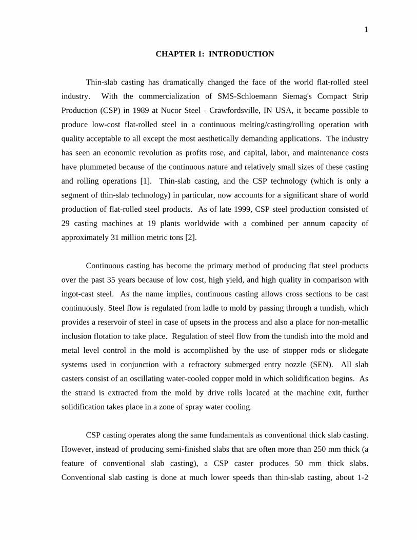
CHAPTER 1: INTRODUCTION
Thin-slab casting has dramatically changed the face of the world flat-rolled steel
industry. With the commercialization of SMS-Schloemann Siemag's Compact Strip
Production (CSP) in 1989 at Nucor Steel - Crawfordsville, IN USA, it became possible to
produce low-cost flat-rolled steel in a continuous melting/casting/rolling operation with
quality acceptable to all except the most aesthetically demanding applications. The industry
has seen an economic revolution as profits rose, and capital, labor, and maintenance costs
have plummeted because of the continuous nature and relatively small sizes of these casting
and rolling operations [1]. Thin-slab casting, and the CSP technology (which is only a
segment of thin-slab technology) in particular, now accounts for a significant share of world
production of flat-rolled steel products. As of late 1999, CSP steel production consisted of
29 casting machines at 19 plants worldwide with a combined per annum capacity of
approximately 31 million metric tons [2].
Continuous casting has become the primary method of producing flat steel products
over the past 35 years because of low cost, high yield, and high quality in comparison with
ingot-cast steel. As the name implies, continuous casting allows cross sections to be cast
continuously. Steel flow is regulated from ladle to mold by passing through a tundish, which
provides a reservoir of steel in case of upsets in the process and also a place for non-metallic
inclusion flotation to take place. Regulation of steel flow from the tundish into the mold and
metal level control in the mold is accomplished by the use of stopper rods or slidegate
systems used in conjunction with a refractory submerged entry nozzle (SEN). All slab
casters consist of an oscillating water-cooled copper mold in which solidification begins. As
the strand is extracted from the mold by drive rolls located at the machine exit, further
solidification takes place in a zone of spray water cooling.
CSP casting operates along the same fundamentals as conventional thick slab casting.
However, instead of producing semi-finished slabs that are often more than 250 mm thick (a
feature of conventional slab casting), a CSP caster produces 50 mm thick slabs.
Conventional slab casting is done at much lower speeds than thin-slab casting, about 1-2
2
m/min compared with 3-6 m/min for thin-slab casting. The size of the casting machine in
thin-slab casting is much smaller, as the three- to fivefold reduction in slab thickness results
in thin-slab casters being three
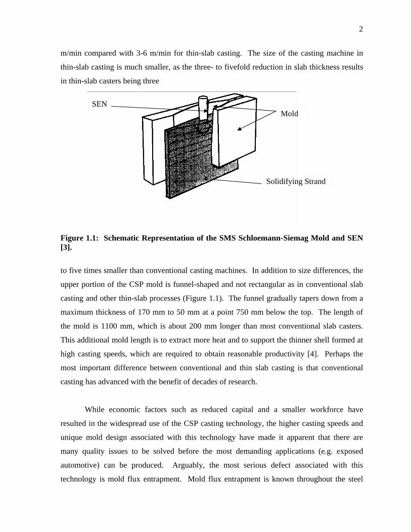
Figure 1.1: Schematic Representation of the SMS Schloemann-Siemag Mold and SEN [3].
to five times smaller than conventional casting machines. In addition to size differences, the
upper portion of the CSP mold is funnel-shaped and not rectangular as in conventional slab
casting and other thin-slab processes (Figure 1.1). The funnel gradually tapers down from a
maximum thickness of 170 mm to 50 mm at a point 750 mm below the top. The length of
the mold is 1100 mm, which is about 200 mm longer than most conventional slab casters.
This additional mold length is to extract more heat and to support the thinner shell formed at
high casting speeds, which are required to obtain reasonable productivity [4]. Perhaps the
most important difference between conventional and thin slab casting is that conventional
casting has advanced with the benefit of decades of research.
While economic factors such as reduced capital and a smaller workforce have
resulted in the widespread use of the CSP casting technology, the higher casting speeds and
unique mold design associated with this technology have made it apparent that there are
many quality issues to be solved before the most demanding applications (e.g. exposed
automotive) can be produced. Arguably, the most serious defect associated with this
technology is mold flux entrapment. Mold flux entrapment is known throughout the steel
Mold
Solidifying Strand
SEN
3
industry as a major cause of both internal and external defects in continuously cast steel.
While much is known about the defect, relatively little is understood as to how flux
properties and flux/steel interactions affect the formation of the defect. Most previous work
on mold flux entrapment defects has been confined to conventional slab casting since thin
slab casting is a relatively new technology [1,5-17].
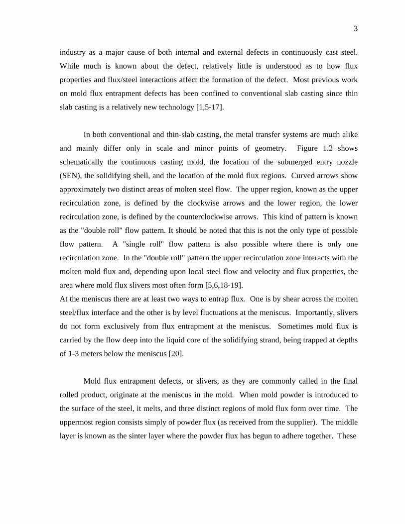
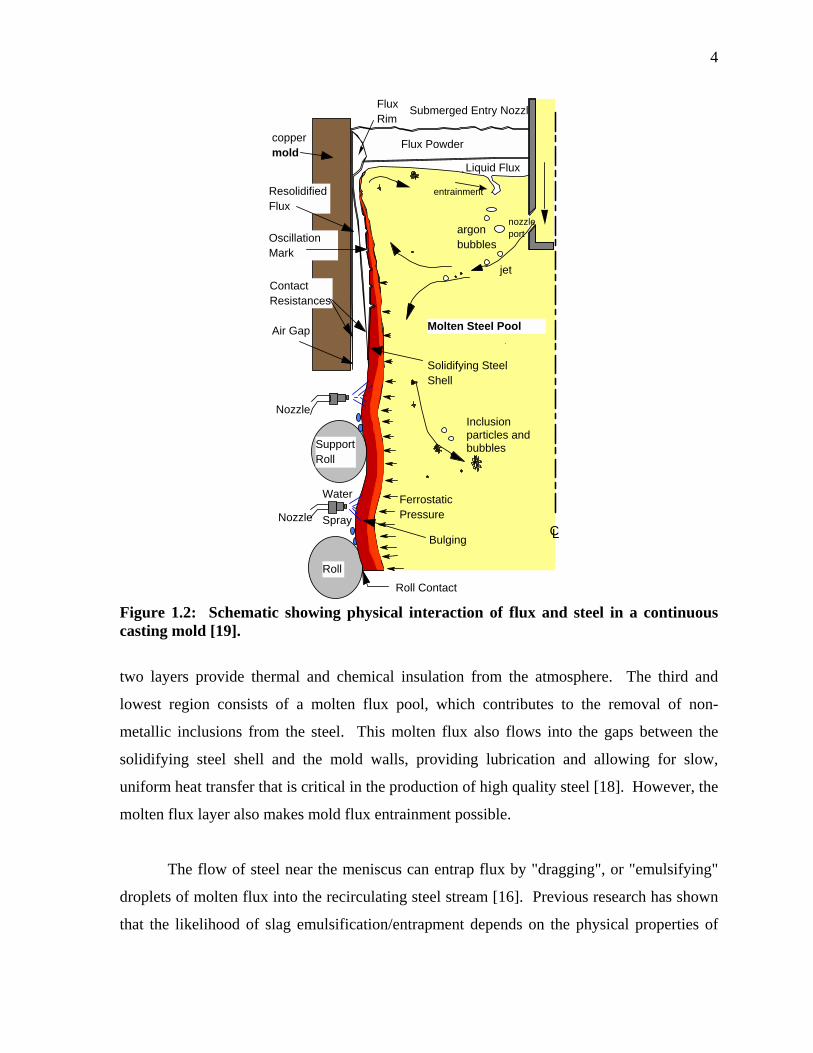
In both conventional and thin-slab casting, the metal transfer systems are much alike
and mainly differ only in scale and minor points of geometry. Figure 1.2 shows
schematically the continuous casting mold, the location of the submerged entry nozzle
(SEN), the solidifying shell, and the location of the mold flux regions. Curved arrows show
approximately two distinct areas of molten steel flow. The upper region, known as the upper
recirculation zone, is defined by the clockwise arrows and the lower region, the lower
recirculation zone, is defined by the counterclockwise arrows. This kind of pattern is known
as the "double roll" flow pattern. It should be noted that this is not the only type of possible
flow pattern. A "single roll" flow pattern is also possible where there is only one
recirculation zone. In the "double roll" pattern the upper recirculation zone interacts with the
molten mold flux and, depending upon local steel flow and velocity and flux properties, the
area where mold flux slivers most often form [5,6,18-19].
At the meniscus there are at least two ways to entrap flux. One is by shear across the molten
steel/flux interface and the other is by level fluctuations at the meniscus. Importantly, slivers
do not form exclusively from flux entrapment at the meniscus. Sometimes mold flux is
carried by the flow deep into the liquid core of the solidifying strand, being trapped at depths
of 1-3 meters below the meniscus [20].
Mold flux entrapment defects, or slivers, as they are commonly called in the final
rolled product, originate at the meniscus in the mold. When mold powder is introduced to
the surface of the steel, it melts, and three distinct regions of mold flux form over time. The
uppermost region consists simply of powder flux (as received from the supplier). The middle
layer is known as the sinter layer where the powder flux has begun to adhere together. These
4
Water
Spray
Molten Steel Pool
Solidifying Steel Shell
Flux Rim
Submerged Entry Nozzle
Support Roll
Roll Contact
Ferrostatic Pressure
Bulging
Roll
Nozzle
Nozzle
copper mold
Liquid Flux
Air Gap
Flux Powder
jet
nozzle portargon
bubbles
Inclusion particles and bubbles
Resolidified Flux
Contact Resistances
Oscillation Mark
entrainment
CL
Figure 1.2: Schematic showing physical interaction of flux and steel in a continuous casting mold [19].
two layers provide thermal and chemical insulation from the atmosphere. The third and
lowest region consists of a molten flux pool, which contributes to the removal of non-
metallic inclusions from the steel. This molten flux also flows into the gaps between the
solidifying steel shell and the mold walls, providing lubrication and allowing for slow,
uniform heat transfer that is critical in the production of high quality steel [18]. However, the
molten flux layer also makes mold flux entrainment possible.
The flow of steel near the meniscus can entrap flux by "dragging", or "emulsifying"
droplets of molten flux into the recirculating steel stream [16]. Previous research has shown
that the likelihood of slag emulsification/entrapment depends on the physical properties of
5
the molten flux and also on the velocity of local steel flow [9,10,12,15]. While the effects of
molten slag properties are studied elsewhere, the measurement of steel velocity remains
difficult. The likelihood of flux entrapment greatly increases when the flow velocity past the
interface exceeds a critical value that creates shear forces necessary to draw flux into the
steel. To date, most methods for obtaining steel stream velocity are costly and very sensitive
to the surroundings, which makes them somewhat impracticable to measure velocity in an
industrial setting [21-24].
An interesting method using nailboards (normally used for measuring mold flux
depth) was thought to show some potential as a tool for indirectly measuring/calculating flow
velocity in molten metals [18]. It was believed that with some novel additional
measurements and application of flow phenomena, the "nailboard" technique could yield
meniscus steel flow velocities that could aid in the prediction of slag emulsification.
Together with high-frequency operating data, a review of literature on mold flux
emulsification and defect generation, and these measurements, this work aims to allow CSP
operators to measure and understand velocity and flow-related aspects of the process. Most
importantly, this work was undertaken with the aim to improve the understanding of defect
formation by correlating measured operating parameters with each other and with defects and
process conditions.

6
CHAPTER 2: LITERATURE REVIEW
This chapter discusses the necessary background information critical for
understanding fluid flow, refractory behavior, slag emulsification, and defect generation
during the continuous slab casting of steel. The vast majority of existing literature has been
based upon the operation of conventional slab casters, which operate at low casting speeds
(<0.2 m/min) and aspect ratios of about ten. This information provides a solid foundation for
studying thin slab casters, which operate at high speed (3-6 m/min) with aspect ratios as high
as fifty.
2.1 Inclusions in Continuously Cast Steel
Inclusions in continuously cast steels are classified into two distinct groups,
indigenous and exogenous. Indigenous inclusions are unavoidable byproducts of large-scale
steel production and refining processes. Exogenous inclusions, on the other hand, are
introduced during liquid metal handling, transit, and casting processes. This type of
inclusion is often more deleterious to product quality. The best way to avoid exogenous
inclusions is to prevent their creation in the first place, but unfortunately situations often are
encountered where their formation is inevitable. Therefore, their removal (if possible)
becomes key to achieving acceptable product quality.
The amount of indigenous inclusions is roughly indicated by tap oxygen content.
More oxygen is required to produce low carbon steels than high carbon steels, as more
carbon in the charge must be oxidized. In a typical basic oxygen furnace (BOF) process a tap
carbon level of 0.03 wt. % corresponds to approximately 750 PPM of oxygen whereas a tap
carbon level of 0.06 wt. % corresponds to approximately 450 PPM of oxygen [25].
Accordingly, more indigenous inclusions are encountered in low carbon steels. In Al-killed
steel, the overwhelming majority of indigenous inclusions consist of alumina (Al2O3), which
is created during steel deoxidation. These inclusions are ubiquitous in the steel grades being
studied, but they usually do not cause serious problems if during ladle refining processes
sufficient stirring time is allowed for them to float up into the slag [14].
7
Exogenous inclusions are often more deleterious to steel quality and are minimized
by developing and following clean steel practices. This is an enormous undertaking, as every
facet of steelmaking, from primary refining to continuous casting, is a potential source of
exogenous inclusions. The carryover of slag from a BOF can lead to the formation of
inclusions [14]. Ladle and tundish treatments, such as calcium wire or Ca-Si wire additions,
can lead to the formation of calcium aluminates and silicates. Poor ladle and tundish
shrouding can lead to air aspiration and reoxidation of the steel. Similarly, poor or improper
use of ladle, tundish, and mold fluxes can lead to reoxidation inclusions being formed. Not
only can these exogenous inclusions be entrapped but they also can cause flow disturbances
in the submerged entry nozzle (SEN) and the casting mold and lead to the entrapment of slag
[14,26]. It has been shown that slag entrapment is the result of emulsification due to fluid
flow, and that all slags can be emulsified [15,16].
Together with efforts to prevent the formation of exogenous inclusions (e.g.. better
shrouding), much has also been done to prevent the entrapment of inclusions that do form.
Argon stirring has been used for the purpose of floating inclusions out of the steel and into
the slag and electromagnetic braking (EMBR) is being increasingly used in the mold to
modify fluid flow patterns in the casting mold with the goal of preventing inclusion
entrapment and slag emulsification [14,26,27].
2.1.1 Indigenous Inclusions
As previously mentioned, indigenous inclusions are either deoxidation or reoxidation
products. Deoxidation alumina forms when aluminum is added to the steel following tap.
Refining practices can have a large impact upon the amount of indigenous inclusions present
in the steel. Vacuum degassing is one method by which the average inclusion level can be
significantly reduced due to decreased oxygen content. Argon bubbling and electromagnetic
stirring (EMS) are also commonly used to transport deoxidation products to the slag so they
can be removed. Argon bubbling has an advantage over EMS in that the argon bubbles
contribute to the attachment, agglomeration, and flotation into the slag of the inclusions. A
long period of gentle argon stirring ought to be performed in order to provide sufficient time
for the inclusions to reach slag or vessel surfaces. A long period of gentle stirring is
8
preferable to a short period of vigorous stirring because, while the vigorous stirring yields
more inclusion collisions, the resulting larger inclusions do not have sufficient time to be
transported to the slag [26]. Such larger inclusions, especially those larger than 50 microns
are unacceptable in exposed applications.
In addition, stirring should never be so vigorous as to form an "eye" on the slag surface as
such an occurrence exposes the steel to air, which greatly increases the likelihood of the
formation of reoxidation alumina [26].
In aluminum-killed steels, the second kind of indigenous inclusion is alumina formed
by reoxidation. The source of aluminum in this case is the aluminum dissolved in the steel
following deoxidation. These inclusions can be formed if the steel is exposed to air, whether
it is due to poor ladle or tundish shrouding, extremely vigorous argon stirring, or insufficient
coverage of the steel by ladle, tundish, or mold fluxes [26]. In addition to those reactions, the
aluminum present in the killed steel may reduce oxides in the refractory materials or fluxes,
or it may also reduce water. Lehmann et al have shown that the reactions are primarily the
following [28].
3SiO2(s) + 4Al(s) → 3Si(s) + 2Al2O3(s) (2.1)
and
3H2O(g) + 2Al(s) → 3H2(g) + Al2O3(s) (2.2)
Indigenous alumina inclusions, whether deoxidation or reoxidation products, can be
problematic as defects in the steel and are the main reason for clogging of tundish SEN's
[14,26,29]. The alumina very often adheres to the SEN refractory in large agglomerations
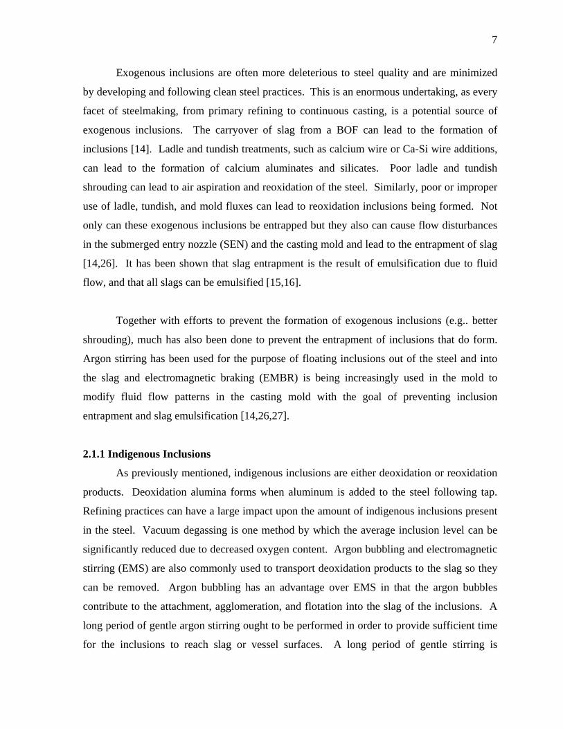
that periodically break away to form large alumina inclusions in the cast product. Figure 2.1
shows that these inclusions can be in excess of 100 microns in size [30]. For applications
such as deep drawing, where the maximum permitted inclusion size is approximately 50
microns, this type of inclusion is unacceptable [14]. Even if the agglomerations of alumina
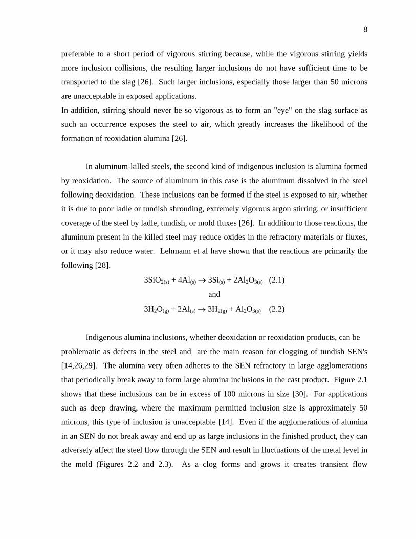
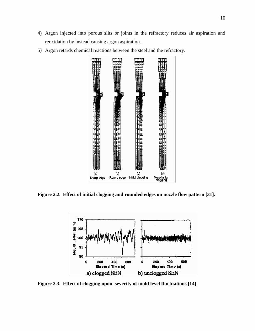
in an SEN do not break away and end up as large inclusions in the finished product, they can
adversely affect the steel flow through the SEN and result in fluctuations of the metal level in
the mold (Figures 2.2 and 2.3). As a clog forms and grows it creates transient flow

9
conditions that favor slag emulsification and slag entrapment in the mold and will be
discussed later[15,16,26].
Höller has stated that alumina inclusions a few microns in size do not noticeably
affect steel quality. Hence, it becomes apparent that a key approach to reducing the adverse
effects of alumina must deal with the prevention of large alumina agglomerations. The two
main efforts at preventing this agglomeration are the optimization of argon gas injection and
Figure 2.1 SEM Image of Reoxidation Alumina Inclusion [ 30].
the development of carbon-free inner bore surfaces of SEN's [29]. With respect to argon
injection, Thomas and Bai cite five possible mechanisms by which it is believed argon may
prevent nozzle clogging and alumina agglomeration [26]. They are as follows:
1) An argon gas film forms on the nozzle wall to prevent inclusion contact. This is likely
only at high gas flow rates, which tend to cause flow disruptions in the mold.
2) Argon bubbles attach to the alumina inclusions and carry them into the slag.
3) Argon bubbling increases turbulence, which causes the delicate inclusion network to
break away from the nozzle wall. However, this may be detrimental due to the increased
likelihood of particle contact with the nozzle wall.
10 µm
10
4) Argon injected into porous slits or joints in the refractory reduces air aspiration and
reoxidation by instead causing argon aspiration.
5) Argon retards chemical reactions between the steel and the refractory.
Figure 2.2. Effect of initial clogging and rounded edges on nozzle flow pattern [31].
Figure 2.3. Effect of clogging upon severity of mold level fluctuations [14]
11
Furthermore, it is noted that argon can greatly change the steel flow patterns in the mold,
often leading to transient metal level fluctuations and the formation of exogenous inclusions
[26].
Modification of the inner bore surface to make the surface less wettable for alumina
deposition is attractive because it may lessen mold metal level fluctuations associated with
argon. Various protective coatings (including non-wettable nitride materials) for the inner
bore have been tried, but their application is complicated by their peeling during preheating.
These protective coatings are particularly sensitive to peeling as they tend to be very brittle
and do not adhere well to the substrate refractory. In addition, the application of such
coatings is very expensive. Despite these disadvantages, a promising method to combat
alumina adherence is the creation of a carbon-free layer [29]. A major obstacle to the use of
carbon-free layers is that carbon-free materials have rougher, more porous surfaces than the
carbon-bearing refractory. Therefore, while chemically the material retards wetting by
alumina, the rough nature of the surface provides sites for deposition of alumina [29].
2.1.2 Exogenous Inclusions
As indigenous inclusions can lead to the entrapment of exogenous inclusions due to
fluctuations of metal level in the mold, it should also be noted that metal level fluctuations in
the tundish are also a source of exogenous inclusions. Exogenous inclusions consist of mold,
tundish, or ladle fluxes; products of calcium or calcium-silicon wire treatments; and products
of reactions between indigenous alumina inclusions with MgO, CaO, and SiO2, which are
commonly found in refractory materials and fluxes [14,26]. For purposes of clarity and
organization, exogenous inclusions will be divided into three areas: 1) inclusions formed due
to emulsification and entrapment of steelmaking fluxes, 2) inclusions created during wire- or
other ladle treatments, and 3) inclusions created as the result of reactions of the steel or
indigenous inclusions with steelmaking refractory.
Emulsification of Slags
An important concept to understand entrapment of exogenous inclusions is the
emulsification of steelmaking slags. Several researchers, most notably Cramb and Thomas,

12
have shown that slag emulsification occurs due to shear forces generated by the flow of
liquid steel at the steel/liquid flux interface in the direction toward the SEN.
All slags can be emulsified, but the physical properties of the mold flux and the
nature of the steel flow dictate the relative ease/difficulty with which a given slag may be
emulsified. Slag viscosity, differential density, slag density, slag depth, and interfacial
tension have been identified as the influencing physical factors upon emulsification
[12,13,15,16]. Cramb has identified five processing conditions in which slag emulsification
can be expected to occur [12].
1) Vessel filling (associated with high pouring energies existing in the steel and
pouring through slag)
2) Vessel drainage (e.g. vortexing)
3) Excessive turbulence at the metal/slag interface because of wave motion or stream
impingement
4) Gas injection rates that exceed critical values
5) Interfacial level fluctuations that exceed critical levels
In addition to this, it is known that emulsification is a common cause of inclusions that are
larger than 20 microns in diameter [12,14]. Table 2.1 shows how such large inclusions can
be problematic when attempting to produce sheet for high-end applications[12].
Harman and Cramb carried out a study of the effect of fluid physical properties upon
emulsification using a silicon oil and water model not to model emulsification in a real
casting system, but to model a mechanism of emulsification and entrapment with the goal of
understanding the effects of fluid properties upon emulsification.
Table 2.1. Requirements for high purity and ultra-clean steels [12].
Product Purity Cleanliness Notes Automotive Sheet C < 30 PPM
N < 30 PPM T[O] < 20 PPM d < 100µm
Ultra-deep drawing applications
Drawn and ironed cans
C < 30 PPM N < 30 PPM
T[O] < 20 PPM d < 20µm
Two-piece beverage and battery cans
13
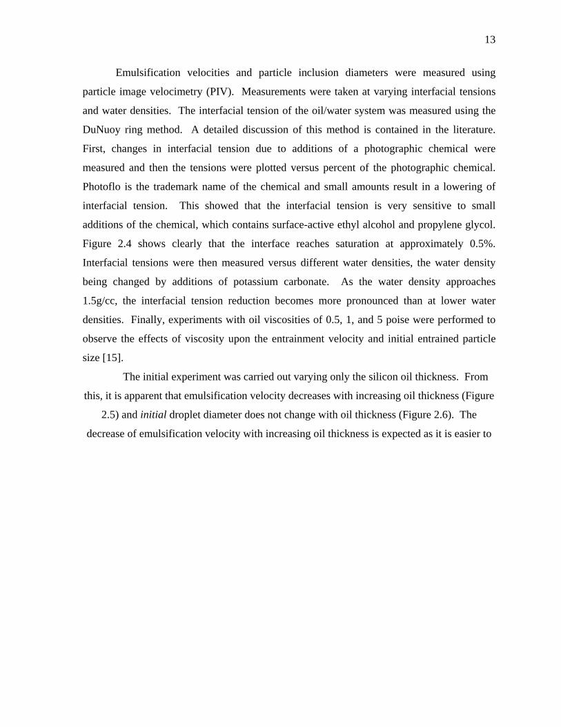
Emulsification velocities and particle inclusion diameters were measured using
particle image velocimetry (PIV). Measurements were taken at varying interfacial tensions
and water densities. The interfacial tension of the oil/water system was measured using the
DuNuoy ring method. A detailed discussion of this method is contained in the literature.
First, changes in interfacial tension due to additions of a photographic chemical were
measured and then the tensions were plotted versus percent of the photographic chemical.
Photoflo is the trademark name of the chemical and small amounts result in a lowering of
interfacial tension. This showed that the interfacial tension is very sensitive to small
additions of the chemical, which contains surface-active ethyl alcohol and propylene glycol.
Figure 2.4 shows clearly that the interface reaches saturation at approximately 0.5%.
Interfacial tensions were then measured versus different water densities, the water density
being changed by additions of potassium carbonate. As the water density approaches
1.5g/cc, the interfacial tension reduction becomes more pronounced than at lower water
densities. Finally, experiments with oil viscosities of 0.5, 1, and 5 poise were performed to
observe the effects of viscosity upon the entrainment velocity and initial entrained particle
size [15].
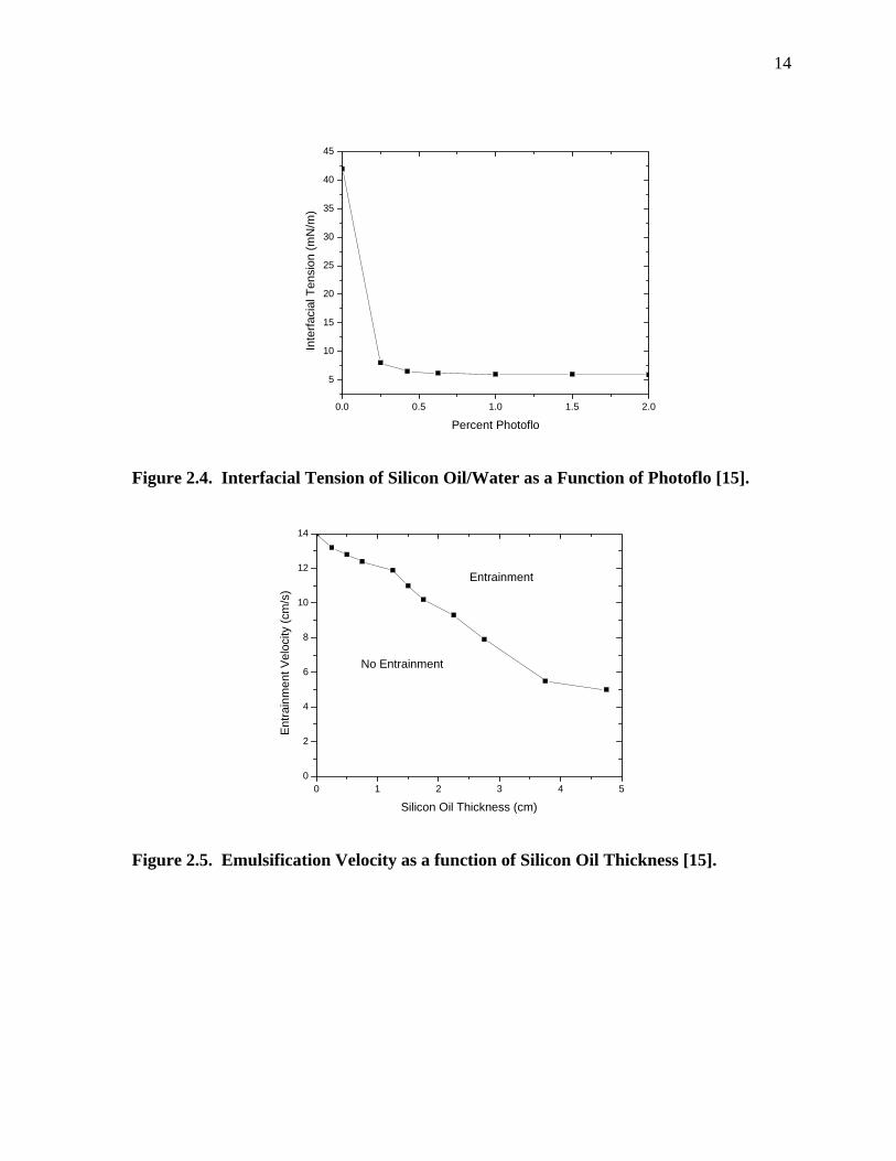
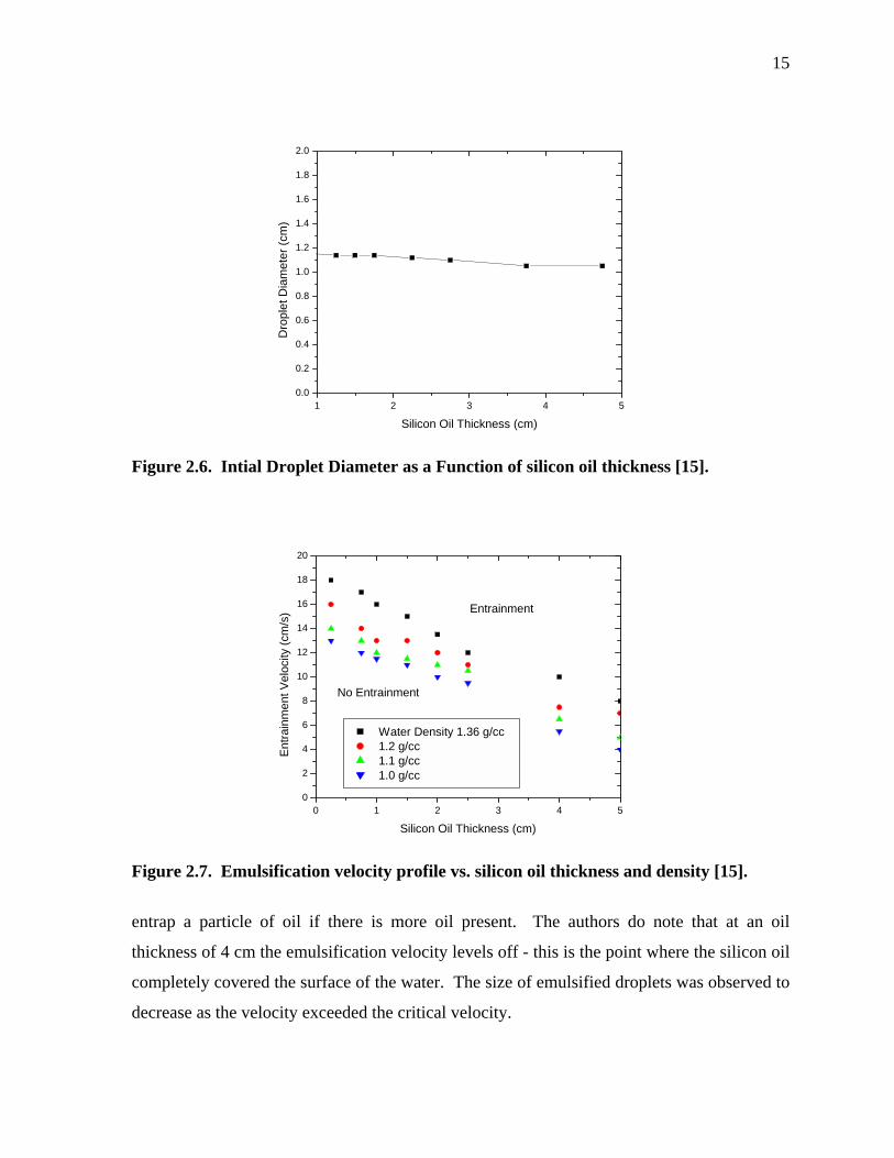
The initial experiment was carried out varying only the silicon oil thickness. From
this, it is apparent that emulsification velocity decreases with increasing oil thickness (Figure
2.5) and initial droplet diameter does not change with oil thickness (Figure 2.6). The
decrease of emulsification velocity with increasing oil thickness is expected as it is easier to
14
0.0 0.5 1.0 1.5 2.0
5
10
15
20
25
30
35
40
45
Inte
rfaci
al T
ensi
on (m
N/m
)
Percent Photoflo
Figure 2.4. Interfacial Tension of Silicon Oil/Water as a Function of Photoflo [15].
0 1 2 3 4 50
2
4
6
8
10
12
14
No Entrainment
Entrainment
Entra
inm
ent V
eloc
ity (c
m/s
)
Silicon Oil Thickness (cm)
Figure 2.5. Emulsification Velocity as a function of Silicon Oil Thickness [15].
15
1 2 3 4 50.0
0.2
0.4
0.6
0.8
1.0
1.2
1.4
1.6
1.8
2.0
Dro
plet
Dia
met
er (c
m)
Silicon Oil Thickness (cm)
Figure 2.6. Intial Droplet Diameter as a Function of silicon oil thickness [15].
0 1 2 3 4 50
2
4
6
8
10
12
14
16
18
20
No Entrainment
Entrainment
Entra
inm
ent V
eloc
ity (c
m/s
)
Silicon Oil Thickness (cm)
Water Density 1.36 g/cc 1.2 g/cc 1.1 g/cc 1.0 g/cc
Figure 2.7. Emulsification velocity profile vs. silicon oil thickness and density [15].
entrap a particle of oil if there is more oil present. The authors do note that at an oil
thickness of 4 cm the emulsification velocity levels off - this is the point where the silicon oil
completely covered the surface of the water. The size of emulsified droplets was observed to
decrease as the velocity exceeded the critical velocity.
16
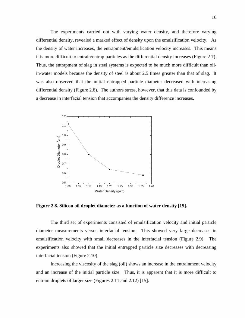
The experiments carried out with varying water density, and therefore varying
differential density, revealed a marked effect of density upon the emulsification velocity. As
the density of water increases, the entrapment/emulsification velocity increases. This means
it is more difficult to entrain/entrap particles as the differential density increases (Figure 2.7).
Thus, the entrapment of slag in steel systems is expected to be much more difficult than oil-
in-water models because the density of steel is about 2.5 times greater than that of slag. It
was also observed that the initial entrapped particle diameter decreased with increasing
differential density (Figure 2.8). The authors stress, however, that this data is confounded by
a decrease in interfacial tension that accompanies the density difference increases.
1.00 1.05 1.10 1.15 1.20 1.25 1.30 1.35 1.400.5
0.6
0.7
0.8
0.9
1.0
1.1
1.2
Dro
plet
Dia
met
er (c
m)
Water Density (g/cc)
Figure 2.8. Silicon oil droplet diameter as a function of water density [15].
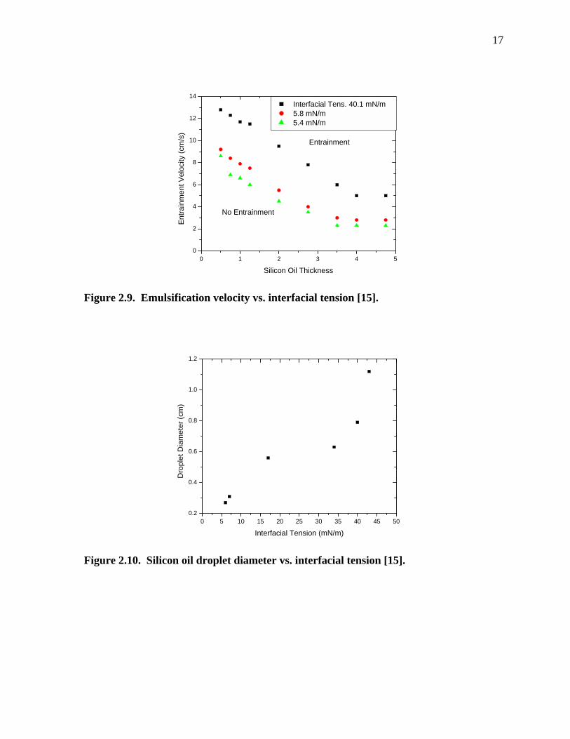
The third set of experiments consisted of emulsification velocity and initial particle
diameter measurements versus interfacial tension. This showed very large decreases in
emulsification velocity with small decreases in the interfacial tension (Figure 2.9). The
experiments also showed that the initial entrapped particle size decreases with decreasing
interfacial tension (Figure 2.10).
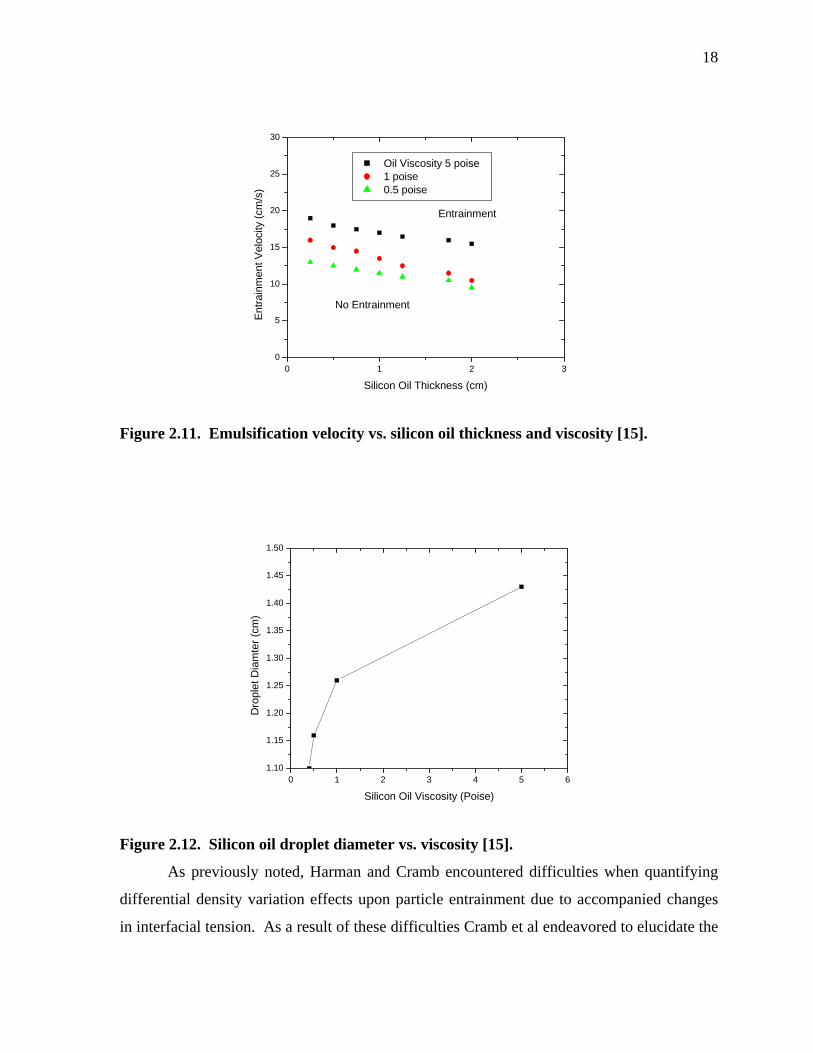
Increasing the viscosity of the slag (oil) shows an increase in the entrainment velocity
and an increase of the initial particle size. Thus, it is apparent that it is more difficult to
entrain droplets of larger size (Figures 2.11 and 2.12) [15].
17
0 1 2 3 4 50
2
4
6
8
10
12
14
No Entrainment
Entrainment
Entra
inm
ent V
eloc
ity (c
m/s
)
Silicon Oil Thickness
Interfacial Tens. 40.1 mN/m 5.8 mN/m 5.4 mN/m
Figure 2.9. Emulsification velocity vs. interfacial tension [15].
0 5 10 15 20 25 30 35 40 45 500.2
0.4
0.6
0.8
1.0
1.2
Dro
plet
Dia
met
er (c
m)
Interfacial Tension (mN/m)
Figure 2.10. Silicon oil droplet diameter vs. interfacial tension [15].
18
0 1 2 30
5
10
15
20
25
30
Entrainment
No Entrainment
Entra
inm
ent V
eloc
ity (c
m/s
)
Silicon Oil Thickness (cm)
Oil Viscosity 5 poise 1 poise 0.5 poise
Figure 2.11. Emulsification velocity vs. silicon oil thickness and viscosity [15].
0 1 2 3 4 5 61.10
1.15
1.20
1.25
1.30
1.35
1.40
1.45
1.50
Dro
plet
Dia
mte
r (cm
)
Silicon Oil Viscosity (Poise)
Figure 2.12. Silicon oil droplet diameter vs. viscosity [15].
As previously noted, Harman and Cramb encountered difficulties when quantifying
differential density variation effects upon particle entrainment due to accompanied changes
in interfacial tension. As a result of these difficulties Cramb et al endeavored to elucidate the
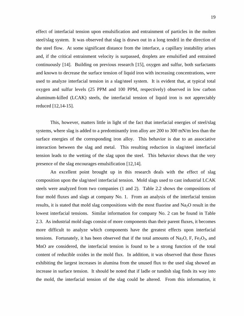
19
effect of interfacial tension upon emulsification and entrainment of particles in the molten
steel/slag system. It was observed that slag is drawn out in a long tendril in the direction of
the steel flow. At some significant distance from the interface, a capillary instability arises
and, if the critical entrainment velocity is surpassed, droplets are emulsified and entrained
continuously [14]. Building on previous research [15], oxygen and sulfur, both surfactants
and known to decrease the surface tension of liquid iron with increasing concentrations, were
used to analyze interfacial tension in a slag/steel system. It is evident that, at typical total
oxygen and sulfur levels (25 PPM and 100 PPM, respectively) observed in low carbon
aluminum-killed (LCAK) steels, the interfacial tension of liquid iron is not appreciably
reduced [12,14-15].
This, however, matters little in light of the fact that interfacial energies of steel/slag
systems, where slag is added to a predominantly iron alloy are 200 to 300 mN/m less than the
surface energies of the corresponding iron alloy. This behavior is due to an associative
interaction between the slag and metal. This resulting reduction in slag/steel interfacial
tension leads to the wetting of the slag upon the steel. This behavior shows that the very
presence of the slag encourages emulsification [12,14].
An excellent point brought up in this research deals with the effect of slag
composition upon the slag/steel interfacial tension. Mold slags used to cast industrial LCAK
steels were analyzed from two companies (1 and 2). Table 2.2 shows the compositions of
four mold fluxes and slags at company No. 1. From an analysis of the interfacial tension
results, it is stated that mold slag compositions with the most fluorine and Na2O result in the
lowest interfacial tensions. Similar information for company No. 2 can be found in Table
2.3. As industrial mold slags consist of more components than their parent fluxes, it becomes
more difficult to analyze which components have the greatest effects upon interfacial
tensions. Fortunately, it has been observed that if the total amounts of Na2O, F, Fe2O3, and
MnO are considered, the interfacial tension is found to be a strong function of the total
content of reducible oxides in the mold flux. In addition, it was observed that those fluxes
exhibiting the largest increases in alumina from the unused flux to the used slag showed an
increase in surface tension. It should be noted that if ladle or tundish slag finds its way into
the mold, the interfacial tension of the slag could be altered. From this information, it
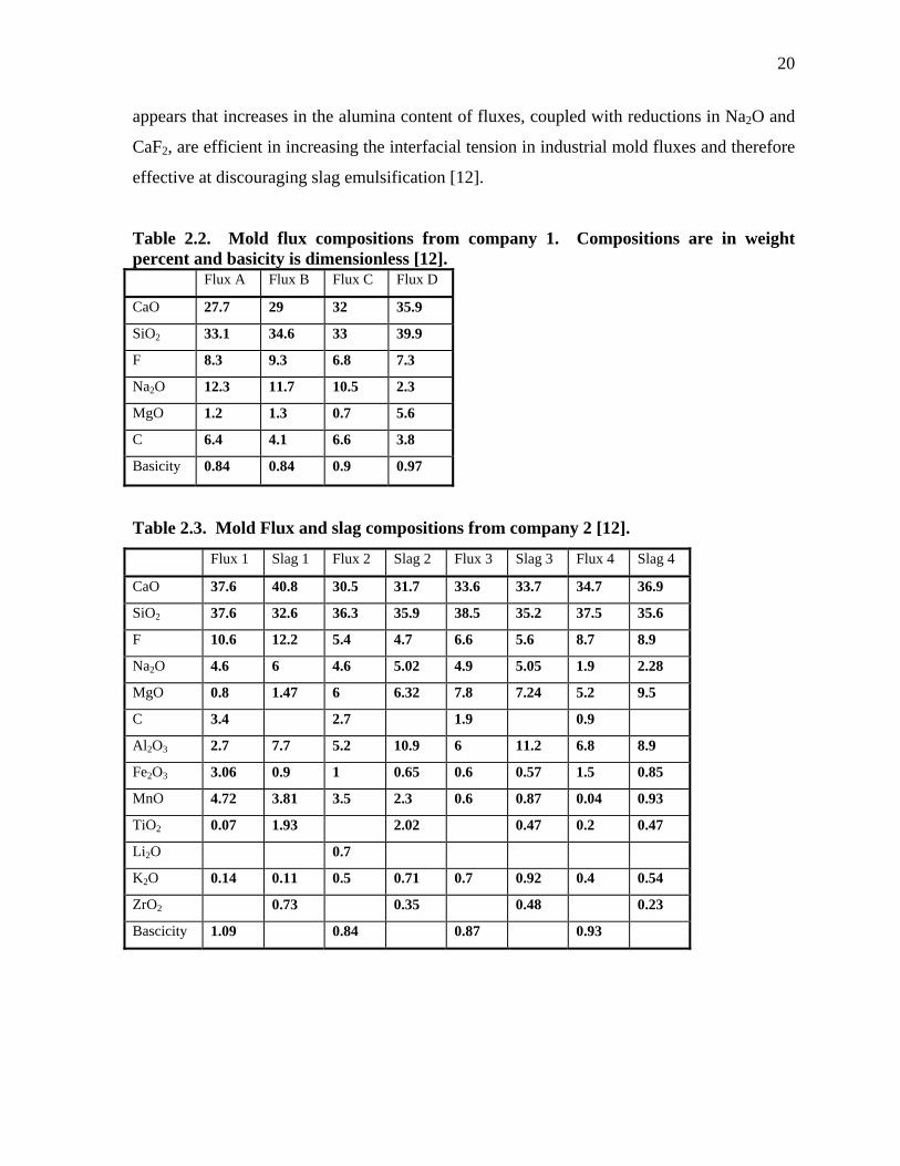
20
appears that increases in the alumina content of fluxes, coupled with reductions in Na2O and
CaF2, are efficient in increasing the interfacial tension in industrial mold fluxes and therefore
effective at discouraging slag emulsification [12].
Table 2.2. Mold flux compositions from company 1. Compositions are in weight percent and basicity is dimensionless [12]. Flux A Flux B Flux C Flux D
CaO 27.7 29 32 35.9
SiO2 33.1 34.6 33 39.9
F 8.3 9.3 6.8 7.3
Na2O 12.3 11.7 10.5 2.3
MgO 1.2 1.3 0.7 5.6
C 6.4 4.1 6.6 3.8
Basicity 0.84 0.84 0.9 0.97
Table 2.3. Mold Flux and slag compositions from company 2 [12].
Flux 1 Slag 1 Flux 2 Slag 2 Flux 3 Slag 3 Flux 4 Slag 4
CaO 37.6 40.8 30.5 31.7 33.6 33.7 34.7 36.9
SiO2 37.6 32.6 36.3 35.9 38.5 35.2 37.5 35.6
F 10.6 12.2 5.4 4.7 6.6 5.6 8.7 8.9
Na2O 4.6 6 4.6 5.02 4.9 5.05 1.9 2.28
MgO 0.8 1.47 6 6.32 7.8 7.24 5.2 9.5
C 3.4 2.7 1.9 0.9
Al2O3 2.7 7.7 5.2 10.9 6 11.2 6.8 8.9
Fe2O3 3.06 0.9 1 0.65 0.6 0.57 1.5 0.85
MnO 4.72 3.81 3.5 2.3 0.6 0.87 0.04 0.93
TiO2 0.07 1.93 2.02 0.47 0.2 0.47
Li2O 0.7
K2O 0.14 0.11 0.5 0.71 0.7 0.92 0.4 0.54
ZrO2 0.73 0.35 0.48 0.23
Bascicity 1.09 0.84 0.87 0.93
21
2.1.3 Mold Flux and Mold Slag Properties
From the previous discussion it is quite apparent that the properties of mold fluxes and
slags are very important not only for heat transfer, lubrication, and insulation, but for quality
in very complex ways. Feldbauer has conveniently listed five purposes that mold fluxes
serve in continuous casting molds [10].
! Provide lubrication between solidifying steel shell and the mold
! Moderate heat transfer between the shell and mold
! Prevent reoxidation
! Provide thermal insulation
! Act as reservoir for the absorption of inclusions, liquid and solid, from the molten steel
Also listed are seven problems caused by inappropriate mold flux application. Three of the
these are applicable for this project.
! Sub-surface cleanliness problems in the cast product
! Slag patches on the surface of continuously cast sections
! Chemical interaction between the liquid steel and the liquid flux pool [10].
This list of flux functions and potential problems illustrates, along with the emulsification
discussion, that mold flux and mold slag design must be performed very meticulously to
produce fluxes that facilitate the production of clean steel. Of particular interest in the work
of Feldbauer is the claim that interfacial tension increases with increasing amounts of CaF2
and Na2O [10]. This contradicts the results of Cramb, et al, which claim the opposite
behavior [12]. One possible reason for this is that Feldbauer measured interfacial tensions
with slags containing between 30 and 60% CaF2 and Na2O while Cramb dealt with slags
containing less than 20% of those compounds. With the exception of fluorospar and soda,
Feldbauer recommends that a flux have a high viscosity, high interfacial tension, and small
amounts of reducible oxides (most notably FeO and MnO) to avoid slag emulsification. It is
noted that such fluxes may lead to a greater likelihood of sticking in the mold and therefore,
to costly breakouts. Therefore, the utmost care must be taken by the flux manufacturer to
balance the properties of the flux to be both somewhat resistant to emulsification while
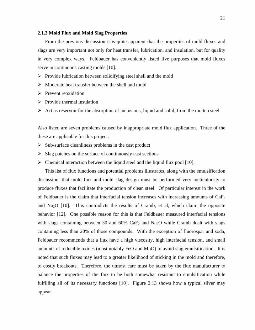
fulfilling all of its necessary functions [10]. Figure 2.13 shows how a typical sliver may
appear.
22
Figure 2.13. Typical mold flux sliver.
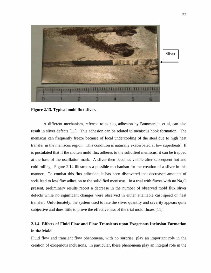
A different mechanism, referred to as slag adhesion by Bommaraju, et al, can also
result in sliver defects [11]. This adhesion can be related to meniscus hook formation. The
meniscus can frequently freeze because of local undercooling of the steel due to high heat
transfer in the meniscus region. This condition is naturally exacerbated at low superheats. It
is postulated that if the molten mold flux adheres to the solidified meniscus, it can be trapped
at the base of the oscillation mark. A sliver then becomes visible after subsequent hot and
cold rolling. Figure 2.14 illustrates a possible mechanism for the creation of a sliver in this
manner. To combat this flux adhesion, it has been discovered that decreased amounts of
soda lead to less flux adhesion to the solidified meniscus. In a trial with fluxes with no Na2O
present, preliminary results report a decrease in the number of observed mold flux sliver
defects while no significant changes were observed in either attainable cast speed or heat
transfer. Unfortunately, the system used to rate the sliver quantity and severity appears quite
subjective and does little to prove the effectiveness of the trial mold fluxes [11].
2.1.4 Effects of Fluid Flow and Flow Transients upon Exogenous Inclusion Formation
in the Mold
Fluid flow and transient flow phenomena, with no surprise, play an important role in the
creation of exogenous inclusions. In particular, these phenomena play an integral role in the
Sliver
23
emulsification of slags. Again, for purposes of scope and relevance, only the flow behavior
of the casting mold will be discussed. While flow behavior is different near the slag/steel
interfaces in ladles and tundishes, the concepts of the relationship between fluid flow and
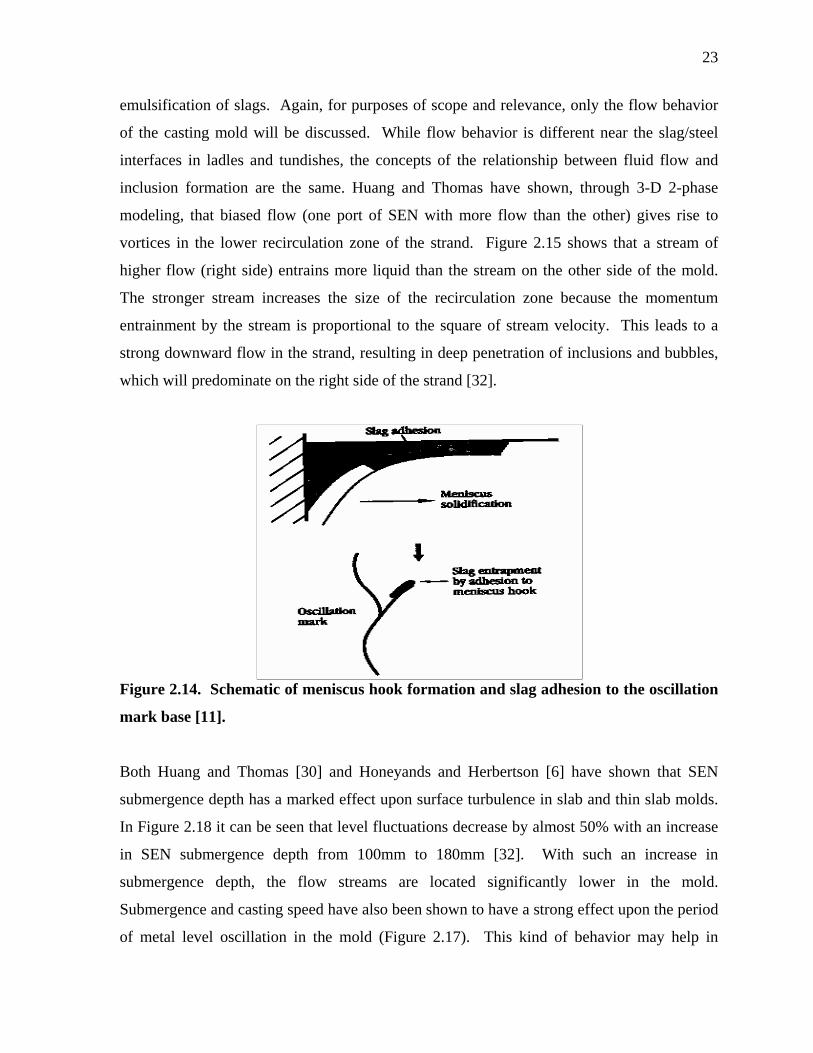
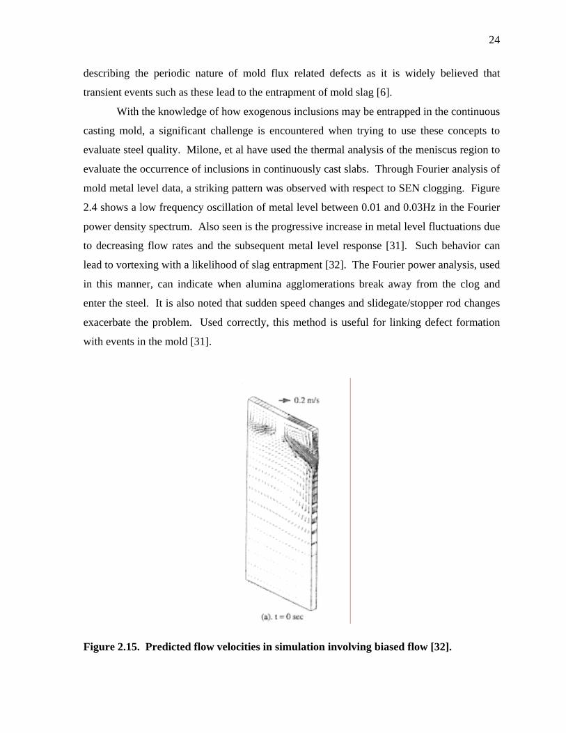
inclusion formation are the same. Huang and Thomas have shown, through 3-D 2-phase
modeling, that biased flow (one port of SEN with more flow than the other) gives rise to
vortices in the lower recirculation zone of the strand. Figure 2.15 shows that a stream of
higher flow (right side) entrains more liquid than the stream on the other side of the mold.
The stronger stream increases the size of the recirculation zone because the momentum
entrainment by the stream is proportional to the square of stream velocity. This leads to a
strong downward flow in the strand, resulting in deep penetration of inclusions and bubbles,
which will predominate on the right side of the strand [32].
Figure 2.14. Schematic of meniscus hook formation and slag adhesion to the oscillation
mark base [11].
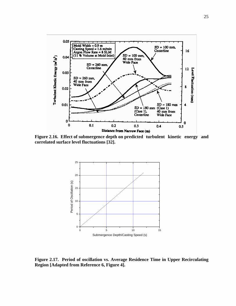
Both Huang and Thomas [30] and Honeyands and Herbertson [6] have shown that SEN
submergence depth has a marked effect upon surface turbulence in slab and thin slab molds.
In Figure 2.18 it can be seen that level fluctuations decrease by almost 50% with an increase
in SEN submergence depth from 100mm to 180mm [32]. With such an increase in
submergence depth, the flow streams are located significantly lower in the mold.
Submergence and casting speed have also been shown to have a strong effect upon the period
of metal level oscillation in the mold (Figure 2.17). This kind of behavior may help in
24
describing the periodic nature of mold flux related defects as it is widely believed that
transient events such as these lead to the entrapment of mold slag [6].
With the knowledge of how exogenous inclusions may be entrapped in the continuous
casting mold, a significant challenge is encountered when trying to use these concepts to
evaluate steel quality. Milone, et al have used the thermal analysis of the meniscus region to
evaluate the occurrence of inclusions in continuously cast slabs. Through Fourier analysis of
mold metal level data, a striking pattern was observed with respect to SEN clogging. Figure
2.4 shows a low frequency oscillation of metal level between 0.01 and 0.03Hz in the Fourier
power density spectrum. Also seen is the progressive increase in metal level fluctuations due
to decreasing flow rates and the subsequent metal level response [31]. Such behavior can
lead to vortexing with a likelihood of slag entrapment [32]. The Fourier power analysis, used
in this manner, can indicate when alumina agglomerations break away from the clog and
enter the steel. It is also noted that sudden speed changes and slidegate/stopper rod changes
exacerbate the problem. Used correctly, this method is useful for linking defect formation
with events in the mold [31].
Figure 2.15. Predicted flow velocities in simulation involving biased flow [32].
25
Figure 2.16. Effect of submergence depth on predicted turbulent kinetic energy and correlated surface level fluctuations [32].
Figure 2.17. Period of oscillation vs. Average Residence Time in Upper Recirculating Region [Adapted from Reference 6, Figure 4].
0 5 10 150
5
10
15
20
25
Perio
d of
Osc
illat
ion
(s)
Submergence Depth/Casting Speed (s)
26
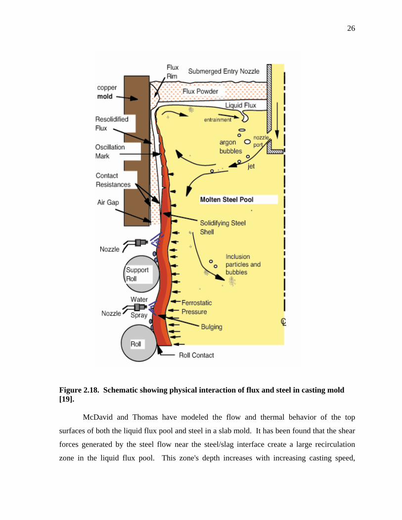
Figure 2.18. Schematic showing physical interaction of flux and steel in casting mold [19]. McDavid and Thomas have modeled the flow and thermal behavior of the top
surfaces of both the liquid flux pool and steel in a slab mold. It has been found that the shear
forces generated by the steel flow near the steel/slag interface create a large recirculation
zone in the liquid flux pool. This zone's depth increases with increasing casting speed,
27
increasing mold flux conductivity, and decreasing mold flux viscosity. Figure 2.18 shows a
schematic of the physical interaction of flux and steel in a generic continuous slab casting
mold. The purpose of the modeling was to quantify the phenomena of powder melting and
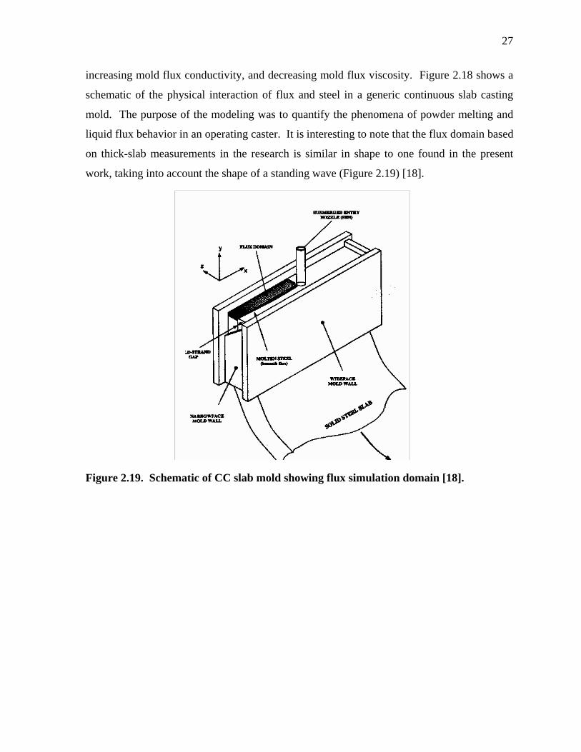
liquid flux behavior in an operating caster. It is interesting to note that the flux domain based
on thick-slab measurements in the research is similar in shape to one found in the present
work, taking into account the shape of a standing wave (Figure 2.19) [18].
Figure 2.19. Schematic of CC slab mold showing flux simulation domain [18].
28
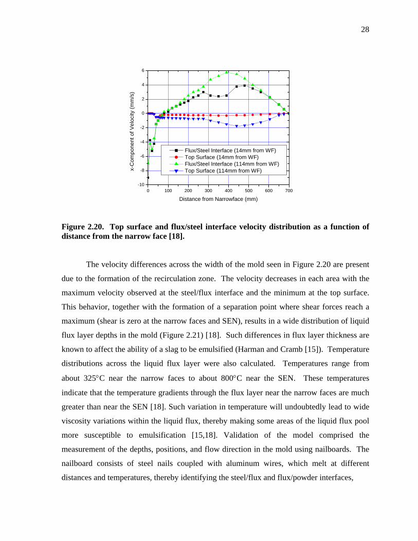
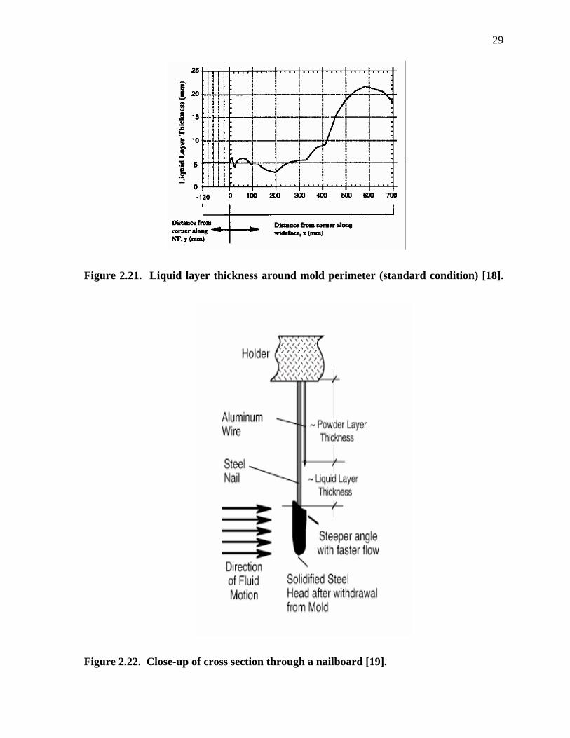
Figure 2.20. Top surface and flux/steel interface velocity distribution as a function of distance from the narrow face [18]. The velocity differences across the width of the mold seen in Figure 2.20 are present
due to the formation of the recirculation zone. The velocity decreases in each area with the
maximum velocity observed at the steel/flux interface and the minimum at the top surface.
This behavior, together with the formation of a separation point where shear forces reach a
maximum (shear is zero at the narrow faces and SEN), results in a wide distribution of liquid
flux layer depths in the mold (Figure 2.21) [18]. Such differences in flux layer thickness are
known to affect the ability of a slag to be emulsified (Harman and Cramb [15]). Temperature
distributions across the liquid flux layer were also calculated. Temperatures range from
about 325°C near the narrow faces to about 800°C near the SEN. These temperatures
indicate that the temperature gradients through the flux layer near the narrow faces are much
greater than near the SEN [18]. Such variation in temperature will undoubtedly lead to wide
viscosity variations within the liquid flux, thereby making some areas of the liquid flux pool
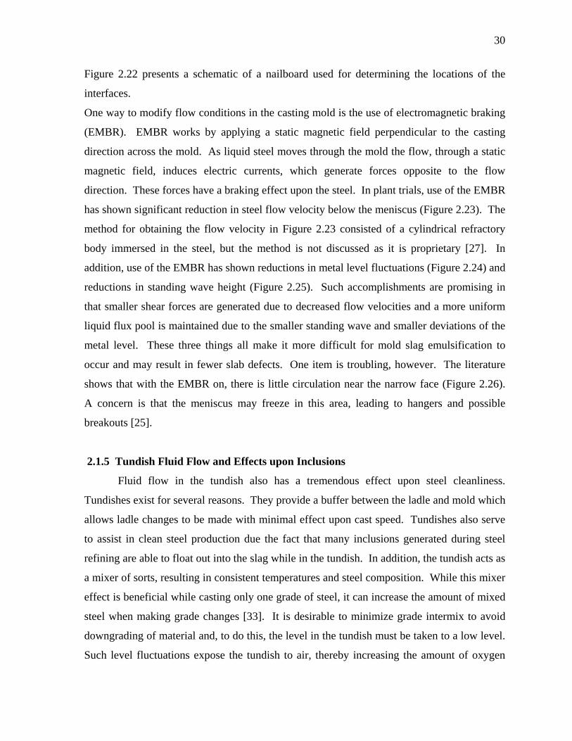
more susceptible to emulsification [15,18]. Validation of the model comprised the
measurement of the depths, positions, and flow direction in the mold using nailboards. The
nailboard consists of steel nails coupled with aluminum wires, which melt at different
distances and temperatures, thereby identifying the steel/flux and flux/powder interfaces,
0 100 200 300 400 500 600 700-10
-8
-6
-4
-2
0
2
4
6
x-C
ompo
nent
of V
eloc
ity (m
m/s
)
Distance from Narrowface (mm)
Flux/Steel Interface (14mm from WF) Top Surface (14mm from WF) Flux/Steel Interface (114mm from WF) Top Surface (114mm from WF)
29
Figure 2.21. Liquid layer thickness around mold perimeter (standard condition) [18].
Figure 2.22. Close-up of cross section through a nailboard [19].
30
Figure 2.22 presents a schematic of a nailboard used for determining the locations of the
interfaces.
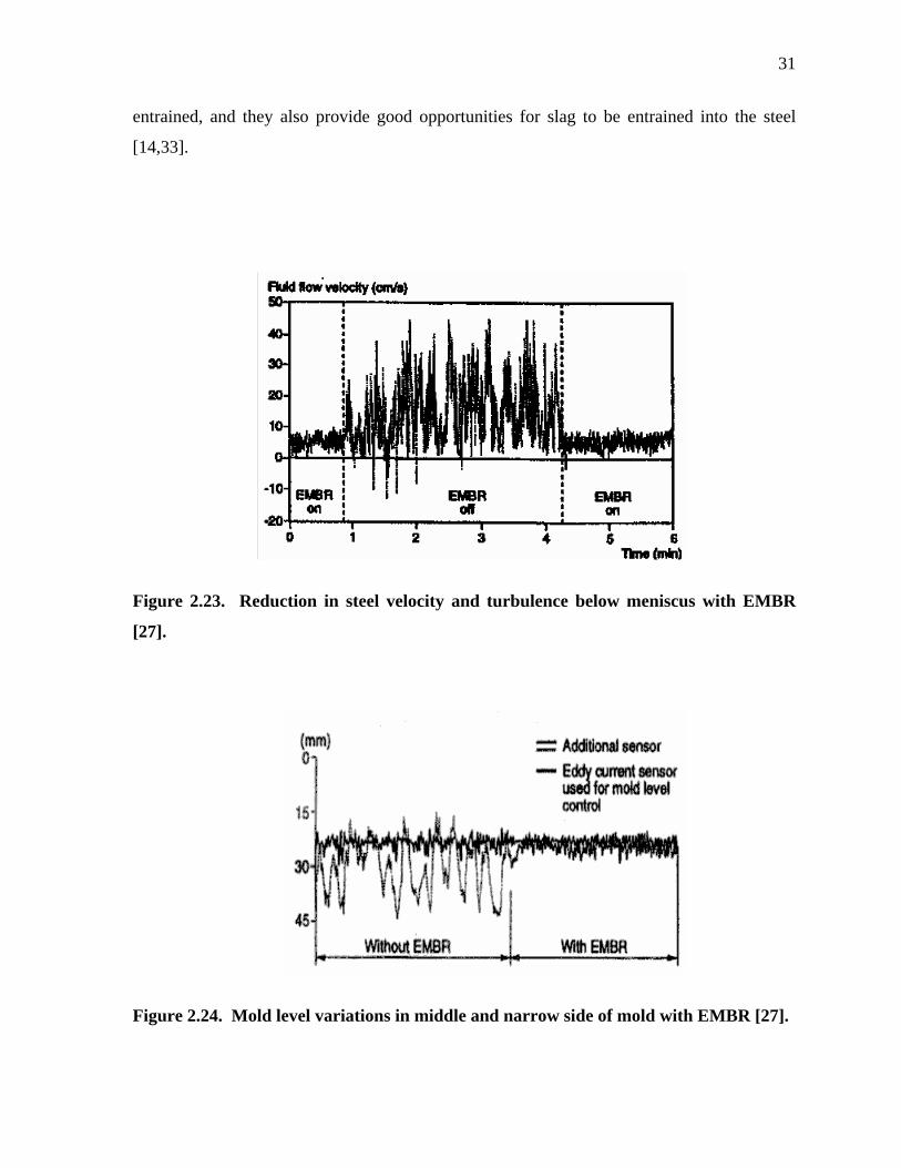
One way to modify flow conditions in the casting mold is the use of electromagnetic braking
(EMBR). EMBR works by applying a static magnetic field perpendicular to the casting
direction across the mold. As liquid steel moves through the mold the flow, through a static
magnetic field, induces electric currents, which generate forces opposite to the flow
direction. These forces have a braking effect upon the steel. In plant trials, use of the EMBR
has shown significant reduction in steel flow velocity below the meniscus (Figure 2.23). The
method for obtaining the flow velocity in Figure 2.23 consisted of a cylindrical refractory
body immersed in the steel, but the method is not discussed as it is proprietary [27]. In
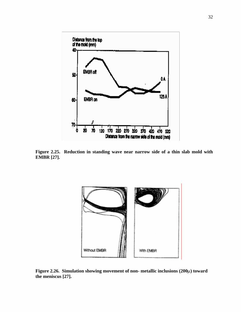
addition, use of the EMBR has shown reductions in metal level fluctuations (Figure 2.24) and
reductions in standing wave height (Figure 2.25). Such accomplishments are promising in
that smaller shear forces are generated due to decreased flow velocities and a more uniform
liquid flux pool is maintained due to the smaller standing wave and smaller deviations of the
metal level. These three things all make it more difficult for mold slag emulsification to
occur and may result in fewer slab defects. One item is troubling, however. The literature
shows that with the EMBR on, there is little circulation near the narrow face (Figure 2.26).
A concern is that the meniscus may freeze in this area, leading to hangers and possible
breakouts [25].
2.1.5 Tundish Fluid Flow and Effects upon Inclusions
Fluid flow in the tundish also has a tremendous effect upon steel cleanliness.
Tundishes exist for several reasons. They provide a buffer between the ladle and mold which
allows ladle changes to be made with minimal effect upon cast speed. Tundishes also serve
to assist in clean steel production due the fact that many inclusions generated during steel
refining are able to float out into the slag while in the tundish. In addition, the tundish acts as
a mixer of sorts, resulting in consistent temperatures and steel composition. While this mixer
effect is beneficial while casting only one grade of steel, it can increase the amount of mixed
steel when making grade changes [33]. It is desirable to minimize grade intermix to avoid
downgrading of material and, to do this, the level in the tundish must be taken to a low level.
Such level fluctuations expose the tundish to air, thereby increasing the amount of oxygen
31
entrained, and they also provide good opportunities for slag to be entrained into the steel
[14,33].
Figure 2.23. Reduction in steel velocity and turbulence below meniscus with EMBR
[27].
Figure 2.24. Mold level variations in middle and narrow side of mold with EMBR [27].
32
Figure 2.25. Reduction in standing wave near narrow side of a thin slab mold with EMBR [27].
Figure 2.26. Simulation showing movement of non- metallic inclusions (200µ) toward the meniscus [27].
33
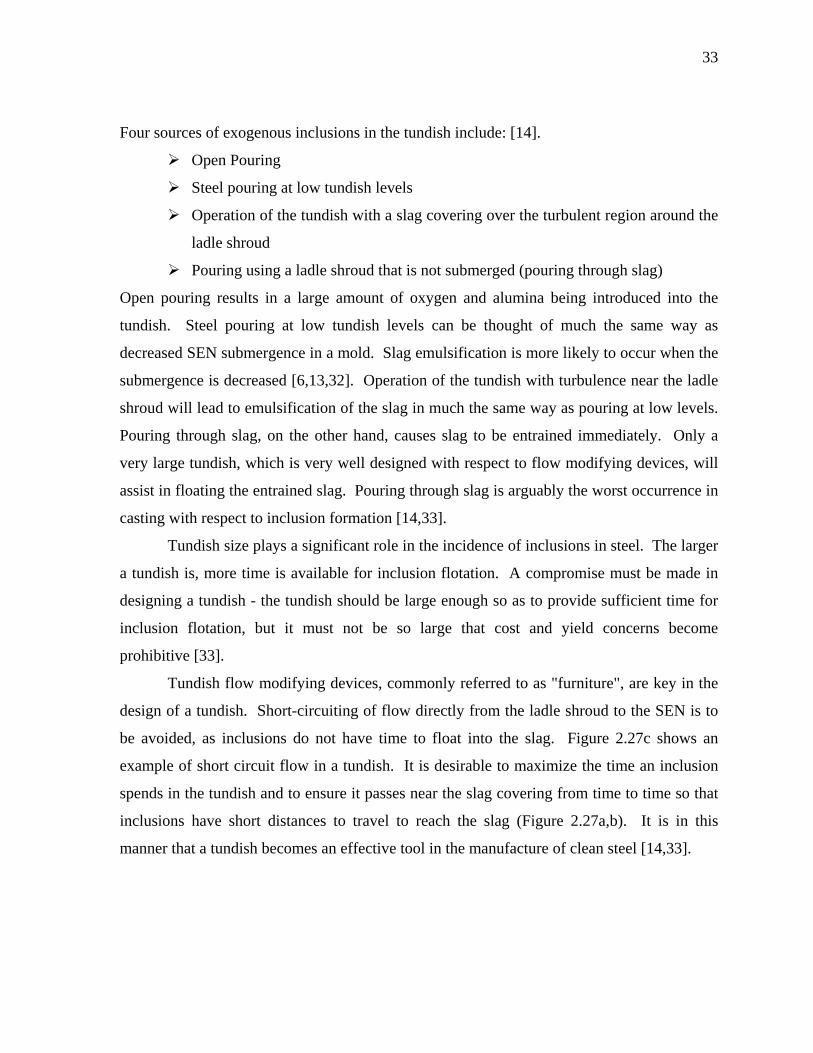
Four sources of exogenous inclusions in the tundish include: [14].
! Open Pouring
! Steel pouring at low tundish levels
! Operation of the tundish with a slag covering over the turbulent region around the
ladle shroud
! Pouring using a ladle shroud that is not submerged (pouring through slag)
Open pouring results in a large amount of oxygen and alumina being introduced into the
tundish. Steel pouring at low tundish levels can be thought of much the same way as
decreased SEN submergence in a mold. Slag emulsification is more likely to occur when the
submergence is decreased [6,13,32]. Operation of the tundish with turbulence near the ladle
shroud will lead to emulsification of the slag in much the same way as pouring at low levels.
Pouring through slag, on the other hand, causes slag to be entrained immediately. Only a
very large tundish, which is very well designed with respect to flow modifying devices, will
assist in floating the entrained slag. Pouring through slag is arguably the worst occurrence in
casting with respect to inclusion formation [14,33].
Tundish size plays a significant role in the incidence of inclusions in steel. The larger
a tundish is, more time is available for inclusion flotation. A compromise must be made in
designing a tundish - the tundish should be large enough so as to provide sufficient time for
inclusion flotation, but it must not be so large that cost and yield concerns become
prohibitive [33].
Tundish flow modifying devices, commonly referred to as "furniture", are key in the
design of a tundish. Short-circuiting of flow directly from the ladle shroud to the SEN is to
be avoided, as inclusions do not have time to float into the slag. Figure 2.27c shows an
example of short circuit flow in a tundish. It is desirable to maximize the time an inclusion
spends in the tundish and to ensure it passes near the slag covering from time to time so that
inclusions have short distances to travel to reach the slag (Figure 2.27a,b). It is in this
manner that a tundish becomes an effective tool in the manufacture of clean steel [14,33].
34
Figure 2.27. Schematic of tundish designs [33].
2.1.6 Inclusions Formed During Ladle Treatment and Reactions with Fluxes and
Refractory
Exogenous inclusions that form during ladle treatment are mostly the products of
reactions between calcium and indigenous alumina inclusions. Calcium aluminates comprise
the majority of these inclusions, although calcium sulfides are also commonly formed
(depending upon sulfur level at time of Ca treatment). Calcium treatment is carried out for
two reasons: 1) calcium will react with alumina to form liquid calcium aluminates, which
can be floated into the slag and 2) to modify the shape of manganese sulfide inclusions in the
rolled product for formability purposes.
At steelmaking temperatures, there are two species of calcium aluminate that exist in
the liquid state. 3CaO-Al2O3 has a melting point of 1535°C and a density of 3.04 g/cc.
12CaO-7Al2O3 melts at 1455°C and has a density of 2.83 g/cc. The C12A7 inclusion exists at
about 50-53% Al2O3 in the binary system with calcia (Figure 2.28). These less dense C12A7
is reported in sizes of 10-15 microns when the aluminum content of the steel is greater than
0.020 wt.%. These inclusions are generally considered more desirable than alumina
inclusions, as the liquid aluminates will not clog the SEN if they are not floated into the ladle
or tundish slag and thereby removed from the steel. This is a great development, provided
these liquid inclusions do not react further with refractory or fluxes to form solid inclusions
35
that stick to stopper rod and SEN refractory, resulting in clogging. In addition, great care
must be taken to ensure that sulfur levels are low (<0.008 wt.%) so that calcium sulfides will
not form. Calcium sulfide is solid at steelmaking temperatures and is notorious for causing
SEN clogging [34].
Calcium aluminates are also believed to form during reactions with ladle, tundish, and
mold slags, especially those with high CaO contents. Carryover slag from the ladle to
tundish provides oxygen for the reoxidation of aluminum present in the steel. It is a calcium
aluminate inclusion with traces of magnesium that is widely thought to result in cracking.
This inclusion may be the result of carryover slag, buildups on the ladle walls, or poor
tundish practice (poor level control, excessive slag, and open pouring). Magnesium is picked
up either by ladle slag or by reaction of alumina with tundish refractory, leading to alumina-
silicate slags with varying amounts of Mg and Ca (depending on slag carryover and
refractory composition) [33,34]. Tundish coverings high in silica (e.g. rice hulls) exacerbate
this problem as the rice hulls are fluxed by the slag, leading to an acid slag [33].
Mold powders and slags may react with the steel or existing inclusions to generate
deleterious inclusions that are unacceptable in cast steel. McPherson and McIntosh have
found that black spot defects found on exposed automotive sheet consisted of a calcium
aluminate with 70% alumina and 30% CaO along with small amounts of manganese, silicon,
and sodium [13]. From the analysis, it is evident that mold flux was the source of the
defects. Through water modeling, it was evident that the mold slag was being entrained by
the steel streams exiting the SEN. It was decided to increase the SEN submergence depth in
an attempt to reduce the frequency of the defect. Following this change, calcium aluminate
incidence on the strip surface dropped dramatically. It was also discovered that the practice
of raising the tundish (and SEN) at the end of cast caused the defect to appear. The practice
was discontinued and the defects disappeared [13]. Submerged entry nozzles also contribute
to the formation of exogenous inclusions. Oxidation, physical erosion, and reactions with
pre-existing inclusions all play a role in the wear of SEN's, and thereby the entrapment of
inclusions in the steel. Excessive oxidation can be encountered if air is aspirated. In addition
to alumina clogging due to air aspiration, the carbon present in the alumina-graphite
refractory (most common material for SEN) will react with oxygen, resulting in degradation
and disintegration of the refractory [29]. The most damaging effects upon SEN refractory
36
and the subsequent generation of inclusions are due to the action of mold fluxes and slags
upon the refractory material. Some of the CaO present in the flux reacts with the alumina
present in the refractory, leading to the formation of calcium aluminates which are washed
away by the steel flow. High fluorine contents, in the form of CaF2, exacerbate the problem
because, as the fluorine is emitted as a gas or reacts with silicon, more calcium becomes
available to attack the refractory. The addition of boron nitride to the refractory (to increase
wear resistance) resulted in the formation of low- melting B2O3-Al2O3 compounds that are
carried away with the flowing steel even faster than calcium aluminate [29].
A common slag band material used in SEN applications is MgO-stabilized zirconia.
The zirconia is able to withstand slag attack better than alumina graphite. The MgO in the
slag band reacts with silicon in the mold slag to form magnesium silicate, which then settles
at the ZrO2 grain boundaries. As the MgO is consumed, the zirconia becomes destabilized
and a martensitic phase transformation occurs. A volume expansion accompanies this
transformation. During this change from a cubic to a monoclinic crystal structure,
microcracks form. The microcracks expose more material to slag attack and erosion of the
slag band continues. Inclusions containing zirconia are then released into the mold and some
of these, in turn, become entrapped in the solidifying steel [35].
Of particular interest with respect to this project is the effect of boron on the SEN and the
quality of the steel. In the area of thin slab casting, boron is being increasingly used to aid
with the uniformity of physical properties of cold-rolled LCAK steels. Many mini-mills
produce steel with nitrogen levels of 95-110 PPM (compared with about 50 PPM in BOF
operations) [25,36]. Added to such steel, boron reacts with nitrogen to form boron nitride.
Boron nitride acts in much the same way as aluminum nitride, pinning grain boundaries.
This grain boundary pinning leads to a more uniform grain size across the width of a cold-
rolled strip as opposed to typical low carbon steel. A common problem with low carbon strip
was that physical properties (Rockwell hardness, in particular) were inconsistent across the
width of the strip. These inconsistencies are believed to have led to such processing
problems as edge wave on the coils. The addition of boron, and the subsequent formation of
boron nitride, caused this problem to go away. At the same time, however, mold powder
related defects rose dramatically. These defects appeared as elongated dark areas on the strip
surface where the steel appeared to blister or delaminate completely from the strip. Analysis
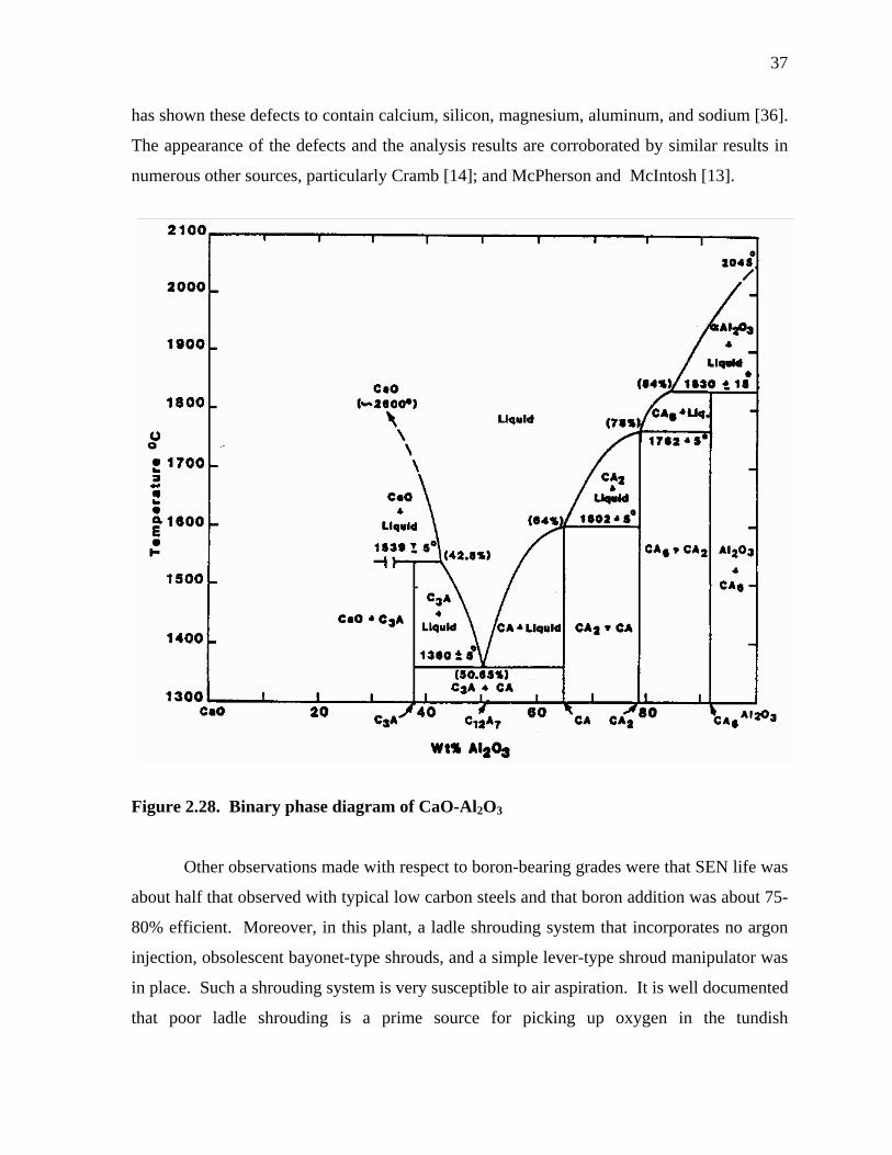
37
has shown these defects to contain calcium, silicon, magnesium, aluminum, and sodium [36].
The appearance of the defects and the analysis results are corroborated by similar results in
numerous other sources, particularly Cramb [14]; and McPherson and McIntosh [13].
Figure 2.28. Binary phase diagram of CaO-Al2O3
Other observations made with respect to boron-bearing grades were that SEN life was
about half that observed with typical low carbon steels and that boron addition was about 75-
80% efficient. Moreover, in this plant, a ladle shrouding system that incorporates no argon
injection, obsolescent bayonet-type shrouds, and a simple lever-type shroud manipulator was
in place. Such a shrouding system is very susceptible to air aspiration. It is well documented
that poor ladle shrouding is a prime source for picking up oxygen in the tundish
38
[10,14,26,33]. Taking this into account, it is thought very likely that unreacted boron in the
steel reacts with oxygen in the tundish to form boron oxide. As a casting sequence
progresses, B2O3 continually reacts with the alumina-graphite refractory of the SEN,
resulting in fairly rapid erosion of the refractory due to the formation of low melting B2O3-
Al2O3 compounds [29]. These compounds may lead to slivers and appear similar to mold
flux defects. A typical SEN used in thin slab casting is bifurcated with a flow-controlling
device positioned at the interior bottom of the nozzle. This device acts to direct the steel
flow into the ports smoothly. It is postulated that as this flow-controlling device is eroded, a
biased fluid flow pattern arises. This process is believed to lead to inclusion formation in the
steel and preliminary in-plant observations support this as increased mold turbulence in the
form of flux “rolling” was seen later in casting sequences (after approximately 5 hours).
2.2 Metal Level and Meniscus Behavior in the Thin Slab Casting Mold
Metal level and meniscus control in the casting mold is a critical aspect of steel
continuous casting. It is at the meniscus that many inclusions/defects are drawn into the
steel. Extensive research has been conducted regarding meniscus behavior and it has been
shown that insufficient and/or erratic control of the metal level in the mold can lead to poor
meniscus behavior and defect formation. This research has been driven by the move towards
technologies that incorporate high-speed casting (especially thin slab casting) and makes the
understanding and control of metal level and meniscus behavior critical [7-9,17-18,31,37-
43].
Most of the research consists of analysis of fluid flow effects upon metal level. This
has been done mainly through mathematical and physical modeling. As casting speeds have
increased from 1.5-2 m/min on conventional slab casters to 5-6 m/min with the CSP
technology, it is evident that steel flow in the CSP mold is much faster and more turbulent
than in conventional slab casting. This is because there is a similar amount of steel flowing
through a much smaller mold in approximately the same amount of time [1-2,5-
6,27,39,42,49-50].
Two other effects upon mold metal level are bulging and SEN clogging. While well
known to cause metal level fluctuations, they are still encountered frequently. Clogging is
the more serious of the two and has been discussed previously. Bulging, however, is not
39
always very serious if the amount of bulging between containment rolls is small and the
grade being cast is not susceptible to core cracking [4,43]. Bulging can be identified easily.
The requisite information for diagnosing and eliminating bulging consists of casting speed,
containment roll diameter and pitch, and metal level data acquired at a sufficient frequency -
usually 5 Hz or higher [43]. It should be noted that the effects of bulging on metal level
fluctuations is not well understood and is the subject of continuing study.
Inclusions formed in the tundish can have a large effect upon SEN clogging. In
studying clog material, Byrne, Cramb, and Fenicle [14] have found a complex oxide
surrounding a core deoxidation/reoxidation product. The complex oxide was discovered to
contain all the components of mold powder and the deoxidation/reoxidation core was found
to be either alumina or magnesium aluminate. Upon further analysis, it became evident that
upon cooling, the complex oxide formed large calcium silicate crystals in a matrix of mold
flux. This observation indicates that the clog was liquid at steelmaking temperatures.
These results suggest a different mechanism for SEN clogging. It is thought that
when a mold flux reacts with SEN refractory, it coats the SEN with a thin film on both the
interior and exterior surfaces that are immersed in the steel [14]. Following the film
formation, deoxidation and reoxidation products present in the steel attach to the film and
begin to dissolve in the slag film. It is in this manner that the slag layer increases in
thickness. This coating then acts like glue and will enhance the adhesion of the clog to the
shroud. Even clean steels with little alumina are susceptible to this type of clog, as any
alumina present will adhere to the clog. If the steel contains a lot of alumina, an alumina-
type clog will then form. Liquid calcium aluminates, unlike alumina, cause the clog material
to become less viscous, resulting in wash-throughs and increased SEN erosion (e.g. with Ca-
Si treated steels). This type of clog will periodically break away during turbulent flow events
in the mold and lead to inclusions in the cast product [14].
2.2.1 Steel Stream Velocity Measurements in the Meniscus Region
One of the most intriguing, yet difficult, tasks in the research of steel continuous
casting is the measurement of velocity in the mold. Steel stream velocity has been measured
in conventional slab casting molds using several different techniques. Argyropoulos has
classified seven such techniques according to their advantages and disadvantages. With the
40
exception of the sphere-melting technique, the methods commonly used for measuring fluid
flow velocity in a cavity are unsuitable and somewhat impractical for used in the harsh steel
mill environment [22]. Another method exists for measuring velocity through the detection
of Karman vortices, which are generated by fluid flow past a submerged refractory cylinder.
While this method is quite accurate for measuring velocity, it cannot be continuously used
for mold monitoring because of the sensitivity of the requisite apparatus to heat and dirt [21-
24].
The sphere-melting, Karman vortex, and MFC (from AMEPA) sensor methods have
produced results that agree very well with the stream velocities predicted by many
mathematical simulations and physical models [17-24,32,38-39,42,48-51]. Despite these
promising results, none of the methods has been used extensively for the measurement of
steel flow velocity in the meniscus region on any casters under normal operating conditions
and hence, there is little real data in existence for flow velocity of continuous casting molds.
Considering only the CSP technology, there is currently no existing real data, only data
generated by mathematical and water models [42].
A different method for measuring velocity is the nailboard. The nailboard operates
upon the same concept of the flux depth measurement; a series of steel nails are driven
through a board marginally smaller than the mold thickness and an aluminum wire is set
parallel to each nail. Upon submergence (about 10 seconds) in the mold, the nails and Al
wires melt to distinguish the meniscus line and the thickness of the liquid flux layer. Also
available is the depth of the powder/sinter flux layers. McDavid and Thomas have also used
nailboards to show the direction of flow in the mold since a knob of steel is left on the end of
each nail. The highest point of each knob shows from which direction flow predominated. It
has also been hypothesized that this method could also be used for measuring velocity in the
mold, but this has not yet been attempted [18].
41
CHAPTER 3: SCOPE AND OBJECTIVES
It is apparent from the preceding chapter that most of the scarce literature on CSP
casting consists mostly of mathematical and physical modeling results. Constructing
numerical models is very challenging with such a mold [40]. In addition, there has been little
validation of models with in-plant experiments. Most experimental results are from
conventional casting operations. When the CSP technology was commercialized in 1989, it
was envisioned as a low capital venture aimed at making inroads into the bottom end of steel
markets. This was quickly realized and increasingly there has been demand for higher
quality steel to be produced by the CSP technology. Researchers have attempted to apply
results from conventional casting to CSP casting with some success, but there have been
more failures than successes in this respect. The funnel-shaped mold is too different from
conventional molds to be compared on an equal basis and the high casting speeds and fluid
flow rates introduce challenges never before encountered in slab casting. These factors, as
well as the demand put forth by customers (mainly in the automotive market) have induced
steel companies that use CSP technology to begin extensive research into the improvement of
surface quality. The financial success of this technology, based on low production costs and
resultant favorable profit margins (even with lower selling prices than conventionally cast
steel), has contributed significantly to this development. To achieve the quality level
necessary for exposed automotive applications, extensive research into this technology is
required so it can be developed to the fullest extent possible. To be useful, this research must
begin on a basic level, much as research on conventional casting did over thirty years ago [1-
4].
To date, there have been three plant trials conducted at Nucor Steel in Crawfordsville,
Indiana USA. The current project is just the first step in understanding this emerging casting
technology. The scope is somewhat broad, but necessary as there is no existing body of work
of this type that has been performed on CSP technology. Performing such in-plant
experiments on a relatively little-known technology is difficult as obstacles often arise and
must then be overcome - the learning curve regarding CSP casting is yet steep.

42
This project was initiated to provide a solid base of knowledge and real casting data
that will be relevant in subsequent studies of fluid flow behavior and defect generation in
CSP continuously cast sheet steels. The objectives of the project were:
1a) To evaluate available literature to establish the current level of knowledge with respect
to flow behavior and related defects during CSP casting.
1b) To investigate flow phenomena in the CSP mold.
1c) To measure simultaneously many different plant data.
2) To perform plant trials on an operating CSP caster (Nucor Crawfordsville) aiming to
evaluate the nailboard method as an inexpensive and physically robust tool for measuring
and elucidating meniscus behavior, primarily in the determination of flux depths, flow
direction, and flow velocity.
3) To investigate a possible relationship between meniscus velocity results and surface
defect generation.
4) To compare the meniscus velocity calculations of this project to those generated by
mathematical and physical models. This will determine to what extent the results of this
project are compatible/relevant to previous understanding.
5) To develop correlations between the nailboard/meniscus data and high-frequency casting
data.
6) To use all the methods employed in the project to evaluate meniscus flow differences
between casting with two-port and four-port submerged entry nozzles.
As one of the first phases in CSP research, it is believed that this project will
encourage further research into the fluid flow, mold flux, and refractory behavior in this new
and rapidly growing sector of the steel casting industry.
43
CHAPTER 4: EXPERIMENTAL PROCEDURE - INDUSTRIAL TRIALS
As part of this project studying the mold flux entrapment during the CSP thin-slab
casting, three extended plant trials were conducted at Nucor Steel - Crawfordsville, IN USA.
The trials took place in June 2000, February 2001, and June 2001. As the project unfolded
and new information acquired, measurement techniques and emphasis changed accordingly.
This chapter will summarize the casting conditions and measurements made in this work.
4.1 Casting Machine and Operating Practices
The Nucor-Crawfordsville CSP caster produces slabs that are 50 mm thick and 985-
1460 mm wide for various hot-rolled and cold-rolled sheet applications. The plant has two
casters of one strand apiece. The trials were all conducted on Caster #2 on 125-ton heats cast
at speeds between 3.3 and 5.5 m/min.. This caster consists of an 1100 mm-long CSP mold
with a funnel width of 985 mm and a funnel depth of 165 mm at the top of the mold. The
funnel gradually flattens out, with the mold becoming parallel 850 mm from the top of the
mold. Tundish capacity is 20 tons and flow from tundish to mold is controlled via a stopper
rod and SEN system. The stopper rod controls flow by seating into the head of the SEN,
which cannot be exchanged during casting. The specifications of the casting machine are
presented in Table 4.1.
4.1.1 Trial Casting Parameters
Experimental parameters varied during the trials include steel composition, casting
speed, mold width, and metal level setpoint and nozzle design. Experiments were conducted
during casting to simultaneously measure processed metal level signal, stopper rod position,
pinch roll speed, pinch roll current, and the raw output from the radioactive source /receiver
used for metal level control. Ranges of each measured variable are given in Table 4.2 to
elucidate their effects upon fluid flow in the mold and the resulting quality of finished
product. In addition, other nailboard measurements, slag samples, steel samples analyzed for
defects after subsequent processing stages were collected. Operating details pertaining to the
four experimental parameters are presented in Table 4.3. The compositions for all of the
heats involved are listed in Table 4.4.
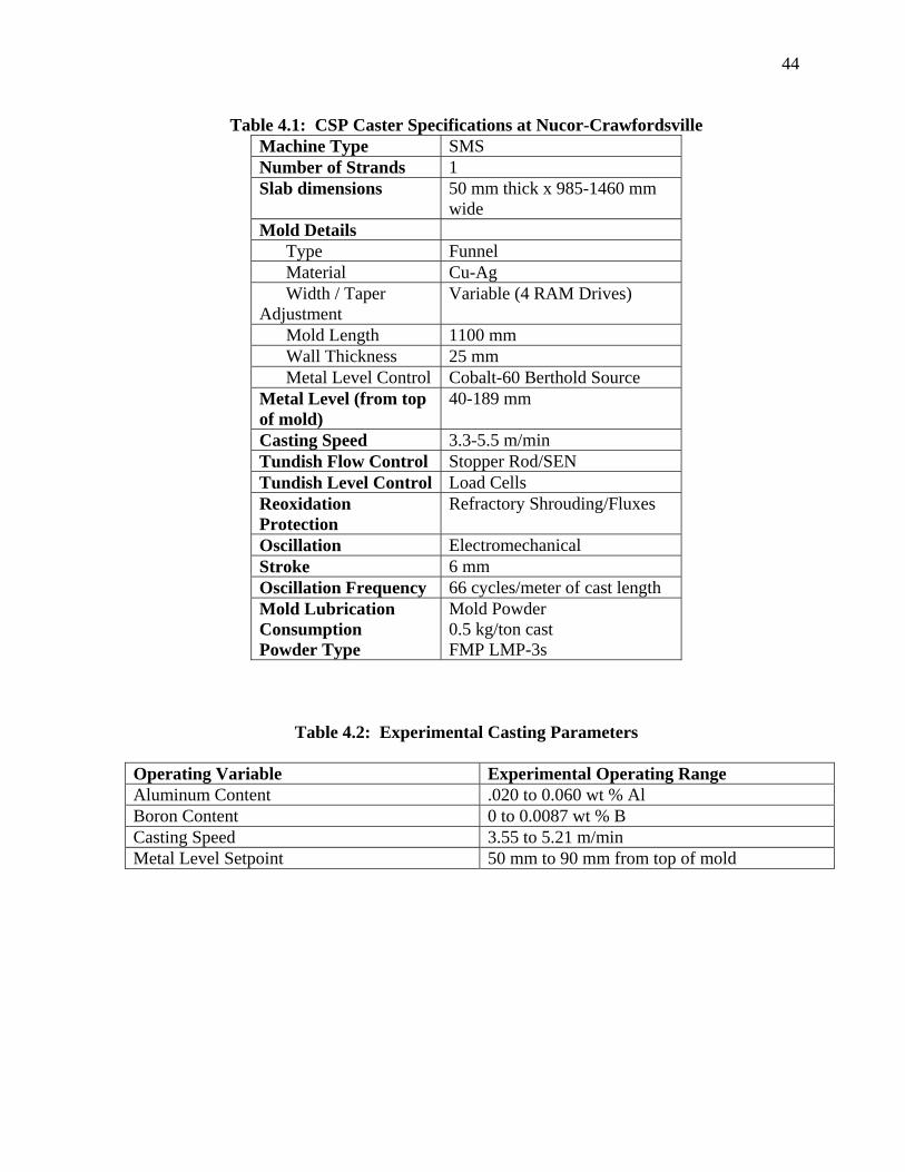
44
Table 4.1: CSP Caster Specifications at Nucor-Crawfordsville
Machine Type SMS Number of Strands 1 Slab dimensions 50 mm thick x 985-1460 mm
wide Mold Details Type Funnel Material Cu-Ag Width / Taper Adjustment
Variable (4 RAM Drives)
Mold Length 1100 mm Wall Thickness 25 mm Metal Level Control Cobalt-60 Berthold Source Metal Level (from top of mold)
40-189 mm
Casting Speed 3.3-5.5 m/min Tundish Flow Control Stopper Rod/SEN Tundish Level Control Load Cells Reoxidation Protection
Refractory Shrouding/Fluxes
Oscillation Electromechanical Stroke 6 mm Oscillation Frequency 66 cycles/meter of cast length Mold Lubrication Consumption Powder Type
Mold Powder 0.5 kg/ton cast FMP LMP-3s
Table 4.2: Experimental Casting Parameters Operating Variable Experimental Operating Range Aluminum Content .020 to 0.060 wt % Al Boron Content 0 to 0.0087 wt % B Casting Speed 3.55 to 5.21 m/min Metal Level Setpoint 50 mm to 90 mm from top of mold
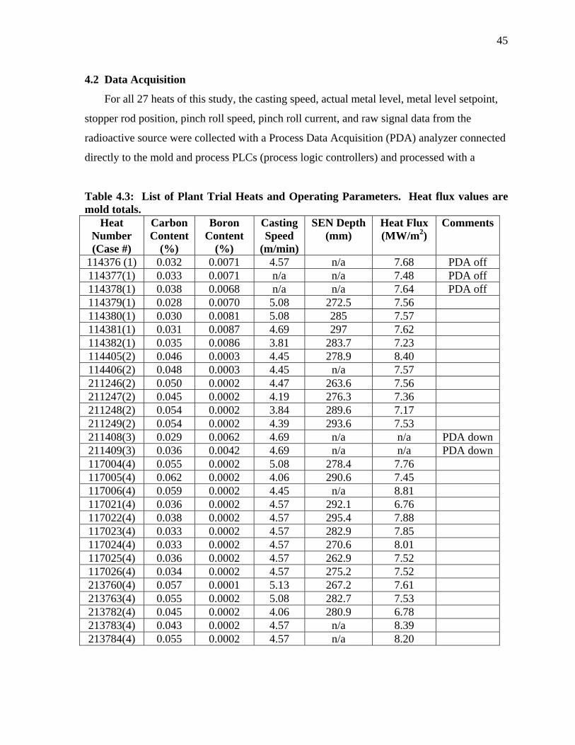
45
4.2 Data Acquisition
For all 27 heats of this study, the casting speed, actual metal level, metal level setpoint,
stopper rod position, pinch roll speed, pinch roll current, and raw signal data from the
radioactive source were collected with a Process Data Acquisition (PDA) analyzer connected
directly to the mold and process PLCs (process logic controllers) and processed with a
Table 4.3: List of Plant Trial Heats and Operating Parameters. Heat flux values are mold totals.
Heat Number (Case #)
Carbon Content
(%)
Boron Content
(%)
Casting Speed
(m/min)
SEN Depth (mm)
Heat Flux (MW/m2)
Comments
114376 (1) 0.032 0.0071 4.57 n/a 7.68 PDA off 114377(1) 0.033 0.0071 n/a n/a 7.48 PDA off 114378(1) 0.038 0.0068 n/a n/a 7.64 PDA off 114379(1) 0.028 0.0070 5.08 272.5 7.56 114380(1) 0.030 0.0081 5.08 285 7.57 114381(1) 0.031 0.0087 4.69 297 7.62 114382(1) 0.035 0.0086 3.81 283.7 7.23 114405(2) 0.046 0.0003 4.45 278.9 8.40 114406(2) 0.048 0.0003 4.45 n/a 7.57 211246(2) 0.050 0.0002 4.47 263.6 7.56 211247(2) 0.045 0.0002 4.19 276.3 7.36 211248(2) 0.054 0.0002 3.84 289.6 7.17 211249(2) 0.054 0.0002 4.39 293.6 7.53 211408(3) 0.029 0.0062 4.69 n/a n/a PDA down 211409(3) 0.036 0.0042 4.69 n/a n/a PDA down 117004(4) 0.055 0.0002 5.08 278.4 7.76 117005(4) 0.062 0.0002 4.06 290.6 7.45 117006(4) 0.059 0.0002 4.45 n/a 8.81 117021(4) 0.036 0.0002 4.57 292.1 6.76 117022(4) 0.038 0.0002 4.57 295.4 7.88 117023(4) 0.033 0.0002 4.57 282.9 7.85 117024(4) 0.033 0.0002 4.57 270.6 8.01 117025(4) 0.036 0.0002 4.57 262.9 7.52 117026(4) 0.034 0.0002 4.57 275.2 7.52 213760(4) 0.057 0.0001 5.13 267.2 7.61 213763(4) 0.055 0.0002 5.08 282.7 7.53 213782(4) 0.045 0.0002 4.06 280.9 6.78 213783(4) 0.043 0.0002 4.57 n/a 8.39 213784(4) 0.055 0.0002 4.57 n/a 8.20
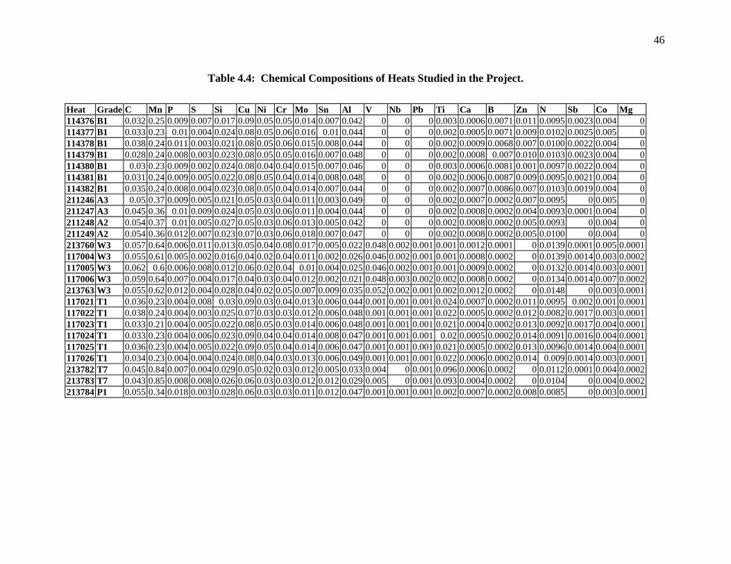
46
Table 4.4: Chemical Compositions of Heats Studied in the Project.
Heat Grade C Mn P S Si Cu Ni Cr Mo Sn Al V Nb Pb Ti Ca B Zn N Sb Co Mg 114376 B1 0.032 0.25 0.009 0.007 0.017 0.09 0.05 0.05 0.014 0.007 0.042 0 0 0 0.003 0.0006 0.0071 0.011 0.0095 0.0023 0.004 0114377 B1 0.033 0.23 0.01 0.004 0.024 0.08 0.05 0.06 0.016 0.01 0.044 0 0 0 0.002 0.0005 0.0071 0.009 0.0102 0.0025 0.005 0114378 B1 0.038 0.24 0.011 0.003 0.021 0.08 0.05 0.06 0.015 0.008 0.044 0 0 0 0.002 0.0009 0.0068 0.007 0.0100 0.0022 0.004 0114379 B1 0.028 0.24 0.008 0.003 0.023 0.08 0.05 0.05 0.016 0.007 0.048 0 0 0 0.002 0.0008 0.007 0.010 0.0103 0.0023 0.004 0114380 B1 0.03 0.23 0.009 0.002 0.024 0.08 0.04 0.04 0.015 0.007 0.046 0 0 0 0.003 0.0006 0.0081 0.001 0.0097 0.0022 0.004 0114381 B1 0.031 0.24 0.009 0.005 0.022 0.08 0.05 0.04 0.014 0.008 0.048 0 0 0 0.002 0.0006 0.0087 0.009 0.0095 0.0021 0.004 0114382 B1 0.035 0.24 0.008 0.004 0.023 0.08 0.05 0.04 0.014 0.007 0.044 0 0 0 0.002 0.0007 0.0086 0.007 0.0103 0.0019 0.004 0211246 A3 0.05 0.37 0.009 0.005 0.021 0.05 0.03 0.04 0.011 0.003 0.049 0 0 0 0.002 0.0007 0.0002 0.007 0.0095 0 0.005 0211247 A3 0.045 0.36 0.01 0.009 0.024 0.05 0.03 0.06 0.011 0.004 0.044 0 0 0 0.002 0.0008 0.0002 0.004 0.0093 0.0001 0.004 0211248 A2 0.054 0.37 0.01 0.005 0.027 0.05 0.03 0.06 0.013 0.005 0.042 0 0 0 0.002 0.0008 0.0002 0.005 0.0093 0 0.004 0211249 A2 0.054 0.36 0.012 0.007 0.023 0.07 0.03 0.06 0.018 0.007 0.047 0 0 0 0.002 0.0008 0.0002 0.005 0.0100 0 0.004 0213760 W3 0.057 0.64 0.006 0.011 0.013 0.05 0.04 0.08 0.017 0.005 0.022 0.048 0.002 0.001 0.001 0.0012 0.0001 0 0.0139 0.0001 0.005 0.0001117004 W3 0.055 0.61 0.005 0.002 0.016 0.04 0.02 0.04 0.011 0.002 0.026 0.046 0.002 0.001 0.001 0.0008 0.0002 0 0.0139 0.0014 0.003 0.0002117005 W3 0.062 0.6 0.006 0.008 0.012 0.06 0.02 0.04 0.01 0.004 0.025 0.046 0.002 0.001 0.001 0.0009 0.0002 0 0.0132 0.0014 0.003 0.0001117006 W3 0.059 0.64 0.007 0.004 0.017 0.04 0.03 0.04 0.012 0.002 0.021 0.048 0.003 0.002 0.002 0.0008 0.0002 0 0.0134 0.0014 0.007 0.0002213763 W3 0.055 0.62 0.012 0.004 0.028 0.04 0.02 0.05 0.007 0.009 0.035 0.052 0.002 0.001 0.002 0.0012 0.0002 0 0.0148 0 0.003 0.0001117021 T1 0.036 0.23 0.004 0.008 0.03 0.09 0.03 0.04 0.013 0.006 0.044 0.001 0.001 0.001 0.024 0.0007 0.0002 0.011 0.0095 0.002 0.001 0.0001117022 T1 0.038 0.24 0.004 0.003 0.025 0.07 0.03 0.03 0.012 0.006 0.048 0.001 0.001 0.001 0.022 0.0005 0.0002 0.012 0.0082 0.0017 0.003 0.0001117023 T1 0.033 0.21 0.004 0.005 0.022 0.08 0.05 0.03 0.014 0.006 0.048 0.001 0.001 0.001 0.021 0.0004 0.0002 0.013 0.0092 0.0017 0.004 0.0001117024 T1 0.033 0.23 0.004 0.006 0.023 0.09 0.04 0.04 0.014 0.008 0.047 0.001 0.001 0.001 0.02 0.0005 0.0002 0.014 0.0091 0.0016 0.004 0.0001117025 T1 0.036 0.23 0.004 0.005 0.022 0.09 0.05 0.04 0.014 0.006 0.047 0.001 0.001 0.001 0.021 0.0005 0.0002 0.013 0.0096 0.0014 0.004 0.0001117026 T1 0.034 0.23 0.004 0.004 0.024 0.08 0.04 0.03 0.013 0.006 0.049 0.001 0.001 0.001 0.022 0.0006 0.0002 0.014 0.009 0.0014 0.003 0.0001213782 T7 0.045 0.84 0.007 0.004 0.029 0.05 0.02 0.03 0.012 0.005 0.033 0.004 0 0.001 0.096 0.0006 0.0002 0 0.0112 0.0001 0.004 0.0002213783 T7 0.043 0.85 0.008 0.008 0.026 0.06 0.03 0.03 0.012 0.012 0.029 0.005 0 0.001 0.093 0.0004 0.0002 0 0.0104 0 0.004 0.0002213784 P1 0.055 0.34 0.018 0.003 0.028 0.06 0.03 0.03 0.011 0.012 0.047 0.001 0.001 0.001 0.002 0.0007 0.0002 0.008 0.0085 0 0.003 0.0001
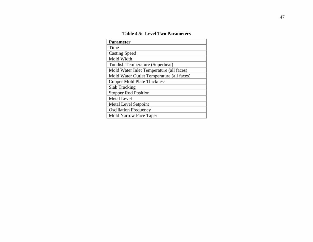
47
Table 4.5: Level Two Parameters
Parameter Time Casting Speed Mold Width Tundish Temperature (Superheat) Mold Water Inlet Temperature (all faces) Mold Water Outlet Temperature (all faces) Copper Mold Plate Thickness Slab Tracking Stopper Rod Position Metal Level Metal Level Setpoint Oscillation Frequency Mold Narrow Face Taper
48
Windows NT workstation. The data sampling frequency was 33.33 Hz (30-millisecond period).
The raw data from the source were converted from a 4-20 mA range into a distance below the
top of the mold using linear interpolation, 4 mA at a metal level 189 mm from the top of the
mold and 20 mA a metal level 40 mm from the top of the mold.
In addition to the PDA data, "level two" data were also collected every 0.94 meters of
cast length. Table 4.5 presents the data collected via the level two system. This information
includes time of production, casting speed, mold width, tundish temperature (superheat), mold
water inlet temperature, mold water exit temperature, mold thickness, cast length (for slab
tracking), stopper rod position, metal level, metal level setpoint, oscillator frequency, and narrow
face taper. These data were used to calculate mold heat transfer, monitor slab length, double-
check the PDA data, monitor superheat, and to discover disturbances in the casting process.
4.2.1 Nailboard Measurements
During the course of the project, 47 individual nailboard tests were performed. Three
sets of nailboards were initially constructed in order to account for three different width ranges:
985-1100 mm, 1100-1280 mm, and 1280-1460 mm. Individual boards measured 45 mm across
and 12.5 mm thick for the east and west halves of the mold. Four number 20 common nails were
driven through each at about 20, 85, 225, and 315 mm from the narrow face of the mold.
Following placement of the four nails, a length of 2.5 mm diameter aluminum wire was placed
next to each nail. This was done as prescribed by McDavid and Thomas [18]. The time required
to set up each board was about 5-7 minutes. To improve safety, handles were fastened to each
board so the measurer could keep face and hands relatively clear of the mold opening to reduce
the chance of injury from molten metal splashes, which occur without warning. A small level
was tacked to the top of the board to ensure the nails and wires were vertical to eliminate uneven
board placement as a source of error during the measurement. The nails were immersed in the
mold from 5-7 seconds. Immersion times shorter than this resulted in not being able to obtain
measurements where immersion times that were longer resulted in complete melting and loss of
the nails into the mold. Finally, 15 to 20 minutes additional time were required for the nails to
cool down to make and record measurements, depending upon the condition of the nails
following immersion. Initially, the only measurements made were the distances from the top of
49
the steel knob on the nail to the bottom of the board and the length of aluminum wire left (to
determine flux depth). This time for measuring and recording increased slightly as more
measurements were made on the nails, especially for steel knob diameter and the angle at the top
of the steel knob.
4.3 Slag Sample Collection
For a few heats during the February 2001 trial, slag samples were obtained from the
Ladle Metallurgical Facility (LMF) for the ladle slag, from the tundish, and from the mold. The
compositions of the slags were measured using x-ray fluorescence (XRF).
It was found that getting slag samples for every heat from all processing locations was
impracticable for one person while making nailboard measurements, which are time consuming.
Since the same slag-forming materials were still in use during subsequent trials, it was assumed
that the XRF analyses were still valid. Slag samples were therefore only collected for the trials
of February 14-15, 2001.
4.4 Steel Sample Collection
In addition to data collection and physical measurements, samples were collected
throughout the processing of the material. Samples of as-cast, hot-rolled, skin-passed, pickled,
cold-rolled, and galvanized steel product were collected, inspected, and analyzed with the goal of
relating the occurrence of defects to events in the mold. Steel composition data were also
collected through a level two database, but this could be done at any time following casting and
was very easy to accomplish (table 4.4).
Scheduling proved to be an important obstacle in obtaining these samples. Customer
requirements and equipment availability often dictated how casting sequences were set up. To
collect rolled samples and perform inspection and analysis it was common to wait for days or
weeks for the opportunity to do so. This was primarily due to mill scheduling, particularly on
the reversing mill and slitter line, where the inspections were performed.
50
CHAPTER 5: RESULTS OF INDUSTRIAL PLANT TRIALS
This chapter presents the results of the trials performed in this work. In particular,
this section will describe the results of the measured plant data of metal level and the other
casting parameters and the measured results of the nailboard experiments and briefly discuss
the inspection and evaluation of slab and strip samples collected during the course of the
trials. Strip quality and defect composition consisted of visual and EDX analyses coupled
with fast Fourier transform (FFT) analysis using Microcal Origin of the metal level data to
identify the frequencies at which events in the casting mold occurred [52]. Detailed analysis
of the data, discussion of the effect of mechanical and fluid flow transients upon slag
emulsification and sliver defect formation, and the calculation of the steel stream velocity
will be covered in the following chapters.
5.1 Metal Level Measurements
Metal level in the mold is influenced by numerous other variables of the casting
process. If a casting variable has an adverse effect upon metal level, it was expected that it
should exhibit some periodic behavior with and associated identifiable frequency of the metal
level fluctuations. For the first trial (case 1), conducted during June and July 2000, data were
collected solely by way of level two for every 0.94 meters cast as discussed in chapter 4.
Table 5.1 presents a typical body of data collected during the experiments. The data analysis
showed that important events were much shorter than this, so the June 2000 data were
deemed unsuitable for numerical analysis, but was still employed in the evaluation of the
nailboard measurements and defect samples.
5.1.1 High Frequency Data
For the second trial (case 2) in February 2001, data were collected at 30 millisecond
intervals to ensure all events with an occurrence frequency of up to 16.67 Hz would be
recorded [9, 49-50]. 16.67 Hz is the maximum because the FFT analysis can distinguish
frequencies having at most half of the sampling frequency.
Because of the high sampling frequency, there exists an extremely large body of data for
every heat. With ten parameters recorded at 33.33 Hz, 1.2 million numbers were collected
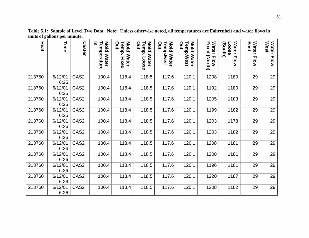
51
Table 5.1: Sample of Level Two Data. Note: Unless otherwise noted, all temperatures are Fahrenheit and water flows in units of gallons per minute.
Heat
Time
Caster
Mold W
ater Tem
perature In
Mold W
ater Tem
p. Fixed O
ut
Mold W
ater Tem
p. Loose O
ut
Mold W
ater Tem
p.East O
ut
Mold W
ater Tem
p.West
Out
Water Flow
Fixed (N
orth)
Water Flow
Loose (South)
Water Flow
East
Water Flow
W
est
213760 6/12/01 6:25
CAS2 100.4 118.4 118.5 117.6 120.1 1208 1180 29 29
213760 6/12/01 6:25
CAS2 100.4 118.4 118.5 117.6 120.1 1192 1180 29 29
213760 6/12/01 6:25
CAS2 100.4 118.4 118.5 117.6 120.1 1205 1183 29 29
213760 6/12/01 6:25
CAS2 100.4 118.4 118.5 117.6 120.1 1199 1182 29 29
213760 6/12/01 6:26
CAS2 100.4 118.4 118.5 117.6 120.1 1203 1178 29 29
213760 6/12/01 6:26
CAS2 100.4 118.4 118.5 117.6 120.1 1203 1182 29 29
213760 6/12/01 6:26
CAS2 100.4 118.4 118.5 117.6 120.1 1208 1181 29 29
213760 6/12/01 6:26
CAS2 100.4 118.4 118.5 117.6 120.1 1208 1181 29 29
213760 6/12/01 6:26
CAS2 100.4 118.4 118.5 117.6 120.1 1196 1181 29 29
213760 6/12/01 6:26
CAS2 100.4 118.4 118.5 117.6 120.1 1220 1187 29 29
213760 6/12/01 6:26
CAS2 100.4 118.4 118.5 117.6 120.1 1208 1182 29 29
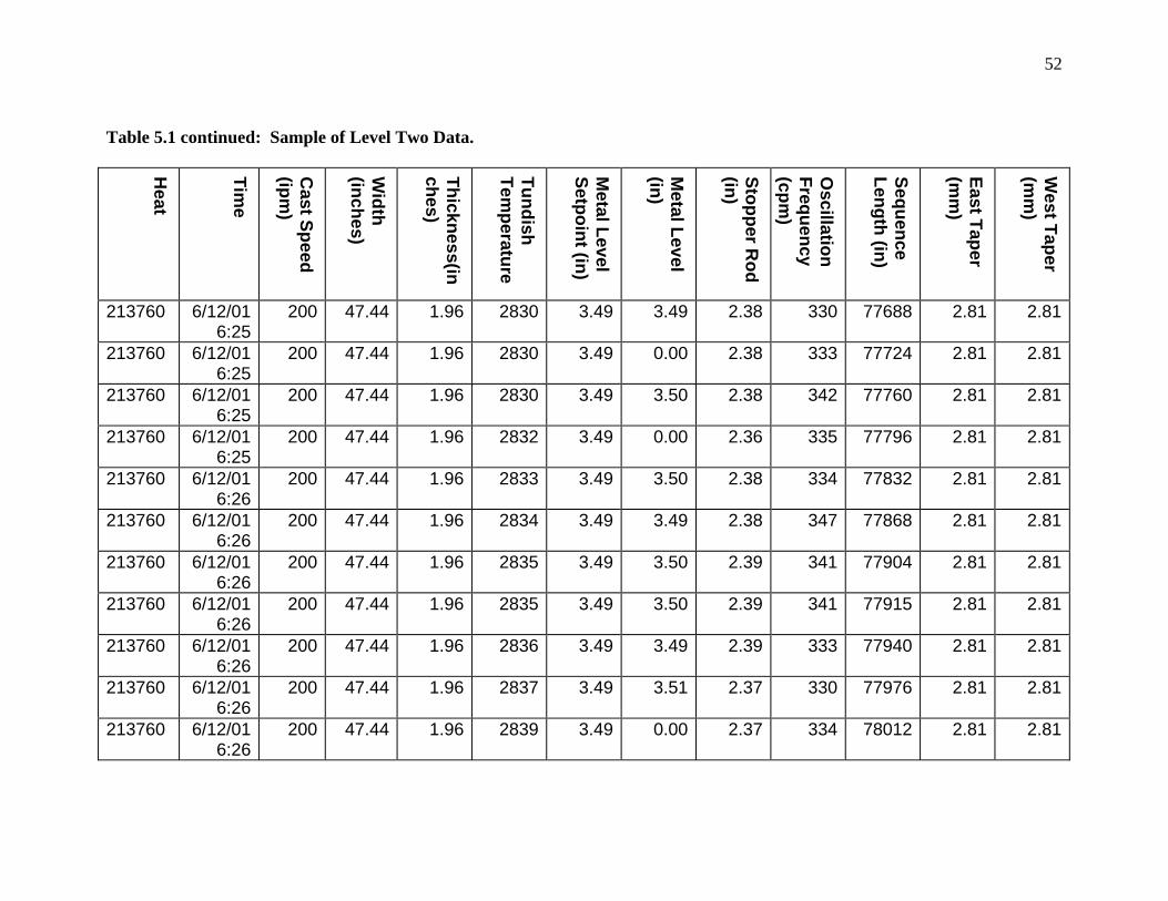
52
Table 5.1 continued: Sample of Level Two Data.
Heat
Time
Cast Speed
(ipm)
Width
(inches)
Thickness(inches)
Tundish Tem
perature
Metal Level
Setpoint (in)
Metal Level
(in)
Stopper Rod
(in)
Oscillation
Frequency (cpm
)
Sequence Length (in)
East Taper (m
m)
West Taper
(mm
)
213760 6/12/01 6:25
200 47.44 1.96 2830 3.49 3.49 2.38 330 77688 2.81 2.81
213760 6/12/01 6:25
200 47.44 1.96 2830 3.49 0.00 2.38 333 77724 2.81 2.81
213760 6/12/01 6:25
200 47.44 1.96 2830 3.49 3.50 2.38 342 77760 2.81 2.81
213760 6/12/01 6:25
200 47.44 1.96 2832 3.49 0.00 2.36 335 77796 2.81 2.81
213760 6/12/01 6:26
200 47.44 1.96 2833 3.49 3.50 2.38 334 77832 2.81 2.81
213760 6/12/01 6:26
200 47.44 1.96 2834 3.49 3.49 2.38 347 77868 2.81 2.81
213760 6/12/01 6:26
200 47.44 1.96 2835 3.49 3.50 2.39 341 77904 2.81 2.81
213760 6/12/01 6:26
200 47.44 1.96 2835 3.49 3.50 2.39 341 77915 2.81 2.81
213760 6/12/01 6:26
200 47.44 1.96 2836 3.49 3.49 2.39 333 77940 2.81 2.81
213760 6/12/01 6:26
200 47.44 1.96 2837 3.49 3.51 2.37 330 77976 2.81 2.81
213760 6/12/01 6:26
200 47.44 1.96 2839 3.49 0.00 2.37 334 78012 2.81 2.81
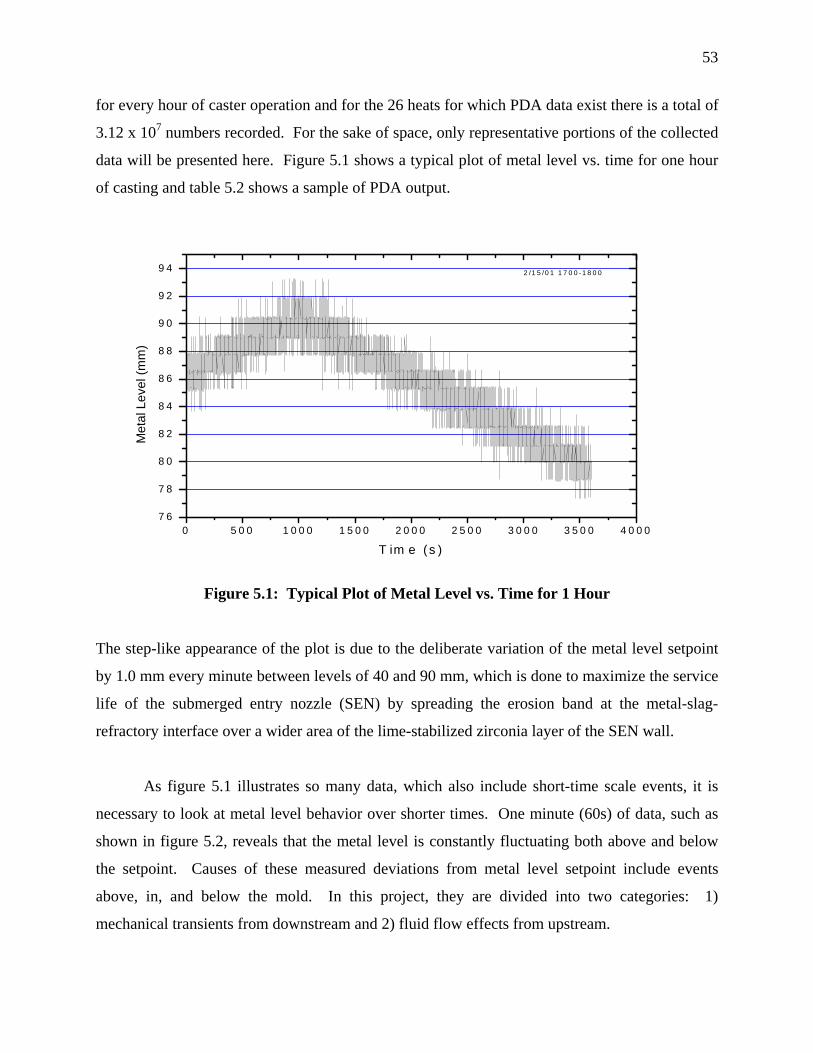
53
for every hour of caster operation and for the 26 heats for which PDA data exist there is a total of
3.12 x 10⁷ numbers recorded. For the sake of space, only representative portions of the collected
data will be presented here. Figure 5.1 shows a typical plot of metal level vs. time for one hour
of casting and table 5.2 shows a sample of PDA output.
Figure 5.1: Typical Plot of Metal Level vs. Time for 1 Hour
The step-like appearance of the plot is due to the deliberate variation of the metal level setpoint
by 1.0 mm every minute between levels of 40 and 90 mm, which is done to maximize the service
life of the submerged entry nozzle (SEN) by spreading the erosion band at the metal-slag-
refractory interface over a wider area of the lime-stabilized zirconia layer of the SEN wall.
As figure 5.1 illustrates so many data, which also include short-time scale events, it is
necessary to look at metal level behavior over shorter times. One minute (60s) of data, such as
shown in figure 5.2, reveals that the metal level is constantly fluctuating both above and below
the setpoint. Causes of these measured deviations from metal level setpoint include events
above, in, and below the mold. In this project, they are divided into two categories: 1)
mechanical transients from downstream and 2) fluid flow effects from upstream.
0 5 0 0 1 0 0 0 1 5 0 0 2 0 0 0 2 5 0 0 3 0 0 0 3 5 0 0 4 0 0 07 6
7 8
8 0
8 2
8 4
8 6
8 8
9 0
9 2
9 4 2 /1 5 /0 1 1 7 0 0 -1 8 0 0
Met
al L
evel
(mm
)
T im e (s )
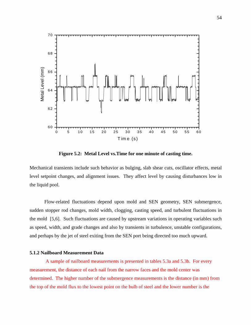
54
Figure 5.2: Metal Level vs.Time for one minute of casting time.
Mechanical transients include such behavior as bulging, slab shear cuts, oscillator effects, metal
level setpoint changes, and alignment issues. They affect level by causing disturbances low in
the liquid pool.
Flow-related fluctuations depend upon mold and SEN geometry, SEN submergence,
sudden stopper rod changes, mold width, clogging, casting speed, and turbulent fluctuations in
the mold [5,6]. Such fluctuations are caused by upstream variations in operating variables such
as speed, width, and grade changes and also by transients in turbulence, unstable configurations,
and perhaps by the jet of steel exiting from the SEN port being directed too much upward.
5.1.2 Nailboard Measurement Data
A sample of nailboard measurements is presented in tables 5.3a and 5.3b. For every
measurement, the distance of each nail from the narrow faces and the mold center was
determined. The higher number of the submergence measurements is the distance (in mm) from
the top of the mold flux to the lowest point on the bulb of steel and the lower number is the
0 5 10 15 20 25 30 35 40 45 50 55 6060
62
64
66
68
70
Met
al L
evel
(mm
)
T im e (s )
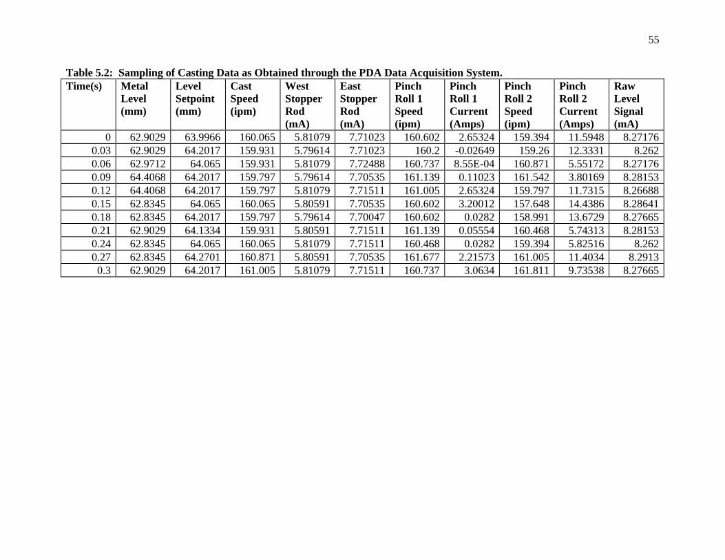
55
Table 5.2: Sampling of Casting Data as Obtained through the PDA Data Acquisition System. Time(s) Metal
Level (mm)
Level Setpoint (mm)
Cast Speed (ipm)
West Stopper Rod (mA)
East Stopper Rod (mA)
Pinch Roll 1 Speed (ipm)
Pinch Roll 1 Current (Amps)
Pinch Roll 2 Speed (ipm)
Pinch Roll 2 Current (Amps)
Raw Level Signal (mA)
0 62.9029 63.9966 160.065 5.81079 7.71023 160.602 2.65324 159.394 11.5948 8.271760.03 62.9029 64.2017 159.931 5.79614 7.71023 160.2 -0.02649 159.26 12.3331 8.2620.06 62.9712 64.065 159.931 5.81079 7.72488 160.737 8.55E-04 160.871 5.55172 8.271760.09 64.4068 64.2017 159.797 5.79614 7.70535 161.139 0.11023 161.542 3.80169 8.281530.12 64.4068 64.2017 159.797 5.81079 7.71511 161.005 2.65324 159.797 11.7315 8.266880.15 62.8345 64.065 160.065 5.80591 7.70535 160.602 3.20012 157.648 14.4386 8.286410.18 62.8345 64.2017 159.797 5.79614 7.70047 160.602 0.0282 158.991 13.6729 8.276650.21 62.9029 64.1334 159.931 5.80591 7.71511 161.139 0.05554 160.468 5.74313 8.281530.24 62.8345 64.065 160.065 5.81079 7.71511 160.468 0.0282 159.394 5.82516 8.2620.27 62.8345 64.2701 160.871 5.80591 7.70535 161.677 2.21573 161.005 11.4034 8.29130.3 62.9029 64.2017 161.005 5.81079 7.71511 160.737 3.0634 161.811 9.73538 8.27665
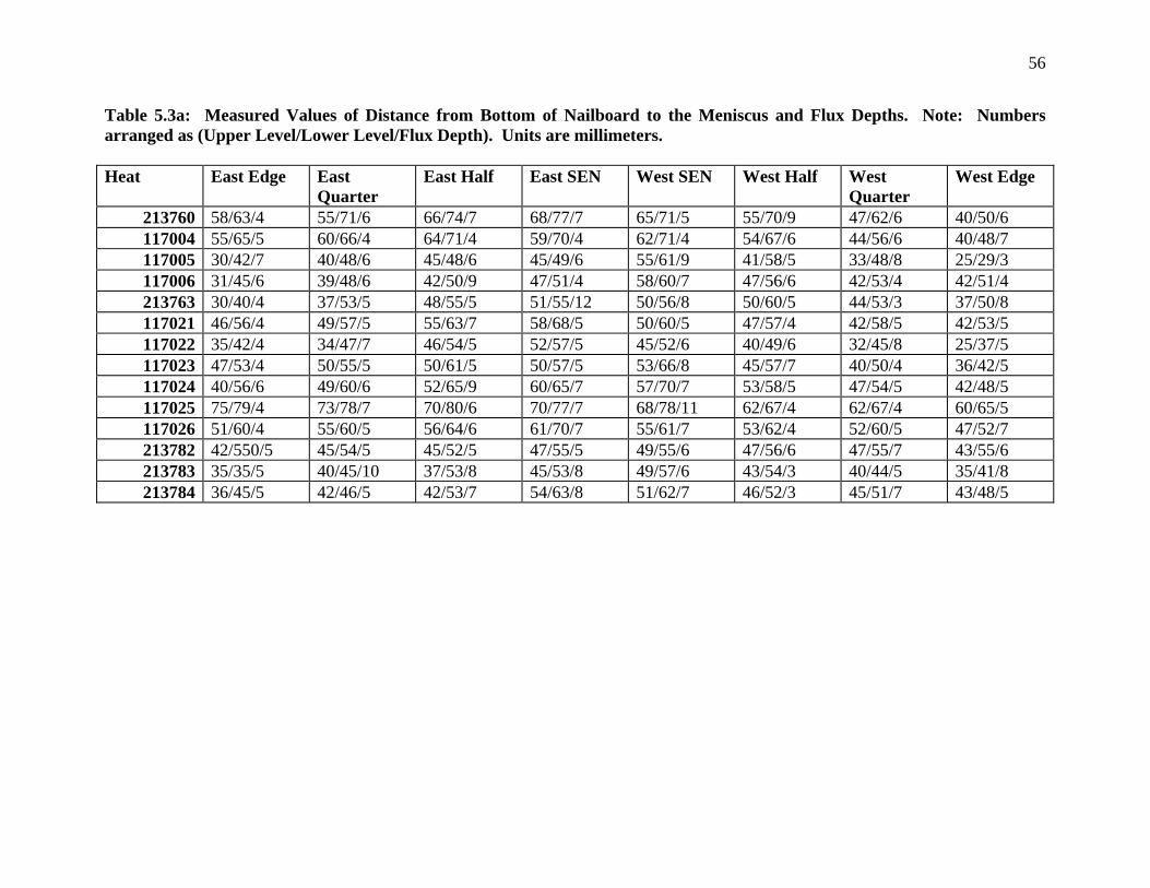
56
Table 5.3a: Measured Values of Distance from Bottom of Nailboard to the Meniscus and Flux Depths. Note: Numbers arranged as (Upper Level/Lower Level/Flux Depth). Units are millimeters. Heat East Edge East
Quarter East Half East SEN West SEN West Half West
Quarter West Edge
213760 58/63/4 55/71/6 66/74/7 68/77/7 65/71/5 55/70/9 47/62/6 40/50/6 117004 55/65/5 60/66/4 64/71/4 59/70/4 62/71/4 54/67/6 44/56/6 40/48/7 117005 30/42/7 40/48/6 45/48/6 45/49/6 55/61/9 41/58/5 33/48/8 25/29/3 117006 31/45/6 39/48/6 42/50/9 47/51/4 58/60/7 47/56/6 42/53/4 42/51/4 213763 30/40/4 37/53/5 48/55/5 51/55/12 50/56/8 50/60/5 44/53/3 37/50/8 117021 46/56/4 49/57/5 55/63/7 58/68/5 50/60/5 47/57/4 42/58/5 42/53/5 117022 35/42/4 34/47/7 46/54/5 52/57/5 45/52/6 40/49/6 32/45/8 25/37/5 117023 47/53/4 50/55/5 50/61/5 50/57/5 53/66/8 45/57/7 40/50/4 36/42/5 117024 40/56/6 49/60/6 52/65/9 60/65/7 57/70/7 53/58/5 47/54/5 42/48/5 117025 75/79/4 73/78/7 70/80/6 70/77/7 68/78/11 62/67/4 62/67/4 60/65/5 117026 51/60/4 55/60/5 56/64/6 61/70/7 55/61/7 53/62/4 52/60/5 47/52/7 213782 42/550/5 45/54/5 45/52/5 47/55/5 49/55/6 47/56/6 47/55/7 43/55/6 213783 35/35/5 40/45/10 37/53/8 45/53/8 49/57/6 43/54/3 40/44/5 35/41/8 213784 36/45/5 42/46/5 42/53/7 54/63/8 51/62/7 46/52/3 45/51/7 43/48/5
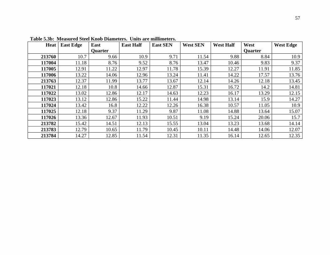
57
Table 5.3b: Measured Steel Knob Diameters. Units are millimeters.
Heat East Edge East Quarter
East Half East SEN West SEN West Half West Quarter
West Edge
213760 10.7 9.66 10.9 9.71 11.54 9.88 8.84 10.9117004 11.18 8.76 9.52 8.76 13.47 10.46 9.83 9.37117005 12.91 11.22 12.97 11.78 15.39 12.27 11.91 11.85117006 13.22 14.06 12.96 13.24 11.41 14.22 17.57 13.76213763 12.37 11.99 13.77 13.67 12.14 14.26 12.18 13.45117021 12.18 10.8 14.66 12.87 15.31 16.72 14.2 14.81117022 13.02 12.86 12.17 14.63 12.23 16.17 13.29 12.15117023 13.12 12.86 15.22 11.44 14.98 13.14 15.9 14.27117024 13.42 16.8 12.22 12.26 16.38 10.57 11.05 10.9117025 12.18 9.37 11.29 9.87 11.08 14.88 13.64 15.07117026 13.36 12.67 11.93 10.51 9.19 15.24 20.06 15.7213782 15.42 14.51 12.13 15.55 13.04 13.23 13.68 14.14213783 12.79 10.65 11.79 10.45 10.11 14.48 14.06 12.07213784 14.27 12.85 11.54 12.31 11.35 16.14 12.65 12.35
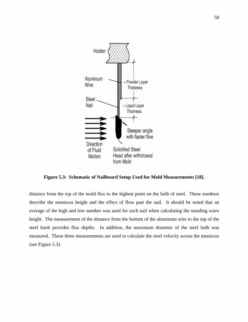
58
Figure 5.3: Schematic of Nailboard Setup Used for Mold Measurements [18].
distance from the top of the mold flux to the highest point on the bulb of steel. These numbers
describe the meniscus height and the effect of flow past the nail. It should be noted that an
average of the high and low number was used for each nail when calculating the standing wave
height. The measurement of the distance from the bottom of the aluminum wire to the top of the
steel knob provides flux depths. In addition, the maximum diameter of the steel bulb was
measured. These three measurements are used to calculate the steel velocity across the meniscus
(see Figure 5.3).
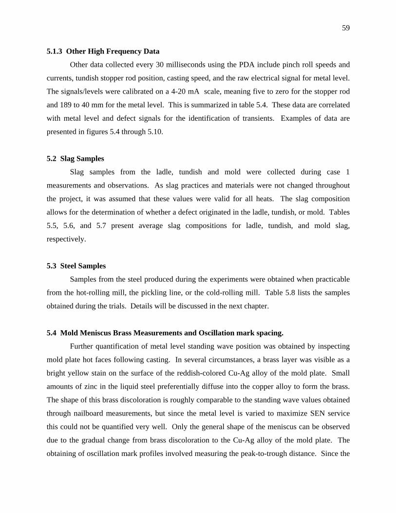
59
5.1.3 Other High Frequency Data
Other data collected every 30 milliseconds using the PDA include pinch roll speeds and
currents, tundish stopper rod position, casting speed, and the raw electrical signal for metal level.
The signals/levels were calibrated on a 4-20 mA scale, meaning five to zero for the stopper rod
and 189 to 40 mm for the metal level. This is summarized in table 5.4. These data are correlated
with metal level and defect signals for the identification of transients. Examples of data are
presented in figures 5.4 through 5.10.
5.2 Slag Samples
Slag samples from the ladle, tundish and mold were collected during case 1
measurements and observations. As slag practices and materials were not changed throughout
the project, it was assumed that these values were valid for all heats. The slag composition
allows for the determination of whether a defect originated in the ladle, tundish, or mold. Tables
5.5, 5.6, and 5.7 present average slag compositions for ladle, tundish, and mold slag,
respectively.
5.3 Steel Samples
Samples from the steel produced during the experiments were obtained when practicable
from the hot-rolling mill, the pickling line, or the cold-rolling mill. Table 5.8 lists the samples
obtained during the trials. Details will be discussed in the next chapter.
5.4 Mold Meniscus Brass Measurements and Oscillation mark spacing.
Further quantification of metal level standing wave position was obtained by inspecting
mold plate hot faces following casting. In several circumstances, a brass layer was visible as a
bright yellow stain on the surface of the reddish-colored Cu-Ag alloy of the mold plate. Small
amounts of zinc in the liquid steel preferentially diffuse into the copper alloy to form the brass.
The shape of this brass discoloration is roughly comparable to the standing wave values obtained
through nailboard measurements, but since the metal level is varied to maximize SEN service
this could not be quantified very well. Only the general shape of the meniscus can be observed
due to the gradual change from brass discoloration to the Cu-Ag alloy of the mold plate. The
obtaining of oscillation mark profiles involved measuring the peak-to-trough distance. Since the
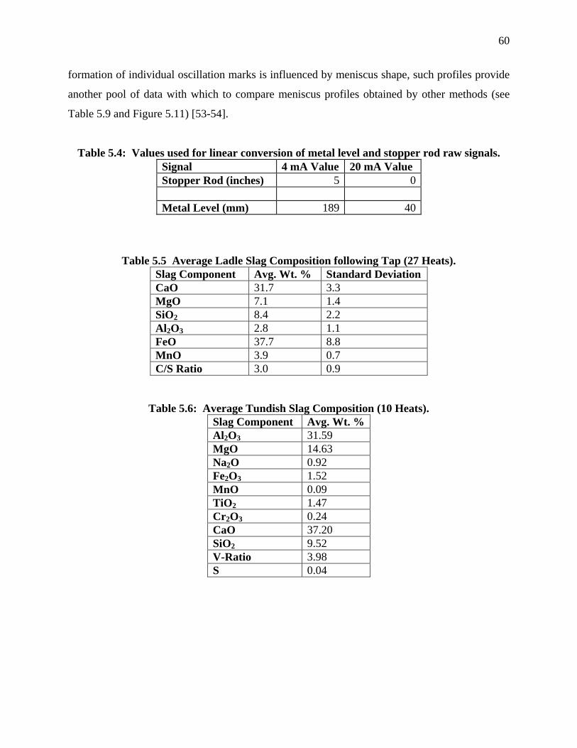
60
formation of individual oscillation marks is influenced by meniscus shape, such profiles provide
another pool of data with which to compare meniscus profiles obtained by other methods (see
Table 5.9 and Figure 5.11) [53-54].
Table 5.4: Values used for linear conversion of metal level and stopper rod raw signals. Signal 4 mA Value 20 mA Value Stopper Rod (inches) 5 0
Metal Level (mm) 189 40
Table 5.5 Average Ladle Slag Composition following Tap (27 Heats). Slag Component Avg. Wt. % Standard Deviation CaO 31.7 3.3 MgO 7.1 1.4 SiO2 8.4 2.2 Al2O3 2.8 1.1 FeO 37.7 8.8 MnO 3.9 0.7 C/S Ratio 3.0 0.9
Table 5.6: Average Tundish Slag Composition (10 Heats). Slag Component Avg. Wt. %Al2O3 31.59 MgO 14.63 Na2O 0.92 Fe2O3 1.52 MnO 0.09 TiO2 1.47 Cr2O3 0.24 CaO 37.20 SiO2 9.52 V-Ratio 3.98 S 0.04
61
Table 5.7: Average Mold Slag Composition (24 Heats). Slag Component Avg. Wt. % Standard Deviation Na2O 9.72 0.46 MgO 2.06 0.44 Al2O3 6.52 0.58 SiO2 35.27 0.36 K2O 0.21 0.04 CaO 34.87 0.24 TiO2 0.05 0 MnO2 1.47 0.15 Fe2O3 1.63 2.18 ZrO2 0.19 0.09 P2O5 0.13 0.03 SO3 0.18 0.11 V-Ratio 0.99 0.013 Alumina Pick-Up 0.72 0.58
Table 5.8: Defect Samples Collected during Inspection. (OS-Operator Side, DS-Drive side) Coil # Gauge
(mm) Defect Location Appearance/Cause Comments
299485 0.48 Top, 0.25 m in from OS Top, 0.3 m in from OS
1.4 m long sliver 0.25 m long sliver
Mold powder Mold powder
297189 0.48 2, top, 0.3 m in from OS 2 – 1.4 m long slivers
Mold powder
298440 0.48 0.5 m in from OS, 10350’ from head end top
0.37 m sliver Mold powder
295367 0.48 41 defects, 0.2 to 0.3 m in from DS top
0.23 to 0.62 m long slivers
All mold powder, delaminated
295370 0.48 None N/A clean 294655 0.48 None N/A clean 297192 1.45 3 defects, OS top, DS top,
OS top 0.08, 0.87 and 0.38m slivers
Mold powder, delaminated scab appear.
298537 0.77 2 defects, OS top 0.18 and 0.04 m long pitted
Rolled-in scale, trace mold powder
300115 0.48 Repeating defect every 1.44 m
Roll mark Rolled-in scale
300116 0.48 None N/A N/A 300069 2.03 4 elliptical defects, 0.45 m
in from OS, 0.59 m in from DS
0.13 to 0.25 m long line defects, black color
Mold powder and rolled-in scale
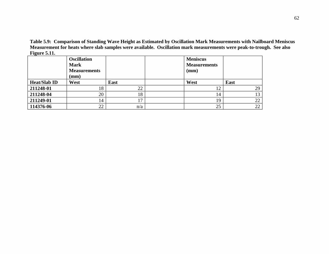
62
Table 5.9: Comparison of Standing Wave Height as Estimated by Oscillation Mark Measurements with Nailboard Meniscus Measurement for heats where slab samples were available. Oscillation mark measurements were peak-to-trough. See also Figure 5.11.
Oscillation Mark Measurements (mm)
Meniscus Measurements (mm)
Heat/Slab ID West East West East 211248-01 18 22 12 29211248-04 20 18 14 13211249-01 14 17 19 22114376-06 22 n/a 25 22
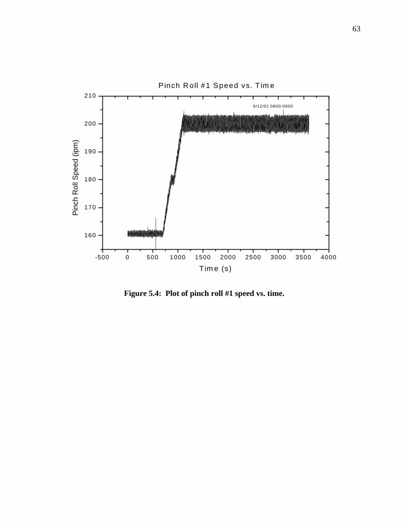
63
Figure 5.4: Plot of pinch roll #1 speed vs. time.
-500 0 500 1000 1500 2000 2500 3000 3500 4000
160
170
180
190
200
2106/12/01 0800-0900
P inch R oll #1 Speed vs. T im eP
inch
Rol
l Spe
ed (i
pm)
T im e (s)
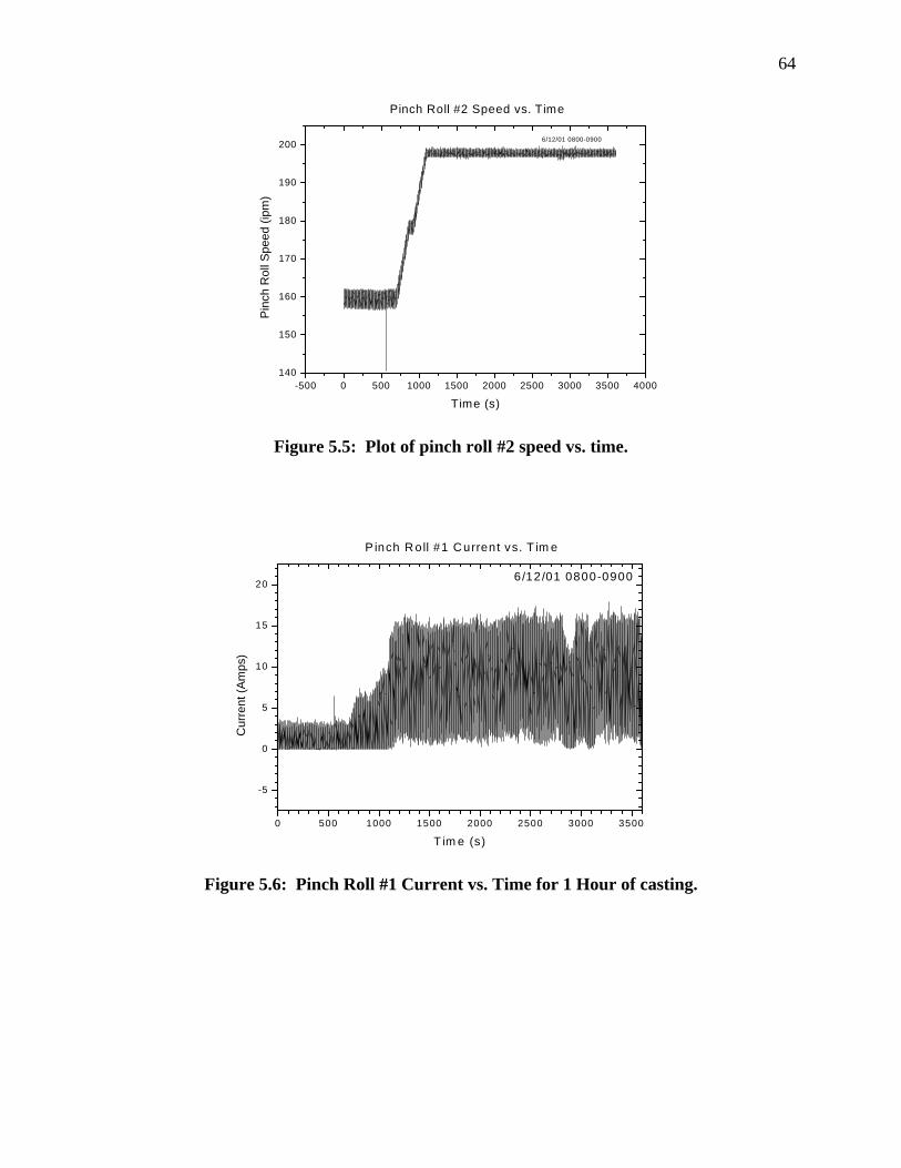
64
Figure 5.5: Plot of pinch roll #2 speed vs. time.
Figure 5.6: Pinch Roll #1 Current vs. Time for 1 Hour of casting.
-500 0 500 1000 1500 2000 2500 3000 3500 4000140
150
160
170
180
190
200 6/12/01 0800-0900
Pinch Roll #2 Speed vs. Time
Pin
ch R
oll S
peed
(ipm
)
Time (s)
0 500 1000 1500 2000 2500 3000 3500
-5
0
5
10
15
20
6 /12/01 0800-0900
P inch R oll #1 C urrent vs. T im e
Cur
rent
(Am
ps)
T im e (s)
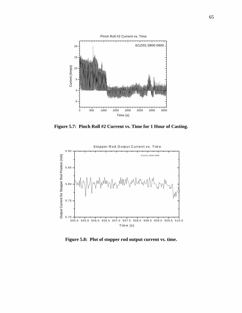
65
Figure 5.7: Pinch Roll #2 Current vs. Time for 1 Hour of Casting.
Figure 5.8: Plot of stopper rod output current vs. time.
0 500 1000 1500 2000 2500 3000 3500
-5
0
5
10
15
20
6/12/01 0800-0900
Pinch Roll #2 Current vs. Time
Cur
rent
(Am
ps)
Time (s)
5 0 5 .0 5 0 5 .5 5 0 6 .0 5 0 6 .5 5 0 7 .0 5 0 7 .5 5 0 8 .0 5 0 8 .5 5 0 9 .0 5 0 9 .5 5 1 0 .05 .7 0
5 .7 5
5 .8 0
5 .8 5
5 .9 06 /1 2 /0 1 0 8 0 0 -0 9 0 0
S to p p e r R o d O u tp u t C u rre n t v s . T im e
Out
put C
urre
nt fo
r Sto
pper
Rod
Pos
ition
(mA
)
T im e (s )
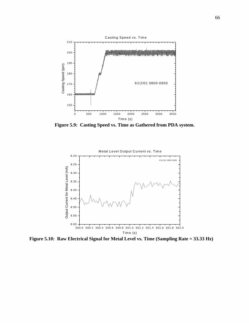
66
Figure 5.9: Casting Speed vs. Time as Gathered from PDA system.
Figure 5.10: Raw Electrical Signal for Metal Level vs. Time (Sampling Rate = 33.33 Hz)
0 500 1000 1500 2000 2500 3000 3500
150
160
170
180
190
200
210
6 /12/01 0800-0900
C asting Speed vs. T im e
Cas
ting
Spe
ed (i
pm)
T im e (s)
500.0 500.2 500.4 500.6 500.8 501.0 501.2 501.4 501.6 501.8 502.08.60
8.55
8.50
8.45
8.40
8.35
8.30
8.25
8.206/12/01 0800-0900
M eta l Level O utput C urrent vs. T im e
Out
put C
urre
nt fo
r Met
al L
evel
(mA)
T im e (s)
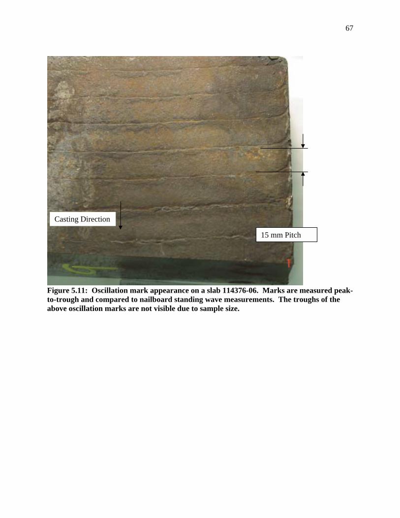
67
Figure 5.11: Oscillation mark appearance on a slab 114376-06. Marks are measured peak-to-trough and compared to nailboard standing wave measurements. The troughs of the above oscillation marks are not visible due to sample size.
Casting Direction
15 mm Pitch
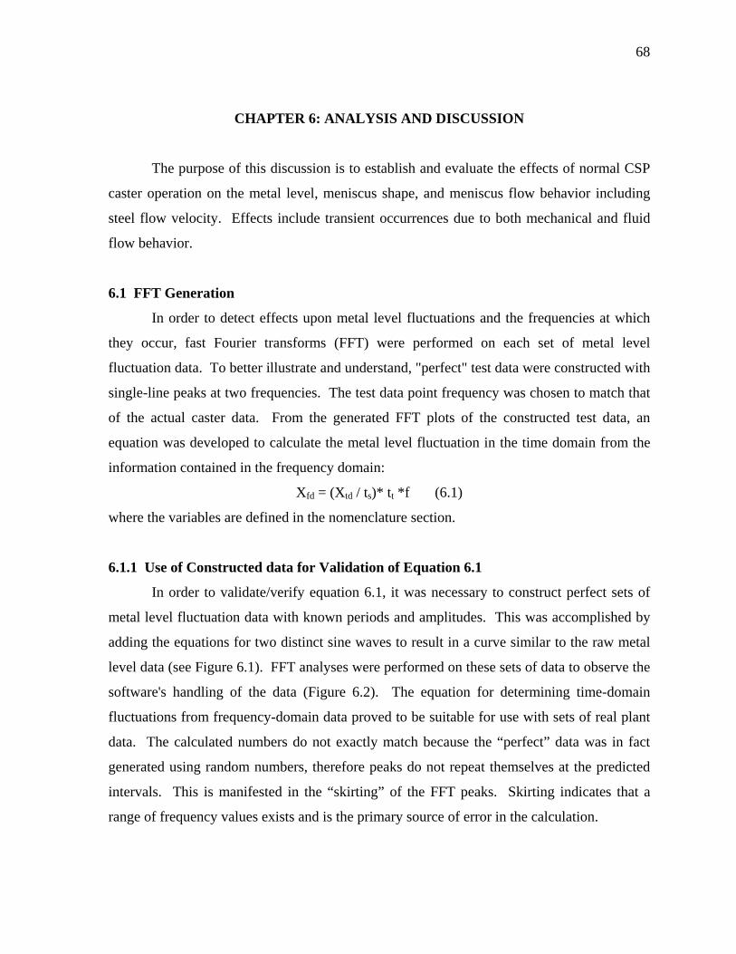
68
CHAPTER 6: ANALYSIS AND DISCUSSION
The purpose of this discussion is to establish and evaluate the effects of normal CSP
caster operation on the metal level, meniscus shape, and meniscus flow behavior including
steel flow velocity. Effects include transient occurrences due to both mechanical and fluid
flow behavior.
6.1 FFT Generation
In order to detect effects upon metal level fluctuations and the frequencies at which
they occur, fast Fourier transforms (FFT) were performed on each set of metal level
fluctuation data. To better illustrate and understand, "perfect" test data were constructed with
single-line peaks at two frequencies. The test data point frequency was chosen to match that
of the actual caster data. From the generated FFT plots of the constructed test data, an
equation was developed to calculate the metal level fluctuation in the time domain from the
information contained in the frequency domain:
Xfd = (Xtd / ts)* tt *f (6.1)
where the variables are defined in the nomenclature section.
6.1.1 Use of Constructed data for Validation of Equation 6.1
In order to validate/verify equation 6.1, it was necessary to construct perfect sets of
metal level fluctuation data with known periods and amplitudes. This was accomplished by
adding the equations for two distinct sine waves to result in a curve similar to the raw metal
level data (see Figure 6.1). FFT analyses were performed on these sets of data to observe the
software's handling of the data (Figure 6.2). The equation for determining time-domain
fluctuations from frequency-domain data proved to be suitable for use with sets of real plant
data. The calculated numbers do not exactly match because the “perfect” data was in fact
generated using random numbers, therefore peaks do not repeat themselves at the predicted
intervals. This is manifested in the “skirting” of the FFT peaks. Skirting indicates that a
range of frequency values exists and is the primary source of error in the calculation.
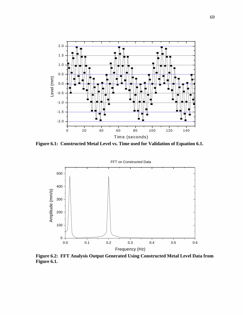
69
0 20 40 60 80 100 120 140
-2.0
-1.5
-1.0
-0.5
0.0
0.5
1.0
1.5
2.0
Leve
l (m
m)
T im e (seconds) Figure 6.1: Constructed Metal Level vs. Time used for Validation of Equation 6.1.
Figure 6.2: FFT Analysis Output Generated Using Constructed Metal Level Data from Figure 6.1.
0.0 0.1 0.2 0.3 0.4 0.5 0.60
100
200
300
400
500
FFT on Constructed Data
Frequency (Hz)
Am
plitu
de (m
m/s
)
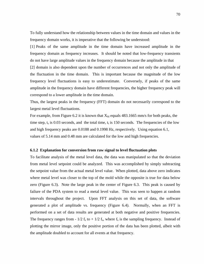
70
To fully understand how the relationship between values in the time domain and values in the
frequency domain works, it is imperative that the following be understood:
[1] Peaks of the same amplitude in the time domain have increased amplitude in the
frequency domain as frequency increases. It should be noted that low-frequency transients
do not have large amplitude values in the frequency domain because the amplitude in that
[2] domain is also dependent upon the number of occurrences and not only the amplitude of
the fluctuation in the time domain. This is important because the magnitude of the low
frequency level fluctuations is easy to underestimate. Conversely, if peaks of the same
amplitude in the frequency domain have different frequencies, the higher frequency peak will
correspond to a lower amplitude in the time domain.
Thus, the largest peaks in the frequency (FFT) domain do not necessarily correspond to the
largest metal level fluctuations.
For example, from Figure 6.2 it is known that Xfd equals 483.1665 mm/s for both peaks, the
time step, ts is 0.03 seconds, and the total time, tt is 150 seconds. The frequencies of the low
and high frequency peaks are 0.0188 and 0.1998 Hz, respectively. Using equation 6.1,
values of 5.14 mm and 0.48 mm are calculated for the low and high frequencies.
6.1.2 Explanation for conversion from raw signal to level fluctuation plots
To facilitate analysis of the metal level data, the data was manipulated so that the deviation
from metal level setpoint could be analyzed. This was accomplished by simply subtracting
the setpoint value from the actual metal level value. When plotted, data above zero indicates
where metal level was closer to the top of the mold while the opposite is true for data below
zero (Figure 6.3). Note the large peak in the center of Figure 6.3. This peak is caused by
failure of the PDA system to read a metal level value. This was seen to happen at random
intervals throughout the project. Upon FFT analysis on this set of data, the software
generated a plot of amplitude vs. frequency (Figure 6.4). Normally, when an FFT is
performed on a set of data results are generated at both negative and positive frequencies.
The frequency ranges from - 1/2 fs to + 1/2 fs, where fs is the sampling frequency. Instead of
plotting the mirror image, only the positive portion of the data has been plotted, albeit with
the amplitude doubled to account for all events at that frequency.
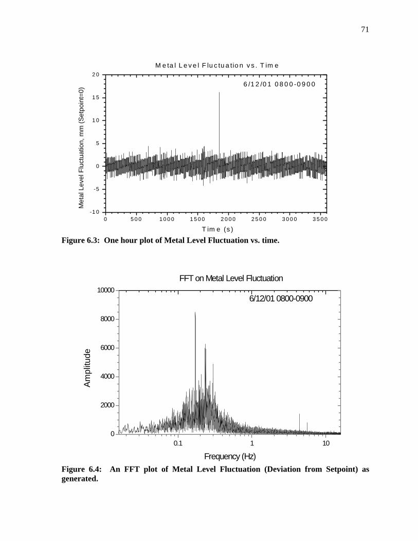
71
Figure 6.3: One hour plot of Metal Level Fluctuation vs. time.
Figure 6.4: An FFT plot of Metal Level Fluctuation (Deviation from Setpoint) as generated.
0.1 1 100
2000
4000
6000
8000
10000
FFT on Metal Level Fluctuation
6/12/01 0800-0900
Frequency (Hz)
Am
plitu
de
0 5 0 0 1 0 0 0 1 5 0 0 2 0 0 0 2 5 0 0 3 0 0 0 3 5 0 0-1 0
-5
0
5
1 0
1 5
2 0
6 /1 2 /0 1 0 8 0 0 -0 9 0 0
M e ta l L e v e l F lu c tu a tio n v s . T im e
Met
al L
evel
Flu
ctua
tion,
mm
(Set
poin
t=0)
T im e (s )
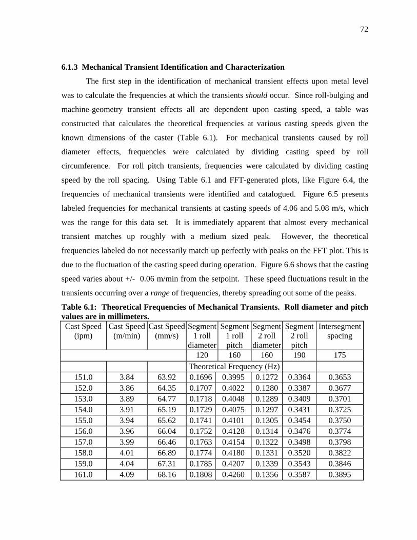
72
6.1.3 Mechanical Transient Identification and Characterization
The first step in the identification of mechanical transient effects upon metal level
was to calculate the frequencies at which the transients should occur. Since roll-bulging and
machine-geometry transient effects all are dependent upon casting speed, a table was
constructed that calculates the theoretical frequencies at various casting speeds given the
known dimensions of the caster (Table 6.1). For mechanical transients caused by roll
diameter effects, frequencies were calculated by dividing casting speed by roll
circumference. For roll pitch transients, frequencies were calculated by dividing casting
speed by the roll spacing. Using Table 6.1 and FFT-generated plots, like Figure 6.4, the
frequencies of mechanical transients were identified and catalogued. Figure 6.5 presents
labeled frequencies for mechanical transients at casting speeds of 4.06 and 5.08 m/s, which
was the range for this data set. It is immediately apparent that almost every mechanical
transient matches up roughly with a medium sized peak. However, the theoretical
frequencies labeled do not necessarily match up perfectly with peaks on the FFT plot. This is
due to the fluctuation of the casting speed during operation. Figure 6.6 shows that the casting
speed varies about +/- 0.06 m/min from the setpoint. These speed fluctuations result in the
transients occurring over a range of frequencies, thereby spreading out some of the peaks.
Table 6.1: Theoretical Frequencies of Mechanical Transients. Roll diameter and pitch values are in millimeters. Cast Speed
(ipm) Cast Speed
(m/min) Cast Speed
(mm/s) Segment
1 roll diameter
Segment 1 roll pitch
Segment 2 roll
diameter
Segment 2 roll pitch
Intersegment spacing
120 160 160 190 175 Theoretical Frequency (Hz)
151.0 3.84 63.92 0.1696 0.3995 0.1272 0.3364 0.3653 152.0 3.86 64.35 0.1707 0.4022 0.1280 0.3387 0.3677 153.0 3.89 64.77 0.1718 0.4048 0.1289 0.3409 0.3701 154.0 3.91 65.19 0.1729 0.4075 0.1297 0.3431 0.3725 155.0 3.94 65.62 0.1741 0.4101 0.1305 0.3454 0.3750 156.0 3.96 66.04 0.1752 0.4128 0.1314 0.3476 0.3774 157.0 3.99 66.46 0.1763 0.4154 0.1322 0.3498 0.3798 158.0 4.01 66.89 0.1774 0.4180 0.1331 0.3520 0.3822 159.0 4.04 67.31 0.1785 0.4207 0.1339 0.3543 0.3846 161.0 4.09 68.16 0.1808 0.4260 0.1356 0.3587 0.3895
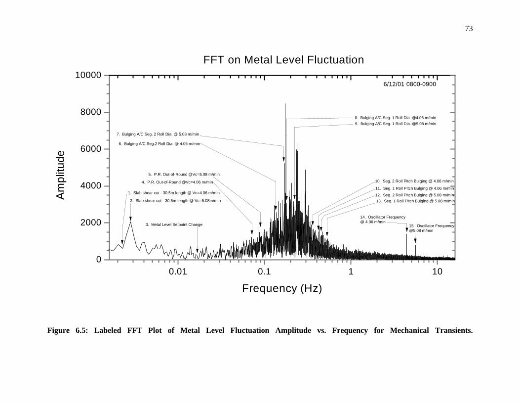
73
Figure 6.5: Labeled FFT Plot of Metal Level Fluctuation Amplitude vs. Frequency for Mechanical Transients.
0.01 0.1 1 100
2000
4000
6000
8000
10000
14. Oscillator Frequency@ 4.06 m/min
13. Seg. 1 Roll Pitch Bulging @ 5.08 m/min12. Seg. 2 Roll Pitch Bulging @ 5.08 m/min
10. Seg. 2 Roll Pitch Bulging @ 4.06 m/min
11. Seg. 1 Roll Pitch Bulging @ 4.06 m/min
8. Bulging A/C Seg. 1 Roll Dia. @4.06 m/min9. Bulging A/C Seg. 1 Roll Dia. @5.08 m/min
6. Bulging A/C Seg.2 Roll Dia. @ 4.06 m/min
7. Bulging A/C Seg. 2 Roll Dia. @ 5.08 m/min
3. Metal Level Setpoint Change
1. Slab shear cut - 30.5m length @ Vc=4.06 m/min
2. Slab shear cut - 30.5m length @ Vc=5.08m/min
5. P.R. Out-of-Round @Vc=5.08 m/min
4. P.R. Out-of-Round @Vc=4.06 m/min
15. Oscillator [email protected] m/min
FFT on Metal Level Fluctuation
6/12/01 0800-0900
Frequency (Hz)
Am
plitu
de
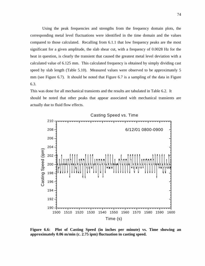
74
Using the peak frequencies and strengths from the frequency domain plots, the
corresponding metal level fluctuations were identified in the time domain and the values
compared to those calculated. Recalling from 6.1.1 that low frequency peaks are the most
significant for a given amplitude, the slab shear cut, with a frequency of 0.0028 Hz for the
heat in question, is clearly the transient that caused the greatest metal level deviation with a
calculated value of 6.125 mm. This calculated frequency is obtained by simply dividing cast
speed by slab length (Table 5.10). Measured values were observed to be approximately 5
mm (see Figure 6.7). It should be noted that Figure 6.7 is a sampling of the data in Figure
6.3.
This was done for all mechanical transients and the results are tabulated in Table 6.2. It
should be noted that other peaks that appear associated with mechanical transients are
actually due to fluid flow effects.
Figure 6.6: Plot of Casting Speed (in inches per minute) vs. Time showing an approximately 0.06 m/min (c. 2.75 ipm) fluctuation in casting speed.
1500 1510 1520 1530 1540 1550 1560 1570 1580 1590 1600190
192
194
196
198
200
202
204
206
208
210
6/12/01 0800-0900
Casting Speed vs. Time
Cas
ting
Spee
d (ip
m)
Time (s)
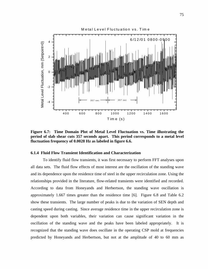
75
Figure 6.7: Time Domain Plot of Metal Level Fluctuation vs. Time illustrating the period of slab shear cuts 357 seconds apart. This period corresponds to a metal level fluctuation frequency of 0.0028 Hz as labeled in figure 6.6.
6.1.4 Fluid Flow Transient Identification and Characterization
To identify fluid flow transients, it was first necessary to perform FFT analyses upon
all data sets. The fluid flow effects of most interest are the oscillation of the standing wave
and its dependence upon the residence time of steel in the upper recirculation zone. Using the
relationships provided in the literature, flow-related transients were identified and recorded.
According to data from Honeyands and Herbertson, the standing wave oscillation is
approximately 1.667 times greater than the residence time [6]. Figure 6.8 and Table 6.2
show these transients. The large number of peaks is due to the variation of SEN depth and
casting speed during casting. Since average residence time in the upper recirculation zone is
dependent upon both variables, their variation can cause significant variation in the
oscillation of the standing wave and the peaks have been labeled appropriately. It is
recognized that the standing wave does oscillate in the operating CSP mold at frequencies
predicted by Honeyands and Herbertson, but not at the amplitude of 40 to 60 mm as
4 0 0 6 0 0 8 0 0 1 0 0 0 1 2 0 0 1 4 0 0 1 6 0 0
-4
-2
0
2
4
3 5 7 s e c3 5 7 s e c
6 /1 2 /0 1 0 8 0 0 -0 9 0 0
M e ta l L e v e l F lu c tu a tio n v s . T im e
Met
al L
evel
Flu
ctua
tion,
mm
(Set
poin
t=0)
T im e (s )
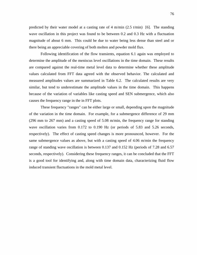
76
predicted by their water model at a casting rate of 4 m/min (2.5 t/min) [6]. The standing
wave oscillation in this project was found to be between 0.2 and 0.3 Hz with a fluctuation
magnitude of about 6 mm. This could be due to water being less dense than steel and or
there being an appreciable covering of both molten and powder mold flux.
Following identification of the flow transients, equation 6.1 again was employed to
determine the amplitude of the meniscus level oscillations in the time domain. These results
are compared against the real-time metal level data to determine whether these amplitude
values calculated from FFT data agreed with the observed behavior. The calculated and
measured amplitudes values are summarized in Table 6.2. The calculated results are very
similar, but tend to underestimate the amplitude values in the time domain. This happens
because of the variation of variables like casting speed and SEN submergence, which also
causes the frequency range in the in FFT plots.
These frequency "ranges" can be either large or small, depending upon the magnitude
of the variation in the time domain. For example, for a submergence difference of 29 mm
(296 mm to 267 mm) and a casting speed of 5.08 m/min, the frequency range for standing
wave oscillation varies from 0.172 to 0.190 Hz (or periods of 5.83 and 5.26 seconds,
respectively). The effect of casting speed changes is more pronounced, however. For the
same submergence values as above, but with a casting speed of 4.06 m/min the frequency
range of standing wave oscillation is between 0.137 and 0.152 Hz (periods of 7.28 and 6.57
seconds, respectively). Considering these frequency ranges, it can be concluded that the FFT
is a good tool for identifying and, along with time domain data, characterizing fluid flow
induced transient fluctuations in the mold metal level.
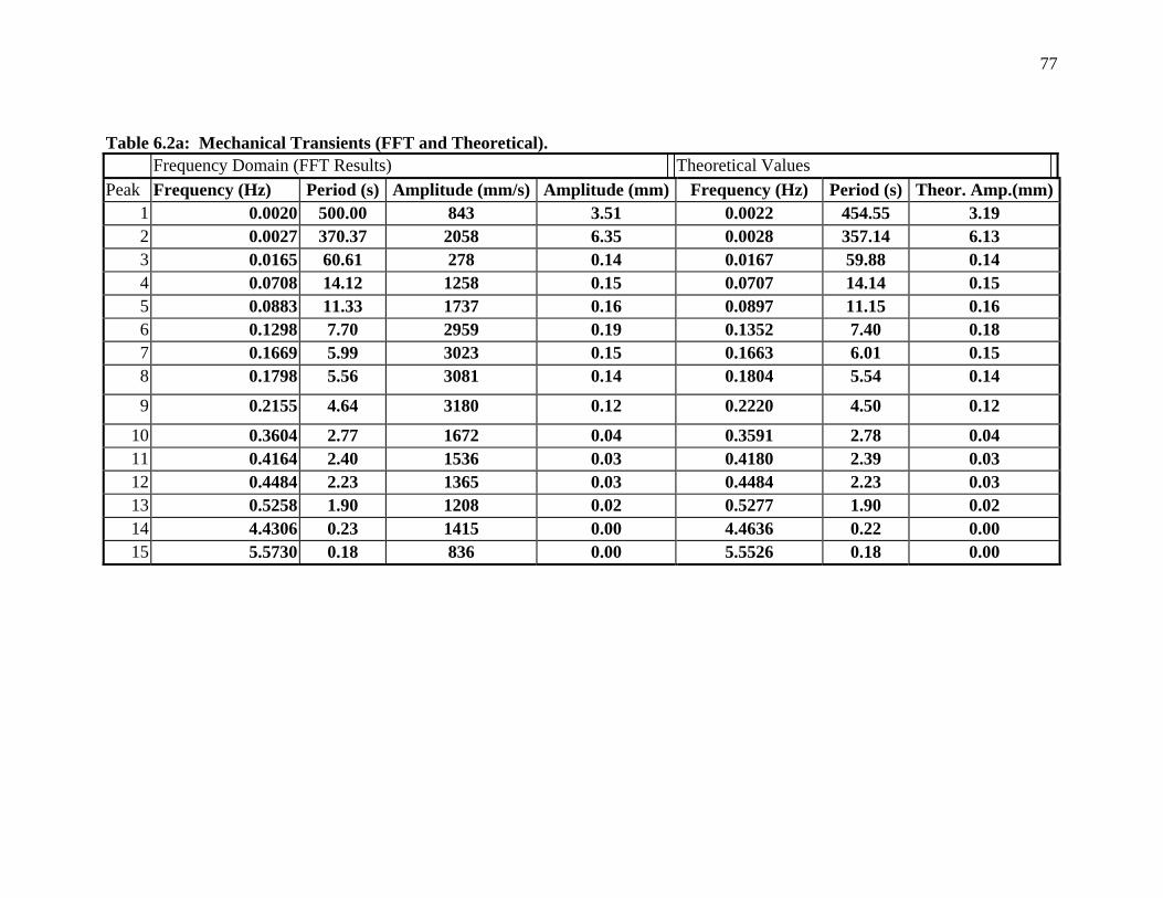
77
Table 6.2a: Mechanical Transients (FFT and Theoretical). Frequency Domain (FFT Results) Theoretical Values
Peak Frequency (Hz) Period (s) Amplitude (mm/s) Amplitude (mm) Frequency (Hz) Period (s) Theor. Amp.(mm)1 0.0020 500.00 843 3.51 0.0022 454.55 3.19 2 0.0027 370.37 2058 6.35 0.0028 357.14 6.13 3 0.0165 60.61 278 0.14 0.0167 59.88 0.14 4 0.0708 14.12 1258 0.15 0.0707 14.14 0.15 5 0.0883 11.33 1737 0.16 0.0897 11.15 0.16 6 0.1298 7.70 2959 0.19 0.1352 7.40 0.18 7 0.1669 5.99 3023 0.15 0.1663 6.01 0.15 8 0.1798 5.56 3081 0.14 0.1804 5.54 0.14
9 0.2155 4.64 3180 0.12 0.2220 4.50 0.12
10 0.3604 2.77 1672 0.04 0.3591 2.78 0.04 11 0.4164 2.40 1536 0.03 0.4180 2.39 0.03 12 0.4484 2.23 1365 0.03 0.4484 2.23 0.03 13 0.5258 1.90 1208 0.02 0.5277 1.90 0.02 14 4.4306 0.23 1415 0.00 4.4636 0.22 0.00 15 5.5730 0.18 836 0.00 5.5526 0.18 0.00
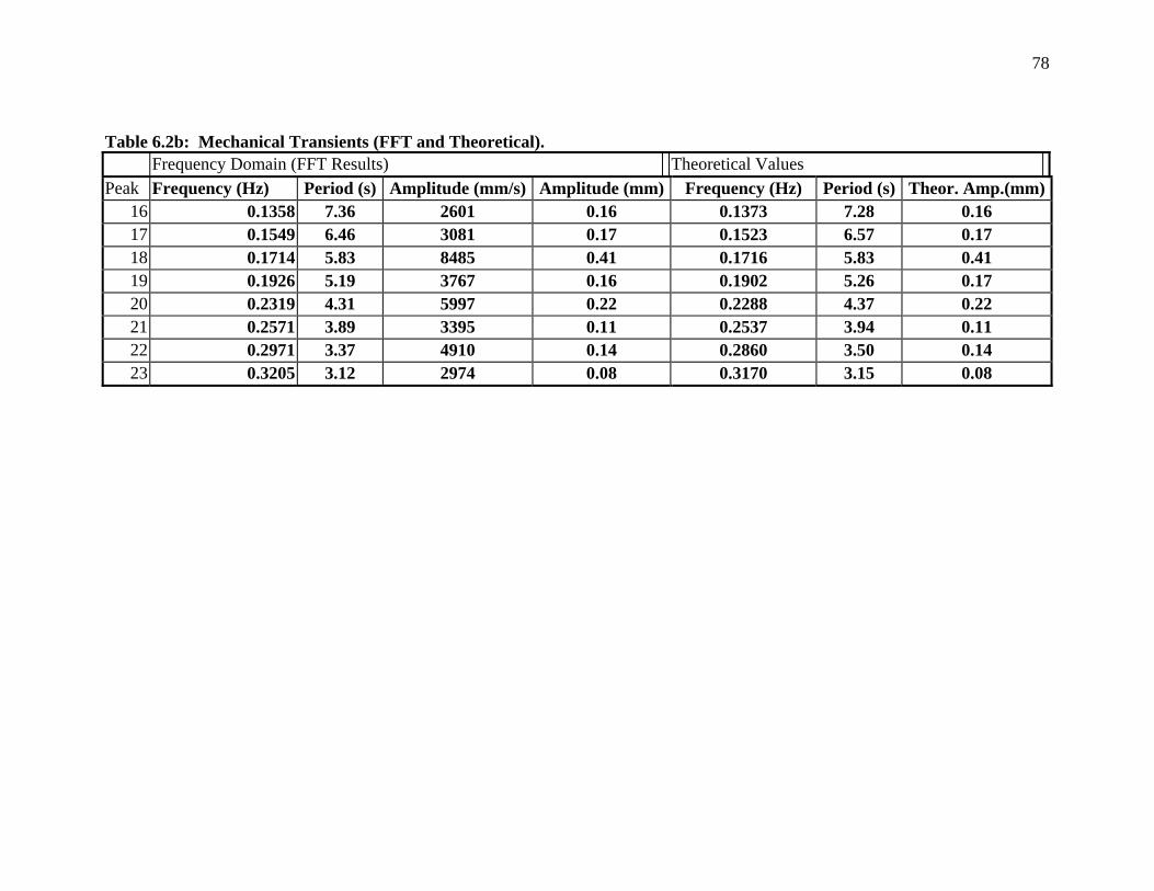
78
Table 6.2b: Mechanical Transients (FFT and Theoretical). Frequency Domain (FFT Results) Theoretical Values
Peak Frequency (Hz) Period (s) Amplitude (mm/s) Amplitude (mm) Frequency (Hz) Period (s) Theor. Amp.(mm)16 0.1358 7.36 2601 0.16 0.1373 7.28 0.16 17 0.1549 6.46 3081 0.17 0.1523 6.57 0.17 18 0.1714 5.83 8485 0.41 0.1716 5.83 0.41 19 0.1926 5.19 3767 0.16 0.1902 5.26 0.17 20 0.2319 4.31 5997 0.22 0.2288 4.37 0.22 21 0.2571 3.89 3395 0.11 0.2537 3.94 0.11 22 0.2971 3.37 4910 0.14 0.2860 3.50 0.14 23 0.3205 3.12 2974 0.08 0.3170 3.15 0.08
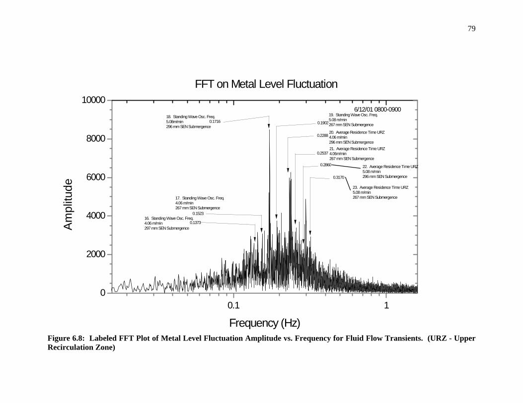
79
Figure 6.8: Labeled FFT Plot of Metal Level Fluctuation Amplitude vs. Frequency for Fluid Flow Transients. (URZ - Upper Recirculation Zone)
0.1 10
2000
4000
6000
8000
10000
23. Average Residence Time URZ5.08 m/min267 mm SEN Submergence
22. Average Residence Time URZ5.08 m/min296 mm SEN Submergence
21. Average Residence Time URZ4.06m/min267 mm SEN Submergence
20. Average Residence Time URZ4.06 m/min296 mm SEN Submergence
19. Standing Wave Osc. Freq.5.08 m/min267 mm SEN Submergence
16. Standing Wave Osc. Freq.4.06 m/min297 mm SEN Submergence
17. Standing Wave Osc. Freq.4.06 m/min267 mm SEN Submergence
18. Standing Wave Osc. Freq.5.08m/min296 mm SEN Submergence
0.3170
0.2860
0.2537
0.2288
0.19020.1716
0.1523
0.1373
FFT on Metal Level Fluctuation
6/12/01 0800-0900
Frequency (Hz)
Am
plitu
de
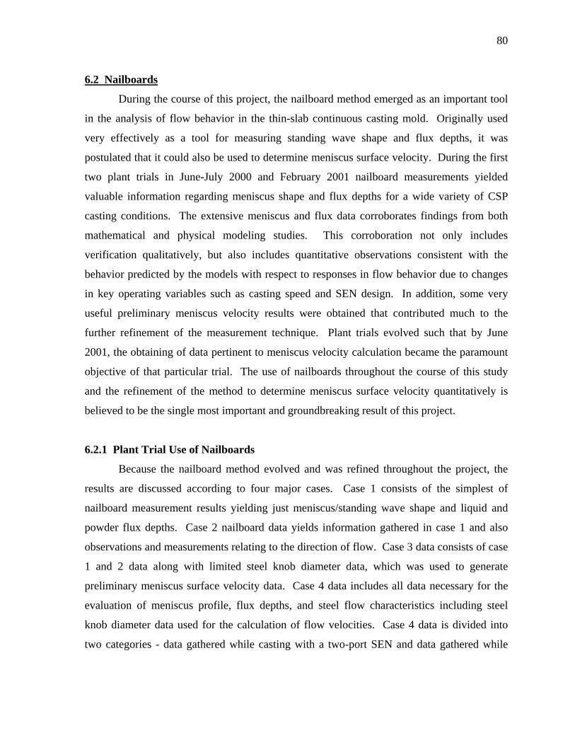
80
6.2 Nailboards
During the course of this project, the nailboard method emerged as an important tool
in the analysis of flow behavior in the thin-slab continuous casting mold. Originally used
very effectively as a tool for measuring standing wave shape and flux depths, it was
postulated that it could also be used to determine meniscus surface velocity. During the first
two plant trials in June-July 2000 and February 2001 nailboard measurements yielded
valuable information regarding meniscus shape and flux depths for a wide variety of CSP
casting conditions. The extensive meniscus and flux data corroborates findings from both
mathematical and physical modeling studies. This corroboration not only includes
verification qualitatively, but also includes quantitative observations consistent with the
behavior predicted by the models with respect to responses in flow behavior due to changes
in key operating variables such as casting speed and SEN design. In addition, some very
useful preliminary meniscus velocity results were obtained that contributed much to the
further refinement of the measurement technique. Plant trials evolved such that by June
2001, the obtaining of data pertinent to meniscus velocity calculation became the paramount
objective of that particular trial. The use of nailboards throughout the course of this study
and the refinement of the method to determine meniscus surface velocity quantitatively is
believed to be the single most important and groundbreaking result of this project.
6.2.1 Plant Trial Use of Nailboards
Because the nailboard method evolved and was refined throughout the project, the
results are discussed according to four major cases. Case 1 consists of the simplest of
nailboard measurement results yielding just meniscus/standing wave shape and liquid and
powder flux depths. Case 2 nailboard data yields information gathered in case 1 and also
observations and measurements relating to the direction of flow. Case 3 data consists of case
1 and 2 data along with limited steel knob diameter data, which was used to generate
preliminary meniscus surface velocity data. Case 4 data includes all data necessary for the
evaluation of meniscus profile, flux depths, and steel flow characteristics including steel
knob diameter data used for the calculation of flow velocities. Case 4 data is divided into
two categories - data gathered while casting with a two-port SEN and data gathered while
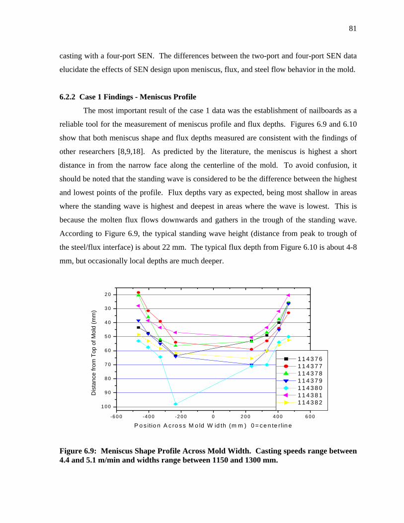
81
casting with a four-port SEN. The differences between the two-port and four-port SEN data
elucidate the effects of SEN design upon meniscus, flux, and steel flow behavior in the mold.
6.2.2 Case 1 Findings - Meniscus Profile
The most important result of the case 1 data was the establishment of nailboards as a
reliable tool for the measurement of meniscus profile and flux depths. Figures 6.9 and 6.10
show that both meniscus shape and flux depths measured are consistent with the findings of
other researchers [8,9,18]. As predicted by the literature, the meniscus is highest a short
distance in from the narrow face along the centerline of the mold. To avoid confusion, it
should be noted that the standing wave is considered to be the difference between the highest
and lowest points of the profile. Flux depths vary as expected, being most shallow in areas
where the standing wave is highest and deepest in areas where the wave is lowest. This is
because the molten flux flows downwards and gathers in the trough of the standing wave.
According to Figure 6.9, the typical standing wave height (distance from peak to trough of
the steel/flux interface) is about 22 mm. The typical flux depth from Figure 6.10 is about 4-8
mm, but occasionally local depths are much deeper.
-6 0 0 -4 0 0 -2 0 0 0 2 0 0 4 0 0 6 0 0
1 0 0
9 0
8 0
7 0
6 0
5 0
4 0
3 0
2 0
1 1 4 3 7 6 1 1 4 3 7 7 1 1 4 3 7 8 1 1 4 3 7 9 1 1 4 3 8 0 1 1 4 3 8 1 1 1 4 3 8 2
Dis
tanc
e fro
m T
op o
f Mol
d (m
m)
P o s itio n A c ro s s M o ld W id th (m m ) 0 = ce n te rlin e
Figure 6.9: Meniscus Shape Profile Across Mold Width. Casting speeds range between 4.4 and 5.1 m/min and widths range between 1150 and 1300 mm.
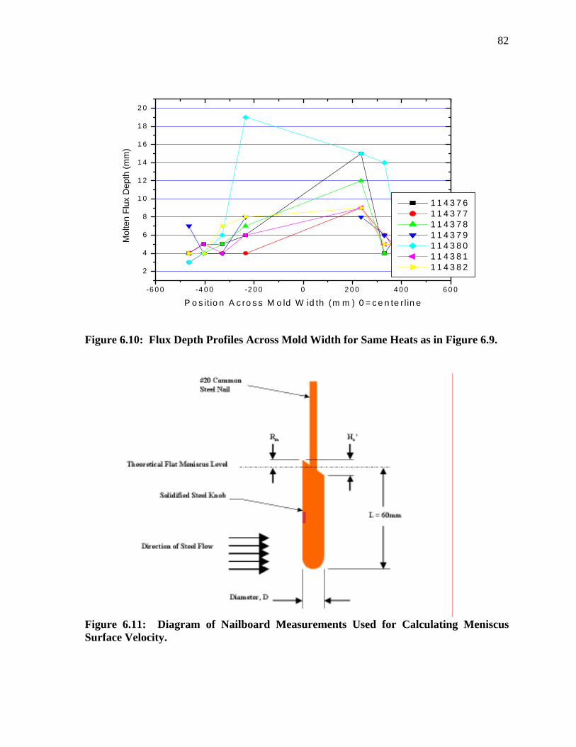
82
-6 0 0 -4 0 0 -2 0 0 0 2 0 0 4 0 0 6 0 0
2
4
6
8
1 0
1 2
1 4
1 6
1 8
2 0
1 1 4 3 7 6 1 1 4 3 7 7 1 1 4 3 7 8 1 1 4 3 7 9 1 1 4 3 8 0 1 1 4 3 8 1 1 1 4 3 8 2
Mol
ten
Flux
Dep
th (m
m)
P o s it io n A c ro s s M o ld W id th (m m ) 0 = c e n te r l in e
Figure 6.10: Flux Depth Profiles Across Mold Width for Same Heats as in Figure 6.9.
Figure 6.11: Diagram of Nailboard Measurements Used for Calculating Meniscus Surface Velocity.
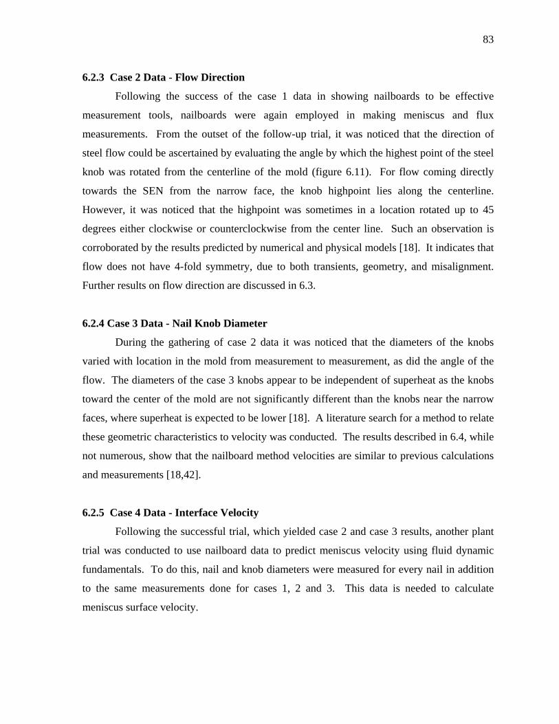
83
6.2.3 Case 2 Data - Flow Direction
Following the success of the case 1 data in showing nailboards to be effective
measurement tools, nailboards were again employed in making meniscus and flux
measurements. From the outset of the follow-up trial, it was noticed that the direction of
steel flow could be ascertained by evaluating the angle by which the highest point of the steel
knob was rotated from the centerline of the mold (figure 6.11). For flow coming directly
towards the SEN from the narrow face, the knob highpoint lies along the centerline.
However, it was noticed that the highpoint was sometimes in a location rotated up to 45
degrees either clockwise or counterclockwise from the center line. Such an observation is
corroborated by the results predicted by numerical and physical models [18]. It indicates that
flow does not have 4-fold symmetry, due to both transients, geometry, and misalignment.
Further results on flow direction are discussed in 6.3.
6.2.4 Case 3 Data - Nail Knob Diameter
During the gathering of case 2 data it was noticed that the diameters of the knobs
varied with location in the mold from measurement to measurement, as did the angle of the
flow. The diameters of the case 3 knobs appear to be independent of superheat as the knobs
toward the center of the mold are not significantly different than the knobs near the narrow
faces, where superheat is expected to be lower [18]. A literature search for a method to relate
these geometric characteristics to velocity was conducted. The results described in 6.4, while
not numerous, show that the nailboard method velocities are similar to previous calculations
and measurements [18,42].
6.2.5 Case 4 Data - Interface Velocity
Following the successful trial, which yielded case 2 and case 3 results, another plant
trial was conducted to use nailboard data to predict meniscus velocity using fluid dynamic
fundamentals. To do this, nail and knob diameters were measured for every nail in addition
to the same measurements done for cases 1, 2 and 3. This data is needed to calculate
meniscus surface velocity.
84
6.3 Flow Direction as Indicated by Nailboard data
As mentioned previously, during the gathering of case 2 data it was noticed that the
location of the highpoint of the steel knob following immersion indicated the direction from
which the steel was flowing. Most of the time, no rotation was observed meaning that there
was no velocity component in the through-thickness direction. Rotations were measured to
be from about 5 degrees to 60 degrees with the flow always coming from the direction of the
narrow face towards the SEN. This behavior has been predicted by several numerical models
[18]. Several factors may affect this behavior. They include SEN alignment, flow oscillation
at the SEN exit, flow within the mold and the cavity of the solidifying strand, and mold
geometry effects. This observed rotation may affect the velocity values themselves. Since
only a few instances of this rotation were noted and measured, it is not yet possible to
conclusively determine whether this is so. Preliminary results show that large flow rotations
above 45 degrees correlate slightly with a lower standing wave relative to heats cast at
similar speeds with no observed flow rotation (Figure 6.12). This suggests that perfectly
aligned jet impingement upon the narrow face produces a higher standing wave, which is
logical. Further study is needed to determine if this is really the case.
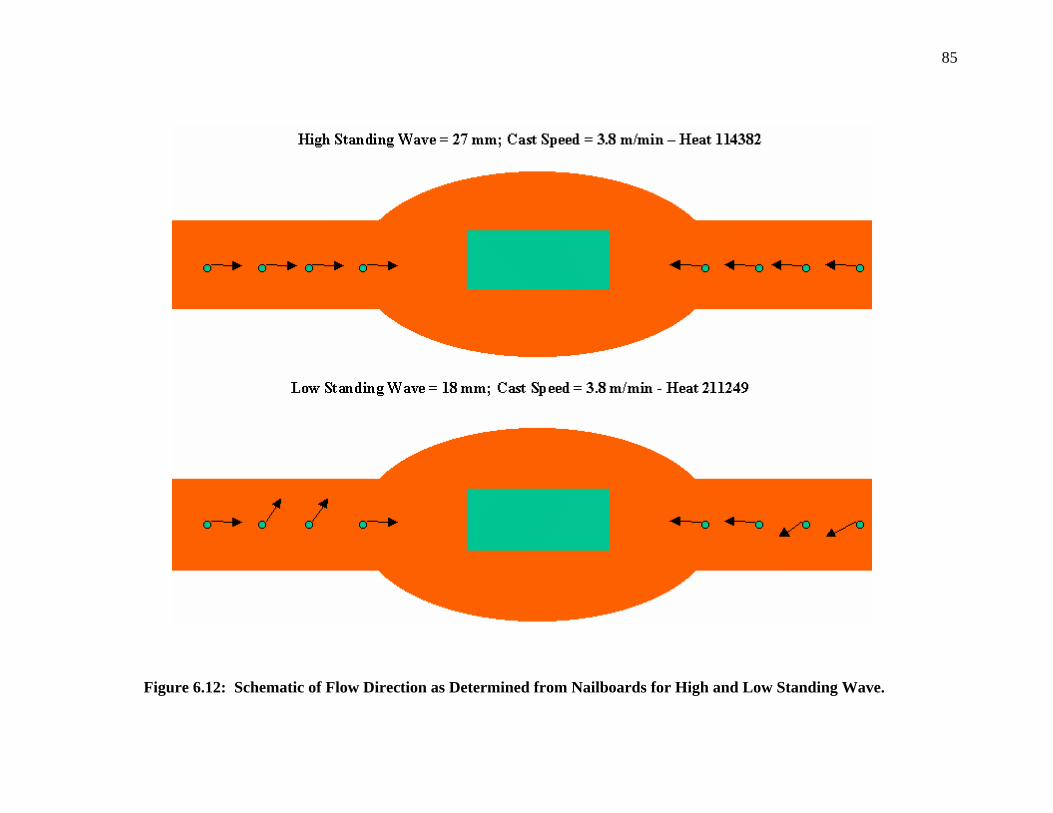
85
Figure 6.12: Schematic of Flow Direction as Determined from Nailboards for High and Low Standing Wave.
86
6.4 Explanation of Morison Equation and Description of Calculation Method
A method developed by Morison for round cylinders immersed in water was extended
and applied to correlate steel knob shape with meniscus velocity. Morsion's original work
calculated the force of water flowing past immersed piles. Since it was not known at the
beginning of this trial that the knob diameters were important to surface velocity, only
limited meniscus velocity results were obtained from heats cast near the conclusion of the
trial (Case 4 data). The values that were measured for the meniscus velocity calculation are
as follows (see also figure 6.11):
• High and low points of steel knob
• Unrefracted wave height, Ho'
• Diameter, D, of steel knob following immersion
• Depth, L, of nail immersion below flat level (0.060 m)
Constants that must be used are listed below:
• Ratio, k, of wave crest elevation above still liquid level to the wave height (0.78)
• Euler's Constant, γ (0.5772)
• Steel Density, ρ (7800 kg/m3)
• Inertia Coefficient, Cm (1+k)
• Acceleration due to gravity, g (9.8 m/s2)
• Fluid flow constant, δ (3π/8)
6.4.1 Suitability of the Morison Equation for Small Cylinders
Since the Morison equation was originally used to calculate forces upon large pilings
it was necessary to determine whether it was applicable for small cylinders like the nails.
Following a literature search it was deemed appropriate because of the geometry of the
individual nails. Sarpkaya reports that a diameter to length ratio above 0.2 is required
because the equation takes into consideration the effects of wave diffraction. That ratio for a
nail with no knob is 0.05, but for a nail with a steel knob, it ranged from 0.2 to approximately
0.3 so the equation was assumed applicable [55].
87
6.4.2 Calculation of Meniscus Stream Velocity Using Fluid Dynamics/Morison
Equation
After obtaining all of the above values and calculating an initial wave height (Ho), the
maximum force of steel against the nail/knob can be calculated. Up to this point, Morison's
equation is followed exactly. Velocity was then calculated using the relationship between
force and velocity for vertically oriented circular cylinders immersed in a flowing fluid.
The first step in the calculation of meniscus surface velocity values is to establish a
run-up height for the steel as it flows past a submerged nail. For this case, the run-up height
is assumed to be half of the unrefracted wave height, Ho', which is defined as the distance
between the high point and low point on each steel knob. Recall that the angle at the top of
the steel knob and the diameter of the knob are indicators of flow direction and velocity.
Equation 6.2 predicts the wave run-up height from the total wave height (Ho). Equation 6.3
is used to calculate hypothetical wave run-up values (Rm).
Ho = H'o * k (6.2)
Rm = Ho * 0.5{1 +k2[ln(k/2) + (2γ + 3]}0.5 (6.3)
which simplifies to
Rm = 0.507 Ho' (6.4)
The variables are defined in the nomenclature. Wiegel and Beebe have observed that
the ratio, k, of the initial wave height (Ho) to the unrefracted wave height (H'o) for an
immersed cylinder is 0.78 [56]. Accordingly, the run-up height, Rm, corresponds to about
half of the measured unrefracted wave height, Ho', agreeing with Sorenson [56].
Next, the maximum force of flowing steel acting upon the steel knob on the nail is calculated.
The equation is derived from the Morison equation for an unrefracted wave and is:
F = π2ρHoLD2 / 8t2 * Cm*k (6.5)
The value, t, is an empirical maximum frequency wave period and is assumed to be 0.030
seconds, which corresponds to the maximum frequency detectable in this study. With force
calculated, it was necessary to calculate velocities associated with it. To obtain a horizontal
velocity the following equation is used [57]:
88
U = (F / L * 2 / (ρCD) )0.5 (6.6)
C is the force coefficient corresponding to the total in-line force and has a value of six for the
conditions in this study [57]. While the root mean square velocity may underestimate the
actual maximum velocity, it does take into consideration flow oscillation and flow ellipticity,
which is common with flow about a vertically-oriented circular cylinder [57].
6.5 Evaluation of the Calculated Meniscus Stream Velocity Values
The calculated meniscus stream velocities values are compared against values
obtained and/or calculated through mathematical and physical water modeling and through
the other velocity measurement methods discussed previously. As shown in table 6.4, the
values obtained using the method just described are 30% to 100% greater than velocities
predicted by two mathematical models [18, 42]. However, the casting conditions are very
different, as is mold geometry.
6.5.1 Comparison with Mathematical Model Predictions
The two mathematical models from which velocity data were obtained for
comparison were from a rectangular mold and a CSP mold, done by McDavid and Thomas
[18] and Nam et al [42], respectively. Table 6.3 and Figures 6.14a and 6.14b show
calculated velocity across the width of the mold. As can be seen from Figure 6.13, the
predicted velocity profiles have similar shape, but appreciably lower values than do the
velocity profiles generated during the course of this project. The discrepancy might also be
due to the shape and magnitude of the standing wave, or level fluctuations or fluctuations in
the standing wave, which were not modeled. The design of the SEN and casting conditions
such as casting speed and mold geometry in the mathematical models differ substantially
from operating conditions in this project, which included casting with both 2-port and 4-port
SEN designs. Moreover, since there are only four locations per side where nailboard data is
obtained, the scarcity of data is very much a factor in limiting the construction of a velocity
profile.
In addition to these, numerous other factors may affect the velocity at the meniscus.
Some of these include:
! SEN alignment and funnel geometry effects

89
! Integrity of flow control through the SEN (e.g. biased flow)
! SEN exit stream oscillation
! Stopper Rod Irregularities
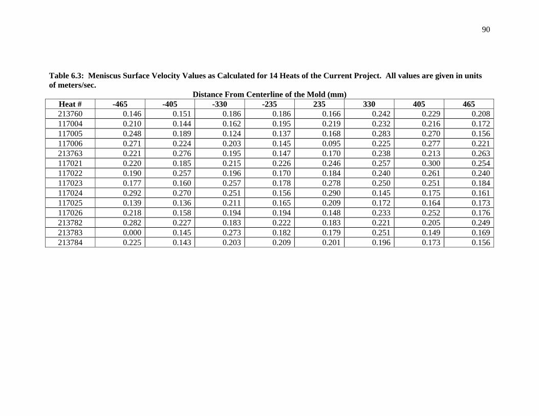
90
Table 6.3: Meniscus Surface Velocity Values as Calculated for 14 Heats of the Current Project. All values are given in units of meters/sec.
Distance From Centerline of the Mold (mm) Heat # -465 -405 -330 -235 235 330 405 465 213760 0.146 0.151 0.186 0.186 0.166 0.242 0.229 0.208117004 0.210 0.144 0.162 0.195 0.219 0.232 0.216 0.172117005 0.248 0.189 0.124 0.137 0.168 0.283 0.270 0.156117006 0.271 0.224 0.203 0.145 0.095 0.225 0.277 0.221213763 0.221 0.276 0.195 0.147 0.170 0.238 0.213 0.263117021 0.220 0.185 0.215 0.226 0.246 0.257 0.300 0.254117022 0.190 0.257 0.196 0.170 0.184 0.240 0.261 0.240117023 0.177 0.160 0.257 0.178 0.278 0.250 0.251 0.184117024 0.292 0.270 0.251 0.156 0.290 0.145 0.175 0.161117025 0.139 0.136 0.211 0.165 0.209 0.172 0.164 0.173117026 0.218 0.158 0.194 0.194 0.148 0.233 0.252 0.176213782 0.282 0.227 0.183 0.222 0.183 0.221 0.205 0.249213783 0.000 0.145 0.273 0.182 0.179 0.251 0.149 0.169213784 0.225 0.143 0.203 0.209 0.201 0.196 0.173 0.156
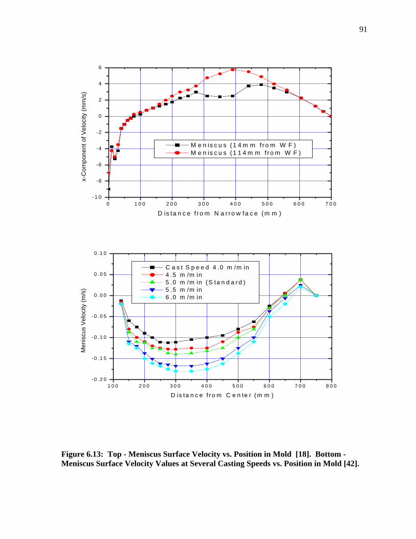
91
Figure 6.13: Top - Meniscus Surface Velocity vs. Position in Mold [18]. Bottom - Meniscus Surface Velocity Values at Several Casting Speeds vs. Position in Mold [42].
0 1 0 0 2 0 0 3 0 0 4 0 0 5 0 0 6 0 0 7 0 0-1 0
-8
-6
-4
-2
0
2
4
6
x-C
ompo
nent
of V
eloc
ity (m
m/s
)
D is ta n c e f r o m N a r ro w fa c e (m m )
M e n is c u s (1 4 m m f ro m W F ) M e n is c u s (1 1 4 m m f ro m W F )
1 0 0 2 0 0 3 0 0 4 0 0 5 0 0 6 0 0 7 0 0 8 0 0- 0 .2 0
- 0 .1 5
- 0 .1 0
- 0 .0 5
0 .0 0
0 .0 5
0 .1 0
Men
iscu
s Ve
loci
ty (m
/s)
D is ta n c e f r o m C e n te r (m m )
C a s t S p e e d 4 .0 m /m in 4 .5 m /m in 5 .0 m /m in (S ta n d a rd ) 5 .5 m /m in 6 .0 m /m in
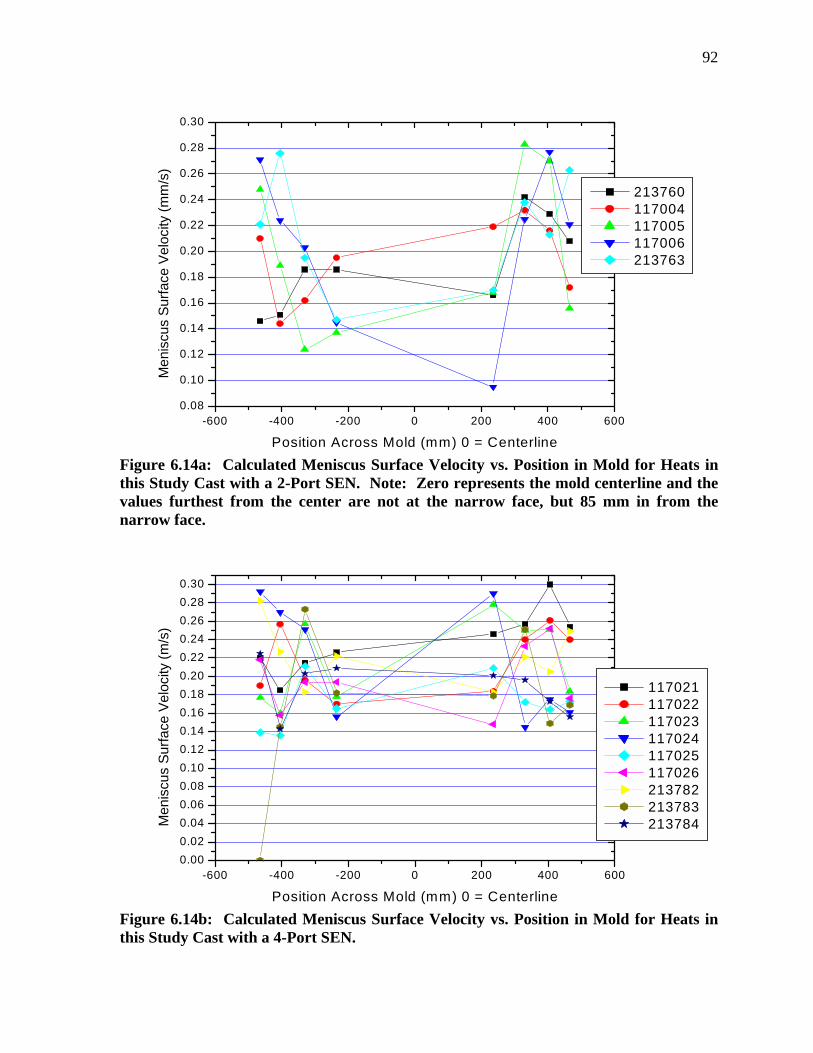
92
Figure 6.14a: Calculated Meniscus Surface Velocity vs. Position in Mold for Heats in this Study Cast with a 2-Port SEN. Note: Zero represents the mold centerline and the values furthest from the center are not at the narrow face, but 85 mm in from the narrow face.
Figure 6.14b: Calculated Meniscus Surface Velocity vs. Position in Mold for Heats in this Study Cast with a 4-Port SEN.
-600 -400 -200 0 200 400 6000.08
0.10
0.12
0.14
0.16
0.18
0.20
0.22
0.24
0.26
0.28
0.30
Men
iscu
s Su
rface
Vel
ocity
(mm
/s)
Position Across Mold (mm) 0 = Centerline
213760 117004 117005 117006 213763
-600 -400 -200 0 200 400 6000.000.020.040.060.080.100.120.140.160.180.200.220.240.260.280.30
Men
iscu
s Su
rface
Vel
ocity
(m/s
)
Position Across Mold (mm) 0 = Centerline
117021 117022 117023 117024 117025 117026 213782 213783 213784
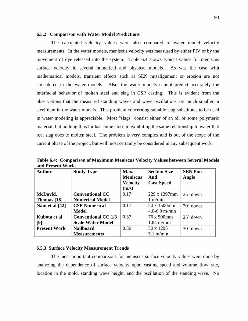
93
6.5.2 Comparison with Water Model Predictions
The calculated velocity values were also compared to water model velocity
measurements. In the water models, meniscus velocity was measured by either PIV or by the
movement of dye released into the system. Table 6.4 shows typical values for meniscus
surface velocity in several numerical and physical models. As was the case with
mathematical models, transient effects such as SEN misalignment or erosion are not
considered in the water models. Also, the water models cannot predict accurately the
interfacial behavior of molten steel and slag in CSP casting. This is evident from the
observations that the measured standing waves and wave oscillations are much smaller in
steel than in the water models. This problem concerning suitable slag substitutes to be used
in water modeling is appreciable. Most "slags" consist either of an oil or some polymeric
material, but nothing thus far has come close to exhibiting the same relationship to water that
real slag does to molten steel. The problem is very complex and is out of the scope of the
current phase of the project, but will most certainly be considered in any subsequent work.
Table 6.4: Comparison of Maximum Meniscus Velocity Values between Several Models and Present Work. Author Study Type Max.
Meniscus Velocity (m/s)
Section Size And Cast Speed
SEN Port Angle
McDavid, Thomas [18]
Conventional CC Numerical Model
0.17 229 x 1397mm 1 m/min
25° down
Nam et al [42] CSP Numerical Model
0.17 50 x 1500mm 4.0-6.0 m/min
70° down
Kubota et al [9]
Conventional CC 1/3 Scale Water Model
0.37 76 x 500mm 1.84 m/min
25° down
Present Work Nailboard Measurements
0.30 50 x 1295 5.1 m/min
30° down
6.5.3 Surface Velocity Measurement Trends
The most important comparisons for meniscus surface velocity values were done by
analyzing the dependence of surface velocity upon casting speed and volume flow rate,
location in the mold, standing wave height, and the oscillation of the standing wave. No
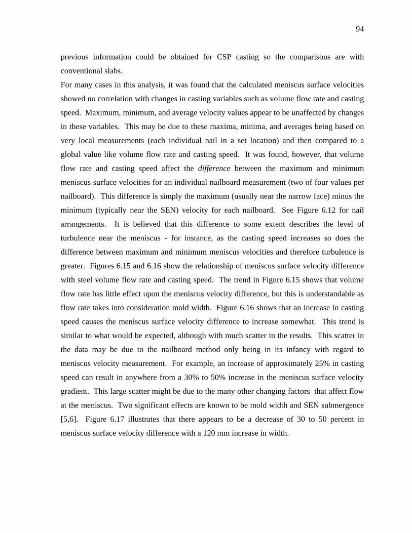
94
previous information could be obtained for CSP casting so the comparisons are with
conventional slabs.
For many cases in this analysis, it was found that the calculated meniscus surface velocities
showed no correlation with changes in casting variables such as volume flow rate and casting
speed. Maximum, minimum, and average velocity values appear to be unaffected by changes
in these variables. This may be due to these maxima, minima, and averages being based on
very local measurements (each individual nail in a set location) and then compared to a
global value like volume flow rate and casting speed. It was found, however, that volume
flow rate and casting speed affect the difference between the maximum and minimum
meniscus surface velocities for an individual nailboard measurement (two of four values per
nailboard). This difference is simply the maximum (usually near the narrow face) minus the
minimum (typically near the SEN) velocity for each nailboard. See Figure 6.12 for nail
arrangements. It is believed that this difference to some extent describes the level of
turbulence near the meniscus - for instance, as the casting speed increases so does the
difference between maximum and minimum meniscus velocities and therefore turbulence is
greater. Figures 6.15 and 6.16 show the relationship of meniscus surface velocity difference
with steel volume flow rate and casting speed. The trend in Figure 6.15 shows that volume
flow rate has little effect upon the meniscus velocity difference, but this is understandable as
flow rate takes into consideration mold width. Figure 6.16 shows that an increase in casting
speed causes the meniscus surface velocity difference to increase somewhat. This trend is
similar to what would be expected, although with much scatter in the results. This scatter in
the data may be due to the nailboard method only being in its infancy with regard to
meniscus velocity measurement. For example, an increase of approximately 25% in casting
speed can result in anywhere from a 30% to 50% increase in the meniscus surface velocity
gradient. This large scatter might be due to the many other changing factors that affect flow
at the meniscus. Two significant effects are known to be mold width and SEN submergence
[5,6]. Figure 6.17 illustrates that there appears to be a decrease of 30 to 50 percent in
meniscus surface velocity difference with a 120 mm increase in width.
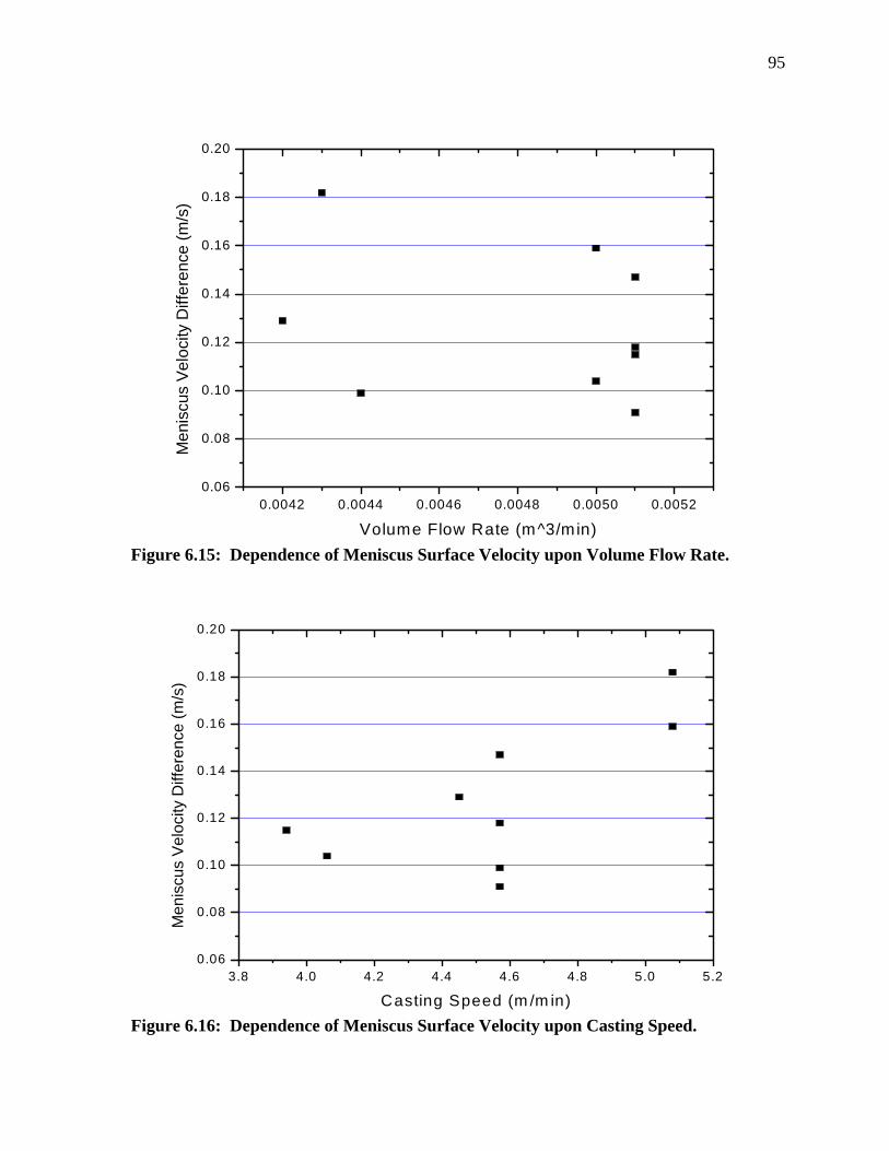
95
Figure 6.15: Dependence of Meniscus Surface Velocity upon Volume Flow Rate.
Figure 6.16: Dependence of Meniscus Surface Velocity upon Casting Speed.
0.0042 0.0044 0.0046 0.0048 0.0050 0.00520.06
0.08
0.10
0.12
0.14
0.16
0.18
0.20
Men
iscu
s Ve
loci
ty D
iffer
ence
(m/s
)
Volume Flow Rate (m^3/min)
3.8 4.0 4.2 4.4 4.6 4.8 5.0 5.20.06
0.08
0.10
0.12
0.14
0.16
0.18
0.20
Men
iscu
s V
eloc
ity D
iffer
ence
(m/s
)
Casting Speed (m /m in)
96
This makes good sense because as the mold width increases, there is more space for the steel
flowing from the SEN to lose more of its momentum as it flows, resulting in lower velocities
at the surface. Interestingly, increased SEN submergence depth appears to increase the
meniscus surface velocity (and the difference) (Figure 6.18), which might be due to the small
(29 mm) range of SEN submergence values. While this at first appears misleading,
Honeyands et al have shown that maximum wave height increases in water models when
SEN submergence exceeds approximately 225 mm [5]. On the other hand, Figure 6.19
shows that SEN submergence has no effect upon standing wave height. A more important
relationship is presented in Figure 6.20. This figure shows a moderate correlation between
standing wave height and meniscus surface velocity difference. This certainly makes sense
and is another indication that the meniscus surface velocity values calculated from nailboard
data reflect meniscus behavior.
An interesting observation regarding the diameter of the steel knobs that form on the
nails during immersion in the mold is that the knob diameter decreases with increasing
casting speed (Figure 6.21) yet increases with increasing meniscus surface velocity (Figure
6.22). The limited amount of data available at this point make it difficult to come to any
conclusions, but it is believed that with a large body of meniscus velocity data the nail/steel
knob diameter will decrease with increasing meniscus surface velocity and that there also
may be an effect of superheat.
6.6 Meniscus Surface Velocity Relationship with Standing Wave Fluctuation and
Oscillation
Meniscus surface velocity and the fluctuation of the standing wave (or the long-period wave)
were determined by Kubota et al to be related linearly [9]. A similar trend was observed in
the course of this project, although with lower surface velocities. Figure 6.23 shows a very
rough correlation with scatter, but with velocities varying only from 0.25 m/s to 0.30 m/s. It
is believed that the differences are due to Kubota's results being based on 1/3-scale water
model results and different mold geometry. To further investigate this phenomenon, the
period of the standing wave fluctuation was plotted versus the value of SEN submergence
divided by casting speed. Honeyands and Herbertson have shown a linear relationship
between the two in continuous slab casting [6]. Figure 6.24 shows similar results obtained
97
during this project. The value of SEN submergence divided by casting speed can be thought
of as the average residence time in the upper recirculation region of the mold. The solid
diamonds in Figure 6.24 represent standing wave oscillation periods as predicted by the
Honeyands/Herbertson water model and the open squares represent the actual standing wave
oscillation period as obtained through metal level fluctuation data and FFT analysis. The
error in the measured data is believed to originate with the variations in casting speed and
SEN submergence during operation.
6.7 Defects
For the June-July, 2000 trials, typical coil rejections were approximately 20%, mostly
for mold flux-related defects. Following a grade change from a boron-containing grade to
one without boron, a rejection rate of 0.5% was achieved thereafter and in the subsequent
trials in February and June, 2001. Finally, with the trial of the 4-port SEN, a rejection rate of
zero was achieved, albeit only with 54 coils (Table 5.5). The mold flux - related defects were
typical in appearance as described in the literature and contained trace amounts of sodium
and potassium, which are present only in mold fluxes (Figure 6.25)[13-14, 16].
Mold flux-related defects were found to occur with greatest frequency when boron-
containing grades were being produced. Prior to this project, internal rejection rates for mold
flux slivers were as high as 20-30%. Upon analysis of mold slags from both boron-
containing steels and steels without boron, it was found that the slags from boron-steels
picked up about 50% more alumina and anywhere from 20-100% more zirconia than slags
from regular carbon steels. The importance of boron and boron oxide has been discussed
previously in the literature review. One of the coils from a boron grade was found to have
41 mold flux sliver defects while coils of carbon steel of the same gauge with mold flux
slivers had only between one and five individual defects [58].
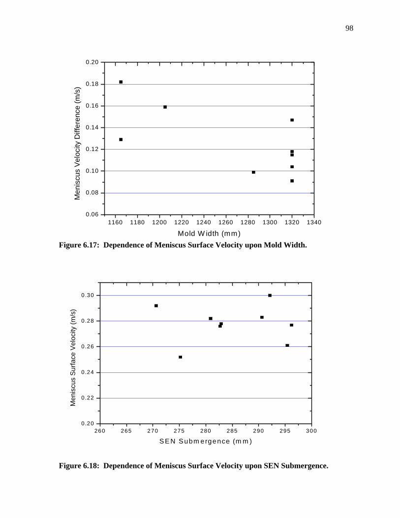
98
Figure 6.17: Dependence of Meniscus Surface Velocity upon Mold Width.
Figure 6.18: Dependence of Meniscus Surface Velocity upon SEN Submergence.
1160 1180 1200 1220 1240 1260 1280 1300 1320 13400.06
0.08
0.10
0.12
0.14
0.16
0.18
0.20
Men
iscu
s Ve
loci
ty D
iffer
ence
(m/s
)
Mold W idth (mm)
260 265 270 275 280 285 290 295 3000.20
0.22
0.24
0.26
0.28
0.30
Men
iscu
s Su
rface
Vel
ocity
(m/s
)
S E N S ubm ergence (m m )
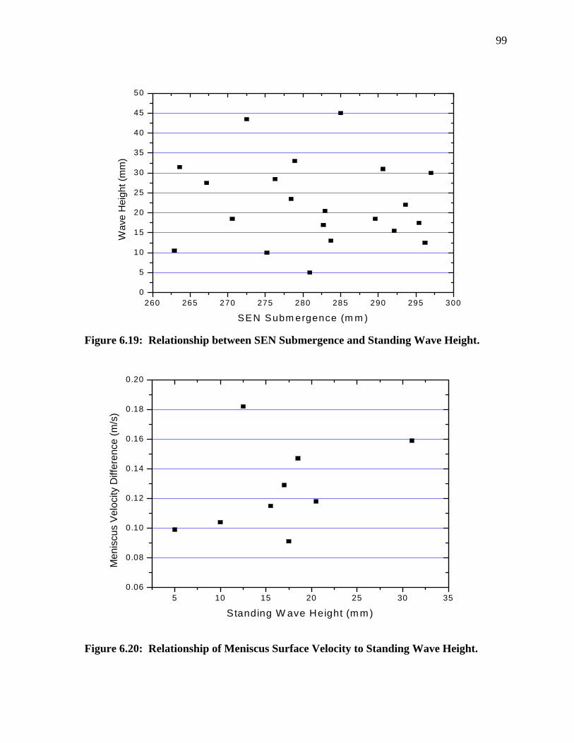
99
260 265 270 275 280 285 290 295 3000
5
10
15
20
25
30
35
40
45
50
Wav
e H
eigh
t (m
m)
SEN Subm ergence (m m ) Figure 6.19: Relationship between SEN Submergence and Standing Wave Height.
Figure 6.20: Relationship of Meniscus Surface Velocity to Standing Wave Height.
5 10 15 20 25 30 350.06
0.08
0.10
0.12
0.14
0.16
0.18
0.20
Men
iscu
s V
eloc
ity D
iffer
ence
(m/s
)
S tanding W ave Height (m m)
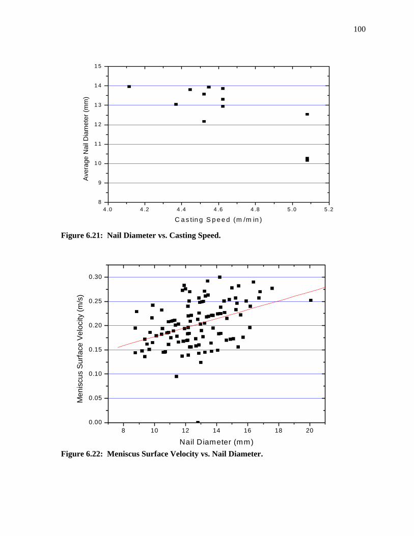
100
4 .0 4 .2 4 .4 4 .6 4 .8 5 .0 5 .28
9
1 0
1 1
1 2
1 3
1 4
1 5
Aver
age
Nai
l Dia
met
er (m
m)
C a s tin g S p e e d (m /m in ) Figure 6.21: Nail Diameter vs. Casting Speed.
Figure 6.22: Meniscus Surface Velocity vs. Nail Diameter.
8 10 12 14 16 18 200.00
0.05
0.10
0.15
0.20
0.25
0.30
Men
iscu
s Su
rface
Vel
ocity
(m/s
)
Nail Diameter (mm)
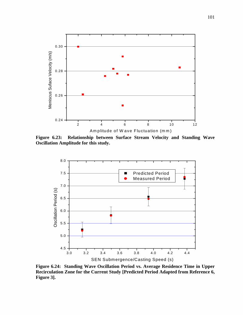
101
Figure 6.23: Relationship between Surface Stream Velocity and Standing Wave Oscillation Amplitude for this study.
Figure 6.24: Standing Wave Oscillation Period vs. Average Residence Time in Upper Recirculation Zone for the Current Study [Predicted Period Adapted from Reference 6, Figure 3].
3.0 3.2 3.4 3.6 3.8 4.0 4.2 4.44.5
5.0
5.5
6.0
6.5
7.0
7.5
8.0
Predicted Period Measured Period
Osc
illatio
n Pe
riod
(s)
SEN Submergence/Casting Speed (s)
2 4 6 8 10 120.24
0.26
0.28
0.30
Men
iscu
s Su
face
Vel
ocity
(m/s
)
A m p litude o f W ave F luctua tion (m m )
102
Mold flux sliver defects were observed to occur at seemingly random locations across
the width of the strip. Also appearing to be somewhat random were the estimated depths of
the defects. The depth of a defect could not always be estimated, however, as some amount
of delaminated steel that comes away from the rest of the coil is necessary to make such
estimations. Some defects appeared with no delaminated steel and the mold flux/slag residue
was visible along the entire length of the defect. Most slivers did exhibit some degree of
delamination and the thickness of this delaminated steel is believed to be proportional to the
depth at which the defect was deposited into the solidifying shell during casting. For
example, a defect with a delaminated steel thickness of 0.10 mm on a 0.50 mm coil is
estimated to have been deposited in the shell at a distance of 10 mm from the surface
(assuming a 100x reduction from a 50 mm thick slab).
Once the grade change was made and no boron was present in the steel, mold flux
sliver internal rejections average about 0.5%, but this was deemed too high. Further
inspection of mold flux slivers yielded some interesting results. For example, one defect had
a delaminated steel thickness of 0.06 mm. Since the slab was 50 mm thick and the finished
coil 0.50 mm thick (a 100x reduction), the defect was estimated to have been entrained at a
depth of 6 mm in from the slab surface (Figure 6.25).
Using the equation:
x = kt1/2 (6.7) [4]
where k is a caster constant (26 mm / min1/2) and t is the time in minutes, the depth in the
mold where the defect was deposited was calculated. The variable, x, is the depth of the
defect in millimeters. For a 6 mm defect depth, a time of 3.19 seconds is obtained and
knowing the casting speed to have been 5.08 m/min, it can be deduced the defect was
entrained in the steel shell at a distance of about 270 mm from the meniscus. In addition, it
was also observed that this defect occurred near the edge of the sheet. These factors indicate
that the mold flux slag was entrained by being drawn away from the meniscus steel/flux
interface then carried by the steel flow in the upper recirculation zone into the SEN exit
stream. This strong SEN exit flow then probably caused the entrained flux to be deposited
where it was, only to be exposed during rolling.
It is thought that the lack of observed mold flux defects on the steel produced using
the four-port SEN was due to the flow patterns in the mold. While details of the SEN are
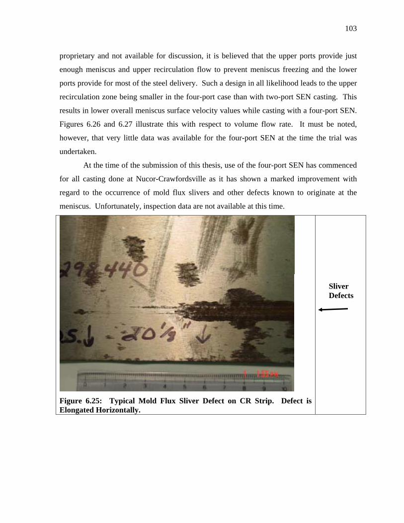
103
proprietary and not available for discussion, it is believed that the upper ports provide just
enough meniscus and upper recirculation flow to prevent meniscus freezing and the lower
ports provide for most of the steel delivery. Such a design in all likelihood leads to the upper
recirculation zone being smaller in the four-port case than with two-port SEN casting. This
results in lower overall meniscus surface velocity values while casting with a four-port SEN.
Figures 6.26 and 6.27 illustrate this with respect to volume flow rate. It must be noted,
however, that very little data was available for the four-port SEN at the time the trial was
undertaken.
At the time of the submission of this thesis, use of the four-port SEN has commenced
for all casting done at Nucor-Crawfordsville as it has shown a marked improvement with
regard to the occurrence of mold flux slivers and other defects known to originate at the
meniscus. Unfortunately, inspection data are not available at this time.
Figure 6.25: Typical Mold Flux Sliver Defect on CR Strip. Defect is Elongated Horizontally.
Sliver Defects
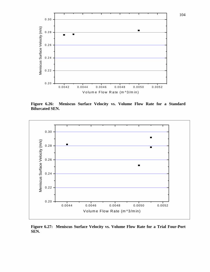
104
Figure 6.26: Meniscus Surface Velocity vs. Volume Flow Rate for a Standard Bifurcated SEN.
Figure 6.27: Meniscus Surface Velocity vs. Volume Flow Rate for a Trial Four-Port SEN.
0.0044 0.0046 0.0048 0.0050 0.00520.20
0.22
0.24
0.26
0.28
0.30
Men
iscu
s Su
rface
Vel
ocity
(m/s
)
V o lum e F low R ate (m ^3/m in)
0 .0 0 4 2 0 .0 0 4 4 0 .0 0 4 6 0 .0 0 4 8 0 .0 0 5 0 0 .0 0 5 20 .2 0
0 .2 2
0 .2 4
0 .2 6
0 .2 8
0 .3 0
Men
iscu
s S
urfa
ce V
eloc
ity (m
/s)
V o lu m e F lo w R a te (m ^3 /m in )
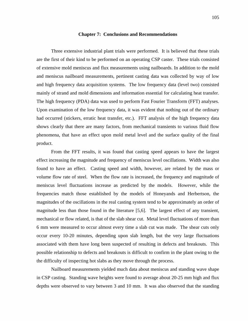
105
Chapter 7: Conclusions and Recommendations
Three extensive industrial plant trials were performed. It is believed that these trials
are the first of their kind to be performed on an operating CSP caster. These trials consisted
of extensive mold meniscus and flux measurements using nailboards. In addition to the mold
and meniscus nailboard measurements, pertinent casting data was collected by way of low
and high frequency data acquisition systems. The low frequency data (level two) consisted
mainly of strand and mold dimensions and information essential for calculating heat transfer.
The high frequency (PDA) data was used to perform Fast Fourier Transform (FFT) analyses.
Upon examination of the low frequency data, it was evident that nothing out of the ordinary
had occurred (stickers, erratic heat transfer, etc.). FFT analysis of the high frequency data
shows clearly that there are many factors, from mechanical transients to various fluid flow
phenomena, that have an effect upon mold metal level and the surface quality of the final
product.
From the FFT results, it was found that casting speed appears to have the largest
effect increasing the magnitude and frequency of meniscus level oscillations. Width was also
found to have an effect. Casting speed and width, however, are related by the mass or
volume flow rate of steel. When the flow rate is increased, the frequency and magnitude of
meniscus level fluctuations increase as predicted by the models. However, while the
frequencies match those established by the models of Honeyands and Herbertson, the
magnitudes of the oscillations in the real casting system tend to be approximately an order of
magnitude less than those found in the literature [5,6]. The largest effect of any transient,
mechanical or flow related, is that of the slab shear cut. Metal level fluctuations of more than
6 mm were measured to occur almost every time a slab cut was made. The shear cuts only
occur every 10-20 minutes, depending upon slab length, but the very large fluctuations
associated with them have long been suspected of resulting in defects and breakouts. This
possible relationship to defects and breakouts is difficult to confirm in the plant owing to the
the difficulty of inspecting hot slabs as they move through the process.
Nailboard measurements yielded much data about meniscus and standing wave shape
in CSP casting. Standing wave heights were found to average about 20-25 mm high and flux
depths were observed to vary between 3 and 10 mm. It was also observed that the standing
106
wave is always higher near the narrow face and flux depths are greater nearer the SEN under
ordinary casting conditions. When used in conjunction with oscillation mark measurement
and FFT results that provide magnitudes of standing wave height and level fluctuations due
to mechanical and flow-induced transients, a new consistent understanding of mold/meniscus
behavior in thin-slab casting has emerged. These nailboard measurements are believed to be
the first on a CSP process. However, they differ from previous research for reasons that are
unclear and require further investigation. One interesting result of this use of the nailboard
data in conjunction with FFT data is the similarity of flow and standing wave behavior when
compared to the work of Honeyands and Herbertson – the oscillation of the standing wave
with changes in the steel residence time in the upper recirculating region in this project match
almost perfectly their results [6]. This is important because their work was carried out on
water models, conventional slab casters, and rectangular mold thin-slab casters.
The most groundbreaking findings of this project stem from refinement of the
nailboard method. These measurements have built on previous findings of meniscus/standing
wave and flux depth behavior (from conventional casting studies) and have yielded data
pertaining to the fluid flow behavior in the molten steel/flux interfacial region, including
meniscus surface velocities. Flow direction as determined from nailboard inspection has
been observed to possibly have an impact upon standing wave height. At flow rotations
greater than 45 degrees, a slight decrease in standing wave has been detected when compared
to other heats cast under similar conditions. The calculated meniscus velocity values appear
to be consistent with the values found in the literature even though no experimental values
for CSP casting with similar conditions to those in this project have been published to date.
Typical average meniscus surface velocities determined in the study average about 0.25 m/s
at a casting speed of approximately 5 m/min and a mold width of 1200 mm. This compares
favorably with published velocity values even though the casting conditions in this study are
not to be found in the literature. Dependence of meniscus surface velocity upon casting
speed and volume flow rate is at present inconclusive with no apparent correlation.
However, a trend showing that the difference between maximum and minimum meniscus
velocities increases with casting speed was noted and may possibly be an indication of
increased turbulence in the meniscus region. A similar trend was also observed with respect

107
to standing wave height, as would be expected since standing wave height is known to vary
directly with casting speed and volume flow rate.
The observation that meniscus surface velocity decreases with increasing mold width
suggests that flow velocity and the resultant turbulence and defects might be related to the
geometry of the upper recirculation zone. This is somewhat supported by the results of the
four-port SEN trial where no defects were observed. The calculated meniscus surface
velocities were similar for both the two- and four-port SEN, but the construction of the SENs
is very different, which certainly has a large impact upon the geometry of the upper
recirculation zone.
This preliminary work will allow operators to perform this very simple and
inexpensive test several times during a shift. Prior to any measurement of the steel knob on
the ends of the nails, an operator will be able to get an approximate idea of the standing wave
dimensions and any crossflow that might be occurring. If these visual observations are made
frequently during a sequence, much may be learned about the evolution of steel flow due to
SEN wear/erosion. From three simple measurements that can be made with calipers, a local
meniscus velocity can be calculated, which can then be used in evaluating the likelihood of
slag emulsification and defect generation.
108
REFERENCES
[1] J.K. Brimacombe and I.V. Samarasekera. "The Challenges of Thin Slab Casting." Near-Net-Shape Casting in the Minimills Conference, Vancouver, British Columbia, August 19-23, 1995, p.33-53. [2] W. Hennig, F. Quix, and D. Schulz. "CSP Concepts/Strategies - Developments over the last 10 Years." 12th Seminario de Aceria of the Instituto Argentino de Siderurgia (IAS), Buenos Aires, November 2-5, 1999, p.439-448. [3] E. Hoffken, P. Kappes, and H. Lax. "The Production of Continuously Cast Strip on the Pilot Plant at Buschhutten." Stahl und Eisen, v. 106, no. 23, p. 27-33, 1986. [4] USS Research Continuous Casting Technology Course. December 5-9, 1994, Monroeville, PA. [5] T. Honeyands, J. Lucas, J. Chambers, and J. Herbertson. "Preliminary Modelling of Steel Delivery to Thin Slab Caster Moulds." 1992 Steelmaking Conference Proceedings, 1992, p. 451-459. [6] T.A. Honeyands and J. Herbertson. "Oscillations in Thin Slab Caster Mould Flows." 127th ISIJ Meeting, March, 1994, Tokyo, Japan. [7] J.Y. Lamant, M. Larrecq, A. Mouchette, Y. Codur, J. Gancarz, A. Leclercq. "Advanced Control of Mold Operation and Improved Slab Surface Quality on Sollac Continuous Casters." Proceedings of the Sixth International Iron and Steel Congress, 1990, Nagoya, Japan, p. 317-324. [8] H. Tanaka, H. Kuwatori, and R. Nisihara. "Analysis of Continuous Casting Powder Entrapping Phenomena by Water-Model Experiments." Journal of the ISIJ, Vol. 78, no. 5, 1992, p. 73-78. [9] J. Kubota, K. Okimoto, M. Suzuki, A. Shirayama, and T. Masaoka. "Mechanism of Level Fluctuation and Mold Powder Catching in Slab Continuous Casting at High Speeds." Proceedings of the Sixth International Iron and Steel Congress, 1990, Nagoya, Japan, p. 356-363. [10] S. Feldbauer, I. Jimbo, A. Sharan, K. Shimizu, W. King, J. Stepanek, J. Harman, and A.W. Cramb. "Physical Properties of Mold Slags That Are Relevant to Clean Steel Manufacture." 1995 Steelmaking Conference Proceedings, 1995, p. 655-667. [11] R. Bommaraju, T. Jackson, J. Lucas, and G. Skoczylas. "Design, Development and Application of Mold Powder to Reduce Slivers." Continuous Casting Volume Seven, ISS, 1995, p. 165-171.
109
[12] A.W. Cramb, Y. Chung, J. Harman, A. Sharan, and I. Jimbo. "The Slag/Metal Interface and Associated Phenomena." Iron and Steelmaker (USA), Vol. 74, no. 3, 1997, p. 77-83. [13] N.A. McPherson and S.L. McIntosh. "Mould Powder Related Defects in Some Continuously Cast Steel Products." Continuous Casting Volume Seven, ISS, 1995, p. 145-153. [14] M. Byrne, A.W. Cramb, and T.W. Fenicle. "The Sources of Exogenous Inclusions in Continuous Cast, Aluminum-Killed Steels." Continuous Casting Volume Seven, ISS, 1995, p. 133-143. [15] J.M. Harman and A.W. Cramb. "A Study of the Effect of Fluid Physical Properties upon Droplet Emulsification." 1996 Steelmaking Conference Proceedings, 1996, p. 773-784. [16] S. Feldbauer and A.W. Cramb. "Insights into Slag Entrainment in the Mold of a Continuous Caster." 13th PTD Conference Proceedings, 1996, p. 327-340. [17] M. Gebhard, Q.L. He, and J. Herbertson. "Vortexing Phenomena in Continuous Slab Casting Moulds." 1993 Steelmaking Conference Proceedings, 1993, p. 441-446. [18] R.M. McDavid and B.G. Thomas. "Flow and Thermal Behavior of the Top Surface Flux/Powder Layers in Continuous Casting Molds." Metallurgical and Materials Transactions B, Vol. 27B, August, 1996, p. 672-685. [19] B.G. Thomas, Q Yuan, S. Sivaramakrishnan, T. Shi, S.P. Vanka, M.B. Assar. "Comparison of Four Methods to Evaluate Fluid Velocities in a Continuous Slab Casting Mold." ISIJ International, Vol. 41, No. 10, 2001, p. 1262-1271. [20] B.G. Thomas, A. Dennisov and H. Bai. "Behavior of Argon Bubbles During Continuous Casting of Steel." 1997 Steelmaking Conference Proceedings, 1997, p. 375-391. [21] A.C. Mikrovas and S.A. Argyropoulos. "A Novel Technique to Estimate Velocity in Liquid Steel and in Other High Temperature Liquid Metals." Iron and Steelmaker, October 1993, p. 85-93. [22] M. Hanao, M. Kawamoto, H. Mizukami, and K. Hanazaki. "Influence of Velocity of Molten Steel Flow near the Meniscus in a Continuous Casting Mold on Surface Quality of Slabs." 1999 Steelmaking Conference Proceedings, 1999, p. 63-70. [23] H. Mizukami, M. Hanao, S. Hiraki, and M. Kawamoto, T. Watanabe, A. Hayashi, and M. Iguchi. "Measurement of Meniscus Flow Velocity in High Speed Continuous Casting Mold." Tetsu-to-Hagane, Vol. 86, no. 4, 2000, p. 63-68.
110
[24] S.A. Argyropoulos. "Measurement of Velocity in High Temperature Metals and Slags." Fundamentals of Metallurgical Processing: The James M. Toguri Symposium (Canada), August 2000, p. 31-42. [25] T. Koeplin. Telephone conversation in October 2000. [26] B.G. Thomas and Hua Bai. "Tundish Nozzle Clogging - Application of Computational Models." 18th PTD Conference Proceedings, Vol. 18, 2001. [27] S.G. Kollberg, H.R. Hackl, and P.J. Hanley. "Improving quality of flat rolled products using electromagnetic brake (EMBR) in continuous casting." Iron and Steel Engineer, Vol. 73, no. 7, 1996, p. 24-28. [28] J. Lehmann, M. Boher, and M.C. Kaerle. "An experimental study of the interactions between liquid steel and a MgO-based tundish refractory." CIM Bulletin, Vol. 90, no. 1013, 1997, p. 69-74. [29] W. Holler. "Prevention of alumina clogging in submerged nozzles for continuous casting of steel by introduction of a carbon-free inner layer." Veitsch-Radex Rundschau (Germany), Vol. 1, 1999, p. 30-39. [30] Ravi Rastogi and Alan Cramb. Personal Communication, 2002. [31] W. Lai, M. Milone, and I.V. Samarasekera. "Meniscus Thermal Analysis as a Tool for Evaluating Slab Surface Quality." Unpublished Research, University of British Columbia, 1999. [32] X. Huang and B.G. Thomas. "Modeling of Transient Flow Phenomena in Continuous Casting of Steel." Canadian Metallurgical Quarterly, Vol. 37, no. 3-4, 1998, p. 197-212. [33] M. Byrne and A.W. Cramb. "Operating Experience with Large Tundishes." Continuous Casting Volume Seven, ISS, 1995, p. 155-164. [34] Continuous Casting Volume Seven, ISS, 1995. [35] C.G. Aneziris, E.M. Pfaff, and H.R. Maier. "The Zirconia/Slag/Air Interface of Zirconia Based Submerged Entry Nozzles During Near Net Shape Steel Casting." British Ceramic Proceedings (UK), Vol. 60, no. 1, 1999, p. 459-460. [36] D.E. Larson. Nucor Steel, Personal Communication, December 18-20, 2000. [37] M.S. Jenkins, B.G. Thomas, W.C. Chen, and R.B. Mahapatra. "Investigation of Strand Surface Defects Using Mold Instrumentation and Modelling." 1994 Steelmaking Conference Proceedings, 1994, p. 337-345.
111
[38] F.M. Najjar, B.G. Thomas, and D.E. Hershey. "Numerical Study of Steady Turbulent Flow through Bifurcated Nozzles in Continuous Casting." Metallurgical and Materials Transactions B, Vol. 26B, August 1995, p. 749-765. [39] H.B.M. Schulte, R.H.M.G. Nabben, D.W. van der Plas, and D. Triezenberg. "Study of the fluid flow in the mould for high quality slab casting." Le Revue de Metallurgie-CIT, June 1997, p. 751-759. [40] A. Vaterlaus. "Innovative Clogging Prevention and Mold Flow Optimization by the Whirl SEN." 1997 Steelmaking Conference Proceedings, 1997, p. 165-172. [41] L.J. Heaslip and J. Schade. "Physical Modeling and Visualization of Liquid Steel Flow Behavior During Continuous Casting." Iron and Steelmaker, Vol. 26, no. 1, 1999, p. 33-41. [42] H. Nam, H. Park, and J.K. Yoon. "Numerical Analysis of Influences of Operation Parameters on Fluid Flow and Heat Transfer in Funnel Type Mold of Thin Slab Casters." Second International Conference on Processing Materials for Properties, TMS, 2000, p. 363-368. [43] J.D. Lee and C.H. Yim. "The Mechanism of Unsteady Bulging and Its Analysis with the Finite Element Method for Continuously Cast Steel." ISIJ International, Vol. 40, no. 8, 2000, p. 765-770. [44] S. Kumar, B.N. Walker, I.V. Samarasekera, and J.K. Brimacombe. "Chaos at the Meniscus - The Genesis of Defects in Continuously Cast Steel Billets." 13th PTD Conference Proceedings, 1995, p. 119-141. [45] D.T. Stone and B.G. Thomas. "Measurement and Modeling of Heat Transfer Across Interfacial Mold Flux Layers." Canadian Metallurgical Quarterly, Vol. 38, no. 5, 1999, p. 363-375. [46] H. Yasunaka, K. Nakayama, K. Ebina, T. Saito, M. Kimura, and H. Matuda. "Improvement of Transverse Corner Cracks in Continuously Cast Hypoeutectic Slabs." Tetsu-to-Hagane, Vol. 81, no. 9, 1995, p. 894-899. [47] R.B. Mahapatra, J.K. Brimacombe, I.V. Samarasekera, N. Walker, E.A. Patterson, and J.D. Young. "Mold Behavior and Its Influence on Quality in the Continuous Casting of Steel Slabs: Part 1. Industrial Trials, Mold Temperature Measurements, and Mathematical Modeling." Metallurgical Transactions B, Vol. 22B, December 1991, p. 861-874. [48] R.B. Mahapatra, J.K. Brimacombe, I.V. Samarasekera. ". "Mold Behavior and Its Influence on Quality in the Continuous Casting of Steel Slabs: Part 2. Mold Heat Transfer, Mold Flux Behavior, Formation of Oscillation Marks, Longitudinal Off-Corner Depressions, and Subsurface Cracks." Metallurgical Transactions B, Vol. 22B, December 1991, p. 875-888.
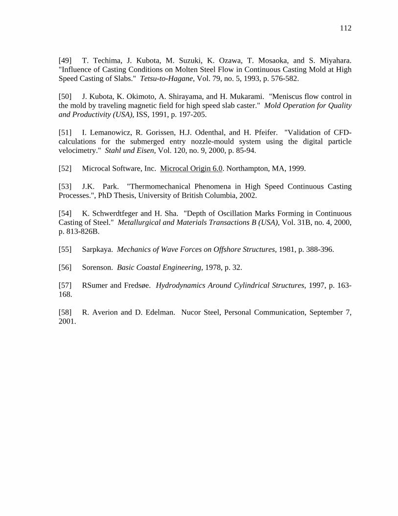
112
[49] T. Techima, J. Kubota, M. Suzuki, K. Ozawa, T. Mosaoka, and S. Miyahara. "Influence of Casting Conditions on Molten Steel Flow in Continuous Casting Mold at High Speed Casting of Slabs." Tetsu-to-Hagane, Vol. 79, no. 5, 1993, p. 576-582. [50] J. Kubota, K. Okimoto, A. Shirayama, and H. Mukarami. "Meniscus flow control in the mold by traveling magnetic field for high speed slab caster." Mold Operation for Quality and Productivity (USA), ISS, 1991, p. 197-205. [51] I. Lemanowicz, R. Gorissen, H.J. Odenthal, and H. Pfeifer. "Validation of CFD-calculations for the submerged entry nozzle-mould system using the digital particle velocimetry." Stahl und Eisen, Vol. 120, no. 9, 2000, p. 85-94. [52] Microcal Software, Inc. Microcal Origin 6.0. Northampton, MA, 1999. [53] J.K. Park. "Thermomechanical Phenomena in High Speed Continuous Casting Processes.", PhD Thesis, University of British Columbia, 2002. [54] K. Schwerdtfeger and H. Sha. "Depth of Oscillation Marks Forming in Continuous Casting of Steel." Metallurgical and Materials Transactions B (USA), Vol. 31B, no. 4, 2000, p. 813-826B. [55] Sarpkaya. Mechanics of Wave Forces on Offshore Structures, 1981, p. 388-396. [56] Sorenson. Basic Coastal Engineering, 1978, p. 32. [57] RSumer and Fredsøe. Hydrodynamics Around Cylindrical Structures, 1997, p. 163-168. [58] R. Averion and D. Edelman. Nucor Steel, Personal Communication, September 7, 2001.

113
APPENDIX 1: METAL LEVEL, FFT, AND RAW NAILBOARD RESULTS FOR 2-PORT SEN TRIAL
(CASE 4 DATA)

114
Table A1.1: Pertinent Information for Heats That Were Part of 2-Port SEN Trial. Heat Grade Interval Size (s) Cast Speed(m/min) Width (mm) 213760 W3 1100 5.08 1205 117004 W3 3600 5.08 1205 117005 W3 1800 5.08 1205 117006 W3 1800 5.08 1185 213763 W3 1800 4.45 1150
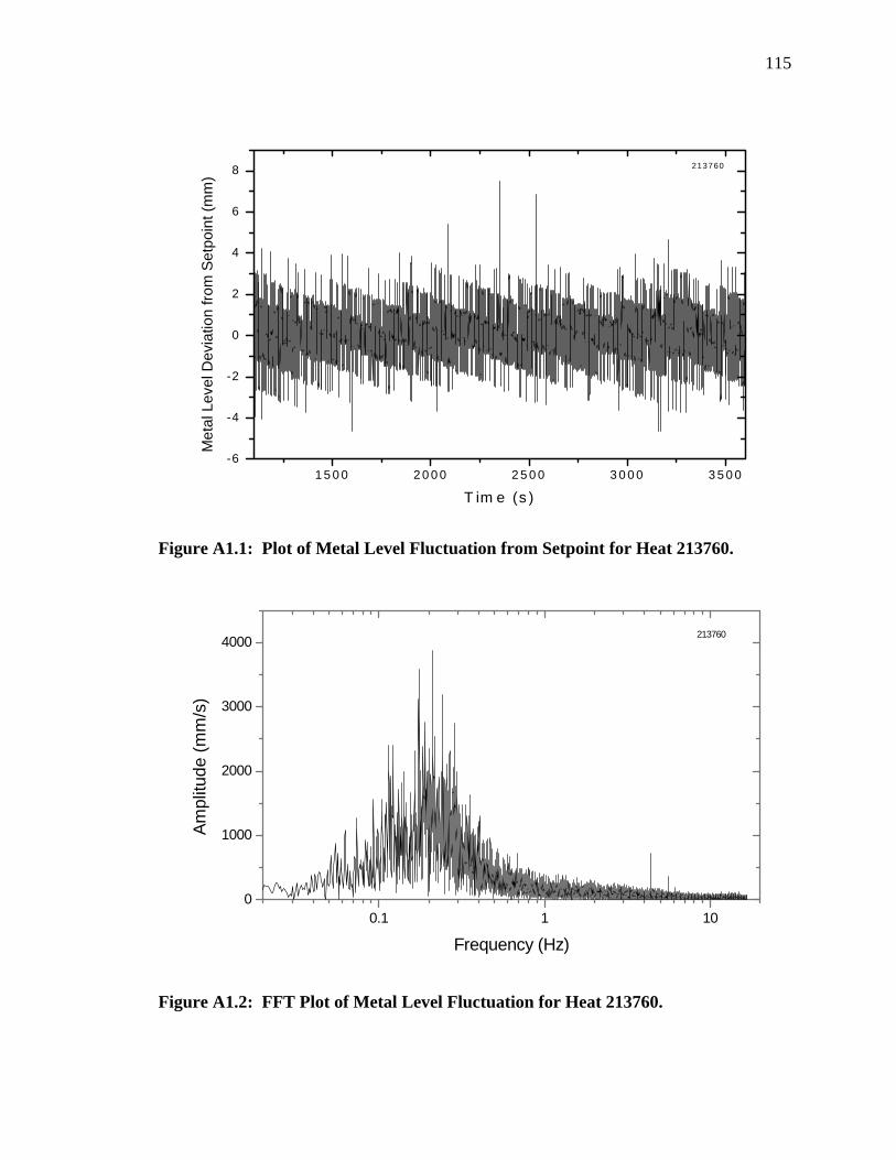
115
Figure A1.1: Plot of Metal Level Fluctuation from Setpoint for Heat 213760.
Figure A1.2: FFT Plot of Metal Level Fluctuation for Heat 213760.
1 5 0 0 2 0 0 0 2 5 0 0 3 0 0 0 3 5 0 0-6
-4
-2
0
2
4
6
8 213760
Met
al L
evel
Dev
iatio
n fro
m S
etpo
int (
mm
)
T im e (s )
0.1 1 100
1000
2000
3000
4000 213760
Frequency (Hz)
Ampl
itude
(mm
/s)
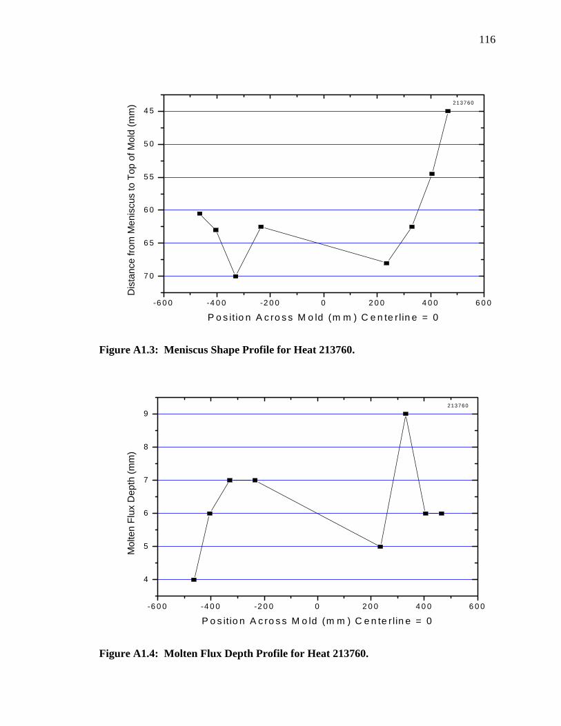
116
Figure A1.3: Meniscus Shape Profile for Heat 213760.
Figure A1.4: Molten Flux Depth Profile for Heat 213760.
-6 0 0 -4 0 0 -2 0 0 0 2 0 0 4 0 0 6 0 0
7 0
6 5
6 0
5 5
5 0
4 5213760
Dis
tanc
e fro
m M
enis
cus
to T
op o
f Mol
d (m
m)
P o s it io n A c ro s s M o ld (m m ) C e n te r lin e = 0
-6 0 0 -4 0 0 -2 0 0 0 2 0 0 4 0 0 6 0 0
4
5
6
7
8
9213760
Mol
ten
Flux
Dep
th (m
m)
P o s itio n A c ro s s M o ld (m m ) C e n te r lin e = 0
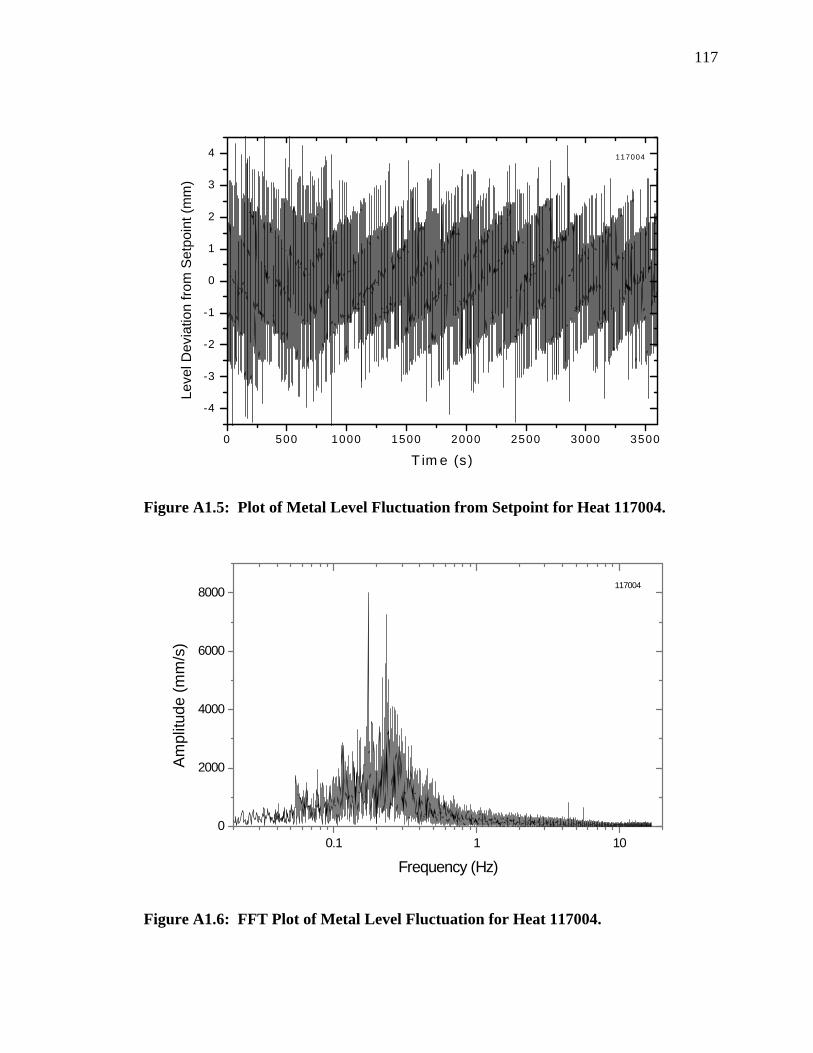
117
Figure A1.5: Plot of Metal Level Fluctuation from Setpoint for Heat 117004.
Figure A1.6: FFT Plot of Metal Level Fluctuation for Heat 117004.
0 500 1000 1500 2000 2500 3000 3500
-4
-3
-2
-1
0
1
2
3
4 117004
Leve
l Dev
iatio
n fro
m S
etpo
int (
mm
)
T im e (s)
0.1 1 100
2000
4000
6000
8000 117004
Frequency (Hz)
Ampl
itude
(mm
/s)
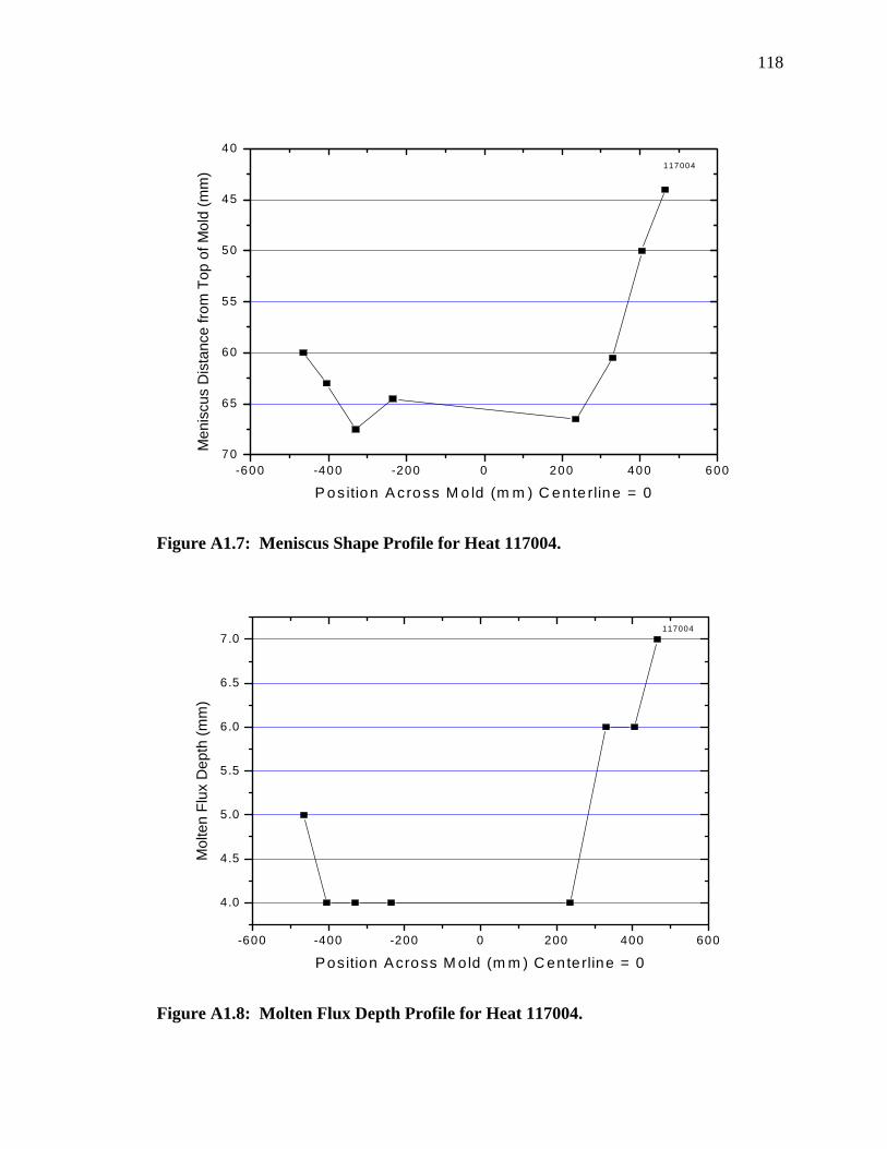
118
Figure A1.7: Meniscus Shape Profile for Heat 117004.
Figure A1.8: Molten Flux Depth Profile for Heat 117004.
-600 -400 -200 0 200 400 60070
65
60
55
50
45
40117004
Men
iscu
s D
ista
nce
from
Top
of M
old
(mm
)
P os ition A cross M o ld (m m ) C en te rline = 0
-600 -400 -200 0 200 400 600
4.0
4.5
5.0
5.5
6.0
6.5
7.0117004
Mol
ten
Flux
Dep
th (m
m)
Position Across M old (m m ) C enterline = 0
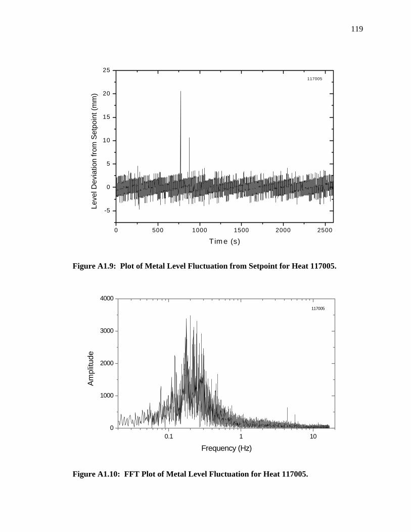
119
Figure A1.9: Plot of Metal Level Fluctuation from Setpoint for Heat 117005.
Figure A1.10: FFT Plot of Metal Level Fluctuation for Heat 117005.
0 500 1000 1500 2000 2500
-5
0
5
10
15
20
25117005
Leve
l Dev
iatio
n fro
m S
etpo
int (
mm
)
T im e (s)
0.1 1 100
1000
2000
3000
4000117005
Frequency (Hz)
Ampl
itude
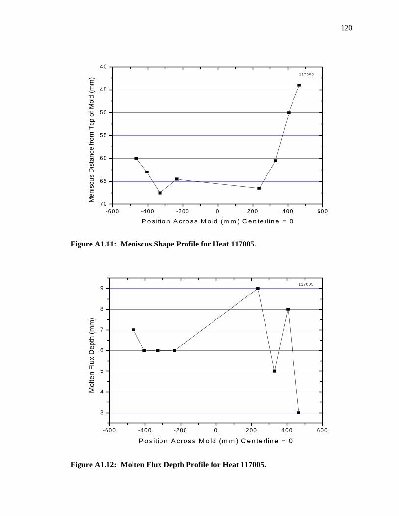
120
Figure A1.11: Meniscus Shape Profile for Heat 117005.
Figure A1.12: Molten Flux Depth Profile for Heat 117005.
-600 -400 -200 0 200 400 60070
65
60
55
50
45
40117005
Men
iscu
s D
ista
nce
from
Top
of M
old
(mm
)
P os ition A cross M o ld (m m ) C en te rline = 0
-600 -400 -200 0 200 400 600
3
4
5
6
7
8
9117005
Mol
ten
Flux
Dep
th (m
m)
Position Across M old (m m ) C enterline = 0
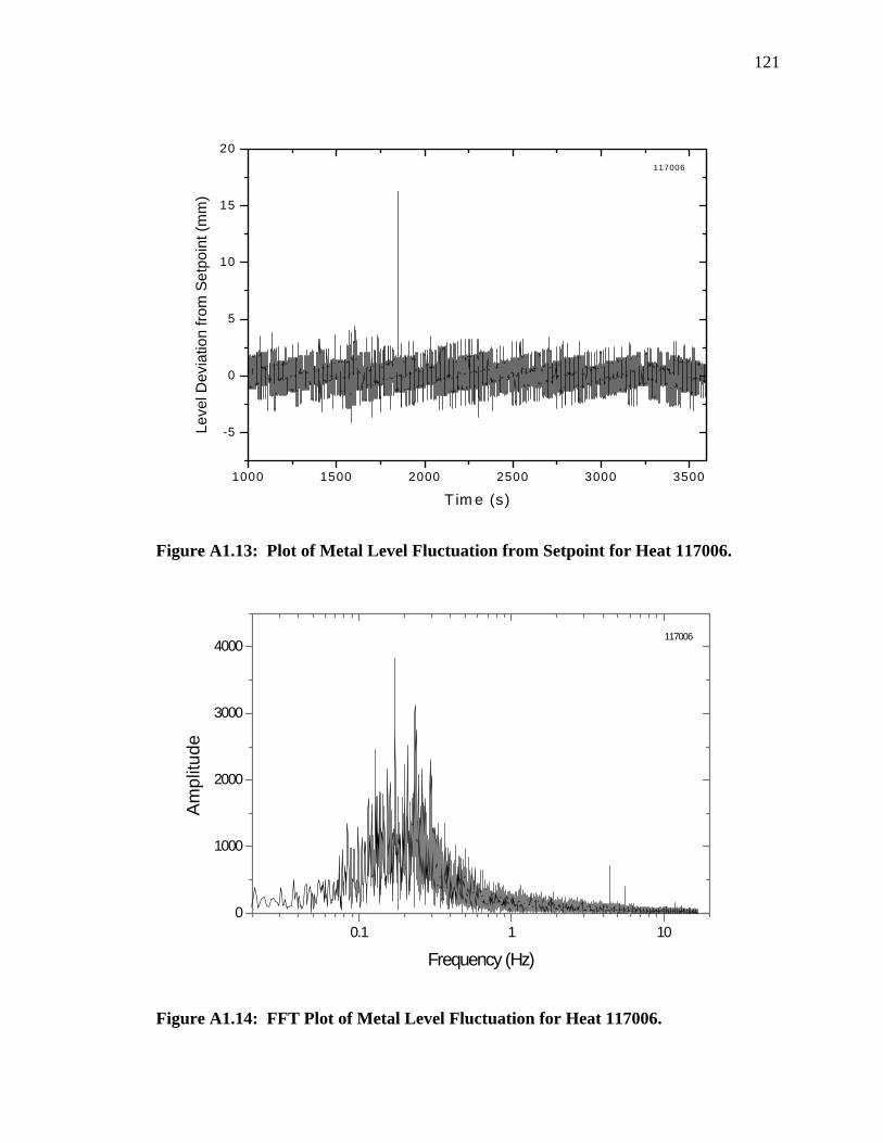
121
Figure A1.13: Plot of Metal Level Fluctuation from Setpoint for Heat 117006.
Figure A1.14: FFT Plot of Metal Level Fluctuation for Heat 117006.
1000 1500 2000 2500 3000 3500
-5
0
5
10
15
20117006
Leve
l Dev
iatio
n fro
m S
etpo
int (
mm
)
T im e (s)
0.1 1 100
1000
2000
3000
4000117006
Frequency (Hz)
Am
plitu
de
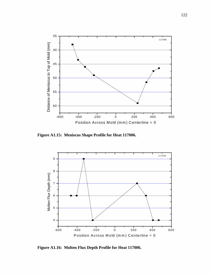
122
Figure A1.15: Meniscus Shape Profile for Heat 117006.
Figure A1.16: Molten Flux Depth Profile for Heat 117006.
-600 -400 -200 0 200 400 600
60
55
50
45
40
35117006
Dis
tanc
e of
Men
iscu
s to
Top
of M
old
(mm
)
Position Across Mold (m m ) Centerline = 0
-600 -400 -200 0 200 400 600
4
5
6
7
8
9117006
Mol
ten
Flux
Dep
th (m
m)
P o s itio n A c ro ss M o ld (m m ) C e n te rlin e = 0
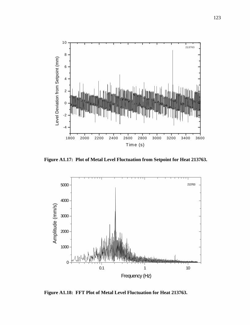
123
Figure A1.17: Plot of Metal Level Fluctuation from Setpoint for Heat 213763.
Figure A1.18: FFT Plot of Metal Level Fluctuation for Heat 213763.
1800 2000 2200 2400 2600 2800 3000 3200 3400 3600
-4
-2
0
2
4
6
8
10213763
Leve
l Dev
iatio
n fro
m S
etpo
int (
mm
)
T im e (s)
0.1 1 100
1000
2000
3000
4000
5000 213763
Frequency (Hz)
Ampl
itude
(mm
/s)
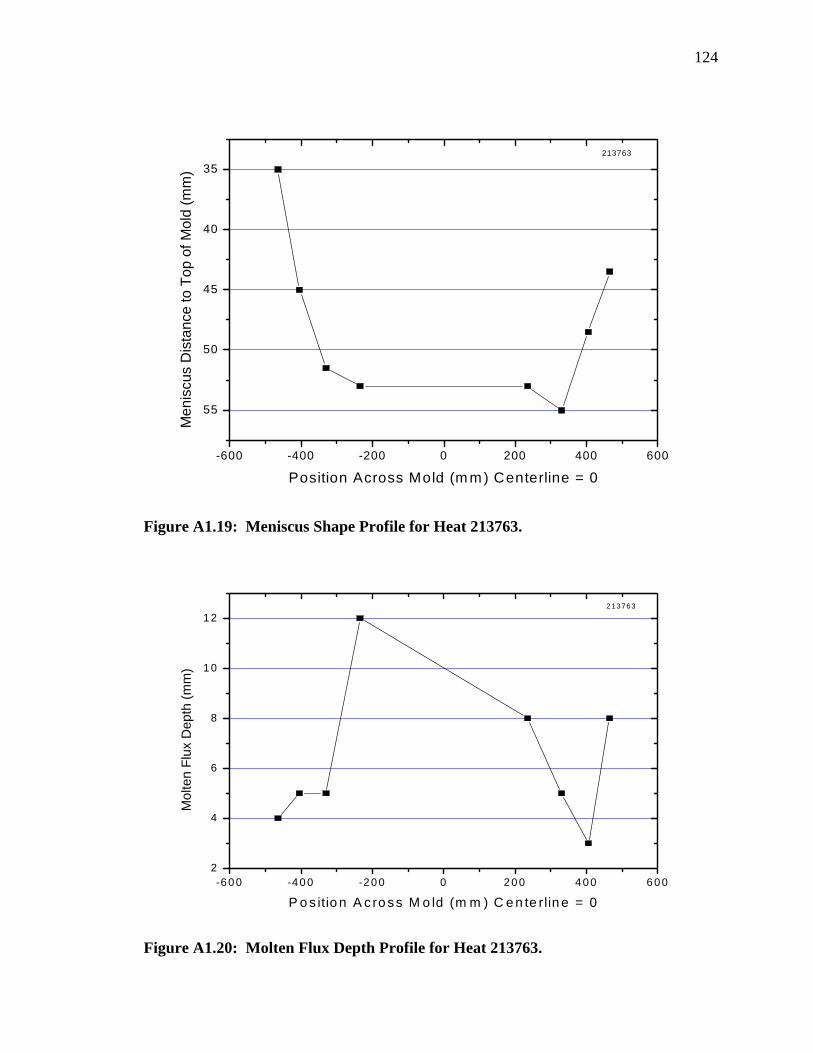
124
Figure A1.19: Meniscus Shape Profile for Heat 213763.
Figure A1.20: Molten Flux Depth Profile for Heat 213763.
-600 -400 -200 0 200 400 600
55
50
45
40
35213763
Men
iscu
s D
ista
nce
to T
op o
f Mol
d (m
m)
Position Across Mold (m m) Centerline = 0
-6 0 0 -4 0 0 -2 0 0 0 2 0 0 4 0 0 6 0 02
4
6
8
1 0
1 22 13 76 3
Mol
ten
Flux
Dep
th (m
m)
P o s itio n A c ro ss M o ld (m m ) C e n te rlin e = 0

125
APPENDIX 2: METAL LEVEL, FFT, AND RAW NAILBOARD RESULTS FOR 4-PORT SEN TRIAL
(CASE 4 DATA)

126
Table A2.1: Pertinent Information for Heats That Were Part of 4-Port SEN Trial. Heat Grade Interval Size (s) Cast Speed(m/min) Width (mm) 117021 T1 1000 3.94 1392 117022 T1 1800 4.57 1392 117023 T1 1800 4.57 1320 117024 T1 1800 4.57 1320 117025 T1 1800 4.57 1320 117026 T1 1700 4.06 1320 213782 T7 1200 4.57 1320 213783 T7 1800 4.57 1285 213784 P1 1800 4.57 1280
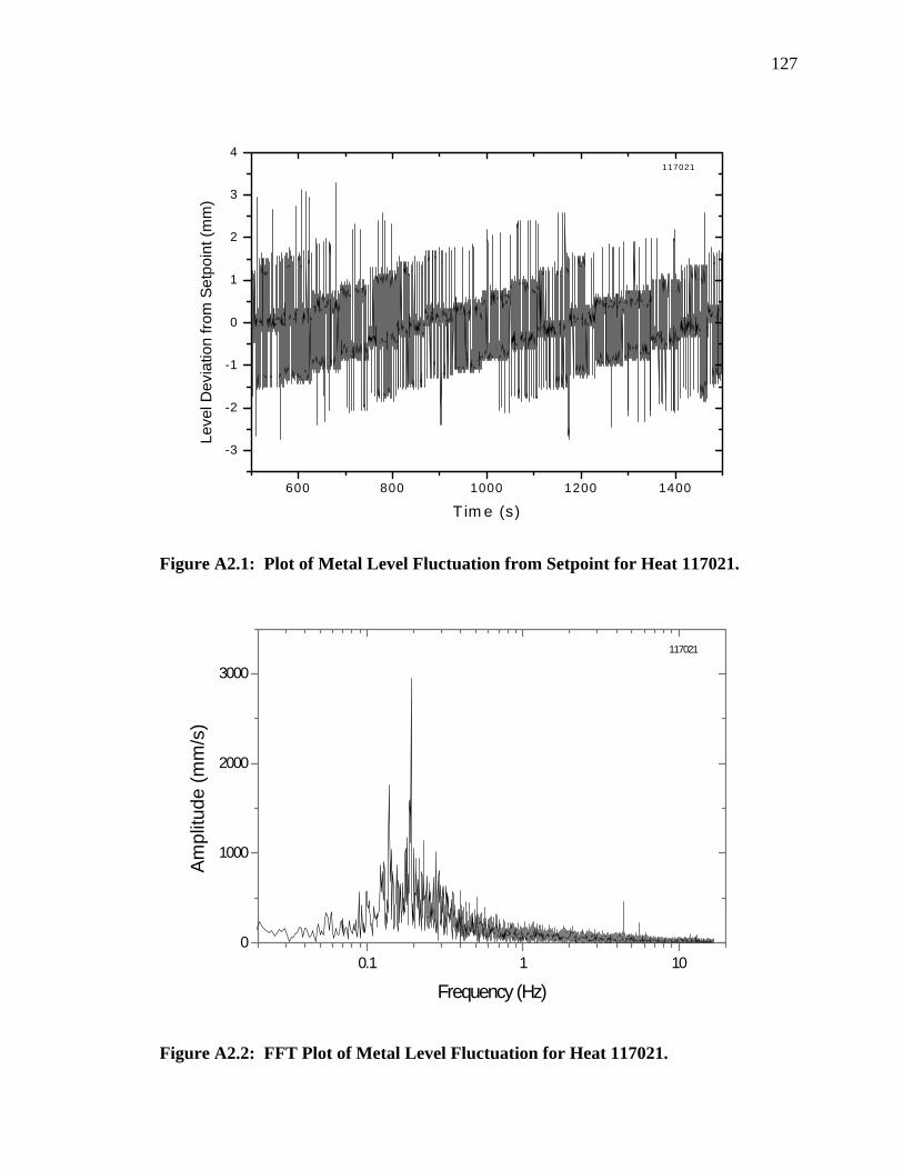
127
Figure A2.1: Plot of Metal Level Fluctuation from Setpoint for Heat 117021.
Figure A2.2: FFT Plot of Metal Level Fluctuation for Heat 117021.
600 800 1000 1200 1400
-3
-2
-1
0
1
2
3
4117021
Leve
l Dev
iatio
n fro
m S
etpo
int (
mm
)
T im e (s)
0.1 1 100
1000
2000
3000117021
Frequency (Hz)
Am
plitu
de (m
m/s
)
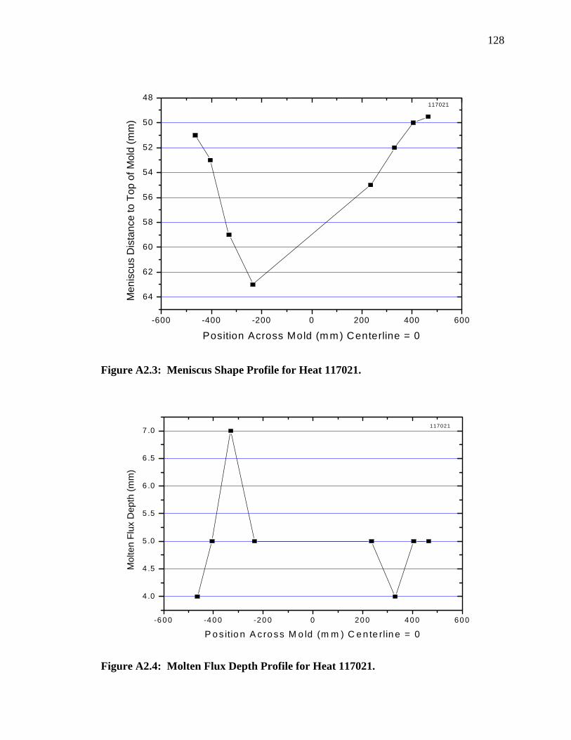
128
Figure A2.3: Meniscus Shape Profile for Heat 117021.
Figure A2.4: Molten Flux Depth Profile for Heat 117021.
-600 -400 -200 0 200 400 600
64
62
60
58
56
54
52
50
48117021
Men
iscu
s D
ista
nce
to T
op o
f Mol
d (m
m)
Position Across Mold (m m) Centerline = 0
-6 00 -40 0 -20 0 0 200 4 00 60 0
4 .0
4 .5
5 .0
5 .5
6 .0
6 .5
7 .0117021
Mol
ten
Flux
Dep
th (m
m)
P o s itio n A cro ss M o ld (m m ) C e n te rlin e = 0
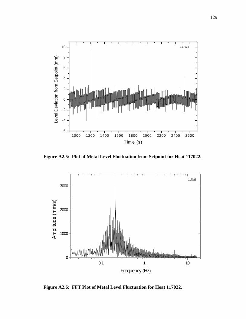
129
Figure A2.5: Plot of Metal Level Fluctuation from Setpoint for Heat 117022.
Figure A2.6: FFT Plot of Metal Level Fluctuation for Heat 117022.
1000 1200 1400 1600 1800 2000 2200 2400 2600-6
-4
-2
0
2
4
6
8
10 117022
Leve
l Dev
iatio
n fro
m S
etpo
int (
mm
)
T im e (s)
0.1 1 100
1000
2000
3000117022
Frequency (Hz)
Ampl
itude
(mm
/s)
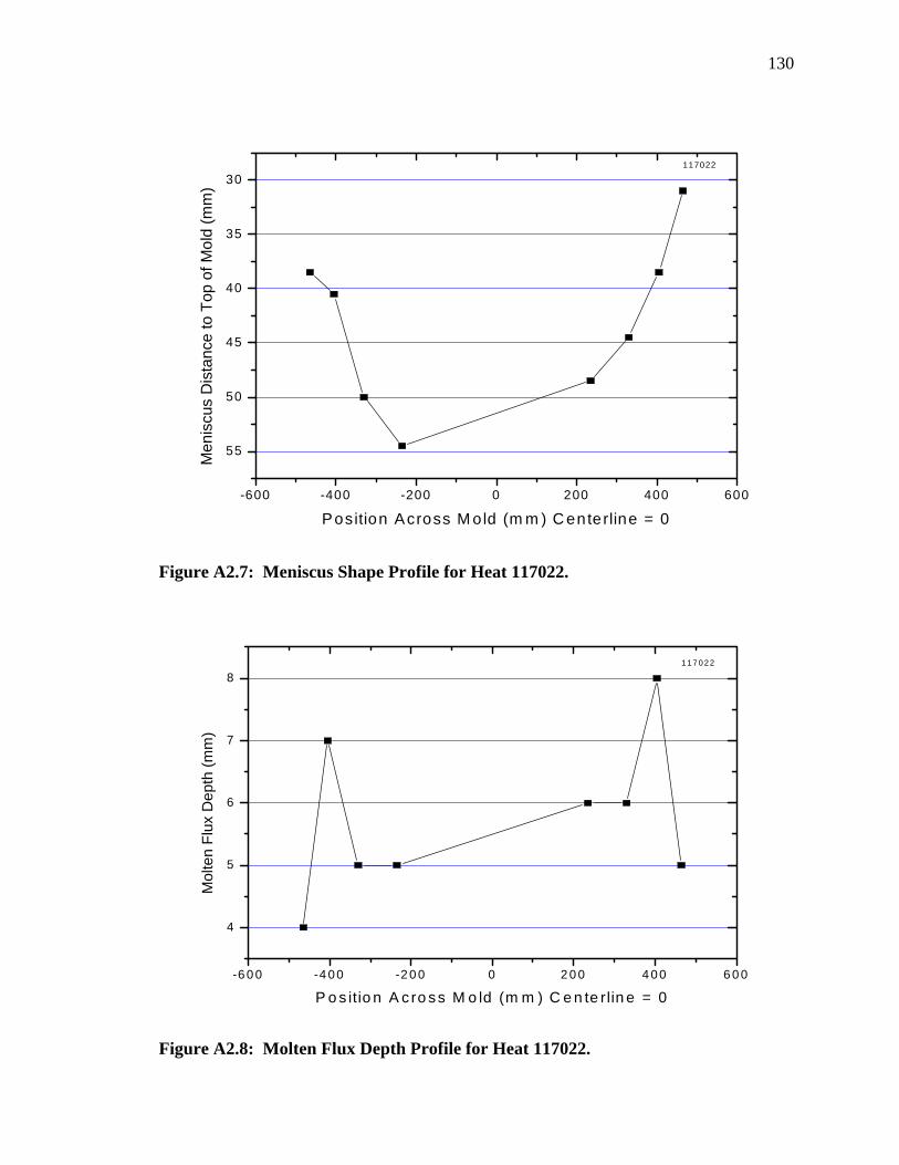
130
Figure A2.7: Meniscus Shape Profile for Heat 117022.
Figure A2.8: Molten Flux Depth Profile for Heat 117022.
-600 -400 -200 0 200 400 600
55
50
45
40
35
30117022
Men
iscu
s D
ista
nce
to T
op o
f Mol
d (m
m)
Position Across M old (m m ) C enterline = 0
-6 0 0 -4 00 -2 0 0 0 2 0 0 4 00 6 0 0
4
5
6
7
81 17 022
Mol
ten
Flux
Dep
th (m
m)
P o s itio n A c ro ss M o ld (m m ) C e n te rlin e = 0
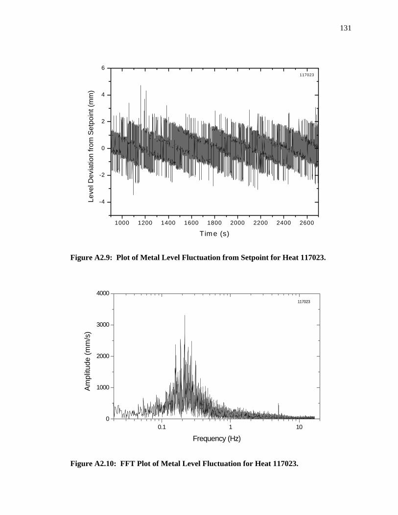
131
Figure A2.9: Plot of Metal Level Fluctuation from Setpoint for Heat 117023.
Figure A2.10: FFT Plot of Metal Level Fluctuation for Heat 117023.
1000 1200 1400 1600 1800 2000 2200 2400 2600
-4
-2
0
2
4
6117023
Leve
l Dev
iatio
n fro
m S
etpo
int (
mm
)
T ime (s)
0.1 1 100
1000
2000
3000
4000117023
Frequency (Hz)
Am
plitu
de (m
m/s
)
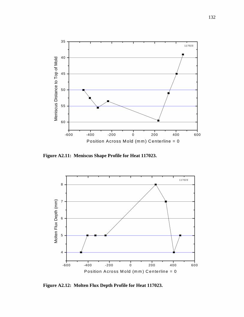
132
Figure A2.11: Meniscus Shape Profile for Heat 117023.
Figure A2.12: Molten Flux Depth Profile for Heat 117023.
-600 -400 -200 0 200 400 600
60
55
50
45
40
35117023
Men
iscu
s D
ista
nce
to T
op o
f Mol
d
Position Across Mold (m m ) Centerline = 0
-600 -400 -200 0 200 400 600
4
5
6
7
8117023
Mol
ten
Flux
Dep
th (m
m)
P os ition A cross M o ld (m m ) C en te rline = 0
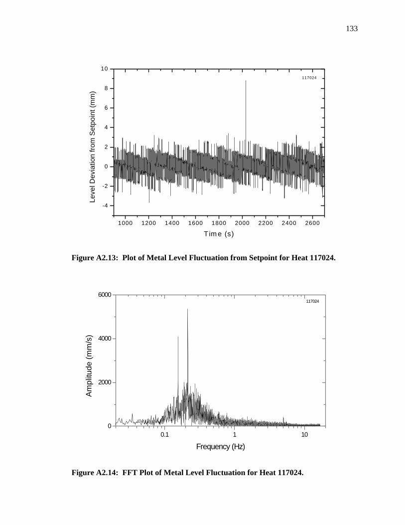
133
Figure A2.13: Plot of Metal Level Fluctuation from Setpoint for Heat 117024.
Figure A2.14: FFT Plot of Metal Level Fluctuation for Heat 117024.
1000 1200 1400 1600 1800 2000 2200 2400 2600
-4
-2
0
2
4
6
8
10117024
Leve
l Dev
iatio
n fro
m S
etpo
int (
mm
)
T im e (s)
0.1 1 100
2000
4000
6000117024
Frequency (Hz)
Am
plitu
de (m
m/s
)
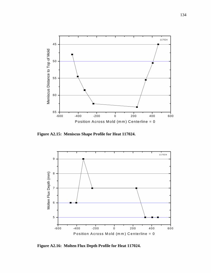
134
Figure A2.15: Meniscus Shape Profile for Heat 117024.
Figure A2.16: Molten Flux Depth Profile for Heat 117024.
-600 -400 -200 0 200 400 60065
60
55
50
45117024
Men
iscu
s D
ista
nce
to T
op o
f Mol
d
Position Across Mold (m m ) Centerline = 0
-600 -400 -200 0 200 400 600
5
6
7
8
9117024
Mol
ten
Flux
Dep
th (m
m)
P o s itio n A c ro ss M o ld (m m ) C e n te rlin e = 0
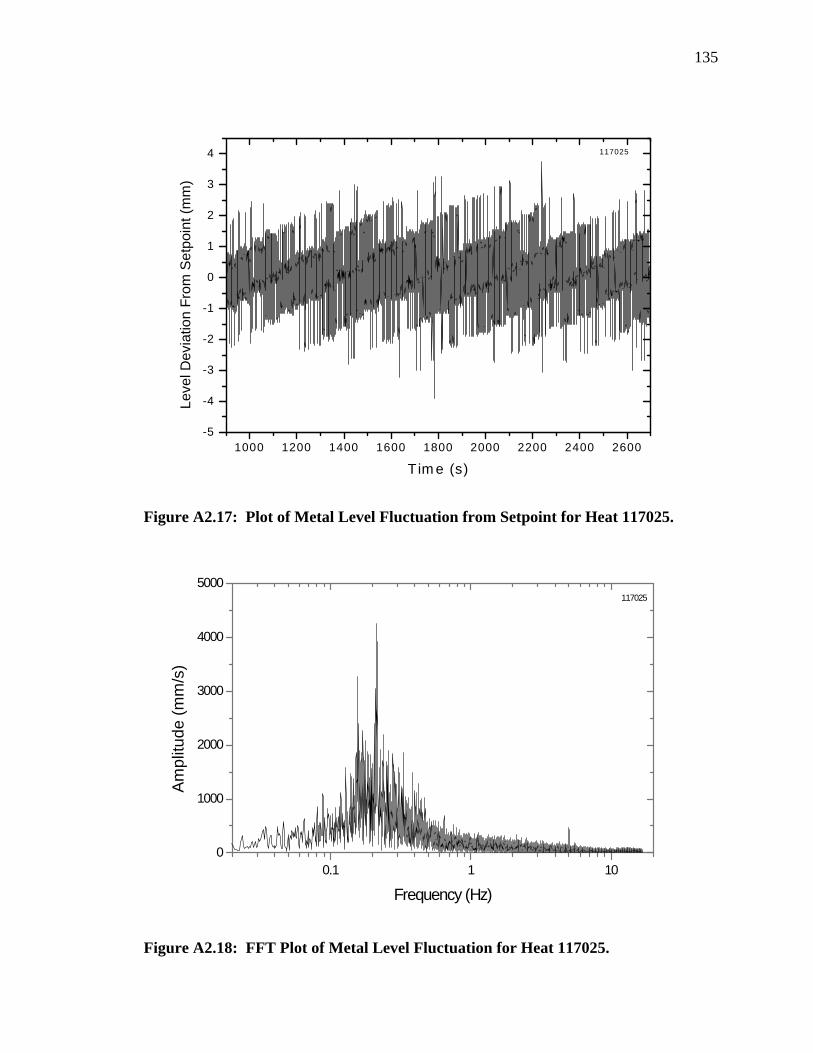
135
Figure A2.17: Plot of Metal Level Fluctuation from Setpoint for Heat 117025.
Figure A2.18: FFT Plot of Metal Level Fluctuation for Heat 117025.
1000 1200 1400 1600 1800 2000 2200 2400 2600-5
-4
-3
-2
-1
0
1
2
3
4 117025
Leve
l Dev
iatio
n Fr
om S
etpo
int (
mm
)
T im e (s)
0.1 1 100
1000
2000
3000
4000
5000117025
Frequency (Hz)
Ampl
itude
(mm
/s)
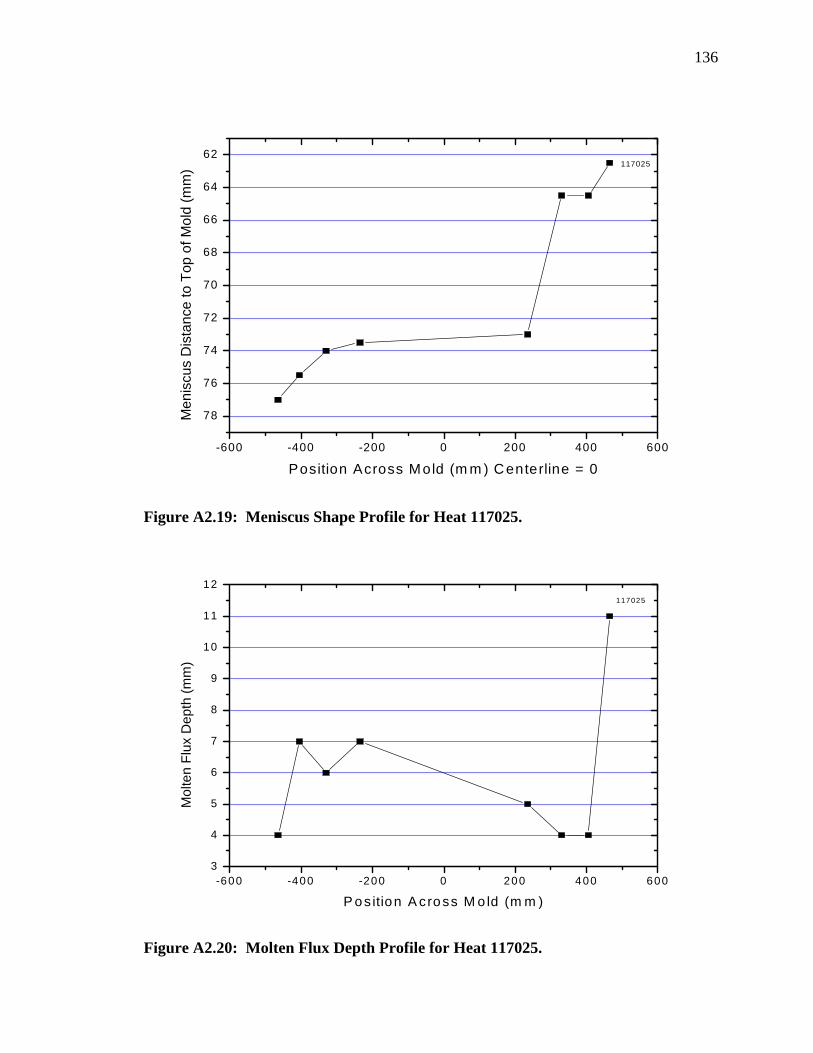
136
Figure A2.19: Meniscus Shape Profile for Heat 117025.
Figure A2.20: Molten Flux Depth Profile for Heat 117025.
-600 -400 -200 0 200 400 600
78
76
74
72
70
68
66
64
62117025
Men
iscu
s D
ista
nce
to T
op o
f Mol
d (m
m)
Position Across Mold (m m ) Centerline = 0
-600 -400 -200 0 200 400 6003
4
5
6
7
8
9
10
11
12117025
Mol
ten
Flux
Dep
th (m
m)
P os ition A cross M o ld (m m )
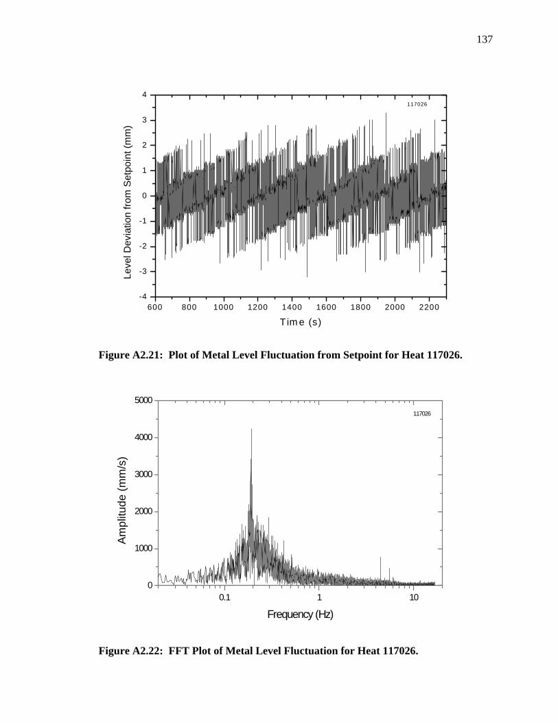
137
Figure A2.21: Plot of Metal Level Fluctuation from Setpoint for Heat 117026.
Figure A2.22: FFT Plot of Metal Level Fluctuation for Heat 117026.
600 800 1000 1200 1400 1600 1800 2000 2200-4
-3
-2
-1
0
1
2
3
4117026
Leve
l Dev
iatio
n fro
m S
etpo
int (
mm
)
T im e (s)
0.1 1 100
1000
2000
3000
4000
5000117026
Frequency (Hz)
Ampl
itude
(mm
/s)
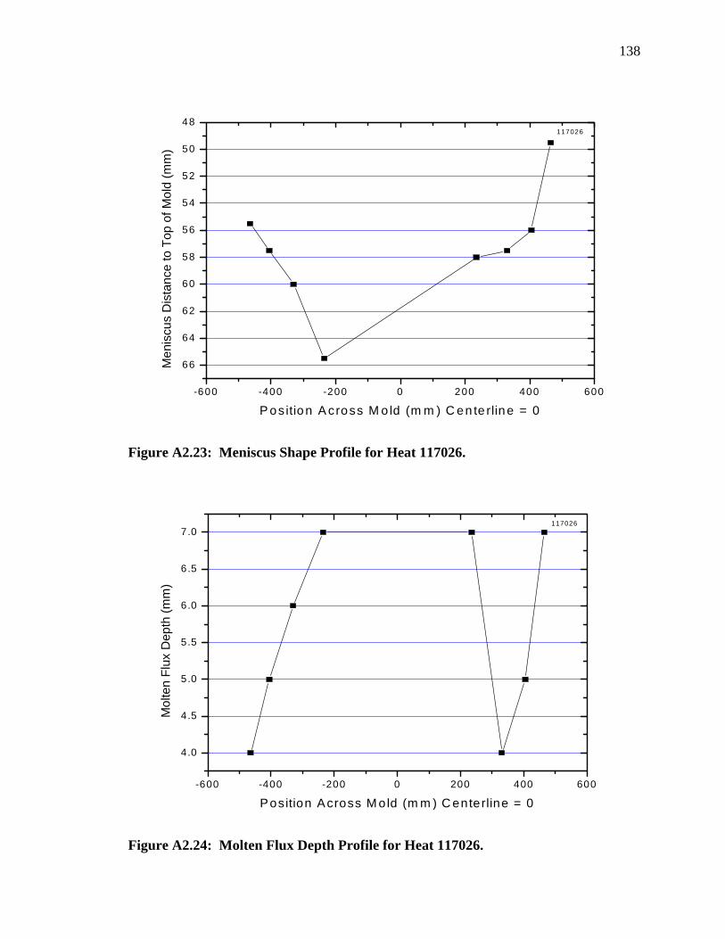
138
Figure A2.23: Meniscus Shape Profile for Heat 117026.
Figure A2.24: Molten Flux Depth Profile for Heat 117026.
-600 -400 -200 0 200 400 600
66
64
62
60
58
56
54
52
50
48117026
Men
iscu
s D
ista
nce
to T
op o
f Mol
d (m
m)
P os ition A cross M o ld (m m ) C en te rline = 0
-600 -400 -200 0 200 400 600
4.0
4.5
5.0
5.5
6.0
6.5
7.0117026
Mol
ten
Flux
Dep
th (m
m)
Position Across M old (m m ) C enterline = 0
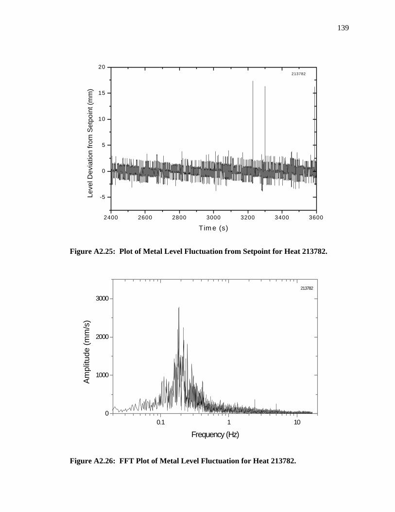
139
Figure A2.25: Plot of Metal Level Fluctuation from Setpoint for Heat 213782.
Figure A2.26: FFT Plot of Metal Level Fluctuation for Heat 213782.
2400 2600 2800 3000 3200 3400 3600
-5
0
5
10
15
20213782
Leve
l Dev
iatio
n fro
m S
etpo
int (
mm
)
T im e (s)
0.1 1 100
1000
2000
3000213782
Frequency (Hz)
Ampl
itude
(mm
/s)
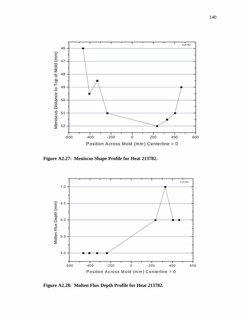
140
Figure A2.27: Meniscus Shape Profile for Heat 213782.
Figure A2.28: Molten Flux Depth Profile for Heat 213782.
-600 -400 -200 0 200 400 600
52
51
50
49
48
47
46213782
Men
iscu
s D
ista
nce
to T
op o
f Mol
d (m
m)
Position Across Mold (mm) Centerline = 0
-600 -400 -200 0 200 400 600
5.0
5.5
6.0
6.5
7.0213782
Mol
ten
Flux
Dep
th (m
m)
P os ition Across M o ld (m m ) C enterline = 0
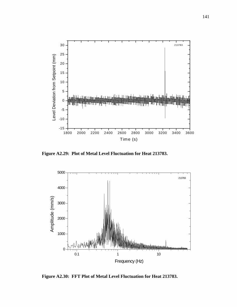
141
Figure A2.29: Plot of Metal Level Fluctuation for Heat 213783.
Figure A2.30: FFT Plot of Metal Level Fluctuation for Heat 213783.
1800 2000 2200 2400 2600 2800 3000 3200 3400 3600-15
-10
-5
0
5
10
15
20
25
30 213783
Leve
l Dev
iatio
n fro
m S
etpo
int (
mm
)
T ime (s)
0.1 1 100
1000
2000
3000
4000
5000213783
Frequency (Hz)
Am
plitu
de (m
m/s
)
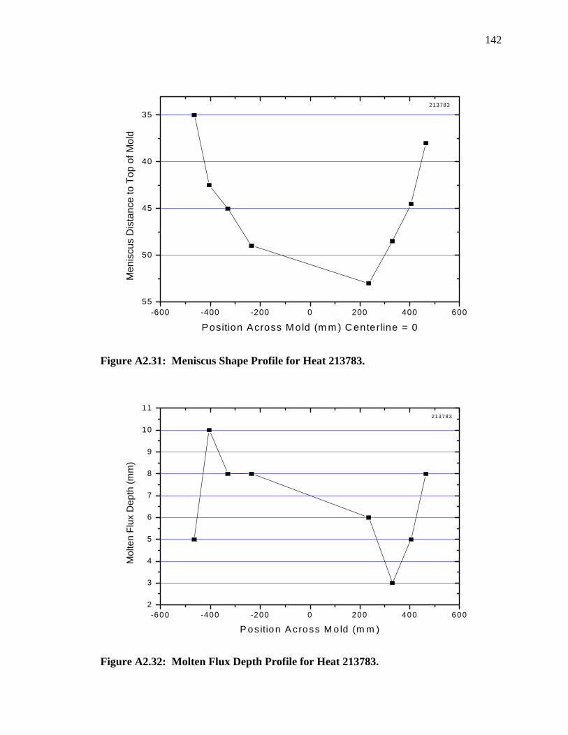
142
Figure A2.31: Meniscus Shape Profile for Heat 213783.
Figure A2.32: Molten Flux Depth Profile for Heat 213783.
-600 -400 -200 0 200 400 60055
50
45
40
35213783
Men
iscu
s D
ista
nce
to T
op o
f Mol
d
Position Across Mold (m m ) Centerline = 0
-600 -400 -200 0 200 400 6002
3
4
5
6
7
8
9
10
11213783
Mol
ten
Flux
Dep
th (m
m)
P os ition A cross M o ld (m m )
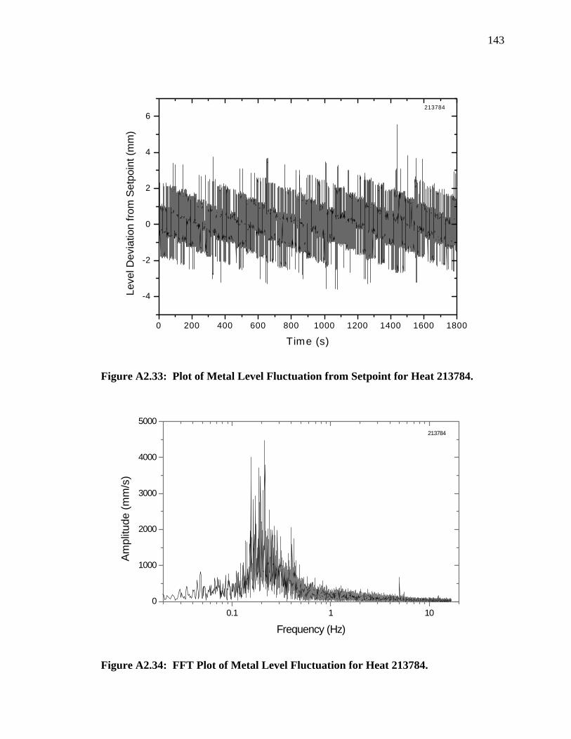
143
Figure A2.33: Plot of Metal Level Fluctuation from Setpoint for Heat 213784.
Figure A2.34: FFT Plot of Metal Level Fluctuation for Heat 213784.
0 200 400 600 800 1000 1200 1400 1600 1800
-4
-2
0
2
4
6213784
Leve
l Dev
iatio
n fro
m S
etpo
int (
mm
)
Time (s)
0.1 1 100
1000
2000
3000
4000
5000213784
Frequency (Hz)
Am
plitu
de (m
m/s
)
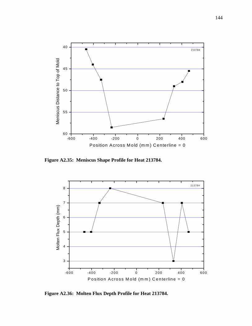
144
Figure A2.35: Meniscus Shape Profile for Heat 213784.
Figure A2.36: Molten Flux Depth Profile for Heat 213784.
-600 -400 -200 0 200 400 60060
55
50
45
40213784
Men
iscu
s D
ista
nce
to T
op o
f Mol
d
Position Across Mold (m m ) Centerline = 0
-600 -400 -200 0 200 400 600
3
4
5
6
7
8213784
Mol
ten
Flux
Dep
th (m
m)
P o s itio n A c ro ss M o ld (m m ) C e n te rlin e = 0


![New directions in synthetic solid state chemistry ...chemgroups.northwestern.edu/kanatzidis/Reprints/...of flux-assembled [P,Q,]“- (Q=S,Se) anions with metal centers (using molten](https://img.pdfslide.us/doc/110x75/5ed780f728a0984b5c033b65/new-directions-in-synthetic-solid-state-chemistry-of-flux-assembled-pqaoe-.jpg)