Measurement Uncertainty in Non-Destructive Testing

Be Absolutely Assured

Technical Note 35 - June 2011

Issued: June 2011

Measurement Uncertainty in Non-Destructive Testing

© Copyright National Association of Testing Authorit ies, Australia 2011 All intellectual property rights in this publication are the property of the National Association of Testing Authorities, Australia (NATA). Users of this publication acknowledge that they do not have the right to use this material without written permission from NATA. This publication is protected by copyright under the Commonwealth of Australia Copyright Act 1968. You must not modify copy, reproduce, republish, frame, upload to a third party, store in a retrieval system, post, transmit or distribute this content in any way or any form or by any means, except as expressly authorised by NATA.

Technical Note 35 - Measurement Uncertainty in Non-Destructive Testing

June 2011 Page 3 of 13

Contents

Part 1: Background.................................... ..................................................................................................... 3

1. Dealing with Numerical Specifications.................................................................................... 3 2. Uncertainty Estimation ............................................................................................................ 3 3. Estimating Uncertainty Using Error Range Conversions3....................................................... 4 4. Empirical Estimation of Uncertainty ........................................................................................ 5 5. Conclusion to Part 1................................................................................................................ 5

Part 2: Worked Examples (MT, UTT, PT, UT Sizing)............ ........................................................................ 6

1. Magnetic particle (magnetic flow) MU estimate ...................................................................... 7 2. Ultrasonic Thickness – MU estimate for thicknesses greater than 5mm............................... 9 3. Penetrant testing (solvent removable/water washable method) MU estimate .................... 10 4. Ultrasonic Testing MU estimate: Height Sizing (Maximum Amplitude Technique) -

Refer Note A for defect configuration ................................................................................... 12

Part 1: Background

1. Dealing with Numerical Specifications

Determining compliance with NDT specifications most often involves assessing whether certain defect types are present or absent, rather than an assessment of numerical test outcomes. Consequently, the concept of probability of detection (and the related problem of defect classification uncertainty) is of the utmost importance in non-destructive testing and is at the heart of NDT method validation. However, in particular cases where numerical compliance criteria apply (such as a minimum allowable thickness or maximum allowable defect size), then the measurement uncertainty (or sizing accuracy) does need to be considered. ISO/IEC 17025 specifically requires1 information on “uncertainty” to be included in test reports in cases where it affects compliance to a specification limit. Sentencing a product to a numerical compliance specification without appropriate consideration of measurement uncertainty involves exposure to risk in relation to any results that are not unequivocally compliant. For this reason NATA accreditation requires that, where a result does not fall within the specification limits2 by an amount at least equivalent to the expected variability in the result, compliance cannot be stated. In such cases the test report may indicate the need for referral to the client engineer or the project principal. In an endeavour to provide a framework for considering these issues within the field of NDT, some worked examples of estimated measurement uncertainty have been prepared for the purposes of illustration. Examples for magnetic particle testing, penetrant testing, ultrasonic thickness testing and ultrasonic sizing are provided in Part 2 of this document. It is hoped that this information will encourage companies to further consider the factors affecting variability of measurements and to counteract any perception that NDT methods are straightforward, ie, without recognition of the many factors which can influence the accuracy of the test result.

2. Uncertainty Estimation

It is most important to appreciate that any real-life assessment of measurement uncertainty will only be an estimation. There are plenty of theoretical papers on performing uncertainty calculations, but deriving estimates for real-world situations typically means getting to grips with a variety of simplifying assumptions and best-guesses. In this sense, the practitioner’s depth of previous practical experience in the technique is often the single biggest element in successful estimation of measurement uncertainty as it provides the basis for vital checking of how realistic the outputs are. Indeed a rough, but valid, approach to estimating uncertainty is to simply make an estimate, based on practical experience, of the error range that would likely account for 95% of the variation in results. However, there are better alternatives than this simplistic approach and two possible approaches for uncertainty estimation are described below. The first is a simplified approach involving conversion of contributing error ranges to uncertainties (applicable to straightforward measurements) and the second is an empirical approach to uncertainty estimation.



3. Estimating Uncertainty Using Error Range Convers ions 3

3.1 List the sources of uncertainty and their error ranges

This step is usually the hardest to perform – it is important to be honest, thorough and take the time to critically review every item. It is necessary to list each aspect of the testing activity which contributes uncertainty to the final measurement and to make an estimate of the maximum reasonable contribution that each could make to the final test result – that is, the maximum amount by which the true value could be missed due to the particular source of error. This range is expressed as a +/- value. For example, variations in the penetrant dye viscosity might be considered as introducing a maximum error of +/- 1mm in defect measurement. It is important to differentiate between those sources of error that will be present in all cases and those that might only sometimes apply (eg, limited access to the test surface due to confined space for example). If there is an error source that only sometimes applies and has an associated error range that is large enough for it to significantly affect the final result, unfortunately it will need to be considered as a special case, ie, considered under a separate uncertainty estimate that is applicable to the specific situations where the additional error source does apply. Note that this is a different matter to an error source which always applies but only occasionally has an effect (such as poor contact between the yoke and the test surface in magnetic particle testing).

3.2 Convert each range to a standard uncertainty

A standard uncertainty reflects the degree of scattering for an error distribution and so it may not be surprising that there are some statistical “tricks” which can be used for conversion of an error range to a “standard uncertainty” dependent upon any assumptions that are to be made regarding the nature of scattering for a given source of error. One possible approach is to assume that a given error source follows a so-called normal distribution (the most common distribution pattern for random events) and that the attributed range of values covers at least 99% of expected outcomes (ie, that being out by more than the attributed range would happen on average less than one time in a hundred). Under these assumptions, simply dividing the “semi-range” (the numerical value of the estimated error neglecting the “+/-“) by 3 will yield4 an upper limit for the estimate of standard uncertainty for the particular error source (ie, while the true standard uncertainty may well be lower it is safer to err on the high side than the low side). One downside of this approach is that it is quite difficult to meaningfully estimate the 99% range, even with extensive experience in the technique. Alternatively, and more conservatively, if nothing is known about the error source other than that errors are “more likely” to be clustered closer to the true value rather than at the extremity of the error range then for simplicity the pattern of errors can be approximated as being “triangular”. More conservatively again, if there is absolutely no information at all about the pattern of errors, or if any errors are expected to be roughly uniformly distributed across the range (ie results at any point within the range are equally likely) then a rectangular distribution is a reasonable assumption. Statisticians5 tell us that, for triangular distributions, the standard uncertainty is calculated by dividing the semi-range by the square root of 6 and, for rectangular distributions, division by the square root of 3 (which naturally results in a bigger uncertainty estimate than for the triangular case).

3.3 Combining the contributions from each source

In the simplest6 case it might be assumed that each error source has an equal chance of contributing to the overall result (as is assumed to be the case in the worked examples provided in this document) and in such instances it is appropriate to proceed directly to combining the standard uncertainties. Once a list of our standard uncertainties (or weighted6 standard uncertainties as the case may be) has been created, these are combined by taking the square root of the sum of squares. The reason for using this somewhat laborious calculation is that simply adding the standard uncertainties would inflate the estimate since, statistically, it would be expected that many of the contributing errors would cancel themselves out. Now, it is important to recognise that this method of directly combining uncertainties is only applicable for those error sources where a given error adds directly to the final measurement outcome - as is the case in the worked examples on the NATA website. There are ways7 to handle the alternative case where the output of a given error source is first combined with another value (which also has an associated error) prior to the final outcome of the measurement.



The square root of the sum of squares of the individual standard uncertainties gives the value of the overall standard uncertainty for the measurement. Multiplying this result by 2 gives us the most commonly expressed version of uncertainty - the “expanded uncertainty” for the 95% confidence range, which is to say that the true result is expected to within the quoted range 95% of the time. Similarly, multiplying by 3 gives the expanded uncertainty for the 99% confidence range (but the 95% range is more commonly used). For example, if the standard uncertainty for measurement of a particular defect (or thickness) using a particular test method has been estimated to be 1mm then the expanded uncertainty for the 95% range will be 2mm. An individual test result might then be reported as 15mm +/- 2mm. The worked examples provided in this document assume testing under normal conditions. In adverse testing conditions, for example where access to the test surface may be restricted, such conditions are likely have an additional effect on the estimated uncertainty - and may indeed be the major component of the overall estimated uncertainty. In any similar non-empirical approaches to estimating uncertainty it is vital to keep in mind the need for a reality check on the outputs of the estimation process.

4. Empirical Estimation of Uncertainty

For facilities which have the luxury of repeatedly testing similar items under a wide range of representative conditions, or where records for inter-laboratory comparisons are available, an empirical approach to uncertainty is possible, and in some circumstances can lead to a more reliable estimate of uncertainty. Provided that the sample size is large enough, twice the standard deviation of all measurements of a given item, performed by different technicians using different equipment, ideally over an extended time period, would be expected to approximate to an estimate of uncertainty for the 95% range. The PTA magnetic proficiency testing program carried out from 2005 to 2007 (PTA Report #542, May 2007) indicated that defect measurements within 3mm of the assigned reference value was achieved in 94% (262 of 278 measurements) of results, suggesting an uncertainty (95% range) of quite close to 3mm. Pleasingly, this is actually in quite reasonable agreement with the uncertainty estimate of 3.1mm in the worked example provided below.

5. Conclusion to Part 1

Measurement uncertainty does need to be considered in cases where numerical compliance criteria apply. There are many methods for handling uncertainty of measurement, only some of which have been considered above, and it is not the intention of this document to suggest that any particular approach is more valid than another. Testing facilities are encouraged to carry out their own reading on the topic to assist in finding the approach which they believe best reflects their specific situation but it is important to recognize that often the single biggest element in successful estimation of measurement uncertainty is simply having sufficient practical experience in a technique to give a good “feel” for how realistic the outputs are. NOTES TO PART 1:

1. Clause 5.10.3.1 (c) in AS ISO/IEC 17025:2005 General requirements for the competence of testing and calibration laboratories, Standards Australia

2. That is unless the permissible uncertainty is prescribed in the specification itself, or the specification defines the compliance decision rule to be used or the customer and test provider have agreed to a compliance decision rule. It is acknowledged that these are not likely circumstances in Non-destructive Testing.

3. There are some caveats which should be stated in relation to this particular approach. Firstly, there is the assumption (which may or may not be true) that the pattern of errors for each source is expected to be symmetrically arranged about the true value. There is a further assumption that each source of errors can be treated independently – ie, that errors arising from one source do not affect any other sources of errors (there are ways to deal with such effects but these, for the sake of simplicity, will not be dealt with here).

4. Analogously, division by 2 applies for an assumption that the attributed range covers at least 95% of cases.

5. Assessment of Uncertainty of Measurement for Calibration and Testing Laboratories by R R Cook, published by NATA (2nd edition, 2002).

6. If it is recognized that some error sources might only occasionally have an effect then each standard uncertainty can be multiplied by a fraction which reflects the reduced likelihood of that particular component having an effect on the result. Weighting should be applied with caution as it will reduce the final estimate of uncertainty.



7. In some cases the output of a given error source is combined with another value (which also has an associated error) before it contributes to the final measurement – this commonly applies where values are combined according to a formula applied as part of the measurement calculation. In this circumstance each standard uncertainty is divided by the mean value (yielding the “relative standard deviation”), and the square root of the sum of the square of each of relative standard deviation yields the standard uncertainty of the combined contribution.

Part 2: Worked Examples (MT, UTT, PT, UT Sizing)

NATA’s requirement in regard to measurement uncertainty is for laboratories to come up with ‘reasonable’ estimates. The values for measurement uncertainty in the following examples are intended to illustrate how this may be achieved. While differing approaches have been used in each of the following examples, this does not reflect any suggestion that a particular approach should be preferred for a particular technique but merely indicates a desire to illustrate a variety of different assumptions which can legitimately be made. Importantly, the treatment is limited to dimensional uncertainty and does not cover probability of detection in any way. Probability of detection, if considered, normally would require specific assessment for a particular testing application for any given technique. The component error range estimates shown are considered to represent reasonable industry practice. Facilities and individuals may elect to use other error sources and values based on their knowledge and experience. The practical experience of staff should be seen as valuable resource to develop and check uncertainty estimates. Estimates of measurement uncertainty are not meant to take poor practice, gross errors or blunders into account. Gross errors, such as of excessive coating thickness (sufficient to mask the visibility of an indication) when conducting magnetic particle testing, or excessive penetrant removal (sufficient to draw most or all of the penetrant out of the defect) when conducting pentrant testing would negate the estimated uncertainty calculations provided below for those methods. While all of the worked examples below are based on the process of error range conversion (using a variety of assumptions), empirical approaches (such as those based on results of inter-laboratory comparisons or other studies involving multiple measurements of the same defect) are equally valid. Generally, twice the standard deviation of measurements, performed at different times by different technicians using different equipment, would be expected to approximate to an estimate of measurement uncertainty (95% confidence). It is important to point out that the assumptions provided in the tables regarding distribution (normal, triangular or rectangular) for the error sources are made for illustrative purposes and may not reflect reality. The following examples have been based partly on information kindly supplied to NATA by Jim Scott of ASC Pty Ltd, and his work is greatly appreciated and acknowledged. Invaluable advice from Graham Roberts of NATA is also gratefully acknowledged.



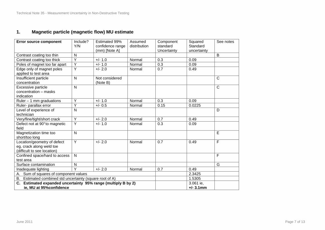
1. Magnetic particle (magnetic flow) MU estimate

Error source component

Include? Y/N

Estimated 99% confidence range (mm) [Note A]

Assumed distribution

Component standard Uncertainty

Squared Standard uncertainty

See notes

Contrast coating too thin N B Contrast coating too thick Y +/- 1.0 Normal 0.3 0.09 Poles of magnet too far apart Y +/- 1.0 Normal 0.3 0.09 Edge only of magnet poles applied to test area

Y +/- 2.0 Normal 0.7 0.49

Insufficient particle concentration

N Not considered (Note B)

C

Excessive particle concentration – masks indication

N C

Ruler – 1 mm graduations Y +/- 1.0 Normal 0.3 0.09 Ruler- parallax error Y +/- 0.5 Normal 0.15 0.0225 Level of experience of technician

N D

Very/fine/tight/short crack Y +/- 2.0 Normal 0.7 0.49 Defect not at 90° to magnetic field

Y +/- 1.0 Normal 0.3 0.09

Magnetization time too short/too long

N

E

Location/geometry of defect eg, crack along weld toe (difficult to see location)

Y +/- 2.0 Normal 0.7 0.49 F

Confined space/hard to access test area

N F

Surface contamination N G Inadequate lighting Y +/- 2.0 Normal 0.7 0.49 A. Sum of squares of component values 2.3425 B. Estimated combined std uncertainty (square root of A) 1.5305 C. Estimated expanded uncertainty 95% range (mul tiply B by 2) ie, MU at 95%confidence

3.061 ie, +/- 3.1mm



Notes to the Magnetic Particle MU table: A The assumption of normal distribution in this example is used for illustrative purposes only (alternative distributions are used in the UTT and UT sizing examples).

For normal distribution, conversion of the 99% range to a component standard uncertainty is achieved by dividing the range by a factor of 3. Because a normal distribution has no range limits, the shortcoming of this approach is that estimating the error range’s 99th percentile (or alternatively the 95th percentile, which involves a factor of 2 to derive the component standard uncertainty) is essentially an impossible task. Therefore, in practice, the estimate should be made to cover at least 99% of results (so that the associated uncertainty is more likely to be an over-estimate than an under-estimate).

Items not considered in calculations in the table above were not included for the reasons given below. B Covered in technicians training C Premixed consumables are commonly used. These are manufactured within specification limits. D Technicians are qualified. Trainees or Level 1 technicians must work under direct supervision of a Level 2. Normal imprecision of an experienced technician is considered under other contributions to the overall MU. E Technicians trained to apply magnetic field for time sufficient to allow development of indications. F Geometry and/or access issues only apply in individual situations and should only be included in the calculation if relevant to the item under test. In this example

the geometry contribution is included, whereas, if this component does not apply, the MU becomes ±2.7 mm (95% confidence). If geometry and access issues both influence the measurement at the levels estimated then the MU becomes ±3.4 mm (95% confidence).

G Surface cleanliness is given importance in technicians training.



2. Ultrasonic Thickness – MU estimate for thicknes ses greater than 5mm


Include? Y/N (Note A)

Estimated typical range (T= Material Thickness)

Assumed Distribution (Note A)

Component standard Uncertainty (T= Material Thickness)

Squared standard uncertainty (T= Material Thickness)

See notes

Thickness meter response and readout resolution

Y +/- ¼ % of T Triangular 0.001T 0.000001T2

Probe response Y +/- ¼ % of T Triangular 0.001T 0.000001T2 Procedure too generic Y +/- ¾ % of T Triangular 0.003T 0.000009T2 Operator proficiency Y +/- ¾ % of T Triangular 0.003T 0.000009T2 Surface profile (curved/flat) Y +/- 1/10 % of T Triangular 0.0005T 0.0000003T2 Surface coating (type) Y +/- 1/10 % of T Triangular 0.0005T 0.0000003T2 Surface condition (pitted/porous/imperfections

Y +/- ¾ % of T Triangular 0.003T 0.000009T2

Sub-surface reflectors (laminations) Y +/- ¾ % of T Triangular 0.003T 0.000009T2 Probe alignment Y +/- ½ % of T Triangular 0.002T 0.000004T2 Calibration block material type N B Material geometry N B Material type Y +/- ¼ % of T Rectangular 0.0015T 0.000002T2 Meter/probe drift N B Probe wear N B Material temperature N B Couplant issues N B Material too thin N C A. Sum of squares of component values 0.0000446T2 B. Estimated combined std uncertainty (square root of A) 0.0067T C. Estimated combined uncertainty 95% range (m ultiply B by 2) 0.013T ie,

+/- 1.3% of T

Notes to the UT Thickness MU table: A An assumption of triangular and/or rectangular distribution for error sources is made for illustrative purposes and may not reflect reality

-for a triangular distribution divide the range by square root of 6 to get component standard uncertainty -for a rectangular distribution divide the range by square root of 3 to get component standard uncertainty

B It is considered that the items not included in the estimation process would have only a negligible effect in most situations C Depending on probe type, thickness testing of material <5mm may be less reliable, making the above estimate invalid



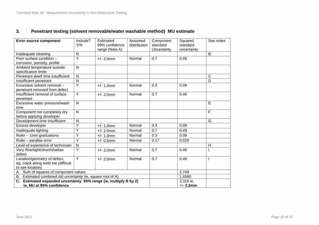
3. Penetrant testing (solvent removable/water washa ble method) MU estimate


Include? Y/N

Estimated 99% confidence range (Note A)

Assumed distribution

Component standard Uncertainty

Squared standard uncertainty

See notes

Inadequate cleaning N B Poor surface condition – corrosion, porosity, profile

Y +/- 2.0mm Normal 0.7 0.49

Ambient temperature outside specification limits

N

Penetrant dwell time insufficient N C Insufficient penetrant N D Excessive solvent removal – penetrant removed from defect

Y +/- 1.0mm Normal 0.3 0.09

Insufficient removal of surface penetrant

Y +/- 2.0mm Normal 0.7 0.49

Excessive water pressure/wash time

N E

Component not completely dry before applying developer

N F

Development time insufficient N G Excess developer Y +/- 1.0mm Normal 0.3 0.09 Inadequate lighting Y +/- 2.0mm Normal 0.7 0.49 Ruler – 1mm graduations Y +/- 1.0mm Normal 0.3 0.09 Ruler – parallax error Y +/- 0.5mm Normal 0.17 0.029 Level of experience of technician N H Very /fine/tight/short/shallow defect

Y +/- 2.0mm Normal 0.7 0.49 I

Location/geometry of defect, eg, crack along weld toe (difficult to see location)

Y +/- 2.0mm Normal 0.7 0.49 I

A. Sum of squares of component values 2.749 B. Estimated combined std uncertainty (ie, square root of A) 1.6580 C. Estimated expanded uncertainty 95% range (ie, multiply B by 2) ie, MU at 95% confidence

3.316 ie, +/- 3.3mm



Notes to the Penetrant MU table: A The assumption of normal distribution in this example is used for illustrative purposes only (alternative distributions are used in the UTT and UT sizing examples).

For normal distribution, conversion of the 99% range to a component standard uncertainty is achieved by dividing the range by a factor of 3. Because a normal distribution has no range limits, the shortcoming of this approach is that estimating the error range’s 99th percentile (or alternatively the 95th percentile, which involves a factor of 2 to derive the component standard uncertainty) is essentially an impossible task. Therefore, in practice, the estimate should be made to cover at least 99% of results (so that the associated uncertainty is more likely to be an over-estimate than an under-estimate).

Items not considered in calculations in the table above were not included for the reasons given below. B Covered in technicians training – cleanliness/non-contamination of test surface is emphasised C Technicians are well versed in observing specified minimum dwell times D Typical outcome of penetrant application is a well-coated surface. Covered in technicians training. E This is an alternative to the solvent removable method. When this method is used, a similar value to that used for excessive solvent removal may be used. F Poor practice. Covered in technicians training. G Technicians are well versed in observing specified minimum development times H Technicians are qualified. Trainees or Level 1 technicians must work under direct supervision of a Level 2. Normal imprecision of an experienced technician is considered under other contributions to the overall MU. I Only include this component if relevant to the measurement made. If these two components do not apply to a measurement result, the MU becomes ±2.6 mm (95% confidence)



4. Ultrasonic Testing MU estimate: Height Sizing (M aximum Amplitude Technique) - Refer Note A for defe ct configuration

Error source component (Note A)

Influencing factor(s) Include? Y/N

Estimated range (mm)

Assumed Distribution (Note C)

Component standard uncertainty (mm)

Squared standard uncertainty (mm)

Systematic error associated with the sizing technique (ie, max amp technique) (Note D)

Edge roughness Shape (1.0mm systematic undersize per edge is assumed, ie +2.0mm total) (Note B)

Y (see item D in table below)

-

-

-

-

Random error associated with the sizing technique (ie, max amp technique)

Beam path/distance (this example involves a beam path of 56mm on the full skip)

Y ±4.0 Triangular 1.63 2.67

Flaw detector – range calibration

Ranges to top and bottom of defect Beam angle


Beam angle calibration Beam angle Range


Beam angle error due to scanning surface error of form

Weld cap Parent metal


Range reading error Analogue screen Range

Y (analogue units)

±1.0 Triangular 0.41 0.17

Time base non-linearity Y ±0.5 Triangular 0.20 0.04 Defect plotting Range

Beam angle Y ±0.5 Triangular 0.20 0.04

Coupling variations caused by surface finish


Random error sources only: A. Sum of squares of random error component values 3.34 B. Estimated combined standard (random) uncertainty (square root of A) 1.83 C. Estimated expanded (random) uncertainty 95% range (multiply B by 2) 3.66 ie, +/- 3.7mm Combined (systematic and random) error sources: D. Estimated 95% uncertainty range (after systematic error included) (Notes D) ± 3.7+2 mm ie, -1.7 to 5.7 mm



Notes to the UT (Height Sizing) Table: A This exercise considers an embedded linear pipe-weld defect running along the fusion face of a single-V butt weld with the defect height extending equally above

and below the pipe wall centre-line. Maximum amplitude sizing technique is assumed (70º probe, full skip) with the apparent height of the defect (as it appears ultrasonically) given as 5mm (wall thickness is 12.5mm). The example is taken from the UK HSE Information for the Procurement and Conduct of NDT: Part 4: Ultrasonic Sizing Errors and Their Implication for Defect Assessment – April 2008. The various error sources considered for this measurement are the same as used in the HSE document but different error range estimates have been used due to the differing treatment of error ranges in this exercise. While maximum amplitude sizing has been used, the above approach may be considered as broadly applicable to alternative sizing techniques except that the error ranges may require to be re-estimated.

B The HSE document referred to above quotes Chapman, R. K. Code of Practice. The Errors Assessment of Defect

Measurement Errors in the Ultrasonic NDT of Welds, CEGB Guidance Document , OED/STN/87/20137/R Issue 1 July 1987 as the source for the estimation of systematic sizing error of 1 mm undersizing per edge. In practice, the magnitude of the systematic undersize error using maximum amplitude sizing technique would be expected to depend on the discontinuity shape and edge roughness. The random component of the sizing error is treated separately in the table (and should strictly incorporate an estimate for the error range of the value used for the systematic sizing error).

C The assumption of a triangular distribution for error sources is made for illustrative purposes only and may not reflect reality. For a triangular distribution, the

estimated range is divided by 2.45 (ie,√6) to obtain the standard uncertainty. D This approach to handling systematic error assumes that the height reported is the ultrasonically measured height (5mm). An alternative approach would be to

adjust the measured height by the systematic error prior to reporting, in which case the uncertainty estimate accompanying the reported result would comprise only the random error uncertainty estimate.

Documents

Measurement Uncertainty in Non-Destructive Testing