1

THERMOPHYSICS 2001

Meeting of the Thermophysical Society Working Group of the Slovak Physical Society

Račkova dolina, October 23, 2001

Editor Libor Vozár

Constantine the Philosopher University in Nitra Faculty of Natural Sciences

2001

2

© CPU Nitra, 2001 THERMOPHYSICS 2001 Proceedings of the Meeting of the Thermophysical Society Working Group of the Slovak Physical Society Račkova dolina, October 23, 2001 Editor Libor Vozár Issued by Constantine the Philosopher University in Nitra First Edition Released in 2001 Printed by Cart print, Nitra Published with the support by the Slovak Science Grant Agency under the contract 1/6115/99.

ISBN 80-8050-491-1 EAN 9788080504915

3

CONTENTS PREFACE 5 COMPUTATIONAL MODELING OF TURBULENT FLOWS DURING CdZnTe CRYSTALLIZATION FROM THE MELT 7 Robert Černý, Jan Toman, Petr Přikryl HIGH TEMPERATURE STEP BY STEP CALORIMETRY AND DROP CALORIMETRY OF METALS 13 Emília Illeková, Jean-Claude Gachon, Jean-Jacques Kuntz, France-Anne Kuhnast INVESTIGATION OF SURFACE EFFECTS ON PMMA BY PULSE TRANSIENT METHOD 21 Vlastimil Boháč, Ľudovít Kubičár CONTACT CONSTRICTION AND FREE SURFACE EFFECTS IN PULSE TRANSIENT METHOD 27 Ľudovít Kubičár, Vlastimil Boháč, Viliam Vretenár MEASUREMENT OF THERMOPHYSICAL PARAMETERS OF POROFEN BY PULSE TRANSIENT METHOD 37 Viliam Vretenár, Ľudovít Kubičár, Vlastimil Boháč THERMAL DIFFUSIVITY OF FIBROUS COMPOSITES 43 Tatiana Šrámková, Ján Spišiak, Pavol Štefánik, Pavol Šebo THE TEMPERATURE DISTRIBUTION IN A COMPOSITE MATERIAL 49 Peter Hudcovič, Libor Vozár, Pavol Štefánik STEADY-STATE MEASUREMENTS OF THE MOISTURE DEPENDENCE OF THE CAPILLARY-POROUS MATERIALS THERMAL CONDUCTIVITY 55 Oľga Koronthályová, Peter Matiašovský MODELLING THE THERMAL CONDUCTIVITY PROPERTIES OF ULTRA - THIN LAYERS: 1-DIMENSIONAL CASE – VERIFICATION 63 Aba Teleki EXPERIMENTAL VERIFICATION OF TWO METHODS FOR SOLVING INVERSE HEAT CONDUCTION PROBLEMS 71 Jozefa Lukovičová, Juraj Veselský SYNTHESIS, THERMAL AND IR SPECTRAL PROPERTIES OF Mg(II) COMPLEXES WITH HETEROCYCLIC LIGANDS 75 Subhash Chandra Mojumdar, Milan Melník, Eugen Jóna, Alžbeta Krutošíková

4

THERMOPHYSICAL PROPERTIES OF BLENDS FROM PORTLAND AND SULFOALUMINATE - BELITE CEMENTS 81 Subhash Chandra Mojumdar, Ivan Janotka OPTIMAL EXPERIMENTAL DESIGN ANALYSIS OF THE FLASH METHOD WITH REPEATED PULSES 87 Libor Vozár, Wolgang Hohenauer, Gabriela Smetanková THERMOPHYSICAL PROPERTIES AND APPLICATIONS OF MACRO-DEFECT-FREE CEMENTS 93 Subhash Chandra Mojumdar THERMOPHYSICAL PROPERTIES OF THE GLASS BK7 99 Gabriela Smetanková, Libor Vozár THERMODILATOMETRY OF TEXTURED ELECTROCERAMIC MATERIAL 105 Igor Štubňa, Libor Vozár, Gabriela Smetanková

5

PREFACE It is pleasures for our research group at the Department of Physics, Faculty of Natural Sciences at the Constantine the Philosopher University in Nitra to host the sixth regular meeting of the Thermophysical Society - Working Group of the Slovak Physical Society.

The Thermophysics workshop has been established as a periodical annual meeting of scientists working in the field of investigation of heat transfer and measurement of thermophysical and other transport properties of materials.

Organizers of the meeting were delighted to have heard an increased number of contributions – participants delivered 16 original lectures in which their authors presented current research progress and original results achieved at their home institutions.

A special thank goes to my colleges Gabriela Smetanková and Branislav Karafa for their help with organizing of the workshop and Mr. Slavomír Janáčik for his contribution in the preparation of the proceedings.

The proceedings are also available in a digital form at the homepage of the Thermophysical Society – http://www.tpl.ukf.sk/thermophysics, or upon a request at the e-mail address vozar@nr.sanet.sk.

Libor Vozár

6

7

COMPUTATIONAL MODELING OF TURBULENT FLOWS DURING CDZNTE CRYSTALLIZATION FROM THE MELT Robert Černý1, Jan Toman2 and Petr Přikryl3 1 Department of Structural Mechanics, Faculty of Civil Engineering, Czech Technical

University, Thákurova 7, 166 29 Prague 6, Czech Republic 2 Department of Physics, Faculty of Civil Engineering, Czech Technical University,

Thákurova 7, 166 29 Prague 6, Czech Republic 3 Mathematical Institute of the Academy of Sciences of the Czech Republic, Žitná 25, 115 67 Prague 1, Czech Republic

Email: cernyr@fsv.cvut.cz, toman@fsv.cvut.cz, prikryl@math.cas.cz Abstract The paper presents a computational model of binary alloy solidification that takes also the fluid flow in the melt into account. The differences between considering the melt flow as laminar and turbulent are discussed. In a practical application of the model, the CdZnTe crystallization process in the vertical Bridgman method is simulated and the results of the computational experiments analyzed. Key words: computational modeling, crystal growth, melt flow, turbulence, moving

boundary 1 Computational model of crystal growth from the melt We will be concerned with the following model problem. A binary alloy in the liquid state is in a cylindrical ampoule of radius R and length L. The system is cooled either from below or from above, so that the solidification process begins either on the bottom or on the top of the ampoule. The boundary conditions for temperatures are applied at the lateral area of the ampoule (for instance by one or two furnaces), while both base sides are thermally insulated. Both the ampoule and the facilities asserting the boundary conditions for temperatures can move up and down with translation velocity υamp, and therefore the solidification process can also be initiated from any intermediate state when the solid/liquid interface is somewhere between the top and the bottom of the ampoule.

The model assumes that no chemical reactions occur in the system and employs the methods of continuum physics, linear irreversible thermodynamics, and linear theory of mixtures to formulate the balance equations in the solid and liquid phases and at the phase interface. Then, the cylindrical symmetry of the experimental situation is utilized and the model equations are written in cylindrical coordinates (r, φ, z). Owing to the symmetry of the modeled situation we may consider only a rectangular section of the ampoule in the (r, z)-plane. We assume that the moving melt/crystal phase interface can be described in the form z - Z(r; t) where Z is a function unknown a priori.

The laminar model used by the authors previously simulated two characteristic methods of crystal growth commonly employed by experimentalists, namely the vertical

8

Bridgman method and the vertical gradient method. In the Bridgman technique of crystallization, two furnaces at the lateral area of the ampoule are applied, the upper of them being at a higher temperature than the melting point while the lower one is below the melting point. Thus, the system is cooled from below, and the solidification process begins from the bottom of the ampoule. During the crystallization, the Bridgman furnaces move upwards the ampoule and therefore the solidification process continues. With our model, it was possible to study the influence of various experimental parameters (furnace temperatures, temperature gradients, geometry of the apparatus, translation etc.). We also studied the influence of the accuracy of material parameters as their reliability is sometimes critical for the adequacy of the model. Mathematically, the model was a moving boundary problem for the system of partial differential equations comprising the heat transfer equation, the diffusion equation and the Navier-Stokes equations. The detailed description of the laminar model and the computational experiments with it may be found in [1].

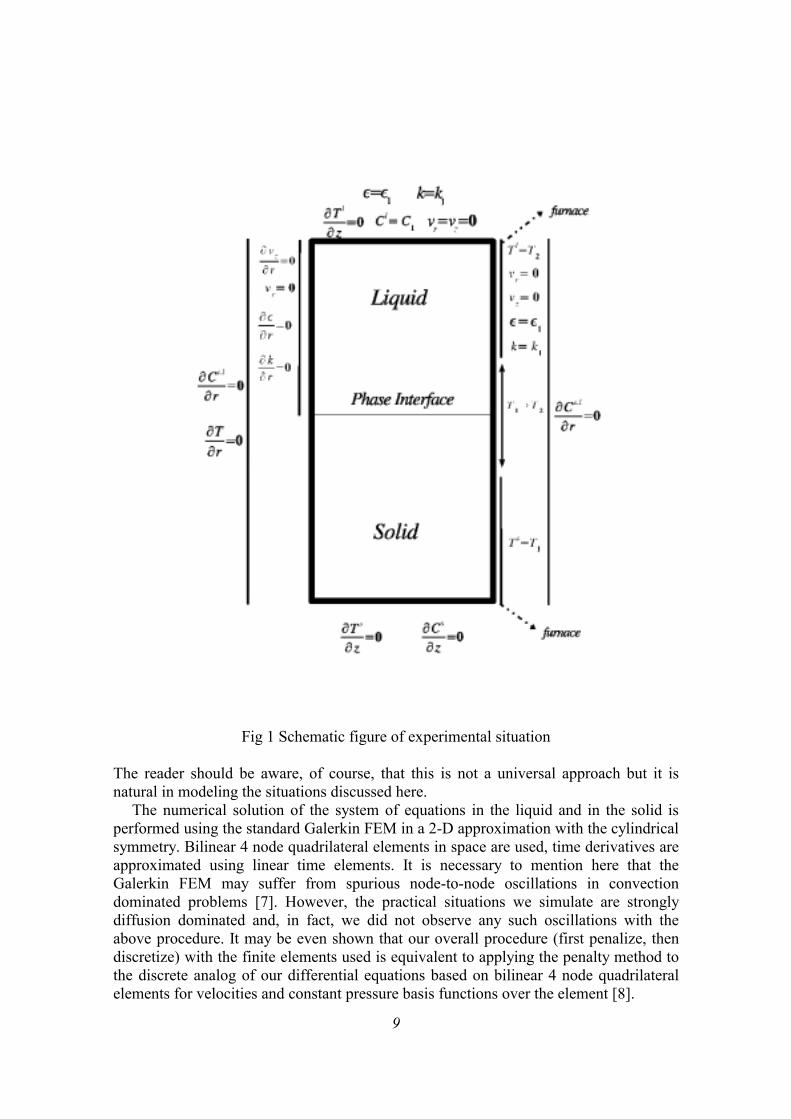
Our approach to treating turbulence is based on time averaged variables and leads to the well-known class of two-equation k - ε turbulent models. In the framework of these models, two new variables, the kinetic turbulent energy k and the rate of dissipation of turbulent kinetic energy ε, and the relevant balance equations are incorporated. In the presence of the convection governed by buoyancy forces only-as is the case with the presented problem-the original k - ε model must be modified to account properly for the transient character of the flow. The model then belongs to the class of so-called low-Reynolds models of turbulence. The low-Reynolds modifications we incorporated in our model are due to Davidson [2] and Lam & Bremhorst [3] and differ in the definition of the turbulent dynamic viscosity that appears in all balance equations except for the continuity equation and in the form of the damping functions that appear in the balance equations for k and ε. Appropriate initial and boundary conditions for T, C, and υ are formulated in a common way corresponding to the particular experimental setup. We employ constant initial conditions for k and ε and Dirichlet boundary conditions for these variables. The boundary conditions at the axis of symmetry are treated in the standard way. The model situation is depicted schematically in Fig. 1. 2 Computer implementation The simulations presented in the paper were done on similar lines as those with our previous laminar model and based on the Galerkin finite element method (FEM). One of the main difficulties in the computational solution of our model equations is connected with the continuity equation and its appropriate numerical approximation in the framework of FEM. To solve this well-known problem we employ the penalty method using a slightly modified form of the continuity equation, where an artificial term єpp with a small єp is added. This method is well understood today and easy to implement (see, for example, [5] and [6]). We then treat the modified continuity equation in such a way that we eliminate the pressure from the differential equations of the model. This elimination of the pressure from the unknown variables not only simplifies the computational implementation but also reduces the computational time as the resulting systems of algebraic equations are smaller. Another point in this respect is that we are not interested in the pressure field in our practical simulations, one of the reasons being the lack of experimental data to compare the possibly computed pressure fields with.

9

Fig 1 Schematic figure of experimental situation The reader should be aware, of course, that this is not a universal approach but it is natural in modeling the situations discussed here.

The numerical solution of the system of equations in the liquid and in the solid is performed using the standard Galerkin FEM in a 2-D approximation with the cylindrical symmetry. Bilinear 4 node quadrilateral elements in space are used, time derivatives are approximated using linear time elements. It is necessary to mention here that the Galerkin FEM may suffer from spurious node-to-node oscillations in convection dominated problems [7]. However, the practical situations we simulate are strongly diffusion dominated and, in fact, we did not observe any such oscillations with the above procedure. It may be even shown that our overall procedure (first penalize, then discretize) with the finite elements used is equivalent to applying the penalty method to the discrete analog of our differential equations based on bilinear 4 node quadrilateral elements for velocities and constant pressure basis functions over the element [8].

10

The moving boundary problem was solved by a front-fixing method, which transforms the two-dimensional variable space regions [0; R]x[0; Z(r; t)], [0; R]x[Z(r; t); L] occupied by the solid and liquid phases, respectively, to the fixed space domains [0; 1] x [0; 1]. This approach proposed by Landau [9] for one-dimensional problems originally is applicable here owing to our assumption on the form of the moving boundary.

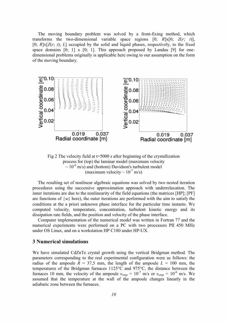
Fig 2 The velocity field at t=5000 s after beginning of the crystallization process for (top) the laminar model (maximum velocity

~ 10-6 m/s) and (bottom) Davidson's turbulent model (maximum velocity ~ 10-7 m/s)

The resulting set of nonlinear algebraic equations was solved by two nested iteration

procedures using the successive approximation approach with underrelaxation. The inner iterations are due to the nonlinearity of the field equations (the matrices [HP]; [PF] are functions of w here), the outer iterations are performed with the aim to satisfy the conditions at the a priori unknown phase interface for the particular time instants. We computed velocity, temperature, concentration, turbulent kinetic energy and its dissipation rate fields, and the position and velocity of the phase interface.

Computer implementation of the numerical model was written in Fortran 77 and the numerical experiments were performed on a PC with two processors PII 450 MHz under OS Linux, and on a workstation HP C180 under HP-UX. 3 Numerical simulations We have simulated CdZnTe crystal growth using the vertical Bridgman method. The parameters corresponding to the real experimental configuration were as follows: the radius of the ampoule R = 37,5 mm, the length of the ampoule L = 100 mm, the temperatures of the Bridgman furnaces 1125°C and 975°C, the distance between the furnaces 10 mm, the velocity of the ampoule υamp = 10-7 m/s or υamp = 10-6 m/s. We assumed that the temperature at the wall of the ampoule changes linearly in the adiabatic zone between the furnaces.

11

The observed structure of the turbulent flow was very complicated. The pattern flow was time dependent and highly variable through the entire computational domain. Several isolated recirculating flow regions arise in the domain in the vicinity of the phase interface, while on the opposite side practically no flow is observed. The average magnitude of the turbulent velocities was 10-7 m/s. A perturbation of flow occurs near the wall and near the phase interface, which can affect final quality of the produced crystal.

The results obtained by the turbulent model were compared with those of our previous laminar model [1]. As can be seen from Fig. 2, there are significant differences in the melt flow behavior among both the models. The computed velocity fields differ not only in the maximum magnitudes but also in the structure and stability of the flow pattern.

The laminar model produces a flow field that is formed by two stable vortices with mutual rotational symmetry along the vertical axis of the ampoule. We suppose that this structure is affected by the buoyancy forces mainly, driven by the temperature and concentration gradient. The structure of the computed laminar velocity field was observed to be time independent and the maximum values of velocities were not affected by the translation rate υamp of the ampoule in the interval [10-7, 10-6] m/s considered in our simulations.

In the case of our turbulent model, we observed dependence of the maximum melt flow velocities on the translation rate of the ampoule: these velocities were of order 10-8 m/s for υamp = 10-7 m/s and of order 10-7 m/s for υamp = 10-6 m/s. Moreover, the velocity pattern was strongly time dependent exhibiting a periodic character. It seems that the turbulent flow was largely affected by the movement of the phase interface, contrary to the laminar model. We note that this observation is in conflict with the common view of the causes of the melt movement during the crystallization processes driven by buoyancy forces.

The shape and velocity of the phase interface were for υamp - 10-7 m/s practically identical for both the models in the time interval in question. However, for υamp - 10-6 m/s differences in the interface position were observed since t ≈ 6000 s. The turbulent interface moved more slowly. In addition, melting of the phase interface was observed in the vicinity of the wall for these larger times. This fact may be the result of a very irregular flow structure that arises in this region.

The temperature fields obtained by both the models compared were practically identical. This seems to be due to the Dirichlet boundary conditions imposed and to the fact that the time development of this field was determined by the movement of the furnaces with respect to the ampoule.

On the other hand, the structure and time history of the concentration fields were different for both the models. We observed instabilities in the concentration profiles in the grown crystal both in the vertical and horizontal directions. We note that the concentration profiles are time dependent in the turbulent model as they are driven by the instabilities in the turbulent velocity field. Moreover, the maximum concentrations depended on υamp in the turbulent model; they were larger for smaller translation rates.

The results obtained with the turbulent model indicate the melt flow in the case studied is affected mainly by the movement of the phase interface and that the buoyancy effects play a secondary role. They tend to establish a stable structure in the flow but in the case of the turbulent model their influence is dumped by additional viscous dissipation.

12

4 Conclusion The convergence of the iterative procedures in the two-equation k - ε model we used, which is very sensitive to unrealistic model conditions, can support the evidence of a slightly turbulent or transient flow instead of pure laminar flow in the melt during.crystallization. Hence, the turbulent model presented in the paper is more appropriate to simulate the processes occurring in the melt. The laminar model is not able to describe these processes in detail because it cannot represent the processes running in smaller scales than the size of the computational mesh used. However, the small dissipative eddies play a significant role in the transport phenomena here and thus have an important impact on the whole process of crystallization. Our turbulent model brings thus more insight into the study of the crystal growth techniques in question and is a usable tool for the computer optimization of experimental setups of the common techniques represented by the Bridgman method. Acknowledgement This paper is based upon work supported by the Grant Agency of the Czech Republic, under grants # 202/99/1646 and 201/01/1200. References [1] Černý R, Kalbáč A, Přikryl P, 2000 Comp. Materials Sci., 17, 34 [2] Davidson L, 1990 Num. Heat Transfer, 18, 129 [3] Lam C K G, Bremhorst, K A, 1981 ASME J. Fluids Engng., 103, 456 [4] Frost W, Moulden T H, 1992 Handbook of Turbulence, (New York, Plenum Press) [5] Hughes T J R, Liu W T, Brooks A J, 1979 J. Comput. Phys., 30, 1 [6] Bercovier M, Engelman M, 1979 J. Comput. Phys., 30, 181 [7] Sani R L, Gresho P M, Lee R L and Griffiths D F, 1981 Int. J. Numer. Methods

Fluids, 1, 17, 171 [8] FIDAP 7.0 Theory Manual, Sec. 5.3. Fluid Dynamics International, Inc., 1993 [9] Landau H G, 1950 Quart. Appl. Math., 8, 81

13

HIGH TEMPERATURE STEP BY STEP CALORIMETRY AND DROP CALORIMETRY OF METALS Emília Illeková1, Jean-Claude Gachon2, Jean-Jacques Kuntz2, France-Anne Kuhnast2 1 Institute of Physics, Slovak Academy of Sciences, Dúbravská cesta 9,

SK-842 28 Bratislava, Slovakia 2 UMR 7555, Groupe Thermodynamique et Corrosion, Université Henri Poincaré,

Nancy 1, BP 239, F-54506 Vandoeuvre-lès-Nancy, Cedex, France Email: fyziille@savba.sk, Jean-Claude.Gachon@lcsm.uhp-nancy.fr Abstract Molar heat capacities at constant pressure of tetragonal-Al3Nb were determined each 10 K by the step by step method using differential scanning calorimetry from 310 to 1080 K and each 200 K by the drop calorimetry from 1095 to 1473 K. The experimental values have been fitted by polynomial Cp(T) = a + bT + cT2 + dT-1 + eT-2. Key words: Al3Nb compound, differential scanning calorimetry, drop calorimetry,

heat capacity, high temperatures, intermetallics 1 Introduction Amorphous and nanocrystalline Al-based materials belong to the best lightweight materials. The knowledge of thermodynamic properties relative to intermediate phase formations is necessary to understand the chemical bonding of the intermetallics, the glass forming ability of the precursor systems and the stability of the products. Unfortunately, heat capacities are most often unknown and estimations available in the literature are not accurate enough. This is the reason of this work in our program of experimental determination of thermodynamic properties of intermetallics [1-3].

In this paper, the measurement of the molar heat capacity under normal pressure, Cp, of a bulk equilibrium Al3Nb sample up to 1473 K is presented. The standard step by step differential scanning calorimetry and the drop calorimetry methods are used. The data of the Al3Nb compound will be used in the future as the calibration standard data for the high temperature specific heat measurements of the Al-based materials by the continuous heating Perkin-Elemer differential scanning calorimetry (DSC). 2 Experimental 2.1 Preparation of the sample The elemental Al of 99.9 % purity and Au of 99.99 % purity were used and measured as the standard materials.

The Al3Nb compound was prepared by induction melting of Al, and Nb elements of 99.9 % purity in argon atmosphere. Powder X-ray diffraction patterns were obtained

14

with Philips PW 1370 diffractometer using CuKα radiation. Only the tetragonal-Al3Nb (D4h

17 symmetry) diffraction lines were detected. (Our DSC data confirmed also the presence of some Al-based phase, as will be shown later.) No oxides were present. 2.2 Differential scanning calorimetry: step by step heat capacity measurements The heat capacities at constant pressure, Cp, were determined every 10 K between 310 and 1080 K, except for Al sample with lower melting temperature, by a step by step method. Measurements were carried out using a Setaram 111, designed as a Calvet type calorimeter with horizontal reference and laboratory cells surrounded by two thermal flowmeters connected against each other. Samples of 0.17-0.36 g were introduced in an alumina laboratory crucible in the laboratory cell under argon. The empty alumina crucible was used in the reference cell. For each temperature step the heating rate (dT/dt) was 3 K min-1 during 200 s (∆T = 10 K) and then temperature was kept constant during 400 s. This combination gave an overall (dT/dt) 1 K min-1. The thermopile signal, ∆Jl-r(T), proportional to the difference of heat flows between the laboratory and reference cells and their surroundings was recorded and integrated during 600 s.

Three temperature runs were necessary, one with the empty laboratory crucible (blank), one with the calibration sample (alumina SRM 720) and the last one with the product. By subtracting the blank integral value from the others, the results, for each of the individual temperature steps ∆T, were proportional to the enthalpy increments ∆HT

T+∆T of laboratory cell actual content and the proportionality coefficient was given by the calibration material. The Cp mean value on the 10 K step could be deduced as

THC

TTTTT

Tp ∆∆=⟩⟨

∆+∆+ , (1)

TTTcalp

cal

meas

meas

calTT

Trblank

TT

T rcal

TT

Trblank

TT

T rmeasTT

Tp CMM

mm

dtTJdtTJ

dtTJdtTJC ∆+

∆+

−

∆+

−

∆+

−

∆+

−∆+ ⟩⟨⋅⋅⋅

∆−∆

∆−∆=⟩⟨

∫∫

∫∫,

)()(

)()( . (2)

Mmeas and Mcal are the molar masses, mmeas and mcal are the masses, ∆Jmeas-r(T), ∆Jcal-r(T) and ∆Jblank-r(T) are the thermopile signals of the measured, calibration and blank samples, respectively. The Cp(T+∆T/2) data of pure alumina tabulated in [4] were used as the known reference data <Cp,cal>T

T+∆T. The complete architecture of the automatic measuring and data acquisition program have been described in [5] and used in our previous Cps determinations [1-3].

No appreciable oxidation, weight losses or reaction between the samples and the crucible were observed at the end of measurements. 2.3 Drop calorimetry: heat capacity measurements The calorimeter has been devised for measuring heat effects at temperatures ranging from 800 to 1800 K. It is heated in a vertical furnace (SETARAM 2400) specially built for the calorimetric applications. The calorimetric cell is made from 17 thermocouples connected in series. The length of the junctions is about 1 cm. All junctions of one type are around the working crucible positioned in two different levels while the junctions of

15

the other type surround the inert crucible all at the same level. This disposition ensures that i) the part of the heat transport between the sample and the calorimeter passing through the thermocouples is maximal, ii) the effect of the filling of the crucible is minimized. The technical details of the calorimeter as well as of the accuracy of the experiment are in [6].

The samples of 0,023-0,075 g are introduced into the vacuum tight entrance lock of the calorimeter at room temperature, (To), then put under argon and dropped down into the working crucible kept at the temperature of the experiment, (Ta). Ta is given by the e.m.f. of one junction in touch with the working crucible. The calorimetric signal, Y(t) ~ ∆T(t), is given by the e.m.f. of the thermopile. The integral of the calorimetric signal is proportional to the heat transfer, (∆QTo

Ta), between the sample and the calorimeter. The calibration provides the conversion factor. Each experiment includes i) the calibration and ii) the measurement. The calibration is made with alumina samples. One alumina sample was dropped before the measurement and one afterwards. For each alumina sample the signal was integrated. Using the heat content tabulated in [4] the converting factor of the calorimeter was calculated and the mean value of these two measurements was taken as the calibration coefficient of the calorimeter. The finally presented increment of the sample enthalpy is always the average value of the sequence

a

o

a

o

TToa

TT QTHTHH ∆=−=∆ )()( (3)

of seven two-step experimental results. Providing that neither any reaction nor any transformation occurs in the sample it is just the heat content necessary for the heating of the sample. Then the sample Cp mean value on the temperature interval between two Ta temperatures can be defined as

12

12

2

1aa

TT

TTT

Tp TTHH

Ca

o

a

oa

a −∆−∆

=⟩⟨ . (4)

The experiments were preformed at Ta = 1095K, 1273 K and 1473 K, To = 297 K. Signal was recorded and integrated during 720 s. No appreciable oxidation, weight losses or reaction between the samples and the crucible were observed at the end of the experiments. 2.4 Differential scanning calorimetry: characterization of the purity of the samples

The samples were subjected to the high-temperature differential scanning calorimetry (DSC). The measurements were performed in the Perkin-Elmer Differential thermal analyzer PE DTA7 in the DSC mode at a heating rate 10 K min-1 between 300 and 1770 K. The measuring of the Al and Au NBS standards performed the enthalpy calibration. The melting enthalpy, ∆1Hf,i, of each crystalline phase, i, in the 1g sample was deduced by integration and normalization of the DSC signal in its endothermal peak. The nitrogen atmosphere and the covered alumina sample and reference crucibles were practiced. A covered empty crucible was used as the reference. No reaction between the samples (~ 40 mg) and the sample crucible was observed at the end of the experiments.

16

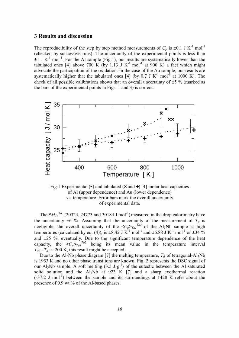
3 Results and discussion The reproducibility of the step by step method measurements of Cp is ±0.1 J K-1 mol-1 (checked by successive runs). The uncertainty of the experimental points is less than ±1 J K-1 mol-1. For the Al sample (Fig.1), our results are systematically lower than the tabulated ones [4] above 700 K (by 1.13 J K-1 mol-1 at 900 K) a fact which might advocate the participation of the oxidation. In the case of the Au sample, our results are systematically higher that the tabulated ones [4] (by 0.7 J K-1 mol-1 at 1000 K). The check of all possible calibrations shows that an overall uncertainty of ±5 % (marked as the bars of the experimental points in Figs. 1 and 3) is correct.

400 600 800 1000Temperature [ K ]

25

30

35

Hea

t cap

acity

[ J

/ m

ol K

]

Fig 1 Experimental (• ) and tabulated (×××× and ++++) [4] molar heat capacities of Al (upper dependence) and Au (lower dependence)

vs. temperature. Error bars mark the overall uncertainty of experimental data.

The ∆HTo

Ta (20324, 24773 and 30184 J mol-1) measured in the drop calorimetry have the uncertainty ±6 %. Assuming that the uncertainty of the measurement of Ta is negligible, the overall uncertainty of the <Cp>Ta1

Ta2 of the Al3Nb sample at high tempertures (calculated by eq. (4)), is ±8.42 J K-1 mol-1 and ±6.88 J K-1 mol-1 or ±34 % and ±25 %, eventually. Due to the significant temperature dependence of the heat capacity, the <Cp>Ta1

Ta2 being its mean value in the temperature interval Ta2 –Ta1 ~ 200 K, this result might be accepted.

Due to the Al-Nb phase diagram [7] the melting temperature, Tf, of tetragonal-Al3Nb is 1953 K and no other phase transitions are known. Fig. 2 represents the DSC signal of our Al3Nb sample. A soft melting (3.5 J g-1) of the eutectic between the Al saturated solid solution and the Al3Nb at 923 K [7] and a sharp exothermal reaction (-37.2 J mol-1) between the sample and its surroundings at 1428 K refer about the presence of 0.9 wt % of the Al-based phases.

17

600 800 1000 1200 1400Temperature [ K ]

-0.3

0.0

0.3

0.5H

eat f

low

[ W

/ g

]

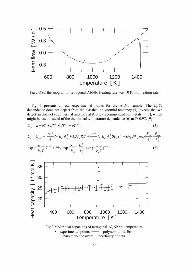
Fig 2 DSC thermogram of tetragonal-Al3Nb. Heating rate was 10 K min-1 eating rate.

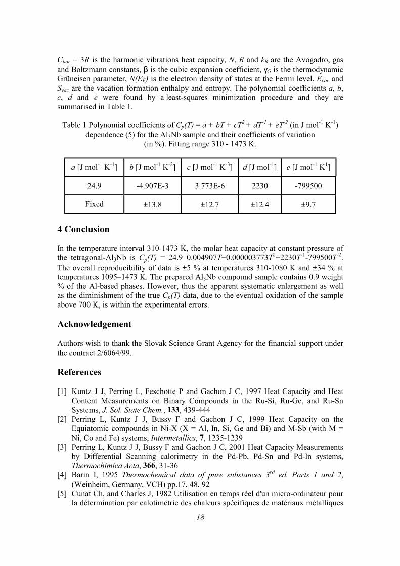
Fig. 3 presents all our experimental points for the Al3Nb sample. The Cp(T) dependence does not depart from the classical polynomial tendency (5) (except that we detect an distinct endothermal anomaly at 910 K) recommended for metals in [8], which might be used instead of the theoretical temperature dependence (6) at T<0.9Tf [9]

212 −− ++++= eTdTcTbTaC p , (5)

2

222

22

2

exp)(3

2]3)(3

2[B

vac

b

vacBGGBFGBFharp k

Ek

SNkTkENTRkENCC βγβγπβγπ ++++=

22

21 expexpexp −− −+− T

TkE

kE

kS

NkTTk

E

B

vac

B

vac

B

vacB

B

vac . (6)

400 600 800 1000 1200 1400Temperature [ K ]

20

25

30

35

Hea

t cap

acity

[ J

/ m

ol K

]

Fig 3 Molar heat capacities of tetragonal-Al3Nb vs. temperature: • - experimental points, ______ - polynomial fit. Error

bars mark the overall uncertainty of data.

18

Char = 3R is the harmonic vibrations heat capacity, N, R and kB are the Avogadro, gas and Boltzmann constants, β is the cubic expansion coefficient, γG is the thermodynamic Grüneisen parameter, N(EF) is the electron density of states at the Fermi level, Evac and Svac are the vacation formation enthalpy and entropy. The polynomial coefficients a, b, c, d and e were found by a least-squares minimization procedure and they are summarised in Table 1.

Table 1 Polynomial coefficients of Cp(T) = a + bT + cT2 + dT-1 + eT-2 (in J mol-1 K-1) dependence (5) for the Al3Nb sample and their coefficients of variation

(in %). Fitting range 310 - 1473 K.

a [J mol-1 K-1] b [J mol-1 K-2] c [J mol-1 K-3] d [J mol-1] e [J mol-1 K1]

24.9 -4.907E-3 3.773E-6 2230 -799500

Fixed ±13.8 ±12.7 ±12.4 ±9.7

4 Conclusion In the temperature interval 310-1473 K, the molar heat capacity at constant pressure of the tetragonal-Al3Nb is Cp(T) = 24.9–0.004907T+0.000003773T2+2230T-1-799500T-2. The overall reproducibility of data is ±5 % at temperatures 310-1080 K and ±34 % at temperatures 1095–1473 K. The prepared Al3Nb compound sample contains 0.9 weight % of the Al-based phases. However, thus the apparent systematic enlargement as well as the diminishment of the true Cp(T) data, due to the eventual oxidation of the sample above 700 K, is within the experimental errors. Acknowledgement Authors wish to thank the Slovak Science Grant Agency for the financial support under the contract 2/6064/99. References [1] Kuntz J J, Perring L, Feschotte P and Gachon J C, 1997 Heat Capacity and Heat

Content Measurements on Binary Compounds in the Ru-Si, Ru-Ge, and Ru-Sn Systems, J. Sol. State Chem., 133, 439-444

[2] Perring L, Kuntz J J, Bussy F and Gachon J C, 1999 Heat Capacity on the Equiatomic compounds in Ni-X (X = Al, In, Si, Ge and Bi) and M-Sb (with M = Ni, Co and Fe) systems, Intermetallics, 7, 1235-1239

[3] Perring L, Kuntz J J, Bussy F and Gachon J C, 2001 Heat Capacity Measurements by Differential Scanning calorimetry in the Pd-Pb, Pd-Sn and Pd-In systems, Thermochimica Acta, 366, 31-36

[4] Barin I, 1995 Thermochemical data of pure substances 3rd ed. Parts 1 and 2, (Weinheim, Germany, VCH) pp.17, 48, 92

[5] Cunat Ch, and Charles J, 1982 Utilisation en temps réel d'un micro-ordinateur pour la détermination par calotimétrie des chaleurs spécifiques de matériaux métalliques

19

et des enthalpies et paramètres cinétiques de transition de phases, J. Mem. Scient. Revue de Métallurgie,177-187

[6] Gachon J C and Hertz J, 1983 Enthalpies of Formation of Binary Phases in the Systems FeTi, FeZr, CoTi, CoZr, NiTi, and NiZr, by Direct Reaction Calorimetry, CALPHAD, 7, 1-12

[7] Kattner U R, 1990 Al-Nb (Aluminium-Niobium), Binary Alloy Phase Diagrams, Vol. 1, sec. ed. (Massalski T B, ASM International) pp. 179-181

[8] Kraftmakher Y, 1998 Equilibrium vacancies and thermophysical properties of metals, Physics Reports, 299, 79-188

[9] Grimvall G, 1999 Thermophysical properties of materials, (Amsterdam, Elsevier) pp. 118-184

20

21

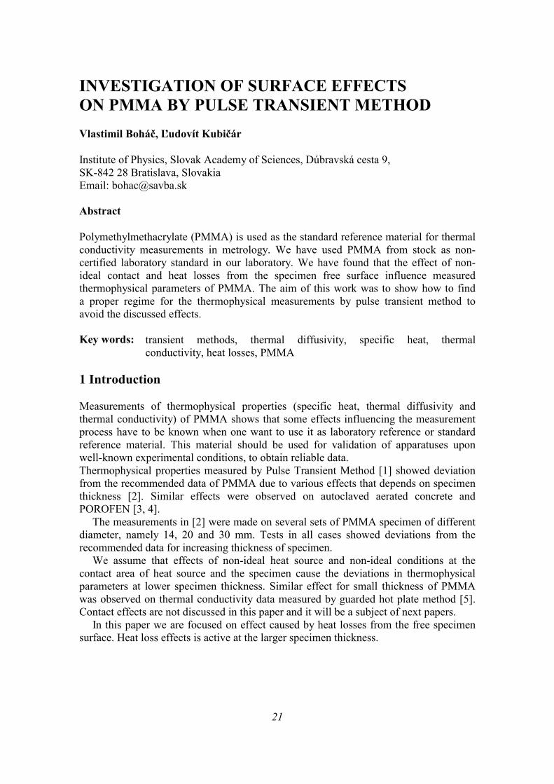
INVESTIGATION OF SURFACE EFFECTS ON PMMA BY PULSE TRANSIENT METHOD Vlastimil Boháč, Ľudovít Kubičár Institute of Physics, Slovak Academy of Sciences, Dúbravská cesta 9, SK-842 28 Bratislava, Slovakia Email: bohac@savba.sk Abstract Polymethylmethacrylate (PMMA) is used as the standard reference material for thermal conductivity measurements in metrology. We have used PMMA from stock as non-certified laboratory standard in our laboratory. We have found that the effect of non-ideal contact and heat losses from the specimen free surface influence measured thermophysical parameters of PMMA. The aim of this work was to show how to find a proper regime for the thermophysical measurements by pulse transient method to avoid the discussed effects. Key words: transient methods, thermal diffusivity, specific heat, thermal

conductivity, heat losses, PMMA 1 Introduction Measurements of thermophysical properties (specific heat, thermal diffusivity and thermal conductivity) of PMMA shows that some effects influencing the measurement process have to be known when one want to use it as laboratory reference or standard reference material. This material should be used for validation of apparatuses upon well-known experimental conditions, to obtain reliable data. Thermophysical properties measured by Pulse Transient Method [1] showed deviation from the recommended data of PMMA due to various effects that depends on specimen thickness [2]. Similar effects were observed on autoclaved aerated concrete and POROFEN [3, 4].

The measurements in [2] were made on several sets of PMMA specimen of different diameter, namely 14, 20 and 30 mm. Tests in all cases showed deviations from the recommended data for increasing thickness of specimen.

We assume that effects of non-ideal heat source and non-ideal conditions at the contact area of heat source and the specimen cause the deviations in thermophysical parameters at lower specimen thickness. Similar effect for small thickness of PMMA was observed on thermal conductivity data measured by guarded hot plate method [5]. Contact effects are not discussed in this paper and it will be a subject of next papers.

In this paper we are focused on effect caused by heat losses from the free specimen surface. Heat loss effects is active at the larger specimen thickness.

22

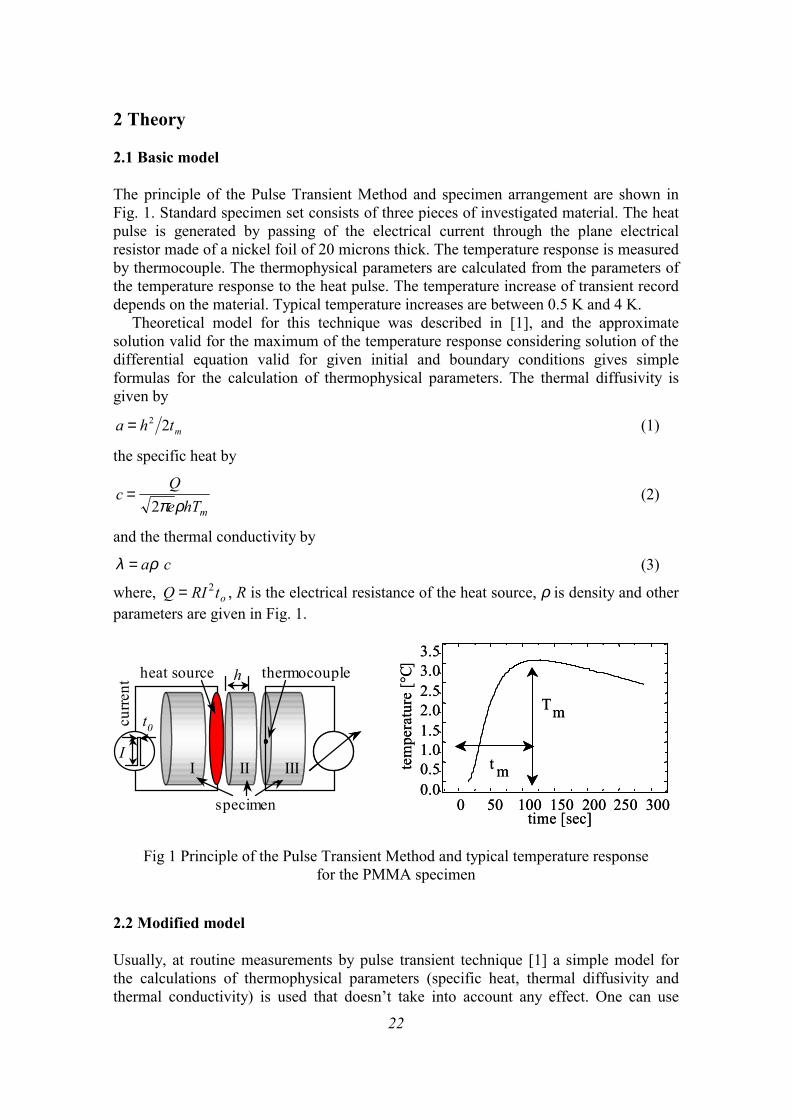
2 Theory 2.1 Basic model The principle of the Pulse Transient Method and specimen arrangement are shown in Fig. 1. Standard specimen set consists of three pieces of investigated material. The heat pulse is generated by passing of the electrical current through the plane electrical resistor made of a nickel foil of 20 microns thick. The temperature response is measured by thermocouple. The thermophysical parameters are calculated from the parameters of the temperature response to the heat pulse. The temperature increase of transient record depends on the material. Typical temperature increases are between 0.5 K and 4 K.

Theoretical model for this technique was described in [1], and the approximate solution valid for the maximum of the temperature response considering solution of the differential equation valid for given initial and boundary conditions gives simple formulas for the calculation of thermophysical parameters. The thermal diffusivity is given by

mtha 22= (1)

the specific heat by

cQe hTm

=2π ρ

(2)

and the thermal conductivity by

caρλ = (3)

where, Q RI to= 2 , R is the electrical resistance of the heat source, ρ is density and other parameters are given in Fig. 1.

heat source thermocouple

specimen

II IIII

h

I

curre

nt

t0

0 50 100 150 200 250 300

0.00.51.01.52.02.53.03.5

tem

pera

ture

[°C]

time [sec]

t m

Tm

0 50 100 150 200 250 3000.00.51.01.52.02.53.03.5

tem

pera

ture

[°C]

time [sec]

t m

Tm

Fig 1 Principle of the Pulse Transient Method and typical temperature response for the PMMA specimen

2.2 Modified model Usually, at routine measurements by pulse transient technique [1] a simple model for the calculations of thermophysical parameters (specific heat, thermal diffusivity and thermal conductivity) is used that doesn’t take into account any effect. One can use

23

more complicated model involving various effects in a cost of complicated temperature function and time consuming calculations.

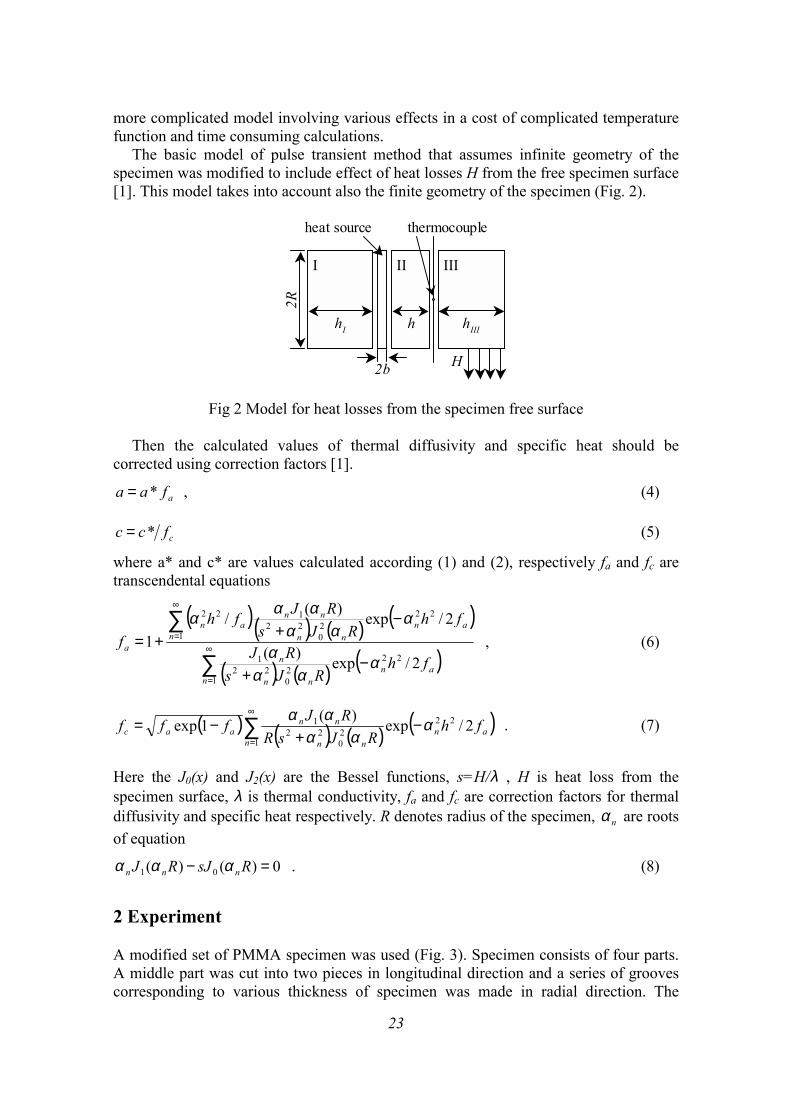
The basic model of pulse transient method that assumes infinite geometry of the specimen was modified to include effect of heat losses H from the free specimen surface [1]. This model takes into account also the finite geometry of the specimen (Fig. 2).

III

hI h hIII

2b

heat source thermocouple

H

2R

III

Fig 2 Model for heat losses from the specimen free surface

Then the calculated values of thermal diffusivity and specific heat should be corrected using correction factors [1].

afaa *= , (4)

cfcc *= (5)

where a* and c* are values calculated according (1) and (2), respectively fa and fc are transcendental equations

( )( ) ( ) ( )

( ) ( ) ( )∑

∑∞

=

∞

=

−+

−++=

1

2220

221

1

2220

22122

2/exp)(

2/exp)(/1

nan

nn

n

nan

nn

nnan

a

fhRJs

RJ

fhRJs

RJfhf

ααα

α

ααα

ααα , (6)

( ) ( ) ( ) ( )ann nn

nnaac fh

RJsRRJfff 2/exp)(1exp 22

120

221 α

αααα

−+

−= ∑∞

=

. (7)

Here the J0(x) and J2(x) are the Bessel functions, s=H/λ , H is heat loss from the specimen surface, λ is thermal conductivity, fa and fc are correction factors for thermal diffusivity and specific heat respectively. R denotes radius of the specimen, nα are roots of equation

0)()( 01 =− RsJRJ nnn ααα . (8)

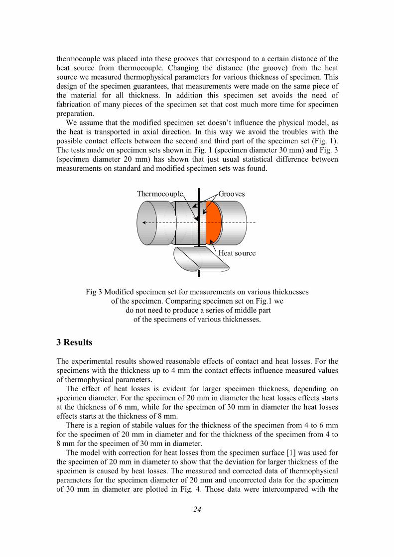
2 Experiment A modified set of PMMA specimen was used (Fig. 3). Specimen consists of four parts. A middle part was cut into two pieces in longitudinal direction and a series of grooves corresponding to various thickness of specimen was made in radial direction. The

24

thermocouple was placed into these grooves that correspond to a certain distance of the heat source from thermocouple. Changing the distance (the groove) from the heat source we measured thermophysical parameters for various thickness of specimen. This design of the specimen guarantees, that measurements were made on the same piece of the material for all thickness. In addition this specimen set avoids the need of fabrication of many pieces of the specimen set that cost much more time for specimen preparation.

We assume that the modified specimen set doesn’t influence the physical model, as the heat is transported in axial direction. In this way we avoid the troubles with the possible contact effects between the second and third part of the specimen set (Fig. 1). The tests made on specimen sets shown in Fig. 1 (specimen diameter 30 mm) and Fig. 3 (specimen diameter 20 mm) has shown that just usual statistical difference between measurements on standard and modified specimen sets was found.

Heat source

GroovesThermocouple

Fig 3 Modified specimen set for measurements on various thicknesses of the specimen. Comparing specimen set on Fig.1 we

do not need to produce a series of middle part of the specimens of various thicknesses.

3 Results The experimental results showed reasonable effects of contact and heat losses. For the specimens with the thickness up to 4 mm the contact effects influence measured values of thermophysical parameters.

The effect of heat losses is evident for larger specimen thickness, depending on specimen diameter. For the specimen of 20 mm in diameter the heat losses effects starts at the thickness of 6 mm, while for the specimen of 30 mm in diameter the heat losses effects starts at the thickness of 8 mm.

There is a region of stabile values for the thickness of the specimen from 4 to 6 mm for the specimen of 20 mm in diameter and for the thickness of the specimen from 4 to 8 mm for the specimen of 30 mm in diameter.

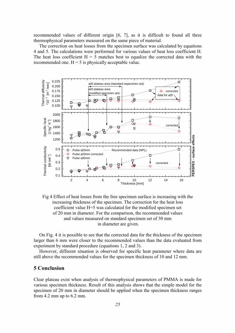
The model with correction for heat losses from the specimen surface [1] was used for the specimen of 20 mm in diameter to show that the deviation for larger thickness of the specimen is caused by heat losses. The measured and corrected data of thermophysical parameters for the specimen diameter of 20 mm and uncorrected data for the specimen of 30 mm in diameter are plotted in Fig. 4. Those data were intercompared with the

25

recommended values of different origin [6, 7], as it is difficult to found all three thermophysical parameters measured on the same piece of material.

The correction on heat losses from the specimen surface was calculated by equations 4 and 5. The calculations were performed for various values of heat loss coefficient H. The heat loss coefficient H = 5 matches best to equalize the corrected data with the recommended one. H = 5 is physically acceptable value.

0.1000.1250.1500.1750.2000.225

correcteddata for φ20

φ30 plateau area (standard sepecimen set)

φ20 plateau area (modified specimen set)

Pulse φ20mm Pulse φ20mm corrected Pulse φ30mm

Ther

mal

diff

usiv

ity*1

0 -6 [

m 2 /s

ec]

1200

1400

1600

1800

2000

corrected

Spec

ific

heat

[J k

g-1 K

-1]

2 4 6 8 10 12 14 160.1

0.2

0.3

0.4

0.5

corrected

Recommended data (NPL)

Thickness [mm]

PER

SPEX

- su

rfac

e ef

fect

s

Ther

mal

con

duct

ivity

[W m

K-1]

Fig 4 Effect of heat losses from the free specimen surface is increasing with the

increasing thickness of the specimen. The correction for the heat loss coefficient value H=5 was calculated for the modified specimen set of 20 mm in diameter. For the comparison, the recommended values

and values measured on standard specimen set of 30 mm in diameter are given.

On Fig. 4 it is possible to see that the corrected data for the thickness of the specimen

larger than 6 mm were closer to the recommended values than the data evaluated from experiment by standard procedure (equations 1, 2 and 3).

However, different situation is observed for specific heat parameter where data are still above the recommended values for the specimen thickness of 10 and 12 mm. 5 Conclusion Clear plateau exist when analysis of thermophysical parameters of PMMA is made for various specimen thickness. Result of this analysis shows that the simple model for the specimen of 20 mm in diameter should be applied when the specimen thickness ranges from 4.2 mm up to 6.2 mm.

26

Reliable data can be obtained for broader range of thickness when larger specimen diameters (see data for 30 mm in diameter specimen) are used.

It was shown that the deviation of thermophysical data from the recommended values for bigger thickness of the specimen is possible to explain within a theory for heat losses from the specimen free surface. Data corrected by (4) and (5) are closer to recommended data.

Providing, that the experimental setup is designed within presented analysis, the simple model can be used for reliable data determination. Acknowledgement Authors wish to thank the Slovak Science Grant Agency VEGA under Nr. 2/5084/98 for the financial support. References [1] Kubičár Ľ, 1990 Pulse Method of Measuring Basic Thermophysical Parameters, in

Comprehensive Analytical Chemistry Vol. XII Thermal Analysis Part E, (Ed. Svehla G, Amsterdam, Oxford, New York, Tokyo: Elsevier)

[2] Boháč V, Kubičár Ľ, Gustafsson M K, In THERMOPHYSICS 2000, Meeting of the Thermophysical Society, Working Group of the Slovak Physical Society Nitra, October 20, 2000 (Ed. Libor Vozár ISBN 80-8050-361-3) pp. 49

[3] Kubičár Ľ, Boháč V, Proc. of 26th International Thermal Conductivity Conference, 14th International Thermal Expansion Conference, Cambridge, Massachussets USA, In print.

[4] Vretenár V, Kubičár Ľ, Boháč V, In Proc. THERMOPHYSICS 2001, Nov. 2001 [5] Koniorczyk P, Zmywaczyk J, 1996 Proc. of TEMPECO ’96, (Ed. Piero Marcarino,

Torino: Levrotto & Bella) pp 543 – 547 [6] Salmon D, Thermophysical Properties Section at the National Physical Laboratory,

(Teddington, UK.NPL) [7] Maglić K D, Cezairliyan A and Peletsky V E, 1992, in Compendium of

Thermophysical Property Measurement Methods, Vol 2, Recommended Measurement Techniques and Practices (Eds: Maglic K D, Cezairliyan A, Peletsky V E, New York, London: Plenum Press)

27

CONTACT CONSTRICTION AND FREE SURFACE EFFECTS IN PULSE TRANSIENT METHOD Ľudovít Kubičár, Vlastimil Boháč, Viliam Vretenár Institute of Physics, Slovak Academy of Sciences, Dubravska cesta 9, 842 28 Bratislava, Slovakia Email: fyzikubo@nic.savba.sk Abstract Interference effects that act in measuring process by pulse transient method are discussed. Thermal contact constriction, induced constriction by heat source and heat loss from the free surface of the specimen influence experimental data. Data stability interval is sought where high data reliability can be reached. The discussed effects are verified on PMMA, autoclaved aerated concrete and stainless steel A 310. Key words: thermal conductivity, thermal diffusivity, specific heat, pulse transient method 1 Introduction A set of measurements methods were developed to cover a broad range of materials forms and specific measurement conditions. The requirements of the practice can be divided into two classes: 1. Requirements on method. - Short measuring time is required. To fulfil this requirement small specimen has to be

used. In addition a transient measuring regime significantly shorts the measuring time. This optimal method should work with small specimen and transient measuring regime.

- Simple specimen form is required. Cylinders or parallepipets, easy machining and simple specimen fixing into the chamber are prerequisites of the successful method.

- Data reliability. Fulfilment of data consistency relation λ = acρ is a crucial condition of data reliability. While predominant part of the measurement methods determines one parameter, only some of the transient methods determine three parameters (thermal diffusivity, thermal conductivity and specific heat). Then data consistency relation is automaticaly fulfilled, however, data might be shifted. Measurements using different methods in various laboratories is the only way how to obtain picture regarding data reliability.

2. Thermodynamic requirements on measuring process. - Geometry of the specimen used depends on the size of inhomogenities in tested

material. Therefore, the used method should work with the apropriate specimen size to obtain the reliable data of the inhomogeneous material. The specimen size should be ten times larger then the characteristic dimension of the inhomogenity.

- Thermophysical data depends on thermodynamic state of material to be tested. Therefore used method cannot change the thermodynamic state during the measuring process. A regime of thermal analysis i. e. isothermal or non-isothermal measuring

28

regime has to be used to obtain a picture regarding thermodynamic state of material to be tested.

- Surrounding atmosphere significantly influences thermophysical parameters of the porous materials. Therefore, method used should work in any atmosphere and vacuum to obtain a picture regarding thermophysical properties of skeleton and of pores. This contribution is concentrated to transient pulse method where the main

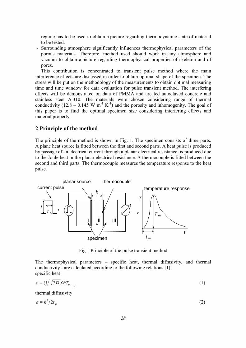
interference effects are discussed in order to obtain optimal shape of the specimen. The stress will be put on the methodology of the measurements to obtain optimal measuring time and time window for data evaluation for pulse transient method. The interfering effects will be demonstrated on data of PMMA and areated autoclaved concrete and stainless steel A 310. The materials were chosen considering range of thermal conductivity (12.8 – 0.145 W m-1 K-1) and the porosity and inhomogenity. The goal of this paper is to find the optimal specimen size considering interfering effects and material property. 2 Principle of the method The principle of the method is shown in Fig. 1. The specimen consists of three parts. A plane heat source is fitted between the first and second parts. A heat pulse is produced by passage of an electrical current through a planar electrical resistance. is produced due to the Joule heat in the planar electrical resistance. A thermocouple is fitted between the second and third parts. The thermocouple measures the temperature response to the heat pulse.

specimen

current pulse

It o

planar source thermocouple

I II III

temperature response

T

t

T m

t m

h

Fig 1 Principle of the pulse transient method

The thermophysical parameters – specific heat, thermal diffusivity, and thermal conductivity - are calculated according to the following relations [1]: specific heat

c Q e hTm= 2π ρ , (1)

thermal diffusivity

a h tm= 2 2 (2)

29

and thermal conductivity

λ ρ= ac (3)

where Q RI t= 20 , R is the electrical resistance of the planar heat source, to is the width

of the current pulse, ρ is the density, and the other parameters are defined in Fig. 1.

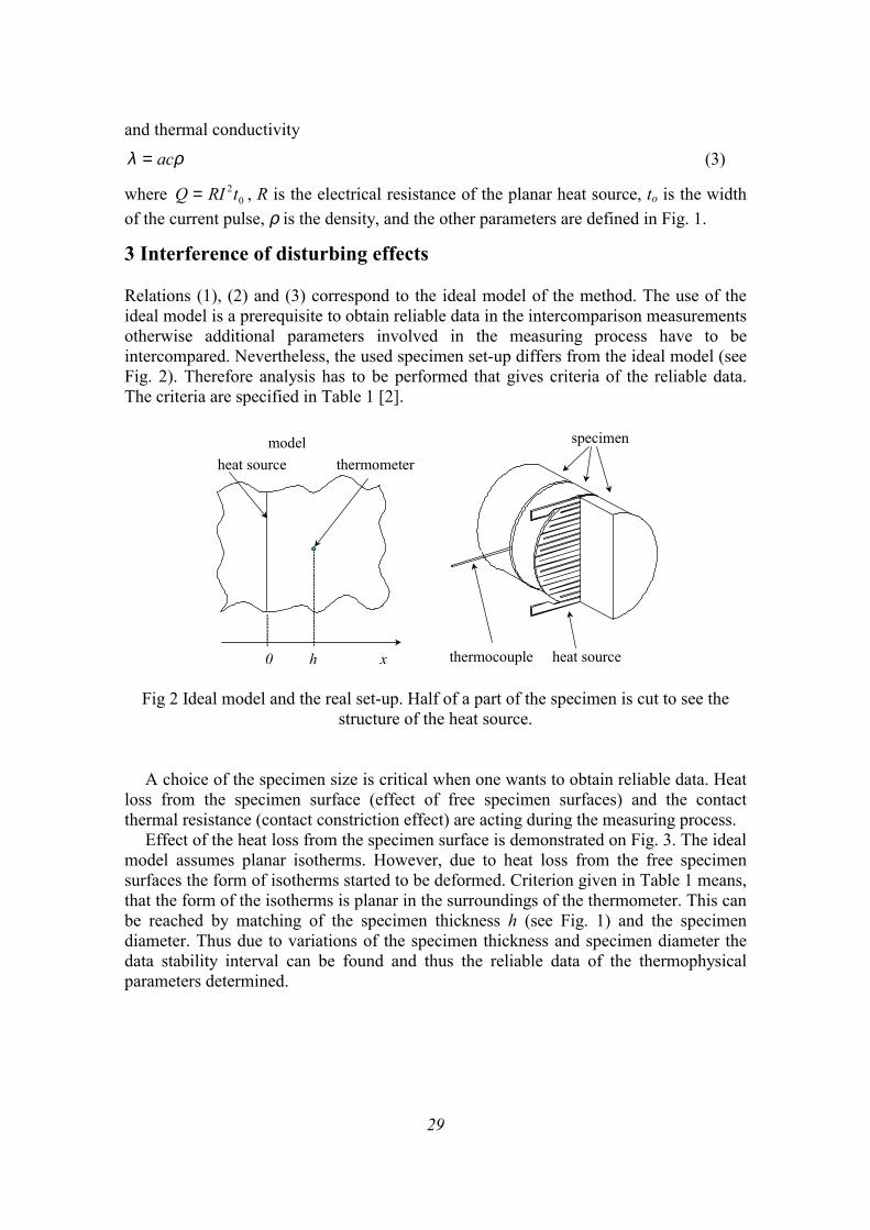
3 Interference of disturbing effects Relations (1), (2) and (3) correspond to the ideal model of the method. The use of the ideal model is a prerequisite to obtain reliable data in the intercomparison measurements otherwise additional parameters involved in the measuring process have to be intercompared. Nevertheless, the used specimen set-up differs from the ideal model (see Fig. 2). Therefore analysis has to be performed that gives criteria of the reliable data. The criteria are specified in Table 1 [2].

specimen

thermocouple heat source0 h x

modelheat source thermometer

Fig 2 Ideal model and the real set-up. Half of a part of the specimen is cut to see the structure of the heat source.

A choice of the specimen size is critical when one wants to obtain reliable data. Heat loss from the specimen surface (effect of free specimen surfaces) and the contact thermal resistance (contact constriction effect) are acting during the measuring process.

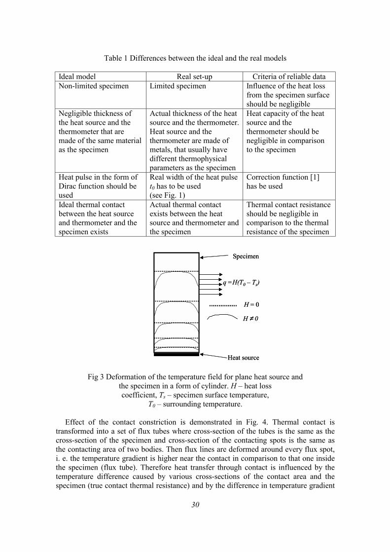
Effect of the heat loss from the specimen surface is demonstrated on Fig. 3. The ideal model assumes planar isotherms. However, due to heat loss from the free specimen surfaces the form of isotherms started to be deformed. Criterion given in Table 1 means, that the form of the isotherms is planar in the surroundings of the thermometer. This can be reached by matching of the specimen thickness h (see Fig. 1) and the specimen diameter. Thus due to variations of the specimen thickness and specimen diameter the data stability interval can be found and thus the reliable data of the thermophysical parameters determined.

30

Table 1 Differences between the ideal and the real models Ideal model Real set-up Criteria of reliable data Non-limited specimen Limited specimen Influence of the heat loss

from the specimen surface should be negligible

Negligible thickness of the heat source and the thermometer that are made of the same material as the specimen

Actual thickness of the heat source and the thermometer. Heat source and the thermometer are made of metals, that usually have different thermophysical parameters as the specimen

Heat capacity of the heat source and the thermometer should be negligible in comparison to the specimen

Heat pulse in the form of Dirac function should be used

Real width of the heat pulse t0 has to be used (see Fig. 1)

Correction function [1] has be used

Ideal thermal contact between the heat source and thermometer and the specimen exists

Actual thermal contact exists between the heat source and thermometer and the specimen

Thermal contact resistance should be negligible in comparison to the thermal resistance of the specimen

Fig 3 Deformation of the temperature field for plane heat source and

the specimen in a form of cylinder. H – heat loss coefficient, Ts – specimen surface temperature,

T0 – surrounding temperature.

Effect of the contact constriction is demonstrated in Fig. 4. Thermal contact is transformed into a set of flux tubes where cross-section of the tubes is the same as the cross-section of the specimen and cross-section of the contacting spots is the same as the contacting area of two bodies. Then flux lines are deformed around every flux spot, i. e. the temperature gradient is higher near the contact in comparison to that one inside the specimen (flux tube). Therefore heat transfer through contact is influenced by the temperature difference caused by various cross-sections of the contact area and the specimen (true contact thermal resistance) and by the difference in temperature gradient

Specimen

Heat source

q =H(T0 – Ts)

H = 0

H ≠ 0

Specimen

Heat source

q =H(T0 – Ts)

H = 0

H ≠ 0

31

near contact caused by the constriction effect and inside the specimen (constriction thermal resistance).

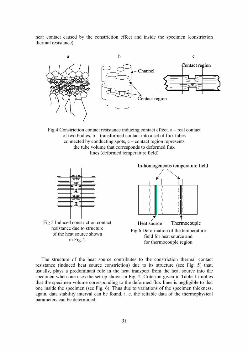
Fig 4 Constriction contact resistance inducing contact effect. a – real contact

of two bodies, b – transformed contact into a set of flux tubes connected by conducting spots, c – contact region represents

the tube volume that corresponds to deformed flux lines (deformed temperature field)

Fig 5 Induced constriction contact resistance due to structure of the heat source shown

in Fig. 2

Fig 6 Deformation of the temperature field for heat source and for thermocouple region

The structure of the heat source contributes to the constriction thermal contact resistance (induced heat source constriction) due to its structure (see Fig. 5) that, usually, plays a predominant role in the heat transport from the heat source into the specimen when one uses the set-up shown in Fig. 2. Criterion given in Table 1 implies that the specimen volume corresponding to the deformed flux lines is negligible to that one inside the specimen (see Fig. 6). Thus due to variations of the specimen thickness, again, data stability interval can be found, i. e. the reliable data of the thermophysical parameters can be determined.

Contact region

ChannelContact region

a b c

Contact region

ChannelContact regionContact region

a b c

In-homogeneous temperature field

Heat source Thermocouple

In-homogeneous temperature field

Heat source Thermocouple

32

4 Experiment PMMA, aerated autoclaved concrete and stainless steel A 310 were chosen to verify the constriction and free surface effects. Table 1 gives overview on specimen material, specimen geometry and characteristics of the heat source.

Table 2 Experimental characteristics Experiment-al parameter

PMMA Autoclaved aerated concrete

Stainless steel A 310

Density 1184 kg m-3 517 kg m-3 7902 kg m-3 Specimen dimension

Φ = 20 mm Φ = 30 mm

150x150 mm Φ = 20 mm

Heat source characteris-tics (see Fig. 2)

Width of strip 0.5 mm Width of empty line 0.1 mm

Width of strip 2.5 mm Width of empty line 2.5 mm

Width of strip 0.5 mm Width of empty line 0.1 mm

Thermal conductivity

0.192 W m-1 K-1 [4] 0.138 W m-1 K-1 [5] 12.8 W m-1 K-1 [6]

Instruments RT 1.02 and RTB 1.01 (Institute of Physics SAS) were used for

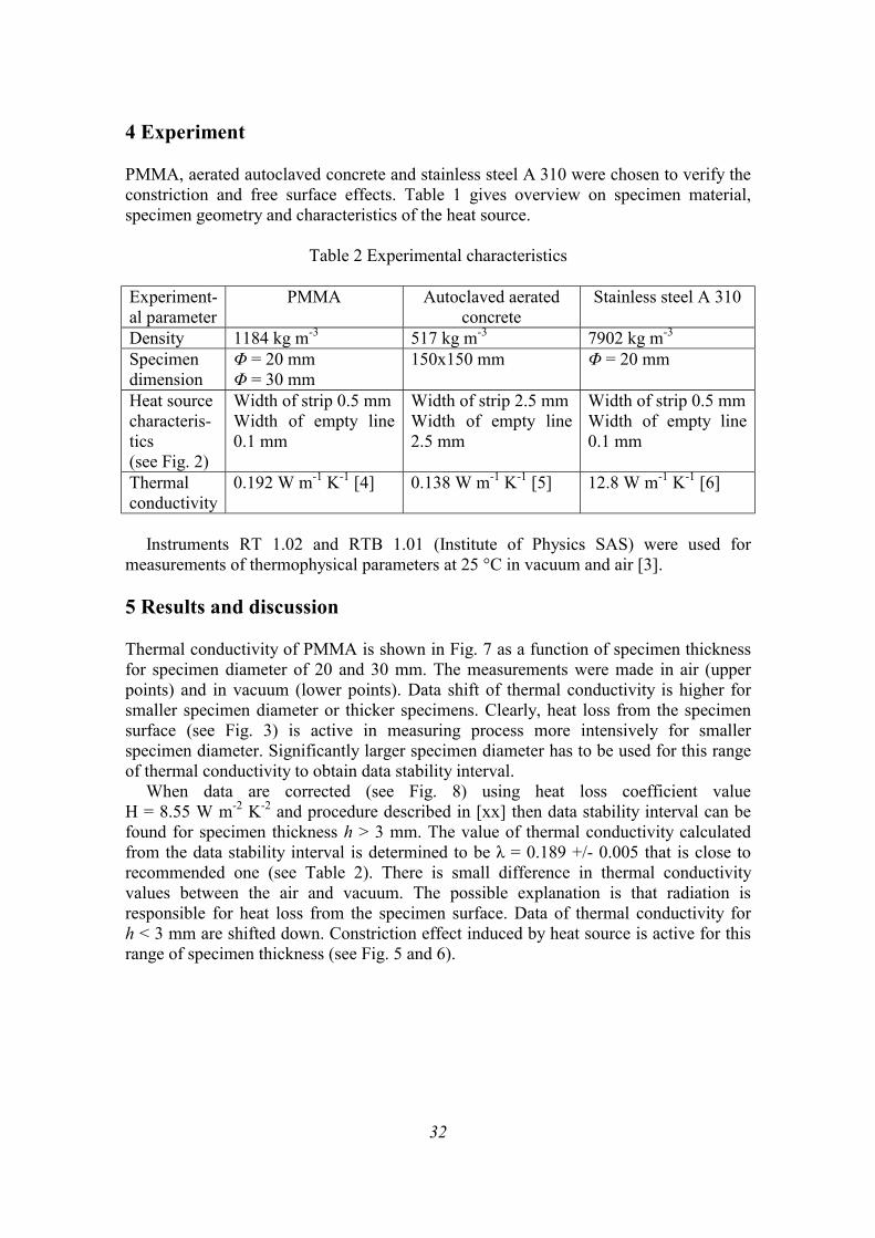
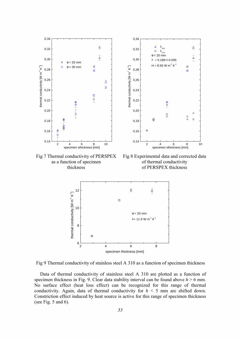
measurements of thermophysical parameters at 25 °C in vacuum and air [3]. 5 Results and discussion Thermal conductivity of PMMA is shown in Fig. 7 as a function of specimen thickness for specimen diameter of 20 and 30 mm. The measurements were made in air (upper points) and in vacuum (lower points). Data shift of thermal conductivity is higher for smaller specimen diameter or thicker specimens. Clearly, heat loss from the specimen surface (see Fig. 3) is active in measuring process more intensively for smaller specimen diameter. Significantly larger specimen diameter has to be used for this range of thermal conductivity to obtain data stability interval.

When data are corrected (see Fig. 8) using heat loss coefficient value H = 8.55 W m-2 K-2 and procedure described in [xx] then data stability interval can be found for specimen thickness h > 3 mm. The value of thermal conductivity calculated from the data stability interval is determined to be λ = 0.189 +/- 0.005 that is close to recommended one (see Table 2). There is small difference in thermal conductivity values between the air and vacuum. The possible explanation is that radiation is responsible for heat loss from the specimen surface. Data of thermal conductivity for h < 3 mm are shifted down. Constriction effect induced by heat source is active for this range of specimen thickness (see Fig. 5 and 6).

33

Fig 7 Thermal conductivity of PERSPEX as a function of specimen

thickness

Fig 8 Experimental data and corrected data of thermal conductivity of PERSPEX thickness

Fig 9 Thermal conductivity of stainless steel A 310 as a function of specimen thickness

Data of thermal conductivity of stainless steel A 310 are plotted as a function of specimen thickness in Fig. 9. Clear data stability interval can be found above h > 6 mm. No surface effect (heat loss effect) can be recognized for this range of thermal conductivity. Again, data of thermal conductivity for h < 5 mm are shifted down. Constriction effect induced by heat source is active for this range of specimen thickness (see Fig. 5 and 6).

2 4 6 8 100,14

0,16

0,18

0,20

0,22

0,24

0,26

0,28

0,30

0,32

0,34

λexp

λcorrφ = 20 mmλ = 0.189+/-0.005

H = 8.55 W m-2 K-2

ther

mal

con

duct

ivity

[W m

-1 K

-1]

specimen sthickness [mm]2 4 6 8 10

0,14

0,16

0,18

0,20

0,22

0,24

0,26

0,28

0,30

0,32

0,34

φ = 20 mm φ = 30 mm

ther

mal

con

duct

ivity

[W m

-1 K

-1]

specimen sthickness [mm]

2 4 6 86

8

10

12

φ = 20 mm

λ= 11.9 W m-1 K-1

ther

mal

con

duct

ivity

[W m

-1 K

-1]

specimen thickness [mm]

34

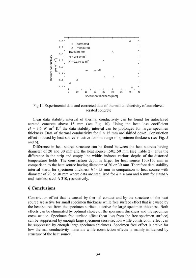
Fig 10 Experimental data and corrected data of thermal conductivity of autoclaved aerated concrete

Clear data stability interval of thermal conductivity can be found for autoclaved

aerated concrete above 15 mm (see Fig. 10). Using the heat loss coefficient H = 3.6 W m-2 K-1 the data stability interval can be prolonged for larger specimen thickness. Data of thermal conductivity for h < 15 mm are shifted down. Constriction effect induced by heat source is active for this range of specimen thickness (see Fig. 5 and 6).

Difference in heat source structure can be found between the heat sources having diameter of 20 and 30 mm and the heat source 150x150 mm (see Table 2). Thus the difference in the strip and empty line widths induces various depths of the distorted temperature fields. The constriction depth is larger for heat source 150x150 mm in comparison to the heat source having diameter of 20 or 30 mm. Therefore data stability interval starts for specimen thickness h > 15 mm in comparison to heat source with diameter of 20 or 30 mm where data are stabilized for h > 4 mm and 6 mm for PMMA and stainless steel A 310, respectively. 6 Conclusions Constriction effect that is caused by thermal contact and by the structure of the heat source are active for small specimen thickness while free surface effect that is caused by the heat source from the specimen surface is active for large specimen thickness. Both effects can be eliminated by optimal choice of the specimen thickness and the specimen cross-section. Specimen free surface effect (heat loss from the free specimen surface) can be suppressed by enough large specimen cross-section while constriction effect can be suppressed by enough large specimen thickness. Specimen free effect is active for low thermal conductivity materials while constriction effects is mainly influenced by structure of the heat source.

5 10 15 20 25 30 35 40 45

0,12

0,13

0,14

0,15

0,16

0,17

0,18

0,19

corrected measured

150x150 mmH = 3.6 W m-2

λ = 0.144 W m-2

ther

mal

con

duct

ivity

[W m

-1 K

-1]

specimen thickness [mm]

35

Acknowledgements The authors are grateful to the Thermophysical Properties Section at the National Physical Laboratory for providing specimens of stainless steel A 320 and to Dr. Matiasovsky for providing specimens of autoclaved aerated concrete and to Mr. Markovic for the assistance during experiment. This work was supported by grant agency VEGA under Nr. 2/6066/2001. References [1] Kubičár Ľ, 1990 Pulse Method of Measuring Basic Thermophysical Parameters, in

Comprehensive Analytical Chemistry Vol. XII Thermal Analysis Part E, (Ed Svehla G, Amsterdam, Oxford, New York, Tokyo: Elsevier), pp. 350

[2] Kubičár Ľ, Boháč V, 1990 Review of several dynamic methods of measuring thermophysical parameters, in Proc. of 24th Int. Conf on Thermal Conductivity / 12th Int. Thermal Expansion Symposium October 26 – 29 1997 (Eds. P S Gaal and D E Apostolescu, Lancaster: Technomic Publishing Company), p. 135 – 149

[3] Thermophysical transient tester RT 1.02, RTB 1.01, Manual, Institute of Physics SAS, 2000

[4] Salmon D. R., 1999 personal communication National Physical Laboratory (Teddington, TW11 0LW, UK)

[5] Matiašovský P, Koronthalyová O, 1994 Building Research Journal, 42, 265 [6] Corsan J, Budd N and Hemminger W, 1991 High Temp. – High Press, 23, 119 –

128

36

37

MEASUREMENT OF THERMOPHYSICAL PARAMETERS OF POROFEN BY PULSE TRANSIENT METHOD Viliam Vretenár, Ľudovít Kubičár, Vlastimil Boháč Institute of Physics, Slovak Academy of Sciences, Dubravska cesta 9, 842 28 Bratislava, Slovakia Email: fyzikubo@nic.savba.sk Abstract The measurement of thermophysical parameters of Porofen by pulse transient method is presented. The measurement is realized by generating a dynamic temperature field in a form of the heat pulse in the specimen, where the temperature response is recorded at certain distance from the heat source. Theory of the method, its experimental arrangement and treatment of measured data (difference analysis) are presented. Differences between ideal model and real experiment was investigated and discussed. Keywords: transient method, thermophysical parameters, difference analysis 1 Introduction The pulse transient method[1] for measurement of specific heat, thermal diffusivity and thermal conductivity belongs to the class of the transient methods [2], which have shown improvements during the last years. The method is based on the generation of dynamic temperature field inside the specimen by the passage of the electrical current through a planar electrical resistance. In this method the heat is produced in the form of a pulse. A thermocouple placed apart from the heat source measures the temperature response, from which the thermophysical parameters are calculated.

Fulfilment of ideal model criteria [1] play predominant role for accuracy and reproducibility of an experiment. Unfortunately, in real experiment it is impossible to fulfil these criteria. The differences between the real and the ideal model can lead to data shift and data scattering. Therefore, we have to adjust the experimental arrangement in order to achieve as wide range as can do to score the experiment. One manner how to perform experimnet in the correct way, is the use of the difference analysis after each measurement. In this analysis, we look for differences between the ideal and the real temperature response in chosen time interval, which is consecutive shifted over the time. Then, we are able to decide, whether the experiment fulfils the criteria for ideal model in appropriate accuracy.

The measurements were caried out on building light-weight material Porofen. Thermophysical parameters were measured for several thickness in order to determine proper thickness range, where we can find stabile data. In this way the fulfilment of ideal model criteria (boundary conditions etc.) can be verified. Thermophysical transient tester model RTB 1.02 (Physical Intitute of Slovak Academy of Sciences) was used for measuring this bulding material.

38

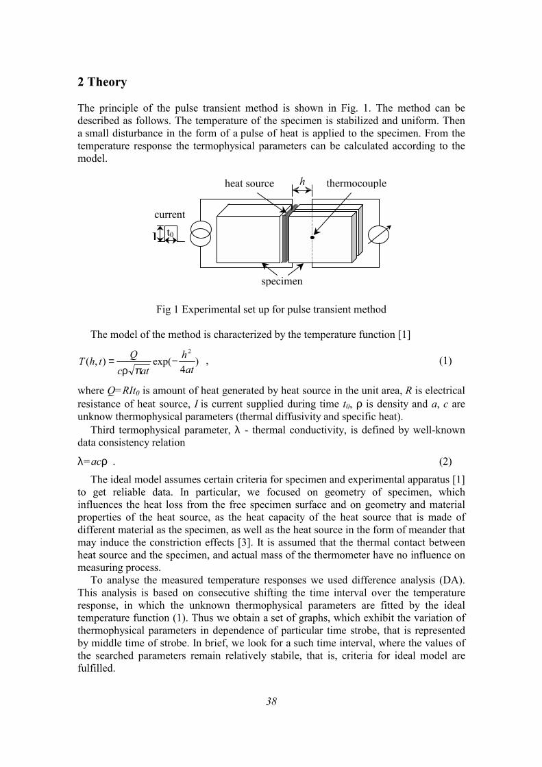
2 Theory The principle of the pulse transient method is shown in Fig. 1. The method can be described as follows. The temperature of the specimen is stabilized and uniform. Then a small disturbance in the form of a pulse of heat is applied to the specimen. From the temperature response the termophysical parameters can be calculated according to the model.

Fig 1 Experimental set up for pulse transient method

The model of the method is characterized by the temperature function [1]

)4

exp(),(2

ath

atcQthT −πρ

= , (1)

where Q=RIt0 is amount of heat generated by heat source in the unit area, R is electrical resistance of heat source, I is current supplied during time t0, ρ is density and a, c are unknow thermophysical parameters (thermal diffusivity and specific heat).

Third termophysical parameter, λ - thermal conductivity, is defined by well-known data consistency relation

λ=acρ . (2)

The ideal model assumes certain criteria for specimen and experimental apparatus [1] to get reliable data. In particular, we focused on geometry of specimen, which influences the heat loss from the free specimen surface and on geometry and material properties of the heat source, as the heat capacity of the heat source that is made of different material as the specimen, as well as the heat source in the form of meander that may induce the constriction effects [3]. It is assumed that the thermal contact between heat source and the specimen, and actual mass of the thermometer have no influence on measuring process.

To analyse the measured temperature responses we used difference analysis (DA). This analysis is based on consecutive shifting the time interval over the temperature response, in which the unknown thermophysical parameters are fitted by the ideal temperature function (1). Thus we obtain a set of graphs, which exhibit the variation of thermophysical parameters in dependence of particular time strobe, that is represented by middle time of strobe. In brief, we look for a such time interval, where the values of the searched parameters remain relatively stabile, that is, criteria for ideal model are fulfilled.

h thermocouple heat source

specimen

current t0I

39

3 Experimental set-up The specimen having dimension of 150x150 mm was cut from light-weight building material Porofen with density ρ = 31.64 kg.m-3 into two parts and are arranged symetricaly considering heat source (Fig. 1). The thickness of both parts is 70 mm. The second part is again cut longitudinal in order to realize measurements in various distances from the heat source. The thin isolated metal foil (fy Minco) of thickness 0.25 mm in form of meander is used as the heat source. The electrical resistance of the heat source was ≈ 10 Ω. A thermocouple, made of insulated Chromel and Alumel wires having the thickness of 0.07 mm, is placed apart of the heat source among the longitudinal cut surfaces.

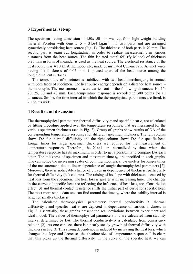
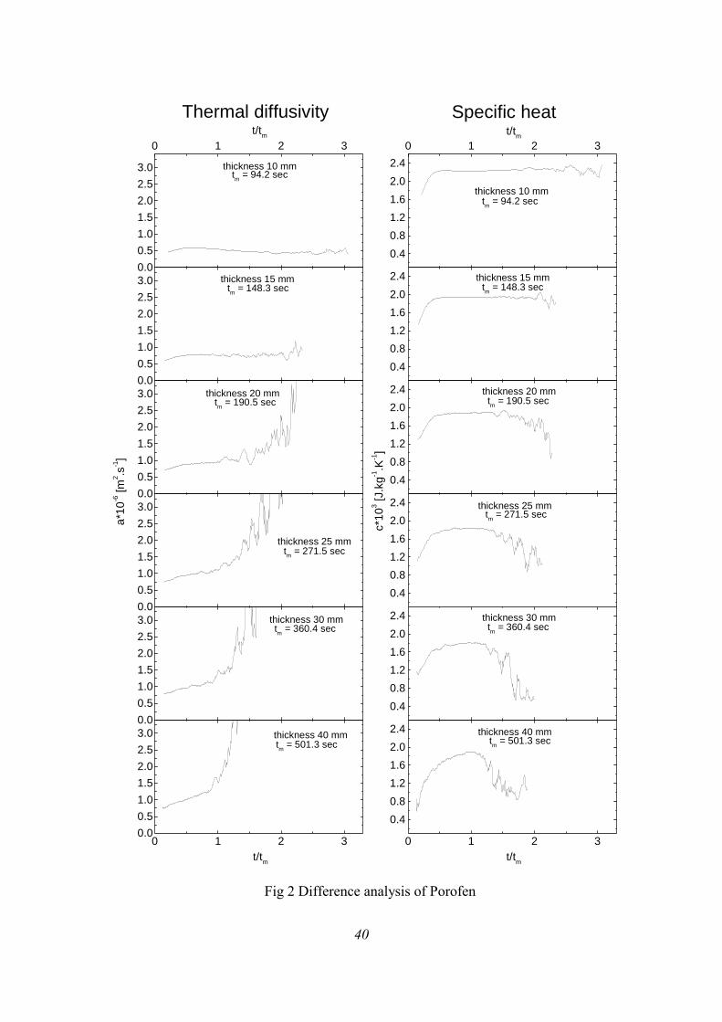
The temperature of specimen is stabilized with two heat interchangers, in contact with both faces of specimen. The heat pulse energy depends on a distance heat source – thermocouple. The measurements were carried out in the following distances: 10, 15, 20, 25, 30 and 40 mm. Each temperature response is recorded in 300 points for all distances. Strobe, the time interval in which the thermophysical parameters are fitted, is 20 points wide. 4 Results and discussion The thermophysical parameters: thermal diffusivity a and specific heat c, are calculated by fitting procedure applied over the temperature responses, that are mesasured for the various specimen thickness (see in Fig. 2). Group of graphs show results of DA of the corresponding temperature responses for different specimen thickness. The left column shows DA for thermal diffusivity and the right column shows DA for specific heat. Longer times for larger specimen thickness are required for the measurement of temperature responses. Therefore, the X-axis are normalized by time, where the temperature response has its maximum, in order to get a possibility to compare DA each other. The thickness of specimen and maximum time tm are specified in each graphs. One can notice the increasing scater of both thermophysical parameters for longer times of the measurement, due to linear dependence of sought thermophysical parameters [2]. Moreover, there is noticeable change of curves in dependence of thickness, particularly for thermal diffusivity (left column). The raising of its slope with thickness is caused by heat loss from the specimen. The heat loss is greater with increasing time. The changes in the curves of specific heat are reflecting the influence of heat loss, too. Constriction effect [3] and thermal contact resistance shifts the initial part of curve for specific heat. The most more stable data one can find around the time tm, where the stability interval is large for smaller thickness.

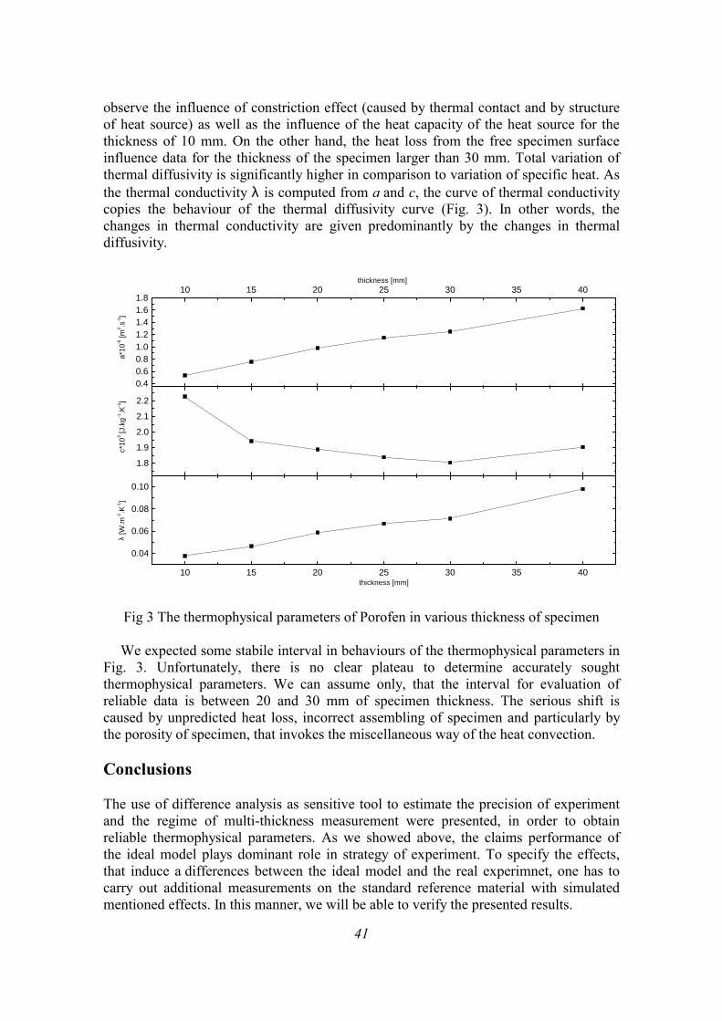
The calculated thermophysical parameters: thermal conductivity λ, thermal diffusivity a and specific heat c, are depicted in dependence of various thickness in Fig. 3. Essentially, these graphs present the real deviations between experiment and ideal model. The values of thermophysical parameters a, c are calculated from stability interval determined by DA. The thermal conductivity λ is calculated from consistency relation (2). As one can see, there is a nearly steady growth of thermal diffusivity with thickness in Fig. 3. This strong dependence is induced by increasing the heat loss, which changes the slope and decreases the absolute size of temperature response. It is clear, that this picks up the thermal diffusivity. In the curve of the specific heat, we can

40

0.00.51.01.52.02.53.0

0 1 2 3

tm = 94.2 sec

t/tm

thickness 10 mm

0.40.81.21.62.02.4

0 1 2 3

tm = 94.2 sec

t/tm

thickness 10 mm

0.00.51.01.52.02.53.0

tm = 148.3 sec

thickness 15 mm

0.40.81.21.62.02.4

tm = 148.3 sec

thickness 15 mm

0.00.51.01.52.02.53.0

tm = 190.5 sec

thickness 20 mm

0.40.81.21.62.02.4

tm = 190.5 sec

thickness 20 mm

0.00.51.01.52.02.53.0

tm = 271.5 sec

thickness 25 mm

a*10

-6 [m

2 .s-1]

0.40.81.21.62.02.4

Specific heatThermal diffusivity

tm = 271.5 sec

thickness 25 mm

c*10

3 [J.k

g-1.K

-1]

0.00.51.01.52.02.53.0

tm = 360.4 sec

thickness 30 mm

0.40.81.21.62.02.4

tm = 360.4 sec

thickness 30 mm

0 1 2 30.00.51.01.52.02.53.0

t/tm

tm = 501.3 sec

thickness 40 mm

0 1 2 3

0.40.81.21.62.02.4

t/tm

tm = 501.3 sec

thickness 40 mm

Fig 2 Difference analysis of Porofen

41

observe the influence of constriction effect (caused by thermal contact and by structure of heat source) as well as the influence of the heat capacity of the heat source for the thickness of 10 mm. On the other hand, the heat loss from the free specimen surface influence data for the thickness of the specimen larger than 30 mm. Total variation of thermal diffusivity is significantly higher in comparison to variation of specific heat. As the thermal conductivity λ is computed from a and c, the curve of thermal conductivity copies the behaviour of the thermal diffusivity curve (Fig. 3). In other words, the changes in thermal conductivity are given predominantly by the changes in thermal diffusivity.

10 15 20 25 30 35 40

0.04

0.06

0.08

0.10

λ [W

.m-1.K

-1]

thickness [mm]

1.8

1.9

2.0

2.1

2.2

c*10

3 [J.k

g-1.K

-1]

0.40.60.81.01.21.41.61.8

10 15 20 25 30 35 40 thickness [mm]

a*10

-6 [m

2 .s-1]

Fig 3 The thermophysical parameters of Porofen in various thickness of specimen

We expected some stabile interval in behaviours of the thermophysical parameters in Fig. 3. Unfortunately, there is no clear plateau to determine accurately sought thermophysical parameters. We can assume only, that the interval for evaluation of reliable data is between 20 and 30 mm of specimen thickness. The serious shift is caused by unpredicted heat loss, incorrect assembling of specimen and particularly by the porosity of specimen, that invokes the miscellaneous way of the heat convection. Conclusions The use of difference analysis as sensitive tool to estimate the precision of experiment and the regime of multi-thickness measurement were presented, in order to obtain reliable thermophysical parameters. As we showed above, the claims performance of the ideal model plays dominant role in strategy of experiment. To specify the effects, that induce a differences between the ideal model and the real experimnet, one has to carry out additional measurements on the standard reference material with simulated mentioned effects. In this manner, we will be able to verify the presented results.

42

Acknowledgement The authors wish to thank to Mr. Markovic for the assistance during experiment. This work was supported by the Slovak Science Grant Agency VEGA under Nr. 2/5084/98. References [1] Kubičár Ľ, 1990 Pulse Method of Measuring Basic Thermophysical Parameters,

in Comprehensive Analytical Chemistry, Vol XII, Thermal Analysis, Part E (Ed Svehla G, Amsterdam, Oxford, New York, Tokyo: Elsevier)

[2] Kubičár Ľ; Boháč V, 1990 Review of several dynamic methods of measuring thermophysical parameters, in Proc. of 24th Int. Conf on Thermal Conductivity / 12th Int. Thermal Expansion Symposium October 26 – 29 1997 (Eds Gaal P S and Apostolescu D E, Lancaster: Technomic Publishing Company) pp. 135 – 149

[3] Degiovanni A, Moyne C, 1989 Resistance thermique de contact en regime pemanent, Unfluence de la geometry du contact, Rev Generale Thermique, 334, pp. 557-564

[4] Beck J V, Arnold K, 1997 Parameter Estimation in Engineering and Sciences (New York, London, Sidney, Toronto, John Willey)

43

THERMAL DIFFUSIVITY OF FIBROUS COMPOSITES Tatiana Šrámková1, Ján Spišiak1, Pavol Štefánik2, Pavol Šebo2 1 Institute of Physics, Slovak Academy of Sciences, Dúbravská cesta 9,

842 28 Bratislava, Slovak Republic 2 Institute of Materials and Machine Mechanics, Slovak Academy of Sciences,

Račianska 75, 831 02 Bratislava, Slovak Republic Email: spisiak@savba.sk Abstract The effective thermal diffusivity of carbon fiber reinforced copper matrix composites (Cu-Cf MMC) has been measured by the flash method. The thermal diffusivity measurements of unidirectional (transversal and longitudinal) composites with fiber volumes 40, 50, and 60 % are compared with values predicted by the theoretical models. Key words: flash method, composite, Cu-Cf MMC, effective thermal diffusivity,

effective thermal conductivity 1 Introduction The carbon fiber reinforced - copper matrix composite are now of great interest of the composite industry for their interesting thermomechanical properties, which are good machinability, good thermal conductivity and adjustable coefficient of thermal expansion. These features make them a good candidate for a potential use in the electronics packaging industry. The aim of studying of these materials is to find a composite with the thermal conductivity close to that of pure copper and the thermal expansion coefficient of the order of ceramics. Light and stiff carbon fibers help to reduce the thermal expansion coefficient of the copper matrix. Their thermal conductivity could vary from very low to very high values of the order of copper.

Thermal conductivity can be obtained precisely by steady-state methods. As these methods are generally time consuming, thermal conductivity is often determined by using dynamic methods. The measured quantity is thermal diffusivity and thermal conductivity is calculated if specific heat and density of the measured material are known. For heterogeneous materials, an effective thermal conductivity can be defined by the Fourier law, using the average value of the temperature gradient over a region that is large compared to the scale of heterogenity. A considerable progress has been made in relating the effective steady-state thermal conductivity of a composite to the conductivities of its individual components. However, under transient conditions there are fewer known models that relate the heterogeneous thermal diffusivity to that of individual components as in the steady-state case. The predicted effective thermal diffusivity is usually obtained by numerical simulations, e. g. by using finite element methods, if the microscopic picture of a material is known. Recently, an effort to derive an equation for the effective thermal diffusivity has been done [1] by using effective

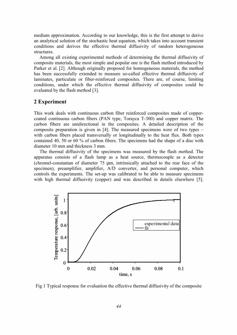
44

medium approximation. According to our knowledge, this is the first attempt to derive an analytical solution of the stochastic heat equation, which takes into account transient conditions and derives the effective thermal diffusivity of random heterogeneous structures.

Among all existing experimental methods of determining the thermal diffusivity of composite materials, the most simple and popular one is the flash method introduced by Parker et al. [2]. Although originally proposed for homogeneous materials, the method has been successfully extended to measure so-called effective thermal diffusivity of laminates, particulate or fiber-reinforced composites. There are, of course, limiting conditions, under which the effective thermal diffusivity of composites could be evaluated by the flash method [3]. 2 Experiment This work deals with continuous carbon fiber reinforced composites made of copper-coated continuous carbon fibers (PAN type, Torayca T-300) and copper matrix. The carbon fibers are unidirectional in the composites. A detailed description of the composite preparation is given in [4]. The measured specimens were of two types – with carbon fibers placed transversally or longitudinally to the heat flux. Both types contained 40, 50 or 60 % of carbon fibers. The specimens had the shape of a disc with diameter 10 mm and thickness 3 mm.

The thermal diffusivity of the specimens was measured by the flash method. The apparatus consists of a flash lamp as a heat source, thermocouple as a detector (chromel-constantan of diameter 75 µm, intrinsically attached to the rear face of the specimen), preamplifier, amplifier, A/D converter, and personal computer, which controls the experiments. The set-up was calibrated to be able to measure specimens with high thermal diffusivity (copper) and was described in details elsewhere [5].

0

0.2

0.4

0.6

0.8

1

0 0.02 0.04 0.06 0.08 0.1time, s

Tem

pera

ture

resp

onse

, [ar

b. u

nits]

experimental datafit

0

0.2

0.4

0.6

0.8

1

0 0.02 0.04 0.06 0.08 0.1time, s

Tem

pera

ture

resp

onse

, [ar

b. u

nits]

experimental datafit

Fig 1 Typical response for evaluation the effective thermal diffusivity of the composite

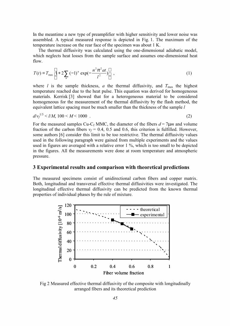
45

In the meantime a new type of preamplifier with higher sensitivity and lower noise was assembled. A typical measured response is depicted in Fig. 1. The maximum of the temperature increase on the rear face of the specimen was about 1 K.

The thermal diffusivity was calculated using the one-dimensional adiabatic model, which neglects heat losses from the sample surface and assumes one-dimensional heat flow.

−−+= ∑ )exp()1(21)( 2

22

max latnTtT

n

n π , (1)

where l is the sample thickness, a the thermal diffusivity, and Tmax the highest temperature reached due to the heat pulse. This equation was derived for homogeneous materials. Kerrisk [3] showed that for a heterogeneous material to be considered homogeneous for the measurement of the thermal diffusivity by the flash method, the equivalent lattice spacing must be much smaller than the thickness of the sample l

d/vf1/3 < l/M, 100 < M < 1000 . (2)

For the measured samples Cu-Cf MMC, the diameter of the fibers d = 7µm and volume fraction of the carbon fibers vf = 0.4, 0.5 and 0.6, this criterion is fulfilled. However, some authors [6] consider this limit to be too restrictive. The thermal diffusivity values used in the following paragraph were gained from multiple experiments and the values used in figures are averaged with a relative error 1 %, which is too small to be depicted in the figures. All the measurements were done at room temperature and atmospheric pressure. 3 Experimental results and comparison with theoretical predictions The measured specimens consist of unidirectional carbon fibers and copper matrix. Both, longitudinal and transversal effective thermal diffusivities were investigated. The longitudinal effective thermal diffusivity can be predicted from the known thermal properties of individual phases by the rule of mixture.

0

20

40

60

80

100

120

0 0.2 0.4 0.6 0.8 1Fiber volume fraction

Ther

mal

diff

usiv

ity [1

0-6m

2 /s]

theoreticalexperimental

0

20

40

60

80

100

120

0 0.2 0.4 0.6 0.8 1Fiber volume fraction

Ther

mal

diff

usiv

ity [1

0-6m

2 /s]

theoreticalexperimental

Fig 2 Measured effective thermal diffusivity of the composite with longitudinally arranged fibers and its theoretical prediction

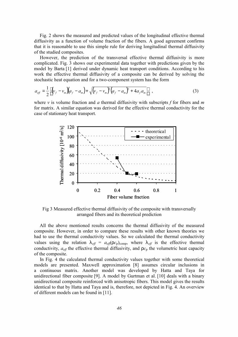
46

Fig. 2 shows the measured and predicted values of the longitudinal effective thermal diffusivity as a function of volume fraction of the fibers. A good agreement confirms that it is reasonable to use this simple rule for deriving longitudinal thermal diffusivity of the studied composites.

However, the prediction of the transversal effective thermal diffusivity is more complicated. Fig. 3 shows our experimental data together with predictions given by the model by Barta [1] derived under dynamic heat transport conditions. According to his work the effective thermal diffusivity of a composite can be derived by solving the stochastic heat equation and for a two-component system has the form

( )( ) ( ) ( )

+−−+−−= mfmfmfmfmfeff aaaavvaavva 4

21 22 , (3)

where v is volume fraction and a thermal diffusivity with subscripts f for fibers and m for matrix. A similar equation was derived for the effective thermal conductivity for the case of stationary heat transport.

0

20

40

60

80

100

120

0 0.2 0.4 0.6 0.8 1Fiber volume fraction

Ther

mal

diff

usiv

ity [1

0-6m

2 /s]

theoreticalexperimental

0

20

40

60

80

100

120

0 0.2 0.4 0.6 0.8 1Fiber volume fraction

Ther

mal

diff

usiv

ity [1

0-6m

2 /s]

theoreticalexperimental

Fig 3 Measured effective thermal diffusivity of the composite with transversally arranged fibers and its theoretical prediction

All the above mentioned results concerns the thermal diffusivity of the measured

composite. However, in order to compare these results with other known theories we had to use the thermal conductivity values. So we calculated the thermal conductivity values using the relation λeff = aeff(ρcp)comp, where λeff is the effective thermal conductivity, aeff the effective thermal diffusivity, and ρcp the volumetric heat capacity of the composite.

In Fig. 4 the calculated thermal conductivity values together with some theoretical models are presented. Maxwell approximation [8] assumes circular inclusions in a continuous matrix. Another model was developed by Hatta and Taya for unidirectional fiber composite [9]. A model by Gurtman et al. [10] deals with a binary unidirectional composite reinforced with anisotropic fibers. This model gives the results identical to that by Hatta and Taya and is, therefore, not depicted in Fig. 4. An overview of different models can be found in [11].

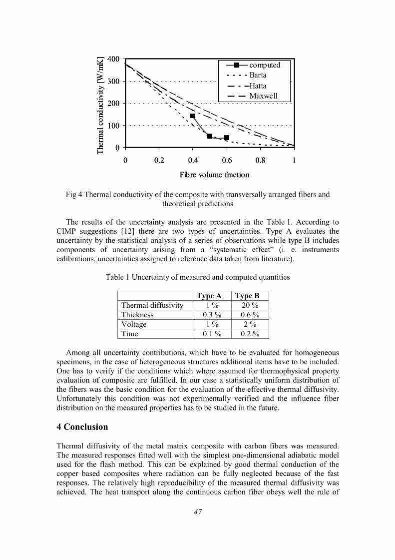
47

0

100

200

300

400

0 0.2 0.4 0.6 0.8 1

Fibre volume fraction

Ther

mal

con

duct

ivity

[W/m

K]

Bartacomputed

HattaMaxwell

0

100

200

300

400

0 0.2 0.4 0.6 0.8 1

Fibre volume fraction

Ther

mal

con

duct

ivity

[W/m

K]

Bartacomputed

HattaMaxwell

Bartacomputed

HattaMaxwell

Fig 4 Thermal conductivity of the composite with transversally arranged fibers and theoretical predictions

The results of the uncertainty analysis are presented in the Table 1. According to

CIMP suggestions [12] there are two types of uncertainties. Type A evaluates the uncertainty by the statistical analysis of a series of observations while type B includes components of uncertainty arising from a “systematic effect” (i. e. instruments calibrations, uncertainties assigned to reference data taken from literature).

Table 1 Uncertainty of measured and computed quantities

Type A Type B Thermal diffusivity 1 % 20 % Thickness 0.3 % 0.6 % Voltage 1 % 2 % Time 0.1 % 0.2 %

Among all uncertainty contributions, which have to be evaluated for homogeneous

specimens, in the case of heterogeneous structures additional items have to be included. One has to verify if the conditions which where assumed for thermophysical property evaluation of composite are fulfilled. In our case a statistically uniform distribution of the fibers was the basic condition for the evaluation of the effective thermal diffusivity. Unfortunately this condition was not experimentally verified and the influence fiber distribution on the measured properties has to be studied in the future. 4 Conclusion Thermal diffusivity of the metal matrix composite with carbon fibers was measured. The measured responses fitted well with the simplest one-dimensional adiabatic model used for the flash method. This can be explained by good thermal conduction of the copper based composites where radiation can be fully neglected because of the fast responses. The relatively high reproducibility of the measured thermal diffusivity was achieved. The heat transport along the continuous carbon fiber obeys well the rule of

48

mixture. For the transversally placed fibers the best agreement between the measured data and the theoretical prediction was obtained by using the model by Barta. Acknowledgement Authors wish to thank the Slovak Science Grant Agency for the financial support under the contract 2/1125/21 and 2/2046/21. References [1] Barta Š, 2000 Effective thermal diffusivity in porous materials, in Proceedings of

the Meeting of the Thermophysical Society – Working Group of the Slovak Physical Society (Ed: Vozár L, Nitra) pp. 7-12

[2] Parker W J, Jenkins R J, Butler C P and Abbott G L, 1961 Flash Method of Determining Thermal Diffusivity, Heat Capacity and Thermal Conductivity, J. Appl. Phys., 32, pp. 1679-1684

[3] Kerrisk, 1984 J. Appl. Phys., 43, pp. 1679-1684 [4] Koráb J, 1999 Thermophysical Properties of Continuous Carbon Fibre Reinforced

Copper Matrix Composites, PhD Thesis, (Trautmannsdorf, Matrix Verlag) [5] Spišiak J and Šrámková T, 2000 Determination of the response delay parameters

for a measurement system using the flash method, in Proceedings of the Meeting of the Thermophysical Society – Working Group of the Slovak Physical Society (Ed: Vozár L, Nitra) pp. 7-12

[6] Lee H J and Taylor R E, 1976 Thermal diffusivity of dispersed composites, J. Appl. Phys., 32, pp. 148-151

[7] Araki N, Tang D W, Makino A, Hashimoto M and Sano T, 1998 Transient characteristics in Dispersed Composites, Int J Thermophys, 19(4), pp. 1239 - 1251

[8] Maxwell J C, 1904 A Treatise on Electricity and Magnetism, 3rd edition , Oxford University Press, pp. 435-440

[9] Hatta H and Taya M, 1986 Int. J.Eng.Sci., 24(7), pp. 1159-1172 [10] Gurtman G A, 1989 in Metal Matrix Composites (Eds: Taya M and Arsenault J R,

Pergamon Press) [11] Mirmira S R, Jackson, M. C., Fletcher, L. S., 2001 Effective Thermal Conductivity

and Thermal Contact Conductance of Graphite Fiber Composites, J Thermophys and Heat Transfer, 15(1), pp. 18-26

12] Taylor B N and Kuyatt C E, 1994 Guidelines for Evaluating and Expressing the Uncertainty of NIST Measurement Results, NIST Technical Note 1297, NIST

49

THE TEMPERATURE DISTRIBUTION IN A COMPOSITE MATERIAL Peter Hudcovič1, Libor Vozár2, Pavol Štefánik1 1 Institute of Material and Machine Mechanics, Slovak Academy of Sciences,

Račianska 75, 831 02, Bratislava 3, Slovakia 2 Department of Physics, Faculty of Sciences, Constantine the Philosopher University,

Tr. A. Hlinku 1, SK-949 74 Nitra, Slovakia Email: ummshudc@savba.sk, vozar@nr.sanet.sk, ummsstef@savba.sk Abstract The paper deals with analytical description of heat transfer in three-dimensional orthotropic composite material. The derived theory is the basis for an experimental investigation of the thermal diffusivity of the tested material. The initial and boundary conditions taken into account correspond to real transient step heating experiment. Key words: orthotropic composite, thermal diffusivity, temperature distribution, step-heating 1 Introduction Metal matrix composites can be utilized as heat sinks in electronic devices. It is required that the material thermal expansion is similar to a ceramics that holds heat-producing components. Metals (copper, aluminum, etc.) are materials of relatively high thermal conductivity but also of relatively very high thermal expansion. To decrease the thermal expansion of copper carbon fibres are utilized that have negative coefficient of thermal expansion [1]. The high anisotropy caused by fibres orientation significantly influences heat distribution in the composite. The three dimensional orthotropic anisotropy has to be taken into account to describe heat transfer in this composite material.

Because of the requirement of an application of the composite the thermophysical properties of the material are of a great importance. There are two groups of methods for measurement thermophysical properties - stationary and transient. Stationary methods use simple theory, but they require more complicated apparatus and measurement may be extremely time-consuming, especially when investigating anisotropic material. Because of the features of the measured material the transient step-heating method [2, 3] appears to be the most suitable for experimental investigations. The proper modification method allows: - to measure composite of the shape of squared sample with dimensions 50×50×1 mm, - to use a flat heat source of different shape, - to perform measurement in the air. The aim of the present paper is to develop appropriate analytical theory of the temperature distribution in the composite. The model should not only take into account of the real experimental conditions of the step heating technique but it has also to include the orthotropic properties of the test material. The theory will be utilized for

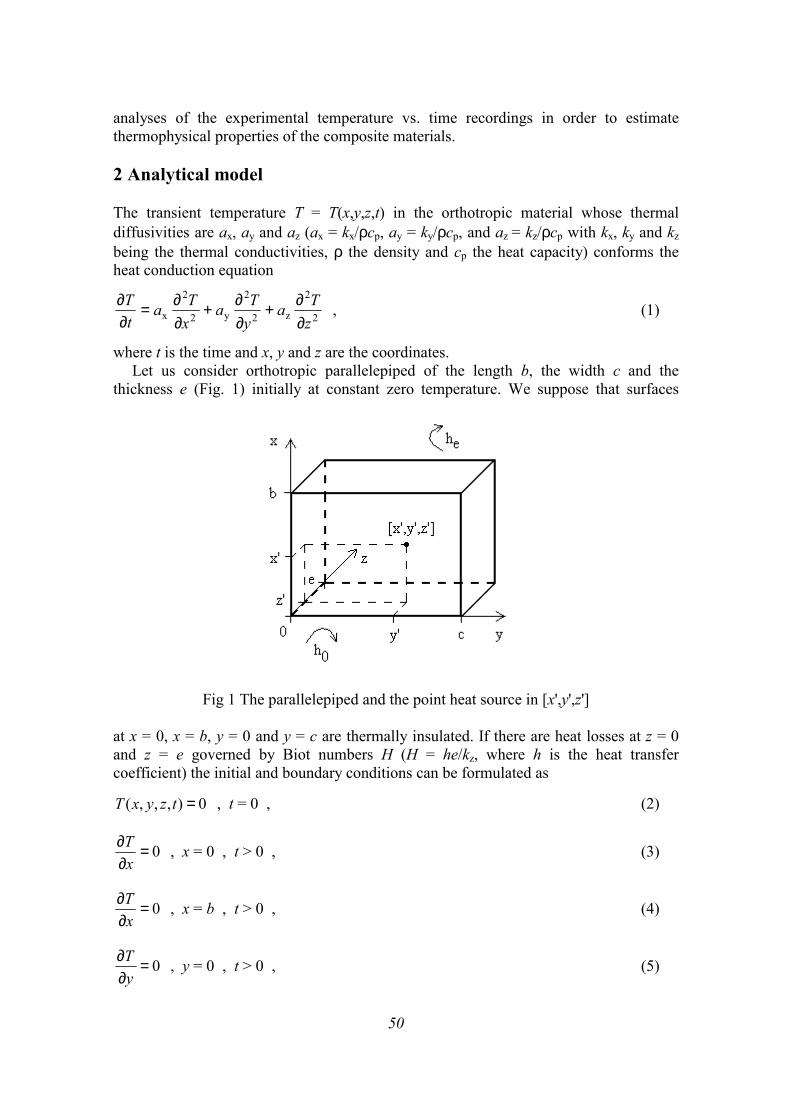
50

analyses of the experimental temperature vs. time recordings in order to estimate thermophysical properties of the composite materials. 2 Analytical model The transient temperature T = T(x,y,z,t) in the orthotropic material whose thermal diffusivities are ax, ay and az (ax = kx/ρcp, ay = ky/ρcp, and az = kz/ρcp with kx, ky and kz being the thermal conductivities, ρ the density and cp the heat capacity) conforms the heat conduction equation

2

2

z2

2

y2

2

x zTa

yTa

xTa

tT

∂∂+

∂∂+

∂∂=

∂∂ , (1)

where t is the time and x, y and z are the coordinates. Let us consider orthotropic parallelepiped of the length b, the width c and the

thickness e (Fig. 1) initially at constant zero temperature. We suppose that surfaces

Fig 1 The parallelepiped and the point heat source in [x',y',z']

at x = 0, x = b, y = 0 and y = c are thermally insulated. If there are heat losses at z = 0 and z = e governed by Biot numbers H (H = he/kz, where h is the heat transfer coefficient) the initial and boundary conditions can be formulated as

0),,,( =tzyxT , t = 0 , (2)

0=∂∂

xT , x = 0 , t > 0 , (3)

0=∂∂

xT , x = b , t > 0 , (4)

0=∂∂

yT , y = 0 , t > 0 , (5)

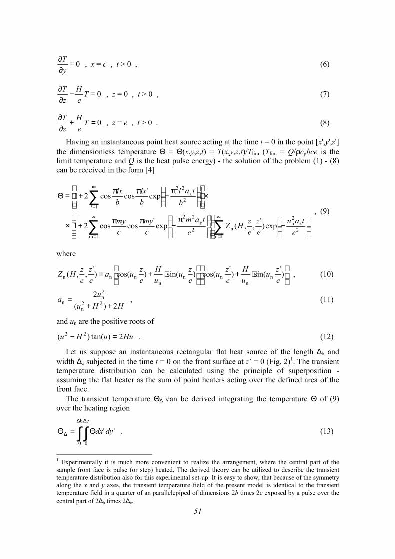
51

0=∂∂

yT , x = c , t > 0 , (6)

0=−∂∂ T

eH

zT , z = 0 , t > 0 , (7)

0=+∂∂ T

eH

zT , z = e , t > 0 . (8)

Having an instantaneous point heat source acting at the time t = 0 in the point [x',y',z'] the dimensionless temperature Θ = Θ(x,y,z,t) = T(x,y,z,t)/Tlim (Tlim = Q/ρcpbce is the limit temperature and Q is the heat pulse energy) - the solution of the problem (1) - (8) can be received in the form [4]

−

π−ππ+×

×

π−ππ+=Θ

∑∑

∑∞

=

∞

=

∞

=

2z

2n

1nn

1m2

y22

12

x22

exp)',,(exp'coscos21

exp'coscos21

etau

ez

ezHZ

ctam

cmy

cmy

btal

blx

blx

l , (9)

where

⋅+

⋅+= )'sin()'cos()sin()cos()',,( n

nnn

nnnn e

zuuH

ezu

ezu

uH

ezua

ez

ezHZ , (10)

HHuua

2)(2

22n

2n

n ++= , (11)

and un are the positive roots of

HuuHu 2)tan()( 22 =− . (12)

Let us suppose an instantaneous rectangular flat heat source of the length ∆b and width ∆c subjected in the time t = 0 on the front surface at z’ = 0 (Fig. 2)1. The transient temperature distribution can be calculated using the principle of superposition - assuming the flat heater as the sum of point heaters acting over the defined area of the front face.

The transient temperature Θ∆ can be derived integrating the temperature Θ of (9) over the heating region

∫ ∫∆ ∆

∆ Θ=Θb

0

c

0

''dydx . (13)

1 Experimentally it is much more convenient to realize the arrangement, where the central part of the sample front face is pulse (or step) heated. The derived theory can be utilized to describe the transient temperature distribution also for this experimental set-up. It is easy to show, that because of the symmetry along the x and y axes, the transient temperature field of the present model is identical to the transient temperature field in a quarter of an parallelepiped of dimensions 2b times 2c exposed by a pulse over the central part of 2∆b times 2∆c.

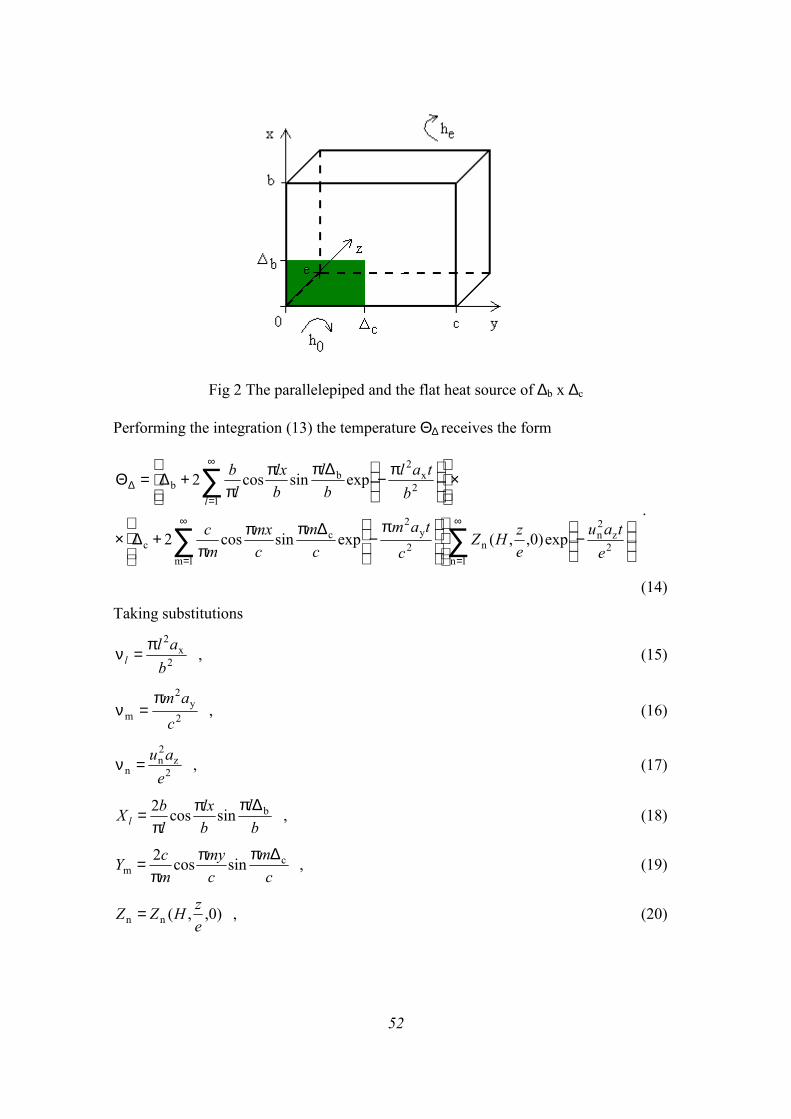
52

Fig 2 The parallelepiped and the flat heat source of ∆b x ∆c

Performing the integration (13) the temperature Θ∆ receives the form

−

π−∆ππ

π+∆×

×

π−∆πππ

+∆=Θ

∑∑

∑∞

=

∞

=

∞

=∆

2z

2n

1nn

1m2

y2

cc

12

x2

bb

exp)0,,(expsincos2

expsincos2

etau

ezHZ

ctam

cm

cmx

mc

btal

bl

blx

lb

l .

(14)

Taking substitutions

2x

2

bal

lπ=ν , (15)

2y

2

m camπ

=ν , (16)

2z

2n

n eau=ν , (17)

bl

blx

lbX l

bsincos2 ∆πππ

= , (18)

cm

cmy

mcY c

m sincos2 ∆πππ

= , (19)

)0,,(nn ezHZZ = , (20)

53

the equation (14) can be rewritten into the simplified form

∑∑∑∞

=

∞

=

∞

=∆ ν−

ν−+∆

ν−+∆=Θ

1nnn

1mmmc

1b )exp()exp()exp( tZtYtX

lll . (21)

Assuming the step heating since the time t = 0 as a sequence of instantaneous pulses applied in the times t = t’, t’ > 0, providing that the function φ(t) that describes the shape of the heating is normalized, i.e.

1)(0

=φ∫∞

dtt . (22)

The transient temperature ΘS∆ can be accordingly to the principle of superposition derived using the formula

( )∫ −Θφ=Θ ∆∆

t

dtttt0

S '')( . (23)

Performing integration (23) the temperature ΘS∆ receives the form

( )[ ]

( )[ ] ( )[ ]∑∑∑∑∑

∑∑∑∞

=

∞

=

∞

=

∞

=

∞

=

∞

=

∞

=

∞

=∆

ν+ν+νν+ν+ν−−+

ν+νν+ν−−∆+

+ν+ν

ν+ν−−∆+ν

ν−−∆∆=Θ

1 1m 1n nm

nmnm

1 1n n

nnc

1m 1n nm

nmnmb

1n n

nncbS

exp1exp1

exp1)exp(1

l l

ll

l l

ll

tZYXtZX

tZYtZ

.

(24)

3 Conclusion The achieved equation (24), that describes the transient temperature distribution in an orthotropic parallelepiped under the defined transient step heating condition, can be utilized as a working equation for an experimental investigation on a three-dimensional orthotropic composite material. Proposing a proper experimental design the thermal diffusivities in three orthotropic directions can be calculated analyzing the experimental temperature rise vs. time recordings. Acknowledgement Authors wish to thank the Slovak Science Grant Agency for the financial support under the contract 1/6115/99 and 2/1046/21. References [1] Koráb J, 1999 Thermophysical properties of continous carbon fibre reinforced

copper matrix composites, PhD Thessis (TU Vienna)

54

[2] Bittle R R, Taylor R E, 1984 Step-Heating Technique for Thermal Diffusivity Measurements of Large-Grained Heterogeneous Materials, J. Amer. Ceram. Soc., 67, 186-190

[3] Vozár L, Šrámková T, 1997 Two Data Reduction Methods for Evaluation of Thermal Diffusivity from Step Heating Measurements, Int. J. Heat Mass Transfer, 40, 1647-1656

[4] Carslaw H S, Jaeger J C, 1959 Conduction of Heat in Solids (Oxford, Clarendon Press) p. 373

55

STEADY-STATE MEASUREMENTS OF THE MOISTURE DEPENDENCE OF THE CAPILLARY-POROUS MATERIALS THERMAL CONDUCTIVITY Oľga Koronthályová1, Peter Matiašovský2 1 Institute of Construction and Architecture, Slovak Academy of Sciences, Dubravska

cesta 9, SK-84220 Bratislava, Slovakia 2 Institute of Construction and Architecture, Slovak Academy of Sciences, Dubravska

cesta 9, SK-84220 Bratislava, Slovakia Email: usarkoro@savba.sk, usarmat@savba.sk Abstract Steady-state thermal conductivity measurements of a moist porous materials are complicated by the coupled moisture transport processes. The result of steady-state thermal conductivity measurement of a moist porous material is apparent thermal conductivity, which includes the effects of the ethalpy flow and the possible non-linear moisture content distribution. The numerical simulation of temperature-moisture content field enables to determine the effects of the moisture transport and the phase change on the apparent thermal conductivity for the measured material, moisture content and the used boundary conditions. Key words: capillary-porous materials, thermal conductivity, moisture content 1 Introduction Steady-state thermal conductivity measurements of a moist porous material are complicated by the superposition of the heat transport by the coupled moisture transport processes. The applied temperature difference results in moisture transfer in the vapour and liquid phase. The water vapour transfer is result of lower water vapour pressure in cold regions. The water vapour migrates by diffusion from hot to cold regions. The vapour migration leads to a decrease of the water content in the hot regions and therefore to a decrease of capillary pressure in this zone. The capillary pressure difference induces a liquid phase movement in the direction opposite to the vapour flow. In a system with constant moisture content after some time an equilibrium state is reached, when the vapour movement by diffusion is balanced by capillary liquid flow. If the results of steady-state thermal conductivity measurements of moist materials are evaluated the following aspects have to be taken into account.

The value of heat flow can increase as the result of additional heat transfer caused by moisture transfer.

In some cases in the equilibrium state the non-linear moisture distribution is reached. Because the samples with the same moisture content but different moisture distribution give different mean thermal conductivities (a sample with uniform moisture content

56

distribution has the highest moisture conductivity) the measured (apparent) value of thermal conductivity is then lower than the real one. 2 Transport equations Heat and moisture transport in capillary-porous material is described by folloving coupled non-linear equatios [1]:

( ) ( ) ( )[ ]

+∇+∇∇=

=−+++++⋅

∑••

voekkeff

iomivoevaaww

mhmc

whcwhccwcwct

θθλ

θθθρ∂∂

, (1)

)()(

wviwv mm

twww ••

+∇=++

∂∂

. (2)

The water and water vapour flows are equal to:

θρ θ ∇−∇−=•

DwDm ww , (3)

θθ

ψ ∇⋅−

⋅−=•

ddp

TRpPPDm vv

1 . (4)

θ temperature [°C] t time [s] wv, ww, wi vapour, liquid and ice content [kg/m3]

•m v,

•m w vapour and liquid flow [kg/s]

ρ bulk density [kg/m3] c, cw, ca, cv specific heat capacities for solid, liquid,

air and water vapour [J/kg.K] Τ temperature [K] hoe, hom transition heat for evaporation and freezing [J/kg] λeff effective thermal conductivity [W/m.K] k = a, v and w for air, vapour and water P atmospheric pressure [Pa] ψ relative water vapour diffusion coefficient [-] ϕ relative humidity [-] Dv binary diffusion coefficient of water vapour in air [m2/s] Dw moisture diffusivity [m2/s] Dθ thermal moisture diffusion coefficient [m2/K.s] p vapour pressure [Pa] R specific gas constant for water vapour [J/kg.K] In next considerations the air flow is not taken into account.

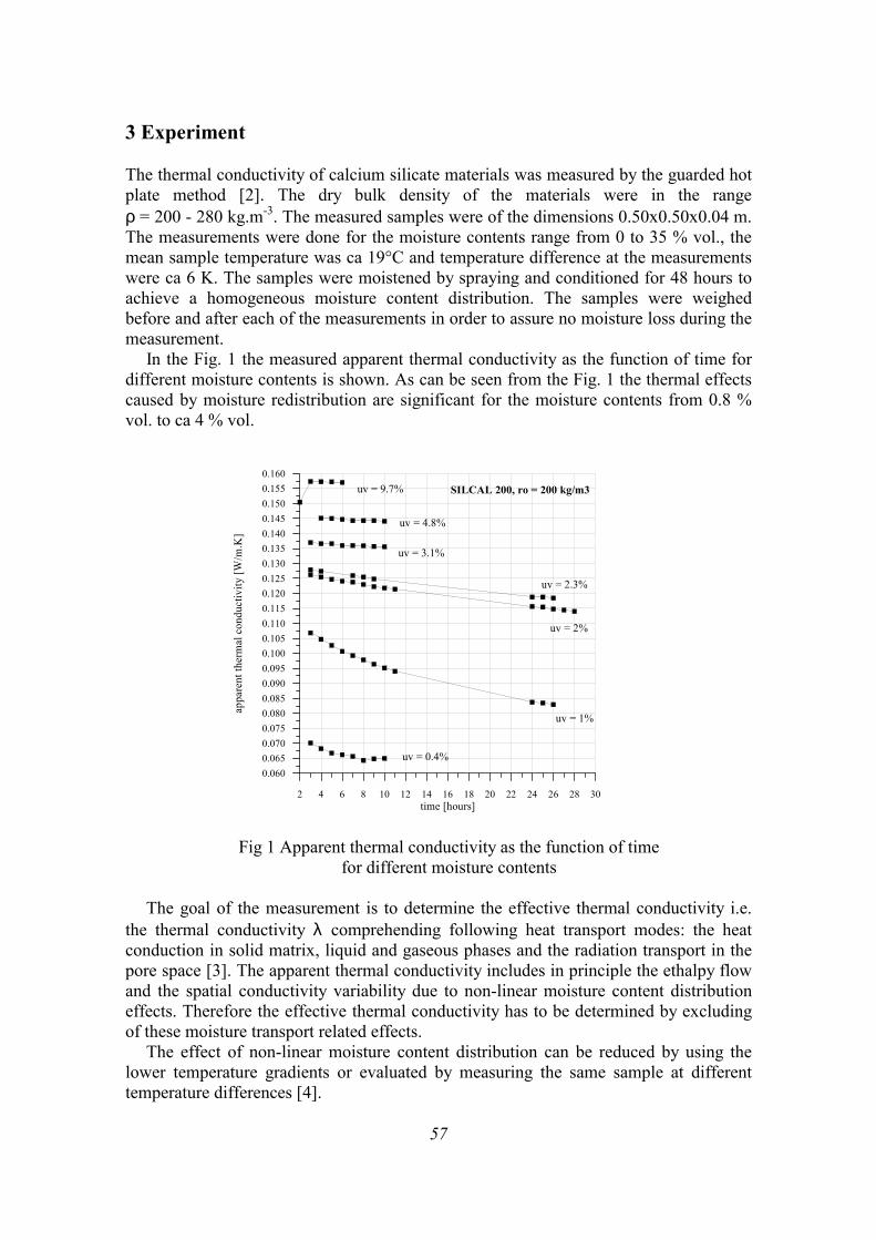
57

3 Experiment The thermal conductivity of calcium silicate materials was measured by the guarded hot plate method [2]. The dry bulk density of the materials were in the range ρ = 200 - 280 kg.m-3. The measured samples were of the dimensions 0.50x0.50x0.04 m. The measurements were done for the moisture contents range from 0 to 35 % vol., the mean sample temperature was ca 19°C and temperature difference at the measurements were ca 6 K. The samples were moistened by spraying and conditioned for 48 hours to achieve a homogeneous moisture content distribution. The samples were weighed before and after each of the measurements in order to assure no moisture loss during the measurement.

In the Fig. 1 the measured apparent thermal conductivity as the function of time for different moisture contents is shown. As can be seen from the Fig. 1 the thermal effects caused by moisture redistribution are significant for the moisture contents from 0.8 % vol. to ca 4 % vol.

Fig 1 Apparent thermal conductivity as the function of time for different moisture contents

The goal of the measurement is to determine the effective thermal conductivity i.e.

the thermal conductivity λ comprehending following heat transport modes: the heat conduction in solid matrix, liquid and gaseous phases and the radiation transport in the pore space [3]. The apparent thermal conductivity includes in principle the ethalpy flow and the spatial conductivity variability due to non-linear moisture content distribution effects. Therefore the effective thermal conductivity has to be determined by excluding of these moisture transport related effects.

The effect of non-linear moisture content distribution can be reduced by using the lower temperature gradients or evaluated by measuring the same sample at different temperature differences [4].

2 4 6 8 10 12 14 16 18 20 22 24 26 28 30time [hours]

0.0600.0650.0700.0750.0800.0850.0900.0950.1000.1050.1100.1150.1200.1250.1300.1350.1400.1450.1500.1550.160

appa

rent

ther

mal

con

duct

ivity

[W/m

.K]

uv = 1%

uv = 0.4%

uv = 2%

uv = 3.1%

uv = 4.8%

uv = 2.3%

uv = 9.7% SILCAL 200, ro = 200 kg/m3

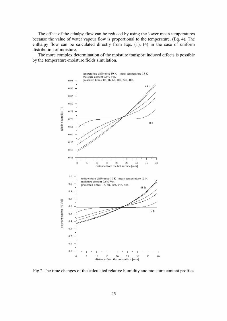
58

The effect of the ethalpy flow can be reduced by using the lower mean temperatures because the value of water vapour flow is proportional to the temperature. (Eq. 4). The enthalpy flow can be calculated directly from Eqs. (1), (4) in the case of uniform distribution of moisture.

The more complex determination of the moisture transport induced effects is possible by the temperature-moisture fields simulation.

Fig 2 The time changes of the calculated relative humidity and moisture content profiles

0 5 10 15 20 25 30 35 40distance from the hot surface [mm]

0.45

0.50

0.55

0.60

0.65

0.70

0.75

0.80

0.85

0.90

0.95

rela

tive

hum

idity

[-]

temperature difference 10 K mean temperature 15 Kmoisture content 0.6% Vol.presented times: 0h, 1h, 6h, 10h, 24h, 48h.

0 h

48 h

0 5 10 15 20 25 30 35 40distance from the hot surface [mm]

0.0

0.1

0.2

0.3

0.4

0.5

0.6

0.7

0.8

0.9

1.0

moi

stur

e co

nten

t [%

Vol

]

temperature difference 10 K mean temperature 15 Kmoisture content 0.6% Vol.presented times: 1h, 6h, 10h, 24h, 48h.

0 h

48 h

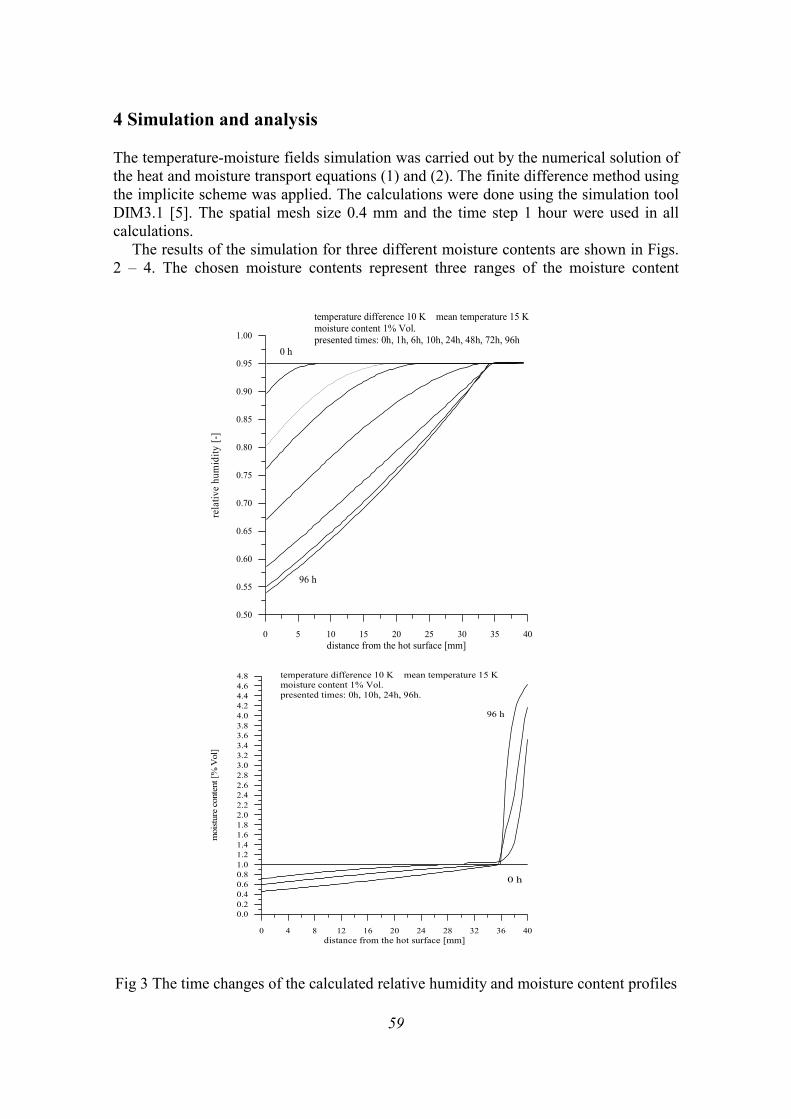
59

4 Simulation and analysis The temperature-moisture fields simulation was carried out by the numerical solution of the heat and moisture transport equations (1) and (2). The finite difference method using the implicite scheme was applied. The calculations were done using the simulation tool DIM3.1 [5]. The spatial mesh size 0.4 mm and the time step 1 hour were used in all calculations.

The results of the simulation for three different moisture contents are shown in Figs. 2 – 4. The chosen moisture contents represent three ranges of the moisture content

Fig 3 The time changes of the calculated relative humidity and moisture content profiles

0 5 10 15 20 25 30 35 40distance from the hot surface [mm]

0.50

0.55

0.60

0.65

0.70

0.75

0.80

0.85

0.90

0.95

1.00

rela

tive

hum

idity

[-]

temperature difference 10 K mean temperature 15 Kmoisture content 1% Vol.presented times: 0h, 1h, 6h, 10h, 24h, 48h, 72h, 96h

96 h

0 h

0 4 8 12 16 20 24 28 32 36 40distance from the hot surface [mm]

0.00.20.40.60.81.01.21.41.61.82.02.22.42.62.83.03.23.43.63.84.04.24.44.64.8

moi

stur

e co

nten

t [%

Vol

]

temperature difference 10 K mean temperature 15 Kmoisture content 1% Vol.presented times: 0h, 10h, 24h, 96h.

96 h

0 h

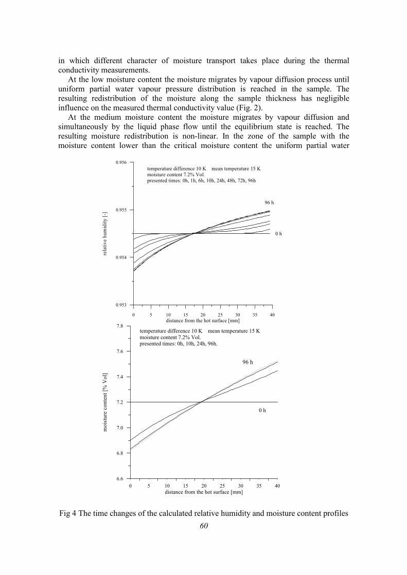
60

in which different character of moisture transport takes place during the thermal conductivity measurements.

At the low moisture content the moisture migrates by vapour diffusion process until uniform partial water vapour pressure distribution is reached in the sample. The resulting redistribution of the moisture along the sample thickness has negligible influence on the measured thermal conductivity value (Fig. 2).

At the medium moisture content the moisture migrates by vapour diffusion and simultaneously by the liquid phase flow until the equilibrium state is reached. The resulting moisture redistribution is non-linear. In the zone of the sample with the moisture content lower than the critical moisture content the uniform partial water

Fig 4 The time changes of the calculated relative humidity and moisture content profiles

0 5 10 15 20 25 30 35 40distance from the hot surface [mm]

0.953

0.954

0.955

0.956

rela

tive

hum

idity

[-]

temperature difference 10 K mean temperature 15 Kmoisture content 7.2% Vol.presented times: 0h, 1h, 6h, 10h, 24h, 48h, 72h, 96h

0 h

96 h

0 5 10 15 20 25 30 35 40distance from the hot surface [mm]

6.6

6.8

7.0

7.2

7.4

7.6

7.8

moi

stur

e co

nten

t [%

Vol

]

temperature difference 10 K mean temperature 15 Kmoisture content 7.2% Vol.presented times: 0h, 10h, 24h, 96h.

96 h

0 h

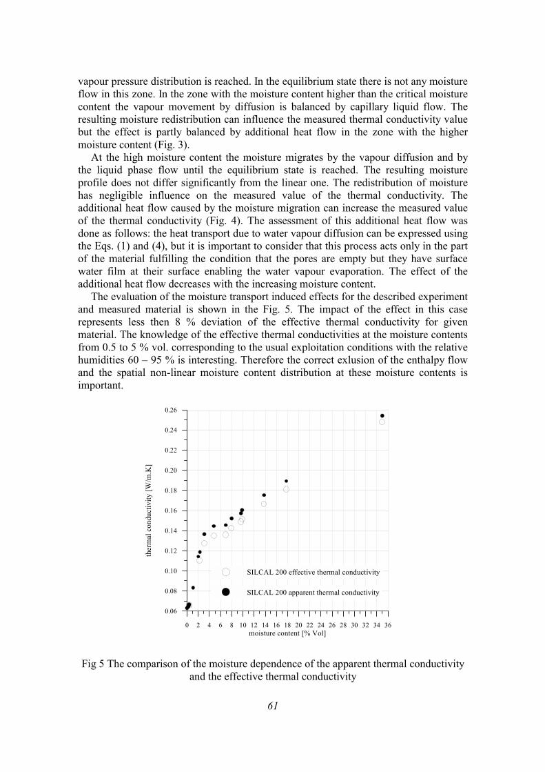
61

vapour pressure distribution is reached. In the equilibrium state there is not any moisture flow in this zone. In the zone with the moisture content higher than the critical moisture content the vapour movement by diffusion is balanced by capillary liquid flow. The resulting moisture redistribution can influence the measured thermal conductivity value but the effect is partly balanced by additional heat flow in the zone with the higher moisture content (Fig. 3).

At the high moisture content the moisture migrates by the vapour diffusion and by the liquid phase flow until the equilibrium state is reached. The resulting moisture profile does not differ significantly from the linear one. The redistribution of moisture has negligible influence on the measured value of the thermal conductivity. The additional heat flow caused by the moisture migration can increase the measured value of the thermal conductivity (Fig. 4). The assessment of this additional heat flow was done as follows: the heat transport due to water vapour diffusion can be expressed using the Eqs. (1) and (4), but it is important to consider that this process acts only in the part of the material fulfilling the condition that the pores are empty but they have surface water film at their surface enabling the water vapour evaporation. The effect of the additional heat flow decreases with the increasing moisture content.

The evaluation of the moisture transport induced effects for the described experiment and measured material is shown in the Fig. 5. The impact of the effect in this case represents less then 8 % deviation of the effective thermal conductivity for given material. The knowledge of the effective thermal conductivities at the moisture contents from 0.5 to 5 % vol. corresponding to the usual exploitation conditions with the relative humidities 60 – 95 % is interesting. Therefore the correct exlusion of the enthalpy flow and the spatial non-linear moisture content distribution at these moisture contents is important. Fig 5 The comparison of the moisture dependence of the apparent thermal conductivity

and the effective thermal conductivity

0 2 4 6 8 10 12 14 16 18 20 22 24 26 28 30 32 34 36moisture content [% Vol]

0.06

0.08

0.10

0.12

0.14

0.16

0.18

0.20

0.22

0.24

0.26

ther

mal

con

duct

ivity

[W/m

.K]

SILCAL 200 apparent thermal conductivity

SILCAL 200 effective thermal conductivity

62

5 Conclusion The numerical simulation of the changing temperature-moisture field in the sample during the guarded hot plate measurements enables to determine the time, necessary for reaching the equilibrium state for the measured material, moisture content and used boundary conditions.

The simulation also enables to determine the regions of low, medium and high moisture content and to quantify the effects of the moisture transport and the phase change on the apparent thermal conductivity for the measured material and the used boundary conditions.

Determination of the actual time development of the moisture content and relative humidity distribution enables to calculate the effective thermal conductivity from the apparent thermal conductivity values in spite of the fact that the equilibrium state is not reached and consequently to shorten the measurement time.

The reliability of the temperature-moisture field simulation results depends on reliability of the used material parameters, especially of the moisture diffusivity, relative water vapour diffusion coefficient and the water retention curve. Acknowledgement

Authors wish to thank the VEGA (Grant No 2/1085/21) for the financial support of this work. References [1] Hens H, 1996 Heat, Air, and Moisture Transfer in Insulated Enveloped Parts. Task

1: Modelling (Acco Leuven) [2] Klarsfeld S, 1984 Guarded Hot Plate Method for Thermal Conductivity

Measurement, in Compendium of Thermophysical Property Measurement Methods, Vol.1 Survey of Measurement Techniques (Eds: Maglic K D, Cezairliyan A, Peletsky V E, New York, London: Plenum Press) pp. 169-230

[3] ISO 10051 1996 Thermal insulation – Moisture effects on heat transfer – Determination of thermal transmissivity of a moist material

[4] Rudtsch S, Thermal conductivity measurements for the separation of heat and mass diffusion in moist porous materials, High temperatures – High Pressures, 32, pp. 445-451

[5] Grunewald J, 1999 Development and new methodology to analyse the durability of facade repair and retrofitting systems. Final report. Task 5. Full documentation of the numerical simulation program DIM3.1. (Dresden)

63

MODELLING THE THERMAL CONDUCTIVITY PROPERTIES OF ULTRA - THIN LAYERS: 1-DIMENSIONAL CASE – VERIFICATION Aba Teleki Department of Physics, Faculty of Natural Sciences, Constantine the Philosopher University, Tr. A. Hlinku 1, SK-94974 Nitra, Slovakia Email: ateleki@ukf.sk Abstract We apply the technique of modelling the conductivity properties of ultra-thin layers shown in [1]. We verify this technique by using Laplace transformation to show nontrivial conductivity properties of the ultra-thin layers applicable to multi-layered structures as well (see [2]). Key words: thermal conductivity, layers, Laplace transformation 1 Introduction We consider a one-dimensional system (more precisely: a system infinitely extended in the direction perpendicular to the direction assumed in our description) consisted of two half-lines connected at one point. The thermal characteristics of such a system are constant and homogeneous. Our goal is to show the presence of the third kind of Dirichlet’s boundary conditions for the temperature T(x,t) at the connection point x = 0. We make use of some specific thermal characteristics and the technique of ultra-thin slide used in [1] combined by the exact solution.

Let us have identical thermal diffusivity α, and thermal conductivity k in any part of the system – we illustrate these specific thermal characteristics in Fig. 1 and Fig. 2. In [1] it was shown, that the heat-transfer properties of the boundary may be characterized by only two coefficients hsy and has due to the fact that the heat source acts on the boundary x = 0. This will be shown here as well. 2 Solving the specific case The system’s configuration is shown in Fig. 1. We assume zero initial temperatures

( ) 00, =xT j for any point x and for j = 1,2,3 . (1)

The temperature is zero at infinity

( ) ( ) 0,lim,lim 31 ==+∞→−∞→

txTtxTxx

for any t . (2)

The heat-transfer equations have the form

( ) ( ) ( ) 0,,, 11 =+∂−∂ −− txgktxTtxT jjtjxx α for j = 1,2,3 . (3)

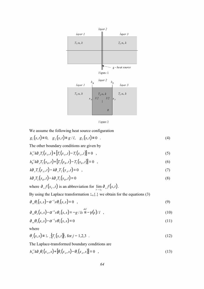
64

We assume the following heat source configuration

( ) ( ) ( ) 0,,/,,0, 321 ≡≡≡ txglgtxgtxg . (4)

The other boundary conditions are given by

( ) ( ) ( )[ ] 0,,, 1111 =−+∂− txTtxTtxTkh AAAxA , (5)

( ) ( ) ( )[ ] 0,,, 3221 =−+∂− txTtxTtxTkh BBBxB , (6)

( ) ( ) 0,, 21 =∂−∂ txTktxTk AxAx , (7)

( ) ( ) 0,, 32 =∂−∂ txTktxTk BxBx (8)

where ( )txf Cx ,∂ is an abbreviation for ( )txfxxx C

,lim ∂→

.

By using the Laplace transformation Ls. we obtain for the equations (3)

( ) ( ) 0,, 11

1 =−∂ − sxssxxx θαθ , (9)

( ) ( ) ( ) lslsgsxssxdef

xx //,, 21

2 γθαθ −≡−=−∂ −

, (10)

( ) ( ) 0,, 31

3 =−∂ − sxssxxx θαθ (11)

where

( ) ( ) txTsx jsj ,, L≡θ , for j = 1,2,3 . (12)

The Laplace-transformed boundary conditions are

( ) ( ) ( )[ ] 0,,, 1111 =−+∂− sxsxsxkh AAAxA θθθ , (13)

65

( ) ( ) ( )[ ] 0,,, 3221 =−+∂− sxsxsxkh BBBxB θθθ , (14)

( ) ( ) 0,, 21 =∂−∂ sxksxk AxAx θθ , (15) ( ) ( ) 0,, 32 =∂−∂ sxksxk BxBx θθ . (16)

The solutions of (9) - (11) are

( ) 2/12/112

2/12/1111 expexp, ααθ xsCxsCsx +−= , (17)

( ) ( ) lxsxsCxsCsx 2expexp, 22/12/122

2/12/1212 γααθ −+−= , (18)

( ) 2/12/132

2/12/1313 expexp, ααθ xsCxsCsx +−= (19)

where

01211 == CC , (20)

because of (2). By plugging (17) - (19) into the boundary conditions (13) - (16) we obtain

( )( )

( ) ( )( )

+−

=

−

−

+

−

−

−−

+

−−

−−

−

−

BB

BBBB

AA

A

xxx

xx

B

x

B

xxx

xxx

A

lhsxkhxlhsx

lhsxklsx

CCCC

eee

eehke

hk

eee

eeehk

BBB

BBB

AAA

AAA

γγ

γγ

σσσ

σσ

σσσ

σ

σσσ

σσσ

σσσ

σσσ

1

2

0

110

0

01

2

31

22

21

12

(21) where σ is an abbreviation for αs . By solving this system of equations one can obtain C12, C21, C22 and C13. The inverse Laplace transformation of (17)-(19) by using the Cij coefficients gives the temperatures T1, T2 and T3. These temperatures depend on the parameter l (the dimension of the middle slide). The final step is to calculate the limit l → 0.

Remark 1 This program is technically very difficult. To overcome these difficulties we use the uniqueness of the Laplace transformation and the uniqueness of the inverse Laplace transformation. The inverse Laplace transformation is unique in the sense, that

( ) ( ) sftF t1

1−= L and ( ) ( ) sftF t

12

−= L also, then ( ) ( )( ) 00 21 =−∫ dttFtFT

for any T > 0,

T finite. The consequence of this uniqueness is, that it is possible to calculate the limit l → 0

in (21) directly. We obtain

( )( )( )

=

−−+−

−−−+

B

B

A

hk

hk

hk

hshshs

CCCC

BB

A

222

0

01110

00111

31

22

21

12

γγγ

σσσ

σσσσσ

σ

(22)

66

where xA = –l/2 and xB = l/2 were used. We are interested on C12 and C31 because of the role of T1(x,t) and T2(x,t). The solutions of (22) are

( )

+−=

−1

12 1α

αγ shk

hh

hh

sksC

syasB

, (23)

( )

++=

+

+=

−− 1

12

1

31 111α

αγαα

shk

hh

hh

sksCs

hks

hkC

syasABA

(24)

where

( )1111 2 −−−− += BAsy hhh , and ( )1111 2 −−−− +−= BAas hhh . (25)

With the use of (23) and (24) we can express C21 and C22. We assume that the Laplace transform of the temperature T2(0,t) is the sum 2221 CC + because of the limit procedure

0→l done above. We obtain

( ) ( ) ( ) 1

22112 1−

+++

+=+

αγαγγ s

hk

hhs

sks

hhsCC

as

sy

BA

. (26)

Now, the temperature T2(0,t) is given as

( )

−+++

= tkh

kth

hgh

kt

hhgtT sy

as

sy

BA

αα

πα erfcexp12,0 2

2

22 (27)

where

( ) ∫∞

−=x

dex ξπ

ξ 22erfc . (28)

One can see, that ( ) 0,02 →∂ tTt for large t and systems goes to thermal equilibrium. We can express the temperatures T1 and T3 as

( ) ( ) ( )

−=

assyB

sy

hhtxkG

htxF

kgh

txT ,,,1 , (29)

( ) ( ) ( )

+=

assyA

sy

hhtxkG

htxF

kgh

txT ,,,2 (30)

where

( ) ,2

erfc2,

−=

tx

xttxFπ

(31)

( ) ( ) ( )∫

−−

−

−= −

ttx

a dtt

xe

xaeatxG

0

2

2

4

2erfc

21erfc4,

2

2

22

ξπξ

ξπξξ ξξ (32)

67

with k

ha sy= .

3 Results obtained by using the Dirichlet’s boundary conditions of the

third kind In [1] was shown (for more general case) the possibility of modeling a thin layer with non-trivial heat-transfer properties by using special boundary conditions.

The heat transform equations are given as

( ) ( ) 0,, 1 =∂−∂ − txTtxT jtjxx α for j = 1,3 (30)

and the form of the boundary conditions are given as (see [1] p. 74)

( ) ( ) ( )[ ] ( )tGhtTtTtTkh Axsy 21

3111 ,0,0,0 −− =−+∂ , (31)

( ) ( ) ( )[ ] ( )tGhtTtTtTkh Bxsy 21

3131 ,0,0,0 −− −=−+∂ (32)

where

( ) ( ),222 tlgtG −∆−≡ and ( ) ( )[ ]∫−

→

− ∂=∆2/

2/202 ,lim

l

ltl

txTdxt . (33)

Remark 2 These conditions form an “easy to solve system” if the Laplace transformation is used. A little disadvantage of the procedure shown in [1] is, that the term −∆ 2 is known a priory only in the case of the thermal equilibrium (then −∆ 2 = 0). This disadvantage one may to eliminate by using the limit procedure for the Laplace transformed functions shown above.

By using the Laplace transformation on (30) - (32) we obtain

( ) ( ) 0,, 1 =−∂ − sxssx jjxx θαθ for j = 1,3 . (34)

The solutions are

( ) ( ) αα θθ sxsx eCsxeCsx −== 313121 ,,, . (35)

By using these solutions with the boundary conditions

( ) ( ) ( )[ ] ( )shssskh Axsy γθθθ 1311

1 ,0,0,0 −− =−+∂ , (36)

( ) ( ) ( )[ ] ( )shssskh Bxsy γθθθ 1313

1 ,0,0,0 −− −=−+∂ (37)

we obtain

( ) ( )Asy hsCCs

hk γ

α=+ 3112 , (38)

( ) ( )Bsy hsCCs

hk γ

α=−

+ 31121 (39)

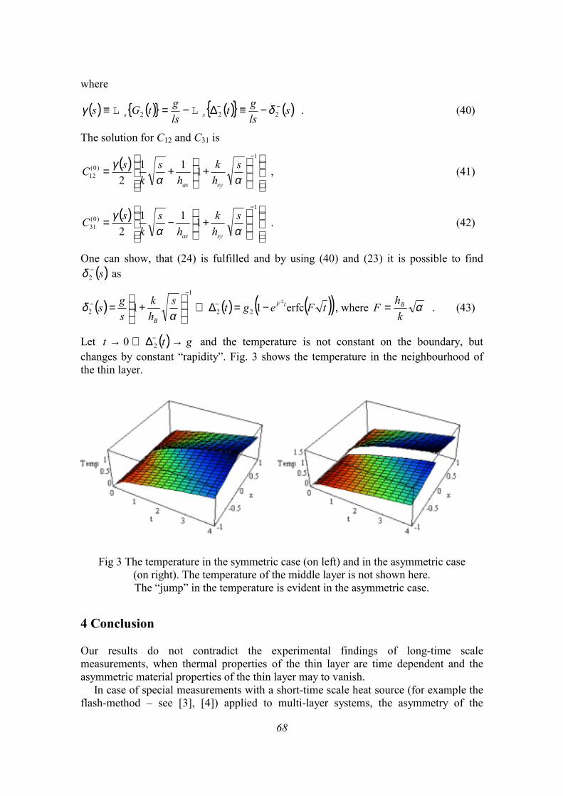
68

where

( ) ( ) ( ) ( )slsgt

lsgtGs ss

−− −≡∆−=≡ 222 δγ LL . (40)

The solution for C12 and C31 is

( )

++=

−1

)0(12 111

2 ααγ s

hk

hs

ksC

syas

, (41)

( )

+−=

−1

)0(31 111

2 ααγ s

hk

hs

ksC

syas

. (42)

One can show, that (24) is fulfilled and by using (40) and (23) it is possible to find ( )s−

2δ as

( ) ( ) ( )( )tFegtshk

sgs tF

B

erfc112

22

1

2 −=∆⇒

+= −

−

−

αδ , where α

khF B= . (43)

Let ( ) gtt →∆⇒→ −20 and the temperature is not constant on the boundary, but

changes by constant “rapidity”. Fig. 3 shows the temperature in the neighbourhood of the thin layer.

Fig 3 The temperature in the symmetric case (on left) and in the asymmetric case (on right). The temperature of the middle layer is not shown here. The “jump” in the temperature is evident in the asymmetric case.

4 Conclusion Our results do not contradict the experimental findings of long-time scale measurements, when thermal properties of the thin layer are time dependent and the asymmetric material properties of the thin layer may to vanish.

In case of special measurements with a short-time scale heat source (for example the flash-method – see [3], [4]) applied to multi-layer systems, the asymmetry of the

69

material properties of the thin layers may play interesting role in the evolution of the whole system. Aknowledgment Author wishes to thank the Slovak Science Grant Agency for the financial support under the contract 1/6115/99. References [1] Teleki A, 2000 Modelling of the Thermal Conductivity Properties of Ultra-thin

Layers – 1-Dimensional Case in Thermophysics 2000 – Meeting of the Thermophysical Society Working Group of the Slovak Physical Society (Ed: Vozár L, Constantine the Philosopher University in Nitra) pp. 71-76

[2] Teleki A, 2000 Matrix Solution of the Heat Conduction in Multi-Layered Structures in General Case in Thermophysics 1999 – Meeting of the Thermophysical Society Working Group of the Slovak Physical Society (Ed: Vozár L, Constantine the Philosopher University in Nitra) pp. 49-54

[3] Vozár L, Hohenauer W, 2000 Measurement of the Thermal Diffusivity Using the Laser Flash Method with Repeated Pulses, High Temp. High Press, 33, 9-16

[4] Vozár L, Hohenauer W, 2000 An Apparatus for the Thermal Diffusivity Measurement Using the Flash Method, Meeting of the Thermophysical Society Working Group of the Slovak Physical Society (Ed: Vozár L, Constantine the Philosopher University in Nitra) pp. 83-88

70

71

EXPERIMENTAL VERIFICATION OF TWO METHODS FOR SOLVING INVERSE HEAT CONDUCTION PROBLEMS Jozefa Lukovičová, Juraj Veselský Department of Physics, Faculty of Civil Engineering, Slovak University of Technology, Radlinského 11, 813 68 Bratislava, Slovakia Email: lukovico@svf .stuba.sk, vesel@svf.stuba.sk Abstract Two methods for simultaneously determining the temperature dependent thermal conductivity and heat capacity of porous materials, based on the solution of the inverse nonlinear one-dimensional heat conduction problem are validated using the experimental data. The experimental data of the temperature histories of the body are compared to the corresponding numerically calculated temperature fields, which are obtained from the application of thermal conductivity and heat capacity determined by both methods. The real temperature fields are measured on the furnace slag-based concrete. Keywords: thermal conductivity, heat capacity, inverse problem, porous material 1 Introduction Determining the thermal properties of porous materials can be determined by standard measuring methods as well by the solution inverse problem of heat conduction. The inverse methods can be considered as a reasonable alternative to the classical methods, because for it is possible to determine thermal properties as functions of a broad temperature range and one makes not very time-consuming. Significant contributions made in the field of inverse heat conduction problems have been published by Kozdoba [l], Beck, et al. [2], Kurpicz [3].

This contribution presents the results of the experimental verification of two inverse methods for determining the temperature-dependent thermal conductivity and heat capacity of porous material. The experimental verification is carried out the comparison between the measured temperature field of the examined sample and the corresponding temperature fields, which are calculated using thermal conductivity and heat capacity determined both methods. The methods are described in previous paper [4]. 2 Nonlinear thermal system In the verification of both inverse methods is employed the one-dimensional, transient, nonlinear heat conduction problem in slab geometry, which is modelled by an equation

)),()((),()(x

txTTkxt

txTTc∂

∂∂∂

∂∂ρ = ],0(),0(),( etLtx ×∈ . (1a)

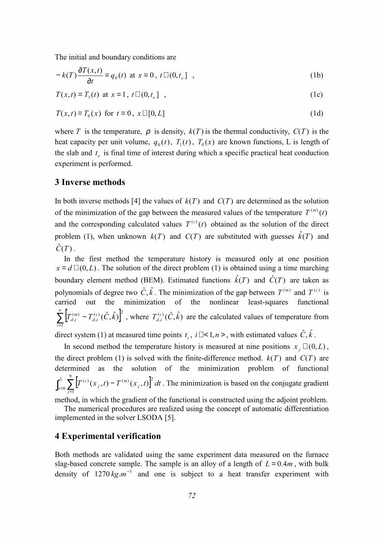
72

The initial and boundary conditions are

)(),()( 0 tqt

txTTk =∂

∂− at x = 0 , ],0( ett ∈ , (1b)

)(),( 1 tTtxT = at x =1 , ],0( ett ∈ , (1c)

T x t T x( , ) ( )= 0 for t = 0 , ],0[ Lx ∈ (1d)

where T is the temperature, ρ is density, k T( ) is the thermal conductivity, C T( ) is the heat capacity per unit volume, q t0 ( ) , T t1 ( ) , T x0 ( ) are known functions, L is length of the slab and et is final time of interest during which a specific practical heat conduction experiment is performed. 3 Inverse methods In both inverse methods [4] the values of k T( ) and C T( ) are determined as the solution of the minimization of the gap between the measured values of the temperature )()( tT m and the corresponding calculated values )()( tT c obtained as the solution of the direct problem (1), when unknown k T( ) and C T( ) are substituted with guesses )(ˆ Tk and

)(ˆ TC . In the first method the temperature history is measured only at one position

),0( Ldx ∈= . The solution of the direct problem (1) is obtained using a time marching boundary element method (BEM). Estimated functions )(ˆ Tk and )(ˆ TC are taken as polynomials of degree two kC ˆ ,ˆ . The minimization of the gap between )(mT and )(cT is carried out the minimization of the nonlinear least-squares functional

[ ]∑=

−n

i

cid

mid kCTT

1

2)(,

)(, )ˆ,ˆ( , where )ˆ,ˆ()(

, kCT cid are the calculated values of temperature from

direct system (1) at measured time points it , >∈< ni ,1 , with estimated values kC ˆ ,ˆ . In second method the temperature history is measured at nine positions ),0( Lx j ∈ ,

the direct problem (1) is solved with the finite-difference method. k T( ) and C T( ) are determined as the solution of the minimization problem of functional

[ ]∫ ∑==

−et

tj

jm

jc dttxTtxT

0

9

1

2)()( ),(),( . The minimization is based on the conjugate gradient

method, in which the gradient of the functional is constructed using the adjoint problem. The numerical procedures are realized using the concept of automatic differentiation

implemented in the solver LSODA [5]. 4 Experimental verification Both methods are validated using the same experiment data measured on the furnace slag-based concrete sample. The sample is an alloy of a length of mL 4.0= , with bulk density of 3. 1270 −mkg and one is subject to a heat transfer experiment with

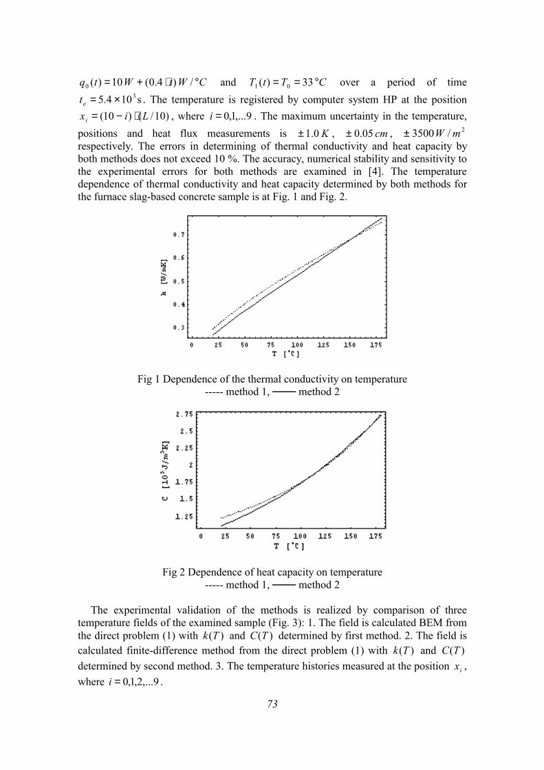
73

CWtWtq °⋅+= / )4.0( 10)(0 and CTtT °== 33)( 01 over a period of time s104.5 3×=et . The temperature is registered by computer system HP at the position

)10/()10( Lixi ⋅−= , where 9,...1,0=i . The maximum uncertainty in the temperature, positions and heat flux measurements is K 0.1± , cm 05.0± , 2/ 3500 mW± respectively. The errors in determining of thermal conductivity and heat capacity by both methods does not exceed 10 %. The accuracy, numerical stability and sensitivity to the experimental errors for both methods are examined in [4]. The temperature dependence of thermal conductivity and heat capacity determined by both methods for the furnace slag-based concrete sample is at Fig. 1 and Fig. 2.

Fig 1 Dependence of the thermal conductivity on temperature ----- method 1, method 2

Fig 2 Dependence of heat capacity on temperature ----- method 1, method 2

The experimental validation of the methods is realized by comparison of three

temperature fields of the examined sample (Fig. 3): 1. The field is calculated BEM from the direct problem (1) with )(Tk and )(TC determined by first method. 2. The field is calculated finite-difference method from the direct problem (1) with )(Tk and )(TC determined by second method. 3. The temperature histories measured at the position ix , where 9,...2,1,0=i .

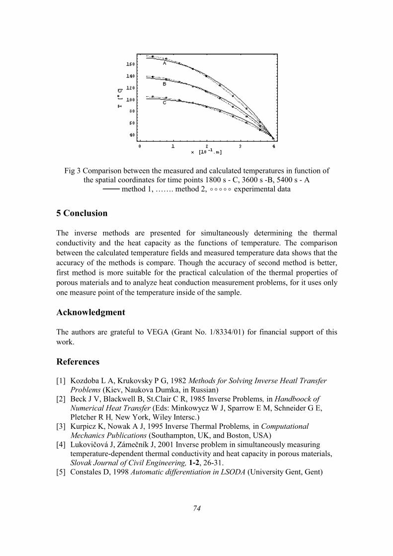
74

Fig 3 Comparison between the measured and calculated temperatures in function of the spatial coordinates for time points 1800 s - C, 3600 s -B, 5400 s - A

method 1, ……. method 2, !!!!! experimental data

5 Conclusion The inverse methods are presented for simultaneously determining the thermal conductivity and the heat capacity as the functions of temperature. The comparison between the calculated temperature fields and measured temperature data shows that the accuracy of the methods is compare. Though the accuracy of second method is better, first method is more suitable for the practical calculation of the thermal properties of porous materials and to analyze heat conduction measurement problems, for it uses only one measure point of the temperature inside of the sample. Acknowledgment The authors are grateful to VEGA (Grant No. 1/8334/01) for financial support of this work. References [1] Kozdoba L A, Krukovsky P G, 1982 Methods for Solving Inverse Heatl Transfer

Problems (Kiev, Naukova Dumka, in Russian) [2] Beck J V, Blackwell B, St.Clair C R, 1985 Inverse Problems, in Handboock of

Numerical Heat Transfer (Eds: Minkowycz W J, Sparrow E M, Schneider G E, Pletcher R H, New York, Wiley Intersc.)

[3] Kurpicz K, Nowak A J, 1995 Inverse Thermal Problems, in Computational Mechanics Publications (Southampton, UK, and Boston, USA)

[4] Lukovičová J, Zámečník J, 2001 Inverse problem in simultaneously measuring temperature-dependent thermal conductivity and heat capacity in porous materials, Slovak Journal of Civil Engineering, 1-2, 26-31.

[5] Constales D, 1998 Automatic differentiation in LSODA (University Gent, Gent)

75

SYNTHESIS, THERMAL AND IR SPECTRAL PROPERTIES OF MG(II) COMPLEXES WITH HETEROCYCLIC LIGANDS Subhash Chandra Mojumdar1, Milan Melník2, Eugen Jóna3, Alžbeta Krutošíková4

1 Institute of Inorganic Chemistry, Slovak Academy of Sciences, Dubravska Cesta 9,

SK-842 36 Bratislava, Slovakia 2 Department of Organic Chemistry, Slovak University of Technology, Radlinského 9,

SK-812 37 Bratislava 3 Department of Chemistry and Technology of Inorganic Materials, University

of Trenčín, SK-02032 Púchov, Slovakia

4 Department of Chemistry, Faculty of Natural Sciences, University of St. Cyril and Methodius, SK-917 01 Trnava, Slovakia

Email: scmojumdar@hotmail.com, melnik@cvt.stuba.sk, krutosik@ucm.sk Abstract TG, DTG, DTA and other analytical methods have been applied to the investigation of the thermal behaviour and structure of the complexes Mg(pc)(na)2.2H2O(I), Mg(pc)(Et2na)2.3H2O(II), Mg(pc)(mpc)2.H2O(III) and Mg(pc)(ron).2H2O(IV), where pc = 2,6-pyridindicarboxylate, na = nicotinamide, Et2na = N,N-diethylnicotinamide, mpc = methyl-3-pyridyl carbamate and ron = 3-pyridylcarbinol (ronicol). Thermal decomposition of these compounds is multi-stage process. The composition of the complexes and the solid state intermediate and resultant products of thermolysis had been identified by means of elemental analysis and complexometric titration. The possible scheme of destruction of the complexes is suggested. Heating the compounds first results in a release of water molecules. In complexes I, II and IV the loss of the molecular ligands (na, Et2na and ron) occurs (on the TG curves) in one step (-2na, -2Et2na and -ron) and in complex III in two steps (-mpc, -mpc). The final product of the thermal decomposition was MgO. The thermal stability of the complexes can be ordered in the sequence: II < III < I < IV. Et2na na, mpc and ron were coordinated to Mg(II) through the N atom of the respective heterocyclic ring. IR data suggest to a unidentate coordination of carboxylates to Mg(II) in complexes I-IV. Keywords: Mg (II) complexes, TG, DTA, IR-spectra, heterocyclic ligands 1 Introduction Investigations of heterocyclic ligands have resulted in discovering many biologically active compounds. It is not surprising, therefore, that many authors have investigated heterocyclic compounds and also examined them as ligands in coordination complexes of several central atoms [1-5]. In order to enhance understanding of drug-metal ion interactions, we have been studying the thermal properties of Mg(II) complexes with 2,6-pyridindicarboxylic acid (pch) and Et2na, na, mpc or ron, which are known as important components of biological systems. This work is a continuation of our previously reported studies [6-10] on the thermal and spectral properties of Mg(II)

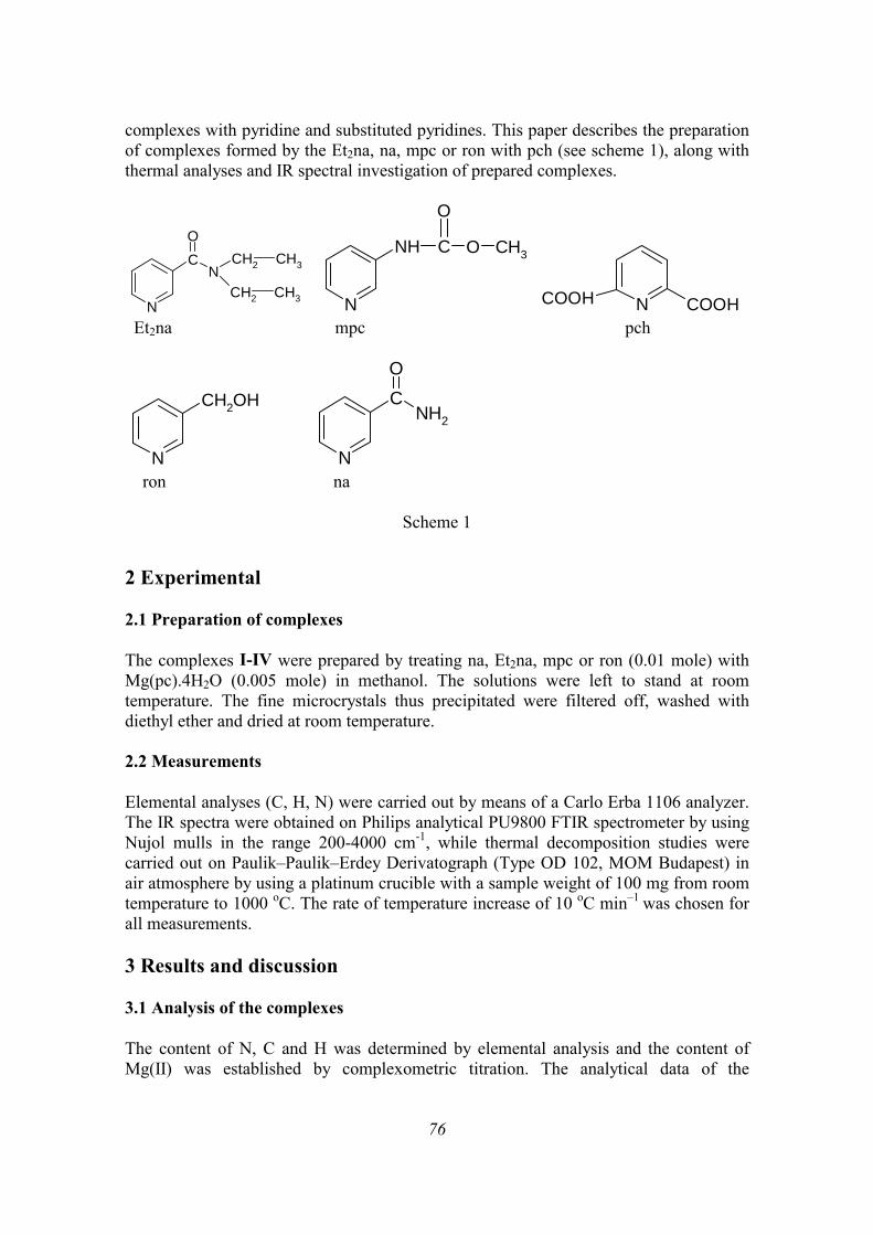
76

complexes with pyridine and substituted pyridines. This paper describes the preparation of complexes formed by the Et2na, na, mpc or ron with pch (see scheme 1), along with thermal analyses and IR spectral investigation of prepared complexes.

N

CO

NCH2 CH3

CH2 CH3 N

NH C

O

O CH3

N COOHCOOH

Et2na mpc pch

N

CH2OH

N

CO

NH2

ron na

Scheme 1

2 Experimental 2.1 Preparation of complexes The complexes I-IV were prepared by treating na, Et2na, mpc or ron (0.01 mole) with Mg(pc).4H2O (0.005 mole) in methanol. The solutions were left to stand at room temperature. The fine microcrystals thus precipitated were filtered off, washed with diethyl ether and dried at room temperature. 2.2 Measurements Elemental analyses (C, H, N) were carried out by means of a Carlo Erba 1106 analyzer. The IR spectra were obtained on Philips analytical PU9800 FTIR spectrometer by using Nujol mulls in the range 200-4000 cm-1, while thermal decomposition studies were carried out on Paulik–Paulik–Erdey Derivatograph (Type OD 102, MOM Budapest) in air atmosphere by using a platinum crucible with a sample weight of 100 mg from room temperature to 1000 oC. The rate of temperature increase of 10 oC min–1 was chosen for all measurements. 3 Results and discussion 3.1 Analysis of the complexes The content of N, C and H was determined by elemental analysis and the content of Mg(II) was established by complexometric titration. The analytical data of the

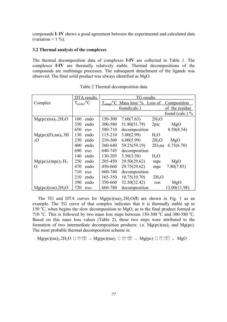
77

compounds I–IV shows a good agreement between the experimental and calculated data (variation < 1 %). 3.2 Thermal analysis of the complexes The thermal decomposition data of complexes I-IV are collected in Table 1. The complexes I-IV are thermally relatively stable. Thermal decompositions of the compounds are multistage processes. The subsequent detachment of the ligands was observed. The final solid product was always identified as MgO.

Table 2 Thermal decomposition data Complex

DTA results Tpeaks/oC

TG results Trange/oC Mass loss/ % Loss of Composition found(calc.) of the residue found (calc.) %

Mg(pc)(na)2.2H2O Mg(pc)(Et2na)2.3H2O Mg(pc)2(mpc)2.H2O Mg(pc)(ron).2H2O

160 endo 350 endo 650 exo 130 endo 230 endo 400 endo 690 exo 140 endo 250 endo 470 endo 710 exo 210 endo 390 endo 720 exo

150-300 7.60(7.63) 2H2O 300-580 51.80(51.79) 2pic MgO 580-710 decomposition 8.50(8.54) 115-210 3.00(2.99) H2O 210-360 6.00(5.99) 2H2O MgO 360-640 59.25(59.19) 2Et2na 6.75(6.70) 640-745 decomposition 130-205 3.50(3.50) H2O 205-450 29.50(29.62) mpc MgO 450-660 29.75(29.62) mpc 7.80(7.85) 660-740 decomposition 165-350 10.75(10.70) 2H2O 350-660 32.50(32.42) ron MgO 660-780 decomposition 12.00(11.98)

The TG and DTA curves for Mg(pc)(na)2.2H2O(I) are shown in Fig. 1 as an

example. The TG curve of that complex indicates that it is thermally stable up to 150 oC, when begins the slow decomposition to MgO, as to the final product formed at 710 oC. This is followed by two mass loss steps between 150-300 oC and 300-580 oC. Based on this mass loss values (Table 2), these two steps were attributed to the formation of two intermediate decomposition products: i.e. Mg(pc)(na)2 and Mg(pc). The most probable thermal decomposition scheme is:

Mg(pc)(na)2.2H2O 150 300− → o C Mg(pc)(na)2

300 580− → o C Mg(pc) 580 710− → o C MgO .

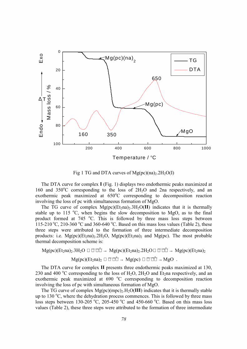
78

200 400 600 800 1000100

80

60

40

20

0

650

350160 MgO

Mg(pc)

Mg(pc)(na)2

End

o

E

xo

∆ T

TG

DTA

Mas

s lo

ss /

%

Temperature / oC

Fig 1 TG and DTA curves of Mg(pc)(na)2.2H2O(I)

The DTA curve for complex I (Fig. 1) displays two endothermic peaks maximized at

160 and 350oC corresponding to the loss of 2H2O and 2na respectively, and an exothermic peak maximized at 650oC corresponding to decomposition reaction involving the loss of pc with simultaneous formation of MgO.

The TG curve of complex Mg(pc)(Et2na)2.3H2O(II) indicates that it is thermally stable up to 115 oC, when begins the slow decomposition to MgO, as to the final product formed at 745 oC. This is followed by three mass loss steps between 115-210 oC, 210-360 oC and 360-640 oC. Based on this mass loss values (Table 2), these three steps were attributed to the formation of three intermediate decomposition products: i.e. Mg(pc)(Et2na)2.2H2O, Mg(pc)(Et2na)2 and Mg(pc). The most probable thermal decomposition scheme is:

Mg(pc)(Et2na)2.3H2O 115 210− → o C Mg(pc)(Et2na)2.2H2O 210 360− →

o C Mg(pc)(Et2na)2

Mg(pc)(Et2na)2 360 640− → o C Mg(pc) 640 745− →

o C MgO .

The DTA curve for complex II presents three endothermic peaks maximized at 130, 230 and 400 oC corresponding to the loss of H2O, 2H2O and Et2na respectively, and an exothermic peak maximized at 690 oC corresponding to decomposition reaction involving the loss of pc with simultaneous formation of MgO.

The TG curve of complex Mg(pc)(mpc)2.H2O(III) indicates that it is thermally stable up to 130 oC, where the dehydration process commences. This is followed by three mass loss steps between 130-205 oC, 205-450 oC and 450-660 oC. Based on this mass loss values (Table 2), these three steps were attributed to the formation of three intermediate

79

decomposition products: i.e. Mg(pc)(mpc)2., Mg(pc)(mpc) and Mg(pc) while the final solid product is concluded to be MgO. The most probable thermal decomposition scheme is:

Mg(pc)(mpc)2.H2O 130 205− → o C Mg(pc)(mpc)2

205 450− → o C Mg(pc)(mpc) 450 660− →

o C Mg(pc)

Mg(pc) 660 740− → o C MgO .

The DTA curve for complex III displays three endothermic peaks maximized at 140, 250 and 470 oC corresponding to the loss of H2O, mpc and mpc respectively, and an exothermic peak maximized at 710 oC corresponding to decomposition reaction involving the loss of pc with simultaneous formation of MgO.

The TG curve of complex Mg(pc)(ron).2H2O(IV) indicates that it is thermally stable up to 165 oC, where the dehydration process commences. This is followed by two mass loss steps between 165-350 oC and 350-660 oC. Based on this mass loss values (Table 2), these two steps were attributed to the formation of two intermediate decomposition products: i.e. Mg(pc)(ron) and Mg(pc) while the final solid product is concluded to be MgO. The most probable thermal decomposition scheme is:

Mg(pc)(ron).2H2O 165 350− → o C Mg(pc)(ron) 350 660− →

o C Mg(pc) 660 780− → o C MgO .

The DTA curve for complex IV displays two endothermic peaks maximized at 210 and 390 oC corresponding to the loss of 2H2O and ron respectively, and an exothermic peak maximized at 720 oC corresponding to decomposition reaction involving the loss of pc with simultaneous formation of MgO. 3.3 IR-spectra The modes of the coordinated ligands in the complexes have been investigated by means of IR spectra. The IR spectra of complexes I-IV show broad absorption bands in the range 3249-3385 cm-1. These frequencies of complexes I-IV correspond to the antisymmetric and symmetric OH stretch. These bands clearly confirm the presence of water in complexes I-IV. The compounds showed the carboxylate stretching frequencies, νCOO

- (sym) in the range 1406-1423 cm-1 and νCOO

-(asym) in the range 1693-1699 cm-1. The position of the bands are characteristic of metal(II) carboxylate compounds. Calculated from the examined spectra values of ∆COO = νCOO–(as)–COO-

(s) are in the range 293–275 cm–1. These values and three bands (COO deformation) at 920–720 cm–1 of complexes I-IV is in good accord with the literature data for unidentately bonded acetate structures [11]. The stretching vibration of the C=N in the pyridine ring appeared at 1590 cm-1. Upon complex formation the peak shifts to higher frequencies. The shifts in complexes I-IV (in the range 1605-1608 cm-1) may suggest that the bond formation of the Mg(II) with the N of pyridine ring, increases the dipolar contribution of C=N+ in the heterocyclic ring [9]. 4 Conclusions All of the complexes I-IV are hydrated, stable in air and soluble in water, ethanol, methanol and dimethylsulfoxide. In complexes I, II and IV loss of the neutral ligands occurs (on the TG curves) in one step and in complex III in two steps. The thermal stability of the complexes can be ordered in the sequence: II < III < I < IV. The stoichiometry of thermal decomposition can also be influenced by the changes of

80

experimental conditions [12]. IR spectral data is in good accord with the literature data for unidentately bonded acetate structures. The preliminary study has shown that the complexes do have a biological activity. Without X–ray analysis, no definite structure can be described for the different components. However, spectroscopic and analytical data available enable us to predict structures and we can also use thermal decomposition studies to help us. Acknowledgment We wish to thank the Ministry of Education of the Slovak Republic for financial support. References [1] Enamullah M and Linert W, 1995 Spin-crossover of [Fe(Cl-BZIMPY)2](ClO4)2

induced by deprotonation, J. Coord. Chem., 35, 325-335 [2] Skoršepa J S, Györyová K and Melník M, 1995 Preparation, identification and

thermal properties of (CH3CH2COO)Zn.2L.H2O (L= thiourea, nicotinamide, caffeine or theobromine), J. Thermal Anal., 44, 169-177

[3] Wolodkiewicz W, Brzyska W and Glowiak T, 1998 Preparation, structure and thermal decomposition of Cu(II) 3,5-dichlorobenzoate trihydrate, 129, 111-119

[4] Jóna E, Sirota A, Šimon P and Kubranová M, 1995 Thermochemical investigation of nickel(II)-nicotinamide-solvent interactions in solid halogeno and thiocyanato complexes, Thermochim. Acta, 258, 161-173

[5] Sun J, Lu Z, Li Y and Dai J, 1999 Thermal behavior and decomposition kinetics for two palladium(II) complexes with 1-aminopyrene and its derivative, J. Thermal Anal. Cal., 58, 383-391

[6] Mojumdar S C, 2001 Thermoanalytical and IR spectroscopy investigation of Mg(II) complexes with heterocyclic ligands, J. Therm. Anal. Cal., 64, 629-636

[7] Mojumdar S C, Melník M and Jóna E, 2000 Thermal and IR properties of Mg(II) complexes with heterocyclic ligands, Thermochim. Acta, 352, 129-134

[8] Mojumdar S C, Melník M and Jóna E, 1999 The thermal decomposition and IR-spectra of Mg(II) compounds with caffeine, Chem. Papers, 53, 309 –314

[9] Mojumdar S C, Melník M and Valko M, 1999 Spectral and Thermal properties of copper(II) complexes with methyl-3-pyridyl carbamate, Polish J. Chem., 73, 457-463

[10] Mojumdar S C, Melník M and Jóna E, 1998 The Thermal Decomposition of Mg(II) complexes with SCN, Pyridine, Nicotinamide and N,N-Diethylnicotinamide, J. Anal. Appl. Pyrolysis, 46, 147-156

[11] Nakamoto K, 1986 Infrared and Raman Spectra of Inorganic and Coordination Compounds, in Complexes of carboxylic acids, 4th Edn. (New York, J. Wiley) p. 59.

[12] Jóna E, Šramko T and Gažo J, 1979 Thermal properties of solid nickel(II) coordination compounds, J. Thermal Anal., 12, 213-229

81

THERMOPHYSICAL PROPERTIES OF BLENDS FROM PORTLAND AND SULFOALUMINATE - BELITE CEMENTS Subhash Chandra Mojumdar1, Ivan Janotka2 1 Institute of Inorganic Chemistry, Slovak Academy of Sciences, Dubravska cesta 9,

SK-842 36 Bratislava, Slovakia 2 Institute of Construction and Architecture, Slovak Academy of Sciences, Dubravska

cesta 9, SK-842 36 Bratislava, Slovakia Email: scmojumdar@hotmail.com, usarivan@savba.sk Abstract The behaviour of mortars with blends consisting of sulfoaluminate - belite (SAB) cements and ordinary Portland cement (OPC) made with cement to sand ratio of 1 : 3 (weight) and w/c = 0.5 maintained for 90 days at 20 ºC either at 60 % relative humidity (RH) - dry air or 100 % RH - wet air was studied. The results show insufficient character of hydraulic activity of SAB cements. Their quality has been improved. The replacement of 15 % of SAB cement by OPC influences strength positively and elasticity modulus values as well as hydrated phase and pore structure development of SAB/OPC blends relative to pure SAB cement systems. The mortars with mixed cement show excellent protective properties against corrosion of steel comparable to that of mortars made from OPC and blastfurnace - slag Portland cement (BFSPC). Steel is depassivated in SAB cement mortars. The above statements confirm the possible making technologies, when improvements in SAB cement quality were achieved. One can easily anticipate the competition in usages between SAB/OPC and BFSPC systems in the practice. SAB cements are a great advantage from the viewpoint of energy savings and quantity of CO2 released during their production. Keywords: OPC, Sulphoaluminate- belite cements, Mortar; Hydration Products 1 Introduction Blended cements have attracted intensive attention. There have been many successful utilization of blended cements in the concrete industry in past. In recent times, more attention has been given to the development of some modified special cement clinkers, leading to energy saving [1]. One of such cement containing the main phases C2S, C4A3S, C4AF and CS

__

was developed and reported by many authors [2-4]. The best properties were obtained with cements containing 30 - 40 % C4A3S

__

at water to cement ratio about 0.35 to 0.50 [5]. Cements containing C4A3S, β - C2S and CS

__

at 1.5 : 1 : 1 weight ratio hydrate rapidly to ettringite and develop early strength. All these compositions have very good dimensional stabilities, similar to OPC and have good resistance to atmospheric carbonation, although the ettringite component in hydrated cement tends to carbonation [6, 7]. Preliminary results show that sulfoaluminate cements are resistant to hydrochloric acid, sodium sulfate, and sodium chloride

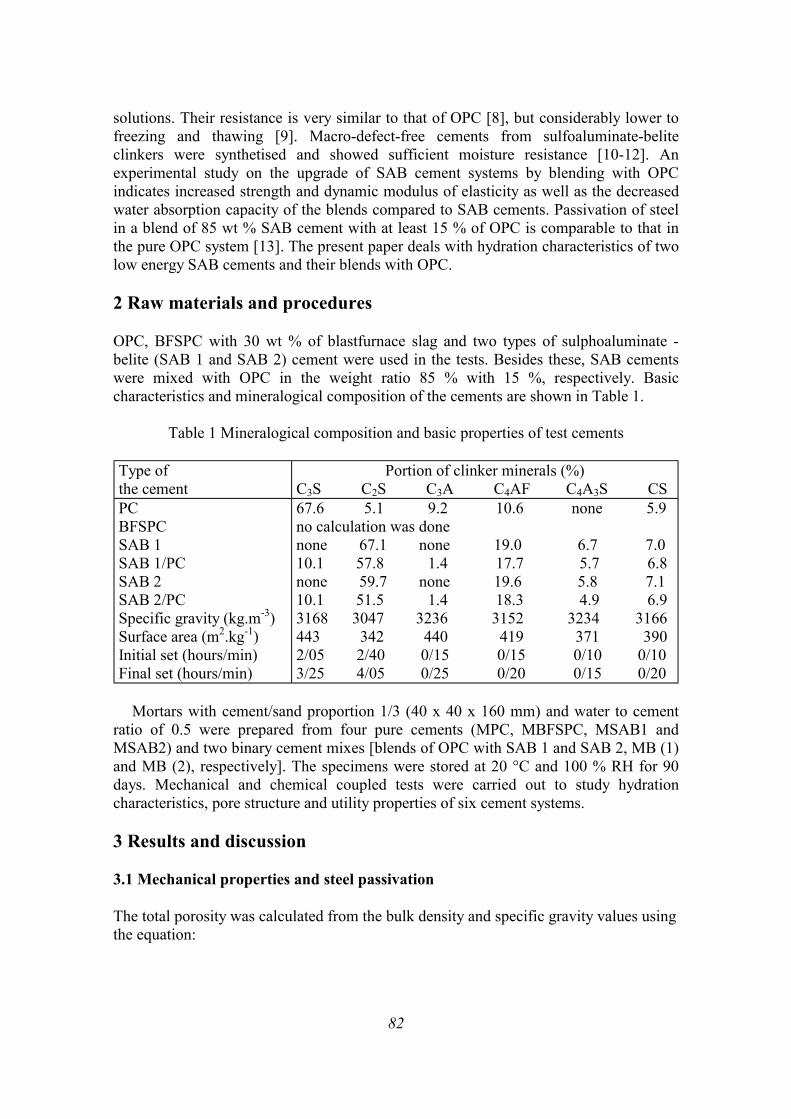
82

solutions. Their resistance is very similar to that of OPC [8], but considerably lower to freezing and thawing [9]. Macro-defect-free cements from sulfoaluminate-belite clinkers were synthetised and showed sufficient moisture resistance [10-12]. An experimental study on the upgrade of SAB cement systems by blending with OPC indicates increased strength and dynamic modulus of elasticity as well as the decreased water absorption capacity of the blends compared to SAB cements. Passivation of steel in a blend of 85 wt % SAB cement with at least 15 % of OPC is comparable to that in the pure OPC system [13]. The present paper deals with hydration characteristics of two low energy SAB cements and their blends with OPC. 2 Raw materials and procedures OPC, BFSPC with 30 wt % of blastfurnace slag and two types of sulphoaluminate - belite (SAB 1 and SAB 2) cement were used in the tests. Besides these, SAB cements were mixed with OPC in the weight ratio 85 % with 15 %, respectively. Basic characteristics and mineralogical composition of the cements are shown in Table 1.

Table 1 Mineralogical composition and basic properties of test cements Type of the cement

Portion of clinker minerals (%) C3S C2S C3A C4AF C4A3S CS

PC BFSPC SAB 1 SAB 1/PC SAB 2 SAB 2/PC Specific gravity (kg.m-3) Surface area (m2.kg-1) Initial set (hours/min) Final set (hours/min)

67.6 5.1 9.2 10.6 none 5.9 no calculation was done none 67.1 none 19.0 6.7 7.0 10.1 57.8 1.4 17.7 5.7 6.8 none 59.7 none 19.6 5.8 7.1 10.1 51.5 1.4 18.3 4.9 6.9 3168 3047 3236 3152 3234 3166 443 342 440 419 371 390 2/05 2/40 0/15 0/15 0/10 0/10 3/25 4/05 0/25 0/20 0/15 0/20

Mortars with cement/sand proportion 1/3 (40 x 40 x 160 mm) and water to cement

ratio of 0.5 were prepared from four pure cements (MPC, MBFSPC, MSAB1 and MSAB2) and two binary cement mixes [blends of OPC with SAB 1 and SAB 2, MB (1) and MB (2), respectively]. The specimens were stored at 20 °C and 100 % RH for 90 days. Mechanical and chemical coupled tests were carried out to study hydration characteristics, pore structure and utility properties of six cement systems. 3 Results and discussion 3.1 Mechanical properties and steel passivation The total porosity was calculated from the bulk density and specific gravity values using the equation:

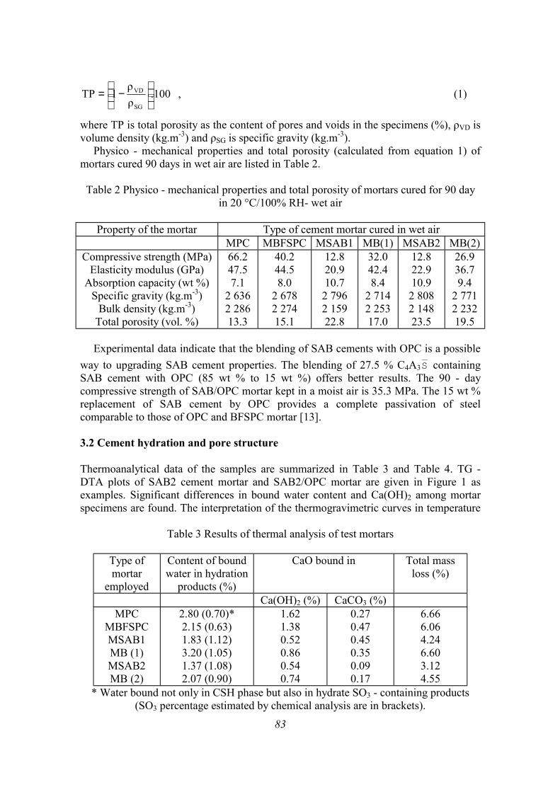
83

.100ρρ

1TPSG

VD

−= , (1)

where TP is total porosity as the content of pores and voids in the specimens (%), ρVD is volume density (kg.m-3) and ρSG is specific gravity (kg.m-3).

Physico - mechanical properties and total porosity (calculated from equation 1) of mortars cured 90 days in wet air are listed in Table 2.

Table 2 Physico - mechanical properties and total porosity of mortars cured for 90 day in 20 °C/100% RH- wet air

Property of the mortar Type of cement mortar cured in wet air

MPC MBFSPC MSAB1 MB(1) MSAB2 MB(2) Compressive strength (MPa)

Elasticity modulus (GPa) Absorption capacity (wt %)

Specific gravity (kg.m-3) Bulk density (kg.m-3)

Total porosity (vol. %)

66.2 47.5 7.1

2 636 2 286 13.3

40.2 44.5 8.0

2 678 2 274 15.1

12.8 20.9 10.7 2 796 2 159 22.8

32.0 42.4 8.4

2 714 2 253 17.0

12.8 22.9 10.9 2 808 2 148 23.5

26.9 36.7 9.4

2 771 2 232 19.5

Experimental data indicate that the blending of SAB cements with OPC is a possible

way to upgrading SAB cement properties. The blending of 27.5 % C4A3S__

containing SAB cement with OPC (85 wt % to 15 wt %) offers better results. The 90 - day compressive strength of SAB/OPC mortar kept in a moist air is 35.3 MPa. The 15 wt % replacement of SAB cement by OPC provides a complete passivation of steel comparable to those of OPC and BFSPC mortar [13]. 3.2 Cement hydration and pore structure Thermoanalytical data of the samples are summarized in Table 3 and Table 4. TG - DTA plots of SAB2 cement mortar and SAB2/OPC mortar are given in Figure 1 as examples. Significant differences in bound water content and Ca(OH)2 among mortar specimens are found. The interpretation of the thermogravimetric curves in temperature

Table 3 Results of thermal analysis of test mortars

Type of mortar

employed

Content of bound water in hydration

products (%)

CaO bound in Total mass loss (%)

Ca(OH)2 (%) CaCO3 (%) MPC

MBFSPC MSAB1 MB (1) MSAB2 MB (2)

2.80 (0.70)* 2.15 (0.63) 1.83 (1.12) 3.20 (1.05) 1.37 (1.08) 2.07 (0.90)

1.62 1.38 0.52 0.86 0.54 0.74

0.27 0.47 0.45 0.35 0.09 0.17

6.66 6.06 4.24 6.60 3.12 4.55

* Water bound not only in CSH phase but also in hydrate SO3 - containing products (SO3 percentage estimated by chemical analysis are in brackets).

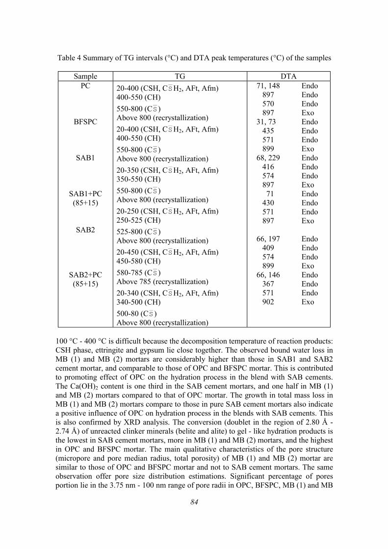
84

Table 4 Summary of TG intervals (°C) and DTA peak temperatures (°C) of the samples

Sample TG DTA PC

BFSPC

SAB1

SAB1+PC (85+15)

SAB2

SAB2+PC (85+15)

20-400 (CSH, CS__

H2, AFt, Afm) 400-550 (CH) 550-800 (CS

__

) Above 800 (recrystallization) 20-400 (CSH, CS

__

H2, AFt, Afm) 400-550 (CH) 550-800 (CS

__

) Above 800 (recrystallization) 20-350 (CSH, CS

__

H2, AFt, Afm) 350-550 (CH) 550-800 (CS

__

) Above 800 (recrystallization) 20-250 (CSH, CS

__

H2, AFt, Afm) 250-525 (CH) 525-800 (CS

__

) Above 800 (recrystallization) 20-450 (CSH, CS

__

H2, AFt, Afm) 450-580 (CH) 580-785 (CS

__

) Above 785 (recrystallization) 20-340 (CSH, CS

__

H2, AFt, Afm) 340-500 (CH) 500-80 (CS

__

) Above 800 (recrystallization)

71, 148 Endo 897 Endo 570 Endo 897 Exo 31, 73 Endo 435 Endo 571 Endo 899 Exo 68, 229 Endo 416 Endo 574 Endo 897 Exo 71 Endo 430 Endo 571 Endo 897 Exo 66, 197 Endo 409 Endo 574 Endo 899 Exo 66, 146 Endo 367 Endo 571 Endo 902 Exo

100 °C - 400 °C is difficult because the decomposition temperature of reaction products: CSH phase, ettringite and gypsum lie close together. The observed bound water loss in MB (1) and MB (2) mortars are considerably higher than those in SAB1 and SAB2 cement mortar, and comparable to those of OPC and BFSPC mortar. This is contributed to promoting effect of OPC on the hydration process in the blend with SAB cements. The Ca(OH)2 content is one third in the SAB cement mortars, and one half in MB (1) and MB (2) mortars compared to that of OPC mortar. The growth in total mass loss in MB (1) and MB (2) mortars compare to those in pure SAB cement mortars also indicate a positive influence of OPC on hydration process in the blends with SAB cements. This is also confirmed by XRD analysis. The conversion (doublet in the region of 2.80 Å - 2.74 Å) of unreacted clinker minerals (belite and alite) to gel - like hydration products is the lowest in SAB cement mortars, more in MB (1) and MB (2) mortars, and the highest in OPC and BFSPC mortar. The main qualitative characteristics of the pore structure (micropore and pore median radius, total porosity) of MB (1) and MB (2) mortar are similar to those of OPC and BFSPC mortar and not to SAB cement mortars. The same observation offer pore size distribution estimations. Significant percentage of pores portion lie in the 3.75 nm - 100 nm range of pore radii in OPC, BFSPC, MB (1) and MB

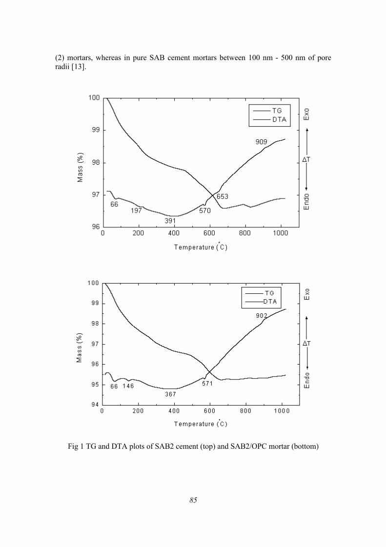
85

(2) mortars, whereas in pure SAB cement mortars between 100 nm - 500 nm of pore radii [13].

Fig 1 TG and DTA plots of SAB2 cement (top) and SAB2/OPC mortar (bottom)

86

4 Conclusions The replacement of 15 wt % of SAB cements by OPC in the pure SAB cement systems results to (i) increasing in the strength and elasticity modulus of SAB/OPC blends on values similar to BFSPC, (ii) attaining passivation ability to protect steel against corrosion comparable to that of OPC and BFSPC, (iii) accelerating hydrate phase formation and (iv) improving pore structure development and pore size distribution on the levels closely related to that of OPC and BFSPC mortar. The more attention will be paid to making progress in hydraulic activity of pure SAB cements in future. References [1] Mehta P K, 1991 Investigation on energy saving cement, World Cement

Technology, 11, 166-177 [2] Ali M, Gopal S and Handoo S K, 1994 Studies on the formation kinetics of calcium

sulfoaluminate, Cem. Concr. Res., 24, 715-720 [3] Moir G K and Glasser F P, 1992 Mineralisers, Modifiers and activators in the

clinkering process, Proc. 9th Int. Congr. Chem. Cem., New Delhi, 1, 125-152 [4] Wang Y, Li S, Su M, Xu J and Zhang F, 1997 Sulpho-aluminate cement with low

alkalinity, Proc. 10th Int. Congr. Chem. Cem., Gothenburg, 4, 4iv030 [5] Beretka J, Marroccoli M, Sherman N and Valenti G L, 1996 The influence of

C4A3S content and w/s ratio on the performance of calcium sulfoaluminate-based cements, Cem. Conc. Res., 26, 1673-1681

[6] Strigáč J, Palou M T, Krištin J and Majling J, 2000 Morphology and chemical composition on minerals inside the phase assemblage C-C2S-C4A3S -C4AF-CS relevant to sulphoaluminate belite cements, CERAMICS - Silikaty, 44, 26-34

[7] Sherman N, Beretka J, Santoro L and Valenti G L, 1995 Long-term behaviour of hydraulic binders based on calcium sulfoaluminate and calcium sulfosilicate, Cem. Concr. Res., 25, 113-126

[8] Živica V and Janotka I, 1999 Chemical resistance of sulfoaluminate-belite cement-based materials, Build. Res. J., 47, 117-134

[9] Janotka I and Krajči Ľ, 2000 Resistance to freezing and thawing of mortar specimens made from sulphoaluminate-belite cement, Bul. Mat. Sci., 23, 521-527

[10] Mojumdar S C, 2001 Processing-moisture resistance and thermal analysis of MDF materials, J. Therm. Anal. Cal., 64, 1133-1139

[11] Drabik M, Mojumdar S C and Galikova L, 2001 Changes of thermal events of macro-defect-free (MDF) cements due to the environmental deterioration, Cem. Concr. Res., 31, 751-755

[12] Mojumdar S C, 2001 Macro-defect-free cements with improved moisture resistance after delayed drying, Challenges for Coordination chemistry in the new century, 5, 453-458

[13] Janotka I and Krajči Ľ, 1999 An experimental study on the upgrade of sulfoaluminate-belite cement systems by blending with Portland cement, Adv. Cem. Res., 11, 35-41

87

OPTIMAL EXPERIMENTAL DESIGN ANALYSIS OF THE FLASH METHOD WITH REPEATED PULSES Libor Vozár1, Wolgang Hohenauer2, Gabriela Smetanková1 1 Department of Physics, Faculty of Sciences, Constantine the Philosopher University,

Tr. A. Hlinku 1, SK-949 74 Nitra, Slovakia 2 Department of Materials Research, Austrian Research Centers Seibersdorf,

A-2444 Seibersdorf, Austria Email: vozar@nr.sanet.sk, wolfgang.hohenauer@arcs.ac.at, gsmetankova@ukf.sk Abstract The paper deals with analytical aspects of the laser flash method with repeated pulses that is a photothermal experimental method for measurement of the thermal diffusivity of solids. It concentrates on the data reduction - an estimation of the thermal diffusivity from the experimental data. Special attention is given to the technique of correction of the width and the shape of the heat pulses. Results of sensitivity and optimal experimental design analyses are presented and discussed here. Key words: flash method, sensitivity, experimental design, repeated pulses, thermal

diffusivity 1 Introduction The laser flash method with repeated pulses is a photothermal experimental method for measurement of the thermal diffusivity of solids. The method uses a small disk-shaped sample similarily as the standard laser flash method [1]. Here the one (front) surface of the sample is subjected to several repeated heat pulses originated by consecutive laser pulses. The resulting temperature rise on the opposite (rear) face of the sample is measured, and the thermal diffusivity is computed from the temperature rise vs. time data [2] [3].

The purpose of the present work is to perform experimental design analysis [4] and to discuss the achieved results. Here the concept of sensitivity coefficients S [5] as well as the formalism based on the criterion to maximize the ratio of determinants ∆/∆2 of STS, which contains the product of the sensitivities and their transpose [6] is utilized. Results give arguments for optimal setting the experimental parameters in order to increase the sensitivity of the method as well it gives information concerning the optimum time of duration of an experiment. 2 Analytical basis The analytical model considers a homogeneous opaque slab of thickness e with uniform and constant thermophysical properties and the density ρ. The sample front face is exposed to instantaneous heat pulses repeated with the period tp, analytically described by the shape φ(t) = Qδ(t - ktp); k = 0,1,..., p. Here Q is the heat supplied by a pulse to the

88

unit area of the front face, δ(t) the Dirac’s function and (p+1) is the number of pulses. If there is a heat transfer between the sample and its environment, governed by Biot numbers H0 and He at the front and rear faces, respectively, the transient rear face temperature T(t) can be expressed in the form of Fourier series [3]

( )[ ]∑ ∑∞

= =

−ν=1n

k

0ipe0nlim exp),()( ttiHHATtT n , (1)

where limT is the adiabatic limit temperature ( limT =Q/ρce with c being the heat capacity), t is the time, a the thermal diffusivity

))(())((

)sin)(cos(2),(

e02ne0

2e

2n

20

2n

nn

0n

2e

2n

2n

e0n HHuHHHuHu

uuH

uHuuHHA

+++++

++= , H0 > 0; He > 0.., (2)

2

2n

n eau=ν , (3)

p

pp

1)( ; 1-0,1,...,

tpttkttk

pp

k≥

+<≤⟨= (4)

and un are the positive roots of equation

uHHuHHu )()tan()( e0e02 +=− . (5)

3. Sensivity analyses The simulated curves were calculated using the formula (1). The temperature Tlim was chosen to be 1 K. Axial and radial heat losses from the sample were assumed to be the same H = H0 = He = 0.05. Sensitivities are defined as

β∂∂β=βTS (6)

where T is the rear face temperature and β the appropriated parameter - thermal diffusivity a, the adiabatic limit temperature Tlim, or the Biot number H, respectively.

Fig. 1 presents the simulated temperature rise and sensitivities vs. dimensionless time (τ = at/e2) curves. Five pulses that follow with the time period τp = atpe-2 = 0.1 are considered here. Because of the linear dependence of the temperature rise on the adiabatic limit temperature Tlim the temperature rise curve corresponds to the sensitivity to the adiabatic limit temperature Tlim vs. time curve STlim. The figure shows, that curves STlim, Sa (Sa is the sensitivity to the thermal diffusivity) and SH (SH - sensitivity to the Biot number), respectively, have different shapes and the curves are uncorrelated. Fig. 1 shows that the sensitivity to thermal diffusivity is in its magnitude comparable to the temperature. This confirms that the flash method with repeated pulses is reasonable sensitive to changes in the thermal diffusivity.

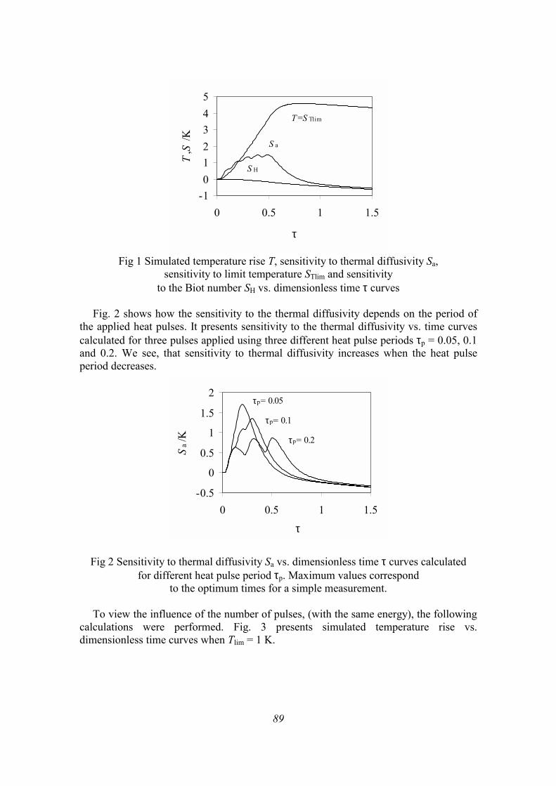
89

-1012345

0 0.5 1 1.5

τ

T,S

/K

T =S Tlim

S a

S H

Fig 1 Simulated temperature rise T, sensitivity to thermal diffusivity Sa,

sensitivity to limit temperature STlim and sensitivity to the Biot number SH vs. dimensionless time τ curves

Fig. 2 shows how the sensitivity to the thermal diffusivity depends on the period of

the applied heat pulses. It presents sensitivity to the thermal diffusivity vs. time curves calculated for three pulses applied using three different heat pulse periods τp = 0.05, 0.1 and 0.2. We see, that sensitivity to thermal diffusivity increases when the heat pulse period decreases.

-0.5

0

0.5

1

1.5

2

0 0.5 1 1.5

τ

Sa

/K

τp= 0.05

τp= 0.1

τp= 0.2

Fig 2 Sensitivity to thermal diffusivity Sa vs. dimensionless time τ curves calculated for different heat pulse period τp. Maximum values correspond

to the optimum times for a simple measurement.

To view the influence of the number of pulses, (with the same energy), the following calculations were performed. Fig. 3 presents simulated temperature rise vs. dimensionless time curves when Tlim = 1 K.

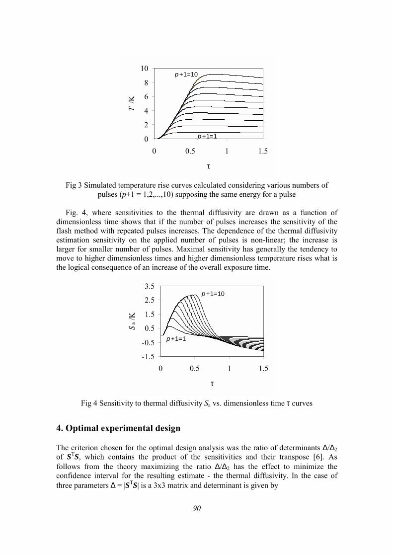
90

0

2

4

6

8

10

0 0.5 1 1.5

τ

T /K

p+1=10

p+1=1

Fig 3 Simulated temperature rise curves calculated considering various numbers of

pulses (p+1 = 1,2,...,10) supposing the same energy for a pulse

Fig. 4, where sensitivities to the thermal diffusivity are drawn as a function of dimensionless time shows that if the number of pulses increases the sensitivity of the flash method with repeated pulses increases. The dependence of the thermal diffusivity estimation sensitivity on the applied number of pulses is non-linear; the increase is larger for smaller number of pulses. Maximal sensitivity has generally the tendency to move to higher dimensionless times and higher dimensionless temperature rises what is the logical consequence of an increase of the overall exposure time.

-1.5

-0.5

0.5

1.5

2.5

3.5

0 0.5 1 1.5

τ

Sa /

K

p+1=10

p+1=1

Fig 4 Sensitivity to thermal diffusivity Sa vs. dimensionless time τ curves

4. Optimal experimental design The criterion chosen for the optimal design analysis was the ratio of determinants ∆/∆2 of STS, which contains the product of the sensitivities and their transpose [6]. As follows from the theory maximizing the ratio ∆/∆2 has the effect to minimize the confidence interval for the resulting estimate - the thermal diffusivity. In the case of three parameters ∆ = |STS| is a 3x3 matrix and determinant is given by

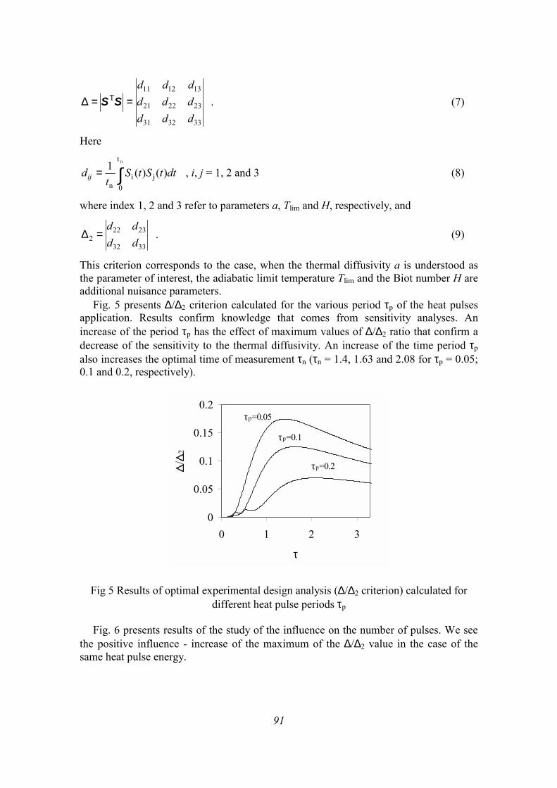
91

333231

232221

131211T

ddddddddd

==∆ SS . (7)

Here

dttStSt

dij )()(1j

t

0i

n

n

∫= , i, j = 1, 2 and 3 (8)

where index 1, 2 and 3 refer to parameters a, Tlim and H, respectively, and

3332

23222 dd

dd=∆ . (9)

This criterion corresponds to the case, when the thermal diffusivity a is understood as the parameter of interest, the adiabatic limit temperature Tlim and the Biot number H are additional nuisance parameters.

Fig. 5 presents ∆/∆2 criterion calculated for the various period τp of the heat pulses application. Results confirm knowledge that comes from sensitivity analyses. An increase of the period τp has the effect of maximum values of ∆/∆2 ratio that confirm a decrease of the sensitivity to the thermal diffusivity. An increase of the time period τp also increases the optimal time of measurement τn (τn = 1.4, 1.63 and 2.08 for τp = 0.05; 0.1 and 0.2, respectively).

0

0.05

0.1

0.15

0.2

0 1 2 3

τ

/2

τp=0.05

τp=0.1

τp=0.2

Fig 5 Results of optimal experimental design analysis (∆/∆2 criterion) calculated for different heat pulse periods τp

Fig. 6 presents results of the study of the influence on the number of pulses. We see

the positive influence - increase of the maximum of the ∆/∆2 value in the case of the same heat pulse energy.

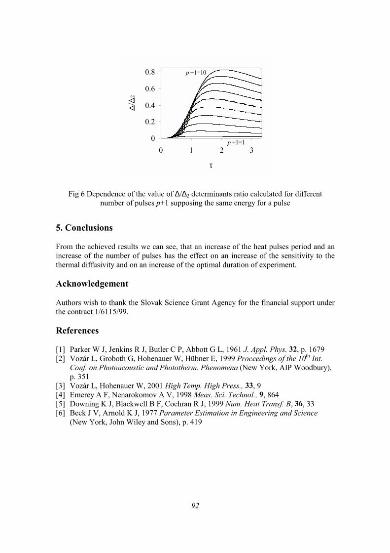
92

0

0.2

0.4

0.6

0.8

0 1 2 3

τ

/2

p +1=10

p +1=1

Fig 6 Dependence of the value of ∆/∆2 determinants ratio calculated for different number of pulses p+1 supposing the same energy for a pulse

5. Conclusions From the achieved results we can see, that an increase of the heat pulses period and an increase of the number of pulses has the effect on an increase of the sensitivity to the thermal diffusivity and on an increase of the optimal duration of experiment. Acknowledgement Authors wish to thank the Slovak Science Grant Agency for the financial support under the contract 1/6115/99. References [1] Parker W J, Jenkins R J, Butler C P, Abbott G L, 1961 J. Appl. Phys. 32, p. 1679 [2] Vozár L, Groboth G, Hohenauer W, Hübner E, 1999 Proceedings of the 10th Int.

Conf. on Photoacoustic and Phototherm. Phenomena (New York, AIP Woodbury), p. 351

[3] Vozár L, Hohenauer W, 2001 High Temp. High Press., 33, 9 [4] Emerey A F, Nenarokomov A V, 1998 Meas. Sci. Technol., 9, 864 [5] Downing K J, Blackwell B F, Cochran R J, 1999 Num. Heat Transf. B, 36, 33 [6] Beck J V, Arnold K J, 1977 Parameter Estimation in Engineering and Science

(New York, John Wiley and Sons), p. 419

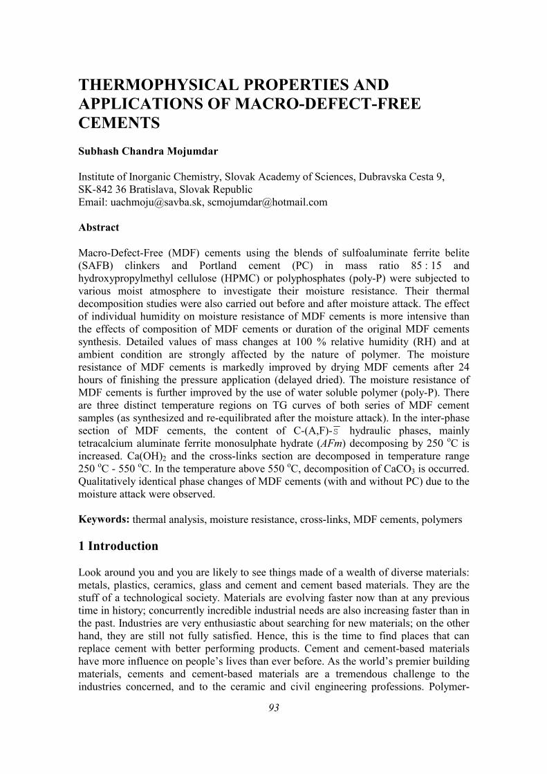
93

THERMOPHYSICAL PROPERTIES AND APPLICATIONS OF MACRO-DEFECT-FREE CEMENTS Subhash Chandra Mojumdar Institute of Inorganic Chemistry, Slovak Academy of Sciences, Dubravska Cesta 9, SK-842 36 Bratislava, Slovak Republic Email: uachmoju@savba.sk, scmojumdar@hotmail.com Abstract Macro-Defect-Free (MDF) cements using the blends of sulfoaluminate ferrite belite (SAFB) clinkers and Portland cement (PC) in mass ratio 85 : 15 and hydroxypropylmethyl cellulose (HPMC) or polyphosphates (poly-P) were subjected to various moist atmosphere to investigate their moisture resistance. Their thermal decomposition studies were also carried out before and after moisture attack. The effect of individual humidity on moisture resistance of MDF cements is more intensive than the effects of composition of MDF cements or duration of the original MDF cements synthesis. Detailed values of mass changes at 100 % relative humidity (RH) and at ambient condition are strongly affected by the nature of polymer. The moisture resistance of MDF cements is markedly improved by drying MDF cements after 24 hours of finishing the pressure application (delayed dried). The moisture resistance of MDF cements is further improved by the use of water soluble polymer (poly-P). There are three distinct temperature regions on TG curves of both series of MDF cement samples (as synthesized and re-equilibrated after the moisture attack). In the inter-phase section of MDF cements, the content of C-(A,F)-S hydraulic phases, mainly tetracalcium aluminate ferrite monosulphate hydrate (AFm) decomposing by 250 oC is increased. Ca(OH)2 and the cross-links section are decomposed in temperature range 250 oC - 550 oC. In the temperature above 550 oC, decomposition of CaCO3 is occurred. Qualitatively identical phase changes of MDF cements (with and without PC) due to the moisture attack were observed. Keywords: thermal analysis, moisture resistance, cross-links, MDF cements, polymers 1 Introduction Look around you and you are likely to see things made of a wealth of diverse materials: metals, plastics, ceramics, glass and cement and cement based materials. They are the stuff of a technological society. Materials are evolving faster now than at any previous time in history; concurrently incredible industrial needs are also increasing faster than in the past. Industries are very enthusiastic about searching for new materials; on the other hand, they are still not fully satisfied. Hence, this is the time to find places that can replace cement with better performing products. Cement and cement-based materials have more influence on people’s lives than ever before. As the world’s premier building materials, cements and cement-based materials are a tremendous challenge to the industries concerned, and to the ceramic and civil engineering professions. Polymer-

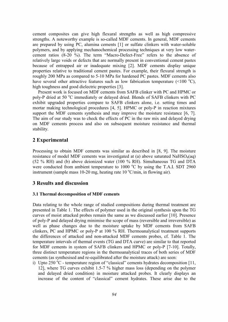
94

cement composites can give high flexural strengths as well as high compressive strengths. A noteworthy example is so-called MDF cements. In general, MDF cements are prepared by using PC, alumina cements [1] or sulfate clinkers with water-soluble polymers, and by applying mechanochemical processing techniques at very low water-cement ratios (8-20 %). The term “Macro-Defect-Free” refers to the absence of relatively large voids or defects that are normally present in conventional cement pastes because of entrapped air or inadequate mixing [2]. MDF cements display unique properties relative to traditional cement pastes. For example, their flexural strength is roughly 200 MPa as compared to 5-10 MPa for hardened PC pastes. MDF cements also have several other attractive features such as low fabrication temperature (<100 oC), high toughness and good dielectric properties [3].

Present work is focused on MDF cements from SAFB clinker with PC and HPMC or poly-P dried at 50 oC immediately or delayed dried. Blends of SAFB clinkers with PC exhibit upgraded properties compare to SAFB clinkers alone, i.e. setting times and mortar making technological procedures [4, 5]. HPMC or poly-P in reaction mixtures support the MDF cements synthesis and may improve the moisture resistance [6, 7]. The aim of our study was to check the effects of PC in the raw mix and delayed drying on MDF cements process and also on subsequent moisture resistance and thermal stability. 2 Experimental Processing to obtain MDF cements was similar as described in [8, 9]. The moisture resistance of model MDF cements was investigated at (a) above saturated NaHSO4(aq) (52 % RH) and (b) above deionized water (100 % RH). Simultaneous TG and DTA were conducted from ambient temperature to 1000 oC by using the T.A.I. SDT 2960 instrument (sample mass 10-20 mg, heating rate 10 oC/min, in flowing air). 3 Results and discussion 3.1 Thermal decomposition of MDF cements Data relating to the whole range of studied compositions during thermal treatment are presented in Table 1. The effects of polymer used in the original synthesis upon the TG curves of moist attacked probes remain the same as we discussed earlier [10]. Presence of poly-P and delayed drying minimise the scope of mass (reversible and irreversible) as well as phase changes due to the moisture uptake by MDF cements from SAFB clinkers, PC and HPMC or poly-P at 100 % RH. Thermoanalytical treatment supports the differences of attacked and non-attacked MDF cements probes, cf. Table 1. The temperature intervals of thermal events (TG and DTA curve) are similar to that reported for MDF cements in system of SAFB clinkers and HPMC or poly-P [7-10]. Totally, three distinct temperature regions in the thermoanalytical traces of both series of MDF cements (as synthesised and re-equilibrated after the moisture attack) are seen: i) Upto 250 oC - temperature region of “classical” cements hydrates decomposition [11, 12], where TG curves exhibit 1.5-7 % higher mass loss (depending on the polymer and delayed dried condition) in moisture attacked probes. It clearly displays an increase of the content of “classical” cement hydrates. These arise due to the

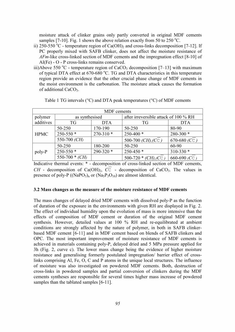
95

moisture attack of clinker grains only partly converted in original MDF cements samples [7-10]. Fig. 1 shows the above relation exactly from 50 to 250 oC.

ii) 250-550 oC - temperature region of Ca(OH)2 and cross-links decomposition [7-12]. If PC properly mixed with SAFB clinker, does not affect the moisture resistance of AFm-like cross-linked section of MDF cements and the impregnation effect [8-10] of Al(Fe) - O - P cross-links remains conserved.

iii) Above 550 oC - temperature region of CaCO3 decomposition [7–13] with maximum of typical DTA effect at 670-680 oC. TG and DTA characteristics in this temperature region provide an evidence that the other crucial phase change of MDF cements in the moist environment is the carbonation. The moisture attack causes the formation of additional CaCO3.

Table 1 TG intervals (°C) and DTA peak temperatures (°C) of MDF cements

MDF cements

as synthesised after irreversible attack of 100 % RH polymer additives TG DTA TG DTA

50-250 170-190 50-250 80-90 250-550 * 270-310 * 250-400 * 280-300 * HPMC 550-700 (CH) 500-700 (CH),(CC ) 670-680 (CC ) 50-250 180-200 50-250 60-90 250-550 * 290-320 * 250-450 * 310-330 * poly-P 550-700 * (CH) 500-720 * (CH),(CC ) 660-690 (CC )

Indicative thermal events: * - decomposition of cross-linked section of MDF cements, CH - decomposition of Ca(OH)2, CC - decomposition of CaCO3. The values in presence of poly-P ((NaPO3)n or (Na5P3O10) are almost identical.

3.2 Mass changes as the measure of the moisture resistance of MDF cements The mass changes of delayed dried MDF cements with dissolved poly-P as the function of duration of the exposure in the environments with given RH are displayed in Fig. 2. The effect of individual humidity upon the evolution of mass is more intensive than the effects of composition of MDF cement or duration of the original MDF cement synthesis. However, detailed values at 100 % RH and re-equilibrated at ambient conditions are strongly affected by the nature of polymer, in both in SAFB clinker-based MDF cement [6-11] and in MDF cement based on blends of SAFB clinkers and OPC. The most important improvement of moisture resistance of MDF cements is achieved in materials containing poly-P, delayed dried and 5 MPa pressure applied for 3h (Fig. 2, curve c). The lower mass change being the evidence of higher moisture resistance and generalising formerly postulated impregnation/ barrier effect of cross-links comprising Al, Fe, O, C and P atoms in the unique local structures. The influence of moisture was also investigated on powdered MDF cements. Both, destruction of cross-links in powdered samples and partial conversion of clinkers during the MDF cements syntheses are responsible for several times higher mass increase of powdered samples than the tablated samples [6-11].

96

0 500 100080

85

90

95

100

∆ TEn

do

Exo

667oC

315oC

76oC

3.67%

2.82%

11.97% TG DTA

Wei

ght (

%)

Temperature (oC)

Fig 1 TG and DTA curves for a sample made from SAFB clinker, PC

and powdered poly-P (Na5P3O10), irreversibly attacked at an extreme level of moisture (100 % RH, for 17 days

and subsequently ambient conditions for additional 6 days).

0 5 1 0 1 5 2 0 2 5 3 00

1

2

3

4

5

a b c d

∆ ∆∆∆ m

/ %

T i m e / d a y s

Fig 2 Mass change ∆m as a function of time for delayed dried MDF cements made

from SAFB clinkers and PC with dissolved poly-P - (NaPO3)n and pressure was applied for (a) 0.5h, (b) 1h, (c) 3h and (d) 5h, and treated

at 52 % RH (until 7th day), at 100 % RH (from 8th to 24th day) and under the ambient conditions (from 25th to 30th day).

97

4 Applications There have been examined a few potential applications of MDF cements, which are designed to meet market needs. Thermal insulator for specific applications, reinforcement for ordinary cement paste or mortars, and shells for specific applications are promising. The technology utilized in making a cement shell of a solar powered car can be easily applied to form armors also. Loudspeaker cabinets were also introduced by Alford and Birchall. Generally a material higher in damping (tan δ), Young modulus and specific gravity has good acoustic properties. The applications described above are by no means comprehensive but illustrate the range of potential uses that exist for high flexural strength polymer cement composite or, at least, provide guidelines for application oriented experiments. More comprehensive overview of potential applications has been described in [14] as presented by Maeta Techno-Research in its concise market survey of Japanese and European manufacturing industries. 5 Conclusions Study of mass equilibration and thermal analysis give an effective knowledge of the moisture sensitivity phenomenon of MDF cements. The results favour our previous hypothesis on the impregnation/barrier effect of poly-P incorporated in the structure of MDF cements. There have been examined a few potential applications of MDF cements, which are designed to meet market needs. Thermal insulators for specific applications, reinforcement for ordinary cement paste or mortars, and shells for specific applications are promising. The technology utilized in making a cement shell of a solar powered car can be easily applied to form armors also. Loudspeaker cabinets were also introduced by Alford and Birchall [14].

Materials are evolving faster now than at any previous time in history; concurrently incredible industrial needs are also increasing faster than in the past. Industries are very enthusiastic about searching for new materials; on the other hand, they are still not fully satisfied. Hence, this is the time to find places that can replace cement with better performing products. Our studies display the advantage and prospectus of poly-P for the MDF cements synthesized from SAFB clinker with poly-P and blends of these with PC. The recent development of moisture resistance of MDF cements (only about 1 % mass increase at 100 % RH) proved that the old saying “where there’s a will there’s a way” is very true with MDF cements and their future developments. Acknowledgement Author wish to thank the Slovak Science Grant Agency for the financial support under the project (VEGA 6039). References [1] Birchal J D, Howard A J, Kendal K and Raistrick J H, 1988 Cementitious

Composition and Cementitious Product of High Flexural Strength. European Pat. Specification, June B1, No. 0055035, 1-17

[2] Lewis J A and Desai P G, 1996 Microstructure-Property Relations in Organocement Composites Derived from CaAl2O4-Coated Al2O3 Powders, MAETA

98

Workshop on High Flexural Polymer-Cement Composite, Sakata, 3-4 October, p. 49-58

[3] Kendal K, Howard A J and Birchal J D, 1983 The Relation between Porosity, Microstructure and Strength and the Approach to Advanced Cement-based Materials. Philos. Trans. R. Soc. London, A310, 139-153

[4] Janotka I and Krajči Ľ, 1999 An experimental study on the upgrade of sulfoaluminate-belite cement systems by blending with Portland cement, Adv. Cem. Res., 11, 35-41

[5] Strigáč J, Palou M T, Krištin J and Majling J, 2000 Morphology and chemical composition on minerals inside the phase assemblage C-C2S-C4A3S -C4AF-CS relevant to sulphoaluminate belite cements, CERAMICS - Silikaty, 44, 26-34

[6] Drabik M, Galikova L, Hanic F and Sharp J H, 1997 MDF-related Compositions based on Novel Low-energy Clinkers, Chem. Papers, 51, 363-366

[7] Drabik M, Mojumdar S C and Galikova L, 2001 Changes of thermal events of macro-defect-free (MDF) cements due to the environmental deterioration, Cem. Concr. Res, 31, 751-755

[8] Mojumdar S C, 2001 Processing-moisture resistance and thermal analysis of MDF materials, J. Therm. Anal. Cal., 64, 1133-1139

[9] Mojumdar S C, 2001 Macro-defect-free cements with improved moisture resistance after delayed drying, Challenges for Coordination chemistry in the new century, 5, 453-458

[10] Mojumdar S C and Drabik M, 2001 Macro-Defect-Free cements in the new millennium, Science of cement and cncrete-Kurdowski symposium, June 20-21, Cracow, Poland, p. 257-264

[11] Drabik M, Galikova L and Mojumdar S C, 2001 Macro-defect-free cements: Chemistry and Impact of the Environment, Key Engineering Materials, 206, 1867-1870

[12] Taylor H F W, 1998 Hydration of the Calcium Silicate Phases, Cement Chemistry, 2nd Ed. (London, Thomas Telford) p. 113

[13] Strydom C A and Potgieter J H, 1997 An Investigation into the Chemical Nature of the reactivity of Lime, in Proceedings of 10th International Congress on the Chemistry of Cement (Ed: Justnes H, Gothenburg), paper 2ii049

[14] Pushpalal G K, Maeda N, Kawano T and Kojimi H, 1996 High strength phenol resin-cement composite. Part 3: Applications, MAETA Workshop on High Flexural Polymer-Cement Composite, Sakata, 3-4 October, p. 35-48

99

THERMOPHYSICAL PROPERTIES OF THE GLASS BK7 Gabriela Smetanková, Libor Vozár Department of Physics, Faculty of Natural Sciences, Constantine the Philosopher University, Tr. A. Hlinku 1, SK-949 74 Nitra, Slovakia Email: smetankova@pobox.sk, vozar@nr.sanet.sk Abstract The paper deals with the measurement of the thermophysical properties (effusivity, thermal conductivity, thermal diffusivity and specific heat) of the glass BK 7 using the dynamic plane source method. The theory of the dynamic plane source method is summarized and described. The experimental measurements were performed at room temperature, on air, under atmospheric pressure. Key words: thermophysical properties, glass BK 7, dynamic plane source method 1 Introduction The dynamic plane source method (DPS) uses a plane source, which acts both as the heat source and the temperature detector. The plane source is placed between two identical samples of finite length. The rear surface of the samples is in contact with a very good heat conducting material (heat sink) kept at the constant temperature. This creates constant temperature boundary condition at the rear surface of the samples. The hot plane has the same shape as the samples cross profile. The method assumes one dimensional heat flow across the samples.

Advantage of the dynamic plane source method consists in fact that the method gives a possibility to obtain several thermophysical properties of the measured material from one thermogram, simultaneously. 2 Principle of the dynamic plate source method The ideal theory considers [1] an ideal heater - the homogeneous hot plane of negligible thickness and mass that is in perfect thermal contact with the front face of the sample, an ideal thermal contact (zero thermal contact resistance) between the sample and the temperature stabilizer - the block of very good heat conducting material (heat sink) as well as zero heat losses from the lateral surfaces of the samples.

We consider the ideal plane heat source at x = 0 placed between two identical square shaped samples from measured materials of the thickness L. The samples occupy the region –L < x < L. Rear surface of the samples at x = –L and x = L are kept at constant temperature being in a perfect contact with the temperature stabilizer made of a high conducting material.

If the system has zero initial temperature T0 and if qs is the total output of power per unit area dissipated by the heater, then the temperature increase as a function of time is given by [1]

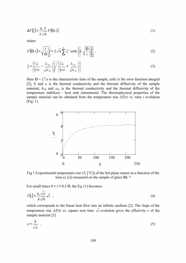
100

( ) ( )tFLq

tT s ,πλ

Θ=∆ (1)

where

( )

Θ+Θ

=Θ ∑∞

=1ierfcξπ21,

n

n

tnttF , (2)

+

−=

Al

Al

Al

Al

aaaaλλλλξ . (3)

Here Θ = L2/a is the characteristic time of the sample, ierfc is the error function integral [2], λ and a is the thermal conductivity and the thermal diffusivity of the sample material, λAl and aAl is the thermal conductivity and the thermal diffusivity of the temperature stabilizer - heat sink (aluminum). The thermophysical properties of the sample material can be obtained from the temperature rise ∆T(t) vs. time t evolution (Fig. 1).

Fig 1 Experimental temperature rise (Ti [°C]) of the hot plane sensor as a function of the

time (ti [s]) measured on the sample of glass BK 7 For small times 0 < t < 0,3 Θ, the Eq. (1) becomes

( ) taq

tT s

πλ= , (4)

which corresponds to the linear heat flow into an infinite medium [2]. The slope of the temperature rise ∆T(t) vs. square root time t evolution gives the effusivity e of the sample material [3]

ae λ= . (5)

0 50 100 150 2000

2

4

66

0

Ti

2300 ti

101

In the case of an ideal heat sink (ξ = -1) the equation (1) can be simplified as

( )( )

( )

Θ

++

−=∆ ∑∞

=0

22

22 4π1n2

-exp12

1π81

λ2 n

s tn

LqtT (6)

and for large times t > 2 Θ [4], the temperature rise conforms the formula

( )λ2Lq

tT s=∆ , (7)

that can be easily used for the thermal conductivity λ of the sample material estimation. The thermal diffusivity a can be calculated from the effusivity e and the thermal conductivity λ values using the equation

2λ

=

ea . (8)

For times t > 0,5 Θ, the natural logarithm of the derivative of the equation (6) except n = 0 gives the formula

( )Θ

−=∆

4lnln

2

V

tLc

qtd

tTd π . (9)

The graph of ln[d∆T(t)/dt] again t represent a straight line, which intercept gives specific heat per unit volume cV and the slope gives Θ and thus the thermal diffusivity a. When we know the effusivity of the sample material (from the slope of the temperature rise ∆T(t) vs. square root time t ) then the value of ξ can be calculated using the equation (3). So we can plot the graph ∆T(t) again F(Θ,t) whose the slope for times t < 0,7 Θ, gives the value of the thermal conductivity λ of the sample material.

We can observe, using the dynamic plane source method, it is possible obtained from a single measurement all the thermal transport properties of the sample material from the different stages of the thermogram using the proper evaluation procedure for each stage. 3 Experimental hot plane apparatus The plane heat source (supplied by the Institute of Physics, SAS Bratislava) is made of a 23 µm thick Ni foil, protected from both sides by an insulating layer made of 25 µm thick kapton. It is placed between two identical square shaped samples having the same profile as the heater. The rear surfaces of the samples are connected to stabilizer blocks (heat sinks). They are made of sufficiently thick disks of a very good heat conducting material (aluminium). The plane heat source serves both as a heat source and as the resistance temperature detector. The thermophysical properties of the sample material are estimated analyzing the measured temperature rise vs. time evolution subjected by the application of the step heating by flowing the electrical current through the hot plane source. The temperature variation at the hot plane sensor is determined by measuring the change of the voltage ∆U(t) across the source

( ) ( )tTRItU ∆=∆ α00 (10)

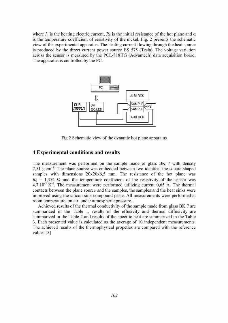
102

where I0 is the heating electric current, R0 is the initial resistance of the hot plane and α is the temperature coefficient of resistivity of the nickel. Fig. 2 presents the schematic view of the experimental apparatus. The heating current flowing through the heat source is produced by the direct current power source BS 575 (Tesla). The voltage variation across the sensor is measured by the PCL-818HG (Advantech) data acquisition board. The apparatus is controlled by the PC.

Fig 2 Schematic view of the dynamic hot plane apparatus

4 Experimental conditions and results The measurement was performed on the sample made of glass BK 7 with density 2,51 g.cm-3. The plane source was embedded between two identical the square shaped samples with dimensions 20x20x6,5 mm. The resistance of the hot plane was R0 = 1,354 Ω and the temperature coefficient of the resistivity of the sensor was 4,7.10-3 K-1. The measurement were performed utilizing current 0,65 A. The thermal contacts between the plane source and the samples, the samples and the heat sinks were improved using the silicon sink compound paste. All measurements were performed at room temperature, on air, under atmospheric pressure.

Achieved results of the thermal conductivity of the sample made from glass BK 7 are summarized in the Table 1, results of the effusivity and thermal diffusivity are summarized in the Table 2 and results of the specific heat are summarized in the Table 3. Each presented value is calculated as the average of 10 independent measurements. The achieved results of the thermophysical propeties are compared with the reference values [5]

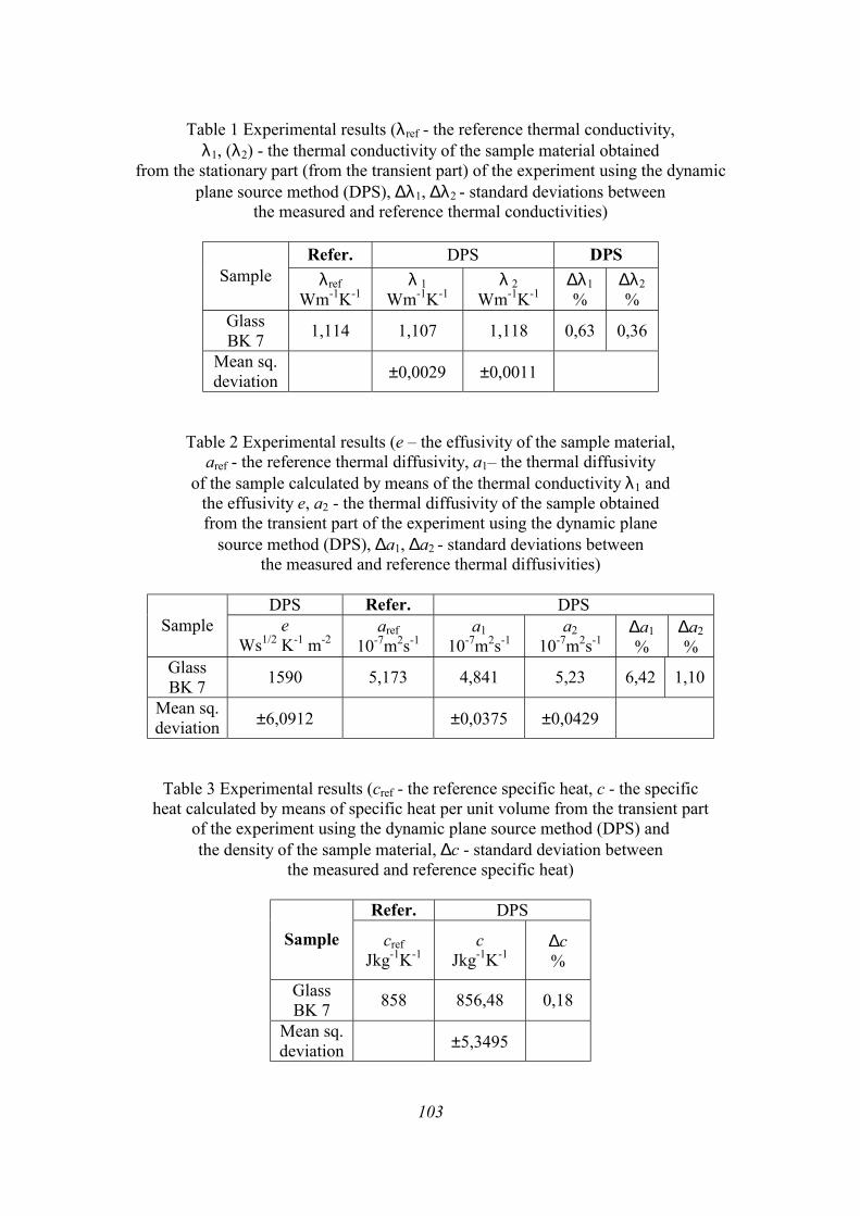
103

Table 1 Experimental results (λref - the reference thermal conductivity, λ1, (λ2) - the thermal conductivity of the sample material obtained

from the stationary part (from the transient part) of the experiment using the dynamic plane source method (DPS), ∆λ1, ∆λ2 - standard deviations between

the measured and reference thermal conductivities)

Refer. DPS DPS Sample λref

Wm-1K-1

λ 1 Wm-1K-1

λ 2 Wm-1K-1

∆λ1 %

∆λ2 %

Glass BK 7 1,114 1,107 1,118 0,63 0,36

Mean sq. deviation ±0,0029 ±0,0011

Table 2 Experimental results (e – the effusivity of the sample material, aref - the reference thermal diffusivity, a1– the thermal diffusivity

of the sample calculated by means of the thermal conductivity λ1 and the effusivity e, a2 - the thermal diffusivity of the sample obtained from the transient part of the experiment using the dynamic plane

source method (DPS), ∆a1, ∆a2 - standard deviations between the measured and reference thermal diffusivities)

DPS Refer. DPS

Sample e Ws1/2 K-1 m-2

aref 10-7m2s-1

a1 10-7m2s-1

a2 10-7m2s-1

∆a1 %

∆a2 %

Glass BK 7 1590 5,173 4,841 5,23 6,42 1,10

Mean sq. deviation ±6,0912 ±0,0375 ±0,0429

Table 3 Experimental results (cref - the reference specific heat, c - the specific heat calculated by means of specific heat per unit volume from the transient part

of the experiment using the dynamic plane source method (DPS) and the density of the sample material, ∆c - standard deviation between

the measured and reference specific heat)

Refer. DPS

Sample cref Jkg-1K-1

c Jkg-1K-1

∆c %

Glass BK 7 858 856,48 0,18

Mean sq. deviation ±5,3495

104

5 Conclusion All Tables show very low dispersion of the results of the thermophysical properties of the sample made from glass BK 7 as well as a very good agreement with the reference values. Using the simple experimental arangement of the hot plane apparatus we can obtain all basic thermophysical properties. Advantage of the dynamic plane source method is possibility of the simultaneous estimation of the thermophysical properties. We can see that the coincidence between the results obtained from the different parts of the experimental thermogram is satisfactory. Acknowledgement Authors wish to thank the Slovak Science Grant Agency for the financial support under the contract 1/6115/99. References [1] Karawacki E, Suleiman B M, ul-Haq I, Nhi B T, 1992 An extension to the dynamic

plane source technique for measuring thermal conductivity, thermal diffusivity and specific heat of dielectric solids, Rev. Sci. Instrum., 63, 10, p. 4390

[2] Carslav H S, Jaeger J C, 1959 Conduction of Heat in Solid, 2nd Ed. (Oxford Univ. Press, Oxford)

[3] Karawacki E, Suleiman B M, 1991 Dynamic plane-source technique for the study of the thermal transport properties of solids, High Temp. – High Press., 23, p. 215

[4] Krempaský J, 1969 Meranie termofyzikálnych veličín, (Bratislava, Veda) [5] http://www.layertec.de/bk7.html

105

THERMODILATOMETRY OF TEXTURED ELECTROCERAMIC MATERIAL Igor Štubňa, Libor Vozár, Gabriela Smetanková Department of Physics, Constantine the Philosopher University, Tr. A. Hlinku 1, 949 74 Nitra, Slovakia Email: istubna@ukf.sk Abstract Thermodilatometry of ceramic samples prepared from the mixture of 50 % kaolin, 25 % feldspar and 25 % quartz and kaolin samples was studied in the temperature range of 20 - 1000 °C. The shrinkage of the samples is caused by: 1. evaporation of the capillary water (20 - 200 °C), 2. escaping of the OH groups from the octahedral sheets of the kaolinite crystals (430 - 750 °C), 3. high-temperature changes of metakaolinite (above 850 °C). The shrinkage should be bigger in the perpendicular direction to the basal planes. This assumption is confirmed in these temperature ranges except the region of dehydroxylation. To explain this result, the extension of the kaolinite crystals and blocks of these crystals by steam passing along the octahedral sheets and crystal boundaries was supposed. Key words: thermodilatometry, texture, ceramics 1 Introduction Anisometric platelike kaolinite crystals represent the main part (up to 50 %) of unfired ceramic mass designed for high voltage insulator production. Forming of wet ceramic mass by means of the vacuum extruder sets the anisometric crystals in order into a new macroscopic structure with a different local degree of the order. This structure is called a technological texture. Measurements show the anisotropy of mechanical strength [1], sound propagation velocity and Young's modulus [2, 3], thermal diffusivity [4], and electrical properties [5, 6]. The texture affects the dimensions of a wet sample during its drying [1] and the sample dilatation during heating up to 900 °C [7]. Also an influence of the texture on dehydroxylation kinetics was found [7].

The influence of the texture on performance properties is usually unfavourable. Neighbour volume blocks with different texture could cause the defects on block boundaries from elevated mechanical stress to creation of cracks during firing. The most important physical parameters connected with these appearances are the coefficient of linear thermal expansion, module of elasticity and thermal conductivity. The aim of this paper is an experimental study of the linear thermal expansion of textured electroceramic samples in relation to temperature and compare these results with the linear thermal expansion of pure textured kaolin samples.

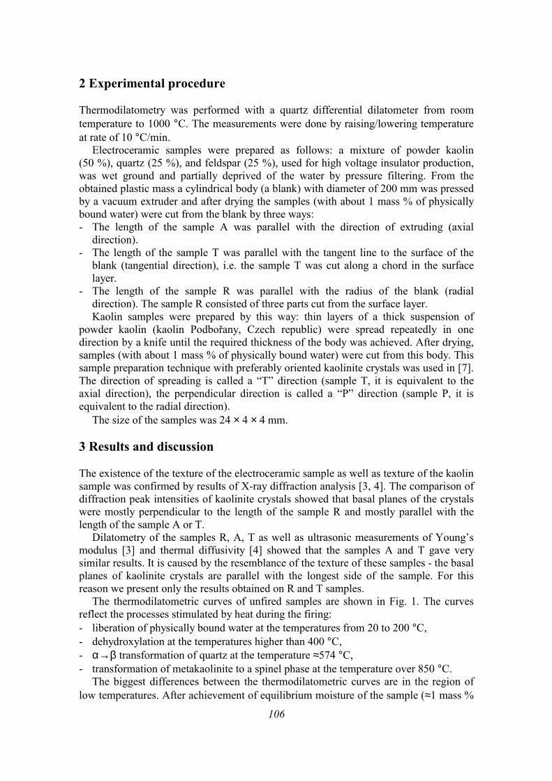
106

2 Experimental procedure Thermodilatometry was performed with a quartz differential dilatometer from room temperature to 1000 °C. The measurements were done by raising/lowering temperature at rate of 10 °C/min.

Electroceramic samples were prepared as follows: a mixture of powder kaolin (50 %), quartz (25 %), and feldspar (25 %), used for high voltage insulator production, was wet ground and partially deprived of the water by pressure filtering. From the obtained plastic mass a cylindrical body (a blank) with diameter of 200 mm was pressed by a vacuum extruder and after drying the samples (with about 1 mass % of physically bound water) were cut from the blank by three ways: - The length of the sample A was parallel with the direction of extruding (axial

direction). - The length of the sample T was parallel with the tangent line to the surface of the

blank (tangential direction), i.e. the sample T was cut along a chord in the surface layer.

- The length of the sample R was parallel with the radius of the blank (radial direction). The sample R consisted of three parts cut from the surface layer. Kaolin samples were prepared by this way: thin layers of a thick suspension of

powder kaolin (kaolin Podbořany, Czech republic) were spread repeatedly in one direction by a knife until the required thickness of the body was achieved. After drying, samples (with about 1 mass % of physically bound water) were cut from this body. This sample preparation technique with preferably oriented kaolinite crystals was used in [7]. The direction of spreading is called a “T” direction (sample T, it is equivalent to the axial direction), the perpendicular direction is called a “P” direction (sample P, it is equivalent to the radial direction).

The size of the samples was 24 × 4 × 4 mm. 3 Results and discussion The existence of the texture of the electroceramic sample as well as texture of the kaolin sample was confirmed by results of X-ray diffraction analysis [3, 4]. The comparison of diffraction peak intensities of kaolinite crystals showed that basal planes of the crystals were mostly perpendicular to the length of the sample R and mostly parallel with the length of the sample A or T.

Dilatometry of the samples R, A, T as well as ultrasonic measurements of Young’s modulus [3] and thermal diffusivity [4] showed that the samples A and T gave very similar results. It is caused by the resemblance of the texture of these samples - the basal planes of kaolinite crystals are parallel with the longest side of the sample. For this reason we present only the results obtained on R and T samples.

The thermodilatometric curves of unfired samples are shown in Fig. 1. The curves reflect the processes stimulated by heat during the firing: - liberation of physically bound water at the temperatures from 20 to 200 °C, - dehydroxylation at the temperatures higher than 400 °C, - α→β transformation of quartz at the temperature ≈574 °C, - transformation of metakaolinite to a spinel phase at the temperature over 850 °C.

The biggest differences between the thermodilatometric curves are in the region of low temperatures. After achievement of equilibrium moisture of the sample (≈1 mass %

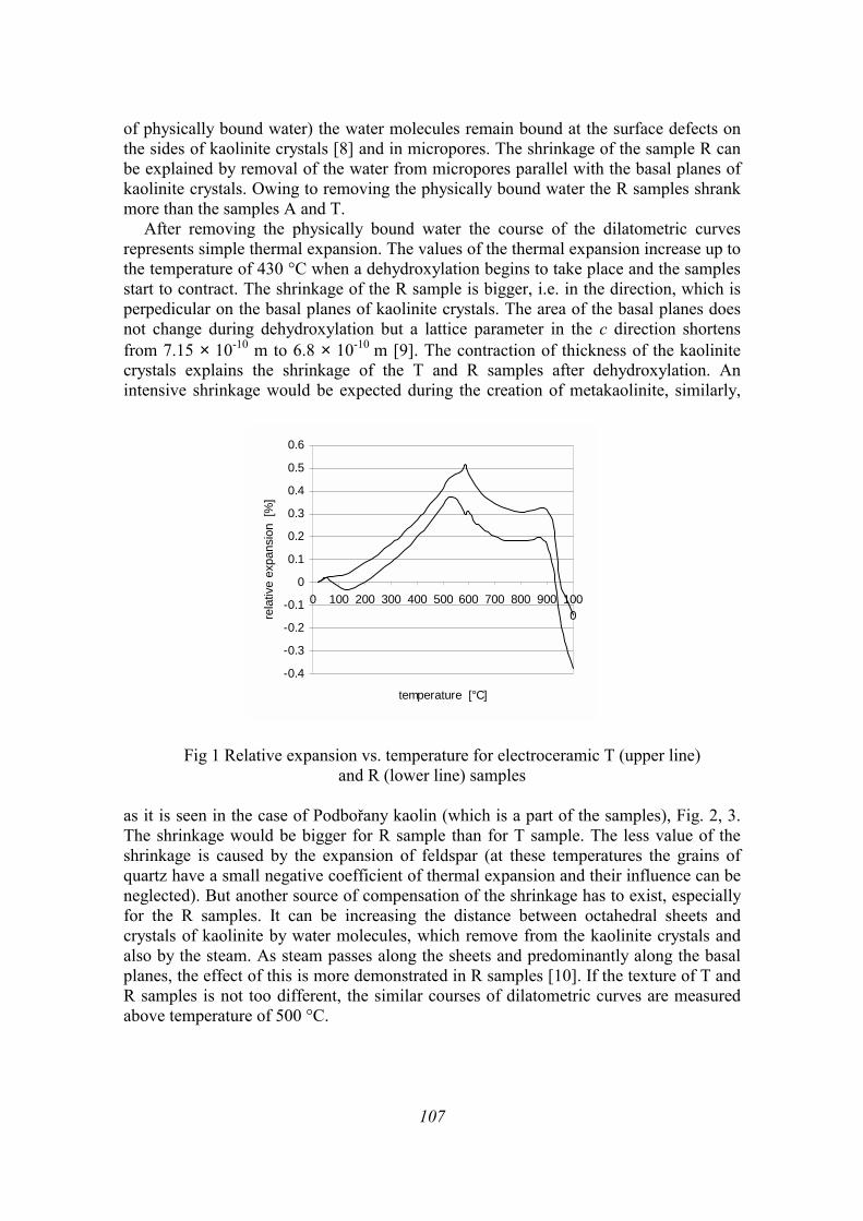
107

of physically bound water) the water molecules remain bound at the surface defects on the sides of kaolinite crystals [8] and in micropores. The shrinkage of the sample R can be explained by removal of the water from micropores parallel with the basal planes of kaolinite crystals. Owing to removing the physically bound water the R samples shrank more than the samples A and T.

After removing the physically bound water the course of the dilatometric curves represents simple thermal expansion. The values of the thermal expansion increase up to the temperature of 430 °C when a dehydroxylation begins to take place and the samples start to contract. The shrinkage of the R sample is bigger, i.e. in the direction, which is perpedicular on the basal planes of kaolinite crystals. The area of the basal planes does not change during dehydroxylation but a lattice parameter in the c direction shortens from 7.15 × 10-10 m to 6.8 × 10-10 m [9]. The contraction of thickness of the kaolinite crystals explains the shrinkage of the T and R samples after dehydroxylation. An intensive shrinkage would be expected during the creation of metakaolinite, similarly,

Fig 1 Relative expansion vs. temperature for electroceramic T (upper line)

and R (lower line) samples as it is seen in the case of Podbořany kaolin (which is a part of the samples), Fig. 2, 3. The shrinkage would be bigger for R sample than for T sample. The less value of the shrinkage is caused by the expansion of feldspar (at these temperatures the grains of quartz have a small negative coefficient of thermal expansion and their influence can be neglected). But another source of compensation of the shrinkage has to exist, especially for the R samples. It can be increasing the distance between octahedral sheets and crystals of kaolinite by water molecules, which remove from the kaolinite crystals and also by the steam. As steam passes along the sheets and predominantly along the basal planes, the effect of this is more demonstrated in R samples [10]. If the texture of T and R samples is not too different, the similar courses of dilatometric curves are measured above temperature of 500 °C.

-0.4

-0.3

-0.2

-0.1

0

0.1

0.2

0.3

0.4

0.5

0.6

0 100 200 300 400 500 600 700 800 900 1000

temperature [°C]

rela

tive

expa

nsio

n [%

]

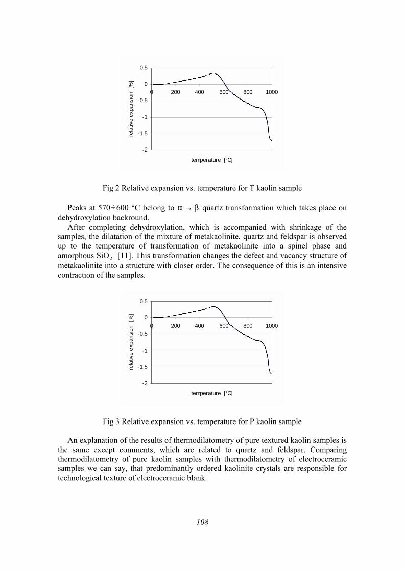
108

-2

-1.5

-1

-0.5

0

0.5

0 200 400 600 800 1000

temperature [°C]

rela

tive

expa

nsio

n [%

]

Fig 2 Relative expansion vs. temperature for T kaolin sample

Peaks at 570÷600 °C belong to α β→ quartz transformation which takes place on dehydroxylation backround.

After completing dehydroxylation, which is accompanied with shrinkage of the samples, the dilatation of the mixture of metakaolinite, quartz and feldspar is observed up to the temperature of transformation of metakaolinite into a spinel phase and amorphous SiO2 [11]. This transformation changes the defect and vacancy structure of metakaolinite into a structure with closer order. The consequence of this is an intensive contraction of the samples.

-2

-1.5

-1

-0.5

0

0.5

0 200 400 600 800 1000

temperature [°C]

rela

tive

expa

nsio

n [%

]

Fig 3 Relative expansion vs. temperature for P kaolin sample

An explanation of the results of thermodilatometry of pure textured kaolin samples is the same except comments, which are related to quartz and feldspar. Comparing thermodilatometry of pure kaolin samples with thermodilatometry of electroceramic samples we can say, that predominantly ordered kaolinite crystals are responsible for technological texture of electroceramic blank.

109

4 Summary The main influence on the results of thermodilatometry of unfired samples containing kaolin, quartz and feldspar have the kaolinite crystals. The dilatation or contraction in two directions (perpendicular to base planes or parallel with base planes of the kaolinite crystals) is connected with removing of physically bound water and with changes of kaolinite structure, which are different in these two directions.

The shrinkage should be bigger in the perpendicular direction to the basal planes. This assumption is confirmed in these temperature ranges except the region of dehydroxylation. To explain this result, the expansion of the kaolinite crystals and blocks of these crystals by steam passing along the octahedral sheets and crystal boundaries was supposed. Acknowledgment This work was supported by the grant VEGA 1/6115/99. References [1] Vycudilík P, 1978 Sklář a keramik, 28, N10, p. 301-303 [2] Štubňa I, Kozík T, Koubek V, 1981 Sklář a keramik, 31, N8, p. 224-226 [3] Kalužná M, Kaprálik I, Štubňa I, 1987 Sklář a keramik, 37, N10, p. 291-294 [4] Kalužná M, Vozár L a kol, 1992 Ceramics-Silikáty, 36, N1, p. 15-19 [5] Belianin A N, Rudakov V N, 1968 Defektoskopia, 4, N3, p. 1-4 [6] Kalužná M, Kluvanec D, 1984 In. Zb. PF v Nitre - Fyzika II, Nitra, p. 43-51 [7] Lučininova N I et al., 1979 Steklo i keramika, N12, p. 16-18 [8] Polakovič J, Polakovičová J, Sokoly J, 1983 In. Proc. 5th Meeting European Clay

Groups, Praha, p. 279-282 [9] Freund F, 1967 Ber. Deutsch. Keram. Ges., 44, N7, p. 6-13 [10] Štubňa I, Trnovcová V, 1998 Ceramics–Silikáty, 42, N1, p. 21-24 [11] Brown I W M et al., 1985 J. Amer. Ceram. Soc., 68, N.6, p. 298-301