Embed Size (px)
Citation preview

MEASUREMENT OF THE MUON ATMOSPHERICPRODUCTION DEPTH WITH THE WATER
CHERENKOV DETECTORS OF THE PIERRE AUGEROBSERVATORY
Laura Molina BuenoUniversidad de Granada
1st September 2015
Advisor:Prof. Antonio Bueno Villar
Co-advisor:Dr. Sergio Pastor Carpi
Departamento de Física Teórica y del Cosmos & CAFPE

Editorial: Universidad de Granada. Tesis DoctoralesAutora: Laura Molina BuenoISBN: 978-84-9125-244-3URI: http://hdl.handle.net/10481/40899
La doctoranda Laura Molina Bueno y los directores de la tesis Antonio Bueno Villar ySergio Pastor Carpi garantizamos, al firmar esta tesis doctoral, que el trabajo ha sidorealizado por la doctoranda bajo la dirección de los directores de la tesis y hasta dondenuestro conocimiento alcanza, en la realización del trabajo, se han respetado los derechosde otros autores al ser citados, cuando se han utilizado sus resultados o publicaciones.
Granada, 1 de septiembre de 2015.
Directores de la tesis Doctoranda
Fdo: Antonio Bueno Villar, Sergio Pastor Carpi Laura Molina Bueno

D. Antonio Bueno Villar, Catedrático de Universidad,
CERTIFICA: que la presente tesis doctoral, MEASUREMENT OF THE MUON ATMOSPHERICPRODUCTION DEPTH WITH THE WATER CHERENKOV DETECTORS OF THE PIERRE AUGER OB-SERVATORY, ha sido realizada por Da Laura Molina Bueno bajo su dirección en el Dpto. deFísica Teórica y del Cosmos de la Universidad de Granada, así como que ésta ha realizadouna estancia en el extranjero por un periodo superior a tres meses en la Universidad Pierrey Marie Curie-LPNHE.
Granada, 1 de septiembre de 2015
Fdo: Antonio Bueno Villar

Contents
1 Ultra High Energy Cosmic Rays 11.1 Features of the cosmic ray spectrum . . . . . . . . . . . . . . . . . . . . . . . 1
1.1.1 The Knee . . . . . . . . . . . . . . . . . . . . . . . . . . . . . . . . . 21.1.2 The Ankle . . . . . . . . . . . . . . . . . . . . . . . . . . . . . . . . . 31.1.3 The end of the cosmic ray energy spectrum . . . . . . . . . . . . . . 3
1.2 Origin of cosmic rays . . . . . . . . . . . . . . . . . . . . . . . . . . . . . . . 41.3 UHE photon and neutrino limits . . . . . . . . . . . . . . . . . . . . . . . . . 51.4 Arrival direction distribution . . . . . . . . . . . . . . . . . . . . . . . . . . . 61.5 Extensive air showers . . . . . . . . . . . . . . . . . . . . . . . . . . . . . . . 8
1.5.1 Heitler model of electromagnetic showers . . . . . . . . . . . . . . . 81.5.2 Extension of the Heitler model to hadronic showers . . . . . . . . . . 10
1.6 Mass composition of UHECR . . . . . . . . . . . . . . . . . . . . . . . . . . . 11
2 The Pierre Auger Observatory 152.1 Surface Detector . . . . . . . . . . . . . . . . . . . . . . . . . . . . . . . . . 16
2.1.1 Calibration . . . . . . . . . . . . . . . . . . . . . . . . . . . . . . . . 172.1.2 Trigger . . . . . . . . . . . . . . . . . . . . . . . . . . . . . . . . . . . 18
2.2 Fluorescence Detector . . . . . . . . . . . . . . . . . . . . . . . . . . . . . . 212.2.1 Trigger . . . . . . . . . . . . . . . . . . . . . . . . . . . . . . . . . . . 222.2.2 Calibration . . . . . . . . . . . . . . . . . . . . . . . . . . . . . . . . 232.2.3 Fluorescence yield . . . . . . . . . . . . . . . . . . . . . . . . . . . . 232.2.4 Atmospheric monitoring . . . . . . . . . . . . . . . . . . . . . . . . . 232.2.5 FD reconstruction . . . . . . . . . . . . . . . . . . . . . . . . . . . . 25
3 SD event reconstruction 313.1 Event selection . . . . . . . . . . . . . . . . . . . . . . . . . . . . . . . . . . 313.2 Geometry reconstruction . . . . . . . . . . . . . . . . . . . . . . . . . . . . . 323.3 Reconstruction of the lateral signal distribution . . . . . . . . . . . . . . . . 32
3.3.1 Signal variance . . . . . . . . . . . . . . . . . . . . . . . . . . . . . . 333.3.2 Angular resolution . . . . . . . . . . . . . . . . . . . . . . . . . . . . 403.3.3 LDF maximum likelihood fit . . . . . . . . . . . . . . . . . . . . . . . 42
3.4 Energy estimation . . . . . . . . . . . . . . . . . . . . . . . . . . . . . . . . 43

VIII
4 Revision of the Muon Arrival Time Model 494.1 MPD algorithm . . . . . . . . . . . . . . . . . . . . . . . . . . . . . . . . . . 494.2 Classic (previous) kinematic delay parameterization . . . . . . . . . . . . . 534.3 New approach . . . . . . . . . . . . . . . . . . . . . . . . . . . . . . . . . . . 58
5 Muon Production Depth in an event by event basis 655.1 MPD features . . . . . . . . . . . . . . . . . . . . . . . . . . . . . . . . . . 65
5.1.1 Motivation of Xµ
max as mass composition observable . . . . . . . . . . 665.2 MPD reconstruction for individual events . . . . . . . . . . . . . . . . . . . . 68
5.2.1 Breakdown of the different contributions to X
µ
max bias . . . . . . . . 715.2.2 Final bias . . . . . . . . . . . . . . . . . . . . . . . . . . . . . . . . . 84
5.3 Contributions to X
µ
max resolution . . . . . . . . . . . . . . . . . . . . . . . . 855.4 Application to SD Data . . . . . . . . . . . . . . . . . . . . . . . . . . . . . 86
6 Average MPD analysis 916.1 Reconstruction of the average MPD distribution . . . . . . . . . . . . . . . . 916.2 MC studies . . . . . . . . . . . . . . . . . . . . . . . . . . . . . . . . . . . . 92
6.2.1 Bias contributions to the average X
µ
max . . . . . . . . . . . . . . . . . 926.2.2 Deconvolution . . . . . . . . . . . . . . . . . . . . . . . . . . . . . . 956.2.3 Final bias and shape after all the reconstruction chain . . . . . . . . 99
6.3 Application to SD data . . . . . . . . . . . . . . . . . . . . . . . . . . . . . . 1046.3.1 Systematic uncertainties . . . . . . . . . . . . . . . . . . . . . . . . . 1046.3.2 Estimation of cosmic ray mass composition through the mean logar-
ithmic mass, lnA . . . . . . . . . . . . . . . . . . . . . . . . . . . . . 108
7 New detector configurations and potential improvements of MPD studies 1157.1 Implementation of new configurations in Offline software . . . . . . . . . . 1157.2 Resolution of the maximum of the MPD distributions . . . . . . . . . . . . . 121
Conclusions and future prospects 123
Conclusiones y perspectivas futuras 127
A Example of outliers 131A.1 1500 m Array and different angular ranges . . . . . . . . . . . . . . . . . . 132
List of figures 135
List of tables 142
Bibliography 154
Introduction
Ultra-high-energy cosmic rays (UHECR) are particles of uncertain origin and composition,with energies above 1 EeV (1018 eV or 0.16 J). The measured flux of UHECR is a steeply de-creasing function of energy. Above 1 J, we expect to collect one event per year per km2 persteradian. This low flux makes it impossible to detect them above the atmosphere. Thiskind of extremely energetic primary particle thus gives rise to huge shower containingbillions of daughter particles. We have no first-hand access to the identity of the primaryparticle and are therefore forced to build huge arrays of particle detectors at the ground ifwe want to study the nature of this non-thermal sort of radiation that continuously bom-bards the Earth’s atmosphere. The fact that we can only record and study those secondaryparticles, customarily known as Extensive Air Showers (EAS), add extra difficulties in ourquest to understand what are UHECR, where they are produced and what mechanismsare at work to deliver such extraordinary energies, which are far from being matched byany man-made particle accelerators.
The field of UHECR is therefore not short in supply of unanswered questions. Notsurprisingly it was and continues to be a very active field, where large international col-laborations assemble to understand the physics behind this extreme manifestation of thenon-thermal Universe. The largest and most sensitive apparatus built to date to recordand study EAS is the Pierre Auger Observatory. Covering 3000 km2 it was devised to re-veal the nature of charged cosmic rays thanks to the simultaneous use of two detectiontechniques: the detection of fluorescence light and the sampling of the particles that reachthe ground. It is thus a hybrid detector with improved capabilities since its calibration isdata-driven and for this purpose it does not rely on cumbersome simulations affected bylarge uncertainties.
The Pierre Auger Observatory has produced the largest and finest amount of data evercollected for UHECR. A broad physics program is being carried out covering all relevanttopics of the field. Among them, one of the most interesting is the problem related to theestimation of the mass composition of cosmic rays in this energy range. Currently the bestmeasurements of mass are those obtained by studying the longitudinal development of theelectromagnetic part of the EAS with the Fluorescence Detector. However, the collectedstatistics is small, specially at energies above several tens of EeV. Although less precise, thevolume of data gathered with the Surface Detector is nearly a factor ten larger than thefluorescence data. So new ways to study composition with data collected at the groundare under investigation.
The subject of this thesis follows one of those new lines of research. Using prefer-

X
entially the time information associated with the muons that reach the ground, we tryto build observables related to the composition of the primaries that initiated the EAS.A simple phenomenological model relates the arrival times with the depths in the atmo-sphere where muons are produced. The experimental confirmation that the distributionsof muon production depths (MPD) correlate with the mass of the primary particle wasdone in [1]. This opened the way to a variety of studies of which this thesis is a continu-ation of the original work with the aim of enlarging and improving its range of applicab-ility.
This document is organized as follows: chapter 1 contains introductory text to themost important milestones reached in cosmic ray physics. In chapter 2 the Pierre AugerObservatory and the main features of this hybrid detector are described. Since this thesisis based on the analysis of the data registered by the Surface Detector, we discuss in depthin chapter 3 how the properties of the primary cosmic rays are reconstructed using theinformation provided by the Water-Cherenkov Detectors (WCD) [2, 3]. In chapter 4 werevisit the phenomenological model which is at the root of the analysis and discuss a newway to improve some aspects of the model [4]. In chapter 5 we carried out a thoroughrevision of the original analysis with the aim to understand the different contributionsto the total bias and resolution when building MPDs on an event-by-event basis [5, 6].Chapter 6 is focused on an alternative way to build MPDs: we consider average MPDsfor ensembles of air-showers with the aim of enlarging the range of applicability of thiskind of analyses. Finally, in chapter 7 we analyze how different improvements in the WCDelectronics and its internal configuration affect the resolution of the MPD [7]. We concludesummarizing the main results and discussing potential ways to improve MPD-based masscomposition studies.
Introducción
Los rayos cósmicos de ultra alta energía (UHECR de sus siglas en inglés) son partículas deorigen y composición incierta cuyas energías se encuentran por encima de 1 EeV (1018 eVo 0.16 J). Su flujo es una función fuertemente decreciente con la energía. Por encima de1 J, esperamos medir una de dichas partículas por año, km2 y esterreoradián. Esto haceimpensable detectar de manera directa en las capas altas de la atmósfera estas partícu-las primarias de energías extremas, antes de que interaccionen y den lugar a cascadas debillones de partículas secundarias. En definitiva no tenemos información directa sobre lapartícula primaria y por eso estamos obligados a construir enormes sistemas de detectoresen el suelo si pretendemos estudiar la naturaleza de este tipo de radiación no térmicaque continuamente bombardea la atmósfera terrestre. El hecho de que sólo podamos es-tudiar los productos de la interacción, conocidos habitualmente como Cascada Extensa dePartículas (EAS), añade dificultades extra a nuestra investigación para conocer qué sonlos UHECR, dónde se producen y qué mecanismos le confieren tan extraordinarias ener-gías, las cuales somos incapaces de alcanzar con la tecnología actual de aceleradores departículas.
El campo de los UHECR no está exento de poseer un buen número de preguntas sinrespuesta. Por tanto no es sorprendente que dicho campo fuera y siga siendo muy activo,en el cual grandes colaboraciones internacionales trabajan unidas para entender los mis-terios de estas manifestaciones extremas del Universo no térmico. El detector más grandey sensible hasta ahora construido para el estudio de los EAS es el Observatorio PierreAuger. Cubre una superficie de 3000 km2 y fue diseñado para revelar los secretos de losrayos cósmicos cargados mediante el uso de dos técnicas de detección: la medida de la luzde fluorescencia producida en la atmósfera y la detección de una parte de las partículasque llegan al suelo. Es por tanto un detector híbrido capaz de realizar calibraciones a par-tir de los datos experimentales recogidos. Esto reduce los sistemáticos asociados pues nodependen de complicadas simulaciones plagadas de grandes incertidumbres.
Pierre Auger ha sido capaz de recoger el conjunto de datos más grande y de mejorcalidad en la historia de los UHECR. Gracias a ello se está llevando a cabo un amplioprograma de física que cubre los asuntos más relevantes del campo. Entre las líneas deinvestigación más interesantes se encuentra el estudio de la composición en masas de losrayos cósmicos. Actualmente las mejores inferencias en lo que a masas se refiere son lasque se obtienen a través de las medidas hechas con el Detector de Fluorescencia. Esteestudia el desarrollo longitudinal de la parte electromagnética de la cascada. Sin embargoel conjunto de datos recogidos no es muy grande, especialmente a las más altas energías
XII
que es la zona de mayor interés. Aunque de menor precisión, el conjunto de los datosdel Detector de Superficie es casi un factor diez más grande que el conjunto de datosde fluorescencia. Por tanto nuevas formas de inferir las masas de los primarios se estándesarrollando basándose en la información dada por los detectores de superficie.
Esta tesis sigue una de esas nuevas líneas de investigación. Usando principalmente lainformación temporal de los muones detectados en el suelo, tratamos de construir ob-servables físicos relacionados con la composición del primario que inició la cascada. Unmodelo fenomenológico simple relaciona los tiempos de llegada con las profundidadesatmosféricas a las que se producen los muones. La confirmación experimental de que lasdistribuciones de producción de muones (MPD) están correlacionadas con la masa de lapartícula primaria fue hecha por primera vez en [1]. Este trabajo abrió nuevas líneas deestudio, siendo esta tesis una continuación de ese trabajo original con el objetivo de ver sipodemos ampliar y mejorar el rango de aplicación de esta técnica.
El presente documento se organiza como sigue: el capítulo 1 contiene una someradescripción de los hitos más importantes alcanzados en la historia de la Física de RayosCósmicos. El capítulo 2 explica qué es y de qué partes está compuesto el ObservatorioPierre Auger. Ya que esta tesis está basada en los datos registrados por el Detector deSuperficie, en el capítulo 3 discutimos en profundidad cómo se reconstruyen los sucesos apartir de la información que proporcionan los detectores Cherenkov de agua (WCD) [2, 3].En el capítulo 4 revisamos el modelo fenomenológico que constituye la base de este trabajoe introducimos formas de mejorar algunos aspectos del mismo [4]. Una revisión completadel análisis original aplicado a sucesos individuales se lleva a cabo en el capítulo 5 con elfin de evaluar cuáles son las diferentes fuentes que contribuyen al sesgo y la resolución enla medida de los máximos de las MPD reconstruidas [5, 6]. El capítulo 6 se centra en unaforma alternativa de usar MPD: construimos MPD promedio para conjuntos de sucesos deenergías similares con el fin de aumentar el rango de aplicabilidad de este tipo de análisis.Finalmente en el capítulo 7 presentamos posibles mejoras al análisis de las MPD mediantela mejora de la electrónica y/o la estructura interna de los WCD [7]. Este documento secierra con las conclusiones más importantes de los estudios realizados y unas indicacionessobre posibles líneas de trabajo para el futuro.

1Ultra High Energy Cosmic Rays
Astroparticle Physics started more than 100 years ago with the seminal work of V. Hess [8].Nowadays one of the biggest mysteries of this field is associated to cosmic rays of ultra-high energy. Their energy is several orders of magnitude larger than the limits reachedin particle accelerators (a cosmic ray of 1017 eV produces an energy in center of massequivalent to the 14 TeV reached at LHC with proton-proton collisions). As a consequence,when drawing conclusions from observations the main subject of uncertainty comes fromthe theoretical models used which are extrapolations of much lower-energy data. We arestill unable to identify unequivocally the source of production, mechanisms of accelerationor chemical composition of UHECR [9, 10, 11, 12, 13].
The exploration of cosmic rays began as a mixture of physics and environmental stud-ies more than a century ago. After the discovery of natural radioactivity in 1896 byBequerel [14], it was noticed that between 10 and 20 ions were generated per cubic cen-timeter of air every second. The main question that physicists wanted to addressed was ifthis ionization comes from the Earth. However, Victor Hess in 1912 [8], by flying ioniza-tion chambers in a series of balloon flights, found that the ionization of air at 5000 m wasmore than twice that at sea-level. Kolhörster measured an even higher ionization rate inanother flight. These measurements demonstrated that this radiation comes from outsidethe Earth. The term cosmic rays was coined by R.A. Millikan in 1926 given that gammarays were the most penetrating radiation known at that moment [15].
In 1930s Rossi, Schmeiser, Bothe, Kolhörster and Auger realized that these particlesreaching the ground were correlated in time, leading to the discovery of EAS. They weregiven this name because when the cosmic ray interacts in the atmosphere generates a sub-sequent shower of particles which can be detected at the ground covering several squarekilometers. The first claim for an EAS detection above 1020 was done by Linsley in 1963at Volcano Ranch [16]. The details of how EAS evolve in the atmosphere will be discussedin a forthcoming section.
1.1 Features of the cosmic ray spectrum
The energy spectrum of cosmic rays (primary particle flux as a function of energy, J) canbe described as a rather featureless power law function extending from energies around

2 Chapter 1. Ultra High Energy Cosmic Rays
109 eV up to 1020 eV. The exponent of this power law (the spectral index), is close to 3(J / dN
dE
/ E
�3). The flux falls by 25 orders of magnitude over 11 decades of energy.This behaviour is expected in the case of stochastic acceleration of charged particles atastrophysical shocks [17].
Figure 1.1 shows the cosmic ray flux (number of particles per unit of area, energy, solidangle and time) as measured by different experiments. Three regions of the spectrumexhibit a particularly interesting deviation from the average behavior, the ‘’Knee” (at ⇠1015 eV), the ‘’Ankle” (at ⇠ 1018 eV) and the highest region of the spectrum. The propertiesof these regions will be explored in the following sections. In order to see clearly thedifferent features the flux is multiplied by E
2.65. A change in the acceleration mechanism,or in the the propagation processes through the medium or in the hadronic interactioncross section with increasing energy can explain the different spectral features.
(E/eV)10
log12 13 14 15 16 17 18 19 20
))1.
65 e
V-1
sr
-1 s
-2 J
/(m
2.65
( E10
log
15.5
16
16.5
17
17.5
18
18.5
19
19.5
E[eV]1210 1310 1410 1510 1610 1710 1810 1910 2010
Auger (ICRC 2015) 0.900 )×Telescope Array (ICRC 2015) (E
0.897 )×ARGO (ICRC 2015) (E KASCADE-Combined (QGSJetII4, 2015)ATIC
0.931 )×Tibet ASg (QGSJet+HD) (E 0.804 )×GAMMA (ICRC 2011) (E
0.786 )×IceTop-26, 2 comp. (E
Figure 1.1: Spectrum of cosmic rays measured by different experiments [18].
1.1.1 The Knee
The knee is the point where the spectral index changes from ⇡ 2.7 to ⇡ 3.1 (at ⇠ 1015 eV)(see [19] for more details). There, the flux of particles is about one per square meter andper year. Several experiments have confirmed the existence of this change in the spectrum:Yakutsk [20] and Akeno [21], KASCADE [22] and its extension KASCADE-Grande [23]
In some models this feature is related to acceleration processes. It is assumed thatcosmic rays are accelerated in shock fronts from supernova explosions and the drop in thespectrum occurs when it reaches the maximum energy. In other models the knee is caused

1.1. Features of the cosmic ray spectrum 3
by the leakage of cosmic rays from our Galaxy or to interactions with background particlesin the Galaxy.
Another scenario consider that the knee is the result of a change of the hadronic in-teractions at these energies [24]. In this case this feature is not a characteristic of thespectrum itself, it is the result of its observation at Earth.
1.1.2 The Ankle
The ankle corresponds to a flattening of the spectrum to a spectral index which is againclose to � ⇡ 2.7 at an energy ⇠ 1018 eV. This change in the spectrum was clearly ob-served by the Fly’s Eye experiment [25], and different explanations are assumed to be theresponsible of this feature.
Some models associate this change to the transition from galactic to extragalactic ori-gin of the cosmic rays [26, 27]. In the ankle model the extragalactic component is thoughtto have a pure proton composition. The ankle is the point where the two componentscontribute equally to the total flux. However, in the the mixed composition model [28] isfavoured the possibility of a mixed composition above 1019 eV.
On the other hand, the dip model [29, 30, 31], predicts that the extragalactic com-ponent, composed mainly by protons, dominates at much lower energies. Thus, in theankle region the galactic component already disappeared. The change in the spectral in-dex is just a propagation effect: the interaction of protons with the cosmic microwavebackground (CMB) produces an electron-positron pair and the energy of the primary isreduced. This causes a suppression of the flux at high energies, increasing it at low ones,and therefore causing the appearance of the ankle.
1.1.3 The end of the cosmic ray energy spectrum
The spectrum measured by the Pierre Auger Observatory has established the suppressionof the cosmic ray flux at 4⇥ 1019 eV unambiguously [32]. However, why it occurs is still amystery.
Greisen [33], and independently Zatsepin and Kuzmin [34] predicted in 1966 afterthe discovery of the CMB by Penzias and Wilson [35] that the energy spectrum shouldsteepen near 4⇥ 1019 eV if the sources are distributed uniformly throughout the Universe.This effect is commonly known as the GZK suppression. Cosmic rays lose energy on theirpath to Earth interacting with the CMB. The reaction is:
p+ �CMB �! �+ �! p+ ⇡
0, n+ ⇡
+ (1.1)
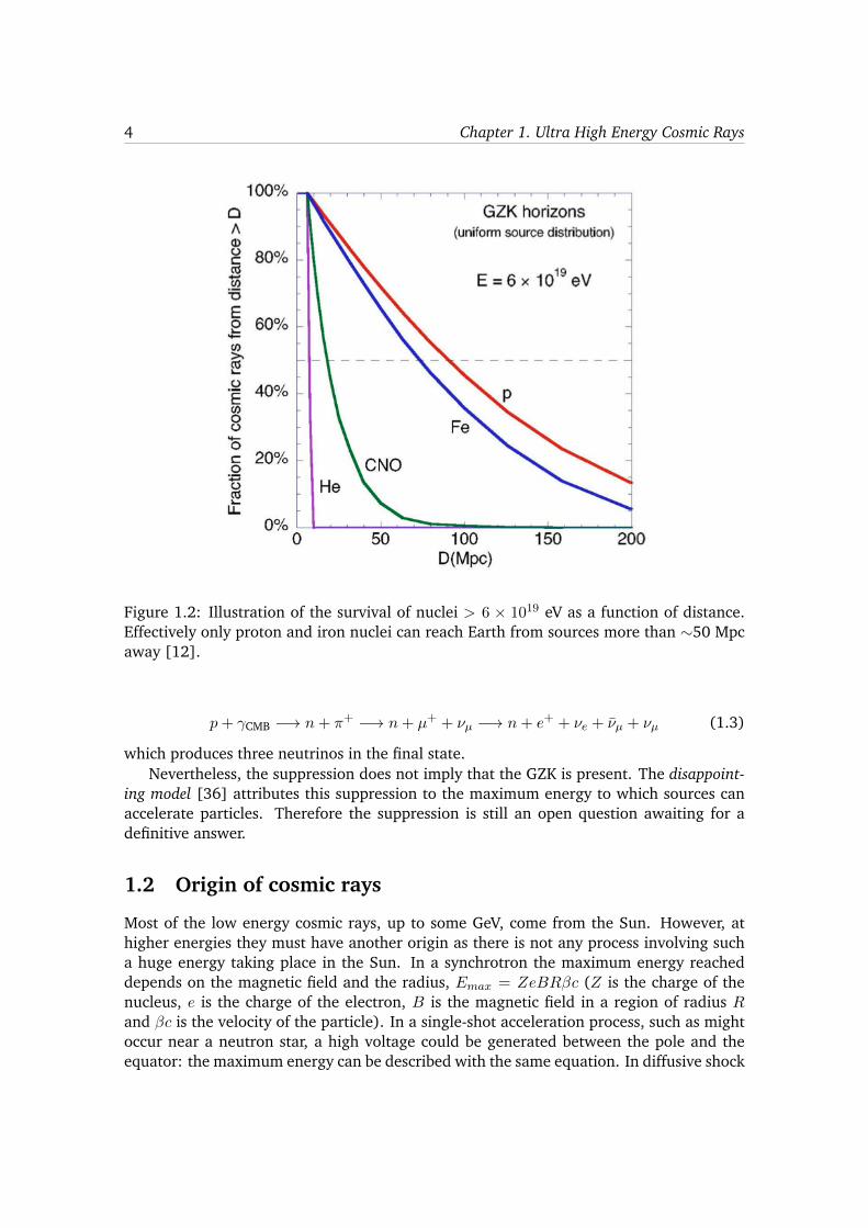
The proton loses about 20% of its energy in this process and it limits the distance fromwhich a high-energy particle have traveled before detection to ⇠100 Mpc (see figure 1.2).The pions resulting from the GZK reaction are producing photons and neutrinos of veryhigh energy:
p+ �CMB �! p+ ⇡
0 �! p+ �� (1.2)
resulting in two cosmogenic photons, and the second one
4 Chapter 1. Ultra High Energy Cosmic Rays
Figure 1.2: Illustration of the survival of nuclei > 6 ⇥ 1019 eV as a function of distance.Effectively only proton and iron nuclei can reach Earth from sources more than ⇠50 Mpcaway [12].
p+ �CMB �! n+ ⇡
+ �! n+ µ
+ + ⌫
µ
�! n+ e
+ + ⌫
e
+ ⌫
µ
+ ⌫
µ
(1.3)
which produces three neutrinos in the final state.Nevertheless, the suppression does not imply that the GZK is present. The disappoint-
ing model [36] attributes this suppression to the maximum energy to which sources canaccelerate particles. Therefore the suppression is still an open question awaiting for adefinitive answer.
1.2 Origin of cosmic rays
Most of the low energy cosmic rays, up to some GeV, come from the Sun. However, athigher energies they must have another origin as there is not any process involving sucha huge energy taking place in the Sun. In a synchrotron the maximum energy reacheddepends on the magnetic field and the radius, E
max
= ZeBR�c (Z is the charge of thenucleus, e is the charge of the electron, B is the magnetic field in a region of radius R
and �c is the velocity of the particle). In a single-shot acceleration process, such as mightoccur near a neutron star, a high voltage could be generated between the pole and theequator: the maximum energy can be described with the same equation. In diffusive shock
1.3. UHE photon and neutrino limits 5
acceleration essentially the same relationship can be applied: here E
max
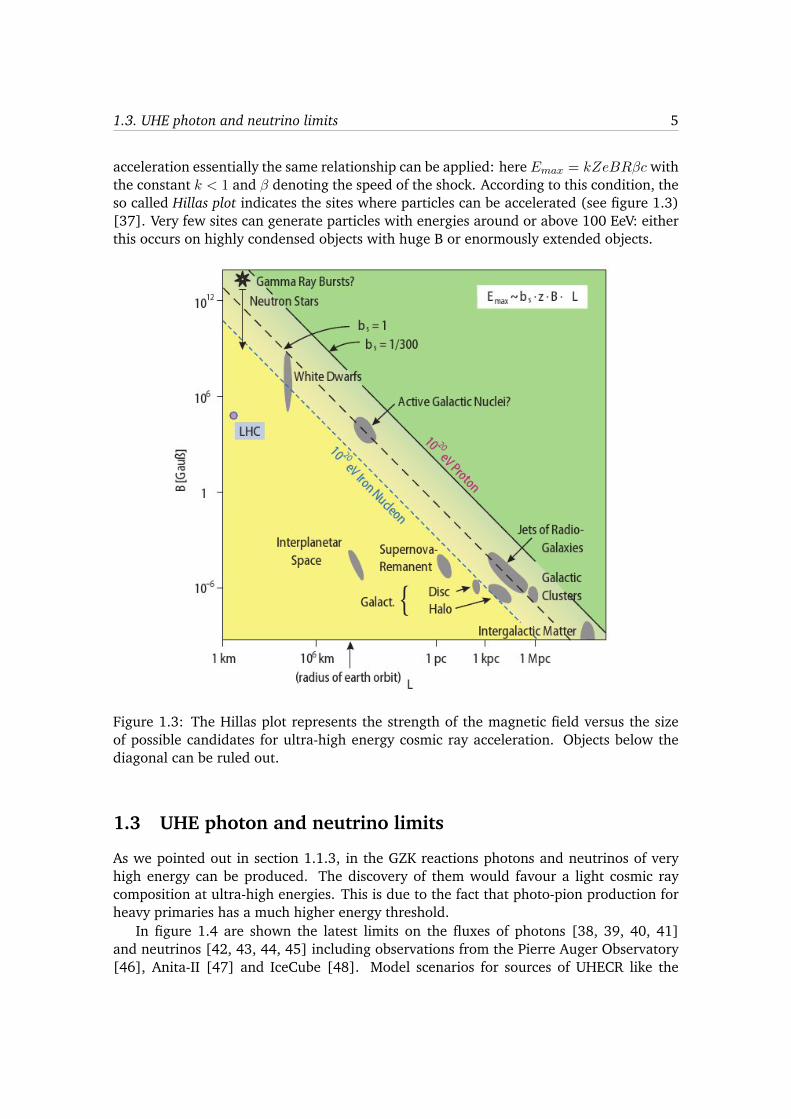
= kZeBR�c withthe constant k < 1 and � denoting the speed of the shock. According to this condition, theso called Hillas plot indicates the sites where particles can be accelerated (see figure 1.3)[37]. Very few sites can generate particles with energies around or above 100 EeV: eitherthis occurs on highly condensed objects with huge B or enormously extended objects.
Figure 1.3: The Hillas plot represents the strength of the magnetic field versus the sizeof possible candidates for ultra-high energy cosmic ray acceleration. Objects below thediagonal can be ruled out.
1.3 UHE photon and neutrino limits
As we pointed out in section 1.1.3, in the GZK reactions photons and neutrinos of veryhigh energy can be produced. The discovery of them would favour a light cosmic raycomposition at ultra-high energies. This is due to the fact that photo-pion production forheavy primaries has a much higher energy threshold.
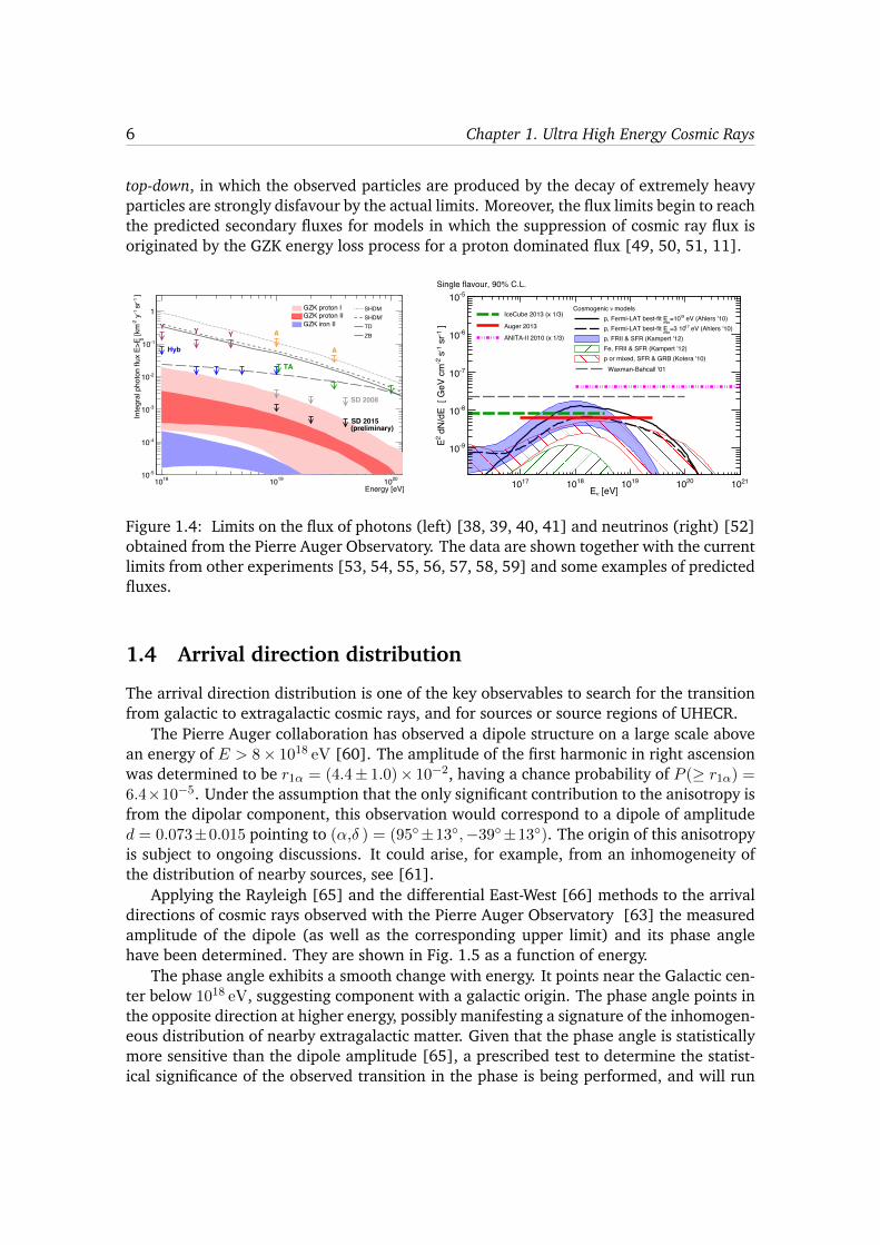
In figure 1.4 are shown the latest limits on the fluxes of photons [38, 39, 40, 41]and neutrinos [42, 43, 44, 45] including observations from the Pierre Auger Observatory[46], Anita-II [47] and IceCube [48]. Model scenarios for sources of UHECR like the
6 Chapter 1. Ultra High Energy Cosmic Rays
top-down, in which the observed particles are produced by the decay of extremely heavyparticles are strongly disfavour by the actual limits. Moreover, the flux limits begin to reachthe predicted secondary fluxes for models in which the suppression of cosmic ray flux isoriginated by the GZK energy loss process for a proton dominated flux [49, 50, 51, 11].
Energy [eV]1810 1910 2010
]-1
sr
-1 y
-2 [k
m0
Inte
gral
pho
ton
flux
E>E
-510
-410
-310
-210
-110
1 SHDMSHDM’TDZB
GZK proton IGZK proton IIGZK iron II
YYY A
AHyb
SD 2008
SD 2015
TA
(preliminary)
[eV]νE1710 1810 1910 2010 2110
]-1
sr
-1 s
-2 d
N/d
E [
GeV
cm
2 E -910
-810
-710
-610
-510Single flavour, 90% C.L.
IceCube 2013 (x 1/3)
Auger 2013
ANITA-II 2010 (x 1/3)
modelsνCosmogenic eV (Ahlers '10)19=10
minp, Fermi-LAT best-fit E
eV (Ahlers '10)17=3 10min
p, Fermi-LAT best-fit Ep, FRII & SFR (Kampert '12)Fe, FRII & SFR (Kampert '12)p or mixed, SFR & GRB (Kotera '10)
Waxman-Bahcall '01
Figure 1.4: Limits on the flux of photons (left) [38, 39, 40, 41] and neutrinos (right) [52]obtained from the Pierre Auger Observatory. The data are shown together with the currentlimits from other experiments [53, 54, 55, 56, 57, 58, 59] and some examples of predictedfluxes.
1.4 Arrival direction distribution
The arrival direction distribution is one of the key observables to search for the transitionfrom galactic to extragalactic cosmic rays, and for sources or source regions of UHECR.
The Pierre Auger collaboration has observed a dipole structure on a large scale abovean energy of E > 8⇥ 1018 eV [60]. The amplitude of the first harmonic in right ascensionwas determined to be r1↵ = (4.4± 1.0)⇥ 10�2, having a chance probability of P (� r1↵) =6.4⇥10�5. Under the assumption that the only significant contribution to the anisotropy isfrom the dipolar component, this observation would correspond to a dipole of amplituded = 0.073±0.015 pointing to (↵,� ) = (95�±13�,�39�±13�). The origin of this anisotropyis subject to ongoing discussions. It could arise, for example, from an inhomogeneity ofthe distribution of nearby sources, see [61].
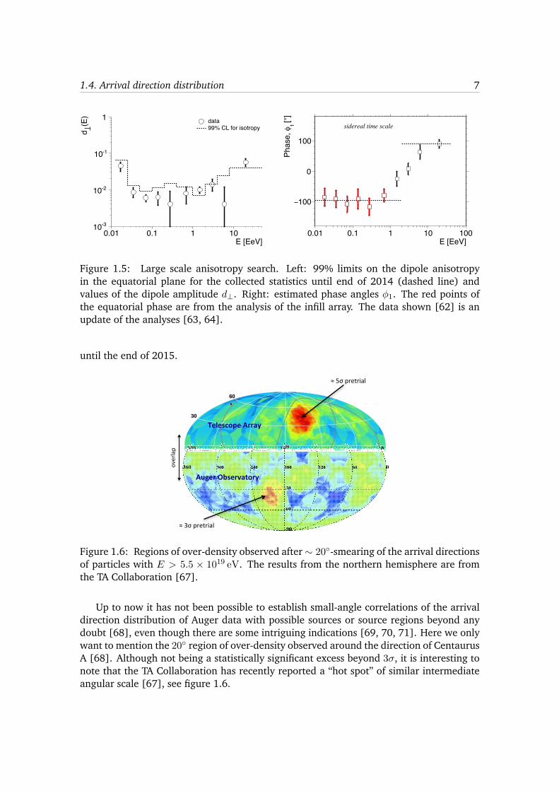
Applying the Rayleigh [65] and the differential East-West [66] methods to the arrivaldirections of cosmic rays observed with the Pierre Auger Observatory [63] the measuredamplitude of the dipole (as well as the corresponding upper limit) and its phase anglehave been determined. They are shown in Fig. 1.5 as a function of energy.
The phase angle exhibits a smooth change with energy. It points near the Galactic cen-ter below 1018 eV, suggesting component with a galactic origin. The phase angle points inthe opposite direction at higher energy, possibly manifesting a signature of the inhomogen-eous distribution of nearby extragalactic matter. Given that the phase angle is statisticallymore sensitive than the dipole amplitude [65], a prescribed test to determine the statist-ical significance of the observed transition in the phase is being performed, and will run
1.4. Arrival direction distribution 7
E [EeV]0.01 0.1 1 10
(E)
d
-310
-210
-110
1 data99% CL for isotropy
E [EeV]0.01 0.1 1 10 100
]° [ 1φPh
ase,
100−
0
100
sidereal time scale
Figure 1.5: Large scale anisotropy search. Left: 99% limits on the dipole anisotropyin the equatorial plane for the collected statistics until end of 2014 (dashed line) andvalues of the dipole amplitude d?. Right: estimated phase angles �1. The red points ofthe equatorial phase are from the analysis of the infill array. The data shown [62] is anupdate of the analyses [63, 64].
until the end of 2015.
Telescope&Array
Auger&Observatory
≈'3σ'pretrial
overlap
≈'5σ'pretrial
Figure 1.6: Regions of over-density observed after ⇠ 20�-smearing of the arrival directionsof particles with E > 5.5 ⇥ 1019 eV. The results from the northern hemisphere are fromthe TA Collaboration [67].
Up to now it has not been possible to establish small-angle correlations of the arrivaldirection distribution of Auger data with possible sources or source regions beyond anydoubt [68], even though there are some intriguing indications [69, 70, 71]. Here we onlywant to mention the 20� region of over-density observed around the direction of CentaurusA [68]. Although not being a statistically significant excess beyond 3�, it is interesting tonote that the TA Collaboration has recently reported a “hot spot” of similar intermediateangular scale [67], see figure 1.6.

8 Chapter 1. Ultra High Energy Cosmic Rays
1.5 Extensive air showers
When a cosmic ray interacts with an atom of the atmosphere a cascade of secondaryparticles is produced (i.e. an EAS is created). The generated number of particles is avast number: about 1010 particles for events having 1019 eV. Extensive air showers canbe described as the superposition of different components (see figure 1.7). The mostimportant ones are the hadronic, muonic and electromagnetic cascades. Photons andelectrons/positrons represent 99% of these particles and they transport 85% of the totalenergy. They initiate what is called the electromagnetic cascade. The remaining particlesare muons, pions and in smaller proportion neutrinos and baryons.
Eo
muonic component |10% Eo
neutrinos |1% Eo
(nuclear fragments)
hadronic component |4% Eo
electromagnetic component |85% Eo
J o e+e-
e- o e- J
So o J J (98.8%) Sr o Pr + QP (99.9%)
Kr o Pr + QP (63.5%)
Kr o Sr + So (21.2%)
Primary Particle
Nuclear interaction with air molecule
Hadronic cascade
Cherenkov & fluorescence
radiation
pair-creation
Figure 1.7: Main components of extensive air showers.
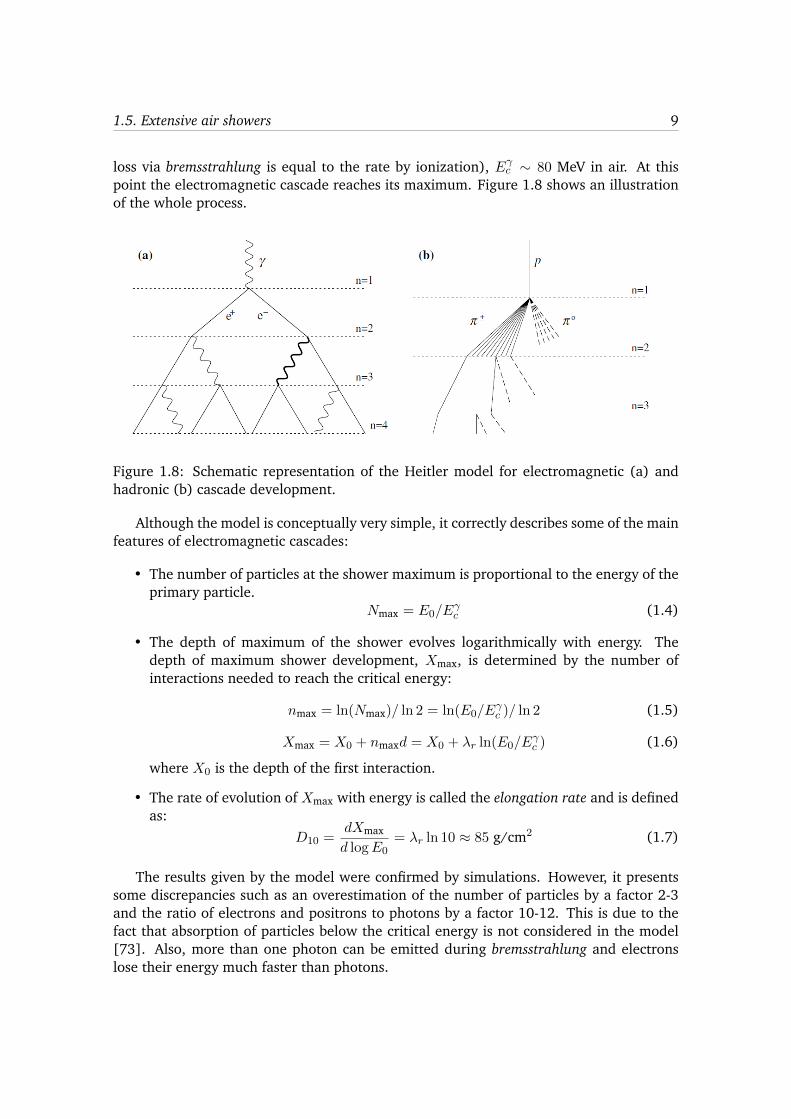
The basic properties of the development of a cascade can be described with a modeldeveloped by Heitler [72]. This model was extended by Matthews [73] to include thedescription of hadronic showers.
1.5.1 Heitler model of electromagnetic showers
In this simplified model at each step all particles interact producing two secondary particlesof equal energy. Electrons, positrons and photons interact after traveling an interactionlength d = �
r
ln 2, where �
r
is the radiation length of the medium (�r
= 37 g/cm2 inair). After each step electrons divide their energies in half via bremsstrahlung emissionof a single photon while photons produce a pair e
+e
� of equal energy. After n steps theparticle number is N
n
= 2n and their individual energy is E0/Nn
. The process ends whenthe individual energy drops below the critical value (energy at which the rate of energy
1.5. Extensive air showers 9
loss via bremsstrahlung is equal to the rate by ionization), E�
c
⇠ 80 MeV in air. At thispoint the electromagnetic cascade reaches its maximum. Figure 1.8 shows an illustrationof the whole process.
Figure 1.8: Schematic representation of the Heitler model for electromagnetic (a) andhadronic (b) cascade development.
Although the model is conceptually very simple, it correctly describes some of the mainfeatures of electromagnetic cascades:
• The number of particles at the shower maximum is proportional to the energy of theprimary particle.
Nmax = E0/E�
c
(1.4)
• The depth of maximum of the shower evolves logarithmically with energy. Thedepth of maximum shower development, Xmax, is determined by the number ofinteractions needed to reach the critical energy:
nmax = ln(Nmax)/ ln 2 = ln(E0/E�
c
)/ ln 2 (1.5)
Xmax = X0 + nmaxd = X0 + �
r
ln(E0/E�
c
) (1.6)
where X0 is the depth of the first interaction.
• The rate of evolution of Xmax with energy is called the elongation rate and is definedas:
D10 =dXmax
d logE0= �
r
ln 10 ⇡ 85 g/cm2 (1.7)
The results given by the model were confirmed by simulations. However, it presentssome discrepancies such as an overestimation of the number of particles by a factor 2-3and the ratio of electrons and positrons to photons by a factor 10-12. This is due to thefact that absorption of particles below the critical energy is not considered in the model[73]. Also, more than one photon can be emitted during bremsstrahlung and electronslose their energy much faster than photons.
10 Chapter 1. Ultra High Energy Cosmic Rays
1.5.2 Extension of the Heitler model to hadronic showers
In analogy with the electromagnetic cascade, the hadronic component can be describedassuming that after each interaction the main products are pions. This was done by Mat-thews [73] and is thoroughly described in [9]. In this extension, the relevant parameter isthe hadronic interaction length �
I
. After each step of thickness �I
ln 2, 2N⇡
charged pionsare produced and N
⇡
neutral ones. The ⇡0 will decay and go into the electromagnetic cas-cade and charged pions interact further producing the hadronic cascade (see figure 1.8b).In this case, the end of the cascade is determined by the energy at which pions start todecay into muons.
The number of muons in the shower is obtained assuming that all pions decay intomuons when they reach the critical energy, E⇡
c
. Thus, Nµ
= (2N⇡
)nc , where n
c
= ln(E0/E⇡
c
)ln(3N
⇡
)
is the number of steps for the pions to reach E
⇡
c
. Introducing � = ln 2N⇡
/ ln 3N⇡
the
number of muons can be written as: Nµ
=⇣
E0E
⇡
c
⌘�
.
The determination of the position of the shower maximum is more complex in thecase of hadronic shower than in the electromagnetic one. The larger cross-section and thelarger multiplicity at each step will reduce the value of the maximum and the energy evol-ution of those quantities will modify the rate of change of Xmax with energy. In additionthe inelasticity of the interaction will also modify both the position of the maximum andthe elongation rate. The energy transfer from the hadronic component to the electromag-netic one at each step and a correct superposition of each electromagnetic sub-shower tocompute Xmax is needed. A good approximation is the assumption made in [73]. There,the effect of the hadronic cascade is consider only in the first interaction. Therefore, forproton showers
D
p
10 = D
�
10 +dX0
d logE0(1.8)
where D
�
10 is the elongation rate for electromagnetic showers and X0 = �
I
ln 2 the depthof the first interaction. Introducing a realistic parameterization of the dependence of�
I
as a function of the energy, such as the one given in [74], the elongation rate isD
p
10 ⇡ 62 g/cm2. Moreover, since hadronic interaction models predict an approximatelylogarithmic decrease of �
I
with energy, Dp
10 is approximately constant.An important consequence of equation (1.8) was noted by Linsley in 1977: the Elong-
ation Rate Theorem [75]. This theorem stipulates that regardless of the particular para-meterization of �
I
that is chosen, (1.8) will always decrease with increasing energy, andthus the second term in the equation is always negative. Therefore, the elongation ratefor electromagnetic showers is always bigger than the one for hadronic shower.
The extension of this description to air showers initiated by different nuclear primariescan be done with the theoretical framework called superposition model. In this model, aprimary nucleus of mass A and energy E is described as the superposition of A nucleonsof energy E
0 = E/A (for more details see e.g. [11]). Showers from heavy nuclei willdevelop higher, faster and with less shower to shower fluctuations than showers initiatedby lighter nuclei. From these simple assumptions some of the most important phenomenathat are correctly described are:

1.6. Mass composition of UHECR 11
• Nuclei initiated showers will be on average less penetrating than those generated byprotons of the same energy
X
A
max (E0) = X
p
max (E0/A) = X
p
max (E0)� �
r
A (1.9)
• The number of muons is larger for heavier primaries than for light primaries of thesame energy
N
A
µ
(E0) =AX
i
N
p
µ
(E0/A) = N
p
µ
(E0)A1�� (1.10)
• The elongation rate is the same regardless of the mass of the primary. It shows upas parallel lines in an Xmax vs energy plot.
D
A
10 =dX
A
maxd logE0
=d (Xp
max � �
r
A)
d logE0=
dX
p
max
d logE0= D
p
10 (1.11)
• The shower to shower fluctuations of Xmax is smaller for heavy nuclei than for lightones.
The superposition model is a simplification and cannot fully describe hadronic EAS, asit does not account for nuclear effects such as re-interaction in the target nucleus or nuc-lear fragmentation. In order to consider all of these processes and others, more realistictransport codes are used, such as CORSIKA [76], AIRES [77] or COSMOS [78], togetherwith hadronic interaction models like EPOS [79], QGSJET-II [80] or SIBYLL [81] (see e.g.[82] for a comprehensive review of air shower simulations).
1.6 Mass composition of UHECR
The composition of cosmic rays of energies below the knee can be measured directly byspace-based experiments. However, at higher energies, the only possibility is to charac-terise the properties of the EAS generated by different primaries. Nevertheless, due tofluctuations of the properties of the first few hadronic interactions in the cascade, theprimary mass can not be measured on an event-by-event basis. It must be inferred stat-istically from the distribution of shower maxima of a set of air showers. The longitudinalprofile of the energy deposit of an air shower as a function of the atmospheric slant depthcan be directly measured with fluorescence telescopes. The depth at which the energydeposit reaches the maximum is called Xmax. The global Xmax distribution results fromthe superposition of the distributions produced by different nuclei of mass A
i
:
f(Xmax
) =X
i
p
i
f
i
(Xmax
) (1.12)
where p
i
represents the fraction of primary particle of type i. Showers generated byprotons have an average value of Xmax about 100 g/cm2 larger than showers produced byiron nuclei of the same energy, so it is possible to do inferences about mass compositionwith this observable. This was achieved for the first time by the Fly’s Eye collaboration
12 Chapter 1. Ultra High Energy Cosmic Rays
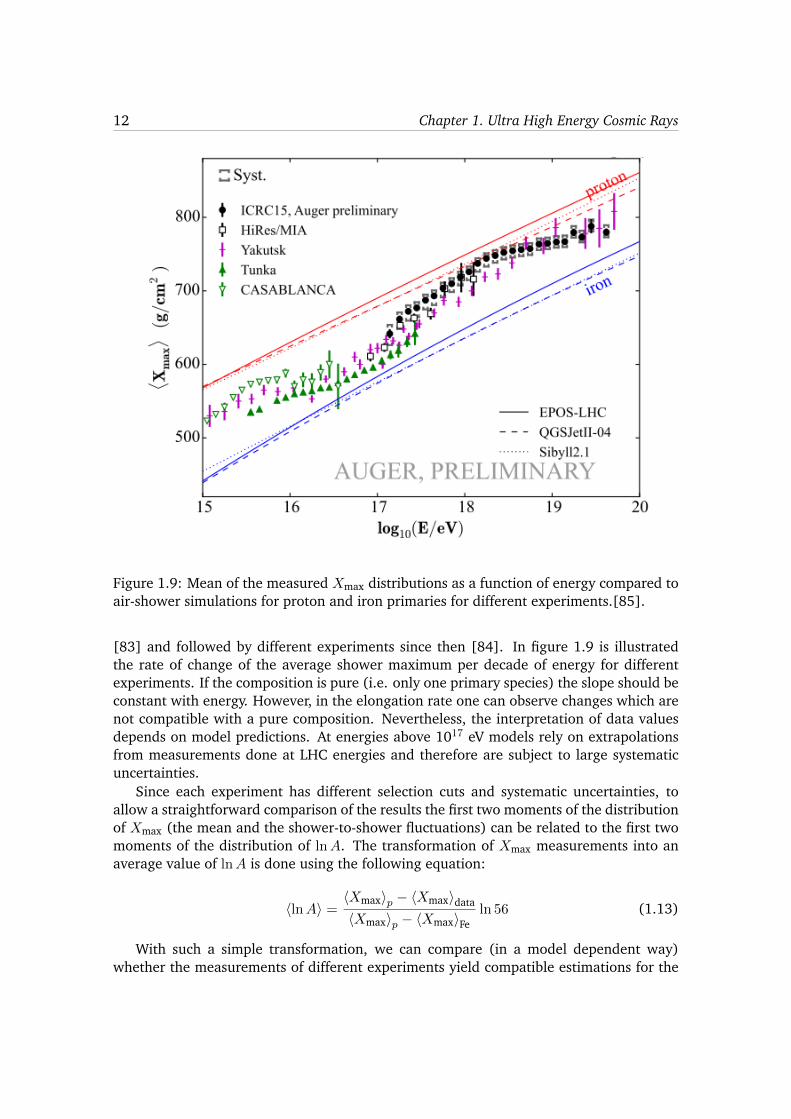
Figure 1.9: Mean of the measured Xmax distributions as a function of energy compared toair-shower simulations for proton and iron primaries for different experiments.[85].
[83] and followed by different experiments since then [84]. In figure 1.9 is illustratedthe rate of change of the average shower maximum per decade of energy for differentexperiments. If the composition is pure (i.e. only one primary species) the slope should beconstant with energy. However, in the elongation rate one can observe changes which arenot compatible with a pure composition. Nevertheless, the interpretation of data valuesdepends on model predictions. At energies above 1017 eV models rely on extrapolationsfrom measurements done at LHC energies and therefore are subject to large systematicuncertainties.
Since each experiment has different selection cuts and systematic uncertainties, toallow a straightforward comparison of the results the first two moments of the distributionof Xmax (the mean and the shower-to-shower fluctuations) can be related to the first twomoments of the distribution of lnA. The transformation of Xmax measurements into anaverage value of lnA is done using the following equation:
hlnAi =hXmaxi
p
� hXmaxidata
hXmaxip
� hXmaxiFeln 56 (1.13)
With such a simple transformation, we can compare (in a model dependent way)whether the measurements of different experiments yield compatible estimations for the

1.6. Mass composition of UHECR 13
mass of UHECR. As a matter of fact the situation concerning mass composition is nowadaysunclear and more precise measurements are required. The main subject of this thesis isan attempt to contribute to the ongoing discussion about composition. In what followswe will focus on making inferences about the masses of UHECR using new observablesextracted from the data collected by the Surface Detector of the Pierre Auger Observatory.


2The Pierre Auger Observatory
The Pierre Auger Observatory has been conceived to measure the main properties (flux,arrival direction and mass composition) of cosmic rays from 1018 eV up to the largestenergies with high statistical significance [86].
Figure 2.1: Map of the Pierre Auger Observatory. Red dots indicate SD detectors and greenlines show the field of view of the FD telescopes.
The Observatory is located at the "pampa amarilla" near Malargüe, in the Provinceof Mendoza (Argentina), at a mean altitude of 1400 m (depth = 879 g/cm2). It wascompleted in 2008 and is taking data since 2004. The site is relatively flat and near thebase of the Andes mountains. It covers a ground area of 3000 km2 and contains 1600water-Cherenkov detectors, the Surface Detector (SD), arranged on a triangular grid, witha 1.5 km separation among detectors, overlooked from 4 sites by optical stations (figure2.1), the Fluorescence Detector (FD). These stations contain 6 telescopes each, designed todetect air-fluorescence light emitted by atmospheric nitrogen when it is excited by chargedparticles. The WCD detect particles at the ground (mainly muons, electrons, positrons and
16 Chapter 2. The Pierre Auger Observatory
photons) via the Cherenkov light emitted while they cross the ultra-pure water inside thedetectors. The precise calorimetric information provided by the FD allows a calibration ofthe SD array in a data-driven way, thus avoiding the systematics associated with the useof simulated EAS.
Several enhancements have been built recently at the Observatory. First of all, to studythe energy spectrum down to energies of 0.1 EeV, a small portion of the SD array (' 24km2, known as the Infilled array) has been equipped with 61 WCD laid out in a densergrid of 750 m spacing. The Infilled array is overlooked from one observation site by threehigh-elevation telescopes (HEAT) [87] whose field of view cover elevations from 30� to60�, allowing the study of lower energy showers. With the aim of measuring with betterprecision the muon content of the recorded air showers, the AMIGA project is deployingscintillation muon counters (each with an area of 30 m2 and buried 2.3 m underground)near the WCD of the Infilled array [88]. Other programs are focused on the detection ofthe radio emission that takes place while the shower of particles evolves in the atmosphere.The Auger Engineering Radio Array (AERA) operates in the 30 to 80 MHz frequency rangeto detect the radio emission. It consists of 153 self-triggered antennas covering approx-imately 17 km2. We are also exploring the possibility of detecting microwave emission(GHz range) with an array of 61 antennas (EASIER) covering 100 km2, and with imagingparabolic dish detectors AMBER and MIDAS [86].
2.1 Surface Detector
To guarantee a high rate of events at the highest energies a large area is required. TheSurface Detector of the Pierre Auger Observatory covers an area of more than 3000 km2.The spacing between WCD, 1.5 km, is the result of a compromise between cost considera-tions and the energy threshold. The surface is covered by WCD because of their low costand robustness. Moreover, it is a well known detector for air-showers: the same principlewas used succesfully in other experiments like Haverah Park [89].
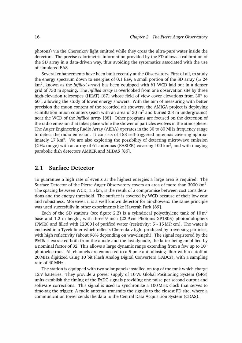
Each of the SD stations (see figure 2.2) is a cylindrical polyethylene tank of 10 m2
base and 1.2 m height, with three 9 inch (22.9 cm Photonis XP1805) photomultipliers(PMTs) and filled with 12000 l of purified water (resistivity: 5 - 15 M⌦ cm). The water isenclosed in a Tyvek liner which reflects Cherenkov light produced by traversing particles,with high reflectivity (about 98% depending on wavelength). The signal registered by thePMTs is extracted both from the anode and the last dynode, the latter being amplified bya nominal factor of 32. This allows a large dynamic range extending from a few up to 105
photoelectrons. All channels are connected to a 5 pole anti-aliasing filter with a cutoff at20 MHz digitized using 10 bit Flash Analog Digital Converters (FADCs), with a samplingrate of 40 MHz.
The station is equipped with two solar panels installed on top of the tank which charge12 V batteries. They provide a power supply of 10 W. Global Positioning System (GPS)units establish the timing of the FADC signals providing one pulse per second output andsoftware corrections. This signal is used to synchronize a 100 MHz clock that serves totime-tag the trigger. A radio antenna transmits the signals to the closest FD site, where acommunication tower sends the data to the Central Data Acquisition System (CDAS).
2.1. Surface Detector 17
(a) Photo of an SD station deployed in the field. (b) Schematic view of the station components.
Figure 2.2: View and scheme of an SD station of the Pierre Auger Observatory.
2.1.1 Calibration
The SD obtains a measurement of the Cherenkov light produced by shower particlespassing through the detector. The unit used to measure the Cherenkov light is the signalproduced by a vertical and central through-going muon (VCT), named vertical equivalentmuon (VEM). The goal of the calibration procedure is to measure the value of 1 VEM inFADC units.
Atmospheric muons passing through the WCD give an excellent method to estimatethe value of a VEM since they produce a peak in a charge histogram. In addition, theatmospheric muons calibration assures the uniformity of the signal size over the entirearray. The calibration of each detector is performed locally and automatically so eachdetector is independent of the others. The most important quantities to calibrate an SDstation are the average charge, QVEM, and the amplitude of the signal, Ipeak
VEM , produced ina PMT by a VEM [90].
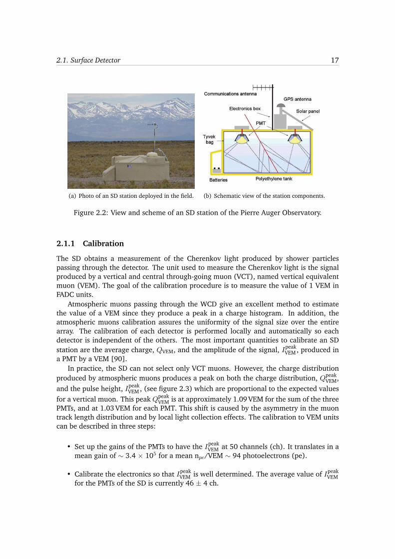
In practice, the SD can not select only VCT muons. However, the charge distributionproduced by atmospheric muons produces a peak on both the charge distribution, Qpeak
VEM,and the pulse height, Ipeak
VEM , (see figure 2.3) which are proportional to the expected valuesfor a vertical muon. This peak Q
peakVEM is at approximately 1.09 VEM for the sum of the three
PMTs, and at 1.03 VEM for each PMT. This shift is caused by the asymmetry in the muontrack length distribution and by local light collection effects. The calibration to VEM unitscan be described in three steps:
• Set up the gains of the PMTs to have the I
peakVEM at 50 channels (ch). It translates in a
mean gain of ⇠ 3.4 ⇥ 105 for a mean npe
/VEM ⇠ 94 photoelectrons (pe).
• Calibrate the electronics so that IpeakVEM is well determined. The average value of Ipeak
VEMfor the PMTs of the SD is currently 46 ± 4 ch.
18 Chapter 2. The Pierre Auger Observatory
(a) VEM Charge. (b) VEM Peak.
Figure 2.3: Charge and pulse height histograms for an SD station with a 3-fold trigger(signal in all 3 PMTs). The signal is the sum of the three PMTs. In the solid histogramthe second peak is produced by vertical through-going atmospheric muons, while the firstpeak is a trigger effect. The dashed histogram is produced by vertical and central muons(VEMs) selected with an external muon telescope.
• Determine the value of QpeakVEM from the charge distribution, and use it to establish the
conversion to VEM units.
The calibration must also be able to convert the raw FADC traces into integrated chan-nels. For this, the baseline of all six FADC inputs are needed, and the gain ratio betweenthe dynode and anode (D/A). Averaging large pulses and performing a linear time-shiftedfit we obtain both D/A and the phase delay between the dynode and anode. This methoddetermines the D/A with a 2% resolution.
The calibration parameters, QpeakVEM and I
peakVEM , are determined every 60 seconds and
sent to the CDAS together with every triggering event.
2.1.2 Trigger
The SD trigger is configured to detect the cosmic rays in a wide range of primary energies,for vertical and very inclined showers with an efficiency larger than 95% for cosmic raysabove 1018.5 eV. The wireless communication system represents the main constraint to therate of recordable events. To satisfy both physical and technical requirements the triggersystem has been designed in a hierarchical form [91].
Station triggers
Two trigger levels, T1 and T2 are performed locally. At T1 level, different trigger modesare implemented to detect, in a complementary way, the electromagnetic and muonic
2.1. Surface Detector 19
components of an EAS. The threshold trigger, Thr1, requires a coincidence between the3 PMTs each above 1.75 VEM. This trigger is used to select large signals that are notnecessarily spread in time corresponding to the muonic component. It also reduces therate due to atmospheric muons from ⇠ 3 kHz to ⇠ 100 Hz. The Time over Threshold (ToT)trigger asks for a coincidence of at least two PMTs with more than 12 FADC bins above0.2 VEM above the baseline within a window of 120 time bins. It is optimised for selectingsmall but spread signals, typical from high energy distant EAS or from low energy showersdominated by the electromagnetic component. Two additional triggers were implementedand operated since June 2013 in the local station software to increase the sensitivity ofthe SD to low energy air-showers and enlarge the distance on the ground up to which wecan still observe the particles that are reaching the ground. These triggers are the Timeover Threshold deconvoluted, ToTd, and the Multiplicity of positive steps MoPS bothdesigned to increase the sensitivity of the SD to signals dominated by the electromagneticcomponents [92, 93, 94].
The second level, T2, is coded in the station software to reduce to about 20 Hz the rateof signals per detector. All TOT-T1 triggers are promoted to the T2 level. However, theThr1 should pass a higher threshold of 3.2 I
peakVEM in coincidence in the 3 PMTs. Only T2
triggers are used for the definition of a first level event trigger, T3.
Event trigger
The lowest event trigger (T3) looks for spatial and temporal coincidences in the T2 signals,and tries to associate them to an air shower. All data satisfying the T3 trigger are stored.Two kind of patterns are taken into account, 3-fold and 4-fold:
• 3-fold: One of the detectors must have one of its closest neighbours and one of itssecond closest neighbour triggered. The allowed time window considers the distanceamong stations in the following way: two stations have to be in the first two crownsaround the first one considered. If this criteria is passed, the pattern is tagged as T3-3ToT. This trigger is extremely relevant since 90% of the selected events are showersand is mostly efficient for vertical showers.
• 4-fold: Four stations with T2 (Thr2 or ToT) have to be in coincidence with a moder-ate compactness requirement. In this case, the fourth station is being accepted if it iswithin four crowns around the reference station. This condition is only relevant forshowers of large zenith angle with wide-spread topological patterns. The efficiencyof this trigger is only 2%.
Physics trigger
The T3 trigger does not necessarily guarantee a relevant air shower. Thus, the physicstrigger, T4 is necessary to select real showers from the stored T3 data. Two criteria aredefined:
• 3ToT (see figure 2.4(b)): it requires at least 3 stations with a ToT trigger and it isa stricter version of T3-3ToT in a non-aligned compact configuration. About 99% ofthe vertical events are selected with this trigger condition [95, 96].

20 Chapter 2. The Pierre Auger Observatory
• 4C1 (see figure 2.4(a)): events with four stations with any T2 trigger and a config-uration of one station with 3 close neighbours. This condition is only important fornearly-horizontal air showers that do not fulfill the 3ToT condition.
Compatibility in time between stations forming the trigger is required in every T4event. The difference in their start time has to be smaller than the distance between themdivided by the speed of light in vacuum, allowing for a marginal limit of 200 ns.
(a) Examples of T4-4C1 configurations.
(b) Examples of T4-3ToT configurations. (c) 6T5 and 5T5 quality configurations.
Figure 2.4: T4 and T5 configurations. 2.4(a): The three minimal compact configurationsfor the T4-4C1 trigger. 2.4(b): The two minimal compact configurations for the T4-3ToTconfiguration. 2.4(c): Example of the 6T5 hexagon (shadow) and the 5T5 hexagon (darkshadow).
Quality trigger
The quality trigger T5 is the highest level of trigger in the Pierre Auger Observatory. Itmainly excludes events falling close to the border or in any hole of the array, where dueto a possible missing signal, the reconstruction of the air shower variables has a worseresolution. To fulfill this trigger the highest signal station should be sorrounded at thetime of triggering by six working stations (not necessarily triggered). This is the so-called6T5 trigger. A less restrictive criteria requires only five stations working in the first crown,5T5. Due to the large number of stations, around 1% of the detectors may not work atany moment, even with constant maintenance.

2.2. Fluorescence Detector 21
2.2 Fluorescence Detector
(a) Aerial photo of the FD site at Los Leones.
(b) Schematic top view of an FD site. (c) Schematic lateral view of an FD telescope.
Figure 2.5: View and schemes of an FD site of the Pierre Auger Observatory.
Charged particles generated from a cosmic ray shower traversing the atmosphere ex-cite atmospheric nitrogen molecules. These molecules emit fluorescence light with discretewavelengths between 300 and 430 nm. The FD measures the longitudinal developmentprofile dE/dX(X) of the air shower as a function of the atmospheric slant depth. It alsogives a calorimetric measurement of the energy of the primary cosmic ray.
There are 24 Schmidt telescopes located on four observation sites: Los Leones, LosMorados, Loma Amarilla and Coihueco, all of them situated on hills between 40 and150 metres high surrounding the SD array. Each telescope has a field of view of 30�⇥ 30�.The optical system consists of a 1.7 m diameter diaphragm. The collected light is reflectedby a 12 m2 spherical mirror with a radius of curvature of 3.4 m and then focused onto acamera comprised of 440 hexagonal PMTs in a 22 ⇥ 20 matrix (see figure 2.5). Each PMT
22 Chapter 2. The Pierre Auger Observatory
has a diameter of 45 mm and a quantum efficiency of about 25%. The light collected bythe PMTs is converted into an electrical signal, and finally digitised by analogue-to-digitalconverters (ADCs) [97].
2.2.1 Trigger
The fluorescence detector trigger consists of four levels:
• First level trigger (FLT): The functions of the FLT are implemented in 4 FPGA(Field Programmable Gate Array), each controlling 6 channels, whose main task isto generate the pixel trigger using a threshold cut on the integrated ADC signal. Thethreshold is dynamically adjusted to mantain a pixel trigger rate of 100 MHz. TheFADC values are integrated over 10 bins improving the signal to noise ratio by afactor of
p10.
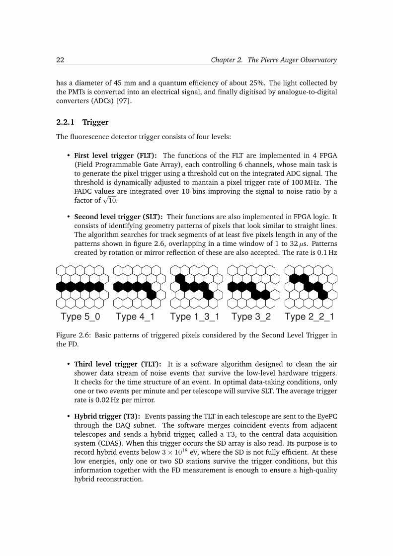
• Second level trigger (SLT): Their functions are also implemented in FPGA logic. Itconsists of identifying geometry patterns of pixels that look similar to straight lines.The algorithm searches for track segments of at least five pixels length in any of thepatterns shown in figure 2.6, overlapping in a time window of 1 to 32µs. Patternscreated by rotation or mirror reflection of these are also accepted. The rate is 0.1 Hz
Type 5_0 Type 4_1 Type 1_3_1 Type 3_2 Type 2_2_1
Figure 2.6: Basic patterns of triggered pixels considered by the Second Level Trigger inthe FD.
• Third level trigger (TLT): It is a software algorithm designed to clean the airshower data stream of noise events that survive the low-level hardware triggers.It checks for the time structure of an event. In optimal data-taking conditions, onlyone or two events per minute and per telescope will survive SLT. The average triggerrate is 0.02 Hz per mirror.
• Hybrid trigger (T3): Events passing the TLT in each telescope are sent to the EyePCthrough the DAQ subnet. The software merges coincident events from adjacenttelescopes and sends a hybrid trigger, called a T3, to the central data acquisitionsystem (CDAS). When this trigger occurs the SD array is also read. Its purpose is torecord hybrid events below 3⇥ 1018 eV, where the SD is not fully efficient. At theselow energies, only one or two SD stations survive the trigger conditions, but thisinformation together with the FD measurement is enough to ensure a high-qualityhybrid reconstruction.
2.2. Fluorescence Detector 23
2.2.2 Calibration
The reconstruction of an air shower longitudinal profile depends on the ability to convertADC counts into light flux at the telescope aperture for each channel that receives a portionof the signal from a shower. A calibration procedure is necessary to evaluate the responseof each pixel to a given flux of incident photons.
The calibration of the FD is performed following two complementary strategies: anabsolute calibration called “drum calibration” and a step by step sequence of dedicatedcalibration runs which are performed at the beginning of every data-taking night. Thedrum calibration consists in beaming a 2.5 diameter calibrated light source onto eachtelescope. It provides an uniform response for each pixel of 5 photons per ADC. This sortof calibration is performed only once every two or three years.
2.2.3 Fluorescence yield
As we have described previously, the photons measured by the FD are emitted isotropic-ally and in the wavelength range between 300 and 430 nm. The fluorescence yield is akey ingredient for the FD reconstruction because it is the proportionality factor betweenthe number of photons emitted and the energy deposited in the atmosphere. The para-meters that characterize the fluorescence yield include an absolute normalization of thewavelength spectrum, the relative intensities in different spectral bands, an their depend-encies on pressure, temperature and humidity. The measurement of the absolute yieldtaken in the reconstruction is the one made by the Airfly collaboration. Nowadays themost accurate measurement in the 337 nm band, which has an uncertainty of 4% [98].
2.2.4 Atmospheric monitoring
In addition to the absolute calibration of the telescope, a detailed analysis of the atmo-sphere above the SD array is a key to obtain the absolute number of photons emitted atthe shower axis.
The rate of development of an air shower depends strongly on the atmospheric densityand temperature as a function of altitude, and both evolve significantly over time, both ona short, daily and on a large, yearly scale. Moreover, there are additional effects affectingthe production of light by secondary particles. The most relevant are Mie and Rayleighscattering, both depending on the amount of aerosols in the air, and also light absorption.
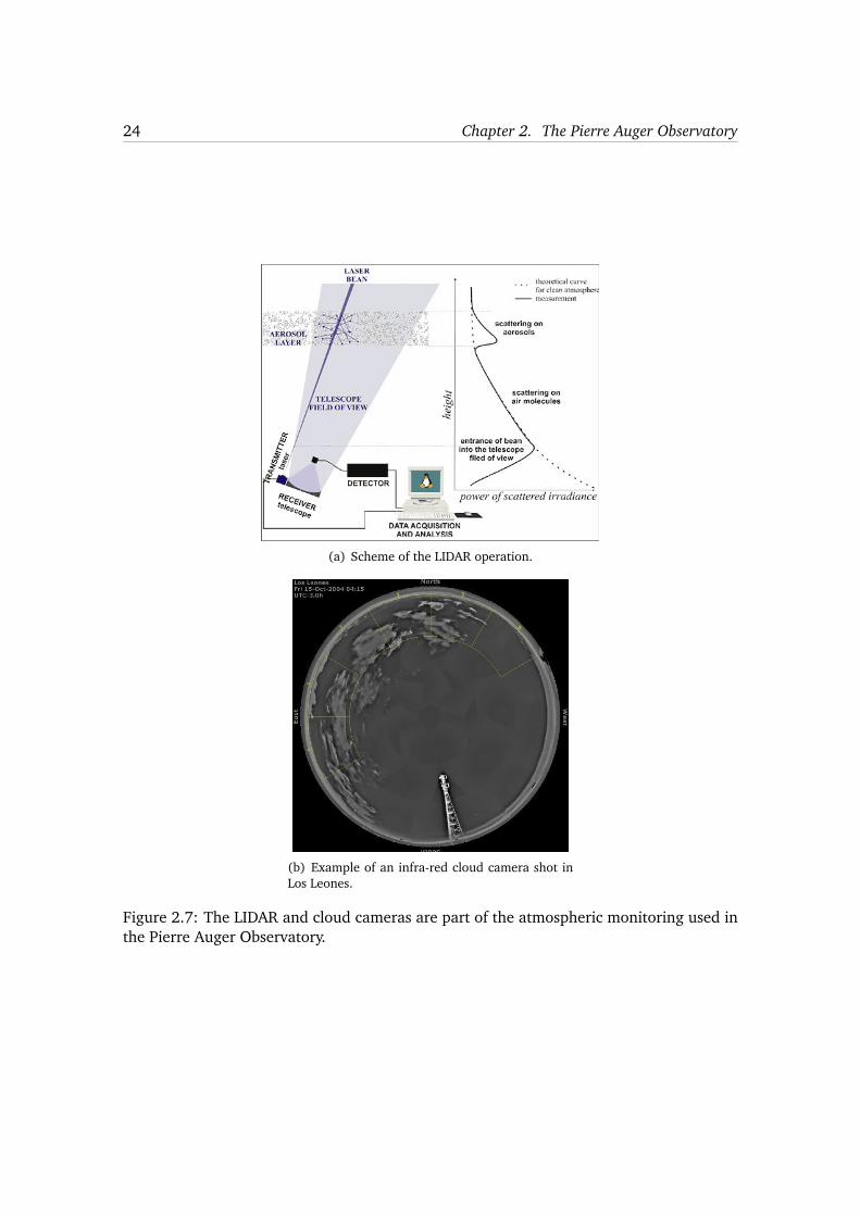
The atmospheric monitoring in the Pierre Auger Observatory [99] is performed by fourlight detection and ranging (LIDAR) stations adjacent to each FD building, and also by thecentral laser facility (CLF), located near the centre of the SD array. In the four LIDARs, abeam of ultra-violet (UV) laser light is directed into the atmosphere at periodic intervals(see figure 2.7(a)). Each LIDAR has a PMT that detects the backscattered light from theUV laser pulses. The intensity and direction of the returning light collected by the LIDARmirrors is used to measure the optical transmission conditions near the FD telescopes[100]. This allows the estimate of the aerosol content of the atmosphere. Infra-red cloudcameras and meteorological weather stations are also used to measure cloud coverage,humidity and other parameters in the vicinity of each FD site (see picture 2.7(b)).
24 Chapter 2. The Pierre Auger Observatory
(a) Scheme of the LIDAR operation.
(b) Example of an infra-red cloud camera shot inLos Leones.
Figure 2.7: The LIDAR and cloud cameras are part of the atmospheric monitoring used inthe Pierre Auger Observatory.
2.2. Fluorescence Detector 25
Similarly, the CLF shoots a laser light into the atmosphere following a predeterminedsequence of directions and zenith elevations every hour. The reconstructed energy anddirection is compared to the true values, with a typical discrepancy of about 15%, dueto the atmospheric effects previously mentioned. The CLF laser shots are used as well tocalibrate the GPS timing of both the FD and the SD.
2.2.5 FD reconstruction
In the FD reconstruction, the first step consists in the reconstruction of the geometry ofthe event:
Geometry reconstruction
A hybrid detector achieves the best geometrical accuracy using timing informations ofboth components, FD pixels and SD stations. In addition, the hybrid capability extendsthe sensitivity of the detector at energies below 3 EeV, an energy range not accesible forthe SD alone. Each element records a pulse of light from which can be determined notonly the amount of light, but also the arrival time of the signal and its uncertainty. Thistemporal information is utilised to reconstruct the shower axis through a �
2 minimisationprocedure [97].
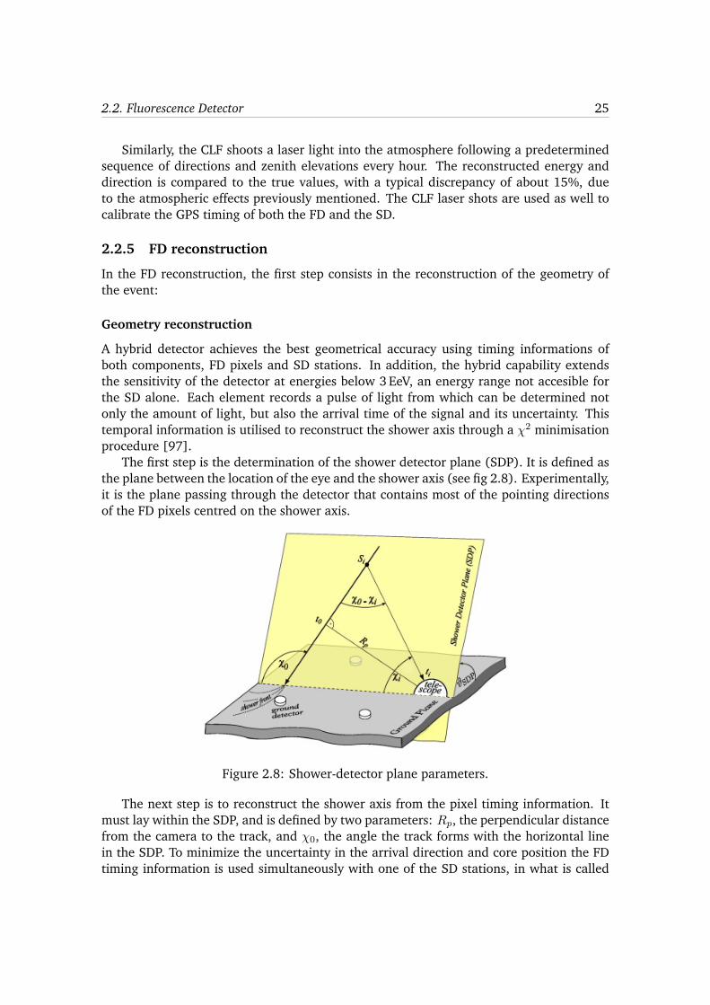
The first step is the determination of the shower detector plane (SDP). It is defined asthe plane between the location of the eye and the shower axis (see fig 2.8). Experimentally,it is the plane passing through the detector that contains most of the pointing directionsof the FD pixels centred on the shower axis.
Figure 2.8: Shower-detector plane parameters.
The next step is to reconstruct the shower axis from the pixel timing information. Itmust lay within the SDP, and is defined by two parameters: R
p
, the perpendicular distancefrom the camera to the track, and �0, the angle the track forms with the horizontal linein the SDP. To minimize the uncertainty in the arrival direction and core position the FDtiming information is used simultaneously with one of the SD stations, in what is called
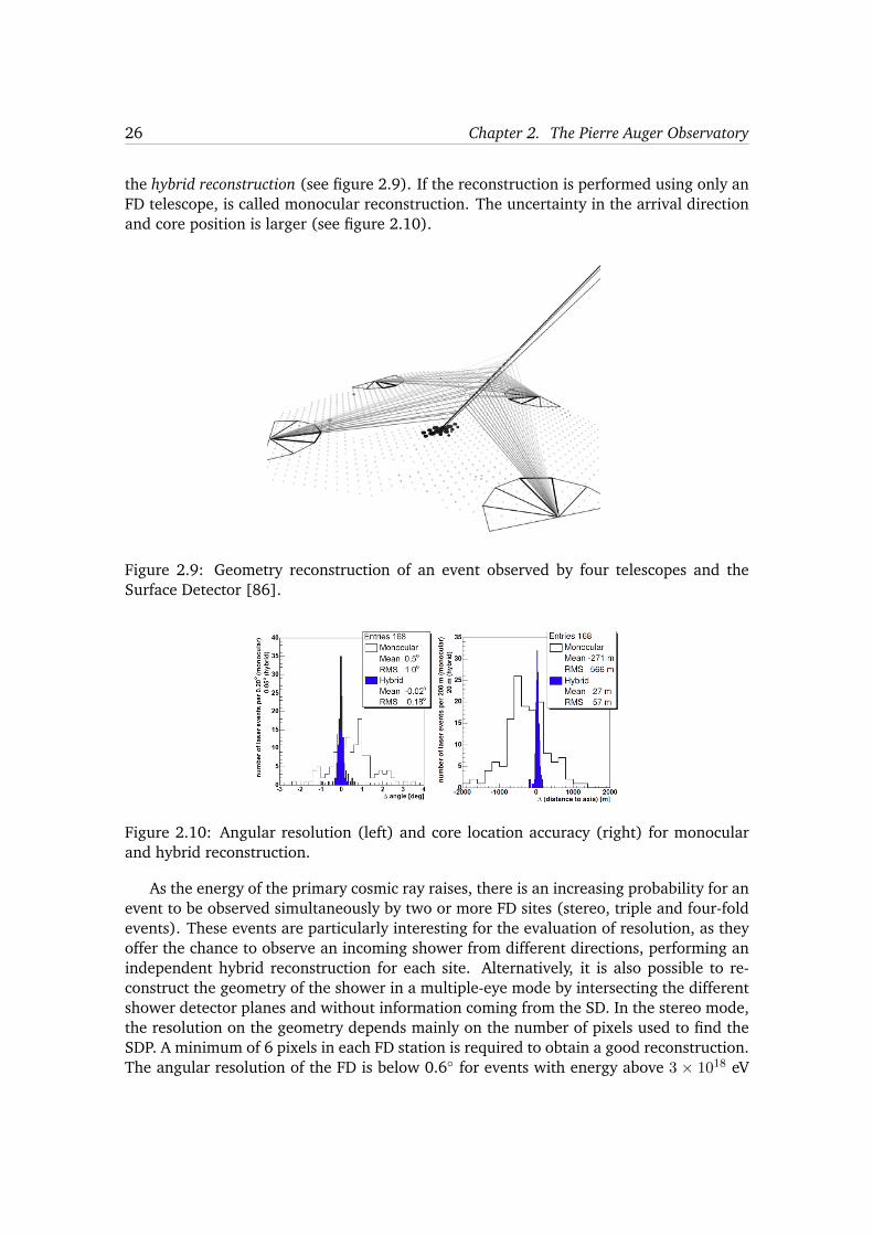
26 Chapter 2. The Pierre Auger Observatory
the hybrid reconstruction (see figure 2.9). If the reconstruction is performed using only anFD telescope, is called monocular reconstruction. The uncertainty in the arrival directionand core position is larger (see figure 2.10).
Figure 2.9: Geometry reconstruction of an event observed by four telescopes and theSurface Detector [86].
Figure 2.10: Angular resolution (left) and core location accuracy (right) for monocularand hybrid reconstruction.
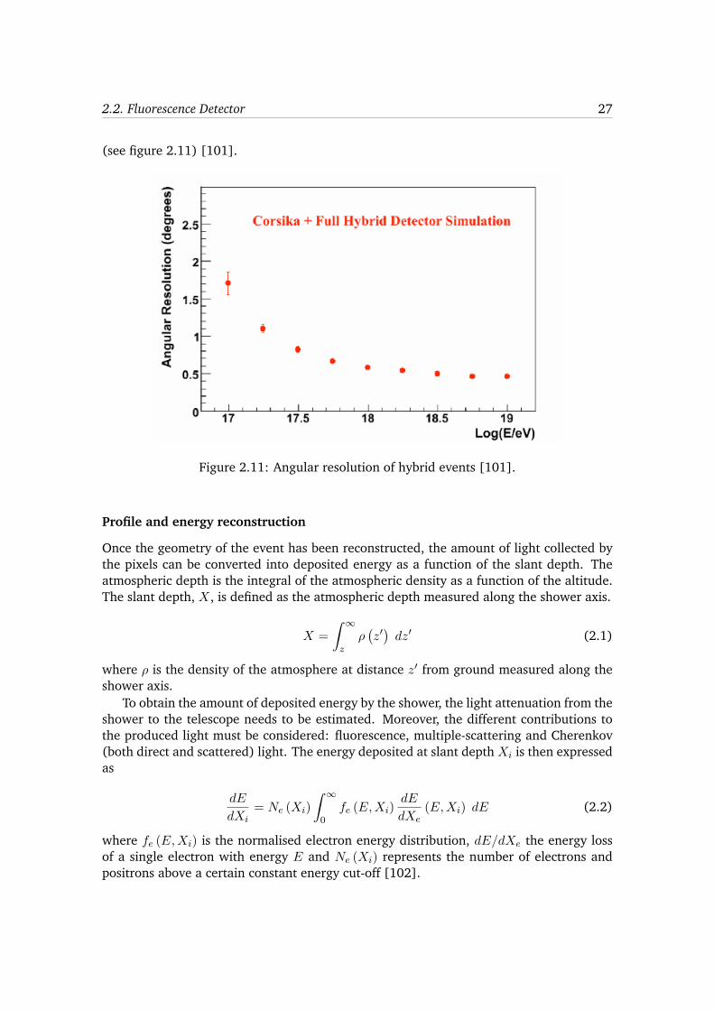
As the energy of the primary cosmic ray raises, there is an increasing probability for anevent to be observed simultaneously by two or more FD sites (stereo, triple and four-foldevents). These events are particularly interesting for the evaluation of resolution, as theyoffer the chance to observe an incoming shower from different directions, performing anindependent hybrid reconstruction for each site. Alternatively, it is also possible to re-construct the geometry of the shower in a multiple-eye mode by intersecting the differentshower detector planes and without information coming from the SD. In the stereo mode,the resolution on the geometry depends mainly on the number of pixels used to find theSDP. A minimum of 6 pixels in each FD station is required to obtain a good reconstruction.The angular resolution of the FD is below 0.6� for events with energy above 3 ⇥ 1018 eV
2.2. Fluorescence Detector 27
(see figure 2.11) [101].
Figure 2.11: Angular resolution of hybrid events [101].
Profile and energy reconstruction
Once the geometry of the event has been reconstructed, the amount of light collected bythe pixels can be converted into deposited energy as a function of the slant depth. Theatmospheric depth is the integral of the atmospheric density as a function of the altitude.The slant depth, X, is defined as the atmospheric depth measured along the shower axis.
X =
Z 1
z
⇢
�z
0�dz
0 (2.1)
where ⇢ is the density of the atmosphere at distance z
0 from ground measured along theshower axis.
To obtain the amount of deposited energy by the shower, the light attenuation from theshower to the telescope needs to be estimated. Moreover, the different contributions tothe produced light must be considered: fluorescence, multiple-scattering and Cherenkov(both direct and scattered) light. The energy deposited at slant depth X
i
is then expressedas
dE
dX
i
= N
e
(Xi
)
Z 1
0f
e
(E,X
i
)dE
dX
e
(E,X
i
) dE (2.2)
where f
e
(E,X
i
) is the normalised electron energy distribution, dE/dX
e
the energy lossof a single electron with energy E and N
e
(Xi
) represents the number of electrons andpositrons above a certain constant energy cut-off [102].
28 Chapter 2. The Pierre Auger Observatory
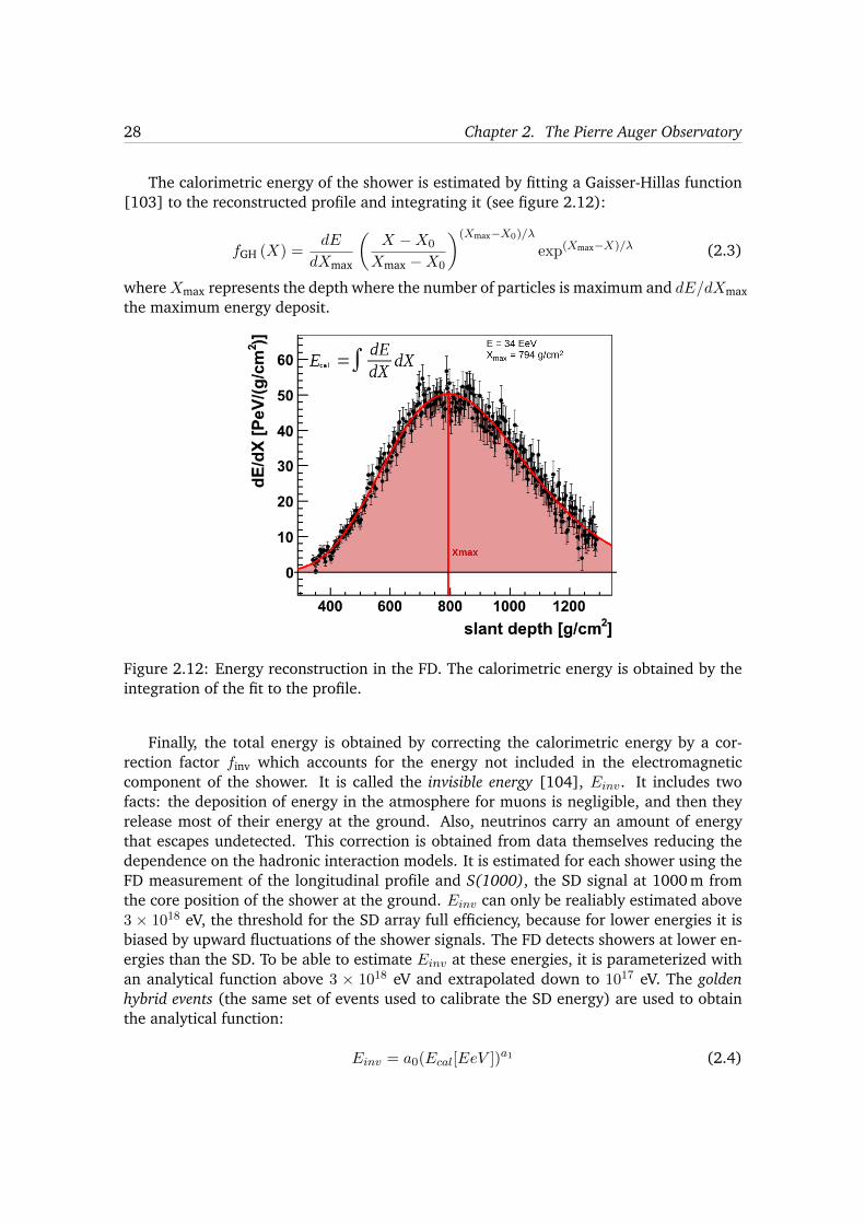
The calorimetric energy of the shower is estimated by fitting a Gaisser-Hillas function[103] to the reconstructed profile and integrating it (see figure 2.12):
fGH (X) =dE
dXmax
✓X �X0
Xmax �X0
◆(Xmax�X0)/�
exp(Xmax�X)/� (2.3)
where Xmax represents the depth where the number of particles is maximum and dE/dXmaxthe maximum energy deposit.
Figure 2.12: Energy reconstruction in the FD. The calorimetric energy is obtained by theintegration of the fit to the profile.
Finally, the total energy is obtained by correcting the calorimetric energy by a cor-rection factor finv which accounts for the energy not included in the electromagneticcomponent of the shower. It is called the invisible energy [104], E
inv
. It includes twofacts: the deposition of energy in the atmosphere for muons is negligible, and then theyrelease most of their energy at the ground. Also, neutrinos carry an amount of energythat escapes undetected. This correction is obtained from data themselves reducing thedependence on the hadronic interaction models. It is estimated for each shower using theFD measurement of the longitudinal profile and S(1000), the SD signal at 1000 m fromthe core position of the shower at the ground. E
inv
can only be realiably estimated above3 ⇥ 1018 eV, the threshold for the SD array full efficiency, because for lower energies it isbiased by upward fluctuations of the shower signals. The FD detects showers at lower en-ergies than the SD. To be able to estimate E
inv
at these energies, it is parameterized withan analytical function above 3 ⇥ 1018 eV and extrapolated down to 1017 eV. The goldenhybrid events (the same set of events used to calibrate the SD energy) are used to obtainthe analytical function:
E
inv
= a0(Ecal
[EeV ])a1 (2.4)
2.2. Fluorescence Detector 29
where a0 = (0.174± 0.001)⇥ 1018 eV and a1 = (0.914± 0.008) [105].The resolution in the measurement of the energy achieved by the FD depends on the
uncertainties associated to variations in the atmosphere, ranging from 4.5% at 3⇥ 1018 eVto 6.9% at 1020 eV, the invisible energy (1.5%) and the geometry reconstruction, whichranges from 5.2% to 3.3% for the same energy interval. The resulting overall energyresolution is almost constant with energy in the range [3, 100] EeV, and lies between 7%and 8% [106].

3SD event reconstruction
The measurement of the energy and the arrival direction of the cosmic rays producing airshowers that have triggered the Surface Detector array is based on the sizes and times ofsignals registered from individual SD stations. By sampling both the arrival times and thedeposited signal in the detector array, the geometry, the arrival direction and the showersize of the incident cosmic ray can be determined.
The reconstruction technique used depends upon the zenith angle (✓) of the direc-tion of the incident cosmic ray which defines the amount of atmosphere traversed by theshower, and therefore the level of attenuation of the shower components. We distinguishbetween vertical, showers with ✓ < 60�, and inclined reconstruction, with 60� < ✓ < 80�.
To build the relevant physics quantities we use a dedicated software called O↵ line1[107].It is a framework divided in modules that contains all the tools required to simulate andreconstruct the events. In the following sections we will describe the main details of theSD reconstruction performed in O↵ line [108].
3.1 Event selection
All the stations passing the trigger criteria are not part of the event. To determine whichones belong to the actual air shower a selection at the station and PMT level is necessary.Candidate stations in the reconstruction procedure are the ones compatible in space andtime with the propagation of a plane shower front.
The reasons to remove a station from the reconstruction are bad calibration and/oraccidental timing information. Atmospheric muons can also trigger a station. This ac-cidental triggered stations are removed using a compactness criteria. In addition to theregular stations, some are placed in special configurations. For signal and timing accuracystudies one or two are located at 11 m off the standard ones (they formed the doublets ortriplets). These stations are not used in the reconstruction.
1Another SD reconstruction software, CDAS, is available in the Pierre Auger Collaboration, but it will notbe discussed here.
32 Chapter 3. SD event reconstruction
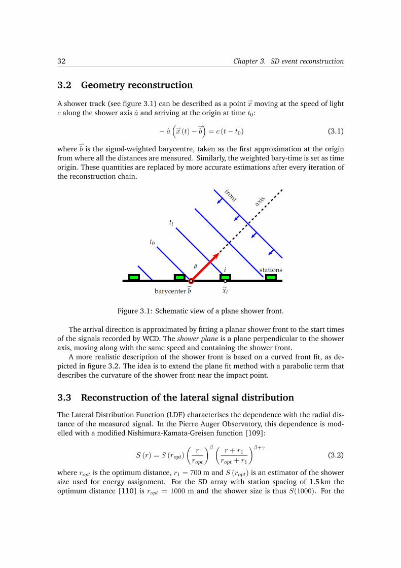
3.2 Geometry reconstruction
A shower track (see figure 3.1) can be described as a point (x moving at the speed of light
c along the shower axis a and arriving at the origin at time t0:
� a
⇣(x (t)�
(b
⌘= c (t� t0) (3.1)
where(b is the signal-weighted barycentre, taken as the first approximation at the origin
from where all the distances are measured. Similarly, the weighted bary-time is set as timeorigin. These quantities are replaced by more accurate estimations after every iteration ofthe reconstruction chain.
Figure 3.1: Schematic view of a plane shower front.
The arrival direction is approximated by fitting a planar shower front to the start timesof the signals recorded by WCD. The shower plane is a plane perpendicular to the showeraxis, moving along with the same speed and containing the shower front.
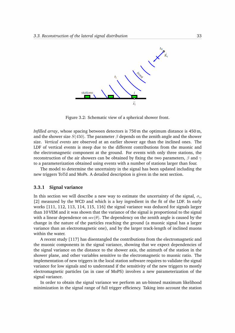
A more realistic description of the shower front is based on a curved front fit, as de-picted in figure 3.2. The idea is to extend the plane fit method with a parabolic term thatdescribes the curvature of the shower front near the impact point.
3.3 Reconstruction of the lateral signal distribution
The Lateral Distribution Function (LDF) characterises the dependence with the radial dis-tance of the measured signal. In the Pierre Auger Observatory, this dependence is mod-elled with a modified Nishimura-Kamata-Greisen function [109]:
S (r) = S (ropt
)
✓r
r
opt
◆�
✓r + r1
r
opt
+ r1
◆�+�
(3.2)
where r
opt
is the optimum distance, r1 = 700 m and S (ropt
) is an estimator of the showersize used for energy assignment. For the SD array with station spacing of 1.5 km theoptimum distance [110] is r
opt
= 1000 m and the shower size is thus S(1000). For the
3.3. Reconstruction of the lateral signal distribution 33
Figure 3.2: Schematic view of a spherical shower front.
Infilled array, whose spacing between detectors is 750 m the optimum distance is 450 m,and the shower size S(450). The parameter � depends on the zenith angle and the showersize. Vertical events are observed at an earlier shower age than the inclined ones. TheLDF of vertical events is steep due to the different contributions from the muonic andthe electromagnetic component at the ground. For events with only three stations, thereconstruction of the air showers can be obtained by fixing the two parameters, � and �
to a parameterization obtained using events with a number of stations larger than four.The model to determine the uncertainty in the signal has been updated including the
new triggers ToTd and MoPs. A detailed description is given in the next section.
3.3.1 Signal variance
In this section we will describe a new way to estimate the uncertainty of the signal, �i
,[2] measured by the WCD and which is a key ingredient in the fit of the LDF. In earlyworks [111, 112, 113, 114, 115, 116] the signal variance was deduced for signals largerthan 10 VEM and it was shown that the variance of the signal is proportional to the signalwith a linear dependence on sec(✓). The dependency on the zenith angle is caused by thechange in the nature of the particles reaching the ground (a muonic signal has a largervariance than an electromagnetic one), and by the larger track-length of inclined muonswithin the water.
A recent study [117] has disentangled the contributions from the electromagnetic andthe muonic components in the signal variance, showing that we expect dependencies ofthe signal variance on the distance to the shower axis, the azimuth of the station in theshower plane, and other variables sensitive to the electromagnetic to muonic ratio. Theimplementation of new triggers in the local station software requires to validate the signalvariance for low signals and to understand if the sensitivity of the new triggers to mostlyelectromagnetic particles (as in case of MoPS) involves a new parameterization of thesignal variance.
In order to obtain the signal variance we perform an un-binned maximum likelihoodminimization in the signal range of full trigger efficiency. Taking into account the station
34 Chapter 3. SD event reconstruction
( S/[VEM] )10
log-1 -0.5 0 0.5 1 1.5 2 2.5 3 3.5 4
entri
es
1
10
210
310
410
510Non-saturated
HG saturated
LG saturated
TOTdMoPs
(a)
(<LDF>/[VEM])10
log-0.5 0 0.5 1 1.5 2
Trig
ger p
roba
bilit
y
0
0.2
0.4
0.6
0.8
1 All triggersTOT || TOTd || MoPSTOTTOTdMOPs
(b)
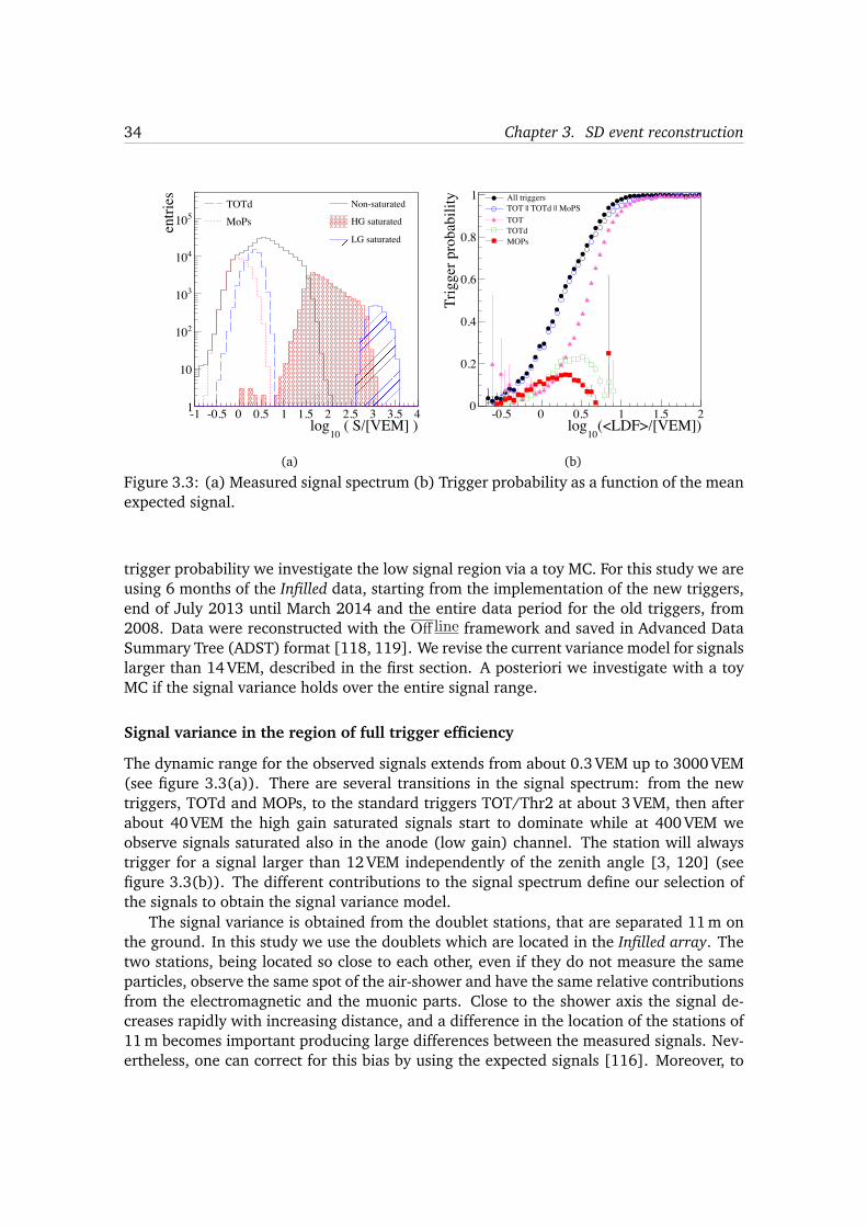
Figure 3.3: (a) Measured signal spectrum (b) Trigger probability as a function of the meanexpected signal.
trigger probability we investigate the low signal region via a toy MC. For this study we areusing 6 months of the Infilled data, starting from the implementation of the new triggers,end of July 2013 until March 2014 and the entire data period for the old triggers, from2008. Data were reconstructed with the O↵ line framework and saved in Advanced DataSummary Tree (ADST) format [118, 119]. We revise the current variance model for signalslarger than 14 VEM, described in the first section. A posteriori we investigate with a toyMC if the signal variance holds over the entire signal range.
Signal variance in the region of full trigger efficiency
The dynamic range for the observed signals extends from about 0.3 VEM up to 3000 VEM(see figure 3.3(a)). There are several transitions in the signal spectrum: from the newtriggers, TOTd and MOPs, to the standard triggers TOT/Thr2 at about 3 VEM, then afterabout 40 VEM the high gain saturated signals start to dominate while at 400 VEM weobserve signals saturated also in the anode (low gain) channel. The station will alwaystrigger for a signal larger than 12 VEM independently of the zenith angle [3, 120] (seefigure 3.3(b)). The different contributions to the signal spectrum define our selection ofthe signals to obtain the signal variance model.
The signal variance is obtained from the doublet stations, that are separated 11 m onthe ground. In this study we use the doublets which are located in the Infilled array. Thetwo stations, being located so close to each other, even if they do not measure the sameparticles, observe the same spot of the air-shower and have the same relative contributionsfrom the electromagnetic and the muonic parts. Close to the shower axis the signal de-creases rapidly with increasing distance, and a difference in the location of the stations of11 m becomes important producing large differences between the measured signals. Nev-ertheless, one can correct for this bias by using the expected signals [116]. Moreover, to
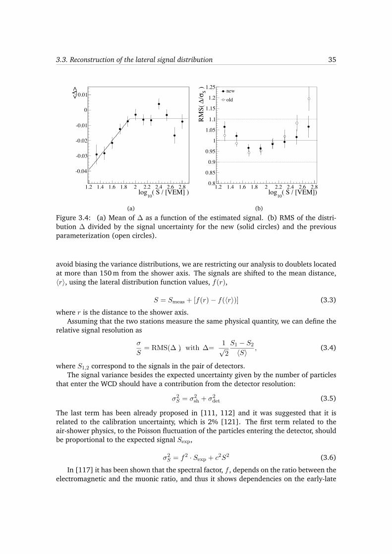
3.3. Reconstruction of the lateral signal distribution 35
( S / [VEM] )10
log1.2 1.4 1.6 1.8 2 2.2 2.4 2.6 2.8
>∆<
-0.04
-0.03
-0.02
-0.01
0
0.01
(a)
( S / [VEM])10
log1.2 1.4 1.6 1.8 2 2.2 2.4 2.6 2.8
) Sσ/∆RM
S(
0.8
0.85
0.9
0.95
1
1.05
1.1
1.15
1.2
1.25new
old
(b)
Figure 3.4: (a) Mean of � as a function of the estimated signal. (b) RMS of the distri-bution � divided by the signal uncertainty for the new (solid circles) and the previousparameterization (open circles).
avoid biasing the variance distributions, we are restricting our analysis to doublets locatedat more than 150 m from the shower axis. The signals are shifted to the mean distance,hri, using the lateral distribution function values, f(r),
S = Smeas + [f(r)� f(hri)] (3.3)
where r is the distance to the shower axis.Assuming that the two stations measure the same physical quantity, we can define the
relative signal resolution as
�
S
= RMS(� ), with �=1p2
S1 � S2
hSi , (3.4)
where S1,2 correspond to the signals in the pair of detectors.The signal variance besides the expected uncertainty given by the number of particles
that enter the WCD should have a contribution from the detector resolution:
�
2S
= �
2sh + �
2det (3.5)
The last term has been already proposed in [111, 112] and it was suggested that it isrelated to the calibration uncertainty, which is 2% [121]. The first term related to theair-shower physics, to the Poisson fluctuation of the particles entering the detector, shouldbe proportional to the expected signal Sexp,
�
2S
= f
2 · Sexp + c
2S
2 (3.6)
In [117] it has been shown that the spectral factor, f , depends on the ratio between theelectromagnetic and the muonic ratio, and thus it shows dependencies on the early-late
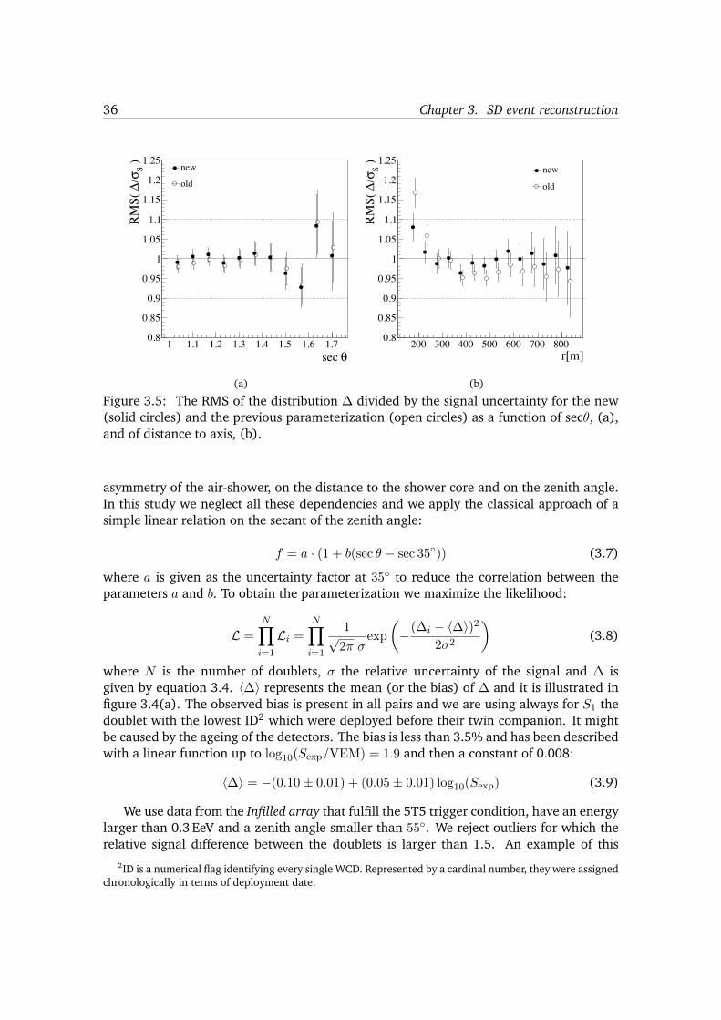
36 Chapter 3. SD event reconstruction
θsec 1 1.1 1.2 1.3 1.4 1.5 1.6 1.7
) Sσ/∆RM
S(
0.8
0.85
0.9
0.95
1
1.05
1.1
1.15
1.2
1.25new
old
(a)
r[m]200 300 400 500 600 700 800
) Sσ/∆RM
S(
0.8
0.85
0.9
0.95
1
1.05
1.1
1.15
1.2
1.25new
old
(b)
Figure 3.5: The RMS of the distribution � divided by the signal uncertainty for the new(solid circles) and the previous parameterization (open circles) as a function of sec✓, (a),and of distance to axis, (b).
asymmetry of the air-shower, on the distance to the shower core and on the zenith angle.In this study we neglect all these dependencies and we apply the classical approach of asimple linear relation on the secant of the zenith angle:
f = a · (1 + b(sec ✓ � sec 35�)) (3.7)
where a is given as the uncertainty factor at 35� to reduce the correlation between theparameters a and b. To obtain the parameterization we maximize the likelihood:
L =
NY
i=1
Li
=NY
i=1
1p2⇡ �
exp
✓�(�
i
� h�i)2
2�2
◆(3.8)
where N is the number of doublets, � the relative uncertainty of the signal and � isgiven by equation 3.4. h�i represents the mean (or the bias) of � and it is illustrated infigure 3.4(a). The observed bias is present in all pairs and we are using always for S1 thedoublet with the lowest ID2 which were deployed before their twin companion. It mightbe caused by the ageing of the detectors. The bias is less than 3.5% and has been describedwith a linear function up to log10(Sexp/VEM) = 1.9 and then a constant of 0.008:
h�i = �(0.10± 0.01) + (0.05± 0.01) log10(Sexp) (3.9)
We use data from the Infilled array that fulfill the 5T5 trigger condition, have an energylarger than 0.3 EeV and a zenith angle smaller than 55�. We reject outliers for which therelative signal difference between the doublets is larger than 1.5. An example of this
2ID is a numerical flag identifying every single WCD. Represented by a cardinal number, they were assignedchronologically in terms of deployment date.
3.3. Reconstruction of the lateral signal distribution 37
type of outliers is given in appendix A. We also reject the doublets for which the timedifference between them is larger than 200 ns. We obtain the variance model in the regionof full trigger efficiency: in order to avoid a cut on the signal which might influence thedistributions in the cut region we select the pairs which are at a distance where the triggerefficiency is more than 98% as given by the lateral trigger probabilities (LTP) describedin [3].
The minimization leads to the parameters:
a = 0.865± 0.007, b = 0.593± 0.006, c = 0.023± 0.002 (3.10)
The RMS of the pull distribution, �/�, is illustrated in figure 3.4(b) as a function of thesignal for the new parameterization compared to the one from a previous parameterization[116]. As can be observed both parameterizations present a small bias evolving withsignal. Nevertheless the new variance, being smaller between 40 and 100 VEM, leads to avalue closer to the expected one. The high signal region is also better described by the newparameterization. In figure 3.5(a) the same variable shows no dependency on the zenithangle. There is a dependency on the distance to the shower axis (see figure 3.5(b)). Itmight indicate that the signal variance should be larger than the one obtained, but thiscan be an effect of the lateral distribution correction. Let us note that in principle by goingcloser to the shower axis the signal variance factor, f , should decrease due to the largercontribution of the electromagnetic component.
We have obtained the signal variance with the Infilled array for energies spanningthe 0.4-1 EeV range. As in principle the signal variance should have an energy depend-ency [117], we have checked at energies above 3 EeV if the same parameterization holds.In appendix A.1 the Infilled data are compared to the larger array. There is a very goodagreement between the two data samples. As a remark the statistics of the doublets in theregular array is a factor 10 smaller using data starting from 2004.
Signal variance for low signals
The signal variance in the whole range is shown in figure 3.6(a). In the previous sectionwe obtained the relative signal uncertainty as a function of the expected signal above14 VEM. We can distinguish three different regions. Above 400 VEM the trend is almostflat because the detector resolution contribution becomes significant. The region between14 and 1000 VEM is the physical region where the Surface Detector is fully efficient. Below12 VEM we are dominated by trigger effects.
The distribution of � in each bin can be described by a Gaussian with a mean of zero.Going to lower signals, the distribution starts to be truncated due to trigger effects, there-fore the RMS decreases as a consequence of not measuring all the signals. Furthermore,the bias in � distribution starts to be significant. The combination of these two facts res-ults in the change of trend that we observe. For the case of standard triggers, TOT andT2, the probability of having a triggered station for signals smaller than 3 VEM is almostzero (see figure 3.3(b)). However, in the case of the new triggers, the non-zero probabilityextends up to 0.5 VEM. Even so, as the contribution of new triggers is not very large, still12 VEM are needed to reach full trigger efficiency.

38 Chapter 3. SD event reconstruction
(<S>/[VEM])10
log-0.5 0 0.5 1 1.5 2 2.5 3
)∆RM
S(
0.1
0.2
0.3
0.4
0.5
0.6All triggers
TOT or T2
(a)
(<S>/[VEM])10
log1.2 1.4 1.6 1.8 2 2.2 2.4 2.6 2.8 3
)∆RM
S(
0.05
0.1
0.15
0.2
0.25Toy MCData
(b)
Figure 3.6: (a) RMS(�) versus mean signal for old triggers (open circles), TOT and T2,and including the new ones, TOTd and MoPS. (b) RMS(�) versus mean signal for the toyMC (solid circles) and for data (open circles), in the region where the trigger efficiency islarger than 98%.
A toy MC is built in order to understand the signal variance in the low signal region.The first ingredient to calculate the relative signal accuracy is the incident signal distri-bution. We draw randomly the signal from the measured distribution weighted by thetrigger probability. To obtain the two measured signals, we smear this value with a normaldistribution with a sigma given by the variance parameterization. To include the triggerprobability we use the parameterizations described in [3].
In figure 3.6(b) the signal uncertainty as a function of the mean signal, consideringonly the signals with a trigger probability larger than 98%, is illustrated. The varianceestimation was obtained in the radial distance where the LTPs are larger than 98%. As canbe seen the agreement is very good over the whole signal range. In addition, the cut inLTP is equivalent to the cut in the trigger signal probability, as in both cases signals above14 VEM are selected.
Considering all the signals we build the RMS(�) as a function of the signal for trig-gers TOT and T2 (figure 3.7(a)), and include new triggers, TOTd and MoPs as well (fig-ure 3.7(c)). In both cases the agreement between the toy MC and data for signals largerthan 0.6 VEM is very good. The ratio of the relative signal accuracy and the parameteriz-ation as a function of the mean signal is illustrated in figure 3.7(b) for standard triggersand in 3.7(d) for all of them. In both cases we reach a plateau for signals larger than12 VEM where the array is fully efficient, as it is expected. These plots have been done inthe zenith range between 0 and 55 degrees. As the trigger probability parameterizationdepends on zenith angle we have included in appendix A.1 the plots in 5 different ranges:the results are compatible in all cases. From these results we can conclude that the signalvariance obtained in the signal region between 14 to 1000 VEM holds in the entire signalrange.

3.3. Reconstruction of the lateral signal distribution 39
(<S>/[VEM])10
log-0.5 0 0.5 1 1.5 2 2.5 3
)∆RM
S(
0.1
0.2
0.3
0.4
0.5
0.6Toy MCData
(a) TOT, Thr2
(<S>/[VEM])10
log-0.5 0 0.5 1 1.5 2 2.5 3
) Sσ/∆RM
S(
0.2
0.4
0.6
0.8
1
1.2
1.4
1.6
1.8 Toy MCData
(b) TOT, Thr2
(<S>/[VEM])10
log-0.5 0 0.5 1 1.5 2 2.5 3
)∆RM
S(
0.1
0.2
0.3
0.4
0.5
0.6Toy MCData
(c) all triggers
(<S>/[VEM])10
log-0.5 0 0.5 1 1.5 2 2.5 3
) Sσ/∆RM
S(
0.2
0.4
0.6
0.8
1
1.2
1.4
1.6
1.8 Toy MCData
(d) all triggers
Figure 3.7: (a,c): The RMS(�) versus mean signal compared to the toy MC. (b,d): theRMS of � divided by the parameterization. A good agreement is observed between dataand the toy MC.
Impact on the Infilled reconstruction The signal variance model obtained in this workdoes not differ too much from the one that is used in the official analysis and thus theimpact on the reconstruction is not expected to be large. We have reconstructed the Infilleddata with both signal variance models. The mean change on the energy is less than 0.5%with a spread of less than 1%. The core is shifted less than 20 m with a negligible impacton the angle. The only effect is, as expected, on the energy uncertainty. Having a signalvariance that is smaller for parts of the signal spectrum, the �
2 has larger values for thenew parameterization, which leads to a reduction of the energy uncertainty by about 10%at 1016 eV, 3% at 1017.5 eV and less that 0.5% above 1018 eV. Nevertheless very few events(0.02%) have a change in the location of the impact point on the ground of more than
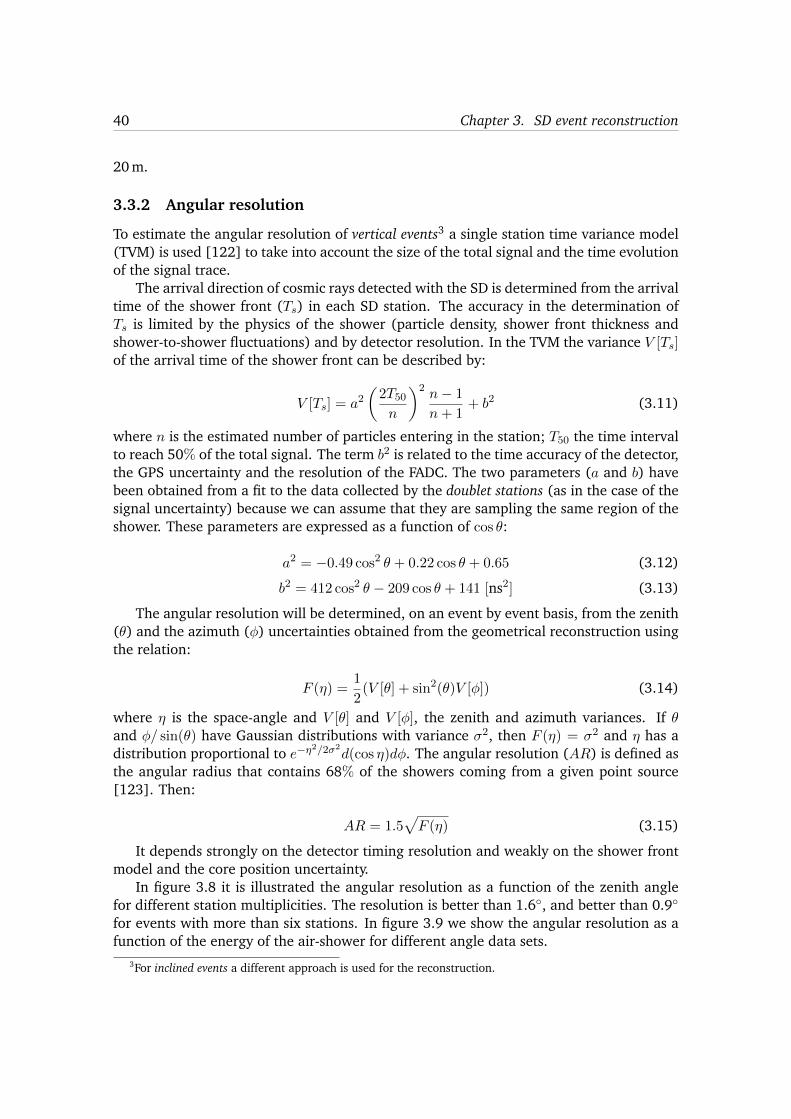
40 Chapter 3. SD event reconstruction
20 m.
3.3.2 Angular resolution
To estimate the angular resolution of vertical events3 a single station time variance model(TVM) is used [122] to take into account the size of the total signal and the time evolutionof the signal trace.
The arrival direction of cosmic rays detected with the SD is determined from the arrivaltime of the shower front (T
s
) in each SD station. The accuracy in the determination ofT
s
is limited by the physics of the shower (particle density, shower front thickness andshower-to-shower fluctuations) and by detector resolution. In the TVM the variance V [T
s
]of the arrival time of the shower front can be described by:
V [Ts
] = a
2
✓2T50
n
◆2n� 1
n+ 1+ b
2 (3.11)
where n is the estimated number of particles entering in the station; T50 the time intervalto reach 50% of the total signal. The term b
2 is related to the time accuracy of the detector,the GPS uncertainty and the resolution of the FADC. The two parameters (a and b) havebeen obtained from a fit to the data collected by the doublet stations (as in the case of thesignal uncertainty) because we can assume that they are sampling the same region of theshower. These parameters are expressed as a function of cos ✓:
a
2 = �0.49 cos2 ✓ + 0.22 cos ✓ + 0.65 (3.12)
b
2 = 412 cos2 ✓ � 209 cos ✓ + 141 [ns2] (3.13)
The angular resolution will be determined, on an event by event basis, from the zenith(✓) and the azimuth (�) uncertainties obtained from the geometrical reconstruction usingthe relation:
F (⌘) =1
2(V [✓] + sin2(✓)V [�]) (3.14)
where ⌘ is the space-angle and V [✓] and V [�], the zenith and azimuth variances. If ✓
and �/ sin(✓) have Gaussian distributions with variance �
2, then F (⌘) = �
2 and ⌘ has adistribution proportional to e
�⌘
2/2�2
d(cos ⌘)d�. The angular resolution (AR) is defined asthe angular radius that contains 68% of the showers coming from a given point source[123]. Then:
AR = 1.5pF (⌘) (3.15)
It depends strongly on the detector timing resolution and weakly on the shower frontmodel and the core position uncertainty.
In figure 3.8 it is illustrated the angular resolution as a function of the zenith anglefor different station multiplicities. The resolution is better than 1.6�, and better than 0.9�
for events with more than six stations. In figure 3.9 we show the angular resolution as afunction of the energy of the air-shower for different angle data sets.
3For inclined events a different approach is used for the reconstruction.
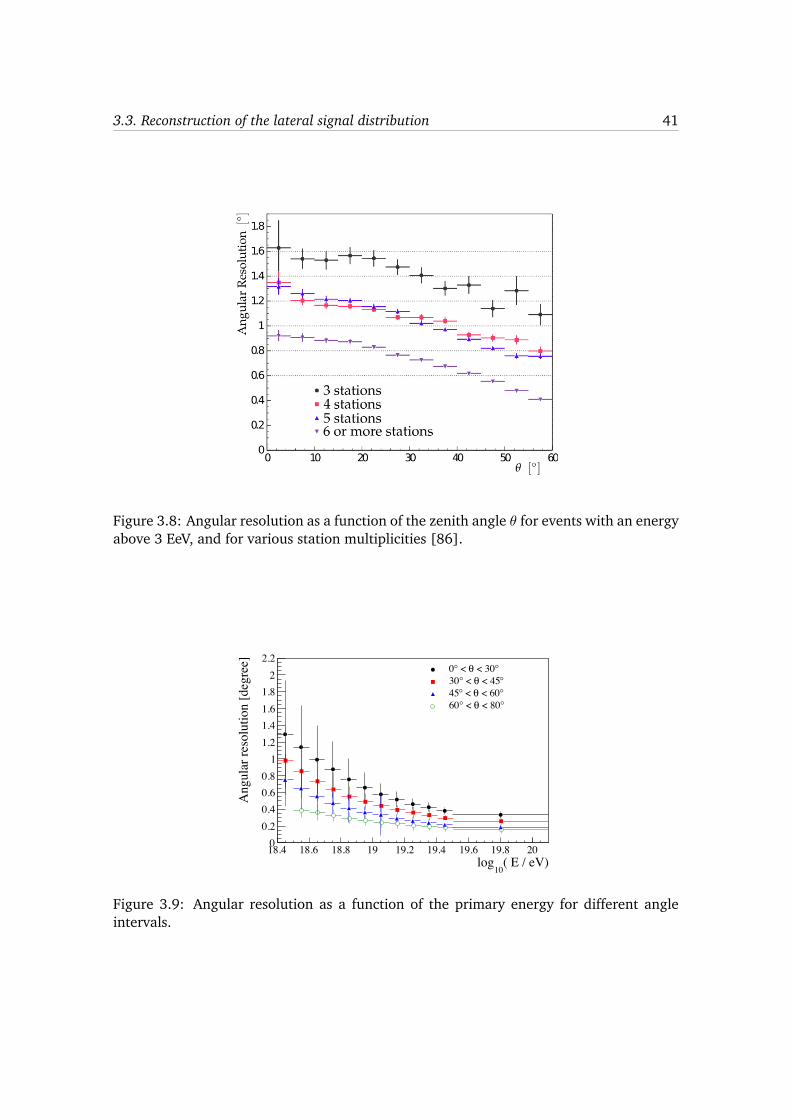
3.3. Reconstruction of the lateral signal distribution 41
Figure 3.8: Angular resolution as a function of the zenith angle ✓ for events with an energyabove 3 EeV, and for various station multiplicities [86].
( E / eV)10
log18.4 18.6 18.8 19 19.2 19.4 19.6 19.8 20
Ang
ular
reso
lutio
n [d
egre
e]
00.20.40.60.8
11.21.41.61.8
22.2
° < 30θ < °0° < 45θ < °30° < 60θ < °45° < 80θ < °60
Figure 3.9: Angular resolution as a function of the primary energy for different angleintervals.

42 Chapter 3. SD event reconstruction
3.3.3 LDF maximum likelihood fit
The LDF fit is based on a log-likelihood maximization. It allows us to include: non-triggering stations with signal below trigger threshold, small or large signal, and the signalof saturated stations. Therefore, it is important to correctly estimate the uncertainty in thesignal for each station as discussed previously.
The energy deposit in the WCD, or equivalently the number of registered photo-electrons depends on the particle type, injection point and incident angle. Although thesignal is calibrated in VEM there is no simple conversion between photo-electrons andparticles.
The main contributions to the total signal measured in a detector are the electromag-netic and the muonic part:
S = S
µ
+ S
e/�
(3.16)
The signal Se/�
is much smaller on average than S
µ
and the mean conversion factorfor electrons and muons is smaller than 1 VEM. The total number of particles that haveproduced the signal is estimated as:
n = pS (3.17)
where n is the number of particles, S the collected signal and p the Poisson factor, approx-imated in this minimal model by:
p = p (✓) =
8<
:
1p�
S
(✓), if �
S
(✓) � 1
1 , otherwise(3.18)
independent of primary energy, mass and distance to the core.The likelihood function to maximize, gathering the sampled imformation of detector i
at distance r
i
is:
L =Y
i
f
P
(ni
, µ
i
)Y
i
f
G
(ni
, µ
i
)Y
i
Fsat(ni
, µ
i
)Y
i
Fzero(ni
, µ
i
) (3.19)
and thus the log-likelihood function is
` =X
i
ln fP
(ni
, µ
i
) +X
i
ln fG
(ni
, µ
i
) +X
i
lnFsat(ni
, µ
i
) +X
i
lnFzero(ni
, µ
i
) (3.20)
with n
i
the effective number of particles detected in the detector as obtained using equa-tion (3.17), and µ
i
the corresponding LDF expectation. The four members of this equationrepresent each of the four possibilities for a station signal:
• Small signals: (n < 30 particles) A Poissonian distribution is assumed
ln fP
(ni
, µ
i
) = n
i
lnµi
� µ
i
�n
iX
j=1
ln j (3.21)
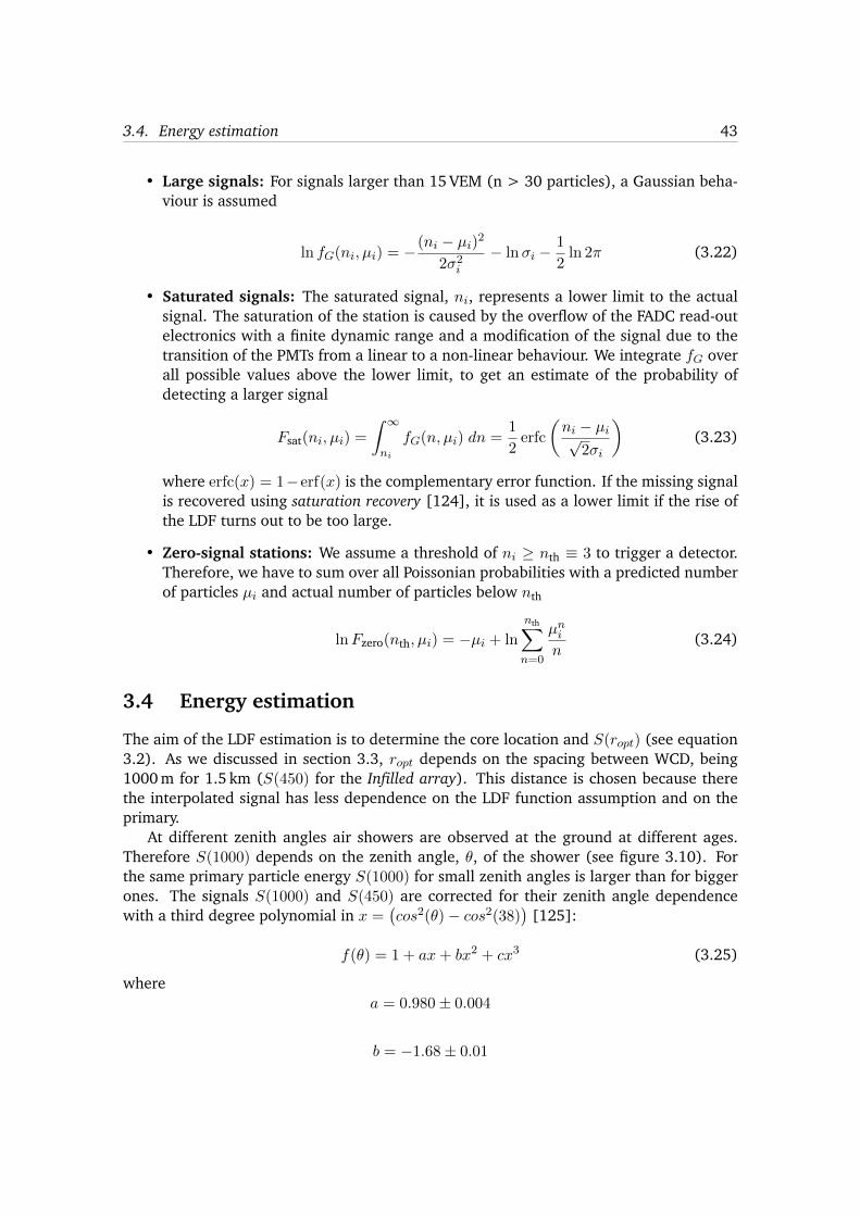
3.4. Energy estimation 43
• Large signals: For signals larger than 15 VEM (n > 30 particles), a Gaussian beha-viour is assumed
ln fG
(ni
, µ
i
) = �(ni
� µ
i
)2
2�2i
� ln�i
� 1
2ln 2⇡ (3.22)
• Saturated signals: The saturated signal, ni
, represents a lower limit to the actualsignal. The saturation of the station is caused by the overflow of the FADC read-outelectronics with a finite dynamic range and a modification of the signal due to thetransition of the PMTs from a linear to a non-linear behaviour. We integrate f
G
overall possible values above the lower limit, to get an estimate of the probability ofdetecting a larger signal
Fsat(ni
, µ
i
) =
Z 1
n
i
f
G
(n, µi
) dn =1
2erfc
✓n
i
� µ
ip2�
i
◆(3.23)
where erfc(x) = 1�erf(x) is the complementary error function. If the missing signalis recovered using saturation recovery [124], it is used as a lower limit if the rise ofthe LDF turns out to be too large.
• Zero-signal stations: We assume a threshold of ni
� nth ⌘ 3 to trigger a detector.Therefore, we have to sum over all Poissonian probabilities with a predicted numberof particles µ
i
and actual number of particles below nth
lnFzero(nth, µi
) = �µ
i
+ ln
nthX
n=0
µ
n
i
n
(3.24)
3.4 Energy estimation
The aim of the LDF estimation is to determine the core location and S(ropt
) (see equation3.2). As we discussed in section 3.3, r
opt
depends on the spacing between WCD, being1000 m for 1.5 km (S(450) for the Infilled array). This distance is chosen because therethe interpolated signal has less dependence on the LDF function assumption and on theprimary.
At different zenith angles air showers are observed at the ground at different ages.Therefore S(1000) depends on the zenith angle, ✓, of the shower (see figure 3.10). Forthe same primary particle energy S(1000) for small zenith angles is larger than for biggerones. The signals S(1000) and S(450) are corrected for their zenith angle dependencewith a third degree polynomial in x =
�cos
2(✓)� cos
2(38)�
[125]:
f(✓) = 1 + ax+ bx
2 + cx
3 (3.25)
wherea = 0.980± 0.004
b = �1.68± 0.01

44 Chapter 3. SD event reconstruction
c = �1.30± 0.45
Figure 3.10: Attenuation curve described by a third degree polynomial function inx =
�cos
2(✓)� cos
2(38)�. In this example the polynomial coefficients are deduced from
S(1000) dependence at S38 ⇠ 50 VEM which corresponds to an energy of about 10.5 EeV[86].
The equivalent signal at median zenith angle of 38� (35�), S38 ( S35), will be the energyestimator used for vertical events. Note that for the 750 m array, only events with zenithangle below 55� are accepted.
Inclined air-showers are characterised by the dominance of secondary muons at theground, as the electromagnetic component is largely absorbed in the large atmosphericdepth traversed by the shower. The reconstruction of inclined events is performed witha different method. It is based on the estimate of the relative muon content, N19, withrespect to a simulated proton shower with energy 1019 eV [126].
A subset of high-quality events is used, the so-called Golden hybrids events, to calibratethe SD energy estimators with the calorimetric measurement obtained with the FD, E
FD
.They are high-quality hybrid T5 events which have an energy above the SD full efficiencytrigger threshold [91] registered between January 2004 and December 2013. The correl-ation between the two variables is obatined from a maximum likelihood method whichtakes into account the evolution of uncertainties with energy, as well as event migrationsdue to the finite energy resolution of the SD. The relation between the different SD energyestimators and E
FD
is well described by a single power-law function,
E
FD
= A (S)B (3.26)
where the resulting parameters for the different observables are given in table 3.1. Thecorrelation between the different energy estimators and EFD is shown in figure 3.11(a).In the table is also illustrated the energy threshold for the different data sets. In the caseof the SD data: vertical, inclined and Infilled this value represents the energy at which the
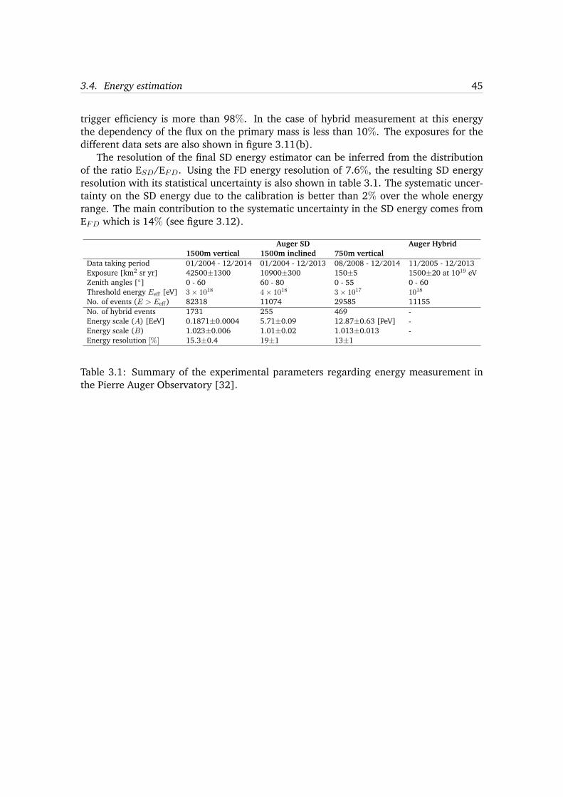
3.4. Energy estimation 45
trigger efficiency is more than 98%. In the case of hybrid measurement at this energythe dependency of the flux on the primary mass is less than 10%. The exposures for thedifferent data sets are also shown in figure 3.11(b).
The resolution of the final SD energy estimator can be inferred from the distributionof the ratio E
SD
/EFD
. Using the FD energy resolution of 7.6%, the resulting SD energyresolution with its statistical uncertainty is also shown in table 3.1. The systematic uncer-tainty on the SD energy due to the calibration is better than 2% over the whole energyrange. The main contribution to the systematic uncertainty in the SD energy comes fromEFD
which is 14% (see figure 3.12).
Auger SD Auger Hybrid1500m vertical 1500m inclined 750m vertical
Data taking period 01/2004 - 12/2014 01/2004 - 12/2013 08/2008 - 12/2014 11/2005 - 12/2013Exposure [km2 sr yr] 42500±1300 10900±300 150±5 1500±20 at 1019 eVZenith angles [�] 0 - 60 60 - 80 0 - 55 0 - 60Threshold energy Ee↵ [eV] 3⇥ 1018 4⇥ 1018 3⇥ 1017 1018
No. of events (E > Ee↵) 82318 11074 29585 11155No. of hybrid events 1731 255 469 -Energy scale (A) [EeV] 0.1871±0.0004 5.71±0.09 12.87±0.63 [PeV] -Energy scale (B) 1.023±0.006 1.01±0.02 1.013±0.013 -Energy resolution [%] 15.3±0.4 19±1 13±1
Table 3.1: Summary of the experimental parameters regarding energy measurement inthe Pierre Auger Observatory [32].
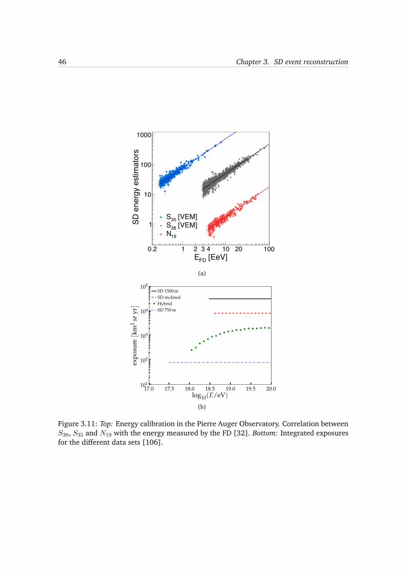
46 Chapter 3. SD event reconstruction
[EeV]FDE0.2 1 2 3 4 10 20 100
SD
ene
rgy
estim
ator
s
1
10
100
1000
[VEM]35S [VEM]38S
19N
(a)
17.0 17.5 18.0 18.5 19.0 19.5 20.0log10(E/eV)
101
102
103
104
105
expo
sure
⇥ km2
sryr
⇤
SD 1500 mSD inclinedHybridSD 750 m
(b)
Figure 3.11: Top: Energy calibration in the Pierre Auger Observatory. Correlation betweenS38, S35 and N19 with the energy measured by the FD [32]. Bottom: Integrated exposuresfor the different data sets [106].
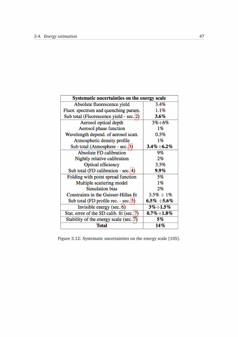
3.4. Energy estimation 47
Figure 3.12: Systematic uncertainties on the energy scale [105].

4Revision of the Muon ArrivalTime Model
When building muon production depth (MPD) distributions, the main source of distortioncomes from effects like the under-sampling of the detector, the tank response to muonsand the geometry resolution [1, 127, 128, 129]. To a lesser extent, the algorithm usedto convert the times recorded by the SD detectors into muon production distances alsodeforms the average profile1. In this chapter, we quantify among other things, the distor-tion introduced by the latter effect using events with energies and zenith angles similar tothose used in the standard analysis (i.e., E > 20 EeV and ✓ ✏ [55�, 65�]) and two differentdistance cuts: r > 1000 m or r > 1700 m. In particular, we follow a new approach toparameterize the kinematic delay that results in a sensible reduction of the bias associatedto the reconstructed X
µ
max.
4.1 MPD algorithm
With the SD detectors we can measure the positions and the times of muons reaching theground. Starting from this information the challenge is to reconstruct the longitudinaldevelopment of the muonic cascade (i.e. the MPD distribution).
Muons mainly come from the decay of pions (99% branching ratio) and kaons (64%branching ratio). Also kaons will decay to charged pions with a 28.5% probability. Hence,we can assume that muons mainly come from pions. The muon parent particle travels ata certain angle from the shower axis. The muon time measured at the ground thereforecontains the path traveled before decaying by the parent particle:
t
SD
= t
⇡
+ t
µ
(4.1)
In our calculation it is mandatory to set a reference start time. This time is the arrivaltime of the shower front at the position of each muon at the ground (tfront). Thus, we willbe interested in relative quantities (i.e. time delays). They are defined as:
⌧ = (t⇡
+ t
µ
)� tfront (4.2)
1i.e., the sum of all the MPD distributions for a particular energy bin

50 Chapter 4. Revision of the Muon Arrival Time Model
The breakdown of the different contributions to the total delay is summarized in whatfollows [130]:
• Geometric delay, ⌧g
: The minimum muon time of flight assuming they are masslessparticles (their velocity equals speed of light) that suffer no interactions and there-fore follow trajectories that are straight lines. This delay can be deduced by meansof elementary geometry arguments (see figure 4.1):
Figure 4.1: Geometry used to obtain the muon traveled distance.
l =
qr
2 + (z ��)2 = ct
min
(4.3)
where tmin would be the minimum arrival time of the muon at the ground, r thedistance to the shower core and z the production point of the muon along the showeraxis.
The difference of this time with respect to the arrival time of the shower front is thegeometric delay:
c⌧
g
= (ctmin
+ ct
⇡
)� ctfront = (ctmin + ct
⇡
)� (z1st ��) =
qr
2 + (z ��)2� (z ��)(4.4)
where � represents the distance from the point at the ground to the shower front,defined as a plane traveling at the speed of light perpendicularly to the shower axis.For a horizontal ground plane:
� (r,⇣ ) = r cos ⇣ tan ✓ (4.5)
✓ being the zenith angle of the air-shower, ⇣ the azimuth and r the distance to theshower axis. ct
⇡
is the path traveled by the parent particle. Given the position of thefirst interaction point on the shower axis, z1st, then

4.1. MPD algorithm 51
ct
⇡
= z1st � z. (4.6)
• Kinematic delay, ⌧kin
: Muons are massive particles so they do not travel at the speedof light and their velocities depend on energy. They lose energy mainly because ofinelastic collisions with atomic electrons in the air. The difference with respect to aparticle traveling at c is referred to as ⌧
kin
.
• Multiple scattering, ⌧MS
: Muons do not travel following straight lines. Whilst tra-versing the air they can be deflected mainly due to Coulomb scattering from nuclei.
• Geomagnetic field, ⌧
B
: Muons are charged particles so the magnetic field of theEarth affects their trajectories, changing the impact point on the ground and delay-ing the arrival time. The longer the path of the muon, the larger this effect. Henceit is especially important for very inclined events.
The total delay of the muon at the ground is:
⌧ = ⌧
g
+ ⌧
kin
+ ⌧
B
+ ⌧
Rem
(4.7)
where ⌧
Rem
accounts for multiple scattering and any remanent delay due to model ap-proximations.
The goal of the reconstruction is to obtain the production distance from the measureddelay which contains all the contributions. The simplest way to do it will be by invertingequation (4.4), the mapping between production distances and geometric delays:
z =1
2
✓r
2
c⌧
g
� c⌧
g
◆+� (4.8)
where ⌧
g
can be obtained from equation (4.7):
⌧
g
= ⌧ � ⌧
kin
� ⌧
B
� ⌧
Rem
(4.9)
Nevertheless, to use this expression we need to evaluate the different corrections tothe total delay. Figure 4.2 shows the relative contributions for each of those corrections.
The effect of multiple scattering is negligible for muons in air and the deflectionsuffered by them caused by the geomagnetic field is also small at this zenith range. Hencethe contribution of the last two terms, ⌧
B
+ ⌧
Rem
is of the order of a few percent respectto the other ones (see figure 4.2).
Therefore, the main correction to the geometric delay is the kinematic one. Assumingconstant energy loses along their flying path, E
f
= E
i
� ⇢al, it can be expressed as:
⌧
kin
=1
c⇢a
qE
2i
� [mc
2]�q
E
2f
� [mc
2]
�� l
c
(4.10)
where E
i
is the muon energy at production, Ef
the muon energy at ground, a the stoppingpower (considered constant here) and ⇢ the atmospheric density. At larger distances (morethan 1000 m) and for zenith angles ✓ = 60�, the kinematic delay typically amounts to lessthan 30% of the total delay [130], becoming negligible as we go farther from the core. It
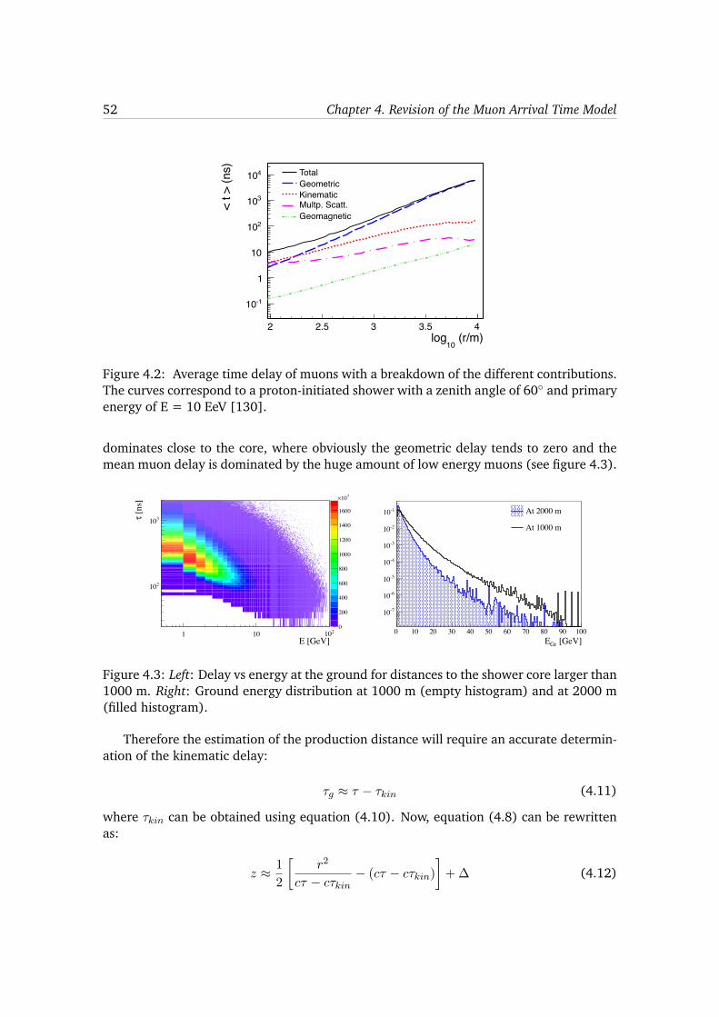
52 Chapter 4. Revision of the Muon Arrival Time Model
(r/m)10
log2 2.5 3 3.5 4
< t >
(ns)
-110
1
10
210
310
410 TotalGeometricKinematicMultp. Scatt.Geomagnetic
Figure 4.2: Average time delay of muons with a breakdown of the different contributions.The curves correspond to a proton-initiated shower with a zenith angle of 60� and primaryenergy of E = 10 EeV [130].
dominates close to the core, where obviously the geometric delay tends to zero and themean muon delay is dominated by the huge amount of low energy muons (see figure 4.3).
E [GeV]1 10 210
[ns]
τ
210
310
0
200
400
600
800
1000
1200
1400
1600
310×
[GeV]GrE0 10 20 30 40 50 60 70 80 90 100
-710
-610
-510
-410
-310
-210
-110 At 2000 m
At 1000 m
Figure 4.3: Left: Delay vs energy at the ground for distances to the shower core larger than1000 m. Right: Ground energy distribution at 1000 m (empty histogram) and at 2000 m(filled histogram).
Therefore the estimation of the production distance will require an accurate determin-ation of the kinematic delay:
⌧
g
⇡ ⌧ � ⌧
kin
(4.11)
where ⌧
kin
can be obtained using equation (4.10). Now, equation (4.8) can be rewrittenas:
z ⇡ 1
2
r
2
c⌧ � c⌧
kin
� (c⌧ � c⌧
kin
)
�+� (4.12)

4.2. Classic (previous) kinematic delay parameterization 53
In figure 4.4 we illustrate the goodness of this approach to deduce the true MPD distri-bution. Dashed line represents the distribution without applying the kinematic correction,assuming muons traveling at c. The shape is distorted and widened compare to the truedistribution (continuous line). A dramatic overestimation of Xµ
max is observed. However,if we apply the kinematic correction of equation (4.10) (filled histogram) we reproducealmost perfectly the true distribution at the two selected distances. The difference withrespect to the true one comes from the approximations done.
]2 [g/cmµX0 200 400 600 800 1000 1200 14000
20406080
100120140160180200220240
610× given by CorsikaµXkinτtrue
=0kinτwith µX
(a) 1000 < r < 4000 m
]2 [g/cmµX0 200 400 600 800 1000 1200 14000
10
20
30
40
50
60
70
80
610× given by CorsikaµXkinτtrue
=0kinτwith µX
(b) 1700 < r < 4000 m
Figure 4.4: MPD distributions obtained for proton QGSJET-II-04 at 1019.75 eV. Continuousline represents the distribution obtained directly from the simulations (the true distribu-tion). The dashed line is the one obtained using only the geometric delay, and the filledhistogram is the result after correcting by the kinematic delay, using equation (4.10).
In what follows we further investigate the role of the kinematic delay in the recon-struction of the muon production distances.
4.2 Classic (previous) kinematic delay parameterization
In order to compute the kinematic delay, an estimation of the muon energy is required.Unfortunately, with the Auger SD detectors we can not get a direct measurement of thisquantity. Thus, to account for it in the reconstruction algorithm, an approximation isperformed. In the standard analysis, the average kinematic delay ht
kin
i is parameterizedusing an approximation of the muon energy spectrum [131] (in this reference they re-ferred to the kinematic delay as ht
"
i). In [132, 131] it is parameterized as a functionof the distance to the shower core and the production distance arriving to the followingexpression:
ht"
i = 1
2c
r
2
l
✏(r, z ��) (4.13)
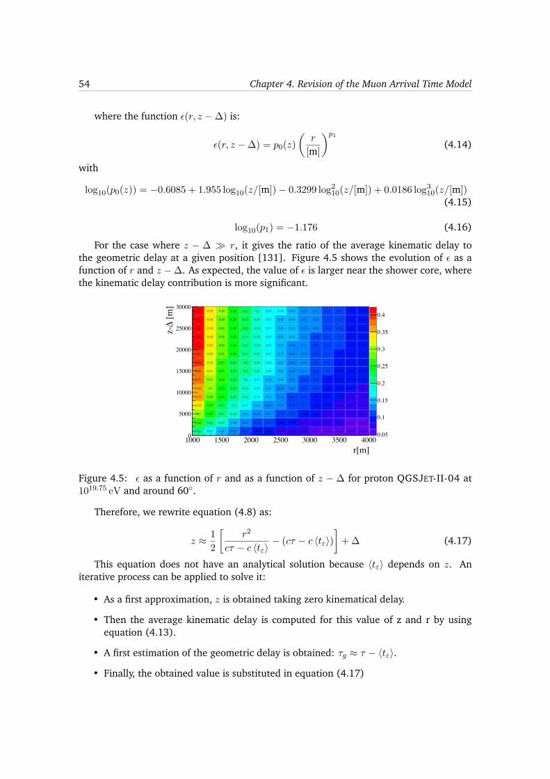
54 Chapter 4. Revision of the Muon Arrival Time Model
where the function ✏(r, z ��) is:
✏(r, z ��) = p0(z)
✓r
[m]
◆p1
(4.14)
with
log10(p0(z)) = �0.6085 + 1.955 log10(z/[m])� 0.3299 log210(z/[m]) + 0.0186 log310(z/[m])(4.15)
log10(p1) = �1.176 (4.16)
For the case where z � � � r, it gives the ratio of the average kinematic delay tothe geometric delay at a given position [131]. Figure 4.5 shows the evolution of ✏ as afunction of r and z ��. As expected, the value of ✏ is larger near the shower core, wherethe kinematic delay contribution is more significant.
0.21 0.17 0.14 0.12 0.11 0.096 0.086 0.078 0.071 0.065 0.06 0.056 0.052 0.049 0.046
0.26 0.21 0.18 0.15 0.14 0.12 0.11 0.098 0.089 0.082 0.076 0.07 0.066 0.061 0.058
0.3 0.25 0.21 0.18 0.16 0.14 0.13 0.11 0.1 0.096 0.088 0.082 0.076 0.072 0.067
0.33 0.27 0.23 0.2 0.17 0.15 0.14 0.12 0.11 0.1 0.096 0.089 0.084 0.078 0.073
0.35 0.29 0.24 0.21 0.18 0.16 0.15 0.13 0.12 0.11 0.1 0.095 0.089 0.083 0.078
0.36 0.3 0.25 0.22 0.19 0.17 0.15 0.14 0.13 0.12 0.11 0.099 0.092 0.087 0.081
0.37 0.31 0.26 0.22 0.2 0.17 0.16 0.14 0.13 0.12 0.11 0.1 0.095 0.089 0.084
0.38 0.31 0.27 0.23 0.2 0.18 0.16 0.15 0.13 0.12 0.11 0.1 0.098 0.092 0.086
0.39 0.32 0.27 0.23 0.2 0.18 0.16 0.15 0.14 0.12 0.12 0.11 0.1 0.094 0.088
0.4 0.33 0.28 0.24 0.21 0.19 0.17 0.15 0.14 0.13 0.12 0.11 0.1 0.095 0.089
0.4 0.33 0.28 0.24 0.21 0.19 0.17 0.15 0.14 0.13 0.12 0.11 0.1 0.097 0.091
0.41 0.34 0.28 0.24 0.21 0.19 0.17 0.16 0.14 0.13 0.12 0.11 0.1 0.098 0.092
0.41 0.34 0.29 0.25 0.22 0.19 0.17 0.16 0.14 0.13 0.12 0.11 0.11 0.099 0.093
0.42 0.34 0.29 0.25 0.22 0.19 0.17 0.16 0.14 0.13 0.12 0.11 0.11 0.1 0.094
0.42 0.35 0.29 0.25 0.22 0.2 0.18 0.16 0.15 0.13 0.12 0.12 0.11 0.1 0.095
r[m]1000 1500 2000 2500 3000 3500 4000
[m]
∆z-
0
5000
10000
15000
20000
25000
30000
0.05
0.1
0.15
0.2
0.25
0.3
0.35
0.4
Figure 4.5: ✏ as a function of r and as a function of z � � for proton QGSJET-II-04 at1019.75 eV and around 60�.
Therefore, we rewrite equation (4.8) as:
z ⇡ 1
2
r
2
c⌧ � c ht"
i � (c⌧ � c ht"
i)�+� (4.17)
This equation does not have an analytical solution because ht"
i depends on z. Aniterative process can be applied to solve it:
• As a first approximation, z is obtained taking zero kinematical delay.
• Then the average kinematic delay is computed for this value of z and r by usingequation (4.13).
• A first estimation of the geometric delay is obtained: ⌧g
⇡ ⌧ � ht"
i.
• Finally, the obtained value is substituted in equation (4.17)
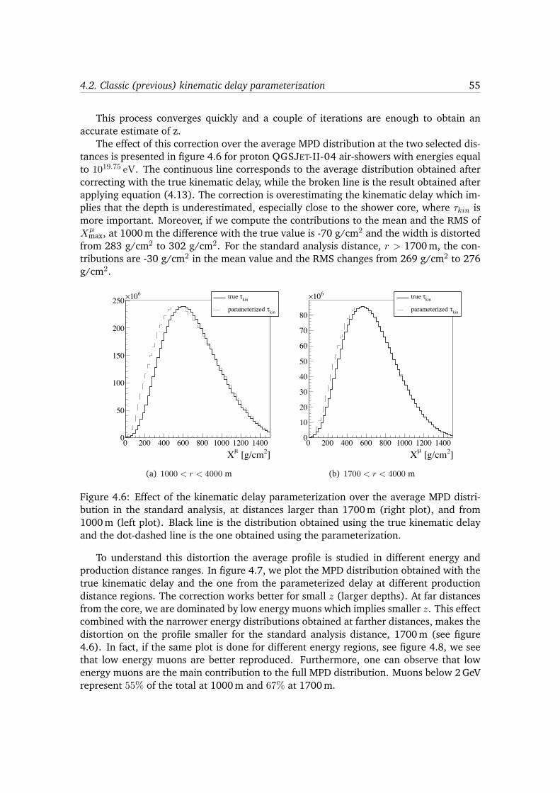
4.2. Classic (previous) kinematic delay parameterization 55
This process converges quickly and a couple of iterations are enough to obtain anaccurate estimate of z.
The effect of this correction over the average MPD distribution at the two selected dis-tances is presented in figure 4.6 for proton QGSJET-II-04 air-showers with energies equalto 1019.75 eV. The continuous line corresponds to the average distribution obtained aftercorrecting with the true kinematic delay, while the broken line is the result obtained afterapplying equation (4.13). The correction is overestimating the kinematic delay which im-plies that the depth is underestimated, especially close to the shower core, where ⌧
kin
ismore important. Moreover, if we compute the contributions to the mean and the RMS ofX
µ
max, at 1000 m the difference with the true value is -70 g/cm2 and the width is distortedfrom 283 g/cm2 to 302 g/cm2. For the standard analysis distance, r > 1700 m, the con-tributions are -30 g/cm2 in the mean value and the RMS changes from 269 g/cm2 to 276g/cm2.
]2 [g/cmµX0 200 400 600 800 1000 1200 14000
50
100
150
200
250610× kinτtrue
kinτparameterized
(a) 1000 < r < 4000 m
]2 [g/cmµX0 200 400 600 800 1000 1200 14000
10
20
30
40
50
60
70
80
610× kinτtrue
kinτparameterized
(b) 1700 < r < 4000 m
Figure 4.6: Effect of the kinematic delay parameterization over the average MPD distri-bution in the standard analysis, at distances larger than 1700 m (right plot), and from1000 m (left plot). Black line is the distribution obtained using the true kinematic delayand the dot-dashed line is the one obtained using the parameterization.
To understand this distortion the average profile is studied in different energy andproduction distance ranges. In figure 4.7, we plot the MPD distribution obtained with thetrue kinematic delay and the one from the parameterized delay at different productiondistance regions. The correction works better for small z (larger depths). At far distancesfrom the core, we are dominated by low energy muons which implies smaller z. This effectcombined with the narrower energy distributions obtained at farther distances, makes thedistortion on the profile smaller for the standard analysis distance, 1700 m (see figure4.6). In fact, if the same plot is done for different energy regions, see figure 4.8, we seethat low energy muons are better reproduced. Furthermore, one can observe that lowenergy muons are the main contribution to the full MPD distribution. Muons below 2 GeVrepresent 55% of the total at 1000 m and 67% at 1700 m.
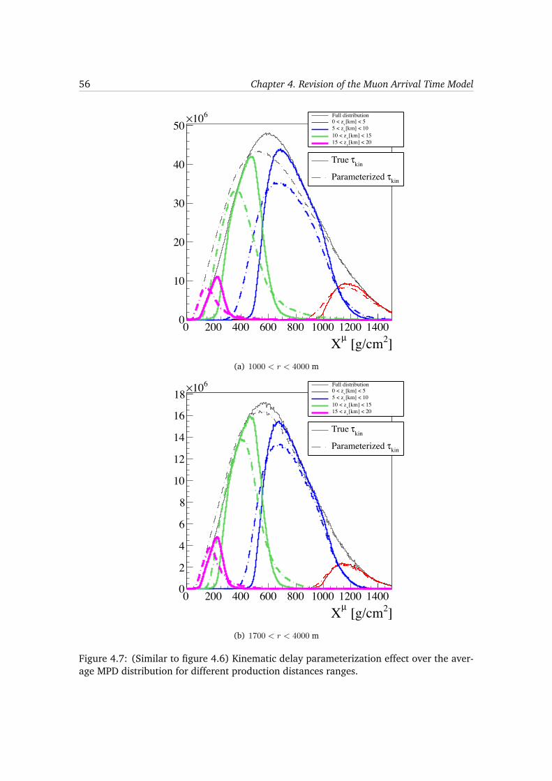
56 Chapter 4. Revision of the Muon Arrival Time Model
]2 [g/cmµX0 200 400 600 800 1000 1200 14000
10
20
30
40
50610× Full distribution
[km] < 5v0 < z[km] < 10v5 < z
[km] < 15v10 < z[km] < 20v15 < z
kinτTrue
kinτParameterized
(a) 1000 < r < 4000 m
]2 [g/cmµX0 200 400 600 800 1000 1200 14000
2
4
6
8
10
12
14
16
18610× Full distribution
[km] < 5v0 < z[km] < 10v5 < z
[km] < 15v10 < z[km] < 20v15 < z
kinτTrue
kinτParameterized
(b) 1700 < r < 4000 m
Figure 4.7: (Similar to figure 4.6) Kinematic delay parameterization effect over the aver-age MPD distribution for different production distances ranges.
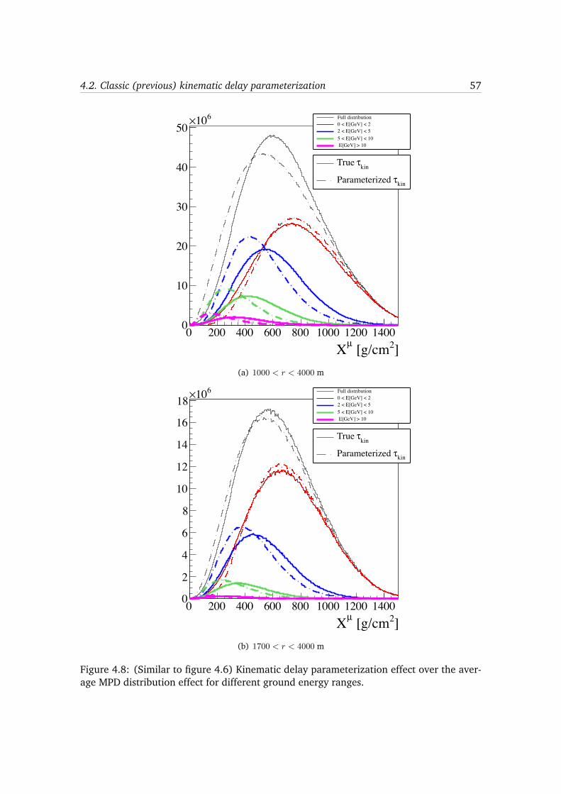
4.2. Classic (previous) kinematic delay parameterization 57
]2 [g/cmµX0 200 400 600 800 1000 1200 14000
10
20
30
40
50610× Full distribution
0 < E[GeV] < 22 < E[GeV] < 55 < E[GeV] < 10 E[GeV] > 10
kinτTrue
kinτParameterized
(a) 1000 < r < 4000 m
]2 [g/cmµX0 200 400 600 800 1000 1200 14000
2
4
6
8
10
12
14
16
18610× Full distribution
0 < E[GeV] < 22 < E[GeV] < 55 < E[GeV] < 10 E[GeV] > 10
kinτTrue
kinτParameterized
(b) 1700 < r < 4000 m
Figure 4.8: (Similar to figure 4.6) Kinematic delay parameterization effect over the aver-age MPD distribution effect for different ground energy ranges.
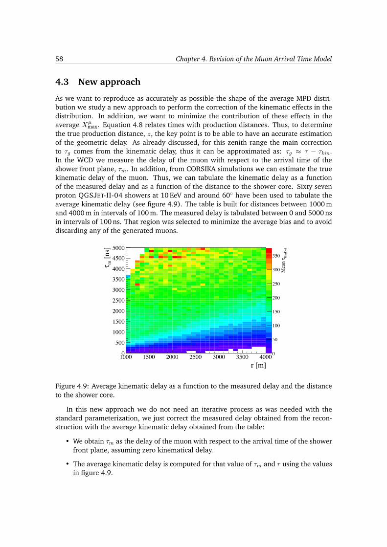
58 Chapter 4. Revision of the Muon Arrival Time Model
4.3 New approach
As we want to reproduce as accurately as possible the shape of the average MPD distri-bution we study a new approach to perform the correction of the kinematic effects in thedistribution. In addition, we want to minimize the contribution of these effects in theaverage X
µ
max. Equation 4.8 relates times with production distances. Thus, to determinethe true production distance, z, the key point is to be able to have an accurate estimationof the geometric delay. As already discussed, for this zenith range the main correctionto ⌧
g
comes from the kinematic delay, thus it can be approximated as: ⌧
g
⇡ ⌧ � ⌧
kin
.In the WCD we measure the delay of the muon with respect to the arrival time of theshower front plane, ⌧
m
. In addition, from CORSIKA simulations we can estimate the truekinematic delay of the muon. Thus, we can tabulate the kinematic delay as a functionof the measured delay and as a function of the distance to the shower core. Sixty sevenproton QGSJET-II-04 showers at 10 EeV and around 60� have been used to tabulate theaverage kinematic delay (see figure 4.9). The table is built for distances between 1000 mand 4000 m in intervals of 100 m. The measured delay is tabulated between 0 and 5000 nsin intervals of 100 ns. That region was selected to minimize the average bias and to avoiddiscarding any of the generated muons.
r [m]1000 1500 2000 2500 3000 3500 4000
[ns]
mτ
0
500
1000
1500
2000
2500
3000
3500
4000
45005000
Kin
Del
τM
ean
0
50
100
150
200
250
300
350
Figure 4.9: Average kinematic delay as a function to the measured delay and the distanceto the shower core.
In this new approach we do not need an iterative process as was needed with thestandard parameterization, we just correct the measured delay obtained from the recon-struction with the average kinematic delay obtained from the table:
• We obtain ⌧
m
as the delay of the muon with respect to the arrival time of the showerfront plane, assuming zero kinematical delay.
• The average kinematic delay is computed for that value of ⌧m
and r using the valuesin figure 4.9.

4.3. New approach 59
• The geometric delay is obtained as: ⌧g
⇡ ⌧
m
� < ⌧
kinDel
>.
• Finally, the computed ⌧
g
value is substituted in equation (4.17)
]2 [g/cmµX0 200 400 600 800 1000 1200 14000
50
100
150
200
250610× kinτtrue
kinτparameterized
(a) 1000 < r < 4000 m
]2 [g/cmµX0 200 400 600 800 1000 1200 14000
10
20
30
40
50
60
70
80
610× kinτtrue
kinτparameterized
(b) 1700 < r < 4000 m
Figure 4.10: Effect of the new approximation used to compute the kinematic delay for twodistance ranges. Black line is the distribution obtained using the true kinematic delay fromthe simulations and the dot-dashed line is the one obtained using the new approximation.
Figure 4.10 illustrates the effect of our kinematic delay correction for the two selecteddistances to the core for proton QGSJET-II-04 at 1019.75 eV. Now, the distortion of theprofile has been sensibly diminished reproducing quite accurately the shape of the originaldistribution. Applying the new parameterization, the bias to the mean X
µ
max
and its RMSare significantly reduced. At 1000 m, the bias amounts to 7 g/cm2 and for the standardanalysis distance cut it is 5 g/cm2. Regarding the RMS, it changes from 283 g/cm2 to 280at 1000 m, and from 269 g/cm2 to 264 g/cm2 at 1700 m. In addition, a breakdown of thedifferent production distance and energy contributions is represented in figures 4.11 and4.12. The improvement when compared to the results in figures 4.7 and 4.8 is remarkable.
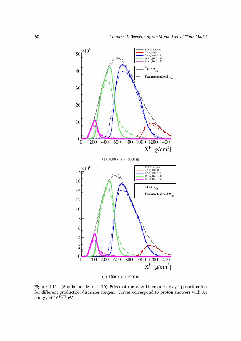
60 Chapter 4. Revision of the Muon Arrival Time Model
]2 [g/cmµX0 200 400 600 800 1000 1200 14000
10
20
30
40
50610× Full distribution
[km] < 5v0 < z[km] < 10v5 < z
[km] < 15v10 < z[km] < 20v15 < z
kinτTrue
kinτParameterized
(a) 1000 < r < 4000 m
]2 [g/cmµX0 200 400 600 800 1000 1200 14000
2
4
6
8
10
12
14
16
18610× Full distribution
[km] < 5v0 < z[km] < 10v5 < z
[km] < 15v10 < z[km] < 20v15 < z
kinτTrue
kinτParameterized
(b) 1700 < r < 4000 m
Figure 4.11: (Similar to figure 4.10) Effect of the new kinematic delay approximationfor different production distances ranges. Curves correspond to proton showers with anenergy of 1019.75 eV.
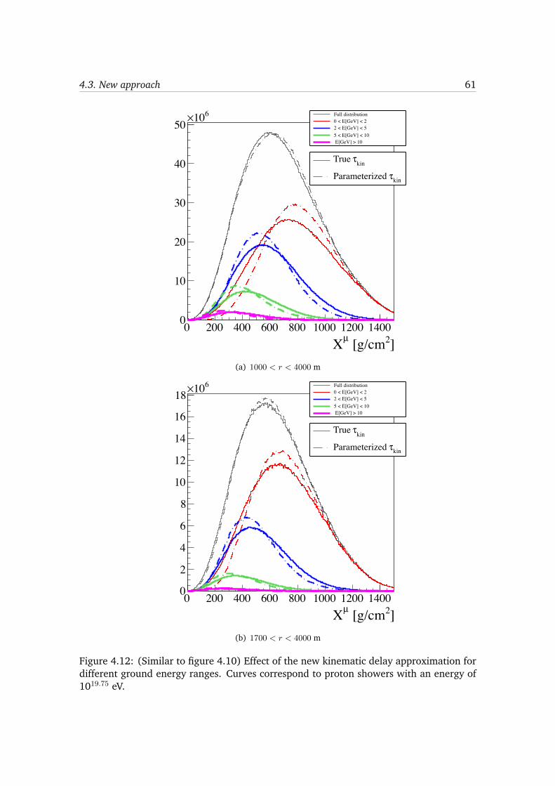
4.3. New approach 61
]2 [g/cmµX0 200 400 600 800 1000 1200 14000
10
20
30
40
50610× Full distribution
0 < E[GeV] < 22 < E[GeV] < 55 < E[GeV] < 10 E[GeV] > 10
kinτTrue
kinτParameterized
(a) 1000 < r < 4000 m
]2 [g/cmµX0 200 400 600 800 1000 1200 14000
2
4
6
8
10
12
14
16
18610× Full distribution
0 < E[GeV] < 22 < E[GeV] < 55 < E[GeV] < 10 E[GeV] > 10
kinτTrue
kinτParameterized
(b) 1700 < r < 4000 m
Figure 4.12: (Similar to figure 4.10) Effect of the new kinematic delay approximation fordifferent ground energy ranges. Curves correspond to proton showers with an energy of1019.75 eV.
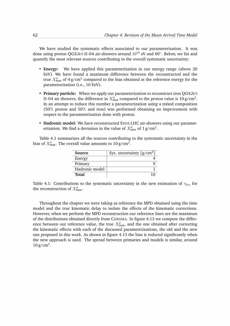
62 Chapter 4. Revision of the Muon Arrival Time Model
We have studied the systematic effects associated to our parameterization. It wasdone using proton QGSJET-II-04 air-showers around 1019 eV and 60�. Below, we list andquantify the most relevant sources contributing to the overall systematic uncertainty:
• Energy: We have applied this parameterization in our energy range (above 20EeV). We have found a maximum difference between the reconstructed and thetrue X
µ
max of 4 g/cm2 compared to the bias obtained at the reference energy for theparameterization (i.e., 10 EeV).
• Primary particle: When we apply our parameterization to reconstruct iron QGSJET-II-04 air showers, the difference in X
µ
max compared to the proton value is 10 g/cm2.In an attempt to reduce this number a parameterization using a mixed composition(50% proton and 50% and iron) was performed obtaining no improvement withrespect to the parameterization done with proton.
• Hadronic model: We have reconstructed EPOS LHC air-showers using our paramet-erization. We find a deviation in the value of Xµ
max of 1 g/cm2.
Table 4.1 summarizes all the sources contributing to the systematic uncertainty in thebias of Xµ
max. The overall value amounts to 10 g/cm2.
Source Sys. uncertainty [g/cm2]Energy 4Primary 9Hadronic model 1Total 10
Table 4.1: Contributions to the systematic uncertainty in the new estimation of ⌧kin
forthe reconstruction of Xµ
max.
Throughout the chapter we were taking as reference the MPD obtained using the timemodel and the true kinematic delay to isolate the effects of the kinematic corrections.However, when we perform the MPD reconstruction our reference lines are the maximumof the distributions obtained directly from CORSIKA. In figure 4.13 we compute the differ-ence between our reference value, the true X
µ
max, and the one obtained after correctingthe kinematic effects with each of the discussed parameterizations, the old and the newone proposed in this work. As shown in figure 4.13 the bias is reduced significantly whenthe new approach is used. The spread between primaries and models is similar, around10 g/cm2.
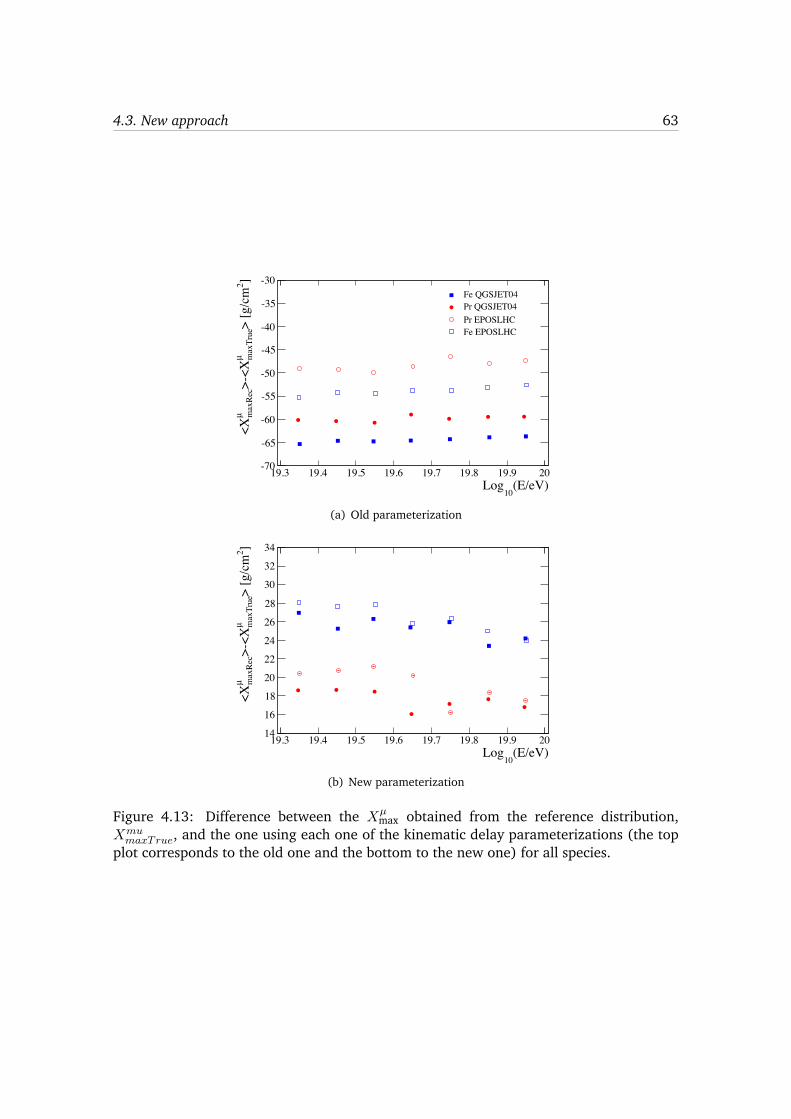
4.3. New approach 63
(E/eV)10
Log19.3 19.4 19.5 19.6 19.7 19.8 19.9 20
]2>
[g/c
mm
axTr
ueµ
>-<X
max
Rec
µ<X
-70
-65
-60
-55
-50
-45
-40
-35
-30Fe QGSJET04Pr QGSJET04Pr EPOSLHCFe EPOSLHC
(a) Old parameterization
(E/eV)10
Log19.3 19.4 19.5 19.6 19.7 19.8 19.9 20
]2>
[g/c
mm
axTr
ueµ
>-<X
max
Rec
µ<X
14
16
18
20
22
24
26
28
30
32
34
(b) New parameterization
Figure 4.13: Difference between the X
µ
max obtained from the reference distribution,X
mu
maxTrue
, and the one using each one of the kinematic delay parameterizations (the topplot corresponds to the old one and the bottom to the new one) for all species.

5Muon Production Depth in anevent by event basis
In the previous chapter we have described the theoretical framework supporting the MPDanalysis. In this chapter we focus our interest in the reconstruction of the distributions atdetector level. The features of the MPD distributions and the different steps followed inthe event by event reconstruction are discussed in [1] and in [133]. Here, we assess theeffect that each one of the intermediate steps have in the total bias and resolution we getby going from the true distribution (the one obtained directly from CORSIKA) to the finalone after the whole reconstruction chain has been applied.
5.1 MPD features
The MPD is reconstructed using the FADC signals provided by the water-Cherenkov detect-ors. The finite area of the detectors induces fluctuations due to the different muon samplesbeing collected. In addition, the shape of the MPD distribution observed from differentpositions at the ground varies because of differences in the probability of in-flight decayand because muons are not produced isotropically around the shower axis. It is an integ-ration over distance, r, which enables the estimation of the dN
µ
/dX distribution or MPDdistribution (where N
µ
refers to the number of produced muons). However, for discretedetector arrays, measurements at just a handful of r values are available and are limitedto a small number of muons due to the finite collection surface (for Auger detectors itamounts to 10 m2 cross-section for vertical incidence).
Another important feature of the MPD distribution observed at the ground is its de-pendence on the zenith angle. There are two reasons for this. The first one is due tothe fact that inclined events mostly evolve in a less dense atmosphere than more verticalones. This makes pions reach their critical energies (✏⇡
c
) at higher altitude resulting ina shallower development of the shower. While the shapes of the muon distribution atproduction are almost unaffected by this difference in reaching ✏
⇡
c
[130], their productiondepths are shifted. For proton showers at 1019 eV, the difference between the distributionof maxima for vertical and 60� events is approximately 20 g/cm2. The second and mainreason for the zenith angle dependence of the MPD distribution is a consequence of themuon-decay probability. This effect influences not only the location of the maximum butalso the shape of the observed MPD distribution. Figure 5.1 demonstrates this dependence
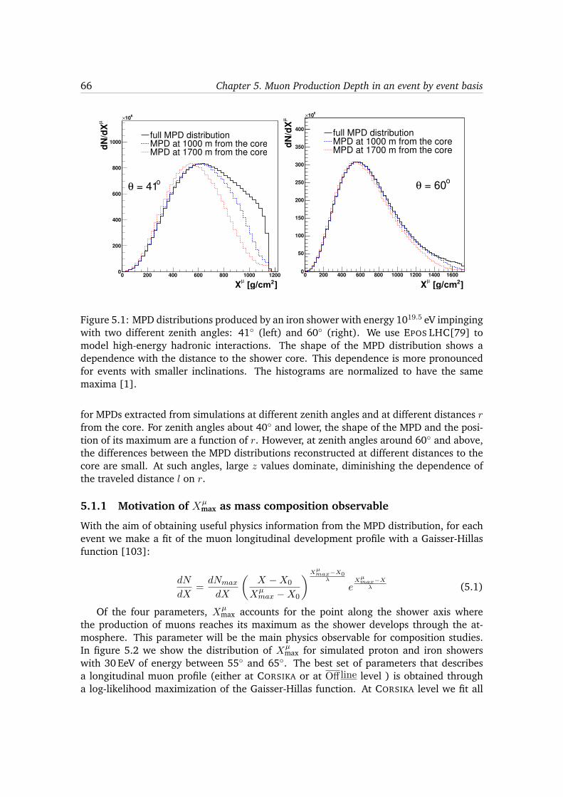
66 Chapter 5. Muon Production Depth in an event by event basis
]2[g/cmµX0 200 400 600 800 1000 1200
µdN
/dX
0
200
400
600
800
1000
610◊
full MPD distribution
MPD at 1000 m from the core
MPD at 1700 m from the core
o
= 41�
]2[g/cmµX0 200 400 600 800 1000 1200 1400 1600
µdN
/dX
0
50
100
150
200
250
300
350
400
610◊
full MPD distribution
MPD at 1000 m from the core
MPD at 1700 m from the core
o
= 60�
Figure 5.1: MPD distributions produced by an iron shower with energy 1019.5 eV impingingwith two different zenith angles: 41� (left) and 60� (right). We use EPOS LHC[79] tomodel high-energy hadronic interactions. The shape of the MPD distribution shows adependence with the distance to the shower core. This dependence is more pronouncedfor events with smaller inclinations. The histograms are normalized to have the samemaxima [1].
for MPDs extracted from simulations at different zenith angles and at different distances rfrom the core. For zenith angles about 40� and lower, the shape of the MPD and the posi-tion of its maximum are a function of r. However, at zenith angles around 60� and above,the differences between the MPD distributions reconstructed at different distances to thecore are small. At such angles, large z values dominate, diminishing the dependence ofthe traveled distance l on r.
5.1.1 Motivation of Xµ
max as mass composition observable
With the aim of obtaining useful physics information from the MPD distribution, for eachevent we make a fit of the muon longitudinal development profile with a Gaisser-Hillasfunction [103]:
dN
dX
=dN
max
dX
✓X �X0
X
µ
max
�X0
◆X
µ
max
�X0�
e
X
µ
max
�X
� (5.1)
Of the four parameters, X
µ
max accounts for the point along the shower axis wherethe production of muons reaches its maximum as the shower develops through the at-mosphere. This parameter will be the main physics observable for composition studies.In figure 5.2 we show the distribution of X
µ
max for simulated proton and iron showerswith 30 EeV of energy between 55� and 65�. The best set of parameters that describesa longitudinal muon profile (either at CORSIKA or at O↵ line level ) is obtained througha log-likelihood maximization of the Gaisser-Hillas function. At CORSIKA level we fit all
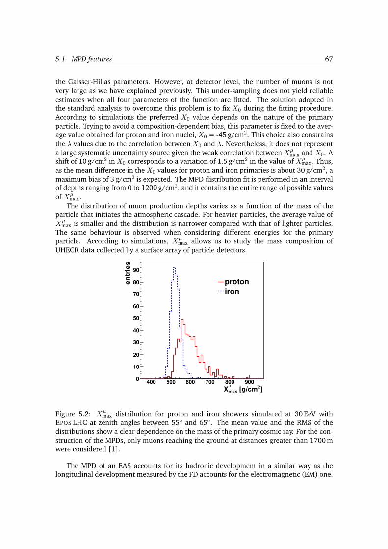
5.1. MPD features 67
the Gaisser-Hillas parameters. However, at detector level, the number of muons is notvery large as we have explained previously. This under-sampling does not yield reliableestimates when all four parameters of the function are fitted. The solution adopted inthe standard analysis to overcome this problem is to fix X0 during the fitting procedure.According to simulations the preferred X0 value depends on the nature of the primaryparticle. Trying to avoid a composition-dependent bias, this parameter is fixed to the aver-age value obtained for proton and iron nuclei, X0 = -45 g/cm2. This choice also constrainsthe � values due to the correlation between X0 and �. Nevertheless, it does not representa large systematic uncertainty source given the weak correlation between X
µ
max and X0. Ashift of 10 g/cm2 in X0 corresponds to a variation of 1.5 g/cm2 in the value of Xµ
max. Thus,as the mean difference in the X0 values for proton and iron primaries is about 30 g/cm2, amaximum bias of 3 g/cm2 is expected. The MPD distribution fit is performed in an intervalof depths ranging from 0 to 1200 g/cm2, and it contains the entire range of possible valuesof Xµ
max.The distribution of muon production depths varies as a function of the mass of the
particle that initiates the atmospheric cascade. For heavier particles, the average value ofX
µ
max is smaller and the distribution is narrower compared with that of lighter particles.The same behaviour is observed when considering different energies for the primaryparticle. According to simulations, X
µ
max allows us to study the mass composition ofUHECR data collected by a surface array of particle detectors.
]2[g/cmmaxµX
400 500 600 700 800 900
entr
ies
0
10
20
30
40
50
60
70
80
90
protoniron
Figure 5.2: X
µ
max distribution for proton and iron showers simulated at 30 EeV withEPOS LHC at zenith angles between 55� and 65�. The mean value and the RMS of thedistributions show a clear dependence on the mass of the primary cosmic ray. For the con-struction of the MPDs, only muons reaching the ground at distances greater than 1700 mwere considered [1].
The MPD of an EAS accounts for its hadronic development in a similar way as thelongitudinal development measured by the FD accounts for the electromagnetic (EM) one.
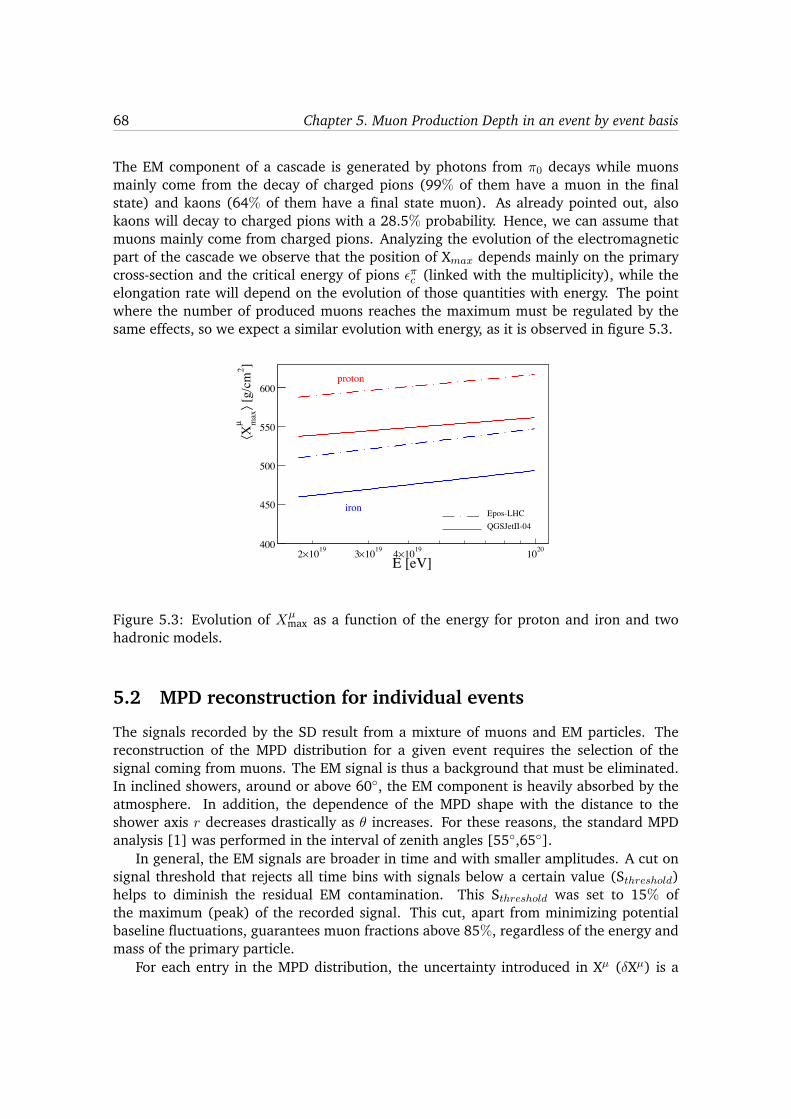
68 Chapter 5. Muon Production Depth in an event by event basis
The EM component of a cascade is generated by photons from ⇡0 decays while muonsmainly come from the decay of charged pions (99% of them have a muon in the finalstate) and kaons (64% of them have a final state muon). As already pointed out, alsokaons will decay to charged pions with a 28.5% probability. Hence, we can assume thatmuons mainly come from charged pions. Analyzing the evolution of the electromagneticpart of the cascade we observe that the position of X
max
depends mainly on the primarycross-section and the critical energy of pions ✏
⇡
c
(linked with the multiplicity), while theelongation rate will depend on the evolution of those quantities with energy. The pointwhere the number of produced muons reaches the maximum must be regulated by thesame effects, so we expect a similar evolution with energy, as it is observed in figure 5.3.
E [eV]1910×2 1910×3 1910×4 2010
]2 [g
/cm
⟩m
ax
µX⟨
400
450
500
550
600
Epos-LHCQGSJetII-04
proton
iron
Figure 5.3: Evolution of Xµ
max as a function of the energy for proton and iron and twohadronic models.
5.2 MPD reconstruction for individual events
The signals recorded by the SD result from a mixture of muons and EM particles. Thereconstruction of the MPD distribution for a given event requires the selection of thesignal coming from muons. The EM signal is thus a background that must be eliminated.In inclined showers, around or above 60�, the EM component is heavily absorbed by theatmosphere. In addition, the dependence of the MPD shape with the distance to theshower axis r decreases drastically as ✓ increases. For these reasons, the standard MPDanalysis [1] was performed in the interval of zenith angles [55�,65�].
In general, the EM signals are broader in time and with smaller amplitudes. A cut onsignal threshold that rejects all time bins with signals below a certain value (S
threshold
)helps to diminish the residual EM contamination. This S
threshold
was set to 15% ofthe maximum (peak) of the recorded signal. This cut, apart from minimizing potentialbaseline fluctuations, guarantees muon fractions above 85%, regardless of the energy andmass of the primary particle.
For each entry in the MPD distribution, the uncertainty introduced in Xµ (�Xµ) is a
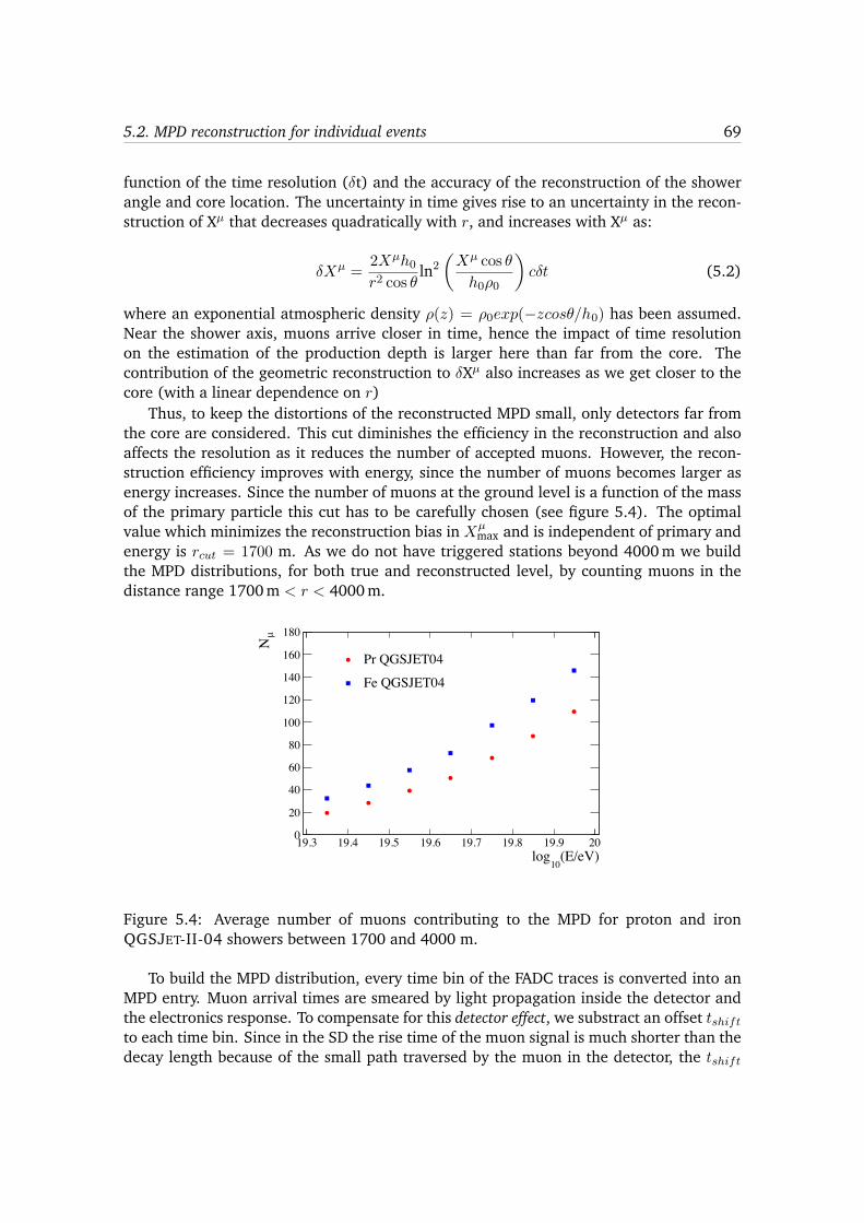
5.2. MPD reconstruction for individual events 69
function of the time resolution (�t) and the accuracy of the reconstruction of the showerangle and core location. The uncertainty in time gives rise to an uncertainty in the recon-struction of Xµ that decreases quadratically with r, and increases with Xµ as:
�X
µ =2Xµ
h0
r
2 cos ✓ln2
✓X
µ cos ✓
h0⇢0
◆c�t (5.2)
where an exponential atmospheric density ⇢(z) = ⇢0exp(�zcos✓/h0) has been assumed.Near the shower axis, muons arrive closer in time, hence the impact of time resolutionon the estimation of the production depth is larger here than far from the core. Thecontribution of the geometric reconstruction to �Xµ also increases as we get closer to thecore (with a linear dependence on r)
Thus, to keep the distortions of the reconstructed MPD small, only detectors far fromthe core are considered. This cut diminishes the efficiency in the reconstruction and alsoaffects the resolution as it reduces the number of accepted muons. However, the recon-struction efficiency improves with energy, since the number of muons becomes larger asenergy increases. Since the number of muons at the ground level is a function of the massof the primary particle this cut has to be carefully chosen (see figure 5.4). The optimalvalue which minimizes the reconstruction bias in X
µ
max and is independent of primary andenergy is r
cut
= 1700 m. As we do not have triggered stations beyond 4000 m we buildthe MPD distributions, for both true and reconstructed level, by counting muons in thedistance range 1700 m < r < 4000 m.
(E/eV)10
log19.3 19.4 19.5 19.6 19.7 19.8 19.9 20
µN
0
20
40
60
80
100
120
140
160
180
Pr QGSJET04
Fe QGSJET04
Figure 5.4: Average number of muons contributing to the MPD for proton and ironQGSJET-II-04 showers between 1700 and 4000 m.
To build the MPD distribution, every time bin of the FADC traces is converted into anMPD entry. Muon arrival times are smeared by light propagation inside the detector andthe electronics response. To compensate for this detector effect, we substract an offset t
shift
to each time bin. Since in the SD the rise time of the muon signal is much shorter than thedecay length because of the small path traversed by the muon in the detector, the t
shift
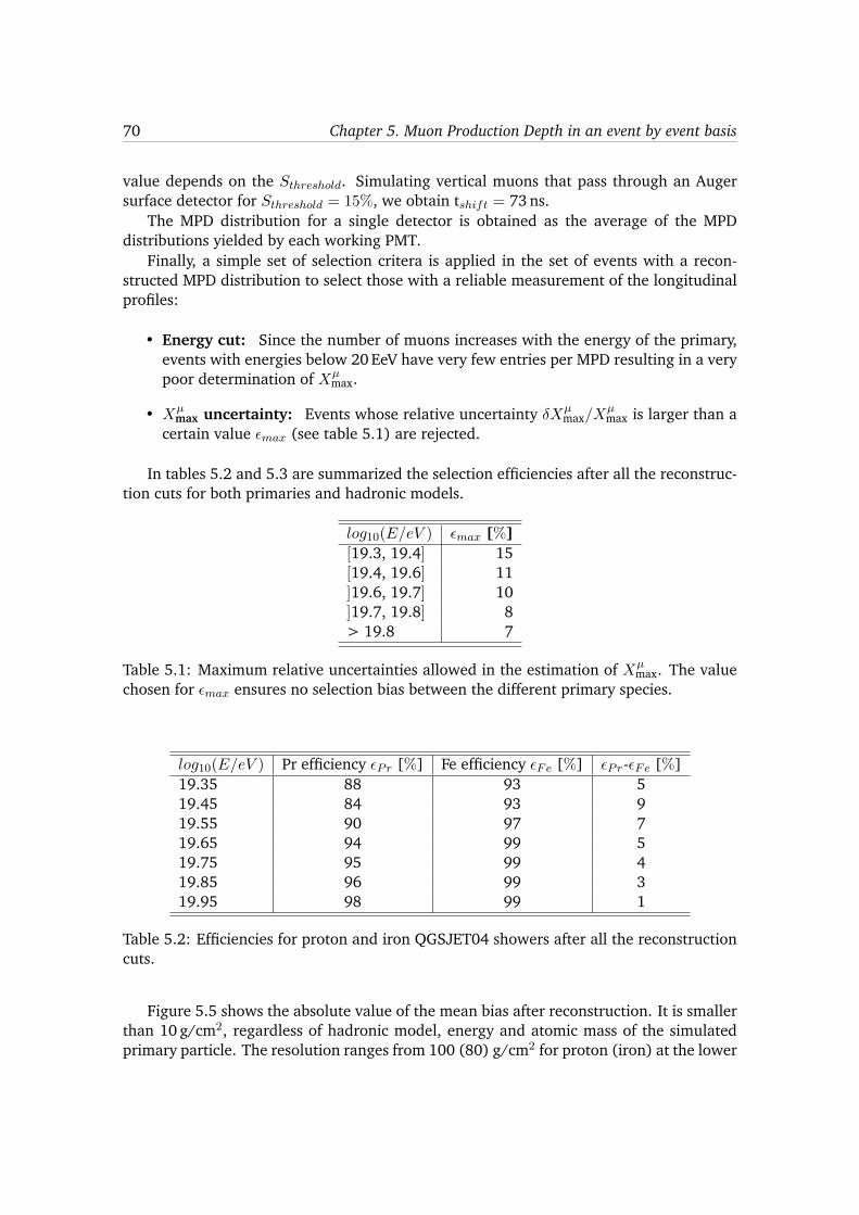
70 Chapter 5. Muon Production Depth in an event by event basis
value depends on the S
threshold
. Simulating vertical muons that pass through an Augersurface detector for S
threshold
= 15%, we obtain tshift
= 73 ns.The MPD distribution for a single detector is obtained as the average of the MPD
distributions yielded by each working PMT.Finally, a simple set of selection critera is applied in the set of events with a recon-
structed MPD distribution to select those with a reliable measurement of the longitudinalprofiles:
• Energy cut: Since the number of muons increases with the energy of the primary,events with energies below 20 EeV have very few entries per MPD resulting in a verypoor determination of Xµ
max.
• X
µ
max uncertainty: Events whose relative uncertainty �X
µ
max/Xµ
max is larger than acertain value ✏
max
(see table 5.1) are rejected.
In tables 5.2 and 5.3 are summarized the selection efficiencies after all the reconstruc-tion cuts for both primaries and hadronic models.
log10(E/eV ) ✏
max
[%][19.3, 19.4] 15[19.4, 19.6] 11]19.6, 19.7] 10]19.7, 19.8] 8> 19.8 7
Table 5.1: Maximum relative uncertainties allowed in the estimation of Xµ
max. The valuechosen for ✏
max
ensures no selection bias between the different primary species.
log10(E/eV ) Pr efficiency ✏
Pr
[%] Fe efficiency ✏
Fe
[%] ✏
Pr
-✏Fe
[%]19.35 88 93 519.45 84 93 919.55 90 97 719.65 94 99 519.75 95 99 419.85 96 99 319.95 98 99 1
Table 5.2: Efficiencies for proton and iron QGSJET04 showers after all the reconstructioncuts.
Figure 5.5 shows the absolute value of the mean bias after reconstruction. It is smallerthan 10 g/cm2, regardless of hadronic model, energy and atomic mass of the simulatedprimary particle. The resolution ranges from 100 (80) g/cm2 for proton (iron) at the lower
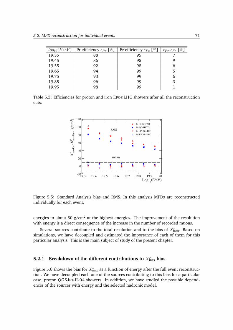
5.2. MPD reconstruction for individual events 71
log10(E/eV ) Pr efficiency ✏
Pr
[%] Fe efficiency ✏
Fe
[%] ✏
Pr
-✏Fe
[%]19.35 88 95 719.45 86 95 919.55 92 98 619.65 94 99 519.75 93 99 619.85 96 99 319.95 98 99 1
Table 5.3: Efficiencies for proton and iron EPOS LHC showers after all the reconstructioncuts.
(E/eV)10
Log19.3 19.4 19.5 19.6 19.7 19.8 19.9 20
]2 [g
/cm
max
True
µ-X
max
Rec
µ X
-20
0
20
40
60
80
100
120Pr QGSJET04Fe QGSJET04Pr EPOS-LHCFe EPOS-LHC
RMS
mean
Figure 5.5: Standard Analysis bias and RMS. In this analysis MPDs are reconstructedindividually for each event.
energies to about 50 g/cm2 at the highest energies. The improvement of the resolutionwith energy is a direct consequence of the increase in the number of recorded muons.
Several sources contribute to the total resolution and to the bias of Xµ
max. Based onsimulations, we have decoupled and estimated the importance of each of them for thisparticular analysis. This is the main subject of study of the present chapter.
5.2.1 Breakdown of the different contributions to Xµ
max bias
Figure 5.6 shows the bias for Xµ
max as a function of energy after the full event reconstruc-tion. We have decoupled each one of the sources contributing to this bias for a particularcase, proton QGSJET-II-04 showers. In addition, we have studied the possible depend-ences of the sources with energy and the selected hadronic model.
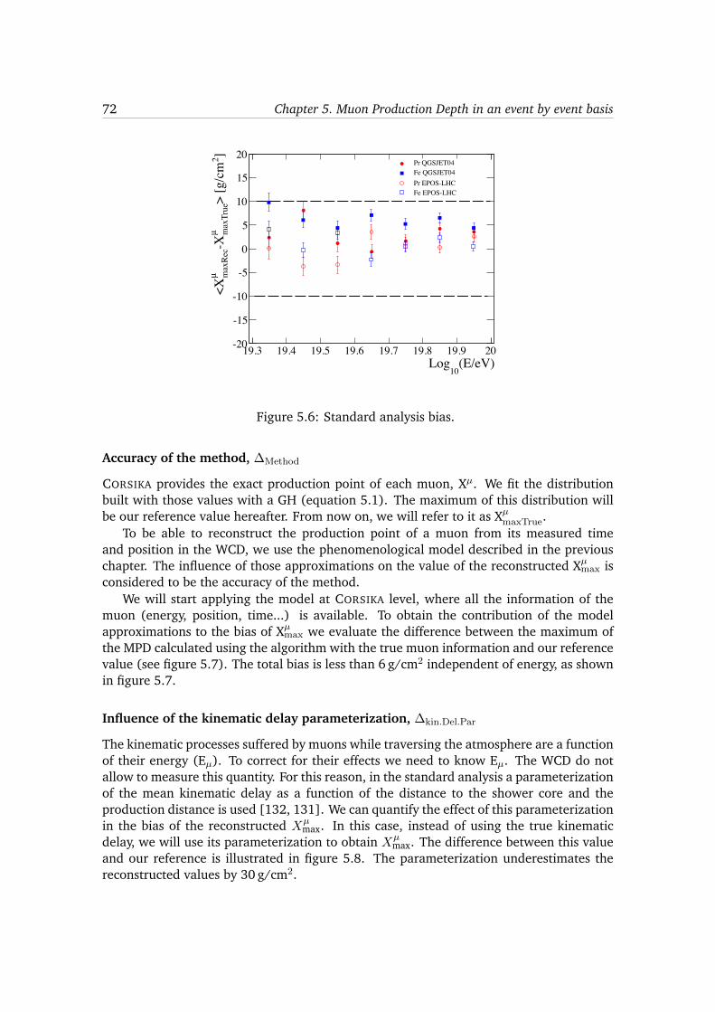
72 Chapter 5. Muon Production Depth in an event by event basis
(E/eV)10
Log19.3 19.4 19.5 19.6 19.7 19.8 19.9 20
]2>
[g/c
mm
axTr
ueµ
-Xm
axRe
cµ
<X
-20
-15
-10
-5
0
5
10
15
20Pr QGSJET04Fe QGSJET04Pr EPOS-LHCFe EPOS-LHC
Figure 5.6: Standard analysis bias.
Accuracy of the method, �Method
CORSIKA provides the exact production point of each muon, Xµ. We fit the distributionbuilt with those values with a GH (equation 5.1). The maximum of this distribution willbe our reference value hereafter. From now on, we will refer to it as Xµ
maxTrue.To be able to reconstruct the production point of a muon from its measured time
and position in the WCD, we use the phenomenological model described in the previouschapter. The influence of those approximations on the value of the reconstructed Xµ
max isconsidered to be the accuracy of the method.
We will start applying the model at CORSIKA level, where all the information of themuon (energy, position, time...) is available. To obtain the contribution of the modelapproximations to the bias of Xµ
max we evaluate the difference between the maximum ofthe MPD calculated using the algorithm with the true muon information and our referencevalue (see figure 5.7). The total bias is less than 6 g/cm2 independent of energy, as shownin figure 5.7.
Influence of the kinematic delay parameterization, �kin.Del.Par
The kinematic processes suffered by muons while traversing the atmosphere are a functionof their energy (E
µ
). To correct for their effects we need to know Eµ
. The WCD do notallow to measure this quantity. For this reason, in the standard analysis a parameterizationof the mean kinematic delay as a function of the distance to the shower core and theproduction distance is used [132, 131]. We can quantify the effect of this parameterizationin the bias of the reconstructed X
µ
max. In this case, instead of using the true kinematicdelay, we will use its parameterization to obtain X
µ
max. The difference between this valueand our reference is illustrated in figure 5.8. The parameterization underestimates thereconstructed values by 30 g/cm2.

5.2. MPD reconstruction for individual events 73
(E/eV)10
Log19.4 19.5 19.6 19.7 19.8 19.9
]2>
[g/c
mm
axTr
ueµ
-Xm
axRe
cµ
<X
-100
-50
0
50
100
150
200
250
2 0.1 g/cm±5.6
Figure 5.7: Contribution to the bias of Xµ
max reconstructed from the approximations donein the muon arrival time model.
(E/eV)10
Log19.4 19.5 19.6 19.7 19.8 19.9
]2 >
[g/c
mm
axTr
ueµ
-Xm
axRe
cµ
< X
-100
-50
0
50
100
150
200
250
2 0.1 g/cm±-30.6
(a) CORSIKA
(E/eV)10
Log19.4 19.5 19.6 19.7 19.8 19.9
]2 >
[g/c
mm
axTr
ueµ
-Xm
axRe
cµ
< X
-100
-50
0
50
100
150
200
250
2 0.4 g/cm±-60.8
(b) O↵ line
Figure 5.8: Effect of the kinematic delay parameterization in the mean value of Xµ
maxRec
at CORSIKA (left plot) and at O↵ line level (right plot).
In O↵ line simulations we have access to the true properties of the muon at the ground(times, geometry, ...). Thus, the impact of the kinematic delay parameterization can like-wise be assessed at O↵ line level1. At detector level, the number of muons contributingto each MPD is very small in comparison with CORSIKA. For proton showers we have 20muons on average at 20 EeV. This comes from the spacing between the WCD and ourdistance cut. To reduce possible distortions due to the lack of statistics, particularly atlow energies, we simulate the showers in a dense array2 where we enlarge the number of
1The true kinematic delay can not be evaluated at O↵ line level because we can not access the muon energyat production.
2WCD separated 750 m instead of 1500 m.

74 Chapter 5. Muon Production Depth in an event by event basis
muons by a factor 3 (see figure 5.9). The observed underestimation of Xµ
max due to thekinematic delay parameterization is two times bigger when we evaluate it using O↵ line
simulations (see figure 5.8 right).
(E/eV)10
log19.3 19.4 19.5 19.6 19.7 19.8 19.9 20
µN
0
50
100
150
200
250
300
350
400
Figure 5.9: Number of muons as a function of the energy in the standard array (filleddots) and in a dense array (empty dots) for protons simulated using QGSJET04.
This discrepancy must come from subtle differences between the information obtainedfrom CORSIKA and the true information obtained from O↵ line simulations. In principle,apart from the number of muons contributing to each MPD, the conditions in CORSIKA andin O↵ line (using the true information) are the same. However, to produce the CORSIKAfiles we use the thinning algorithm because the CPU time required for the simulation offull (non-thinned) EAS on a large scale is unmanageable. In this approximation, amongthe vast number of particles generated in the simulation, only a subsample of them arefollowed up to the end. Statistical weights are assigned to the surviving particles in rep-resentation of those ones that, in similar regions of phase space, have been removed alongthe procedure. In particular, we use simulated showers with a thinning level of 10�6. Thechoice of this thinning level can affect the MPD distribution. We evaluate this effect com-paring showers at CORSIKA level with a thinning of 10�5, 10�6 and 10�7. The differencesobtained are smaller than 2 g/cm2, see figure 5.10.
The surface of each WCD is small compared to their spacing. In these conditionsthe simulation output contains very few particles falling exactly onto each detector. Todeal with this problem it is implemented the un-thinning or resampling procedure. Itspurpose is to use a wider sampling in the ground particle file to obtain a fair simulationof the particles entering in the detector. A reliable simulation of any detector responsedepends on the quality of the estimation of the local density of particles at the position ofthe detector. Within this context, these fluxes are obtained as averages over more or lessextended areas around the location of interest. The module doing this in the O↵ line isthe CachedShowerRegenerator. For the injection of a realistic flux of particles in a specificsurface detector, the resampling method defines a sampling-area (see figure 5.11) whichis defined by two parameters: a radial distance (�) and an angular aperture (↵) from the
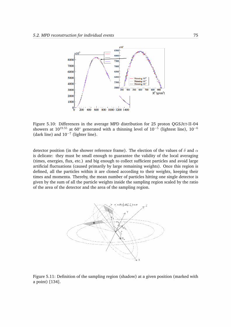
5.2. MPD reconstruction for individual events 75
Figure 5.10: Differences in the average MPD distribution for 25 proton QGSJET-II-04showers at 1019.55 at 60� generated with a thinning level of 10�5 (lightest line), 10�6
(dark line) and 10�7 (lighter line).
detector position (in the shower reference frame). The election of the values of � and ↵
is delicate: they must be small enough to guarantee the validity of the local averaging(times, energies, flux, etc.) and big enough to collect sufficient particles and avoid largeartificial fluctuations (caused primarily by large remaining weights). Once this region isdefined, all the particles within it are cloned according to their weights, keeping theirtimes and momenta. Thereby, the mean number of particles hitting one single detector isgiven by the sum of all the particle weights inside the sampling region scaled by the ratioof the area of the detector and the area of the sampling region.
Figure 5.11: Definition of the sampling region (shadow) at a given position (marked witha point) [134].
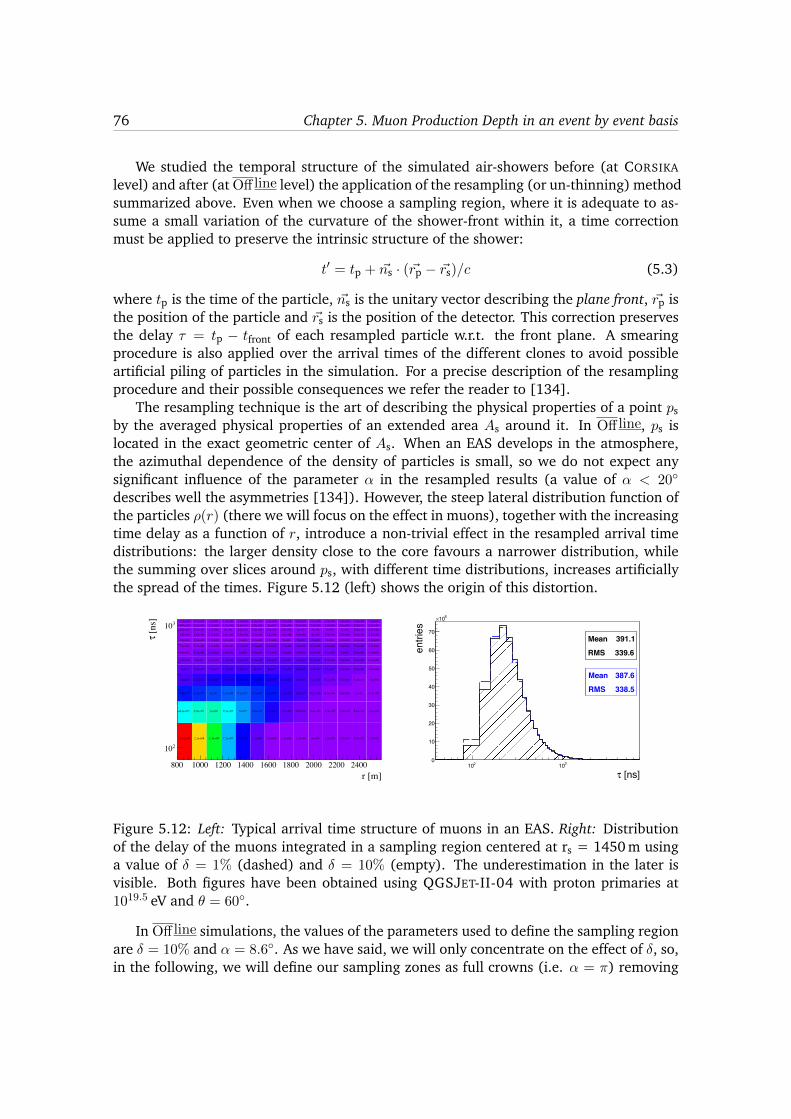
76 Chapter 5. Muon Production Depth in an event by event basis
We studied the temporal structure of the simulated air-showers before (at CORSIKAlevel) and after (at O↵ line level) the application of the resampling (or un-thinning) methodsummarized above. Even when we choose a sampling region, where it is adequate to as-sume a small variation of the curvature of the shower-front within it, a time correctionmust be applied to preserve the intrinsic structure of the shower:
t
0 = tp + ~ns · (~rp � ~rs)/c (5.3)
where tp is the time of the particle, ~ns is the unitary vector describing the plane front, ~rp isthe position of the particle and ~rs is the position of the detector. This correction preservesthe delay ⌧ = tp � tfront of each resampled particle w.r.t. the front plane. A smearingprocedure is also applied over the arrival times of the different clones to avoid possibleartificial piling of particles in the simulation. For a precise description of the resamplingprocedure and their possible consequences we refer the reader to [134].
The resampling technique is the art of describing the physical properties of a point psby the averaged physical properties of an extended area As around it. In O↵ line, ps islocated in the exact geometric center of As. When an EAS develops in the atmosphere,the azimuthal dependence of the density of particles is small, so we do not expect anysignificant influence of the parameter ↵ in the resampled results (a value of ↵ < 20�
describes well the asymmetries [134]). However, the steep lateral distribution function ofthe particles ⇢(r) (there we will focus on the effect in muons), together with the increasingtime delay as a function of r, introduce a non-trivial effect in the resampled arrival timedistributions: the larger density close to the core favours a narrower distribution, whilethe summing over slices around ps, with different time distributions, increases artificiallythe spread of the times. Figure 5.12 (left) shows the origin of this distortion.
2.5e+08 2.1e+08 1.3e+08 7.2e+07 3.2e+07 1.2e+07 3.9e+06 1.1e+06 2.7e+05 6e+04 1.2e+04 2.5e+03 5.9e+02 1.3e+02
8.6e+07 9.9e+07 1e+08 9.1e+07 7e+07 4.6e+07 2.7e+07 1.3e+07 5.9e+06 2.4e+06 8.5e+05 2.9e+05 8.6e+04 2.4e+04
3.6e+07 4.3e+07 5e+07 5.3e+07 5.1e+07 4.5e+07 3.6e+07 2.5e+07 1.6e+07 9.3e+06 4.9e+06 2.4e+06 1e+06 4.3e+05
1.8e+07 2.2e+07 2.6e+07 2.9e+07 3.1e+07 3.1e+07 2.9e+07 2.4e+07 1.9e+07 1.4e+07 9.2e+06 5.7e+06 3.2e+06 1.8e+06
1e+07 1.3e+07 1.5e+07 1.7e+07 1.9e+07 2e+07 2e+07 1.9e+07 1.6e+07 1.4e+07 1.1e+07 7.7e+06 5.2e+06 3.4e+06
6.5e+06 8e+06 9.1e+06 1.1e+07 1.2e+07 1.3e+07 1.3e+07 1.3e+07 1.3e+07 1.1e+07 9.7e+06 7.8e+06 5.9e+06 4.3e+06
4.6e+06 5.3e+06 6.2e+06 6.9e+06 8e+06 8.5e+06 9.2e+06 9.4e+06 9.3e+06 8.9e+06 8.1e+06 7e+06 5.8e+06 4.6e+06
3.1e+06 3.7e+06 4.1e+06 4.8e+06 5.3e+06 5.9e+06 6.3e+06 6.7e+06 6.8e+06 6.7e+06 6.4e+06 5.8e+06 5.1e+06 4.3e+06
2.2e+06 2.6e+06 3.1e+06 3.5e+06 4e+06 4.3e+06 4.5e+06 5e+06 5e+06 5e+06 5e+06 4.7e+06 4.2e+06 3.8e+06
1.5e+06 1.8e+06 2.3e+06 2.6e+06 2.9e+06 3.1e+06 3.4e+06 3.6e+06 3.8e+06 4e+06 3.9e+06 3.7e+06 3.5e+06 3.2e+061.2e+06 1.5e+06 1.7e+06 2e+06 2.2e+06 2.4e+06 2.6e+06 2.8e+06 3e+06 3e+06 3e+06 3e+06 2.8e+06 2.7e+069.7e+05 1.1e+06 1.3e+06 1.5e+06 1.6e+06 1.9e+06 2e+06 2.2e+06 2.3e+06 2.4e+06 2.4e+06 2.4e+06 2.3e+06 2.3e+067.5e+05 8.7e+05 1e+06 1.2e+06 1.3e+06 1.5e+06 1.5e+06 1.8e+06 1.8e+06 1.9e+06 1.9e+06 1.9e+06 1.9e+06 1.9e+06
r [m]800 1000 1200 1400 1600 1800 2000 2200 2400
[ns]
τ
210
310
Mean 387.6
RMS 338.5
[ns]τ210 310
entri
es
0
10
20
30
40
50
60
70
610×
Mean 387.6
RMS 338.5
Mean 391.1
RMS 339.6
Mean 391.1
RMS 339.6
Figure 5.12: Left: Typical arrival time structure of muons in an EAS. Right: Distributionof the delay of the muons integrated in a sampling region centered at rs = 1450 m usinga value of � = 1% (dashed) and � = 10% (empty). The underestimation in the later isvisible. Both figures have been obtained using QGSJET-II-04 with proton primaries at1019.5 eV and ✓ = 60�.
In O↵ line simulations, the values of the parameters used to define the sampling regionare � = 10% and ↵ = 8.6�. As we have said, we will only concentrate on the effect of �, so,in the following, we will define our sampling zones as full crowns (i.e. ↵ = ⇡) removing

5.2. MPD reconstruction for individual events 77
any dependence on ↵, while we increase the number of particles. Using CORSIKA, we“mimic” the O↵ line conditions at a distance rs from the core, by integrating the numberof particles (muons) in the crown defined by |rs � r| < 0.1|rs|. We define the true valueswhen � = 1%. Under that condition, we have verified that the weighted/integrated valueof r in the crown correlates perfectly with rs at each position (correlation factor ⇡ 1), sowe assume no bias.
Figure 5.12 (right) shows the “true” and the “O↵ line” distributions of muon delays ina sampling region centered at rs = 1450 m, and for a sample of proton showers simulatedusing QGSJET-II-04 with E = 1019.5 eV and zenith angle ✓ = 60�. As we see in the fig-ure 5.12 (left), the number of muons decreases rapidly with r while the delay ⌧ increases.The resampling procedure favors a bias towards smaller values of ⌧ for large values of �,as we see in the right-panel of that figure.
r [m]1000 1500 2000 2500 3000 3500 4000
> [n
s]τ
<
200400600800
100012001400160018002000
r [m]1500 2000 2500 3000 3500
> [n
s]τ
< ∆
-40
-35
-30
-25
-20
-15
-10
-5
0
Figure 5.13: Left: Averaged time front curvatures obtained for two different definitionsof the sampling region: �true = 1% (circles) and �off = 10% (triangles). Right: Averagedvalues of the expected bias in the muon delay in O↵ line by the resampling procedure.The fit to a quadratic function is also shown just to guide the eyes. This figure has beenobtained using proton showers simulated with CORSIKA with QGSJET-II-04, E = 1019.5 eVand ✓ = 60�.
The averaged delay of the muons (for the same sample of simulations) as a functionof the distance to the shower axis is shown in figure 5.13. In the left panel, we show theresults for two values of �: 1% (circles) and 10% (triangles). To quantify the magnitudeof this bias and its dependence with the position, in the panel on the right we show theresiduals of h⌧i (O↵ line � true) as a function of r. It is important to notice that close tothe core (< 2000 m) the underestimation of h⌧i is small (< 10 ns) for the O↵ line value of�. The value of the bias increases with r (approximately with r
2) becoming very large atlarge distances from the core, but its relative importance decreases given the attenuationon the number of muons with r.
As expected, the dependence of the bias with the particular choice of � is large, asshown in figure 5.14 (left), where the results obtained for half (5%) and twice (20%) thevalue used in O↵ line are shown. In [134] some corrections are suggested, based on gen-eral assumptions that preserve the shower-to-shower fluctuations, to reduce the differentbiases. In figure 5.14 (right) we show the result of applying two of those corrections: (i)
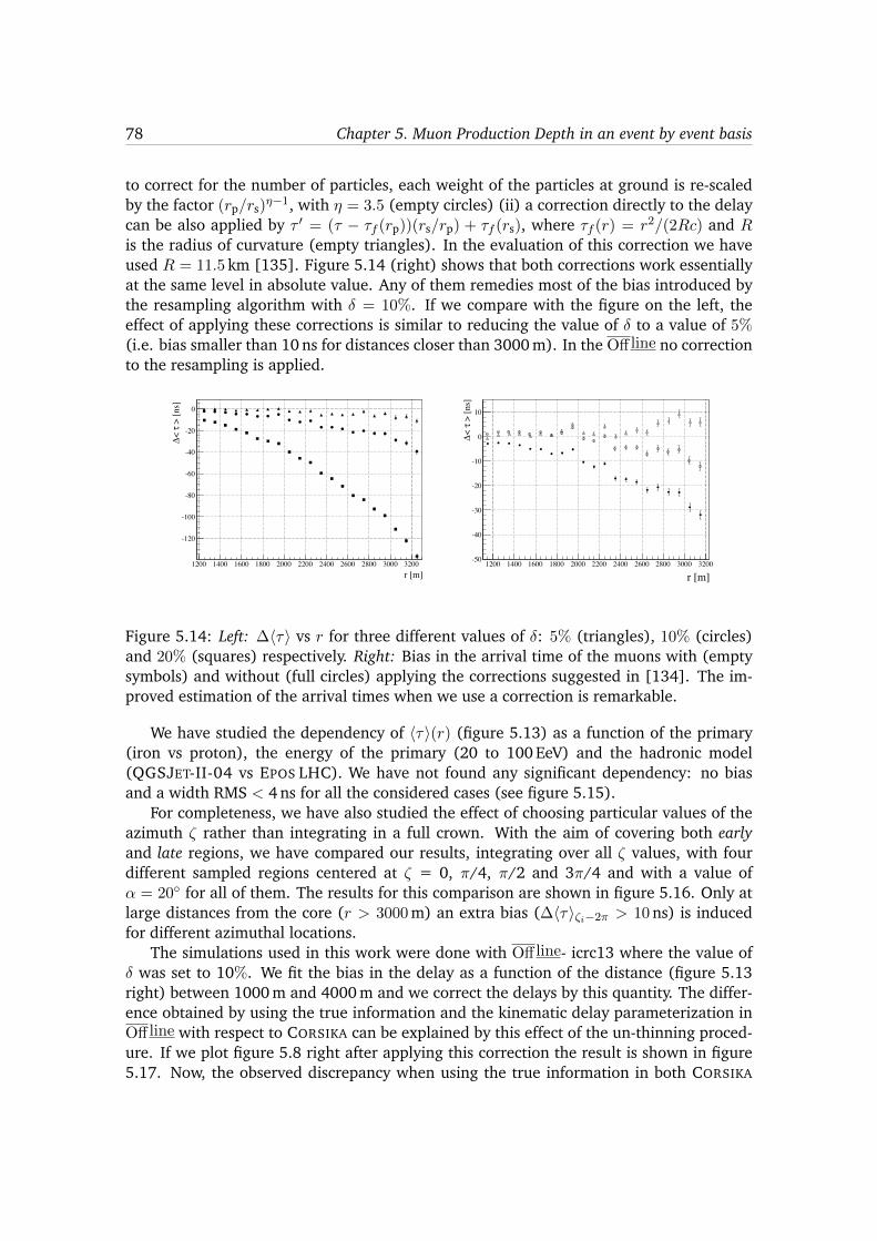
78 Chapter 5. Muon Production Depth in an event by event basis
to correct for the number of particles, each weight of the particles at ground is re-scaledby the factor (rp/rs)
⌘�1, with ⌘ = 3.5 (empty circles) (ii) a correction directly to the delaycan be also applied by ⌧
0 = (⌧ � ⌧
f
(rp))(rs/rp) + ⌧
f
(rs), where ⌧
f
(r) = r
2/(2Rc) and R
is the radius of curvature (empty triangles). In the evaluation of this correction we haveused R = 11.5 km [135]. Figure 5.14 (right) shows that both corrections work essentiallyat the same level in absolute value. Any of them remedies most of the bias introduced bythe resampling algorithm with � = 10%. If we compare with the figure on the left, theeffect of applying these corrections is similar to reducing the value of � to a value of 5%(i.e. bias smaller than 10 ns for distances closer than 3000 m). In the O↵ line no correctionto the resampling is applied.
r [m]1200 1400 1600 1800 2000 2200 2400 2600 2800 3000 3200
> [n
s]
τ< ∆
-120
-100
-80
-60
-40
-20
0
r [m]1200 1400 1600 1800 2000 2200 2400 2600 2800 3000 3200
> [n
s]τ
< ∆
-50
-40
-30
-20
-10
0
10
Figure 5.14: Left: �h⌧i vs r for three different values of �: 5% (triangles), 10% (circles)and 20% (squares) respectively. Right: Bias in the arrival time of the muons with (emptysymbols) and without (full circles) applying the corrections suggested in [134]. The im-proved estimation of the arrival times when we use a correction is remarkable.
We have studied the dependency of h⌧i(r) (figure 5.13) as a function of the primary(iron vs proton), the energy of the primary (20 to 100 EeV) and the hadronic model(QGSJET-II-04 vs EPOS LHC). We have not found any significant dependency: no biasand a width RMS < 4 ns for all the considered cases (see figure 5.15).
For completeness, we have also studied the effect of choosing particular values of theazimuth ⇣ rather than integrating in a full crown. With the aim of covering both earlyand late regions, we have compared our results, integrating over all ⇣ values, with fourdifferent sampled regions centered at ⇣ = 0, ⇡/4, ⇡/2 and 3⇡/4 and with a value of↵ = 20� for all of them. The results for this comparison are shown in figure 5.16. Only atlarge distances from the core (r > 3000m) an extra bias (�h⌧i
⇣
i
�2⇡ > 10ns) is inducedfor different azimuthal locations.
The simulations used in this work were done with O↵ line- icrc13 where the value of� was set to 10%. We fit the bias in the delay as a function of the distance (figure 5.13right) between 1000 m and 4000 m and we correct the delays by this quantity. The differ-ence obtained by using the true information and the kinematic delay parameterization inO↵ line with respect to CORSIKA can be explained by this effect of the un-thinning proced-ure. If we plot figure 5.8 right after applying this correction the result is shown in figure5.17. Now, the observed discrepancy when using the true information in both CORSIKA
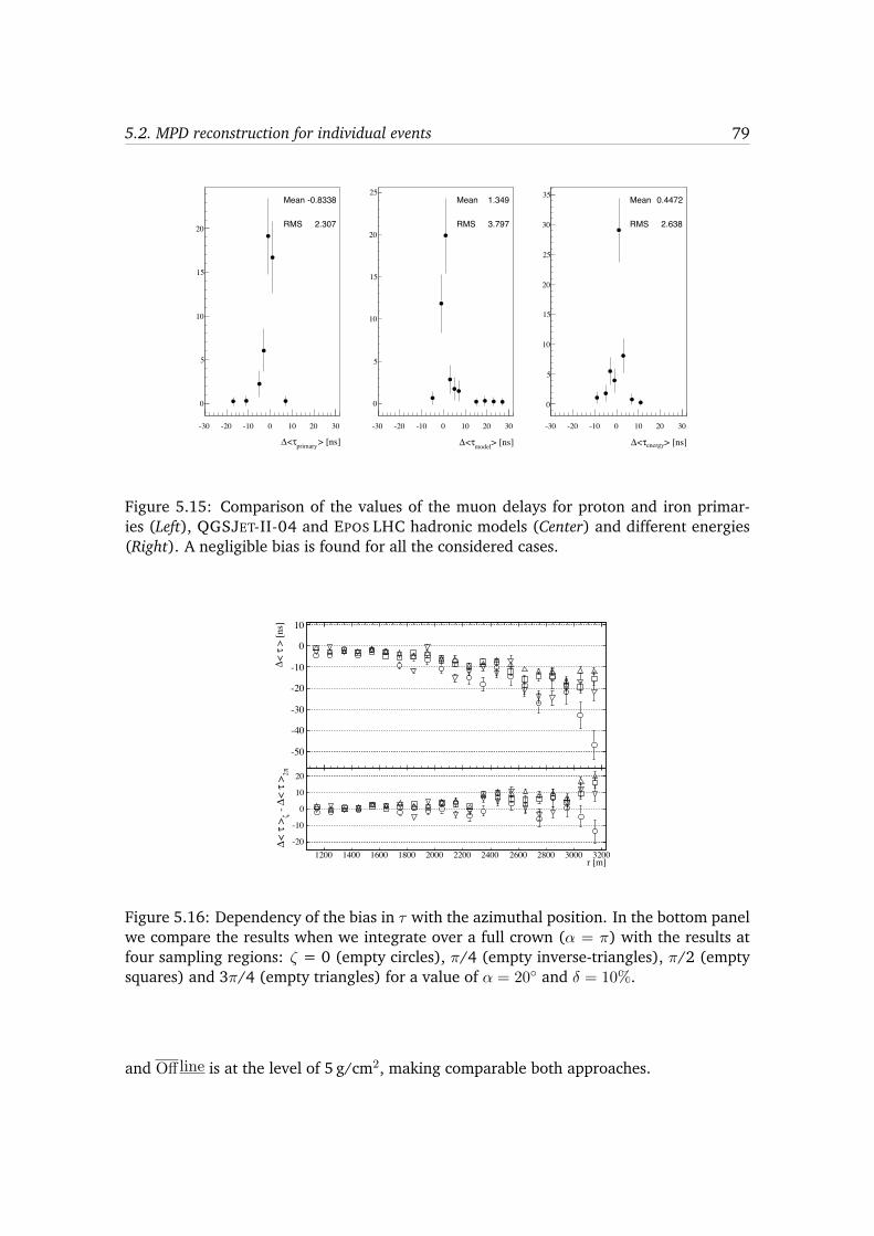
5.2. MPD reconstruction for individual events 79
Mean -0.8338
RMS 2.307
> [ns]primaryτ<∆-30 -20 -10 0 10 20 30
0
5
10
15
20
Mean -0.8338
RMS 2.307
Mean 1.349
RMS 3.797
> [ns]modelτ<∆
-30 -20 -10 0 10 20 30
0
5
10
15
20
25Mean 1.349
RMS 3.797
Mean 0.4472
RMS 2.638
> [ns]energyτ<∆
-30 -20 -10 0 10 20 30
0
5
10
15
20
25
30
35 Mean 0.4472
RMS 2.638
Figure 5.15: Comparison of the values of the muon delays for proton and iron primar-ies (Left), QGSJET-II-04 and EPOS LHC hadronic models (Center) and different energies(Right). A negligible bias is found for all the considered cases.
1200 1400 1600 1800 2000 2200 2400 2600 2800 3000 3200
> [n
s]τ
< ∆
-50
-40
-30
-20
-10
0
10
r [m]1200 1400 1600 1800 2000 2200 2400 2600 2800 3000 3200
π2 >τ
< ∆ - ζ
>τ< ∆ -20
-10
0
10
20
Figure 5.16: Dependency of the bias in ⌧ with the azimuthal position. In the bottom panelwe compare the results when we integrate over a full crown (↵ = ⇡) with the results atfour sampling regions: ⇣ = 0 (empty circles), ⇡/4 (empty inverse-triangles), ⇡/2 (emptysquares) and 3⇡/4 (empty triangles) for a value of ↵ = 20� and � = 10%.
and O↵ line is at the level of 5 g/cm2, making comparable both approaches.
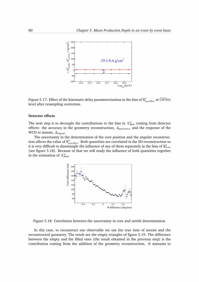
80 Chapter 5. Muon Production Depth in an event by event basis
(E/eV)10
Log19.4 19.5 19.6 19.7 19.8 19.9
]2 >
[g/c
mm
axTr
ueµ
-Xm
axRe
cµ
< X
-100
-50
0
50
100
150
200
250
2 0.4 g/cm±-35
Figure 5.17: Effect of the kinematic delay parameterization in the bias of Xµ
maxRec at O↵ line
level after resampling correction.
Detector effects
The next step is to decouple the contributions to the bias in X
µ
max coming from detectoreffects: the accuracy in the geometry reconstruction, �geometry and the response of theWCD to muons, �signal.
The uncertainty in the determination of the core position and the angular reconstruc-tion affects the value of Xµ
maxRec. Both quantities are correlated in the SD reconstruction soit is very difficult to disentangle the influence of any of them separately in the bias of Xµ
max
(see figure 5.18). Because of that we will study the influence of both quantities togetherin the estimation of Xµ
max.
difference [degrees]θ-0.4 -0.2 0 0.2 0.4
Core
diff
eren
ce [m
]
60
80
100
120
140
160
180
200
Figure 5.18: Correlation between the uncertainty in core and zenith determination.
In this case, to reconstruct our observable we use the true time of muons and thereconstructed geometry. The result are the empty triangles of figure 5.19. The differencebetween the empty and the filled ones (the result obtained in the previous step) is thecontribution coming from the addition of the geometry reconstruction. It amounts to

5.2. MPD reconstruction for individual events 81
(E/eV)10
Log19.3 19.4 19.5 19.6 19.7 19.8 19.9 20
]2 >
[g/c
mm
axTr
ueµ
-Xm
axRe
cµ
< X
-100
-50
0
50
100
150
200
250
2 0.4 g/cm±85.8
method + kin.Del
method + kin.Del + geometry
Figure 5.19: Contribution to the bias from the geometry reconstruction.
86 g/cm2.
[degree]θ56 58 60 62 64
]2 B
ias [
g/cm
-60
-40
-20
0
20
40
60
80
100
120
Rec. geometryTrue geometry
Figure 5.20: Bias vs ✓ comparing true and reconstructed geometry.
Furthermore, plotting the bias in X
µ
max as a function of the zenith angle for the caseswhere the true and the reconstructed geometry are used, we find a trend starting around61� when the reconstructed geometry is considered (filled dots of figure 5.20)3.
The fact that the response of the WCD to muons shows a spread on time affects ourestimation of X
µ
max. If we compare the reconstructed X
µ
max after all the reconstructionchain (i.e., adding the signal to all the other contributions) with its true value, the resultare the squares that we show in figure 5.21. The difference between the squares and theempty triangles is the bias added by this last contribution. It amounts to 126 g/cm2 and itis by far the largest contribution to the bias.
In table 5.4 and figure 6.5 we summarize and quantify all the identified sources con-tributing to the bias of Xµ
max.
3Investigations using the inclined reconstruction as implemented in O↵ line icrc13 have shown that thesame trend is observed.

82 Chapter 5. Muon Production Depth in an event by event basis
(E/eV)10
Log19.3 19.4 19.5 19.6 19.7 19.8 19.9 20
]2 >
[g/c
mm
axTr
ueµ
-Xm
axRe
cµ
< X
-100
-50
0
50
100
150
200
250
2 0.6 g/cm±125.6
Figure 5.21: Signal contribution to X
µ
max bias.
(E/eV)10
Log19.4 19.5 19.6 19.7 19.8 19.9
]2>
[g/c
mm
axTr
ueµ
-Xm
axRe
cµ
<X
-100
-50
0
50
100
150
200
250
Figure 5.22: Summary of all the bias contributions. Filled dots correspond to the methodaccuracy. The filled triangles include the kinematic delay parameterization plus themethod. The empty triangles contain the method, the kinematic delay parameterizationand the geometry reconstruction. Finally, the squares represent the bias after the wholechain is applied (i.e. including the method, the kinematic delay parameterization, thegeometry reconstruction and the effect of the signal spread).
Source Bias [g/cm2] Source Bias [g/cm2]�Method 6 �Method 6+ �kin.Del.Par -29 + �kin.Del.Par -29+ �geometry 56 + �Signal 114+ �Signal 182 + �geometry 182
Table 5.4: Cumulative contributions to X
µ
max bias.

5.2. MPD reconstruction for individual events 83
(E/eV)10
Log19.3 19.4 19.5 19.6 19.7 19.8 19.9 20
]2>
[g/c
mm
axTr
ueµ
-Xm
axRe
cµ
<X
-100
-50
0
50
100
150
200
250
2 0.6 g/cm±143.4
method + kin.Del. + signal
method + kin.Del
Figure 5.23: Signal contribution to X
µ
max bias where true geometry is considered.
(E/eV)10
Log19.3 19.4 19.5 19.6 19.7 19.8 19.9 20
]2>
[g/c
mm
axTr
ueµ
-Xm
axRe
cµ
<X
-100
-50
0
50
100
150
200
250
2 0.6 g/cm±68
method + kin.Del + signal + geometry
method + kin.Del. + signal
Figure 5.24: Contribution to the bias due to the geometry reconstruction.
To quantify in first place the contribution from the detector response we have inver-ted the order, i.e. we first evaluate this effect using the true geometry. In this case theWCD response makes a difference in the X
µ
max bias of 143 g/cm2 (see figure 5.23), whilethe remaining geometry bias is 68 g/cm2, as illustrated in figure 5.24. The difference inthe values coming just by switching the order is caused by the correlation between thegeometry reconstruction and the detector response.
The response of the muon in the WCD is an asymmetric function. When we use thetrue time of the muons we have delta functions. Thus, it is not straightforward to comparethese effects following the proposed approaches. In fact, we can study the dependencyof our bias with the asymmetry of the signal. For example, if we cut at a certain signalthreshold we will remove part of the tails. We have evaluated the geometry reconstructionbias for different signal thresholds and we have observed a dependence on that. When wecut at 50% of the peak, the difference between the true and the reconstructed geometryincreases by 10 g/cm2, as we expect from the result obtained when using the true timeof the muon. In table 5.5 we quote the evolution of this bias as a function of the signal
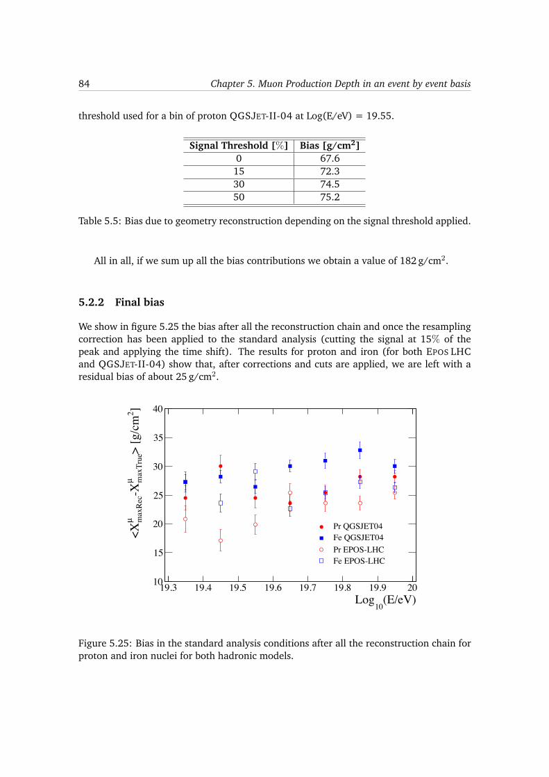
84 Chapter 5. Muon Production Depth in an event by event basis
threshold used for a bin of proton QGSJET-II-04 at Log(E/eV) = 19.55.
Signal Threshold [%] Bias [g/cm2]0 67.6
15 72.330 74.550 75.2
Table 5.5: Bias due to geometry reconstruction depending on the signal threshold applied.
All in all, if we sum up all the bias contributions we obtain a value of 182 g/cm2.
5.2.2 Final bias
We show in figure 5.25 the bias after all the reconstruction chain and once the resamplingcorrection has been applied to the standard analysis (cutting the signal at 15% of thepeak and applying the time shift). The results for proton and iron (for both EPOS LHCand QGSJET-II-04) show that, after corrections and cuts are applied, we are left with aresidual bias of about 25 g/cm2.
(E/eV)10
Log19.3 19.4 19.5 19.6 19.7 19.8 19.9 20
]2>
[g/c
mm
axTr
ueµ
-Xm
axRe
cµ
<X
10
15
20
25
30
35
40
Pr QGSJET04Fe QGSJET04Pr EPOS-LHCFe EPOS-LHC
Figure 5.25: Bias in the standard analysis conditions after all the reconstruction chain forproton and iron nuclei for both hadronic models.

5.3. Contributions to X
µ
max resolution 85
(E/eV)10
Log19.3 19.4 19.5 19.6 19.7 19.8 19.9 20
]2 )[
g/cm
max
True
µ-X
max
Rec
µRM
S( X
20
30
40
50
60
70
80
90
100
110
120Pr QGSJET04Fe QGSJET04Pr EPOS-LHCFe EPOS-LHC
Figure 5.26: Standard analysis RMS.
5.3 Contributions to Xµ
max resolution
Several sources contribute to the total resolution in the measurement of Xµ
max. In figure5.26 is illustrated the RMS for all the species. Based on simulations we have decoupledeach of the sources as we did for the case of the bias in X
µ
max. For this study we havetaken a bin of proton QGSJET-II-04 at 1019.55 eV. The histogram for this energy bin of thedifference between the reconstructed and the generated value is shown in figure 5.27.
Entries 1044Mean 24.47
RMS 75.16
]2 [g/cmmaxTrueµ - XmaxRec
µX-1000 -800 -600 -400 -200 0 200 400 600 800 1000
1
10
210Entries 1044Mean 24.47
RMS 75.16
Figure 5.27: Difference between X
µ
max reconstructed and the true one after all the recon-struction chain for proton QGSJET-II-04 at 1019.55 eV.
The total RMS of Xµ
max has four contributions:

86 Chapter 5. Muon Production Depth in an event by event basis
RMSTotal =qRMS
2Method+Kin.Del.Par +RMS
2Time +RMS
2geometry +RMS
2Statistics = 75.2g/cm2
(5.4)The influence of the method accuracy plus the kinematic delay parameterization in the
RMS, RMSMethod+Kin.Del.Par, is negligible. We have built the histogram of the differencebetween X
µ
max reconstructed using the model and the parameterized kinematic delay, andthe reference one. The RMS of this histogram is 6.5 g/cm2
.
The largest contribution comes from the number of selected muons, RMSStatistics. Toestimate this quantity we have compared the contribution of the method to the RMS atCORSIKA level (built with a large number of muons) with the one obtained in O↵ line
simulations selecting the true geometry and the true times, RMSO↵ line:
RMSstatistics =qRMS
2O↵ line
�RMS
2Method+Kin.Del.Par =
p56.042 � 6.52 = 55.7g/cm2
(5.5)The time uncertainty of the detector also affects the accuracy in the reconstruction of
X
µ
max. To evaluate this number we have compared the RMS of the distribution obtainedusing the true time of the muon plus the reconstructed geometry (at O↵ line level) withthe one obtained after all the reconstruction chain:
RMSTime =qRMS
2Total �RMS
2True Time =
p75.162 � 65.672 = 36.6g/cm2 (5.6)
Finally, the accuracy of the reconstruction of the shower geometry influences the de-termination of Xµ
max too. We can estimate this effect comparing the RMS of the distribu-tion obtained using the true time and the true geometry (at O↵ line level) with the oneobtained using only the true time:
RMSgeometry =qRMS
2True Time �RMS
2True Time + True Geometry =
p65.672 � 56.042 = 34.2g/cm2
(5.7)The contributions of the geometry and the time uncertainty have been minimized due
to the optimization of the distance cut. Both effects are larger when we go closer to theshower core.
Finally, Table 5.6 summarizes the contributions to the RMS. The main source is thelimited number of muons contributing to each MPD distribution.
5.4 Application to SD Data
In [1] the bias due to the resampling procedure was assumed to be negligible. The re-siduals between the bias obtained with and without the resampling correction are shownin figure 5.28 for both primaries and hadronic models. A linear fit to the biases for pro-ton (iron) QGSJET-II-04 as a function of the energy leads to an estimation of �(Xµ
Rec �X
µ
True) = 23.9 ± 0.8 (�(Xµ
Rec � X
µ
True) = 23.7 ± 0.7) g/cm2. Those values do not depend
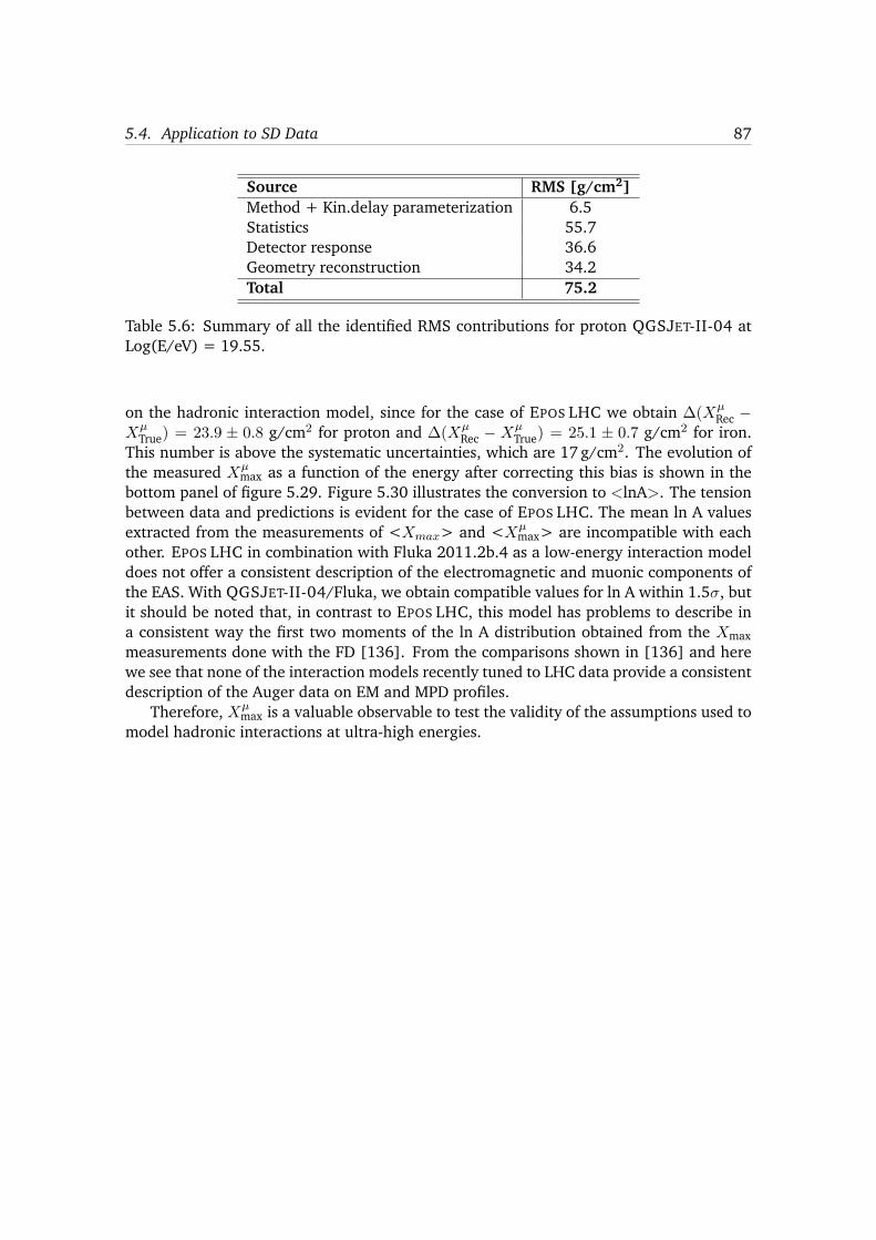
5.4. Application to SD Data 87
Source RMS [g/cm2]Method + Kin.delay parameterization 6.5Statistics 55.7Detector response 36.6Geometry reconstruction 34.2Total 75.2
Table 5.6: Summary of all the identified RMS contributions for proton QGSJET-II-04 atLog(E/eV) = 19.55.
on the hadronic interaction model, since for the case of EPOS LHC we obtain �(Xµ
Rec �X
µ
True) = 23.9 ± 0.8 g/cm2 for proton and �(Xµ
Rec � X
µ
True) = 25.1 ± 0.7 g/cm2 for iron.This number is above the systematic uncertainties, which are 17 g/cm2. The evolution ofthe measured X
µ
max as a function of the energy after correcting this bias is shown in thebottom panel of figure 5.29. Figure 5.30 illustrates the conversion to <lnA>. The tensionbetween data and predictions is evident for the case of EPOS LHC. The mean ln A valuesextracted from the measurements of <X
max
> and <X
µ
max> are incompatible with eachother. EPOS LHC in combination with Fluka 2011.2b.4 as a low-energy interaction modeldoes not offer a consistent description of the electromagnetic and muonic components ofthe EAS. With QGSJET-II-04/Fluka, we obtain compatible values for ln A within 1.5�, butit should be noted that, in contrast to EPOS LHC, this model has problems to describe ina consistent way the first two moments of the ln A distribution obtained from the Xmaxmeasurements done with the FD [136]. From the comparisons shown in [136] and herewe see that none of the interaction models recently tuned to LHC data provide a consistentdescription of the Auger data on EM and MPD profiles.
Therefore, Xµ
max is a valuable observable to test the validity of the assumptions used tomodel hadronic interactions at ultra-high energies.
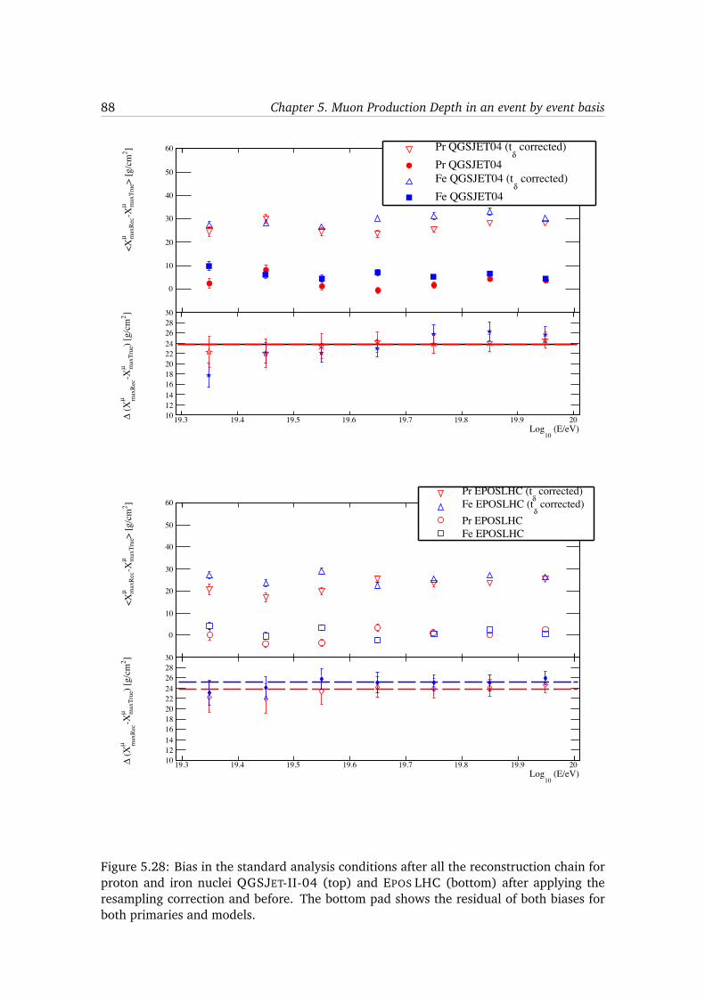
88 Chapter 5. Muon Production Depth in an event by event basis
(E/eV)10
Log19.3 19.4 19.5 19.6 19.7 19.8 19.9 20
]2>
[g/c
mm
axTr
ueµ
-Xm
axRe
cµ
<X
-10
0
10
20
30
40
50
60 / ndf 2χ 14.8 / 6p0 0.539± 26.6
corrected)δ
Pr QGSJET04 (tPr QGSJET04
corrected)δ
Fe QGSJET04 (tFe QGSJET04
(E/eV)10
Log19.3 19.4 19.5 19.6 19.7 19.8 19.9 20
]2) [
g/cm
max
True
µ-X
max
Rec
µ (X∆ 10
12141618202224262830
(E/eV)10
Log19.3 19.4 19.5 19.6 19.7 19.8 19.9 20
]2>
[g/c
mm
axTr
ueµ
-Xm
axRe
cµ
<X
-10
0
10
20
30
40
50
60 corrected)
δPr EPOSLHC (t
corrected)δ
Fe EPOSLHC (tPr EPOSLHCFe EPOSLHC
(E/eV)10
Log19.3 19.4 19.5 19.6 19.7 19.8 19.9 20
]2) [
g/cm
max
True
µ-X
max
Rec
µ (X∆ 10
12141618202224262830
Figure 5.28: Bias in the standard analysis conditions after all the reconstruction chain forproton and iron nuclei QGSJET-II-04 (top) and EPOS LHC (bottom) after applying theresampling correction and before. The bottom pad shows the residual of both biases forboth primaries and models.
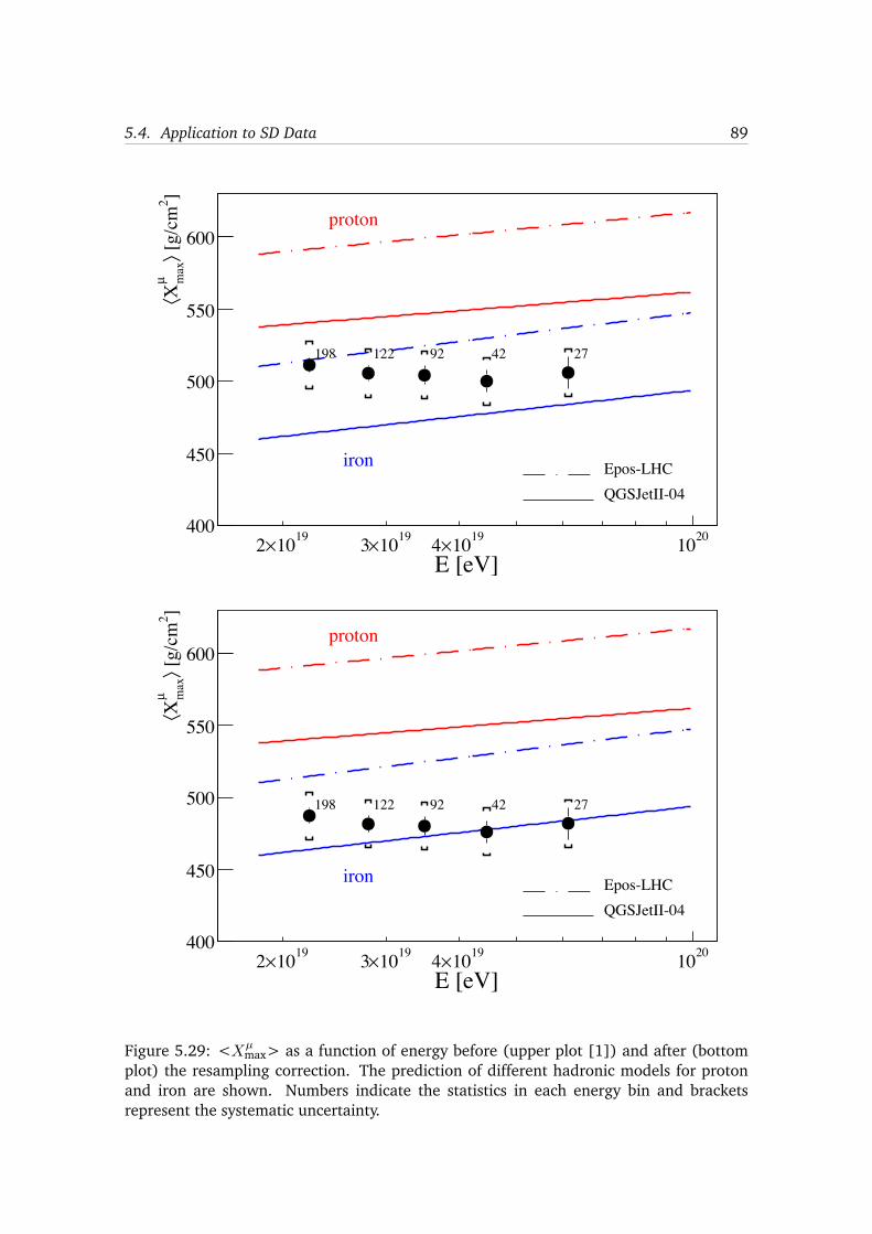
5.4. Application to SD Data 89
E [eV]1910×2 1910×3 1910×4 2010
]2 [g
/cm
⟩m
axµ
X⟨
400
450
500
550
600
198 122 92 42 27
Epos-LHCQGSJetII-04
proton
iron
E [eV]1910×2 1910×3 1910×4 2010
]2 [g
/cm
⟩m
axµ
X⟨
400
450
500
550
600
198 122 92 42 27
Epos-LHCQGSJetII-04
proton
iron
Figure 5.29: <X
µ
max> as a function of energy before (upper plot [1]) and after (bottomplot) the resampling correction. The prediction of different hadronic models for protonand iron are shown. Numbers indicate the statistics in each energy bin and bracketsrepresent the systematic uncertainty.
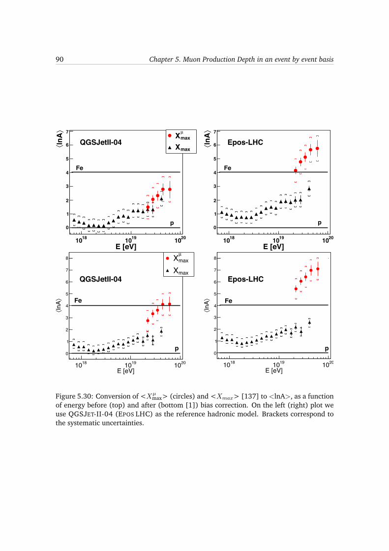
90 Chapter 5. Muon Production Depth in an event by event basis
E [eV]1810 1910 2010
⟩ln
A⟨
0
1
2
3
4
5
6
7maxµ Xmax XQGSJetII-04
Fe
p
E [eV]1810 1910 2010
⟩ln
A⟨
0
1
2
3
4
5
6
7
Epos-LHC
Fe
p
E [eV]1810 1910 2010
⟩ln
A⟨
0
1
2
3
4
5
6
7
8 maxµ Xmax X
QGSJetII-04
Fe
p
E [eV]1810 1910 2010
⟩ln
A⟨
0
1
2
3
4
5
6
7
8
Epos-LHC
Fe
p
Figure 5.30: Conversion of <X
µ
max> (circles) and <X
max
> [137] to <lnA>, as a functionof energy before (top) and after (bottom [1]) bias correction. On the left (right) plot weuse QGSJET-II-04 (EPOS LHC) as the reference hadronic model. Brackets correspond tothe systematic uncertainties.
6Average MPD analysis
In chapter 5 we have decoupled the main sources contributing to the resolution foundin the event-by-event measurement of Xµ
max. The main contribution is due to the lack ofmuons entering in each MPD distribution. The energy threshold in the MPD analysis isalso a consecuenquence of the scarce number of available muons (for protons we haveon average around 20 muons at 20 EeV) [1]. Therefore, to be able to extend the energyrange of aplicability of MPD studies we need to enlarge the number of muons. Previousworks address this issue by going closer to the shower core [127, 128, 129]. We usehere a different approach to bypass this problem. Instead of using an event-by-eventobservable, we study the average MPD distribution of all the events that belong to aparticular energy bin. We investigate the feasibility of reducing the distance cut by usingall the stations above 1000 m. We are going to explore how low in energy we can gowith this new approach. The analysis is focused on events with the same zenith range,around 60�, as those used for the published MPD analysis. No attempt is made in thisanalysis to enlarge the angular window. Since our interest now focuses on average MPDdistributions, this sort of study introduces an additional complication: not only the meanvalue of Xµ
max matters, now we must reproduce as accurately as possible the shape of theMPD distribution, as well.
6.1 Reconstruction of the average MPD distribution
In chapter 5 we have explained the main features of the MPD distributions and theirreconstruction for an event-by-event analysis. The maximum of the distribution is anSD observable that can be used as a discriminant for mass composition. In the analysisdescribed in this chapter, we add up all the distributions belonging to a given energy binand we build an average profile (see figure 6.1). From now on, the average Xµ
max, <X
µ
max>,will be our physics observable. As in the standard analysis, the best set of parametersthat describes the average longitudinal muon profile (at CORSIKA and at O↵ line level)are obtained through a log-likelihood maximization of the GH function. We fit all theparameters in a chosen interval of depths ranging from 0 to 1200 g/cm2. With this choicewe guarantee that we contain the entire range of possible <X
µ
max> values.
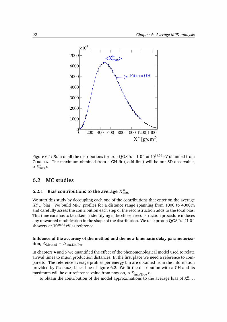
92 Chapter 6. Average MPD analysis
]2 [g/cmµX0 200 400 600 800 1000 1200 14000
1000
2000
3000
4000
5000
6000
7000
310×
>maxµ<X
Fit to a GH
Figure 6.1: Sum of all the distributions for iron QGSJET-II-04 at 1019.55 eV obtained fromCORSIKA. The maximum obtained from a GH fit (solid line) will be our SD observable,<X
µ
max>.
6.2 MC studies
6.2.1 Bias contributions to the average Xµ
max
We start this study by decoupling each one of the contributions that enter on the averageX
µ
max bias. We build MPD profiles for a distance range spanning from 1000 to 4000 mand carefully assess the contribution each step of the reconstruction adds to the total bias.This time care has to be taken in identifying if the chosen reconstruction procedure inducesany unwanted modification in the shape of the distribution. We take proton QGSJET-II-04showers at 1019.55 eV as reference.
Influence of the accuracy of the method and the new kinematic delay parameteriza-tion, �Method + �kin.Del.Par
In chapters 4 and 5 we quantified the effect of the phenomenological model used to relatearrival times to muon production distances. In the first place we need a reference to com-pare to. The reference average profiles per energy bin are obtained from the informationprovided by CORSIKA, black line of figure 6.2. We fit the distribution with a GH and itsmaximum will be our reference value from now on, <X
µ
maxTrue>.To obtain the contribution of the model approximations to the average bias of Xµ
max
,
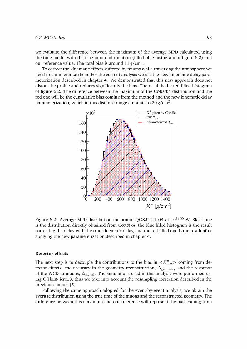
6.2. MC studies 93
we evaluate the difference between the maximum of the average MPD calculated usingthe time model with the true muon information (filled blue histogram of figure 6.2) andour reference value. The total bias is around 11 g/cm2.
To correct the kinematic effects suffered by muons while traversing the atmosphere weneed to parameterize them. For the current analysis we use the new kinematic delay para-meterization described in chapter 4. We demonstrated that this new approach does notdistort the profile and reduces significantly the bias. The result is the red filled histogramof figure 6.2. The difference between the maximum of the CORSIKA distribution and thered one will be the cumulative bias coming from the method and the new kinematic delayparameterization, which in this distance range amounts to 20 g/cm2.
]2 [g/cmµX0 200 400 600 800 1000 1200 14000
20
40
60
80
100
120
140
160
610× given by CorsikaµXkinτtrue
kinτparameterized
Figure 6.2: Average MPD distribution for proton QGSJET-II-04 at 1019.55 eV. Black lineis the distribution directly obtained from CORSIKA, the blue filled histogram is the resultcorrecting the delay with the true kinematic delay, and the red filled one is the result afterapplying the new parameterization described in chapter 4.
Detector effects
The next step is to decouple the contributions to the bias in <X
µ
max> coming from de-tector effects: the accuracy in the geometry reconstruction, �geometry and the responseof the WCD to muons, �signal. The simulations used in this analysis were performed us-ing O↵ line- icrc13, thus we take into account the resampling correction described in theprevious chapter [5].
Following the same approach adopted for the event-by-event analysis, we obtain theaverage distribution using the true time of the muons and the reconstructed geometry. Thedifference between this maximum and our reference will represent the bias coming from
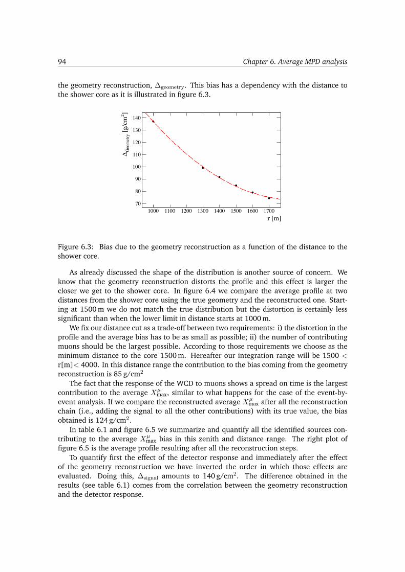
94 Chapter 6. Average MPD analysis
the geometry reconstruction, �geometry. This bias has a dependency with the distance tothe shower core as it is illustrated in figure 6.3.
r [m]1000 1100 1200 1300 1400 1500 1600 1700
]2 [g
/cm
Geo
met
ry∆
70
80
90
100
110
120
130
140
Figure 6.3: Bias due to the geometry reconstruction as a function of the distance to theshower core.
As already discussed the shape of the distribution is another source of concern. Weknow that the geometry reconstruction distorts the profile and this effect is larger thecloser we get to the shower core. In figure 6.4 we compare the average profile at twodistances from the shower core using the true geometry and the reconstructed one. Start-ing at 1500 m we do not match the true distribution but the distortion is certainly lesssignificant than when the lower limit in distance starts at 1000 m.
We fix our distance cut as a trade-off between two requirements: i) the distortion in theprofile and the average bias has to be as small as possible; ii) the number of contributingmuons should be the largest possible. According to those requirements we choose as theminimum distance to the core 1500 m. Hereafter our integration range will be 1500 <
r[m]< 4000. In this distance range the contribution to the bias coming from the geometryreconstruction is 85 g/cm2
The fact that the response of the WCD to muons shows a spread on time is the largestcontribution to the average X
µ
max, similar to what happens for the case of the event-by-event analysis. If we compare the reconstructed average X
µ
max after all the reconstructionchain (i.e., adding the signal to all the other contributions) with its true value, the biasobtained is 124 g/cm2.
In table 6.1 and figure 6.5 we summarize and quantify all the identified sources con-tributing to the average X
µ
max bias in this zenith and distance range. The right plot offigure 6.5 is the average profile resulting after all the reconstruction steps.
To quantify first the effect of the detector response and immediately after the effectof the geometry reconstruction we have inverted the order in which those effects areevaluated. Doing this, �signal amounts to 140 g/cm2. The difference obtained in theresults (see table 6.1) comes from the correlation between the geometry reconstructionand the detector response.
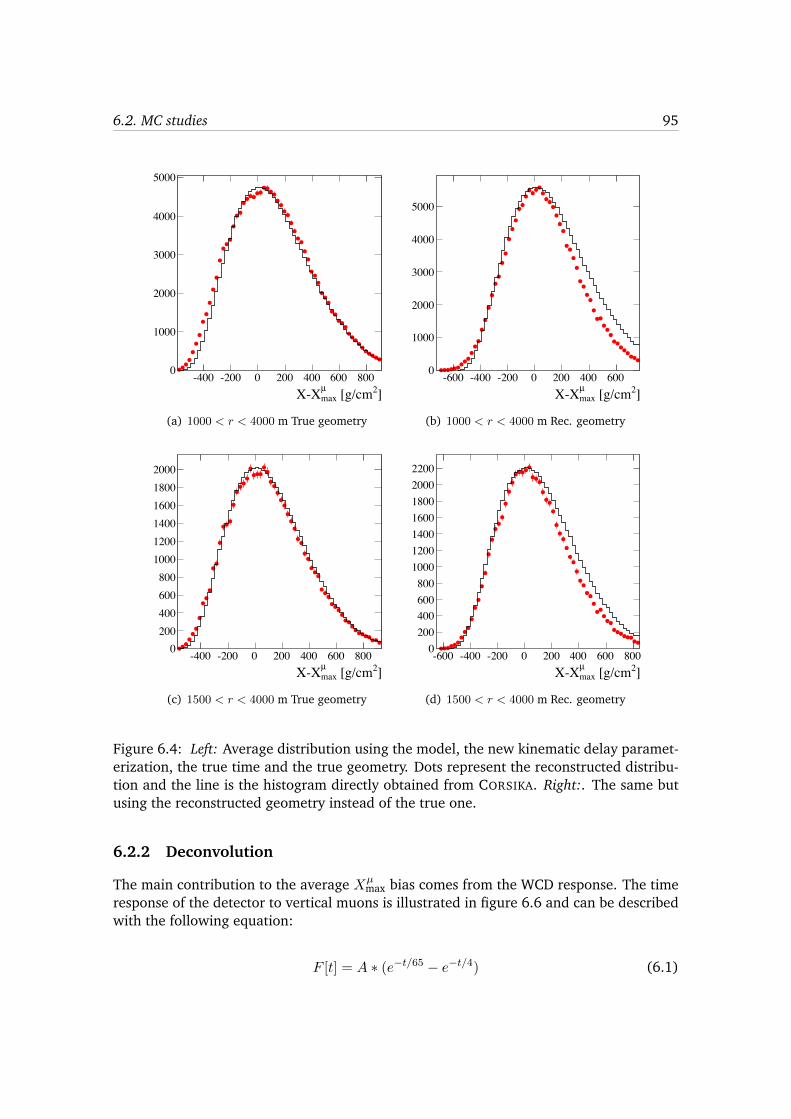
6.2. MC studies 95
]2 [g/cmmaxµX-X
-400 -200 0 200 400 600 8000
1000
2000
3000
4000
5000
(a) 1000 < r < 4000 m True geometry
]2 [g/cmmaxµX-X
-600 -400 -200 0 200 400 6000
1000
2000
3000
4000
5000
(b) 1000 < r < 4000 m Rec. geometry
]2 [g/cmmaxµX-X
-400 -200 0 200 400 600 8000200400600800
100012001400160018002000
(c) 1500 < r < 4000 m True geometry
]2 [g/cmmaxµX-X
-600 -400 -200 0 200 400 600 8000200400600800
1000120014001600180020002200
(d) 1500 < r < 4000 m Rec. geometry
Figure 6.4: Left: Average distribution using the model, the new kinematic delay paramet-erization, the true time and the true geometry. Dots represent the reconstructed distribu-tion and the line is the histogram directly obtained from CORSIKA. Right:. The same butusing the reconstructed geometry instead of the true one.
6.2.2 Deconvolution
The main contribution to the average X
µ
max bias comes from the WCD response. The timeresponse of the detector to vertical muons is illustrated in figure 6.6 and can be describedwith the following equation:
F [t] = A ⇤ (e�t/65 � e
�t/4) (6.1)
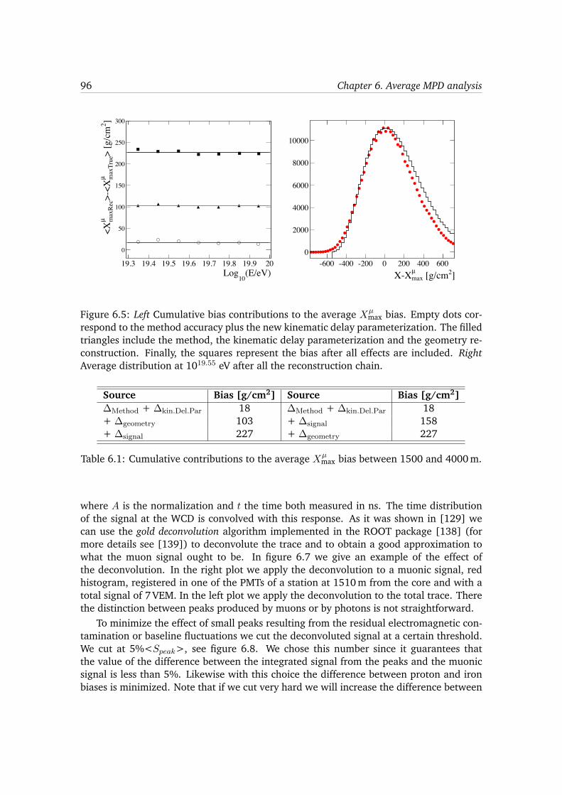
96 Chapter 6. Average MPD analysis
(E/eV)10
Log19.3 19.4 19.5 19.6 19.7 19.8 19.9 20
]2>
[g/c
mm
axTr
ueµ
>-<X
max
Rec
µ<X
0
50
100
150
200
250
300
]2 [g/cmmaxµX-X
-600 -400 -200 0 200 400 6000
2000
4000
6000
8000
10000
Figure 6.5: Left Cumulative bias contributions to the average X
µ
max bias. Empty dots cor-respond to the method accuracy plus the new kinematic delay parameterization. The filledtriangles include the method, the kinematic delay parameterization and the geometry re-construction. Finally, the squares represent the bias after all effects are included. RightAverage distribution at 1019.55 eV after all the reconstruction chain.
Source Bias [g/cm2] Source Bias [g/cm2]�Method + �kin.Del.Par 18 �Method + �kin.Del.Par 18+ �geometry 103 + �signal 158+ �signal 227 + �geometry 227
Table 6.1: Cumulative contributions to the average X
µ
max bias between 1500 and 4000 m.
where A is the normalization and t the time both measured in ns. The time distributionof the signal at the WCD is convolved with this response. As it was shown in [129] wecan use the gold deconvolution algorithm implemented in the ROOT package [138] (formore details see [139]) to deconvolute the trace and to obtain a good approximation towhat the muon signal ought to be. In figure 6.7 we give an example of the effect ofthe deconvolution. In the right plot we apply the deconvolution to a muonic signal, redhistogram, registered in one of the PMTs of a station at 1510 m from the core and with atotal signal of 7 VEM. In the left plot we apply the deconvolution to the total trace. Therethe distinction between peaks produced by muons or by photons is not straightforward.
To minimize the effect of small peaks resulting from the residual electromagnetic con-tamination or baseline fluctuations we cut the deconvoluted signal at a certain threshold.We cut at 5%<S
peak
>, see figure 6.8. We chose this number since it guarantees thatthe value of the difference between the integrated signal from the peaks and the muonicsignal is less than 5%. Likewise with this choice the difference between proton and ironbiases is minimized. Note that if we cut very hard we will increase the difference between
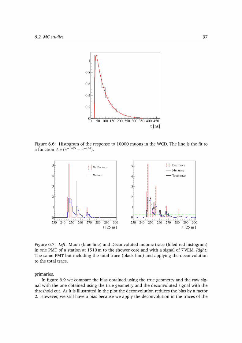
6.2. MC studies 97
t [ns]0 50 100 150 200 250 300 350 400 4500
0.2
0.4
0.6
0.8
1
Figure 6.6: Histogram of the response to 10000 muons in the WCD. The line is the fit toa function A ⇤ (e�t/65 � e
�t/4).
t [25 ns]230 240 250 260 270 280 290 3000
1
2
3
4
5 Mu. Dec. trace
Mu. trace
t [25 ns]230 240 250 260 270 280 290 3000
1
2
3
4
5 Dec TraceMu. traceTotal trace
Figure 6.7: Left: Muon (blue line) and Deconvoluted muonic trace (filled red histogram)in one PMT of a station at 1510 m to the shower core and with a signal of 7 VEM. Right:The same PMT but including the total trace (black line) and applying the deconvolutionto the total trace.
primaries.In figure 6.9 we compare the bias obtained using the true geometry and the raw sig-
nal with the one obtained using the true geometry and the deconvoluted signal with thethreshold cut. As it is illustrated in the plot the deconvolution reduces the bias by a factor2. However, we still have a bias because we apply the deconvolution in the traces of the
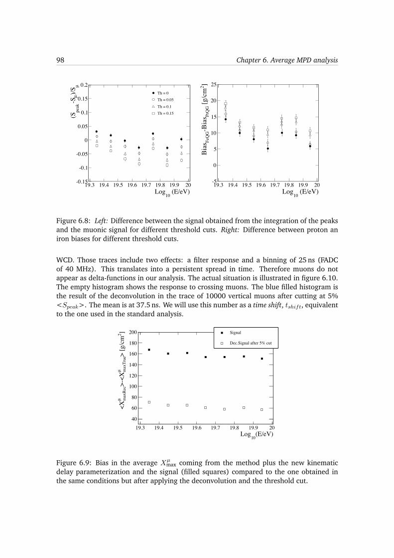
98 Chapter 6. Average MPD analysis
(E/eV)10
Log19.3 19.4 19.5 19.6 19.7 19.8 19.9 20
µ)/S µ
-Spe
ak(S
-0.15
-0.1
-0.05
0
0.05
0.1
0.15
0.2Th = 0Th = 0.05Th = 0.1Th = 0.15
(E/eV)10
Log19.3 19.4 19.5 19.6 19.7 19.8 19.9 20
]2 [g
/cm
PrQ
G-B
ias
FeQ
GBi
as
-5
0
5
10
15
20
25
Figure 6.8: Left: Difference between the signal obtained from the integration of the peaksand the muonic signal for different threshold cuts. Right: Difference between proton aniron biases for different threshold cuts.
WCD. Those traces include two effects: a filter response and a binning of 25 ns (FADCof 40 MHz). This translates into a persistent spread in time. Therefore muons do notappear as delta-functions in our analysis. The actual situation is illustrated in figure 6.10.The empty histogram shows the response to crossing muons. The blue filled histogram isthe result of the deconvolution in the trace of 10000 vertical muons after cutting at 5%<S
peak
>. The mean is at 37.5 ns. We will use this number as a time shift, tshift
, equivalentto the one used in the standard analysis.
(E/eV)10
Log19.3 19.4 19.5 19.6 19.7 19.8 19.9 20
]2>
[g/c
mm
axTr
ueµ
>-<X
max
Rec
µ<X
40
60
80
100
120
140
160
180
200 Signal
Dec.Signal after 5% cut
Figure 6.9: Bias in the average X
µ
max coming from the method plus the new kinematicdelay parameterization and the signal (filled squares) compared to the one obtained inthe same conditions but after applying the deconvolution and the threshold cut.
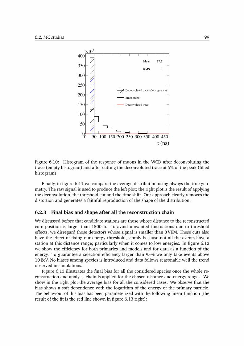
6.2. MC studies 99
Mean 37.5
RMS 0
t (ns)0 50 100 150 200 250 300 350 400 4500
50
100
150
200
250
300
350
400310×
Mean 37.5
RMS 0
Deconvoluted trace after signal cut
Muon trace
Deconvoluted trace
Figure 6.10: Histogram of the response of muons in the WCD after deconvoluting thetrace (empty histogram) and after cutting the deconvoluted trace at 5% of the peak (filledhistogram).
Finally, in figure 6.11 we compare the average distribution using always the true geo-metry. The raw signal is used to produce the left plot; the right plot is the result of applyingthe deconvolution, the threshold cut and the time shift. Our approach clearly removes thedistortion and generates a faithful reproduction of the shape of the distribution.
6.2.3 Final bias and shape after all the reconstruction chain
We discussed before that candidate stations are those whose distance to the reconstructedcore position is larger than 1500 m. To avoid unwanted fluctuations due to thresholdeffects, we disregard those detectors whose signal is smaller than 3 VEM. These cuts alsohave the effect of fixing our energy threshold, simply because not all the events have astation at this distance range; particularly when it comes to low energies. In figure 6.12we show the efficiency for both primaries and models and for data as a function of theenergy. To guarantee a selection efficiency larger than 95% we only take events above10 EeV. No biases among species is introduced and data follows reasonable well the trendobserved in simulations.
Figure 6.13 illustrates the final bias for all the considered species once the whole re-construction and analysis chain is applied for the chosen distance and energy ranges. Weshow in the right plot the average bias for all the considered cases. We observe that thebias shows a soft dependence with the logarithm of the energy of the primary particle.The behaviour of this bias has been parameterized with the following linear function (theresult of the fit is the red line shown in figure 6.13 right):
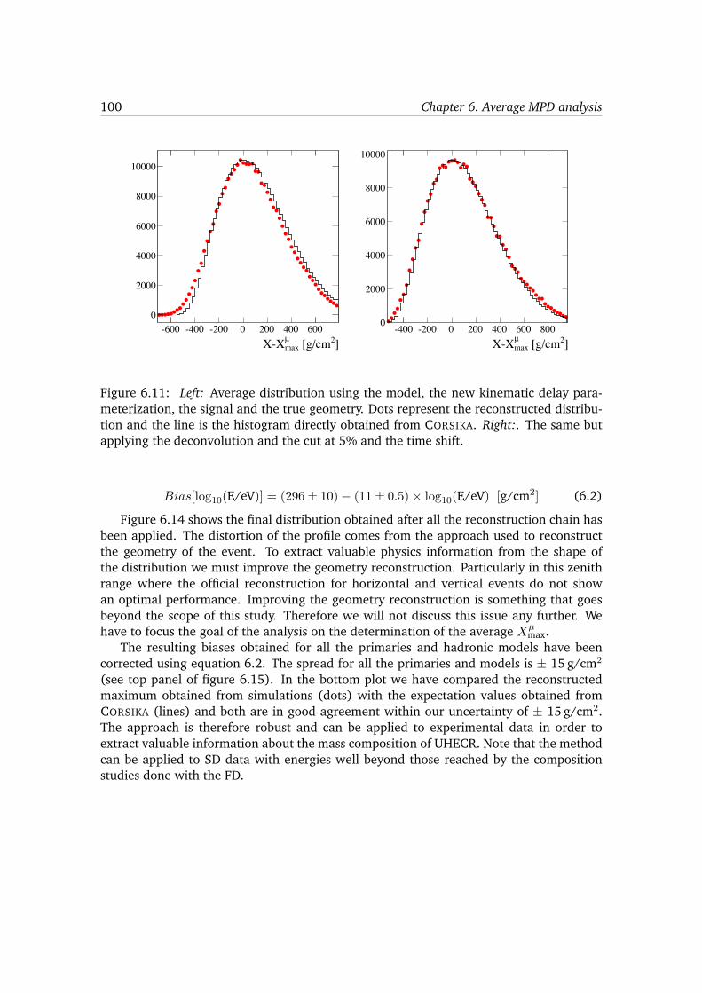
100 Chapter 6. Average MPD analysis
]2 [g/cmmaxµX-X
-600 -400 -200 0 200 400 6000
2000
4000
6000
8000
10000
]2 [g/cmmaxµX-X
-400 -200 0 200 400 600 8000
2000
4000
6000
8000
10000
Figure 6.11: Left: Average distribution using the model, the new kinematic delay para-meterization, the signal and the true geometry. Dots represent the reconstructed distribu-tion and the line is the histogram directly obtained from CORSIKA. Right:. The same butapplying the deconvolution and the cut at 5% and the time shift.
Bias[log10(E/eV)] = (296± 10)� (11± 0.5)⇥ log10(E/eV) [g/cm2] (6.2)
Figure 6.14 shows the final distribution obtained after all the reconstruction chain hasbeen applied. The distortion of the profile comes from the approach used to reconstructthe geometry of the event. To extract valuable physics information from the shape ofthe distribution we must improve the geometry reconstruction. Particularly in this zenithrange where the official reconstruction for horizontal and vertical events do not showan optimal performance. Improving the geometry reconstruction is something that goesbeyond the scope of this study. Therefore we will not discuss this issue any further. Wehave to focus the goal of the analysis on the determination of the average X
µ
max.The resulting biases obtained for all the primaries and hadronic models have been
corrected using equation 6.2. The spread for all the primaries and models is ± 15 g/cm2
(see top panel of figure 6.15). In the bottom plot we have compared the reconstructedmaximum obtained from simulations (dots) with the expectation values obtained fromCORSIKA (lines) and both are in good agreement within our uncertainty of ± 15 g/cm2.The approach is therefore robust and can be applied to experimental data in order toextract valuable information about the mass composition of UHECR. Note that the methodcan be applied to SD data with energies well beyond those reached by the compositionstudies done with the FD.
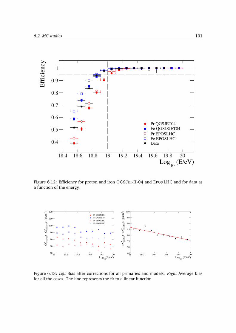
6.2. MC studies 101
(E/eV)10
Log18.4 18.6 18.8 19 19.2 19.4 19.6 19.8 20
Effic
ienc
y
0.4
0.5
0.6
0.7
0.8
0.9
1
Pr QGSJET04Fe QGSJSJET04Pr EPOSLHCFe EPOSLHCData
Figure 6.12: Efficiency for proton and iron QGSJET-II-04 and EPOS LHC and for data asa function of the energy.
(E/eV)10
Log19 19.2 19.4 19.6 19.8 20
]2>
[g/c
mm
axTr
ueµ
>-<X
max
Rec
µ<X
60
70
80
90
100
110
120Pr QGSJET04Fe QGSJET04Pr EPOSLHCFe EPOSLHC
(E/eV)10
Log19 19.2 19.4 19.6 19.8 20
]2>
[g/c
mm
axTr
ueµ
>-<X
max
Rec
µ<X
65
70
75
80
85
90
95
100
Figure 6.13: Left Bias after corrections for all primaries and models. Right Average biasfor all the cases. The line represents the fit to a linear function.

102 Chapter 6. Average MPD analysis
]2 [g/cmmaxµX-X
-600 -400 -200 0 200 400 600 8000
2000
4000
6000
8000
10000
Figure 6.14: Average distribution after all the reconstruction chain.
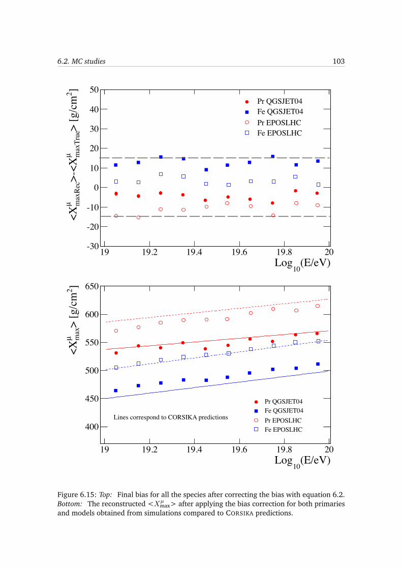
6.2. MC studies 103
(E/eV)10
Log19 19.2 19.4 19.6 19.8 20
]2>
[g/c
mm
axTr
ueµ
>-<X
max
Rec
µ<X
-30
-20
-10
0
10
20
30
40
50Pr QGSJET04Fe QGSJET04Pr EPOSLHCFe EPOSLHC
(E/eV)10
Log19 19.2 19.4 19.6 19.8 20
]2>
[g/c
mm
axµ
<X
400
450
500
550
600
650
Pr QGSJET04Fe QGSJET04Pr EPOSLHCFe EPOSLHC
Lines correspond to CORSIKA predictions
Figure 6.15: Top: Final bias for all the species after correcting the bias with equation 6.2.Bottom: The reconstructed <X
µ
max> after applying the bias correction for both primariesand models obtained from simulations compared to CORSIKA predictions.
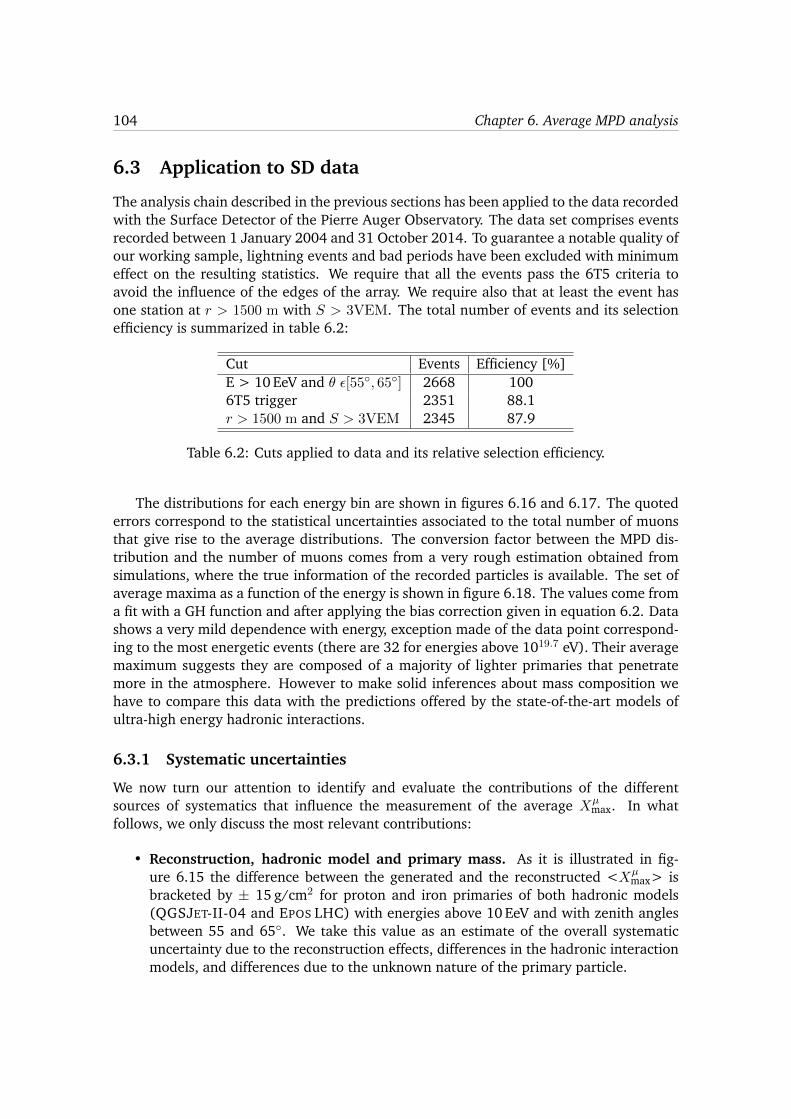
104 Chapter 6. Average MPD analysis
6.3 Application to SD data
The analysis chain described in the previous sections has been applied to the data recordedwith the Surface Detector of the Pierre Auger Observatory. The data set comprises eventsrecorded between 1 January 2004 and 31 October 2014. To guarantee a notable quality ofour working sample, lightning events and bad periods have been excluded with minimumeffect on the resulting statistics. We require that all the events pass the 6T5 criteria toavoid the influence of the edges of the array. We require also that at least the event hasone station at r > 1500 m with S > 3VEM. The total number of events and its selectionefficiency is summarized in table 6.2:
Cut Events Efficiency [%]E > 10 EeV and ✓ ✏[55�, 65�] 2668 1006T5 trigger 2351 88.1r > 1500 m and S > 3VEM 2345 87.9
Table 6.2: Cuts applied to data and its relative selection efficiency.
The distributions for each energy bin are shown in figures 6.16 and 6.17. The quotederrors correspond to the statistical uncertainties associated to the total number of muonsthat give rise to the average distributions. The conversion factor between the MPD dis-tribution and the number of muons comes from a very rough estimation obtained fromsimulations, where the true information of the recorded particles is available. The set ofaverage maxima as a function of the energy is shown in figure 6.18. The values come froma fit with a GH function and after applying the bias correction given in equation 6.2. Datashows a very mild dependence with energy, exception made of the data point correspond-ing to the most energetic events (there are 32 for energies above 1019.7 eV). Their averagemaximum suggests they are composed of a majority of lighter primaries that penetratemore in the atmosphere. However to make solid inferences about mass composition wehave to compare this data with the predictions offered by the state-of-the-art models ofultra-high energy hadronic interactions.
6.3.1 Systematic uncertainties
We now turn our attention to identify and evaluate the contributions of the differentsources of systematics that influence the measurement of the average X
µ
max. In whatfollows, we only discuss the most relevant contributions:
• Reconstruction, hadronic model and primary mass. As it is illustrated in fig-ure 6.15 the difference between the generated and the reconstructed <X
µ
max> isbracketed by ± 15 g/cm2 for proton and iron primaries of both hadronic models(QGSJET-II-04 and EPOS LHC) with energies above 10 EeV and with zenith anglesbetween 55 and 65�. We take this value as an estimate of the overall systematicuncertainty due to the reconstruction effects, differences in the hadronic interactionmodels, and differences due to the unknown nature of the primary particle.
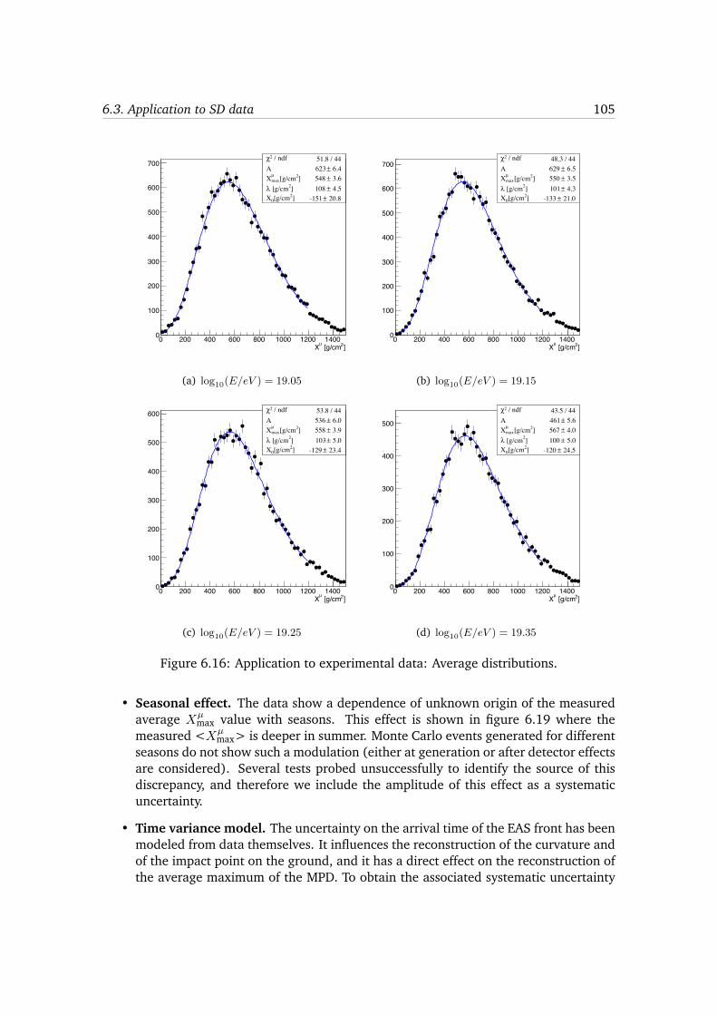
6.3. Application to SD data 105
/ ndf 2χ 51.8 / 44A 6.4± 623
] 2[g/cmmaxµX 3.6± 548
] 2 [g/cmλ 4.5± 108 ] 2[g/cm0X 20.8± -151
]2 [g/cmµX0 200 400 600 800 1000 1200 14000
100
200
300
400
500
600
700 / ndf 2χ 51.8 / 44
A 6.4± 623 ] 2[g/cmmax
µX 3.6± 548 ] 2 [g/cmλ 4.5± 108 ] 2[g/cm0X 20.8± -151
(a) log10(E/eV ) = 19.05
/ ndf 2χ 48.3 / 44A 6.5± 629
] 2[g/cmmaxµX 3.5± 550
] 2 [g/cmλ 4.3± 101 ] 2[g/cm0X 21.0± -133
]2 [g/cmµX0 200 400 600 800 1000 1200 14000
100
200
300
400
500
600
700 / ndf 2χ 48.3 / 44
A 6.5± 629 ] 2[g/cmmax
µX 3.5± 550 ] 2 [g/cmλ 4.3± 101 ] 2[g/cm0X 21.0± -133
(b) log10(E/eV ) = 19.15
/ ndf 2χ 53.8 / 44A 6.0± 536
] 2[g/cmmaxµX 3.9± 558
] 2 [g/cmλ 5.0± 103 ] 2[g/cm0X 23.4± -129
]2 [g/cmµX0 200 400 600 800 1000 1200 14000
100
200
300
400
500
600 / ndf 2χ 53.8 / 44A 6.0± 536
] 2[g/cmmaxµX 3.9± 558
] 2 [g/cmλ 5.0± 103 ] 2[g/cm0X 23.4± -129
(c) log10(E/eV ) = 19.25
/ ndf 2χ 43.5 / 44A 5.6± 461
] 2[g/cmmaxµX 4.0± 567
] 2 [g/cmλ 5.0± 100 ] 2[g/cm0X 24.5± -120
]2 [g/cmµX0 200 400 600 800 1000 1200 14000
100
200
300
400
500
/ ndf 2χ 43.5 / 44A 5.6± 461
] 2[g/cmmaxµX 4.0± 567
] 2 [g/cmλ 5.0± 100 ] 2[g/cm0X 24.5± -120
(d) log10(E/eV ) = 19.35
Figure 6.16: Application to experimental data: Average distributions.
• Seasonal effect. The data show a dependence of unknown origin of the measuredaverage X
µ
max value with seasons. This effect is shown in figure 6.19 where themeasured <X
µ
max> is deeper in summer. Monte Carlo events generated for differentseasons do not show such a modulation (either at generation or after detector effectsare considered). Several tests probed unsuccessfully to identify the source of thisdiscrepancy, and therefore we include the amplitude of this effect as a systematicuncertainty.
• Time variance model. The uncertainty on the arrival time of the EAS front has beenmodeled from data themselves. It influences the reconstruction of the curvature andof the impact point on the ground, and it has a direct effect on the reconstruction ofthe average maximum of the MPD. To obtain the associated systematic uncertainty

106 Chapter 6. Average MPD analysis
/ ndf 2χ 42.3 / 44A 5.1± 382
] 2[g/cmmaxµX 4.2± 560
] 2 [g/cmλ 5.0± 95.9 ] 2[g/cm0X 26.4± -142
]2 [g/cmµX0 200 400 600 800 1000 1200 14000
50
100
150
200
250
300
350
400
/ ndf 2χ 42.3 / 44A 5.1± 382
] 2[g/cmmaxµX 4.2± 560
] 2 [g/cmλ 5.0± 95.9 ] 2[g/cm0X 26.4± -142
(a) log10(E/eV ) = 19.45
/ ndf 2χ 30.5 / 44A 4.7± 322
] 2[g/cmmaxµX 4.7± 560
] 2 [g/cmλ 5.7± 101 ] 2[g/cm0X 26.9± -114
]2 [g/cmµX0 200 400 600 800 1000 1200 1400
0
50
100
150
200
250
300
350
/ ndf 2χ 30.5 / 44A 4.7± 322
] 2[g/cmmaxµX 4.7± 560
] 2 [g/cmλ 5.7± 101 ] 2[g/cm0X 26.9± -114
(b) log10(E/eV ) = 19.55
/ ndf 2χ 76.8 / 44A 3.7± 197
] 2[g/cmmaxµX 6.0± 563
] 2 [g/cmλ 7.2± 95.5 ] 2[g/cm0X 37.0± -121
]2 [g/cmµX0 200 400 600 800 1000 1200 1400
0
50
100
150
200
250 / ndf 2χ 76.8 / 44A 3.7± 197
] 2[g/cmmaxµX 6.0± 563
] 2 [g/cmλ 7.2± 95.5 ] 2[g/cm0X 37.0± -121
(c) log10(E/eV ) = 19.65
/ ndf 2χ 37.2 / 44A 3.8± 202
] 2[g/cmmaxµX 6.4± 588
] 2 [g/cmλ 8.1± 89.9 ] 2[g/cm0X 50.1± -163
]2 [g/cmµX0 200 400 600 800 1000 1200 1400
0
50
100
150
200
/ ndf 2χ 37.2 / 44A 3.8± 202
] 2[g/cmmaxµX 6.4± 588
] 2 [g/cmλ 8.1± 89.9 ] 2[g/cm0X 50.1± -163
(d) log10(E/eV ) = 19.79
Figure 6.17: Application to experimental data: Average distributions.
introduced by this model we compared two different parameterizations of the timevariance model [122]. They both have a common contribution from the resolutionon the absolute time given by the GPS and from the 40 MHz sampling of the FADCs,but they differ in the modeling of the fluctuations of the arrival time of the firstparticle. We include as a systematic uncertainty the difference between the twomodels on the determination of the <X
µ
max>. It amounts to 5 g/cm2.
• Accidental signals. In real events, a background of random accidental signals mightappear. The most frequent source of random noise is created by single particles (gen-erally isolated atmospheric muons) and, more rarely, by a bunch of particles arrivingat the same time from a low-energy shower close to a SD station. In general, it isvery difficult to identify and take into account all possible sources of accidental sig-
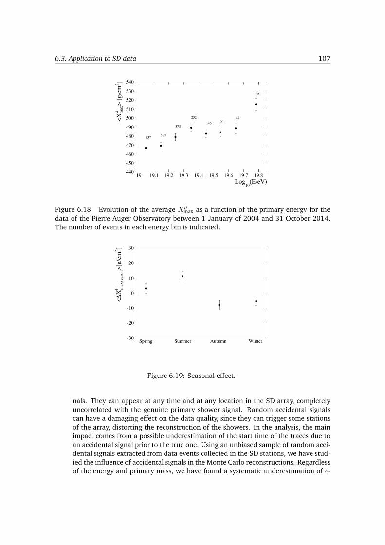
6.3. Application to SD data 107
(E/eV)10
Log19 19.1 19.2 19.3 19.4 19.5 19.6 19.7 19.8
]2>
[g/c
mm
axµ
<X
440
450460
470
480
490
500
510
520
530
540
837 588
375
232146 90
45
32
Figure 6.18: Evolution of the average X
µ
max as a function of the primary energy for thedata of the Pierre Auger Observatory between 1 January of 2004 and 31 October 2014.The number of events in each energy bin is indicated.
Spring Summer Autumn Winter
]2>[g/cm
maxSeason
µX∆<
-30
-20
-10
0
10
20
30
Figure 6.19: Seasonal effect.
nals. They can appear at any time and at any location in the SD array, completelyuncorrelated with the genuine primary shower signal. Random accidental signalscan have a damaging effect on the data quality, since they can trigger some stationsof the array, distorting the reconstruction of the showers. In the analysis, the mainimpact comes from a possible underestimation of the start time of the traces due toan accidental signal prior to the true one. Using an unbiased sample of random acci-dental signals extracted from data events collected in the SD stations, we have stud-ied the influence of accidental signals in the Monte Carlo reconstructions. Regardlessof the energy and primary mass, we have found a systematic underestimation of ⇠
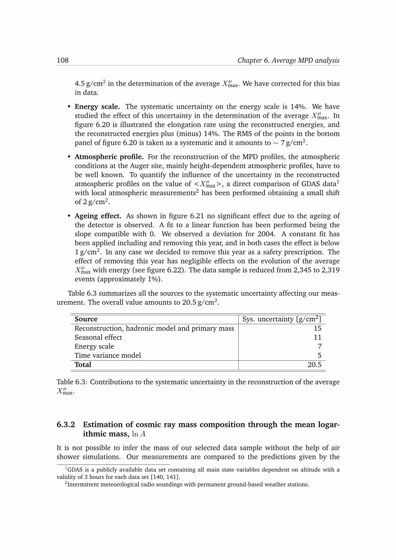
108 Chapter 6. Average MPD analysis
4.5 g/cm2 in the determination of the average X
µ
max. We have corrected for this biasin data.
• Energy scale. The systematic uncertainty on the energy scale is 14%. We havestudied the effect of this uncertainty in the determination of the average X
µ
max. Infigure 6.20 is illustrated the elongation rate using the reconstructed energies, andthe reconstructed energies plus (minus) 14%. The RMS of the points in the bottompanel of figure 6.20 is taken as a systematic and it amounts to ⇠ 7 g/cm2.
• Atmospheric profile. For the reconstruction of the MPD profiles, the atmosphericconditions at the Auger site, mainly height-dependent atmospheric profiles, have tobe well known. To quantify the influence of the uncertainty in the reconstructedatmospheric profiles on the value of <X
µ
max>, a direct comparison of GDAS data1
with local atmospheric measurements2 has been performed obtaining a small shiftof 2 g/cm2.
• Ageing effect. As shown in figure 6.21 no significant effect due to the ageing ofthe detector is observed. A fit to a linear function has been performed being theslope compatible with 0. We observed a deviation for 2004. A constant fit hasbeen applied including and removing this year, and in both cases the effect is below1 g/cm2. In any case we decided to remove this year as a safety prescription. Theeffect of removing this year has negligible effects on the evolution of the averageX
µ
max with energy (see figure 6.22). The data sample is reduced from 2,345 to 2,319events (approximately 1%).
Table 6.3 summarizes all the sources to the systematic uncertainty affecting our meas-urement. The overall value amounts to 20.5 g/cm2.
Source Sys. uncertainty [g/cm2]Reconstruction, hadronic model and primary mass 15Seasonal effect 11Energy scale 7Time variance model 5Total 20.5
Table 6.3: Contributions to the systematic uncertainty in the reconstruction of the averageX
µ
max.
6.3.2 Estimation of cosmic ray mass composition through the mean logar-ithmic mass, lnA
It is not possible to infer the mass of our selected data sample without the help of airshower simulations. Our measurements are compared to the predictions given by the
1GDAS is a publicly available data set containing all main state variables dependent on altitude with avalidity of 3 hours for each data set [140, 141].
2Intermittent meteorological radio soundings with permanent ground-based weather stations.
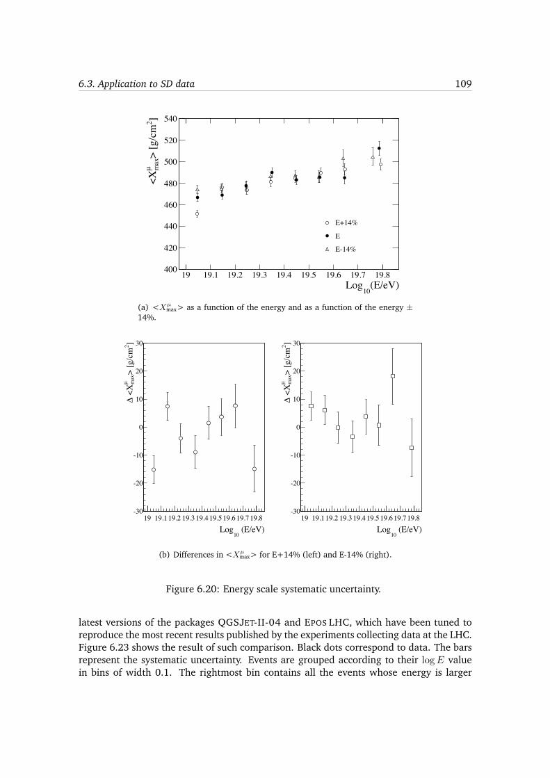
6.3. Application to SD data 109
(E/eV)10
Log19 19.1 19.2 19.3 19.4 19.5 19.6 19.7 19.8
]2>
[g/c
mm
axµ
<X
400
420
440
460
480
500
520
540
E+14%
E
E-14%
(a) <Xµ
max> as a function of the energy and as a function of the energy ±14%.
(E/eV)10
Log19 19.119.2 19.319.419.519.619.719.8
]2>
[g/c
mm
axµ
<X
∆
-30
-20
-10
0
10
20
30
(E/eV)10
Log19 19.119.2 19.319.419.519.619.719.8
]2>
[g/c
mm
axµ
<X
∆
-30
-20
-10
0
10
20
30
(b) Differences in <Xµ
max> for E+14% (left) and E-14% (right).
Figure 6.20: Energy scale systematic uncertainty.
latest versions of the packages QGSJET-II-04 and EPOS LHC, which have been tuned toreproduce the most recent results published by the experiments collecting data at the LHC.Figure 6.23 shows the result of such comparison. Black dots correspond to data. The barsrepresent the systematic uncertainty. Events are grouped according to their logE valuein bins of width 0.1. The rightmost bin contains all the events whose energy is larger

110 Chapter 6. Average MPD analysis
Year2004 2006 2008 2010 2012 2014
]2>[
g/cm
max
2004
µ>
- <X
max
Year
µ<X
-40
-30
-20
-10
0
10
20
/ ndf 2χ 23.9 / 9p0 1.18e+03± 931 p1 0.589± -0.463
/ ndf 2χ 23.9 / 9p0 1.18e+03± 931 p1 0.589± -0.463
(a) Fit with a linear function.
Year2004 2006 2008 2010 2012 2014
]2>[
g/cm
max
2004
µ>
- <X
max
Year
µ<X
-40
-30
-20
-10
0
10
20
/ ndf 2χ 24.5 / 10p0 1.53± 0.0251
/ ndf 2χ 24.5 / 10p0 1.53± 0.0251
(b) Fit with a constant including all the years.
Year2004 2006 2008 2010 2012 2014
]2>[
g/cm
max
2004
µ>
- <X
max
Year
µ<X
-40
-30
-20
-10
0
10
20
/ ndf 2χ 21 / 9p0 1.53± 0.331
/ ndf 2χ 21 / 9p0 1.53± 0.331
(c) Fit with a constant removing 2004.
Figure 6.21: Aging effect.
(E/eV)10
Log19 19.1 19.2 19.3 19.4 19.5 19.6 19.7 19.8
]2>
[g/c
mm
axµ
<X
440
450460
470
480
490
500
510
520
530
540
All yearsNo 2004
Figure 6.22: Average X
µ
max as a function of the primary energy for all the data set (filleddots) and excluding 2004 (empty dots).
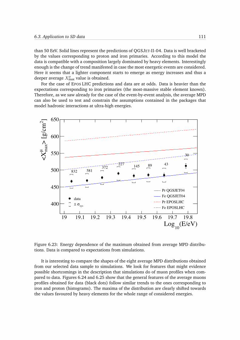
6.3. Application to SD data 111
than 50 EeV. Solid lines represent the predictions of QGSJET-II-04. Data is well bracketedby the values corresponding to proton and iron primaries. According to this model thedata is compatible with a composition largely dominated by heavy elements. Interestinglyenough is the change of trend manifested in case the most energetic events are considered.Here it seems that a lighter component starts to emerge as energy increases and thus adeeper average X
µ
max value is obtained.For the case of EPOS LHC predictions and data are at odds. Data is heavier than the
expectations corresponding to iron primaries (the most-massive stable element known).Therefore, as we saw already for the case of the event-by-event analysis, the average MPDcan also be used to test and constrain the assumptions contained in the packages thatmodel hadronic interactions at ultra-high energies.
(E/eV)10
Log19 19.1 19.2 19.3 19.4 19.5 19.6 19.7 19.8
]2>
[g/c
mm
axµ
<X
400
450
500
550
600
650
832 581372
227 145 89 43
30
Pr QGSJET04Fe QGSJET04Pr EPOSLHCFe EPOSLHC
datasysσ ±
Figure 6.23: Energy dependence of the maximum obtained from average MPD distribu-tions. Data is compared to expectations from simulations.
It is interesting to compare the shapes of the eight average MPD distributions obtainedfrom our selected data sample to simulations. We look for features that might evidencepossible shortcomings in the description that simulations do of muon profiles when com-pared to data. Figures 6.24 and 6.25 show that the general features of the average muonsprofiles obtained for data (black dots) follow similar trends to the ones corresponding toiron and proton (histograms). The maxima of the distribution are clearly shifted towardsthe values favoured by heavy elements for the whole range of considered energies.
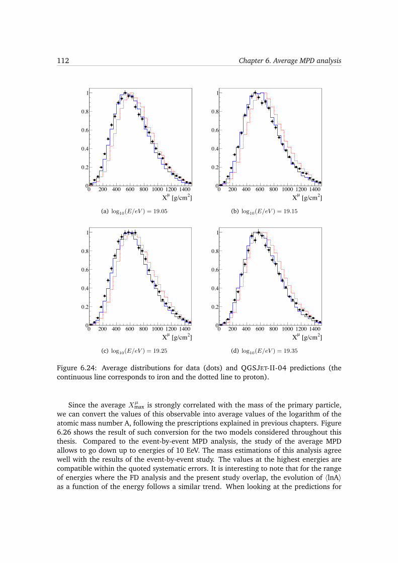
112 Chapter 6. Average MPD analysis
]2 [g/cmµX0 200 400 600 800 1000 1200 14000
0.2
0.4
0.6
0.8
1
(a) log10(E/eV ) = 19.05
]2 [g/cmµX0 200 400 600 800 1000 1200 14000
0.2
0.4
0.6
0.8
1
(b) log10(E/eV ) = 19.15
]2 [g/cmµX0 200 400 600 800 1000 1200 14000
0.2
0.4
0.6
0.8
1
(c) log10(E/eV ) = 19.25
]2 [g/cmµX0 200 400 600 800 1000 1200 14000
0.2
0.4
0.6
0.8
1
(d) log10(E/eV ) = 19.35
Figure 6.24: Average distributions for data (dots) and QGSJET-II-04 predictions (thecontinuous line corresponds to iron and the dotted line to proton).
Since the average X
µ
max is strongly correlated with the mass of the primary particle,we can convert the values of this observable into average values of the logarithm of theatomic mass number A, following the prescriptions explained in previous chapters. Figure6.26 shows the result of such conversion for the two models considered throughout thisthesis. Compared to the event-by-event MPD analysis, the study of the average MPDallows to go down up to energies of 10 EeV. The mass estimations of this analysis agreewell with the results of the event-by-event study. The values at the highest energies arecompatible within the quoted systematic errors. It is interesting to note that for the rangeof energies where the FD analysis and the present study overlap, the evolution of hlnAias a function of the energy follows a similar trend. When looking at the predictions for
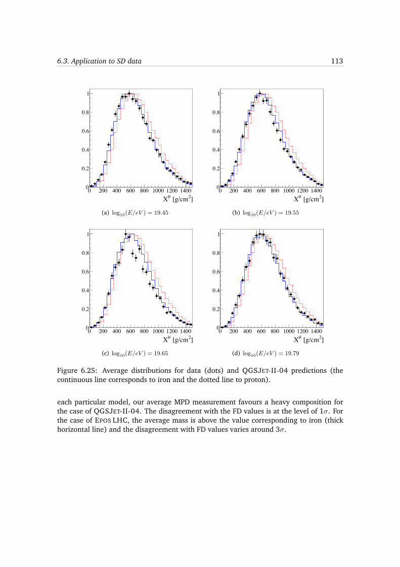
6.3. Application to SD data 113
]2 [g/cmµX0 200 400 600 800 1000 1200 14000
0.2
0.4
0.6
0.8
1
(a) log10(E/eV ) = 19.45
]2 [g/cmµX0 200 400 600 800 1000 1200 14000
0.2
0.4
0.6
0.8
1
(b) log10(E/eV ) = 19.55
]2 [g/cmµX0 200 400 600 800 1000 1200 14000
0.2
0.4
0.6
0.8
1
(c) log10(E/eV ) = 19.65
]2 [g/cmµX0 200 400 600 800 1000 1200 14000
0.2
0.4
0.6
0.8
1
(d) log10(E/eV ) = 19.79
Figure 6.25: Average distributions for data (dots) and QGSJET-II-04 predictions (thecontinuous line corresponds to iron and the dotted line to proton).
each particular model, our average MPD measurement favours a heavy composition forthe case of QGSJET-II-04. The disagreement with the FD values is at the level of 1�. Forthe case of EPOS LHC, the average mass is above the value corresponding to iron (thickhorizontal line) and the disagreement with FD values varies around 3�.
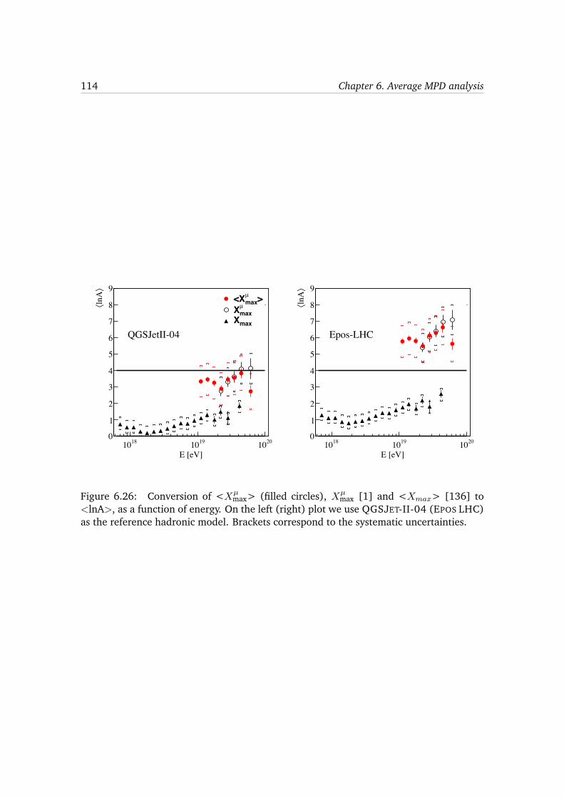
114 Chapter 6. Average MPD analysis
E [eV]1810 1910 2010
⟩ln
A⟨
0
1
2
3
4
5
6
7
8
9>max
µ <Xmaxµ Xmax X
QGSJetII-04
E [eV]1810 1910 2010
⟩ln
A⟨
0
1
2
3
4
5
6
7
8
9
Epos-LHC
Figure 6.26: Conversion of <X
µ
max> (filled circles), X
µ
max [1] and <X
max
> [136] to<lnA>, as a function of energy. On the left (right) plot we use QGSJET-II-04 (EPOS LHC)as the reference hadronic model. Brackets correspond to the systematic uncertainties.
7New detector configurations andpotential improvements of MPDstudies
During the last two years the Pierre Auger collaboration has been actively devising propos-als for the upgrade of the Surface Detector. The final decision was to use scintillators ontop of the WCD and to update the current electronics [142]. Those configurations had tobe simulated to evaluate the expected improvements with respect to the current detector.
For reasons that will become more evident later in the chapter, one of the proposalsthat could influence more MPD-based analyses was to change the internal properties ofthe liner in order to reduce the time response of the WCD [143]. Motivated by this ideawe proceed to implement the required changes in the O↵ line [107] software to be ableto perform Geant4 simulations. All the changes have been implemented in a new branch,v2r8-blacktank-experimental [144]. The configuration of the electronics has been updatedto match the features of the proposed upgrade.
In this chapter we document the changes done in the branch and discuss the cross-checks we performed to understand the impact the proposed changes will have in thephysics. We also describe how the resolution on the reconstruction of the maximum ofthe muon production distance is affected by those changes. Finally we redo this analysisconsidering the case of a dense array of WCD.
7.1 Implementation of new configurations in Offline software
As introduced in chapter 3, the Auger offline software, O↵ line, is a framework whichprovides the mechanisms for encapsulating in modules the steps involved in the simulationand reconstruction of EAS. It also provides the means to configuring and sequencing thesemodules by external files. It has three principal components: a Framework, a detectordescription and an event description. We applied the required changes in each one of thecomponents.
Framework changes The detector properties are coded inside the Framework. Becausethe physical properties of the Surface Detector were not expected to be changed, some ofthem were hard-coded. The main changes that had to be tracked all along the differentmodules were the length of the trace, the sampling frequency and the dynamic range.Another WCD property that has been changed at Framework level is the number of PMTs.
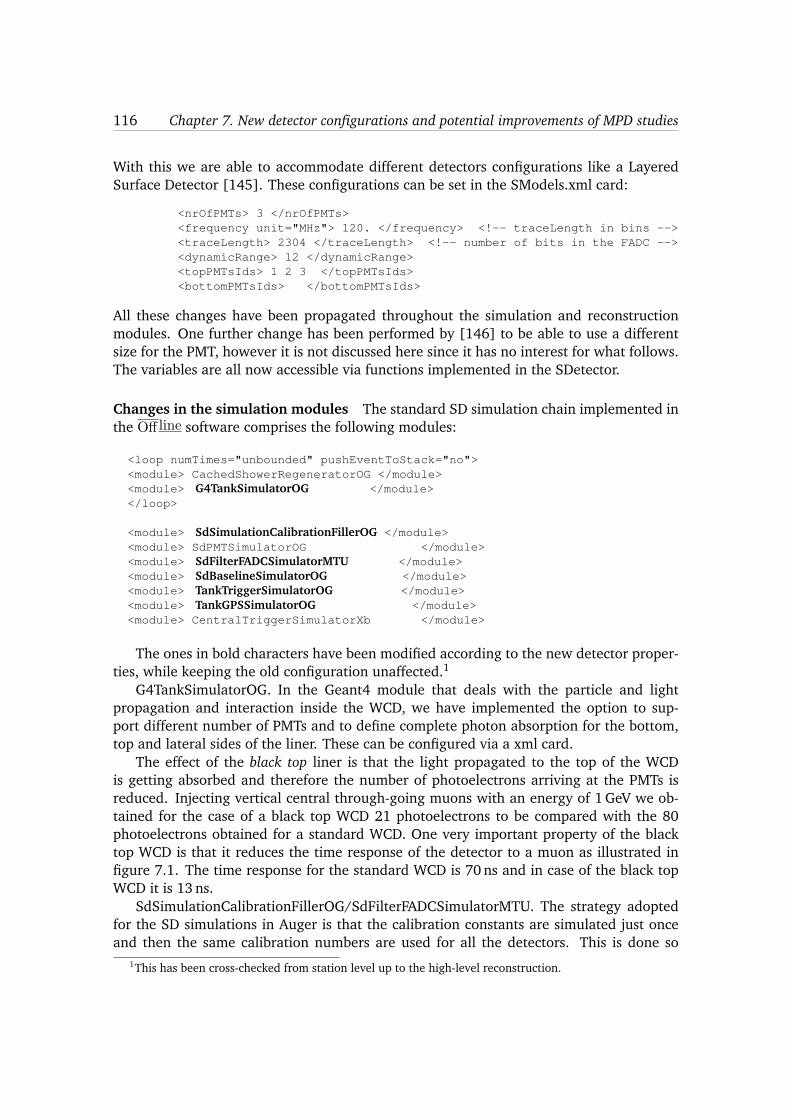
116 Chapter 7. New detector configurations and potential improvements of MPD studies
With this we are able to accommodate different detectors configurations like a LayeredSurface Detector [145]. These configurations can be set in the SModels.xml card:
<nrOfPMTs> 3 </nrOfPMTs><frequency unit="MHz"> 120. </frequency> <!-- traceLength in bins --><traceLength> 2304 </traceLength> <!-- number of bits in the FADC --><dynamicRange> 12 </dynamicRange><topPMTsIds> 1 2 3 </topPMTsIds><bottomPMTsIds> </bottomPMTsIds>
All these changes have been propagated throughout the simulation and reconstructionmodules. One further change has been performed by [146] to be able to use a differentsize for the PMT, however it is not discussed here since it has no interest for what follows.The variables are all now accessible via functions implemented in the SDetector.
Changes in the simulation modules The standard SD simulation chain implemented inthe O↵ line software comprises the following modules:
<loop numTimes="unbounded" pushEventToStack="no"><module> CachedShowerRegeneratorOG </module><module> G4TankSimulatorOG </module></loop>
<module> SdSimulationCalibrationFillerOG </module><module> SdPMTSimulatorOG </module><module> SdFilterFADCSimulatorMTU </module><module> SdBaselineSimulatorOG </module><module> TankTriggerSimulatorOG </module><module> TankGPSSimulatorOG </module><module> CentralTriggerSimulatorXb </module>
The ones in bold characters have been modified according to the new detector proper-ties, while keeping the old configuration unaffected.1
G4TankSimulatorOG. In the Geant4 module that deals with the particle and lightpropagation and interaction inside the WCD, we have implemented the option to sup-port different number of PMTs and to define complete photon absorption for the bottom,top and lateral sides of the liner. These can be configured via a xml card.
The effect of the black top liner is that the light propagated to the top of the WCDis getting absorbed and therefore the number of photoelectrons arriving at the PMTs isreduced. Injecting vertical central through-going muons with an energy of 1 GeV we ob-tained for the case of a black top WCD 21 photoelectrons to be compared with the 80photoelectrons obtained for a standard WCD. One very important property of the blacktop WCD is that it reduces the time response of the detector to a muon as illustrated infigure 7.1. The time response for the standard WCD is 70 ns and in case of the black topWCD it is 13 ns.
SdSimulationCalibrationFillerOG/SdFilterFADCSimulatorMTU. The strategy adoptedfor the SD simulations in Auger is that the calibration constants are simulated just onceand then the same calibration numbers are used for all the detectors. This is done so
1This has been cross-checked from station level up to the high-level reconstruction.
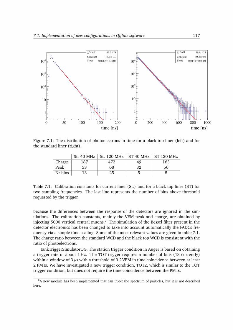
7.1. Implementation of new configurations in Offline software 117
/ ndf 2χ 43.7 / 78Constant 0.0± 10.7 Slope 0.0007± -0.0767
time [ns]0 50 100 150 200
1
10
210
310
410
/ ndf 2χ 43.7 / 78Constant 0.0± 10.7 Slope 0.0007± -0.0767
/ ndf 2χ 395 / 473Constant 0.0± 10.2 Slope 0.0000± -0.0143
time [ns]0 200 400 600 800 1000
1
10
210
310
410
/ ndf 2χ 395 / 473Constant 0.0± 10.2 Slope 0.0000± -0.0143
Figure 7.1: The distribution of photoelectrons in time for a black top liner (left) and forthe standard liner (right).
St. 40 MHz St. 120 MHz BT 40 MHz BT 120 MHzCharge 187 472 49 163Peak 53 68 32 56Nr bins 13 25 5 8
Table 7.1: Calibration constants for current liner (St.) and for a black top liner (BT) fortwo sampling frequencies. The last line represents the number of bins above thresholdrequested by the trigger.
because the differences between the response of the detectors are ignored in the sim-ulations. The calibration constants, mainly the VEM peak and charge, are obtained byinjecting 5000 vertical central muons.2 The simulation of the Bessel filter present in thedetector electronics has been changed to take into account automatically the FADCs fre-quency via a simple time scaling. Some of the most relevant values are given in table 7.1.The charge ratio between the standard WCD and the black top WCD is consistent with theratio of photoelectrons.
TankTriggerSimulatorOG. The station trigger condition in Auger is based on obtaininga trigger rate of about 1 Hz. The TOT trigger requires a number of bins (13 currently)within a window of 3µs with a threshold of 0.2 VEM in time coincidence between at least2 PMTs. We have investigated a new trigger condition, TOT2, which is similar to the TOTtrigger condition, but does not require the time coincidence between the PMTs.
2A new module has been implemented that can inject the spectrum of particles, but it is not describedhere.
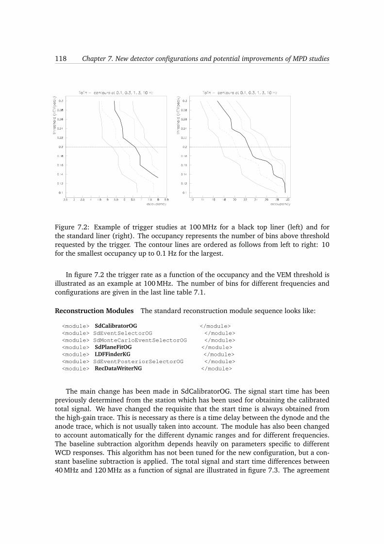
118 Chapter 7. New detector configurations and potential improvements of MPD studies
Figure 7.2: Example of trigger studies at 100 MHz for a black top liner (left) and forthe standard liner (right). The occupancy represents the number of bins above thresholdrequested by the trigger. The contour lines are ordered as follows from left to right: 10for the smallest occupancy up to 0.1 Hz for the largest.
In figure 7.2 the trigger rate as a function of the occupancy and the VEM threshold isillustrated as an example at 100 MHz. The number of bins for different frequencies andconfigurations are given in the last line table 7.1.
Reconstruction Modules The standard reconstruction module sequence looks like:
<module> SdCalibratorOG </module><module> SdEventSelectorOG </module><module> SdMonteCarloEventSelectorOG </module><module> SdPlaneFitOG </module><module> LDFFinderKG </module><module> SdEventPosteriorSelectorOG </module><module> RecDataWriterNG </module>
The main change has been made in SdCalibratorOG. The signal start time has beenpreviously determined from the station which has been used for obtaining the calibratedtotal signal. We have changed the requisite that the start time is always obtained fromthe high-gain trace. This is necessary as there is a time delay between the dynode and theanode trace, which is not usually taken into account. The module has also been changedto account automatically for the different dynamic ranges and for different frequencies.The baseline subtraction algorithm depends heavily on parameters specific to differentWCD responses. This algorithm has not been tuned for the new configuration, but a con-stant baseline subtraction is applied. The total signal and start time differences between40 MHz and 120 MHz as a function of signal are illustrated in figure 7.3. The agreement

7.1. Implementation of new configurations in Offline software 119
(<S>/VEM)10
log0 0.5 1 1.5 2 2.5 3 3.5 4 4.5
[%]
40 M
Hz
)/ S
120
MH
z- S
40 M
Hz
(S
-5
-4
-3
-2-1
0
1
23
4
5All Stations
HG Saturated
(<S>/VEM)10
log1 1.5 2 2.5 3 3.5 4 4.5
(ns)
120
MH
z- t
40 M
Hz
t
-5
-4
-3
-2-1
0
1
23
4
5
All StationsLG SaturatedHG Saturated
Figure 7.3: Station level variables. Total signal differences between stations versus totalsignal using 120 MHz and 40 MHz with 12 bits and white top.
Mean RMS�S(1000)/S(1000) [%] �0.81± 0.04 0.59± 0.03�E/E [%] �0.83± 0.05 0.72± 0.03Angle [deg.] 0.152± 0.007 0.114± 0.005Core [m] 1.49± 0.09 m 1.36± 0.06 m
Table 7.2: Reconstruction differences between 40 and 120 MHz for the standard WCD.
between the signals is very good, with the mean differences being smaller than 1% and5 ns respectively.
The SdPlaneFitOG and LDFFinderKG are indirectly affected by the changes in thetrunk. One of the modifications that affects marginally the angular reconstruction is re-lated to the inclusion in the time variance model of the changes in frequency and GPSresolution. The reconstruction of the lateral distribution function is also slightly affectedwhen one changes the dynamic range of the signal reading. Modifications have also beenmade in RecDataWriterNG to include new variables like a changing number of PMTs andfrequencies. The EventBrowser can display now automatically different detector configur-ations.
All the changes have been checked up to the finest details. We have simulated 200air-showers, half with protons as primary particle and half with iron. We used CORSIKA(Fluka/QGSJet II) with an energy of 30 EeV and an isotropic angular distributed between0 and 60 degrees. The particles on the ground were fed to the detector simulations usingpermutations between different configurations: 40 MHz, 120 MHz, black top liner (BT),10 bit FADCs and 12 bit FADCs .
The results for the comparisons of the main variables, i.e. S(1000), energy, angleand core location, are given in table 7.2 for two frequencies, 40 MHz and 120 MHz. Thedifferences are less than 1% in S(1000) and energy, with an angular difference of less

120 Chapter 7. New detector configurations and potential improvements of MPD studies
Mean RMS�S(1000)/S(1000) [%] �0.8± 0.3 3.88± 0.18�E/E [%] �0.8± 0.3 4.09± 0.19Angle [deg] 0.248± 0.014 0.216± 0.010Core [m] 17.5± 1.0 m 15.4± 0.7 m
Table 7.3: Reconstruction differences between standard and black top WCD at 120 MHz.
Mean RMSFrequency 40 MHz 120 MHz 40 MHz 120 MHzCandidates 16.5± 0.3 17.8± 0.4 5.4± 0.2 5.5± 0.3Candidates (BT) 17.8± 0.4 19.3± 0.1 5.5± 0.3 6.1± 0.1
Core 66± 3 m 66± 3 m 45± 2 m 45± 2 mCore (BT) 66± 3 m 62± 3 m 45± 2 m 45± 2 mEnergy [%] �32.9± 0.8 �32.1± 0.8 12.4± 0.6 12.4± 0.6Energy (BT) [%] �32.1± 0.8 �31.3± 0.7 12.4± 0.6 11.1± 0.5
Angle [deg.] 0.33± 0.01 0.31± 0.01 0.21± 0.01 0.19± 0.01Angle (BT) [deg.] 0.31± 0.01 0.31± 0.01 0.19± 0.01 0.19± 0.01
Table 7.4: Resolutions for 120 MHz white and black top (BT). The candidates repres-ent the mean number of stations used in the reconstruction, and the rest represent thedifferences to the generated values.
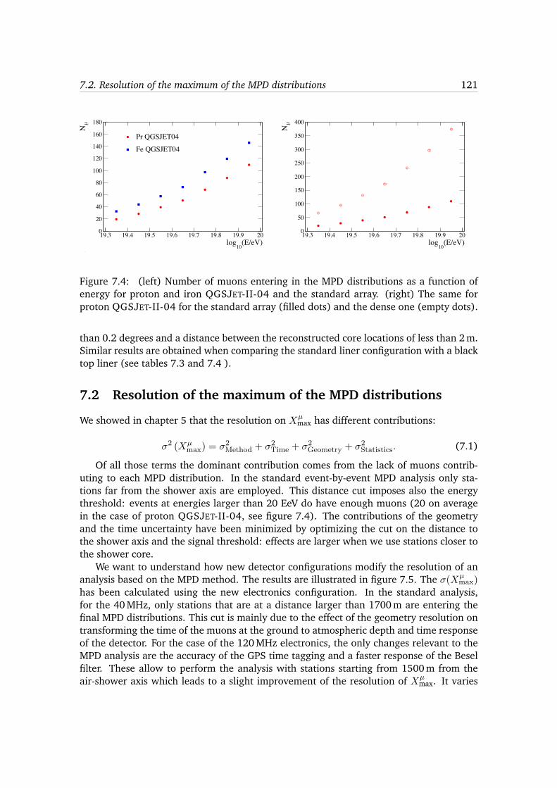
7.2. Resolution of the maximum of the MPD distributions 121
a(E/eV)
10log
19.3 19.4 19.5 19.6 19.7 19.8 19.9 20
µN
0
20
40
60
80
100
120
140
160
180
Pr QGSJET04
Fe QGSJET04
(E/eV)10
log19.3 19.4 19.5 19.6 19.7 19.8 19.9 20
µN
0
50
100
150
200
250
300
350
400
Figure 7.4: (left) Number of muons entering in the MPD distributions as a function ofenergy for proton and iron QGSJET-II-04 and the standard array. (right) The same forproton QGSJET-II-04 for the standard array (filled dots) and the dense one (empty dots).
than 0.2 degrees and a distance between the reconstructed core locations of less than 2 m.Similar results are obtained when comparing the standard liner configuration with a blacktop liner (see tables 7.3 and 7.4 ).
7.2 Resolution of the maximum of the MPD distributions
We showed in chapter 5 that the resolution on X
µ
max has different contributions:
�
2 (Xµ
max) = �
2Method + �
2Time + �
2Geometry + �
2Statistics. (7.1)
Of all those terms the dominant contribution comes from the lack of muons contrib-uting to each MPD distribution. In the standard event-by-event MPD analysis only sta-tions far from the shower axis are employed. This distance cut imposes also the energythreshold: events at energies larger than 20 EeV do have enough muons (20 on averagein the case of proton QGSJET-II-04, see figure 7.4). The contributions of the geometryand the time uncertainty have been minimized by optimizing the cut on the distance tothe shower axis and the signal threshold: effects are larger when we use stations closer tothe shower core.
We want to understand how new detector configurations modify the resolution of ananalysis based on the MPD method. The results are illustrated in figure 7.5. The �(Xµ
max)has been calculated using the new electronics configuration. In the standard analysis,for the 40 MHz, only stations that are at a distance larger than 1700 m are entering thefinal MPD distributions. This cut is mainly due to the effect of the geometry resolution ontransforming the time of the muons at the ground to atmospheric depth and time responseof the detector. For the case of the 120 MHz electronics, the only changes relevant to theMPD analysis are the accuracy of the GPS time tagging and a faster response of the Beselfilter. These allow to perform the analysis with stations starting from 1500 m from theair-shower axis which leads to a slight improvement of the resolution of Xµ
max. It varies
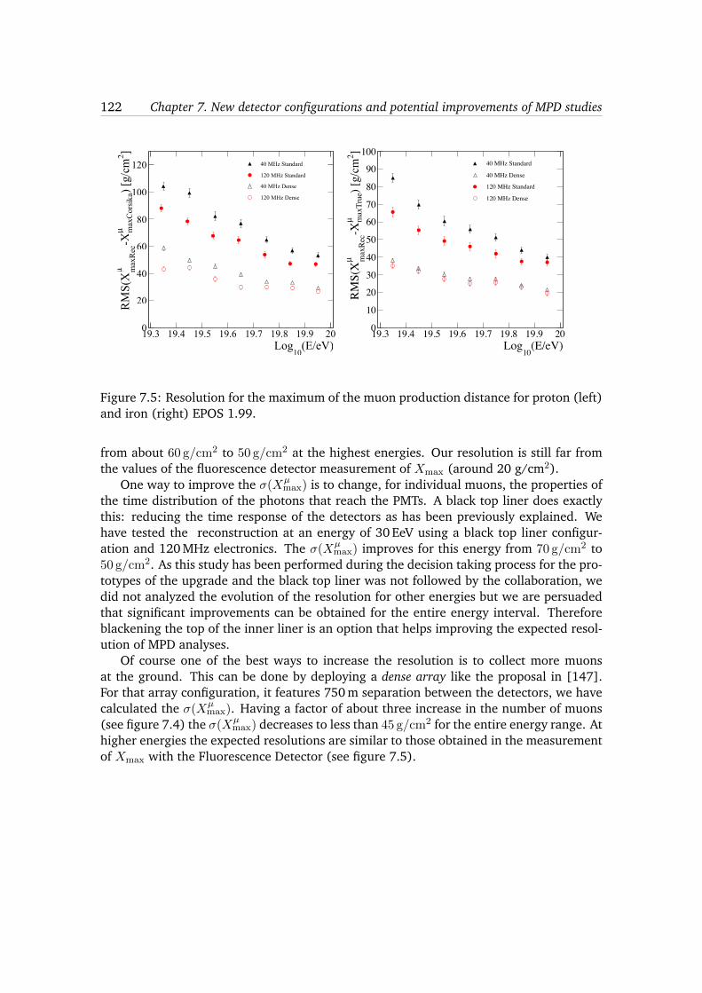
122 Chapter 7. New detector configurations and potential improvements of MPD studies
(E/eV)10
Log19.3 19.4 19.5 19.6 19.7 19.8 19.9 20
]2) [
g/cm
max
Cor
sika
µ-X
max
Rec
µR
MS(
X
0
20
40
60
80
100
120 40 MHz Standard
120 MHz Standard
40 MHz Dense
120 MHz Dense
(E/eV)10
Log19.3 19.4 19.5 19.6 19.7 19.8 19.9 20
]2) [
g/cm
max
True
µ-X
max
Rec
µRM
S(X
0
10
20
30
40
50
60
70
80
90
10040 MHz Standard
40 MHz Dense
120 MHz Standard
120 MHz Dense
Figure 7.5: Resolution for the maximum of the muon production distance for proton (left)and iron (right) EPOS 1.99.
from about 60 g/cm2 to 50 g/cm2 at the highest energies. Our resolution is still far fromthe values of the fluorescence detector measurement of Xmax (around 20 g/cm2).
One way to improve the �(Xµ
max) is to change, for individual muons, the properties ofthe time distribution of the photons that reach the PMTs. A black top liner does exactlythis: reducing the time response of the detectors as has been previously explained. Wehave tested the reconstruction at an energy of 30 EeV using a black top liner configur-ation and 120 MHz electronics. The �(Xµ
max) improves for this energy from 70 g/cm2 to50 g/cm2. As this study has been performed during the decision taking process for the pro-totypes of the upgrade and the black top liner was not followed by the collaboration, wedid not analyzed the evolution of the resolution for other energies but we are persuadedthat significant improvements can be obtained for the entire energy interval. Thereforeblackening the top of the inner liner is an option that helps improving the expected resol-ution of MPD analyses.
Of course one of the best ways to increase the resolution is to collect more muonsat the ground. This can be done by deploying a dense array like the proposal in [147].For that array configuration, it features 750 m separation between the detectors, we havecalculated the �(Xµ
max). Having a factor of about three increase in the number of muons(see figure 7.4) the �(Xµ
max) decreases to less than 45 g/cm2 for the entire energy range. Athigher energies the expected resolutions are similar to those obtained in the measurementof Xmax with the Fluorescence Detector (see figure 7.5).

Conclusions and futureprospects
This thesis is a contribution to the ongoing questions related to the mass composition ofthe UHECR and how accurately hadronic interaction models describe data. This workbuilds on the information recorded by the SD of the Pierre Auger Observatory, that is whyour starting point was a revision of the SD event reconstruction.
⌅ Improvements in the SD event reconstruction
• The impact point on the ground of the air-shower and its energy are determinedthrough a fit of the lateral distribution of the signals. One of the key ingredients fora reliable estimation of those quantities is the uncertainty of the WCD signals.
• Using the Infill data we revised the signal variance model and updated it to includethe new triggers implemented in the array, the ToTd and MOPs. The new modelwas tested in the interval of full trigger efficiency for the SD. A new component of2.3% was added to the signal uncertainty that might be related to the uncertaintyof the calibration. The new signal variance model does not change significantly thereconstructed variables and it has only a mild impact on the uncertainties.
• With the help of a toy Monte Carlo which includes the effects of the trigger on thesignal variance distributions, we showed that the signal variance form is valid inthe entire signal range. It can be extrapolated to the very low signals (i.e. down to0.5 VEM) observed with the new triggers ToTd and MOPs.
The next part of the thesis discusses in detail how the recorded arrival times of muonsprovide a variable which is highly sensitive to the nature of UHECRs.
⌅ Update of the Muon Arrival Time Model: a description of a new kinematicdelay parameterization
• We revised the muon arrival time distribution model with special focus on how itaffects the bias of X
µ
max and the shape of the MPD distribution. In particular, thekinematic delay approximation was carefully studied. We found that the classicapproach overestimates this contribution, and therefore the reconstructed z are ingeneral underestimated.
124 Conclusions and future prospects
• To reduce the distortions coming from this effect, we explored new ways to derivethe kinematic delays. The average kinematic delay obtained from simulations wastabulated as a function of the measured delay in the detectors and the distance tothe shower core (for r >1000 m and ✓ ⇠60�). As a result, the absolute value ofX
µ
max bias was reduced by a factor of 3, and the distortion in the shape of the MPDdistribution was successfully removed.
⌅ Revision of the MPD analysis on an event-by-event basis: Decoupling themain contributions to Xµ
max bias and RMS.
• This work was the first one able to fully understand the different contributions tothe X
µ
max bias. Among all the contributing sources, it was found that the response ofthe muon in the WCD is the main source of bias.
• We studied the impact the un-thinning or resampling procedure, performed in theofficial Auger simulation software, on the muon arrival times in the WCD. An un-derestimation of these times, increasing almost quadratically with the distance tothe shower core, r, was found. It ranges from a few nanoseconds, for small valuesof r, up to several tens of nanoseconds for larger distances. We proved that for afixed zenith angle, around 60�, this underestimation is universal (i.e. independentof the nature of the primary particle, the energy and the hadronic model used in thesimulations), being an effect of the algorithm itself.
• The resampling procedure done in the Auger software induces a bias in the determ-ination of Xµ
max. The estimated final bias after the whole reconstruction chain is 24g/cm2 which has to be taken into account when analyzing the data. After correctingfor this effect in the data, the tension with hadronic models is aggravated.
• The different contributions to X
µ
max resolution were fully understood. The maincontribution is due to the lack of muons contributing to each MPD distribution.
⌅ Average MPD analysis
• With the aim of enlarging the energy range of applicability of MPD studies and toalleviate the problem of lack of statistics to build MPD distributions, we proposed tostudy the behaviour with energy of average MPD distributions (i.e. we build singledistributions with all the air showers belonging to a particular energy bin).
• As our interest was to study the shape of the MPD, we decoupled each contributionto the bias of the average X
µ
max and identified all the distortion sources. The maincontribution to the bias is the response of the WCD to muons, as in the event-by-event case. However, we found that the geometry reconstruction also modifies theshape. To minimize the effect of the reconstruction and its influence on the bias ofthe average X
µ
max we restricted the analysis to distances larger than 1500 m.
• The distance cut imposes the energy threshold. Requesting a selection efficiencylarger than 95% implies that the average X
µ
max can be extended down to only 10 EeVwhich is a factor two better than the baseline event-by-event analysis.
125
• We fine-tune and apply the deconvolution to remove part of the MPD distortion in-duced by the WCD response. Nevertheless, to be able to study the shape of thedistribution at very high level of detail an improvement of the geometry reconstruc-tion in this zenith range region is mandatory. This will also help the event-by-eventanalysis.
• We analyzed the data collected by the Pierre Auger Observatory between January2004 and October 2014. After the selection cuts we are left with 2319 events above10 EeV in a zenith angle range around 60�.
• The analysis was performed in the same zenith angle range as in [1] but in the futureit can be extended to other regions.
• The main sources of systematic uncertainties yield an overall value of ⇠20.5 g/cm2
being dominated by the contribution of the hadronic models.
• The lnA obtained from the reconstructed data is compatible with the result pub-lished in [1], confirming the tension between hadronic interaction models and thedata which persists also between 10 and 22 EeV. Therefore, it is difficult to drawsolid conclusions about the mass composition of UHECR.
⌅ New detector configurations and its influence on MPD analysis
• The MPD analysis was applied to different detector configurations which we imple-mented in the official Auger software. We have shown that an intrinsically fastertime response of the WCD to particles (for example when using a black-top liner)might improve the resolution of X
µ
max. Increasing only the sampling frequencydoes not provide a significant improvement. However, we conclude that only amuch denser array could provide a resolution compatible with the FD measurementsthanks to the sizable increase in the number of detected muons at the ground.

Conclusiones y perspectivasfuturas
Esta tesis es un intento de contribuir al debate acerca de la composición de los rayoscósmicos de ultra alta energía y cómo de precisos son los modelos hadrónicos a la hora dedescribir los datos. Este trabajo se ha hecho con la información registrada en el detectorde superficie del Observatorio Pierre Auger por lo que el punto de partida ha sido unarevisión de la reconstrucción de los sucesos registrados por dicho detector.
⌅ Mejoras en la reconstrucción de los sucesos del detector de superficie
• El punto de impacto en el suelo y la energía de las cascadas se determinan a partirdel ajuste a una función de distribución lateral de las señales registradas. Una de lasclaves en el proceso de ajuste para estimar de forma precisa estas cantidades es ladeterminación de los errores de las señales de los detectores
• Usando los datos registrados por el detector Infilled, se ha revisado y actualizado elmodelo que describe las varianzas de las señales para así incluir los nuevos triggersque se han implementado en el detector de superficie, ToTd y MOPs. El modelo se harevisado en la región de máxima eficiencia de trigger para el detector de superficie.Una nueva componente que podría estar relacionada con incertidumbres en la cali-bración del 2.3 % se ha añadido al error de la señal. El nuevo modelo para describirlos errores en la señal no cambia mucho las variables reconstruidas y tiene un leveimpacto en sus incertidumbres.
• Con la ayuda de un toy Monte Carlo que contiene los efectos de trigger en las distri-buciones de la varianza de las señales, hemos demostrado que el modelo funcionaen todo el rango de señales. Además puede extrapolarse hasta señales muy bajasdonde los nuevos triggers ToTd y MOPs son sensibles.
La siguiente parte de la tesis describe en detalle cómo los tiempos de llegada de losmuones registrados en los detectores dan lugar a una variable muy sensible a la composi-ción química de los rayos cósmicos de ultra alta energía.
⌅ Actualización del modelo de los tiempos de llegada de los muones: des-cripción de un nuevo retraso cinemático.
• El modelo se ha revisado haciendo hincapié en cómo afecta al sesgo de X
µ
max y ala forma de la distribución de la MPD. En particular, se ha estudiado la aproxima-
128 Conclusione
ción que se usa para estimar el retraso cinemático. Hemos demostrado que la actualdescripción sobrestimaba esta contribución subestimando los valores de las z recons-truidas.
• Una nueva forma de calcular el retraso cinemático se ha desarrollado para reducirlas distorsiones que este provocaba en el perfil. Se ha tabulado el retraso cinemá-tico promedio con simulaciones en función del retraso medido en los detectores yla distancia al eje de la cascada (para r >1000 m, ✓ ⇠60�). Hemos reducido el va-lor absoluto del sesgo en un factor 3, y eliminado la distorsión en el perfil de ladistribución de la MPD.
⌅ Revisión del análisis de la MPD suceso a suceso: Separación de las princi-pales contribuciones al sesgo y a la resolución de Xµ
max.
• Este trabajo ha sido el primero en desacoplar las diferentes contribuciones al sesgode X
µ
max. Entre todas ellas, hemos visto que la principal es debida a la respuesta delos detectores a los muones.
• Hemos estudiado el impacto del proceso de un-thinning o resampling que se lleva acabo en la versión O↵ line-icrc2013 en el tiempo de llegada de los muones a los de-tectores. Encontramos una subestimación de estos tiempos que aumentaba cuadráti-camente con la distancia al eje de la cascada, variando de unos pocos nanosegundoscerca del eje a decenas de nanosegundos a distancias lejanas. Probamos que estasubestimación es universal (independiente de la naturaleza de la partícula primaria,la energía y el modelo hadrónico usado en las simulaciones) siendo un efecto delalgoritmo en sí.
• El proceso de resampling realizado en O↵ line-icrc2013 induce un sesgo en la deter-minación de X
µ
max. El sesgo final después de toda la cadena de reconstrucción es de24 g/cm2 y tiene que tomarse en cuenta al analizar los datos. Tras tener en cuentaeste efecto en los datos, se agrava la tensión con los modelos hadrónicos.
• Se han estudiado las diferentes contribuciones a la resolución de X
µ
max, siendo elprincipal factor la falta de muones que contribuyen a cada distribución de la MPD.
⌅ Análisis de la distribución promedio de la MPD
• Con el propósito de extender el rango de aplicabilidad de los estudios de MPD y paraaliviar la falta de estadística a la hora de construir cada distribución de MPD, hemospropuesto estudiar el comportamiento con la energía de la distribución promediode la MPD (es decir, construimos la distribución resultante de todos los sucesos quepertenecen a un intervalo de energía, en particular).
• Como nuestro objetivo era estudiar el perfil de la distribución, desacoplamos cadauna de las contribuciones al sesgo del máximo de la distribución promedio e iden-tificamos todas las fuentes de distorsión. La principal contribución al sesgo es larespuesta de los detectores a los muones, al igual que en el análisis suceso a suce-so. Sin embargo, encontramos que la reconstrucción de la geometría también puede

129
modificar el perfil. Para minimizar estos efectos de la reconstrucción y su influenciaen el sesgo de X
µ
max hacemos el análisis a distancias mayores de 1500 m.
• El corte en distancia impone un corte en energía. Requerimos que la eficiencia deselección sea mayor del 95 %, lo que implica seleccionar sucesos con energía mayorde 10 EeV.
• Aplicamos la deconvolución para eliminar la distorsión del perfil provocada por laseñal pero para ser capaces de estudiar el perfil de la distribución es necesaria unamejora de la reconstrucción geométrica en esta región de ángulo cenital. Esto ayu-daría también al análisis suceso a suceso.
• Hemos analizado los datos registrados por el Observatorio Pierre Auger entre enerode 2004 y octubre de 2014. Después de los cortes de selección tenemos 2319 sucesospor encima de 10 EeV.
• El análisis se ha desarrollado en la misma región de ángulo cenital que [1] pero enun futuro podría extenderse a otras regiones.
• Las principales fuentes de sistemáticos resultan en un valor total de ⇠ 20,5 g/cm2
dominado por las contribuciones de los modelos hadrónicos.
• El lnA obtenido de la reconstrucción de los datos es compatible con el resultadopublicado en [1], confirmando así la tensión entre los modelos hadrónicos y losdatos. Por tanto, es difícil extraer conclusiones sólidas acerca de la masa de los rayoscósmicos de ultra alta energía.
⌅ Nuevas configuraciones de detector y su influencia en el análisis de la MPD
• Se ha elaborado el análisis de la MPD para diferentes configuraciones de detector. Encuanto a la mejora en la resolución de X
µ
max, una respuesta temporal más rápida delos detectores a las partículas, por ejemplo un liner con la superficie opaca, ayudaríaa mejorarla. Aumentar sólo la frecuencia de muestreo no produce mejoras aprecia-bles en la resolución. Sin embargo, tener muchos más detectores, un array denso,nos permitiría tener muchos más muones y así obtener una resolución compatiblecon la de las medidas del FD.


AExample of outliers
r [m]200 400 600 800 1000 1200 1400 1600
Sign
al [V
EM]
1
10
210 Stage: 4.5/Ndf: 0.5/ 32χ
candidatesnot-triggeredremoved
(a)
r [m]200 400 600 800 1000 1200 1400 1600
Sign
al [V
EM]
1
10
210
Stage: 4.5/Ndf: 0.5/ 32χ
candidatesnot-triggeredremoved
(b)
Figure A.1: Lateral distribution function for events where the difference between signalsis larger than 1.5. (a) Event 6466282. The signal candidate station of the doublet, station734, observed 69.6 VEM, while the partner, station 93, has a signal of 1.8 VEM. (b) Event14995513. The candidate station, 669, has a signal of 139.4 VEM, while the partner,station 80, measured 2.3 VEM.
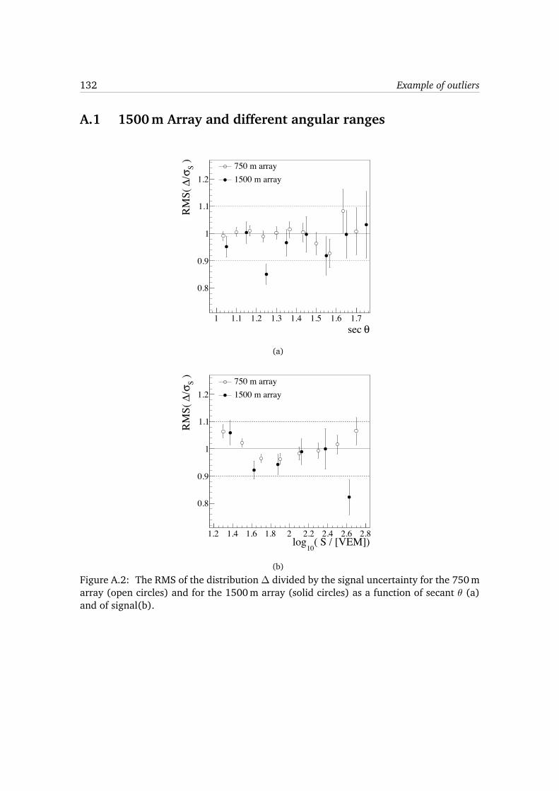
132 Example of outliers
A.1 1500 m Array and different angular ranges
θsec 1 1.1 1.2 1.3 1.4 1.5 1.6 1.7
) Sσ/∆RM
S(
0.8
0.9
1
1.1
1.2750 m array1500 m array
(a)
( S / [VEM])10
log1.2 1.4 1.6 1.8 2 2.2 2.4 2.6 2.8
) Sσ/∆RM
S(
0.8
0.9
1
1.1
1.2750 m array1500 m array
(b)
Figure A.2: The RMS of the distribution � divided by the signal uncertainty for the 750 marray (open circles) and for the 1500 m array (solid circles) as a function of secant ✓ (a)and of signal(b).
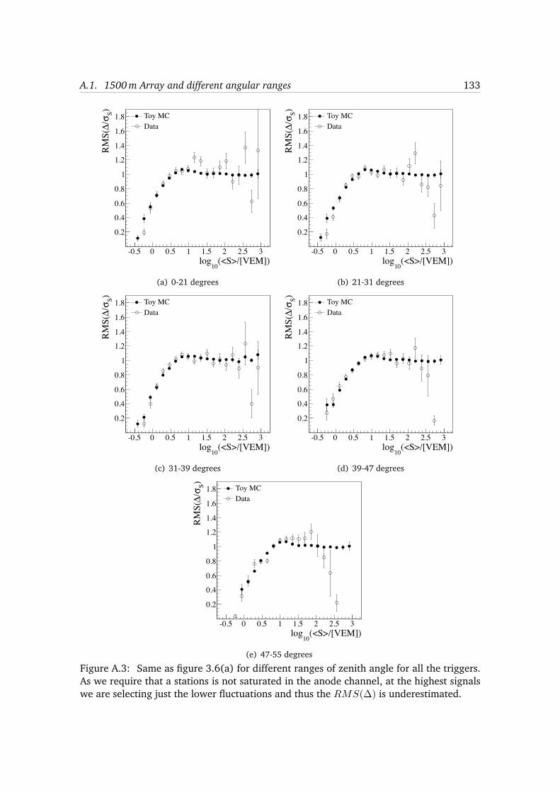
A.1. 1500 m Array and different angular ranges 133
(<S>/[VEM])10
log-0.5 0 0.5 1 1.5 2 2.5 3
) Sσ/∆RM
S(
0.2
0.4
0.6
0.8
1
1.2
1.4
1.6
1.8 Toy MCData
(a) 0-21 degrees
(<S>/[VEM])10
log-0.5 0 0.5 1 1.5 2 2.5 3
) Sσ/∆RM
S(
0.2
0.4
0.6
0.8
1
1.2
1.4
1.6
1.8 Toy MCData
(b) 21-31 degrees
(<S>/[VEM])10
log-0.5 0 0.5 1 1.5 2 2.5 3
) Sσ/∆RM
S(
0.2
0.4
0.6
0.8
1
1.2
1.4
1.6
1.8 Toy MCData
(c) 31-39 degrees
(<S>/[VEM])10
log-0.5 0 0.5 1 1.5 2 2.5 3
) Sσ/∆RM
S(
0.2
0.4
0.6
0.8
1
1.2
1.4
1.6
1.8 Toy MCData
(d) 39-47 degrees
(<S>/[VEM])10
log-0.5 0 0.5 1 1.5 2 2.5 3
) Sσ/∆RM
S(
0.2
0.4
0.6
0.8
1
1.2
1.4
1.6
1.8 Toy MCData
(e) 47-55 degrees
Figure A.3: Same as figure 3.6(a) for different ranges of zenith angle for all the triggers.As we require that a stations is not saturated in the anode channel, at the highest signalswe are selecting just the lower fluctuations and thus the RMS(�) is underestimated.
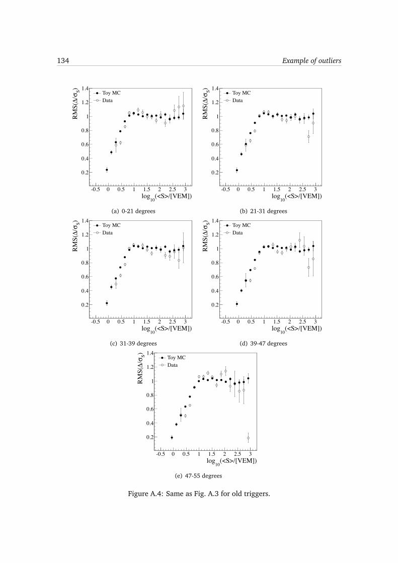
134 Example of outliers
(<S>/[VEM])10
log-0.5 0 0.5 1 1.5 2 2.5 3
) Sσ/∆RM
S(
0.2
0.4
0.6
0.8
1
1.2
1.4Toy MCData
(a) 0-21 degrees
(<S>/[VEM])10
log-0.5 0 0.5 1 1.5 2 2.5 3
) Sσ/∆RM
S(
0.2
0.4
0.6
0.8
1
1.2
1.4Toy MCData
(b) 21-31 degrees
(<S>/[VEM])10
log-0.5 0 0.5 1 1.5 2 2.5 3
) Sσ/∆RM
S(
0.2
0.4
0.6
0.8
1
1.2
1.4Toy MCData
(c) 31-39 degrees
(<S>/[VEM])10
log-0.5 0 0.5 1 1.5 2 2.5 3
) Sσ/∆RM
S(
0.2
0.4
0.6
0.8
1
1.2
1.4Toy MCData
(d) 39-47 degrees
(<S>/[VEM])10
log-0.5 0 0.5 1 1.5 2 2.5 3
) Sσ/∆RM
S(
0.2
0.4
0.6
0.8
1
1.2
1.4Toy MCData
(e) 47-55 degrees
Figure A.4: Same as Fig. A.3 for old triggers.
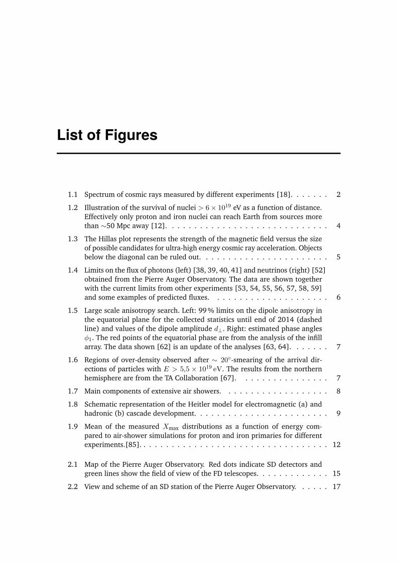
List of Figures
1.1 Spectrum of cosmic rays measured by different experiments [18]. . . . . . . 2
1.2 Illustration of the survival of nuclei > 6⇥ 1019 eV as a function of distance.Effectively only proton and iron nuclei can reach Earth from sources morethan ⇠50 Mpc away [12]. . . . . . . . . . . . . . . . . . . . . . . . . . . . . 4
1.3 The Hillas plot represents the strength of the magnetic field versus the sizeof possible candidates for ultra-high energy cosmic ray acceleration. Objectsbelow the diagonal can be ruled out. . . . . . . . . . . . . . . . . . . . . . . 5
1.4 Limits on the flux of photons (left) [38, 39, 40, 41] and neutrinos (right) [52]obtained from the Pierre Auger Observatory. The data are shown togetherwith the current limits from other experiments [53, 54, 55, 56, 57, 58, 59]and some examples of predicted fluxes. . . . . . . . . . . . . . . . . . . . . 6
1.5 Large scale anisotropy search. Left: 99 % limits on the dipole anisotropy inthe equatorial plane for the collected statistics until end of 2014 (dashedline) and values of the dipole amplitude d?. Right: estimated phase angles�1. The red points of the equatorial phase are from the analysis of the infillarray. The data shown [62] is an update of the analyses [63, 64]. . . . . . . 7
1.6 Regions of over-density observed after ⇠ 20�-smearing of the arrival dir-ections of particles with E > 5,5 ⇥ 1019 eV. The results from the northernhemisphere are from the TA Collaboration [67]. . . . . . . . . . . . . . . . 7
1.7 Main components of extensive air showers. . . . . . . . . . . . . . . . . . . 8
1.8 Schematic representation of the Heitler model for electromagnetic (a) andhadronic (b) cascade development. . . . . . . . . . . . . . . . . . . . . . . . 9
1.9 Mean of the measured Xmax distributions as a function of energy com-pared to air-shower simulations for proton and iron primaries for differentexperiments.[85]. . . . . . . . . . . . . . . . . . . . . . . . . . . . . . . . . . 12
2.1 Map of the Pierre Auger Observatory. Red dots indicate SD detectors andgreen lines show the field of view of the FD telescopes. . . . . . . . . . . . . 15
2.2 View and scheme of an SD station of the Pierre Auger Observatory. . . . . . 17

136 List of Figures
2.3 Charge and pulse height histograms for an SD station with a 3-fold trig-ger (signal in all 3 PMTs). The signal is the sum of the three PMTs. Inthe solid histogram the second peak is produced by vertical through-goingatmospheric muons, while the first peak is a trigger effect. The dashed his-togram is produced by vertical and central muons (VEMs) selected with anexternal muon telescope. . . . . . . . . . . . . . . . . . . . . . . . . . . . . . 18
2.4 T4 and T5 configurations. 2.4(a): The three minimal compact configura-tions for the T4-4C1 trigger. 2.4(b): The two minimal compact configura-tions for the T4-3ToT configuration. 2.4(c): Example of the 6T5 hexagon(shadow) and the 5T5 hexagon (dark shadow). . . . . . . . . . . . . . . . . 20
2.5 View and schemes of an FD site of the Pierre Auger Observatory. . . . . . . . 212.6 Basic patterns of triggered pixels considered by the Second Level Trigger in
the FD. . . . . . . . . . . . . . . . . . . . . . . . . . . . . . . . . . . . . . . . 222.7 The LIDAR and cloud cameras are part of the atmospheric monitoring used
in the Pierre Auger Observatory. . . . . . . . . . . . . . . . . . . . . . . . . . 242.8 Shower-detector plane parameters. . . . . . . . . . . . . . . . . . . . . . . . 252.9 Geometry reconstruction of an event observed by four telescopes and the
Surface Detector [86]. . . . . . . . . . . . . . . . . . . . . . . . . . . . . . . 262.10 Angular resolution (left) and core location accuracy (right) for monocular
and hybrid reconstruction. . . . . . . . . . . . . . . . . . . . . . . . . . . . . 262.11 Angular resolution of hybrid events [101]. . . . . . . . . . . . . . . . . . . . 272.12 Energy reconstruction in the FD. The calorimetric energy is obtained by the
integration of the fit to the profile. . . . . . . . . . . . . . . . . . . . . . . . 28
3.1 Schematic view of a plane shower front. . . . . . . . . . . . . . . . . . . . . 323.2 Schematic view of a spherical shower front. . . . . . . . . . . . . . . . . . . 333.3 (a) Measured signal spectrum (b) Trigger probability as a function of the
mean expected signal. . . . . . . . . . . . . . . . . . . . . . . . . . . . . . . 343.4 (a) Mean of � as a function of the estimated signal. (b) RMS of the distri-
bution � divided by the signal uncertainty for the new (solid circles) andthe previous parameterization (open circles). . . . . . . . . . . . . . . . . . 35
3.5 The RMS of the distribution � divided by the signal uncertainty for thenew (solid circles) and the previous parameterization (open circles) as afunction of sec✓, (a), and of distance to axis, (b). . . . . . . . . . . . . . . . 36
3.6 (a) RMS(�) versus mean signal for old triggers (open circles), TOT andT2, and including the new ones, TOTd and MoPS. (b) RMS(�) versus meansignal for the toy MC (solid circles) and for data (open circles), in the regionwhere the trigger efficiency is larger than 98%. . . . . . . . . . . . . . . . . 38
3.7 (a,c): The RMS(�) versus mean signal compared to the toy MC. (b,d): theRMS of � divided by the parameterization. A good agreement is observedbetween data and the toy MC. . . . . . . . . . . . . . . . . . . . . . . . . . 39
3.8 Angular resolution as a function of the zenith angle ✓ for events with anenergy above 3 EeV, and for various station multiplicities [86]. . . . . . . . 41
3.9 Angular resolution as a function of the primary energy for different angleintervals. . . . . . . . . . . . . . . . . . . . . . . . . . . . . . . . . . . . . . 41
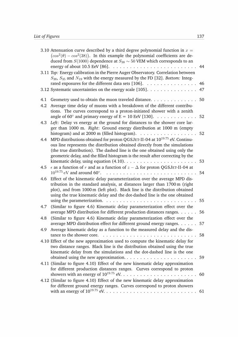
List of Figures 137
3.10 Attenuation curve described by a third degree polynomial function in x =�cos
2(✓)� cos
2(38)�. In this example the polynomial coefficients are de-
duced from S(1000) dependence at S38 ⇠ 50 VEM which corresponds to anenergy of about 10.5 EeV [86]. . . . . . . . . . . . . . . . . . . . . . . . . . 44
3.11 Top: Energy calibration in the Pierre Auger Observatory. Correlation betweenS38, S35 and N19 with the energy measured by the FD [32]. Bottom: Integ-rated exposures for the different data sets [106]. . . . . . . . . . . . . . . . 46
3.12 Systematic uncertainties on the energy scale [105]. . . . . . . . . . . . . . . 47
4.1 Geometry used to obtain the muon traveled distance. . . . . . . . . . . . . . 504.2 Average time delay of muons with a breakdown of the different contribu-
tions. The curves correspond to a proton-initiated shower with a zenithangle of 60� and primary energy of E = 10 EeV [130]. . . . . . . . . . . . . 52
4.3 Left: Delay vs energy at the ground for distances to the shower core lar-ger than 1000 m. Right: Ground energy distribution at 1000 m (emptyhistogram) and at 2000 m (filled histogram). . . . . . . . . . . . . . . . . . 52
4.4 MPD distributions obtained for proton QGSJET-II-04 at 1019.75 eV. Continu-ous line represents the distribution obtained directly from the simulations(the true distribution). The dashed line is the one obtained using only thegeometric delay, and the filled histogram is the result after correcting by thekinematic delay, using equation (4.10). . . . . . . . . . . . . . . . . . . . . . 53
4.5 ✏ as a function of r and as a function of z �� for proton QGSJET-II-04 at1019.75 eV and around 60�. . . . . . . . . . . . . . . . . . . . . . . . . . . . 54
4.6 Effect of the kinematic delay parameterization over the average MPD dis-tribution in the standard analysis, at distances larger than 1700 m (rightplot), and from 1000 m (left plot). Black line is the distribution obtainedusing the true kinematic delay and the dot-dashed line is the one obtainedusing the parameterization. . . . . . . . . . . . . . . . . . . . . . . . . . . . 55
4.7 (Similar to figure 4.6) Kinematic delay parameterization effect over theaverage MPD distribution for different production distances ranges. . . . . . 56
4.8 (Similar to figure 4.6) Kinematic delay parameterization effect over theaverage MPD distribution effect for different ground energy ranges. . . . . . 57
4.9 Average kinematic delay as a function to the measured delay and the dis-tance to the shower core. . . . . . . . . . . . . . . . . . . . . . . . . . . . . 58
4.10 Effect of the new approximation used to compute the kinematic delay fortwo distance ranges. Black line is the distribution obtained using the truekinematic delay from the simulations and the dot-dashed line is the oneobtained using the new approximation. . . . . . . . . . . . . . . . . . . . . . 59
4.11 (Similar to figure 4.10) Effect of the new kinematic delay approximationfor different production distances ranges. Curves correspond to protonshowers with an energy of 1019.75 eV. . . . . . . . . . . . . . . . . . . . . . . 60
4.12 (Similar to figure 4.10) Effect of the new kinematic delay approximationfor different ground energy ranges. Curves correspond to proton showerswith an energy of 1019.75 eV. . . . . . . . . . . . . . . . . . . . . . . . . . . . 61

138 List of Figures
4.13 Difference between the X
µ
max obtained from the reference distribution, Xmu
maxTrue
,and the one using each one of the kinematic delay parameterizations (thetop plot corresponds to the old one and the bottom to the new one) for allspecies. . . . . . . . . . . . . . . . . . . . . . . . . . . . . . . . . . . . . . . 63
5.1 MPD distributions produced by an iron shower with energy 1019.5 eV impingingwith two different zenith angles: 41� (left) and 60� (right). We use EPOS LHC[79]to model high-energy hadronic interactions. The shape of the MPD distri-bution shows a dependence with the distance to the shower core. Thisdependence is more pronounced for events with smaller inclinations. Thehistograms are normalized to have the same maxima [1]. . . . . . . . . . . 66
5.2 X
µ
max distribution for proton and iron showers simulated at 30 EeV withEPOS LHC at zenith angles between 55� and 65�. The mean value andthe RMS of the distributions show a clear dependence on the mass of theprimary cosmic ray. For the construction of the MPDs, only muons reachingthe ground at distances greater than 1700 m were considered [1]. . . . . . . 67
5.3 Evolution of Xµ
max as a function of the energy for proton and iron and twohadronic models. . . . . . . . . . . . . . . . . . . . . . . . . . . . . . . . . . 68
5.4 Average number of muons contributing to the MPD for proton and ironQGSJET-II-04 showers between 1700 and 4000 m. . . . . . . . . . . . . . . 69
5.5 Standard Analysis bias and RMS. In this analysis MPDs are reconstructedindividually for each event. . . . . . . . . . . . . . . . . . . . . . . . . . . . 71
5.6 Standard analysis bias. . . . . . . . . . . . . . . . . . . . . . . . . . . . . . 72
5.7 Contribution to the bias of X
µ
max reconstructed from the approximationsdone in the muon arrival time model. . . . . . . . . . . . . . . . . . . . . . . 73
level (right plot).73figure.5.8
5.9 Number of muons as a function of the energy in the standard array (filleddots) and in a dense array (empty dots) for protons simulated using QGS-JET04. . . . . . . . . . . . . . . . . . . . . . . . . . . . . . . . . . . . . . . . 74
5.10 Differences in the average MPD distribution for 25 proton QGSJET-II-04showers at 1019.55 at 60� generated with a thinning level of 10�5 (lightestline), 10�6 (dark line) and 10�7 (lighter line). . . . . . . . . . . . . . . . . 75
5.11 Definition of the sampling region (shadow) at a given position (markedwith a point) [134]. . . . . . . . . . . . . . . . . . . . . . . . . . . . . . . . 75
5.12 Left: Typical arrival time structure of muons in an EAS. Right: Distributionof the delay of the muons integrated in a sampling region centered at rs= 1450 m using a value of � = 1% (dashed) and � = 10% (empty). Theunderestimation in the later is visible. Both figures have been obtainedusing QGSJET-II-04 with proton primaries at 1019.5 eV and ✓ = 60�. . . . . . 76
by the resampling procedure. The fit to a quadratic function is also shown just to guidethe eyes. This figure has been obtained using proton showers simulated with CORSIKA withQGSJET-II-04, E = 1019.5 eV and ✓ = 60�.77figure.5.13

List of Figures 139
5.14 Left: �h⌧i vs r for three different values of �: 5% (triangles), 10% (circles)and 20% (squares) respectively. Right: Bias in the arrival time of the muonswith (empty symbols) and without (full circles) applying the correctionssuggested in [134]. The improved estimation of the arrival times when weuse a correction is remarkable. . . . . . . . . . . . . . . . . . . . . . . . . . 78
5.15 Comparison of the values of the muon delays for proton and iron primaries(Left), QGSJET-II-04 and EPOS LHC hadronic models (Center) and differ-ent energies (Right). A negligible bias is found for all the considered cases. . 79
5.16 Dependency of the bias in ⌧ with the azimuthal position. In the bottompanel we compare the results when we integrate over a full crown (↵ = ⇡)with the results at four sampling regions: ⇣ = 0 (empty circles), ⇡/4 (emptyinverse-triangles), ⇡/2 (empty squares) and 3⇡/4 (empty triangles) for avalue of ↵ = 20� and � = 10%. . . . . . . . . . . . . . . . . . . . . . . . . . . 79
level after resampling correction.80figure.5.175.18 Correlation between the uncertainty in core and zenith determination. . . . 805.19 Contribution to the bias from the geometry reconstruction. . . . . . . . . . . 815.20 Bias vs ✓ comparing true and reconstructed geometry. . . . . . . . . . . . . . 815.21 Signal contribution to X
µ
max bias. . . . . . . . . . . . . . . . . . . . . . . . . 825.22 Summary of all the bias contributions. Filled dots correspond to the method
accuracy. The filled triangles include the kinematic delay parameteriza-tion plus the method. The empty triangles contain the method, the kin-ematic delay parameterization and the geometry reconstruction. Finally,the squares represent the bias after the whole chain is applied (i.e. in-cluding the method, the kinematic delay parameterization, the geometryreconstruction and the effect of the signal spread). . . . . . . . . . . . . . . 82
5.23 Signal contribution to X
µ
max bias where true geometry is considered. . . . . 835.24 Contribution to the bias due to the geometry reconstruction. . . . . . . . . . 835.25 Bias in the standard analysis conditions after all the reconstruction chain
for proton and iron nuclei for both hadronic models. . . . . . . . . . . . . . 845.26 Standard analysis RMS. . . . . . . . . . . . . . . . . . . . . . . . . . . . . . 855.27 Difference between X
µ
max reconstructed and the true one after all the recon-struction chain for proton QGSJET-II-04 at 1019.55 eV. . . . . . . . . . . . . 85
5.28 Bias in the standard analysis conditions after all the reconstruction chain forproton and iron nuclei QGSJET-II-04 (top) and EPOS LHC (bottom) afterapplying the resampling correction and before. The bottom pad shows theresidual of both biases for both primaries and models. . . . . . . . . . . . . 88
5.29 <X
µ
max> as a function of energy before (upper plot [1]) and after (bottomplot) the resampling correction. The prediction of different hadronic mod-els for proton and iron are shown. Numbers indicate the statistics in eachenergy bin and brackets represent the systematic uncertainty. . . . . . . . . 89
5.30 Conversion of <X
µ
max> (circles) and <X
max
> [137] to <lnA>, as a func-tion of energy before (top) and after (bottom [1]) bias correction. On theleft (right) plot we use QGSJET-II-04 (EPOS LHC) as the reference had-ronic model. Brackets correspond to the systematic uncertainties. . . . . . . 90
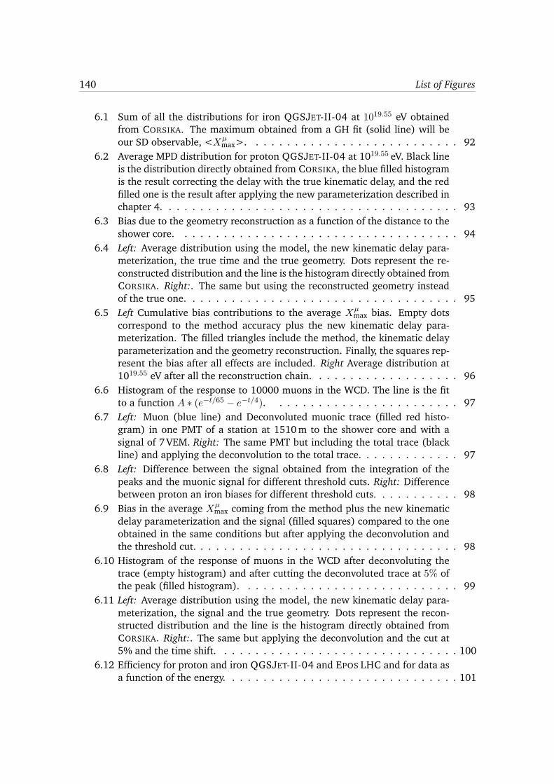
140 List of Figures
6.1 Sum of all the distributions for iron QGSJET-II-04 at 1019.55 eV obtainedfrom CORSIKA. The maximum obtained from a GH fit (solid line) will beour SD observable, <X
µ
max>. . . . . . . . . . . . . . . . . . . . . . . . . . . 926.2 Average MPD distribution for proton QGSJET-II-04 at 1019.55 eV. Black line
is the distribution directly obtained from CORSIKA, the blue filled histogramis the result correcting the delay with the true kinematic delay, and the redfilled one is the result after applying the new parameterization described inchapter 4. . . . . . . . . . . . . . . . . . . . . . . . . . . . . . . . . . . . . . 93
6.3 Bias due to the geometry reconstruction as a function of the distance to theshower core. . . . . . . . . . . . . . . . . . . . . . . . . . . . . . . . . . . . 94
6.4 Left: Average distribution using the model, the new kinematic delay para-meterization, the true time and the true geometry. Dots represent the re-constructed distribution and the line is the histogram directly obtained fromCORSIKA. Right:. The same but using the reconstructed geometry insteadof the true one. . . . . . . . . . . . . . . . . . . . . . . . . . . . . . . . . . . 95
6.5 Left Cumulative bias contributions to the average X
µ
max bias. Empty dotscorrespond to the method accuracy plus the new kinematic delay para-meterization. The filled triangles include the method, the kinematic delayparameterization and the geometry reconstruction. Finally, the squares rep-resent the bias after all effects are included. Right Average distribution at1019.55 eV after all the reconstruction chain. . . . . . . . . . . . . . . . . . . 96
6.6 Histogram of the response to 10000 muons in the WCD. The line is the fitto a function A ⇤ (e�t/65 � e
�t/4). . . . . . . . . . . . . . . . . . . . . . . . 976.7 Left: Muon (blue line) and Deconvoluted muonic trace (filled red histo-
gram) in one PMT of a station at 1510 m to the shower core and with asignal of 7 VEM. Right: The same PMT but including the total trace (blackline) and applying the deconvolution to the total trace. . . . . . . . . . . . . 97
6.8 Left: Difference between the signal obtained from the integration of thepeaks and the muonic signal for different threshold cuts. Right: Differencebetween proton an iron biases for different threshold cuts. . . . . . . . . . . 98
6.9 Bias in the average X
µ
max coming from the method plus the new kinematicdelay parameterization and the signal (filled squares) compared to the oneobtained in the same conditions but after applying the deconvolution andthe threshold cut. . . . . . . . . . . . . . . . . . . . . . . . . . . . . . . . . . 98
6.10 Histogram of the response of muons in the WCD after deconvoluting thetrace (empty histogram) and after cutting the deconvoluted trace at 5% ofthe peak (filled histogram). . . . . . . . . . . . . . . . . . . . . . . . . . . . 99
6.11 Left: Average distribution using the model, the new kinematic delay para-meterization, the signal and the true geometry. Dots represent the recon-structed distribution and the line is the histogram directly obtained fromCORSIKA. Right:. The same but applying the deconvolution and the cut at5% and the time shift. . . . . . . . . . . . . . . . . . . . . . . . . . . . . . . 100
6.12 Efficiency for proton and iron QGSJET-II-04 and EPOS LHC and for data asa function of the energy. . . . . . . . . . . . . . . . . . . . . . . . . . . . . . 101
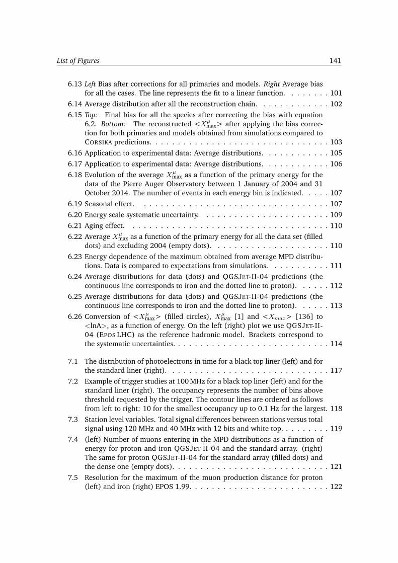
List of Figures 141
6.13 Left Bias after corrections for all primaries and models. Right Average biasfor all the cases. The line represents the fit to a linear function. . . . . . . . 101
6.14 Average distribution after all the reconstruction chain. . . . . . . . . . . . . 1026.15 Top: Final bias for all the species after correcting the bias with equation
6.2. Bottom: The reconstructed <X
µ
max> after applying the bias correc-tion for both primaries and models obtained from simulations compared toCORSIKA predictions. . . . . . . . . . . . . . . . . . . . . . . . . . . . . . . . 103
6.16 Application to experimental data: Average distributions. . . . . . . . . . . . 1056.17 Application to experimental data: Average distributions. . . . . . . . . . . . 1066.18 Evolution of the average X
µ
max as a function of the primary energy for thedata of the Pierre Auger Observatory between 1 January of 2004 and 31October 2014. The number of events in each energy bin is indicated. . . . . 107
6.19 Seasonal effect. . . . . . . . . . . . . . . . . . . . . . . . . . . . . . . . . . 1076.20 Energy scale systematic uncertainty. . . . . . . . . . . . . . . . . . . . . . . 1096.21 Aging effect. . . . . . . . . . . . . . . . . . . . . . . . . . . . . . . . . . . . 1106.22 Average X
µ
max as a function of the primary energy for all the data set (filleddots) and excluding 2004 (empty dots). . . . . . . . . . . . . . . . . . . . . 110
6.23 Energy dependence of the maximum obtained from average MPD distribu-tions. Data is compared to expectations from simulations. . . . . . . . . . . 111
6.24 Average distributions for data (dots) and QGSJET-II-04 predictions (thecontinuous line corresponds to iron and the dotted line to proton). . . . . . 112
6.25 Average distributions for data (dots) and QGSJET-II-04 predictions (thecontinuous line corresponds to iron and the dotted line to proton). . . . . . 113
6.26 Conversion of <X
µ
max> (filled circles), X
µ
max [1] and <X
max
> [136] to<lnA>, as a function of energy. On the left (right) plot we use QGSJET-II-04 (EPOS LHC) as the reference hadronic model. Brackets correspond tothe systematic uncertainties. . . . . . . . . . . . . . . . . . . . . . . . . . . . 114
7.1 The distribution of photoelectrons in time for a black top liner (left) and forthe standard liner (right). . . . . . . . . . . . . . . . . . . . . . . . . . . . . 117
7.2 Example of trigger studies at 100 MHz for a black top liner (left) and for thestandard liner (right). The occupancy represents the number of bins abovethreshold requested by the trigger. The contour lines are ordered as followsfrom left to right: 10 for the smallest occupancy up to 0.1 Hz for the largest. 118
7.3 Station level variables. Total signal differences between stations versus totalsignal using 120 MHz and 40 MHz with 12 bits and white top. . . . . . . . . 119
7.4 (left) Number of muons entering in the MPD distributions as a function ofenergy for proton and iron QGSJET-II-04 and the standard array. (right)The same for proton QGSJET-II-04 for the standard array (filled dots) andthe dense one (empty dots). . . . . . . . . . . . . . . . . . . . . . . . . . . . 121
7.5 Resolution for the maximum of the muon production distance for proton(left) and iron (right) EPOS 1.99. . . . . . . . . . . . . . . . . . . . . . . . . 122

142 List of Figures
A.1 Lateral distribution function for events where the difference between sig-nals is larger than 1.5. (a) Event 6466282. The signal candidate station ofthe doublet, station 734, observed 69.6 VEM, while the partner, station 93,has a signal of 1.8 VEM. (b) Event 14995513. The candidate station, 669,has a signal of 139.4 VEM, while the partner, station 80, measured 2.3 VEM. 131
A.2 The RMS of the distribution � divided by the signal uncertainty for the750 m array (open circles) and for the 1500 m array (solid circles) as afunction of secant ✓ (a) and of signal(b). . . . . . . . . . . . . . . . . . . . . 132
A.3 Same as figure 3.6(a) for different ranges of zenith angle for all the triggers.As we require that a stations is not saturated in the anode channel, at thehighest signals we are selecting just the lower fluctuations and thus theRMS(�) is underestimated. . . . . . . . . . . . . . . . . . . . . . . . . . . . 133
A.4 Same as Fig. A.3 for old triggers. . . . . . . . . . . . . . . . . . . . . . . . . 134
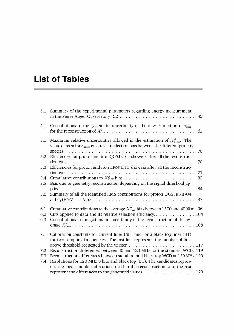
List of Tables
3.1 Summary of the experimental parameters regarding energy measurementin the Pierre Auger Observatory [32]. . . . . . . . . . . . . . . . . . . . . . . 45
4.1 Contributions to the systematic uncertainty in the new estimation of ⌧
kin
for the reconstruction of Xµ
max. . . . . . . . . . . . . . . . . . . . . . . . . . 62
5.1 Maximum relative uncertainties allowed in the estimation of X
µ
max. Thevalue chosen for ✏
max
ensures no selection bias between the different primaryspecies. . . . . . . . . . . . . . . . . . . . . . . . . . . . . . . . . . . . . . . 70
5.2 Efficiencies for proton and iron QGSJET04 showers after all the reconstruc-tion cuts. . . . . . . . . . . . . . . . . . . . . . . . . . . . . . . . . . . . . . 70
5.3 Efficiencies for proton and iron EPOS LHC showers after all the reconstruc-tion cuts. . . . . . . . . . . . . . . . . . . . . . . . . . . . . . . . . . . . . . 71
5.4 Cumulative contributions to X
µ
max bias. . . . . . . . . . . . . . . . . . . . . . 825.5 Bias due to geometry reconstruction depending on the signal threshold ap-
plied. . . . . . . . . . . . . . . . . . . . . . . . . . . . . . . . . . . . . . . . 845.6 Summary of all the identified RMS contributions for proton QGSJET-II-04
at Log(E/eV) = 19.55. . . . . . . . . . . . . . . . . . . . . . . . . . . . . . . 87
6.1 Cumulative contributions to the average X
µ
max bias between 1500 and 4000 m. 966.2 Cuts applied to data and its relative selection efficiency. . . . . . . . . . . . . 1046.3 Contributions to the systematic uncertainty in the reconstruction of the av-
erage X
µ
max. . . . . . . . . . . . . . . . . . . . . . . . . . . . . . . . . . . . . 108
7.1 Calibration constants for current liner (St.) and for a black top liner (BT)for two sampling frequencies. The last line represents the number of binsabove threshold requested by the trigger. . . . . . . . . . . . . . . . . . . . . 117
7.2 Reconstruction differences between 40 and 120 MHz for the standard WCD. 1197.3 Reconstruction differences between standard and black top WCD at 120 MHz.1207.4 Resolutions for 120 MHz white and black top (BT). The candidates repres-
ent the mean number of stations used in the reconstruction, and the restrepresent the differences to the generated values. . . . . . . . . . . . . . . 120


Bibliography
[1] Pierre Auger Collaboration, A. Aab et al., Muons in air showers at the Pierre AugerObservatory: Measurement of atmospheric production depth, Phys. Rev. D90, 012012(2014), arXiv:1407.5919.
[2] L. Molina Bueno, P. Billoir, and I. C. Maris, GAP Report No. 035, 2014 (unpub-lished).
[3] M. Settimo, P. Billoir, I. Maris, and L. Molina Bueno, GAP Report No. 014, 2013(unpublished).
[4] A. Bueno, D. Garcia-Gamez, and L. Molina Bueno, GAP Report No. 020, 2015(unpublished).
[5] D. Garcia-Gamez and L. Molina Bueno, GAP Report No. 006, 2015 (unpublished).
[6] A. Bueno, D. Garcia-Gamez, and L. Molina Bueno, GAP Report No. 034, 2015(unpublished).
[7] L. Molina Bueno, P. Billoir, A. Bueno, D. Garcia-Gamez, and I. Maris, GAP ReportNo. 066, 2015 (unpublished).
[8] V. F. Hess, Über Beobachtungen der durchdringenden Strahlung bei sieben Freiballon-fahrten, Phys. Z. 13, 1084 (1912).
[9] T. Stanev, High Energy Cosmic Rays (Springer Berlin Heidelberg, 2010).
[10] A. Letessier-Selvon and T. Stanev, Ultrahigh energy cosmic rays, Rev. Mod. Phys.83, 907 (2011).
[11] K. H. Kampert and M. Unger, Measurements of the cosmic ray composition with airshower experiments, Astropart. Phys. 35, 660 (2012).
[12] A. Watson, High-Energy Cosmic Rays and the Greisen-Zatsepin-Kuzmin Effect, (2013),arXiv:1310.0325.
[13] K.-H. Kampert and A. Watson, Extensive Air Showers and Ultra High-Energy CosmicRays: A Historical Review, (2012), arXiv:1207.4827.
[14] H. Becquerel, Sur les radiations émises par phosphorescence, Comptes rendus del’Acad. des Sciences 420 (1896).

146 Bibliography
[15] R. A. Millikan and G. H. Cameron, High Frequency Rays of Cosmic Origin III. Meas-urements in Snow-Fed Lakes at High Altitudes, Phys. Rev. 28, 851 (1926).
[16] J. Linsley, Evidence for a Primary Cosmic-Ray Particle with Energy 1020 eV, Phys.Rev. Lett. 10, 146 (1963).
[17] E. Fermi, On the origin of the Cosmic Radiation, Phys. Rev. 75, 1169 (1949).
[18] Courtesy of Ioana Maris.
[19] J. R. Hörandel, Models of the knee in the energy spectrum of cosmic rays, Astropart.Phys. 21, 241 (2004).
[20] A. A. Ivanov, S. P. Knurenko, and I. Y. Sleptsov, Measuring extensive air showers withCherenkov light detectors of the Yakutsk array: the energy spectrum of cosmic rays,New J. Phys. 11, 065008 (2009).
[21] M. Nagano et al., Energy spectrum of primary cosmic rays above 1017.0 eV determinedfrom extensive air shower experiments at Akeno, J. Phys. G Nucl. Partic. 18, 423(1992).
[22] T. Antoni et al., KASCADE measurements of energy spectra for elemental groups ofcosmic rays: Results and open problems, Astropart. Phys. 24, 1 (2005).
[23] The KASKADE-Grande Collaboration, W. D. Apel et al., KASCADE-Grande measure-ments of energy spectra for elemental groups of cosmic rays, Astropart. Phys. 47, 54(2013), arXiv:1306.6283.
[24] A. D. Erlykin and A. W. Wolfendale, Properties of cosmic ray interactions at PeVenergies, Astropart. Phys. 18, 151 (2002), arXiv:astro-ph/0112553.
[25] D. J. Bird et al., Evidence for correlated changes in the spectrum and composition ofcosmic rays at extremely high energies, Phys. Rev. Lett. 71, 3401 (1993).
[26] A. M. Hillas, Cosmic Rays: Recent Progress and some Current Questions, (2006),arXiv:astro-ph/0607109.
[27] D. De Marco and T. Stanev, On the shape of the ultrahigh energy cosmic ray spectrum,Phys. Rev. D 72, 081301 (2005).
[28] D. Allard, E. Parizot, and A. Olinto, On the transition from galactic to extragalacticcosmic-rays: Spectral and composition features from two opposite scenarios, Astro-part. Phys. 27, 61 (2007).
[29] V. Berezinsky, Transition from galactic to extragalactic cosmic rays, (2007),arXiv:0710.2750.
[30] V. Berezinsky, S. Grigorieva, and B. Hnatyk, Extragalactic UHE proton spectrum andprediction for iron-nuclei flux at 108 – 109 GeV, Astropart. Phys. 21, 617 (2004).
Bibliography 147
[31] V. Berezinsky, Extragalactic UHE proton spectrum and prediction of flux of iron-nucleiat 108–109 GeV, Nucl. Phys. B Proc. Sup. 151, 497 (2006).
[32] I. Valiño for the Pierre Auger Collaboration, The flux of ultra-high energy cosmicrays after ten years of operation of the Pierre Auger Observatory, Proceedings of the34th International Cosmic Ray Conference, The Hague (2015).
[33] K. Greisen, End to the cosmic ray spectrum?, Phys. Rev. Lett. 16, 748 (1966).
[34] G. Zatsepin and V. Kuzmin, Upper limit of the spectrum of cosmic rays, JETP Lett. 4,78 (1966).
[35] A. A. Penzias and R. W. Wilson, A Measurement of excess antenna temperature at4080-Mc/s, Astrophys. J. 142, 419 (1965).
[36] R. Aloisio, V. Berezinsky, and A. Gazizov, Ultra high energy cosmic rays: The disap-pointing model, Astropart. Phys. 34, 620 (2011).
[37] A. Hillas, The origin of ultra-high-energy cosmic rays, Annual review of astronomyand astrophysics. 22, 425 (1984).
[38] Pierre Auger Collaboration, J. Abraham et al., An upper limit to the photon fractionin cosmic rays above 1019 eV from the Pierre Auger observatory, Astropart. Phys. 27,155 (2007), astro-ph/0606619.
[39] Pierre Auger Collaboration, J. Abraham et al., Upper limit on the cosmic-ray photonflux above 1019 eV using the surface detector of the Pierre Auger Observatory, Astro-part. Phys. 29, 243 (2008), arXiv:0712.1147.
[40] Pierre Auger Collaboration, J. Abraham et al., Upper limit on the cosmic-ray photonfraction at EeV energies from the Pierre Auger Observatory, Astropart. Phys. 31, 399(2009), arXiv:0903.1127.
[41] Pierre Auger Collaboration, M. Settimo et al., An update on a search for ultra-highenergy photons using the Pierre Auger Observatory, Proc of 32nd Int. Cosmic RayConf., Beijing, China 2, 55 (2011), arXiv:1107.4805.
[42] Pierre Auger Collaboration, J. Abraham et al., Upper limit on the diffuse flux ofUHE tau neutrinos from the Pierre Auger Observatory, Phys. Rev. Lett. 100, 211101(2008), arXiv:0712.1909.
[43] Pierre Auger Collaboration, P. Abreu et al., A Search for Ultra-High Energy Neutrinosin Highly Inclined Events at the Pierre Auger Observatory, Phys. Rev. D84, 122005(2011), arXiv:1202.1493.
[44] Pierre Auger Collaboration, P. Abreu et al., Search for point-like sources of ultra-highenergy neutrinos at the Pierre Auger Observatory and improved limit on the diffuse fluxof tau neutrinos, Astrophys. J. 755, L4 (2012), arXiv:1210.3143.
[45] Pierre Auger Collaboration, P. Abreu et al., Ultrahigh Energy Neutrinos at the PierreAuger Observatory, Adv. High Energy Phys. 2013, 708680 (2013), arXiv:1304.1630.

148 Bibliography
[46] Pierre Auger Collaboration, P. Abreu et al., A Search for Ultra-High Energy Neutrinosin Highly Inclined Events at the Pierre Auger Observatory, Phys. Rev. D 84, 122005(2011), arXiv:1202.1493.
[47] ANITA Collaboration, P. W. Gorham et al., New Limits on the Ultra-high EnergyCosmic Neutrino Flux from the ANITA Experiment, Phys. Rev. Lett. 103, 051103(2009), arXiv:0812.2715.
[48] IceCube Collaboration, A. Achterberg et al., First year performance of the IceCubeneutrino telescope, Astropart. Phys. 26, 155 (2006), arXiv:astro-ph/0604450.
[49] G. Gelmini, O. Kalashev, and D. V. Semikoz, GZK Photons as Ultra High EnergyCosmic Rays, J. Exp. Theor. Phys. 106, 1061 (2008), arXiv:astro-ph/0506128.
[50] M. Ahlers, L. Anchordoqui, M. Gonzalez-Garcia, F. Halzen, and S. Sarkar, GZKNeutrinos after the Fermi-LAT Diffuse Photon Flux Measurement, Astropart. Phys.34, 106 (2010), arXiv:1005.2620.
[51] K. Kotera, D. Allard, and A. Olinto, Cosmogenic Neutrinos: parameter space anddetectabilty from PeV to ZeV, JCAP 1010, 013 (2010), arXiv:1009.1382.
[52] Pierre Auger Collaboration, P. Pieroni, Ultra-high energy neutrinos at the PierreAuger Observatory, Proceedings of the 33rd International Cosmic Ray Conference,Rio de Janeiro, Brazil (2013), arXiv:1307.5059.
[53] IceCube Collaboration, M. Aartsen et al., Probing the origin of cosmic-rays with ex-tremely high energy neutrinos using the IceCube Observatory, Phys. Rev. D88, 112008(2013), arXiv:1310.5477.
[54] ANITA Collaboration, P. Gorham et al., New Limits on the Ultra-high Energy CosmicNeutrino Flux from the ANITA Experiment, Phys. Rev. Lett. 103, 051103 (2009),arXiv:0812.2715.
[55] ANITA Collaboration, P. Gorham et al., The Antarctic Impulsive Transient AntennaUltra-high Energy Neutrino Detector Design, Performance, and Sensitivity for 2006-2007 Balloon Flight, Astropart. Phys. 32, 10 (2009), arXiv:0812.1920.
[56] ANITA Collaboration, P. Gorham et al., Erratum: Observational Constraints on theUltra-high Energy Cosmic Neutrino Flux from the Second Flight of the ANITA Experi-ment, Phys. Rev. D85, 049901 (2012), arXiv:1011.5004.
[57] RICE Collaboration, I. Kravchenko et al., Updated Results from the RICE Experimentand Future Prospects for Ultra-High Energy Neutrino Detection at the South Pole,Phys. Rev. D85, 062004 (2012), arXiv:1106.1164.
[58] HiRes Collaboration, R. U. Abbasi et al., An upper limit on the electron-neutrino fluxfrom the HiRes detector, Astrophys. J. 684, 790 (2008), arXiv:0803.0554 [astro-ph].
[59] Telescope Array Collaboration, T. Abu-Zayyad et al., Upper limit on the flux ofphotons with energies above 1019 eV using the Telescope Array surface detector, Phys.Rev. D88, 112005 (2013), arXiv:1304.5614.
Bibliography 149
[60] Pierre Auger Collaboration, A. Aab et al., Large scale distribution of ultra highenergy cosmic rays detected at the Pierre Auger Observatory with zenith angles up to80�, Astrophys. J. 802, 111 (2015), arXiv:1411.6953.
[61] D. Harari, S. Mollerach, and E. Roulet, Anisotropies of ultrahigh energy cos-mic rays diffusing from extragalactic sources, Phys. Rev. D89, 123001 (2014),arXiv:1312.1366.
[62] I. Al Samarai for the Pierre Auger Collaboration, Large-scale cosmic rays anisotrop-ies searches with Auger data, Proceedings of the 34th International Cosmic RayConference, The Hague (2015).
[63] Pierre Auger Collaboration, P. Abreu et al., Search for First Harmonic Modulationin the Right Ascension Distribution of Cosmic Rays Detected at the Pierre Auger Obser-vatory, Astropart. Phys. 34, 627 (2011), arXiv:1103.2721.
[64] Pierre Auger Collaboration, I. Sidelnik, Measurement of the first harmonic modula-tion in the right ascension distribution of cosmic rays detected at the Pierre Auger Ob-servatory: towards the detection of dipolar anisotropies over a wide energy range, Pro-ceedings of the 33rd International Cosmic Ray Conference, Rio de Janeiro, Brazil(2013), arXiv:1307.5059.
[65] J. Linsley, Fluctuation effects on directional data, Phys. Rev. Lett. 34, 1530 (1975).
[66] R. Bonino et al., The East-West method: an exposure-independent method tosearch for large scale anisotropies of cosmic rays, Astrophys. J. 738, 67 (2011),arXiv:1106.2651.
[67] Telescope Array Collaboration, R. Abbasi et al., Indications of Intermediate-ScaleAnisotropy of Cosmic Rays with Energy Greater Than 57 EeV in the Northern SkyMeasured with the Surface Detector of the Telescope Array Experiment, Astrophys. J.790, L21 (2014), arXiv:1404.5890.
[68] Pierre Auger Collaboration, A. Aab et al., Searches for Anisotropies in the ArrivalDirections of the Highest Energy Cosmic Rays Detected by the Pierre Auger Observatory,Astrophys. J. 804, 15 (2015), arXiv:1411.6111.
[69] Pierre Auger Collaboration, J. Abraham et al., Correlation of the highest en-ergy cosmic rays with nearby extragalactic objects, Science 318, 938 (2007),arXiv:0711.2256.
[70] Pierre Auger Collaboration, J. Abraham et al., Correlation of the highest-energycosmic rays with the positions of nearby active galactic nuclei, Astropart. Phys. 29,188 (2008), arXiv:0712.2843.
[71] Pierre Auger Collaboration, P. Abreu et al., Update on the correlation of the highestenergy cosmic rays with nearby extragalactic matter, Astropart. Phys. 34, 314(2010), arXiv:1009.1855.
150 Bibliography
[72] W. Heitler, The Quantum Theory of Radiation. Dover Books on Physics and Chem-istry (Dover Publications, 1954).
[73] J. Matthews, A Heitler model of extensive air showers, Astropart. Phys. 22, 387(2005).
[74] J. Alvarez-Muniz, R. Engel, T. Gaisser, J. A. Ortiz, and T. Stanev, Hybrid simulationsof extensive air showers, Phys. Rev. D 66, 033011 (2002).
[75] J. Linsley, Structure of large air showers at depth 834 g/cm2. III - Applications, Int.Cosm. Ray Conf. 12, 89 (1977).
[76] D. Heck, G. Schatz, T. Thouw, J. Knapp, and J. Capdevielle, CORSIKA: A MonteCarlo code to simulate extensive air showers, FZKA-6019 (1998).
[77] S. Sciutto, AIRES: A System for air shower simulations. User’s guide and referencemanual. Version 2.2.0., (1999), arXiv:astro-ph/9911331.
[78] S. Roh et al., Comparison of CORSIKA and COSMOS simulations, American Instituteof Physics Conference Series 1367, 177 (2011), arXiv:1104.1005.
[79] T. Pierog and K. Werner, Muon Production in Extended Air Shower Simulations, Phys.Rev. Lett. 101, 171101 (2008).
[80] S. Ostapchenko, Monte Carlo treatment of hadronic interactions in enhancedPomeron scheme: QGSJET-II model, Phys. Rev. D 83, 014018 (2011).
[81] E. Ahn, R. Engel, T. K. Gaisser, P. Lipari, and T. Stanev, Cosmic ray interaction eventgenerator SIBYLL 2.1., Phys. Rev. D 80, 094003 (2009).
[82] J. Knapp, D. Heck, S. Sciutto, M. Dova, and M. Risse, Extensive air shower simula-tions at the highest energies , Astropart. Phys. 19, 77 (2003).
[83] T. K. Gaisser et al., Cosmic-ray composition around 1018 eV, Phys. Rev. D 47, 1919(1993).
[84] M. Nagano and A. A. Watson, Observations and implications of the ultra high-energycosmic rays, Rev. Mod. Phys. 72, 689 (2000).
[85] A. Porcelli for the Pierre Auger Collaboration, Measurements of Xmax above 1017
eV with the fluorescence detector of the Pierre Auger Observatory, Talk at the 34thInternational Cosmic Ray Conference, The Hague (2015).
[86] Pierre Auger Collaboration, A. Aab et al., The Pierre Auger Cosmic Ray Observatory,Accepted for publication in Nucl. Instrum. Meth. (2015), arXiv:1502.01323.
[87] T. Mathes for the Pierre Auger Collaboration, The HEAT Telescopes of the PierreAuger Observatory. Status and First Data, Proceedings of the 32nd InternationalCosmic Ray Conference Proceedings, Beijing (2011).
Bibliography 151
[88] F. Sanchez for the Pierre Auger Collaboration, The AMIGA Detector of the PierreAuger Observatory: An Overview, Proceedings of the 32nd International CosmicRay Conference, Beijing (2011).
[89] M. A. Lawrence, R. J.O. Reid, and A. A. Watson, The cosmic ray energy spectrumabove 4x10¹⁷ eV as measured by the Haverah Park array, J.Phys.G 17, 733 (1991).
[90] X. Bertou et al., Calibration of the surface array of the Pierre Auger Observatory,Nucl. Instrum. Meth. A 568, 839 (2006).
[91] Pierre Auger Collaboration, J. Abraham et al., Trigger and aperture of the surface de-tector array of the Pierre Auger Observatory, Nucl. Instrum. Meth. A613, 29 (2010),arXiv:1111.6764.
[92] P. Billoir, GAP Report No. 179, 2009 (unpublished).
[93] P. Billoir, P. Ghia, D. Nitz, and R. Sato, GAP Report No. 032, 2011 (unpublished).
[94] P. Billoir, GAP Report No. 089, 2011 (unpublished).
[95] P. Ghia, GAP Report No. 018, 2004 (unpublished).
[96] P. Ghia and G. Navarra, GAP Report No. 007, 2003 (unpublished).
[97] Pierre Auger Collaboration, J. Abraham et al., The fluorescence detector of the PierreAuger Observatory, Nucl. Instrum. Meth. A 620, 227 (2010), arXiv:0907.4282.
[98] AIRFLY Collaboration, M. Ave et al., Precise measurement of the absolute fluorescenceyield of the 337 nm band in atmospheric gases, Astropart. Phys. 42, 90 (2013),arXiv:1210.6734.
[99] Pierre Auger Collaboration, P. Abreu et al., The rapid atmospheric monitoring systemof the Pierre Auger Observatory, JINST 7, P09001 (2012), arXiv:1208.1675.
[100] L. Wiencke and the Pierre Auger Collaboration, Atmospheric calorimetry above 1019
eV: Shooting lasers at the Pierre Auger Cosmic-Ray Observatory, J. Phys. Conf. Ser.160, 012037 (2009), arXiv:0807.2884.
[101] C. Bonifazi for the Pierre Auger Collaboration, The angular resolution of the PierreAuger Observatory, Nucl. Phys. B Proc. Sup. 190, 20 (2009), arXiv:0901.3138,Proceedings of the 31st International Cosmic Ray Conference.
[102] M. Unger, GAP Report No. 010, 2006 (unpublished).
[103] T. Gaisser and A. Hillas, Reliability of the method of constant intensity cuts for recon-structing the average development of vertical showers, Int. Cosm. Ray Conf. 8, 353(1977).
[104] M. Tueros for the Pierre Auger Collaboration, Estimate of the non-calorimetric energyof showers observed with the fluorescence and surface detectors, Proceedings of the33rd International Cosmic Ray Conference, Rio de Janeiro (2013).
152 Bibliography
[105] V. Verzi for the Pierre Auger Collaboration, The energy scale of the Pierre AugerObservatory, Proceedings of the 33rd International Cosmic Ray Conference, Rio deJaneiro (2013).
[106] Pierre Auger Collaboration, A. Aab et al., The Pierre Auger Observatory: Contri-butions to the 33rd International Cosmic Ray Conference (ICRC 2013), (2013),arXiv:1307.5059.
[107] S. Argirò et al., The offline software framework of the Pierre Auger Observatory, Nucl.Instrum. Meth. A 580, 1485 (2007), arXiv:0707.1652.
[108] D. Veberic and M. Roth, GAP Report No. 035, 2005 (unpublished).
[109] Pierre Auger Collaboration, M. Roth, The Lateral distribution function of showersignals in the surface detector of the Pierre Auger Observatory, p. 333 (2003),arXiv:astro-ph/0308392.
[110] D. Newton, J. Knapp, and A. A. Watson, The Optimum Distance at which to Determ-ine the Size of a Giant Air Shower, Astropart. Phys. 26, 414 (2007), arXiv:astro-ph/0608118.
[111] M. Ave, P. Bauleo, and T. Yamamoto, GAP Report No. 030, 2003 (unpublished).
[112] A. Castellina, GAP Report No. 031, 2003 (unpublished).
[113] P. Bauleo, A. Castellina, R. Knapik, G. Navarra, and J. Harton, GAP Report No. 047,2004 (unpublished).
[114] Pierre Auger Collaboration, J. Abraham et al., The accuracy of signal measurementwith the water Cherenkov detectors of the Pierre Auger Observatory, Nucl. Instrum.Meth. A578, 180 (2007).
[115] M. Rammes, Investigating signal fluctuations of the surface detector array of thePierre Auger Observatory using pair tanks, PhD thesis, University of Siegen, (2008),Masther Thesis.
[116] R. Hiller and M. Roth, GAP Report No. 012, 2012 (unpublished).
[117] P. Billoir, GAP Report No. 005, 2001 (unpublished).
[118] I.C. Maris, F. Schüessler, R. Ulrich and M. Unger, GAP Report No. 081, 2006 (un-published).
[119] I.C. Maris, S. Müller, F. Schüessler, R. Ulrich and M. Unger, GAP Report No. 012,2009 (unpublished).
[120] I. Lhenry-Yvon, GAP Report No. 021, 2014 (unpublished).
[121] C. Jillings et al., GAP Report No. 037, 2002 (unpublished).
[122] C. Bonifazi, A. Letessier-Selvon, and E. Santos, A model for the time uncertaintymeasurements in the Auger surface detector array, Astropart. Phys. 28, 523 (2008).
Bibliography 153
[123] C. Bonifazi and A. Letessier-Selvon, GAP Report No. 016, 2006 (unpublished).
[124] D. Veberic for the Pierre Auger Collaboration, Estimation of Signal in SaturatedStations of Pierre Auger Surface Detector, Proceedings of the 33rd InternationalCosmic Ray Conference, Rio de Janeiro (2013).
[125] Pierre Auger Collaboration, P. Abreu et al., The Pierre Auger Observatory I: TheCosmic Ray Energy Spectrum and Related Measurements, (2011), arXiv:1107.4809.
[126] Pierre Auger Collaboration, A. Aab et al., Reconstruction of inclined air showers de-tected with the Pierre Auger Observatory, JCAP 1408, 019 (2014), arXiv:1407.3214.
[127] E. dos Santos, GAP Report No. 014, 2014 (unpublished).
[128] B. Zamorano, GAP Report No. 039, 2014 (unpublished).
[129] L. Collica, GAP Report No. 103, 2014 (unpublished).
[130] L. Cazon, R. Conceição, M. Pimenta, and E. Santos, A model for the transport ofmuons in extensive air showers, Astropart. Phys. 36, 211 (2012).
[131] L. Cazón, R. Vázquez, and E. Zas, Depth development of extensive air showers frommuon time distributions, Astropart. Phys. 23, 393 (2005).
[132] L. Cazón, R. Vázquez, A. Watson, and E. Zas, Time structure of muonic showers,Astropart. Phys. 21, 71 (2004).
[133] D. Garcia Gamez, Muon Arrival Time distributions and its relationship to the masscomposition of Ultra High Energy Cosmic Rays: An application to the Pierre AugerObservatory, PhD thesis, Universidad de Granada, (2010), PhD Thesis.
[134] P. Billoir, A sampling procedure to regenerate particles in a ground detector from a’thinned’ air shower simulation output, Astropart. Phys. 30, 270 (2008).
[135] Ioana Maris, private communication.
[136] Pierre Auger Collaboration, A. Aab et al., Depth of maximum of air-shower profilesat the Pierre Auger Observatory. I. Measurements at energies above 1017.8eV, Phys.Rev. D90, 122005 (2014), arXiv:1409.4809.
[137] L. Collica for the Pierre Auger Collaboration, Measurement of the muon content inair showers at the Pierre Auger Observatory, Proceedings of the 34th InternationalCosmic Ray Conference, The Hague (2015).
[138] ROOT Data analysis Framework,https://root.cern.ch/drupal/.
[139] M. Morhac et al., Efficient one- and two-dimensional Gold deconvolution and itsapplication to gamma-ray spectra decomposition, Nucl. Instrum. Meth. A 401, 385(1997).
154 Bibliography
[140] NOAA Air Resources Laboratory (ARL), Global Data Assimilation System (GDAS1)Archive Information,http://ready.arl.noaa.gov/gdas1.php.
[141] Pierre Auger Collaboration, P. Abreu et al., The Pierre Auger Observatory IV: Op-eration and Monitoring, in Proceedings, 32nd International Cosmic Ray Conference(ICRC 2011), 2011, arXiv:1107.4806.
[142] P. Auger, Upgrade design report,https://www.auger.unam.mx/AugerWiki/UTF_Home.
[143] P. Billoir, GAP Report No. 106, 2014 (unpublished).
[144] v2r8-blacktank-experimental,https://devel-ik.fzk.de/svn/auger/Offline/branches/v2r8-blacktank-experimental.
[145] A. Letessier-Selvon, P. Billoir, M. Blanco, I. C. Maris, and M. Settimo, Layered waterCherenkov detector for the study of ultra high energy cosmic rays, Nucl. Instrum.Meth. A767, 41 (2014), arXiv:1405.5699.
[146] Scherini, V. and Perrone, L. and Maldera, S., GAP Report No. 089, 2014 (unpub-lished).
[147] O. Deligny, P. Ghia, Antoine, Letessier-Selvon, and A. Watson, GAP Report No. 040,2013 (unpublished).