Measurement of the B- lifetime using a simulation free

Physics

Physics Research Publications

Purdue University Year

Measurement of the B- lifetime using a

simulation free approach for trigger bias

correctionT. Aaltonen, J. Adelman, B. A. Gonzalez, S. Amerio, D. Amidei, A. Anastassov,A. Annovi, J. Antos, G. Apollinari, J. Appel, A. Apresyan, T. Arisawa, A. Ar-tikov, J. Asaadi, W. Ashmanskas, A. Attal, A. Aurisano, F. Azfar, W. Badgett,A. Barbaro-Galtieri, V. E. Barnes, B. A. Barnett, P. Barria, P. Bartos, G.Bauer, P. H. Beauchemin, F. Bedeschi, D. Beecher, S. Behari, G. Bellettini, J.Bellinger, D. Benjamin, A. Beretvas, A. Bhatti, M. Binkley, D. Bisello, I. Biz-jak, R. E. Blair, C. Blocker, B. Blumenfeld, A. Bocci, A. Bodek, V. Boisvert,D. Bortoletto, J. Boudreau, A. Boveia, B. Brau, A. Bridgeman, L. Brigliadori,C. Bromberg, E. Brubaker, J. Budagov, H. S. Budd, S. Budd, K. Burkett,G. Busetto, P. Bussey, A. Buzatu, K. L. Byrum, S. Cabrera, C. Calancha, S.Camarda, M. Campanelli, M. Campbell, F. Canelli, A. Canepa, B. Carls, D.Carlsmith, R. Carosi, S. Carrillo, S. Carron, B. Casal, M. Casarsa, A. Castro,P. Catastini, D. Cauz, V. Cavaliere, M. Cavalli-Sforza, A. Cerri, L. Cerrito, S.H. Chang, Y. C. Chen, M. Chertok, G. Chiarelli, G. Chlachidze, F. Chlebana,K. Cho, D. Chokheli, J. P. Chou, K. Chung, W. H. Chung, Y. S. Chung, T.Chwalek, C. I. Ciobanu, M. A. Ciocci, A. Clark, D. Clark, G. Compostella,M. E. Convery, J. Conway, M. Corbo, M. Cordelli, C. A. Cox, D. J. Cox, F.Crescioli, C. C. Almenar, J. Cuevas, R. Culbertson, J. C. Cully, D. Dagenhart,N. d’Ascenzo, M. Datta, T. Davies, P. de Barbaro, S. De Cecco, A. Deisher, G.De Lorenzo, M. Dell’Orso, C. Deluca, L. Demortier, J. Deng, M. Deninno, M.d’Errico, A. Di Canto, B. Di Ruzza, J. R. Dittmann, M. D’Onofrio, S. Donati,P. Dong, T. Dorigo, S. Dube, K. Ebina, A. Elagin, R. Erbacher, D. Errede, S.Errede, N. Ershaidat, R. Eusebi, H. C. Fang, S. Farrington, W. T. Fedorko, R.G. Feild, M. Feindt, J. P. Fernandez, C. Ferrazza, R. Field, G. Flanagan, R.Forrest, M. J. Frank, M. Franklin, J. C. Freeman, I. Furic, M. Gallinaro, J. Gal-yardt, F. Garberson, J. E. Garcia, A. F. Garfinkel, P. Garosi, H. Gerberich, D.Gerdes, A. Gessler, S. Giagu, V. Giakoumopoulou, P. Giannetti, K. Gibson, J.L. Gimmell, C. M. Ginsburg, N. Giokaris, M. Giordani, P. Giromini, M. Giunta,G. Giurgiu, V. Glagolev, D. Glenzinski, M. Gold, N. Goldschmidt, A. Golos-

sanov, G. Gomez, G. Gomez-Ceballos, M. Goncharov, O. Gonzalez, I. Gorelov,A. T. Goshaw, K. Goulianos, A. Gresele, S. Grinstein, C. Grosso-Pilcher, R. C.Group, U. Grundler, J. G. da Costa, Z. Gunay-Unalan, C. Haber, S. R. Hahn,E. Halkiadakis, B. Y. Han, J. Y. Han, F. Happacher, K. Hara, D. Hare, M.Hare, R. F. Harr, M. Hartz, K. Hatakeyama, C. Hays, M. Heck, J. Heinrich,M. Herndon, J. Heuser, S. Hewamanage, D. Hidas, C. S. Hill, D. Hirschbuehl,A. Hocker, S. Hou, M. Houlden, S. C. Hsu, R. E. Hughes, B. T. Huffman, M.Hurwitz, U. Husemann, M. Hussein, J. Huston, J. Incandela, G. Introzzi, M.Iori, A. Ivanov, E. James, D. Jang, B. Jayatilaka, E. J. Jeon, M. K. Jha, S.Jindariani, W. Johnson, M. Jones, K. K. Joo, S. Y. Jun, J. E. Jung, T. R.Junk, T. Kamon, D. Kar, P. E. Karchin, Y. Kato, R. Kephart, W. Ketchum,J. Keung, V. Khotilovich, B. Kilminster, D. H. Kim, H. S. Kim, H. W. Kim, J.E. Kim, M. J. Kim, S. B. Kim, S. H. Kim, Y. K. Kim, N. Kimura, L. Kirsch,S. Klimenko, K. Kondo, D. J. Kong, J. Konigsberg, A. Korytov, A. V. Kotwal,M. Kreps, J. Kroll, D. Krop, N. Krumnack, M. Kruse, V. Krutelyov, T. Kuhr,N. P. Kulkarni, M. Kurata, S. Kwang, A. T. Laasanen, S. Lami, S. Lammel,M. Lancaster, R. L. Lander, K. Lannon, A. Lath, G. Latino, I. Lazzizzera, T.LeCompte, E. Lee, H. S. Lee, J. S. Lee, S. W. Lee, S. Leone, J. D. Lewis, C.J. Lin, J. Linacre, M. Lindgren, E. Lipeles, A. Lister, D. O. Litvintsev, C. Liu,T. Liu, N. S. Lockyer, A. Loginov, L. Lovas, D. Lucchesi, J. Lueck, P. Lujan,P. Lukens, G. Lungu, L. Lyons, J. Lys, R. Lysak, D. MacQueen, R. Madrak,K. Maeshima, K. Makhoul, P. Maksimovic, S. Malde, S. Malik, G. Manca, A.Manousakis-Katsikakis, F. Margaroli, C. Marino, C. P. Marino, A. Martin, V.Martin, M. Martinez, R. Martinez-Ballarin, P. Mastrandrea, M. Mathis, M. E.Mattson, P. Mazzanti, K. S. McFarland, P. McIntyre, R. McNulty, A. Mehta, P.Mehtala, A. Menzione, C. Mesropian, T. Miao, D. Mietlicki, N. Miladinovic, R.Miller, C. Mills, M. Milnik, A. Mitra, G. Mitselmakher, H. Miyake, S. Moed, N.Moggi, M. N. Mondragon, C. S. Moon, R. Moore, M. J. Morello, J. Morlock, P.M. Fernandez, J. Mulmenstadt, A. Mukherjee, T. Muller, P. Murat, M. Mussini,J. Nachtman, Y. Nagai, J. Naganoma, K. Nakamura, I. Nakano, A. Napier, J.Nett, C. Neu, M. S. Neubauer, S. Neubauer, J. Nielsen, L. Nodulman, M. Nor-man, O. Norniella, E. Nurse, L. Oakes, S. H. Oh, Y. D. Oh, I. Oksuzian, T.Okusawa, R. Orava, K. Osterberg, S. P. Griso, C. Pagliarone, E. Palencia, V.Papadimitriou, A. Papaikonomou, A. A. Paramanov, B. Parks, S. Pashapour,J. Patrick, G. Pauletta, M. Paulini, C. Paus, T. Peiffer, D. E. Pellett, A. Penzo,T. J. Phillips, G. Piacentino, E. Pianori, L. Pinera, K. Pitts, C. Plager, L. Pon-drom, K. Potamianos, O. Poukhov, N. L. Pounder, F. Prokoshin, A. Pronko,F. Ptohos, E. Pueschel, G. Punzi, J. Pursley, J. Rademacker, A. Rahaman,V. Ramakrishnan, N. Ranjan, I. Redondo, P. Renton, M. Renz, M. Rescigno,S. Richter, F. Rimondi, L. Ristori, A. Robson, T. Rodrigo, T. Rodriguez, E.Rogers, S. Rolli, R. Roser, M. Rossi, R. Rossin, P. Roy, A. Ruiz, J. Russ, V.Rusu, B. Rutherford, H. Saarikko, A. Safonov, W. K. Sakumoto, L. Santi, L.Sartori, K. Sato, V. Saveliev, A. Savoy-Navarro, P. Schlabach, A. Schmidt, E. E.Schmidt, M. A. Schmidt, M. P. Schmidt, M. Schmitt, T. Schwarz, L. Scodellaro,A. Scribano, F. Scuri, A. Sedov, S. Seidel, Y. Seiya, A. Semenov, L. Sexton-Kennedy, F. Sforza, A. Sfyrla, S. Z. Shalhout, T. Shears, P. F. Shepard, M.

Shimojima, S. Shiraishi, M. Shochet, Y. Shon, I. Shreyber, A. Simonenko, P.Sinervo, A. Sisakyan, A. J. Slaughter, J. Slaunwhite, K. Sliwa, J. R. Smith,F. D. Snider, R. Snihur, A. Soha, S. Somalwar, V. Sorin, P. Squillacioti, M.Stanitzki, R. S. Denis, B. Stelzer, O. Stelzer-Chilton, D. Stentz, J. Strologas,G. L. Strycker, J. S. Suh, A. Sukhanov, I. Suslov, A. Taffard, R. Takashima,Y. Takeuchi, R. Tanaka, J. Tang, M. Tecchio, P. K. Teng, J. Thom, J. Thome,G. A. Thompson, E. Thomson, P. Tipton, P. Ttito-Guzman, S. Tkaczyk, D.Toback, S. Tokar, K. Tollefson, T. Tomura, D. Tonelli, S. Torre, D. Torretta, P.Totaro, M. Trovato, S. Y. Tsai, Y. Tu, N. Turini, F. Ukegawa, S. Uozumi, N. vanRemortel, A. Varganov, E. Vataga, F. Vazquez, G. Velev, C. Vellidis, M. Vidal,I. Vila, R. Vilar, M. Vogel, I. Volobouev, G. Volpi, P. Wagner, R. G. Wagner, R.L. Wagner, W. Wagner, J. Wagner-Kuhr, T. Wakisaka, R. Wallny, S. M. Wang,A. Warburton, D. Waters, M. Weinberger, J. Weinelt, W. C. Wester, B. White-house, D. Whiteson, A. B. Wicklund, E. Wicklund, S. Wilbur, G. Williams,H. H. Williams, P. Wilson, B. L. Winer, P. Wittich, S. Wolbers, C. Wolfe, H.Wolfe, T. Wright, X. Wu, F. Wurthwein, A. Yagil, K. Yamamoto, J. Yamaoka,U. K. Yang, Y. C. Yang, W. M. Yao, G. P. Yeh, K. Yi, J. Yoh, K. Yorita, T.Yoshida, G. B. Yu, I. Yu, S. S. Yu, J. C. Yun, A. Zanetti, Y. Zeng, X. Zhang,Y. Zheng, and S. Zucchelli

This paper is posted at Purdue e-Pubs.

http://docs.lib.purdue.edu/physics articles/1086

Measurement of the B� lifetime using a simulation free approach fortrigger bias correction

T. Aaltonen,24 J. Adelman,14 B. Alvarez Gonzalez,12,x S. Amerio,44b,44a D. Amidei,35 A. Anastassov,39 A. Annovi,20

J. Antos,15 G. Apollinari,18 J. Appel,18 A. Apresyan,49 T. Arisawa,58 A. Artikov,16 J. Asaadi,54 W. Ashmanskas,18

A. Attal,4 A. Aurisano,54 F. Azfar,43 W. Badgett,18 A. Barbaro-Galtieri,29 V. E. Barnes,49 B. A. Barnett,26

P. Barria,47c,47a P. Bartos,15 G. Bauer,33 P.-H. Beauchemin,34 F. Bedeschi,47a D. Beecher,31 S. Behari,26

G. Bellettini,47b,47a J. Bellinger,60 D. Benjamin,17 A. Beretvas,18 A. Bhatti,51 M. Binkley,18,a D. Bisello,44b,44a

I. Bizjak,31,ee R. E. Blair,2 C. Blocker,7 B. Blumenfeld,26 A. Bocci,17 A. Bodek,50 V. Boisvert,50 D. Bortoletto,49

J. Boudreau,48 A. Boveia,11 B. Brau,11,b A. Bridgeman,25 L. Brigliadori,6b,6a C. Bromberg,36 E. Brubaker,14

J. Budagov,16 H. S. Budd,50 S. Budd,25 K. Burkett,18 G. Busetto,44b,44a P. Bussey,22 A. Buzatu,34 K. L. Byrum,2

S. Cabrera,17,z C. Calancha,32 S. Camarda,4 M. Campanelli,31 M. Campbell,35 F. Canelli,14,18 A. Canepa,46 B. Carls,25

D. Carlsmith,60 R. Carosi,47a S. Carrillo,19,o S. Carron,18 B. Casal,12 M. Casarsa,18 A. Castro,6b,6a P. Catastini,47c,47a

D. Cauz,55a V. Cavaliere,47c,47a M. Cavalli-Sforza,4 A. Cerri,29 L. Cerrito,31,r S. H. Chang,28 Y. C. Chen,1 M. Chertok,8

G. Chiarelli,47a G. Chlachidze,18 F. Chlebana,18 K. Cho,28 D. Chokheli,16 J. P. Chou,23 K. Chung,18,p W.H. Chung,60

Y. S. Chung,50 T. Chwalek,27 C. I. Ciobanu,45 M.A. Ciocci,47c,47a A. Clark,21 D. Clark,7 G. Compostella,44a

M. E. Convery,18 J. Conway,8 M. Corbo,45 M. Cordelli,20 C. A. Cox,8 D. J. Cox,8 F. Crescioli,47b,47a

C. Cuenca Almenar,61 J. Cuevas,12,x R. Culbertson,18 J. C. Cully,35 D. Dagenhart,18 N. d’Ascenzo,45,w M. Datta,18

T. Davies,22 P. de Barbaro,50 S. De Cecco,52a A. Deisher,29 G. De Lorenzo,4 M. Dell’Orso,47b,47a C. Deluca,4

L. Demortier,51 J. Deng,17,g M. Deninno,6a M. d’Errico,44b,44a A. Di Canto,47b,47a B. Di Ruzza,47a J. R. Dittmann,5

M. D’Onofrio,4 S. Donati,47b,47a P. Dong,18 T. Dorigo,44a S. Dube,53 K. Ebina,58 A. Elagin,54 R. Erbacher,8

D. Errede,25 S. Errede,25 N. Ershaidat,45,dd R. Eusebi,54 H. C. Fang,29 S. Farrington,43 W. T. Fedorko,14 R. G. Feild,61

M. Feindt,27 J. P. Fernandez,32 C. Ferrazza,47d,47a R. Field,19 G. Flanagan,49,t R. Forrest,8 M. J. Frank,5 M. Franklin,23

J. C. Freeman,18 I. Furic,19 M. Gallinaro,51 J. Galyardt,13 F. Garberson,11 J. E. Garcia,21 A. F. Garfinkel,49

P. Garosi,47c,47a H. Gerberich,25 D. Gerdes,35 A. Gessler,27 S. Giagu,52b,52a V. Giakoumopoulou,3 P. Giannetti,47a

K. Gibson,48 J. L. Gimmell,50 C.M. Ginsburg,18 N. Giokaris,3 M. Giordani,55b,55a P. Giromini,20 M. Giunta,47a

G. Giurgiu,26 V. Glagolev,16 D. Glenzinski,18 M. Gold,38 N. Goldschmidt,19 A. Golossanov,18 G. Gomez,12

G. Gomez-Ceballos,33 M. Goncharov,33 O. Gonzalez,32 I. Gorelov,38 A. T. Goshaw,17 K. Goulianos,51

A. Gresele,44b,44a S. Grinstein,4 C. Grosso-Pilcher,14 R. C. Group,18 U. Grundler,25 J. Guimaraes da Costa,23

Z. Gunay-Unalan,36 C. Haber,29 S. R. Hahn,18 E. Halkiadakis,53 B.-Y. Han,50 J. Y. Han,50 F. Happacher,20 K. Hara,56

D. Hare,53 M. Hare,57 R. F. Harr,59 M. Hartz,48 K. Hatakeyama,5 C. Hays,43 M. Heck,27 J. Heinrich,46 M. Herndon,60

J. Heuser,27 S. Hewamanage,5 D. Hidas,53 C. S. Hill,11,d D. Hirschbuehl,27 A. Hocker,18 S. Hou,1 M. Houlden,30

S.-C. Hsu,29 R. E. Hughes,40 B. T. Huffman,43 M. Hurwitz,14 U. Husemann,61 M. Hussein,36 J. Huston,36

J. Incandela,11 G. Introzzi,47a M. Iori,52b,52a A. Ivanov,8,q E. James,18 D. Jang,13 B. Jayatilaka,17 E. J. Jeon,28

M.K. Jha,6a S. Jindariani,18 W. Johnson,8 M. Jones,49 K.K. Joo,28 S. Y. Jun,13 J. E. Jung,28 T. R. Junk,18 T. Kamon,54

D. Kar,19 P. E. Karchin,59 Y. Kato,42,n R. Kephart,18 W. Ketchum,14 J. Keung,46 V. Khotilovich,54 B. Kilminster,18

D. H. Kim,28 H. S. Kim,28 H.W. Kim,28 J. E. Kim,28 M. J. Kim,20 S. B. Kim,28 S. H. Kim,56 Y.K. Kim,14 N. Kimura,58

L. Kirsch,7 S. Klimenko,19 K. Kondo,58 D. J. Kong,28 J. Konigsberg,19 A. Korytov,19 A. V. Kotwal,17 M. Kreps,27

J. Kroll,46 D. Krop,14 N. Krumnack,5 M. Kruse,17 V. Krutelyov,11 T. Kuhr,27 N. P. Kulkarni,59 M. Kurata,56

S. Kwang,14 A. T. Laasanen,49 S. Lami,47a S. Lammel,18 M. Lancaster,31 R. L. Lander,8 K. Lannon,40,v A. Lath,53

G. Latino,47c,47a I. Lazzizzera,44b,44a T. LeCompte,2 E. Lee,54 H. S. Lee,14 J. S. Lee,28 S.W. Lee,54,y S. Leone,47a

J. D. Lewis,18 C.-J. Lin,29 J. Linacre,43 M. Lindgren,18 E. Lipeles,46 A. Lister,21 D.O. Litvintsev,18 C. Liu,48 T. Liu,18

N. S. Lockyer,46 A. Loginov,61 L. Lovas,15 D. Lucchesi,44b,44a J. Lueck,27 P. Lujan,29 P. Lukens,18 G. Lungu,51

L. Lyons,43 J. Lys,29 R. Lysak,15 D. MacQueen,34 R. Madrak,18 K. Maeshima,18 K. Makhoul,33 P. Maksimovic,26

S. Malde,43 S. Malik,31 G. Manca,30,f A. Manousakis-Katsikakis,3 F. Margaroli,49 C. Marino,27 C. P. Marino,25

A. Martin,61 V. Martin,22,l M. Martınez,4 R. Martınez-Balların,32 P. Mastrandrea,52a M. Mathis,26 M. E. Mattson,59

P. Mazzanti,6a K. S. McFarland,50 P. McIntyre,54 R. McNulty,30,k A. Mehta,30 P. Mehtala,24 A. Menzione,47a

C. Mesropian,51 T. Miao,18 D. Mietlicki,35 N. Miladinovic,7 R. Miller,36 C. Mills,23 M. Milnik,27 A. Mitra,1

G. Mitselmakher,19 H. Miyake,56 S. Moed,23 N. Moggi,6a M.N. Mondragon,18,o C. S. Moon,28 R. Moore,18

M. J. Morello,47a J. Morlock,27 P. Movilla Fernandez,18 J. Mulmenstadt,29 A. Mukherjee,18 Th. Muller,27 P. Murat,18

M. Mussini,6b,6a J. Nachtman,18,p Y. Nagai,56 J. Naganoma,56 K. Nakamura,56 I. Nakano,41 A. Napier,57 J. Nett,60

PHYSICAL REVIEW D 83, 032008 (2011)

1550-7998=2011=83(3)=032008(30) 032008-1 � 2011 American Physical Society

C. Neu,46,bb M. S. Neubauer,25 S. Neubauer,27 J. Nielsen,29,h L. Nodulman,2 M. Norman,10 O. Norniella,25 E. Nurse,31

L. Oakes,43 S. H. Oh,17 Y.D. Oh,28 I. Oksuzian,19 T. Okusawa,42 R. Orava,24 K. Osterberg,24 S. Pagan Griso,44b,44a

C. Pagliarone,55a E. Palencia,18 V. Papadimitriou,18 A. Papaikonomou,27 A.A. Paramanov,2 B. Parks,40 S. Pashapour,34

J. Patrick,18 G. Pauletta,55b,55a M. Paulini,13 C. Paus,33 T. Peiffer,27 D. E. Pellett,8 A. Penzo,55a T. J. Phillips,17

G. Piacentino,47a E. Pianori,46 L. Pinera,19 K. Pitts,25 C. Plager,9 L. Pondrom,60 K. Potamianos,49 O. Poukhov,16,a

N. L. Pounder,43 F. Prokoshin,16,aa A. Pronko,18 F. Ptohos,18,j E. Pueschel,13 G. Punzi,47b,47a J. Pursley,60

J. Rademacker,43,d A. Rahaman,48 V. Ramakrishnan,60 N. Ranjan,49 I. Redondo,32 P. Renton,43 M. Renz,27

M. Rescigno,52a S. Richter,27 F. Rimondi,6b,6a L. Ristori,47a A. Robson,22 T. Rodrigo,12 T. Rodriguez,46 E. Rogers,25

S. Rolli,57 R. Roser,18 M. Rossi,55a R. Rossin,11 P. Roy,34 A. Ruiz,12 J. Russ,13 V. Rusu,18 B. Rutherford,18

H. Saarikko,24 A. Safonov,54 W.K. Sakumoto,50 L. Santi,55b,55a L. Sartori,47a K. Sato,56 V. Saveliev,45,w

A. Savoy-Navarro,45 P. Schlabach,18 A. Schmidt,27 E. E. Schmidt,18 M.A. Schmidt,14 M. P. Schmidt,61,a M. Schmitt,39

T. Schwarz,8 L. Scodellaro,12 A. Scribano,47c,47a F. Scuri,47a A. Sedov,49 S. Seidel,38 Y. Seiya,42 A. Semenov,16

L. Sexton-Kennedy,18 F. Sforza,47b,47a A. Sfyrla,25 S. Z. Shalhout,59 T. Shears,30 P. F. Shepard,48 M. Shimojima,56,u

S. Shiraishi,14 M. Shochet,14 Y. Shon,60 I. Shreyber,37 A. Simonenko,16 P. Sinervo,34 A. Sisakyan,16 A. J. Slaughter,18

J. Slaunwhite,40 K. Sliwa,57 J. R. Smith,8 F. D. Snider,18 R. Snihur,34 A. Soha,18 S. Somalwar,53 V. Sorin,4

P. Squillacioti,47c,47a M. Stanitzki,61 R. St. Denis,22 B. Stelzer,34 O. Stelzer-Chilton,34 D. Stentz,39 J. Strologas,38

G. L. Strycker,35 J. S. Suh,28 A. Sukhanov,19 I. Suslov,16 A. Taffard,25,g R. Takashima,41 Y. Takeuchi,56 R. Tanaka,41

J. Tang,14 M. Tecchio,35 P. K. Teng,1 J. Thom,18,i J. Thome,13 G. A. Thompson,25 E. Thomson,46 P. Tipton,61

P. Ttito-Guzman,32 S. Tkaczyk,18 D. Toback,54 S. Tokar,15 K. Tollefson,36 T. Tomura,56 D. Tonelli,18 S. Torre,20

D. Torretta,18 P. Totaro,55b,55a M. Trovato,47d,47a S.-Y. Tsai,1 Y. Tu,46 N. Turini,47c,47a F. Ukegawa,56 S. Uozumi,28

N. van Remortel,24,c A. Varganov,35 E. Vataga,47d,47a F. Vazquez,19,o G. Velev,18 C. Vellidis,3 M. Vidal,32 I. Vila,12

R. Vilar,12 M. Vogel,38 I. Volobouev,29,y G. Volpi,47b,47a P. Wagner,46 R. G. Wagner,2 R. L. Wagner,18 W. Wagner,27,cc

J. Wagner-Kuhr,27 T. Wakisaka,42 R. Wallny,9 S.M. Wang,1 A. Warburton,34 D. Waters,31 M. Weinberger,54

J. Weinelt,27 W.C. Wester III,18 B. Whitehouse,57 D. Whiteson,46,g A. B. Wicklund,2 E. Wicklund,18 S. Wilbur,14

G. Williams,34 H.H. Williams,46 P. Wilson,18 B. L. Winer,40 P. Wittich,18,i S. Wolbers,18 C. Wolfe,14 H. Wolfe,40

T. Wright,35 X. Wu,21 F. Wurthwein,10 A. Yagil,10 K. Yamamoto,42 J. Yamaoka,17 U. K. Yang,14,s Y. C. Yang,28

W.M. Yao,29 G. P. Yeh,18 K. Yi,18,p J. Yoh,18 K. Yorita,58 T. Yoshida,42,m G. B. Yu,17 I. Yu,28 S. S. Yu,18 J. C. Yun,18

A. Zanetti,55a Y. Zeng,17 X. Zhang,25 Y. Zheng,9,e and S. Zucchelli6b,6a

(CDF Collaboration)

1Institute of Physics, Academia Sinica, Taipei, Taiwan 11529, Republic of China2Argonne National Laboratory, Argonne, Illinois 60439, USA

3University of Athens, 157 71 Athens, Greece4Institut de Fisica d’Altes Energies, Universitat Autonoma de Barcelona, E-08193, Bellaterra (Barcelona), Spain

5Baylor University, Waco, Texas 76798, USA6aIstituto Nazionale di Fisica Nucleare Bologna, I-40127 Bologna, Italy

6bUniversity of Bologna, I-40127 Bologna, Italy7Brandeis University, Waltham, Massachusetts 02254, USA

8University of California, Davis, Davis, California 95616, USA9University of California, Los Angeles, Los Angeles, California 90024, USA

10University of California, San Diego, La Jolla, California 92093, USA11University of California, Santa Barbara, Santa Barbara, California 93106, USA

12Instituto de Fisica de Cantabria, CSIC-University of Cantabria, 39005 Santander, Spain13Carnegie Mellon University, Pittsburgh, Pennsylvania 15213, USA

14Enrico Fermi Institute, University of Chicago, Chicago, Illinois 60637, USA15Comenius University, 842 48 Bratislava, Slovakia; Institute of Experimental Physics, 040 01 Kosice, Slovakia

16Joint Institute for Nuclear Research, RU-141980 Dubna, Russia17Duke University, Durham, North Carolina 27708, USA

18Fermi National Accelerator Laboratory, Batavia, Illinois 60510, USA19University of Florida, Gainesville, Florida 32611, USA

20Laboratori Nazionali di Frascati, Istituto Nazionale di Fisica Nucleare, I-00044 Frascati, Italy21University of Geneva, CH-1211 Geneva 4, Switzerland

22Glasgow University, Glasgow G12 8QQ, United Kingdom23Harvard University, Cambridge, Massachusetts 02138, USA

T. AALTONEN et al. PHYSICAL REVIEW D 83, 032008 (2011)

032008-2

24Division of High Energy Physics, Department of Physics, University of Helsinki and Helsinki Institute of Physics,FIN-00014, Helsinki, Finland

25University of Illinois, Urbana, Illinois 61801, USA26The Johns Hopkins University, Baltimore, Maryland 21218, USA

27Institut fur Experimentelle Kernphysik, Karlsruhe Institute of Technology, D-76131 Karlsruhe, Germany28Center for High Energy Physics: Kyungpook National University, Daegu 702-701, Korea; Seoul National University, Seoul 151-742,Korea; Sungkyunkwan University, Suwon 440-746, Korea; Korea Institute of Science and Technology Information, Daejeon 305-806,

Korea; Chonnam National University, Gwangju 500-757, Korea; Chonbuk National University, Jeonju 561-756, Korea29Ernest Orlando Lawrence Berkeley National Laboratory, Berkeley, California 94720, USA

30University of Liverpool, Liverpool L69 7ZE, United Kingdom31University College London, London WC1E 6BT, United Kingdom

32Centro de Investigaciones Energeticas Medioambientales y Tecnologicas, E-28040 Madrid, Spain33Massachusetts Institute of Technology, Cambridge, Massachusetts 02139, USA

34Institute of Particle Physics: McGill University, Montreal, Quebec H3A 2T8, Canada; Simon Fraser University, Burnaby, BritishColumbia V5A 1S6, Canada; University of Toronto, Toronto, Ontario M5S 1A7, Canada;

and TRIUMF, Vancouver, British Columbia V6T 2A3, Canada35University of Michigan, Ann Arbor, Michigan 48109, USA

36Michigan State University, East Lansing, Michigan 48824, USA37Institute for Theoretical and Experimental Physics, ITEP, Moscow 117259, Russia

38University of New Mexico, Albuquerque, New Mexico 87131, USA39Northwestern University, Evanston, Illinois 60208, USA40The Ohio State University, Columbus, Ohio 43210, USA

41Okayama University, Okayama 700-8530, Japan42Osaka City University, Osaka 588, Japan

43University of Oxford, Oxford OX1 3RH, United Kingdom44aIstituto Nazionale di Fisica Nucleare, Sezione di Padova-Trento, I-35131 Padova, Italy

44bUniversity of Padova, I-35131 Padova, Italy45LPNHE, Universite Pierre et Marie Curie/IN2P3-CNRS, UMR7585, Paris, F-75252 France

46University of Pennsylvania, Philadelphia, Pennsylvania 19104, USA47aIstituto Nazionale di Fisica Nucleare Pisa, I-56127 Pisa, Italy

47bUniversity of Pisa, I-56127 Pisa, Italy47cUniversity of Siena, I-56127 Pisa, Italy

47dScuola Normale Superiore, I-56127 Pisa, Italy48University of Pittsburgh, Pittsburgh, Pennsylvania 15260, USA

49Purdue University, West Lafayette, Indiana 47907, USA50University of Rochester, Rochester, New York 14627, USA

51The Rockefeller University, New York, New York 10021, USA52aIstituto Nazionale di Fisica Nucleare, Sezione di Roma 1, I-00185 Roma, Italy

52bSapienza Universita di Roma, I-00185 Roma, Italy53Rutgers University, Piscataway, New Jersey 08855, USA

54Texas A&M University, College Station, Texas 77843, USA55aIstituto Nazionale di Fisica Nucleare Trieste/Udine, I-34100 Trieste, I-33100 Udine, Italy

55bUniversity of Trieste/Udine, I-33100 Udine, Italy56University of Tsukuba, Tsukuba, Ibaraki 305, Japan57Tufts University, Medford, Massachusetts 02155, USA

58Waseda University, Tokyo 169, Japan59Wayne State University, Detroit, Michigan 48201, USA

60University of Wisconsin, Madison, Wisconsin 53706, USA61Yale University, New Haven, Connecticut 06520, USA(Received 28 April 2010; published 16 February 2011)

The collection of a large number of B-hadron decays to hadronic final states at the CDF II Detector is

possible due to the presence of a trigger that selects events based on track impact parameters.

However, the nature of the selection requirements of the trigger introduces a large bias in the observed

proper-decay-time distribution. A lifetime measurement must correct for this bias, and the conventional

approach has been to use a Monte Carlo simulation. The leading sources of systematic uncertainty in the

conventional approach are due to differences between the data and the Monte Carlo simulation. In this

paper, we present an analytic method for bias correction without using simulation, thereby removing any

uncertainty due to the differences between data and simulation. This method is presented in the form of a

measurement of the lifetime of the B� using the mode B� ! D0��. The B� lifetime is measured as

MEASUREMENT OF THE B� LIFETIME USING A . . . PHYSICAL REVIEW D 83, 032008 (2011)

032008-3

�B� ¼ 1:663� 0:023� 0:015 ps, where the first uncertainty is statistical and the second systematic. This

new method results in a smaller systematic uncertainty in comparison to methods that use simulation to

correct for the trigger bias.

DOI: 10.1103/PhysRevD.83.032008 PACS numbers: 14.40.Nd, 13.25.Hw, 29.85.Fj

I. INTRODUCTION

The weak decay of quarks depends on fundamentalparameters of the standard model, including the Cabibbo-Kobayashi-Maskawa matrix, which describes mixing be-tween quark families [1,2]. Extraction of these parametersfrom weak decays is complicated because the quarks areconfined within color-singlet hadrons, as described byquantum chromodynamics. An essential tool used in thisextraction is the heavy-quark–expansion technique [3]. Inheavy-quark expansion, the total decay width of a heavyhadron is expressed as an expansion in inverse powers ofthe heavy-quark mass mq. At Oð1=mbÞ, the lifetimes of all

B hadrons are identical. Corrections to this simplificationare given by Oð1=m2

bÞ and Oð1=m3bÞ calculations, leading

to the predicted lifetime hierarchy: �ðB�Þ> �ðB0Þ ��ðB0

sÞ> �ð�bÞ � �ðBcÞ and quantitative predictions ofthe lifetime ratios with respect to the B0 meson [4–9].

The Tevatron p �p Collider atffiffiffis

p ¼ 1:96TeV has theenergy to produce all B-hadron species. The decays ofthese hadrons are selected by a variety of successivetrigger-selection criteria applied at three trigger levels.Unique to the CDF II Detector is the silicon vertex trigger

(SVT), which selects events based on pairs of tracks dis-placed from the primary interaction point. This exploits thelong-lived nature of B hadrons and collects samples of Bhadrons in several decay modes, targeting, in particular, thefully hadronic B decays. Many different measurements ofthe properties of B hadrons have been made using samplesselected by this trigger, examples of which are given inRefs. [10–14].However, this trigger preferentially selects those events

in which the decay time of the B hadron is long. Thisleads to a biased proper-decay-time distribution. The con-ventional approach to correct this bias has been throughthe use of a full detector and trigger simulation. Animportant source of systematic uncertainty, inherent inthis conventional approach, is how well the simulationrepresents the data. A full and accurate simulation of datacollected by this trigger is particularly difficult due to thedependence on many variables, including particle kine-matics, beam-interaction positions, and the instantaneousluminosity. The differences between data and simulationare the dominant systematic uncertainties in the recentCDF measurement of the �b lifetime [15]. These system-atic uncertainties will be the limiting factor in obtaining

aDeceasedbVisitor from University of Massachusetts Amherst, Amherst, MA 01003, USAcVisitor from Universiteit Antwerpen, B-2610 Antwerp, Belgium,dVisitors from University of Bristol, Bristol BS8 1TL, United KingdomeVisitor from Chinese Academy of Sciences, Beijing 100864, ChinafVisitor from Istituto Nazionale di Fisica Nucleare, Sezione di Cagliari, 09042 Monserrato (Cagliari), ItalygVisitors from University of California Irvine, Irvine, CA 92697, USAhVisitor from University of California Santa Cruz, Santa Cruz, CA 95064, USAiVisitors from Cornell University, Ithaca, NY 14853, USAjVisitor from University of Cyprus, Nicosia CY-1678, CypruskVisitor from University College Dublin, Dublin 4, IrelandlVisitor from University of Edinburgh, Edinburgh EH9 3JZ, United Kingdom

mVisitor from University of Fukui, Fukui City, Fukui Prefecture, 910-0017 JapannVisitor from Kinki University, Higashi-Osaka City, 577-8502 JapanoVisitors from Universidad Iberoamericana, Mexico D.F., MexicopVisitors from University of Iowa, Iowa City, IA 52242, USAqVisitor from Kansas State University, Manhattan, KS 66506, USArVisitor from Queen Mary, University of London, London, E1 4NS, EnglandsVisitor from University of Manchester, Manchester M13 9PL, EnglandtVisitor from Muons, Inc., Batavia, IL 60510, USAuVisitor from Nagasaki Institute of Applied Science, Nagasaki, JapanvVisitor from University of Notre Dame, Notre Dame, IN 46556, USAyVisitors from Texas Tech University, Lubbock, TX 79609, USAzVisitor from IFIC (CSIC-Universitat de Valencia), 56071 Valencia, SpainaaVisitor from Universidad Tecnica Federico Santa Maria, 110v Valparaiso, ChilebbVisitor from University of Virginia, Charlottesville, VA 22906, USAccVisitor from Bergische Universitat Wuppertal, 42097 Wuppertal, GermanyddVisitor from Yarmouk University, Irbid 211-63, JordaneeOn leave from J. Stefan Institute, Ljubljana, Slovenia


032008-4

http://dx.doi.org/10.1103/PhysRevD.83.032008

precision measurements of b-hadron lifetimes in datasamples collected by methods that introduce a time-distribution bias. In this paper, we present a new analyticaltechnique for correction of the bias induced by such atrigger. This technique uses no information from simula-tions of the detector or physics processes and, thus, incursnone of the uncertainties intrinsic to the simulation-basedmethod.

The technique is presented in a measurement of theB�-meson lifetime using the decay mode B� ! D0��(charge-conjugate decays are implied throughout). Thisdecay channel is used, as the high yield available in thischannel allows a good comparison to the well-knownworld average. This measurement demonstrates the abilityof this method to reduce the overall systematic uncertaintyon a lifetime measurement. A displaced track trigger isexpected to operate at the LHCb Detector, and the tech-nique of lifetime measurement presented here is applicableto any data where the method of collection induces a bias inthe proper-decay-time distribution.

II. OVERVIEW

The simulation-independent method, presented here, forremoving the trigger-induced lifetime bias is based onusing a candidate-by-candidate efficiency function foreach B-meson candidate. This efficiency function is calcu-lated from the event data, without recourse to simulation.This approach is based on the observation that, for a givenset of decay kinematics of the decay B� ! D0�� (i.e., thefour-momenta of the final-state particles and the flightdistance of the D), the decay-time–dependent efficiencyfunction has a simple shape that can easily be calculatedfrom the measured decay kinematics and the known decay-time–dependent cuts. This provides a simple and robustmethod for taking into account the effect of the trigger bycalculating a different efficiency function for each candi-date and applying it, candidate-by-candidate, in a likeli-hood fit. The details of this calculation are presented inSec. V.

As discussed in Ref. [16], if a candidate-by-candidatequantity (here, the efficiency function) enters a fit with asignal and background component, the probability densityfunction (PDF) for this quantity needs to be included in thefit, unless it happens to be identical for both components.In our case, this constitutes a significant complication, as itrequires fitting a distribution of efficiency functions ratherthan just numbers. This is accomplished with an unusualapplication of the Fisher discriminant method to translateeach efficiency function into a single number, described inSec. VII.

While we do not use any input from simulation inextracting the B lifetime from the data, we do use simu-lated events to test our analysis method and also to evaluatesystematic uncertainties. We use a full GEANT3-based de-

tector simulation [17] (which includes a trigger simula-tion), as well as a detailed fast simulation for high-statisticsstudies. The results of the simulation studies are presentedin Secs. VI and IX. In Sec. VIII, we show the results ofapplying the method to our data, and, in Sec. X, wesummarize our conclusions. A brief description of therelevant components of the CDF Detector—in particular,the trigger—is given in Sec. III, followed by the descrip-tion of the event reconstruction, data selection, and samplecomposition in Sec. IV.

III. THE CDF II DETECTOR AND TRIGGERSELECTION

This analysis uses data corresponding to 1 fb�1 of inte-grated luminosity collected by the CDF II Detector at theFermilab Tevatron using p �p collisions at

ffiffiffis

p ¼ 1:96TeV.The data were collected during the first four years (2002–2006) of the ongoing Run-II data-taking period. The CDFII Detector is described in detail elsewhere [18]. A briefdescription of the most relevant detector components forthis analysis follows.

A. CDF II Detector

The CDF II Detector has a cylindrical geometry withforward-backward symmetry. It includes a tracking systemin a 1.4 T magnetic field, coaxial with the beam. Thetracking system is surrounded by calorimeters and muondetection chambers. A cylindrical coordinate system,ðr; �; zÞ, is used with origin at the geometric center ofthe detector, where r is the perpendicular distance fromthe beam,� is the azimuthal angle, and the z direction is inthe direction of the proton beam. The polar angle �, withrespect to the proton beam, defines the pseudorapidity �,which is given by � ¼ � lnðtan�2Þ.The CDF II Detector tracking system consists of an

open-cell argon-ethane gas drift chamber called the centralouter tracker (COT) [19], a silicon vertex microstrip de-tector (SVX-II) [20], and an intermediate silicon layerdetector (ISL) [21]. The SVX-II is 96 cm long, with threesubsections in z, and has five concentric layers of double-sided silicon microstrip detectors from r ¼ 2:45 to r ¼10:60 cm, segmented into 12 wedges in �. The COT is310 cm long, consisting of 96 sense wire layers groupedinto eight alternating axial and 2� stereo super layers. TheISL lies between a radius of 20.0 and 29.0 cm and helps inextending the � coverage of the SVX-II and the COT.Together the SVX-II, ISL, and COT provide r�� and zmeasurements in the pseudorapidity range j�j< 2 orj�j< 1 for tracks traversing all eight COT super layers.

B. Track parametrization

A charged particle has a helical trajectory in a constantmagnetic field. A description of the five parameters used to


032008-5

describe charged particle tracks at the CDF experimentfollows. In the transverse plane, which is the planeperpendicular to the beam direction and described by xand y coordinates, the helix is parametrized with trackcurvature C, impact parameter d0, and azimuthal angle�0. The projection of the track helix onto the transverseplane is a circle of radius R, and the absolute value of thetrack curvature is jCj ¼ 1

2R . The curvature is related to the

magnitude of the track’s transverse momentum, pT , by

jCj ¼ 1:498 98�10�3�BpT

, where C is in cm�1, B is in Tesla,

and pT is in GeV=c, where c is the speed of light in avacuum. The sign of the curvature matches the sign of thetrack charge. The absolute value of d0 corresponds to thedistance of closest approach of the track to the beam line.

The sign of d0 is taken to be that of ðp� dÞ � z, where p is

the unit vector in the direction of the particle trajectory, d isthe direction of the vector from the primary interactionpoint to the point of closest approach to the beam, and z isthe unit vector in the direction of increasing z. The angle�0 is the azimuthal angle between x and the particlemomentum at closest approach. The two remaining pa-rameters that uniquely define the helix in three dimensionsare the cotangent of the angle � between the z axis and themomentum of the particle and z0, the position along the zaxis at the point of closest approach to the beam.

C. Trigger selection

The CDF II Detector’s hadronic B trigger is at the heartof this analysis. It collects large quantities of hadronic Bdecays, but biases the measured proper-decay-time distri-bution through its impact-parameter–based selection. TheCDF II Detector has a three-level trigger system. The firsttwo levels, level 1 (L1) and level 2 (L2), are implementedin hardware, and the third level, level 3 (L3), is imple-mented in software on a cluster of computers using recon-struction algorithms similar to those used offline. The CDFtrigger has many different configurations of selection re-quirements designed to retain specific physics signatures.In this paper, we refer to the family of triggers aimed atcollecting samples of multibody hadronic B decays as the‘‘two-track trigger.’’

At L1, the trigger uses information from the ExtremelyFast Tracker [22]. It requires two tracks in the COT andimposes criteria on track pT and the opening angle. At L2,the SVT [23], which uses silicon hits and fast patternrecognition, reapplies the pT criteria, associates siliconhits with each Extremely Fast Tracker track, and requiresthat the absolute value of each track’s d0 lies between 120and 1000�m.

A determination of the beam-collision point or primaryvertex is continuously made by the SVT during each data-taking period (defining a run) and is used by all relevanttriggers. After data taking is complete, the offline algo-rithm uses full detector information and fully reconstructedthree-dimensional tracks for a more accurate determina-

tion. At L2, additional criteria are imposed on variablescalculated from each track pair found by the SVT. Thevariables are: the product of the track charges (opposite orsame sign), a track-fit �2 quantity, the opening angle of thetwo tracks in the transverse plane, the scalar sum of the pT

of the two tracks, and the Lxy, where the Lxy is the projec-

tion of the distance between the primary vertex andtwo-track intersection along the direction of the sum ofthe two-track pt. The L3 trigger uses a full reconstructionof the event with all detector information (although using aslightly simpler tracking algorithm than the one used off-line) and reconfirms the criteria imposed by L2. In addi-tion, the difference in z0 of the two tracks is required to beless than 5 cm, removing events where the pair of tracksoriginates from different collisions within the same cross-ing of p and �p bunches. The impact parameter for anygiven track measured by the L2 (SVT) is, in general,different from the impact parameter calculated by the L3or offline reconstruction algorithms for the same track, dueto the differing algorithms. These different measurementsof impact parameter are referred to in this paper as dL20 ,

dL30 , and doff0 from L2 (SVT), L3, and offline algorithms,

respectively.Three different two-track trigger configurations are used

in this analysis. Their criteria are summarized in Table I interms of the quantities described above. It is clear that theimpact parameter and Lxy requirements will preferentially

select long-livedB-hadron decays over prompt background.The three selections are referred to as the low-pT ,medium-pT , and high-pT selections. This is a reference totheir single-track pT (> 2:0; 2:0; 2:5 GeV=c, respectively)and track-pair pT scalar sum (> 4:0; 5:5; 6:5 GeV=c, re-spectively) selection requirements.The requirements of the three trigger selections mean

that any event that passes the high-pT selection simulta-neously satisfies the requirements of the low- andmedium-pT selections. The three separate selection criteriaexist because of the need to control the high trigger accep-tance rates that occur at high instantaneous luminosity dueto high track multiplicity. The rates are controlled by theapplication of prescaling, which is the random rejection ofa predefined fraction (dependent on the instantaneous lu-minosity) of events accepted by each trigger selection.Therefore, only the higher-purity, but less-efficient,high-pT selection is available to accept events at higherluminosities.The SVT single-track-finding efficiency as a function of

doff0 , "ðdoff0 Þ, is an important factor in this analysis. There

have been three improvements in the SVT efficiency overthe course of the data-taking time period used by thisanalysis due to changes in the pattern-recognition algo-rithm. These have led to three consecutive time periods inwhich "ðdoff0 Þ has improved. These three periods and differ-

ent resulting efficiencies are incorporated into the analysisas described in Sec. VI.


032008-6

IV. DATA SELECTION AND EVENTRECONSTRUCTION

A. Reconstruction of the decay B� ! D0��

The reconstruction of the decay B� ! D0�� uses datacollected by the two-track trigger described in Sec. III C.Standard track-quality–selection criteria are applied to allindividual tracks: each track is required to have pT >0:4 GeV=c, j�j< 2, a minimum of five hits in at leasttwo axial COT super layers, a minimum of five hits in atleast two stereo COT super layers, and a minimum of threesilicon hits in the SVX-II r�� layers. Candidates

D0 ! K��þ or D0 ! Kþ�� are searched-for first. Asno particle identification is used in this analysis, the search

for D0ðD0Þ candidates considers all pairs of oppositelycharged tracks, which are then assumed to be K� and�þ (�� and Kþ) and assigned the kaon and pion (pionand kaon) masses, respectively. The two tracks are thenconstrained to come from a common vertex, and the in-variant mass (mD0) and pTðD0Þ are calculated. Candidatesare required to have a mass within 0:06GeV=c2 of theworld average D0 mass, 1:8645GeV=c2 [24], andpTðD0Þ> 2:4GeV=c. The K��þ pair is required not toexceed a certain geometric separation in the detector.

Defining the separation in the �� plane, in terms of

the differences in � and � of the two tracks, as �R ¼ffiffiffiffiffiffiffiffiffiffiffiffiffiffiffiffiffiffiffiffiffiffiffiffiffiffi��2 þ��2

p, we require �R< 2. The separation in z0 of

the two tracks is required to be �z0 < 5 cm. The candidateD0 is then combined with each remaining negativelycharged track with pT > 1GeV=c in the event. These areassumed to be pions from the decay B� ! D0��. The D0

and the�� are constrained to a common vertex assumed tobe the decay point of the B�, with theD0 mass constrainedto the world average. The three tracks can be combined tomeasure the invariant mass of the candidate B�, mB.Proper-decay-time calculations in this paper are made

using distances measured in the plane transverse to thebeam. The proper decay time of the B�, t, is given by

t ¼ Lxy

cð�ÞT ¼ Lxy � mB

cpT

; (1)

where Lxy is the projection of the distance from the pri-

mary vertex to the B� vertex along the direction of thetransverse momentum of the B�, and ð�ÞT ¼ pT

mBis the

transverse Lorentz factor. The statistical uncertainty onLxy, Lxy

, is calculated from the full covariance matrix of

the vertex-constrained fit and is dominated by the primary

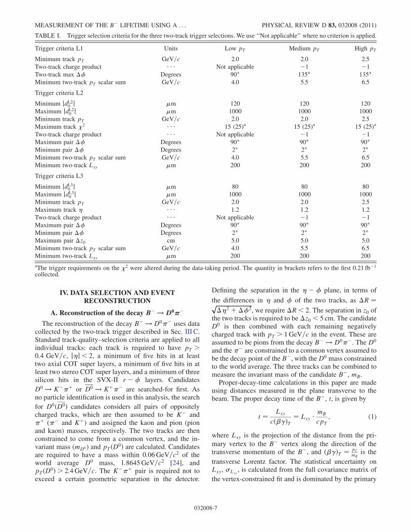
TABLE I. Trigger selection criteria for the three two-track trigger selections. We use ‘‘Not applicable’’ where no criterion is applied.

Trigger criteria L1 Units Low pT Medium pT High pT

Minimum track pT GeV=c 2.0 2.0 2.5

Two-track charge product � � � Not applicable �1 �1Two-track max �� Degrees 90� 135� 135�Minimum two-track pT scalar sum GeV=c 4.0 5.5 6.5

Trigger criteria L2

Minimum jdL20 j �m 120 120 120

Maximum jdL20 j �m 1000 1000 1000


Maximum track �2 � � � 15 (25)a 15 (25)a 15 (25)a

Two-track charge product � � � Not applicable �1 �1Maximum pair �� Degrees 90� 90� 90�Minimum pair �� Degrees 2� 2� 2�Minimum two-track pT scalar sum GeV=c 4.0 5.5 6.5

Minimum two-track Lxy �m 200 200 200

Trigger criteria L3

Minimum jdL30 j �m 80 80 80

Maximum jdL30 j �m 1000 1000 1000


Maximum track � � � � 1.2 1.2 1.2

Two-track charge product � � � Not applicable �1 �1Maximum pair �� Degrees 90� 90� 90�Minimum pair �� Degrees 2� 2� 2�Maximum pair �z0 cm 5.0 5.0 5.0

Minimum two-track pT scalar sum GeV=c 4.0 5.5 6.5

Minimum two-track Lxy �m 200 200 200

aThe trigger requirements on the �2 were altered during the data-taking period. The quantity in brackets refers to the first 0:21 fb�1

collected.


032008-7

vertex resolution, which is approximately 33�m. We haveused the average beam position per run, which is calculatedoffline for each run, as an estimate of the primary vertexposition. The uncertainty on the proper decay time iscalculated by transforming Lxy

into the B rest frame.

To reduce background, we require that the B� candidatemust have: 5:23<mB < 5:5GeV=c2, 0< t < 10 ps, pT >5:5GeV=c, Lxy > 350�m, that the impact parameter of

the B with respect to the beam spot is smaller than 80�m,and that t < 0:333 ps, where t is the decay-time uncer-tainty. We also require that the �2 of the vertex-constrainedfit is less than 15, that all tracks have z0 within 5 cm of eachother, and that �RðD0; ��Þ< 2.

It is possible to reconstruct candidates where no pair oftracks in the final state meets the trigger criteria. The life-time measurement method presented here cannot be usedon these candidates, and they are removed by reconfirmingthe trigger. We require that at least one track pair from eachcandidate decay pass the L2 and L3 trigger-selection re-quirements. The particular L2 and L3 selection that thedecay must pass depends on which trigger selection ac-cepted the event during data taking. In the case where morethan one trigger selection was satisfied during data taking,we require that the candidate satisfies the least-stringentselection. Reconfirmation of the trigger requires that theoffline-reconstructed tracks are associated to L2 and L3tracks in the event. To match an offline track to a L2 or

L3 track, we calculate the �2 ¼ ð�CCÞ2 þ ð��

Þ2 between an

offline track and each L2 or L3 track in the candidate,where �C and �� are the differences between the offlineand L2 or L3 tracks C (curvature) and �, respectively, andC and � are the mean uncertainties on the offline tracks

C and �, respectively. The L2 or L3 track that has thelowest�2 is associated with the corresponding offline track.If the �2 of the L2 (L3) track with the lowest �2 is greaterthan 95 (25), we consider the match unsuccessful and deemthat the offline track has no L2 (L3) matched track.

Collectively, the trigger-selection requirements and thecuts made on offline or derived variables are referred to asthe selection criteria. The kinematics of each track are usedto calculate the efficiency function central to this method.We use the following nomenclature to refer to each indi-vidual track. The pion originating from the B� vertex isreferred to as �B, and the pion and kaon originating fromthe D vertex are referred to as �D and KD, respectively.

B. Sample composition and signal yield

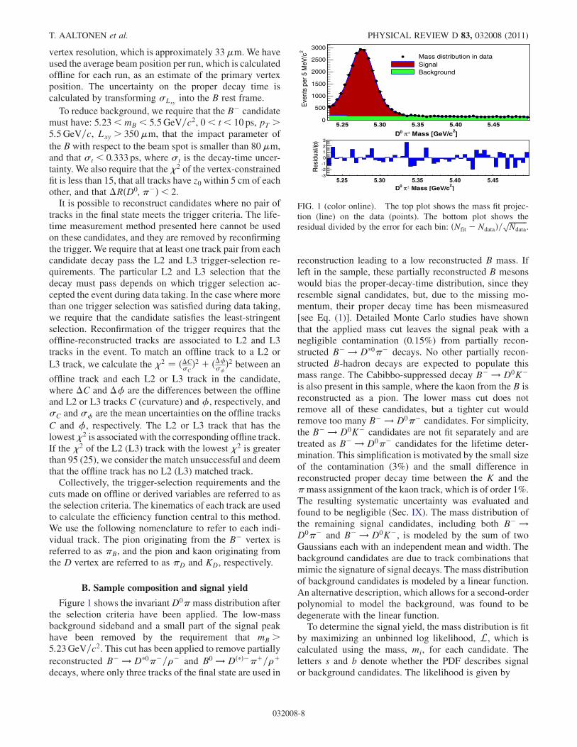
Figure 1 shows the invariantD0�mass distribution afterthe selection criteria have been applied. The low-massbackground sideband and a small part of the signal peakhave been removed by the requirement that mB >5:23GeV=c2. This cut has been applied to remove partially

reconstructed B� ! D�0��=�� and B0 ! Dð�Þ��þ=�þdecays, where only three tracks of the final state are used in

reconstruction leading to a low reconstructed B mass. Ifleft in the sample, these partially reconstructed B mesonswould bias the proper-decay-time distribution, since theyresemble signal candidates, but, due to the missing mo-mentum, their proper decay time has been mismeasured[see Eq. (1)]. Detailed Monte Carlo studies have shownthat the applied mass cut leaves the signal peak with anegligible contamination (0:15%) from partially recon-structed B� ! D�0�� decays. No other partially recon-structed B-hadron decays are expected to populate thismass range. The Cabibbo-suppressed decay B� ! D0K�is also present in this sample, where the kaon from the B isreconstructed as a pion. The lower mass cut does notremove all of these candidates, but a tighter cut wouldremove too many B� ! D0�� candidates. For simplicity,the B� ! D0K� candidates are not fit separately and aretreated as B� ! D0�� candidates for the lifetime deter-mination. This simplification is motivated by the small sizeof the contamination (3%) and the small difference inreconstructed proper decay time between the K and the�mass assignment of the kaon track, which is of order 1%.The resulting systematic uncertainty was evaluated andfound to be negligible (Sec. IX). The mass distribution ofthe remaining signal candidates, including both B� !D0�� and B� ! D0K�, is modeled by the sum of twoGaussians each with an independent mean and width. Thebackground candidates are due to track combinations thatmimic the signature of signal decays. The mass distributionof background candidates is modeled by a linear function.An alternative description, which allows for a second-orderpolynomial to model the background, was found to bedegenerate with the linear function.To determine the signal yield, the mass distribution is fit

by maximizing an unbinned log likelihood, L, which iscalculated using the mass, mi, for each candidate. Theletters s and b denote whether the PDF describes signalor background candidates. The likelihood is given by

]2

Mass [GeV/c±π0D

5.25 5.30 5.35 5.40 5.45

2E

vent

s pe

r 5 M

eV/c

0

500

1000

1500

2000

2500

3000

Mass distribution in dataSignalBackground

]2

Mass [GeV/c±π0D5.25 5.30 5.35 5.40 5.45

)σR

esid

ual/(

-3-2-10123

FIG. 1 (color online). The top plot shows the mass fit projec-tion (line) on the data (points). The bottom plot shows theresidual divided by the error for each bin: ðNfit � NdataÞ=

ffiffiffiffiffiffiffiffiffiffiNdata

p.


032008-8

logðLÞ ¼ log

�YNi

½fsP ðmijsÞ þ ð1� fsÞP ðmijbÞ�; (2)

where fs is the signal fraction, and P ðmijsÞ is given by

P ðmijsÞ ¼�

f1

1

ffiffiffiffiffiffiffi2�

p e�f½ðmi�m1Þ2=ð221Þg

þ ð1� f1Þ2


p e�f½ðmi�m2Þ2=ð222Þg��A; (3)

where the factorA is required to satisfy the normalizationcondition Z mhigh

mlow

P ðmijsÞdmi ¼ 1: (4)

P ðmijbÞ is described by a first-order polynomial and isgiven by:

P ðmijbÞ ¼ 1� �mi

½mhigh �mlow � �2 ðm2

high �m2lowÞ

; (5)

where mlow and mhigh are the lower and upper mass limits,

5.23 and 5:5GeV=c2, respectively.The free parameters in the mass fit arem1,m2,1,2,�,

f1, and fs. The data are fit, and the mass fit projection isshown in Fig. 1. From the results of the mass fit, a yield of23 900� 200 signal candidates is determined. We definethe upper sideband to be the candidates with 5:38<mB <5:5GeV=c2. These candidates are retained to constrain theparameters of the background component of the lifetimefit. The best-fit parameters are given in Appendix 4.

The results of the mass fit are also used to extract thesignal distribution of various parameters using backgroundsubtraction. We use this technique in several places forcross-checks, but not as a method to extract the lifetime orany other fit parameter. For the purpose of backgroundsubtraction, we define a signal window by 5:25<mB <5:31GeV=c2. The results of the mass fit are used to calcu-late the fraction of background candidates in the signalregion. For any given parameter, we subtract an appropri-ately scaled high-mass sideband distribution from the dis-tribution found in the signal region to obtain the signaldistribution in data.

V. REMOVING THE SELECTION-INDUCED BIASFOR SIGNAL EVENTS

A. Introduction

In this section, we derive the PDF that takes into accountlifetime bias due to the trigger and other selection criteriawithout input from simulation. Only the case of pure signalis considered in this section, whereas the complicationsintroduced by the presence of background candidates arediscussed in Sec. VII.

Before describing the PDF in detail, we give a shortoverview of the essential idea behind our method of cor-recting for the trigger effects in a completely data-drivenway. We start by considering an unbiased proper-decay-time distribution, which is given by an exponential. To

incorporate detector effects, the exponential is convolvedwith a resolution function. For the purpose of this mea-surement, the proper-decay-time–resolution function at theCDF detector is adequately described by a single Gaussianof fixed width. For a decay with mean lifetime � andGaussian proper-decay-time resolution of width t, theprobability density to observe a signal candidate decayingwith proper time ti, where the subscript i labels the candi-date, is given by

P ðti; �jsÞ ¼ 1

�e½ð�tiÞ=�þ½ð2

t Þ=ð2�2ÞF�tit

� t

�

�;

where FðxÞ ¼ 1ffiffiffiffiffiffiffi2�

pZ x

�1e½ð�y2Þ=2dy;

(6)

and s indicates that this PDF is for signal events only. Nowconsider a data set subject to the requirement that thelifetime t is within the interval t 2 ½a; b. In this case,the PDF in Eq. (6) must be modified to take into accountthis selection. The effect of the selection can be accountedfor by correct normalization, so that the PDF is now

P ðti; �jsÞ ¼1� e

½ð�tiÞ=�þ½ð2t Þ=ð2�2ÞF

�tit� t

�

Rba1� e

½ð�tÞ=�þ½ð2t Þ=ð2�2ÞF

�tt� t

�

dt

: (7)

The same equation can be written as

P ðti;�jsÞ¼EðtÞjt¼ti

1�e

½ð�tiÞ=�þ½ð2t Þ=ð2�2ÞFð tit

�t

� ÞR1�1EðtÞ1�e½ð�tÞ=�þ½ð2

t Þ=ð2�2ÞFð tt�t

� Þdt; (8)

where, for the example given here, the value of the effi-ciency function EðtÞ is one for a < t < b and zero other-wise. This is essentially the form of the lifetime PDF forcandidates collected by the selection criteria at CDF, ex-cept that the function EðtÞ will take a slightly more com-plicated form and will be different candidate-by-candidate.We indicate this by adding a subscript i that labels thecandidate, Eiðt; "sÞ. The introduction of "s is made becausethe efficiency function will also be shown to depend on "s,which is the single-track-finding efficiency at level 2. Thiscandidate-by-candidate efficiency function Eiðt; "sÞ is thecrux of this analysis and it will be described in detail in thefollowing sections.The CDF trigger selects on the impact parameters of the

tracks in the decay. The impact-parameter requirementscan be translated to an upper and lower decay-time selec-tion for each candidate. These upper and lower lifetimelimits depend on the kinematics of the decay and, there-fore, differ for each candidate—hence, the need for acandidate-by-candidate Eiðt; "sÞ.In order to calculate the efficiency function, Eiðt; "sÞ, for

a given candidate, we require: the individual candidate’sdecay kinematics, measured in the data; the single-track–finding efficiency "s (also extracted from the data); and thetrigger and offline criteria, collectively referred to by thesymbol T. In terms of these variables, the PDF for acandidate with decay time ti is


032008-9

P ½ti;�jT;Eiðt;"sÞ;s

¼ Eiðt;"sÞjt¼ti � 1�e

½ð�tiÞ=�þ½ð2t Þ=ð2�2ÞFð tit

�t

� ÞR1�1Eiðt;"sÞ� 1

�e½ð�tÞ=�þ½ð2

t Þ=ð2�2ÞFð tt�t

� Þdt: (9)

To summarize, we use a different efficiency functionEiðt; "sÞ for each candidate i, which ensures the correctnormalization of the lifetime PDF, given the selection. Wecalculate each Eiðt; "sÞ analytically from the candidate’sdecay kinematics and the selection criteria, in a completelydata-driven way, without recourse to Monte Carlo. Theexact form of Eiðt; "sÞ, and how it is calculated, is dis-cussed next.

B. Calculation of Eiðt; "sÞ1. Scanning through different potential proper

decay times

In order to find the function Eiðt; "sÞ for a given candi-date i, we need to find the trigger efficiency for thatcandidate for all possible B proper decay times. We scanthrough different B-decay times by translating the B-decayvertex along the B-flight direction, defined by the recon-structed B momentum. At each point in the scan, werecalculate all decay-time–dependent properties of thecandidate, in particular, the impact parameters and decaydistance. Properties that are independent of proper decaytime (before selection is applied), such as the four-momenta of all particles or the flight distance of theintermediate D meson, remain constant. We reapply thetrigger and other selection criteria to the translated candi-date. If the translated candidate fails the selection criteria,Eiðt; "sÞ is zero for that candidate at the correspondingdecay time. Otherwise, Eiðt; "sÞ is nonzero at time t, andits exact value depends on the SVT (L2) track-findingefficiency, "s. This method of scanning through differentpotential proper decay times allows for the determinationof the effective upper and lower decay-time cuts applied bythe selection criteria. This process is illustrated and de-scribed in detail in Sec. VB4. Prior to this, we discuss twocomplications to the basic idea presented above. The SVThas a track-finding efficiency smaller than that of offlinetrack-finding efficiency. The SVT track-finding efficiencyvaries as a function of the track impact parameter. Theimpact of this variation and the necessary changes to thebasic idea are discussed in Sec. VB2. A secondary com-plication is that, at different stages in the event reconstruc-tion and selection, different algorithms are used tocalculate the track parameters—very fast algorithms atL2, more detailed ones at L3, and finally the full trackingand vertexing in the final offline reconstruction. The mea-sured values of track parameters, such as impact parame-ters, differ slightly depending on the algorithm used for thecalculation. Section VB3 describes how the differentmeasurements of impact parameter are accounted for.

2. The value of Eiðt; "sÞ and its dependence on the SVTtrack-finding efficiency

The need to include the dependence on "s.—If the track-finding efficiency is independent of proper decay time, onecan base a fit on a PDF given that a certain track combi-nation has been reconstructed and seen by the trigger. Thiswould imply that the track-finding efficiency is constant asa function of the impact parameter, since the decay timeand the impact parameter are correlated. In the case wherethe track-finding efficiency is proper-decay-time–indepen-dent, the set of tracks seen by the trigger would be treatedexactly in the same way as the decay kinematics, i.e., assomething that can be kept constant as the decay distance ischanged for the efficiency-function evaluation. Given thata certain track combination has been found, the triggerefficiency at a certain decay time is either 1 (passes selec-tion) or 0 (fails), independent of "s. This PDF would ignoreone factor: the probability that exactly this track combina-tion has been found. If this factor is proper-decay-time–independent, it does not affect the maximum of thelikelihood and, hence, the result of the fit.The level-3 tracking algorithms are very similar to those

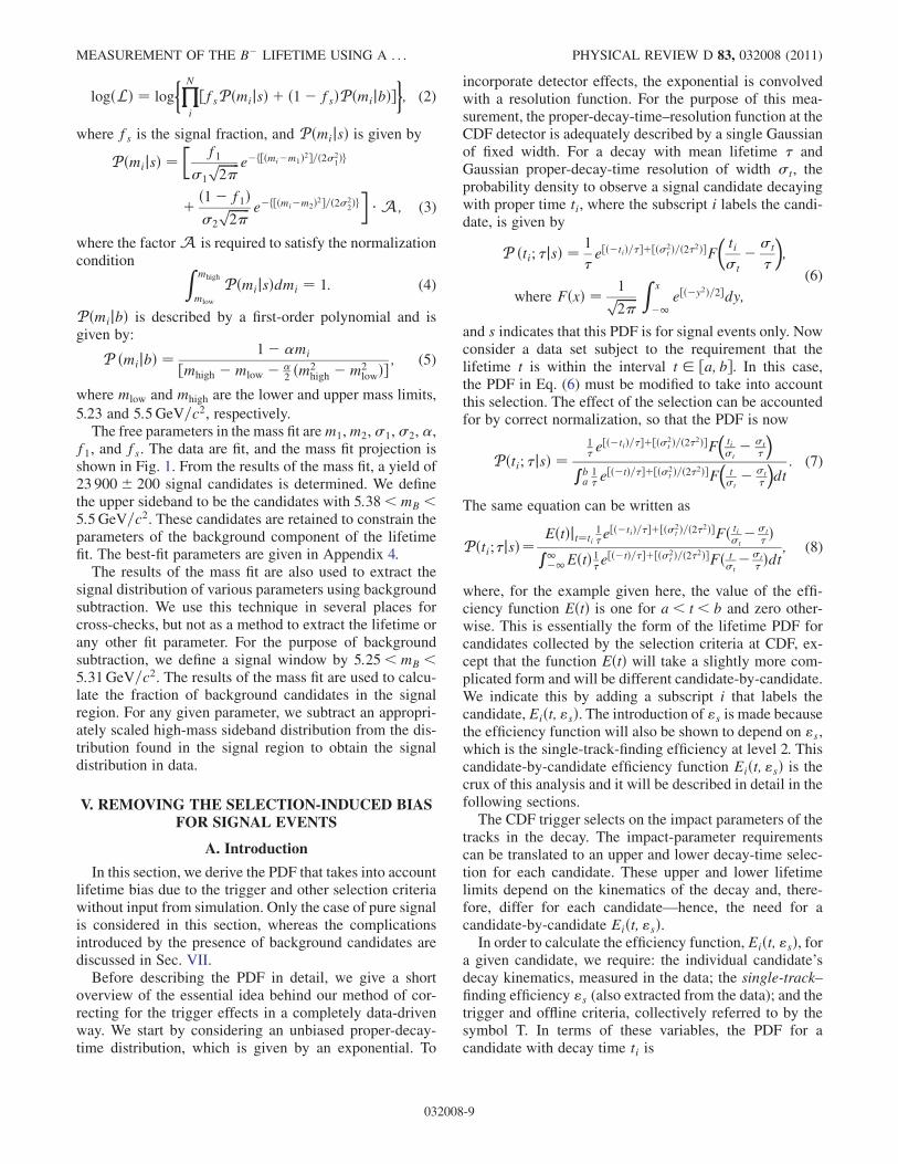
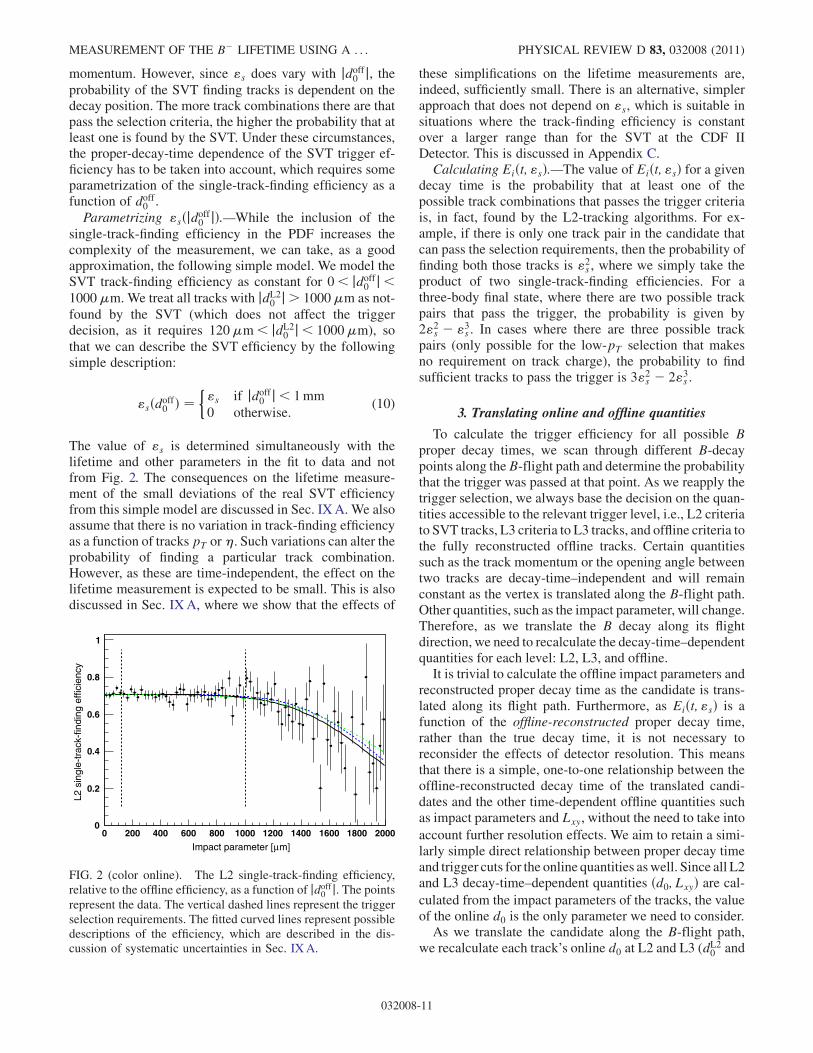
used offline, and the level-3 track-finding efficiency asa function of offline impact parameter is constant.Therefore, the track-finding efficiency at level 3 is decay-time–independent and of the situation that is describedabove; the level-3 trigger efficiency is a time-independentconstant for all decay times that pass the selection criteria.Therefore, it is not necessary to consider the effect of thelevel-3 track-finding efficiency further. However, the situ-ation at level 2 is more complicated.Figure 2 shows the SVT track-finding efficiency for

tracks found in the offline reconstruction, in data, as afunction of the track’s offline impact parameter jdoff0 j.Figure 2 shows that the SVT track-finding efficiency ofthe CDF II Detector depends on the track impact parameterand, therefore, on the decay time of the parent particle. TheSVT track-finding efficiency is approximately constantfor 0< jdoff0 j< 1000�m and falls rapidly for jdoff0 j>1000�m. The efficiency distribution is obtained from thesignal region of the data sample used in the fit, using thefollowing method: the efficiency prior to triggering isobtained by considering the subsample of candidateswhere two particular tracks can pass the trigger require-ments. For these candidates, the remaining third track isused to obtain the SVT track-finding efficiency.Even though "s is approximately constant within the

trigger acceptance requirements, the rapid drop afterjdoff0 j> 1000�m introduces a particular problem. The

trigger efficiency is calculated depending on which tracksare found by the SVT. If "s is constant for all impactparameters, then the tracks which were actually found bythe SVT can be used to calculate the trigger efficiency, andwe can assume that the same tracks would be found as thedecay vertex is scanned along the direction of the B


032008-10

momentum. However, since "s does vary with jdoff0 j, theprobability of the SVT finding tracks is dependent on thedecay position. The more track combinations there are thatpass the selection criteria, the higher the probability that atleast one is found by the SVT. Under these circumstances,the proper-decay-time dependence of the SVT trigger ef-ficiency has to be taken into account, which requires someparametrization of the single-track-finding efficiency as afunction of doff0 .

Parametrizing "sðjdoff0 jÞ.—While the inclusion of the

single-track-finding efficiency in the PDF increases thecomplexity of the measurement, we can take, as a goodapproximation, the following simple model. We model theSVT track-finding efficiency as constant for 0< jdoff0 j<1000�m. We treat all tracks with jdL20 j> 1000�m as not-

found by the SVT (which does not affect the triggerdecision, as it requires 120�m< jdL20 j< 1000�m), so

that we can describe the SVT efficiency by the followingsimple description:

"sðdoff0 Þ ¼�"s if jdoff0 j< 1mm0 otherwise.

(10)

The value of "s is determined simultaneously with thelifetime and other parameters in the fit to data and notfrom Fig. 2. The consequences on the lifetime measure-ment of the small deviations of the real SVT efficiencyfrom this simple model are discussed in Sec. IXA. We alsoassume that there is no variation in track-finding efficiencyas a function of tracks pT or�. Such variations can alter theprobability of finding a particular track combination.However, as these are time-independent, the effect on thelifetime measurement is expected to be small. This is alsodiscussed in Sec. IXA, where we show that the effects of

these simplifications on the lifetime measurements are,indeed, sufficiently small. There is an alternative, simplerapproach that does not depend on "s, which is suitable insituations where the track-finding efficiency is constantover a larger range than for the SVT at the CDF IIDetector. This is discussed in Appendix C.Calculating Eiðt; "sÞ.—The value of Eiðt; "sÞ for a given

decay time is the probability that at least one of thepossible track combinations that passes the trigger criteriais, in fact, found by the L2-tracking algorithms. For ex-ample, if there is only one track pair in the candidate thatcan pass the selection requirements, then the probability offinding both those tracks is "2s , where we simply take theproduct of two single-track-finding efficiencies. For athree-body final state, where there are two possible trackpairs that pass the trigger, the probability is given by2"2s � "3s . In cases where there are three possible trackpairs (only possible for the low-pT selection that makesno requirement on track charge), the probability to findsufficient tracks to pass the trigger is 3"2s � 2"3s .

3. Translating online and offline quantities

To calculate the trigger efficiency for all possible Bproper decay times, we scan through different B-decaypoints along theB-flight path and determine the probabilitythat the trigger was passed at that point. As we reapply thetrigger selection, we always base the decision on the quan-tities accessible to the relevant trigger level, i.e., L2 criteriato SVT tracks, L3 criteria to L3 tracks, and offline criteria tothe fully reconstructed offline tracks. Certain quantitiessuch as the track momentum or the opening angle betweentwo tracks are decay-time–independent and will remainconstant as the vertex is translated along the B-flight path.Other quantities, such as the impact parameter, will change.Therefore, as we translate the B decay along its flightdirection, we need to recalculate the decay-time–dependentquantities for each level: L2, L3, and offline.It is trivial to calculate the offline impact parameters and

reconstructed proper decay time as the candidate is trans-lated along its flight path. Furthermore, as Eiðt; "sÞ is afunction of the offline-reconstructed proper decay time,rather than the true decay time, it is not necessary toreconsider the effects of detector resolution. This meansthat there is a simple, one-to-one relationship between theoffline-reconstructed decay time of the translated candi-dates and the other time-dependent offline quantities suchas impact parameters and Lxy, without the need to take into

account further resolution effects. We aim to retain a simi-larly simple direct relationship between proper decay timeand trigger cuts for the online quantities aswell. Since all L2and L3 decay-time–dependent quantities ðd0; LxyÞ are cal-culated from the impact parameters of the tracks, the valueof the online d0 is the only parameter we need to consider.As we translate the candidate along the B-flight path,

we recalculate each track’s online d0 at L2 and L3 (dL20 and

m]µImpact parameter [0 200 400 600 800 1000 1200 1400 1600 1800 2000

L2 s

ingl

e-tr

ack-

findi

ng e

ffici

ency

0

0.2

0.4

0.6

0.8

1

FIG. 2 (color online). The L2 single-track-finding efficiency,relative to the offline efficiency, as a function of jdoff0 j. The pointsrepresent the data. The vertical dashed lines represent the triggerselection requirements. The fitted curved lines represent possibledescriptions of the efficiency, which are described in the dis-cussion of systematic uncertainties in Sec. IXA.


032008-11

dL30 ) by assuming that the differences between online and

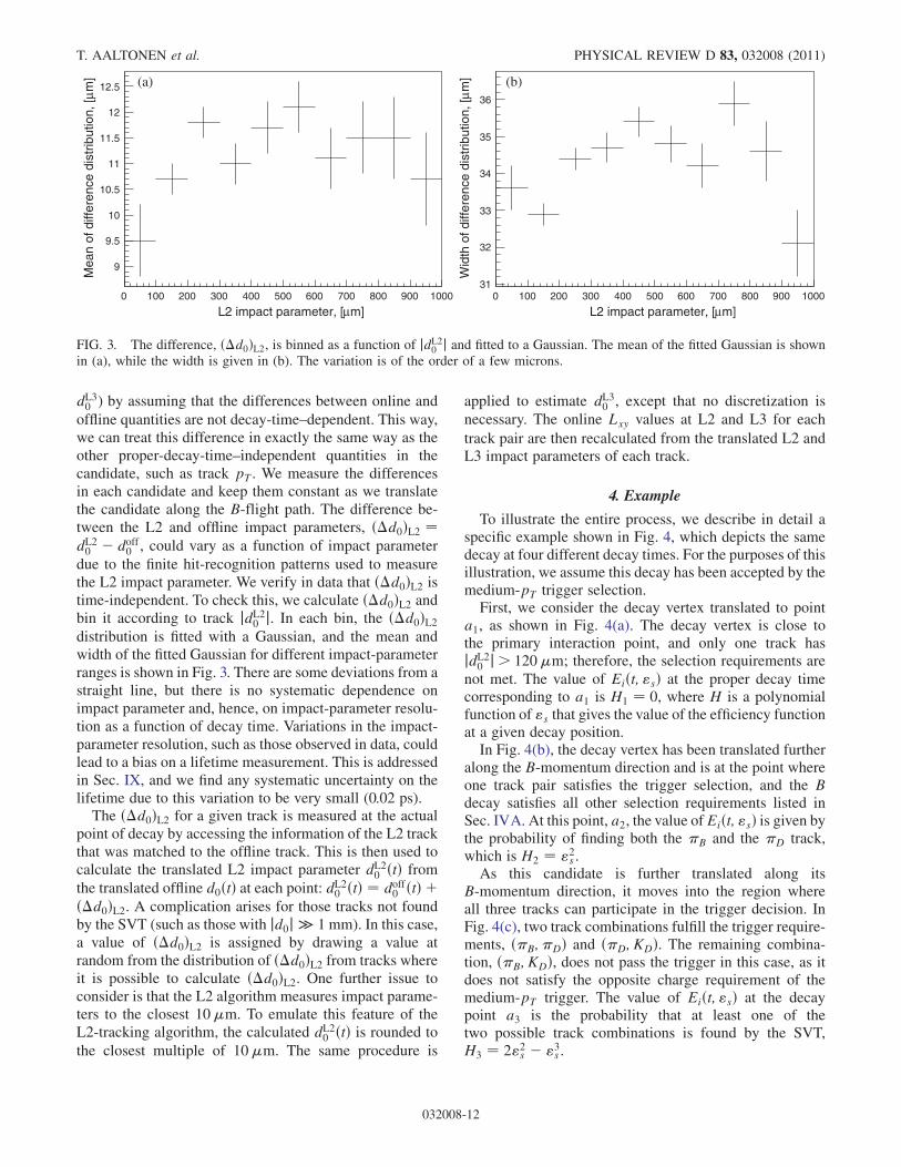
offline quantities are not decay-time–dependent. This way,we can treat this difference in exactly the same way as theother proper-decay-time–independent quantities in thecandidate, such as track pT . We measure the differencesin each candidate and keep them constant as we translatethe candidate along the B-flight path. The difference be-tween the L2 and offline impact parameters, ð�d0ÞL2 ¼dL20 � doff0 , could vary as a function of impact parameter

due to the finite hit-recognition patterns used to measurethe L2 impact parameter. We verify in data that ð�d0ÞL2 istime-independent. To check this, we calculate ð�d0ÞL2 andbin it according to track jdL20 j. In each bin, the ð�d0ÞL2distribution is fitted with a Gaussian, and the mean andwidth of the fitted Gaussian for different impact-parameterranges is shown in Fig. 3. There are some deviations from astraight line, but there is no systematic dependence onimpact parameter and, hence, on impact-parameter resolu-tion as a function of decay time. Variations in the impact-parameter resolution, such as those observed in data, couldlead to a bias on a lifetime measurement. This is addressedin Sec. IX, and we find any systematic uncertainty on thelifetime due to this variation to be very small (0.02 ps).

The ð�d0ÞL2 for a given track is measured at the actualpoint of decay by accessing the information of the L2 trackthat was matched to the offline track. This is then used tocalculate the translated L2 impact parameter dL20 ðtÞ fromthe translated offline d0ðtÞ at each point: dL20 ðtÞ ¼ doff0 ðtÞ þð�d0ÞL2. A complication arises for those tracks not foundby the SVT (such as those with jd0j � 1 mm). In this case,a value of ð�d0ÞL2 is assigned by drawing a value atrandom from the distribution of ð�d0ÞL2 from tracks whereit is possible to calculate ð�d0ÞL2. One further issue toconsider is that the L2 algorithm measures impact parame-ters to the closest 10�m. To emulate this feature of theL2-tracking algorithm, the calculated dL20 ðtÞ is rounded to

the closest multiple of 10�m. The same procedure is

applied to estimate dL30 , except that no discretization is

necessary. The online Lxy values at L2 and L3 for each

track pair are then recalculated from the translated L2 andL3 impact parameters of each track.

4. Example

To illustrate the entire process, we describe in detail aspecific example shown in Fig. 4, which depicts the samedecay at four different decay times. For the purposes of thisillustration, we assume this decay has been accepted by themedium-pT trigger selection.First, we consider the decay vertex translated to point

a1, as shown in Fig. 4(a). The decay vertex is close tothe primary interaction point, and only one track hasjdL20 j> 120�m; therefore, the selection requirements are

not met. The value of Eiðt; "sÞ at the proper decay timecorresponding to a1 is H1 ¼ 0, where H is a polynomialfunction of "s that gives the value of the efficiency functionat a given decay position.In Fig. 4(b), the decay vertex has been translated further

along the B-momentum direction and is at the point whereone track pair satisfies the trigger selection, and the Bdecay satisfies all other selection requirements listed inSec. IVA. At this point, a2, the value of Eiðt; "sÞ is given bythe probability of finding both the �B and the �D track,which is H2 ¼ "2s .As this candidate is further translated along its

B-momentum direction, it moves into the region whereall three tracks can participate in the trigger decision. InFig. 4(c), two track combinations fulfill the trigger require-ments, ð�B;�DÞ and ð�D;KDÞ. The remaining combina-tion, ð�B;KDÞ, does not pass the trigger in this case, as itdoes not satisfy the opposite charge requirement of themedium-pT trigger. The value of Eiðt; "sÞ at the decaypoint a3 is the probability that at least one of thetwo possible track combinations is found by the SVT,H3 ¼ 2"2s � "3s .

m]µL2 impact parameter, [0 100 200 300 400 500 600 700 800 900 1000

m]

µM

ean

of d

iffer

ence

dis

trib

utio

n, [

9

9.5

10

10.5

11

11.5

12

12.5 (a)

m]µL2 impact parameter, [0 100 200 300 400 500 600 700 800 900 1000

m]

µW

idth

of d

iffer

ence

dis

trib

utio

n, [

31

32

33

34

35

36

(b)

FIG. 3. The difference, ð�d0ÞL2, is binned as a function of jdL20 j and fitted to a Gaussian. The mean of the fitted Gaussian is shownin (a), while the width is given in (b). The variation is of the order of a few microns.


032008-12

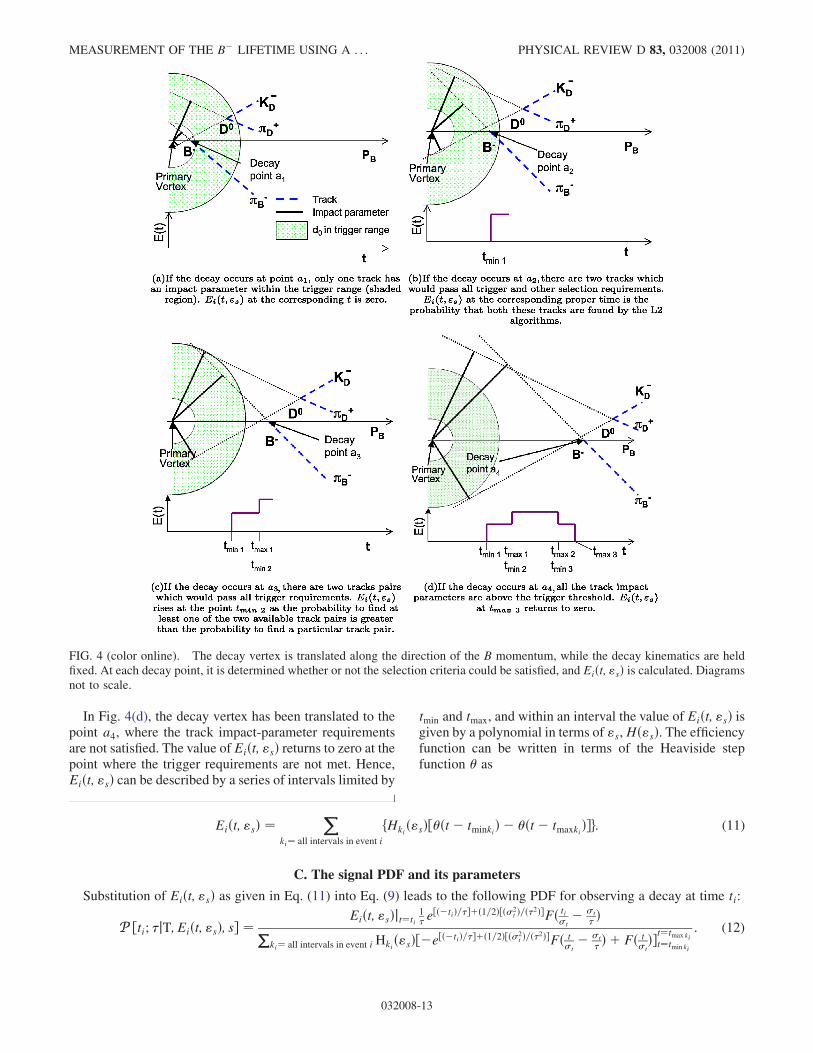
In Fig. 4(d), the decay vertex has been translated to thepoint a4, where the track impact-parameter requirementsare not satisfied. The value of Eiðt; "sÞ returns to zero at thepoint where the trigger requirements are not met. Hence,Eiðt; "sÞ can be described by a series of intervals limited by

tmin and tmax, and within an interval the value of Eiðt; "sÞ isgiven by a polynomial in terms of "s,Hð"sÞ. The efficiencyfunction can be written in terms of the Heaviside stepfunction � as

Eiðt; "sÞ ¼X

ki¼ all intervals in event i

fHkið"sÞ½�ðt� tminkiÞ � �ðt� tmaxkiÞg: (11)

C. The signal PDF and its parameters

Substitution of Eiðt; "sÞ as given in Eq. (11) into Eq. (9) leads to the following PDF for observing a decay at time ti:

P ½ti; �jT; Eiðt; "sÞ; s ¼Eiðt; "sÞjt¼ti

1� e

½ð�tiÞ=�þð1=2Þ½ð2t Þ=ð�2ÞFð tit

� t

� ÞPki¼ all intervals in event i Hkið"sÞ½�e½ð�tiÞ=�þð1=2Þ½ð2

t Þ=ð�2ÞFð tt� t

� Þ þ Fð ttÞt¼tmax kit¼tmin ki

: (12)

FIG. 4 (color online). The decay vertex is translated along the direction of the B momentum, while the decay kinematics are heldfixed. At each decay point, it is determined whether or not the selection criteria could be satisfied, and Eiðt; "sÞ is calculated. Diagramsnot to scale.


032008-13

We describe the decay-time resolution of the detector as aGaussian with width t ¼ 0:087 ps. This is the averageof the calculated candidate-by-candidate ti of thebackground-subtracted signal region in data. Using a singleGaussian based on a single, global t, instead of acandidate-by-candidate value, significantly simplifies theanalysis and is justified, since the PDF is not very sensitiveto the exact value of t. This is the case for two reasons:the lifetime to be measured, Oð1:6 psÞ, is much larger thant ¼ 0:087 ps; and the selection requirements remove themajority of candidates with low decay times.

In terms of the PDF in Eq. (12), this implies that allterms containing t only have a small effect on the PDFbecause t=� � 1

22t =�

2 and Fð tt� t

� Þ � Fð ttÞ � 1. These

approximations are not made in the PDF, but they illustratewhy the dependence on t is small. In Sec. IX, we confirmthat the systematic uncertainty due to the resolution pa-rametrization is small.

To use this PDF to extract the lifetime, knowledge of "sis also required. Although Eq. (12) could be used to simul-taneously fit � and "s, there is extra information availablein the data that can be used to help determine "s with

greater precision. The extra information used is simplythe knowledge of exactly which tracks do, and do not,have L2 information. To add this information to the PDF,we introduce a candidate observable called track configu-ration,Ci. This observable is defined both by n, the numberof tracks that are within the reach of the SVT (pT >2:0GeV=c, jdoff0 j 2 ½0; 1mm), and by r, the number of

those that have L2 information. The configuration alsodistinguishes which specific tracks have L2 information,i.e., a specific set of r tracks have matches, while theremaining n� r do not. The probability of observing aparticular Ci is given by

P ½CijT; Eiðt; "sÞ; ti; s ¼ "rsð1� "sÞðn�rÞ

Eiðt; "sÞjt¼ti

; (13)

where the factor Eiðt; "sÞjt¼ti provides the correct normal-

ization, as it is the sum of all possible configurations thatcould have passed the trigger.We multiply the probabilities defined in Eqs. (12) and

(13) to obtain the PDF, which is used to simultaneously fitthe proper decay time and "s. It is given by

P ½ti;�jT;Eiðt; "sÞ; s �P ½CijT;Eiðt;"sÞ; ti; s

¼ "rsð1� "sÞðn�rÞ 1�e


� t

� ÞPki¼ all intervals in event iHkið"sÞ½�e½ð�tÞ=�þð1=2Þ½ð2

t Þ=ð�2ÞFð tt� t

� ÞþFð ttÞt¼tmaxkit¼tminki

: (14)

In the case of a two-body decay, we would always find, inboth the numerator and denominator of the expression, thatHkið"sÞ ¼ "rsð1� "sÞn�r ¼ "2s ; all factors containing "swould cancel, and we would recover the expression fortwo-body decays derived in Ref. [25]. If there is no upperimpact-parameter cut or equivalent (tmax ¼ 1), and thelower cut is hard enough so that for each candidatetmin � t, Eq. (14) reduces to

1� e

�ðt�tminÞ=�, equivalent toa redefinition of t ¼ 0, as used by the DELPHICollaboration in Ref. [26]. Other special cases leading tosome simplifications are discussed in Appendix C.However, none of these apply here, and we use the fullexpression given in Eq. (14).

VI. VALIDATION OF THE METHOD

We test the signal PDF derived in Sec. V and the fullPDF with both signal and background components that willbe derived in Sec. VII on simulated events. We use twokinds of simulations: a full GEANT3-based [17] detectorsimulation and a fast parametric simulation for high-statistics studies.

A. The full detector simulation

We use the full CDF II Detector simulation to testwhether the signal PDF constructed in Sec. V can correctlyremove the selection bias. The simulated data samples usedfor this test consist of single B hadrons generated with pT

spectra consistent with next-to-leading-order quantumchromodynamics [27,28] and decayed with EVTGEN [29].A detailed GEANT3-based detector and trigger simulation isused to produce the detector response, which is processedusing the same reconstruction algorithms as data. In addi-tion to a B� ! D0�� sample, we also use samples of threeother decay modes: B0 ! Dþ��ðDþ ! K��þ�þÞ,Bs ! ��, and Bs ! KþK�, where the offline-selectioncriteria applied are broadly similar to those of the B� !D0�� candidates. These distinct samples, with differingtopologies, allow for further cross-checks of the basis ofthe method to correct the selection biases. The calculationof the efficiency function is easily extended to includefour-track decays, using the same principle of scanningthrough all possible proper decay times as described inSec. V.As these samples contain only signal events, we use the

PDF described in Eq. (14) to simultaneously extract the


032008-14

lifetime and the L2 single-track-finding efficiency. Thefitted lifetimes, along with the input truth lifetimes andthe size of each sample, are given in Table II.

The fitted lifetime is consistent with the input lifetimefor each Monte Carlo sample. These results indicate thatthe method of calculating the event efficiency can be usedto correct the selection biases.

B. The fast simulation

In addition to the full CDF II Detector simulation, weuse a custom fast simulation which is several orders ofmagnitude faster than the detailed simulation. It allowsproduction of many thousands of independent samples,each approximately the size of the data yield (24 000 signalevents), that are used for the extensive validation andstudies of systematic uncertainty. The fast simulation isused for validating the technique with simulated signal andbackground events and for evaluating systematic uncer-tainties. Neither the fast simulation nor the full simulationdescribed earlier is used to determine or constrain any ofthe parameters that enter the likelihood fit to data fromwhich we extract the B� lifetime. Below, we describe thefast simulation with its default settings. These formthe basis of the validation studies presented later. Howthe default behavior is altered to estimate systematic un-certainties is discussed in Sec. IX.

In order to reproduce the data as well as possible with arelatively simple simulation, we generate many of thekinematic variables in each event based on distributions

observed in data, in particular when generating back-ground. The most important ones are summarized inTable III.For every event i, we generate the B� proper decay time,

ti, the reconstructed mass, mi, the measured momentum,Pi, and the D0-meson proper decay time. The B� mass isgenerated from the PDF described in Eq. (3) using the best-fit parameters from the mass fit to the data sample. Forsignal events, the B� and D0 proper decay times aregenerated as exponentials using the 2008 world averagevalues of the lifetimes, which are 1.637 and 0.41 ps for theB� and D0 mesons, respectively [24]. The generatedproper decay times are smeared by a Gaussian of width0.087 ps to simulate the detector resolution. The generationof the reconstructed B� proper decay time in backgroundevents is based on the PDF described in Sec. VII A. Itsparameters are determined from data by fitting the lifetimedistribution of the events in the upper mass sideband. Thebackground D0 proper decay time is taken from the D0-decay-time distribution observed in the upper mass side-band. The direction of the B� momentum is generateduniformly in � and �. As transverse quantities are usedto determine the measured proper decay time in data, it isimportant to match the pT distribution in the simulation tothat observed in data. The magnitude of the B momentumis generated such that, after the selection criteria are ap-plied, the distribution of pT of the remaining simulatedsignal events matches the pT distribution observed in thebackground-subtracted signal region. Similarly, we gener-ate the magnitude of the momentum for backgroundevents, so that after selection there is agreement betweenthe pT of simulated events and the upper sideband in data.We calculate the remaining kinematic variables as fol-

lows. In the rest frame of the B� particle, the magnitudes ofthe reconstructed D0 and �B momenta are defined by thegenerated mass of the B� meson and the world averagevalues for theD0 and �masses [24]. The reconstructedD0

mass is kept fixed because, in data, the mass-constrainedvertex forces the reconstructed D0 mass to the worldaverage value. We pick a direction for the �B-momentum

TABLE II. The fit results on full detector-simulated B-decaysamples. The table also gives the true input lifetime and the sizeof the sample after selection cuts had been applied.

Decay Sample size Input lifetime Measured lifetime

B� ! D0�� 75 000 496�m 493:3� 3:2�mB0 ! Dþ�� 71 000 464�m 467:8� 2:8�mBs ! �� 35 000 438�m 443� 5�mBs ! KþK� 75 000 438�m 441:5� 2:9�m

TABLE III. Kinematic parameters of the fast simulation and the parent distribution used for generation. Details are given in the text.

Randomly generated parameter Parent distribution

t Reconstructed decay time of B� (Signal) 1�Be�t=�B 1ffiffiffiffiffi

2�p

te�½ðt2Þ=ð22

t Þ

tD Reconstructed decay time of D0 (Signal) 1�De�tD=�D 1ffiffiffiffiffi

2�p

te�½ðt2DÞ=ð22

t Þ

jPj Magnitude of B� momentum (Signal) Background-subtracted data

mB B� mass (Signal) PDF given in Eq. (3), fitted to data

t Reconstructed decay time of B� (Background) PDF given in Eq. (18), fitted to data

tD Reconstructed decay time of D0 (Background) Sideband data

jPj Magnitude of B� momentum (Background) Sideband data

mB B� mass (Background) PDF given in Eq. (5), fitted to data

� Azimuth angle of B� momentum Uniform

� Pseudorapidity of B� Uniform with j�j< 1:5�dL20 dL20 � doff0 Gaussian, then round dL20 to nearest 10�m.


032008-15

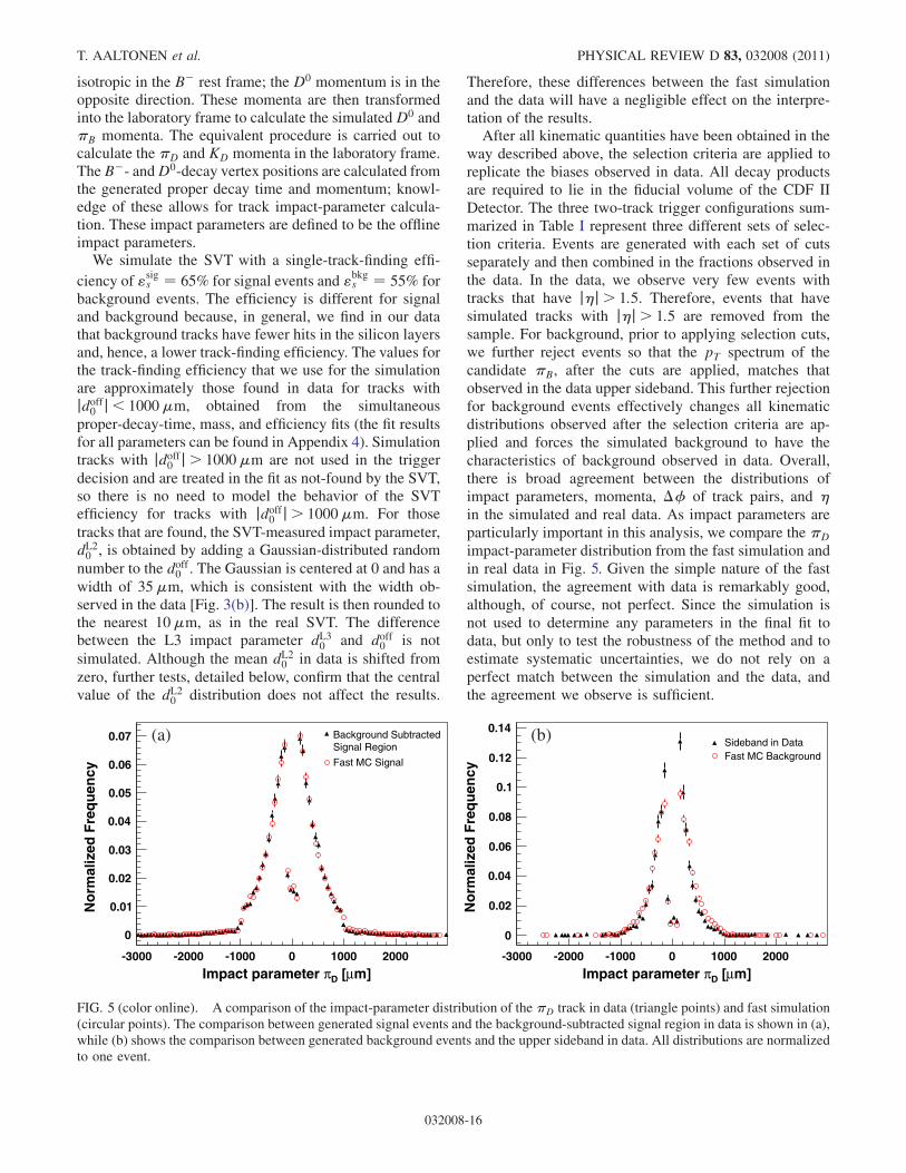
isotropic in the B� rest frame; the D0 momentum is in theopposite direction. These momenta are then transformedinto the laboratory frame to calculate the simulated D0 and�B momenta. The equivalent procedure is carried out tocalculate the �D and KD momenta in the laboratory frame.The B�- andD0-decay vertex positions are calculated fromthe generated proper decay time and momentum; knowl-edge of these allows for track impact-parameter calcula-tion. These impact parameters are defined to be the offlineimpact parameters.

We simulate the SVT with a single-track-finding effi-

ciency of "sigs ¼ 65% for signal events and "bkgs ¼ 55% forbackground events. The efficiency is different for signaland background because, in general, we find in our datathat background tracks have fewer hits in the silicon layersand, hence, a lower track-finding efficiency. The values forthe track-finding efficiency that we use for the simulationare approximately those found in data for tracks withjdoff0 j< 1000�m, obtained from the simultaneous

proper-decay-time, mass, and efficiency fits (the fit resultsfor all parameters can be found in Appendix 4). Simulationtracks with jdoff0 j> 1000�m are not used in the trigger

decision and are treated in the fit as not-found by the SVT,so there is no need to model the behavior of the SVTefficiency for tracks with jdoff0 j> 1000�m. For those

tracks that are found, the SVT-measured impact parameter,dL20 , is obtained by adding a Gaussian-distributed random

number to the doff0 . The Gaussian is centered at 0 and has a

width of 35�m, which is consistent with the width ob-served in the data [Fig. 3(b)]. The result is then rounded tothe nearest 10�m, as in the real SVT. The differencebetween the L3 impact parameter dL30 and doff0 is not

simulated. Although the mean dL20 in data is shifted from

zero, further tests, detailed below, confirm that the centralvalue of the dL20 distribution does not affect the results.

Therefore, these differences between the fast simulationand the data will have a negligible effect on the interpre-tation of the results.After all kinematic quantities have been obtained in the

way described above, the selection criteria are applied toreplicate the biases observed in data. All decay productsare required to lie in the fiducial volume of the CDF IIDetector. The three two-track trigger configurations sum-marized in Table I represent three different sets of selec-tion criteria. Events are generated with each set of cutsseparately and then combined in the fractions observed inthe data. In the data, we observe very few events withtracks that have j�j> 1:5. Therefore, events that havesimulated tracks with j�j> 1:5 are removed from thesample. For background, prior to applying selection cuts,we further reject events so that the pT spectrum of thecandidate �B, after the cuts are applied, matches thatobserved in the data upper sideband. This further rejectionfor background events effectively changes all kinematicdistributions observed after the selection criteria are ap-plied and forces the simulated background to have thecharacteristics of background observed in data. Overall,there is broad agreement between the distributions ofimpact parameters, momenta, �� of track pairs, and �in the simulated and real data. As impact parameters areparticularly important in this analysis, we compare the �D

impact-parameter distribution from the fast simulation andin real data in Fig. 5. Given the simple nature of the fastsimulation, the agreement with data is remarkably good,although, of course, not perfect. Since the simulation isnot used to determine any parameters in the final fit todata, but only to test the robustness of the method and toestimate systematic uncertainties, we do not rely on aperfect match between the simulation and the data, andthe agreement we observe is sufficient.

m]µ [DπImpact parameter -3000 -2000 -1000 0 1000 2000

No

rmal

ized

Fre

qu

ency

0

0.01

0.02

0.03

0.04

0.05

0.06

0.07 Background SubtractedSignal Region

Fast MC Signal

(a)

m]µ [DπImpact parameter -3000 -2000 -1000 0 1000 2000

No

rmal

ized

Fre

qu

ency

0

0.02

0.04

0.06

0.08

0.1

0.12

0.14Sideband in DataFast MC Background

(b)

FIG. 5 (color online). A comparison of the impact-parameter distribution of the �D track in data (triangle points) and fast simulation(circular points). The comparison between generated signal events and the background-subtracted signal region in data is shown in (a),while (b) shows the comparison between generated background events and the upper sideband in data. All distributions are normalizedto one event.


032008-16

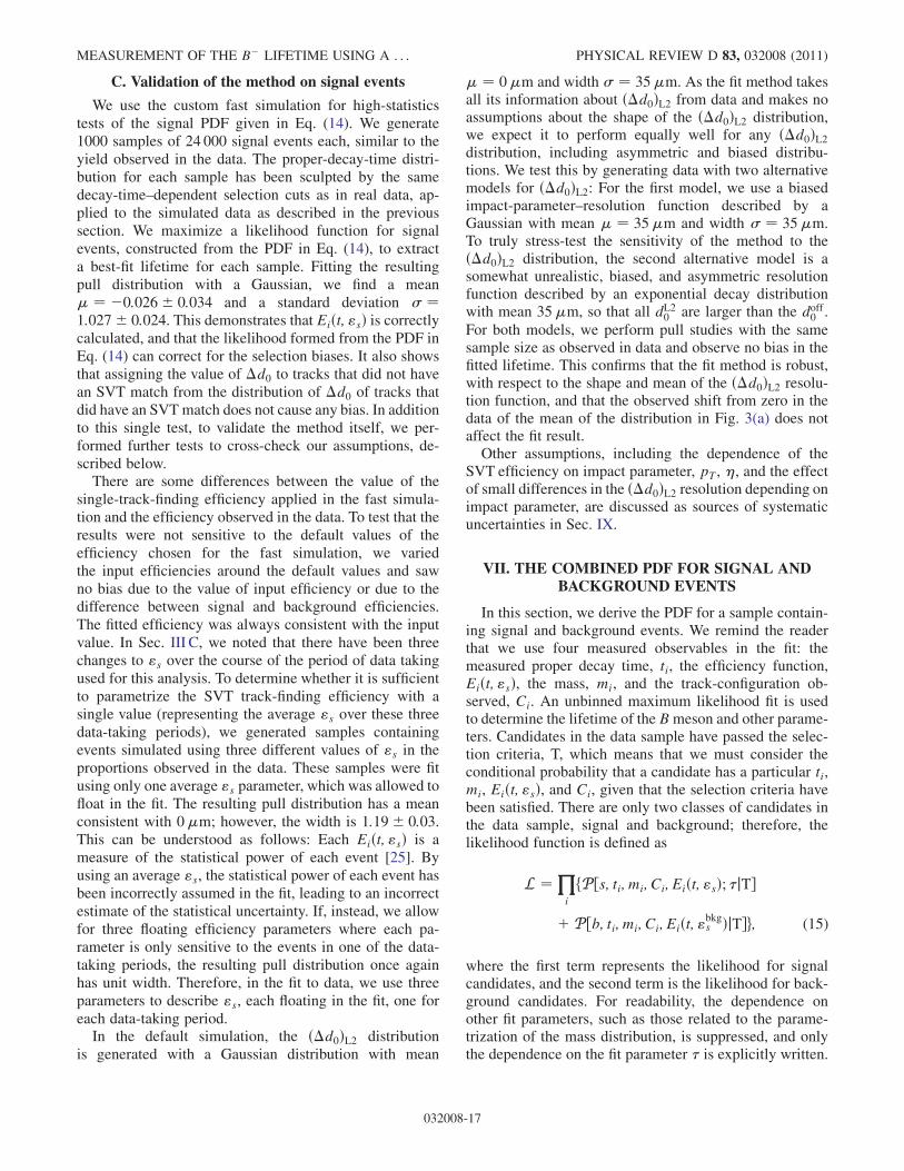
C. Validation of the method on signal events

We use the custom fast simulation for high-statisticstests of the signal PDF given in Eq. (14). We generate1000 samples of 24 000 signal events each, similar to theyield observed in the data. The proper-decay-time distri-bution for each sample has been sculpted by the samedecay-time–dependent selection cuts as in real data, ap-plied to the simulated data as described in the previoussection. We maximize a likelihood function for signalevents, constructed from the PDF in Eq. (14), to extracta best-fit lifetime for each sample. Fitting the resultingpull distribution with a Gaussian, we find a mean� ¼ �0:026� 0:034 and a standard deviation ¼1:027� 0:024. This demonstrates that Eiðt; "sÞ is correctlycalculated, and that the likelihood formed from the PDF inEq. (14) can correct for the selection biases. It also showsthat assigning the value of �d0 to tracks that did not havean SVT match from the distribution of �d0 of tracks thatdid have an SVTmatch does not cause any bias. In additionto this single test, to validate the method itself, we per-formed further tests to cross-check our assumptions, de-scribed below.

There are some differences between the value of thesingle-track-finding efficiency applied in the fast simula-tion and the efficiency observed in the data. To test that theresults were not sensitive to the default values of theefficiency chosen for the fast simulation, we variedthe input efficiencies around the default values and sawno bias due to the value of input efficiency or due to thedifference between signal and background efficiencies.The fitted efficiency was always consistent with the inputvalue. In Sec. III C, we noted that there have been threechanges to "s over the course of the period of data takingused for this analysis. To determine whether it is sufficientto parametrize the SVT track-finding efficiency with asingle value (representing the average "s over these threedata-taking periods), we generated samples containingevents simulated using three different values of "s in theproportions observed in the data. These samples were fitusing only one average "s parameter, which was allowed tofloat in the fit. The resulting pull distribution has a meanconsistent with 0�m; however, the width is 1:19� 0:03.This can be understood as follows: Each Eiðt; "sÞ is ameasure of the statistical power of each event [25]. Byusing an average "s, the statistical power of each event hasbeen incorrectly assumed in the fit, leading to an incorrectestimate of the statistical uncertainty. If, instead, we allowfor three floating efficiency parameters where each pa-rameter is only sensitive to the events in one of the data-taking periods, the resulting pull distribution once againhas unit width. Therefore, in the fit to data, we use threeparameters to describe "s, each floating in the fit, one foreach data-taking period.

In the default simulation, the ð�d0ÞL2 distributionis generated with a Gaussian distribution with mean

� ¼ 0�m and width ¼ 35�m. As the fit method takesall its information about ð�d0ÞL2 from data and makes noassumptions about the shape of the ð�d0ÞL2 distribution,we expect it to perform equally well for any ð�d0ÞL2distribution, including asymmetric and biased distribu-tions. We test this by generating data with two alternativemodels for ð�d0ÞL2: For the first model, we use a biasedimpact-parameter–resolution function described by aGaussian with mean � ¼ 35�m and width ¼ 35�m.To truly stress-test the sensitivity of the method to theð�d0ÞL2 distribution, the second alternative model is asomewhat unrealistic, biased, and asymmetric resolutionfunction described by an exponential decay distributionwith mean 35�m, so that all dL20 are larger than the doff0 .

For both models, we perform pull studies with the samesample size as observed in data and observe no bias in thefitted lifetime. This confirms that the fit method is robust,with respect to the shape and mean of the ð�d0ÞL2 resolu-tion function, and that the observed shift from zero in thedata of the mean of the distribution in Fig. 3(a) does notaffect the fit result.Other assumptions, including the dependence of the

SVT efficiency on impact parameter, pT , �, and the effectof small differences in the ð�d0ÞL2 resolution depending onimpact parameter, are discussed as sources of systematicuncertainties in Sec. IX.

VII. THE COMBINED PDF FOR SIGNAL ANDBACKGROUND EVENTS

In this section, we derive the PDF for a sample contain-ing signal and background events. We remind the readerthat we use four measured observables in the fit: themeasured proper decay time, ti, the efficiency function,Eiðt; "sÞ, the mass, mi, and the track-configuration ob-served, Ci. An unbinned maximum likelihood fit is usedto determine the lifetime of the Bmeson and other parame-ters. Candidates in the data sample have passed the selec-tion criteria, T, which means that we must consider theconditional probability that a candidate has a particular ti,mi, Eiðt; "sÞ, and Ci, given that the selection criteria havebeen satisfied. There are only two classes of candidates inthe data sample, signal and background; therefore, thelikelihood function is defined as

L ¼ Yi

fP ½s; ti; mi; Ci; Eiðt; "sÞ; �jT

þ P ½b; ti; mi; Ci; Eiðt; "bkgs ÞjTg; (15)

where the first term represents the likelihood for signalcandidates, and the second term is the likelihood for back-ground candidates. For readability, the dependence onother fit parameters, such as those related to the parame-trization of the mass distribution, is suppressed, and onlythe dependence on the fit parameter � is explicitly written.


032008-17

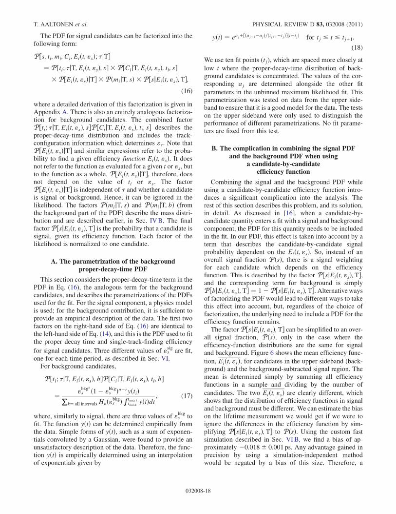
The PDF for signal candidates can be factorized into thefollowing form:

P ½s; ti; mi; Ci; Eiðt; "sÞ; �jT¼ P ½ti; �jT; Eiðt; "sÞ; s � P ½CijT; Eiðt; "sÞ; ti; s

� P ½Eiðt; "sÞjT � P ðmijT; sÞ � P ½sjEiðt; "sÞ;T;(16)

where a detailed derivation of this factorization is given inAppendix A. There is also an entirely analogous factoriza-tion for background candidates. The combined factorP ½ti; �jT; Eiðt; "sÞ; sP ½CijT; Eiðt; "sÞ; ti; s describes theproper-decay-time distribution and includes the track-configuration information which determines "s. Note thatP ½Eiðt; "sÞjT and similar expressions refer to the proba-bility to find a given efficiency function Eiðt; "sÞ. It doesnot refer to the function as evaluated for a given t or "s, butto the function as a whole. P ½Eiðt; "sÞjT, therefore, doesnot depend on the value of ti or "s. The factorP ½Eiðt; "sÞjT is independent of � and whether a candidateis signal or background. Hence, it can be ignored in thelikelihood. The factors P ðmijT; sÞ and P ðmijT; bÞ (fromthe background part of the PDF) describe the mass distri-bution and are described earlier, in Sec. IVB. The finalfactor P ½sjEiðt; "sÞ;T is the probability that a candidate issignal, given its efficiency function. Each factor of thelikelihood is normalized to one candidate.

A. The parametrization of the backgroundproper-decay-time PDF

This section considers the proper-decay-time term in thePDF in Eq. (16), the analogous term for the backgroundcandidates, and describes the parametrizations of the PDFsused for the fit. For the signal component, a physics modelis used; for the background contribution, it is sufficient toprovide an empirical description of the data. The first twofactors on the right-hand side of Eq. (16) are identical tothe left-hand side of Eq. (14), and this is the PDF used to fitthe proper decay time and single-track-finding efficiency

for signal candidates. Three different values of "sigs are fit,

one for each time period, as described in Sec. VI.For background candidates,

P ½ti; �jT; Eiðt; "sÞ; bP ½CijT; Eiðt; "sÞ; ti; b

¼ "bkgn

s ð1� "bkgs Þn�ryðtiÞPk¼ all intervalsHkð"bkgs ÞRtmax k

tmin kyðtÞdt ; (17)

where, similarly to signal, there are three values of "bkgs tofit. The function yðtÞ can be determined empirically fromthe data. Simple forms of yðtÞ, such as a sum of exponen-tials convoluted by a Gaussian, were found to provide anunsatisfactory description of the data. Therefore, the func-tion yðtÞ is empirically determined using an interpolationof exponentials given by

yðtÞ ¼ eajþ½ðajþ1�ajÞ=ðtjþ1�tjÞðt�tjÞ for tj � t � tjþ1:

(18)

We use ten fit points (tj), which are spaced more closely at

low t where the proper-decay-time distribution of back-ground candidates is concentrated. The values of the cor-responding aj are determined alongside the other fit

parameters in the unbinned maximum likelihood fit. Thisparametrization was tested on data from the upper side-band to ensure that it is a good model for the data. The testson the upper sideband were only used to distinguish theperformance of different parametrizations. No fit parame-ters are fixed from this test.

B. The complication in combining the signal PDFand the background PDF when using

a candidate-by-candidateefficiency function

Combining the signal and the background PDF whileusing a candidate-by-candidate efficiency function intro-duces a significant complication into the analysis. Therest of this section describes this problem, and its solution,in detail. As discussed in [16], when a candidate-by-candidate quantity enters a fit with a signal and backgroundcomponent, the PDF for this quantity needs to be includedin the fit. In our PDF, this effect is taken into account by aterm that describes the candidate-by-candidate signalprobability dependent on the Eiðt; "sÞ. So, instead of anoverall signal fraction P ðsÞ, there is a signal weightingfor each candidate which depends on the efficiencyfunction. This is described by the factor P ½sjEiðt; "sÞ;T,and the corresponding term for background is simplyP ½bjEiðt; "sÞ;T ¼ 1� P ½sjEiðt; "sÞ;T. Alternative waysof factorizing the PDF would lead to different ways to takethis effect into account, but, regardless of the choice offactorization, the underlying need to include a PDF for theefficiency function remains.The factor P ½sjEiðt; "sÞ;T can be simplified to an over-

all signal fraction, P ðsÞ, only in the case where theefficiency-function distributions are the same for signaland background. Figure 6 shows the mean efficiency func-

tion, Eiðt; "sÞ, for candidates in the upper sideband (back-ground) and the background-subtracted signal region. Themean is determined simply by summing all efficiencyfunctions in a sample and dividing by the number of

candidates. The two Eiðt; "sÞ are clearly different, whichshows that the distribution of efficiency functions in signaland background must be different. We can estimate the biason the lifetime measurement we would get if we were toignore the differences in the efficiency function by sim-plifying P ½sjEiðt; "sÞ;T to P ðsÞ. Using the custom fastsimulation described in Sec. VI B, we find a bias of ap-proximately �0:018� 0:001 ps. Any advantage gained inprecision by using a simulation-independent methodwould be negated by a bias of this size. Therefore, a


032008-18

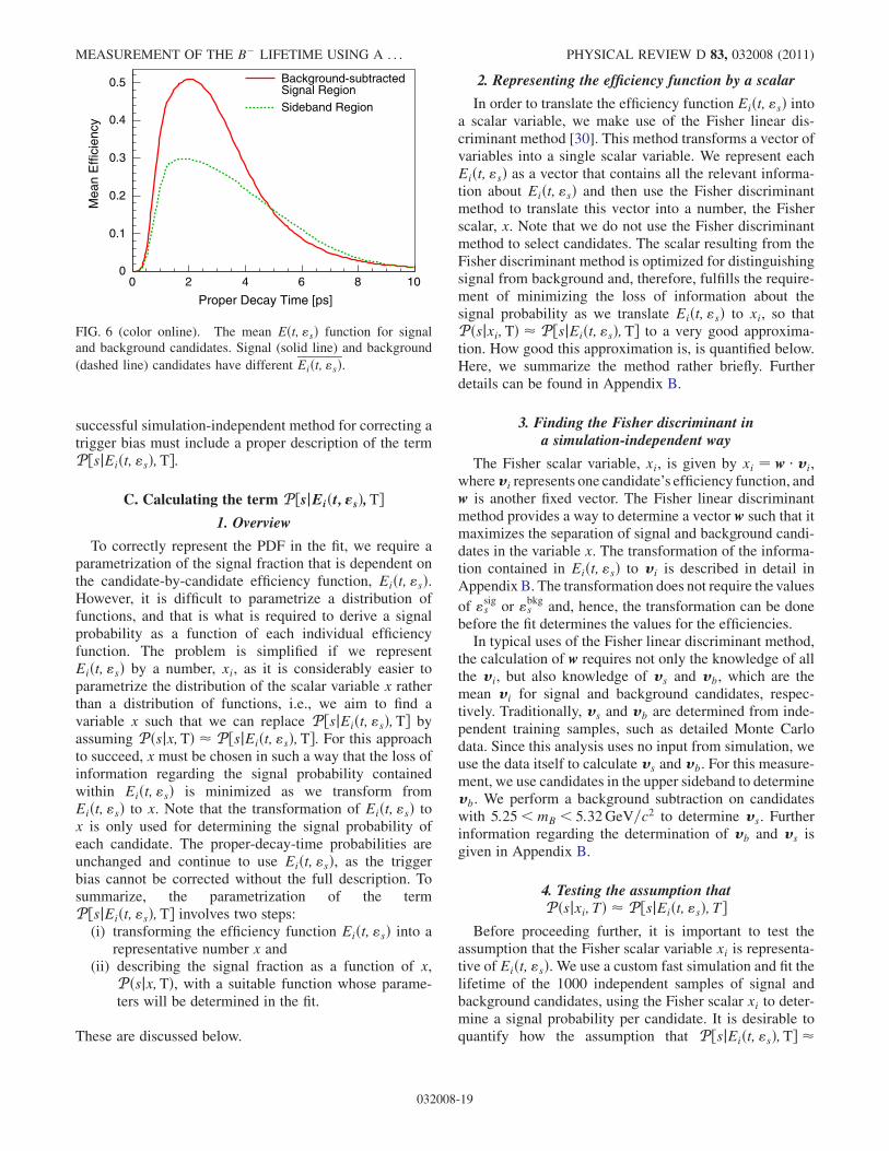
successful simulation-independent method for correcting atrigger bias must include a proper description of the termP ½sjEiðt; "sÞ;T.

C. Calculating the term P ½sjEiðt; "sÞ;T1. Overview

To correctly represent the PDF in the fit, we require aparametrization of the signal fraction that is dependent onthe candidate-by-candidate efficiency function, Eiðt; "sÞ.However, it is difficult to parametrize a distribution offunctions, and that is what is required to derive a signalprobability as a function of each individual efficiencyfunction. The problem is simplified if we representEiðt; "sÞ by a number, xi, as it is considerably easier toparametrize the distribution of the scalar variable x ratherthan a distribution of functions, i.e., we aim to find avariable x such that we can replace P ½sjEiðt; "sÞ;T byassuming P ðsjx;TÞ � P ½sjEiðt; "sÞ;T. For this approachto succeed, x must be chosen in such a way that the loss ofinformation regarding the signal probability containedwithin Eiðt; "sÞ is minimized as we transform fromEiðt; "sÞ to x. Note that the transformation of Eiðt; "sÞ tox is only used for determining the signal probability ofeach candidate. The proper-decay-time probabilities areunchanged and continue to use Eiðt; "sÞ, as the triggerbias cannot be corrected without the full description. Tosummarize, the parametrization of the termP ½sjEiðt; "sÞ;T involves two steps:

(i) transforming the efficiency function Eiðt; "sÞ into arepresentative number x and

(ii) describing the signal fraction as a function of x,P ðsjx;TÞ, with a suitable function whose parame-ters will be determined in the fit.

These are discussed below.

2. Representing the efficiency function by a scalar

In order to translate the efficiency function Eiðt; "sÞ intoa scalar variable, we make use of the Fisher linear dis-criminant method [30]. This method transforms a vector ofvariables into a single scalar variable. We represent eachEiðt; "sÞ as a vector that contains all the relevant informa-tion about Eiðt; "sÞ and then use the Fisher discriminantmethod to translate this vector into a number, the Fisherscalar, x. Note that we do not use the Fisher discriminantmethod to select candidates. The scalar resulting from theFisher discriminant method is optimized for distinguishingsignal from background and, therefore, fulfills the require-ment of minimizing the loss of information about thesignal probability as we translate Eiðt; "sÞ to xi, so thatP ðsjxi;TÞ � P ½sjEiðt; "sÞ;T to a very good approxima-tion. How good this approximation is, is quantified below.Here, we summarize the method rather briefly. Furtherdetails can be found in Appendix B.

3. Finding the Fisher discriminant ina simulation-independent way

The Fisher scalar variable, xi, is given by xi ¼ w � vi,wherevi represents one candidate’s efficiency function, andw is another fixed vector. The Fisher linear discriminantmethod provides a way to determine a vector w such that itmaximizes the separation of signal and background candi-dates in the variable x. The transformation of the informa-tion contained in Eiðt; "sÞ to vi is described in detail inAppendix B. The transformation does not require the values

of "sigs or "bkgs and, hence, the transformation can be donebefore the fit determines the values for the efficiencies.In typical uses of the Fisher linear discriminant method,

the calculation of w requires not only the knowledge of allthe vi, but also knowledge of vs and vb, which are themean vi for signal and background candidates, respec-tively. Traditionally, vs and vb are determined from inde-pendent training samples, such as detailed Monte Carlodata. Since this analysis uses no input from simulation, weuse the data itself to calculate vs and vb. For this measure-ment, we use candidates in the upper sideband to determinevb. We perform a background subtraction on candidateswith 5:25<mB < 5:32GeV=c2 to determine vs. Furtherinformation regarding the determination of vb and vs isgiven in Appendix B.

4. Testing the assumption thatP ðsjxi; TÞ � P ½sjEiðt; "sÞ; T

Before proceeding further, it is important to test theassumption that the Fisher scalar variable xi is representa-tive of Eiðt; "sÞ. We use a custom fast simulation and fit thelifetime of the 1000 independent samples of signal andbackground candidates, using the Fisher scalar xi to deter-mine a signal probability per candidate. It is desirable toquantify how the assumption that P ½sjEiðt; "sÞ;T �

Proper Decay Time [ps]

0 2 4 6 8 10

Mea

n E

ffici

ency

0

0.1

0.2

0.3

0.4

0.5 Background-subtractedSignal RegionSideband Region

FIG. 6 (color online). The mean Eðt; "sÞ function for signaland background candidates. Signal (solid line) and background

(dashed line) candidates have different Eiðt; "sÞ.


032008-19

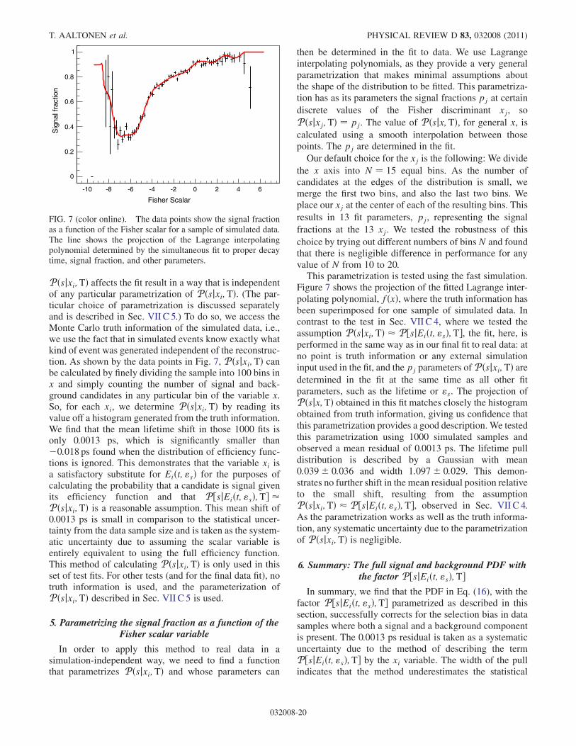
P ðsjxi;TÞ affects the fit result in a way that is independentof any particular parametrization of P ðsjxi;TÞ. (The par-ticular choice of parametrization is discussed separatelyand is described in Sec. VII C 5.) To do so, we access theMonte Carlo truth information of the simulated data, i.e.,we use the fact that in simulated events know exactly whatkind of event was generated independent of the reconstruc-tion. As shown by the data points in Fig. 7, P ðsjxi;TÞ canbe calculated by finely dividing the sample into 100 bins inx and simply counting the number of signal and back-ground candidates in any particular bin of the variable x.So, for each xi, we determine P ðsjxi;TÞ by reading itsvalue off a histogram generated from the truth information.We find that the mean lifetime shift in those 1000 fits isonly 0.0013 ps, which is significantly smaller than�0:018 ps found when the distribution of efficiency func-tions is ignored. This demonstrates that the variable xi isa satisfactory substitute for Eiðt; "sÞ for the purposes ofcalculating the probability that a candidate is signal givenits efficiency function and that P ½sjEiðt; "sÞ;T �P ðsjxi;TÞ is a reasonable assumption. This mean shift of0.0013 ps is small in comparison to the statistical uncer-tainty from the data sample size and is taken as the system-atic uncertainty due to assuming the scalar variable isentirely equivalent to using the full efficiency function.This method of calculating P ðsjxi;TÞ is only used in thisset of test fits. For other tests (and for the final data fit), notruth information is used, and the parameterization ofP ðsjxi;TÞ described in Sec. VII C 5 is used.

5. Parametrizing the signal fraction as a function of theFisher scalar variable

In order to apply this method to real data in asimulation-independent way, we need to find a functionthat parametrizes P ðsjxi;TÞ and whose parameters can

then be determined in the fit to data. We use Lagrangeinterpolating polynomials, as they provide a very generalparametrization that makes minimal assumptions aboutthe shape of the distribution to be fitted. This parametriza-tion has as its parameters the signal fractions pj at certain

discrete values of the Fisher discriminant xj, so

P ðsjxj;TÞ ¼ pj. The value of P ðsjx;TÞ, for general x, iscalculated using a smooth interpolation between thosepoints. The pj are determined in the fit.

Our default choice for the xj is the following: We divide

the x axis into N ¼ 15 equal bins. As the number ofcandidates at the edges of the distribution is small, wemerge the first two bins, and also the last two bins. Weplace our xj at the center of each of the resulting bins. This

results in 13 fit parameters, pj, representing the signal

fractions at the 13 xj. We tested the robustness of this

choice by trying out different numbers of bins N and foundthat there is negligible difference in performance for anyvalue of N from 10 to 20.This parametrization is tested using the fast simulation.

Figure 7 shows the projection of the fitted Lagrange inter-polating polynomial, fðxÞ, where the truth information hasbeen superimposed for one sample of simulated data. Incontrast to the test in Sec. VII C 4, where we tested theassumption P ðsjxi;TÞ � P ½sjEiðt; "sÞ;T, the fit, here, isperformed in the same way as in our final fit to real data: atno point is truth information or any external simulationinput used in the fit, and the pj parameters of P ðsjxi;TÞ aredetermined in the fit at the same time as all other fitparameters, such as the lifetime or "s. The projection ofP ðsjx;TÞ obtained in this fit matches closely the histogramobtained from truth information, giving us confidence thatthis parametrization provides a good description. We testedthis parametrization using 1000 simulated samples andobserved a mean residual of 0.0013 ps. The lifetime pulldistribution is described by a Gaussian with mean0:039� 0:036 and width 1:097� 0:029. This demon-strates no further shift in the mean residual position relativeto the small shift, resulting from the assumptionP ðsjxi;TÞ � P ½sjEiðt; "sÞ;T, observed in Sec. VII C 4.As the parametrization works as well as the truth informa-tion, any systematic uncertainty due to the parametrizationof P ðsjxi;TÞ is negligible.

6. Summary: The full signal and background PDF withthe factor P ½sjEiðt; "sÞ;T

In summary, we find that the PDF in Eq. (16), with thefactor P ½sjEiðt; "sÞ;T parametrized as described in thissection, successfully corrects for the selection bias in datasamples where both a signal and a background componentis present. The 0.0013 ps residual is taken as a systematicuncertainty due to the method of describing the termP ½sjEiðt; "sÞ;T by the xi variable. The width of the pullindicates that the method underestimates the statistical

Fisher Scalar

-10 -8 -6 -4 -2 0 2 4 6

Sig

nal f

ract

ion

0

0.2

0.4

0.6

0.8

1

FIG. 7 (color online). The data points show the signal fractionas a function of the Fisher scalar for a sample of simulated data.The line shows the projection of the Lagrange interpolatingpolynomial determined by the simultaneous fit to proper decaytime, signal fraction, and other parameters.


032008-20

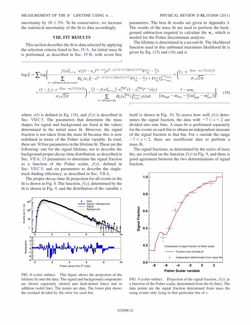
uncertainty by 10� 3%. To be conservative, we increasethe statistical uncertainty of the fit to data accordingly.

VIII. FIT RESULTS

This section describes the fit to data selected by applyingthe selection criteria listed in Sec. IVA. An initial mass fitis performed, as described in Sec. IVB, with seven free

parameters. The best fit results are given in Appendix 4.The results of the mass fit are used to perform the back-ground subtraction required to calculate the vs, which isneeded for the Fisher discriminant analysis.The lifetime is determined in a second fit. The likelihood

function used in this unbinned maximum likelihood fit isgiven by Eq. (15) and (16) and is

logL¼Xi

log

� fðxÞjx¼xi �"rsð1�"sÞðn�rÞ 1�e


�t

� ÞPki¼all intervals inevent i

Hkið"sÞ½�e½ð�tÞ=�þð1=2Þ½ð2t Þ=ð�2ÞFð t

t�t

� ÞþFð ttÞt¼tmaxkit¼tminki

��f1 �e�f½ðmi�m1Þ2=ð22

1Þg

1


p

þð1�f1Þ �e�f½ðmi�m2Þ2=ð222Þg

2


p�þ½1�fðxÞjx¼xi �"bkg

n

s ð1�"bkgs Þn�ryðtiÞPk¼all intervals

Hkð"bkgs ÞRtmaxktmink

yðtÞdt � 1��mi

½mhigh�mlow��2 ðm2

high�m2lowÞ

�; (19)

where yðtÞ is defined in Eq. (18), and fðxÞ is described inSec. VII C 5. The parameters that determine the massshapes for signal and background are fixed at the valuesdetermined in the initial mass fit. However, the signalfraction is not taken from the mass fit because this is nowredefined in terms of the Fisher scalar variable. In total,there are 30 free parameters in the lifetime fit. These are thefollowing: one for the signal lifetime; ten to describe thebackground proper-decay-time distribution, as described inSec. VII A; 13 parameters to determine the signal fractionas a function of the Fisher scalar, fðxÞ, defined inSec. VII C 5; and six parameters to describe the single-track-finding efficiency, as described in Sec. VII A.

The proper-decay-time fit projection for all events in thefit is shown in Fig. 8. The function, fðxÞ, determined by thefit is shown in Fig. 9, and the distribution of the variable x

itself is shown in Fig. 10. To assess how well fðxÞ deter-mines the signal fraction, the data with �7< x< 2 aredivided into nine bins. A mass fit is performed separatelyfor the events in each bin to obtain an independent measureof the signal fraction in that bin. For x outside the range�7< x< 2, there are insufficient data to perform amass fit.The signal fractions, as determined by the series of mass

fits, are overlaid on the function fðxÞ in Fig. 9, and there isgood agreement between the two determinations of signalfraction.

1086420

Eve

nts

per

0.1

ps

1

10

210

310 DataSignal + BackgroundSignalBackground

[ps]±π0Proper decay time D

0 2 4 6 8 10

)σR

esid

ual/(

-3

-2

-1

0

1

2

3

FIG. 8 (color online). This figure shows the projection of thelifetime fit onto the data. The signal and background componentsare shown separately (dotted and dash-dotted lines) and inaddition (solid line). The points are data. The lower plot showsthe residual divided by the error for each bin.

Fisher Scalar variable

-8 -6 -4 -2 0 2

Sig

nal

Fra

ctio

n

0.0

0.2

0.4

0.6

0.8

1.0

Comparison of signal fraction vs fisher scalar

Function from full data fit

Independent determination from mass fits

FIG. 9 (color online). Projection of the signal fraction, fðxÞ, asa function of the Fisher scalar, determined from the fit (line). Thedata points are the signal fraction determined from mass fitsusing events only lying in that particular bin of x.


032008-21

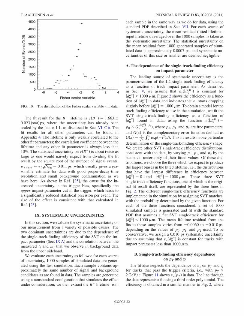
The fit result for the B� lifetime is �ðB�Þ ¼ 1:663�0:023 ðstatÞ ps, where the uncertainty has already beenscaled by the factor 1.1, as discussed in Sec. VII C 6. Thefit results for all other parameters can be found inAppendix 4. The lifetime is only weakly correlated to theother fit parameters; the correlation coefficient between thelifetime and any other fit parameter is always less than10%. The statistical uncertainty on �ðB�Þ is about twice aslarge as one would naively expect from dividing the fitresult by the square root of the number of signal events,

� naive � �=ffiffiffiffiffiffiffiffiNsig

p ¼ 0:011 ps, which usually gives a rea-

sonable estimate for data with good proper-decay-timeresolution and small background contamination as wehave here. As shown in Ref. [25], the cause for the in-creased uncertainty is the trigger bias, specifically theupper impact-parameter cut in the trigger, which leads toa significantly reduced statistical precision per event. Thesize of the effect is consistent with that calculated inRef. [25].

IX. SYSTEMATIC UNCERTAINTIES

In this section, we evaluate the systematic uncertainty onour measurement from a variety of possible causes. Thetwo dominant uncertainties are due to the dependence ofthe single-track-finding efficiency of the SVT on the im-pact parameter (Sec. IXA) and the correlation between themeasured ti and mi that we observe in background datafrom the upper sideband.

We evaluate each uncertainty as follows: for each sourceof uncertainty, 1000 samples of simulated data are gener-ated using the fast simulation. Each sample contains ap-proximately the same number of signal and backgroundcandidates as are found in data. The samples are generatedusing a nonstandard configuration that simulates the effectunder consideration; we then extract the B� lifetime from

each sample in the same way as we do for data, using thestandard PDF described in Sec. VII. For each source ofsystematic uncertainty, the mean residual (fitted lifetime–input lifetime), averaged over the 1000 samples, is taken asthe systematic uncertainty. The statistical uncertainty onthe mean residual from 1000 generated samples of simu-lated data is approximately 0.0007 ps, and systematic un-certainties of this size or smaller are deemed negligible.

A. The dependence of the single-track-finding efficiencyon impact parameter

The leading source of systematic uncertainty is theparametrization of the L2 single-track-finding efficiencyas a function of track impact parameter. As describedin Sec. V, we assume that "sðjdoff0 jÞ is constant for

jdoff0 j< 1000�m. Figure 2 shows the efficiency as a func-

tion of jdoff0 j in data and indicates that "s starts droppingslightly before jdoff0 j ¼ 1000�m. To obtain a model for the

track-finding efficiency to use in the simulation, we fit theSVT single-track-finding efficiency as a function ofjdoff0 j found in data, using the function "ðjdoff0 jÞ ¼p0 �Gðjdoff0 j�p1

p2Þ, where p0, p1, and p2 are free parameters,

and GðxÞ is the complementary error function defined asGðxÞ ¼ 2ffiffiffi

�p R1

x expð�t2Þdt. This fit results in one particulardetermination of the single-track-finding efficiency shape.We create other SVT single-track efficiency distributions,consistent with the data, by varying p0, p1, and p2 by thestatistical uncertainty of their fitted values. Of these dis-tributions, we choose the three which we expect to producethe largest biases in the fitted lifetime, i.e., the distributionsthat have the largest difference in efficiency betweenjdoff0 j ¼ 0 and jdoff0 j ¼ 1000�m. These three SVT

single-track efficiency functions, one of which is the origi-nal fit result itself, are represented by the three lines inFig. 2. The different single-track efficiency functions areimplemented in the simulation by assigning SVT matches,with the probability determined by the given function. Foreach of the three functions considered, a set of 1000simulated samples is generated and fit with the standardPDF that assumes a flat SVT single-track efficiency forjdoff0 j< 1000�m. The mean lifetime residual from the

fits to these samples varies from �0:0060 to �0:010 ps,depending on the values of p0, p1, and p2 used. To beconservative, we assign a 0.010 ps systematic uncertaintydue to assuming that "sðdoff0 Þ is constant for tracks with

impact parameter less than 1000�m.

B. Single-track-finding efficiency dependenceon pT and �

The fit also neglects the dependence of "s on pT and �for tracks that pass the trigger criteria, i.e., with pT >2GeV=c. Figure 11 shows "sðpTÞ in data. The line throughthe data represents a fit using a third-order polynomial. Theefficiency is obtained in a similar manner to Fig. 2, where

Fisher scalar variable

-8 -6 -4 -2 0 2 4

Num

ber

of E

vent

s/0.

26

0

500

1000

1500

2000

2500

3000

3500

4000

4500

FIG. 10. The distribution of the Fisher scalar variable x in data.


032008-22

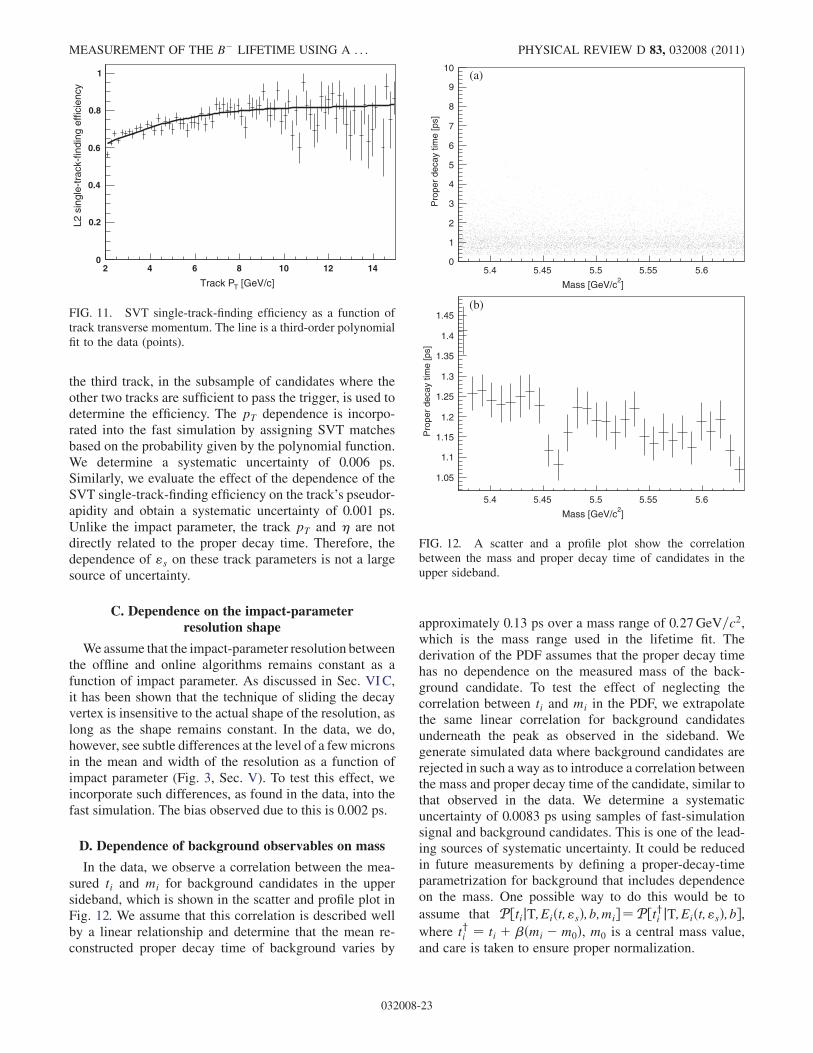
the third track, in the subsample of candidates where theother two tracks are sufficient to pass the trigger, is used todetermine the efficiency. The pT dependence is incorpo-rated into the fast simulation by assigning SVT matchesbased on the probability given by the polynomial function.We determine a systematic uncertainty of 0.006 ps.Similarly, we evaluate the effect of the dependence of theSVT single-track-finding efficiency on the track’s pseudor-apidity and obtain a systematic uncertainty of 0.001 ps.Unlike the impact parameter, the track pT and � are notdirectly related to the proper decay time. Therefore, thedependence of "s on these track parameters is not a largesource of uncertainty.

C. Dependence on the impact-parameterresolution shape

Weassume that the impact-parameter resolution betweenthe offline and online algorithms remains constant as afunction of impact parameter. As discussed in Sec. VIC,it has been shown that the technique of sliding the decayvertex is insensitive to the actual shape of the resolution, aslong as the shape remains constant. In the data, we do,however, see subtle differences at the level of a fewmicronsin the mean and width of the resolution as a function ofimpact parameter (Fig. 3, Sec. V). To test this effect, weincorporate such differences, as found in the data, into thefast simulation. The bias observed due to this is 0.002 ps.

D. Dependence of background observables on mass

In the data, we observe a correlation between the mea-sured ti and mi for background candidates in the uppersideband, which is shown in the scatter and profile plot inFig. 12. We assume that this correlation is described wellby a linear relationship and determine that the mean re-constructed proper decay time of background varies by

approximately 0.13 ps over a mass range of 0:27GeV=c2,which is the mass range used in the lifetime fit. Thederivation of the PDF assumes that the proper decay timehas no dependence on the measured mass of the back-ground candidate. To test the effect of neglecting thecorrelation between ti and mi in the PDF, we extrapolatethe same linear correlation for background candidatesunderneath the peak as observed in the sideband. Wegenerate simulated data where background candidates arerejected in such a way as to introduce a correlation betweenthe mass and proper decay time of the candidate, similar tothat observed in the data. We determine a systematicuncertainty of 0.0083 ps using samples of fast-simulationsignal and background candidates. This is one of the lead-ing sources of systematic uncertainty. It could be reducedin future measurements by defining a proper-decay-timeparametrization for background that includes dependenceon the mass. One possible way to do this would be to

assume that P ½tijT;Eiðt;"sÞ;b;mi¼P ½tyi jT;Eiðt;"sÞ;b,where tyi ¼ ti þ �ðmi �m0Þ, m0 is a central mass value,and care is taken to ensure proper normalization.

]2

Mass [GeV/c

5.4 5.45 5.5 5.55 5.6

Pro

per

deca

y tim

e [p

s]

0

1

2

3

4

5

6

7

8

9

10(a)

]2

Mass [GeV/c

5.4 5.45 5.5 5.55 5.6

Pro

per

deca

y tim

e [p

s]

1.05

1.1

1.15

1.2

1.25

1.3

1.35

1.4

1.45(b)

FIG. 12. A scatter and a profile plot show the correlationbetween the mass and proper decay time of candidates in theupper sideband.

[GeV/c]TTrack P

2 4 6 8 10 12 14

L2 s

ingl

e-tr

ack-

findi

ng e

ffici

ency

0

0.2

0.4

0.6

0.8

1

FIG. 11. SVT single-track-finding efficiency as a function oftrack transverse momentum. The line is a third-order polynomialfit to the data (points).


032008-23

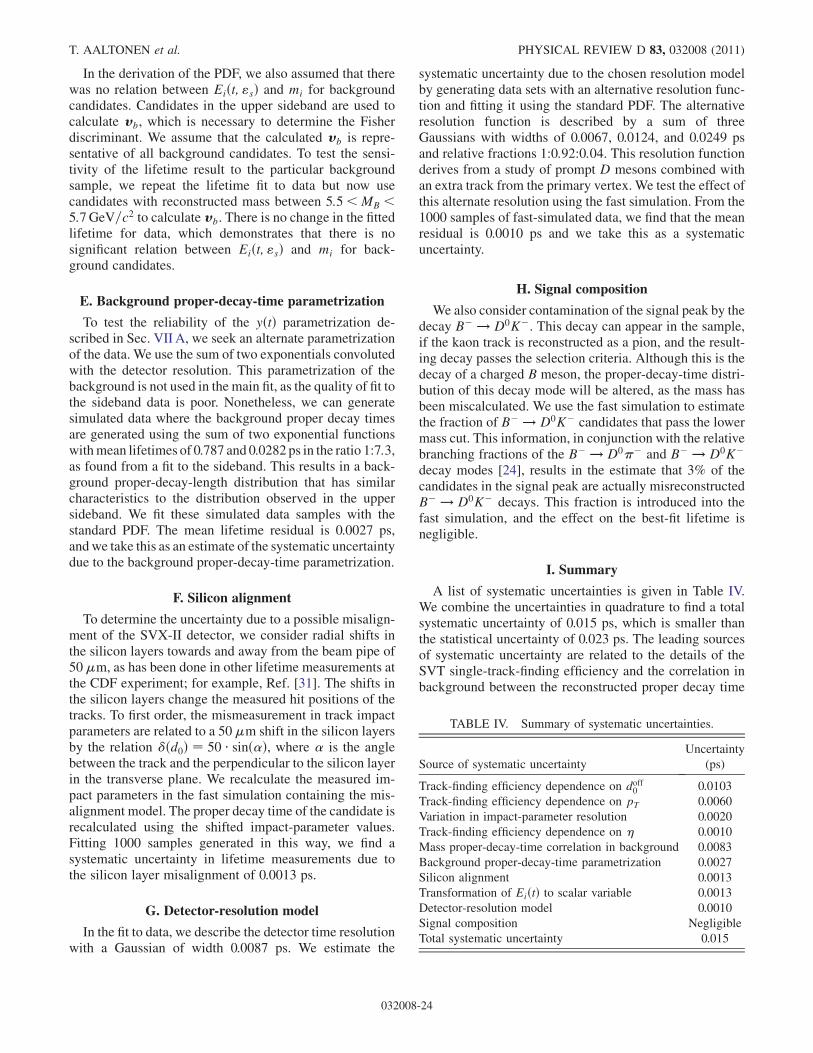
In the derivation of the PDF, we also assumed that therewas no relation between Eiðt; "sÞ and mi for backgroundcandidates. Candidates in the upper sideband are used tocalculate vb, which is necessary to determine the Fisherdiscriminant. We assume that the calculated vb is repre-sentative of all background candidates. To test the sensi-tivity of the lifetime result to the particular backgroundsample, we repeat the lifetime fit to data but now usecandidates with reconstructed mass between 5:5<MB <5:7GeV=c2 to calculate vb. There is no change in the fittedlifetime for data, which demonstrates that there is nosignificant relation between Eiðt; "sÞ and mi for back-ground candidates.

E. Background proper-decay-time parametrization

To test the reliability of the yðtÞ parametrization de-scribed in Sec. VII A, we seek an alternate parametrizationof the data. We use the sum of two exponentials convolutedwith the detector resolution. This parametrization of thebackground is not used in the main fit, as the quality of fit tothe sideband data is poor. Nonetheless, we can generatesimulated data where the background proper decay timesare generated using the sum of two exponential functionswithmean lifetimes of 0.787 and 0.0282 ps in the ratio 1:7:3,as found from a fit to the sideband. This results in a back-ground proper-decay-length distribution that has similarcharacteristics to the distribution observed in the uppersideband. We fit these simulated data samples with thestandard PDF. The mean lifetime residual is 0.0027 ps,and we take this as an estimate of the systematic uncertaintydue to the background proper-decay-time parametrization.

F. Silicon alignment

To determine the uncertainty due to a possible misalign-ment of the SVX-II detector, we consider radial shifts inthe silicon layers towards and away from the beam pipe of50�m, as has been done in other lifetime measurements atthe CDF experiment; for example, Ref. [31]. The shifts inthe silicon layers change the measured hit positions of thetracks. To first order, the mismeasurement in track impactparameters are related to a 50�m shift in the silicon layersby the relation ðd0Þ ¼ 50 � sinð�Þ, where � is the anglebetween the track and the perpendicular to the silicon layerin the transverse plane. We recalculate the measured im-pact parameters in the fast simulation containing the mis-alignment model. The proper decay time of the candidate isrecalculated using the shifted impact-parameter values.Fitting 1000 samples generated in this way, we find asystematic uncertainty in lifetime measurements due tothe silicon layer misalignment of 0.0013 ps.

G. Detector-resolution model

In the fit to data, we describe the detector time resolutionwith a Gaussian of width 0.0087 ps. We estimate the

systematic uncertainty due to the chosen resolution modelby generating data sets with an alternative resolution func-tion and fitting it using the standard PDF. The alternativeresolution function is described by a sum of threeGaussians with widths of 0.0067, 0.0124, and 0.0249 psand relative fractions 1:0:92:0:04. This resolution functionderives from a study of prompt D mesons combined withan extra track from the primary vertex. We test the effect ofthis alternate resolution using the fast simulation. From the1000 samples of fast-simulated data, we find that the meanresidual is 0.0010 ps and we take this as a systematicuncertainty.

H. Signal composition

We also consider contamination of the signal peak by thedecay B� ! D0K�. This decay can appear in the sample,if the kaon track is reconstructed as a pion, and the result-ing decay passes the selection criteria. Although this is thedecay of a charged B meson, the proper-decay-time distri-bution of this decay mode will be altered, as the mass hasbeen miscalculated. We use the fast simulation to estimatethe fraction of B� ! D0K� candidates that pass the lowermass cut. This information, in conjunction with the relativebranching fractions of the B� ! D0�� and B� ! D0K�decay modes [24], results in the estimate that 3% of thecandidates in the signal peak are actually misreconstructedB� ! D0K� decays. This fraction is introduced into thefast simulation, and the effect on the best-fit lifetime isnegligible.

I. Summary

A list of systematic uncertainties is given in Table IV.We combine the uncertainties in quadrature to find a totalsystematic uncertainty of 0.015 ps, which is smaller thanthe statistical uncertainty of 0.023 ps. The leading sourcesof systematic uncertainty are related to the details of theSVT single-track-finding efficiency and the correlation inbackground between the reconstructed proper decay time

TABLE IV. Summary of systematic uncertainties.

Source of systematic uncertainty

Uncertainty

(ps)

Track-finding efficiency dependence on doff0 0.0103

Track-finding efficiency dependence on pT 0.0060

Variation in impact-parameter resolution 0.0020

Track-finding efficiency dependence on � 0.0010

Mass proper-decay-time correlation in background 0.0083

Background proper-decay-time parametrization 0.0027

Silicon alignment 0.0013

Transformation of EiðtÞ to scalar variable 0.0013

Detector-resolution model 0.0010

Signal composition Negligible

Total systematic uncertainty 0.015


032008-24

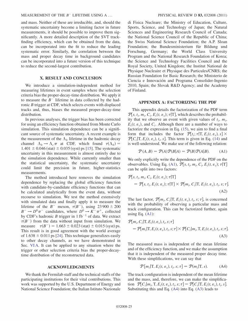
and mass. Neither of these are irreducible, and, should thesystematic uncertainty become a limiting factor in futuremeasurements, it should be possible to improve them sig-nificantly. A more detailed description of the SVT track-finding efficiency, which can be obtained from the data,can be incorporated into the fit to reduce the leadingsystematic error. Similarly, the correlation between themass and proper decay time in background candidatescan be incorporated into a future version of this techniqueto reduce the second-largest contribution.

X. RESULT AND CONCLUSION

We introduce a simulation-independent method formeasuring lifetimes in event samples where the selectioncriteria bias the proper-decay-time distribution. We apply itto measure the B� lifetime in data collected by the had-ronic B trigger at CDF, which selects events with displacedtracks and, thus, biases the measured proper-decay-timedistribution.

In previous analyses, the trigger bias has been correctedfor using an efficiency function obtained fromMonte Carlosimulation. This simulation dependence can be a signifi-cant source of systematic uncertainty. A recent example isthe measurement of the �b lifetime in the hadronic decaychannel �b ! �c� at CDF, which found �ð�bÞ ¼1:401� 0:046 ðstatÞ � 0:035 ðsystÞ ps [15]. The systematicuncertainty in this measurement is almost entirely due tothe simulation dependence. While currently smaller thanthe statistical uncertainty, the systematic uncertaintycould limit the precision in future, higher-statisticsmeasurements.

The method introduced here removes the simulationdependence by replacing the global efficiency functionwith candidate-by-candidate efficiency functions that canbe calculated analytically from the event data, withoutrecourse to simulation. We test the method extensivelywith simulated data and finally apply it to measure thelifetime of the B� meson, �ðB�Þ, using 23 900� 200B� ! D0�� candidates, where D0 ! K��þ, collectedby CDF’s hadronic B trigger in 1 fb�1 of data. We extract�ðB�Þ from the data without input from simulation. Wemeasure �ðB�Þ ¼ 1:663� 0:023 ðstatÞ � 0:015 ðsystÞ ps.This result is in good agreement with the world averageof 1:638� 0:011 ps [24]. This technique generalizes easilyto other decay channels, as we have demonstrated inSec. VIA. It can be applied to any situation where thetrigger or other selection criteria bias the proper-decay-time distribution of the reconstructed data.

ACKNOWLEDGMENTS

We thank the Fermilab staff and the technical staffs of theparticipating institutions for their vital contributions. Thiswork was supported by the U.S. Department of Energy andNational Science Foundation; the Italian Istituto Nazionale

di Fisica Nucleare; the Ministry of Education, Culture,Sports, Science, and Technology of Japan; the NaturalSciences and Engineering Research Council of Canada;the National Science Council of the Republic of China;the Swiss National Science Foundation; the A.P. SloanFoundation; the Bundesministerium fur Bildung undForschung, Germany; the World Class UniversityProgram and the National Research Foundation of Korea;the Science and Technology Facilities Council and theRoyal Society, United Kingdom; the Institut National dePhysique Nucleaire et Physique des Particules/CNRS; theRussian Foundation for Basic Research; the Ministerio deCiencia e Innovacion and Programa Consolider-Ingenio2010, Spain; the Slovak R&D Agency; and the Academyof Finland.

APPENDIX A: FACTORIZING THE PDF

This appendix details the factorization of the PDF termP ½s; ti; mi; Ci; Eiðt; "sÞ; �jT, which describes the probabil-ity that we observe an event with given values of ti, mi,Eiðt; "sÞ, and Ci. Although there are a number of ways tofactorize the expression in Eq. (15), we aim to find a finalform that includes the factor P ½ti; �jT; Eiðt; "sÞ; s �P ½CijT; Eiðt; "sÞ; ti; s. This term is given in Eq. (14) andis well-understood. We make use of the following relation:

P ðA; BÞ ¼ P ðAÞP ðBjAÞ ¼ P ðBÞP ðAjBÞ: (A1)

We only explicitly write the dependence of the PDF on theobservables. Using Eq. (A1), P ½s; ti; mi; Ci; Eiðt; "sÞ; �jTcan be split into two factors:

P ½s; ti; mi; Ci; Eiðt; "sÞ; �jT¼ P ½s; ti; Eiðt; "sÞ; �jT � P ½mi; CijT; Eiðt; "sÞ; ti; s; �:

(A2)

The last factor, P ½mi; CijT; Eiðt; "sÞ; ti; s; �, is concernedwith the probability of observing a particular mass andtrack configuration. This can be factorized further, againusing Eq. (A1):

P ½mi;CijT;Eiðt;"sÞ;ti;s;�¼P ½mijT;Eiðt;"sÞ; ti;s;��P ½Cijmi;T;Eiðt;"sÞ;ti;s;�:

(A3)

The measured mass is independent of the mean lifetimeand of the efficiency function, and we make the assumptionthat it is independent of the measured proper decay time.With these simplifications, we can say that

P ½mijT; Eiðt; "sÞ; ti; s; � ¼ P ðmijT; sÞ: (A4)

The track configuration is independent of the mean lifetimeand the mass, and, therefore, we can make the simplifica-tion P ½Cijmi;T;Eiðt; "sÞ; ti; s;� ¼ P ½CijT;Eiðt; "sÞ; ti; s.Substituting this and Eq. (A4) into Eq. (A3) leads to


032008-25

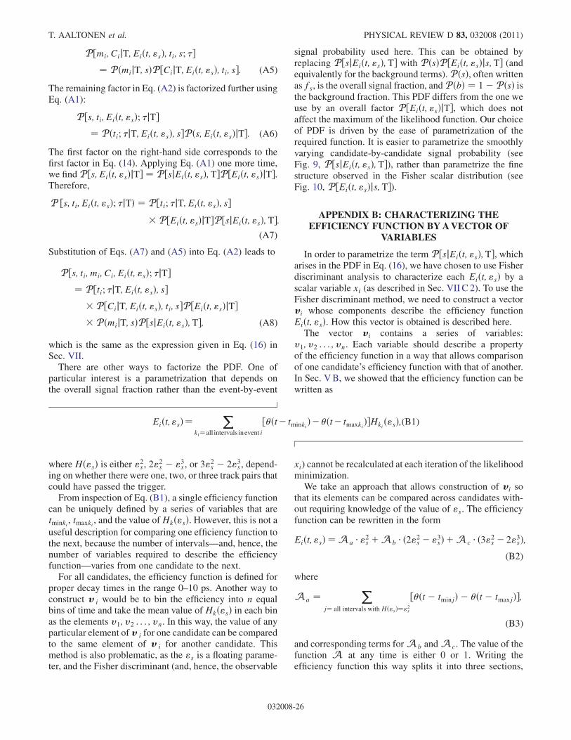
P ½mi; CijT; Eiðt; "sÞ; ti; s; �¼ P ðmijT; sÞP ½CijT; Eiðt; "sÞ; ti; s: (A5)

The remaining factor in Eq. (A2) is factorized further usingEq. (A1):

P ½s; ti; Eiðt; "sÞ; �jT¼ P ðti; �jT; Eiðt; "sÞ; sP ðs; Eiðt; "sÞjT: (A6)

The first factor on the right-hand side corresponds to thefirst factor in Eq. (14). Applying Eq. (A1) one more time,we find P ½s; Eiðt; "sÞjT ¼ P ½sjEiðt; "sÞ;TP ½Eiðt; "sÞjT.Therefore,

P ½s; ti; Eiðt; "sÞ; �jTÞ ¼ P ½ti; �jT; Eiðt; "sÞ; s� P ½Eiðt; "sÞjTP ½sjEiðt; "sÞ;T:

(A7)

Substitution of Eqs. (A7) and (A5) into Eq. (A2) leads to

P ½s; ti; mi; Ci; Eiðt; "sÞ; �jT¼ P ½ti; �jT; Eiðt; "sÞ; s

� P ½CijT; Eiðt; "sÞ; ti; sP ½Eiðt; "sÞjT� P ðmijT; sÞP ½sjEiðt; "sÞ;T; (A8)

which is the same as the expression given in Eq. (16) inSec. VII.

There are other ways to factorize the PDF. One ofparticular interest is a parametrization that depends onthe overall signal fraction rather than the event-by-event

signal probability used here. This can be obtained byreplacing P ½sjEiðt; "sÞ;T with P ðsÞP ½Eiðt; "sÞjs;T (andequivalently for the background terms). P ðsÞ, often writtenas fs, is the overall signal fraction, andP ðbÞ ¼ 1� P ðsÞ isthe background fraction. This PDF differs from the one weuse by an overall factor P ½Eiðt; "sÞjT, which does notaffect the maximum of the likelihood function. Our choiceof PDF is driven by the ease of parametrization of therequired function. It is easier to parametrize the smoothlyvarying candidate-by-candidate signal probability (seeFig. 9, P ½sjEiðt; "sÞ;T), rather than parametrize the finestructure observed in the Fisher scalar distribution (seeFig. 10, P ½Eiðt; "sÞjs;T).

APPENDIX B: CHARACTERIZING THEEFFICIENCY FUNCTION BYAVECTOR OF

VARIABLES

In order to parametrize the term P ½sjEiðt; "sÞ;T, whicharises in the PDF in Eq. (16), we have chosen to use Fisherdiscriminant analysis to characterize each Eiðt; "sÞ by ascalar variable xi (as described in Sec. VII C 2). To use theFisher discriminant method, we need to construct a vectorvi whose components describe the efficiency functionEiðt; "sÞ. How this vector is obtained is described here.The vector vi contains a series of variables:

v1; v2 . . . ; vn. Each variable should describe a propertyof the efficiency function in a way that allows comparisonof one candidate’s efficiency function with that of another.In Sec. VB, we showed that the efficiency function can bewritten as

Eiðt;"sÞ¼X

ki¼all intervals inevent i

½�ðt� tminkiÞ��ðt� tmaxkiÞHkið"sÞ;(B1)

where Hð"sÞ is either "2s , 2"2s � "3s , or 3"2s � 2"3s , depend-

ing on whether there were one, two, or three track pairs thatcould have passed the trigger.

From inspection of Eq. (B1), a single efficiency functioncan be uniquely defined by a series of variables that aretminki , tmaxki , and the value ofHkð"sÞ. However, this is not auseful description for comparing one efficiency function tothe next, because the number of intervals—and, hence, thenumber of variables required to describe the efficiencyfunction—varies from one candidate to the next.

For all candidates, the efficiency function is defined forproper decay times in the range 0–10 ps. Another way toconstruct v i would be to bin the efficiency into n equalbins of time and take the mean value of Hkð"sÞ in each binas the elements v1; v2 . . . ; vn. In this way, the value of anyparticular element of v i for one candidate can be comparedto the same element of v i for another candidate. Thismethod is also problematic, as the "s is a floating parame-ter, and the Fisher discriminant (and, hence, the observable

xi) cannot be recalculated at each iteration of the likelihoodminimization.We take an approach that allows construction of vi so

that its elements can be compared across candidates with-out requiring knowledge of the value of "s. The efficiencyfunction can be rewritten in the form

Eiðt;"sÞ ¼Aa �"2s þAb � ð2"2s �"3sÞþAc � ð3"2s � 2"3sÞ;(B2)

where

Aa ¼X

j¼ all intervals with Hð"sÞ¼"2s

½�ðt� tminjÞ � �ðt� tmaxjÞ;

(B3)

and corresponding terms forAb andAc. The value of thefunction A at any time is either 0 or 1. Writing theefficiency function this way splits it into three sections,


032008-26

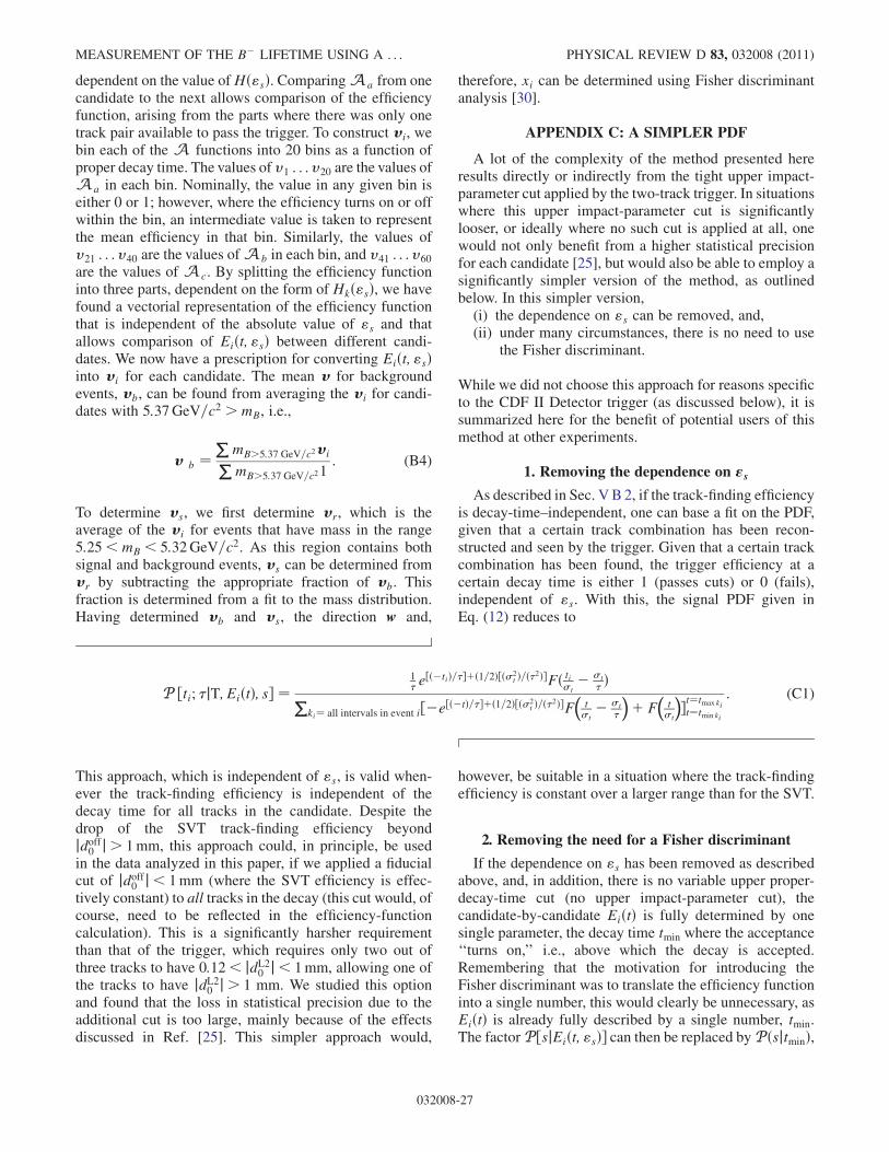
dependent on the value ofHð"sÞ. ComparingAa from onecandidate to the next allows comparison of the efficiencyfunction, arising from the parts where there was only onetrack pair available to pass the trigger. To construct vi, webin each of the A functions into 20 bins as a function ofproper decay time. The values of v1 . . .v20 are the values ofAa in each bin. Nominally, the value in any given bin iseither 0 or 1; however, where the efficiency turns on or offwithin the bin, an intermediate value is taken to representthe mean efficiency in that bin. Similarly, the values ofv21 . . .v40 are the values ofAb in each bin, and v41 . . .v60

are the values of Ac. By splitting the efficiency functioninto three parts, dependent on the form of Hkð"sÞ, we havefound a vectorial representation of the efficiency functionthat is independent of the absolute value of "s and thatallows comparison of Eiðt; "sÞ between different candi-dates. We now have a prescription for converting Eiðt; "sÞinto vi for each candidate. The mean v for backgroundevents, vb, can be found from averaging the vi for candi-dates with 5:37GeV=c2 >mB, i.e.,

v b ¼P

mB>5:37 GeV=c2viPmB>5:37 GeV=c21

: (B4)

To determine vs, we first determine vr, which is theaverage of the vi for events that have mass in the range5:25<mB < 5:32GeV=c2. As this region contains bothsignal and background events, vs can be determined fromvr by subtracting the appropriate fraction of vb. Thisfraction is determined from a fit to the mass distribution.Having determined vb and vs, the direction w and,

therefore, xi can be determined using Fisher discriminantanalysis [30].

APPENDIX C: A SIMPLER PDF

A lot of the complexity of the method presented hereresults directly or indirectly from the tight upper impact-parameter cut applied by the two-track trigger. In situationswhere this upper impact-parameter cut is significantlylooser, or ideally where no such cut is applied at all, onewould not only benefit from a higher statistical precisionfor each candidate [25], but would also be able to employ asignificantly simpler version of the method, as outlinedbelow. In this simpler version,(i) the dependence on "s can be removed, and,(ii) under many circumstances, there is no need to use

the Fisher discriminant.

While we did not choose this approach for reasons specificto the CDF II Detector trigger (as discussed below), it issummarized here for the benefit of potential users of thismethod at other experiments.

1. Removing the dependence on "s

As described in Sec. VB2, if the track-finding efficiencyis decay-time–independent, one can base a fit on the PDF,given that a certain track combination has been recon-structed and seen by the trigger. Given that a certain trackcombination has been found, the trigger efficiency at acertain decay time is either 1 (passes cuts) or 0 (fails),independent of "s. With this, the signal PDF given inEq. (12) reduces to

P ½ti; �jT; EiðtÞ; s ¼1� e


� t

� ÞPki¼ all intervals in event i½�e½ð�tÞ=�þð1=2Þ½ð2

t Þ=ð�2ÞF�tt� t

�

þ F

�tt

t¼tmax kit¼tmin ki

: (C1)

This approach, which is independent of "s, is valid when-ever the track-finding efficiency is independent of thedecay time for all tracks in the candidate. Despite thedrop of the SVT track-finding efficiency beyondjdoff0 j> 1mm, this approach could, in principle, be usedin the data analyzed in this paper, if we applied a fiducialcut of jdoff0 j< 1mm (where the SVT efficiency is effec-tively constant) to all tracks in the decay (this cut would, ofcourse, need to be reflected in the efficiency-functioncalculation). This is a significantly harsher requirementthan that of the trigger, which requires only two out ofthree tracks to have 0:12< jdL20 j< 1mm, allowing one ofthe tracks to have jdL20 j> 1 mm. We studied this optionand found that the loss in statistical precision due to theadditional cut is too large, mainly because of the effectsdiscussed in Ref. [25]. This simpler approach would,

however, be suitable in a situation where the track-findingefficiency is constant over a larger range than for the SVT.

2. Removing the need for a Fisher discriminant

If the dependence on "s has been removed as describedabove, and, in addition, there is no variable upper proper-decay-time cut (no upper impact-parameter cut), thecandidate-by-candidate EiðtÞ is fully determined by onesingle parameter, the decay time tmin where the acceptance‘‘turns on,’’ i.e., above which the decay is accepted.Remembering that the motivation for introducing theFisher discriminant was to translate the efficiency functioninto a single number, this would clearly be unnecessary, asEiðtÞ is already fully described by a single number, tmin.The factor P ½sjEiðt; "sÞ can then be replaced by P ðsjtminÞ,


032008-27

with P ½bjEiðt; "sÞ ¼ P ðbjtminÞ ¼ 1� P ðsjtminÞ. There isnow no need for the Fisher scalar variable, although thePDF term still requires a description of the signal fractionas a function of tmin.

3. Even simpler: Redefining t ¼ 0

Finally, in the case where there is no upper lifetime cut(i.e., tmax ¼ 1), and the lower lifetime cut is hard enough

to satisfy tmin � t, all the ‘‘F-terms’’ in Eq. (C1) are 1,and the equation reduces to

P ðtÞ ¼ 1

�e�ðt�tminÞ=�; (C2)

which is equivalent to an event-by-event redefinition oft ¼ 0, as used by the DELPHI Collaboration in Ref. [26].

APPENDIX D: FULL FIT RESULTS

TABLE VII. Summary of best-fit background proper-decay-time parameters and uncertainties.The ct value represents the points where the background proper-decay-time distribution issampled as defined by tj in Eq. (18).

Background parameter ctj (�m) Best fit Uncertainty

a1 0 10.80 �0:39

a2 146.9 7.08 �0:06

a3 322.6 4.79 �0:04

a4 532.7 2.73 �0:04

a5 783.9 1.29 �0:07

a6 1084.3 1.28 �0:10

a7 1443.5 �1:19 �0:19

a8 1873.1 �1:93 �0:29

a9 2386.7 �2:73 �0:47

a10 3000 �7:16 �2:87

TABLE VI. Summary of best-fit efficiency parameters and uncertainties. The three periodscorrespond to the changes in the SVT described in Sec. III C.

Efficiency parameter Best fit Uncertainty

Signal Period 1 0.488 �0:033Signal Period 2 0.656 �0:009Signal Period 3 0.725 �0:006Background Period 1 0.496 �0:064Background Period 2 0.502 �0:019Background Period 3 0.560 �0:017

TABLE V. Summary of best-fit mass parameters and uncertainties.

Parameter Best fit Uncertainty

m1 [GeV=c2] 5.2762 �0:0004m2 [GeV=c2] 5.2711 �0:00251 [GeV=c2] 0.0247 �0:00332 [GeV=c2] 0.0138 �0:0010f1 0.481 �0:13fs 0.741 �0:0050� [ðGeV=c2Þ�1] �0:1658 �0:0035


032008-28

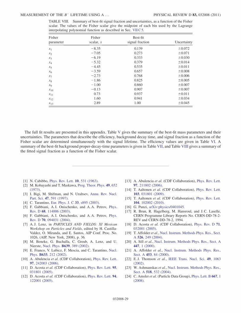
The full fit results are presented in this appendix. Table V gives the summary of the best-fit mass parameters and theiruncertainties. The parameters that describe the efficiency, background decay time, and signal fraction as a function of theFisher scalar are determined simultaneously with the signal lifetime. The efficiency values are given in Table VI. Asummary of the best-fit background proper-decay-time parameters is given in Table VII, and Table VIII gives a summary ofthe fitted signal fraction as a function of the Fisher scalar.

[1] N. Cabibbo, Phys. Rev. Lett. 10, 531 (1963).[2] M. Kobayashi and T. Maskawa, Prog. Theor. Phys. 49, 652

(1973).[3] I. Bigi, M. Shifman, and N. Uraltsev, Annu. Rev. Nucl.

Part. Sci. 47, 591 (1997).[4] C. Tarantino, Eur. Phys. J. C 33, s895 (2003).[5] F. Gabbiani, A. I. Onischenko, and A.A. Petrov, Phys.

Rev. D 68, 114006 (2003).[6] F. Gabbiani, A. I. Onischenko, and A.A. Petrov, Phys.

Rev. D 70, 094031 (2004).[7] A. J. Lenz, in PARTICLES AND FIELDS: XI Mexican

Workshop on Particles and Fields, edited by H. Castilla-Valdez, O. Miranda, and E. Santos, AIP Conf. Proc. No.1026, (AIP, New York, 2008), p. 36.

[8] M. Beneke, G. Buchalla, C. Greub, A. Lenz, and U.Nierste, Nucl. Phys. B639, 389 (2002).

[9] E. Franco, V. Lubicz, F. Mescia, and C. Tarantino, Nucl.Phys. B633, 212 (2002).

[10] A. Abulencia et al. (CDF Collaboration), Phys. Rev. Lett.97, 242003 (2006).

[11] D. Acosta et al. (CDF Collaboration), Phys. Rev. Lett. 95,031801 (2005).

[12] D. Acosta et al. (CDF Collaboration), Phys. Rev. Lett. 94,122001 (2005).


[14] T. Aaltonen et al. (CDF Collaboration), Phys. Rev. Lett.103, 031801 (2009).

[15] T. Aaltonen et al. (CDF Collaboration), Phys. Rev. Lett.104, 102002 (2010).

[16] G. Punzi, arXiv:physics/0401045.[17] R. Brun, R. Hagelberg, M. Hansroul, and J. C. Laselle,

CERN Programme Library Reports No. CERN-DD-78-2-REV and CERN-DD-78-2, 1994.

[18] D. Acosta et al. (CDF Collaboration), Phys. Rev. D 71,032001 (2005).

[19] T. Affolder et al., Nucl. Instrum. Methods Phys. Res., Sect.A 526, 249 (2004).

[20] A. Sill et al., Nucl. Instrum. Methods Phys. Res., Sect. A447, 1 (2000).

[21] A. Affolder et al., Nucl. Instrum. Methods Phys. Res.,Sect. A 453, 84 (2000).

[22] E. J. Thomson et al., IEEE Trans. Nucl. Sci. 49, 1063(2002).

[23] W. Ashmanskas et al., Nucl. Instrum. Methods Phys. Res.,Sect. A 518, 532 (2004).

[24] C. Amsler et al. (Particle Data Group), Phys. Lett. B 667, 1(2008).

TABLE VIII. Summary of best-fit signal fraction and uncertainties, as a function of the Fisherscalar. The values of the Fisher scalar give the midpoint of each bin used by the Lagrangeinterpolating polynomial function as described in Sec. VII C 5.

Fisher

parameter

Fisher

scalar, xBest-fit

signal fraction Uncertainty

x1 �8:35 0.139 �0:072x2 �7:05 0.273 �0:071x3 �6:19 0.333 �0:030x4 �5:32 0.379 �0:014x5 �4:45 0.535 �0:011x6 �3:59 0.657 �0:008x7 �2:73 0.768 �0:006x8 �1:86 0.825 �0:005x9 �1:00 0.860 �0:007x10 �0:13 0.907 �0:007x11 0.73 0.937 �0:011x12 1.60 0.941 �0:034x13 2.89 1.00 �0:045


032008-29

http://dx.doi.org/10.1103/PhysRevLett.10.531

http://dx.doi.org/10.1143/PTP.49.652

http://dx.doi.org/10.1143/PTP.49.652

http://dx.doi.org/10.1146/annurev.nucl.47.1.591

http://dx.doi.org/10.1146/annurev.nucl.47.1.591

http://dx.doi.org/10.1140/epjcd/s2003-03-1006-y





http://dx.doi.org/10.1016/S0550-3213(02)00561-8

http://dx.doi.org/10.1016/S0550-3213(02)00262-6

http://dx.doi.org/10.1016/S0550-3213(02)00262-6













http://arXiv.org/abs/physics/0401045



http://dx.doi.org/10.1016/j.nima.2004.02.020


http://dx.doi.org/10.1016/S0168-9002(00)00166-2

http://dx.doi.org/10.1016/S0168-9002(00)00166-2

http://dx.doi.org/10.1016/S0168-9002(00)00610-0

http://dx.doi.org/10.1016/S0168-9002(00)00610-0

http://dx.doi.org/10.1109/TNS.2002.1039615

http://dx.doi.org/10.1109/TNS.2002.1039615



http://dx.doi.org/10.1016/j.physletb.2008.07.018

http://dx.doi.org/10.1016/j.physletb.2008.07.018

[25] J. Rademacker, Nucl. Instrum. Methods Phys. Res., Sect.A 570, 525 (2007).

[26] W. Adam et al. (DELPHI Collaboration), Z. Phys. C 68,363 (1995).

[27] P. Nason, S. Dawson, and R.K. Ellis, Nucl. Phys. B303,607 (1988).

[28] P. Nason, S. Dawson, and R.K. Ellis, Nucl. Phys. B327, 49(1989).

[29] D. J. Lange, Nucl. Instrum. Methods Phys. Res., Sect. A462, 152 (2001).

[30] R. A. Fisher, Ann. of Eugenics 7, 179(1936).



032008-30



http://dx.doi.org/10.1007/BF01620712

http://dx.doi.org/10.1007/BF01620712

http://dx.doi.org/10.1016/0550-3213(88)90422-1

http://dx.doi.org/10.1016/0550-3213(88)90422-1

http://dx.doi.org/10.1016/0550-3213(89)90286-1

http://dx.doi.org/10.1016/0550-3213(89)90286-1

http://dx.doi.org/10.1016/S0168-9002(01)00089-4

http://dx.doi.org/10.1016/S0168-9002(01)00089-4



Documents

Measurement of the B- lifetime using a simulation free