Embed Size (px)
Citation preview
Measurement of Surface and Interfacial Energies between Solid
Materials Using an Elastica Loop
Jia Qi
Thesis submitted to the faculty of the
Virginia Polytechnic Institute and State University
in partial fulfillment of the requirements for the degree of
Master of Science
in
Engineering Mechanics
APPROVED BY:
David A. Dillard, Chairman
Raymond H. Plaut
John G. Dillard
September 11, 2000 Blacksburg, Virginia
Keywords: Interfacial Energy, Surface Energy, Work of Adhesion, Contact Mechanics,
Elastica, JKR technique
Copyright 2000, Jia Qi

Measurement of Surface and Interfacial Energies between Solid
Materials Using an Elastica Loop
(ABSTRACT)
The measurement of the work of adhesion is of significant technical interest in a
variety of applications, ranging from a basic understanding of material behavior to the
practical aspects associated with making strong, durable adhesive bonds. The objective
of this thesis is to investigate a novel technique using an elastica loop to measure the
work of adhesion between solid materials. Considering the range and resolution of the
measured parameters, a specially designed apparatus with a precise displacement control
system, an analytical balance, an optical system, and a computer control and data
acquisition interface is constructed. An elastica loop made of poly(dimethylsiloxane)
[PDMS] is attached directly to a stepper motor in the apparatus. To perform the
measurement, the loop is brought into contact with various substrates as controlled by the
computer interface, and information including the contact patterns, contact lengths, and
contact forces is obtained. Experimental results indicate that due to anticlastic bending,
the contact first occurs at the edges of the loop, and then spreads across the width as the
displacement continues to increase. The patterns observed show that the loop is
eventually flattened in the contact region and the effect of anticlastic bending of the loop
is reduced. Compared to the contact diameters observed in the classical JKR tests, the
contact length obtained using this elastica loop technique is, in general, larger, which
provides potential for applications of this technique in measuring interfacial energies
between solid materials with high moduli. The contact procedure is also simulated to
investigate the anticlastic bending effect using finite element analysis with ABAQUS.
The numerical simulation is conducted using a special geometrically nonlinear, elastic,
contact mechanics algorithm with appropriate displacement increments. Comparisons of
the numerical simulation results, experimental data, and the analytical solution are made.

iii
ACKNOWLEDGEMENTS
I would like to thank Dr. David A. Dillard for acting as my advisor, giving me
this opportunity to go deep in this project and providing his guidance throughout my
research and writing efforts. I would also like to thank Dr. Raymond H. Plaut of the Civil
and Environmental Engineering Department and Dr. John G. Dillard of the Chemistry
Department for serving as my committee members.
Additionally, I appreciate the assistance from Prof. M. Chaudhury and his student
Hongquan She of Lehigh University, Bob Simonds, as well as all the members in the
Adhesion Mechanics Lab. Furthermore, I would like to acknowledge the support of the
National Science Foundation under grant CMS-9713949, and the Center for Adhesive
and Sealant Science of Virginia Tech.
I would like to take this opportunity to thank my parents for continually supplying
me with their love and support throughout my life. Finally, I would like to thank my
husband, Dr. Buo Chen, for his endless supply of love, advice, and understanding.
iv
Table of Contents
CHAPTER 1 Introduction .......................................................................................... 1
1.1 Adhesion and role of the interface ................................................ 1
1.2 Contact mechanics and measurement of surface energies ............. 2
1.3 Outline of the study.................................................................... 14
CHAPTER 2 Experimental Study............................................................................. 18
2.1 Abstract...................................................................................... 18
2.2 Construction of elastica loop ...................................................... 18
2.3 Sample preparation and material property characterization......... 19
2.3.1 Sample preparation ......................................................... 19
2.3.2 Tensile tests.................................................................... 20
2.3.3 Orientation of the elastica loop ....................................... 21
2.4 Apparatus................................................................................... 22
2.4.1 Displacement control device ........................................... 22
2.4.2 Force measurement device.............................................. 24
2.4.3 Optical system and calibration ........................................ 24
2.4.4 Computer control interface and data acquisition system.. 25
2.5 Measurement using the JKR method .......................................... 25
2.6 Measurement using elastica loop................................................ 27
2.6.1 Contact patterns.............................................................. 28
2.6.2 Experimental results and discussion................................ 29
2.6.3 Hysteresis ....................................................................... 32
CHAPTER 3 Numerical Analysis............................................................................. 65
3.1 Abstract...................................................................................... 65
3.2 Meshes and boundary conditions................................................ 65
3.3 Simulation of the loop formation................................................ 66
3.4 Contact simulation ..................................................................... 67
3.4.1 Contact principle ............................................................ 67

v
3.4.2 Contact procedure........................................................... 70
3.4.3 Contact patterns.............................................................. 70
3.4.4 Strain of the elastica loop after contact............................ 71
3.4.5 Contact force and contact area ........................................ 71
3.4.6 Poisson's ratio effects...................................................... 72
CHAPTER 4 Comparison of Experimental, Numerical, and Analytical Results........ 93
4.1 Analytical solution ..................................................................... 93
4.2 Comparison of numerical and analytical results.......................... 95
4.3 Comparison of experimental and analytical results ..................... 97
4.4 Sensitivity studies of errors ........................................................ 99
4.5 PDMS loop in contact with various substrates.......................... 101
CHAPTER 5 Conclusions and Recommendations for Future Work........................ 121
5.1 Summary and conclusions........................................................ 121
5.2 Limitations............................................................................... 123
5.3 Future work.............................................................................. 124
References ......................................................................................................... 126
Appendix A. Mathematica file for fitting the work of adhesion using traditional JKR
testing technique. .............................................................................. 132
Appendix B. ABAQUS input file for contact simulation........................................ 133
vi
List of Figures
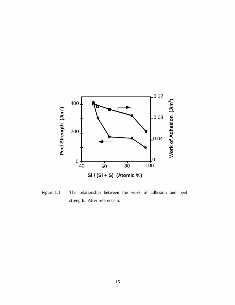
Figure 1.1 The relationship between the work of adhesion and peel strength.
After reference 6.................................................................................... 15
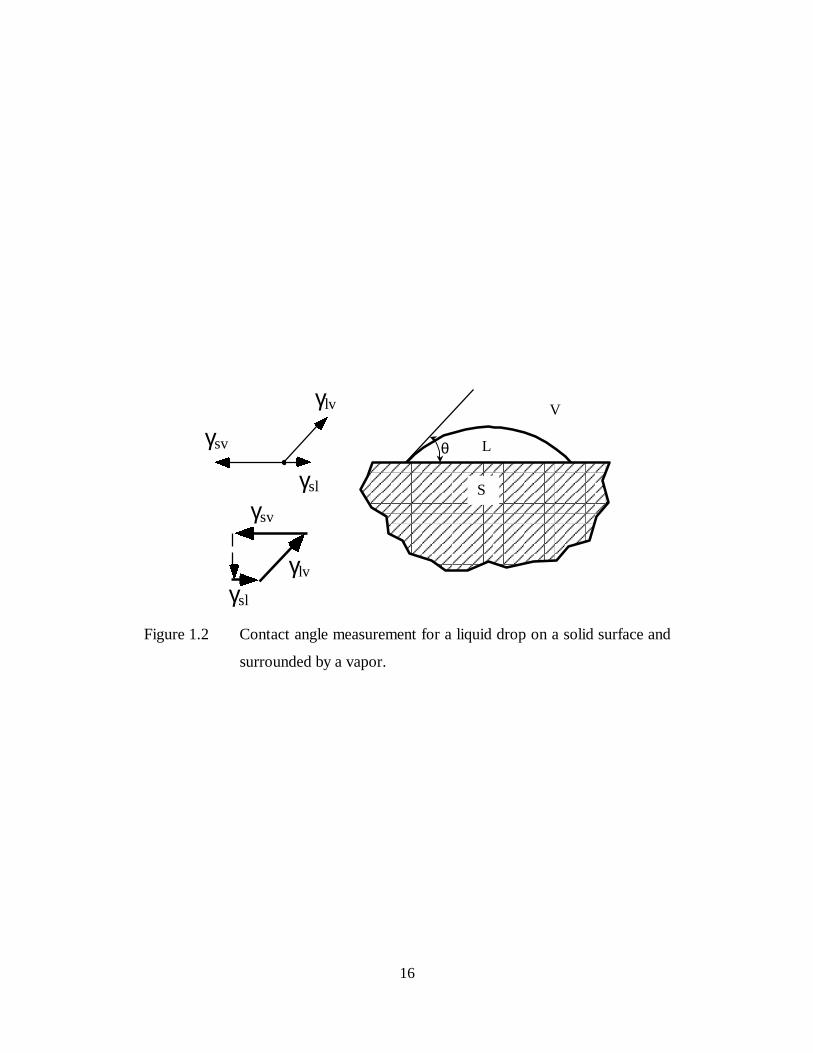
Figure 1.2 Contact angle measurement for a liquid drop on a solid surface and
surrounded by a vapor............................................................................ 16
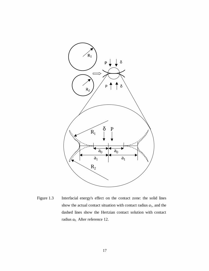
Figure 1.3 Interfacial energy's effect on the contact zone: the solid lines show the
actual contact situation with contact radius a1, and the dashed lines
show the Hertzian contact solution with contact radius a0. After
reference 12. .......................................................................................... 17
Figure 2.1 Elastica loop configuration .................................................................... 35
Figure 2.2 A typical stress-strain plot for a PDMS strip. ......................................... 36
Figure 2.3 Young’s moduli for eight PDMS samples of the first batch and their
average. The error bar represents ±one standard deviation..................... 37
Figure 2.4 Young’s moduli for four PDMS samples of the second batch and their
average. The error bar represents ±one standard deviation..................... 38
Figure 2.5 Young’s moduli for four PDMS samples of the third batch and their
average. The error bar represents ±one standard deviation..................... 39
Figure 2.6 Geometry of an elatica loop probe ......................................................... 40
Figure 2.7 Schematic of apparatus .......................................................................... 41
Figure 2.8 Photograph of the apparatus................................................................... 42
Figure 2.9 Front panel of LabVIEW VI created for the computer acquisition
system. .................................................................................................. 43
Figure 2.10 Interaction between a PDMS lens in contact with a PDMS film coated
on a glass substrate. The dimensions of the figure are not to scale. ........ 44
Figure 2.11 Typical contact pattern of a PDMS lens in contact with a PDMS film
coated on a glass substrate. .................................................................... 45
vii
Figure 2.12 Plot of contact radius, a, vs. force, F, in JKR testing: a PDMS lens in
contact with a PDMS film coated on a glass substrate. ........................... 46
Figure 2.13 Plot of cube of contact radius vs. contact force: the dots represent
loading and unloading experimental data and the solid lines represent
fitting curves obtained using a numerical regression method.................. 47
Figure 2.14 Interaction between a PDMS loop in contact with a PDMS film coated
on a glass substrate. ............................................................................... 48
Figure 2.15 Anticlastic bending of an elastica loop. .................................................. 49
Figure 2.16 Initial contact zone of a PDMS elastic loop in contact with a PDMS
coating on a glass substrate, and about two-thirds of the loop width is
shown. ................................................................................................... 50
Figure 2.17 Further contact zone of a PDMS elastic loop in contact with a PDMS
coating on a glass substrate, but the contact length is smaller than one
third of the elastica loop width. .............................................................. 51
Figure 2.18 A typical contact zone of a PDMS elastica loop in contact with a
PDMS coating on a glass substrate......................................................... 52
Figure 2.19 Plot of contact length, 2B vs. contact force, F: a PDMS loop in contact
with PDMS coating on a glass plate. The solid lines represent the fits
of data within the two different regions, which indicate that each
region has a different contact spreading rate........................................... 53
Figure 2.20 Plot of contact force vs. the displacement of the loop: PDMS loop in
contact with PDMS substrate. ................................................................ 54
Figure 2.21 Plot of contact length, 2B vs. contact force, F: PDMS loop in contact
with a glass plate. The solid lines represent the fits of data within the
two different regions, which indicate that each region has a different
contact spreading rate. ........................................................................... 55
Figure 2.22 Plot of contact force vs. displacement of the loop: PDMS loop in
contact with a glass plate. ...................................................................... 56
viii
Figure 2.23 Plot of contact length, 2B vs. contact force, F: PDMS loop in contact
with a PC plate. The solid lines represent the fits of data within the
two different regions, which indicate that each region has a different
contact spreading rate. ........................................................................... 57
Figure 2.24 Plot of contact force vs. the displacement of the loop: PDMS loop in
contact with a PC plate. ......................................................................... 58
Figure 2.25 Plot of contact length, 2B, vs. contact force, F: PDMS loop in contact
with backing of commercial cellulose acetate substrate (3M ScotchTM
Transparent Tape 600). The solid lines represent the fits of data within
the two different regions, which indicate that each region has a
different contact spreading rate. ............................................................. 59
Figure 2.26 Plot of contact force vs. the displacement of the loop: PDMS loop in
contact with backing of commercial cellulose acetate substrate (3M
ScotchTM Transparent Tape 600).......................................................... 60
Figure 2.27 DMA creep test results using a rectangular PDMS strip at room
temperature with a 0.2 MPa stress.......................................................... 61
Figure 2.28 Room temperature stress-strain curves of PDMS for three loading-
unloading cycles. The loading and unloading rate used in the tests was
5mm/min. .............................................................................................. 62
Figure 2.29 Plots of contact length, 2B vs. contact force, F for three loading-
unloading cycles: PDMS loop in contact with PDMS substrate. ............. 63
Figure 2.30 Plots of contact length, 2B, vs. contact force, F, for two constant
loading-unloading rates with zero dwell intervals: PDMS loop in
contact with PDMS substrate. ................................................................ 64
Figure 3.1 FEA mesh of elastica loop with dimensions 14.71 mm × 0.956 mm ×
0.165 mm, modulus 1.81 MPa, and a series of Poisson’s ratios of 0,
0.1, 0.2, 0.3, 0.4, 0.49. ........................................................................... 75
Figure 3.2 Simulating formation of the elastica loop. .............................................. 76
Figure 3.3 Longitudinal strains on the concave side of the loop before contact........ 77

ix
Figure 3.4 Transverse strains of the loop on the concave side before contact........... 78
Figure 3.5 Contact schemes. ................................................................................... 79
Figure 3.6 Contact actions simulated in FEA. ......................................................... 80
Figure 3.7 Contours of displacement of initial contact at edges with insert
showing corresponding experimental results. ......................................... 81
Figure 3.8 Compressive stress distribution on the upper loop suface of initial
contact at edges...................................................................................... 82
Figure 3.9 Contours of displacement after contact area spreading with insert
showing corresponding experimental result............................................ 83
Figure 3.10 Contours of contact pressure on the upper loop surface after contact
area spreading........................................................................................ 84
Figure 3.11 Longitudinal strain on the concave side of the loop after contact............ 85
Figure 3.12 Transverse strain on the concave side of the loop after contact............... 86
Figure 3.13 Plot of contact length vs. contact force: the contact lengths were
measured at the center point of the contact front. ................................... 87
Figure 3.14 The effects of the measurement position on contact length: the
dimensions of the elastica strip are 14.7 mm × 0.96 mm × 0.17 mm,
E= 1.81 MPa, ν = 0.49, and 2C = 6.38 mm. ........................................... 88
Figure 3.15 Effects of Poisson’s ratio on the contact patterns with full width of the
modeled elastica loop............................................................................. 89
Figure 3.16 The relationship between contact length and contact force. The
contact length was taken as the center of the contact front...................... 90
Figure 3.17 The relationship between contact length and the contact force. The
contact length was taken as the point with maximum pressure. .............. 91
Figure 3.18 The relationship between contact length and contact force. The
contact length was taken as the outer edge of the contact front. .............. 92
Figure 4.1 An elastica loop in contact with a flat, rigid, smooth, horizontal
surface. After reference 46.................................................................. 104
Figure 4.2 Definitions of variables. After reference 46......................................... 105

x
Figure 4.3 Model adhesion effects. After reference 46. ........................................ 106
Figure 4.4 Comparison of numerical and analytical results: contact lengths were
measured at different positions............................................................. 107
Figure 4.5 Comparison of numerical and analytical results: contact lengths were
measured in the cases with different value of Poisson’s ratio at the
center of contact front. ......................................................................... 108
Figure 4.6 Comparison of numerical and analytical results: contact lengths were
measured in the cases with different values of Poisson’s ratio at the
points of maximum pressure. ............................................................... 109
Figure 4.7 Comparison of numerical and analytical results: contact lengths were
measured in the cases with different values of Poisson’s ratio at the
outer edge of contact front. .................................................................. 110
Figure 4.8 Comparison of the experimental and analytical results: PDMS loop in
contact with PDMS film coated on glass plate...................................... 111
Figure 4.9 Comparison of the experimental and analytical results: PDMS loop in
contact with a glass plate. .................................................................... 112
Figure 4.10 Comparison of the experimental and analytical results: the PDMS loop
in contact with cellulose acetate substrate (3M ScotchTM Transparent
Tape 600). ........................................................................................... 113
Figure 4.11 Comparison of analytical, experimental and numerical results: PDMS
loop in contact with PDMS film coated on a glass plate, and the
contact lengths were taken from the center of contact front. ................. 114
Figure 4.12 Effects of reducing length by 5%, 10%, 20%. ...................................... 115
Figure 4.13 Effects of increasing width by 10%, 20%, and 30%. ............................ 116
Figure 4.14 Effects of increasing thickness by 5%, 10%, and 15%.......................... 117
Figure 4.15 Effects of reducing the separation distance between the ends by 5%,
10%, and 20%...................................................................................... 118
Figure 4.16 Effects of increasing Young’s modulus by 10%, 20%, and 30%........... 119

xi
Figure 4.17 Plots of contact length, 2B vs. contact force, F: PDMS loop in contact
with four different substrates................................................................ 120

xii
List of Tables
Table 2.1 Young’s modulus of the tensile specimens from different batches.......... 34
Table 4.1 Nondimensionalization process............................................................ 103
1
CHAPTER 1 Introduction
1.1 Adhesion and role of the interface
Adhesion is a phenomenon by which two materials in contact form a region of
adhesive bond that is able to sustain and transmit stresses. The formation of adhesive
bonds is governed by molecular interactions occurring at the interface of the adhering
materials. As discussed in Kinloch [1], scientists have recognized for many years that
intimate molecular contact and active interactions are necessary, though sometimes
insufficient, requirements to form strong adhesive bonds. As summarized by Mangipudi
and Tirrell [2], these interactions include: i) van der Waals or other non-covalent
interactions that form bonds across the interface; ii) interdiffusion of polymer chains
across the interface and coupling of the interfacial chains with the bulk polymer; and iii)
formation of primary chemical bonds between chains or molecules at or across the
interface.
The van der Waals and other non-covalent interactions at the interface are
macroscopic intrinsic material characteristics, and they are quantified as the surface and
interfacial energies. Defined as the energy required to create a unit area of surface of a
material in a thermodynamically reversible manner, the surface energy of a material, γ,
and the interfacial energy between two materials in contact, γ12, determine the work of
cohesion, Wcoh, for two identical surfaces, or the work of adhesion, Wadh, for two
dissimilar surfaces in contact [3]. For two identical surfaces in contact, Wcoh is given by
γ2=cohW (1)
For two dissimilar surfaces in contact, Wadh is given by
1221 γγγ −+=adhW (2)
where γ1 and γ2 are the surface energies of materials 1 and 2, respectively, γ12 is the
interfacial energy between materials 1 and 2.
2
Although the practical fracture toughness of an adhesive bond, which is usually
quantified as the critical strain energy release rate Gc, is in general several orders of
magnitude larger than the thermodynamic work of adhesion Wadh, sufficient evidence in
the literature has shown that the strength or fracture toughness of adhesive bonds is
directly associated with the work of adhesion [[4], [5], [6]]. As indicated in Figure 1.1,
Wightman et al. [6] showed that the peel strength of a pressure sensitive tape increases
significantly as the work of adhesion increases. Other examples can be found in
references [4] and [5]. Gent and Schultz [4] proposed that the fracture toughness, Gc, and
work of adhesion, Wadh, follow the relationship
( )[ ]TvWG adhc ,1 Φ+= (3)
where Φ represents the viscoelastic energy dissipation associated with the debonding
process, and is a function of the debonding rate v and testing temperature T.
Although equation (3) is obtained directly based on experimental observations,
the equation underlines the importance of the thermodynamic work of adhesion to a
strong and durable adhesive joint. Consequently, measurement of surface and interfacial
energies is of significant technical importance in aspects such as obtaining a basic
understanding of material behavior and manufacturing durable adhesive bonds.
1.2 Contact mechanics and measurement of surface energies
The measurement of surface energies of solids has been a difficult task [7]. This
is due to the fact that the moduli of solids in general are relatively high (as compared to
liquids and vapors), and the deformation due to the surface energy is usually insufficient
to be measured. Historically, estimates of the surface energies of solids have been
obtained through measuring the surface energy of the melt and assuming that the
energetics of the solid and liquid are similar. However, since the surface energy of a
material is closely related to the surface temperature, results obtained using this melting
technique contain significant errors [3]. Moreover, this technique is very difficult to
3
apply to high-molecular-weight polymers, which are very viscous even in the melt. In
addition, this technique cannot be applied to cross-linked polymers, because cross-linked
polymers cannot be melted.
Currently, the most widely used technique to estimate surface energies of solids is
the wetting method [3]. The basis of this technique is Young’s wetting equation, which
is given by
slsvlv γγθγ +=cos (4)
where, as shown in Figure 1.2, subscripts s, l, and v denote the solid, liquid, and vapor
phases, and γlv, γsv, and γsl are the interfacial energies between the various phases. In
practice, a serie of liquid droplets with different liquid-vapor interfacial energies is used
as probes to measure contact angles θ with a solid surface. If the solid-liquid interfacial
energy is assumed to be small, an estimate of the solid-vapor interfacial energy γsv can
then be obtained by extrapolating the results to θ = 0, which is also referred as the critical
surface tension γc. This wetting procedure was first introduced by Zisman, and is
relatively easy to perform [3]. However, the solid-liquid interactions are essentially
ignored in the method, which reduces the accuracy of the results significantly in some
cases. More importantly, especially for the purpose of adhesion, this technique cannot be
extended to the measurement of interfacial energies between two solids.
Another useful quantity for characterizing the interactions between two materials
is the work of adhesion, Wadh, [3]. After the contact angle of a droplet is measured, the
work of adhesion between the substrate and the liquid of the droplet can be obtained as
( )θγ cos1+= lvadhW (4)
By knowing the work of adhesion between various solids and liquids, interactions
between two solids can be estimated. However, some critical assumptions are often
required and consequently errors are introduced, which in some cases may not be
negligible.
4
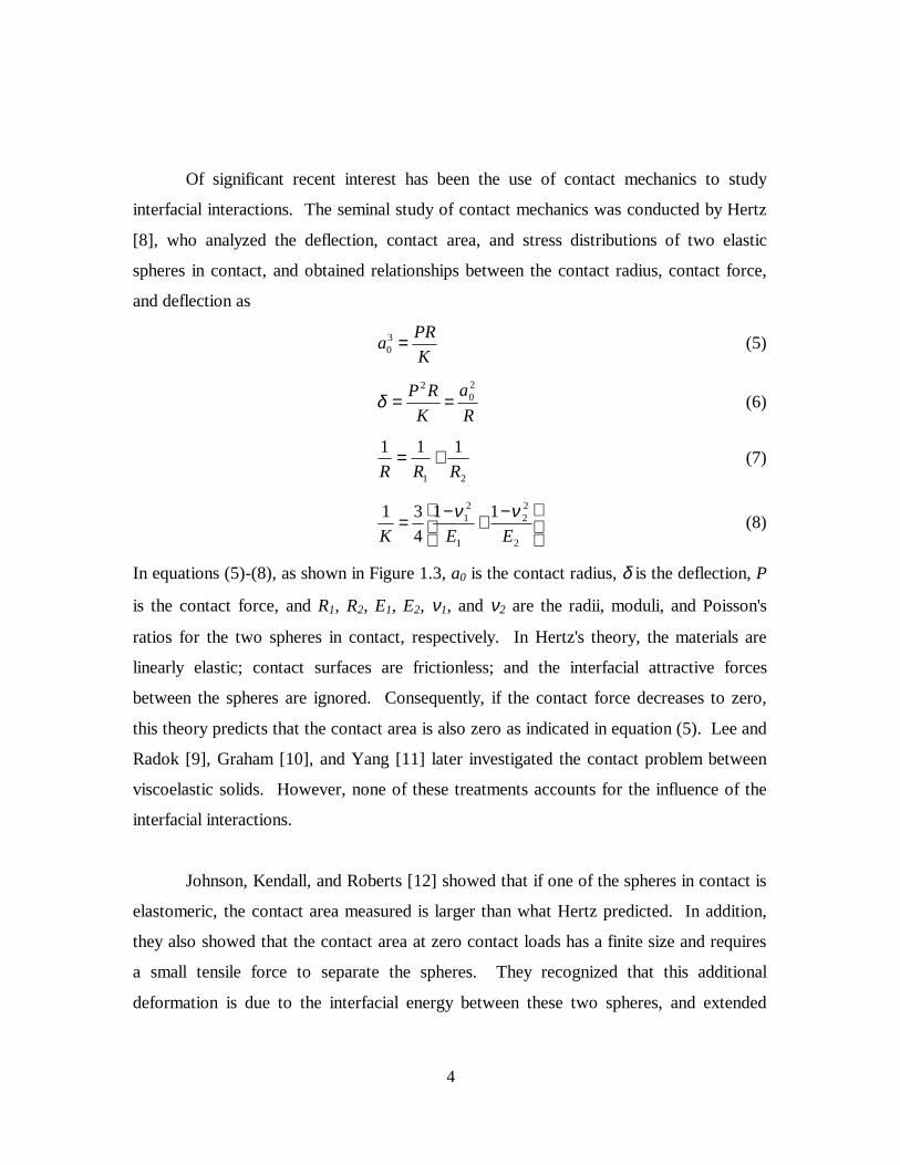
Of significant recent interest has been the use of contact mechanics to study
interfacial interactions. The seminal study of contact mechanics was conducted by Hertz
[8], who analyzed the deflection, contact area, and stress distributions of two elastic
spheres in contact, and obtained relationships between the contact radius, contact force,
and deflection as
K
PRa =3
0 (5)
R
a
K
RP 20
2
==δ (6)
21
111
RRR+= (7)
−+−=2
22
1
21 11
4
31
EEK
νν (8)
In equations (5)-(8), as shown in Figure 1.3, a0 is the contact radius, δ is the deflection, P
is the contact force, and R1, R2, E1, E2, ν1, and ν2 are the radii, moduli, and Poisson's
ratios for the two spheres in contact, respectively. In Hertz's theory, the materials are
linearly elastic; contact surfaces are frictionless; and the interfacial attractive forces
between the spheres are ignored. Consequently, if the contact force decreases to zero,
this theory predicts that the contact area is also zero as indicated in equation (5). Lee and
Radok [9], Graham [10], and Yang [11] later investigated the contact problem between
viscoelastic solids. However, none of these treatments accounts for the influence of the
interfacial interactions.
Johnson, Kendall, and Roberts [12] showed that if one of the spheres in contact is
elastomeric, the contact area measured is larger than what Hertz predicted. In addition,
they also showed that the contact area at zero contact loads has a finite size and requires
a small tensile force to separate the spheres. They recognized that this additional
deformation is due to the interfacial energy between these two spheres, and extended
5
Hertzian theory to include the influence of surface energies in their analysis, which is
now known as the JKR theory.
In developing the JKR theory, Johnson et al. [12] considered two similar, solid,
homogeneous, linearly elastic spheres with frictionless surfaces in contact with each
other under a normal applied load P as shown in Figure 1.3. The shear tractions acting
on the contact surfaces are identically zero. The deformation of the spheres is assumed
to be small so that linear continuum mechanics theory can be used. In particular, small
strains are required so that there is no distinction between the deformed and undeformed
configurations of the bodies as far as equilibrium is concerned. In addition, the bonding
and debonding process at the interface is assumed to be reversible and the energy
available for debonding is independent of the local failure process.
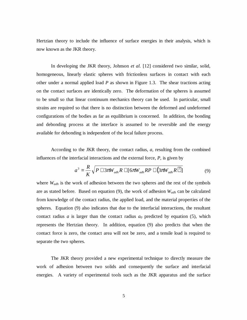
According to the JKR theory, the contact radius, a, resulting from the combined
influences of the interfacial interactions and the external force, P, is given by
( ) ]36[3 23 RWRPWRWPK
Ra adhadhadh πππ +++= (9)
where Wadh is the work of adhesion between the two spheres and the rest of the symbols
are as stated before. Based on equation (9), the work of adhesion Wadh can be calculated
from knowledge of the contact radius, the applied load, and the material properties of the
spheres. Equation (9) also indicates that due to the interfacial interactions, the resultant
contact radius a is larger than the contact radius a0 predicted by equation (5), which
represents the Hertzian theory. In addition, equation (9) also predicts that when the
contact force is zero, the contact area will not be zero, and a tensile load is required to
separate the two spheres.
The JKR theory provided a new experimental technique to directly measure the
work of adhesion between two solids and consequently the surface and interfacial
energies. A variety of experimental tools such as the JKR apparatus and the surface
6
force apparatus (SFA) also have been developed. All of the apparatuses are based on the
JKR theory and measure the same quantities, i.e., the contact area (by means of contact
radius or contact length) and the applied load. Using these tools, many research
investigations in various areas have been conducted.
Tabor [13] examined the effects of surface roughness and material ductility on the
adhesion of solids. The results indicated that the adhesion between two surfaces
decreases as the roughness of the surface increases. However, the rate of decrease
depends on the moduli of the materials in contact. Chaudhury and Whitesides [14] tested
the surface energies of poly(dimethylsiloxane) [PDMS] in air and in mixtures of water
and methanol. The results showed that the interfacial interactions decrease in the
mixtures of water and methanol as the methanol content increases. However, a small
interaction persists, even in pure methanol. In both the Tabor [13] and Chaudhury and
Whitesides’ [14] experiments, the probes used were hemispherical elastomeric lenses.
After the success in measuring the interfacial energy between elastomeric
materials, efforts have been made to measure the interfacial energy between glassy
polymers. Using their surface force apparatus (SFA), Mangipudi et al. [15] obtained the
thermodynamic work of cohesion and adhesion between poly(ethylene terephthalate)
[PET] and polyethylene thin films. The surface energy of PET determined by the direct
force measurement is higher than the critical surface tension of wetting. They later
applied the surface force apparatus (SFA) to measure the surface energies of
polyethylene films modified with corona treatment [16]. Comparing the results with
those obtained using the contact angle measurement technique, they also believed that
the contact angle measurement technique is not sensitive to small changes in surface
composition, and SFA can directly measure the true surface energy of polymer films.
Tirrell [17] discussed the applications of JKR theory for glassy or semi-
crystalline polymers. In his experiments, high modulus materials were coated on the
7
elastomer lenses and contacted with flat surfaces coated with the same polymer. He also
compared the results with those obtained using contact angle measurements, and
obtained similar conclusions as Mangipudi et al [15] that the results obtained using the
contact JKR method are larger than those obtained using the contact angle technique.
Tirrell [17] attributed the difference to the rearrangement of the polymer functionality
group on the surface. For polar materials, high-energy functional groups on the surface
may be buried when in contact with air, but might rearrange to expose themselves when
in contact with a polar polymer surface.
Mangipudi et al. [18] further expanded the applicability of the classical JKR
experiment to allow measurements of the work of adhesion between glassy polymers
using a novel method to prepare samples, and they measured the surface energies of
polystyrene [PS] and poly(methyl methacrylate) [PMMA]. In these experiments, the
spherical cap was made of O2-plasma modified cross-linked PDMS, and the glassy
polymer was coated on the PDMS cap as a thin layer about 0.1 µm thick by solvent
casting. Detailed experimental procedures are presented in their paper. During their
experiments, contact hysteresis was observed in PMMA-PMMA and PS-PS interfaces.
Similar to Tirrell [17], they also concluded that contact hysteresis is due to contact
induced rearrangements of the interface since no contact hysteresis was observed in
PDMS-PS and PDMS-PMMA interfaces. Ahn and Shull [19] investigated the work of
adhesion between a lightly cross-linked poly(n-butyl acrylate) [PNBA] hemispherical
lens and a PMMA flat surface, and contact hysteresis was observed at all accessible rates
of unloading. More contact hysteresis work will be discussed later in this section. Other
work worth mentioning is Shull et al. [20], who investigated nonlinear elasticity effects
and extended the small contact radius assumption used in the JKR theory by using a
correction factor.
Besides the spherical geometry, other sample geometries have also been used to
study interfacial interactions. Using SFA and adhering thin mica sheets to two

8
cylindrical glass lenses, Horn et al. [21] investigated the contact between two solids. In
their study, the axes of the two cylinders were perpendicular to each other, and the
separation distance between the mica layers was measured using an optical
interferometer through a layer of silver coating between the mica sheets and the glass
lenses. The SFA apparatus was either filled with a KCL solution or N2 during the
experiments in order to achieve different interfacial interactions. For the tests involving
KCL solution, which represents non-adhesive contact, the contact radius increases with
the load following the Hertzian theory. For the tests involving N2, which represents the
adhesive contact, results indicated that a greater contact area is observed under the same
load, and a finite contact area exists under zero load conditions that can be analyzed
using the JKR theory. However, due to the layered structure, Sridhar et al. [22] pointed
out that there will be some errors using JKR theory to analyze the experiment, and they
developed an extended JKR theory to analyze the layered structure by introducing an
adhesion parameter 31
*1
22
hE
RWadh=α , layer thickness ratio, and the ratio of elastic moduli
to characterize the interfacial interactions. In their paper, Sridhar et al. [22] also
conducted a finite element analysis using ABAQUS to simulate the contact procedure
and verify their analytical model.
In JKR theory, the interfacial forces are assumed to act only within the contact
region, and consequently a stress singularity results at the contact edge. Derjaguin et al.
[23] suggested that the attractive forces between two solids also exist in a small zone just
outside of the contact region, and developed a new theory. In their analysis, deformation
was assumed to follow Hertzian theory, and the attractive forces were modeled as van
der Waals' force. However, Muller et al. [24] showed that more accuracy would be
gained by using a Lennard-Jones potential to model the attractive forces. Errors in
Derjaguin et al. [23] were corrected in Muller et al. [25] and Pashley [26], in which
equilibrium conditions were obtained by balancing the elastic reaction forces with the
9
surface forces and the applied load. Due to the efforts of these researchers, this theory is
now known as the DMT theory.
Because different approaches had been used to develop the theories, and results
predicted were significantly different [27], there was controversy between the JKR and
the DMT theories. However, the controversy has been satisfactorily resolved.
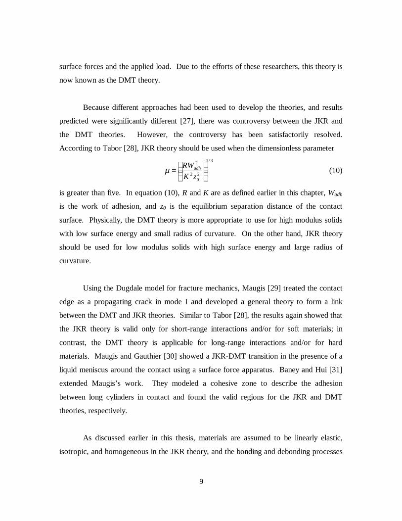
According to Tabor [28], JKR theory should be used when the dimensionless parameter
3/1
20
2
2
=
zK
RWadhµ (10)
is greater than five. In equation (10), R and K are as defined earlier in this chapter, Wadh
is the work of adhesion, and z0 is the equilibrium separation distance of the contact
surface. Physically, the DMT theory is more appropriate to use for high modulus solids
with low surface energy and small radius of curvature. On the other hand, JKR theory
should be used for low modulus solids with high surface energy and large radius of
curvature.
Using the Dugdale model for fracture mechanics, Maugis [29] treated the contact
edge as a propagating crack in mode I and developed a general theory to form a link
between the DMT and JKR theories. Similar to Tabor [28], the results again showed that
the JKR theory is valid only for short-range interactions and/or for soft materials; in
contrast, the DMT theory is applicable for long-range interactions and/or for hard
materials. Maugis and Gauthier [30] showed a JKR-DMT transition in the presence of a
liquid meniscus around the contact using a surface force apparatus. Baney and Hui [31]
extended Maugis’s work. They modeled a cohesive zone to describe the adhesion
between long cylinders in contact and found the valid regions for the JKR and DMT
theories, respectively.
As discussed earlier in this thesis, materials are assumed to be linearly elastic,
isotropic, and homogeneous in the JKR theory, and the bonding and debonding processes
10
are assumed to be reversible. While this is true for some model systems, most systems
exhibit some irreversibility. As a result, hysteresis appears during the loading and
unloading process as discussed in Mangipudi et al. [18] and Ahn and Shull [19]. Due to
the contact hysteresis, a lower compressive force is needed to obtain a given contact
radius during the unloading phase than is required during the loading phase. Silerzan et
al. [32] demonstrated that there is a large hysteresis between the loading and unloading
regimes of siloxane elastomers, and proposed a generalized JKR model to explain the
experimental data. Kim and his co-workers [33], [34] studied the adhesion and adhesion
hysteresis using cross-linked PDMS hemispherical surfaces and a self-assembled model
surface containing different chemical functional groups. Using the JKR method, they
observed that the hysteresis resulting from a fast relaxation process is practically
eliminated using stepwise loading and unloading protocols. The contact pressure-
induced, interfacial hydrogen bonds were shown to make significant contributions to the
contact hysteresis and were used to explain the phenomena observed. She et al. [35]
used a rolling contact geometry to study the effects of dispersion forces and specific
interactions on interfacial adhesion hysteresis. Hemi-cylindrical elastomers (both
unmodified and plasma oxidized) were rolled on PDMS thin films bonded to silicon
wafers. The results indicated that the adhesion hysteresis in the PDMS-plasma oxidized
PDMS system depends significantly on the molecular weight of the grafted polymer,
whereas the hysteresis is rather negligible for the pure unmodified PDMS system. These
results are explained in terms of hydrogen bonding, and orientation and relaxation of
polymer chains. Li and Tirrell [36] measured the surface energy of an acrylic pressure
sensitive adhesive PSA-LN-NoAA and the hysteresis behavior under different
loading/unloading speeds. They showed that 27% adhesion hysteresis exists between the
equilibrium values from the curves of contact radius versus force in the loading and
unloading procedures.
To investigate the work of adhesion, JKR theory has also been applied to the
atomic force microscope (AFM), which provides a higher accuracy for the contact radius

11
and load measurement. Carpick et al. [37] used a platinum coated AFM tip in contact
with the surface of mica in an ultrahigh vacuum, and determined the interfacial adhesion
energy and shear stresses using the JKR theory. Gracias and Somorjai [38] modified the
AFM using a tip with a large radius of curvature to reduce the pressure in the contact
region. They then measured the surface energies of low-density polyethylene, high-
density polyethylene, isotactic polypropylene, and atactic polypropylene. K. Takahashi
et al. [39] studied the stiffness of the measurement system such as the AFM cantilever
and the significant figures of measured displacement. They again confirmed the
transition between JKR theory and DMT theory discussed by Maugis [29].
Contact mechanics has also been substantially used in investigations for the
adhesion of particles to various substrates. Rimai et al. [40] measured the surface force-
induced contact radii of 20 µm glass particles deposited on polyurethane substrates with
a 5 µm thick thermoplastic layer. The results showed that the size of the deformations
depends only on the coating and not on the modulus of the underlying substrate. Soltani
et al. [41] studied the particle removal mechanism from rough surfaces due to an
accelerating substrate. The rough surface was modeled by asperities of the same radius
of curvature and with heights following a Gaussian distribution. The JKR theory and the
theory of critical moment, sliding, and detachment were used to analyze particle pull-off
forces, and to evaluate the critical substrate accelerations for particle removal.
Reasonable agreement between the model prediction and experimental data was obtained
for aluminum and glass particles. Gady et al. [42] measured the force needed to remove
micrometer-size polystyrene particles from elastomeric substrates with Young’s moduli
of 3.8 and 320 MPa using an atomic force technique. They found that the removal force
differed by an order of magnitude between the two substrates. When the more compliant
substrate was overcoated with a thin layer of the more rigid material, the removal force
increased with increasing applied load, which is in conflict with the predictions by the
JKR theory and can be explained by taking into account the roughness of the particle and
the amount of embedment of the particle into the substrate.

12
In brief, contact mechanics technology has brought great success in the
measurement of interfacial interactions. Recently, Mangipudi and Tirrell [2] gave a
complete review of the recent developments in the theories of contact mechanics, and
their applications in the design and interpretation of experimental measurement of
molecular level adhesion between elastomers, glassy polymers and viscoelastic
polymers. They also identified some potential applications in other fields, such as
biomaterials.
Despite all the successes achieved so far in the measurement of surface and
interfacial energies, techniques presently used are only applicable to certain types of
materials. For example, the JKR apparatus requires a compliant, elastomeric lens.
However, not all solid polymers of interest for interfacial energy measurement have bulk
mechanical properties amenable to the JKR-type of analysis. In particular, many
materials have a modulus higher than is convenient to measure a significant increase in
contact radius in the linear contact mechanics regime. If the hemispherical lens is
directly made of a stiffer material, such as an epoxy, the change of contact zone due to
interfacial interactions is too small to be measured easily. Liechti et al. [43] reported
pioneering investigations measuring the work of adhesion of the epoxy/glass interface
and compared it with the work of adhesion obtained from contact angle measurement. If
interfacial energies between two solid materials, neither of which is an elastomer, are
desired, the lens must be coated with one of the materials of interest, which can be an
inconvenience. In addition, not all materials can be deposited on such a lens. As an
example, present testing methods cannot be used to determine the interfacial energy
between aluminum and steel. Consequently, efforts have also been made to investigate
other testing technologies, by which the surface energies for a broader range of materials
can be measured directly.
13
Recently, Shanahan [44] published a mathematical model to measure interfacial
energies using a spherical membrane or "balloon". In his model, a spherical membrane
under slight internal pressure is brought into contact with a flat and rigid surface. The
results of his analysis showed that the interfacial energy depends on the square of the
contact radius rather than the cube of the contact radius as with the JKR theory. As a
result, the potential inaccuracy induced from the measurement error of the contact radius
can be significantly reduced. Additionally, Shanahan [44] also showed that the contact
area observed using the balloon method is approximately 10 times larger than that
observed in JKR tests under the same load. This greater contact area also provides
greater convenience for the test. However, in practice, sample preparation for this
method is very difficult, and no experimental data has yet been published.
Plaut et al. [45] modeled an elastica loop with a fixed separation distance pushed
into contact with a flat surface. In their analysis, the surface energies of the materials
were ignored, and the elastica was assumed to be thin, uniform, smooth, inextensible,
and flexible in bending. Through the analysis, the conformations of an elastica loop for a
given displacement of the loop as well as the contact length and the resultant contact
force were obtained. Because the structure of the elastica loop is very compliant even
though the modulus of the material is high, measurable deformations due to interfacial
interactions when the loop is in contact with another surface may be obtained. The
analysis of Plaut et al. [45] provides a potential method to measure the surface and
interfacial energies between arbitrary material systems. In conjunction with this thesis,
Dalrymple [46] extended the solution of Plaut et al. [45] and included surface energies in
the analysis. The study [46] serves as the analytical background of this study.
In this study, a novel technique using “soft structures” instead of “soft materials”
(i.e. elastomers) is proposed and investigated to measure surface and interfacial energies
between solids. In practice, a probe is first constructed as a thin, uniform, smooth, and
flexible-in-bending elastica loop using the material of interest. Then the elastica loop is
14
brought into contact with a flat rigid surface made of another material of interest.
Because of the compliant structure, measurable changes in the deformation of the elastica
due to interfacial interactions are obtained. Since the final conformation of the elastica is
the result of the applied load and the interfacial attractive forces, the interfacial energy
can be estimated by analyzing the relationship between the contact area and the applied
load of the loop.
1.3 Outline of the study
This thesis is divided into five chapters. Chapter 1 gives the project background,
the literature review, the objective of this research, and the outline of the study. Chapter
2 discusses the development of the testing method, the experimental procedure, and the
results. Chapter 3 shows the numerical analysis of the contact procedure of the elastica
loop in contact with a rigid flat surface using ABAQUS 5.8 [47]. The comparison and
discussion among the experimental results, numerical simulation, and analytical results
are presented in Chapter 4. Finally, in Chapter 5, the major conclusions are summarized
as well as some suggestions related to this research work.
15
Figure 1.1 The relationship between the work of adhesion and peel
strength. After reference 6.
400
200
0 40 60 80 100
0
0.04
0.08
0.12
Pee
l Str
engt
h (
J/m
2 )
Wor
k of
Adh
esio
n (
J/m
2 ) Si / (Si + S) (Atomic %)
16
Figure 1.2 Contact angle measurement for a liquid drop on a solid surface and
surrounded by a vapor.
S
θ L
V
γsl
γsv
γlv
γlv
γsv
γsl
S
17
Figure 1.3 Interfacial energy's effect on the contact zone: the solid lines
show the actual contact situation with contact radius a1, and the
dashed lines show the Hertzian contact solution with contact
radius a0. After reference 12.
3
a 0
a 1 a 1
a 0
R 1
R 2
P δ
5�
5�
3 δ
δ
18
CHAPTER 2 Experimental Study
2.1 Abstract
In the attempt to develop a method that can be used to measure surface and
interfacial energies of solids for a broader range of material types, the use of a flexible
structure has been proposed. An elastica loop was chosen for use in this research. In the
apparatus, the elastica loop is directly attached to the shaft of a stepper motor that is
controlled by a computer. When the elastica loop is brought into contact with a flat
substrate, the interfacial attractive force produces a measurable change in contact area.
The contact pattern is observed in the monitor through a Nikon macro lens with a
magnification factor of 50x, and the contact length is measured. At the same time, the
force F between the loop and flat substrate is also measured using an analytical balance.
Distinct contact patterns of the elastica loop made of poly(dimethylsiloxane)
[PDMS] in contact with a variety of substrates are observed, and the effect of anticlastic
bending is eliminated in the center of the contact area due to the flattening of the loop.
As compared to the classical JKR tests, the force applied is smaller, the contact length is
larger, and the displacement of the loop applied is also larger. Large contact hysteresis
with a tail due to interfacial interactions has also been observed in the tests.
2.2 Construction of elastica loop
To directly measure surface and interfacial energies of solids for a broader range
of materials compared to the JKR technique, an elastica loop probe with characteristics
of a compliant structure is prepared using the material of interest. To achieve the desired
structural compliance, the elastica strip is prepared to be thin, uniform, smooth, and
flexible in bending. During the test, the elastica loop is brought into contact with a rigid,
flat surface made of, or coated with another material of interest, and the compliant

19
structure permits measurable deformation due to small interfacial attractions. Through
the analysis of the deformation, the interfacial energy between the two materials can be
obtained. The analytical solution for an elastica in contact with a flat surface is given in
Dalrymple’s thesis [46].
The dimensions of the elastica and the forces acting on the system are defined as
follows. The total length of the elastica strip is 2L, the width of the strip is W, the
thickness is t, the bending stiffness is EI, and the distance between the two ends of the
strip is 2C. The ends of the elastica are first lifted, bent, and then clamped vertically at
an equal height with a specified distance apart. When the bent elastica strip is brought
into contact with a flat substrate, the contact length is a result of the applied load and the
interfacial attractive force. The total the contact length is defined as 2B, and the resulting
reaction force is indicated as F in Figure 2.1.
2.3 Sample preparation and material property characterization
2.3.1 Sample preparation
In this study, the major material used for the elastica loop is SYLGARD 184
silicone elastomer (PDMS) provided by the Dow Corning Company because this
material is very stable over a wide temperature range (-50°C to 200°C), and has a very
low water absorption and very good radiation resistance. The choice of an elastomeric
material for the elastica loop allows comparison of the results with findings obtained
using the JKR method. This comparison is a necessary step to verify the methodology.
The SYLGARD 184 silicone elastomer contains a silicone base and curing agents and is
supplied in a two-part kit comprised of liquid components. The base and the curing
agent were mixed in a ratio of 10 parts base to 1 part curing agent by weight with gentle
stirring for about 10 minutes to minimize the amount of air introduced. The mixture then
rested in air for 30 minutes to remove the air bubbles before use. The PDMS liquid

20
mixture was then poured on a glass plate cleaned with acetone, and a doctor's blade was
used to spread the liquid and to control the thickness of the film to be 1.0 mm.
SYLGARD 184 silicone elastomer offers a flexible cure temperature from 25°C to
150°C for various amounts of time, and requires no post-cure. In this study, after the
PDMS liquid mixture was spread on the glass surface, the plate was then placed in a
programmable oven. The curing process started from room temperature and the
temperature was increased at a rate of 5°C/min until 100°C, where the temperature was
maintained for 1 hour. Then the temperature was decreased to room temperature at a rate
of 5°C/min. After curing, the film was peeled off from the glass plate. The product was
a homogeneous, transparent, and flexible film with a final thickness about 0.2 mm, which
varied slightly from batch to batch. Specimens were then cut from the film with
appropriate dimensions for various mechanical tests.
Various substrates were selected to perform the measurement of surface energies.
They were glass plates coated with PDMS, acetone-washed glass plates, polycarbonate
[PC] plates, and a commercial cellulose acetate substrate (3M ScotchTM Transparent
Tape 600). The preparation of the substrates was relatively straightforward and after
preparation, all the substrates, as well as the elastomer films, were stored in a desiccator
at room temperature with relative humidity controlled at 30%RH.
2.3.2 Tensile tests
The Young’s modulus of the elastica loop is directly related to the compliance of
the loop and therefore is a very important factor in the analysis. The Young’s modulus
of the elastomer was determined via tensile tests conducted as part of this study using an
Instron 4505 universal testing frame. The tests were performed at room temperature
under a constant crosshead rate of 5 mm/min using a pair of pneumatic grips to clamp the
sample. Because the films are very thin (about 0.25 mm) and the modulus of the material
is relatively low, attachment of an extensometer to the film would significantly affect the
results of the measurement. To resolve this problem, the sample geometry was chosen to
21
be a rectangular strip instead of the regular dog-bone shape, and the strain was calculated
based on the ratio of the crosshead displacement to the sample’s original length between
grips. To reduce end effects, the ratio of the length to the width of the samples was
controlled to be greater than 10.
A typical stress-strain curve in the test from a particular batch of the PDMS
material is shown in Figure 2.2. The Young’s modulus was obtained using a data fit
algorithm of the linear portion of the curve. Figure 2.3, Figure 2.4, and Figure 2.5 show
the modulus data for specimens from different batches. These figures indicate that the
stress-strain curves are very repeatable within a given batch but differ slightly from one
batch to another. Table 2.1 summarizes all the modulus data for all the different batches
of the material tested. One possible reason for variations of the modulus among different
batches is the lack of precise control of the ratio between the base material and the curing
agent. As indicated by the data sheet provided by the Dow Corning Company, the
content of the curing agent will have some effect on cure time and the physical properties
of the final cured elastomer. Lowering the curing agent concentration will result in a
softer and weaker elastomer; increasing the concentration of the curing agent too much
will result in over-hardening of the cured elastomer and will tend to degrade the physical
and thermal properties.
2.3.3 Orientation of the elastica loop
A narrow strip was first cut from the cured PDMS film prepared earlier. The
ends of the strips were lifted, bent, and fixed vertically with a known separation distance.
The specimen was then attached to a sample holder as shown in Figure 2.6. The angles
of the PDMS strip at the fixed ends were 90°. The height of the loop, h, depended on the
total length of the loop, 2L, and the distance between the clamped ends of the loop, 2C.

22
2.4 Apparatus
There are four major components in the experimental apparatus as indicated in
Figure 2.7: 1) the displacement control device; 2) the force measurement device; 3) the
optical system; and 4) the computer control and data acquisition system (not shown in
the figure). The elastica loop is directly attached to the shaft of the stepper motor, which
is a major part of the displacement device and is controlled by a computer. When the
elastica loop is brought into contact with a flat substrate by the displacement device, the
interfacial attractive force produces a measurable change in contact area. The contact
zones are observed in the monitor through a Nikon macro lens using a magnification
factor of 50x, and the contact length, 2B, can be measured directly from the monitor
provided a careful calibration is performed before the test. At the same time, the contact
force F between the loop and the flat substrate can be measured using an analytical
balance mounted on the force measurement device. The whole contact sequence and
data acquisition were controlled by the computer control and data acquisition system. In
the following sections, detailed descriptions for each component of the apparatus are
given.
2.4.1 Displacement control device
Based on the dimensions of the specimen and the deformation level of the loop
induced by the interfacial interactions, a low speed, low vibration, and high-resolution
displacement control system is required for the study. From a broad search of various
positioning products, the IW-710 INCHWORM motor from Burleigh Instruments, Inc.
was chosen as the major component for the high-resolution positioning system. This IW-
710 INCHWORM motor uses compact piezoelectric ceramic actuators to achieve
nanometer-scale positioning steps over several millimeters. This motor offers a range of
motion for 6 mm and is featured with a mechanical resolution of approximately 4 nm
over the entire range of motion with a maximum speed specified as 1.5 mm/sec. In
addition, this motor has a very high lateral stability with a lateral shaft runout of ±0.2µm.

23
This instrument also provides a non-rotating shaft and forward and reverse limit
switches, providing a convenient way to control the contact procedure. The motor can
sustain a light load (less than 1000 grams), and consequently, the elastica loop was
directly attached to the shaft in the tests. The position of the elastica loop is read through
an integral encoder associated with the IW-710 motor. The resolution of the encoder is
0.5 µm with an accuracy up to ±1 µm. The motor and the encoder are controlled by the
Burleigh 6200ULN closed-loop controller, which can be operated in either manual or
computer control mode. In manual mode, the motor speed and the stop and start
functions are all operated through the controller. In addition, the controller can actuate a
moving procedure consisting of a series of predetermined increments with the size being
as small as the resolution of the encoder. If the controller is operating under the
computer control mode, the motor is controlled by the controller through the 671
interface with the computer in a bi-directional communication mode. The bi-directional
interface has the following functions, which can be combined arbitrarily to perform a
task: 1) load an absolute target displacement value; 2) load a step size; 3) set motor
speed; 4) read current motor position; 5) read the current status of the motor and
controller; 6) control position maintenance (On/Off); 7) perform motor stall test; 8) set
zero reference and clear counter.
As the major component of the displacement device, the IW-710 motor is
positioned in the apparatus as shown in Figure 2.8. The outer cylinder made of
polycarbonate [PC] rests on the base of the analytical balance and is used to support the
motor and reduce air circulation around the elastica loop. The inner PC cylinder has no
connection with the motor and rests on the scale pan of the balance. The substrate is
placed on the top of the inner cylinder with the surface of interest facing down. When
the motor is controlled to move through the contact sequence, the elastica loop attached
to the shaft is brought into contact with the substrate and then withdraws to separate the
contact. The contact force is measured through the force measurement system, and
simultaneously, the contact length is measured through the optical system.
24
2.4.2 Force measurement device
The attractive force between two solid bodies in this study is several milligrams,
which requires a high-resolution force measurement device. To satisfy this requirement,
an SA 210 analytical balance from Scientech, Inc. was chosen. This balance is equipped
with a high standard of accuracy and has a resolution of 0.1 mg over the entire weight
range of 210 grams. The balance is also equipped with a very reliable electronic filtering
system, which helps to stabilize the weight reading when mechanical damping of the
balance is insufficient. As a result, the display of the balance is prompt, clear, and
reliable. In addition, the stability indicator in the balance will also show an “OK” sign
when the reading is valid insuring reliable results. In the setup for this study, the
analytical balance is placed on a vibration reduction table along with the optical system,
and is connected to the computer through an RS-232 interface for the purpose of data
acquisition.
2.4.3 Optical system and calibration
To measure the contact pattern and the contact length with adequate accuracy, an
optical system is needed. In this study, the optical system mainly consists of a Nikon
macro lens with up to 50X magnification, an FOI-150 fiber optic illuminator with two
goosenecks, a TK-66 CCD Shutter camera from Micro-techica, Inc, a monitor, and a
VCR as partially indicated in Figure 2.7. During the tests, the contact patterns are
observed through the macro lens, and the FOI-150 provides uniform illumination in a
focused area with white light. Through the digital video camera the entire contact
procedure can be observed and can be recorded if necessary using the VCR. The support
of the macro lens also rests on the vibration reduction table to enhance the visual
observation.
The contact length or contact area is measured directly from the monitor.
However, careful calibration is needed before any measurement is taken. To calibrate
the readings from the monitor, a fine scale with 20µm resolution was set beside the
25
substrate underneath the micro lens and, once the system was in focus, readings of the
scale were taken from the monitor. According to readings taken, a ruler was made and
was directly attached to monitor, from which the contact length can be measured.
2.4.4 Computer control interface and data acquisition system
The computer control program used in this study was written in LabVIEW 5.0
from National Instruments [48]. LabVIEW is a graphic programming language, and is a
very powerful tool in areas such as control, automated testing, and data acquisition.
LabVIEW provides the flexibility and comprehensive functionality available in standard
C programming languages. A LabVIEW virtual instrument (VI) consists of a front panel
and a block diagram. The source code uses an intuitive block diagram approach that
works much like schematics and flow charts to solve problems. In addition, LabVIEW is
platform-independent, so the programs created on one platform can easily be exported to
other platforms without any modification.
In this study, the control software written in LabVIEW 5.0 was used primarily to
control the movement of the motor and collect the readings from the balance. The
analytical balance is equipped with an RS-232 interface and a subVI was therefore
written to set up a bi-directional communication between the balance and the computer
serial port in order to tare the balance and start or stop collecting data. The
INCHWORM stepper motor is supplied with a data acquisition board and a control
subVI. Both the subVIs for the balance and for the motor were then imbedded into the
main VI to form a complete control and data acquisition software. The final interface of
the control software is shown in Figure 2.9.
2.5 Measurement using the JKR method
In order to compare and validate results obtained using the novel technique with
those obtained using the JKR technique, measurements of the interfacial interactions
using the JKR technique were taken using the apparatus discussed above. First,
26
hemispherical lenses and thin films using the SYLGARD 184 silicone elastomer (PDMS)
were prepared. The hemispherical lenses were provided by Lehigh University and the
thin films were then coated on glass substrates. The hemispherical lens was directly
attached on top of the shaft of the step motor. A glass substrate was then set on the inner
cylinder of the apparatus with the side of the surface coated with the same PDMS
material facing down as shown in Figure 2.10.
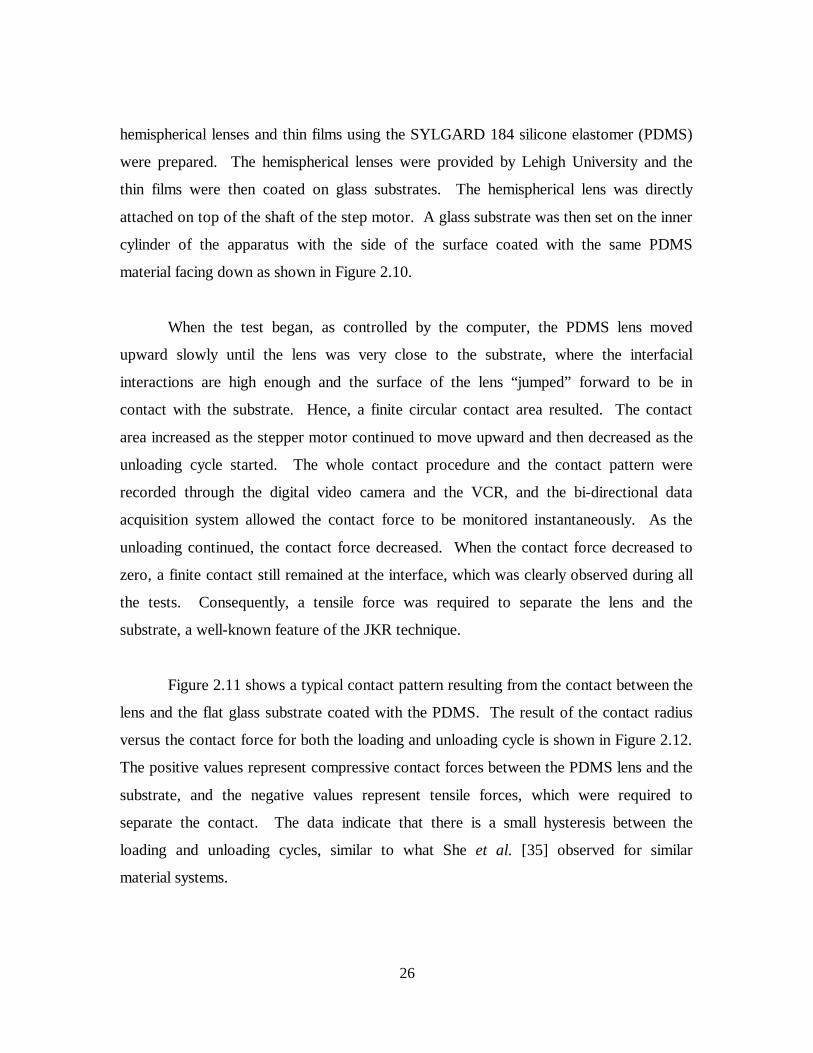
When the test began, as controlled by the computer, the PDMS lens moved
upward slowly until the lens was very close to the substrate, where the interfacial
interactions are high enough and the surface of the lens “jumped” forward to be in
contact with the substrate. Hence, a finite circular contact area resulted. The contact
area increased as the stepper motor continued to move upward and then decreased as the
unloading cycle started. The whole contact procedure and the contact pattern were
recorded through the digital video camera and the VCR, and the bi-directional data
acquisition system allowed the contact force to be monitored instantaneously. As the
unloading continued, the contact force decreased. When the contact force decreased to
zero, a finite contact still remained at the interface, which was clearly observed during all
the tests. Consequently, a tensile force was required to separate the lens and the
substrate, a well-known feature of the JKR technique.
Figure 2.11 shows a typical contact pattern resulting from the contact between the
lens and the flat glass substrate coated with the PDMS. The result of the contact radius
versus the contact force for both the loading and unloading cycle is shown in Figure 2.12.
The positive values represent compressive contact forces between the PDMS lens and the
substrate, and the negative values represent tensile forces, which were required to
separate the contact. The data indicate that there is a small hysteresis between the
loading and unloading cycles, similar to what She et al. [35] observed for similar
material systems.

27
The data were then analyzed using the JKR theory and a numerical regression
method as discussed in Appendix A was used to obtain Wadh and K. Figure 2.13 shows
the fitting curves of the experimental data, where a3 is plotted as a function of P. The
calculation method is based on the work in reference [14]. The best fit between the
experimental loading data and equation (9) yielded values Wcoh = 45.8 mJ/m2 and K =
1.73 MPa, which are consistent with the values measured by other researchers [[14],
[17]]. However, the best fit between the experimental unloading data and equation (9)
yielded Wcoh = 60.2 mJ/m2. The resultant high value for Wcoh in unloading procedure is
possibly due to energy loss or molecular interdiffusion across the interface during the
loading and unloading cycle, which has not been taken into account in the JKR theory.
The data from the loading cycle were therefore chosen to determine the surface and
interfacial energies in this study. According to equation (1), the surface energy of the
PDMS material is half of the work of cohesion in this case and thus γ = 22.9 mJ/m2.
2.6 Measurement using elastica loop
In this test, the PDMS films coated on glass substrates were prepared in the same
way as discussed in the previous section. The PDMS elastica loop was carefully attached
to the shaft of the motor with a tight connection. Before the test started, a volume static
eliminator VSE 3000 from Chapman Corp. was used to remove static charges through
blowing both the loop and the substrate for 10 minutes. Following a similar control
algorithm as in the JKR test, the loop moved upward and then contact occurred between
the loop and the substrate as shown in Figure 2.14. The contact length increased as the
loading cycle continued and then decreased when the unloading cycle started. Finally,
separation occurred when a tensile force was applied on the loop. Considering the
effects of the interfacial interactions acting on the system and the time needed to reach
equilibrium, the loading speed was selected as 10.1 µm/sec for each step, and between
any two steps during the loading cycle, the sample was allowed to dwell for an interval
of 200 sec. For the unloading cycle, the dwelling interval was increased to 300 sec/step,
because the thermodynamic equilibrium took more time to reach. The whole contact
28
procedure as well as the contact patterns and contact forces were again recorded and
stored for future analysis.
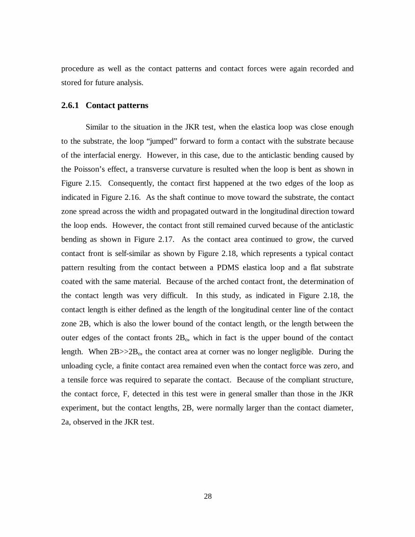
2.6.1 Contact patterns
Similar to the situation in the JKR test, when the elastica loop was close enough
to the substrate, the loop “jumped” forward to form a contact with the substrate because
of the interfacial energy. However, in this case, due to the anticlastic bending caused by
the Poisson’s effect, a transverse curvature is resulted when the loop is bent as shown in
Figure 2.15. Consequently, the contact first happened at the two edges of the loop as
indicated in Figure 2.16. As the shaft continue to move toward the substrate, the contact
zone spread across the width and propagated outward in the longitudinal direction toward
the loop ends. However, the contact front still remained curved because of the anticlastic
bending as shown in Figure 2.17. As the contact area continued to grow, the curved
contact front is self-similar as shown by Figure 2.18, which represents a typical contact
pattern resulting from the contact between a PDMS elastica loop and a flat substrate
coated with the same material. Because of the arched contact front, the determination of
the contact length was very difficult. In this study, as indicated in Figure 2.18, the
contact length is either defined as the length of the longitudinal center line of the contact
zone 2B, which is also the lower bound of the contact length, or the length between the
outer edges of the contact fronts 2Bo, which in fact is the upper bound of the contact
length. When 2B>>2Bo, the contact area at corner was no longer negligible. During the
unloading cycle, a finite contact area remained even when the contact force was zero, and
a tensile force was required to separate the contact. Because of the compliant structure,
the contact force, F, detected in this test were in general smaller than those in the JKR
experiment, but the contact lengths, 2B, were normally larger than the contact diameter,
2a, observed in the JKR test.

29
2.6.2 Experimental results and discussion
In the following, detailed experimental observations and discussions are given for
the PDMS elastica loop in contact with different substrates.
1. PDMS loop to PDMS substrate
In this test, both the elastica loop and substrate surface were made of the PDMS
elastomer. The substrate consists of a piece of glass and a layer of the PDMS film about
0.2 mm thick. The film was coated using the same method discussed earlier. The glass
was cleaned with acetone and de-ionized water before coating. The dimensions of the
elastica strip were 14.7 mm × 0.96 mm × 0.17 mm. The distance between the two ends
of the loop, 2C, was 6.38 mm and the modulus of the loop was 1.81 MPa.
A plot of contact length versus the contact force was obtained in the test and is
shown in Figure 2.19. In the figure, a negative force value indicates a tensile force
between the elastica loop and the substrate, and a positive force value indicates a
compressive force. The diamond and square data are the loading and unloading curves
corresponding to the inner contact lengths, 2B, which are the lower bounds of the contact
length; and the triangle and circle data are the loading and unloading curves
corresponding to the outer contact lengths, 2Bo, which are the upper bounds of the
contact length. Figure 2.19 indicates that the geometry of the contact front does not
change during the test because the difference between the inner contact curve and outer
contact curve remains almost the same. More specifically, in the test,
2Bo=2B+0.35±0.04 mm (10)
The result indicates that the contact spread occurred in a self-similar manner. Because
the analytical solution, which will be discussed later, was developed based on beam
theory and the effect of anticlastic bending was ignored, the choice of location to
determine the contact length will influence the comparison between the experimental
results and analytical predictions.
30
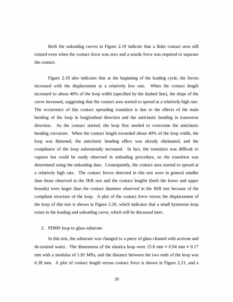
Both the unloading curves in Figure 2.19 indicate that a finite contact area still
existed even when the contact force was zero and a tensile force was required to separate
the contact.
Figure 2.19 also indicates that at the beginning of the loading cycle, the forces
increased with the displacement at a relatively low rate. When the contact length
increased to about 40% of the loop width (specified by the dashed line), the slope of the
curve increased, suggesting that the contact area started to spread at a relatively high rate.
The occurrence of this contact spreading transition is due to the effects of the main
bending of the loop in longitudinal direction and the anticlastic bending in transverse
direction. As the contact started, the loop first needed to overcome the anticlastic
bending curvature. When the contact length exceeded about 40% of the loop width, the
loop was flattened, the anticlastic bending effect was already eliminated, and the
compliance of the loop substantially increased. In fact, the transition was difficult to
capture but could be easily observed in unloading procedure, so the transition was
determined using the unloading data. Consequently, the contact area started to spread at
a relatively high rate. The contact forces detected in this test were in general smaller
than those observed in the JKR test and the contact lengths (both the lower and upper
bounds) were larger than the contact diameter observed in the JKR test because of the
compliant structure of the loop. A plot of the contact force versus the displacement of
the loop of this test is shown in Figure 2.20, which indicates that a small hysteresis loop
exists in the loading and unloading curve, which will be discussed later.
2. PDMS loop to glass substrate
In this test, the substrate was changed to a piece of glass cleaned with acetone and
de-ionized water. The dimensions of the elastica loop were 15.8 mm × 0.94 mm × 0.17
mm with a modulus of 1.81 MPa, and the distance between the two ends of the loop was
6.38 mm. A plot of contact length versus contact force is shown in Figure 2.21, and a
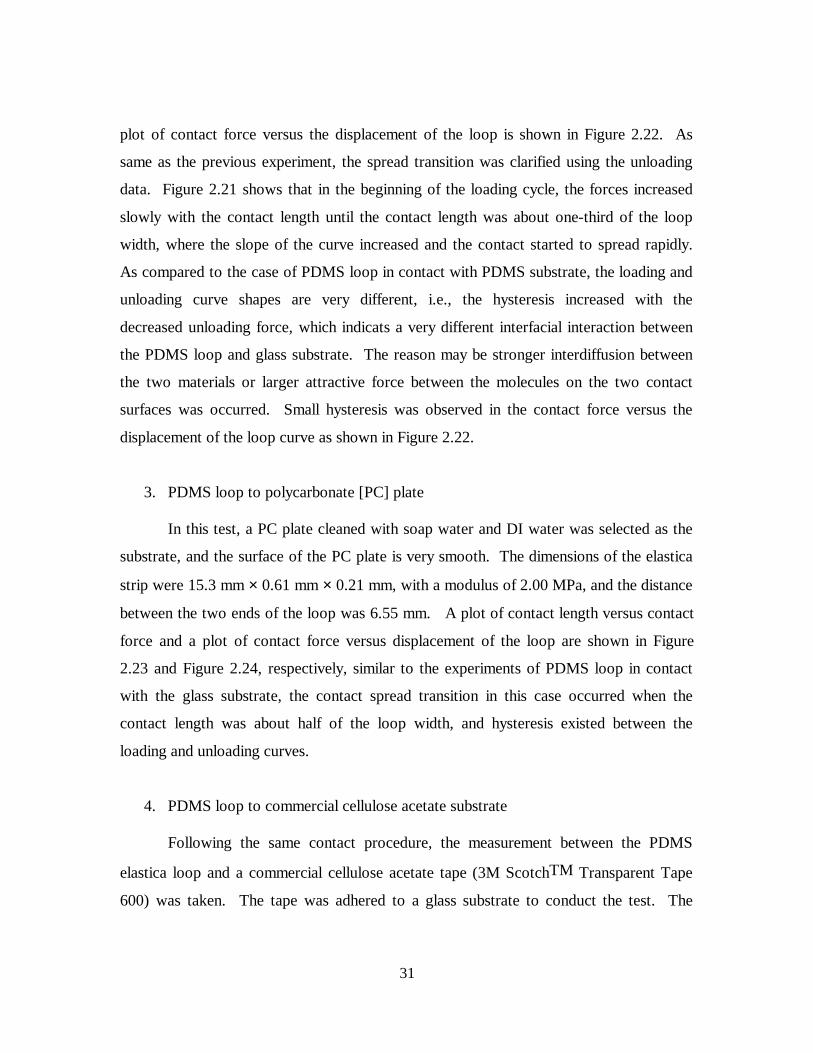
31
plot of contact force versus the displacement of the loop is shown in Figure 2.22. As
same as the previous experiment, the spread transition was clarified using the unloading
data. Figure 2.21 shows that in the beginning of the loading cycle, the forces increased
slowly with the contact length until the contact length was about one-third of the loop
width, where the slope of the curve increased and the contact started to spread rapidly.
As compared to the case of PDMS loop in contact with PDMS substrate, the loading and
unloading curve shapes are very different, i.e., the hysteresis increased with the
decreased unloading force, which indicats a very different interfacial interaction between
the PDMS loop and glass substrate. The reason may be stronger interdiffusion between
the two materials or larger attractive force between the molecules on the two contact
surfaces was occurred. Small hysteresis was observed in the contact force versus the
displacement of the loop curve as shown in Figure 2.22.
3. PDMS loop to polycarbonate [PC] plate
In this test, a PC plate cleaned with soap water and DI water was selected as the
substrate, and the surface of the PC plate is very smooth. The dimensions of the elastica
strip were 15.3 mm × 0.61 mm × 0.21 mm, with a modulus of 2.00 MPa, and the distance
between the two ends of the loop was 6.55 mm. A plot of contact length versus contact
force and a plot of contact force versus displacement of the loop are shown in Figure
2.23 and Figure 2.24, respectively, similar to the experiments of PDMS loop in contact
with the glass substrate, the contact spread transition in this case occurred when the
contact length was about half of the loop width, and hysteresis existed between the
loading and unloading curves.
4. PDMS loop to commercial cellulose acetate substrate
Following the same contact procedure, the measurement between the PDMS
elastica loop and a commercial cellulose acetate tape (3M ScotchTM Transparent Tape
600) was taken. The tape was adhered to a glass substrate to conduct the test. The
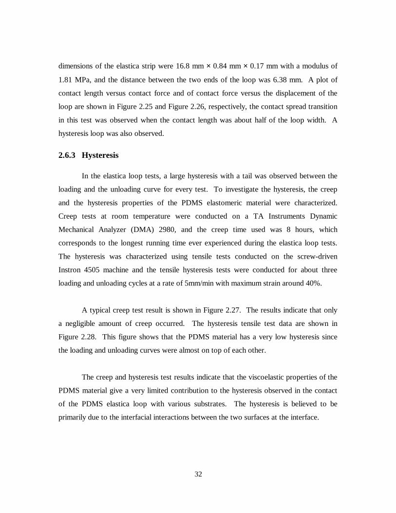
32
dimensions of the elastica strip were 16.8 mm × 0.84 mm × 0.17 mm with a modulus of
1.81 MPa, and the distance between the two ends of the loop was 6.38 mm. A plot of
contact length versus contact force and of contact force versus the displacement of the
loop are shown in Figure 2.25 and Figure 2.26, respectively, the contact spread transition
in this test was observed when the contact length was about half of the loop width. A
hysteresis loop was also observed.
2.6.3 Hysteresis
In the elastica loop tests, a large hysteresis with a tail was observed between the
loading and the unloading curve for every test. To investigate the hysteresis, the creep
and the hysteresis properties of the PDMS elastomeric material were characterized.
Creep tests at room temperature were conducted on a TA Instruments Dynamic
Mechanical Analyzer (DMA) 2980, and the creep time used was 8 hours, which
corresponds to the longest running time ever experienced during the elastica loop tests.
The hysteresis was characterized using tensile tests conducted on the screw-driven
Instron 4505 machine and the tensile hysteresis tests were conducted for about three
loading and unloading cycles at a rate of 5mm/min with maximum strain around 40%.
A typical creep test result is shown in Figure 2.27. The results indicate that only
a negligible amount of creep occurred. The hysteresis tensile test data are shown in
Figure 2.28. This figure shows that the PDMS material has a very low hysteresis since
the loading and unloading curves were almost on top of each other.
The creep and hysteresis test results indicate that the viscoelastic properties of the
PDMS material give a very limited contribution to the hysteresis observed in the contact
of the PDMS elastica loop with various substrates. The hysteresis is believed to be
primarily due to the interfacial interactions between the two surfaces at the interface.

33
To further investigate the hysteresis problem, the PDMS elastica loop versus
PDMS substrate contact tests were conducted again. However, in this experiment, the
loading and unloading cycles were performed in a cyclic fashion for three cycles. The
loading rate was still 10.1 µm/sec for each step, and between any two steps during the
loading cycle, the sample was allowed to dwell for an interval of 200 sec. For the
unloading cycle, the dwelling interval was increased to 300 sec/step, because it took
more time to reach the thermodynamic equilibrium. The experimental results for contact
radius versus contact force in Figure 2.29 clearly show that the hysteresis increased
significantly with the contact cycle since the area enclosed by the loading and unloading
curves increased from the first contact cycle to the third contact cycle. This increase of
hysteresis with the contact cycle is possibly due to the molecular inter-diffusion between
the two surfaces occurred when they were in contact, which altered the interfacial
interactions between these two surfaces.
The effect of contact rate on the contact hysteresis was also investigated in this
study using the same testing procedure. In the tests, the loading and unloading cycles
were performed continuously using constant testing rates with zero dwell time between
any two steps, and two testing rates were evaluated in this study.
Plots of contact radius versus contact force obtained in the tests are shown in
Figure 2.30. A testing rate of 5.1 µm/sec was the highest rate that could be achieved
with the current apparatus. Figure 2.30 shows that although not significant, the contact
hysteresis increases with the testing rate, which again indicates that the interfacial
interaction is a time-dependent phenomenon.
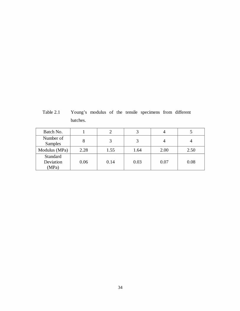
34
Table 2.1 Young’s modulus of the tensile specimens from different
batches.
Batch No. 1 2 3 4 5 Number of Samples
8 3 3 4 4
Modulus (MPa) 2.28 1.55 1.64 2.00 2.50 Standard Deviation
(MPa) 0.06 0.14 0.03 0.07 0.08

35
Figure 2.1 Elastica loop configuration
�%�
�&
)

36
\ ����[
5� ����
�
���
���
���
���
�
���
� ��� ��� ��� ��� ���
6WUDLQ� ε
6WUHVV�
σ�0
3D�
Figure 2.2 A typical stress-strain plot for a PDMS strip.
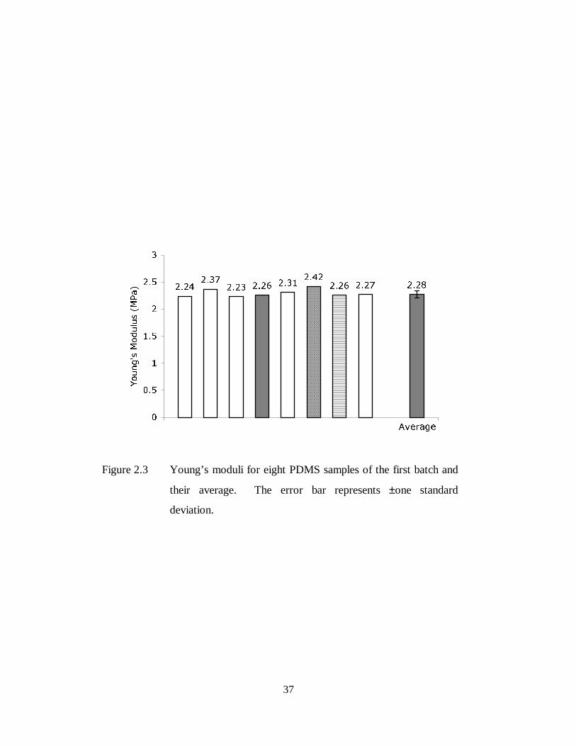
37
Figure 2.3 Young’s moduli for eight PDMS samples of the first batch and
their average. The error bar represents ±one standard
deviation.
��������
���� ���� ��������
���� ���� ����
�
���
�
���
�
���
�
<RXQJV0RGXOXV�0
3D�
$YHUDJH
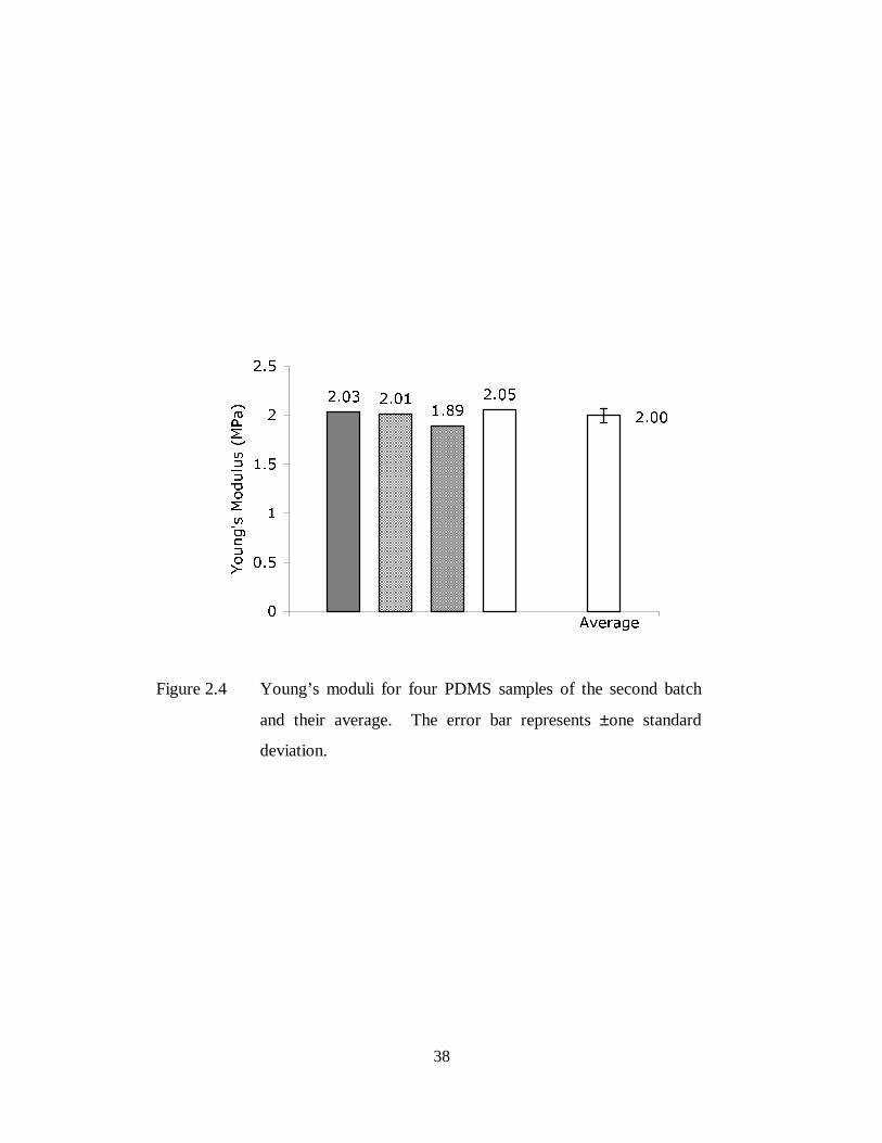
38
���� ��������
����
����
�
���
�
���
�
���
<RXQJV
0RGXOXV�0
3D�
$YHUDJH
Figure 2.4 Young’s moduli for four PDMS samples of the second batch
and their average. The error bar represents ±one standard
deviation.
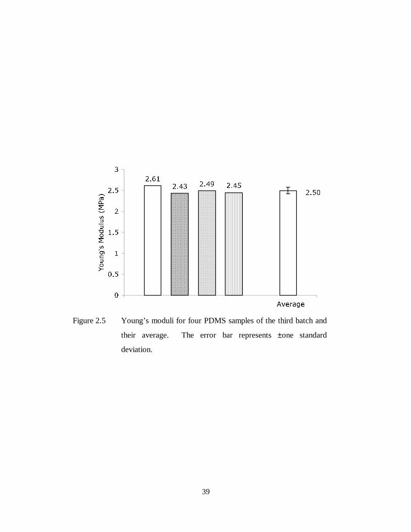
39
�������� ���� ����
����
�
���
�
���
�
���
�
<RXQJV0RGXOXV�0
3D�
$YHUDJH
Figure 2.5 Young’s moduli for four PDMS samples of the third batch and
their average. The error bar represents ±one standard
deviation.
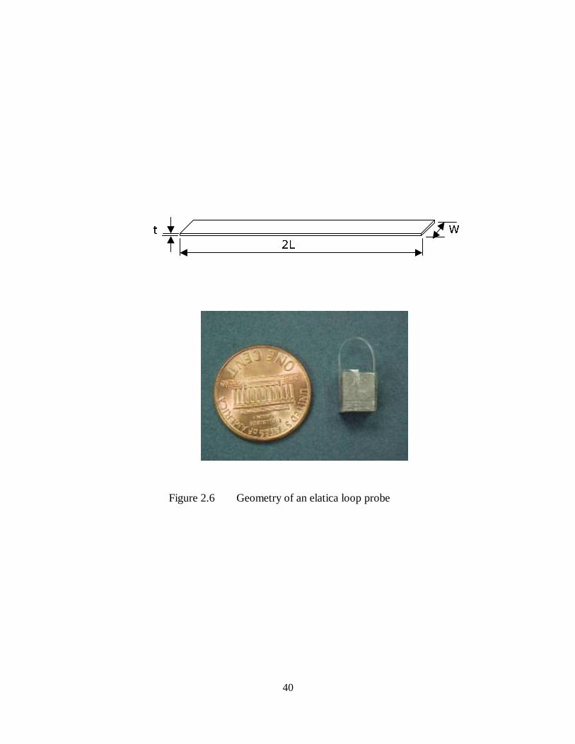
40
Figure 2.6 Geometry of an elatica loop probe
�/
:W

41
Figure 2.7 Schematic of apparatus
(ODVWLFD ORRS
9LEUDWLRQ UHGXFWLRQ WDEOH
$QDO\WLFDO EDODQFH
*ODVV VOLGH
&RPSXWHU
0DFUR�OHQV� ��[
&RQWUROOHU
0RQLWRU
6XSSRUW
,OOXPLQDWRU
6WHSSHU PRWRU
2XWVLGH F\OLQGHU
,QVLGH F\OLQGHU
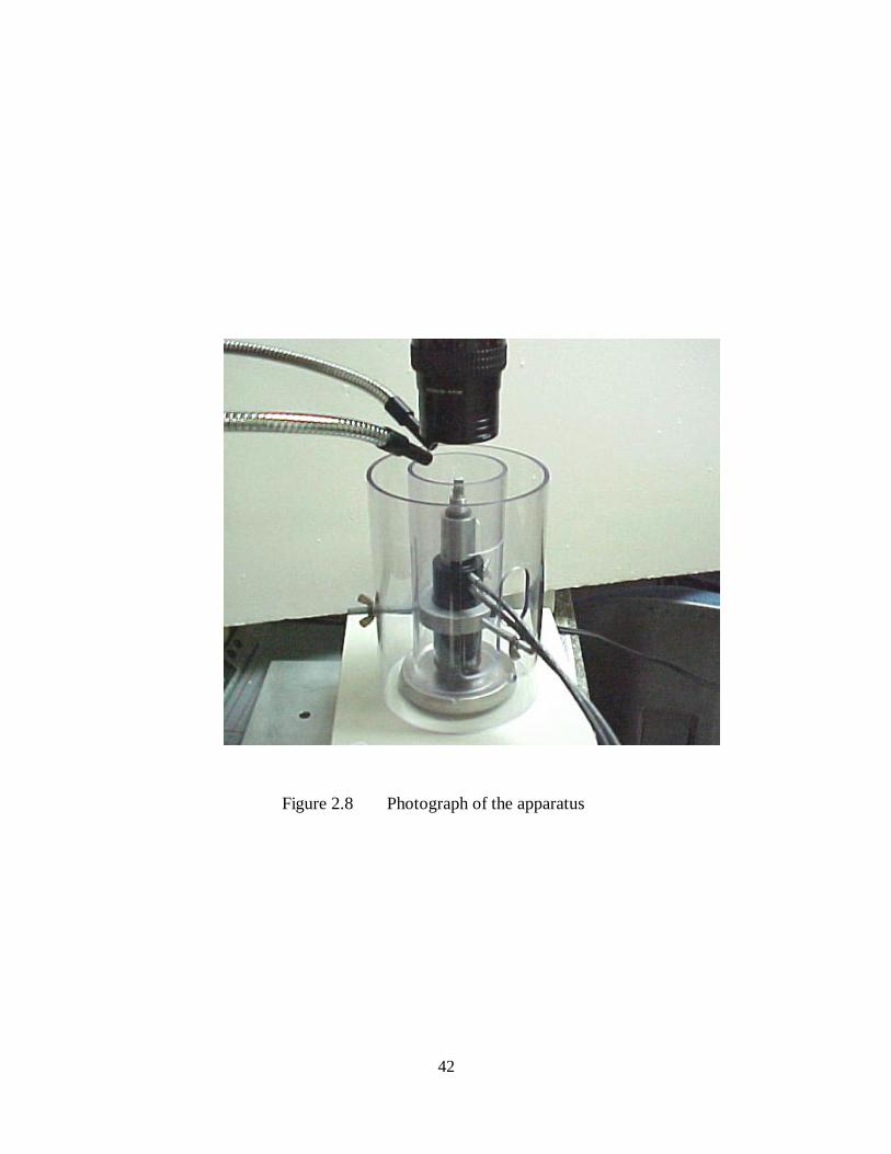
42
Figure 2.8 Photograph of the apparatus

43
Figure 2.9 Front panel of LabVIEW VI created for the computer
acquisition system.
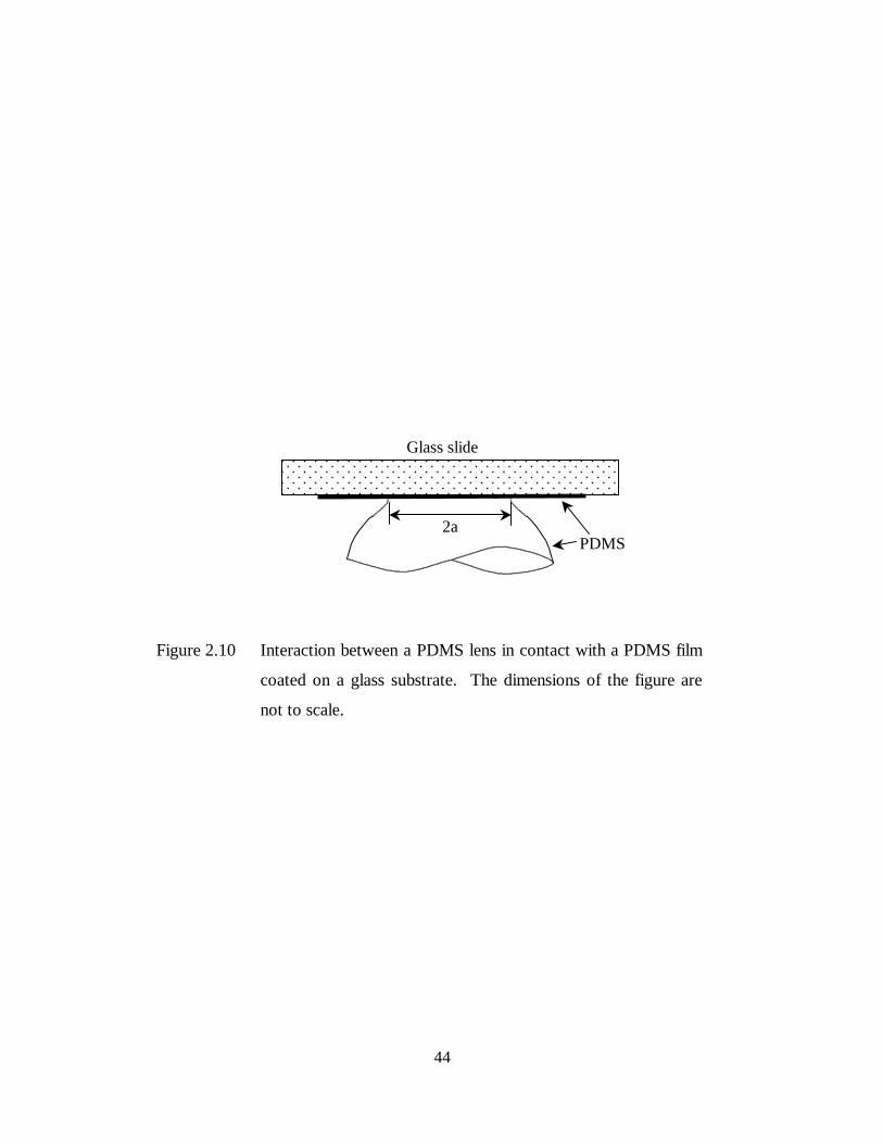
44
Figure 2.10 Interaction between a PDMS lens in contact with a PDMS film
coated on a glass substrate. The dimensions of the figure are
not to scale.
PDMS
Glass slide
2a
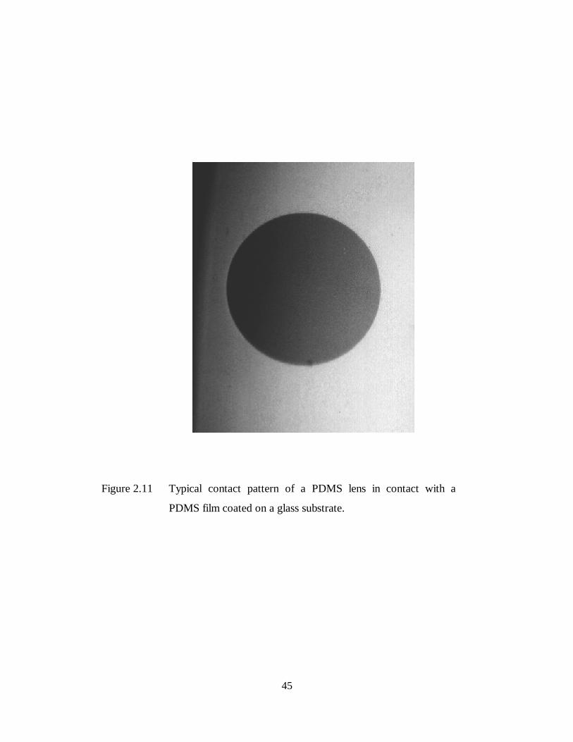
45
Figure 2.11 Typical contact pattern of a PDMS lens in contact with a
PDMS film coated on a glass substrate.
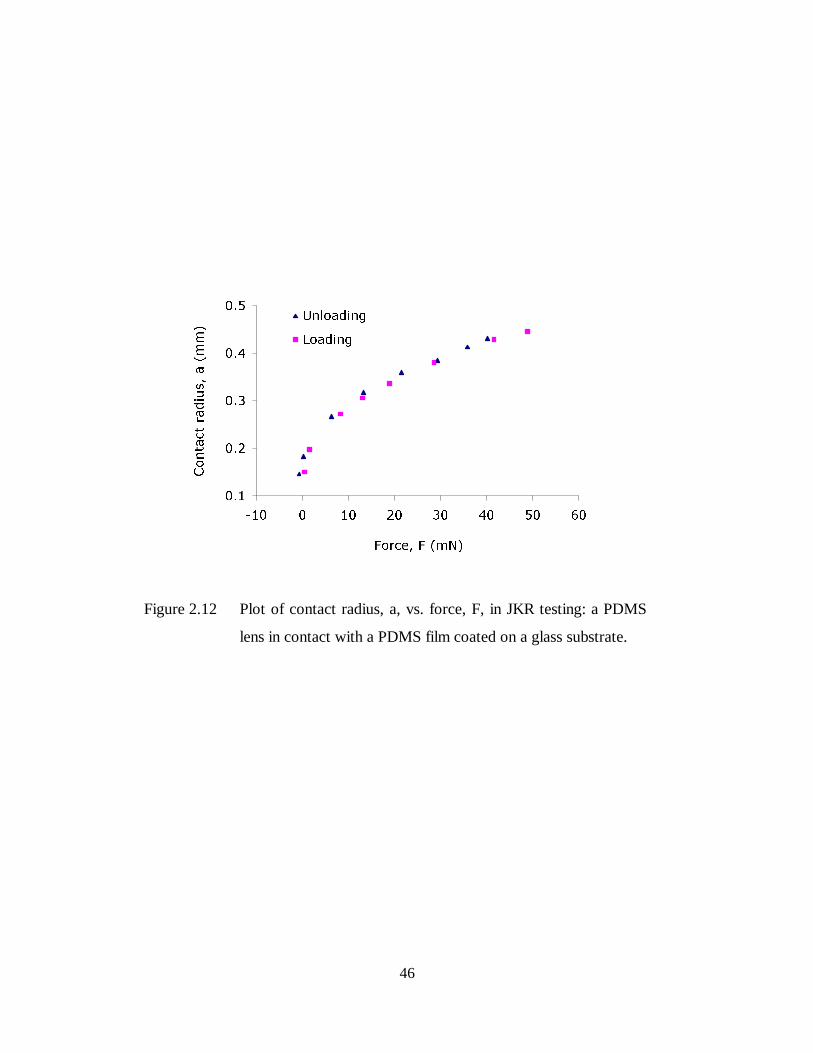
46
���
���
���
���
���
��� � �� �� �� �� �� ��
)RUFH� ) �P1�
&RQWDFWUDGLXV�D�P
P�
8QORDGLQJ
/RDGLQJ
Figure 2.12 Plot of contact radius, a, vs. force, F, in JKR testing: a PDMS
lens in contact with a PDMS film coated on a glass substrate.
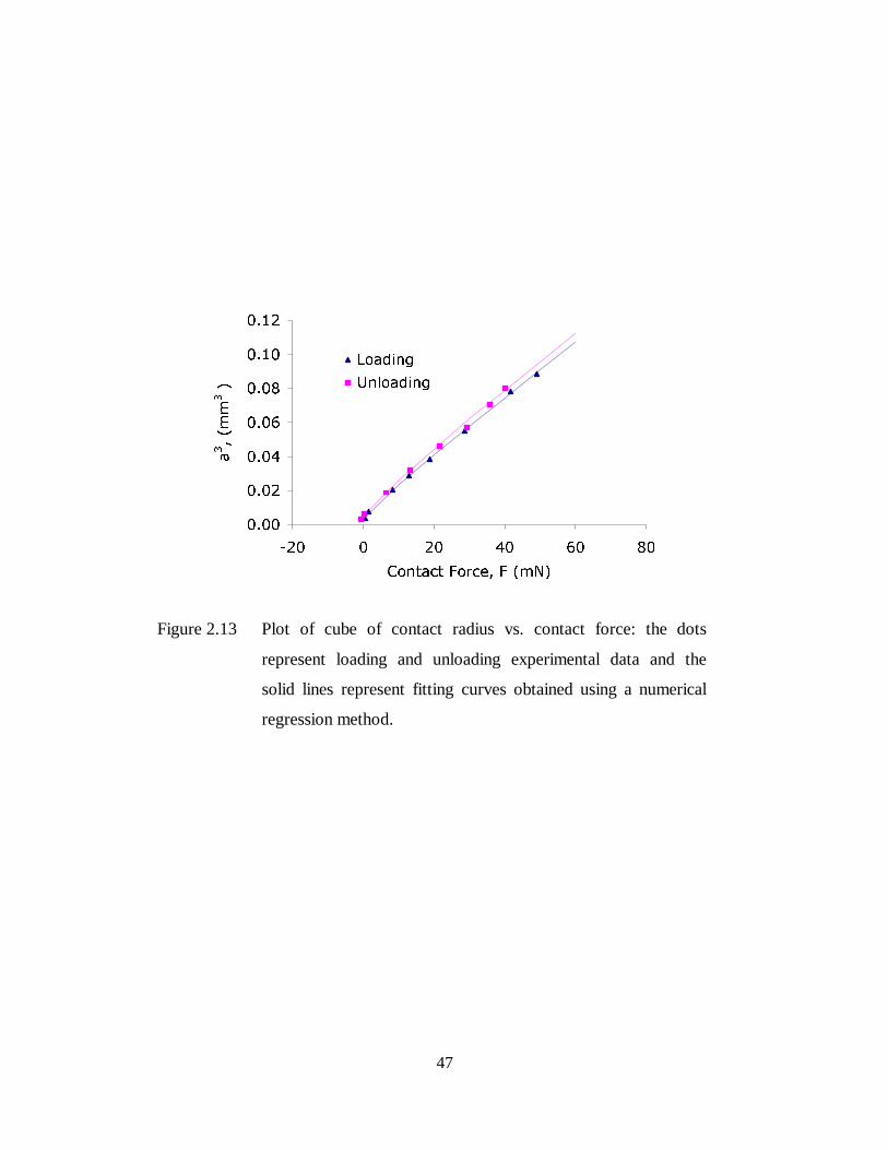
47
����
����
����
����
����
����
����
��� � �� �� �� ��
&RQWDFW )RUFH� ) �P1�
D���P
P��
/RDGLQJ
8QORDGLQJ
Figure 2.13 Plot of cube of contact radius vs. contact force: the dots
represent loading and unloading experimental data and the
solid lines represent fitting curves obtained using a numerical
regression method.
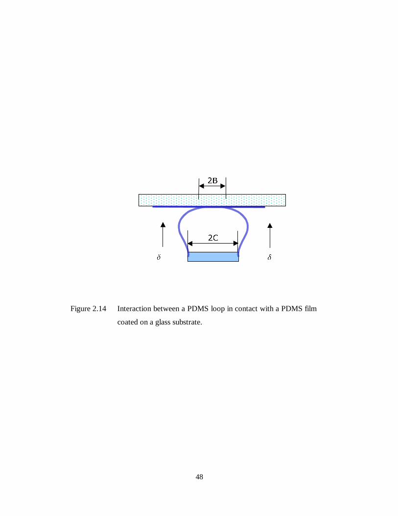
48
Figure 2.14 Interaction between a PDMS loop in contact with a PDMS film
coated on a glass substrate.
�%
G G
�&
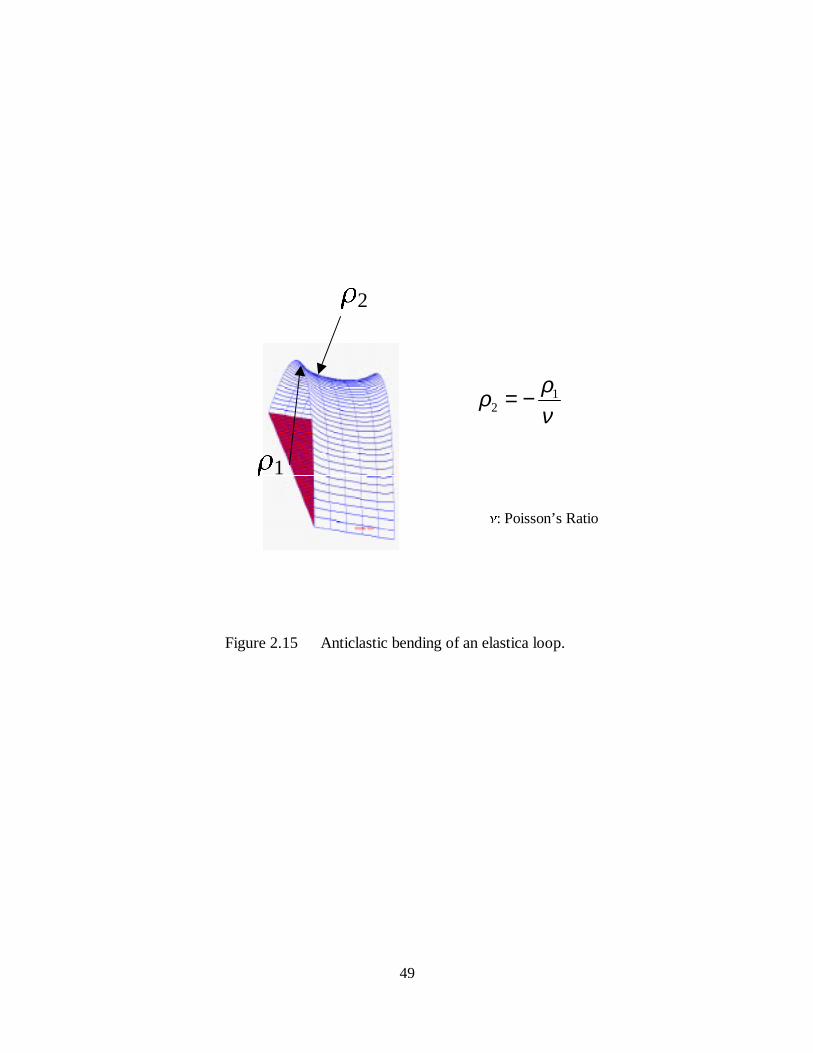
49
Figure 2.15 Anticlastic bending of an elastica loop.
Q: Poisson’s Ratio
U2
U1
νρρ 1
2 −=
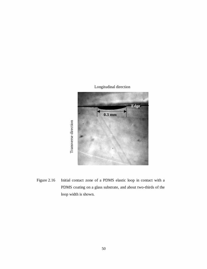
50
Edge
0.3 mm
Tra
nsve
rse
dire
ctio
n
Longitudinal direction
Figure 2.16 Initial contact zone of a PDMS elastic loop in contact with a
PDMS coating on a glass substrate, and about two-thirds of the
loop width is shown.

51
0.96
mm
Figure 2.17 Further contact zone of a PDMS elastic loop in contact with a
PDMS coating on a glass substrate, but the contact length is
smaller than one third of the elastica loop width.
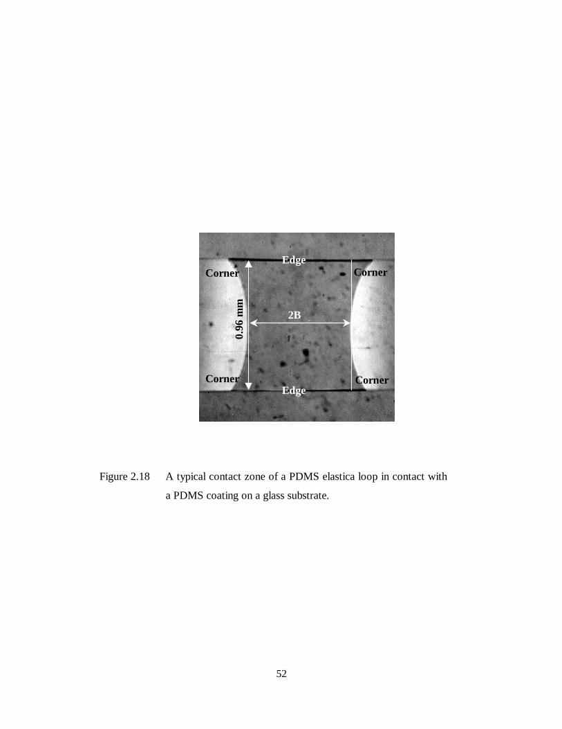
52
Edge
Edge
2B
Corner Corner
Corner Corner
0.96
mm
Figure 2.18 A typical contact zone of a PDMS elastica loop in contact with
a PDMS coating on a glass substrate.
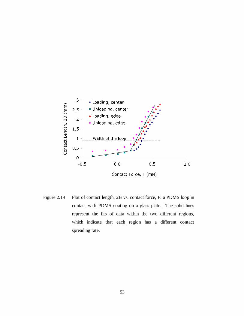
53
�
���
�
���
�
���
�
���� ��� ��� ���
&RQWDFW )RUFH� ) �P1�
&RQWDFW/HQJWK��%�P
P� /RDGLQJ� FHQWHU
8QORDGLQJ� FHQWHU
/RDGLQJ� HGJH
8QORDGLQJ� HGJH
:LGWK RI WKH ORRS
Figure 2.19 Plot of contact length, 2B vs. contact force, F: a PDMS loop in
contact with PDMS coating on a glass plate. The solid lines
represent the fits of data within the two different regions,
which indicate that each region has a different contact
spreading rate.
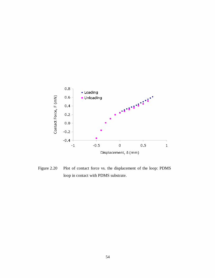
54
����
����
���
���
���
���
���
�� ���� � ��� �
'LVSODFHPHQW� δ �PP�
&RQWDFW)RUFH�)�P
1�
/RDGLQJ
8QORDGLQJ
Figure 2.20 Plot of contact force vs. the displacement of the loop: PDMS
loop in contact with PDMS substrate.

55
���
���
���
���
���
���
���
���� ���� ��� ��� ���
&RQWDFW )RUFH� ) �P1�
&RQWDFW/HQJWK��%�P
P� /RDGLQJ
8QORDGLQJ
:LGWK RI WKH ORRS
Figure 2.21 Plot of contact length, 2B vs. contact force, F: PDMS loop in
contact with a glass plate. The solid lines represent the fits of
data within the two different regions, which indicate that each
region has a different contact spreading rate.
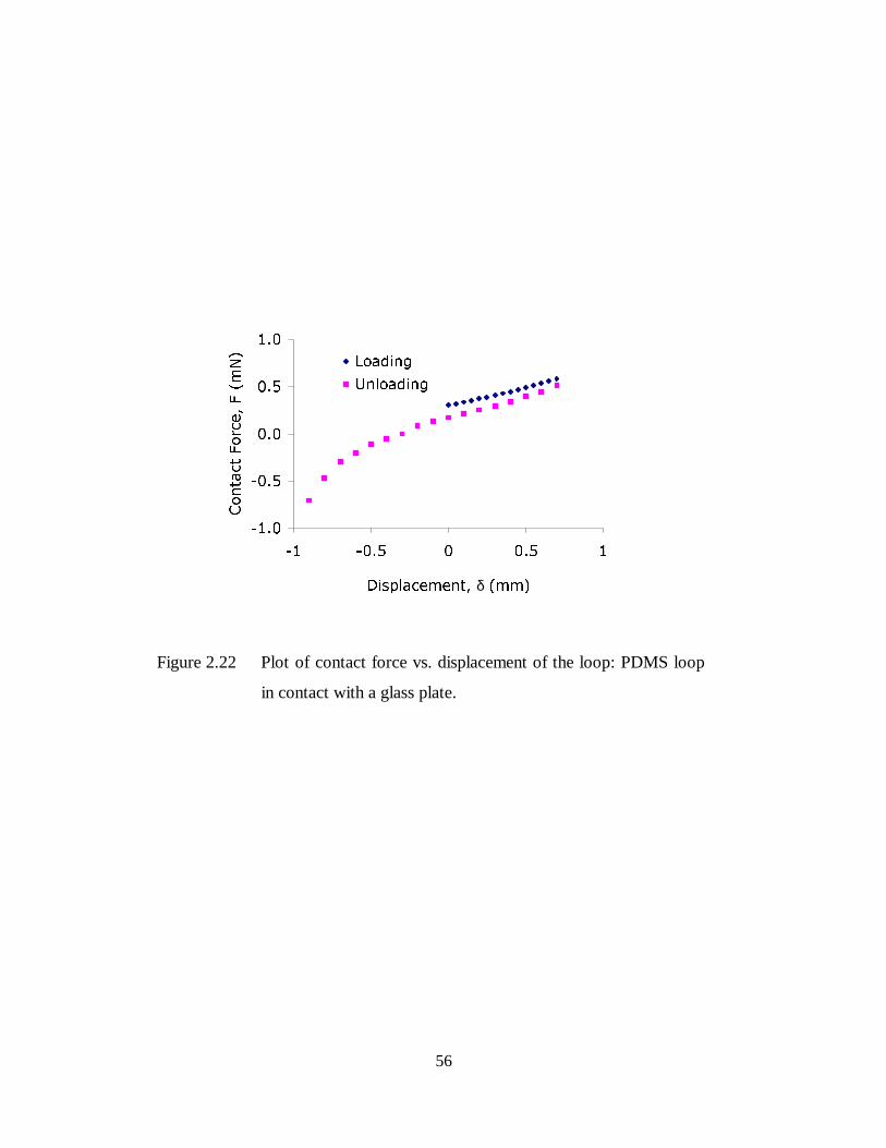
56
����
����
���
���
���
�� ���� � ��� �
'LVSODFHPHQW� δ �PP�
&RQWDFW)RUFH�)�P
1�
/RDGLQJ
8QORDGLQJ
Figure 2.22 Plot of contact force vs. displacement of the loop: PDMS loop
in contact with a glass plate.

57
���
���
���
���
���
���
���� ���� ��� ��� ��� ���
&RQWDFW IRUFH� ) �P1�
&RQWDFWOHQJWK��%�P
P� /RDGLQJ
8QORDGLQJ
:LGWK RI WKH ORRS
Figure 2.23 Plot of contact length, 2B vs. contact force, F: PDMS loop in
contact with a PC plate. The solid lines represent the fits of
data within the two different regions, which indicate that each
region has a different contact spreading rate.
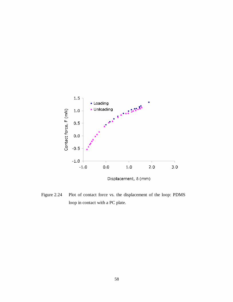
58
����
����
���
���
���
���
���� ��� ��� ��� ���
'LVSODFHPHQW� δ �PP�
&RQWDFWIRUFH�)�P
1�
/RDGLQJ
8QORDGLQJ
Figure 2.24 Plot of contact force vs. the displacement of the loop: PDMS
loop in contact with a PC plate.
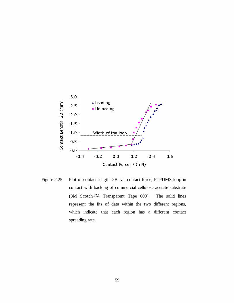
59
���
���
���
���
���
���
���
���� ���� ��� ��� ��� ���
&RQWDFW )RUFH� ) �P1�
&RQWDFW/HQJWK��%�P
P�
/RDGLQJ
8QORDGLQJ
:LGWK RI WKH ORRS
Figure 2.25 Plot of contact length, 2B, vs. contact force, F: PDMS loop in
contact with backing of commercial cellulose acetate substrate
(3M ScotchTM Transparent Tape 600). The solid lines
represent the fits of data within the two different regions,
which indicate that each region has a different contact
spreading rate.

60
����
����
���
���
���
���
�� ���� � ��� �
'LVSODFHPHQW� δ �PP�
&RQWDFW)RUFH�)�P
1� /RDGLQJ
8QORDGLQJ
Figure 2.26 Plot of contact force vs. the displacement of the loop: PDMS
loop in contact with backing of commercial cellulose acetate
substrate (3M ScotchTM Transparent Tape 600).

61
�
���
���
���
���
� ��� ��� ��� ���
7LPH� W �PLQ�
&UHHS&RPSOLDQFH�&���0
3D�
Figure 2.27 DMA creep test results using a rectangular PDMS strip at room
temperature with a 0.2 MPa stress.

62
\ ����[
5� ����
�
���
�
���
� ��� ��� ��� ��� ���
6WUDLQ� ε
6WUHVV�
σ�0
3D�
�VW F\FOH
�QG F\FOH
�UG F\FOH
Figure 2.28 Room temperature stress-strain curves of PDMS for three
loading-unloading cycles. The loading and unloading rate used
in the tests was 5mm/min.
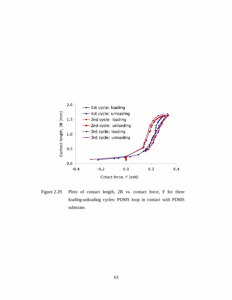
63
���
���
���
���
���
���� ���� ��� ��� ���
&QWDFW IRUFH� ) �P1�
&RQWDFWOHQJWK��%�P
P�
�VW F\FOH� ORDGLQJ
�VW F\FOH� XQORDGLQJ
�QG F\FOH� ORDGLQJ
�QG F\FOH� XQORDGLQJ
�UG F\FOH� ORDGLQJ
�UG F\FOH� XQORDGLQJ
Figure 2.29 Plots of contact length, 2B vs. contact force, F for three
loading-unloading cycles: PDMS loop in contact with PDMS
substrate.
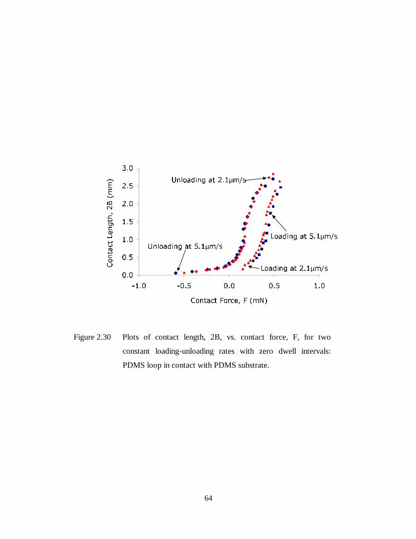
64
���
���
���
���
���
���
���
���� ���� ��� ��� ���
&RQWDFW )RUFH� ) �P1�
&RQWDFW/HQJWK��%�P
P�
/RDGLQJ DW ���µP�V8QORDGLQJ DW ���µP�V
8QORDGLQJ DW ���µP�V
/RDGLQJ DW ���µP�V
Figure 2.30 Plots of contact length, 2B, vs. contact force, F, for two
constant loading-unloading rates with zero dwell intervals:
PDMS loop in contact with PDMS substrate.

65
CHAPTER 3 Numerical Analysis
3.1 Abstract
3-D finite element analyses using ABAQUS 5.8 [47] are conducted to calculate
the effect of anticlastic bending of the elastica loop and simulate the contact process
between the loop and a flat rigid surface. The finite element model constructed is a
geometrically nonlinear elastic contact mechanics model, and the analysis used
appropriate mesh, element size, and step increments to simulate the contact procedure.
The effect of Poisson's ratio on the contact behavior is given in this chapter.
3.2 Meshes and boundary conditions
To understand the mechanical behavior of the contact procedure at a quantitative
level and to verify the analytical 2-D solution by Plaut et al. [45], numerical simulations
of an elastica loop in contact with a flat rigid surface were conducted using the finite
element method. The finite element package used was ABAQUS 5.8, which provides a
very powerful tool to deal with general nonlinear and large-deformation problems. In the
numerical analyses, the interfacial interactions were ignored due to the limitation of the
ABAQUS codes.
The numerical simulation scheme started with a straight elastica strip and a flat
surface. The dimensions of the elastica strip were taken from the actual specimens. The
Young’s modulus of the strip was taken from the tensile experimental data in Chapter 2,
and the Poisson’s ratio was chosen as Q=0.49, which represents a typical value for
elastomeric materials. The flat surface was modeled as a rigid surface. Making use of
symmetry, only one half of the strip was modeled. The elements used to model the
elastic strip were the S4R four-node shell elements since this is a geometric nonlinear
contact mechanics problem. In the central area of the strip, where the contact initiates, a
66
fine mesh with minimum element size about 0.05 mm × 0.05 mm was used. Moving
toward the end of the loop, the mesh became coarser. Shown in Figure 3.1 is a typical
mesh used in this study for the elastica strip. When the specimen size changed, the
element sizes would also change but the density of the mesh would remain about the
same. The constraint for the fixed end of the loop was modeled as a built-in constraint.
3.3 Simulation of the loop formation
Numerically the elastica loop was formed from a straight strip in several steps.
The end of the straight strip was rotated 90° clockwise and moved toward the center for a
certain distance as indicated in Figure 3.2. In the analysis by Plaut et al. [45], the loop
was assumed to be an inextensible beam and the analysis was two-dimensional.
However, the actual specimen used in the test was a three-dimensional object with a
relatively low modulus. Once the loop was formed, there was anticlastic bending in the
loop due to the Poisson’s ratio effect. The relationship between the curvatures of the
longitudinal bending and anticlastic bending is given by νρρ 12 −= as indicated in
Figure 2.15, where ρ1 and ρ2 are the curvatures of the longitudinal and anticlastic
bending, and ν is the Poisson’s ratio of the loop. Because of the effect of anticlastic
bending, the strain state in the elastica loop is more complex than the 2-D solution
discussed by Plaut et al. [45]. As indicated by the finite element analysis results shown
in Figure 3.3 and Figure 3.4, where the longitudinal and transverse strain on the concave
side along the loop are shown, respectively, the maximum absolute value of the
longitudinal strain (3.4%) occurred in the center of the loop, where the longitudinal
curvature reached the maximum value. The minimum longitudinal strain (zero) occurred
at the end of the loop. Similarly, the maximum absolute transverse strain (1.5%)
occurred in the center of the loop because this was the location with maximum transverse
curvature. The minimum transverse strain (zero) occurred at the fixed end. Although the
strains along the loop were not zero, their level was quite low, which supported the

67
inextensible elastica loop assumption made by Plaut et al. [45] in developing the
analytical solution for an elastica in contact with a flat rigid surface.
3.4 Contact simulation
3.4.1 Contact principle
When two solid bodies are in contact, stresses are transmitted across the interface.
If the interface is frictionless, only the stresses normal to the interface will be transmitted.
On the other hand, if friction is present at the interface, shear stresses will also be
transmitted. Contact problems normally involve material property discontinuities and
severe stress discontinuities across the interface, which sometimes causes serious
numerical convergence problems. If large deformations also need to be considered, finite
sliding at the interface between the two solids has to be taken into account and the
numerical increments have to be very small. Consequently, the modeling usually
requires a lot of computing time.
To model a contact problem, surfaces in contact are defined as master and slave
surfaces in ABAQUS. The choice for master and slave surfaces is strict and each surface
has different requirements for the mesh. In general, the slave surface requires a finer
mesh since only the slave surface allows penetration, and if possible, the surface with a
lower modulus material is usually chosen as the slave surface. In addition, the
orientation of the master surface needs to be properly defined. The slave surface always
has to be on the same side as the outward normal of the master surface. Otherwise,
ABAQUS may detect severe overclosure and fail to converge. ABAQUS determines the
overclosure, h, through calculating the relative distances between the integration points
on the contact surfaces as indicated in Figure 3.5. The contact behavior is determined
through c, h, and contact pressure p. In this study, the surface of the elastica loop was
defined as the slave surface, named as SURF, and the rigid surface was defined as the
master surface, named as RIGID. Because of the compliant structure of the loop, a

68
geometrically nonlinear finite element simulation scheme was used. At the interface,
finite sliding conditions were applied to be compatible with the geometrically nonlinear
model. According to suggestions in the ABAQUS manuals and after a series of trial
calculations, the following contact simulation algorithm was chosen to simulate the
contact procedure.
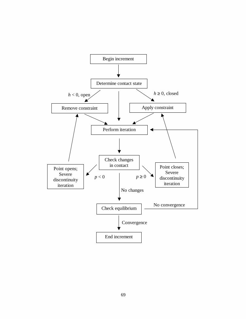
69
Determine contact state
Remove constraint Apply constraint
Perform iteration
h < 0, open h ≥ 0, closed
Point opens; Severe
discontinuity iteration
Point closes; Severe
discontinuity iteration
Check changes in contact
p < 0 p ≥ 0
Begin increment
Check equilibrium
No changes
End increment
Convergence
No convergence
70
3.4.2 Contact procedure
As the contact simulation started, the elastica loop was first formed through
bending the strip, and the end was moved toward the center for a certain distance, which
was taken from the actual sample geometry. Then the flat substrate, which was defined
as a rigid surface, was moved toward the loop, and finally they were in contact with each
other as shown schematically in Figure 3.6. The displacement increments and the
initiation time were selected differently in different steps in order to deal with the
nonlinear problem properly. Contact patterns, normal contact stresses, strain
distribution, and displacement profiles were obtained during the analysis.
3.4.3 Contact patterns
Through the finite element analysis, the whole contact procedure was simulated.
When the rigid plate was brought into contact with the loop, the contact first initiated at
the edge of the loop because of the anticlastic curvature, as shown in Figure 3.7. The
maximum normal contact stress was located in the center of the contact zone along the
edge, as shown in Figure 3.8. As compared to the experimental observation of the
contact zone as shown in the insert of Figure 3.7, the contact shape predicted by the finite
element modeling in Figure 3.8 appears to be consistent. However, difference in contact
shape has been noticed between the finite element result shown in Figure 3.7 and the
experimental observation, which was possibly caused by the computer display error itself
or the calculation error due to the use of symmetry at center line. As the displacement
increased, the compressive force also increased, and the contact zone spread across the
width and propagated outward longitudinally toward the loop end. The curved contact
front, which was also due to the anticlastic bending, was clearly observed as shown in
Figure 3.9. This result was also consistent with the experimental observations as shown
in the insert of Figure 3.9.
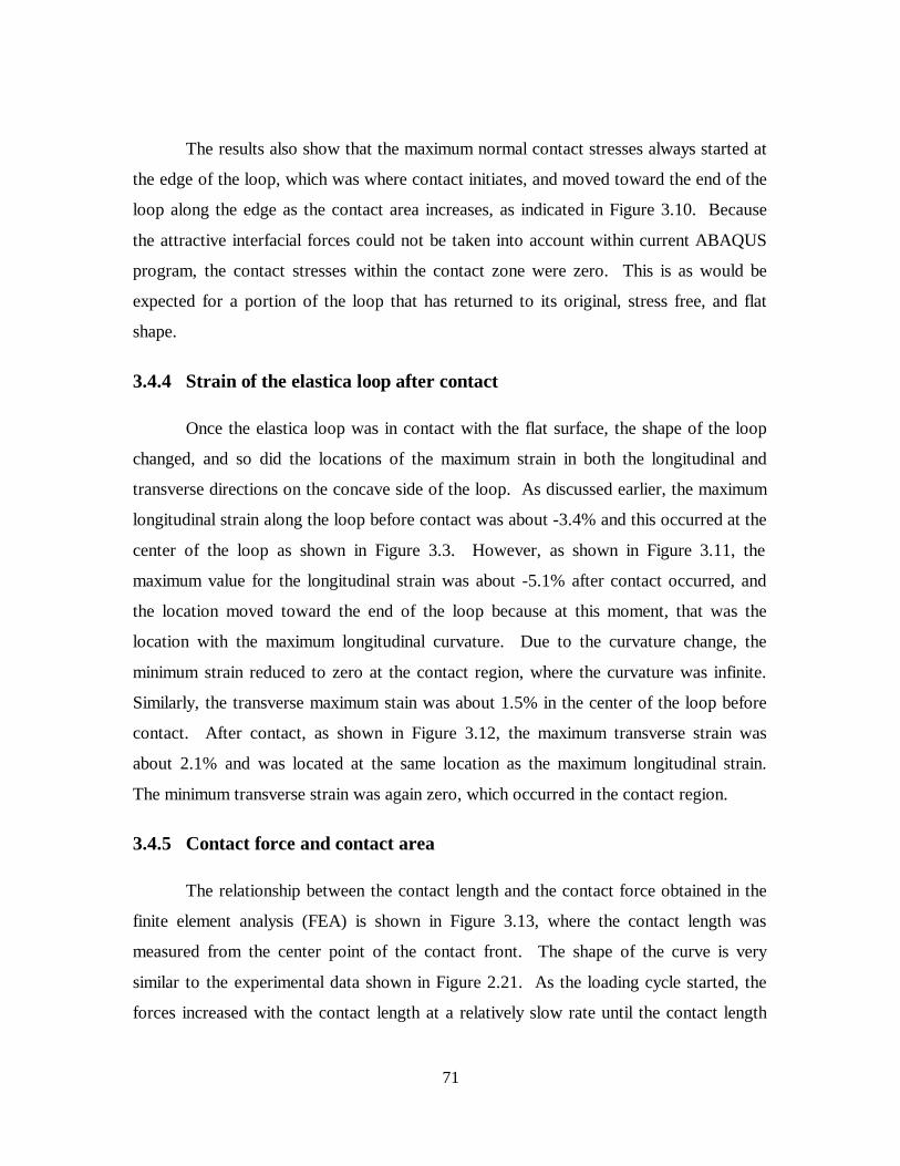
71
The results also show that the maximum normal contact stresses always started at
the edge of the loop, which was where contact initiates, and moved toward the end of the
loop along the edge as the contact area increases, as indicated in Figure 3.10. Because
the attractive interfacial forces could not be taken into account within current ABAQUS
program, the contact stresses within the contact zone were zero. This is as would be
expected for a portion of the loop that has returned to its original, stress free, and flat
shape.
3.4.4 Strain of the elastica loop after contact
Once the elastica loop was in contact with the flat surface, the shape of the loop
changed, and so did the locations of the maximum strain in both the longitudinal and
transverse directions on the concave side of the loop. As discussed earlier, the maximum
longitudinal strain along the loop before contact was about -3.4% and this occurred at the
center of the loop as shown in Figure 3.3. However, as shown in Figure 3.11, the
maximum value for the longitudinal strain was about -5.1% after contact occurred, and
the location moved toward the end of the loop because at this moment, that was the
location with the maximum longitudinal curvature. Due to the curvature change, the
minimum strain reduced to zero at the contact region, where the curvature was infinite.
Similarly, the transverse maximum stain was about 1.5% in the center of the loop before
contact. After contact, as shown in Figure 3.12, the maximum transverse strain was
about 2.1% and was located at the same location as the maximum longitudinal strain.
The minimum transverse strain was again zero, which occurred in the contact region.
3.4.5 Contact force and contact area
The relationship between the contact length and the contact force obtained in the
finite element analysis (FEA) is shown in Figure 3.13, where the contact length was
measured from the center point of the contact front. The shape of the curve is very
similar to the experimental data shown in Figure 2.21. As the loading cycle started, the
forces increased with the contact length at a relatively slow rate until the contact length

72
reached a certain value, where the contact started to spread rapidly. In the experimental
data shown in Figure 2.21, this contact rate transition occurred when the contact length
was about 40% of the loop width. On the other hand, in the FEA result shown in Figure
3.13, this transition occurred when the contact length was a very small value. These
results indicate that the transition in the experiment with the elastica loop is primarily
due to the combined effects of the main bending along the longitudinal direction, the
anticlastic bending and the interfacial energies. The difference between the experiment
data and numerical result is the effects of interfacial energies between the loop and
substrate.
Because of the curved contact front, the determination of the contact length is
ambiguous. In this numerical study, the contact lengths measured from three different
locations have been taken as indicated in Figure 3.14: 1) the outer edge point on the
contact front; 2) the point with maximum pressure; or 3) the center point on the contact
front. Figure 3.14 also shows the relationship between the contact forces and the contact
lengths measured at different locations. This result indicates that if the attractive
interfacial energy is not present, the curvature of the contact front remains constant as the
contact length increases, since the relative distance among these three curves remains
almost the same. This conclusion is consistent with the experimental observation
discussed in Chapter 2, where the final curvature of the contact front resulted from the
combined effects of the longitudinal main bending, the anticlastic bending and the
interfacial interactions.
3.4.6 Poisson's ratio effects
In the analysis by Plaut et al. [45], the elastica loop was analyzed using beam
theory. As a result, the Poisson’s ratio, ν, of the loop has no effect on the solution
because the width effects, including anticlastic bending, were not modeled. In the finite
element analysis in this study, the elastica loop was treated as a three-dimensional object,
and the results showed that the anticlastic bending affected the contact pattern, contact
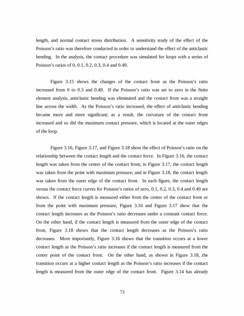
73
length, and normal contact stress distribution. A sensitivity study of the effect of the
Poisson’s ratio was therefore conducted in order to understand the effect of the anticlastic
bending. In the analysis, the contact procedure was simulated for loops with a series of
Poisson’s ratios of 0, 0.1, 0.2, 0.3, 0.4 and 0.49.
Figure 3.15 shows the changes of the contact front as the Poisson’s ratio
increased from 0 to 0.3 and 0.49. If the Poisson’s ratio was set to zero in the finite
element analysis, anticlastic bending was eliminated and the contact front was a straight
line across the width. As the Poisson’s ratio increased, the effect of anticlastic bending
became more and more significant; as a result, the curvature of the contact front
increased and so did the maximum contact pressure, which is located at the outer edges
of the loop.
Figure 3.16, Figure 3.17, and Figure 3.18 show the effect of Poisson’s ratio on the
relationship between the contact length and the contact force. In Figure 3.16, the contact
length was taken from the center of the contact front; in Figure 3.17, the contact length
was taken from the point with maximum pressure; and in Figure 3.18, the contact length
was taken from the outer edge of the contact front. In each figure, the contact length
versus the contact force curves for Poisson’s ratios of zero, 0.1, 0.2, 0.3, 0.4 and 0.49 are
shown. If the contact length is measured either from the center of the contact front or
from the point with maximum pressure, Figure 3.16 and Figure 3.17 show that the
contact length increases as the Poisson’s ratio decreases under a constant contact force.
On the other hand, if the contact length is measured from the outer edge of the contact
front, Figure 3.18 shows that the contact length decreases as the Poisson’s ratio
decreases. More importantly, Figure 3.16 shows that the transition occurs at a lower
contact length as the Poisson’s ratio increases if the contact length is measured from the
center point of the contact front. On the other hand, as shown in Figure 3.18, the
transition occurs at a higher contact length as the Poisson’s ratio increases if the contact
length is measured from the outer edge of the contact front. Figure 3.14 has already
74
demonstrated the effect of the measuring position of the contact length on the contact
transition for the case of ν = 0.49. These results provide valuable insights into how the
interfacial energy measurements with an elastica loop ought to be performed to obtain
the most sensitive observation of the effect of the interfacial interactions. More
specifically a good understanding of the Poisson ratio’s effects obtained in the FEA
analyses can help us determine the proper measuring point of the contact length. For
example, for the case of the PDMS loop used in this study, the proper point to measure
the contact length is the central point of the contact front, because the FEA results and
the experimental data have shown that the effect of the interfacial interactions on the
contact spread transition were most clearly observed for this case.

75
Figure 3.1 FEA mesh of elastica loop with dimensions 14.71 mm × 0.956
mm × 0.165 mm, modulus 1.81 MPa, and a series of Poisson’s
ratios of 0, 0.1, 0.2, 0.3, 0.4, 0.49.
D
E F
G
3RUWLRQ PRGHOHG
/
:
D
E F
G
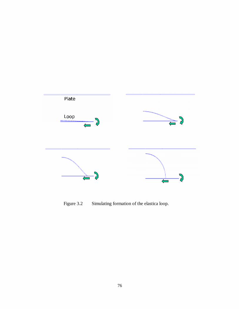
76
Figure 3.2 Simulating formation of the elastica loop.
3ODWH
/RRS
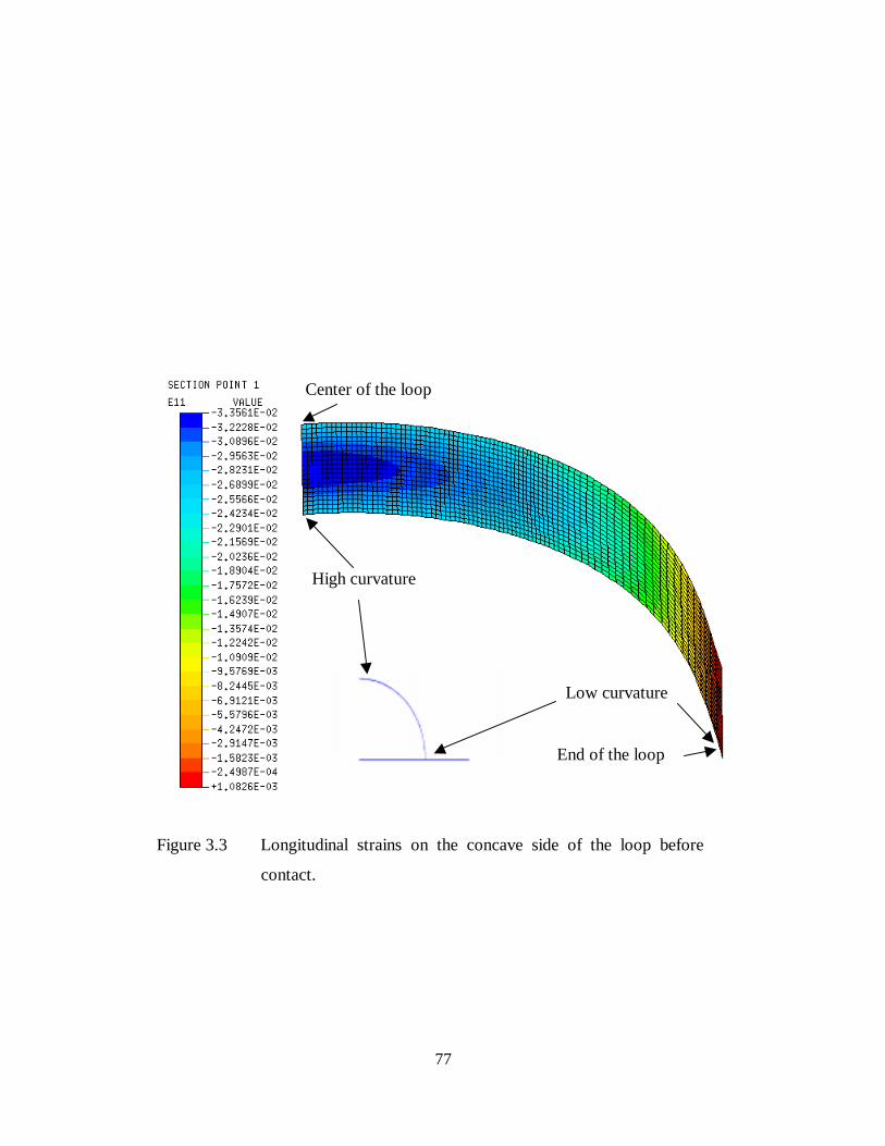
77
Figure 3.3 Longitudinal strains on the concave side of the loop before
contact.
Center of the loop
End of the loop
High curvature
Low curvature
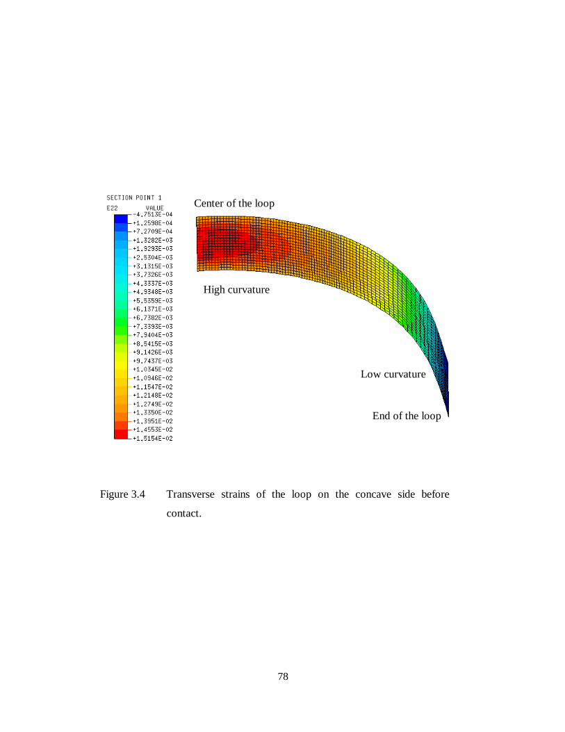
78
Figure 3.4 Transverse strains of the loop on the concave side before
contact.
Center of the loop
End of the loop
Low curvature
High curvature
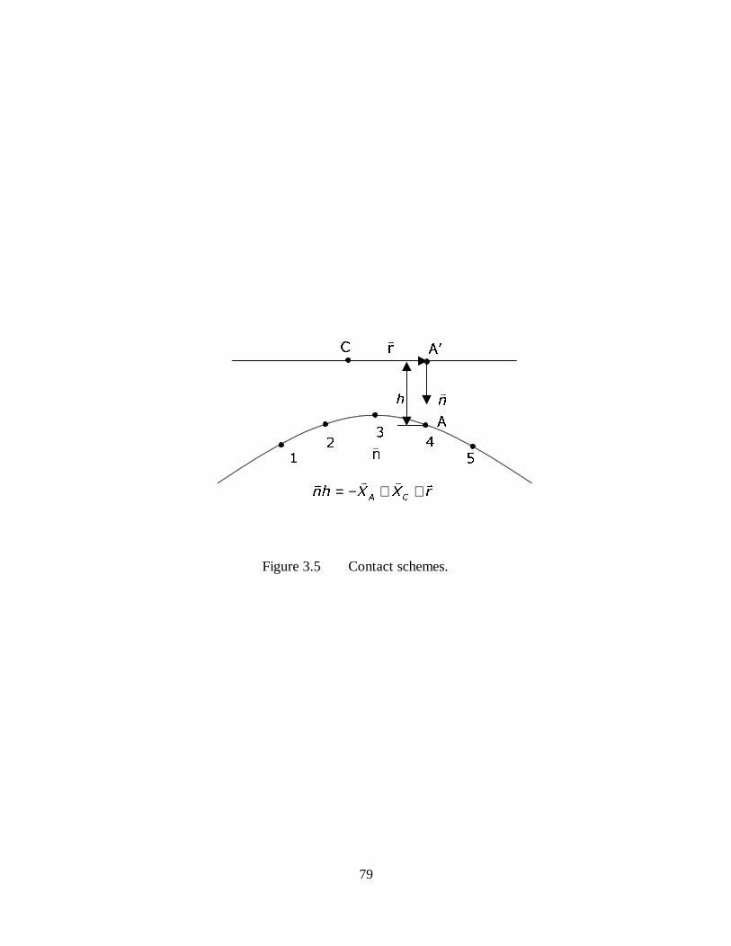
79
Figure 3.5 Contact schemes.
��
��
�
& $
$
Q*
Q*
K
U*
U;;KQ&$
*
**
*
++−=
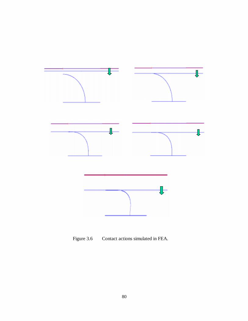
80
Figure 3.6 Contact actions simulated in FEA.
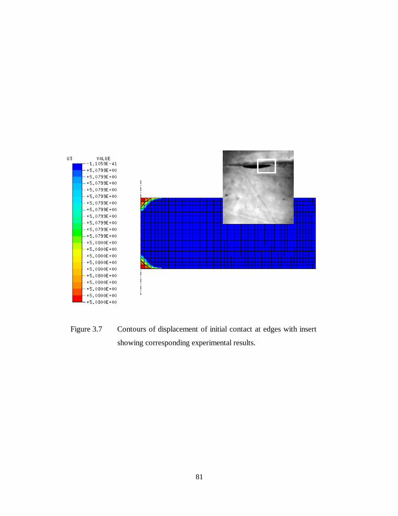
81
Figure 3.7 Contours of displacement of initial contact at edges with insert
showing corresponding experimental results.
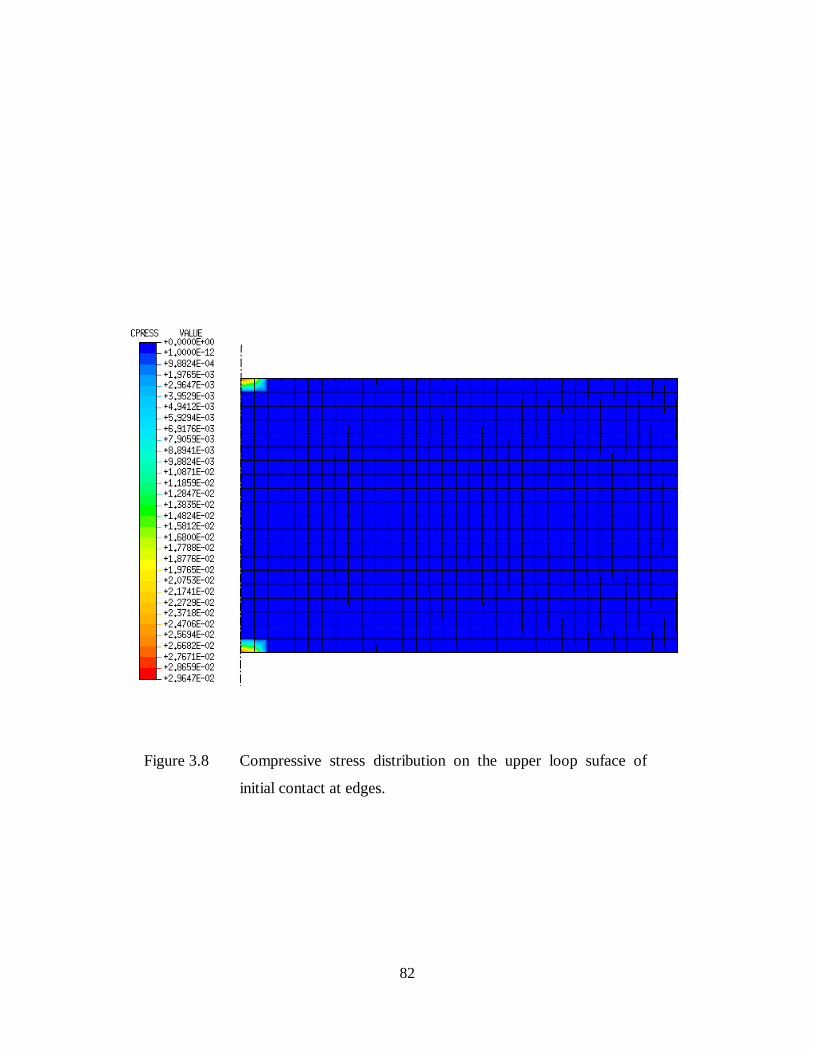
82
Figure 3.8 Compressive stress distribution on the upper loop suface of
initial contact at edges.
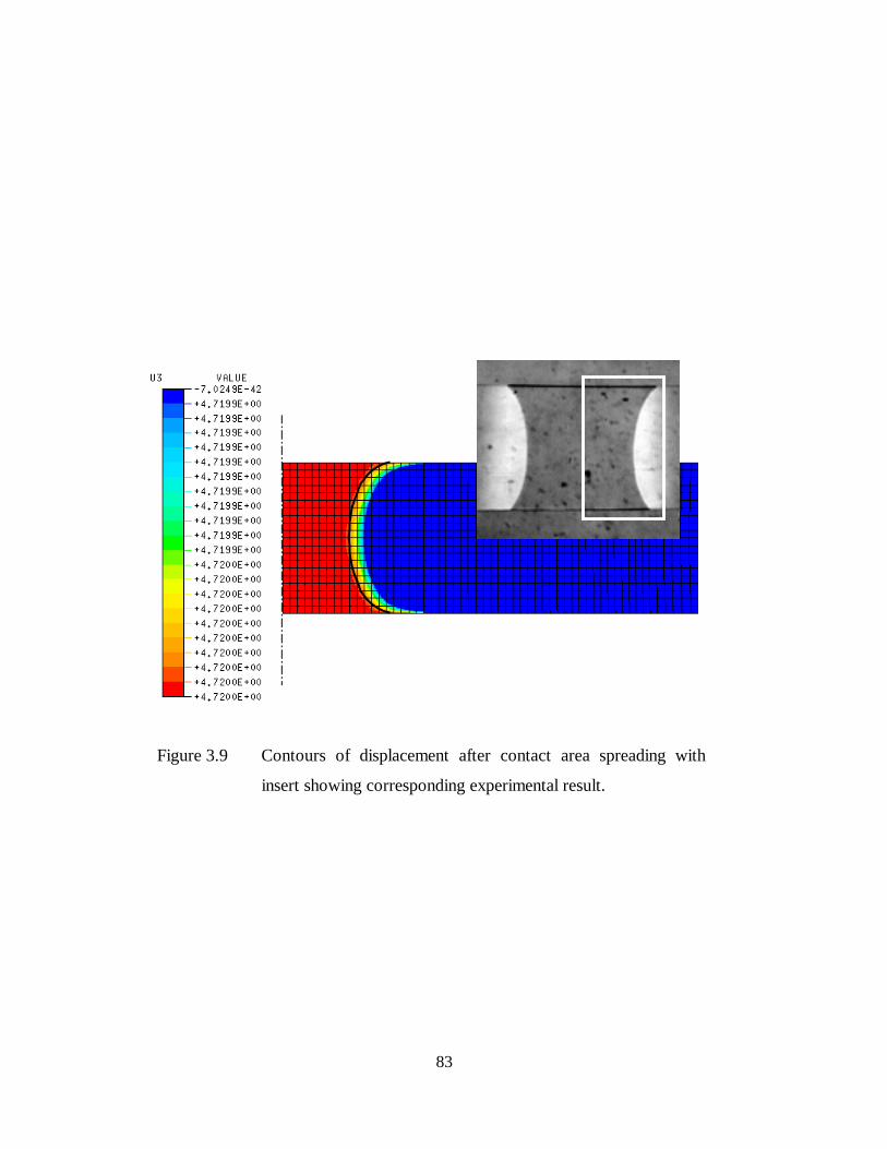
83
Figure 3.9 Contours of displacement after contact area spreading with
insert showing corresponding experimental result.
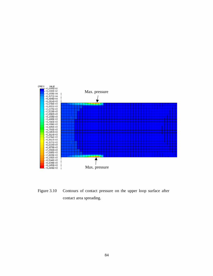
84
Figure 3.10 Contours of contact pressure on the upper loop surface after
contact area spreading.
Maximum contact pressure
Max. pressure
Max. pressure

85
Figure 3.11 Longitudinal strain on the concave side of the loop after
contact.
Low curvature High curvature
Center of the loop
End of the loop
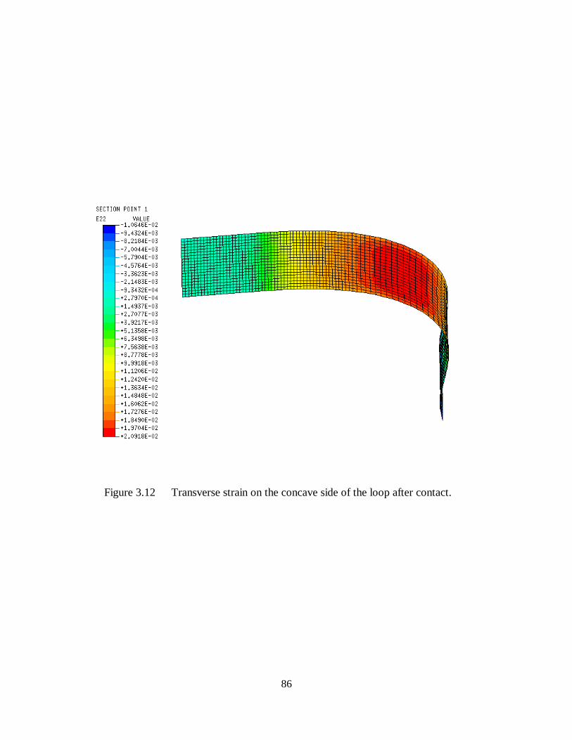
86
Figure 3.12 Transverse strain on the concave side of the loop after contact.

87
���
���
���
���
��� ��� ��� ��� ���
&RQWDFW )RUFH� ) �P1�
&RQWDFW/HQJWK��%�P
P�
:LGWK RI WKH ORRS
Figure 3.13 Plot of contact length vs. contact force: the contact lengths
were measured at the center point of the contact front.
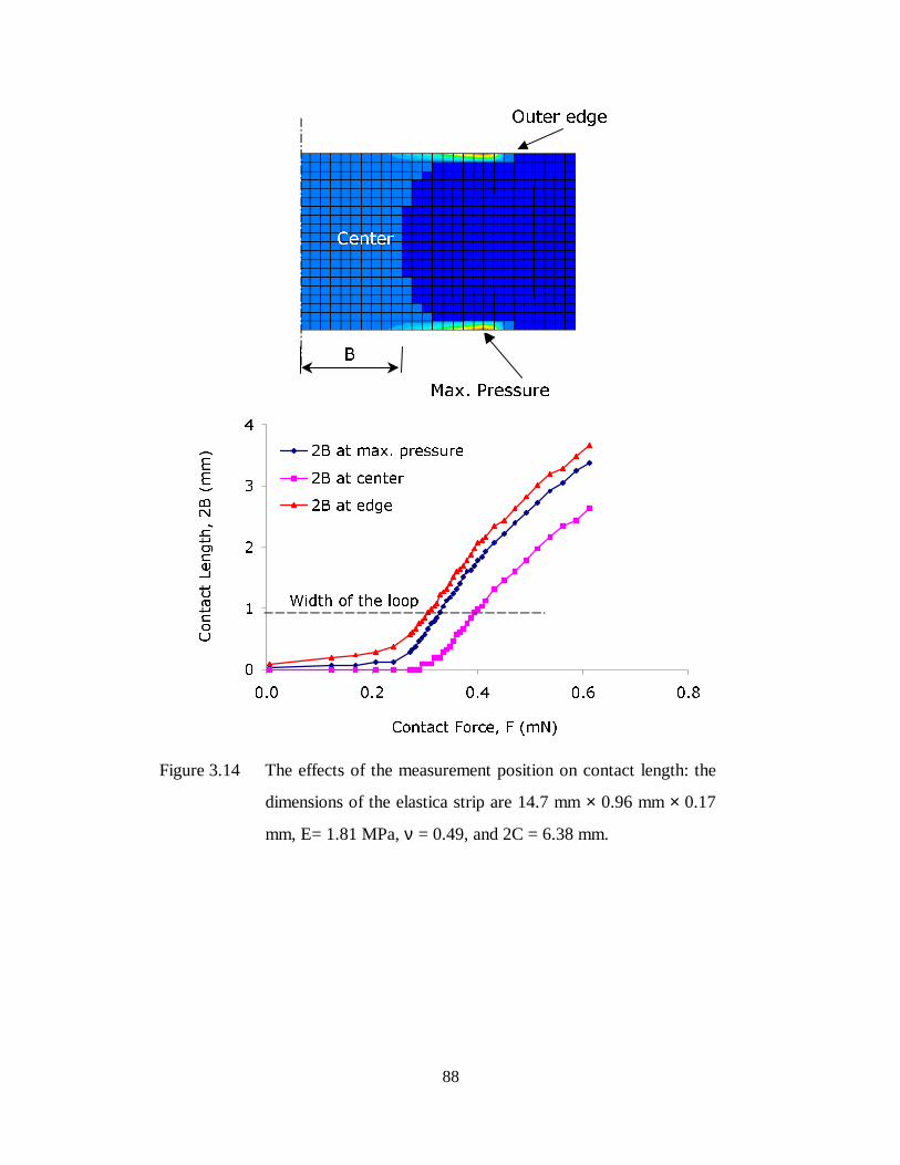
88
�
�
�
�
�
��� ��� ��� ��� ���
&RQWDFW )RUFH� ) �P1�
&RQWDFW/HQJWK��%�P
P� �% DW PD[� SUHVVXUH
�% DW FHQWHU
�% DW HGJH
:LGWK RI WKH ORRS
Figure 3.14 The effects of the measurement position on contact length: the
dimensions of the elastica strip are 14.7 mm × 0.96 mm × 0.17
mm, E= 1.81 MPa, ν = 0.49, and 2C = 6.38 mm.
0D[� 3UHVVXUH
2XWHU HGJH
%
&HQWHU
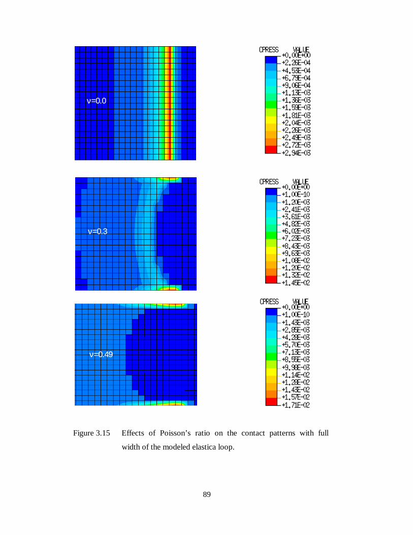
89
Figure 3.15 Effects of Poisson’s ratio on the contact patterns with full
width of the modeled elastica loop.
ν=0.3
ν=0.0
ν=0.49

90
�
�
�
�
�
��� ��� ��� ��� ���
&RQWDFW )RUFH� ) �P1�
&RQWDFW/HQJWK��%�P
P�
ν=0.49
ν=0.4
ν=0.3
ν=0.2
ν=0.1
ν=0
Figure 3.16 The relationship between contact length and contact force. The
contact length was taken as the center of the contact front.
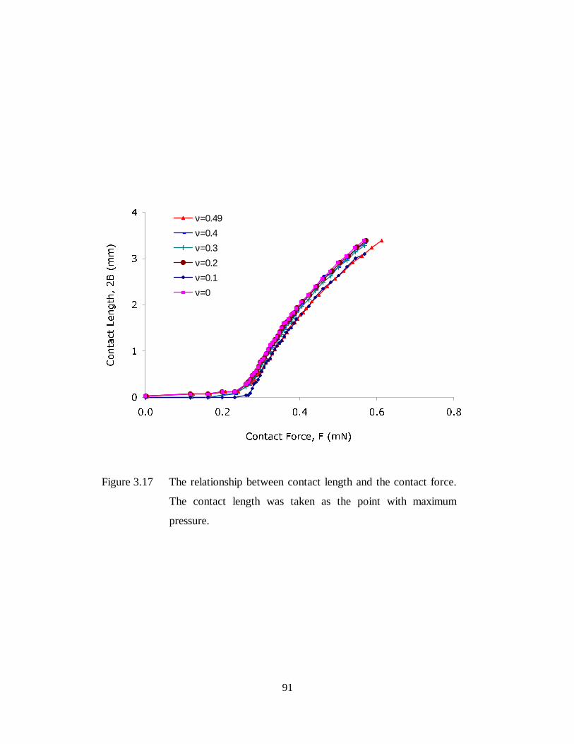
91
�
�
�
�
�
��� ��� ��� ��� ���
&RQWDFW )RUFH� ) �P1�
&RQWDFW/HQJWK��%�P
P�
ν=0.49ν=0.4ν=0.3ν=0.2ν=0.1ν=0
Figure 3.17 The relationship between contact length and the contact force.
The contact length was taken as the point with maximum
pressure.
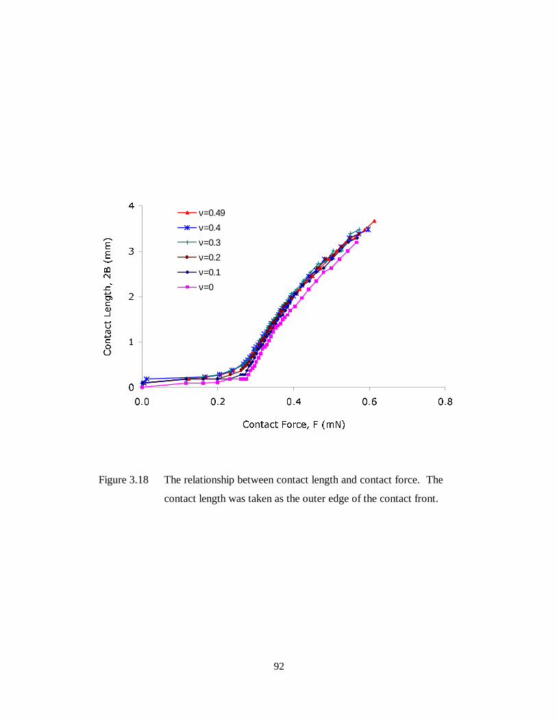
92
�
�
�
�
�
��� ��� ��� ��� ���
&RQWDFW )RUFH� ) �P1�
&RQWDFW/HQJWK��%�P
P�
ν=0.49ν=0.4ν=0.3ν=0.2ν=0.1ν=0
Figure 3.18 The relationship between contact length and contact force. The
contact length was taken as the outer edge of the contact front.
93
CHAPTER 4 Comparison of Experimental, Numerical,
and Analytical Results
4.1 Analytical solution
Analytical studies of an elastica loop in contact with a flat surface have been
conducted by Dalrymple [46]. In her analysis, the elastica strip was assumed to be a thin,
uniform, inextensible beam, which was very flexible in bending. To form the loop, both
of the ends were lifted to an equal height, rotated, and clamped vertically at a specified
distance apart. The loop was then moved downward and brought into contact with a flat,
rigid, horizontal surface as shown in Figure 4.1. The friction between the strip and the
flat surface was neglected, and attractive interfacial forces existed within the region of
contact between the elastica and the rigid substrate. As the load applied on the loop
continued to increase, the contact area increased and the strip flattened onto the substrate.
Due to the interfacial energy between the two surfaces, the attractive forces acting in the
region of contact caused additional loop deformation and extra contact area. By
comparing the differences of the contact length before and after the interfacial energy
was considered in the analysis, the adhesion effect can be determined.
The nondimensional length of the elastica was defined as 2l=2L/L=2. Based on
the length L and flexible rigidity, all other parameters in the analysis were
nondimensionalized such as the work of adhesion, wadh, contact length, b, contact forces,
q, displacement, δ, and the separation distance between the clamped ends, 2c, as listed in
Table 4.1, in which the value for Wadh, E, I, L, and C used were all taken directly from
the experiments. According to Figure 4.2, where the definitions of all the variables are
shown, the governing equations for an elastica in contact with a flat surface are given by

94
θcos=ds
dx, θsin=
ds
dy, m
ds
dEI =θ
, and θθ cossin qpds
dm +−=
where s is the arc length, θ is the angle of the tangent of the curve with respect to the
horizontal direction, p and q are the forces parallel to the x and y directions, respectively,
m is the moment, and EI is the flexural rigidity of the elastica. The appropriate end
conditions were then applied to solve for the desired parameters. For the no contact or
single-point contact cases, x = y =0 at s = 0, and x = c, θ = π/2 at s = 1. When a finite
contact area existed, the boundary conditions were x = y = θ =0 at s = 0 and x = c-b, θ =
π/2 at s=1-b, with s=0 at the lift-off point.
A shooting method was used to solve the governing nonlinear equilibrium
equations numerically in Mathematica. To use this method, initial values of p and m(0)
at s=0 were guessed, then the elastica equations were numerically integrated until s = 1
for the no contact and single-point contact cases, and s=1-b for the finite contact cases.
Once p and m(0) were determined to the desired precision, the shapes for the loop were
otained using the equations for x and y. To consider the effect of the interfacial
attraction, a moment, mb, as shown in Figure 4.3 was allowed to assume a non-zero value
at the point of the contact separation between the elastica and the substrate. The moment
mb was determined in the process of minimizing the total energy of the system with
respect to the contact length b.
Due to the lack of the surface energy term in the governing equations for an
elastica in contact with a flat surface, an energy minimization method was used to
account for its presence and to obtain the equilibrium position. The nondimensionalized
total energy of the system uT consisted of the strain energy, uE, mechanical potential
energy, uM, and adhesion energies, uΑ, as uT = uE + uM + uΑ . To determine the
equilibrium solution, the total energy uT was calculated for a variety of equilibrium loop
shapes obtained using the shooting method with constant end separation distance, c, and
vertical force, q, but varying contact length, b. The equilibrium shape with a minimum
95
total energy was determined as the equilibrium solution. Once the equilibrium solution
was obtained, the values mb and b were also determined. Obviously, the total calculation
process requires a series of iterations before a convergent solution can be obtained.
In addition, differences in the results caused by different loading cycles or
different control methods were also modeled in the analyses. The vertical forces and
displacements experienced by the elastica as the loop traveled through the no contact,
point contact, and line contact regions were dependent upon whether the elastica was
being pushed onto or pulled off of the substrate, or whether the vertical displacement or
the vertical force was being controlled during the contact sequence. When the vertical
displacement was controlled, the vertical force experienced a sudden jump in value.
When the vertical force was controlled, the vertical displacement experienced a sudden
jump in value. Similar findings are well known for JKR tests [22].
4.2 Comparison of numerical and analytical results
A comparison between the numerical results and the analytical results was made
through examining the contact length versus contact force curves obtained numerically
and analytically. To accomplish this, the geometry and material properties of the
samples were first nondimensionalized according to Table 4.1. Then the
nondimensionalized variables were input into the analytical solution program discussed
earlier to calculate the contact length versus contact force curve. The curve was then
converted back to quantities with units in order to compare with the numerical results.
Since the effect of interfacial energy was not present in the finite element analysis,
comparisons were made only between curves with no surface energy. Although the finite
element model did not include the effect of adhesion forces, the analysis did take into
account the anticlastic bending effect of the strip, a factor not included in the analytical
solution.
96
Figure 4.4 shows the contact length versus contact force curves obtained both
numerically and analytically. The dimensions of the loop used in the analyses were 14.7
mm in length, 0.96 mm in width, and 0.17 mm in thickness. The separation distance
between the two ends was 6.38 mm, the modulus of the material was 1.81 MPa, and the
Poisson’s ratio was 0.49. Due to the curved contact front caused by the anticlastic
bending of the strip, contact lengths were measured from the three different locations on
the contact front, i.e., the outer edge point of the contact front, center point of the arched
contact front, and the point with maximum contact pressure. Since beam theory was
used in the analytical solution, the effect of anticlastic bending was not considered. The
results show that the contact length predicted by the analytical solution is higher than the
contact length measured at the center point of the contact front, but is slightly lower than
the contact length measured at the point with maximum pressure. This difference in
results is very well understood when anticlastic bending is considered. Overall, the
analytical predictions agree with the numerical results. However, the analytical solution
fails to predict the portion of the numerical curves corresponding to contact lengths less
than half of the width of the loop. According to the numerical results, the contact length
increases with contact force slowly as the contact starts until the contact length passes a
certain value depending on the measuring position, where the contact starts to spread
rapidly. According to the figure, the analytical solution did not predict this contact
transition accurately.
Figure 4.5, Figure 4.6, and Figure 4.7 compare the analytical solution against
numerical predictions with different Poisson’s ratios and further demonstrate the effect of
anticlastic bending. In these figures, the contact lengths obtained in the numerical
analysis were taken from the three different locations discussed earlier, and each
numerical curve corresponds to a different Poisson’s ratio. If the contact length is
measured either from the center of the contact front or from the outer edge of the contact
front, Figure 4.6 and Figure 4.7 show that the analytical solution is relatively close to the
numerical curves with relatively low Poisson’s ratios. If the contact length is measured

97
from the point with maximum pressure, Figure 4.6 indicates that the analytical solution
agrees relatively well with the numerical curve with Poisson’s ratio of 0.49. These
results can again be explained using the effect of anticlastic bending. In the analytical
solution, the width effects of the loop were not modeled. As a result, the contact front in
the analytical solution is a straight line, which is comparable to the case of ν = 0 in the
finite element analysis when the contact length is measured from either the center point
of the contact front or from the outer edge. These results provide useful insights into the
choice of the proper point for measuring the contact length in the experiments and also
provide a possibility to estimate the error between the experiments and the analytical
solution.
4.3 Comparison of experimental and analytical results
Similarly, a comparison between the experimental data and the analytical results
was made by comparing the contact length versus contact force curves obtained
experimentally and analytically. To accomplish this, the geometry and the material
properties of the samples were first nondimensionalized according to Table 4.1. Then
the nondimensionalized variables were input into the analytical solution program
discussed earlier along with the interfacial energy measured in the JKR experiments to
calculate the contact length versus contact force curve. After the analytical solution was
obtained, the results were then converted back to quantities with units to compare with
the experimental results.
For the case of the PDMS loop in contact with a PDMS substrate, the dimensions
of the elastica loop were 14.7 mm in length, 0.96 mm in width, and 0.17 mm in
thickness. The separation distance between the two ends was 6.38 mm, the modulus of
the material was 1.81 MPa, and the Poisson’s ratio was assumed to be 0.49. The work of
adhesion measured between the two surfaces by the JKR technique was 43.6 mJ/m2,
which consequently leads to an interfacial energy value of 21.8 mJ/m2. Figure 4.8 shows
the analytical contact length versus contact force curve and the experimental data for
98
both the loading and unloading cycles. Due to the contact hysteresis discussed earlier,
the unloading data are shifted to the left of the loading data.
Figure 4.8 shows that the analytical solution and the experimental data have very
similar characteristics. Both results show that the contact length increases with the
contact force once the contact spreading occurs. On the other hand, the figure shows that
the portion of the experimental data corresponding to the contact lengths greater than half
of the width of the loop agree closely with the analytical curve obtained by ignoring the
surface energy. This result indicates that the effect of interfacial energy on the
deformation of the loop becomes less significant as the contact area increases, which is
possibly due to the decrease of the compliance of the loop when the contact length
increases, and the interfacial attractive force is not large enough to produce measurable
deformation. Moreover, the analytical solution fails to predict the portion of the
experimental data corresponding to the contact lengths less than half of the width of the
loop, which were obtained during the early stage of the contact procedure. Possible
reasons for the inconsistency of the experimental data with the analytical solution are:
a) Transverse sliding at the interface might occur during the contact procedure as the
load increased.
b) According to the analytical solution [45], when the loop is in contact with the
substrate, the contact pressure in the contact region is zero. Since the surface
attractive force only acts within a very small range near the surface and decreases
rapidly with the distance from the surface (proportional to r-3 according to
reference 3, where the r is the distance from the surface). Consequently, a small
asperity on the surface of the loop or slight contamination on the substrate may
decrease the degree of the intimate contact between the two surfaces in the center
of the loop. However, this decrease in the degree of intimate contact may not be
able to observe optically under the current macrolens system because the
wavelengths used might be essentially larger than the distance between these two
surfaces in the center of the loop. Although in the tests of this study, the PDMS
99
films were all carefully prepared and cured with little control of the surface
smoothness, microscopic-scale asperity or blisters caused by a small amount of
air trapped in the PDMS gel may still exist, which would certainly decrease the
degree of intimate contact between the two surfaces.
c) The effect of the anticlastic bending was not fully understood.
Very similar results have been found for the cases of the PDMS loop in contact
with a glass surface and the commercially available cellulose acetate substrate (3M
ScotchTM Transparent Tape 600) as indicated in Figure 4.9 and Figure 4.10. In the test
of the PDMS loop in contact with a glass surface, the dimension of this loop was 15.8
mm in length, 0.94 in width, and 0.17 mm in thickness. The separation distance between
the two ends was 6.38 mm, the modulus of the material was 1.81 MPa, and the Poisson’s
ratio was estimated as 0.49. In the case of the PDMS loop in contact with the
commercially available cellulose acetate substrate (3M ScotchTM Transparent Tape 600),
the dimensions of this loop were 15.8 mm in length, 0.84 in width, and 0.17 mm in
thickness. The separation distance between the two ends was 6.38 mm, the modulus of
the material was 1.81 MPa, and the Poisson’s ratio was estimated as 0.49. Figure 2.9 and
Figure 4.10 again show that the experimental data points corresponding to the contact
lengths greater than half of the width of the loop fall near the analytical curve obtained
by ignoring the presence of surface energy, and the analytical solution fails to predict the
portion of the experimental curve corresponding to the contact lengths less than half of
the width of the loop.
In summary, Figure 4.11 shows a comparison of the experimental, numerical, and
analytical results for tests of the PDMS-PDMS system.
4.4 Sensitivity studies of errors
To investigate the effect of errors in measuring geometry and material properties
on the predictions of the analytical solution, sensitivity studies were performed by
100
changing the sample geometry and material modulus in the analytical solution. The case
of the PDMS loop in contact with PDMS substrate was chosen for this study. The actual
dimensions of the elastica loop were 14.7 mm in length, 0.96 mm in width, and 0.17 mm
in thickness. The actual separation distance between the two ends was 6.38 mm, the
modulus of the material was 1.81 MPa, and the Poisson’s ratio was 0.49. The work of
adhesion measured between the two surfaces was 43.6 mJ/m2, which consequently led to
the interfacial energy value of 21.8 mJ/m2.
Figure 4.12 shows the effect of reducing the length of the strip 2L by 5%, 10%,
and 20% on the resultant contact length versus contact force curve. The figure shows
that the analytical curve leaned toward the experimental results as the length of the strip
decreased, and at the same time the overall curvature of the curve increased, which
indicates that overestimating the length of the strip would cause the analytical solution to
differ from the experimental results. On the other hand, underestimating the length of the
strip would cause the analytical solution to be closer to the experimental results.
Similarly, the effect of changing the width of the loop W was studied and the
results are shown in Figure 4.13. The effect of varying the thickness of the loop t is
shown in Figure 4.14, and the effect of reducing the separation distance 2C between the
two clamped ends is shown in Figure 4.15. All the figures indicate that increasing W or t
and reducing C would make the analytical solution closer to the experimental data, which
can help us identify possible sources of measurement errors.
Young’s modulus was also considered as a possible source of errors. Therefore,
the effect of changing the modulus of the loop was studied by increasing the modulus by
10%, 20%, and 30% in the analysis, and the results are shown in Figure 4.16. The figure
shows that the analytical contact length versus contact force curve has a trend moving
closer to the experimental data as the modulus increases. On the other hand, reducing the

101
modulus of the loop will cause the analytical solution to differ more from the
experimental data.
4.5 PDMS loop in contact with various substrates
Because all the experimental results are close to the analytical solution with γ=0,
experiments of PDMS loop in contact with four different substrates were performed to
study the sensitivity of this technology with respect to various interfacial interactions.
The four substrates were a glass plate treated with chemical Au etch, a glass plate
deposited with a layer of Cu, acetone cleaned glass plate, and a glass plate with a 30 min
treatment of vinylsilane. Following the testing procedure discussed in Chapter 2, the
relationships of the contact length 2B versus contact force F were obtained for these four
substrates as shown in Figure 4.17. The figure indicates that the differences between the
loading curves for the four interfaces are relatively small. However, the unloading
curves and the hysteresis loop for these four interfaces significantly differ from each
other, which is possible due to the different interfacial interactions.
A possible explanation for the small differences between the loading curves is
that intimate contact especially in the center of the loop as the contact increased was not
achieved between the surfaces in contact, and experimental data differed from the
analytical solution with γ > 0 significantly but agree with the analytical solution with γ =
0 more. As discussed earlier, according to the analytical solution [45], when the loop is
in contact with the substrate, the contact pressure in the contact region is zero. Since the
surface attractive force only acts within a very small range near the surface and decreases
rapidly with the distance from the surface (proportional to r-3 according to reference 3,
where the r is the distance from the surface). Consequently, a small asperity on the
surface of the loop or slight contamination on the substrate may decrease the degree of
the intimate contact between these two surfaces in the center of the loop. However, this
decrease in the degree of intimate contact may not be able to observe optically under the
current microscope system because the wavelengths used might be essentially larger than
102
the distance between these two surfaces in the center of the loop. Although in the tests of
this study, the PDMS films were all carefully prepared and cured with little control of the
surface smoothness, microscopic-scale asperity or blisters caused by a small amount of
air trapped in the PDMS gel may still exist, which would certainly decrease the degree of
intimate contact between the two surfaces.
The testing apparatus may also have possible sources of errors. In the analytical
solution, the vertically symmetric line of the loop passing through the center of the loop
and the middle point of the end separation distance were assumed to be perfectly
perpendicular to the substrate. However, this perfect alignment was very difficult to
accomplish during the tests, which may cause slight changes in the readings of the
contact lengths. Additionally, in the analytical solution, the substrate was considered as
a flat, rigid, and smooth surface. But in the experiments, the coatings with certain
thickness were not perfectly rigid, which, although the effect was estimated to be small in
this study, may still cause some errors for the tests. Knowing these possible sources of
error will help us improve the accuracy of the analytical solution and the experimental
measurements.
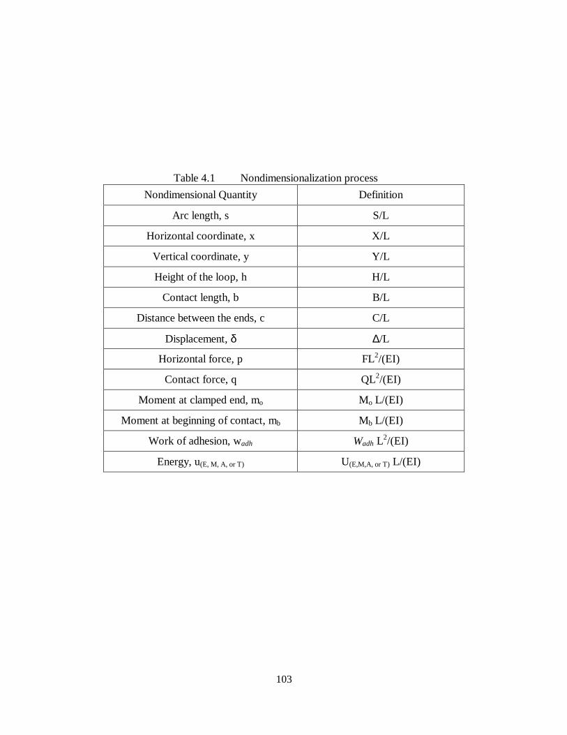
103
Table 4.1 Nondimensionalization process
Nondimensional Quantity Definition
Arc length, s S/L
Horizontal coordinate, x X/L
Vertical coordinate, y Y/L
Height of the loop, h H/L
Contact length, b B/L
Distance between the ends, c C/L
Displacement, δ ∆/L
Horizontal force, p FL2/(EI)
Contact force, q QL2/(EI)
Moment at clamped end, mo Mo L/(EI)
Moment at beginning of contact, mb Mb L/(EI)
Work of adhesion, wadh Wadh L2/(EI)
Energy, u(E, M, A, or T) U(E,M,A, or T) L/(EI)
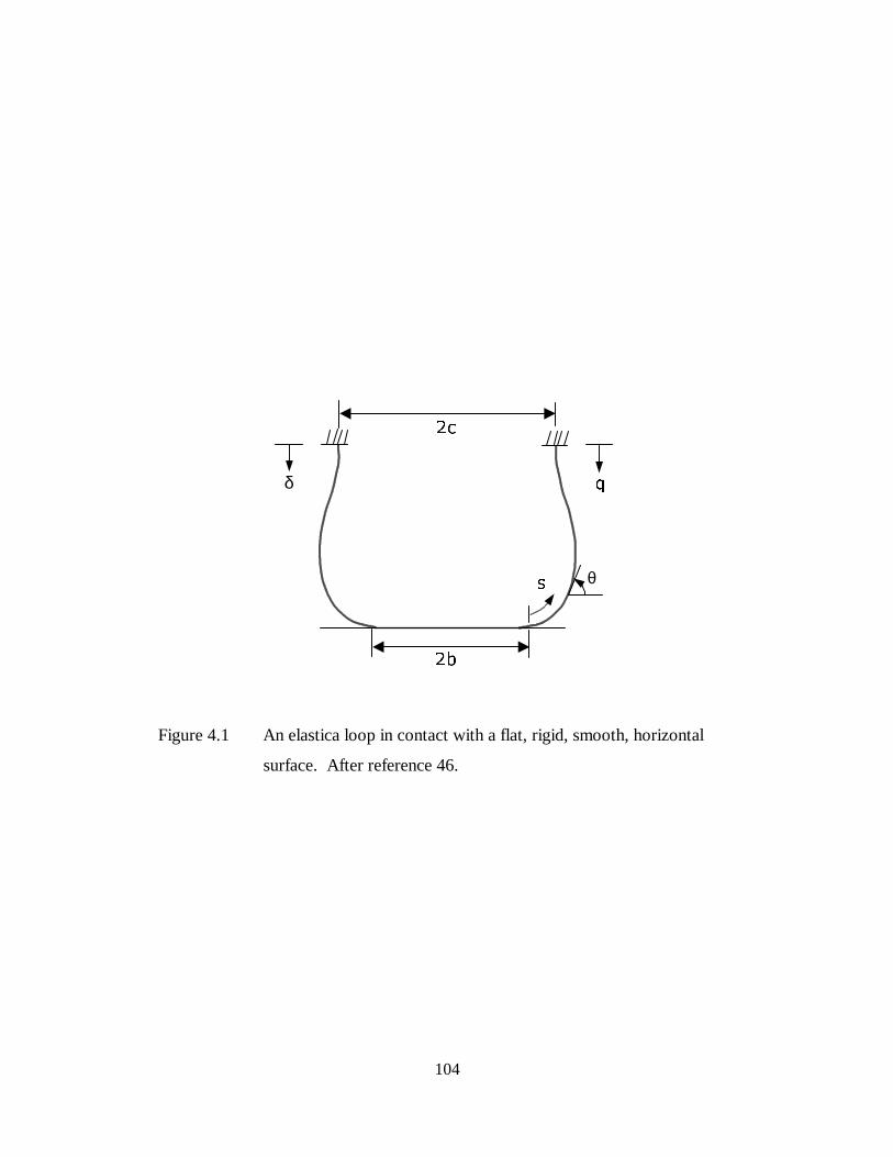
104
Figure 4.1 An elastica loop in contact with a flat, rigid, smooth, horizontal
surface. After reference 46.
θ
�E
�F
Tδ
V
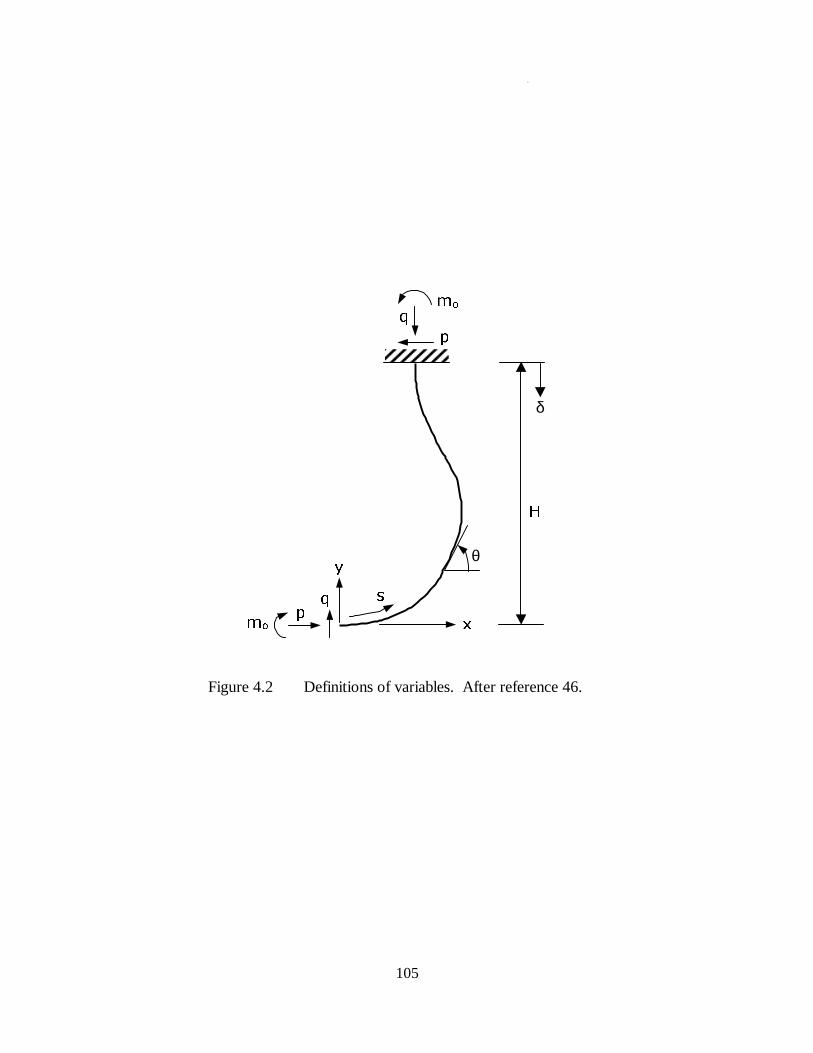
105
Figure 4.2 Definitions of variables. After reference 46.
+
PR
T
T
S
SPR [
\θ
δ
V
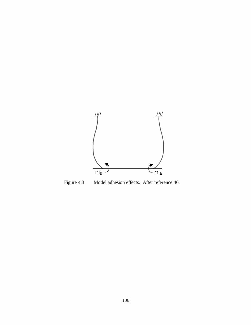
106
Figure 4.3 Model adhesion effects. After reference 46.
PE PE
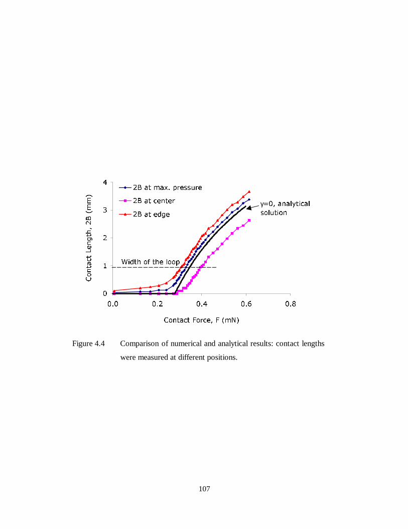
107
�
�
�
�
�
��� ��� ��� ��� ���
&RQWDFW )RUFH� ) �P1�
&RQWDFW/HQJWK��%�P
P�
�% DW PD[� SUHVVXUH
�% DW FHQWHU
�% DW HGJH
γ �� DQDO\WLFDOVROXWLRQ
:LGWK RI WKH ORRS
Figure 4.4 Comparison of numerical and analytical results: contact lengths
were measured at different positions.

108
�
�
�
�
�
��� ��� ��� ��� ���
&RQWDFW )RUFH� ) �P1�
&RQWDFW/HQJWK��%�P
P�
ν=0.49ν=0.3ν=0.1ν=0γ=0 $QDO\WLFDO
VROXWLRQ
Figure 4.5 Comparison of numerical and analytical results: contact lengths
were measured in the cases with different value of Poisson’s
ratio at the center of contact front.
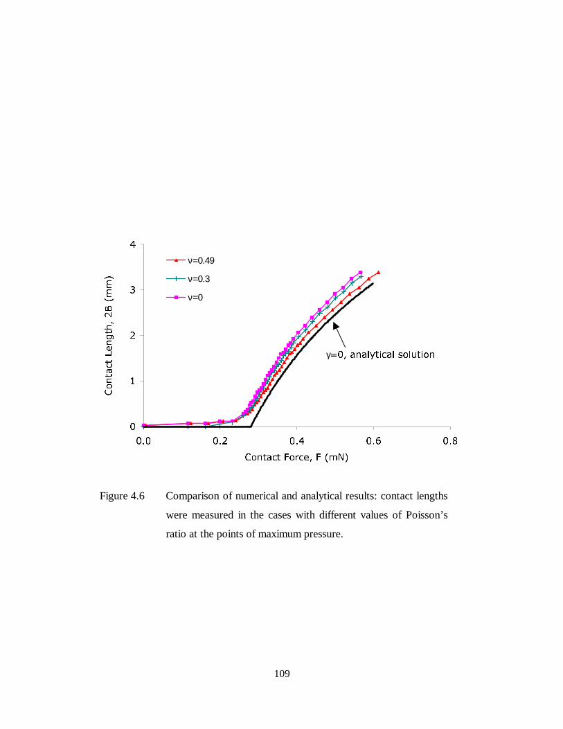
109
�
�
�
�
�
��� ��� ��� ��� ���
&RQWDFW )RUFH� ) �P1�
&RQWDFW/HQJWK��%�P
P�
ν=0.49
ν=0.3
ν=0
γ �� DQDO\WLFDO VROXWLRQ
Figure 4.6 Comparison of numerical and analytical results: contact lengths
were measured in the cases with different values of Poisson’s
ratio at the points of maximum pressure.
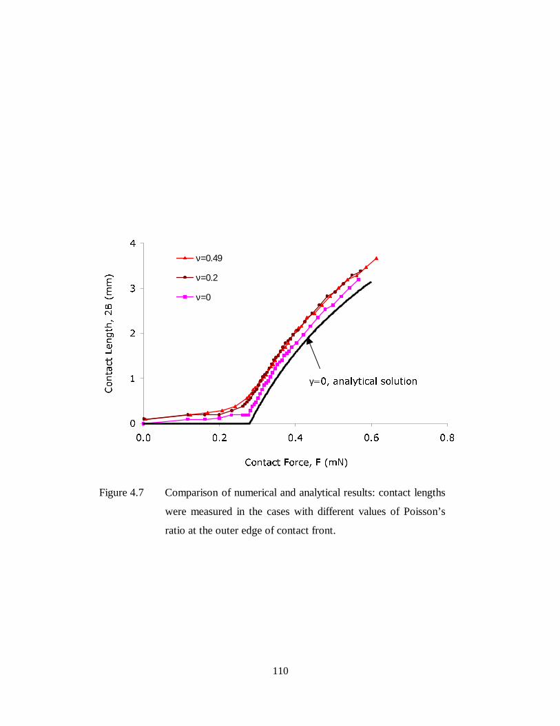
110
�
�
�
�
�
��� ��� ��� ��� ���
&RQWDFW )RUFH� ) �P1�
&RQWDFW/HQJWK��%�P
P�
ν=0.49
ν=0.2
ν=0
γ �� DQDO\WLFDO VROXWLRQ
Figure 4.7 Comparison of numerical and analytical results: contact lengths
were measured in the cases with different values of Poisson’s
ratio at the outer edge of contact front.
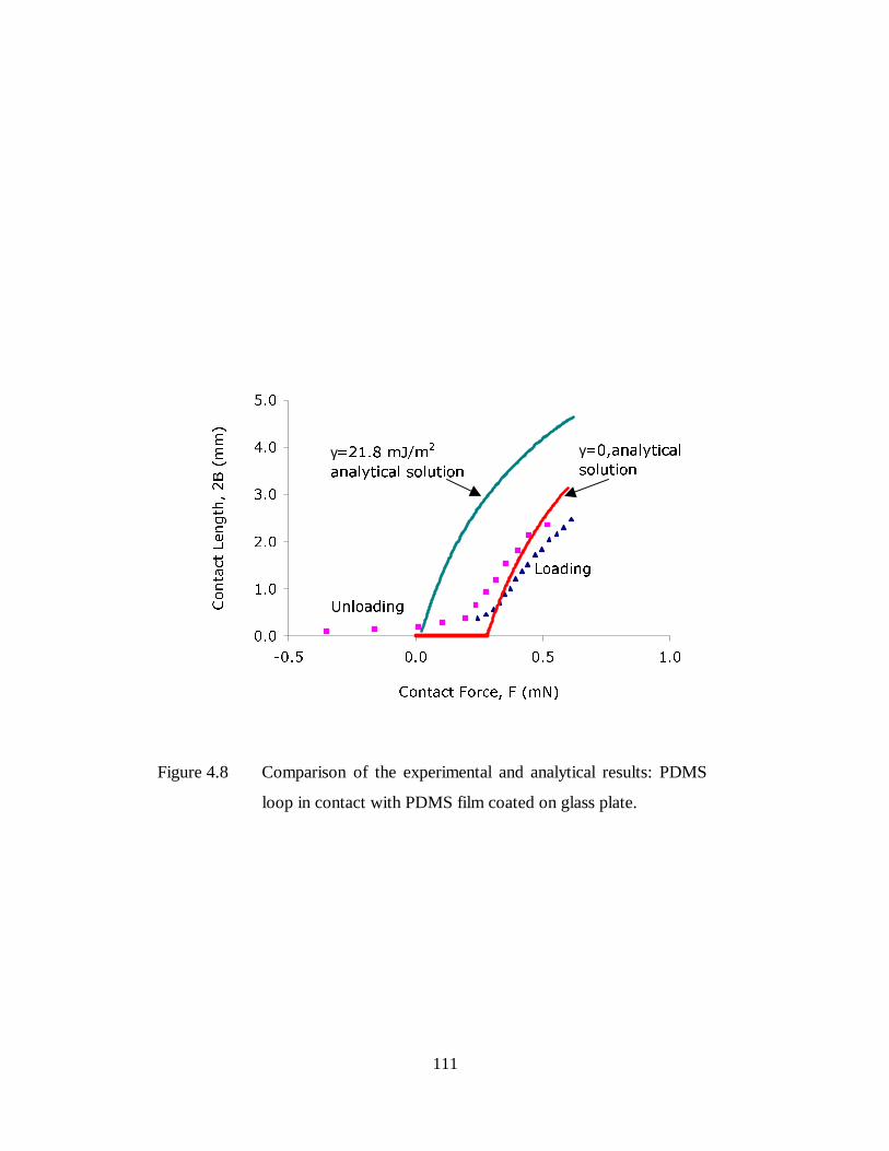
111
���
���
���
���
���
���
���� ��� ��� ���
&RQWDFW )RUFH� ) �P1�
&RQWDFW/HQJWK��%�P
P�
γ ���� P-�P�
DQDO\WLFDO VROXWLRQ
γ ��DQDO\WLFDOVROXWLRQ
/RDGLQJ
8QORDGLQJ
Figure 4.8 Comparison of the experimental and analytical results: PDMS
loop in contact with PDMS film coated on glass plate.
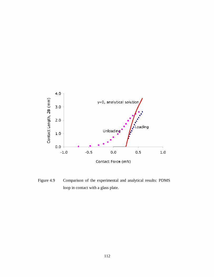
112
���
���
���
���
���
���� ���� ��� ��� ���
&RQWDFW )RUFH �P1�
&RQWDFW/HQJWK��%�P
P�
γ �� DQDO\WLFDO VROXWLRQ
/RDGLQJ8QORDGLQJ
Figure 4.9 Comparison of the experimental and analytical results: PDMS
loop in contact with a glass plate.
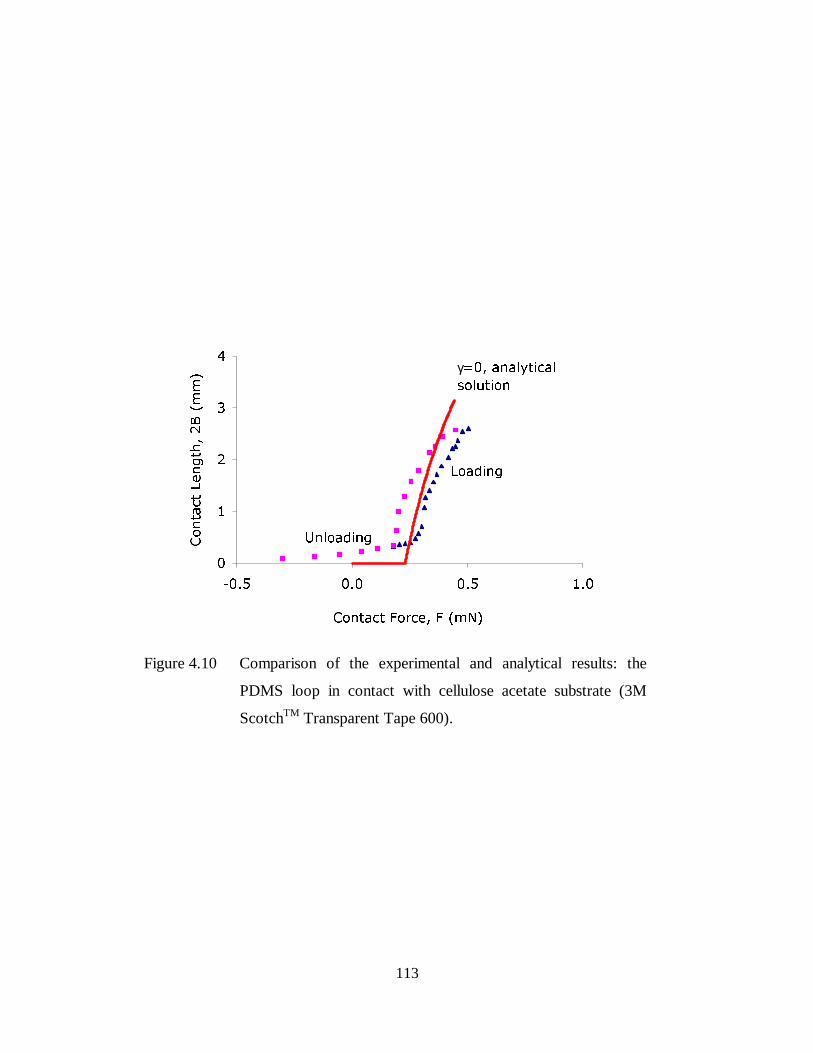
113
�
�
�
�
�
���� ��� ��� ���
&RQWDFW )RUFH� ) �P1�
&RQWDFW/HQJWK��%�P
P�
γ �� DQDO\WLFDOVROXWLRQ
8QORDGLQJ
/RDGLQJ
Figure 4.10 Comparison of the experimental and analytical results: the
PDMS loop in contact with cellulose acetate substrate (3M
ScotchTM Transparent Tape 600).
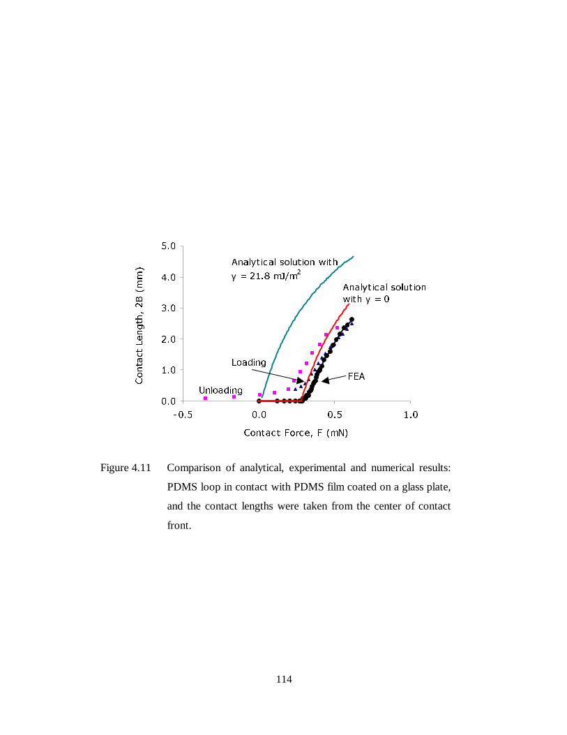
114
���
���
���
���
���
���
���� ��� ��� ���
&RQWDFW )RUFH� ) �P1�
&RQWDFW/HQJWK��%�P
P�
/RDGLQJ
$QDO\WLFDO VROXWLRQ
ZLWK γ �
8QORDGLQJ
$QDO\WLFDO VROXWLRQ ZLWK
γ ���� P-�P�
)($
Figure 4.11 Comparison of analytical, experimental and numerical results:
PDMS loop in contact with PDMS film coated on a glass plate,
and the contact lengths were taken from the center of contact
front.

115
�
�
�
�
�
�
���� ��� ��� ��� ���
&RQWDFW )RUFH� ) �P1�
&RQWDFW/HQJWK��%�P
P�
γ � ZLWK /
γ ���� P-�P�ZLWK
8QORDGLQJ
/RDGLQJ
��������
���
Figure 4.12 Effects of reducing length by 5%, 10%, 20%.
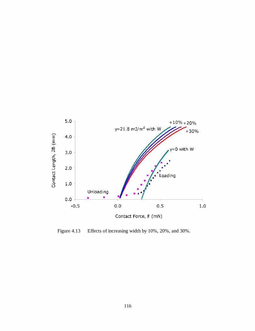
116
���
���
���
���
���
���
���� ��� ��� ���
&RQWDFW )RUFH� ) �P1�
&RQWDFW/HQJWK��%�P
P�
γ ���� P-�P�ZLWK :
γ � ZLWK :
8QORDGLQJ
/RDGLQJ
����
��������
Figure 4.13 Effects of increasing width by 10%, 20%, and 30%.
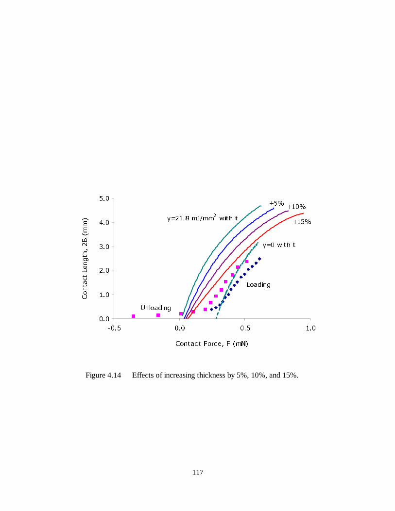
117
Figure 4.14 Effects of increasing thickness by 5%, 10%, and 15%.
���
���
���
���
���
���
���� ��� ��� ���
&RQWDFW )RUFH� ) �P1�
&RQWDFW/HQJWK��%�P
P�
/RDGLQJ
8QORDGLQJ
γ ���� P-�PP�ZLWK W
γ � ZLWK W
���
����
����
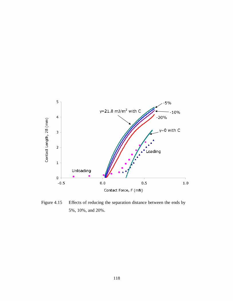
118
�
�
�
�
�
�
���� ��� ��� ���
&RQWDFW )RUFH� ) �P1�
&RQWDFW/HQJWK��%�P
P�
γ ���� P-�P�ZLWK &
γ � ZLWK &
/RDGLQJ
8QORDGLQJ
����
����
���
Figure 4.15 Effects of reducing the separation distance between the ends by
5%, 10%, and 20%.
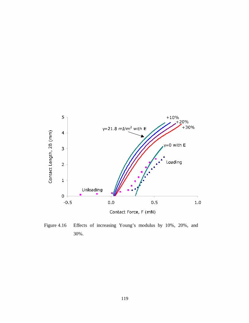
119
�
�
�
�
�
�
���� ��� ��� ���
&RQWDFW )RUFH� ) �P1�
&RQWDFW/HQJWK��%�P
P� γ ���� P-�P�
ZLWK (
γ � ZLWK (
����
��������
/RDGLQJ
8QORDGLQJ
Figure 4.16 Effects of increasing Young’s modulus by 10%, 20%, and
30%.
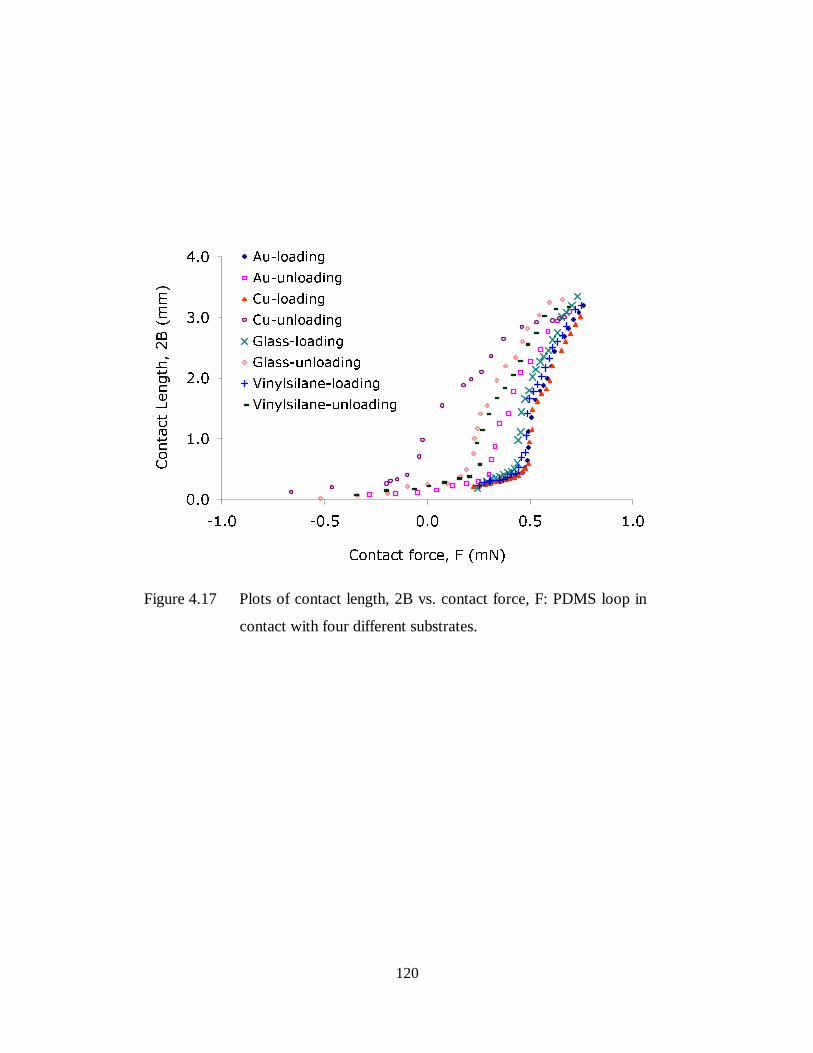
120
���
���
���
���
���
���� ���� ��� ��� ���
&RQWDFW IRUFH� ) �P1�
&RQWDFW/HQJWK��%�P
P�
$X�ORDGLQJ
$X�XQORDGLQJ
&X�ORDGLQJ
&X�XQORDGLQJ
*ODVV�ORDGLQJ
*ODVV�XQORDGLQJ
9LQ\OVLODQH�ORDGLQJ
9LQ\OVLODQH�XQORDGLQJ
Figure 4.17 Plots of contact length, 2B vs. contact force, F: PDMS loop in
contact with four different substrates.

121
CHAPTER 5 Conclusions and Recommendations for
Future Work
5.1 Summary and conclusions
In this thesis, a novel technique has been developed to measure the surface and
interfacial energies between solids using an elastica loop. The apparatus consists of a
precise displacement control device, an accurate force measurement device, an optical
system, and a computer control interface that has been built in order to perform the
measurement in a well-controlled manner. Experiments of a PDMS elastica loop in
contact with four different substrates have been conducted along with the conventional
JKR tests. Through the investigations of the experimental procedure, experimental data,
and comparisons between the experimental, numerical, and analytical results, the
following conclusions are made:
1. Overall, the current apparatus is a successful design, upon which both the
conventional JKR measurement and the elastica loop test can be conducted. For
the PDMS-PDMS system tested, the JKR test results obtained using the apparatus
were consistent with those reported in the literature.
2. For transparent materials, the contact patterns for both the JKR and elastica loop
tests can be observed using the current optical system with about 50x
magnification factor. Due to the compliant structure design, the contact length
observed in the elastica loop test was in general larger than the contact diameter
observed in the JKR test. However, due to anticlastic bending, the contact front
observed in the elastica loop test was curved. Based on a variety of experimental
observations and finite element analyses, the shape of the contact front remained
relatively constant during the entire contact process.

122
3. The displacement control system provided very precise contact process control.
Because of the precise displacement control, the events such as the initiation,
spread, and separation of the contact were well controlled and the finite contact
area at the moment of contact initiation and separation were clearly observed and
were accurately measured.
4. With the force measurement device and the computer control interface, the
contact force can be measured simultaneously with the displacement at a
specified rate of data acquisition. As compared to the conventional JKR test, the
contact force measured in the elastica loop test was in general smaller.
5. Through testing a PDMS elastica loop in contact with various substrates, the
relationships between the contact lengths versus contact forces were obtained for
each system. The results indicated that the contact length increased slowly with
the contact force as the contact started until the contact length exceeded about
half of the width of the loop, when the contact started to spread rapidly. The
finite element analyses indicated that this contact rate transition was due to the
combined effects of longitudinal main bending and anticlastic bending. The
difference between the experimental data and FEA results should be the effect of
the interfacial energies.
6. Large hysteresis has been observed in the contact length versus contact force
curves for all the material systems tested. The hysteresis was primarily caused by
interfacial interactions in the contact region and appeared to be rate dependent.
7. The FEA numerical analyses successfully simulated the contact procedure.
Through the analyses, the relationship between the contact length and the contact
force for the case with no interfacial energy was obtained, which was used to
verify the analytical solution. The numerical analyses also helped to investigate
the strain and stress states of the elastica loop, the contact pressure distribution,
and the effect of the anticlastic bending.
8. The FEA numerical analyses successfully demonstrated the effect of anticlastic
bending. Due to the effect of anticlastic bending, the contact front between the
123
loop and the flat surface was curved, and the curvature was larger than that of the
contact front observed in the experiments, indicating the effect of the interfacial
interaction. The results also showed that the anticlastic bending effect decreased
as the Poisson’s ratio decreased and vanished when the Poisson’s ratio was zero.
9. Overall the analytical solution agreed with the numerical analyses results
corresponding to ν = 0 after the contact rate transition had occurred. However,
since the anticlastic bending was not considered in the analytical solution,
differences did exist, especially when the contact length is measured from the
center of the contact front. In addition, for the same reason, the analytical
solution did not predict the contact rate transition and the contact initiation.
10. The agreement between the analytical solution and the experimental data was
relatively poor. Possible reasons for this poor agreement were discussed in the
sensitivity studies through identifying possible sources of errors in the tests.
These possible sources of errors include the measurement errors of the geometry
and modulus of the loop and testing misalignment. In addition, transverse sliding
at the interface might occur during the contact procedure as the load increased;
intimate contact in the center of the loop might not achieved; and the effect of the
anticlastic bending might not fully understood.
5.2 Limitations
Despite the poor agreement with the analytical solution, this elastica loop test still
remains a novel technique with potential for measuring interfacial energies between
solids. However, there are still limitations with the current apparatus and technique.
First of all, this technique requires very careful sample preparation. The elastica
strips need to be very thin to achieve desirable loop compliance, which, especially for
materials with high modulus, sometimes may be very difficult. In order to use this
technique, the surfaces of the loop and the substrate need to be very smooth because the
124
interfacial attraction only acts within a very small range, and surface asperities will
significantly decrease the effect of surface energy on the deformation of the elastica loop.
The settings of the optical system in the current apparatus can only work with
transparent substrate in order to observe the contact area from the top of the interface.
To work with non-transparent material as the substrate, a new optical system which
would allow observation of the contact from the side of the interface would be necessary
to overcome the limitation.
In all the tests conducted in this study, low modulus PDMS loops were used.
However, this technique possibly can be used to measure the interfacial energies between
materials with high modulus. If one of the materials of interest is transparent, this
material has to be used as the substrate with the current setup. On the other hand, if none
of the materials of interest is transparent, then the new optical systems mentioned earlier
are needed. However, for the loops made of high modulus materials, the thickness of the
loop needs to be very thin to achieve a desirable structural compliance. Some trial
experiments also showed that contact buckling occurred easily in testing a loop with high
modulus, which greatly increases the difficulty of the test. In addition, intimate contact
between the loop and the substrate may also be very difficult to achieve. Consequently,
the test should also be focused on achieving contact initiation and spread curves in order
to obtain information on interfacial interactions.
5.3 Future work
For the future work, the most important experimental issue needs to be addressed
is to detect the intimate contact level because the interfacial interactions are not able to
detect if intimate contact is not achieved between the surfaces in contact. To this end,
experimental devices can be further improved. For example, special filters can be added
to the light source of the microscope system to achieve a light with single short wave
length, which can help us to detect the contact level more clearly. The measuring device
125
for contact length can also be redesigned so that measurements can be taken either from
the top or from the side of the interface. More experiments involving stiffer materials
can be investigated. To perform the tests, substrates narrower than the elastica loop can
possibly be used and contact can be controlled to only occur in the center of the width of
the loop since the effect of anticlastic bending has been thoroughly investigated and
understood. In this way, a relatively uniform contact length will result, and the
possibility of contact buckling will also be reduced. In addition, investigations to take
the adhesion forces into account in the numerical analysis can be conducted, and the rigid
substrate can be modeled as a high modulus material with a coating on the surface in
order to simulate the contact behavior more accurately.

126
References
[1]. A. J. Kinloch, Adhesion and Adhesives: Science and Technology, Chapman & Hall,
1994.
[2]. V. S. Mangipudi and M. Tirrell, Contact-mechanics-based studies of adhesion
between polymers, Rubber Chemistry and Technology, 71, 407-447, 1998.
[3]. A. W. Adamson and A. P. Gast, Physical Chemistry of Surfaces, Wiley-
Interscience, New York, 1997.
[4]. A. N. Gent and J. Schultz, Effect of wetting liquids on the strength of adhesion of
viscoelastic materials, Journal of Adhesion, 3, 281, 1972.
[5]. E. H. Andrews and A. J. Kinloch, Mechanics of Adhesive, Proc. R. Soc. London,
Ser. A 332, 385-389, 1973.
[6]. J. P. Wightman, T.D. Lin, and H. F. Webster, Surface chemical aspects of
polymer/metal adhesion, International Journal of Adhesion and Adhesives, 12,
133-137, 1992.
[7]. J. N. Israelachvili, Intermolecular and Surface Forces: with Application to
Colloidal and Biological Systems, Academic Press, London, 1985.
[8]. K. L. Johnson, Contact mechanics, Cambridge University Press, Cambridge,
England, 1985.
[9]. E. H. Lee and J. R. M. Radok, The contact problem for viscoelastic bodies, J. Appl.
Mech., 27, 438-444, 1960.

127
[10]. G. A. C. Graham, The contact problem in the linear theory of viscoelasticity when
the time dependent contact area has any number of maximum and minimum, Int. J.
Engng. Sci., 5, 495-514, 1967.
[11]. W. H. Yang, The contact problem for viscoelastic bodies, J. Appl. Mech., 33, 359-
401, 1966.
[12]. K. L. Johnson, K. Kendall, and A. D. Roberts, Surface energy and the contact of
elastic solids, Proc. R. Soc. London, A 324, 301-313, 1971.
[13]. D. Tabor, Surface forces and surface interactions, Journal of Colloid and Interface
Science, 58, 2-13, 1977.
[14]. M. K. Chaudhury, and G. M. Whitesides, Direct measurement of interfacial
interactions between semispherical lenses and flat sheets of poly(dimethlysiloxane)
and their chemical derivatives, Langmuir, 7, 1013-1025, 1991.
[15]. V. S. Mangipudi, M. Tirrell and A. V. Pocius, Direct measurement of molecular
level adhesion between poly(ethylene terephthalate) and polyethylene films:
determination of surface and interfacial energies, Journal of Adhesion Science and
Technology, 8, 1251-1270, 1994.
[16]. V. S. Mangipudi, M. Tirrell, and A. V. Pocius, Direct measurement of the surface
energy of Corona-treated polyethylene using the surface forces apparatus,
Langmuir, 11, 19-23, 1995.
[17]. M. Tirrell, Measurement of interfacial energy at solid polymer surfaces, Langmuir,
12, 4548-4551, 1996.
[18]. V. S. Mangipudi, E. Huang, M. Tirrell, and A. V. Pocius, Measurement of
interfacial adhesion between glassy polymers and using JKR method, Macromol.
Symp., 102, 131-143, 1996.

128
[19]. D. Ahn and K. R. Shull, JKR studies of acrylic elastomer adhesion to glassy
polymer substrate, Macromolecules, 29, 4381-4390, 1996.
[20]. K. R. Shull, D. Ahn, and C. L. Mowery, Finite-size correction to the JKR
technique for measuring adhesion: soft spherical caps adhering to flat, rigid
surface, Langmuir, 13, 1799-1804, 1997.
[21]. R. G. Horn, J. N. Israelachvili, and F. Pribac, Measurement of the deformation and
adhesion of solids in contact, Journal of Colloid and Interface Science, 115, 480-
492, 1987.
[22]. I. Sridhar, K. L. Johnson and N. A. Fleck, Adhesion mechanics of the surface force
apparatus, Journal of Physics, D: Applied Physics, 30, 1710-1719, 1997.
[23]. B. V. Derjaguin, V. M. Muller and Y. P. Toporov, Effect of contact deformations
on the adhesion of particles, Journal of Colloid and Interface Science, 53, 314-326,
1975.
[24]. V. M. Muller, V. S. Yushchenko and B. V. Derjaguin, On the influence of
molecular forces on the deformation of an elastic sphere and its sticking to a rigid
plane, Journal of Colloid and Interface Science, 77, 91-101, 1980.
[25]. V. M. Muller, V. S. Yushchenko and B. V. Derjaguin, General theoretical
consideration of the influence of surface forces on contact deformations and the
reciprocal adhesion of elastic spherical particles, Journal of Colloid and Interface
Science, 92, 92-101, 1983.
[26]. M. D. Pashley, Further consideration of the DMT model for elastic contact,
Colloids and Surfaces, 12, 69-77, 1984.
[27]. D. J. Tabor, Role of molecular forces in contact deformations, Journal of Colloid
and Interface Science, 73, 294, 1980.
129
[28]. D. J. Tabor, Surface forces and surface interactions, Journal of Colloid and
Interface Science, 58, 2-13, 1977.
[29]. D. Maugis, Adhesion of spheres: the JKR-DMT transition using the Dugdale
model, Journal of Colloid and Interface Science, 150, 243-269, 1992.
[30]. D. Maugis and M. B. Gauthier, JKR-DMT transition in the presence of a liquid
meniscus, Journal of Adhesion Science and Technology, 8, 1311-1322, 1994.
[31]. J. M. Baney and C. Y. Hui, A cohesive zone model for the adhesion of cylinders,
Journal of Adhesion Science and Technology, 11, 393-406, 1997.
[32]. P. Silberzan, S. Perutz, E. J. Kramer and M. K. Chaudhury, Study of the self-
adhesion hysteresis of a siloxane elastomer using the JKR method, Langmuir, 10,
2466-2470, 1994.
[33]. G. Y. Choi, S. Kim, and A. Ulman, Adhesion hysteresis studies of extracted
poly(dimethylsiloxane) using contact mechanics, Langmuir, 13, 6333-6338, 1997.
[34]. S. Kim, G. Y. Choi, A. Ulman and C. Fleischer, Effect of chemical functionality on
adhesion hysteresis, Langmuir, 13, 6850-6856, 1997.
[35]. H. She, D. Malotky, M. K. Chaudhury, Estimation of adhesion hysteresis at
polymer/oxide interfaces using rolling contact mechanics, Langmuir, 14, 3090-
3100, 1998.
[36]. L. Li and M. Tirrell, Adhesion studies on acrylic pressure sensitive adhesives:
temperature and composition effect, Proceedings of the 23rd Annual Meeting of the
Adhesion Society, Myrtle Beach, SC, USA, 31-35, 2000.
[37]. R. W. Carpick, N. Agrait, D. F. Ogletree, and M. Salmeron, Variation of the
interfacial shear strength and adhesion of a nanometer sized contact, Langmuir, 12,
3334-3340, 1996.
130
[38]. D. H. Gracias and G. A. Somorjai, Continuum forces microscopy study of the
elastic modulus, hardness and friction of polyethylene and polypropylene surfaces,
Macromolecules, 31, 1269-1276, 1998.
[39]. K. Takahashi, N. A. Burnham, H. M. Pollock, and T. Onzawa, Stiffness of
measurement system and significant figures of displacement which are required to
interpret adhesional force curves, IEICE Transaction on Electronics, E80-C, 255-
262, 1997.
[40]. D. S. Rimai, L. P. Demejo, and W. B. Vreeland, Effect of thin semi-rigid coatings
on the adhesion-induced deformations between rigid particles and soft substrates,
Journal of Applied Physics, 73, 668-672, 1993.
[41]. M. Soltani, G. Ahmadi, R. G. Bayer, and M. A. Gaynes, Particle detachment
mechanisms from rough surfaces under substrate acceleration, Journal of Adhesion
Science and Technology, 9, 453-473, 1995.
[42]. B. Gady, R. Reifenberger, and D. M. Schaefer, R. C. Bowen, D. S. Dimai, L. P.
Demejo, and W. Vreeland, Particle adhesion to elastomeric substrates and
elastomeric substrates with semi-rigid coatings, Journal of Adhesion, 67, 19-36,
1998.
[43]. K. M. Liechti, S. T. Schnapp and J. G. Swadener, Contact angle and contact
mechanics of a glass/epoxy interface, International Journal of Fracture, 86, 361-
374, 1997.
[44]. M. E. R. Shanahan, A novel test for the appraisal of solid/solid interfacial
interactions, Journal of Adhesion, 63, 15-29, 1997.

131
[45]. R. H. Plaut, S. Suherman, D. A. Dillard, B. E. Williams, and L. T. Watson,
Deflections and buckling of a bent elastica in contact with a flat surface,
International Journal of Solids and Structures, 36, 1209-1229, 1999.
[46]. A. J. Dalrymple, The effect of adhesion on the contact of an elastica with a rigid
surface, MS thesis, Virginia Tech, 1999.
[47]. ABAQUS 5.8, Hibbitt, Karlsson & Sorensen, Inc., Pawtucket, Rhode Island, 1998.
[48]. LabVIEW 5.0, National Instruments Corporation, Austin, Texas, 1999.
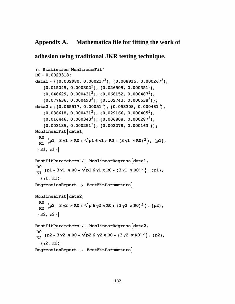
132
Appendix A. Mathematica file for fitting the work of
adhesion using traditional JKR testing technique.
�� Statistics`NonlinearFit̀ R0 0.0023318; data1 ��0.002980, 0.000217 3�, �0.008915, 0.000267 3�,
�0.015245, 0.000302 3�, �0.026509, 0.000351 3�,
�0.048629, 0.000431 3�, �0.066152, 0.000487 3�,
�0.077636, 0.000493 3�, �0.102743, 0.000538 3��;
data2 ��0.065517, 0.00051 3�, �0.053308, 0.000481 3�,
�0.036618, 0.000431 3�, �0.029166, 0.000405 3�,
�0.016446, 0.000343 3�, �0.006808, 0.000287 3�,
�0.003135, 0.000251 3�, �0.002278, 0.000163 3��; NonlinearFit $data1,
R0K1
,p1 � 3 J1 S R0�r
p1 6 J1 S R0� +3 J1 S R0/2 0, �p1�,
�K1, J1�( BestFitParameters s. NonlinearRegress $data1,
R0K1
,p1 � 3 J1 S R0�r
p1 6 J1 S R0� +3 J1 S R0/2 0, �p1�,
�J1, K1 �,
RegressionReport �! BestFitParameters ( NonlinearFit $data2,
R0K2
,p2 � 3 J2 S R0�r
p 6 J2 S R0� +3 J2 S R0/2 0, �p2�,
�K2, J2�( BestFitParameters s. NonlinearRegress $data2,
R0K2
,p2 � 3 J2 S R0�r
p2 6 J2 S R0� +3 J2 S R0/2 0, �p2�,
�J2, K2 �,
RegressionReport �! BestFitParameters (

133
Appendix B. ABAQUS input file for contact simulation
****************************************************************** ** 14.712 mm * 0.956 mm * 0.165 mm (7.356,0.0.956,0.165 half sample) ** GEOMETRIC NON-LINEAR SHELL ELEMENT: S4R ** 20*50 & 20*30 NODE 21 * 36 ** BOUNDARY CONDITION: BUILD IN ** CONSTRAINS : ROTATE 90 DEGREE, AND MOVE INSIDE ** OUTPUT: REACTION FORCES ** c=6.375 mm ****************************************************************** *HEADING CONTACT PROBLEM USING SHELL ELEMENT *************************************************** ** DEFINE NODES: X 81; Y 21 *************************************************** *NODE 1,0.0,0.0,0.0 21,0.0,0.956,0.0 1051,2.356,0.0,0.0 1071,2.356,0.956,0.0 1072,2.406,0.0,0.0 1092,2.406,0.956,0.0 1660,6.99495,0.0,0.0 1680,6.99495,0.956,0.0 1681,7.356,0.0,0.0 1701,7.356,0.956,0.0 2000,0.0,0.0,6.5 *NGEN,NSET=SIDE1 1,21,1 *NGEN,NSET=SIDE2 1051,1071,1 *NGEN,NSET=SIDE3 1681,1701,1 *NGEN,NSET=SIDE4 1072,1092,1 *NGEN,NSET=SIDE5 1660,1680,1 *NFILL,NSET=ALL SIDE1,SIDE2,50,21 *NFILL,NSET=ALL,BIAS=0.931828 SIDE2,SIDE3,30,21

134
SIDE4,SIDE5,28,21 ********************************** ** DEFINE ELEMENTS : X 40; Y 10 ********************************** *ELEMENT,TYPE=S4R,ELSET=RUBBER 1,1,22,23,2 *ELGEN,ELSET=RUBBER 1,20,1,1,80,21,20 ********************************************** ** DEFINE MATERIAL: RUBBER: E=1.81 MPA, V=0.49 ********************************************** *MATERIAL,NAME=RUBBER *ELASTIC, TYPE=ISOTROPIC 1.81,0.49 ************************ ** THICKNESS=0.165 mm ** ************************ *SHELL GENERAL SECTION,ELSET=RUBBER,MATERIAL=RUBBER 0.165 ******************************* ** SURFACE DEFINITION ** ******************************* *RIGID SURFACE,NAME=RIGID,TYPE=CYLINDER,REF NODE=2000 5.0,0.0,6.5,5.0,0.1,6.5 6.0,0.0,6.5 START,-1.0,0.0 LINE,2.0,0.0 *SURFACE DEFINITION,NAME=SURF RUBBER,SPOS ******************************* ** TYPE OF CONTACT ** ******************************* *CONTACT PAIR,INTERACTION=HERTZ SURF,RIGID *SURFACE INTERACTION,NAME=HERTZ ********************************************************************* ** DEFINE BOUNDARY: END IS BUILD IN ********************************************************************* *NSET,NSET=END,GEN 1681,1701,1 *NSET,NSET=XMID,GEN 1,21,1 **NSET,NSET=YMID,GEN

135
**1,1660,21 *BOUNDARY END,1,5 XMID,1 XMID,5 2000,1,6 *********************** ** STEP PROCEDURE ** *********************** ******************************************** ** STEP 1, APPLY LOAD *STEP,NLGEOM,INC=1000 *STATIC 1.0,1.0,0.001 *CLOAD XMID,3,1.0E-6 *RESTART,WRITE,OVERLAY *EL PRINT,FREQUENCY=0 S *NODE PRINT,FREQUENCY=0 U *END STEP ******************************************** **2 *STEP,NLGEOM,INC=1000 *STATIC 1.0,1.0,0.001 *BOUNDARY end,1,1,-0.25 *RESTART,WRITE,OVERLAY *EL PRINT,FREQUENCY=0 S *NODE PRINT,FREQUENCY=0 U *END STEP **STEP 3 *STEP,NLGEOM, INC=1000 *STATIC 1.0,1.0,0.01 *BOUNDARY end,5,5,0.1 *RESTART,WRITE,OVERLAY *EL PRINT,FREQUENCY=0

136
S *NODE PRINT,FREQUENCY=0 U *END STEP **4 *STEP,NLGEOM,INC=1000 *STATIC 0.002,10.0,0.00001 *BOUNDARY end,5,5,0.2 *RESTART,WRITE,OVERLAY *EL PRINT,FREQUENCY=0 S *NODE PRINT,FREQUENCY=0 U *END STEP **5 *STEP,NLGEOM,INC=1000 *STATIC 0.002,10.0,0.00001 *BOUNDARY end,5,5,0.3 *RESTART,WRITE,OVERLAY *EL PRINT,FREQUENCY=0 S *NODE PRINT,FREQUENCY=0 U *END STEP **6 *STEP,NLGEOM,INC=1000 *STATIC 0.002,10.0,0.00001 *BOUNDARY end,1,1,-0.5 *RESTART,WRITE,OVERLAY *EL PRINT,FREQUENCY=0 S *NODE PRINT,FREQUENCY=0 U *END STEP **7 *STEP,NLGEOM,INC=1000 *STATIC

137
0.002,10.0,0.00001 *BOUNDARY end,5,5,0.522 *RESTART,WRITE,OVERLAY *EL PRINT,FREQUENCY=0 S *NODE PRINT,FREQUENCY=0 U *END STEP **8 *STEP,NLGEOM,INC=1000 *STATIC 0.002,10.0,0.00001 *BOUNDARY end,1,1,-0.7 *RESTART,WRITE,OVERLAY *EL PRINT,FREQUENCY=0 S *NODE PRINT,FREQUENCY=0 U *END STEP **9 *STEP,NLGEOM,INC=1000 *STATIC 0.02,10.0,0.00001 *BOUNDARY end,1,1,-1.0 *RESTART,WRITE,OVERLAY *EL PRINT,FREQUENCY=0 S *NODE PRINT,FREQUENCY=0 U *END STEP **10 *STEP,NLGEOM,INC=1000 *STATIC 0.02,10.0,0.00001 *BOUNDARY end,5,5,0.698 *RESTART,WRITE,OVERLAY *EL PRINT,FREQUENCY=0 S *NODE PRINT,FREQUENCY=0

138
U *END STEP **11 *STEP,NLGEOM,INC=1000 *STATIC 0.02,10.0,0.000011 *BOUNDARY end,1,1,-1.5 *RESTART,WRITE,OVERLAY *EL PRINT,FREQUENCY=0 S *NODE PRINT,FREQUENCY=0 U *END STEP **12 *STEP,NLGEOM,INC=1000 *STATIC 0.02,10.0,0.00001 *BOUNDARY end,1,1,-2.1685 *RESTART,WRITE,OVERLAY *END STEP **13 *STEP,NLGEOM,INC=1000 *STATIC 0.02,10.0,0.00001 *BOUNDARY end,1,1,-3.1685 *RESTART,WRITE,OVERLAY *EL PRINT,FREQUENCY=0 S *NODE PRINT,FREQUENCY=0 U *END STEP **14 *STEP,NLGEOM,INC=1000 *STATIC 0.02,10.0,0.00001 *BOUNDARY end,1,1,-4.1685 *RESTART,WRITE,OVERLAY *EL PRINT,FREQUENCY=0 S

139
*NODE PRINT,FREQUENCY=0 U *END STEP ******************************************** **15 UNLOADING *STEP,INC=1000 *STATIC 0.02,10.0,0.00001 *CLOAD,OP=NEW *RESTART,WRITE,OVERLAY *EL PRINT,FREQUENCY=0 S *NODE PRINT,FREQUENCY=0 U *END STEP ******************************************** **16 *STEP,NLGEOM,INC=1000 *STATIC 0.02,10.0,0.00001 *BOUNDARY end,5,5,0.872 *RESTART,WRITE,OVERLAY *EL PRINT,FREQUENCY=0 S *NODE PRINT,FREQUENCY=0 U *END STEP **17 *STEP,NLGEOM,INC=1000 *STATIC 0.02,10.0,0.00001 *BOUNDARY end,5,5,0.96 *RESTART,WRITE,OVERLAY *EL PRINT,FREQUENCY=0 S *NODE PRINT,FREQUENCY=0 U *END STEP **18 *STEP,NLGEOM,INC=1000 *STATIC

140
0.02,10.0,0.00001 *BOUNDARY end,5,5,1.04 *RESTART,WRITE,OVERLAY *EL PRINT,FREQUENCY=0 S *NODE PRINT,FREQUENCY=0 U *END STEP **19 *STEP,NLGEOM,INC=1000 *STATIC 0.02,10.0,0.00001 *BOUNDARY end,5,5,1.13 *RESTART,WRITE,OVERLAY *EL PRINT,FREQUENCY=0 S *NODE PRINT,FREQUENCY=0 U *END STEP **20 *STEP,NLGEOM,INC=1000 *STATIC 0.02,10.0,0.00001 *BOUNDARY end,5,5,1.22 *RESTART,WRITE,OVERLAY *EL PRINT,FREQUENCY=0 S *NODE PRINT,FREQUENCY=0 U *END STEP **21 *STEP,NLGEOM,INC=1000 *STATIC 0.02,10.0,0.00001 *BOUNDARY end,5,5,1.31 *RESTART,WRITE,OVERLAY *EL PRINT,FREQUENCY=0 S *NODE PRINT,FREQUENCY=0

141
U *END STEP **22 *STEP,NLGEOM,INC=1000 *STATIC 0.02,10.0,0.00001 *BOUNDARY end,5,5,1.40 *RESTART,WRITE,OVERLAY *EL PRINT,FREQUENCY=0 S *NODE PRINT,FREQUENCY=0 U *END STEP **23 *STEP,NLGEOM,INC=1000 *STATIC 0.02,10.0,0.00001 *BOUNDARY end,5,5,1.48 *RESTART,WRITE,OVERLAY *EL PRINT,FREQUENCY=0 S *NODE PRINT,FREQUENCY=0 U *END STEP **24 *STEP,NLGEOM,INC=1000 *STATIC 0.02,10.0,0.00001 *BOUNDARY end,5,5,1.57 *RESTART,WRITE,OVERLAY *EL PRINT,FREQUENCY=0 S,E *NODE PRINT,FREQUENCY=0 U *END STEP ******************************************* **25 RIGID SURFACE MOVES DOWN ** ******************************************* *STEP,NLGEOM,INC=1000 *STATIC

142
0.02,10.0,0.00001 *BOUNDARY 2000,3,3,-0.6 *RESTART,WRITE,OVERLAY *EL PRINT,FREQUENCY=0 *NODE PRINT,FREQUENCY=0 *END STEP **26 *STEP,NLGEOM,INC=1000 *STATIC 0.02,10.0,0.00001 *BOUNDARY 2000,3,3,-0.8 *RESTART,WRITE,OVERLAY *EL PRINT,FREQUENCY=0 S,E *NODE PRINT,FREQUENCY=0 U *CONTACT PRINT,TOTAL=YES,SLAVE=SURF,MASTER=RIGID,FREQUENCY=15 carea,cfn,cft *CONTACT FILE,SLAVE=SURF,MASTER=RIGID,FREQUENCY=15 carea,cfn,cft *NODE PRINT,TOTAL=YES,NSET=END,FREQUENCY=15 RF *END STEP **27 *STEP,NLGEOM,INC=1000 *STATIC 0.02,10.0,0.00001 *BOUNDARY 2000,3,3,-1.0 *RESTART,WRITE,OVERLAY *EL PRINT,FREQUENCY=0 S,E *NODE PRINT,FREQUENCY=0 U *CONTACT PRINT,TOTAL=YES,SLAVE=SURF,MASTER=RIGID,FREQUENCY=15 carea,cfn,cft *CONTACT FILE,SLAVE=SURF,MASTER=RIGID,FREQUENCY=15 carea,cfn,cft *NODE PRINT,TOTAL=YES,NSET=END,FREQUENCY=15

143
RF *END STEP **28 *STEP,NLGEOM,INC=1000 *STATIC 0.02,10.0,0.00001 *BOUNDARY 2000,3,3,-1.1 *RESTART,WRITE,OVERLAY *EL PRINT,FREQUENCY=0 S *NODE PRINT,FREQUENCY=0 U *CONTACT PRINT,TOTAL=YES,SLAVE=SURF,MASTER=RIGID,FREQUENCY=15 carea,cfn,cft *CONTACT FILE,SLAVE=SURF,MASTER=RIGID,FREQUENCY=15 carea,cfn,cft *NODE PRINT,TOTAL=YES,NSET=END,FREQUENCY=15 RF *END STEP **29 *STEP,NLGEOM,INC=1000 *STATIC 0.02,10.0,0.00001 *BOUNDARY 2000,3,3,-1.2 *RESTART,WRITE,OVERLAY *EL PRINT,FREQUENCY=0 S *NODE PRINT,FREQUENCY=0 U *CONTACT PRINT,TOTAL=YES,SLAVE=SURF,MASTER=RIGID,FREQUENCY=15 carea,cfn,cft *CONTACT FILE,SLAVE=SURF,MASTER=RIGID,FREQUENCY=15 carea,cfn,cft *NODE PRINT,TOTAL=YES,NSET=END,FREQUENCY=15 RF *END STEP **30 *STEP,NLGEOM,INC=1000 *STATIC

144
0.02,10.0,0.00001 *BOUNDARY 2000,3,3,-1.3 *RESTART,WRITE,OVERLAY *EL PRINT,FREQUENCY=0 S *NODE PRINT,FREQUENCY=0 U *CONTACT PRINT,TOTAL=YES,SLAVE=SURF,MASTER=RIGID,FREQUENCY=15 carea,cfn,cft *CONTACT FILE,SLAVE=SURF,MASTER=RIGID,FREQUENCY=15 carea,cfn,cft *NODE PRINT,TOTAL=YES,NSET=END,FREQUENCY=15 RF *END STEP **31 *STEP,NLGEOM,INC=1000 *STATIC 0.02,10.0,0.00001 *BOUNDARY 2000,3,3,-1.4 *RESTART,WRITE,OVERLAY *EL PRINT,FREQUENCY=0 S *NODE PRINT,FREQUENCY=0 U *CONTACT PRINT,TOTAL=YES,SLAVE=SURF,MASTER=RIGID,FREQUENCY=15 carea,cfn,cft *CONTACT FILE,SLAVE=SURF,MASTER=RIGID,FREQUENCY=15 carea,cfn,cft *NODE PRINT,TOTAL=YES,NSET=END,FREQUENCY=15 RF *END STEP **32 *STEP,NLGEOM,INC=1000 *STATIC 0.02,10.0,0.00001 *BOUNDARY 2000,3,3,-1.42 *RESTART,WRITE,OVERLAY *EL PRINT,FREQUENCY=0

145
S *NODE PRINT,FREQUENCY=0 U *CONTACT PRINT,TOTAL=YES,SLAVE=SURF,MASTER=RIGID,FREQUENCY=15 carea,cfn,cft *CONTACT FILE,SLAVE=SURF,MASTER=RIGID,FREQUENCY=15 carea,cfn,cft *NODE PRINT,TOTAL=YES,NSET=END,FREQUENCY=15 RF *END STEP **33 *STEP,NLGEOM,INC=1000 *STATIC 0.02,10.0,0.00001 *BOUNDARY 2000,3,3,-1.44 *RESTART,WRITE,OVERLAY *EL PRINT,FREQUENCY=0 S *NODE PRINT,FREQUENCY=0 U *CONTACT PRINT,TOTAL=YES,SLAVE=SURF,MASTER=RIGID,FREQUENCY=15 carea,cfn,cft *CONTACT FILE,SLAVE=SURF,MASTER=RIGID,FREQUENCY=15 carea,cfn,cft *NODE PRINT,TOTAL=YES,NSET=END,FREQUENCY=15 RF *END STEP **34 *STEP,NLGEOM,INC=1000 *STATIC 0.02,10.0,0.00001 *BOUNDARY 2000,3,3,-1.46 *RESTART,WRITE,OVERLAY *EL PRINT,FREQUENCY=0 S *NODE PRINT,FREQUENCY=0 U *CONTACT PRINT,TOTAL=YES,SLAVE=SURF,MASTER=RIGID,FREQUENCY=15

146
carea,cfn,cft *CONTACT FILE,SLAVE=SURF,MASTER=RIGID,FREQUENCY=15 carea,cfn,cft *NODE PRINT,TOTAL=YES,NSET=END,FREQUENCY=15 RF *END STEP **35 *STEP,NLGEOM,INC=1000 *STATIC 0.02,10.0,0.00001 *BOUNDARY 2000,3,3,-1.48 *RESTART,WRITE,OVERLAY *EL PRINT,FREQUENCY=0 S *NODE PRINT,FREQUENCY=0 U *CONTACT PRINT,TOTAL=YES,SLAVE=SURF,MASTER=RIGID,FREQUENCY=15 carea,cfn,cft *CONTACT FILE,SLAVE=SURF,MASTER=RIGID,FREQUENCY=15 carea,cfn,cft *NODE PRINT,TOTAL=YES,NSET=END,FREQUENCY=15 RF *END STEP **36 *STEP,NLGEOM,INC=1000 *STATIC 0.02,10.0,0.00001 *BOUNDARY 2000,3,3,-1.50 *RESTART,WRITE,OVERLAY *EL PRINT,FREQUENCY=0 S *NODE PRINT,FREQUENCY=0 U *CONTACT PRINT,TOTAL=YES,SLAVE=SURF,MASTER=RIGID,FREQUENCY=15 carea,cfn,cft *CONTACT FILE,SLAVE=SURF,MASTER=RIGID,FREQUENCY=15 carea,cfn,cft *NODE PRINT,TOTAL=YES,NSET=END,FREQUENCY=15 RF
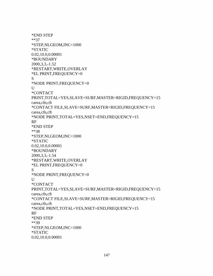
147
*END STEP **37 *STEP,NLGEOM,INC=1000 *STATIC 0.02,10.0,0.00001 *BOUNDARY 2000,3,3,-1.52 *RESTART,WRITE,OVERLAY *EL PRINT,FREQUENCY=0 S *NODE PRINT,FREQUENCY=0 U *CONTACT PRINT,TOTAL=YES,SLAVE=SURF,MASTER=RIGID,FREQUENCY=15 carea,cfn,cft *CONTACT FILE,SLAVE=SURF,MASTER=RIGID,FREQUENCY=15 carea,cfn,cft *NODE PRINT,TOTAL=YES,NSET=END,FREQUENCY=15 RF *END STEP **38 *STEP,NLGEOM,INC=1000 *STATIC 0.02,10.0,0.00001 *BOUNDARY 2000,3,3,-1.54 *RESTART,WRITE,OVERLAY *EL PRINT,FREQUENCY=0 S *NODE PRINT,FREQUENCY=0 U *CONTACT PRINT,TOTAL=YES,SLAVE=SURF,MASTER=RIGID,FREQUENCY=15 carea,cfn,cft *CONTACT FILE,SLAVE=SURF,MASTER=RIGID,FREQUENCY=15 carea,cfn,cft *NODE PRINT,TOTAL=YES,NSET=END,FREQUENCY=15 RF *END STEP **39 *STEP,NLGEOM,INC=1000 *STATIC 0.02,10.0,0.00001

148
*BOUNDARY 2000,3,3,-1.56 *RESTART,WRITE,OVERLAY *EL PRINT,FREQUENCY=0 S *NODE PRINT,FREQUENCY=0 U *CONTACT PRINT,TOTAL=YES,SLAVE=SURF,MASTER=RIGID,FREQUENCY=15 carea,cfn,cft *CONTACT FILE,SLAVE=SURF,MASTER=RIGID,FREQUENCY=15 carea,cfn,cft *NODE PRINT,TOTAL=YES,NSET=END,FREQUENCY=15 RF *END STEP **40 *STEP,NLGEOM,INC=1000 *STATIC 0.02,10.0,0.00001 *BOUNDARY 2000,3,3,-1.58 *RESTART,WRITE,OVERLAY *EL PRINT,FREQUENCY=0 S *NODE PRINT,FREQUENCY=0 U *CONTACT PRINT,TOTAL=YES,SLAVE=SURF,MASTER=RIGID,FREQUENCY=15 carea,cfn,cft *CONTACT FILE,SLAVE=SURF,MASTER=RIGID,FREQUENCY=15 carea,cfn,cft *NODE PRINT,TOTAL=YES,NSET=END,FREQUENCY=15 RF *END STEP **41 *STEP,NLGEOM,INC=1000 *STATIC 0.02,10.0,0.00001 *BOUNDARY 2000,3,3,-1.60 *RESTART,WRITE,OVERLAY *EL PRINT,FREQUENCY=0 S

149
*NODE PRINT,FREQUENCY=0 U *CONTACT PRINT,TOTAL=YES,SLAVE=SURF,MASTER=RIGID,FREQUENCY=15 carea,cfn,cft *CONTACT FILE,SLAVE=SURF,MASTER=RIGID,FREQUENCY=15 carea,cfn,cft *NODE PRINT,TOTAL=YES,NSET=END,FREQUENCY=15 RF *END STEP **42 *STEP,NLGEOM,INC=1000 *STATIC 0.02,10.0,0.00001 *BOUNDARY 2000,3,3,-1.62 *RESTART,WRITE,OVERLAY *EL PRINT,FREQUENCY=0 S *NODE PRINT,FREQUENCY=0 U *CONTACT PRINT,TOTAL=YES,SLAVE=SURF,MASTER=RIGID,FREQUENCY=15 carea,cfn,cft *CONTACT FILE,SLAVE=SURF,MASTER=RIGID,FREQUENCY=15 carea,cfn,cft *NODE PRINT,TOTAL=YES,NSET=END,FREQUENCY=15 RF *END STEP **43 *STEP,NLGEOM,INC=1000 *STATIC 0.02,10.0,0.00001 *BOUNDARY 2000,3,3,-1.64 *RESTART,WRITE,OVERLAY *EL PRINT,FREQUENCY=0 S *NODE PRINT,FREQUENCY=0 U *CONTACT PRINT,TOTAL=YES,SLAVE=SURF,MASTER=RIGID,FREQUENCY=15 carea,cfn,cft

150
*CONTACT FILE,SLAVE=SURF,MASTER=RIGID,FREQUENCY=15 carea,cfn,cft *NODE PRINT,TOTAL=YES,NSET=END,FREQUENCY=15 RF *END STEP **44 *STEP,NLGEOM,INC=1000 *STATIC 0.02,10.0,0.00001 *BOUNDARY 2000,3,3,-1.66 *RESTART,WRITE,OVERLAY *EL PRINT,FREQUENCY=0 S *NODE PRINT,FREQUENCY=0 U *CONTACT PRINT,TOTAL=YES,SLAVE=SURF,MASTER=RIGID,FREQUENCY=15 carea,cfn,cft *CONTACT FILE,SLAVE=SURF,MASTER=RIGID,FREQUENCY=15 carea,cfn,cft *NODE PRINT,TOTAL=YES,NSET=END,FREQUENCY=15 RF *END STEP **45 *STEP,NLGEOM,INC=1000 *STATIC 0.02,10.0,0.00001 *BOUNDARY 2000,3,3,-1.68 *RESTART,WRITE,OVERLAY *EL PRINT,FREQUENCY=0 S *NODE PRINT,FREQUENCY=0 U *CONTACT PRINT,TOTAL=YES,SLAVE=SURF,MASTER=RIGID,FREQUENCY=15 carea,cfn,cft *CONTACT FILE,SLAVE=SURF,MASTER=RIGID,FREQUENCY=15 carea,cfn,cft *NODE PRINT,TOTAL=YES,NSET=END,FREQUENCY=15 RF *END STEP

151
**46 *STEP,NLGEOM,INC=1000 *STATIC 0.02,10.0,0.00001 *BOUNDARY 2000,3,3,-1.7 *RESTART,WRITE,OVERLAY *EL PRINT,FREQUENCY=0 S *NODE PRINT,FREQUENCY=0 U *CONTACT PRINT,TOTAL=YES,SLAVE=SURF,MASTER=RIGID,FREQUENCY=15 carea,cfn,cft *CONTACT FILE,SLAVE=SURF,MASTER=RIGID,FREQUENCY=15 carea,cfn,cft *NODE PRINT,TOTAL=YES,NSET=END,FREQUENCY=15 RF *END STEP **47 *STEP,NLGEOM,INC=1000 *STATIC 0.02,10.0,0.00001 *BOUNDARY 2000,3,3,-1.72 *RESTART,WRITE,OVERLAY *EL PRINT,FREQUENCY=0 S *NODE PRINT,FREQUENCY=0 U *CONTACT PRINT,TOTAL=YES,SLAVE=SURF,MASTER=RIGID,FREQUENCY=15 carea,cfn,cft *CONTACT FILE,SLAVE=SURF,MASTER=RIGID,FREQUENCY=15 carea,cfn,cft *NODE PRINT,TOTAL=YES,NSET=END,FREQUENCY=15 RF *END STEP **48 *STEP,NLGEOM,INC=1000 *STATIC 0.02,10.0,0.00001 *BOUNDARY
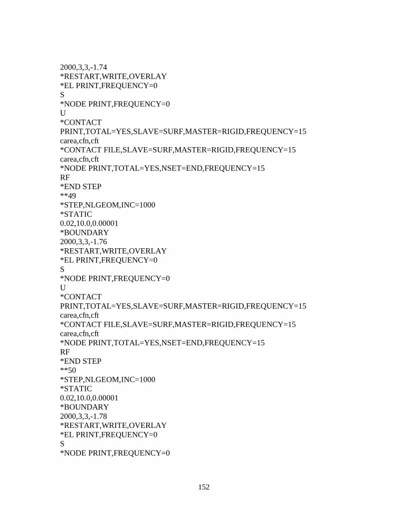
152
2000,3,3,-1.74 *RESTART,WRITE,OVERLAY *EL PRINT,FREQUENCY=0 S *NODE PRINT,FREQUENCY=0 U *CONTACT PRINT,TOTAL=YES,SLAVE=SURF,MASTER=RIGID,FREQUENCY=15 carea,cfn,cft *CONTACT FILE,SLAVE=SURF,MASTER=RIGID,FREQUENCY=15 carea,cfn,cft *NODE PRINT,TOTAL=YES,NSET=END,FREQUENCY=15 RF *END STEP **49 *STEP,NLGEOM,INC=1000 *STATIC 0.02,10.0,0.00001 *BOUNDARY 2000,3,3,-1.76 *RESTART,WRITE,OVERLAY *EL PRINT,FREQUENCY=0 S *NODE PRINT,FREQUENCY=0 U *CONTACT PRINT,TOTAL=YES,SLAVE=SURF,MASTER=RIGID,FREQUENCY=15 carea,cfn,cft *CONTACT FILE,SLAVE=SURF,MASTER=RIGID,FREQUENCY=15 carea,cfn,cft *NODE PRINT,TOTAL=YES,NSET=END,FREQUENCY=15 RF *END STEP **50 *STEP,NLGEOM,INC=1000 *STATIC 0.02,10.0,0.00001 *BOUNDARY 2000,3,3,-1.78 *RESTART,WRITE,OVERLAY *EL PRINT,FREQUENCY=0 S *NODE PRINT,FREQUENCY=0

153
U *CONTACT PRINT,TOTAL=YES,SLAVE=SURF,MASTER=RIGID,FREQUENCY=15 carea,cfn,cft *CONTACT FILE,SLAVE=SURF,MASTER=RIGID,FREQUENCY=15 carea,cfn,cft *NODE PRINT,TOTAL=YES,NSET=END,FREQUENCY=15 RF *END STEP **51 *STEP,NLGEOM,INC=1000 *STATIC 0.02,10.0,0.00001 *BOUNDARY 2000,3,3,-1.8 *RESTART,WRITE,OVERLAY *EL PRINT,FREQUENCY=0 S *NODE PRINT,FREQUENCY=0 U *CONTACT PRINT,TOTAL=YES,SLAVE=SURF,MASTER=RIGID,FREQUENCY=15 carea,cfn,cft *CONTACT FILE,SLAVE=SURF,MASTER=RIGID,FREQUENCY=15 carea,cfn,cft *NODE PRINT,TOTAL=YES,NSET=END,FREQUENCY=15 RF *END STEP **52 *STEP,NLGEOM,INC=1000 *STATIC 0.02,10.0,0.00001 *BOUNDARY 2000,3,3,-1.82 *RESTART,WRITE,OVERLAY *EL PRINT,FREQUENCY=0 S *NODE PRINT,FREQUENCY=0 U *CONTACT PRINT,TOTAL=YES,SLAVE=SURF,MASTER=RIGID,FREQUENCY=15 carea,cfn,cft *CONTACT FILE,SLAVE=SURF,MASTER=RIGID,FREQUENCY=15
154
carea,cfn,cft *NODE PRINT,TOTAL=YES,NSET=END,FREQUENCY=15 RF *END STEP **53 *STEP,NLGEOM,INC=1000 *STATIC 0.02,10.0,0.00001 *BOUNDARY 2000,3,3,-1.84 *RESTART,WRITE,OVERLAY *EL PRINT,FREQUENCY=0 S *NODE PRINT,FREQUENCY=0 U *CONTACT PRINT,TOTAL=YES,SLAVE=SURF,MASTER=RIGID,FREQUENCY=15 carea,cfn,cft *CONTACT FILE,SLAVE=SURF,MASTER=RIGID,FREQUENCY=15 carea,cfn,cft *NODE PRINT,TOTAL=YES,NSET=END,FREQUENCY=15 RF *END STEP **54 *STEP,NLGEOM,INC=1000 *STATIC 0.02,10.0,0.00001 *BOUNDARY 2000,3,3,-1.86 *RESTART,WRITE,OVERLAY *EL PRINT,FREQUENCY=0 S *NODE PRINT,FREQUENCY=0 U *CONTACT PRINT,TOTAL=YES,SLAVE=SURF,MASTER=RIGID,FREQUENCY=15 carea,cfn,cft *CONTACT FILE,SLAVE=SURF,MASTER=RIGID,FREQUENCY=15 carea,cfn,cft *NODE PRINT,TOTAL=YES,NSET=END,FREQUENCY=15 RF *END STEP **55

155
*STEP,NLGEOM,INC=1000 *STATIC 0.02,10.0,0.00001 *BOUNDARY 2000,3,3,-1.90 *RESTART,WRITE,OVERLAY *EL PRINT,FREQUENCY=0 S *NODE PRINT,FREQUENCY=0 U *CONTACT PRINT,TOTAL=YES,SLAVE=SURF,MASTER=RIGID,FREQUENCY=15 carea,cfn,cft *CONTACT FILE,SLAVE=SURF,MASTER=RIGID,FREQUENCY=15 carea,cfn,cft *NODE PRINT,TOTAL=YES,NSET=END,FREQUENCY=15 RF *END STEP **56 *STEP,NLGEOM,INC=1000 *STATIC 0.02,10.0,0.00001 *BOUNDARY 2000,3,3,-1.95 *RESTART,WRITE,OVERLAY *EL PRINT,FREQUENCY=0 S *NODE PRINT,FREQUENCY=0 U *CONTACT PRINT,TOTAL=YES,SLAVE=SURF,MASTER=RIGID,FREQUENCY=15 carea,cfn,cft *CONTACT FILE,SLAVE=SURF,MASTER=RIGID,FREQUENCY=15 carea,cfn,cft *NODE PRINT,TOTAL=YES,NSET=END,FREQUENCY=15 RF *END STEP **57 *STEP,NLGEOM,INC=1000 *STATIC 0.02,10.0,0.00001 *BOUNDARY 2000,3,3,-2.0

156
*RESTART,WRITE,OVERLAY *EL PRINT,FREQUENCY=0 S *NODE PRINT,FREQUENCY=0 U *CONTACT PRINT,TOTAL=YES,SLAVE=SURF,MASTER=RIGID,FREQUENCY=15 carea,cfn,cft *CONTACT FILE,SLAVE=SURF,MASTER=RIGID,FREQUENCY=15 carea,cfn,cft *NODE PRINT,TOTAL=YES,NSET=END,FREQUENCY=15 RF *END STEP **58 *STEP,NLGEOM,INC=1000 *STATIC 0.02,10.0,0.00001 *BOUNDARY 2000,3,3,-2.05 *RESTART,WRITE,OVERLAY *EL PRINT,FREQUENCY=0 S *NODE PRINT,FREQUENCY=0 U *CONTACT PRINT,TOTAL=YES,SLAVE=SURF,MASTER=RIGID,FREQUENCY=15 carea,cfn,cft *CONTACT FILE,SLAVE=SURF,MASTER=RIGID,FREQUENCY=15 carea,cfn,cft *NODE PRINT,TOTAL=YES,NSET=END,FREQUENCY=15 RF *END STEP **59 *STEP,NLGEOM,INC=1000 *STATIC 0.02,10.0,0.00001 *BOUNDARY 2000,3,3,-2.1 *RESTART,WRITE,OVERLAY *EL PRINT,FREQUENCY=0 S *NODE PRINT,FREQUENCY=0 U

157
*CONTACT PRINT,TOTAL=YES,SLAVE=SURF,MASTER=RIGID,FREQUENCY=15 carea,cfn,cft *CONTACT FILE,SLAVE=SURF,MASTER=RIGID,FREQUENCY=15 carea,cfn,cft *NODE PRINT,TOTAL=YES,NSET=END,FREQUENCY=15 RF *END STEP **60 *STEP,NLGEOM,INC=1000 *STATIC 0.02,10.0,0.00001 *BOUNDARY 2000,3,3,-2.15 *RESTART,WRITE,OVERLAY *EL PRINT,FREQUENCY=0 S *NODE PRINT,FREQUENCY=0 U *CONTACT PRINT,TOTAL=YES,SLAVE=SURF,MASTER=RIGID,FREQUENCY=15 carea,cfn,cft *CONTACT FILE,SLAVE=SURF,MASTER=RIGID,FREQUENCY=15 carea,cfn,cft *NODE PRINT,TOTAL=YES,NSET=END,FREQUENCY=15 RF *END STEP **61 *STEP,NLGEOM,INC=1000 *STATIC 0.02,10.0,0.00001 *BOUNDARY 2000,3,3,-2.20 *RESTART,WRITE,OVERLAY *EL PRINT,FREQUENCY=0 S *NODE PRINT,FREQUENCY=0 U *CONTACT PRINT,TOTAL=YES,SLAVE=SURF,MASTER=RIGID,FREQUENCY=15 carea,cfn,cft *CONTACT FILE,SLAVE=SURF,MASTER=RIGID,FREQUENCY=15 carea,cfn,cft

158
*NODE PRINT,TOTAL=YES,NSET=END,FREQUENCY=15 RF *END STEP **62 *STEP,NLGEOM,INC=1000 *STATIC 0.02,10.0,0.00001 *BOUNDARY 2000,3,3,-2.25 *RESTART,WRITE,OVERLAY *EL PRINT,FREQUENCY=0 S *NODE PRINT,FREQUENCY=0 U *CONTACT PRINT,TOTAL=YES,SLAVE=SURF,MASTER=RIGID,FREQUENCY=15 carea,cfn,cft *CONTACT FILE,SLAVE=SURF,MASTER=RIGID,FREQUENCY=15 carea,cfn,cft *NODE PRINT,TOTAL=YES,NSET=END,FREQUENCY=15 RF *END STEP **63 *STEP,NLGEOM,INC=1000 *STATIC 0.02,10.0,0.00001 *BOUNDARY 2000,3,3,-2.3 *RESTART,WRITE,OVERLAY *EL PRINT,FREQUENCY=0 S *NODE PRINT,FREQUENCY=0 U *CONTACT PRINT,TOTAL=YES,SLAVE=SURF,MASTER=RIGID,FREQUENCY=15 carea,cfn,cft *CONTACT FILE,SLAVE=SURF,MASTER=RIGID,FREQUENCY=15 carea,cfn,cft *NODE PRINT,TOTAL=YES,NSET=END,FREQUENCY=15 RF *END STEP *******************************************

159
Vita
Jia Qi was born on June 16, 1970 in Shijiazhuang, China. She graduated from
Chengdu University of Science and Technology in July of 1992. In July of 1995, she
completed her Master of Science in Mechanics from Peking University in Beijing, China.
Following graduation, she worked at the Research and Development Center of Beijing
Urban Construction Incorporation. In 1998, the author began to pursue her Master of
Science in Engineering Mechanics at Virginia Tech.


![1 Interfacial Rheology System. 2 Background of Interfacial Rheology Interfacial Shear Stress Interfacial Shear Viscosity = [ ]](https://img.pdfslide.us/doc/110x75/56649d1f5503460f949f3d29/1-interfacial-rheology-system-2-background-of-interfacial-rheology-interfacial.jpg)