L O A N COPY: RETLJ3Pd -;'> AFWL TECHNICAL LIBRARY

KIRTLAND AFB, N. M. MEASUREMENT OF LAKE ICE THICKNESS WITH A SHORT-PULSE RADAR SYSTEM

Dule W. Cooper, Robert A. Mueller, und Ronuld J. Schertler

Lewis Research Center cleuehnd, Ohio 44135

N A T I O N A L AERO1,IAUTICS A N D SPACE A D M I N I S T R A T I O N W A S H I N G T O N , D. C. M A R C H 1976

https://ntrs.nasa.gov/search.jsp?R=19760013526 2018-05-27T09:35:17+00:00Z

~~

2. Government Accession No. . -

1. Report NO. 1 NASA TND-8189 - .

4. Title and Subtitle

MEASUREMENT OF LAKE ICE THICKNESS WITH A SHORT-PULSE RADAR SYSTEM

~ ~~

20. Security Classif. (of this page)

Unclassified

. . 7. Authods)

Dale W. Cooper, Robert A. Mueller, and Ronald J. Schertler i

21. No. of Pages 22. Price

24 $ 3 .

9. Performing Organization Name and Address

Lewis Research Center National Aeronautics and Space Administration Cleveland, Ohio 44135

National Aeronautics and Space Administration Washington, D. C. 20546

i 12. Sponsoring Agency Name and Address

~~

5. Report Date March 1976 -_ ~

6. Performing Organization Code

8. Performing Organization Repor

~

E-8573 .

10. Work Unit No.

177 -54 11. Contract or Grant No.

13. Type of Report and Period 0

Technical Note 14. Sponsoring Agency Code

15. Supplementary Notes

APPENDIX - EQUATIONS FOR ICE THICKNESS WITH NONNORMAL INCIDENCE by John Heighway

16. Abstract

Measurements of lake ice thickness were made during March 1975 at the Straits of Mackin by using a short-pulse r ada r sys tem aboard an a l l - te r ra in vehicle. These measurements compared with ice thicknesses determined with a n auger. Over 25 s i t e s were explored wh had i c e thicknesses in the range 29 to 60 cm. The maximum difference between r a d a r and auger measurements was less than 9 .8 percent. The magnitude of the e r r o r was less that &3.5 cm. The NASA operating short-pulse r ada r sys tem used in monitoring lake ice thick from an a i rc raf t is a lso described.

17. Key Words (Suggested by Authork ) )

Lake i ce thickness Short-pulse r a d a r Microwave measurement Remote sensing

Unclassified

- 19. Security Classif. (of this report)

I 18. Distribution Statement

Unclassified - unlimited STAR Category 43 (rev. 1

1 ~. 1 I

* For sa le by the National Techn ica l Information Service, Spr ingf ie ld . V i rg in ia 22161

MEASUREMENT OF LAKE ICE THICKNESS WITH A SHORT-PULSE RADAR SYSTEM

by Dale W. Cooper, Robert A. M u e l l e r , a n d Rona ld J. S c h e r t l e r

Lewis Research Cen te r

SUMMARY

Measurements of lake ice thickness were made during March 1975 at the Straits of Mackinac by using a short-pulse radar system aboard an all-terrain vehicle. These measurements were compared with ice thicknesses determined with an auger. Over 25 sites were explored which had ice thicknesses in the range 29 to 60 centimeters. The maximum difference between radar and auger measurements was less than 9.8 percent. The magnitude of the e r r o r was less than *3.5 centimeters. pulse radar system used in monitoring lake ice thickness from an aircraft is also described.

The NASA operating short-

INTRODUCTION

During the past 3 years NASA, in conjunction with the U. S . Coast Guard, the Na- tional Oceanographic and Atmospheric Administration, and the U. S . Army Corps of Engineers, has been developing an all-weather Great Lakes ice information system to aid in extending the winter navigation season. An extended season has the potential of saving millions of dollars in coal and ore shipping costs, since cargo must now be shipped by costly rail or truck routes or stored until spring thaws. The entire opera- tional information system is scheduled to be turned over to the Coast Guard by the end of the 1975-1976 ice season.

The Great Lakes ice information system uses a side-looking airborne radar (SLAR) aboard a U. S. Coast Guard C-130 aircraft. The SLAR provides an all-weather aerial view of the ice cover, which is then transmitted to the Geophysical Operational Environ- mental Satellite (GOES). From GOES the information is transmitted to a NOAA station at Wallops Island, Virginia, and then through telephone lines to the Coast Guard Great Lakes Ice Center at Cleveland for interpretation. Detailed ice maps are then con- structed by the Coast Guard and sent with radio facsimile to any ship on the Great Lakes with the appropriate recording equipment. The response time of the ice information

system is only a few hours, which gives vessels almost current ice charts. Daily flights allow new charts t o be made which can reflect ice shifts due to wind.

terns, and movement on the Great Lakes in all types of weather. The SLAR is sensitive to surface roughness and discontinuities and readily gives the location of pressure ridges. However, because the surface pattern is most often a relic of the early history of the ice, the SLAR imagery cannot be interpreted directly to give ice thickness. Ice auger teams have been used in the past to supplement the S U R data. However, the measurements a re laborious, time consuming, expensive, weather dependent, and dan- gerous to personnel and cannot be done on a large enough scale to map an entire lake in a reasonable amount of time. It is for this reason that a short-pulse S-band radar sys- tem was developed to profile the thickness of ice remotely.

sibility during the winter of 1972-1973 and flown successfully on a U. S. Coast Guard Sikorsky H-53 helicopter at altitudes up to 100 meters (ref. 1).

be used as an ice profiler aboard a NASA C-47 aircraft (ref. 2). This system proved operational at altitudes up to 2300 meters and ground speeds of 75 meters per second. The radar was able to detect ice thicknesses from 10 to 92 centimeters, the upper limit being the thickest ice found on the Great Lakes in the past two ice seasons. Data from the short-pulse radar system were used in an operational program in support of the SLAR during the ice seasons of 1973-1974 and 1974-1975.

radar. Results of the C-47 flights had shown that the radar was unable to detect less than 10 centimeters of ice, and measurements were precluded wherever surface melt water exceeded about 1 millimeter in thickness because of lack of penetration. Snow cover on the ice surface was never a problem, and the radar system worked well in any type of weather except rain, which, of course, had the same effect as melt water.

Calibration of the system could not be performed readily in the laboratory because of the large amount of ice and water needed to approximate a planar surface. It would also be difficult to make any supporting structure nonreflective to microwaves.

was taken. Some additional calibration of the short-pulse radar system on the C-47 air- craft was done in conjunction with an ice auger team on Brevoort Lake, in the upper peninsula of Michigan west of the Straits of Mackinac, during the ice season of 1973- 1974. The lake was of relatively uniform thickness and was easy to locate by aircraft. The radar data checked the auger team data to within 2 centimeters.

Because locating an auger team directly on a flight line for system calibration of an airborne radar was considered nearly impossible, it was decided to build a low-power radar which could be mounted on an all-terrain vehicle. With this configuration the

2

The SLAR system has proven to be very effective in determining ice location, pat-

The remote ice thickness measuring system was first designed and tested for fea-

For the next ice season (1973-1974) the nanosecond radar system was redesigned to

Some questions still remained as to the operational limitations and accuracy of the

During some initial helicopter checkout flights a small amount of calibration data

radar could be checked easily without location ambiguity. A low power radar was re - quired to ensure personnel safety. A portable gasoline generator supplied the auxiliary 115-volt, 60-hertz electric power. The all-terrain vehicle was borrowed from the Coastal Zone Laboratory of the University of Michigan at Traverse City, Michigan. The research using the all-terrain vehicle on the Straits of Mackinac was performed in the second week of March 1975.

A derivation of equations for ice thickness with nonnormal radar pulse incidence by John E.

C

D,H,S

h

L

t

X

r, 6

€1'

e cp

Heighway is given in the appendix.

SYMBOLS

speed of light in vacuum, 29.98 cm/nsec

distance, cm

horn height, cm

distance between horns, cm

time, nsec

ice thickness, cm

angle, deg

relative dielectric constant

angle to normal in air at ice surface, deg

angle to normal in ice at ice surface, deg

Subscripts :

r receiver

t transmitter

1

2

wave reflected from air-ice interface

wave reflected from ice-water interface

EVALUATION OF ICE THICKNESS FROM RADAR RETURN

From an aircraft the radar pulse may be considered a plane wave which is partially reflected upon incidence at the interface of the air and ice or snow and ice, as shown in figure 1. Part of the wave continues on through the ice at a slower velocity because of the increased relative dielectric constant. At the ice -water interface total reflection

3

takes place. A receiver which measures the t ime between these two reflected pulses can give a remote observer a measurement of ice thickness. In addition to ice thickness, a measure of the time that the partially reflected incident wave takes to return to the air- craft gives aircraft altitude. For a plane wave at normal incidence the time delay t2 - tl, in nanoseconds, is related to the ice thickness x, in centimeters, by the follow- ing expression:

where c is the speed of light in a vacuum (29.98 cm/nsec), and is the relative di- electric constant of ice.

Measurements of the dielectric constant of lake ice samples were made by Stanford Research Institude (ref. 3) during the 1973-1974 ice season. The dielectric constant was relatively independent of frequency (from 1 to 12 GHz) for all samples. It was 3. 17 for lake ice with no air inclusions, 2.99 for lake ice with large (0.6-cm) air inclusions, and 3.08 for milky ice with small (less than 0.05-cm) air inclusions. An intermediate value of 3 .1 was assumed for reduction of pulsed radar data when ice type was unknown.

When pulsed radar was used on an all-terrain vehicle, the nearness of the ice intro- duced new factors. It was necessary to determine that the ice surface was in the f a r , not near, field of the transmitting antenna. Near field calculations (refs. 4 and 5) made on the S-band pyramidal ridged transmitting horn used in this experiment showed that at least 20 centimeters of separation were required between the transmitting horn and the ice surface. In the all-terrain vehicle design the transmitting horn was maintained in a position 1. 3 meters above the ice surface.

Personnel safety was of primary importance, so the radio frequency power density in all personnel areas was designed to be below 1 milliwatt per square centimeter. This level was a decade below usual U. S. safe standards; fortunately it still allowed sufficient power to make thickness measurements. On the C-47 aircraft, a direct wave from transmitter to receiver horn as shown in figure 2 was inconsequential because it oc- curred microseconds prior to the two return pulses separated only by nanoseconds and could be readily removed from the receiver return. On the all-terrain vehicle, this direct pulse existed in all the data as the first pulse; the thickness data were contained in the time between the second and third pulses.

close to the ice surface, computer iteration was used to obtain ice thickness from the measured pulse times. The geometry of the configuration is shown in figure 3. The equations for ice thickness are given in the appendix (eqs. (A3) and (A4)). For

Since the receiving and transmitting horns were in a nonsymmetric configuration and

4

parameters corresponding to the all-terrain-vehicle radar system, the computer solu- tion yielded the following approximate equation for ice thickness for cy = 3.1:

In the appendix a small-angle approximate solution is derived which also yields this equation.

S-BAND AIRBORNE SHORT-PULSE RADAR SYSTEM

The all-terrain-vehicle short-pulse radar configuration was built to allow easy radar calibration without location ambiguity. This configuration is essentially a low - power electronic duplication of an airborne version presently flown by NASA on a C-47 aircraft. SLAR imagery during the ice seasons of 1973-1974 and 1974-1975. As previously men- tioned, precise knowledge of aircraft location is important to provide thickness informa- tion useful to vessels. The C-47 is equipped with an inertial navigation system which is accurate to 4 . 8 5 kilometers after 1 hour.

Both C- and S-band versions were used on the C-47 aircraft , but the S-band proved operationally superior because of better system components. A system block diagram is shown in figure 4 . The S-band system used either random-noise or continuous-wave modulation at 2. 86 gigahertz. The random-noise modulation was used to avoid the pos- sibility of coherent interference between the transmitted pulse and other interferring signals. In actual operation this problem did not occur as theorized.

figuration this pulse, when mixed with the 2.86 -gigahertz oscillator signal, allows only a few cycles of radio frequency power to be transmitted. mixer system is employed to decrease feedthrough from each double balanced mixer. The coaxial transmission line to the second mixer is cut to the proper length so that both pulses, the output of the first mixer and the output of the pulse generator, arrive simultaneously. The transmitting traveling wave tube amplifier gives over 20 watts of peak power at the pulse maximum. The entire system bandwidth must be greater than 1 gigahertz, as dictated by the 1-nanosecond pulse.

For the purpose of narrowing the receiver antenna pattern, four ridged horns feed a combiner and then a low-noise (3. 8-dB noise figure) solid-state amplifier, all located in close proximity. A 1-gigahertz sampling oscilloscope was used for the final display. The radar was initially triggered by the clock, which operated from 40 to 250 kilohertz. The oscilloscope was triggered from the delay unit, which started the scope at the

The airborne version has made ice thickness measurements in support of

The heart of the system is the 1-nanosecond pulse generator. With the S-band con-

For this purpose, a dual

5

precise time that the return pulses were received. A manual adjustment was used on the delay unit, which required constant manipulation by the operator as the aircraft al- titude changed to keep the data displayed on the oscilloscope face. Recording of data was done with an oscilloscope camera. A new design is now being formulated which will determine the thickness electronically and correct for any aircraft altitude changes. In addition, this new system will profile the ice surface and detect ice ridges.

The C-47 radar system was separated into three different physical units. They were the transmitting antenna, receiving pod, and operator's console. The operator's console contained the oscillator, noise source, switch, mixer, clock, delay unit, Sam- pling oscilloscope, and traveling wave tube amplifier for both C- and S-band systems, as shown in figure 5. The C- and S-band receiving pod is shown in figure 6. The pod contained the receiving antennas, combiners, and amplifiers for both frequency bands. A fiberglass sheet in the bottom of the pod allowed the microwaves to be received inside. Typical aircraft ice return displays may be found in references 1 and 2.

S-BAND ALL-TERRAIN-VEHICLE SHORT -PULSE RADAR SYSTEM

The radar for the all-terrain vehicle is simpler than the airborne system because of the lower power levels involved. The system block diagram is shown in figure 7. This system differs from the one diagramed figure 4 in that there was no random-noise source, transmitter traveling wave tube amplifier, or delay unit. The low transmitter power level, 10 milliwatts, ensured personnel safety. Triggering of the sampling oscil- loscope came directly from the clock without a delay unit.

Figure 8 shows the details of the transmitting and receiving radar unit, which weighs 2. 7 kilograms. The 1-nanosecond pulse network cover has been removed to show the in- ternal circuitry. Direct-current power supplies are located on the ends of the box. Ex- ternal to the transmitting and receiving radar unit a re three other subsystems, the clock, the sampling oscilloscope, and the two ridged pyramidal horns. The locations of the sampling oscilloscope, clock, transmitting and receiving radar unit, and auxiliary 115-volt, alternating-current, 60-hertz power generator are shown in figure 9.

The all-terrain vehicle is shown in operation in figure 10. This vehicle allowed three persons to be carried at speeds up to 48 kilometers per hour. Because of the low bottom of the vehicle, deep snow and high ridges were impassable. Polyethylene bags were put over the horn antennas to keep water and mud out of them in transit. With clean bags over the antennas the system was completely operational on the ice.

The antennas were extended 1.5 meters from the rear deck of the all-terrain vehicle, and both were adjusted in the transverse plane while pointing downward to have maximum output. The source of radiation from the transmitting horn was estimated to be 1.30 meters above the ice surface, while the point of collection of the receiving horn was

6

estimated to be 1.14 meters above the ice surface. The distance between these points measured parallel to the ice was 1.25 meters.

Data were originally to be taken with an oscilloscope camera. The severe cold caused the shutter to stick, and visual data could be taken only with a 35-millimeter camera. A typical ice return is shown in figure 11. Negative pulses are displayed be- cause a negative crystal was used. This photograph was taken on the Straits of Mackinac near Se. Helena, where the auger team measured an ice thickness of 39 centimeters. Note the direct pulse occurs first and is followed by the reflected pulses from the upper ice surface and from the ice-water interface. This ice was covered by 8 centimeters of snow, which is not detectable. The ice appeared milky and had some small air inclusions.

CALIBRATION TEST RESULTS

The short-pulse radar was calibrated by comparing auger and radar measurements. This calibration was done on the Straits of Mackinac from March 12 to 14, 1975.

Over 25 test sites were examined, and measurements at these sites were compared. Considerable effort was made to find varied areas, that is, different ice types and thick- nesses. An augered ice measurement is shown in figure 12. Occasionally deep snow made the all-terrain vehicle inoperable. Essentially all the encountered ice was snow covered. Up to 25 centimeters of snow was found at the radar si tes, but the snow did not affect any of the radar measurements except when it had a slushy crust , which it had at only one location. When possible, snow was removed around the site to identify the ice type; otherwise a dielectric constant of 3.1 was assumed.

Previously the airborne radar had sometimes become inoperable in warm temper- atures. Surface melting was assumed to be the problem. To demonstrate this effect a test site was selected and measured (fig. 13). Approximately 400 cubic centimeters of distilled water was poured on the ice surface. As expected, the radar pulse did not penetrate the ice (fig. 14). Only pulses from the direct wave and the wet surface were present. Two minutes la ter , after the surface had refrozen, penetration did occur, as shown in figure 15, and an accurate measurement of ice thickness was again obtained. Lake water, as well, prevented penetration.

The all-terrain vehicle was very limited in crossing ridges because of its low under- side. Because there was fear of becoming immobile in deep snow, hourly check-ins by marine radio were made to the local U.S. Coast Guard station.

Near the Mackinac Bridge, a pressure ridge was studied where two large slabs had refrozen, one over the other. The radar quickly revealed an ice step from 29 to 50 centimeters. Auger measurements supported this finding. A high rafted area 82 centi- meters thick gave inaccurate radar results of about 35 centimeters, but investigation

7

revealed that the ice had a slushy interior. Another rafted area measured 110 centi- meters with the auger, but the radar gave a reading of only 93 centimeters. Large air pockets were present, which indicated that the relative dielectric constant cr was as- sumed too high at 3.1.

For uniform ice with small air inclusions the radar and auger measurements were in close agreement with cr assumed to be 3.1 for over 25 sites, as shown in figure 16 The line represents exact agreement between auger and radar measurements. These sites had ice thicknesses in the range 29 to 60 centimeters.

DISCUSSION OF ERROR

Some of the data scatter in figure 16 was directly attributable to the ice auger meas- urements. These measurements could have been as much as *l centimeter in e r ror be- cause of an e r ro r in tape reading, a local convexity or concavity at the bore hole, and top and/or bottom surface roughness. This estimate is based on considerable past ground truth experience which showed that the bottom of lake ice is quite smooth and flat.

The radar measurements shown in figure 16 were normalized to the auger measure- ments for comparison. The maximum overestimate between radar and auger was 9.8 percent, while the maximum underestimate was 6.6 percent. The standard deviation of the 26 measurements was 4.6 percent. The magnitude of the e r ror was less than k3.5 centimeters.

Another concern was that the true electrical interface could have been either below or above the bottom ice surface. Water could have penetrated the ice, or an air pocket could have existed between the ice and the water. No evaluation of this type of e r ror was made.

The uncertainty of the relative dielectric constant of ice may have been another radar error . In fact, all measurements could be considered exact if the dielectric constant of ice varied from 2.8 to 3.8. These numbers a re well out of the range of what ice is thought to be, and obviously other factors were contributing to the errors . Since the di- electric constant varied the data by the square root, this factor did not change the results appreciably.

In the present configuration the pulse time delay could be accurately read only to 0.2 nanosecond, which corresponded to a 1.75-centimeter thickness e r ror and was probably the largest single e r ror .

because it is not possible to separate the two return pulses. The aircraft system has de- tected lake ice 92 centimeters thick, which is the thickest lake ice we have found in the past two ice seasons.

The aircraft system has not been able to measure ice thinner than 10 centimeters

CONCLUDING FUIMARKS

As an ice-measuring device, the short-pulse radar system, when used aboard an all-terrain vehicle, has been demonstrated to be accurate to within *3.5 centimeters of actual auger results. This accuracy should directly apply to the short-pulse radar air- borne systems now being flown by NASA in support of the Great Lakes ice information system.

ments even at altitudes of 2300 meters and ground speeds of 75 meters per second. Sur- face melting and rain, however, have precluded measurements.

must be made on the resolution by having a shorter pulse and on improved display. New radar units have been completed which will be monocycle systems at S-band, while al- lowing only a few transmitted cycles when used at C -band. While C -band operation will be more easily affected by surface roughness of the ice, it has the advantage of requiring small transmitting and receiving antennas, which a re easier to mount in airborne instal- lations. Electronic processing of the oscilloscope display should also improve the s y s - tem accuracy.

Adverse weather o r snow cover has not interferred with making airborne measure-

If better accuracy is required for this remote sensing device, further improvement

Lewis Research Center, National Aeronautics and Space Administration,

Cleveland, Ohio, January 7, 1976, 177 -54.

9

APPENDIX - EQUATIONS FOR ICE THICKNESS WITH NONNORMAL INCIDENCE

by John E. Heighway

Equations for ice thickness with nonnormal radar pulse incidence are derived in this appendix. The subscripts 1 and 2 refer to the reflected wave from the air-ice interface and the reflected wave from the ice-water interface, respectively. With the geometry and notation of figure 3 ,

ht + hr = [(ct1)' - L2]1/2

(ht + hr) tan 8 + 2x tan cp = L

(ht + hr) sec e + 2x 4 cr sec q = ct2

Snell's Law yields

E sin q = s i n e G Rearranging equations (Al) and (A2), we have

2x sin e = (ht + hr) tan e + (.. - sin2 e)'/'

2x Er

(Er - sin2 (ht + hr) sec e + = C t 2

Eliminating x yields

erL - ct2 sin 8 (Er - 1) tan e = ip

which determines e. Then x may be determined by

10

An approximate but explicit solution for x in terms of tl and t2 can be obtained as follows: For brevity let

-1 L H

r = t m -

D = c(t2 - tl)

Our aim is to obtain the first term of a power series expressing the ice thickness x in terms of the delay length D.

In te rms of the symbols just introduced, equation (A3) becomes

(er - l ) H tan (r - 6) = erL - (S + D) sin (I' - 6) (A5)

The angle 6 to the lowest order is a linear function of D. Using

2 t a n ( r - 6 ) = t a n r - 6 s e c r + . . .

sin (I? - 6) = sin - 6 cos r + . . .

we may rewrite equation (A5)

2 (er - l ) H tan r - 6(er - l ) H sec r = crL - S sin r + 6s cos r - D sin r + 6D cos r + . . .

But H tan r = S sin I' = L and S cos r = H. Thus,

6 [(er - 1) sec' r + 11 H = D sin r - 6~ cos r

11

I.

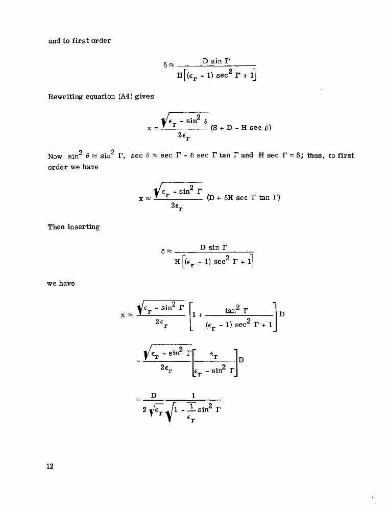
and to first order

Rewriting equation (A4) gives

V c r - sin" e x = (S + D - H sec 6 )

2 2 Now sin 0 = sin r, sec 0 * sec r - 6 sec I? tan I? and H sec r = S; thus, to first order we have

d e r - sin 2 r X = (D + 6H sec I? tan I?)

Then inserting

D sin I?

H [(Er - 1) sec' r + 11 i3=

we have

1 4 2dtrd1--Sin 'r

12

where

2 L2 - L2 sin r = - - L2 + H2

In the present instance L M 1.25 meters and H = 2.44 meters. Using cr = 3.1, one has

= 1.0353 1

Thus,

x M 8.81 (5 - t l )

with cy = 3. 1 for the all-terrain vehicle. tion given in the main text.

This approximate value agrees with the solu-

13

REFERENCES

1. Vickers, R. S. ; Heighway, J. ; and Gedney, R. : Airborne Profiling of Ice Thickness Using A Short Pulse Radar. NASA TM X-71481, 1973.

2. Cooper, Dale W. ; et al. : Remote Profiling of Lake Ice Thickness Using A Short Pulse Radar System Aboard A C-47 Aircraft. NASA TM X-71588, 1974.

3. Vickers, R. S. : Microwave Roperties of Ice From The Great Lakes. Stanford Research Inst. WAS3 -19092), 1974.

4. Stratton, Julius A. : Electromagnetic Theory. McGraw-Hill Book Co., Inc., 1941.

5. Harrington, Roger F. : Time-Harmonic Electromagnetic Fields. McGraw-Hill Book Co., Inc., 1961.

14

rir

,, ~ Reflected wave

Ice

Reflected wave i Figure 1. - Basic radar operation f rom a i r c r a f t

Water

Figure 2. - Operational diagram for short-pulse radar o n a l l - t e r ra in vehicle.

15

Figure 3. - Ray t rac ing geometry for short-pulse radar o n a l l - t e r ra in vehicle.

16

Random-noise source .----------1

Four- h o r n receiv ing array-,

I I

Four-port )'

Figure 4. - Block diagram of S-band short-pulse radar system used o n C-41 aircraf t .

Figure 5. - Operator's console for C- and S-band short-pulse radar aboard C-47 aircraf t .

17

Figure 6. - Receiving pod for C- and S-band radar instal led under wing of C-47 aircraft.

Transmit t ing h o r n

Solid-state 1, \

2.8-GHz amplif ier, ',

Receiving h o r n

Solid-state amplif ier,

Detector 1-GHz sampling osc i I loscope

noise f i gu re

Figure 7. - Block diagram of S-band short-pulse radar system used o n a l l - t e r ra in vehicle.

18

Receiving ampl i f ier ->,

Crystal FOsci l iator detector,

-M ixe rs

C 721164

Figure 8. - S-band short-pulse t ransmit ter and receiver u n i t for use o n a l l - t e r ra in vehicle.

Figure 9. - Location of electronic equipment in all-terrain vehicle.

19

c-75-2919 -

Figure 10. - A l l - t e r r a i n vehicle i n operation on Straits of Mackinac.

Figure 11. - Typical ice return shown on face of sampling oscilloscope (2 nsec/division).

20

Figure 12. - Ice thickness measurement made with ice auger.

Figure 13. - Test site near Mackinac Bridge. Snow depth, 6.5 centimeters; ice thickness, 40 centimeters.

2 1

Figure 14. - Oscilloscope output at test site in figure 13 after site had been wet with water (2 nsec 'division).

Figure 15. - Oscilloscope output at test site in figure 13 after site had refrozen (2 nsec/division).

22

I

10 20 30 40 50 60 Thickness measured by radar, cm

Figure 16. - Comparison of ice thickness measurements made by auger and radar w i th relative dielectr ic con- stant assumed to be 3.1.

{MA-Langley, 1976 E-8573 23

NATIONAL AERONAUTICS AND SPACE ADMINISTRATION WASHINGTON. D.C. 20546

USMAIL

POSTAGE A N D FEES P A I D N A T I O N A L AERONAUTICS A N D

OFFICIAL BUSINESS SPACE A D M I N I S T R A T I O N PENALTY FOR P R I V A T E USE 1300 SPECIAL FOURTH-CLASS R A T E 451

BOOK

POsTMASTBR : If Undeliverable (Section 158 Postal itliiniiiil) Do Not Return

“The aeronautical and space activities of the United States shall be conducted so as to contribute . . . to the expansion. of human Lnowl- edge of phenomena i n the atmosphere and space. T h e Administration shall provide for the wzdest practicable and appropriate dissemination of information concerning its activities and the resalts thereof.”

-NATIONAL AERONAUTICS AND SPACE ACT OF 1958

NASA SCIENTIFIC AND TECHNICAL PUBLICATIONS TECHNICAL REPORTS: Scientific and technical information considered important, complete, and a lasting contribution to existing knowledge.

TECHNICAL NOTES: Information less broad in scope but nevertheless of importance as a contribution to existing knowledge.

TECHNICAL MEMORANDUMS: Information receiving limited distribution because of preliminary data, security classifica- tion, or other reasons. Also inciudes conference proceedings with either limited or unlimited distribution.

CONTRACTOR REPORTS: Scientific and technical information generated under a NASA contract or grant and considered an important contribution to existing knowledge.

-

TECHNICAL TRANSLATIONS: Information published in a foreign language considered to merit NASA distribution in English.

SPECIAL PUBLICATIONS: Information derived from or of value to NASA activities. Publications include final reports of major projects, monographs, data compilations, handbooks, sourcebooks, and special bibliographies.

TECHNOLOGY UTILIZATION PUBLICATIONS : Information on technology used by NASA that may be of particular interest in commercial and other- non-aerospace applications. Publications include Tech Briefs, Technology Utilization Reports and Technology Surveys.

Details on the availability of these publications may b e obtained from:

SCIENTIFIC A N D TECHNICAL INFORMATION OFFICE

N A T I O N A L A E R O N A U T I C S A N D SPACE A D M I N I S T R A T I O N Washington, D.C. 20546

1