Embed Size (px)
Citation preview

i
MEASUREMENT OF AILERON HINGE MOMENTS AND THE EFFECT OF AILERON TRAILING EDGE THICKNESS
Sjouke Willem Schekman
A dissertation submitted to the Faculty of Engineering and the Built Environment, University of
the Witwatersrand, Johannesburg, in fulfilment of the requirements for the degree of Master of
Science in Engineering.
Johannesburg, July-2015

ii
DECLARATION
I declare that this dissertation is my own, unaided work, except where otherwise acknowledged.
It is being submitted for the degree Master of Science in Engineering in the University of the
Witwatersrand, Johannesburg. It has not been submitted before for any degree or examination
at any other university.
Signed this 23 July 2015
________________________________
Sjouke Willem Schekman
iii
ABSTRACT
The objective of this research was twofold. The first objective was for the design and testing of
a compact force measurement device, capable of fitting inside the wind tunnel model and
measuring aileron hinge moments. Using the hinge moment balance, the second objective was
to test the effect of varying the trailing edge thickness of the aileron. A plain type aileron, with
a 20.6% chord and 40% span, was attached to a NACA 0012 wing. Four aileron test pieces
with trailing edge thicknesses from 0.39%c to 1.22%c were used. A external balance capable of
measuring the wing rolling and yawing moments was used in conjunction with the hinge
moment balance. Validation of the results and performance of the hinge moment balance was
done by comparisons to the data obtained from previous research and investigations using flow
visualization. The results indicated that the system performed in a manner that was expected
and predictable. The data from the hinge moment balance had an uncertainty of 4.2% which
was deemed satisfactory for the purposes of this research. For the majority of the test cases the
effects of the varied trailing edge thickness was found to be negligible. Small differences were
noted at high angles of attack, above 15°, and high aileron deflections, above 20°. As these
conditions were seen to be outside the typical flight envelope of general aviation aircraft, these
small differences were seen as inconsequential. It was concluded that the use of an aileron with
a thicker trailing edge would not have a negative effect on the performance of the aileron while
allowing for less restrictions on the manufacture of the aileron itself.

iv
TABLE OF CONTENTS
Declaration ................................................................................................................................... ii
Abstract ....................................................................................................................................... iii
Table of Contents ........................................................................................................................ iv
List of Figures ............................................................................................................................ vii
List of Tables ............................................................................................................................. xii
1 Introduction .......................................................................................................................... 1
1.1 Background ................................................................................................................. 1
1.2 Motivation ................................................................................................................... 4
1.3 Objectives .................................................................................................................... 4
2 Literature Survey .................................................................................................................. 5
2.1 Previous Research ....................................................................................................... 5
2.1.1 Blunt Trailing Edges ............................................................................................... 6
2.1.2 Data Accuracy ....................................................................................................... 10
2.1.3 Testing Methodology ............................................................................................ 10
2.2 Aileron Performance Characterization ...................................................................... 11
2.2.1 Rolling Performance ............................................................................................. 11
2.2.2 Adverse Yaw ......................................................................................................... 12
2.2.3 Control Loads ........................................................................................................ 13
2.3 Low Reynolds Number Testing ................................................................................. 13
2.4 Hinge Moment Measurement Techniques ................................................................. 15
2.5 Test Model Configurations ........................................................................................ 17
3 Method ............................................................................................................................... 18
3.1 Test Matrix ................................................................................................................ 18
3.2 Test Equipment Requirements ................................................................................... 19
4 Facilities and equipment..................................................................................................... 20
4.1 Wind tunnel ............................................................................................................... 21
4.2 External Balance ........................................................................................................ 22
4.3 Test Model ................................................................................................................. 25
4.3.1 Design ................................................................................................................... 25
4.3.2 Manufacture .......................................................................................................... 26
v
4.3.3 Lateral Control Device .......................................................................................... 27
4.3.4 Hinge Moment Balance ......................................................................................... 30
4.4 Data Acquisition ........................................................................................................ 31
4.4.1 Data Acquisition Device (DAQ) ........................................................................... 31
4.4.2 Atmospheric Data ................................................................................................. 32
4.4.3 Power Supply ........................................................................................................ 33
4.4.4 Wiring ................................................................................................................... 34
4.5 Flow Visualization..................................................................................................... 34
5 Data Processing .................................................................................................................. 35
6 Error Propagation ............................................................................................................... 37
6.1 Data Uncertainty ........................................................................................................ 37
6.2 Signal Sensitvity ........................................................................................................ 37
6.2.1 Loadcells Signal Sensitivity .................................................................................. 37
6.2.2 Potentiometer Signal Sensitivity ........................................................................... 39
6.2.3 Ghosting Effect ..................................................................................................... 40
6.2.4 Signal Drift ............................................................................................................ 41
6.3 Data Distribution and Manipulation .......................................................................... 42
7 Calibration .......................................................................................................................... 44
7.1 External Balance Calibration ..................................................................................... 44
7.2 Hinge Moment Calibration ........................................................................................ 47
7.3 Aileron Deflection ..................................................................................................... 49
8 Results and Discussion ....................................................................................................... 51
8.1 Typical Data Set ........................................................................................................ 51
8.2 Flow Visualization Results ........................................................................................ 56
8.3 Comparisons to Previous Research ........................................................................... 62
8.4 Variation of Aileron Trailing Edge Thickness .......................................................... 68
9 Conclusions ........................................................................................................................ 80
10 Recommendations .............................................................................................................. 81
11 References .......................................................................................................................... 82
Appendix A : Previous Research Data ........................................................................................ 87
Appendix B : Engineering Drawings .......................................................................................... 91
vi
Appendix C : Equipment Datasheets ........................................................................................ 102
Appendix D : Derivation of Uncertainty ................................................................................... 115
Appendix E : Loadcell Sensitivity Check Setup and Procedures .............................................. 118
E.1. External Balance Loadcells ..................................................................................... 118
E.2. Hinge Moment Balance Loadcell ............................................................................ 118
Appendix F : Calibration Setup and Procedures ....................................................................... 120
F.1. External Balance ...................................................................................................... 120
F.2. Hinge Moment Balance ........................................................................................... 121
F.3. Aileron Deflection ................................................................................................... 122
Appendix G : external Balance Cross Coupling Effect ............................................................. 124
Appendix H : Test Precautions ................................................................................................. 125
Appendix I : Full List of Results ............................................................................................... 126
vii
LIST OF FIGURES
Figure 1.1: Three different trailing edge angles (Toll, 1946). ....................................................... 1 Figure 1.2: Frequency and distribution of previous publications .................................................. 2 Figure 2.1: Plain Flap Type Aileron indicating definition of aileron chord used in calculations
(Rogallo & Purser, 1941) .............................................................................................................. 6 Figure 2.2: Examples of Frise ailerons investigated in previous tests (Toll, 1946) ...................... 6 Figure 2.3: Lift of an 0018 airfoil with and without a blunt trailing edge, produced by cutting
off the trailing edge (Hoerner & Borst, 1985) ............................................................................... 7 Figure 2.4: Change in drag coefficient of a streamline body brought on by removal of bodies
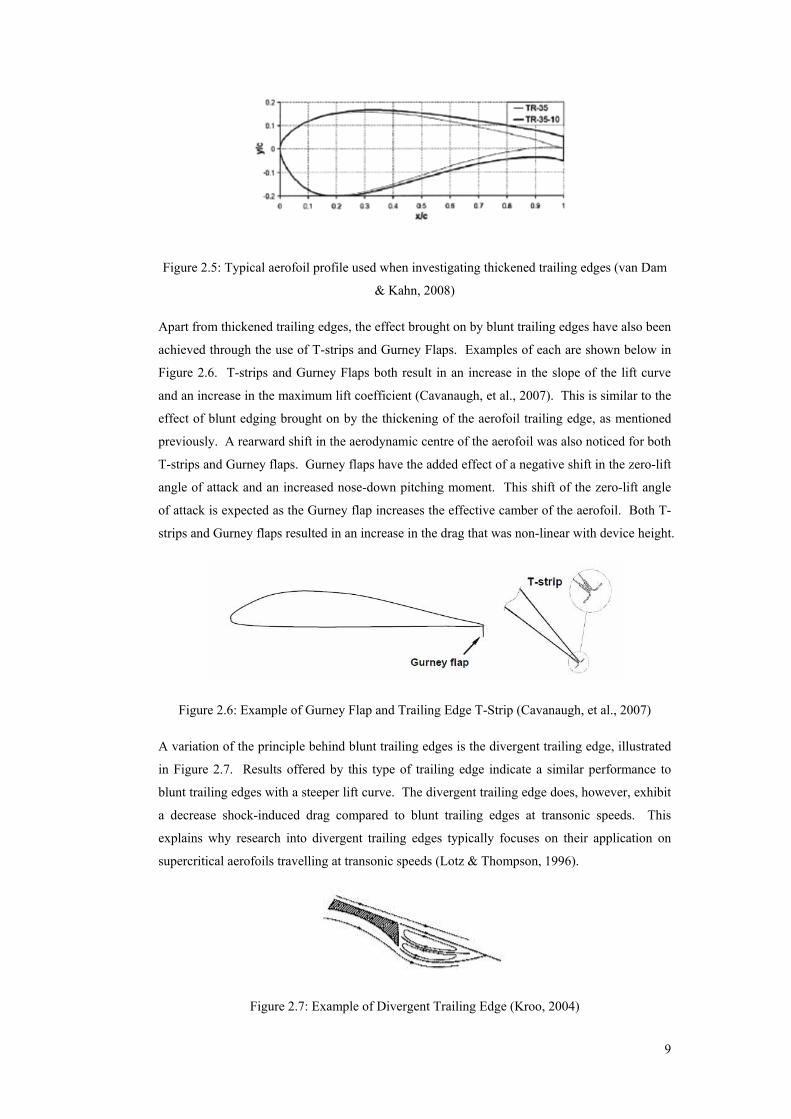
trailing edge (Hoerner, 1965) ........................................................................................................ 8 Figure 2.5: Typical aerofoil profile used when investigating thickened trailing edges (van Dam
& Kahn, 2008) .............................................................................................................................. 9 Figure 2.6: Example of Gurney Flap and Trailing Edge T-Strip (Cavanaugh, et al., 2007) ......... 9 Figure 2.7: Example of Divergent Trailing Edge (Kroo, 2004) .................................................... 9 Figure 2.8: Aerofoil data for NACA 0012 conducted for a range of Reynolds numbers between
170 000 and 3 180 0000 (Jacobs & Sherman, 1937)................................................................... 14 Figure 2.9: Seperation occurring on an airfoil at a low angle of attack, at low a Reynolds
number (a) and an increased Reynolds number (b) (van Dyke, 2005) ........................................ 15 Figure 2.10: Previously used Hinge Moment Measurement Arrangement (Monish, 1930) ....... 16 Figure 2.11: Test setup as used by Rogallo (Rogallo & Lowry, 1942) ....................................... 16 Figure 2.12: Cable-tension recorder as employed by Goranson (1946) during flight tests. ........ 17 Figure 4.1 Wind tunnel cross section and internal dimensions ................................................... 21 Figure 4.2: External Balance Axis System ................................................................................. 21 Figure 4.3 External Balance Isometric View .............................................................................. 24 Figure 4.4: External Balance 3 View .......................................................................................... 24 Figure 4.5 Wing Alignment Plate ............................................................................................... 25 Figure 4.6: Half wing cut-outs .................................................................................................... 27 Figure 4.7: Aileron profile to be tested ....................................................................................... 27 Figure 4.8: Aileron Design.......................................................................................................... 29 Figure 4.9: Internal Hinge Moment Balance Configuration ....................................................... 30 Figure 5.1: Property mapping due inversion of the wing about the x-y plane ............................ 36
Figure 6.1: Variation in yawing moment loadcell signal, measured in με, with an increase in
mass directly applied to the loadcell. .......................................................................................... 38
Figure 6.2: Variation in hinge moment loadcell signal, measured in με, with an increase in mass
directly applied to the loadcell .................................................................................................... 39
Figure 6.3: Change in loadcell signals, measured in με, recorded for each loadcell when a
yawing moment was applied. ...................................................................................................... 40 Figure 6.4: Variation of rolling moment loadcell signal over a 20 hour period plotted against the
variation in ambient air temperature over the same time. ........................................................... 41
viii
Figure 6.5: Distribution of rolling moment raw signal data, measured in με, obtained from a
single test plotted against a Gaussian distribution, 15° AoA, Thickness 2, δ=-10°, V=14.7m/s.42 Figure 6.6: Comparison of raw and filtered rolling moment signal data from example test, 15°
AoA, δ=10°, V= 14.5m/s. Lowpass filter of 5Hz applied. ......................................................... 43 Figure 7.1: Rolling moment calibration results for the rolling moment loadcell ........................ 44 Figure 7.2: Rolling moment calibration results for the yawing moment loadcell ....................... 46 Figure 7.3: Hinge moment balance calibration plot .................................................................... 47 Figure 7.4: Aileron deflection calibration plot of deflection against voltage recorded ............... 49 Figure 8.1: Zeroed yawing moment loadcell signals, including reversed signals, -5° and +5°
AoA, plain sealed aileron, Thickness 2, V=14.6m/s. .................................................................. 52 Figure 8.2: Comparison of data before and after application of calibration for yawing moment
loads at 5° AoA, plain sealed aileron, Thickness 2, V=14.6m/s ................................................. 54 Figure 8.3: Comparison of data before and after application of calibration for rolling moment
loads at 5° AoA, plain sealed aileron, Thickness 2, V=14.6m/s ................................................. 55 Figure 8.4: Yawing Moment Coefficients at 5° AoA, Thickness 2, V=14.6m/s ......................... 55 Figure 8.5: Variation of hinge moment strain uncertainty with aileron deflection for 5° and 10°
AoA, Thickness 2, V=14.6m/s .................................................................................................... 56 Figure 8.6: Rolling moment coefficient trend (a) and corresponding flow field (b) for 12.5°
AoA, Thickness 2, V=14.6m/s .................................................................................................... 57 Figure 8.7: Rolling moment coefficient trend (a) and corresponding flow field (b) for 15° AoA,
Thickness 2, V=14.5m/s ............................................................................................................. 58 Figure 8.8: Flow visualization at 12.5° AoA, aileron deflection at -30° (a) and +30° (b),
Thickness 2, V=14.7m/s ............................................................................................................. 59 Figure 8.9: Rolling moment coefficient trend (a) and corresponding flow field (b) for 20° AoA,
Thickness 2, V=14.8m/s ............................................................................................................. 60 Figure 8.10: Rolling moment coefficients with modified trend line for 20° AoA, Thickness 2,
V=14.8m/s .................................................................................................................................. 61 Figure 8.11: Hinge Moment Coefficients for a NACA 0012 at 12.5° AoA, plain sealed 0.206c
0.4b/2 aileron Thickness 2, V=14.6m/s ...................................................................................... 62 Figure 8.12: Comparison between delta rolling moment coefficients for primary test data,
Thickness 2, 10° AoA, V=14.7m/s, and data obtained from Rogallo (1941). ............................ 64 Figure 8.13: Comparison between delta yawing moment coefficients for primary test data,
Thickness 2, and data obtained from Rogallo (1941), 10° AoA, V=14.7m/s. ............................ 66 Figure 8.14: Comparison between hinge moment coefficients for primary test data, Thickness 2,
and data obtained from Rogallo (1941), 10° AoA, V=14.7m/s. ................................................. 67 Figure 8.15: Comparison of delta rolling moment coefficients for 4 aileron trailing edge
thicknesses, 5° AoA, V=14.6m/s ................................................................................................ 70 Figure 8.16: Comparison of delta rolling moment coefficients for 4 aileron trailing edge
thicknesses, 5°, 12.5° and 15° AoA, V=14.6m/s ........................................................................ 71
ix
Figure 8.17: Comparison of delta rolling moment coefficients for 4 aileron trailing edge
thicknesses, 20° AoA, V=14.8m/s .............................................................................................. 72 Figure 8.18: Delta yawing moment coefficient trends for each AoA, aileron Thickness 2,
V=14.8m/s .................................................................................................................................. 73 Figure 8.19: Comparison of delta yawing moment coefficients for 4 aileron trailing edge
thicknesses, 5° AoA, V=14.6m/s ................................................................................................ 74 Figure 8.20: Comparison of delta yawing moment coefficients for 4 aileron trailing edge
thicknesses, 15° AoA, V=14.5m/s .............................................................................................. 75 Figure 8.21: Comparison of delta yawing moment coefficients for 4 aileron trailing edge
thicknesses, 20° AoA, V=14.8m/s .............................................................................................. 75 Figure 8.22: Comparison of delta yawing moment coefficient variation with delta rolling
moment coefficient, for 4 aileron trailing edge thicknesses, 5° AoA, V=14.6m/s ...................... 76 Figure 8.23: Comparison of delta yawing moment coefficient variation with delta rolling
moment coefficient, for 4 aileron trailing edge thicknesses, 20° AoA, V=14.8m/s .................... 76 Figure 8.24: Comparison of hinge moment coefficients for 4 aileron trailing edge thicknesses,
5° AoA, V=14.6m/s .................................................................................................................... 77 Figure 8.25: Comparison of hinge moment coefficients for 4 aileron trailing edge thicknesses,
15° AoA, V=14.5m/s .................................................................................................................. 77 Figure 8.26: Comparison of hinge moment coefficients for 4 aileron trailing edge thicknesses,
20° AoA, V=14.8m/s .................................................................................................................. 78
Figure A.1: Aerodynamic characteristics of a 0.20c by 0.37 b/2 plain grease-sealed aileron
without balance on an NACA 23012 airfoil. V, 40mph (Rogallo & Purser, 1941) .................... 87 Figure A.2: Typical rolling and hinge moment coefficient curves for plain ailerons (Jones &
Weick, 1937). .............................................................................................................................. 88 Figure A.3: Aerofoil section characteristics of a NACA0012 as affected by variations of the
Reynolds number (Jacobs & Sherman, 1937). ............................................................................ 89 Figure A.4: Seperation occurring on an airfoil at a low angle of attack, at low a Reynolds
number (a) and an increased Reynolds number (b) (Jacobs & Sherman, 1937) ......................... 90
Figure B.1: External Balance ISO View ..................................................................................... 92 Figure B.2: External Balance 3 View ......................................................................................... 93 Figure B.3: External Balance Cage ............................................................................................. 94 Figure B.4: Balance Arm ............................................................................................................ 95 Figure B.5: Wing Alignment Plate ............................................................................................. 96 Figure B.6: Wing Assembly........................................................................................................ 97 Figure B.7: Wing Half ................................................................................................................ 98 Figure B.8: Aileron Assembly .................................................................................................... 99 Figure B.9: Hinge Moment Balance Overview ......................................................................... 100
x
Figure B.10: Hinge Moment Balance ....................................................................................... 101
Figure E.1: Setup used in the calibration of the hinge moment loadcell through the application
of load directly to the loadcell. .................................................................................................. 119
Figure F.1: Calibration setup used for rolling moment calibration ........................................... 120 Figure F.2: External Balance calibration configuration ............................................................ 121 Figure F.3: Hinge moment balance calibration setup. ............................................................... 122 Figure F.4: Aileron Deflection calibration configuration ......................................................... 123
Figure G.1: Diagram explaining yawing moment load direction depending on applied rolling
moment direction ...................................................................................................................... 124
Figure I.1: Comparison of delta rolling moment coefficients for 4 aileron trailing edge
thicknesses, 0° AoA, V=14.9m/s .............................................................................................. 126 Figure I. 2: Comparison of delta rolling moment coefficients for 4 aileron trailing edge
thicknesses, 5° AoA, V=14.6m/s .............................................................................................. 126 Figure I. 3: Comparison of delta rolling moment coefficients for 4 aileron trailing edge
thicknesses, 10° AoA, V=14.7m/s ............................................................................................ 127 Figure I. 4: Comparison of delta rolling moment coefficients for 4 aileron trailing edge
thicknesses, 12.5° AoA, V=14.6m/s ......................................................................................... 127 Figure I. 5: Comparison of delta rolling moment coefficients for 4 aileron trailing edge
thicknesses, 15° AoA, V=14.5m/s ............................................................................................ 128 Figure I. 6: Comparison of delta rolling moment coefficients for 4 aileron trailing edge
thicknesses, 17.5° AoA, V=14.7m/s ......................................................................................... 128 Figure I. 7: Comparison of delta rolling moment coefficients for 4 aileron trailing edge
thicknesses, 20° AoA, V=14.8m/s ............................................................................................ 129 Figure I. 8: Comparison of delta yawing moment coefficients for 4 aileron trailing edge
thicknesses, 0° AoA, V=14.9m/s .............................................................................................. 129 Figure I. 9: Comparison of delta yawing moment coefficients for 4 aileron trailing edge
thicknesses, 5° AoA, V=14.6m/s .............................................................................................. 130 Figure I. 10: Comparison of delta yawing moment coefficients for 4 aileron trailing edge
thicknesses, 10° AoA, V=14.7m/s ............................................................................................ 130 Figure I. 11: Comparison of delta yawing moment coefficients for 4 aileron trailing edge
thicknesses, 12.5° AoA, V=14.6m/s ......................................................................................... 131 Figure I. 12: Comparison of delta yawing moment coefficients for 4 aileron trailing edge
thicknesses, 15° AoA, V=14.5m/s ............................................................................................ 131
xi
Figure I. 13: Comparison of delta yawing moment coefficients for 4 aileron trailing edge
thicknesses, 17.5° AoA, V=14.7m/s ......................................................................................... 132 Figure I. 14: Comparison of delta yawing moment coefficients for 4 aileron trailing edge
thicknesses, 20° AoA, V=14.8m/s ............................................................................................ 132 Figure I. 15: Comparison of hinge moment coefficients for 4 aileron trailing edge thicknesses,
0° AoA, V=14.9m/s .................................................................................................................. 133 Figure I. 16: Comparison of hinge moment coefficients for 4 aileron trailing edge thicknesses,
5° AoA, V=14.6m/s .................................................................................................................. 133 Figure I. 17: Comparison of hinge moment coefficients for 4 aileron trailing edge thicknesses,
10° AoA, V=14.7m/s ................................................................................................................ 134 Figure I. 18: Comparison of hinge moment coefficients for 4 aileron trailing edge thicknesses,
12.5° AoA, V=14.6m/s ............................................................................................................. 134 Figure I. 19: Comparison of hinge moment coefficients for 4 aileron trailing edge thicknesses,
15° AoA, V=14.5m/s ................................................................................................................ 135 Figure I. 20: Comparison of hinge moment coefficients for 4 aileron trailing edge thicknesses,
17.5° AoA, V=14.7m/s ............................................................................................................. 135 Figure I. 21: Comparison of hinge moment coefficients for 4 aileron trailing edge thicknesses,
20° AoA, V=14.8m/s ................................................................................................................ 136
xii
LIST OF TABLES
Table 4.1: Aileron Trailing Edge Thicknesses ............................................................................ 28 Table 6.1: Approximate loads and change in signal values to be measured by each of the three
loadcells during testing. .............................................................................................................. 39
Table E.1: Mass loads applied during calibration of sting balance loadcells ............................ 118 Table E.2: Mass loads applied during direct calibration of hinge moment loadcell ................. 118
Table F.1: Moment arms and masses applied during calibration .............................................. 121 Table F.2: Moment loads applied during calibration of hinge moment measurement balance . 122
1
1 INTRODUCTION
1.1 Background
The previous research into aileron performance has typically focused on the measurement of the
rolling, yawing and hinge moments produced by an aileron during flight conditions. The hinge
moment characteristics of ailerons have been found to be heavily dependent on the aileron
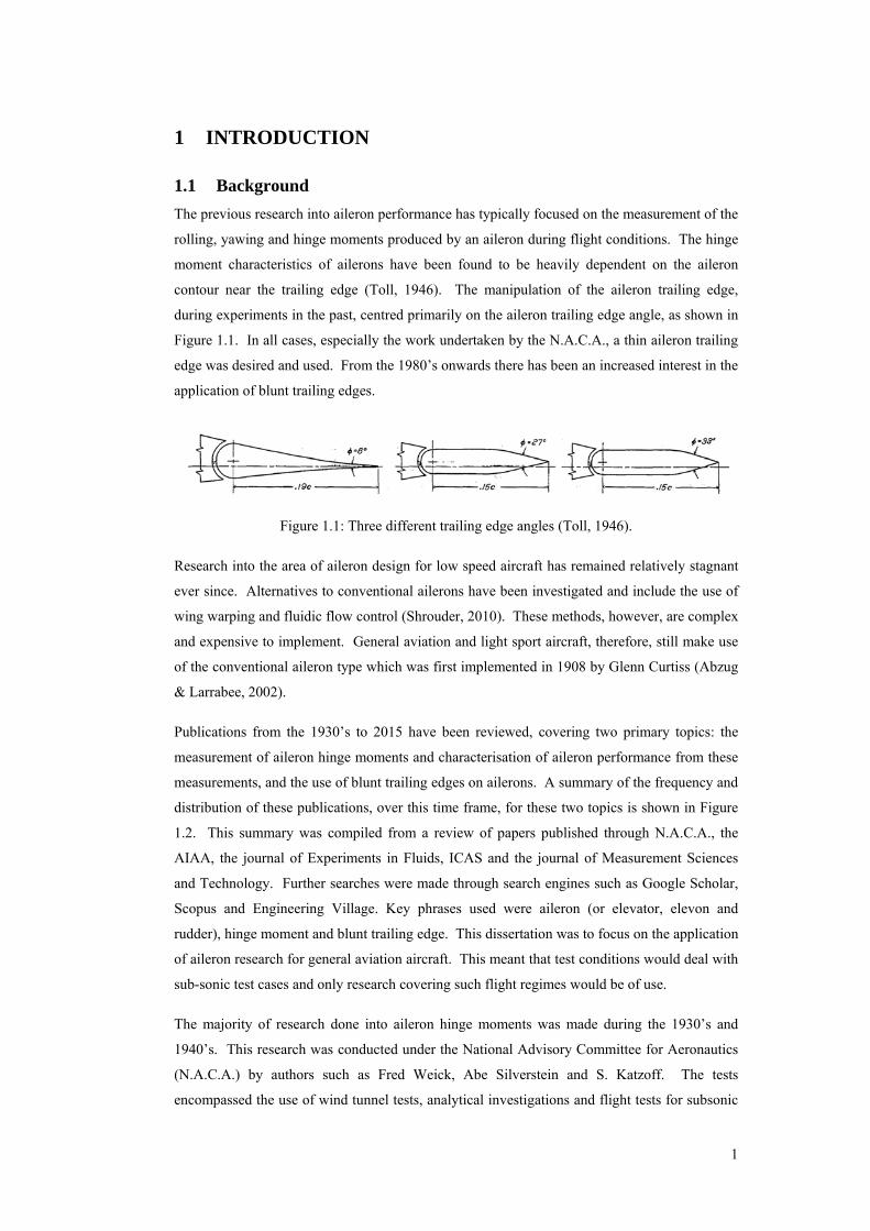
contour near the trailing edge (Toll, 1946). The manipulation of the aileron trailing edge,
during experiments in the past, centred primarily on the aileron trailing edge angle, as shown in
Figure 1.1. In all cases, especially the work undertaken by the N.A.C.A., a thin aileron trailing
edge was desired and used. From the 1980’s onwards there has been an increased interest in the
application of blunt trailing edges.
Figure 1.1: Three different trailing edge angles (Toll, 1946).
Research into the area of aileron design for low speed aircraft has remained relatively stagnant
ever since. Alternatives to conventional ailerons have been investigated and include the use of
wing warping and fluidic flow control (Shrouder, 2010). These methods, however, are complex
and expensive to implement. General aviation and light sport aircraft, therefore, still make use
of the conventional aileron type which was first implemented in 1908 by Glenn Curtiss (Abzug
& Larrabee, 2002).
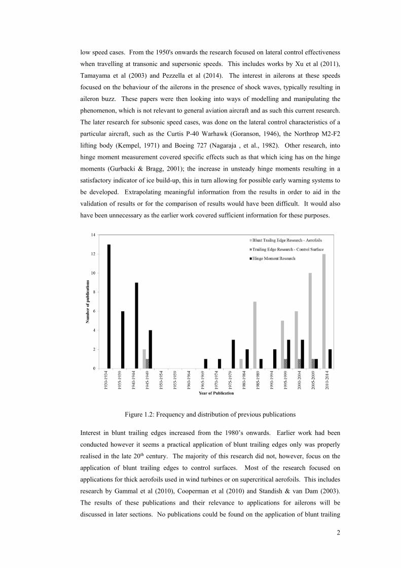
Publications from the 1930’s to 2015 have been reviewed, covering two primary topics: the
measurement of aileron hinge moments and characterisation of aileron performance from these
measurements, and the use of blunt trailing edges on ailerons. A summary of the frequency and
distribution of these publications, over this time frame, for these two topics is shown in Figure
1.2. This summary was compiled from a review of papers published through N.A.C.A., the
AIAA, the journal of Experiments in Fluids, ICAS and the journal of Measurement Sciences
and Technology. Further searches were made through search engines such as Google Scholar,
Scopus and Engineering Village. Key phrases used were aileron (or elevator, elevon and
rudder), hinge moment and blunt trailing edge. This dissertation was to focus on the application
of aileron research for general aviation aircraft. This meant that test conditions would deal with
sub-sonic test cases and only research covering such flight regimes would be of use.
The majority of research done into aileron hinge moments was made during the 1930’s and
1940’s. This research was conducted under the National Advisory Committee for Aeronautics
(N.A.C.A.) by authors such as Fred Weick, Abe Silverstein and S. Katzoff. The tests
encompassed the use of wind tunnel tests, analytical investigations and flight tests for subsonic
2
low speed cases. From the 1950's onwards the research focused on lateral control effectiveness
when travelling at transonic and supersonic speeds. This includes works by Xu et al (2011),
Tamayama et al (2003) and Pezzella et al (2014). The interest in ailerons at these speeds
focused on the behaviour of the ailerons in the presence of shock waves, typically resulting in
aileron buzz. These papers were then looking into ways of modelling and manipulating the
phenomenon, which is not relevant to general aviation aircraft and as such this current research.
The later research for subsonic speed cases, was done on the lateral control characteristics of a
particular aircraft, such as the Curtis P-40 Warhawk (Goranson, 1946), the Northrop M2-F2
lifting body (Kempel, 1971) and Boeing 727 (Nagaraja , et al., 1982). Other research, into
hinge moment measurement covered specific effects such as that which icing has on the hinge
moments (Gurbacki & Bragg, 2001); the increase in unsteady hinge moments resulting in a
satisfactory indicator of ice build-up, this in turn allowing for possible early warning systems to
be developed. Extrapolating meaningful information from the results in order to aid in the
validation of results or for the comparison of results would have been difficult. It would also
have been unnecessary as the earlier work covered sufficient information for these purposes.
Figure 1.2: Frequency and distribution of previous publications
Interest in blunt trailing edges increased from the 1980’s onwards. Earlier work had been
conducted however it seems a practical application of blunt trailing edges only was properly
realised in the late 20th century. The majority of this research did not, however, focus on the
application of blunt trailing edges to control surfaces. Most of the research focused on
applications for thick aerofoils used in wind turbines or on supercritical aerofoils. This includes
research by Gammal et al (2010), Cooperman et al (2010) and Standish & van Dam (2003).
The results of these publications and their relevance to applications for ailerons will be
discussed in later sections. No publications could be found on the application of blunt trailing
3
edges to ailerons. Those reports, in the Figure 1.2, referring to control surface trailing edge
research are either for the use of a blunt trailing edge on a slat (Khorrami, et al., 2000) or for
other trailing edge modifications (serrated edges rather than blunt trailing edges (Lemes &
Catalano, 2004)). A report was found from 1950, published by NACA, for the application of
blunt trailing edges on an aileron, however this was for a super-sonic case; the blunt trailing
edge eliminated the occurrence of control reversal during the transonic range (Strauss & Fields,
1950). As control reversal is not a factor that needs considering for general aviationThis data is
therefore of little use in the current scope of research.
4
1.2 Motivation
The manipulation of control surface hinge moments in aircraft has its advantages. Regulations,
such as FAR 23.395, state minimum design factors that need be applied to the computed aileron
hinge moment when designing the control system for an aircraft. Regulations also exist for
limiting the maximum allowable force or torque that a pilot can be expected to apply. By
manipulating the hinge moment required, the system can therefore be designed more efficiently.
This could result in the possibility of a lighter and/or cheaper control system. Basic aircraft
performance analysis techniques, such as those suggested by Torenbeek (1976), show that an
aircraft with a lower mass, due to a lighter actuation system, would be capable of carrying a
larger payload, or for the same load it would use less fuel. The lowering of the mass of the
actuation system would in some part reduce the rolling mass moment of inertia of the wing;
allowing for a more responsive aircraft. A decrease in the hinge moments of a particular aileron
could potentially allow for an aileron with a larger span to be used; aileron hinge moments
being proportional to the aileron span. Conversely an increase in hinge moments would allow
for smaller ailerons and therefore the use of larger flaps which would improve the take-off and
landing performance of the aircraft.
One area that remains relatively untested in the manipulation of aileron hinge moments deals
with the aileron trailing edge thickness. A general trend with the design of aerofoils for general
aviation aircraft is to have them manufactured with thin, sharp trailing edges. This is reflected
in the common reference to theoretical aerodynamics such as the Kutta condition. The issue is
that the requirement for a sharp trailing edge increases the difficulty in the manufacturing of the
aileron. The use of blunt trailing edges on wings has been investigated previously, with works
by Hoerner (1950) and Baker (2008). Their work showed that blunt trailing edges offered an
increase in the maximum lift produced by a wing along with an increase in the aerodynamic
drag. Hoerner commented on the possible application of these effects on the performance of
ailerons (Hoerner & Borst, 1985). By allowing for a thicker trailing edge, the aileron
manufacturing costs and complexity could be reduced. There is, then, merit in the investigation
into the use of ailerons with thicker trailing edges.
1.3 Objectives
The following objectives were undertaken for the research specified in this dissertation.
1. Design and test a hinge moment balance capable of accurately measuring the aileron hinge
moments that occur.
2. Compare and validate the results obtained from the hinge moment balance with those
obtained from previous tests.
3. Investigate the effect of a change in the aileron trailing edge thickness on the aileron
performance.
5
2 LITERATURE SURVEY
2.1 Previous Research
The previous research into aileron performance has been extensive. As stated in the previous
chapter, the majority of the research, that is pertinent to this dissertation, was conducted in the
1930’s and 1940’s. The experiments conducted by Toll, Wenzinger, Katzoff, and Heald,
among others, looked at various aspects of aileron performance. These included:
• The effectiveness of ailerons at high angles of attack (Wenzinger & Weick, 1932)
• Adverse yaw affects (Heald, 1933)
• Lateral stability (Toll, 1946)
• The downwash and wake behind ailerons (Katzoff, et al., 1938)
• Auto rotation tests (Toll, 1946)
• Effect of wing shape (Wenzinger, 1937), (Shortal & Weick, 1933)
• The lift distribution over ailerons (Bacon, 1924)
• Effect of altitude (Toll, 1946)
• Application of roughness strips on the aileron trailing edges (Toll, 1946)
• Aileron oscillations (Toll, 1946)
• Effect of balancing and sealing (Sears, 1942), (Rogallo & Purser, 1941)
Throughout the above mentioned experiments, multiple lateral control types were investigated.
This included, but was not limited to, the following aileron types:
• Plain flap (ordinary) (Wenzinger & Weick, 1931)
• Frise (Noyes & Weick, 1932)
• Floating tip (Harris & Weick, 1932)
• Slot lip (Shortal & Weick, 1935)
• Split and upper surface (Wenzinger & Weick, 1934)
• Spoiler (Shortal & Weick, 1932)
• Various combinations of the above types (Toll, 1946),
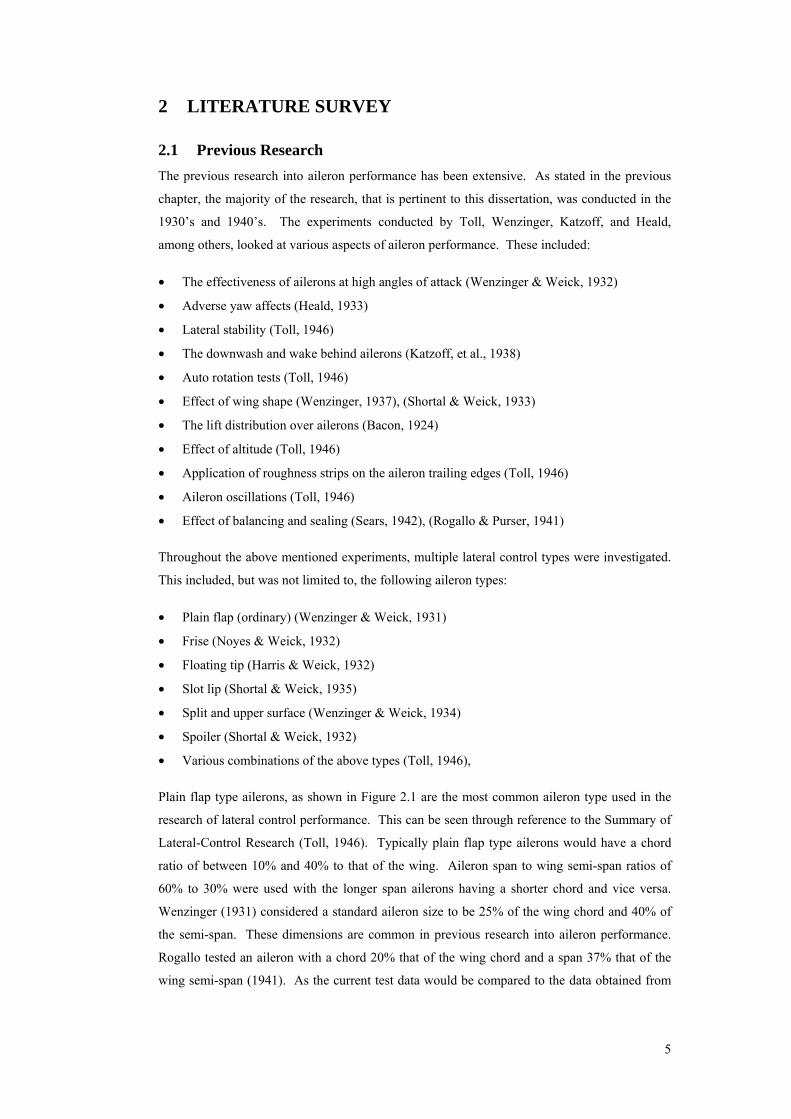
Plain flap type ailerons, as shown in Figure 2.1 are the most common aileron type used in the
research of lateral control performance. This can be seen through reference to the Summary of
Lateral-Control Research (Toll, 1946). Typically plain flap type ailerons would have a chord
ratio of between 10% and 40% to that of the wing. Aileron span to wing semi-span ratios of
60% to 30% were used with the longer span ailerons having a shorter chord and vice versa.
Wenzinger (1931) considered a standard aileron size to be 25% of the wing chord and 40% of
the semi-span. These dimensions are common in previous research into aileron performance.
Rogallo tested an aileron with a chord 20% that of the wing chord and a span 37% that of the
wing semi-span (1941). As the current test data would be compared to the data obtained from
6
Rogallo’s work, for reasons to be discussed further on, similar aileron dimensions would be
implemented for the current tests.
One reason for the popularity of the plain flap type is that aerodynamic theory can be
successfully applied to the calculation of the rolling and yawing moments of plain ailerons
(Jones & Weick, 1937). This makes it easier to validate data obtained from tests and predict
loads to be encountered. The rolling and hinge moment trends are also approximately linear
functions of the aileron deflection for a plain aileron. Plain ailerons also have the advantage of
being easier to manufacture than the more complex shapes such as Frise ailerons.
Figure 2.1: Plain Flap Type Aileron indicating definition of aileron chord used in calculations
(Rogallo & Purser, 1941)
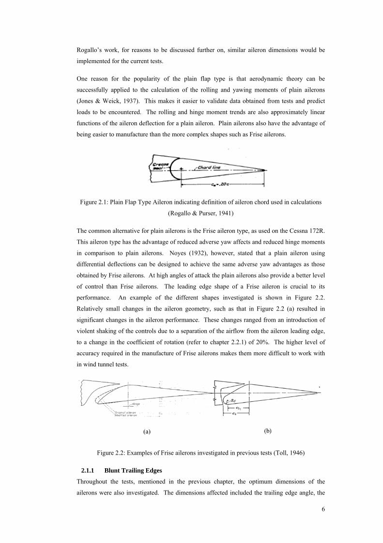
The common alternative for plain ailerons is the Frise aileron type, as used on the Cessna 172R.
This aileron type has the advantage of reduced adverse yaw affects and reduced hinge moments
in comparison to plain ailerons. Noyes (1932), however, stated that a plain aileron using
differential deflections can be designed to achieve the same adverse yaw advantages as those
obtained by Frise ailerons. At high angles of attack the plain ailerons also provide a better level
of control than Frise ailerons. The leading edge shape of a Frise aileron is crucial to its
performance. An example of the different shapes investigated is shown in Figure 2.2.
Relatively small changes in the aileron geometry, such as that in Figure 2.2 (a) resulted in
significant changes in the aileron performance. These changes ranged from an introduction of
violent shaking of the controls due to a separation of the airflow from the aileron leading edge,
to a change in the coefficient of rotation (refer to chapter 2.2.1) of 20%. The higher level of
accuracy required in the manufacture of Frise ailerons makes them more difficult to work with
in wind tunnel tests.
Figure 2.2: Examples of Frise ailerons investigated in previous tests (Toll, 1946)
2.1.1 Blunt Trailing Edges
Throughout the tests, mentioned in the previous chapter, the optimum dimensions of the
ailerons were also investigated. The dimensions affected included the trailing edge angle, the
7
aileron chord, span and taper, the alignment of the aileron hinge lines and the curving of the
aileron tips (Jones & Weick, 1937), (Shortal & Weick, 1933). Despite the results from previous
research into blunt trailing edges, indicating the application of the noted effects on aspects of
aileron performance (Hoerner & Borst, 1985), research into the matter has seen little to no light.
Aerofoils as opposed to ailerons with a blunt trailing edge, however, have been investigated.
This included works by Thompson & Whitelaw (1989), Drela (1989), Standish & van Dam
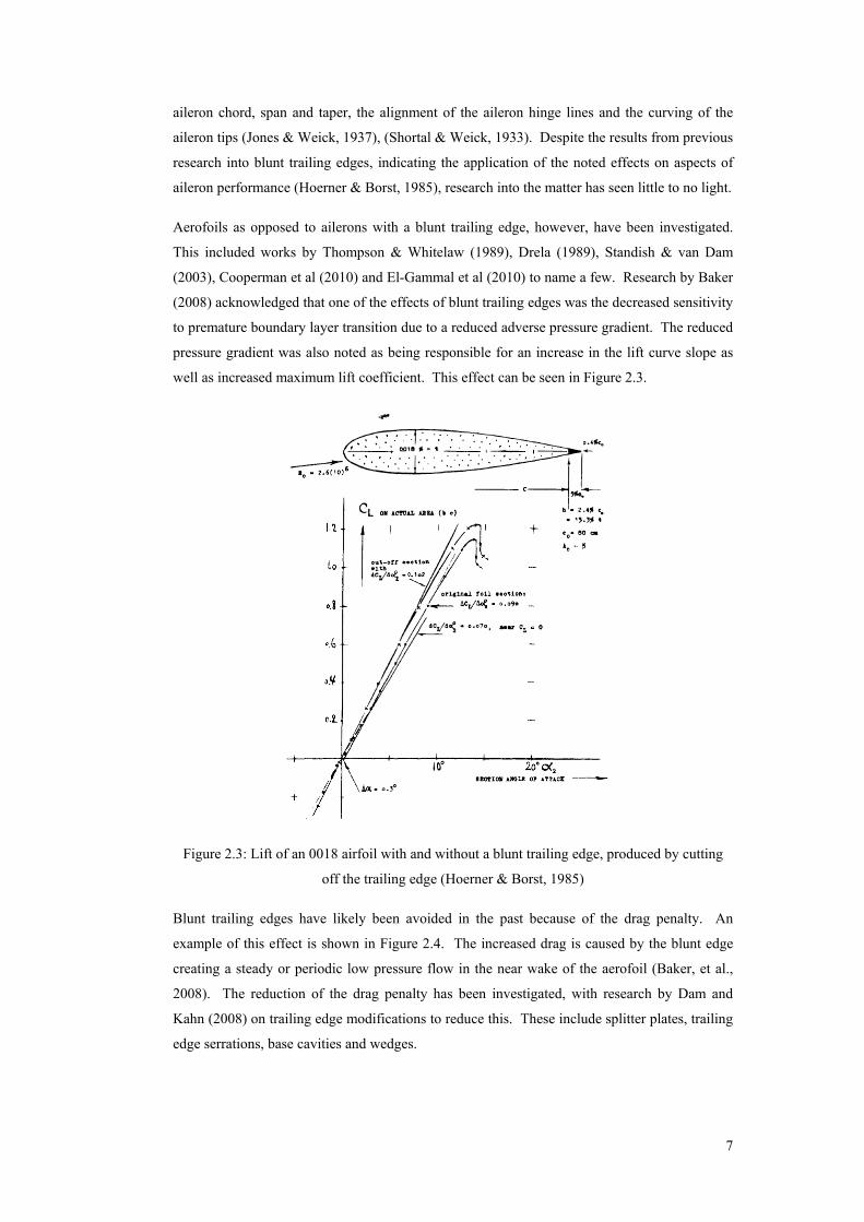
(2003), Cooperman et al (2010) and El-Gammal et al (2010) to name a few. Research by Baker
(2008) acknowledged that one of the effects of blunt trailing edges was the decreased sensitivity
to premature boundary layer transition due to a reduced adverse pressure gradient. The reduced
pressure gradient was also noted as being responsible for an increase in the lift curve slope as
well as increased maximum lift coefficient. This effect can be seen in Figure 2.3.
Figure 2.3: Lift of an 0018 airfoil with and without a blunt trailing edge, produced by cutting
off the trailing edge (Hoerner & Borst, 1985)
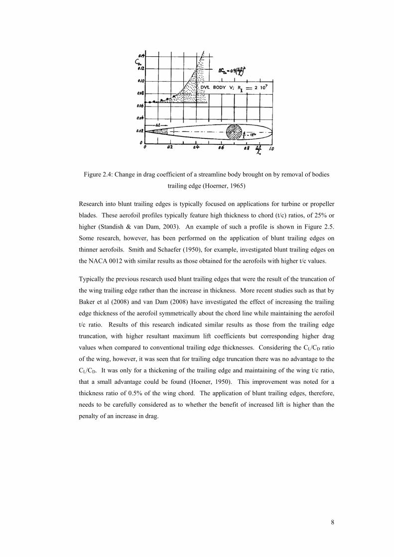
Blunt trailing edges have likely been avoided in the past because of the drag penalty. An
example of this effect is shown in Figure 2.4. The increased drag is caused by the blunt edge
creating a steady or periodic low pressure flow in the near wake of the aerofoil (Baker, et al.,
2008). The reduction of the drag penalty has been investigated, with research by Dam and
Kahn (2008) on trailing edge modifications to reduce this. These include splitter plates, trailing
edge serrations, base cavities and wedges.
8
Figure 2.4: Change in drag coefficient of a streamline body brought on by removal of bodies
trailing edge (Hoerner, 1965)
Research into blunt trailing edges is typically focused on applications for turbine or propeller
blades. These aerofoil profiles typically feature high thickness to chord (t/c) ratios, of 25% or
higher (Standish & van Dam, 2003). An example of such a profile is shown in Figure 2.5.
Some research, however, has been performed on the application of blunt trailing edges on
thinner aerofoils. Smith and Schaefer (1950), for example, investigated blunt trailing edges on
the NACA 0012 with similar results as those obtained for the aerofoils with higher t/c values.
Typically the previous research used blunt trailing edges that were the result of the truncation of
the wing trailing edge rather than the increase in thickness. More recent studies such as that by
Baker et al (2008) and van Dam (2008) have investigated the effect of increasing the trailing
edge thickness of the aerofoil symmetrically about the chord line while maintaining the aerofoil
t/c ratio. Results of this research indicated similar results as those from the trailing edge
truncation, with higher resultant maximum lift coefficients but corresponding higher drag
values when compared to conventional trailing edge thicknesses. Considering the CL/CD ratio
of the wing, however, it was seen that for trailing edge truncation there was no advantage to the
CL/CD. It was only for a thickening of the trailing edge and maintaining of the wing t/c ratio,
that a small advantage could be found (Hoener, 1950). This improvement was noted for a
thickness ratio of 0.5% of the wing chord. The application of blunt trailing edges, therefore,
needs to be carefully considered as to whether the benefit of increased lift is higher than the
penalty of an increase in drag.
9
Figure 2.5: Typical aerofoil profile used when investigating thickened trailing edges (van Dam
& Kahn, 2008)
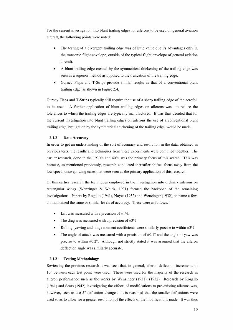
Apart from thickened trailing edges, the effect brought on by blunt trailing edges have also been
achieved through the use of T-strips and Gurney Flaps. Examples of each are shown below in
Figure 2.6. T-strips and Gurney Flaps both result in an increase in the slope of the lift curve
and an increase in the maximum lift coefficient (Cavanaugh, et al., 2007). This is similar to the
effect of blunt edging brought on by the thickening of the aerofoil trailing edge, as mentioned
previously. A rearward shift in the aerodynamic centre of the aerofoil was also noticed for both
T-strips and Gurney flaps. Gurney flaps have the added effect of a negative shift in the zero-lift
angle of attack and an increased nose-down pitching moment. This shift of the zero-lift angle
of attack is expected as the Gurney flap increases the effective camber of the aerofoil. Both T-
strips and Gurney flaps resulted in an increase in the drag that was non-linear with device height.
Figure 2.6: Example of Gurney Flap and Trailing Edge T-Strip (Cavanaugh, et al., 2007)
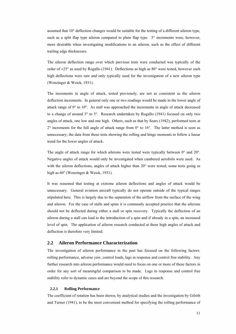
A variation of the principle behind blunt trailing edges is the divergent trailing edge, illustrated
in Figure 2.7. Results offered by this type of trailing edge indicate a similar performance to
blunt trailing edges with a steeper lift curve. The divergent trailing edge does, however, exhibit
a decrease shock-induced drag compared to blunt trailing edges at transonic speeds. This
explains why research into divergent trailing edges typically focuses on their application on
supercritical aerofoils travelling at transonic speeds (Lotz & Thompson, 1996).
Figure 2.7: Example of Divergent Trailing Edge (Kroo, 2004)
10
For the current investigation into blunt trailing edges for ailerons to be used on general aviation
aircraft, the following points were noted:
• The testing of a divergent trailing edge was of little value due its advantages only in
the transonic flight envelope, outside of the typical flight envelope of general aviation
aircraft.
• A blunt trailing edge created by the symmetrical thickening of the trailing edge was
seen as a superior method as opposed to the truncation of the trailing edge.
• Gurney Flaps and T-Strips provide similar results as that of a conventional blunt
trailing edge, as shown in Figure 2.4.
Gurney Flaps and T-Strips typically still require the use of a sharp trailing edge of the aerofoil
to be used. A further application of blunt trailing edges on ailerons was to reduce the
tolerances to which the trailing edges are typically manufactured. It was thus decided that for
the current investigation into blunt trailing edges on ailerons the use of a conventional blunt
trailing edge, brought on by the symmetrical thickening of the trailing edge, would be made.
2.1.2 Data Accuracy
In order to get an understanding of the sort of accuracy and resolution in the data, obtained in
previous tests, the results and techniques from these experiments were compiled together. The
earlier research, done in the 1930’s and 40’s, was the primary focus of this search. This was
because, as mentioned previously, research conducted thereafter shifted focus away from the
low speed, unswept wing cases that were seen as the primary application of this research.
Of this earlier research the techniques employed in the investigation into ordinary ailerons on
rectangular wings (Wenzinger & Weick, 1931) formed the backbone of the remaining
investigations. Papers by Rogallo (1941), Noyes (1932) and Wenzinger (1932), to name a few,
all maintained the same or similar levels of accuracy. These were as follows:
• Lift was measured with a precision of ±1%.
• The drag was measured with a precision of ±3%.
• Rolling, yawing and hinge moment coefficients were similarly precise to within ±3%.
• The angle of attack was measured with a precision of ±0.1° and the angle of yaw was
precise to within ±0.2°. Although not strictly stated it was assumed that the aileron
deflection angle was similarly accurate.
2.1.3 Testing Methodology
Reviewing the previous research it was seen that, in general, aileron deflection increments of
10° between each test point were used. These were used for the majority of the research in
aileron performance such as the works by Wenzinger (1931), (1932). Research by Rogallo
(1941) and Sears (1942) investigating the effects of modifications to pre-existing ailerons was,
however, seen to use 5° deflection changes. It is reasoned that the smaller deflections were
used so as to allow for a greater resolution of the effects of the modifications made. It was thus
11
assumed that 10° deflection changes would be suitable for the testing of a different aileron type,
such as a split flap type aileron compared to plain flap type. 5° increments were, however,
more desirable when investigating modifications to an aileron, such as the effect of different
trailing edge thicknesses.
The aileron deflection range over which previous tests were conducted was typically of the
order of ±25° as used by Rogallo (1941). Deflections as high as 80° were tested, however such
high deflections were rare and only typically used for the investigation of a new aileron type
(Wenzinger & Weick, 1931).
The increments in angle of attack, tested previously, are not as consistent as the aileron
deflection increments. In general only one or two readings would be made in the lower angle of
attack range of 0° to 10°. As stall was approached the increments in angle of attack decreased
to a change of around 3° to 5°. Research undertaken by Rogallo (1941) focused on only two
angles of attack, one low and one high. Others, such as that by Sears (1942), performed tests at
2° increments for the full angle of attack range from 0° to 16°. The latter method is seen as
unnecessary; the data from these tests showing the rolling and hinge moments to follow a linear
trend for the lower angles of attack.
The angle of attack range for which ailerons were tested were typically between 0° and 20°.
Negative angles of attack would only be investigated when cambered aerofoils were used. As
with the aileron deflections, angles of attack higher than 20° were tested; some tests going as
high as 60° (Wenzinger & Weick, 1931).
It was reasoned that testing at extreme aileron deflections and angles of attack would be
unnecessary. General aviation aircraft typically do not operate outside of the typical ranges
stipulated here. This is largely due to the separation of the airflow from the surface of the wing
and aileron. For the case of stalls and spins it is commonly accepted practice that the ailerons
should not be deflected during either a stall or spin recovery. Typically the deflection of an
aileron during a stall can lead to the introduction of a spin and if already in a spin, an increased
level of spin. The application of aileron research conducted at these high angles of attack and
deflection is therefore very limited.
2.2 Aileron Performance Characterization
The investigation of aileron performance in the past has focused on the following factors:
rolling performance, adverse yaw, control loads, lags in response and control free stability. Any
further research into aileron performance would need to focus on one or more of these factors in
order for any sort of meaningful comparison to be made. Lags in response and control free
stability refer to dynamic cases and are beyond the scope of this research.
2.2.1 Rolling Performance
The coefficient of rotation has been shown, by analytical studies and the investigation by Gilrith
and Turner (1941), to be the most convenient method for specifying the rolling performance of
12
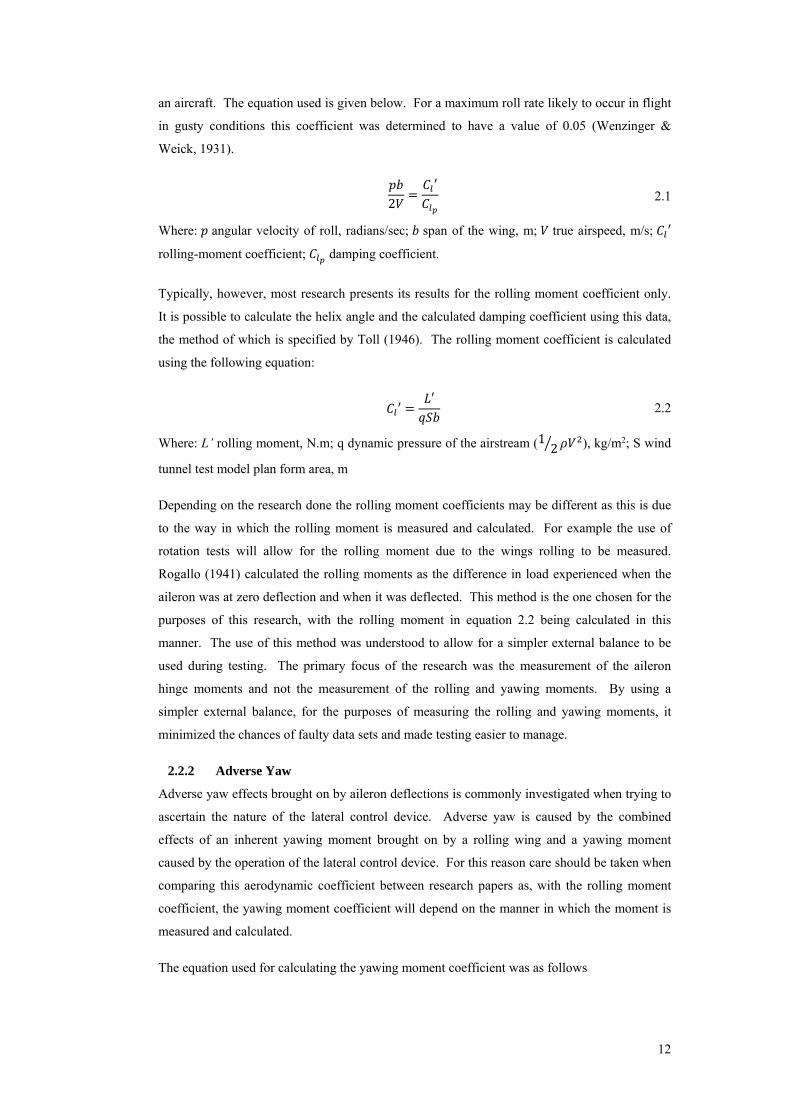
an aircraft. The equation used is given below. For a maximum roll rate likely to occur in flight
in gusty conditions this coefficient was determined to have a value of 0.05 (Wenzinger &
Weick, 1931).
2 = ′ 2.1
Where: angular velocity of roll, radians/sec; span of the wing, m; true airspeed, m/s; ′ rolling-moment coefficient; damping coefficient.
Typically, however, most research presents its results for the rolling moment coefficient only.
It is possible to calculate the helix angle and the calculated damping coefficient using this data,
the method of which is specified by Toll (1946). The rolling moment coefficient is calculated
using the following equation:
′ = ′ 2.2
Where: L’ rolling moment, N.m; q dynamic pressure of the airstream (1 2 ), kg/m2; S wind
tunnel test model plan form area, m
Depending on the research done the rolling moment coefficients may be different as this is due
to the way in which the rolling moment is measured and calculated. For example the use of
rotation tests will allow for the rolling moment due to the wings rolling to be measured.
Rogallo (1941) calculated the rolling moments as the difference in load experienced when the
aileron was at zero deflection and when it was deflected. This method is the one chosen for the
purposes of this research, with the rolling moment in equation 2.2 being calculated in this
manner. The use of this method was understood to allow for a simpler external balance to be
used during testing. The primary focus of the research was the measurement of the aileron
hinge moments and not the measurement of the rolling and yawing moments. By using a
simpler external balance, for the purposes of measuring the rolling and yawing moments, it
minimized the chances of faulty data sets and made testing easier to manage.
2.2.2 Adverse Yaw
Adverse yaw effects brought on by aileron deflections is commonly investigated when trying to
ascertain the nature of the lateral control device. Adverse yaw is caused by the combined
effects of an inherent yawing moment brought on by a rolling wing and a yawing moment
caused by the operation of the lateral control device. For this reason care should be taken when
comparing this aerodynamic coefficient between research papers as, with the rolling moment
coefficient, the yawing moment coefficient will depend on the manner in which the moment is
measured and calculated.
The equation used for calculating the yawing moment coefficient was as follows
13
′ = ′ 2.3
Where: N’ yawing moment, N.m.
For the purposes of this research the same technique as used by Rogallo (1941), and as used for
the rolling moments, was used in the measurement and calculation of the yawing moments.
The reasons for which were explained in the previous chapter. In this way the yawing moment
used in the above equation was the difference between the moment at zero aileron deflection
and with the aileron deflected.
2.2.3 Control Loads
The control loads specified for lateral control devices in previous research is either presented as
stick loads that a pilot would experience during flight or the hinge moment coefficient. Stick
loads are typically only given for research conducted during flight tests and are of little use in
comparisons unless for aircraft of a similar type or if the control system specifications are
known. The most useful way in which aileron loads are specified, therefore, is through the
hinge moment coefficient, calculated using the equation below:
= 2.4
Where: Ha hinge moment of the aileron, N.m; ca aileron chord, m; ba is the aileron span in, m
The hinge moment used here is the absolute value measured and not, like the rolling and
yawing moments, a difference in the load from a zero deflection and the measured deflection. It
should be noted however that the aileron chord used in the above equation is measured from the
aileron hinge line to its trailing edge, as shown in Figure 2.1, and not from the aileron leading
edge. This is a typical convention used in the analysis of aileron performance characteristics.
A result of this is that the nose shape of the aileron is not taken into account. Toll (1946),
however, provided correction factors that can be applied to the aileron hinge moments to
compensate for different aileron nose shapes.
2.3 Low Reynolds Number Testing
Due to limitations placed on the current research by the available facilities, tests are conducted
at Reynolds Numbers of around 300 000. Most of the research conducted previously on aileron
performance was conducted at Reynolds numbers of one million or higher. This difference in
Reynolds numbers means that the nature of the airflow over the aerofoils will be different. The
significance of this will be discussed below.
Jacobs (1937) performed research on the effect of low Reynolds numbers on common aerofoil
characteristics. The discussion into the effect, as laid out by Jacobs, deals mostly with airflow
separation. At high angles of attack the energy in the airflow ultimately becomes too low
leading to the separation of the airflow over the aerofoil upper surface, this separation affecting
the maximum lift of the wing; the lower the Reynolds number, the lower the maximum lift
14
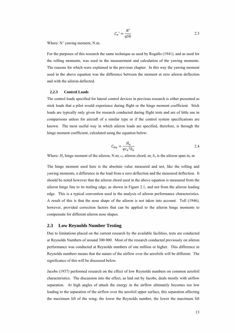
possible. This can be seen in the results shown in Figure 2.8 for the effect of Reynolds number
on the maximum lift coefficient (a larger copy of this image is given in Figure A.3. The trend
of the drag coefficient, at high angles of attack, also changes as the Reynolds number is
decreased; the drag being higher for a lower Reynolds number at a given angle of attack.
Figure 2.8: Aerofoil data for NACA 0012 conducted for a range of Reynolds numbers between
170 000 and 3 180 0000 (Jacobs & Sherman, 1937).
Furthermore Jacobs found that while operating in the Reynolds number range, of 400 000 to
800 000, two or more drag values were possible (Jacobs & Sherman, 1937). This dual solution
would have either a high or low drag value occurring if the system was disturbed. Operating in
this range of Reynolds numbers was therefore not advisable. At the low Reynolds numbers
achievable in the current wind tunnel facilities it would thus be preferable to operate below this
range. The maximum lift coefficients obtained from tests conducted at 300 000 and 1000 000
would therefore be very different at high angles of attack. Likewise the drag coefficients, at
high angles of attack would be different as well.
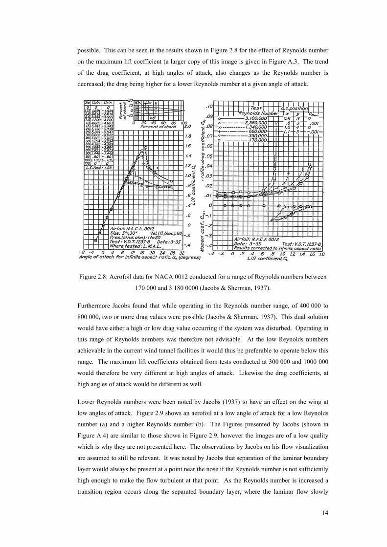
Lower Reynolds numbers were been noted by Jacobs (1937) to have an effect on the wing at
low angles of attack. Figure 2.9 shows an aerofoil at a low angle of attack for a low Reynolds
number (a) and a higher Reynolds number (b). The Figures presented by Jacobs (shown in
Figure A.4) are similar to those shown in Figure 2.9, however the images are of a low quality
which is why they are not presented here. The observations by Jacobs on his flow visualization
are assumed to still be relevant. It was noted by Jacobs that separation of the laminar boundary
layer would always be present at a point near the nose if the Reynolds number is not sufficiently
high enough to make the flow turbulent at that point. As the Reynolds number is increased a
transition region occurs along the separated boundary layer, where the laminar flow slowly
15
transitions to the fully developed turbulent layer. The transition region moves forward towards
to the leading edge, as the Reynolds number is increased. The resulting turbulence thickens the
boundary layer between the dead air, beneath the separated airflow, and the overrunning flow.
The thickening of the boundary layer ultimately leads to the separated airflow being reattached.
While not clearly stated by Jacobs (1937), it was assumed that the low Reynolds numbers
referred to are of the order of 50 000. This assumption was based on the lowest Reynolds
number for which the data was presented; this value, as seen in Figure 2.8, being 170 000. At
low angles of attack, in Figure 2.8, there is a lack of any noticeable difference in trends or
magnitudes of the aerodynamic coefficients. It was therefore assumed that the effect of the low
Reynolds number, discussed here and observed by Jacobs (1937), is not prevalent at Reynolds
numbers above 170 000 at low angles of attack. In order to ensure that any meaningful
comparisons could be made between the previous research, conducted at higher Reynolds
numbers, and the current research it would be necessary to operate at a Reynolds number above
170 000 in order to ensure that the laminar boundary layer did not separate.
Figure 2.9: Seperation occurring on an airfoil at a low angle of attack, at low a Reynolds
number (a) and an increased Reynolds number (b) (van Dyke, 2005)
Operating at a Reynolds number of 300 000 was therefore seen as the optimal value. In this
way the test conditions were well below the dual solutions cases occurring above 400 000 and
high enough to ensure the separation of the laminar boundary layer did not occur. A Reynolds
number of 300 000 was also within the capabilities of the current wind tunnel testing facilities
being used.
2.4 Hinge Moment Measurement Techniques
Previous methods used in the measurement of aileron hinge moments were investigated. It was
seen that the methods and techniques used in the past for the measurement of hinge moments
were varied. Most the techniques used for wind tunnel testing by NACA were of a similar type
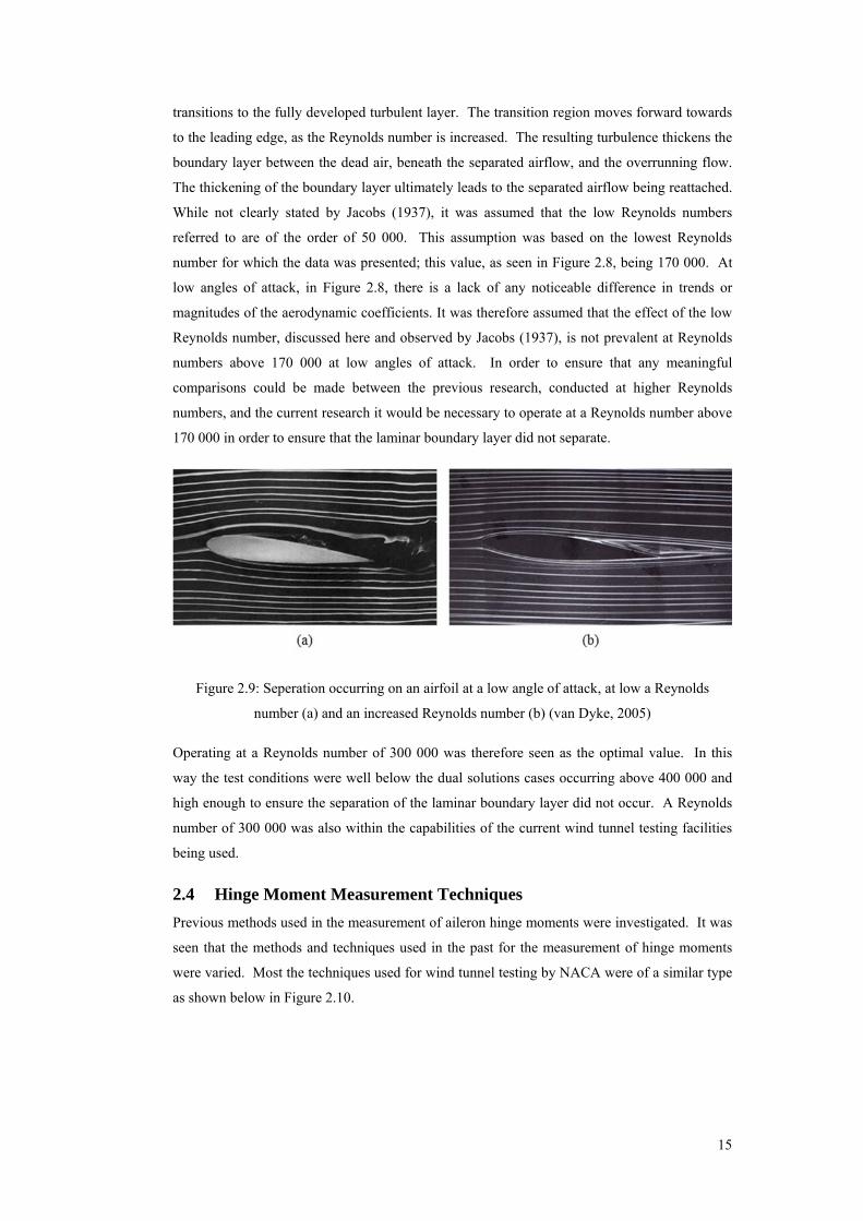
as shown below in Figure 2.10.
16
Figure 2.10: Previously used Hinge Moment Measurement Arrangement (Monish, 1930)
Problems with this technique are that there are intrusions into the airflow that may cause
adverse effects on the results. Although it was stated by Monish that these affects were
negligible it was still viewed as unsatisfactory as to need such intrusions. Another
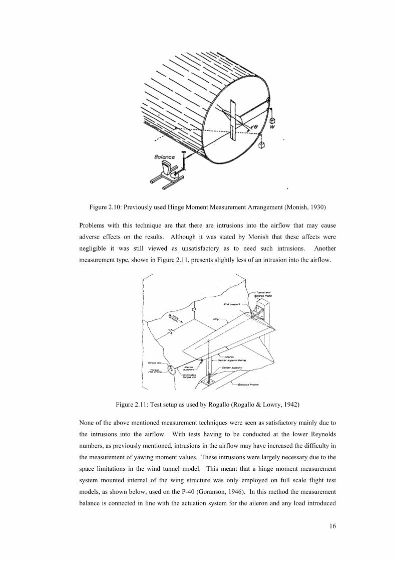
measurement type, shown in Figure 2.11, presents slightly less of an intrusion into the airflow.
Figure 2.11: Test setup as used by Rogallo (Rogallo & Lowry, 1942)
None of the above mentioned measurement techniques were seen as satisfactory mainly due to
the intrusions into the airflow. With tests having to be conducted at the lower Reynolds
numbers, as previously mentioned, intrusions in the airflow may have increased the difficulty in
the measurement of yawing moment values. These intrusions were largely necessary due to the
space limitations in the wind tunnel model. This meant that a hinge moment measurement
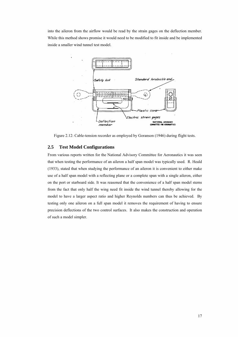
system mounted internal of the wing structure was only employed on full scale flight test
models, as shown below, used on the P-40 (Goranson, 1946). In this method the measurement
balance is connected in line with the actuation system for the aileron and any load introduced
17
into the aileron from the airflow would be read by the strain gages on the deflection member.
While this method shows promise it would need to be modified to fit inside and be implemented
inside a smaller wind tunnel test model.
Figure 2.12: Cable-tension recorder as employed by Goranson (1946) during flight tests.
2.5 Test Model Configurations
From various reports written for the National Advisory Committee for Aeronautics it was seen
that when testing the performance of an aileron a half span model was typically used. R. Heald
(1933), stated that when studying the performance of an aileron it is convenient to either make
use of a half span model with a reflecting plane or a complete span with a single aileron, either
on the port or starboard side. It was reasoned that the convenience of a half span model stems
from the fact that only half the wing need fit inside the wind tunnel thereby allowing for the
model to have a larger aspect ratio and higher Reynolds numbers can thus be achieved. By
testing only one aileron on a full span model it removes the requirement of having to ensure
precision deflections of the two control surfaces. It also makes the construction and operation
of such a model simpler.
18
3 METHOD
The three objectives of this research were for the design and testing of a balance capable of
accurately measuring the hinge moment of an aileron during testing, the validation of the results
obtained from the hinge moment balance design and investigation into the effects of differing
aileron trailing edge thicknesses on the aileron hinge moment. The tests would be conducted on
a static system with no investigation into the dynamic loads. In order to ensure these objectives
were met and a comprehensive test regime was followed, a test matrix was drawn up. This
ensured that all aspects to be covered would be tested.
The use of CFD simulations was seen as not being appropriate for this research. This was based
on the added uncertainties associated with the use of CFD results and difficulties associated in
measuring the resulting hinge moments (Soinne, 2000). For these reasons no CFD simulations
were undertaken.
3.1 Test Matrix
The following factors would be varied during testing:
• Angle of Attack (0° ; 5° ; 10° ; 12.5° ; 15° ; 17.5° ; 20°)
• Aileron deflection (-25o to +25o in increments of 5o)
• Aileron trailing edge thickness (between 0.25% and 1.5% of wing chord)
For each test the rolling, yawing and hinge moments produced by the aileron would be
measured and recorded.
Previous research, as mentioned in chapter 2.1.2, used 5° increments in angle of attack when
testing aileron performance. Initial tests showed that these increment levels proved to be
inadequate in the stalling region of between 10° and 20° angle of attack. It was therefore
decided to make use of 2.5° increments in this angle of attack range. 5° increments would still
be used for the lower angles of attack as this was seen as adequate for realization of any
occurrences or areas of interest.
The average aileron deflection increment used in previous research was approximately 5°.
Smaller increments were desired to allow for a greater resolution of the results and data trends.
It was realised that this would not always be possible, especially at high aileron deflections;
increments as small as 2° would be attempted during testing nevertheless.
Aileron trailing edge thickness would be varied in order to determine what effect the differing
thicknesses had on the aerodynamic coefficients of the wing. Four distinct trailing edge
thicknesses would be focused on. The range of thicknesses tested would encompass the critical
0.5% h/c noted by Hoerner (1985). For each case a set aileron test piece would be installed, the
angle of attack set and the deflections run through.
19
Each test would consist of the zero load signals being recorded before the tunnel was activated.
Data would then be recorded with the tunnel at the test speed. The wind tunnel would then be
turned off and the test model set for the next configuration. At each point the balance forces, air
temperature, pressure and humidity, air speed inside the tunnel and measured aileron deflection
would be recorded. A separate file was recorded for each test case, a naming convention using
the speed setting and deflection being used to allow for easy reading in of the data later as well
as for easy reference.
In light of the effect of the lower Reynolds numbers on the airflow over the wing and aileron,
discussed in chapter 2.3, it was decided to carry out flow visualization of certain test conditions.
These test conditions would be chosen based on an investigation of the test results.
The precautions followed during testing can be found in Appendix H.
3.2 Test Equipment Requirements
The following points contain the list of requirements for the test equipment and facilities.
These were created to ensure that the above test matrix could be complied with and a sufficient
level of accuracy could be obtained. The values given were based on the findings and
conclusions made throughout chapter 2.
Requirements
• Tests should be conducted at a Reynolds number of 300 000.
• A common aerofoil type should be used.
• A plain flap type aileron should be used.
• The aileron chord should be ~20% of the wing chord
• The aileron span should be ~40% of the wing semi-span
• A maximum aileron deflection of ±25° should be possible
• Have a minimum achievable aileron deflection increment of 5°
• The measured aileron deflection should be measured with a precision of ±0.1°
• The angle of attack should be measured with a precision ±0.1°
• Rolling, yawing and hinge moment coefficients should be measured with a precision of
±3%
20
4 FACILITIES AND EQUIPMENT
The following chapters, summarised here, detail the facilities and equipment used during
experimentation. Wind tunnel tests were the main focus of this research. The 1.49m x 1.49m
draw down wind tunnel, in the North West Engineering building of the University of the
Witwatersrand, was selected for this purpose. The wind tunnel allowed for air speeds of 15m/s
to be reached during testing.
A rectangular plan form NACA0012, 0.75m semi-span by 0.38m chord, wing was cast and
machined from a polyurethane resin. The wing was mounted vertically in the wind tunnel and
had an aileron with a 20.6% chord and 40% span. A hinge moment balance was designed and
installed inside the wind tunnel model allowing for the actuation of the aileron and
measurement of its hinge moment during testing. The hinge moment balance had a resolution
of 0.06% of the maximum applied loading. Aileron deflection was measured through the use of
a small voltage potentiometer that allowed for an uncertainty of ±0.1° in the measured
deflection.
For the purposes of measuring the wings aerodynamic loads a 3 axis external balance was
installed underneath the wind tunnel. This balance was used to measure the rolling and yawing
moments produced by the wing during tests. The rolling and yawing moments would be
measured with a resolution of 0.13% and 0.17% of the applied aerodynamic loads respectively.
Rolling, yawing and hinge moment loads were all measured through the use of off the shelf
loadcells.
Loadcell signals and the measured voltage across the potentiometer was recorded digitally
through the use of a 16 bit NI USB6211 DAQ and Labview software. High levels of signal
noise were encountered in initial experiments and this was addressed as best possible through
the use of filters and averaging functions built into the recording software. The sensors were
powered by a custom built power supply utilising six 12V lead acid batteries and voltage
regulators ensuring isolation from the mains supply and associated signal noise issues. The
power supply allowed for a constant supply voltage for up to 20 hours of continuous testing.
Air Temperature, ambient air pressure, airflow dynamic pressure and humidity were all
measured and recorded during testing. The temperature was measured by a k-type
thermocouple plugged into a 20 bit USB-TC01 Temperature DAQ allowing for a resolution of
±0.6°C. The pressure manometer, used for the measurement of ambient air pressure, had a
precision of ±1%. The velocity was measured through the use of a Digital pocket manometer
and pitot tube with a precision of 3%. A weather station measured the air humidity with a
precision of 1%.
21
4.1 Wind tunnel
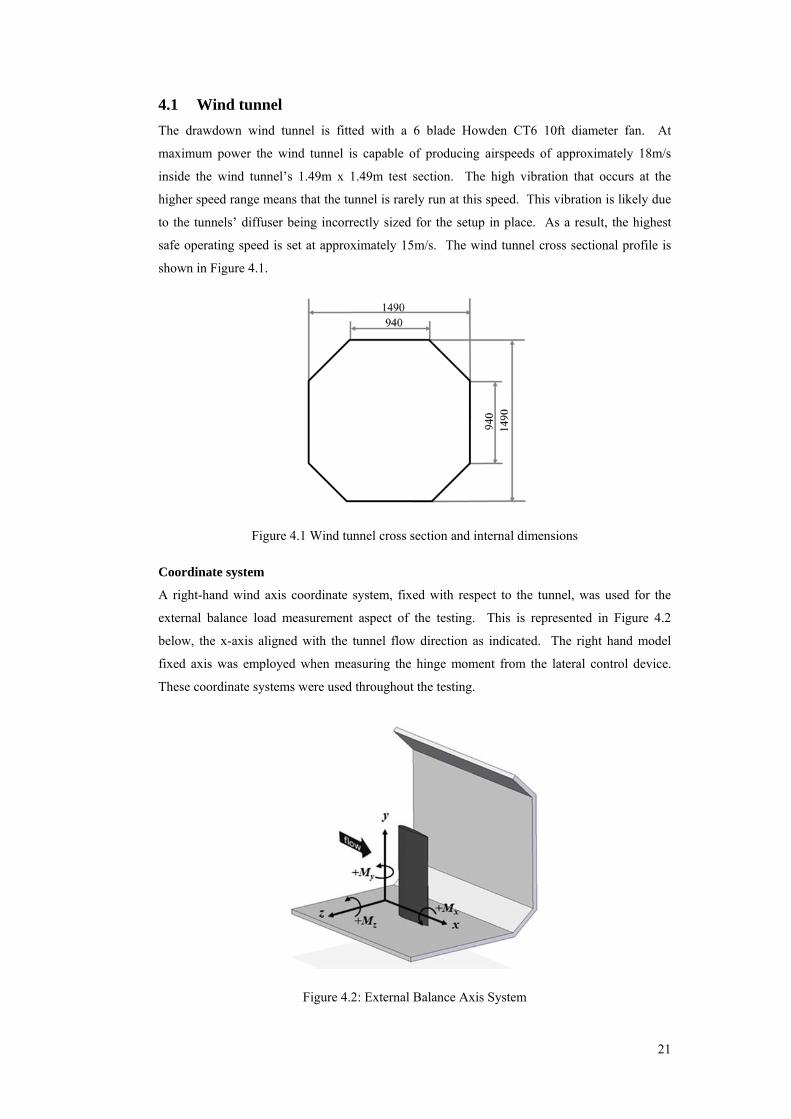
The drawdown wind tunnel is fitted with a 6 blade Howden CT6 10ft diameter fan. At
maximum power the wind tunnel is capable of producing airspeeds of approximately 18m/s
inside the wind tunnel’s 1.49m x 1.49m test section. The high vibration that occurs at the
higher speed range means that the tunnel is rarely run at this speed. This vibration is likely due
to the tunnels’ diffuser being incorrectly sized for the setup in place. As a result, the highest
safe operating speed is set at approximately 15m/s. The wind tunnel cross sectional profile is
shown in Figure 4.1.
Figure 4.1 Wind tunnel cross section and internal dimensions
Coordinate system
A right-hand wind axis coordinate system, fixed with respect to the tunnel, was used for the
external balance load measurement aspect of the testing. This is represented in Figure 4.2
below, the x-axis aligned with the tunnel flow direction as indicated. The right hand model
fixed axis was employed when measuring the hinge moment from the lateral control device.
These coordinate systems were used throughout the testing.
Figure 4.2: External Balance Axis System
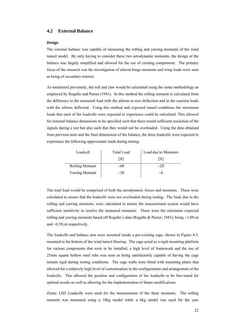
22
4.2 External Balance
Design
The external balance was capable of measuring the rolling and yawing moments of the wind
tunnel model. By only having to consider these two aerodynamic moments, the design of the
balance was largely simplified and allowed for the use of existing components. The primary
focus of the research was the investigation of aileron hinge moments and wing loads were seen
as being of secondary interest.
As mentioned previously, the roll and yaw would be calculated using the same methodology as
employed by Rogallo and Purser (1941). In this method the rolling moment is calculated from
the difference in the measured load with the aileron at zero deflection and in the reaction loads
with the aileron deflected. Using this method and expected tunnel conditions the maximum
loads that each of the loadcells were expected to experience could be calculated. This allowed
for external balance dimensions to be specified such that there would sufficient resolution of the
signals during a test but also such that they would not be overloaded. Using the data obtained
from previous tests and the final dimensions of the balance, the three loadcells were expected to
experience the following approximate loads during testing:
Loadcell Total Load
[N]
Load due to Moments
[N]
Rolling Moment ~60 ~20
Yawing Moment ~30 ~6
The total load would be comprised of both the aerodynamic forces and moments. These were
calculated to ensure that the loadcells were not overloaded during testing. The load, due to the
rolling and yawing moments, were calculated to ensure the measurement system would have
sufficient sensitivity to resolve the measured moments. These were the maximum expected
rolling and yawing moments based off Rogallo’s data (Rogallo & Purser, 1941); being ~1.0N.m
and ~0.3N.m respectively.
The loadcells and balance arm were mounted inside a pre-existing cage, shown in Figure 4.3,
mounted to the bottom of the wind tunnel flooring. The cage acted as a rigid mounting platform
for various components that were to be installed, a high level of framework and the use of
25mm square hollow steel tube was seen as being satisfactorily capable of having the cage
remain rigid during testing conditions. The cage walls were fitted with mounting plates that
allowed for a relatively high level of customization in the configurations and arrangement of the
loadcells. This allowed the position and configuration of the loadcells to be fine-tuned for
optimal results as well as allowing for the implementation of future modifications.
Zemic L6D Loadcells were used for the measurement of the three moments. The rolling
moment was measured using a 10kg model while a 6kg model was used for the yaw
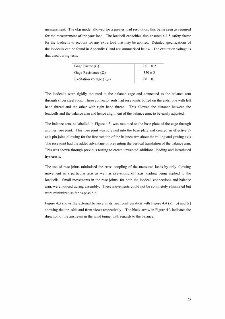
23
measurement. The 6kg model allowed for a greater load resolution, this being seen as required
for the measurement of the yaw load. The loadcell capacities also ensured a 1.5 safety factor
for the loadcells to account for any extra load that may be applied. Detailed specifications of
the loadcells can be found in Appendix C and are summarised below. The excitation voltage is
that used during tests.
Gage Factor (G) 2.0 ± 0.2
Gage Resistance (Ω) 350 ± 3
Excitation voltage (VEX) 9V ± 0.1
The loadcells were rigidly mounted to the balance cage and connected to the balance arm
through silver steel rods. These connector rods had rose joints bolted on the ends, one with left
hand thread and the other with right hand thread. This allowed the distance between the
loadcells and the balance arm and hence alignment of the balance arm, to be easily adjusted.
The balance arm, as labelled in Figure 4.3, was mounted to the base plate of the cage through
another rose joint. This rose joint was screwed into the base plate and created an effective 2-
axis pin joint, allowing for the free rotation of the balance arm about the rolling and yawing axis.
The rose joint had the added advantage of preventing the vertical translation of the balance arm.
This was shown through previous testing to create unwanted additional loading and introduced
hysteresis.
The use of rose joints minimised the cross coupling of the measured loads by only allowing
movement in a particular axis as well as preventing off axis loading being applied to the
loadcells. Small movements in the rose joints, for both the loadcell connections and balance
arm, were noticed during assembly. These movements could not be completely eliminated but
were minimized as far as possible.
Figure 4.3 shows the external balance in its final configuration with Figure 4.4 (a), (b) and (c)
showing the top, side and front views respectively. The black arrow in Figure 4.3 indicates the
direction of the airstream in the wind tunnel with regards to the balance.
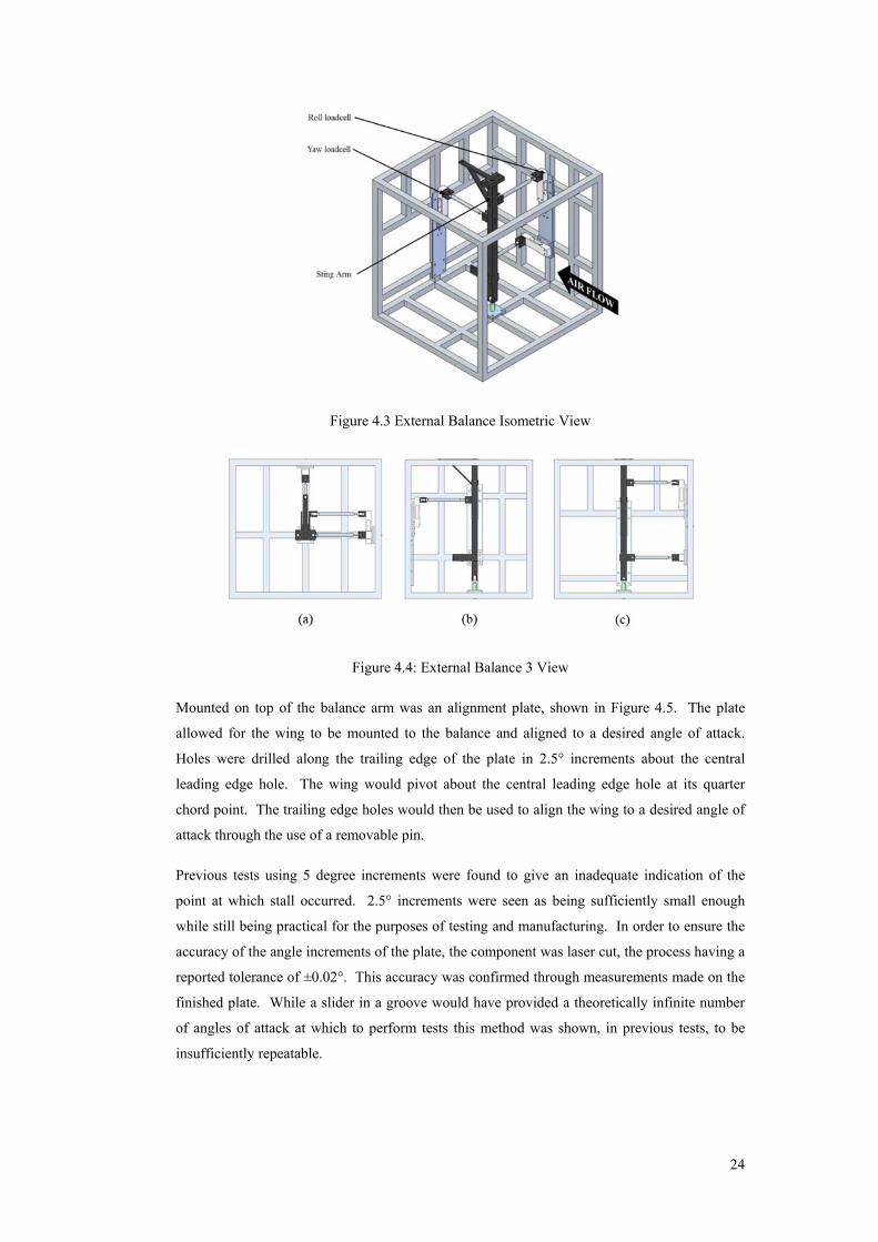
24
Figure 4.3 External Balance Isometric View
Figure 4.4: External Balance 3 View
Mounted on top of the balance arm was an alignment plate, shown in Figure 4.5. The plate
allowed for the wing to be mounted to the balance and aligned to a desired angle of attack.
Holes were drilled along the trailing edge of the plate in 2.5° increments about the central
leading edge hole. The wing would pivot about the central leading edge hole at its quarter
chord point. The trailing edge holes would then be used to align the wing to a desired angle of
attack through the use of a removable pin.
Previous tests using 5 degree increments were found to give an inadequate indication of the
point at which stall occurred. 2.5° increments were seen as being sufficiently small enough
while still being practical for the purposes of testing and manufacturing. In order to ensure the
accuracy of the angle increments of the plate, the component was laser cut, the process having a
reported tolerance of ±0.02°. This accuracy was confirmed through measurements made on the
finished plate. While a slider in a groove would have provided a theoretically infinite number
of angles of attack at which to perform tests this method was shown, in previous tests, to be
insufficiently repeatable.
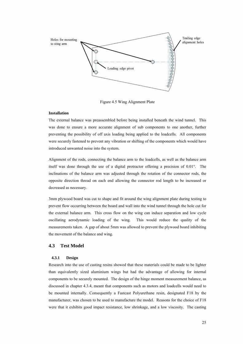
25
Figure 4.5 Wing Alignment Plate
Installation
The external balance was preassembled before being installed beneath the wind tunnel. This
was done to ensure a more accurate alignment of sub components to one another, further
preventing the possibility of off axis loading being applied to the loadcells. All components
were securely fastened to prevent any vibration or shifting of the components which would have
introduced unwanted noise into the system.
Alignment of the rods, connecting the balance arm to the loadcells, as well as the balance arm
itself was done through the use of a digital protractor offering a precision of 0.01°. The
inclinations of the balance arm was adjusted through the rotation of the connector rods, the
opposite direction thread on each end allowing the connector rod length to be increased or
decreased as necessary.
3mm plywood board was cut to shape and fit around the wing alignment plate during testing to
prevent flow occurring between the board and wall into the wind tunnel through the hole cut for
the external balance arm. This cross flow on the wing can induce separation and low cycle
oscillating aerodynamic loading of the wing. This would reduce the quality of the
measurements taken. A gap of about 5mm was allowed to prevent the plywood board inhibiting
the movement of the balance and wing.
4.3 Test Model
4.3.1 Design
Research into the use of casting resins showed that these materials could be made to be lighter
than equivalently sized aluminium wings but had the advantage of allowing for internal
components to be securely mounted. The design of the hinge moment measurement balance, as
discussed in chapter 4.3.4, meant that components such as motors and loadcells would need to
be mounted internally. Consequently a Fastcast Polyurethane resin, designated F18 by the
manufacturer, was chosen to be used to manufacture the model. Reasons for the choice of F18
were that it exhibits good impact resistance, low shrinkage, and a low viscosity. The casting
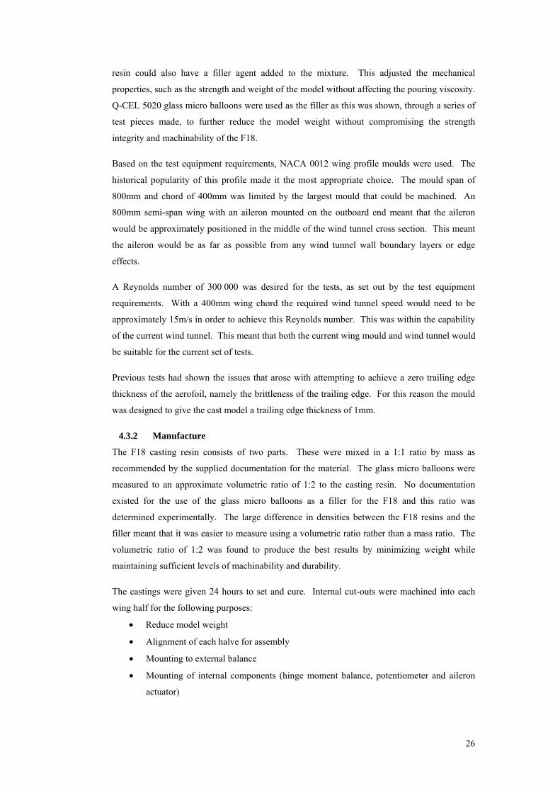
26
resin could also have a filler agent added to the mixture. This adjusted the mechanical
properties, such as the strength and weight of the model without affecting the pouring viscosity.
Q-CEL 5020 glass micro balloons were used as the filler as this was shown, through a series of
test pieces made, to further reduce the model weight without compromising the strength
integrity and machinability of the F18.
Based on the test equipment requirements, NACA 0012 wing profile moulds were used. The
historical popularity of this profile made it the most appropriate choice. The mould span of
800mm and chord of 400mm was limited by the largest mould that could be machined. An
800mm semi-span wing with an aileron mounted on the outboard end meant that the aileron
would be approximately positioned in the middle of the wind tunnel cross section. This meant
the aileron would be as far as possible from any wind tunnel wall boundary layers or edge
effects.
A Reynolds number of 300 000 was desired for the tests, as set out by the test equipment
requirements. With a 400mm wing chord the required wind tunnel speed would need to be
approximately 15m/s in order to achieve this Reynolds number. This was within the capability
of the current wind tunnel. This meant that both the current wing mould and wind tunnel would
be suitable for the current set of tests.
Previous tests had shown the issues that arose with attempting to achieve a zero trailing edge
thickness of the aerofoil, namely the brittleness of the trailing edge. For this reason the mould
was designed to give the cast model a trailing edge thickness of 1mm.
4.3.2 Manufacture
The F18 casting resin consists of two parts. These were mixed in a 1:1 ratio by mass as
recommended by the supplied documentation for the material. The glass micro balloons were
measured to an approximate volumetric ratio of 1:2 to the casting resin. No documentation
existed for the use of the glass micro balloons as a filler for the F18 and this ratio was
determined experimentally. The large difference in densities between the F18 resins and the
filler meant that it was easier to measure using a volumetric ratio rather than a mass ratio. The
volumetric ratio of 1:2 was found to produce the best results by minimizing weight while
maintaining sufficient levels of machinability and durability.
The castings were given 24 hours to set and cure. Internal cut-outs were machined into each
wing half for the following purposes:
• Reduce model weight
• Alignment of each halve for assembly
• Mounting to external balance
• Mounting of internal components (hinge moment balance, potentiometer and aileron
actuator)
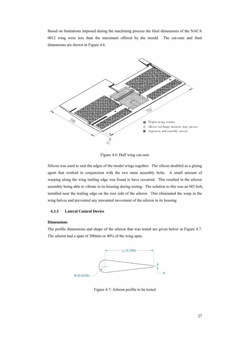
27
Based on limitations imposed during the machining process the final dimensions of the NACA
0012 wing were less than the maximum offered by the mould. The cut-outs and final
dimensions are shown in Figure 4.6.
Figure 4.6: Half wing cut-outs
Silicon was used to seal the edges of the model wings together. The silicon doubled as a gluing
agent that worked in conjunction with the two main assembly bolts. A small amount of
warping along the wing trailing edge was found to have occurred. This resulted in the aileron
assembly being able to vibrate in its housing during testing. The solution to this was an M3 bolt,
installed near the trailing edge on the root side of the aileron. This eliminated the warp in the
wing halves and prevented any unwanted movement of the aileron in its housing
4.3.3 Lateral Control Device
Dimensions
The profile dimensions and shape of the aileron that was tested are given below in Figure 4.7.
The aileron had a span of 300mm or 40% of the wing span.
Figure 4.7: Aileron profile to be tested
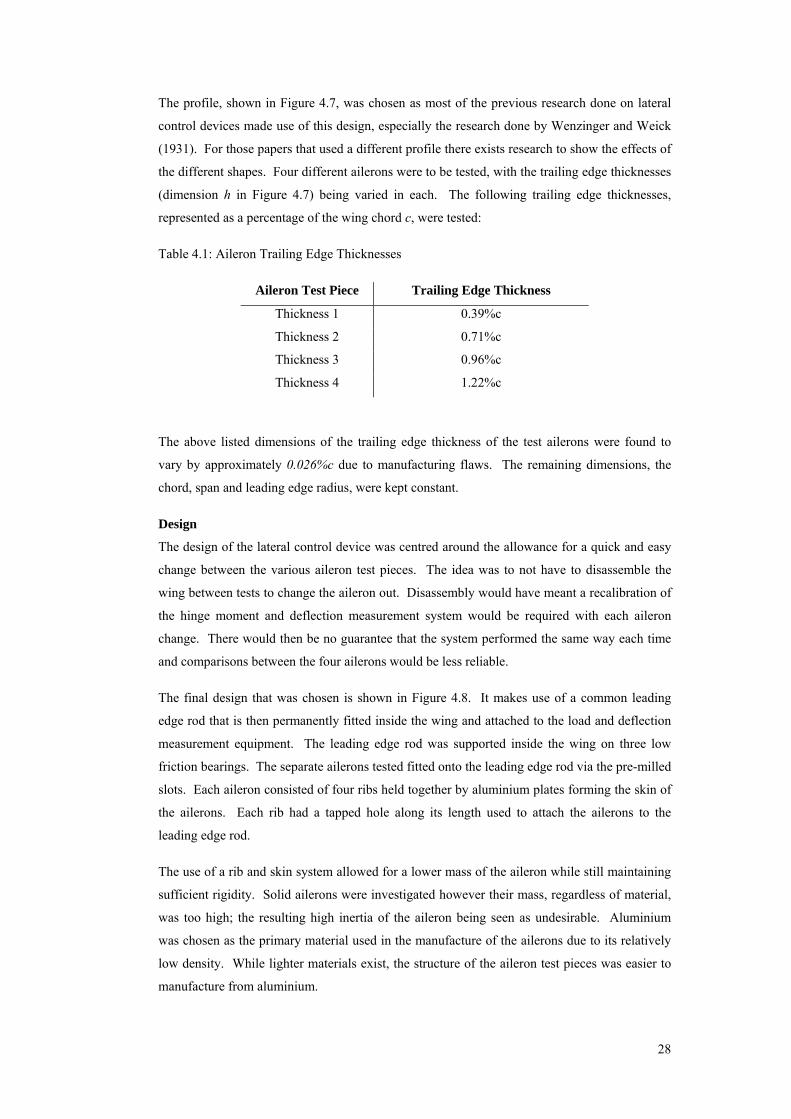
28
The profile, shown in Figure 4.7, was chosen as most of the previous research done on lateral
control devices made use of this design, especially the research done by Wenzinger and Weick
(1931). For those papers that used a different profile there exists research to show the effects of
the different shapes. Four different ailerons were to be tested, with the trailing edge thicknesses
(dimension h in Figure 4.7) being varied in each. The following trailing edge thicknesses,
represented as a percentage of the wing chord c, were tested:
Table 4.1: Aileron Trailing Edge Thicknesses
Aileron Test Piece Trailing Edge Thickness
Thickness 1 0.39%c
Thickness 2 0.71%c
Thickness 3 0.96%c
Thickness 4 1.22%c
The above listed dimensions of the trailing edge thickness of the test ailerons were found to
vary by approximately 0.026%c due to manufacturing flaws. The remaining dimensions, the
chord, span and leading edge radius, were kept constant.
Design
The design of the lateral control device was centred around the allowance for a quick and easy
change between the various aileron test pieces. The idea was to not have to disassemble the
wing between tests to change the aileron out. Disassembly would have meant a recalibration of
the hinge moment and deflection measurement system would be required with each aileron
change. There would then be no guarantee that the system performed the same way each time
and comparisons between the four ailerons would be less reliable.
The final design that was chosen is shown in Figure 4.8. It makes use of a common leading
edge rod that is then permanently fitted inside the wing and attached to the load and deflection
measurement equipment. The leading edge rod was supported inside the wing on three low
friction bearings. The separate ailerons tested fitted onto the leading edge rod via the pre-milled
slots. Each aileron consisted of four ribs held together by aluminium plates forming the skin of
the ailerons. Each rib had a tapped hole along its length used to attach the ailerons to the
leading edge rod.
The use of a rib and skin system allowed for a lower mass of the aileron while still maintaining
sufficient rigidity. Solid ailerons were investigated however their mass, regardless of material,
was too high; the resulting high inertia of the aileron being seen as undesirable. Aluminium
was chosen as the primary material used in the manufacture of the ailerons due to its relatively
low density. While lighter materials exist, the structure of the aileron test pieces was easier to
manufacture from aluminium.
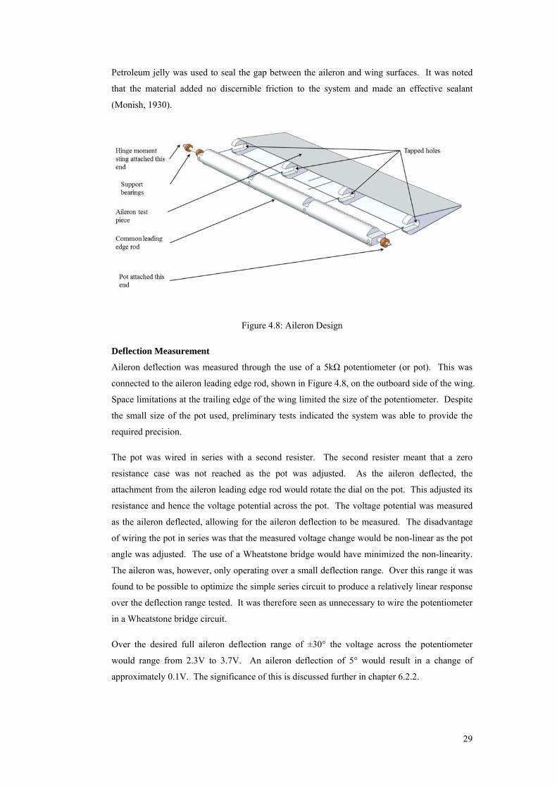
29
Petroleum jelly was used to seal the gap between the aileron and wing surfaces. It was noted
that the material added no discernible friction to the system and made an effective sealant
(Monish, 1930).
Figure 4.8: Aileron Design
Deflection Measurement
Aileron deflection was measured through the use of a 5kΩ potentiometer (or pot). This was
connected to the aileron leading edge rod, shown in Figure 4.8, on the outboard side of the wing.
Space limitations at the trailing edge of the wing limited the size of the potentiometer. Despite
the small size of the pot used, preliminary tests indicated the system was able to provide the
required precision.
The pot was wired in series with a second resister. The second resister meant that a zero
resistance case was not reached as the pot was adjusted. As the aileron deflected, the
attachment from the aileron leading edge rod would rotate the dial on the pot. This adjusted its
resistance and hence the voltage potential across the pot. The voltage potential was measured
as the aileron deflected, allowing for the aileron deflection to be measured. The disadvantage
of wiring the pot in series was that the measured voltage change would be non-linear as the pot
angle was adjusted. The use of a Wheatstone bridge would have minimized the non-linearity.
The aileron was, however, only operating over a small deflection range. Over this range it was
found to be possible to optimize the simple series circuit to produce a relatively linear response
over the deflection range tested. It was therefore seen as unnecessary to wire the potentiometer
in a Wheatstone bridge circuit.
Over the desired full aileron deflection range of ±30° the voltage across the potentiometer
would range from 2.3V to 3.7V. An aileron deflection of 5° would result in a change of
approximately 0.1V. The significance of this is discussed further in chapter 6.2.2.
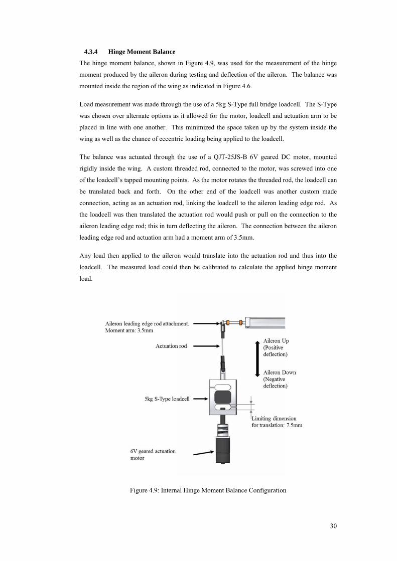
30
4.3.4 Hinge Moment Balance
The hinge moment balance, shown in Figure 4.9, was used for the measurement of the hinge
moment produced by the aileron during testing and deflection of the aileron. The balance was
mounted inside the region of the wing as indicated in Figure 4.6.
Load measurement was made through the use of a 5kg S-Type full bridge loadcell. The S-Type
was chosen over alternate options as it allowed for the motor, loadcell and actuation arm to be
placed in line with one another. This minimized the space taken up by the system inside the
wing as well as the chance of eccentric loading being applied to the loadcell.
The balance was actuated through the use of a QJT-25JS-B 6V geared DC motor, mounted
rigidly inside the wing. A custom threaded rod, connected to the motor, was screwed into one
of the loadcell’s tapped mounting points. As the motor rotates the threaded rod, the loadcell can
be translated back and forth. On the other end of the loadcell was another custom made
connection, acting as an actuation rod, linking the loadcell to the aileron leading edge rod. As
the loadcell was then translated the actuation rod would push or pull on the connection to the
aileron leading edge rod; this in turn deflecting the aileron. The connection between the aileron
leading edge rod and actuation arm had a moment arm of 3.5mm.
Any load then applied to the aileron would translate into the actuation rod and thus into the
loadcell. The measured load could then be calibrated to calculate the applied hinge moment
load.
Figure 4.9: Internal Hinge Moment Balance Configuration
31
A moment arm of 3.5mm was chosen so as to magnify the hinge moment loads produced by the
aileron during testing. The distance was optimized such that the loads introduced into the
system, during testing would be easily picked up by the loadcell. These loads were based off
the use of hinge moment data obtained from Rogallo (1941). Using his data, the expected hinge
moment loads that the aileron would experience were calculated to apply a maximum load of
approximately 15N on the loadcell.
The actuation motor was set to rotate at approximately 5RPM, depending on the loading it was
seeing. This translated to an approximate aileron deflection of 2° every second. This allowed
for a relatively high level of control of the aileron position when attaining a desired deflection.
In order to prevent unwanted movement of the loadcell inside the cavity of the wind tunnel
model, lubricated rollers and guide arms were used. These held the loadcell in position,
preventing its movement out of plane while not significantly inhibiting its ability to measure the
applied loading.
Limited by the dimension of the loadcell, as indicated in Figure 4.9, the system was only
allowed 7.5mm of rearward translation before the threaded rod would press against the inner
wall of the loadcell and cause damage. Forward translation restrictions were similar at 9mm;
the threaded rod disconnecting from the loadcell were it to be exceeded. With the aileron
moment arm, however, this still allowed for a deflection of over 50° in both directions from
zero deflection. The primary limiting factor to maximum possible deflection was, however,
created by the link between the actuator rod and aileron leading edge rod. A maximum negative
deflection of approximately +10° was achievable before the mechanism locked up against itself.
A maximum negative deflection of approximately -45° was allowed before the mechanism
would become over extended and was unable to return itself back to zero deflection unaided. In
order to prevent this occurring, the aileron was not operated below a deflection of -40°.
Investigations of previous tests showed that any effective comparisons would ideally require
deflections of +25° or higher. By using a symmetrical wing profile, however, it was seen that a
negative aileron deflection with the wing at a positive angle of attack would be equivalent to a
positive aileron deflection with the wing at a negative angle of attack. The wing would then be
tested for the allowable aileron deflection range, of -25° to +10°, for both the negative and
positive angles of attack. Reversing the data for the negative angles of attack then ensured that
a full swing of the aileron deflection could be tested. It also meant that for an aileron deflection
range of -10° to +10° the data would ideally be repeated. This could be used to validate how
well the external balance and hinge moment balance performed.
4.4 Data Acquisition
4.4.1 Data Acquisition Device (DAQ)
For the purposes of data acquisition a 16 channel NI USB-6211 multifunction DAQ was used.
The DAQ had a 16 bit resolution, capable of input ranges of ±0.2V to ±10V. Using an input
32
range of ±0.2V the device had a precision, at full scale, of 0.088mV and a precision of 2.690mV
when using an input range of ±10V. This uncertainty encompassed residual gain error, residual
offset error and random noise. The signal resolution is quoted as 91.6μV and 4.8μV
respectively for the two ranges. A maximum sampling rate of 250 kS/s was available, shared
amongst all the channels. The full specifications of the DAQ can be found in Appendix C
Labview
Labview was used in order to process and record the data input into the DAQ. A sampling rate
of 1000Hz was used for the measurements of the loadcell and potentiometer signals. While
higher sampling rates were technically available from the DAQ, the computer system memory
proved to be the limiting factor. Smaller sample rates would have been suitable for the
purposes of the current testing as the loads were being examined under static conditions. It was
decided, however, to rather have the system read in data at a higher rate as it was less likely that
unwanted occurrences, such as blips in the supply voltage or the vibration of the wind tunnel,
would affect the data in any substantial way. The effect of these disturbances and sampling
rates is discussed later in chapter 6.
The data from the loadcells was recorded by Labview as strains rather than voltages.
Preliminary tests showed that this setting produced a better signal quality than having the
loadcell signals recorded as voltages. This is because the DAQ unit had inbuilt signal
conditioning for strain inputs that further filtered the incoming signal. It was decided that the
added uncertainty associated with the loadcell gauge factor used in converting the voltage input
to a strain reading, still resulted in an overall better signal quality. The following equation is
used by Labview to convert the voltage inputs into strain units.
= 1× × 1000 . 4.1
Where: µε micro strain; VEX excitation voltage, V; G loadcell gauge factor; Vin measured voltage,
mV
Input ranges for the loadcells were set at ±1000µε in Labview. This equated, using equation 4.1,
to a voltage input range of ±18mV. The smallest range that the 16 bit DAQ could measure,
however, was ±200mV. The signal resolution at this range was 4.8µV which equated to a
resolution of 0.267µε for the loadcells at full scale (1000µε).
Further improvements to the signal were made through the use of filters and averaging
functions. These are discussed further in chapter 6.
4.4.2 Atmospheric Data
Temperature DAQ
A separate single channel USB-TC01 temperature DAQ was used for the purposes of
measuring the air temperature during the tests. This DAQ has a resolution of 20 bits allowing
33
for an accuracy of 0.6°C between 0°C and 65°C. A K-type thermocouple was plugged into the
DAQ. The thermocouple was positioned in the wind tunnel, downstream of the test model and
was shielded from the flow to eliminate convention effects.
Air Velocity
Airstream velocity was measured through the use of a DPM ST650M digital pocket manometer
and pitot tube inserted into the airstream during testing. The device had a precision of 3% of
the reading.
Pressure
Ambient air pressure was recorded during testing. This was done through the use of an AD-
1000 pressure transducer. The transducer had a precision of ±1%.
Humidity
The air humidity was manually recorded through the use of an Oregon BAR206 Weather
Forecast Station. The device has a resolution of 1% for humidity.
4.4.3 Power Supply
Previous work conducted at the drawdown wind tunnel showed a high level of electronic noise
was encountered; this being attributed in large part to the buildings’ main power supply.
Specifically an oscillating frequency was introduced into the system that the inbuilt filters of the
data acquisition system had some difficulty in accurately filtering out. The use of a chargeable
battery system was successful in isolating the electronics from the buildings power; this
eliminating a lot of the noise encountered.
In order to power the actuation motor used in the hinge moment balance, a separate DC power
supply was used. While this power supply was connected to the buildings power supply it was
isolated from the rest of the instrumentation, being used solely to power the actuation motor and
relays.
Battery Power Supply
6 12V lead acid batteries were used, each plugging into a custom made charging board that
allowed the batteries to be charged in situ. It was found, however, that the charger had to be
disconnected from the building power supply during the test otherwise the unwanted system
noise found its way into the data.
The output voltage from each battery was regulated down to 9V±0.1V using LM317 regulators
before being sent to the instrumentation. In this way the input voltage to the loadcells and other
instrumentation could be kept constant, at least until the battery voltage dropped too low.
Through testing it was found that that from a full charge the batteries could operate for over
20hrs before the voltage supplied by the batteries would dip below 10V and the output voltage
from the regulator would become inconsistent.
34
4.4.4 Wiring
In an effort to further reduce the signal noise that was encountered the use of shielded cable was
investigated with positive results. In the end 2 core and 4 core shielded wiring were used in the
wiring of the loadcells and potentiometer.
In certain cases 3m of cable were used to link the loadcells to the power supply and DAQ.
Tests were conducted to ascertain what effect these long lengths of cable would have on the
signal and corresponding noise levels. While an increase was noticed upon close inspection it
was deemed to still be within satisfactory levels.
4.5 Flow Visualization
In order to aid in the explanation of possible phenomenon, flow visualization was required.
This was achieved through the use of an SAI helium bubble generator. The device operates by
creating and injecting helium filled soap bubbles into the airstream ahead of the test model.
Careful adjustment of the ratio of helium to soap formula would allow the bubbles to be
neutrally buoyant and more accurately represent the airflow. By blocking out all outside light
and using a concentrated light source these bubbles would become illuminated and allow for a
direct visualization of the flow field around the wing at test conditions.
These flow fields can then be photographed. By varying the shutter speed of the camera it
becomes possible to view the individual bubbles passing over the wind tunnel model or, by
increasing the exposure, create flow lines of varying lengths. This is valuable in the
visualization of stall conditions, wingtip vortices and the interaction between separate bodies.
35
5 DATA PROCESSING
Data processing of the test results was primarily done through the use of Microsoft Excel and
Visual Basic for Applications (VBA). The VBA code was used to pull the data from multiple
sources, manipulate and process it. Further code would generate plots of the processed data,
allowing for trends to be seen. These codes required the data files from the tests to be
specifically named and placed in set folders. For the most part this was done during the testing
however a quick run through the output files was done to ensure the files were where they
needed to be and named correctly.
Gravitational Acceleration was taken as 9.79m/s2.
The following process was followed:
1. Data was pulled and collated from the separate test files into a single excel spreadsheet
using a VBA code. This data would include: the angle of attack, the roll, yaw, and
aileron hinge moment signal data along with the temperature. A separate column set
pulled the standard deviation in each test set for each signal input, calculated for a 95%
confidence interval. The value recorded from each signal input was averaged over the
test time.
2. The rows of data read in would alternate between zero load values and test load values.
Checks were made through the data based on the signal noise levels, indicated by the
standard deviations, to identify areas of concern. For those points that were identified,
the original output files were examined to see what caused the error. These data points
would be subsequently removed from the data set were they found to contain an error
or random occurrence.
3. A second VBA code was written to zero the signal values, subtracting the zero load
signals from the test load values. The standard deviation values for the test load cases
were kept, the values at zero load simply consulted in the previous step to ensure the
data was satisfactory. Both the zero load and test load potentiometer voltage values
were kept as this allowed for the tracking of aileron deflection change as the tunnel
was turned on.
4. The aileron deflection calibration was then applied using the potentiometer voltage
signal. The speed values at each of the tests were manually inputted, from the
recordings made during testing. The aileron deflection calibration was applied to the
total voltage signal and not a difference between the zero load and loaded cases, as
done with the loadcells.
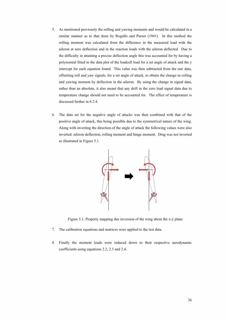
36
5. As mentioned previously the rolling and yawing moments and would be calculated in a
similar manner as to that done by Rogallo and Purser (1941). In this method the
rolling moment was calculated from the difference in the measured load with the
aileron at zero deflection and in the reaction loads with the aileron deflected. Due to
the difficulty in attaining a precise deflection angle this was accounted for by having a
polynomial fitted to the data plot of the loadcell load for a set angle of attack and the y
intercept for each equation found. This value was then subtracted from the raw data,
offsetting roll and yaw signals, for a set angle of attack, to obtain the change in rolling
and yawing moment by deflection in the aileron. By using the change in signal data,
rather than an absolute, it also meant that any drift in the zero load signal data due to
temperature change should not need to be accounted for. The effect of temperature is
discussed further in 6.2.4.
6. The data set for the negative angle of attacks was then combined with that of the
positive angle of attack, this being possible due to the symmetrical nature of the wing.
Along with inverting the direction of the angle of attack the following values were also
inverted: aileron deflection, rolling moment and hinge moment. Drag was not inverted
as illustrated in Figure 5.1.
Figure 5.1: Property mapping due inversion of the wing about the x-y plane
7. The calibration equations and matrices were applied to the test data.
8. Finally the moment loads were reduced down to their respective aerodynamic
coefficients using equations 2.2, 2.3 and 2.4.
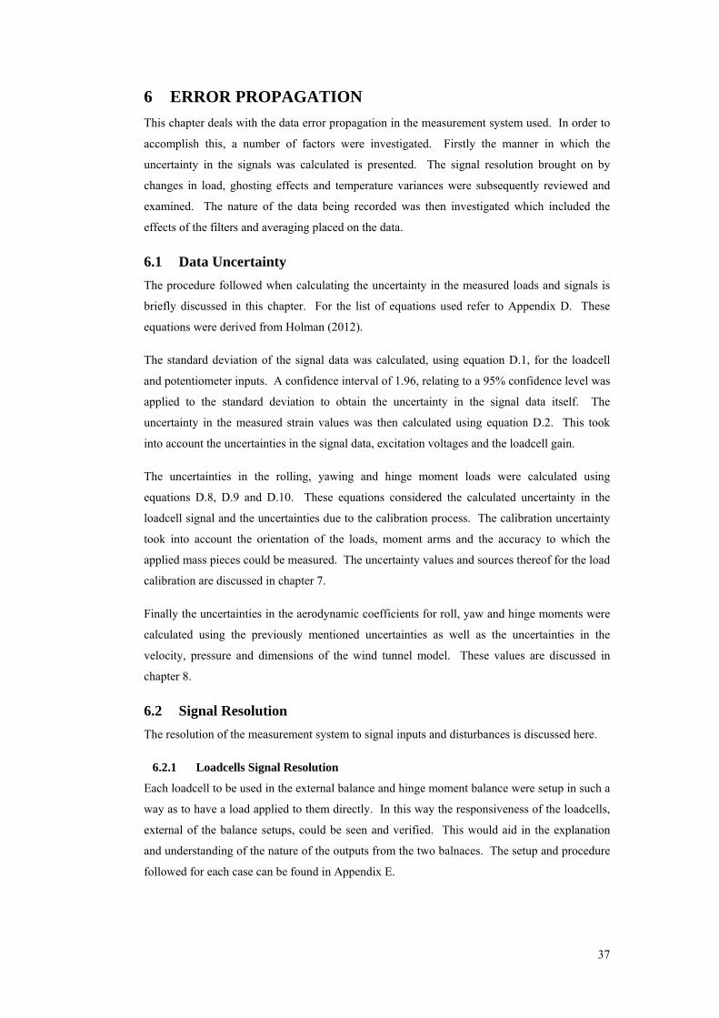
37
6 ERROR PROPAGATION
This chapter deals with the data error propagation in the measurement system used. In order to
accomplish this, a number of factors were investigated. Firstly the manner in which the
uncertainty in the signals was calculated is presented. The signal resolution brought on by
changes in load, ghosting effects and temperature variances were subsequently reviewed and
examined. The nature of the data being recorded was then investigated which included the
effects of the filters and averaging placed on the data.
6.1 Data Uncertainty
The procedure followed when calculating the uncertainty in the measured loads and signals is
briefly discussed in this chapter. For the list of equations used refer to Appendix D. These
equations were derived from Holman (2012).
The standard deviation of the signal data was calculated, using equation D.1, for the loadcell
and potentiometer inputs. A confidence interval of 1.96, relating to a 95% confidence level was
applied to the standard deviation to obtain the uncertainty in the signal data itself. The
uncertainty in the measured strain values was then calculated using equation D.2. This took
into account the uncertainties in the signal data, excitation voltages and the loadcell gain.
The uncertainties in the rolling, yawing and hinge moment loads were calculated using
equations D.8, D.9 and D.10. These equations considered the calculated uncertainty in the
loadcell signal and the uncertainties due to the calibration process. The calibration uncertainty
took into account the orientation of the loads, moment arms and the accuracy to which the
applied mass pieces could be measured. The uncertainty values and sources thereof for the load
calibration are discussed in chapter 7.
Finally the uncertainties in the aerodynamic coefficients for roll, yaw and hinge moments were
calculated using the previously mentioned uncertainties as well as the uncertainties in the
velocity, pressure and dimensions of the wind tunnel model. These values are discussed in
chapter 8.
6.2 Signal Resolution
The resolution of the measurement system to signal inputs and disturbances is discussed here.
6.2.1 Loadcells Signal Resolution
Each loadcell to be used in the external balance and hinge moment balance were setup in such a
way as to have a load applied to them directly. In this way the responsiveness of the loadcells,
external of the balance setups, could be seen and verified. This would aid in the explanation
and understanding of the nature of the outputs from the two balnaces. The setup and procedure
followed for each case can be found in Appendix E.
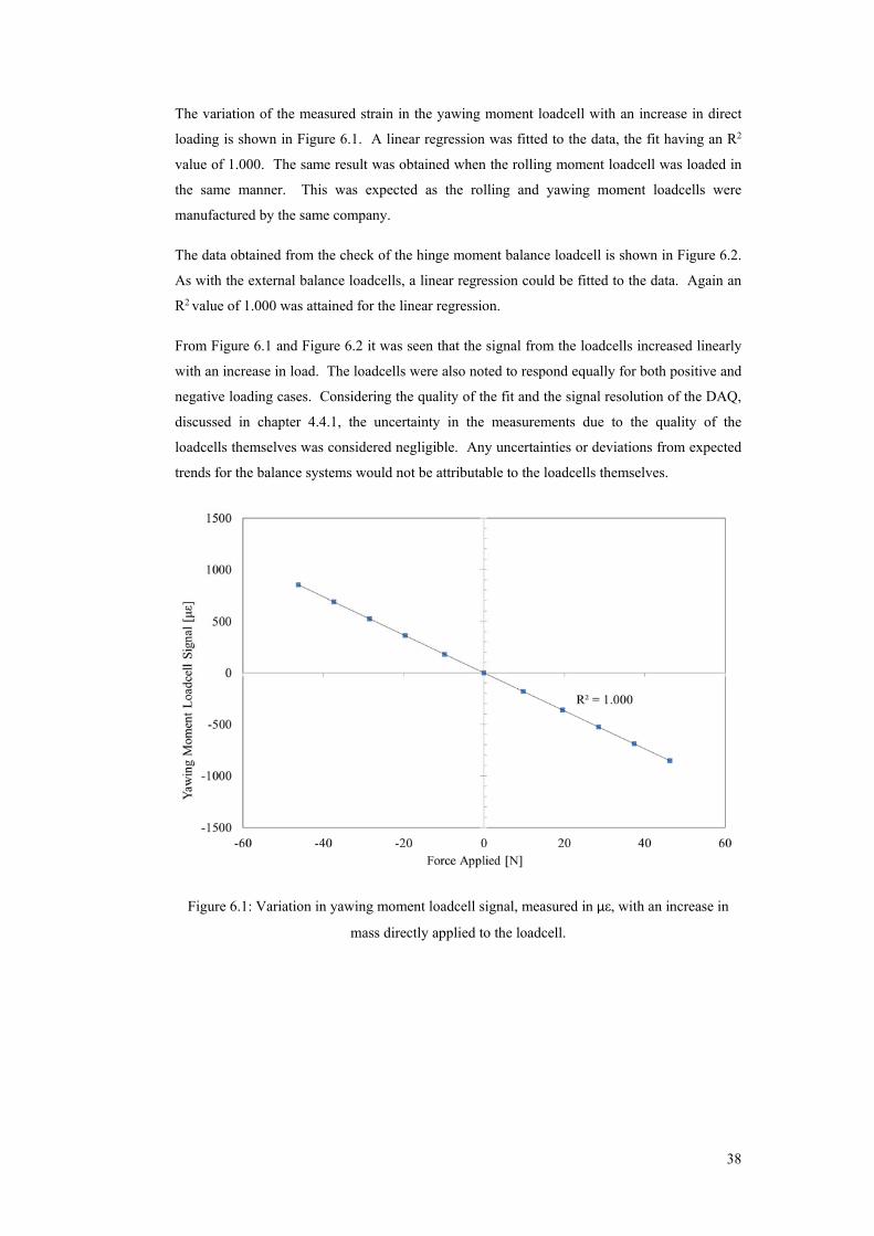
38
The variation of the measured strain in the yawing moment loadcell with an increase in direct
loading is shown in Figure 6.1. A linear regression was fitted to the data, the fit having an R2
value of 1.000. The same result was obtained when the rolling moment loadcell was loaded in
the same manner. This was expected as the rolling and yawing moment loadcells were
manufactured by the same company.
The data obtained from the check of the hinge moment balance loadcell is shown in Figure 6.2.
As with the external balance loadcells, a linear regression could be fitted to the data. Again an
R2 value of 1.000 was attained for the linear regression.
From Figure 6.1 and Figure 6.2 it was seen that the signal from the loadcells increased linearly
with an increase in load. The loadcells were also noted to respond equally for both positive and
negative loading cases. Considering the quality of the fit and the signal resolution of the DAQ,
discussed in chapter 4.4.1, the uncertainty in the measurements due to the quality of the
loadcells themselves was considered negligible. Any uncertainties or deviations from expected
trends for the balance systems would not be attributable to the loadcells themselves.
Figure 6.1: Variation in yawing moment loadcell signal, measured in με, with an increase in
mass directly applied to the loadcell.
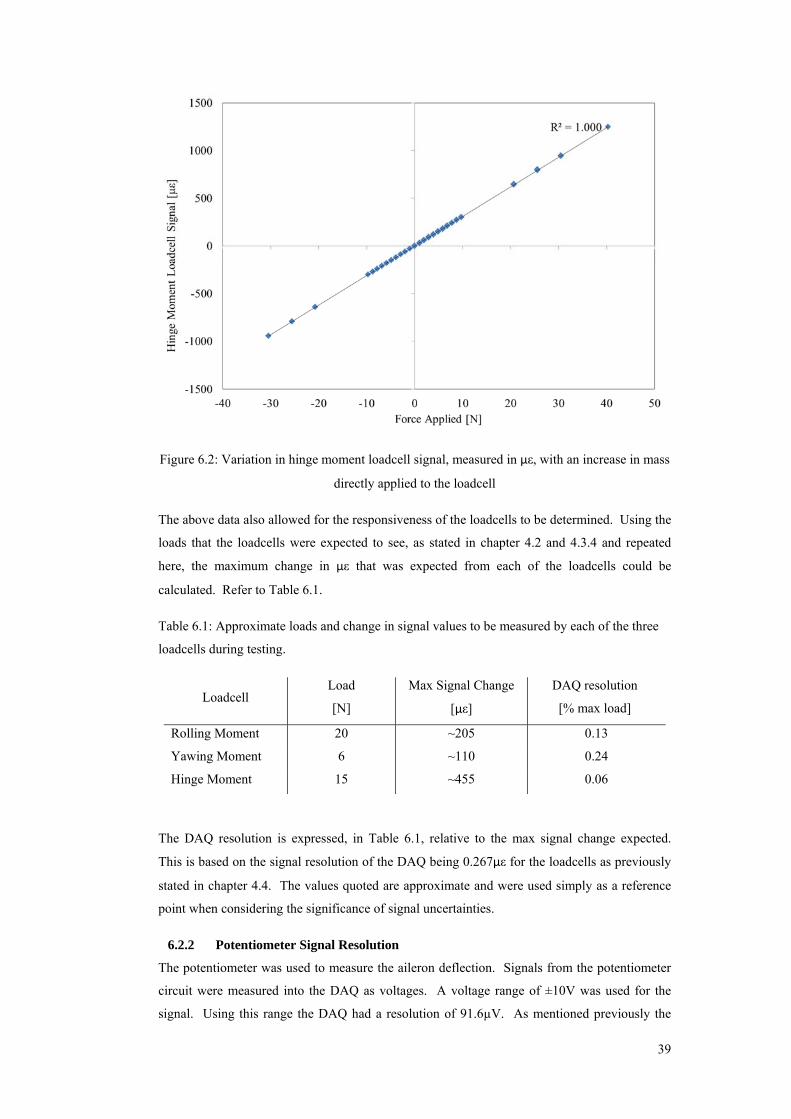
39
Figure 6.2: Variation in hinge moment loadcell signal, measured in με, with an increase in mass
directly applied to the loadcell
The above data also allowed for the responsiveness of the loadcells to be determined. Using the
loads that the loadcells were expected to see, as stated in chapter 4.2 and 4.3.4 and repeated
here, the maximum change in με that was expected from each of the loadcells could be
calculated. Refer to Table 6.1.
Table 6.1: Approximate loads and change in signal values to be measured by each of the three
loadcells during testing.
Loadcell Load
[N]
Max Signal Change
[με]
DAQ resolution
[% max load]
Rolling Moment 20 ~205 0.13
Yawing Moment 6 ~110 0.24
Hinge Moment 15 ~455 0.06
The DAQ resolution is expressed, in Table 6.1, relative to the max signal change expected.
This is based on the signal resolution of the DAQ being 0.267με for the loadcells as previously
stated in chapter 4.4. The values quoted are approximate and were used simply as a reference
point when considering the significance of signal uncertainties.
6.2.2 Potentiometer Signal Resolution
The potentiometer was used to measure the aileron deflection. Signals from the potentiometer
circuit were measured into the DAQ as voltages. A voltage range of ±10V was used for the
signal. Using this range the DAQ had a resolution of 91.6µV. As mentioned previously the
40
minimum measurable aileron deflection was required to be 5° based on the measurement
system requirements, stipulated in chapter 3.2. A 5° deflection change would result in a
measured voltage change of 0.1V across the potentiometer. The DAQ resolution was therefore
seen as being more than suitable for the purpose.
6.2.3 Ghosting Effect
One of the effects that were checked for was that of ghosting between the loadcell signals.
Specifically, the ghosting effects with regards to the change in signal for one loadcell when
another loadcell was loaded. While the system had been designed and wired up in such a way as
to prevent this occurring it was still seen as necessary to check nevertheless. This was checked
by wiring up the three loadcells, measuring the rolling, yawing and hinge moments. Each
loadcell was then individually loaded and the signals recorded for all three loadcells.
Comparisons between the signal data would then allow for the detection of any ghosting effects
that may have occurred. In this way the electrical system was checked for errors such as dry
solder joints, grounding issues and failures in the system. The data in Figure 6.3 is typical of
the data obtained in each of the load cases. Figure 6.3 is for a pure yawing moment load case.
Figure 6.3: Change in loadcell signals, measured in με, recorded for each loadcell when a
yawing moment was applied.
From Figure 6.3 a clear distinction can be seen between the signal data recorded for the yawing
moment loadcell and the other two loadcells. The signal inputs from the rolling, and hinge
moment loadcells varied by less than 0.5με over the range of loads applied. As the DAQ was
only sensitive enough to pick up 0.267µε the variance of the signals for the rolling and hinge
moment loadcells was seen as negligible.
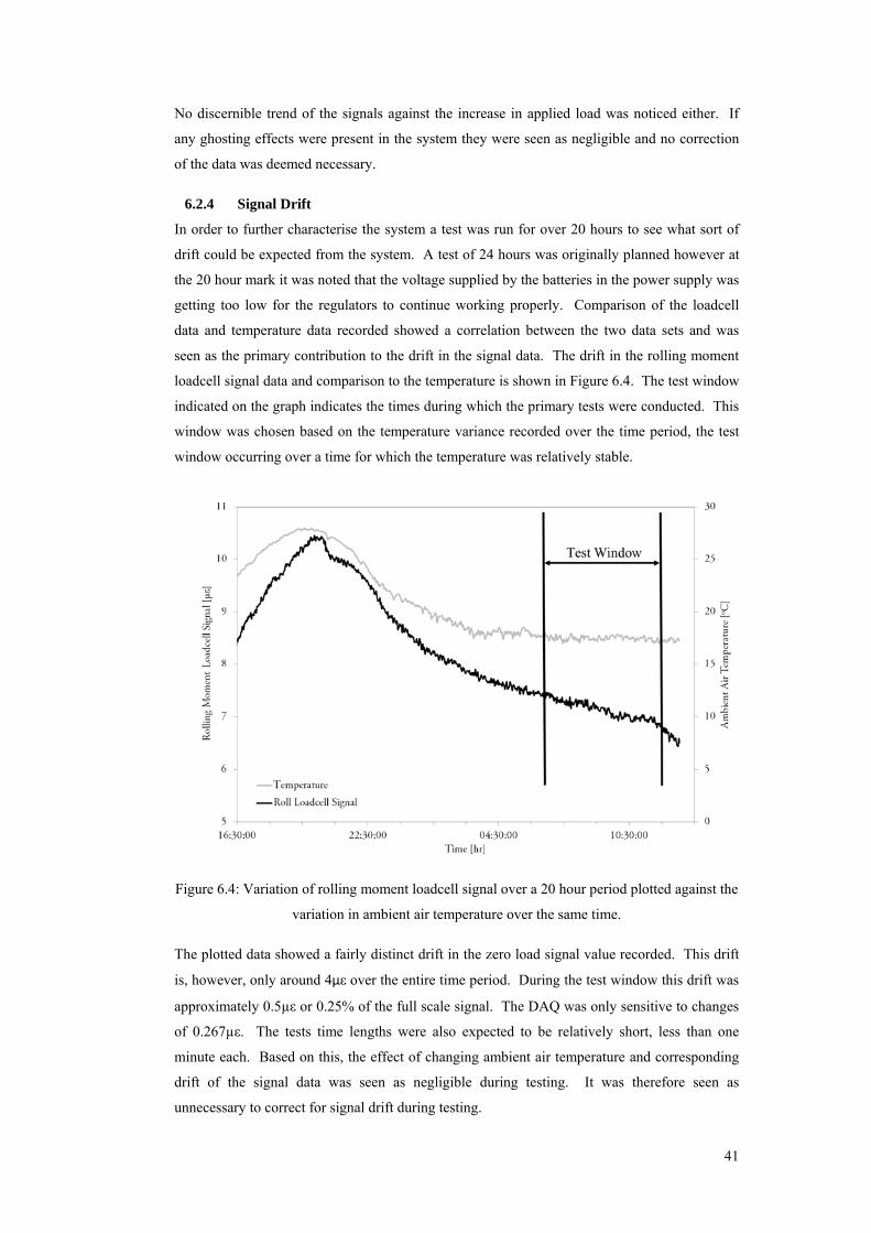
41
No discernible trend of the signals against the increase in applied load was noticed either. If
any ghosting effects were present in the system they were seen as negligible and no correction
of the data was deemed necessary.
6.2.4 Signal Drift
In order to further characterise the system a test was run for over 20 hours to see what sort of
drift could be expected from the system. A test of 24 hours was originally planned however at
the 20 hour mark it was noted that the voltage supplied by the batteries in the power supply was
getting too low for the regulators to continue working properly. Comparison of the loadcell
data and temperature data recorded showed a correlation between the two data sets and was
seen as the primary contribution to the drift in the signal data. The drift in the rolling moment
loadcell signal data and comparison to the temperature is shown in Figure 6.4. The test window
indicated on the graph indicates the times during which the primary tests were conducted. This
window was chosen based on the temperature variance recorded over the time period, the test
window occurring over a time for which the temperature was relatively stable.
Figure 6.4: Variation of rolling moment loadcell signal over a 20 hour period plotted against the
variation in ambient air temperature over the same time.
The plotted data showed a fairly distinct drift in the zero load signal value recorded. This drift
is, however, only around 4με over the entire time period. During the test window this drift was
approximately 0.5µε or 0.25% of the full scale signal. The DAQ was only sensitive to changes
of 0.267µε. The tests time lengths were also expected to be relatively short, less than one
minute each. Based on this, the effect of changing ambient air temperature and corresponding
drift of the signal data was seen as negligible during testing. It was therefore seen as
unnecessary to correct for signal drift during testing.
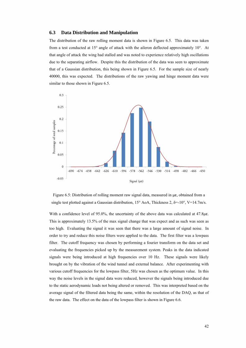
42
6.3 Data Distribution and Manipulation
The distribution of the raw rolling moment data is shown in Figure 6.5. This data was taken
from a test conducted at 15° angle of attack with the aileron deflected approximately 10°. At
that angle of attack the wing had stalled and was noted to experience relatively high oscillations
due to the separating airflow. Despite this the distribution of the data was seen to approximate
that of a Gaussian distribution, this being shown in Figure 6.5. For the sample size of nearly
40000, this was expected. The distributions of the raw yawing and hinge moment data were
similar to those shown in Figure 6.5.
Figure 6.5: Distribution of rolling moment raw signal data, measured in με, obtained from a
single test plotted against a Gaussian distribution, 15° AoA, Thickness 2, δ=-10°, V=14.7m/s.
With a confidence level of 95.0%, the uncertainty of the above data was calculated at 47.8με.
This is approximately 13.5% of the max signal change that was expect and as such was seen as
too high. Evaluating the signal it was seen that there was a large amount of signal noise. In
order to try and reduce this noise filters were applied to the data. The first filter was a lowpass
filter. The cutoff frequency was chosen by performing a fourier transform on the data set and
evaluating the frequencies picked up by the measurement system. Peaks in the data indicated
signals were being introduced at high frequencies over 10 Hz. These signals were likely
brought on by the vibration of the wind tunnel and external balance. After experimenting with
various cutoff frequencies for the lowpass filter, 5Hz was chosen as the optimum value. In this
way the noise levels in the signal data were reduced, however the signals being introduced due
to the static aerodynamic loads not being altered or removed. This was interpreted based on the
average signal of the filtered data being the same, within the resolution of the DAQ, as that of
the raw data. The effect on the data of the lowpass filter is shown in Figure 6.6.
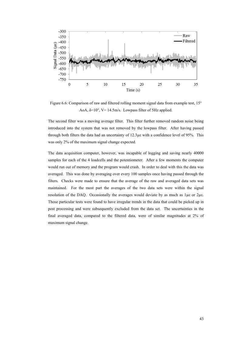
43
Figure 6.6: Comparison of raw and filtered rolling moment signal data from example test, 15°
AoA, δ=10°, V= 14.5m/s. Lowpass filter of 5Hz applied.
The second filter was a moving average filter. This filter further removed random noise being
introduced into the system that was not removed by the lowpass filter. After having passed
through both filters the data had an uncertainty of 12.3µε with a confidence level of 95%. This
was only 2% of the maximum signal change expected.
The data acquisition computer, however, was incapable of logging and saving nearly 40000
samples for each of the 4 loadcells and the potentiometer. After a few moments the computer
would run out of memory and the program would crash. In order to deal with this the data was
averaged. This was done by averaging over every 100 samples once having passed through the
filters. Checks were made to ensure that the average of the raw and averaged data sets was
maintained. For the most part the averages of the two data sets were within the signal
resolution of the DAQ. Occasionally the averages would deviate by as much as 1µε or 2µε.
Those particular tests were found to have irregular trends in the data that could be picked up in
post processing and were subsequently excluded from the data set. The uncertainties in the
final averaged data, compared to the filtered data, were of similar magnitudes at 2% of
maximum signal change.
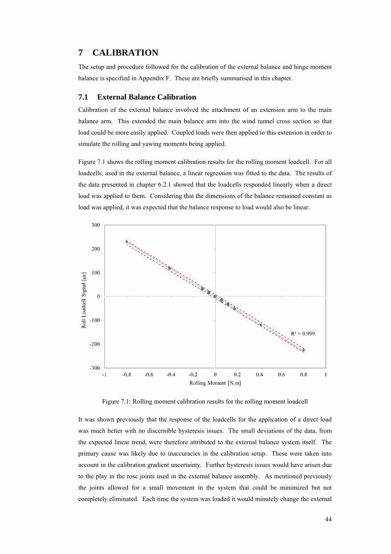
44
7 CALIBRATION
The setup and procedure followed for the calibration of the external balance and hinge moment
balance is specified in Appendix F. These are briefly summarised in this chapter.
7.1 External Balance Calibration
Calibration of the external balance involved the attachment of an extension arm to the main
balance arm. This extended the main balance arm into the wind tunnel cross section so that
load could be more easily applied. Coupled loads were then applied to this extension in order to
simulate the rolling and yawing moments being applied.
Figure 7.1 shows the rolling moment calibration results for the rolling moment loadcell. For all
loadcells, used in the external balance, a linear regression was fitted to the data. The results of
the data presented in chapter 6.2.1 showed that the loadcells responded linearly when a direct
load was applied to them. Considering that the dimensions of the balance remained constant as
load was applied, it was expected that the balance response to load would also be linear.
Figure 7.1: Rolling moment calibration results for the rolling moment loadcell
It was shown previously that the response of the loadcells for the application of a direct load
was much better with no discernible hysteresis issues. The small deviations of the data, from
the expected linear trend, were therefore attributed to the external balance system itself. The
primary cause was likely due to inaccuracies in the calibration setup. These were taken into
account in the calibration gradient uncertainty. Further hysteresis issues would have arisen due
to the play in the rose joints used in the external balance assembly. As mentioned previously
the joints allowed for a small movement in the system that could be minimized but not
completely eliminated. Each time the system was loaded it would minutely change the external
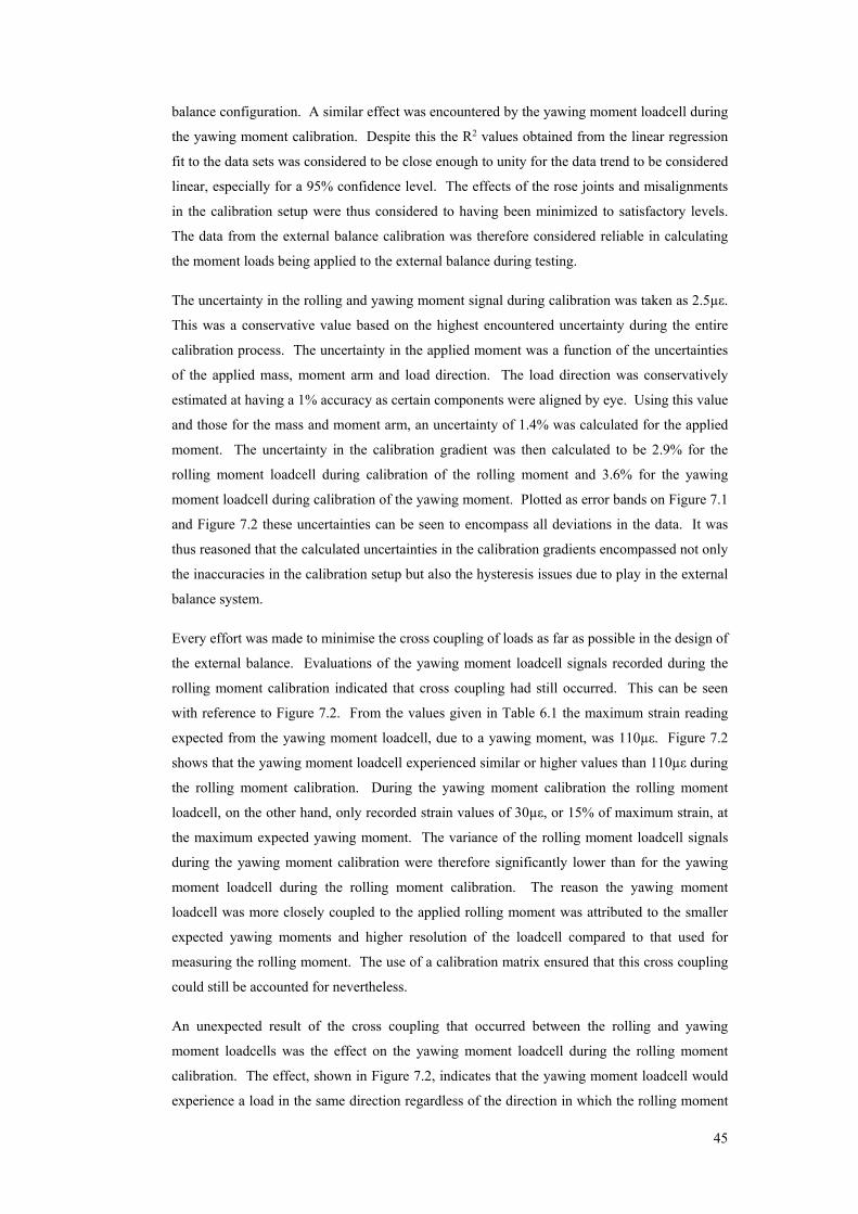
45
balance configuration. A similar effect was encountered by the yawing moment loadcell during
the yawing moment calibration. Despite this the R2 values obtained from the linear regression
fit to the data sets was considered to be close enough to unity for the data trend to be considered
linear, especially for a 95% confidence level. The effects of the rose joints and misalignments
in the calibration setup were thus considered to having been minimized to satisfactory levels.
The data from the external balance calibration was therefore considered reliable in calculating
the moment loads being applied to the external balance during testing.
The uncertainty in the rolling and yawing moment signal during calibration was taken as 2.5µε.
This was a conservative value based on the highest encountered uncertainty during the entire
calibration process. The uncertainty in the applied moment was a function of the uncertainties
of the applied mass, moment arm and load direction. The load direction was conservatively
estimated at having a 1% accuracy as certain components were aligned by eye. Using this value
and those for the mass and moment arm, an uncertainty of 1.4% was calculated for the applied
moment. The uncertainty in the calibration gradient was then calculated to be 2.9% for the
rolling moment loadcell during calibration of the rolling moment and 3.6% for the yawing
moment loadcell during calibration of the yawing moment. Plotted as error bands on Figure 7.1
and Figure 7.2 these uncertainties can be seen to encompass all deviations in the data. It was
thus reasoned that the calculated uncertainties in the calibration gradients encompassed not only
the inaccuracies in the calibration setup but also the hysteresis issues due to play in the external
balance system.
Every effort was made to minimise the cross coupling of loads as far as possible in the design of
the external balance. Evaluations of the yawing moment loadcell signals recorded during the
rolling moment calibration indicated that cross coupling had still occurred. This can be seen
with reference to Figure 7.2. From the values given in Table 6.1 the maximum strain reading
expected from the yawing moment loadcell, due to a yawing moment, was 110µε. Figure 7.2
shows that the yawing moment loadcell experienced similar or higher values than 110µε during
the rolling moment calibration. During the yawing moment calibration the rolling moment
loadcell, on the other hand, only recorded strain values of 30µε, or 15% of maximum strain, at
the maximum expected yawing moment. The variance of the rolling moment loadcell signals
during the yawing moment calibration were therefore significantly lower than for the yawing
moment loadcell during the rolling moment calibration. The reason the yawing moment
loadcell was more closely coupled to the applied rolling moment was attributed to the smaller
expected yawing moments and higher resolution of the loadcell compared to that used for
measuring the rolling moment. The use of a calibration matrix ensured that this cross coupling
could still be accounted for nevertheless.
An unexpected result of the cross coupling that occurred between the rolling and yawing
moment loadcells was the effect on the yawing moment loadcell during the rolling moment
calibration. The effect, shown in Figure 7.2, indicates that the yawing moment loadcell would
experience a load in the same direction regardless of the direction in which the rolling moment
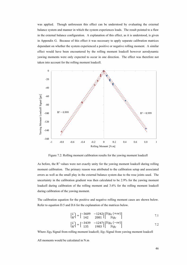
46
was applied. Though unforeseen this effect can be understood by evaluating the external
balance system and manner in which the system experiences loads. The result pointed to a flaw
in the external balance configuration. A explanation of this effect, as it is understood, is given
in Appendix G. Because of this effect it was necessary to apply separate calibration matrices
dependant on whether the system experienced a positive or negative rolling moment. A similar
effect would have been encountered by the rolling moment loadcell however aerodynamic
yawing moments were only expected to occur in one direction. The effect was therefore not
taken into account for the rolling moment loadcell.
Figure 7.2: Rolling moment calibration results for the yawing moment loadcell
As before, the R2 values were not exactly unity for the yawing moment loadcell during rolling
moment calibration. The primary reason was attributed to the calibration setup and associated
errors as well as the small play in the external balance system due to the rose joints used. The
uncertainty in the calibration gradient was then calculated to be 2.9% for the yawing moment
loadcell during calibration of the rolling moment and 3.6% for the rolling moment loadcell
during calibration of the yawing moment.
The calibration equation for the positive and negative rolling moment cases are shown below.
Refer to equation D.5 and D.6 for the explanation of the matrices below.
′′ = −3609 −1242142 2081 + 7.1
′′ = −3439 −1247135 1983 − 7.2
Where SigR Signal from rolling moment loadcell; SigY Signal from yawing moment loadcell
All moments would be calculated in N.m
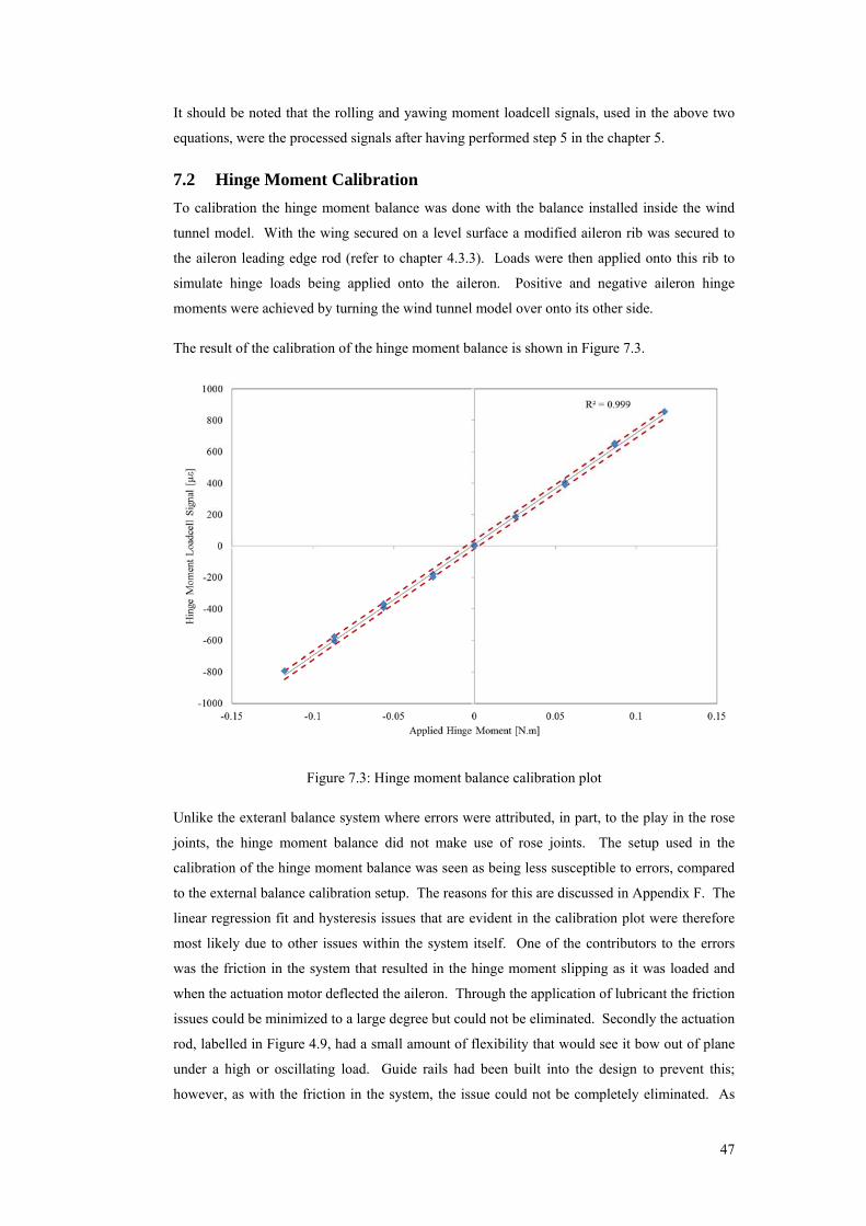
47
It should be noted that the rolling and yawing moment loadcell signals, used in the above two
equations, were the processed signals after having performed step 5 in the chapter 5.
7.2 Hinge Moment Calibration
To calibration the hinge moment balance was done with the balance installed inside the wind
tunnel model. With the wing secured on a level surface a modified aileron rib was secured to
the aileron leading edge rod (refer to chapter 4.3.3). Loads were then applied onto this rib to
simulate hinge loads being applied onto the aileron. Positive and negative aileron hinge
moments were achieved by turning the wind tunnel model over onto its other side.
The result of the calibration of the hinge moment balance is shown in Figure 7.3.
Figure 7.3: Hinge moment balance calibration plot
Unlike the exteranl balance system where errors were attributed, in part, to the play in the rose
joints, the hinge moment balance did not make use of rose joints. The setup used in the
calibration of the hinge moment balance was seen as being less susceptible to errors, compared
to the external balance calibration setup. The reasons for this are discussed in Appendix F. The
linear regression fit and hysteresis issues that are evident in the calibration plot were therefore
most likely due to other issues within the system itself. One of the contributors to the errors
was the friction in the system that resulted in the hinge moment slipping as it was loaded and
when the actuation motor deflected the aileron. Through the application of lubricant the friction
issues could be minimized to a large degree but could not be eliminated. Secondly the actuation
rod, labelled in Figure 4.9, had a small amount of flexibility that would see it bow out of plane
under a high or oscillating load. Guide rails had been built into the design to prevent this;
however, as with the friction in the system, the issue could not be completely eliminated. As
48
with the external balance calibration plots the R2 value for the linear regression fitted to the
above data was 0.999. The effects of the friction and flexibility of the hinge moment balance
thus considered to having been minimized to satisfactory levels. The data from the hinge
moment balance calibration was therefore considered reliable in calculating the moment loads
being applied to the aileron during testing.
Further precautions were taken, during calibration and testing, whereby measurements were
taken for an aileron sweep with the aileron moving in only one direction; a change in deflection
direction of the aileron, by the actuation system, being found to alter the zero load reading. In
this way the hinge moment balance was loaded, during calibration, in a similar manner to which
the system would be loaded during the wind tunnel testing. It also meant that similar friction or
flexibility issues that affected the data during wind tunnel testing would have occurred during
the calibration. This allowed for a little more reliability in the calibration.
Checks were conducted to ascertain whether the calibration data would still be valid as the
aileron was deflected. This was because, as the aileron was deflected, the effective moment
arm between the aileron hinge axis and loadcell load axis would change. The hinge moment
balance had been designed in such a way as for this to not be significant over the deflection
range for which testing was required. Calibration plots were generated for the aileron at 3
distinct deflections, a high positive and negative deflection and a zero deflection. Comparisons
between the three plots showed that the calibration gradient changed by less than 1% over the
three cases. As such as the effect of the ailerons deflection was considered negligible when
applying the hinge moment balance calibration.
The uncertainty in the hinge moment signal was calculated as 2.0µε. This was a conservative
value based on the highest average uncertainty during the entire calibration process for load
cases. Due to the high level of accuracy to which the mass of the applied mass pieces were
measured, their uncertainty was considered negligible in comparison to the uncertainty of the
moment arms and applied load alignment. The uncertainty in the applied moment was thus
calculated at being 2.2% of the applied moment. The uncertainty in the calibration gradient for
the hinge moment balance was therefore calculated to be 2.5%, using equation D.3. This
uncertainty is plotted as an error bands on Figure 7.3. As with the external balance calibration
plots the uncertainty in the hinge calibration gradient can be seen to encompass all deviations in
the data. It was thus reasoned that the calculated uncertainties in the calibration gradients
encompassed not only the inaccuracies in the calibration setup but also the hysteresis issues due
to friction and unwanted bowing in the hinge moment balance. This based on the similar nature
in which the hinge moment balance was loaded during calibration and testing.
The equation used for calculating the hinge moments, based is given below
= 138 × 7.3
Where Signal from hinge moment loadcell
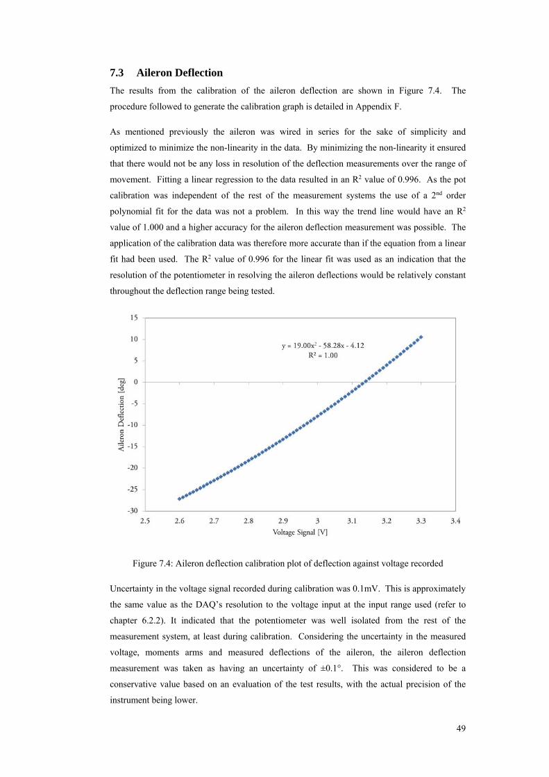
49
7.3 Aileron Deflection
The results from the calibration of the aileron deflection are shown in Figure 7.4. The
procedure followed to generate the calibration graph is detailed in Appendix F.
As mentioned previously the aileron was wired in series for the sake of simplicity and
optimized to minimize the non-linearity in the data. By minimizing the non-linearity it ensured
that there would not be any loss in resolution of the deflection measurements over the range of
movement. Fitting a linear regression to the data resulted in an R2 value of 0.996. As the pot
calibration was independent of the rest of the measurement systems the use of a 2nd order
polynomial fit for the data was not a problem. In this way the trend line would have an R2
value of 1.000 and a higher accuracy for the aileron deflection measurement was possible. The
application of the calibration data was therefore more accurate than if the equation from a linear
fit had been used. The R2 value of 0.996 for the linear fit was used as an indication that the
resolution of the potentiometer in resolving the aileron deflections would be relatively constant
throughout the deflection range being tested.
Figure 7.4: Aileron deflection calibration plot of deflection against voltage recorded
Uncertainty in the voltage signal recorded during calibration was 0.1mV. This is approximately
the same value as the DAQ’s resolution to the voltage input at the input range used (refer to
chapter 6.2.2). It indicated that the potentiometer was well isolated from the rest of the
measurement system, at least during calibration. Considering the uncertainty in the measured
voltage, moments arms and measured deflections of the aileron, the aileron deflection
measurement was taken as having an uncertainty of ±0.1°. This was considered to be a
conservative value based on an evaluation of the test results, with the actual precision of the
instrument being lower.

50
From the calibration the following equation was derived.
= 19.00 − 58.28 − 4.12 7.4
Where δ aileron deflection, deg; measured voltage across the potentiometer, V
As mentioned in chapter 5, the measured voltage, applied to equation 7.4, was the total voltage.
Unlike the measured loadcell signals, the voltage across the potentiometer was not zeroed
during testing.
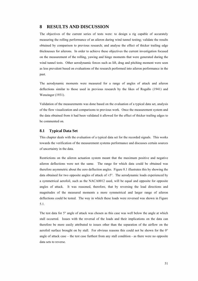
51
8 RESULTS AND DISCUSSION
The objectives of the current series of tests were: to design a rig capable of accurately
measuring the rolling performance of an aileron during wind tunnel testing; validate the results
obtained by comparison to previous research; and analyse the effect of thicker trailing edge
thicknesses for ailerons. In order to achieve these objectives the current investigation focused
on the measurement of the rolling, yawing and hinge moments that were generated during the
wind tunnel tests. Other aerodynamic forces such as lift, drag and pitching moment were seen
as less prevalent based on evaluations of the research performed into aileron performance in the
past.
The aerodynamic moments were measured for a range of angles of attack and aileron
deflections similar to those used in previous research by the likes of Rogallo (1941) and
Wenzinger (1931).
Validation of the measurements was done based on the evaluation of a typical data set, analysis
of the flow visualization and comparisons to previous work. Once the measurement system and
the data obtained from it had been validated it allowed for the effect of thicker trailing edges to
be commented on.
8.1 Typical Data Set
This chapter deals with the evaluation of a typical data set for the recorded signals. This works
towards the verification of the measurement systems performance and discusses certain sources
of uncertainty in the data.
Restrictions on the aileron actuation system meant that the maximum positive and negative
aileron deflections were not the same. The range for which data could be obtained was
therefore asymmetric about the zero deflection angles. Figure 8.1 illustrates this by showing the
data obtained for two opposite angles of attack of ±5°. The aerodynamic loads experienced by
a symmetrical aerofoil, such as the NACA0012 used, will be equal and opposite for opposite
angles of attack. It was reasoned, therefore, that by reversing the load directions and
magnitudes of the measured moments a more symmetrical and larger range of aileron
deflections could be tested. The way in which these loads were reversed was shown in Figure
5.1.
The test data for 5° angle of attack was chosen as this case was well below the angle at which
stall occurred. Issues with the reversal of the loads and their implications on the data can
therefore be more easily attributed to issues other than the separation of the airflow on the
aerofoil surface brought on by stall. For obvious reasons this could not be shown for the 0°
angle of attack case – the test case furthest from any stall condition - as there were no opposite
data sets to reverse.
52
The result of the load reversal is shown in Figure 8.1 for the yawing moment signals. Similar
results were observed for the rolling and hinge moment signals however the result was simply
more clearly evident in the yawing moment signal.
Figure 8.1: Zeroed yawing moment loadcell signals, including reversed signals, -5° and +5°
AoA, plain sealed aileron, Thickness 2, V=14.6m/s.
The trend lines were fitted, in Figure 8.1, to give an approximate indication of the differences
between the positive and negative angle of attack data sets over the common aileron deflections.
It would be expected that if the loads were symmetrical for opposite angles of attack, the signals
would correlate over the aileron deflection range that was common to both data sets.
Depending on the test, this range was typically between ±10° aileron deflections.
There is a good correlation between the yawing moment signals for the negative aileron
deflections. For the positive aileron deflections, however, there is a slight divergence noticed in
the trends. This could be due to a few factors. If the wing was not completely symmetrical due
to manufacturing flaws the reversal of the signals would not correlate as expected. The data
trends between the positive and negative angle of attack cases would appear skewed and offset.
This would be seen for all 3 moments, rolling, yawing and hinge, were it the case. Figure 8.3
shows the rolling moment signal trend that was obtained for the same test condition as the
yawing moment signals, shown in Figure 8.1. Over the ±10° aileron deflection range the
correlation is good for both the positive and negative deflections. Any deviation is well within
the uncertainty for the data points. While the symmetry of the wing cannot be said to be perfect
based on this, any asymmetry is considered negligible.
The apparent difference between the positive and negative angles of attack data sets for the
yawing moment is likely due to a combination of the yawing moment resolution and uncertainty
in the signals. The results of the calibration showed that the yawing moment loads were very
53
sensitive to changes in the rolling moment, leading to a significant cross coupling that occurred
between the two measurements. This made the yawing moment loadcell more susceptible to
disturbances in the system. The rolling moment loadcell, on the other hand, was less sensitive
to such disturbances. This further explains why the correlation between the positive and
negative deflections for the rolling moment signals in Figure 8.3 is much better than for the
yawing moment signals in Figure 8.1.
The uncertainty values shown in Figure 8.1are those of the strain values. At ±5° angle of attack
these values were ± 2.5µε or approximately 2% of the maximum load. These values, expressed
as error bars in Figure 8.1, can account, in part, for the noted divergence of the yawing moment
signals. Combined then with the higher resolution of the yawing moment signals, compared to
the rolling and even hinge moment signals, the divergence in the signals can be explained. It
was understood to mean that the analysis method of reversing the signals of the opposite angle
of attack was valid. The resolution of the external balance to yawing moments, however, is
therefore lower than that shown by the uncertainty values. Further interpretation of the yawing
moment data would then need to take this into account.
One further observations that can be made of the data shown in Figure 8.1 deals with the
specific aileron deflections from which the moments were recorded. Evaluation of the data for
the negative and unreversed positive angles of attack show a distinct difference in the
increments of aileron deflections for which data was recorded. The uncertainty in the measured
aileron deflection was on average ±0.1°. This then does not account for the differences noted.
It was intended to test at specific aileron deflections and be consistent with these throughout the
tests. In this way it would have made comparisons between the results for the different aileron
thicknesses, easier. Unfortunately the aileron and hinge moment balance was found to deflect
in a slightly unpredictable manner as aerodynamic loads were applied to the aileron. This
deflection was expected however the random variances were not. Actuation of the hinge
moment balance under load was found to offset the zero load signal value, meaning that the
change in load on the loadcell could not be calculated. The aileron could therefore not be
precisely set to a specific deflection, once under load, during testing. This was not significant
in the processing of the data as the aileron deflection was measured directly. It implied,
however, that hinge moment balance and aileron system did not respond exactly the same way
each time. The significance of this will be discussed later on.
The calibration matrix was applied to the rolling and yawing moments from each data set. The
cross coupling in the external balance meant that the trends of the two moments were adjusted
slightly after the application of the matrix. This can be seen in both Figure 8.2 and Figure 8.3
for the yawing and rolling moments respectively. The yawing moment loadcell was, as
discussed, more sensitive to applied loads. The data points therefore experienced larger
changes to the trend than the rolling moment loadcell data points. The implication of this is that
the recorded signals from the loadcells cannot be evaluated on their own without the application
of the calibration matrix beforehand.
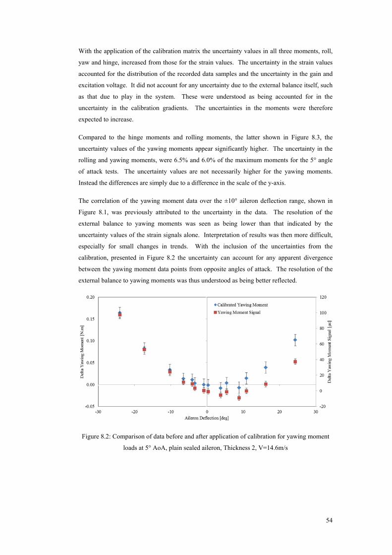
54
With the application of the calibration matrix the uncertainty values in all three moments, roll,
yaw and hinge, increased from those for the strain values. The uncertainty in the strain values
accounted for the distribution of the recorded data samples and the uncertainty in the gain and
excitation voltage. It did not account for any uncertainty due to the external balance itself, such
as that due to play in the system. These were understood as being accounted for in the
uncertainty in the calibration gradients. The uncertainties in the moments were therefore
expected to increase.
Compared to the hinge moments and rolling moments, the latter shown in Figure 8.3, the
uncertainty values of the yawing moments appear significantly higher. The uncertainty in the
rolling and yawing moments, were 6.5% and 6.0% of the maximum moments for the 5° angle
of attack tests. The uncertainty values are not necessarily higher for the yawing moments.
Instead the differences are simply due to a difference in the scale of the y-axis.
The correlation of the yawing moment data over the ±10° aileron deflection range, shown in
Figure 8.1, was previously attributed to the uncertainty in the data. The resolution of the
external balance to yawing moments was seen as being lower than that indicated by the
uncertainty values of the strain signals alone. Interpretation of results was then more difficult,
especially for small changes in trends. With the inclusion of the uncertainties from the
calibration, presented in Figure 8.2 the uncertainty can account for any apparent divergence
between the yawing moment data points from opposite angles of attack. The resolution of the
external balance to yawing moments was thus understood as being better reflected.
Figure 8.2: Comparison of data before and after application of calibration for yawing moment
loads at 5° AoA, plain sealed aileron, Thickness 2, V=14.6m/s
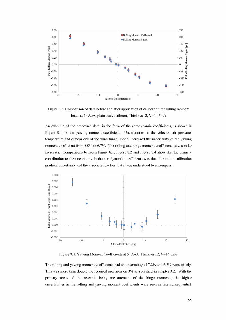
55
Figure 8.3: Comparison of data before and after application of calibration for rolling moment
loads at 5° AoA, plain sealed aileron, Thickness 2, V=14.6m/s
An example of the processed data, in the form of the aerodynamic coefficients, is shown in
Figure 8.4 for the yawing moment coefficient. Uncertainties in the velocity, air pressure,
temperature and dimensions of the wind tunnel model increased the uncertainty of the yawing
moment coefficient from 6.0% to 6.7%. The rolling and hinge moment coefficients saw similar
increases. Comparisons between Figure 8.1, Figure 8.2 and Figure 8.4 show that the primary
contribution to the uncertainty in the aerodynamic coefficients was thus due to the calibration
gradient uncertainty and the associated factors that it was understood to encompass.
Figure 8.4: Yawing Moment Coefficients at 5° AoA, Thickness 2, V=14.6m/s
The rolling and yawing moment coefficients had an uncertainty of 7.2% and 6.7% respectively.
This was more than double the required precision on 3% as specified in chapter 3.2. With the
primary focus of the research being measurement of the hinge moments, the higher
uncertainties in the rolling and yawing moment coefficients were seen as less consequential.
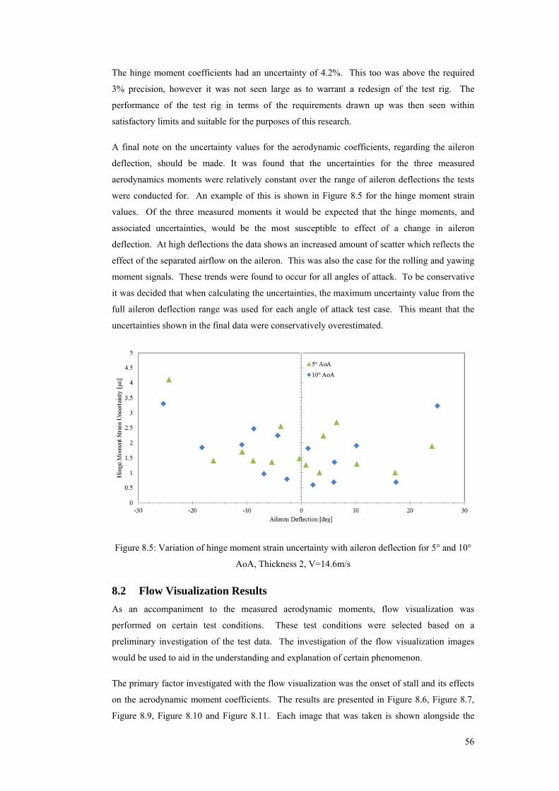
56
The hinge moment coefficients had an uncertainty of 4.2%. This too was above the required
3% precision, however it was not seen large as to warrant a redesign of the test rig. The
performance of the test rig in terms of the requirements drawn up was then seen within
satisfactory limits and suitable for the purposes of this research.
A final note on the uncertainty values for the aerodynamic coefficients, regarding the aileron
deflection, should be made. It was found that the uncertainties for the three measured
aerodynamics moments were relatively constant over the range of aileron deflections the tests
were conducted for. An example of this is shown in Figure 8.5 for the hinge moment strain
values. Of the three measured moments it would be expected that the hinge moments, and
associated uncertainties, would be the most susceptible to effect of a change in aileron
deflection. At high deflections the data shows an increased amount of scatter which reflects the
effect of the separated airflow on the aileron. This was also the case for the rolling and yawing
moment signals. These trends were found to occur for all angles of attack. To be conservative
it was decided that when calculating the uncertainties, the maximum uncertainty value from the
full aileron deflection range was used for each angle of attack test case. This meant that the
uncertainties shown in the final data were conservatively overestimated.
Figure 8.5: Variation of hinge moment strain uncertainty with aileron deflection for 5° and 10°
AoA, Thickness 2, V=14.6m/s
8.2 Flow Visualization Results
As an accompaniment to the measured aerodynamic moments, flow visualization was
performed on certain test conditions. These test conditions were selected based on a
preliminary investigation of the test data. The investigation of the flow visualization images
would be used to aid in the understanding and explanation of certain phenomenon.
The primary factor investigated with the flow visualization was the onset of stall and its effects
on the aerodynamic moment coefficients. The results are presented in Figure 8.6, Figure 8.7,
Figure 8.9, Figure 8.10 and Figure 8.11. Each image that was taken is shown alongside the
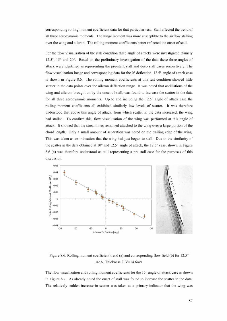
57
corresponding rolling moment coefficient data for that particular test. Stall affected the trend of
all three aerodynamic moments. The hinge moment was more susceptible to the airflow stalling
over the wing and aileron. The rolling moment coefficients better reflected the onset of stall.
For the flow visualization of the stall condition three angle of attacks were investigated, namely
12.5°, 15° and 20°. Based on the preliminary investigation of the data these three angles of
attack were identified as representing the pre-stall, stall and deep stall cases respectively. The
flow visualization image and corresponding data for the 0° deflection, 12.5° angle of attack case
is shown in Figure 8.6. The rolling moment coefficients at this test condition showed little
scatter in the data points over the aileron deflection range. It was noted that oscillations of the
wing and aileron, brought on by the onset of stall, was found to increase the scatter in the data
for all three aerodynamic moments. Up to and including the 12.5° angle of attack case the
rolling moment coefficients all exhibited similarly low levels of scatter. It was therefore
understood that above this angle of attack, from which scatter in the data increased, the wing
had stalled. To confirm this, flow visualization of the wing was performed at this angle of
attack. It showed that the streamlines remained attached to the wing over a large portion of the
chord length. Only a small amount of separation was noted on the trailing edge of the wing.
This was taken as an indication that the wing had just begun to stall. Due to the similarity of
the scatter in the data obtained at 10° and 12.5° angle of attack, the 12.5° case, shown in Figure
8.6 (a) was therefore understood as still representing a pre-stall case for the purposes of this
discussion.
Figure 8.6: Rolling moment coefficient trend (a) and corresponding flow field (b) for 12.5°
AoA, Thickness 2, V=14.6m/s
The flow visualization and rolling moment coefficients for the 15° angle of attack case is shown
in Figure 8.7. As already noted the onset of stall was found to increase the scatter in the data.
The relatively sudden increase in scatter was taken as a primary indicator that the wing was
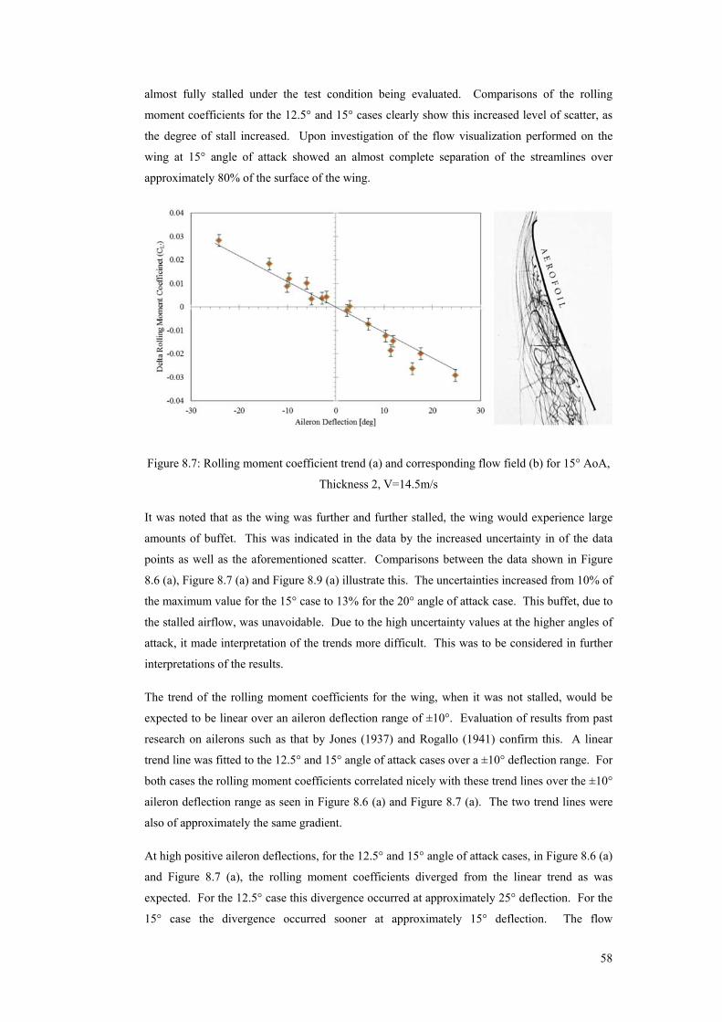
58
almost fully stalled under the test condition being evaluated. Comparisons of the rolling
moment coefficients for the 12.5° and 15° cases clearly show this increased level of scatter, as
the degree of stall increased. Upon investigation of the flow visualization performed on the
wing at 15° angle of attack showed an almost complete separation of the streamlines over
approximately 80% of the surface of the wing.
Figure 8.7: Rolling moment coefficient trend (a) and corresponding flow field (b) for 15° AoA,
Thickness 2, V=14.5m/s
It was noted that as the wing was further and further stalled, the wing would experience large
amounts of buffet. This was indicated in the data by the increased uncertainty in of the data
points as well as the aforementioned scatter. Comparisons between the data shown in Figure
8.6 (a), Figure 8.7 (a) and Figure 8.9 (a) illustrate this. The uncertainties increased from 10% of
the maximum value for the 15° case to 13% for the 20° angle of attack case. This buffet, due to
the stalled airflow, was unavoidable. Due to the high uncertainty values at the higher angles of
attack, it made interpretation of the trends more difficult. This was to be considered in further
interpretations of the results.
The trend of the rolling moment coefficients for the wing, when it was not stalled, would be
expected to be linear over an aileron deflection range of ±10°. Evaluation of results from past
research on ailerons such as that by Jones (1937) and Rogallo (1941) confirm this. A linear
trend line was fitted to the 12.5° and 15° angle of attack cases over a ±10° deflection range. For
both cases the rolling moment coefficients correlated nicely with these trend lines over the ±10°
aileron deflection range as seen in Figure 8.6 (a) and Figure 8.7 (a). The two trend lines were
also of approximately the same gradient.
At high positive aileron deflections, for the 12.5° and 15° angle of attack cases, in Figure 8.6 (a)
and Figure 8.7 (a), the rolling moment coefficients diverged from the linear trend as was
expected. For the 12.5° case this divergence occurred at approximately 25° deflection. For the
15° case the divergence occurred sooner at approximately 15° deflection. The flow
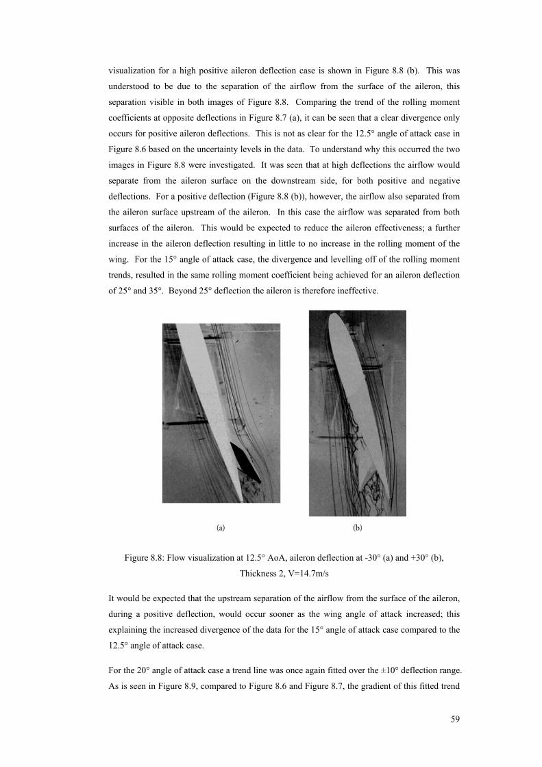
59
visualization for a high positive aileron deflection case is shown in Figure 8.8 (b). This was
understood to be due to the separation of the airflow from the surface of the aileron, this
separation visible in both images of Figure 8.8. Comparing the trend of the rolling moment
coefficients at opposite deflections in Figure 8.7 (a), it can be seen that a clear divergence only
occurs for positive aileron deflections. This is not as clear for the 12.5° angle of attack case in
Figure 8.6 based on the uncertainty levels in the data. To understand why this occurred the two
images in Figure 8.8 were investigated. It was seen that at high deflections the airflow would
separate from the aileron surface on the downstream side, for both positive and negative
deflections. For a positive deflection (Figure 8.8 (b)), however, the airflow also separated from
the aileron surface upstream of the aileron. In this case the airflow was separated from both
surfaces of the aileron. This would be expected to reduce the aileron effectiveness; a further
increase in the aileron deflection resulting in little to no increase in the rolling moment of the
wing. For the 15° angle of attack case, the divergence and levelling off of the rolling moment
trends, resulted in the same rolling moment coefficient being achieved for an aileron deflection
of 25° and 35°. Beyond 25° deflection the aileron is therefore ineffective.
Figure 8.8: Flow visualization at 12.5° AoA, aileron deflection at -30° (a) and +30° (b),
Thickness 2, V=14.7m/s
It would be expected that the upstream separation of the airflow from the surface of the aileron,
during a positive deflection, would occur sooner as the wing angle of attack increased; this
explaining the increased divergence of the data for the 15° angle of attack case compared to the
12.5° angle of attack case.
For the 20° angle of attack case a trend line was once again fitted over the ±10° deflection range.
As is seen in Figure 8.9, compared to Figure 8.6 and Figure 8.7, the gradient of this fitted trend
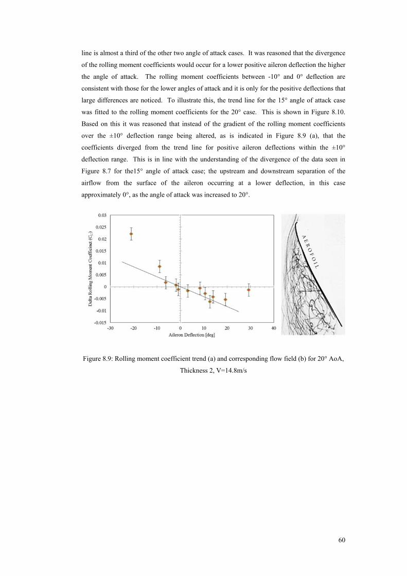
60
line is almost a third of the other two angle of attack cases. It was reasoned that the divergence
of the rolling moment coefficients would occur for a lower positive aileron deflection the higher
the angle of attack. The rolling moment coefficients between -10° and 0° deflection are
consistent with those for the lower angles of attack and it is only for the positive deflections that
large differences are noticed. To illustrate this, the trend line for the 15° angle of attack case
was fitted to the rolling moment coefficients for the 20° case. This is shown in Figure 8.10.
Based on this it was reasoned that instead of the gradient of the rolling moment coefficients
over the ±10° deflection range being altered, as is indicated in Figure 8.9 (a), that the
coefficients diverged from the trend line for positive aileron deflections within the ±10°
deflection range. This is in line with the understanding of the divergence of the data seen in
Figure 8.7 for the15° angle of attack case; the upstream and downstream separation of the
airflow from the surface of the aileron occurring at a lower deflection, in this case
approximately 0°, as the angle of attack was increased to 20°.
Figure 8.9: Rolling moment coefficient trend (a) and corresponding flow field (b) for 20° AoA,
Thickness 2, V=14.8m/s
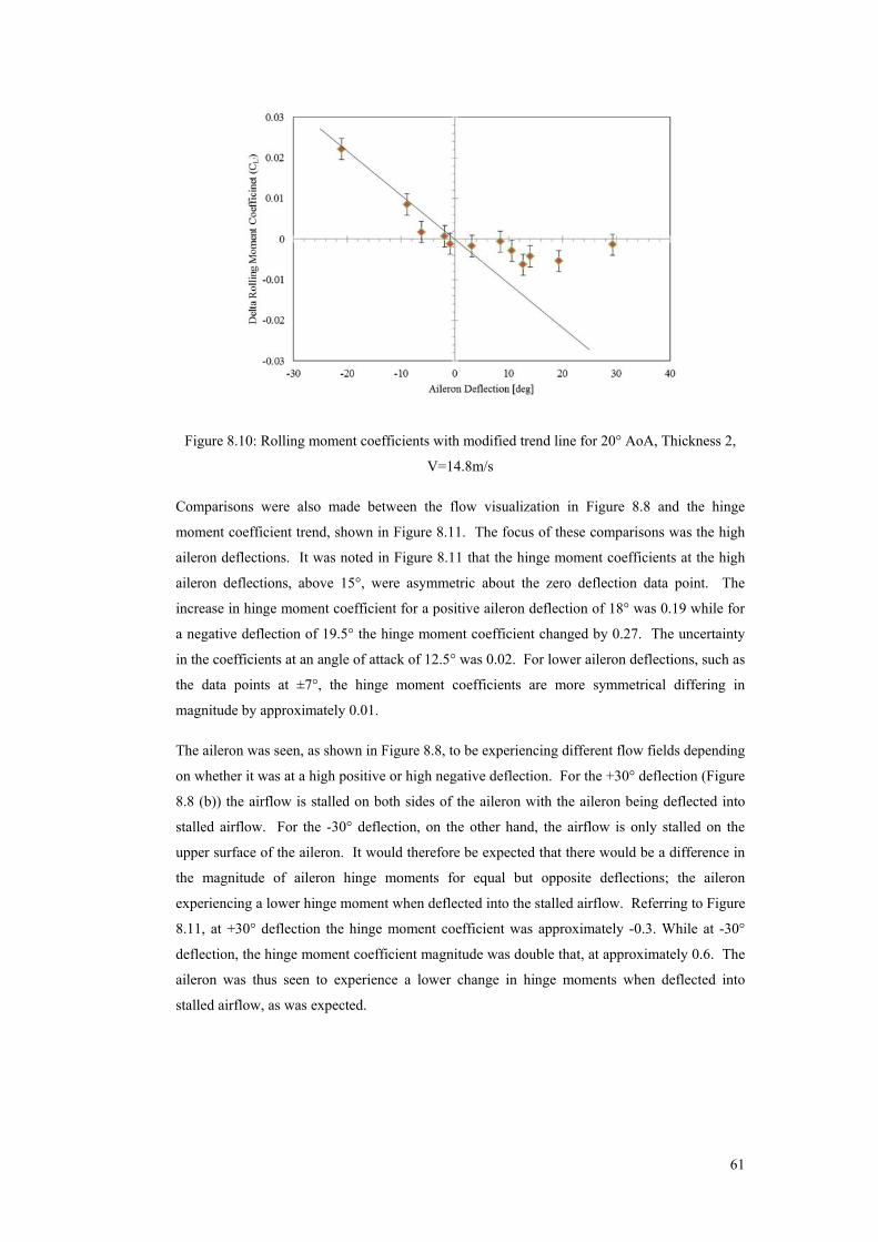
61
Figure 8.10: Rolling moment coefficients with modified trend line for 20° AoA, Thickness 2,
V=14.8m/s
Comparisons were also made between the flow visualization in Figure 8.8 and the hinge
moment coefficient trend, shown in Figure 8.11. The focus of these comparisons was the high
aileron deflections. It was noted in Figure 8.11 that the hinge moment coefficients at the high
aileron deflections, above 15°, were asymmetric about the zero deflection data point. The
increase in hinge moment coefficient for a positive aileron deflection of 18° was 0.19 while for
a negative deflection of 19.5° the hinge moment coefficient changed by 0.27. The uncertainty
in the coefficients at an angle of attack of 12.5° was 0.02. For lower aileron deflections, such as
the data points at ±7°, the hinge moment coefficients are more symmetrical differing in
magnitude by approximately 0.01.
The aileron was seen, as shown in Figure 8.8, to be experiencing different flow fields depending
on whether it was at a high positive or high negative deflection. For the +30° deflection (Figure
8.8 (b)) the airflow is stalled on both sides of the aileron with the aileron being deflected into
stalled airflow. For the -30° deflection, on the other hand, the airflow is only stalled on the
upper surface of the aileron. It would therefore be expected that there would be a difference in
the magnitude of aileron hinge moments for equal but opposite deflections; the aileron
experiencing a lower hinge moment when deflected into the stalled airflow. Referring to Figure
8.11, at +30° deflection the hinge moment coefficient was approximately -0.3. While at -30°
deflection, the hinge moment coefficient magnitude was double that, at approximately 0.6. The
aileron was thus seen to experience a lower change in hinge moments when deflected into
stalled airflow, as was expected.
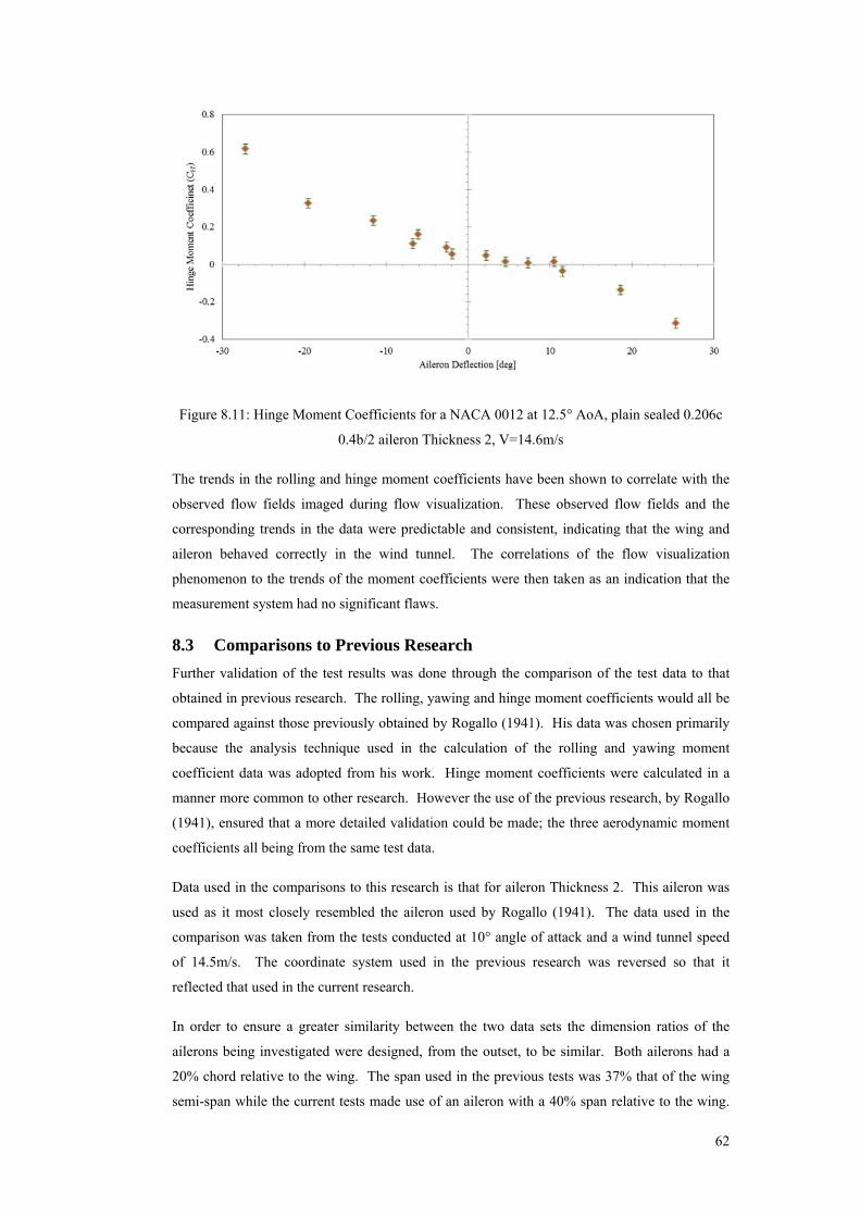
62
Figure 8.11: Hinge Moment Coefficients for a NACA 0012 at 12.5° AoA, plain sealed 0.206c
0.4b/2 aileron Thickness 2, V=14.6m/s
The trends in the rolling and hinge moment coefficients have been shown to correlate with the
observed flow fields imaged during flow visualization. These observed flow fields and the
corresponding trends in the data were predictable and consistent, indicating that the wing and
aileron behaved correctly in the wind tunnel. The correlations of the flow visualization
phenomenon to the trends of the moment coefficients were then taken as an indication that the
measurement system had no significant flaws.
8.3 Comparisons to Previous Research
Further validation of the test results was done through the comparison of the test data to that
obtained in previous research. The rolling, yawing and hinge moment coefficients would all be
compared against those previously obtained by Rogallo (1941). His data was chosen primarily
because the analysis technique used in the calculation of the rolling and yawing moment
coefficient data was adopted from his work. Hinge moment coefficients were calculated in a
manner more common to other research. However the use of the previous research, by Rogallo
(1941), ensured that a more detailed validation could be made; the three aerodynamic moment
coefficients all being from the same test data.
Data used in the comparisons to this research is that for aileron Thickness 2. This aileron was
used as it most closely resembled the aileron used by Rogallo (1941). The data used in the
comparison was taken from the tests conducted at 10° angle of attack and a wind tunnel speed
of 14.5m/s. The coordinate system used in the previous research was reversed so that it
reflected that used in the current research.
In order to ensure a greater similarity between the two data sets the dimension ratios of the
ailerons being investigated were designed, from the outset, to be similar. Both ailerons had a
20% chord relative to the wing. The span used in the previous tests was 37% that of the wing
semi-span while the current tests made use of an aileron with a 40% span relative to the wing.
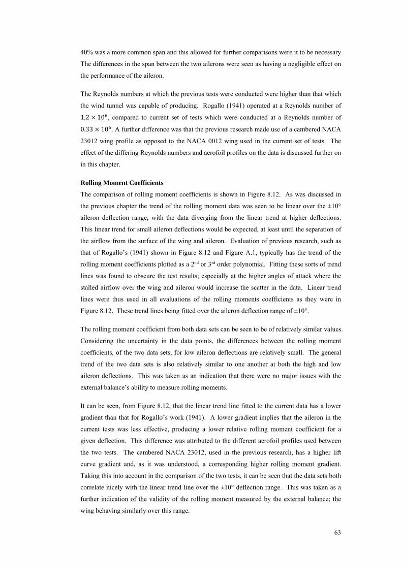
63
40% was a more common span and this allowed for further comparisons were it to be necessary.
The differences in the span between the two ailerons were seen as having a negligible effect on
the performance of the aileron.
The Reynolds numbers at which the previous tests were conducted were higher than that which
the wind tunnel was capable of producing. Rogallo (1941) operated at a Reynolds number of 1,2 × 10 , compared to current set of tests which were conducted at a Reynolds number of 0.33 × 10 . A further difference was that the previous research made use of a cambered NACA
23012 wing profile as opposed to the NACA 0012 wing used in the current set of tests. The
effect of the differing Reynolds numbers and aerofoil profiles on the data is discussed further on
in this chapter.
Rolling Moment Coefficients
The comparison of rolling moment coefficients is shown in Figure 8.12. As was discussed in
the previous chapter the trend of the rolling moment data was seen to be linear over the ±10°
aileron deflection range, with the data diverging from the linear trend at higher deflections.
This linear trend for small aileron deflections would be expected, at least until the separation of
the airflow from the surface of the wing and aileron. Evaluation of previous research, such as
that of Rogallo’s (1941) shown in Figure 8.12 and Figure A.1, typically has the trend of the
rolling moment coefficients plotted as a 2nd or 3rd order polynomial. Fitting these sorts of trend
lines was found to obscure the test results; especially at the higher angles of attack where the
stalled airflow over the wing and aileron would increase the scatter in the data. Linear trend
lines were thus used in all evaluations of the rolling moments coefficients as they were in
Figure 8.12. These trend lines being fitted over the aileron deflection range of ±10°.
The rolling moment coefficient from both data sets can be seen to be of relatively similar values.
Considering the uncertainty in the data points, the differences between the rolling moment
coefficients, of the two data sets, for low aileron deflections are relatively small. The general
trend of the two data sets is also relatively similar to one another at both the high and low
aileron deflections. This was taken as an indication that there were no major issues with the
external balance’s ability to measure rolling moments.
It can be seen, from Figure 8.12, that the linear trend line fitted to the current data has a lower
gradient than that for Rogallo’s work (1941). A lower gradient implies that the aileron in the
current tests was less effective, producing a lower relative rolling moment coefficient for a
given deflection. This difference was attributed to the different aerofoil profiles used between
the two tests. The cambered NACA 23012, used in the previous research, has a higher lift
curve gradient and, as it was understood, a corresponding higher rolling moment gradient.
Taking this into account in the comparison of the two tests, it can be seen that the data sets both
correlate nicely with the linear trend line over the ±10° deflection range. This was taken as a
further indication of the validity of the rolling moment measured by the external balance; the
wing behaving similarly over this range.
64
Figure 8.12: Comparison between delta rolling moment coefficients for primary test data,
Thickness 2, 10° AoA, V=14.7m/s, and data obtained from Rogallo (1941).
Jacobs (1937) researched the effect of Reynolds number on the performance of NACA aerofoils.
His results showed that different Reynolds numbers affected the maximum coefficient of lift
and data trend of the lift coefficients at high angles of attack; this resulting in the wing stalling
at lower angles of attack for lower Reynolds numbers. With reference to Figure 2.8, it was seen
that the gradient of the linear portion of the lift coefficients is unaffected by increased or
decreased Reynolds numbers, at least at the Reynolds numbers for which the previous research
and the current tests were performed. It was thus understood that a similar effect would be
noted for the rolling moment coefficients. In this way the differing Reynolds number would
have no discernable effect on the rolling moment coefficients in the aileron deflection range of
±10°. In this range the rolling moment coefficients have been seen to respond linearly. This
holds provided the angle of attack was not so high as to have the airflow stalled over the surface
of the wing. Considering the differing aerofoil profiles, the wings performed similarly over the
linear deflection range.
As was discussed in the previous chapter, the airflow only began stalling over the surface of the
wing at angles of attack around 12.5°. The tests being compared in Figure 8.12 were conducted
at lower angles of attack and it was assumed that the airflow was still attached to the upper
surface of the wing. Figure 8.8 showed that the airflow over the aileron would stall at high
aileron deflections even if the wing is not yet stalled. Differences between the two data sets
being compared would then be expected at the higher aileron deflections; the airflow stalling
over the surface of the aileron for lower deflections at lower Reynolds numbers. Referring to
65
Figure 8.12, this difference is clear for the positive aileron deflections. The rolling moment
coefficients of the current data begin to diverge above 10° deflection. The rolling moment
coefficients of Rogallo’s data (1941) only began to diverge above 20°. This is in line with the
understanding of Jacob’s research (1937).
For the negative aileron deflections the differences between the two data sets are not as distinct.
Rogallo’s data (1941) deviates far more from the linear trend, at the high negative deflections,
than the current data set. This deviation was attributed, in the previous chapter, to the
separation of the airflow over the surface of the aileron. A small deviation of the rolling
moment coefficients, of the current data, is noted at approximately -17° deflection. This
deviation is barely more than the uncertainty in the rolling moment coefficients at 10° angle of
attack. The data point at the next, higher, negative deflection coincides once again coincident
with the linear trend plotted. The deviation of previous data at -20° deflection, from the linear
trend, was noted to have not changed from the previous data point. Despite this the rolling
moment coefficients for previous data at the high negative aileron deflections are still greater
than those from the current tests. This once again agrees with the research by Jacobs (1937).
The exact reason as to why the rolling moment coefficients do not deviate as much from the
linear trend as those from Rogallo’s data (1941), at high negative aileron deflections, is not
quite understood. It is assumed that the differences are due to the differing Reynolds numbers
and associated turbulence intensities. As a precaution to be taken in the further analysis of the
rolling moment coefficients, little emphasis will be placed for the data obtained at high negative
aileron deflections.
Yawing Moment Coefficient
The comparison of the yawing moment coefficients between the current tests and the previous
research data from Rogallo (1941) is shown in Figure 8.13. The general trends of both data sets
can be seen to be relatively similar to one another. The main difference between the two data
sets was the aileron deflection for which the minimum yawing moment would occur. For the
current data set this occurs at approximately 9° deflection while in the previous data this occurs
at 18°. This is due to the fact that aerofoil profile used in the current tests was symmetrical
while the wing, used in the previous research, was cambered. The minimum drag coefficient
for a symmetrical wing occurs at 0° angle of attack. For a cambered aerofoil the angle of attack
is above 0°. In the same way it would be expected that the minimum yawing moment
coefficient, due to an aileron deflection, for a cambered aerofoil would be higher than that for a
symmetrical aerofoil. The differing aerofoil profiles were therefore seen as the primary reason
for the different yawing moment coefficients between the two data sets.
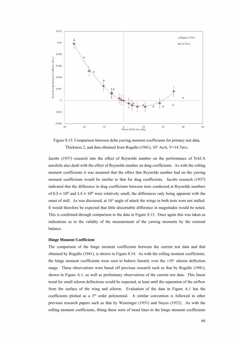
66
Figure 8.13: Comparison between delta yawing moment coefficients for primary test data,
Thickness 2, and data obtained from Rogallo (1941), 10° AoA, V=14.7m/s.
Jacobs (1937) research into the effect of Reynolds number on the performance of NACA
aerofoils also dealt with the effect of Reynolds number on drag coefficients. As with the rolling
moment coefficients it was assumed that the effect that Reynolds number had on the yawing
moment coefficients would be similar to that for drag coefficients. Jacobs research (1937)
indicated that the difference in drag coefficients between tests conducted at Reynolds numbers
of 0.3 × 10 and 1.4 × 10 were relatively small, the differences only being apparent with the
onset of stall. As was discussed, at 10° angle of attack the wings in both tests were not stalled.
It would therefore be expected that little discernable difference in magnitudes would be noted.
This is confirmed through comparison to the data in Figure 8.13. Once again this was taken as
indications as to the validity of the measurement of the yawing moments by the external
balance.
Hinge Moment Coefficient
The comparison of the hinge moment coefficients between the current test data and that
obtained by Rogallo (1941), is shown in Figure 8.14. As with the rolling moment coefficients,
the hinge moment coefficients were seen to behave linearly over the ±10° aileron deflection
range. These observations were based off previous research such as that by Rogallo (1941),
shown in Figure A.1, as well as preliminary observations of the current test data. This linear
trend for small aileron deflections would be expected, at least until the separation of the airflow
from the surface of the wing and aileron. Evaluation of the data in Figure A.1 has the
coefficients plotted as a 3rd order polynomial. A similar convention is followed in other
previous research papers such as that by Wenzinger (1931) and Noyes (1932). As with the
rolling moment coefficients, fitting these sorts of trend lines to the hinge moment coefficients
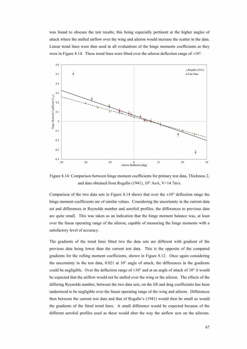
67
was found to obscure the test results; this being especially pertinent at the higher angles of
attack where the stalled airflow over the wing and aileron would increase the scatter in the data.
Linear trend lines were thus used in all evaluations of the hinge moments coefficients as they
were in Figure 8.14. These trend lines were fitted over the aileron deflection range of ±10°.
Figure 8.14: Comparison between hinge moment coefficients for primary test data, Thickness 2,
and data obtained from Rogallo (1941), 10° AoA, V=14.7m/s.
Comparison of the two data sets in Figure 8.14 shows that over the ±10° deflection range the
hinge moment coefficients are of similar values. Considering the uncertainty in the current data
set and differences in Reynolds number and aerofoil profiles, the differences to previous data
are quite small. This was taken as an indication that the hinge moment balance was, at least
over the linear operating range of the aileron, capable of measuring the hinge moments with a
satisfactory level of accuracy.
The gradients of the trend lines fitted two the data sets are different with gradient of the
previous data being lower than the current test data. This is the opposite of the compared
gradients for the rolling moment coefficients, shown in Figure 8.12. Once again considering
the uncertainty in the test data, 0.021 at 10° angle of attack, the differences in the gradients
could be negligible. Over the deflection range of ±10° and at an angle of attack of 10° it would
be expected that the airflow would not be stalled over the wing or the aileron. The effects of the
differing Reynolds number, between the two data sets, on the lift and drag coefficients has been
understood to be negligible over the linear operating range of the wing and aileron. Differences
then between the current test data and that of Rogallo’s (1941) would then be small as would
the gradients of the fitted trend lines. A small difference would be expected because of the
different aerofoil profiles used as these would alter the way the airflow acts on the ailerons.
68
Based on the calculated uncertainties, however, this difference cannot be commented on
accurately.
Due to the differing magnitudes in the two data sets, the overall trend of the hinge moment
coefficients from the previous research, by Rogallo (1941), is not that clear. Compared to the
overall trend in the current data, seen in Figure 8.12, and the typical hinge moment trend in
Figure A.2, the overall trend of the hinge moment coefficients from the previous research, seen
in Figure A.1, is relatively similar. It was thus understood that the apparent differences in the
trends between the two data sets, presented in Figure 8.12, were not because of a fault in the
hinge moment balance but rather aerodynamic differences that are most likely attributable to the
different Reynolds numbers.
Above the ±10° deflection range the two data sets diverge quickly with large differences in the
data noted at the higher aileron deflections. It has already been discussed that at the high
aileron deflections the airflow is stalled over the surface of the aileron. The separation of the
airflow from the surface of the aileron would be expected to non-linearly increase the drag
acting on the aileron. This in turn would result in a non-linear increase in the hinge moment
acting on the aileron. The larger the aileron deflection, the higher the degree of stall, the higher
the drag acting on the aileron and subsequently the higher the aileron hinge moment. The data
published by Jacobs (1937) showed that for stall conditions the drag force acting on a surface at
a lower Reynolds numbers would be higher than on a surface at a higher Reynolds number.
Based on the large difference in Reynolds number that the current tests and Rogallo’s data
(1941) was obtained at, it would be expected that larger differences in drag forces would be
noted. This would explain the high differences noted in Figure 8.12 at high aileron deflections.
Further interpretation of the hinge moment data would need to consider the effect of the lower
Reynolds numbers. The trend of the hinge moment coefficients at high aileron deflections is
exaggerated compared to existing published data. It would be expected that small differences in
hinge moment coefficients, brought on by the different aileron trailing edge thicknesses, may
appear larger than they would be for a test conducted at higher Reynolds numbers.
Based on the comparisons made above, the measurement system is considered to be reliable.
Conclusions as to the effects of different aileron trailing edge thicknesses, within the mentioned
limitations, can then be confidently made.
8.4 Variation of Aileron Trailing Edge Thickness
This chapter evaluates the effect of varying the aileron trailing edge thickness. Due to
similarities in the data for various angles of attack only selected data sets are presented here.
The full list of results can be found in Appendix I.
So as to avoid clutter in the Figures of this chapter, the uncertainty values for only one of the
four aileron data sets is plotted for each of the Figures. This is also the case for the Figures in
Appendix I. The differences between the uncertainty values for the four ailerons tested were
69
noted as being, on average, the same within the resolution of the DAQ. In order to be
conservative, if there was a larger difference, the highest uncertainty values between the four
data sets were used. The uncertainty values shown for Aileron Thickness 2 can therefore be
assumed to be the same for the other three ailerons tested
Previous research has been done into the effects of thicker trailing edges by the likes of Hoerner
(1950) and Baker (2008). The effects, discussed, were with reference to wing aerodynamic
characteristics rather than aileron performance. It was, however, noted by Hoerner (1985) that
the noted effects would possibly apply to ailerons as well. The effects of an increased trailing
edge thickness included an increase in the lift curve slope and maximum lift coefficient.
Applied to aileron performance, it would be expected that this would result in a similar increase
in the rolling moment slope, over the linear range, and a delayed divergence of the moment data
from the linear trend.
Coinciding with the increase in lift coefficients was the increase in drag coefficients for wings
with thicker trailing edges (Hoerner & Borst, 1985). As with the rolling moment coefficients, it
was understood that an increase in the drag coefficients would imply an increase in the yawing
moment coefficients measured as well. The increase in the trailing edge thickness of the aileron
would therefore be expected to result in an increase of the yawing moments coefficients.
Typically the CL/CD values remained constant for blunt trailing edges with little advantage
noted compared to sharp trailing edges. A small increase was seen to occur when the trailing
edge thickness to chord ratio was increased to approximately 0.5% (Hoener, 1950). The aileron
trailing edge thickness to wing-chord ratios that were tested were 0.39%, 0.71%, 0.96% and
1.22%. It would therefore be expected that in a comparison between the rolling and yawing
moment coefficients an optimal thickness could be identified.
Rolling Moment Coefficient
Figure 8.15 shows the rolling moment coefficients for each aileron tested at 5° angle of attack.
The trend line, seen in the plot, is fitted to aileron Thickness 2 data in order to aid in the
comparison of the four data sets. Considering the uncertainty in the data, the differing trailing
edge thicknesses can be seen to result in no discernable effect on the rolling moment
coefficients. All four data sets behave in a similar manner, being linear over the ±10° aileron
deflection range and diverging from the linear trend at a high positive aileron deflection. The
expected change in the rolling moment coefficients, being the change in the slope over the
linear range and delayed divergence of the data from the linear trend is not evidently clear. A
small difference between the data of Thickness 4 and Thickness 2 can be seen at 25° deflection.
This difference could indicate a small delay in the onset of the data divergence for the thicker
trailing edged aileron, Thickness 4. The difference is, however, just within the uncertainty error
bars of the two data sets and as such the difference could in fact be negligible. The noted
increase in the scatter of the data, at this deflection, due to the airflow over the aileron being
stalled, would also account for the noted differences.
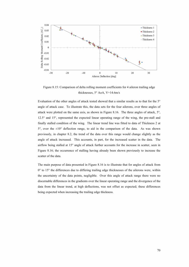
70
Figure 8.15: Comparison of delta rolling moment coefficients for 4 aileron trailing edge
thicknesses, 5° AoA, V=14.6m/s
Evaluation of the other angles of attack tested showed that a similar results as to that for the 5°
angle of attack case. To illustrate this, the data sets for the four ailerons, over three angles of
attack were plotted on the same axis, as shown in Figure 8.16. The three angles of attack, 5°,
12.5° and 15°, represented the expected linear operating range of the wing, the pre-stall and
finally stalled condition of the wing. The linear trend line was fitted to data of Thickness 2 at
5°, over the ±10° deflection range, to aid in the comparison of the data. As was shown
previously, in chapter 8.2, the trend of the data over this range would change slightly as the
angle of attack increased. This accounts, in part, for the increased scatter in the data. The
airflow being stalled at 15° angle of attack further accounts for the increase in scatter, seen in
Figure 8.16; the occurrence of stalling having already been shown previously to increase the
scatter of the data.
The main purpose of data presented in Figure 8.16 is to illustrate that for angles of attack from
0° to 15° the differences due to differing trailing edge thicknesses of the ailerons were, within
the uncertainty of the data points, negligible. Over this angle of attack range there were no
discernable differences in the gradients over the linear operating range and the divergence of the
data from the linear trend, at high deflections, was not offset as expected; these differences
being expected when increasing the trailing edge thickness.
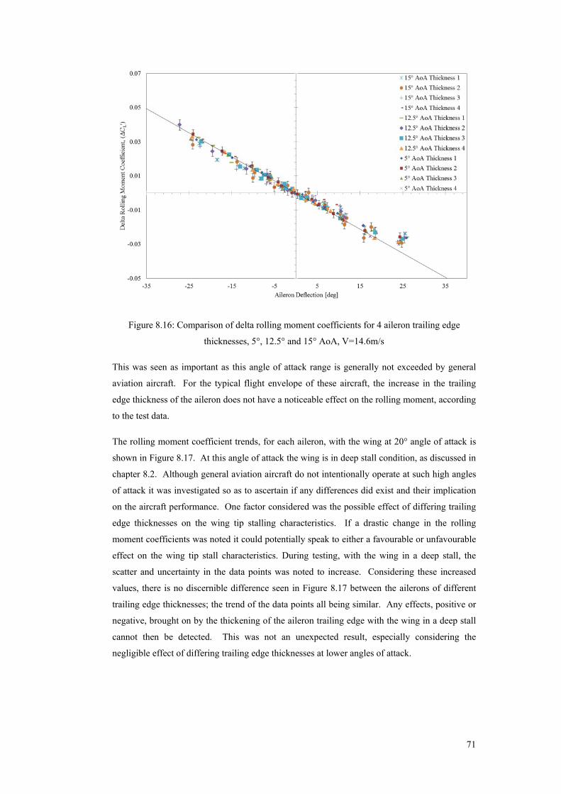
71
Figure 8.16: Comparison of delta rolling moment coefficients for 4 aileron trailing edge
thicknesses, 5°, 12.5° and 15° AoA, V=14.6m/s
This was seen as important as this angle of attack range is generally not exceeded by general
aviation aircraft. For the typical flight envelope of these aircraft, the increase in the trailing
edge thickness of the aileron does not have a noticeable effect on the rolling moment, according
to the test data.
The rolling moment coefficient trends, for each aileron, with the wing at 20° angle of attack is
shown in Figure 8.17. At this angle of attack the wing is in deep stall condition, as discussed in
chapter 8.2. Although general aviation aircraft do not intentionally operate at such high angles
of attack it was investigated so as to ascertain if any differences did exist and their implication
on the aircraft performance. One factor considered was the possible effect of differing trailing
edge thicknesses on the wing tip stalling characteristics. If a drastic change in the rolling
moment coefficients was noted it could potentially speak to either a favourable or unfavourable
effect on the wing tip stall characteristics. During testing, with the wing in a deep stall, the
scatter and uncertainty in the data points was noted to increase. Considering these increased
values, there is no discernible difference seen in Figure 8.17 between the ailerons of different
trailing edge thicknesses; the trend of the data points all being similar. Any effects, positive or
negative, brought on by the thickening of the aileron trailing edge with the wing in a deep stall
cannot then be detected. This was not an unexpected result, especially considering the
negligible effect of differing trailing edge thicknesses at lower angles of attack.
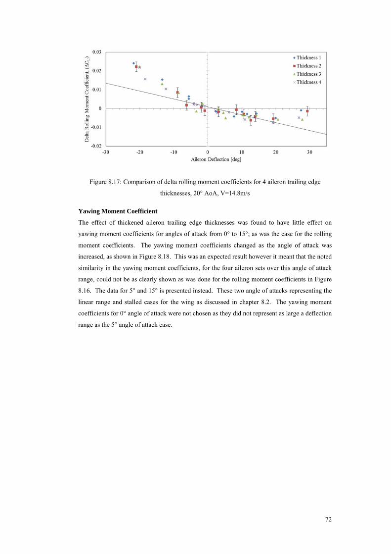
72
Figure 8.17: Comparison of delta rolling moment coefficients for 4 aileron trailing edge
thicknesses, 20° AoA, V=14.8m/s
Yawing Moment Coefficient
The effect of thickened aileron trailing edge thicknesses was found to have little effect on
yawing moment coefficients for angles of attack from 0° to 15°; as was the case for the rolling
moment coefficients. The yawing moment coefficients changed as the angle of attack was
increased, as shown in Figure 8.18. This was an expected result however it meant that the noted
similarity in the yawing moment coefficients, for the four aileron sets over this angle of attack
range, could not be as clearly shown as was done for the rolling moment coefficients in Figure
8.16. The data for 5° and 15° is presented instead. These two angle of attacks representing the
linear range and stalled cases for the wing as discussed in chapter 8.2. The yawing moment
coefficients for 0° angle of attack were not chosen as they did not represent as large a deflection
range as the 5° angle of attack case.
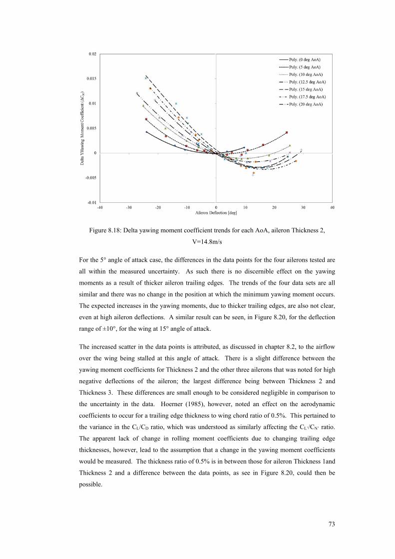
73
Figure 8.18: Delta yawing moment coefficient trends for each AoA, aileron Thickness 2,
V=14.8m/s
For the 5° angle of attack case, the differences in the data points for the four ailerons tested are
all within the measured uncertainty. As such there is no discernible effect on the yawing
moments as a result of thicker aileron trailing edges. The trends of the four data sets are all
similar and there was no change in the position at which the minimum yawing moment occurs.
The expected increases in the yawing moments, due to thicker trailing edges, are also not clear,
even at high aileron deflections. A similar result can be seen, in Figure 8.20, for the deflection
range of ±10°, for the wing at 15° angle of attack.
The increased scatter in the data points is attributed, as discussed in chapter 8.2, to the airflow
over the wing being stalled at this angle of attack. There is a slight difference between the
yawing moment coefficients for Thickness 2 and the other three ailerons that was noted for high
negative deflections of the aileron; the largest difference being between Thickness 2 and
Thickness 3. These differences are small enough to be considered negligible in comparison to
the uncertainty in the data. Hoerner (1985), however, noted an effect on the aerodynamic
coefficients to occur for a trailing edge thickness to wing chord ratio of 0.5%. This pertained to
the variance in the CL/CD ratio, which was understood as similarly affecting the CL’/CN’ ratio.
The apparent lack of change in rolling moment coefficients due to changing trailing edge
thicknesses, however, lead to the assumption that a change in the yawing moment coefficients
would be measured. The thickness ratio of 0.5% is in between those for aileron Thickness 1and
Thickness 2 and a difference between the data points, as see in Figure 8.20, could then be
possible.
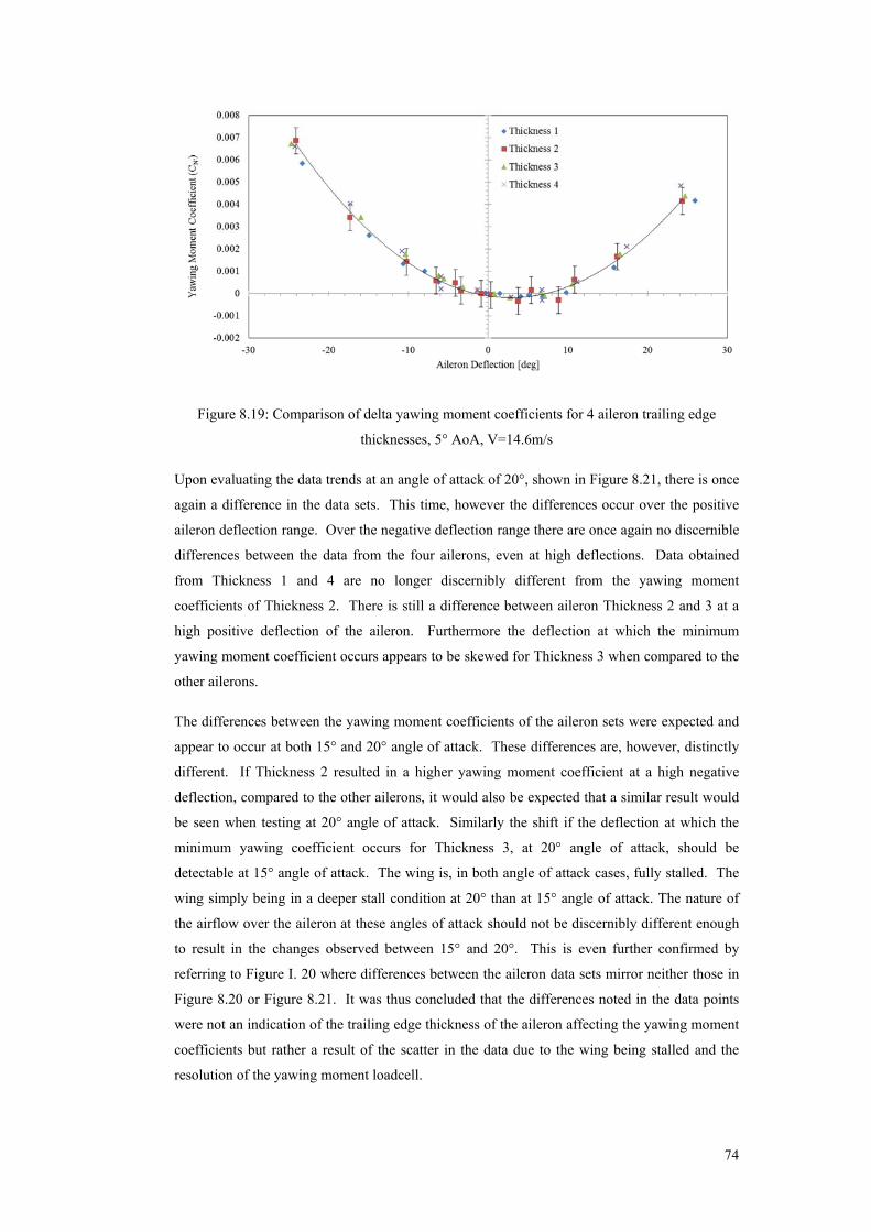
74
Figure 8.19: Comparison of delta yawing moment coefficients for 4 aileron trailing edge
thicknesses, 5° AoA, V=14.6m/s
Upon evaluating the data trends at an angle of attack of 20°, shown in Figure 8.21, there is once
again a difference in the data sets. This time, however the differences occur over the positive
aileron deflection range. Over the negative deflection range there are once again no discernible
differences between the data from the four ailerons, even at high deflections. Data obtained
from Thickness 1 and 4 are no longer discernibly different from the yawing moment
coefficients of Thickness 2. There is still a difference between aileron Thickness 2 and 3 at a
high positive deflection of the aileron. Furthermore the deflection at which the minimum
yawing moment coefficient occurs appears to be skewed for Thickness 3 when compared to the
other ailerons.
The differences between the yawing moment coefficients of the aileron sets were expected and
appear to occur at both 15° and 20° angle of attack. These differences are, however, distinctly
different. If Thickness 2 resulted in a higher yawing moment coefficient at a high negative
deflection, compared to the other ailerons, it would also be expected that a similar result would
be seen when testing at 20° angle of attack. Similarly the shift if the deflection at which the
minimum yawing coefficient occurs for Thickness 3, at 20° angle of attack, should be
detectable at 15° angle of attack. The wing is, in both angle of attack cases, fully stalled. The
wing simply being in a deeper stall condition at 20° than at 15° angle of attack. The nature of
the airflow over the aileron at these angles of attack should not be discernibly different enough
to result in the changes observed between 15° and 20°. This is even further confirmed by
referring to Figure I. 20 where differences between the aileron data sets mirror neither those in
Figure 8.20 or Figure 8.21. It was thus concluded that the differences noted in the data points
were not an indication of the trailing edge thickness of the aileron affecting the yawing moment
coefficients but rather a result of the scatter in the data due to the wing being stalled and the
resolution of the yawing moment loadcell.
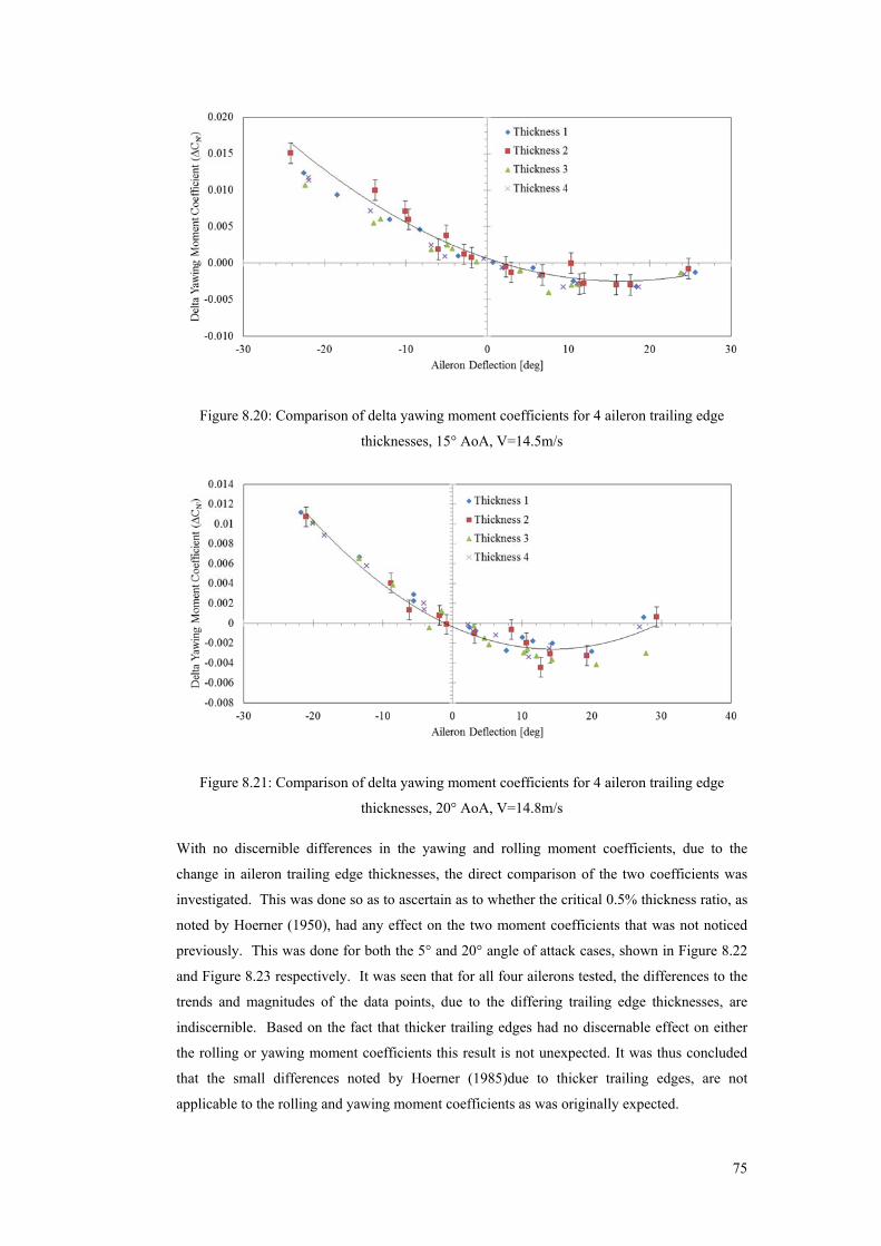
75
Figure 8.20: Comparison of delta yawing moment coefficients for 4 aileron trailing edge
thicknesses, 15° AoA, V=14.5m/s
Figure 8.21: Comparison of delta yawing moment coefficients for 4 aileron trailing edge
thicknesses, 20° AoA, V=14.8m/s
With no discernible differences in the yawing and rolling moment coefficients, due to the
change in aileron trailing edge thicknesses, the direct comparison of the two coefficients was
investigated. This was done so as to ascertain as to whether the critical 0.5% thickness ratio, as
noted by Hoerner (1950), had any effect on the two moment coefficients that was not noticed
previously. This was done for both the 5° and 20° angle of attack cases, shown in Figure 8.22
and Figure 8.23 respectively. It was seen that for all four ailerons tested, the differences to the
trends and magnitudes of the data points, due to the differing trailing edge thicknesses, are
indiscernible. Based on the fact that thicker trailing edges had no discernable effect on either
the rolling or yawing moment coefficients this result is not unexpected. It was thus concluded
that the small differences noted by Hoerner (1985)due to thicker trailing edges, are not
applicable to the rolling and yawing moment coefficients as was originally expected.
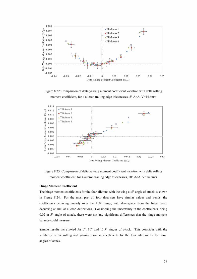
76
Figure 8.22: Comparison of delta yawing moment coefficient variation with delta rolling
moment coefficient, for 4 aileron trailing edge thicknesses, 5° AoA, V=14.6m/s
Figure 8.23: Comparison of delta yawing moment coefficient variation with delta rolling
moment coefficient, for 4 aileron trailing edge thicknesses, 20° AoA, V=14.8m/s
Hinge Moment Coefficient
The hinge moment coefficients for the four ailerons with the wing at 5° angle of attack is shown
in Figure 8.24. For the most part all four data sets have similar values and trends; the
coefficients behaving linearly over the ±10° range, with divergence from the linear trend
occurring at similar aileron deflections. Considering the uncertainty in the coefficients, being
0.02 at 5° angle of attack, there were not any significant differences that the hinge moment
balance could measure.
Similar results were noted for 0°, 10° and 12.5° angles of attack. This coincides with the
similarity in the rolling and yawing moment coefficients for the four ailerons for the same
angles of attack.
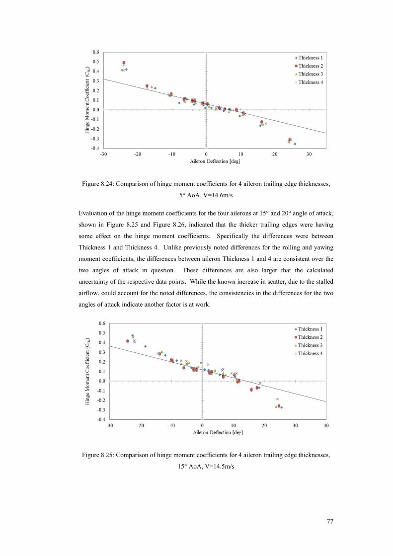
77
Figure 8.24: Comparison of hinge moment coefficients for 4 aileron trailing edge thicknesses,
5° AoA, V=14.6m/s
Evaluation of the hinge moment coefficients for the four ailerons at 15° and 20° angle of attack,
shown in Figure 8.25 and Figure 8.26, indicated that the thicker trailing edges were having
some effect on the hinge moment coefficients. Specifically the differences were between
Thickness 1 and Thickness 4. Unlike previously noted differences for the rolling and yawing
moment coefficients, the differences between aileron Thickness 1 and 4 are consistent over the
two angles of attack in question. These differences are also larger that the calculated
uncertainty of the respective data points. While the known increase in scatter, due to the stalled
airflow, could account for the noted differences, the consistencies in the differences for the two
angles of attack indicate another factor is at work.
Figure 8.25: Comparison of hinge moment coefficients for 4 aileron trailing edge thicknesses,
15° AoA, V=14.5m/s
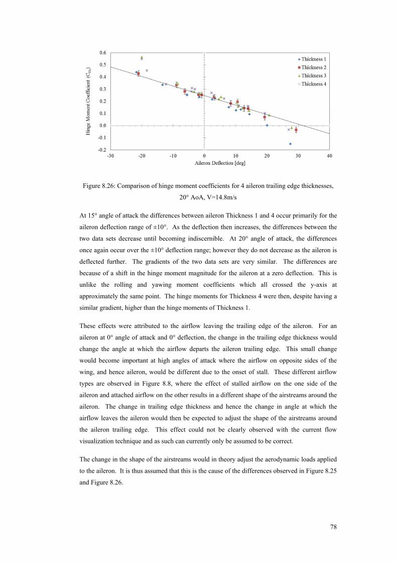
78
Figure 8.26: Comparison of hinge moment coefficients for 4 aileron trailing edge thicknesses,
20° AoA, V=14.8m/s
At 15° angle of attack the differences between aileron Thickness 1 and 4 occur primarily for the
aileron deflection range of ±10°. As the deflection then increases, the differences between the
two data sets decrease until becoming indiscernible. At 20° angle of attack, the differences
once again occur over the ±10° deflection range; however they do not decrease as the aileron is
deflected further. The gradients of the two data sets are very similar. The differences are
because of a shift in the hinge moment magnitude for the aileron at a zero deflection. This is
unlike the rolling and yawing moment coefficients which all crossed the y-axis at
approximately the same point. The hinge moments for Thickness 4 were then, despite having a
similar gradient, higher than the hinge moments of Thickness 1.
These effects were attributed to the airflow leaving the trailing edge of the aileron. For an
aileron at 0° angle of attack and 0° deflection, the change in the trailing edge thickness would
change the angle at which the airflow departs the aileron trailing edge. This small change
would become important at high angles of attack where the airflow on opposite sides of the
wing, and hence aileron, would be different due to the onset of stall. These different airflow
types are observed in Figure 8.8, where the effect of stalled airflow on the one side of the
aileron and attached airflow on the other results in a different shape of the airstreams around the
aileron. The change in trailing edge thickness and hence the change in angle at which the
airflow leaves the aileron would then be expected to adjust the shape of the airstreams around
the aileron trailing edge. This effect could not be clearly observed with the current flow
visualization technique and as such can currently only be assumed to be correct.
The change in the shape of the airstreams would in theory adjust the aerodynamic loads applied
to the aileron. It is thus assumed that this is the cause of the differences observed in Figure 8.25
and Figure 8.26.
79
This difference was attributed to the resulting bending of the streamlines flowing from the
underside of the wing over the edge of the aileron. Due to the separated airflow over the upper
surface of the wing, due to the angle of attack, the streamlines would be expected to bend
upwards after leaving the trailing edge of the aileron. As the aileron trailing edge thickness was
increased it would be expected that these streamlines would have to bend more in order to
establish the same flow region in the trailing wake of the wing. This change would be
indiscernible in the flow visualization. It would mean, however, that a higher hinge moment
would be measured for a thicker trailing edge; the increased bending in the streamlines leaving
the aileron trailing edge resulting in an increased force acting on the aileron.
The differences in the data, noted in Figure 8.25 and Figure 8.26, occur between the ailerons
with the smallest and largest trailing edge thickness. The differences between the hinge
moments as discussed above would be expected to have a critical tailing edge thickness for
which they would occur. It was noted that for the 15° angle of attack case the hinge moments
for Thickness 2 and 3 correlated better with those of Thickness 1 indicating that the critical
thickness would be somewhere between Thickness 3 and 4. At 20°, however, the hinge
moments for Thickness 2 and 3 appear to correlate better with those of Thickness 4, indicating
now that the critical thickness would appear to be between Thickness1 and 2.
These differences only become apparent at the high aileron deflections and high angles of attack.
Considering the known increase in the scatter of the data at such deflections and angles of
attack, the differences may ultimately be negligible. It should also be noted then that ailerons
are not typically operated in this range and wings are not flown at these angles of attack. While
the differences in the hinge moments brought on by the differing trailing edge thicknesses were
notable they occur outside of the aircrafts typical flight envelope. It is therefore not necessary
to consider these noted differences in the design of ailerons in the future.
Considering then the range of angles of attack for which general aviation aircraft typically
operate, between 0° to 15°, there were no discernible effects to the rolling, yawing and hinge
moments brought on by the changing of the trailing edge thickness. The usual philosophy of
manufacturing sharp trailing edges for ailerons may therefore be unnecessary; the manufacture
and implementation of ailerons with thicker trailing edges having no discernible effect on the
rolling performance of the aileron, while potentially lowering the complexity and manufacture
costs.
80
9 CONCLUSIONS
A compact hinge moment balance was designed, capable of measuring the hinge moment
produced by an aileron. Unlike previous designs this balance could be housed inside the
internal structure of the wind tunnel test model eliminating any intrusions into the airflow by
tensioned cables. The test model was mounted to a basic external balance that allowed for the
measurement of the rolling and yawing moments due to a deflection of the aileron.
Validation of the measurement system was done through an evaluation of a typical data set,
flow visualization and comparison to previous results. The typical data set and flow
visualization indicated that the wing and aileron performed in a manner that was expected. The
Comparisons between the rolling, yawing and hinge moments coefficients calculated from
currents tests and those conducted previously showed a good correlation in the general trend of
the data for the full aileron deflection range. Differences were, however, noted between the two
data sets; these occurring at high aileron deflections. These differences were primarily
attributed to the current tests being conducted with different aerofoil profiles and at lower
Reynolds numbers.
The data obtained from the hinge moment balance and external balance was still seen as
satisfactory, allowing for use in measuring the effects of aileron trailing edge manipulations.
Four aileron test pieces with increasing trailing edge thicknesses were tested. The effects of this
change in thickness was investigated at four different angle of attack cases, namely low angles
of attack, just before stall, at stall and above stall. For the pre-stall cases it was seen that the
increase in the trailing edge thickness of the aileron produced negligible effects on the the
rolling, yawing or hinge moment coefficients in either the trend of the data or magnitude of the
coefficients. Small changes were noted for the hinge moment coefficients at high angles of
attack; however these were seen as inconsequential. This was largely due to the conditions
under which differences occurred, being outside the typical flight envelope of general aviation
aircraft.
It was concluded, from the test results, that the trailing edge thickness of an aileron need not be
manufactured to the conventional thickness that is commonly desired. The allowance for a
thicker aileron trailing edge thickness in the design of future aircraft will have minimal effect
on the aileron performance while allowing for less restrictions in their manufacture.
81
10 RECOMMENDATIONS
The results from the investigation into the effect of thicker aileron trailing edges showed that
there was little effect on the aerodynamic coefficients of the aerofoil and aileron itself. Based
on this the following list are recommendations for future work in the investigation of aileron
trailing edge manipulations:
• The measurement of and effect that thicker aileron trailing edge thicknesses has on the lift
and drag and pitching moment coefficients should be investigated. This will allow for a
more thorough description of the effect of having thicker trailing edges. The addition of
lift coefficient data will also allow for better comparisons to previous research and hence
further validation of the results.
• Investigations into the use of thicker ailerons would also be recommended to ascertain if
there is a turning point at which the use of a thicker aileron begins to show noticeable
deteriations in the aileron performance or if there exists an aileron trailing edge thickness
for which an improvement in the aileron performance can be seen.
• The effect that thicker trailing edges has on other aileron shapes and configurations such as
Frise ailerons could also be insightful. This could show whether the effects seen from the
investigation of plain flap type ailerons also pertains to these other aileron types.
• A method for locking the aileron at a particular deflection would also be of use. This
would prevent the oscillation of the aileron at higher angles of attack, allowing for cleaner
data to be obtained for the aerofoil aerodynamic coefficients such as roll and yaw. The
aileron could then be unlocked and the hinge data could be obtained without spoiling the
data for other coefficients. The use of an internal or external balance for the aileron could
also assist in the reduction of the oscillations.
82
11 REFERENCES
Abzug, M. J. & Larrabee, E. E., 2002. Airplane Stability and Control. s.l.:Cambridge University
Press.
Anon., n.d.
Bacon, D. L., 1924. N.A.C.A. Report 161: The Distribution of Lift Over Wing Tips and Ailerons,
Langley Field: Langley Memorial Aeronautical Laboratory.
Baker, J. P., van Dam, C. P. & Gilbert, B. L., 2008. Flatback Airfoil Wind Tunnel Experiment.
New Mexico: Sandia National Laboratories.
Cavanaugh, M. A., Robertson, P. & Mason, W. H., 2007. Wind Tunnel Test of Gurney Flaps
and T-Strips on an NACA 23012 Wing, Virginia: American Institute of Aeronautics and
Astronautics.
Cooperman, A. M. et al., 2010. Aerodynamic Performance of Thick Blunt Trailing Edge.
Chicago, AIAA.
Drela, M., 1989. Integral Boundary Layer Formulation for Blunt Trailng Edges, Massachusetts:
Massachusetts Institute of Technology.
El-Gammal, M., Naughton, J. W. & Hangan, H., 2010. Drag Force Balance of a Blunt and
Divergent Trailing-Edge Airfoil. Journal of Aircraft, Volume 47.
Gammal, M., Naughton, J. & Hangan, H., 2010. Drag Force Balance of a Blunt and Divergent
Trailing-Edge Airfoil. Journal of Aircraft, Volume 47.
Gilrith, R. R. & Turner, W. N., 1941. Lateral Control Required for Satisfactory Flying
Qualities Based on Flight Tests of Numerous Airplanes, Langely Field: National Advisory
Committee for Aeronautics.
Goranson, R. F., 1946. N.A.C.A. Technical Note 1085: Flight Tests of Experimental Beveled-
Trailing-Edge Frise Ailerons on a Fighter Airplane, Langely Field: Langley Memorial
Aeronautical Laboratory.
Gurbacki, H. & Bragg, M., 2001. Sensing Aircraft Icing Effects by Unsteady Flap Hinge-
Moment Measurement. Journal of Aircraft, Volume 38.
Harris, T. A. & Weick, F. E., 1932. N.A.C.A. Report 424: Wind-Tunnel Research Comparing
Lateral Control Devices, Particularly at High Angles of Attack IV - Floating Tip Ailerons on
Rectangular Wings, Langely Field: Langely Memorial Aeronautical Laboratory.
Heald, R. H., 1933. N.A.C.A. Technical Note 441: Rolling, Yawing, and Hinge Moments
Produced by Rectangular Ailerons, Washington: Bureau of Standards.
83
Heald, R. H., 1933. N.A.C.A. Technical Note 448: Effect of Aileron Displacement on Wing
Characteristics, Washington: Bureau of Standards.
Hoener, 1950. Base Drag and Thick Trailing Edges, s.l.: Journal Aeronautical Sciences.
Hoerner, S. F., 1965. Fluid-Dyamic Drag. Bakersfield: S. F. Hoerner.
Hoerner, S. F. & Borst, H. V., 1985. Fluid Dynamic Lift, New York: L A Hoerner.
Holman, J. P., 2012. Experimental Methods for Engineers. New York: McGraw-Hill.
Jacobs, E. N. & Sherman, A., 1937. Airfoil Section Characteristics as Affected by Variations of
the Reynolds Number, Langely Virginia: National Advisory Committee of Aeronautics.
Jacobs, E. N. & Sherman, A., 1937. N.A.C.A. Report 586: Airfoil Section Characteristics as
Affected by Variations of the Reynolds Number, Langely Virginia: National Advisory
Committee of Aeronautics.
Jones, R. T. & Weick, F. E., 1937. N.A.C.A. Report 605: Resume and Analysis of N.A.C.A.
Lateral Control Research, Langely Field: Langely Memorial Aeronautical Laboratory.
Katzoff, S., Silverstein, A. & Bullivant, W. K., 1938. N.A.C.A. Report 651: Downwash and
Wake Behind Plain and Flapped Airfoils, Langely Field: Langely Memorial Aeronautical
Laboratory.
Kempel, R. W., 1971. N.A.S.A. TN D-6496 Analysis of a Coupled Roll-Spiral-Mode, Pilot-
Induced Oscillation Experienced With The M2-F2 Lifting Body, Edwards: NASA Flight
Research Center.
Khorrami, M., Berkman, M. & Choudhari, M., 2000. Unsteady Flow Computations of a Slat
with a Blunt Trialing Edge. AIAA, Volume 38.
Kroo, I., 2004. Future Technology and Aircraft Types. [Online]
Available at: http://adg.stanford.edu/aa241/intro/futureac.html
[Accessed 27 May 2014].
Lemes, R. & Catalano, F., 2004. Experimental Analysis of the confluent boundary layer
between flpa and a main element with saw-toothed trailing edge. Japan, ICAS.
Lotz, R. D. & Thompson, B. E., 1996. Divergent-Trailing-Edge Airfoil Flow, New York:
Journal of Aircraft.
Monish, B. H., 1930. N.A.C.A. Report 370: Effect of Variation of Chord and Span of Ailerons
on Hinge Moments at Several Angles of Pitch, Washington: Bureau of Standards.
Nagaraja , K., Lakin, G. & Bartley, J., 1982. Flutter and Oscillatory Pressure Tests on a 727
Aileron in a Wind Tunnel. Journal of Aircraft, Volume 19, pp. 781-786.
84
Noyes, R. W. & Weick, F. E., 1932. N.A.C.A. Report 422: Wind-Tunnel Research Comparing
Lateral Control Devices, Particularly at High Angles of Attack II - Slotted Ailerons and Frise
Ailerons, Langely Field: Langley Memorial Aeronautical Laboratory.
Pezzella, G. et al., 2014. Aerodynamic characterization of HEXAFLY scramjet propelled
hypersonic vehicle. Atlanta, AIAA.
Rogallo, F. M. & Lowry, J. G., 1942. N.A.C.A. Wartime Report 481 - Wind-tunnel Investigation
of a Plain Aileron and a Balanced Aileron on a Tapered Wing with Full-Span Duplex Flaps,
Langely Field: Langely Memorial Aeronautical Laboratory.
Rogallo, F. M. & Purser, P. E., 1941. N.A.C.A. Wartime Report 374: Wind-Tunnel Investigation
of 20 percent chord plain and frise ailerons on an NACA 23012 Airfoil, Langely Virginia:
National Advisory Committee for Aeronautics.
Sears, R. I., 1942. N.A.C.A. Wartime Report 346 - Application of Balancing Tabs to Ailerons,
Langely Field: Langely Memorial Aeronautical Laboratory.
Sears, R. I. & Liddell, R. B., 1942. N.A.C.A. Wartime Report 454: Wind-Tunnel Investigation of
Control-Surface Characteristics VI - A 30-Percent-Chord Plain Flap on the NACA 0015 Airfoil,
LangelyField: National Advisory Committee for Aeronautics.
Shortal, J. A. & Weick, F. E., 1932. N.A.C.A. Report 439: Wind-Tunnel Research Comparing
Lateral Control Devices, Particularly at High Angles of Attack V - Spoilers and Ailerons on
Rectangular Wings, Langely Field: Langely Memorial Aeronautical Laboratory.
Shortal, J. A. & Weick, F. E., 1933. N.A.C.A. Technical Note 445: Wind-Tunnel Research
Comparing Lateral Control Devices, Particularly at High Angles of Attack VIII - Straight and
Skewed Aileorns on Wings with Rounded Tips, Langely Field: Langely Memorial Aeronautical
Laboratory.
Shortal, J. A. & Weick, F. E., 1935. N.A.C.A. Report 547: Development of the N.A.C.A. Slot-Lip
Aileron, Langely Field: Langely Memorial Aeronautical Laboratory.
Shrouder, S., 2010. Showcase UAV Demonstrates Flapless Flight. [Online]
Available at:
http://www.baesystems.com/AboutUs/ShowcaseUAVDemonstratesFlaplessFlight/index.htm
[Accessed 31 03 2011].
Smith, H. A. & Schaefer, R. F., 1950. N.A.C.A. Technical Note 2074: Aerodynamic
Characteristics at Reynolds Numbers of 3.0 x 10^6 and 6.0 x 10^6 of Three Airfoil Sections
Formed by Cutting Off Various Amounts from the Rear Portion of the NACA 0012 Airfoil
Section, New York: National Advisory Committee for Aeronautics.
85
Soinne, E., 2000. Aerodynamic and Flight Dynamic Simulations of Aileron Characteristics,
Stockholm: Department of Aeronautics Royal Institute of Technology.
Standish, K. J. & van Dam, C. P., 2003. Aerodynamic Analysis of Blunt Trailing Edge Airfoils,
Davis: University of California.
Strauss, H. & Fields, M., 1950. Flight Investigation of the Effect of Thickening the Aileron
Trailing Edge on Control Effectiveness for Sweptback Tapered Wings having sharp and round
nose sections, Washington: NACA.
Tamayama, M., Kheirandish, H. & Nakamichi, J., 2003. Study of the Transonic Flows around a
Thin Wing with an Aileron. Transactions of the Japan Society for Aeronautical and Space
Sciences, Volume 46, pp. 186-194.
Thompson, B. E. & Whitelaw, J. H., 1989. Trailing Edge Region of Airfoils. Journal of Aircraft,
Volume 26.
Toll, T. A., 1946. N.A.C.A. Report 868: Summary of Lateral-Control Research, Langely Field:
Langley Memorial Aeronautical Laboratory.
Torenbeek, E., 1976. Synthesis of Subsonic Airplane Design. Rotterdam: Delft University Press.
van Dam, C. P. & Kahn, D. L., 2008. Trailing Edge Modifications for Flatback Airfoils, New
Mexico: Sandia National Laboratories.
van Dyke, M., 2005. An Album of Fluid Motion. California: Stanford University.
Wenzinger, C. J., 1937. N.A.C.A. Report 611 - Wind-Tunnel Investigation of Tapered Wings
with Ordinary Ailerons and Partial-Span Split Flaps, Langely Field: Langely Memorial
Aeronautical Laboratory.
Wenzinger, C. J. & Weick, F. E., 1931. N.A.C.A. Report 419: Wind-Tunnel Research
Comparing Lateral Control Devices, Particularly at High Angles of Attack I - Ordinary
Ailerons on Rectangular Wings, Langely Field: Langley Memorial Aeronautical Laboratory.
Wenzinger, C. J. & Weick, F. E., 1932. N.A.C.A. Report 423: Wind-Tunnel Research
Comparing Lateral Control Devices, Particularly at High Angles of Attack III - Ordinary
Ailerons Rigged Up 10 Degrees When Neutral, Langely Field: Langely Memorial Aeronautical
Laboratory.
Wenzinger, C. J. & Weick, F. E., 1932. N.A.C.A. Report 443: Wind-Tunnel Research
Comparing Lateral Control Devices, Particularly at High Angles of Attack VII - Handley Page
Tip and Full Span Slots With Ailerons and Spoilers, Langely Field: Langley Memorial
Aeronautical Laboratory.
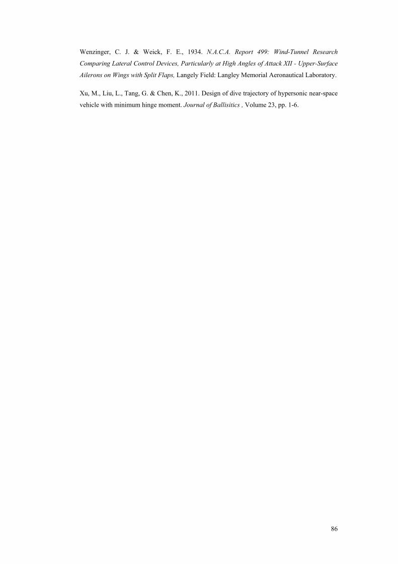
86
Wenzinger, C. J. & Weick, F. E., 1934. N.A.C.A. Report 499: Wind-Tunnel Research
Comparing Lateral Control Devices, Particularly at High Angles of Attack XII - Upper-Surface
Ailerons on Wings with Split Flaps, Langely Field: Langley Memorial Aeronautical Laboratory.
Xu, M., Liu, L., Tang, G. & Chen, K., 2011. Design of dive trajectory of hypersonic near-space
vehicle with minimum hinge moment. Journal of Ballisitics , Volume 23, pp. 1-6.
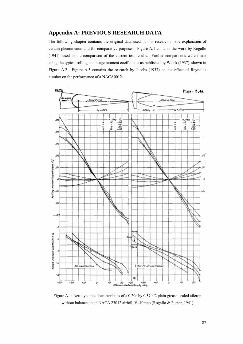
87
Appendix A: PREVIOUS RESEARCH DATA
The following chapter contains the original data used in this research in the explanation of
certain phenomenon and for comparative purposes. Figure A.1 contains the work by Rogallo
(1941), used in the comparison of the current test results. Further comparisons were made
using the typical rolling and hinge moment coefficients as published by Weick (1937), shown in
Figure A.2. Figure A.3 contains the research by Jacobs (1937) on the effect of Reynolds
number on the performance of a NACA0012.
Figure A.1: Aerodynamic characteristics of a 0.20c by 0.37 b/2 plain grease-sealed aileron
without balance on an NACA 23012 airfoil. V, 40mph (Rogallo & Purser, 1941)
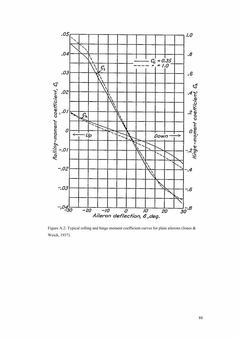
88
Figure A.2: Typical rolling and hinge moment coefficient curves for plain ailerons (Jones &
Weick, 1937).
89
Figure A.3: Aerofoil section characteristics of a NACA0012 as affected by variations of the
Reynolds number (Jacobs & Sherman, 1937).
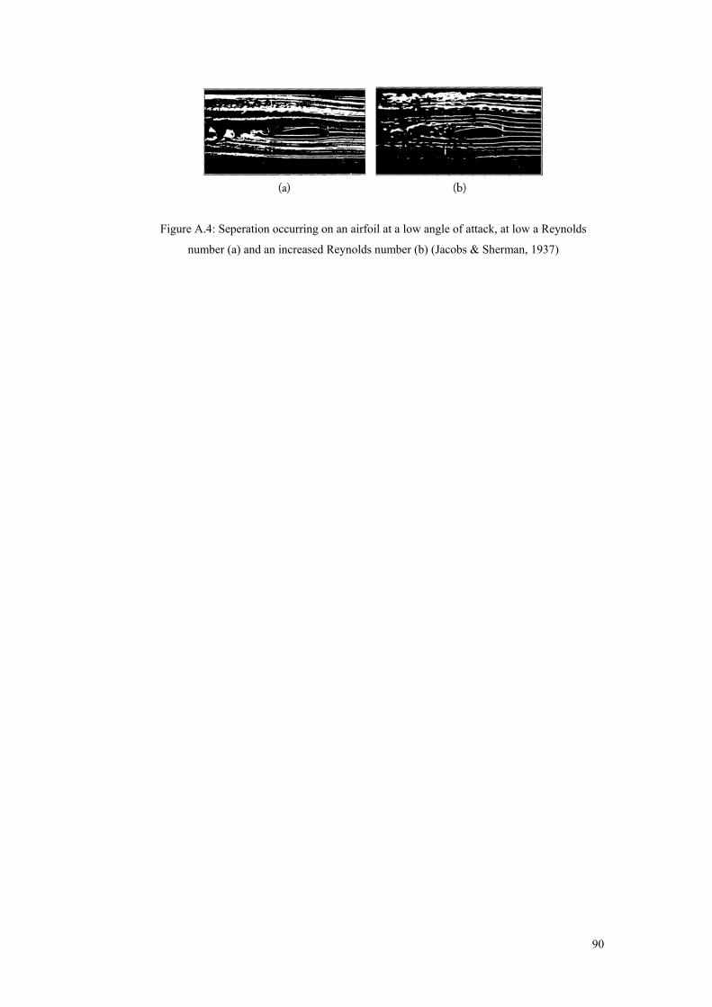
90
Figure A.4: Seperation occurring on an airfoil at a low angle of attack, at low a Reynolds
number (a) and an increased Reynolds number (b) (Jacobs & Sherman, 1937)

91
Appendix B: ENGINEERING DRAWINGS
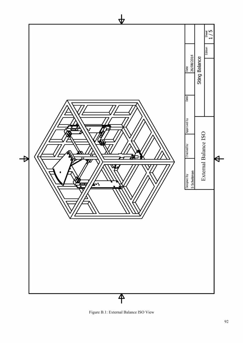
92
Figure B.1: External Balance ISO View
Ext
erna
l Bal
ance
IS
O
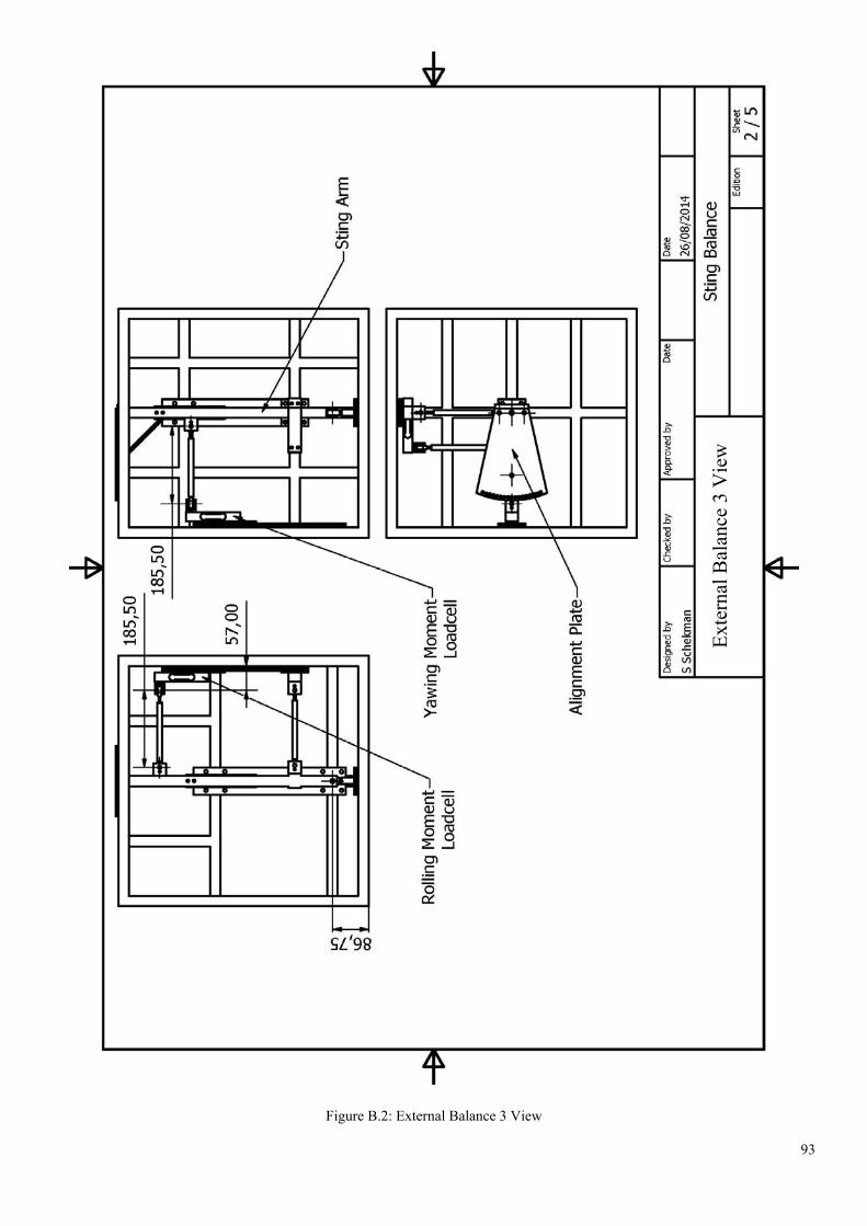
93
Figure B.2: External Balance 3 View
Ext
erna
l Bal
ance
3 V
iew
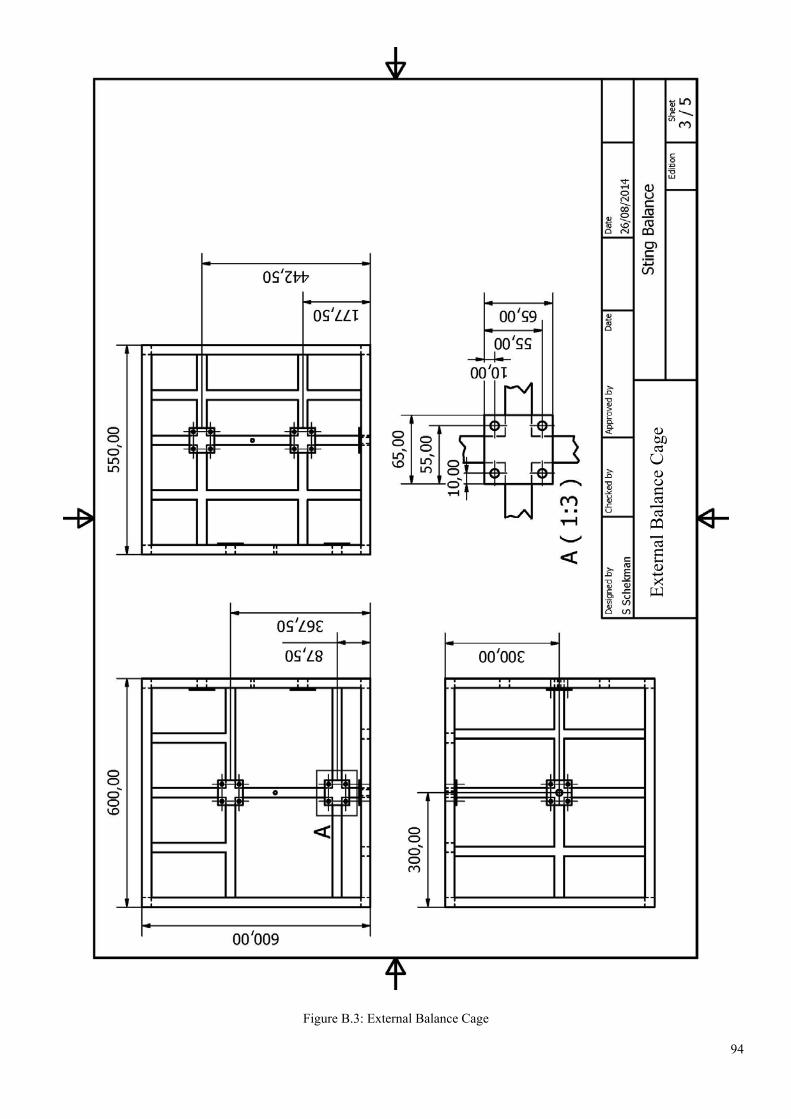
94
Figure B.3: External Balance Cage
Ext
erna
l Bal
ance
Cag
e
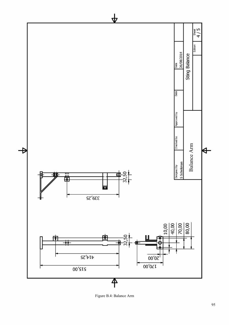
95
Figure B.4: Balance Arm
Bal
ance
Arm
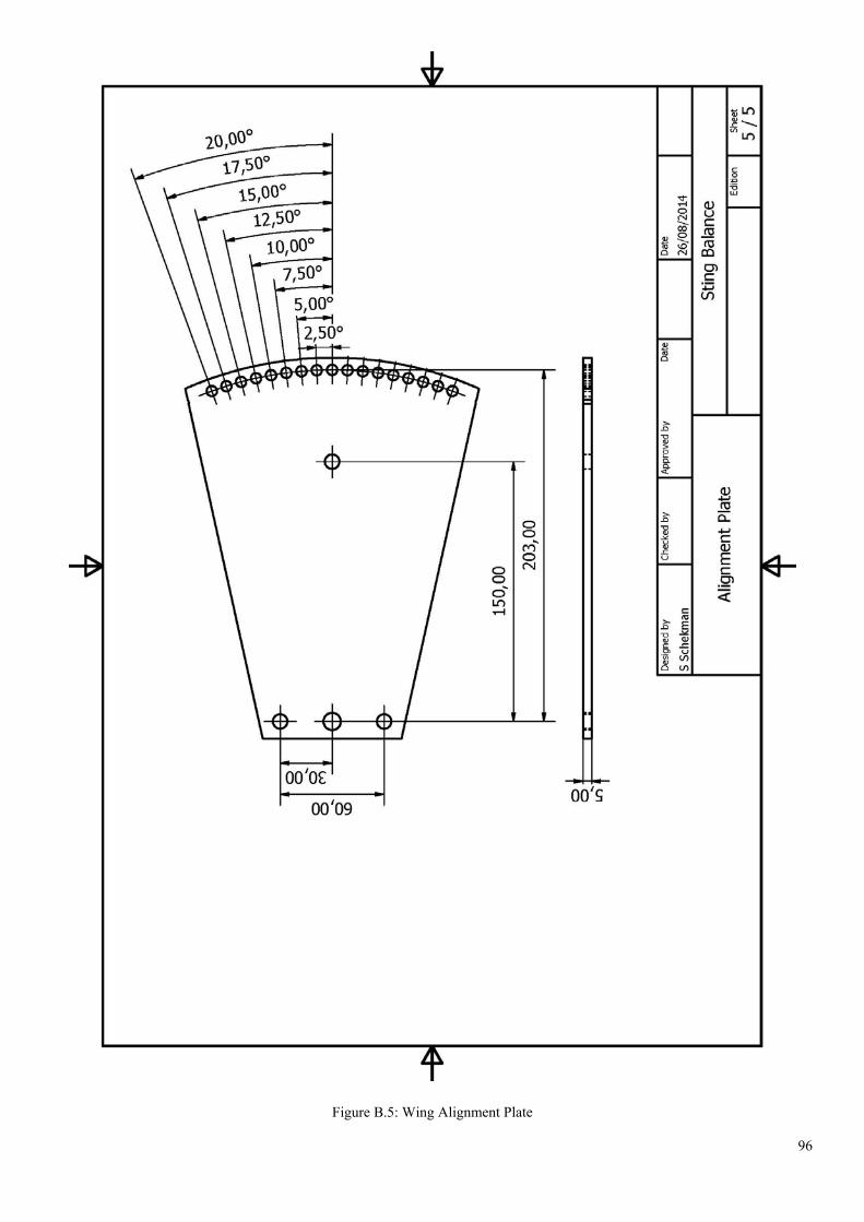
96
Figure B.5: Wing Alignment Plate
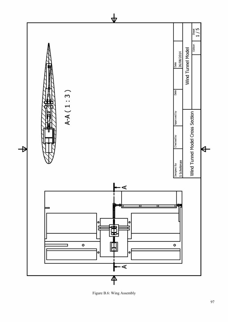
97
Figure B.6: Wing Assembly
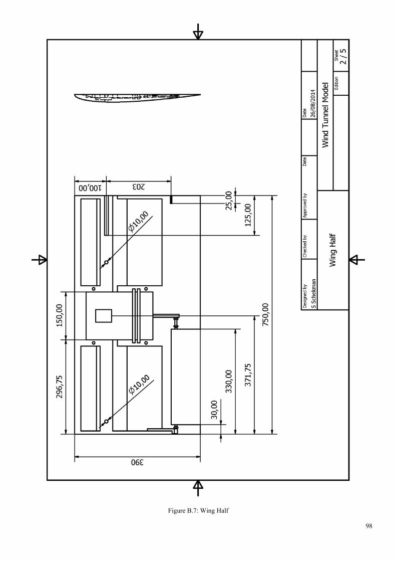
98
Figure B.7: Wing Half
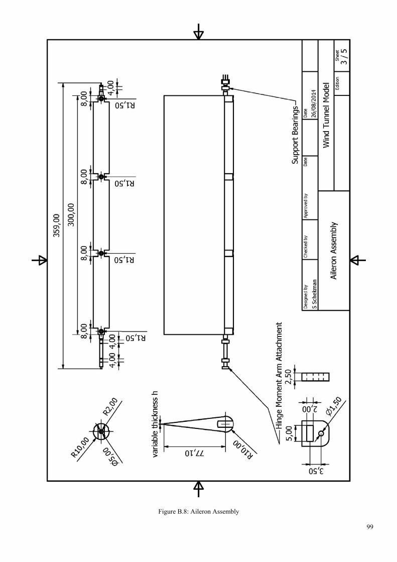
99
Figure B.8: Aileron Assembly
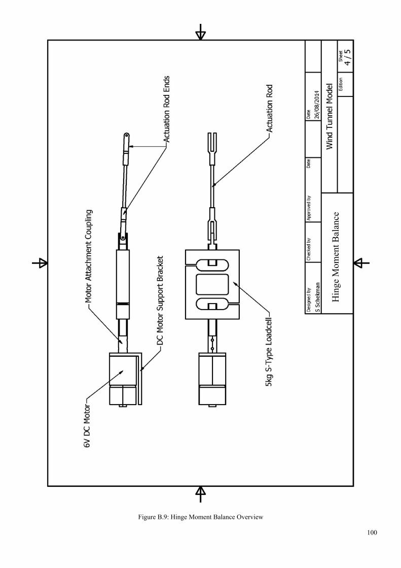
100
Figure B.9: Hinge Moment Balance Overview
Hin
ge M
omen
t Bal
ance
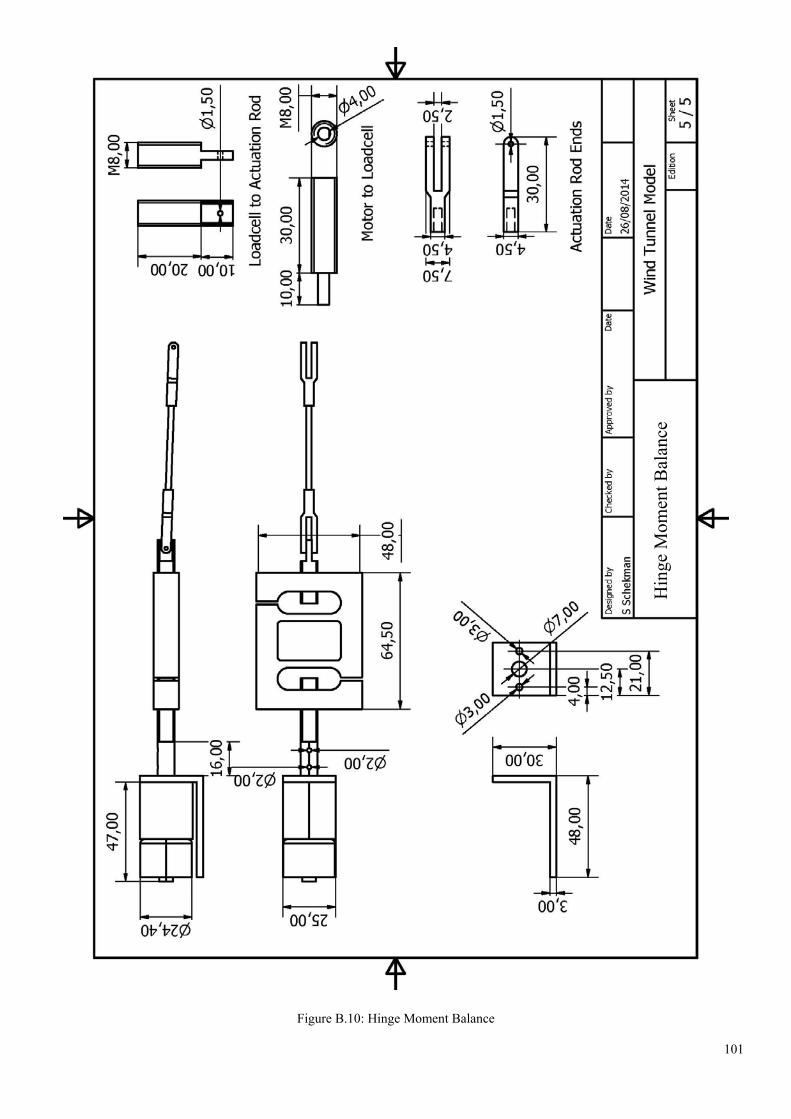
101
Figure B.10: Hinge Moment Balance
Hin
ge M
omen
t Bal
ance
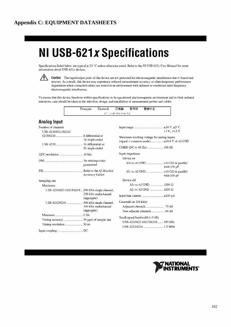
102
Appendix C: EQUIPMENT DATASHEETS
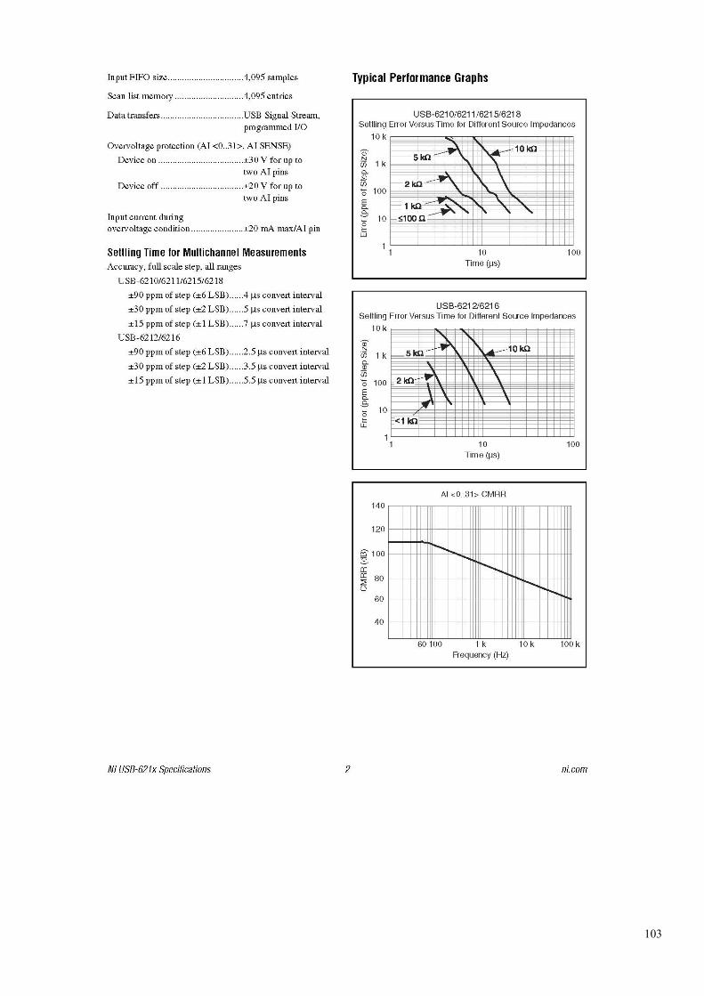
103
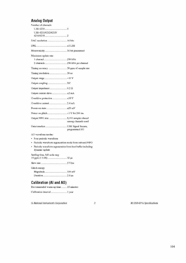
104
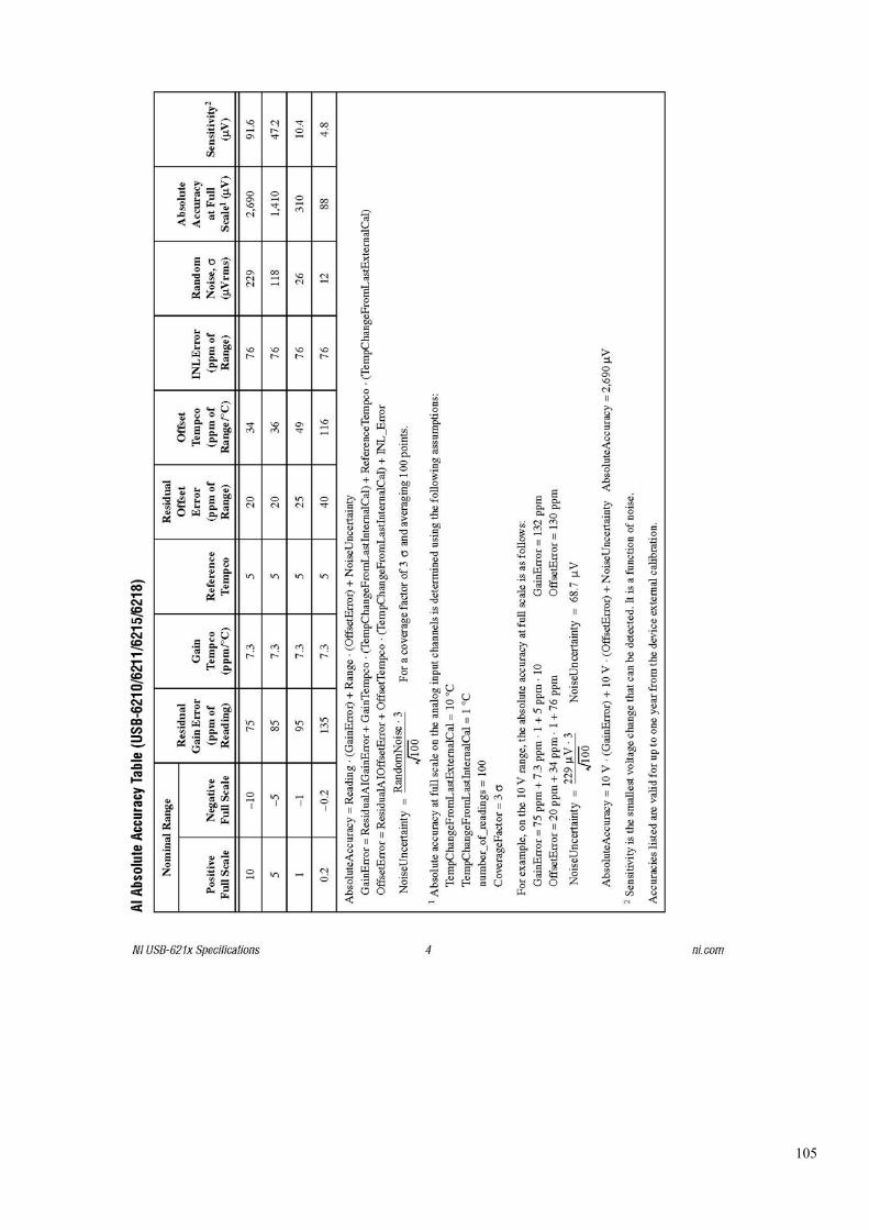
105
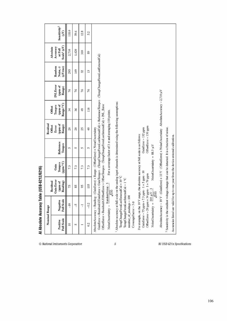
106
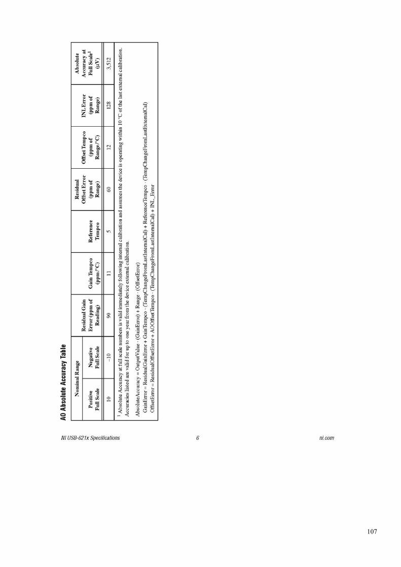
107
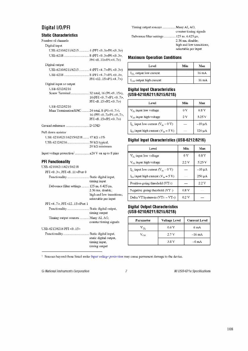
108
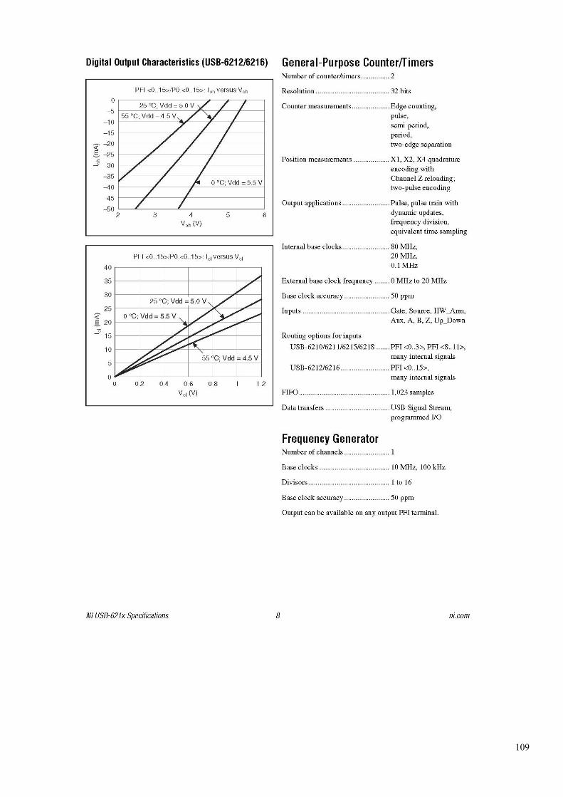
109
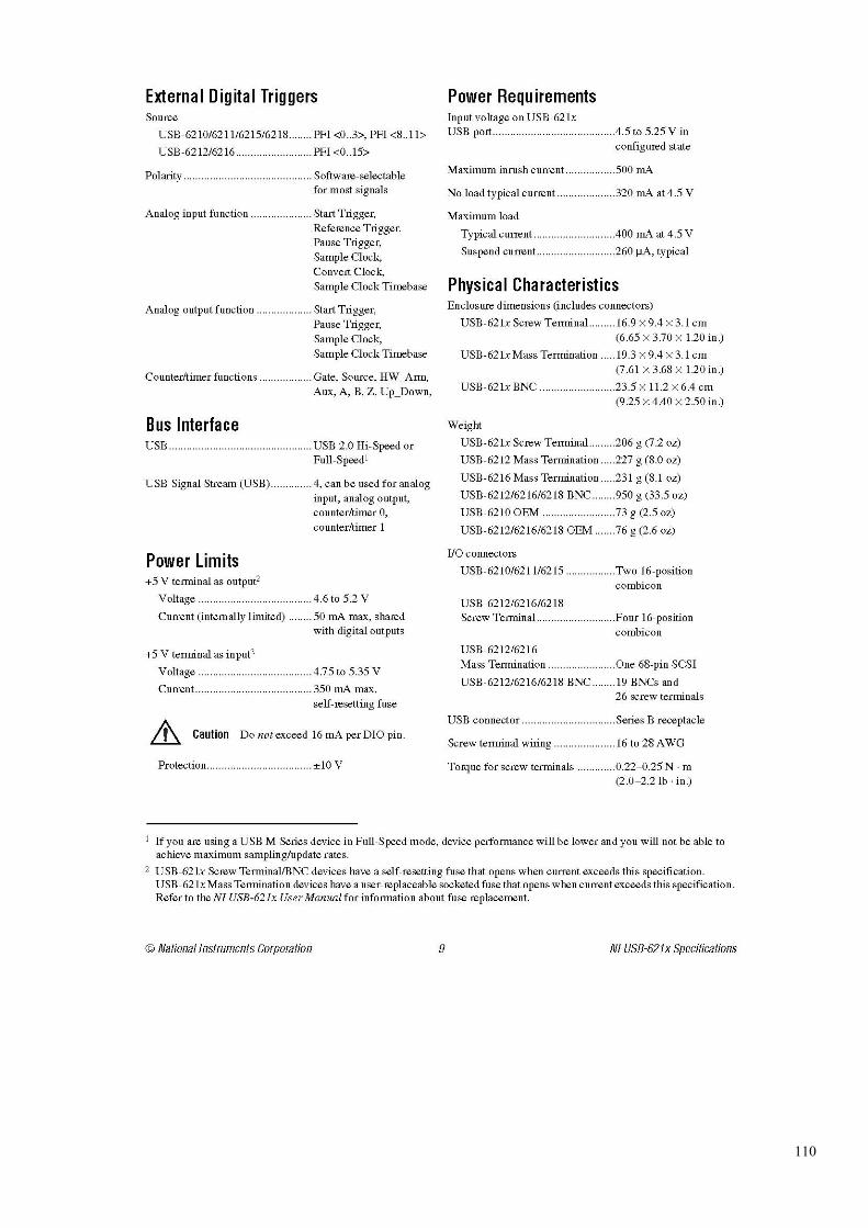
110
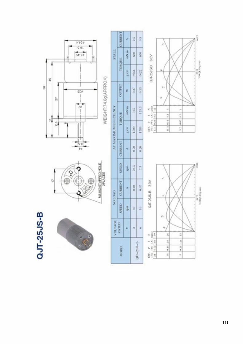
111
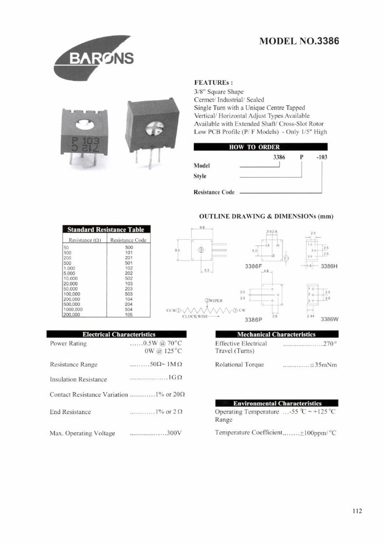
112
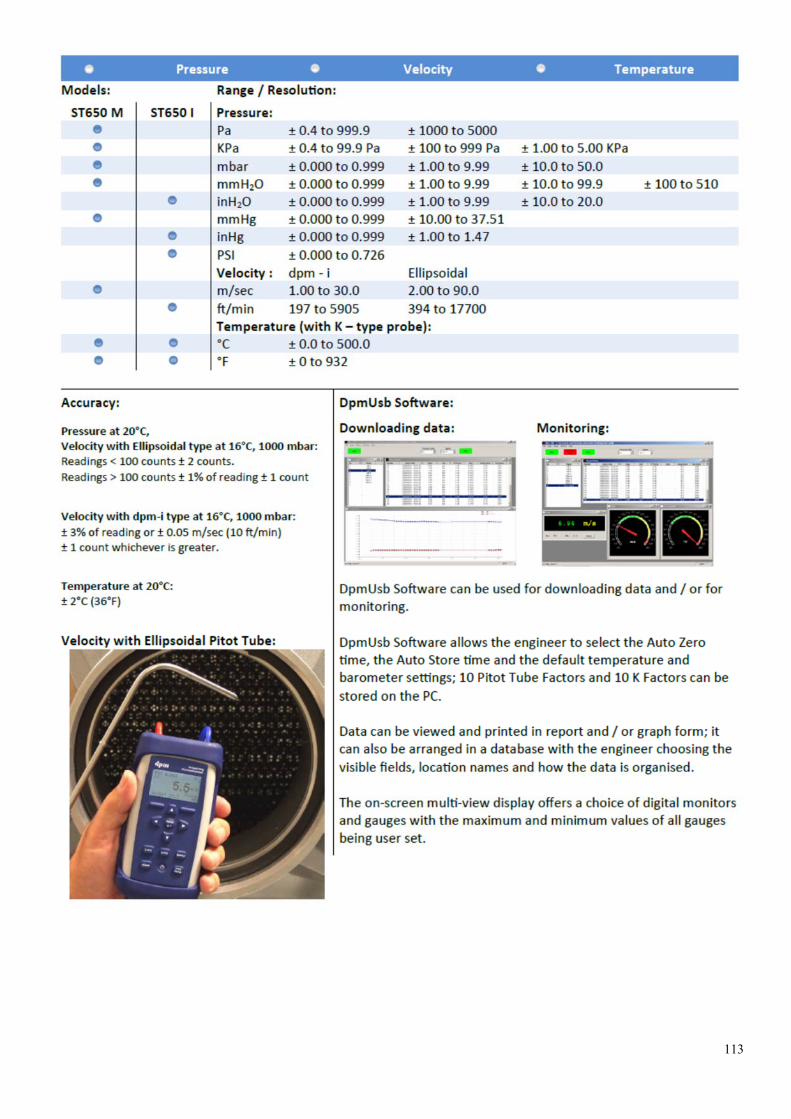
113
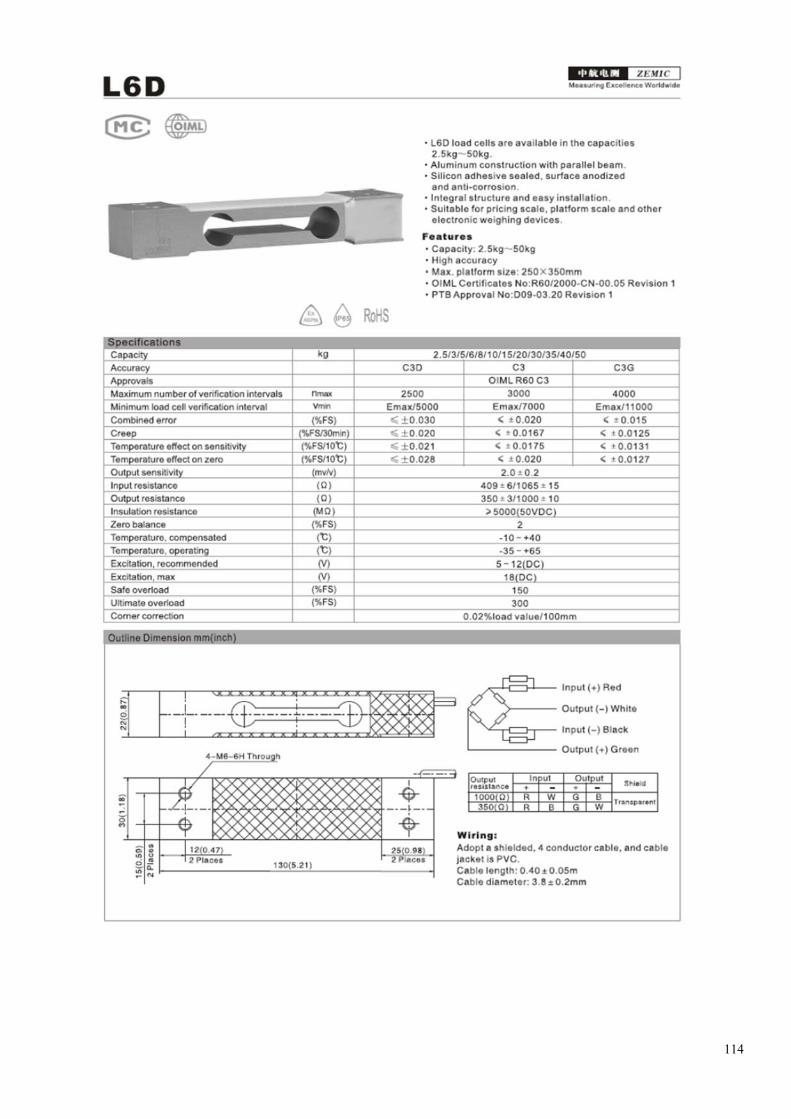
114

115
Appendix D: DERIVATION OF UNCERTAINTY
The following chapter details the derivation of the equations used to calculate the uncertainties
in the measured data. A data set was recorded for each test condition that was to be
investigated. The loadcell data contained in these sets were the filtered and averaged results of
the raw data discussed in chapter 6.3. Each data set comprised the signals from the rolling,
yawing and hinge moment loadcells, the potentiometer and the temperature thermocouple.
Signal Uncertainty
The uncertainty in the signal data was calculated by first calculating the standard deviation for
the respective data set. The equation below was used for the calculation of the standard
deviation.
= ∑ − D.1
A confidence interval of 1.96, relating to a 95% confidence level, was applied to the standard
deviation to calculate the uncertainty in the input voltage. The uncertainties in the excitation
voltage, , and loadcell gain, G, were included in the uncertainty for each loadcell strain
reading using the equation below.
∆ = ∆ + ∆ + ∆ D.2
Calibration Uncertainty
The uncertainty in the calibration gradients was calculated using the derived equation, below
∆ = ∆ + ∆ ′ D.3
Where R is the calibration gradient (for the rolling moment loadcell as an example)
The uncertainty in the applied load was calculated using the derived equation below
∆ ′ = ∆ + ∆ + ∆ + ∆ D.4
Where m is the mass of the applied mass pieces, g; x is the moment arm, mm; θ and α is the
alignment of the applied load, rad.
Moment Uncertainty
The uncertainty in the rolling and yawing moment loads and aileron deflection was found using
the calculated uncertainty in the loadcell signal, given by equation D.2, and the uncertainty due
to the calibration process. This uncertainty in the moment loads was derived from the from the
calibration matrix, below.

116
′′ = D.5
Where SigR Signal from rolling moment loadcell; SigY Signal from yawing moment loadcell;
is the calibration matrix in the form
= D.6
Where R1, R2, Y1 and Y2 Calibration gradients
The inverse calibration matrix was calculated using the equation below
= 1| | −− D.7
From equation D.5, the equations for the uncertainty in the rolling and yawing moments, given
below, were derived.
∆ = | | ∆ + ∆ + ∆| || |+ | | ∆ + ∆ + ∆| || |
D.8
∆ = | | ∆ + ∆ + ∆| || |+ | | ∆ + ∆ + ∆| || |
D.9
The uncertainty in the applied loading and direction of the loading was taken into account in the
uncertainty of gradients calculated for each calibration.
The equation for the uncertainty of the aileron hinge moment was simpler as there was no cross
coupling between the hinge moment loadcell and any other loadcell. The equation is given
below.
∆ = ∆ + ∆ D.10
Where Calibration gradient of hinge moment loadcell.
The uncertainty values and their sources for the equations shown above are discussed in chapter
7.
Aerodynamic Coefficient Uncertainty
The uncertainties in the aerodynamic coefficients were calculated using the following equations,
derived from the equations in chapter 2.2.

117
∆ ′′ = ∆ ′′ + ∆ + ∆ + ∆ D.11
∆ ′′ = ∆ ′′ + ∆ + ∆ + ∆ D.12
∆ = ∆ + ∆ + 2∆ + ∆ D.13
The values obtained from the above equations are discussed in chapter 8.
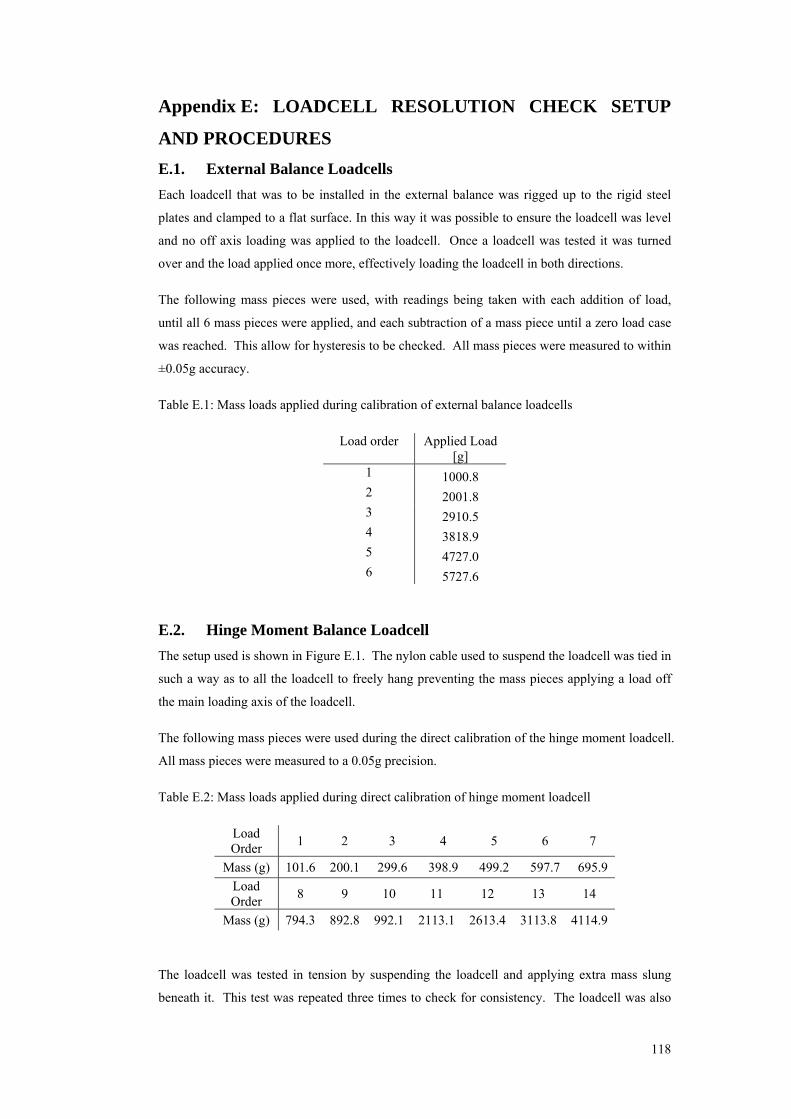
118
Appendix E: LOADCELL RESOLUTION CHECK SETUP
AND PROCEDURES
E.1. External Balance Loadcells
Each loadcell that was to be installed in the external balance was rigged up to the rigid steel
plates and clamped to a flat surface. In this way it was possible to ensure the loadcell was level
and no off axis loading was applied to the loadcell. Once a loadcell was tested it was turned
over and the load applied once more, effectively loading the loadcell in both directions.
The following mass pieces were used, with readings being taken with each addition of load,
until all 6 mass pieces were applied, and each subtraction of a mass piece until a zero load case
was reached. This allow for hysteresis to be checked. All mass pieces were measured to within
±0.05g accuracy.
Table E.1: Mass loads applied during calibration of external balance loadcells
Load order Applied Load [g]
1 1000.8 2 2001.8 3 2910.5 4 3818.9 5 4727.0 6 5727.6
E.2. Hinge Moment Balance Loadcell
The setup used is shown in Figure E.1. The nylon cable used to suspend the loadcell was tied in
such a way as to all the loadcell to freely hang preventing the mass pieces applying a load off
the main loading axis of the loadcell.
The following mass pieces were used during the direct calibration of the hinge moment loadcell.
All mass pieces were measured to a 0.05g precision.
Table E.2: Mass loads applied during direct calibration of hinge moment loadcell
Load Order
1 2 3 4 5 6 7
Mass (g) 101.6 200.1 299.6 398.9 499.2 597.7 695.9
Load Order
8 9 10 11 12 13 14
Mass (g) 794.3 892.8 992.1 2113.1 2613.4 3113.8 4114.9
The loadcell was tested in tension by suspending the loadcell and applying extra mass slung
beneath it. This test was repeated three times to check for consistency. The loadcell was also

119
checked with a compressive load by resting the loadcell on a flat surface and applying a direct
load. This was done simply to confirm that the signal to load relationship was the same in both
compression and tension and was not repeated. For each test data was recorded for a minute
before the next mass was added.
Figure E.1: Setup used in the calibration of the hinge moment loadcell through the application
of load directly to the loadcell.
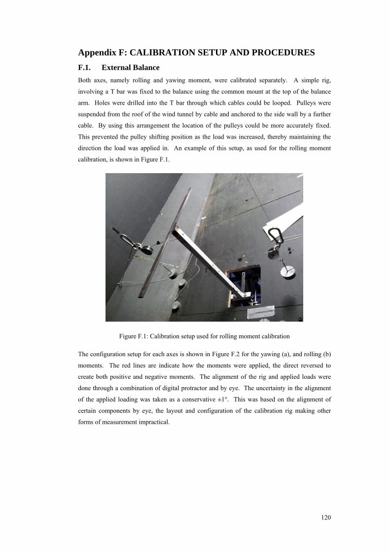
120
Appendix F: CALIBRATION SETUP AND PROCEDURES
F.1. External Balance
Both axes, namely rolling and yawing moment, were calibrated separately. A simple rig,
involving a T bar was fixed to the balance using the common mount at the top of the balance
arm. Holes were drilled into the T bar through which cables could be looped. Pulleys were
suspended from the roof of the wind tunnel by cable and anchored to the side wall by a further
cable. By using this arrangement the location of the pulleys could be more accurately fixed.
This prevented the pulley shifting position as the load was increased, thereby maintaining the
direction the load was applied in. An example of this setup, as used for the rolling moment
calibration, is shown in Figure F.1.
Figure F.1: Calibration setup used for rolling moment calibration
The configuration setup for each axes is shown in Figure F.2 for the yawing (a), and rolling (b)
moments. The red lines are indicate how the moments were applied, the direct reversed to
create both positive and negative moments. The alignment of the rig and applied loads were
done through a combination of digital protractor and by eye. The uncertainty in the alignment
of the applied loading was taken as a conservative ±1°. This was based on the alignment of
certain components by eye, the layout and configuration of the calibration rig making other
forms of measurement impractical.
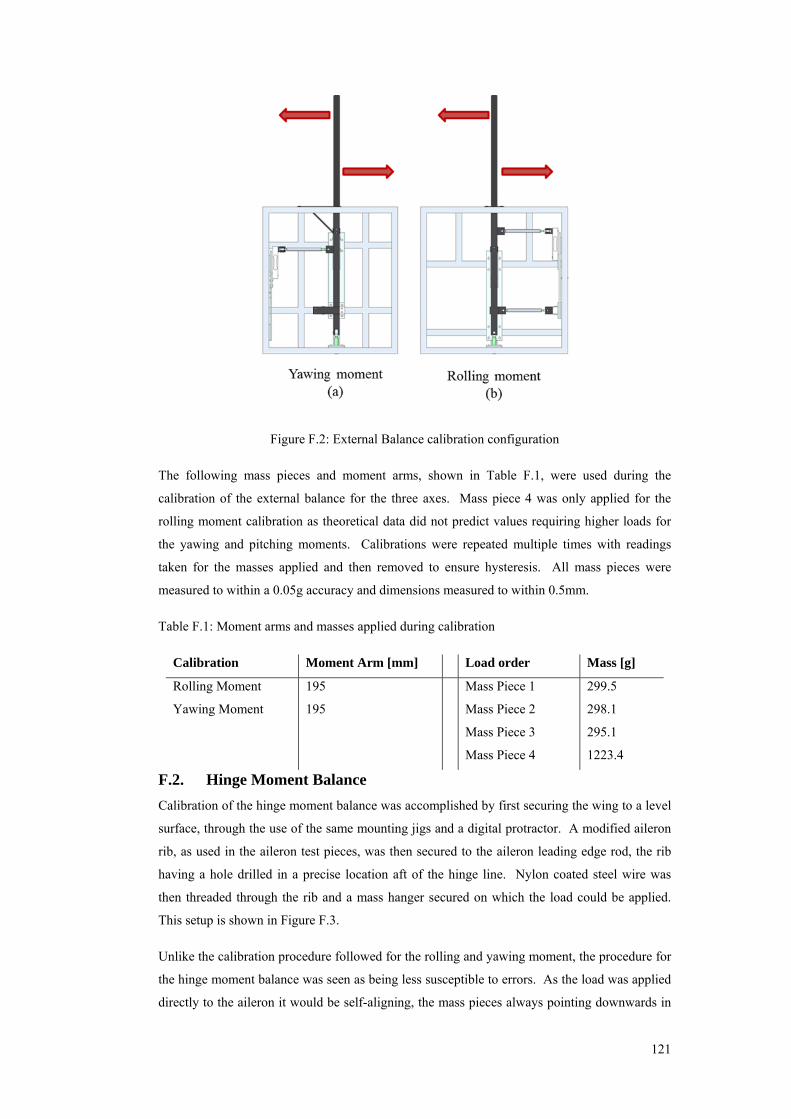
121
Figure F.2: External Balance calibration configuration
The following mass pieces and moment arms, shown in Table F.1, were used during the
calibration of the external balance for the three axes. Mass piece 4 was only applied for the
rolling moment calibration as theoretical data did not predict values requiring higher loads for
the yawing and pitching moments. Calibrations were repeated multiple times with readings
taken for the masses applied and then removed to ensure hysteresis. All mass pieces were
measured to within a 0.05g accuracy and dimensions measured to within 0.5mm.
Table F.1: Moment arms and masses applied during calibration
Calibration Moment Arm [mm]
Load order Mass [g]
Rolling Moment 195
Mass Piece 1 299.5
Yawing Moment 195
Mass Piece 2 298.1
Mass Piece 3 295.1
Mass Piece 4 1223.4
F.2. Hinge Moment Balance
Calibration of the hinge moment balance was accomplished by first securing the wing to a level
surface, through the use of the same mounting jigs and a digital protractor. A modified aileron
rib, as used in the aileron test pieces, was then secured to the aileron leading edge rod, the rib
having a hole drilled in a precise location aft of the hinge line. Nylon coated steel wire was
then threaded through the rib and a mass hanger secured on which the load could be applied.
This setup is shown in Figure F.3.
Unlike the calibration procedure followed for the rolling and yawing moment, the procedure for
the hinge moment balance was seen as being less susceptible to errors. As the load was applied
directly to the aileron it would be self-aligning, the mass pieces always pointing downwards in
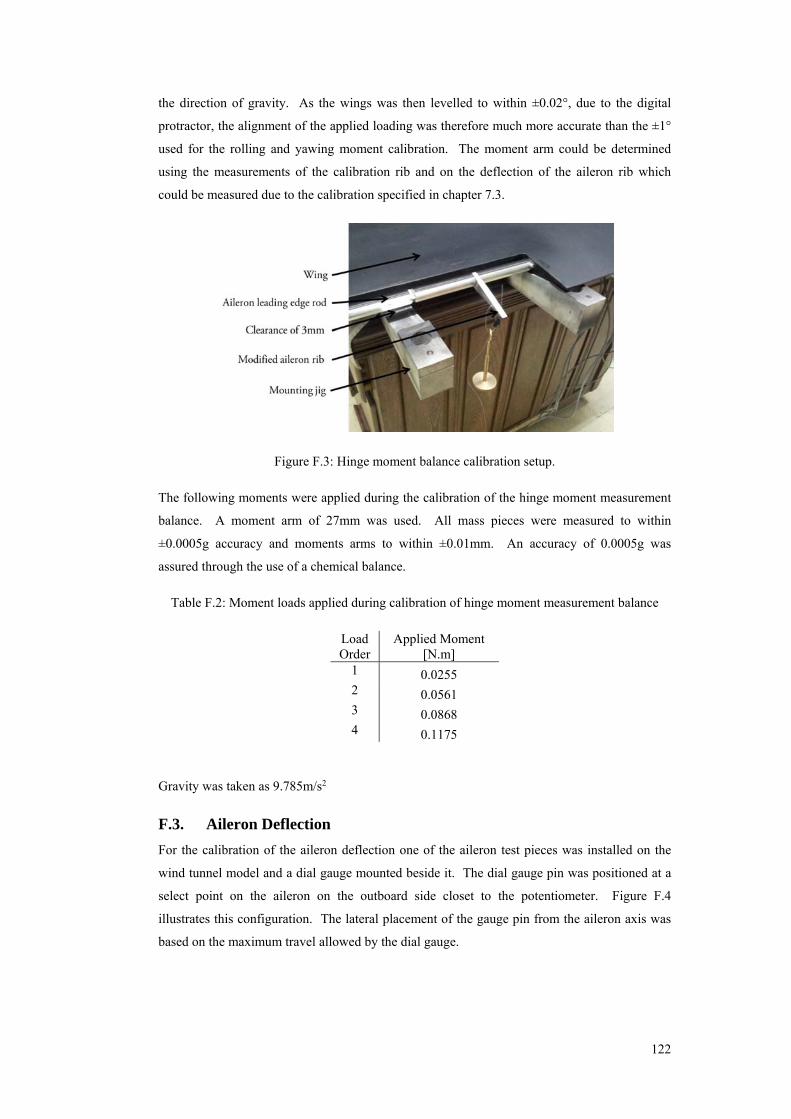
122
the direction of gravity. As the wings was then levelled to within ±0.02°, due to the digital
protractor, the alignment of the applied loading was therefore much more accurate than the ±1°
used for the rolling and yawing moment calibration. The moment arm could be determined
using the measurements of the calibration rib and on the deflection of the aileron rib which
could be measured due to the calibration specified in chapter 7.3.
Figure F.3: Hinge moment balance calibration setup.
The following moments were applied during the calibration of the hinge moment measurement
balance. A moment arm of 27mm was used. All mass pieces were measured to within
±0.0005g accuracy and moments arms to within ±0.01mm. An accuracy of 0.0005g was
assured through the use of a chemical balance.
Table F.2: Moment loads applied during calibration of hinge moment measurement balance
Load Order
Applied Moment [N.m]
1 0.0255 2 0.0561 3 0.0868 4 0.1175
Gravity was taken as 9.785m/s2
F.3. Aileron Deflection
For the calibration of the aileron deflection one of the aileron test pieces was installed on the
wind tunnel model and a dial gauge mounted beside it. The dial gauge pin was positioned at a
select point on the aileron on the outboard side closet to the potentiometer. Figure F.4
illustrates this configuration. The lateral placement of the gauge pin from the aileron axis was
based on the maximum travel allowed by the dial gauge.
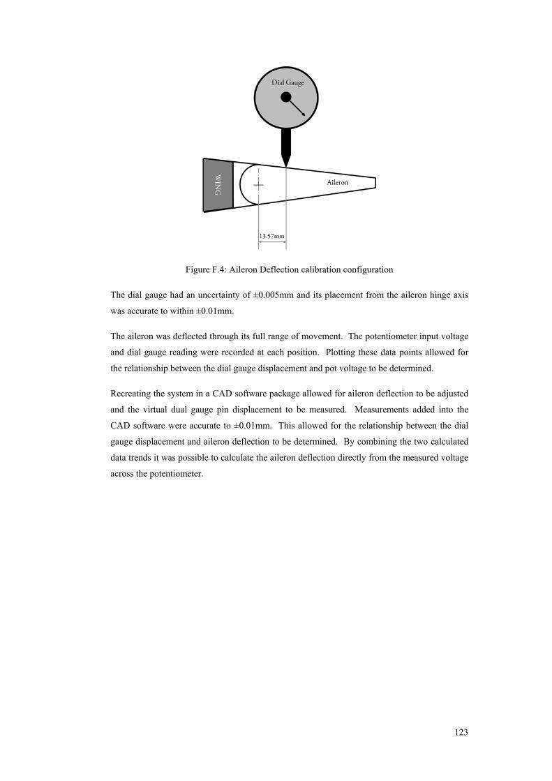
123
Figure F.4: Aileron Deflection calibration configuration
The dial gauge had an uncertainty of ±0.005mm and its placement from the aileron hinge axis
was accurate to within ±0.01mm.
The aileron was deflected through its full range of movement. The potentiometer input voltage
and dial gauge reading were recorded at each position. Plotting these data points allowed for
the relationship between the dial gauge displacement and pot voltage to be determined.
Recreating the system in a CAD software package allowed for aileron deflection to be adjusted
and the virtual dual gauge pin displacement to be measured. Measurements added into the
CAD software were accurate to ±0.01mm. This allowed for the relationship between the dial
gauge displacement and aileron deflection to be determined. By combining the two calculated
data trends it was possible to calculate the aileron deflection directly from the measured voltage
across the potentiometer.
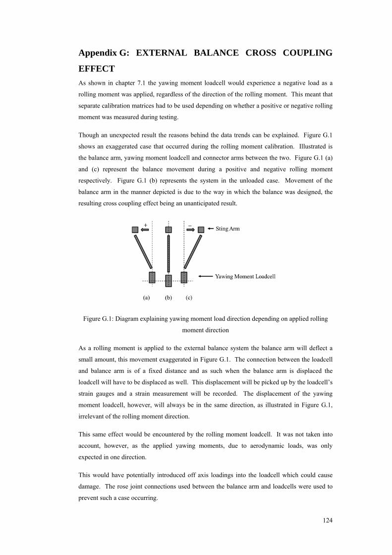
124
Appendix G: EXTERNAL BALANCE CROSS COUPLING
EFFECT
As shown in chapter 7.1 the yawing moment loadcell would experience a negative load as a
rolling moment was applied, regardless of the direction of the rolling moment. This meant that
separate calibration matrices had to be used depending on whether a positive or negative rolling
moment was measured during testing.
Though an unexpected result the reasons behind the data trends can be explained. Figure G.1
shows an exaggerated case that occurred during the rolling moment calibration. Illustrated is
the balance arm, yawing moment loadcell and connector arms between the two. Figure G.1 (a)
and (c) represent the balance movement during a positive and negative rolling moment
respectively. Figure G.1 (b) represents the system in the unloaded case. Movement of the
balance arm in the manner depicted is due to the way in which the balance was designed, the
resulting cross coupling effect being an unanticipated result.
Figure G.1: Diagram explaining yawing moment load direction depending on applied rolling
moment direction
As a rolling moment is applied to the external balance system the balance arm will deflect a
small amount, this movement exaggerated in Figure G.1. The connection between the loadcell
and balance arm is of a fixed distance and as such when the balance arm is displaced the
loadcell will have to be displaced as well. This displacement will be picked up by the loadcell’s
strain gauges and a strain measurement will be recorded. The displacement of the yawing
moment loadcell, however, will always be in the same direction, as illustrated in Figure G.1,
irrelevant of the rolling moment direction.
This same effect would be encountered by the rolling moment loadcell. It was not taken into
account, however, as the applied yawing moments, due to aerodynamic loads, was only
expected in one direction.
This would have potentially introduced off axis loadings into the loadcell which could cause
damage. The rose joint connections used between the balance arm and loadcells were used to
prevent such a case occurring.

125
Appendix H: TEST PRECAUTIONS
1. Ensure that the battery charger is unplugged during the tests.
2. Before starting a test run the aileron through its full deflection range and check for any
lagging or jumping in the movement indicative of an obstruction or clearance issue. Clean
the area causing problems if necessary.
3. Do not touch, adjust or rest anything on the external balance during a test.
4. During testing avoid changing the direction in which the aileron is deflected, pick one
direction and use that. Should the aileron move too quickly decrease the DC motor supply
voltage.
5. Do not operate the aileron beyond the following deflections: <-35o and >10o, otherwise it
risks serious damage to the hinge moment loadcell.
6. Once the wind tunnel has been turned up to the test speed the aileron must not be deflected
as this would vary the zero values for all measured loads, rendering the data obtained as
useless.
7. Ensure the bolt at the wind tunnel models quarter chord point is tightened before each test
otherwise there is a risk of the wing leaning against the tunnel floor.
8. Using the live plots outputted from Labview as a guideline, the data should only be
recorded once a measure of stability in the data has been reached (this typically takes 15 to
30 seconds).
9. Upon conclusion of testing, return the aileron to a zero deflection
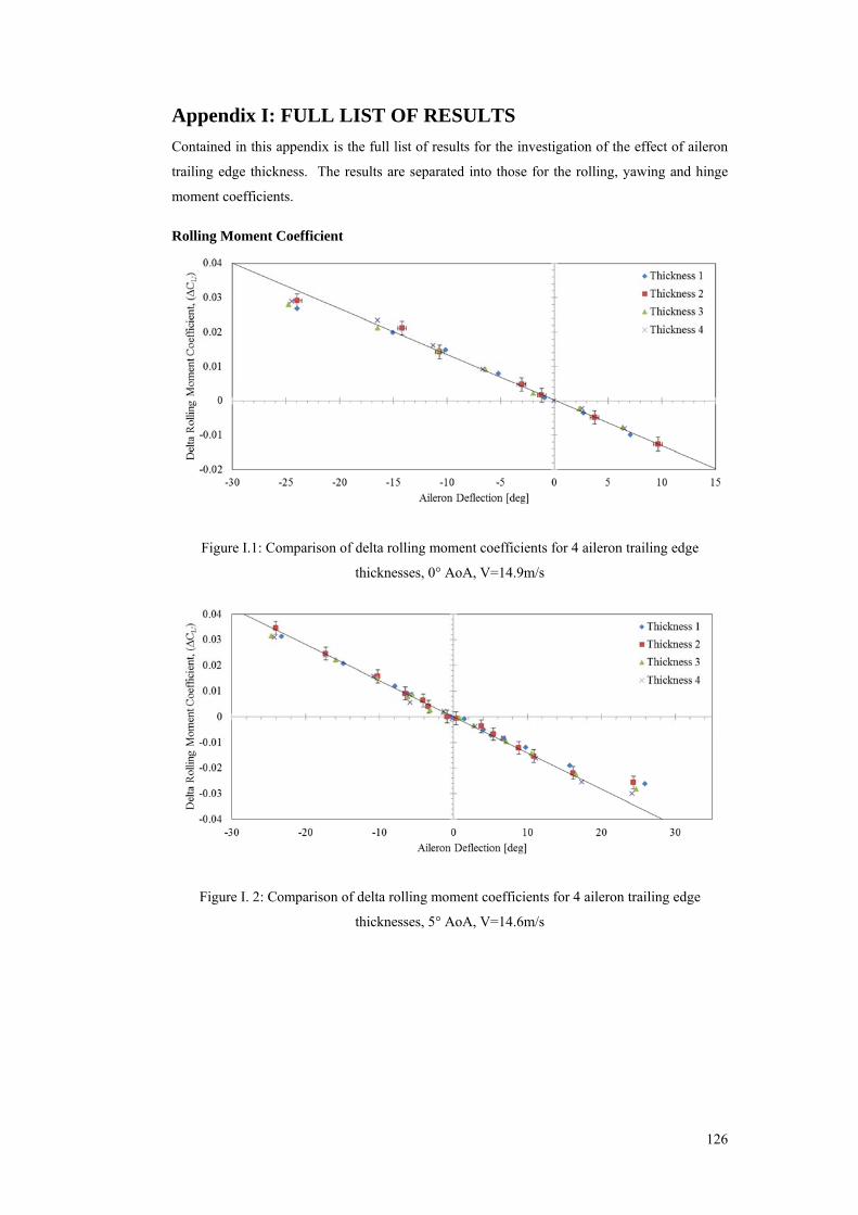
126
Appendix I: FULL LIST OF RESULTS
Contained in this appendix is the full list of results for the investigation of the effect of aileron
trailing edge thickness. The results are separated into those for the rolling, yawing and hinge
moment coefficients.
Rolling Moment Coefficient
Figure I.1: Comparison of delta rolling moment coefficients for 4 aileron trailing edge
thicknesses, 0° AoA, V=14.9m/s
Figure I. 2: Comparison of delta rolling moment coefficients for 4 aileron trailing edge
thicknesses, 5° AoA, V=14.6m/s
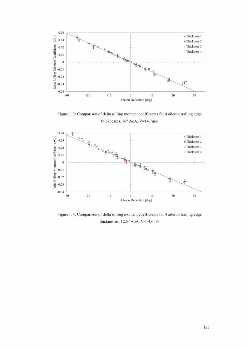
127
Figure I. 3: Comparison of delta rolling moment coefficients for 4 aileron trailing edge
thicknesses, 10° AoA, V=14.7m/s
Figure I. 4: Comparison of delta rolling moment coefficients for 4 aileron trailing edge
thicknesses, 12.5° AoA, V=14.6m/s
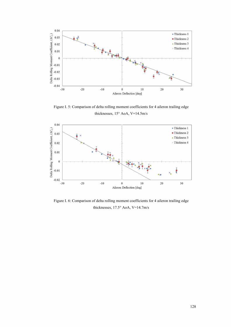
128
Figure I. 5: Comparison of delta rolling moment coefficients for 4 aileron trailing edge
thicknesses, 15° AoA, V=14.5m/s
Figure I. 6: Comparison of delta rolling moment coefficients for 4 aileron trailing edge
thicknesses, 17.5° AoA, V=14.7m/s
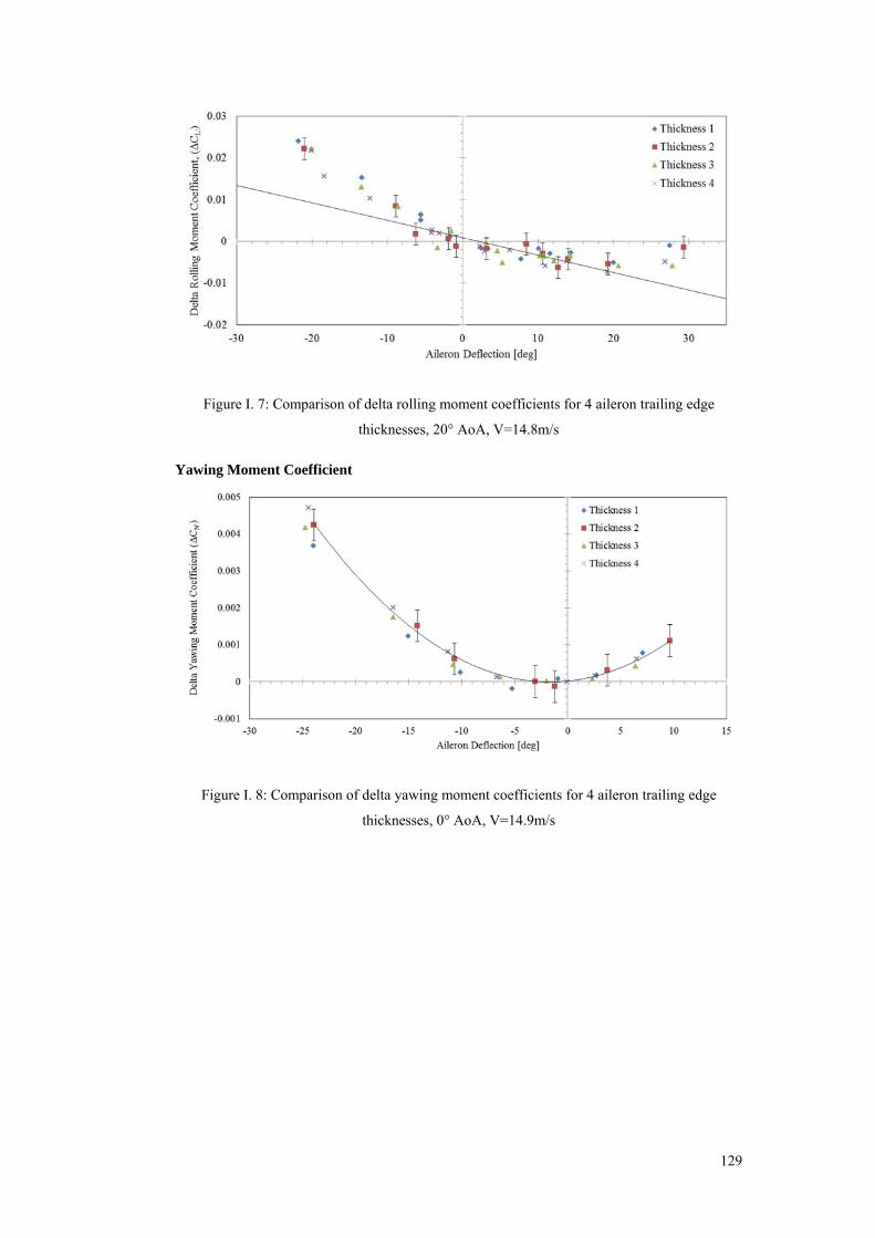
129
Figure I. 7: Comparison of delta rolling moment coefficients for 4 aileron trailing edge
thicknesses, 20° AoA, V=14.8m/s
Yawing Moment Coefficient
Figure I. 8: Comparison of delta yawing moment coefficients for 4 aileron trailing edge
thicknesses, 0° AoA, V=14.9m/s
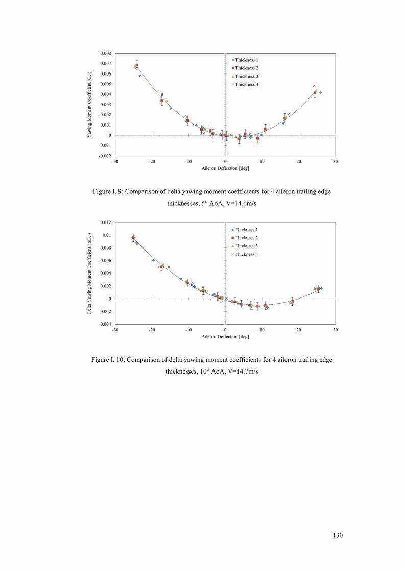
130
Figure I. 9: Comparison of delta yawing moment coefficients for 4 aileron trailing edge
thicknesses, 5° AoA, V=14.6m/s
Figure I. 10: Comparison of delta yawing moment coefficients for 4 aileron trailing edge
thicknesses, 10° AoA, V=14.7m/s
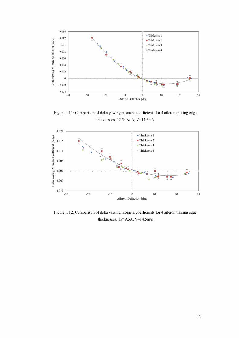
131
Figure I. 11: Comparison of delta yawing moment coefficients for 4 aileron trailing edge
thicknesses, 12.5° AoA, V=14.6m/s
Figure I. 12: Comparison of delta yawing moment coefficients for 4 aileron trailing edge
thicknesses, 15° AoA, V=14.5m/s
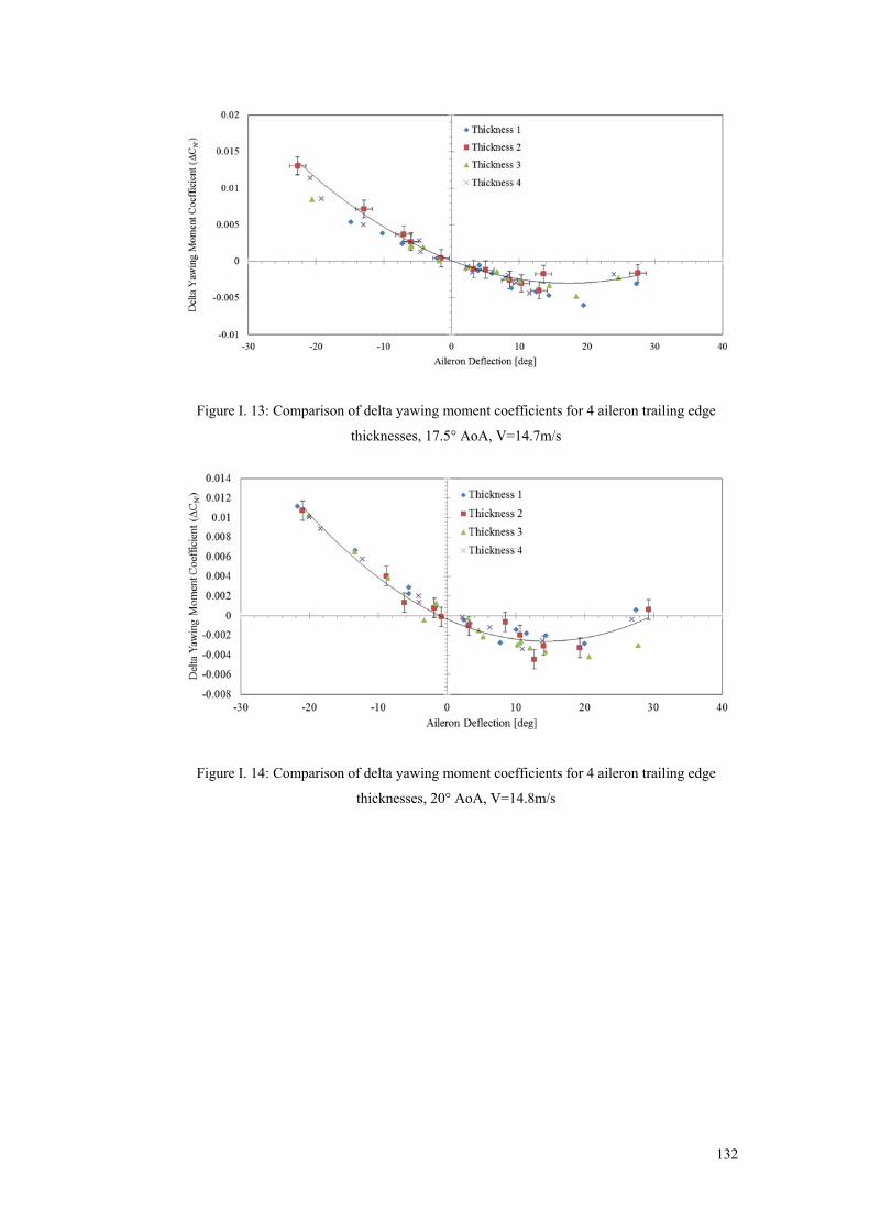
132
Figure I. 13: Comparison of delta yawing moment coefficients for 4 aileron trailing edge
thicknesses, 17.5° AoA, V=14.7m/s
Figure I. 14: Comparison of delta yawing moment coefficients for 4 aileron trailing edge
thicknesses, 20° AoA, V=14.8m/s
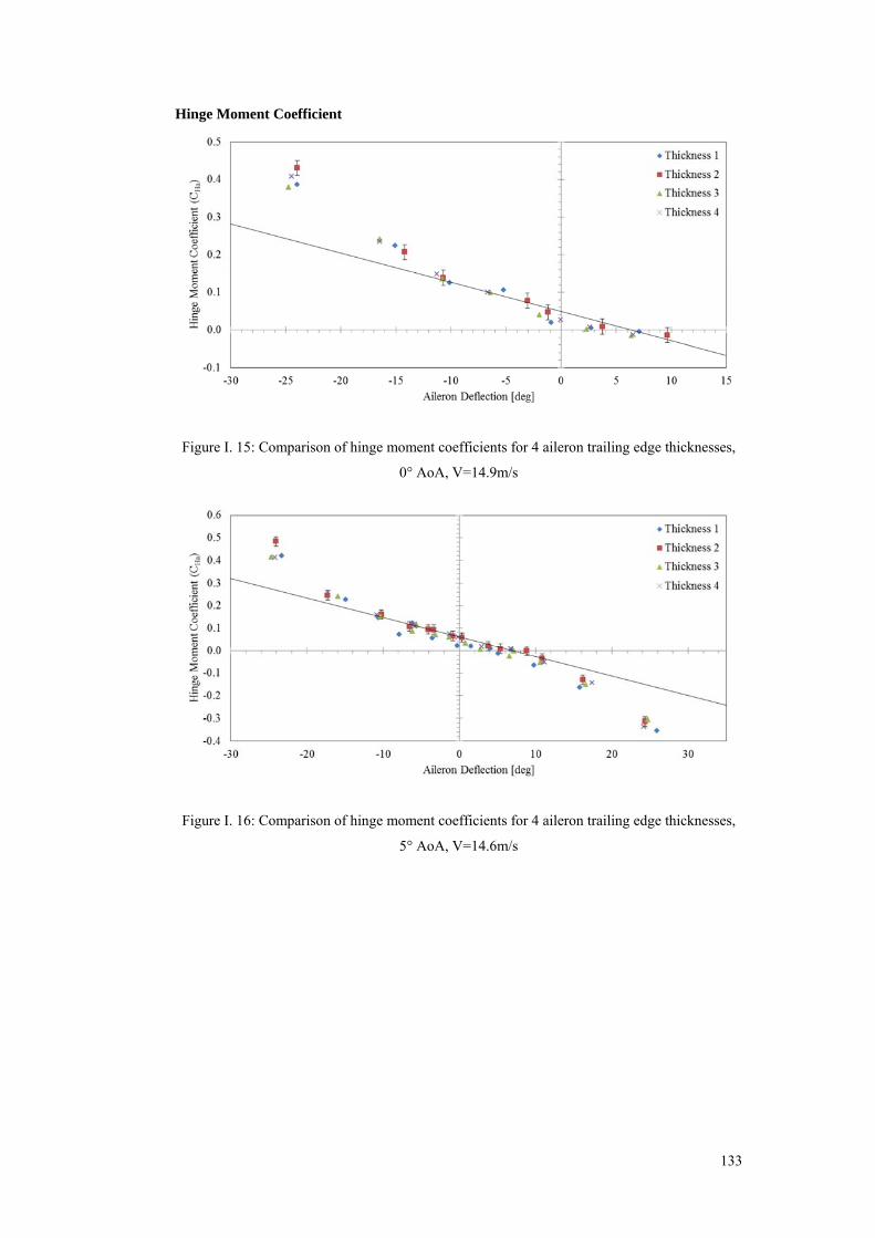
133
Hinge Moment Coefficient
Figure I. 15: Comparison of hinge moment coefficients for 4 aileron trailing edge thicknesses,
0° AoA, V=14.9m/s
Figure I. 16: Comparison of hinge moment coefficients for 4 aileron trailing edge thicknesses,
5° AoA, V=14.6m/s
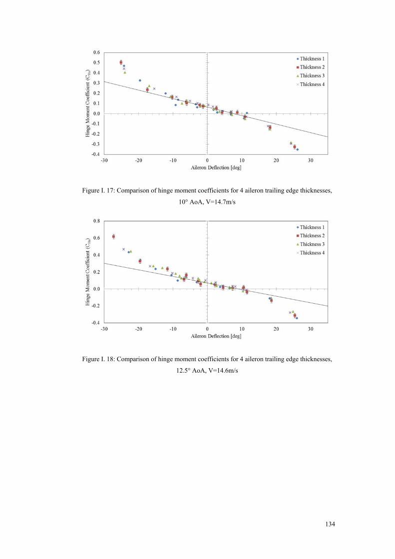
134
Figure I. 17: Comparison of hinge moment coefficients for 4 aileron trailing edge thicknesses,
10° AoA, V=14.7m/s
Figure I. 18: Comparison of hinge moment coefficients for 4 aileron trailing edge thicknesses,
12.5° AoA, V=14.6m/s
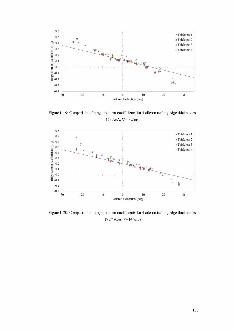
135
Figure I. 19: Comparison of hinge moment coefficients for 4 aileron trailing edge thicknesses,
15° AoA, V=14.5m/s
Figure I. 20: Comparison of hinge moment coefficients for 4 aileron trailing edge thicknesses,
17.5° AoA, V=14.7m/s
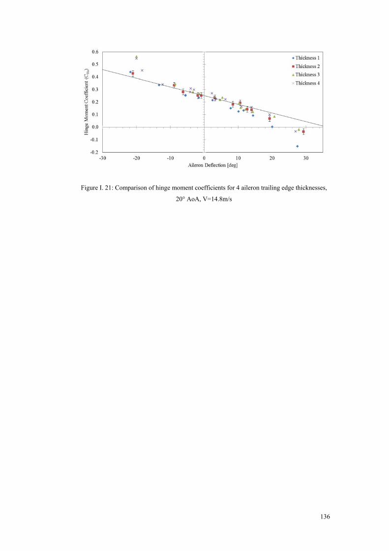
136
Figure I. 21: Comparison of hinge moment coefficients for 4 aileron trailing edge thicknesses,
20° AoA, V=14.8m/s