Embed Size (px)
Citation preview

Measurement
and Modelling
of Radiowave
Propagation in
Urban
Microcells
Y.L.C. de Jong


Measurement and Modelling of RadiowavePropagation in Urban Microcells
PROEFSCHRIFT
ter verkrijging van de graad van doctor aan deTechnische Universiteit Eindhoven, op gezag vande Rector Magnificus, prof.dr. M. Rem, vooreen commissie aangewezen door het Collegevoor Promoties in het openbaar te verdedigen op
donderdag 21 juni 2001 te 16.00 uur
door
Yvo Leon Christiaan de Jong
geboren te Vlaardingen
Dit proefschrift is goedgekeurd door de promotoren:
prof.dr.ir. G. Brussaardenprof.dr. R.J.C. Bultitude
Copromotor: dr.ir. M.H.A.J. Herben
CIP-DATA LIBRARY TECHNISCHE UNIVERSITEIT EINDHOVEN
Jong, Yvo L.C. de
Measurement and modelling of radiowave propagation in urban microcells /by Yvo L.C. de Jong. – Eindhoven : Technische Universiteit Eindhoven, 2001.Proefschrift. – ISBN 90-386-1860-3NUGI 832Trefw.: mobiele telecommunicatie / radiogolfvoortplanting /elektromagnetische metingen.Subject headings: mobile communication / microcellular radio /radiowave propagation / direction-of-arrival estimation.
Cover design by ZO, ’s-Hertogenbosch
c© 2001 by Y.L.C. de Jong, Dordrecht
All rights reserved. No part of this publication may be reproduced or transmitted inany form or by any means, electronic, mechanical, including photocopy, recording,or any information storage and retrieval system, without the prior written permissionof the copyright owner.

Aan mijn oudersAan Nathalie

vi
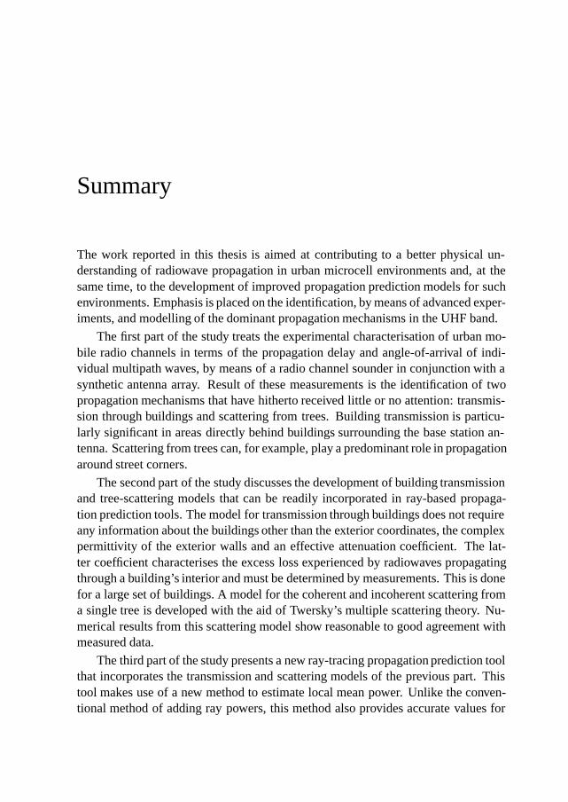
Summary
The work reported in this thesis is aimed at contributing to a better physical un-derstanding of radiowave propagation in urban microcell environments and, at thesame time, to the development of improved propagation prediction models for suchenvironments. Emphasis is placed on the identification, by means of advanced exper-iments, and modelling of the dominant propagation mechanisms in the UHF band.
The first part of the study treats the experimental characterisation of urban mo-bile radio channels in terms of the propagation delay and angle-of-arrival of indi-vidual multipath waves, by means of a radio channel sounder in conjunction with asynthetic antenna array. Result of these measurements is the identification of twopropagation mechanisms that have hitherto received little or no attention: transmis-sion through buildings and scattering from trees. Building transmission is particu-larly significant in areas directly behind buildings surrounding the base station an-tenna. Scattering from trees can, for example, play a predominant role in propagationaround street corners.
The second part of the study discusses the development of building transmissionand tree-scattering models that can be readily incorporated in ray-based propaga-tion prediction tools. The model for transmission through buildings does not requireany information about the buildings other than the exterior coordinates, the complexpermittivity of the exterior walls and an effective attenuation coefficient. The lat-ter coefficient characterises the excess loss experienced by radiowaves propagatingthrough a building’s interior and must be determined by measurements. This is donefor a large set of buildings. A model for the coherent and incoherent scattering froma single tree is developed with the aid of Twersky’s multiple scattering theory. Nu-merical results from this scattering model show reasonable to good agreement withmeasured data.
The third part of the study presents a new ray-tracing propagation prediction toolthat incorporates the transmission and scattering models of the previous part. Thistool makes use of a new method to estimate local mean power. Unlike the conven-tional method of adding ray powers, this method also provides accurate values for

viii
the often occurring case of spatially correlated multipath signals. Path loss predic-tions for two urban microcell environments are shown to illustrate the remarkableimprovement in prediction accuracy that can be achieved with the new model.
Contents
1 Introduction 11.1 Background . . . . . . . . . . . . . . . . . . . . . . . . . . . . . . 11.2 Previous work at TU/e . . . . . . . . . . . . . . . . . . . . . . . . 31.3 Scope and outline of the dissertation . . . . . . . . . . . . . . . . . 3
2 High-resolution angle-of-arrival measurements: method 52.1 Introduction . . . . . . . . . . . . . . . . . . . . . . . . . . . . . . 52.2 Measurement system . . . . . . . . . . . . . . . . . . . . . . . . . 6
2.2.1 Channel sounder . . . . . . . . . . . . . . . . . . . . . . . 72.2.2 Synthetic array . . . . . . . . . . . . . . . . . . . . . . . . 102.2.3 Antennas . . . . . . . . . . . . . . . . . . . . . . . . . . . 12
2.3 Data model . . . . . . . . . . . . . . . . . . . . . . . . . . . . . . 142.4 Angular superresolution . . . . . . . . . . . . . . . . . . . . . . . . 16
2.4.1 Beamspace processing . . . . . . . . . . . . . . . . . . . . 182.4.2 UCA-MUSIC . . . . . . . . . . . . . . . . . . . . . . . . . 192.4.3 Forward/backward averaging . . . . . . . . . . . . . . . . . 202.4.4 Effects of a finite data set . . . . . . . . . . . . . . . . . . . 212.4.5 Summary of the algorithm . . . . . . . . . . . . . . . . . . 23
2.5 Resolution threshold . . . . . . . . . . . . . . . . . . . . . . . . . 232.6 Numerical results . . . . . . . . . . . . . . . . . . . . . . . . . . . 26
2.6.1 Resolution threshold . . . . . . . . . . . . . . . . . . . . . 262.6.2 Estimation of the number of signals . . . . . . . . . . . . . 28
2.7 Experimental results . . . . . . . . . . . . . . . . . . . . . . . . . 302.8 Conclusions . . . . . . . . . . . . . . . . . . . . . . . . . . . . . . 32
3 High-resolution angle-of-arrival measurements: results 353.1 Introduction . . . . . . . . . . . . . . . . . . . . . . . . . . . . . . 353.2 Transmission through buildings . . . . . . . . . . . . . . . . . . . . 36
3.2.1 Realistic urban microcell environment – Bern . . . . . . . . 36

x Contents
3.2.2 Controlled environment . . . . . . . . . . . . . . . . . . . 403.3 Scattering from trees . . . . . . . . . . . . . . . . . . . . . . . . . 42
3.3.1 Realistic urban microcell environment – Fribourg . . . . . . 423.3.2 Controlled environment . . . . . . . . . . . . . . . . . . . 46
3.4 Conclusions . . . . . . . . . . . . . . . . . . . . . . . . . . . . . . 48
4 Propagation into and through buildings 494.1 Introduction . . . . . . . . . . . . . . . . . . . . . . . . . . . . . . 494.2 Building transmission model . . . . . . . . . . . . . . . . . . . . . 51
4.2.1 Surface fields . . . . . . . . . . . . . . . . . . . . . . . . . 524.2.2 Interior fields . . . . . . . . . . . . . . . . . . . . . . . . . 544.2.3 Transmitted fields . . . . . . . . . . . . . . . . . . . . . . . 584.2.4 External scattering . . . . . . . . . . . . . . . . . . . . . . 60
4.3 Numerical results . . . . . . . . . . . . . . . . . . . . . . . . . . . 614.3.1 Field around a building corner . . . . . . . . . . . . . . . . 614.3.2 Field behind a building . . . . . . . . . . . . . . . . . . . . 63
4.4 Experimental results . . . . . . . . . . . . . . . . . . . . . . . . . 654.4.1 Measurement equipment and procedure . . . . . . . . . . . 664.4.2 Determination of the transmitted field . . . . . . . . . . . . 664.4.3 Determination of the attenuation coefficient . . . . . . . . . 684.4.4 Reproducibility . . . . . . . . . . . . . . . . . . . . . . . . 694.4.5 Description of the buildings . . . . . . . . . . . . . . . . . 714.4.6 Results . . . . . . . . . . . . . . . . . . . . . . . . . . . . 71
4.5 Conclusions . . . . . . . . . . . . . . . . . . . . . . . . . . . . . . 77
5 Scattering from trees 795.1 Introduction . . . . . . . . . . . . . . . . . . . . . . . . . . . . . . 795.2 Vegetation model . . . . . . . . . . . . . . . . . . . . . . . . . . . 80
5.2.1 Overall problem geometry . . . . . . . . . . . . . . . . . . 815.2.2 Scattering from branches . . . . . . . . . . . . . . . . . . . 825.2.3 Scattering from leaves . . . . . . . . . . . . . . . . . . . . 845.2.4 Equivalent scattering amplitude and cross section . . . . . . 86
5.3 Scattered field . . . . . . . . . . . . . . . . . . . . . . . . . . . . . 885.3.1 Mean field inside the canopy . . . . . . . . . . . . . . . . . 885.3.2 Coherent scattered field . . . . . . . . . . . . . . . . . . . . 905.3.3 Incoherent scattered field . . . . . . . . . . . . . . . . . . . 94
5.4 Numerical results . . . . . . . . . . . . . . . . . . . . . . . . . . . 965.4.1 Branch and leaf parameters . . . . . . . . . . . . . . . . . . 965.4.2 Attenuation coefficients . . . . . . . . . . . . . . . . . . . 98

Contents xi
5.4.3 Scattering cross sections of branches and leaves . . . . . . . 985.4.4 Coherent scattered field . . . . . . . . . . . . . . . . . . . . 1005.4.5 Incoherent scattered field . . . . . . . . . . . . . . . . . . . 103
5.5 Experimental results . . . . . . . . . . . . . . . . . . . . . . . . . 1045.5.1 Measurement equipment and procedure . . . . . . . . . . . 1055.5.2 Attenuation . . . . . . . . . . . . . . . . . . . . . . . . . . 1065.5.3 Scattering cross section . . . . . . . . . . . . . . . . . . . . 107
5.6 Conclusions . . . . . . . . . . . . . . . . . . . . . . . . . . . . . . 109
6 A ray-tracing propagation prediction model for urban microcells 1116.1 Introduction . . . . . . . . . . . . . . . . . . . . . . . . . . . . . . 1116.2 Model description . . . . . . . . . . . . . . . . . . . . . . . . . . . 112
6.2.1 Database preprocessing . . . . . . . . . . . . . . . . . . . . 1146.2.2 Ray-tracing . . . . . . . . . . . . . . . . . . . . . . . . . . 1156.2.3 Channel parameter estimation . . . . . . . . . . . . . . . . 118
6.3 Estimation of local mean power . . . . . . . . . . . . . . . . . . . 1196.3.1 Formulation . . . . . . . . . . . . . . . . . . . . . . . . . . 1196.3.2 Computation of local mean power . . . . . . . . . . . . . . 1206.3.3 Numerical results . . . . . . . . . . . . . . . . . . . . . . . 1226.3.4 Conclusions and discussion . . . . . . . . . . . . . . . . . 127
6.4 Prediction results . . . . . . . . . . . . . . . . . . . . . . . . . . . 1286.4.1 Transmission through buildings – Bern . . . . . . . . . . . 1286.4.2 Scattering from trees – Fribourg . . . . . . . . . . . . . . . 132
6.5 Conclusions . . . . . . . . . . . . . . . . . . . . . . . . . . . . . . 135
7 Summary, conclusions and recommendations 1377.1 Summary and conclusions . . . . . . . . . . . . . . . . . . . . . . 1377.2 Recommendations . . . . . . . . . . . . . . . . . . . . . . . . . . . 140
References 143
Samenvatting 151
Acknowledgments 153
Curriculum vitae 155

xii Contents
1Introduction
1.1 Background
Since the early 1990’s, with the introduction of the Global System for Mobile Com-munications (GSM) and comparable systems, the world has seen an explosive growthof the mobile telecommunications market. In 2001, mobile telecom operators areproviding voice and short message services to around 700 million subscribers world-wide. Third-generation (3G) systems such as the Universal Mobile Telecommunica-tion System (UMTS), which is expected to be taken into service in 2002 and to havereached widespread deployment around the world in 2005, are planned to providewireless data services like Internet access at data rates up to 2 Mbps in dense urbanand indoor environments [1]. The ultra-high frequency (UHF) band is attractive forproviding mobile services from a propagation point of view, but radio spectrum inthis band has become a scarce and therefore expensive commodity. In Europe, atotal of 155 MHz has been assigned for terrestrial 3G systems, and mobile operatorsin most European countries have received licenses for 15 MHz of paired spectrumor less. The ability of operators to meet the expected high demands on network ca-pacity using this limited bandwidth will be essential for the success of 3G mobilecommunications.
Present-day mobile networks are designed according to the so-called cellularconcept, in which the service area (e.g. an entire country) is divided into separate

2 Introduction
geographical zones called cells. Each cell is equipped with its own radio transceiver,called base station, which serves the mobile stations located inside the cell usinga subset of the available radio channels. With this method each channel can beused by many different base stations, provided that the distances between them arelarge enough to guarantee that the co-channel interference is below the acceptancelevel. Probably the best way to achieve the high capacity in urban environmentsrequired for 3G systems is the deployment of cells with radii much smaller than the1-2 km typical for the macrocells presently used for GSM. These so-called urbanmicrocellsemploy small, low-power base stations which are placed well below theaverage rooftop level of the surrounding buildings, e.g. on lamp posts or buildingwalls. The power radiated from the base station antenna is thus confined to a smallcoverage area (maximum dimension typically in the order of a few hundred meters),the shape of which is strongly dependent on the local street pattern. As the line-of-sight (LOS) propagation path is often blocked, radiowave propagation via othermechanisms – such as reflection, diffraction and scattering – becomes significant inurban microcell configurations.
In order to evaluate the quality and cost-efficiency of different network scenariosbefore purchasing and installing the costly network hardware, the planner of cellularnetworks must be able to produce an accurate area prediction of relevant radio chan-nel parameters such as path loss. This process is usually referred to as propagationprediction. Since all coverage and interference calculations in the planning stage ofcellular radio networks are based on it, propagation prediction plays a very importantrole in network planning. A planner who is unable to accurately predict propagationwill either produce a too expensive network or – just as likely – produce a networkof bad quality [2].
For the planning of macrocells, radio network planners have been relying on em-pirical propagation prediction models, which treat the channel transfer function as arandom process, of which the statistical parameters are found from extensive mea-surements [3]. Although the parameters used to describe the channel statistics areusually chosen to be dependent on the general topographic characteristics of the areaaround the mobile station (open, suburban, urban, etc.), these models do not describethe effects of specific propagation conditions (e.g. obstruction of the LOS path). Foropen macrocell environments, these models are capable of providing a root-mean-square (rms) prediction error of about 6 dB, which is considered a satisfactory valuefor planning purposes [2]. In urban microcell environments however, propagationstrongly depends on local features of the environment (such as locations, shapes anddielectric properties of the buildings), and the channel characteristics become verylocation-specific. For these environments, purely empirical models do not providean acceptable prediction accuracy [2, 4].

1.2 Previous work at TU/e 3
In recent years, so-called fundamental – or deterministic – propagation predic-tion models, capable of providing location-specific channel predictions on the basisof an accurate building database and physical models of propagation mechanismssuch as reflection and diffraction, have received much attention [4, 5]. In partic-ular, ray-based propagation prediction, in which the propagation of radiowaves isdescribed in terms of straight trajectories in space called rays, has become a well-established method. Although considerably better than their statistical counterpartswith regard to urban microcell scenarios, ray-based models in many cases do notprovide the same prediction accuracy that can at present be achieved for macrocells.Attempts to reduce the prediction error by increasing the considered number of re-flections and diffractions, and by increasing the accuracy and degree of detail of thebuilding database, have not closed this gap in accuracy. This observation has ledto the conjecture that reflection and diffraction – the only propagation phenomenaconsidered by most existing models – may be insufficient to model the urban radiochannel, and to the conclusion that it would be desirable to obtain a better, more fun-damental understanding of the dominant propagation mechanisms in urban microcellenvironments. This is the subject of the present study.
1.2 Previous work at TU/e
The research at Eindhoven University of Technology (TU/e) in the area of radiowavepropagation in urban environments goes back to the work of Van Dooren [6], whichwas mainly concerned with field strength prediction for the planning of land mo-bile satellite (LMS) systems. One of the results of this work was the fully three-dimensional ray-tracing tool named FiPre (“Field Prediction”), which is based ongeometrical optics (GO) and the uniform theory of diffraction (UTD). Under a con-tract with Royal PTT Netherlands (KPN), the FiPre software was later adapted forpropagation prediction for terrestrial mobile communication systems such as GSM[7]. In 1996, the collaboration between KPN and the TU/e was continued in the formof an investigation of the dominant propagation mechanisms in urban microcell envi-ronments and the development of a propagation prediction model specifically suitedfor the planning of urban microcells. The present dissertation reports on the scientificresults of this study.
1.3 Scope and outline of the dissertation
The purpose of this dissertation is to contribute to the development of improveddeterministic propagation prediction models for urban microcell environments. Atthe same time, it is aimed to be a contribution to a better physical understanding of

4 Introduction
radiowave propagation in such environments. Emphasis is placed on the identifica-tion, by means of advanced experiments, and modelling of the dominant propagationmechanisms in the UHF band.
Chapter 2 presents a method for the high-resolution measurement of the direc-tional properties of multipath waves. This method, which is based on the use ofa wideband radio channel sounder and a synthetic array of antennas, enables thecharacterisation of the mobile radio channel at the level of individual multipaths,by separating the multipath signals on the basis of their different propagation delaytimes and angles-of-arrival.
In Chapter 3, measurement results obtained in urban microcell environments,using the method proposed in the previous chapter, are discussed. Two importantpropagation mechanisms are identified that hitherto have received little or no atten-tion: transmission through buildings and scattering by trees. These mechanisms arefurther examined in the Chapters 4 and 5.
Chapter 4 is concerned with the modelling of propagation into and through build-ings. A ray-optical transmission model based on asympotic physical optics is pro-posed, in which the effects of the building interior are described by a specific attenu-ation factor which can be chosen freely. A simple and accurate method is presentedfor the measurement of the losses associated with transmission through buildings,and empirical attenuation factors obtained using this method are presented for a largeset of buildings.
In Chapter 5, a physical model is developed for the scattering of radiowavesfrom deciduous trees. Tree canopies are modelled as homogeneous random me-dia containing randomly distributed and oriented branches – modelled as dielectriccylinders – and leaves – modelled as thin dielectric disks. Expressions are derivedfor the coherent and incoherent tree-scattered fields and a comparison is made withexperimental data.
Chapter 6 discusses a novel ray-tracing propagation prediction tool for urban mi-crocells, which incorporates the transmission and scattering models of the previouschapters. The considerable improvement in accuracy that can be achieved using thistool is illustrated by a comparison of prediction results with measured data.
In Chapter 7, a summary is given of the main results reported in this disserta-tion, and overall conclusions are drawn. Also, some recommendations are made forfollow-up research.
2High-resolution angle-of-arrival
measurements: method
2.1 Introduction
Due to the important role expected for deterministic propagation prediction modelsin the planning stage of cellular radio networks, there is a growing need for a morefundamental understanding of the dominant propagation mechanisms in the mobileradio channel. For this purpose, a number of groups have been active in the measure-ment of channel characteristics at the level of the individual multipath components,in particular by separating the multipath signals on the basis of their different prop-agation delay times and angles-of-arrival (AOAs) [8–13].
Delay measurements are usually performed in the time domain using the pseudo-noise (PN) correlation approach [14, 15]. For the measurement of AOAs, both di-rectional antennas [8] and (synthetic) phased arrays have been applied, the latter ofwhich benefit from their relative ease of use and suitability for digital data processingschemes, such as high-resolution (or “superresolution”) algorithms. Synthetic arrayshave the inherent advantages that mutual coupling between adjacent array elementsis avoided, and that the radiation pattern of the elements is not affected. The mostcommon array geometries used in practice are the uniform linear array (ULA) [12],the rectangular lattice [9, 10] and the uniform circular array (UCA) [11, 13]. A ma-

6 High-resolution angle-of-arrival measurements: method
jor drawback of the ULA is that it is not suited for two-dimensional (azimuth andelevation) AOA estimation. As has been pointed out in [9], the common assumptionthat all waves impinge from the horizontal plane leads to considerable errors in theazimuth estimation if the elevation differs from zero. In comparison with the rectan-gular array, the UCA can be synthesized in a particularly simple fashion, by placingan antenna on a rotating arm. Furthermore, due to the rotational symmetry of thearray configuration, the resolution performance is independent of the azimuth anglesof the incident waves.
Thus far, superresolution estimation of multipath wave AOAs using a UCAhas been disregarded in the literature due to the assumed low robustness of high-resolution algorithms to noise and their requirement of a priori knowledge of thenumber of incident waves [13]. Also, AOA estimation using a UCA has hithertobeen limited to azimuth angles only. In this chapter, a high-resolution approach to-ward two-dimensional (azimuth and elevation) AOA estimation is presented whichis suited for this array configuration. The increased resolution capability enables theidentification of the dominant propagation paths contributing to the total receivedfield strength, and a quantitative analysis of the propagation mechanisms involved.
The organisation of this chapter is as follows. Section 2.2 gives a description ofthe measurement equipment. In Section 2.3, the data model and some notation thatwill be used in the rest of the chapter are introduced. The algorithm for the accurateestimation of AOAs is described in Section 2.4, and an expression for the resolutionthreshold, which is an important performance measure, is derived in Section 2.5. Re-sults of computer simulations of the resolution performance are given in Section 2.6,and Section 2.7 presents experimental results that were obtained in an actual built-upenvironment. Finally, conclusions are drawn in Section 2.8.
2.2 Measurement system
The experimental results presented in this thesis were obtained using two differentmeasurement systems. The first system, which was made available by Ericsson Mo-bile Business Networks, Enschede, The Netherlands, on several occasions in theperiod from June 1997 to November 1998, operates at 1900 or 2000 MHz. It willfurther be referred to as the Ericsson system. The second measurement system wasdeveloped for the Eindhoven University of Technology (TU/e) at the Communica-tions Research Centre, Ottawa, Canada, according to specifications very similar tothose of the Ericsson system, and has been in use at the TU/e since February 1999.This system operates at 1900 MHz and will be referred to as the TU/e system. Fromthe viewpoint of functionality the TU/e equipment is almost identical to the Ericssonequipment (view Table 2.1). The description in this section therefore applies to both

2.2 Measurement system 7
Table 2.1: Measurement system specifications.
Ericsson system TU/e system
Carrier frequency (MHz) 1900/2000 1900
1-dB Bandwidth (MHz) 180 100
Nominal output power (dBm) 30 30
Receiver type stepping-correlator sliding-correlator
Resolution (ns) 20† 20†
PN sequence length 511 511
Unambiguous range (µs) 10.22 10.22
Effective sampling rate (samples/bit) 1 4
Instantaneous dynamic range (dB) 40 40
Acquisition rate (CIR/s) 12.8 9.8
Antenna rotation time (s) 8.3 16.0
Number of synthetic array elements 106 157
Synthetic array radius (m) 0.30 0.30
† In practice, the resolution is slightly worse than 20 ns due to the limited system bandwidth.
systems, except where specifically indicated otherwise.
2.2.1 Channel sounder
The measurement system is built up around a wideband radio channel sounder,which is based on the popular pseudonoise (PN) correlation method [14, 15]. Thistechnique utilises a periodic PN binary sequence with period T , say a(t), and ex-ploits the properties of its autocorrelation function
x(τ ) = 1
T
∫ T
0a(t)a(t − τ)dt, (2.1)
which has a pulse-like shape, to provide an estimate of the complex impulse re-sponse (CIR) of the channel under measurement. A schematic diagram of the chan-nel sounder is given in Fig. 2.1. The abbreviation CIR is also used here and in thefollowing to indicate a complex impulse response estimate, although it is acknowl-edged that this is, strictly speaking, not entirely accurate.
At the channel sounder transmitter, a 50 MHz clock signal drives a shift regis-ter to produce a 50 Mbit/s reference PN sequence with a period of 511 bits. Thissequence then modulates a 1900 or 2000 MHz carrier, using the binary phase-shiftkeying (BPSK) scheme. The modulator output is amplified to a power of 30 dBm,bandpass filtered, and subsequently radiated via a suitable antenna.

8 High-resolution angle-of-arrival measurements: method
PN SEQUENCEGENERATOR
FREQUENCYSYNTHESIZER
RUBIDIUMSTANDARD
BANDPASSFILTER
10 MHz
50 MHz
BPSKMODULATOR
ERICSSON: 1900 / 2000 MHzTU/e: 1900 MHz
ERICSSON: 180 MHzTU/e: 100 MHz
POWERAMPLIFIER
30 dBm
(a)
PN SEQUENCEGENERATOR
FREQUENCYSYNTHESIZER
RUBIDIUMSTANDARD
BANDPASSFILTER
10 MHz
REPLICASEQUENCE TIMING
50 MHz
BPSKMODULATOR
90°HYBRID
ERICSSON: 90 MHzTU/e: 900 MHz
INTEGRATOR
INTEGRATOR
ERICSSON: 1810 / 1910 MHzTU/e: 2800 MHz
CONTROLLOGIC
ANTENNAPOSITIONCONTROL
DA
TA
ST
OR
AG
E
A/D
A/D
I/Q-CONVERSION AND CORRELATIONDOWN-
CONVERSION
0...20 ns
ERICSSON: 180 MHzTU/e: 100 MHz
DELAY UNIT(ERICSSON ONLY)
DELAYFINE
CONTROL
(b)
Fig. 2.1: Wideband radio channel sounder. (a) Transmitter. (b) Receiver.

2.2 Measurement system 9
At the channel sounder receiver, which is installed in a measurement vehicle, theCIR of the radio channel is estimated by demodulating and correlating the receivedsignal with a locally generated, exact replica maximum-length sequence, which istime-shifted relative to the reference sequence. This time shifting is accomplished indifferent ways in the two channel sounders that were used. In the Ericsson system,which is of the stepping-correlator type, the replica sequence is delayed in discretesteps of 20 ns by means of the replica sequence timing unit. In the TU/e channelsounder receiver, the replica sequence generator is driven at a slightly lower rate(49.995 MHz) than the reference sequence generator. This produces a sequenceidentical with the transmitted sequence, but drifting slowly by it in time. This typeof receiver is known as sliding-correlator receiver.
The in-phase and quadrature signals at the output of the correlator are time-stretchedcopies of the signals that would be seen at the output of an “ordinary”quadrature receiver if a short pulse of the form of the autocorrelation function x(τ )were transmitted over the same path through the radio channel and the transmitterand receiver filters. Thus, the channel sounder produces high-resolution time delaymeasurements of the channel without requiring high-speed sampling of the receiveroutput.
At the output of the Ericsson channel sounder receiver, a single CIR sample isproduced every 0.15 ms, and the acquisition of a complete impulse response takes78 ms. For the TU/e system these measurement times are 0.05 and 102 ms, respec-tively. In both systems, the measurement data samples are digitised, transferred toa personal computer and stored on a hard disk. The resulting measurement filescontain CIRs with an unambiguous range of 10.22 µs (511 bits of 20 ns each) anda maximum instantaneous dynamic range of 40 dB, i.e. the ratio between the peakvalue of the measured delay profile and the noise floor is smaller than 40 dB. In theEricsson system, the measured CIR is sampled at an equivalent of one sample perbit of the PN sequence; in the TU/e system the effective sampling rate is 4 samplesper bit. By means of the delay unit in the Ericsson system, the clock signal thatis applied to the replica sequence generator can be delayed by an additional, fixeddelay time which can be externally adjusted in the range from 0 to 20 ns. Thus, theexact locations of the sample points on the measured CIR can be varied betweenmeasurements.
In order to be able to accurately measure the relative phases of multipath sig-nals, the transmitter and receiver frequency synthesizers are locked to highly stablerubidium clocks (short-term stability better than 5×10 −11). To ensure accurate mea-surements of absolute multipath intensities, the channel sounder is calibrated priorto the measurements by connecting a known attenuation between the transmitter andthe receiver.

10 High-resolution angle-of-arrival measurements: method
2.2.2 Synthetic array
The channel sounder receiver is equipped with a single omnidirectional antenna ona rotating arm which is placed on top of the measurement vehicle and positionedby a motor, under control of the personal computer used for data acquisition (viewFig. 2.2(a)). Microwave absorbing material is used to minimise the effects of thevehicle roof.
During measurements the vehicle is not moving. While the channel sounder isacquiring a pre-specified number of channel responses, the antenna is rotated at con-stant speed along a horizontal circle with radius r = 0.30 m. Under the assumptionthat the radio channel remains stationary during the measurement, this procedureis effectively identical to the simultaneous measurement of the channel CIR at theelements of a uniform circular array of antennas (Fig. 2.2(b)). In the Ericsson sys-tem, one revolution of the antenna is completed after 8.3 s, which corresponds tothe acquisition time of M = 106 impulse responses. Using the TU/e system, onerevolution takes 16.0 s and M = 157.
The continuous movement of the rotating antenna introduces sensor positioningerrors with respect to the assumed fixed positions γ 0, γ1, . . . , γM−1 of the UCA ele-ments (view Fig. 2.2(b)). These errors are dependent on the position i of the consid-ered delay instant within the measured CIRs and can be as large as 360 o/106 = 3.4o
(for the Ericsson system), which is unacceptable for the application under consid-eration. They can however be completely compensated for in post-processing [16].
An important UCA parameter is its radius r . As the angular estimation accuracyand resolution capability decrease with decreasing array dimensions, it is importantto choose the UCA radius sufficiently large. However, there are also some importantfactors that limit the array size to be employed.
1. Plane wave assumption. The assumption that the electromagnetic field aroundthe array can be modelled as the superposition of plane waves, which is usedby the angular superresolution algorithm, requires the array size to be smallcompared to the distance of the array to the nearest scattering centre.
2. Narrowband array assumption. To ensure that each multipath wave is re-ceived identically at all array elements except for a phase factor, which isanother assumption underlying the angular superresolution algorithm, the ar-ray size should be small compared to the distance covered at the speed of lightduring a bit period. This distance is 6 m in the present case.
3. Practical considerations. Practical requirements with respect to size andweight also put limitations on the UCA radius.

2.2 Measurement system 11
MOTOR
MICROWAVEABSORBER
MOTOR
ANTENNA ONGROUND PLANE
ANTENNA ONGROUND PLANE
ANTENNA ONGROUND PLANE
(a)
(b)
Fig. 2.2: Synthetic uniform circular array. (a) Photograph of the rotating antenna on thevehicle roof. (b) Diagram of the antenna array.
12 High-resolution angle-of-arrival measurements: method
In the preparation of the experiments various array dimensions were tried out, and aUCA radius of 30 cm, which is approximately two times the wavelength, was foundto be a good compromise between the above factors.
Although the transmitter and receiver oscillators are locked to very precise fre-quency standards, in general there is a slow drift of the measured phase due to in-evitable frequency differences. This phase drift must be compensated before themeasured data can be further processed. To this end, the channel response is mea-sured during two consecutive cycles of the rotating antenna, and the phase drift isestimated from the average phase difference φd between the second and the firstcycle. This is done for a fixed delay instant, usually the one corresponding withthe highest peak in the average power delay profile. The measured phase is then cor-rected by multiplication of the array outputs by the phase factors exp(− jmφ d/M),m = 0, 1, . . . ,M − 1. Experience with the channel sounding systems described inthis section has shown that the oscillators’ relative frequency offset can easily betuned to within 2 × 10⁻¹⁰, which corresponds to a frequency difference of approxi-mately 0.4 Hz at 1900 and 2000 MHz.
A point should be noted regarding the assumed (physical) channel stationarityduring the measurements. In actual mobile environments, complete channel station-arity is impossible to achieve, which is principally due to movements of vegetationsuch as trees caused by wind, and passing vehicles. In the present study, attention isfocused on the influence of constantfeatures of microcell environments rather thanthe effects of moving objects, which are only considered here because they form adisturbing factor during measurements. Wind effects were largely avoided by mea-suring only on days with little or no wind. The disturbances caused by movingtraffic, which typically last several seconds, were diminished by means of averagingmany measurements taken over several minutes of time. This averaging over manymeasurements (“snapshots”) is inherent to subspace-based angular superresolutionmethods such as UCA-MUSIC, as will be discussed in Section 2.4.
2.2.3 Antennas
Considerable attention was paid to the choice of the antennas. At the receiver enda 2-dBi sleeve monopole antenna with an omnidirectional radiation pattern in theazimuth plane was used. The bandwidth of this antenna, defined with respect to thevoltage standing wave ratio (VSWR), extends from 1700 to 2000 MHz.
In the estimation of elevation angles with a UCA, there exists a twofold ambigu-ity with respect to waves coming from the upper and the lower hemisphere, as is thecase for any type of planar array. Since multipath contributions incident on the arrayfrom below the plane of the array – which are likely to be the result of scattering fromthe measurement vehicle or other objects near the antenna that do not form part of

2.2 Measurement system 13
the propagation environment under study – are of little or no interest, it is desirablefor the receiving antenna to have reduced sensitivity for negative elevation angles. Inthe literature on outdoor AOA measurements with a mobile receiver it is sometimesassumed that the metal roof of the vehicle makes the receiving antenna insensitive towaves arriving from below the horizontal plane of the synthetic array [9]. In realityhowever, these disturbing multipaths will not be completely blocked, due to diffrac-tion by the edges of the vehicle roof. Waves diffracted at the roof edges also resultin distortion of the azimuthal symmetry of the radiation pattern of the receiving an-tenna. To minimise the antenna’s interaction with the vehicle roof, it was placedover a circular, conducting ground plane with diameter D = 5λ (view Fig. 2.2(a)).Here, λ denotes the wavelength. The measured azimuth and elevation patterns ofthis antenna configuration are shown in Fig. 2.3.
At the transmitter end, for the various experiments conducted in the course ofthe present study several types of directive antennas were used to exploit the fulldynamic range of the channel sounding system even in situations with high pathloss.
30
210
60
240
90 270
120
300
150
330
180
0
5
0
−5
−10
−15
−20
(a)
60
−60
30
−30
0 0
−30
30
−60
60
−90
90
5
0
−5
−10
−15
−20
(b)
Fig. 2.3: Measured radiation patterns of the receiving antenna with ground plane(D/λ = 5). (a) Azimuth pattern (H-plane). (b) Elevation pattern (E-plane).

14 High-resolution angle-of-arrival measurements: method
2.3 Data model
In the considered data model, the PN sounding signal a(t) has a period T , and thebit duration is Tc. The electromagnetic field around the mobile unit is assumed to becomposed of N plane-wave multipath contributions arriving from different angles.The mobile is equipped with a UCA of radius r consisting of M vertically polarisedantenna elements with an omnidirectional azimuth pattern (as in Fig. 2.3(a)). Incomplex baseband notation, the signal ym(τi ), i = 0, 1, 2, . . . , at the correlator out-put corresponding with the mth antenna element (m = 0, 1, . . . ,M −1) can then bewritten as
ym(τi ) =N∑
n=1
cng(ζn)ej ζn cos(ϕn−γm)x(τi − Tn)+ ηm(τi ), (2.2)
with τi = iTc+τ ,τ being a random delay offset with uniform probability densityon the interval 0 < τ < Tc. The interval (iTc, (i + 1)Tc) will be referred to as thei th delay interval or delay bin, as shown in Fig. 2.4. In the above expression, γ m =2πm/M is the azimuth of the mth antenna element (view Fig. 2.2), cn and Tn are thecomplex amplitude and the relative delay of the nth multipath wave, respectively, ϕ n
is its azimuth angle, and ζn = 2πr cos(ϑn)/λ represents the elevation dependence.Here, ϑn is the elevation of the nth wave. Further, g(ζ ) is the elevation amplitudepattern of the array elements (which can be obtained from Fig. 2.3(b)), x(τ ) is theautocorrelation function of the applied PN sequence (defined in (2.1)), and ηm(τ ) isan additive white Gaussian noise signal.
The variable delay offset τ is realised as follows. In the Ericsson system it iscontrolled manually, by means of the delay unit shown in Fig. 2.1(b). In the courseof a series of measurements, τ is varied evenly in the range from 0 to 20 ns, butduring each measurement its value is fixed. In experiments conducted with the TU/esystem, each measured CIR, which is sampled at 4 samples per bit, is decomposedinto four CIRs sampled at 1 sample per bit. Thus, during a single cycle of the rotatingantenna, four sets of array output data – with delay offsets τ = 0, 0.25Tc, 0.5Tc
and 0.75Tc – are obtained. The actual probability distribution of τ is, obviously,not perfectly uniform. However, for the considered application a uniform probabilitydensity function forms a sufficiently accurate model.
The autocorrelation function x(τ ) is a periodic function which consists of trian-gular peaks with a base width of 2Tc, and has a negligible, constant value (54 dBbelow the peak values) in between, as illustrated in Fig. 2.4. In expression (2.2),the time in which the radiowaves travel across the array is assumed to be negligiblecompared with the bit period Tc (narrowband array assumption). Also, the effectsof the limited bandwidth of the channel sounding system are neglected. For later

2.3 Data model 15
DELAY
AM
PL
ITU
DE
DELAYBIN i
DELAYBIN 1i+
iTc (i+ )T1 c Tn
Fig. 2.4: Example of the correlation signal due to a multipath with delay Tn. Each multipathwave contributes to at most three consecutive delay bins.
use and for notational convenience a parameter θ , which represents the AOA of amultipath in terms of both azimuth and elevation, is defined as
θ = ζejϕ. (2.3)
Due to the limited width of the autocorrelation function x(τ ) each received mul-tipath wave contributes to at most three consecutive delay bins, and its contributionsto the other delay bins are negligible (view Fig. 2.4). When all N − N (i ) negligiblecontributions to the i th delay bin are omitted, the expression (2.2) can be rewrittenas
ym(τi ) =N(i)∑n=1
c(i )n g(ζ (i )n )ej ζ (i)n cos(ϕ(i)n −γm)x(τi − T (i )
n )+ ηm(τi ), (2.4)
where c(i )n , T (i )n , ϕ(i )n and ζ (i )n are the re-indexed amplitudes, delays, azimuth angles
and elevation dependences, respectively, of the N (i ) ≤ N non-negligible multipathsignals contributing to the i th delay interval.
In vector notation, the UCA response at the i th delay instant is given by
y(τi ) = [y0(τi ), y1(τi ), . . . , yM−1(τi )]T
=N(i)∑n=1
u(θ (i )n )s(i )n (τi )+ η(τi ),
(2.5)
where s(i )n (τi ) = c(i )n g(ζ (i )n )x(τi − T (i )n ),
u(θ) = [ej ζ cos(ϕ−γ0), ej ζ cos(ϕ−γ1), . . . , ej ζ cos(ϕ−γM−1)]T
(2.6)

16 High-resolution angle-of-arrival measurements: method
represents the array steering vector in the direction represented by θ , and
η(τi ) = [η0(τi ), η1(τi ), . . . , ηM−1(τi )]T
(2.7)
contains the noise signals at the array elements. In the above expressions, the super-script “T” denotes transpose. In matrix notation, (2.5) is rewritten as
y(τi ) = U(i )s(i )(τi )+ η(τi ), (2.8)
where
U(i ) = [u(θ (i )1 ), u(θ (i )2 ), . . . , u(θ (i )N(i))],
s(i )(τi ) = [s(i )1 (τi ), s
(i )2 (τi ), . . . , s
(i )N(i)(τi )]T.
(2.9)
The noise at each array element is assumed to be uncorrelated with the signals andthe noise at the other elements, and also to have zero mean and variance σ 2.
2.4 Angular superresolution
In conventional beamforming [17], the array element output signals are phase-shiftedand combined in such a way that they add up coherently for a given direction. Ex-pressed in terms of a vector inner product, the beamformer response R(θ ′; τi ) in thesteering direction represented by θ ′, at delay instant τ i , is written as
R(θ ′; τi ) = u†(θ ′)y(τi ) = MN(i)∑n=1
D(θ (i )n ; θ ′)s(i )n (τi )+ u†(θ ′)η(τi ), (2.10)
where D(θ ; θ ′) = u†(θ ′)u(θ)/M represents the normalised array factor of a UCAwith the main beam steered in the direction θ ′. The superscript “†” denotes conjugatetranspose. Using a series representation of e± j ζ cosϕ , given by [18]
e± j ζ cosϕ =∞∑
h=−∞(± j )h Jh(ζ )e
jhϕ, (2.11)
and Graf’s addition theorem for Bessel functions [19], it can be shown that
D(θ ; θ ′) = J0(∣∣θ − θ ′∣∣) , (2.12)
provided that M � min(ζ, ζ ′). Here, Jh(·) denotes the Bessel function of the firstkind of order h. The array factor D(θ ; θ ′) is plotted in Fig. 2.5.
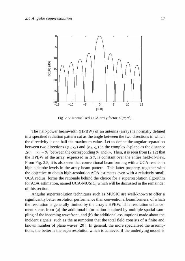
2.4 Angular superresolution 17
−15 −10 −5 0 5 10 15−30
−25
−20
−15
−10
−5
0
|θ−θ′|
D(θ
;θ′ )
(dB
)
Fig. 2.5: Normalised UCA array factor D(θ; θ ′).
The half-power beamwidth (HPBW) of an antenna (array) is normally definedin a specified radiation pattern cut as the angle between the two directions in whichthe directivity is one-half the maximum value. Let us define the angular separationbetween two directions (ϕ1, ζ1) and (ϕ2, ζ2) in the complex θ -plane as the distanceθ = |θ1 −θ2| between the corresponding θ1 and θ2. Then, it is seen from (2.12) thatthe HPBW of the array, expressed in θ , is constant over the entire field-of-view.From Fig. 2.5, it is also seen that conventional beamforming with a UCA results inhigh sidelobe levels in the array beam pattern. This latter property, together withthe objective to obtain high-resolution AOA estimates even with a relatively smallUCA radius, forms the rationale behind the choice for a superresolution algorithmfor AOA estimation, named UCA-MUSIC, which will be discussed in the remainderof this section.
Angular superresolution techniques such as MUSIC are well-known to offer asignificantly better resolution performance than conventional beamformers, of whichthe resolution is generally limited by the array’s HPBW. This resolution enhance-ment stems from (a) the additional information obtained by multiple spatial sam-pling of the incoming wavefront, and (b) the additional assumptions made about theincident signals, such as the assumption that the total field consists of a finite andknown number of plane waves [20]. In general, the more specialised the assump-tions, the better is the superresolution which is achieved if the underlying model is

18 High-resolution angle-of-arrival measurements: method
conformed to by the measured data. For a general review of superresolution AOAestimation algorithms, including their performance, sensitivity and limitations, thereader is referred to [17, 20, 21].
2.4.1 Beamspace processing
The elements of the vector u(θ) may be thought of as samples of the signal
u(γ, θ) = ej ζ cos(ϕ−γ ), (2.13)
which is periodic in γ with period 2π and can therefore be represented by the Fourierseries [19]
u(γ, θ) =∞∑
h=−∞j |h|ah(θ)e
− jhγ , (2.14)
of which the coefficients ah(θ) – which have the same magnitudes as, but are notequal to the Fourier coefficients j |h|ah(θ) – are found using (2.11) as
ah(θ) = J|h|(ζ )ejhϕ. (2.15)
Although the spectral width of the signal u(γ, θ) is infinite in theory, the magnitudesJ|h|(ζ ) of the Fourier coefficients decrease fast for |h| > ζ , and are in fact boundedby [13]
|J|h|(ζ )| ≤(ζe
2|h|)|h|
≤(πre
λ|h|)|h|
, h �= 0, (2.16)
where e, as before, is a constant with the value 2.71828 . . . . For sufficiently large|h|, the coefficients ah(θ) for which |h| > πre/λ become negligibly small. Aliasingcan hence be avoided by choosing the number of array elements (the spatial samplefrequency) M > 2πre/λ, and we are only interested in the non-negligible coeffi-cients ah(θ), −H ≤ h ≤ H , with H = �πre/λ�, where �·� is the largest integersmaller than the argument (entier function). Note that in the present case (r = 0.30m, λ � 0.15 m and M = 106 or M = 157), the above condition is well satisfied.
A unit-norm vector of coefficients
a(θ) = [a−H (θ), . . . , a0(θ), . . . , aH (θ)]T
(2.17)
can be obtained directly from u(θ) by the transformation
a(θ) = 1√M
CVu(θ), (2.18)
2.4 Angular superresolution 19
where
C = diag{
j −H , . . . , j 0, . . . , j −H},
V = 1√M
[v0, v1, . . . , vM−1
],
vm = [ω−mH, . . . , ω0, . . . , ωmH]T,
(2.19)
ω = exp( j 2π/M), which is based on the (2H + 1) × M submatrix of the spatialdiscrete Fourier transform [18, 22]. Multiplication of (2.8) by the matrix CV yields
z(τi ) = CVy(τi ) = A(i )s(i )(τi ) + n(τi ), (2.20)
where
A(i ) = √M[a(θ (i )1 ), a(θ (i )2 ), . . . , a(θ (i )N(i) )
],
n(τi ) = CVη(τi ).(2.21)
Processing of the array measurement data in the spatial frequency domain is re-ferred to as phase mode excitation-based beamspace processing [22] and has impor-tant advantages over element space processing, such as reduced sensitivity to noiseand modelling errors [17], and the possibility to employ forward/backward averag-ing [22], as will be discussed in Section 2.4.3.
2.4.2 UCA-MUSIC
The UCA-MUSIC algorithm uses the eigenstructure of the beamspace array outputcovariance matrix as a basis for AOA estimation. In the present case, covariancematrices are estimated for all time delay intervals
(iTc, (i + 1)Tc
), i = 0, 1, . . . ,
and for each interval UCA-MUSIC provides AOA estimates of the N (i ) multipathsignals that contribute to the measured channel response. The covariance matrixcorresponding to the i th delay bin can be expressed as
R(i ) = E{z(τi )z†(τi )
} = A(i )S(i )A(i )† + σ 2I, (2.22)
where S(i ) = [s(i )mn
]is the signal covariance matrix, of which the elements
s(i )mn = E{s(i )m (τi )s(i )†n (τi )
}(2.23)
represent the temporal correlations between pairs of signals. In the above expres-sions, E {·} denotes statistical expectation, and in (2.22) use has been made of thefact that CVV†C† = I.

20 High-resolution angle-of-arrival measurements: method
Let λ(i )1 ≥ λ(i )2 ≥ . . . ≥ λ
(i )L denote the L = 2H + 1 eigenvalues of R(i ),
and e(i )1 , e(i )2 , . . . , e(i )L the corresponding normalised eigenvectors. Provided that S (i )
is non-singular, A(i )S(i )A(i )† is of rank N(i ) , and it follows that λ(i )l > σ 2, l =1, . . . , N(i ), and λ(i )l = σ 2, l = N(i ) + 1, . . . , L, as long as N(i ) < L. Further-more, e(i )†l a(θ (i )n ) = 0, l = N(i ) + 1, . . . , L; n = 1, . . . , N(i ) , i.e., the eigenvectorsassociated with the L − N (i ) smallest eigenvalues (spanning the noise subspace) areorthogonal to the space spanned by the N (i ) beamspace steering vectors (the sig-nal subspace) [23]. MUSIC-based estimation algorithms exploit this orthogonalityproperty to form a null spectrum, which is in our case given by
Q(i )(θ) =L∑
l=N(i)+1
∣∣e(i )†l a(θ)∣∣2 = 1 −
N(i)∑l=1
∣∣e(i )†l a(θ)∣∣2. (2.24)
A two-dimensional search for the nulls of Q (i )(θ) over the full field-of-view yieldsunbiased and zero-variance estimates of the N (i ) actual AOAs, regardless of signal-to-noise ratio and angular spacing between the sources. The corresponding signalpowers, which are on the main diagonal of the matrix S (i ), are obtained via the least-squares solution to (2.22). Assuming the noise variance to be negligible comparedto the signal powers, S(i ) can be found using
S(i ) = (A(i )†A(i ))−1
A(i )†R(i )A(i ) (A(i )†A(i ))−1. (2.25)
Note that in practical applications of MUSIC-like estimation algorithms, onlyestimates of the actual covariance matrix R(i ) are available and it is therefore notpossible to obtain unbiased, zero-variance estimates of the AOAs.
2.4.3 Forward/backward averaging
Eigenstructure-based superresolution algorithms such as UCA-MUSIC fail when thesignal covariance matrix S(i ) – of which the elements are given by (2.23) – is singular,which occurs when two or more signals are perfectly correlated or coherent, i.e.,when at least one of the temporal correlation coefficients
ρ(i )t,mn = s(i )mn
E{∣∣s(i )m (τi )
∣∣}E{∣∣s(i )n (τi )∣∣} , m> n, (2.26)
ρ(i )t,mn = ρ
(i )∗t,nm, m < n, lies on the unit circle. The superscript “∗” denotes complex
conjugate. In the present case, signal coherence occurs only when two or moremultipaths have exactly the same propagation delay. However, in practice UCA-MUSIC will be less accurate when two or more signals are strongly correlated, i.e.,

2.4 Angular superresolution 21
when the difference between the delays of two multipaths is very small compared toTc.
In order to improve the UCA-MUSIC performance in a correlated signals sce-nario, the covariance matrix R(i ) can be forward/backward (FB) averaged prior to thecalculation of its eigenvalues and eigenvectors [22, 24]. The FB averaging techniquehinges on the fact that the beamspace array steering vector a(θ) is centro-Hermitian,which means that it satisfies Ja(θ) = a(θ)∗, where J is the reverse permutationmatrix1 [22].
The FB averaged covariance matrix is
R(i ) = 1
2
(R(i ) + JR(i )∗J
) = A(i )S(i )A(i )† + σ 2I, (2.27)
where
S(i ) = 1
2
(S(i ) + S(i )∗
)(2.28)
is the FB averaged signal covariance matrix. The eigenvalues of R(i ) are denotedby λ(i )1 ≥ λ
(i )2 ≥ . . . ≥ λ
(i )L and the corresponding normalised eigenvectors by
e(i )1 , e(i )2 , . . . , e(i )L .The elements of S(i ) can be expressed in terms of ρ (i )t,mn, the effective temporal
correlation coefficient after FB averaging, as
s(i )mn = ρ(i )t,mn E
{∣∣s(i )m (τi )∣∣} E
{∣∣s(i )n (τi )∣∣}. (2.29)
The coefficients ρ(i )t,mn and ρ(i )t,mn are related through
ρ(i )t,mn = Re
{ρ(i )t,mn
} = ∣∣ρ(i )t,mn
∣∣ cos(φ(i )mn), (2.30)
where φ(i )mn represents the phase difference between the signals s(i )m (τi ) and s(i )n (τi ).The result of the FB averaging preprocessing is that the magnitudes of the correlationcoefficients ρ(i )t,mn, m �= n, are effectively decreased, i.e., the signals are decorrelated.Thus, FB averaging improves the condition of the array output covariance matrixand consequently the performance of the UCA-MUSIC algorithm.
2.4.4 Effects of a finite data set
In practical applications of UCA-MUSIC the covariance matrix R(i ) is estimatedfrom a finite number of beamspace data snapshots z(τ i ;k), with τi ;k = τi + τk,
1The reverse permutation matrix J = [Jmn]
is defined by Jmn = δm,N−n, where N is the dimen-sion of the matrix and δmn is the Kronecker delta.

22 High-resolution angle-of-arrival measurements: method
k = 1, 2, . . . , K , where τk is a realisation of the random delay offset τ . Theresulting estimated covariance matrix is
R(i ) = 1
2K
K∑k=1
(z(τi ;k)z†(τi ;k) + Jz∗(τi ;k)zT(τi ;k)J
), (2.31)
with eigenvalues λ(i )1 ≥ λ(i )2 ≥ . . . ≥ λ
(i )L , and corresponding normalised eigenvec-
tors e(i )1 , e(i )2 , . . . , e(i )L . The estimated null spectrum can be written as
Q(i )(θ) =L∑
l=N(i)+1
∣∣e(i )†l a(θ)∣∣2 = 1 −
N(i)∑l=1
∣∣e(i )†l a(θ)∣∣2, (2.32)
and the AOA estimates are obtained by searching for its N (i ) deepest local minima.In general, the estimated matrix R(i ) differs from the true FB averaged covariancematrix R(i ), which causes a perturbation of the estimated null spectrum from thetrue null spectrum. This in turn causes errors in the AOA estimates and limits thecapability to discriminate between closely spaced sources (resolution threshold, viewSection 2.5).
Another consequence of the estimation of R(i ) from finite data is that the eigen-values become all different with probability one, so that it is no longer straight-forward to estimate the dimensionality of the noise subspace. However, an objectiveestimate of the number of multipath signals contributing to the considered time delaybin can be obtained by applying certain criteria from information theory such as FB-AIC (Akaike’s information criterion) and FB-MDL (minimum description length)[24]. The former scheme was originally proposed by Akaike [25] for application intime series analysis, later used for the estimation of the number of incident signalsin array processing [26], and then modified to work correctly when FB averaging isemployed [24]. According to the FB-AIC scheme, the number of signals is estimatedas the value of N(i ) that minimises the criterion
AIC(N(i )) = −K (M − N(i )) ln
L∏
l=N(i)+1
λ(i )l
1/(L−N(i))
1
L − N(i )
L∑l=N(i)+1
λ(i )l
, (2.33)
where ln denotes the natural logarithm. The relative performance of FB-AIC andFB-MDL was investigated in [24, 27] and is also addressed briefly in Section 2.6.2of this chapter.

2.5 Resolution threshold 23
2.4.5 Summary of the algorithm
The procedure to obtain high-resolution AOA estimates from a finite number of CIRsnapshots y(τ i ;k), i = 0, 1, . . . , k = 1, 2, . . . , K , measured at the elements of aUCA is summarised in the following. It is assumed that the phase drift resultingfrom the frequency difference between the transmitter and receiver frequency stan-dards has been compensated (cf. Section 2.2.2), and that the impulse response esti-mates are obtained at the exact positions represented by γ 0, γ1, . . . , γM−1.
For each delay interval(iTc, (i + 1)Tc
):
1. form the K beamspace array output vectors z(τi ;k) = CVy(τi ;k);
2. form the estimated covariance matrix R(i ) according to equation(2.31);
3. compute the L eigenvalues λ(i )l and corresponding normalised eigen-vectors e(i )l of R(i ), sorted in the order of descending eigenvalues;
4. evaluate the FB-AIC criterion (2.33) for N(i ) = 0, 1, . . . , L − 1, andselect the value of N(i ) that gives the lowest value;
5. using any non-linear minimisation method, find the values of θ inthe domain formed by 0 < ϕ < 2π and 0 < ζ < 2πr/λ thatare associated with the N(i ) deepest local minima of Q(i )(θ) =1 −∑N(i)
l=1 |e(i )†l a(θ)|2 and call them θ(i )1 , θ
(i )2 , . . . , θ
(i )
N(i);
6. reconstruct the matrix A(i ) = √M[a(θ (i )1 ), a(θ (i )2 ), . . . , a(θ (i )
N(i))];
7. compute the matrix S(i ) = (A(i )†A(i ))−1 A(i )†R(i )A(i )
(A(i )†A(i )
)−1.
The complex values θ (i )n , n = 1, 2, . . . , N(i ) represent the estimated AOAs and theelements on the main diagonal of S(i ) are the corresponding estimated signal powers.
2.5 Resolution threshold
The UCA-MUSIC algorithm, like other eigenstructure-based techniques, can exactlydetermine the AOAs of any two closely spaced sources when the true covariance ma-trix of the array output data is available. In practice, however, the covariance matrixis estimated from a finite set of snapshots. The deviation between the estimated andthe true covariance matrices produces a perturbation of the null spectrum, which in

24 High-resolution angle-of-arrival measurements: method
turn causes biased estimates and limits the capability of the algorithm to discriminatebetween closely spaced sources. The objective of this section is to derive an expres-sion for the resolution threshold of UCA-MUSIC, which is the signal-to-noise ratio(SNR) below which two closely spaced multipath waves, with equal signal powersP, can no longer be “resolved”, i.e. when the null spectrum at either of the two trueAOAs, which will be called θ1 and θ2, is greater than at the angle θm = (θ1 + θ2)/2between the true AOAs with more than 50% probability. The notation used in thissection is the same as in the previous sections, but, for convenience, the superscripts“(i )” will be omitted.
General expressions for the mean of the MUSIC null spectrum, generated from aFB averaged covariance matrix estimated from finite data, were derived in [28] andlater used in [27]. Neglecting terms of order 1/K 2, the mean null spectrum for twosources is given by
E{Q(θ)
} = Q(θ)+ 1
2K
2∑l=1
λlσ2
(λl − σ 2)2
[(L − 2)
∣∣e†l a(θ)
∣∣2 − Q(θ)], (2.34)
Here, λl , el and Q(θ) are the eigenvalues, normalised eigenvectors and null spec-trum, respectively, corresponding with the FB averaged ensemble covariance matrixR. The resolution threshold ξT is found as the smallest SNR for which the inequality
E{Q(θl )
} ≤ E{Q(θm)
}, l = 1, 2 (2.35)
is satisfied [27].With the aid of (2.34) and a derivation similar to that in [27], the expectations
in (2.35) can be expressed in terms of the two largest eigenvalues µ l = λl − σ 2,l = 1, 2, of the “noise-free” covariance matrix
ASA = M P[a(θ1), a(θ2)
] [ 1 ρt
ρt 1
] [a(θ1), a(θ2)
]†= M P
[e1, e2
] [µ′1 0
0 µ′2
] [e1, e2
]†,
(2.36)
in which ρt = ρt,12 denotes the temporal correlation between the two signals afterFB averaging (cf. Section 2.4.3) and µ′
l = µl /M P. This yields
E{Q(θl )
} = L − 2
2K
{− 1
M2ξ2µ′1µ
′2
+ 1 − ρ2s
Mξµ′1µ
′2
[1 + µ′
1 + µ′2
Mξµ′1µ
′2
]}, l = 1, 2,
(2.37)
2.5 Resolution threshold 25
and
E{Q(θm)
} =Q(θm)+ L − 2
2K
{(µ′
1 + µ′2)− 2ρ2
m(1 + ρt )
Mξµ′1µ
′2
+ (µ′21 + µ′
1µ′2 + µ′2
2 )− 2ρ2m(1 + ρt )(µ
′1 + µ′
2)
M2ξ2µ′21 µ
′22
},
(2.38)
where ξ = P/σ 2 is the SNR of each of the signals, ρs = a†(θ1)a(θ2) is the spatialcorrelation between the sources, and ρm = a†(θ1)a(θm) = a†(θ2)a(θm) is the spatialcorrelation between either one of the sources and a wave arriving from the directioncorresponding with θm. By using Graf’s addition theorem for Bessel functions [19],it can be shown that
ρs = J0(θ) and ρm = J0(θ/2), (2.39)
where θ = |θ1 − θ2| denotes the difference between the “angles” θ1 and θ2.The resolution threshold ξT is obtained by solving the quadratic equation that
results after equating (2.37) and (2.38). Using a derivation similar to that in [28], itfollows from equation (2.36) that
µ′l = 1 + ρsρt ± ∣∣ρs + ρt
∣∣, l = 1, 2. (2.40)
This leads to the following closed-form expression for ξ T :
ξT = L − 2
4K M Q(θm)A
{1 +
√1 + 8K Q(θm)
L − 2B
}, (2.41)
where A and B are given by
A = (1 − ρ2s)+ 2ρ2
m(1 + ρt)− 2(1 + ρsρt)[1 − Q(θm)
](1 − ρ2
s )(1 − ρ2t )
, (2.42)
B = 2(1 + ρsρt )
(1 − ρ2s)+ 2ρ2
m(1 + ρt)− 2(1 + ρsρt)[1 − Q(θm)
] . (2.43)
Note from (2.41) that the resolution threshold is inversely proportional to K , thenumber of snapshots, and reduces to zero for K → ∞. This means that resolutionis always achieved if the true covariance matrix is exactly known, regardless of theSNR or the spacing between the AOAs.
For the evaluation of the null spectrum height Q(θm), use is made of the follow-ing expression for the normalised eigenvectors:
el = a(θ1)± a(θ2)∣∣a(θ1)± a(θ2)∣∣, l = 1, 2, (2.44)
26 High-resolution angle-of-arrival measurements: method
which, again, is obtained from a derivation similar to that in [28]. This yields
Q(θm) = 1 − ∣∣e1a(θm)∣∣2 − ∣∣e2a(θm)
∣∣2 = 1 − 2ρ2m
1 + ρs. (2.45)
The resolution threshold for two sources of equal power, as derived here for thespecial case of a UCA, is a very useful performance parameter for AOA estimationalgorithms, and is often used in the published literature. It should be noted, however,that the superposition principle does not hold for non-linear superresolution algo-rithms such as UCA-MUSIC. One must therefore be very careful in extrapolatingresults obtained from (2.41) to a larger number of sources or to other more generalcases.
2.6 Numerical results
Computer simulations of the performance of the UCA-MUSIC algorithm and theeffect of FB averaging preprocessing are presented in this section. As in the previoussection, the superscripts “(i)” are omitted.
2.6.1 Resolution threshold
First, simulations are shown of the resolution threshold ξ T for two equipoweredmultipath signals, for which a theoretical expression was derived in the previoussection. Fig. 2.6 shows simulated and theoretical values of ξ T , as a function of theangular spacing θ = |θ2 − θ1|, and for different propagation delay differencesT = T2 − T1. In the simulation, the considered delay interval is the zeroth bin(0, Tc), the AOAs of the multipath components are equal to θ 1,2 = ±θ/2, θbeing a real number, their delay times are T1,2 = (Tc ±T)/2, and their SNRs are
ξn = E{∣∣sn(τi )
∣∣2}σ 2
= 1
σ 2Tc
∫ Tc
0
∣∣sn(τi )∣∣2dτ, n = 1, 2. (2.46)
The simulated noise was produced by a pseudorandom normal number generator.The number of snapshots was taken to be K = 20, and all other parameters werechosen the same as for the Ericsson measurement system described in Section 2.2(M = 106, Tc = 20 ns). Each of the simulated threshold values in Fig. 2.6 is basedon 50 independent trials.
The theoretical and simulated results presented in Fig. 2.6 show reasonable togood agreement. As expected, the resolution capability of UCA-MUSIC is observedto decrease with decreasing T (and hence increasing signal correlation). With FBaveraging however, the signal correlation is effectively reduced and the performance

2.6 Numerical results 27
0 0.5 1 1.5 20
5
10
15
20
25
30
35
40
∆θ = |θ2−θ
1|
ξ T (
dB)
φ12
=0
φ12
=π/2
φ12
=π
(a)
0 0.5 1 1.5 20
5
10
15
20
25
30
35
40
∆θ = |θ2−θ
1|
ξ T (
dB)
φ12
=0
φ12
=π/2
φ12
=π
(b)
Fig. 2.6: Theoretical and simulated resolution thresholds, for propagation delay differences(a) T = 0.5Tc and (b) T = 0.1Tc. M = 106, K = 20, Tc = 20 ns. “Closed” markers
correspond with FB averaging; “open” markers represent performance without FBaveraging. Simulated thresholds are based on 50 independent trials.

28 High-resolution angle-of-arrival measurements: method
degradation is therefore only limited, except when the phase difference φ 12 betweenthe signals is either 0 or π . The small improvements due to FB averaging for φ 12 = 0and φ12 = π that can still be seen in Fig. 2.6 are the result of the fact that this schemeeffectively doubles the number of snapshots [24]. Because the array’s directionalproperties are uniform in the complex θ -plane, the above results are representativeof the resolution capability over the entire field-of-view. Also, they are independentof the array radius r and the wavelength λ, which are both included in the definitionof θ (view Section 2.3).
In comparison with conventional beamforming, of which the capability to re-solve two equipowered waves is generally limited by the array HPBW (θ−3dB �2.2, cf. Fig. 2.5), the resolution performance of UCA-MUSIC is considerably bet-ter – except in the exceptional case of weak, highly correlated signals with a phasedifference near 0 or π .
2.6.2 Estimation of the number of signals
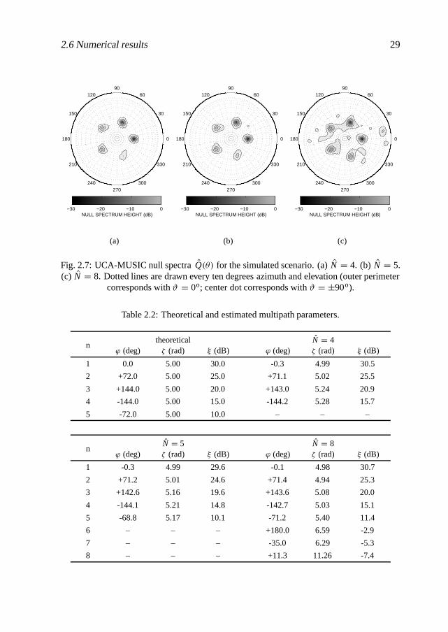
In addition to the foregoing resolution considerations, simulations were made to il-lustrate how poor estimates of the number of paths N impact the UCA-MUSIC nullspectrum and the AOA estimation. To this end, a scenario with five incident multi-path waves was simulated, with the parameters given in Table 2.2. The signal phasesφn and delays Tn were chosen randomly. Fig. 2.7(a)-(c) show the null spectrum forN = 4, 5 and 8, respectively. The corresponding estimated AOAs and SNRs aregiven in the table.
From Fig. 2.7 it is observed that a modest under- or overestimation of N does notlead to dramatic changes of the null spectrum. Increasing underestimation of N gen-erally leads to shallower local minima, and ultimately to the vanishing of the localminima corresponding with the weakest multipath waves. A modest overestimationof N introduces spurious local minima which, however, hardly alter the positionsof the deeper nulls corresponding with the true AOAs. Table 2.2 shows that theestimated signal powers of the falsely detected waves are all around or below thenoise level, and therefore insignificant in comparison with the dominant multipathsignals which are of primary interest. From these observations it is concluded thatit is better to tolerate a small overestimation of N than to underestimate the numberof incident waves, which would lead to undetected multipath contributions. Of theavailable objective criteria for detecting the number of sources from a FB averagedcovariance matrix, FB-AIC and FB-MDL [24], the former scheme provides slightlyhigher estimates of N for a small number of snapshots. Furthermore, for the sce-nario considered in [27], this scheme was shown to offer the highest probability ofcorrectly detecting the number of waves for small values of K .
2.6 Numerical results 29
30
210
60
240
90
270
120
300
150
330
180 0
NULL SPECTRUM HEIGHT (dB)−30 −20 −10 0
(a)
30
210
60
240
90
270
120
300
150
330
180 0
NULL SPECTRUM HEIGHT (dB)−30 −20 −10 0
(b)
30
210
60
240
90
270
120
300
150
330
180 0
NULL SPECTRUM HEIGHT (dB)−30 −20 −10 0
(c)
Fig. 2.7: UCA-MUSIC null spectra Q(θ) for the simulated scenario. (a) N = 4. (b) N = 5.(c) N = 8. Dotted lines are drawn every ten degrees azimuth and elevation (outer perimeter
corresponds with ϑ = 0o; center dot corresponds with ϑ = ±90o).
Table 2.2: Theoretical and estimated multipath parameters.
theoretical N = 4n
ϕ (deg) ζ (rad) ξ (dB) ϕ (deg) ζ (rad) ξ (dB)
1 0.0 5.00 30.0 -0.3 4.99 30.5
2 +72.0 5.00 25.0 +71.1 5.02 25.5
3 +144.0 5.00 20.0 +143.0 5.24 20.9
4 -144.0 5.00 15.0 -144.2 5.28 15.7
5 -72.0 5.00 10.0 – – –
N = 5 N = 8n
ϕ (deg) ζ (rad) ξ (dB) ϕ (deg) ζ (rad) ξ (dB)
1 -0.3 4.99 29.6 -0.1 4.98 30.7
2 +71.2 5.01 24.6 +71.4 4.94 25.3
3 +142.6 5.16 19.6 +143.6 5.08 20.0
4 -144.1 5.21 14.8 -142.7 5.03 15.1
5 -68.8 5.17 10.1 -71.2 5.40 11.4
6 – – – +180.0 6.59 -2.9
7 – – – -35.0 6.29 -5.3
8 – – – +11.3 11.26 -7.4

30 High-resolution angle-of-arrival measurements: method
2.7 Experimental results
This section discusses the results of two measurements carried out in a residen-tial area in Leidschendam, The Netherlands, which is characterised by 5-15 m highbuildings, scattered vegetation, and low traffic density (view Fig. 2.8). The objec-tive of the measurements was to determine whether the method described in thischapter can be used in real built-up environments to identify the dominant propaga-tion mechanisms. The channel sounding system used was the Ericsson equipment,and the carrier frequency was 1900 MHz. The transmitting antenna was located ina tower at 46 m above ground level, well above the average rooftop level of mostother buildings in the area. This was done to prevent “complex” propagation paths,resulting from multiple interactions with the environment, from becoming impor-tant. The antenna was a 7.1-dBi vertically polarised double-ridged pyramidal hornantenna with an azimuthal 3-dB beamwidth of 53o and a bandwidth (defined withrespect to the VSWR) covering the frequency region from 1 to 18 GHz. During themeasurements described in this section, it was pointed south-east. The number ofsnapshots taken for each measurement was K = 20.
Figs. 2.9 and 2.10 show the temporal and angular multipath distributions mea-sured at the two mobile station (MS) locations indicated in Fig. 2.8, together with360-degree panorama photographs taken from the receiver perspective, which serveas an accurate angular reference. In these figures, the marker size indicates the am-
86.5 86.6 86.7 86.8 86.9 87 87.1 87.2455.4
455.5
455.6
455.7
455.8
X (km)
Y (
km)
0
10
20
30
40
50
BU
ILD
ING
HE
IGH
T (m
)
2
TX
BL
AF
BKBR
WL1
B
Fig. 2.8: Map of the measurement site. Gray levels indicate building heights.
2.7 Experimental results 31
0.5
1
1.5
2
2.5
−100−80−60
TIM
E D
ELA
Y (µ
s)
POWER DENSITY(dBm/T
c)
0 dB −10 dB −20 dBζ
(RA
D)
0
5
10
15
AZIMUTH ANGLE (DEG)
BR T1 WL
−100−50050100150200
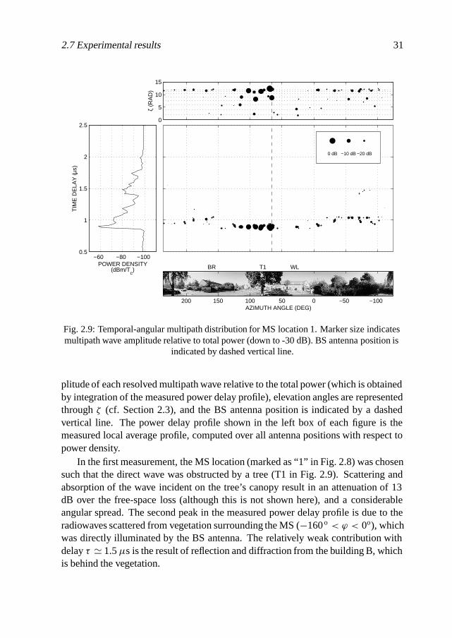
Fig. 2.9: Temporal-angular multipath distribution for MS location 1. Marker size indicatesmultipath wave amplitude relative to total power (down to -30 dB). BS antenna position is
indicated by dashed vertical line.
plitude of each resolved multipath wave relative to the total power (which is obtainedby integration of the measured power delay profile), elevation angles are representedthrough ζ (cf. Section 2.3), and the BS antenna position is indicated by a dashedvertical line. The power delay profile shown in the left box of each figure is themeasured local average profile, computed over all antenna positions with respect topower density.
In the first measurement, the MS location (marked as “1” in Fig. 2.8) was chosensuch that the direct wave was obstructed by a tree (T1 in Fig. 2.9). Scattering andabsorption of the wave incident on the tree’s canopy result in an attenuation of 13dB over the free-space loss (although this is not shown here), and a considerableangular spread. The second peak in the measured power delay profile is due to theradiowaves scattered from vegetation surrounding the MS (−160 o < ϕ < 0o), whichwas directly illuminated by the BS antenna. The relatively weak contribution withdelay τ � 1.5µs is the result of reflection and diffraction from the building B, whichis behind the vegetation.
32 High-resolution angle-of-arrival measurements: method
1.5
2
2.5
3
3.5
−100−80−60
TIM
E D
ELA
Y (µ
s)
POWER DENSITY(dBm/T
c)
0 dB −10 dB −20 dB
ζ (R
AD
)
0
5
10
15
AZIMUTH ANGLE (DEG)
BL AF BK
−50050100150200250
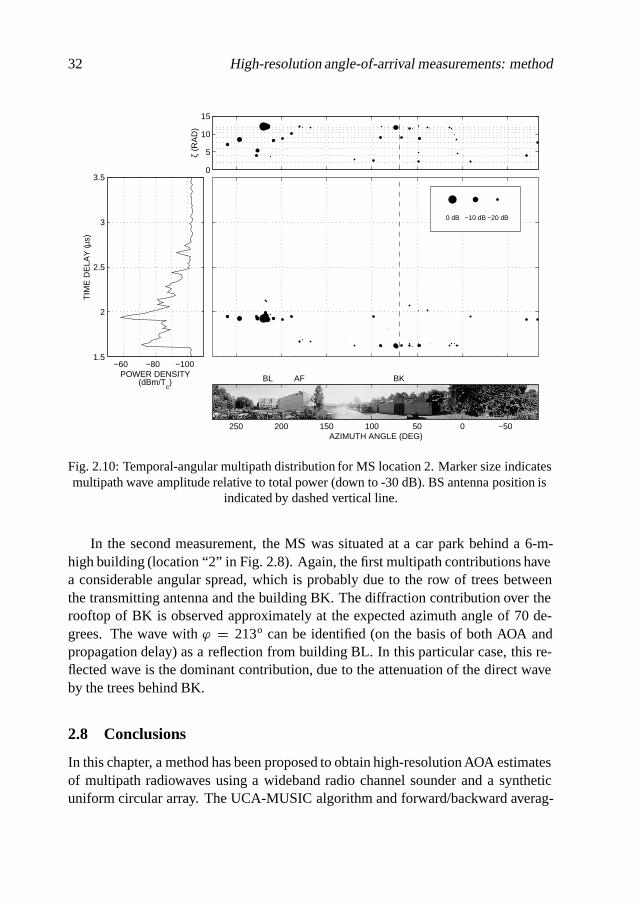
Fig. 2.10: Temporal-angular multipath distribution for MS location 2. Marker size indicatesmultipath wave amplitude relative to total power (down to -30 dB). BS antenna position is
indicated by dashed vertical line.
In the second measurement, the MS was situated at a car park behind a 6-m-high building (location “2” in Fig. 2.8). Again, the first multipath contributions havea considerable angular spread, which is probably due to the row of trees betweenthe transmitting antenna and the building BK. The diffraction contribution over therooftop of BK is observed approximately at the expected azimuth angle of 70 de-grees. The wave with ϕ = 213o can be identified (on the basis of both AOA andpropagation delay) as a reflection from building BL. In this particular case, this re-flected wave is the dominant contribution, due to the attenuation of the direct waveby the trees behind BK.
2.8 Conclusions
In this chapter, a method has been proposed to obtain high-resolution AOA estimatesof multipath radiowaves using a wideband radio channel sounder and a syntheticuniform circular array. The UCA-MUSIC algorithm and forward/backward averag-

2.8 Conclusions 33
ing were demonstrated to be suitable algorithms for the high-resolution estimationof two-dimensional (azimuth and elevation) AOAs from complex impulse responsemeasurement data obtained with this array configuration. Problems of the algorithmwith respect to robustness to noise, which were expected by the authors of [13], werenot experienced. The problem of the a priori estimation of the number of incidentsignals based on a finite set of measurement data was solved by applying a modifiedversion of Akaike’s information criterion (FB-AIC) [24].
Expressions were derived for the theoretical resolution capability of the UCA-MUSIC algorithm. The achievable angular resolution was shown to depend on anumber of factors, including the signal-to-noise ratio, the temporal correlation be-tween the signals and the number of snapshots. Roughly, for the array radius consid-ered in the present work, an azimuthal resolution better than 5 degrees is achievableif K = 20 or higher, and if the incidence directions of the incident waves are closeto horizontal. For high elevation angles, the resolution capability is relatively poor.
It was demonstrated that the combination of high-resolution AOA estimates andtime delay information enables the identification of the dominant multipaths in anactual built-up environment. The determination of the elevation angles of the ra-diowaves permits one to obtain additional information about the nature of the in-volved propagation mechanisms.

34 High-resolution angle-of-arrival measurements: method

3High-resolution angle-of-arrival
measurements: results
3.1 Introduction
In the previous chapter, a method was presented for the measurement, with high res-olution, of the angle-of-arrival (AOA) of multipath radiowaves. Experimental resultsobtained in a suburban environment with the base station antenna above the rooftoplevel were provided to demonstrate the capability of the method to identify the dom-inant propagation mechanisms in realistic built-up environments. In the frameworkof a collaboration between the TU/e, KPN and Swisscom (formerly Swiss TelecomPTT), measurements of this type were also carried out in urban environments in Bernand Fribourg, Switzerland, under microcellular conditions, i.e. with the simulatedbase station antenna under the rooftop level. The objective of these measurementswas to verify and possibly improve the accuracy of existing propagation predictionmodels. In particular, an investigation was made of the dominant propagation mech-anisms in urban microcell environments. A selection of the results of these measure-ments is presented in this chapter. In addition, results are shown of experiments thatwere conducted later to further investigate the propagation mechanisms identified inthe Swiss measurement campaign.
Section 3.2 provides experimental results that identify the transmission of ra-
36 High-resolution angle-of-arrival measurements: results
diowaves through buildings as an important propagation mechanism in configura-tions where the line-of-sight path is obstructed by a building or a row of buildings.In Section 3.3 it is shown that, under certain circumstances, scattering from trees canplay a prominent role. Conclusions are drawn in Section 3.4.
3.2 Transmission through buildings
Most existing deterministic propagation models developed for propagation predic-tion in urban microcell environments treat the buildings as being opaque, i.e. trans-mitted field contributions are neglected. In fact, the assumption that the first build-ings surrounding the base station antenna obstruct the radiated field, and thus largelyconfine the signal power to the area enclosed by them, is at the heart of the micro-cellular concept. In [29], Rizk observed that, for some particular configurations, ex-isting propagation models seriously underestimate the field strength behind the firstrow of buildings. A possible explanation for this discrepancy is that, contrary to thecommonly made assumption mentioned above, the buildings in this scenario werenot opaque at UHF frequencies, and were “leaking” a significant portion of the fieldincident on them. In view of this, it is of interest to obtain a better understanding ofthe propagation phenomena responsible for the field directly behind buildings, andto investigate whether transmission through buildings is an important one of them.
This section presents results of high-resolution AOA measurements conductedbehind a building, or a row of buildings, obstructing the line-of-sight propagationpath to the base station antenna. The first of these measurements were carried outin a realistic urban microcell environment in Bern, Switzerland, using the Ericssonchannel sounding equipment (view Table 2.1) at 2000 MHz. They are describedin Section 3.2.1. Section 3.2.2 discusses an additional AOA measurement, whichwas conducted in a more “controlled” environment, using the TU/e equipment, at acarrier frequency of 1900 MHz.
3.2.1 Realistic urban microcell environment – Bern
The area in Bern selected for the measurements, which is depicted in Fig. 3.1, ischaracterised by a relatively regular street pattern, narrow streets (10-15 m) facedby three- to five-storey concrete buildings with irregular faces – primarily causedby balconies and windows. Scattered trees are found in the entire area, as well asparked cars along the curbs. The traffic density in the area is low, except in RodtmattStreet, which is wider than the other streets in the area. A vertically polarised, 3-dBi, omnidirectional base station antenna was located in the middle of the area, at aheight of 5 m. This location is marked as “BS” in Fig. 3.1.
In an earlier study conducted by Swisscom and reported in [29], narrowband
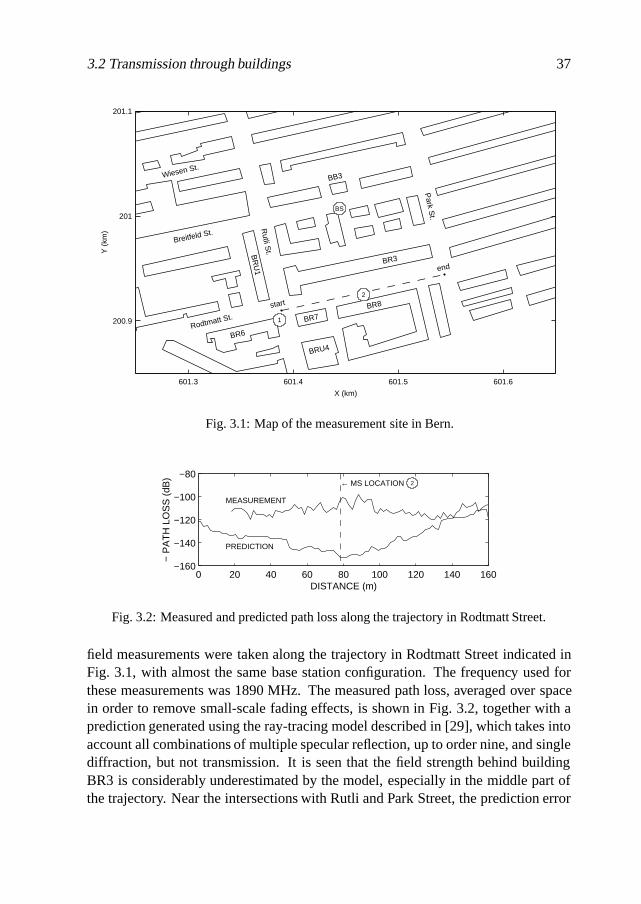
3.2 Transmission through buildings 37
601.3 601.4 601.5 601.6
200.9
201
201.1
BS
X (km)
Y (
km)
start
end
1
2
BR3
BR8
BB3
BR
U1
BRU4
BR6
BR7
Wiesen St.
Rodtmatt St.
Breitfeld St.
Rutli S
t.
Park S
t.
Fig. 3.1: Map of the measurement site in Bern.
0 20 40 60 80 100 120 140 160−160
−140
−120
−100
−80
DISTANCE (m)
− P
AT
H L
OS
S (
dB)
MEASUREMENT
PREDICTION
← MS LOCATION 2
Fig. 3.2: Measured and predicted path loss along the trajectory in Rodtmatt Street.
field measurements were taken along the trajectory in Rodtmatt Street indicated inFig. 3.1, with almost the same base station configuration. The frequency used forthese measurements was 1890 MHz. The measured path loss, averaged over spacein order to remove small-scale fading effects, is shown in Fig. 3.2, together with aprediction generated using the ray-tracing model described in [29], which takes intoaccount all combinations of multiple specular reflection, up to order nine, and singlediffraction, but not transmission. It is seen that the field strength behind buildingBR3 is considerably underestimated by the model, especially in the middle part ofthe trajectory. Near the intersections with Rutli and Park Street, the prediction error
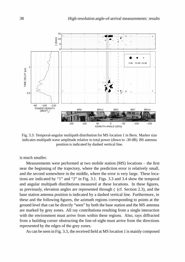
38 High-resolution angle-of-arrival measurements: results
0.5
1
−120−100−80
TIM
E D
ELA
Y (µ
s)
POWER DENSITY(dBm/T
c)
0 dB −10 dB −20 dB
ζ (R
AD
)
0
5
10
15
AZIMUTH ANGLE (DEG)
BRU1 BR3BR6 BR7 BRU4
−150−100−50050100150
Fig. 3.3: Temporal-angular multipath distribution for MS location 1 in Bern. Marker sizeindicates multipath wave amplitude relative to total power (down to -30 dB). BS antenna
position is indicated by dashed vertical line.
is much smaller.Measurements were performed at two mobile station (MS) locations – the first
near the beginning of the trajectory, where the prediction error is relatively small,and the second somewhere in the middle, where the error is very large. These loca-tions are indicated by “1” and “2” in Fig. 3.1. Figs. 3.3 and 3.4 show the temporaland angular multipath distributions measured at these locations. In these figures,as previously, elevation angles are represented through ζ (cf. Section 2.3), and thebase station antenna position is indicated by a dashed vertical line. Furthermore, inthese and the following figures, the azimuth regions corresponding to points at theground level that can be directly “seen” by both the base station and the MS antennaare marked by grey zones. All ray contributions resulting from a single interactionwith the environment must arrive from within these regions. Also, rays diffractedfrom a building corner obstructing the line-of-sight must arrive from the directionsrepresented by the edges of the grey zones.
As can be seen in Fig. 3.3, the received field at MS location 1 is mainly composed

3.2 Transmission through buildings 39
0
0.5
1
−120−100−80−60
TIM
E D
ELA
Y (µ
s)
POWER DENSITY(dBm/T
c)
0 dB −10 dB −20 dBζ
(RA
D)
0
5
10
15
AZIMUTH ANGLE (DEG)
BR3BR8
−150−100−50050100150200
Fig. 3.4: Temporal-angular multipath distribution for MS location 2 in Bern. Marker sizeindicates multipath wave amplitude relative to total power (down to -30 dB). BS antenna
position is indicated by dashed vertical line.
of contributions due to multipath radiowaves propagating through Breitfeld Street,around the corner with Rutli Street and then on to the receiver. The fact that mostwaves arrive from outside the grey area indicates that they are the result of repeatedinteractions with the buildings, e.g. of multiple reflection between the buildings onboth sides of the streets. These observations are in agreement with the results of theprediction. The AOAs of the very first contributions arriving at the MS are close tothe direction of the base station antenna. As their elevation angles are relatively high,these waves are most likely the result of propagation over building BR3. However,their contribution to the total received field is negligible.
According to the propagation model used to produce the prediction of Fig. 3.2,the field received at MS location 2 is composed of multipath waves propagatingaround both sides of the building block between Breitfeld Street and Rodtmatt Street.Because the reflection and diffraction losses associated with these propagation pathsare high, the predicted field strength for this scenario is very low. Fig. 3.4 shows thetemporal-angular multipath distribution measured at this MS location. The received

40 High-resolution angle-of-arrival measurements: results
field is dominated by a series of strong contributions arriving from the direction ofbuilding BR3. For the corresponding time delays, the average power delay profileshows two high peaks, which can be determined to be 28 and 35 dB below the free-space level. The ζ -values of these contributions show that they cannot be the resultof over-rooftop propagation (for which the elevation angle ϑ should be greater than25o, or ζ < 11.4 radians), but must result from transmission through BR3. The smallangular spread of these multipath waves is probably the result of multiple scatteringtaking place inside the building. The waves arriving from ϕ � 200 o are reflectedfrom building BR8, which is on the other side of the MS.
The second peak of the measured power delay profile appears as a second clus-ter of points in Fig. 3.4. The time delay difference between both clusters suggeststhat the second contribution is due to reflection from building BB3 (with reflectioncoefficient -7 dB) and subsequent transmission through BR3.
3.2.2 Controlled environment
Additional AOA measurements behind buildings were later carried out on the TU/ecampus, which is a more “controlled” environment than most real urban microcellenvironments: during weekends, it was possible to perform measurements in the ab-sence of disturbing factors such as traffic, parked cars and people inside and aroundthe buildings. The results shown here were obtained for the configuration of Fig. 3.5,in which the building TR obstructs the line-of-sight path between the base station an-tenna – a vertically polarised, 12-dBi, omnidirectional antenna with a vertical 3-dBbeamwidth of 6o, placed at a height of 6.5 m – and the mobile station. A detaileddescription of this building is given in Section 4.4.2.
0.7 0.75 0.8 0.85 0.9 0.95 10.4
0.45
0.5
0.55
0.6
X (km)
Y (
km)
BS
MS
TR
LP
EH
PT
Fig. 3.5: Map of the measurement site on the TU/e campus.
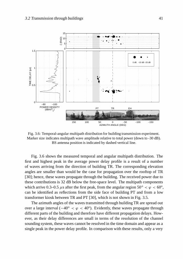
3.2 Transmission through buildings 41
0
0.5
1
1.5
−100−80
TIM
E D
ELA
Y (µ
s)
POWER DENSITY(dBm/T
c)
0 dB −10 dB −20 dBζ
(RA
D)
0
5
10
15
AZIMUTH ANGLE (DEG)
EHTRPT
−150−100−50050100150
Fig. 3.6: Temporal-angular multipath distribution for building transmission experiment.Marker size indicates multipath wave amplitude relative to total power (down to -30 dB).
BS antenna position is indicated by dashed vertical line.
Fig. 3.6 shows the measured temporal and angular multipath distribution. Thefirst and highest peak in the average power delay profile is a result of a numberof waves arriving from the direction of building TR. The corresponding elevationangles are smaller than would be the case for propagation over the rooftop of TR[30]; hence, these waves propagate through the building. The received power due tothese contributions is 32 dB below the free-space level. The multipath componentswhich arrive 0.3–0.5 µs after the first peak, from the angular region 50o < ϕ < 60o,can be identified as reflections from the side face of building PT and from a lowtransformer kiosk between TR and PT [30], which is not shown in Fig. 3.5.
The azimuth angles of the waves transmitted through building TR are spread outover a large interval (−40o < ϕ < 40o). Evidently, these waves propagate throughdifferent parts of the building and therefore have different propagation delays. How-ever, as their delay differences are small in terms of the resolution of the channelsounding system, these waves cannot be resolved in the time domain and appear as asingle peak in the power delay profile. In comparison with these results, only a very

42 High-resolution angle-of-arrival measurements: results
small angular spread is observed at MS location 2 in Bern (view Fig. 3.4). This isprobably a result of the fact that only a small part of the obstructing building BR3was directly illuminated by the base station antenna, as can be seen in Fig. 3.1.
3.3 Scattering from trees
Scattering of radiowaves from objects such as trees has been brought up in severalstudies as a possible explanation for observed discrepancies between field strengthpredictions and measurements in urban microcell environments – especially for sce-narios in which propagation around street corners is important [31, 32]. It has provedto be difficult or even impossible, however, to obtain hard evidence for the signifi-cance of this phenomenon from conventional, narrowband field measurements. Themeasurement technique described in the previous chapter makes it possible to sepa-rate scattered waves from other multipath components, and is therefore more suitablefor this purpose.
Section 3.3.1 presents AOA measurement results obtained in an urban microcellconfiguration in Fribourg, Switzerland, which provide evidence for the importanceof scattering from vegetation. These measurements were performed at 2000 MHz,using the Ericsson channel sounding equipment (view Table 2.1). In Section 3.3.2,results are shown of a measurement on a single tree, conducted using the TU/e equip-ment, at a carrier frequency of 1900 MHz.
3.3.1 Realistic urban microcell environment – Fribourg
A plan of the area in Fribourg selected for the AOA experiments is shown in Fig. 3.7.This environment is characterised by four- to six-storey concrete buildings with ir-regular faces (balconies and windows), trees lining both sides of the main street (Per-olles), and moderate to high traffic density. Cars are parked along the curbs. A smallpark with trees is located opposite to one of the side streets (Jacques-Gachoud). Thelocation of this park is sketched in the plan. In the recent past, Swisscom performedextensive measurements in the area of Fig. 3.7 [29, 31]. One of the results of thesemeasurements was that the received field strength could not be predicted satisfac-torily using a model based on reflection and diffraction. This was conjectured tobe a result of inadequate modelling of the mechanisms responsible for propagationaround the street corners, particularly the neglect of tree scattering effects. The AOAexperiments discussed in the following were performed to verify this hypothesis.
A vertically polarised, 3-dBi, omnidirectional base station antenna was placedat the location indicated by “BS” in Fig. 3.7. The base station antenna height was 5m. Results obtained at two MS locations in Perolles Street, which are indicated inthe same figure, are shown in Figs. 3.8 and 3.10. As before, the grey zones in these

3.3 Scattering from trees 43
−0.1 0 0.1 0.2−0.2
−0.1
0
PARKBS
X (km)
Y (
km)
1
2
BP2
BP3
BP4
BP5
BP7
BP8
BP9
BP10
Perolles St.
Industrie St.
Jacq
ues−Gach
oud St.
Fig. 3.7: Map of the measurement site in Fribourg.
figures indicate the angular regions in which points at the ground level can be “seen”directly by both the base station and the MS antenna.
The first contributions received at MS location 1 arrive from the direction ofthe street in which the base station is located (Jacques-Gachoud). These waves arethe result of (multiple) reflection between the buildings BP4 and BP5, possibly fol-lowed by diffraction from BP4 or BP5. The strongest contributions, however, arrivefrom the angular region −30o < ϕ < 10o, corresponding with the park opposite toJacques-Gachoud Street. The objects in this region, which was directly illuminatedby the base station, are mostly trees (view Fig. 3.9). The waves from this region aretherefore, most likely, the result of scattering from trees. The total bistatic scatteringcross section of these scatterers can be estimated using the bistatic radar equation,and the resulting value of 60 m2 is in good agreement with the theoretical value fora number of large trees (view Section 5.5.3). The waves arriving from directions inthe interval 75o < ϕ < 120o are the result of scattering from the trees in the park,and subsequent reflection from building BP5.
Theoretically, the field received at MS location 2 is dominated by third- andhigher-order reflected rays arriving from the direction of building BP9 [33]. Contri-butions reflected from this building are indeed visible in the measurement results

44 High-resolution angle-of-arrival measurements: results
0
0.5
1
−100−80−60
TIM
E D
ELA
Y (µ
s)
POWER DENSITY(dBm/T
c)
0 dB −10 dB −20 dB
ζ (R
AD
)
0
5
10
15
AZIMUTH ANGLE (DEG)
BP5 BP9 BP10BP4
−200−150−100−50050100
Fig. 3.8: Temporal-angular multipath distribution for MS location 1 in Fribourg. Markersize indicates multipath wave amplitude relative to total power (down to -30 dB). BS
antenna position is indicated by dashed vertical line.
AZIMUTH ANGLE (DEG)−40−30−20−1001020
Fig. 3.9: Enlarged section of the panorama photograph taken at MS location 1 in Fribourg.
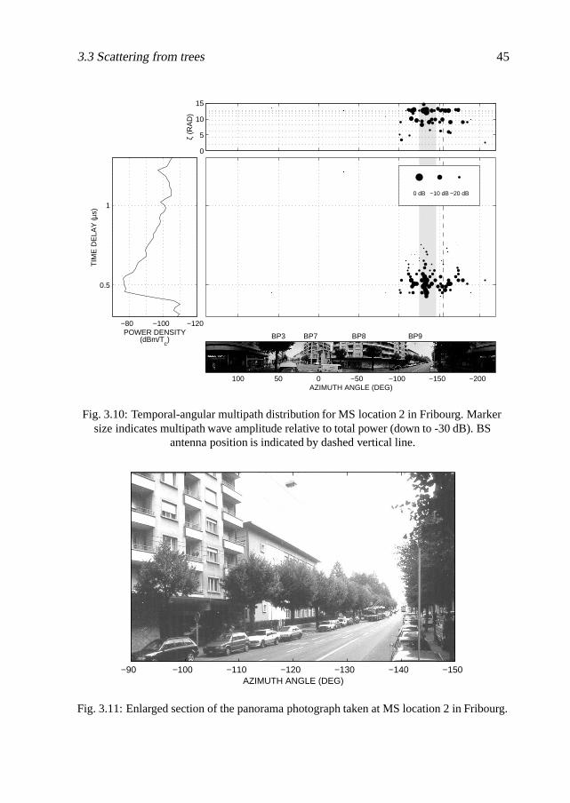
3.3 Scattering from trees 45
0.5
1
−120−100−80
TIM
E D
ELA
Y (µ
s)
POWER DENSITY(dBm/T
c)
0 dB −10 dB −20 dBζ
(RA
D)
0
5
10
15
AZIMUTH ANGLE (DEG)
BP7 BP8 BP9BP3
−200−150−100−50050100
Fig. 3.10: Temporal-angular multipath distribution for MS location 2 in Fribourg. Markersize indicates multipath wave amplitude relative to total power (down to -30 dB). BS
antenna position is indicated by dashed vertical line.
AZIMUTH ANGLE (DEG)−150−140−130−120−110−100−90
Fig. 3.11: Enlarged section of the panorama photograph taken at MS location 2 in Fribourg.

46 High-resolution angle-of-arrival measurements: results
of Fig. 3.10, but they are less prominent than the series of waves arriving fromϕ � −130o, which corresponds to the direction of the park opposite to Jacques-Gachoud Street. The front side of this park was directly illuminated by the basestation antenna. A better view of this angular region is given in Fig. 3.11 (the trol-ley bus seen in this figure was not present during the measurement). The multipathcomponents arriving from this direction have a considerable delay spread, which isa strong indication that they are the result of scattering from a number of spatiallydispersed scatterers, such as the trees in the park. Based on the received power in thetime delay interval around τ � 0.5 µs, the total bistatic scattering cross section ofthese scatterers can be estimated as approximately 30 m2. Again, this value is simi-lar to the theoretical scattering cross section of a group of large trees (view Section5.5.3).
3.3.2 Controlled environment
In order to verify the hypothesis that scattering from trees is a significant propagationphenomenon which may account for some of the discrepancies between propagationpredictions and measurements, additional AOA experiments were performed on asingle deciduous tree in a “controlled” environment. This environment is formed bya large farmer’s field in Boxtel, The Netherlands, on which no objects other than thetree are present. A plan of this configuration is sketched in Fig. 3.12. A photographof the tree, which was in full leaf during the measurements, is shown in Fig. 5.6on page 97 of this thesis. The base station antenna, a 7.1-dBi vertically polarised
−0.05 0 0.05
−0.05
0
0.05
X (km)
Y (
km)
TREEBS
MS
Fig. 3.12: Map of the measurement site in Boxtel.
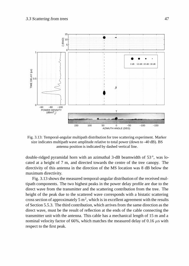
3.3 Scattering from trees 47
0
0.5
1
−100−80−60
TIM
E D
ELA
Y (µ
s)
POWER DENSITY(dBm/T
c)
0 dB −10 dB −20 dB −30 dBζ
(RA
D)
0
5
10
15
AZIMUTH ANGLE (DEG)
T
−150−100−50050100150
Fig. 3.13: Temporal-angular multipath distribution for tree scattering experiment. Markersize indicates multipath wave amplitude relative to total power (down to -40 dB). BS
antenna position is indicated by dashed vertical line.
double-ridged pyramidal horn with an azimuthal 3-dB beamwidth of 53 o, was lo-cated at a height of 7 m, and directed towards the centre of the tree canopy. Thedirectivity of this antenna in the direction of the MS location was 8 dB below themaximum directivity.
Fig. 3.13 shows the measured temporal-angular distribution of the received mul-tipath components. The two highest peaks in the power delay profile are due to thedirect wave from the transmitter and the scattering contribution from the tree. Theheight of the peak due to the scattered wave corresponds with a bistatic scatteringcross section of approximately 5 m2, which is in excellent agreement with the resultsof Section 5.5.3. The third contribution, which arrives from the same direction as thedirect wave, must be the result of reflection at the ends of the cable connecting thetransmitter unit with the antenna. This cable has a mechanical length of 15 m and anominal velocity factor of 66%, which matches the measured delay of 0.16 µs withrespect to the first peak.
48 High-resolution angle-of-arrival measurements: results
3.4 Conclusions
In this chapter, results of wideband AOA measurements obtained under microcellu-lar conditions, i.e. with low simulated base station antennas, were presented. Trans-mission through buildings, which is not taken into account by most existing propa-gation prediction models, was demonstrated to be the dominant propagation mech-anism in two different configurations. In fact, as will be shown in Chapter 4, thisphenomenon plays a significant role in most of the many building transmission ex-periments that were carried out in a later stage of the present study. In the twoexamples discussed in this chapter, the path losses of the transmitted contributions,relative to the free-space loss, are approximately 30 dB. Such a low shielding ef-fectiveness of buildings, if disregarded in the planning stage of urban microcellularnetworks, may lead to unacceptable levels of co-channel interference.
Results obtained in two other configurations show that scattering from trees canbe significant in situations where the line-of-sight propagation path is obstructed andreflection and diffraction contributions are weak, for example in streets perpendic-ular to the street in which the base station is located. This may well explain whymodels based on reflection and diffraction alone have proved to be unsatisfactory,under circumstances reported in [31, 32], in modelling propagation around streetcorners. A theoretical model for the scattering from trees is presented in Chapter 5.

4Propagation into and through buildings
4.1 Introduction
Propagation research for mobile communications in urban microcells has hithertobeen focused mainly on the modelling of reflection and diffraction of radiowavesfrom buildings. These buildings are usually treated as being opaque for radiowavesat the UHF frequencies used for mobile communications. Yet, it was shown in Chap-ter 3 that transmission through buildings can be the dominant propagation mode inat least parts of the coverage area. In the framework of the European COST 231project and in some other studies, effort has been put into the modelling of buildingpenetration [4, 34, 35] and transmission [36, 37]. The results of this work are rele-vant to the present study, but have not led to transmission models that can be directlyincorporated in ray-tracing-based propagation prediction tools.
The rigorous computation of the fields due to building penetration and transmis-sion, using e.g. the method of moments [38], finite-difference time domain (FDTD)methods [39, 40], or indoor ray-tracing [41, 42], presumes the availability of detailedknowledge of the buildings’ geometrical and dielectric properties, both external andinternal. In the practice of cellular network planning such detailed databases arenot available and simpler models – using only a few parameters for each buildingdescribing its penetration and transmission characteristics – are more desirable.
The primary objective of this chapter is to present a ray-optical model for the

50 Propagation into and through buildings
transmission of radiowaves through buildings for which only the exterior coordi-nates and very limited additional information are available. The unknown interiorof each building is characterised by an effective attenuation constant α b. The newtransmission model can be used in conjunction with “conventional” models for ray-optical reflection and (external) diffraction based on the uniform theory of diffrac-tion (UTD), but it introduces two additional types of radiowave interaction with thebuildings. According to the new model, rays incident on one of the planar facesthat together make up the building surface (or exterior wall) can penetrate into thebuilding. These rays are called geometric-optical (GO) transmitted rays. Also, raysincident on one of the vertical building edges joining two planar faces give rise tointernallydiffracted rays, i.e. diffracted rays that propagate into the building interior.Rays that have propagated into the building in either of these ways can then againpropagate into the free space surrounding the building via GO transmission or inter-nal diffraction. The field outside a building due to such so-called transmitted raysisreferred to as the (total) transmitted field due to that building.
To date, no high-frequency asymptotic solution exists for the canonical problemof scattering from a dielectric wedge, from which the exact external and internalUTD diffraction coefficients required for a rigorous ray-optical transmission modelcould be derived. The diffraction coefficients used in this chapter provide an ap-proximate solution to this canonical problem. Contrary to the well-known diffrac-tion coefficients proposed by Luebbers [43] and Tiberio-Maliuzhinets [44], whichare also approximations but very commonly used to model external diffraction fromdielectric wedges, they can also be used to compute internal diffraction fields. Thenew diffraction coefficients are derived from integral representations of the fieldsjust inside and outside the exterior wall of the building. In accordance with the lawsof physical optics (PO), these surface fields are approximated by GO fields. Thetheory in this chapter closely follows the work by Taket, Burge and co-workers ondiffraction by conducting and lossless dielectric wedges [45, 46]. However, the newtransmission model forms an extension to this work in the sense that it also takesinto account the losses in the interiors of the scattering objects (the buildings).
The organisation of this chapter is as follows. The new building transmissionmodel is presented in Section 4.2. Section 4.3 provides some numerical results thatwere generated by this model. It is shown, among other things, that the field in thedeep shadow behind a rectangular building is determined entirely by GO transmis-sion. This observation forms the basis of the experiments discussed in Section 4.4.In that section, empirical values of αb are obtained for a set of 22 buildings, by fittingthe expression for the GO transmitted field to the results of field measurements takenin the buildings’ deep shadow regions. Section 4.5 concludes the chapter.
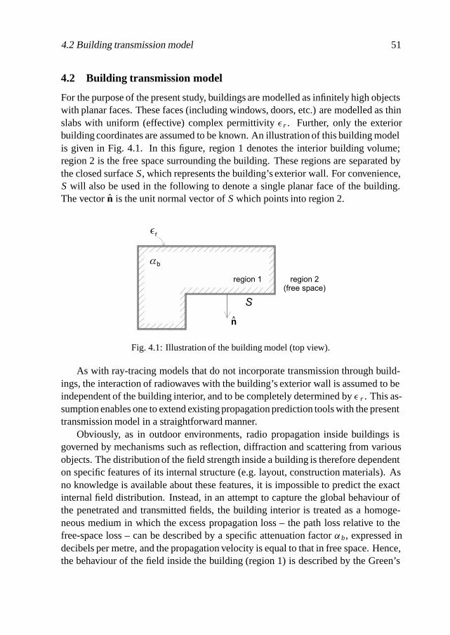
4.2 Building transmission model 51
4.2 Building transmission model
For the purpose of the present study, buildings are modelled as infinitely high objectswith planar faces. These faces (including windows, doors, etc.) are modelled as thinslabs with uniform (effective) complex permittivity ε r . Further, only the exteriorbuilding coordinates are assumed to be known. An illustration of this building modelis given in Fig. 4.1. In this figure, region 1 denotes the interior building volume;region 2 is the free space surrounding the building. These regions are separated bythe closed surface S, which represents the building’s exterior wall. For convenience,S will also be used in the following to denote a single planar face of the building.The vector n is the unit normal vector of Swhich points into region 2.
Fig. 4.1: Illustration of the building model (top view).
As with ray-tracing models that do not incorporate transmission through build-ings, the interaction of radiowaves with the building’s exterior wall is assumed to beindependent of the building interior, and to be completely determined by ε r . This as-sumption enables one to extend existing propagation prediction tools with the presenttransmission model in a straightforward manner.
Obviously, as in outdoor environments, radio propagation inside buildings isgoverned by mechanisms such as reflection, diffraction and scattering from variousobjects. The distribution of the field strength inside a building is therefore dependenton specific features of its internal structure (e.g. layout, construction materials). Asno knowledge is available about these features, it is impossible to predict the exactinternal field distribution. Instead, in an attempt to capture the global behaviour ofthe penetrated and transmitted fields, the building interior is treated as a homoge-neous medium in which the excess propagation loss – the path loss relative to thefree-space loss – can be described by a specific attenuation factor αb, expressed indecibels per metre, and the propagation velocity is equal to that in free space. Hence,the behaviour of the field inside the building (region 1) is described by the Green’s
52 Propagation into and through buildings
function
G1(r, r′) = e− jk1|r−r′|
4π |r − r′| , (4.1)
with k1 = k − jαb/8.686, k being the free-space wavenumber. In general, raysincident on an interface between free space and a lossy medium are refracted, i.e. thetransmission angle is not equal to the incidence angle, even if the phase constant inthe lossy medium is equal to k [47]. However, as |Im k1| = αb/8.686 � k for therelatively small values of αb found in practice (view Section 4.4), refraction of raysat the exterior wall can be neglected.
4.2.1 Surface fields
The field incident on the building from region 2 is assumed to be a ray-optical fieldand can therefore be written as
Ei2(r) = Ai (r) exp
{− j kSi (r)}, (4.2)
where k is the free-space wavenumber. The eikonal of the incident field may beexpanded up to second order about any point r 0 on the building surface, as
Si (r) = Si (r0)+ ki · (r − r0)+ 1
2(r − r0) ·
[x1x1
r1+ x2x2
r2
]· (r − r0), (4.3)
where ki is the incident wave direction at r0. Furthermore, r1 and r2 are the principalradii of curvature of the incident wavefront, and x1 and x2 are unit vectors, eachof which in combination with ki defines one of the principal planes of curvature.It is assumed that x1 is oriented vertically, parallel to the building surface, and x 2
is oriented horizontally. The amplitude factor Ai (r) varies only slowly, and can beconsidered constant in the neighbourhood of r 0, i.e. Ai (r) = Ai (r0) if r is near r0.
According to the PO approximation, the field on the exterior surface of the build-ing is assumed to be zero at all surface points that are not directly illuminated by theincident field. Of the field incident on any directly illuminated surface point, a frac-tion is reflected back into region 2, and part is transmitted into the building interior.The GO reflected field can be written as
Er2(r) = Ai (r0)R(r0) exp
{− j kSi(r − 2nn · (r − r0)
)}, r near r0, (4.4)
where R(r0) is the reflection coefficient of the wall, which, in general, depends onthe dielectric properties of the external-side building materials and the angle of the

4.2 Building transmission model 53
incident wave with respect to the building surface at r 0. The total GO exterior fieldnear r0 is
EGO2 (r) = Ei
2(r) + Er2(r), r near r0. (4.5)
Likewise, the GO transmitted field in region 1 can be written as
Et1(r) = Ai (r0)T (r0) exp
{− j kSi (r0) − j k1[Si (r)− Si (r0)]}, r near r0, (4.6)
where T(r0) is the transmission coefficient of the wall at r 0. The GO interior fieldnear r0, just inside the exterior wall, is completely due to the transmitted field andtherefore
EGO1 (r) = Et
1(r), r near r0. (4.7)
In principle, the reflection and transmission coefficients of the exterior wall inequations (4.4) and (4.6) can be chosen freely. In cases in which the geometrical anddielectric properties of the exterior wall are precisely known it may be possible tofind the exact coefficients, otherwise approximate reflection and transmission coef-ficients must be used. In the present case, use is made of the soft Fresnel reflectioncoefficient (view Fig. 4.2 for the definition of the incidence angle θ i )
R(r) = cos θi −√εr − sin2 θi
cos θi +√εr − sin2 θi
. (4.8)
This reflection coefficient, in combination with values of the complex permittivityεr within a range that applies to most common building materials, is well knownto provide an accurate approximation of the fields reflected from building faces (forvertical polarisation), and is used in most deterministic propagation prediction mod-els. A permittivity equal to 5 was shown to be an optimum choice in two independentstudies [48, 49] and will be used in the following.
Application of the Fresnel reflection coefficient implies that a fraction of theincident field equal to the soft Fresnel transmission coefficient
T2 = 2 cosθi
cos θi +√εr − sin2 θi
(4.9)
is transmitted across the outer boundary of the wall. Of this field, in turn, a fraction istransmitted into the building interior (region 1). Because |Im k1| = αb/8.686 � k,the corresponding transmission coefficient can be written as
T1 = 2 cosθt
cos θt +√
1/εr − sin2 θt
(4.10)
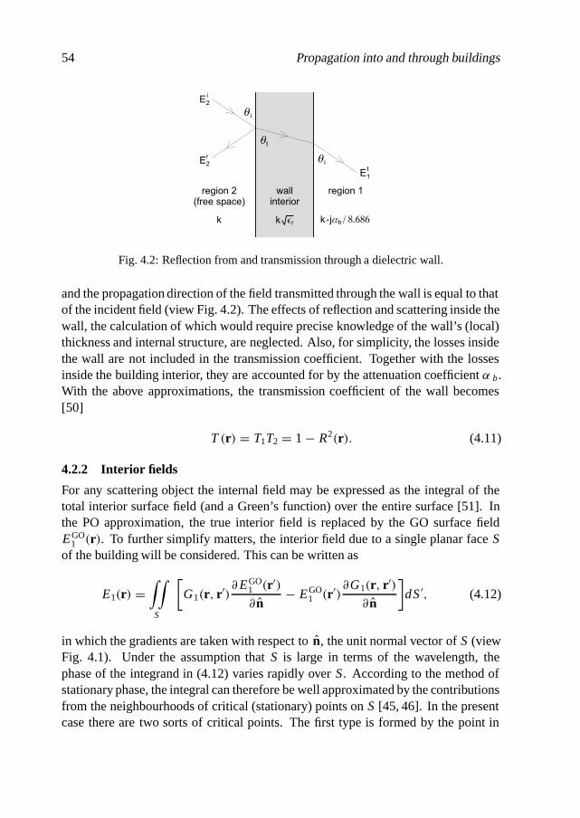
54 Propagation into and through buildings
Fig. 4.2: Reflection from and transmission through a dielectric wall.
and the propagation direction of the field transmitted through the wall is equal to thatof the incident field (view Fig. 4.2). The effects of reflection and scattering inside thewall, the calculation of which would require precise knowledge of the wall’s (local)thickness and internal structure, are neglected. Also, for simplicity, the losses insidethe wall are not included in the transmission coefficient. Together with the lossesinside the building interior, they are accounted for by the attenuation coefficient α b.With the above approximations, the transmission coefficient of the wall becomes[50]
T (r) = T1T2 = 1 − R2(r). (4.11)
4.2.2 Interior fields
For any scattering object the internal field may be expressed as the integral of thetotal interior surface field (and a Green’s function) over the entire surface [51]. Inthe PO approximation, the true interior field is replaced by the GO surface fieldEGO
1 (r). To further simplify matters, the interior field due to a single planar face Sof the building will be considered. This can be written as
E1(r) =∫∫
S
[G1(r, r′)
∂EGO1 (r′)∂ n
− EGO1 (r′)
∂G1(r, r′)∂ n
]dS′, (4.12)
in which the gradients are taken with respect to n, the unit normal vector of S (viewFig. 4.1). Under the assumption that S is large in terms of the wavelength, thephase of the integrand in (4.12) varies rapidly over S. According to the method ofstationary phase, the integral can therefore be well approximated by the contributionsfrom the neighbourhoods of critical (stationary) points on S [45, 46]. In the presentcase there are two sorts of critical points. The first type is formed by the point in
4.2 Building transmission model 55
the interior of S where the phase is stationary, if it exists. The second type are thosepoints on the vertical edges of S where the phase of the integrand is stationary withrespect to movement along the edge. There can be maximally two critical pointsof the second type per building face, depending on whether the edges are directlyilluminated by the incident field. These points correspond with the edge-diffractionpoints in the UTD.
The interior field is evaluated at a point with position vector r. It is convenientto express this point in terms of its displacement from an (arbitrary) critical point r 0
on S. For surface points r′ in the neighbourhood of r0, the Green’s function can beapproximated by
G1(r0+sks, r′) = exp{− j k1
[s − ks · (r′ − r0)
]}4πs
× exp
{− j k1
[(r′ − r0) · (I − ksks) · (r′ − r0)
2s
]},
(4.13)
where s = |r − r0| is the distance from r0 to the observation point, the unit vectorks = (r − r0)/s denotes the scattering direction, and I is the unit dyadic. With thisapproximation, the interior field due to the isolated critical point at r 0 can be writtenas (cf. [45, 46])
Ec1(r0 + sks) = − j k1e− jk1s
4πsEi
2(r0)T(r0) n · (ki + ks)
×∫∫Sc
exp{− j k1
[b · (r′ − r0)+ 1
2(r′ − r0) · C · (r′ − r0)
]}dS′, (4.14)
where
b = ki − ks
C = I − ksks
s+ x1x1
r1+ x2x2
r2,
(4.15)
and the integration domain Sc is a subdomain of S which contains only the criticalpoint at r0. The total interior field at r = r0 + sks is calculated as the sum of thecontributions from all critical points.
If the face S contains a critical point of the first type, which is the case if thereis a (directly illuminated) point r0 within S for which ks = ki , its contribution tothe total interior field is found by replacing the integration domain Sc in (4.14) bythe whole infinite plane S∞ of which S is a subdomain [45]. The stationary-phase
56 Propagation into and through buildings
approximation of the resulting double integral is given by
Et1(r0 + sks) = Ei
2(r0)T(r0)
√r1r2
(r1 + s)(r2 + s)e− jk1s. (4.16)
This field contribution is recognised as the field associated with a GO “transmittedray” propagating along the direct path from the source of the incident field, througha transmission point at r0, to r. In the special case that the critical point of the firstkind (i.e., the GO transmission point) lies on an edge of S, the transmitted field in(4.16) must be multiplied by a factor 1/2.
The diffraction contributions from the critical points of the second type must betreated separately. For each of these points, a set of coordinates (t ′, z′) in the planeof S is defined by (view Fig. 4.3)
r′ = r0 + t ′t + z′ z, (4.17)
where t is a unit vector in the plane of Swhich points to the side of the edge on whichthe surface lies, and z is a vertical unit vector pointing upwards. The contributionfrom each diffraction point can be found by taking the integration domain Sc in(4.14) to be [45]
Sc ={
S, if t · b > 0
S− S∞, if t · b < 0.(4.18)
Then, after performing the integrations over t ′ (from 0 to ±∞, depending on thesign of t · b) and z′ (from −∞ to ∞), it follows that [46]
Ed1 (r0 + sks) = Ei
2(r0) D2→1int
√r1
s(r1 + s)e− jk1s, (4.19)
where
D2→1int = −1
2sgn[t · b
]T (r0) n · (ks + ki )
√C K−
(√k1C[t · b
]22
)(4.20)
is the internal diffraction coefficient for diffraction from region 2 into region 1. Here,the vector ks points into the building interior. Furthermore, the function sgn(·) isdefined as
sgn(x) =
1, if x > 0,
0, if x = 0,
−1, if x < 0,
(4.21)

4.2 Building transmission model 57
the parameter C is written as
C = 1
t · C · t(4.22)
and the function
K−(τ ) = 1√π
ej (τ 2+π/4)∫ ∞
τ
e− j t 2dt (4.23)
is the modified Fresnel integral. An accurate algorithm for computing K −(·), whichcan be used for complex argument values, is presented in [52]. This algorithm in-volves the evaluation of a polynomial function, the coefficients of which have to becomputed only once by a fast Fourier transformation. The vector inner products andthe parameter C in (4.20) can be expressed in terms of the incident and scatteringangles ϕ ′ and ϕ, which are defined from the exterior side of S (view Fig. 4.3), asfollows:
t · b = − cosϕ′ − cosϕ
n · ki = − sinϕ ′
n · ks = sinϕ
C =[
sin2 ϕ′
r2+ sin2 ϕ
s
]−1
.
(4.24)
Fig. 4.3: Definition of coordinate vectors and incident and scattering angles relative to theplanar face S (top view).
To calculate the interior field due to diffraction from the wedge formed by abuilding corner, the two planar faces that compose the corner must be treated sepa-rately, i.e., a diffraction coefficient is evaluated for each face that is illuminated bythe incident field.
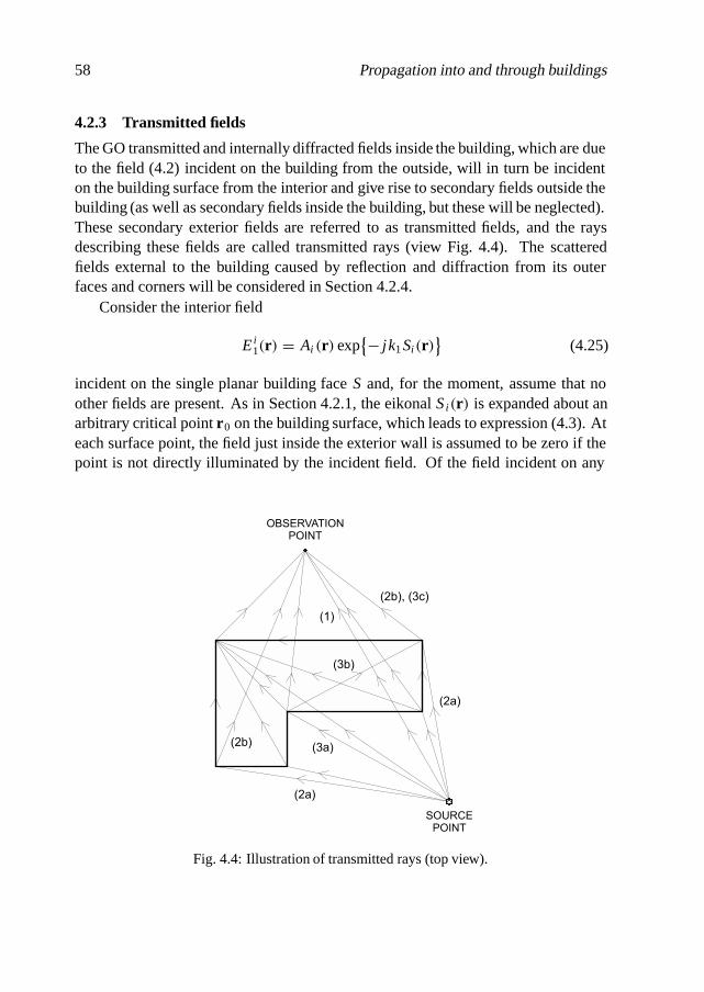
58 Propagation into and through buildings
4.2.3 Transmitted fields
The GO transmitted and internally diffracted fields inside the building, which are dueto the field (4.2) incident on the building from the outside, will in turn be incidenton the building surface from the interior and give rise to secondary fields outside thebuilding (as well as secondary fields inside the building, but these will be neglected).These secondary exterior fields are referred to as transmitted fields, and the raysdescribing these fields are called transmitted rays (view Fig. 4.4). The scatteredfields external to the building caused by reflection and diffraction from its outerfaces and corners will be considered in Section 4.2.4.
Consider the interior field
Ei1(r) = Ai (r) exp
{− j k1 Si (r)}
(4.25)
incident on the single planar building face S and, for the moment, assume that noother fields are present. As in Section 4.2.1, the eikonal Si (r) is expanded about anarbitrary critical point r0 on the building surface, which leads to expression (4.3). Ateach surface point, the field just inside the exterior wall is assumed to be zero if thepoint is not directly illuminated by the incident field. Of the field incident on any
OBSERVATIONPOINT
SOURCEPOINT
(2b), (3c)
(2b)
(1)
(3b)
(2a)
(3a)
(2a)
Fig. 4.4: Illustration of transmitted rays (top view).

4.2 Building transmission model 59
directly illuminated surface point, a part is transmitted into region 2 and forms theGO exterior field. For observation points r close to r 0, this field can be written as
EGO2 (r) = Et
2(r) = Ai (r0)T(r0)
× exp{− j k1 Si (r0)− j k[Si (r)− Si (r0)]
}, r near r0. (4.26)
The field that is reflected back into the building interior is neglected.The total transmitted field due to S at any observation point in region 2 can
be written as an integral of the exterior surface field due to E i1(r) (and a Green’s
function) over S [51]. As before, this surface field is replaced by the GO surfacefield due to Ei
1(r), which yields
E2(r) = −∫∫
S
[G2(r, r′)
∂EGO2 (r′)∂ n
− EGO2 (r′)
∂G2(r, r′)∂ n
]dS′, (4.27)
where G2(r, r′) is the free-space Green’s function. As before, the unit normal vectorn points into region 2 (view Fig. 4.1). As S is large in terms of the wavelength,the transmitted field E2(r) is principally due to a GO contribution (if S contains acritical point of the first type) and maximally two diffraction contributions from theedges of S. The GO transmitted field is
Et2(r0 + sks) = Ei
1(r0)T(r0)
√r1r2
(r1 + s)(r2 + s)e− jks, (4.28)
and the edge-diffracted fields can each be written as
Ed2 (r0 + sks) = Ei
1(r0)D1→2int
√r1
s(r1 + s)e− jks, (4.29)
where
D1→2int = 1
2sgn[t · b
]T(r0) n · (ks + ki )
√C K−
(√kC[t · b
]22
)(4.30)
is the internal diffraction coefficient for diffraction from region 1 into region 2. Inthis case, the scattering direction vector ks points into the exterior region of thebuilding (region 2). As before, s is the distance between the critical point r 0 andthe observation point r = r0 + sks, and the vector inner products and the parameterC used in (4.30) can be expressed in terms of the incident and scattering angles ϕ ′and ϕ, according to (4.24). The two faces of every corner must be treated separately,

60 Propagation into and through buildings
so that the diffraction coefficient D 1→2int is evaluated for each face that is illuminated
from the inside. Again, in the special case that the transmission point lies on an edgeof S, the GO transmitted field must be multiplied by a factor 1/2.
Consequent accounting for all possible combinations of GO transmission and in-ternal diffraction, according to the approach described above, can lead to maximallythree different types of transmitted rays:
1. the GO transmitted ray, which passes through two transmission points;
2. single-diffracted rays, which pass through one transmission point and onediffraction point;
3. double-diffracted rays, which pass through two (different) diffraction points.
As an example, Fig. 4.4 shows all possible transmitted rays for a relatively simpleconfiguration. For some of these rays, the categories in which they fall are indicatedby bracketed numbers. The transmission points of the GO transmitted ray coalesceif the observation point is located on a shadow boundary of the incident field. Trans-mitted rays of type (2) with coincident transmission and diffraction points occur forevery ray incident on a building corner of which only one face is visible from thesource point. Together with the externally diffracted rays that will be discussed inSection 4.2.4, these rays ensure the continuity of the total field across the shadowboundary of the incident field.
4.2.4 External scattering
The scattered fields external to the building that have been considered so far are theresult of interaction with the building interior. The fields reflected and diffractedfrom the building’s outer surface, which have not been considered yet, can be pre-dicted by means of “standard” reflection and diffraction models, e.g. by using theFresnel reflection coefficient discussed in Section 4.2.1 and the diffraction coeffi-cient of Luebbers [43] or Tiberio-Maliuzhinets [44]. Expressions for these fields canalso be obtained, however, as part of the theory of the previous sections.
The evaluation of the stationary-phase contributions to an integral of the form(4.27), but with the exterior surface field E2(r) equal to that in (4.5), cf. [45, 46],leads to a reflected field given by
Er2(r0 + sks) = Ei
2(r0)R(r0)
√r1r2
(r1 + s)(r2 + s)e− jks, (4.31)
which is identical to the expression normally used in the published literature on
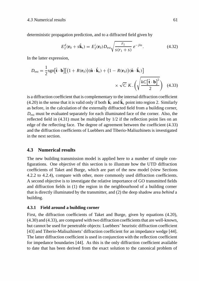
4.3 Numerical results 61
deterministic propagation prediction, and to a diffracted field given by
Ed2 (r0 + sks) = Ei
2(r0)Dext
√r1
s(r1 + s)e− jks. (4.32)
In the latter expression,
Dext = 1
2sgn[t · b
][(1 + R(r0)
)(n · ks)+ (1 − R(r0)
)(n · ki )
]
× √C K−
(√kC[t · b
]22
)(4.33)
is a diffraction coefficient that is complementary to the internal diffraction coefficient(4.20) in the sense that it is valid only if both ki and ks point into region 2. Similarlyas before, in the calculation of the externally diffracted field from a building corner,Dext must be evaluated separately for each illuminated face of the corner. Also, thereflected field in (4.31) must be multiplied by 1/2 if the reflection point lies on anedge of the reflecting face. The degree of agreement between the coefficient (4.33)and the diffraction coefficients of Luebbers and Tiberio-Maliuzhinets is investigatedin the next section.
4.3 Numerical results
The new building transmission model is applied here to a number of simple con-figurations. One objective of this section is to illustrate how the UTD diffractioncoefficients of Taket and Burge, which are part of the new model (view Sections4.2.2 to 4.2.4), compare with other, more commonly used diffraction coefficients.A second objective is to investigate the relative importance of GO transmitted fieldsand diffraction fields in (1) the region in the neighbourhood of a building cornerthat is directly illuminated by the transmitter, and (2) the deep shadow area behindabuilding.
4.3.1 Field around a building corner
First, the diffraction coefficients of Taket and Burge, given by equations (4.20),(4.30) and (4.33), are compared with two diffraction coefficients that are well-known,but cannot be used for penetrable objects: Luebbers’ heuristic diffraction coefficient[43] and Tiberio-Maliuzhinets’ diffraction coefficient for an impedance wedge [44].The latter diffraction coefficient is used in conjunction with the reflection coefficientfor impedance boundaries [44]. As this is the only diffraction coefficient availableto date that has been derived from the exact solution to the canonical problem of
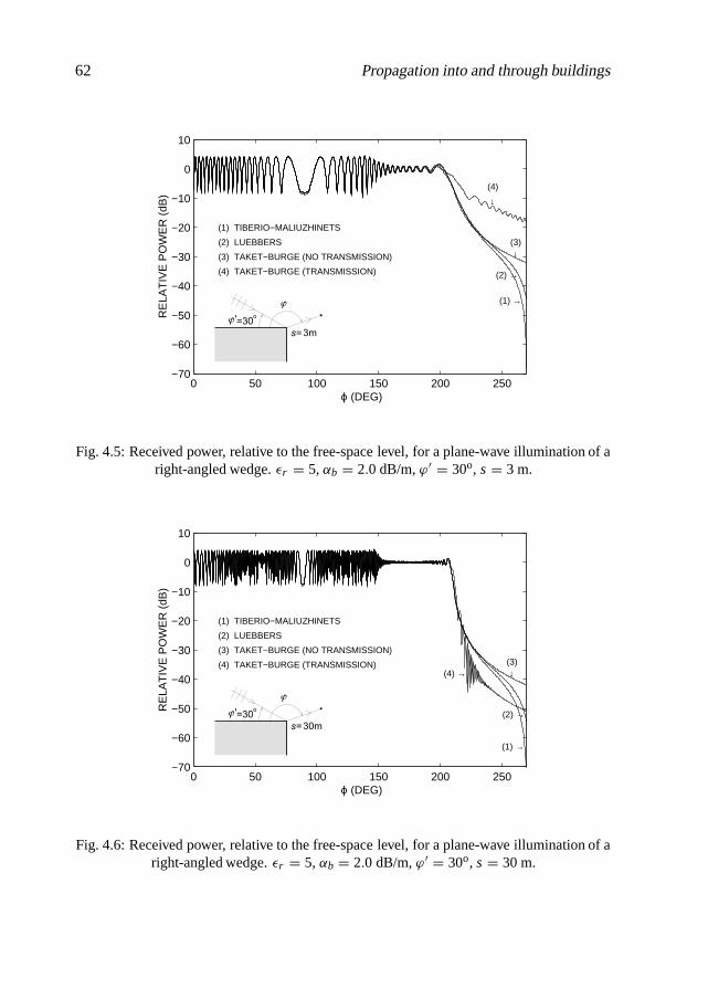
62 Propagation into and through buildings
0 50 100 150 200 250−70
−60
−50
−40
−30
−20
−10
0
10
ϕ (DEG)
RE
LAT
IVE
PO
WE
R (
dB)
(1) TIBERIO−MALIUZHINETS
(1) →
(2) LUEBBERS
(2) →
(3) TAKET−BURGE (NO TRANSMISSION)
(3)↓
(4) TAKET−BURGE (TRANSMISSION)
(4)
↓
�
�'=30o
s= 3m
Fig. 4.5: Received power, relative to the free-space level, for a plane-wave illumination of aright-angled wedge. εr = 5, αb = 2.0 dB/m, ϕ′ = 30o, s = 3 m.
0 50 100 150 200 250−70
−60
−50
−40
−30
−20
−10
0
10
ϕ (DEG)
RE
LAT
IVE
PO
WE
R (
dB)
(1) TIBERIO−MALIUZHINETS
(1) →
(2) LUEBBERS
(2) →
(3) TAKET−BURGE (NO TRANSMISSION)(3)↓
(4) TAKET−BURGE (TRANSMISSION)(4) →
�
�'=30o
s= 30m
Fig. 4.6: Received power, relative to the free-space level, for a plane-wave illumination of aright-angled wedge. εr = 5, αb = 2.0 dB/m, ϕ′ = 30o, s = 30 m.
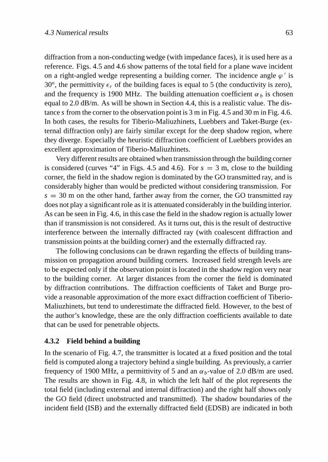
4.3 Numerical results 63
diffraction from a non-conducting wedge (with impedance faces), it is used here as areference. Figs. 4.5 and 4.6 show patterns of the total field for a plane wave incidenton a right-angled wedge representing a building corner. The incidence angle ϕ ′ is30o, the permittivity εr of the building faces is equal to 5 (the conductivity is zero),and the frequency is 1900 MHz. The building attenuation coefficient α b is chosenequal to 2.0 dB/m. As will be shown in Section 4.4, this is a realistic value. The dis-tance s from the corner to the observation point is 3 m in Fig. 4.5 and 30 m in Fig. 4.6.In both cases, the results for Tiberio-Maliuzhinets, Luebbers and Taket-Burge (ex-ternal diffraction only) are fairly similar except for the deep shadow region, wherethey diverge. Especially the heuristic diffraction coefficient of Luebbers provides anexcellent approximation of Tiberio-Maliuzhinets.
Very different results are obtained when transmission through the building corneris considered (curves “4” in Figs. 4.5 and 4.6). For s = 3 m, close to the buildingcorner, the field in the shadow region is dominated by the GO transmitted ray, and isconsiderably higher than would be predicted without considering transmission. Fors = 30 m on the other hand, farther away from the corner, the GO transmitted raydoes not play a significant role as it is attenuated considerably in the building interior.As can be seen in Fig. 4.6, in this case the field in the shadow region is actually lowerthan if transmission is not considered. As it turns out, this is the result of destructiveinterference between the internally diffracted ray (with coalescent diffraction andtransmission points at the building corner) and the externally diffracted ray.
The following conclusions can be drawn regarding the effects of building trans-mission on propagation around building corners. Increased field strength levels areto be expected only if the observation point is located in the shadow region very nearto the building corner. At larger distances from the corner the field is dominatedby diffraction contributions. The diffraction coefficients of Taket and Burge pro-vide a reasonable approximation of the more exact diffraction coefficient of Tiberio-Maliuzhinets, but tend to underestimate the diffracted field. However, to the best ofthe author’s knowledge, these are the only diffraction coefficients available to datethat can be used for penetrable objects.
4.3.2 Field behind a building
In the scenario of Fig. 4.7, the transmitter is located at a fixed position and the totalfield is computed along a trajectory behind a single building. As previously, a carrierfrequency of 1900 MHz, a permittivity of 5 and an αb-value of 2.0 dB/m are used.The results are shown in Fig. 4.8, in which the left half of the plot represents thetotal field (including external and internal diffraction) and the right half shows onlythe GO field (direct unobstructed and transmitted). The shadow boundaries of theincident field (ISB) and the externally diffracted field (EDSB) are indicated in both
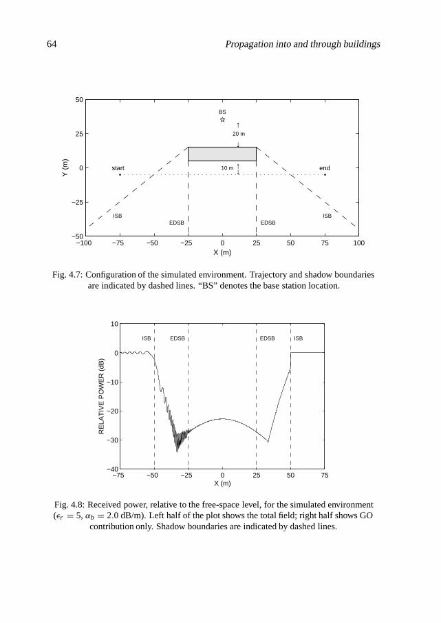
64 Propagation into and through buildings
−100 −75 −50 −25 0 25 50 75 100−50
−25
0
25
50
↑
↓20 m
BS
start end↑↓10 m
ISB ISBEDSB EDSB
X (m)
Y (
m)
Fig. 4.7: Configuration of the simulated environment. Trajectory and shadow boundariesare indicated by dashed lines. “BS” denotes the base station location.
−75 −50 −25 0 25 50 75−40
−30
−20
−10
0
10
X (m)
RE
LAT
IVE
PO
WE
R (
dB)
ISBISB EDSBEDSB
Fig. 4.8: Received power, relative to the free-space level, for the simulated environment(εr = 5, αb = 2.0 dB/m). Left half of the plot shows the total field; right half shows GO
contribution only. Shadow boundaries are indicated by dashed lines.
4.4 Experimental results 65
figures.From Fig. 4.8 it is obvious that GO transmission plays a dominant role in the
GO shadow region between the ISBs. The most significant differences between thetotal field and the GO field occur around the shadow boundaries and in the vicinity ofpoints where the GO transmitted ray passes through one of the other building corners(X = ±33.3 m). At these boundaries the GO field exhibits “jumps” while the totalfield remains continuous. Even in these regions, however, the difference between thetwo fields is smaller than 4 dB.
It is further seen that the field in the region between the EDSBs (-25 m < X <
25 m in this example) is determined entirely by the GO transmitted field, i.e., contri-butions from diffracted rays are negligible. This observation forms the basis of theexperiments discussed in Section 4.4, in which empirical values of α b are obtainedby fitting the expression for the GO transmitted field to measured data taken in thedeep shadow area directly behind a building.
4.4 Experimental results
The free parameter αb used in the transmission model of Section 4.2 is related tothe internal building structure in a highly complicated way and must therefore bedetermined empirically, i.e., from measurements of the path loss – relative to thefree-space loss – experienced by waves transmitted through buildings. This excesspath loss will be referred to as the building transmission loss L t .
A major concern in the measurement of building transmission losses is formedby the disturbing effect of multipath contributions entering the receiving antenna viaobjects in the environment of the considered building. A solution to this problemmay be found in the use of wideband and/or directional measurement techniques,which offer the possibility to separate multipath waves on the basis of their differentpropagation delay times and angles-of-arrival (AOAs), respectively [16]. Using acombination of these techniques, it was demonstrated in [53] that it is indeed possi-ble to distinguish the radiowaves transmitted through an obstructing building fromother multipath contributions in a realistic microcell environment. However, impor-tant practical disadvantages of this method are the relatively complex measurementprocedure and the long time needed to measure the transmitted field, even for a singlereceiver location.
This section introduces a fast, simple and yet accurate method to measure thetransmitted field along a trajectory behind an obstructing building, using a widebandradio channel sounder [54]. Furthermore, it presents results of building transmissionloss measurements for a set of 22 buildings that can be considered typical for urbanenvironments in The Netherlands. Empirical values of the attenuation coefficient α b
66 Propagation into and through buildings
are determined for each of these buildings.
4.4.1 Measurement equipment and procedure
The building transmission measurements discussed in this section were performedusing the TU/e radio channel sounding system that was described in detail in Section2.2 of this thesis. This system operates at 1900 MHz and has a temporal resolution of20 ns. Instead of the rotating antenna that was used to estimate the AOA of multipathwaves, a fixed, vertically polarised, omnidirectional receiving antenna was mountedon the roof of a measurement vehicle, at 2.4 m above ground level. The radiationpatterns of this antenna are shown in Fig. 2.3 on page 13 of this thesis.
The transmitting antenna – a vertically polarised, 12-dBi, omnidirectional an-tenna with a vertical 3-dB beamwidth of 6o – was positioned on one of the longsides of the building under test, at a height of 6.5 m, typical for the base station con-figuration in urban microcells. During a measurement, impulse response data wererecorded every 0.1 s while the measurement vehicle was moving at a low, constantspeed (usually around 1.5 m/s) along a straight trajectory on the other side of thebuilding. Road lay-out and other local circumstances influenced the final choices ofthe transmitting antenna location and the measurement trajectory.
4.4.2 Determination of the transmitted field
To illustrate how the absolute transmitted field strength can be determined from theimpulse response data, a typical data set – measured behind a 15-m high office build-ing on the TU/e campus (view the plan in Fig. 4.9 and the photograph in Fig. 4.14(f)on page 73 of this thesis) – is shown in Fig. 4.10. In this measurement, the trans-mitting antenna was at the location marked as “Tx1” in Fig. 4.9. The major part ofthe building consists of small offices separated by brick walls, with wooden doorsopening to a central corridor. A large restaurant hall is situated in the right part. Thebuilding has a concrete, metal and glass external construction.
The set of power delay profiles recorded along the trajectory is denoted byp(τ ; d), τ being the propagation delay time and d being the distance along the trajec-tory. For each d, the values of τ for which p(τ ; d) has local maxima form estimatesof the propagation delays of the dominant multipaths. The values of p(τ ; d) at eachof these τ s is proportional to the multipath intensity. The proportionality factor be-tween the two can be determined prior to the measurement by connecting a knownattenuation between the transmitter and receiver.
The received field is composed of several multipath waves propagating aroundthe building via reflection, diffraction and scattering from surrounding objects, anda contribution due to transmission through the building. The waves propagatingaround the building arrive at the receiving antenna roughly from the front and back

4.4 Experimental results 67
Fig. 4.9: Plan view of the measurement environment.
Fig. 4.10: Measured power delay profiles along the trajectory.Transmitter is at location “Tx1”.
68 Propagation into and through buildings
of the vehicle. As the distance along the trajectory increases, the profile maximacorresponding to these waves move along the delay axis at an approximately constantrate (see Fig. 4.10). The sign of this rate depends on whether a wave propagatesaround the left or the right side of the building. Generally, as in Fig. 4.10, the firsttransmitted contribution can easily be identified by its hyperbolic shape and becauseit has minimum delay for all d. The weaker “clutter” arriving directly after thisfirst contribution is possibly the result of waves undergoing (multiple) backward andforward reflection in the building interior, and will be ignored.
To simplify the determination of the transmitted field, the building is modelled asa rectangular box having the same length as the building behind which the measure-ment was made, and a width equal to its maximum width (view Fig. 4.11). Diffrac-tion effects – which are insignificant in the deep shadow region directly behind thebuilding (view Section 4.3) – are neglected, and the transmitted field is assumed tobe the result of a single GO transmitted ray propagating directly from the transmit-ting antenna through the building to the receiving antenna, at a propagation velocityequal to that in free space (cf. Section 4.2). In Fig. 4.10, the solid line representsthe theoretical delay τt(d) associated with the GO transmitted ray. This delay isseen to be in very good agreement with the measured delay of the first transmittedcontribution. The absolute transmitted field strength, required to determine L t , isobtained from p(τ ; d) by setting τ = τ t(d) and multiplying by the proportionalityfactor found in the calibration.
4.4.3 Determination of the attenuation coefficient
The thin solid line in Fig. 4.12 represents the measured building transmission lossfor the example discussed in the previous section. This loss exhibits strong and rapidspatial fluctuations, which indicates that, in reality, the transmitted field is the resultof two or more waves propagating along paths of approximately the same length.These fast fading effects are neglected for the purpose of fitting the proposed modelto the global behaviour of the measured transmitted field. The large-scale fadingcomponent of the measured Lt , represented in Fig. 4.12 by the thick solid line, is ob-tained by averaging over 40 wavelengths [55], which corresponds to approximately6 m.
According to the transmission model of Section 4.2, the building transmissionloss experienced by the GO transmitted field is equal to
Lt = αb · din − 20 log∣∣T (r1)
∣∣− 20 log∣∣T(r2)
∣∣ dB, (4.34)
where din is the length of the transmitted ray path inside the building, r 1 and r2 are thetransmission points on the building surface, and T(r 1) and T(r2) are the associatedtransmission coefficients (view Fig. 4.11). In the case considered here, the angles

4.4 Experimental results 69
OBSERVATIONPOINT
SOURCEPOINT
din
�1
�2r2
r1
(= )�1
Fig. 4.11: Illustration of the simplified building model.
θ1 and θ2 are equal, so that T(r1) = T (r2). Note that the above expression for L t
follows from equations (4.16) and (4.28), after converting to decibels and subtractingthe free-space loss.
The specific attenuation factor αb is chosen such that the root-mean-square (rms)error of the theoretical Lt with respect to the averaged measured data is minimised.For the example under consideration, this results in a value of α b = 1.51 dB/m (forεr = 5), and the rms error is 5.76 dB. The dashed line in Fig. 4.12 represents thetheoretical Lt computed using these parameters. In this particular example, it wouldbe possible to reduce the rms error by using different values of α b for the left and theright half of the building, thus reflecting the fact that there are more internal walls inthe left section (view Fig. 4.9).
4.4.4 Reproducibility
In order to assess the reliability of the transmission loss measurements and the de-termination of αb, the reproducibility of the experimental results was investigatedfor the building under present consideration. Important factors that could cause twosubsequent measurements to yield different results are (1) non-stationarity of the en-vironment, mainly because of movements inside the building, and (2) difficulty toconduct the measurements at exactly the same observation points [48]. The lowercurve in Fig. 4.12 represents the result of a second measurement along the sametrajectory, with the transmitting antenna at location “Tx1”. Apart from a small mis-alignment in distance, caused by speed variations of the measurement vehicle, thisresult is almost identical to that of the first measurement. Fig. 4.13 shows the resultsof two consecutive measurements along the same trajectory, but with the transmit-ting antenna at location “Tx2” (view Fig. 4.9). Again, the measured L t -curve is seen

70 Propagation into and through buildings
0 20 40 60 80 100−80
−70
−60
−50
−40
−30
−20
−10
0
DISTANCE (m)
− L
t (dB
)
MEASURED DATA
AVERAGED DATA (2 RUNS)EQ. (4.34) WITH α
b = 1.51 dB/m
Fig. 4.12: Measured and modelled building transmission loss L t (transmitting antenna atlocation “Tx1”). Lower curve has an offset of -20 dB for clarity.
0 20 40 60 80 100−80
−70
−60
−50
−40
−30
−20
−10
0
DISTANCE (m)
− L
t (dB
)
MEASURED DATA
AVERAGED DATA (2 RUNS)EQ. (4.34) WITH α
b = 1.58 dB/m
Fig. 4.13: Measured and modelled building transmission loss L t (transmitting antenna atlocation “Tx2”). Lower curve has an offset of -20 dB for clarity.
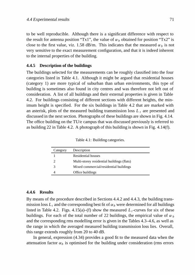
4.4 Experimental results 71
to be well reproducible. Although there is a significant difference with respect tothe result for antenna position “Tx1”, the value of α b obtained for position “Tx2” isclose to the first value, viz. 1.58 dB/m. This indicates that the measured α b is notvery sensitive to the exact measurement configuration, and that it is indeed inherentto the internal properties of the building.
4.4.5 Description of the buildings
The buildings selected for the measurements can be roughly classified into the fourcategories listed in Table 4.1. Although it might be argued that residential houses(category 1) are more typical of suburban than urban environments, this type ofbuilding is sometimes also found in city centres and was therefore not left out ofconsideration. A list of all buildings and their external properties is given in Table4.2. For buildings consisting of different sections with different heights, the min-imum height is specified. For the six buildings in Table 4.2 that are marked withan asterisk, plots of the measured building transmission loss L t are presented anddiscussed in the next section. Photographs of these buildings are shown in Fig. 4.14.The office building on the TU/e campus that was discussed previously is referred toas building 22 in Table 4.2. A photograph of this building is shown in Fig. 4.14(f).
Table 4.1: Building categories.
Category Description
1 Residential houses
2 Multi-storey residential buildings (flats)
3 Mixed commercial/residential buildings
4 Office buildings
4.4.6 Results
By means of the procedure described in Sections 4.4.2 and 4.4.3, the building trans-mission loss L t and the corresponding best fit of αb were determined for all buildingslisted in Table 4.2. Figs. 4.15(a)–(f) show the measured L t -curves for six of thesebuildings. For each of the total number of 22 buildings, the empirical value of α b
and the corresponding rms modelling error is given in the Tables 4.3–4.6, as well asthe range in which the averaged measured building transmission loss lies. Overall,this range extends roughly from 20 to 40 dB.
In general, expression (4.34) provides a good fit to the measured data when theattenuation factor αb is optimised for the building under consideration (rms errors

72 Propagation into and through buildings
Table 4.2: Exterior properties of the buildings selected for the experiments.
External dimensions†
Building Cat. External-side building materialsL (m) W (m) H (m)
1 1 brick / window glass / ceramic roof tiles 47 10 8
2 1 painted wood / window glass / concreteroof tiles
46 10 9
3∗ 1 brick / window glass / concrete roof tiles 73 9 9
4 1 brick / window glass / ceramic roof tiles 36 8 8
5 1 brick / window glass / ceramic roof tiles 73 7 9
6 2 brick / window glass 57 11 23
7 2 brick / wooden panels / window glass 74 11 12
8 2 brick / window glass 119 20 14
9∗ 2 reinforced concrete covered withinsulating material / glass windows /metal railings
98 12 26
10 2 brick / window glass / metal railings 67 19 22
11 3 brick / window glass 65 9 9
12 3 brick / cement panels / window glass 36 12 9
13 3 brick / cement panels / window glass 49 12 9
14∗ 3 brick / cement panels / window glass 36 12 9
15∗ 3 brick (ground floor) / concrete panels(upper storeys) / window glass
58 15 10
16 4 brick / window glass 23 13 10
17 4 concrete panels / window glass 51 13 12
18 4 concrete block / dark-tinted windowglass
62 13 14
19∗ 4 reinforced concrete shell / reflectivewindow glass
40 14 23
20 4 reinforced concrete shell / reflectivewindow glass
45 13 26
21 4 concrete panels / window glass 39 14 18
22∗ 4 reinforced concrete covered with metalpanels / window glass / metal railings
102 18 15
† L(ength) × W(idth) × H(eight).∗ Photographs of these buildings are shown in Fig. 4.14.

4.4 Experimental results 73
(a) Building 3 (b) Building 9
(c) Building 14 (d) Building 15
(e) Building 19 (f) Building 22
Fig. 4.14: Photographs of six of the buildings selected for the experiments.
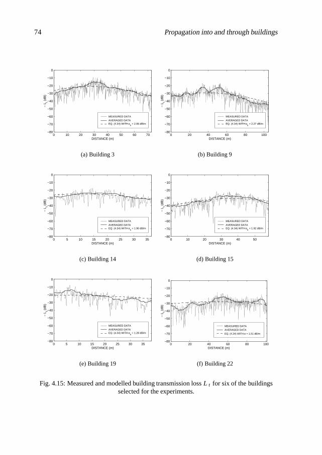
74 Propagation into and through buildings
0 10 20 30 40 50 60 70−80
−70
−60
−50
−40
−30
−20
−10
0
DISTANCE (m)
− L
t (dB
)
MEASURED DATA
AVERAGED DATAEQ. (4.34) WITH α
b = 2.06 dB/m
(a) Building 3
0 20 40 60 80 100−80
−70
−60
−50
−40
−30
−20
−10
0
DISTANCE (m)
− L
t (dB
)
MEASURED DATA
AVERAGED DATAEQ. (4.34) WITH α
b = 2.27 dB/m
(b) Building 9
0 5 10 15 20 25 30 35−80
−70
−60
−50
−40
−30
−20
−10
0
DISTANCE (m)
− L
t (dB
)
MEASURED DATA
AVERAGED DATAEQ. (4.34) WITH α
b = 1.90 dB/m
(c) Building 14
0 10 20 30 40 50−80
−70
−60
−50
−40
−30
−20
−10
0
DISTANCE (m)
− L
t (dB
)
MEASURED DATA
AVERAGED DATAEQ. (4.34) WITH α
b = 1.92 dB/m
(d) Building 15
0 5 10 15 20 25 30 35−80
−70
−60
−50
−40
−30
−20
−10
0
DISTANCE (m)
− L
t (dB
)
MEASURED DATA
AVERAGED DATAEQ. (4.34) WITH α
b = 1.28 dB/m
(e) Building 19
0 20 40 60 80 100−80
−70
−60
−50
−40
−30
−20
−10
0
DISTANCE (m)
− L
t (dB
)
MEASURED DATA
AVERAGED DATA
EQ. (4.34) WITH α = 1.51 dB/m
(f) Building 22
Fig. 4.15: Measured and modelled building transmission loss L t for six of the buildingsselected for the experiments.
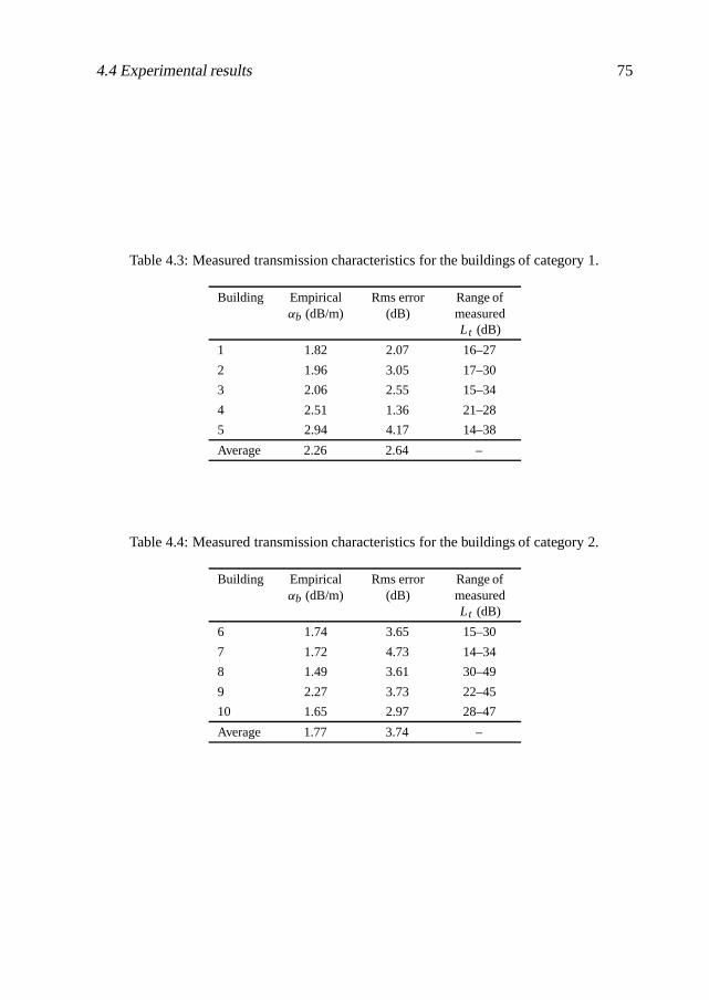
4.4 Experimental results 75
Table 4.3: Measured transmission characteristics for the buildings of category 1.
Building Empiricalαb (dB/m)
Rms error(dB)
Range ofmeasuredLt (dB)
1 1.82 2.07 16–27
2 1.96 3.05 17–30
3 2.06 2.55 15–34
4 2.51 1.36 21–28
5 2.94 4.17 14–38
Average 2.26 2.64 –
Table 4.4: Measured transmission characteristics for the buildings of category 2.
Building Empiricalαb (dB/m)
Rms error(dB)
Range ofmeasuredLt (dB)
6 1.74 3.65 15–30
7 1.72 4.73 14–34
8 1.49 3.61 30–49
9 2.27 3.73 22–45
10 1.65 2.97 28–47
Average 1.77 3.74 –
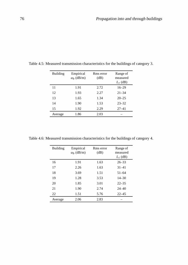
76 Propagation into and through buildings
Table 4.5: Measured transmission characteristics for the buildings of category 3.
Building Empiricalαb (dB/m)
Rms error(dB)
Range ofmeasuredLt (dB)
11 1.91 2.72 16–29
12 1.93 2.27 21–34
13 1.65 1.34 20–25
14 1.90 1.53 23–32
15 1.92 2.29 27–41
Average 1.86 2.03 –
Table 4.6: Measured transmission characteristics for the buildings of category 4.
Building Empiricalαb (dB/m)
Rms error(dB)
Range ofmeasuredLt (dB)
16 1.91 1.63 26–33
17 2.26 1.63 31–41
18 3.69 1.51 51–64
19 1.28 3.53 14–30
20 1.85 3.01 22–35
21 1.90 2.74 24–40
22 1.51 5.76 22–45
Average 2.06 2.83 –
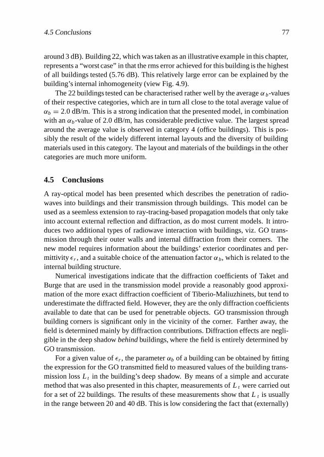
4.5 Conclusions 77
around 3 dB). Building 22, which was taken as an illustrative example in this chapter,represents a “worst case” in that the rms error achieved for this building is the highestof all buildings tested (5.76 dB). This relatively large error can be explained by thebuilding’s internal inhomogeneity (view Fig. 4.9).
The 22 buildings tested can be characterised rather well by the average α b-valuesof their respective categories, which are in turn all close to the total average value ofαb = 2.0 dB/m. This is a strong indication that the presented model, in combinationwith an αb-value of 2.0 dB/m, has considerable predictive value. The largest spreadaround the average value is observed in category 4 (office buildings). This is pos-sibly the result of the widely different internal layouts and the diversity of buildingmaterials used in this category. The layout and materials of the buildings in the othercategories are much more uniform.
4.5 Conclusions
A ray-optical model has been presented which describes the penetration of radio-waves into buildings and their transmission through buildings. This model can beused as a seemless extension to ray-tracing-based propagation models that only takeinto account external reflection and diffraction, as do most current models. It intro-duces two additional types of radiowave interaction with buildings, viz. GO trans-mission through their outer walls and internal diffraction from their corners. Thenew model requires information about the buildings’ exterior coordinates and per-mittivity εr , and a suitable choice of the attenuation factor αb, which is related to theinternal building structure.
Numerical investigations indicate that the diffraction coefficients of Taket andBurge that are used in the transmission model provide a reasonably good approxi-mation of the more exact diffraction coefficient of Tiberio-Maliuzhinets, but tend tounderestimate the diffracted field. However, they are the only diffraction coefficientsavailable to date that can be used for penetrable objects. GO transmission throughbuilding corners is significant only in the vicinity of the corner. Farther away, thefield is determined mainly by diffraction contributions. Diffraction effects are negli-gible in the deep shadow behindbuildings, where the field is entirely determined byGO transmission.
For a given value of εr , the parameter αb of a building can be obtained by fittingthe expression for the GO transmitted field to measured values of the building trans-mission loss L t in the building’s deep shadow. By means of a simple and accuratemethod that was also presented in this chapter, measurements of L t were carried outfor a set of 22 buildings. The results of these measurements show that L t is usuallyin the range between 20 and 40 dB. This is low considering the fact that (externally)
78 Propagation into and through buildings
diffracted fields in the shadow area of a building can easily be more than 40 dB be-low the free-space level. For accurate prediction of the field strength in such heavilyshadowed regions, which are typical for urban microcells, taking into account thetransmitted rays is of great importance.
Empirical αb-values obtained in the present study (assuming a permittivity of5 and zero conductivity) range from 1.3 to 3.7 dB/m, but most are concentratedaround the average value of 2.0 dB/m. Therefore, if it is not feasible to determineαb for each individual building, as will be usually the case in the practice of networkplanning, no large prediction errors are expected if all buildings are characterised bythis average value.
An important benefit of the new transmission model is that it automatically ac-counts for outdoor-to-indoor propagation, i.e. the penetration of radiowaves intobuildings. This phenomenon is receiving increased attention as indoor coverage isbecoming an important aspect of mobile network quality. It is noted, however, thatthe present model can only be expected to provide good results for building penetra-tion at the ground level, due to its two-dimensional nature. A different model has tobe used for the prediction of indoor field strength levels at higher floors.
5Scattering from trees
5.1 Introduction
In Chapter 3 of this thesis it was observed that the scattering of radiowaves fromtrees, which are abundantly found in most European cities, is an important propaga-tion mechanism. Investigations of tree effects on radio channel characteristics havehitherto been restricted mainly to coherent scattering, of which the attenuation ofwaves propagating through the foliage (“tree shadowing”) is the most obvious mani-festation [56, 57]. Incoherent scattered fields – which are due to the macroscopic di-electric heterogeneity of the medium formed by the tree canopy – are often neglected,even though they are generally predominant over the coherent scattered field in di-rections other than the forward direction. In scenarios where the line-of-sight path isobstructed and reflected and diffracted multipath contributions are weak, incoherenttree-scattered fields can become dominant. A specific case in which scattering fromtrees plays an important role was discussed in Section 3.3. The experimental resultsdiscussed in that section indicate that the fields scattered from trees located near astreet intersection can be more significant than the fields diffracted by the buildingcorners. Considering the effects of incoherent tree scattering can therefore lead to abetter modelling of radiowave propagation around street corners.
This chapter presents a new theoretical model for the coherent and incoherentscattering from deciduous trees. As this model finds its application in propagation

80 Scattering from trees
prediction for urban microcell environments, it is kept quasi-two-dimensional. Thismeans that it will be assumed that the reception point and the source of the incidentfield are both at the same height as the centre of the tree canopy, and that the canopyis very high. The wave propagation is in three-dimensional space, as usual. Further-more, attention is restricted to the vertically polarised field components, and hencethe final expressions for the scattered fields are scalar. The tree itself is assumed toconsist of a high, but finite cylindrical volume containing randomly located and ori-ented branches and leaves, modelled as dielectric cylinders and disks, as in [57–59].The effects of the trunk are neglected.
As in previous tree-scattering models, the coherent field in the canopy is com-puted using the multiple scattering theory of Foldy and Twersky [60]. However,unlike these earlier models, the (coherent and incoherent) scattered fields outside thecanopy are obtained as the approximate solutions to a set of integral equations, eachinvolving an integration over the canopy volume. Due to their mathematical form,these solutions are particularly suitable for use in ray-based propagation models.
This chapter is organised as follows. Section 5.2 describes the overall scatter-ing geometry and provides expressions for the scattering from branches and leaves.A model for the scattering of radiowaves from an entire tree canopy is developedin Section 5.3. The expressions derived in that section, as well as the underlyingassumptions and simplifications, are largely original contributions. In Section 5.4,numerical results generated using these expressions are presented, and the accuracyof the approximations made in their derivation is investigated. A comparison withexperimental data is made in Section 5.5. Conclusions are drawn in Section 5.6.
5.2 Vegetation model
From the standpoint of radiowave propagation, a vegetation canopy is a boundedmedium consisting of many discrete, randomly distributed and oriented, dielectricinclusions (branches, leaves, fruit, etc.) in a homogeneous background material(air). Although the medium may, in general, be random in both space and time,in the present study the canopy structure and, consequently, the scattered field areassumed to be time-invariant. At the frequencies used for mobile communications,the dimensions of the inclusions can be comparable to or larger than the wavelength.This means that the canopy cannot be treated as a macroscopically homogeneousdielectric mixture, characterised by an effective dielectric permittivity. Instead, thegeometries and orientations of the various types of inclusions present in the canopyalso have to be taken into account.
In the present study, a tree canopy is assumed to consist of an ensemble of leavesand branches. Leaves are modelled as thin, lossy dielectric disks and branches as fi-

5.2 Vegetation model 81
nite, lossy dielectric cylinders. A consequence of the dielectric heterogeneity of thecanopy volume is that the scattered field has an incoherent (or diffuse) component,which consists of uncorrelated contributions from the individual scatterers. For shortpropagation paths through random media, the incoherent scattered field in the for-ward direction is generally small compared to the coherent scattered field. For thisreason the incoherent scattered field is often disregarded in the literature dealing withtree scattering (attenuation) effects in terrestrial radiowave propagation. However, aswill be shown later in this chapter, this incoherent field is much more important thanthe coherent field in scattering directions other than the forward direction.
5.2.1 Overall problem geometry
Consider the tree canopy in Fig. 5.1, modelled as a vertically oriented, high but finitecylindrical volume V in a rectangular coordinate system defined by the orthonormalvectors x, y and z. This coordinate system, of which the origin r 0 is located at thecentre of the canopy, will be referred to as the reference frame. The radius R andthe height H describe the dimensions of V . The canopy volume contains randomlydistributed and oriented branches and leaves, the former of which can be classifiedinto Nb different size categories. Their number densities are represented by ρb andρl , respectively, where the subscript b is an element of {b1, b2, . . . , bNb} and bn isused to denote branches of the nth size category.
H
R
r0r0 y^
z^
x^
V
(a)
r0
ks
ki = x
s
y^
z^
x^
^
^
^
(b)
Fig. 5.1: Problem geometry. (a) Canopy volume. (b) Incident and scattered directions.

82 Scattering from trees
Incident on the canopy is a vertically polarised wave with wavelength λ anddirection of propagation ki relative to the canopy centre. The source of this wave isassumed to be located far away from the canopy, so that the incident field amplitudecan be approximated as being constant over the canopy volume. The incident waveis scattered in all directions by the scatterers in the canopy volume, and the scatteredfield is observed at an observation point, also located far away from the canopy,in the direction ks relative to the canopy centre. The unit vectors ki and ks areperpendicular to z, and ϕs denotes the azimuthal scattering direction. Without lossof generality, it is assumed that ki = x.
The problem dealt with in Section 5.3 is to compute the mean and variance of the(vertical component of the) scattered field at the observation point. The scatteringamplitude functions of the branches and leaves, as well as some other equations re-quired for the computations in Section 5.3, are given in the remainder of the presentsection (Sections 5.2.2 to 5.2.4). These equations are mostly taken from the pub-lished literature, in particular from [58, 59, 61].
5.2.2 Scattering from branches
Tree branches are composed of several concentric tissue layers (wood, bark, etc.),each of which is made up of many cells that are much smaller than the wavelengthsnormally used for mobile communications. Although it has been shown that theeffective dielectric properties of the branch material can be different from one tissuelayer to the other, and even anisotropic [62], for simplicity branches are modelledhere as homogeneous dielectrics with an effective complex dielectric permittivity ε b.
Consider the finite-length, lossy dielectric cylinder in the rectangular coordinatesystem defined by the orthonormal vectors x ′, y′ and z′. This coordinate system willbe called the local frame of the cylinder. In the local frame, the incident and scattereddirection vectors ki and ks are defined by the angles θ ′
i , ϕ′i , θ
′s and ϕ ′
s (view Fig. 5.2).The cylinder has length hb and radius rb, and is oriented parallel to z ′. The scatteringof an arbitrarily polarised wave incident on the cylinder can be described in terms ofa scattering amplitude tensor. If the field inside the cylinder is estimated as the fieldinside a similar, but infinite cylinder, the elements of this tensor are given by [58, 59]
f bvv (ks, ki ) = k2hb
2(εb − 1)µb(ks, ki )
{e0v(B0 cos θ ′
s cos θ ′i − sin θ ′
sz0)
+ 2∞∑
n=1
[(env cos θ ′
i Bn − j ηhnv An) cos θ ′s
− sin θ ′senvzn
]cos[n(ϕ ′
i − ϕ′s)]}
(5.1a)
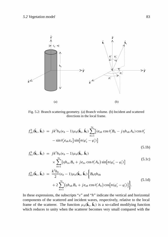
5.2 Vegetation model 83
hb
y’^
z’^
x’^
rb
(a)
y’^
z’^
x’^
s’
i’
ks^ki
^
i’ s’
(b)
Fig. 5.2: Branch scattering geometry. (a) Branch volume. (b) Incident and scattereddirections in the local frame.
f bvh(ks, ki ) = j k2hb(εb − 1)µb(ks, ki )
∞∑n=1
[(enh cos θ ′
i Bn − j ηhnhAn) cos θ ′s
− sin θ ′senhzn
]sin[n(ϕ ′
s − ϕ′i )]
(5.1b)
f bhv(ks, ki ) = j k2hb(εb − 1)µb(ks, ki )
×∞∑
n=1
(ηhnvBn + jenv cos θ ′
i An
)sin[n(ϕ ′
s − ϕ′i )] (5.1c)
f bhh(ks, ki ) = k2hb
2(εb − 1)µb(ks, ki )
{B0ηh0h
+ 2∞∑
n=1
(ηhnhBn + jenh cos θ ′
i An
)cos[n(ϕ ′
s − ϕ′i )]}.
(5.1d)
In these expressions, the subscripts “v” and “h” indicate the vertical and horizontalcomponents of the scattered and incident waves, respectively, relative to the localframe of the scatterer. The function µb(ks, ki ) is a so-called modifying functionwhich reduces to unity when the scatterer becomes very small compared with the
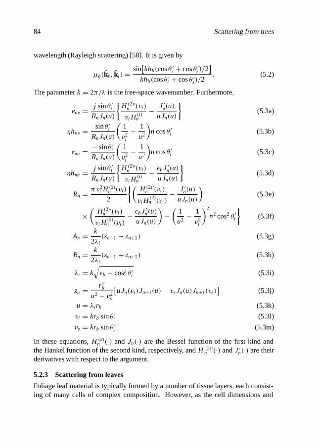
84 Scattering from trees
wavelength (Rayleigh scattering) [58]. It is given by
µb(ks, ki ) = sin[khb(cos θ ′
i + cos θ ′s)/2
]khb(cos θ ′
i + cos θ ′s)/2
. (5.2)
The parameter k = 2π/λ is the free-space wavenumber. Furthermore,
env = j sin θ ′i
Rn Jn(u)
{H (2)′
n (vi )
vi H(i )n
− J ′n(u)
uJn(u)
}(5.3a)
ηhnv = sin θ ′i
Rn Jn(u)
(1
v2i
− 1
u2
)n cos θ ′
i (5.3b)
enh = − sinθ ′i
Rn Jn(u)
(1
v2i
− 1
u2
)n cos θ ′
i (5.3c)
ηhnh = j sin θ ′i
Rn Jn(u)
{H (2)′
n (vi )
vi H(i )n
− εbJ ′n(u)
uJn(u)
}(5.3d)
Rn = πv2i H (2)
n (vi )
2
{(H (2)′
n (vi )
vi H(2)n (vi )
− J ′n(u)
uJn(u)
)(5.3e)
×(
H (2)′n (vi )
vi H(2)n (vi )
− εbJ ′n(u)
uJn(u)
)−(
1
u2− 1
v2i
)2
n2 cos2 θ ′i
}(5.3f)
An = k
2λi(zn−1 − zn+1) (5.3g)
Bn = k
2λi(zn−1 + zn+1) (5.3h)
λi = k√εb − cos2 θ ′
i (5.3i)
zn = r 2b
u2 − v2s
[uJn(vs)Jn+1(u)− vsJn(u)Jn+1(vs)
](5.3j)
u = λi rb (5.3k)
vi = krb sin θ ′i (5.3l)
vs = krb sin θ ′s. (5.3m)
In these equations, H (2)n (·) and Jn(·) are the Bessel function of the first kind and
the Hankel function of the second kind, respectively, and H (2)′n (·) and J ′
n(·) are theirderivatives with respect to the argument.
5.2.3 Scattering from leaves
Foliage leaf material is typically formed by a number of tissue layers, each consist-ing of many cells of complex composition. However, as the cell dimensions and
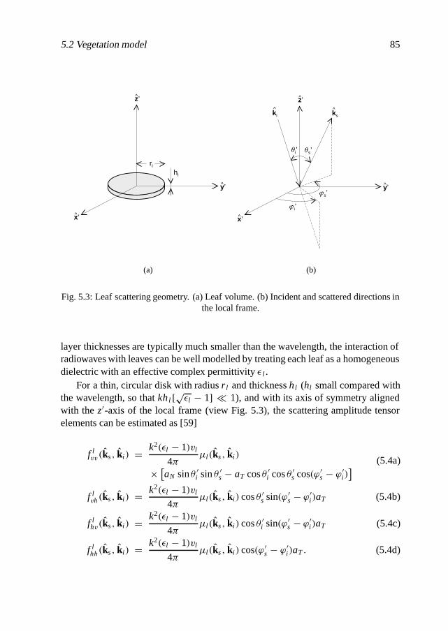
5.2 Vegetation model 85
hl
y’^
z’^
x’^
rl
(a)
y’^
z’^
x’^
s’
i’
ks^ki
^
i’ s’
(b)
Fig. 5.3: Leaf scattering geometry. (a) Leaf volume. (b) Incident and scattered directions inthe local frame.
layer thicknesses are typically much smaller than the wavelength, the interaction ofradiowaves with leaves can be well modelled by treating each leaf as a homogeneousdielectric with an effective complex permittivity ε l .
For a thin, circular disk with radius r l and thickness hl (hl small compared withthe wavelength, so that khl [√εl − 1] � 1), and with its axis of symmetry alignedwith the z′-axis of the local frame (view Fig. 5.3), the scattering amplitude tensorelements can be estimated as [59]
f lvv(ks, ki ) = k2(εl − 1)vl
4πµl (ks, ki )
× [aN sinθ ′i sin θ ′
s − aT cos θ ′i cos θ ′
s cos(ϕ ′s − ϕ′
i )] (5.4a)
f lvh(ks, ki ) = k2(εl − 1)vl
4πµl (ks, ki ) cos θ ′
s sin(ϕ ′s − ϕ′
i )aT (5.4b)
f lhv(ks, ki ) = k2(εl − 1)vl
4πµl (ks, ki ) cos θ ′
i sin(ϕ ′s − ϕ′
i )aT (5.4c)
f lhh(ks, ki ) = k2(εl − 1)vl
4πµl (ks, ki ) cos(ϕ ′
s − ϕ′i )aT . (5.4d)

86 Scattering from trees
In these expressions, vl = πhl r 2l is the leaf volume, and
µl (ks, ki ) = 2J1(Qsirl )
Qsirl(5.5a)
Qsi = k√
sin2 θ ′s + sin2 θ ′
i − 2 sinθ ′s sin θ ′
i cos(ϕ ′s − ϕ′
i ) (5.5b)
is a modifying function similar to that in (5.2). Furthermore, under the reasonableassumption that hl � rl , aN and aT are given by [59]
aN = ε−1l and aT = 1. (5.6)
5.2.4 Equivalent scattering amplitude and cross section
The scattering amplitude tensor for a scatterer with an arbitrary orientation with re-spect to the reference frame, described by the two-dimensional variable� = (α, β),0 < α < 2π , 0 < β < π/2, with α and β defined in Fig. 5.4, can be obtainedfrom the corresponding local-frame scattering amplitude tensor by means of a trans-formation of coordinates. In view of the application considered in this thesis, weare only interested in the vertical components of the fields incident on and scatteredby branches and leaves. The reference-frame scattering amplitude tensor elementwhich relates these fields is written as [61]
Fb,l (ks, ki ) = 1
D(ks, ki )
{tvs[
f b,lvv (ks, ki )tvi − f b,l
vh (ks, ki )thi]
−ths[
f b,lhv (ks, ki )tvi − f b,l
hh (ks, ki )thi]},
(5.7)
where
D(ks, ki ) =√(t2vs + t2
hs)(t2vi + t2
hi) (5.8a)
tvs = − cosβ (5.8b)
ths = sinβ sin(α − ϕs) (5.8c)
tvi = − cosβ (5.8d)
thi = sinβ sinα. (5.8e)
Note that the subscript “vv” of the reference-frame scattering amplitude, which in-dicates vertical polarisation of the incident and scattered fields, is omitted for conve-nience.
The incidence and scattering angles in the local frame are related to ϕ s, α and β

5.2 Vegetation model 87
y^
z^
x^
y’^
z’^
x’^
Fig. 5.4: Orientation of the local frame with respect to the reference frame.
by
θ ′i = π
2− arccos
{sinβ cosα
}(5.9a)
ϕ′i = π
2
[1 − sgn
{cosα cosβ
}]− arctan
{sinα
cosα cos β
}(5.9b)
θ ′s = π
2+ arccos
{sinβ cos(α − ϕs)
}(5.9c)
ϕ′s = π
2
[1 − sgn
{cos(α − ϕs) cosβ
}]− arctan
{sin(α − ϕs)
cos(α − ϕs) cosβ
}, (5.9d)
where the function sgn(·) is defined as
sgn(x) ={
1, if x ≥ 0,
−1, if x < 0.(5.10)
The probability density functions of the orientations of branches and leaves aredenoted by f b
�(α, β) and f l�(α, β), respectively. The statistics of α are assumed to
be independent of those of β, so that
f b,l� (α, β) = f b,l
α (α) f b,lβ (β). (5.11)
Also, the spatial distribution of the scatterers over the canopy volume is assumedto be truly random (with a uniform probability density), i.e. no account is taken
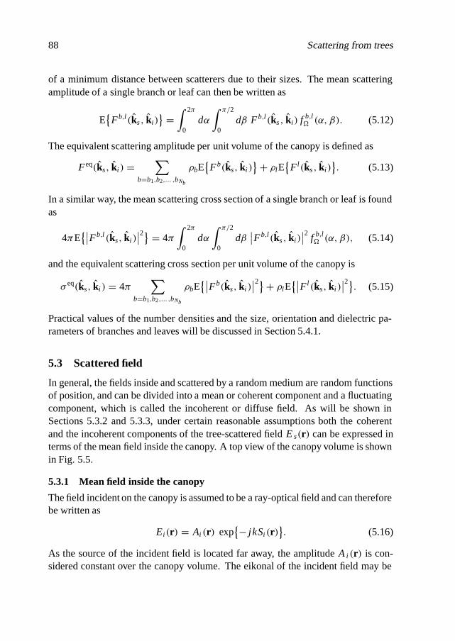
88 Scattering from trees
of a minimum distance between scatterers due to their sizes. The mean scatteringamplitude of a single branch or leaf can then be written as
E{Fb,l (ks, ki )
} =∫ 2π
0dα∫ π/2
0dβ Fb,l (ks, ki ) f b,l
� (α, β). (5.12)
The equivalent scattering amplitude per unit volume of the canopy is defined as
F eq(ks, ki ) =∑
b=b1,b2,... ,bNb
ρbE{Fb(ks, ki )
}+ ρl E{Fl (ks, ki )
}. (5.13)
In a similar way, the mean scattering cross section of a single branch or leaf is foundas
4πE{∣∣Fb,l (ks, ki )
∣∣2} = 4π∫ 2π
0dα∫ π/2
0dβ∣∣Fb,l (ks, ki )
∣∣2 f b,l� (α, β), (5.14)
and the equivalent scattering cross section per unit volume of the canopy is
σ eq(ks, ki ) = 4π∑
b=b1,b2,... ,bNb
ρbE{∣∣Fb(ks, ki )
∣∣2}+ ρl E{∣∣Fl (ks, ki )
∣∣2}. (5.15)
Practical values of the number densities and the size, orientation and dielectric pa-rameters of branches and leaves will be discussed in Section 5.4.1.
5.3 Scattered field
In general, the fields inside and scattered by a random medium are random functionsof position, and can be divided into a mean or coherent component and a fluctuatingcomponent, which is called the incoherent or diffuse field. As will be shown inSections 5.3.2 and 5.3.3, under certain reasonable assumptions both the coherentand the incoherent components of the tree-scattered field Es(r) can be expressed interms of the mean field inside the canopy. A top view of the canopy volume is shownin Fig. 5.5.
5.3.1 Mean field inside the canopy
The field incident on the canopy is assumed to be a ray-optical field and can thereforebe written as
Ei (r) = Ai (r) exp{− j kSi (r)
}. (5.16)
As the source of the incident field is located far away, the amplitude Ai (r) is con-sidered constant over the canopy volume. The eikonal of the incident field may be
5.3 Scattered field 89
x^
y^
�s
s1( )r
s2( )r
ks
^
r0
r
ki
^
R
z^
Fig. 5.5: Top view of the cylindrical canopy volume V .
written in terms of the phase at the canopy centre r0 and the displacement of r fromr0, as
Si (r) = Si (r0)+ ki · (r − r0)+ 1
2(r − r0) ·
[x1x1
r1+ x2x2
r2
]· (r − r0), (5.17)
where r1 and r2 are the principal radii of curvature of the incident wavefront, andx1 and x2 are unit vectors, each of which in combination with ki defines one of theprincipal planes of curvature. It is assumed that x 1 is oriented parallel to z, and x2 isparallel to y. Now, the incident field in the canopy volume is
Ei (r) = E0 exp
{− j kx − 1
2j k
[z2
r1+ y2
r2
]}, r ∈ V, (5.18)
where E0 = Ei (r0).The coherent field E
{Ein(r)
}inside the canopy can be shown [60] to satisfy the
wave equation
(∇2 + K 2)
E{Ein(r)
} = 0, (5.19)
in which
K = k + 2π
kF eq(ki , ki ) = K ′ − j K ′′ (5.20)

90 Scattering from trees
is the effective propagation constant. As F eq(ki , ki ) is in general a complex number,the attenuation constant K ′′ is non-zero and the coherent field attenuates as it prop-agates through the canopy. The specific attenuation in decibels per metre (dB/m) isgiven as
αc = 8.686 K ′′. (5.21)
For the case of a plane wave of the form
Ei (r) = E0 exp{− j k(ki · r)
}(5.22)
incident on a slab containing random scatterers, the coherent field at a point r insidethe slab can be shown to be [60]
E{Ein(r)
} = Ei (r) exp{− j (K − k)s1(r)
}, r ∈ V, (5.23)
where s1(r) is the length of the path through the slab to r, along the incidence direc-tion ki . For a field of the more general form (5.16) incident on the canopy volumeV it is assumed that the mean field inside the canopy can be described by the sameequation (5.23), with Ei (r) as in (5.16) and
s1(r) = x +√
R2 − y2, r ∈ V, (5.24)
which is equal to the length of the path to r through the cylindrical volume V (viewFig. 5.5).
5.3.2 Coherent scattered field
The coherent tree-scattered field can be found using Foldy-Twersky’s integral equa-tion for the coherent field in Twersky’s multiple scattering theory [60]. This the-ory includes all multiple scattering involving chains of successive scattering goingthrough different scatterers, but neglects the scattering paths which go through ascatterer more than once. According to Twersky’s theory, for a uniform density ofscatterers the coherent scattered field is given by
Ecohs (r) = E
{Es(r)
} =∫∫∫
V
U(r, r′) E{Ein(r′)
}dV′, (5.25)
where U(r, r′) is an operator which relates the mean scattered field at r due to a unitvolume of the random medium located at r′, to the field E{E in(r′)} incident on thisvolume. When r is in the far zone of the particles in the unit scattering volume at r ′,U(r, r′) can be approximated by
U(r, r′) = 4πF eq(ks, ki ) G0(r, r′), (5.26)

5.3 Scattered field 91
where
G0(r, r′) = e− jk|r−r′|
4π |r − r′| (5.27)
is the free-space Green’s function. For an observation point r located far away fromthe canopy, this function is well approximated by
G0(r0 + sks, r0+x′x + y′y + z′ z) = exp{− j k
[s − x ′ cosϕs − y′ sinϕs
]}4πs
× exp
{− j k
[(x′ sinϕs − y′ cosϕs)
2 + z′2
2s
]},
(5.28)
where s is the distance from the canopy centre to the observation point.In order to simplify the computation of the coherent tree-scattered field, it is
assumed that the canopy is high compared to the diameter of the first Fresnel zoneat r0, so that the finite integral over z′ in equation (5.25) may be replaced by anintegration from z′ = −∞ to z′ = ∞. Then, after substitution of (5.26), (5.23),(5.18) and (5.28) into (5.25) and performing the z′-integration, the coherent scatteredfield can be written as
Ecohs (r) = E0S
√r1
s(r1 + s)e− jks, (5.29)
where
S=[
2π
k
] 12
e− jπ/4 F eq(ks, ki )
∫∫x′2+y′2<R2
exp{− j (K − k)s1(r′)
}
× exp
{− j k
[x′(1 − cosϕs)− y′ sinϕs
+ y′2
2r2+ (x′ sinϕs − y′ cos ϕs)
2
2s
]}dx′dy′,
(5.30)
is the scattering coefficient. The result (5.29) is similar in form to the general ex-pression for the diffracted field used in the geometrical theory of diffraction (GTD)and its uniform extension (UTD). Physically, it describes the coherent scattered fieldin terms of a “coherently scattered ray” which interacts with the tree at the canopycentre r0.
The next step in the analysis is to find alternative, approximate expressions forthe scattering coefficient (5.30) that require less computational effort to evaluate than
92 Scattering from trees
a numerical double integration. To this end, S is rewritten as
S =[
2π
k
] 12
e− jπ/4 F eq(ks, ki )
R∫−R
Iy′(x′)dx′, (5.31)
in which I y′ is given by
I y′(x′) = I ay′ − I b
y′ =∫ ∞
y′a
ψ(y′)e− jkµ(y′)dy′ −∫ ∞
y′b
ψ(y′)e− jkµ(y′)dy′, (5.32)
with integration endpoints y ′a = −√
R2 − x′2 and y′b = √
R2 − x′2. In these inte-grals,
ψ(y′) = exp{− j (K − k)s1(r′)
}(5.33)
is a complex “amplitude” function, and
µ(y′) = x′(1 − cosϕs)− y′ sinϕs + y′2
2r2+ (x′ sinϕs − y′ cosϕs)
2
2s(5.34)
is a smooth, real “phase” function with first and second derivatives
µ′(y′) = − sinϕs + y′
r2− (x′ sinϕs − y′ cosϕs) cosϕs
s
µ′′(y′) = 1
r2+ cos2 ϕs
s.
(5.35)
According to the method of stationary phase, for large k the integrals I a,by′ can be well
approximated, in closed form, in terms of contributions from the neighbourhoods ofthe critical points, viz. the stationary point
y′s = r2 sinϕs(s + x ′ cosϕs)
r2 cos2 ϕs + s, (5.36)
for which µ′(y′) = 0, and the integration endpoints y ′a,b [63]. For some values of x ′,
however, the stationary point may be near or even equal to one of the endpoints, andthe contributions arising from the neighbourhoods of these points may not be treatedseparately. In the following, two different approaches are discussed to circumventthis problem.
First consider the asymptotic expansion obtained by Lewis in [64]. When appliedto the integrals I a,b
y′ , this expansion is valid uniformly for y ′s in the neighbourhood
5.3 Scattered field 93
of y′a,b, provided that ψ(y′) and µ(y′) are smooth functions on the interval y ′
a − ε ≤y′ ≤ y′
b + ε, where ε > 0. This condition is not satisfied by the amplitude functionψ(y′), which is not differentiable at y ′ = y′
a,b. If, on the other hand, ψ(y′) isapproximated as
ψ(y′) � exp{− j (K − k)
[x′ + R
]}, (5.37)
one obtains
I a,by′ � exp
{− j (K − k)[x′ + R
]}e− jkµ(y′
a,b)
×{[
2
k∣∣µ′′(y′
s)∣∣] 1
2
g−(
sgn(y′a,b − y′
s)
√k∣∣µ(y′
a,b)− µ(y′s)∣∣)− j
kµ′(y′a,b)
},
(5.38)
with
g−(x) = f−(x)− 1
2 j x(5.39)
f−(x) = ejx2∫ ∞
xe− j t 2
dt. (5.40)
The function f−(·) is closely related to the modified Fresnel integral, and can beapproximated by [64, 65]
f−(x) = √π
[1
2√πx2 + x + 1
+ 0.022x exp(−0.29x2)
]
× exp
{− j arctan(x2 + 1.5x + 1)
}, x ≥ 0
(5.41a)
f−(−x) = √π exp
{j (x2 − π/4)
} − f−(x). (5.41b)
The amplitude and phase errors of the estimates of f−(·) obtained with this formulaare contained within 3.4 and 2 percent, respectively. For values of y ′
s that are veryclose to y′
a,b, I a,by′ reduces to
I a,by′ →
[π
2k∣∣µ′′(y′
s)∣∣] 1
2
exp{− j (K − k)
[x′ + R
]}e− jkµ(y′
s)− jπ/4, y′s → y′
a,b.
(5.42)
The scattering coefficient S is computed by performing the single integration over x ′in (5.31) numerically, using a rectangular rule.
94 Scattering from trees
A second approach to arriving at an asymptotic approximation of the doubleintegral in expression (5.30) is to neglect the contributions from the endpoints y ′
a,b,and restrict the analysis to those scattering angles ϕ s for which stationary points existin the canopy volume. This is the case if ϕ s is small (forward scattering), such thatthe observation point is in the shadow area of the tree. For small values of ϕ s, thephase function of (5.34) can be approximated as
µ(y′) � x′(1 − cosϕs) − y′ sinϕs + y′2
2r2+ y′2 cos2 ϕs
2s(5.43)
and the stationary point becomes
y′s � r2ssinϕs
r2 cos2 ϕs + s. (5.44)
If |y′s| <
√R2 − x′2, the integral I y′ is approximated by the contribution arising from
the vicinity of y ′s, which yields
I y′ �[
2π
k
] 12
e− jπ/4√
r2s
r2 cos2 ϕs + sA exp
{− j x ′[K − k cosϕs
]}, (5.45)
with
A = exp{− j (K − k)
√R2 − y′2
s + 1
2j ky′
s sinϕs}. (5.46)
If |y′s| ≥ √
R2 − x′2, Iy′ is assumed to be zero. The integral over x ′ in equation(5.31) can now be evaluated in closed form, and the scattering coefficient is obtainedas
S = −4π j
kF eq(ks, ki )
√r2s
r2 cos2 ϕs + sA
sin[(K − k cosϕs)x′
s
]K − k cosϕs
, (5.47)
in which x ′s = √R2 − y′2
s . Note that, in general, the argument of the sine function inthis expression has a complex value.
5.3.3 Incoherent scattered field
The incoherent (or diffuse) scattered field due to the tree canopy can be obtainedfrom Twersky’s integral equations for the total field intensity in Twersky’s multi-ple scattering theory [60]. According to these equations, for a uniform density of
5.3 Scattered field 95
scatterers, the diffuse field intensity is given by
E{∣∣Edif
s (r)∣∣2} = E
{∣∣Es(r)∣∣2}− ∣∣Ecoh
s (r)∣∣2
=∫∫∫
V
∣∣V(r, r′)∣∣2 E{∣∣Ein(r′)
∣∣2}dV′ (5.48)
V(r, r′) = U(r, r′)+∫∫∫
V
U(r, r′′)V(r′′, r′)dV′′. (5.49)
As in Section 5.3.2, U(r, r′) is an operator which relates the field at r scatteredfrom a unit scattering volume at r ′ to the field incident on the volume. The operatorV(r, r′), which represents the total radiation from a unit scattering volume at r ′ to rthrough multiple scattering, is approximated as
V(r, r′) = 4πF eq(ks, ki ) G0(r, r′) exp{− j (K − k)s2(r′)
}, (5.50)
where s2(r′) is the path length from r ′ to the observation point through the canopyalong the direction of scattering ks (see Fig. 5.5), given by
s2(r) = −x cosϕs − y sinϕs +√
R2 − x2 sin2 ϕs − y2 cos2 ϕs, r ∈ V. (5.51)
The operator V(r, r′) is similar in form to the single-scattering operator U(r, r ′)given by (5.26), except that the propagation constant in the canopy is K rather thank, to account for the additional loss due to multiple scattering.
In general, under the assumption that the scatterers in a random medium havea small scattering albedo, the total field intensity E{|E in(r)|2} in the medium canbe approximated by the coherent intensity |E{E in(r)}|2. This approximation, andthe substitution of (5.18), (5.23), (5.28) and (5.50) into (5.48), lead to the followingexpression for the diffuse scattered field intensity:
E{∣∣Edif
s (r)∣∣2} =
∣∣E0
∣∣24πs2
σ eq(ks, ki )I (ϕs), (5.52)
in which σ eq(ks, ki ), as previously, is the equivalent scattering cross section of a unitvolume within the tree canopy, and
I (ϕs) =∫∫∫
V
exp{−2K ′′[s1(r′)+ s2(r′)
]}dV′. (5.53)
The bistatic scattering cross section of the entire canopy is given by
σ(ks, ki ) = σ eq(ks, ki )I (ϕs). (5.54)
96 Scattering from trees
The integral I (ϕs) describes to what degree each elemental canopy volume dV ′ con-tributes to the total incoherent scattered field, and is closely related to the illumi-nation integral in [66]. When normalised with respect to the total canopy volumeπH R2, it is a function of the scattering angle ϕ s and the product K ′′ R. For K ′′ R< 1,I (ϕs) is approximated by the empirical formula
I (ϕs) = πH R2{1 + [K ′′ R
]2(1 − cosϕs
)}× exp
{−3.62K ′′R + 0.58[K ′′ R
]2} (5.55)
with an accuracy better than 0.7 dB for all ϕs.
5.4 Numerical results
This section presents numerical results generated using the expressions of the pre-vious section, and attempts to assess the loss in accuracy caused by some of theapproximations that were made in the derivations of these expressions. Branch andleaf parameters such as size and orientation statistics and dielectric properties areimportant inputs to the models, and will be discussed in Section 5.4.1.
5.4.1 Branch and leaf parameters
Number densities, size and orientation statistics of branches and leaves were anal-ysed in detail for an oak tree in Boxtel, The Netherlands (view Fig. 5.6), which isconsidered to be a typical example of the trees commonly found in urban environ-ments. The same tree was also used for a number of scattering experiments, whichare reported in Section 5.5. The branches were categorised into Nb = 5 groupsaccording to their radii, and for each group an average branch length and numberdensity were computed. Leaf thickness and radius were determined for a single,representative oak leaf. The size parameter values that were thus obtained are listedin Table 5.1. On average, these values are larger than those found by McDonald etal. [67] and Karam et al. [68] for a walnut orchard. However, the trees examinedby these authors were only six years old and therefore probably less mature than thetree analysed in the present study and most urban trees.
Neither branches nor leaves were found to exhibit a preferred azimuthal orien-tation, and the distribution of α is therefore chosen to be uniform on (0, 2π). Thestatistics of the elevational orientation β of branches and leaves are assumed to bedescribed by the distribution
f b,lβ (β) =
{sinβ/(cosβ1 − cosβ2), if β1 < β < β2,
0, otherwise.(5.56)

5.4 Numerical results 97
(a) (b)
Fig. 5.6: The Boxtel oak tree (a) in full leaf (summer) and (b) defoliated (winter).
The orientation of the larger branches (categories 1 and 2) was observed to be pre-dominantly vertical, and therefore these branches are assigned the values β 1 = 0and β2 = π/4. The smaller branches (categories 3, 4 and 5) and the leaves arecharacterised by β1 = 0 and β2 = π/2, which implies that they have no preferredorientation at all (spherical distribution).
As time did not permit measurements of the effective dielectric permittivity ofbranches and leaves, suitable values were obtained from the literature, as describedbelow. The dielectric properties of branch and leaf material are well known to bestrongly influenced by the gravimetric moisture content M g, defined as the ratiobetween the mass of the moisture contained in the material and the total mass of
Table 5.1: Size and dielectric parameters of branches and leaves.
Scatterer type Radius (cm)Length/
thickness (cm)Relative
permittivityNumber
density (m−3)
Branch (1) 11.4 131 28 − j 7 0.013
Branch (2) 6.0 99 28 − j 7 0.073
Branch (3) 2.8 82 28 − j 7 0.41
Branch (4) 0.7 54 28 − j 7 5.1
Branch (5) 0.2 12 28 − j 7 56
Leaf 3.7 0.02 31 − j 8 420

98 Scattering from trees
the moist material. As the moisture content of branches shows significant diurnaland seasonal variations, their dielectric properties are also strongly time-dependent.From the results presented in [67], the average day-time dielectric permittivity ofbranches at 1.2 GHz is found to be εb = 28 − j 7. From a comparison with thedielectric properties of wood, tabulated in [62] as a function of various parameters, itis concluded that εb remains approximately constant in the high UHF frequency bandused for mobile communications, and is hardly dependent on temperature abovefreezing point.
A semi-empirical formula for the complex permittivity of leaves in terms of M g
and the complex permittivity ε sw of saline water, valid in the frequency range from 1to 100 GHz and for a salinity of about 1%, was proposed in [69] and is written as
εl = 0.689 (Mg − 0.24) εsw + 4.35 − 3.84Mg. (5.57)
For a walnut tree, the moisture content Mg of the leaves was shown in [67] to betime-invariant and have a value of approximately 80%. The dielectric properties ofsaline water are strongly dependent on frequency, and can be evaluated using [70].For a frequency of 2 GHz and a salinity of 1%, εsw takes a value of 77 − j 22,and the leaf permittivity becomes εl = 31 − j 8. Similar to branches, above freezingpoint the temperature-dependence of εl is negligible. The dielectric parameter valuesdiscussed above are also listed in Table 5.1.
5.4.2 Attenuation coefficients
Theoretical values of the attenuation coefficient αc due to the different canopy con-stituents, computed with the aid of (5.13), (5.20) and (5.21), are shown in Table 5.2.Examination of this table shows that most of the attenuation is due to the smallerbranches (size category 4) and the leaves. The total attenuation coefficient for thetree in leaf is 1.10 dB/m; for the defoliated tree this value is 0.80 dB/m. These valuesare comparable to, although somewhat lower than the experimental values publishedin [56] (1.3 and 1.1 dB/m, respectively), which were obtained in the shadow zone ofa single Pecan tree at 1.6 GHz. The difference between these values may be relatedto differences in branch and leaf parameters.
5.4.3 Scattering cross sections of branches and leaves
Fig. 5.7 shows the mean scattering cross sections for single branches and leaves,computed using equation (5.14) with size, orientation and dielectric parameters takenfrom Table 5.1. It can be seen that the scattering from the larger branches is con-centrated in the forward direction, whereas the scattering from the smallest branches(size category 5) and the leaves is almost isotropic. Fig. 5.7 also shows the equiva-lent scattering cross sections per unit volume of canopy, σ eq(ks, ki ), for the tree in
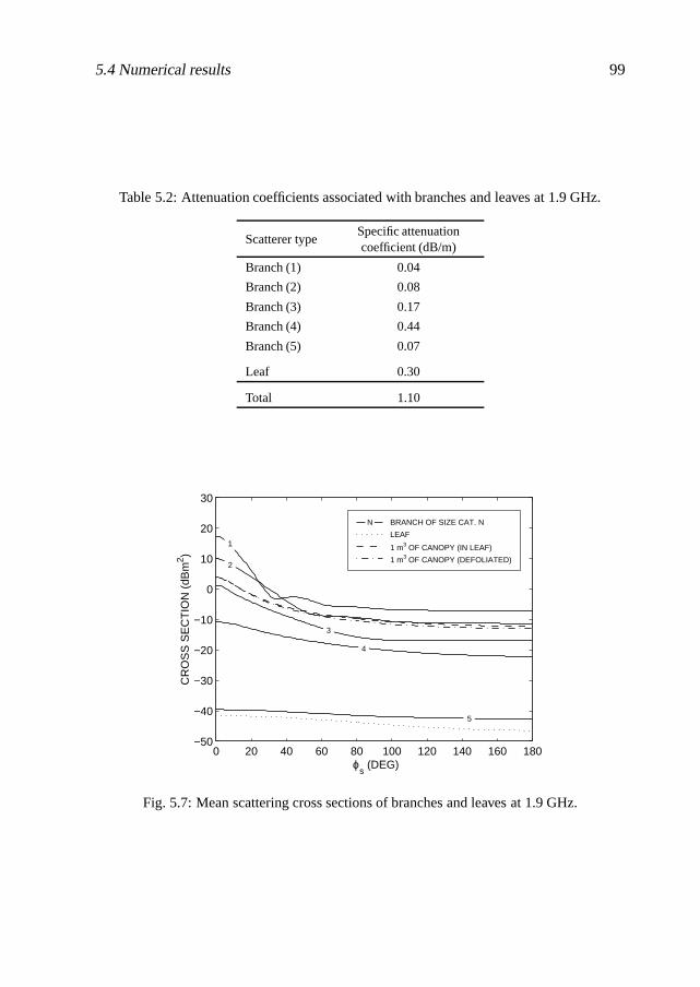
5.4 Numerical results 99
Table 5.2: Attenuation coefficients associated with branches and leaves at 1.9 GHz.
Scatterer typeSpecific attenuationcoefficient (dB/m)
Branch (1) 0.04
Branch (2) 0.08
Branch (3) 0.17
Branch (4) 0.44
Branch (5) 0.07
Leaf 0.30
Total 1.10
0 20 40 60 80 100 120 140 160 180−50
−40
−30
−20
−10
0
10
20
30
ϕs (DEG)
CR
OS
S S
EC
TIO
N (
dBm
2 )
BRANCH OF SIZE CAT. N
LEAF
1 m3 OF CANOPY (IN LEAF)
1 m3 OF CANOPY (DEFOLIATED)
N
1
2
3
4
5
Fig. 5.7: Mean scattering cross sections of branches and leaves at 1.9 GHz.

100 Scattering from trees
full leaf, computed using equation (5.15) and the number densities of Table 5.1, andfor the defoliated tree, computed by setting ρ l = 0. As can be observed in Fig. 5.7,σ eq(ks, ki ) is almost identical for these two cases.
5.4.4 Coherent scattered field
This section compares the coherent scattering patterns obtained by evaluating:
1. the expression (5.30) using a numerical double integration with an estimatedaccuracy of 1 percent (reference method);
2. the integral I y′ using the asymptotic expansion (5.38) and performing the sin-gle integration in (5.31) numerically, using a rectangular rule with fixed stepsize x ′;
3. the closed-form expression (5.47).
All three methods require the computation of the equivalent scattering amplitudeF eq(ks, ki ). This is a very time-consuming task, but has to be performed only once;the computed values are then stored and can be read every time S is evaluated. Thebranch and leaf parameters used to produce the results of this section were takenfrom Table 5.1. The tree was assumed to be in full leaf.
First of all, in order to investigate the influence of the step size x ′ on the ac-curacy of the numerical integration in method (2), the scattering coefficient S wasevaluated for a range of step sizes and for different canopy radii R. An adaptivestep size integration with an estimated accuracy of 1 percent was also performedfor comparison. Normalised scattering patterns obtained in this way are shown inFig. 5.8 for R = 1 and 5 m. The numerical integration accuracy tends to be better inthe forward direction. For R = 1 m, a step size of 0.03λ is sufficient to guarantee anerror smaller than 0.7 dB relative to the “adaptive step size” pattern, over the entireinterval 0 < ϕs < 180o; for R = 5 m, the error is smaller than 0.4 dB for this stepsize. For a step size of 0.01λ, these maximum errors become 0.5 and 0.2 dB, respec-tively. In comparing the curves for R = 1 m and R = 5 m, it is further seen that themain lobe of the scattering pattern – responsible for the attenuation of the total fieldin the forward direction – is considerably wider for the larger canopy. This is not asurprising result as the larger canopy can be expected to have a larger “shadow area”behind it. In this region, the coherent scattered field is nearly equal to the incidentfield but approximately 180 degrees out of phase.
Next, the effects are considered of the approximations made in the derivation ofthe expressions for the coherent scattered field. In Fig. 5.9, the scattering patternsobtained using the approximate methods (2) and (3) are compared with the pattern

5.4 Numerical results 101
0 20 40 60 80 100 120 140 160 180−120
−100
−80
−60
−40
−20
0
ϕs (DEG)
NO
RM
ALI
SE
D |S
| (dB
)
SINGLE INT., REL. ERR. < 10−2
SINGLE INT., ∆x = 0.1λ
SINGLE INT., ∆x = 0.03λ
SINGLE INT., ∆x = 0.01λ
5−M RADIUS
1−M RADIUS
Fig. 5.8: Normalised magnitudes of the scattering coefficient S, for R = 1 m and R = 5 m.r2 = s = 50 m, f = 1.9 GHz. Lower curves have an offset of -20 dB for clarity.
0 5 10 15 20 25 30−80
−60
−40
−20
0
ϕs (DEG)
NO
RM
ALI
SE
D |S
| (dB
)
DOUBLE INT., REL. ERR. < 10−2
SINGLE INT., ∆x = 0.03λ
APPROXIMATION (5.47)
5−M RADIUS
1−M RADIUS
Fig. 5.9: Normalised magnitudes of the scattering coefficient S, for R = 1 m and R = 5 m.r2 = s = 50 m, f = 1.9 GHz. Lower curves have an offset of -20 dB for clarity. Dashed
vertical lines indicate GO shadow boundaries.

102 Scattering from trees
0 5 10 15 20 25 30−30
−20
−10
0
10
ϕs (DEG)
−A
TT
EN
UA
TIO
N (
dB)
DOUBLE INT., REL. ERR. < 10−2
SINGLE INT., ∆x = 0.03λ
APPROXIMATION (5.47)
5−M RADIUS
1−M RADIUS
Fig. 5.10: Excess attenuation due to “tree shadowing”, for R = 1 m and R = 5 m.r1 = r2 = s = 50 m, f = 1.9 GHz. Lower curves have an offset of -20 dB for clarity.
Dashed vertical lines indicate GO shadow boundaries.
obtained using the reference method (1). All patterns in this figure are normalisedwith respect to the magnitude of the reference pattern for ϕs = 0o. In addition,Fig. 5.10 shows the excess attenuation or “shadowing loss” – due to destructive in-terference with the coherent tree-scattered field – of a field originating from a pointsource at 50 m from the canopy centre. Again, the curves in this figure were com-puted using the three different methods mentioned above. In both Figs. 5.9 and 5.10,the boundary of the geometric-optical (GO) shadow region behind the canopy is in-dicated by dashed vertical lines. It is further noted that no comparisons are madefor ϕs > 30o because of the excessive computational load of the double numericalintegration for these angles.
From Fig. 5.9 it is observed that the approximations made in method (2) resultin a fairly small disagreement with the reference method (1), especially in the GOshadow region. For R = 5 m the overall difference is considerably larger than forR = 1 m. This can be explained by the fact that the error made in the approximationof the true path length s1(r′) by x ′ + R in (5.37) is proportional to R. Method (3) isseen to provide a relatively poor approximation of the reference scattering pattern.Also, as this method is only valid if stationary points exist in the canopy volume, itdoes not reproduce the lobes outside the shadow area. However, from Fig. 5.10 it isobserved that, as far as the attenuation of the field behind the tree is concerned, bothmethods (2) and (3) provide a coarse but reasonable approximation.

5.4 Numerical results 103
5.4.5 Incoherent scattered field
To provide insight into the accuracy of the empirical formula (5.55), the integralI (ϕs) in (5.53) was evaluated numerically with an estimated relative accuracy of 1percent, for R = 1 and 5 m and H = 8 m. Fig. 5.11 compares the values of σ(ks, ki )
obtained in this way with values generated using (5.55). The equivalent scatteringcross section per unit volume of the canopy, σ eq(ks, ki ), was computed once andthen stored for use in the computation of σ( ks, ki ). From Fig. 5.11 it is seen thatthe approximation (5.55) results in a maximum error smaller of 0.3 dB for a canopyradius of 5 m. For a radius of 1 m, the maximum error is smaller than 0.2 dB.
Fig. 5.12 compares the coherent and incoherent scattered fields due to an incidentfield radiated by a point source at 50 m from the canopy centre, for R = 1 and 5m. The coherent field is computed by using the asymptotic expansion (5.38) andperforming the single integration in (5.31) numerically, using a rectangular rule withstep size x ′ = 0.03λ. The incoherent scattered field is computed using expression(5.55). All powers in this figure are relative to the power of the wave incident on thecanopy centre. For both radii considered, the coherent scattered field is dominantover the incoherent scattered field in a small region that is approximately identicalto the GO shadow region of the canopy. Outside this region, the incoherent scatteredfield quickly becomes much stronger than the coherent scattered field.
0 20 40 60 80 100 120 140 160 180−10
0
10
20
30
ϕs (DEG)
CR
OS
S S
EC
TIO
N (
dBm
2 )
DOUBLE INT., REL. ERR. < 10−2
APPROXIMATION (5.55)
1−M RADIUS
5−M RADIUS
Fig. 5.11: Theoretical scattering cross sections of the tree in leaf, for R = 1 m and R = 5m. H = 8 m, f = 1.9 GHz.

104 Scattering from trees
0 20 40 60 80 100 120 140 160 180−120
−80
−40
0
R = 5 m
INCOHERENT
COHERENT
0 20 40 60 80 100 120 140 160 180−120
−80
−40
0
ϕs (DEG)
SC
AT
TE
RE
D P
OW
ER
(dB
)
R = 1 m
INCOHERENT
COHERENT
Fig. 5.12: Coherent and incoherent scattered fields due a point source, for R = 1 m andR = 5 m. H = 8 m, r1 = r2 = s = 50 m, f = 1.9 GHz. Dashed vertical lines indicate GO
shadow boundaries.
5.5 Experimental results
This section describes the results of measurements of the field scattered by a singledeciduous tree at 1.9 GHz. Where possible, a comparison is made with theoreticalresults. As with the building transmission measurements described in Chapter 4,one of the major concerns with this kind of measurement is formed by the disturb-ing effects of other multipath contributions entering the receiving antenna, of whichthe direct wave is the most important in the present case. To reduce the effects ofscattering from other objects, a tree was selected that stands in the middle of a large,otherwise empty farmer’s field. This tree was described in detail in Section 5.4.1,and is shown in Fig. 5.6. To distinguish the scattered field contribution from thedirect wave, the TU/e wideband channel sounder – previously described in Section2.2 – was employed. With this equipment multipath waves can be separated on thebasis of their propagation delay times.
All measurements described in this section were conducted twice: the first timein August and September, 1999, when the tree was in full leaf, and the second timein January, 2000, when the tree was bare. On all measurement days there was norain and only a light wind, i.e. leaves were slightly moving, but the branches werestill.
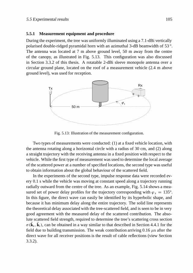
5.5 Experimental results 105
5.5.1 Measurement equipment and procedure
During the experiment, the tree was uniformly illuminated using a 7.1-dBi verticallypolarised double-ridged pyramidal horn with an azimuthal 3-dB beamwidth of 53 o.The antenna was located at 7 m above ground level, 50 m away from the centreof the canopy, as illustrated in Fig. 5.13. This configuration was also discussedin Section 3.3.2 of this thesis. A rotatable 2-dBi sleeve monopole antenna over acircular ground plane, located on the roof of a measurement vehicle (2.4 m aboveground level), was used for reception.
50 ms
TxRx
Fig. 5.13: Illustration of the measurement configuration.
Two types of measurements were conducted: (1) at a fixed vehicle location, withthe antenna rotating along a horizontal circle with a radius of 30 cm, and (2) alonga straight trajectory with the receiving antenna in a fixed position with respect to thevehicle. While the first type of measurement was used to determine the local averageof the scattered power at a number of specified locations, the second type was usefulto obtain information about the global behaviour of the scattered field.
In the experiments of the second type, impulse response data were recorded ev-ery 0.1 s while the vehicle was moving at constant speed along a trajectory runningradially outward from the centre of the tree. As an example, Fig. 5.14 shows a mea-sured set of power delay profiles for the trajectory corresponding with ϕ s = 135o.In this figure, the direct wave can easily be identified by its hyperbolic shape, andbecause it has minimum delay along the entire trajectory. The solid line representsthe theoretical delay associated with the tree-scattered field, and is seen to be in verygood agreement with the measured delay of the scattered contribution. The abso-lute scattered field strength, required to determine the tree’s scattering cross sectionσ(ks, ki ), can be obtained in a way similar to that described in Section 4.4.1 for thefield due to building transmission. The weak contribution arriving 0.16 µs after thedirect wave for all receiver positions is the result of cable reflections (view Section3.3.2).
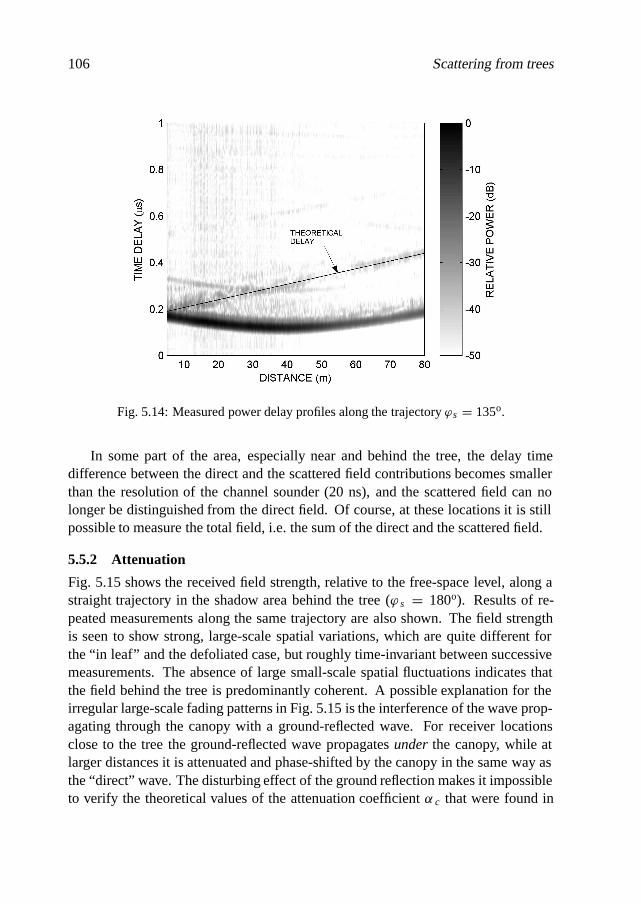
106 Scattering from trees
Fig. 5.14: Measured power delay profiles along the trajectory ϕs = 135o.
In some part of the area, especially near and behind the tree, the delay timedifference between the direct and the scattered field contributions becomes smallerthan the resolution of the channel sounder (20 ns), and the scattered field can nolonger be distinguished from the direct field. Of course, at these locations it is stillpossible to measure the total field, i.e. the sum of the direct and the scattered field.
5.5.2 Attenuation
Fig. 5.15 shows the received field strength, relative to the free-space level, along astraight trajectory in the shadow area behind the tree (ϕ s = 180o). Results of re-peated measurements along the same trajectory are also shown. The field strengthis seen to show strong, large-scale spatial variations, which are quite different forthe “in leaf” and the defoliated case, but roughly time-invariant between successivemeasurements. The absence of large small-scale spatial fluctuations indicates thatthe field behind the tree is predominantly coherent. A possible explanation for theirregular large-scale fading patterns in Fig. 5.15 is the interference of the wave prop-agating through the canopy with a ground-reflected wave. For receiver locationsclose to the tree the ground-reflected wave propagates underthe canopy, while atlarger distances it is attenuated and phase-shifted by the canopy in the same way asthe “direct” wave. The disturbing effect of the ground reflection makes it impossibleto verify the theoretical values of the attenuation coefficient α c that were found in
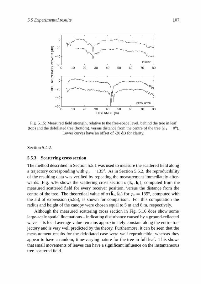
5.5 Experimental results 107
0 10 20 30 40 50 60 70 80−60
−40
−20
0
IN LEAF
0 10 20 30 40 50 60 70 80−60
−40
−20
0
DEFOLIATED
DISTANCE (m)
RE
L. R
EC
EIV
ED
PO
WE
R (
dB)
Fig. 5.15: Measured field strength, relative to the free-space level, behind the tree in leaf(top) and the defoliated tree (bottom), versus distance from the centre of the tree (ϕs = 0o).
Lower curves have an offset of -20 dB for clarity.
Section 5.4.2.
5.5.3 Scattering cross section
The method described in Section 5.5.1 was used to measure the scattered field alonga trajectory corresponding with ϕs = 135o. As in Section 5.5.2, the reproducibilityof the resulting data was verified by repeating the measurement immediately after-wards. Fig. 5.16 shows the scattering cross section σ( ks, ki ), computed from themeasured scattered field for every receiver position, versus the distance from thecentre of the tree. The theoretical value of σ(ks, ki ) for ϕs = 135o, computed withthe aid of expression (5.55), is shown for comparison. For this computation theradius and height of the canopy were chosen equal to 5 m and 8 m, respectively.
Although the measured scattering cross section in Fig. 5.16 does show somelarge-scale spatial fluctuations – indicating disturbance caused by a ground-reflectedwave – its local average value remains approximately constant along the entire tra-jectory and is very well predicted by the theory. Furthermore, it can be seen that themeasurement results for the defoliated case were well reproducible, whereas theyappear to have a random, time-varying nature for the tree in full leaf. This showsthat small movements of leaves can have a significant influence on the instantaneoustree-scattered field.
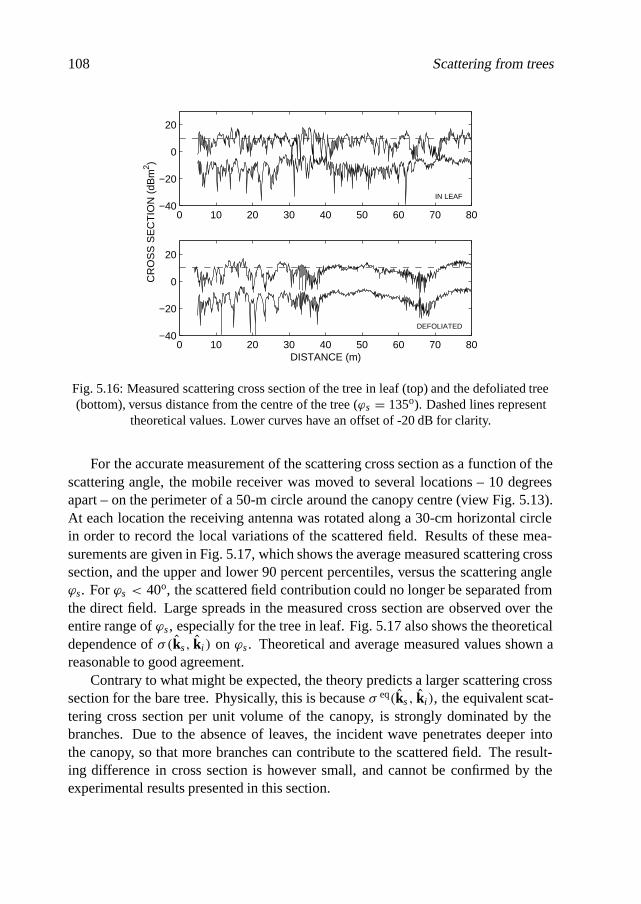
108 Scattering from trees
0 10 20 30 40 50 60 70 80−40
−20
0
20
IN LEAF
0 10 20 30 40 50 60 70 80−40
−20
0
20
DEFOLIATED
DISTANCE (m)
CR
OS
S S
EC
TIO
N (
dBm
2 )
Fig. 5.16: Measured scattering cross section of the tree in leaf (top) and the defoliated tree(bottom), versus distance from the centre of the tree (ϕs = 135o). Dashed lines represent
theoretical values. Lower curves have an offset of -20 dB for clarity.
For the accurate measurement of the scattering cross section as a function of thescattering angle, the mobile receiver was moved to several locations – 10 degreesapart – on the perimeter of a 50-m circle around the canopy centre (view Fig. 5.13).At each location the receiving antenna was rotated along a 30-cm horizontal circlein order to record the local variations of the scattered field. Results of these mea-surements are given in Fig. 5.17, which shows the average measured scattering crosssection, and the upper and lower 90 percent percentiles, versus the scattering angleϕs. For ϕs < 40o, the scattered field contribution could no longer be separated fromthe direct field. Large spreads in the measured cross section are observed over theentire range of ϕs, especially for the tree in leaf. Fig. 5.17 also shows the theoreticaldependence of σ(ks, ki ) on ϕs. Theoretical and average measured values shown areasonable to good agreement.
Contrary to what might be expected, the theory predicts a larger scattering crosssection for the bare tree. Physically, this is because σ eq(ks, ki ), the equivalent scat-tering cross section per unit volume of the canopy, is strongly dominated by thebranches. Due to the absence of leaves, the incident wave penetrates deeper intothe canopy, so that more branches can contribute to the scattered field. The result-ing difference in cross section is however small, and cannot be confirmed by theexperimental results presented in this section.

5.6 Conclusions 109
0 20 40 60 80 100 120 140 160 180−10
0
10
20
30
40
ϕs (DEG)
CR
OS
S S
EC
TIO
N (
dBm
2 )
MEASURED (IN LEAF)
THEORETICAL (IN LEAF)
MEASURED (DEFOLIATED)
THEORETICAL (DEFOLIATED)
Fig. 5.17: Measured and theoretical scattering cross section versus the scattering angle.Vertical bars denote average scattered power and upper and lower 90 percent percentiles.
5.6 Conclusions
In this chapter, a quasi-two-dimensional model has been presented for the scatteringof radiowaves from a single deciduous tree. In addition to coherent scattering, ofwhich the attenuation of the field in the geometric-optical shadow area behind thetree is the most obvious manifestation, the effects of the incoherent scattered fieldhave also been considered. Incoherent scattering is predominant over coherent scat-tering outside the tree’s shadow area, and is a mechanism through which a part ofthe power of an incident field is dispersed in all directions. This can, for example,be an important phenomenon in radio propagation around street corners.
Approximate expressions for the coherent and incoherent tree-scattered fields,suitable to be used in any ray-based propagation model, were derived using Twer-sky’s multiple scattering theory. Further approximations were made so that theseexpressions could be written in closed form. An investigation of numerical resultsshowed that the accuracy of the resulting expressions for the coherent scattered fieldis reasonable, especially in the forward scattering direction, but not very good. Thesimplified expression for the incoherent scattered field, on the other hand, gives ex-cellent results.
Numerical results from the new scattering model were also compared with ex-perimental data that were obtained by means of an accurate wideband measurement

110 Scattering from trees
technique. Measurements of the attenuated field behind the tree were observed tobe disturbed by a ground-reflected wave, and could therefore not be used for a di-rect verification of the theoretical attenuation due to tree shadowing. Separationof ground-reflected waves from the direct wave is a difficult task for measurementconfigurations involving low transmitting and receiving antennas, because they havealmost equal propagation delay times and angles-of-arrival (AOAs). An alternativemethod to measure the canopy’s specific attenuation, which is complicated but prob-ably more accurate, is to raise one of the antennas to a high level and use a directiveantenna on the other side of the tree to eliminate the ground reflection. Values ofαc that were obtained in this way [56] are in good agreement with theoretical valuesfound in this chapter. Theoretical values of the scattering cross section, which alsodepend on αc, were shown to agree reasonably well with average measured data.
According to the new model, leaves have a considerable influence on the attenu-ation of radiowaves propagating through the canopy, but make hardly any differencewith regard to the tree’s scattering cross section. This result, which may at first seemsurprising, was in fact verified by the experimental results discussed in Section 5.5.3,which showed little difference between the scattering cross section of a bare tree andthe same tree in full leaf. From the viewpoint of radio network planning this is aconvenient result, because it implies that (incoherent) tree-scattering models do notneed to be season-dependent.
The new scattering model is unable to predict the considerable spatial fluctu-ations of the scattered field that were observed in the measurements. Indeed, itis likely that the unpredictability of these variations cannot be overcome by anypropagation model, however sophisticated. Still, as the present model is capable ofproviding accurate average values of the scattered field, it can form an importantimprovement of the accuracy of propagation prediction models in vegetated urbanenvironments.
6A ray-tracing propagation prediction model
for urban microcells
6.1 Introduction
With the advent of the microcellular radio networks that are likely to be employedin third-generation mobile communication systems such as UMTS, there is an in-creased interest in propagation models that are able to provide location-specific pre-dictions of channel parameters such as local mean power and delay spread. Ray-tracing-based propagation prediction, in which the propagation of radiowaves is de-scribed in terms of straight trajectories in space called rays, has emerged as the mostsuccessful technique for this purpose. Quasi-two-dimensional ray-tracing models(often just called two-dimensional, or 2-D models) are quite adequate if transmis-sion and receiving heights are well below the average rooftop level [48, 71], as isnormally the case in urban microcells. These models have been reported to provideexcellent prediction results for a variety of urban scenarios. In many other cases how-ever, these models do not provide the same accuracy that can at present be achievedfor macrocells.
Although currently available ray-tracing tools come in a wide variety with regardto the implementation of the ray-tracing algorithm itself, they are generally based onmodels of the same propagation mechanisms: line-of-sight propagation, reflection

112 A ray-tracing propagation prediction model for urban microcells
and diffraction. It was shown in Chapter 3 of this thesis that in a number of fre-quently occurring scenarios these mechanisms alone do not adequately explain theactually observed channel properties. In particular, (1) transmission through build-ings was shown to be a significant phenomenon behind buildings obstructing theline-of-sight to the base station antenna, and (2) scattering from trees located nearstreet intersections was observed to play an important role concerning propagationaround street corners. Models for these propagation mechanisms were developedin the Chapters 4 and 5. The present chapter presents a new 2-D ray-tracing-basedpropagation prediction tool that incorporates these models. It is based on the fullythree-dimensional ray-tracing model FiPre that was originally developed for satelliteapplications [6] and later adapted to handle the large building databases and high rayorders required for propagation prediction for terrestrial mobile communications [7].A detailed description of the implementation of the new tool is outside the scope ofthis thesis and will therefore not be given.
The organisation of this chapter is as follows. Section 6.2 gives a general de-scription of the new propagation prediction model. It addresses the three main stagesof the tool: database preprocessing, ray-tracing and channel parameter estimation.The estimation of local mean power, which is the most important channel parameterfor the purpose of cell planning, is given special attention in Section 6.3. Section6.4 presents prediction results for the two urban microcell environments previouslyconsidered in Chapter 3. Where possible, a comparison is made with measured fieldstrength data. Conclusions are drawn in Section 6.5.
6.2 Model description
The propagation prediction model presented in this chapter is a quasi-2-D model.This means that the geometries of the scattering objects are described in two dimen-sions and that the base station antenna is modelled as being at the same height asthe mobile station (even though this is normally not the case in reality), so that allrays propagate in a horizontal plane. Other than in truly 2-D models [40, 72], thebase station antenna is modelled as a point source in three-dimensional space, whichmeans that the radiated field diverges in both the horizontal and the vertical plane.As reported in [48, 71], quasi-2-D ray-tracing models are quite accurate when trans-mitting and receiving heights are well below the rooftops of surrounding buildings,as is usually the case in urban microcells. Under these conditions propagation takesplace mainly at the street level, and propagation over rooftops is insignificant. Themajor advantage of quasi-2-D ray-tracing models, as compared to fully 3-D models,is their relatively low computational complexity.
The new prediction model accounts for the following propagation mechanisms

6.2 Model description 113
TREES
BS
MS
(2)
(3)
(4)(5)
(6)
Fig. 6.1: Illustration of propagation mechanisms included in the prediction model.
(view Fig. 6.1):
1. direct, unobstructed propagation (not shown in Fig. 6.1),
2. reflection by building faces,
3. transmission through building faces,
4. external diffraction by building corners,
5. internal diffraction by building corners,
6. coherent and incoherent scattering from trees (which is assumed to take placeat the tree centre),
and all possible combinations thereof, up to any predetermined number of interac-tions. In addition, a maximum number of interactions can be specified for eachpropagation mechanism separately. Ground reflections and rays over rooftops areneglected. As the present investigation is relevant to mobile communications, theelectric field is assumed to be parallel to the building walls (vertical polarisation).
Transmission through buildings and scattering from trees are modelled in accor-dance with the theory presented in the Chapters 4 and 5 of this thesis. In additionto the external diffraction coefficient of Taket and Burge [45, 46] used in Chapter 4,

114 A ray-tracing propagation prediction model for urban microcells
Luebbers’ heuristic diffraction coefficient [43] and Tiberio-Maliuzhinets’ diffractioncoefficient for an impedance wedge [44] may be selected. The diffraction coeffi-cients of Taket-Burge and Luebbers are used in conjunction with the Fresnel reflec-tion coefficient; application of Tiberio-Maliuzhinets’ diffraction coefficient requiresthe use of the reflection coefficient for impedance boundaries [44].
The inputs to the model include databases specifying the 2-D coordinates of thecorners of each building and the locations, radii and heights of the trees, the complexpermittivities εr and specific attenuation coefficients αb of the buildings (cf. Section4.2), and tables containing the equivalent scattering amplitudes F eq(ks, ki ) and crosssections σ eq(ks, ki ) per unit volume of the tree canopies (cf. Section 5.2.4). Also,the location and radiation pattern (in the horizontal plane) of the base station, thefrequency and some other simulation parameters, such as the spatial resolution ofthe prediction and the permitted ray order, must be specified. Trees and the basestation may not be located inside a building, but the observation point may be chosenarbitrarily. Modes of operation supported by the prediction model are field strengthprediction over an area or along a trajectory, and determination of all ray trajectoriesfor a set of discrete observation points.
The propagation prediction is basically performed in three phases. The firstphase, which is referred to as database preprocessing, serves to decrease the compu-tational complexity of the second and most intricate phase, which is formed by theray-tracing. In the last phase, relevant channel parameters are predicted from the raydata. The procedures involved in these phases are outlined in the following (Sections6.2.1, 6.2.2 and 6.2.3).
6.2.1 Database preprocessing
Generally, the most computationally intensive aspect of ray-tracing-based propaga-tion prediction is formed by the tracing itself, i.e. by the algorithm that determinesall possible rays between the source and observation points. In comparison, the com-putation of the complex field amplitudes associated with each ray is a small task. Incases in which ray contributions of second or higher order are taken into account, theray-tracing can be accelerated considerably if one knows for all pairs of diffractionand/or scattering points if a ray between these points can exist. As these so-calledvisibility relations are independent of the locations of the base station and the obser-vation points, they have to be determined only once, prior to the actual ray-tracing.The preprocessing procedure applied in the present model is similar to that proposedin [73], but it is more general in the sense that it does not just evaluate if the raybetween two points is obstructed, but also by how many building faces. This isessential for tracing rays that propagate through buildings.
The computation time needed for the ray-tracing can be reduced further by subdi-

6.2 Model description 115
viding the building faces into smaller “tiles” and determining the visibility relationsof the tile centres with other tiles, building corners and trees, together with a numberof angles [73]. As this technique introduces small errors that may obscure the errorsresulting from inadequacies of the physical models presented in this thesis, it is notused here.
The visibility relations of the base station and the observation points with thediffraction and scattering points must be determined during the actual ray-tracing.The processing time required for these computations is reduced through anotherform of preprocessing of the building database. This procedure consists of the com-putation and storage of each building’s bounding circle[74], which is defined bythe building’s centre of gravity [75] and the radius of the smallest circle – centredat the centre of gravity – enclosing the building. When searching for building facesobstructing a given ray path, first a selection is made of buildings whose boundingcircles intersect the ray path. This involves only a relatively simple computation.In practice, this selection procedure excludes the majority of candidate obstructingbuildings from further examination.
6.2.2 Ray-tracing
The ray-tracing algorithm makes use of the concept of virtual sources, which ac-count for the reflections, diffractions and scattering resulting from interaction of thefield radiated from the base station antenna with the environment [48]. As the nameimplies, these virtual sources are not real sources but imaginary ones that, in com-bination with the real source (the base station antenna), form an equivalent systemthat replaces the actual system and gives the same radiated field as the actual systemitself. Five types of virtual sources can be distinguished:
1. reflection sources,
2. external diffraction sources,
3. internal diffraction sources,
4. coherent scattering sources, and
5. incoherent scattering sources.
In the presence of buildings or trees, the real source formed by the base station givesrise to one or more virtual sources. In turn, these sources also interact with theenvironment and generate secondary virtual sources. This process is repeated untilthe specified maximum ray order is reached. If proper account is taken of the zonesin which each source is “visible” (possibly through one or more building faces),
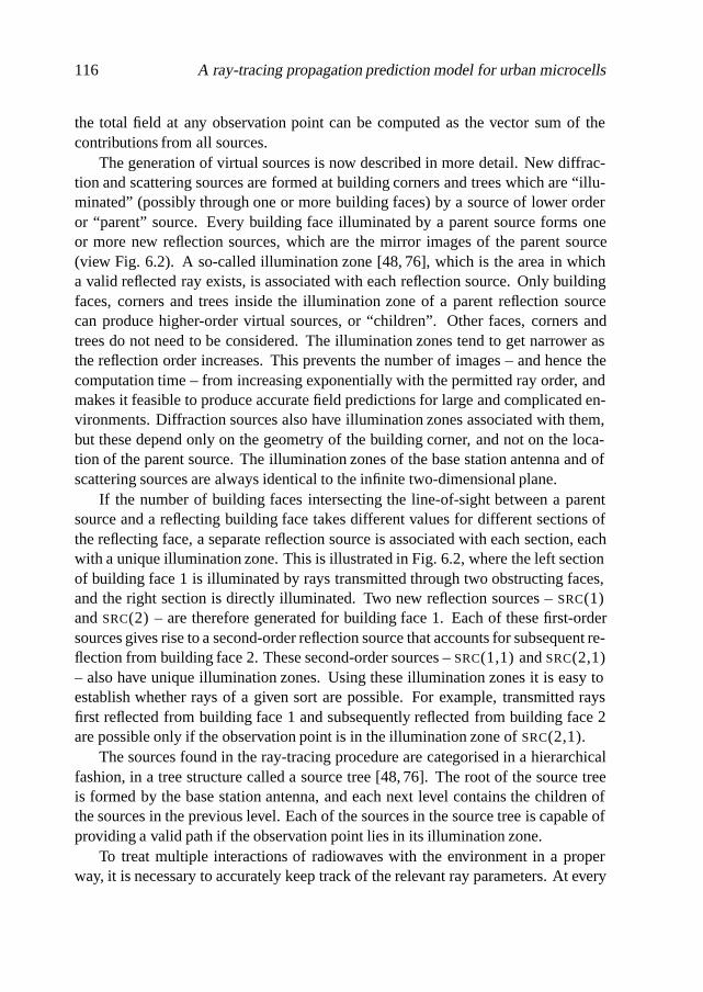
116 A ray-tracing propagation prediction model for urban microcells
the total field at any observation point can be computed as the vector sum of thecontributions from all sources.
The generation of virtual sources is now described in more detail. New diffrac-tion and scattering sources are formed at building corners and trees which are “illu-minated” (possibly through one or more building faces) by a source of lower orderor “parent” source. Every building face illuminated by a parent source forms oneor more new reflection sources, which are the mirror images of the parent source(view Fig. 6.2). A so-called illumination zone [48, 76], which is the area in whicha valid reflected ray exists, is associated with each reflection source. Only buildingfaces, corners and trees inside the illumination zone of a parent reflection sourcecan produce higher-order virtual sources, or “children”. Other faces, corners andtrees do not need to be considered. The illumination zones tend to get narrower asthe reflection order increases. This prevents the number of images – and hence thecomputation time – from increasing exponentially with the permitted ray order, andmakes it feasible to produce accurate field predictions for large and complicated en-vironments. Diffraction sources also have illumination zones associated with them,but these depend only on the geometry of the building corner, and not on the loca-tion of the parent source. The illumination zones of the base station antenna and ofscattering sources are always identical to the infinite two-dimensional plane.
If the number of building faces intersecting the line-of-sight between a parentsource and a reflecting building face takes different values for different sections ofthe reflecting face, a separate reflection source is associated with each section, eachwith a unique illumination zone. This is illustrated in Fig. 6.2, where the left sectionof building face 1 is illuminated by rays transmitted through two obstructing faces,and the right section is directly illuminated. Two new reflection sources – SRC(1)and SRC(2) – are therefore generated for building face 1. Each of these first-ordersources gives rise to a second-order reflection source that accounts for subsequent re-flection from building face 2. These second-order sources – SRC(1,1) and SRC(2,1)– also have unique illumination zones. Using these illumination zones it is easy toestablish whether rays of a given sort are possible. For example, transmitted raysfirst reflected from building face 1 and subsequently reflected from building face 2are possible only if the observation point is in the illumination zone of SRC(2,1).
The sources found in the ray-tracing procedure are categorised in a hierarchicalfashion, in a tree structure called a source tree [48, 76]. The root of the source treeis formed by the base station antenna, and each next level contains the children ofthe sources in the previous level. Each of the sources in the source tree is capable ofproviding a valid path if the observation point lies in its illumination zone.
To treat multiple interactions of radiowaves with the environment in a properway, it is necessary to accurately keep track of the relevant ray parameters. At every
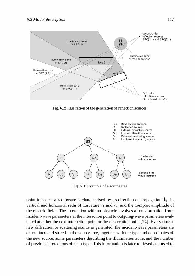
6.2 Model description 117
BS
first-orderreflection sourcesSRC(1) and SRC(2)
second-orderreflection sourcesSRC(1,1) and SRC(2,1)
face 1
face 2
illumination zoneof SRC(1)
illumination zoneof SRC(1,1)
illumination zoneof SRC(2)
illumination zoneof SRC(2,1)
illumination zoneof the BS antenna
Fig. 6.2: Illustration of the generation of reflection sources.
Fig. 6.3: Example of a source tree.
point in space, a radiowave is characterised by its direction of propagation ki , itsvertical and horizontal radii of curvature r 1 and r2, and the complex amplitude ofthe electric field. The interaction with an obstacle involves a transformation fromincident-wave parameters at the interaction point to outgoing-wave parameters eval-uated at either the next interaction point or the observation point [74]. Every time anew diffraction or scattering source is generated, the incident-wave parameters aredetermined and stored in the source tree, together with the type and coordinates ofthe new source, some parameters describing the illumination zone, and the numberof previous interactions of each type. This information is later retrieved and used to
118 A ray-tracing propagation prediction model for urban microcells
generate higher-order sources or to evaluate the field at the observation point. Newreflection sources are treated differently; as the precise location of the reflection pointis unknown when a new reflection source is generated, the associated incident-waveparameters cannot be determined. The reflection points and reflection coefficients of(multiply) reflected rays are computed at a later stage, when higher-order diffractionor scattering sources are generated or the field at the observation point is evaluated.
In the computation of the field amplitude due to the base station antenna or avirtual source which only has reflection sources as its parents, the directivity of thebase station antenna is taken into account, i.e., the field is weighted by the envelopeof the antenna’s radiation pattern in the direction of the launched ray.
6.2.3 Channel parameter estimation
For a given observation point and permitted ray order, the ray-tracing algorithm gen-erates the set of all valid ray trajectories, and the associated complex electric fieldamplitudes. In order to find the complex signals at the output of the receiving an-tenna due to these rays, their field amplitudes are weighted by the envelope of theantenna’s radiation pattern. In the present model, the receiving antenna is assumed tobe non-directional in the horizontal plane, so that it can be characterised by a singlegain value. For each multipath wave, the delay time can be computed from the totallength of the associated ray trajectory and the angle-of-arrival (AOA) is found asthe direction of the (virtual) source that is responsible for the ray. Important channelcharacteristics such as the received field strength, power delay profile, power angularprofile and power Doppler profile (Doppler spectrum), as well as multi-dimensionalcharacteristics like the temporal-angular power distributions discussed in the Chap-ters 2 and 3 of this thesis, can be computed from the ray parameters. In a second step,channel parameters such as delay spread, mean AOA, angular spread, mean Dopplershift and Doppler spread can be derived from these simulated characteristics.
In this chapter it has been assumed that the geometrical and dielectric features ofthe environment, the locations of the base station antenna and the observation points,the frequency, etc. are deterministic, constant and exactly known. The predictedchannel parameters therefore also have a deterministic and constant nature. There isone source of randomness, however, which is very important in propagation predic-tion for the purpose of network planning, and this is the uncertainty with regard tothe exact receiver position. In the planning stage of cellular radio networks, channelparameters are usually determined for a set of discrete points, but they are assumedto be representative for an observation area around each point. The dimensions ofsuch an area (sometimes called pixel) depend on the desired spatial resolution of theprediction, but they are typically in the order of several tens of wavelengths. The ac-tual receiver location is implicitly assumed to be random within the observation area,
6.3 Estimation of local mean power 119
and the radio channel properties at this location can be characterised by local meanchannel parameters, of which the local mean power is probably the most importantone.
The estimation of local mean power from ray parameters generated using a 2-Dray-based propagation prediction model is the subject of the next section. With someminor modifications, this method can also be used to estimate local mean powerdelay profiles.
6.3 Estimation of local mean power
Probably the most important channel parameter used in the planning stage of radionetworks is the local mean power, which is the total received signal intensity, aver-aged in space in order to remove small-scale fading. A method which is often usedto estimate local mean power is to simply add the individual ray powers [48, 71, 77].This method has been referred to as the sum-of-individual-ray-powers (SP) methodin [71]. This section presents an alternative method, which is based on the spatialaverage (SA) of the received power over a given pixel area, but does not require ray-tracing for more than one observation point per pixel [78]. This SA method consistsof the evaluation of an expression for the local mean power that is exact assumingthat the ray amplitudes and AOAs are constant over the pixel area. Unlike the SPmethod, the SA method provides a statistically valid approximation of the expectedfield strength at a random receiver position within a given observation area. Fur-thermore, this method allows a fairer comparison to be made between propagationpredictions and propagation measurement data obtained with a moving receiving an-tenna, in which the long-term fading component is usually also determined by spatialaveraging – albeit in only one dimension.
6.3.1 Formulation
Consider the area S around the observation point O which is assumed to be at theorigin of a rectangular coordinate system (x, y), and assume that N rays are incidenton O from the AOAs ϕn, n = 1, 2, . . . , N (view Fig. 6.4). Associated with eachray is a narrowband signal with amplitude un and phase φn. If un and ϕn do not varyover the observation area S (plane wave assumption), the total received signal s canbe evaluated at any point within S by taking the sum of the individual complex rayamplitudes (e.g. [71, 79]), i.e.
s(x, y)=N∑
n=1
un exp[ j k(x cosϕn + y sinϕn)+ jφn], (6.1)
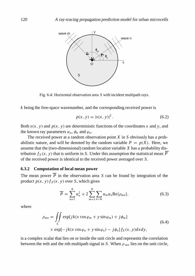
120 A ray-tracing propagation prediction model for urban microcells
O
S
x
y
wave nwave m
ϕ
ϕm
n
Fig. 6.4: Horizontal observation area Swith incident multipath rays.
k being the free-space wavenumber, and the corresponding received power is
p(x, y) = |s(x, y)|2 . (6.2)
Both s(x, y) and p(x, y) are deterministic functions of the coordinates x and y, andthe known ray parameters un, φn and ϕn.
The received power at a random observation point X in S obviously has a prob-abilistic nature, and will be denoted by the random variable P = p(X). Here, weassume that the (two-dimensional) random location variable X has a probability dis-tribution fX(x, y) that is uniform in S. Under this assumption the statistical mean Pof the received power is identical to the received power averaged over S.
6.3.2 Computation of local mean power
The mean power P in the observation area S can be found by integration of theproduct p(x, y) f X(x, y) over S, which gives
P =N∑
n=1
u2n + 2
N∑m=1
∑n<m
umunRe{ρmn}, (6.3)
where
ρmn =∫∫
S
exp[ j k(x cosϕm + y sinϕm)+ jφm]
× exp[− j k(x cosϕn + y sinϕn)− jφn] fX(x, y)dxdy,
(6.4)
is a complex scalar that lies on or inside the unit circle and represents the correlationbetween the mth and the nth multipath signal in S. When ρ mn lies on the unit circle,

6.3 Estimation of local mean power 121
the two signals are fully coherent. If ρmn lies inside the unit circle, the two signalsare only partially correlated, while ρmn = 0 implies totally uncorrelated multipathsignals. The SA method presented in this section consists of the evaluation of equa-tion (6.3), including the terms containing the spatial correlation coefficients, whichare not taken into account by the conventional SP method.
For a rectangular observation area centred at O, with sides of lengths D x and Dy
aligned with the x and y axes, respectively, ρmn can be written as
ρmn = sin[kDx(cos ϕm − cos ϕn)/2]kDx(cosϕm − cosϕn)/2
× sin[kDy(sinϕm − sinϕn)/2]kDy(sinϕm − sinϕn)/2
exp[ j (φm − φn)].(6.5)
The predicted local mean power along a measurement trajectory can be obtainedby locally orienting the (x, y) coordinate system with the x axis parallel to the tra-jectory, making Dx equal to the averaging interval applied in the measurements, andletting Dy → 0, so that the second factor in (6.5) vanishes. For a circular observationarea of diameter D centred at O, ρmn becomes
ρmn = 2J1(kD sin [(ϕm − ϕn)/2]
)kD sin [(ϕm − ϕn)/2]
exp[ j (φm − φn)], (6.6)
where J1(·) is the Bessel function of the first kind of order one. Finally, for theprediction of the mean power received along a horizontal circle centred at O withdiameter D (ring-shaped observation domain), ρmn is given by
ρmn = J0(kD sin [(ϕm − ϕn)/2]
)exp[ j (φm − φn)], (6.7)
where J0(·) is the Bessel function of the first kind of order zero. Plots of the ab-solute correlation |ρ12| between two multipath signals, computed from (6.5)–(6.7),are shown in Fig. 6.5 as a function of the angular difference ϕ = ϕ2 − ϕ1, forkDx = kDy = kD = 100.
Expression (6.3) simplifies for the specific cases in which all multipath signalsare totally correlated or uncorrelated. For nearly uncorrelated multipath signals(ρmn � 0, m �= n), P can be approximated as the sum of the individual multipathsignal powers, as in the SP method:
P �N∑
n=1
u2n. (6.8)
From (6.3)-(6.7) it is seen that the SP method is generally valid only if at least one ofthe dimensions of the observation domain is large in terms of the wavelength, and all
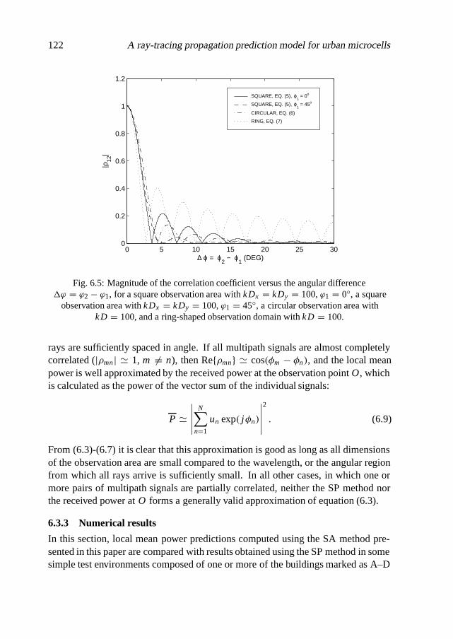
122 A ray-tracing propagation prediction model for urban microcells
0 5 10 15 20 25 300
0.2
0.4
0.6
0.8
1
1.2
∆ ϕ = ϕ2 − ϕ
1 (DEG)
|ρ12
|SQUARE, EQ. (5), ϕ
1 = 0o
SQUARE, EQ. (5), ϕ1 = 45o
CIRCULAR, EQ. (6)
RING, EQ. (7)
Fig. 6.5: Magnitude of the correlation coefficient versus the angular differenceϕ = ϕ2 − ϕ1, for a square observation area with kDx = kDy = 100, ϕ1 = 0◦, a square
observation area with kDx = kDy = 100, ϕ1 = 45◦, a circular observation area withkD = 100, and a ring-shaped observation domain with kD = 100.
rays are sufficiently spaced in angle. If all multipath signals are almost completelycorrelated (|ρmn| � 1, m �= n), then Re{ρmn} � cos(φm − φn), and the local meanpower is well approximated by the received power at the observation point O, whichis calculated as the power of the vector sum of the individual signals:
P �∣∣∣∣∣
N∑n=1
un exp( jφn)
∣∣∣∣∣2
. (6.9)
From (6.3)-(6.7) it is clear that this approximation is good as long as all dimensionsof the observation area are small compared to the wavelength, or the angular regionfrom which all rays arrive is sufficiently small. In all other cases, in which one ormore pairs of multipath signals are partially correlated, neither the SP method northe received power at O forms a generally valid approximation of equation (6.3).
6.3.3 Numerical results
In this section, local mean power predictions computed using the SA method pre-sented in this paper are compared with results obtained using the SP method in somesimple test environments composed of one or more of the buildings marked as A–D

6.3 Estimation of local mean power 123
in Fig. 6.6. Some of the configurations that can be composed in this way, such asthe so-called 2-corner and 4-corner street intersections, have been investigated pre-viously to study radio propagation around street corners [31, 48, 71]. In the presentsimulations, local mean power estimates are compared with each other and with thereceived power along the trajectory indicated in Fig. 6.6, and spatial distributions ofthe error made by the SP method (as compared with the SA method) are given forthe complete coverage area. The transmitter is situated at a fixed location, indicatedby the label “BS”. Reflections up to tenth order and/or diffraction up to order twoare taken into account, and the carrier frequency is 900 MHz. The diffraction contri-butions are computed using the diffraction coefficient for a wedge with impedancefaces [44]. A relative permittivity of εr = 5.3 and zero conductivity, correspondingto dry brick, are selected for the buildings.
−50 0 50 100−50
0
50
X (m)
Y (
m)
BS
start
← →30 m
↓↑ 10 m
C D
B A
Fig. 6.6: Configuration of the test environment. Trajectory is indicated by the dashed line.“BS” denotes the base station location.
Figs. 6.7 and 6.8 show the predicted received power and the local mean powerestimates along the trajectory, evaluated by means of the SP method and the SAmethod, for configurations consisting of buildings A+B (2-corner intersection) andbuildings A+B+C+D (4-corner intersection), respectively. The received power iscomputed every 5 cm, while the local mean power estimates are evaluated every5 m. For the SA method, a 5-m averaging interval (Eqn. (6.5), with Dx = 5 m,Dy = 0) is applied. In the 2-corner intersection case of Fig. 6.7, the received powershows rapid fluctuations at distances close to the transmitter. As desired, the localmean power, estimated by either the SA or the SP method, does not follow thesesmall-scale fluctuations. At larger distances from the transmitter, the SP method no
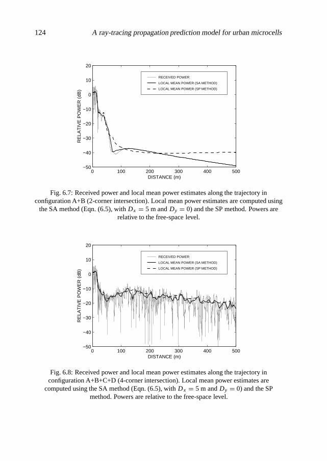
124 A ray-tracing propagation prediction model for urban microcells
0 100 200 300 400 500−50
−40
−30
−20
−10
0
10
20
DISTANCE (m)
RE
LAT
IVE
PO
WE
R (
dB)
RECEIVED POWER
LOCAL MEAN POWER (SA METHOD)
LOCAL MEAN POWER (SP METHOD)
Fig. 6.7: Received power and local mean power estimates along the trajectory inconfiguration A+B (2-corner intersection). Local mean power estimates are computed using
the SA method (Eqn. (6.5), with Dx = 5 m and Dy = 0) and the SP method. Powers arerelative to the free-space level.
0 100 200 300 400 500−50
−40
−30
−20
−10
0
10
20
DISTANCE (m)
RE
LAT
IVE
PO
WE
R (
dB)
RECEIVED POWER
LOCAL MEAN POWER (SA METHOD)
LOCAL MEAN POWER (SP METHOD)
Fig. 6.8: Received power and local mean power estimates along the trajectory inconfiguration A+B+C+D (4-corner intersection). Local mean power estimates are
computed using the SA method (Eqn. (6.5), with Dx = 5 m and Dy = 0) and the SPmethod. Powers are relative to the free-space level.

6.3 Estimation of local mean power 125
longer accurately predicts the local mean power, whereas the SA method provides agood approximation at all distances from the transmitter. The error made by the SPmethod amounts to 10 dB at 500 m from the transmitter. In the 4-corner intersectioncase of Fig. 6.8, on the other hand, the received power shows fast fluctuations alongthe entire 500-m trajectory, and the SA and SP methods provide very similar results.
A physical explanation for the observations made above can be given after con-sidering the spatial distribution of the error made by applying the SP method, ascompared with the SA method. Fig. 6.9 shows the error distribution for a configura-tion composed of building A only (1-corner intersection). The largest errors, rangingup to 7 dB, are found near the shadow boundary of the incident field. In this regionthe first Fresnel zone of the direct wave is partially obstructed by building A, whichis accounted for by ray-based diffraction theory through destructive interference withthe wave diffracted from the corner of building A. In the SP method however, thepower of this diffraction contribution is addedto the power of the direct wave, whichresults in an overestimation of the local mean power. The SA method handles thecontribution of the diffracted ray signal to the local mean power in a correct manner,by taking into account its high correlation with the “direct” signal. In the configura-tion considered here equally large errors do not occur near the reflection boundary,because the field in this region is dominated by the direct wave. Smaller, but signif-icant errors occur in regions where the signals associated with the direct wave andthe reflection from the wall behind the transmitter become strongly correlated.
ER
RO
R (
dB)
−14
−10
−6
−2
2
6
10
14
−100 −50 0 50 100−100
−50
0
50
100
BS
X (m)
Y (
m)
A
Fig. 6.9: Spatial distribution of the SP estimation error (relative to the SA method) forconfiguration A only (1-corner intersection). D x = Dy = 5 m. “BS” denotes the base
station location. Dashed lines indicate shadow and reflection boundaries of the direct ray.

126 A ray-tracing propagation prediction model for urban microcells
ER
RO
R (
dB)
−14
−10
−6
−2
2
6
10
14
−100 −50 0 50 100−100
−50
0
50
100
BS
X (m)
Y (
m)
AB
Fig. 6.10: Spatial distribution of the SP estimation error (relative to the SA method) forconfiguration A+B (2-corner intersection). Dx = Dy = 5 m. “BS” denotes the base station
location. Dashed lines indicate shadow and reflection boundaries of the direct ray.
ER
RO
R (
dB)
−14
−10
−6
−2
2
6
10
14
−100 −50 0 50 100−100
−50
0
50
100
BS
X (m)
Y (
m)
AB
C D
Fig. 6.11: Spatial distribution of the SP estimation error (relative to the SA method) forconfiguration A+B+C+D (4-corner intersection). Dx = Dy = 5 m. “BS” denotes the basestation location. Dashed lines indicate shadow and reflection boundaries of the direct ray.
6.3 Estimation of local mean power 127
Similar plots of the error distributionsfor the configurations A+B and A+B+C+Dare shown in Figs. 6.10 and 6.11. Instead of two there are now many shadow bound-aries, each one associated with one of the many multipath waves reflected and/ordiffracted between the buildings. For the 2-corner intersection of Fig. 6.10 thisresults in considerable errors in large parts of the coverage area, as was also ob-served from Fig. 6.7. On the other hand, in the 4-corner intersection configurationof Fig. 6.11 the diffraction contributions are dominated by multiple reflections in thestreet canyons formed by all four buildings, and these waves impinge on the receiverfrom a relatively wide angular region. The associated multipath signals thereforehave low correlation, so that in this case the SP method provides a good approxima-tion of the local mean power in most of the coverage area, including the trajectoryof Fig. 6.6.
6.3.4 Conclusions and discussion
In this section, an accurate method for determining local mean power using 2-Dray-tracing based propagation prediction models was proposed. This method, whichconsists of the evaluation of equation (6.3), automatically reduces to the commonlyused SP method for uncorrelated multipath signals, but, unlike the SP method, re-mains valid for correlated signals, i.e. for rays arriving at the receiver from a narrowangular region. Although it is based on the spatial average (SA) of the receivedpower, the presented method does not require the calculation of the received powerat many discrete points within each observation area or interval, as in [71].
Numerical results for some simple test configurations show that application ofthe SP method can result in considerable estimation errors, while the new SA methodremains accurate in all cases – at the cost of slightly increased computational com-plexity. They further indicate that poor performance of the SP method occurs par-ticularly near the shadow boundaries associated with diffracted rays. In the mostcomplex test environment considered (Fig. 6.11), the SP method was shown to giveresults similar to the new SA method. Although this may suggest that the conven-tional power sum gives a sufficiently good approximation of the local mean power incomplex environments, it is hard or even impossible to say in general for what build-ing configurations and/or in which parts of a reception area the SP method providesaccurate results.
The presented method can be extended to 3-D ray-tracing models in a straight-forward manner. Computation of the local mean power then involves an integrationof the received power over a volume around each observation point, and the cor-relation between multipath signal pairs will depend on the angular spacing of thecorresponding rays in both azimuth and elevation.
128 A ray-tracing propagation prediction model for urban microcells
6.4 Prediction results
This section presents prediction results for two urban microcell environments thatwere previously discussed in Chapter 3 of this thesis. It is aimed at illustrating theimprovement in accuracy that can be achieved by incorporating appropriate mod-els for transmission through buildings and scattering from trees. Where possible, acomparison is made with measured data.
The predictions in this section are generated for a carrier frequency of 1890MHz. The relative dielectric permittivity of the buildings, ε r , is chosen equal to 5,and the conductivity is zero. The specific attenuation constant α b, which charac-terises the attenuation of waves propagating through buildings, is assumed to be 2.0dB/m, which is the average of the empirical values found in Chapter 4. Reflectedand diffracted fields are computed using the Fresnel reflection coefficient and thediffraction coefficients of Taket and Burge [45, 46], respectively. All branch and leafparameters are taken from Chapter 5, particularly from Table 5.1. The predictionarea is divided into 5 × 5 m2 square pixels. For each pixel the local mean power,required to compute the (local mean) path loss, is obtained using the SA methodproposed in the previous section.
6.4.1 Transmission through buildings – Bern
Fig. 6.12 shows area predictions of path loss for an urban microcell environment inBern (cf. Section 3.2.1), with and without considering transmission through build-ings. In generating the prediction result shown in Fig. 6.12(a), the maximum numberof wall transmissions was set to one, so that rays can penetrate into buildings butcannot be transmitted through them. The results shown in Fig. 6.12(b), on the otherhand, were obtained by setting the maximum transmission order to three, permittingrays to be transmitted through maximally one building and then penetrate a secondone. The diffraction order was one and tree-scattering was not considered. The whiteobservation areas (pixels) that can be seen in both subfigures correspond with areasthat cannot be “reached” by rays permitted in the present simulation. Obviously, alarger fraction of the total area can be reached if transmission through buildings ispermitted. Significant differences between the prediction results of Fig. 6.12(a) and(b) are observed in Rodtmatt Street and Wiesen Street, opposite to the base station.In these areas, differences up to approximately 50 dB occur.
A detailed comparison between measured data obtained from [29, 48] and pre-dictions generated with and without considering building transmission was made forthe trajectory indicated in Fig. 6.12. The number of observation points on this trajec-tory is 92. Table 6.1 shows the mean and rms prediction errors obtained for various(maximum) ray orders. The diffraction order – the maximum number of external
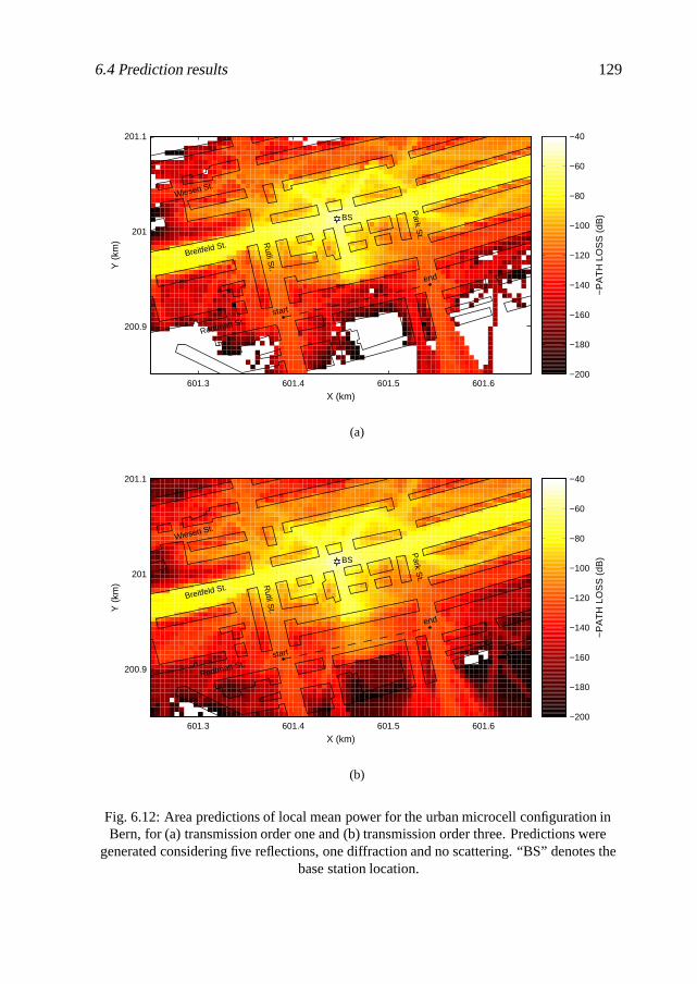
6.4 Prediction results 129
601.3 601.4 601.5 601.6
200.9
201
201.1
BS
start
end
Wiesen St.
Rodtmatt St.
Breitfeld St.
Rutli S
t.
Park S
t.
X (km)
Y (
km)
−200
−180
−160
−140
−120
−100
−80
−60
−40
−P
AT
H L
OS
S (
dB)
(a)
601.3 601.4 601.5 601.6
200.9
201
201.1
BS
start
end
Wiesen St.
Rodtmatt St.
Breitfeld St.
Rutli S
t.
Park S
t.
X (km)
Y (
km)
−200
−180
−160
−140
−120
−100
−80
−60
−40
−P
AT
H L
OS
S (
dB)
(b)
Fig. 6.12: Area predictions of local mean power for the urban microcell configuration inBern, for (a) transmission order one and (b) transmission order three. Predictions were
generated considering five reflections, one diffraction and no scattering. “BS” denotes thebase station location.

130 A ray-tracing propagation prediction model for urban microcells
Table 6.1: Prediction errors and number of sources for the urban microcell configuration inBern, for various ray orders.
Max. ray orderNumber of
sourcesMean error
(dB)Rms error
(dB)
1 refl., 1 transm., 1 diffr., 0 scatt. 826 – –
2 refl., 1 transm., 1 diffr., 0 scatt. 2,955 – –
3 refl., 1 transm., 1 diffr., 0 scatt. 7,475 – –
4 refl., 1 transm., 1 diffr., 0 scatt. 15,697 -31.7 36.7
5 refl., 1 transm., 1 diffr., 0 scatt. 29,048 -29.8 33.7
6 refl., 1 transm., 1 diffr., 0 scatt. 49,441 -28.8 32.4
7 refl., 1 transm., 1 diffr., 0 scatt. 78,897 -27.2 30.6
8 refl., 1 transm., 1 diffr., 0 scatt. 120,120 -26.3 29.4
9 refl., 1 transm., 1 diffr., 0 scatt. 175,568 -26.6 29.7
1 refl., 3 transm., 1 diffr., 0 scatt. 3,211 -14.4 18.4
2 refl., 3 transm., 1 diffr., 0 scatt. 15,252 -10.3 14.1
3 refl., 3 transm., 1 diffr., 0 scatt. 46,298 -8.9 12.4
4 refl., 3 transm., 1 diffr., 0 scatt. 111,475 -8.0 11.5
5 refl., 3 transm., 1 diffr., 0 scatt. 230,853 -7.6 11.2
6 refl., 3 transm., 1 diffr., 0 scatt. 431,439 -7.4 11.0
1 refl., 5 transm., 1 diffr., 0 scatt. 8,121 -13.4 17.0
2 refl., 5 transm., 1 diffr., 0 scatt. 48,273 -10.0 13.9
3 refl., 5 transm., 1 diffr., 0 scatt. 170,128 -8.7 12.2
4 refl., 5 transm., 1 diffr., 0 scatt. 462,008 -7.9 11.4
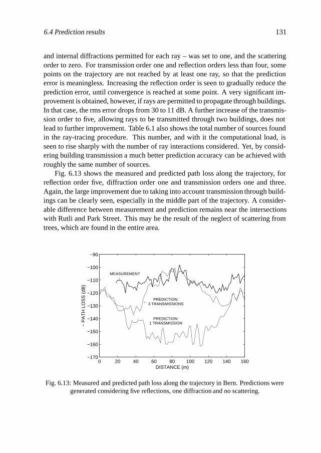
6.4 Prediction results 131
and internal diffractions permitted for each ray – was set to one, and the scatteringorder to zero. For transmission order one and reflection orders less than four, somepoints on the trajectory are not reached by at least one ray, so that the predictionerror is meaningless. Increasing the reflection order is seen to gradually reduce theprediction error, until convergence is reached at some point. A very significant im-provement is obtained, however, if rays are permitted to propagate through buildings.In that case, the rms error drops from 30 to 11 dB. A further increase of the transmis-sion order to five, allowing rays to be transmitted through two buildings, does notlead to further improvement. Table 6.1 also shows the total number of sources foundin the ray-tracing procedure. This number, and with it the computational load, isseen to rise sharply with the number of ray interactions considered. Yet, by consid-ering building transmission a much better prediction accuracy can be achieved withroughly the same number of sources.
Fig. 6.13 shows the measured and predicted path loss along the trajectory, forreflection order five, diffraction order one and transmission orders one and three.Again, the large improvement due to taking into account transmission through build-ings can be clearly seen, especially in the middle part of the trajectory. A consider-able difference between measurement and prediction remains near the intersectionswith Rutli and Park Street. This may be the result of the neglect of scattering fromtrees, which are found in the entire area.
0 20 40 60 80 100 120 140 160−170
−160
−150
−140
−130
−120
−110
−100
−90
DISTANCE (m)
− P
AT
H L
OS
S (
dB)
MEASUREMENT↓
PREDICTION:3 TRANSMISSIONS
←
PREDICTION:1 TRANSMISSION
↓
Fig. 6.13: Measured and predicted path loss along the trajectory in Bern. Predictions weregenerated considering five reflections, one diffraction and no scattering.
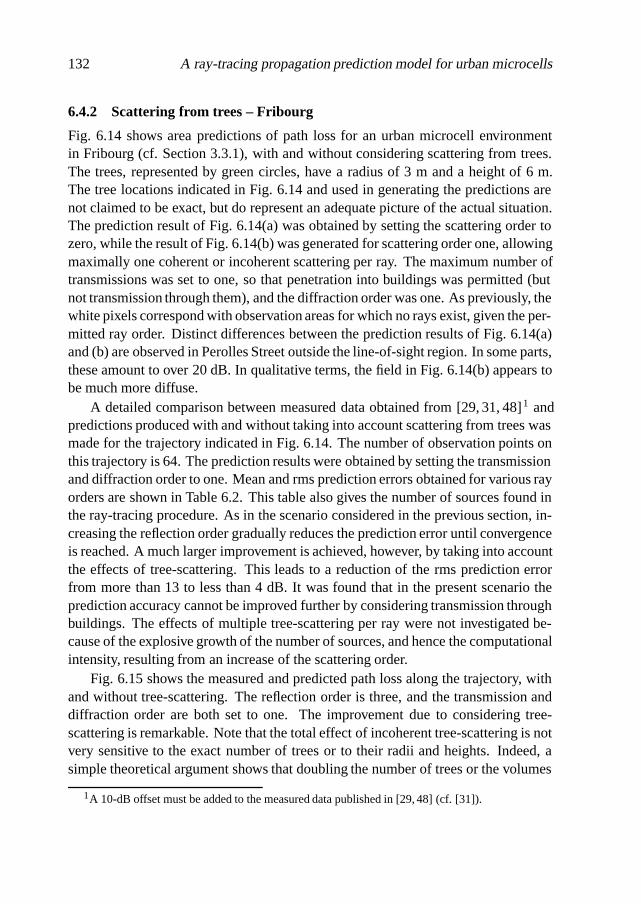
132 A ray-tracing propagation prediction model for urban microcells
6.4.2 Scattering from trees – Fribourg
Fig. 6.14 shows area predictions of path loss for an urban microcell environmentin Fribourg (cf. Section 3.3.1), with and without considering scattering from trees.The trees, represented by green circles, have a radius of 3 m and a height of 6 m.The tree locations indicated in Fig. 6.14 and used in generating the predictions arenot claimed to be exact, but do represent an adequate picture of the actual situation.The prediction result of Fig. 6.14(a) was obtained by setting the scattering order tozero, while the result of Fig. 6.14(b) was generated for scattering order one, allowingmaximally one coherent or incoherent scattering per ray. The maximum number oftransmissions was set to one, so that penetration into buildings was permitted (butnot transmission through them), and the diffraction order was one. As previously, thewhite pixels correspond with observation areas for which no rays exist, given the per-mitted ray order. Distinct differences between the prediction results of Fig. 6.14(a)and (b) are observed in Perolles Street outside the line-of-sight region. In some parts,these amount to over 20 dB. In qualitative terms, the field in Fig. 6.14(b) appears tobe much more diffuse.
A detailed comparison between measured data obtained from [29, 31, 48]1 andpredictions produced with and without taking into account scattering from trees wasmade for the trajectory indicated in Fig. 6.14. The number of observation points onthis trajectory is 64. The prediction results were obtained by setting the transmissionand diffraction order to one. Mean and rms prediction errors obtained for various rayorders are shown in Table 6.2. This table also gives the number of sources found inthe ray-tracing procedure. As in the scenario considered in the previous section, in-creasing the reflection order gradually reduces the prediction error until convergenceis reached. A much larger improvement is achieved, however, by taking into accountthe effects of tree-scattering. This leads to a reduction of the rms prediction errorfrom more than 13 to less than 4 dB. It was found that in the present scenario theprediction accuracy cannot be improved further by considering transmission throughbuildings. The effects of multiple tree-scattering per ray were not investigated be-cause of the explosive growth of the number of sources, and hence the computationalintensity, resulting from an increase of the scattering order.
Fig. 6.15 shows the measured and predicted path loss along the trajectory, withand without tree-scattering. The reflection order is three, and the transmission anddiffraction order are both set to one. The improvement due to considering tree-scattering is remarkable. Note that the total effect of incoherent tree-scattering is notvery sensitive to the exact number of trees or to their radii and heights. Indeed, asimple theoretical argument shows that doubling the number of trees or the volumes
1A 10-dB offset must be added to the measured data published in [29, 48] (cf. [31]).
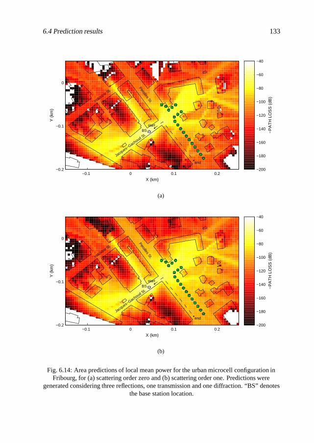
6.4 Prediction results 133
−0.1 0 0.1 0.2−0.2
−0.1
0
BSstart
end
Perolles St.Industrie St.
Jacq
ues−Gach
oud St.
X (km)
Y (
km)
−200
−180
−160
−140
−120
−100
−80
−60
−40
−P
AT
H L
OS
S (
dB)
(a)
−0.1 0 0.1 0.2−0.2
−0.1
0
BSstart
end
Perolles St.Industrie St.
Jacq
ues−Gach
oud St.
X (km)
Y (
km)
−200
−180
−160
−140
−120
−100
−80
−60
−40
−P
AT
H L
OS
S (
dB)
(b)
Fig. 6.14: Area predictions of local mean power for the urban microcell configuration inFribourg, for (a) scattering order zero and (b) scattering order one. Predictions were
generated considering three reflections, one transmission and one diffraction. “BS” denotesthe base station location.
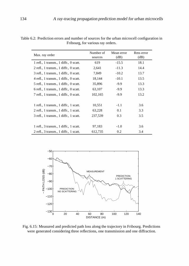
134 A ray-tracing propagation prediction model for urban microcells
Table 6.2: Prediction errors and number of sources for the urban microcell configuration inFribourg, for various ray orders.
Max. ray orderNumber of
sourcesMean error
(dB)Rms error
(dB)
1 refl., 1 transm., 1 diffr., 0 scatt. 619 -15.5 18.1
2 refl., 1 transm., 1 diffr., 0 scatt. 2,641 -11.3 14.4
3 refl., 1 transm., 1 diffr., 0 scatt. 7,849 -10.2 13.7
4 refl., 1 transm., 1 diffr., 0 scatt. 18,144 -10.1 13.5
5 refl., 1 transm., 1 diffr., 0 scatt. 35,896 -9.9 13.3
6 refl., 1 transm., 1 diffr., 0 scatt. 63,107 -9.9 13.3
7 refl., 1 transm., 1 diffr., 0 scatt. 102,165 -9.9 13.2
1 refl., 1 transm., 1 diffr., 1 scatt. 10,551 -1.1 3.6
2 refl., 1 transm., 1 diffr., 1 scatt. 63,228 0.1 3.3
3 refl., 1 transm., 1 diffr., 1 scatt. 237,539 0.3 3.5
1 refl., 3 transm., 1 diffr., 1 scatt. 97,183 -1.0 3.6
2 refl., 3 transm., 1 diffr., 1 scatt. 612,735 0.2 3.4
0 20 40 60 80 100 120 140−130
−120
−110
−100
−90
−80
−70
−60
−50
DISTANCE (m)
− P
AT
H L
OS
S (
dB)
MEASUREMENT↓
PREDICTION:1 SCATTERING
↓
PREDICTION:NO SCATTERING
→
Fig. 6.15: Measured and predicted path loss along the trajectory in Fribourg. Predictionswere generated considering three reflections, one transmission and one diffraction.

6.5 Conclusions 135
of their canopies would result in an increase of the incoherent scattered field by nomore than roughly 3 dB.
6.5 Conclusions
A ray-tracing-based propagation prediction model has been presented that incorpo-rates models for transmission through buildings and scattering from trees. The modelis two-dimensional in the sense that it neglects propagation over rooftops. This ap-proximation is valid for urban microcell configurations in which the base stationantenna is located well below the rooftop level. Due to its relatively low compu-tational complexity, the model is capable of handling large building databases andhigh ray orders in modest computation times, i.e. the most complex computationsconsidered in this section were performed within a few hours.
The model consists of three major stages: database preprocessing, ray-tracingand channel parameter estimation. The first stage is meant to reduce the complexityof the ray-tracing algorithm by determining the so-called visibility relations amongall building corners and trees, and has to be performed only once. The ray-tracingalgorithm is based on the well-known concepts of virtual sources and illuminationzones, but is enhanced in order to cope with rays passing through buildings. In thelast stage, various channel parameters can be estimated from the amplitudes, phases,lengths and AOAs of the traced rays.
A new method was presented for the estimation of local mean power. Thismethod is based on the spatial average of the received power over a given obser-vation area or pixel, but does not require ray-tracing for more than one observationpoint per pixel. Unlike the so-called sum-of-individual-ray-powers, which is themost commonly used method to remove small-scale fading effects from predictionresults, it remains accurate for the often occurring case of spatially correlated multi-path signals.
An important benefit of the propagation model presented in this chapter is thatoutdoor-to-indoor propagation (at ground level) is automatically taken into account,as a “by-product” of the building transmission model. This phenomenon is receivingincreased attention as indoor coverage is becoming an important aspect of mobilenetwork quality.
In the last section of this chapter, path loss predictions obtained using the newmodel were compared with measured data. Considering the effects of transmissionthrough buildings and scattering from trees was shown to result in a very significantimprovement of the prediction accuracy.

136 A ray-tracing propagation prediction model for urban microcells
7Summary, conclusions and
recommendations
7.1 Summary and conclusions
The work reported in this dissertation is aimed at contributing to the development ofimproved propagation prediction models for urban microcell environments and, atthe same time, to a better physical understanding of radiowave propagation in suchareas.
The first part of the study (Chapters 2 and 3) consisted of the experimental char-acterisation of radio channels at the level of the individual multipaths. The objectiveof these experiments was to identify the dominant propagation mechanisms in ur-ban microcell environments. The method employed in the measurements and theprocessing of the data was the subject of Chapter 2. Separation of the receivedsignal into its constituent multipath components was done on the basis of the dif-ferent propagation delay times and angles-of-arrival of the multipath waves. Thedelay measurements were carried out at 1900 and 2000 MHz using a wideband ra-dio channel sounder. For the measurement of the directional properties of multipathcontributions, a synthetic uniform circular array of antennas was employed. An al-gorithm named UCA-MUSIC was developed for the high-resolution estimation ofangles-of-arrival (azimuth and elevation) for each 20-ns time delay interval of the

138 Summary, conclusions and recommendations
measured channel impulse response. Preprocessing techniques, viz. beamspace pro-cessing and forward/backward averaging, were applied to improve the robustness ofthe algorithm against highly correlated multipath signals. The capability of the mea-surement method to identify the dominant propagation mechanisms in a real built-upenvironment was successfully tested.
The technique developed in Chapter 2 was used to perform extensive measure-ments in urban microcell environments in Bern and Fribourg, Switzerland, and alsoin more controlled, laboratory-like outdoor environments in Eindhoven and Box-tel, The Netherlands. These measurements were discussed in detail in Chapter 3.An important result of the measurements was the identification of two propagationmechanisms that have hitherto received little or no attention: transmission throughbuildings and scattering from trees. Building transmission is particularly significantin areas directly behind the buildings surrounding the base station antenna. In theexperiments discussed in Section 3.2 and from additional measurement results pre-sented in Chapter 4, the path loss associated with propagation paths through build-ings was observed to be roughly in the range from 20 to 40 dB above the free-spaceloss. Such a low shielding effectiveness of buildings, if disregarded in the planningstage of urban microcellular networks, may lead to unacceptable levels of co-channelinterference. Scattering from trees can be predominant in situations where the line-of-sight propagation path is obstructed and reflection and diffraction contributionsare weak, for example in streets perpendicular to the street in which the base stationis located. Experimental results discussed in Section 3.3 indicated that the fieldsscattered in all directions by trees located near a street intersection can be more sig-nificant than the fields diffracted by the building corners. Taking into account theeffects of tree scattering will therefore lead to a better modelling of radiowave prop-agation around street corners.
In the second part of the study (Chapters 4 and 5), transmission and scatteringmodels were developed that can be readily incorporated in ray-based propagationprediction tools. Chapter 4 presented a semi-empirical model for the transmission ofradiowaves through buildings. The model is based on a physical-optics (PO) approx-imation of the interior (penetrated) and transmitted fields due to a ray-optical fieldincident on a building with plane faces. It does not require any information aboutthe buildings other than the exterior coordinates, the complex permittivity of the ex-terior walls and an effective attenuation constant α b. This constant characterises theattenuation experienced by radiowaves propagating through the building due to theirinteraction with the unknown building interior, and must be determined empirically.In Section 4.4, a new measurement technique – capable of separating the field due tobuilding transmission from other, disturbing multipath components – was presentedthat can be used for this purpose. With the aid of this technique, α b-values were
7.1 Summary and conclusions 139
determined for a set of 22 buildings. Although these values showed some spread,most were concentrated closely around the average value of 2.0 dB/m. It is thereforeexpected that the model presented herein, in combination with the average value ofαb, has considerable predictive value.
In Chapter 5, a model was developed for the scattering of radiowaves from thecanopy of a single tree. The canopy was modelled as a cylindrical volume contain-ing randomly distributed and oriented cylinders, representing the branches, and thindisks, representing the leaves. The coherent and incoherent scattered fields outsidethe canopy were obtained as approximate solutions to a set of integral equations,each involving an integration over the canopy volume. Further approximations weremade to reduce the computation time required to evaluate the resulting expressions.The accuracy of these approximations was investigated in Section 5.4. It was shownthat the accuracy of the expressions for the coherent scattered field is reasonable, es-pecially in the shadow region behind the tree, but not very good. The simplified ex-pression for the incoherent scattered field, on the other hand, gives excellent results.It was further shown that coherent scattering dominates mainly in the shadow region,whereas incoherent scattering is more important in all other directions. Results ofscattering measurements on a live tree were discussed in Section 5.5. Measurementsof the attenuation behind the tree were disturbed by ground-reflections and could notbe used to verify the coherent scattering model. Measured scattering cross sections,however, were shown to agree well with the incoherent scattering model.
In the third part of the study (Chapter 6) a new ray-tracing-based propagationprediction model, incorporating the transmission and scattering models of the pre-vious chapters, was presented. It models the propagation of radiowaves between amobile station and a low base station, which is modelled as being at the same heightas the mobile station although this is in reality never the case. Buildings are mod-elled as being infinitely high, so that there is no propagation over rooftops. Based onray parameters computed by the ray-tracing algorithm that forms the main stage ofthe prediction model, important channel parameters such as local mean power anddelay spread can be estimated. Outdoor-to-indoor propagation at ground level is au-tomatically taken care of as a “by-product” of the building transmission model. Thisis important as indoor coverage is becoming an important aspect of mobile networkquality. Local mean power is computed using a new method that, unlike the con-ventional “sum-of-individual-ray-powers method”, provides accurate values for theoften occurring case of spatially correlated multipath signals. Path loss predictionsfor two urban microcell environments were shown to illustrate the very significantimprovement in prediction accuracy that the new model can achieve.
140 Summary, conclusions and recommendations
7.2 Recommendations
The following recommendations are made regarding follow-up research on improvedradiowave propagation modelling for urban microcell environments:
1. Ground reflections. Although ground reflections are neglected in the presentwork, it is a simple matter to include their effects in the new propagationmodel, without having to extend it to a three-dimensional model. (Of course,the antenna heights would have to be known.) To this end, the field associatedwith each ray is replaced by the combined field of the same ray plus a ground-reflected ray. This leads to a different behaviour of the ray amplitude as afunction of the ray length, especially for ray lengths beyond the so-called breakpoint [80].
2. Tree shadowing. The coherent tree-scattering model presented in this thesiscan be simplified considerably by approximating the attenuation associatedwith propagation through a tree canopy by the path length through the canopymultiplied by the canopy attenuation coefficient α c, as was proposed in [57].Although this approach neglects the coherent scattered field outside the tree’sshadow area and provides only a crude approximation of the “exact” attenua-tion as predicted using expression (5.30), from the results shown in the citedreference it appears to be quite adequate in describing the general effect of treeshadowing. This approach is particularly advantageous if the attenuation dueto propagation through multiple canopies is computed. In that case, applica-tion of the scattering coefficient of Section 5.3.2 would mean that rays of highscattering order should be taken into account, which would lead to excessivecomputation times.
3. Further experimental verification of the prediction model. In order to as-sess the performance of the propagation model of Chapter 6 in terms of the rmsprediction error that can be achieved in the actual practice of cell planning, itis necessary to compare predicted and measured data for a large number ofpoints in several urban microcell environments. A relevant performance targetis the rms prediction error that can at present be achieved for open macrocellenvironments (approximately 6 dB).
4. Reduction of prediction times. Significant reductions in computation timerequired by the prediction tool could probably be achieved by applying a pre-processing scheme proposed in [73], at the cost of some loss in accuracy. Thistechnique, which subdivides the building faces into smaller “tiles” and de-termines the visibility relations of each tile with other tiles, building corners,

7.2 Recommendations 141
trees, etc. is claimed to accelerate the ray-tracing procedure by a factor of1,000, reducing the ray-tracing time to several seconds on a standard personalcomputer.
5. Prediction of fading statistics. The general idea behind the method used inChapter 6 to estimate local mean power (cf. Section 6.3) can also be used tocompute other local channel parameters, such as the local envelope distribu-tion of the received signal and the local correlation of fading signals betweenthe elements of an antenna array (“fading correlation”). The latter parameteris highly relevant in the design of adaptive antenna array techniques such asspace diversity and space-time processing.
6. Extension to small-cell environments. For so-called “small-cell” configura-tions, in which the base station antenna is located approximately at the rooftoplevel and over-rooftop propagation is no longer negligible, two-dimensionalpropagation prediction models are inadequate [29, 71]. For propagation pre-diction in such configurations it may be desirable to extend the presented trans-mission and scattering models, which are now valid only for horizontal rayincidence, to three dimensions.

142 Summary, conclusions and recommendations

References
[1] The path towards UMTS technologies for the information society, UMTS Fo-rum Report No. 2. UMTS Forum, London, UK, Sept. 1998.
[2] A. Mawira, “Terrestrial land-mobile communications,” Tijdschrift van hetNederlands Elektronica- en Radiogenootschap, vol. 60, no. 1, pp. 19–23, 1995.
[3] M. Hata, “Empirical formula for propagation loss in land mobile radio ser-vices,” IEEE Trans. Veh. Technol., vol. VT-29, no. 3, pp. 317–325, Aug. 1980.
[4] E. Damosso and L.M. Correia, Eds., COST 231 Final Report, Commission ofthe European Community, Torino, Italy, 1996.
[5] B.H. Fleury and P.E. Leuthold, “Radiowave propagation in mobile communi-cations: an overview of European research,” IEEE Commun. Mag., vol. 34, no.2, pp. 70–81, Feb. 1996.
[6] G.A.J. van Dooren, A deterministic approach to the modelling of electromag-netic wave propagation in urban environments, Ph.D. thesis, Eindhoven Uni-versity of Technology, Eindhoven, The Netherlands, 1994.
[7] M.G.J.J. Klaassen and A. Mawira, “A deterministic model for the planning ofmicrocellular mobile radio communication systems,” in Proc. 5th IEEE Int.Symp. Personal, Indoor and Mobile Radio Communications (PIMRC’94), TheHague, The Netherlands, 1994, pp. 389–395.
[8] F. Ikegami and S. Yoshida, “Analysis of multipath propagation structure inurban mobile radio environments,” IEEE Trans. Antennas Propagat., vol. AP-28, no. 4, pp. 531–537, July 1980.
[9] J. Fuhl, J.-P. Rossi, and E. Bonek, “High-resolution 3-D direction-of-arrivaldetermination for urban mobile radio,” IEEE Trans. Antennas Propagat., vol.45, no. 4, pp. 672–682, Apr. 1997.

144 References
[10] J.G.O. Moss, A.M. Street, and D.J. Edwards, “Wideband radio imaging tech-nique for multipath environments,” Electron. Lett., vol. 33, no. 11, pp. 941–942, May 1997.
[11] Y.L.C. de Jong and M.H.A.J. Herben, “Accurate identification of scatterersfor improved microcell propagation modelling,” in Proc. 8th IEEE Int. Symp.Personal, Indoor and Mobile Radio Communications (PIMRC’97), Helsinki,Finland, 1997, vol. 2, pp. 645–649.
[12] K.I. Pedersen, B.H. Fleury, and P.E. Mogensen, “High resolution of electro-magnetic waves in time-varying radio channels,” in Proc. 8th IEEE Int. Symp.Personal, Indoor and Mobile Radio Communications (PIMRC’97), Helsinki,Finland, 1997, vol. 2, pp. 650–654.
[13] J.-P. Rossi, J.-P. Barbot, and A.J. Levy, “Theory and measurement of the angleof arrival and time delay of UHF radiowaves using a ring array,” IEEE Trans.Antennas Propagat., vol. 45, no. 5, pp. 876–884, May 1997.
[14] T. Manabe and H. Takai, “Superresolution of multipath delay profiles measuredby PN correlation method,” IEEE Trans. Antennas Propagat., vol. 40, no. 5,pp. 500–509, May 1992.
[15] D.C. Cox, “Delay Doppler characteristics of multipath propagation at 910 MHzin a suburban mobile radio environment,” IEEE Trans. Antennas Propagat.,vol. AP-20, no. 5, pp. 625–635, Sept. 1972.
[16] Y.L.C. de Jong and M.H.A.J. Herben, “High-resolution angle-of-arrival mea-surement of the mobile radio channel,” IEEE Trans. Antennas Propagat., vol.47, no. 11, pp. 1677–1687, Nov. 1999.
[17] L.C. Godara, “Applications of antenna arrays to mobile communications, partII: beam-forming and direction-of-arrival considerations,” Proc. IEEE, vol. 85,no. 8, pp. 1195–1245, Aug. 1997.
[18] M. Wax and J. Sheinvald, “Direction finding of coherent signals via spatialsmoothing for uniform circular arrays,” IEEE Trans. Antennas Propagat., vol.42, no. 5, pp. 613–620, May 1994.
[19] M. Abramowitz and I.A. Stegun, Handbook of Mathematical Functions, Nat.Bureau Standard, Appl. Math., 1964.
References 145
[20] U. Nickel, “Angular superresolution with phased array radar: a review of al-gorithms and operational constraints,” IEE Proc.-F, vol. 134, no. 1, pp. 53–59,Feb. 1987.
[21] P.J.D. Gething, Radio direction finding and superresolution, Peregrinus, Lon-don, 1991.
[22] C.P. Mathews and M.D. Zoltowski, “Eigenstructure techniques for 2-D angleestimation with uniform circular arrays,” IEEE Trans. Signal Proc., vol. 42,no. 9, pp. 2395–2407, Sept. 1994.
[23] R.O. Schmidt, “Multiple emitter location and signal parameter estimation,”IEEE Trans. Antennas Propagat., vol. AP-34, no. 3, pp. 276–280, Mar. 1986.
[24] G. Xu, R.H. Roy, and T. Kailath, “Detection of number of sources via exploita-tion of centro-symmetry property,” IEEE Trans. Signal Proc., vol. 42, no. 1,pp. 102–112, Jan. 1994.
[25] H. Akaike, “A new look at the statistical model identification,” IEEE Trans.Automat. Contr., vol. AC-19, no. 6, pp. 716–723, Dec. 1974.
[26] M. Wax and T. Kailath, “Detection of signals by information theoretic criteria,”IEEE Trans. Acoust., Speech, Signal Processing, vol. ASSP-33, no. 2, pp. 387–392, Apr. 1985.
[27] L. Chang and C.-C. Yeh, “Resolution threshold for coherent sources usingsmoothed eigenstructure methods,” IEE Proc.-F, vol. 138, no. 5, pp. 470–478,Oct. 1991.
[28] S.U. Pillai and B.H. Kwon, “Forward/backward spatial smoothing techniquesfor coherent signal identification,” IEEE Trans. Acoust., Speech, Signal Pro-cessing, vol. 37, no. 1, pp. 8–15, Jan. 1989.
[29] K. Rizk, Propagation in microcellular and small cell urban environment,Ph.D. thesis, Ecole Polytechnique Federale de Lausanne, Lausanne, Switzer-land, 1997.
[30] M.H.J.L. Koelen, “Measurements and modelling of transmission of radiowavesthrough buildings,” M.S. thesis, Eindhoven University of Technology, Eind-hoven, The Netherlands, 2000.
[31] J.-F. Wagen and K. Rizk, “Ray tracing based prediction of impulse responsesin urban microcells,” in Proc. IEEE 44th Veh. Technol. Conf. (VTC’94), Stock-holm, Sweden, 1994, pp. 210–214.

146 References
[32] R. Jakoby and U. Liebenow, “Modelling of radiowave propagation in micro-cells,” in Proc. Ninth Int. Conf. Antennas Propagat. (ICAP’95), Eindhoven,The Netherlands, 1995, pp. 377–380.
[33] Y.L.C. de Jong and M.H.A.J. Herben, “Experimental verification of ray-tracingbased propagation prediction models for urban microcell environments,” inProc. IEEE 50th Veh. Technol. Conf. (VTC’99–Fall), 1999, vol. 3, pp. 1434–1438.
[34] J. Horikoshi, K. Tanaka, and T. Morinaga, “1.2 GHz band wave propagationmeasurements in concrete building for indoor radio communications,” IEEETrans. Veh. Technol., vol. VT-35, no. 4, pp. 146–152, Nov. 1986.
[35] A. Davidson and C. Hill, “Measurement of building penetration into mediumbuildings at 900 and 1500 MHz,” IEEE Trans. Veh. Technol., vol. 46, no. 1, pp.161–168, Feb. 1997.
[36] C.J. Haslett, “The transmission of microwaves through buildings,” in Proc.Progress In Electromagnetic Research Symposium (PIERS’94), Noordwijk,The Netherlands, 1994, pp. 1–5.
[37] C.J. Haslett and D.A. Jacklin, “Site shielding reduction due to transmissionthrough buildings in a city centre environment,” in Proc. Ninth Int. Conf. onAntennas and Propagation (ICAP’95), Eindhoven, The Netherlands, 1995, pp.37–41.
[38] B. de Backer, F. Olyslager, and F. de Zutter, “An integral equation approach tothe prediction of wave propagation in an indoor environment,” in Proc. IEEE3rd Symp. Commun. and Veh. Technol. in the Benelux (SCVT’95), Eindhoven,The Netherlands, 1995, pp. 28–33.
[39] A. Lauer, “FDTD simulations of indoor propagation,” in Proc. IEEE 44th Veh.Technol. Conf. (VTC’94), Stockholm, Sweden, 1994, pp. 883–886.
[40] W.M.C. Dolmans, Effect of indoor fading on the performance of an adaptiveantenna system, Ph.D. thesis, Eindhoven University of Technology, Eindhoven,The Netherlands, 1997.
[41] S.Y. Seidel and T.S. Rappaport, “Site-specific propagation prediction for wire-less in-building personal communication system design,” IEEE Trans. Veh.Technol., vol. 43, no. 4, pp. 879–891, Nov. 1994.
References 147
[42] W. Honcharenko, H.L. Bertoni, J.L. Dailing, J. Qian, and H.D. Yee, “Mecha-nisms governing UHF propagation on single floors in modern office buildings,”IEEE Trans. Veh. Technol., vol. 41, no. 4, pp. 496–504, Nov. 1992.
[43] R.J. Luebbers, “Finite conductivity uniform GTD versus knife edge diffractionin prediction of propagation path loss,” IEEE Trans. Antennas Propagat., vol.AP-32, no. 1, pp. 70–76, Jan. 1984.
[44] R. Tiberio, G. Pelosi, and G. Manara, “A uniform GTD formulation for thediffraction by a wedge with impedance faces,” IEEE Trans. Antennas Propa-gat., vol. AP-33, no. 8, pp. 867–873, Aug. 1985.
[45] N.D. Taket and R.E. Burge, “A physical optics version of the geometricaltheory of diffraction,” IEEE Trans. Antennas Propagat., vol. 39, no. 6, pp.719–731, June 1991.
[46] R.E. Burge, X.-C. Yuan, B.D. Caroll, N.E. Fisher, T.J. Hall, G.A. Lester, N.D.Taket, and C.J. Oliver, “Microwave scattering from dielectric wedges withplanar surfaces: a diffraction coefficient based on a physical optics version ofGTD,” IEEE Trans. Antennas Propagat., vol. 47, no. 10, pp. 1515–1527, Oct.1999.
[47] C.A. Balanis, Advanced engineering electromagnetics, John Wiley, New York,1989.
[48] K. Rizk, J.-F. Wagen, and F. Gardiol, “Two-dimensional ray tracing modelingfor propagation prediction in microcellular environments,” IEEE Trans. Veh.Technol., vol. 46, no. 2, pp. 508–518, May 1997.
[49] G.E. Athanasiadou and A.R. Nix, “Investigation into the sensitivity of thepower predictions of a microcellular ray tracing propagation model,” IEEETrans. Veh. Technol., vol. 49, no. 4, pp. 1140–1151, July 2000.
[50] W.D. Burnside and K.W. Burgener, “High frequency scattering by a thin loss-less dielectric slab,” IEEE Trans. Antennas Propagat., vol. AP-31, no. 1, pp.104–110, Jan. 1983.
[51] N. Morita, N. Kumagai, and J.R. Mautz, Integral equation methods for elec-tromagnetics, Artech House, Boston, 1990.
[52] J.A.C. Weideman, “Computation of the complex error function,” SIAM J.Numer. Anal., vol. 31, no. 5, pp. 1497–1518, Oct. 1994.

148 References
[53] Y.L.C. de Jong, M.H.A.J. Herben, J.-F. Wagen, and A. Mawira, “Transmis-sion of UHF radiowaves through buildings in urban microcell environments,”Electron. Lett., vol. 35, no. 9, pp. 743–745, Apr. 1999.
[54] Y.L.C. de Jong, M.H.J.L. Koelen, and M.H.A.J. Herben, “Measurement ofbuilding transmission loss using wideband radio channel sounding,” Electron.Lett., vol. 36, no. 12, pp. 1067–1069, June 2000.
[55] W.C.Y. Lee, Mobile communicationsdesign fundamentals, Sams, Indianapolis,1986.
[56] W.J. Vogel and J. Goldhirsh, “Earth-satellite tree attenuation at 20 GHz: foliageeffects,” Electron. Lett., vol. 29, no. 18, pp. 1640–1641, Sept. 1993.
[57] S.A. Torrico, H.L. Bertoni, and R.H. Lang, “Modeling tree effects on path lossin a residential environment,” IEEE Trans. Antennas Propagat., vol. 46, no. 6,pp. 872–880, June 1998.
[58] M.A. Karam, A.K. Fung, and Y.M.M. Antar, “Electromagnetic wave scatteringfrom some vegetation samples,” IEEE Trans. Geosci. Remote Sensing, vol. 26,no. 6, pp. 799–808, Nov. 1988.
[59] M.A. Karam and A.K. Fung, “Electromagnetic scattering from a layer of finitelength, randomly oriented, dielectric, circular cylinders over a rough interfacewith application to vegetation,” Int. J. Remote Sensing, vol. 9, no. 6, pp. 1109–1134, 1988.
[60] A. Ishimaru, Wave propagation and scattering in random media, AcademicPress, New York, 1978.
[61] M.A. Karam and A.K. Fung, “Leaf-shape effects in electromagnetic wavescattering from vegetation,” IEEE Trans. Geosci. Remote Sensing, vol. 27, no.6, pp. 687–697, Nov. 1989.
[62] G.I. Torgovnikov, Dielectric properties of wood and wood-based materials,Springer-Verlag, Berlin, 1993.
[63] L.B. Felsen and N. Marcuvitz, Radiation and scattering of waves, Prentice-Hall, New Jersey, 1973.
[64] R.M. Lewis, “Asymptotic theory of transients,” in Electromagnetic wave the-ory, J. Brown, Ed. Pergamon Press, 1967.

References 149
[65] M. Taher Abuelma’atti, “An improved approximation to the Fresnel integral,”IEEE Trans. Antennas Propagat., vol. 37, no. 7, pp. 946–947, July 1989.
[66] F.T. Ulaby, T.E. van Deventer, J.R. East, T.F. Haddock, and M.E. Coluzzi,“Millimeter-wave bistatic scattering from ground and vegetation targets,” IEEETrans. Geosci. Remote Sensing, vol. 26, no. 3, pp. 229–243, May 1988.
[67] K.C. McDonald, M.C. Dobson, and F.T. Ulaby, “Using MIMICS to model L-band multiangle and multitemporal backscatter from a walnut orchard,” IEEETrans. Geosci. Remote Sensing, vol. 28, no. 4, pp. 477–491, July 1990.
[68] M.A. Karam, A.K. Fung, R.H. Lang, and N.S. Chauhan, “A microwave scatter-ing model for layered vegetation,” IEEE Trans. Geosci. Remote Sensing, vol.30, no. 4, pp. 767–784, July 1992.
[69] C. Matzler, “Microwave (1-100 GHz) dielectric model of leaves,” IEEE Trans.Geosci. Remote Sensing, vol. 32, no. 5, pp. 947–949, Sept. 1994.
[70] F.T. Ulaby, R.K. Moore, and A.K. Fung, Microwave remote sensing: active andpassive, vol. 3, Appendix E, Artech House, Dedham, Massachusetts, 1986.
[71] V. Erceg, A.J. Rustako, and R.S. Roman, “Diffraction around corners and itseffects on the microcell coverage area in urban and suburban environments at900 MHz, 2 GHz, and 6 GHz,” IEEE Trans. Veh. Technol., vol. 43, no. 3, pp.762–766, Aug. 1994.
[72] B. Chopard, P.O. Luthi, and J.-F. Wagen, “Lattice Boltzmann method for wavepropagation in urban microcells,” IEE Proc.-Microw. Antennas Propag., vol.144, no. 4, pp. 251–255, Aug. 1997.
[73] R. Hoppe, G. Wolfle, and F.M. Landstorfer, “Accelerated ray optical propaga-tion modeling for the planning of wireless communication networks,” in Proc.1999 IEEE Radio and Wireless Conf. (RAWCON’99), Piscataway, New Jersey,1999, pp. 159–162.
[74] G.A.J. van Dooren and M.H.A.J. Herben, “A deterministic approach for themodeling of wave propagation around buildings,” J. Electromag. Waves Appl.,vol. 8, no. 2, pp. 175–194, 1994.
[75] P.S. Heckbert, Ed., Graphics Gems IV, pp. 3–6, Academic Press, Cambridge,Massachusetts, 1994.

150 References
[76] G.E. Athanasiadou, A.R. Nix, and J.P. McGeehan, “A microcellular ray-tracingpropagation model and evaluation of its narrow-band and wide-band predic-tions,” IEEE J. Select. Areas Commun., vol. 18, no. 3, pp. 322–335, Mar. 2000.
[77] S.-C. Kim, B.J. Guarino, T.M. Willis, V. Erceg, S.J. Fortune, R.A. Valenzuela,L.W. Thomas, J. Ling, and J.D. Moore, “Radio propagation measurements andprediction using three-dimensional ray tracing in urban environments at 908MHz and 1.9 GHz,” IEEE Trans. Veh. Technol., vol. 48, no. 3, pp. 931–946,May 1999.
[78] Y.L.C. de Jong and M.H.A.J. Herben, “Prediction of local mean power using2-D ray-tracing-based propagation models,” IEEE Trans. Veh. Technol., vol.50, no. 1, pp. 325–331, Jan. 2001.
[79] G. Lampard and T. Vu-Dinh, “The effect of terrain on radio propagation inurban microcells,” IEEE Trans. Veh. Technol., vol. 42, no. 3, pp. 314–317,Aug. 1993.
[80] H.H. Xia, H.L. Bertoni, L.R. Maciel, A. Lindsay-Stewart, and R. Rowe, “Radiopropagation characteristics for line-of-sight microcellular and personal com-munications,” IEEE Trans. Antennas Propagat., vol. 41, no. 10, pp. 1439–1447, Oct. 1993.

Samenvatting
Het in dit proefschrift beschreven werk is bedoeld als bijdrage aan een beter fysischbegrip van radiogolfvoortplanting (radiopropagatie) in stedelijke microcelomgevin-gen en tevens aan de ontwikkeling van verbeterde propagatievoorspellingsmodellenvoor dergelijke omgevingen. Nadruk wordt gelegd op de identificatie, door mid-del van geavanceerde experimenten, en modellering van de dominante propagatie-mechanismen in de UHF band.
Het eerste gedeelte van de studie behandelt de experimentele karakteriseringvan mobiele radiokanalen met betrekking tot de propagatielooptijden en aankomst-hoeken van individuele multipadgolven, met behulp van een radiokanaalsounder incombinatie met een gesynthetiseerd antennestelsel. Resultaat van deze metingenis de identificatie van twee propagatiemechanismen die tot nu toe weinig of geenaandacht hebben gekregen: transmissie door gebouwen en verstrooiing aan bomen.Transmissie door gebouwen is vooral belangrijk direct achter gebouwen rondom debasisstationantenne. Verstrooiing aan bomen kan bijvoorbeeld een overheersenderol spelen bij propagatie om straathoeken.
Het tweede gedeelte behandelt de ontwikkeling van transmissie- en verstrooi-ingsmodellen die eenvoudig zijn op te nemen in propagatievoorspellingsmodellendie op de stralenbenadering zijn gebaseerd. Het model voor transmissie door ge-bouwen vereist geen andere informatie over de gebouwen dan de externe coordina-ten, de permittiviteit van de buitenmuren en een effectieve verzwakkingscoefficient.De laatstgenoemde coefficient karakteriseert de verzwakking van zich door het in-wendige van een gebouw voortplantende radiogolven en moet worden bepaald doormiddel van metingen. Dit wordt gedaan voor een groot aantal gebouwen. Een modelvoor de coherente en incoherente verstrooiing aan een enkele boom wordt ontwik-keld op basis van de meervoudige verstrooiingstheorie van Twersky. Numeriekeresultaten gegenereerd met behulp van dit model komen redelijk tot goed overeenmet meetdata.
Het derde gedeelte van de studie introduceert een nieuw, op de techniek vanray-tracinggebaseerd propagatievoorspellingsmodel, waarin de transmissie- en ver-

152 Samenvatting
strooiingsmodellen van het voorgaande gedeelte zijn opgenomen. Dit model maaktgebruik van een nieuwe methode voor de schatting van lokaal gemiddeld vermogen.In tegenstelling tot de conventionele vermogensoptelling van multipadsignalen pro-duceert deze methode ook correcte waarden voor het veel voorkomende geval vanruimtelijk gecorreleerde signalen. De opmerkelijke nauwkeurigheidsverbetering diekan worden behaald met het nieuwe model wordt geıllustreerd aan de hand van pad-verliesvoorspellingen voor twee stedelijke microcelomgevingen.

Acknowledgments
The completion of this thesis would not have been possible without the support ofthe following people, to whom I would like to express my sincere gratitude.
Staff members and students in the Radiocommunications Group of the Eind-hoven University of Technology were responsible for creating an excellent atmo-sphere, in which it has been a pleasure to work. Jaap Swijghuisen Reigersberg andLudi Wijdemans were always there to provide technical assistance in the many ex-periments performed, even if this meant giving up a day off now and then. Specialthanks go to Matti Herben and Gert Brussaard, for stimulating feedback and dis-cussions, for taking care of many administrative issues and for providing the rightdegree of freedom.
Irene Fernandez Dıaz, Noelia Vazquez Mejuto and Maikel Koelen did a lotof good work during their graduation projects in the Radiocommunications Group,which has contributed much to the research reported in this thesis. Maikel Koelen, inparticular, is responsible for a large part of the experimental work described in Chap-ter 4. In his practical training period Hans Puttenstein rewrote some of the softwarefor the TU/e channel sounder, for which I am grateful.
Colleagues at KPN Research in Leidschendam, in particular Bi Mawira, gaveme the opportunity to have a glance at the dynamic business of mobile telecommu-nications from within, and to learn more about the actual practice of propagationprediction and cell planning. This experience has proved to be invaluable. I amindebted to Peter Rijsdijk of KPN Research for his technical support and pleasantcompany during measurements, and for the excellent preparations he made for theexperiments in Switzerland.
Jean-Frederic Wagen and his former colleagues at Swisscom Corporate Infor-mation and Technology in Bern made possible my stay in Switzerland during fivemonths in 1998. Despite some serious technical problems, which were eventuallysolved thanks to the skills and perseverance of Erich Zimmermann, this period hasbrought me many good memories. Moreover, the experimental results obtained in

154 Acknowledgments
Switzerland are an important element of the work presented in this thesis.
Koen van Staalduinen and Hans van Bruggen, who were with Ericsson Busi-ness Mobile Networks in Enschede at the time, made available the channel soundingequipment that was used for many measurements in 1997 and 1998. Their coopera-tion and support are gratefully acknowledged.
I am grateful to Mr and Mrs Jacobs in Boxtel for being so kind as to let us domeasurements on their land during many days in 1999 and 2000.
Robert Bultitude (Communications Research Centre, Ottawa, and Carleton Uni-versity, Ottawa), Rolf Jakoby (Darmstadt University of Technology, Darmstadt), BiMawira (KPN Research, Leidschendam) and Anton Tijhuis (Eindhoven Universityof Technology) are thanked for reading and commenting on the draft version of thisthesis.
Frank Zomerdijk created the cover of this thesis. I am an admirer of his work.
Other people I would like to thank, for various reasons, are Karim Rizk (Wave-call, Lausanne), Pierre Melancon and Tyler Smith (Communications Research Cen-tre, Ottawa) and Christian Matzler (University of Berne, Bern).
Finally, I thank Nathalie, my parents and other family members for their stimu-lation and support.
Curriculum vitae
Yvo de Jong, the author of this thesis, was born in Vlaardingen, The Netherlands,on June 13, 1972. From 1984 to 1990, he attended secondary school at the Willemvan Oranje College in Waalwijk. In 1996 he received the M.Sc. degree in electri-cal engineering (cum laude) from the Eindhoven University of Technology (TU/e)in Eindhoven, The Netherlands. His Master’s thesis was concerned with a bidirec-tional communication scheme for cable television networks, based on code-divisionmultiple access (CDMA). He then became a Research Assistant in the Radiocom-munications Group of the TU/e, where he has been active in the area of radiowavepropagation modelling with application in mobile communications. In the frame-work of this research he visited KPN Research in Leidschendam, The Netherlands,from January, 1997 to May, 1998, and Swisscom Corporate Information and Tech-nology in Bern, Switzerland, from June to October, 1998. The results of his workhave been published in several internationally available refereed journals and at con-ferences, and have led to this dissertation. As of July, 2001, he will be with theCommunications Research Centre in Ottawa, Canada.

156 Curriculum vitae