Measurement and Deployment Examples

Code: RPG-MWR-STD-MD Issue: 01/01Date: 11.08.2011 Pages: 95

Measurement & Deployment Examples

Radiometer Physics GmbH www.radiometer-physics.de

Measurement and Deployment Examples

Applicable for: HATPRO, LHATPRO, TEMPRO, HUMPRO, LHUMPRO, LWP, LWP-U90, LWP-U72-82, LWP-90-150, Tau-225, Tau-225-350



2 Table of Contents ►

Document Change Log

Date Issue/Rev Change 11.07.2011 00/01 Work 20.07.2011 01/00 Release



Table of Contents ► 3

Table of Contents

Measurement and Deployment Examples ............................................................................ 1 Document Change Log .......................................................................................................... 2 Table of Contents ................................................................................................................... 3 1 Scope of This Document .................................................................................................. 5 2 Measurement Examples ................................................................................................... 5

2.1. Introduction ................................................................................................................... 5 2.2. Temperature Profiling .................................................................................................... 5

2.2.1 Zenith Observation Mode ........................................................................................ 5 2.2.2 Boundary Layer Scanning Mode ............................................................................. 6 2.2.3 Comparison Between the Two Modes ..................................................................... 7 2.2.4 Extreme Inversions ................................................................................................ 18

2.3. Humidity Profiling ........................................................................................................ 20 2.3.1 Examples of Absolute and Relative Humidity Profiles ....................................... 21

2.4. LWP and IWV Measurements ..................................................................................... 34 2.5. Stability Indices ........................................................................................................... 37 2.6. Scanning ..................................................................................................................... 39 2.7. Liquid Water Profiling .................................................................................................. 43

2.7.1 Introduction ........................................................................................................ 43 2.7.2 Existing LWC profiling techniques (and their problems) .................................... 44 2.7.3 PARCWAPT – The RPG Method ....................................................................... 45 2.7.4 Advantages of the PARCWAPT Method ............................................................ 46 2.7.5 Limitations / Discussion ...................................................................................... 47 2.7.6 Measurement Examples .................................................................................... 48 2.7.7 Comparison with Cloud Radar Data ................................................................... 65

2.8. Acknowledgements ..................................................................................................... 69 3 Deployment Examples ................................................................................................... 70

3.1 Europe .......................................................................................................................... 71 3.1.1 University of Cologne / Germany (deployed in Jülich (JOYCE)) ........................ 71 3.1.2 Meteorological Institute, University of Bonn / Germany ..................................... 71 3.1.3 University of Munich, Schneefernerhaus GmbH ................................................ 72 3.1.4 Institute for Ocean Research GEOMAR. Kiel / Germany ................................... 72 3.1.5 Karlsruhe Institute of Technology (KIT), Karlsruhe / Germany .......................... 73 3.1.6 IFT (Institute for Tropospheric Research) Leipzig / Germany ............................ 73 3.1.7 AWI (Alfred Wegener Institute), Potsdam / Germany ........................................ 74 3.1.8 Meteorological Institute Hamburg / Germany ..................................................... 74 3.1.9 Meteorological Institute, University of Munich / Germany .................................. 75 3.1.10 MPI for Meteorology, Hamburg / Germany .................................................... 75 3.1.11 KNMI, Dutch Weather Service, Cabauw / Netherlands .................................. 76 3.1.12 ESA / ESTEC, Nordwijk / Netherlands ........................................................... 76 3.1.13 University of Ireland / Galway, Mace Head Station ........................................ 77 3.1.14 Legionowo / Leba / Wroclaw (Poland) ........................................................... 77 3.1.15 Meteo Swiss / Switzerland ............................................................................. 78 3.1.16 CEAMA, Granada / Spain .............................................................................. 78 3.1.17 UK MetOffice, Camborne / UK ....................................................................... 79 3.1.18 University of Salford, UK ................................................................................ 79 3.1.19 ARPAV, Weather Service of Veneto / Italy .................................................... 80 3.1.20 ENEA, Lampedusa / Italy ............................................................................... 80 3.1.21 Regione Marche, Ancona / Italy ..................................................................... 81



4 Scope of This Document ►

3.1.22 CNES, French Space Agency, Toulouse / France ......................................... 81 3.1.23 Laboratoire d'Aerologie, Observatoire Midi-Pyrenees, Toulouse/France ....... 82 3.1.24 ONERA Centre de Toulouse, France ............................................................. 82 3.1.25 Laboratoire d'Aerologie, Observatoire Midi-Pyrenees, Toulouse/France ....... 83 3.1.26 SIRTA, Ecole Polytechnique, Palaiseau / France .......................................... 83 3.1.27 INOE 2000, Bucarest, Romania ..................................................................... 83

3.2 Asia .............................................................................................................................. 84 3.2.1 KMA Korean Met. Agency / Korea ......................................................................... 84 3.2.2 KAMA Korean Met. Agency (Aviation Department) / Korea .................................. 84 3.2.3 NIMR, National Institute of Meteorological Research, Korea ................................ 85 3.2.4 KASI, Korea Astronomy and Space Science Institute ........................................... 86 3.2.5 ROKAF, Korean Air Force ..................................................................................... 86 3.2.6 Hong Kong Observatory, Met Agency / China ....................................................... 87 3.2.7 Wuhan University, Wuhan / China ......................................................................... 87 3.2.8 China Academy of Space Technology, Xi’an / China ............................................ 88 3.2.9 Center for Atmospheric and Oceanic Sciences, Bangalore / India ........................ 88 3.2.10 University of Calcutta, Centre for Research in Space Environment, Calcutta / India ................................................................................................................................ 89 3.2.11 Inst. Low Temperature Science, Hokkaido University / Japan ............................ 89 3.2.12 Centre of Atmospheric Science, Tohoku-University, Sendai / Japan .................. 90 3.2.13 Civil Engineering, Univ. of Tokyo, Japan ............................................................. 90

3.3 America ........................................................................................................................ 91 3.3.1 ARM Mobile Facility, DOE / USA ........................................................................... 91 3.3.2 ARM SGP Site in Ponca City, Oklahoma / USA .................................................... 91 3.3.3 University of Wisconsin. Madison / USA ................................................................ 92 3.3.4 Summit Station in Greenland (MSF, Mobile Science Facility), altitude 3300 m asl 92 3.3.5 The Aerospace Corporation, Los Angeles / USA .................................................. 93 3.3.6 US Airforce AFRL / RIGD, Rome, NY / USA ......................................................... 93 3.3.7 SINICA Institute of Astronomy and Astrophysics, EUREKA Station / Ellesmere Island, Kanada ................................................................................................................ 94 3.3.8 LMT (INAOE), Large Millimetre Telescope, Puebla / Mexico ................................ 94

3.4 Antarctica ..................................................................................................................... 95 3.4.1 Laboratoire d'Aerologie, Observatoire Midi-Pyrenees, Toulouse/France .............. 95



Measurement Examples ► 2.1. Introduction 5

1 Scope of This Document This document contains information about:

Measurement Examples Instrument deployments all over the world

The examples given here and the deployment information applies to single-polarization radiometers of HATPRO types (profiling radiometers RPG-XXXPRO series), LWP multi-channel radiometers (RPG-LWP-XXX series) and Tau/Tipping radiometers (RPG-Tau-XXX).

2 Measurement Examples

2.1. Introduction The RPG-HATPRO humidity and temperature profiling passive microwave radiometer measures a variety of atmospheric quantities with high temporal and spatial resolution. Due to its two 7 channel filterbank receivers it offers a high speed parallel detection of all 14 channels. In contrast to other systems that utilize a sequential channel scanning e.g. with a synthesizer (the classical spectrum analyzer concept) the RPG-HATPRO is capable of performing fast LWP (Liquid Water Path) sampling with 1 second time resolution and outstanding noise performance of < 2 g/m^2 RMS while simultaneously measuring full troposphere (up to 10 km altitude) profiles of temperature and humidity. In addition the instrument supports two different scanning modes to achieve a maximum accuracy and vertical resolution for temperature profiling in the full troposphere (< 10000 m, vertical resolution 150 – 250 m) and boundary layer (< 1000 m, vertical resolution 50 m). These two modes are referred to as zenith mode (observation only in zenith direction for full troposphere temperature and humidity profiling, LWP, IWV) and boundary layer mode (observation in 6 different elevation angles for boundary layer temperature profiling). In boundary layer mode the system scans the sky in elevation to increase the amount of acquired information by sampling all channels in different directions (down to 5° elevation angle). It has been shown that this method increases the vertical resolution and accuracy of temperature profiles in the atmospheric boundary layer while the zenith mode is best for profiling the whole troposphere with lower vertical resolution. A high vertical resolution in the boundary layer is essential in order to resolve temperature inversions which mainly occur in that layer.

2.2. Temperature Profiling

2.2.1 Zenith Observation Mode In zenith observation mode the radiometer only measures in the vertical direction while scanning the water vapour and oxygen lines in Fig.2.1 continuously. Atmospheric quantities like LWP, IWV and absolute / relative humidity profiles are retrieved from the water vapour line shape and a window channel at 31.4 GHz. The oxygen line complex is only used for temperature profiling of the troposphere. The RPG-HATPRO radiometer comprises 7 channels on the water vapour line / window and 7 channels on the oxygen line. The frequencies and channel bandwidths are listed in table 2.1:



6 Measurement Examples ► 2.2. Temperature Profiling

fc[GHz]

22.24

23.04

23.84

25.44

26.24

27.84

31.40

51.26

52.28

53.86

54.94

56.66

57.30

58.00

b[MHz]

230 230 230 230 230 230 230 230 230 230 230 600 1000 2000

Table 2.1: RPG-HATPRO channel centre frequencies and corresponding bandwidths.

Fig.2.1: Frequency sets observed in zenith observation mode by various RPG instruments.

2.2.2 Boundary Layer Scanning Mode In boundary layer mode the radiometer scans the atmosphere in elevation to acquire more information about the lower atmospheric layer (<1000 m) as shown in Fig.2.2.

RPG-LWP

RPG-HATPRO

RPG-TEMPRO90

23.8 GHz

36.5/31.4 GHz

90 GHz

Water vapour line

Oxygen line

Liquid water continuum



Measurement Examples ► 2.2. Temperature Profiling 7

Fig.2.2: Boundary layer scanning mode with different elevation angles.

For the retrieval of boundary layer temperature profiles only the upper four channels in table 2.1 are used which show the highest absorption below 1000 m. The variation of brightness temperature in a scan is typically in the order of 1 to 4 K. Thus a sensitive receiver and long integration times are required for the method to achieve the required accuracy. The RPG-HATPRO uses integration times of 20-60 seconds per angle (user selectable) with a total scan time of 2-6 minutes. During this time the zenith observation mode is disabled. A good compromise is a 3 minute scan with a repetition period of 10 to 20 minutes so that the zenith mode is active most of the observation time.

2.2.3 Comparison Between the Two Modes Fig.2.3a/b show temperature profile maps of the lowest 1000 m layer measured in zenith mode (Fig.2.3a) and boundary layer scanning mode (Fig.2.3b) for a period of 4 days. Only in the left part of the time chart (the first 1.7 days of the recording period) the boundary layer scanning mode observations do not significantly differ from the zenith mode observations. During that period no inversions occurred (see scan A in Fig.2.4) but after that the boundary layer cooled down (scans B and C in Fig.2.4) and the first elevated inversions occur (scan C). During the next days inversions are formed between midnight and the morning hours (scans E, H) and dissolved until noon time (scans F, I) by strong solar radiation.




Fig.2.3a: Zenith observation mode. In the lower 500 m layer the vertical structure is hardly resolved.

Fig.2.3b: Boundary layer scanning mode. The vertical structure even in the lowest layer <100 m is clearly resolved.




Fig.2.4: Boundary layer scan temperature profile map of the lowest 2000 m layer. Examples of different scans are given below. The time of the diagram is measured in UTC. 00:00:00 corresponds to midnight.

A

A

B

B

C

C

D

D

E F G H I




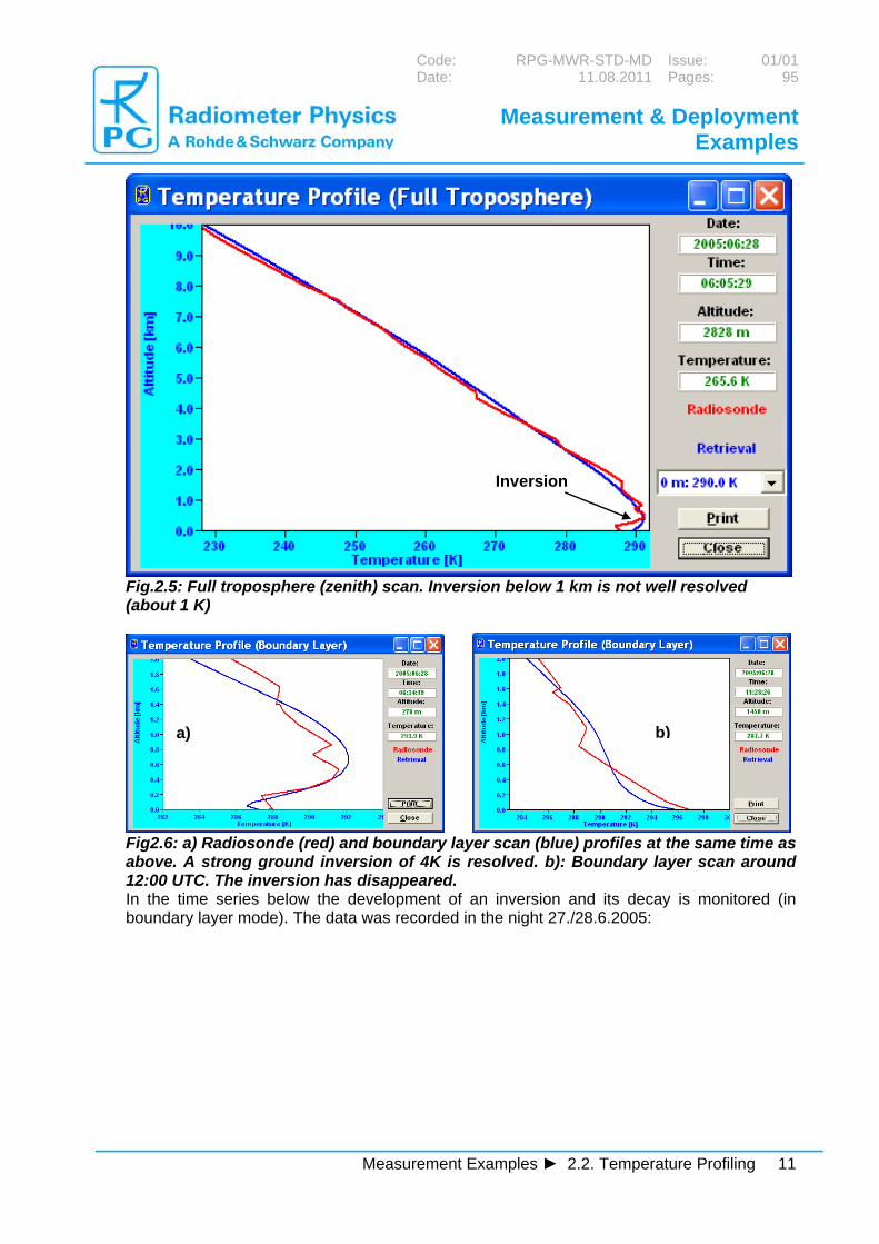
2.2.3.1 Comparison with Radiosonde Data Fig.2.5 is an example for a zenith mode observation of the full troposphere up to 10 km during the morning hours (6:00). The radiosonde (in red) was launched about 20 km away from the radiometer site. The RPG-HATPRO profile (in blue) matches well above 1 km altitude but deviates significantly in the lowest 500 m layer. Fig.2.6 shows the comparison between the radisonde profile and the radiometer data when operated in boundary layer mode in the lowest 2000 m layer. The ground inversion is resolved much better than in zenith mode.

E F

G H

I




Fig.2.5: Full troposphere (zenith) scan. Inversion below 1 km is not well resolved (about 1 K)

Fig2.6: a) Radiosonde (red) and boundary layer scan (blue) profiles at the same time as above. A strong ground inversion of 4K is resolved. b): Boundary layer scan around 12:00 UTC. The inversion has disappeared. In the time series below the development of an inversion and its decay is monitored (in boundary layer mode). The data was recorded in the night 27./28.6.2005:

Inversion

a) b)




20:18:04 21:12:51

22:07:38 23:02:24

00:10:53 01:05:39

02:00:26 03:08:54




04:03:41 05:12:09

06:06:56 07:01:42

07:56:29 09:04:57

10:04:57 11:04:57




2.2.3.2 Comparison with Meteorological Tower Observations 1. LAUNCH campaign in Lindenberg / Germany (September / October 2005) (Courtesy of Prof. Dr. S. Crewell, University of Munich)

The RPG-HATPRO was located about 40 m from a 99 m met. tower of the DWD (Germany Weather Service).

meteorological

tower (99 m)

temp. sensors

every 10 m

RPG-HATPRO

13:20:50 11:21:54




Fig.2.8a: Comparison of time series of tower temp. sensor (black) and HATPRO measurement (red) at 10 m and 100 m. Below is shown the gradient (difference) indicating that all low level inversions were captured by the instrument.

Fig.2.8b: The same measurement for another period of the campaign.




Fig.2.8c: Scatter plots of the comparison.

We also compared the HATPRO temperature profiles for both measurement modes with radiosonde data measured by a Vaisala RS92 sondes launched about 4 km from the radiometer site (4 times a day). Fig.2.9/2.10 show the statistical analysis of the data measured in BL mode and Z mode.

Fig.2.9: RMS and bias of the BLM temperature observations. Due to the 4 km distance between radio sounding and radiometer the details of the boundary layer are not necessarily the same. The BLM data is most accurate for altitudes < 1200 m.

dry adiabatic lapse rate

mast

HATPRO

H

ATPRO

H

ATPRO

mast

bias

RMS




Fig.2.10: RMS and bias of the ZM temperature observations..

2. KNMI Met. Tower Observations at Cabauw / Netherlands (Courtesy of H.Baltink, KNMI Netherlands)

The Dutch Weather Service operates a 200 m meteorological tower in Cabauw / Netherlands. Fig.2.13 shows a one month temperature comparison of the 200 m sensor with HATPRO BLM measurements.

Fig.2.11: Comparison of retrieved HATPRO temperature at 200 m (green) with 200 m temperature sensor reading of met. tower (black) in Cabauw (KNMI) in August 2006. Total number of samples: 1232, no-rain: 836 samples (RMS: 0.36 K, bias: -0.04 K); 396

bias

RMS




rain samples (RMS: 0.45 K, bias: -0.13 K). Rain samples are indicates as blue dots, rain rates are between 1 mm/h (drizzle) and 25 mm/h. BLM data remains accurate.

2.2.4 Extreme Inversions

Fig.2.12: BLM map of one week period. Very strong inversions occurred in the second half of the period indicated by the black lines (Lindenberg, October 2005, courtesy of Univ.of Munich).




Fig.2.13: Inversion comparisons between radio sounding (red) and HATPRO BL mode observations (blue) for the four cases in fig.10 indicated by the black lines.

Fig.2.14a: Examples of comparisons between radio sounding (red) and HATPRO Z mode observations (blue). The boundary layer details are not always accurately resolved.

Fig.2.14b: The Z mode tends to smear out (average) the details of the boundary layer.



20 Measurement Examples ► 2.3. Humidity Profiling

Fig.2.15: Strong solar heating (A) at day time and radiation cooling over night (B) (inversions!) during the AMMA campaign, January 2006, Benin / West Africa.

2.3. Humidity Profiling There is only a zenith mode for humidity measurements because at the water vapour line channel frequencies around 22 GHz the atmosphere is transparent. No saturation of the brightness temperatures occurs even at very low elevation angles like for the oxygen line center. Consequently an elevation scanning mode will not give significantly more information than the zenith mode. Nevertheless more accurate relative humidity profiles in the boundary layer can be generated by combining absolute humidity profiles with boundary layer temperature profiles and computing the relative humidity from these two profile types. The microwave signals the radiometer observes are directly proportional to the absolute humidity above the instrument with offsets due to liquid water introduced by clouds. Consequently, for retrieving humidity by observations of the water vapour line, absolute humidity profiles (humidity measured in g/m3) are the most ‘natural’ type of humidity profiles. Relative humidity profiles can be generated in two ways:

1) Using directly a retrieval for relative humidity without taking into account any temperature profile information.

2) Using a retrieval for absolute humidity and combine this information with temperature profiles generated by zenith and boundary layer modes.

Both methods suffer from severe inaccuracies at high altitude (>5000 m) where the absolute humidity is so low (due to low temperatures) that the microwave detection of this contribution becomes impossible. But method 2 has advantages over method 1 in the boundary layer because the higher accuracy and resolution of the boundary layer temperature profiles can be exploited for relative humidity profiling.

A B



Measurement Examples ► 2.3. Humidity Profiling 21

2.3.1 Examples of Absolute and Relative Humidity Profiles

2.3.1.1 RPG-HATPRO Measurements

Fig.2.16: Absolute humidity profile map for a 5 day period.

Fig.2.17: Sample profile taken from the map in Fig.16 at 12:00 UTC (noon time). In red is the data of a radiosonde for comparison (Larkhill, UK).




Fig. 2.18: Absolute humidity time series at 116 m altitude.

Fig.2.19: Relative humidity map for the full troposphere (up to 10 km) computed from absolute humidity profiles and temperature profiles both measured in zenith mode.

rain events




Fig.2.20: Comparison of relative humidity profile with radiosonde data. As mentioned above the microwave information does not allow for retrieving any details of humidity profiles above 5-6 km. A small error in absolute humidity at low temperatures produces a big error in relative humidity.

Fig.2.21: The lowest 2000 m layer map of Fig.2.11 computed from absolute humidity profiles and temperature profiles both measured in zenith mode.




Fig.2.22: Relative humidity map for boundary layer (up to 2 km) computed from absolute humidity profiles and temperature profiles measured in boundary layer mode. A comparison with Fig.13 clearly shows that more details are resolved in the <500 m range. The relative humidity is modulated by the temperature inversions. Below is shown a sequence of boundary layer humidity profile samples taken from Fig.2.21 (left profiles, Z-Mode (zenith mode)) and from Fig.2.22 (right profiles, BL-Mode (boundary layer mode)): Without temperature inversion the humidity profiles look almost the same.

Z-Mode

Z-Mode

BL-Mode

BL-Mode




temperature inversion present








Z-Mode

Z-Mode

Z-Mode

Z-Mode

Z-Mode BL-Mode

BL-Mode

BL-Mode

BL-Mode

BL-Mode




Fig:2.23: Relative humidity time series at low altitude measured in Z-mode and BL-mode. The BL-mode humidity maxima over night between 22:00 and 7:00 (when inversions are generated) are more pronounced than in Z-mode.

Fig:2.24: Absolute humidity profiles compared to radio soundings (red). Statistical analysis leads to RMS errors of 1 g/m^3.

Z-Mode BL-Mode

Z-Mode

BL-Mode




Fig:2.25: Due to the small number of degrees of freedom in the 22.4 GHz water vapour line the retrieval (dotted line) can only average through the real profiles but the integrated water vapour (IWV) measurement is quite accurate. AMMA campaign, Benin / West Africa (Jan. 2006 to Jan. 2007)

Fig:2.26: Example of a transition from wet to dry period by sea breeze effect in Benin / West Africa with development of absolute humidity profiles and integrated water vapour. Morioka campaign, Japan (Oct. 2006 to Jan. 2007)

45 kg/m^2

27 kg/m^2




Fig.2.27: One month of absolute humidity data from Morioka / Japan. At rain rates >10 mm/h the profile is distorted while at rates < 5mm/h the profile accuracy is reduced by only 20%.

Fig.2.28: Absolute humidity profile map of the lowest 4000 m over 6 days.

Distorted profiles

Rain rate < 10

/h




Fig.2.29: Absolute humidity time series @ 300 m level from period in Fig.28.

2.3.1.2 RPG-LHATPRO Humidity Profiling The same profiling observation modes as used for temperature profiles (BL and zenith) can be applied to humidity profiling with the 183 GHz line. Also the oxygen line channels are included in the humidity retrieval which is essential for resolving low altitude humidity inversions and relative humidity profiles. First results of radiative transfer calculations indicate the following vertical resolution and accuracies:

Full troposphere humidity profiles (0-10000 m): 500 m (<4000 m altitude), 1000 m above, profile accuracy: +/- 0.02 g/m^3 RMS (0-1000 m), +/- 0.04 g/m^3 RMS (>2000 m)

Boundary layer humidity profiles (0-2000 m), 100 m vertical resolution, profile accuracy: +/- 0.03 g/m^3 K RMS (<2000 m).




For the IWV retrieval the following accuracies are expected at very low humidity levels like at DOME C (Antarctica): IWV at Dome C Natural variability (Std.Dev.): 0.189 kg/(m^2) retrieval with 183.31 GHz line: RMS=0.008, Correlation=0.999 LWP accuracy is about 10-20 g/m^2 with RMS noise of 5 g/m^2. Retrieval Performance at Dome C / Antarctica Based on the radiosonde data from the Concordia station (290 soundings from 2006), we calculated the microwave brightness temperatures (BT) for down-welling radiation at several elevation angles. By adding instrument noise (0.5 Kelvin RMS) we obtained a synthetic radiometer measurement. A multi-variate quadratic (sometimes only linear) regression established the inversion of forward-calculated brightness temperatures to atmospheric parameters. Only 80% of the data (randomly chosen) were used for the regression, the rest were used for algorithm testing. The following algorithm performance estimates are based on the application of the regression methods on the unused 20% of the data. All results are preliminary. At a later stage, we will incorporate more data, maybe from Scott base or other similar locations.

data STD

22 GHz line retrieval

183 GHz line retrieval




Fig.2.30: Retrieval accuracy for humidity profiling with the 22 GHz and 183 GHz water vapour line. Integrated water vapour The total column water vapour is very low at Dome C. The brightness temperatures of the 22.235 GHz water vapour line are much too small for water vapour retrievals in low pressure and at very cold climates. We compare the retrieval performance of a sounder with 6 double-side-band channels around 183 GHz with the performance of a standard radiometer for mid-latitudes with 7 channels between 22.24 GHz and 31.4 GHz. The 22 GHz system has a low information content in the BT, thus the retrieved IWV is basically the all-year mean value plus some scatter around it. For the IWV retrieval the following accuracies are expected: Natural variability (Std.Dev.): 0.189 kg/(m^2) retrieval with 22.235 GHz line, RMS=0.140, Cor=0.583 retrieval with 183.31 GHz line, RMS=0.008, Cor=0.999




Fig.2.31: IWV scatter plot.

Humidity profiles with 183 GHz WVL:

Radio sounding

retrieval




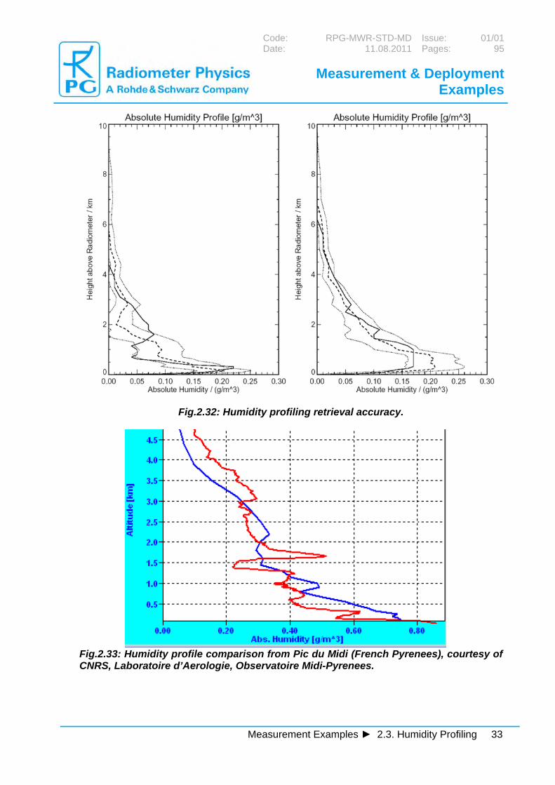
Fig.2.32: Humidity profiling retrieval accuracy.

Fig.2.33: Humidity profile comparison from Pic du Midi (French Pyrenees), courtesy of CNRS, Laboratoire d’Aerologie, Observatoire Midi-Pyrenees.



34 Measurement Examples ► 2.4. LWP and IWV Measurements

Fig.2.34: Example of humidity profile chart from Pic du Midi (French Pyrenees),

courtesy of CNRS, Laboratoire d’Aerologie, Observatoire Midi-Pyrenees .

2.4. LWP and IWV Measurements The RPG-HATPRO is capable of measuring liquid water path (LWP) with a 1 second temporal resolution due to its parallel receiver architecture. The variability of clouds can be analyzed in detail also because of the relatively narrow beam width of 4° HPBW (half power beam width) for the water vapour channels.



Measurement Examples ► 2.4. LWP and IWV Measurements 35

Fig.2.35: High temporal resolution (1 second sampling) LWP time series. The measurement noise is very low (< 2 g/ m2 RMS).

Fig.2.36: IWV time series. Absolute accuracy is +/- 0.3 kg/ m2 with an RMS noise of < 0.05 kg/ m2. The LWP measurement noise is very low (< 2 g/m2 RMS, see Fig.2.35), thus even thin clouds can be resolved. For integrated water vapour measurements (see Fig.2.36) the temporal resolution is not important. A sample rate of 1/minute is sufficient to monitor all IWV details. IWV is the most accurately retrieved atmospheric parameter with an absolute accuracy of +/- 0.3 kg/ m2 and an RMS noise of < 0.05 kg/ m2.



36 Measurement Examples ► 2.4. LWP and IWV Measurements

Fig.2.37: IWV time series over one month (KNMI, May 2006). 140 radio sondings (26. April to 4. July, Cabauw, KNMI). Radiosonds: Vaisala RS-92. No-Rain RMS: 0.43 kg/m^2, Bias: 0.05 kg/m^2

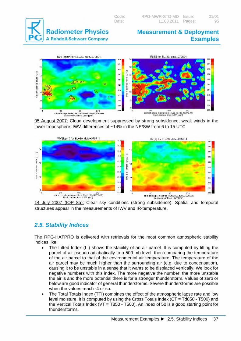
IWV/Sky-Temperature and LWP: The spatial and temporal evolution of integrated water vapour content (IWV), sky-temperature (IR) and liquid water path (LWP) are visualized by Time-Azimuth-(Hovmöller) Diagrams (courtesy of Stefan Kneifel, University of Cologne). 30 July 2007: Development of Cu-convection after frontal passage; Observed IWV varies up to 20% even in regions with low LWP (<50 g/m²); max. LWP~500 g/m²



Measurement Examples ► 2.5. Stability Indices 37

05 August 2007: Cloud development suppressed by strong subsidence; weak winds in the lower troposphere; IWV-differences of ~14% in the NE/SW from 6 to 15 UTC 14 July 2007 (IOP 8a): Clear sky conditions (strong subsidence); Spatial and temporal structures appear in the measurements of IWV and IR-temperature.

2.5. Stability Indices The RPG-HATPRO is delivered with retrievals for the most common atmospheric stability indices like:

The Lifted Index (LI) shows the stability of an air parcel. It is computed by lifting the parcel of air pseudo-adiabatically to a 500 mb level, then comparing the temperature of the air parcel to that of the environmental air temperature. The temperature of the air parcel may be much higher than the surrounding air (e.g. due to condensation), causing it to be unstable in a sense that it wants to be displaced vertically. We look for negative numbers with this index. The more negative the number, the more unstable the air is and the more potential there is for a stronger thunderstorm. Values of zero or below are good indicator of general thunderstorms. Severe thunderstorms are possible when the values reach -4 or so.

The Total Totals Index (TTI) combines the effect of the atmospheric lapse rate and low level moisture. It is computed by using the Cross Totals Index (CT = Td850 - T500) and the Vertical Totals Index (VT = T850 - T500). An index of 50 is a good starting point for thunderstorms.



38 Measurement Examples ► 2.5. Stability Indices

The K Index (KI) represents the thunderstorm potential as a function of vertical temperature lapse rate at 850 mb temperature and 500 mb temperature, low level moisture content at 850 mb dewpoint and the depth of the moist layer at 700 mb dewpoint (George, 1960). KI increases with decreasing static stability between 850 and 500 mb, increasing moisture at 850 mb and increasing relative humidity at 700 mb. KI can be used as an indicator of convection but not as a discriminator of severe versus non-severe convection. Values of KI > 20 generally represent a convective environment capable of producing scattered thunderstorms activity, while KI > 30 represents an atmospheric potential for numerous thunderstorms to occur (Haklander and Van Delden, 2003).

Fig.2.38: When TTI, KI and LI are approaching their critical limits, thunderstorms are likely to occur. This can be seen from the rain flag bar (blue indicates ‘rain’, red means ‘no rain’).

TTI

KI

LI

50

30

thunderstorms likely

thunderstorms likely

KO -2



Measurement Examples ► 2.6. Scanning 39

2.6. Scanning

Figure 2.39: A HATPRO instrument with azimuth positioner during full sky scan operation at the US ARM mobile facility.

o Figure 2.40a: Normalized IWV map. The HATPRO software is fully supporting

the sky scanning capabilities of the azimuth-scanned radiometer. Courtesy of U. Löhnert, Univ. of Cologne / Germany.

Scanning of IWV, LWP, water vapour field, temperature, and cloud coverage.



40 Measurement Examples ► 2.6. Scanning

In order to obtain sky scans, the radiometer needs (a) steerability, and (b) rapid integration (10 degree steps in azimuth and 9 degree steps in zenith result in 324 observations for one sky map).

The RPG-HATPRO instrument has zenith scanning capabilities as a basic feature. The azimuth positioner is adding the second scan direction. The control of both angles for scanning is fully supported by the software.

The RPG-HATPRO instrument can switch to a rapid scan mode with 0.4 s integration time. Adding some time for the movement of scan mirror (zenith) and positioning table (azimuth), one observation point can be acquired within 1 second, resulting in roughly 5 minutes for one hemispheric scan. Longer integration times would render the scanning capabilities for sky maps nearly useless, because the scan needs to be completed faster than the sky is changing it’s pattern.

From the scanned data the software is automatically retrieving the directional dependent values for IWV, LWP, profile of absolute humidity, temperature profile, and cloud coverage. The software supports azimuth-zenith plotting. o

Figure 2.40b: Normalized IWV map. Humidity variations of up to 20% over the sky have been measured. Courtesy of U. Löhnert, Univ. of Cologne / Germany.



Measurement Examples ► 2.6. Scanning 41

Figure 2.40c: Normalized LWP map showing the cloud coverage and cloud thickness variations. Courtesy of U. Löhnert, Univ. of Cologne / Germany.



42 Measurement Examples ► 2.6. Scanning

Fig.2.41: Azimuth scan under clear sky conditions. Displayed are the anomalies of IWV, IR radiometer temperature, LWP and optical camera (fish eye view). IR and IWV match nicely. The IWV variation is about 13% in this plot. Scanning azimuth pitch angle is 5°. A full scan takes 40 seconds. Courtesy of S. Kneifel, Univ. of Cologne and LMU Munich.

IWV from microwave signal

IR radiometer temperatur

LWP variation



Measurement Examples ► 2.7. Liquid Water Profiling 43

Fig.2.42: Under cloudy conditions, the IR radiometer signal is partially saturated while the microwave IWV is still reflecting the water vapour distribution. The IR gets saturated where the LWP level indicates clouds. Courtesy of S. Kneifel, Univ. of Cologne and LMU Munich.

2.7. Liquid Water Profiling

2.7.1 Introduction At Radiometer Physics GmbH (RPG), we are convinced that vertical profiles of liquid water content cannot be derived from passive microwave radiometers with significant retrieval skill, even when the microwave radiometer is combined with an infrared (IR) radiometer. The reason is the limited height information of the emitted radiation. For water vapour and oxygen gases, their spectral lines offer the great advantage of strongly varying optical depth within a small frequency band. For this reason, we can receive radiation from different depths of the atmosphere in different frequency channels.



44 Measurement Examples ► 2.7. Liquid Water Profiling

While oxygen has the strongest variation of optical depth up to totally opaque atmosphere, therefore allowing a good retrieval of the vertical structure of atmospheric temperature, the change of water vapour absorption characteristics with frequency is much weaker, leading to reduced quality of vertical humidity retrievals. Liquid water is not showing spectral emission lines, but a broad absorption continuum with only moderate frequency dependence. It must be stressed that 1 kg of liquid water will emit the same amount of microwave radiation whether it is at 1 km height or at 2 km height.

2.7.2 Existing LWC profiling techniques (and their problems) When using regression schemes to retrieve LWC in each level of a model atmosphere, the LWC profiles tend to produce non-zero LWC at all vertical levels. An example for this behaviour can be found in the ARM programs “Microwave Radiometer Profiler Handbook” by James C. Liljegren (http://www.radiometrics.com/mwrp_handbook.pdf), where one can find (p.60) a comparison of radar LWC profiles (dashed) and Radiometrics microwave radiometer LWC profiles (solid lines). Although this Radiometrics approach is using an IR radiometer, the cloud height is totally inconsistent. The LWC profile is non-zero at all heights, sometimes with significant LWC below the (highly elevated!) cloud. The maximum LWC is not correlated with the real cloud, neither in vertical position (several km away), nor in LWC amplitude. The non-zero LWP at all levels necessarily leads to underestimated LWC amplitudes, because the total area of the curve has to match the LWP (a variable which can be retrieved by microwave radiometers to much better accuracy).




Therefore, the retrieved profiles are showing a LWP-scaled variation of ever the same profile: Maximum LWC close to the surface, non-zero everywhere else, fading out above the cloud to top-of-the-atmosphere. Additionally, this approach can generate artificial clouds under high water vapour concentrations when the IR signal is significantly attenuated. Therefore the IR temperature increases (private communication, UK-MetOffice) and ‘suggests’ a cloud base. An independent check of a low or zero LWP value would easily resolve the error but a single NN retrieval is obviously not capable of handling this. This very limited retrievals skill has to be expected when using regression schemes to retrieve LWC in each level of a model atmosphere: When correlation is bad (e.g., information content in the measurements is small), then a regression will produce results close to the expectation value, which is the mean value of all profiles in the training set. Since clouds usually occur in all levels, with a maximum likelihood of thick rain clouds in lower altitudes, the retrieved profiles are basically showing the mean values, with little variations.

2.7.3 PARCWAPT – The RPG Method The available data (14 channels microwave brightness temperatures, one IR radiometer temperature, ground sensors of RH, T, p) has limited information content of the clouds vertical structure. Therefore, we are not using the usual regression schemes, but more an “expert system” approach. This way, we make optimal use of the information content in our variables. The detailed steps of the PARCWAPT LWC profile retrieval (patent pending):

1. Retrieve temperature profile of the atmosphere. The temperature profile is needed to determine the cloud base height from the IR temperature reading. One of the strongest points of the RPG-HATPRO instruments is the high-precision boundary layer scan obtained with narrow-beam elevation scanning techniques. Regardless of using explicit look-up tables or implicit retrievals using the oxygen line channels, the high quality in the temperature profile will be beneficial for precise cloud base height estimation.

2. Retrieve liquid water path (LWP, total of vertically integrated LWC profile) 3. Retrieve cloud base height by combining IR temperature reading and the T-profile 4. Retrieve the maximum LWC of the cloud (using all 14 microwave channels and the

surface sensor readings)




5. Modify a normalised LWC profile shape to model the actual LWC profile: a. The profile amplitude is scaled to match the retrieved maximum LWC value b. The profile height is then scaled to match the retrieved LWP c. The scaled profile is shifted in vertical position to match the cloud base retrieved

from IR sensor 6. Certain thresholds are applied to ensure rejection of inconsistent cases: 7. very small LWP values indicate thin clouds, which might be transparent to the IR

radiometer, in which case the cloud base would be miscalculated 8. very small values of retrieved maximum LWC are set to a minimum LWC of at least 0.1

g/m3. Obviously, such an algorithm can only retrieve one-layer clouds. The shape of the normalized curve which we use for the LWC profile inside the cloud has a physical meaning (modified adiabatic liquid water content): http://www.springerlink.com/content/k506hwh681823720/ paper by Karstens et al 1993), but the LWC curve inside the actual cloud may differ from this idealistic assumption due to the variety of cloud formation processes.

2.7.4 Advantages of the PARCWAPT Method The RPG algorithm produces LWC profiles with sharp boundaries. Below the cloud base

height and above cloud top height, the LWC is strictly zero:

The vertical position of maximum LWC is highly correlated with cloud height The maximum LWC is constrained to reasonable values by the regression retrieval which

is producing this value from all 14 microwave channels. Cloud base height is precisely following the (high-quality) information from the IR sensor. The vertically integrated LWC is consistent with the LWP retrieval. Typical high-temporal resolution data of the RPG radiometers reveal rapid changes

within the cloud properties and evolution. In contrast to regression schemes (like quadratic regressions and artificial Neural Networks), the RPG mixture of retrieved quantities and “expert system” analytical equations produces physically reasonable cloud profiles in the case of single layer clouds.




2.7.5 Limitations / Discussion Beyond the usual random errors (“noise”) in the retrieved quantities, the RPG LWC algorithm is producing misleading (meaning: incorrect) results whenever the real cloud structure deviates from the underlying assumptions.

Multilayer-clouds: The LWP of all cloud layers will be produced by simply extending the single layer cloud to larger vertical cloud top height. Largest deviations are expected in cases where a small but IR-detectable cloud is at lower levels, and all further cloud levels are at much higher elevations.

Clouds with LWC curves that deviate from the modified adiabatic liquid water content are retrieved with a wrong LWC curve inside the cloud. Possible examples are deep convection, thunderstorms, decaying cloud fields, etc…

Errors in the retrieved maximum LWC directly relate to errors in cloud thickness. We have three free parameters (cloud base height, total water amount LWP (= the integrated LWC), and the maximum LWC inside the cloud. These parameters are used to modify the constant normalised standard profile. A better way would use variable LWC profile shapes, but if LWP and maximum LWC are kept as independent variables, then the degrees of freedom would be higher than 3. With passive microwave radiometers, we just do not have this information.

Using variable profile shapes and adjust maximum LWC or LWP accordingly would result in possibly incorrect and un-physical numbers for these parameters.

In summary, RPG is providing this LWC retrieval as a visualization of parameters that are basically already visible in their raw representation: cloud base height from IR and LWP as the total water amount. Beyond this information, the only new insight into LWC profiles is the retrieved maximum LWC, which acts (when combined with a standard profile shape) as an estimator for cloud thickness.




2.7.6 Measurement Examples All cases were processed with the current version of the HATPRO operating software. Thickening cloud, start of rain. Single LWC from inside the rain period (12:09 UTC).

End of one rain event, cloud cover becomes thin. Lifts up to 3 km.




End of one rain event, lifting of cloud base, decay of LWP in high cloud cover (above low level rain cloud).




rain sensor delay




Rain event with rain-free period (and lifted cloud cover) in the middle.




Moderate cloud thickness, variable cloud base, height of maximum LWC quite uniform.




Very variable LWP, varying cloud thickness, most likely convective precipitation (LWP > 1000 g/m^2).




Thin cloud layer without rain.




Broken cloud layer.




Decreasing cloud base height, increase of LWP and LWC, start of rain.




Two isolated clouds with rather high LWP.




More isolated or broken cloud cover examples.







Heavily precipitating cloud layer, extending down to surface.




Examples of flat cloud base height.













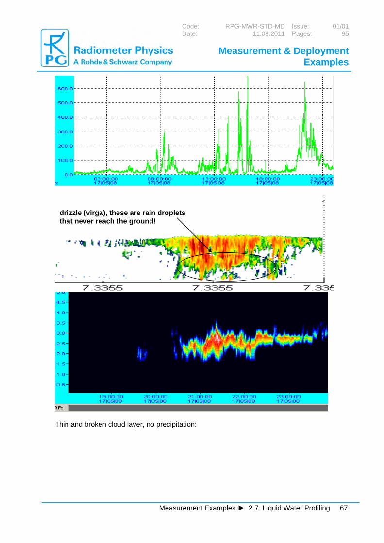
2.7.7 Comparison with Cloud Radar Data A comparison of the Microwave / IR derived LW profiles with active cloud radar data is useful and interesting. The microwave receivers operating in the 22-32 GHz band are not sensitive to ice clouds which show a strong response in the cloud radar data. Therefore a comparison of both data sources allows for the discrimination of ice and liquid water phases. Clouds of high integrated water content often develop a fine curtain of rain with small droplets which never reach the ground (virga). Virga is not detected in the IR but generates a strong signal in the cloud radar. The IR temperature detects the real cloud base.

water in ice phase

water in liquid phase

virga

no rain in this period




no liquid water here

Virga during maximum LWP

Virga not detected by IR and MW

Ice phase




Thin and broken cloud layer, no precipitation:

drizzle (virga), these are rain droplets that never reach the ground!




Heavy clouds and development of temperature inversion, causing a trapped cloud layer with flat cloud top:

temp. inversion generates flat cloud top



Deployment Examples ► 2.8. Acknowledgements 69

2.8. Acknowledgements Data Sources: 1. CSIP (Convective Storms Initiation Project). The RPG-HATPRO instrument was run by the University of Salford who is a member of UFAM (Universities Facilities for Atmospheric Measurements). 2. LAUNCH campaign, University of Munich, Germany 3. AMMA campaign, University of Bonn Germany 4. Morioka / Japan, Japan Meteorological Agency 5. KMNI, Dutch Weather Service, Cabauw / Netherlands 6. CNRS, Laboratoire d’Aerologie, Observatoire Midi-Pyrenees 7. University of Galway / Ireland

trap. alt.



70 Deployment Examples ► 2.8. Acknowledgements

3 Deployment Examples The RPG-HATPRO and other RPG radiometer models have been operated under various environmental conditions.

Fig.3.1: 85 RPG radiometers deployed worldwide in all climate areas (1.1.2011)

Fig.3.2: First operational microwave profiler network worldwide in Korea (10 units) The following list contains a selection of some typical deployment examples.



Deployment Examples ► 3.1 Europe 71

3.1 Europe

3.1.1 University of Cologne / Germany (deployed in Jülich (JOYCE)) Instrumentation: RPG-HATPRO-G2 second generation triple profiler (IR radiometer elevation angle automatically synchronized to microwave observation angle), wind profiler, weather station, 36 GHz cloud radar, IR FFTS (AERI) Applications: Precision brightness temperature measurements, validation of atmospheric spectral models, 2D volume MW / IR scanning Delivery: Dec. 2008

3.1.2 Meteorological Institute, University of Bonn / Germany Instrumentation: RPG-HATPRO, cloud radar, cilometer, wind profiler Application: T/H Profiling, LWP, convection in the tropics (AMMA Project, Barbados) Delivery: August 2005 (delivered on time) Deployment period: Jan.2006 to Dec.2006 in West Africa (AMMA) Deployment period: Apr.2007 to Dec.2007 in Black Forest/Germany (COPS) Since beginning of 2011: Barbados (Caribbean Sea)



72 Deployment Examples ► 3.1 Europe

3.1.3 University of Munich, Schneefernerhaus GmbH Instrumentation: RPG-HATPRO, RPG-DP150-90 (dual pol. 150 GHz + 90 GHz channel), ceilometer, wind profiler, lidar, radiation sensors Application: High altitude atmospheric modelling, boundary layer temperature profiling in alpine locations (Zugspitze area) Delivery: November 2005 (delivered with 1 month delay) Deployment period: Nov.2005 to Nov. 2006 at Schneeferner Haus / Zugspitze Germany Deployment period: Nov.2006 to May 2007 in Darwin / Australia Deployment period: June.2007 until today at Schneeferner Haus / Zugspitze Germany (continuous operation), partly damaged by avalanche in March 2008

3.1.4 Institute for Ocean Research GEOMAR. Kiel / Germany Instrumentation: RPG-HATPRO Application: instrument monitors humidity and temperature profiles over the ocean (between Antarktika and Spitzbergen) on board of the German research ice breaker ‘Polarstern’ Delivery: August 2006 (delivered on time) Deployment period: eight trips on the Polarstern from Bremerhafen/Germany to Capetown/South-Africa or Punta Arenas / Argentina, 5 weeks each, no failures




3.1.5 Karlsruhe Institute of Technology (KIT), Karlsruhe / Germany Instrumentation: RPG-HATPRO, ceilometer Application: climate modelling, boundary layer Delivery: Feb. 2009 (delivered on time) Deployment: since Feb. 2009 at KIT in Karlsruhe

3.1.6 IFT (Institute for Tropospheric Research) Leipzig / Germany Instrumentation: RPG-HATPRO, cloud radar, solar radiation detectors, cloud chamber Application: climate modelling, cloud statistics, boundary layer Delivery: Feb. 2011 (delivered on time)




3.1.7 AWI (Alfred Wegener Institute), Potsdam / Germany Instrumentation: RPG-HATPRO, cloud radar, solar radiation detectors Application: climate modelling in the Arctics Delivery: Dec. 2010 (delivered on time) Deployment: since Feb. 2011: Ny Alesund / Svalbard, AWIPEV Koldewey-Station

3.1.8 Meteorological Institute Hamburg / Germany Instrumentation: RPG-HATPRO, solar radiation detectors, lidars Application: weather forecast, precipitation, temperature profiles Delivery: March. 2011 (delivered on time) Deployment: mobile, northern Germany




3.1.9 Meteorological Institute, University of Munich / Germany Instrumentation: RPG-DP150-90, RPG-HATPRO, ceilometer, solar radiation, sky imager Application: snow and ice particle detection, discrimination of ice and liquid phase in clouds Delivery: March. 2006 (delivered on time) Deployment: until today: Schneefernerhaus / Zugspitze

3.1.10 MPI for Meteorology, Hamburg / Germany Instrumentation: RPG-HALO-KV, RPG-HALO-90-119, RPG-HALO-183, 36 GHz cloud radar, lidar Application: cirrus cloud and LWP detection from on Germany’s research aircraft HALO Delivery: August 2008 (delivered on time) Deployment: until today: Schneefernerhaus / Zugspitze (waiting for HALO)




3.1.11 KNMI, Dutch Weather Service, Cabauw / Netherlands Instrumentation: RPG-HATPRO, ceilometer, 200 m met. tower, cloud radar Application: Weather modelling and prediction, climatology, LWP calibration of cloud radar data Delivery: April 2006 (delivered on time) Deployment period: Apr.2006 until today at KNMI in Cabauw / Netherlands Continuous operation, one interface failure due to lightning discharge, replacement of wire data cable by fibre optics data cable and exchange of data interface

3.1.12 ESA / ESTEC, Nordwijk / Netherlands Instrumentation: RPG-HATPRO + RPG-15-90, fully steerable radiometer combination in Master / Slave operation, wind profiler, 36 GHz cloud radar Application: Atmospheric propagation measurements Delivery: April 2008 (delivered on time)




3.1.13 University of Ireland / Galway, Mace Head Station Instrumentation: RPG-HATPRO, cloud radar, ceilometer, GPS, aerosol Application: modelling of cloud formation in combination with aerosols Delivery: May 2008 (delivery within one month aro)

3.1.14 Legionowo / Leba / Wroclaw (Poland) Polish Meteorological Agency IMGW Instrumentation: 3 x RPG-HATPRO, solar radiation sensors, radio sounding stations, wind profilers Application: Radiometer data is assimilated into weather forecast model Delivery: Dec. 2008 (manufacturing of 3 instruments in 2 month)




3.1.15 Meteo Swiss / Switzerland Instrumentation: 1x RPG-HATPRO, 3 x RPG-TEMPRO (single temp. profiler), ceilometer, wind profiler, lidar, radiation sensors, radiosondes Application: boundary layer temperature profiling in the Mittelland area, convective processes in the lower troposphere Delivery: March 2006, June 2006, June 2007, June 2007 (all instruments delivered on time)

3.1.16 CEAMA, Granada / Spain Instrumentation: RPG-HATPRO-G2, solar flux measurements, X-band cloud radar Application: modelling of cloud formation in combination with aerosols, synergy with lidars Delivery: October 2010




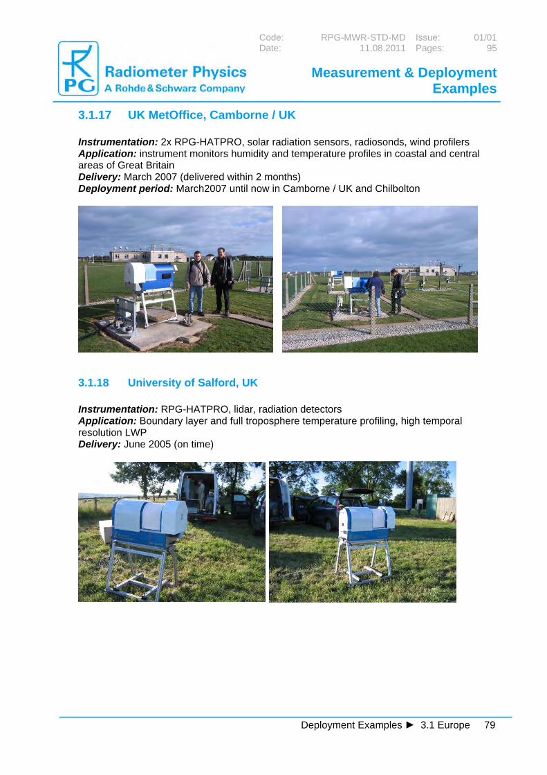
3.1.17 UK MetOffice, Camborne / UK Instrumentation: 2x RPG-HATPRO, solar radiation sensors, radiosonds, wind profilers Application: instrument monitors humidity and temperature profiles in coastal and central areas of Great Britain Delivery: March 2007 (delivered within 2 months) Deployment period: March2007 until now in Camborne / UK and Chilbolton

3.1.18 University of Salford, UK Instrumentation: RPG-HATPRO, lidar, radiation detectors Application: Boundary layer and full troposphere temperature profiling, high temporal resolution LWP Delivery: June 2005 (on time)




3.1.19 ARPAV, Weather Service of Veneto / Italy

Instrumentation: RPG-HATPRO, METEC wind profiler, cloud radar Application: Weather modelling and prediction, now casting, air pollution in the Po plain Delivery: April 2005

3.1.20 ENEA, Lampedusa / Italy Stazione di Osservazioni Climatiche ENEA di Lampedusa Instrumentation: RPG-HATPRO, solar radiation sensors, weather stations, GPS, aerosol Application: Climate modelling of the Mediterranean Sea Delivery: May 2009




3.1.21 Regione Marche, Ancona / Italy Instrumentation: RPG-HATPRO Application: Study of pollution effects, civil protection systems Delivery: April 2006

3.1.22 CNES, French Space Agency, Toulouse / France Centre National D'Etudes Spatiales Instrumentation: RPG-HATPRO Application: Atmospheric attenuation studies for Tele-Communication Satellites Delivery: May 2006 Deployment: North India




3.1.23 Laboratoire d'Aerologie, Observatoire Midi-Pyrenees, Toulouse/France

Instrumentation: RPG-LHATPRO, Tropospheric WV Radiometer Application: Measurement of ultra low humidity profiles in Antarctica Delivery: February 2008 (delivered with 6 weeks delay due to development work) Deployment period: Feb.2008 until now on Pic du Midi / French Pyrenees, no failures Planned deployment in Antarctica: Jan.2009 until Jan.2020

3.1.24 ONERA Centre de Toulouse, France Instrumentation: RPG-HATPRO Application: Atmospheric attenuation, tele-communication Delivery: February 2011




3.1.25 Laboratoire d'Aerologie, Observatoire Midi-Pyrenees, Toulouse/France Instrumentation: RPG-HATPRO Application: Weather forecast studies, fog detection, long term climatology studies Delivery: April 2011 Deployment: Lannemezan / South France

3.1.26 SIRTA, Ecole Polytechnique, Palaiseau / France Instrumentation: RPG-HATPRO, cloud radar, wind profiler, ceilometer, lidar Application: Weather forecast studies, long term climatology studies, LWP Delivery: Febr. 2010

3.1.27 INOE 2000, Bucarest, Romania



84 Deployment Examples ► 3.2 Asia

Instrumentation: RPG-HATPRO, radio soundings, weather stations, lidar Application: Weather forecast studies, long term climatology studies, LWP Delivery: Febr. 2010

3.2 Asia

3.2.1 KMA Korean Met. Agency / Korea First operational network of microwave profilers worldwide Instrumentation: 9 x RPG-HATPRO, wind profilers, weather stations, Application: Radiometer data is assimilated into weather forecast model Delivery: May / August 2009

3.2.2 KAMA Korean Met. Agency (Aviation Department) / Korea



Deployment Examples ► 3.2 Asia 85

Instrumentation: RPG-HUMPRO, wind profiler, weather station, cloud radar, Application: Aviation Delivery: Dec. 2007

3.2.3 NIMR, National Institute of Meteorological Research, Korea Instrumentation: RPG-HATPRO, weather station, photo-meters, rain gauges Application: Atmospheric research, long time series for climate studies Delivery: Nov. 2010




3.2.4 KASI, Korea Astronomy and Space Science Institute Instrumentation: RPG-HATPRO, weather station Application: Site characterisation for radio astronomy locations Delivery: June 2009

3.2.5 ROKAF, Korean Air Force Instrumentation: RPG-HATPRO, weather radar Application: Aviation Delivery: August 2010




3.2.6 Hong Kong Observatory, Met Agency / China Instrumentation: RPG-HATPRO, radio sounding station Application: Assimilation of humidity and temperature profiles into weather forecast models Delivery: February 2008 (delivered one month ahead of schedule)

3.2.7 Wuhan University, Wuhan / China Instrumentation: RPG-HATPRO, Raman lidar Application: modelling of cloud formation in combination with aerosols, climate research, forecasting Delivery: September 2010 (delivered on time)




3.2.8 China Academy of Space Technology, Xi’an / China Instrumentation: RPG-36-90, high precision LWP radiometer Application: microwave attenuation by cloud liquid Delivery: May 2008 (delivered on time)

3.2.9 Center for Atmospheric and Oceanic Sciences, Bangalore / India Instrumentation: RPG-HATPRO Application: weather forecast modelling Delivery: September 2010 (delivered on time)




3.2.10 University of Calcutta, Centre for Research in Space Environment, Calcutta / India Instrumentation: RPG-HATPRO Application: weather forecast modelling Delivery: October 2009 (delivered on time)

3.2.11 Inst. Low Temperature Science, Hokkaido University / Japan Instrumentation: RPG-HATPRO Application: low temperature climatology Delivery: June 2004




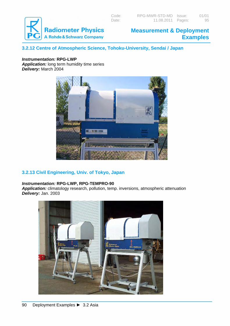
3.2.12 Centre of Atmospheric Science, Tohoku-University, Sendai / Japan Instrumentation: RPG-LWP Application: long term humidity time series Delivery: March 2004

3.2.13 Civil Engineering, Univ. of Tokyo, Japan Instrumentation: RPG-LWP, RPG-TEMPRO-90 Application: climatology research, pollution, temp. inversions, atmospheric attenuation Delivery: Jan. 2003



Deployment Examples ► 3.3 America 91

3.3 America

3.3.1 ARM Mobile Facility, DOE / USA Instrumentation: RPG-150-90, LWP Radiometer Application: Accurate measurement of LWP time series Delivery: June 2007 (delivered with 4 weeks delay) Deployment period: June 2007 until Dec. 2007, COPS campaign in Germany Deployment period: Jan. 2008 until Dec. 2008, Shanghai / China Deployment period: Jan. 2009 until Dec. 2010, Azores / Portugal

3.3.2 ARM SGP Site in Ponca City, Oklahoma / USA Instrumentation: RPG-150-90, LWP Radiometer Application: Accurate measurement of LWP time series Delivery: Sept. 2006 (delivered on time) Deployment period: Nov. 2006 until Sept 2010, SPG Site Oklahoma Deployment period: Oct. 2010 until today, Barrow, North Slope of Alaska



92 Deployment Examples ► 3.3 America

3.3.3 University of Wisconsin. Madison / USA Instrumentation: 1x RPG-HATPRO, 1 x RPG150-90, IR lidar, radiosonds Application: instrument will monitor humidity and temperature profiles and LWP time series at University of Wisconsin/ Madison and shall participate in campaigns of the ARM program, e.g. in Oklahoma (SGP, Southern Great Planes) Delivery: Feb./ May 2007 (delivered 2 month ahead of schedule) Deployment period: Feb.2007 until April 2010, one 50 GHz amplifier failure

3.3.4 Summit Station in Greenland (MSF, Mobile Science Facility), altitude 3300 m asl Instrumentation: RPG-HATPRO, RPG -150-90 Application: tests of absorption models, LWP monitoring, study of temp. inversions, observation of clouds Deployment: since April 2010



Deployment Examples ► 3.3 America 93

3.3.5 The Aerospace Corporation, Los Angeles / USA Instrumentation: RPG-HATPRO, lidar Application: LWP monitoring, study of temp. inversions, observation of clouds Deployment: April 2006 until Nov.2006 in Los Angeles, California Deployment: Nov. 2006 until June 2007 in Big Island, Hawaii

3.3.6 US Airforce AFRL / RIGD, Rome, NY / USA Instrumentation: RPG-LWP-U72-82 Application: atmospheric attenuation measurements, tele-communication Delivery: Oct. 2010 (on time) Deployment: Oct. 2010 until today in Rome / NY



94 Deployment Examples ► 3.3 America

3.3.7 SINICA Institute of Astronomy and Astrophysics, EUREKA Station / Ellesmere Island, Kanada Instrumentation: RPG-TIP-225, 225 GHz tipping radiometer Application: long term characterisation of Tau (atmospheric absorption) at potential radio astronomy sites (Mauna Kea, Summit Station / Greenland) Delivery: Sept. 2010 (on time) Deployment: Oct. 2010 Mauna Kea / Hawaii Deployment: Nov. 2010 until May 2011: Ellesmere Island / Kanada

3.3.8 LMT (INAOE), Large Millimetre Telescope, Puebla / Mexico 4600 m altitude on Sierra Negra volcano Instrumentation: RPG-TIP-225, 225 GHz tipping radiometer Application: long term characterisation of Tau (atmospheric absorption) at potential radio astronomy sites (Mauna Kea, Summit Station / Greenland) Delivery: Sept. 2010 (on time)



Deployment Examples ► 3.4 Antarctica 95

3.4 Antarctica

3.4.1 Laboratoire d'Aerologie, Observatoire Midi-Pyrenees, Toulouse/France Instrumentation: RPG-LHATPRO, Tropospheric WV Radiometer Application: Measurement of ultra low humidity profiles and low temperature inversions in Antarctica Delivery: February 2008 (delivered with 6 weeks delay due to development work) Deployment period: Jan.2010 until now at Dome C (Concordia Station), Antarctica Planned deployment in Antarctica: Jan.2009 until Jan.2020

Documents

Measurement and Deployment Examples