Measured Effects of Turbulence on the Loudness and ... · Measured Effects of Turbulence on the Loudness and Waveforms of Conventional and ... together with a reference unmodified

AIAA-2005-2949

https://ntrs.nasa.gov/search.jsp?R=20050182123 2018-07-15T09:20:29+00:00Z

11th AIAA/CEAS Aeroacoustics Conference23-25 May 2005, Monterey, CA

Measured Effects of Turbulence on the Loudness and Waveforms of Conventional and Shaped Minimized Sonic

Booms

Kenneth J. Plotkin *

Wyle Laboratories, Arlington, VA, 22202

Domenic J. Maglieri† Eagle Aeronautics, Inc, Hampton, VA, 23669

and

Brenda M. Sullivan‡ NASA Langley Research Center, Hampton, Virginia, 23681

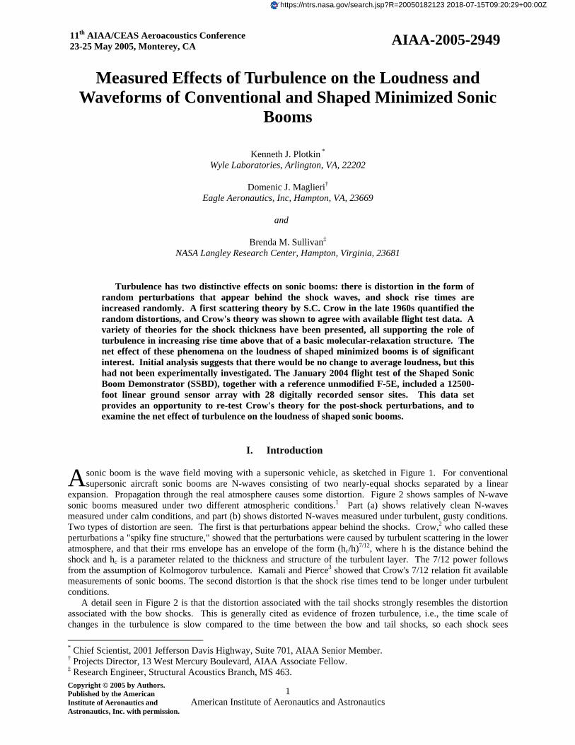
Turbulence has two distinctive effects on sonic booms: there is distortion in the form of random perturbations that appear behind the shock waves, and shock rise times are increased randomly. A first scattering theory by S.C. Crow in the late 1960s quantified the random distortions, and Crow's theory was shown to agree with available flight test data. A variety of theories for the shock thickness have been presented, all supporting the role of turbulence in increasing rise time above that of a basic molecular-relaxation structure. The net effect of these phenomena on the loudness of shaped minimized booms is of significant interest. Initial analysis suggests that there would be no change to average loudness, but this had not been experimentally investigated. The January 2004 flight test of the Shaped Sonic Boom Demonstrator (SSBD), together with a reference unmodified F-5E, included a 12500-foot linear ground sensor array with 28 digitally recorded sensor sites. This data set provides an opportunity to re-test Crow's theory for the post-shock perturbations, and to examine the net effect of turbulence on the loudness of shaped sonic booms.

I. Introduction

sonic boom is the wave field moving with a supersonic vehicle, as sketched in Figure 1. For conventional supersonic aircraft sonic booms are N-waves consisting of two nearly-equal shocks separated by a linear

expansion. Propagation through the real atmosphere causes some distortion. Figure 2 shows samples of N-wave sonic booms measured under two different atmospheric conditions.1 Part (a) shows relatively clean N-waves measured under calm conditions, and part (b) shows distorted N-waves measured under turbulent, gusty conditions. Two types of distortion are seen. The first is that perturbations appear behind the shocks. Crow,2 who called these perturbations a "spiky fine structure," showed that the perturbations were caused by turbulent scattering in the lower atmosphere, and that their rms envelope has an envelope of the form (hc/h)7/12, where h is the distance behind the shock and hc is a parameter related to the thickness and structure of the turbulent layer. The 7/12 power follows from the assumption of Kolmogorov turbulence. Kamali and Pierce3 showed that Crow's 7/12 relation fit available measurements of sonic booms. The second distortion is that the shock rise times tend to be longer under turbulent conditions.

A

A detail seen in Figure 2 is that the distortion associated with the tail shocks strongly resembles the distortion associated with the bow shocks. This is generally cited as evidence of frozen turbulence, i.e., the time scale of changes in the turbulence is slow compared to the time between the bow and tail shocks, so each shock sees * Chief Scientist, 2001 Jefferson Davis Highway, Suite 701, AIAA Senior Member. † Projects Director, 13 West Mercury Boulevard, AIAA Associate Fellow. ‡ Research Engineer, Structural Acoustics Branch, MS 463. Copyright © 2005 by Authors. Published by the American Institute of Aeronautics and Astronautics, Inc. with permission.

American Institute of Aeronautics and Astronautics

1

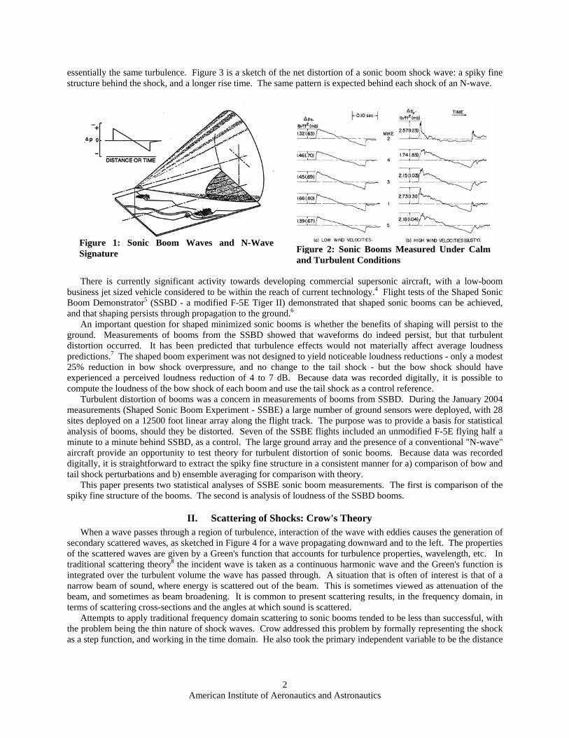
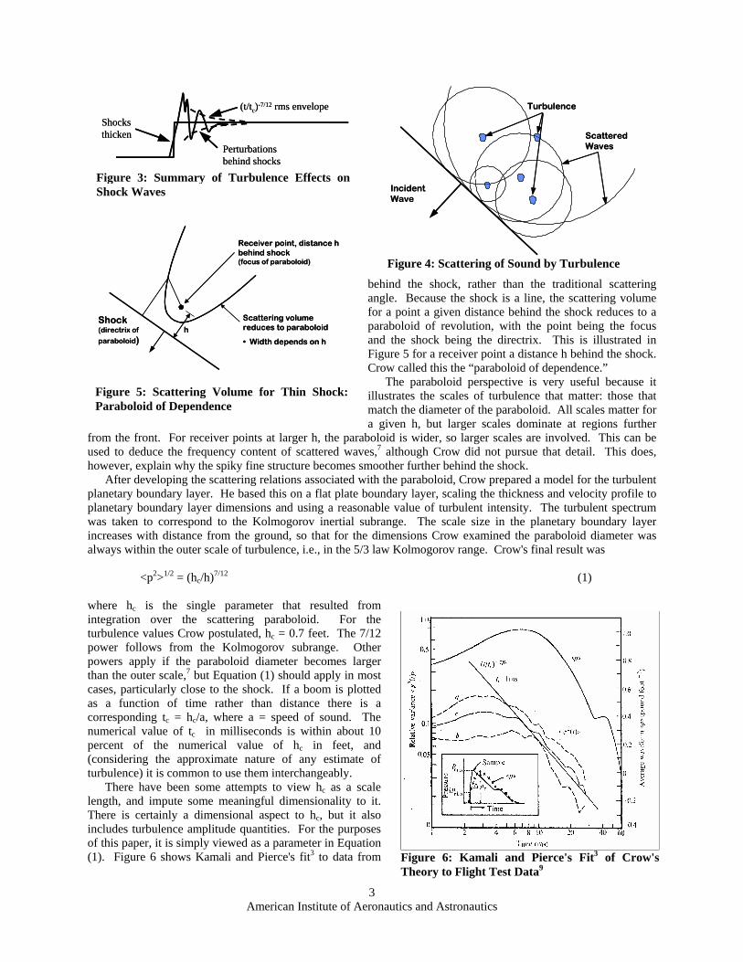
essentially the same turbulence. Figure 3 is a sketch of the net distortion of a sonic boom shock wave: a spiky fine structure behind the shock, and a longer rise time. The same pattern is expected behind each shock of an N-wave.

Figure 1: Sonic Boom Waves and N-Wave Signature Figure 2: Sonic Booms Measured Under Calm

and Turbulent Conditions There is currently significant activity towards developing commercial supersonic aircraft, with a low-boom

business jet sized vehicle considered to be within the reach of current technology.4 Flight tests of the Shaped Sonic Boom Demonstrator5 (SSBD - a modified F-5E Tiger II) demonstrated that shaped sonic booms can be achieved, and that shaping persists through propagation to the ground.6

An important question for shaped minimized sonic booms is whether the benefits of shaping will persist to the ground. Measurements of booms from the SSBD showed that waveforms do indeed persist, but that turbulent distortion occurred. It has been predicted that turbulence effects would not materially affect average loudness predictions.7 The shaped boom experiment was not designed to yield noticeable loudness reductions - only a modest 25% reduction in bow shock overpressure, and no change to the tail shock - but the bow shock should have experienced a perceived loudness reduction of 4 to 7 dB. Because data was recorded digitally, it is possible to compute the loudness of the bow shock of each boom and use the tail shock as a control reference.

Turbulent distortion of booms was a concern in measurements of booms from SSBD. During the January 2004 measurements (Shaped Sonic Boom Experiment - SSBE) a large number of ground sensors were deployed, with 28 sites deployed on a 12500 foot linear array along the flight track. The purpose was to provide a basis for statistical analysis of booms, should they be distorted. Seven of the SSBE flights included an unmodified F-5E flying half a minute to a minute behind SSBD, as a control. The large ground array and the presence of a conventional "N-wave" aircraft provide an opportunity to test theory for turbulent distortion of sonic booms. Because data was recorded digitally, it is straightforward to extract the spiky fine structure in a consistent manner for a) comparison of bow and tail shock perturbations and b) ensemble averaging for comparison with theory.

This paper presents two statistical analyses of SSBE sonic boom measurements. The first is comparison of the spiky fine structure of the booms. The second is analysis of loudness of the SSBD booms.

II. Scattering of Shocks: Crow's Theory When a wave passes through a region of turbulence, interaction of the wave with eddies causes the generation of

secondary scattered waves, as sketched in Figure 4 for a wave propagating downward and to the left. The properties of the scattered waves are given by a Green's function that accounts for turbulence properties, wavelength, etc. In traditional scattering theory8 the incident wave is taken as a continuous harmonic wave and the Green's function is integrated over the turbulent volume the wave has passed through. A situation that is often of interest is that of a narrow beam of sound, where energy is scattered out of the beam. This is sometimes viewed as attenuation of the beam, and sometimes as beam broadening. It is common to present scattering results, in the frequency domain, in terms of scattering cross-sections and the angles at which sound is scattered.

Attempts to apply traditional frequency domain scattering to sonic booms tended to be less than successful, with the problem being the thin nature of shock waves. Crow addressed this problem by formally representing the shock as a step function, and working in the time domain. He also took the primary independent variable to be the distance


2

Turbulence

Scattered Waves

Incident Wave

Turbulence

Scattered Waves

Incident Wave

Figure 4: Scattering of Sound by Turbulence

(t/tc)-7/12 rms envelopeShocks thicken

Perturbations behind shocks

(t/tc)-7/12 rms envelopeShocks thicken

Perturbations behind shocks

Figure 3: Summary of Turbulence Effects on Shock Waves

behind the shock, rather than the traditional scattering angle. Because the shock is a line, the scattering volume for a point a given distance behind the shock reduces to a paraboloid of revolution, with the point being the focus and the shock being the directrix. This is illustrated in Figure 5 for a receiver point a distance h behind the shock. Crow called this the “paraboloid of dependence.”

The paraboloid perspective is very useful because it illustrates the scales of turbulence that matter: those that match the diameter of the paraboloid. All scales matter for a given h, but larger scales dominate at regions further

from the front. For receiver points at larger h, the paraboloid is wider, so larger scales are involved. This can be used to deduce the frequency content of scattered waves,7 although Crow did not pursue that detail. This does, however, explain why the spiky fine structure becomes smoother further behind the shock.

Shock (directrix of

paraboloid)

Receiver point, distance h behind shock (focus of paraboloid)

Scattering volume reduces to paraboloid

• Width depends on h

hShock (directrix of

paraboloid)

Receiver point, distance h behind shock (focus of paraboloid)

Scattering volume reduces to paraboloid

• Width depends on h

h

Figure 5: Scattering Volume for Thin Shock: Paraboloid of Dependence

After developing the scattering relations associated with the paraboloid, Crow prepared a model for the turbulent planetary boundary layer. He based this on a flat plate boundary layer, scaling the thickness and velocity profile to planetary boundary layer dimensions and using a reasonable value of turbulent intensity. The turbulent spectrum was taken to correspond to the Kolmogorov inertial subrange. The scale size in the planetary boundary layer increases with distance from the ground, so that for the dimensions Crow examined the paraboloid diameter was always within the outer scale of turbulence, i.e., in the 5/3 law Kolmogorov range. Crow's final result was

<p2>1/2 = (hc/h)7/12 (1)

where hc is the single parameter that resulted from integration over the scattering paraboloid. For the turbulence values Crow postulated, hc = 0.7 feet. The 7/12 power follows from the Kolmogorov subrange. Other powers apply if the paraboloid diameter becomes larger than the outer scale,7 but Equation (1) should apply in most cases, particularly close to the shock. If a boom is plotted as a function of time rather than distance there is a corresponding tc = hc/a, where a = speed of sound. The numerical value of tc in milliseconds is within about 10 percent of the numerical value of hc in feet, and (considering the approximate nature of any estimate of turbulence) it is common to use them interchangeably.

Figure 6: Kamali and Pierce's Fit3 of Crow's Theory to Flight Test Data9

There have been some attempts to view hc as a scale length, and impute some meaningful dimensionality to it. There is certainly a dimensional aspect to hc, but it also includes turbulence amplitude quantities. For the purposes of this paper, it is simply viewed as a parameter in Equation (1). Figure 6 shows Kamali and Pierce's fit3 to data from


3

three early-afternoon flights at Edwards AFB in 1966.9 They found good agreement with the obtained 7/12 scaling, and obtained a best fit of tc = 1.2 msec, slightly larger than Crow's 0.7.

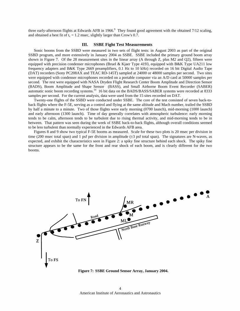
III. SSBE Fight Test Measurements Sonic booms from the SSBD were measured in two sets of flight tests: in August 2003 as part of the original

SSBD program, and more extensively in January 2004 as SSBE. SSBE included the primary ground boom array shown in Figure 7. Of the 28 measurement sites in the linear array (A through Z, plus M2 and Q2), fifteen were equipped with precision condenser microphones (Bruel & Kjaer Type 4193, equipped with B&K Type UA211 low frequency adapters and B&K Type 2669 preamplifiers, 0.1 Hz to 10 kHz) recorded on 16 bit Digital Audio Tape (DAT) recorders (Sony PC208AX and TEAC RD-145T) sampled at 24000 or 48000 samples per second. Two sites were equipped with condenser microphones recorded on a portable computer via an A/D card at 50000 samples per second. The rest were equipped with NASA Dryden Flight Research Center Boom Amplitude and Direction Sensor (BADS), Boom Amplitude and Shape Sensor (BASS), and Small Airborne Boom Event Recorder (SABER) automatic sonic boom recording systems.10 16 bit data on the BADS/BASS/SABER systems were recorded at 8333 samples per second. For the current analysis, data were used from the 15 sites recorded on DAT.

Twenty-one flights of the SSBD were conducted under SSBE. The core of the test consisted of seven back-to-back flights where the F-5E, serving as a control and flying at the same altitude and Mach number, trailed the SSBD by half a minute to a minute. Two of those flights were early morning (0700 launch), mid-morning (1000 launch) and early afternoon (1300 launch). Time of day generally correlates with atmospheric turbulence: early morning tends to be calm, afternoon tends to be turbulent due to rising thermal activity, and mid-morning tends to be in between. That pattern was seen during the week of SSBE back-to-back flights, although overall conditions seemed to be less turbulent than normally experienced in the Edwards AFB area.

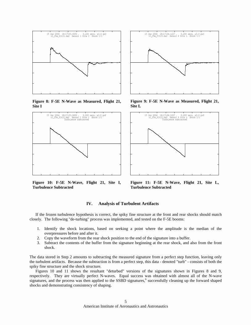
Figures 8 and 9 show two typical F-5E booms as measured. Scale for these two plots is 20 msec per division in time (200 msec total span) and 1 psf per division in amplitude (±3 psf total span). The signatures are N-waves, as expected, and exhibit the characteristics seen in Figure 2: a spiky fine structure behind each shock. The spiky fine structure appears to be the same for the front and rear shock of each boom, and is clearly different for the two booms.

A

Z

M

North Base RunwayRoad

ML

MR

To FS

To FNA

Z

M

North Base RunwayRoad

ML

MR

To FS

To FN

Figure 7: SSBE Ground Sensor Array, January 2004.


4

15 Jan 2004 18:17:03.0650 , 0.200 secs, ±3.0 psfr1_f5e_flt21.da2 Sensor 1 Site I Shock 1/1

Figure 8: F-5E N-Wave as Measured, Flight 21, Site I

15 Jan 2004 18:17:04.1227 , 0.200 secs, ±3.0 psfr1_f5e_flt21.da2 Sensor 4 Site L Shock 1/1

Figure 9: F-5E N-Wave as Measured, Flight 21, Site L

15 Jan 2004 18:17:03.0650 , 0.200 secs, ±3.0 psfr1_f5e_flt21.da2 Sensor 1 Site I Shock 1/1

Turbulence subtracted

Figure 10: F-5E N-Wave, Flight 21, Site I, Turbulence Subtracted

15 Jan 2004 18:17:04.1227 , 0.200 secs, ±3.0 psfr1_f5e_flt21.da2 Sensor 4 Site L Shock 1/1

Turbulence subtracted

Figure 11: F-5E N-Wave, Flight 21, Site L, Turbulence Subtracted

IV. Analysis of Turbulent Artifacts If the frozen turbulence hypothesis is correct, the spiky fine structure at the front and rear shocks should match

closely. The following "de-turbing" process was implemented, and tested on the F-5E booms: 1. Identify the shock locations, based on seeking a point where the amplitude is the median of the

overpressures before and after it. 2. Copy the waveform from the rear shock position to the end of the signature into a buffer. 3. Subtract the contents of the buffer from the signature beginning at the rear shock, and also from the front

shock.

The data stored in Step 2 amounts to subtracting the measured signature from a perfect step function, leaving only the turbulent artifacts. Because the subtraction is from a perfect step, this data - denoted "turb" - consists of both the spiky fine structure and the shock structure.

Figures 10 and 11 shows the resultant "deturbed" versions of the signatures shown in Figures 8 and 9, respectively. They are virtually perfect N-waves. Equal success was obtained with almost all of the N-wave signatures, and the process was then applied to the SSBD signatures,6 successfully cleaning up the forward shaped shocks and demonstrating consistency of shaping.


5

F5-E N-waves, DAT sites105 recordings

0 10 20 30 40 50 60 70 80 90 100Time Behind Shock, msec

-1 0

1Turbulent Perturbations, psf

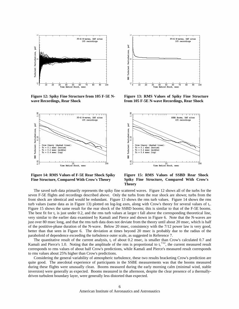
Figure 12: Spiky Fine Structure from 105 F-5E N-wave Recordings, Rear Shock


0 10 20 30 40 50 60 70 80 90 100Time Behind Shock, msec

-1 0

1RMS Turbulent Perturbations, psf

Figure 13: RMS Values of Spiky Fine Structure from 105 F-5E N-wave Recordings, Rear Shock


Crow theory (dashed lines):Tc = 0.1 msec (bottom)Tc = 0.2 msec (middle)Tc = 0.4 msec (top)

1 10 100Time Behind Shock, msec

0.01

0.10

1.00

RMS Turbulent Perturbations, psf

Figure 14: RMS Values of F-5E Rear Shock Spiky Fine Structure, Compared With Crow's Theory

SSBD Booms, DAT sites105 recordings

Crow theory (dashed lines):Tc = 0.1 msec (bottom)Tc = 0.2 msec (middle)Tc = 0.4 msec (top)

1 10 100Time Behind Shock, msec

0.01

0.10

1.00

RMS Turbulent Perturbations, psf

Figure 15: RMS Values of SSBD Rear Shock Spiky Fine Structure, Compared With Crow's Theory

The saved turb data primarily represents the spiky fine scattered waves. Figure 12 shows all of the turbs for the seven F-5E flights and recordings described above. Only the turbs from the rear shock are shown; turbs from the front shock are identical and would be redundant. Figure 13 shows the rms turb values. Figure 14 shows the rms turb values (same data as in Figure 13) plotted on log-log axes, along with Crow's theory for several values of tc. Figure 15 shows the same result for the rear shock of the SSBD booms; this is similar to that of the F-5E booms. The best fit for tc is just under 0.2, and the rms turb values at larger t fall above the corresponding theoretical line, very similar to the earlier data examined by Kamali and Pierce and shown in Figure 6. Note that the N-waves are just over 80 msec long, and that the rms turb data does not deviate from the theory until about 20 msec, which is half of the postitive-phase duration of the N-wave. Below 20 msec, consistency with the 7/12 power law is very good, better than that seen in Figure 6. The deviation at times beyond 20 msec is probably due to the radius of the paraboloid of dependence exceeding the turbulence outer scale, as suggested in Reference 7.

The quantitative result of the current analysis, tc of about 0.2 msec, is smaller than Crow's calculated 0.7 and Kamali and Pierce's 1.0. Noting that the amplitude of the rms is proportional to tc

7/12, the current measured result corresponds to rms values of about half Crow's predictions, while Kamali and Pierce's measured result corresponds to rms values about 25% higher than Crow's predictions.

Considering the general variability of atmospheric turbulence, these two results bracketing Crow's prediction are quite good. The anecdotal experience of participants in the SSBE measurements was that the booms measured during these flights were unusually clean. Booms measured during the early morning calm (minimal wind, stable inversion) were generally as expected. Booms measured in the afternoon, despite the clear presence of a thermally-driven turbulent boundary layer, were generally less distorted than expected.


6

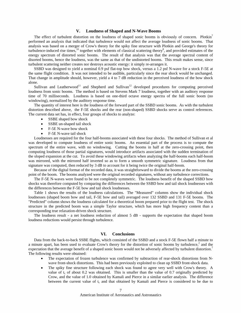
V. Loudness of Shaped and N-Wave Booms The effect of turbulent distortion on the loudness of shaped sonic booms is obviously of concern. Plotkin7

performed an analysis that indicated that turbulence would not affect the average loudness of sonic booms. That analysis was based on a merger of Crow's theory for the spiky fine structure with Plotkin and George's theory for turbulence-induced rise times,10 together with elements of classical scattering theory8, and provided estimates of the energy spectrum of distorted sonic booms. The result of that analysis was that the average spectral content of disorted booms, hence the loudness, was the same as that of the undistorted booms. This result makes sense, since turbulent scattering neither creates nor destroys acoustic energy: it simply re-arranges it.

SSBD was designed to yield a nominal 0.9 psf flat-top bow shock, versus a 1.2 psf N-wave for a stock F-5E at the same flight condition. It was not intended to be audible, particularly since the rear shock would be unchanged. That change in amplitude should, however, yield a 4 to 7 dB reduction in the perceived loudness of the bow shock alone.

Sullivan and Leatherwood11 and Shepherd and Sullivan12 developed procedures for computing perceived loudness from sonic booms. The method is based on Stevens Mark 7 loudness, together with an auditory response time of 70 milliseconds. Loudness is based on one-third octave energy spectra of the full sonic boom (no windowing), normalized by the auditory response time.

The quantity of interest here is the loudness of the forward part of the SSBD sonic booms. As with the turbulent distortion described above, the F-5E shocks and the rear (non-shaped) SSBD shocks serve as control references. The current data set has, in effect, four groups of shocks to analyze:

• SSBE shaped bow shock • SSBE un-shaped tail shock • F-5E N-wave bow shock • F-5E N-wave tail shock

Loudnesses are required for the four half-booms associated with these four shocks. The method of Sullivan et al was developed to compute loudness of entire sonic booms. An essential part of the process is to compute the spectrum of the entire wave, with no windowing. Cutting the booms in half at the zero-crossing point, then computing loudness of those partial signatures, would introduce artifacts associated with the sudden termination of the sloped expansion at the cut. To avoid these windowing artifacts when analyzing the half-booms each half-boom was mirrored, with the mirrored half inverted so as to form a smooth symmetric signature. Loudness from that signature was computed, then reduced by 3 dB to account for it being twice the original half-boom.

Because of the digital format of the recorded data, it was straightforward to divide the booms at the zero-crossing point of the boom. The booms analyzed were the original recorded signatures, without any turbulence corrections.

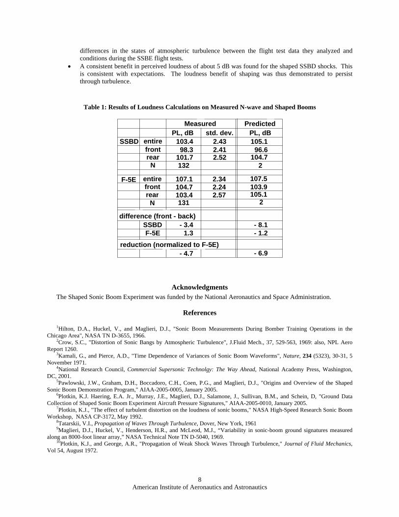
The F-5E N-waves were found to be not completely symmetric. The loudness benefit of the shaped SSBD bow shocks was therefore computed by comparing the differences between the SSBD bow and tail shock loudnesses with the differences between the F-5E bow and tail shock loudnesses.

Table 1 shows the results of the loudness calculations. The "Measured" columns show the individual shock loudnesses (shaped boom bow and tail, F-5E bow and tail) averaged over 132 SSBD and 131 F-5E booms. The "Predicted" column shows the loudness calculated for a theoretical boom prepared prior to the flight test. The shock structure in the predicted boom was a simple Taylor structure, which has more high frequency content than a corresponding true relaxation-driven shock structure.

The loudness result - a net loudness reduction of almost 5 dB - supports the expectation that shaped boom loudness reductions would persist through turbulence.

VI. Conclusions Data from the back-to-back SSBE flights, which consisted of the SSBD and a stock F-5E flown half a minute to

a minute apart, has been used to evaluate Crow's theory for the distortion of sonic booms by turbulence,2 and the expectation that the average benefit of a shaped sonic boom would not be adversely affected by turbulent distortion.7 The following results were obtained:

• The expectation of frozen turbulence was confirmed by subtraction of rear-shock distortions from N-wave front-shock distortions. This had been previously exploited to clean up SSBD front-shock data.

• The spiky fine structure following each shock was found to agree very well with Crow's theory. A value of tc of about 0.2 was obtained. This is smaller than the value of 0.7 originally predicted by Crow, and the value of 1.0 obtained by Kamali and Pierce in a similar earlier analysis. The difference between the current value of tc and that obtained by Kamali and Pierce is considered to be due to


7

differences in the states of atmospheric turbulence between the flight test data they analyzed and conditions during the SSBE flight tests.

• A consistent benefit in perceived loudness of about 5 dB was found for the shaped SSBD shocks. This is consistent with expectations. The loudness benefit of shaping was thus demonstrated to persist through turbulence.

Table 1: Results of Loudness Calculations on Measured N-wave and Shaped Booms

PL, dB std. dev. PL, dBMeasured Predicted

103.498.3

101.7132

2.432.412.52

entire

rear N

frontSSBD 105.1

96.6104.7

2

107.1104.7103.4131

2.242.34

2.57

F-5E entirefrontrear

N

107.5103.9105.1

2

1.3- 3.4SSBD

F-5E - 1.2- 8.1

- 4.7 - 6.9reduction (normalized to F-5E)

difference (front - back)

Acknowledgments The Shaped Sonic Boom Experiment was funded by the National Aeronautics and Space Administration.

References 1Hilton, D.A., Huckel, V., and Maglieri, D.J., "Sonic Boom Measurements During Bomber Training Operations in the

Chicago Area", NASA TN D-3655, 1966. 2Crow, S.C., "Distortion of Sonic Bangs by Atmospheric Turbulence", J.Fluid Mech., 37, 529-563, 1969: also, NPL Aero

Report 1260. 3Kamali, G., and Pierce, A.D., "Time Dependence of Variances of Sonic Boom Waveforms", Nature, 234 (5323), 30-31, 5

November 1971. 4National Research Council, Commercial Supersonic Technolgy: The Way Ahead, National Academy Press, Washington,

DC, 2001. 5Pawlowski, J.W., Graham, D.H., Boccadoro, C.H., Coen, P.G., and Maglieri, D.J., "Origins and Overview of the Shaped

Sonic Boom Demonstration Program," AIAA-2005-0005, January 2005. 6Plotkin, K.J. Haering, E.A. Jr., Murray, J.E., Maglieri, D.J., Salamone, J., Sullivan, B.M., and Schein, D, "Ground Data

Collection of Shaped Sonic Boom Experiment Aircraft Pressure Signatures," AIAA-2005-0010, January 2005. 7Plotkin, K.J., "The effect of turbulent distortion on the loudness of sonic booms," NASA High-Speed Research Sonic Boom

Workshop, NASA CP-3172, May 1992. 8Tatarskii, V.I., Propagation of Waves Through Turbulence, Dover, New York, 1961 9Maglieri, D.J., Huckel, V., Henderson, H.R., and McLeod, M.J., “Variability in sonic-boom ground signatures measured

along an 8000-foot linear array,” NASA Technical Note TN D-5040, 1969. 10Plotkin, K.J., and George, A.R., "Propagation of Weak Shock Waves Through Turbulence," Journal of Fluid Mechanics,

Vol 54, August 1972.


8

11Sullivan, Brenda M.; and Leatherwood, Jack D. "Experimental Studies of Loudness and Annoyance Response to Sonic Booms," in High-Speed Research Sonic Boom (Volume I), the Proceedings of the NASA High Speed Research Sonic Boom Workshop, NASA Conference Publication 10132, May 1993.

12Shepherd, Kevin P.; and Sullivan, Brenda M.: "A Loudness Calculation Procedure applied to Shaped Sonic Booms," NASA TP-3134, Nov. 1991.


9

Documents

Measured Effects of Turbulence on the Loudness and ... · Measured Effects of Turbulence on the Loudness and Waveforms of Conventional and ... together with a reference unmodified