Embed Size (px)
Citation preview


PaulR. Halmos
Measure Theory
Springer-VerlagNewYork-Heidelberg-Berlin

Managing Editors
P. R. Halmos C. C. Moore
Indiana University University of California Department of Mathematics at Berkeley Swain Hall East Department of Mathematics Bloomington, Indiana 47401 Berkeley, California 94720
AMS Subject Classifications (1970) Primary: 28 - 02, 28A10, 28A15, 28A20, 28A25, 28A30, 28A35, 28A40,
28A60, 28A65, 28A70 Secondary: 60A05, 60Bxx
Library of Congress Cataloging in Publication Data
Halmos, Paul Richard, 1914-Measure theory.
(Graduate texts in mathematics, 18) Reprint of the ed. published by Van Nostrand,
New York, in series: The University series in higher mathematics.
Bibliography: p. 1. Measure theory. I. Title. II. Series.
[QA312.H26 1974] 515'.42 74-10690 ISBN 0-387-90088-8
All rights reserved.
No part of this book may be translated or reproduced in any form without written permission from Springer-Verlag.
© 1950 by Litton Educational Publishing, Inc. and 1974 by Springer-Verlag New York Inc.
Printed in the United States of America.
ISBN 0-387-90088-8 Springer-Verlag New York Heidelberg Berlin ISBN 3-540-90088-8 Springer-Verlag Berlin Heidelberg New York


PREFACE
My main purpose in this book is to present a unified treatment of that part of measure theory which in recent years has shown itself to be most useful for its applications in modern analysis. If I have accomplished my purpose, then the book should be found usable both as a text for students and as a source of reference for the more advanced mathematician.
I have tried to keep to a minimum the amount of new and unusual terminology and notation. In the few places where my nomenclature differs from that in the existing literature of measure theory, I was motivated by an attempt to harmonize with the usage of other parts of mathematics. There are, for instance, sound algebraic reasons for using the terms "lattice" and "ring" for certain classes of sets—reasons which are more cogent than the similarities that caused Hausdorff to use "ring" and "field."
The only necessary prerequisite for an intelligent reading of the first seven chapters of this book is what is known in the United States as undergraduate algebra and analysis. For the convenience of the reader, § 0 is devoted to a detailed listing of exactly what knowledge is assumed in the various chapters. The beginner should be warned that some of the words and symbols in the latter part of § 0 are defined only later, in the first seven chapters of the text, and that, accordingly, he should not be discouraged if, on first reading of § 0, he finds that he does not have the prerequisites for reading the prerequisites.
At the end of almost every section there is a set of exercises which appear sometimes as questions but more usually as assertions that the reader is invited to prove. These exercises should be viewed as corollaries to and sidelights on the results more

VI PREFACE
formally expounded. They constitute an integral part of the book; among them appear not only most of the examples and counter examples necessary for understanding the theory, but also definitions of new concepts and, occasionally, entire theories that not long ago were still subjects of research.
It might appear inconsistent that, in the text, many elementary notions are treated in great detail, while, in the exercises,some quite refined and profound matters (topological spaces, transfinite numbers, Banach spaces, etc.) are assumed to be known. The material is arranged, however, so that when a beginning student comes to an exercise which uses terms not defined in this book he may simply omit it without loss of continuity. The more advanced reader, on the other hand, might be pleased at the interplay between measure theory and other parts of mathematics which it is the purpose of such exercises to exhibit.
The symbol | is used throughout the entire book in place of such phrases as "Q.E.D." or "This completes the proof of the theorem" to signal the end of a proof.
At the end of the book there is a short list of references and a bibliography. I make no claims of completeness for these lists. Their purpose is sometimes to mention background reading, rarely (in cases where the history of the subject is not too well known) to give credit for original discoveries, and most often to indicate directions for further study.
A symbol such as u.v> where u is an integer and v is an integer or a letter of the alphabet, refers to the (unique) theorem, formula, or exercise in section u which bears the label v.

A C K N O W L E D G M E N T S
Most of the work on this book was done in the academic year 1947-1948 while I was a fellow of the John Simon Guggenheim Memorial Foundation, in residence at the Institute for Advanced Study, on leave from the University of Chicago.
I am very much indebted to D. Blackwell, J. L. Doob, W. H. Gottschalk, L. Nachbin, B. J. Pettis, and, especially, to J. C. Oxtoby for their critical reading of the manuscript and their many valuable suggestions for improvements.
The result of 3.13 was communicated to me by E. Bishop. The condition in 31.10 was suggested by J. C Oxtoby. The example 52.10 was discovered by J. Dieudonne.
P. R. H.
V l l


CONTENTS
PAGE
Preface v Acknowledgments vii
SECTION
0. Prerequisites 1
CHAPTER I : SETS AND CLASSES
1. Set inclusion 9 2. Unions and intersections 11 3. Limits, complements, and differences 16 4. Rings and algebras 19 5. Generated rings and a-rings 22 6. Monotone classes 26
CHAPTER I I : MEASURES AND OUTER MEASURES
7. Measure on rings 30 8. Measure on intervals 32 9. Properties of measures 37
10. Outer measures 41 11. Measurable sets 44
CHAPTER l i l t EXTENSION OK MEASURES
12. Properties of induced measures 49 13. Extension, completion, and approximation 54 14. Inner measures 58 15 Lebesgue measure 62 16. Non measurable sets 67
CHAPTER IV: MEASURABLE FUNCTIONS
17. Measure spaces 73 18. Measurable functions 76
ix

3t CONTENTS
SECnOtf PAGE
19. Combinations of measurable functions 80 20. Sequences of measurable functions 84 21. Pointwise convergence 86 22. Convergence in measure 90
CHAPTER V: INTEGRATION
23. Integrable simple functions 95 24. Sequences of integrable simple functions 98 25. Integrable functions 102 26. Sequences of integrable functions 107 27. Properties of integrals 112
CHAPTER VI! GENERAL SET FUNCTIONS
28. Signed measures 117 29. Hahn and Jordan decompositions 120 30. Absolute continuity 124 31. The Radon-Nikodym theorem 128 32. Derivatives of signed measures 132
CHAPTER VII: PRODUCT SPACES
33. Cartesian products 137 34. Sections 141 35. Product measures 143 36. Fubini's theorem 145 37. Finite dimensional product spaces 150 38. Infinite dimensional product spaces 154
CHAPTER VIII: TRANSFORMATIONS AND FUNCTIONS
39. Measurable transformations 161 40. Measure rings 165 41. The isomorphism theorem 171 42. Function spaces 174 43. Set functions and point functions 178
CHAPTER IX: PROBABILITY
44. Heuristic introduction 184 45. Independence 191 46. Series of independent functions 196

m m CONTENTS xi
SECTION PAGE
47. The law of large numbers 201 48. Conditional probabilities and expectations 206 49. Measures on product spaces 211
CHAPTER X : LOCALLY COMPACT SPACES
50. Topological lemmas 216 51. Borel sets and Baire sets 219 52. Regular measures 223 53. Generation of Borel measures 231 54. Regular contents 237 55. Classes of continuous functions 240 56. Linear functional 243
CHAPTER XI: HAAR MEASURE
57. Full subgroups 250 58. Existence 251 59. Measurable groups 257 60. Uniqueness 262
CHAPTER XII : MEASURE AND TOPOLOGY IN GROUPS
61. Topology in terms of measure 266 62. Weil topology 270 63. Quotient groups 277 64. The regularity of Haar measure 282
References 291
Bibliography 293
List of frequently used symbols 297
Index 299


§ 0. PREREQUISITES
The only prerequisite for reading and understanding the first seven chapters of this book is a knowledge of elementary algebra and analysis. Specifically it is assumed that the reader is familiar with the concepts and results listed in (l)-(7) below.
(1) Mathematical induction, commutativity and associativity of algebraic operations, linear combinations, equivalence relations and decompositions into equivalence classes.
(2) Countable sets; the union of countably many countable sets is countable.
(3) Real numbers, elementary metric and topological properties of the real line (e.g. the rational numbers are dense, every open set is a countable union of disjoint open intervals), the Heine-Borel theorem.
(4) The general concept of a function and, in particular, of a sequence (i.e. a function whose domain of definition is the set of positive integers); sums, products, constant multiples, and absolute values of functions.
(5) Least upper and greatest lower bounds (called suprema and infima) of sets of real numbers and real valued functions; limits, superior limits, and inferior limits of sequences of real numbers and real valued functions.
(6) The symbols +°o and — °o, and the following algebraic relations among them and real numbers x:
(zfcoo) + (=fcoo) = x + (zfcoo) = (=fcoo) + X = zfcoo;
I" zfcoo i f # > 0 ,
*(=fc°o) - (zfcoo)* = 0 if x = 0,
L=Foo i f # < 0 ; (=boo)(d=oo) = + o o ,
(zfcoo) ( T o o ) = —oo;
*/(±oo) = 0; — 00 < X < -f-CO.
1

2 PREREQUISITES [SEC. 01
The phrase extended real number refers to a real number or one of the symbols zhoo.
(7) If AT and^y are real numbers,
x U y = max {xyy\ = \{x + y + | x - y |),
AT PI ^ = min {#,j>} = \{x + y - | x - jy |).
Similarly, if/ and £ are real valued functions, t h e n / U £ and / fl g are the functions defined by
( / U g)(x) = / (* ) U *(*) and ( / n *)(*) = /(*) n g(x),
respectively. The supremum and infimum of a sequence {xn\ of real numbers are denoted by
Un- i*n and flr-i^n,
respectively. In this notation
l i m SUp n Xn = H n - l U m - » *m
and Hminfn.X'n = U " = l (Xn-nXm.
In Chapter VIII the concept of metric space is used, together with such related concepts as completeness and separability for metric spaces, and uniform continuity of functions on metric spaces. In Chapter VIII use is made also of such slightly more sophisticated concepts of real analysis as one-sided continuity.
In the last section of Chapter IX, TychonofTs theorem on the compactness of product spaces is needed (for countably many factors each of which is an interval).
In general, each chapter makes free use of all preceding chapters; the only major exception to this is that Chapter IX is not needed for the last three chapters.
In Chapters X, XI, and XII systematic use is made of many of the concepts and results of point set topology and the elements of topological group theory. We append below a list of all the relevant definitions and theorems. The purpose of this list is not to serve as a text on topology, but (a) to tell the expert exactly

[SEC. 0] PREREQUISITES 3
which forms of the relevant concepts and results we need, (b) to tell the beginner with exactly which concepts and results he should familiarize himself before studying the last three chapters, (c) to put on record certain, not universally used, terminological conventions, and (d) to serve as an easily available reference for things which the reader may wish to recall.
Topological Spaces
A topological space is a set X and a class of subsets of Xy called the open sets of Xy such that the class contains 0 and X and is closed under the formation of finite intersections and arbitrary (i.e. not necessarily finite or countable) unions. A subset E of X is called a G* if there exists a sequence {Un) of open sets such that E = H^-i Un. The class of all G/s is closed under the formation of finite unions and countable intersections. The topological space X is discrete if every subset of X is open, or, equiva-lently, if every one-point subset of X is open. A set E is closed if X — E is open. The class of closed sets contains 0 and X and is closed under the formation of finite unions and arbitrary intersections. The interior, E°y of a subset E of X is the greatest open set contained in E; the closure, Ey of E is the least closed set containing E. Interiors are open sets and closures are closed sets; if E is open, then E° — Ey and, if E is closed, then E = E. The closure of a set E is the set of all points x such that, for every open set U containing xy E f) U -£ 0. A set £ is dense in Xif E = X. A subset Y of a topological space becomes a topological space (a subspace of X) in the relative topology if exactly those subsets of Y are called open which may be obtained by intersecting an open subset of X with Y. A neighborhood of a point AT in X [or of a subset E of X] is an open set containing x [or an open set containing E\. A base is a class B of open sets such that, for every x in X and every neighborhood U of xy there exists a set B in B such that x e B c U. The topology of the real line is determined by the requirement that the class of all open intervals be a base. A subbase is a class of sets, the class of all finite intersections of which is a base. A space X is separable if it has a countable base. A subspace of a separable space is separable.
4 PREREQUISITES [SEC. 0]
An open covering of a subset £ of a topological space X is a class K of open sets such that E c \JK. If X is separable and K is an open covering of a subset E of Xy then there exists a countable subclass {KXy K2y • • •} of K which is an open covering of E. A set E in X is compact if, for every open covering K of Ey
there exists a finite subclass {K\y • • *, #„} of K which is an open covering of E. A class K of sets has the finite intersection property if every finite subclass of K has a non empty intersection. A space X is compact if and only if every class of closed sets with the finite intersection property has a non empty intersection. A set £ in a space X is or-compact if there exists a sequence {Cn\ of compact sets such that E = U*-i Cn. A space X is locally compact if every point of X has a neighborhood whose closure is compact. A subset £ of a locally compact space is bounded if there exists a compact set C such that E a C. The class of all bounded open sets in a locally compact space is a base. A closed subset of a bounded set is compact. A subset £ of a locally compact space is <r-bounded if there exists a sequence {Cn} of compact sets such that E c JJn-i Cn. To any locally compact but not compact topological space X there corresponds a compact space X* containing X and exactly one additional point #*; X* is called the one-point compactification of X by x*. The open sets of X* are the open subsets of X and the complements (in X*) of the closed compact subsets of X.
If [Xi\ i el} is a class of topological spaces, their Cartesian product is the set X = X l^» : * e ^ l °f a ^ functions x defined on / and such that, for each * in / , x(i) e X* For a fixed i0 in / , let E^be an open subset of Xioy and, for i ?* i0y write £* = Xry
the cmmof open sets in X is determined by the requirement that the class of all sets of the form X {£*'• * e ^ } ^ e a subbase. If the function & on X is defined by £>(#) = #(*), then & is continuous. The Cartesian product of any class of compact spaces is compact.
A topological space is a Hausdorff space if every pair of distinct points have disjoint neighborhoods. Two disjoint compact sets in a Hausdorff space have disjoint neighborhoods. A compact subset of a Hausdorff space is closed. If a locally compact space

[Sic. 0] PREREQUISITES 5
is a Hausdorff space or a separable space, then so is its one-point compactification. A real valued continuous function on a compact set is bounded.
For any topological space X we denote by $ (or $(X)) the class of all real valued continuous functions/ such that 0 ^f(x) g 1 for all ^ in X A Hausdorff space is completely regular if, for every pointy in X and every closed set F not containing^, there is a function/ in £ such that/(jy) = 0 and, for x in Fyf{x) = 1. A locally compact Hausdorff space is completely regular.
A metric space is a set X and a real valued function d (called distance) o n l X l , such thatd{xyy) ^ 0, d(xyy) = 0 if and only if x = yy d(xyy) = d(yyx)y and d{xyy) g d(xyz) + d(zyy). If £ and F are non empty subsets of a metric space Xy the distance between them is defined to be the number d{EyF) = inf {d{xyy)\ x e Ey
y eF}. If F = {x0} is a one-point set, we write d(Eyx0) in place of d(Ey{x0}). A sphere (with center x0 and radius r0) is a subset £ of a metric space X such that, for some point x0 and some positive number r0, E = {x: d(x0yx) < r 0}. The topology of a metric space is determined by the requirement that the class of all spheres be a base. A metric space is completely regular. A closed set in a metric space is a G«. A metric space is separable if and only if it contains a countable dense set. If £ is a subset of a metric space and /(#) = d{Eyx)y then / is a continuous function and E = {#:/(#) = 0 } . If X is the real line, or the Cartesian product of a finite number of real lines, then X i s a locally compact separable Hausdorff space; it is even a metric space if for x = (xly • • •, xn) and y = (yiy • • •, yn) the distance d(xyy) is defined to be (Z)?-i (*» ~" yd2)H- A closed interval in the real line is a,compact set. -^}
A transformation Tfrom a topological space X into a topological space Y is continuous if the inverse image of every open set is open, or, equivalently, if the inverse image of every closed set is closed. The transformation T is open if the image of every open set is open. If B is a subbase in Yy then a necessary and sufficient condition that T be continuous is that T^1(B) be open for every B in B. If a continuous transformation T maps X onto Yy and if X is compact, then Y is compact. A homeomorphism is a one

6 PREREQUISITES [SEC. 0)
to one, continuous transformation of X onto Y whose inverse is also continuous.
The sum of a uniformly convergent series of real valued, continuous functions is continuous. If/ and g are real valued continuous functions, t hen / U g a n d / 0 g are continuous.
Topological Groups
A group is a non empty set X of elements for which an associative multiplication is defined so that, for any two elements a and b of X, the equations ax = b and ya = b are solvable. In every group X there is a unique identity element ey characterized by the fact that ex = xe = x for every x in X. Each element # of X has a unique inverse, tf-1, characterized by the fact that xx~l = x~lx = e. A non empty subset Y of \f is a subgroup if # - \y c y whenever # and j are in Y. If £ is any subset of a group Xy E~l is the set of all elements of the form x~l
y where x e E; if E and F are any two subsets of X, £ F is the set of all elements of the form xy> where x e E and y e F. A non empty subset Y of Jf is a subgroup if and only if y _ 1 Y (Z Y. If # e J!f, it is customary to write xE and £# in place of {x)E and £{#} respectively; the set xE [or Ex] is called a left translation [or right translation] of E. If Y is a subgroup of X, the sets xY and Y* are called (left and right) cosets of Y. A subgroup Y of X is invariant if #Y = Yx for every # in X. If the product of two cosets Yt and Y2 of an invariant subgroup Y is defined to be YiY2> then, with respect to this notion of multiplication, the class of all cosets is a group J?, called the quotient group of X modulo Y and denoted by X/Y. The identity element e of X is Y. If Y is an invariant subgroup of X> and if for every x in X, ir(x) is the coset of Y which contains #, then the transformation 7r is called the projection from X onto X A homomorphism is a transformation T from a group X into a group Y such that T(^y) = T(x)T(y) for every two elements x and jy of X. The projection from a group X onto a quotient group X is a homomorphism.
A topological group is a group X which is a Hausdorflf space such that the transformation (from X X X onto X) which sends

(SEC. 0] PREREQUISITES 7
(xy) into x~ly is continuous. A class N of open sets containing e in a topological group is a base at e if (a) for every x different from e there exists a set £7 in N such that x e' U> (b) for any two sets U and f in N there exists a set W in N such that IV a U V\ V, (c) for any set 1/ in N there exists a set V in N such that V~~lV c £/, (d) for any set U in N and any element x in X, there exists a set V in N such that V c xlfx"1, and (e) for any set £/ in N and any element # in U there exists a set V in N such that Vx c £7. The class of all neighborhoods of e is a base at e\ conversely if, in any group X, N is a class of sets satisfying the conditions described above, and if the class of all translations of sets of N is taken for a base, then, with respect to the topology so defined, X becomes a topological group. A neighborhood V of e is symmetric if V = V"1; the class of all symmetric neighborhoods of e is a base at e. If N is a base at e and if F is any closed set in Xy then F = f| [UF: U eN} .
The closure of a subgroup [or of an invariant subgroup] of a topological group X is a subgroup [or an invariant subgroup] of X. If Y is a closed invariant subgroup of X, and if a subset of J? = X/Y is called open if and only if its inverse image (under the projection w) is open in X, then X is a topological group and the transformation ir from X onto J? is open and continuous.
If C is a compact set and £7 is an open set in a topological group X, and if C C £/, then there exists a neighborhood V o{ e such that ^C^7 c £/. If C and D are two disjoint compact sets, then there exists a neighborhood U of e such that £/C(7 and UDU are disjoint. If C and D are any two compact sets, then C"1
and CD are also compact. A subset £ of a topological group X is bounded if, for every
neighborhood U of e, there exists a finite set {#i, • • •, xn\ (which, in case E ^ 0, may be assumed to be a subset of E) such that E c U?-i x*Um9 tf *s locally compact, then this definition of boundedness agrees with the one applicable in any locally compact space (i.e. the one which requires that the closure of E be compact). If a continuous, real valued function/ on X is such that the set N(J) = {x:/{x) ^ 0} is bounded, then / is uniformly continuous in the sense that to every positive number e there

8 PREREQUISITES . [SEC. 0]
corresponds a neighborhood U of e such that |/(#i) — ffa) \ < « whenever x1x2"
1 e U. A topological group is locally bounded if there exists in it a
bounded neighborhood of e. To every locally bounded topological group Xy there corresponds a locally compact topological group X*y called the completion of X (uniquely determined to within an isomorphism), such that X is a dense subgroup of X*. Every closed subgroup and every quotient group of a locally compact group is a locally compact group.

Chapter 1
SETS A N D CLASSES
§ 1. SET INCLUSION
Throughout this book, whenever the word set is used, it will be interpreted to mean a subset of a given set, which, unless it is assigned a different symbol in a special context, will be denoted by X. The elements of X will be called points; the set X will be referred to as the space, or the whole or entire space, under consideration. The purpose of this introductory chapter is to define the basic concepts of the theory of sets, and to state the principal results which will be used constantly in what follows.
If x is a point of X and £ is a subset of X> the notation
x eE
means that x belongs to E (i.e. that one of the points of E is x); the negation of this assertion, i.e. the statement that x does not belong to E> will be denoted by
xe'E.
Thus, for example, for every point x of Xy we have
x tX,
and for no point x of X do we have
xz' X.
If E and F are subsets of X> the notation
EczF or Fz>E 9

10 SETS AND CLASSES [SEC. 1]
means that E is a subset of F> i.e. that every point of E belongs to F. In particular therefore
EaE
for every set E, Two sets E and F are called equal if and only if they contain exactly the same points, or, equivalently, if and only if
EczF and F c £
This seemingly innocuous definition has as a consequence the important principle that the only way to prove that two sets are equal is to show, in two steps, that every point of either set belongs also to the other.
It makes for tremendous simplification in language and notation to admit into the class of sets a set containing no points, which we shall call the empty set and denote by 0. For every set E we have
O c £ c Z ;
for every point x we have
* e ' 0 .
In addition to sets of points we shall have frequent occasion to consider also sets of sets. If, for instance, X is the real line, then an interval is a set, i.e. a subset of X, but the set of all intervals is a set of sets. To help keep the notions clear, we shall always use the word class for a set of sets. The same notations and terminology will be used for classes as for sets. Thus, for instance, if E is a set and E is a class of sets, then
means that the set E belongs to (is a member of, is an element of) the class E; if E and F are classes, then
E c F
means that every set of E belongs also to F, i.e. that E is a subclass of F.
On very rare occasions we shall also have to consider sets of classes, for which we shall always use the word collection. If,

SEC. 2] SETS AND CLASSES 11
for instance, X is the Euclidean plane and E„ is the class of all intervals on the horizontal line at distance y from the origin, then each E„ is a class and the set of all these classes is a collection.
(1) The relation C between sets is always reflexive and transitive; it is symmetric if and only if X is empty.
(2) Let X be the class of all subsets of X, including of course the empty set 0 and the whole space X; let x be a point of X, let £ be a subset of X (i.e. a member of X), and let E be a class of subsets of X (i.e. a subclass of X). If u and v vary independently over the five symbols xy E> X> E, X, then some of the fifty relations of the forms
uev or u CI v
are necessarily true, some are possibly true, some are necessarily false, and some are meaningless. In particular u e v is meaningless unless the right term is a subset of a space of which the left term is a point, and u C v is meaningless unless u and v are both subsets of the same space.
§ 2 . UNIONS AND INTERSECTIONS
If E is any class of subsets of Xy the set of all those points of X which belong to at least one set of the class E is called the union of the sets of E; it will be denoted by
U E or U ( £ : £ e E ) . The last written symbol is an application of an important and
frequently used principle of notation. If we are given any set of objects denoted by the generic symbol xy and if, for each xy ir{x) is a proposition concerning xy then the symbol
denotes the set of those points x for which the proposition ir(x) is true. If {7r»(#)} is a sequence of propositions concerning xy
the symbol { * : T I ( * ) , * 2 ( * ) , • ••}
denotes the set of those points x for which irn(x) is true for every n = 1, 2, • • •. If, more generally, to every element 7 of a certain index set T there corresponds a proposition iry(x) concerning xy
then we shall denote the set of all those points x for which the proposition icy(x) is true for every 7 in T by
{xnry(x)y 7 el 1}.

12 SETS AND CLASSES [SEC. 2)
Thus, for instance, {x: x cE] = E
and {E:EeE} = E.
For more illuminating examples we consider the sets
{/:0 £ / £ 1}
( = the closed unit interval),
(= the circumference of the unit circle in the plane), and
{»2:« = 1,2, •••}
(= the set of those positive integers which are squares). In accordance with this notation, the upper and lower bounds (supre-mum and infimum) of a set E of real numbers are denoted by
sup[x:xeE} and inf {x: x e E}
respectively. In general the brace {• • •} notation will be reserved for the
formation of sets. Thus, for instance, if x and y are points, then {xyy} denotes the set whose only elements are x and y. It is important logically to distinguish between the point x and the set \x\ whose only element is xy and similarly to distinguish between the set E and the class {E} whose only element is E. The empty set 0, for example, contains no points, but the class {0} contains exactly one set, namely the empty set.
For the union of special classes of sets various special notations are used. If, for instance,
E - {Eu E2) then
( J E = U {Et'.i = 1, 2} is denoted by
Ex U £ 2 ; if, more generally,
£ = { £ „ • • - , £ „ }

[SEC. 2] SETS AND CLASSES 13
is a finite class of sets, then
is denoted by E, U • • • U En or U?-i £*•
If, similarly, {En} is an infinite sequence of sets, then the union of the terms of this sequence is denoted by
£ , U £ , U - or U r - i f t .
More generally, if to every element 7 of a certain index set V there corresponds a set Eyy then the union of the class of sets
is denoted by \}yzTEy Or \Jy Ey.
If the index set r is empty, we shall make the convention that
U? £7 - 0 .
The relations of the empty set 0 and the whole space X to the formation of unions are given by the identities
£ U 0 = £ and E U X - X.
More generally it is true that
EdF if and only if
£ U F = K
If E is any class of subsets of Xy the set of all those points of X which belong to every set of the class E is called the intersection of the sets of E; it will be denoted by
f | E or f| {E-.EeE}.
Symbols similar to those used for unions are used, but with the symbol U replaced by fl, for the intersections of two sets, of a finite or countably infinite sequence of sets, or of the terms of any indexed class of sets. If the index set T is empty, we shall make the somewhat startling convention that
C\y*rEy = X.

14 SETS AND CLASSES [SEC. 2J
There are several heuristic motivations for this convention. One of them is that if Ti and T2 are two (non empty) index sets for which Tx c T2, then clearly
and that therefore to the smallest possible r , i.e. the empty one, we should make correspond the largest possible intersection. Another motivation is the identity
I I7 c Vi u r2 &y == I 17 e Ti &y » ' I I7 e r2 ^yy
valid for all non empty index sets I \ and T2. If we insist that this identity remain valid for arbitrary I \ and r2 , then we are committed to believing that, for every T,
f l 7 e r ^ Y = llycruQ&y = WytT&y H \\yzQ&y\
writing Ey = X for every 7 in T, we conclude that
Union and intersection are sometimes called join and meet, respectively. As a mnemonic device for distinguishing between U and fl (which, by the way, are usually read as cup and cap, respectively), it may be remarked that the symbol U is similar to the initial letter of the word "union" and the symbol D is similar to the initial letter of the word "meet."
The relations of 0 and X to the formation of intersections are given by the identities
£ 0 0 = 0 and E Vi X = E.
More generally it is true that
EaF it and only if
EViF= E.
Two sets E and F are called disjoint if they have no points in common, i.e. if
EViF^O.

[SEC. 21 SETS AND CLASSES 15
A disjoint class is a class E of sets such that every two distinct sets of E are disjoint; in this case we shall refer to the union of the sets of E as a disjoint union.
We conclude this section with the introduction of the useful concept of characteristic function. If £ is any subset of X, the function XE> defined for all x in X by the relations
fl if xeEy
10 if x e' Ej
is called the characteristic function of the set £ . The correspondence between sets and their characteristic functions is one to one, and all properties of sets and set operations may be expressed by means of characteristic functions. As one more relevant illustration of the brace notation, we mention
E = {*:»(*) = 1}.
(1) The formation of unions is commutative and associative, i.e.
E U F - F U E and E U (F U G) = (E U F) U G;
the same is true for the formation of intersections. (2) Each of the two operations, the formation of unions and the formation
of intersections, is distributive with respect to the other, i.e.
E n (F u G) - (E n F) u (E n o and
E U (F fl G) = (F U F) fl (F U G).
More generally the following extended distributive laws are valid:
Ffl (J {F:FeE} - (J \E fl F:FeE} and
F U fl {EiEeE} - fl { £ U F:FeE} .
(3) Does the class of all subsets of AT form a group with respect to either of the operations U and fl ?
(4) XoM = 0, xxM s 1- The relation
XBM ^ X F M
is valid for all x in X if and only if F C F. If E fl F - A and F U F « 5 , then
XA * X^X* = X£ (1 XF and XB = XB + X* - XA = X* U x*.
(5) Do the identities in (4), expressing XA and XB in terms of XB and XF, have generalizations to finite, countably infinite^ and arbitrary unions and intersections?

16 SETS AND CLASSES [SEC 3]
§ 3 . LIMITS, COMPLEMENTS, AND DIFFERENCES
If \En} is a sequence of subsets of Xy the set E* of all those points of X which belong to En for infinitely many values of n is called the superior limit of the sequence and is denoted by
£* = lim supn En.
The set £* of all those points of X which belong to En for all but a finite number of values of n is called the inferior limit of the sequence and is denoted by
£* = lim infn En.
If it so happens that £* - £*,
we shall use the notation
linin En
for this set. If the sequence is such that
En c £ n + i , for n * 1, 2, • • ,
it is called increasing; if
En 3 £n+i, for n = 1, 2, •••,
it is called decreasing. Both increasing and decreasing sequences will be referred to as monotone. It is easy to verify that if {En\ is a monotone sequence, then limn En exists and is equal to
Uȣn Or ClnEn
according as the sequence is increasing or decreasing. The complement of a subset E of X is the set of all those
points of X which do not belong to E; it will be denoted by E'. The operation of forming complements satisfies the following algebraic identities:
£ PI £ ' = 0, E U E - Xy
0' - X , (E')' = E, Z ' = 0, and
if £ c F , then E z> F.

[Sic. 31 SETS AND CLASSES 17
The formation of complements also bears an interesting and very important relation to unions and intersections, expressed by the identities
0 J { £ : £ e E } ) ' - fl {E':EeE}y
(fl {E: E eE})' = U {E':EeE\.
In words: the complement of the union of a class of sets is the intersection of their complements, and the complement of their intersection is the union of their complements. This fact, together with the elementary formulas relating to complements, proves the important principle of duality:
any valid identity among sets, obtained by forming unions, intersections, and complements, remains valid if in it the symbols
PI, C, and 0
are interchanged with
U, =3, and X
respectively (and equality and complementation are left unchanged).
If E and F are subsets of X, the difference between E and Fy
in symbols £ - F ,
is the set of all those points of E which do not belong to F. Since
X - F= F', and, more generally,
E - F = E fl F',
the difference E — F is frequently called the relative complement of F in E. The operation of forming differences, similarly to the operation of forming complements, interchanges \J with H a n d C with 3 , so that, for instance,
£ - ( F U G ) = ( £ ~ f ) n ( £ ~ 6 ) .
The difference E — F is called proper if E 3 F.

18 SETS AND CLASSES [SEC. 3]
As the final and frequently very important operation on sets we introduce the symmetric difference of two sets E and F, denoted by
£ A F , and defined by
£ 4 F = ( £ - F ) U ( F - £ ) = ( £ n F) U (£ ' n F).
The formation of limits, complements, and differences of sets requires a bit of practice for ease in manipulation. The reader is accordingly advised to carry through the proofs of the most important properties of these processes, listed in the exercises that follow.
(1) Another heuristic motivation of the convention
\\y CO Ey = X
is the desire to have the identity
C\y e r Ey =* ( U T C r F7 ' ) ' ,
which is valid for all non empty index sets T, remain valid for T •= 0. (2) If F* = lim infn F» and E* = lim sup„ F„, then
F* = U n - l f | m - o Em CZ | | n - . l \jm~n Em = F*.
(3) The superior limit, inferior limit, and limit (if it exists) of a sequence of sets are unaltered if a finite number of the terms of the sequence are changed.
(4) If En = A or B according as n is even or odd, then
lim inf„ En = A d B and lim supn En = A U B.
(5) If {En\ is a disjoint sequence, then
limn En = 0.
(6) If £* = lim infn En and F* = lim supn En> then
(£*) ' - lim sup„ En' and (F*)' = lim infn En'.
More generally,
F - F* - lim supn (F - En) and F - E* •= lim infn (F - En).
( 7 ) £ - F = £ - ( £ f l R = ( £ U F ) - F ,
E PI (F - G) - (E 0 F) - (F D G), ( £ U F ) - G = ( £ - G ) U ( F - G ) .
(8) (F - G) 0 (F - G) = (F PI F) - G,
( £ - f ) - C - £ - ( F U O , £ - (F - G) - (F - F) U (F fl G),
(F - F) PI (G - H) = (F PI G) - (F U tf).
[SEC. 4] SETS AND CLASSES 19 (9) EAF=FAE9EA(FAG) - (£AF)AG,
E(\ ( F A Q - (EnF)A(EC\G)y
EAO=*E, EAX=E\
£ A £ = 0, EAE' = X,
£ A F = ( £ U F ) - ( £ f l F).
(10) Does the class of all subsets of X form a group with respect to the operation A?
(11) If F* = lim infn En and E* = lim supn £», then
XB*{X) = lim infn XBnW and Xu»(*) •» lim SUpnXswM-
(The expressions on the right sides of these equations refer, of course, to the usual numerical concepts of superior limit and inferior limit.)
(12) Xv « 1 - XR> XB-F = XE(\ - XF)>
XB*F = \XE -XF\=XB + XP (mod 2).
(13) If [En\ is a sequence of sets, write
Di = JBx, D2 - Dx A £2 , D3 = D2 A £3 ,
and, in general,
D„+i = D„ A En+x for » - 1, 2, •••.
The limit of the sequence {D»} exists if and only if limn En ^ 0. If the operation A is thought of as addition (cf. (12)), then this result has the following verbal phrasing: an infinite series of sets converges if and only if its terms approach zero.
§ 4 . RINGS AND ALGEBRAS
A ring (or Boolean ring) of sets is a non empty class R of sets such that if
£ e R and F e R , then
E U F E R and £ - F e R .
In other words a ring is a non empty class of sets which is closed under the formation of unions and differences.
The empty set belongs to every ring R, for if
£ e R , then
0 = £ - £ e R .
20 SETS AND CLASSES [SEC. 4]
Since £ - F = C E U F ) - ^ ,
it follows that a non empty class of sets closed under the formation of unions and proper differences is a ring. Since
£ A F = ( £ - ^ U ( F - £ ) and
EnF-(EUF)-(EAF),
it follows that a ring is closed under the formation of symmetric differences and intersections. An application of mathematical induction and the associative laws for unions and intersections shows that if R is a ring and
Ei; eR, i = 1, • • •, ny
then
U ? - i £ t c R and Cti-iEi**.
Two extreme but useful examples of rings are the class {0} containing the empty set only, and the class of all subsets of X. Another example, for an arbitrary set X9 is the class of all finite sets. A more illuminating example is the following. Let
X = {x: -oo < x < +00}
be the real line, and let R be the class of all finite unions of bounded, left closed, and right open intervals, i.e. the class of all sets of the form
U*n-i (*: -<» <ai£x < b{ < +00}.
Union and intersection are treated unsymmetrically in the definition of rings. While, for instance, it is true that a ring is closed under the formation of intersections, it is not true that a class of sets closed under the formation of intersections and differences is necessarily closed also under the formation of unions. If, however, a non empty class of sets is closed under the formation of intersections, proper differences, and disjoint unions, then it is a ring. (Proof:
£ U F = [ £ - ( £ n F ) ] U [ F - ( £ n f ) ] U ( £ n F).)

[SEC. 4] SETS AND CLASSES 21
It is easily possible to give a definition of rings which is more nearly symmetric in its treatment of union and intersection: a ring may be defined as a non empty class of sets closed under the formation of intersections and symmetric differences. The proof of this statement is in the identities:
E U F = (EAF)A(E PI F) , £ - F = £ A ( £ n ^
If in this form of the definition we replace intersection by union we obtain a true statement: a non empty class of sets closed under the formation of unions and symmetric differences is a ring.
An algebra (or Boolean algebra) of sets is a non empty class R of sets such that
(a) i f £ e R a n d F e R , then £ U F e R , and (b) i f £ e R , then £ ' eR.
Since E - F = E fl F' = (£ ' U F) ' ,
it follows that every algebra is a ring. The relation between the general concept of ring and the more special concept of algebra is simple: an algebra may be characterized as a ring containing X. Since
E' = X - E,
it is clear that every such ring is an algebra; if, conversely, R is an algebra and
£ e R
(we recall that R is non empty), then
X = E U £ ' e R .
(1) The following classes of sets are examples of rings and algebras. (la) X is ^-dimensional Euclidean space; E is the class of all finite unions of
semiclosed "intervals" of the form
{(*i, •'•,*!»): -<» < * • £ Xi <i% < °°, * = 1, • • ' , » } .
(lb) X is an uncountable set; E is the class of all countable subsets of X. (lc) X is an uncountable set; E is the class of all sets which either are count
able or have countable complements. (2) Which topological spaces have the property that the class E of open sets
is a ring?
22 SETS AND CLASSES [SEC. 5)
(3) The intersection of any collection of rings or algebras is again a ring or an algebra, respectively.
(4) If R is a ring of sets and if we define, for E and F in R,
£ O F = £ fl F and £ © F = £ A F ,
then, with respect to the operations of "addition" (©) and "multiplication" (O), the system R is a ring in the algebraic sense of the word. Algebraic rings, such as this one, in which every element is idempotent (i.e. E O E = E for every E in R) are also called Boolean rings. The existence of a very close relation between Boolean rings of sets and Boolean rings in general is the main justification of the ring terminology in the set theoretic case.
(5) If R is a ring of sets and if A is the class of all those sets E for which
either £ e R or else F e R ,
then A is an algebra.
(6) A semiring is a non empty class P of sets such that
(6a) i f £ e P a n d F e P , then £ (1 F e P , and (6b) if F e P a n d F e P a n d E C Fy then there is a finite class {Co, Cu ••-, Cn\
of sets in P such that E = C0 C Cx C • • • C Cn = F and D t = d -Ci_i e P for i = 1, • • - , » .
The empty set belongs to every semiring. If X is any set, then the class P consisting of the empty set and all one-point sets (i.e. sets of the form \x) with x e X) is a semiring. If X is the real line, the class of all bounded, left closed, and right open intervals is a semiring.
§ 5 . GENERATED RINGS AND ff-RINGS
Theorem A. If E is any class of sets, then there exists a unique ring R0 such that R 0 D E and such that if R is any other ring containing E then R0 c R.
The ring R0> the smallest ring containing E, is called the ring generated by E; it will be denoted by R(E).
Proof. Since the class of all subsets of X is a ring, it is clear that at least one ring containing E always exists. Since moreover (cf. 4.3) the intersection of any collection of rings is also a ring, the intersection of all rings containing E is easily seen to be the desired ring R0. |
Theorem B. If E is any class of sets, then every set in R(E) may be covered by a finite union of sets in E.

fSEC. 5] SETS AND CLASSES 23
Proof. The class of all sets which may be covered by a finite union of sets in E is a ring; since this ring contains E, it also contains R(E). |
Theorem C. If E is a countable class of sets> then R(E) is countable.
Proof. For any class C of sets, we write C* for the class of all finite unions of differences of sets of C. It is clear that if C is countable, then so is C*, and if
OeC, then
C c C * .
To prove the theorem we assume, as we may without any loss of generality, that
OeE , and we write
E0 = E, En = E*_x, » = 1,2, ••-.
It is clear that E c U n " . o E n c R ( E ) ,
and that the class Un-oEn
is countable; we shall complete the proof by showing that U"-o E» is a ring. Since
E = EQ C- E I d E2 C • • •,
it follows that if A and B are any two sets in U"-o En , then there exists a positive integer n such that both A and B belong to En, We have
A — B e E n + i , and, since
O e E 0 c E n , it follows also that
A U B = (A -0) \J (B -0) eE n + 1 .

24 SETS AND CLASSES [SEC. 5)
We have proved therefore that both A — B and A U B belong to Un-oE n , i.e. that Un«oE» is indeed closed under the formation of unions and differences. |
A or-ring is a non empty class S of sets such that
(a) if E e S and F e S, then E - F e S, and (b) if £ < e S , i = 1,2, •••, then {J^EizS.
Equivalently a a—ring is a ring closed under the formation of countable unions. If S is a cr-ring and if
Ei e S , i = 1, 2, • • -, and E = U"~i Ei,
then the identity
nr-t £« = £ - ur.i (£ - E^ shows that
i.e. that a o—ring is closed under the formation of countable intersections. It follows also (cf. 3.2) that if S is a cr-ring and
E{ eSy i = 1, 2, • • •,
then both lim inft- Ei and lim sup» £» belong to S. Since the truth and proof of Theorem A remain unaltered if
we replace "ring" by "<7-ring" throughout, we may define the cr-ring S(E) generated by any class E of sets as the smallest <r-ring containing E.
Theorem D. If E is any class of sets and E is any set in S = S(E), then there exists a countable subclass D of E such that E e S(D).
Proof. The union of all those cr-subrings of S which are generated by some countable subclass of E is a <r-ring containing E and contained in S; it is therefore identical with S. |
For every class E of subsets of X and every fixed subset A of Xy we shall denote by
E D A
the class of all sets of the form EDA with E in E.

[SEC. 5] SETS AND CLASSES 25
Theorem E. If E is any class of sets and if A is any subset of Xy then
S(E) fl A = S(E fl A).
Proof. Denote by C the class of all sets of the form B U (C — A)y where
5 e S ( E n ^ ) and C e S ( E ) ;
it is easy to verify that C is a cr-ring. If E e E, then the relation
E - (£ fl A) U (£ - A), together with
E() AeECl A<zS&n A),
shows that £ e C , and therefore that
E c C . It follows that
S(E) c C and therefore that
S(E) 0 A czC n A.
Since, however, it is obvious that
c n ^ = s(EnA it follows that
S(E) fl A aSQZ d A).
The reverse inequality,
S(E Ci A) <z S(E) fl ^ ,
follows from the facts that S(E) fl A is a cr-ring and
E n i c S ( E ) n ^ | (1) For each of the following examples, what is the ring generated by the
class E of sets there described? (la) For a fixed subset E of X> E = {E\ is the class containing E only, (lb) For a fixed subset E of X> E is the class of all sets of which £ is a subset,
i.e.E = | F : £ C F ) . (lc) E is the class of all sets which contain exactly two points. (2) A lattice (of sets) is a class L such that 0 e L and such that if E 8 L and
F e L , then E U F e L and E fl F e L . Let P « P(L) be the class of all sets
26 SETS AND CLASSES [SEC. 6]
of the form F — F, where F e L , F e L , and F CT F; then P is a semiring; (cf.4.6). (Hint: if
Di = Fi - Eiy i - 1, 2
are representations of two sets of P as proper differences of sets of L, and if D\ 3 D2, then for
C - (fi PI F2) - {Ei PI F2),
or, alternatively, for
C - Fi - [£, U (Fx fi F2)],
we have F2 - E2 C C C Fi - Fi.) Is P a ring? (3) Let P be a semiring and let R be the class of all sets of the form (J?» i F,-,
where {Fi, • • •, En\ is an arbitrary finite, disjoint class of sets in P. (3a) R is closed under the formation of finite intersections and disjoint
unions. (3b) I f F e P , F e P , and F C F, then F - F e R . (3c) If F e P , F e R , and F C F, then F - F e R. (3d) If F E R , F e R , and E d F, then F - F e R . (3e) R = R(P). It follows in particular that a semiring which is closed under
the formation of unions is a ring. (4) The fact that the analog of Theorem A for algebras is true may be seen
either by replacing "ring" by "algebra" in its proof or by using 4.5. (5) If P is a semiring and R = R(P), then S(R) = S(P). (6) Is it true that if a non empty class of sets is closed under the formation of
symmetric differences and countable intersections, then it is a c-ring? (7) If E is a non empty class of sets, then every set in S(E) may be covered by
a countable union of sets in E; (cf. Theorem B). (8) If E is an infinite class of sets, then E and R(E) have the same cardinal
number; (cf. Theorem C). (9) The following procedure yields an analog of Theorem C for o-rings;
(cf. also (8)). If E is any class of sets containing 0, write Eo = E, and, for any ordinal a > 0, write, inductively,
Ea=(U{%/3 <«})*,
where C* denotes the class of all countable unions of differences of sets of C. (9a) If 0 < a < 0, then E C E „ C E ^ C S(E). (9b) If 12 is the first uncountable ordinal, then S(E) = U ( E « : « < 8}-(9c) If the cardinal number of E is not greater than that of the continuum,
then the same is true of the cardinal number of S(E). (10) What are the analogs of Theorems D and E for rings instead of c-rings?
§ 6. MONOTONE CLASSES
It is impossible to give a constructive process for obtaining the cr-ring generated by a class of sets. By studying, however, another type of class, less restricted than a cr-ring, it is possible

[SEC. 6] SETS AND CLASSES 27
to obtain a technically very helpful theorem concerning the structure of generated <7-rings.
A non empty class M of sets is monotone if, for every monotone sequence {En\ of sets in M, we have
limn En e M.
Since it is true for monotone classes (just ^ f° r rings and 0—rings) that the class of all subsets of X is a monotone class, and that the intersection of any collection of monotone classes is a monotone class, we may define the monotone class M(E) generated by any class E of sets as the smallest monotone class containing E.
Theorem A. A a-ring is a monotone class ; a monotone ring is a a-ring.
Proof. The first assertion is obvious. To prove the second assertion we must show that a monotone ring is closed under the formation of countable unions. If M is a monotone ring and if
Ei e M , i = 1, 2, • • •,
then, since M is a ring,
U ? - i £ ; e M , » » 1,2, - . - . Since (U?-i ^»1 ls a n increasing sequence of sets whose union is U*-i Eiy the fact that M is a monotone class implies that
U r - i £ i e M . |
Theorem B. If R is a ring, then M(R) = S(R). Hence if a monotone class contains a ring R, then it contains S(R).
Proof. Since a c-ring is a monotone class and since S(R) 3 R, it follows that
S(R) D M = M(R).
The proof will be completed by showing that M is a a—ring; it will then follow, since M(R) => R, that M(R) 3 S(R).
For any set F let K(F) be the class of all those sets E for which E — Fy F — £ , and E U F are all in M. We observe that,

28 SETS AND CLASSES [SEC. 6)
because of the symmetric roles of E and F in the definition of K(F), the relations
EeK(F) and F eK(E)
art equivalent. If {En\ is a monotone sequence of sets in K(JF) ,
then limn En — F = limn (En ~ F ) e M ,
F — limn En « limn (F — £n) e M ,
F U limw £ n = limn (F U £n) e M ,
so that if K(F) is not empty, then it is a monotone class. If E e R and F e R, then, by the definition of a ring, E c K(F).
Since this is true for every E in R, it follows that R c K(F), and therefore, since M is the smallest monotone class containing R , tha t
M c K(F).
Hence if E e M and F e R, then £ e K(F), and therefore F e K(£). Since this is true for every F in R, it follows as before that
M c K(£) .
The validity of this relation for every E in M is equivalent to the assertion that M is a ring; the desired conclusion follows from Theorem A. |
This theorem does not tell us, given a ring R, how to construct the generated cr-ring. It does tell us that, instead of studying the <r-ring generated by R, it is sufficient to study the monotone class generated by R. In many applications that is quite easy to do.
(1) Is Theorem B true for semirings instead of rings? (2) A class N of sets is normal if it is closed under the formation of countable
decreasing intersections and countable disjoint unions. A c-ring is a normal class; a normal ring is a c-ring.
(3) If the smallest normal class containing a class E is denoted by N(E), then, for every semiring P, N(P) = S(P).
(4) If a or-algebra of sets is defined as a non empty class of sets closed under the formation of complements and countable unions, then a c-algebra is a c-ring containing X. If R is an algebra, then M(R) coincides with the smallest ©•-algebra containing R. Is this result true if R is a ring?

[SEC. 6] SETS AND CLASSES 29 (5) For each of the following examples what is the <r-algebra, the <r-ring,
and the monotone class generated by the class E of sets there described ? (5a) Let X be any set and let P be any permutation of the points of X> i.e.
P is a one to one transformation of X onto itself. A subset E of X is invariant under P if, whenever x e Ey then P(x) e E and P~l(x) c E. Let E be the class of all invariant sets.
(5b) Let X and Y be any two sets and let T be any (not necessarily one to one) transformation defined on X and taking X into Y. For every subset E of Y denote by T~l(E) the set of all points x in X for which T(x) e E. Let E be the class of all sets of the form T~l(E)> where E varies over all subsets of Y.
(5c) X is a topological space; E is the class of all sets of the first category. (5d) X is three dimensional Euclidean space. Let a subset E of X be called
a cylinder if whenever (x,y,z) e E> then [xjjL) e E for every real number £. Let E be the class of all cylinders.
(5e) X is the Euclidean plane; E is the class of all sets which may be covered by countably many horizontal lines.

Chapter II
MEASURES A N D O U T E R MEASURES
§ 7. MEASURE ON RINGS
A set function is a function whose domain of definition is a class of sets. An extended real valued set function /x defined on a class E of sets is additive if, whenever
£ e E , F e E , £ U F e E , and E H F = 0,
then KE U F) = M(£) + KF).
An extended real valued set function /x defined on a class E is finitely additive if, for every finite, disjoint class {E\y • • *, £n} of sets in E whose union is also in E, we have
M(U?-I &) = £?-!/*(£<).
An extended real valued set function /* defined on a class E is countably additive if, for every disjoint sequence {En\ of sets in E whose union is also in E, we have
M ( U : - I £ » ) = E:- IMGE«).
A measure is an extended real valued, non negative, and countably additive set function /*, defined on a ring R, and such that /x(0) = 0.
We observe that, in view of the identity,
U?-i £ i = £ i U - " U £ B U 0 U 0 U - " )
a measure is always finitely additive. A rather trivial example of a measure may be obtained as follows. L e t / be an extended
30
ISEC. 7] MEASURES AND OUTER MEASURES 31
real valued, non negative function of the points of a set X. Let the ring R consist of all finite subsets of X; define M by
M({*i, • • •, *»}) - E?-i/(*<) and M(0) = 0.
Less trivial examples will be presented in the following sections. If ju is a measure on a ring R, a set E in R is said to have finite
measure if p(E) < oo; the measure of E is cr-finite if there exists a sequence {En\ of sets in R such that
E c Un-i En and n(En) < oo, » * 1 , 2 , •••.
If the measure of every set E m R is finite [or c-finite], the measure /* is called finite [oro—finite] on R. If X e R (i.e. if R is an algebra) and p(X) is finite or c-finite, then p is called totally finite or totally or-finite respectively. The measure p is called complete if the conditions
£ e R , Fa Ey and /i(JE) = 0
imply that F e R .
(1) If M is an extended real valued, non negative, and additive set function defined on a ring R and such that n(E) < co for at least one £ in R, then /x(0) =* 0.
(2) If E is a non empty class of sets and M is a measure on R(E) such that p(E) < oo whenever E e E, then p is finite on R(E); cf. 5.B.
(3) If M is a measure on a c-ring, then the class of all sets of finite measure is a ring and the class of all sets of c-finite measure is a <r-ring. If, in addition, /x is c-finite, then a necessary and sufficient condition that the class of all sets of finite measure be a c-ring is that /x be finite. Is the latter statement true if /x is not c-finite?
(4) Suppose that /x is a measure on a <r-ring S and that E is a set in S of <r-finite measure. If D is a disjoint class of sets in S, then n{E 0 D) j± 0 for at most countably many sets D in D. (Hint: assume first that fx(E) < oo; for each positive integer n consider the class
D:DeD, n(E fl D ) ^ J - )
(5) If M is an extended real valued, non negative, and additive set function defined on a ring R and such that AI(0) = 0, then /x is finitely additive. The proof of the same statement for a semiring P is not trivial; it may be achieved by the following considerations. A finite, disjoint class {£i, ••• , En\ of sets in P whose union, E, is also in P is called a partition of E. The partition {£»} is called a (t-partition if, for every F in P ,
p(£riF) = £?.1/1(£<nF).

32 MEASURES AND OUTER MEASURES [SEC. 8]
If {Ei} and [Fj] are partitions of E, then {Ei} is called a subpartition of {Fj} if each set £» is contained in one of the sets Fj.
(5a) If {Ei} and {Fj} are partitions of £ , then so is their product, consisting of all sets of the form £» D Fj.
(5b) If a subpartition of a partition {£»} is a /x-partition, then {£,•} is a /ti-partition.
(5c) The product of two /x-partitions is a xi-partition. (5d) UE = CodCxC-CZCn « F, where C»eP, / - 0, 1, • • • , » , and if
D » - Ci- C i - i eP , / = 'l , • • • , » ,
then {£, Di, • • •, Dn} is a jx-partition of F. (5e) Every partition of a set E in P is a /x-partition.
§ 8. MEASURE ON INTERVALS
In order to motivate and illustrate the elementary notions of measure theory, we now propose to discuss an important and classical special case. Throughout this section the underlying space X is to be the real line. We shall denote by P the class of all bounded, left closed, and right open intervals, i.e. the class of all sets of the form
[x: —oo < a ^ x < b < oo};
we shall denote by R the class of all finite, disjoint unions of sets of P, i.e. the class of all sets of the form
U?-i {*: - ° ° < *i'^ x < bi < °°}-
(It is easy to verify that any union of this form may be written as a disjoint union of the same form.)
For simplicity of language we shall always use the expression "semiclosed interval" instead of "bounded, left closed, and right open interval." The consideration of semiclosed intervals, instead of open intervals or closed intervals, is a technical device. If, for instance, a> by c> and d are real numbers, —oo< a < b < c < d < oo, then the difference between the open intervals
{x: a < x < d\ and \x\ b < x < c}
is neither an open interval nor a finite union of open intervals, and the same negative statement holds for the corresponding
[SEC. 8] MEASURES AND OUTER MEASURES 33
closed intervals. The fact that semiclosed intervals are better behaved in this respect is what makes them desirable.
We shall, as usual, write [ayb] for a closed interval,
[ayb] = {x:a g x g b}y
[ayb) for a semiclosed interval,
[a,b) = [x:a g x < b],
and (ayb) for an open interval,
(a,b) = {x:a < x < b\.
In writing any of these symbols it shall always be understood that a £ b.
On the class P of semiclosed intervals we define a set function Mby
M ( W ) ) = & - a.
We observe that when a = by the interval reduces to the empty set, so that
M(0) - 0.
We proceed to investigate the relation of the set function /x to some set theoretic notions in P.
Theorem A. If {Eu • • •, En) is a finite, disjoint class of sets in P, each contained in a given set E0 in P, then
E ? - I M ( £ < ) £ M G E O ) .
Proof. We write £» = [*»,£»), i = 0, 1, • • •, n> and, without any loss of generality, we assume that
a\ 2§ • • • 2* an.
It follows from the assumed properties of \E\> • • - ,£»} that
a0 ^ ax ^ bx ^ • • • g an S bn ^ b0>
and therefore
r?- iM(£*)-z?- i (*<-«i)s
= » — <*i 2» K — *o = A«(£O). I

3 4 MEASURES AND OUTER MEASURES [SEC. 8j
Theorem B. If a closed interval F0 , F 0 = [a0yb oJ, is con-tained in the union of a finite number of bounded, open intervals, Uu - • •, Uny Ui =* (aiybi), i = 1, • • •, ny then
bo — a0 < 2?„ i {bi — ai).
Proof. Let kx be such that a0 e Ukl. If bkl ^ bQy then let k2
be such that bkl e Uki; if bki ^ o> then let k3 be such that bk% e £/*„ and so on by induction. The process stops with km if b^ > b0. There is no loss of generality in assuming that m = n and [/^ = Ui for / = 1, •••, ny because this state of affairs may be achieved merely by omitting superfluous tT/s and changing the notation. In other words we may (and do) assume that
#i < a0 < bXy an < b0 < bny
and, in case n > 1,
a{+i < bi < bi+1 for / = 1, • • •, n - 1;
it follows that
b0 - a0 < bn - ai = (^ - *0 + Z i ^ n - i (*»+i "~ *») =
^ Zi-i to - *<)• |
7/ {£0> £i> ^2, • • •} w * sequence of sets in
E0 c (Ji°-i &<*
M(£o)^Er»iM(£i) .
Proof. We write £* — [*.-,£,•), * = 0, 1, 2, • • -. If a0 = £0> the theorem is trivial; otherwise let € be a positive number such that € < b0 — tfo* If we write, for any positive number 5,
^o = K> h - €] and U{ * f * t - —, ^ j , / = 1, 2, - • •,
then F0 c L^-i t/i
and therefore, by the Heine-Borel theorem, there is a positive
Theorem C. P, such that
then

(SEC. 8] MEASURES AND OUTER MEASURES 35
integer n such that F0 c U"-i Ui. From Theorem B we obtain
M (£o) - € = (*<> - *o) - € < 5 > - i ( * ; - 04 + ^)^
£ET-IM(£<) + «.
Since t and 8 are arbitrary, the conclusion of the theorem follows. |
Theorem D. The set function \i is countably additive on P .
Proof. If {Ei} is a disjoint sequence of sets in P whose union, E, is also in P , then from Theorem A we have
23-1 M(£<) * M(£) for » « 1,2, . . .
It follows that E T - I M ( £ 0 £ M ( £ ) ;
an application of Theorem C completes the proof. |
Theorem E. There exists a unique^ finite measure fi on the ring R such thaty whenever E e P , jx{E) = ix{E).
Proof. We know that every set E in R may be represented as a finite, disjoint union of sets in P . Suppose that
£ = U ? - i £ * and £ = U f - i ^ i
are two such representations of the same set E. Then, for each i = 1, • • • , » ,
Ei - Ur- i (£< n Fi)
is a representation of the set £» in P as a finite, disjoint union of sets in P, and therefore, since /x is finitely additive,
Ef-i M(£.) - S?-i ET-i M(£,- n Ft). Similarly, of course, we have
TT-i m) - ZT-i E?-i /*(£• n F;). It follows that, for every E in R, the function fi, is unambiguously defined by the equation
M(£) = £ ? - I M ( £ ; ) ,

36 MEASURES AND OUTER MEASURES [SEC. 8)
where \EU '' •> En} is a finite, disjoint class of sets in P whose union is E.
It is clear from its definition that the function /Z thus defined coincides with n on P and is finitely additive. Since any function satisfying these conditions must in particular be finitely additive when the terms of the union to be formed are in P, it is also clear that M is unique. The only non trivial thing left to prove is that jx is countably additive.
Let {Ei} be a disjoint sequence of sets in R whose union, £ , is also in R; then each Ei is a finite, disjoint union of sets in P,
Ei = \JjEij and fi(Ei) = Z ; M ( £ ; ; ) .
If E e P , then, since the class of all En is countable and disjoint, it follows from the countable additivity of/x that
M(£) - n(E) = £.•£,• M(£,-;) = E,M(£,) .
In the general case £ is a finite, disjoint union of sets in P,
and, using the result just obtained, we have
« E, Z* £(£,• n Fk) = £,• £(£,). | In view of Theorem E we shall, as we may without any possi
bility of confusion, write ii{E) instead of jl(E) even for sets E which are in R but not in P.
(1) In the notation of the proof of Theorem D, let Eni be that term of the sequence {£,} whose left end point is the left end point of E; let En2 be the term whose left end point is the right end point of Env and so on. It may be shown, without using Theorems A, B, and C, that
U r - i £ % e P and M(U?-i £ J - Z S - i / W -
(2) An alternative proof of Theorem D (which does not use Theorems A, B, and C) proceeds by arranging the terms of the sequence (£»( in the order of magnitude of their left end points and then applying transfinite induction; cf. (1).
(3) Let g be a finite, increasing, and continuous function of a real variable, and write

[SEC. 9] MEASURES AND OUTER MEASURES 37
Theorems D and E remain true if y. is replaced by \kg. (4) Theorems D and E may be generalized to ^-dimensional Euclidean space
by considering "intervals" of the form
£ « {(#1> * * •> *n): ai^Xi< bu / = 1, . . . , n}y
and defining /x by M(£)-n?-i (*«-«<).
(5) If M is a countably additive and non negative set function on a semiring P, such that n(0) = 0, then there is a unique measure /Z on the ring R(P) such that, whenever £ e P , /!(£) = JJL(E). If H is [totally] finite or <r-finite, then so isjK; (cf. 5.3 and the proof of Theorem E).
§ 9. PROPERTIES OF MEASURES
An extended real valued set function n on a class E is monotone if, whenever E eE , F eE , and E c Fy then n(E) ^ p(F). An extended real valued set function ju on a class E is subtractive if, whenever E eE , F e E , £ c F , F - £ eE , and | /*(£) | < oo, then
M(F - £) = M(F) - M(£).
Theorem A. //" /x is a measure on a ring R, then y. is monotone and subtractive.
Proof. I f £ e R , F e R , a n d £ c f , then F - F e R and M(F) = n(E) + n(F — F). The fact that ju is monotone follows now from the fact that it is non negative; the fact that it is subtractive follows from the fact that M(F), if it is finite, may be subtracted from both sides of the last written equation. |
Theorem B. If y is a measure on a ring R, / / £ e R , and if {Ei} is a finite or infinite sequence of sets in R such that E c \Ji Eiy then
M ( £ ) ^ £ ; M ( £ ; ) .
Proof. We make use of the elementary but important fact that if {Fi} is any sequence of sets in a ring R, then there exists a disjoint sequence {Gi} of sets in R such that
GiCzFi and \JiGi = U*Fi-
(Write Gi = Ft- — \J {F,-: 1 £j < /'}.) Applying this result to the sequence {E fl F»}, the desired result follows from the countable additivity and monotoneness of /*• I

38 MEASURES AND OUTER MEASURES [SEC. 91
Theorem C. If /* is a measure on a ringR, if E eR, and if \Ei\ is a finite or infinite disjoint sequence of sets in R such that \JiE{ c £ , then
Proof. If the sequence {£,} is finite, then U*£» e^> a n d it follows that
Z . - M ( ^ ) - M ( U * ^ ) ^ / * ( £ ) .
The validity of the inequality for an infinite sequence of sets is a consequence of its validity for every finite subsequence. |
Theorem D. If n is a measure on a ring R and if \En) is an increasing sequence of sets in R/or which limn En e R, then /i(limn En) = limn ii(En).
Proof. If we write E0 = 0, then
/*(Hm» En) - M(Ur.i £f) = M(U°°-I (Ei - EM)) -
= ET-i M(£< - ^ - i ) = Hmn S? - i M(£i ~ £;-i) =
= limn M(U?.i (£; - £;-i)) = limn M(£m)- I
Theorem E. If ju IJ # measure on a ring R, #w*/ // {£n} w # decreasing sequence of sets in R of which at least one has finite measure and for which lim„ En e R, then ix(l\mn En) = limn n(En).
Proof. If n(Em) < oo, then /x(£„) ^ M(£m) < °o for « ^ w, and therefore /*(limn £n) < °°. It follows from Theorems A and D, and the fact that {Em — En\ is an increasing sequence, that
n(Em) - fi(l\mn En) = ti(Em - limn En) =
= M(limn (£m - £n)) = limn ii{Em - £ n) =
= limn 0*(£») - /*(£«)) =
= /*(£»») - limn ii{En).
Since M(£m) < °°> the proof of the theorem is complete. | We shall say that an extended real valued set function p. do-

[SEC. 9] MEASURES AND OUTER MEASURES 39
-fined on a class E is continuous from below at a set E (in E) if, for every increasing sequence \En) of sets in E for which limn En = Ey we have lim„ n(En) = n(E). Similarly ju is continuous from above at E if, for every decreasing sequence {En} of sets in E for which | n(Em) \ < °° for at least one value of m and for which limn En = Ey we have limn n(En) = y.(E). Theorems D and E assert that if M is a measure, then ju is continuous from above and from below (at every set in the ring of definition of ju); the following result goes in the converse direction.
Theorem F. Let p be a finite, non negative, and additive set junction on a ring R. If ju is either continuous from below at every E in R, or continuous from above at 0, then y. is a measure onR.
Proof. We observe first that the additivity of ju, together with the fact that R is a ring, implies, by mathematical induction, that M is finitely additive. Let {En\ be a disjoint sequence of sets in R, whose union, Ey is also in R and write
Fn = U?-i E*y Gn == E — Fn.
If IJL is continuous from below, then, since {Fn} is an increasing sequence of sets in R with limn Fn = E9 we have
M(£) = HmnM(Fn) - limn E?-i/*(£<) = Z T - I M ( ^ ) .
If/x is continuous from above at 0, then, since {Gn\ is a decreasing sequence of sets in R with limn Gn = 0, and since ju is finite, we have
M(£) = ( E ? - I / * ( £ < ) ) + M(G„) =
= Hmn £ ? _ ! „(£«) + lim. v(Gn) = £T-i /*(£*)• I
(1) Theorems A, B, C, D, and E are true for semirings in place of rings. The proofs may be carried out directly or they may be reduced to the corresponding results for rings by means of 8.5.
(2) If /x is a measure on a ring R, and if E and F are any two sets in R, then
M(£) + KF) = M(£ U F) + /*(£ 0 F).
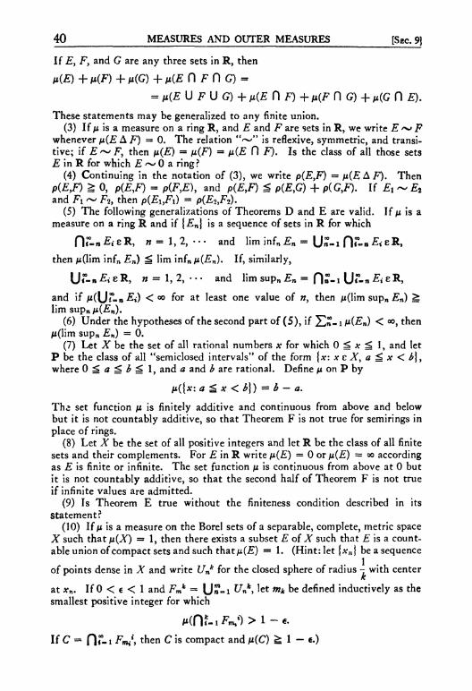
40 MEASURES AND OUTER MEASURES [SEC. 91
If Ey F, and G are any three sets in R, then
p(E) + /i(F) + 91(G) + ix{E fl F 0 G) -
= / i ( £ U F U G) + P(E fl F) + / i ( F 0 G) + M ( G fl F).
These statements may be generalized to any finite union. (3) If p is a measure on a ring R, and E and F are sets in R, we write E ~ F
whenever p(E A F) = 0. The relation " ~ " is reflexive, symmetric, and transitive; if E~ Fy then p(E) = M(F) = p(E fl F). Is the class of all those sets E in R for which £ ^ 0 a ring?
(4) Continuing in the notation of (3), we write p(EyF) = p(E A F). Then p(EyF) £ 0, p(EyF) = p(F,£), and p(£,F) £ p(F,G) + p(G,F). If £ , - F 2
and Fi ~ F2, then p(Fi,Fi) = p(EoyF^), (5) The following generalizations of Theorems D and E are valid. If p is a
measure on a ring R and if {FnJ is a sequence of sets in R for which
f V - n & e R , w = l , 2 , . . . and lim inf n F n = (J«-i D r - . & e R ,
then Mflini infn Fn) ^ lim infnMC£*). If, similarly,
U r - n ^ i e R , w = l , 2 , . . . and lim supn F n = f | » - i U ' - n F t e R ,
and if At(U«°-»Fi) < °° f° r a* least one value of », then /*(lim supn Fn) ^ limsup„M(Fn).
(6) Under the hypotheses of the second part of (5), if £ » - 1 p(En) < «>, then //(lim supn En) = 0.
(7) Let X be the set of all rational numbers x for which 0 ^ # ^ 1, and let P be the class of all "semiclosed intervals" of the form {x: x c Xy a ^ x < b}y
where 0 ?> a t* b =L 1, and 0 and £ are rational. Define JU on P by
p({x:a ^ * < £}) = b - a.
The set function p. is finitely additive and continuous from above and below but it is not countably additive, so that Theorem F is not true for semirings in place of rings.
(8) Let X be the set of all positive integers and let R be the class of all finite sets and their complements. For E in R write p(E) — 0 or p(E) = 00 according as E is finite or infinite. The set function p is continuous from above at 0 but it is not countably additive, so that the second half of Theorem F is not true if infinite values are admitted.
(9) Is Theorem E true without the finiteness condition described in its Statement?
(10) If M is a measure on the Borel sets of a separable, complete, metric space X such that p(X) =» 1, then there exists a subset E of X such that £ is a countable union of compact sets and such that/-i(F) = 1. (Hint: let [xn\ be a sequence
of points dense in X and write Unk for the closed sphere of radius - with center
at xn. If 0 < c < 1 and Fmk =* ( J » - i ^n*> let mk be defined inductively as the
smallest positive integer for which
M(ftt.>JV)>l-«. If C = n«°-t Fmi\ then C is compact and /i(C) ^ 1 - e.)

[SEC. 10] MEASURES AND OUTER MEASURES 41
§ 10. OUTER MEASURES
A non empty class E of sets is hereditary if, whenever E e E and F c Ey then F e E .
A typical example of a hereditary class is the class of all subsets of some subset E of X. The part of the algebraic theory of hereditary classes that we shall need is very easy and it is similar in every detail to the theories of rings, c-rings, and other classes of sets we have considered. It is, in particular, true that the intersection of every collection of hereditary classes is again a hereditary class, and that, therefore, corresponding to any class of sets, there is a smallest hereditary class containing it. We shall be especially interested in hereditary classes which are cr-rings; it is easy to see that a hereditary class is a coring if and only if it is closed under the formation of countable unions. If E is any class of sets, we shall denote the hereditary c-ring generated by E, i.e. the smallest hereditary o—ring containing E, by H(E). The hereditary <7-ring generated by E is, in fact, the class of all sets which can be covered by countably many sets in E; if E is a non empty class closed under the formation of countable unions (for instance if E is a 0—ring), then H(E) is the class of all sets which are subsets of some set in E.
An extended real valued set function ju* defined on a class E of sets is subadditive if, whenever E eE , F eE , and £ U F e E , then
M*(£ U F) ^ M*(£) + M W
An extended real valued set function /i* on E is finitely subadditive if, for every finite class {£i, • • •, En\ of sets in E whose union is also in E, we have
M*(U?.ift)^2^-lM*(£i).
An extended real valued set function ju* on E is countably subadditive if, for every sequence {£,} of sets in E whose union is also in E, we have
M*(ur- i£*)£Er- iM*(£<>.
42 MEASURES AND OUTER MEASURES ISEC. 10}
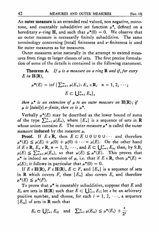
An outer measure is an extended real valued, non negative, monotone, and countably subadditive set function /**, defined on a hereditary <r-ring H, and such that M*(0) = 0. We observe that an outer measure is necessarily finitely subadditive. The same terminology concerning [total] finiteness and <r-finitenes6 is used for outer measures as for measures.
Outer measures arise naturally in the attempt to extend measures from rings to larger classes of sets. The first precise formulation of some of the details is contained in the following statement.
Theorem A. If JU is a measure on a ring R and if, for every E in H(R),
/*•(£) = inf { L : - i M ( £ n ) : £ n eR, » = 1,2, •••;
then ii* is an extension of y. to an outer measure on H(R); if IJL is [totally] a-finite, then so is ju*.
Verbally ix*(E) may be described as the lower bound of sums of the type S^- i M(^M), where {En} is a sequence of sets in R whose union contains E. The outer measure JJL* is called the outer measure induced by the measure ju.
Proof. If E e R, then £ c £ U 0 U 0 U . - - and therefore M*(£) ^ M(£) + M(0) + M(0) + • • • = M(£) . On the other hand if E eR, En eR, n = 1, 2, • • -, and E c (J"«i En9 then, by 9.B, M(£) ^ Z)r«iM(£n), so that n(E) ^ p*(E). This proves that H* is indeed an extension of JU, i.e. that if E e R, then p*(E) = n(E); it follows in particular that M*(0) = 0.
If E cH(R), F e H ( R ) , E c F, and {£n} is a sequence of sets in R which covers F> then {£n} also covers Ey and therefore M*(£) ^ M*(F).
To prove that ju* is countably subadditive, suppose that E and £ t are sets in H(R) such that E c (J"-i £*; let e be an arbitrary positive number, and choose, for each / = 1, 2, • •, a sequence \Eij) of sets in R such that
Ei c U;-i £* and ZZ-i MOE*) ^ M*(£;) + ^

[SEC. 10] MEASURES AND OUTER MEASURES 43
(The possibility of such a choice follows from the definition of ji*(£i).) Then, since the sets En form a countable class of sets in R which covers E,
M*(£) ^ ET-i ZT-i Wit) £ IT-. M*( ) + e. The arbitrariness of e implies that
M*(£)^£r-iM*(£*)-
Suppose, finally, that /* is c-finite and let E be any set in H(R). Then, by the definition of H(R), there exists a sequence {£»} of sets in R such that E C [JT-i E{. Since n is <r-finite, there exists, for each i = 1, 2, • • •, a sequence {£iy} of sets in R such that
Ei c (J •_! £lV and /*(£#) < °°-
Consequently
£ c \j;ml U; . i Ea and /**(£*) = 9*(Ev) < « . |
(1) Is it necessarily true, under the hypotheses of Theorem A, that if /x is finite, then so is/x*?
(2) For any class E of sets we denote by J(E) the smallest hereditary ring containing E. If /x is a real valued, finite, non negative, and finitely additive set function defined on a ring R, and if, for every E in J OR),
/i*(£) = i n f { M ( F ) : £ C l F e R } ,
then /x* is a real valued, finite, non negative, and finitely subadditive set function on J(R). Is it true that, for E in R, n*(E) = n{E) ?
(3) A necessary and sufficient condition that a class H of subsets of a set X be an ideal in the Boolean ring of all subsets of X is that H be a hereditary ring; cf. 4.4.
(4) The following are some examples of set functions defined on hereditary <r-rings; some of them are outer measures, while others violate exactly one of the defining conditions of outer measures.
(4a) X is arbitrary, H is the class of all subsets of X. For any fixed point #o in X, write fx*(E) = Xs(xo).
(4b) X and H are as in (4a); n*(E) = 1 for every E in H. (4c) X = [xj] is a set consisting of exactly two distinct points x and y>
H is the class of all subsets of X> and /** is defined by the relations
M*<0)-0, M * ( W ) = M * ( W ) - 1 0 , M #<*)~ 1.
(4d) AT is a set of 100 points arranged in a square array of 10 columns each mth 10 points; H is the class of all subsets of X; n*(E) is the number of columns which contain at least one point of £ .

44 MEASURES AND OUTER MEASURES [SEC. 11|
(4e) X is the set of all positive integers, H is the class of all subsets of X. For every finite subset E of X> v(E) is the number of points in E\
M*(£) = l i m s u P n - K £ 0 {1, • - . , » } ) . n
(40 X is arbitrary, H is the class of all countable subsets of X> fM*(E) is the number of points in £, (= oo if E is infinite).
(5) If fx* is an outer measure on a hereditary c-ring H and EQ is any set in H, then the set function /uo*, defined by no*(E) = p*(E 0 EQ), is an outer measure on H.
(6) If X* and /i* are outer measures on a hereditary <r-ring H, then the set function v*9 defined by v*(E) = X*(£) U /x*C#)> is an outer measure on H.
(7) If IfJLn*} is a sequence of outer measures on a hereditary c-ring H and \an} is a sequence of positive numbers, then the set function /i* defined by li*(E) — 23n-i anfjLn*(E)i is an outer measure on H.
§ 1 1 . MEASURABLE SETS
Let /x* be an outer measure on a hereditary <r-ring H. A set E in H is M-*-measurable if, for every set A in H,
M * U ) = »*(A n E) + M * V n £')•
The concept of /immeasurability is the most important one in the theory of outer measures. It is rather difficult to get an intuitive understanding of the meaning of /immeasurability except through familiarity with its implications, which we propose to develop below. The following comment may, however, be helpful. An outer measure is not necessarily a countably, nor even finitely, additive set function (cf. 10.4d). In an attempt to satisfy the reasonable requirement of additivity, we single out those sets which split every other set additively—the definition of /immeasurability is the precise formulation of this rather loose description. The greatest justification of this apparently complicated concept is, however, its possibly surprising but absolutely complete success as a tool in proving the important and useful extension theorem of § 13.
Theorem A. If /x* is an outer measure on a hereditary c-ring H and if S is the class of all ^-measurable setsy then S is a rinr.
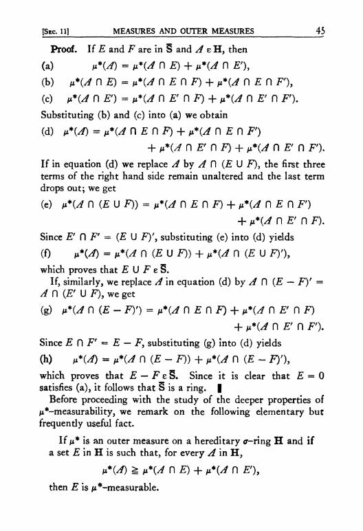
[SEC. 11] MEASURES AND OUTER MEASURES 45
Proof. If £ and F are in § and i e H , then
(a) n*(A) = n*(A n E) + »*(A n F ) ,
(b) n*(A n E) = M*(^ n F n F) + M*(^ n £ n F) , (c) M*(^ n F) = M*(^ n F' n F) + »*(A n F' n F) . Substituting (b) and (c) into (a) we obtain
(d) »*(A) = M*(^ n E n F) + M*(^ n F n F ) + v*{A n F n F) + »*{A n F n F ) .
If in equation (d) we replace /^ by /f D (F U F), the first three terms of the right hand side remain unaltered and the last term drops out; we get
(e) fi*(A PI (F U F)) = p*(A n E n F) + v*(A fl F fl F )
+ M*(/* n F n F). Since F ' fl F ' = (F U F) ' , substituting (e) into (d) yields
(0 ix\A) = »*{A fl (F U F)) + M *(^ fl (F U F) ') ,
which proves that F U F e S. If, similarly, we replace A in equation (d) by A D (F — F ) ' =
<rf n ( F U F) , we get
(g) v*(A n (F - F)') = v*(A n F n F) + M*(^ n F n F) + n*(A n F n F).
Since F fl F ' = F — F, substituting (g) into (d) yields
(h) f{A) - M * U n (F - F)) + M * U 0 (F - F) ' ) ,
which proves that E — FeS. Since it is clear that F = 0 satisfies (a), it follows that § is a ring. |
Before proceeding with the study of the deeper properties of /immeasurability, we remark on the following elementary but frequently useful fact.
If H* is an outer measure on a hereditary <r-ring H and if a set F in H is such that, for every A in H ,
n*(A) ^ p\A n F) + fi*(A n F ) ,
then F is /immeasurable.

46 MEASURES AND OUTER MEASURES [SEC. 11)
The proof of this remark is achieved simply by recalling that the reverse inequality, M*(^) ^ M*(^ H E) + p*(A fl E')y is an automatic consequence of the subadditivity of /**.
Theorem B. If /z* is an outer measure on a hereditary a-ring H and if S is the class of all ^-measurable sets, then 5 is a <r-ring. If A e H and if {En} is a disjoint sequence of sets in § with U r - i En = E, then
^(ADE) = Z : ~ i M * U n £ n ) .
Proof. Replacing E and F in (e) by EY and E2 respectively, we see that
»*(A fl (£ t U £2)) = M *(^ fl Et) + n*(A fl £2).
It follows by mathematical induction that
n*(j n u<-» Et) = E ? . , M V n £,)
for every positive integer w. If we write
Fn = U"- i£<. i f - 1 , 2 , ••-,
then it follows from Theorem A that
n*(A) - M * U n Fn) + M * U n Fn*) *
Since this is true for every w, we obtain
(i) M*U) ^ Zr. i M*(^ n £t) + n*(A n £0 ^
^ n*(A n £) + M*(^ n £r).
ft follows that E e § (so that, by the way, S is closed under the formation of disjoint countable unions), and therefore that
(j) £T-i M*U n Ed + n*(A n Ef) = = n*(A Pi E)+ fi*(A fl E').
Replacing A by A fl £ in (j), we obtain the second assertion of the theorem. (Since p*(A f) E') may be infinite, it is not permissible simply to subtract it from both sides of (j).) Since every countable union of sets in a ring may be written as a disjoint countable union of sets in the ring, we see also that § is a cr-ring. |

[Sac. 11] MEASURES AND OUTER MEASURES 47
Theorem C. If M* is an outer measure on a hereditary a-ring H and if § is the class of all ^-measurable setsy then every set of outer measure zero belongs to § and the set function fly defined for E in § by fi(E) = /**(£), is a complete measure on 8.
The measure p, is called the measure induced by the outer measure /**.
Proof. If E e H and n*(E) = 0, then, for every A in H, we have
p*{A) - M*(£) + n*(A) £ »*{A 0 E) + n*(A 0 £ ' ) ,
so that indeed £ e S . The fact that jx is countably additive on 5 follows from (j) upon replacing A by E. If
E e 3 , F c £ , and M(£) = M*(£) - 0,
then fi*{F) = 0, so that F e S, which proves that £ is complete. |
(1) For the example 10.4d, a set E is ^immeasurable if and only if with every point x in E the entire column which includes x is contained in E. Which sets are /immeasurable in 10.4f ?
(2) If M* is an outer measure on a hereditary <r-ring H, under what additional conditions is the class of /immeasurable sets an algebra?
(3) In the notation of Theorem A, replacing A in equation (d) by A 0 (E' U F') may be used to give a direct proof of the fact that S is closed under the formation of intersections. What would the same technique prove if A were replaced by A fl (F - £ ) ' - A D (E U F')i
(4) Let /i* be a finite, non negative, monotone, and finitely subadditive set function with /i* (0) = 0 on a hereditary ring J; cf. 10.2. The class of all immeasurable sets is a ring, and the set function /i* is additive on this ring.
(5) Suppose that /** is an outer measure on a hereditary <r-ring H and that 5 is the class of all /immeasurable sets. If A e H and {E nj is an increasing sequence of sets in S, then /i*(limn (A 0 En)) = \\mnn*(A fl En). Similarly, if \En\ is a decreasing sequence of sets in §, and if a set A in H is such that fjL*(A fl Em) < oo for at least one value of m> then /i*(lim» {A 0 £»)) ~ l i m n M * U n £ n ) .
(6) If M* is an outer measure on a hereditary c-ring H and if E and F are two sets in H of which at least one is /immeasurable, t n e n ^ - ^-2)
M*(£) +ix*(F) - »*(£ U F) + / i * ( £ 0 F).
(7) The results of this section could also have been obtained by means of partitions (cf. 7.5). A partition is a finite or infinite disjoint sequence [E9\ of

48 MEASURES AND OUTER MEASURES [SEC. 11]
sets such that (J ,Ei = X. If/x* is an outer measure on a hereditary <r-ring H, the partition {Ei) is called a ^"-partition if
for every A in H; a set £ is a |l*-set if the partition {£,£'} is a pi "-partition. If {£,} and {Fj} are partitions, then {£ t | is called a subpartition of {Fj} if each £,• is contained in one of the sets Fj. The product of two partitions, {£,-} and {Fy}, is the partition consisting of all sets of the form Ei f) Fj. We note that a set in H is a /x*-set if and only if it is /immeasurable in the sense of this section.
(7a) The product of two ^"-partitions is a ^"-partition. (7b) If a subpartition of a partition {Ei\ is a /x"-partition, then {Ei} is a
/^"-partition. (7c) A partition {Ei} is a //"-partition if and only if each Ei is a /x*-set. (7d) The class of all /x*-sets is a <r-ring. (Hint: the class of all /x*-sets is a
ring closed under the formation of countable disjoint unions.) (8a) An outer measure /x* °n the class H of all subsets of a metric space X
is a metric outer measure if
/z*(£(JF) =M*(£)+M*(F)
whenever p(E,F) > 0, where p is the metric on X. If/x* is a metric outer meas
ure, if JS is a subset of an open set U in X, and if En = £ fl | # : p(xyU') ^ - | ,
w = 1, 2, ••• , then \\mnH*(En) = p.*(E). (Hint: observe that {£„} is an increasing sequence of sets whose union is E. If EQ = 0, Dn = En+i — Eny and if neither Dn+i nor En is empty, then p(Dn+uEn) > 0, and it follows that
M ^ t » + i ) S E f - i M * ( f t < ) and M*(£2n)^E?-iM*(At-i) .
The desired conclusion is trivial if either of the two series,
Zf-iM*(D2i) and £T_i M*(DM-I),
diverges; if they both converge, then it follows from the relation
„*(£) :g M*(2>2n) + E T . . M * ( D « ) + Er-.+iJ»*(flw-i).)
(8b) If /x* is a metric outer measure, then every open set (and therefore every Borel set) is //"-measurable. (Hint: if U is an open set and A is an arbitrary subset of X, apply (8a) to E = A H U. Since p(En,A Ci U') > 0, it follows that
V*(A) ^ n*(En U (A 0 £/')) = n*(En) + fji*(A fl £/').)
(8c) If/x* is an outer measure on the class of all subsets of a metric space X such that every open set is ^"-measurable, then /u* is a metric outer measure. (Hint: if p{EyF) > 0, let U be an open set such that EdU and F d U =* 0, and test the /immeasurability of U with A =» E U F.)

Chapter III
EXTENSION OF MEASURES
§ 1 2 . PROPERTIES OF INDUCED MEASURES
We have seen that a measure induces an outer measure and that an outer measure induces a measure, both in a certain natural way. If we start with a measure /x, form the induced outer measure n*> and then form the measure fi induced by /u*, what is the relation between /x and M? The main purpose of the present section is to answer this question. Throughout this section we shall assume that
fi is a measure on a ring R, JJL* is the induced outer measure on H(R), and M is the measure induced by /** on the <7-ring § of all /^-measurable sets.
Theorem A. Every set in S(R) is ^-measurable.
Proof. If E eR, A cH(R), and 6 > 0, then, by the definition of M*> there exists a sequence \En\ of sets in R such that A a ( J r - i £ « a n d
n*(A) + e £ : . i M(£n) = 2 ; . 1 (M(£n n E) + M(£n n £')) £
^ fji*(A n E) + fi*(A n £7).
Since this is true for every €, it follows that E is ii*-measurable. In other words, we have proved that R c § ; it follows from the fact that § is a o-ring that S(R) c S . |
49

50 EXTENSION OF MEASURES [SEC. 12)
Theorem B. If E e H(R), then
M*(£) = inf {a(F):E a FeS} =
= in({ji(F):Ec:FeS(R)\.
Equivalent to the statement of Theorem B is the assertion that the outer measure induced by fi on S(R) and the outer measure induced by ji on S both coincide with /**•
Proof. Since, for F in R, /x(F) = fx(F) (by the definition of M and 10.A), it follows that
M*(£) = inf {Z:~ i M(£n): £ c Un"-i Eny En e R,
* = 1 , 2 , . . . | ^
^ inf { Z : . i M(^n): E C ( J ^ i £«, £n e S(R),
« = 1,2, . . . } .
Since every sequence [En\ of sets in S(R) for which
may be replaced by a disjoint sequence with the same property, without increasing the sum of the measures of the terms of the sequence, and since, by the definition of /Z, /1(F) = M*(£) for F in 5, it follows that
lx*(E) ^ inf {H(F):E c Fc S(R)} ^
£ inf {H(F): £ c F e § U M*(£)- I
If E e H(R) and F e S(R), we shall say that F is a measurable cover of E if £ c F and if, for every set G in S(R) for which G c JF - £ , we have /2(G) = 0. Loosely speaking, a measurable cover of a set E in H(R) is a minimal set in S(R) which covers E.
Theorem C. If a set E in H(R) is oj a-finite outer measure, then there exists a set F in S(R) such that p*(E) = ji(F) and such that F is a measurable cover of E.
Proof. If M*(£) = oo, and E c F e S(R), then clearly fi(F) = oo, so that it is sufficient to prove the assertion M*(£) = fi(F) only in the case in which /**(£) < °°. Since a set of o—finite outer measure is a countable disjoint union of sets of finite outer
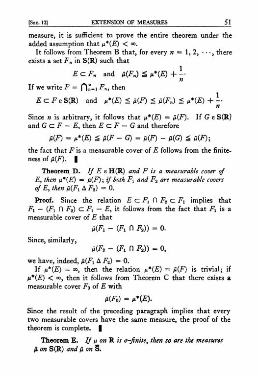
[SEC. 12] EXTENSION OF MEASURES 51
measure, it is sufficient to prove the entire theorem under the added assumption that ii*(E) < <».
It follows from Theorem B that, for every n = 1, 2, • • •, there exists a set Fn in S(R) such that
EczFn and fi(Fn) £ M*(£) + - • n
If we write F = fln-i Fn> then
EaFe S(R) and fi*(E) £ fi(F) £ a(Fn) £ »*(E) + - • n
Since n is arbitrary, it follows that n*(E) = fi(F). If G e S(R) and G a F — E, then E a F — G and therefore
M ( ^ - M*(£) ^ »(F - G) - £(F) - A(G) ^ M(F) ;
the fact that F is a measurable cover of E follows from the finite-ness of p.(F). |
Theorem D. If E e H(R) 070/ F is a measurable cover of E> then IJL*{E) = ji(F); if both Fx and F2 are measurable covers of £ , then M(FX A F2) = 0.
Proof. Since the relation E a FY D F2 c Fi implies that ^i - (Fx 0 F2) c Fi - £ , it follows from the fact that Fx is a measurable cover of E that
A(FX - (Fx 0 F2)) = 0.
Since, similarly,
m - (Fx n F2» = o, we have, indeed, fi(Fx A F2) = 0.
If v*(E) = oo, then the relation ii*(E) = /2(F) is trivial; if ix*(E) < oo, then it follows from Theorem C that there exists a measurable cover F0 of E with
M(F0) = M * ( £ ) .
Since the result of the preceding paragraph implies that every two measurable covers have the same measure, the proof of the theorem is complete. |
Theorem E. If fi onR is a-finite, then so are the measures fi on S(R) and jx on §.

52 EXTENSION OF MEASURES [SEC. 12]
Proof. According to 10.A, if /x is o-finite, then so is M*- Hence for every E in S there exists a sequence {Ei\ of sets in H(R) such that
£cU , " - i £ , -> M * ( £ * ) < « > , * = 1,2, ••••
An application of Theorem C to each set E{ concludes the proof of the theorem. |
The main question at the beginning of this section could have been asked in the other direction. Suppose that we start with an outer measure /**, form the induced measure py and then form the outer measure p* induced by p. What is the relation between ju* and £*? In general these two set functions are not the same; if, however, the induced outer measure p* does coincide with the original outer measure /**> then /** is called regular. The assertion of Theorem B is exactly that the outer measure induced by a measure on a ring is always regular. The converse of this last statement is also true: if M* is regular, then /x* = p* is induced by a measure on a ring, namely by p. on the class of /**-measurable sets. Thus the notions of induced outer measure and regular outer measure are coextensive.
(1) Theorem D asserts that a measurable cover is uniquely determined to within a set of measure zero, if it exists at all; Theorem C asserts that for sets of c-finite outer measure a measurable cover does exist. The following considerations show that the hypothesis of or-finiteness cannot be omitted from Theorem C.
If L is a line in the Euclidean plane X, and E is any subset of X> we shall say that E is full on L if L — E is countable. Let Ro be the class of all those sets E which may be covered by countably many horizontal lines on each of which E is either full or countable; let R be the algebra generated by Ro; (cf. 4.5). If, for every E in R, fx(E) = 0 or oo according as E is countable or not, then /x is a measure on R; it is easy to verify that in this case R = S(R) and S = H(R) is the class of all subsets of X. If £ is they -axis and E C Fe S(R), then there always exists a set G in S(R) such that G C F — E and ju(G) ^ 0.
(2) A subset E of the real line is said to have an infinite condensation point if there are uncountably many points of E outside every finite interval. Let X be the real line and define a set function /x* on every subset E of X as follows: HE is finite or countably infinite, then JJL*(E) = 0; if E is uncountable but does not have an infinite condensation point, then fi*(E) = 1; if E has an infinite condensation point, then n*(E) = «o. Then ft* is a totally c-finite outer measure, but, since the only /x*-measurable sets are the countable sets and their complements, the induced measure p, is not c-finite. Is jx* regular? What can
[SEC. 121 EXTENSION OF MEASURES 53 be said if, instead, n*(E) is defined to be 17 whenever E has an infinite condensation point?
(3) Let n be a fixed positive integer, and let N0, Ki, • • •, **n be the first n + 1 infinite cardinal numbers in the well ordering of the cardinals according to magnitude. If A!' is a set of cardinal number Kn, and E is a finite subset of X9
writen*(E) « 0; if the cardinal number of a subset £ of X is the infinite cardinal Kfc, 0 5* £ ^ w, write ***(£) — *. The set function jit* is an outer measure; is it regular?
(4) If M* is a regular outer measure on a hereditary <r-ring H, and if {En} is an increasing sequence of sets in H with l im»£ n =* Ey then fi*(E) « limnM*CEn). (Hint: if \\mnfi*(En) *» °°> the result is clear. If not, then let Fn be a ^ - m e a s urable cover of En, n — 1,2, • • •, so that the sequence {Fn\ is increasing, and write F = limn Fn. Since fJL*(Fn) = n*(En) ^ M*l£)> we have limnM*0Fn) = p*(F) ^ /**(£); since E d Fy n*(E) ^ p*(F)> Hence F is a measurable cover of E.) This result is not true for non regular outer measures; a counter example may be constructed on the basis of (2) above.
(5) For every subset E of an arbitrary set AT write ji*(E) ~ 0 or 1 according as E is empty or not; the set function M* is a regular outer measure on the class of all subsets of X, If {En\ is a decreasing sequence of non empty sets with an empty intersection (such a sequence exists whenever X is infinite), then
limnM*(£n) = 1 and ii*(Y\mn En) = 0;
in other words the analog of (4) for decreasing sequences is false even for totally finite, regular outer measures.
(6) Let Mi* and jup* be two finite outer measures on the class of all subsets of a set Xy and let S„ / = 1, 2, be the class of/i,*-measurable sets. If, for all subsets E of X,
M*(£)=m*(£)+„,*(£),
then the class S of all /immeasurable sets is the intersection of §i and §2. (Hint: if y.*{A PI E) + »*(A 0 E') * n*(A), then both the inequalities, M»*0* D E) + m*(A fl E') ^ m*{d)> i = 1,2, must become equalities.) What can be said if Mi* and M2* are not necessarily finite?
(7) Let /xi* be any finite, regular outer measure on the class of all subsets of a set Xy and write M2*(£) = 0 or 1 according as £ is empty or not. Then M2* is also a finite, regular outer measure, but, if Mi* assumes more than two values, then Mi* + M2* is not regular.
(8) If A' is a metric space, p is a positive real number, and £ is a subset of AT, then the ^dimensional Hausdorff (outer) measure of E is defined to be the number
MP*(£) » sup«>0 inf {Zf-! ($(£<))': E - \JT-1 Eiy b(Ex) < c, i - 1,2, • • - } ,
where 6(E) denotes the diameter of E. (8a) The set function nP* is a metric outer measure; cf. 11.8a. (8b) The outer measure \kv* is regular; in fact, for every subset E of X,
there exists a decreasing sequence {Un) of open sets containing E such that
MP*to-Mp*(nr-i«j.
54 EXTENSION OF MEASURES [SEC. 13]
§ 13. EXTENSION, COMPLETION, AND APPROXIMATION
Can we always extend a measure on a ring to the generated <r-ring? The answer to this question is essentially contained in the results of the preceding sections; it is formally summarized in the following theorem.
Theorem A. If M is a <j-finite measure on a ring R, then there is a unique measure p. on the a-ring S(R) such that, for E in R, ji(E) = n(E); the measure \x is a-finite.
The measure fi is called the extension of /*; except when it is likely to lead to confusion, we shall write /*(£) instead of fi(E) even for sets E in S(R).
Proof. The existence of p, (even without the restriction of c-finiteness) is proved by l l .C and 12.A. To prove uniqueness, suppose that MI and /*2 are two measures on S(R) such that Hi(E) = n2(E) whenever £ e R , and let M be the class of all sets E in S(R) for which juiOE) = ^(E). If one of the two measures is finite, and if \En) is a monotone sequence of sets in M, then, since
M*(limn En) = limn MtCEn), i = 1,2,
we have limn En e M. (The full justification of this step in the reasoning makes use of the fact that one of the two numbers Hi(En) and iL2(En), and therefore also the other one, is finite for every n = 1, 2, • • •; cf. 9.D and 9.E.) Since this means that M is a monotone class, and since M contains R, it follows from 6.B that M contains S(R).
In the general, not necessarily finite, case we proceed as follows. Let A be any fixed set in R, of finite measure with respect to one of the two measures iix and p2. Since R fl A is a ring and S(R) Ci A is the c-ring it generates (cf. 5.E), it follows that the reasoning of the preceding paragraph applies to R fl A and S(R) fl A> and proves that if E e S(R) fl A, then MI(£) = AfcGE). Since every E in S(R) may be covered by a countable, disjoint union of sets of finite measure in R (with respect to either of the measures MI and M2)> the proof of the theorem is complete. |
The extension procedure employed in the proofs of § 12 yields

(Sue. 13] EXTENSION OF MEASURES 55
slightly more than Theorem A states; the given measure /* can actually be extended to a class (the class of all /immeasurable sets) which is in general larger than the generated c-ring. The following theorems show that it is not necessary to make use of the theory of outer measures in order to obtain this slight enlargement of the domain of JJL.
Theorem B. If n is a measure on a a-ring S, then the class § of all sets of the form E A N> where E e S and N is a subset of a set of measure zero in S, is a a-ringy and the set function p, defined by jx(E A N) = y.{E) is a complete measure on 5 .
The measure fi is called the completion of /*• Proof. If E e S, N c A e S, and y.(A) = 0, then the relations
E U N = (E - A) A [A fl {E U N)] and
£ A i V = (E-A) U [A fl OEAA01
show that the class § may also be described as the class of all sets of the form E U Af, where £ e S and N is a subset of a set of measure zero in S. Since this implies that the class 5, which is obviously closed under the formation of symmetric differences, is closed also under the formation of countable unions, it follows that 5 is a o—ring. If
£ i A ^ = £ 2 A N2y
where E{ e S and Ni is a subset of a set of measure zero in S, i = 1, 2, then
£i A E2 = Nx A N2y
and therefore y.{Ex A E2) = 0. It follows that M(£I) = V>(E2), and hence that p, is indeed unambiguously defined by the relations
ji(E&N) = H(E UiV) = M(£) .
Using the union (instead of the symmetric difference) representation of sets in §, it is easy to verify that /Z is a measure; the completeness of fl is an immediate consequence of the fact that S contains all subsets of sets of measure zero in S. |

56 EXTENSION OF MEASURES [SEC. 13)
The following theorem establishes the connection between the general concept of completion and the particular complete extension obtained by using outer measures.
Theorem C. If /* is a o-finite measure on a ring R, and if /x* is the outer measure induced by /*, then the completion of the extension of ix to S(R) is identical with /x* on the class of all ^-measurable sets.
Proof. Let us denote the class of all /^-measurable sets by S* and the domain of the completion p, of /* by 3 . Since /** on S* is a complete measure, it follows that § is contained in S* and that M and ju* coincide on 8. All that we have left to prove is that S* is contained in 3 ; in view of the cr-finiteness of /z* on S* (cf. 12.E) it is sufficient to prove that if E e S* and n*(E) < oo, then E e 3 .
By 12.C, E has a measurable cover F . Since M*(F) = n(F) = H*(E)y it follows from the finiteness of n*(E)y and the fact that H* is a measure on S*, that p.*(F — E) = 0. Since F — E also has a measurable cover Gy and since
M(G) = M*(F - E) - 0, the relation
£ = ( F - G ) U ( £ n G )
exhibits E as a union of a set in S(R) and a set which is a subset of a set of measure zero in S(R). This shows that E e 8, and thus completes the proof of Theorem C. |
Loosely speaking, Theorem C says that in the o—finite case the cr-ring of all /immeasurable sets and the generated <r-ring S(R) are not very different; every /^-measurable set suitably modified by a set of measure zero belongs to S(R).
We conclude this section with a very useful result concerning the relation between a measure on a ring and its extension to the generated c-ring.
Theorem D. If p is a o-finite measure on a ring R, then, for every set E of finite measure in S(R) and for every positive number e, there exists a set E0 in R such that n(E A E0) 3* €.
(SEC. 13] EXTENSION OF MEASURES 57
Proof. The results of §§ 10,11, and 12, together with Theorem A, imply that
M(£) = i n f { 2 : r - i M ( ^ ) : £ c z U ! 0 - i ^ £ , e R , i - 1, 2, • • • } .
Consequently there exists a sequence {E{] of sets in R such that
ficUtift and n(\jT-iEi)<n(E)+^
Since i i m n M ( U n - . i ^ ) = = M ( U r . i ^ ) ,
there exists a positive integer w such that if
Eo = U?-i E*> then
M(Ur-i £*) ^ M(£0) + «
Clearly E0 e R; since
M(£ - Eo) ^ M(Ur-i £; ~ ^o) - M(U"-I £f) - M(£O) ^ ^
and
M(£0 - £) ^ M(Ur.i £ < - £ ) - M(Ur-i £*) - M(£) ^ 5 ,
the proof of the theorem is complete. |
(1) Let /x be a finite, non negative, and finitely additive set function defined on a ring R. The function JJL* defined by the procedure of § 10 is still an outer measure, and, therefore, the p of l l .C may still be formed, but it is no longer necessarily true that p is an extension of/x; (cf. 10.2, 10.4e, and 11.4).
(2) If p is the extension of the measure jz on the ring R described in § 8, then, for any countable set Ey Ee S(R) and p(E) — 0.
(3) The uniqueness assertion of Theorem A is not true if the class R is not a ring. (Hint: let X = \ajbycyd\ be a space of four points and define the measures Hi and fi2 on the class of all subsets of X by
Mi(W)=Mi(M)-/*i(W)-Mt(W)-l , Mi(W) - Mi(M) - M2({*}) = /*({</}) - 2.)
(4) Is Theorem A true for semirings instead of rings? (5) Let R be a ring of subsets of a countable set X, with the property that
every non empty set in R is infinite and such that S(R) is the class of all subsets of X; (cf. 9.7). If, for every subset E of X, ni(E) is the number of points in E and M2(£) = 2MI(£) , then H2 and y.\ agree on R but not on S(R). In other words,
58 EXTENSION OF MEASURES [SEC. 14]
the uniqueness assertion of Theorem A is not true without the restriction of (r-finiteness on R, even for measures which are totally cr-finite on S(R).
(6) Suppose that/x is a measure on ac-ring S and that ju on S is its completion. If A and B are in S and if A C E C 5, and n(B - A) = 0, then £ e § .
(7) Let X be an uncountable set, let S be the class of all countable sets and their complements, and, for every E in S, let n(E) be the number of points in E. Then \x is a complete measure on S, but every subset of X is /immeasurable; in other words, Theorem C is false without the assumption of c-flniteness.
(8) If n and v are (T-flnite measures on a ring R, then, for every E in S(R) for which both n(E) and v(E) are finite and for every positive number €, there exists a set EQ in R such that
/x(£ A £0) ^ « and v(E A £0) ^ *.
§ 14. INNER MEASURES
We return now to the general study of measures, outer measures, and the relations among them, in order to describe an interesting and historically important part of the theory.
We have seen that if y. is a measure on a cr-ring S, then the set function /** (defined for every E in the hereditary cr-ring H(S) by
M*(£) = in({n(F):E(zFeS})
is an outer measure; in the <r-finite case the induced measure fi on the 0—ring § of all /x*-measurable sets is the completion of /*. Analogously we now define the inner measure M* induced by /*; for every £ in H(S) we write
/!•(£) = s u p { / x ( F ) : £ z > F e S } .
In this section we shall study /i* and its relation to /x*; we shall show that the properties of /i* are in a very legitimate sense the duals of those of ju*. It is very easy to see that the set function JU* is non negative, monotone, and such that JU*(0) = 0; in what follows we shall make use oi these elementary facts without any reference. Throughout this section we shall assume that
li is a ^-finite measure on a <r-ring S, ju* and /i* are the outer measure and the inner measure induced by /x, respectively, and jl on S is the completion of /x;
we recall that p, on S coincides with /** on the class of all /^-measurable sets (cf. 13.C).

[SEC. 14] EXTENSION OF MEASURES <0
Theorem A. If E e H(S), then
/!•(£) = sup {/2(F): F z > F e S } .
Proof. Since S c 5, it is clear from the definition of /** that
M*(£) ^ sup {/2(F): F z > F e § } .
On the other hand 13.B implies that, for every F in 5, there is a G in S with G C F and /2(F) = ii{G). Since this means that every value of /2 on subsets of E in § is also attained by /* on subsets of E in S, the proof is complete. |
If E eH(S) and F e S , we shall say that F is a measurable kernel of £ if F a E and if, for every set G in S for which G c E — Fy we have fi(G) = 0. Loosely speaking a measurable kernel of a set £ in H(S) is a maximal set in S which is contained in F .
Theorem B. Every set E in H(S) has a measurable kernel.
Proof. Let F be a measurable cover of F , let N be a measurable cover of £ — Ey and write F = & — N. We have
F = £ - i V c £ - ( £ - £ ) = £ ,
and, if G c £ — F, then
GaE-(£-N) = EriNc:N-(£-E).
It follows (since TV is a measurable cover of £ — F) , that F is a measurable kernel of F . |
Theorem C. 7 / £ e H ( S ) and F is a measurable kernel of F, then M(F) = n*(E)\ if both Fx and F2 are measurable kernels of F , then JU(FI A F2) = 0.
Proof. Since F c F , it is clear that n(F) ^ /**(£). If /*(F) < /x*(F), then M(F) is finite and, by the definition of/z*(F), there exists a set F0 in S such that FQ a E and M(F0) > n{F). Since
Fo-FaE- F and M(F0 - F) ^ M(F0) - M^O > 0,
this is a contradiction, and therefore indeed /*(F) = n*(E). Since the relation Fi a Fx \J F2 a E implies that (Ft U F2) —

60 EXTENSION OF MEASURES [SEC. 14)
Fi c E — Fu it follows from the fact that Fx is a measurable kernel of E that
M ( ( ^ U F2) - Fx) = 0.
Since, similarly,
M((F! U JPa) - Fa) = 0,
we have ii{Fx A F2) = 0. |
Theorem D. If {En\ is a disjoint sequence of sets in H ( S \ then
M * ( U - i £ n ) ^ z ; - i M * ( £ j .
Proof- If Fn is a measurable kernel of Eny n = 1, 2, •.« then the countable additivity of /x implies that
Er.x M*(£n) = z : - i M(^») = M(U-"-I ^) £ M»(U:-« £»)• i Theorem E. / / i e H ( S ) ««</*/ {En\ is a disjoint sequence
of sets in § with \JZ-i En = E, then
M*un£) = E;.lM*(^n£»). Proof. If F is a measurable kernel of ^ fl E, then
M*U n E) = M(F) - En"-iA(F n En) ^ Y.:Zr*{A n £„) ;
the desired result follows from Theorem D. |
Theorem F. If E e §, /A*»
M * ( £ ) = M * ( £ ) = M(£) ,
#W, conversely, if E e H(S) #w</
M*(£) = M*(£) < « , then £ e S .
Proof. If £ e S, then both the supremum in Theorem A and the infimum in 12.B are attained by /2(£). To prove the converse, let A and B be a measurable kernel and a measurable cover of £, respectively. Since y.(A) = M*(£) < °°> we have
n(B - A) = tx(B) - ix{A) = M*(£) - u * ( ^ - 0.

[SEC. 14] EXTENSION OF MEASURES 61
and the desired conclusion follows from the completeness of ju on§;(cf. l l .C and 13.6). |
Theorem G. If E and F are disjoint sets in H(S), then
M*(£ U f ) ^ * ( £ ) + M*(JF) ^ M*(£ U F).
Proof. Let A be a measurable cover of F and let J5 be a measurable kernel of E U F. Since 5 — A c £ , it follows that
M*(£ U F) = M(*) ^ M(£ - ^ ) + M(^) ^ M*(£) + /**(*).
Dually, let A be a measurable kernel of £ and let B be a measurable cover of E U F. Since B — A ID Fyit follows that
M*(£ U F ) = M(JB) - M U ) + KB - A) §: M*(£) + v*{F). I
Theorem H. If E e §, then J or every subset A of X,
»*(A d E) + p*(A' Cl E) - / * ( £ ) .
Proof. Applying Theorem G to ^ fl £ and ^f fl £ , we obtain
M*(£) ^ M*(^ 0 E) + v*{A' fl E) £ M*(£).
Since £ e §, we have, by Theorem F, M*(£) ^ M*(£) = £(£)• I The results of this section enable us to sketch the steps of an
alternative approach to the extension theorem, an approach that is frequently employed. If n is a 0—finite measure on a ring R, and if M* is the induced outer measure on H(R), then, for every set E in R with p(E) < 00 and for every A in H(R), we have
M*U n E) = n(E) - n*(A' fl E).
If we prove now that whenever E and F are two sets of finite measure in R for which A fl E = A fl F> then it follows that M(£) - n*(A' 0 £) = /i(F) - /**(-<*' 0 £ ) , then we may use the equation for ii*(A f) E) as a definition of inner measure, and we may define a set E in H(R) of finite outer measure to be ^ -meas urable if and only if M*(£) = v>*{E). The details of this procedure may be easily carried out by the interested reader, using the techniques we have introduced in our development of the extension theory.

62 EXTENSION OF MEASURES [SEC. 15]
(1) Do the results of 12.4 remain true if jit* is replaced by /**? (2) With suitable finiteness restrictions the dual of 12.4 is true for inner
measures, but the unaltered result of 12.4 is not; (cf. 12.5). (3) If E is a set ofjinite measure in S, if F C £ , and if £(£) = p*(F) +
H*(E — F), then F e S . In other words the ju*-rneasurability of F may be tested by employing a fixed set E (containing F) in S instead of an arbitrary A in H(S). (Hint: use Theorem H.)
(4) Is an analog of 11.6 true for inner measures? (5) If E e H(S) and F is a measurable cover of £, then, for every /^-measur
able set M, p(F fi M) = n*(E PI M). (Hint: apply Theorem H to E = F fl M andy/ = £'.) Conversely, any set F with this property and such that E C Fe S is a measurable cover of £. Similarly, F is a measurable kernel of E if and only if E 3 F e S and fl(F fl M) = ju*(£ fl Ml for every Min S.
§ 15. LEBESGUE MEASURE
The purpose of this section is to apply the general extension theory to the special measure discussed in § 8, and to introduce some of the classical results and terminology pertinent to this special case. Throughout this section we shall assume that
X is the real line, P is the class of all bounded, semiclosed intervals of the form [ayb)y S is the o--ring generated by P, and M is the set function on P defined by n([a,b)) = b — a.
The sets of the <r-ring S are called the Borel sets of the line; according to the extension theorems 8.E and 13.A, we may assume that ii is defined for all Borel sets. If p, on § is the completion of ju on S, the sets of S are the Lebesgue measurable sets of the line; the measure fi is Lebesgue measure. (The incomplete measure /* on the class S of all Borel sets is usually called Lebesgue measure also.)
Since the entire line X is the union of countably many sets in P, we see that X e S, so that the <r-rings S and S are even <r-algebras. Since clearly n(X) = «>, JU is not finite on S, but, since /* is finite on P, both n on S and / l o n S are totally a-finite. Some of the other interesting properties of /* and (i are contained in the following theorems.
Theorem A. Every countable set is a Borel set of measure zero.

[SEC. 15] EXTENSION OF MEASURES 63
Proof. For any a, — oo < a < oo, we have
{a} = {*: x - *} - fln-i {*: * ^ * < * + - } ,
and therefore
ix(\a}) = limn M (\a,a + -JJ - limn - = 0,
so that every one-point set is a Borel set of measure zero. Since the Borel sets form a a—ring and since jz is countably additive, the theorem follows. |
Theorem B. The class S of all Borel sets coincides with the a-ring generated by the class U of all open sets.
Proof. Since, for every real number a, the set {a} is a Borel set, it follows from the relation (ayb) — [ayb) — {a}y that every bounded open interval is a Borel set. Since every open set on the line is a countable union of bounded open intervals, it follows that S 3 U and consequently that S => S(U). To prove the reverse inequality, we observe that, for every real number a>
{a) - fi:-i(*--,* + ;;),
so that {a} eS(U). It follows from the relation [ayb) = (a,b) U \a) that P c S(U) and consequently that
S = S(P) c S(U). |
Theorem C. If U is the class of all open sets, then, for every E in X>
M*(£) = i n f { M ( l / ) : £ c C/eU}.
Proof. Since n*(E) = inf {p(F): E c F e S}, it follows from the fact that U c S that
M*(£) ^ i n f { M ( * 7 ) ; £ c f / c U } .
If, on the other hand, c is any positive number, then it follows

64 EXTENSION OF MEASURES [SEC. 15]
from the definition of /** that there exists a sequence {[tfnA)} of sets in P such that
E c ( J : - i [anA) and £ ; . 1 (bn - an) £ M*(£) + ^
Consequently
E c U«"-i (*» - ^ , ^n) = U eU,
and
M(C/) ^ I,"-, (in -an) + ^£ M*(£) + <•
The desired result follows from the arbitrariness of e. |
Theorem D. Let T be the one to one transformation oj the entire real line onto itselfr, defined by T(x) — ax + j8, where a and j8 are real numbers and a ^ 0. If, for every subset E of Xy T(E) denotes the set of all points of the form T(x) with x in E> i.e. T(E) = [ax + 0: x e E}, then
»*{T(E)) = I a |M*(£) and n*(T(E)) = | a |M*(£)-
The set T(E) is a Borel set or a Lebesgue measurable set if and only if E is a Borel set or a Lebesgue measurable set, respectively.
Proof. It is sufficient to prove the theorem for a > 0. For, if a < 0, then the transformation T is the result of the iteration of two transformations 7\ and T2, T{x) = Ti(T2(#))> where Ti(x) = | a \x + p and T2(x) = — x. We leave to the reader the verification of the fact that the transformation T2 sends Borel sets and Lebesgue measurable sets into Borel sets and Lebesgue measurable sets, respectively, and that it preserves the inner and outer measures of every set.
Suppose then that a > 0, and let T(S) be the class of all sets of the form T(E) with E in S. It is clear that T(S) is a <r-ring; we are to prove that T(S) = S. If E = [ayb) e P, then E = T(F), where
La a /
so that E e T(S) and therefore S c T(S). By the same reasoning
[SEC. 15] EXTENSION OF MEASURES 65
applied to the transformation T 1>T 1(x) = , we may con-a
elude that S c T^1(S)y and, applying the transformation T to both sides of the last written relation, we obtain, T(S) c S and therefore T(S) = S.
If, for every Borel set Ey we write
MiOE) = M(T(£ ) ) and w ( £ ) - aM(£),
then both HI and /*2 are measures on S. If E = [*,£) eP, then T(£) = [aa + pyab + j8), and
Mi(£) - M(T(£) ) = (<** + ft - ( M + j8) = a(b -a) =
= <*M(£) = AIB(£),
so that, by 8.E and 13.A, p(T(E)) = <*M(£) for every £ in S. Applying the results of the preceding two paragraphs to the
transformation 71"""1, we obtain the relations
M*(T(JE)) = inf {M(F): T(£) c F e S} =
= inf {MT-^F)): E c T ^ F ) eS} =
= a i n f { M ( G ) : £ c G e S j -
= «M*(£) ,
and, replacing inf by sup, n* by M*> and c by 3 throughout,
M*(T(£)) = «M*(£), for every set E.
If £ is a Lebesgue measurable set and A is any set, then
v*{A n T(E)) + »*(A n (T(E))f) =
= n*(T(T-l(A) 0 £)) + n*{T{T-\A) 0 £')) =
= a\p*{T-l{A) 0 £ ) + n*{T~\A) fl £')] -
= ov*{T-\A)) =
so that T(£) is Lebesgue measurable. This result applied to T"1
proves its own converse and completes the proof of the theorem. |

66 EXTENSION OF MEASURES [SEC. 15)
(1) The class of all Borel sets is the c-ring generated by the class C of aU closed sets, and, for every set £ ,
/**(£) = s u p ( / z ( C ) : £ D C e C ) .
(2) To every Lebesgue measurable set E there correspond two Borel sets A and B such that
AdEClB, fi(B - A) = 0,
and such that A is an Fa and B is a G«. (3) A bounded set has finite outer measure. Is the converse of this statement
true? (4) Let {xi, #2, • • •} be an enumeration of the set M of rational numbers in
the closed unit interval X. For every c > 0 and * = 1, 2, • • •, let Fi{e) be the
open interval of length —. whose center is at #», and write
FU) = Uf-1 Fi(e), F = fin-1F Q •
The following statements are true. (4a) There exists an € > 0 and a point x in X such that x e' Fit). (4b) The set F(e) is open and p(F(e)) ^ €. (4c) The set X — F(e) is nowhere dense. (4d) The set X — F is of the first category and therefore, since X is a com
plete metric space, F is uncountable. (Hence, in particular, F 9* M.) (4e) The measure of F is zero. Since F Z) M> the statement (4e) yields a new proof of the fact that the set
M of rational numbers (as every countable set) has measure zero. More interesting than this, however, is the implied existence of an uncountable set of measure zero; cf. (5).
(5) Expand every number x in the closed unit interval Xin the ternary system, i.e. write
^ = E ? - l ^ , «n = 0 ,1 ,2 , » = 1, 2, •••,
and let C be the set of all those numbers x in whose expansion the digit 1 is not needed. (Observe that if, motivated by the customary decimal notation, we write .aw • • for Y^n = \an/3n, then for instance \ = .1000- • • = .0222- • •, and therefore 3- e C, but since \ = .111- • • and since this is the only ternary expansion of I, therefore ^ e' C.) Let X\ be the open middle third of X, X\ = (J, | ) ; let Xi and Xz be the open middle thirds of the two closed intervals which make up X - Xu i.e. X2 = (i , i) and Xz = (£, £); let X4y X6y X6i and Z7 be the the open middle thirds of the four closed intervals which make up
Z ~ ( I i U Z 2 U Xz)9
and so on ad infinitum. The following statements are true. (5a) C = X — U » - i ^ - (Hint: for every x \n X write # = .aia2*--,
a„ = 0, 1, 2, w ~ 1, 2, • • •, in such a way that if x e C, thena» ~ Oor 2, w = 1. 2, • • •. Then the expansion of x is unique and (i) x e X\ if and only if ct\ = !,
{SEC. 161 EXTENSION OF MEASURES 67
(ii) if oti 7 1, then x e X2 U X3 if and only if a2 = 1; (Hi) if «i 9* 1 and a2 s* 1, then x e ^ U ^ U Z e U l y i f and only if a3 = 1; • • •.)
(5b) M(C) = 0 . (5c) C is nowhere dense. (Hint: assume that X contains an open subinterval
whose intersection with ( J n - i Xn is empty.) (5d) C is perfect. (Hint: no two of the intervals X\> A^, • • • have a common
point.) (5e) C has the cardinal number of the continuum. (Hint: consider the corre
spondence which associates with every x in C, x — .aia^***, « n = 0 or 2, n =5 1,2, • • •, the number^ whose binary expansion i s^ = .^1^2• • *, fin — «„/2, n = 1, 2, •••, or, equivalently, y = 2Zn-i of„/2n+1. This correspondence is not one to one between C and X, but it is one to one between the irrational numbers in C and the irrational numbers in X. Alternative hint: use (5d).)
The set C is called the Cantor set. (6) Since the cardinal number of the class of all Borel sets is that of the
continuum (cf. 5.9c), and since every subset of the Cantor set is Lebesgue measurable (cf. (5b)), there exists a Lebesgue measurable set which is not a Borel set.
(7) The set of those points in the closed unit interval in whose binary expansion all the digits in the even places are 0 is a Lebesgue measurable set of measure zero.
(8) Let X be the perimeter of a circle in the Euclidean plane. There exists a unique measure M defined on the Borel sets of X such that n(X) = 1 and such that /x is invariant under all rotations of X, (A subset of a circle is a Borel set if it belongs to the c-ring generated by the class of all open arcs.)
(9) If g is a finite, increasing, and continuous function of a real variable, then there exists a unique complete measure jig defined on a c-ring Sg containing all Borel sets, such that P>g(\ayb)) = g(b) — g(a) and such that for every E in § f there is a Borel set F with pg(E A F) = 0; (cf. 8.3). The measure Jig is called the Lebesgue-Stieltjes measure induced by g.
§ 16. NON MEASURABLE SETS
The discussion in the preceding section is not delicate enough to reveal the complete structure of Lebesgue measurable sets on the real line. It is, for instance, a non trivial task to decide whether or not any non measurable sets exist. I t is the purpose of this section to answer this question, as well as some related ones. Some of the techniques used in obtaining the answer are very different from any we have hitherto employed. Since, however, most of them have repeated applications in measure theory, usually in the construction of illuminating examples, we shall present them in considerable detail. Throughout this section we shall employ the same notation as in § 15.

68 EXTENSION OF MEASURES [SEC. 16}
If £ is any subset of the real line and a is any real number, then E + a denotes the set of all numbers of the form x + ay
with x in E; more generally if £ and F are both subsets of the real line, then E + F denotes the set of all numbers of the form x + y with x in E andy in F. The symbol D(E) will be used to denote the difference set of £ , i.e. the set of all numbers of the form x —• y with x in E and y in E.
Theorem A. If E is a Lebesgue measurable set of positive, finite measure, and if0^a<ly then there exists an open interval U such that /i(£ fl U) ^ ap{U).
Proof. Let U be the class of all open sets. Since, by 15.C, /!(£) = inf \fx(U): E cz U eU}, we can find an open set U0 such that E C U0 and ay.{UQ) ^ fi(E). If { Un) is the disjoint sequence of open intervals whose union is U0y then it follows that
a ET_, M(t/n) ^ Zr. i M(£ n un).
Consequently we must have ay.(Un) ^ fi(E D Un) for at least one value of n; the interval Un may be chosen for U. |
Theorem B. If E is a Lebesgue measurable set of positive measure, then there exists an open interval containing the origin and entirely contained in the difference set D(E).
Proof. If £ is, or at least contains, an open interval, the result is trivial. In the general case we make use of Theorem A, which asserts essentially that a suitable subset of £ is arbitrarily close to an interval, to find a bounded open interval U such that
M(£ fl U) ^ fM(I7).
If -%n(U) < x < \y.{U)y then the set
(£ n u) u ((£ n u) + x)
is contained in an interval (namely U U (C/+ x)) whose length is less than %n(U). If £ fl U and (£ fl U) + x were disjoin^ then, since they have the same measure, we should have
M((£ n u) u [(£ n u) + x]) = 2A(£ n u) ^ MU).

[SEC. 16] EXTENSION OF MEASURES 69
Hence at least one point of E f] U belongs also to (E D U) + x, which proves that x eD(E). In otherwords the interval ( — %n(U)y
\p{U)) satisfies the conditions stated in the theorem. |
Theorem C. If % is an irrational numbery then the set A of all numbers of the form n + m £, where n and m are arbitrary integers^ is everywhere dense on the line; the same is true of the subset B of all numbers of the form n + m£ with n even, and the subset C of numbers of the form n + m£ with n odd.
Proof. For every positive integer i there exists a unique
integer wt- (which may be positive, negative, or zero) such that
0 ^ «» + /£ < 1; we write #, = #,- + /£. If U is any open inter
val, then there is a positive integer k such that n(U) > - • Among k
the k + 1 numbers, X\> • • •, #*+i, in the unit interval, there must
*be at least two, say #»• and Xj> such that | #,- — xj \ < - • I t k
follows that some integral multiple of #»• — Xjy i.e. some element of Ay belongs to the interval [/, and this concludes the proof of the assertion concerning A. The proof for B is similar; we have merely to replace the unit interval by the interval [0,2). The proof for C follows from the fact that C = B + 1. |
Theorem D. There exists at least one set E0 which is not Lebesgue measurable.
Proof. For any two real numbers x and y we write (for the purposes of this proof only) x ~ y if x — y e Ay (where A is the set described in Theorem C). It is easy to verify that the relation " ~ " is reflexive, symmetric, and transitive, and that, accordingly, the set of all real numbers is the union of a disjoint class of sets, each set consisting of all those numbers which are in the relation " ~ " with a given number. By the axiom of choice we may find a set E0 containing exactly one point from each such set; we shall prove that E0 is not measurable.
Suppose that F is a Borel set such that F c E0. Since the difference set D(F) cannot contain any non zero elements of the dense set Ay it follows from Theorem B that F must have meas-
70 EXTENSION OF MEASURES [SFX. 16]
ure zero, so that /**0Eo) = 0- I n other words, if E0 is Lebesgue
measurable, then its measure must be zero. Observe next that if a± and a2 are two different elements of
//, then the sets EQ + ax and E0 + a2 are disjoint. (If #i + ax = #2 + ^2j with Xi in E0 and x2 in E0> then #i — x2 =- a2 — ^ e //.) Since moreover the countable class of sets of the form E0 + ay
where a e A> covers the entire real line, i.e. E0 + A = Xy and since the Lebesgue measurability of E0 would imply that each E0 + a is Lebesgue measurable and of the same measure as E0y
we see that the Lebesgue measurability of EQ would imply the nonsensical result n(X) = 0. |
The construction in the proof of Theorem D is well known, but it is not strong enough to yield certain counter examples needed for later purposes. The following theorem is an improvement.
Theorem E. There exists a subset M of the real line such that, for every Lebesgue measurable set 2£,
li*{M fl E) = 0 and »*{M d E) = /2(£).
Proof. Write A = B U C, as in Theorem C, and, if £ 0 is the set constructed in the proof of Theorem D, write
M = EQ + B.
If F is a Borel set such that F c M, then the difference set D(F) cannot contain any elements of the dense set C, and it follows from Theorem B that n*(M) = 0. The relations
M' = EQ + C - E0 + (B + 1) = M + 1
imply that M*(AO — 0; (cf. 15.D). If E is any Lebesgue measurable set, then the monotone character of M* implies that H*(M fl E) = M*(M' fl E) = 0, and therefore (14.H) M*(M 0 £ )
The proofs of this section imply among other things that it is impossible to extend Lebesgue measure to the class of all subsets of the real line so that the extended set function is still a measure and is invariant under translations.

[SEC. 16] EXTENSION OF MEASURES 71 (1) If E is a Lebesgue measurable set such that, for every number x in an
everywhere dense set, j3(FA(£ + *)) = 0,
then either M(£) = 0 or else M(£') = 0. (2) Let M be a <r-finite measure on a c-ring S of subsets of a set X, and let
H* and M* be the outer measure and the inner measure, respectively, induced by /x on H(S). Let M be any set in H(S), and let § be the <r-ring generated by the class of all sets in S together with M. The chain of assertions below is designed to lead up to a proof of the assertion that p. may be extended to a measure \L on §.
(2a) The (7-ring § is the class of all sets of the form (E fl M) A (F fl M'), where E and F are in S. (Hint: it is sufficient to prove that the class of all sets of the indicated form is a <r-ring. Observe that
(E n M) A (F n M) = (E n M) U (F n MOO
(2b) If fjL*(M) < oo> if G and H are a measurable kernel and a measurable cover of M respectively, and if D = H — G> then the intersection of any set in § with U belongs to S.
(2c) There exist two sets G and H in S such that G C M C H and M*(M - G) = M*(££ — ^ 0 = 0, and such that if D = H — G, then the intersection of any set in S with D' belongs to S. (Hint: there exists a disjoint sequence {Xn\ of sets in S with n(Xn) < oo and M - U « - i ( ^ H *„).)
(2d) In the notation of (2c), M*(M ( 1 2 ) ) = /x*(M' (1 D) « 0, and therefore M*(M f l D ) = /x*(M' fl D) = M(I>).
(2e) In the notation of (2c), if
[(E1 n M) A (Fi n MO] n D = [(£2 n M) A (F2 n MOI n D,
where E\> Fi, £2, and F2 are in S, then
M(£i (1 D) = M(^2 D JD) and M(FI (1 D) - M(F2 (1 D).
(Hint: use the fact that the condition
[(£1A E2) (1 M 11 D] A [(Fx A F2) (1 M' (1 D] - 0
implies that
(Ei fl D) A (£2 (1 Z>) C M' (1 D and (Fi (1 D) A (F2 (1 D) C M fl D.)
(2f) Let a and 0 be non negative real numbers with a + fi = 1. In the notation of (2c) the set function /Z on §, defined by
P((£ fl M) A (F fl M')) -
= /idee n M) A (F n MO] n DO+<*M(£ n D I + W F O D),
is a measure on § which is an extension of/x on S. (3) If ix is a <r-finite measure on a <r-ring S and if {Mi, • • •, Mn} is a finite
class of sets in the hereditary o-ring H(S), then {Mi, • • •, Mn} may be adjoined to S and a measure p. may be defined on the generated <r-ring § so that it is an

72 EXTENSION OF MEASURES [SBC. 16|
extension of M on S. The analogous statement, for an infinite sequence {Mn} of sets in H(S), is not known
(4) The following example is useful for developing intuition about non measurable sets; virtually all general properties of non measurable sets may be illustrated by it. Let X = {(x,y): O ^ x ^ l , O ^ j r ^ l } be the unit square. For every subset E of the interval [0,1], write
£= {(xyy):xeEy 0£y£ 1} C X.
Let S be the class of all sets of the form £> for Lebesgue measurable sets E; define n(£) as the Lebesgue measure of E. A set M such as M = \(xyy)\ 0 ^ x ^ \>y — | } is non measurable; /x*(M) = 0 and n*(M) = 1.
(5) Let /x* be a regular outer measure on the class of all subsets of a set X such that n*(X) = 1, and let M be a subset of X such that p*{M) = 0 and H*(M) = 1; (cf. Theorem E and (4)). If v*(E) = /**(£) +M*(£ 0 A/), then v* is an outer measure; (cf. 10.5 and 10.7).
(5a) A set E is y*-measurable if and only if it is jtt*-measurable; (cf. 12.6). (5b) The infimum of the values of v*(E) over all ^-measurable sets E con
taining a given set A is 2n*(A). (Hint: if £ is j>*-measurable, then n*(E f) M)
(5c) The outer measure v* is not regular. (Hint: test regularity with M'.)

Chapter IF
MEASURABLE F U N C T I O N S
§ 17. MEASURE SPACES
A measurable space is a set X and a c-ring S of subsets of X with the property that \J S = X. Ordinarily it causes no confusion to denote a measurable space by the same symbol as the underlying set X; on the occasions when it is desirable to call attention to the particular o—ring under consideration, we shall write (X>S) for X. It is customary to call a subset E of X measurable if and only if it belongs to the cr-ring S. This terminology is not meant to indicate that S is the a-ring of all ji*-measurable sets with respect to some outer measure M*> n ° r even that a non trivial measure is or may be defined on S.
In the language of measurable sets, the condition in the definition of measurable spaces may be expressed by saying that the union of all measurable sets is the entire space, or, equivalently, that every point is contained in some measurable set. The purpose of this restriction is to eliminate certain obvious and not at all useful pathological considerations, by excluding from the space points (and sets of points) of no measure theoretic relevance.
A measure space is a measurable space (X9S) and a measure y> on S; just as for measurable spaces we shall ordinarily allow ourselves to confuse a measure space whose underlying set is X with the set X. On the occasions when it is desirable to call attention to the particular a—ring and measure under consideration, we shall write (^T,S,JU) for X. The measure space X is called [totally] finite, cr-finite, or complete, according as the measure fi is [totally]
73
74 MEASURABLE FUNCTIONS [SEC. 17)
finite, a—finite, or complete. For measure spaces we may and shall make use, without any further explanation, of the outer measure jn* and (in the a—finite case) the inner measure M* induced by /* on the hereditary a-ring H(S).
Most of the considerations of the preceding chapter show by deductions and examples how certain measurable spaces may be made into measure spaces. In this section we shall make a few general remarks on measurable spaces and measure spaces and then, in the remainder of this chapter and in the following chapters, turn to the discussion of functions on measure spaces, useful ways of making new measure spaces out of old ones, and the theory of some particularly important special cases.
We observe first that a measurable subset X0 of a measure space (XySyjj.) may itself be considered as a measure space ( Y0,So,Mo)> where So is the class of all measurable subsets of X0, and, for E in So, fM)(E) = M(£)- Conversely, if a subset X0 of a set X is a measure space CYojScMo), then X may be made into a measure space (Jf,S,ju), where S is the class of all those subsets of X whose intersection with X0 is in So, and, for E in S, n(E) = Ho(E fl X0). (Entirely similar remarks are valid, of course, for measurable spaces.) A modification of this last construction is frequently useful even if X is already a measure space. If Xo is a measurable subset of Xy a new measure JUQ may be defined on the class of all measurable subsets E of X by the equation fio(E) = n(E fl Xo); it is easy to verify that {X>Syfio) is indeed a measure space.
What happens to the considerations of the preceding paragraph if the subset X0 is not measurable? In order to give the most useful answer to this question, we introduce a new concept. A subset X0 of a measure space (JT,S,/x) is thick if /**(£ — Xo) = 0 for every measurable set E. If X itself is measurable, then X0
is thick if and only if JJL*(X — X0) = 0; if y. is totally finite, then Xo is thick if and only if n*(X0) = MOT- (For examples of thick sets cf. 16.E and 16.4.) Slightly deeper than any of the comments in the preceding paragraph is the following result, which asserts essentially that a thick subset of a measure space may itself be regarded as a measure space.

[SEC. 17] MEASURABLE FUNCTIONS 75
Theorem A. If X0 is a thick subset of a measure space (Z,S,M), if S0 = S fl X0, and if, for E in S, *,(£ ft XQ) -li(E), then (X0,S0,Mo) is a measure space.
Proof. If two sets, Ex and E2, in S are such that Ex 0 X0 = E2 fl X0, then (Ex A £2) fl X0 = 0, so that M(£i A £2) = 0 and therefore M(£I) = V>(E2). In other words MO is indeed unambiguously defined on S0.
Suppose next that {Fn\ is a disjoint sequence of sets in S0, and let En be a set in S such that
Fn = En nX0, » = 1,2, •••.
I f£ n = £n - U {£ i : 1 £ * < » } , » = 1,2, --^then
(£n*En) n z 0 = (Fw- U { ^ - I ^ « < » } ) A F . -
= F n A F n = 0,
so that n(£n A En) = 0, and therefore
= M ( U : - I ^ O = Mo(U:.i^n).
In other words /LIQ is indeed a measure, and the proof of the theorem is complete. |
(1) The following converse of Theorem A is true. If CY,S,M) is a measure space and if Xo is a subset of X such that, for every two measurable sets E\ and £2, the condition £1 fl Xo = Ei fl Xo implies that M(£I) = M(^2), then Afo is thick. (Hint: if F C E - AT0, then
(£ - F) fl Z0 = E fl AT0.)
(2) The extension theorem 16.2 may be used to give an alternative proof of Theorem A in the c-finite case.
(3) The following proposition shows that the concept of a finite measure space is not very different from the apparently much more special concept of a totally finite measure space. If (X,S,n) is a finite measure space, then there exists a thick measurable set Xo. (Hint: write c ~ sup \n(E): EeS}. Let \En\ be a sequence of measurable sets such that lim» fJt{En) = c and write Xo — U n - i En. Observe that JLI(.ATO) = c.) This result enables us, in most applications, to assume that a finite measure space is totally finite, since we may replace X by Xo without significant loss of generality. For an example of a finite measure space which is not totally finite, let X be the real line, let S be the class of all sets of the form E U C, where E is a Lebesgue measurable subset of [0,1] and C U countable, and let /x on S be Lebesgue measure. The method suggested abov*

76 MEASURABLE FUNCTIONS [SEC. 18)
to show the existence of Xo has frequent application in measure theory; it is called the method of exhaustion.
(4) If (X,SjJ,) is a complete, c-finite measure space, then every /immeasurable set is measurable. Hence for complete, c-finite measure spaces the two concepts of measurability collapse into one.
§ 18. MEASURABLE FUNCTIONS
Suppose t h a t / is a real valued function on a set X and let M be any subset of the real line. We shall write
f-\M) = {*:/(*) eM},
i .e . /_ 1(M) is the set of all those points of X which are mapped into M b y / . The s e t / ^ M ) is called the inverse image (under / , or with respect t o / ) of the set M. If, for instance,/ is the characteristic function of a set E in Xy then/"-*({ l}) = E and ^ ({O}) = E'i m ° r e generally
f~\M) « 0, Ey £ ' , or X,
according as M contains neither 0 nor 1, 1 but not 0, 0 but not 1, or both 0 and 1.
It is easy to verify that, for every/,
f-KM-m=f-KM)-f-KN)\ in other words the mapping/""1, from subsets of the line to subsets of Xy preserves all set operations. It follows in particular that if E is a class of subsets of the line (such as a ring or a cr-ring) with certain algebraic properties, then/ _ 1(E) (== the class of all those subsets of X which have the form f~l(M) for some M in E) is a class with the same algebraic properties. Of particular interest for later applications is the case in which E is the class of all Borel sets on the line.
Suppose now that in addition to the set X we are given also a <r-ring S of subsets of X so that (XyS) is a measurable space. For every real valued (and also for every extended real valued) function/ on X> we shall write
W ) = {*:/(*)*<>};

[SEC. 18] MEASURABLE FUNCTIONS 77
if a real valued function/ is such that, for every Borel subset M of the real line the set N(f) n / - 1 ( M ) is measurable, t h e n / is called a measurable function.
Several comments are called for in connection with this definition of measurability. First of all, the special role played by the value 0 should be emphasized. The reason for singling out 0 lies in the fact that it is the identity element of the additive group of real numbers. In the next chapter we shall introduce the concept of integral, defined for certain measurable functions; the fact that integration (which is without doubt the most important concept in measure theory) may be viewed as generalized addition necessitates treating 0 differently from other real numbers.
If / is a measurable function on X and if we take for M the entire real line, then it follows that N(J) is a measurable set. Hence if £ is a measurable subset of X and if M is a Borel subset of the real line, then it follows from the identity
E n y-\M)) = = [E n N(f) n/ CAf)] u [(£ - W)) nz-HM)],
that E ()f~~l(M) is measurable. (Observe that the second term in the last written union is either empty or else equal to E — N(f).) If, in other words, we say that a real valued funct ion/ defined on a measurable set E is to be called measurable on E whenever E Of~l(M) is measurable for every Borel set M, then we have proved that a measurable function is measurable on every measurable set. If, in particular, the entire space X happens to be measurable, then the requirement of measurability o n / is simply t h a t / - 1 (M) be measurable for every Borel subset M of the real line. In other words, in case X is measurable, a measurable function is one whose inverse maps the sets of one prescribed <r-ring (namely the Borel sets on the line) into the sets of another prescribed c-ring (namely S).
It is clear that the concept of measurability for a function depends on the <r-ring S and therefore, on the rare occasions when we shall have more than one c-ring under consideration at the same time, we shall say that a function is measurable with respect to S, or, more concisely, that it is measurable (S). If in particular

78 MEASURABLE FUNCTIONS [SEC. 18J
X is the real line, and S and S are the class of Borel sets and the class of Lebesgue measurable sets respectively, then we shall call a function measurable with respect to S a Borel measurable function, and a function measurable with respect to 8 a Lebesgue measurable function.
It is important to emphasize also that the concept of measur-ability for functions, just as the concept of measurability for sets, as used in § 17, does not depend on the numerical values of a prescribed measure /*> but merely on the prescribed o—ring S. A set or a function is, from this point of view, declared measurable by fiat; the concept is purely set theoretical and is quite independent of measure theory.
The situation is analogous to that in the modern theory of topological spaces, where certain sets are declared open and certain functions continuous, without reference to a numerical distance. The existence or non existence of a metric, in terms of which openness and continuity can be defined, is an interesting but usually quite irrelevant question. The analogy is deeper than it seems: the reader familiar with the theory of continuous functions on topological spaces will recall that a function / is continuous if and only if, for every open set M in the range (in our case the real line), the set f~l(M) belongs to the prescribed family of sets which are called open in the domain.
We shall need the concept of measurability for extended real functions also. We define this concept simply by making the convention that the one-point sets {«>} and { — «>} of the extended real line are to be regarded as Borel sets, and then repeating verbatim the definition for real valued functions. Accordingly a possibly infinite valued function / is measurable, if, for every Borel set M of real numbers, each of the three sets
f~\H), /"HI-*}), and iV(/)n/-'(M)
is measurable. We observe that for the extended concept of Borel set it is no longer true that the class of Borel sets is the a-ring generated by semiclosed intervals.
We shall study and attempt to make clear the structure of

[SEC. 18) MEASURABLE FUNCTIONS 79
measurable functions in great detail below. The following is a preliminary result of considerable use.
Theorem A. A real junction J on a measurable space (X,&) is measurable if and only ify for every real number c> the set N(f) 0 {#:/(#) < c} is measurable.
Proof. If M is the open ray extending from c to - o o o n the real line, i.e. M = {/: / < r}, then M is a Borel set a n d / ^ M ) = {x:f(x) < c\. It is clear therefore that the stated condition is indeed necessary for the measurability of/.
Suppose next that the condition is satisfied. If c\ and C2 are real numbers, C\ ^ c2y then
{*:/(*) < c2\ - {*:/(*) < cx\ = {*: ct £ / ( * ) < c2).
In other words if M is any semiclosed interval, then N(J) 0 f~~l{M) is the difFerence of two measurable sets and is therefore measurable. Let E be the class of all those subsets M of the extended real line for which N(f) [\f~~l(M) is measurable. Since E is a o—ring, and since a a—ring containing all semiclosed intervals contains also all Borel sets, the proof of the theorem is complete. |
(1) Theorem A remains true if < is replaced by ^ or > or ^ . (Hint: if — °o < c < oo, then
{*:/(*) i c ) » fl:-i {*:/(*) << + £}•)
(2) Theorem A remains true if c is restricted to belong to an everywhere dense set of real numbers.
(3) I f / i s a measurable function and c is a real number, then cf is measurable. (4) If a set E is a measurable set, then its characteristic function is a measur
able function. Is the converse of this statement true? (5) A non zero constant function is measurable if and only if X is measurable. (6) If X is the real line and/ is an increasing function, then/ is Borel measur
able. Is every continuous function Borel measurable? (7) Let X be the real line and let E be a set which is not Lebesgue measurable;
write/(#) = x or — x according as x e E or x e' E. I s / Lebesgue measurable? (8) I f / is measurable, then, for every real number ct the set N(J) fl
{#:/(#) = c\ is measurable. Is the converse of this statement true? (9) A complex valued function is called measurable if both its real and
imaginary parts are measurable. A complex valued function / is measurable if and only if, for every open set M in the complex plane, the set N(f) fl f~l{M) is measurable.

80 MEASURABLE FUNCTIONS [SEC. 19)
(10) Suppose t h a t / is a real valued function on a measurable space (XyS)y
and, for every real number /, write B(t) = {#:/(#) ^ / ) . Then
(10a) s < t implies B(s) C £(/),
(10b) . U< B(t) = X and f|< #(') = 0,
(10c) n . < i * ( ' ) = -BM.
Conversely, if {£(/)) is a class of sets with the properties (10a), (10b), and (10c), then there exists a unique, finite, real valued function/such that {#:/(#) Ik t\ = B{t). (Hint: write/(*) = inf {/: x e B(t)\.)
(11) If/ is a measurable function on a totally finite measure space (X9Sji) and if, for every Borel set M on the extended real line, we write v(M) = li(J~l(M)), then v is a measure on the class of all Borel sets. If/ is finite valued, then the function g of a real variable, defined by g(t) = /*({*"•/(*) < /!)» IS
monotone increasing, continuous on the left, and such that g( —») = 0 and £(°°) — MWO; £ is called the distribution function of/. If g is continuous, then the Lebesgue-Stieltjes measure figy induced by g according to the procedure of 15.9, is the completion of v. If/ is the characteristic function of a measurable set £ , then v(M) = XM(\)H(E) + XMIPW).
§ 1 9 . COMBINATIONS OF MEASURABLE FUNCTIONS
Theorem A. Iff and g are extended real valued measurable functions on a measurable space (X>&)> and if c is any real number-, then each of the three sets
A = {*:/(*) <*(*) + *},
5 = {*:/(*) gg(x) + c},
C = \x:f(x) = g(x)+c}y
has a measurable intersection with every measurable set.
Proof. Let M be the set of rational numbers on the line. Since
A= Ur eir [{*'•/(*) <A n {x:r-c < g(x)}},
it follows that A has the desired property. The conclusions for B and C are consequences of the relations
B = X - {x: g(x) < f{x) - c) and C = B- A
respectively. |

[SEC. 19) MEASURABLE FUNCTIONS 81
Theorem B. If <f> is an extended real valued Borel measurable junction on the extended real line such that <£(0) = 0, and if f is an extended real valued measurable function on a measurable space Xy then the function / , defined by f(x) = <t>(J(x))y is a measurable function on X.
Proof. It is convenient to use here the definition of measur-ability (instead of the necessary and sufficient condition of § 18). If M is any Borel set on the extended real line, then
N(J) nj~lm = {*• *(/(*)) eAf - {0}} =-
= {*:/(*) e ^ C M - f O } ) } . Since </>(0) = 0, we have
* - 1 ( M - { 0 } ) = * - 1 ( M - { 0 } ) - { 0 } .
Since <t> is Borel measurable, <j>~~l(M — {0}) is a Borel set and the measurability of the set
N(J) nJ-*{M) - N(f) nz-^CAf - {o})) follows from the measurability of/. |
Since it is easy to verify that, for any positive real number ay
the function <£, defined for every real number / by <£(/) = | / |a , is Borel measurable, it follows that the measurability of a funct i on / implies the measurability of | / | a . Similarly any positive integral power of a measurable function is again a measurable function, and it follows similarly, by an even simpler argument, that a constant (real) multiple of a measurable function is also measurable. By considering Borel measurable functions <t> of two or more real variables a similar argument may be used to prove such statements as that the sum and product of two measurable functions are measurable. Since, however, we have not yet defined and proved any properties of Borel measurability for functions of several variables, we postpone these considerations and turn now to a direct proof of the measurability of sums and products.
Theorem C. Iff and g are extended real valued measurable functions on a measurable space Xy then so also are f + g andfg.

82 MEASURABLE FUNCTIONS [SEC. 19]
Proof. Since the behavior of / + g and /# at those points x at which at least one of the two numbers, f(x) and g(x)y is infinite is easily understood, after the examination of a small number of cases, we restrict our attention to finite valued functions. (We recall incidentally that if f(x) = ±00 and g(x) = Too, then /(*) + s(x) is n o t defined.)
Since if/ and g are finite and if c is a real number, then
ix:f(x)+g(x) < c) = {*:/(*) < c - *(*)},
the measurability of / + g follows from Theorem A (with — g in place of g). The measurability of fg is a consequence of the identity
Since if/ and g are finite we have
/Ug=W + g+\f-g\) and
fng=h(f + g-\f-g\),
Theorems B and C show that the measurability of/ and g implies that of/ U g a n d / f) £. If for every extended real valued funct ion/ we write
/ + = / U 0 and / - = - ( / H O ) , then
/=/+-/- and |/1 =/++/". (The functions /"*" and / " are called the positive part and the negative part of/, respectively.) The comment at the beginning of this paragraph implies that the positive and negative parts of a measurable function are both measurable; conversely, a function with measurable positive and negative parts is itself measurable.
(1) If/ is such that | / | is measurable, does/ have to be measurable? (2) If X is measurable, then Theorem B is true even without the assumption
fhat <f>(0) = 0; in other words, in this case a Borel measurable function of a measurable function is a measurable function.
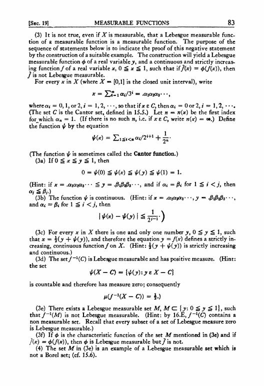
[SEC. 191 MEASURABLE FUNCTIONS 83
(3) It is not true, even if X is measurable, that a Lebesgue measurable function of a measurable function is a measurable function. The purpose of the sequence of statements below is to indicate the proof of this negative statement by the construction of a suitable example. The construction will yield a Lebesgue measurable function 0 of a real variable^, and a continuous and strictly increasing function/of a real variable x, 0 ^ x ^ 1, such that if/(#) = 0(/(#))> then / is not Lebesgue measurable.
For every x in X (where X « [0,1] is the closed unit interval), write
whereat = 0, l , o r 2 , / = 1,2, • • -,so that if* 8 C, thena» =* 0or2 , / = 1,2, • • •• (The set C is the Cantor set* defined in 15.5.) Let n « n(x) be the first index forjvhich ccn = 1. (If there is no such n, i.e. if x e C, write n{x) = oe.) Define the function ^ by the equation
^W = Z i ^ < B ^ / 2 ^ + ~ .
(The function ^ is sometimes called the Cantor function.) (3a) UO^x^y^ 1, then
0 = *(0) s *(*) ^ +(y) £ *( l) = 1.
(Hint: if x = .aia&y • • g y = .ftftft- • *, and if a, = ft for 1 ^ / < ; , then
(3b) The function ^ is continuous. (Hint: if x = .aia^s* • - ^ « ./Siftft* • •, and a* = ft for 1 ^ / <. / , then
(3c) For every # in X there is one and only one number y, 0 ^ y ^ 1, such that * = £(.y + M.y))> and therefore the equation^ = / (* ) defines a strictly increasing, continuous function/on X. (Hint: §(.? + MjO) 1S strictly increasing and continuous.)
(3d) The set/ - 1((?) is Lebesgue measurable and has positive measure. (Hint: the set
is countable and therefore has measure zero; consequently
»<J-\X - O) = |.)
(3e) There exists a Lebesgue measurable set M, M C {.y: 0 ^ .y ^ 1}, such that /_ 1(A^) is not Lebesgue measurable. (Hint: by 16.E, f~l{C) contains a non measurable set. Recall that every subset of a set of Lebesgue measure zero is Lebesgue measurable.)
(3f) If <t> is the characteristic function of the set M mentioned in (3e) and if /(#) = <t>(f(x))> then <t> is Lebesgue measurable b u t / is not.
(4) The set M in (3e) is an example of a Lebesgue measurable set which is not a Borel set; (cf. 15.6).

84 MEASURABLE FUNCTIONS [SEC. 20]
§ 2 0 . SEQUENCES OF MEASURABLE FUNCTIONS
Theorem A. If \fn\ is a sequence of extended real valued^ measurable functions on a measurable space X> then each of the four functions h> £ , /* , andf*> defined by
h{x) = sup {/«(*): n = 1, 2, • • •} ,
g(x) = inf {/*(*):* = 1,2, • - . } ,
/*(*) = lim supn/„(#),
/*(#) = lim infn/n(x),
is measurable.
Proof. It is easy to reduce the general case to the case of finite valued functions. The equation
\x:g{x) <c} = U r - i {*••/«(*) <*}
implies the measurability of g. The result for h follows from the relation
h{x) = - i n f {- / . (*) :» = 1,2, . . . } .
The measurability of/* and/* is a consequence of the relations
/*(*) = infnS1supm^n/m(^), /*(#) = sup„>, infWfcn/m(x),
respectively. | It follows from Theorem A that the set of points of convergence
of a sequence \fn) of measurable functions, i.e. the set
{x: lim supn/n(#) = lim infn/»(*)},
has a measurable intersection with every measurable set, and, consequently, that the function / , defined by f{x) = limn/n(#) at every x for which the limit exists, is a measurable function.
A very useful concept in the theory of measurable functions is that of a simple function. A function/, defined on a measurable space Xy is called simple if there is a finite, disjoint class {E\> • • •,

[SEC. 20] MEASURABLE FUNCTIONS 85
En] of measurable sets and a finite set {ai, • • •, an\ of real numbers such that
/ ( * ) <*{ if x e Eiy i = 1, • • • , # ,
0 if x e' Ex U - . . U En.
(We emphasize the fact that the values of a simple function are to be finite real numbers: this will be essential in the sequel.) In other words a simple function takes on only a finite number of values different from zero, each on a measurable set.
The simplest example of a simple function is the characteristic function XE of a measurable set E. It is easy to verify that a simple function is always measurable; in fact we have, for the simple function/ described above,
/(*) = 2?-i ««*«(*)•
The product of two simple functions, and any finite linear combination of simple functions, are again simple functions.
Theorem B. Every extended real valued measurable junction f is the limit of a sequence [fn\ of simple functions; iff is non negative•, then eachfn may be taken non negative and the sequence {fn} may be assumed increasing.
Proof. Suppose first t h a t / ^ 0. For every n = 1, 2, • • •, and for every x in Xy we write
/ . ( * ) if 1—±z/(x)<±., ; - i , ...,2-«,
2" 2 « if f(x) ^ n
Clearly / „ is a non negative simple function, and the sequence {/„} is increasing. If/(x) < <», then, for some «,
tf/(*) = °°> then/n(#) = » for every n. This proves the second half of the theorem; the first half follows (recalling that the
86 MEASURABLE FUNCTIONS [SEC. 21)
difference of two simple functions is a simple function) by apply-ing the result just proved separately t o / + a n d / - . |
(1) All the concepts and results of this section and the preceding one (except, of course, the ones depending on such order properties of the real numbers as positiveness) can be extended to complex valued functions.
(2) If the function/ in Theorem B is bounded, then the sequence {/«} may be made to converge t o / uniformly.
(3) An elementary function is defined in the same way as a simple function, the only change being that the number of sets £ t , and therefore the number of corresponding values az, is allowed to be countably infinite. Every real valued measurable function/ is the limit of a uniformly convergent sequence of elementary functions.
§ 2 1 . POINTWISE CONVERGENCE
In the preceding three sections we have developed the theory of measurable functions about as far as it is convenient to do so without mentioning measure. From now on we shall suppose that the underlying space X is a measure space {XySyn).
If a certain proposition concerning the points of a measure space is true for every point, with the exception at most of a set of points which form a measurable set of measure zero, it is customary to say that the proposition is true for almost every point, or that it is true almost everywhere. The phrase "almost everywhere" is used so frequently that it is convenient to introduce the abbreviation a.e. Thus, for instance, we might say that a function is a constant a.e.—meaning that there exists a real number c such that {x: f(x) ^ c) is a set of measure zero. A function/ is called essentially bounded if it is bounded a.e., i.e. if there exists a positive, finite constant c such that {x: \f(x) \ > c} is a set of measure zero. The infimum of the values of c for which this statement is true is called the essential supremum of | / | , abbreviated to
ess. sup. | / | *
Let {/n} be a sequence of extended real valued functions which converges a.e. on the measure space .ST to a limit function / . This means, of course, that there exists a set E0 of measure zero (which may be empty) such that, if x e' E0 and c > 0, then an

[SEC. 21] MEASURABIE FUNCTIONS 87
integer nQ = n0(xye) can be found with the property that
/»(*) < - - , if /(*) = - « ,
6
whenever # ^ w0. We shall say that a sequence {/n} of real valued functions is fundamental a.e. if there exists a set E0 of measure zero such that, if x e'E0 and c > 0, then an integer »o = flb(#>«) can be found with the property that
| /n(#) — fm(x) I < €, whenever # ^ w0 and w ^ w0.
Similarly in the theory of real sequences one distinguishes between a sequence [an] of extended real numbers which converges to an extended real number a, and a sequence [an) of finite real numbers which is a fundamental sequence, i.e. which satisfies Cauchy's necessary and sufficient condition for convergence to a finite limit.
It is clear that if a sequence converges to a finite valued limit function a.e., then it is fundamental a.e., and, conversely, that corresponding to a sequence which is fundamental a.e. there always exists a finite valued limit function to which it converges a.e. If moreover the sequence converges a.e. t o / and also converges a.e. to gy then /(#) = g(x) a.e., i.e. the limit function is uniquely determined to within a set of measure zero.
We shall have occasion in the sequel to refer to several different kinds of convergence, and we shall consistently employ terminology similar to that of the preceding paragraphs. Thus, if we define a new kind of convergence of a sequence {/n} to a limit/, by specifying the sense in which/n is to be near t o / for large n> then we shall use without any further explanation the notion of a sequence which is fundamental in this new sense— meaning that, for large n and m> the differences/n —/« are to be near to 0 in the specified sense of nearness.
An example of another kind of convergence for sequences of real valued functions is uniform convergence a.e. The sequence

88 MEASURABLE FUNCTIONS [SBC. 21]
\Jn) converges t o / uniformly a.e. if there exists a set E0 of measure zero such that, for every e > 0, an integer n0 = Wo(<0 can be found with the property that
|/n(#) —fix) ! < «> ^ n ^ «o and # e' £0>
in other words if the sequence of functions converges uniformly to / (in the ordinary sense of that phrase) on the set X — E0. Once more it is true, and easily verified, that a sequence converges uniformly a.e, to some limit function if and only if it is uniformly fundamental a.e.
The following result (known as EgorofPs theorem) establishes an interesting and useful connection between convergence a.e. and uniform convergence.
Theorem A. If E is a measurable set of finite measure^ and if {fn} is a sequence of a.e. finite valued measurable functions which converges a.e. on E to a finite valued measurable function / , theny for every e > 0, there exists a measurable subset F of E such that /*(F) < e and such that the sequence {fn} converges tof uniformly on E — F.
Proof. By omitting, if necessary, a set of measure zero from Ey we may assume that the sequence {fn\ converges t o / everywhere on E. If
I m\ then
Eim czE2m c - . . ,
and, since the sequence {/n} converges t o / o n E,
limn Enm z> E
for every m = I, 2, • • •. Hence limn v{E — Enm) = 0, so that
there exists a positive integer n0 = n^m) such that
M(£ - En0Mm) < £•

[SEC. 21} MEASURABLE FUNCTIONS 89
(To be sure n0 depends also on ey but t remains fixed throughout the entire proof.) If
F = u:- i (£ - Eno(mr),
then F is a measurable set, F C Ey and
M(^) = M(U:-1 (^ - En0(m)m)) ^ E : - l M(£ - £„0(m)m) < *.
Since £ - F = £ n f | m - i En^m)m
y and since, therefore, for w ^ nQ(m) and for # in E — F, we have x e £ n
w , it follows that
\fn(x) — /(*) | < —• > which proves uniform convergence on m
E-F. |
Motivated by EgorofFs theorem we introduce the concept of almost uniform convergence. A sequence \fn\ of a.e. finite valued measurable functions will be said to converge to the measurable function / almost uniformly if, for every c > 0, there exists a measurable set F such that y.(F) < c and such that the sequence {/n} converges t o / uniformly on F\ In this language EgorofFs theorem asserts that on a set of finite measure convergence a.e. implies almost uniform convergence. The following result goes in the converse direction.
Theorem B. If {fn} is a sequence of measurable functions which converges to f almost uniformly», then \fn\ converges to f a.e.
Proof. Let Fn be a measurable set such that u(Fn) < -n
and such that the sequence {/„} converges t o / uniformly on Fn\n = 1,2, • - . . I f F - f i : . i F n , t h e n
M ( / 0 ^ M ( F » ) < - , n
so that p(F) =s 0, and it is clear that, for x in F'y j / n (x) j converges to /(#)• |
We remark that the phrase "almost uniform convergence" is a somewhat confusing (but unfortunately standard) misnomer,

90 MEASURABLE FUNCTIONS [SEC. 22]
which conflicts with the "almost everywhere" terminology. Some such phrase as "nearly uniform convergence" might come closer to suggesting the true state of affairs; as it stands, some care has to be exercised to distinguish between almost uniform convergence and almost everywhere uniform convergence.
(1) I f / is any real valued, Lebesgue measurable function on the real line, then there exists a Borel measurable function g such that /(#) = g(x) a.e. (Hint: write Er = {x: J(x) < r] for every rational number r, and use 13.B to express Er in the form FT A NTy where Fr is a Borel set and Nr has measure zero. Let N be a Borel set of measure zero containing \Jr Nr and define g by
JO if xeN, * W l / M if xe'N.
Cf. 18.2.) (2) If E is a measurable set of positive finite measure, and if {/nj is a sequence
of a.e. finite valued measurable functions which is fundamental a.e., then there exists a positive finite constant c and a measurable subset F of E of positive measure such that, for every n = 1, 2, • • • and for every x in F, \/n(x) \ ^ c*
(3) If E is a measurable set of c-finite measure, and if {/„) is a sequence of a.e. finite valued measurable functions which converges a.e. on E to a finite valued measurable function/, then there exists a sequence {£;) of measurable sets such that n(E — U"-i £»') = 0 anc* such that the sequence (/„} converges uniformly on each £», / = 1, 2, • • •. (Hint: it is sufficient to prove the result if n(E) < oo. In this case apply EgororFs theorem to find E{ so that
M ( £ - U ? - I £ < ) < -tl
and so that {/nJ converges uniformly on E{.) (4) Let X be the set of positive integers, let S be the class of all subsets of
X, and, for E in S, let/u(£) be the number of points in E. If Xn is the characteristic function of the set jl , •••, n}y then the sequence (xn) converges to 1 everywhere but it is not almost uniformly fundamental. In other words, EgorofFs theorem is not true if E is not of finite measure.
(5) For every essentially bounded function/, write | | / | | = ess. sup. [/[. If {/n} is a sequence of essentially bounded measurable functions, then the sequence {/n} converges to/uniformly a.e. if and only if lim„ | | /n ~ / | | = 0.
(6) Is the set 9TI of all essentially bounded measurable functions a Banach space with respect to the norm described in (5)?
§ 22 . CONVERGENCE IN MEASURE
In this section, as in the preceding one, we shall work throughout with a fixed measure space (XySyp).

[SEC. 22] MEASURABLE FUNCTIONS 91
Theorem A. Suppose that} andfny n = 1, 2, • • •, are real valued measurable functions on a set E of finite measure, and write, for every € > 0,
£n(e) = {x: \fn(x) - / ( * ) | ^ € } , n = 1, 2, . •. .
The sequence \fn) converges tof a.e. on E if and only if
for every t > 0.
Proof. It follows from the definition of convergence that the sequence {fn(x)\ of real numbers fails to converge to the real number f(x) if and only if there is a positive number e such that x belongs to En(e) for an infinite number of values of n. In other words, if D is the set of those points x at which {fn(x)\ does not converge to/(#), then
D = U«>0 Km SUpn £n(€) = (Jfc-1 Km SUPn En ( - V
Consequently a necessary and sufficient condition that ix{E fl D) = 0 (i.e. that the sequence {fn\ converge t o / a.e. on E) is that n(E fl lim supn En(e)) = 0 for every e > 0. The desired conclusion follows from the relations
M(£ fl lim supn En(e)) = »(E fl f | : . i U : - n £m(6)) =
= limn M(£ fl U^-n Em(e)). |
The desire to investigate the result of an obvious weakening of the condition of Theorem A motivates the definition of still another method of convergence which has frequent application. A sequence \fn) of a.e. finite valued, measurable functions converges in measure to the measurable function / if, for every e > 0, limn n({x: \fn(x) —/(#) I ^ «}) = 0. In accordance with our general comment on different kinds of convergence in the preceding section, we shall say that a sequence {fn\ of a.e. finite valued measurable functions is fundamental in measure if, for every c > 0,
M({*: |/n(*) ~fm{x) I > c}) -> 0 as n and m -> oo.
92 MEASURABLE FUNCTIONS [SEC. 22]
It follows trivially from Theorem A that if a sequence of finite valued measurable functions converges a.e. to a finite limit [or is fundamental a.e.] on a set E of finite measure, then it converges in measure [or is fundamental in measure] on E. The following theorem is a slight strengthening of this assertion in that it makes no assumptions of finiteness.
Theorem B. Almost uniform convergence implies convergence in measure.
Proof. If \fn) converges to / almost uniformly, then, for any two positive numbers e and 5, there exists a measurable set Fsuch that fi(F) < 5 and such that | /n(#) —/(*) I < *, whenever x belongs to F' and n is sufficiently large. |
Theorem C. If \fn) converges in measure to / , then \fn\ is fundamental in measure. If also {fn} converges in measure to gy thenf = g a.e.
Proof. The first assertion of the theorem follows from the relation
C {*: \Mx) -f(x) | £ ^ U {*: !/„(*) - / ( * ) | ^ i j •
To prove the second assertion, we observe that, similarly,
c { * : \Mx) -f(x) | ^ ^ U {*: | /n(*) - *(*) | ^ } •
Since, by proper choice of n, the measure of both sets on the right can be made arbitrarily small, we have
**({*: |/(*) - *(*) I M ) = 0 for every e > 0; this implies, as asserted, t h a t / = g a.e. |
In addition to these comparatively elementary remarks, we shall present two slightly deeper properties of convergence in measure.

[SEC.22] MEASURABLE FUNCTIONS 93
Theorem D. If [fn\ is a sequence of measurable functions which is fundamental in measure, then some subsequence \fnk} is almost uniformly fundamental.
Proof. For any positive integer k we may find an integer n(k) such that if n ^ n{k) and m ^ n(k), then
M({*:|/.M -/.(*) |fc^})<~ We write
»i - »(1), »2 = (»i + 1) U J?(2), »3 = (»2 + 1) U »(3), • • •;
then #! < n2 < nz < • - -, so that the sequence {fnk\ is indeed an infinite subsequence of {/n}. If
&-[*:|/J*)-U«)l4) and £ ^ i ±S ./, then, for every x which does not belong to Ek U £fc+1 U £jb+2 U • • •, we have
so that, in other words, the sequence {fni} is uniformly fundamental on X — (Ek U Ek+\ U • • •)• Since
M(£* U £fc+1 U • • •) 3 £ : - * M ( £ J < 2^r ,
the proof of Theorem D is complete. |
Theorem E. If {fn} is a sequence of measurable functions which is fundamental in measure, then there exists a measurable
function f such that [fn\ converges in measure tof
Proof. By Theorem D we can find a subsequence {fnk\ which is almost uniformly fundamental and therefore fundamental a.e.; we write f(x) = lim*/njb(;e) for every x for which the limit exists. We observe that, for every e > 0,
94 MEASURABLE FUNCTIONS [SEC. 22]
The measure of the first term on the right is by hypothesis arbitrarily small if n and nk are sufficiently large, and the measure of the second term also approaches 0 (as k —» «>), since almost uniform convergence implies convergence in measure. |
(1) Suppose that the measure space (Af,S,/*) is totally finite, and let {/«} and {gn} be sequences of finite valued measurable functions converging in measure t o / and g respectively.
(la) If a and /3 are real constants, then \a/n + fign} converges in measure to <*/ + te (|/n |} converges in measure to | / | .
(lb) If / = 0 a.e., then {/n2} converges in measure to / 2 .
(lc) The sequence {fng} converges in measure to/jg-. (Hint: given a positive number 5, find a constant c such that if E = \x: | g{x) | ^ r}, then n(X — E) < 5, and consider the situation separately on E and X — E.)
(Id) The sequence {/n2} converges in measure t o / 2 . (Hint: apply (lb) to
(le) The sequence \fngn) converges in measure to jg. (Hint: apply the identity which expresses a product in terms of sums and squares.)
(If) Are the statements (la)-(le) valid for measure spaces which are not totally finite?
(2) Every subsequence of a sequence which is fundamental in measure is fundamental in measure.
(3) If {/n} is a sequence of measurable functions which is fundamental in measure, and if {/«,} and {/my} are subsequences which converge a.e. to the limit functions/ and g respectively, then/ = g a.e.
(4) If X is the set of positive integers, S is the class of all subsets of Xy and, for every E in S, fi(E) is the number of points in £ , then, for the measure space (XyS,n)y convergence in measure is equivalent to uniform convergence everywhere.
(5) Is it necessarily true on a set of infinite measure that convergence a.e. implies convergence in measure? (Cf. 21.4 and (4).)
(6) Let the measure space X be the closed unit interval with Lebesgue measure. If, for n = 1, 2, • • •,
and if Xn* is the characteristic function of £ nl , then the sequence {xi1, X21, X22,
Xa1, X32> X33> • • •} converges in measure to 0, but fails to converge at any point ofX.
(7) Let \En} be a sequence of measurable sets and let Xn be the characteristic function of Eny n = 1, 2, • • •. The sequence \xn\ is fundamental in measure if and only if p(EniEm) —* 0 as n and m —> 00. (For the definition of p see 9.4.)

Chapter V
I N T E G R A T I O N
§ 23 . INTEGRABLE SIMPLE FUNCTIONS
A simple function/ = X?-i <*<X£%. on a measure space (X,S,/i) is integrable if n(Ei) < °o for every index i for which at- p* 0. The integral of/, in symbols
ff(x)dp(x) or ffd»
is defined by I/dp = ]C?-i <*iM(£t)« It follows easily from the ad-
ditivitv of u that if/ is also equal to ^JLiPflCpp then If dp =
S f - i ft-M(-Py)> i-e- that the value of the integral is independent of the representation of/ and is therefore unambiguously defined. We observe that the absolute value of an integrable simple function, a finite, constant multiple of an integrable simple function, and the sum of two integrable simple functions are integrable simple functions.
If £ is a measurable set a n d / is an integrable simple function, then it is easy to see that the function XEJ is an integrable simple function also; we define the integral of/ over E by
J fdn =jxEfdn.
The simplest example of an integrable simple function is the characteristic function of a measurable set E of finite measure;
we have I xsdfi = I d\x = \i{E).
95

96 INTEGRATION [SEC. 231
In the sequel we shall define the notions of integrability and integral on a wider domain than the class of integrable simple functions. Some useful definitions and the statements of several important results (but very few proofs) depend only on such elementary properties of integration as we have already explicitly mentioned. In order to avoid unnecessary duplication, we shall therefore proceed as follows. Throughout this section we shall use the word "function" as an abbreviation for "simple function." As a consequence of this policy all our definitions and theorems will make sense not only for simple functions but also for the wider class we shall subsequently consider. The proofs in this section will, however, apply to simple functions only; we shall complete the proofs, so that they will apply to the more general case also, a little later.
The proofs of Theorem A and B below are omitted; these results are immediate consequences of the definitions and, in the case of Theorem A, an obvious and simple computation.
Theorem A, Iff and g are integrable functions and a and j8 are real numbers, then
f(cf + Pg)dn = affdp + pfgdn.
Theorem B. If an integrable function f is non negative
a.e.y then If dp ^ 0.
Theorem C. Iff and g are integrable functions such that f ^ g a.e.y then
Jfdn ^Jgd»-
Proof. Apply Theorem B t o / — g in place of/. |
Theorem D. Iff and g are integrable functions y then
f\f + gfo*f\J\<l*+f\g\fa Proof. Apply Theorem C to \f \ + \ g \ and \f + g | in place
of/ and gy respectively. |

[SEC. 23] INTEGRATION 97
Theorem E. Iff is an integrablefunction, then
Proof. Apply Theorem C first to | / | a n d / and then to | / | and - / . |
Theorem F. Iff is an integrable junrtion, a and /3 are real numbers, and E is a measurable set such that, for x in E, a £ / ( * ) ^ P,then
ME) £ ffdn ^ ME).
Proof. Since the principal assumption is equivalent to the relation a\E ^ XEf ^ &XEy the desired result follows from Theorem C if 11(E) < 00; the case in which /*(£) = 00 is easily treated by direct application of the definition of integrability. |
The indefinite integral of an integrable function / is the set
function vy defined for every measurable set E by v(E) = I fdp. JE
Theorem G. If an integrable function f is non negative a.e.y
then its indefinite integral is monotone.
Proof. If E and F are measurable sets such that E c Fy
then %Ef ^ XF/a.e., and the desired result follows from Theorem
c 1 A finite valued set function v defined on the class of all measur
able sets of a measure space (XySyp) is absolutely continuous if for every positive number c there exists a positive number 8 such that I v(E) I < e for every measurable set E for which /*(£) < 8.
Theorem IL The indefinite integral of an integrable function is absolutely continuous.
Proof. If c is any positive number greater than all the values of | / | , then, for every measurable set Ey we have
\(fdn\ < c»{E). I

98 INTEGRATION [SEC. 24]
Theorem I. The indefinite integral of an integrable Junction is countably additive.
Proof. I f / is the characteristic function of a measurable set E of finite measure, then the assertion of countable additivity for the indefinite integral of/ is just a restatement of the countable additivity of 11 on measurable subsets of E. The assertion of the theorem for arbitrary integrable simple functions is a consequence of the fact that every such function is a finite linear combination of characteristic functions. |
I f / and g are integrable functions, we define the distance, p(/,£), between them by the equation
p(/,g)=J\/-g\^. The function p deserves the name "distance" in every respect but one. It is true and trivial that
p(A/) = 0, ptfjr) = pQr,/), and p(/*) ^ P{gyh) + P{hJ).
It is not true, however, that if p(f,g) = 0, t hen / = g. The distance between two integrable functions can, for instance, vanish if they are equal almost everywhere (but not necessarily everywhere). In a subsequent section we shall study this phenomenon in some detail.
(1) If one of two simple functions is integrable, then so is their product. (2) If E and F are measurable sets of finite measure, then P(XJJ,XF) =
IJL(EAF). Cf. 9.4 and 22.7. (3) Let (XySji) be the closed unit interval with Lebesgue measure, and, for
some fixed point #o in Xy write v{E) = XJS(*O). Is the set function v absolutely continuous?
(4) If v is an absolutely continuous set function on the class of all measurable sets of a measure space (A^S,/*), then v(E) — 0 for every measurable set E for which JJL(E) = 0.
(5) If a totally finite measure space X consists of a finite number of points, then every real valued measurable function on X is an integrable simple function, and the theory of integration specializes to the theory of finite sums.
§ 2 4 . SEQUENCES OF INTEGRABLE SIMPLE FUNCTIONS
We shall continue in this section to work with a fixed measure space CXTjS,/*), and to use the device of abbreviating "simple

[SEC. 24] TNTFGRATION 99
function" to "function." Since all the methods of this section (with only one minor exception, occurring at the end of the proof of Theorem D) are based on the general results of the preceding section, it will turn out that not only the statements but even the proofs of the following theorems will remain unaltered when we turn to the general case.
A sequence {/„} of integrable functions is fundamental in the mean, or mean fundamental, if
p(fnyfm) —> 0 as n and m —> GO.
Theorem A. A mean fundamental sequence {/n} of Integra-ble functions is fundamental in measure.
Proof. If, for any fixed positive number €,
Enm = {*: | / » ( t f ) —/mi*) \ ^ c } ,
then
P(fnjm) = f\fn - fm W ^ f l / » " / « W ^ ^ W ,
so that jji(Enm) —> 0 as n and m -* <». |
Theorem B. If \fn) is a mean fundamental sequence of integrable functionsy and if the indefinite integral of / „ is vny
n = 1, 2, • • •, then v(E) = limn pn(£)
exists for every measurable set Ey and the set function v is finite valued and countably additive.
Proof. Since | vn(E) - vm(E) \^f\fn-fm \dv -* 0 as n and
m —> oo, the existence, finiteness, and uniformity of the limit are clear, and it follows from the finite additivity of limits that v is finitely additive. If {En\ is a disjoint sequence of measurable sets whose union is Ey then we have, for every pair of positive integers n and k
\v(E)-Y2-i>>{E<)\ ^ £ I v(E) - vn{E) | + | F„(£) - T,1.i *»(£.) I
+ |"»(U?-1^)-KU*-1£,)|.

100 INTEGRATION [SEC. 24)
The first and third terms of the right side of this inequality may be made arbitrarily small by choosing n sufficiently large, and, for fixed ny the middle term may be made arbitrarily small by choosing k sufficiently large. This proves that
v(E) = linn £ ? - ! r(Et) = £,--! v{Et). \
If {vn} is a sequence of finite valued set functions defined for all measurable sets, we say that the terms of the sequence are uniformly absolutely continuous whenever for every positive number c there exists a positive number 5 such that | vn(E) \ < e for every measurable set E for which p(E) < 8, and for every positive integer n.
Theorem C. If \fn\ is a mean fundamental sequence of integrate functions, and if the indefinite integral of fn is vny
n = 1, 2, • • •, then the set functions vn are uniformly absolutely continuous.
Proof. If € > 0, let n0 be a positive integer such that, for n ^ n0 and m ^ n0y
and let 8 be a positive number such that
[\fn\dn < ^ , n = 1, •••, n0
for every measurable set E for which \i{E) < 8; (cf. 23.H). If E is a measurable set for which ix(E) < 8 and if n :g n0y then
K(£)Uf|/„|4.<«; JE
if, on the other hand, n > n0y then
I * „ ( £ ) | ^ f\/n " / n o W + f l / n . W < «• I
Since the following theorem is of no particular importance in the general case, we shall restrict its statement and proof to the case of simple functions only.
[SEC. 24] INTEGRATION 101
Theorem D. If {/„} and \gn\ are mean fundamental sequences of integrable simple functions which converge in measure to the same measurable function / , // the indefinite integrals offn and gn are vn and Xn respectively, and if, for every measurable set Ey
v(E) = limn vn(E) and \(E) « limnXn(£),
then the set functions v and X are identical.
Proof. Since, for every c > 0,
£n= {*:!/.(*)-*.(*) I M C
C {*: | / nW - / ( * ) I ^ ^} U {*: |/(*) - gn(x) | ^ -'} ,
it follows that limn n(En) = 0. Hence, if E is a measurable set of finite measure, then in the relation
f\fn-gn\dn£{ \fn~gn\dn+f \fn W + f \ gn \ft JjE JE-Bn JEnEn JEnEn
the first term on the right is dominated by e/*(£), and the last two terms can be made arbitrarily small by choosing n sufficiently large, because of the uniform absolute continuity proved in Theorem C. I t follows that
limn | vn{E) - Xn(£) | = 0,
and hence that v(E) = X(£). Since v and X are both countably additive, it follows that v{E) = \(E) for every measurable set E of c-finite measure.
Since the / n and gn are simple functions, each of them is defined in terms of a finite class of measurable sets of finite measure. If E0 is the union of all sets in all these finite classes, then E0 is a measurable set of <r-finite measure, and we have, for every measurable set E,
vn(E - E0) = \n(E -E0)=0
and therefore v(E — E0) = \(E — E0) = 0. Since this implies that v(E) = v(E fl E0) and X(£) = X(£ fl E0)y the proof of Theorem D is complete. |

102 INTEGRATION [SEC. 25)
(1) Is the set of all integrable simple functions a complete metric space with respect to the distance p?
(2) In the notation of Theorem B, if \En] is a disjoint sequence of measurable sets, then the series J n - i K ^ n ) converges absolutely. (Hint: the series converges unconditionally.)
§ 25. INTEGRABLE FUNCTIONS
An a.e. finite valued, measurable function / on a measure space (X>S>n) is integrable if there exists a mean fundamental sequence \fn} of integrable simple functions which converges in measure t o / . The integral of/, in symbols
ff(x)Mx) or J / 4 *
is defined by \jd\i = limn l/n^M- It follows from 24.D (with E
= \JnN(fn)) that the value of the integral o f / is uniquely determined by any particular such sequence. We emphasize the fact that the value of the integral is always finite. We observe that it follows from the known and obvious properties of mean convergence and convergence in measure that the absolute value of an integrable function, a finite constant multiple of an integrable function, and the sum of two integrable functions are integrable functions. The relations
r = w\+f) and r-w\-n show also that i f / i s integrable, then/4" a n d / - are integrable.
If E is a measurable set and if \fn) is a mean fundamental sequence of integrable simple functions converging in measure to the integrable function/, then it is easy to see that the sequence {XE/TI} is mean fundamental and converges in measure to XE/>
We define the integral of/ over E by
J ^ ^jXxfdp-
We recall that the theorems of §§ 23 and 24 were stated for general integrable functions but were proved for integrable simple functions only. We are now in a position to complete their proofs.

[SEC. 25] INTEGRATION 103
The results 23.A and 23.B follow immediately from elementary properties of limits; 23.C-23.G follow from 23.B verbatim as before.
To prove the absolute continuity of an indefinite integral, 23.H, let {/n} be a mean fundamental sequence of integrable simple functions which converges in measure to the integrable function/. We have
I \fdv. | £ | [jnd» | + | [fJp. - C/dn |, JE JE JE JE
for every measurable set E. Since t h e / n are simple functions, the theorem 24.C on uniform absolute continuity may be applied to prove that the first term on the right becomes arbitrarily small if the measure of E is taken sufficiently small. The second term on the right approaches 0 as n —> oo, by the definition of
J jd[i.\ this completes the proof of 23.H. E The proof of the countable additivity of an indefinite integral
is even simpler. Indeed, using the notation of the preceding paragraph, the fact that t h e / n are simple functions justifies the application of 24.B, which then yields exactly the assertion of 23.1.
The proofs of 24.A-24.C were based on the statements, and not on the proofs, of the results of § 23, and are therefore valid in the general case. This remark completes the proofs of all the theorems of the preceding two sections.
We shall say that a sequence \fn) of integrable functions converges in the mean, or mean converges, to an integrable function/if
P(fnyf) = J | /« ~ / K ~+ 0 aS ft -» 00.
Our first result concerning this concept is extremely similar, in statement and in proof, to 24.A.
Theorem A, If {fn\ is a sequence of integrable functions which converges in the mean to / , then {/n} converges to f in measure.
104 INTEGRATION [SEC. 25]
Proof. If, for any fixed positive number c,
then
f\fn ~fW ^fE\/n -fW ^ *M(£n),
so that n(En) —> 0 as n -» oo. |
Theorem B. Iff is an a.e. non negative integrable function,
then a necessary and sufficient condition that If dp = 0 is that
/ = 0 a.e.
Proof. If / = 0 a.e., then the sequence each of whose terms is identically zero is a mean fundamental sequence of integrable simple functions which converges in measure t o / , and it follows
that jfdfi = 0. To prove the converse, we observe that if {/n}
is a mean fundamental sequence of integrable simple functions which converges in measure to / , then we may assume that fn ^ 0, since we may replace each/n by its absolute value. The
assumption If dp = 0 implies that limn lfnd\i = 0, i.e. that
{/n} mean converges to 0. It follows from Theorem A that {fn\ converges to 0 in measure and hence the desired result is implied by 22.C. |
Theorem C. Iff is an integrable function and E is a set of measure zero, then
{fdv - 0. JE
Proof. Since I fdjx = I xsfdiiy and since the characteristic
function of a set of measure zero vanishes a.e., the desired result follows from Theorem B. |
Theorem D. Iff is an integrable function which is positive
a.e. on a measurable set E> and if I fdy. = 0, then y.(E) = 0. JE
[SEC. 25] INTEGRATION 105
Proof. We write F0 = {*:/(*) > 0} and Fn = {*:/(*) ^ - ) ,
n = 1, 2, • • •; since the assumption of positiveness implies that E — F0 is a set of measure zero, we have merely to prove that E PI Fo is one also. Since
0 = f fdn^-n(EViFn) £ 0 ,
and since F0 = U"- i ^ e desired result follows from the relation M(£ n F0) ^ EnW-i n{E fl Fn). |
Theorem E. If f is an integrable function such that
J fdn = Ofor every measurable set Fy then/ = 0 a.e. F
Proof. If E = {*:/(#) > 0}, then, by hypothesis, | / //x = 0,
and therefore, by Theorem D, E is a set of measure zero. Applying the same reasoning to —/ shows that {#:/(#) < 0} is a set of measure zero. |
Theorem F. If f is an integrable function, then the set N(J) = ix:/(x) ** 0} to* a-finite measure.
Proof. Let {/n} be a mean fundamental sequence of integrable simple functions which converges in measure to / . For every n = 1, 2, • • •, N(Jn) is a measurable set of finite measure. If E = N{f) — (Jn-i N{fn), and if F is any measurable subset of Ey then it follows from the relation
I fdy. « limn f fndfi * 0
and Theorem E t h a t / = 0 a.e. on E. In view of the definition of N(J) this implies that p(E) = 0; we have
w)cu:.iWn) u£ i It is frequently useful to define the symbol if dp for certain
non integrable functions/. If, for instance,/ is an extended real

106 INTEGRATION [SEC. 25]
valued, measurable function such that / ^ 0 a.e. and if / is not integrable, then we write
j/dfl = 00.
The most general class of functions/ for which it is convenient
to define Ifdy. is the class of all those extended real valued measur
able functions/ for which at least one of the two functions/"1"
and/~ is integrable; in that case we write
J/* = //+^M - J r * .
Since at most one of the two numbers, I / ^ M and \f~dix, is
infinite, the value of If dp is always + 0 0 , — °o, or a finite real
number—it is never the indeterminate form <x> — oo. We shall make free use of this extended notion of integration, but we shall continue to apply the adjective "integrable" to such functions only as are integrable in the sense of our former definitions.
(1) If X is the space of positive integers (described, for instance, in 22.4), then a function/ is integrable if and only if the series ]£n- x |/(w) | is convergent,
and, if this condition is satisfied, then if dp - ]C»«i/(tf).
(2) If/ is a non negative integrable function, then its indefinite integral is a finite measure on the class of ail measurable sets.
(3) If/ is integrable, then, for every positive number €,
M({*: | / (*) | £ « } ) < oo.
(4) If g is a finite, increasing, and continuous function of a real variable, and J2g is the Lebesgue-Stieltjes measure induced by g (cf. 15.9), and if/ is a function
which is integrable with respect to this measure, then the integral \f{x)djxg(x)
is called the Lebesgue-Stieltjes integral of/ with respect to g and is denoted by
I f(x)dg(x)* lf> ln particular, g(x) = x, then we obtain the Lebesgue integral,
f(x)dx. Iff is a continuous function such that N(f) is a bounded
set, t h e n / is Lebesgue integrable.
[SEC. 26] INTEGRATION 107
§ 2 6 . SEQUENCES OF INTEGRABLE FUNCTIONS
Theorem A. If \fn) is a mean fundamental sequence of integrable simple functions which converges in measure to the integrable function j \ then
Pifjn) = J | / - / n | ^ M -» 0 as n -» oo;
hencey to every integrable function f and to every positive number €, there corresponds an integrable simple function g such that p(f,g) < €.
Proof. For any fixed positive integer my {\fn — fm \} is a mean fundamental sequence of integrable simple functions which converges in measure to \f — fm |, and, therefore,
J\f -fm \dp = limn J | / n - /T O \dp.
The fact that the sequence {/n} is mean fundamental implies the desired result. |
Theorem B. If {fn\ is a mean fundamental sequence of integrable functions•, then there exists an integrable function f
such that p(fnyf) —> 0 (and consequently \fndp —> if dp) as n —> oo.
Proof. By Theorem A, for each positive integer n there is an
integrable simple function gn such that p(Jnygn) < - • It follows n
that [gn] is a mean fundamental sequence of integrable simple functions; l e t / be a measurable (and therefore integrable) function such that {gn} converges in measure t o / . Since
0 g I J/J* -fa I <L JV„ -J\dy. - p(/n,f) £
^ P(fn,gn) + p(g«,f),
the desired result follows from Theorem A. |

108 INTEGRATION {SEC. 26)
In order to phrase our next result in a concise and intuitive fashion, we recall first the definition of a certain kind of continuity for set functions. A finite valued set function v on a class E of sets is continuous from above at 0 (cf. § 9) if, for every decreasing sequence {En} of sets in E for which limn En = 0, we have limn v{En) = 0. If {pn\ is a sequence of such finite valued set functions on E, we shall say that the terms of the sequence are equicontinuous from above at 0 if, for every decreasing sequence {En\ of sets in E for which limn En = 0, and for every positive number €, there exists a positive integer m0 such that if m ^ m0y then | vn(Em) | < ey n = 1, 2, • • •.
Theorem C. A sequence \fn\ of integrable functions converges in the mean to the integrate function f if and only if \fn\ converges in measure to f and the indefinite integrals of \fn |, n = 1, 2, • • •, are uniformly absolutely continuous and equicontinuous from above at 0.
Proof. We prove first the necessity of the conditions. Since convergence in measure and uniform absolute continuity follow from 25.A and 24.C respectively, we have only to prove the asserted equicontinuity.
The mean convergence of {/»} to/implies that to every positive number e there corresponds a positive integer n0 such that if
n ^ n0y then I | / n — f\dy. < - . Since the indefinite integral of
a non negative integrable function is a finite measure (23.1), it follows from 9.E that such an indefinite integral is continuous from above at 0. Consequently, if \Em) is a decreasing sequence of measurable sets with an empty intersection, then there exists a positive integer m0 such that, for m > m0y
\\fW<7Z a n d f l / » - / l ^ < ^ , » » 1 , ••-,w0.
Hence, if m > m0y then we have
f \/n W £ f \/n -fW + f \fW < •

[SEC. 26] INTEGRATION 109
for every positive integer n} and this is exactly the desired equicontinuity result.
We turn to the proof of sufficiency. Since a countable union of measurable sets of c-finite measure is a measurable set of c-finite measure, it follows from 25.F that
is such a set. If {En\ is an increasing sequence of measurable sets of finite measure such that lim„ En = E0> and if Fn = £ 0 ~ Eny n = 1, 2, • • •, then {Fn} is a decreasing sequence and lim„ Fn = 0. The assumed equicontinuity implies that, for every positive number 5, there exists a positive integer k such that
I IA \d\t. < - , and consequently JFk 2
f i/m "A W £ f l/m W + f l/» W < «.
If for any fixed e > 0 we write
Gmn = {#: I AC*) - A W I ^ *},
then it follows that
f IA -A |4* f I/- -A I* + f IA ~A I* ^
£ m(Ek) + f | / m - / n l /ju. JEknOmn
By convergence in measure and uniform absolute continuity, the second term on the dominant side of this chain of inequalities may be made arbitrarily small by choosing m and n sufficiently large, so that
lim supmtn J | A - A kM ^ «/*(£*)• JEu
Since € is arbitrary, it follows that
limmtn I | A - A k/* = 0.

110 INTEGRATION [SEC. 26]
Since
= f | / » - / . | * + f \U-U\dih jEk JFk
we have
lim supm,n J | / » - /» | M < 5,
and therefore, since 5 is arbitrary,
Hmm,n J | / m - / n \dii = 0.
We have proved, in other words, that the sequence {/„} is fundamental in the mean; it follows from Theorem B that there exists an integrable function g such that {fn} mean converges to g. Since mean convergence implies convergence in measure, we must h a v e / = g a.e. |
The following result is known as Lebesgue's bounded convergence theorem.
Theorem D. If {fn} is a sequence of integrable functions which converges in measure to f [or else converges to f a.e.]> and if g is an integrable function such that \fn(x) \ ^ | g(x) \ a.e.y
n = 1, 2, • • •, then f is integrable and the sequence {fn\ converges tof in the mean.
Proof. In the case of convergence in measure, the theorem is an immediate corollary of Theorem C—the uniformities required in that theorem are all consequences of the inequality
flM^^fkkM.
The case of convergence a.e. may be reduced to that of convergence in measure (even though the integrals are not necessarily over a set of finite measure, cf. 22.4 and 22.5) by making use of the existence of g. If we assume, as we may without any loss
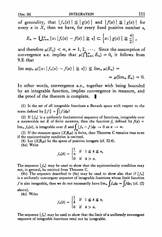
[SEC. 26] INTEGRATION 111
of generality, that | / , (*) | ^ | g(x) | and \f(x)\£ \g(x)\ for every x in Xy then we have, for every fixed positive number €,
En = Ur-n {x: \Mx) -f{x) | 2= A c {*: | *(*) | £ ^ } ,
and therefore n(En) < <*>, H = 1, 2, • • •. Since the assumption of convergence a.e. implies that MCH^-I En) = 0, it follows from 9.E that
lim sup,, /*({*: |/,.(*) - / ( * ) | ^ c}) < limn /i(£m) =
= M(limn En) = 0.
In other words, convergence a.e., together with being bounded by an integrable function, implies convergence in measure, and the proof of the theorem is complete. |
(1) Is the set of all integrable functions a Banach space with respect to the
norm defined by | | / | | = f\/Un?
(2) If {/n} is a uniformly fundamental sequence of functions, integrable over a measurable set E of finite measure, then the function / , defined by /(*) =
limn /nW, is integrable over E and I | / n — / | 4 * —* 0 as n —> *>.
(3) If the measure space (X>$yn) is finite, then Theorem C remains true even if the equicontinuity condition is omitted.
(4) Let (X>$>n) be the space of positive integers (cf. 22.4). (4a) Write
/ (h\ - l« if l ~ k ~ "> JnW = \n
10 if k > n. The sequence {/»} may be used to show that the equicontinuity condition may not, in general, be omitted from Theorem C.
(4b) The sequence described in (4a) may be used to show also that if {/n} is a uniformly convergent sequence of integrable functions whose limit function
/ is also integrable, then we do not necessarily have limn \fndn = \Jd\k\ (cf. (2)
above). (4c) Write
f l if 1 £ k£ ny /.(*) = k
0 if k > n.
The sequence {/«} may be used to show that the limit of a uniformly convergent sequence of integrable functions need not be integrable.

112 INTEGRATION [SEC. 27)
(5) Let X be the closed unit interval with Lebesgue measure and let \En)
be a decreasing sequence of open intervals such that n(En) — - , n = 1,2, •••. n
The sequence {nXEn] m a v De u s e d t o show that the boundedness condition cannot
be omitted from Theorem D. (6) If {/n} is a sequence of integrable functions which converges in the mean
to the integrable function/, and if g is an essentially bounded measurable function, then \fng} mean converges to/?.
(7) If {/„} is a sequence of non negative integrable functions which converges a.e. to an integrable function/, and if \Jnd\k = |//ju> » — 1> 2, • • •, then {/n(
converges t o / in the mean. (Hint: write gn — fn — f and observe that the trivial inequality | / n — / | ^s/n + / implies that 0 ^ #n~ ^ / . The bounded convergence theorem may therefore be applied to the sequence {£n~); the desired result follows from the fact that I gn
+dp — I gn~dp - 0, n = 1, 2, • • •.)
§ 2 7 . PROPERTIES OF INTEGRALS
Theorem A. Iff is measurable', g is integrable, and \f \ ^ | g | a.e., thenf is integrable.
Proof. Consideration of the positive and negative parts of/ shows that it is sufficient to prove the theorem for non negative functions/. If/ is a simple function, the result is clear. In the general case there is an increasing sequence {fn} of non negative simple functions such that lim„ fn(x) = / (# ) for all x in X. Since 0 ^ / n ^ | g |, each/n is integrable and the desired result follows from the bounded convergence theorem. |
Theorem B. If {fn\ is an increasing sequence of extended real valued non negative measurable functions and if limn/nC*)
= /(*) a.e., then limn \fnd\i = \Jd»-
Proof. I f / is integrable, then the result follows from the bounded convergence theorem and Theorem A. The only novel feature of the present theorem is its application to the not necessarily integrable case; we have to prove that if Ifdp = oo, then
limn jfndu = oo, or, in other words, that if limn Jfndfx < oo, then
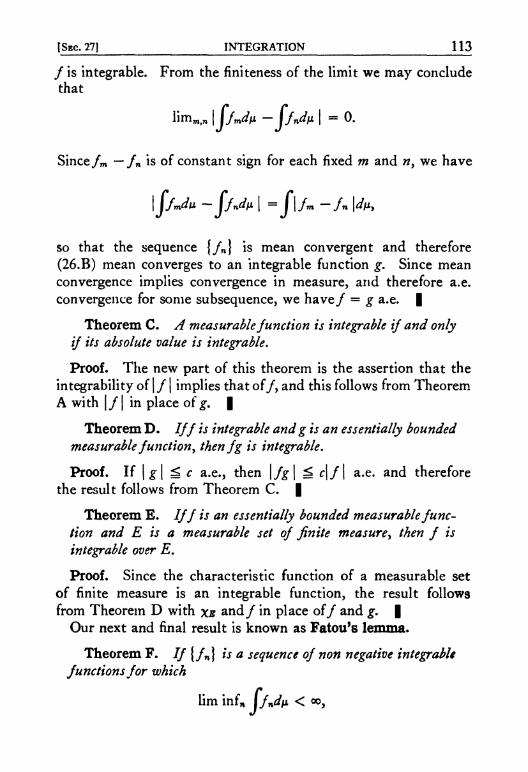
[SEC. 27] INTEGRATION 113
/ is integrable. From the finiteness of the limit we may conclude that
limm,n | Jfmdn -ffndu | = 0.
Since/m — fn is of constant sign for each fixed m and n> we have
\j/mdu -ffndp | = j\fm - / n |^>
so that the sequence {/n} is mean convergent and therefore (26.B) mean converges to an integrable function g. Since mean convergence implies convergence in measure, and therefore a.e. convergence for some subsequence, we h a v e / = g a.e. |
Theorem C. A measurable junction is integrable if and only if its absolute value is integrable.
Proof. The new part of this theorem is the assertion that the integrability of \f | implies that of/, and this follows from Theorem A with | / | in place of g. |
Theorem D. Iff is integrable andg is an essentially bounded measurable function, thenfg is integrable.
Proof. If \g\ ^ c a.e., then \fg\ ^ c\f\ a.e. and therefore the result follows from Theorem C. |
Theorem E. Iff is an essentially bounded measurable function and E is a measurable set of finite measure, then f is integrable over E.
Proof. Since the characteristic function of a measurable set of finite measure is an integrable function, the result follows from Theorem D with %B a n d / in place of/ and g. |
Our next and final result is known as Fatou's lemma.
Theorem F. If {fn} is a sequence of non negative integrable functions for which
lim infn jfndu < <*>,

114 INTEGRATION [SEC. 27]
then the function / , defined by
f(x) = lim infn/n(#), is integrate and
\fd\i ^ lim infn Jfnd^
Proof. If gn(x) = in({fi(x): n ^ i < <*>}, then #n g / n and
the sequence {gn} is increasing. Since I gndfi g \fndn> it follows
that
limn J £n*//z ^ lim infn \fndn < oo.
Since limn£n(;c) = lim infn/n(;c) = /(#) , it follows from Theorem B t h a t / is integrable and
If dp = limn J ^ M ^ lim inf„
(1) I f / is a measurable function, £ is an integrable function, and a and j8 are real numbers such that a ^*f(x) S fi a.e., then there exists a real number 7,
a ^ 7 ^ ft such that J / 1 g \d\k = 7 - J | £ |4*- (Hint:
This result is known as the mean value theorem for integrals. (2) If [fn] is a sequence of integrable functions such that
E:-i/l/.l*<«, then the series X n - i A W converges a.e. to an integrable function/ and
(Hint: apply Theorem B to the sequence of partial sums of the series X n - i | / n W I and recall that absolute convergence implies convergence.)
(3) I f / and/n are integrable functions, n = 1, 2, • • •, such that |/n(*) | ^ | / W I a-e., then the functions / * and /* , defined by
/*(*) = lim supn fn(x) and /*(*) = lim inf» /„(*),
are integrable and
J /*4c ^ lim sup n J / n 4c ^ lim infnJ/n4i > J /*4i-

[SEC. 27] INTEGRATION 115
(Hint: by considering separately the positive and negative parts, reduce the general case to the case of non negative/n> and then apply Fatou's lemma to {/+/„) and {/-/„).)
(4) A measurable function / is integrable over a measurable set E of finite measure if and only if the series
£?_,„(£ n {*: l/M | fc »}) converges. (Hint: use Abel's method of partial summation.) What can be said if n(E) = <», or if the summation is extended from n = 0?
(5) Suppose that {En\ is a sequence of measurable sets and m is any fixed positive integer, and let G be the set of all those points which belong to En
for at least m values of n. Then G is measurable and
» M ( G ) £ E r - i M ( £ > ) .
(Hint: consider £ n - i f X*n(*)*(*).) yo
(6) Suppose t h a t / is a finite valued, measurable function on a totally finite measure space (AT,S,/x), and write
Then
f/4i = lim„ J„ j> in the sense that if/ is integrable, then each series sn is absolutely convergent, the limit exists, and is equal to the integral, and, conversely, if any one of the series sn converges absolutely, then all others do, the limit exists,/is integrable, and the equality holds. (Hint: it is sufficient to prove the result for non negative functions. Write
lo if /(*) - o,
and apply Theorem B. For the converse direction observe that
/ ( * ) £ 2 / n ( * ) + M ( X ) ,
so t h a t / i s integrable and therefore the preceding reasoning applies.) (7) The following considerations are at the basis of an alternative popular
approach to integration. L e t / be a non negative integrable function on a measure space (XySyjJi). For every measurable set E we write
a(E) = i n f {/(*): * e £ } ,
and for every finite, disjoint class C = {E\> • • •, En\ of measurable sets we write
*(C) = E ? - i *(£<)/*(£<).
We assert that the supremum of all numbers of the form J ( C ) is equal to Ifdp.

116 INTEGRATION [SEC. 27]
If/ is a simple function, the result is clear. If g is a non negative simple function such that g ^ / , say g = £ ? . 1 «»Xs»> we write C = {Eh • • •, En]. Then
JW = E?-i ***(&) ^ Ef-i *{Ei)v(Ei) = ,(C).
It follows that if [gn] is an increasing sequence of non negative simple functions converging t o / , then
Y\mnJgndn ^ sup J(C),
and therefore Xjdy. ^ sup J(C), On the other hand, for every C, s(C) ^ \jd^
since J(C) is, in fact, the integral of a function such as g* (7a) Does the result of the preceding paragraph extend to non integrable,
non negative functions? (7b) I f / is an integrable function on a totally finite measure space (A^S,/*),
and if its distribution function g is continuous, (cf. 18.11), then
(cf. 25.4). (Hint: assume/ ^ 0, and make use of (7) above by considering the "approximating sums" J(C) of both integrals.)

Chapter FI
GENERAL SET FUNCTIONS
§ 28 . SIGNED MEASURES
In this chapter we shall discuss a not too difficult but rather useful generalization of the notion of measure; the principal difference between measures and the set functions we now propose to treat is that the latter are not required to be non negative.
Suppose that /*i and /*2 are two measures on a c-ring S of subsets of a set X. If we define, for every set E in S, /*(£) = ^(E) + /*2(£)> then it is clear that /* is a measure, and this result, on the possibility of adding two measures, extends immediately to any finite sum. Another way of manufacturing new measures is to multiply a given measure by an arbitrary non negative constant. Combining these two methods, we see that if {j*i, • • •, y.n) is a finite set of measures and {au • • -, an} is a finite set of non negative real numbers, then the set function /*> defined for every set E in S by
M(£) = £ ? - i <XiM(E), is a measure.
The situation is different if we allow negative coefficients. If, for instance, ixx and /x2 are two measures on S> and if we define ix by /*(£) = i±\{E) — M2(£)> then we face two new possibilities. The first of these, namely that /* may be negative on some sets, is not only not a serious objection but in fact an interesting phenomenon worth investigating. The second possibility presents, however, a difficulty that has to be overcome before the investiga-
"7

118 GENERAL SET FUNCTIONS [SEC. 28)
tion can begin. It can, namely, happen that i*i(E) = n2(E) = °°; what sense, in this case, can we make of the expression for 11(E)}
To avoid the difficulty of indeterminate forms, we shall agree to subtract two measures only if at least one of them is finite. This convention is analogous to the one we adopted in presenting
the most general definition of the symbol \fd\i. (We recall that
j/dfi is defined for a measurable function/ if and only if at least
one of the two functions/+ a n d / ~ is integrable, i.e. if and only if at least one of the two set functions v+ and v~> defined by
"+(£) = f/+4* and P-(E) = ff-dp,
is a finite measure.) The analogy can be carried further: if/ is
a measurable function such that \jd\i is defined, then the set func
tion v9 defined by v(E) = I fd/xy is the difference of two measures. E
The definition that we want to make is sufficiently motivated by the preceding paragraphs. We define a signed measure as an extended real valued, countably additive set function p on the class of all measurable sets of a measurable space (X,S)> such that jit(O) = 0, and such that /* assumes at most one of the values + 0 0 and —00.
We observe that implicit in the requirement of countable addi-tivity is the requirement that if {En\ is a disjoint sequence of measurable sets, then the series X)n-iM(^n) is either convergent or definitely divergent (to + 0 0 or —00)—in any case that the symbol J^iT-i fi(En) makes sense.
The words "[totally] finite" and "[totally] <r-finite" will be used for signed measures just as for measures, except that y.(E) has to be replaced by | ix{E) |, or, equivalently, n(E) < 00 has to be replaced by — 00 < n(E) < 00. For instance, a signed measure ju is totally finite if X is measurable and | ix(X) \ < 00.
One of our objectives in the following study is to prove that every signed measure is the difference of two measures. If this result is granted, it follows that we could have defined the concept

(SEC. 28] GENERAL SET FUNCTIONS 119
of signed measure on a ring and then attempted to copy the ex-tension procedure for measures; and it follows equally that it would have been a waste of time to do so, since we may, instead, reduce the discussion of signed measures to that of measures.
It follows from the definition of signed measures, just as for measures, that a signed measure is finitely additive and, therefore, subtractive.
Theorem A. If E and F are measurable sets and \x is a signed measure such that
EdF and | M(JF) | < <x>,
then | M(£) I < °°.
Proof. We have n(F) = y.{F — E) + n(E). If exactly one of the summands is infinite, then so is fi(F); if they are both infinite, then (since n assumes at most one of the values + 0 0 and -co) they are equal and again p(F) is infinite. Only one possibility remains, namely that both summands are finite, and this proves that every measurable subset of a set of finite signed measure has finite signed measure. |
Theorem B. If y. is a signed measure and {En) is a disjoint sequence of measurable sets such that \ n(\Jn-i En) \ < oo, then the series 2Zn-i n(En) is absolutely convergent.
Proof. Write
= f£ n if M(£n) ^ 0,
10 if n(En) < 0, and
= [En if M(£n) ^ 0,
10 if M(£n) > 0. Then
M(U: - i£» + ) = E : - , M ( £ n+ )
and
M(u:=i£n-) = z;-iM(£n-). Since the terms of both the last written series are of constant sign, and since /* takes on at most one of the values + 0 0 and — oo, it follows that at least one of these series is convergent. Since

120 GENERAL SET FUNCTIONS [SEC. 29]
the sum of the two series is the convergent series ^ " - 1 V>(En)> it follows that they both converge, and, since the convergence of the series of positive terms and the series of negative terms is equivalent to absolute convergence, the proof of the theorem is complete. |
Theorem C. If y. is a signed measure', if \En\ is a monotone sequence of measurable sets, and if, in case {En \ is a decreasing sequence, | y{En) \ < <x> for at least one value of «, then
M(Hmn En) = limn ii(En).
Proof. The proof of the assertion concerning increasing sequences is the same as for measures (replacing {En) by the disjoint sequence [Ei — £ t_i} of differences, cf. 9.D); the same is true for decreasing sequences (reduction to the preceding case by complementation, cf. 9.E), except that Theorem A has to be used to ensure the finiteness of the subtrahends that occur. |
(1) The sum of two [totally] <r-finite measures is a [totally] c-finite measure. Is this assertion valid for infinite sums?
(2) A complex measure on the class of all measurable sets of a measurable space is a set function n such that, for every measurable set E, n(E) = i*i(E) + //X2CE), where / = V — I, and whereMI and /x2 are signed measures in the sense of this section. Are Theorems A, B, and C true for complex measures?
(3) If a signed measure n is the difference of two measures in two ways, M = Mi — M2 and M = v\ — *% then is it true that Mi — v\ and M2 = 2?
(4) The fact that a signed measure assumes at most one of the values +<» and —00 follows from the requirement of additivity. (Hint: if n(E) = +00 and l*(F) = —oo, then the right side of at least one of the relations
M ( £ ) = M ( £ - F ) + M ( £ n F ) ,
M(F) = / * ( * • - £ ) + / ! ( £ O F ) , End
h indeterminate.)
§ 29 . HAHN AND JORDAN DECOMPOSITIONS
If /i is a signed measure on the class of all measurable sets of a measurable space (X,S)y we shall call a set £ positive (with respect to /x) if> for every measurable set Fy E fl F is measurable and n(E fl F ) ^ 0; similarly we shall call E negative if, for every

[SEC. 29] GENERAL SET FUNCTIONS 121
measurable set Fy E fl F is measurable and n(E 0 F) ^ 0. The empty set is both positive and negative in this sense; we do not assert that any other, non trivial, positive sets or negative sets necessarily exist.
Theorem A. If p. is a signed measure, then there exist two disjoint sets A and B whose union is X, such that A is positive and B is negative with respect to p.
The sets A and B are said to form a Hahn decomposition of X with respect to ju.
Proof. Since p assumes at most one of the values +oo and — oo, we may assume that, say
— 00 < fJ,(E) ^ 00
for every measurable set E. Since the difference of two negative sets, and a disjoint, countable union of negative sets are obviously negative, it follows that every countable union of negative sets is negative. We write j8 = inf ju(5) for all measurable negative sets B. Let {5»} be a sequence of measurable negative sets such that lim;juCB;) = /3; if B = U"-i B%9 t ' i e n B 1S a measurable negative set for which n(B) is minimal.
We shall prove that the set A = X — B is a positive set. Suppose that, on the contrary, E0 is a measurable subset of A for which ju(^o) < 0. The set E0 cannot be a negative set, for then B U E0 would be a negative set with a smaller value of n than M(#) , which is impossible. Let kx be the smallest positive integer with the property that E0 contains a measurable set Ex
for which M(£I) ^ T • (Observe that, since n(E0) < 0, M(£O)
and M(£I) are both finite.) Since
M(£o - Ei) - KEo) - M(£I) ^ M(£O) - T- < 0,
the argument just applied to E0 is applicable to E0 — E\ also. Let k2 be the smallest positive integer with the property that
E0 — Ex contains a measurable subset E2 with ii(E2) s= 7 - , and k2
proceed so on ad infinitum. Since n is finite valued for measurable

122 GENERAL SET FUNCTIONS [SEC. 29]
subsets of E0 (28.A), we must have limn— = 0. It follows that,
for every measurable subset F of
FQ = E0 — UJL i Ejy
we have n(F) ^ 0, i.e. that F0 is a measurable negative set. Since Fo is disjoint from By and since
M(Fo) = M(£o) - ETJi M(£y) ^ M(^O) < 0,
this contradicts the minimality of By and we conclude that the hypothesis n(E0) < 0 is untenable. |
I t is not difficult to construct examples to show that a Hahn decomposition is not unique. If, however,
X = Ax U Bx and X = A2 U 5 2
are two Hahn decompositions of Xy then we can prove that, for every measurable set Ey
M(£ fl At) = n(E fl A2) and /i(JE fl 5 J = /i(£ fl 52).
To see this, we observe that
E () (Ax- A2) aE fl Au
so that /*(£ 0 (Ax - ^2)) ^ 0, and
E D (Ax- A2)aE d B2y
so that M(£ n ( ^ - A2)) £ 0. Hence /i(£ fl (Ax - A2)) = 0 and, by symmetry, /*(£ fl (A2 — Ax)) = 0; it follows that
M(£ n Ax) = M(£ n (Ax u ^2)) = M(£ n A 2 ) .
It follows from this result that the equations
M+ (£) = n(E fl ^f) and M"(£) = - M ( £ fl B)
unambiguously define two set functions y.+ and /*~ on the class of all measurable sets, called, respectively, the upper variation and the lower variation of /*. The set function | 111, defined for every measurable set E by | y. \(E) = M + ( £ ) + M~~"CE), is the total variation of /z. (Observe the important notational distinction between | /x \(E) and | /*(£) |.)

[SBC. 29] GENERAL SET FUNCTIONS 123
Theorem B. The upper, lower, and total variations of a signed measure \x are measures and /x(E) = n+(E) — p~~(E) for every measurable set E. If p. is [totally] finite or c-finite, then so also are M+ and n~; at least one of the measures n+ and l*r is always finite.
Proof. The variations of \i are clearly non negative; if every measurable set is a countable union of measurable sets for which /* is finite, it follows from 28.A that the same is true for /*+ and yT. The equation /* = /x+ — p~ follows from the definitions of JU+
and ju"~; the fact that /x takes on at most one of the values +00 and —00 implies that at least one of the set functions fi+ and M~ is always finite. Since the countable additivity of p* and pT is evident, the proof is complete. |
It follows from Theorem B that every signed measure is the difference of two measures (of which at least one is finite); the representation of /* as the difference of its upper and lower variations is called the Jordan decomposition of p..
(1) If/x is a finite signed measure and if {En\ is a sequence of measurable sets such that limn En exists, (i.e. such that lim supn En * Hm infn En)y then
/i(limn£»i) = lim«/x(£n).
(2) A finite signed measure, together with its variations, is bounded. For this reason finite signed measures are often said to be of bounded variation.
(3) If /Lt is a signed measure and if E is a measurable set, then
M+(£) - sup {n(F):E 3 F e S } and n~(E) - - inf {M(F): EZ) F e S } .
An alternative and frequently used proof of the validity of the Jordan decomposition may be given by treating these equations as the definitions of M + and jtt~.
(4) Does the set of all totally finite signed measures on a c-algebra form a Banach space with respect to the norm defined by || n || = | \x |WQ?
(5) If (XySyfi) is a measure space a n d / is an integrable function on X, then
the set function J>, defined by v(E) = I f(x)dn(x), is a finite signed measure, and
What is I v \(E) in terms of/? (6) If n and v are totally finite measures on a <r-algebra S and if E is a set in
S, then, corresponding to every real number /, there exists a set At in S such that AtCZ E and such that, for every set F in S for which F C A% [or for which F C £ - ^ ] w e have v{F) S /M(F) , [or v{F) ^ //*(F)J.
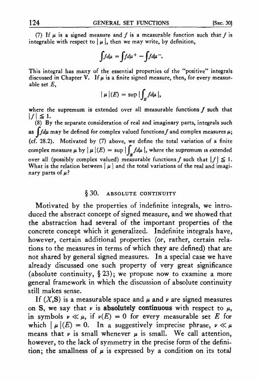
124 GENERAL SET FUNCTIONS [SEC. 30]
(7) If fji is a signed measure and / is a measurable function such that / is integrable with respect to | /x |, then we may write, by definition,
J>M = J /* + -//*". This integral has many of the essential properties of the "positive" integrals discussed in Chapter V. If/x is a finite signed measure, then, for every measurable set £ ,
UI(£)-8uP | / /4» | ,
where the supremum is extended over all measurable functions / such that
(8) By the separate consideration of real and imaginary parts, integrals such
as lyi/jbt may be defined for complex valued functions/ and complex measures M;
(cf. 28.2). Motivated by (7) above, we define the total variation of a finite
complex measure/z by | /x \(E) = sup | I jd\i. |, where the supremum is extended E
over all (possibly complex valued) measurable functions/ such that | / | ^ 1. What is the relation between | n \ and the total variations of the real and imaginary parts of AI?
§ 3 0 . ABSOLUTE CONTINUITY
Motivated by the properties of indefinite integrals, we introduced the abstract concept of signed measure, and we showed that the abstraction had several of the important properties of the concrete concept which it generalized. Indefinite integrals have, however, certain additional properties (or, rather, certain relations to the measures in terms of which they are defined) that are not shared by general signed measures. In a special case we have already discussed one such property of very great significance (absolute continuity, §23); we propose now to examine a more general framework in which the discussion of absolute continuity still makes sense.
If (Xy&) is a measurable space and ii and v are signed measures on S, we say that v is absolutely continuous with respect to ju, in symbols v «ju> if v(E) = 0 for every measurable set E for which | p\(E) = 0. In a suggestively imprecise phrase, v «ju means that v is small whenever y. is small. We call attention, however, to the lack of symmetry in the precise form of the definition; the smallness of p is expressed by a condition on its totaJ

[SEC. 30] GENERAL SET FUNCTIONS 125
variation. Our first result concerning absolute continuity asserts that this asymmetry is only apparent.
Theorem A. If p and v are signed measures, then the conditions
(a) v « M,
(b) P+ « M and p~ « /*>
(c) M«M> are mutually equivalent.
Proof. If (a) is valid, then v(E) = 0 whenever | y. \{E) = 0. If X = A U B is a Hahn decomposition with respect to v> then we have, whenever | M | (E) = 0,
0<\n\(EnJ)^\n\(E)=0 and
o ^ | M | ( £ n 5 ) g | M | ( £ ) - o , and therefore
*+(£) = F ( £ 0 ^ ) = 0 and p~(E) = F ( £ fl 5) = 0; this proves the validity of (b).
The facts that (b) implies (c) and (c) implies (a) follow from the relations
| v |(£) = p+(E) + v-{E) and 0 £ | v{E) \ g | v\{E)
respectively. | The following theorem establishes the relation between our
present form of the definition of absolute continuity and the one we used (for finite valued set functions) in § 23. The theorem asserts essentially that another precise interpretation of "v is small whenever p is small," which is apparently quite diflFerent from the definition of absolute continuity, is in the presence of a finiteness condition equivalent to it.
Theorem B. If v is a finite signed measure and if n is a signed measure such that v «ju, then, corresponding to every positive number e, there is a positive number 5 such that I v \(E) < efor every measurable set Efor which \ n \(E) < 8.

126 GENERAL SET FUNCTIONS [SEC. 301
Proof. Suppose that it is possible, for some c > 0, to find a
sequence {En} of measurable sets such that | n\(En) < — and
| v \(En) ^ e, n = 1, 2, • • •. If E = lim supn En, then
\»m£Zr-n\t*\(Ed<^, » = i ,2, . . . ,
and therefore | JU | (E) = 0. On the other hand (since v is finite)
| v \(E) = limn \v\(En\J En+1 U • • •) £ lim supn | v \{En) £ e.
Since this contradicts the relation v « /*, the proof of the theorem is complete. |
It is easy to verify that the relation "<3C" is reflexive (i.e. JJL «/*) and transitive (i.e. pi «/*2 and ju2 «M3 imply that Mi ^Ma)* Two signed measures ju and ? for which both v « / * and M « ^ are called equivalent, in symbols n = v.
The antithesis of the relation of absolute continuity is the relation of singularity. If (XyS) is a measurable space and /* and v are signed measures on S, we say that y. and v are mutually singular, or more simply that /* and v are singular, in symbols \i ± vy
if there exist two disjoint sets A and B whose union is X such that, for every measurable set Ey A fl E and B 0 E are measurable and | M \(A fl £) = | *> \(B fl £) = 0. Despite the symmetry of the relation, it is occasionally more natural to use an unsymmetric expression such as "v is singular with respect to ixi%
instead of ' V and v are singular." It is clear that singularity is indeed an extreme form of non
absolute continuity. If v is singular with respect to /*, then not only is it false that the vanishing of | /* I implies that of \v\ + but in fact essentially the only sets for which | v | does not necessarily vanish are the ones for which | /* | does.
We conclude this section with the introduction of a new notation. We have already used the traditional and suggestive "almost everywhere" terminology on measure spaces; this is perfectly satisfactory as long as we restrict our attention to one measure at a time. Since, however, in the discussion of absolute continuity and singularity we have necessarily to deal with several measures simultaneously, and since it is clumsy to say "almost
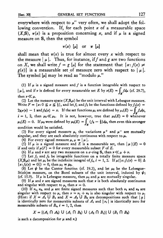
[SEC. 30] GENERAL SET FUNCTIONS 127
everywhere with respect to /*" very often, we shall adopt the following convention. If, for each point x of a measurable space (Jf,S), ir(x) is a proposition concerning x> and if y. is a signed measure on S, then the symbol
7r(#) [/i] Or 7T [/x]
shall mean that w(x) is true for almost every x with respect to the measure | /* |. Thus, for instance, if/ and £ are two functions on Xy we shall write/ = g [/x] for the statement that {x:/(x) ^ g(x)} is a measurable set of measure zero with respect to | it |. The symbol [/*] may be read as "modulo it."
(1) If ft is a signed measure and / is a function integrable with respect to
| n |, and if v is defined for every measurable set E by v(E) = I J dp (cf. 29.7), JE
then v<£fi. (2) Let the measure space (JV,S,)u) be the unit interval with Lebesgue measure.
Write F = {x: 0 ^ # S h\> and let/i and/2 be the functions defined by/i(#) =
2XF(X) — 1 and/2(x) = x. If the set functions it» are defined by iu(E) = I /*//*> B
i = 1, 2, then M2<3CMI- I* is not> however, true that H2\E) = 0 whenever tii(£) = 0 . If M2 were defined by 112(E) = I C/2 — §)4*> t n e n e v e n tn*s stronger
JE condition would be satisfied.
(3) For every signed measure ii, the variations it+ and it" are mutually singular, and they are each absolutely continuous with respect to tt.
(4) For every signed measure M, M — I M |. (5) If/x is a signed measure and E is a measurable set, then \n \(E) = 0
if and only if p(F) = 0 for every measurable subset F of E, (6) If 11 and v are any two measures on a c-ring S, then v<Kn +v. (7) Let /1 and fi be integrable functions on a totally finite measure space
(X$,\i) and let it* be the indefinite integral of/,-, / = 1, 2. If /i({x:/i(x) = 0} A (*:/2(*) = 0}) = 0, then MI = M2.
(8) Let ^ be the Cantor function (cf. 19.3), and let no be the Lebesgue-Stieltjes measure, on the Borel subsets of the unit interval, induced by yp\ (cf. 15.9). If fj. is Lebesgue measure, then no and n are mutually singular.
(9) If n and v are signed measures such that v is both absolutely continuous and singular with respect to /x, then v = 0.
(10) If V\y V2y and n are finite signed measures such that both v\ and V2 are singular with respect to /x, then v = v\ -f- 2 is also singular with respect to /x» (Hint: if X = Ai \J Bi and AT = A2 U ft are decompositions such that | j* | is identically zero for measurable subsets of A{ and | v% | is identically zero for measurable subsets of ft, i = 1,2, then
x »[(^! n 2) u (AX n ft) u {At n ft)] u (ft n ft) is such a decomposition for n and v.)

128 GENERAL SET FUNCTIONS [SEC. 31J
(11) If n and v are measures on a c-algebra S such that jit is finite and P<$CM> then there exists a measurable set E such that X — E is of c-finite measure with respect to v, and such that, for every measurable subset F of E> v(F) is either 0 or oo. (Hint: use the method of exhaustion (cf. 17.3), to find a measurable set E with the property that, for every measurable subset F of £ , v(F) is either 0 or oo, and such that n(E) is maximal; another application of the method of exhaustion shows that X — E is of c-finite measure with respect to v.)
(12) Theorem B is not necessarily true if v is not finite. (Hint: let X be the set of all positive integers, and, for every subset E of X, write
MOE) « E» « * * - , *(£) - £« c E 2\)
§ 3 1 . THE RADON-NIKODYM THEOREM
Theorem A. If y. and v are totally finite measures such that v « ii and v is not identically zero, then there exists a positive number e and a measurable set A such that ix(A) > 0 and such that A is a positive set jor the signed measure v — en. Proof. Let X = An U Bn be a Hahn decomposition with
respect to the signed measure v /*, n = 1, 2, • • •, and write n
AQ = \jn-lAny BQ = (ln-1 Bn-
Since B0 c Bny we have
O^p(Bo) ^ - M ( 5 0 ) , » = 1,2, . . - ,
and consequently ^(5o) = 0. It follows that v(A0) > 0 and therefore, by absolute continuity, that n(A0) > 0. Hence we must have y.(An) > 0 for at least one value of n\ if, for such a
value of ny we write A — An and e = - , the requirements of the n
theorem are all satisfied. | We proceed now to establish the fundamental result (known
as the Radon-Nikodym theorem) concerning absolute continuity
Theorem B. If (^,S,ju) is a totally a-finite measure space and if a <r-finite signed measure v on S is absolutely continuous

{SEC. 31] GENERAL SET FUNCTIONS 129
with respect to JLI> then there exists a finite valued measurable function f on X such that
JE
for every measurable set E. The function/ is unique in the sense
that if also v(E) = I gdpy E e S, then/ = g [/*]. JE
We emphasize the fact t h a t / is not asserted to be integrable; it is, in fact, clear that a necessary and sufficient condition that
f be integrable is that v be finite. The use of the symbol ifdy.
implicitly asserts, however (cf. § 25), that either the positive or the negative part of/ is integrable, corresponding to the fact that either the upper or the lower variation of v is finite.
Proof. Since X is a countable, disjoint union of measurable sets on which both ju and v are finite, there is no loss of generality (for both the existence and the uniqueness proofs) in assuming finiteness in the first place. Since if v is finite, / is integrable, uniqueness follows from 25.E. Since, finally, the assumption v « M is equivalent to the simultaneous validity of the conditions
v+ « M and v~~ « M>
it remains only to prove the existence of/ in the case in which both /x and v are finite measures.
Let OC be the class of all non negative functions/, integrable
with respect to fiy such that I fd\i ^ v{E) for every measurable JE
set £ , and write
a = sup lifdiiife 3C|-
Let \fn) be a sequence of functions in OC such that
lim imn j/ndfi = a.
If E is any fixed measurable set, n is any fixed positive integer, and gn = / i U • • • U / n , then E may be written as a finite, disjoint

130 GENERAL SET FUNCTIONS [SEC. 31j
union of measurable sets, E = E\ U • • • U Eny so that gn(x) = fj{x) for x in Ejyj = 1, • • •, tf. Consequently we have
fgnJn = E"-i f / A ^ E"-i"(£;) = "(£)•
If we write f0(x) = sup {/n(*): » = 1, 2, • • • } , then f0(x) =
l im*^*) and it follows from 27.B that/0 e 3Z and l/o /x = a.
Since/o is integrable, there exists a finite valued function/ such
that /o = / [/*]; toe shall prove that if p0(E) = */(£) - I /dp, E
then the measure i>0 is identically zero. If p0 is not identically zero, then, by Theorem A, there exists a
positive number e and a measurable set yf such that p(A) > 0 and such that
en(E fl A) ^ v0(E (\A)=p(EriA)-C /dp JE n il
for every measurable set E. If £ = / + ^XA, then
JE JE JE—A
for every measurable set Ey so that g e 3C. Since, however,
J W = J/ M + ep(J) > a,
this contradicts the maximality of 1 / ^ and the proof of the
theorem is complete. |
(1) If (X,S,p) is a measure space and if v{E) = I jdp for every measuraDie JE
set Ey then * = {*:/(*) >0} U {*:/(*) ;g0}
is a Hahn decomposition with respect to v. (2a) Suppose that (X,S) is a measurable space and M and v are totally finite
measures on S such that v<&n. K p = p -f- v and if v(E) — I / /Z for every JE
measurable set E> then 0 ^ f(x) < 1 [p], (2b) If | j ^ = \jgdp. for every non negative measurable function gy then
[SEC. 31] GENERAL SET FUNCTIONS 131
JE d\k for every measurable set E. (Hint: rewrite the hypothesis
E 1 — / in the form f#(1 — f)dv = \Jgd\i and, given £ , write g = * • \
(3) Let (XyS>n) be the unit interval with Lebesgue measure and let M be a non measurable set. Let (ofi,jSi) and (fxifi'i) be two pairs of positive real numbers such that <x\ + fii = e*2 + , f t = 1, and let pi be the extension of n> determined by (ctifii), to the <r-ring § generated by S and M, i = 1,2 (cf. 16.2). There exist measurable functions/i and/2 such that
ME)-[fi4k and foW = [/*&! JE JE
for every measurable set E. What are the functions/i and/2? (4) The Radon-Nikodym theorem remains true even if /x is only a signed
measure. (Hint: let X = A U B be a Hahn decomposition with respect to ^ and apply the Radon-Nikodym theorem separately to v and /x+ in A and to v and \i~ in 5.)
(5) Let /x be a totally <r-finite signed measure. Since both /x+ and /x~ a r e absolutely continuous with respect to both /x and | n |, we have
M + ( ^ - f / + * = f*+rf|Ml and M " ( £ ) = f / ^ M = f ^ M |. JE JE JE JE
The functions / + , g+> / _ , and g- satisfy the relations / + = g+ \p] and / _ = —g- [fj]m What are these functions?
(6) If n is a signed measure and if v(E) — I fdp and | J/ \{E) = j ^ | M I fcr
Ju JE every measurable set £ , then £ = | / | \p],
(7) The Radon-Nikodym theorem remains true even \f v is not <r-finite, but, in this case, the integrand/is not necessarily finite valued. (Hint: it is sufficient to consider the case in which v is a measure and M is finite; in this case apply 30.11.)
(8) The Radon-Nikodym theorem is not necessarily true if n is not totally c-finite, even if v remains finite. (Hint: let X be an uncountable set and let S be the class of all those sets which are either countable or have countable complements. For every E in S, let JJL(E) be the number of points in E and let v(E) be 0 or 1 according as E is countable or not.)
(9) If (XyS) is a measurable space and /x and v are c-finite measures on S such that v<Kn> then the Radon-Nikodym theorem may be applied to each measurable set separately. The question might be raised whether or not a function/ may be defined once for all on the whole space X so as to serve as a suitable integrand simultaneously for every measurable set. The answer is no, as the following pathological example shows.
Let A be any uncountable set (with, say, cardinal number a) , and let B be a set of cardinal number ft > a. Let X be the set of all ordered pairs {ajb) with at A and bzB. It is convenient to call a set of the form \{ajb^)\ a e A\ a horizontal line, and a set of the form {{a^b)\ b e B} a vertical line. We shall

132 GENERAL SET FUNCTIONS [SBC. 32)
call a set E full on a horizontal or vertical line L if L — E is countable; (cf. 12.1). Let S be the class of all sets which may be covered by countably many horizontal and vertical lines, and which are such that on every horizontal and vertical line they are either countable or full. For every E in S let/x(£) be the number of horizontal and vertical lines on which E is full, and let v(E) be the number of vertical lines on which E is full. Clearly /x and v are c-finite measures and
v<&ix. Suppose now that there exists a function/on X such that v{E) — I fdp. JE
for every E in S. It is easy to see that the set {#:/(#) = 0} has to be countable on every vertical line and full on every horizontal line. The first requirement implies that the cardinal number of this set is at most aKo = a, and the second requirement implies that the cardinal number of this set is at least P(a - Ko) ^ 0.
(10) There is a condition on measure spaces, which is more general than total <r-finiteness and more restrictive than a-finiteness, in the presence of which the Radon-Nikodym theorem is still true. The condition is that the space be the union of a disjoint class D of measurable sets of finite measure with the property that every measurable set may be covered by countably many sets of D and a set of measure zero. The following is an example of a non totally o—finite measure space satisfying this condition.
Let X be the Euclidean plane, and let S be the class of all those sets which may be covered by countably many horizontal lines and which are Lebesgue measurable on each such line. If £ is a Lebesgue measurable subset of a horizontal line, define n(E) to be the Lebesgue measure of E; for the general E in S, /x is thereby uniquely determined by the requirement of countable additivity.
(11) If, in (9) above, B = A and the cardinal number of this set is Ki (= the smallest uncountable cardinal), then the proof breaks down, i.e. there exists in that case a subset E of X which is countable on every vertical and full on every horizontal line. (Hint: well order Ay i.e. assign to every a in A an ordinal number £(a) < 0 ( = the smallest uncountable ordinal) so that the correspondence is one to one between all points of A and all ordinals less than 0, and write
(12) If n is a totally finite measure and v(E) = I jd\k for every measurable JE
set E, then the set
B(t) = {*:/(*) ^ /)
is a negative set for the signed measure v — tfi; (cf. (1) above). A proof of the Radon-Nikodym theorem may be based on an attempt to reconstruct/ from the sets #(/); (cf. 18.10). The main complication of this approach is the non uniqueness of negative sets. A tool for partially dealing with this complication is to select #(/), for each /, so as to maximize the value of pi(j9(/)).
§ 3 2 . DERIVATIVES OF SIGNED MEASURES
There is a special notation for the functions which occur as integrands in the Radon-Nikodym theorem, which is frequently

[SEC. 32] GENERAL SET FUNCTIONS 133
very suggestive. If 11 is a totally c-finite measure and if v(E) =
I fdjji for every measurable set Ey we shall write
dv / = — or dv = /^M-
All the properties of Radon-Nikodym integrands (which we may also call Radon-Nikodym derivatives), which are suggested by the well known differential formalism, correspond to true theorems.
Some of these are trivial (e.g. = — + — J , while \ dfJL dfJL dfl/
others are more or less deep properties of integration. Examples of the latter kind of result are the chain rule for differentiation and, as an easy corollary, the substitution rule for the differentials occurring under an integral sign; both these results are precisely stated and proved below. It is, of course, important to remember
. . dv . that a Radon-Nikodym derivative — is unique only a.e. with
dfj.
respect to /x> and that, therefore, in the detailed verbal interpretation of a differential formula, frequent use has to be made of the qualifying "almost everywhere/'
Theorem A. If X and /* are totally a-finite measures such that fj. « X and if v is a totally a-finite signed measure such that v « M> then
dv^ _ dv^dji
d\~ dnd\ l J"
Proof. Since the validity of the desired equation for the upper and lower variations of v implies its validity for v itself, we may and do assume that v is a measure; for simplicity of notation we
dv ujJL write — = / and — = g. Since v is non negative, it follows from
dfj, d\
25.D t h a t / ^ 0 [/*] and therefore that there is no loss of generality in assuming t h a t / is everywhere non negative.
Let {/n} be an increasing sequence of non negative simple

134 GENERAL SET FUNCTIONS [SEC. 32]
functions converging at every point t o / , (20.B); then, by 27.B, we have
limn I /ndiJL = { /dp and limn I /ngd\ = I fgdK
for every measurable set E. Since, for every measurable set F,
fxFdfi = p(E fl F) = f gd\ = CxFgdX, JE JE n F JE
it follows that I fndn = I fngd\y n = 1, 2, • • •, and therefore that JE JE
v(E) = ff^ = CfgJ\. | JE JE
Theorem B. If X and /* are totally <r-finite measures such that /i « X, and if f is a finite valued measurable function for
which If dp is defined^ then \fd\x = \f ~jr^
Proof. We write v(E) = I fdy. for every measurable set E> JE
J r dfx ' f—d\ for every E d\
measurable set E\ the desired result follows by putting E = X. | Our next and final result concerning the relations among signed
measures treats the Lebesgue decomposition of a totally c-finite signed measure into an absolutely continuous part and a singular part with respect to another totally <r-finite signed measure.
Theorem C. If (X,S) is a measurable space and JU and v are totally a-finite signed measures on S, then there exist two uniquely determined totally definite signed measures v0 and v\ whose sum is py such that r0 _L M tind v\ « M«
Proof. As usual we may assume that M and v are finite. Since V{(i = 0, 1) will be absolutely continuous or singular with respect to ju according as it is absolutely continuous or singular with respect to | /* |, we may assume that M is a measure. Since, finally, we may treat v+ and v~ separately, we may also assume that v is a measure.

[SEC. 32] GENERAL SET FUNCTIONS 135
The proof of the theorem for totally finite measures is a useful trick, based on the elementary observation that v is absolutely continuous with respect to ju + v. There exists, accordingly, a measurable function/ such that
v(E) - Cfd» + f/dv JE JE
for every measurable set E. Since 0 ^ v(E) ^ p(E) + v(E)y
we have 0 fg / ^ 1 [p + v] and therefore 0 ^ / ^ 1 [p]. If we w r i t e r = {*:/(*) = 1} and 5 = {x:0 g / ( # ) < l}, then
v(A) = fdfi + [dv = n(J) + v{A) JA JA
and therefore (since v is finite) y.{A) = 0. If
v0(E) = v(E fl A) and vx(E) = v(E fl B)
for every measurable set E, then it is clear that VQ -L M; it remains to prove that vx « i i .
If/x(£) = 0, then
f <fr = v(E fl 5) = f / *
and therefore f (1 - f)dv = 0. Since 1 - / ^ O H , it fol,
lows that P\(E) = ?(£ fl 5) = 0; this completes the proof of the existence of v0 and *>i.
If *> = v0 + vi and v ^ vo + P\ are two Lebesgue decompositions of vy then v0 — v0 =* Pi — vi. Since v0 — i>0 is singular (cf. 30.10) and v\ — v\ is absolutely continuous with respect to /x, it follows that v0 — h and v\ = ?i; (cf. 30.9). |
(1) Using the concept of integration with respect to a signed measure, the definition of Radon-Nikodym derivatives may be extended to the case in which /x is a signed measure, and Theorem A remains true if X and pi are signed measures. (Hint: consider a Hahn decomposition with respect to each of the three signed measures X,M> and v, and construct the decomposition o(X into the eight sets obtained by taking one set from each decomposition and forming the intersection of these three sets. On measurable subsets of each of the eight sets each of the functions, X, n, and v> is of constant sign and therefore, after an obvious, slight modification, Theorem A applies.)

136 GENERAL SET FUNCTIONS [SEC. 32]
(2) If M and v are totally c-finite signed measures such that M s v> then df* = l/^L. dv dp
(3) If jit and v are totally <r-finite signed measures such that P<3CM, then
,({„*«-.})-* (4) If Mo, Mi> and M2 are totally finite measures, and if */MO = /W(MO + Mi) —
fiddly -|- M2) — fdQjiQ + MI + M2), then we have, almost everywhere with respect to Mo + Mi + M2,
,, N J 7 T T T T 7 T — / / w / x l f /1W/2W ^ 0,
I 0 if / iW = /2(*) = o.
(5) Given two sequences {jJLn\ and {vn\ of totally finite measures, write
An = £ ? - 1 Mi, ?n = £ ? - 1 viy M = £"«-1 M», ? = Sr« 1 Vi>
and assume that M and v are finite measures. If Pn^CM„, n = 1, 2, • • •, then V<$CM and
hmn -Tj- = — [MJ. dp*. d\k
The proof of this assertion may be based on the following lemmas. (5a) If [En] is a sequence of measurable sets such that /Zn(£n) - 0, n = 1, 2,
•••, thenM(Hmsupn£n) = 0. (Hint: M„(U?=» **) ^ £?-«&(£*)•) (5b) If {<£n} and {^n} are sequences of functions such that <t>n = ^n [Mn],
w = 1, 2, • • •, then, for a.e. x \p]y
limsupn0n(#) = lim supn^n(.v) and lim infn <t>n(x) = lim infn^n(#).
(Hint: write En = [x: <t>n(x) ^ ^»(x)) and apply (5a).) In view of the result (5b) it is sufficient to prove (5) for any fixed determina
tion of the derivatives -—•- If dfin
dvn , , dpn , ^ — = / n and — = gn, w = l , 2 , •••,
then it follows from Theorem A that one such determination is
dvn / i + - - - + / » dfln gl-i h gn
[Mn], » = 1,2,
(5c) L » - i / n = j - and E » - i £n = 1 [M]. (Hint: since
and ZT-i«(£)-f (A+••• + *.)*
£ ? - l * ( £ ) = f ( / l + ' " + / n V M , " = 1,2, •••,
the desired result follows from 27.B and 25.E.)

Chapter VII
P R O D U C T SPACES
§ 3 3 . CARTESIAN PRODUCTS
If X and Y are any two sets (not necessarily subsets of the same space), the Cartesian product X X Y\s the set of all ordered pairs (xyy)y where x e X andy e Y. The best known example of a Cartesian product is the Euclidean plane, which is most often viewed as the product of two coordinate axes. Most of the development in the sequel uses the words and concepts suggested by this example. Thus, for instance, if A c X and B c Y, we shall call the set E - A X B (a subset of X X Y) a rectangle and we shall refer to the component sets A and B as its sides. (Observe that our usage here differs from the classical terminology which speaks of rectangles only if the sides are intervals.)
Theorem A. A rectangle is empty if and only if one of its sides is empty.
Proof. If A X B ?*0y say (#,v) eA X B> then x e A and y e By so that A ^ 0 and 5 ^ 0 . If, on the other hand, neither A nor B is empty, then there is a point (xyy) such that (xyy) e AX By so that A X B * 0. |
Theorem B. If Ex = A\ X Bx and E2 = A2X B2 are non empty rectangles, then E\ c E2 if and only if
Ax c A2 and Bx c J52.
Proof. The "if" is obvious. To prove the converse, let {x>y) be a point in A\ X B\ and suppose that there exists a point x%
137

138 PRODUCT SPACES [SEC. 33J
in Ai such that xx e' A2- Then
(xlyy) e Ax X Bi and (xuy) e' A2 X B2;
it follows that no such point #i can exist and therefore A\ c A2. The same proof with only notational changes shows that Bx c B2. |
Theorem C. If A\ X B\ = A2X B2 is a non empty rectangle, then A\ = A2 and B\ = B2.
Proof. It follows from Theorem B that
Ai C A2 C /f i and B1aB2<z Bx. |
Theorem D. If E = A X By Et = Ax X Bly and E2 = - 2 X B2 are non empty rectangles, then a necessary and sufficient condition that E be the disjoint union of E\ and E2y is that either A is the disjoint union of A\ and A2y and B = Bx = B2y or else B is the disjoint union of B\ and B2y and A = Ax = A2*
Proof. We prove first that the condition is necessary. Since Ei c E and E2 c Ey it follows from Theorem B that Ax c A and A2 c Ay and therefore that A\ U A2 c A\ similarly Bx U B2 c B. Since
£ ! U £ 2 c (Ai U A2) X (Bx U B2)y
it follows that A c A\ U A2 and B c ^ U Z?2, and therefore ^ = /fi U A2 and B = i?i U Z?2. Since, finally, a similar argument shows that
o = £ 1 n £ 2 D ( ^ 1 n A2) x (Bx n B2)y
it follows from Theorem A that at least one of the two sets Ax 0 A2 and Bx fl B2 is empty.
Suppose, for instance, that A\ D A2 = 0; we are to show that in this case B = Bx = <82. (The case Z?i fl Z?2 = 0 is treated similarly.) Suppose on the contrary that there exists a point y in B — 5 lB Then, if # is any pomt in Aly we have (xyy) e £ , but (since y e' Z^), (x,y) e' 2^, and (since x e' ^2)j (*,.y) 8 ' ^ Since this contradicts the assumption £ = £ i U £2 , it follows that B — Z?i = 0 and also, by a similar argument, B — B2 = 0.

[SEC. 33] PRODUCT SPACES 139
The sufficiency of the condition is easier. If, for instance, A is the disjoint union of Ax and A2 and B = Bx = B2y then A 3 AXy
AZ)A2,BZDBUBZ) B2y so that E 3 Ex U £2 . Also if {xyy) e £ , then
(#,jy) e Ex or (#,jy) e E*
according as x e ^ or x e /f2, so that E is indeed the disjoint union of Ex and £2 . I
Theorem E. If S and T *r* nw£j a/" subsets of X and Y respectively, then the class R of all finite, disjoint unions of rectangles of the form A X B> where A e S and B e T, * j a ring.
Proof. We observe first that the intersection of two sets of the form A X B is another set of that form. If either of the two given sets, or their intersection, is empty, this result is trivial. If
£i = Ai X Bu E2 = A2X B2y and {xyy) e Ex D £2 ,
then A: e Ax Ci A2 and ^ e Bx 0 5 2 , so that
ExCl E2a {Ax D /*2) X (5i fl 52).
On the other hand, by Theorem B, (Ax fl A2) X {Bx fl 52) is contained in Ex and £ 2 and therefore in Ex fl £2 , so that
£ ^ £ 2 = {Ax n A2) x (5X n 52).
Since S and T are rings, Ax fl A2 e S and 5i fl 5 2 e T. It follows immediately that the class R is closed under the formation of finite intersections.
Since
{Ax X Bx) - (A2 X B2) =
- [{Ax fl A2) X {Bx - 52)] U [{Ax - ^ 2 ) X 5x1,
we see that the difference of two sets of the given form is a disjoint union of two other sets of that form; since
ur-i Et - u?-i V = \ji-i nr-x (Ei - Fj\ it follows, using the resilt of the preceding paragraph, that the class R is closed under H\L f^rrjnriuii of differences. Since R is

140 PRODUCT SPACES [SEC. 33)
obviously closed under the formation of finite, disjoint unions, the proof of the theorem is complete. |
Suppose now that in addition to the two sets X and Y we are also given two (r-rings S and T of subsets of X and Y respectively. We shall denote by S X T the c-ring of subsets of X X Y generated by the class of all sets of the form A X B> where i e S and B e T.
Theorem F. If (XyS) and (Y,T) are measurable spaces, then {X X Y, S X T) is a measurable space.
The measurable space ( 1 X 7 , S X T) is the Cartesian product of the two given measurable spaces.
Proof. If (x,y) e X X y , then there exist sets A and B such that x e A e S and y e B e T; it follows that (xyy) zA X B e S X T . |
We observe that this is the first time we ever referred to the fact that a measurable space is the union of its measurable sets; in the present chapter we shall make essential use of this property of measurable spaces.
We shall frequently use the concept of measurable rectangle. Two equally obvious and natural definitions of this phrase suggest themselves. According to one, a rectangle in the Cartesian product of two measurable spaces (X>S) and (y,T) is measurable if it belongs to S X T, and, according to the other, A X B is measurable if A e S and B eT . It is an easy consequence of the results we shall obtain that for non empty rectangles the two concepts coincide; for the time being we adopt the second of our proposed definitions. We may say, accordingly, that the class of measurable sets in the Cartesian product of two measurable spaces is the <r-ring generated by the class of all measurable rectangles.
(1) The intersection of any countable class of [measurable] rectangles is a [measurable] rectangle. Does this statement remain true if the word "countable" is omitted?
(2) The "only if" part of Theorem B, Theorem C, and the necessity of the condition in Theorem D are all false for empty rectangles.
(3) Under the hypotheses of Theorem E, the class P of all sets of the form A X By where AeS and B e T, is a semiring. Is this statement true if S and T are not necessarily rings, but merely semirings?

[SEC. 34] PRODUCT SPACES 141
(4) If the rings S and T in (3) each contain at least two different non empty sets, then P is not a ring.
(5) A necessary and sufficient condition that S X T be a <r-algebra is that both S and T be c-algebras.
(6) If (XyS) and (YyT) are measurable spaces, then every measurable set in X X Y is contained in a measurable rectangle. (Hint: the class of all those sets which may be covered by a measurable rectangle is a <r-ring.)
§ 34 . SECTIONS
Let (XyS) and (Y,T) be measurable spaces and let (X X Y, S X T) be their Cartesian product. If £ is any subset of X X Y and x is any point of Xy we shall call the set Ex = {y: (xyy) e E\ a section of E> or, more precisely, the section determined by x. At times when it is important to call attention not so much to the particular point which determines the section as merely to the fact that the section is determined by some point of the space X (and is therefore a subset of Y), we shall use the phrase Jf-section. The main point is to distinguish such a section from a Y-section determined by a pointy in Y; the latter is defined, of course, as the set E? = \x\ (x,y) eE}. We emphasize that a section of a set in a product space is not a set in that product space but a subset of one of the component spaces.
If/ is any function defined on a subset E of the product space X X Y and x is any point of X, we shall call the function fxy
defined on the section Ex by
My) =X*>y),
a section of / , or, more precisely an ./Y-section of / , or, still more precisely, the section determined by x. The concept of a Y-section of/, determined by a point y in Y is defined similarly hyfv(x) =/(*o0-
Theorem A. Every section of a measurable set is a measurable set.
Proof. Let E be the class of all those subsets of X X Y which have the property that each of their sections is measurable. If E = A X B is a measurable rectangle, then every section of E is either empty or else equal to one of the sides, {A or B according

142 PRODUCT SPACES [SEC. 34)
as the section is a Y-section or an X-section), and therefore E e E. Since it is easy to verify that E is a o-ring, it follows that S X T c E. |
Theorem B. Every section of a measurable function is a measurable function.
Proof. Iff is a measurable function on X X Yy if x is a point of Xy and if M is any Borel set on the real line, then the measur-ability of N(fx) f\fx~
l{M) follows from Theorem A and the relations
frxm = [y-My) *M\ = {y:f(x,y) *M\ =
(Observe that N(fx) = (N(f))x.) The proof of the measurability of an arbitrary Y-section off is similar. |
(1) If x is the characteristic function of a subset E of X X Y> then Xx and xv
are the characteristic functions of Ez and E" respectively. If, in particular, x is the characteristic function of a rectangle A X By then
X(*o0 = XA(x)xB(y). Every section of a simple function is a simple function.
(2) Let X = Y — any uncountable set, and S = T = the class of all countable subsets. If D = \(x>y): x = y] is the "diagonal" in X X Yy then every section of D is measurable but D is not; in other words the converse of Theorem A is not true.
(3) If an extended real valued function/defined on the Cartesian product of two measurable spaces X and Y has the property that, for every Borel set M on the real \\nz>f~l(M) intersects every measurable set in a measurable set, then every section of/ also has that property. Does this assertion remain valid if the definition of measurable space is altered by omitting from it the requirement that the space be the union of its measurable sets? What are the implication relations between this property and measurability?
(4) A non empty rectangle is a measurable set if and only if it is a measurable rectangle. (Hint: if A X B is measurable, then every section of A X B is measurable.)
(5) Let (X,S) be a measurable space such that XeS (i.e. such that S is a ir-algebra); let Y be the real line, and let T be the class of all Borel sets. If/ is a real valued, non negative function on X, then the upper ordinate set of/ is defined to be the subset
y*(/) = {(.x,y):xtX> 0£yg/(x)}
ofXXY, and the lower ordinate set of/ is
r»V) = {(xjy.xeX, 0£y<Xx)\.
[SEC, 351 PRODUCT SPACES 143
(Observe that, for instance, the lower ordinate set of the function identically equal to zero is empty.) The following considerations are at the basis of an alternative treatment of measurable functions.
(5a) If/ is a non negative simple function, then V*{f) and V+{f) are measurable. (Hint: each of the sets is the union of a finite number of measurable rectangles.)
(5b) I f / and g are non negative functions such that / (#) ^ g(x) for all x> then V*<J) C V*{g) and V* (J) C V* (*).
(5c) If \jn) is an increasing sequence of non negative functions converging at every point t o / , then {^•(/n)) is an increasing sequence of sets whose union is V*(J)\ similarly if {/n} is decreasing t o / , then {^*(/n)} is a decreasing sequence of sets whose intersection is V (f).
(5d) If / is a non negative measurable function, then V*(J) and V*(J) are measurable sets. (Hint: if/ is bounded, then there exist sequences [gn} and [hn\ of simple functions such that
0 ^ » ^ gn+l ^ / ^ hn+1 ^ hn, tl = 1, 2, • • •
and such that limn gn = limn hn = / .) (5e) If E is any measurable set in X X Y, and if a and & are real numbers
such that a > 0, then the set {(#,.)'): O w + j8) e £} is a measurable subset of X X Y. (Hint: the conclusion is true if £ is a measurable rectangle, and the class of all sets for which the conclusion is true is a c-ring.)
(Sf) I f / i s a non negative function such that V*(J) [or V*{j)) is measurable, then / i s measurable. (Hint: it is sufficient, for the proof of the unparenthetical statement, to show that [x: /(#) > c] is measurable for every positive real number c. If E = V*U)> t n e n
U £ « i {(**?): (*> ^ + c) e £ , J > 0[ = { ( ^ ) : / W > ' > . ? > 0} ;
the desired result follows from the fact that the sides of a measurable rectangle are measurable.)
(5g) If the graph of a (not necessarily non negative) function/ is defined as the set [(x>y):f(x) =• y}> then the graph of a measurable function is a measurable set.
§ 3 5 . PRODUCT MEASURES
Continuing our study of Cartesian products, we turn now to the case where the component spaces are not merely measurable spaces but measure spaces.
Theorem A. If (XySyp) and {YyTyv) are a-finite measure spaces, and if E is any measurable subset of X X Yy then the
functions f and gy defined on X and Y respectively by f{x) = v(Ex) and g(y) = n(Ey)y are non negative measurable functions such that Ifdfx = I gdv.

144 PRODUCT SPACES [SBC. 35)
Proof. If M is the class of all those sets E for which the con-elusion of the theorem is true, then it is easy to see that M is closed under the formation of countable, disjoint unions. We observe that the <r-finiteness of JJL and v implies that every set in S X T may be covered by a countable disjoint union of measurable rectangles, both sides of each of which have finite measure. If, therefore, we could prove that every measurable subset of every measurable rectangle with sides of finite measure belongs to M, it would follow (as stated) that every measurable set belongs to M. In other words, we have reduced the proof to the case of finite measures; we shall complete the proof (for finite measures) by showing that every measurable rectangle (and therefore every finite, disjoint union of measurable rectangles) belongs to M, and that M is a monotone class.
If E = A X B is a non empty measurable rectangle, then
/ = P(B)XA and g = H(A)XB- It follows t h a t / and g are measur
able and that \fd\i = \i{A)*v{E) = \ gdv.
The fact that M is a monotone class is a consequence of the standard theorems on the integration of sequences of functions, specifically 26.D and 27.B. (The finiteness of the measures ju and v is used in justifying the application of these results.)
Since the class of all finite, disjoint unions of measurable rectangles is a ring (33.E), and since, by definition, the class of measurable sets is the <r-ring generated by this ring, it follows (6.B) that every measurable set is in M, and the proof of the theorem is complete. |
Theorem B. If (X,S,/*) and (YyTyv) are a-finite measure spaces^ then the set junction X, definedfor every set E in S X T by
\(E) =fv(Ex)Mx) =fn(E«)My),
is a c-finite measure with the property thatyfor every measurable rectangle A X By
\(AxB) = n(A)-v(B).
The latter condition determines X uniquely.

[SEC. 36] PRODUCT SPACES 145
The measure X is called the product of the given measures n and vy in symbols X = /x X P; the measure space (X X Y> S X T, H X v) is the Cartesian product of the given measure spaces.
Proof. The fact that X is a measure is a consequence of the theorem on the integration of monotone sequences (27.B; cf. also 27.2). The <r-finiteness of X follows from the fact that every measurable subset of X X Y may be covered by countably many measurable rectangles of finite measure; uniqueness is implied by 13.A. |
(1) Let X = Y be the unit interval, and let S = T be the class of Borel sets; let n(E) be the Lebesgue measure of £ , and let p(E) be the number of points in E. If D — {{x>y)i x — y}, then D is a measurable subset of X X Y such that
J v{Dx)dii(x) = 1 and \n(Dv)dv{y) = 0. In other words, Theorem A is not
true if the condition of c-finiteness is omitted. (2) The Cartesian product of two c-finite and complete measure spaces
need not be complete. (Hint: let X = Y be the unit interval, let M be a non measurable subset of X, let y be any point of Y, and consider the set M X {y}; cf. 34.4.)
(3) Suppose that (X&fx) is a totally c-finite measure space and that (YyT,v) is the real line with T = the class of all Borel sets and v = Lebesgue measure; let X be the product measure M X v. We have already seen (34.5) that for any non negative, measurable function, and a fortiori for any non negative, integrable function/on AT, the ordinate sets V*{J) and V+{j) are measurable subsets of
XXY; we now assert that A(/^(/)) = X(P*(/)) = / / * • (Hint: in view
of the known results on approximation of functions by simple functions and integration of sequences of functions, it is sufficient to establish the equation for simple functions / . ) This equation is sometimes used, in an alternative
approach to integration theory, as the definition of 1/4*; it is a precise formula
tion of the statement that "the integral is the area under the curve." (4) Under the hypotheses of (3), the graph of a measurable function has meas
ure zero. (Hint: it is sufficient to consider non negative, bounded, measurable functions on totally finite measure spaces, and to these the result of (3) applies.)
(5) If (A^S,/!) and (y,T,j>) are c-finite measure spaces, and if X = fx X v, then, for every set E in H(S X T), \*(E) is the infimum of sums of the type X)n-iX(iift), where {En} is a sequence of measurable rectangles covering E. (Hint: cf. 33.3, 10.A, and 8.5.)
§ 36 . FUBINl's THEOREM
In this section we shall study the relations between integrals on a product space and integrals on the component spaces.
146 PRODUCT SPACES [SEC. 36]
Throughout this section we shall assume that
(XySyjj) and (YyTyv) are c-finite measure spaces and X is the product measure n X v on S X T.
If a function h on X X Y is such that its integral is defined (i.e. if, for instance, h is an integrable function or a non negative measurable function), then the integral is denoted by
fh(xyy)J\(x,y) or fh(xyy)d(n X v){xyy)
and is called the double integral of h. If hx is such that
fh*(y)My) = /(*)
is defined, and if it happens that \jd\i is also defined, it is cus
tomary to write
fa ^ffajWyMW =fa*)fh(x,y)My).
The symbols 11 h(xyy)dn(x)dv(y) and I dv(y) I h(xyy)dn(x) are de
fined similarly, as the integral (if it exists) of the function g on
y , defined by g(y) = I hy(x)dn(x). The integrals 11 hdpdv and
11 hdpdfi are called the iterated integrals of h. To indicate the
double and iterated integrals of h over a measurable subset E of X X Yy i.e. the integrals of \EK we shall use the symbols
JI hd\y 11 hd[idvy and 11 hdvdy.. JB JJE JJE
Since J\T-sections (of sets or functions) are determined by points in Xy it makes sense to assert that a proposition is true for almost every X-section, meaning, of course, that the set of those points x for which the proposition is not true is a set of measure zero in X. The phrase "almost every Y~section" is defined similarly; if a proposition is true simultaneously for a.e. X-section and a.e.

[SEC. 36] PRODUCT SPACES 14?
Y-section, we shall simply say that it is true for almost every section.
We begin with an elementary but important result.
Theorem A. A necessary and sufficient condition that a measurable subset E of X X Y have measure zero is that almost every X-section [or almost every Y-section] have measure zero.
Proof. By the definition of product measure we have
UEx)d»(x)y
X(£)« n(E«)dp(y).
If \(E) = 0, then the integrals on the right are in particular finite and hence (by 25.B) their non negative integrands must vanish a.e. If, on the other hand, either of the integrands vanishes a.e., then X(£) = 0 . |
Theorem B. If h is a non negative, measurable function on X X y , then
fhd(p X v) = ffhdiidp =ffhdvdii.
Proof. If h is the characteristic function of a measurable set Ey then
fhMMy) = "(£x) and fh(x,y)dn(x) = M (#0 ,
and the desired result follows from 35.B. In the general case we may find an increasing sequence \hn) of non negative simple functions converging to h everywhere, (20.B). Since a simple function is a finite linear combination of characteristic functions, the conclusion of the theorem is valid for every hn in place of h.
By 27.B, limn fhnd\ =fhd\. If /«(*) = fhn(x,y)dp(y)y then
it follows from the properties of the sequence {hn} that \fn) is an increasing sequence of non negative measurable functions

148 PRODUCT SPACES [SBC. 36]
converging for every x tof(x) = I h(xyy)dp(y); (cf. 27.B). Hence
/ is measurable (and obviously non negative); one more application of 27.B yields the conclusion that
limn jfndfx = ydix.
This proves the equality of the double integral and one of the iterated integrals; the truth of the other equality follows similarly. |
Both Theorems A and B are sometimes referred to as parts of Fubini's theorem; the following result is, however, the one most commonly known by that name.
Theorem C. If h is an integrable function on X X Y> then almost every section of h is integrable. If the functions f and g
are defined by f{x) = J h(xyy)dp(y) and g(y) = J h(xyy)dn(x),
thenf and g are integrable and
Jhd(nXp) =ffdn =fgdp
Proof. Since a real valued function is integrable if and only if its positive and negative parts are integrable, it is sufficient to consider only non negative functions h. The asserted identity follows in this case from Theorem B. Since, therefore, the non negative, measurable functions / and g have finite integrals, it follows that they are integrable. Since, finally, this implies that
/ and g are finite valued almost everywhere, the sections of h have the desired integrability properties, and the proof is complete. |
(1) Let X be a set of cardinal number Ki, let S be the class of all countable sets and their complements, and, for A in S, let y.{A) be 0 or 1 according as A is countable or not. If ( F , T » = (A!*,S,)Li), if £ is a set in X X Y which is countable on every vertical line and full on every horizontal line (cf. 31.11), and if h is the characteristic function of Ey then h is a non negative function such that
f/i(x>y)M*) = 1 and fh(x>y)dv{y) = 0.
Why is this not a counter example to Theorem B?
[SEC. 361 PRODUCT SPACES 149
(2) If (JV,S,M) and (Y,T,j>) are the unit interval with Lebesgue measure, and if E is a subset of X X Y such that Ex and X — Ey are countable for every x and^y (cf. (I)), then E is not measurable.
(3) The following considerations indicate an interesting extension of the results of this section. Let (X,S,/x) be a totally finite measure space and let (Y,T) be a measurable space such that F E T . Suppose that to almost every x in X there corresponds a finite measure vx on T so that if <j>{x) = vx{B)y then, for each measurable subset B of Y, <t> is a measurable function on X. Ifv(B) =
I vx{B)dn{x)y if £ is a non negative measurable function on Y, and if/(#) =
I g{y)dvz(y)y then/is a non negative measurable function on X and 1/ tt = I gdv.
(4) The proof of Fubini's theorem sometimes appears to be slightly more complicated than the one we gave—the complication is caused by completing the measure X. In other words, the theorems of this section remain true if X is replaced by X. (Hint: every function which is measurable (S X T) is equal a.e. [X] to a function which is measurable (S X T); (cf. 21.1)).
In (5)-(9) below, we shall assume that the measure spaces (Xfi^) and (YyTyp) are totally finite. It is easy to verify that the results obtained may be extended to totally c-finite measure spaces, and, therefore, to each measurable set in the product of two c-finite measure spaces.
(5) If E and F are measurable subsets of X X Y such that v(Ez) = v(Fx) for [almost] every x in X, then X(£) = X(F). (Certain usually not rigorously stated special cases of this assertion are known as Cavalieri's principle.)
(6) I f / and g are integrable functions on X and Y respectively, then the function hy defined by h(x>y) ~f(x)g(y)y is an integrable function on X X Y and
fhdQiXv) =ffdfJL-fgdr.
(7) Suppose that JJL(X) = v(Y) = 1 and that Ao and Bo are measurable subsets of X and Y respectively such that n{Ao) = K#o) = h- Let X be the characteristic function of (/f0 X Y) A (X X Bo) and write J{x,y) = 2x(xyy). If, for every measurable set E in X X Y,
\(E) = ( f(xiy)d\(xyy)y
then_X is a finite measure on S X T with the property that \{A X Y) — \i(A) and \(X X 5 ) = v{B)y whenever A e S and B e T. In other words, the product measure X is not uniquely determined by its values on such special rectangles.
(8) The existence of the product measure is often proved by the following direct but com bin a tori ally somewhat complicated method. The class of all finite, disjoint unions of measurable rectangles is a ring R, (33.E); if
U i " - i W X A ) and U r - i ( Q X A )
are two representations of the same set in R, then since
U?-i U"-i i u n o x (Bt n D,))

150 PRODUCT SPACES [SEC. 37)
is another representation of the same set, we have
In other words, a set function X is unambiguously defined on R by
X(U?-i ( ^ X B{)) = E S - I M M M A ) .
It can be shown (essentially by proving a weakened form of Fubini's theorem for the sets of R) that X is a measure to which the extension theorem (13.A) may be applied.
(9) If A and B are arbitrary (not necessarily measurable) subsets of X and Y respectively, then
\*(AXB) =n*(A)-v*(B).
(Hint: if A * and B* are measurable covers of A and B respectively, then the relation A X B C A* X B* implies that \*(A X B) g n*(A)-v*(B). The reverse inequality may be proved by considering a measurable cover E* of A X B. Since E* 0 (A* X B*) is also a measurable cover of A X 5, it is permissible to assume that E* CI A* X B*. It follows from Fubini's theorem that
X(£*) ^ f v{Ex*)dn{x) > n(A*)-v*(B).) J A*
§ 3 7 . FINITE DIMENSIONAL PRODUCT SPACES
In the preceding sections we have developed the theory ot product spaces for two factors; our next task is to investigate how this theory may be extended to any finite number of factors. We suppose that n (> 1) is a positive integer, and that Xi> • • •, Xn
are sets; we define the Cartesian product of these sets to be the set of all ordered ^-tuples of the form (*i, • • •, xn)> where x{ e Xiy
i = 1, • • -, n. We shall denote this Cartesian product by
I i X - X l n or X*-iXi °r X \Xn i = 1, • • • ,»}•
If Ai is any subset of X{> i = 1, • • -, n> the set X?-i ^* ^s a
rectangle. It is worth while to ask about Cartesian product, as about
every algebraic operation, whether or not it is associative. If, for instance, Xu X2y and X$ are three sets, then, without changing the order in which they are presented, we may form the three new sets (Xx X X2) X X3y Xx X (X2 X X3)y and Xx X X2 X X3. In what sense may we consider these three Cartesian products to be equal? Clearly they do not consist of the same elements; it is incorrect to confuse the ordered pair ( (^i ,^) ,^) , whose first
[SEC. 37] PRODUCT SPACES 151
element is itself an ordered pair, with the ordered triple (xlyx2yx3). Just as clearly, however, there is a "natural" one to one correspondence between any two of the three Cartesian products under discussion, namely the one which makes the points
((*i,*2)>*s), (*i>(*2,*3))> and (xux2,x3)
correspond to each other. Since it will turn out that this correspondence preserves all those structural properties of product spaces which are of interest to us, we shall wilfully fall into the trap we just pointed out and we shall consistently treat the three products described above as identical. We shall carry this identification procedure to its logical conclusion, and in the case, for instance, of seven factors, we shall consider the element
( ( ( ^ 1 ^ 2 ) ^ 3 ) , ((*4>*5)> (*0>*7)))
of the set ((X1 X X2) X X2) X ((X4 X X5) X (X6 X X7)) to be the same as the element
X7)
of the set Xl X X2 X X3 X XA X X5 X X6 X X7. The identification just described simplifies the language of
many proofs. Since, for instance, we may view Xx X • • • X Xn
as a repeated product
( • • • ( d l X Z 2 ) X l 3 ) X - - - ) X l n
of two factors at a time, we may prove the analogs of the theorems of § 33 by mathematical induction on n. Some slight care has to be exercised in the formulation of the results. The correct version of the generalization of 33.D, for example, is the assertion that if
£-X?- i^« F=X^Biy and G = XUQ
are non empty rectangles, then E is the disjoint union of F and G if and only if there is a j \ 1 ^ j' ^ n, such that A, is the disjoint union of Bj and Cy and such that
Ai = Bi = Ciy for i j* j .

152 PRODUCT SPACES [SEC. 37J
The concept of a section (of a set or a function) also requires a minor modification; an ^—section, determined by a point Xj in Xj> of a set in X?-i Xi }S a subset of
If (A't-jSi), / = 1, • • •, w, are measurable spaces, we shall denote by
S i X - - ' X S n , or X"-iS,-, or X {S,-: i = 1, • • •, n\
the (r-ring generated by the class of all those rectangles X?-i % for which Ai eS,-, / = 1, • • • , # , and we define the Cartesian product of the given measurable spaces as the measurable space (Xi X • • • X Xny S t X • •• X Sn). It follows that every section of a measurable set [or a measurable function] is a measurable set [or a measurable function]. Proceeding by mathematical induction, it is now trivial to define the Cartesian product of o—finite measure spaces (A^S^t)* * = 1, • • •, »; there is one and only one measure ju (denoted by Mi X • • • X j*n) on Si X • • • X Sn
such that
v{Ax X - - - X An) = H?.,M.-(^,0
for every measurable rectangle Ax X • • • X //„. The extension of Fubini's theorem is also immediate, so that the integral of any integrable function in a product space may be evaluated by forming the iterated integral in any order.
It is customary to refer to a product space X = X*«=i Xi as n~dimensional. This terminology is not meant to define dimension, nor to assert that ^-dimensionality is an intrinsic structural property of a space; it serves merely to remind us of the way in which X was built from the components X^ A measure space might appear as three dimensional in one context and two dimensional in another; if, for instance, n = 3, then we may view X as Xi X X2 X Xz or as X0 X XZy (where X0 = Xi X X2).
In (l)-(5) below we shall assume that Xi is the real line, S; is the class of ah Borel sets, and yn is Lebesgue measure, / *= 1, • • •, w; we write
( JTAd-Xf - i (*<£*«).
[SEC. 37] PRODUCT SPACES 153
(1) Sets of the c-ring S are called the Borel sets of w-dimensional Euclidean space. The class of all Borel sets coincides with the cr-ring generated by the class of all open sets.
(2) If <£ is a Borel measurable function on X> and if/i, • • *,/n are real valued, measurable functions on a measurable space (Y,T) for which YeT> then the function/, defined by / (^ ) = 4>(Ji(y)> • • '>/nO0)> is a measurable function on Y; (cf. 19.B).
(3) The completed measure p is called n-dimensional Lebesgue measure; most of the results of §§ 15 and 16 are valid for p. If, in particular, U and C are the class of all open sets and the class of all closed sets respectively, then, for every set E in X>
H*(E) = \nf{n(U):EClUeTJ\ and /**(£) = sup {/z(C): E 3 Ce C}.
(4) If T is any linear transformation defined by
T(xu - • •, xn) = (yh • - -,7n), yi = 2 7 - i aijXj + bi> / « ! , • • • , w,
then, for every set E in A!',
M*(T(£)) = |A | . M *(£) and »*(T(E)) = | A \^(E)9
where A is the determinant of the matrix (ay). (Hint: it is sufficient to prove the assertion for measurable rectangles E whose sides are intervals. Treat first the following special cases.
(4a) yt = Xi + biy i = 1, • • •, n. (4b) yi = Xi if i ^ j and / 5* k; yj = Xk and yk = xy. (4c) yi = Xi if / 5* j ; yj = xj ± xk, where ^ ^ j . (4d) jr* = x» if i y*j\ yj = ex,.
The general case follows from the fact that T may be written as the product of transformations of the types (4a)-(4d).)
(5) T h e function <f>j on Xy defined by
<fe(*l> • • ' , *n) = *jy j = 1, * * *> »> is measurable.
(6) There is a way of defining w-dimensional Lebesgue measure which does not make use of the general theory of product spaces. To indicate this method, we shall consider the space X\ X • • • X Xn, where Xi\ = X = the unit interval. For every x in X, let x = .aia^cxz- • • be a binary expansion of x and write
Xi = .aian+iat2n+i' "> / = 1, • • *, w.
(For each x which has two binary expansions, select a definite one of them, say for instance the terminating one.) The transformation Tfrom X to X\ X • • • X Xn, defined by T(x) = (x\, • • •, xn), has the property that if a set E in X\ X • • • X Xn
is measurable, then T"l(E) = {x: T(x) e £) is a measurable subset of X (For the proof, consider the case in which E is a rectangle whose sides are intervals with binary rational end points.) The equation (jui X • • • X Hn)(E) = ix(T~l(E)) (where/x is Lebesgue measure in X) may be used as the definition of the product measure m X • • • X /xn; this definition is consistent with our earlier one.

154 PRODUCT SPACES [SEC. 38]
(7) By the familiar zig-zag diagonal process, i.e. by writing
#2 = .«3«5«8«12* * *,
#3 = .a&WLupL\% * * * ,
Xi = .aioai4«i9«26 * • *,
the procedure of (6) may be extended to yield a definition of product measure in an "infinite dimensional" analog of Euclidean space.
§ 3 8 . INFINITE DIMENSIONAL PRODUCT SPACES
The first step of an extension of product space theory to infinitely many dimensions suggests itself naturally. If {Xi\ is a sequence of sets, the Cartesian product
is defined as the set of all sequences of the form (xu x2, • • •) where Xi e X^ / = 1, 2, • • •. If each Xi is a measure space, with a a-ring St- of measurable sets and a measure /x,-, it is not quite clear, however, how the concepts of measurability and measure should be defined in X. In this section we shall show how this may be done, under the assumption that the spaces Xi are totally finite measure spaces such that iii(X{) = 1, / = 1, 2, • • -. We observe that the measure on every totally finite measure space (X,S,M)> for which p(X) ^ 0, may be trivially altered (by dividing the measure of every measurable set by n(X)) so that the measure of the entire space is 1. We shall see, however, that since the number 1 plays a distinguished role in the formation of products (particularly of infinite products), the condition jii(Xi) = 1 is not merely an inessential normalization.
Suppose then that, for each / = 1, 2, • • •, Xi is a set, S» is a 0—algebra of subsets of Xi, and yn is a measure on S» such thai m(Xi) = 1. In this case we define a rectangle as a set of the form X*-i di, where Ai c Xi for all i and Ai — Xi for all but a finite number of values of *. We define a measurable rectangle as a rectangle X^-i ^% ^or which each Ai is a measurable subset of Xi\ in view of the preceding definition, this condition is a
[SEC. 38] PRODUCT SPACES 155
restriction on only a finite number of the A's. A subset of Xt"-i Xi will be called measurable if it belongs to the o-ring S (which is in fact a c-algebra) generated by the class of all measurable rectangles; we shall write S = Xt"»i Si.
Suppose that / is any subset of the set / of all positive integers; we shall say that two points
* = (*i, *2> • • •) and y = {yuy2y • • •)
agree on / , in symbols x = y ( /) , if Xj = yj for every j in / . A set E in X is called a /-cylinder if x ss y (/) implies that x and y belong or do not belong to E simultaneously. In other words, E is a /-cylinder if altering those coordinates of any point whose index is not in / cannot remove the point from Ey nor insert it into E if it was not already there (cf. 6.5d). If, for instance, / = {1, • • •, n) and Aj is an arbitrary subset of XJyj = 1, • • •, «, then the rectangle Ax X • • • X An X Xn+i X Xn+2 X • • • is a /-cylinder.
We shall write
X n — /v -n+i Xi, n = 0, 1, 2, • • •;
in view of our identification convention for product spaces, we may write X = X ^ i X{ = (Xx X • • • X Xn) X X(n\ Since each space X(n) is an infinite dimensional product space such as X(= A ^ ) , the considerations applied (above and in the sequel) to Xy may also be applied to X{n). For every point (xly • • •, xn) in Xx X • • • X Xn and every set E in X> we shall denote by E(*u m "ixn) the section of £ (in X{n)) determined by (xu • • •, #n). We observe that every such section of a [measurable] rectangle in X is a [measurable] rectangle in X(n\
Theorem A. If J = {1, •• -,«} and ifa subset E ofX is a [measurable] ]-cylinder> then E = A X X(n\ where A is a [measurable] subset of X\ X • • • X Xn.
Proof. Let C*n+i, xn+2, • • •) be an arbitrary point of Ar(n) and let / / be the A(n)-section (in XY X • • • X Xn) of £, determined by this point. Since both the sets E and A X Xin) are /-cylinders, it follows that if a point (xu x2, • • •) of A belongs to either of them, then so does the point (xu • • •, xny xn+ly xn+2y • • •)• It is clear,

156 PRODUCT SPACES [SEC. 38]
however, that if a point of this latter form belongs to either one of the sets E and A X X{n)
y then it belongs also to the other. Using once more the fact that both these sets are /-cylinders, and hence that if (*i, • • •, xny xn+u *n+2> ' • •) belongs to either of them, then so does (xXy • • •, xny xn+u *n+2> • • •)> w e conclude that E and A X X{n) consist of the same points. The fact that the measurability of E implies that of A follows from 34.A. |
If m and n are positive integers, m < ny then it may happen that a non empty subset E of X is simultaneously a {1, • • •, m\-cylinder and a {1, • • •, n)-cylinder. By Theorem A we conclude that
£ = AX X(m) and E = BX X(n\
where A a XXX'-X Xm and B c ^ X - ' X l n . Since we may rewrite the first of these relations in the form
E= (AX Xm+l X • • -X *») X * ( n ) ,
it follows from 33.C that B = AX Xm+l X • • • X Xn. Consequently if E is measurable, so that both A and B are measurable, then
(MI X • • • X ixm)(A) = (MI X • - - X M»)(5) .
It follows that a set function M is unambiguously defined for every measurable {1, • • •, n\-cylinder A X X{n) by the equation
fx(AXX^) = (MiX---XMn)U).
We shall denote the domain of definition of M> i-e. the class of all measurable sets which are {1, •••, n)-cylinders for some value of w, by F; the sets of F may be referred to as the finite dimensional subsets of X. It is easy to verify that F is an algebra, that S(F) = S, and that the set function /i on F is finite, non negative, and finitely additive.
We shall denote the analogs of F and M in the space Xin\ n = 1, 2, • • •, by F (n ) and M(n) respectively. It follows from our results for finite dimensional product spaces that if E belongs tc F, then every section of the form E(xu • • •, xn) belongs to F ( n ) , and
M(£) = [ fv™(E(*i, • • •> XnVdnfa) • • • dixn(xn).

(SEC. 38J PRODUCT SPACES 157
Theorem B. If {(AT^S*,/**)} is a sequence of totally finite measure spaces with y.i(Xi) = 1, then there exists a unique measure /* on the a-algebra S =* Xt"-i S» with the property that, for every measurable set E of the form A X Xin\
/*(£) = ( W X - X M . ) ( 4
The measure M is called the product of the given measures Mi, M = X«"-i Mi; the measure space
/N/"0 0 -y \ / « 0 Q XXw \
is the Cartesian product of the given measure spaces. Proof. In view of 9.F and 13.A, all we have to prove is that
the set function n on the algebra F of all finite dimensional measurable sets is continuous from above at 0, i.e. that if \En\ is a decreasing sequence of sets in F such that 0 < e ^ y.(E,)yj = 1, 2, •-- , then (V- i EJ ^ °-
If Fj = Ixx: /i(1)(£ ;(^0) > - , then it follows from the relation
M(£,) = JM (1W*I)VMI(*I) =
= f M (1W*I))4"I(*I) + f M(1)(^(*I))*I(*I)
that /x(£y) ^ Mi(^i) + r j and therefore that
Since {F;} is a decreasing sequence of measurable subsets of Xu
and since MI (being countably additive) is continuous from above at 0, it follows that there exists at least one point xx in X\ such
that JU(1)(Ej(xi)) ^ - yj = 1, 2, • • •. Since {Ej(xi)\ is a decreas-
ing sequence of measurable subsets of Xil\ the argument just applied to Xy {Ej}y and € may be repeated for X{1\ {Ej(xi)}y
and - . We obtain a point #2 in X2 such that /i(2)(JEy(#i, x2)) ^ - , 2 4

158 PRODUCT SPACES [SEC. 38]
j = 1, 2, • • •. Continuing in this manner, we obtain a sequence {#i> #2> • • •} such that xn e Jfn, n = 1,2, • • •, and
M(n)(£;(*i, •••,*»)) ^ ^ , 7 = 1,2, ••. .
The point (xu x2> •••) belongs to H/L, £y. To prove this assertion, we consider any particular Ej and we select the positive integer n so that Ej is a {1, •••, «}-cylinder. The fact that /x(n)(jEy(3?!, •••, xn)) > 0 implies that Ej contains at least one point (xly x2y • • •) such that xt- = 5rt- for / = 1, • • -, n. The fact that Ej is a {1, • • •, w}-cylinder implies then that (Jcu x2y • • •) itself belongs to Ej. |
(1) It is not essential for the results of this section that the index set 7 is the set of positive integers; any countably infinite set may be used for 7. (The space X = X \X%'' i e 1\ consists, by definition, of all functions x defined on / and such that their value x(i) at each index / is a point of X{.) The proof of this assertion may be carried out by an enumeration of 7, i.e. by establishing an arbitrary but fixed one to one correspondence between the given set 7 and the set of positive integers. The case, for instance, in which 7 is the set of all integers has many applications.
(2) The generalization of product space theory to uncountably many factors is surprisingly easy. If I is an arbitrary index set, and if, for each / in 7, (XiySijii) is a totally finite measure space with m(Xi) = 1, then we may define X = X [X*' *&I\ as in (1), and the concepts of rectangle, measurable rectangle, and measurable set verbatim as in the countable case. Since the class of all those sets which are /-cylinders for a countable subset 7 of 7 is a a-algebra containing all measurable rectangles, it follows that each measurable set £ is a J-cylinder for a suitable 7. If n(E) is defined to be (X> eJ M>)(^), then ft is a measure on the class of all measurable sets and M has the product property which justifies its being denoted by X* e/Mi-
(3) It is trivial to combine the theories of finite and infinite dimensional product spaces and thus to produce a theory of product spaces in which a finite number of the factors is not required to be a totally finite measure space but allowed to be <r-finite.
(4) If X = X<°-1 X\ 1S a product space such as the one described in Theorem B, and if, for each /, Ei is a measurable set in Xi, then E = X<°= I Ei is a measurable set in X and
KE) = nr-iM.ok) = Km»n?-iM.w (Hint: if Fn = E\ X- • • X En X X{n\ then {Fn\ is a decreasing sequence of measurable sets in X such that
n:.i^*xr.i& and Mf/y-n?-1*(&).)

[SEC. 38] PRODUCT SPACES 159 (5) It is possible to use the theory of product spaces to give a completely non
topological construction of Lebesgue measure on the real line (cf. the proof of 8.C), and hence on w-dimensional Euclidean space (cf. 37.6). To obtain such a construction let CXo,So,/io) be the measure space whose points are the two real numbers 0 and 1, with So = the class of all subsets of Xo, and Mo({0}) = no({ l}) = | . For each i = 1, 2, • • •, write (X^S^m) = ( o,So,)Lio), and form the product space
tfr&M)~(Xr-i-r* Xr-iS,, xr-iMi).
(5a) For each point x = (#i, *2, •••) in Xy the set {x} is measurable and ju(W)=0. (Hint: cf. (4).)
(5b) The set £ of all points x — (#i, #2, • • •) in X for which x» = 1 for all but a finite number of values of i is_ measurable and has measure zero. (Hint: E is countable.) We shall writ£ X = X — £,_and, in wjiat follows, wejshall consider the measure space (XtSfi)t where S = S fl J and ji{E fl X) = »(E)yEeS.
(5c) If for each x = (#1, #2, • • •) in X we write z(x) = £?L 1 #»-/2*, then the function 2 establishes a one to one correspondence between X and the interval Z = {2: 0 ^ 2 < 1}. (Hint: consider the binary expansion of each z in Z with the agreement that, if the expansion is not unique, the terminating expansion is selected in preference to the infinite one.)
(5d) If A = {2: 0 ^ a ^ 2 < b ^ 1}, and £ = {x: z(x)eJ}> then £ is measurable and ji(E) = h — a. (Hint: it is sufficient to consider the case in which a and b are binary rational numbers.)
(5e) If A is any Borel set in Z and E = {x: z(x) e A}9 then E is measurable and ji(E) is equal to the Lebesgue measure of A. (Hint: the set function v, defined by v{A) = /Z(£), is a measure which coincides with Lebesgue measure on intervals.)
The considerations of (5a)-(5e) serve to construct Lebesgue measure on the interval Z. Lebesgue measure on the entire real line may be obtained by considering the line as a countable, disjoint union of such intervals. Alternatively we may consider the space / of all integers (with the class of all subsets of / playing the role of the class of measurable sets and the measure of a set defined to be the number of its points), and observe the existence of an obvious one to one correspondence between the real line and the product space / X Z.
(6) A construction similar to the one in (5) may be obtained by considering the space (Xo,So,Mo), where Xo is the set of all positive integers, So is the class of all subsets of Xo, and Po(E) — ]T< e E 2~*. We form as before the product space X — X*»i Xi, whose points this time are sequences of positive integers. For each x — (#1, #2, • • •) in X we write
By the consideration of binary expansions it may be proved that the conclusions of (5c), (5d), and (5e) are valid for this 2.
(7) Suppose that Xo = {x: 0 ^ #0 < 1} is the semiclosed unk interval; let So be the class of all Borel sets in Xo and let JJLO be Lebesgue measure on So. We write
(XiySiytii) = (ZcSo^o), i = 1, 2, • - •,

160 PRODUCT SPACES [SEC. 38)
and we form the product space X = X«°-1 %%• There exists a one to one correspondence between X and Xo such that every Borel set in Xo corresponds to a measurable set (i.e. to a set belonging to X*- iS , ) in X, and such that corresponding sets have equal measures. (Hint: if Yo is the two-point space described in (5) and denoted there by Xo> and if Yij = Yo for i = 0, 1, 2, • • • and./ = 1, 2, • • •, then Xi = X*- i »i> * — 0> 1> 2, • • •. The correspondence is based on the usual correspondence between doubly infinite sequences, i.e. elements of X = X<°-1 X% — X*« I XT-1 »i> a nd simple sequences, i.e. elements of -Xo = XT-i *V)

Chapter Fill
TRANSFORMATIONS A N D F U N C T I O N S
§ 3 9 . MEASURABLE TRANSFORMATIONS
In every mathematical system it is of interest to investigate the transformations that leave some or all structural properties of the system invariant. While it is not our intention to study in great detail the transformations that occur in measure theory, we shall in this section discuss some of their fundamental properties.
A transformation is a function T defined for every point of a set X and taking values in a set Y. The set X is called the domain of T; the set of those points of Y which are of the form T(x) for some x in X is the range of T. A transformation whose domain is X and whose range is in Y is often described as a transformation from X into Y; if the range of T is Y, T is called a transformation from X onto Y. For every subset E of Xy the image of E under T> in symbols T(E)y is the range of the transformation T from E into Y; for every subset F of Y, the inverse image of F under T, in symbols T~1{F)y is defined to be the set of all those points of X whose image is in F\ i.e.
T~\F) - {x:T(x)eF}.
A transformation T is one to one if T(x{) = T(x2) occurs when and only when x\ = x2. The inverse of a one to one transformation Ty denoted by T~~l> is the transformation which is defined for every y = T(x) in the range of T by T~~l(y) = x.
If T is a transformation from X into Y and S is a transformation from Y into Z, the product of S and T, in symbols ST, is the transformation from X into Z defined by (ST)(x) = S(T(x)).
161
162 TRANSFORMATIONS AND FUNCTIONS [SEC. 39)
A transformation T from X into Y assigns in an obvious way a function/ on X to every function g on Y\j is defined by/(#) = g(T(x)). It is convenient and natural to wri te / = gT.
Theorem A. If T is a transformation from X into Y, if g is a function on Y, and if M is any subset of the space in which the values of g lie, then
{x: (gT)(*) eM} = T-\\y:g{y) e M\).
Proof. The following statements are mutually equivalent: (a) *o c {x: (gT)(x)cM}y (b) g(T(x0)) n M, (c) if y0 = T(x0), then g(yo) c My and (d) T(x0) c{y: g(y) zM). The equivalence of the first and last ones of these statements is exactly the assertion of the theorem. |
If (XyS) and (Y,T) are measurable spaces and if T is a transformation from X into Y, how should the concept of measurability be defined for T? Motivated by the special case in which Y is the real line, we shall say that T is a measurable transformation if the inverse image of every measurable set is measurable. We observe that this language is inconsistent with our earlier one concerning measurable functions; because of the special role of the real number 0, a measurable function is not necessarily a measurable transformation. This slight inconsistency is amply repaid by convenience in applications; confusion can always be avoided by use of the proper one of the terms "function" and "transformation." In the important case in which X itself belongs to S and Y is the real line, the two concepts, measurable transformation and measurable function, coincide.
If T is a measurable transformation from (XyS) into (Y,T), we shall denote by T~l(T) the class of all those subsets of X which have the form T~~l(F) for some F in T; it is clear that T~X(T) is a <7-ring contained in S.
Theorem B. If T is a measurable transformation from (J%T,S) into (Y,T), and if g is an extended real valued measurable
function on Y, then gT is measurable with respect to the a-ring T~l(T).
Proof. Theorem A implies that, for every Borel set M on the real line,
[SEC. 39] TRANSFORMATIONS AND FUNCTIONS 163
N(gT) 0 (gT)~l(M) = {x: (gT)(x) eM - {0}} =
= T-l({y:g(y)eM-{0}}) - T-*(N(g) Cl g-\M));
it follows from the measurability of T that the set on the left belongs to T~l(T). |
A measurable transformation T from (XyS) into (Y,T) assigns in an obvious way a set function v on T to every set function ^ o n S ; v is defined for every F in T by v(F) = ^(T^iF)). It is convenient and natural to write v = pT"1.
Theorem C If T is a measurable transformation from a measure space (X,&>IJL) into a measurable space (Y,T), and if g is an extended real valued measurable function on Y> then
fgd(»T->) =f(gT)Jn,
in the sense that if either integral exists, then so does the other and the two are equal.
Proof. It is sufficient to treat non negative functions g. If g is the characteristic function of a measurable set F in Y, then it follows from Theorem A that gT is the characteristic function of T~l{F) and therefore
fgd(^T^) = (fiT-'KF) = n(T-*(F)) =f(gT)dp.
It follows from this relation that the asserted equality is valid whenever g is a simple function. In the general case let { n} be an increasing sequence of simple functions converging to g; then {gnT} is an increasing sequence of simple functions converging to gT and the desired conclusion follows by taking limits. |
If, in the notation of Theorem C, F is a measurable subset of Y, then an application of Theorem C to the function %Fg yields the relation
f g(y)^T-\y) = f g(T(x))dn(x).
We observe that either side of this equation may be obtained from the other by the formal substitution y = T(x).
164 TRANSFORMATIONS AND FUNCTIONS [SEC. 39)
Theorem D. If T is a measurable transformation from a measure space (XyS>iJ.) into a totally <s-finite measure space (YyTyp)y such that \iT~~x is absolutely continuous with respect to Vy then there exists a non negative measurable function 4> on Y such that
fg(T(x))M*) =fg(y)*(y)My)
for every measurable function gy in the sense that if either integral exists, then so does the other and the two are equal.
The function <t> plays the role of the Jacobian (or, rather, the absolute value of the Jacobian) in the theory of transformations of multiple integrals.
d(nT-1) Proof. Write <£ = -—-, (cf. §32), and apply 32.B to the
dp result of Theorem C. |
If T is a one to one transformation from a measurable space (XyS) onto a measurable space (Y,T), and if both T and T"1
are measurable, we shall say that T is measurability preserving. A measurability preserving transformation T from a measure space (X,S,JLI) onto a measure space (Y,T» is measure preserving if/iT"1 « * .
(1) The product of two measurable transformations is measurable. (2) If T is a measurable transformation from (X,S) into (Y>T), and if a func
t ion /on X is measurable with respect to T~~l(T), then/(#i) =/(*a) whenever T(x{) = T(x<i). (Hint: if F\ is a measurable set in Y containing T(x{)y then there exists a measurable set F in Y such that
{*-./(*) =/(*i)} n T-HFI) = T-m.
The fact that *i 8 T~l(F) implies that x2 8 T'^F).) (3) If T is a measurable transformation from (XyS) onto (VjT), and if a real
valued function/on X is measurable with respect to T_1(T), then there exists a unique measurable function g on Y such that / = gT. (Hint: in view of (2), g is unambiguously defined for every y — T(x) by g(y) = / (# ) . The fact that we have, for every Borel set M on the real line,
T-*(\y:g(y)eM}) = {*:/(*) 8 M},
implies, since T(X) = F, that N(g) 0 [y:g(y) 8 M\ e T.) Does this result remain true if T maps X into V?

{SBC. 40] TRANSFORMATIONS AND FUNCTIONS 165
(4) Suppose that X = Y = the unit interval, S = the class of all Borel sets, and T = the class of all countable sets. If the transformation T is defined by T(x) = #, then T is a one to one, measurable transformation from X onto Y, but T is not measurability preserving. Is it possible to construct such an example for which (XJ&) = (y,T)?
(5) If T is a measurable transformation from (XyS) into (Y,T), and if M and v are two measures on S such that P<K/I, then vT~l<^iy.T~l.
§ 40. MEASURE RINGS
A Boolean ring is a ring in the usual algebraic sense, with the property that every element is idempotent. Equivalently, a Boolean ring is a set R and two algebraic operations (called addition and multiplication) defined for pairs of elements of R, subject to the following restrictions, (a) Both addition and multiplication are commutative and associative, and multiplication is distributive with respect to addition, (b) There exists in R a unique element (denoted by 0) such that the result of adding 0 to any element E is E. (c) The result of adding any element to itself is 0. (d) The result of multiplying any element E by itself is E.
A typical example of a Boolean ring is a ring of subsets of a set X with ELF and EOF playing the roles of the sum and the product of E and F> respectively. Since our introduction of Boolean rings is motivated exclusively by rings of sets, we shall adopt the mnemonic device of always denoting addition and multiplication in Boolean rings by A and fl.
Most of the concepts we introduced and results we established for rings of sets carry over without change to Boolean rings in general. If, in particular, the formation of unions and differences is defined by
£ U F = ( £ A F ) A ( £ n F ) and
E-F= EL(E OF),
then these operations are subject to the same formal identities as the corresponding operations on sets. A similar statement is true about the inclusion relations E c F and E 3 F> defined by
EDF = E and E d F = F respectively.
166 TRANSFORMATIONS AND FUNCTIONS [SEC. 40j
We recall that the union of any class of sets is the smallest set containing them all and their intersection is the largest set contained in them; similar statements are true about unions and intersections (as far as they can be formed) in every Boolean ring. If, for instance, E and F are elements of a Boolean ring R, then E U F is indeed the smallest element containing both E and F; i.e. EcEUF, FCLEUF, and, if G is an element of R for which E a G and F c G, then E U F a G. For an infinite set of elements in a Boolean ring, however, there need not be any element that contains them all, and, even if there is one, there need not be a smallest one. A Boolean cr-ring is a Boolean ring S with the property that every countable set of elements in S has a union; it is easy to verify that every countable set of elements in a Boolean <r-ring has an intersection. A typical example of a Boolean <r-ring is, of course, a c-ring of subsets of a set X.
A Boolean algebra is a Boolean ring R in which there exists an element different from 0 (which, for obvious reasons, we shall denote by X)y with the property that E c X for every E in R. A Boolean <r-algebra is a Boolean cr-ring which is a Boolean algebra.
The definitions of the concepts of additivity, measure, cr-finite-ness, etc. for functions defined on a Boolean ring are the same as the corresponding definitions for set functions on a ring of sets. A measure M on a Boolean ring is positive if it vanishes for the zero element only.
A measure /i on a c-ring S of subsets of a set X is usually not positive. There are, however, several well known procedures which have the effect of making a positive measure out of /x. One such procedure is to consider the class N of measurable sets of measure zero and then, after observing that N is an ideal in the ring S (these words being used in their customary algebraic sense) to replace S by the quotient ring S/N. Another (equivalent) procedure is to write E~F whenever n(EAF) = 0 and then, after observing that the relation "~" is reflexive, symmetric, and transitive, to replace S by the set of all equivalence classes with respect to the relation ~ .
The most usual and most convenient procedure in measure theory (which is the one we shall adopt) is still another one.
[SEC. 40] TRANSFORMATIONS AND FUNCTIONS 167
We shall not replace S by another system—the elements of the Boolean <7-ring that we propose to consider are to be measurable sets. We shall, however, redefine the concept of equality; if two sets E and F in S are such that n(E A F) = 0, then we shall consider them equal and we shall write E = F [p]. If En = Fn [M]> n = 1, 2, • • •, then
El-F1=E2-F2 and Un"-i En = ( J - i Fn [ML
so that even with the altered concept of equality, S is a Boolean <r-ring with respect to the familiar set operations. If E = F (ju], then n(E) = n(F)y so that even with the altered concept of equality, the measure M is unambiguously defined on S. Since the statements p(E) = 0 and E = 0 [ju] are obviously equivalent, we see that, after the alteration of the concept of equality, /x becomes a positive measure.
If (XySyfx) is a measure space, we shall use the symbol S(ju) to denote the o-ring S with equality interpreted modulo M> as described above.
A measure ring (S,ju) is a Boolean <r-ring S and a positive measure p on S. The preceding considerations show that if (XySyn) is a measure space, then (S(JU),AO is a measure ring; we shall call it the measure ring associated with X or simply the measure ring of X. A measure algebra is a Boolean algebra which is at the same time a measure ring. The phrases [totally] finite and <r-finite are used for measure rings and measure algebras in the same way as for measure spaces.
An isomorphism between two measure rings (S,M) and (T,^) is a one to one transformation T from S onto T such that
T(E ~F) = T(E) - T(F), T(\J:., En) = U n ^ T{En),
and r(E) = v{T{E))y
whenever E> Fy and En are elements of S, n = 1, 2, • • •. Two measure rings are isomorphic if there exists an isomorphism between them. Two measure spaces (^¥,S,M) and (YyTyp) are isomorphic if their associated measure rings (S(/i),/*) and (T(v)yp) are isomorphic.

168 TRANSFORMATIONS AND FUNCTIONS [SEC. 40]
An atom of a measure ring (S,M) [or of a measure /*] is an element E different from 0 such that if F c E, then either F = 0 or F = E\ a measure ring with no atoms is non atomic* If (X,S,M) is a measure space whose measure ring is non atomic, then both the measure space X and the measure /* are called non atomic.
If (S,M) is a measure ring, we shall denote by S [or §(/*)] the set of elements of finite measure in S and, for any two elements E and F in S, we shall write
p ( £ , F ) = M ( £ A F ) .
It is easy to verify that the function p is a metric for S; we shall call S the metric space associated with (S,/*), or, simply, the metric space of (S,M). We shall also use the symbol S(M) for the metric space associated with the measure ring (S(M),M) of a measure space (XySyfx). A measure ring or a measure space is called separable if the associated metric space is separable.
Theorem A. If S is the metric space of a measure ring (S,ju), and if
f(E,F) = £ U F and g(E,F) = E fl Fy
then f^ g, and also /x, are all uniformly continuous functions of their arguments.
Proof. The desired results are immediate consequences of the relations
M((£, U FX) - (E2 U Ft)) + M((£2 U F2) - (£, U F1))) ^
M((£i n Ft) - (E2 n F2)) + M((£2 n F2) - (E1 n Fl))\ ~
^ ,x(El - E2) + M(F, - F2) + M(£2 - Ed + n(F2 - Ft)
and
[ n(E) - M(F) I = | M(£ - F) - KF - E) | ^
& *{E - F) + v(F - E). |
Theorem B. If (A",S,/x) is a a-finite measure space such that the a-ring S has a countable set of generators'> then the metric space S(/*) of measurable sets of finite measure is separable.
[SEC. 40] TRANSFORMATIONS AND FUNCTIONS 169
Proof. Let {En} be a sequence of sets in S such that S = S({£n}). Because of the oHfiniteness of ju> there is no loss of generality in assuming that ii(En) < <x> for every n = 1, 2, Since (5.C) the ring generated by {En} is also countable, we may assume that the class {En: n = 1, 2, •••} is a ring. It follows from 13.D that, for every E in S(ju) and for every positive number e, there exists a positive integer n such that p(E>En) < e. Since this means that a countable set is dense in §(/*), the proof of the theorem is complete. |
(1) The metric space S of a measure space (XyS^) is complete. (Hint: if {En} is a fundamental sequence in S, and if x* is the characteristic function of En, n = 1, 2, • • •, then {xn\ is fundamental in measure and therefore 22.E may be applied.)
(2) Is the metric space of a measure ring complete? (3) There is a concept of completeness for Boolean rings which is related to
but not identical with the concept of the same name for metric spaces. A Boolean ring R is complete if every subset E of R has a union. Clearly every complete Boolean ring is a Boolean c-algebra; in the converse direction it is true that every totally finite measure algebra is complete. (Hint: letJE be the set of all finite unions of elements of E. Write a = sup \n(E): £ e E } , find a sequence [En\ of elements of E such that lim„/*(£„) = or, and set E = ( J n - i £*•)
(4) The result of (3) remains true for totally c-finite measure algebras. (5) If p is the metric on the metric space S of a measure ring (S,/i), then p
is translation invariant in the sense that p(EAGy FAG) — p(E,F) whenever E, F> and G are in S.
(6) If a one to one transformation T from a measure ring (S,/i) onto a measure ring (T,*) is such that T(E - F) = T(E) - T(F)y T(E U F) = T(E) U T(F), and JJL(E) = v(T(E)), whenever E and F are in S, then T is an isomorphism.
(7) If a one to one transformation Tfrom a measure ring (S,/i) onto a measure ring (T,*/) is such that n(E) = v(T(E)) and E C F\i and only if T(E) C T(F), then T is an isomorphism.
(8) A metric space S with metric p is convex if, for any two distinct elements E and F in S, there exists an element G, different from both E and F and such that
p ( £ , F ) = p ( £ , G ) + p ( G ^ ) .
The metric space of a c-finite measure ring is convex if and only if the measure ring is non atomic.
(9) An isomorphism between two measure rings is an isometry between their metric spaces.
(10) A totally <r-finite measure ring has (at most) countably many atoms. (11) If S is the metric space of a measure space (JT,S,)u) and if v is a finite
measure on S such that i '«jw, then the function v is unambiguously defined and continuous on S.
(12) If (X,S,)u) is a c-finite measure space and {vn\ is a sequence of finite signed measures on S such that each vn is absolutely continuous with respect to

170 TRANSFORMATIONS AND FUNCTIONS [SEC. 40)
ix and such that limn vn{E) exists and is finite for every E in S, then the set functions pn are uniformly absolutely continuous with respect to /*. (Hint; let S be the metric space of (A^S,^) and write, for each fixed positive number €,
S* = f in-* rim-* {E: E e S, | vn(E) - vm(E) | g -^ •
Since, by (11), each 8* is closed, and since, by (1), S is a complete metric space, the Baire category theorem implies that there exists a positive integer £o, a positive number ro, and a set Eo in S such that {E: p(£,£o) < ro} C &ko. Let
8 be a positive number such that 8 < ro and such that | vn(E) \ < - whenever
n(E) < 8 and n = 1, • • •, k0. Observe that \f JJL(E) < £, then
p(£o — E,Eo) < r0 and p(£0 U £,£0) < r0, and
K(£)|£ ^ I ?*„(£) I + I "»(£o U E) - K*0(£0 U £ ) I + I vn(E0 -E)- ^ 0 ( £ 0 - E) \.)
(13) If, in the notation of (12), v(E) = lim„ vn{E), then v is a finite signed measure and >»<£/*•
(14) If \vn\ is a sequence of finite signed measures such that lim„ !»,,(£) = v(E) exists and is finite for every measurable set E, then v(E) is a signed measure.
(Hint: if | vn(E) | £ * « , » - 1, 2, • • •, write M(£) - £ ? - 1 ^ I "» l(£) »"<!
apply (13).) (15a) Every Boolean ring R is isomorphic (in the customary algebraic sense
of that word) to a ring of subsets of some set X. (Hint: consider the Boolean algebra Ro of two elements 0 and 1, and let X be the set of all homomorphisms of R into R0. If, for every E in R,
T(E) = {x:xeX,x{E) = l } ,
then !Tis a homomorphism from R into the algebra of all subsets of X; all that remains to be proved is that if E e R and E ?± 0, then there exists an x in X for which x(E) = 1. If R is finite, this result is easy. In the general case let X* be the set of all functions from R into Ro; in the customary product topologv X* is a compact Hausdorft" space. If ft is any finite subring of R such that £ eft, and if X*(ft) is the set of aU those functions x* in X* which are homomorphisms on ft and for which x*(E) = 1, then the relation
n ? . i P ( R i ) 3 P ( R )
(where ft is the ring generated by fti, • • •, ftn) shows that the class {X*(ft)} of sets has the finite intersection property.) This result is known as Stone's theorem.
(15b) The proof of Stone's theorem, outlined above, shov/s that R is isomorphic to a ring of open-closed sets in a compact Hausdorff space. If R is a Boolean algebra, then R is isomorphic to the ring of all open-closed sets in a compact Hausdorfr* space. (Hint: changing the notation of (15a) slightly, let X be the

[SEC. 41] TRANSFORMATIONS AND FUNCTIONS 171
set of all those homomorphisms of R into RQ which map the maximal element of R on 1. Then the image of R under T contains a base for the topology of X. If a class of open-closed subsets of a compact Hausdorff space is a base and is closed under the formation of finite unions, then it contains every open-closed set.)
(15c) Every Boolean <r-algebra S is isomorphic to a c-algebra of subsets of some set X modulo a c-ideal. (Hint: map S by an algebraic isomorphism T on the algebra of all open-closed sets in a compact Hausdorff space X; let So be the c-ring generated by the class of all open-closed subsets of X and let N§ be the class of all sets of the first category in So. If \En\ is a sequence of open-closed sets, write E = T(Un«i T'^En)); it follows that E - (Jn- i^n is nowhere dense. In other words, the class of all open-closed sets is closed, modulo No, under the formation of countable unions. The only essential thing that is still lacking is the fact, which ensures that T remains an isomorphism even after reduction modulo No, that no non empty open-closed set belongs to No; this result is, however, a special case of the Baire category theorem, which is just as valid for locally compact spaces as for complete metric spaces.)
§ 4 1 . THE ISOMORPHISM THEOREM
The purpose of this section is to prove that the concept of a measure ring is not as general as it might appear. We shall show, in fact, that every measure ring, subject to certain not too restrictive conditions, is the measure ring of a measure space. Of the many theorems of this type we shall discuss only a rather special one, which we selected because it is important both historically and in current applications.
In what follows we restrict our attention to totally finite measure algebras. If (S,ju) is a totally finite measure algebra, then, unless we explicitly say otherwise, the symbol X will denote the maximal element of S; the algebra S and the measure M are called normalized if n(X) = 1. A partition of an element E of S is a finite set P of disjoint elements of S whose union is E. The norm of a partition P = {£x, • • •, Ek}y denoted by | P |, is the maximum of the numbers MCEI), • • •, y.(Ek). I fP = \Eiy ••-,£&} is a partition of E and if F is any element of S contained in Ey
we shall write P fl F for the partition {Ex (1 F, • • •, Ek PI F\ ofF.
If Pi and P2 are partitions, we shall write Pi ^ P2 if each element of Pi is contained in some element of P 2 ; a sequence {Pn} of partitions is decreasing if Pn+i ^ Pn for n = 1, 2, A sequence {Pn} of partitions is dense if to every element E of S

172 TRANSFORMATIONS AND FUNCTIONS [SEC. 4\)
and to every positive number e there corresponds a positive integer n and an element E0 of S which is equal to a union of elements of P n and is such that p(EyE0) = p(E A E0) < e.
Theorem A. If (S,/*) is a totally finite*, non atomic measure algebra, and if {Pn} is a dense, decreasing sequence of partitions of Xy then lim„ | Pn | = 0.
Proof. Since {|Pn |} is a decreasing sequence of positive numbers, it has a limit; we shall derive a contradiction from the assumption that this limit is a positive number 5.
If Pi = {Eiy •••, Ek}y then at least one of the elements E{ must be such that
| P» n Ei\ ^ 5 for n - 1,2, •••.
Let Fi be such an element and consider the sequence {P„ 0 F:} of partitions of Fi. By a repetition of the argument just used we may find an element F2 of the partition P2 such that F2 c F\ and
|Pn 0 F 2 | ^ 5 for n = 1,2, •••,
and we may proceed so on ad infinitum. If F = fln-i Fny then fx(F) ^ 5 > 0, and therefore, since F is
not an atom, there exists an element F0 such that F0 c F and 0 < MO^O) < MC?7)- We observe that the element F0 is either contained in or disjoint from every element of each of the partitions P n , n = 1, 2, • • •. It follows that if e is a number smaller than either of the numbers /*(F0) and /x(F) — /x(F0), then no element of S which is a union of such partition elements can have a distance less than e from F0. Since this contradicts the density of {Pn}, the proof of the theorem is complete. |
Theorem B. If Y is the unit interval, T is the class of all Borel subsets of Yy and v is Lebesgue measure on T, and if \ Qn\ is a sequence of partitions into intervals of the maximal element Y of the measure algebra (T,P), such that lim„ | Qn | = 0, then {Qn} is dense.
Proof. To every positive number e there corresponds a posi
tive integer n such that | Qtl | < - . If £ is any subinterval of Y,

[SBC. 41] TRANSFORMATIONS AND FUNCTIONS 173
let Ei be the uniquely determined interval of the partition Qn
with the property that the left end point of E is contained in Ex. If E\ does not contain the right end point of E, let E2 be the interval of Qn which is adjacent to E\ on the right, and proceed so on a finite number of times until the process terminates with an interval E& of Qn which does contain the right end point of E. The union of the intervals £1, -•»,£& is at a distance less than e from E\ this proves that every subinterval of Y may be approximated by unions of elements of {Qn}. Since the class of all finite unions of intervals is dense, the proof of the theorem is complete. |
Theorem C. Every separable, non atomic, normalized measure algebra (S,M) is isomorphic to the measure algebra (T,*>) of the unit interval.
Proof. Let \En) be a dense sequence in the metric space S(ju) of (S,ju). For each n = 1, 2, • • •, the set of elements of the form f l i - i «> where, for each / = 1, • • • , » , /f,- is either Ei or X — Eiy is a partition P n of X. It is clear that the sequence {Pn} of partitions is decreasing; the density of {En} implies that the sequence {Pn} of partitions is dense. It follows from Theorem A that limn | P n | = 0 .
To each element E of the partition Pi we may make correspond a subinterval T{E) of Y so that /*(£) = P(T(E)) and so that these intervals constitute a partition of Y. Separately within each of these intervals we imitate similarly the behavior of P2 , and we proceed so on by induction. We obtain in this manner a sequence {Qn\ of partitions of Y into intervals; the fact that the transformation T, from partition elements of {Pn} into intervals, is measure preserving implies that limn | Qn | = 0, and therefore, by Theorem B, that {Qn} is dense.
If we define T not only for partition elements occurring in {Pn} but also for finite unions of such elements by assigning to each such finite union the corresponding finite union of partition elements of {Qn}> then the transformation T is an isometry from a dense subset of the metric space S(JLI) onto a dense subset of 3(*>). It follows that there is a unique isometric transformation T from S(M) onto 3(?) which coincides with T everywhere that

174 TRANSFORMATIONS AND FUNCTIONS [SEC. 42)
the latter is defined. Since T preserves unions and differences, and since these operations are uniformly continuous functions of their arguments, it follows that T is an isomorphism. |
(1) If (S,/x) is a cr-finite, non atomic measure ring and if £ o e S , Eo 5 0, then, for every positive number e, there exists an element E of S such that E C Eo and 0 < n(E) < €. (Hint: if M(£O) < °° and if E\ is an element of S such that E\ C Eo and 0 < ii(E\) < n(Eo), then either fx(Ei) ^ |M(£O) or niEo - Ei) g iKEo).)
(2) If (S,M) is a ff-finite, non atomic measure ring, and if Eo e S, then, for every extended real number a with O ^ a ^ M(£O)> there exists an element E in S such that E C Eo and n(E) = a. (Hint: since the case a = oo is trivial, there is no loss of generality in assuming that n(Eo) < «>. The desired result follows by a transflnite exhaustion process. The method is similar to the one used in proving that any two points in a complete, convex metric space may be joined by a segment, and in fact the present assertion is a special case of this general theorem in metric geometry; (cf. 40.2 and 40.8).)
(3) If (S,/i) is a totally <r-finite, non atomic measure algebra, and if EoeSy
then, for every extended real number a with /JL(EO) ^ a. ^ n(X), there exists an element E in S such that EQ(Z E and y>{E) = a. (Hint: if cu is finite, apply (2) to X —- Eo and n(X) — a.)
(4) If (S,/x) is a totally finite measure algebra, then the set of all values of JJL is a closed set.
(5) If a c-finite, non atomic measure ring (S,ju) contains at least one element different from 0, then its metric space S(/tx) has no isolated points. Is it true that, conversely, if S(ji) has no isolated points, then (S,/i) is non atomic?
(6) Every separable, non atomic, totally tr-finite measure algebra (S,pi) such that p(X) = oo, is isomorphic to the measure algebra (T,J>) of the real line. (Hint: it follows from (2) that there exists a sequence {Xn\ of elements in S such that X = U » - i Xn and n(Xn) = 1, w = 1, 2, • • •, and hence such that Theorem C is applicable, for each w, to the algebra of subelements of Xn.)
(7) Every measure algebra is isomorphic to the measure algebra of a measure space; (cf. 40.15c).
§ 42 . FUNCTION SPACES
There are certain metric spaces associated with an arbitrary measure space (X,S,ii) which are similar to the space s(ju) of measurable sets of finite measure. The one lying nearest at hand is the class £i (or £I(M)) of all (extended real valued) integrable functions. If for / in £x we write
i i / i i-Ji/ i*. and for / and g in ^ we write p(fyg) = \\f — g II, (cf. § 23), then
[SEC. 42] TRANSFORMATIONS AND FUNCTIONS 175
the function p has all but one of the usual properties of a metric. The missing property is, of course, the positiveness of p; if p(f,g) = 0, it does not necessarily follow that / = g. We know what does follow: by 25.B, p(/,#) = 0 is equivalent t o / = g [/*]. We adopt again the same attitude as in the case of the space of measurable sets of finite measure. Two elements (i.e. functions) in £i are to be regarded as equal if their distance is zero, or, equivalently, if they are equal almost everywhere [/*]; with this understanding £x becomes a metric space which (cf. 26.B) is even known to be complete.
For some purposes in analysis it is desirable to generalize these considerations. Up is a real number, p > 1, we shall denote by £p (or £P(M)) the class of all those measurable functions / for which \/\p is integrable. In analogy with the situation in £i we shall identify two elements of £p if they are equal almost everywhere [M]; up to a certain point the theory of £p imitates that of £x very closely. We define, for instance, for/ in £p ,
ii/iip = (/ l / l^)1 / P ,
and we write, if/ and g are in £p, pp(f,g) = | | / — g ||p. At this stage we run into difficulties. While it is clear that pp(f,g) = Pp(g>f) ^ 0, and while it is equally clear that pP(fg) = 0 if and only if/ = g [/*], it is not clear that the triangle inequality is valid, nor yet, and this is much more serious, that pp is always finite. In order to settle these difficulties we proceed now to present proofs of two classical results; the following one is known as Holder's inequality.
Theorem A. If p and q are real numbers greater than 1
such that - + - = 1, and if / e £p and g e £qy then fg e £i
and\\fg\\^\\f\\p-\\g\\,.
Proof. We consider an auxiliary function <t> defined for all tp t~~q
positive real numbers / by <f>{t) = — | . Differentiating we P 9
obtain 0'(/) = /p-i - r«~\

176 TRANSFORMATIONS AND FUNCTIONS [SEC. 42]
so that 1 is (in the domain under consideration) the only critical value of <t>. Since
l im f_o0(» = lim /-€O0(/) = oo,
it follows that the value of 0 at 1 is a minimum, and therefore that
- + — = *(/) ^0(1) = - + - = 1 . P 9 P 9
If a and b are any two positive numbers, and if we write / = all9/bllp, it follows that
1 ^ -7 1 or ab ^ —I , bp aq p q
and it is clear that the latter inequality remains valid even if a and b are allowed to be 0.
We turn now to the proof of the theorem. If either | | / ||p = 0 o r II Z II* = 0> then the result is trivial; in all other cases we may write
* = „ , „ and b 1 1 / U P I I ; II,
Applying the last written inequality we obtain
\fg\ ^ 1 i / ip , 1 \g\< 11/II,-II* Jl/I^M qf\g\"^
Since fg is measurable, this inequality shows already that fg e £x; by integrating it we obtain the desired result. |
Our next result is known as Minkowski's inequality.
Theorem B. If p is a real number greater than 1, and iff and g are in £p , thenf + g e £p and
11/+ * 11,3 11/UP+||* II,. Proof. Holder's inequality for a measure space containing
two points, each of measure 1, yields the elementary inequality
I axbx + a2b2 I S (| ax |p + I a2 \*y">(\ bx\« + \ b2 |«)*/«,

[SEC. 42] TRANSFORMATIONS AND FUNCTIONS 177
where, as before, —h - = 1. It follows that P 1
^ (\f\p + \g\pVlp-(2\S + g\*(p-ny'q,
and hence that
\j + g\p£ 2""(\f\p + \g\P).
This implies t h a t / + g e £p; the desired inequality follows from the relations
(li/+*lip)'=/l/+*hfrs
£f\/\-\f + g\p-lJn+f\g\-\f + g\p-lJv£
^(j\/\p^)'P(j\f+g\p^)1"'
+ (/Mp^)1/P(/i/+dW)1/g =
= (ii/iiP + ikiiP)(ii/+^yp /9 . i Since it follows from Theorem B that if/, g> and h are in £py
then
pP(/,g) = \\f-g UP ^ 11/ -h\\P+\\h-g !|P = Pp(f,h) + Pp(h,g\
we see that £v is indeed a metric space; the proof that serves to establish the completeness of £1 carries over with only trivial changes and establishes the completeness of £p.
(1) The metric space £P(JJ) on a measure space (XyS^) is separable if and only if the space S(M) of measurable sets of finite measure is separable. (Hint: if a class of sets is dense in S(/x), then the set of all finite linear combinations with rational coefficients of the characteristic functions of these sets is dense in <CP(M)0
(2) Another occasionally useful space is the set 9TI of all essentially bounded measurable functions. If we write, for any / in 9TI,
| | / | | „ = ess. sup. {|/(*) | : * e * }

178 TRANSFORMATIONS AND FUNCTIONS [SEC. 43]
and, for/ and g in 9TC, p^i/yg) = 11/ — g IL> then Sflt (with our by now familiar conventions as to what constitutes equality for two elements of a measure theoretically defined function space) becomes a complete metric space.
(3) The space £>i is deservedly the most extensively studied of the function spaces we described; it is in a legitimate sense the most direct and fruitful generalization of ordinary, finite dimensional, Euclidean space. A linear functional on £2 is a real valued function A on £2 such that
A(a/ + fe)==aA(/)+0A(ir)
whenever a and fi are real numbers a n d / and g are in £2. A linear functional A is bounded if there exists a positive, finite constant c such that | A(/) | ^ f | | / | |2 for every / in £2. It is an elementary geometric property of £2 (whose proof depends on nothing deeper than that £2 is complete) that corresponding to every bounded linear functional A there exists an element g of £2 such that
A(/) = XfgdyL for every / in £2. This fact may be used to prove the Radon-
Nikodym theorem (of which, incidentally, it is in turn a reasonably easy consequence). For the sake of simplicity we shall restrict our outline of this proof to the case of finite measures. Suppose then that jit and v are two finite measures such that v <£ M and write X = n + v.
(3a) If, for eve ry / in £2(X), A(/) = \fdv> then A is a bounded linear func
tional on £2(X).
(3b) If A(/) = ffgd\i then 0 g g ^ 1 [X]. (Hint: if/ is the characteristic
function of a measurable set £ , then A(/) = v(E) ^ A(£).) (3c) If E = \x:g(x) = 1}, then \(E) = 0. (Hint: X(£) = v(E).)
(3d) 1/(1 — g)dv = Ifgdu for every non negative measurable function/.
(3e) If £0 — -« > then, for every measurable set E, v(E) = I goeifi. (Hint: 1 — jr JE
J 1 - z )
g YJ? \
wnte_ g
(4) Suppose that (^S,//) is a finite measure space and write, for any two real valued measurable functions/ and g,
»(/*>-/! I V * I** The function po is a metric; convergence with respect to po is equivalent to convergence in measure.
§ 4 3 . SET FUNCTIONS AND POINT FUNCTIONS
In this section we shall study the connection between certain functions of a real variable and finite measures on the real line. Throughout this section we shall assume that

[SEC. 43] TRANSFORMATIONS AND FUNCTIONS 179
X is the real line, S is the class of all Borel sets, and JU is Lebesgue measure on S.
We shall consider monotone, non decreasing functions / on Xy
i.e. functions/ for which/(*) ^f(y) whenever x ^ y; for brevity of expression we shall simply call such functions monotone. If/ is a bounded monotone function, then it is easy to see that
lim* _> _ «,/(#) and lim* _ + „/(#)
always exist and are finite; it is customary to denote these limits by / ( —oo) and/(+°°) respectively.
Theorem A. If v is a finite measure on S and if, for every real number x>
then fv is a bounded monotone function, continuous on the left and such that fv( — <x>) = 0.
Proof. The boundedness and monotoneness of/„ follow from the corresponding properties of v. Since/„( — ?7) = v(( — °°, — n))y
n = 1, 2, • • •, it follows that
/ , ( -«>) = \imnM-n) = Kf|n»o {/: - » < / < - » } ) =
= K0) = o.
To prove tha t / , is continuous on the left at each x> suppose that {xn\ is an increasing sequence of numbers such that limn xn = x; we have
0 = Kfln-i [xnjc)) = \imn v([xn,x)) = limn (/„(*) -Mxn)). I
The following result goes in the converse direction.
Theorem B. Iff is a bounded monotone function, continuous on the left and such thatf( — <x>) = 0, then there exists a unique
finite measure v on S such thatf = /„.
Proof. In all details this proof parallels the construction of Lebesgue measure. If, in other words, we define v for every semiclosed interval by v([ayb)) = f{b) —f(a)y then the results of § 8 are valid for v in place of \i and hence the extension theorem

180 TRANSFORMATIONS AND FUNCTIONS [SEC. 43]
13.A may be applied. The only argument which needs modification is the one used to establish 8.C. We are to prove that if [#o> o) is a semiclosed interval contained in the union of a sequence U*»A*)} of semiclosed intervals, then
HKA))^Zr-iKkA)). If #o = &o> the result is trivial; otherwise let c be a positive number such that c < b0 — a0. Since/ is continuous on the left at aiy
to every positive number 5 and every positive integer i there corresponds a positive number c» such that
/(*,) - / ( a * - e,) < - , / = 1,2, •••.
If F0 = [#oA ~ *] and £7» = {a{ — €,-,£,•), * = 1, 2, • • •, then ^o c: Ui°,i C/t-, and therefore, by the Heine-Borel theorem, there is a positive integer n such that
From the analog of 8.B for v we obtain
m - o -/(«<>) ^ a , (/(**) - / («* - «<•)• = = L?-i (/(*<) - / ( * ) ) + Irf-i (/(«.-) -/(«•• - «<)) ^
Since c and S are arbitrary, the desired result follows from the fact t h a t / is continuous on the left at b0. |
Theorems A and B establish a one to one correspondence between all finite measures v on S and some functions/, of a real variable; the following two theorems show how certain measure theoretic properties of v may be characterized in terms of the corresponding function/,.
Theorem C. If v is a finite measure on S, then a necessary and sufficient condition thatfv be continuous is that v(\x\) = 0 for every point x.
Proof. If {xn\ is a decreasing sequence of numbers such that limn xn = xy then
p({x)) = K f l » - i W ) = \imnp([xyxn)) = limn (/„(*„) - /„ (*)) .
[SEC. 431 TRANSFORMATIONS AND FUNCTIONS 181
The proof is completed by the observation t h a t / , is continuous at x if and only if the last term of this relation vanishes. |
A real valued function / of a real variable is called absolutely continuous if to every positive number € there corresponds a positive number 5 such that
Eli Wi) -/(*.) I < * for every finite, disjoint class {(<?»,£»)'- i = 1, • • • ,»} of bounded open intervals for which 23?-1 ( » """"* a*) < *•
Theorem D, If v is a finite measure on S, then a necessary and sufficient condition that fv be absolutely continuous is that v be absolutely continuous with respect to /*.
Proof. If v « / i , then to every positive number € there corresponds a positive number 5 such that v(E) < 6 for every Borel set E for which /*(£) < 6. Hence if {(aiybi): i = 1,* • • - , #} is a finite, disjoint class of bounded open intervals for which
M(U"-I toA)) = 22-i & - «»•) < *, then
22-1 \AVi) -Mad | = E?-i KkA)) = = KU?-i [Mi)) < *
Suppose, conversely, that /„ is absolutely continuous. Let € be any positive number and let 5 be a positive number such that 2 2 - i {bi - a%) < 5 implies 22-1 \Mh) - / , ( * • ) \ < e. If £ is a Borel set of Lebesgue measure zero, then there exists a disjoint sequence {[#»,£»)} of semiclosed intervals such that
E c Ur- i k A ) and 2 " - i (*< - *<) < 8.
Since it follows that 23?-I \fr(h) —fv(ai) | < € for every positive integer w, we have
y(E) ^ £r=,Kk-A)) = E,"-i l/r(*0 -Mad | ^ c. Since e is arbitrary, we must have v(E) = 0. |
For the statement of the next result (which is an easy but frequently useful consequence of the Lebesgue decomposition theorem) we need one more definition. We shall say that a finite

182 TRANSFORMATIONS AND FUNCTIONS [SEC. 43)
measure v on S is purely atomic if there exists a countable set C such that v{X - C) - 0.
Theorem E. If v is a finite measure on S, then there exist three uniquely determined measures vu p2y and vz on S whose sum is v and which are such that v\ is absolutely continuous with respect to ju, v2 is purely atomicy and vz is singular with respect to M but v^{{x\) = 0/or every point x.
Proof. According to the Lebesgue decomposition theorem (32.C) there exist two measures v0 and vi on S whose sum is v and which are such that v0 is singular and vx is absolutely continuous with respect to /*. Let C be the set of those points x for which ?<)({#}) ^ 0; the finiteness of v implies that C is countable. If we write
V2{E) = v0(E fl C) and p3(E) - v0(E - C),
then it is clear that the decomposition v = v\ + v2 + 3 has all the desired properties. Uniqueness follows from the uniqueness of the Lebesgue decomposition and the easily verifiable uniqueness of C. I
(1) All the results of this section remain true for signed measures v if the condition that/„ be monotone is replaced by the condition that it be of bounded variation. (Hint: every function of bounded variation is the difference of two monotone functions.)
(2) Several of the well known properties of monotone functions and absolutely continuous functions may be proved by using the methods of this section; we indicate two examples.
(2a) A monotone function has (at most) countably many discontinuities. (Hint: for bounded monotone functions/which are continuous on the left and such that /(—00) = 0, apply Theorem B and the reasoning in the proof of Theorem C. The general case can be reduced to this special case by some obvious transformations.)
(2b) If a bounded monotone function / is absolutely continuous and such that/(—00) = 0, then there exists a non negative Lebesgue integrable function
<j> such that/(*) = J <f>{t)dix{t). (Hint: apply Theorems B and D.)
(3) The purpose of the following considerations is to show that the results of 15.C and 15.1 can be extended to a very wide class of measures including the ones discussed in this section.
(3a) If two finite measures y. and v on a <7-ring S of subsets of X agree on a lattice L of sets in S, then p and v agree on the <7-ring S(L) generated by L.
[SEC. 43] TRANSFORMATIONS AND FUNCTIONS 183
(Hint: if E eL, F e L , and E C F, then /z(F - £ ) = v(F - £ ) . Apply 5.2, 8.5, and 13.A.)
(3b) If two finite measures /i and v are defined on the class of Borel subsets of a metric space X and agree on the class U of open subsets of X, then they agree for all Borel sets.
(3c) If fx is a finite measure defined on the class of Borel subsets of a metric space X, and U is the class of open subsets of X, then n(E) = inf {p(U): E C UeTJ} for every Borel set E. (Hint: the set function v* defined by v*{E) = inf [p(U): Ed UeTJ] is a finite metric outer measure which defines a measure v on the class of Borel sets, and v agrees with JJL on U.)
(3d) If n is a measure on the class of Borel subsets of a metric space X, and C is the class of closed subsets of X that have finite measure, then JJL(E) = sup \p(C): E ID CeC) for every Borel set E of a-finite measure. (Hint: it is sufficient to consider sets E of finite measure. Write v[F) = fi(E 0 F) and apply (3c) to v and X — E.)
(3e) If/x is a measure on the class of Borel subsets of a separable, complete, metric space X, and C0 is the class of compact subsets of X that have finite measure, then fi(E) = sup {n(C): E Z) Ce Co} for every Borel set E of or-finite measure. (Hint: apply (3d) and 9.10.)
(4) If v is a finite measure on S and if a Borel set Eo is an atom of v, then there exists a point x0 in Eo such that P(E0 — {#o}) = 0. (Hint: by means of (3) the general case may be reduced to the case in which Eo is closed and bounded.)
(5) If v is a finite measure on S, then a necessary and sufficient condition that /, be continuous is that v be non atomic.
(6) Most of the results of this section remain true for measures and signed measures v which are not necessarily finite; what is essential is that y(E) be finite whenever £ is a bounded interval.
(7) In connection with (6) and for the purpose of constructing counter examples, it is interesting to observe that there exist <r-finite measures v on S which are absolutely continuous with respect to /i, but for which v(E) — oo for every interval E with a non empty interior. (Hint: l e t / be a positive, Lebesgue
pd\x — oo for every positive number e; for
example write/(#) = (e V l * I )~~l- ^ {ri> r2> " *'} is a n enumeration of the set of all rational numbers, if, for every #,
and if, for every Borel set E, v(E) = | #V/i, then v has all the desired properties.
Observe that since Igdu = Z)»- i ^ f/4*> the functionjfis finite valued a.e. \ji].)

Chapter IX
PROBABILITY
§ 4 4 . HEURISTIC INTRODUCTION
The purpose of this section is to give an intuitive justification for the measure theoretic treatment of probability.
The principal undefined term in the theory of probability is "event." Intuitively speaking, an event is one of the possible outcomes of some physical experiment. To take a rather popular example, consider the experiment of rolling an ordinary six-sided die and observing the number x (— 1, 2, 3, 4, 5, or 6) showing on the top face of the die. "The number x is even"—"it is less than 4"—"it is equal to 6"—each such statement corresponds to a possible outcome of the experiment. From this point of view there are as many events associated with this particular experiment as there are combinations of the first six positive integers taken any number at a time. If, for the sake of aesthetic completeness and later convenience, we consider also the impossible event, "the number x is not equal to any of the first six positive integers/' then there are altogether 26 admissible events associated with the experiment of the rolling die. For the purpose of studying this example in more detail let us introduce some notation. We write {2,4,6} for the event "x is even," {1,2,3} for "x is less than 4," and so on. The impossible event and the certain event ( = {1,2,3,4,5,6}) deserve special names; we reserve for them the symbols 0 and X respectively.
Everyday language concerning events uses such phrases as these: "two events E and F are incompatible or mutually exclu*
184

[SEC. 44] PROBABILITY 185
sive," "the event E is the opposite of the event F or complementary to Fy" "the event E consists of the simultaneous occurrence of F and G," and "the event E consists of the occurrence of at least one of the two events F and G." Such phrases suggest that there are relations between events and ways of making new events out of old that should certainly be a part of their mathematical theory.
The notion of complementary event is probably closest to the surface. If E is an event, we denote the complementary event by E': an experiment, one of whose outcomes is Ey will be said to result in E' if and only if it does not result in E. Thus if E = {2,4,6}, then E1 = {1,3,5}. We may also introduce combinations of events suggested by the logical concepts of "and" and "or." With any two events E and F we associate their "union" E U F and their "intersection" E fl F\ here E U F occurs if and only if at least one of the two events E and F occurs, while E fl F occurs if and only if both E and F occur. Thus if E = {2,4,6} and F= {1,2,3}, then EU F= {1,2,3,4,6} and E f) F
The considerations of the preceding paragraphs, and their obvious generalizations to more complicated experiments, justify the conclusion that probability theory consists of the study of Boolean algebras of sets. An event is a set, and its opposite event is the complementary set; mutually exclusive events are disjoint sets, and an event consisting of the simultaneous occurrence of two other events is a set obtained by intersecting two other sets— it is clear how this glossary, translating physical terminology into set theoretic terminology, may be continued.
For the traditional theory of probability, concerned with simple gambling games such as the rolling die, in which the total number of possible events is finite, the above heuristic reduction of the class of all pertinent events to a Boolean algebra of sets is adequate. For situations arising in modern theory and practice, and even for the more complicated gambling games, it is necessary to make an additional assumption. This assumption is that the system of events is closed under the formation of countably infinite unions, or, in the technical language we have already used, that the Boolean algebra is in fact a o—algebra.

186 PROBABILITY [SEC. 44}
Perhaps an example, though a somewhat artificial one, might illustrate the need for the added assumption. Suppose that a player determines to roll a die repeatedly until the first time that the number showing on top is 6. Let En be the event that the first 6 appears only on the wth roll. The event E = (Jn-i En occurs if and only if the game ends in a finite number of rolls. The occurrence of the opposite event Ef is at least logically (even if not practically) conceivable, and it seems reasonable to want to include a discussion of it in a general theory of probability. Numerous examples of this kind, together with some rather deep lying technical reasons, justify the statement that the mathematical theory of probability consists of the study of Boolean cr-alge-bras of sets.
This is not to say that all Boolean o—algebras of sets are within the domain of probability theory. In general, statements concerning such algebras and the relations between their elements are merely qualitative; probability theory differs from the general theory in that it studies also the quantitative aspects of Boolean algebras. We proceed now to describe and motivate the introduction of numerical probabilities.
When we ask "what is the probability of a certain event?", we expect the answer to be a number, a number associated with the event. In other words, probability is a numerically valued function p of events E> that is of sets of a Boolean c-algebra. On intuitive and practical grounds we demand that the number tx(E) should give information about the occurrence habits of the event E. If, in a large number of repetitions of the experiment which may result in the event Ey we observe that E actually occurs only a quarter of the time (the remaining three quarters of the experiments resulting therefore in E')> we may attempt to summarize this fact by saying that y.(E) = \. Even this very rough first approximation to what is desired yields some suggestive clues concerning the nature of the function ju.
If, to begin with, p(E) is to represent the proportion of times that E is expected to occur, then n(E) must be a non negative real number, in fact a number in the unit interval [0,1]. If E and F are mutually exclusive events—say E — {1} and F = {2,4,6} in the example of the die—then the proportion of times

(SEC. 44] PROBABILITY 187
that the union £ U F ( = {1,2,4,6} in the example) occurs is clearly the sum of the proportions associated with E and F separately. If an ace shows up one sixth of the time and an even number half the time, then the proportion of times in which the top face is either an ace or an even number is \ + J. It follows therefore that the function JU cannot be completely arbitrary; it is necessary to subject it to the condition of additivity, that is to require that if E fl F = 0, then n(E U F) should be equal to n(E) + v(F). Since the certain event X occurs every time, we should also require that n(X) = 1.
We are now separated from the final definition of probability theory only by a seemingly petty (but in fact very important) technicality. If /z is an additive set function on a Boolean 0—algebra of sets, and if {En} is an infinite disjoint sequence of sets in the algebra, then it may or may not be true that /*(Un-i En) = 2JJT-I A*(£n). The general condition of countable additivity is a further restriction on p—a restriction without which modern probability theory could not function. It is a tenable point of view that our intuition demands infinite additivity just as much as finite additivity. At any rate, however, infinite additivity does not contradict our intuitive ideas, and the theory built on it is sufficiently far developed to assert that the assumption is justified by its success. To sum up:
numerical probability is a measure ju on a Boolean c-algebra S of subsets of a set X> such that n(X) = 1.
In our development of measure theory in the preceding chapters, the concepts "measurable function," "integral," and "product space" played important roles; in the immediately following paragraphs we shall introduce the probability meaning of these concepts.
We begin with the frequently used term "random variable." "A random variable is a quantity whose values are determined by chance." What does that mean? The word "quantity" suggests magnitude—numerical magnitude. Ever since rigor has come to be demanded in mathematical definitions, it has been recognized that the word "variable," particularly a variable whose values are "determined" somehow or other, means in precise

188 PROBABILITY [SEC. 44)
language a function. Accordingly a random variable is a function: a function whose numerical values are determined by chance. This means, in other words, that a random variable is a function attached to an experiment—once the experiment has been performed the value of the function is known. We have seen that the analytic correspondent of an experiment is a measure space X\ it follows that a function of outcomes is a function of the points x of X. A random variable is a real valued function on the measure space X.
The preceding sentence does not yet fully describe the customary usage of "random variable." A function/on the measure space X is called a random variable only if probability questions concerning the values of/ can be answered. An example of such a question is "what is the probability t h a t / lies between a and /??" In measure theoretic language: "what is the measure of the set of those points x for which the inequality a ^/(x) ^ j8 is satisfied ?" In order for all such questions to be answerable, it is necessary and sufficient that the sets that occur in them belong to the basic c-algebra S of X\ in other words a random variable is a measurable function.
Let us consider in detail the random variable/ associated with an honest die by the definition /(#) = x. The possible values of / are the first six positive integers. The arithmetic mean of these values, that is the number | (1 + 2 + 3 + 4 + 5 + 6), is of considerable interest in probability theory; it is called the average, or mean value, or expectation of the random variable/. If the die is loaded, so that the probability px associated with x is not necessarily £, then the arithmetic mean is replaced by a weighted average; in this case the expectation of / is \-px +- —+ 6-p6-The analogs of such weighted sums, in cases where the number of values of the function need not be finite, are given by integrals; if the measurable function is integrable, then its expectation is by definition the value of its integral.
We see thus that measurable functions and their integrals have their probability interpretations; in order to find such an interpretation of product spaces, we continue to study the example of the die. For simplicity we make again the classical assumption that any two faces are equally likely to turn up and that conse-
[SEC. 44] PROBABILITY 189
quently the probability of any particular face showing is . Consider the events E = {2,4,6} and F = {1,2}. The first notion we want to introduce, the notion of conditional probability, can be used to answer such questions as these: "what is the probability of E when F is known to have occurred?" In the case of the example: if we know that x is less than 3, what can we say about the probability that x is even? The adjective "conditional" is clearly called for in the answer to a question of this type: we are evaluating probabilities subject to certain preassigned conditions.
To get a clue to the answer, consider first the event G = {2} and ask for the conditional probability of E, given that G has already occurred. The intuitive answer is perfectly clear in this case, and is independent as it happens of any such numerical assumptions as the equal likelihood of the faces. If x is known to be 2, then x is certainly even, and the probability must be 1. What made the answer easy was the fact that G was contained in E. The general question of conditional probability asks us to evaluate the extent (measured by a numerical probability or proportion) to which the given event F is contained in the unknown event E. Phrased in this way, the question almost suggests its own answer: the extent to which F is contained in E can be measured by the extent to which E and F are likely to occur simultaneously, that is by n(E 0 F). Almost—not quite. The trouble is that ix(E H F) may be very small for two reasons: one is that not much of F is contained in Ey and the other is that there is not very much of E altogether. In other words it is not merely the absolute size of E Ci F that matters: it is the relation or proportion of this size to the size of F that is relevant.
We are led therefore to define the conditional probability of Ey given that F has already occurred, in symbols iiF(E)y as the ratio n(E f) F)/p(F). For E = {2,4,6} and G = {2}, this gives the answer we derived above, MGCE) = 1; for £ = {2,4,6} and F = {1,2}, we get the rather reasonable figure HF(E) = | . In other words if it is known that x is either 1 or 2, then x is odd or even (i.e. equal to 1 or equal to 2) each with probability | .
Consider now the following two questions: "F happened, what is the chance of EV and simply "what is the chance of E?"

190 PROBABILITY [SEC. 441
The answers of course are MF(£) and fi(E) respectively. It might happen, and it does happen in the example given above, that the two answers are the same, that, in other words, knowledge of F contributes nothing to our knowledge of the probability of E. It seems natural in this situation to use the word "independent": the probability distribution of E is independent of the knowledge of F. This motivates the precise definition: two events E and F are independent if MF(£) = /*(£)• The definition is transformed into its more usual form and at the same time gains in symmetry if we recall the definition of JJLF(E). In symmetric form, E and F are independent in the sense of probability (statistically or stochastically independent) if and only if /*(£ fl F) = n(E)p(F).
Suppose now that we wish to make two independent trials of the same experiment—say, for example, to roll an honest die twice in succession. In a compound experiment such as this one, we do not expect the reported outcome of the experiment to be a number, but rather a pair of numbers (xiyx2). The points of the measure space associated with the compound experiment are, in other words, the points of the Cartesian product of the original measure space with itself; the problem is to determine how the probability is distributed among these points. For a clue to the answer, consider the events E = "#i < 3" and F = "x2 < 4." We have n(E) = ^andn(F) = ^;if we interpret the independence of trials to mean the independence of any two events such as E and F, we should have n(E 0 F) = f.
On the basis of the preceding paragraph we shall say that, if the analytic description of an experiment is given by a measure space (X>S,n), then the analytic description of the experiment consisting of two independent trials of the given one is the Cartesian product of (X,S,/*) with itself.
What we can do once we can do again. Just as two repetitions of an experiment give rise to two dimensional Cartesian products, similarly any finite number of repetitions (say n) give rise to w-dimensional Cartesian products. The procedure can be extended also to infinity: the analytic model of an infinite sequence of independent repetitions of an experiment is an infinite dimensional Cartesian product space. Even if an actually infinite sequence of repetitions of an experiment is practically unthinkable,

[SEC. 45] PROBABILITY 191
there is a point in considering infinite dimensional product spaces. The point is that many probability statements are assertions concerning what happens in the long run—assertions which can be made precise only by carefully formulated theorems concerning limits. Hence even if practice yields only approximations to infinity, it is the infinite sequence space that is the touchstone whereby the mathematical theory of probability can be tested against our intuitive ideas.
We leave now these heuristic considerations and, in the next section, turn to the detailed investigation of the basic concepts and results of probability theory.
§ 45 . INDEPENDENCE
A probability space is a totally finite measure space (Jf,S,/*) for which p(X) = 1; the measure y. on a probability space is called a probability measure.
If E is a finite or infinite class of measurable sets in a probability space GXT,S,ju), the sets of the class E are (stochastically) independent if
M(n?-i EH = nu M(£,O
for every finite class {£*: i = 1, • • •, n) of distinct sets in E. In case the class E contains only two sets E and Fy the condition of independence is expressed by the equation
MGE n F) = M G E M * " ) .
An illuminating example of two independent sets E and F is obtained by taking for X the unit square with Lebesgue measure, X = {(xyy): 0 ^ x ^ 1, 0 ^ y ^ 1}, and writing E = {(xj)i 0 ^ x ^ 1, a £y ^ b) and F = {(xyy):cS x ^ d, O^y ^ 1}, where ay by cy and d are arbitrary numbers in the closed unit interval. We remark that it is not sufficient for the independence of the sets of a class E (even if E is a finite class) that any two distinct sets of E be independent.
If 8 is a finite or infinite set of real valued measurable functions
192 PROBABILITY [SEC. 45J
on a probability space (Jf,S,/x), the functions of the set 8 are (stochastically) independent if
M(n?-i {**/<(*) eM<)) = II?-i/*({* = /<(*) eAf,}) for every finite subset {/,•: i = 1, • • •, n) of distinct functions in 8 and every finite class {M{\ i = 1, • • •, n\ of Borel sets on the real line. An equivalent way of expressing this condition is to say that if, for each/ in 8, Mf is a Borel set on the real line, then, for every possible choice of the Borel sets A//, the sets of the class E = {f~~l(Mf)\f z z) are independent. An illuminating example of two independent functions/ and g is obtained by taking for X the unit square, as in the preceding paragraph, and defining / and g by f(xyy) = x and g(xyy) = y.
As our examples of independent sets and functions might indicate, there is a very close connection between the concepts of stochastic independence and Cartesian product. Suppose, in fact, that / i and/2 are two independent functions on a probability space (X,S,M) and consider the transformation T from X into the Euclidean plane, defined by
If measurability in the plane is interpreted in the sense of Borel, then the facts that X is a measurable set and/i and/2 are measurable functions imply that T is a measurable transformation; similarly, of course, the functions/i and/2 are themselves measurable transformations from X into the real line. A direct comparison with the definition of independence shows that the fact tha t / ! and / 2 are independent can be very simply expressed by the equation
MT" 1 = M/I"1 X M/2"1.
(If the transformation T is denoted, as it may well be, by the symbol/x X / 2 , then the last written equation takes the form of an easily remembered distributive law.) If the functions £i and g2 on the plane are defined by
gi(yuy2) = yi and g2(yi,y2) = j2,
then it is easy to verify that / i = gxT and/2 = g2T. From these

[SEC. 45] PROBABILITY 193
very simple considerations we may already draw a non trivial conclusion.
Theorem A. If fi andf2 are independent junctions ', neither of which vanishes a.e.y then a necessary and sufficient condition that both f\ and f2 be integrable is that their product fxf2 be integrable; if this condition is satisfied^ then
\f\hd[i ^jfidfx' lf2dti.
Proof. Using the notation established above, we see (by 39.C) that the integrability of |/t-1 is equivalent to the integrability of giy i = 1,2, and, by Fubini's theorem, the integrability of | g\ I and | g2 | implies that of | gig2 |. Conversely, of course, if | gig2 \ is integrable, then almost every section of Igii^l is integrable. Since each such section is a constant multiple of [ gx | or of | g2 \ and since the assumption that/x and/2 do not vanish a.e. implies that these constant factors may be selected to be different from zero, it follows that the integrability of | gig2 | implies that of | gi | and | g2 |. Since, finally, another application of 39.C shows that | gig2 | is integrable if and only if \f\f2 | is integrable, the assertion concerning integrability is proved. The multiplicative relation follows from Fubini's theorem. |
The use of product spaces in the study of independent functions extends far beyond the simple case indicated by the reasoning above. Suppose, for instance, that {/n} is a sequence of independent functions and let Y be the Cartesian product of a sequence of real lines in each of which measurability is interpreted in the sense of Borel. If, for every x>
TO = (/,(*),/2(*), •••), then T is a measurable transformation from X into Y; a necessary and sufficient condition that the functions/n be independent is that ixT~l = M/I"1 X yf2"
1 X • • •. If the functions gn on Y are defined to be the coordinate functions, gn(yi, J2> • • •) = yn> n = 1, 2, • • •, then/ n = gnT> n = 1, 2, • • •. Similar results are true of course for arbitrary (finite, countable, or uncountable) sets of functions.

194 PROBABILITY [SEC. 45]
Theorem B. If {/,-,•: i = 1, • • •, k;j = 1, • • •, w;} is a set of independent functions y if fa is a real valued, Borel measurable
function of n{ real variables, i = 1, • • •, ky and if
/ ; ( * ) = 4>i(fii(*)3 • * •>/.»,(*))>
then the functions J\y • • •,/& are independent.
Proof. The theorem is an easy application of the relations established above between product spaces and independence. Suppose that Y^ is the real line, / = 1, • • •, kyj = 1, • • •, «,-, and Y = Xo* Y& If we write
T(X) = (/il W, • • ' , / imW, ' ' ' , / t l W , * ' ',/*.*(*)),
and
then fi = giTy i = 1, • • •, k. Since the independence of the giS is obvious, the independence of the/i 's follows. |
We conclude this section by introducing a frequently used notation of probability theory. If / is a real valued measurable function on a probability space (X,S,/x), such tha t / 2 is integrable, then it follows from Schwarz's inequality (i.e. Holder's inequality with p = 2, cf. 42.A) t h a t / itself is integrable and that, in fact,
( / / * ) ' « / / *
If If dp = a, then the variance of/, denoted by <r2(/), is defined
by o*2(/) = I ( / — «)2^M- Since the integral of a constant function over a probability space is equal to the value of the constant, it follows from the definition of ay by multiplying out the last written integrand, that
•*(/) - (J>*) - (J/4*)2; it is clear that, for any real constant cy <x2(</) = fVC/) .

[SEC. 45] PROBABILITY 195
Theorem C. Iff and g are independent functions with a finite variance^ then
Proof. We have
«*(/ + g) = / ( / + gfdv - (J(f + g)d^ =
=J><fr + 2ffgdn +fg*Jn - (J/4*)2
the desired result follows from Theorem A. |
(1) If F i s a measurable set of positive measure in a probability space (XySji)y
and if, for every measurable set E, HF(E) = /-i(F fl F)//-i(F), then pif is a probability measure on S such that MF(F) = 1; the sets E and F are independent if and only if HF(E) = MC&)- The number MF(F) is called the conditional probability of E given F.
(2) If [Eii i — 1, • • •, n\ is a finite class of measurable sets of positive measure, then
jU(£l D • • • D En) = n(Ei)nEl(E2) • • • M*i n — n En-tiEn). This result is known as the multiplication theorem for conditional probabilities.
(3) If (F»: i — 1, • • • ,»} is a finite, disjoint class of measurable sets of positive measure whose union is X (i.e. if {E{\ is a partition of A"), then, for every measurable set F, n(F) = ]C?-i M(fiWi(^)) an^> if ^ ^ a s positive measure,
/*(£;) = rtEdiiBiW/JS-irtEifrxlF).
This result is known as Bayes* theorem. (4) Two partitions of J\T, say {£»:; '= 1, ••*,«) and \F?.j = 1, • • - , »*} , are
called independent if /*(£* fl Fy) = n(Ei)fjL(Fj) for * = 1, •••, n and j = 1, • • -, m. Two sets F and F are independent if and only if the partitions {F,F'j and {F,F'j are independent.
(5) Let X = [x: 0 ^ A; S£ 1} be the unit interval with Lebesgue measure. For every positive integer n define a function fn on J\T by setting fn(x) = + 1
or —1 according as the integer / for which ^ # < — is odd or even.
The functions/n are called the Rademacher functions. Any two of the functions /i>/2, and/1/2 are independent, but the three together are not.
(6) If/ and g are independent integrable functions, if M is a Borel set on the
real line, and if E =-f~"l(M)y then I fgdfx = I /dp- \gdn* (Hint: observe that

196 PROBABILITY [SEC. 46]
Xk(x) — XM(/M) and apply Theorem B to show that the product of/andxM(/) is independent of g.)
(7) If/ andg are measurable functions with finite variances such that <r(J)cr (g) 7* 0, their coefficient of correlation is defined by
_ r ( / ^ ) = —«wF)—* where cr(f) = v <r2(f) is the standard deviation of/. The functions/ and g are uncorrelated if r(f,g) = 0. If / and £ are independent, then they are uncorrelated. A necessary and sufficient condition that a2{f + g) = c2(/) + <r2(g) is t h a t / and £ be uncorrelated.
(8) Is it true that if/ and g are uncorrelated, then they are independent? (Hint: let X be the unit interval and write/(#) = sin 2irx> g(x) = cos 2wx.)
(9) I f / and £ are independent integrable functions such that ( / + g)2 is integrable, then/ 2 and g2 are integrable.
§ 46 . SERIES OF INDEPENDENT FUNCTIONS
Throughout this section we shall work with a fixed probability space (XySyfi). Our first result is known as KolmogorofFs inequality.
Theorem A. Iffiy i = 1, • • •, n are independent functions
such that jfidfjL = 0, andiffdix < oo, / = 1, • • •, ny and if
/(#) = U*- i I iCf-i-M*) I (*•*•/ *J ' ^ maximum of the abso
lute values of the partial sums of thefi's)y thenyfor every positive
number ey
Proof. We write
£ = {* : | / (* ) |*e}> ^ ^ E t i / i and
£& = {*: I sk(x) | ^ e} 0 fliss^* (*: I J<(*) I < €l-
We have
£ f J»V/i ^ M(£*)€2.

[SEC. 46] PROBABILITY 197
Since E = U*-i &* a n ( l since the sets Eh are disjoint, it follows that
£2-i oV*) = J(/i + • • •+A)8* 3s J V * =
Theorem B. If \fn) is a sequence of independent functions
such thatjfnd/x = 0 and £ n - i ^ ( A ) < °°> then the series
En- iA(*) converges a.e.
Proof. If we write
^nW = Z?-l/. '(*), » = IJ 2, • • •,
« m M = SUp {| Jm+Jb(*) — J m W |: * = 1, 2 , • • • } ,
a(#) = inf {*w(x): w = 1, 2, •• • } ,
then a necessary and sufficient condition for the convergence of En-iAC*") a t * is that *(*) = 0. By KolmogorofFs inequality we have, for every positive number e and every pair of positive integers m and n>
M({*: UZ-I | sm+k(x) - Sm(x) | £ «}) g 4 Ef--+i **(/*),
and therefore
M({*: fl»M ^ €}) ^ - 2*—.+1 o^CA).
It follows that
*({*:*(*) ^ 6}) ^ ^ E * - « + i ^ ( A )
and therefore, using the convergence of ]CT-i or2(A), that /*({#: *(*) ^ c}) = 0. The desired result is implied by the arbitrariness of €. |
The next result goes in the converse direction.
Theorem C. If {fn) is a sequence of independent functions
and c is a positive constant such that [fndp = 0and\fn(x) | ^ c

198 PROBABILITY [SEC. 46j
a.e., n = 1, 2, • • •, and if ^ n - i / n M converges on a set of positive measure, then
E:-i^(/„)<». Proof. If s0(x) = 0 and sn(x) = E"-i/<(*)> » = 1, 2,
then Egoroff's theorem implies (cf. 21.2) that there exists a positive number d such that the set
E = fin"-.) [x: | *,(*) | g </}
has positive measure. If we write
En = n?-i i*--1 j.-w i ^ i > »= o, i, 2, •.•, then {£n} is a decreasing sequence of sets whose intersection is E.
If Fn = £ n _! - £ n , n = 1, 2, • • •, and an = | jn24t, » = 0,
1,2, ••-, then
an — orn-i = I sn2dfj. — I Jn
2^M ~ I Sn-i2dp =
= f /n2^M + 2 f fnSn-ldll - f JnV/i, ft B 1, 2, - - - . %/En—l %/En—l J Fn
Since
f / „ V M = M ^ n - l V C / n ) a n d f fnSn-lJp = 0,
and since /*(£n_i) ^ /*(£) and | j n W | ^ ^ + ^ for # in F n , H = 1, 2, • • -, it follows that
an ~ C*n-1 ^ n{E)o*(Jn) ~ (* + i ) W n ) , If = 1 , 2 , • • •.
Summing over « from 1 to k we obtain
* ^ M ( £ * ) ^ £ «* ^ M(£) E n - i o*(/.) - (r + </)2. |
We remark that Theorems B and C imply that if {/n} is a uniformly bounded sequence of independent functions such that
jfndu = 0 for n = 1, 2, • • -, then the series 2l)n-i/n(#) either
converges a.e. or diverges a.e.; the measure of the convergence set is always one of the extreme values, 0 or 1.

[SEC. 46] PROBABILITY 199
Theorem D. If {fn} is a sequence of independent functions and c is a positive constant such that \fn(x)\^c a.e.y n = 1, 2, • • -, then ^ n - i / n M converges a.e. if and only if both the
series £ n - i jfndfi and 2 n - i ^ ( /n ) are convergent.
Proof. The " i f follows by applying Theorem B to the se
quence {gn} defined by gn(x) = / n (* ) - \fJtiy n = 1, 2, •••.
To prove the converse, we consider the Cartesian product of the space X with itself and on it the functions hn defined by hn(xyy) = /n(#) — fn(y), n = 1, 2, •••. Since the convergence a.e. of E n - i / n W implies that ]£"-i hn(xyy) converges a.e., and since
fhnd(ji X M) = 0,
it follows from Theorem C that 2Z"-i a?(fin) < oo. Since, however, (^(hn) = 2<r2(/n), we see that 5^?-i a?(Jn) < <*>. Since <^(gn) = ^ ( / n ) , it follows from Theorem B that X)*-iifn(#) converges a.e. and therefore the relation
ffndn=fn(x) - gn(x)y n = \y 2,
implies the convergence of £)n-i I /n^M- I
All our preceding results on series are included in the following very general assertion, known as KolmogorofPs three series theorem.
Theorem E. If {fn\ is a sequence of independent functions and c is a positive constanty and if En = {x: \fn(x)\ ^ c)y
n = 1, 2, • • •, then a necessary and sufficient condition for the convergence a.e. of 2n- i /n (#) l#J ^e convergence of all three series
(a) E T - I M ( £ « 0 ,
(b) Z»"-i f Mih JEn

200 PROBABILITY [Src. 46J
(c) L:-J (X /nV" - (L/nd,i)y Proof. If we write
£„(*) = and hn{x) = if . If l - f l | / n ( * ) | > ' ,
then it is clear that the series £ n - l / n ( * ) , £ , ? - ! £»(*)> a n d 5 3 » - i A n ( * )
converge at the same points. It follows from Theorem D (applied separately to \gn} and {A„}) that ]£)»•.i/n(#) converges a.e. if and only if all four series
(d) Z:=i(£/n^zb^(£/)),
(e) E:-i (£ /« 2 ^ " (X / ^ M ) 2 + <W»V(£./)
T2^(£»0JV^M)
are convergent. It is readily verified that the convergence of (d) and (e) (with all choices of the ambiguous signs) is equivalent to the convergence of (a), (b), and (c). All that the verification requires, in addition to the obvious additions and subtractions, is the remark that, since the terms of a convergent series are bounded, the termwise product of two convergent series one of which has non negative terms is convergent. |
(1) The following result, which is implicitly contained in our earlier discussion of the relation between mean convergence and convergence in measure, is known as TchebychefTs inequality. If / is a measurable function with finite variance, then, for every positive number €,
KolmogorofFs inequality for n = 1 reduces to TchebychefFs. Since, in the notation of Theorem A,
{*: |/W | 2s e) = U2-i {*' I EJ-i/<(«) I * H , an application of TchebychefFs inequality separately to each partial sum yields
M({*: |X*) | § «}) £ I £?_, (» - k + l)a«C/t).
f SBC, 47] PROBABILITY 201
(2) An interesting special case of Theorem D is obtained by considering the sequence {/n} of Rademacher functions; (cf. 45.5). If {cn\ is a sequence of real numbers, then £ n - I cnfn(x) converges or diverges a.e. according as the series £ n - i ^ n 2 converges or diverges. In the language of probability: a necessary and sufficient condition for the convergence with probability 1 of the series £ » - i ± cn is the convergence of ]Cn-i fn
2, it being understood that + and — are equally likely and that the ambiguous signs are determined independently of each other.
(3) The fact that the convergence set of a series of independent functions must have measure 0 or 1 is a consequence of the following very general principle, known as the zero-one law. Suppose that the probability space X is the Cartesian product of a sequence \Xn] of probability spaces. If, for each positive integer w, Jn — {n + 1, n + 2, • • • ) , and if a measurable set E in X is a ^-cylinder for every w, then p{E) = 0 or 1. (Hint: write, for every measurable set F, v(F) = n(E H F). If F is a /-cylinder for a finite set / , then v{F) = n(E)n(F); since a finite measure on the class of all measurable subsets of X is uniquely determined by its values on such cylinders, this relation remains valid for E in place of F.)
(4) If {En} is a sequence of independent sets, then /x(lim sup„ En) = 0 if and only if £ « « i n(En) < «>; (cf. 9.6). (Hint: let \n be the characteristic func* tion of Eny and apply Theorem D to the sequence }xn).) This result is known as the Borel-Cantelli lemma.
(5) Two sequences {/„) and [gn\ are equivalent in the sense of Khintchine if
Z n » l M ( { ^ : / n W ^ i T n W } ) < ^
If \fn) is a sequence of independent functions, then a necessary and sufficient condition for the convergence a.e. of the series £ n - i / n ( # ) is the existence of an equivalent sequence [gn\ of independent functions with finite variances such
that the series £ £ « I J Z*dp and £ n - i <r2(gn) are convergent.
(6) If [fn] is a sequence of integrable functions and i f / is a measurable function with finite variance such that, for every positive integer w, the functions
/l, •••,/»,/ - ( / ! + ' • •+/»)
are independent, then each/n has finite variance and the series
converges a.e. (Hint: apply 45.9 and the three series theorem.) § 47 . THE LAW OF LARGE NUMBERS
There are several limit theorems in the theory of probability which are collectively known as the law of large numbers; in this section we present two typical ones. The first of these is known as Bernoulli's theorem or the weak law of large numbers.
202 PROBABILITY [Sic. 471
Theorem A. If \fn) is a sequence of independent functions
with finite variances, such thatjfndfi = 0, n = 1, 2, • • •, and
limn — 2 ? - 1 ^(fi) = 0, then the sequence \- £ ? - i / » of aver-n2, \n J
ages converges to 0 in measure.
Proof. Since a2 is homogeneous of degree 2 and, for independent functions, additive, we have
/ ( i s? - / - ) * - ^Tf-J) - i & . **</.>. In other words, the principal assumption of the theorem is equivalent to the assumption that the sequence of averages converges to zero in the mean of order two (i.e. converges to zero in the space £2), a n d this implies convergence in measure. |
Two real valued measurable functions/ and g on a probability space (X,S>n) have the same distribution if M C / " " 1 ^ ) ) = p(g~~l(M)) for all real Borel sets M. It is easy to verify that if/ and g are two integrable functions with the same distribution and if F =
f~l(M) and G = g~l(M)y for some real Borel set My then I fdp = JF
J gdfi. An interesting special case of Bernoulli's theorem is the G
one in which every two terms of the sequence {/n} have the same distribution. In this case c^C/n) = <^(/i) for every positive integer
ny and hence — X3?-i <^(fd = ~ ff2(Ji)y s o that the assumption on
the asymptotic behavior of \(^{fn)) is automatically satisfied. As auxiliary propositions for the proof of a sharper form of
the law of large numbers we need the following two results from elementary analysis.
Theorem B. If {yn\ is a sequence of real numbers which
converges to a finite limit yy then limn - 2? - i ^» = y»
Proof. Corresponding to every positive number c, there exists
a positive integer n0 such that if n > n0y then | yn — _y j < - . Let

[SEC. 47] PROBABILITY 203
»i be a positive integer greater than n0 and such that
-j-E».l*-.H<5-If n > n\, then
1 « i . n — n0 e <-3>-i\yi-y\+ - • « < « • I
«i n L
Theorem C. If {yn\ is a sequence of real numbers such that
the series £ n - i -yn is convergent^ then limn - 2 ? - i ^ t = 0. n n
Proof. We write
_ 1 sQ = 0, sn = 2]?-i ".?« '* = 2Ji-iyi, n = 1, 2, • • •.
Since j , - = /(J,- — J»~i), * = 1, 2, • • •, and
/«+i ~ Z"il *< - E<il w<-i = - £?-i * + (» + iK+n
» = 1,2, • -, it follows that
w + 1 » + 1 »
Since the sequence {jn} converges to a finite limit, and since, by
- 2 ? - i s*\ converges to the same limit, Theorem B, the sequence
we have
hmfl - - - =- 0. | ;/ + 1

204 PROBABILITY [SEC. 47j
Theorem D. If \fn} is a sequence of independent functions
with finite variances, such that \fnd\i = 0, » = 1, 2, • • •, and
2 n « i — T ~ - < °°> then the sequence \~ £ ? - i / i i converges to 0 nr \n )
almost everywhere.
We remark that the hypothesis and, correspondingly, the conclusion of Theorem D are stronger than those of Theorem A. The present theorem is one form of the strong law of large numbers.
Proof. We write gn(x) = -/n(#)> n = 1, 2, •••, and apply n
46.B to the sequence {gn}* Since \gndyL = 0, n = 1, 2, • • •, and
n* it follows that the series
n
converges a.e.; the desired result follows from Theorem C. |
(1) Two measurable functions have the same distribution if and only if they have the same distribution function; (cf. 18.11).
(2) If {cr?) is a sequence of non negative real numbers and if m and n are positive integers such that m < «, then
g"!2 H h <Tn2 < <Tl2 -I h (Tm2 . O W l * . , < ^
n2 - w2 ^ ( w + l ) 2 ^ ' ""*" « 2 '
This inequality can be used to show that the assumptions of Theorem D are not weaker than those of Theorem A. That they are properly stronger may be shown by constructing a sequence {/«} of independent functions for which
log (if + 1) (3) Theorem D is the best possible result of its kind (involving restrictions on
0"2(/n) only) in the following sense: if {<rn2} is a sequence of non negative real
numbers such that 52n«i~i" = °°, then there exists a sequence {/n} of inde
pendent functions such that J/n^i = 0, <T2(Jn) = <rn2, n = 1, 2, •••, and

(SEC. 47] PROBABILITY 205
\- ]£?=!/»[ does not converge to 0 a.e. (Hint: construct/n so that if <rn2 ^ n\
then
2n2' M((*:AW - »}) = M({*:/nM - - » } ) ^
^ : / n M = 0 ) ) = l - ^ ,
and if <rn2 > w2, then
/*<{*•-Ato - ^ } ) = /*({*: A M = -*»)) = J.
Observe that if limn~ 2?- i .? i ~ 0> t n e n l imn -^„ = 0, and apply the Borel-n n
Cantelli lemma to [x: \/n(x) | s£ w}0 (4) If {/n} is a sequence of independent functions satisfying the conditions
of Theorem D, then there exists an equivalent sequence {gn\ of independent functions such that
in other words, the converse of the strong law of large numbers is not true. (5) The following weak converse of the strong law of large numbers is true.
If {/n} is a sequence of independent functions and c is a positive constant, such
that jfndfjL = 0 and J - A M I ^ c a.e., n = 1, 2, • • •, and if { - Z ? - i / < | con
verges to 0 a.e. then
for every positive number e. (Hint: if [yn} is a sequence of real numbers such
that limn - X?» \y% = 0 > o r e v e n s u c h that the sequence i~ £ ? - i.?i f *s bounded,
then the series 2JH~\ T+l1S convergent for every positive number €.)
(6) The conclusion of Theorem D remains true if the assumption \jr4p = 0,
n = 1, 2, • • •, is replaced by limn - £?« i \fidy. = 0.
(7) The following is another theorem which is sometimes known as the strong law of large numbers. If {/n} is a sequence of independent integrable functions
with the same distribution, such that j/n^U = 0, then l im n - H?»i/» — 0 a.e.
The sequence of assertions below is designed to lead up to a proof of this result.
(7a) If En = {x: \Mx) \ ^ »}, then Z n - i ~ 2 f A 2 * < » . (Hint: let 71 JEn
Xn be the characteristic function of £ n , and write g = ]££,. x —^ Xnfi2* If
£ — 1 < | fi(x) | £ ky then XnW = 0 whenever n < k, and this implies by an elementary computation that \g(x) | <2 | / i (# ) | and hence that g is integrable.)
206 PROBABILITY [SEC. 48)
(7b) If Fn = {x: J/nW | g n) and if gn = XFn/n, then the sequence [gn] of independent functions is equivalent to {/n}.
(7c) limn^ £ ? - i / M « = 0. (Hint: JV*/M " J ^ M * "J*/1*4 and ^ is
an increasing sequence of measurable sets whose union is X; (cf. Theorem B).)
(7d) Z ; . i A ^ n ) < oo. (Hint: observe that f^nVM = i fn2^ = f / M *
and apply (7a). This establishes the convergence of ]Cn-i -5 I nV/*J t n e c° n-
vergence of X)n-1 "I ( I £ 1 ^ ) follows from the relation
(J**)'* (jUl*)*-) (8) The following converse of the version of the strong law of large numbers
stated in (7) is true. If [fn] is a sequence of independent functions with the
same distribution such that limn - X)?-1/* ~ 0 a-e*> t n e n A is integrable.
(Hint: the relation lim„ ~/n = 0 a.e., together with the Borel-Cantelli lemma,
implies the convergence of the series X]n»i/*({•*"• |/n(#) | > n}). Observe that /*({*•• l/«(*) I > »}) = /*({*: I / I W I > »)) ^ d apply 27.4.)
(9) Applying the strong law of large numbers to the Rademacher functions we obtain the celebrated theorem of Borel on normal numbers: almost every number in the unit interval has in its binary expansion an equal number of 0's and l's. Similar considerations are valid with respect to any other radix r in place of 2 (r ^ 3), and yield the theorem concerning absolutely normal numbers: almost every number is normal with respect to every radix simultaneously.
§ 4 8 . CONDITIONAL PROBABILITIES AND EXPECTATIONS
If E and F are measurable subsets of a probability space (Jf,S,/*) such that ix(F) 9^ 0, we have defined the conditional probability of E given F by the equation
ME) = M(£ n F)/p{F)
(cf. §44 and 45.1), and we have investigated slightly its dependence on E. We are now interested in the way in which ixF{E) depends on F. If F is such that both n(F) and ii{F') are different from 0, we introduce a measurable space Y consisting of exactly two points y\ and y2 (with the understanding that every subset of Y is measurable), and a measurable transformation T from X
[SEC. 48] PROBABILITY 207
into Y, defined by T(x) = jvi or y2 according as x e F or x e F'\ If for every subset A of Y we write
F,(if) = M(£ n T-'iA)) and F ( ^ ) = F X ( ^ 0 = tiT~l(A)),
then, clearly,
In other words conditional probability may be viewed as a measurable function on Y—that function which is, roughly speaking, the ratio of the two measures PB and v.
Generalizing the considerations of the preceding paragraph, we may consider a finite, disjoint class {Fi, • • •, Fn\ of measurable sets of positive measure such that U*-i F% = ^ anc* correspondingly we may introduce a measurable space Y of n points yiy
- • -y yn. If T(x) = yi whenever x eFiy i = 1, • • •, w, then T is a measurable transformation from X into Y, and once more we may represent conditional probabilities as ratios of two measures on Y. These considerations motivate the following general definition. If Tis any measurable transformation from the probability space (XySyiJ.) into a measurable space (Y,T), and if we write VE(F) = y.(E fl T~~l(F)) whenever E and F are measurable subsets of X and Y respectively, then it is clear that VE and pT~l
(= vx) are measures on T such that vE « / i T " 1 . It follows from the Radon-Nikodym theorem that there exists an integrable function ps on Y such that
MGE n T-l(F)) = (pB{y)d,xT-\y) up
for every F in T; the function ps is uniquely determined modulo nT"1. We shall call ps(y) the conditional probability of E given y or the conditional probability of E given that T(x) = y. Sometimes we shall use the phrase "the conditional probability of E for a given value of T(x)" to refer to the number pE(T(x)). We shall generally write p(Eyy) for psiy); on the occasions when it is necessary to consider p as a function of its first argument we shall write pv(E) = p(E,y).

208 PROBABILITY [SEC. 481
If F is such that n(T 1(F)) 5* 0, we may divide the equation which defines p by p(T~l(F)) and obtain the relation
Mr-HP)CE) « "(E n ^ ^ - 1 f p(Eyy)d^(y).
Since the extreme left term of this relation is the conditional proba-bility of E given T~~l(F)y it is formally plausible that as "F shrinks to y," the left term should tend to the conditional probability of £ given y and the right term should tend to the integrand p(Eyy). The use of the Radon-Nikodym theorem is a rigorous substitute for this rather shaky "difference quotient" approach.
Theorem A. For each fixed measurable set E in Xy
0 g p(Ej) g 1 [MT" 1 ] ;
for each fixed disjoint sequence \En} of measurable sets in Xy
Proof. The inequality is an immediate consequence of the fact that 0 ^ /x(£ PI T~l{F)) ^ JU(£) for every measurable subset F of y . To prove the equation, observe that
fp(\J^iEnyy)d„T^(y) = M((U*"-I£») n T'l(F)) = J f>
= En"=iM(£n 0 T~l(F)) = 2 : . , f p(EnJ)d„T-\y) = Jf
= {(T,:=ip(En,y)WT-i(y),
and apply the uniqueness assertion of the Radon-Nikodym theorem. |
Theorem A asserts that pv behaves in certain respects like a measure. It is easy to obtain more evidence in this direction and to prove, for instance, that p(Xyy) = 1 [ M ^ - 1 ] , that if Et a E2y
then p(Eiyy) ^ p(E2yy) [M?1"1], and that if {En} is a decreasing sequence of measurable sets in Xy then
p{fi:-iEnjr) = Wmnp(Enyy) [nT"1].

[SEC. 48] PROBABILITY 209
It is important, however, to remember that the exceptional sets of measure zero depend in each of these cases on the particular sets Ei under consideration, and it is in general incorrect to conclude that py is a measure for almost all values of y.
The defining equation of p(Eyy) may also be written in the form
m XE(X)M*) = p(E,y)d»T~\y). If, more generally, / is JT-HF) JF any integrable function on X> then we may consider its indefinite integral v> defined by
v(F) = f JT
f(x)d/x(x)y r~l(F)
for all measurable sets F in Y, as a signed measure on T. Since clearly v « ixT~~l
y it follows from the Radon-Nikodym theorem that there exists an integrable function e/ on Y such that
f /(*)</„(*) = (es(y)duT-Ky) JT~HF) JF
for every F in T; the function ej is uniquely determined modulo fxT~K We shall call ef(y) the conditional expectation of/ given y; we shall also write e(fyy) instead of ef(y).
Since the relation between p and e is similar to the relation between a measure and an indefinite integral, it might seem that some such equation as
e(f>y) = J/(*)^(*)
ought to hold. Since, however, pv is not in general a measure, the right term of this equation is undefined; the misbehavior of D is reflected, slightly enlarged, in the misbehavior of e.
Theorem B. If f is an integrable function on Y, then fT is an integrable function on X and e(fTyy) = / ( j ) [v>T~1].
Proof. It follows from 39.C that fT is integrable and that
f f(T(x))M*) = (f{y)dnT-\y) for every F in T. | JT-HF) JF
(1) Suppose that CAT,S,M) and (Y>Tyv) are probability spaces and consider their Cartesian product ( I X Y , S X T , / i X v). If T(x9y) = *, then T is a measurable transformation from X X Y onto X. For every measurable set E

210 PROBABILITY {SEC. 48]
in X X Y,/>(£,#) = v(Ex) [M]> and hence, in this case,p£ may indeed be defined for each E so that px is a measure for every x.
(2) Suppose that (A^S,/*) and ( Y / I » are probability spaces and let X be a
probability measure on S X T such that \ « j u X ^ , say \{E) = I fd{\x X v).
If T(x,y) = x, then, for every measurable set E in X X Y,
/>(£,*) = fxs(*,y)f(x,y)My) W.
(3) If T is a measurable transformation from a probability space (X,S,/u) into a measurable space (Y,T), then p(T~\F)>y) = XFOO [ M ^ - 1 ] for every measurable set F in Y.
(4) The purpose of the following considerations is the construction of an example for which the conditional probabilities p(E,y) cannot be determined so that pv is a measure for almost every y. Let Y be the closed unit interval, let T be the class of all Borel subsets of Y, and let v be Lebesgue measure on T. Write X — Y and let S be the c-ring generated by T and a set M such that both M and M' are thick in Y. A probability measure M is unambiguously defined on S by writing
/*(Gf n M) u (B n MO) - v(A) whenever A and B are in T; we consider the transformation T from X onto Y defined by T(x) = #. Suppose that there exists a set Co of measure zero in T such that pv is a measure on S whenever^ e' Co.
(4a) If Do = {y: p(M,y) ^ 1}, then v(DQ) = 0. (4b) If Eo is the set of those points^ for which it is not true that p(T~l(F),y)
= XF(y) identically for all F in T, then v(Eo) = 0. (Hint: let R be a countable ring such that S(R) = T. If, for each F in R,
Eo(F) = {y:p(T-HF)yy)*XF(y)},
then v(E0(F)) = 0. Make use of the fact that if two probability measures agree on R, then they agree on T also.)
(4c) If^ e' Co U Do U £0 , then.y e M. (Hint: the relations p(M,y) = 1 and p(T~l([y\),y) = 1, together with the fact that pv is a measure, imply that
Since (4c) implies that the Borel set Co' fl Do' 0 EQ of measure 1 is contained in the set Af, we have derived a contradiction with the assumption that M' is thick.
(5) If X is the real line and n is a probability measure on the class S of all Borel sets in X, and if T is a measurable transformation from X into a measurable space (Y,T), then the conditional probabilities p(E,y) may be determined so that pv is a measure for almost every y. (Hint: write q{xyy) = p((—«>,#),.?). There exists a measurable set Co in Y such that nT~~l(Co) = 0 and such that if y e' Co, then qv is a monotone function on the set of all rational numbers in X
and, moreover, limn^v f x J = gv(x) for every rational number x. Let qv
be a left continuous monotone function on X which agrees with q* for rational

[SEC. 49] PROBABILITY 211
values of * and let fy be the measure on S determined by the conditions F( ( - °° ,* ) ) = §"(*); write f(E,y) = ?"(£)•)
(6) If T is a measurable transformation from a probability space {X,S,n) into a measurable space (YyT)> and if it is possible to determine the conditional probabilities p(E,y) so that pv is a measure for almost every y, then
<<J,y)=$A*)dp«(x)WT-*\
for every integrable function/ on X. (Hint: the relation is true if/ is the characteristic function of a measurable set.)
(7) If Tis a measurable transformation from a probability space (A^S,/*) into a measurable space (y,T), and if/ and g are integrable functions with respect to/x and pT~l respectively, such that the function h defined by h(x) = f(x)g(T(x)) is integrable on X, then
e(h,y) = e(f9y)g(y) feiT"1].
§ 49. MEASURES ON PRODUCT SPACES
Does there exist a sequence of independent random variables with prescribed distributions? More precisely, if {/*n} is a sequence of probability measures on the Borel sets of the real line, does there exist a probability space (X>Syp) and a sequence \fn) of independent functions on X such that n(fn~~l(E)) = fin(E) for every Borel set E and every positive integer n? More generally, if {(XnySnyfjin)} is a sequence of probability spaces, does there exist a probability space (Jf>S,/x) and, for each positive integer ny a measurable transformation Tn from X into Zi X • • • X Xn such that fiTn~
l = MI X • • • X Mn? The affirmative answers to these questions are given by 38.B.
It is important for the purposes of probability theory to introduce the concept of independence, and, at the same time, to emphasize that it is not the general case. The main purpose of this section is to formulate and prove a theorem which does for dependent random variables what 38.B did for independent ones— a theorem, in other words, which asserts that there always exists a sequence of random variables with prescribed joint distributions. Unlike 38.B, however, the theorem of this section will apply to the case of uniformly bounded, real valued functions only; in other words, the components of the product space which we shall treat are all unit intervals. The result and its proof extend to
212 PROBABILITY [SEC. 49]
more general cases, which, however, all have in common the fact that they depend on topological concepts. This peculiar and somewhat undesirable circumstance appears to be unavoidable; it is known that the general measure theoretic analog of Theorem A below is not true.
Suppose that, for each positive integer ny Xn is the closed unit interval and Sn is the class of all Borel sets in Xny and write (Z,S) = X n - i (XnySn). Let F n be the a-ring of all measurable {1, • • •, n\-cylinders in X and let F (= U " - i F n ) be the ring of all measurable, finite dimensional subsets of X\ (cf. § 38).
Theorem A. If p is a set function on F such that, for each positive integer ny /* is a probability measure on Fn , then /x has a unique extension to a probability measure on S.
Proof. We define a measurable transformation Tny from X onto the measurable space Yn = X?- i ^*> by
Tn(xiy '-,xny xn+Xy • • •) = (#!, • • -, #n), n = 1, 2, - • •,
and we write, for every measurable subset A of Yny vn{A) = n(Tn~~l(A)). If {Ei) is a decreasing sequence of sets in F such that 0 < e ^ M(£;)> i• = 1> 2, • • •, then, for each fixed i, there is a positive integer n and a Borel set Ai in Yn such that Ei = Tn'^Ai). Let Bi be a closed subset of A{ such that vn{Ai — Bi)
^ - T ^ - • If Fi = Tn~~l(Bi)y then F t is a compact subset of the
product space X (in its product topology) and ix(Ei — Fi) ^ ——
If Gk = H i - J Ei> ^ e n {Gk} is a decreasing sequence of compact subsets of X. Since
M(£* - G») = P(U?-i (** " *"<)) ^ M(U?-I (*< ~ #)) ^ |>
it follows that
M(G*) = M(£*) ~ M ( ^ - G*) ^ - ,
and hence that Gk ^ 0, k = 1,2, • • •. Since a decreasing sequence of non empty compact sets has a non empty intersection, it follows that M is continuous from above at 0 and hence countably additive; the desired result follows from 13.A. |

[SEC. 49] PROBABILITY 213
Retaining the notation established above we proceed to the proof of an interesting property of product spaces of the type discussed in Theorem A.
Theorem B. For every measurable set E in Xy
l\mn p(E,Tn(x)) = XB(X) [/I];
in other words, the conditional probabilities of Ey for given values of the first n coordinates of a point xy converge (except perhaps on a set of x's of measure zero) to 0 or 1 according as x e E or x e' E.
Proof. It is convenient to prove almost uniform convergence instead of almost everywhere convergence—it follows, of course, from 21.A and 21.B that the two are equivalent. Let € and 5 be any two positive numbers and suppose that 5 < 1. By 13.D there exists a positive integer n0 and a measurable {1, • • •, n0}~
ed cylinder E0 such that p(E A Eo) < —. We write B = E A E0
and we observe that if x e' By then
XE(X) = X*o(*)-
If Cn = {x: p(ByTn(x)) ^ 5}, Dn = Cn- U i ^ < n C „ n = 1, 2, • • •, and C = Un- i Cn = (Jn-i Dn, then, for each ny Cn and Dn
are measurable {1, • • •, w}-cylinders. It follows that
v(B n Dn) = f p(ByTn(x))dn(x) ^ 6»(Dn)y
and hence that
| > y.{B) ^ n(B n o = M(5 n U:-i £>») =
= 8M(U:=I Dn) = 6n(C). eh e
If we write A = B U C, then /t(//) ^ — + - < e. Since
|/>(£,Tn(*)) - p(E0,Tn(x)) \^p(EA E0,T»M) [M],
» = 1,2, •••,

214 PROBABILITY [SEC. 49]
we may assume that these relations are valid for every x in X. If n ^ n0y then it follows from 38.A and 48.B that
| p(E,Tn(x)) - XEQ(X) I ^ p(B,Tn(x)).
If, in addition, x e' A> then, in the first place XE0(X) = XE(X) and, in the second place p(ByTn(x)) < 5, so that | p(EyTn(x)) - XE(X) \ <i. |
(1) Suppose that {(Xn>SniHn)} is a sequence of probability spaces, (XtS) = X » - 1 (^n,Sn), and M is a set function on F such that, for each positive integer ny
/i is a probability measure on Fn. If, on each Fn, n is absolutely continuous with respect to the product measure X«°- I M»> tn^n /x has a unique extension to a probability measure on S. (Hint: cf. the proof of 38.B.) The result and the method of proof extend to all cases in which the conditional probabilities p(E,Tn(x)) may be determined so that for almost every fixed x they define probability measures on each F*.
(2) The statement and the proof of Theorem A remain correct if the spaces Xn are compact metric spaces. It follows, by a trivial compactification, that Theorem A is true if each Xn is the real line. Does it remain true for arbitrary compact spaces?
(3) Retaining the notation of (1), we proceed to give an example to show that Theorem A is not necessarily true if the spaces Xn are not intervals. Let Y be the unit interval, T the class of all Borel subsets of Y, and v Lebesgue measure on T. Let {Xn\ be a decreasing sequence of thick subsets of Y such that f l n - i Xn = 0. Write Sn = T fl Xn; if E e Sn, so that E = F 0 Xn with F in T, then write//«(£) = v(F). Form the product space (Z,S) = Xn-1 (Xi,Sn), and, for each positive integer w, let Sn be the measurable transformation from Xn into XiX-"X Xn defined by Sn(xn) = (zi, • • •, zn), Z{ = xn, i = 1, • • - ,» .
(3a) For each measurable {l, • • •, n\-cylinder E in X>
(£ = i X l n + i X ^ » + J X - , ^ e S i X - ^ X S n ) ,
write n(E) = nn(Sn~l(d))* The set function /x is thereby unambiguously defined on F and, for each fixed positive integer w, n is a probability measure on Fn.
(3b) If Ei is the set of all those points (#i, #2, • •') in X whose first i coordinates are all equal to each other, i ~ 1, 2, • • •, then Ei eF*. (Hint: if
A = l(yu --,yi)iyi = ••• = .*•},
then D» is a measurable subset of the /-dimensional Cartesian product of Y with itself, and
Ei = (Did (XiX---XXi)) XXi+1XXi+2X--.)
(3c) The set function /zonF is not continuous from above at 0. (Hint: consider the sets £», / = 1, 2, •••, defined in (3b), and observe that n{Ex) = 1 andflr-i^-O.)
(4) The zero-one law (46.3) is a special case of Theorem B. Indeed if E is a

(SEC. 49] PROBABILITY 215
/n-cylinder and if F i s a measurable subset of Yn> then Tn~l(F) is a {1, • • -, n] -cylinder and
M(£ 0 Tn~\F)) - n(E)nTn-*(F) = £ M (£ )*n ,
and therefore p(E>Tn(x)) is a constant (== /*(£)) almost everywhere [/*]. It follows from Theorem B that XB(X) = A*C&) [/x], and hence that n(E) is either Oor 1.
Chapter X
LOCALLY COMPACT SPACES
§ 50. TOPOLOGICAL LEMMAS
In this section we shall derive a few auxiliary topological results which, because of their special nature, are usually not discussed in topology books.
Throughout this chapter, unless in a special context we explicitly say otherwise, we shall assume that X is a locally compact Hausdorff space. We shall use the symbol tf for the class of all real valued, continuous functions/ on X such that 0 ^f{x) ^ 1 for all x in X.
Theorem A. If C is a compact set and U and V are open sets such that C C U U Vy then there exist compact sets D and E such that DaUyE<zF,andC=D[JE.
Proof. Since C — U and C — V are disjoint compact sets, there exist two disjoint open sets 0 and P such that C — U a 0 and C - V c /?; we write D = C - V and E = C - P. It is easy to verify that D (Z Uy E c Vy and that D and E are compact; since 0 fl V = 0, we have D U E = (C - V) U (C - V) = C - (0 fl P) = C. |
Theorem B. If C is a compact sety F is a closed sety and C fl F — 0, then there exists a junction} in <F such thatf{x) = 0 for x in C andf{x) = 1 for x in F.
Proof. Since X is completely regular, corresponding to each point.y in C there exists a function fy in 2F such that/j,(j>) = 0 and fy(x) ~ 1 for -v in i7. Since the class of all sets of the form
216

[SEC. 50] LOCALLY COMPACT SPACES 217
\x:fv(x) < %}, y in C, is an open covering of C, and since C is compact, there exists a finite subset \yu • • -> yn] of C such that
If we write g(x) = II"-i/i/t(*)> t h e n S e * > s i n c e ° = /i/(*) ^ 1 for all # in X and all jr in C, it follows that g(x) < \ for A: in C and £(*) = 1 for x in F. It is easy to verify that if/ = (2g — 1) U 0, t h e n / e £,/(*) = 0 for # in C, and/(A;) = 1 for # in F . |
It is sometimes relevant to know not only whether or not a function/ (in $) can be found which vanishes on C, as in Theorem B, but also whether or not it may be chosen so as not to vanish anywhere else. The answer is in general negative; the following theorem contains some of the pertinent details.
Theorem C. If f is a real valued continuous function on X and c is a real number', then each of the three sets
{*:/(*)£<}, {*:/(*) S*}, and {*:/(*)='}
is a closed G$. If> conversely, C is a compact G*y then there exists a function f in % such that C = {#:/(*) = 0 } .
Proof. Since [x: f(x) ^ c} = {x: —f(x) < —c} and since {*:/(*) = c\ = {#:/(*) ^ c) 0 \x\f(x) S c}> it is sufficient to consider the set {x:f(x) ^ c}. The fact that this set is closed
(and that, for every n = 1, 2, • • -, the set Ix: f(x) < c + -\
is open) follows from the continuity of/; the fact that it is a Gi is shown by the relation
{*:/(*) ^c) = d:.i {*:/(*) < C + -} -I n)
Suppose, conversely, that C = fln-i t^n, where C is compact and \Un) is a sequence of open sets. For every n = 1, 2, • • •, there exists a function/n in ff (Theorem B) such that fn(x) = 0 for x in C and/n(#) = 1 for x in X — C7n. If we write f{x) =
2 n - i — /n(*)> then / e f f and /(A:) = 0 tor x in C. For any
x in Jf — C there exists at least one positive integer n for which
218 LOCALLY COMPACT SPACES [SEC. 50)
x zX — Un; it follows that, for ^ i n l - C, f(x) ^ — fn(x) =
— > 0, and therefore that C = {*:/(*) = 0}. |
Theorem D. If C is compact, U is open, and CaU, then there exist sets C0 and U0 such that C0 is a compact Gs, U0 is a a-compact open set, and
C c UQ c C0 c U.
Proof. Since there exists a bounded open set V such that C c V C £/, there is no loss of generality in assuming that U is bounded. Let / be a function in ff such that f(x) = 0 for x in C and f(x) = 1 for x in X — Uy (Theorem B); write
U0 = {*:/(*) < I) and C0 = {*:/(*) £ $}.
Clearly C c U0 C C0 a U and, by Theorem C, C0 is a closed G5. The fact that Co is compact follows from the boundedness of U; the fact that UQ is c-compact is shown by the relation
tfo = U:-i{*:/(*) s^-^}- I
Theorem E. If X is separable, then every compact subset C of X is a Gfi.
Proof. If a point x of X is not in C, then there exist two disjoint open sets U(x) and V(x) such that C a U(x) and* e ^(*). Since X is separable and since the class {V(x): x e' C} is an open covering of .AT — C, there exists a sequence [xn\ of points in X such that
I t follows that
n:-i u(xn) 3 c 3 n:-i (x - r(*o) => n:.i u(xn). i (1) An alternative proof of Theorem B may be given by introducing the one-
point compactification of X and using the known fact that every compact Hausdorff space is normal, and that therefore if C and D are two disjoint closed subsets of a compact Hausdorff space, then there exists a function/ in $ such that /W = 0 for x in C and /(*) = 1 for * in D.

[SEC. 51] LOCALLY COMPACT SPACES 219
(2) Theorem C may be applied to prove the result, which is also easy to prove directly, that the class of all compact Gi's is closed under the formation of finite unions and countable intersections.
(3) If X* is the one-point compactification, by **, of an uncountable discrete space Xy then the one-point set \x*\ is a compact set which is not a Gs.
(4) Let / be an arbitrary uncountable set; for each i in / , let Xi be the (compact Hausdorff) space consisting of the two real numbers 0 and 1, and let X be the Cartesian product X* Xi.
(4a) Every one-point set in X is a compact set which is not a Gs. (4b) We call a subset E of X an No-set if there exists a countable set / i n /
such that £ is a /-cylinder; (cf. 38.2). A compact set C in X is a Gj if and only if it is an tfo-set. (Hint: if C is compact, U is open, and C C U, then, by the definition of topology in Xy there exist a finite subset / o f / and an open set Uo which is a /-cylinder such that C C Uo C U)
(4c) If / is any real valued continuous function on X and M is any Borel set on the real line, then/""1^) is an Ko-set.
(5) Let X* and Y* be the one-point compactifications (by x* and y*) of a countably infinite and an uncountable discrete space, respectively. The subsets
({**} XY*)- {(x*,y*)) and {X* X [y*}) - {(*V*)}
of the locally compact Hausdorff space (X* X Y*) — [(x*,y*)} may be used to show that Theorem B is false if C is not required to be compact.
(6) The class of all o—compact open sets is a base; (cf. Theorem D).
§ 51 . BOREL SETS AND BAIRE SETS
The relations between measurability and continuity are most interesting, and have been studied most, in locally compact spaces. We continue with our study of a fixed locally compact Hausdorff space X; in the present section we shall introduce the basic concepts and results of a theory of measurability in X.
We shall denote by C the class of all compact subsets of X, by S the <r-ring generated by C, and by U the class of all open sets belonging to S. We shall call the sets of S the Borel sets of X> so that, for instance, U may be described as the class of all open Borel sets. A real valued function on X is Borel measurable (or simply a Borel function) if it is measurable with respect to the <r~ring S.
Theorem A. Every Borel set is <r-bounded\ every a-bounded open set is a Borel set.
Proof. Every compact set is trivially bounded and therefore 0—bounded. The class of all o—bounded sets is a a-ring; since this

220 LOCALLY COMPACT SPACES [SEC. 51)
o—ring includes C, it contains every set of the <r-ring generated byC.
Suppose, conversely, that Uis open and that {Cn\ is a sequence of compact sets such that
Since, for n = 1, 2, • • •, Cn — U is compact, it follows that
Z>= U : ~ i ( C n - C/)eS;
since D = K - Uy it follows that t/ = tf - (AT - U) eS . | We shall denote by C0 the class of all those compact subsets
of X which are Gs's, by S0 the c-ring generated by C0, and by XJ0
the class of all open sets belonging to S0. We shall call the sets of So the Baire sets of Xy so that, for instance, U0 may be described as the class of all open Baire sets. A real valued function on X is Baire measurable (or simply a Baire function) if it is measurable with respect to the o—ring S0.
On first glance it might appear that the Borel sets are the obvious objects of measure theoretic investigation in locally compact spaces. There are, however, several natural reasons for the introduction of the apparently artificial concept of Baire set. First: the theory of Baire sets is in some respects simpler than the theory of Borel sets, and knowledge about Baire sets frequently provides a successful tool for dealing with Borel sets; (cf. § 63). Second: the study of Baire sets is connected with the reasonable requirement that the concept of measurability in X should be so defined as to ensure that every continuous function (or at least every continuous function which vanishes outside some compact set) is measurable; (cf. Theorem B below). Third: the class of all Baire sets plays a distinguished role, in that it is the minimal o—ring which contains sufficiently many sets to describe the topology of X\ (cf. Theorem C below). Fourth: in all classical special cases of the theory of measure in topological spaces (e.g. in Euclidean spaces) the concepts of Borel set and Baire set coalesce; (cf. 50.E).
Theorem B. If a real valued, continuous function f on X is such that the set N(f) = {#:/(*) T* 0} is v-bounded, then f is Baire measurable.

[SEC. 51j LOCALLY COMPACT SPACES 221
Proof. If a (r-bounded open set U is an Fay then there exists a sequence {Cn} of compact sets such that U = U"~i £»• By 50.D, for each positive integer n there exists a compact Baire set Dn such that Cn a Dn c U. It follows that U = U " - i A» and hence that C7 is a Baire set. The assumptions on / imply that, for every real number cy the set N(f) Ci {x:f(x) < c) is a c-bounded open set which is an Fa. |
Theorem C. If B w a subbase and if S is a c-ring containing B, then S 3 S0.
Proof. If C is a compact set and U is an open set containing Cy then there exists a set E which is a finite union of finite intersections of sets of B (and which therefore belongs to §) such that C c E c U. Hence, if C = Hn-i Uny where each Un is open, then, for every n — 1, 2, • • •, there exists a set £ n in S such that C c En a Un; it follows that C = f ln-i En c S. Since we have thus proved that C0 c S, the desired result follows from the definition of So. |
The class of Baire sets was defined to be the <r-ring generated by the class of compact Gs's; it appears conceivable (though upon reflection somewhat improbable) that a compact set may be a Baire set without being a G$, i.e. that compact sets other than the generating ones manage to get into S0. The purpose of the following theorem is to show that this does not happen.
Theorem D. Every compact Baire set is a G5.
Proof. Let C be a compact set in S0; by 5.D, there exists a sequence {Cn\ of sets in Co such that C belongs to the a—ring S({Cn}). By 50.C, for every n = 1, 2, • • •, there exists a function fn in ff such that C„ = {x:fn(x) = 0}. If for each pair, x and jy, of points in X we write
then d(xyx) = 0, dix^y) = d(y,x)y and 0 ^ d{xyy) ^ d(x,z) + ^(z>7)« It follows that if we write x =s y whenever d(xyy) = 0, then the relation "==" is reflexive, symmetric, and transitive, and therefore an equivalence relation; we denote the set of all equiv-

222 LOCALLY COMPACT SPACES [SEC. 51)
alence classes by E. For every x in X we write £ = T(x) for the (uniquely determined) equivalence class which contains x.
If T(xi) = T(yi) and T(x2) = T(y2) (i.e. if #1 = yx and #2 == y2)y
then
d{pciyx2) ^ ^ i , ^ i ) + d(yuy2) + d(y2yx2) = d(yuy2)y
and, by symmetry, d(yuy2) g d(xux2)y so that d(xXyx2) = d(yuy2). This means that if £1 = T(x*i) and £2 = ^(^2) are two elements of E, then the equation 8(£i,£2) = d(xiyX2) unambiguously defines the number 6(^,^2). Since 5(£i,£2) = 0 implies that £1 = £2, the function 8 is a metric on S. If £0 = 7X*o) is any point of the metric space E, if r0 is any positive number, and if E = {£: 5(£o>£) < r0}, then T~~l(E) = {#: ^(tfo,*) < 7b}; since d(x0yx) depends continuously on x, this proves that T is a continuous transformation from X onto S.
A subset of X is the inverse image (under T) of a subset of S if and only if it has the property that it contains, along with any of its points, all points equivalent to that one (i.e. if and only if it is a union of equivalence classes). Since each Cn has this property, since the class of all inverse image sets is a cr-ring, and since CeS({Cn}), it follows that there exists a subset T of 3 with T~l(T) = C. Since T(T^(^)) = T9 since T is continuous, and since C is compact, it follows that Y is compact. Since every closed (and therefore every compact) subset of a metric space is a G«, there exists a sequence \An} of open subsets of 2 with
r = n«"-iAn.
If we write Un = T-l(An), n = 1, 2, • • •, then C = fln-i Un\ since, by the continuity of T, Un is open, it follows that CeC 0 . |
Theorem E. If X and Y are locally compact Hausdorff spaces, and if Ao, B0, and S0 are the <r~rings of Baire sets in X, y , and X X Y respectively, then S0 = Ao X B0.
Proof. If A and B are compact Baire sets in X and Y respectively, then A X B is a compact G5, and hence a compact Baire set in X X Y. Since Ao X B0 is the cr-ring generated by the class of all sets of the form A X B, it follows that Ao X B0 c S0. If U and V are open Baire sets in X and Y respectively, then

[SEC. 52] LOCALLY COMPACT SPACES 223
U X F e A o X B o . Since the class of all sets of the form U X V is a base for X X Y> it follows from Theorem C that A Q X B O D
So- I We conclude this section by stating, for the purpose of refer
ence, an easily verified theorem related to the generation of Borel sets and Baire sets; (cf. 5.2 and 5.3).
Theorem F. The class of all finite^ disjoint unions of proper differences of sets of C [or of C0] is a ring; the a-ring it generates coincides with S [or> respectively, with S0].
(1) The definition of Borel set for the real line, when it is considered as a locally compact space, is equivalent with the definition in § 15.
(2) The entire space AT is a Borel set if and only if it is <r~compact. (3) The c-ring generated by the class of all bounded open sets, or, equivalently,
the (T-ring generated by U, coincides with S. (Hint: for every compact set C, let U be a bounded open set containing C, and consider U — (U — C).)
(4) If X is the product space of 50.4, then the class of Baire sets coincides with the class of measurable sets, as defined in § 38.
(5) The <r-ring generated by the class of all bounded open Baire sets, or, equivalently, the <r-ring generated by Uo, coincides with So. (Hint: if C is compact, U is open, and C C U, then there exists a bounded open Baire set Uo such that C C i 7 0 C 17.)
(6) The term "Baire set" is suggested by the term "Baire function" as used in analysis. If (B is the smallest class of functions which contains all continuous functions and contains the limit of every pointwise (but not necessarily uniformly) convergent sequence of functions in it, then the functions of (B are called the Baire functions on X. A necessary and sufficient condition that a set be a Baire set is that it be a Borel set and that its characteristic function be a Baire function.
(7) Every Boolean <r-algebra is isomorphic to the class of all Baire sets, modulo Baire sets of the first category, in a totally disconnected, compact HausdorfT space. (Hint: cf. 40.15c and observe that the <r-ring generated by the class of all open-closed sets in a totally disconnected, compact Hausdorff space coincides with the class of all Baire sets.)
§ 52. REGULAR MEASURES
A Borel measure is a measure M defined on the class S of all Borel sets and such that IJL(C) < oo for every C in C; a Baire measure is a measure MO defined on the class So of all Baire sets and such that Mo(C*o) < °° ^or e v e I T Co in C0.
Several aspects of the theories of Borel measures and Baire measures are so similar to each other that it is worth while to

224 LOCALLY COMPACT SPACES [SEC. S2\
develop them simultaneously; for this purpose we adopt the following notational device. Throughout this section we shall use C, ft, and S to stand either for C, U, and S or else for C0, U0)
and S0, respectively, and we shall study a measure A which is a Borel measure if § = S and a Baire measure if S = S0.
A set E in S is outer regular (with respect to the measure A) if
A(£) = \nf{H(U):Ec: t / e f t } ;
a set £ in § is inner regular (with respect to A) if
ACE) = sup {/1(C): £ D C e C ) .
A set E in S is regular if it is both inner regular and outer regular; a measure A is regular if every set E in S is regular.
Loosely speaking, a measure is regular if all its values may be calculated from its values on the topologically important compact sets and open sets; if it is desired that the measure theoretic structure of X be not completely unrelated to its topological structure, the condition of regularity is a natural one to impose. The measure theoretic behavior of a non regular set is very pathological.
It is easy to verify that if E e!§ and (x(E) = oo, or if E eft, or if E is the intersection of a sequence of sets of finite measure in ft, then E is outer regular. Dually, if E e S and (1(E) = 0, or if E e C, or if E is the union of a sequence of sets in C, then E is inner regular. Our first purpose in the sequel is to show that the regularity of certain sets implies the regularity of many others. The motivation of the particular steps in the proof is furnished by 51.F; we progress from compact sets to their differences, and from differences to unions of differences. After that we shall show that the class of regular sets has sufficient closure properties to justify the application of the theorem on the monotone class generated by a ring, and thus we shall obtain the conclusion that certain measures are necessarily regular.
Theorem A. If every set in C is outer regular, then so is every proper difference of two sets of C; if every bounded set in ft is inner regular, then so is every proper difference of two sets oft.
[SEC. 52] LOCALLY COMPACT SPACES 225
Proof. Let C and D be two sets in C such that C 3 D. If C is outer regular, then, for every t > 0, there is a set U in ft such that C c U and d{U) ^ £(C) + e. Since C - D c t Z - D e t J , the relations
d(U - D) - £(C - D) = A((C/ - D) - (C - Z») =
= /2(C7 - O - /2(E7) - £(C) g c
imply that C — D is outer regular. To prove the assertion concerning inner regularity, let U be a
bounded set in tJ such that C c U. If the bounded set C/ — D (in tJ) is inner regular, then, for every e > 0, there is a set £ in C such that E c C7 - D and £(£/ - D) ^ £(£) + *. Since C - D = C 0 (£/ - D) 3 C n £ e C, the relations
A(C - D) - £(C fl £) = £((C - D ) - ( C n £)) =
= /2((C - £ > ) - £ ) < :
^ /!(([/ - D ) - £ ) =
= (L(U - D) - /2(E) ^ c
imply that C — D is inner regular. |
Theorem B. A finite, disjoint union of inner regular sets of finite measure is inner regular.
Proof. If {Ely • • •, En\ is a finite, disjoint class of inner regular sets of finite measure, then, for every e > 0 and for every / = 1, • • •, n> there exists a set Ct in C such that
d c Ei and (L{Ei) S M(C<) + - • n
If C = U?-i c*' a n d £=* U?-i £ i> t h e n £ ^ C e C , and the relations
fi(E) - £ ? . , A(£<) ^ L" - i ACQ + € = /1(C) + «
imply that E is inner regular. | I t is easy, but unnecessary, to prove the analogous result for
outer regular sets; the following theorem is much more inclusive.

226 LOCALLY COMPACT SPACES [SEC. 52]
Theorem C. The union of a sequence of outer regular sets is outer regular; the union of an increasing sequence of inner regular sets is inner regular.
Proof. If {£{} is a sequence of outer regular sets, then, for every e > 0 and for every i = 1, 2, • • •, there exists a set U{ in XI such that
E{ c Ui ana d(U%) g fi(E%) + ~ ;
we write U = ( J ^ i U{. If E = U»"~i E{ and £(£) = «>, then E is trivially outer regular; if (l(E) < oo> then
A(t/) - £(£) = W - £) £ /i(U."-i (£/.• - £,)) ^
^ E."-i KUi ~ Ed = £ - - , (Wd - fi(Et)) £ e. If {Ei} is an increasing sequence of inner regular sets and
E = U"-i E%> w e make use of the relation
fi(E) = \\mid(Ei).
We are to prove that, for every real number c with c < [1(E), there is a set £ in C such that C a E and r < /2(C). To prove this, we need only select a value of / so that c < /2(£t), and then, using the inner regularity of Eiy find a set C in C such that C c Ei and c < (HP). |
Theorem D. TA* intersection of a sequence of inner regular sets of finite measure is inner regular; the intersection of a decreasing sequence of outer regular sets of finite measure is outer regular.
Proof. If {Ei} is a sequence of inner regular sets of finite measure, then, for every e > 0 and for every / = 1, 2, • • •, there exists a set C» in C such that
d c Ei and (L(E%) ^ H(d) + ~ ;
we write C = f j ! 0 ^ C\. If E = fV=i £«> then £ o C e C and
/>(£) - /2(C) = fL{E - C) £ / l (Ur. i (£,- - C*)) ^
^ ZT-i KEi - co = Zr.i (KEi) - A(Ct)) ^ e.

[SEC. 52] LOCALLY COMPACT SPACES 227
If {Ei} is a decreasing sequence of outer regular sets of finite measure and E = fV-i £*> w e make use of the relation
(1(E) = lim, £(£<).
We are to prove that, for every real number c with c > /2(2£), there is a set U in "& such that E d U and c > /2({7). To prove this we need only select a value of i so that c > A(£t) and then, using the outer regularity of E^ find a set £7 in "& such that £ , c U and M(*7) < r. |
The duality between inner and outer regularity is even more thoroughgoing than is indicated by the similarities among the above proofs; we proceed to prove that the two kinds of regularity are essentially the same.
Theorem E. A necessary and sufficient condition that every set in C be outer regular is that every bounded set in "& be inner regular.
Proof. Suppose that every set in C is outer regular, let U be a bounded set in "&, and let e be a positive number. Let C be a set in C such that U C C; since C — U is compact and belongs to S, it follows from 51.D that C — U e C, and therefore that there exists a set V in "& such that
C -UczV and (L{V) ^ (L(C - U) + e.
Since U = C - (C - U) 3 C - V e C, the relations
/2(J7) - /2(C ~ *0 - W " (C - ^)) = £(£/ fl *0 ^
^ /2(r - (C - £/)) = (k(V) - (L(C - U) ^ c
imply that U is inner regular. Suppose next that every bounded set in "0 is inner regular, let
C be a set in C, and let e be a positive number. Let U be a bounded set in "0 such that C a U; since U — C is a bounded set in "0, there exists a set D in C such that
DczU - C and £(£/ - C) ^ /2(D) + c.
228 LOCALLY COMPACT SPACES [SEC. 52J
Since C = U - {U - C) c U - D e tt, the relations
/2(C7 - D) - M(C) = A((t/ - D) - O - fi((U -Q-D) =
- £((/ - C) - /2(D) ^ 6
imply that C is outer regular. |
Theorem F. Either the outer regularity of every set in C or the inner regularity of every bounded set in ft is a necessary and sufficient condition for the regularity of the measure p..
Proof. The necessity of both conditions is trivial. To prove sufficiency, it is enough (Theorem C) to prove that every bounded set in S is regular, since every set in S is the union of an increasing sequence of bounded sets in S. Let E0 be a bounded set in § and let C0 be a set in C such that E0 a C0. By 5.E, the <r-ring S (1 C0 is generated by the class of all sets of the form C fl C0, where C e C . By 51.F (applied to the compact space C0), this oaring is generated by the ring of all sets of the form E fl C0, where £ is a finite, disjoint union of proper differences of sets of C. According as the condition on C or on "0 is assumed, it follows from Theorems A, B, and C that every set in this ring is outer or inner regular. Since, by Theorems C and D, the class of outer regular subsets of C0 and the class of inner regular subsets of C0
are both monotone classes, it follows from 6.B and Theorem E that, assuming either of the two conditions, if a subset of C0 is in S, then it is regular, and hence, in particular, that E0 is regular. |
Theorem G. Every Baire measure v is regular \ / / C e C , then
p*(C) = inf{KC/o):Cc t/ocUo},
andy if U e U, then
v*{U) = sup{KCb): UzDC0eC0\.
Proof. Since every set in C0 may be written as the intersection of a decreasing sequence of sets of finite measure in U0, the regularity of v follows from Theorem F. Since, by definition of outer measure,
p*(C) = inf{*(£ 0 ) :CcjEoeSo} ^ inf {p(I/0): C c U0eV0}y

[SEC. 52) LOCALLY COMPACT SPACES 229
for every e > 0, there exists a set E0 in S0 such that C c E0 and
v(Eo) ^ v*(Q + ~• The outer regularity of E0 implies the
existence of a set U0 in U0 such that
E0 C U0 and v(U0) ^ v(E0) + ^ ;
it follows that C C U0 and v(U0) ^ v*(Q + e. The proof of the assertion concerning inner measure exploits, in an entirely similar way, the inner regularity of every Baire set E0. |
Theorem H. Let \xbe a Borel measure and let v be the Baire contraction of y. {definedfor every Baire set E by v(E) = n(E)). Either of the two conditions y
M(C) = v*(C) for all C in C,
li(U) = v*(U) for all bounded open U in U,
is necessary and sufficient for the regularity of p. If two regular Borel measures agree on all Baire setsy then they agree on all Borel sets.
Proof. If, for some C in C, fx(C) = v*(C), then according to Theorem G, for every e > 0 there exists a set U0 in Uo such that
C c Uo and M(C70) = r(U0) ^ v*(C) + e = M(C) + c;
this implies that C is outer regular and hence that /* is regular. The proof of the sufficiency of the condition involving v+ exploits, in an entirely similar way, the last assertion of Theorem G.
Suppose next that ju is regular and let e be an arbitrary positive number. For any C in C, there exists a bounded set U in U such that C C U and y.(U) g ix(C) + c; similarly, for any bounded set U in U, there exists a set C in C such that C c U and p{U) ^ JJL(C) + c. In either case, there exist sets C0 in C0 and U0 in U0
such that C c U0 c C0 c U, (50.D). It follows from Theorem G that
v*(Q ^ v(U0) = n(U0) ^ v{U) ^ M(C) + €, and
MU) ^ KCo) - M(0>) ^ n(C) ^ n(U) - c.

230 LOCALLY COMPACT SPACES [SEC. 52)
The arbitrariness of c implies that
**(C) ^ n(C) and v*{U) £ M(17);
the reverse inequality is obvious in both cases. Since it has thus been shown that the values of a regular measure on the Baire sets uniquely determine its values on the compact sets, the last assertion of the theorem follows from 51.F. |
We conclude this section by introducing a concept which sometimes provides a useful tool for proving regularity. If ju is any Borel measure, its Baire contraction /io, defined for all E in S0
by JUOCE) = fi(E)y is a Baire measure associated with n in a natural way. If it happens that every set in C or every bounded set in U, and therefore in either case, every set in S is /^-measurable (i.e. if all compact sets, and therefore all Borel sets, belong to the domain of definition of the completion of /AQ), then we shall say that the Borel measure ju is completion regular. If /* is completion regular, then to every Borel set E there correspond two Baire sets A and B such that
AaEczB and IK>(B - A) = 0;
it follows from Theorem H that completion regularity implies regularity.
(1) Every Borel measure is <r-flnite. (2) If the space X is compact, then the class of all regular sets is a normal
class; (cf. 6.2). (3) If fi is a Borel measure and if there exists a countable set Y such that
fi(E) = n(E fl Y) for every Borel set Ey then n is regular. (4) If A!" is the Euclidean plane and if fi is Lebesgue measure on the class of all
Borel sets, then pi is a regular Borel measure in the sense of this section. If, however, for every Borel set E, fi(E) is defined to be the sum of the linear measures of all horizontal sections of £ , then JJL is not a Borel measure.
(5) Suppose that X is compact and x* is a point such that {#*} is not a G$; (cf., for instance, 50.3). If, for every E in S, n(E) = xs(x*)y then /x is a regular Borel measure which is not completion regular.
(6) If lit, M2> and fi are Borel measures such that li = Mi + M2, then the regularity of any two of them implies that of the third. (Hint: if C e C , t / eU s
C C Uy and /x((7) ^ n(C) + €, then
Mi(0 + fn(CT) ^ viU) £ Mi(C) + H2(Q + €.)

fSEC 53] LOCALLY COMPACT SPACES 231
(7) Suppose that X and Y are compact Hausdorff spaces, T is a continuous transformation from X onto Y, and /x is a Borel measure on X. If v = nT"1, and if D is a compact subset of Y, then D is regular with respect to v if and only i f C = T~l{D) is regular with respect to p. (Hinf . i fCC L7 e U, then T(X - U) and Z) are disjoint compact sets in Y. If V is a neighborhood of D which is disjoint from T(X - £7), then C C 7 - l (*0 C £7.)
(8) If /x is a regular Borel measure, then, for every <r-bounded set E,
H*{E) = i n f { / x ( ^ ) : £ C UeU} and /* (£ ) = sup |M(C): £ Z) CeC} .
(9) If /LX and v are Borel measures such that /x is regular and P<KM> then v is regular. _
(10a) Let Q be the first uncountable ordinal, and let X be the set of all ordinals less than or equal to 12. Write X = X — [Q], If the class of all "intervals^ of the form {x: a < x ^ 0} together with the set {0} is taken for a base, then X is compact.
(10b) The class of all unbounded, closed subsets of X is closed under the formation of countable intersections^
(10c) If, for every Borel set E in Xy n(E) = 1 or 0 according as E does or does not contain an unbounded, closed subset of Xy then /x is a Borel measure.
(lOd) The Borel measure /z is not regular. (Hint: every interval containing Q has measure 1.)
§ 53. GENERATION OF BOREL MEASURES
The purpose of this section is to show how certain (regular) Borel measures may be obtained from more primitive set functions.
We define a content as a non negative, finite, monotone, additive, and subadditive set function on the class C of all compact sets. In other words, a content is a set function X on C which is such that (a) 0 ^ X(C) < oo for all C in C, (b) if C and D are compact sets for which C a D, then X(C) ^ X(D), (c) if C and D are disjoint compact sets, then X(C U D ) * X(C) + X(D), and (d) if C and Dare any two compact sets, then X(C U D ) ^ X(C) + X(D). We observe that, since X(0) + X(0) = X(0 U 0 ) = X(0) < oo, a content must always vanish on the empty set.
The outline of our procedure from now on will be as follows. In terms of a given content X we shall define a set function X* on the class of open Borel sets, and in terms of X* we shall define an outer measure JJL* on the class of all c-bounded sets. Then we shall use the already established theory of /**-measurability to obtain from the outer measure y* a measure n which will, in fact, turn out to be a regular Borel measure.

232 LOCALLY COMPACT SPACES [SEC. 53]
The inner content X*, induced by a content X, is the set function defined for every U in U by
X*(£7) = sup{X(C): C / o C e C } .
Theorem A. The inner content X* induced by a content X vanishes at 0, and is monotone, countably subadditive, and countably additive.
Proof. It is obvious that X*(0) = 0 . If U and V are in U, if U c V, and if C is a compact set contained in £/, then C c V and therefore X(C) g X*(^). It follows that
X*(£7) = sup X(C) ^ X*(J0.
If £7 and V are in U and if C is a compact set such that C c U U ^ , then (50.A) there exist compact sets D and E such that D dUy EaFy and C = D U £ . Since X(C) ^ X(D) + X(£) ^ X*(£/) + X*(P), it follows that
X*(*7 U V) = supX(C) ^ X*(£7) + X*(^),
i.e. that X* is subadditive. It follows immediately, by mathematical induction, that X* is finitely subadditive. If {£/,•} is a sequence of sets in U and if C is a compact set such that C c UT-i Uiy then, by the compactness of C, there is a positive integer n such that C C U"-i ^ - It follows that
x(C) ^ x,(U?-i Ud ^ ZUiUiUd ^ T,:~iMUd,
and therefore that
x*ujr-i = supxcc) Er-i^(^), i.e. that X* is countably subadditive.
Suppose next that U and V are two disjoint sets in U and let C and D be compact sets such that C cz U and D cz V. Since C and D are disjoint and since C U D c f/ U J , we have
X(C) + X(D) = X(C U D) ^ X*(E7 U //) ,
and therefore
X*(t7) + X*(P) = sup X(C) + sup X(D) ^ X*(£7 U JQ.
The subadditivity of X* implies now that X* is additive and hence,

[SEC. 53] LOCALLY COMPACT SPACES 233
by mathematical induction, that X* is finitely additive. If {£/,} is a disjoint sequence of sets in U, then
X*(Ur-i Ux) ^ X*(U?-i Ud = £?_, U(Ui); since this is true for every n = 1, 2, • • •, it follows that
x*(U:-i^)^Er=iX*(^). The countable additivity of X* follows from its already proved countable subadditivity. |
If X is a content and X* is the inner content induced by X, we define a set function n* on the hereditary a—ring of all c-bounded sets by
/i*(£) = i n f { X * ( t / ) : £ c C7eU}.
The set function JU* is called the outer measure induced by X; the terminology is justified by the following result.
Theorem B. The outer measure JA* induced by a content X is an outer measure.
Proof. The equation M*(0) = 0 follows from the facts that O c O c U and X*(0) = 0 . If £ and F are two (r-bounded sets such that E c F, and if C/ is a set in U such that F c Uy then E c U and therefore ii*(E) ^ X*(17). It follows that
M*(£) ^ inf U(U) = n*(F).
If \Ei} is a sequence of <r-bounded sets, then, for every e > 0 and for every / = 1,2, • • •, there exists a set f/» in U such that
Ei c Ui and X*(17,) g M*(£<) + ~
It follows that
M*(ur.i£i) ^ x*(u.w.i t/o ^ Lr-iJww) ^ zr-iM*(^> + e;
the arbitrariness of c implies the countable subadditivity of n*. | It might be conjectured that the procedures of Theorems A and
B actually yield extensions of X and X* respectively, i.e., for instance, that ju* is such that M * ( 0 = X(C) for every compact set C. This is not true in general; the best that can be said is contained in the following result.

234 LOCALLY COMPACT SPACES [SEC. 53)
Theorem C. If X* is the inner content and ju* is the outer measure induced by a content X, then n*(U) = \*{U) for every U in U and M*(C°) g X(C) g n*(C)for every C in C.
(We recall that C° denotes the interior of the set C.)
Proof. If U eU, then the relation U a U eJJ implies thai H*(U) ^ X*(tf). If V eU and U c F , then X*(I7) ^ X*(*0 and therefore
X*(£7) £ inf X*(*0 - M*(17).
If C e C , f / eU, and C c £7, then X(C) ^ X*(£7), and there-fore
X(C) ^ inf X*(17) = M * ( 0 .
If C e C , D e C , and D a C° (a C), then X(D) ^ X(C), and therefore
M*(C°) = X*(C°) = supX(D) ^ X(C). |
Theorem D. If /** /J M* outer measure induced by a content X, then a a-bounded set E is ^-measurable if and only if
M*(C7) ^ M*(C7 fl E) + n*(U 0 E')
for every U in U.
Proof. Let X* be the inner content induced by X, let A be an arbitrary ^-bounded set, and let U be a set in U such that A a U. From the relations
\>(U) = M*(c/) ^ M*(c/ n E) + M*(C/ n £') ^
> M*U n £) + n*(A n F) it follows that
M"V) = inf x*(t/) ^ M*(^ n £) + M*U n £');
the reverse inequality and the converse follow from the subaddi-tivity of ju* and the definition of /immeasurability. |
Theorem E. If /** is the outer measure induced by a content X, then the set function /*, defined for every Borel set E by li(E) = M*(£)> is a regular Borel measure.
We shall call y. the Borel measure induced by the content X.
ISEC. 53] LOCALLY COMPACT SPACES 235
Proof. We shall prove first that every compact set C (and therefore every Borel set) is ju*-measurable; it will then follow immediately that /* is a measure on the class of all Borel sets. In virtue of Theorem D it is sufficient to prove that
v*(U) ^ n*(u nc) + p*(u n o for all U in U. Let D be a compact subset of U fl C and let £ be a compact subset of U fl D'; we observe that both the sets UriC and U fl D' belong to U. Since D fl E = 0 and D U E a Uy it follows that
M*(£7) = X*(£7) £ X(D U £) - \(D) + X(£),
where X* is, of course, the inner content induced by X. Therefore
M*(£7) ^ X(D) + sup X(£) = X(D) + X*(C/ 0 D') =
= X(D) + n*(U fl D') ^ X(D) + M*(17 fl C);
this in turn implies that
M*(£/) ^ M*(tf n o + supx(D) = n*{u nc) + x*(c/ n o = = n*(u nc) + n*(u n c).
To prove that n(C) < <», we observe that there exists a compact set F such that C c F°; it follows that
M(C) = M *(0 g p*(F°) £ \(F) < oo.
The fact that the measure p is regular follows, finally, from the relations
M(C) = M * ( C ) = inf{X*(£7): Cd !7eU) =
= inf{M*(C7):Cc f /eU) = inf {M(£7): C c I / e U } . |
We conclude with a result which we shall have opportunity to vise later.
Theorem F. Suppose that T is a homeomorphism of X onto itself and that X is a content. If> for every C in C, X(C) = \(T(C))y and if y. and (L are the Borel measures induced by X and % respectively, then (1(E) = fi(T(E)) for every Borel set E. Ify in particular^ X is invariant under T, then the same is true qf)i.

236 LOCALLY COMPACT SPACES fSEc. 531
Proof. If X* and X* are the inner contents induced by X and X respectively, and if U e U, then the relations
{X(C): Uz>C^C} = [\(T(C))i U 3 C e C} =
= {X(D): D = T(C), [ / D C e C j =
= {X(D):£/3T-1(Z>) B C ) =
= ( X ( D ) : T ( [ / ) D D e C )
imply that X*(£/) = X*(T(f/)). If JLI* and A* are the outer measures induced by X and X respectively, then a similar computation shows that, for every <r-bounded set £ , (L*(E) = IJL*(T(E)), and hence that, for every Borel set E> (1(E) = n(T(E)). The last assertion of the theorem is an immediate consequence of the preceding ones. |
(1) The following are examples of non negative, finite set functions defined on the class C of all compact subsets of a locally compact Hausdorff space; some of them are contents, while others fail to possess exactly one of the principal defining properties (monotoneness, additivity, and subadditivity) of a content.
(la) X* is the one-point compactification of an infinite discrete space X; for every compact set C in X*> X(C) = 0 or 1 according as C is finite or infinite.
(lb) X is a discrete space consisting of a finite number of points; A(C) = 1 for every compact set C.
(lc) X is the closed interval [—1, +1] ; X(C) = 1 or 0 according as 0 e C° or Oe'C0.
(Id) X* = {X,x*\ is, as in (la), the one-point compactification of an infinite discrete space X; X(C) = 1 or 0 according as x* e C or x* e' C
(le) X = jo, =fc - : w = I, 2, • • • | . If C contains infinitely many nega
tive numbers, then X(C) = 0; otherwise X(C) = 1 or 0 according as 0 e C or
Oe'C. (If) Let no be a Baire measure on X, and, for every C in C, write
X(C) = sup (MO(CO): C 3 CO e CO}.
(lg) Let /x be a Borel measure on X, and, for every C in C, writeX(C) = n(C°). (2) If X and X are two contents inducing the outer measures /u* and j&* respec
tively, and if, for every C in C, X(C) ^ X(C) g fjL*(C)y then M* = A*. (Hint: in view of the first part of Theorem C, it is sufficient to prove that fx*(U) = sup (X(C): UZD CzC) for every U in U.)
(3) The result of (2) may be strengthened to the following converse of Theorem C, If X and X are two contents, inducing the outer measures /-i* and p.* respec-

[SEC. 54] LOCALLY COMPACT SPACES 237
tively, and if, for every C in C, /i*(C°) ^ X(C) ^ M * ( Q , then /i* = fl*. (Hint: Theorem E implies that
H*(U) = sup \fi*(C): UZDCeC}
for every (7 in U. It is to be proved that
M*(I7) = sup{X(C): UZDCeC}.
If € > 0 and Uc U, then there exists a set C in C such that C C £7 and ***(£/) ^ ju*(C) -f- €, and there exists a set D in C such that C <Z LP CZ D <Z U.)
(4) If/* is the Borel measure induced by a content X, and if X(C) > 0 whenever C° 9* 0, then M(^0 > 0 for every non empty U in U.
(5) Independently of any content X we might consider those outer measures JU* on the class of all c-bounded sets which have the property that
M*(C) - inf \fji*(U): C C UeTJ} < oo
for every C in C. Are Theorems D and E true for any such outer measure?
§ 5 4 . REGULAR CONTENTS
We have remarked before on the fact that the values of a coru tent need not coincide (on compact sets, of course) with the values of the Borel measure it induces. There is, however, an important class of contents which are such that the process of § 53 is actually an extension. In this section we shall study such contents and use our results to derive an important extension theorem which asserts, in fact, the existence of certain Borel measures whose uniqueness was established in 52.H.
A content X is regular if, for every C in C,
X(C) = i n f { X ( D ) : C c D ° c D e C } .
This definition of regularity for contents imitates the definition of (outer) regularity for measures as closely as possible in view of the restricted domain of definition of a content.
Theorem A. If M is the Borel measure induced by a regular content X, then /x(C) = X(C) for every C in C.
Proof. If C e C, then, because of the regularity of X, for every € > 0 there exists a set D in C such that
CaD° and X(D) S X(C) + c.

238 LOCALLY COMPACT SPACES [SEC. 54)
I t follows from 53.C that
X(C) £ n(C) £ M(D°) £ X(D) ^ X(C) + *;
the desired result follows from the arbitrariness of e. | The following result goes in the converse direction.
Theorem B. If y. is a regular Borel measure and if,for every C in C, X(C) = ix(C)y then X is a regular content and the Borel measure induced by X coincides with \i.
Proof. I t is clear that X is a content. The regularity of ju implies that, for every C in C and for every c > 0, there exists a set U in U such that
C c U and p(U) £ y(C) + €.
If D is a set in C such that C c D° c D a U, then
X(D) = M(D) g n(U) £ M(C) + c = X(C) + 6;
this proves the regularity of X. If (L is the Borel measure induced by X, then, by Theorem A, /2(C) = X(C) = n(C) for every C in C, and therefore, indeed, /2 = JU« I
Theorem C. If y^ is a Baire measure and ify for every C in C,
X(C) = inf{iuo(f7o):Cc?7oeUo},
then X is a regular content.
Proof. It is easy to verify that X is non negative, finite, and monotone.
If C and D are sets in C and U0 and F0 are sets in U0 such that C c U0 and D c F0y then C (J D a U0 U F0 eTJ0y and therefore
X(C U D) ^ Mo(C70 U VQ) ^ /IOCI/O) + Mo(^o).
I t follows that
X(C U D ) g inf MO(C/O) + inf MO(^O) = X(C) + X(Z>),
i.e. that X is subadditive.

[SEC. 54] LOCALLY COMPACT SPACES 239
If C and D are disjoint sets in C, then there exist disjoint sets U0 and V0 in U0 such that C c U0 and D c F0. I f C U D c W0
e U0, then
x(C) + x(D) ^ /i0(c/0 n fr0) + ^{v0 n ^0) ^ MOTO,
and therefore
X(C) + \(D) ^ inf/xo(^o) = X(C U D).
The fact that X is additive follows from the fact, proved above, that X is subadditive.
To prove that X is regular, let C be any compact set and let € be any positive number. By the definition of X, there exists a set U0 in U0 such that
CczUo and ^(U0) £ X(C) + €.
If D is a compact set such that C C D° C D c U0y then
X(D) ^ no(U0) £ X(C) + c. |
Theorem D. If JU0 is a Baire measure, then there exists a unique, regular Bore/ measure n such that /x(£) = IIQ(E) for every Baire set E.
Proof. If, for every C in C,
X(C) = inf{Mo(f/o):CcC70eUo},
then, by Theorem C, X is a regular content; let n be the regular Borel measure induced by X. By Theorem A, /*(C) = X(C) for every C in C. Since (52.G) every Baire measure is regular, we have X(C) = JUO(C), and consequently 11(C) = HQ(C) for every C in C0. This proves the existence of jz; uniqueness was explicitly stated and proved in 52.H. |
(1) Which of the set functions described in 53.1 are regular? (2) If, in the notation of 53.F, X is a regular content, then so is X. (3) If /x is a Borel measure and if, for every C in C, X(C) = sup (M(CO):
C ZD Co e Co}, then /x is completion regular if and only if X is a regular content; (cf. 53.10-
(4) A content X is inner regular if, for every C in C, X(C) = sup {X(D): C ° D D e C | . The following analogs of Theorems A and B are true.

240 LOCALLY COMPACT SPACES [SEC. 55]
(4a) If n is the Borel measure induced by an inner regular content X, then M(C°) = X(C) for every C in C.
(4b) If jit is a regular Borel measure and if, for every C in C, X(C) = M(C°)> then X is an inner regular content and the Borel measure induced by X coincides with p.
§ 55. CLASSES OF CONTINUOUS FUNCTIONS
If X is, as usual, a locally compact Hausdorff space, we shall denote by £{X) or simply by £ the class of all those real valued, continuous functions on X which vanish outside a compact set. In other words £ is the class of all those continuous functions/ on X for which the set
N(f) = {*:/(*) * 0}
is bounded. If X is not compact and if X* ?s the one-point com-pactification of X by x*y then the point x* is frequently called the point at infinity, and consequently £ may be described as the class of all those continuous functions which vanish in a neighborhood of infinity. We shall denote by £+(X) or simply by £+
the subclass of all non negative functions in £. The first of our results concerning these function spaces has been implicit in many of our preceding constructions.
Theorem A. If C is any compact Baire set, then there exists a decreasing sequence {/„} of functions in <£+ such that
limn/n(#) = xc{x) for every x in X.
Proof. If C = fln-i ^nj where each Un is a bounded open set, then for each positive integer n there exists a function gn
in $ (cf. § 50) such that
j f M . f 1 if xeC> &n\XJ — 1 A . r f TT
10 if x e' c/n. If/n = £i PI • • • fl gny then {fn} is a decreasing sequence of non negative continuous functions such that
limn/n(*) = xc(x)

(SEC. 55] LOCALLY COMPACT SPACES 241
for every x in X\ the fact that Un is bounded implies tha t / n e «£+, » = 1 ,2 , - - - . |
If juo is a Baire measure in X, if/ e £, and if {x:f(x) 5 0} c C e C0, then the facts that MO(C) < °° and t h a t / is bounded and Baire measurable (51.B) imply t h a t / is integrable with respect to JUQ and that
j/^Mo = I /^Mo.
These statements are true, in particular, if /x is a Borel measure and MO is its Baire contraction.
Theorem B. If a Baire measure n is such that the measure of every non empty Baire open set is positive, and if f e <£+,
then a necessary and sufficient condition that \fd\i = 0 is that
f(x) = Ofor every x in X.
Proof. The sufficiency of the condition is trivial. To prove
necessity, suppose that If dp = 0 and let U be a bounded open
Baire set such that {*:/(*) ^ 0} C U. If E = {*:/(*) = 0}, then, since
0 = ffdui ^ f yaiu, J JU-E
it follows from the fact t ha t / i s non negative that p(U — E) = 0. Since U — E is an open Baire set, we must have U — E = 0, or £ / c £ . I
Theorem C. If no is a Baire measure and e > 0, M^w, corresponding to every integrable simple Baire function / , /A r* am/j tfw integrable simple function gy
S = Z»?-i <*0tco
such that Ci is a compact Baire set, i = 1, • • - , » , #w*/
/ l / -* l*os£ <•
Proof. W r i t e / = 2 ? - i a i X ^ and let c be a positive number such that J /(#) J ^ ^ for every x in \f (i.e. such that | a» | ^ £

242 LOCALLY COMPACT SPACES [SEC. 55]
for i = 1, • • -, n). The regularity of MO implies that, for each i = 1, • • -, n> there exists a compact Baire set d such that
C< c Ei and /io(JE0 ^ juo(C;) + — •
It follows that if g = 2?« i a<x<*> then
Theorem D. If MO « <* AMV* measure, if c > 0, «»*/ j /" g = ]!C?-i atXc< *J * simple function such that C, /j # compact Baire set, i = 1, • • • , » , /fotf /A*r* fx/j/j a function h in £ jwrA that
J\g - h\dtoS e.
Proof. Since {G, • • •, Cn} is a finite, disjoint class of compact sets, there exists a finite, disjoint class {Uly • •, t/n} of bounded open Baire sets such that C» c t/;, i = 1, • • •, H. Because of the regularity of JUQ, there is no loss of generality in assuming that
Mo(tf<) ^ M o ( C , ) + - , i = l, • • • , » ,
where r is a positive number such that | g(x) | ^ r for every x in X. For each / = 1, •••, n, there exists a function A,- in 5 such that A;(.v) = 1 for x in C» and hi(x) = 0 for x in X — £7t-; we write A = ]C?-i a»^»* Since A» e £+, / = 1, • • • , » , it is clear that h e £; the disjointness of the U{ implies that | h{x) | g c for all # in X We have
J JUi-Ci
(1) If jtt is a regular Borel measure, then the class of all finite linear combinations of characteristic functions of compact sets is dense in £P(M), 1 ^ p < °°.
(2) If/x is a regular Borel measure, then £ is dense in £P(A0, 1 ^ p < <». (3) If fx is a regular Borel measure, £ is a Borel set of finite measure, and/
is a Borel measurable function on E> then, for every c > 0. there exists a compact set C in E such that n{E — C) ^ c and such that/ is continuous on C (Hint: if/ is a simple function, the result may be proved by the technique used in the

[SEC. 56] LOCALLY COMPACT SPACES 243
proof of Theorem C. In the general case, there exists a sequence {/n} of simple functions converging t o / ; by EgorofTs theorem and the regularity of/x, there
exists a compact set Co in E such that p(E) ^ n(Co) + - and such that {/n|
converges to / uniformly on Co. Let Cn be a compact subset of E such that
1*{E) £ n(Cn) + —£{ and such t ha t / n is continuous on C„; the set
C = fln-O Cn
satisfies the required conditions.) This result is known as Lusin's theorem.
§ 56. LINEAR FUNCTIONALS
A linear functional on £ is a real valued function A of the functions in £ such that
A ( o / + f t ) = aA(/) +/3AQr)
for every pair , / and g, of functions in £ and every pair, a and 0, of real numbers. A linear functional A on £ is positive if A(/) ^ 0 for every/ in £+. We observe that a positive linear functional A is monotone in the sense that if / e £, g e <£, and / *z g> then A(/) ^ A(#). It is easy to verify that if/XQ is a Baire measure in
X and if A(/) = Ifdfio for every/ in «£, then A is a positive linear
functional; the main purpose of this section is to show that every positive linear functional may be obtained in this way.
We shall find it convenient to employ a somewhat unusual but very suggestive notation. If E is any subset of X a n d / is any real valued function on X> then we shall write E c / [or E ZDf] if XE(X) ^ / ( * ) [or XE(X) ^/(•*)] for every x in X.
Theorem A. If A is a positive linear functional on £ and if, for every C in C,
X(C) = inf { A ( / ) : C c / e £ + } ,
then X is a regular content. If /x is the Borel measure induced by X, then
y.(U) :£ AOO
for every bounded open set U and for every/ in £>+for which Ucf.

244 LOCALLY COMPACT SPACES [SEC. 561
Proof. The fact that A is positive implies that X(C) ^ 0 for every C in C. To prove that X is finite, let C be any compact set and let U be any bounded open set containing C. Since there exists a function/ in £+ such that/(*) = 1 for x in C and/(#) = 0 for x in X — U, it follows that C c / e £ + and therefore
X(C) ^ A(/) < oo.
If C and D are compact sets, C ZD D> and if C c / e £ + , then D cf, and, therefore, X(D) ^ A(/) . It follows that X(D) ^ inf A(/) = X(C), i.e. that X is monotone.
If C and D are compact sets, and if C c / e £ + and D a g e £ + , then
C U D C / + J E £ + )
and therefore X(C U D) ^ A(/ + g) = A(/) + A(g). It follows that
X(C U D ) g inf A(/) + inf A(# = X(C) + X(D),
i.e. that X is subadditive. If C and D are disjoint compact sets, then there exist disjoint
bounded open sets U and V such that C c U and D a V. Let / and £ be functions in £+ such that/(#) = 1 for x in C,/(#) = 0 for * in X — £7, £•(#) = 1 for x in D, and g(x) = 0 for x in JiT — f\ If C U D c h £ + ) then
X(C) + X(D) ^ A(#) + A(A*) = A(A(/ + *)) ^ A(A).
It follows that
X(C) + X(D) £ inf A(A) = X(C U D);
the additivity of X now follows from its subadditivity. We have thus proved that X is a content; it remains to prove
that X is regular. For every C in C and for every € > 0, there exists a function/ in £+ such that
Caf and A(/) rg X(C) + ~
[SEC. 56] LOCALLY COMPACT SPACES 245
If 7 is a real number, 0 < y < 1, and if D = {#:/(#) ^ 7}, then
C c {*:/(*) ^ 1} C {*:/(*) > 7} C D° C D e C.
Since D a -f e £+, it follows that 7
X(D)g-A(/)^(x(O+0-
Since 7 may be chosen so that
J(x(C)+^X(C) + c,
it follows that X(D) X(C) + e; the arbitrariness of e implies that X is regular.
The last assertion of t;he theorem is an easy consequence of the regularity of /*. Indeed, if C is a compact set contained in C7, then C af and therefore
n(Q = X(C) g AC/);
it follows that /*(£/) = sup M(C) ^ A(/). |
Theorem B. If A is a positive linear junctional on £, if, for every C in C,
X(C) = i n f { A ( / ) : C c / e £ + } ,
£ w<i //11 is the Borel measure induced by the content X, then
J>M £ A(/) for every f in £+.
Proof. Since both \fd\i and A(/) depend linearly on / , it is
sufficient to prove the inequality for functions / such that 0 £ / (* ) ^ 1 for all x in X.

246 LOCALLY COMPACT SPACES (SEC. S6J
Let n be a fixed positive integer and write, for / = 1, • • •, »,
i - \
M*) =
0
/ ( * ) -
if /(*) < / - 1
1 *
1 n n
n 1 if - < / ( * ) .
n
Since, for i = 1, • • •, w,
fi = ([»/ - (i - l)] u o) n i = (W - (i - i)] n i) u o,
the functions /,• all belong to £4.. Since for any x for which
^ f{x) ^ - , we have n n
/.(*) 1 if 1 ^ t' ^ j - 1,
0 if j ' + 1 £ f £ »,
1
it follows that/(#) = — X)?-i/*(*) for every x in AT.
If, for i = 0, 1, • • •, », t/. = \x: /(*) > n)
, then Ui is a
bounded open set such that, for / = 1, • • - , » , Ui c / » , and hence, by Theorem A, M(^») ^ A(/<). Since U0 => L7i z> • • • z> £/„ = 0, we have
AC/) = - r?-i A(/.) ^ - z?.i M(^) =
-zr-.(i-^W<>-
- E r t — M W - ui+1) - -M(C/,) £

(SEC. 56] LOCALLY COMPACT SPACES 247
Jui-Ui+i n
Jc/i » J n
The arbitrariness of w and the finiteness of fi(U0) imply the desired result. |
Theorem C. If A w * positive linear functional on £, jf, /or *o*ry C m C,
X(C) « i n f { A ( / ) : C c / e J B + } ,
aw*/ jf /n is the Borel measure induced by the content X, then, corresponding to every compact set C and every positive number €, there exists a function f0 in <£+ such that C c / 0 , / o ^ 1, aw*/
Hfo)^jfodn + e.
Proof. Let £0 be a function in <£+ such that
Cdgo and Afco) ^ KQ + e.
If/o = ^ 0 H I , then it follows that
A ( / 0 ) ^ A ( C I ) ^ M ( C ) + « J S / / O * + €. I
Theorem D. If A is a positive linear functional on «£, then there exists a Borel measure fi such thaty for every f in £,
A(/) - J > * .
Proof. Write X(C) = inf {A(/) : C c / e «£+} for every C in C, let /* be the Borel measure induced by the content X, and l e t / be any fixed function in <£.
Let C be a compact set such that {#:/(#) ^ 0} c C, and let e be a positive number. According to Theorem C, there exists a
function/o in £+ such that C c / 0 , / 0 ^ 1, and A(/0)
248 LOCALLY COMPACT SPACES [SEC. 561
We observe that since C c / 0 , it follows that ff0 = / . If r is a positive number such that \f(x) | ^ c for all x in X, then the function ( / + c)fo belongs to £+ and hence, by Theorem B,
A(/) + fA(/0) = A((/ + ^)/o) * / ( / + cWn =
It follows that
A(/) £ ftdv + c [ J V M - A(/0)] 2? J> M - ct;
rem the arbitrariness of e implies that A(/) ^ Ifdn, i.e. that Theo
B is true for a l l / i n <£. Applying this inequality to —/yields its own reverse. |
Theorem E. If y. is a regular Bore/ measure, if, for every
f in £, A(/) = If dp, and if for every C in C,
X(C) - inf{A(/): Cdfe£+},
then n(C) = X(C) for every C in C. Hence, in particular, the representation of a positive linear functional as an integral with respect to a regular Borel measure is unique.
Proof. It is clear that y(C) S X(C). If C e C and e > 0, then, by the regularity of ix, there exists a bounded open set U containing C such that n(U) g n(C) + e. Let / be a function in $ such that/(#) = 1 for x in C and f(x) = 0 for x in X — U\ then C c / e £+ and
X(C) S A(/) = J > M ^ M(tf) ^ M(C) + c.
The arbitrariness of c implies the desired result. |
(1) If #o is a point of X and A(/) = /(#o) for every/in <£, and if/Lt(£) = XE(XQ)
for every Borel set £ , then A(/) = \jd\i..
(2) If )Uo is a Baire measure and A(/) = J/ Mo for every/ in JB, and if jit is a

(SEC. 56] LOCALLY COMPACT SPACES 249
Borel measure such that A(/) = j/4*> then n(E) = }XQ(E) for every Baire set E.
(3) If/zo is a Baire measure and A(/) = J/4K> for every/ in JC, write
X*(C7) = s u p { A ( / ) : l / 3 / e £ + j
for every U in U, and
M*(£) - inf {X*( t f ) :£C UeTJ}
for every c-bounded set E; then /x*(£) = Mo(£) for every Baire set E. (4) Let X be the one-point compactification, by oo, of the countable discrete
space of positive integers. A function/ in £ is, in this case, a convergent sequence \f(n)\ of real numbers with/(oo) = limn/(w); the most general positive linear functional A is defined by
A(/) = £i^n^»/(w)A„,
where S„ An is a convergent series of positive numbers. (5) A linear functional A on £ is bounded if there exists a constant k such that
| A(/) | 2g k sup {\/(x) |: x e X\ for every/in £. Every bounded (but not necessarily positive) linear functional is the difference of two bounded positive linear functionals. The proof of this assertion is not trivial; it may be achieved by imitating the derivation of the Jordan decomposition of a signed measure.
(6) If X is compact, then every positive linear functional on £ is bounded.

Chapter XI
HAAR MEASURE
§ 57. FULL SUBGROUPS
Before beginning our investigation of measure theory in topological groups, we shall devote this brief section to the proof of two topological results which have important measure theoretic applications. The results concern full subgroups; a subgroup Z of a topological group X is full if it has a non empty interior. We shall show that a full subgroup Z of a topological group X embraces the entire topological character of X—everything in X that goes beyond Z is described by the left coset structure of Z which is topologically discrete. We shall show also that a locally compact topological group always has sufficiently small full subgroups—i.e. full subgroups in which none of the measure theoretic pathology of the infinite can occur.
Theorem A. If Z is a full subgroup of a topological group X, then every union of left cosets of Z is both open and closed in X.
Proof. Since the complement of any union of left cosets is itself such a union and since a set whose complement is open is closed, it is sufficient to prove that every such union is open. Since a union of open sets is open, it is sufficient to prove that each left coset of Z is open, and for this, in turn, it is sufficient to prove that Z is open.
Since Z° ^ 0, there is an element 2Q in Z°. If z is any element of Z, then ZZQ"1 e Z and therefore zz^Z = Z. I t follows that
250

[SEC. 58] HAAR MEASURE 251
ZZQ 1Z° = Z° and hence that
z = (zzo-^zo ^ Z°.
Since z is an arbitrary element of Z, we have thereby proved that Z c Z°, i.e. that Z is open. |
Theorem B. If E is any Borel set in a locally compact topological group X> then there exists a a-compact full subgroup Zqf X such that EdZ.
Proof. It is sufficient to prove (cf. 51.A) that if {Cn\ is a sequence of compact sets in Xy then there exists a o—compact full subgroup Z of X such that Cn c Z for n = 1, 2, • • •.
Let D be a compact set which contains a neighborhood of e. We write D0 = D and, for n = 0, 1, 2, • • -,
£>n+l = Dn^Dn U Cn+1 .
If Z = U*-o ^n, then Z is c-compact, has a non empty interior, and contains each Cn; we shall complete the proof by showing that Z~lZ c Z.
We show first that if, for any n = 0, 1, 2, • • y e e Dn , then Dn c Dn + 1 . Indeed, if * e Dn , then * e Dn"1; it follows that if x eZ)n, then
Since e e D0, it follows by mathematical induction that Dn c Dn+i for w = 0, 1,2, . . . .
If # and 7 are any two elements of Z, then, because of the result of the preceding paragraph, both x and y belong to Dn for some positive integer n> and therefore
x^yeDn-'DnCzDn+t aZ. |
§ 58. EXISTENCE
A Haar measure is a Borel measure ju in a locally compact topological group Xy such that fx(U) > 0 for every non empty Borel open set U> and n(xE) = /*(£) for every Borel set E. The
252 HAAR MEASURE [SEC. 58]
purpose of this section is to prove, for every locally compact topological group, the existence of at least one Haar measure.
The second defining property of a Haar measure may be called left in variance (or invariance under left translations); we observe that the first property is equivalent to the assertion that /x is not identically zero. Indeed, if n{U) = 0 for some non empty Borel open set Uy and if C is any compact set, then the class {xU: x eC} is an open covering of C. Since C is compact, there exists a finite subset {*i, • • •, xn\ of C such that C a U»n=i #<^> and the left invariance of M implies that M ( 0 ^ ]C?=i M(*I£0
== WM(^0 = 0. Since the vanishing of /x on the class C of all compact sets implies its vanishing on the class S of all Borel sets, we obtain the desired result: a Haar measure is a left invariant Borel measure which is not identically zero.
Before exhibiting the construction of Haar measures, we remark on the asymmetry of their definition. Left translations and right translations play a perfectly symmetrical role in groups; there is something unfair about our emphasis on left invariance. The concept we defined should really be called "left Haar measure"; an analogous definition of "right Haar measure" should accompany it, and the relations between the two should be thoroughly investigated. Indeed in the sequel we shall occasionally make use of this modified (and thereby more precise) terminology. In most contexts, however, and specifically in connection with the problem of the existence of Haar measures, the perfect left-right symmetry justifies an asymmetric treatment; since the mapping which sends each x in X into x~x interchanges left and right and preserves all other topological and group theoretic properties, every "left theorem" automatically implies and is implied by its corresponding "right theorem." It is, in particular, easy to verify that if n is a left Haar measure, and if the set function v is defined, for every Borel set E, by v{E) = fx(JE_1), then v is a right Haar measure, and conversely.
If E is any bounded set and F is any set with a non empty interior, we define the "ratio" £ : F as the least non negative integer n with the property that E may be covered by n left translations of F, i.e. that there exists a set \x\> • • •, xn\ of n elements in X such that E c \Ji-iXiF. 'fc IS casY r o verify

(SEC. 58] HAAR MEASURE 253
that (since E is bounded and F° is not empty) E:F is always finite, and that, if A has the properties of both E and F> i.e. if A is a bounded set with a non empty interior, then
E\F^ (E:A)(A:F).
Our construction of Haar measure is motivated by the following considerations. In order to construct a Borel measure in a locally compact HausdorfF space it is sufficient, in view of the results of the preceding chapter, to construct a content X, i.e. a set function with certain additivity properties on C. If C is a compact set and U is a non empty open set, then the ratio C: U serves as a comparison between the sizes of C and £/. If we form the limit, in a certain sense, of the product of this ratio by a suitable factor depending on the size of Uy as U becomes smaller and smaller, the resulting number should serve as the value of Xa tC .
The outline in the preceding paragraph is not quite accurate. In order to illustrate the inaccuracy and make our procedure more intuitive, we mention an example. Suppose that X is the Euclidean plane, n is Lebesgue measure, and C is an arbitrary compact set. If Ur is the interior of a circle of radius r, and if we write, for every r > 0, n(r) = C:Ury then, clearly, n(r)irr2 ^ M ( 0 - It is known that limr_»0 n(r)irr2 exists and is
equal not to n(C) but to —-— A*(C); in other words, starting
with the usual notion of measure, which assigns the value irr2 to Ur> our procedure yields a different measure which is a constant multiple of the original one. For this reason, in an attempt to eliminate such a factor of proportionality, we shall replace the ratio C: U by the ratio of two ratios, i.e. by (C: U)/(A: 17) 9 where A is a fixed compact set with a non empty interior.
Theorem A. For each fixed, non empty open set U and compact set A with a non empty interior', the set junction X^, defined for all compact sets C by
C:U
254 HAAR MEASURE [Sac. S8|
is non negative, finite, monotone, subadditive, and left invariant; it is additive in the restricted sense that if C and D are compact sets for which CC/"1 0 DC/-1 = 0, then
\u(C U D) = \V(C) + \V(D).
Proof. The verification of all parts of this theorem, except possibly the last, consists of a straightforward examination of the definition of ratios such as C: U. To prove the last assertion, let xU be a left translation of U and observe that if C D xU ^ 0, then x e CC7""1 and if D fi xU ^ 0, then x e DC/"1. It follows that no left translation of U can have a non empty intersection with both C and D and hence that \u has the stated additivity property. |
Theorem B. In every locally compact topological group X there exists at least one regular Haar measure.
Proof. In view of 53.E and 53.F it is sufficient to construct a left invariant content which is not identically zero; 53.C implies that the induced measure is not identically zero and hence is a regular Haar measure.
Let A be a fixed compact set with a non empty interior and let N be the class of all neighborhoods of the identity. For each U in N, we construct the set function Xt/, defined for all compact
C' U sets C by \V(C) = ~— ; since C:U ^ (C\A)(A\U), it follows
A \ U that 0 ^ Xc/(C) ^ C'.A for every C in C. Theorem A shows that each \u is almost a content; it fails to be a content only because it is not necessarily additive. We shall make use of the modern form of Cantor's diagonal process, i.e. of TychonofFs theorem on the compactness of product spaces, to pick out a limit of the Xi/s which has all their properties and is in addition additive.
If to each set C in C we make correspond the closed interval [0,C:A], and if we denote by $> the Cartesian product (in the topological sense) of all these intervals, then * is a compact HausdorfF space whose points are real valued functions $ defined on C, such that, for each C in C, 0 g <f>(C) ^ C'.A. For each U in N the function \u is a point in this space.
?SEC. 58] HAAR MEASURE 255
For each U in N we denote by A(C7) the set of all those functions \v for which V c U; i.e.
A(J7) = {\v:Uz>FeH}.
If {C7i, • • •, Un} is any finite class of neighborhoods of the identity, i.e. any finite subclass of N, then H?-i Uils ^so a neighborhood of the identity and, moreover,
(V-iUiCUj, ./ = 1, • • • , » .
It follows that A ( n ? . i ^ ) c n ? - i A ( ^ ) ,
and hence, since A(t7) always contains \u and is therefore non empty, that the class of all sets of the form A(£7), U e N, has the finite intersection property. The compactness of 3> implies that there is a point X in the intersection of the closures of all A(C7):
X c f | {A(Z7):C7eN}.
We shall prove that X is the desired content. It is clear that 0 ^ X(C) ^ C\A < <x> for every C in C. To
prove that X is monotone, we remark that if, for each fixed C in C, £c(<t>) = <t>(C)> then £c is a continuous function on 3>, and hence, for any two compact sets C and D, the set
is closed. If C c D and C7 e N, then X# e A and consequently A(U) c A. The fact that A is closed implies that X e A(U) c A, i.e. that X is monotone.
The proof of the subadditivity of X is entirely similar to the above continuity argument; we omit it and turn instead to the proof that X is additive. If C and D are compact sets such that C fl D = 0, then there exists a neighborhood U of e such that CU-1 fl DU~l = 0. If V e N and V c Uy then CV~l fl D/^"1
= 0 and hence (Theorem A)
\V(C U D ) = XF(C) + XV(D).
This means that, whenever V c C7, Xp belongs to the closed set

256 HAAR MEASURE [SEC. 58)
A = {<f>: <t>(C U D) = <f>(C) + <t>(D)}y and hence that A(C7) c A. It follows that X e A(£/) C A, i.e. that X is additive.
Another application of the continuity argument shows that \{A) = 1 (since \u(d) = 1 for every U in N), and hence that the set function X (which is already known to be a content) is not identically zero. The fact that X is left invariant follows, again by continuity, from the left invariance of each \u- I
(1) The existence cf a right Haar measure follows from the existence of a left Haar measure by consideration of the group j£ dual to X, The group Jt has, by definition, the same elements and the same topology as X; the product (in £) of two elements x and y (in that order) is, however, defined to be the product (in X) of y and x (in that order).
(2) Haar measure is obviously not unique, since, for any Haar measure /J and any positive number £, the product en is also a Haar measure.
(3) If, for every U in N, Xy is the set function described in Theorem A, then,
for every compact set C with C° 5* 0, 0 < - j - ^ ^ Xt/(C). It follows tnaf
X(C) > 0 whenever C° ^ 0. (4) The following is a well known example of a group in which the left and
right Haar measures are essentially different. Let X be the set of all matrices
of the form f j , where 0 < x < °o and — <» < y < +°°; it is easy to verify
that, with respect to ordinary matrix multiplication, X is a group. rIf X is topologized in the obvious way as a subset (half plane) of the Euclidean plane, then X becomes a locally compact topological group. If we write, for every Borel set E in X,
fx(E) = (( \ dxdy and v{E) = W - dxdy JJE x JJE x
(where the integrals are with respect to Lebesgue measure in the half plane), then /x and v are, respectively, left and right Haar measures in X. Since n(E~l) = v(E)y this example shows also that there may exist measurable sets E for which
n(E) < oo and n(E~l) = « . (5) If C and D are two compact sets such that /x(C) = fx(D) = 0, does it
follow that M(CD) = 0? (6) If n is a Haar measure in X, then a necessary and sufficient condition
that X be discrete is that n({x\) ?* 0 for at least one x in X. (7) Every locally compact topological group with Haar measure satisfies the
condition of 31.10; (cf. §57). (8) If a Haar measure /x in X is finite, then X is compact. (9) If M is a Haar measure in Xy then the following four assertions are mutually
equivalent: (a) X is (^-compact; (b) \i is totally c-finite; (c) every disjoint class of non empty open Borel sets is countable; and (d) for every non empty open Borel set U> there exists a sequence [x„] of elements in X such that
X= Un-l*n£/.

[SEC. 59] HAAR MEASURE 257
§ 59. MEASURABLE GROUPS
A topological group is, by definition, a group X with a topology satisfying a suitable separation axiom and such that the transformation (from X X X onto X) which takes (xyy) into x~ly is continuous. For our present purposes it is convenient to replace this definition by an equivalent one which requires that the transformation S (from X X X onto itself), defined by S(xyy) = (XyXy) be a homeomorphism. If, indeed, X is a topological group in the usual sense, then it follows that S is continuous; since S is clearly one to one and S~x(xyv) = (xjc~ly), it follows similarly that S~x is continuous, and hence that S is a homeomorphism. If, conversely, it is known that S is a homeomorphism, then S*1
is continuous and, therefore, so is the transformation S~~l followed by projection on the second coordinate. (In case X is the real line, the transformation S is easy to visualize; its effect is that of a shearing which moves every point in the plane vertically by an amount equal to its distance from the j-axis.)
Motivated by the preceding paragraph and the fact that every locally compact topological group has a Haar measure, we define the following measure theoretic analog of the concept of a topological group. A measurable group is a <r-finite measure space (XySyii) such that (a) n is not identically zero, (b) X is a group, (c) the <r-ring S and the measure M are invariant under left translations, and (d) the transformation S of X X X onto itself, defined by S(xyy) = (xyxy)y is measurability preserving. (To say that S is invariant under left translations means, of course, that xE e S for every x in X and every E in S; by a measurable subset of X X X we mean, as always, a set in the a—ring S X S.)
If X is a locally compact group, S is the class of all Baire sets in Xy and ju is a Haar measure, then the fact that S is a homeomorphism (and therefore Baire measurability preserving), together with the fact (51.E) that the class of all Baire sets in X X X coincides with S X S, implies that CY,S,/x) is a measurable group. The main purpose of the following discussion of measurable groups is to see how much one can say about a locally compact topological group by exploiting its measure theoretic structure only.
258 HAAR MEASURE [SEC. 59)
If X is any measurable space (and hence, in particular, if X is any measurable group), then the one to one transformation R of X X X onto itself, defined by R(xyy) = (yyx)y is measurability preserving—the reason for this is the immediately verifiable fact that if £ is a measurable rectangle, then so also are R(E) and R~l (E) (= R(E)). Since the product of measurability preserving transformations is measurability preserving, this remark gives us a large stock of measurability preserving transformations in a measurable group—namely all transformations which may be obtained by multiplying powers of S and R. We shall in particular frequently use, in addition to the shearing transformation S> its reflected analog T = R~~XSR; we observe that T{xyy) = (yxyy).
Throughout the remainder of this section we shall assume that
fi and v are two measures (possibly but not necessarily identical) such that (X.Syfi) and (XySyv) are measurable groups, and Ry S> and T are the measurability preserving transformations described in the preceding paragraphs.
Theorem A. If E is any subset of X X X, then
(S(E))x = xEx and (T(E))" = yE>
for every x and y in X.
Proof. The result for £ follows from the relation XstB)(x,y) = XE(xyx~ly)y
together with the facts that^y e (S(E))X if and only if xs(E)(xyy) = 1, and x~ly e Ex if and only if Xflfo*"1.?) = *• The proof for T is similar. |
Theorem B. The transformations S and T are measure preserving transformations of the measure space (X X Xy
S X S, M X v) onto itself.
Proof. If E is a measurable subset of X X Xy then, by Fubini's theorem and Theorem A,
(M X P)(S(E)) =fr((S(E))x)Jp{x) = jv(xEx)dn(x) =
= fv(Ex)dn(x) = (M X P)(E);

[SEC. 59] HAAR MEASURE 259
this establishes the measure preserving character of S. The result for T follows similarly by considering the sections (T(E))V. |
Theorem C. If Q = S~lRS, then
(Q(A X *)),-» = xA fl B~\ and
KQ{A X B)rx - { ^ \ Ay if yeB,
if yz'B.
Proof. We observe that Q{x,y) = (xy,y~l) and that Q~x = 0. The first conclusion follows from the relation
XQ(AXB)(x-l>y) = XAXs(*~1.y>.>'-1) ^ XXAC^XBC^^1) ,
together with the facts that y e (Q(A X #))*-* if and only if XQ(AXB)(x~\y) = l,andjy e#/tf fl 5 _ 1 if and only if XxA(y)xB(y~l) = 1. The second conclusion follows from the relation
XQuxB^y-1) = XAXB(xy~\y) = XAy(x)xB(y),
together with the facts that x e (Q(A X B))v~l if and only if XQUxB)(xjy~1) = 1> and that x e Ay and y eB if and only if X ^ M X B O O = 1. |
Theorem D. If A is a measurable subset of X [of positive measure], and y e X, then Ay is a measurable set [of positive measure] and A~x is a measurable set [of positive measure]. If f is a measurable function, A is a measurable set of positive measure, and, for every x in X, g(x) = f{x~l)/^{Ax), then g is measurable.
Proof. The measurability of Ay follows by selecting any measurable set B containing y and observing that, according to Theorem C, Ay is a section of the measurable set Q{A X B) (where Q = S~lRS). For the remainder of the proof we shall make use of the fact that Q is a measure preserving transformation of (X X X, S X S, n X n) onto itself. It follows that if ix(A) > 0, then, by Theorem C,
0 < (n(A))2 - (M X nXQ(A X A)) = JMC*"1^ fl A~v)dn(x),

260 HAAR MEASURE [SEC. 59j
and hence, in particular, that x~~xA fl A~~x is a measurable set of positive measure for at least one value of x. We have proved, in other words, that if A is a measurable set of positive measure, then there exists a measurable set fl of positive measure such that B C A"1. (This implies, in particular, that as soon as we will have proved that A"1 is measurable, the result concerning the positiveness of ix(A~~x) will follow automatically.) Since B c A"1 implies that y~lB <z.y~xA~~Xy and since fx(y~~xB) = /*(J3), another application of our result yields the existence of a measurable set C of positive measure such that C c (jy^fl)""1 C {y~lA~x)~l = Ay. This settles all our assertions about Ay. To prove the measurability of A~~x we observe that it follows from Theorem C and what we have just proved that, if fx(A) > 0, then
{y:K(Q(^XA))y)>0} =A~K
This proves that if ^(A) > 0, then A~~x is measurable; if n(A) = 0, we may find a measurable set B of positive measure, disjoint from Ay and deduce the measurability of A"1 from the relation A-1 = U U 5 ) " 1 - fl"1.
What we have already proved implies that \f f(x) = /(x,~"i)> t h e n / is measurable. If A and B are measurable sets, if/o(j) = vHQ(A X fl))v), and if/oO0 = My"1), then bo th / 0 and / 0 are measurable, and we have, by Theorem C,
My) = v(Ay)xB(y).
We have proved, in other words, that if h(y) = viAy), then h
is measurable on everv measurable set. and it follows that - has h
the same property. | Theorem E. If A and B are measurable sets of positive
measure, then there exist measurable sets C\ and C2 of positive measure and elements xu yu x2y and y2y such that
xiCi c Ay yxCi c By C2x2 c A> C2y2 c B.
Proof. Since fx(B) > 0 implies that n(B~l) > 0, it follows that (M X y)(A X fl"1) = MC^MCB"""1) > 0. Theorem C implies that x~~lA D fl is measurable for every x in X and of positive measure for at least one x in X. If xx is such that pix^A fl fl)

[SRC. 591 HAAR MEASURE 261
> 0, and if^i = e> then, for d = Xi~lA 0 By we have .*iCi c A andjyiCi c B.
Applying this result to A~l and B~~l we may find C0, x0y y0
so that x0C0 c A~~x andy0C0 c 5""1, and we may write C2 = Co""1,
Theorem F. If A and B are measurable sets and iff(x) = li(x~~lA fl Z?), then/ is a measurable function and
7/ £•(#) = ix(xA AB)y and if e < M(^) + MC#), / ^ W the set \x\ g(x) < e} is measurable.
The first half of this result is sometimes known as the average theorem.
Proof. The first assertion follows from the fact that if, as before, Q = S~lRS, then Q is a measure preserving transformation of (X X Xy S X S, fj, X M) onto itself and
/(*) = MQ(A X B~*))x).
If/(#) = / ( # - 1 ) , then it follows t h a t / i s measurable. The second assertion is a consequence of this and the relation
{*: g(x) < *) = {*:/(*) > i(M(^0 + M(5) - «)}• |
(1) Is the Cartesian product of two measurable groups a measurable group? (2) If IJL is a Haar measure in a compact group X of cardinal number greater
than that of the continuum, then (XJSJX) is not a measurable group. (Hint: let D = \(x,y): x = y\ = S(AT X {<?}). If D is in S X S, then there exists a countable class R of rectangles such that DeS(R) . Let E be the [countable] class of sides of rectangles belonging to R. Since D e S(E) X S(E), it follows that every section of D belongs to S(E). Since, however, by 5.9c, S(E) has cardinal number not greater than that of the continuum, this contradicts the assumption on the cardinal number of X.)
(3) If /x is a Haar measure on a locally compact group X, then, for every Baire set E and every x in X, the vanishing of any one of the numbers,
M(£), M(*£), /»(£*), and M ( £ ~ 1 ) ,
implies the vanishing of all others. (4) If (XyS,n) is a measurable group such that p is totally finite, and if A
is any measurable set such that \i{xA — A) = 0 for every x in X> then either n{A) = 0 or n(X — A) = 0. (Hint: apply the average theorem to A and

262 HAAR MEASURE [SEC. 60]
X — A.) Properly formulated, this result remains valid even if /x is not necessarily finite; in the language of ergodic theory it asserts that a measurable group, considered as a group of measure preserving transformations on itself, is metrically transitive.
(5) If n is a Haar measure on a compact group X> then, for every Baire set E and every x in X>
n(E) = M(*£) = n(Ex) = MCE"1).
§ 60. UNIQUENESS
Our purpose in this section is to prove that the measure in a measurable group is essentially unique.
Theorem A. If JJL and v are two measures such that (XySyij) and (XySyp) are measurable groups, and if E in S is such that 0 < v{E) < oo, theny/or every non negative measurable function f on Xy
The important part of this result, as far as it concerns the uniqueness proof, is its qualitative aspect, which asserts that every ju-integral may be expressed in terms of a ^-integral.
Proof. If g(y) = f{y~l)/v(Ey)y then our results in the preceding section imply that g is a non negative measurable function along with/ . If, as before, we write
S(*j) = (*>*y) and T(xyy) = (yxyy)y
then in the measure space ( I X l , S x S , j ^ X i ' ) both the transformations S and T are measure preserving and, therefore, so is the transformation S~~lT. Since S^T^x^y) == {yXyX~~l)y it follows from Fubini's theorem that
n(E)fg(y)My) =fxE(x)M*)fg(y)My) =
= JXE(x)g(y)d(n X v)(x,y) =
= JJ XE(yx)g(x-1)dp(y)dix(x) =
= fg(x-l)v(Ex-*)Mx).

[SEC. 60] HAAR MEASURE 263
Since g(x l)v(Ex l) = / (*) , the desired result follows from a comparison of the extreme terms of this chain of equalities. |
Theorem B. If /i and v are two measures such that (XySyjj) and (XySyp) are measurable groups, and if E in S is such that 0 < v(E) < oo, thenjor every F in S, ii{E)v{F) = v{E)ii{F).
We remark that this result is indeed a uniqueness theorem; it asserts that, for every F in S, p(F) = cp(F)y where c is the non
M(£) negative finite constant , i.e. that p and v coincide to within a multiplicative constant.
Proof. Let / be the characteristic function of F. Since Theorem A is true, in particular, if the two measures /* and v are both equal to vy we have
Multiplying by /*(£) and applying Theorem A, we obtain
v(E)ff(x)Jv(x) = v(E)f/(x)M*)- I
Theorem C. If JJL and v are regular Haar measures on a locally compact topological group X> then there exists a positive finite constant c such that p(E) = cv{E) for every Borel set E.
Proof. If So is the class of all Baire sets in Xy then (J^,S0,M)
and (JfjSo,^) are measurable groups and hence, by Theorem B, y.{E) = CP(E) for every Baire set Ey with a non negative finite constant c; the fact that c is positive may be inferred by choosing E to be any bounded open Baire set. Any two regular Borel measures (such as /* and CP) which coincide on Baire sets coincide also on all Borel sets; (cf. 52.H). |
(1) The Haar measure of the multiplicative group of all non zero real numbers is absolutely continuous with respect to Lebesgue measure; what is its Radon-Nikodym derivative?
(2) If A" and Y are two locally compact groups with Haar measures n and v respectively, and if X is a Haar measure in X X Y> then, on the class of all Baire sets in X X Y, X is a constant multiple of p. X^.
(3) The metric transitivity established in 59.4 may be used to prove the uniqueness theorem for measurable groups with a finite measure. Suppose

264 HAAR MEASURE [SEC. 60)
first that fx and v are left invariant measures such that v<£n; then there exists a non negative integrable function/ such that
K£) = f A*)Mx) JB
for every measurable set E. It follows that
v{yE) = f A*)*W = f Ar-'*)*(*),
and hence, since y is 'eft invariant, that /(#) = J{y~xx) \p\. If iV* = {*:/(*) < ' } , then
MWV, - tff) = v({x-/(y-lx) < /} - {*:/(*) < /}) = 0,
and hence, for each real number /, either n(Nt) — 0 or fx(N/) = 0. Since this implies that/ is a constant a.e. [fi], it follows that v — CJJ.. To treat the general, not necessarily absolutely continuous, case, replace JJL by \i + v. Just as in 59.4, these considerations may be extended to apply to not necessarily finite cases also.
(4) If (X,Stn) is a measurable group and if E and F are measurable sets, then there exist two sequences {xn} and \yn} of elements of X and a sequence [An\ of measurable sets such that (a) the sequences \xnAn) and j^n^n) are disjoint sequences of subsets of E and F respectively, and (b) at least one of the two measurable sets,
E0 = E - (Jn« i xn4n and Fo = F - U » - i yn^n,
has measure zero. (Hint: if either E or F has measure zero, the assertion is trivial. If both E and F have positive measure, apply 59.E to find #j, yu A\ so that n(A\) > 0, #i/fi C £ , ji/^i C F. If either E — x\Ai or F — y\A\ has measure zero, the assertion is true; if not, then 59.E may be applied again, and the argument may be repeated by countable but possibly transfinite induction.)
Since this result is valid for all left invariant measures, it may be used to give still another proof of the uniqueness theorem. It may be shown that if [i and v are both left invariant measures, then the correspondence which, for every measurable set E, assigns JJL(E) to v{E)> is an unambiguously defined, one to one correspondence between the set of all values of JJL and the set of all values of v. A more detailed, but not particularly difficult, examination of this correspondence yields the uniqueness theorem.
(5) Let /i be a regular Haar measure on a locally compact group X. Since, for each x in Xy the set function /*x, defined for every Borel set E by /-ix(F) = n(Ex)y is also a regular Haar measure, it follows from the uniqueness theorem that /JL(EX) = A(x)n(E)> where 0 < A(x) < oo.
(5a) A(*y) - A(x)A(y); A(e) = 1. (5b) If x is in the center of X, then A(x) = 1. (5c) If x is a commutator, and hence, more generally, if x is in the commutator
subgroup of Xy then A(x) = 1. (5d) The function A is continuous. (Hint: let C be a compact set of positive
measure and let e be any positive number. By regularity, there exists a bounded
[SEC. 60] HAAR MEASURE 265
open set U such that C C U and f.i(U) ^ (1 + €)JJL(C). If V is a neighborhood of e such that V = J7""1 and CV C (7, and \i xzV, then
A W M ( C ) = M(Gc) £ n(U) £ (1 + «WC) and
^ g = M(C*-*) ^ M(C7) * (1 + 6)M(C),
so that y - j — £ A(^) £ 1 + €.)
(5e) The results (5a) and (5d) yield another proof of the identity of left and right invariant measures on a compact group X, since they imply that A(X) is a compact subgroup of the multiplicative group of positive real numbers.
(5f) For every Borel set E9 MCE - 1) — I T T T ^ M M ' (Hint: by the unique-JE A(#)
ness theorem for right invariant measures, n(E~l) =^ c\ -r-r-rdfi(x) for some JE AW
positive finite constant c. This implies that \f(x~l)dii(x) = c• I -j—rdn(x)
for every integrable function / . Replacing /(#) by / ( ^ - 1 ) , writing g(x~*) = /(#-1)/A(#)> a nd applying the last written equation to g in place of/, yields the result that
; J*(*-l)*(*) = C'fgix-'Mx).)
(5g) If r(#) is the right handed analog of A(.v), i.e. if, for a right invariant
measure v, T is defined by v(xE) = T(#)?(£), then r(#) = — • A{x)
(6) A relatively invariant measure on a locally compact group X is a Baire measure >>, not identically zero, such that for each fixed x\n X the measure PX> defined by vx(E) = v(xE)> is a constant non zero multiple of v. A necessary and sufficient condition that v be relatively invariant is that v(E) = I <t>(y)dn(y),
where JJL is Haar measure and <f> is a continuous representation of Jf in the multiplicative group of positive real numbers. (Hint: if c/> is non negative, continuous,
and such that <t>(xy) = 0(#)0(jO> and if v(E) = I <f>(y)du(y)> then
= fE<t>(*)<t>(yW(y) - <*>(*>(£)•
If, conversely, *>(#£) = <t>(x)v(E)> then it follows (cf. (5)) that <K*y) = <t>(*)<t>(y)
and <£ is continuous. Consequently p(E) = I <t>{y~l)dv{y) may be formed, •/is
and by the uniqueness theorem jEZ = /i.) (7) If pi is a c-finite, left invariant measure on the class So of Baire sets in a
locally compact group X> then pi is a constant multiple of the Baire contraction cf Haar measure, and hence, in particular, /u is finite on compact sets. (Hint: If ix is not identically zero, then (Z,SO,AO is a measurable group.)
Chapter XII
MEASURE AND TOPOLOGY IN GROUPS
§ 6 1 . TOPOLOGY IN TERMS OF MEASURE
In the preceding chapter we showed that in every locally compact group it is possible to introduce a left invariant Baire measure (or a left invariant, regular Borel measure) in an essentially unique manner. In this chapter we shall show that there are very close connections between the measure theoretic and the topological structures of such a group. In particular, in this section we shall establish some of the many results whose total efFect is the assertion that not only is the measure determined by the topology, but that, conversely, all topological concepts may be described in measure theoretic terms. Throughout this section we shall assume that
X is a locally compact topological group, p. is a regular Haar measure on Xy and p{EyF) = p(E A F) for any two Borel sets E and F.
Theorem A. If E is a Borel set of finite measure and if f(x) = p(xEyE)yfor every x in Xy then f is continuous.
Proof. If € > 0, then, because of the regularity of p.y there
exists a compact set C such that p{EyC) < - and there exists an
open Borel set U containing C such that p(UyC) < - . Let V be 4
a neighborhood of e such that V = V"1 and VC C U. Ify""1* e Vy 266

[SEC. 61] MEASURE AND TOPOLOGY IN GROUPS 267
then x~~ly e V and therefore
P(xCyyC) = ix(xC - yC) + n(yC - xC) =
= p(y~lxC - C) + ix{x~lyC - C) £
^2n(FC- C) £ 2 M ( £ / - C) <Y
It follows that
1 P(xEyE) - p(.y£,£) | ^
^ pCxJEjfJE) ^ p(xEyxC) + P(xCyyC) + P(yCyyE) < €. |
Theorem A implies that for every Borel set E of finite measure, and for every positive number 6, the set {x: p(xEyE) < e} is open. Our next result shows that there are enough open sets of this kind.
Theorem B. If U is any neighborhood of ey then there exist a Baire set E of positivey finite measure and a positive number € such that {x: p(xEyE) < e} c U.
Proof. Let V be a neighborhood of e such that VV~l c U and let £ be a Baire set of positive, finite measure such that E c K If e is such that 0 < e < 2/i(£), then
\x:p(xEyE) < e} c {x:xE PI E ^ 0} = EE~l c VV"1 c U. |
Theorems A and B together imply that the class of all sets of the form \x\ p(xEyE) < c} is a base at ey and hence that it is indeed possible to describe all topological concepts in measure theoretic terms. To illustrate in detail how such descriptions are made, we proceed to give a measure theoretic characterization of boundedness.
Theorem C. A necessary and sufficient condition that a set A be bounded is that there exist a Baire set E of positivey finite measure and a number 6, 0 ^ e < 2p.(E)y such that
A c {x: p(xE,E) ^ c}.
Proof. In order to prove the sufficiency of the condition, we shall show that if £ is a Baire set of positive, finite measure, and
268 MEASURE AND TOPOLOGY IN GROUPS [SEC. 61)
if 0 g € < 2fx(E)y then the set \x: p(xEyE) ^ c} is bounded. Let 5 be a positive number such that 45 < 2JJL(E) — ey and let C be a compact subset of E such that y.(E) — 5 < p.{C). It follows that
p{xCyC) ^ P(xCyxE) + p{xEyE) + p(EyC) < 25 + p{xEyE)
and hence that
{x: p(xEyE) ^ e} C {*: p(*C,C) ^ c + 25}.
Since c + 25 < 2/i(C), it follows that
{x: p(xEyE) £ e} c {*: M(*C fl C) ^ 0} c CC"1.
To prove the necessity of the condition, let C be a compact set such that A cz C and let D be a compact set of positive measure. Suppose that the Baire set E of positive, finite measure is selected so that E 3 C~lD U D. Since D a Ey and since, for * in C, D c xC~lD c #£, it follows that, for # in C, D cz xE 0 E. This implies that
^ c C c {*: D c *£ fl £} c {*:p(*£,£) g *},
where c = 2(/i(£) - M(D)). |
(1) The analogs of Theorems A, B, and C with n(xE fl F) in place of p(xE,E) are true, where E and F are Baire sets of positive finite measure.
(2) If, for a fixed Borel set E of finite measure,/(#) = xE, t h e n / is a continuous function from X to the metric space of measurable sets of finite measure.
(3) If E is any Borel set of positive measure, then there exists a neighborhood U of e such that U CZ EE~l.
(4) X is separable if and only if the metric space of measurable sets of finite measure is separable.
(5) If £ is any bounded Borel set, and if, for every x in X and every bounded neighborhood U of e,
, , , M(£ n ux)
then /j7 converges in the mean (and therefore in measure) to XK as C7 —> *. In other words, for every positive number € there exists a bounded neighborhood
V of e such that if U C Vy then I |/c/ — \B \dn < €. This result may be called
the density theorem for topological groups. (Hint: let V be a neighborhood of
* such that if.y £ f, then p(yE,E) < - . If £7 C J7 and if f is any Borel set, then
[SEC. 611 MEASURE AND TOPOLOGY IN GROUPS 269
\ > m LI'XE{yx) - x*w I * « * W
- l£ CM*) - x*W)*W I.
[Recall t h a t — ^ = / D ( for any Borel sets ^ and B and every # in X; cf. 60.5.] M(W M(#*)
The desired conclusion follows upon applying this result first to
F = \x:M*) ~XE(X)>0}
and then to F = {#:/tf(*) - XffM < 0}.) (6) If v is any finite signed measure on the class of all Baire sets in X, then
(cf. 17.3) there exists a Baire set Nv such that v(E) = ?(£ H iV„) for every Baire set £ . If X and v are any two such finite signed measures, their convolution X * v is defined, for every Baire set £ , by
(X * v){E) = $N^XNXE{xy)d{\ X v)(xyy\
If X and v are the indefinite integrals (with respect to Haar measure n) of the integrable functions/ and g respectively, then X * v is the indefinite integral of hy where
(7) If X and P are finite signed measures (cf. (6)), then
If the group J\T is abelian, then X * v = J> * X. (8) If X and P are finite measures on the class of all Baire sets of a locally
compact, c-compact, abelian group X, then \\(xE)dv(x) = I vixE'^dXix).
(HintrifsKE) = K^" 1 ) , then
f\(xE)Mx) = §\{x-lE)dv(x) and §v(xE~l)d\{x) - J V ^ ^ M ;
the desired result follows from the relation X * P = V * X.) (9) If/ and g are two bounded, continuous, monotone functions on the real
line, then (cf. 25.4)
fjdg +£gdf =/(%(*) -J(a)g(a\

270 MEASURE AND TOPOLOGY IN GROUPS [SEC. 62)
i.e. the usual equation for integration by parts is valid. (Hint: let X and v be the measures induced by / and g respectively, and apply (8) with E = [x: -oo < * < 0 } . )
§ 62 . WEIL TOPOLOGY
We have seen that every locally compact group in which measur-ability is interpreted in the sense of Baire is a measurable group, and that, moreover, the topology of the group is uniquely determined by its measure theoretic structure. In this section we shall treat the converse problem: is it possible to introduce a natural topology in a measurable group so that it becomes a locally compact topological group ? We shall see that the answer is essentially affirmative; we proceed to the precise description of the details.
Throughout this section we shall work with a fixed measurable group (XyS>ij); as usual, we shall write p(EyF) = /*(£AF) for any two measurable sets E and F. We shall denote by A the class of all sets of the form EE~l
y where £ is a measurable set of positive, finite measure, and by N the class of all sets of the form {x: p(xEyE) < e}y where £ is a measurable set of positive, finite measure and € is a real number such that 0 < e < 2/x(£).
Theorem A. If N = {x: p(xEyE) < e\ e N, then every measurable set F of positive measure contains a measurable subset G of positive', finite measure such that GG~l C N.
Proof. I t is sufficient to treat the case in which F has finite measure. If T(xyy) = (yx,y)> then T(E X F) is a measurable set of finite measure in X X X and hence there exists a set A in X X X such that A is a finite union of measurable rectangles and
4
= j j I XT<BxF)(x*y) ~ XA(*OO \M*)d»iy) £

[SEC. 62] MEASURE AND TOPOLOGY IN GROUPS 271
If we write C = \y:j\ xs{y lx) - XA(*,JO \dii(x) ^ -J , then
it follows that p.(F fl C) ^ ifi(F) and hence that
M(F - C) £ IM(^) > 0.
I f ^ e F - C, then
p(yEyA") = J | x i ^ 1 * ) ~ Ju(*dO \dp{x) < Y
Since A is a. finite union of measurable rectangles, there are only a finite number of distinct sets of the form Av-y we denote them by AXy • • •, An. What we have proved may now be expressed by the relation
F-Ca\J^y.P{yE,Ai)<^-
Since - < p.(E) = fi(yE) it follows from 59.F that each of the
sets \y: p(yEyAi) < -\ is measurable, and therefore, since
n(F — C) > 0, that at least one of them intersects F — C in a set of positive measure. We select an index / such that if
G0 = ( F - C ) n [y.P{yEM<^,
then /x(G0) > 0. It is clear that G0 is a measurable set of positive, finite measure and that G0 c F. If yx e Go"1 and^2 e G0
_1, then
p(yiy2^EyE) = p(y2^Eyyi~lE) £
g p(y2"1EyAi) + p(yrlEyA%) < ey
so that G0~lG0 C AT. We have proved, in other words, the
existence of a set G0 satisfying all the requirements of the theorem except that instead of GG~l c N we have G0
_1Go c N. If we apply this result to F"1 in place of Fy and if we denote the set so obtained by G""1, then the set G satisfies all the requirements without exception. |
Theorem A asserts in particular that every set in N contains a set in A. We shall also need the following result which goes in the opposite direction.

272 MEASURE AND TOPOLOGY IN GROUPS [SEC. 62]
Theorem B. If A = EE~X e A and 0 < c < 2/i(£), *«</ //
AT = {*:p(#£,£) < € } ,
then N e N # #</ N a A.
Proof. It is trivial that iVeN; to see that N <z A> observe that N c {*: *£ n £ ^ 0} = EE~\ |
Theorem C. If N = {#: p(xEyE) < e] eN , /^/* iV w tf measurable set of positive measure. If ix{E~l) < QO, /A<?W
M(A0 < «.
Proof. Since N x: fi(xE fl E) > fi(E) — - } , the measur-
ability of N follows from 59.F. To prove that /x(N) > 0, we apply Theorem A. If G is a measurable set of positive measure such that GG~~l c Ny then, in particular, Gy"1 a N for any y in G. The last assertion of the theorem follows from the relations
(M(£) - ^)M(A0 SJTM(*£ n £)4*(*) g
Sf»(xE fl £)</„(*) = viEME-1). |
Theorem D. 7/ A and B are any two sets of A, then there exists a set C in A such that C C A 0 B.
Proof. Let E and F be measurable sets of positive, finite measure such that A = EE~l and B = Fi7"1 . By 59.E there exists a measurable set G of positive, finite measure and there exist two elements x and y in X such that
Gx d E and Gy c F.
If C = GG"1, then C e A and
C = (GtfXG*)-1 c ^ and C = (Gy)(Gy)~l c 5 . |
Before introducing the promised topology in Xy we need to define one more concept. We recall that our definition of a measurable group was motivated by the continuity properties of topological groups and ignored entirely the separation axiom
[SEC. 62) MEASURE AND TOPOLOGY IN GROUPS 273
which is an essential part of the definition of a topological group. One way of phrasing the relevant separation axiom is this: if an element x of the group is different from e> then there exists a neighborhood U of e such that x e' U. Guided by these considerations and 61 .A and 61. B, we shall say that a measurable group X is separated if whenever an element x of the group is different from e> then there exists a measurable set E of positive, finite measure such that p(xE,E) > 0.
Theorem E. If X is separated^ and if the class N is taken for a base at ey then, with respect to the induced topology, X is a topological group.
We shall refer to this topology of the measurable group X as the Weil topology.
Proof. We shall verify that N satisfies the conditions (a), (b), (c), ( d ) , a n d ( e ) o f § 0 .
Suppose that x0 is an element of X, x0 ^ <?, and that £ is a measurable set of positive, finite measure such that p(x0EyE) > 0. If € is a positive number such that 0 < c < p(x0E>E)> then 6 < 2p.(E). It follows that if N = {x: p(xEyE) < e}, then N e N, and, clearly, x0 e7 N.
If N and M are in N, then by Theorem A, there exist sets A and B in A such that A c N and B a M. By Theorem D, there exists a set C in A such that C C A fl B\ by an application of Theorem B, we obtain a set K in N such that
KaCaAnBaNriM.
If N = {x: p(xEyE) < e}, we write M = \x: P(xE,E) < 1 -
If #o and y0 are any two elements of M, then
p{x0y0-lE,E) ^ p{yo~lE,E) + p{x<rxEJE) =
= p(y0E,E) + p(x0EyE) < e,
and therefore MM~l a N. If N e N and x e Xy then by Theorem A, there exists a measur
able set E of positive, finite measure such that EE~~l c N.

274 MEASURE AND TOPOLOGY IN GROUPS [SEC. 621
Applying Theorem B to the set (xE)(xE)~~1 in A, we may find a set M in N such that
M c (xE)(xE)~l = xEE-lx~l c xNx~\
If, finally, N = {x:p(xE,E) < e} e N and if #0eN> then p(x0E,E) < €. Since € < 2p.(E), it follows that 6 — p(x0E,E) < 2ii(x0E) and hence that if
M = {x: p(xx0E,x0E) < c - p(x0E,E)},
then M e N . Since
Afro"""1 = {xx0~l: p(xE,E) < c} = {AT: p(xx0E,E) < e}>
we have, for every # in M,
p(xx0E,E) ^ p(xx0Eyx0E) + p(x0E,E) <
< (6 - p(x0E,E)) + p(x0EyE) = €.
This implies that AT e Nx0~x and hence that Mv0 C JV. |
Theorem F. If X is a separated, measurable group, then X is locally bounded with respect to its Weil topology. If a measurable set E has a non empty interior, then p.(E) > 0; if a measurable set E is bounded, then p.(E) < oo.
Proof. Let iVo be an arbitrary set of finite measure in N (see Theorem C), and let M0 be a set in N such that MoMo"1 c iV0. We shall prove that M0 is bounded. If MQ is not bounded, then there exists a set Af in N and a sequence {*n} of elements in Mo such that
Xn+i e'\jUi*iN, n = 1,2, -•-.
By Theorem A, there exists a measurable set E of positive, finite measure such that E c Mo"1 and EE~l c N. Since the condition on {xn} implies that the sequence {xnE\ is disjoint, and since xnE c M0M0~~l c JV0, it follows that fx(No) = oo. Since this contradicts Theorem C, we have proved the first assertion of the theorem.
The fact that a measurable set with a non empty interior has positive measure follows from Theorem C; the last assertion is

[SEC. 62) MEASURE AND TOPOLOGY IN GROUPS 275
a consequence of Theorem C and the fact that, by definition, a bounded set may be covered by a finite number of left translations of any set in N. |
Theorem F is in a certain sense the best possible result in this direction. If, however, we make use of the fact that every locally bounded group may be viewed as a dense subgroup of a locally compact group, then we may reformulate our results in a somewhat more useful way. We do this in Theorem H; first we prove an auxiliary result concerning arbitrary (i.e. not necessarily right or left invariant) Baire measures in locally compact groups.
Theorem G. If y. is any Baire measure in a locally compact topological group Xy and if Y is the set of all those elements yfor which ix(yE) = y(E) for all Baire sets Ey then Y is a closed subgroup of X.
Proof. The fact that Y is a subgroup of X is trivial. To prove that Y is closed, let y0 be any fixed element of Y and let C be any compact Baire set. If U is any open Baire set such that yoC c Uy then there exists a neighborhood V of e such that Vy0C c U. Since Fy0 is a neighborhood of y0y it follows that there exists an element y in Y such that y e Fy0. Since yC c Vy^C c Uy it follows that
M(C) = fi(yC) £ M(C7),
and hence, by the regularity of ju, that p(C) ^ M(JVOO- Applying this conclusion to jv0
_1 and^C* in place of yo and C we obtain the reverse inequality, and hence the identity, n(C) = n(yoC) for all C. It follows that y.(E) = M(JVO£) for every Baire set E and hence that y0eY. |
By a thick subgroup of a measurable group we mean a subgroup which is a thick set; (cf. § 17).
Theorem H. If (XySyij) is a separatedy measurable groupy
then there exists a locally compact topological group X with a Haar measure (L on the class § of all Baire setsy such that X is a thick subgroup of £y S 3 § d Xy and ix(E) = &.(£) whenever £e&andE = £() X.

276 MEASURE AND TOPOLOGY IN GROUPS [SEC. 62]
Proof. Let j£ be the completion of X in its Weil topology; i.e. J£ is a locally compact group containing AT as a dense subgroup. Consider the class of all those subsets E of £ for which £ fl X e S. It is clear that this class is a c-ring; in order to show that this <7-ring contains all Baire sets, we shall show that it contains a base for the topology of Jf.
Suppose that x is any point of j£ and U is any neighborhood of e in X; let P be a neighborhood of e such that P~lP c tJ. Since /^ fl ^f is an open set in Xy there exists a measurable open set Z/7 in X such that J¥ a P (\ X\ since the topology of ^f is (by the definition of J?) the relative topology it inherits from j£, there exists an open set ffi in X such that W = ffr fl X. Since we may replace IV by / ^ fl /?, there is no loss of generality in assuming that IP a P. Since X is dense in X, there exists a point x m X such that # e xfp^"1; it follows that
xexf^cz &lp-lJP c */?~1^ C *tf.
If we define /2 by writing (L{£) = p(£ d X) for every £ in §, then it is easy to verify that (L is a Baire measure in X. It follows from Theorem G, and the fact that jl(x£) = /2(i?) whenever x e X and £ e S , that (L is left invariant. The uniqueness theorem implies therefore that /2 coincides on § with a Haar measure in X. It follows that if £ e S and £ fl AT = 0, then £(£) = M(£ n A) = 0, i.e. that X is thick in X. |
(1) Let X be any locally compact topological group with a Haar measure n on the class S of all Baire sets. If X — X X X, if S is the class of all sets of the form E X Xy where E e S, and if p(E X l ) = n(E), then (X,Sji) is a measurable group which is not separated. To what extent is this example typical of non separated measurable groups in general?
(2) If X is a separated measurable group, then a set E is bounded with respect to the Weil topology of X if and only if there exists a measurable set A of positive, finite measure such that EA is contained in a measurable set of finite measure.
(3) Is Theorem G true for Borel measures? (4) Is the subgroup Y described in Theorem G necessarily invariant? (5) Under the hypotheses of Theorem G, write /(#) = p(xE) for every x in
X and every Baire set £. I s / a continuous function? (6) The purpose of the following considerations is to give a non trivial example
of a thick subgroup. Let X be the real line and consider the locally compact

[SEC. 63] MEASURE AND TOPOLOGY IN GROUPS 277
topological group X X X. A subset B of X is linearly independent if the conditions 2 ? - 1 r»*» = 0> x»e# , i = 1, •••, w, with rational numbers r», imply that ri = • • • = rn = 0.
(6a) If £ is a Borel set of positive measure in X X X and if B is a linearly independent set in Xy of cardinal number smaller than that of the continuum, then there exists a point (x,y) in E such that B U (#} is a linearly independent set. (Hint: there exists a value of y such that Ev has positive measure and therefore has the cardinal number of the continuum.)
(6b) There exists a set C of points in X X X such that (i) C fl E ^ 0 for every Borel set £ of positive measure in X X AT, (ii) the set Z? of first coordinates of points of C is linearly independent, and (iii) C intersects every vertical line in at most one point. (Hint: well order the class of all Borel sets of positive measure \n X X X and construct C, using (6a), by transfinite induction.)
(6c) A Hamel basis is a linearly independent set B in X with the property that for every x in X there exists a finite subset {#i, • • •, xn\ of B and a corresponding finite set {ri, • • •, rn) of rational numbers such that x = £ ? - I r**»-The expression of x as a rational linear combination of elements of B is unique. Every linearly independent set is contained in a Hamel basis. (Hint: use transfinite induction or Zorn's lemma.)
(6d) By (6b) and (6c) there exists a set C of points in X X X having the properties (i), (ii), and (iii) described in (6b) and such that the set B of first coordinates of points of C is a Hamel basis. If x = 2 " . x nxi, where n is rational and (*»,vt) e C, i = 1, • • •, w, write/(*) = 2 ? - 1 ny* If Z = {(xyy):y = / (* ) ] (i.e. if 2J is the graph o(/)y then Z is a thick subgroup of X X X
§ 6 3 . QUOTIENT GROUPS
Throughout this section we shall assume that
X is a locally compact topological group and M is a Haar measure in X; Y is a compact, invariant subgroup of Xy
i> is a Haar measure in Y such that v(Y) = 1, and 7r is the projection from X onto the quotient group J? = X/Y.
While most of the important results of this section are valid for closed (but not necessarily compact) subgroups Y, we restrict our attention to the compact case because this will be sufficient for our purposes and because the proofs in this case are slightly simpler.
Theorem A. If a compact set C is a union of cosets of Y and if U is an open set containing Cy then there exists an open set P in X such thai
Ccz*-\P)<ZU.

278 MEASURE AND TOPOLOGY IN GROUPS [SEC. 63]
Proof. There is no loss of generality in assuming that U is bounded. If we write X0 = UY> then it follows that X0 is compact. We assert that X0 is, just as UYy a union of cosets of Y. To prove this, suppose that xx e X0 and 7r(#i) = T(X2) (SO that Xi~~lx2 e Y); we are to prove that x2 e X0. If V is any neighborhood of #2, then Vx2~
xxx is a neighborhood of Xi and therefore UY D Vx2~
lxx T* 0. Since ^ i " 1 ^ e Y, it follows that
UY n v = UYxrl*2 n J^- 1 *^- 1 ^ = = (UY n r^-^o^-^a^O;
since V is arbitrary, this implies that x2 e X0. The fact that C is a union of cosets of Y implies that ir(X0 — U)
fl TT(C) = TT((X0 - U) fl C) = 0. Since the sets TT(X0 - U) and T(C) are compact, and since ir(U) is an open set containing 7r(C), there exists an open set P in X such that
TT(C) <ZP<Z T(U) C 7T(^0) and V fl TT(Z0 - IT) = 0.
If xzir~l(P)y so that TT(X) zP, then 7r(#) e'TT(X0 — J7) and therefore x e' Z 0 — £/. Since, however, # e Jf0, it follows that x e U and therefore that C C TC~X(P) C £7. |
Theorem B. If C is a compact subset of £> then T"1{C)
is a compact subset of X; if £ is a Baire set [or a Borel set] in J£> then ir~~l(£) is a Baire set [or a Borel set] in X.
Proof. Suppose that K is an open covering of 7r~1((?). Since, for each x in C, ir~l({x\) is a coset of Y, and therefore compact, it follows that K contains a finite subclass K(#) such that n~~l({x\) c U(x) = (J K(#). By Theorem A there is an open set P(x) in X such that
TT-*({*}) C V{$) = v~l (?(*)) C U(x).
Since C is compact, there exists a finite subset {^, • • -, ;?»} of £ such that C c U?-i ^(**); it follows that
and hence that T T " 1 ^ ) is compact. The assertion concerning Baire sets and Borel sets follows from
the preceding paragraph and the additional facts that the inverse

[SEC. 63] MEASURE AND TOPOLOGY IN GROUPS 279
image (under T) of a G* is a G«, and that the class of all those sets in £ whose inverse image lies in a prescribed o—ring is a <r-ring. |
Theorem B implies that if measurability in both X and J? is interpreted in the sense of Baire, or else in the sense of Borel, then the transformation ir is measurable. In other words, TT"1
maps measurable sets satisfactorily; how does it map their measures?
Theorem C. 1/(1 = M7*"-*1* then (L is a Haar measure in X.
Proof. The fact that jft is finite on compact sets and positive on non empty open Borel sets follows from the fact that the inverse image (under TT) of a compact set or a non empty open set is a compact set or a non empty open set, respectively. I t remains only to prove that (L is left invariant.
If £ is a Borel set in j£ and ^0 e X let x0 be an element of X such that 7r(#o) = #o- If # e ^ o ^ " 1 ^ ) , then (since ir is a homo-morphism) TT(X) e Xo£y so that
If, conversely, x e Tr""1^^), then v(x) e x0£ and therefore TT^O-"1^)
= Ao~lir(x) e £. This implies that x0~~lx e ir^ify and hence that x e x^"l{£). Since we have thus proved that
1C~I(X0£) CXoTT-!(£),
it follows tha*
Theorem D. J / / e £+(Z) <W //
g{*) =ff(*y)My)>
then g e £+(X) and there exists a {uniquely determined) function g in £+(£) such that g = gir.
Proof, lffz(y) —f{xy)> then the continuity of / implies the continuity, and hence integrability, offx on Y. S ince/ is uniformly continuous, to every positive number e there corresponds a
280 MEASURE AND TOPOLOGY IN GROUPS [SEC. 63)
neighborhood U of e such that if xxx2 ~l e U> then |/(*i) — f(x2) \ < e. If X\X2~~l e Uy then
(tfijOtejO""1 = tfi^-1 e U and therefore
U(*i) - gM | £ f |/(*u0 -Xx*y) \dv{y) < *,
so that g is continuous. Since g is clearly non negative and since {*: g(x) ?* 0} C {*:/(*) T* 0} • F , it follows that g e £+(X).
If 7r(#i) = 7r(^2), then xl~1x2 e Y and it follows from the left
invariance of v that
*(*) = fMy)My) = (Axi(xrl*2y))dv(y) - *(*).
Consequently writing £(#) = g(x)y whenever x = ir(x)y unambiguously defines a function £ on X; clearly g = £TT. Since (39.A), for every open subset M of the real line,
{*:£(*) eM} - *({x:g(x) e Mj),
the continuity of £ follows from the openness of TT. Since ir maps the bounded set {x: g(x) ^ 0} on a bounded subset of J?, it follows that £ e <C+(J?); the uniqueness of £ is a consequence of the fact that TT maps X 0W/0 X. |
Theorem E. If C is a compact Baire set in X and if g(x) = v(x~lC fl Y), M<?w /A<?r£ exists a (uniquely determined) Baire measurable and integrate function $ on £ such that
g = £71*. If C is a union of cosets of Y, then I gd(L = ix(C).
Proof* Let {/»} be a decreasing sequence of functions in £+(X) such that limn/n(#) = xc(x) for every # in X. If
£n(*) = (Mxy)dv(y), n * 1, 2, • • •,
then \gn\ is a decreasing sequence of functions in £+(X) (cf

[SEC. 63] MEASURE AND TOPOLOGY IN GROUPS 281
Theorem D), and hence (by, for instance, the bounded convergence theorem)
limn£n(*) = I xc(*y)dv(y) = \ Xz~*c(y)dv(y) = Jy "Y
- vix-'C fl Y) = g(x)
for every * in X By Theorem D, for each positive integer n there is a function
gn in -£+(j£) such that gn = gnw. Since the sequence {£n| is decreasing, we may write g(x) = \\mn gn(x); clearly g = gir. Since (39.C)
J V A =fgd» =fv(x-'C 0 Y)dfx(x)y
and since {*: y(*-xC fl Y) * 0} c {*: * _ 1 C fl Y ^ 0} = CY, the integrability of g follows from the finiteness of v.
If, finally, C is a union of cosets of Y, then
rtnr-lY " "?' 10 if * e ' C ,
and therefore
fad = J g * =fv{*-lc n Y)</M(*) = M(C). I
Theorem F. 7/",/or ^cA jB /r set E in X>
gE{x) = , (*-*£ fl Y),
/A*# /A<?re fxiV/.r tf {uniquely determined) Baire measurable function £# GH j£ J«CA /A*/ £g = £^ 7r.
Proof. We observe first that (by the definition of topology in Y) the set x~~xE fl Yis always a Baire set in Y and, consequently, that gE(x) is always defined.
If we denote by E the class of all those sets E for which the desired conclusion is valid, then, by Theorem E, it follows that every compact Baire set belongs to E. Since the elementary properties of the (finite) measure v imply that E is closed under the formation of proper differences, finite disjoint unions, and

282 MEASURE AND TOPOLOGY TN GROUPS [SEC. 64)
monotone unions and intersections, it follows that E contains all Baire sets. |
Theorem G. If, for each Baire set E in X> gE is the unique Baire measurable function on Xfor which
1*(T(*)) = K * - l £ n Y) = gE(*)
for every x in Xy then
fgEdfi = /*(£)
for every Baire set E.
Proof. Write X(£) = (gEdfL = §v{x~xE fl Y)dn(x) for every
Baire set E in X. Since X(C) is finite for every compact Baire set C (Theorem E) and since X is clearly non negative, we see that X is a Baire measure in X. If x0 e Xy then
X(*0£) =fg*s{x)M*) ^Jvix-'xoE fl Y)dtx{x) =
= fp((x0-lx)-lE 0 Y)dn(x) =fgE{x0-
lx)Mx) -
-fgB(x)Mx) = X(£),
so that X is left invariant. It follows from the uniqueness theorem that X(£) = cjx(E) for a suitable constant c. Since, by Theorem E, X(C) = fx(C) whenever C is a compact Baire set which is a union of cosets of y , and since there exist such sets with jti(C) > 0, it follows that c = 1. |
§ 64. THE REGULARITY OF HAAR MEASURE
The purpose of this section is to prove that every Haar measure is regular. Throughout this section, up to the statement of the final, general result, we shall assume that
[SEC. 64] MEASURE AND TOPOLOGY IN GROUPS 283
X is a locally compact and c-compact topological group, and /i is a left invariant Baire measure in X which is not identically zero (and which, therefore, is positive on all non empty open Baire sets).
It is convenient to introduce an auxiliary concept; by an invariant <r~ring we shall mean a o—ring T of Baire sets such that if E e T and x eXy then xE e T. Since the class of all Baire sets is an invariant <r-ring, and since the intersection of any collection of invariant <r-rings is itself an invariant <r-ring, we may define the invariant cr-ring generated by any class E of Baire sets as the intersection of all invariant c-rings containing E.
Theorem A. If E is a class of Baire sets and T is the invariant a-ring generated by E, then T coincides with the cr-ring To generated by the class {xE: x e Xy E e E}.
Proof. Since xE e T for every x in X and every E in E, it follows that T0 c T; it is sufficient therefore to prove that T0
is invariant. Let x0 be any fixed element of X. The class of all those Baire sets F for which x0F eT 0 is a o—ring; since, for every x in X and every E in E, x0(xE) = (x0x)E eT0 , it follows that this o—ring contains T0. We have proved, in other words, that if F e T0, then x0F e T0. |
Theorem B. If E is a countable class of Baire sets of finite measure and T is the invariant <j-ring generated by E, then the metric space 3 of all sets of finite measure in T {with the metric p defined by p(EyF) = fi(E A F)) is separable.
Proof. Since every subspace of a separable metric space is separable, it is sufficient to prove that there exists a cr-ring T0
of Baire sets such that T c T 0 and such that T0 has a countable set of generators of finite measure; (cf. 40.B). Since X is a Baire set, it follows that X X E is a Baire set in X X X for each E in E. If we write, as before, S{x,y) = (xyxy)> then S(X X E) is also a Baire set in X X X for each E in E. Consequently there exists, for each E in E, a countable class R^ of rectangles of finite measure such that S(X X E) eS(R £) . If we denote by T0 the cr-ring generated by the class of all sides of all rectangles in all

284 MEASURE AND TOPOLOGY IN GROUPS [SEC. 64]
RJBT, £ e E , then clearly
S(XXE) e T o X T o
for every E in E. Since every section of a set in T0 X T0 belongs to T0, it follows that, for every x in X and every E in E,
xE = x(X X E)x = (S(X X E))s eT0 ,
and hence (by Theorem A) that T c T 0 . |
Theorem C. If T is an invariant a-ring, if J is a function in £ which is measurable (T), and if y in X is such that p(yEyE) = 0 for every E in T, then f(y~lx) = f(x) for every x in X.
Proof. If E is any set of finite measure in T, then
0 =» P(yEyE) = f\ XVE{X) - XE(X) W{x) =
= J I XB(y^x) - XE(X) \dii{x).
It follows that
for every integrable simple function g which is measurable (T),
and hence, by approximation, that I \f(y~lx) — f(x) \dn(x) = 0.
Since the integrand of the last written integral belongs to £ + , the desired conclusion follows from 55.B. |
Theorem D. If T is an invariant a-ring generated by its sets of finite measure and containing at least one bounded set of positive measure, if JL is a class of sets dense in the metric space of sets of finite measure in T> and if
F = {y:P(yE,E)=0, £ e E } ,
then Y is a compact, invariant subgroup of X.
Proof. If y 0 « {y: p{yE,E) = 0 , £ e T } , then clearly Y0 C Y. On the other hand if EQ is a set of finite measure in T and € is a

[SEC. 64] MEASURE AND TOPOLOGY IN GROUPS 285
positive number, then there exists a set E in E such that
p(E0yE) < - • It follows that if y e Yy then
0 ^ p(yE0,E0) ^ p(yE0,yE) + P(yEyE) + p(EyE0) < e.
Since e is arbitrary, this implies that y e Y0, and hence that Y = Y°-
If yi and y2 are in Y and E is in T, then
0 ^ P(yrly2EyE) £ p(yi-ly2Eyy2E) + P(y2EyE).
Since y2E eT and p{y\~ly2Eyy2E) = p(y2Ejiy2E)y it follows that yi~ly2 e F, so that Y is indeed a subgroup of X. If y e y , ^ e l , and E eTy then x £ e T and therefore p{x~lyxEyE) = p(yxEyxE) = 0, so that y is invariant.
If EQ is a bounded set of positive measure in T, then the fact that p(yE0yEo) = 0 for every y in Y implies that yEQ fl E0 ^ 0. It follows that y e EQE0~
l and hence that Y is contained in the bounded set JE0£O - 1- TO prove, finally, that Y is closed (and therefore compact) we observe that
r=n*eB{.y:p(.y£,£)=o}; the desired result follows from 61 .A. |
Theorem E. If E is any Baire set in Xy then there exists a compacty invariant Baire subgroup Y of X such that E is a union of cosets of Y.
Proof. Let {C»} be a sequence of compact Baire sets, of which at least one has positive measure, such that E eS({C»}). For each /, let {/tJj be a decreasing sequence of functions in £+(X) such that limjfij(x) = xc.(^) f° r every x in X. For each positive rational number r, the set {#:/»;(#) ig r) is a compact Baire set; let T be the invariant cr-ring generated by the class of all sets of this form. It follows from Theorem B that the metric space of all sets of finite measure in T is separable; let {£»} be a sequence which is dense in this metric space. If

286 MEASURE AND TOPOLOGY IN GROUPS [SEC. 64]
then it follows from Theorem D that Y is a compact invariant subgroup of X and it follows from 61 .A that Y is a Baire set.
Since each / y is measurable (T), Theorem C implies that fijiy"1*) = fij{x) for every y in Y and every x in X. It follows that xct(y~1*) = Xc»(*)> i-e- that ^Cf = C\, for every jy in Y and every / = 1, 2, • • •. Since, for each jr in Y, the class of all those sets F for which yF = F is a o—ring, it follows that yE = £ for every jy in y . Hence E = y £ = \JxeE Yx\ that is, £ is a union of cosets of the invariant subgroup Y. |
Theorem F. If [e] is a Baire sety then X is separable.
Proof. Let { Un) be a sequence of bounded open sets such that \e\ = f l r«i Un; we have seen before that there is no loss of generality in assuming that
Un+l aUn, n = 1,2, •••.
There exists a sequence {C,} of compact sets such that X = UT-i £*»> s i n c e each Ci is compact there exists, for each / and ny
a finite subset {x»/n)| o f d s u c h t h a t C- c: U i *i*n)Un. We shall prove that the countable class {#i/n)E/„} is a base.
We prove first that if U is any neighborhood of e, then there exists a positive integer n such that e zUn a U. Indeed since
\e] = f l n t f n = f l n O ' n a n d * 8 C7,
it follows that fin (Pn ~U) = ( f |« Un)-U = 0.
Since { f7n — U} is a decreasing sequence of compact sets with an empty intersection, it follows that Un — U(cz Un — U) is empty for at least one value of n.
Suppose now that x is any element of X and V is any neighborhood of x. Since x~~lV is a neighborhood of ey there exists a neighborhood U of e such that U~~lU C x^V, and, by the preceding paragraph, there is a positive integer n such that e e Un a U. Since ^ e UT-i C\> there is a value of i such that x e Ct- and therefore there is a value of j such that x ex; / n ) t / n . Since the last written relation implies that #,/n) e xt/n"1, we have
xeXijMUn c xUn~lUn c xC/^C/ c x*" 1 ^ = P. |

[SEC. 64] MEASURE AND TOPOLOGY IN GROUPS 287
Theorems E and F together yield the following startling and useful result.
Theorem G. If E is any Baire set in Xy then there exists a compact^ invariant subgroup Y of X such that E is a union of cosets of Y, and such that the quotient group X/Y is separable.
Proof. By Theorem E, there exists a compact, invariant Baire subgroup Y such that £ is a union of cosets of Y. If { Un) is a sequence of open sets such that Y = Hn- i Un, then, for each positive integer ny there exists an open set t)n in the quotient group % = X/Y such that
where ir is the projection from X onto £; (cf. 63.A). It follows that y = fV- i *~\&n) and hence that {e} = fU- i #>; the separability of X is now implied by Theorem F. |
Theorem H. Every Haar measure in X is completion regular.
Proof. It is sufficient to prove that if U is any bounded open set, then there exists a Baire set E contained in U such that U — E may be covered by a Baire set of measure zero. Given Uy we select the Baire set E ( c U) so that y.(E) is maximal; by Theorem G there exists a compact invariant subgroup Y of X such that £ is a union of cosets of Y and such that the quotient group J?(= X/Y) is separable.
Let 7r be the projection from X onto J£> and write F = ir~lTr(U - £ ) ; w e shall prove that F is a Baire set of measure zero. The fact that £ is a union of cosets of Y implies that 7r(C7 — E) = ic(U) — 7r(£); since ir(U) is an open set in a separable space, 7r(C7) is a Baire set in J?; (cf. 50.E). It follows from the relation F = ir^iriU) — E that F is indeed a Baire set.
Since the Baire open sets of X form a base, corresponding to each point x in U — E there is a Baire open set V{x) such that x e V{x) a U. Since {^(^(x)): x e U — E) is an open covering of ir(U — E)y it follows from the separability of X that there exists a sequence {#»} of points in U — E such that
*(tf-jB)c:U<T(P(*0).

288 MEASURE AND TOPOLOGY IN GROUPS [SEC. 64)
Since v(U — E) = *•(£/) — TT(£), we have
*(U - E) c ( I M W ) ) - »(£) - I W O O - E).
I t follows from these considerations that it is sufficient, in order to complete the proof of the theorem, to prove that
M & r - V C - J E ) ) ) = 0
for every Baire open set V contained in U; we turn therefore to the proof of this result. (Observe that the reasoning, used above to show that irmmml7r{U — E) is a Baife set, may also be applied to V in place of 17.)
If V is a Baire open set contained in Uy then it follows from the maximal property of E that y.{V — E) = 0. If v is a Haar measure in Y such that v(Y) = 1, and if we write # = HIT"1 and #(#) = v{x~x{V - £) fl y ) , then (63.G) there exists a (non negative) Baire measurable function | o n X such that £ = gir and such that
0 = p{r - £) - JV/1 -
- f#//i ^ f K*"1^7 - £) n y)*W ^ o. We have
x-\v - £ ) n y = c*-1^ n y ) - (*-*£ n y).
U xzVy then * e tf-1/^ D F and if * e' £ , then x~lE 0 7 = 0, so that if x e V — £ , then x~x(V — £) (1 Y is a non empty open subset of y . It follows that if x e ^{V — £ ) , so that ir(x) = 7r(#o) for some x0 in V — E^ then
*(*) = *(*(*)) - *«*o) ) = *(*o) > 0,
and therefore, by 25.D, ^-^{V - £)) = 0. |
Theorem I. If X is an arbitrary (not necessarily a-compact) locally compact topological groups and if n is a left invariant Borel measure in X> then p is completion regular.

[SBC. 64] MEASURE AND TOPOLOGY IN GROUPS 289
Proof. Given any Borel set E in Xy there exists a c-compact full subgroup Z of X such that E c Z. By Theorem H, y. on Z is completion regular and therefore there exist two sets A and 5 in Z which are Baire subsets of Z and for which
A czEaB and /z(£ - A) = 0.
Since Z is both open and closed in Xy A and B are also Baire subsets of X. |


REFERENCES
(The numbers in brackets refer to the bibliography that follows.)
§0. (l)-(7): [7] and [15]. Topology: [1, Chapters I and II] and [42, Chapter I]. Metric spaces: [41]. TychonofFs theorem: [14]. Topological groups: [58, Chapters I, II, and III] and [73, Chapter I]. Completion of topological groups: [72].
§ 4. Rings and algebras: [27], Semirings: [52]. §5. Lattices: [6]. (3): [52, p. 70]. §6. (2): [61, p. 85]. §7. (5): [52, pp. 77-78]. §9. (10): [57, p. 561].
§11. Outer measures and measurability: [12, Chapter V]. Metric outer measures: [61, pp. 43-47]; cf. also [10].
§ 12. Hausdorff measure: [29, Chapter VII]. § 17. Thick sets: [3, p. 108]. Theorem A and (1): [19, pp. 109-110]. § 18. (10): [51, pp. 602-603] and [20, pp. 91-92]. Distribution func
tions: [16]. § 21. Egoroff's theorem: [61, pp. 18-19]. §26. (7): [63]. § 29. Jordan decomposition, (3): [61, pp. 10-11]. §31. Radon-Nikodym theorem: [56, p. 168], [61, pp. 32-36], and
[74]. §37. (4): [12, pp. 340-349]. § 38. Theorem B: [64]; cf. also [32]. §39. [25]. §40. Boolean rings: [6, Chapter VI] and [68]. (8): [49]. (12):
[59] and [60]. (15a): [21] and [66]. (15b): [68] and [69]. (15c): [47]. § 41. Theorem C: [22]. (2): [50, pp. 85-87]. (1), (2), (3), and (4):
[11], [24], and [44]. Theorem C and (7): [48]; cf. also [8]. §42. Holder's and Minkowski's inequalities: [26, pp. 139-143 and
pp. 146-150]. Function spaces: [5]. (3): [54, p. 130]. § 43. Point functions and set functions: [28]. Theorem E: [28, p. 338
and p. 603]. §44. [23], [45], and [67].
291

292 REFERENCES
§46. [71]. Kolmogoroff's inequality: [37, p. 310]. Series theorems: [35], [37], [38].
§ 47. Law of large numbers: [30] and [39]. Normal numbers: [9, p. 260].
§48. Conditional probabilities and expectations: [40, Chapter V]. (4): [18] and [20, p. 96].
§49. Theorem A: [40, pp. 24-30]. Theorem B: [43, pp. 129-130]. (3): [20, p. 92] and [65].
§ 51. Borel sets and Baire sets: [33] and [36]. §52. [55]. (10): [17]. § 54. Regular contents: [2]. § 55. Lusin's theorem: [61, p. 72] and [62]. § 56. Linear functionals: [5, p. 61] and [31, p. 1008]. § 58. [73, pp. 33-34]. Circles covering plane sets: [34]. §59. [73, pp. 140-149]. §60. [13], [46], [53]. § 61. Integration by parts: [61, p. 102] and [70]. §62. (6): [36, p. 93]. § 63. [4]; cf. also [73, pp. 42-45]. §64. [33].

BIBLIOGRAPHY
1. P. ALEXANDROFF and H. HOPF, Topologie, Berlin, 1935. 2. W. AMBROSE, Lectures on topological groups (unpublished),
Ann Arbor, 1946. 3. W. AMBROSE, Measures on locally compact topological groups,
Trans. A.M.S. 61 (1947) 106-121. 4. W. AMBROSE, Direct sum theorem for Haar measures. Trans. A.M.S.
61 (1947) 122-127. 5. S. BANACH, Theorie des operations linSaires, Warszawa, 1932. 6. G. BIRKHOFF, Lattice theory. New York, 1940. 7. G. BIRKHOFF and S. MACLANE, A survey of modern algebra,
New York, 1941. 8. A. BISCHOF, Beitrdge zur Caratheodoryschen Algebraisierung des
Integralbegriffs, Schr. Math. Inst. u. Inst. Angew. Math. Univ. Berlin 5 (1941) 237-262.
9. E. BOREL, Les probabilitSs dSnombrables et leurs applications arithmitiques, Rend. Circ. Palermo 27 (1909) 247-271.
10. N. BOURBAKI, Sur un theorime de Caratheodory et la mesure dans les espaces topologiques, C. R. Acad. Sci. Paris 201 (1935) 1309-1311.
11. K. R. BUCH, Some investigations of the set of values of measures in abstract space, Danske Vid. Selsk. Math.-Fys. Medd. 21 (1945) No. 9.
12. C. CARATHEODORY, Vorlesungen uber reelle Funktionen, Leipzig-Berlin, 1927.
13. H. CARTAN, Sur la mesure de Haar, C. R. Acad. Sci. Paris 211 (1940) 759-762.
14. C. CHEVALLEY and O. FRINK, Bicompactness of Cartesian products^ Bull. A.M.S. 47 (1941) 612-614.
15. R. COURANT, Differential and integral calculus, London-Glasgow, 1934.
16. H. CRAMER, Random variables and probability distributions, Cam* bridge, 1937.
293

294 BIBLIOGRAPHY
17. J. DIEUDONN£, Un exemple d*espace normal non susceptible d'une structure uniforme d'espace complet, C. R. Acad. Sci. Paris 209 (1939) 145-147.
18. J. DIEUDONN£, Sur le thiorime de Lebesgue-Nikodym (III), Ann. Univ. Grenoble 23 (1948) 25-53.
19. J. L. DOOB, Stochastic processes depending on a continuous parameter, Trans. A.M.S. 42 (1937) 107-140.
20. J. L. DOOB, Stochastic processes with an integral-valued parameter, Trans. A.M.S. 44 (1938) 87-150.
21. O. FRINK, Representations of Boolean algebras. Bull. A.M.S. 47 (1941) 755-756.
22. P. R. HALMOS and J. v, NEUMANN, Operator methods in classical mechanics, II, Ann. Math. 43 (1942) 332-350.
23. P. R. HALMOS, The foundations of probability, Amer. Math. Monthly 51 (1944) 493-510.
24. P. R. HALMOS, The range of a vector measure, Bull. A.M.S. 54 (1948) 416-421.
25. P. R. HALMOS, Measurable transformations, Bull. A.M.S., 55 (1949) 1015-1034.
26. G. H. HARDY, J. E. LITTLEWOOD, and G. P6LYA, Inequalities, Cambridge, 1934.
27. F. HAUSDORFF, Mengenlehre (zweite Auflage), Berlin-Leipzig, 1927.
28. E. W. HOBSON, The theory of functions of a real variable and the theory of Fourier s series (vol. I, third edition), Cambridge, 1927.
29. W. HUREWICZ and H. WALLMAN, Dimension theory, Princeton, 1941.
30. M. KAC, Sur les fonctions independantes (I), Studia Math. 6 (1936) 46-58.
31. S. KAKUTANI, Concrete representation of abstract (M)-spaces, Ann. Math. 42 (1941) 994-1024.
32. S. KAKUTANI, Notes on infinite product measure spaces, I, Proc. Imp. Acad. Tokyo 19 (1943) 148-151.
33. S. KAKUTANI and K. KODAIRA, Uber das Haarsche Mass in der lokal bikompakten Gruppe, Proc. Imp. Acad. Tokyo 20 (1944) 444-450.
34. R. KERSHNER, The number of circles covering a set, Am. J. Math. 61 (1939) 665-671.
35. A. KHINTCHINE and A. KOLMOGOROFF, Uber Konvergenz von Reihen, deren Glieder durch den Zufall bestimmt werden, Mat. Sbornik 32 (1925) 668-677.

BIBLIOGRAPHY 295
36. K. KODAIRA, Uber die Beziehung zwischen den Mas sen und Topo-logien in einer Gruppe, Proc. Phys.-Math. Soc. Japan 23 (1941) 67-119.
37. A. KOLMOGOROFF, Uber die Summen durch den Zufall bestimmter unabhangiger Grossen, Math. Ann. 99 (1928) 309-319.
38. A. KOLMOGOROFF, Bemerkungen zu meiner Arbeit "Uber die Summen zufalliger Grossen,19 Math. Ann. 102 (1930) 484-488.
39. A. KOLMOGOROFF, Sur la hi forte des grandes nombres, C. R. Acad. Sci. Paris 191 (1930) 910-912.
40. A. KOLMOGOROFF, Grundbegriffe der JVahrscheinlichkeitsrechnung, Berlin, 1933.
41. C. KURATOWSKI, Topologie, Warszawa-Lwow, 1933. 42. S. LEFSCHETZ, Algebraic topology, New York, 1942. 43. P. LEVY, Theorie de P addition des variables aleatoires, Paris, 1937. 44. A. LIAPOUNOFF, Sur les fonctions-vecteurs completement additives,
Bull. Acad. Sci. URSS 4 (1940) 465-478. 45. A. LOMNICKI, Nouveaux fondements du calcul des probability,
Fund. Math. 4 (1923) 34-71. 46. L. H. LOOMIS, Abstract congruence and the uniqueness of Haar
measure, Ann. Math. 46 (1945) 348-355. 47. L. H. LOOMIS, On the representation of <r-complete Boolean algebras,
Bull. A.M.S. 53 (1947) 757-760. 48. D. MAHARAM, On homogeneous measure algebras, Proc. N.A.S. 28
(1942) 108-111. 49. E. MARCZEWSKI, Sur Visomorphie des mesures separables, Colloq.
Math. 1 (1947) 39-40. 50. K. MENGER, Untersuchungen uber allgemeine Metrik, Math. Ann.
100 (1928) 75-163. 51. J. v. NEUMANN, Zur Operatorenmethode in der klassischen Mecha
nic Ann. Math. 33 (1932) 587-642. 52. J. v. NEUMANN, Functional operators, Princeton, 1933-1935. 53. J. v. NEUMANN, The uniqueness of Haars measure, Mat. Sbornik
1 (1936) 721-734. 54. J. v. NEUMANN, On rings of operators, III , Ann. Math. 41 (1940)
94-161. 55. J. v. NEUMANN, Lectures on invariant measures (unpublished),
Princeton, 1940. 56. O. NIKODYM, Sur une gineralisation des intSgrales de M. J. Radon,
Fund. Math. 15 (1930) 131-179. 57. J. C. OXTOBY and S. M. ULAM, On the existence of a measure
invariant under a transformation, Ann. Math. 40 (1939) 560-566. 58. L. PONTRJAGIN, Topological groups, Princeton, 1939.

296 BIBLIOGRAPHY
59. S. SAKS, On some Junctionals•, Trans. A.M.S. 35 (1933) 549-556. 60. S. SAKS, Addition to the note on some Junctionalsy Trans. A.M.S.
35 (1933) 965-970. 61. S. SAKS, Theory oj the integral Warszawa-Lwow, 1937. 62. H. M. SCHAERF, On the continuity oj measurable Junctions in
neighborhood spacesy Portugaliae Math. 6 (1947) 33-44. 63. H. SCHEFFE, A usejul convergence theorem Jor probability distribu-
tionsy Ann. Math. Stat. 18 (1947) 434-438. 64. E. SPARRE ANDERSEN and B. JESSEN, Some limit theorems on
integrals in an abstract sety Danske Vid. Selsk. Math.-Fys. Medd. 22 (1946) No. 14.
65. E. SPARRE ANDERSEN and B. JESSEN, On the introduction oj measures in infinite product setsy Danske Vid. Selsk. Math.-Fys. Medd. 25 (1948) No. 4.
66. E. R. STABLER, Boolean representation theoryy Amer. Math. Monthly 51 (1944) 129-132.
67. H. STEINHAUS, Les probability dSnombrables et leur rapport a la thSorie de la mesurey Fund. Math. 4 (1923) 286-310.
68. M. H. STONE, The theory oj representations Jor Boolean algebras, Trans. A.M.S. 40 (1936) 37-111.
69. M. H. STONE, Applications oj the theory oj Boolean rings to general topologyy Trans. A.M.S. 41 (1937) 375-481.
70. G. TAUTZ, Eine Verallgemeinerung der partiellen Integration; uneigentliche mehrdimensionale Stieltjes integrate y Jber. Deutsch. Math. Verein. 53 (1943) 136-146.
71. E. R. VAN KAMPEN, Infinite product measures and infinite convolu-tionsy Am. J. Math. 62 (1940) 417-448.
72. A. WEIL, Sur les espaces a structure uniforme et sur la topologit giniraky Paris, 1938.
73. A. WEIL, LJintegration dans les groupes topologiques et ses applica-tionsy Paris, 1940.
74. K. YOSIDA, Vector lattices and additive set Junctionsy Proc. Imp. Acad. Tokyo 17 (1941) 228-232.

LIST OF FREQUENTLY USED SYMBOLS
(References are to the pages on which the symbols are defined)
(aj), \aj>), W\, 33 C, 219 C0, 220 XE> 15 dv * - 1 3 3
e, 6 E°,E,3 {£1,12 £',16 E~\ EF, 6 Ex, £», 141 Ex, 6 E c F, E => F, 9 Eli F, 12 E - F, 17 £ A F , 18 E 0 A, 24 U» £., 13 C\n En, 13 e, e', 9 ff, 5 /V" , 82 f-\M),rl($), 76 A,/", 141 / U g,f 0 *, 2 fo, 95,102
Gs,3 gT, 162 H(E), 41 £, £+, 240 £u £p, 174, 175 MfE), 27 H 127 /**>/**, 74 M+ , M~, ( M |, 122 M « v, 124 n = v, 126 M X r, 126 /iXi-, 145 JIT -1 , 163 X . M<, 152,157 N(/), 76 0,10 p(Ej), 207 R(E), 22 P(AZ), 98
P(£,F), 168 S, 219 S0, 220 S(E), 24 S(M), (S,M), 167 §0z), 168 S X T, 140 X,S,,152,155 <r2(/), 194
297

298 LIST OF FREQUENTLY USED SYMBOLS
T(E), T-\F), 161 U,219 Uo, 220 1*1, {**?}, 12 {*:*(*)(, 11 xE, 6 xi)y>x C\y,2
U» *" fin * , 9 (X,S), 73 (*,S,M), 73 */F,6 Z X Y, 137 X*»150,154

INDEX
Absolute continuity, 124 for functions of a real variable,
181 for set functions, 97
Absolutely normal numbers, 206 Additive set functions, 30
on semirings, 31 Algebra of sets, 21 Almost everywhere, 86 Almost uniform convergence, 89 Approximation of sets in a o—ring
by sets in a ring, 56 Associated:
measure ring, 167 metric space, 168
Atom, 168 Average theorem, 261
Baire: contraction of a Borel measure,
229 functions, 223 measurable functions on a locally
compact space, 220 measure, 223 sets, 220
Base, 3 at ey 1
Bayes' theorem, 195 Bernoulli's theorem, 201 Boolean:
algebra, 166 algebra of sets, 21
Boolean (Cont.): ring, 22, 165 ring of sets, 19 c-algebra, 166 c-ring, 166
Borel-Cantelli lemma, 201 Borel:
measurable functions on a locally compact space, 219
measurable functions on the real line, 78
measure, 223 sets of a locally compact space,
219 sets of ^-dimensional Euclidean
space, 153 sets of the real line, 62
Bounded convergence theorem, 110 Bounded linear functional:
on £, 249 on £2> 178
Bounded sets: in locally compact spaces, 4 in topological groups, 7
Bounded variation, 123
Cantor: function, 83 set, 67
Cartesian product: of measurable spaces, 140 of measure spaces, 145, 152,
157

300 INDEX
Cartesian product (Cont.)\ of non 0—finite measure spaces,
145 of sets, 137, 150 of topological spaces, 4
Cavalieri's principle, 149 Center, 5 Characteristic function, 15 Class, 10 Closed sets, 3 Closure, 3 Coefficient of correlation, 196 Collection, 10 Compact sets, 4 Complement, 16 Complete:
Boolean ring, 169 measure, 31
Completely regular spaces, 5 Completion:
of a measure, 55 of a topological group, 8 regular measure, 230
Complex measure, 120 Conditional:
expectation, 209 probability, 195, 207 probability as a measure, 210
Content, 231 Continuity and additivity:
of infinite valued set functions, 40
of set functions on rings, 39 of set functions on semirings,
40 Continuity from above and below,
39 Continuous transformations, 5 Convergence:
a.e., 86 a.e. and in measure, 89, 90 in measure, 91 in the mean, 103 of a series of sets. 19
Convergence {Cont.): of sequences of measures, 170
Convex metric spaces, 169 Convolution, 269 Coset, 6 Countably:
additive, 30 subadditive, 41
Cylinder, 29, 155
Decreasing sequences: of partitions, 171^ of sets, 16
Dense: sequences of partitions, 171 sets, 3
Density theorem, 268 Derivatives of set functions, 133 Difference:
of two sets, 17 set, 68
Dimension, 152 Discontinuity from above of regu
lar outer measures, 53 Discrete topological space, 3 Disjoint, 15
sequences of sets, 38 Distance between integrable func
tions, 98 Distribution function, 80 Domain, 161 Double integral, 146
EgorofFs theorem, 88 on a set of infinite measure, 90
Elementary function, 86 Empty set, 10 Entire space, 9 Equal sets, 10 Equicontinuous, 108 Equivalent:
sequences of functions, 201 signed measures, 126
Essentially bounded functions, 86

INDEX 301
Essentia) supremum, 86 Exhaustion, 76 Extended real number, 2 Extension of measures, 54
to larger o-rings, 71
Fatou's lemma, 113 Finite:
and totally finite measure spaces, 73
intersection property, 4 measure, 31
Finitely: additive, 30 subadditive, 41
Fubini's theorem, 148 Full:
sets, 52, 132 subgroups, 250
Fundamental: in measure, 91 in the mean, 99 sequence, 87
Generated: hereditary class, 41 invariant <r-ring, 283 monotone class, 27 ring, 22 <r-ring, 24
Graph, 143 Group, 6
Haar measure, 251 Hahn decomposition, 121 Hamel basis, 277 Hausdorff:
measure, 53 space, 4
Hereditary class, 41 Holder's inequality, 175 Homeomorphism, 5 Homomorphism, 6 Horizontal line, 131
Identity, 6 Image, 161 Increasing sequence of sets, 16 Indefinite integral, 97 Independent:
functions, 192 sets, 191
Induced: Borel measure, 234 inner content, 232 measure, 47 outer measure, 42, 233
Inequivalence of two definitions of absolute continuity, 128
Inf, 12 Inferior limit, 16 Infimum, 1 Inner:
content, 232 measure, 58 regular content, 239 regular set, 224
Integrable: functions, 102 simple functions, 95
Integral, 95, 102 Integration by parts, 269 Interior, 3 Intersection, 13 Into, 161 Invariant:
sets, 29 curings, 283 subgroups, 6
Inverse, 6 Inverse image, 76, 161 Isomorphism, 167 Iterated integral, 146
Jacobian, 164 /-cylinder, 155 Join, 14 Jordan decomposition, 123

302 INDEX
KolmogorofFs inequality, 196
Lattice of sets, 25 Lebesgue:
decomposition, 134 integral, 106 measurable function, 78 measurable set, 62 measure, 62, 153 -Stieltjes measure, 67
Left: Haar measure, 252 invariance, 252 translation, 6
Lim inf, limit, lim sup, 16 Linear functional:
on <£, 243 on £2 , 178
Linearly independent sets, 277 Locally:
bounded, 8 compact, 4
Lower: ordinate set, 142 variation, 122
LusuVs theorem, 243
Mean: convergence, 103 fundamental, 99 value theorem, 114
Measurability preserving transformation, 164
Measurable: cover, 50 function, 77 function of a measurable func
tion, 83 group, 257 kernel, 59 rectangle, 140, 154 set, 73 set which is not a Borel set, 67,
83
Measurable {Cont.)\ space, 73 transformation, 162
Measure, 30 algebra, 167 on intervals, 35 preserving transformation, 164 ring, 167 in metric spaces, 40 space, 73
Meet, 14 Metric:
outer measures, 48 spaces, 5
Minkowski's inequality, 176 Modulo, 127 Monotone:
class, 27 class generated by a ring, 27 functions of a real variable, 179 sequences, 16 set functions, 37
Multiplication theorem, 195 Mutually singular, 126 /immeasurable sets, 44 M*-partition, 48 /x-partition, 31
Negative: part, 82 sets, 120
Neighborhood, 3 Non atomic, 168 Non coincidence of complete (r-ring
and o—ring of /**-measurable sets, 58
Non measurable sets, 69 Non product measures in product
spaces, 214 Non regular:
measures, 231 outer measures, 52, 53, 72
Non term by term integrability, 111,112

INDEX 303
Non uniqueness of extension, 57 Normal class, 28 Normalized, 171 Normal numbers, 206 Norm, 171
One-point compactification, 4 One to one, 161
measurab le t r ans fo rmat ion which is not measurability preserving, 165
Onto, 161 Open:
covering, 4 set, 3 transformation, 5
Outer: measure, 42 measures on metric spaces, 48 regular sets, 224
Partition, 31, 47, 171 Point, 9
at infinity, 240 Positive:
linear functional, 243 measure, 166 part, 82 sets, 120
Principle of duality, 17 Probability measures and spaces,
191 Product:
measures, 145 of a sequence of measures, 157 of partitions, 32, 48 of transformations, 161
Projection, 6 Proper difference, 17 Purely atomic, 182
Quotient group, 6
Rademacher functions, 195 Radius, 5
Radon-Nikodym theorem, 128 counter examples to generaliza
tions, 131 Range, 161 Rectangle, 137, 150, 154 Regular:
contents, 237 measures, 224 outer measures, 52 sets, 224
Relative: complement, 17 topology, 3
Relatively invariant measure, 265 Residual set of measure zero, 66 Right:
Haar measure, 252 translation, 6
Ring: generated by a lattice, 26 of sets, 19
Same distribution, 202 Section, 141 Semiclosed interval, 32 Semiring, 22 Separable:
measure space, 168 topological space, 3
Separated measurable group, 273 Set, 9 Set function, 30 Sides of a rectangle, 137 Signed measure, 118 o—algebra, 28 <r-bounded, 4 o-compact, 4 <r-finite measure, 31
which is infinite on every interval, 183
(r~ring, 24 Simple function, 84 Singular, 126 Space, 9

304 INDEX
Sphere, 5 Standard deviation, 196 Stone's theorem, 170 Strong law of large numbers, 204,
205 Subadditive, 41 Subbase, 3 Subgroup, 6 Sum of regular outer measures, 53 Subpartition, 32, 48 Subspace, 3 Subtractive, 37 Sup, 12 Superior limit, 16 Supremum, 1 Symmetric:
difference, 18 neighborhood, 7
Tchebycheffs inequality, 200 Thick:
sets, 74 subgroups, 275, 276
Three series theorem, 199 Topological:
group, 6 group with different left and
right Haar measures, 256
Topological (Cont.): space, 3
Topology: of a metric space, 5 of the real line, 3
Totally finite and c-finite, 31 Total variation, 122 Transfinite generation of or-rings,
26 Transformation, 161
Uncorrected, 196 Uniform:
absolute continuity, 100 continuity, 7 convergence a.e., 87
Union, 11 Upper:
ordinate set, 142 variation, 122
Variance, 194 Vertical line, 131
Weak law of large numbers, 201 Weil topology, 273 Whole space, 9
Zero-one law, 201


![Algebra [Graduate Texts in Mathematics]](https://img.pdfslide.us/doc/110x75/5477fec6b4af9fa2108b4aac/algebra-graduate-texts-in-mathematics.jpg)