Embed Size (px)
Citation preview

Mean-field approximations for coupled populations of
generalized linear model spiking neurons with Markov
refractoriness
Taro Toyoizumi1∗, Kamiar Rahnama Rad2, and Liam Paninski1,2
1Department of Neuroscience and 2Department of Statistics, Columbia University
1051 Riverside Drive, Unit 87, New York, NY 10032
∗Correspondence: [email protected]
September 19, 2008
Abstract
There has recently been a great deal of interest in inferring network connectivity
from the spike trains in populations of neurons. One class of useful models which can
be fit easily to spiking data is based on generalized linear point process models from
statistics. Once the parameters for these models are fit, the analyst is left with a
nonlinear spiking network model with delays, which in general may be very difficult
to understand analytically. Here we develop mean-field methods for approximat-
ing the stimulus-driven firing rates (both in the time-varying and steady-state case),
1

auto- and cross-correlations, and stimulus-dependent filtering properties of these net-
works. These approximations are valid when the contributions of individual network
coupling terms are small and, hence, the total input to a neuron is approximately
Gaussian. These approximations lead to deterministic ordinary differential equations
that are much easier to solve and analyze than direct Monte Carlo simulation of the
network activity. These approximations also provide analytical way to evaluate the
linear input-output filter of neurons and how the filters are modulated by network in-
teractions and some stimulus feature. Finally, in the case of strong refractory effects,
the mean-field approximations in the generalized linear model become inaccurate;
therefore we introduce a model that captures strong refractoriness, retains all of the
easy fitting properties of the standard generalized linear model, and leads to much
more accurate approximations of mean firing rates and cross-correlations that retain
fine temporal behaviors.
1 Introduction
One of the fundamental problems in the statistical analysis of neural data is to infer the
connectivity and stimulus-dependence of a network of neurons given an observed sequence
of extracellular spike times in the network [Brown et al., 2004]. Estimating the parameters
of network models from data is in general a computationally difficult problem because of
the high dimensionality of the parameter space and the possible complexity of the model’s
objective function given an observed data set of network spike times.
One class of models that has proven quite useful is known in the statistics literature
2

as the “generalized linear model” (GLM) [Brillinger, 1988, Chornoboy et al., 1988] (see
also [Martignon et al., 2000, Kulkarni and Paninski, 2007, Nykamp, 2007b]), variants of
which have been applied successfully in the hippocampus [Harris et al., 2003,Okatan et al.,
2005], motor cortex [Paninski et al., 2004,Truccolo et al., 2005], retina [Pillow et al., 2007],
and cultured cortical slice [Rigat et al., 2006]. In its simplest form, this model incorporates
both stimulus-dependence terms and direct coupling terms between each observed neuron
in the network; fitting the model parameters leads to an inhomogeneous (stimulus-driven),
nonlinear coupled spiking model with delay terms. Statistically speaking, the model is
attractive due to its explicitly probabilistic nature, and because fitting the model parame-
ters is surprisingly simple: under certain simple conditions, the loglikelihood function with
respect to the model parameters is concave, and the maximum likelihood estimation of the
parameters can be easily performed via standard ascent methods [Paninski, 2004,Paninski
et al., 2007].
Once the model parameters are obtained, we are left with an obvious question: what do
we do next? One of the key applications of such a network model is to better understand
the input-output properties of the network. For example, we would like to be able to
predict the mean firing response of the network given a novel input, and to dissect out the
impact of the network coupling terms on this stimulus-response relationship (e.g., how does
local inhibition impact the stimulus filtering properties of the network?). We would also
like to know how the correlation properties of spike trains in the network might depend on
the stimulus, and in general how correlations might encode stimulus information [Riehle
et al., 1997,Hatsopoulos et al., 1998,Oram et al., 2001,Nirenberg et al., 2002, Schnitzer
3

and Meister, 2003,Kohn and Smith, 2005,Pillow et al., 2007].
We can in general study these questions via direct Monte Carlo simulations. However,
simulation of a large scale probabilistic spiking network is computationally expensive, since
we often need to draw many samples (i.e., run many simulated trials) in order to compute
the quantities of interest to the desired precision. More importantly, direct numerical
simulation often provides limited analytical insight into the mechanisms underlying the
observed phenomena.
The goal of this study is to investigate how much of the behaviors of these GLM
networks can be understood using standard analytical “mean-field” approximations [Renart
et al., 2003,Wilson and Cowan, 1972,Amit and Tsodyks, 1991,Ginzburg and Sompolinsky,
1994,Hertz et al., 1991,Kappen and Spanjers, 2000,Gerstner and Kistler, 2002,Meyer and
van Vreeswijk, 2002]. In particular, we develop approximations for the mean firing rates of
the network given novel stimuli, as well as the auto- and cross-crosscorrelation and input-
output filtering properties of these networks. These approximations are valid when the
contributions of individual network coupling terms are small, and lead to deterministic
ordinary differential equations that are much easier to solve and analyze than direct Monte
Carlo simulation of the network activity.
However, in the case of strong refractory effects, these mean-field approximations be-
come inaccurate, since the spike-history terms in the generalized linear model must be large
to induce strong refractoriness, and this pushes our approximations beyond their region
of accuracy. Therefore we introduce a modified model, a generalized linear model with
Markovian refractoriness. This model has several advantages in this setting: it captures
4

strong refractoriness, retains all of the easy fitting properties of the standard generalized
linear model, and leads to much more accurate mean field approximations.
2 The generalized linear point process model
We begin by precisely defining the generalized linear point process model. We consider
N recurrently connected spiking neurons, modeled as a multivariate point process [Snyder
and Miller, 1991]. The firing rate (conditional intensity function) of neuron i at time t is
a function of the total input, ui(t), the neuron receives:
λi(t) = f(ui(t)), (1)
where f(.) is a smooth, nonnegative and monotonically increasing function. For numerical
simulations, we use exponential nonlinarity, i.e., f(u) = eu but the analysis in this paper
is not limited to this exponential nonlinearity. The total input to the neuron is expressed
as the sum of external input Ii and recurrent input Hi;
ui(t) = Ii(t) + Hi(t). (2)
The recurrent input is modeled as a sum of identical responses caused by each presynaptic
spike, and written as
Hi(t) =
N∑
j=1
∑
tj,n<t
wji (t − tj,n), (3)
where wji (t) is a coupling term from neuron j (upper index) to i (lower index), tj,n is the
n-th spike time of neuron j. Without loss of generality, we may express each coupling term
5

wji (t) as a weighted sum of exponential functions of different time constants. As we will
see below, this sum-of-exponentials representation is extremely useful: we will take full
advantage of the Markovian nature of the decaying exponential function. To keep notation
under control, we will restrict our attention to the case of a single exponential function
with time constant τ ji , i.e.,
wji (t) = J j
i exp(−t/τ ji )Θ(t), (4)
where Θ is the Heaviside step function, which takes one for positive arguments and takes
zero otherwise; generalizations to the case where wji (t) is given by a sum of exponentials
with different time constants will be left implicit and will be straightforward in all cases.
If we write the output spike train of neuron i as
Si(t) =∑
n
δ(t − ti,n), (5)
the recurrent input of Eq. (3) is rewritten as the convolution of the synaptic filter and the
presynaptic spike train:
Hi(t) =N∑
j=1
∫
ds wji (t − s)Sj(s)
=N∑
j=1
J ji h
ji (t) (6)
with
hji (t) =
∫ t
−∞e−(t−s)/τ j
i Sj(s)ds. (7)
This model is a generalization of the inhomogeneous Poisson process, since past output
spikes modulate the firing intensity function; if we set all the coupling weights J ji to zero we
6

recover the the inhomogeneous Poisson process model. The model is also closely related to
the “spike-response model” of [Gerstner and Kistler, 2002] and the inhomogeneous Markov
interval process of [Kass and Ventura, 2001], in which the firing rate depends only on the
last observed spike; note that in the GLM the firing intensity of a neuron may depend
not only on the last spike of the neuron but on the past several spikes of this neuron (see
e.g. [Paninski, 2004, Paninski et al., 2007] for further discussion). As mentioned in the
introduction, this model is attractive because it is fairly easy to fit to data and seems
to capture the firing statistics of neural populations in a variety of experimental settings.
However, in this paper we will not discuss the estimation problem, but rather limit our
attention to the problem of determining the network firing rate, etc., given fixed, known
model parameters.
3 Master equation
The main object we would like to compute here is P (h, t): this is the distribution of the
state variable h = (h11, . . . , h
NN)T at time t. From Eq. (4), the recurrent interaction term
Hi can be expressed as Hi(t) =∑
j J ji h
ji (t). These hj
i are the solutions of the multivariate
coupled Markov process
dhji (t)
dt= −hj
i (t)
τ ji
+ Sj(t), (8)
and therefore solving for P (h, t) will allow us to compute a number of important quantities.
For example, to compute the mean firing intensity νi(t) = E[Si(t)] of neuron i given some
7

Figure 1: A schematic illustration of the generalized linear point process model.
input {Ii(t)}, we may compute
νi(t) =
∫
P (h, t)λi(t)dh
=
∫
P (h, t)f
(
Ii(t) +∑
j
J ji h
ji
)
dh,
where E[.] is the average over the spike history {Si(t)|i = 1, . . . , N, 0 ≤ t < T} in an
entire duration T given external input {Ii(t)}. Hence, we can read the mean firing rate off
directly from P (h, t).
We begin by writing down the “master equation,” the Kolmogorov forward equation
8

that governs the time evolution of this Markov process [Oksendal, 2002]:
∂P (h, t)
∂t=∑
i,j
(
1
τ ji
∂[hji P (h, t)]
∂hji
)
+∑
j
λj(h − ej, t)P (h − ej , t) −∑
j
λj(h, t)P (h, t), (9)
with λi(h, t) = f(Ii(t) +∑
j J ji h
ji ) as in Eq. (1) and the term ej denoting the vector with
its {i′j′} slot δjj′. Note that there are no diffusion terms here; the random nature of the
stochastic differential equation enters instead through the jump terms.
While this jump-advection partial differential equation in principle completely describes
the behavior of this system, unfortunately this equation remains difficult to handle either
analytically (due to the nonlinearity in the λ terms) or numerically (due to the large
dimensionality of the state variable h). We will pursue a direct analysis of this PDE
elsewhere; here we will attack this system using a different approach, based on a self-
consistent expansion of the first and second moments of Si(t).
In the one-dimensional case (i.e., a single neuron, with one h(.)), however, we may easily
solve the PDE numerically to obtain an exact solution for the mean firing rate. Figure 2
compares this exact solution versus the mean-field approximations derived in the following
section. As we will discuss, the mean-field approximation is reasonably good here, but not
perfect because of the fluctuation in the recurrent input (J = −1, τ = 10ms).
4 Mean-field approximation of GLM statistics
Now we turn to the main topic of this paper. As emphasized above, we would like to cal-
culate the mean-firing intensities of neurons, νi(t) = E[Si(t)], or the spike-cross-correlation
function between neurons, φij(t, t′) = E[Si(t)Sj(t
′)]. The calculation of these statistics is
9

difficult, however, because of the nonlinearity f and the recurrent input term H in the
model. A typical way of approximating these recurrent effects is to replace the interac-
tion term H by its “mean-field” [Renart et al., 2003,Wilson and Cowan, 1972,Amit and
Tsodyks, 1991,Ginzburg and Sompolinsky, 1994,Hertz et al., 1991,Kappen and Spanjers,
2000,Gerstner and Kistler, 2002,Meyer and van Vreeswijk, 2002].
Let us assume that each neuron receives input from some subset, Nc, of the total
population of neurons N . If the synaptic strength scales J ∼ 1/Nc with Nc, and assuming
that the population is in the “asynchronous” state, then it is known that the crosscovariance
function between two neurons ∆φij(t, t′) = Cov[Si(t), Sj(t
′)] scales with 1/Nc for large
Nc [Ginzburg and Sompolinsky, 1994]. This means that the contribution of each network
interaction term is negligible and all the neuron activities are independent in the Nc → ∞
limit. Hence, the calculation of the mean firing intensities and cross-correlations are easy
in this limit.
We will first derive the mean-firing intensity in the limit of Nc → ∞, and then evaluate
the finite size effect of order 1/Nc. Note that this mean-field solution is a good approxima-
tion not only when Nc is very large; equivalently, this is a good approximation when the
synaptic coupling J is small for fixed Nc, where the contribution of an individual synapse
is small.
Now our first key approximation is to appeal to the central limit theorem applied to
the sum of Eq. (6), and to assume that the recurrent input H is roughly Gaussian. Now we
can express the mean firing intensities of the neurons in our network as a function of two
sufficient state variables, the mean recurrent input E[H ] and the variance of the recurrent
10

input V ar[H ]:
νi(t) = E[λi(t)]
= E[f(Ii(t) + Hi(t))]
≈ F (Ii(t) + µi(t), σi(t)), (10)
where, in the third line, the distribution of the recurrent input, Hi(t), is assumed to be
Gaussian with mean µi(t) = E[Hi(t)] and variance σ2i (t) = V ar[Hi(t)], and the expectation
was replaced by a Gaussian integral
F (µ, σ) =
∫
f(u)√2πσ2
e−(u−µ)2
2σ2 du. (11)
Note for an exponential nonlinearity f(u) = eu, the Gaussian integral is given by F (µ, σ) =
exp(µ + σ2/2).
Next we calculate the crosscorrelation function
φij(t, t′) = E[Si(t)Sj(t
′)]
= δijδ(t − t′)E[Si(t)] + Θ(t − t′)E[λi(t)Sj(t′)] + Θ(t′ − t)E[Si(t)λj(t
′)]
= δijδ(t − t′)νi(t) + Θ(t − t′)νij(t|t′)νj(t′) + Θ(t′ − t)νji(t
′|t)νi(t), (12)
where in the second line we decomposed the correlation function into the three terms: the
first term shows the simultaneous correlation with its amplitude proportional to the firing
intensity due to the point-process nature of the spike train, the second term shows the
correlation when t > t′ (the spike variable Si(t) is averaged given past spike history to
yield λi(t)), and the third term is the correlation for t′ > t. In the third line we introduced
11

conditional firing intensity
νij(t|t′) = E[Si(t)|spike of j at t′] =E[Si(t)Sj(t
′)]
E[Sj(t′)](13)
that describes the probability of neuron i firing at t given the spike of j at t′. We also intro-
duce an abbreviation in the following and write E[.|Sj(t′)] instead of E[.|spike of j at t′].
Similar to the approximation in Eq. (10), we assume a Gaussian distribution of H given a
spike of neuron j at time t′ to find
νij(t|t′) = E[λi(t)|Sj(t′)]
= E[f(Ii(t) + Hi(t))|Sj(t′)]
≈ F (Ii(t) + µij(t|t′), σij(t|t′)) (14)
for t > t′ with conditional mean, µij(t|t′) = E[Hi(t)|Sj(t′)], and conditional variance,
σ2ij(t|t′) = V ar[Hi(t)|Sj(t
′)]. Note that Eq. (14) is only valid for t > t′; if t < t′ instead,
we evaluate νji(t′|t) and use the Bayes theorem to calculate νij(t|t′) = νji(t
′|t)νi(t)/νj(t′).
The unconditional and conditional mean and variance of H in Eq. (10) and Eq. (14) are
evaluated as
µi(t) =∑
k
Jki αk
i (t),
µij(t|t′) =∑
k
Jki αk
ij(t|t′),
σ2i (t) =
∑
k,l
Jki J l
iAkli (t),
σ2ij(t|t′) =
∑
k,l
Jki J l
iAklij (t|t′), (15)
12

where we defined
αki (t) = E[hk
i (t)] =
∫ t
−∞ds e−(t−s)/τk
i νk(s), (16)
αkij(t|t′) = E[hk
i (t)|Sj(t′)] =
∫ t
−∞ds e−(t−s)/τk
i νkj(s|t′),
Akli (t) = Cov[hk
i (t), hli(t)] =
∫ t
−∞ds
∫ t
−∞ds′ e−(t−s)/τk
i −(t−s′)/τ li ∆φkl(s, s
′),
Aklij (t|t′) = Cov[hk
i (t), hli(t)|Sj(t
′)] =
∫ t
−∞ds
∫ t
−∞ds′ e−(t−s)/τk
i −(t−s′)/τ li Cov[Sk(s), Sl(s
′)|Sj(t′)],
with ∆φkl(s, s′) = φkl(s, s
′) − νk(s)νl(s′). The evolution of αk
i , αkij, and Akl
i in Eq. (16)
follows simple ODEs and easy to simulate:
d
dtαk
i (t) = −αki (t)
τki
+ νk(t), (17)
d
dtαk
ij(t|t′) = −αk
ij(t|t′)τki
+ νkj(t|t′),
d
dtAkl
i (t) = −(
1
τki
+1
τ li
)
Akli (t) + lim
ǫ→0
[
∫ t+|ǫ|
−∞e−(t−s)/τk
i ∆φkl(s, t)ds +
∫ t−|ǫ|
−∞e−(t−s′)/τ l
i ∆φkl(t, s′)ds′
]
= −Akli (t)
τkli
+ limǫ→0
[
∫ t+|ǫ|
−∞e−(t−s)/τk
i ∆νkl(s|t)νl(t)ds +
∫ t−|ǫ|
−∞e−(t−s′)/τ l
i ∆νlk(s′|t)νk(t)ds′
]
= −Akli (t)
τkli
+ ∆αkil(t
+|t)νl(t) + ∆αlik(t
−|t)νk(t),
where 1/τkli = 1/τk
i + 1/τ li , ∆νij(t|t′) = νij(t|t′) − νi(t), ∆φkl(s, s
′) = ∆νkl(s|s′)νl(s′) =
∆νlk(s′|s)νk(s), ∆αk
ij(t|t′) = αkij(t|t′) − αk
i (t) and ∆αkil(t
±|t) = limǫ→0 ∆αkil(t ± |ǫ||t). Note
that the differentiation of Akli (t) for k = l is a little tricky because ∆φkl(s, s
′) has a delta-
peak at s = s′. While the definition of Akli (t) in Eq. (16) is clear, we have to make sure
in the evaluation ofdAkl
i (t)
dtnot to double-count the integration of the delta-peak. Hence,
in the third equation of Eq. (17), we included the delta-peak along the integration over
s (including the peak at s = t) but excluded this peak from the integration along s′
13

(excluding the peak at s′ = t).
4.1 Solution in the mean-field limit
In this section we evaluate mean firing intensities, νi, and crosscorrelation functions, φij,
in the mean-field limit of Nc → ∞ (which is also valid in the non-coupled limit J → 0 for
finite Nc), i.e., synaptic strengths are scaled J ∼ 1/Nc so that individual contribution of a
spike is negligible for large Nc; and we also assume, as discussed above, that the network is
in the asynchronous state. Under these conditions, the crosscovariances between neurons
are known to scale as ∆φij ∼ 1/Nc for i 6= j and ∆φij ∼ 1 for i = j [Ginzburg and
Sompolinsky, 1994]. Then, we can easily see σ2i (t) ∼ 1/Nc because Akl
i ∼ 1 for k = l and
Akli ∼ 1/Nc for k 6= l from Eq. (16). Hence, in the limit of Nc → ∞, we obtain from
Eq. (10) and Eq. (17),
νi(t) → f (Ii(t) + µi(t)) ,
µi(t) =∑
k
Jki αk
i (t),
d
dtαk
i (t) = −αki (t)
τki
+ νk(t). (18)
This self-consistent update rule corresponds to a well known mean-field dynamics of the
mean-firing intensity [Ginzburg and Sompolinsky, 1994]. Similarly the scaling of crossco-
variance ∆φij ∼ 1/Nc for i 6= j implies ∆αkij(t|t′) ∼ 1/Nc for k 6= j and ∆αk
ij(t|t′) ∼ 1 for
k = j from Eq. (16). Moreover the conditional covariance Cov[Sk(s), Sl(s′)|Sj(t
′)] scales
with 1/Nc for k 6= l 6= j and thus σ2ij(t|t′) ∼ 1/Nc. Hence, in the limit of Nc → ∞, we find
14

νij(t|t′) → νi(t) for t > t′ and, from Eq. (12),
∆φij(t, t′) → δijδ(t − t′)νi(t). (19)
These equations are very easy to simulate and the approximation of the mean firing inten-
sity is good even for a small Nc if J is small (Fig. 2A). On the other hand, the mean-field
approximation is not good for large J (see Fig. 3 and Fig. 4B). This is because, for fixed Nc,
the fluctuation of the recurrent input increases with J , making the mean-field assumption
(which neglects these fluctuations) invalid. Figure 4 shows the crosscorrelation functions
between two neurons. Because the self interaction term J ∼ 1/Nc vanishes for the large
Nc limit, the autocorrelation function in this limit can only capture the Poisson peak at
t = t′ but does not capture any non trivial correlation caused by the interaction term J
for finite Nc (Fig. 4).
4.2 Estimating the finite size effect
In the previous section, we calculated the mean-firing intensity, νi(t), and the crosscovari-
ance function, φij(t, t′), in the Nc → ∞ limit. Ideally, once provided the true σ2
ij(t|t′) term,
which is of order 1/N2c different from σ2
i (t), we can iteratively evaluate Eqs. (10)-(17)
starting from the mean-field limit solution of Eq. (18) and Eq. (19) to find the precise
approximation of νi(t) and φij(t, t′) as long as the Gaussian H assumption is valid. How-
ever, we need the third order correlations to evaluate σ2ij(t|t′) and the equations are not
closed. Here, we give up evaluating O(1/N2c ) terms and just evaluate the finite size cor-
rections of νi(t) and φij(t, t′) up to O(1/Nc) terms. Up to this order it can be argued that
15

σ2ij(t|t′) ≈ σ2
i (t), and under this approximation we obtain a self-consistent expression for
νi(t) and φij(t, t′). The substitution of the mean-field solution Eq. (18) and Eq. (19) in
Eq. (10) and (14) yields, up to the first order of 1/Nc,
νi(t) = F (Ii(t) + µi(t), σi(t)),
νij(t|t′) = F (Ii(t) + µij(t|t′), σi(t)), (20)
where σ2ij(t|t′) ≈ σ2
i (t) to the first order of 1/Nc. The above equation can be evaluated
using Eqs. (15)-(17), which we repeat here for convenience:
µi(t) =∑
k
Jki αk
i (t),
µij(t|t′) =∑
k
Jki αk
ij(t|t′),
(σi(t))2 =
∑
k,l
Jki J l
iAkli (t),
d
dtαk
i (t) = −αki (t)
τki
+ νk(t),
d
dtαk
ij(t|t′) = −αk
ij(t|t′)τki
+ νkj(t|t′),
d
dtAkl
i (t) = −Akli (t)
τkli
+ ∆αkil(t
+|t)νl(t) + ∆αlik(t
−|t)νk(t);
note that only Eq. (20) has changed here.
In principle, the above equations are valid even with time dependent input, and several
iteration of the above set of equations yield time dependent crosscorrelation functions.
However, evaluation of the above equations is computationally expensive with time depen-
dent input. If one neuron is connected to Nc surrounding neurons, and time is discretised
in to T time bins, it takes O(N2 ·Nc · T 2) operations and memory to evaluate αkij(t|t′). On
the other hand, if the input is constant in time, αkij(t|t′) is a function of t− t′ only, and just
16

O(N2 · Nc · T ) operations are required to solve the equations. Therefore, we focus on cal-
culating the finite size effect for constant input in this paper1. Generally, several iterations
of the above set of equations are required for the convergence of mean firing intensities and
cross correlations. However, if we initially set those variables to the solution in the limit
of Nc → ∞, we practically found good approximations after a couple of iterations in many
cases.
The mean firing rate and crosscorrelation functions calculated from Eq. (20)-(21) are
precise for small J and large Nc because the recurrent input is close to Gaussian in this case
(Fig. 4A). On the other hand, for large J and small Nc, the Gaussian input approximation
is poor, and therefore the approximation becomes worse (Fig. 4B). One key result here is
that both the autocorrelations and the cross-correlations in these networks depend on the
inputs I(t) in general, as can be seen from Eqs. (15-17); changing just the baseline (mean)
of the input I(t) can significantly change the correlation structure in the network (as seen
in a number of physiological preparations, e.g., [Hatsopoulos et al., 1998,Kohn and Smith,
2005]), even if the coupling terms J and w are unchanged.
1Note that the computational complexity to calculate the finite size effect is not N2 but N2 · Nc
because each synaptic time constant, τki , is distinct. Hence, we needed to evaluate each αk
ij = E[hki |Sj ]
term separately. However, if all the synaptic constants onto each neuron are constant, i.e., τki = τi, we can
directly evaluate µij =∑
k Jki αk
ij without evaluating αkij separately, and the computational complexity to
evaluate the finite size effect reduces to O(N2 · T ).
17

4.3 Linear input-output filter
The ODE derived in Eq. (18) is general and may be applied given arbitrary time dependent
input {Ii(t)}. In this section, we will exploit these equations to explore the linear response
properties of these spiking networks. A standard physiological technique is “white noise
analysis” [Marmarelis and Marmarelis, 1978,Rieke et al., 1997], in which we inject white
noise input in order to study a network’s input-output filtering properties. Applying this
analysis to our GLM system, the external input is given by Ii(t) =∫
Ki(t − s)ξi(s)ds,
where Ki is neuron i’s linear stimulus filter and ξi(t) is the white noise stimulus with mean
〈ξ(t)〉 = ξ(0)i , and small variance 〈(ξi(t) − ξ
(0)i )(ξj(t
′) − ξ(0)j )〉 = σ2
ξδijδ(t − t′); we keep the
input variance small here in order that we can treat the input as almost constant and
develop a consistent linear response theory. Note that 〈.〉 describes the average over the
fluctuating stimulus ξi(t) here. We use δX = X−〈X〉 for any function X of input stimulus,
and neglect O(δI2) terms in the following calculations.
Let us summarize the calculations in the mean-field (Nc → ∞) limit. The mean firing
intensity of a neuron is given by the following self-consistent equations:
νi(t) = f(Ii(t) + µi(t)),
µi(t) =∑
k
∫
wki (t − s)νk(s)ds. (21)
In particular, for a constant stimulus, ξi(t) = ξ(0)i , we obtain
ν(0)i = f(I
(0)i + µ
(0)i ),
µ(0)i =
∑
k
τki Jk
i ν(0)k (22)
18

from Eq. (4). Note that X(0) describes responses at constant stimulus ξ(0)i , for example,
I(0)i = ξ
(0)i
∫
K(t)dt. We can solve the zeroth order terms in Eq. (22) self-consistently by
finding the roots of the equations ν(0)i = f(I
(0)i +
∑
k τki Jk
i ν(0)k ); in Fig. 5, we compared this
self-consistent mean-field solution with numerical simulation of a single neuron as a function
of constant input, I(0), and self-inhibition strength J . We see that the approximation is
good for small values of self-interaction J , but that the error increases with |J | and I(0),
as expected given the analysis in the previous section.
To perform the linear response analysis we require the first-order terms. Differentiation
of Eq. (18) with respect to stimulus perturbation, δξ, yields
δνi(t) = f ′(I(0)i + µ
(0)i )(δIi(t) + δµi(t)) (23)
= f ′(I(0)i + µ
(0)i )
∫
Ki(t − s)δξi(s)ds + f ′(I(0)i + µ
(0)i )∑
k
∫
wki (t − s)δνk(s)ds.
Now, we can rewrite Eq. (23) by introducing vector notation as
δν(t) =
∫
(K(t − s)δξ(s) + w(t − s)δν(s)) ds, (24)
where we defined [K(s)]ij = δijf′(I
(0)i + µ
(0)i )Ki(s) and [w(s)]ij = f ′(I
(0)i + µ
(0)i )wj
i (s).
Therefore, the Fourier transformation of Eq. (24) yields
δν(ω) = K(ω)δξ(ω) + w(ω)δν(ω)
= G(ω)δξ(ω) (25)
with a gain function G(t) =∫
dω2π
eiωt[I − w(ω)]−1K(ω). Note that I is an identity matrix
here (not the input vector). We should note that a mathematically identical linear response
19

filter was derived for a related model in [Ginzburg and Sompolinsky, 1994]. One difference
is that, in their model, spin-like binary variables flip depending on input level with a
fixed time constant. This corresponds, in our model, to the case that all the synaptic
time constants τ ji are identical. Hence, the linear response filter in Eq. (25) is a natural
generalization of their result.
We show, in Fig. 6A, a simulated normalized receptive field of a single neuron and
the analytical result of Eq. (25). In this single-neuron case, where K is set to be a single
exponential function with time constant τI , for simplicity, the Fourier transformations of
the synaptic filter and the input filter are w(ω) = τ/(1 + iωτ) and K(ω) = τI/(1 + iωτI),
respectively. In this case, we obtain, after a Fourier inverse transformation by a Cauchy
integral,
G(t) =f ′
1 + Jf ′τ−e−t/τI +
Jf ′2τ−1 + Jf ′τ−
e−(1/τ−Jf ′)t, (26)
where τ− = (1/τI − 1/τ)−1 and f ′ = f ′(I(0) + µ(0)). We see that the linear response may
be described as a combination of the stimulus-filter term K along with an additional term
due to the recurrent filter w; of course, in the limit J → 0, we recover G → K. Note
also that the input-output filter changes with the baseline input through f ′; In case of the
exponential nonlinearity, f , and J < 0, the larger the input baseline the sharper the linear
filter. This is because the effective strength of of the spike-history effect is modulated by
the input-output nonlinearity and the baseline input level. See, e.g., [Bryant and Segundo,
1976] for some similar effects in an in vitro physiological preparation.
Next, we calculate how interactions between neurons can change the input-output
20

filter. For concreteness, we consider two neurons that receive a spatio-temporal white
noise stimulus ξ(z, t) with unit variance. Input to the neuron i is described by ξi(t) =
∫∞−∞ dzLi(z)ξ(t, z), where Li(z) = 1√
2πe−(z−zi)2/2 are spatial filters with means z1 = 1 and
z2 = −1. For simplicity, we assume that two neurons receive the same baseline of input,
I(0)1 = I
(0)2 = I(0) = 2 with an identical temporal stimulus filter, K(t) = e−t/τI Θ(t), and
have symmetric synaptic interactions J12 = J21 = J = −1, J11 = J22 = 0 and τki = τI =
τ = 10ms. The derivative of the nonlinear function is described by f ′i = f(I
(0)i + µ
(0)i )
for i = 1, 2. Proceeding as above, we can calculate the spatio-temporal input-output filter
of neuron i as Gi(t, z) =∑
j Gij(t)Lj(z). Similar to the previous single neuron case, the
Fourier transformation of the temporal stimulus filter is [K(ω)]ij = δijf ′
i
1/τ+iω, while the
synaptic filter is [w(ω)]ij =f ′
iJij
1/τ+iω, which yield the Fourier transformation of the temporal
input-output filter
G(ω) = [I − w(ω)]−1K(ω)
=1/(1/τ + iω)
1 − (f ′1f
′2J
2)/(1/τ + iω)2
f ′1 f ′
1f′2J/(1/τ + iω)
f ′1f
′2J/(1/τ + iω) f ′
2
. (27)
After a Fourier inverse transformation using Cauchy integration, we find
G(t) = e−t/τΘ(t)
f ′1 cosh(
√
f ′1f
′2Jt)
√
f ′1f
′2 sinh(
√
f ′1f
′2Jt)
√
f ′1f
′2 sinh(
√
f ′1f
′2Jt) f ′
2 cosh(√
f ′1f
′2Jt)
. (28)
Figure 6B compares the analytically derived input-output filter of Eq. (28) with numerical
simulation for different input baseline I(0) = 2 and I(0) = 4. It is also shown, in Fig. 6B, the
spatio-temporal input-output filter of neuron 1, G1(t, z) = G11(t)L1(z) + G12(t)L2(z), for
the two input baselines. Under large input baseline conditions, we see stronger interactions
21

between the two neurons and, hence, significant differences in the effective input-output
filtering properties of the neuron in the two conditions. Thus, as emphasized above, the
filtering properties of the network can change in a stimulus-dependent way, without any
changes in the system parameters K, J , or w. See, e.g., [Pillow et al., 2007], for some related
results concerning the effects of interneuronal coupling terms on the filtering properties of
populations of primate retinal ganglion neurons.
5 The generalized linear point process model with
Markov refractoriness
In the last section we saw that we could derive simple approximate expressions for many
important quantities (firing rate, correlations) in the basic generalized linear point process
model, as long as the individual synaptic coupling terms |J | are not so large that the
accuracy of the mean-field expansion is compromised (Fig. 3-4).
In particular, the small |J | condition is likely acceptable for the multineuronal coupling
terms, since in many cases the inferred coupling parameters (in motor cortex [Paninski
et al., 2004,Truccolo et al., 2005] and retina [Pillow et al., 2007], for example) have been
empirically found to be small (though larger network effects are found in hippocampus
[Harris et al., 2003, Okatan et al., 2005]). Similarly, we might expect the “slow” self-
inhibition-terms in the GLM (the terms responsible for adaptation in the firing rate, for
example) to be relatively small as well [Pillow et al., 2005,Truccolo et al., 2005].
22

However, it is clear that the generalized linear model with small weights |J | will not be
able to account for the strong refractoriness that is a fundamental feature of neural point-
process dynamics at fine timescales: in the GL model, strong, brief inhibition is produced
by large, negatively weighted and sharply decaying history effects wii(t), and these large
wii(t) terms spoil our mean-field approximation. Thus it is clear that we need to adapt the
methods introduced above in order to handle strong refractory effects.
One possible solution would be to take a discrete-time approach: instead of modeling
neural responses as point processes in continuous time, we could simply model each cell’s
spike count within a discrete time bin as a Bernoulli random variable whose rate νi(t)
is an increasing function of ui(t), very much as in the continuous-time model described
above [Chornoboy et al., 1988, Okatan et al., 2005]. This discrete-time Bernoulli model
shares much of the ease of fitting (including concavity of the log-likelihood [Escola and
Paninski, 2007]) as the continuous-time model; in fact, the discrete-time model converges
in a natural sense to the continuous-time model as the time binwidth dt becomes small.
The advantage of this discrete-time formalism is that the firing rate νi(t) can never exceed
1/dt (since the Bernoulli probabilities νi(t)dt can not exceed one), and therefore, in a crude
sense, the discrete-time model has a refractory effect of length dt. A mean-field analysis can
be developed for this discrete-time model which exactly mirrors that developed above in
the continuous-time model; we simply need to exchange our ordinary differential equations
for discrete-time difference equations.
Of course, this discrete-time approach is unsatisfactory in at least one respect, since we
would like, if possible, to model the firing behavior of neurons down to a millisecond time
23

scale [Berry and Meister, 1998,Keat et al., 2001,Pillow et al., 2005,Paninski et al., 2007],
and the discrete-time approach, by construction, ignores these fine timescales. Thus we
introduce a model that allows us to incorporate strong refractory effects directly. We set
the rates
λi(t) = f(ui(t))I(xi(t) = M), (29)
where f(.) and ui(t) are defined as in section 4 and I(.) is the indicator function which takes
the value 1 if the argument is true. We have introduced an auxiliary refractory variable
xi(t), which takes a discrete state from 1 to M . We assume that this variable xi(t) is itself
Markovian, with transition rates
Wi(t) =
−1/τr 0 0 0 Si(t)
1/τr −1/τr 0 0 . . . 0
0 1/τr −1/τr 0 0
.... . . −Si(t)
; (30)
i.e., when xi(t) is in state M , it will transition to state 1 with each spike, and then
transitions occur from state m to state m + 1 with rate 1/τr, until xi(t) has reached the
spiking state M once again. Refractoriness in this model is enforced because the neuron
is silent whenever xi(t) is in one of the post-spike quiescent states xi(t) < M . It is easy to
see that this is a kind of inhomogeneous renewal model (the delay τd required for the state
variable xi to move from state 1 to first reache the active state M is a sum of (M − 1)
independent and identically distributed exponential random variables of mean τr, and so
τd is an i.i.d. gamma variable with parameters (M − 1, 1/τr)), and may be considered
24

a special case of the “inhomogeneous Markov interval” model introduced by [Kass and
Ventura, 2001]. By adjusting the number of states M and the rate 1/τr, we may adjust
the refractory properties of the model: for example, M = 1 implies that we have an
inhomogeneous Poisson model, while M = 2 provides an exponentially-decaying relative
refractory effect, and if we let M be large, with τr scaling like τr ∼ τ/M , we obtain an
absolute refractory effect of length τ .
Finally, it is easy to show that the additional Markov term in the definition of the
rate λi(t) does not negatively impact the estimation of the GL model parameters J given
spiking data; as discussed in [Paninski, 2004], maximizing the likelihood in this model
(or constructing an EM algorithm, as in [Escola and Paninski, 2007]) requires that we
maximize a nonnegatively-weighted version of the standard point-process loglikelihood,
and this weighted loglikelihood retains all of the concavity properties of the original GL
model. Thus this new model requires just a single concave optimization, and is as easy
to fit as the standard GL point process model. The advantage is that a strong relative
refractory effect is intrinsic to the model, and does not need to be enforced by a large, brief,
negative wii(t) term. Instead, we may use small adjustments to the J i
i terms to fine-tune
the model to the match the short-time details of the observed inter-spike interval density2.
2In this paper, we mostly use M = 3 (except for Fig. 7B where the effect of abrupt refractoriness is
studied), because this is the smallest value of M that requires the following mean-field formulation (we
do not need a vector formulation for a M = 2 case because there is only one degree of freedom that
corresponds to the probability of being in the active state). It is worth noting that [Escola and Paninski,
2007] discuss methods for additionally estimating an optimal transition matrix Wi(t) via an EM algorithm.
This provides another method for adjusting the short-time details of the model’s responses. In addition,
25
As we will see below, this leads to much more accurate mean-field approximations of the
firing rates and correlation functions in these networks.
Let us define the probability pi(t) = (P (xi(t) = 1), . . . , P (xi(t) = M))T that the
neuron i is in state xi(t) = 1, . . . , M . Note that the bold face characters denote vectors.
The dynamics of pi is described by
dpi(t)
dt= W i(t)pi(t), (31)
where W i(t) has the same elements as Wi(t) of Eq. (30) except for
[W i(t)]1M = −[W i(t)]MM = E[Si(t)|xi(t) = M ]
=E[Si(t)I(xi(t) = M)]
E[I(xi(t) = M)]
=νi(t)
pi(t), (32)
which describes the probability of neuron i firing at time t given xi(t) = M . Note that
we used νi(t) = E[Si(t)] = E[Si(t)I(xi(t) = M)] and wrote the last component of pi(t) as
[pi(t)]M = pi(t).
We also define [pij(t|t′)]m = E[I(xi(t) = m)|Sj(t′)] as the probability of neuron i being
in state m given a spike of neuron j at time t′. In particular, the last component is written
as pij(t|t′) = [pij(t|t′)]M . The evolution of pij(t|t′) is described by a similar equation
dpij(t|t′)dt
= W ij(t|t′)pij(t|t′), (33)
we may extend many of the mean-field methods developed below to the case of more general rate matrices
Wi(t). However, for simplicity, we will not pursue these extensions here.
26

where the transition matrix W ij(t|t′) has the same elements as Wi(t) of Eq. (30) except for
[W ij(t|t′)]1M = −[W ij(t|t′)]MM = E[Si(t)|xi(t) = M, Sj(t′)]
=E[Si(t)I(xi(t) = M)|Sj(t
′)]
E[I(xi(t) = M)|Sj(t′)]
=νij(t|t′)pij(t|t′)
. (34)
Before turning to “mean-field” approximation, it is worth noting that we may solve
for the firing rates and correlations exactly in the special case of no synaptic couplings,
J = 0. (The analogous case in the standard GL model is the inhomogeneous Poisson case,
which is of course trivial.) We can proceed by exploiting either the renewal nature of the
model [Gerstner and Kistler, 2002], which leads to convolution or infinite-sum formulae
for the firing rate, or the Markovian structure, which leads to somewhat more intuitive
ordinary differential equations. We pursue the second approach here.
In this case the mean firing intensity is given by
νi(t) = E[f(Ii(t))I(xi(t) = M)] = f(Ii(t))pi(t). (35)
This, in turn gives together with Eq. (32), [W i(t)]1M = −[W i(t)]MM = f(Ii(t)). Hence, we
can find the dynamics of mean firing intensity by solving Eq. (31). In the special case of
constant input Ii, it is easy to solve the fixed point of pi(t); we find for the last component
pi = [1 + (M − 1)τrf(Ii)]−1.
The autocorrelation function in this case is similarly easy to derive. (Note that the
cross-covariance functions are zero in this J = 0 case, since the cross-coupling terms are
27

set to zero.) In case of no couplings, J = 0, the conditional firing intensity is given by
νij(t|t′) = E[f(Ii(t))I(xi(t) = M)|Sj(t′)] = f(Ii(t))pij(t|t′) (36)
for t > t′. We find those conner elements of W ij(t|t′) as
[W ij(t|t′)]1M = −[W ij(t|t′)]MM = f(Ii(t)) (37)
for t > t′. This means that W ij(t|t′) = W i(t) for t > t′. Hence, pij(t|t′) follows the same
differential equation as pi(t) in this J = 0 case but starting from the initial condition
pij(t|t−) = limǫ→0
pij(t|t − |ǫ|)
= δij(1, 0, . . . , 0)T + (1 − δij)pi(t) (38)
because the state xi is reset to state 1 just after a given spike of neuron i.
In the following sections we will apply mean-field approximations for the firing rates
and correlations in the nonzero J case.
5.1 Mean-field approximation of the GL model with Markov re-
fractoriness
Let us approximate the mean firing intensity and the crosscorrelations of GL model with
Markov refractoriness assuming that the contribution of individual synaptic coupling is
small. Similar to the calculation without the Markov refractoriness, we assume a Gaussian
28

distribution of recurrent input Hi(t) given xi(t) = M to find
νi(t) = E[f(ui(t))I(xi(t) = M)]
= E[f(ui(t))|xi(t) = M)]pi(t)
≈ F (Ii(t) + µi(t), σi(t))pi(t) (39)
with conditional mean µi(t) = E[Hi(t)|xi(t) = M ] and conditional variance σ2i (t) =
V ar[Hi(t)|xi(t) = M ]. Also, assuming a Gaussian distribution of recurrent input Hi(t)
given xi(t) = M and a spike of neuron j at time t′, we find
νij(t|t′) = E[f(ui(t))I(xi(t) = M)|Sj(t′)]
= E[f(ui(t))|xi(t) = M, Sj(t′)]E[I(xi(t) = M)|Sj(t
′)]
≈ F (Ii(t) + µij(t|t′), σij(t|t′))pij(t|t′) (40)
for t > t′ with conditional mean µij(t|t′) = E[Hi(t)|xi(t) = M, Sj(t′)] and σ2
ij(t|t′) =
V ar[Hi(t)|xi(t) = M, Sj(t′)]. The dynamics of pi(t) and pij(t|t′) are described by Eq. (31)
and Eq. (33), respectively.
Next we calculate the conditional means and variances of the recurrent input. We find
µi(t) =∑
k
Jki
βki (t)
pi(t),
µij(t|t′) =∑
k
Jki
βkij(t|t′)
pij(t|t′),
σ2i (t) =
∑
k,l
Jki J l
i
Bkli (t)
pi(t),
σ2ij(t|t′) =
∑
k,l
Jki J l
i
Bklij (t|t′)
pij(t|t′)(41)
29

with auxiliary variables defined as
[
βki (t)]
m= E[hk
i (t)|xi(t) = m] · [pi(t)]m, (42)
[
βkij(t|t′)
]
m= E[hk
i (t)|xi(t) = m, Sj(t′)] · [pij(t|t′)]m,
[
Bkli (t)
]
m= Cov[hk
i (t), hli(t)|xi(t) = m] · [pi(t)]m,
[
Bklij (t|t′)
]
m= Cov[hk
i (t), hli(t)|xi(t) = m, Sj(t
′)] · [pij(t|t′)]m.
Note that we use the final component of the above quantities without an index (for example,
βki (t) =
[
βki (t)]
M). After some calculation (see Appendix), we obtain
βki (t) =
∫ t
−∞ds e−(t−s)/τk
i pik(t|s)νk(s), (43)
βkij(t|t′) =
∫ t
−∞ds e−(t−s)/τk
i pikj(t|s, t′)νkj(s|t′),
[
Bkli (t)
]
m=
∫ t
−∞ds
∫ t
−∞ds′ e−(t−s)/τk
i −(t−s′)/τ li
{
[pikl(t|s, s′)]mφkl(s, s′) − [pik(t|s)]m[pil(t|s′)]m
[pi(t)]mνk(s)νl(s
′)
}
,
where [pikl(t|s, s′)]m = E[I(xi(t) = m)|Sk(s), Sl(s′)] and, particularly, the last component
is written as pikl(t|s, s′) = [pikl(t|s, s′)]M .
5.2 Solution in the mean-field limit
Similar to the case without Markov refractoriness we first derive a self-consistent equation
for the mean-firing intensity and crosscovariances in the mean-field limit Nc → ∞, where
J ∼ 1/Nc and assuming an asynchronous state so that ∆φij ∼ 1/Nc. Because all the
crosscovariance functions vanishes and σ2i (t) → 0 in the limit, we find, from Eq. (39)-(41)
30

for t > t′,
νi(t) → f(Ii(t) + µi(t))pi(t), (44)
νij(t|t′) → f(Ii(t) + µi(t))pij(t|t′),
µi(t) =∑
k
Jki
βki (t)
pi(t),
while the crosscorrelation function is given by Eq. (12). For the corner terms of the
transition matrices, we find [W i(t)]1M → f(Ii(t)+µi(t)) from Eq. (32) and [W ij(t|t′)]1M →
f(Ii(t) + µi(t)) for t > t′ from Eq. (34). Hence the evolution of pi(t) and pij(t|t′) are
described by
dpi(t)
dt= W i(t)pi(t),
dpij(t|t′)dt
= W i(t)pij(t|t′)
(45)
for t > t′, where the initial condition of pij(t|t′) is given by Eq. (38). Finally, from Eq. (43),
the evolution of βi(t) is written as an ODE
d
dtβk
i (t) =
(
− 1
τki
+ W i(t)
)
βki (t) + pik(t|t−)νk(t), (46)
where we can apply Eq. (38) to evaluate pik(t|t−) in this limit. Figure 7 plots the mean-
firing intensity calculated from the above equations for various input, and the mean-field
approximation provides good approximation of the time dependent firing intensities. Fig-
ure 8 compares the above approximation (Nc → ∞ limit) with the mean-field approx-
imation including the finite size effect that we will discuss in the next section. In the
31

mean-field limit, all the cross-correlations vanish and the autocorrelation functions are ap-
proximated by including the Markov refractory effect but not the self-interaction terms
J ii . We can also calculate the linar input-output filter discussed in section 4.3 with this
Markov refractoriness (see Appendix).
5.3 Estimating the finite size effect
Similarly to the case without Markov refractoriness, we evaluate the mean-firing intensity
and crosscovariance functions up to 1/Nc terms. We find, as in the case without Markov
refractoriness, ∆φij(t, t′) ∼ 1/Nc for i 6= j, ∆pik(t|s) ∼ 1/Nc for i 6= k, and the third
order covariances, such as ∆pikl(t|s, s′), are of order 1/N2c under asynchronous state if the
contributions of individual synaptic weights are small, J ∼ 1/Nc. This implies σ2ij(t|t′) −
σ2i (t) ∼ 1/N2
c .
The dynamics of pi(t) and pij(t|t′) are described by Eq. (31) and Eq. (33), respectively.
We now want to calculate µi(t), µij(t|t′), and σ2i (t) to the first order of 1/Nc. First, direct
differentiation of βki (t) in Eq. (43) yields an ODE update equation (see Appendix):
d
dtβk
i (t) =
(
− 1
τki
+ W i(t)
)
βki (t) + pik(t|t−)νk(t) − m
[
βki (t) − αk
ii(t−|t)pi(t)
] νi(t)
pi(t),
(47)
with m = (1, 0, . . . , 0,−1)T . The origin of the second term in the right hand side of
Eq. (47) is due to the correlation of spike variable Sk(s) and the refractory variable xi(t).
Next, we need to evaluate βkij(t|t′) to the zeroth order of 1/Nc for k = i or k = j because
J ∼ 1/Nc makes the contribution of them ∼ 1/Nc, and we need to evaluate βkij(t|t′) to the
32

first order of 1/Nc for k 6= i and k 6= j case. Except for the case i = j = k, we find (see
Appendix)
βkij(t|t′) ≈ βk
i (t) + αkij(t|t′)pij(t|t′) − αk
i (t)pi(t) (48)
to the order described above. The precise evaluation of this term for i = j = k is much
harder but, to a good approximation, Eq. (48) holds (see Appendix). Note that the approx-
imation of the i = j = k term affects the order 1/Nc term of the autocovariance function,
∆φii(t, t′), but only affects O(1/N2
c ) terms of the mean-firing intensities and crosscovarance
functions.
Finally, dropping higher order tems that result as O(1/N2c ) on the quantities in Eq. (41),
we find (see Appendix)
Bkli (t) ≈ pi(t)A
kli (t). (49)
Altogether, using Eq. (21), we obtain the following update equations to evaluate the
33

finite size effect up to order 1/Nc:
νi(t) = F (Ii(t) + µi(t), σi(t))pi(t), (50)
νij(t|t′) = F (Ii(t) + µij(t|t′), σi(t))pij(t|t′),
µi(t) =∑
k
Jki
βki (t)
pi(t),
µij(t|t′) =∑
k
Jki
[
αkij(t|t′) +
βki (t) − αk
i (t)pi(t)
pij(t|t′)
]
,
σ2i (t) =
∑
k,l
Jki J l
iAkli (t),
d
dtαk
i (t) = −αki (t)
τki
+ νk(t),
d
dtαk
ij(t|t′) = −αk
ij(t|t′)τki
+ νkj(t|t′),
d
dtAkl
i (t) = −Akli (t)
τkli
+ ∆αkil(t
+|t)νl(t) + ∆αlik(t
−|t)νk(t),
d
dtβk
i (t) =
(
− 1
τki
+ W i(t)
)
βki (t) + pik(t|t−)νk(t) − m
[
βki (t) − αk
ii(t−|t)pi(t)
] νi(t)
pi(t),
and the dynamics of pi(t) and pij(t|t′) follows Eq. (31) and Eq. (33). As is the case without
the Markov refractoriness, calculating this finite size effect is computationally expensive
for time dependent input, although in principle this equations should work under that case
as well. We plot the mean-firing intensities of two neurons and crosscorrelations in Fig. 8.
The finite size effect well captures the crosscorrelation functions. The finite size effect also
successfully captures a peak in the cross-correlation function if two neurons are not directly
connected but receive a common input from a third neuron (Fig. 8). Again, if the values
of the above equations are initially set to the solution in the limit of Nc → ∞ given by
Eq. (44)-(46), practically only a couple of iterations of the above equations is sufficient for
the evaluation of crosscorrelation functions.
34

6 Discussion
We have introduced mean-field methods for analyzing the dynamics of a coupled popula-
tion of neurons whose activity may be well-approximated as the output of a generalized
linear point process model. Our approximations for the mean time-varying firing rate and
correlations in the population are exact in the mean-field limit (Nc → ∞ under J ∼ 1/Nc
scaling), though we have found numerically that the finite size correction to the mean-field
equations is useful even for physiologically relevant connectivity strengths. The approxi-
mations may be computed by solving a set of coupled ordinary differential equations; this
approach is much more computationally tractable than direct Monte Carlo sampling and
may lead to greater analytical insight into the behavior of the network. In addition, we
have introduced a new model, the generalized linear point process model with Markovian
refractoriness, which captures strong refractoriness, retains all of the easy fitting properties
of the standard generalized linear model, and whose firing rate dynamics are much more
amenable to mean field analysis than the standard model. Note that most of our illustra-
tions involved the simulation of only a couple mutually connected neurons; this small-Nc
case can be considered a kind of worst-case analysis, since with more asynchronous neurons
(larger Nc) the central limit theorem becomes progressively applicable, the distribution of
recurrent input approaches the assumed Gaussian distribution, and our approximations
become more accurate.
This kind of mean-field analysis — or more generally, approaches for reducing the
complexity of the dynamics of networks of noisy, nonlinear neurons — has a long history in
35

computational neuroscience, as reviewed, e.g., in the books [Hertz et al., 1991,Gerstner and
Kistler, 2002], or the chapter [Renart et al., 2003]. While the point-process models we have
discussed here are somewhat distinct from the noisy integrate-and-fire-type models that
have been analyzed most extensively in this literature (e.g., [Mattia and Del Giudice, 2002,
Shriki et al., 2003,Moreno-Bote and Parga, 2004,Moreno-Bote and Parga, 2006,Fourcaud-
Trocme et al., 2003,Chizhov and Graham, 2007,Doiron et al., 2004,Lindner et al., 2005]), it
is more important to stress the differences in the motivation of this work and this previous
literature. Our main goal here was to provide analytical tools that an experimentalist
who has fit a point process model to his or her data (as in, e.g., [Paninski, 2004,Truccolo
et al., 2005,Okatan et al., 2005,Pillow et al., 2007]) may use to understand the behavior
of the network or single-cell models which have just been inferred. In particular, we were
interested in predicting, for example, the mean firing rate of a specific GLM network to
a novel arbitrary dynamic input stimulus. This contrasts with the literature cited above,
which has for the most part focused on the mean firing rates, first-order response, and fixed-
point stability properties behavior of idealized, infinitely-large populations ( [Mattia and
Del Giudice, 2002] is an exception here) with homogeneous membrane and connectivity
properties. In addition, most analytical studies of the input-output property of model
neurons with dynamical input start from a Fokker-Planck formalism and rely on a direct
numerical simulation of the partial differential equation [Nykamp and Tranchina, 2000,
Knight et al., 2000,Chizhov and Graham, 2007] (this direct approach is feasible only in the
case that the system dynamics may be reduced to a state space of dimension at most two or
so, and therefore does not apply in the networks studied here), or on linear response theory
36

that assumes a small time dependent component relative to the baseline component [Shriki
et al., 2003, Fourcaud-Trocme et al., 2003, Doiron et al., 2004, Lindner et al., 2005], or
on some quasi-stationary assumption [Knight et al., 2000,Mattia and Del Giudice, 2002,
Fourcaud-Trocme and Brunel, 2005,Moreno-Bote and Parga, 2004,Moreno-Bote and Parga,
2006] restricting the applicable input stimulus to slowly changing one or to simple step
stimuli with sufficiently long gaps between steps that the network may reach equilibrium.
Thus it is difficult to apply the insights developed in these previous analyses directly to
obtain a quantitative prediction of the dynamic firing rates of a specific non-homogeneous,
non-symmetric network.
We derived, in this paper, the finite size correction to the mean-field equation that
captures cross-correlation functions between neurons. This finite size effect originates from
the Jij ∼ 1/Nc scaling of synaptic strengths that guarantees O(1/√
Nc) fluctuation of
inputs under asynchronous states. Hence, the finite size effect described in this paper is
the contribution of small fluctuation in the input around the mean. However, another
kind of finite size effect has also been discussed in the literature. In a sparsely connected
network, correlations between two neurons disappear if Nc is sufficiently smaller than
the total number of neurons, N [Derrida et al., 1987]. The finite Nc effect has been
evaluated using stochastic Fokker-Planck equations [Brunel and Hakim, 1999,Mattia and
Del Giudice, 2002]. One should note, however, that the evaluation of this finite size effect for
an experimentally estimated network structure is generally not straight forward because the
evaluation of a Fokker-Planck equation with many state space variables is computationally
hard. Finally, Jij ∼ 1/Nc is not the unique way to scale synapses. Under the balanced
37

input assumption, Jij ∼ 1/√
Nc yields order one fluctuation of input even in the limit of
Nc → ∞ [Sompolinksy et al., 1988,van Vreeswijk and Sompolinsky, 1996,van Vreeswijk and
Sompolinsky, 1998]. However, non-trivial cross-correlation functions cannot be captured
under the standard asynchronous assumption of mean-field analysis in the Nc → ∞ limit.
The calculation of the finite size effect of a network with Jij ∼ 1/√
Nc is not the scope of
this paper.
Two works that bear a stronger mathematical resemblance to ours are [Ginzburg and
Sompolinsky, 1994] and [Meyer and van Vreeswijk, 2002]; these authors applied mean-field
approximations to coupled model neurons to study the mean firing rates and autocorrela-
tion and cross-correlation functions in the network. However, the two-state neuron model
discussed in [Ginzburg and Sompolinsky, 1994] (where the neurons flip between “active”
and “inactive” firing states according to a Markov process with some finite rate constant) is
somewhat distinct from the point-process models we have treated here (where the neuron
remains in the “active” state for negligible time — i.e., the neuron spikes instantaneously),
and we have not been able to translate these earlier results to the problems of interest
in this paper. On the other hand renewal point spiking neuorns are analyzed in [Meyer
and van Vreeswijk, 2002] and their results are closer to ours. However, according to their
refractory model, one has to consider infinitely many refractory states in the continuous
time limit, where as our spiking neuron model has M refractory state; M can be as small
as 2 while keeping the order 1 strong refractory effect. Accordingly, their cross-correlations
should be evaluated by integral equations which are computationally (and conceptually)
somewhat more involved, while the methods developed here require us to evaluate just a
38

couple differential equations.
Finally, the effect of common input on the cross-correlation function was previously
studied in a related model [Nykamp, 2007a], using an expansion of the output f(.) nonlin-
earity arround J = 0. One major difference between the analysis we have presented here
and this previous work is that a simple expansion around J = 0 does not lead to a good
approximation of the firing rate, even in the mean-field limit of Nc → ∞, because the
recurrent input changes the baseline firing rate (c.f. Fig. 5); thus it is much more accurate
to expand around the zeroth order firing rate given by the roots of Eq. (21), as discussed
in section 4.3 above. (On the other hand, our mean-field approach does require a Gaussian
approximation that is known to be inaccurate in the case of large J terms.) It would be in-
teresting to explore whether the methods developed here could help lead to more accurate
inference of the common-input effects discussed in [Nykamp, 2007a].
There are many possible applications of this mean-field method for problems that re-
quire fast evaluation of mean-firing rates and cross-correlation functions. One example is
to evaluate the information coded by spiking of a recurrently connected network about
the input stimulus. This kind of information calculation usually requires averaging over
recent spike history [Toyoizumi et al., 2006], but the Gaussian approximation of the input
described here could greatly ease the computational complexity to evaluate the information
of stimulus coded by the network. We hope to pursue this direction in future work.
39

Appendix A: Mathematical details
In this appendix we collect the details of the expansion analyses summarized in the main
text.
A.1 Calculation of βki , βk
ij, and Bkli
In this appendix, we use Dki s = e−(t−s)/τk
i ds to simplify some expressions. Direct evaluation
of Eq. (42) yields
[
βki (t)]
m= E[hk
i (t)|xi(t) = m] · [pi(t)]m
= E[hki (t)I(xi(t) = m)] (51)
=
∫ t
−∞Dk
i s E[Sk(s)I(xi(t) = m)]
=
∫ t
−∞Dk
i s [pik(t|s)]mνk(s),
[
βkij(t|t′)
]
m= E[hk
i (t)|xi(t) = m, Sj(t′)] · [pij(t|t′)]m
= E[hki (t)I(xi(t) = m)|Sj(t
′)],
=
∫ t
−∞Dk
i s E[Sk(s)I(xi(t) = m)|Sj(t′)],
=
∫ t
−∞Dk
i s [pikj(t|s, t′)]mνkj(s|t′),
40

where [pik(t|s)]m = E[I(xi(t) = m)|Sk(s)] and [pikj(t|s, t′)]m = E[I(xi(t) = m)|Sk(s), Sj(t′)].
Similarly, we find
[
Bkli (t)
]
m= Cov[hk
i (t), hli(t)|xi(t) = m] · [pi(t)]m (52)
= {E[hki (t)h
li(t)|xi(t) = m] − E[hk
i (t)|xi(t) = m]E[hli(t)|xi(t) = m]} · [pi(t)]m
= E[hki (t)h
li(t)I(xi(t) = m)] − [βk
i (t)]m[βli(t
′)]m[pi(t)]m
=
∫ t
−∞Dk
i s
∫ t
−∞Dl
is′{
E[Sk(s)Sl(s′)I(xi(t) = m)] − [pik(t|s)]m[pil(t|s′)]m
[pi(t)]mνk(s)νl(s
′)
}
=
∫ t
−∞Dk
i s
∫ t
−∞Dl
is′{
[pikl(t|s, s′)]mφkl(s, s′) − [pik(t|s)]m[pil(t|s′)]m
[pi(t)]mνk(s)νl(s
′)
}
.
A.2 Approximation of βki (t), βk
ij(t|t′) and Bkli (t)
In order to evaluate the finite size effect, i.e., order 1/Nc terms of the mean firing intensity
and crosscovariance functions, we need to evaluate µi(t)pi(t) =∑
k Jki βk
i (t), µij(t|t′)pij(t|t′) =
∑
k Jki βk
ij(t|t′), and σ2i (t)pi(t) =
∑
k,l Jki J l
iBkli (t) to the first order of 1/Nc. Assuming that
the synaptic strengths scale as J ∼ 1/Nc, we need to evaluate
βki (t) =
∫ t
−∞Dk
i s pik(t|s)νk(s)
to the first order of 1/Nc,
βkij(t|t′) =
∫ t
−∞Dk
i s pikj(t|s, t′)νkj(s|t′)
to the zeroth order of 1/Nc if k = i or k = j because J ∼ 1/Nc but to the first order of 1/Nc
otherwise (in the following we divide in to five cases and consider each case separately),
and
[
Bkli (t)
]
m=
∫ t
−∞Dk
i s
∫ t
−∞Dl
is′{
[pikl(t|s, s′)]mφkl(s, s′) − [pik(t|s)]m[pil(t|s′)]m
[pi(t)]mνk(s)νl(s
′)
}
41
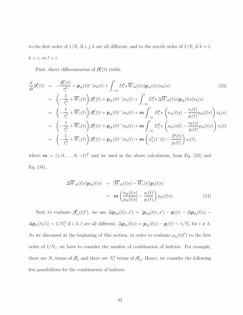
to the first order of 1/Nc if i, j, k are all different, and to the zeroth order of 1/Nc if k = l,
k = i, or l = i.
First, direct differentiation of βki (t) yields
d
dtβk
i (t) = −βki (t)
τki
+ pik(t|t−)νk(t) +
∫ t
−∞Dk
i s W ik(t|s)pik(t|s)νk(s) (53)
=
(
− 1
τki
+ W i(t)
)
βki (t) + pik(t|t−)νk(t) +
∫ t
−∞Dk
i s ∆W ik(t|s)pik(t|s)νk(s)
=
(
− 1
τki
+ W i(t)
)
βki (t) + pik(t|t−)νk(t) + m
∫ t
−∞Dk
i s
(
νik(t|s) −νi(t)
pi(t)pik(t|s)
)
νk(s)
=
(
− 1
τki
+ W i(t)
)
βki (t) + pik(t|t−)νk(t) + m
∫ t
−∞Dk
i s
(
νki(s|t) −νk(s)
pi(t)pik(t|s)
)
νi(t)
=
(
− 1
τki
+ W i(t)
)
βki (t) + pik(t|t−)νk(t) + m
(
αkii(t
−|t) − βki (t)
pi(t)
)
νi(t),
where m = (1, 0, . . . , 0,−1)T and we used in the above calculation, from Eq. (32) and
Eq. (34),
∆W ik(t|s)pik(t|s) = [W ik(t|s) − W i(t)]pi(t|s)
= m
(
νik(t|s)pik(t|s)
− νi(t)
pi(t)
)
pik(t|s). (54)
Next to evaluate βkij(t|t′), we use ∆pikl(t|s, s′) = [pikl(t|s, s′) − pi(t) − ∆pik(t|s) −
∆pil(t|s′)] ∼ 1/N2c if i, k, l are all different; ∆pik(t|s) = pik(t|s) − pi(t) ∼ 1/Nc for i 6= k.
As we discussed at the beginning of this section, in order to evaluate µij(t|t′) to the first
order of 1/Nc, we have to consider the number of combination of indexes. For example,
there are Nc terms of βiii and there are N2
c terms of βiij . Hence, we consider the following
five possibilities for the combination of indexes:
42

• Case 1 (i 6= j, i 6= k); evaluated up to the first order of 1/Nc:
βkij(t|t′) ≈
∫ t
−∞Dk
i s [pi(t) + ∆pik(t|s) + ∆pij(t|t′)]νkj(s|t′)
=
∫ t
−∞Dk
i s [pi(t)νkj(s|t′) + ∆pik(t|s)(νk(s) + ∆νkj(s|t′)) + ∆pij(t|t′)(νk(s) + ∆νkj(s|t′))]
≈∫ t
−∞Dk
i s [pi(t)νkj(s|t′) + ∆pik(t|s)νk(s) + ∆pij(t|t′)νk(s)]
=
∫ t
−∞Dk
i s [pi(t)νkj(s|t′) + (pik(t|s) − pi(t))νk(s) + ∆pij(t|t′)νk(s)]
= pi(t)αkij(t|t′) + (βk
i (t) − pi(t)αki (t)) + ∆pij(t|t′)αk
i (s)
= βki (t) + pi(t)∆αk
ij(t|t′) + ∆pij(t|t′)αki (s)
≈ βki (t) + pij(t|t′)αk
ij(t|t′) + pi(t)αki (s). (55)
Note that, in the second line, we used ∆pik ∼ 1/Nc and ∆νij ∼ 1/Nc, for example,
and neglected higher order terms such as ∆pik∆νkj.
• Case 2 (i = j, k 6= i); evaluated up to the first order of 1/Nc:
βkii(t|t′) ≈
∫ t
−∞Dk
i s [pii(t|t′) + ∆pik(t|s)]νki(s|t′)
=
∫ t
−∞Dk
i s [pii(t|t′)νki(s|t′) + (pik(t|s) − pi(t))νk(s)]
= pii(t|t′)αkii(t|t′) + (βk
i (t) − pi(t)αki (t))
= βki (t) + pii(t|t′)αk
ii(t|t′) − pi(t)αki (t). (56)
• Case 3 (i = k, i 6= j); evaluated up to the zeroth order of 1/Nc:
βiij(t|t′) ≈
∫ t
−∞Di
is pii(t|s)νi(s)
= βii(t)
≈ βii(t) + pij(t|t′)αi
ij(t|t′) − pi(t)αii(s). (57)
43
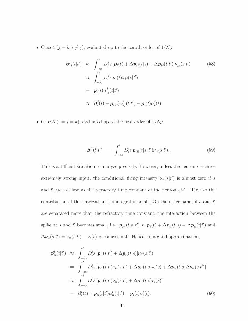
• Case 4 (j = k, i 6= j); evaluated up to the zeroth order of 1/Nc:
βjij(t|t′) ≈
∫ t
−∞Dj
i s [pi(t) + ∆pij(t|s) + ∆pij(t|t′)]νjj(s|t′) (58)
≈∫ t
−∞Dj
i s pi(t)νjj(s|t′)
= pi(t)αjij(t|t′)
≈ βji (t) + pi(t)α
jij(t|t′) − pi(t)α
ji (t).
• Case 5 (i = j = k); evaluated up to the first order of 1/Nc:
βiii(t|t′) =
∫ t
−∞Di
is piii(t|s, t′)νii(s|t′). (59)
This is a difficult situation to analyze precisely. However, unless the neuron i receives
extremely strong input, the conditional firing intensity νii(s|t′) is almost zero if s
and t′ are as close as the refractory time constant of the neuron (M − 1)τr; so the
contribution of this interval on the integral is small. On the other hand, if s and t′
are separated more than the refractory time constant, the interaction between the
spike at s and t′ becomes small, i.e., piii(t|s, t′) ≈ pi(t) + ∆pii(t|s) + ∆pii(t|t′) and
∆νii(s|t′) = νii(s|t′) − νi(s) becomes small. Hence, to a good approximation,
βiii(t|t′) ≈
∫ t
−∞Di
is [pii(t|t′) + ∆pii(t|s)]νii(s|t′)
=
∫ t
−∞Di
is [pii(t|t′)νii(s|t′) + ∆pii(t|s)νi(s) + ∆pii(t|s)∆νii(s|t′)]
≈∫ t
−∞Di
is [pii(t|t′)νii(s|t′) + ∆pii(t|s)νi(s)]
= βii(t) + pii(t|t′)αi
ii(t|t′) − pi(t)αii(t). (60)
44

The validity of this intuitive approximation should be examined by numerical simu-
lations. Note that βiii(t|t′) contributes to the order 1/Nc term of the autocovariance
function ∆φii(t, t′) but only contributes to order 1/N2
c terms of the mean firing in-
tensity νi(t) and crosscovariance functions ∆φij(t, t′) with i 6= j.
Finally, we can rewrite Bkli as
[
Bkli (t)
]
m=
∫ t
−∞Dk
i s
∫ t
−∞Dl
is′{
[pikl(t|s, s′)]mφkl(s, s′) − [pik(t|s)]m[pil(t|s′)]m
[pi(t)]mνk(s)νl(s
′)
}
(61)
=
∫ t
−∞Dk
i s
∫ t
−∞Dl
is′{
[pikl(t|s, s′)]m∆φkl(s, s′) +
(
[pikl(t|s, s′)]m − [pik(t|s)]m[pil(t|s′)]m[pi(t)]m
)
νk(s)νl(s′)
}
=
∫ t
−∞Dk
i s
∫ t
−∞Dl
is′{
[pikl(t|s, s′)]m∆φkl(s, s′) +
(
[∆pikl(t|s, s′)]m − [∆pik(t|s)]m[∆pil(t|s′)]m[pi(t)]m
)
νk(s)νl(s′)
}
,
where we used ∆pik(t|s) = pik(t|s) − pi(t) and ∆pikl(t|s, s′) = pikl(t|s, s′) − pi(t) −
∆pik(t|s) − ∆pil(t|s′). We need to evaluate Bkli up to the first order of 1/Nc if i, k, l
are all different, and up to the zeroth order of 1/Nc if k = l, k = i, or l = i. Up to these
orders, Bkli can be approximated as
Bkli (t) ≈
∫ t
−∞Dk
i s
∫ t
−∞Dl
is′pi(t)∆φkl(s, s
′)
= pi(t)Akli (t). (62)
Note that ∆pik ∼ 1/Nc for i 6= k, ∆pikl(t|s, s′) ∼ 1/N2c if i, k, l are different, and
∆piik(t|s, s′) ∼ 1/Nc for i 6= k.
45

A.3 Calculation of the linear filter in the generalized linear model
with Markov refractoriness
We assume that the input is given by
Ii(t) =
∫
Ki(t − s)ξi(s)ds (63)
with stimulus ξi = ξ(0)i + δξi(t), and calculate the linearized input output filter for small
stimulus fluctuation δξi(t) about a constiant baseline ξ(0)i .
In the limit of Nc → ∞, the mean-field equation is given by
νi(t) = f(Ii(t) + µi(t))pi(t), (64)
µi(t) =∑
k
Jki
βki (t)
pi(t),
d
dtpi(t) = W i(t)pi(t),
d
dtβk
i (t) =
(
− 1
τki
+ W i(t)
)
βki (t) + pi(t)νk(t).
First, for a constant input I(0)i , we obtain
ν(0)i = f
(0)i p
(0)i , (65)
µ(0)i =
∑
k
Jki
βki
(0)
p0i
,
0 = W(0)
i p(0)i ,
βki
(0)=
[
1
τki
− W(0)
i
]−1
p(0)i ν
(0)k , (66)
where f(0)i = f(I
(0)i + µ
(0)i ) and the last equation is easily solvable with respect to p
(0)i ; we
46

find
[
p(0)i
]
m=
τrf(0)i
1+(M−1)τrf(0)i
(m = 1, . . . , M − 1)
1
1+(M−1)τrf(0)i
(m = M).
(67)
Next, the linear response to a small perturbation δIi(t) =∫
Ki(t − s)δξi(s)ds is given
by
δνi(t) = f ′i(0)
(δIi(t) + δµi(t))p(0)i + f
(0)i δpi(t), (68)
δµi(t) =∑
k
Jki
[
δβki (t)
p(0)i
− βki
(0)δpi(t)
(p(0)i )2
]
,
d
dtδpi(t) = δW i(t)p
(0)i + W
(0)
i δpi(t),
d
dtδβk
i (t) =
(
− 1
τki
+ W(0)
i
)
δβki (t) + δW i(t)β
ki
(0)+ δpi(t)ν
(0)k + p
(0)i δνk(t),
where f ′i(0) = f ′(I0
i + µ(0)i ) and δW i(t) = meT
M [δνi(t)/p(0)i − ν
(0)i δpi(t)/(p
(0)i )2]. Rememer
that m = (1, 0, . . . , 0,−1)T and eM = (0, . . . , 0, 1)T . Fourier transformation of the above
equations give
δνi(ω) = f ′i(0)
(δIi(ω) + δµi(ω))p(0)i + f
(0)i δpi(ω), (69)
δµi(ω) =∑
k
Jki
[
δβki (ω)
p(0)i
− βki
(0)δpi(ω)
(p(0)i )2
]
,
δpi(ω) = Li(ω)mδνi(ω),
δβk
i (ω) = qki (ω)δνi(ω) + R
k
i (ω)δνk(ω),
where Li(ω) = [iω + meTMν
(0)i /p
(0)i −W
(0)
i ]−1, qki (ω) = [iω + 1/τk
i −W(0)
i ]−1[mβki
(0)/p
(0)i −
meTMLi(ω)mβk
i(0)
ν(0)i /(p
(0)i )2 + Li(ω)mν
(0)k ], and R
k
i (ω) = [iω + 1/τki −W
(0)
i ]−1p(0)i . Note
that i is the imaginary unit.
47

The above equation is still very complicated. So, it is worth thinking about the special
case Jki = 0. In this case, the linear response is described by
δνi(ω) =f ′
i(0)p
(0)i
1 − f(0)i eT
MLi(ω)mδIi(ω). (70)
The calculation of Li(ω) is straight forward thanks to the bidiagonal nature of [iω +
meTMν
(0)i /p
(0)i − W
(0)
i ]. After direct matrix inversion, we find
Li(ω) = τrρ
1 0 0 · · · 0
ρ 1 0...
ρ2 ρ 1
.... . .
ρM−2 · · · ρ 1 0
ρM−1η · · · ρ2η ρη η
(71)
with ρ = 1/(1 + iωτr) and η = 1 + 1/(iωτr). Hence, the linear response is simplified as
δνi(ω) =f ′
i(0)p
(0)i
1 − f(0)i τrρη(ρM−1 − 1)
δIi(ω). (72)
In particular, if M = 2, we find that the Fourier inverse transformation of the gain function
G(ω) = δνi(ω)/δIi(ω) =f ′
i(0)p
(0)i
1+f(0)i τr/(1+iωτr)
has an analytical form, i.e, using p(0)i = 1/(1 +
τrf(0)i ), we find
G(t) =f ′
i(0)
1 + τrf(0)i
[
δ(t) − f(0)i e−(fi
(0)+1/τr)tΘ(t)]
. (73)
Note that in the limit of τr → 0, the trivial gain function is G(t) → f ′i(0)δ(t). Hence, we
can see that the suppressive kernel is added to this instantaneous gain function due to the
48
Markov refractoriness. This linear response for Jki = 0 case is a special case of a more
general linear response for a renewal neuron [Gerstner and Kistler, 2002]. Note that, in
Eq. (69), we discussed a more general case and considered the interaction between the
refractory effect and spike-interaction effect of network of recurrently connected neurons.
Acknowledgements
We thank E. Shea-Brown for helpful conversations. TT is supported by The Robert Leet
and Clara Guthrie Patterson Trust Postdoctoral Fellowship, Bank of America, Trustee.
LP is supported by an NSF CAREER award, an Alfred P. Sloan Research Fellowship, the
McKnight Scholar award, and by NEI grant EY018003.
References
[Amit and Tsodyks, 1991] Amit, D. J. and Tsodyks, M. V. (1991). Quantitative study of
attractor neural networks retrieving at low spike rates. i: Substrate — spikes, rates, and
neuronal gain. Network, 2:259–273.
[Berry and Meister, 1998] Berry, M. and Meister, M. (1998). Refractoriness and neural
precision. J. Neurosci., 18:2200–2211.
[Brillinger, 1988] Brillinger, D. (1988). Maximum likelihood analysis of spike trains of
interacting nerve cells. Biological Cyberkinetics, 59:189–200.
49

[Brown et al., 2004] Brown, E., Kass, R., and Mitra, P. (2004). Multiple neural spike train
data analysis: state-of-the-art and future challenges. Nature Neuroscience, 7:456–461.
[Brunel and Hakim, 1999] Brunel, N. and Hakim, V. (1999). Fast global oscillations in net-
works of integrate-and-fire neurons with low firing rates. Neural Computation, 11:1621–
1671.
[Bryant and Segundo, 1976] Bryant, H. and Segundo, J. (1976). Spike initiation by trans-
membrane current: a white-noise analysis. Journal of Physiology, 260:279–314.
[Chizhov and Graham, 2007] Chizhov, A. V. and Graham, L. J. (2007). Population
model of hippocampal pyramidal neurons, linking a refractory density approach to
conductance-based neurons. Phys Rev E Stat Nonlin Soft Matter Phys, 75:011924.
[Chornoboy et al., 1988] Chornoboy, E., Schramm, L., and Karr, A. (1988). Maximum
likelihood identification of neural point process systems. Biological Cybernetics, 59:265–
275.
[Derrida et al., 1987] Derrida, B., Gardner, E., and Zippelius, A. (1987). An exactly solv-
able asymmetric neural network model. Europhys. Lett., 4:167–173.
[Doiron et al., 2004] Doiron, B., Lindner, B., Longtin, A., Maler, L., and Bastian, J.
(2004). Oscillatory activity in electrosensory neurons increases with the spatial cor-
relation of the stochastic input stimulus. Phys Rev Lett, 93(4):048101.
50
[Escola and Paninski, 2007] Escola, S. and Paninski, L. (2007). Hidden Markov models
applied toward the inference of neural states and the improved estimation of linear
receptive fields. Under review, Neural Computation.
[Fourcaud-Trocme and Brunel, 2005] Fourcaud-Trocme, N. and Brunel, N. (2005). Dy-
namics of the instantaneous firing rate in response to changes in input statistics. J
Comput Neurosci, 18:311–321.
[Fourcaud-Trocme et al., 2003] Fourcaud-Trocme, N., Hansel, D., van Vreeswijk, C., and
Brunel, N. (2003). How spike generation mechanisms determine the neuronal response
to fluctuating inputs. J Neurosci, 23:11628–11640.
[Gerstner and Kistler, 2002] Gerstner, W. and Kistler, W. (2002). Spiking Neuron Models:
Single Neurons, Populations, Plasticity. Cambridge University Press.
[Ginzburg and Sompolinsky, 1994] Ginzburg, I. and Sompolinsky, H. (1994). Theory of
correlations in stochastic neural networks. Phys Rev E, 50(4):3171–3191.
[Harris et al., 2003] Harris, K., Csicsvari, J., Hirase, H., Dragoi, G., and Buzsaki, G.
(2003). Organization of cell assemblies in the hippocampus. Nature, 424:552–556.
[Hatsopoulos et al., 1998] Hatsopoulos, N., Ojakangas, C., Paninski, L., and Donoghue,
J. (1998). Information about movement direction obtained by synchronous activity of
motor cortical neurons. PNAS, 95:15706–15711.
[Hertz et al., 1991] Hertz, J., Krogh, A., and Palmer, R. G. (1991). Introduction to the
Theory of Neural Computation. Addison-Wesley, Redwood City CA.
51

[Kappen and Spanjers, 2000] Kappen, H. J. and Spanjers, J. J. (2000). Mean field theory
for asymmetric neural networks. Phys Rev E, 61(5 Pt B):5658–5663.
[Kass and Ventura, 2001] Kass, R. and Ventura, V. (2001). A spike-train probability
model. Neural Comp., 13:1713–1720.
[Keat et al., 2001] Keat, J., Reinagel, P., Reid, R., and Meister, M. (2001). Predicting
every spike: a model for the responses of visual neurons. Neuron, 30:803–817.
[Knight et al., 2000] Knight, B., Omurtag, A., and Sirovich, L. (2000). The approach of a
neuron population firing rate to a new equilibrium: an exact theoretical result. Neural
Computation, 12:1045–1055.
[Kohn and Smith, 2005] Kohn, A. and Smith, M. (2005). Stimulus dependence of neuronal
correlation in primary visual cortex of the macaque. Journal of Neuroscience, 25:3661–
3673.
[Kulkarni and Paninski, 2007] Kulkarni, J. and Paninski, L. (2007). Common-input mod-
els for multiple neural spike-train data. Network: Computation in Neural Systems,
18:375–407.
[Lindner et al., 2005] Lindner, B., Doiron, B., and Longtin, A. (2005). Theory of oscilla-
tory firing induced by spatially correlated noise and delayed inhibitory feedback. Phys
Rev E Stat Nonlin Soft Matter Phys, 72(6 Pt 1):061919.
[Marmarelis and Marmarelis, 1978] Marmarelis, P. and Marmarelis, V. (1978). Analysis
of physiological systems: the white-noise approach. Plenum Press, New York.
52

[Martignon et al., 2000] Martignon, L., Deco, G., Laskey, K., Diamond, M., Freiwald, W.,
and Vaadia, E. (2000). Neural coding: higher-order temporal patterns in the neuro-
statistics of cell assemblies. Neural Computation, 12:2621–2653.
[Mattia and Del Giudice, 2002] Mattia, M. and Del Giudice, P. (2002). Population dynam-
ics of interacting spiking neurons. Phys Rev E Stat Nonlin Soft Matter Phys, 66:051917.
[Meyer and van Vreeswijk, 2002] Meyer, C. and van Vreeswijk, C. (2002). Temporal cor-
relations in stochastic networks of spiking neurons. Neural Comput, 14:369–404.
[Moreno-Bote and Parga, 2004] Moreno-Bote, R. and Parga, N. (2004). Role of synaptic
filtering on the firing response of simple model neurons. Phys Rev Lett, 92:028102.
[Moreno-Bote and Parga, 2006] Moreno-Bote, R. and Parga, N. (2006). Auto- and cross-
correlograms for the spike response of leaky integrate-and-fire neurons with slow
synapses. Phys Rev Lett, 96:028101.
[Nirenberg et al., 2002] Nirenberg, S., Carcieri, S., Jacobs, A., and Latham, P. (2002).
Retinal ganglion cells act largely as independent encoders. Nature, 411:698–701.
[Nykamp, 2007a] Nykamp, D. (2007a). A mathematical framework for inferring connec-
tivity in probabilistic neuronal networks. Math Biosci, 205:204–251.
[Nykamp, 2007b] Nykamp, D. (2007b). A mathematical framework for inferring connec-
tivity in probabilistic neuronal networks. Mathematical Biosciences, 205:204–251.
53
[Nykamp and Tranchina, 2000] Nykamp, D. and Tranchina, D. (2000). A population den-
sity approach that facilitates large-scale modeling of neural networks: analysis and an
application to orientation tuning. Journal of Computational Neuroscience, 8:19–50.
[Okatan et al., 2005] Okatan, M., Wilson, M., and Brown, E. (2005). Analyzing functional
connectivity using a network likelihood model of ensemble neural spiking activity. Neural
Computation, 17:1927–1961.
[Oksendal, 2002] Oksendal, B. (2002). Stochastic Differential Equations. Springer.
[Oram et al., 2001] Oram, M., Hatsopoulos, N., Richmond, B., and Donoghue, J. (2001).
Excess synchrony in motor cortical neurons provides redundant direction information
with that from coarse temporal measures. Journal of Neurophysiology, 86:1700–1716.
[Paninski, 2004] Paninski, L. (2004). Maximum likelihood estimation of cascade point-
process neural encoding models. Network: Computation in Neural Systems, 15:243–262.
[Paninski et al., 2004] Paninski, L., Fellows, M., Shoham, S., Hatsopoulos, N., and
Donoghue, J. (2004). Superlinear population encoding of dynamic hand trajectory in
primary motor cortex. J. Neurosci., 24:8551–8561.
[Paninski et al., 2007] Paninski, L., Pillow, J., and Lewi, J. (2007). Statistical models for
neural encoding, decoding, and optimal stimulus design. In Cisek, P., Drew, T., and
Kalaska, J., editors, Computational Neuroscience: Progress in Brain Research. Elsevier.
54

[Pillow et al., 2005] Pillow, J., Paninski, L., Uzzell, V., Simoncelli, E., and Chichilnisky,
E. (2005). Prediction and decoding of retinal ganglion cell responses with a probabilistic
spiking model. Journal of Neuroscience, 25:11003–11013.
[Pillow et al., 2007] Pillow, J., Shlens, J., Paninski, L., Simoncelli, E., and Chichilnisky,
E. (2007). Visual information coding in multi-neuronal spike trains. Nature, In press.
[Renart et al., 2003] Renart, A., Brunel, N., and Wang, X.-J. (2003). Computational Neu-
roscience: A Comprehensive Approach, chapter Mean-field theory of recurrent cortical
networks: from irregularly spiking neurons to working memory. CRC Press, Boca Raton.
[Riehle et al., 1997] Riehle, A., Grun, S., Diesmann, M., and Aertsen, A. (1997). Spike
synchronization and rate modulation differentially involved in motor cortical function.
Science, 278:1950–1953.
[Rieke et al., 1997] Rieke, F., Warland, D., de Ruyter van Steveninck, R., and Bialek, W.
(1997). Spikes: Exploring the neural code. MIT Press, Cambridge.
[Rigat et al., 2006] Rigat, F., de Gunst, M., and van Pelt, J. (2006). Bayesian modelling
and analysis of spatio-temporal neuronal networks. Bayesian Analysis, 1:733–764.
[Schnitzer and Meister, 2003] Schnitzer, M. and Meister, M. (2003). Multineuronal firing
patterns in the signal from eye to brain. Neuron, 37:499–511.
[Shriki et al., 2003] Shriki, O., Hansel, D., and Sompolinsky, H. (2003). Rate models for
conductance-based cortical neuronal networks. Neural Comput, 15:1809–1841.
55
[Snyder and Miller, 1991] Snyder, D. and Miller, M. (1991). Random Point Processes in
Time and Space. Springer-Verlag.
[Sompolinksy et al., 1988] Sompolinksy, H., Crisanti, A., and Sommers, H. (1988). Chaos
in random neural networks. Physical Review Letters, 61:259–262.
[Toyoizumi et al., 2006] Toyoizumi, T., Aihara, K., and Amari, S. (2006). Fisher informa-
tion for spike-based population decoding. Phys. Rev. Lett., 97:098102.
[Truccolo et al., 2005] Truccolo, W., Eden, U., Fellows, M., Donoghue, J., and Brown, E.
(2005). A point process framework for relating neural spiking activity to spiking history,
neural ensemble and extrinsic covariate effects. Journal of Neurophysiology, 93:1074–
1089.
[van Vreeswijk and Sompolinsky, 1996] van Vreeswijk, C. and Sompolinsky, H. (1996).
Chaos in neuronal networks with balanced excitatory and inhibitory activity. Science,
274:1724–1726.
[van Vreeswijk and Sompolinsky, 1998] van Vreeswijk, C. and Sompolinsky, H. (1998).
Chaotic balanced state in a model of cortical circuits. Neural Computation, 10:1321–
1371.
[Wilson and Cowan, 1972] Wilson, H. R. and Cowan, J. D. (1972). Excitatory and in-
hibitory interactions in localized populations of model neurons. Biophys J, 12(1):1–24.
56

A B
Figure 2: Direct solution of the master equation in the one-dimensional case. (A) Top: A
single neuron is simulated with a pulse input I(t) shown. Bottom: Comparison of the firing
rates computed via: direct Monte Carlo sampling (simulation); the inhomogeneous Poisson case,
with no history dependence, i.e., w = 0 (noH); the master equation of Eq. (8) (exact); and the
mean-field approximation methods in the limit of Nc → ∞ introduced in section 4. the mean-field
approximation gives good approximations of the output firing intensity. (B) Top: The probability
distribution P (h, t); color axis indicates the height of the probability density. The self-history
term h(t) was the convolution of the output spike train and a single exponential filter with time
constant τ = 10 ms and weight J = −1; thus the neuron was inhibited for a brief period following
each spike. Note the discontinuous behavior visible at stimulus onset, where probability mass
jumps significantly towards h = 1, then decays back down towards zero, according to equation
(8). (C) The mean of h calculated from the probability distribution P (h, t). This E[h] also
increases following the input pulse, which has the effect of slowing down the firing rate: since the
weight J is negative, the history term is inhibitory here.
57

A B
Figure 3: Comparison of the direct Monte Carlo simulation of a single neuron (solid),
the firing intensity without recurrent input H (dotted), and the mean-field approximation
(dashed). (A) Low step input (baseline I = 2, peak I = 4) is applied. The self inhibition
term is set to J = −5 and τ = 2 ms. (B) High step input (baseline I = 2, peak I = 8)
is applied. The self inhibition terms is set to J = −5 and τ = 2 ms. Because of the large
non-Gaussian fluctuations of input caused by the strong self-inhibition, the mean-field
approximation loses accuracy here.
58

A B
Figure 4: Comparison of cross-correlation functions of two neurons calculated by direct
simulation (solid), calculated from the mean-field approximation (Eqs. (18-19); dashed),
and the mean-field approximation with finite size correction (Eqs. (15-17 and 20); dot-
dashed). (A) Weak self-interaction: parameters are set to J11 = −1, J22 = −1, J21 =
1, J12 = −0.5, τ11 = 10ms, τ22 = 10ms, τ21 = 10ms, τ12 = 20ms, and I1 = 2, I2 = 4.
The result is after 5 iterations of mean-field equations. The calculation in the mean-field
limit only captures the steady state firing intensity but not any temporal cross correlation
function. Cross correlation functions are well approximated with the finite size correction
terms. (B) Strong self-interaction: parameters are set to J11 = −5, J22 = −5, J21 = 1, J12 =
−0.5, τ11 = 2ms, τ22 = 2ms, τ21 = 10ms, τ12 = 20ms, and I1 = 2, I2 = 4. Because of the
large non-Gaussian fluctuation of the input caused by the strong self-inhibition term, the
mean-field approximations does not work very well. In this case the mean-field solution
converges rather slowly. Hence, the result is after 10 iterations of mean-field equations.
59

A B C
Figure 5: Comparison of (A) a simulated firing rates of a single neuron and (B) the self-
consistent solutions of Eq. (21) for different input levels, I(0), and self-inhibition strengths,
J . (C) The percentage errors of the mean-field approximation are shown with respect to
the simulated firing intensity. We set τ = 10 ms.
60

A B
Figure 6: Comparison of the analytically derived and simulated input-output filters. (A)
A simulated normalized linear input-output filter for I(0) = 2 (thin-dotted) and I(0) = 4
(thick-dotted) are compared with analytical results at I(0) = 2 (thin-solid) and I(0) = 4
(thick-solid) of Eq. (26). Because the strength of the self-inhibition component changes
with the baseline input through f ′(I(0)+µ(0)), the input-filter is sharpened for high baseline
input. Other parameters are set to J = 1, τ = 10 ms, K(t) = e−t/τI Θ(t) with τI = 20
ms and σξ = 1 Hz. All filter amplitudes are normalized by their maximum amplitudes.
(B) Left panels show the comparison of analytically derived input-output filters G11(t) and
G12(t) of Eq. (28) (solid lines) and simulated input-output filters (dotted lines) for I(0) = 2
(thin lines) and I(0) = 4 (thick lines). Right panels show neuron 1’s spatio-temporal input-
output filter G1(t, z) for I(0) = 2 (top) and I(0) = 4 (bottom). See text for parameter
values.
61

A B
C D
Figure 7: Comparison of the mean firing intensity obtained from direct simulation of a single
neuron (solid), without recurrent input H and no Markov refractory effect (dotted), and the
mean-field equation in the limit of Nc → ∞ (dashed). In all the cases, the markov refractory
effect with τr = 2ms/(M−1) was included. (A) Weak step input (baseline I = 2, peak I = 4) and
refractoriness M = 3; J = −1, τ = 10 ms. Although the model includes strong Markov refractory
effect, the mean-field approximation is not abolished. (B) Strong step input (baseline I = 2,
peak I = 8) and refractoriness M = 10; J = −1, τ = 10ms. The mean-field approximation also
approximates very well the transient oscillation caused by the the strong refractory effect and steep
current. (C) The mean-field approximation works for colored noise input: τIdI(t)
dt = −I(t) + ξ(t)
with E[ξ(t)] = 4, Cov[ξ(t), ξ(t′)] = 0.1δ(t − t′), and τI = 20 ms; M = 3, J = −1, τ = 10ms. The
initial error is due to the preset initial values deviates from the true ones. (D) Sinusoidal input
input: I(t) = 2 + sin(2π · 10Hz · t); M = 3, J = −1, τ = 10ms. The mean-field results give good
approximations. 62
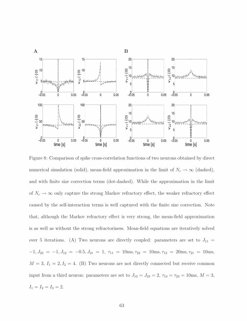
A B
Figure 8: Comparison of spike cross-correlation functions of two neurons obtained by direct
numerical simulation (solid), mean-field approximation in the limit of Nc → ∞ (dashed),
and with finite size correction terms (dot-dashed). While the approximation in the limit
of Nc → ∞ only capture the strong Markov refractory effect, the weaker refractory effect
caused by the self-interaction terms is well captured with the finite size correction. Note
that, although the Markov refractory effect is very strong, the mean-field approximation
is as well as without the strong refractoriness. Mean-field equations are iteratively solved
over 5 iterations. (A) Two neurons are directly coupled: parameters are set to J11 =
−1, J22 = −1, J12 = −0.5, J21 = 1, τ11 = 10ms, τ22 = 10ms, τ12 = 20ms, τ21 = 10ms,
M = 3, I1 = 2, I2 = 4. (B) Two neurons are not directly connected but receive common
input from a third neuron: parameters are set to J13 = J23 = 2, τ13 = τ23 = 10ms, M = 3,
I1 = I2 = I3 = 2.
63


![Quantum strong energy inequalitieseprints.whiterose.ac.uk/140592/1/Quantum_journal.pdf · nonminimally coupled scalar field and deduced, by the methods of [18], a Hawking-type sin-gularity](https://img.pdfslide.us/doc/110x75/5f9e0cc40f85d13e5a461128/quantum-strong-energy-nonminimally-coupled-scalar-ield-and-deduced-by-the-methods.jpg)


![Cosmological dynamics with non-minimally coupled scalar ... · induced gravity [30]. While the simplest inflationary model with a minimally coupled scalar field and a quadratic](https://img.pdfslide.us/doc/110x75/5e115aa7fb5dc04ebc6ce678/cosmological-dynamics-with-non-minimally-coupled-scalar-induced-gravity-30.jpg)