ME8281 - Last updated: April 21, 2008 (c) Perry Li Robust ... · ME8281 - Last updated: April 21, 2008 (c) ... the control sensitivity so that output disturbance or ... Robust Stability

ME8281 - Last updated: April 21, 2008 (c) Perry Li

Robust stability and Performance

Topics: ([ author ] is supplementary source)

• Sensitivities and internal stability (Goodwin 5.1-5.4)

• Modeling Error and Model Uncertainty (Goodwin4.12-4.13, Doyle 4.1)

• Robust stability (Goodwin 5.7-5.10, Doyle 4.2)

• Robust performance (Doyle 4.3-4.4, Goodwin 5.9)

• Loop-shaping technique (Doyle 7.1) [We will coverthis only briefly]

• Innovation feedback and affine parameterizationapproach to tuning S and T (see Goodwin Chapters15, 16, 18.5-6 for details)

The following topic(s) are for your information:

• Performance limitation (Glad 7.3-7.4, Doyle 6.1-6.2,Goodwin [8.6],9.1-9.3)

M.E. University of Minnesota 137


Nominal Sensitivity Functions

To(s) =

(Y (s)

Dm(s)=Y (s)

R(s)=

)Go(s)C(s)

1 +Go(s)C(s)(18)

So(s) =

(Y (s)

Do(s)=

)1

1 +Go(s)C(s)(19)

Sio(s) =

(Y (s)

Di(s)=

)Go(s)

1 +Go(s)C(s)(20)

Suo(s) =

(U(s)

Do(s)=

)C(s)

1 +Go(s)C(s)(21)

• To - Complementary sensitivity (goal: small fornoise, ≈ 1 for command following)

• So - Sensitivity (goal: small)

• Sio - Input disturbance sensitivity (goal: small)

• Suo - Control sensitivity (goal: small)



Internal Stability

The nominal loop is internally stable if and only if alleight transfer functions below is stable:

(Yo(s)Uo(s)

)

=

(Go(s)C(s) Go(s) 1 −Go(s)C(s)

C(s) −Go(s)C(s) −C(s) −C(s)

)

1 +Go(s)C(s)

H(s)R(s)Di(s)Do(s)Dm(s)

Let C(s) = P (s)/L(s), and Go(s) = Bo(s)/Ao(s).

Proposition The system is internally stable if and onlyif the roots of the nominal closed loop characteristicequation

Ao(s)L(s) +Bo(s)P (s) = 0

all lie in the open left half plane.



Example Consider

Go(s) =s

(s+ 4)(−s+ 2), C(s) =

−s+ 2

s

where pole-zero cancellations at s = 2 and s = 0occur.

Complementary sensitivity is stable:

To(s) = −Y (s)/Dm(s) =G(s)C(s)

1 +Go(s)C(s)=

1

s+ 5

Sensitivity is also stable:

S(s) = 1 − To(s) =s+ 4

s+ 5

However, control sensitivity is marginally stable:

Suo(s) =U(s)

Dm(s)=

C(s)

1 +Go(s)C(s)=

(−s+ 2)(s+ 4)

(s+ 5)s

And, input disturbance sensitivity is unstable:

Sio(s) =Y (s)

Di(s)=

s

(−s+ 2)(s+ 5)



• The effect of unstable pole at s = 2 shows up inSio as input disturbance will drive the output Y tobe unbounded. This effect is not observed by thecontroller as it is blocked by its zero.

• The effect of unstable pole at s = 0 shows up inthe control sensitivity so that output disturbance ormeasurement noise will drive the control output tobe unbounded. This effect is not observed at theoutput as it is blocked by the plant’s zero.

• Characteristic equation has unstable and marginallystable poles:

(−s+ 2)s+ (s+ 4)(−s+ 2)s = (−s+ 2)(s+ 5)s

predicting correctly that the system is NOTinternally stable.



Modeling Error

For linear systems, if Go(s) is the nominal system, andthe actual system is G(s), then define:

• Additive uncertainty:

Gǫ(s) = G(s) −Go(s)

• Multiplicative uncertainty:

Go(s)G∆(s) = G(s) −Go(s)

or

G∆(s) =G(s) −Go(s)

Go(s)



Example: Time delays - τ

The transfer function of time delay is e−τs. Since it isnot rational, one often models it as

e−τs ≈

(−τs+ 2k

τs+ 2k

)k

where k = 0, 1, 2, . . ..

The additive modeling error is:

Gǫ(s) = e−τs −

(−τs+ 2k

τs+ 2k

)k

The multiplicative modeling error is:

G∆(s) =

[

e−τs −

(−τs+ 2k

τs+ 2k

)k]

/

(−τs+ 2k

τs+ 2k

)k

.



10−2

10−1

100

101

102

10−10

10−8

10−6

10−4

10−2

100

102

ω rad/s

MM

E

Multiplicative Modeling error of approximation of various orders for 1s time delay

k=0k=1k=2k=3k=5

Other examples:

• Uncertain pole location:

1/(s+Am) → 1/(s+A) where A ∈ [A0, A1]

• Neglected (possibly structural) dynamics:

ω2n/(s

2 + 2ζωns+ ω2n) → 1.

• Neglected compressibility effect, etc...



Robust Stability

Let Go(s) be the nominal plant. Consider a family ofplants characterized by:

P := {G(s) = (1 +Wu(s)∆(s))Go(s)}

where

• G∆(s) = Wu(s)∆(s) is the multiplicative modeluncertainty

• Wu(s) is a given stable uncertainty weightingfunction

• ∆(s) is the uncertainty itself, which is any stabletransfer function with |∆(jω)| < 1 for all ω ∈ ℜ.

The question of robust stability is whether a controllerdesigned for Go(s) also stabilizes the any plant G(s) ∈P . If so, we say that the controller provides robuststability.



Robust Stability Theorem: Assume that thecontroller C(s) internally stabilizes the nominal plantGo(s). Suppose that G(s)C(s) and Go(s)C(s) havethe same number of unstable (openloop) poles on theopen right half plane. Then,

1. If |G∆(jω)| · |To(jω)| < 1 for all ω ∈ ℜ (in otherwords, ‖G∆ · To‖∞ < 1) then the controller C(s)internally stabilizes the perturbed plant G(s).

2. C(s) provides robust stability for the plant set P ifand only if

‖Wu · To‖∞ < 1 (22)

where To(s) is the complementary sensitivityfunction:

To(s) =Lo(s)

1 + Lo(s)where Lo(s) = Go(s)C(s).

Remark:

• ‖F‖∞ := supω∈ℜ|F (jω)| is the so called infinitynorm of the transfer function F (s).

• Every plant G(s) ∈ P corresponds to a G∆(s) thatsatisfies ‖G∆ · To‖∞ < 1. So the extra interestingaspect of robust stability condition is the necessity.



Before we give a proof of this theorem, recall theNyquist theorem:

Nyquist Theorem: Suppose that L(s) has P unstablepoles on the open RHP. Then, the Nyquist plot (i.e.the plot of L(s) on the complex plane, as s traversesthe Nyquist contour (i.e. the imaginary axis, indentedto the right in case of poles of L(s) on the imaginaryaxis, and a half circle at infinity encircling the RHP),encircles the (−1, 0) point clockwise N = Z−P times,where Z is the number of unstable poles of the closedloop system:

L(s)

1 + L(s)

Corollary: The closed loop system is stable if and onlyif the Nyquist plot of L(s) encircles the (−1, 0) pointP times in the counter-clockwise direction.

This is obtained by setting Z = 0.

Note: P is the number of open-loop unstable poles.



Return now to the robust stability theorem.

Notice that the perturbed plant lies in a family ofdisks of size |Lo(jω)Wu(jω)| centered at Lo(jω). Theperturbed plant is at a distance |G∆(jω)Lo(jω)| fromLo(jω).

Geometric interpretation: Since

|ToWu|s=jω = |Lo(jω)Wu(jω)|/|1 + Lo(jω)|

and 1 + Lo(jω) is the distance between (−1, 0) andLo(jω), |ToWu|s=jω < 1 if and only

|Lo(jω)Wu(jω)| < |1 + Lo(jω)|

Thus, the robust stability theorem states that thefamily of disks of size |Lo(jω)Wu(jω)| centered atLo(jω) should not contain the (−1, 0) point.



Proof of Robust Stability:

Item 1 and sufficiency in item 2:

• Show that the number of encirclement of (-1, 0)does not change

• The distance from Lo(jω) to (−1, 0) is:

|1 + Lo(jω)|

• However, since

|To(jω)G∆(jω)| < 1 ⇒

∣∣∣∣

Lo(jω)

1 + Lo(jω)G∆(jω)

∣∣∣∣< 1

This implies that

|G∆(s)Lo(jω)| < |1 + Lo(jω)| = distance to (-1, 0)

Hence, the perturbed plant cannot reach (and hencechange the encirclement of) the (−1, 0) point.

• This is the case because if the perturbed plant doeschange the encirclement of (−1, 0) there wouldbe a β < 1 such that the perturbed plant (1 +βG∆(s))Lo(s) touches (−1, 0) at some s = jω1.



Necessity in item 2:

• Suppose that ‖Wu · To‖∞ ≥ 1 (i.e. the robuststability condition not satisfied) hence,

|Wu(jω1) · To(jω1)| = γ1 ≥ 1

at some ω1.

• We need to construct a ∆(s) with ‖∆‖∞ < 1 suchthat, withG∆(s) = Wu(s)∆(s), (1+G∆(jω))Lo(s)touches the (−1, 0) point.

• To do this consider ∆(s) of the form:

∆(s) =±1

γ

(s− β)

(s+ β)

• Note that |∆(jω)| = 1/|γ| for all ω (i.e. all passfilter) so that:

∆(jω) =1

γejφ(β,ω)

where φ(β, ω) = π − 2tan−1(ω/β). Thus, for anyω, by choice of β, it is possible to achieve anyφ(β, ω) ∈ (0, π].



• Thus, we can choose γ = γ1 and β such that

1+Lo(jω1) =±1

γ1Wu(jω1)e

jφ(β,ω1) = Lo(jω1)G∆(jω1)

• This makes the perturbed Nyquist plot touch the(-1, 0) point.

QED.

Remarks:

• The perturbed closed loop system can be formulatedinto a closed loop system between G1(s) =G∆(s) = Wu(s)∆(s) and G2(s) = To(s).

• Sufficiency part of robust stability is a special caseof the Small Gain Theorem (SGT).



Small Gain Theorem (SGT): Let G1 and G2 be(possibly nonlinear) stable systems with finite input-output gains. Let ‖G1‖ and ‖G2‖ denote theirrespective gains, i.e. their induced norms. If

‖G1‖ · ‖G2‖ < 1,

then the closed loop system consisting of G1 and G2

will also be stable.

Remarks: If we consider Gi : u(·) 7→ y(·) then, theinduced norm (gain) of Gi is defined to be:

‖Gi‖i := supu(·)

‖y(·)‖

‖u(·)‖

where ‖u(·)‖ and ‖y(·)‖ are the respective signal normsof the input and output. By using different signalnorms, different induced norms of the system can beobtained.

For linear systems, it turns out that ‖G‖∞ is theinduced 2-norm. i.e. the input and output aremeasured using the 2-norm:

‖u(·)‖2 =

(∫ ∞

−∞

u(t)2dt

)12

.



Therefore, the sufficiency of (22) is exactly whatis provided by the Small Gain Theorem. What isinteresting for LTI systems is that (22) is also necessarycondition.



Robust PerformanceWe assume that the performance is specified by thesmallness of the achieved sensitivity S(s).

S(s) =1

1 +G(s)C(s)=

1

1 + L(s)

Nominal performance:

‖WpSo‖∞ < 1; So(s) =1

1 + Lo(s)

where Lo(s) = Go(s)C(s), Wp(s) is the sensitivityperformance weight.



How to specify sensitivity weighting Wp ?

For example, output disturbance is

do = k + asin(ωt+ φ)

where

• DC disturbance: k ∈ [0, 10],

• AC disturbance: ω ∈ [2, 4]rads−1, a ≤ A.

If we would like the effect of disturbance to be smallerthan 1, then, we would choose |S(j0)| < 1/10 tosatisfy DC disturbance; and |S(jω)| < 1/A for ω ∈[2, 4]rads−1 to satisfy AC disturbance requirements.

Similar methodology can be used to specifyrequirements for Suo, Sio etc.



Consider a family of plants characterized by:

P := {G(s) = (1 +Wu(s)∆(s))Go(s)}

• G∆(s) = Wu(s)∆(s) is the multiplicative modelerror

• Wu(s) is a given stable uncertainty weightingfunction

• ∆(s) is the uncertainty itself, which is any stabletransfer function with |∆(jω)| < 1 for all ω ∈ ℜ.

Perturbed sensitivity:

S(s) =1

1 + (1 +G∆)Lo(s)=

So

1 +G∆(s)To(s)

where To(s) = Lo(s)1+Lo(s)

.

We are interested in the controller C(s) stabilizing allplants in set P and also satisfying the performancespecification ‖WpS‖∞ < 1.

Robust performance means: ∀‖∆‖∞ < 1,

‖WuTo‖∞ < 1 and

∥∥∥∥

WpSo

1 + ∆WuTo

∥∥∥∥∞

< 1 (23)



Theorem: A necessary and sufficient condition forrobust performance is:

‖|WpSo| + |WuTo|‖∞ < 1 (24)

Sketch of Proof:

Sufficency Suppose that (24) is satisfied.

• Clearly (23) implies that ‖WuTo‖∞ < 1

• We need only show that∥∥∥

WpSo

1+∆WuTo

∥∥∥∞< 1 for any

allowable ∆(s).

• Since |WpSo| + |WuTo| < 1, we have

∥∥∥∥

WpSo

1 − |WuTo|

∥∥∥∥∞

< 1

It is easy to see that for any ‖∆(s)‖∞ < 1,

∥∥∥∥

WpSo

1 − |WuTo|

∥∥∥∥∞

≥

∥∥∥∥

WpSo

1 + ∆|WuTo|

∥∥∥∥∞



(worst case with ‖∆‖∞ < 1 is for RHS to equalLHS) thus, we have

∥∥∥∥

WpSo

1 + ∆WuTo

∥∥∥∥∞

< 1

Necessity: Assume that (23) is true.

• Construct a ∆ such that

|WpSo|

1 − |WuTo|=

|WpSo|

1 + ∆WuTo

at the frequency where the LHS is maximized. Sincethe RHS < 1 by robust performance,

∥∥∥∥

WpSo

1 − |WuTo|

∥∥∥∥∞

< 1

and hence (24) is true.



Geometric interpretation:The robust performance theorem states that at allω, disks of size |Lo(jω)Wu(jω)| centered at Lo(jω)should not intersect disk with radius |Wp(jω)| the(−1, 0) point.

This is because:

|Wp(jω)So(jω)| = |Wp(jω)|/|1 + Lo(jω)|

|Wu(jω)To(jω)| = |Wu(jω)Lo(jω)|/|1 + Lo(jω)|

Thus, ‖|WpSo| + |WuTo|‖∞ < 1 if and only if:

|Wp(jω)| + |Wu(jω)Lo(jω)| < |1 + Lo(jω)|

the latter is the distance between (−1, 0) and Lo(jω).



(−1, 0)

Lo(jw)

|Wp(jw)|

|Wu(jw)| |Lo(jw)|



Robust performance can be achieved by robust stabilityand nominal performance

Proposition: If a controller provides

• Nominal performance ‖WpSo‖∞ < 1 for aperformance weighting Wp(s).

• Robust stability ‖WuTo‖∞ < 1 for an uncertaintyweighting Wu(s).

then the controller provides for robust performancew.r.t

‖|1

2WpSo| + |

1

2WuTo|‖∞ < 1.

i.e. when the performance requirement, anduncertainty requirements are halved.

Proof:

‖ |1

2WpSo|

︸︷︷︸<0.5

+ |1

2WuTo|

︸︷︷︸<0.5

‖∞ < ‖1

2+

1

2‖ ≤ 1 Q.E.D.

We can also run the argument backwards. To solvethe robust performance criteria for:

‖|W ′pSo| + |W ′

uTo|‖∞ < 1.



we can design a controller that satisfies

• Nominal performance with double requirement:‖(2W ′

p)So‖∞ < 1

• Robust stability with double uncertainty:‖(2Wu)T‖∞ < 1

Note: Other ratios are also possible. For example,0 < β < 1.

‖|βWpSo| + |(1 − β)WuTo|‖∞ < 1.

Choose β to be large or small depending on whichof performance or robust stability can be more easilysatisfied.



Other Performance Specification?

Robust performance theorem is stated for performancein terms of S. What about other performancespecifications? e.g.

• Complementary sensitivity T (noise to output)

• Input-disturbance sensitivity Si

• Control sensitity Su (output disturbance tocontrol)?

Perturbed plant:

G(s) = (1 +G∆(s))Go(s); ‖∆(·)‖∞ < 1

Error sensitivity:

S∆(s) =1

1 + To(s)G∆(s)

Perturbed sensitivities in terms of nominal:

S(s) = So(s)S∆(s)

T (s) = To(s)(1 +G∆(s))S∆(s)

Si(s) = Sio(s)(1 +G∆(s))S∆(s)

Su(s) = Suo(s)S∆(s)



A Conservative Result:

• Design the nominal performance to be acceptable

• Try to ensure that achieved performances are similarto the nominal performance. This will be the caseif the error sensitivity

S∆(s) ≈ 1 + j0.

• This is the case if |To(jω)G∆(jω)| <<< 1.

• Hence, To(jω) should roll off before G∆(jω)becomes significant, or

|To(jω)Wu(jω)| <<< 1

Notice that this condition is similar, but morestringent than just robust stability. This resultmeans that to achieve robust performance whenperformance is specified using sensitivities that arenot S, one can design the nominal system to havegood performance, and then make sure that thecomplementary sensitivity has rolled off before theuncertainty becomes important.



Servo-hydraulic Example

Consider a servo-valve controlled hydraulic actuatorwith precisely controlled flow rate.

Nominal model based on incompressible fluid is just anintegrator:

X(s)

U(s)= Go(s) =

1

s

where x(t) represents the displacement, and u(t) isthe flow rate (normalized by the piston area) into theactuator.

The fluid in the actual system has compressibility whichmanifests itself as:

mx+ bx+ kf(x− y) = 0;

y = u

This gives the transfer function from u to x to be:

⇒ G(s) =K

s(ms2 + bs+K)



Thus, the multiplicative model error (MME) is:

G∆(s) =G(s) −Go(s)

Go(s)

=−(ms2 + bs)

m2 + bs+K=

−(s2 + 2ζwns)

s2 + 2ζwns+ w2n

wn and ζ depend on fluid compressibility which is highlyvariable due to aeration, dirt, temperature, additivesetc.

Uncertainty: wn ∈ [200, 500], ζ ∈ [0.1, 0.5].

Let us define bounds for uncertainty weights Wu(s)so that

|G∆(jω)| < |Wu(jω)|

This should ensure that for any allowable G∆(s), wecan write it as:

G∆(s) = Wu(s)∆(s);

for some ‖∆(s)‖ < 1.



10−3

10−2

10−1

100

101

102

103

104

10−10

10−8

10−6

10−4

10−2

100

102

104

Performance Weight − Wp

Wu = 9 s

s + 1200

Wu = 9 s (s+200)

(s + 1200)2

Wp = 100

(s + 20)5

Various G∆(s) and 2 definitions of Wu



Since the bound of the uncertainty looks like a20dB/decade rise flattening out at about 1500 Hz,we first define

Wu =9s

s+ 1500The value 9 is chosen so that it bounds the uncertaintysufficiently. The bound is not very tight at low andhigh frequencies. This may cause performance to beconservative at low frequency.

Secondly try:

Wu =9s(s+ 200)

(s+ 1500)2

This is motivated by the desire to lower the size inlow frequency portion, and to introduce a boost atthe resonance frequency. Thus we added a lead-lag inthe weighting. This turns out to be adequate for lowfrequencies (at least for at least up to 1000 rad/s).



Next we define the performance criteria. Thespecifications are:

• Bandwidth of ωc = 20 rad/s

• Output disturbance attenuation of 1/100 withinbandwidth.

Define performance weighting to be: wc = 20rad/s.

Wp(s) =100w5

c

(s+ wc)5

The “100” is used, so that we have the 1/100attenuation at D.C..

We used a high order filter to make sure that we don’ttry too hard to achieve any performance above thebandwidth wc.

The performance requirement is: for all ω,

|Wp(jω)S(jω)| < 1

where S is sensitivity function.



Proportional control:

U(s) = K ∗ (R(s) −X(s))

Nominal complementary sensitivity and sensitivity:

To =K

s+K, So =

s

s+K.

Consider first nominal performance design.

Criteria is ‖So(s)Wp(s)‖ < 1.

After several iterations, this is achieved by K = 600.

10−1

100

101

102

103

104

10−10

10−8

10−6

10−4

10−2

100

102

Nominal Performance −WpS

K = 600 Nominal design:

WuT

WpS

Robust stability −WuT

Nominal sensitivity and nominal complementarysensitivity for K = 600



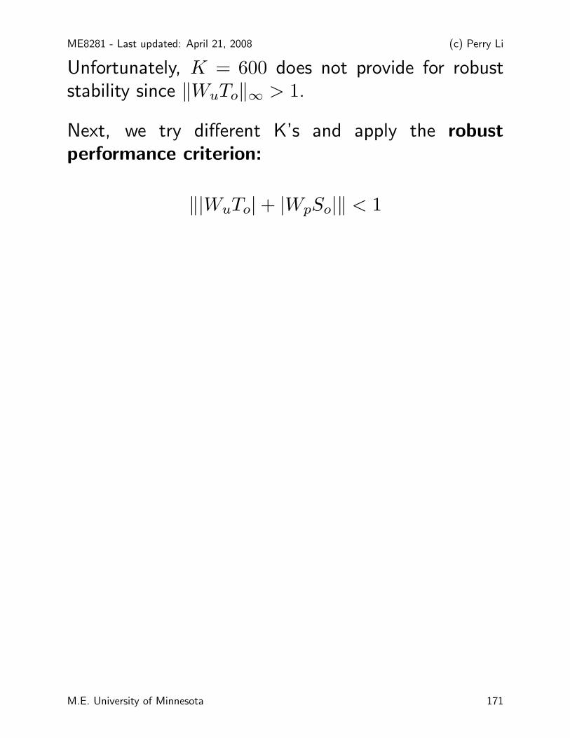
Unfortunately, K = 600 does not provide for robuststability since ‖WuTo‖∞ > 1.

Next, we try different K’s and apply the robustperformance criterion:

‖|WuTo| + |WpSo|‖ < 1



K = 160

10−5

100

105

10−6

10−4

10−2

100

Sensitivity −S

10−5

100

105

10−6

10−4

10−2

100

Robust Stability −WuT

10−5

100

105

10−20

10−10

100

1010


10−5

100

105

10−4

10−2

100

102

Robust Performance −WpS + WuT

Proportional Control − K=160

K = 180

10−5

100

105

10−6

10−4

10−2

100

Sensitivity −S

10−5

100

105

10−6

10−4

10−2

100


10−5

100

105

10−20

10−10

100

1010


10−5

100

105

10−4

10−2

100

102





K = 200

10−5

100

105

10−6

10−4

10−2

100

Sensitivity −S

10−5

100

105

10−6

10−4

10−2

100

102


10−5

100

105

10−20

10−10

100

1010


10−5

100

105

10−4

10−2

100

102



K = 220

10−5

100

105

10−6

10−4

10−2

100

Sensitivity −S

10−5

100

105

10−6

10−4

10−2

100

102


10−5

100

105

10−20

10−10

100

1010


10−5

100

105

10−4

10−2

100

102





Gain - K ‖WuTo‖ ‖WpSo‖ ‖WuTo +WpSo‖160.0000 0.8670 3.4806 3.5330180.0000 0.9643 3.0948 3.1503200.0000 1.0581 2.7859 2.8437220.0000 1.1484 2.5330 2.5926240.0000 1.2350 2.3222 2.3831260.0000 1.3178 2.1437 2.2058280.0000 1.4071 1.9907 2.0537300.0000 1.4943 1.8581 1.9218

Conclusion: Proportional control cannot simultaneouslyprovide robust stability and performance.

Options:

• Reduce performance specification - e.g. reducebandwidth wc

• Reduce allowable size of uncertainties - e.g. bettersystem identification to nail down fluid / structurenatural frequency and damping ratio ωn, ζ, thusreducing Wu.

• Use a different type controller ⇒ loop shaping.



K = 180.

102

103

104

10−1


100

101

102

10−4

10−2

100


K = 180

Sensitivity peaks at ≈ 15 rad/s whereas robust stabilitypeaks at 1500 rad/s.

Can we design a controller that only modifies thesensitivities around 5 to 50 rad/s, but have little effectat other frequencies?



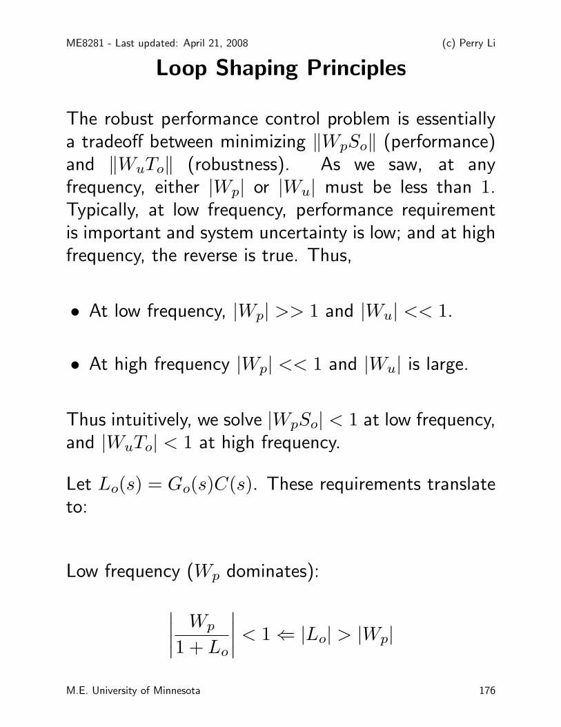
Loop Shaping Principles

The robust performance control problem is essentiallya tradeoff between minimizing ‖WpSo‖ (performance)and ‖WuTo‖ (robustness). As we saw, at anyfrequency, either |Wp| or |Wu| must be less than 1.Typically, at low frequency, performance requirementis important and system uncertainty is low; and at highfrequency, the reverse is true. Thus,

• At low frequency, |Wp| >> 1 and |Wu| << 1.

• At high frequency |Wp| << 1 and |Wu| is large.

Thus intuitively, we solve |WpSo| < 1 at low frequency,and |WuTo| < 1 at high frequency.

Let Lo(s) = Go(s)C(s). These requirements translateto:

Low frequency (Wp dominates):

∣∣∣∣

Wp

1 + Lo

∣∣∣∣< 1 ⇐ |Lo| > |Wp|



High frequency (Wu >> 1 dominates):

∣∣∣∣

WuLo

1 + Lo

∣∣∣∣< 1 ⇐ |Lo| <

1

|Wu|

This provides some guidelines for designing Lo(s) tosatisfy robust performance.

To be more precise, we need to find bounds based onthe robust performance criterion itself.

We consider the cases of 1) when |Wp| < 1 (highfrequency) and 2) when |Wu| < 1 (low frequency) anddetermine the necessary and sufficient conditions forrobust performance.

Case 1: |Wp| < 1: (High frequency - uncertainty isimportant)

• Sufficient condition:

|Lo| <1 − |Wp|

1 + |Wu|⇒ |WpSo| + |WuTo| < 1.

• Necessary condition:

|Lo| <1 − |Wp|

|Wu| − 1⇐ |WpSo| + |WuTo| < 1.



• If |Wu| >> 1, both conditions approach,

|Lo| <1 − |Wp|

|Wu|(25)

Case 2: |Wu| < 1: (Low frequency - performance isimportant)

• Sufficient condition:

|Lo| >|Wp| + 1

1 − |Wu|⇒ |WpSo| + |WuTo| < 1.

• Necessary condition:

|Lo| >|Wp| − 1

1 − |Wu|⇐ |WpSo| + |WuTo| < 1.

• If |Wp| >> 1, both conditions approach,

|Lo| >|Wp|

1 − |Wu|(26)

These bounds (25)-(26) determine the design rule forLo(s) = C(s)Go(s).



Loop Shaping Procedure

Setup:

• Open loop plant G(s) is stable, and minimum phase(no RHP zeros)

• Wu(s) and Wp(s) are designed such that

min{|Wu(jω)|, |Wp(jω)|} < 1, ∀ω

Procedure:

1. Plot on log-log sacle, magnitude versus frequency(25)-(26):

• At frequencies where |Wp| > 1 > |Wu| (lowfrequencies):

|Wp|

1 − |Wu|,

• At frequencies where |Wu| > 1 > |Wp| (highfrequencies):

1 − |Wp|

|Wu|



2. Construct Lo(s) = Go(s)C(s) such that |Lo(jω)|within the required bounds

• |Lo| > low frequency bound• |Lo| < high frequency bound

3. Choose Lo(s) such that at Lo(jω) passes through|Lo(jω)| = 1 with gentle slope (-20db/decade or-40dB/decade). This determines the phase margin.

4. Roll off Lo(s) (at least) as fast as Go(s) so thatC(s) is proper.

5. Check robust performance - |WpSo|+|WuTo| < 1.

6. Check nominal stability: roots of 1 + Lo(s) = 0should lie on open LHP.

7. Determine C(s) from the Lo(s).



One possibility is to construct a nice looking Lo(s)first, and then take

C(s) = Lo(s)/Go(s)

Another possibility is to start with L0o(s) = kG(s) and

then successively modify,

L1o(s) = kGo(s) → L2

o(s) = kC1(s)Go(s)

→L3o(s) = kC2(s)C1(s)Go(s) → . . .

where Ci(s) are typically lead-lag controller,

Ci(s) =βi

αi

(s+ αi)

s+ βi.

The controller is then

C(s) = kCm(s)Cm−1(s) . . . C1(s).

Cross-over region can be tricky to ensure robustperformance is achieved.



Loop shaping example: EH actuator

Recall that using proportional control, it is not possibleto have both adequate performance and robustness atthe same time. However, for C(s) = K = 180,

• Performance curve |WpSo| peaks at 10 − 15 rad/s

• Robust stability |WuTo| peaks at 1500 rad/s withadequate margin.

Thus, it seems feasible that if we can improve |WpSo|at around 10-15 rad/s without disturbing |WuTo| athigh frequencies too much, robust performane can beachieved.

We use loop shaping techniques to guide us.



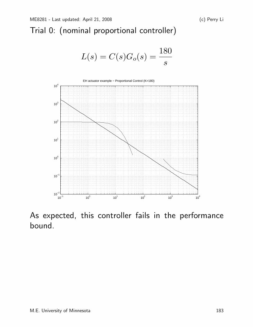
Trial 0: (nominal proportional controller)

L(s) = C(s)Go(s) =180

s

10−1

100

101

102

103

104

10−2

10−1

100

101

102

103

104

EH actuator example − Proportional Control (K=180)

As expected, this controller fails in the performancebound.



Trial 1: Boost gain between 1 to 10 rad/s

Lo(s) = 180s+ 1

(s/10 + 1)Go(s) = 180

s+ 1

s(s/10 + 1)

10−1

100

101

102

103

104

10−2

10−1

100

101

102

103

104

EH actuator example − Proportional + lead

Performance bound is satisfied at the expense ofviolating the robustness bound. This is verifiedby plotting the robustness stability and performancecurves.



10−2

100

102

104

10−4

10−3

10−2

10−1

100

Sensitivity −S

10−2

100

102

104

10−6

10−4

10−2

100

102


10−2

100

102

104

10−15

10−10

10−5

100


10−2

100

102

104

10−2

10−1

100

101


Robust stability, nominal performance, robustperformance curves for

C(s) = 180s+ 1

s/10 + 1



Trial 2: Reduce gain at high frequency to regainrobustness

Lo(s) = 180s/100 + 1

(s/10 + 1)·

s+ 1

s/10 + 1Go(s)

= 180s/100 + 1

s(s/10 + 1)2

10−1

100

101

102

103

104

10−2

10−1

100

101

102

103

104

Trial 0

Trial 1

Trial 2

Both performance and robustness bounds are satisfied.Need to check robust performance curve.



10−2

100

102

104

10−4

10−3

10−2

10−1

100

Sensitivity −S

10−2

100

102

104

10−5

100


10−2

100

102

104

10−15

10−10

10−5

100


10−2

100

102

104

10−2

10−1

100


Robust stability, nominal performance, robustperformance curves for

C(s) = 180(s+ 1)(s/100 + 1)

(s/10 + 1)2

Robust performance is satisfied.

Make sure to check that the system is nominally stable.



The characteristic polynomial is:

180(s+ 1)(s/100 + 1) + s(s/10 + 1)2

Roots are: −99.5 ± 90.5j and −0.996. Thus thesystem is stable.

Nyquist plot confirms that the nominal loop is stable.Thus, by robust stability, the system is robustly stableas well.

−1.2 −1 −0.8 −0.6 −0.4 −0.2 0

−20

−15

−10

−5

0

5

10

Nyquist Diagram

Real Axis

Imag

inar

y A

xis



Control design via innovation feedback

Recall that using observer state feedback,

˙x = Ax+Bu− L(Cx− y)

u = −Kx

the controller itself satisfies [See Goodwin pp. 512 forproof]:

L(s)

E(s)U(s) = −

P (s)

E(s)Y (s) + V (s) (27)

where

L(s)

E(s)= 1 +KT1(s) =

det(sI −A+ LC +BK)

E(s)

P (s)

E(s)= KT2(s) =

KAdj(sI −A)J

E(s)

P (s)

L(s)= K(sI −A+ LC +BK)−1L



Controller can be written as a two degree of freedomcontroller form:

U(s) =E(s)

L(s)

(

V (s) −P (s)

E(s)Y (s)

)

Or as a 1 degree of freedom controller form:

U(s) =P (s)

E(s)(R(s) − Y (s))

where V (s) = P (s)E(s)R(s).

The innovation is the output prediction error:

ν := y − Cx = −Ce

Therefore,

ν(s) = Y (s) − CX(s)

= Y (s) − CT1(s)U(s) − CT2(s)Y (s)

= (1 − CTs(s))Y (s) − CT1(s)U(s)

where

T1(s) = (sI −A+ LC)−1B

T2(s) = (sI −A+ LC)−1L



In transfer function form:

L(s)

E(s)U(s) = −

P (s)

E(s)Y (s)

G(s) =Bo(s)

Ao(s)=CAdj(sI −A)B

det(sI −A)

E(s) = det(sI −A+ LC)

F (s) = det(sI −A+BK)

L(s) = det(sI −A+ LC +BK)

P (s) = KAdj(sI −A)L

P (s)

L(s)= K [sI −A+ LC +BK]

−1L

Then, it can be shown (see Goodwin P545) that theinnovation

ν(s) =Ao(s)

E(s)Y (s) −

Bo(s)

E(s)U(s)

Consider now that observer state feedback augmented



with innovation feedback,

u = v −Kx−Qu(s)ν

where Qu(s)ν is ν filtered by the stable filter Qu(s)(to be designed). Then,

L(s)

E(s)U(s) = −

P (s)

E(s)Y (s)+Qu(s)

[B(s)

E(s)U(s) −

A(s)

E(s)Y (s)

]

The controller transfer function becomes then:

C(s) =

P (s)E(s) +Qu(s)A(s)

E(s)

L(s)E(s) −Qu(s)B(s)

E(s)

The nominal sensitivity functions, which define therobustness and performance criteria, are modifiedaffinely by Qu(s):

So(s) =Ao(s)L(s)

E(s)F (s)−Qu(s)

Bo(s)Ao(s)

E(s)F (s)(28)

To(s) =Bo(s)P (s)

E(s)F (s)+Qu(s)

Bo(s)Ao(s)

E(s)F (s)(29)



For plants that are open-loop stable with tolerable polelocations, we can set K = 0 so that

F (s) = Ao(s)

L(s) = E(s)

P (s) = 0

so that

So(s) = 1 −Qu(s)Bo(s)

E(s)

To(s) = Qu(s)Bo(s)

E(s)

In this case, it is common to use Q(s) := Qu(s)Ao(s)E(s)

to get the formulae:

So(s) = 1 −Q(s)Go(s) (30)

To(s) = Q(s)Go(s) (31)

Thus the design of Qu(s) (or Q(s)) can be used todirectly influence the sensitivity functions.



For instance, using Eqs.(28)-(29):

Minimize sensitivity ‖Wp(s)S(s)‖ for nominalperformance:

Qu(s) =L(s)

Bo(s)F1(s)

Minimize complementary sensitivity ‖Wu(s)T (s)‖:

Qu(s) = −P(s)

Ao(s)F2(s)

where F1(s), F2(s) are close to 1 at frequencies where‖S(s)‖ and ‖T (s)‖ need to be decreased.

Similarly, using Eqs.(30)-(31) for stable open loopsystems:

Minimize sensitivity ‖Wp(s)S(s)‖ for nominalperformance:

Q(s) = G−1o (s)F1(s)

Minimize complementary sensitivity ‖Wu(s)T (s)‖:

Qu(s) = −G−1o F2(s)



where F1(s), F2(s) are close to 1 at frequencies where‖S(s)‖ and ‖T (s)‖ need to be decreased. Notice thatit is not possible to do both at the same time.

Remarks:

• Generally, if F1(s) and F2(s) need to be active inoverlapping ranges, then the control design will notbe feasible.

• The internal stability of the system is ensured ifQu(s) is stable.

• How Qu(s) should be designed need to be modifiedin case when Bo(s) or Ao(s) are non-minimumphase.



Electrohydraulic Actuator Example using

Qu(s) feedback

Simplified model for the EH system,

G(s) =Bo(s)

Ao(s)=

1

s

States space model:

x = u+ di

y = x+ do

where di and do are input and output disturbances.

The observer is:

˙x = u− L(x− y)

(s+ L)x(s) = u(s) + Ly(s)



The innovation ν is:

ν = y − y = y − x

ν(s) = y(s) −u+ Ly

s+ L

=s · y(s)

s+ L−

u(s)

s+ L

Let the observer state-feedback with innovationfeedback be:

u(s) = −Kx(s) −Qu(s)ν(s)

[(s+K + L) −Qu(s)]u(s) = −(KL+Qu(s)s)y(s)

So(s) =y(s)

do(s)=

s(s+K + L)

(s+ L)(s+K)−Qu(s)

s

(s+ L)(s+K)

To(s) =u(s)

di(s)=

KL

(s+K)(s+ L)+Qu(s)

s

(s+ L)(s+K)

This is consistent with the formulae (28)-(29) with



these definitions:

E(s) = s+ L

F (s) = s+K

L(s) = (s+ L+K)

P (s) = LK

First we consider K = 180. Without Qu(s) feedback,this is robustly stable, but does not have the requiredperformance.

10−2

100

102

104

10−15

10−10

10−5

100

105

Nominal Performance

10−2

100

102

104

10−5

100

Robust stability

10−2

100

102

104

10−3

10−2

10−1

100

101

Robust performance

0

0.5

1

Mag

nitu

de (

dB)

100

101

0

0.5

1

Pha

se (

deg)

Bode Diagram

Frequency (rad/sec)

To improve nominal performance, we focus onfrequency below 200 rad/s:



>> wc1=200;

>> [B1,A1]=butter(2,wc1,’s’);

Q(s) =(s+ L+K) ∗B1(s)

A1(s)

10−2

100

102

104

10−15

10−10

10−5

100

Nominal Performance

10−2

100

102

104

10−5

100

Robust stability

10−2

100

102

104

10−5

100

Robust performance

−50

0

50

100

Mag

nitu

de (

dB)

101

102

103

104

105

−180

−90

0

Pha

se (

deg)

Bode Diagram

Frequency (rad/sec)

This satisfies the robust performance criteria easily.

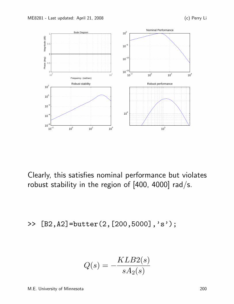
Let’s try starting out with performance. SetK = 1200.Without Qu(s), do not satisfy robust stability.



10−2

100

102

104

10−15

10−10

10−5

100

Nominal Performance

10−2

100

102

104

10−6

10−4

10−2

100

102

Robust stability

103

100

Robust performance

0

0.5

1

Mag

nitu

de (

dB)

100

101

0

0.5

1

Pha

se (

deg)

Bode Diagram

Frequency (rad/sec)

Clearly, this satisfies nominal performance but violatesrobust stability in the region of [400, 4000] rad/s.

>> [B2,A2]=butter(2,[200,5000],’s’);

Q(s) = −KLB2(s)

sA2(s)



10−2

100

102

104

10−15

10−10

10−5

100

Nominal Performance

10−2

100

102

104

10−5

100

Robust stability

10−2

100

102

104

10−3

10−2

10−1

100

Robust performance

−100

−50

0

50

100

Mag

nitu

de (

dB)

100

102

104

106

−360

0

360

Pha

se (

deg)

Bode Diagram

Frequency (rad/sec)

This also satisfies robust performance!



Constraints on Wp and Wu

Wp(s) and Wu(s) specify the desired performance andallowable model uncertainties.

However, we cannot define Wp and Wu to be arbitrarilylarge and expect that that a controller can be foundthat solves the the robust performance problem. Here,we show that they must respect each other, and respectthe limitations of the open-loop system.

Knowledge of these limitations help us definemeaningful performance specifications (Wp), and ourneed to do accurate modeling (Wu).

First, some preliminary results ....



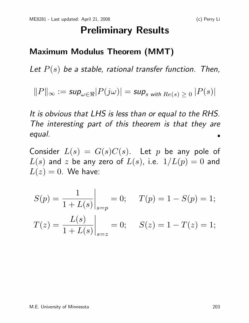
Preliminary Results

Maximum Modulus Theorem (MMT)

Let P (s) be a stable, rational transfer function. Then,

‖P‖∞ := supω∈ℜ|P (jω)| = sups with Re(s) ≥ 0 |P (s)|

It is obvious that LHS is less than or equal to the RHS.The interesting part of this theorem is that they areequal.

Consider L(s) = G(s)C(s). Let p be any pole ofL(s) and z be any zero of L(s), i.e. 1/L(p) = 0 andL(z) = 0. We have:

S(p) =1

1 + L(s)

∣∣∣∣s=p

= 0; T (p) = 1 − S(p) = 1;

T (z) =L(s)

1 + L(s)

∣∣∣∣s=z

= 0; S(z) = 1 − T (z) = 1;



Constraint 1: Wu & Wp cannot simultaneously belarge

For the robust performance to be solvable, a necessarycondition is: for all ω ∈ ℜ,

min{|Wu(jω)| , |Wp(jω)|} < 1.

Proof: Suppose that |Wu| ≤ |Wp| (reverse theargument otherwise). At each ω,

|Wu| = |Wu(S+T )| ≤ |WuS|+|WuT | ≤ |WuS|+|WpT |

Thus, |WuS|+|WpT | < 1 (robust performance) impliesthat |Wu| < 1.

Significance: We cannot simultaneously tolerateuncertainty, and expect good performance at anyfrequencies.

• One cannot have better than open-loop performance(|S| < 1 as guranteed by |WpS| ≤ 1 and |Wp| > 1)when uncertainty is larger than 100% (|Wu| > 1).



Constraint 2: Right Half Plane poles and zeros limitrobustness (Wu) and performance (Wp)

Suppose that C(s) internally stabilizes the nominalplant Go(s). Let So and To be the nominal sensitivities,and p and z are respectively an unstable pole, and anon-minimum phase zero of Lo(s) = Go(s)C(s), i.e.1/Lo(p) = 0 with Re(p) ≥ 0; and Lo(z) = 0 withRe(z) ≥ 0.

• The nominal (and robust) performance problemcannot be solved if |Wp(z)| ≥ 1, since

‖WpSo‖ = supRe(s)≥0|WpSo|

≥ |Wp(z)So(z)| = |Wp(z)|.

• The robust stability (and robust performance)problem cannot be solved if |Wu(p)| ≥ 1, since

‖WuTo‖ = supRe(s)≥0|WuTo|

≥ |Wu(p)To(p)| = |Wu(p)|.

The remedy for this is to reduce performancerequirement (smaller |Wp(z)|), and better systemidentification (lower uncertainty, and smaller |Wu(p)|).



The problem is more acute if there is a pair of RHPpole and zero close to each other.

Consider the open loop system:

G(s) =s− z

s− pG1(s)

where z and p are RHP zero and pole, G1(s) does nothave any RHP poles or zeros. Then, it can be shownthat:

‖WpSo‖∞ ≥ |Wp(z)|

∣∣∣∣

z + p

z − p

∣∣∣∣

‖WuTo‖∞ ≥ |Wu(p)|

∣∣∣∣

z + p

z − p

∣∣∣∣

Thus, as p ≈ z, the lower bounds for ‖WpS‖∞ and‖WuT‖∞ is significantly amplified. This is related tothe fact that the unstable pole is nearly canceled out bythe non-minimum phase zero. Thus, the unstable modebecomes either nearly uncontrollable or unobservable.



Constraints due to Bode IntegralThese constraints are sometimes referred to as the“principle of conservation of dirts” or the area formula.The general meaning is that for systems that satisfy theconditions of the theorems, it is not possible to improvethe performance / robustness at all frequencies.

Theorem: (Bode Integral Theorem for Sensitivity)Let the open loop system L(s) = G(s)C(s) have thefollowing properties:

• It has relative degree (i.e. order of denominatorminus order of numerator) nr ≥ 1.

• L(s) has M ≥ 0 RHP (unstable) poles (countingmultiplicity): p1, p2, . . . , pM , Re(pi) > 0.

• Let κ := lims→∞sL(s). [Note: κ = 0 if nr ≥ 2]

• Sensitivity function is given by S(s) = 11+L(s).

Then, the sensitivity function S(jω) satisfies:

∫ ∞

0

ln|S(jω)|dω = π ·

M∑

i=1

Re(pi). nr > 1 (32)

∫ ∞

0

ln|S(jω)|dω = −κπ

2+ π ·

M∑

i=1

Re(pi). nr = 1.

(33)



Significance:

• L(s) has relative degree nr > 1 if both plant G(s)and controller C(s) are strictly proper. Then, (32)applies.

• Decreasing |S(jω)| at some frequencies ω willincrease it at other frequencies. Hence, the “dirt”is conserved.

• The total amount of “dirt” is increased if the open-loop system L(s) is unstable since the RHS of(32)-(33) is increased.

• When nr = 1, the total amount of “dirt” isdecreased by increasing the high frequency gain(e.g. L(s) = K/s).

• The sensitivity peak ‖S‖∞ which is inversely relatedto robustness may be increased.



Example: Proportional control of 2nd order plant withno zeros.

L(s) = kG(s) =k

s2 + s+ 1;

S(s) =s2 + s+ 1

s2 + s+ (1 + k)

0 1 2 3 4 5 6 7 8 9 1010

−2

10−1

100

101

k=0

k=10

log S(jw)

L(s) = k 1

s2 + s + 1

ω rad/s

Note that as k increases, the sensitivity at lowfrequencies decreases but the peaks increase at otherfrequencies.



Theorem: (Bode Integral Theorem for ComplementarySensitivity) Let the open loop system L(s) = G(s)C(s)have the following properties:

• L(s) has at least 1 pole at 0 (i.e. L−1(0) = 0 orT (0) = 1).

• L(s) has M ≥ 0 RHP (non-minimum phase) zeros(counting multiplicity): c1, c2, . . . , cM , Re(ci) > 0.

• kv is the velocity constant - i.e.

kv = −

(

lims→0dT (s)

ds

)−1

= −lims→0sL(s)

• Complementary sensitity is given by T (s) = L(s)1+L(s).

Then, the sensitivity function T (jω) satisfies:

∫ ∞

0

1

ω2ln|T (jω)|dω = π ·

M∑

i=1

1

ci−

π

2kv(34)



Significance:

• If L(s) has at least 2 free integrators (poles at 0),then kv = ∞. This ensures that steady error is 0for ramp input.

• Decreasing |T (jω)| at some frequencies ω willincrease it at other frequencies. Hence, the similarto the S(s) story, “dirt” is conserved.

• The total amount of “dirt” is increased if the open-loop system L(s) has non-minimum phase zeros,since the RHS of (34) is increased.

• If L(s) has only 1 free integrator, one can decreasethe total dirt by tolerating steady state error due toramp input.

• If L(s) does not have free integrators (i.e. L−1(0) 6=0 or T (0) 6= 1, then a similar relation to (34) exists,

except that in the integral we have ln|T (jω)|T (0)| . This

however, does not pose limitation on making T (jω)small in all frequencies.



Application: Closed loop bandwidth and

Open loop unstable pole

Constraints on Wp, Wu imply the following design rule:

“The closed loop bandwidth should be larger than themagnitude of the unstable open loop pole”

Usually a factor of 2 is used.

Reasoning 1: (From complementary sensitivityfunction)

Suppose that the uncertainty weighting is chosen sothat it is important at high frequency, unimportant atlow frequencies. This roughly translates to requirementon To since ‖WuTo‖ < 1.

One possibility is Wu(s) = sωo

+ 1T. So that

W−1u =

T ωo

(sT + ω); |To(jωo)| ≈ |W−1

u (jωo)|.

Hence, the cross over frequency is ωo, and Wu(0) =T−1. Here, we can interpret ωo as the bandwidth ofthe system, since beyond which, we allow To(jω) tobe small.



Let p ∈ ℜ be a real unstable pole of the open loopplant Go(s).

Then, from the constraint that |Wu(p)| < 1,

|p|

ωo+

1

T< 1 ⇒ ωo >

p

1 − 1/T≥ |p|.

If T is 2 (50% uncertainty at D.C.), then this gives therule of thumb with the factor of 2.

Reasoning 2: (From sensitivity function)

Let Go(s) have a real unstable pole at p ∈ ℜ, andLo(s) = Go(s)C(s).

As a rough approximation, let the open loop gain|Lo(jω)| ≈ 0 when ω > ωo where ωo is the bandwidthof the closed loop system. This implies that So(jω) ≈1 (ln|So(jω)| ≈ 0) when ω > ωo. Let M be the maxof |So(jω)| (sensitivity peak)

From Bode integral (32),

πp =

∫ ωo

0

ln|So(jω)|dω +

∫ ∞

ωo

ln|So(jω)|dω ≤ ωoln(M)



This shows that the sensitivity peak M ≥ eπp/ωo.Since M should be reasonably small (otherwise, thesystem will behave much worse than open loop), p/ωo

should not be large. In particular, if ωo = p, thenM = eπ ≈ 23 which is unacceptable in most cases.When, ωo = 2p, the estimated lower bound for M is4.81.

Note: M >> 1 is bad also for robustness, sinceT = 1−S. Thus, large T requires very good modelingeffort to maintain stability. Also, recall |S−1

o (jω)| isdistance of Lo(jω) to (−1, 0).



Application: Closed loop bandwidth and

Open loop non-minimum phase zero

The constraints on Wu and Wp also imply the followingdesign rule:

“The closed loop bandwidth should be smaller thanthe magnitude of the non-minimum phase zero”

Suppose that the performance weighting Wp(s)satisfies:

W−1p = S

s

s+ ωSThus, the sensitivity becomes important for ω < ωo;high frequency sensitivity requirement is given by S.

Let z be a real non-minimum phase (RHP) zero ofGo(s). Then from the necessary condition, |Wp(z)| <1,

z + ωoS

Sz< 1 ⇒ ωo < (1 − 1/S)z < z



Limitations - summary

• Wu and Wp cannot be large simultaneously.

• Open loop RHP poles and zeros limit how Wu andWp can be defined

• Conservation of dirt theorems say that improvingsensitivity So(jω) in some frequencies requirepayment at others.

• Similar theorem for To(jω), especially when infiniteopen loop D.C. gain (open loop integrators).

• Design implications:

– Closed loop pole should be faster than open loopunstable pole;

– Closed loop pole should be slower than open loopnon-minimum phase zero.

– Problem when open loop pole is fast, and non-minimum phase zero is slow ⇒ consider changingsystem architecture.



Example: Inverted pendulum

Balancing a beam on a palm. Let u be the force onthe palm and M is its mass; m and l are the mass andthe length of the beam. Assume that the beam massis concentrated at the tip. Let y be the tip positionand x be the position of the palm.

Transfer function from u to x:

Gux(s) =ls2 − g

s2(Mls2 − (M +m)g)

This has an unstable pole at +√

(M+m)gMl , and a non-

minimum phase zero at +√

g/l.

Transfer function from u to y:

Guy(s) =g

s2(Mls2 − (M +m)g)

This does not have any zeros.



Conclusions:

• Control is more difficult as the beam becomesshorter, or if the beam is heavier, as the unstablepole gets larger. This requires faster bandwidth onthe part of the human controller.

• Control by looking at the palm (x) is virtuallyimpossible, especially for short beams, because ofthe unstable pole is faster than the non-minimumphase zero. Thus, there will inevitably be alarge sensitivity peak (‖So‖∞) and hence robustnessproblems.

• Control by looking at the tip of the beam (y)is easier since there are no zeros. For l = 0.5m,assume that the palm is much heavier than the beam(M >> m). Using a factor of 2 × p the requiredbandwidth is 1.4 Hz. This is quite reasonable forhumans.


Documents

ME8281 - Last updated: April 21, 2008 (c) Perry Li Robust ... · ME8281 - Last updated: April 21, 2008 (c) ... the control sensitivity so that output disturbance or ... Robust Stability