Me, Myself and I: Time-Inconsistent Stochastic Control

Me, Myself and I: Time-Inconsistent Stochastic Control,Contract Theory and Backward Stochastic Volterra

Integral Equations

Miguel Camilo Hernández Ramírez

Submitted in partial fulfillment of therequirements for the degree of

Doctor of Philosophyunder the Executive Committee

of the Graduate School of Arts and Sciences

COLUMBIA UNIVERSITY

2021

© 2021


All Rights Reserved

Abstract

Me, Myself and I: time-inconsistent stochastic control, contract theory and

backward stochastic Volterra integral equations


This thesis studies the decision-making of agents exhibiting time-inconsistent prefer-

ences and its implications in the context of contract theory. We take a probabilistic approach

to continuous-time non-Markovian time-inconsistent stochastic control problems for sophisticated

agents. By introducing a refinement of the notion of equilibrium, an extended dynamic program-

ming principle is established. In turn, this leads to consider an infinite family of BSDEs analogous

to the classical Hamilton–Jacobi–Bellman equation. This system is fundamental in the sense that

its well-posedness is both necessary and sufficient to characterise equilibria and its associated value

function. In addition, under modest assumptions, the existence and uniqueness of a solution is

established.

With the previous results in mind, we then study a new general class of multidimensional type-I

backward stochastic Volterra integral equations. Towards this goal, the well-posedness of a system

of infinite family of standard backward stochastic differential equations is established. Interestingly,

its well-posedness is equivalent to that of the type-I backward stochastic Volterra integral equation.

This result yields a representation formula in terms of semilinear partial differential equation of

Hamilton–Jacobi–Bellman type. In perfect analogy to the theory of backward stochastic differen-

tial equations, the case of Lipschitz continuous generators is addressed first and subsequently the

quadratic case. In particular, our results show the equivalence of the probabilistic and analytic

approaches to time-inconsistent stochastic control problems.

Finally, this thesis studies the contracting problem between a standard utility maximiser prin-

cipal and a sophisticated time-inconsistent agent. We show that the contracting problem faced

by the principal can be reformulated as a novel class of control problems exposing the complica-

tions of the agent’s preferences. This corresponds to the control of a forward Volterra equation

via constrained Volterra type controls. The structure of this problem is inherently related to the

representation of the agent’s value function via extended type-I backward stochastic differential

equations. Despite the inherent challenges of this class of problems, our reformulation allows us to

study the solution for different specifications of preferences for the principal and the agent. This

allows us to discuss the qualitative and methodological implications of our results in the context

of contract theory: (i) from a methodological point of view, unlike in the time-consistent case,

the solution to the moral hazard problem does not reduce, in general, to a standard stochastic

control problem; (ii) our analysis shows that slight deviations of seminal models in contracting

theory seem to challenge the virtues attributed to linear contracts and suggests that such contracts

would typically cease to be optimal in general for time-inconsistent agents; (iii) in line with some

recent developments in the time-consistent literature, we find that the optimal contract in the

time-inconsistent scenario is, in general, non-Markovian in the state process X.

Table of Contents

Acknowledgments . . . . . . . . . . . . . . . . . . . . . . . . . . . . . . . . . . . . . . . . vi

Dedication . . . . . . . . . . . . . . . . . . . . . . . . . . . . . . . . . . . . . . . . . . . . vii

Preface . . . . . . . . . . . . . . . . . . . . . . . . . . . . . . . . . . . . . . . . . . . . . . 1

Notation . . . . . . . . . . . . . . . . . . . . . . . . . . . . . . . . . . . . . . . . . . . . . 2

I Introduction 4

Chapter 1: Introduction . . . . . . . . . . . . . . . . . . . . . . . . . . . . . . . . . . . . . 5

1.1 Contract theory in continuous-time models . . . . . . . . . . . . . . . . . . . . . . . 6

1.1.1 The dynamic programming approach . . . . . . . . . . . . . . . . . . . . . . . 8

1.2 Part II: non-Markovian time-inconsistent control . . . . . . . . . . . . . . . . . . . . 11

1.2.1 Existing results for Markovian time-inconsistent problems . . . . . . . . . . . 17

1.2.2 Contributions . . . . . . . . . . . . . . . . . . . . . . . . . . . . . . . . . . . . 23

1.3 Part III: backward stochastic Volterra integral equations . . . . . . . . . . . . . . . . 26

1.3.1 Contributions . . . . . . . . . . . . . . . . . . . . . . . . . . . . . . . . . . . . 32

1.4 Part IV: time-inconsistent contract theory . . . . . . . . . . . . . . . . . . . . . . . . 34

1.4.1 Contributions . . . . . . . . . . . . . . . . . . . . . . . . . . . . . . . . . . . . 36

1.5 Perspectives and future research . . . . . . . . . . . . . . . . . . . . . . . . . . . . . 40

1.6 Outline of the thesis . . . . . . . . . . . . . . . . . . . . . . . . . . . . . . . . . . . . 44

i

II Time-inconsistent control 46

Chapter 2: Non-Markovian time-inconsistent control for sophisticated agents . . . . . . . . . 47

2.1 Problem formulation . . . . . . . . . . . . . . . . . . . . . . . . . . . . . . . . . . . . 47

2.1.1 Probabilistic framework . . . . . . . . . . . . . . . . . . . . . . . . . . . . . . 47

2.1.2 Controlled state dynamics . . . . . . . . . . . . . . . . . . . . . . . . . . . . . 50

2.1.3 Objective functional . . . . . . . . . . . . . . . . . . . . . . . . . . . . . . . . 54

2.1.4 Game formulation . . . . . . . . . . . . . . . . . . . . . . . . . . . . . . . . . 55

2.2 Related work and our results . . . . . . . . . . . . . . . . . . . . . . . . . . . . . . . 59

2.2.1 On the different notions of equilibrium . . . . . . . . . . . . . . . . . . . . . . 59

2.2.2 Dynamic programming principle . . . . . . . . . . . . . . . . . . . . . . . . . 65

2.2.3 BSDE system associated to (P) . . . . . . . . . . . . . . . . . . . . . . . . . . 68

2.2.4 Necessity of (H) . . . . . . . . . . . . . . . . . . . . . . . . . . . . . . . . . . 73

2.2.5 Verification . . . . . . . . . . . . . . . . . . . . . . . . . . . . . . . . . . . . . 75

2.2.6 Well-posedness . . . . . . . . . . . . . . . . . . . . . . . . . . . . . . . . . . . 76

2.3 Example: optimal investment . . . . . . . . . . . . . . . . . . . . . . . . . . . . . . . 78

2.4 Extensions of our results . . . . . . . . . . . . . . . . . . . . . . . . . . . . . . . . . . 81

2.5 Proof of Theorem 2.2.2 . . . . . . . . . . . . . . . . . . . . . . . . . . . . . . . . . . . 87

2.6 The BSDE system . . . . . . . . . . . . . . . . . . . . . . . . . . . . . . . . . . . . . 95

2.6.1 Functional spaces and norms . . . . . . . . . . . . . . . . . . . . . . . . . . . 95

2.7 Proof of Theorem 2.2.10 . . . . . . . . . . . . . . . . . . . . . . . . . . . . . . . . . . 101

2.8 Proof of Theorem 2.2.12 . . . . . . . . . . . . . . . . . . . . . . . . . . . . . . . . . . 105

2.9 Well-posedness: the uncontrolled volatility case . . . . . . . . . . . . . . . . . . . . . 114

2.10 Auxiliary results . . . . . . . . . . . . . . . . . . . . . . . . . . . . . . . . . . . . . . 116

2.10.1 Optimal investment and consumption for log utility . . . . . . . . . . . . . . 116

ii

2.10.2 Extensions . . . . . . . . . . . . . . . . . . . . . . . . . . . . . . . . . . . . . 118

2.10.3 Auxiliary lemmata . . . . . . . . . . . . . . . . . . . . . . . . . . . . . . . . . 128

III Backward stochastic Volterra integral equations 131

Chapter 3: Lipschitz backward stochastic Volterra integral equations . . . . . . . . . . . . . 132

3.1 On Volterra BSDEs . . . . . . . . . . . . . . . . . . . . . . . . . . . . . . . . . . . . 132

3.2 The stochastic basis on the canonical space . . . . . . . . . . . . . . . . . . . . . . . 134


3.3 An infinite family of Lipschitz BSDEs . . . . . . . . . . . . . . . . . . . . . . . . . . 137

3.4 Well-posedness of Lipschitz type-I BSVIEs . . . . . . . . . . . . . . . . . . . . . . . . 142

3.5 Time-inconsistency, type-I BSVIEs and parabolic PDEs . . . . . . . . . . . . . . . . 147

3.5.1 A representation formula for adapted solutions of type-I BSVIEs . . . . . . . 147

3.5.2 On equilibria and their value function in time-inconsistent control problems . 149

3.6 Analysis of the BSDE system . . . . . . . . . . . . . . . . . . . . . . . . . . . . . . . 152

3.6.1 Regularity of the system and the diagonal processes . . . . . . . . . . . . . . 152

3.6.2 A priori estimates . . . . . . . . . . . . . . . . . . . . . . . . . . . . . . . . . 158

3.6.3 Proof of Theorem 3.3.5 . . . . . . . . . . . . . . . . . . . . . . . . . . . . . . 166

Chapter 4: Quadratic backward stochastic Volterra integral equations . . . . . . . . . . . . 172

4.1 Practical motivations . . . . . . . . . . . . . . . . . . . . . . . . . . . . . . . . . . . . 173

4.2 Preliminaries . . . . . . . . . . . . . . . . . . . . . . . . . . . . . . . . . . . . . . . . 175

4.2.1 The stochastic basis on the canonical space . . . . . . . . . . . . . . . . . . . 175


4.2.3 Auxiliary inequalities . . . . . . . . . . . . . . . . . . . . . . . . . . . . . . . . 179

4.3 The BSDE system . . . . . . . . . . . . . . . . . . . . . . . . . . . . . . . . . . . . . 180

iii

4.3.1 The Lipschitz–quadratic case . . . . . . . . . . . . . . . . . . . . . . . . . . . 183

4.3.2 The quadratic case . . . . . . . . . . . . . . . . . . . . . . . . . . . . . . . . . 187

4.4 Muldimensional quadratic type-I BSVIEs . . . . . . . . . . . . . . . . . . . . . . . . 189

4.5 Proof of the linear–quadratic case . . . . . . . . . . . . . . . . . . . . . . . . . . . . . 193

4.6 Proof of the quadratic case . . . . . . . . . . . . . . . . . . . . . . . . . . . . . . . . 207

4.7 Auxiliary results . . . . . . . . . . . . . . . . . . . . . . . . . . . . . . . . . . . . . . 216

4.7.1 Proofs of Section 4.2 . . . . . . . . . . . . . . . . . . . . . . . . . . . . . . . . 216

4.7.2 Proofs of Section 4.5 . . . . . . . . . . . . . . . . . . . . . . . . . . . . . . . . 217

IV Time-inconsistent contract theory 222

Chapter 5: Time-inconsistent contract theory for sophisticated agents . . . . . . . . . . . . 223

5.1 Problem statement . . . . . . . . . . . . . . . . . . . . . . . . . . . . . . . . . . . . . 223

5.1.1 Controlled state equation . . . . . . . . . . . . . . . . . . . . . . . . . . . . . 224

5.1.2 The agent’s problem . . . . . . . . . . . . . . . . . . . . . . . . . . . . . . . . 225

5.1.3 The principal’s problem . . . . . . . . . . . . . . . . . . . . . . . . . . . . . . 230

5.2 The first-best problem . . . . . . . . . . . . . . . . . . . . . . . . . . . . . . . . . . . 231

5.2.1 Non-separable utility . . . . . . . . . . . . . . . . . . . . . . . . . . . . . . . . 232

5.2.2 Separable utility . . . . . . . . . . . . . . . . . . . . . . . . . . . . . . . . . . 235

5.3 The second-best problem: general scenario . . . . . . . . . . . . . . . . . . . . . . . . 237

5.3.1 Integrability spaces and Hamiltonian . . . . . . . . . . . . . . . . . . . . . . . 237

5.3.2 Characterising equilibria and the BSDE system . . . . . . . . . . . . . . . . . 239

5.3.3 The family of restricted contracts . . . . . . . . . . . . . . . . . . . . . . . . . 241

5.4 The second-best problem: examples . . . . . . . . . . . . . . . . . . . . . . . . . . . 246

5.4.1 Agent with discounted utility reward . . . . . . . . . . . . . . . . . . . . . . . 246

5.4.2 Agent with separable utility . . . . . . . . . . . . . . . . . . . . . . . . . . . . 252

iv

5.4.3 Agent with utility of discounted income . . . . . . . . . . . . . . . . . . . . . 259

5.5 On time-inconsistency for BSVIE-type rewards . . . . . . . . . . . . . . . . . . . . . 264

5.6 On forward stochastic Volterra integral equations . . . . . . . . . . . . . . . . . . . . 272

5.7 Proofs of Section 5.4 . . . . . . . . . . . . . . . . . . . . . . . . . . . . . . . . . . . . 275

5.7.1 Proof of Proposition 5.4.5 . . . . . . . . . . . . . . . . . . . . . . . . . . . . . 275

5.7.2 Proof of Lemma 5.4.7 . . . . . . . . . . . . . . . . . . . . . . . . . . . . . . . 277

5.7.3 Proof of Lemma 5.4.14 . . . . . . . . . . . . . . . . . . . . . . . . . . . . . . . 279

5.7.4 Proof of Proposition 5.4.17 . . . . . . . . . . . . . . . . . . . . . . . . . . . . 280

Conclusion . . . . . . . . . . . . . . . . . . . . . . . . . . . . . . . . . . . . . . . . . . . . 282

References . . . . . . . . . . . . . . . . . . . . . . . . . . . . . . . . . . . . . . . . . . . . 300

v

Acknowledgements

The past 5 years have been an exceptional journey and I want to thank those who have

helped make it a memorable experience.

This whole adventure would have never prospered without my advisor Dylan Possamaï. I was

fortunate enough to have coincided at Columbia with Dylan and have him as my doctoral advisor.

The contributions made by this dissertation are proof that he is the finest advisor I could have

expected as well as an admirable mentor to any student. I am grateful for your incessant devotion

to my academic development, for always be rooting for me, and for your sensible advice.

I would like to thank the exemplary list of researchers that offered valuable knowledge, thought-

ful conversations and advice throughout these years and accepted to be in my defence committee:

Jakša Cvitanić, Daniel Lacker, Philip Protter, Wenpin Tan, Jianfeng Zhang and Xunyu Zhou.

My special gratitude goes to those who found ways to be there for me throughout these years.

To David and both Joses (Bastidas and Habeych) for the long calls, the constant companion and

the cherished moments we spent together. To those who are part of my ever changing family

in New York, Laura, Luis, Malena, Isa, Alessandro, Aldo, Rassa, Herreño, Jaramillo, Kika, Ale,

Sebastian and Zarruk. To my fellow classmates and doctoral students at Columbia University

Agathe, Enrique, Juju and Luc.

Last but certainly not least, I want to thank my family Vilma, Miguel and Paola, and Lili. I

want to thank you for all the love, patience and care for me. Despite my constant absences, even

when I am physically present, and my impatience, you hold a special place in my heart, are a

personal inspiration to me and a constant source of support. I am grateful for having you in my

life.

vi

Para Vilma y MiguelPor todo el amor y el orgullo de tenerlos en mi vida

vii

Preface

In the typical situation of interest, a principal, who is offering a contract, is imperfectly

informed about the actions of a time-inconsistent agent, who can accept or reject the contract. The

goal is to design a contract, compatible with the agent’s preferences, that maximises the utility of

the principal while that of the agent is held to a given level.

Being able to provide a satisfactory solution requires a complete understanding of the agent’s

preferences. As such, a large part of this thesis is devoted to tackling several fundamental questions

in the study of time-inconsistent stochastic control problems for sophisticated agents, also known

as the game-theoretic approach. First, the results in the existing literature depend critically on

the Markovian structure of the formulation: can these results be extended once we abandon this

framework? Second, it is known that a solution to a system of equations provide an equilibrium

strategy and its associated value function: in what sense is the converse true? Do all equilibria

arise as solutions to such system? Third, what can be said about the existence and uniqueness

of equilibria? Answering these questions is necessary to proceed to study the challenges of the

problem faced by the principal. In the time-consistent case, the contracting problem can, without

loss of generality, be reformulated as an optimal control problem: is there an analogue in the time-

inconsistent case? To what extend does said reformulation help in finding a solution? Finally, how

do the agent’s preferences change the form of the contract?

In the following, we put forward the tools and the pieces needed to provide answers to these

questions.

1

Notation

Throughout this document we take the convention ∞−∞ := −∞, and we fix a time horizon

T > 0. R+ and R?+ denote the sets of non-negative and positive real numbers, respectively. Given

(E, ‖ · ‖) a Banach space, a positive integer p, and a non-negative integer q, Cpq (E) (resp. Cpq,b(E))

will denote the space of functions from E to Rp which are at least q times continuously differentiable

(resp. and bounded with bounded derivatives). We set Cq,b(E) := C1q,b(E), i.e. the space of q times

continuously differentiable bounded functions with bounded derivatives from E to R . Whenever

E = [0, T ] (resp. q = 0 or b is not specified), we suppress the dependence on E (resp. on q or b),

e.g. Cp denotes the space of continuous functions from [0, T ] to Rp. Given x ∈ Cp, we denote by x·∧t

the path of x stopped at time t, i.e. x·∧t := (x(r ∧ t), r ≥ 0). Given (x, x) ∈ Cp × Cp and t ∈ [0, T ],

we define their concatenation x⊗t x ∈ Cp by (x⊗t x)(r) := x(r)1r≤t + (x(t) + x(r)− x(t))1r≥t,

r ∈ [0, T ].

For ϕ ∈ Cpq (E) with q ≥ 2, ∂2xxϕ will denote its Hessian. For a function φ : [0, T ] × E with

s 7−→ φ(s, α) uniformly continuous uniformly in α, we denote by ρφ : [0, T ] −→ R its modulus of

continuity, which we recall satisfies ρφ(`) −→ 0 as ` −→ 0. For (u, v) ∈ Rp × Rp, u · b will denote

their usual inner product, and |u| the corresponding norm. For positive integersm and n, we denote

byMm,n(R) the space of m×n matrices with real entries. For M ∈Mm,n(R), M:i and Mi: denote

the i-th column and row. S+n (R) denotes the set of n×n symmetric positive semi-definite matrices,

while Tr[M ] denotes the trace of M ∈ Mm(R), and |M | :=√

Tr[M>M ] for M ∈ Mm,n(R). By

0m,n and In we denote the m × n matrix of zeros and the identity matrix ofMn(R) :=Mn,n(R),

respectively. S+n (R) denotes the set of n × n symmetric positive semi-definite matrices. Tr[M ]

denotes the trace of a matrix M ∈Mn(R).

For (Ω,F) a measurable space, Prob(Ω) denotes the collection of all probability measures on

(Ω,F). For a filtration F := (Ft)t∈[0,T ] on (Ω,F), Pprog(E,F) (resp. Ppred(E,F), Popt(E,F)) will

denote the set of E-valued, F-progressively measurable processes (resp. F-predictable processes,

F-optional processes). For P ∈ Prob(Ω) and a filtration F, FP := (FPt )t∈[0,T ], denotes the P-

2

augmentation of F. We recall that for any t ∈ [0, T ], FPt := Ft ∨ σ(N P), where N P := N ⊆ Ω :

∃B ∈ F , N ⊆ B and P[B] = 0. With this, the probability measure P can be extended so that

(Ω,F ,FP,P) becomes a complete probability space, see Karatzas and Shreve [150, Chapter II.7].

FP+ denotes the right limit of FP, i.e. FP

t+ :=⋂ε>0FP

t+ε, t ∈ [0, T ), and FPT+ := FP

T , so that FP+ is the

smallest filtration that contains F and satisfies the usual conditions. Moreover, given P ⊆ Prob(Ω)

we introduce the set of P-polar sets NP := N ⊆ Ω : N ⊆ B, for some B ∈ F with supP∈P P[B] =

0, as well as the P-completion of F, FP := (FPt )t∈[0,T ], with FPt := Ft∨σ(NP), t ∈ [0, T ] together

with the corresponding right-continuous limit FP+ := (FPt+)t∈[0,T ], with FPt+ :=⋂ε>0FPt+ε, t ∈ [0, T ),

and FPT+ := FPT . For s, t ⊆ [0, T ], with s ≤ t, Ts,t(F) denotes the collection of [t, T ]-valued

F–stopping times.

Additionally, given A ⊆ Rk, A denotes the collection of finite and positive Borel measures on

[0, T ] × A whose projection on [0, T ] is the Lebesgue measure. In other words, any q ∈ A can be

disintegrated as q(dt, da) = qt(da)dt, for an appropriate Borel measurable kernel qt which is unique

up to (Lebesgue–) almost everywhere equality. We are particularly interested in the set A0, of

q ∈ A of the form q = δφt(da)dt, where δφ the Dirac mass at a Borel function φ : [0, T ] −→ A.

We also recall the elementary inequalities

( n∑i=1

ai

)2≤ n

n∑i=1

a2i , (I.1)

valid for any positive integer n and any collection (ai)1≤i≤n of non-negative numbers, as well as,

Young’s inequality which guarantees that for any ε > 0, 2ab ≤ εa2 + ε−1b2.

3

Part I

Introduction

Chapter 1

Introduction

An extremely important point that has redrawn the attention of many academic disciplines in

recent years is that human beings do not necessarily behave as perfectly rational economic agents.

Hence, their criteria for evaluating their well-being are most of the time a lot more involved than

the ones used in the classic economic literature. This has been amplified due to the rapid advent

and flourishment of new economies, such as e-commerce and online advertisement. These activities

are characterised by, notably, a higher number of agents from both the supply and demand sides,

and an unprecedentedly large menu of tailor-made and personalised services. Naturally, this has led

to more intricate behaviours and interactions at all levels of the economy. Though the development

of large scale algorithms provides practical tools to circumvent the intricacies of these kind of

behaviours, there is also a growing demand for models that shed some light into how these agents

make their decisions and facilitate a deeper analysis. Notably of interest are models that study how

to incentivise such agents so that they perform a particular task. This is how time-inconsistency

and contract theory intersect.

In the moral hazard contracting problem between a principal (she) and an agent (he), the

principal’s objective is to use the information available to create the appropriate incentives, in

the form of a contract, to: (i) encourage the agent, whose actions influence an output process,

to accept the contract; (ii) maximise her utility. Though this is quite a simple scenario it has

the virtue of being able to accommodate a wide spectrum of possibilities: the agent performing a

task on the principal’s behalf, the agent consuming a good produced by the principal, the agent

buying something from the principal... The main problem is then to design contracts (that is wages,

prices,...) such that the agent accepts them, and is given proper incentives to behave in a way that

allows the principal to get the most out of the contract.

5

This thesis studies the previous situation in the case were the agent’s preferences are time-

inconsistent. Fortunately, there is a well-established blueprint for how to solve principal–agent

problems in continuous-time in the case of a classical time-consistent utility maximiser agent. The

following section serves as an introduction to contract theory models in continuous-time and, in

particular, the dynamic programming approach will be presented. By virtue of the clarity of this

approach, the steps necessary to successfully extend these ideas to the time-inconsistent case will

become apparent. Developing and putting these steps together will guide much of the work of this

thesis.

1.1 Contract theory in continuous-time models

In this thesis, we are interested in the moral hazard contracting problem between a principal and

an agent with time-inconsistent preferences. A principal–agent problem is a problem of optimal

contracting between two parties. The principal, who is interested in hiring the agent, offers a

contract. Provided the agent accepts, he can influence a random process, the outcome, via his

actions. A key feature in these models is the amount of information available to the principal when

designing the contract. There are three classical cases studied in the literature: risk-sharing with

symmetric information, hidden action, and hidden type. We are only concerned with the first two

in this work.

In the risk-sharing scenario, also referred to as the first-best, both parties have the same in-

formation and have to agree on how to share the underlying risk. In the first-best problem, the

principal has all the bargaining power, i.e. she offers the contract and dictates the agent’s actions

(the agent is compelled to follow or else he would be severely penalised). In the case of hidden ac-

tions, the principal is imperfectly informed about the agent’s actions. Either they are too costly to

be monitored or simply unobservable. Consequently, the principal expects to receive a second-best

utility compared to the risk-sharing scenario. As the agent is allowed to take actions that are not in

the principal’s best interest, this situation is also referred to as moral hazard, and incentives play a

crucial role. Indeed, the principal hopes to influence the agent’s actions by offering an appropriate

contract.

In the case of a traditional (time-consistent) agent, a common feature of these models is that

6

their resolution boils down to standard stochastic control models. Indeed, in light of the principal’s

bargaining power, the first-best case is always cast as a stochastic control problem for a single

individual, the principal, who chooses both the contract and the actions under the participation

constraint. On the other hand, in the second-best problem, it being a two-stage Stackelberg game,

one has to solve the agent’s problem for any given fixed contract before moving to study the

principal’s problem. In principle, this renders a much more complicated structure on the problem.

Since the introduction of the continuous-time framework, it took time for the literature to present

a general approach that arrived at the same conclusion for the second-best problem.

The study of the moral hazard problem in continuous time has its roots in the seminal paper

of Holmström and Milgrom [130]. In this model, the principal and the agent have CARA utility

functions, and the agent’s effort influences the drift of the output process, the solution to a con-

trolled diffusion, but not the volatility. The resulting optimal contract is an affine function of the

aggregate output. The model in [130] drew great attention as the resolution of the, seemingly more

complicated, continuous-time formulation was much more amenable, could be rigorously justified

and provided useful explicit solutions for the economic analysis. This was not the case for most of

the discrete-time models that dominated the existing literature., see Laffont and Martimort [162].

For instance, Schättler and Sung [222, 223] study the validity of the so-called first order approach.

Sung [234, 235] provides extensions to the case of diffusion control and hierarchical structures. The

linearity of the optimal contract, a feature also present in [130] and [234], is further studied in

Müller [187, 188], Hellwig [126] and Hellwig and Schmidt [127] for the first-best problem and in

the interplay between the discrete- and continuous-time models, respectively.1 Notably, Williams

[262, 263, 264] and Cvitanić, Wan, and Zhang [60, 61, 62] characterise the optimal contract for

general utilities by means of the so-called stochastic maximum principle and forward–backward

stochastic differential equations (FBSDEs).2

1The previous list is my no means exhaustive. Other early continuous-time contract theory models were introducedin Adrian and Westerfield [1], Biais, Mariotti, Plantin, and Rochet [26], Biais, Mariotti, Rochet, and Villeneuve [27],Biais, Mariotti, and Rochet [28], Capponi and Frei [44], DeMarzo and Sannikov [72], DeMarzo, Fishman, He, andWang [73], Fong [100], He [124], Hoffmann and Pfeil [129], Ju and Wan [145], Keiber [154], Leung [166], Mirrlees andRaimondo [186], Myerson [189], Ou-Yang [195], Pagès [198], Pagès and Possamaï [199], Piskorski and Tchistyi [204],Piskorski and Westerfield [205], Sannikov [218], Schroder, Sinha, and Levental [224], Van Long and Sorger [239],Westerfield [261], Zhang [274], Zhou [275], and Zhu [276]

2We refer to the monograph Cvitanić and Zhang [59] for a general framework that systematically surveys a greatportion of the literature exploiting the maximum principle, in models driven by Brownian Motion.

7

Nevertheless, it was not until the approach in Sannikov [219], see also Sannikov [220], was

available that the study of the moral hazard problem was, once again, reinvigorated and arrived

finally at the methodical programme presented in Cvitanić, Possamaï, and Touzi [63, 64]. The idea

of this approach is to focus on the dynamic continuation value of the agent as a state variable for the

principal’s problem, an idea already acknowledged in the discrete-time literature, see for instance

Spear and Srivastava [231]. In a nutshell, this method leverages the dynamic programming principle

and the theory of backward stochastic differential equations (BSDEs) to reformulate the principal’s

problem as a standard optimal stochastic control problem with an additional state variable, namely,

the agent’s continuation utility.

1.1.1 The dynamic programming approach

Let us describe, informally, the dynamic programming approach as derived in [64], for the case

of a time-consistent agent, i.e. an agent that discounts according to an exponential parameter

ρ > 0. To ease the presentation, we will exclude the case of volatility control here, and will take

both the principal and agent risk-neutral. A denotes the set of A-valued3 admissible actions used

by the agent to control the distribution of the state process X, the canonical process on the space

of Rd-valued continuous functions on [0, T ], as follows. For ν ∈ A and a Pν–Brownian motion W ν

(depending on ν), X satisfies the dynamics

Xt = x0 +∫ t

0σr(X·∧r)

(br(X·∧r, νr)dr + dW ν

r

), t ∈ [0, T ], Pν–a.s.,

where X·∧t denotes the path up to time t of the state process X and x denotes its past trajectory.

Let F := (Ft)t∈[0,T ] denote the augmented filtration generated by X, and R0 ∈ R the agent’s

reservation utility below which he refuses the contract. Given an arbitrary fixed contract ξ ∈ Ξ,

the utility drawn by the agent is given by

VA(ξ) = supν∈A

EPν[e−ρT ξ −

∫ T

0e−ρrcr(Xr∧·, νr)dr

].

Let A?(ξ) denote the optimal responses to contract ξ, ν? ∈ A. The problem of the principal is3A is, for instance, a subset of Rk for some non-negative integer k

8

given by

VP = supξ∈Ξ

supν?∈A?(ξ)

EPν? [XT − ξ].

Let us note that both the agent’s and the principal’s problems are non-standard stochastic

control problems. Indeed, the agent’s problem is non-Markovian and the principal’s involves the

optimisation over the set Ξ. Recall ξ, and all the data, is allowed to be of non-Markovian nature.

Moreover, the principal’s optimisation is, a priori, a control problem that can not be approached by

dynamic programming. Let us expand on this last comment regarding VP. As a typical two-stage

Stackelberg game, for a long time, the predominant approach taken in the literature consisted of

characterising the agent’s value process, or continuation/promised utility, and his optimal actions

given an arbitrary contract payoff. This, in turn, enabled the analysis of the principal’s maximisa-

tion problem over all possible payoffs.4 Yet, this approach may be challenging for several reasons:

(i) it may be difficult to solve the agent’s stochastic control problem given an arbitrary, possibly

non-Markovian, payoff; (ii) it may be hard for the principal to maximise over all such contracts.;

(iii) the agent’s optimal control may depend on the given contract in a highly nonlinear manner,

rendering the principal’s optimisation problem even more complicated.

The following three steps summarise the dynamic programming approach.

Step 1: Establish a dynamic programming principle (DPP) for VA0 (ξ), i.e.

VA(ξ) = supν∈A

EPν[VAτ (ξ)−

∫ τ

σe−ρ(r−σ)cr(Xr∧·, νr)dr

∣∣∣∣Fσ], VAT (ξ) = ξ.

Note that this implies that the value process VA· (ξ) admits the representation via the standard

backward stochastic differential equation (BSDE)

Yt = ξ +∫ T

tHr(Xr∧·, Yr, Zr)dr −

∫ T

tZrdXr, t ∈ [0, T ], Pν–a.s.,

where H denotes the Hamiltonian, given by

Ht(x, y, z) := supa∈A

σt(x)bt(x, a)·z − ct(x, a)

− ρy.

4For completeness we remark the different approach in Evans, Miller, and Yang [97], where for each possible actionprocess of the agent, they characterise contracts that are incentive compatible for it.

9

Moreover, the principal identifies all the agent’s optimal actions as the maximisers of H,

a?(r, x, z), which, to ease the presentation, we assume to be unique.

Step 2: For an appropriate admissibility class H, introduce the family of contracts

Ξ :=Y Y0,ZT : Y Y0,Z

t := Y0−∫ t

0Hr(Xr∧·, Y

Y0,Zr , Zr)dr+

∫ t

0ZrdXr, t ∈ [0, T ], (Y0, Z) ∈ [R0,∞)×H

,

and establish there is no lost of generality in offering such contracts, i.e. Ξ = Ξ.

Step 3: Conclude that the problem of the principal equals the standard stochastic control

problem

VP = supY0≥R0

supZ∈H

EP?(Z)[XT − Y Y0,Z

T

]where P?(Z) := Pa?(·,X·,Z·) denotes the probability induced by the agent’s optimal response. In the

above problem, Z is the control variable and (X,Y Y0,Z) the state variables. The control on X is

via the probability P?(Z).

This methodology has been extended to several scenarii including random horizon contracting

Possamaï and Touzi [209] and Lin, Ren, Touzi, and Yang [172], ambiguity features from the point

of view of the principal, as in Mastrolia and Possamaï [180], Hernández Santibáñez and Mastrolia

[128], Chen and Sung [48], and Sung [236], a principal contracting a finite number of agents Élie and

Possamaï [90], several principals contracting a common agent Mastrolia and Ren [181], hierarchical

contracting problems Hubert [140], a principal contracting a mean-field of agents Élie, Mastrolia,

and Possamaï [91], and applications in, optimal electricity demand response contracting, as in

Aïd, Possamaï, and Touzi [6], Alasseur, Chaton, and Hubert [7], and Élie, Hubert, Mastrolia,

and Possamaï [92], market microstructure, as in El Euch, Mastrolia, Rosenbaum, and Touzi [83]

and Baldacci, Possamaï, and Rosenbaum [16], green bond markets Baldacci and Possamaï [15],

pandemic control Hubert, Mastrolia, Possamaï, and Warin [141]. The road map suggested by this

approach is quite clear: (i) identify the generic dynamic programming representation of the agent’s

value process, (ii) express the contract payment in terms of the value process, (iii) optimise the

principal’s objective over such payments.

Not surprisingly, each of these steps would bring its own challenges in the case of a time-

inconsistent agent. Notably, as we will see next, the distinctive feature of time-inconsistent pref-

10

erences is that they do not satisfy a dynamic programming principle. This casts doubt upon the

very starting point of our strategy.

1.2 Part II: non-Markovian time-inconsistent control

Let us begin by considering the following illustrative example in discrete time. When choosing

his working routine an agent chooses an action ν ∈ nap,work. The utility at time t corresponds

to the discounted flow of utilities, given by

J(t, ν) := ut(xνt ) + β(ρut+1(xνt+1) + ρ2ut+2(xνt+2) + . . .

),

where xνt denotes the value of the Agent’s state variable induced by ν, and ut(xνt ) the corresponding

utility at time t. (ρ, β) are the parameters of the so-called quasi-hyperbolic discounting for which

its distinguishing parameter β acts as an intra-personal weight which may bias towards present

(β < 1) or future (resp. β > 1) utilities and δ is a classic discount factor. Assume that working

today generates an immediate disutility of −2/3 and a postponed benefit of 1, and normalise the

utility of napping to 0. Then, for ρ = 1 and β = 1/2, it is not hard to see that at time t the agent

prefers napping today (0 > −2/3 + 1/2) and defers working for tomorrow (−1/3 + 1/2 > 0). All

together, the discounting structure induces dynamically inconsistent preferences, i.e. for any time

reference t, at time t the agent prefers to work at time t+ 1, but at time t+ 1 the agent prefers to

nap.

Time-inconsistency has recently redrawn the attention of many academic disciplines, ranging

from mathematics to economics, due to both the mathematical challenges that rigorously under-

standing this phenomenon carries, as well as the need for the development of economic theories

that are able to explain the behaviour of agents that fail to comply with the usual rationality as-

sumptions. Indeed, one can find clear evidence of such attitudes in a number of applications, from

consumption problems to finance, from crime to voting, from charitable giving to labour supply, see

Rabin [213] and Dellavigna [71] for detailed reviews. In recent years, the need for thorough studies

of this phenomenon has become more urgent, due notably to the rapid advent of new economies

such as e-commerce and online advertisement.

11

The distinctive feature in these situations is that human beings do not necessarily behave as

what neoclassical economists refer to perfectly rational decision-makers. Such idealised individuals

are aware of their alternatives, form expectations about any unknowns, have clear preferences, and

choose their actions deliberately after some process of optimisation, see Osborne and Rubinstein

[194, Chapter 1]. In reality, their criteria for evaluating their well-being are in many cases a lot more

involved than the ones considered in the classic literature. For instance, empirical studies suggest

that relative preferences of agents do seem to change with time, see Frederick, Loewenstein, and

O’Donoghue [101] and Fang and Silverman [98]. Similarly, there is robust evidence of an inclination

for imminent gratification even if accompanied by harmful delayed consequences, see Mehra and

Prescoot [183], Friedman and Savage [104], Ellsberg [93] and Allais [8]. In mathematical terms, this

translates into stochastic control problems in which the classic dynamic programming principle, or

in other words the Bellman optimality principle, is not satisfied.

Let us consider the form of pay-off functionals at the core of the continuous-time optimal

stochastic control literature in a non-Markovian framework. Given a time reference t ∈ [0, T ],

where T > 0 is a fixed time horizon, a past trajectory x for the state process X, whose path up to

t we denote by X·∧t, and an action plan ν, that is to say, a probability distribution for X and an

action process, the reward derived by an agent is

J(t, x, ν) = EP[ ∫ T

tfr(X·∧r, νr)dr + ξ(X·∧T )

].

However, as pointed out by Samuelson [217, pp. 159], ‘it is completely arbitrary to assume that

the individual behaves so as to maximise an integral of the form envisaged above. This involves the

assumption that at every instant of time the individual’s satisfaction depends only upon the action

at that time, and that, furthermore, the individual tries to maximise the sum of instantaneous

satisfactions reduced to some comparable base by time discount.’ As a consequence, adds [217],

‘the solution to the problem of maximising these type of rewards holds only for an agent deciding

her actions throughout the period at the beginning of it, and, as she moves along in time, there

is a perspective phenomenon in that her view of the future in relation to her instantaneous time

position remains invariant, rather than her evaluation of any particular year.[...] Moreover, these

results will remain unchanged even if she were to discount from the existing point of time rather

12

than from the beginning of the period. Therefore, the fact that this is so is in itself a presumption

that individuals do behave in terms of these functionals.’ Consequently, understanding the rationale

behind the actions of a broader class of economic individuals calls for the incorporation of functionals

able to include the previous one as a particular case. This is the motivation behind any theory of

time-inconsistency.

Time-inconsistency is generally the fact that marginal rates of substitution between goods

consumed at different dates change over time, see Strotz [233], Laibson [163], Gul and Pesendorfer

[110], Fudenberg and Levine [105], O’Donoghue and Rabin [192, 193]. For example, the marginal

rate of substitution between immediate consumption and some later consumption is different from

what it was when these two dates were seen from a remote prior date. In many applications, these

time-inconsistent preferences introduce a conflict between ‘an impatient present self and a patient

future self ’, see Brutscher [43]. In [233], where this phenomenon was first treated, three different

types of agents are described: the pre-committed agent does not revise her initially decided strategy

even if that makes her strategy time-inconsistent; the naive agent revises his strategy without taking

future revisions into account even if that makes her strategy time-inconsistent; the sophisticated

agent revises her strategy taking possible future revisions into account, and by avoiding such makes

her strategy time-consistent.

Which type is more relevant depends on the entire framework of the decision in question.

Marín-Solano and Navas [179] comment on which strategies the three different types of agents

should use, see also Harris and Laibson [117] and Vieille and Weibull [242] for explanations of

the deep mathematical problems arising in seemingly benign situations, such as non uniqueness.

Indeed, in some applications one is interested in the rational decision-maker who pre-commits his

future behaviour by precluding future options and conforming to his present desire, for instance

individuals who make irrevocable trusts or buy life insurance. This is in stark contrast to the one

who, aware of his inconsistency, searches for strategies where the inconsistency is anticipated and

embedded in her decision plan. In this thesis we are interested in the latter type.

Let us illustrate these ideas in the context of contract theory, in line with the example at the

beginning of this section. Suppose an online ride-sharing platform wants to revise its contracts

scheme as it has noticed a decline in the frequency drivers are available in the platform. The

13

company is considering to make available different bonus packs whose access depends on the number

of rides fulfilled. In such scenario one could find, due to time-inconsistency, how bonus plans can

be designed so as to motivate drivers to fulfil rides in a short amount of time. This is similar in

spirit as to how, with credit cards and non-traditional mortgages, consumers are motivated to repay

their loan fast, and why delaying repayment carries large penalties, see Heidhues [125] and Eliaz

and Splieger [89]. Now, provided empirical evidence confirms drivers indeed have time-inconsistent

preferences, in light of the dynamic programming approach presented above one must develop the

tools in order to thoroughly understand the decision-making behind time-inconsistent sophisticated

drivers before addressing the contracting situation mentioned above.

The study of time-inconsistency has a long history. The game-theoretic approach started with

[233] where the phenomenon was introduced in a continuous-time setting, and it was proved that

preferences are time-consistent if, and only if, the discount factor representing time preferences

is exponential with a constant discount rate. Pollak [206] gave the right solution to the problem

for both naive and sophisticated agents under a logarithmic utility function. For a long period

of time, most of the attention was given to the discrete-time setting introduced by Phelps and

Pollak [203]. This was, presumably, due to the unavailability of a well-stated system of equations

providing a general method for solving the problem, at least for sophisticated agents. Nonetheless,

the theory for time-inconsistent problems for sophisticated agents progressed, and results were

extended to new frameworks, although this was mostly on a case-by-case basis. For example, Barro

[18] studied a modified version of the neoclassical growth model by including a variable rate of

time preference, and [163] considered the case of quasi-hyperbolic time preferences. Notably, Basak

and Chabakauri [19] treated the mean–variance portfolio problem and derived its time-consistent

solution by cleverly decomposing the nonlinear term and then applying dynamic programming.

In addition, Goldman [107] presented one of the first proofs of existence of an equilibrium under

quite general conditions. More recently, [242] showed how for infinite horizon dynamic optimisation

problems with non-exponential discounting, the multiplicity of solutions (with different pay-offs)

was the rule rather than the exception.

To treat these problems in a systematic way, the series of works carried out by Ekeland and

Lazrak [80, 81], and Ekeland and Pirvu [82] introduced and characterised the first notion of sub-

14

game perfect equilibria in continuous-time, where the source of inconsistency is non-exponential

discounting. [80] consider a deterministic setting, whereas [81] extend these ideas to Markovian

diffusion dynamics. In [82], the authors provide the first existence result in a Markovian context

encompassing the one in their previous works. This was the basis for a general Markovian theory

developed by Björk and Murgoci [35] in discrete-time and Björk, Khapko, and Murgoci [38] in

continuous-time. Inspired by the notion of equilibrium in [81] and their study in the discrete-

time scenario in [35], in [38] the authors consider a general Markovian framework with diffusion

dynamics for the controlled state process X, and provide a system of PDEs whose solution allows to

construct an equilibrium for the problem. Recently, He and Jiang [120] fills in a missing step in [38]

by deriving rigorously the PDE system and refining the definition of equilibrium while Lindensjö

[173] shows that solving the PDE system is a necessary condition for a refinement of the notion of

equilibrium which enforces additional regularity.

Simultaneously, extensions have been considered, and unsatisfactory seemingly simple scenarii

have been identified. Björk, Murgoci, and Zhou [36] study the time-inconsistent version of the

portfolio selection problem for diffusion dynamics and a mean–variance criterion. Czichowsky [65]

considers an extension of this problem for general semi-martingale dynamics. Hu, Jin, and Zhou

[135, 136] provide a rigorous characterisation of the linear-quadratic model, and Huang and Zhou

[137] perform a careful study in a Markov chain environment. Regarding the expected utility

paradigm, Karnam, Ma, and Zhang [151] introduce the idea of the dynamic utility under which an

original time-inconsistent problem (under the originally fixed utility) becomes a time-consistent one.

He, Strub, and Zariphopoulou [123] propose the concept of forward rank-dependent performance

processes, by means of the notion of conditional nonlinear expectation introduced by Ma, Wong,

and Zhang [178], to incorporate probability distortions without assuming that the model is fully

known at the initial time. One of the first negative results was introduced by Landriault, Li, Li,

and Young [164], here the authors present an example, stemming from a mean–variance investment

problem, in which uniqueness of the equilibrium via the PDE characterisation of [35] fails.

A different approach is presented in Yong [270] and Wei, Yong, and Yu [260], where, in the

framework of recursive utilities, an equilibrium is defined as a limit of discrete-time games leading

to a system of FBSDEs. Building upon the analysis in [260], Wang and Yong [245] consider the

15

case where the cost functional is determined by a so-called backward stochastic Volterra integral

equation (BSVIE) which covers the general discounting situation with a recursive feature. An HJB

equation is associated in order to obtain a verification result. Moreover, Wang and Yong [245]

establish the well-posedness of the HJB equation and derive a probabilistic representation in terms

of a novel type of BSVIEs. Han and Wong [116] study the case where the state variable follows a

Volterra process and, by associating an extended path-dependent Hamilton–Jacobi–Bellman equa-

tion system, obtains a verification theorem. Hamaguchi [115] provides a necessary condition for an

open-loop equilibria in a Markovian time-inconsistent consumption–investment problem. Finally,

Mei and Zhu [184] deals with a class of time-inconsistent control problems for McKean–Vlasov

dynamics which are, for example, a natural framework to study mean–variance problems.

When it comes to time-inconsistent stopping problems, recent works have progressed signific-

antly in understanding this setting, yet many peculiarities and questions remain open. A novel

treatment of optimal stopping for a Markovian diffusion process with a payoff functional involving

probability distortions, for both naïve and sophisticated agents, is carried out by Huang, Nguyen-

Huu, and Zhou [139]. Huang and Zhou [138] consider a stopping problem under non-exponential

discounting, and looks for an optimal equilibrium, one which generates larger values than any other

equilibrium does on the entire state space. He, Hu, Obłój, and Zhou [122] study the problem of a

pre-committed gambler and compare his behaviour to that of a naïve one. Another series of works

is that of Christensen and Lindensjö [55]; Christensen and Lindensjö [54, 53] and Bayraktar, Zhang,

and Zhou [20]. [55] study a discrete-time Markov chain stopping problem and propose a definition

of sub-game perfect Nash equilibria for which necessary and sufficient equilibrium conditions are

derived, and an existence result is obtained. They extend their study to the continuous-time set-

ting by considering diffusion dynamics in [54], and study in [53] a moment constrained version of

the optimal dividend problem for which both the pre-committed and sub-game perfect solutions

are studied. Independently, [20] studied a continuous Markov chain process and proposed another

notion of equilibrium. The authors thoroughly obtain the relation between the notions of optimal-

mild, weak and strong equilibrium introduced in [139], [54] and [20], respectively, and provide a

novel iteration method which directly constructs an optimal-mild equilibrium bypassing the need

to find first all mild-equilibria. Notably, Tan, Wei, and Zhou [237] gives an example of nonexist-

16

ence of an equilibrium stopping plan. On the other hand, Nutz and Zhang [191] provide a first

approach to the recently introduced conditional optimal stopping problems which are inherently

time-inconsistent.

In light of the limitations of the existing literature and keeping in mind the dynamic program-

ming approach, presented in Section 1.1.1, it is clear that our analysis needs to start at the level

of the problem faced by a generic time-inconsistent agent in a non-Markovian framework. The

purpose of the next section is to review some of the main results in the literature which remained

focused on the Markovian case.

1.2.1 Existing results for Markovian time-inconsistent problems

In this section, we present some of the results available in the literature in the Markovian case

which are relevant to our goal. As a note to the reader, we will do our best to balance the main

ideas, and the notation and specifics of the statements. That being said, they should nevertheless

be considered as informal presentations. We will refer to the original sources accordingly. We also

mention that a review encompassing most of the classical results, as well as some recent development

in the time-inconsistent literature is available in He and Zhou [121].

The existence literature on time-inconsistent control has focused on the strong formulation of

the problem in a Markovian framework. Given T > 0, on the time interval [0, T ] a fixed filtered

probability space(Ω,F,FT ,P

)supporting a Brownian motion W is given. Here, F denotes the

P-augmented Brownian filtration. Let A denote the set of admissible actions. For a process ν ∈ A,

representing an action process, the state process X is given by the unique strong solution to the

Rn-valued SDE

Xr,x,νt = x +

∫ t

rbs(X0,x,ν

s , νs)ds+∫ t

rσs(X0,x,ν

s , νs)dWs, for t ∈ [r, T ].

The agent’s reward is given, for (t, x, ν) ∈ [0, T ]× Rn ×A, by

J(t, x, ν) = E[ ∫ T

tfr(t, x, Xt,x,ν

r , νr)dr + ξ(t, x, Xt,x,ν

T

)∣∣∣∣Ft]+G(t, x,E[Xt,x,ν

T

∣∣Ft]),where E[·|Ft] denotes the expectation operator conditional on Xt,x,ν

t = x. Let us remark that the

17

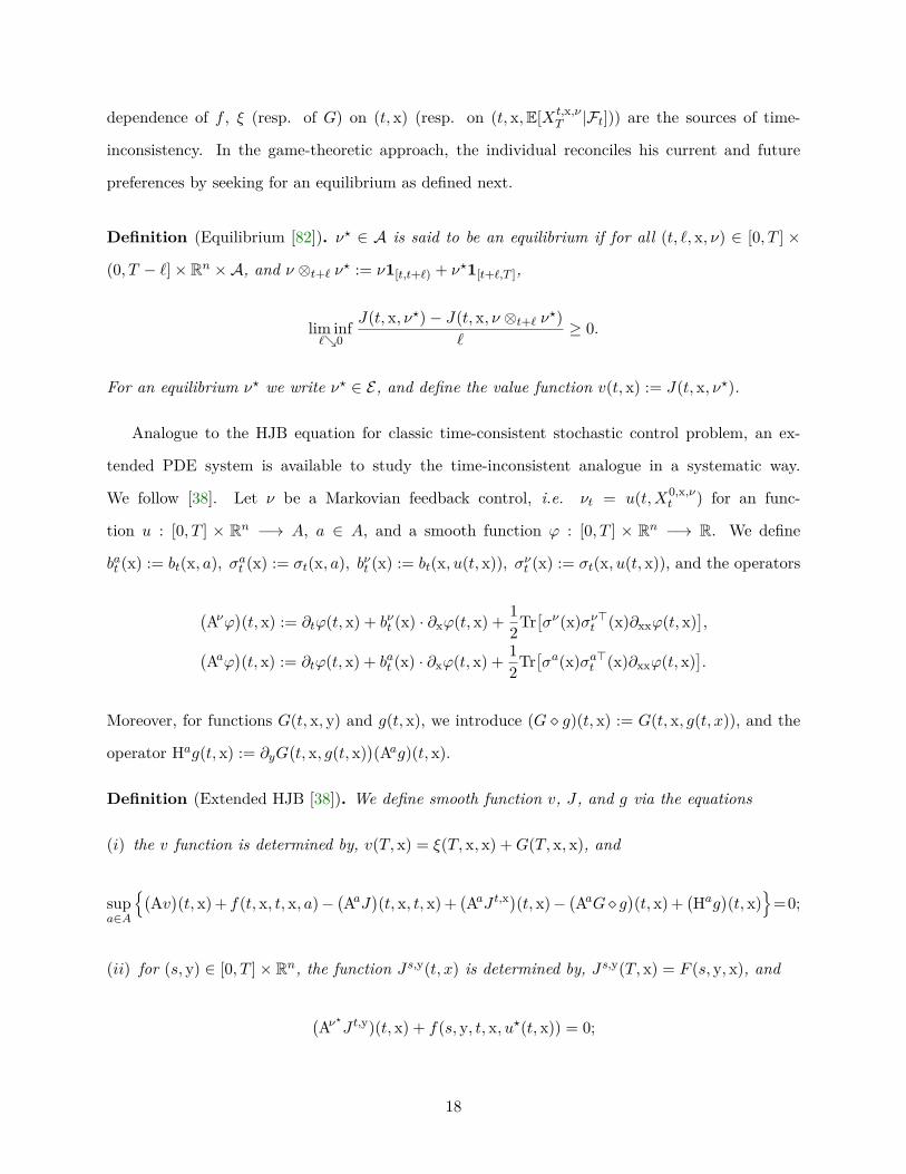
dependence of f , ξ (resp. of G) on (t, x) (resp. on (t, x,E[Xt,x,νT |Ft])) are the sources of time-

inconsistency. In the game-theoretic approach, the individual reconciles his current and future

preferences by seeking for an equilibrium as defined next.

Definition (Equilibrium [82]). ν? ∈ A is said to be an equilibrium if for all (t, `, x, ν) ∈ [0, T ] ×

(0, T − `]× Rn ×A, and ν ⊗t+` ν? := ν1[t,t+`) + ν?1[t+`,T ],

lim inf`0

J(t, x, ν?)− J(t, x, ν ⊗t+` ν?)`

≥ 0.

For an equilibrium ν? we write ν? ∈ E, and define the value function v(t, x) := J(t, x, ν?).

Analogue to the HJB equation for classic time-consistent stochastic control problem, an ex-

tended PDE system is available to study the time-inconsistent analogue in a systematic way.

We follow [38]. Let ν be a Markovian feedback control, i.e. νt = u(t,X0,x,νt ) for an func-

tion u : [0, T ] × Rn −→ A, a ∈ A, and a smooth function ϕ : [0, T ] × Rn −→ R. We define

bat (x) := bt(x, a), σat (x) := σt(x, a), bνt (x) := bt(x, u(t, x)), σνt (x) := σt(x, u(t, x)), and the operators

(Aνϕ

)(t, x) := ∂tϕ(t, x) + bνt (x) · ∂xϕ(t, x) + 1

2Tr[σν(x)σν>t (x)∂xxϕ(t, x)

],(

Aaϕ)(t, x) := ∂tϕ(t, x) + bat (x) · ∂xϕ(t, x) + 1

2Tr[σa(x)σa>t (x)∂xxϕ(t, x)

].

Moreover, for functions G(t, x, y) and g(t, x), we introduce (G g)(t, x) := G(t, x, g(t, x)), and the

operator Hag(t, x) := ∂yG(t, x, g(t, x)

)(Aag)(t, x).

Definition (Extended HJB [38]). We define smooth function v, J , and g via the equations

(i) the v function is determined by, v(T, x) = ξ(T, x, x) +G(T, x, x), and

supa∈A

(Av)(t, x) + f(t, x, t, x, a)−

(AaJ

)(t, x, t, x) +

(AaJ t,x

)(t, x)−

(AaG g

)(t, x) +

(Hag

)(t, x)

=0;

(ii) for (s, y) ∈ [0, T ]× Rn, the function Js,y(t, x) is determined by, Js,y(T, x) = F (s, y, x), and

(Aν?J t,y)(t, x) + f(s, y, t, x, u?(t, x)) = 0;

18

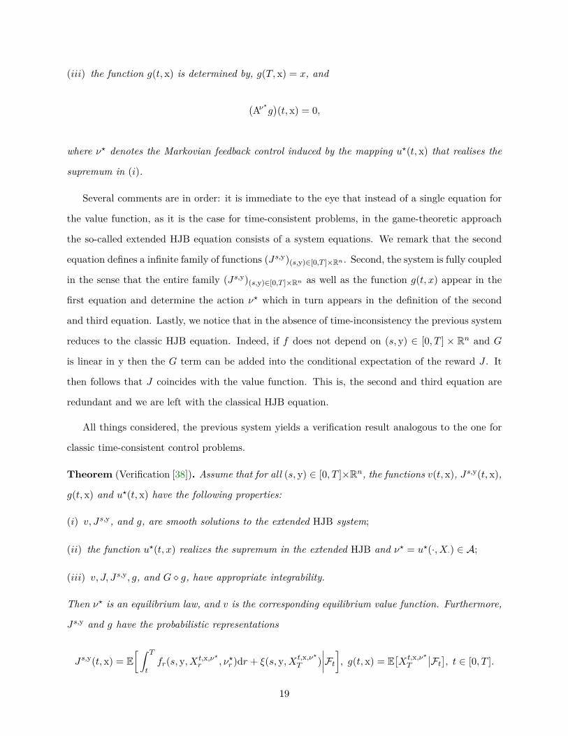
(iii) the function g(t, x) is determined by, g(T, x) = x, and

(Aν?g

)(t, x) = 0,

where ν? denotes the Markovian feedback control induced by the mapping u?(t, x) that realises the

supremum in (i).

Several comments are in order: it is immediate to the eye that instead of a single equation for

the value function, as it is the case for time-consistent problems, in the game-theoretic approach

the so-called extended HJB equation consists of a system equations. We remark that the second

equation defines a infinite family of functions (Js,y)(s,y)∈[0,T ]×Rn . Second, the system is fully coupled

in the sense that the entire family (Js,y)(s,y)∈[0,T ]×Rn as well as the function g(t, x) appear in the

first equation and determine the action ν? which in turn appears in the definition of the second

and third equation. Lastly, we notice that in the absence of time-inconsistency the previous system

reduces to the classic HJB equation. Indeed, if f does not depend on (s, y) ∈ [0, T ] × Rn and G

is linear in y then the G term can be added into the conditional expectation of the reward J . It

then follows that J coincides with the value function. This is, the second and third equation are

redundant and we are left with the classical HJB equation.

All things considered, the previous system yields a verification result analogous to the one for

classic time-consistent control problems.

Theorem (Verification [38]). Assume that for all (s, y) ∈ [0, T ]×Rn, the functions v(t, x), Js,y(t, x),

g(t, x) and u?(t, x) have the following properties:

(i) v, Js,y, and g, are smooth solutions to the extended HJB system;

(ii) the function u?(t, x) realizes the supremum in the extended HJB and ν? = u?(·, X·) ∈ A;

(iii) v, J, Js,y, g, and G g, have appropriate integrability.

Then ν? is an equilibrium law, and v is the corresponding equilibrium value function. Furthermore,

Js,y and g have the probabilistic representations

Js,y(t, x) = E[ ∫ T

tfr(s, y, Xt,x,ν?

r , ν?r )dr + ξ(s, y, Xt,x,ν?T )

∣∣∣∣Ft], g(t, x) = E[Xt,x,ν?T

∣∣Ft], t ∈ [0, T ].

19

In simple terms, the previous theorem provides a sufficient set of conditions that certifies

whenever an action is an equilibrium and identifies its corresponding value function. Regularity

assumptions aside, we remark that for the purposes of solving a time-inconsistent control problem,

i.e. finding an equilibrium and its value function, the previous result does the job.

Another matter of interest bring us back to the very own definition of the sophisticated agent.

Let us recall, this agent revises his strategy taking possible future revisions into account, and by

avoiding such makes his strategy time-consistent. Therefore, one expects some form of dynamic

programming principle to hold for this kind of problems. This is the purpose of [37, Proposition 8.1],

which provides a link between time-inconsistent and time-consistent Markovian control problems.

Recall this is a crucial, actually the initial, step in the dynamic programming approach of [64], see

Section 1.1.1. Indeed, it allows to establish the reverse direction of the standard verification result,

which we will refer to as a necessity result.

Proposition (A primer DPP [37]). For every time inconsistent problem in the present framework

there exists a standard, time consistent optimal control problem with the following properties:

(i) the optimal value function for the standard problem coincides with the equilibrium value function

for the time inconsistent problem;

(ii) the optimal control for the standard problem coincides with the equilibrium control for the time

inconsistent problem.

[37, Proposition 8.1] states that (in the framework of strong formulation with Markovian feed-

back actions) given an equilibrium, as defined above, for any time-inconsistent stochastic control

problem it is possible to associate a classical time-consistent optimal stochastic control problem

which attains the same value and satisfies a dynamic programming principle. However, the argu-

ment layed down in [37, Proposition 8.1], which we have ommitted, assumes a priori a smooth

solution to the above PDE system. This is, it presupposes that the value function associated to

the equilibrium action and the decoupled pay-off functionals belong to C1,2([0, T ]× Rd), and is in

the spirit of the (easy direction) of the Feynman–Kac representation formula. This means that the

class of equilibria for which the DPP used in [37] holds is actually a sub-class of the ones given

by classical definition via the liminf presented above. Moreover, it was recently shown that these

20

would correspond to regular equilibria as defined in in [173]. In fact, as explained in [173, Remark

3.9], regular equilibria are a priori required to be continuous in time and space. We remark that

even for time-consistent problems the previous regularity assumptions on the value function and

the control it is known to often not hold.

Even more critical in our view, in the context of classic time-consistent control, the argument

in [37, Proposition 8.1] would be equivalent to assuming that the HJB equation has a smooth

classical solution to prove the DPP. We find this line of argument to be quite atypical in the sense

that: (i) this is usually done the other way around: the DPP allows one to show that the value

function is related to the HJB PDE, usually in the viscosity sense; (ii) quid of the cases where

the value function fails to be smooth, which are ubiquitous in the literature? In classical control

problems, the DPP holds under mere Borel-measurability of the value function, see El Karoui and

Tan [85, 86], and we do not feel that it is reasonable to assume smoothness a priori to prove it.

All in all, in order to obtain a useful necessity result one should obtain the underlying DPP

circumventing these a priori assumptions on the value function of the associated equilibria. More

generally, one should aim to obtain a proof of a DPP from first principles, by which we mean

that by introducing a refinement on the notion of equilibrium a DPP can be establish as a direct

consequence of it. Such approach, will open the door to a necessity result which remained mostly

absent in the literature.

Indeed, the community quickly started to investigate such necessity type results hoping to arrive

to a complete characterisation of equilibria and their value function. This is, both a necessary and

sufficient condition for an admissible action to be an equilibrium. For this we follow [120] and

introduce some additional notation.

For (s, t, r, y, x, ν) ∈ [0, T ]3 × Rn × A, let fs,y,ν(t, x) := Et,x[ft(s, y, x, u(t, x))

], fs,y,r(t, x) :=

Et,x[fs,y,ν

?(r,Xt,x,ν?r )

], ξs,y(t, x) := Et,x

[ξ(s, y, Xt,x,ν?

T )], and

Γs,y,ν?(t, x, ν) := f s,y,ν(t, x)− f s,y,ν?(t, x) +∫ T

t

(Aν f s,y,r

)(t, x)dr

+(Aνξs,y

)(t, x) + ∂yG(s, y, g(t, x))(Aνg)(t, x).

21

Theorem (Characterisation of Markovian equilibria [120]). Under appropriate assumptions

lim inf`0

J(t, x, ν?)− J(t, x, ν ⊗t+` ν?)`

= −Γt,x,ν?(t, x, ν), ∀(t, x, ν) ∈ [0, T ]× Rn ×A.

Moreover, ν? is an equilibrium if and only if

Γt,x,ν?(t, x, a) ≥ 0, ∀(t, x, a) ∈ [0, T )× Rn ×A.

The previous result is quite remarkable as [120] succeeds in characterising equilibria via the

mapping Γ. Yet, we highlight that we have remained vague regarding the assumptions of the pre-

vious theorem. Indeed, the conditions under which such result holds are quite stringent, requiring

for instance that the optimal action and the mappings involve in the definition of Γ to be differen-

tiable in time and with spacial derivatives of polynomial growth. This relates to the fact that the

argument in [120] makes a strong use of the infinitesimal generator operator and may, in general,

limit the class of equilibria that are able to be identified by the previous result. Moreover, the

previous characterisation bypasses the extended HJB system and makes no direct link between it

and Γ.

For the purposes of the discussion in this chapter, the previous results summarise the state of

the understanding of Markovian time-inconsistent control problems. According to [38, Section 10],

the following remained as open research problems at the time of its writing:

• ‘[t]he present theory depends critically on the Markovian structure. It would be interesting

to see what can be done without this assumption’;

• ‘[a] related (hard) open problem is to prove existence and/or uniqueness for solutions of the

extended HJB system’;

• ‘[a]n open and difficult problem is to provide conditions on primitives which guarantee that

the functions V and f are regular enough to satisfy the extended HJB system’;

• ‘[a]nother problem is to give conditions on primitives which guarantee that the assumptions

of the verification theorem are satisfied’.

22

To not get ahead of ourselves, we will just mention that this thesis makes contributions to

each of these problems. We highlight that the third point above is making reference to a type of

necessity result, which we stress again, is crucial in the dynamic programming approach of [64],

see Section 1.1.1. As we mentioned earlier, one avenue to arrive at this result is to provide a DPP

circumventing any kind of a priori assumptions on the value function of the associated equilibria.

In this way, we can conduct the analysis in a non-Markovian framework, and, at the same time,

we will remain at the greatest level of generality possible, i.e. without implicit assumptions on the

class of equilibria into consideration.

In the following section, we present an informal description of our contributions to the time-

inconsistent literature. In synthesis, inspired by the results of [64] in the context of contract theory,

we take a probabilistic approach that allow us to, among other things, extends the results for

Markovian models with time-inconsistency to the non-Markovian framework and provide answers

to each of the previous items.

1.2.2 Contributions

In the second part of this thesis, we develop a probabilistic theory for continuous-time non-

Markovian stochastic control problems which are inherently time-inconsistent. Our formulation is

cast within the framework of a controlled non-Markovian forward stochastic differential equation,

and a general objective functional. To illustrate our results, suppose the dynamics of the controlled

state process are given as in Section 1.1.1. Suppose the utility drawn by the Agent, from an effort

action ν at time t ∈ [0, T ] and past trajectory x ∈ X 5, is given by

JA(t, x, ν) = EPν[f(T − t)UA(ξ)−

∫ T

tf(r − t)cr(X·∧r, νr)dr

∣∣∣∣Ft],where f : [0, T ] −→ R, f(0) = 1, denotes a generic discount function. We remark that its pres-

ence in the terminal utility and the running cost, are the sources of inconsistency. We adopt a

game-theoretic approach to study such problems, meaning that we seek for sub-game perfect Nash

equilibrium points. As a first novelty of this work, we introduce and motivate a refinement on the5To alleviate the notation we set X := Cd, which we recall denotes the space of Rd-valued continuous functions on

[0, T ] endowed with the sup topology

23

notion of equilibrium from which one can directly and rigorously establish an extended dynamic

programming principle, in the same spirit as in the classical theory, which takes the following form.

Theorem (Extended DPP Chapter 2). Let ν? ∈ E. For any stopping times σ ≤ τ , P–a.s.

VAσ = sup

ν∈AEPν

[VAτ −∫ τ

σ

(cr(X·∧r, νr)+EPν?

[f ′(T−r)UA(ξ)−

∫ T

rf ′(u−r)cu(X·∧r, ν?u)du

∣∣∣∣Fr])dr∣∣∣∣Fσ].

As an immediate consequence of this result, we can associate a system of BSDEs to study

equilibria in the case of uncontrolled volatility, i.e. σt(x, a) = σt(x). Let us introduce the system

which for any s ∈ [0, T ] satisfies

Yt = UA(ξ) +∫ T

t

(Hr(X·∧r,Zr)− ∂Y r

r

)dr −

∫ T

tZr · dXr, t ∈ [0, T ], P–a.s.,

∂Y st = −f ′(T − s)UA(ξ) +

∫ T

t∇h?r(s,X·∧r, ∂Zsr ,Zr)dr −

∫ T

t∂Zsr · dXr, t ∈ [0, T ], P–a.s.,

(H)

where

Ht(x, z) := supa∈A

σt(x)bt(x, a)·z − ct(x, a)

,

∇h?t (s, x, z, z) := σt(x)bt(x, a?(t, x, x))·z + f ′(t− s)ct(x, a?(t, x, x)),

and a?(t, x, z) denotes the unique, by assumption, maximiser in H. The previous system is of

an infinite-dimensional nature as the second equation induces a family of BSDEs, one for every

s ∈ [0, T ]. Moreover, it is fully-coupled as the diagonal term of the family (∂Y s)s∈[0,T ] appears in

the generator of the first equation and Z appears, via a?, in the generator of the family of BSDEs.

Be it as it may, we are able to show that: (i) (H) is of both sufficient and necessary to characterise

equilibria α? ∈ E , in particular our results establish that any equilibria must arise from a solution

to the system, and thus, the existence of an equilibria is equivalent to the existence of a solution

to (H); (ii) Y coincides with the value function VA, and α? always arises as a maximiser of the

Hamiltonian; and (iii) (H) is well-defined, and consequently, in the case of drift control, there exists

a unique equilibria.

Let us mention that (H) extends naturally to a system incorporating second-order BSDEs

(2BSDEs) in the case the agent is allowed to control the volatility. Indeed, the extended DPP

24

holds true in the case the Agent controls the volatility as well. For such system we are able to show

(i) and (ii) still hold. Nevertheless, (iii) becomes a much more delicate matter as the existence

of a solution requires the existence of an optimal measure P?. This problem is worth of analysis

in the future, as we discuss later in this chapter, see Section 1.5. As a final comment, we also

address the extensions of (H) to the case of more general rewards. In particular, to those with

mean–variance type of criteria which are indispensable, for example, in applications in portfolio

selection, or energy consumption management.

Lastly, we remark that a central part of our analysis is based on establishing that letting

h?t (s, x, z, z) := σt(x)bt(x, a?(t, x, x)) ·z − f(t − s)ct(x, a?(t, x, x)), given a solution to (H) we can

introduce the family of BSDEs

Y st = f(T − s)UA(ξ) +

∫ T

th?r(s,X·∧r, Zsr ,Zr)dr −

∫ T

tZsr · dXr, t ∈ [0, T ], P–a.s.

and verify that

VAt = Yt = Y t

t , t ∈ [0, T ], P–a.s., and, Zt = Ztt , dt⊗ dP–a.e.

This is, (Y,Z) prescribe a solution to a so called type-I backward stochastic Volterra integral

equation (BSVIE) of the form

Y st = f(T − s)UA(ξ) +

∫ T

th?r(s,X·∧r, Zsr , Zrr )dr −

∫ T

tZsr · dXr, t ∈ [0, T ], P–a.s.

In the context of Section 1.1.1, the extended DPP and the previous observation are the analogous

version of Step 1 in the time-inconsistent case. This is, we have successfully provided an extended

DPP and are able to identify the natural probabilistic objects, analogous to the BSDE, that are

associated with it. Moreover, in Chapter 2 we show that in the absence of time-inconsistency, i.e.

when f(t) = e−ρt, the extended DPP (resp. the system (H) or, equivalently, the previous BSVIE)

reduces to the classic DPP (resp. the BSDE in Section 1.1.1).

The link between the previous time-inconsistent control problem and type-I BSVIEs was the

motivation of our analysis in the following part of the thesis were we explore the well-posedness of

25

a general class of type-I BSVIEs in both the case of Lipschitz and quadratic generators.

1.3 Part III: backward stochastic Volterra integral equations

Seeking to understand the parallel stream of works that study time-inconsistency via BSVIEs, in

Part III we questioned the extent to which our approach via system (H) relates to those via BSVIEs

of the form described at the end of the previous section. Building upon the strategy devised in

Chapter 2, we addressed the well-posedness of a general and novel class of multidimensional type-I

BSVIEs, that we coined extended BSVIEs.

BSVIEs are regarded as natural extensions of backward stochastic differential equations, BSDEs

for short. On a complete filtered probability space (Ω,G,G,P), supporting an n-dimensional

Brownian motion B, and denoting by G the P-augmented natural filtration generated by B, one is

given data, that is to say a GT -measurable random variable ξ, and a mapping g, referred to respect-

ively as the terminal condition and the generator. A solution to a BSDE is a pair of G-adapted

processes (Y·, Z·) such that

Yt = ξ +∫ T

tgr(Yr, Zr)dr −

∫ T

tZrdBr, t ∈ [0, T ], P–a.s. (1.3.1)

BSDEs of linear type were first introduced by Bismut [31, 32] as an adjoint equation in the

Pontryagin stochastic maximum principle. Actually, the contemporary work of Davis and Varaiya

[67]6 studied a precursor of a linear BSDE for characterising the value function and the optimal

controls of stochastic control problems with drift control only. In the same context of the stochastic

maximum principle, BSDEs of linear type are present in Arkin and Saksonov [12], Bensoussan [22]

and Kabanov [146]. Remarkably, the extension to the non-linear case is due to Bismut [33], as a

type of Riccati equation, as well as Chitashvili [50], and Chitashvili and Mania [51, 52]. Later,

the seminal work of Pardoux and Peng [201] presented the first systematic treatment of BSDEs

in the general nonlinear case, while the celebrated survey paper of El Karoui, Peng, and Quenez

[88] collected a wide range of properties of BSDEs and their applications to finance. Among such6Indeed, [67] was received for publication on October 27, 1971 and it is part of the bibliography of [32].

26

properties we recall the so-called flow property, that is to say, for any 0 ≤ r ≤ T ,

Yt(T, ξ) = Yt(r, Yr(T, ξ)), t ∈ [0, r], P–a.s., and Zt(T, ξ) = Zt(r, Yr(T, ξ)), dt⊗dP–a.e. on [0, r]×Ω,

where (Y (T, ξ), Z(T, ξ)) denotes the solution to the BSDE with terminal condition ξ and final time

horizon T .

A natural extension of (1.3.1) arises by considering a collection of GT -measurable random vari-

ables (ξ(t))t∈[0,T ], referred in the literature of BSVIEs as the free term, as well as a generator g. In

such a setting, a solution to a BSVIE is a pair (Y·, Z ·· ) of processes such that

Yt = ξ(t) +∫ T

tgr(t, Yr, Ztr, Zrt )dr −

∫ T

tZtrdBr, P–a.s., t ∈ [0, T ]. (1.3.2)

Of noticeable interest is the case in which the term Zrt is absent in the generator, i.e.

Yt = ξ(t) +∫ T

tgr(t, Yr, Ztr)dr −

∫ T

tZtrdBr, P–a.s., t ∈ [0, T ]. (1.3.3)

Nowadays (1.3.3) and (1.3.2) are referred in the literature as type-I and type-II BSVIEs, re-

spectively. The first mention of such equations is, to the best of our knowledge, due to Hu and Peng

[132]. Indeed, in the context of well-posedness of BSDEs valued in a Hilbert space, a prototype of

type-I BSVIEs (1.3.3) is considered, see the comments following [132, Remark 1.1]. Two decades

passed before a direct consideration of BSVIEs of the form given by (1.3.3) was made by Lin [171],

where the author studied the case ξ(t) = ξ, t ∈ [0, T ], for a GT -measurable ξ. The general form

of (1.3.2) was first addressed in Yong [267, 269] in the context of optimal control of (forward)

stochastic Volterra integral equations (FSVIEs, for short).

There are significant distinctions between BSDEs and BSVIEs. Nevertheless, a satisfactory

concept of solution for such equations can be defined by extrapolating from the theory of BSDEs.

In broad terms, a pair (Y·, Z ·· ) is said to be a solution to a BSVIE, see [269], if for each s ∈ [0, T ),

the mapping t 7−→ (Yt, Zst ) is G-adapted on [s, T ], (Y,Z) is appropriately integrable and satisfies

(1.3.2). It is also worth pointing out the distinctions between type-I and type-II BSVIEs. As a

consequence of the presence of Zst in the generator, to obtain a solution to a type-II BSVIE one

27

has to determine Zst for (t, s) ∈ [0, T ]2, and (1.3.2) alone does not give enough restrictions. Indeed,

[269] showed that an adapted solution to the type-II BSVIE (1.3.2) may, in general, not be unique.

This is in contrasts with type-I BSVIEs, where it suffices to determine Zst for (t, s) ∈ [0, T ]2,

0 ≤ s ≤ t ≤ T . Moreover, without additional assumptions, a solution to a general type-II BSVIE

does not satisfy the flow property.

Since their introduction, BSVIEs have been extended to much more general frameworks than

the one presented above. Hence, Wang [248] studies the case of random Lipschitz data; Wang and

Zhang [258] and Shi and Wang [225] deal with general non-Lipschitz data; Coulibaly and Aman [58]

study time-delayed generators; mean-field BSVIEs are considered in Shi, Wang, and Yong [226];

Lu [176], Hu and Øksendal [131], Overbeck and Röder [196] and Popier [207] studied extensions

to general filtrations and the case where B is replaced by more general processes; infinite horizon

BSVIEs are investigated in Hamaguchi [113]; Djordjević and Janković [79, 78] were interested in

perturbed BSVIEs, i.e. when the coefficients depend additively on small perturbations; BSVIEs in

Hilbert spaces have been investigated in Anh and Yong [10], Anh, Grecksch, and Yong [11], and

Ren [214]; and an analysis of numerical schemes for BSVIEs has been proposed in Bender and

Pokalyuk [21]. There is also a wide spectrum of applications of BSVIEs. Hence, dynamic risk

measures have been considered in Yong [268], Wang and Shi [252, 253], Wang, Sun, and Yong [246]

and Agram [2]. Kromer and Overbeck [159] also studied the question of dynamic capital allocations

via BSVIEs. Wang and Shi [251] dealt with a risk minimisation problem by means of the maximum

principle for FBSVIEs, while the optimal control of SVIEs and BSVIEs via the maximum principle

has been studied in Chen and Yong [47], Wang [250], Agram, Øksendal, and Yakhlef [4, 5], Shi,

Wang, and Yong [227], Shi, Wen, and Xiong [228], see also Wei and Xiao [259] for the case with

state constraints.

Since their first appearance, a natural and non-trivial question for BSVIEs has been that of the

regularity in time of their solutions. The best known probabilistic results for general type-II BSVIEs

guarantee the regularity of the solutions in an Lp sense only, see Wang [249] and Li, Wu, and Wang

[169]. Nevertheless, analytic results via a representation formula, guarantee the pathwise regularity

of a solution to type-I BSVIEs, see Wang and Yong [255] and Wang, Yong, and Zhang [247] for

results regarding the representation of BSVIEs in the Markovian and non-Markovian framework,

28

respectively. Regarding BSVIEs driven by discontinuous processes, it is known that type-I BSVIEs

are known to be much more amenable to the analysis, for example [207; 258] are able to study the

regularity of type-I BSVIEs with jumps by probabilistic methods.These results stress the fact that

extending these ideas to type-II BSVIEs is a more challenging task. General discontinuous BSVIEs

are out of the scope of the current document.

Out of the class of processes described by BSVIEs, a broader family than that of standard type-

I BSVIEs (1.3.3) is known to arise in the study of time-inconsistent control problems. Recently,

Agram and Djehiche [3] studied reflected backward stochastic Volterra integral equations and their

relations to a time-inconsistent optimal stopping problem. Earlier connections were suggested in the

concluding remarks of Wang and Yong [255]. Indeed, BSVIEs provide a probabilistic representations

of the system of partial differential equation (PDE, for short) appearing in the study of time-

inconsistent optimal control problems, e.g. see Yong [270] and Wei, Yong, and Yu [260] for PDEs

obtained via Pontryagin’s and Bellman’s principle, respectively. A natural link was then made

rigorous independently by Wang and Yong [245, Section 5] and Lemma 2.10.3.1 in Chapter 2.

Although following different approaches, their analyses lead to introduce type-I BSVIEs of the

form

Yt = ξ(t) +∫ T

tgr(t, Yr, Ztr, Zrr )dr −

∫ T

tZtrdBr, P–a.s., t ∈ [0, T ]. (1.3.4)

These are BSVIEs in which the diagonal of Z appears in the generator. We highlight that, until

the present work, the only well-posedness results in the literature for type-I BSVIEs (1.3.4) are

available in [245] and Chapter 2. Both results hold for the particular case in which the driver g is

linear in Ztr. Indeed, the argument in [245] follows as a consequence of the representation formula,

i.e. an analytic argument via PDEs, and holds in a Markovian setting. On the other hand, the

probabilistic argument in Chapter 2 holds in the non-Markovian case.

Likewise, Hamaguchi [112, 114] studied a time-inconsistent control problem where the cost

functional is defined by the Y component of the solution of a type-I BSVIE (1.3.3), in which g

depends on a control. Via Pontryagin’s optimal principle, the author noticed that the adjoint

equations correspond to an extended type-I BSVIE, as first introduced in Wang [244] in the context

of generalising the celebrated Feynman–Kac formula. An extended type-I BSVIE consists of a pair

29

(Y ·· , Z ·· ), with appropriate integrability, such that s 7−→ Y s is continuous in an appropriate sense

for s ∈ [0, T ], Y s· is pathwise continuous, Zs· is predictable, and

Y st = ξ(s) +

∫ T

tgr(s, Y s

r , Zsr , Y

rr )dr −

∫ T

tZsrdBr, t ∈ [0, T ], P–a.s., s ∈ [0, T ]. (1.3.5)

We highlight that the noticeable feature of (1.3.4) and (1.3.5) is the appearance of the ‘diagonal’

processes (Y tt )t∈[0,T ] and (Ztt )t∈[0,T ], respectively. A prerequisite for rigorously introducing these

processes is some regularity of the solution. Indeed, the regularity of s 7−→ (Y s, Zs) in combination

with the pathwise continuity of Y and the introduction of a derivative of Zs with respect to s, as

first discussed in Chapter 2, make the analysis possible.

Put succinctly, type-I BSVIEs, understood in a broader sense than that of (1.3.3), provide a

rich framework to address new classes of problems in mathematical finance and control. In the case

of time-inconsistent control problems, (1.3.4) and (1.3.5) appear as a consequence of the study of

such problems via Bellman’s and Pontryagin’s principles, respectively.

We also remark that, to the best of our knowledge, there are no well-posedness results for

multidimensional quadratic type-I BSVIEs as general as (1.3.4) or (1.3.5). In fact, the study of

non-Lipschitz BSVIEs remains limited to Ren [214], Shi and Wang [225], Wang, Sun, and Yong

[246], and Wang and Zhang [258]. In [258] and [214], the authors study solutions to general

multidimensional type-I (1.3.3) and type-II (1.3.2) BSVIEs, respectively, where the generator is

increasing and concave in y and Lipschitz in z. [225] continued the study of type-II BSVIEs (1.3.2)

and settled some flaws in the analysis of [214]. On the other hand, [246] presents the first analysis

of BSVIEs whose generator have quadratic growth on z. Indeed, the authors consider a standard

one dimensional type-I BSVIE (1.3.3) in which the generator is Lipschitz in y and quadratic in z,

which we will refer as the Lipschitz–quadratic case, provided the data of the BSVIE is bounded.

The need to introduce this additional assumption is due to underlying results for quadratic BSDEs

that were employed in [246].

Even in the case of one dimensional BSDEs, establishing their well-posedness in the case of

generators with quadratic growth in z is known to be more delicate that in the Lipschitz case and

requires to impose extra assumptions on the data of the problem. The first result in this setting

30

was provided by Kobylanski [155] in the case of bounded and Lipschitz–quadratic data. Building

upon the ideas in [155], Briand and Hu [41, 42] showed that imposing sufficiently large exponential

moments on the terminal condition ξ are actually enough. We stress that this approach allows

for unbounded terminal conditions but is limited to the one dimensional Lipschitz–quadratic case.

BSDEs with superquadratic growth were studied in Lepeltier and San Martín [165] and Delbaen,

Hu, and Bao [68]. On the other hand, the original method introduced in Tevzadze [238] takes a

different view of this problem and is able to cover quadratic BSDEs, in both y and z, but requires,

once again, the data to be bounded.

In the multidimensional case, new approaches become necessary as the tools that are usually

used in the one dimensional case, like monotone convergence or Girsanov transformation, are no

longer available. In fact, Frei and Dos Reis [103] provide a simple example of a multidimensional

quadratic BSDE with a bounded terminal condition for which there is no solution. This counter-

example shows that a direct generalisation of the approaches in [155; 41; 42] or the classic approach

in [201] would be unsuccessful in the case of BSDEs and, naturally, of BSVIEs. Nevertheless, it is

known that well-posedness results for BSDEs can be obtained exploiting the theory of BMO mar-

tingales and imposing further structural conditions on the generator. See, for instance, Cheridito

and Nam [49] for specific choices of generators, Hu and Tang [133] for the case of diagonally quad-

ratic generators, the generalisations in Jamneshan, Kupper, and Luo [143] and Kupper, Luo, and

Tangpi [161], as well as Rouge and El Karoui [215] Hu, Imkeller, and Müller [134] for some ap-

plications. To unify these approaches, Harter and Richou [118] provides a well-posedness result

by approximating the solution of a Lipschitz–quadratic BSDE, assuming the a priori existence of

uniform estimates on the BMO norm of the local martingale∫ ·

0 Znr dWr and exploiting the Malliavin

calculus. In providing scenarri in which such estimates can be obtained [118] recover several results

available in the literature. On the other hand, the methodology devised in [238] reveals that a

positive answer can be stated if the data of the problem is bounded and sufficiently small. We also

mention Frei [102] and Kramkov and Pulido [158] which provide generalisations to slightly more

general terminal condition, as well as, the remarkable global existence result in Xing and Žitković

[265] for Markovian quadratic BSDEs.

Extending the ideas in [41; 42] to the case of BSVIEs was the motivation behind [246] and it

31

explains the framework of their result, i.e. scalar BSVIEs with Lipschitz quadratic generator a

bounded data. Moreover, as [246, pp. 4] states: ‘[t]he case [of] Y being higher dimensional will

be significantly different in general.’ Therefore, it is not expected that these ideas would be able

to cover the general multidimensional quadratic BSVIE. Fortunately, a close look at the argument

provided in [238] reveals that a positive answer can be stated as soon as the data of the problem

is bounded and sufficiently small. This will be the inspiration of our approach to address the

quadratic case.

1.3.1 Contributions

In this part of the thesis we built upon the strategy devised in Chapter 2 and address the

well-posedness of a general and novel class of type-I BSVIEs. We let X be the solution to a drift-

less stochastic differential equation (SDE, for short) under a probability measure P, and F be the

P-augmentation of the filtration generated by X, and consider a tuple (Y ·· , Z ·· , N ·· ), of F-adapted

processes, satisfying for every s ∈ [0, T ]

Y st = ξ(s) +

∫ T

tgr(s,X, Y s

r , Zsr , Y

rr , Z

rr )dr −

∫ T

tZsrdXr −

∫ T

tdN s

r , t ∈ [0, T ], P–a.s. (1.3.6)

We remark that the additional process N corresponds to a martingale process which is P-

orthogonal to X. This is a consequence of the fact that we work with a general filtration F. To

the best of our knowledge, a theory for type-I BSVIEs, as general as the ones introduced above,

remains absent in the literature. Moreover, such class of type-I BSVIEs has only been mentioned

in [114, Remark 3.8] as an interesting generalisation of (1.3.5).

Our approach is based on the following class of infinite families of BSDEs, which for every

s ∈ [0, T ] satisfy

Yt = ξ(T,X·∧T ) +∫ T

thr(X·∧r,Yr,Zr, Y r

r , Zrr , ∂Y

rr )dr −

∫ T

tZ>r dXr, t ∈ [0, T ], P–a.s.,

Y st = η(s,X·∧T ) +

∫ T

tgr(s,X·∧r, Y s

r , Zsr ,Yr,Zr)dr −

∫ T

tV sr>dXr, t ∈ [0, T ], P–a.s.,

∂Y st =∂sη(s,X·∧T ) +

∫ T

t∇gr(s,X·∧r, ∂Y s

r , ∂Zsr , Y

sr , Y

sr ,Yr,Zr)dr −

∫ T

t∂Zsr

>dXr, t ∈ [0, T ], P–a.s.,

where (Y,Z,N , Y, Z,N, ∂Y, ∂Z, ∂N) are unknown, and required to have appropriate integrability.

32

As a first step, in Chapter 3 we worked under classical Lipschitz growth assumptions and

showed that for an appropriate choice of η and h its well-posedness is equivalent to that of the

type-I BSVIE (1.3.6). In addition, we recovered classical results for this general class of BSVIEs:

(i) we provided a priori estimates; (ii) established the stability of solutions; and (iii) provided a

representation formula in terms of a semilinear PDEs. Our approach can naturally be specialised

to recover the version of these results for BSVIEs previously studied in the literature. Lastly, as it

was the motivation for this project, we considered the game-theoretic approach to time-inconsistent

stochastic control problems and showed that as a consequence of our results, one can reconcile the

two current probabilistic approaches to this problem. Moreover, we provided an equivalent result

for two earlier analytic approaches, based on semi-linear PDEs. We believe this helps to elucidate

connections between the different takes on the problem available in the literature.

Our work in this part of the thesis does not end there. Some of the cornerstone models in the

literature in stochastic control are based on either mean–variance or linear–quadratic models. In

fact, we recall the results in [164], where the authors present a mean–variance investment problem

in which uniqueness of the equilibrium via the PDE characterisation of [35] fails. Consequently,

a natural extension of the results in Chapter 3 is the case of generator with quadratic growth.

For example, such extension becomes necessary when dealing with applications to contract theory

models were the agent has a cost which is quadratic in his effort. As such, this is the objective of

Chapter 4, the second chapter of Part III.

Recall that in Chapter 3 and Chapter 2 we studied a system consisting of an infinite family of

BSDEs in a Lipschitz framework. In general terms, by introducing the equivalent weighted versions

of the classic integrability spaces in the literature on BSDEs and choosing a weight large enough we

were able to obtain its well-posedness. In the setting of this paper, the Lipschitz assumption for the

generators is abandoned. As a consequence, one cannot recover a contraction by simply choosing

a weight large enough. In fact, given our growth assumptions, the usual candidate for providing

a contractive map is no longer Lipschitz–continuous, but only locally Lipschitz-continuous. For-

tunately, by exploiting the theory of bounded mean oscillating (BMO) martingales we can obtain

well-posedness results in the quadratic case in two scenarii: (i) Lipschitz–quadratic generators in

(Y, Z), respectively and data with sufficiently small norm; (ii) fully quadratic generators in (Y,Z)

33

and data with sufficiently small norm.

Our results in Chapter 4 follows the idea initially proposed in Tevzadze [238] for multidimen-

sional quadratic BSDEs, namely, that we can localise the usual procedure to a ball of radius R,

thus making the application Lipschitz-continuous again, and then to choose the radius of such a

ball so as to recover a contraction. The crucial contribution of [238] was to show that such controls

can be obtained by taking the norm of the data of the system to be small enough. The procedure

we followed is inspired by this idea and incorporates it into the strategy devised in Chapter 3 to

address the well-posedness of these kind of systems and of extended type-I BSVIEs. We decided

to work on weighted spaces as, in our opinion, it does significantly simplify the arguments in the

proof. We also mention that we estimated the greatest ball, i.e. the largest radius R, for which

such a localisation procedure leads to a contraction.

Bringing ourselves back to the context of contract theory, we echo that the analysis in this part

of the thesis does elucidate the connections between the different approaches to time-inconsistent

control problem at the analytic level, between PDEs in the Markovian setting, and the probabilistic

level, between (H) and extended type-I BSVIEs in the non-Markovian counterpart. This in turn,

leaves us educated enough to bring our attention back to the contracting problem.

1.4 Part IV: time-inconsistent contract theory

When it comes to incorporating time-inconsistent features into contract theory models, the eco-

nomic literature is abundant in discrete-time models with two, and up to three periods. A common

feature in this literature is adopting quasi-hyperbolic discounting structures to draw conclusions

in different mechanism design problems. Yet, the method of resolution in each problem remained

limited to a case-by-case analysis. For instance, Amador, Werning, and Angeletos [9] and Bond and

Sigurdsson [39] study the feasibility of commitment in models of consumption and savings, whereas

Galperti [106] considers the optimal provision of commitment devices to people who value both

commitment and flexibility. Bisin, Lizzeri, and Yariv [30] examines policymakers’ responses to the

political demands of agents with self-control problems, Halac and Yared [111] looks into a fiscal

policy model in which the government has time-inconsistent preferences, while Lim and Yurukoglu

[170] assesses the effects of time-inconsistency on monopoly regulation of electricity distribution.

34

Heidhues [125] and Karaivanov and Martin [148] integrate time-inconsistent preferences into credit,

mortgage and insurance contract design problems, respectively. Englmaier, Fahn, and Schwarz [94],

Gottlieb [108] and Gottlieb and Zhang [109] study contracting problems between firms and sophist-

icated, partially naive and naive present-biased consumers. Yılmaz [271, 272] considers a repeated

moral hazard problem involving a sophisticated and naive agent, respectively. Ma [177] studies a

multi-period model in which contracts are subject to renegotiations, and the agent’s action has a

long-term effect. Balbus, Reffett, and Wozny [14] shows the existence of time-consistent equilibria

for dynamic models with generalised discounting. A survey of some of the state of behavioural

economics research in contract theory was provided in Kószegi [156].

In continuous-time, where the dynamic models are sometimes more tractable and the solu-

tions enjoy better interpretability, the literature becomes rather scarce. Models dealing with a

pre-committed agent have been considered in Li and Qiu [167], in which a non-constant exponen-

tial discount factor is the source of time-inconsistency, and Djehiche and Helgesson [75], where

the agent is allowed to have mean–variance utility functions. The case of a sophisticated agent

was considered in Li, Mu, and Yang [168], Liu, Mu, and Yang [174], Liu, Huang, Liu, and Mu

[175] and Wang, Huang, Liu, and Zhang [257] in the case of hyperbolic discounting. However,

the time-inconsistency is restricted in the sense that it manifests only at discrete random times

that are exponentially distributed. Lastly, Cetemen, Feng, and Urgun [46] considers a Markovian

continuous-time contracting problem and dynamic inconsistency arising from non-exponential dis-

counting. The authors’ examples are limited to the case of a principal having time-inconsistent

preferences and the agent has standard time-consistent preferences. Altogether, a thorough ana-

lysis of the general non-Markovian continuous-time contracting problem between a standard utility

maximiser principal and a sophisticated time-inconsistent agent is still missing in the literature.

This is because, in our opinion, the crux of the problem lies in identifying a proper description of

the problem of the principal. In the case of a classic time-consistent agent and a time-inconsistent

principal, following [64], one expects the problem of the principal to boil down to a non-Markovian

time-inconsistent control problem with an additional state variable. As studied in [38], these prob-

lems are characterised by the so called extended HJB equation. Therefore, we expect that the

problem considered in this document will open the door to a complete analysis of the problem in

35

which both the principal and the agent are time-inconsistent.

1.4.1 Contributions

The set-up is as follows: given a contract ξ, i.e. an FT -measurable random variable, the agent,

allowed to control only the drift b, as in Section 1.1.1, receives a reward given by JA( · ; ξ), as in

Section 1.2.2 and where we now emphasise its dependence on the contract ξ. We call E(ξ) the set

of all equilibria associated to ξ. Moreover, the agent has a reservation utility R0 ∈ R below which

he refuses the contract ξ. We therefore let the set of admissible contracts be given by Ξ :=ξ :

VA0 (ξ, α) ≥ R0, for α ∈ E(ξ)

. The principal has her own utility function UP : X × R −→ R, and

solves the infinite dimensional problem

VP := supξ∈Ξ

supα∈E(ξ)

EPα[UP(X·∧T , ξ

)].

In light of our results in Chapter 2, for ξ ∈ Ξ the problem solved by the Agent is characterised by

the solution to (H), which we denote (Y(ξ),Z(ξ), ∂Y (ξ), ∂Z(ξ)). Nevertheless, the infinite dimen-

sional nature of (H) posed an obstacle for a direct application of the results in [64]. Fortunately, in

Chapter 2 we identified a link between time-inconsistent control problems and BSVIEs. Such type

of links appeared first in the concluding remarks of Wang and Yong [255] and then later in [245].

In our setting, such an equation is satisfied by the value of the agent along the equilibrium, namely

Y(ξ), which coincides with the diagonal process (Y tt (ξ))t∈[0,T ] of the family (Y s(ξ))s∈[0,T ] defined,

for s ∈ [0, T ], by

Y st (ξ) = f(T − s)UA(ξ) +

∫ T

th?r(s,X·∧r, Z

sr (ξ), Zrr (ξ)

)dr −

∫ T

tZsr (ξ) · dXr, t ∈ [0, T ], P–a.s.

The previous equation provides, in principle, infinitely many representations of ξ. Nevertheless,

provided UA has an inverse, it holds that

U(−1)A

(Y sT (ξ)

)f(T − s) = ξ =

U(−1)A

(Y uT (ξ)

)f(T − u) , P–a.s., (s, u) ∈ [0, T ]2.

This is, understanding the properties of solutions to the BSVIE, we are able to identify the structure

of the contracts that induce equilibria for the Agent. In light of our previous observation, we

36

introduce a family of restricted contract payments Ξ. For any contract in this family, we can

solve the associated time-inconsistent control problem faced by the agent. Moreover, we show

that any admissible contract available to the principal admits a representation as a contract in

Ξ. Consequently, the principal’s optimal expected utility is not reduced if she restricts herself to

offer contracts in this family and optimises. To present these results, we need to introduce the set

I := y0 ∈ C11 : y0

0 ≥ R0

Definition (Reduced family of contracts Chapter 5). (i) We denote by H2,2 the collection of pro-

cesses Z, with appropriate integrability satisfying:

for y0 ∈ I, there exists a process Y y0,Z , which satisfies for every s ∈ [0, T ],

Y s,y0,Zt = ys0 −

∫ t

0h?r(s,X·∧r, Y

s,y0,Zr , Zsr , Y

r,y0,Zr , Zrr

)dr +

∫ t

0Zsr · dXr, t ∈ [0, T ], P–a.s.

and

U(−1)A

(Y s,y0,ZT

)f(T − s) = ξ =

U(−1)A

(Y u,y0,ZT

)f(T − u) , P–a.s., (s, u) ∈ [0, T ]2.

(ii) We denote Ξ the set of contracts of the form

U(−1)A

(T, Y T,y0,Z

T

), (y0, Z) ∈ I ×H2,2.

The main novelties of our argument, compared to that in the time-consistent case are: (i)

the agent’s time-inconsistent preferences yield that the so-called continuation utility Y y0,Z is now

described by a forward Volterra equation; (ii) as such, the setH2,2 now consist of family of processes

Z; (iii) lastly H2,2 imposes a constraint on its elements, and therefore, it is essential to verify that

H2,2 6= ∅.

We are now ready to state our main result, in words it guarantees that there is no loss of

generality for the principal in offering contracts of the form given by Ξ.

Theorem (Characterisation of principal’s problem Chapter 5). (i) We have Ξ = Ξ. Moreover,

37

for any contract ξ ∈ Ξ, associated to (y0, Z) ∈ I ×H2,2, we have

E(ξ) =a?(t,X·∧t, Y

t,y0,Zt , Ztt

)t∈[0,T ]

, VA

0 (ξ) = y00.

(ii) Let P?(Z) := Pa?(·,X·,Y·,y0,Z· ,Z·· ). The problem of the principal admits the following representa-

tion

VP = supy0∈I

V (y0), where V (y0) := supZ∈H2,2

EP?(Z)[UP

(X·∧T ,U(−1)

A

(T, Y T,y0,Z

T

))].

Let us emphasise that contrary to the classic time-consistent scenario studied in [64], the pre-

vious problem V (y0) is not a standard control problem in the sense that the Principal optimises

over a family of Volterra controls in H2,2 which satisfy a novel type of Volterra constraint. This

motivates the study of H2,2 under particular specifications of utility functions for both the agent

and the principal, hoping to be able to: (i) reduce the complexity of the set H2,2; (ii) exploit its

particular structure to formulate an ansatz to the problem of the principal. This is exactly what

we do in the last part of Chapter 5. The general case remains subject of further research.

To give a hint of our results let us present the solution to the example considered in this

section. Under additional assumptions on the model, including coefficients independent of X, one

can proceed with the resolution. For instance, in the case of risk-neutral principal and agent, i.e.

UA(x) = UP(x) = x, we found that an optimal contract is given by

ξ? := R0f(T ) − f(T )−1

∫ T

0

(σtb

?t (z?(t))− f(t)c?t (z?(t))

)dt+

∫ T

0

z?(t)f(T − t)dXt,

for some deterministic function z?(t) which depends on the data of the problem, and in particular,

on the discounting function f . Moreover, the family Z? ∈ H2,2, solution to V (y0), is given, for any

s ∈ [0, T ], by

Zst := f(T − s)f(T − t) z

?(t), t ∈ [0, T ].

Two noticeable features are worth commenting: (i) the optimal contract takes the form of

a non-Markovian linear function of the output process X, which is a reflection of the intrinsic

38

non-Markovian nature of contracting theory in continuous time; (ii) the optimal family Z? is,

surprisingly, deterministic.

Nevertheless, the extent to which the previous structure of the family Z and the optimal contral

ξ? is true in greater generality is a challenging problem. Let us just mention that: (i) we succeed in

extending the previous result to the case of random non-Markovian coefficients; (ii) we also address

the solution under another two specfications of preferences for both the prinpical and the agent. In

particular, we consider the case of an agent with time-inconsistent CARA preferences analogue to

the seminal work of [130].

Regarding the implications of our results we can mention the following:

(i) from a methodological point of view, unlike in the time-consistent case, the solution to the

moral hazard problem does not reduce, in general, to a standard stochastic control problem. Nev-

ertheless, the solution to the risk-sharing problem between a utility maximiser principal and a

time-inconsistent sophisticated agent does, see Section 2. This suggest a dire difference between

the first-best and second-best problems as soon as the agent is allowed to have time-inconsistent

preferences;

(ii) a second takeaway from our analysis is associated with the so-called optimality of linear con-

tracts. These are contracts consisting of a constant part and a term proportional to the terminal

value of the state process as in the seminal work of [130]. We study two examples that can be

regarded as (time-inconsistent) variations of [130], which we refer to as discounted utility, and

utility of discounted income. In the former case, by virtue of the simplicity of the source of time-

inconsistency, we find that optimal contract is linear. In the latter case, we find that the optimal

contract is no longer linear unless there is no discounting (as in [130]). Our point here is that slight

deviations of the model in [130] seem to challenge the virtues attributed to linear contracts and

this suggests that would typically cease to be optimal in general for time-inconsistent agents;

(iii) lastly, we comment on the non-Markovian nature of the optimal contract. It is known that,

beyond the realm of the model in [130], the optimal contract in the time-consistent scenario is,

in general, non-Markovian in the state process X, see [64]. Indeed, we find the same result in

the case of an agent with separable time-inconsistent preferences. Moreover, in our context the

39

non-Markovian structure is also manifestation of the agent’s time-inconsistent preferences.

1.5 Perspectives and future research

The topic of time-inconsistency has proven to be a sufficiently rich area of study, yet, the research

conducted for this thesis has revealed numerous questions that still remained unanswered and

cleared the way for a whole new set of applications incorporating the behaviour of non-traditional

economic agents. Let us now comment on some of them.

Inconsistent mixed optimal control/stopping

Arguably, one of the limitations of the framework presented in the previous section is the fact

that the contracts are strictly binding and do not allow the Agent to terminate the contract, i.e.

to quit, before the terminal time T . Therefore, extensions to mixed optimal control/stopping

problems could also prove interesting. This is the scenario in which the Agent chooses a pair (α, τ)

consisting of an action and a stopping time. In this case, the first equation in (H) should become

a reflected BSDE, giving us a candidate equilibrium stopping time in addition to a candidate

equilibrium action. Such stopping time will in turn play the role of the terminal horizon for the

second equation in (H). We conjecture the system to be of the following form, where (ξt)t∈[0,T ] is

the salary when contract ends at t, and K is a non-decreasing process starting at 0,

Yt = UA(ξT ) +∫ T

t

(Hr(X·∧r,Zr)− ∂Y r

r

)dr −

∫ T

tZr · dXr +

∫ T

tdKr

∂Y st = f ′(T − s)UA(ξτ?) +

∫ τ?

t∇h?r(s,X·∧r, ∂Zsr ,Zr)dr −

∫ τ?

t∂Zsr · dXr,

Yt ≥ UA(ξt), t ∈ [0, T ],∫ T

0

(Yr −UA(ξr)

)dKr = 0, τ? := inft ≥ 0 : Kt > 0.

Naturally, these results would lead to contracting models in which the Agent is given the

possibility to quit his job and in this way to draw economic intuitions on how the principal may

deter the agent to do so.

40

Relaxed BSDEs and existence of equilibria

One central question that has been addressed for discrete-time principal–agent models, see

Balder [17], Page Jr. [197], is that of existence of a contract. Yet, there are no results available

in the continuous-time literature, not even in the time-consistent setting. As can be inferred from

the results [64], existence of an optimal contract boils down to the existence of optimal controls in

a general stochastic control problem. It is known, see Haussmann and Lepeltier [119], El Karoui,

Nguyen, and Jeanblanc-Picqué [87], that randomisation (that is considering actions as probability

measure-valued processes) is in general necessary to compactify the set of controls and obtain

existence. Moreover, randomisation has been employed in one-period principal–agent models to

argue existence of optimal contracts, see Kadan, Reny, and Swinkels [147]. As such, we plan

to study this question using these techniques and prove general existence results for randomised

contracts. Recall that in this setting the agent solves

VAt := sup

αEPα

[UA(ξ)−

∫ T

tcr(X·∧r, α)dr

∣∣∣∣Ft], t ∈ [0, T ],

Let A be the collection of all finite and positive Borel measures on [0, T ]×A, whose projection

on [0, T ] is the Lebesgue measure. Consider the canonical space Ω := Cd×A, with canonical process

(X,Λ) and Borel σ-algebra F . Let Pt := P ∈ Prob(Ω,F) : M(ϕ) is a P-local martingale on [t, T ]

for all ϕ ∈ C2,b(Rd),7 and for any (t, ϕ) ∈ [0, T ]× C2,b(Rd)

Mt(ϕ) := ϕ(Xt)−∫∫

[0,t]×A

(σr(X, a)br(X, a) · ∂xϕ(Xr) + 1

2Tr[(σσ>)r(X, a)∂2

xxϕ(Xr)])

Λ(dr, da).

We then consider the so-called relaxed formulation to the Agent’s problem defined by

VA,rt := sup

P∈PtEPα

[UA(ξ)−

∫ ∫[t,T ]×A

cr(X, a)Λ(dr, da)], t ∈ [0, T ].

Our goal is then to obtain a probabilistic representation of the relaxed formulation. We recall the

theory of 2BSDEs provides such representation for both weak and strong formulations, i.e. without7Prob(Ω,F) denotes the set of all probability measures on (Ω,F) and C2,b(Rd) is the set of bounded twice con-

tinuously differentiable functions from Rd to R, with bounded first and second derivatives.

41

randomisation, of this control problem, see Possamaï, Tan, and Zhou [210]. To extend these results

to the relaxed formulation we would develop a new theory of relaxed 2BSDEs. Preliminary results

suggest the following.

Conjecture. We have VA,r0 = supP∈P0

EP[Y0] where (Y, Z,K) solves the following relaxed 2BSDE

Yt = ξ −∫∫

[t,T ]×AFr(X·∧r, Zr(a),Σ(a))Λ(dr, da)−

∫∫[t,T ]×A

Zr(a)ΛP(dr, da) +∫ T

tdKr,P–a.s.,

where,

• Pt is defined as Pt with b = 0;

• ΛP is a martingale measure, in the sense of [87], with P-quadratic variation Λ, and

Ft(x, z,Σ

):= supa∈A:(σσ>)t(x,a)=Σ

Σ

12 bt(x, a) · z − ct(x, a)

;

• K is a non-decreasing process satisfying infP∈P EP[KT ] = 0;

• moreover, there exists P? ∈ P such that EP? [KT ] = 0.

Provided this holds, one expects to be able to characterise optimal relaxed controls as maximisers

in F and the probability measure P?. This is in itself a result with implications that go beyond

the applications in contract theory. Indeed, it encompasses any stochastic control problem and will

also open the way to numerical considerations for relaxed optimal control, through the numerical

simulation of these new 2BSDEs, see Possamaï and Tan [208]. However, these existence results are

abstract and non-constructive in general, which makes the study of properties of optimal controls

(and thus of optimal contracts) delicate. In a second step, one should push the analysis further, by

finding characterisations of optimal controls in relaxed stochastic control problems.

Volterra control of forward Volterra processes

Another avenue of research that emerges from our study of principal–agent problems involving a

time-inconsistent agent pertains the thorough understanding of the novel class of control problems

that characterise the problem of the principal. In the easiest set up we could consider the following.

42

Let A be an appropriate class of A-valued doubly indexed controls of the form (αst )(s,t)∈[0,T ]2 . We

would then let the dynamics of the controlled state process X be given by

Xs,x0,αt = xs0 +

∫ t

0br(s,Xs,x0,α

r , Xr,x0,αr , αsr, α

rr

)dr +

∫ t

0σr(s,Xs,x0,α

r , Xr,x0,αr , αsr, α

rr

)dBr,

where B is a P–Brownian motion. This is, the dynamics of X correspond to a forward Volterra

process. Notably the control α is allowed to impact the dynamics of X via both processes αs and

its diagonal (αtt)t∈[0,T ]. With this a control problem is then defined by

v(t, x) := supα∈A

EP[ξ(XT,x0,αT

)∣∣∣Ft]

In the general situation, it is unclear—at least to us—how to address this class of problems.

In fact, our discussion in Chapter 5 shows that under mild regularity assumptions on the data

and the class of controls there are two possible representations for the term XT,x0,αT appearing in

the reward of the principal, each coming with its own challenges. For simplicity, let us assume

σt(s, x, x, a, a) = σt(s) for some deterministic mapping σt(s).

Indeed, it is possible to show that XT,x0,αT corresponds to the final value of the process Xt,x0,α

t

given by the system

Xt,x0,Zt = x0

0 −∫ t

0

(br(r,Xr,x0,α

r , Xr,x0,αr , αrr, α

rr

)− ∂Xr,x0,α

r

)dr +

∫ t

0σr(r) · dBr,

∂Xs,x0,Zt = ∂xs0 −

∫ t

0∇br

(s, ∂Xs,x0,α

r , Xs,x0,αr , Xr,x0,α

r , αsr, ∂αsr, α

rr

)dr +

∫ t

0∇σr

(s)· dBr.

(i) If we choose to focus on the dynamics of Xt,x0,Zt as given by the first equation, one can ex-

ploit the fact that the action of the control is only through the diagonal (αt)t∈[0,T ]. Moreover,

given (∂Xt,x0,Zt )t∈[0,T ], the first equation implies (Xt,x0,α

t )t∈[0,T ] is an Itô process. Nevertheless, as

(∂Xt,x0,αt )t∈[0,T ] is not given, there is no direct access to the dynamics of (∂Xt,x0,α

t )t∈[0,T ] that is

amenable to the analysis, i.e. that would allow us to use Itô calculus. Moreover, the process ∂X

process is neither Markov nor a semi-martingale and does not satisfy a flow property

∂Xs,x0,Zs 6= ∂Xt,x0,Z

t −∫ s

t∇br

(s, ∂Xs,x0,α

r , Xs,x0,αr , Xr,x0,α

r , αsr, ∂αsr, α

rr

)dr +

∫ t

0∇σr

(s)· dBr,

43

(ii) Alternatively, suppose we choose the representation as in the statement of the problem. In

that case, the problem of the principal involves the control of the family of FSVIEs Xs,x0,Zt ,

where the controls consist of a Volterra type processes α ∈ A that impacts the dynamics via

((αt)t∈[0,T ], (αs)t∈[0,T ]). The fact that the dependence is through both arguments makes the recent

approach in Viens and Zhang [243] for controlled FSVIEs inoperable.

In general, this seems to be quite a challenging problem. We shall leave the analysis of these

class of problems for future research.

1.6 Outline of the thesis

Overall, the contributions of this thesis can be encompassed into the area of stochastic control

and can be classified into two categories:

(i) infinite families backward stochastic differential equations (BSDEs), and backward stochastic

Volterra integral equations (BSVIEs);

(ii) time-inconsistency and contract theory for sophisticated agents.

These categories correspond to the tools and their applications. That being said, this thesis is

structure into four parts, the third of which being divided into two chapters.

Part I, which consists of this chapter, was dedicated to introduce the main ideas in contract

theory, including a description of the dynamic programming approach; to describe the phenomenon

known as time-inconsistency; to comment on a selection of the existing results in the literature on

Markovian time-inconsistent control problem; to present our contributions; and to communicate

some perspectives and future directions of research.

Part II, which consist of Chapter 2, we develop a probabilistic theory for continuous-time non-

Markovian stochastic control problems which are inherently time-inconsistent. Our formulation is

cast within the framework of a controlled non-Markovian forward stochastic differential equation,

and a general objective functional setting. We adopt a game-theoretic approach to study such

problems, meaning that we seek for sub-game perfect Nash equilibrium points. As a first novelty

of this work, we introduce and motivate a refinement on the definition of equilibrium that allows

44

us to establish rigorously an extended dynamic programming principle, in the same spirit as in the

classical theory. This in turn allows us to introduce a system of backward stochastic differential

equations analogous to the classical HJB equation. We prove that this system is fundamental, in

the sense that its well-posedness is both necessary and sufficient to characterise the value function

and equilibria. As a final step we provide an existence and uniqueness result. Some examples and

extensions of our results are also presented.

Part III, which consist of Chapter 3 and Chapter 4, we take a temporary detour from the world

of contract theory and dedicate ourselves to understanding the tools the appeared in the study

of the time-inconsistent problem faced by a sophisticated agent. This is we study a novel general

class of multidimensional type-I backward stochastic Volterra integral equations. Toward this goal,

we introduce an infinite family of standard backward SDEs and establish its well-posedness, and

we show that it is equivalent to that of a type-I backward stochastic Volterra integral equation.

In light of the inherent nature of the cornerstone models in the literature, we study the cases of

Lipschitz, Chapter 3, and quadratic generators, Chapter 4.

In Part IV, which consist of Chapter 5, we come back to the moral hazard problem equipped

with all the knowledge gained in Part II and Part III. This is, we study the contracting problem

between a time-consistent principal and sophisticated time-inconsistent agent. Our main contribu-

tion consists of a characterisation of the moral hazard problem faced by the principal. Nevertheless,

this characterisation yields, as far as we know, a novel class of control problems that involve the

control of a forward Volterra equation via constrained Volterra type controls. Despite the inherent

challenges of these class of problems, we study the solution to this problem under three different

specifications of utility functions for both the agent and the principal and draw implications from

the form of the optimal contract. The general case remains the subject of future research.

45

Part II

Time-inconsistent control

Chapter 2

Non-Markovian time-inconsistent control for

sophisticated agents

This chapter is devoted to develop a theory for continuous-time non-Markovian stochastic con-

trol problems which are inherently time-inconsistent. Their distinguishing feature is that the clas-

sical Bellman optimality principle no longer holds. Our formulation is cast within the framework of

a controlled non-Markovian forward stochastic differential equation, and a general objective func-

tional setting. We adopt a game-theoretic approach to study such problems, meaning that we

seek for sub-game perfect Nash equilibrium points. As a first novelty of this work, we introduce

and motivate a new definition of equilibrium that allows us to establish rigorously an extended

dynamic programming principle, in the same spirit as in the classical theory. This in turn allows

us to introduce a system of backward stochastic differential equations analogous to the classical

HJB equation. We prove that this system is fundamental, in the sense that its well-posedness is

both necessary and sufficient to characterise the value function and equilibria. As a final step we

provide an existence and uniqueness result. Some examples and extensions of our results are also

presented.

2.1 Problem formulation

2.1.1 Probabilistic framework

Let d and n be two positive integers. For consistency and in order to alleviate the notation we

set X := Cd. We will work on the canonical space Ω := X ×Cn×A, whose elements we will denote

47

generically by ω := (x,w, q), and with canonical process (X,W,Λ), where

Xt(ω) := x(t), Wt(ω) := w(t), Λ(ω) := q, (t, ω) ∈ [0, T ]× Ω.

X and Cd are endowed with the topology T∞, induced by the norm ‖x‖∞ := sup0≤t≤T |x(t)|,

x ∈ X , while A is endowed with the topology Tw induced by weak convergence, which we recall is

metrisable, for instance, by the Prohorov metric, see Stroock and Varadhan [232, Theorem 1.1.2].

With these norms, both spaces are Polish.

For (t, ϕ) ∈ [0, T ]× Cb([0, T ]×A), we define

∆t[ϕ] :=∫∫

[0,t]×Aϕ(r, a)Λ(dr, da), so that ∆t[ϕ](ω) =

∫∫[0,t]×A

ϕ(r, a)qr(da)dr, for any ω ∈ Ω.

We denote by F the Borel σ-field on Ω. We will work with the filtrations F := (Ft)t∈[0,T ] and

FX := (FXt )t∈[0,T ] defined for t ∈ [0, T ] by

Ft := σ((Xr,Wr,∆r[ϕ]) : (r, ϕ) ∈ [0, t]× Cb([0, T ]×A)

),

FXt := σ((Xr,∆r[ϕ]) : (r, ϕ) ∈ [0, t]× Cb([0, T ]×A)

).

Additionally, we will work with processes ψ : [0, T ] × X −→ E, (t, x) 7−→ ψ(t, x), for E some

Polish space, which are G-optional, with G an arbitrary filtration, i.e. Popt(E,G)-measurable. In

particular, these processes are automatically non-anticipative, that is to say, ψr(X) := ψr(X·∧r) for

any r ∈ [0, T ]. We denote by πX the canonical projection from Ω to X and let πX#P := P (πX )−1

denote the push-forward of P. As the previous processes are defined on [0, T ]×X ( [0, T ]×Ω, we

emphasise that throughout this chapter, the assertion

‘P–a.e.x ∈ X ’, will always mean that(πX#P

)[X ] = 1. (2.1.1)

P ∈ Prob(Ω) will be called a semi-martingale measure if X is an (F,P)–semi-martingale. By

Karandikar [149], there then exists an F-predictable process, denoted by 〈X〉 = (〈X〉t)t∈[0,T ], which

coincides with the quadratic variation of X, P–a.s., for every semi-martingale measure P. Thus, we

48

can introduce the d×d symmetric positive semi-definite matrix σ as the square root of σ2 given by

σ2t := lim sup

ε0

〈X〉t − 〈X〉t−εε

, t ∈ [0, T ]. (2.1.2)

We also recall the celebrated result on the existence of a well-behaved ω-by-ω version of the

conditional expectation. We also introduce the concatenation of a measure and a stochastic kernel.

These objects are key for the statement of our results in the level of generality we are working with.

Recall Ω is a Polish space and F is a countably generated σ-algebra. For P ∈ Prob(Ω) and

τ ∈ T0,T (F), Fτ is also countably generated, so there exists an associated regular conditional

probability distribution (r.c.p.d. for short) (Pτω)ω∈Ω, see [232, Theorem 1.3.4], satisfying

(i) for every ω ∈ Ω, Pτω is a probability measure on (Ω,F);

(ii) for every E ∈ F , the mapping ω 7−→ Pτω[E] is Fτ -measurable;

(iii) the family (Pτω)ω∈Ω is a version of the conditional probability measure of P given Fτ , that is

to say for every P-integrable, F-measurable random variable ξ, we have EP[ξ|Fτ ](ω) = EPτω [ξ], for

P–a.e. ω ∈ Ω;

(iv) for every ω ∈ Ω, Pτω[Ωωτ ] = 1, where Ωω

τ := ω′ ∈ Ω : ω′(r) = ω(r), 0 ≤ r ≤ τ(ω).

Moreover, for P ∈ Prob(Ω) and an Fτ -measurable stochastic kernel (Qτω)ω∈Ω such that Qτ

ω[Ωωτ ] =

1 for every ω ∈ Ω, the concatenated probability measure is defined by

P⊗τ Q·[A] :=∫

ΩP(dω)

∫Ω

1A(ω ⊗τ(ω) ω)Qω(dω), ∀A ∈ F . (2.1.3)

The following result, see [232, Theorem 6.1.2], gives a rigorous characterisation of the concatenation

procedure.

Theorem 2.1.1 (Concatenated measure). Consider a stochastic kernel (Qω)ω∈Ω, and let τ ∈

T0,T (F). Suppose the map ω 7−→ Qω is Fτ -measurable and Qω[Ωωτ ] = 1 for all ω ∈ Ω. Given

P ∈ Prob(Ω), there is a unique probability measure P⊗τ(·) Q· on (Ω,F) such that P⊗τ(·) Q· equals

P on (Ω,Fτ ) and (δω⊗τ(ω)Qω)ω∈Ω is an r.c.p.d. of P⊗τ(·)Q·|Fτ . In particular, for some t ∈ [0, T ],

suppose that τ ≥ t, that M : [t, T ] × Ω −→ R is a right-continuous, F–progressively measurable

49

function after t, such that Mt is P ⊗τ(·) Q·-integrable, that for all r ∈ [t, T ], (Mr∧τ )r∈[t,T ] is an

(F,P)-martingale, and that (Mr −Mr∧τ(ω))r∈[t,T ] is an (F,Qω)-martingale, for all ω ∈ Ω. Then

(Mr)r∈[t,T ] is an (F,P⊗τ(·) Q·)-martingale.

In particular, if ξ is an F-measurable function, we have EP⊗τPτ· [ξ] = EP[EP[ξ|Fτ ]] = EP[ξ]. This

is nothing else than the classical tower property. We also mention that the reverse implication in

the last statement in Theorem 2.1.1 holds as a direct consequence of [232, Theorem 1.2.10].

2.1.2 Controlled state dynamics

Let k be a positive integer, and let A ⊆ Rk. An action process ν is an FX -predictable process

taking values in A. Given an action process ν, the controlled state equation is given by the stochastic

differential equation (SDE for short)

Xt = x0 +∫ t

0σr(X, νr)

(br(X, νr)dr + dWr

), t ∈ [0, T ]. (2.1.4)

where W is an n-dimensional Brownian motion, x0 ∈ Rd, and

σ : [0, T ]×X ×A −→Md,n(R), b : [0, T ]×X ×A −→ Rn, bounded, (2.1.5)

with (t, x) 7−→ (σ, b)(t, x, a), FX -optional for any a ∈ A.

In this work we characterise the controlled state equation in terms of weak solutions to (2.1.4).

These are elegantly introduced via the so-called martingale problems, see [232, Chapter 6]. Let

X := (X,W ) and σ : [0, T ]×X −→Mn+d(R) given by

σ :=(σ 0d,nIn 0n,d

).

For any (t, x) ∈ [0, T ]×X , we define P(t, x) as the collection of P ∈ Prob(Ω) such that

(i) there exists w ∈ Cn such that P (X·∧t,W·∧t)−1 = δ(x·∧t,w·∧t);

50

(ii) for all ϕ ∈ C2,b(Rd+n), the process Mϕ : [t, T ]× Ω −→ R defined by

Mϕr := ϕ(Xr)−

∫∫[t,r]×A

12Tr

[(σσ>)u(X, a)(∂2

xxϕ)(Xu)]Λ(du,da), r ∈ [t, T ], (2.1.6)

is an (F,P)–local martingale;

(iii) P[Λ ∈ A0] = 1.

There are classical conditions ensuring that the set P(t, x) is non-empty. For instance, it

is enough that the mapping x 7−→ σt(x, a) is continuous for some constant control a, see [232,

Theorem 6.1.6]. We also recall that uniqueness of a solution, i.e. there is a unique element in

P(t, x) , holds when in addition σσ>t (x, a) is uniformly positive away from zero, i.e. there is λ > 0

s.t. θ>σσ>t (x, a)θ ≥ λ|θ|2, (t, x, θ) ∈ [0, T ]×X × Rd, see [232, Theorem 7.1.6].

Given P ∈ P(x) := P(0, x),W is an n-dimensional P–Brownian motion and there is an A-valued

process ν such that

Xt = x0 +∫ t

0σr(X, νr)dWr, t ∈ [0, T ], P–a.s. (2.1.7)

Remark 2.1.2. We remark some properties of the previous martingale problem which, in particular,

justify (2.1.7)

(i) for any P ∈ P(t, x) and ν verifying P[Λ ∈ A0] = 1, (2.1.6) implies

σ2r = (σσ>)r(X, νr), dr ⊗ dP–a.e., on [t, T ]× Ω; (2.1.8)

(ii) we highlight the fact that our approach is to enlarge the canonical space right from the beginning

of the formulation. This is in contrast to, for instance, El Karoui and Tan [86, Remark 1.6], where

the canonical space is taken as X × A and enlargements are considered as properly needed. As

P(t, x) ought to describe the law of X as in (2.1.7), this cannot be done unless the canonical space

is extended. We feel our approach simplifies the readability and understanding of the analysis at

no extra cost. Indeed, the extra canonical process W allows us to get explicitly the existence of

a P–Brownian motion by virtue of Lévy’s characterisation. By [232, Theorem 4.5.2] and (2.1.8),

51

since (σ 0In 0

)(σ> In

0 0

)=(σ2 σ

σ> In

),

it follows

(Xt

Wt

)=(x0

w0

)+∫ t

0

(σ 0In 0

)dWs, t ∈ [0, T ]; (2.1.9)

(iii) the reader might notice that the notation P(t, x) does not specify an initial condition for

neither the process W , nor for the measure valued process Λ. Arguably, given our choice of Ω,

one is naturally led to introduce P(t, ω), with initial condition ω = (x,w, q) ∈ Ω. Nevertheless, by

(2.1.6) and (2.1.9), we see that the dynamics of X depends on the increments of the application

[0, T ] 3 t 7−→ ∆t[σσ>](ω) ∈Md(R) for ω ∈ Ω. It is clear from this that the initial condition on W

and Λ are irrelevant. This yields P(t, ω) = P(t, ω) for all ω = (x, w, q) ∈ Ω.

We now introduce the class of admissible actions. We let A denote the set of A-valued and FX -

predictable processes. At the formal level, we will say ν ∈ A is admissible whenever (2.1.7) has a

unique weak solution. A proper definition requires first to introduce some additional notations. We

will denote by (Pνt,x)(t,x)∈[0,T ]×X the corresponding family of solutions associated to ν. Moreover,

we recall that uniqueness guarantees the measurability of the application (t, x) 7−→ Pνt,x, see [232,

Exercise 6.7.4]. For (t, x,P) ∈ [0, T ]×X × P(t, x), we define

A0(t, x,P) :=ν ∈ A : Λ(dr, da) = δνr(da)dr, dr ⊗ dP–a.e. on [t, T ]× Ω

,

M0(t, x) :=(P, ν) ∈ P(t, x)×A0(t, x,P)

,

P0(t, x, ν) :=P ∈ Prob(Ω) : (P, ν) ∈M0(t, x)

.

Letting A0(t, x) :=⋃

P∈P(t,x)A0(t, x,P), we define rigorously the class of admissible actions

A(t, x) :=ν ∈ A0(t, x) : P0(t, x, ν) = Pνt,x

. (2.1.10)

We set A(x) := A(0, x) and define similarly, A(t, x,P), P(t, x, ν), M(t, x), A(x,P), M(x) and

P(x, ν).

Remark 2.1.3. (i) We remark that the sets M(t, x) and A(t, x) are equivalent parametrisations of

52

the admissible solutions to (2.1.7). This follows since uniqueness of weak solutions for fixed actions

implies that the sets A(t, x,P) are disjoint, i.e.

A(t, x) =⋃·

P∈P(t,x)A(t, x,P).

(ii) The convenience of introducing the sets A(t, x,P) is that it allows us to better handle action

processes for which the quadratic variation of X is the same. For different P ∈ P(t, x) the dis-

crepancy among such probability measures can be read from (2.1.8), i.e. in the (support of the)

quadratic variation of X. This reflects the fact that different diffusion coefficients of (2.1.7) might

induce mutually singular probability measures in P(t, x). We also recall that in general P(t, x) is

not finite since it is a convex set, see Jacod and Shiryaev [142, Proposition III.2.8].

Remark 2.1.4. (i) Since b is bounded, it follows that given (P, ν) ∈ M(x), if we define M :=

(Pν , ν) with

dPν

dP := exp(∫ T

0br(X, νr) · dWr −

∫ T

0|br(X, νr)|2dr

),

WMt := Wt −

∫ t

0br(X, νr)dr, t ∈ [0, T ],

we have that WM is a Pν–Brownian motion, and

Xt = x0 +∫ t

0σr(X, νr)

(br(X, νr)dr + dWM

r

), Pν–a.s.

(ii) We will exploit the previous fact and often work under the drift-less dynamics (2.1.7). We

stress that in contrast to the strong formulation setting, in the weak formulation the state process

X is fixed and the action process ν allows to control the distribution of X via Pν .

In light of the previous discussion, we define the collection of admissible models with initial

conditions (t, x) ∈ [0, T ]×X

M(t, x) :=(Pν , ν) : (P, ν) ∈M(t, x)

.

and we set M(x) := M(0, x). To ease notations we set Tt,T := Tt,T (F), for any τ ∈ T0,T ,

53

Pτ· := (Pτω)ω∈Ω, and for any (τ, ω) ∈ T0,T × Ω, P(τ, x) := P(τ(ω), x), M(τ, x) := M(τ(ω), x),

andM(τ, x) :=M(τ(ω), x).

We will take advantage in the rest of this chapter of the fact that we can move freely from

objects inM to their counterparts in M, see Lemma 2.10.3.2. Also, we mention that we will make

a slight abuse of notation, and denote by M elements in both M(t, x) andM(t, x). It will be clear

from the context whether M refers to a model for (2.1.4), or the drift-less dynamics (2.1.7).

2.1.3 Objective functional

Let us introduce the running and terminal cost functionals

f : [0, T ]× [0, T ]×X ×A −→ R, ξ : [0, T ]×X −→ R, Borel-measurable,

with f·(s, ·, a), FX -optional, for any (s, a) ∈ [0, T ]×A.

We are interested in a generic pay-off functional of the form

J(t, x, ν) := EPν[ ∫ T

tfr(t,X, νr)dr + ξ(t,X·∧T )

], (t, x, ν) ∈ [0, T ]×X ×A(t, x).

Remark 2.1.5. (i) As we work on an enlarged probability space, one might wonder whether the

value of the reward under both formulations coincide or not. We recall that we chose to enlarge

the canonical space, see Section 2.1.2, to explicitly account for the randomness driving (2.1.4), i.e.

the process W . Nevertheless, as for any ω ∈ Ω and M ∈M(t, x), the latter depends only on x, see

Remark 2.1.2, we see that given M, J is completely specified by (t, x).

(ii) Given the form of the pay-off functional J , the problem of maximising A(x) 3 ν 7−→ J(0, x, ν)

has a time-inconsistent nature. More precisely, the dependence of both f and ξ on the current time

t is here the source of inconsistency.

Due to the nature of the pay-off functional, the classic dynamic programming principle falls

apart, and the action prescribed by a maximiser is in general not optimal at future times. In

this work, out of the three approaches to time-inconsistency, namely naive, pre-committed and

sophisticated planning, we adopt the latter. Thus, we study this problem from a game-theoretic

54

perspective and look for equilibrium laws. The next section is dedicated to explaining these concepts

more thoroughly.

2.1.4 Game formulation

In order to define a game, say G, one has to specify a certain number of elements, see Osborne

and Rubinstein [194]: a set of I players; a set of decision nodes D; a specification of the unique

immediate predecessor Υ; a set of actions Θ; a set H forming a partition of D referred to as

information sets; a function H : D 7−→ H that assigns each decision node into an information set;

a probability distribution P on (Ω,F ,F) that dictates nature’s moves and the rewards J.

Let x ∈ X , D := (s, t, x) ∈ [0, T ] × [0, T ] × X : s = t and x(0) = x(0), H :=z : z ∈ D

and z 7−→ H(z) := z ∈ H. Defining Υ is one of the bottlenecks in a continuum setting which we

address via our definition of equilibrium. We define G := [0, T ], [0, T ],A,H,H, (Ω,F ,F,P), J as a

non-cooperative game in which

(i) we have one player for each point in time s ∈ [0, T ], we refer to this player as ‘Player s’;

(ii) at time t = s, Player s can control the process X exactly at time t. He does that by choosing

an admissible action model, (Pν , ν) ∈M(t,X·∧t), after negotiating with future versions of himself,

i.e. s ∈ [t, T ];

(iii) when all players reach a ‘successful’ negotiation, we end up with an action model(Pν

?

, ν?)∈

M(x);

(iv) the reward to Player s is given by J(s, s,X·∧s, ν

?), where following [35], for (s, t, x, ν) ∈

[0, T ]× [s, T ]×X ×A(s, x) we introduce

J(s, t, x, ν) := EPν[ ∫ T

tfr(s,X, νr)dr + ξ(s,X·∧T )

]. (2.1.11)

To motivate the concept of equilibrium law we will introduce in the sequel, we recall the idea

behind the concept of a Nash equilibrium. An action profile is a Nash equilibrium if no player can do

better by unilaterally deviating from his strategy while the other players still play the equilibrium.

In other words, imagine that each player asks himself: ‘knowing the strategies of the others, and

55

treating them as fixed, can I benefit by changing my strategy?’. If the answer is no, then the current

combination of strategies is a Nash equilibrium. In the context of dynamic games, the concept of

sub-game perfection has been commonly adopted, see [194]. To introduce this concept we recall

that a sub-game is any part, i.e. subset, of a game that satisfies

• the initial decision node is in a singleton information set, which means that only one possible

sequence of actions could have led to the sub-game’s initial decision node;

• if a decision node is contained in the sub-game, then so are all of its subsequent decision

nodes;

• if a decision node in a particular information set is in the sub-game, then all members of that

information set belong to the sub-game.

In our framework, the first condition translates into the fact that every player, together with a

past trajectory, define a new sub-game. In the particular case of the first player, i.e. s = 0, we

will write, now and in the following, x ∈ X so that the initial decision node is well defined. Note

this corresponds to fixing an initial value for the trajectories of X. The last two conditions imply

that, given a player s ∈ [0, T ], every sub-game of which a subsequent player s ≤ t ≤ T is part of,

must be part of the sub-game defined by s. These three conditions together yield sub-games of the

form [s, T ], together with a past trajectory. A strategy profile is therefore sub-game perfect if it

prescribes a Nash equilibrium in any sub-game. This motivates the idea behind the definition of

an equilibrium model, see among others [233], [80] and [34].

Let x ∈ X , ν? ∈ A(x) be an action, which is a candidate for an equilibrium, (t, ω) ∈ [0, T ]× Ω

an arbitrary initial condition, ` ∈ (0, T − t], τ ∈ Tt,t+` and ν ∈ A(τ, x). We define

ν ⊗τ ν? := ν1[t,τ) + ν?1[τ,T ].

Definition 2.1.6 (Equilibrium). Let x ∈ X , ν? ∈ A(x). For ε > 0 let

`ε := inf` > 0 : ∃P ∈ P(x),

P[x ∈ X : ∃(t, ν) ∈ [0, T ]×A(t, x), J

(t, t, x, ν?

)< J

(t, t, x, ν ⊗t+` ν?

)− ε`

]> 0

.

56

If for any ε > 0, `ε > 0 then ν? is an equilibrium model, and we write ν? ∈ E(x).

Remark 2.1.7. We now make a few remarks regarding our definition.

(i) The first advantage of Definition 2.1.6 is that `ε is monotone in ε. Indeed, let 0 < ε′ ≤ ε, then

by definition, `ε satisfies the condition in the definition of `ε′, thus `ε′ ≤ `ε.

(ii) We chose A(t, x) for the class of actions to be compared to in the equilibrium condition. One

could have chosen instead

A(t, x, t+ `) :=ν ∈ A(t, x) : ν ⊗t+` ν? ∈ A(t, x)

, (2.1.12)

as it was actually considered in [82]. Clearly, A(t, x, t + `) ⊆ A(t, x) for ` > 0 and, a priori,

A(t, x, t+`) could be considered as a more sensible choice, since there is no guarantee that ν⊗t+`ν? ∈

A(t, x) for any ν ∈ A(t, x). It turns out that under the assumption of weak uniqueness, this is indeed

the case, see Lemma 2.10.3.1.

(iii) From the definition, given (ε, `) ∈ R?+ × (0, `ε), for P(x)–q.e. x ∈ X and any (t, ν) ∈ [0, T ]×

A(t, x)

J(t, t, x, ν?)− J(t, t, x, ν ⊗t+` ν?) ≥ −ε`. (2.1.13)

From this we can better appreciate two distinguishing features of our definition. The fist one is that

(2.1.13) holds for P(x)–q.e. x ∈ X . This is in contrast to [35] and [120], where the rewards are

respectively compared for all x ∈ X and x in the support of Pν? ∈ P(x). The approach in [35] is

too stringent as it might impose a condition on trajectories that are not reachable by any admissible

action. On the other hand, requiring it to hold only in the support of the probability measure

associated with the equilibrium might lead to situations which fail to be sub-game perfect. Our

choice is motivated by the rationale behind sub-game perfection, i.e. a sub-game perfect equilibrium

should prescribed a (ε–)Nash equilibrium in any possible sub-game, i.e. for P(x)–q.e. x ∈ X . The

second one is that Definition 2.1.6 imposes (2.1.13) for all ` < `ε. This local feature had not been

considered in the literature before, and it will be key to rigorously prove that these equilibria lead to

an extended DPP, see Section 2.2.1 for more details.

57

(iv) Alternatively, we could have introduced `ε,t,ν > 0, i.e. let the choice of ` depend on ε, t and ν,

via (2.1.13), which we will refer here as lax equilibria. These equilibria are in close connection

with the current standard definition of equilibrium in the Markovian context. Furthermore, we

could have also considered strict equilibria as those lax equilibria for which (2.1.13) holds with

ε = 0. While this document was being finalised, we were made aware of the works [137] and [120]

where this last notion of equilibrium, referred there as regular equilibrium, was studied. See once

more Section 2.2.1 for a discussion on how we compare our definition to this and other notions of

equilibria in the literature.

(v) In addition, one could analyse something that we would coin f-equilibria. This corresponds

to considering, for a given increasing right-continuous function f : R?+ −→ R+ with f(`) −→ 0 as

` −→ 0, the criterion

J(t, t, x, ν?)− J(t, t, x, ν ⊗t+` ν?) ≥ −εf(`), for any 0 < ` < `ε.

With this, one could study the optimal speed at which the term on the left-hand side converges to

zero. It is known that provided extra regularity of the action process, f would be in general linear in

`. Nevertheless, as in this work the action processes are only measurable, in general, f needs to be

appropriately chosen, and it need not be linear in `. In the case of strict equilibria, [120, Theorems 1

and 2] state sufficient conditions on the data of the problem for the term on the left hand side in the

above inequality to be a linear (or quadratic) decreasing function of `, respectively. Insights on how

f is related to the dynamics of X can be drawn from [65], where X is a general semi-martingale.

Motivated by the Dambis–Dubins–Schwarz theorem on time-change for continuous martingales, see

[150, Theorem III.4.6], the quadratic variation of the controlled process is exploited to define an

equilibria. See again Section 2.2.1 for more details.

In the rest of the this chapter we fix x ∈ X and study the problem

v(t, x) := J(t, t, x, ν?), (t, x) ∈ [0, T ]×X , ν? ∈ E(x). (P)

The previous functional is well-defined for all (t, x) ∈ [0, T ] × X and measurable. This follows

from the weak uniqueness assumption.

58

Remark 2.1.8. We emphasise that (P) is fundamentally different from the problem of maximising

A(t, x) 3 ν 7−→ J(t, t, x, ν). First, (P) is solved by finding ν? ∈ A(x) and then defining the value

function. This contrasts with the classical formulation of optimal control problems. Second, the

previous maximisation problem will correspond to finding the pre-committed strategy for player t,

i.e. solving an optimal control problem for which dynamic programming does not hold.

In fact, given the sequential nature of G, our definition of equilibrium which compares rewards

on sub-games of the form [t, T ] via coalitions among players [t, t+ `], is compatible with sub-game

perfection. Indeed, to find his best response, Player t reasons as follows: for any τ ∈ [t, t + `ε)

knowing that Players [τ, T ] are following the equilibrium ν?, i.e. the sub-game [τ, T ] is following

the equilibrium, and treating the actions of those players as fixed, the action prescribed by the

equilibrium to Player t is such that he is doing at least as good as in any coalition/deviation ν from

the equilibrium with players t+` ∈ [t, τ), give or take ε`. This allows us to interpret the equilibrium

as Player t’s ε–best response for all sub-games containing [t, T ] via coalitions. Consequently the

equilibrium agrees with an ε–sub-game perfect Nash equilibrium.

Additionally, note that according to our definition, if ν? is an equilibrium action model for

the game [0, T ], by sub-game perfection it is also an equilibrium for [t, T ]. Indeed, this follows

immediately from the fact `ε in Definition 2.1.6 is uniform in t ∈ [0, T ]. Therefore, we expect the

value of the game to be time-consistent. This feature motivates why these type of solutions are

referred in the literature as consistent plans, see [233].

2.2 Related work and our results

As a preliminary to the presentation of our contributions, this section starts by comparing our

setting with the ones considered in the extant literature.

2.2.1 On the different notions of equilibrium

We now make a few comments on our definition of equilibria, its relevance and compare it with

the ones previously proposed. Let us begin by recalling the set-up adopted by most of the existing

literature in time-inconsistent stochastic control models in continuous time.

59

Given T > 0, on the time interval [0, T ] a fixed filtered probability space(Ω,FW ,FWT ,P

)supporting a Brownian motionW is given. Here, FW denotes the P-augmented Brownian filtration.

Let A denote the set of admissible actions and G a (possibly) smaller filtration than FW . For a

G-adapted process ν ∈ A, representing an action process, the state process X is given by the unique

strong solution to the SDE

X0,x0,νt = x0 +

∫ t

0bs(X0,x0,ν

s , νs)ds+∫ t

0σs(X0,x0,ν

s , νs)dWs, for t ∈ [0, T ]. (2.2.1)

As introduced in [82], ν? is then said to be an equilibrium if for all (t, x, ν) ∈ [0, T ]×X ×A

lim inf`0

J(t, t, x, ν?)− J(t, t, x, ν ⊗t+` ν?)`

≥ 0.

If we examine closely the above condition, we obtain that for any κ := (t, x, ν) ∈ [0, T ] × X × A,

ε > 0 and sequence (`n)n∈N ⊆ [0, T ], `n −→ 0, there is a positive integer Nκε such that

∀n ≥ Nκε , J(t, t, x, ν?)− J(t, t, x, ν ⊗t+`n ν?) ≥ −ε`n. (2.2.2)

From (2.2.2) it is clear that the classical definition of equilibrium is an ε-like notion of equilibrium.

Now, ever since its introduction, the distinctive case in which the lim inf is 0 has been noticed. In

fact, a situation in which the agent is worse-off in a sequence of coalitions with future versions of

himself but in the limit is indifferent, conforms with this definition. This case is excluded when ε =

0, i.e. the case of regular equilibria in [120]. We also remark that [120, Section 4] presents several

examples from the existing literature on time-inconsistent control in which a classical equilibria fails

to be a strict equilibria, recall Remark 2.1.7. This is a consequence of the fact that (2.1.13) does

in general depend on (t, x, ν). From these examples one can further show that classical equilibria

fail to be an equilibrium as in Definition 2.1.6.

At this point we want to emphasise the main idea in our approach to time-inconsistent control

for sophisticated agents: any useful definition of equilibrium for a sophisticated agent ought to

lead to a dynamic programming principle. This idea has substantial justification from both the

economical as well as the mathematical perspectives to the problem. Firstly, the idea behind the

reasoning of the sophisticated agent is that he ‘internalises’ his time-inconsistency, so as to design

60

a plan that reconciles present and future preferences, i.e. versions of himself. Consequently, this

leads to time-consistent game values under equilibria from which a dynamic programming principle

is expected. Secondly, one expects, and we chose, this to be a direct consequence of the notion of

equilibrium and as such a necessary condition to achieve this is a nice local behaviour. Thus, a

definition with no local features in the windows for ‘negotiation’ prescribed by ` is not amenable

to our analysis of the problem. As we will see in the next section, once a DPP is available, all the

pieces necessary for a complete theory of time-inconsistent non-Markovian stochastic control will

become apparent.

We also mention that the definition proposed in this work is by no means the only definition

complying with the features just described. The notion of strict equilibrium, which is point-wise in

(t, ν) and imposes a sign condition on (2.1.13) leads, under extra assumptions, to the same dynamic

programming principle we obtain for equilibria, see Remark 2.2.5.

We use the rest of this section to address different works in the area.

(i) The inaugural papers on the sophisticated, i.e. game theoretic, approach to inconsistent control

problems are the sequence of papers by Ekeland and Lazrak [80, 81], and Ekeland and Pirvu [82].

In their initial work [80], the authors consider a strong formulation framework, i.e. (2.2.1) and

G = GX denotes the augmented natural filtration of X0,x0,ν , and seek for closed loop, i.e. GX -

measurable, action processes defined via spike perturbations of the form

(a⊗t+` ν)r := a1[t,t+`)(r) + ν(X0,x0,νr )1[t+`,T ](r), (2.2.3)

that maximise the corresponding Hamiltonian. However as already pointed out by Wei, Yong, and

Yu [260], the local comparison is made between a Markovian feedback control, i.e. G = GX and

νr = ν(X0,x0,νr ), and an open-loop control value a, i.e. G = FW , and there is no argument as

to whether admissibility is preserved. The later two works [82] and [81] introduce the definition

of equilibrium via (2.2.2), in which admissibility is defined by progressively measurable open loop

processes with moments of all orders. This last condition is imposed to guarantee uniqueness of

a strong solution to the dynamics of the state process. In our framework we do not need such

condition as the state dynamics hold in the sense of weak solutions.

61

(ii) The study in the linear quadratic set-up is carried out by Hu, Jin, and Zhou [135, 136]. There,

the dynamics are stated in strong formulation. To bypass the admissibility issues in [80], [82] and

[81], the class of admissible actions is open loop, i.e. G = FW . Equilibria are defined via (2.2.2) but

contrasting against spike perturbation as in (2.2.3). In [135], the authors obtain a condition which

ensures that an action process is an equilibrium, and in [136] the authors are able to complete

their analysis and provide a sufficient and necessary condition, via a flow of forward-backward

stochastic differential equations. The approach taken to characterise equilibria in both [135] and

[136] leverages on the particular structure of the linear quadratic setting and the admissibility

class. Moreover, the authors are able to prove uniqueness of the equilibrium in the setting of a

mean–variance portfolio selection model in a complete financial market, where the state process is

one-dimensional and the coefficients in the formulation are deterministic. Unlike theirs, our results

require standard Lipschitz assumptions.

(iii) Another sequence of works that has received great attention is by Björk and Murgoci [35] and

Björk, Khapko, and Murgoci [38]. There, the authors approach the problem of inconsistent control

in strong formulation, i.e. (2.2.1), and admissibility is defined by Markovian feedback actions,

i.e. G = GX and νr = ν(X0,x0,νr ). The first of these works deals with the problem in discrete-

time, a scenario in which the classic backward induction algorithm is implemented to obtain an

equilibrium by seeking for a sign on the difference of the pay-offs corresponding to ν? and ν⊗t+` ν?.

In their subsequent paper, the results are extended to a continuous-time setting, implementing the

definition of equilibrium (2.2.2). Their main contribution is to provide a system of PDEs associated

to the problem and provide a verification theorem. Nevertheless, the derivation of such system is

completely formal and, in addition, there is no rigorous argument about the well-posedness of the

system.

(iv) The study of more general dynamics for the state processes X began in Czichowsky [65] where

the mean–variance portfolio selection problem was considered for general semi-martingales. There,

the author developed a time-consistent formulation, based on a local notion of optimality called

local mean–variance efficiency. Namely, given GX , the augmented natural filtration of the semi-

martingales X, an increasing partition Π = (ti)1≤i≤m ⊆ [0, T ] and two action processes ν and µ,

62

the author introduces

uΠ[ν, µ] :=m−1∑i=1

J(ti, ti, x,P, ν)− J(ti, ti, x,P, ν + µ1(ti,ti+1])E[〈X〉ti+1 − 〈X〉ti |GXti ]

.

With this, given a sequence of increasing partitions (Πn)n∈N, Πn ⊂ [0, T ] with mesh, i.e. ‖Πn‖ :=

maxi |tni+1− tni |, tending to zero, a strategy ν? if said to be locally mean–variance efficient (LMVE)

if

lim infn→∞

uΠn [ν?, ν] ≥ 0.

We highlight how the notion of LMVE serves as a justification as to why the dependence in ` in

(2.2.2) is linear. Clearly extensions of our results to more general state processes would call for such

considerations to be taken into account, via the study of f -equilibria, as mentioned in Remark 2.1.7.

(v) A different setting is taken in Wei, Yong, and Yu [260] and Wang and Yong [245], see ref-

erences therein too. Both works study a time-inconsistent recursive optimal control problem in

strong formulation setting, i.e. (2.2.1), in which the class of admissible actions are Markovian

feedback, i.e. G = GX and νr = νr(X0,x0,νr ). The motivation is the following: when J(t;x0, ν) :=

EP[e−λ(T−t)ξ(X0,x0,νT )|Gt], it is known that J(t;x0, ν) = Yt, t ∈ [0, T ], P–a.s., where the pair (Y,Z)

solves the BSDE dYt = −λYtdt+ZtdXt, YT = ξ(X0,x0,νT ). In other words, in the case of exponential

discounting, the generator of the BSDE representing the reward functional depends (linearly) on

the Y term of the solution (Y,Z). Therefore, [260] studies the natural extension to a general time-

inconsistent recursive utility problem. An equilibrium is defined as the unique continuous solution

to a forward–backward system that describes the controlled state process and the reward function-

als of the players, and satisfy a local approximate optimality property. More precisely, u is the limit

of a sequence of locally optimal controls at discrete times. Such property builds upon the known

fact, see [35], that in discrete-time, equilibria are optimal given the best response of subsequent

players. We highlight that in addition to a verification theorem, the authors are able to prove

well-posedness of their system in the uncontrolled volatility scenario. However, we do not think

their definition of an equilibrium is tractable in theory or practice. The definition is lengthy enough

to fit a whole page, making the overall definition quite hindered and hard to check in practice. We

believe this is due to the fact that their approach relies heavily on the approximation of the solution

63

to the continuous game by discretised problems, and requires the equilibrium to be continuous in

time, as opposed to mere measurability which is the case for us, see Equation (2.1.10). Overall, we

feel it might send the wrong impression and make the sophisticated approach to time-inconsistent

stochastic control problems look somehow excessively cumbersome and convoluted to deal with.

We believe the approach taken in this work makes a good case to show the opposite. We also would

like to mention [245] which, building upon the ideas in [260], modelled the reward functional by a

BSVIE and look for a time-consistent locally near optimal equilibrium strategy. The authors are

able to extend the results of the previous paper, but more importantly, they argue that a BSVIE is

a more suitable way to represent a recursive reward functional with non-exponential discounting.

On this matter, we highlight that in our approach, (H) allows us to identify as well a BSVIE, see

Section 2.2.3 and Section 2.10.3.

(vi) Other recent works on this subject are Huang and Zhou [137] and He and Jiang [120]. The

first article considers an infinite-horizon stochastic control problem in which the agent can control

the generator of a time-homogeneous, continuous-time, finite-state Markov chain at each time. The

authors begin by introducing two variations of the notion of lax equilibria, referred there as strong

and weak equilibria. Exploiting the structure on their dynamics, and in particular by computing

an expansion of the reward at a given equilibria, they derive necessary and sufficient conditions for

both notions of equilibria. Moreover, under compactness of the set of admissible actions, existence

of an equilibria is proved. In the second work, motivated by the missing steps in [38] and working in

the same framework, i.e. strong formulation (2.2.1), and Markovian feedback actions, i.e. G = GX

and νr = ν(X0,x0,νr ), the authors ‘perform the analysis of the derivation of the system posed in

[38], i.e. lay down sufficient conditions under which the value function satisfies the system’. In

addition to their analysis, the authors introduce two new notions of equilibria, regular and strong

equilibria. Regular equilibria compare rewards in (2.1.13) with feasible actions different from ν? at

t, and strong equilibria allow comparisons with any feasible actions. These notions correspond to

pointwise versions of our notion of equilibrium with ε = 0, see Remark 2.1.7. By requiring extra

regularity on the actions, the authors provide necessary and sufficient conditions for a strategy

to be a regular or a strong equilibria. It is our opinion that our definition of equilibrium is both

natural and advantageous compared to their setting, as it allows to derive an extended DPP which

64

in turn naturally links the value function to an appropriate system of equations. Moreover, even

though their notion of equilibrium is a variation of ours, an extended DPP can be also be obtained,

but extra requirements are necessary, see Remark 2.2.5. Finally, we mention that even though [120]

succeeds in characterising regular equilibria, the conditions under which such results hold are, as

expected, quite stringent, requiring for instance that the optimal action is differentiable in time

and with derivatives of polynomial growth.

We emphasise that in our setting the dynamics of the state process are non-Markovian, and

the class of admissible actions is ‘closed loop’1 and non-Markovian, i.e. FX -adapted see Sec-

tion 2.1.1, both being novelties of this work. Additionally, another novelty of our treatment of

time-inconsistent control problems is our weak formulation set-up. which is an extension on all the

previous works in the subject. See Zhang [273, Section 4.5] for a presentation of weak formulation

in optimal stochastic control and [64] for an application in contract theory in which both features

are essential.

The remaining of this section is devoted to present the main results of this chapter.

2.2.2 Dynamic programming principle

Our first main result for the study of time-inconsistent stochastic control problems for soph-

isticated agents, Theorem 2.2.2, concerns the local behaviour of the value function v as defined in

(P). This result is the first of its kind in a continuous-time setting and it is the major milestone for

a complete theory. This result confirms the intuition drawn from the behaviour of a sophisticated

agent, in the sense that v does indeed satisfy a dynamic programming principle. In fact, it can be

regarded as an extended one, as it does reduce to the classic result known in optimal stochastic

control in the case of exponential discounting, see Remark 2.5.5. This result requires the following

main assumptions.

Assumption A. (i) The map s 7−→ ξ(s, x) (resp. s 7−→ ft(s, x, a)) is continuously differentiable

uniformly in x (resp. in (t, x, a)), and we denote its derivative by ∂sξ(s, x) (resp. ∂sft(s, x, a)).

1This is not a closed-loop formulation per se, as our controls are allowed to be adapted as well to the informationgenerated by the canonical process Λ.

65

(ii) a 7−→ ft(s, x, a) is uniformly Lipschitz-continuous, i.e. ∃C > 0, s.t. ∀(s, t, x, a, a′) ∈ [0, T ]2 ×

X ×A2,

∣∣ft(s, x, a)− ft(s, x, a′)∣∣ ≤ C|a− a′|.

(iii) (a) x 7−→ ξ(t, x) is lower-semicontinuous uniformly in t, i.e. ∀(x, ε) ∈ X × R?+, ∃Ux ∈

T∞, x ∈ Ux, ∀(t, x) ∈ [0, T ]× Ux,

ξ(t, x) ≥ ξ(t, x0)− ε, when ξ(t, x0) > −∞.

(b) x 7−→ (b, σ)(t, x, a) is uniformly Lipschitz-continuous, i.e. ∃C > 0, s.t. ∀(t, x, x′, a) ∈ [0, T ]×

X 2 ×A,

|bt(x, a)− bt(x′, a)|+ |σt(x, a)− σt(x′, a)| ≤ C‖x·∧t − x′·∧t‖∞.

Remark 2.2.1. Let us comment on the above assumptions. As it will be clear from our analysis in

Section 2.5 and Section 2.7, to study time-inconsistent stochastic control problems for sophisticated

agents under our notion of equilibrium, one needs to make sense of a system. The fact that we

get such a system should be compared to the classical stochastic control framework, where only one

BSDE suffices to characterise the value function and the optimal control, see [273, Section 4.5].

Consequently, Assumption A.(i) and Assumption A.(ii) are fairly mild requirements in order

to understand the behaviour of the reward functionals on the agent’s type, which is the source of

inconsistency. We also remark that Assumption A.(i) guarantees that the map t 7−→ ft(t, x, a) is

continuous, uniformly in (x, a), which ensures extra regularity in type and time for the player’s

running rewards. Lastly, given our approach and our choice to not impose regularity on the action

process, in order to get a rigorous dynamic programming principle, we cannot escape imposing

extra assumptions. Namely, if we do not want to assume that t 7−→ νt(X) is continuous, we have

to impose regularity in x, which is exactly what Assumption A.(iii) does. This allows us to use

the result in [86] regarding piece-wise constant approximations of stochastic control problems. We

believe our choice is the least stringent and it is clearly much weaker than any regularity assumptions

66

made in the existing literature, see [35], [260], [120]. For details see the discussion after (2.5.3) and

Remark 2.5.3.

Our dynamic programming principle takes the following form.

Theorem 2.2.2. Let Assumption A hold, and ν? ∈ E(x). For σ, τ ⊆ Tt,T , σ ≤ τ and

P(x)–q.e. x ∈ X , we have

v(σ, x) = supν∈A(σ,x)

EPν[v(τ,X) +

∫ τ

σ

(fr(r,X, νr)− EPν

?

r,·

[∂sξ(r,X·∧T ) +

∫ T

r∂sfu(r,X, ν?u)du

])dr].

Moreover, ν? attains the sup.

Remark 2.2.3. (i) In light of Theorem 2.2.2 we are led to consider a system consisting of a second

order BSDE (2BSDE for short) and a infinite dimensional collection of processes in order to solve

Problem (P). This will be the object of the next section. As a by-product, we recover below a

connection already mentioned in [37, Proposition 8.1] between time-inconsistent control problems

and optimal stochastic control problems in a Markovian setting. In words, it says that given an

equilibrium for a time-inconsistent stochastic control problem, it is possible to associate a classical

time-consistent optimal stochastic control problem which attains the same value.

(ii) We emphasize that Theorem 2.2.2 is a direct consequence of Definition 2.1.6. Moreover, it

differs from [37, Proposition 8.1] in that the latter argues via the PDE (2.2.9). In fact, the result

in [37] is obtained assuming a solution exists and it is in the spirit of the Feynman–Kac represent-

ation formula. This would be analogous to us assuming a solution to the 2BSDE in the proof of

Theorem 2.2.2 which, among other things, would automatically rule out the possibility to prove the

necessity of the 2BSDE, i.e. that any equilibria prescribes a solution to such system. In our prob-

abilistic framework, the proof of Theorem 2.2.2 will ultimately allow us to bypass this and establish

the necessity result.

(iii) We also point out that even for classic optimal control in discrete time proving a DPP in

fairly general settings is a very difficult task because of crucial measurability issues, see for instance

Bertsekas and Shreve [25, Section 1.2].

(iv) Lastly, we mention that the extend to which this result holds true goes beyond the type of

67

reward functionals considered in this chapter. Indeed, in Section 2.4 (resp. Chapter 5) we consider

a broader class of time-inconsistent rewards, namely those with mean–variance type of rewards

(resp. those given by standard type-I BSVIEs).

Corollary 2.2.4. Let Assumption A hold, and ν? ∈ E(x). There exists a time-consistent stochastic

control problem with the same value v, for which ν? prescribes an optimal control. Namely let

[0, T ]×X ×A −→ R, (t, x, a) 7−→ kt(x, a) := ft(t, x, a)−EPν?

t,x

[∂sξ(t,X·∧T ) +

∫ T

t∂sfu(t,X, ν?u)du

],

Then, for P(x)–q.e. x ∈ X

v(t, x) = supν∈A(t,x)

EPν[ ∫ T

tkr(X, νr)dr + ξ(T,X·∧T )

].

Remark 2.2.5. (i) For the purposes of this work, this is as much as we can gain from this last

result as it requires knowing the equilibrium strategy a priori, since the functional k does depend

on ν?. This is obviously of little practical use as it was already mentioned in [38, Proposition 8.1].

Nevertheless, as a direct consequence of Theorem 2.2.2, we are led to consider a system consisting

of a second order BSDE and a infinite dimensional collection of processes in order to solve Problem

(P), which will be the object of the next section.

(ii) We remark that all the results in this section are true for strict equilibria, provided there is

more control of `ε,t,ν , see Remark 2.1.7 and Remark 2.5.4. Namely, it suffices, for instance, to have

that for P(x)–q.e. x ∈ X

inf(t,ν)∈[0,T ]×A(t,x)

`0,t,ν > 0.

2.2.3 BSDE system associated to (P)

Let us introduce the functionals needed to state the rest of our results. As in the classical

theory of optimal control, we introduce the Hamiltonian operator associated to this problem. For

(s, t, x, z, γ,Σ, u, v, a) ∈ [0, T )2 ×X × Rd × Sd(R)× Sd(R)× R× Rd ×A, let

ht(s, x, z, γ, a) :=ft(s, x, a) + bt(x, a) · σt(x, a)>z + 12Tr

[(σσ>)t(x, a)γ

],

68

Ht(x, z, γ, u) := supa∈A

ht(t, x, z, γ, a)

− u.

Following the approach of Soner, Touzi, and Zhang [230], we introduce the range of our squared

diffusions coefficient and the inverse map which assigns to every squared diffusion the corresponding

set of generating actions

Σt(x) :=Σt(x, a) ∈ Sd(R) : a ∈ A

, where Σt(x, a) := (σσ>)t(x, a),

At(x,Σ) :=a ∈ A : (σσ>)t(x, a) = Σ

, Σ ∈ Σt(x).

The previous definitions allow us to isolate the partial maximisation with respect to the squared

diffusion. Let

ht(s, x, z, a) := ft(s, x, a) + bt(x, a) · σt(x, a)>z,

∇ht(s, x, v, a) := ∂sft(s, x, a) + bt(x, a) · σt(x, a)>v,

Ft(x, z,Σ, u) := supa∈At(x,Σ)

ht(t, x, z, a)

− u.

With this, 2H = (−2F )∗ is the covex conjugate of −2F , i.e.

Ht(x, z, γ, u) = supΣ∈Σt(x)

Ft(x, z,Σ, u) + 1

2Tr[Σγ]. (2.2.4)

Moreover, we assume there exists a unique A-valued Borel-measurable map V?(t, x, z) satisfying2

[0, T ]×X × Rd 3 (t, x, z) 7−→ V?(t, x, z) ∈ arg maxa∈At(x,σ2

t (x))ht(t, x, z, a). (2.2.5)

In the most general setting for (P) considered in this chapter, where control on both the drift

and the volatility are allowed, to ξ, ∂sξ, ∂sf , and F as above, we associate the system

Yt = ξ(T,X·∧T ) +∫ T

tFr(X,Zr, σ2

r , ∂Yrr )dr −

∫ T

tZr · dXr +

∫ T

tdKP

r , t ∈ [0, T ], P(x)–q.s.,

∂Y st (ω) := EPν

?

t,x

[∂sξ(s,X·∧T ) +

∫ T

t∂sfr(s,X,V?(r,X,Zr))dr

], (s, t) ∈ [0, T ]2, ω ∈ Ω.

(H)

2The existence of such mapping is guaranteed by Schäl [221, Theorem 3] in the case of A bounded and a 7→ht(t, x, z, γ, a) Lipschitz for every (t, x, z, γ) ∈ [0, T ]×X × Rd × Sd(R)

69

where Pν? ∈ P(x) with ν?t := V?(t,X,Zt) ∈ A(x).

If only drift control is allowed, i.e. σt(x) := σt(x, a) for all a ∈ A, the weak uniqueness

assumption for (2.1.7) implies P(x) = P. Letting

hot (s, x, z, a) := ft(s, x, a) + bt(x, a) · σt(x)>z, ∇hot (s, x, z, a) := ∂sft(s, x, a) + bt(x, a) · σt(x)>z,

Hot (x, z, u) := sup

a∈Ahot (t, x, z, a) − u,

we show, see Proposition 2.9.1, that (H) reduces to the system, which for any s ∈ [0, T ], holds

P–a.s., for any t ∈ [0, T ]

Yt = ξ(T,X·∧T ) +∫ T

tHor (X,Zr, ∂Y r

r )dr −∫ T

tZr · dXr,

∂Y st = ∂sξ(s,X·∧T ) +

∫ T

t∇hor(s,X, ∂Zsr ,V?(r,X,Zr))dr −

∫ T

t∂Zsr · dXr.

(Ho)

Though BSDEs have been previously incorporated in the formulation and analysis of control prob-

lems which are time-inconsistent, the kind of systems of BSDEs prescribed by (H) and (Ho) are new

in the literature. Indeed, in [82] an auxiliary family of BSDEs was introduced in order to argue, in

combination with the stochastic maximum principle, that a given action process complies with the

definition of equilibrium (2.2.2). This was a reasonable line of arguments as we recall at the time

no verification theorem was available. More recently, [245] studied the case in which the reward

functional is represented by a type-I BSVIEs, a generalisation of the concept of BSDEs. In fact,

[245] argues that when the running cost rate and the terminal cost are time dependent, then the

reward functional does satisfy a BSVIE. As it happens, in order to conduct our analysis of (Ho),

we also identify a link to such type of equations, namely we obtained that the process (∂Y tt )t∈[0,T ]

satisfies a type-I BSVIE, see Lemmata 2.8.2 and 2.8.3.

In the general case, the first equation in (H) defines a 2BSDE, whereas the second defines an

infinite dimensional family of processes, (∂Y s)0≤s≤T , each of which admits a BSDE representation.

We chose to introduce such processes via the family (Pν?t,x)(t,x)∈[0,T ]×X , since in the first equation

one needs an object defined on the support of every P ∈ P(x). We recall that when the volatility

is controlled, the supports of the measures in P(x) may be disjoint, whereas in the drift case, the

support is always the same. Had we chosen to introduce the BSDE representation, we would have

70

obtained an object defined only on the support of Pν?

. Moreover, as we work with non-dominated

probabilities measures, this last choice would not have been consistent with our extended DPP, nor

would have sufficed to obtain the rest of our results.

The novel features of system (H) mentioned above raise several theoretical challenges. At

the core of such system is the coupling arising from the appearance of ∂Y tt , the diagonal process

prescribed by the infinite dimensional family (∂Y s)0≤s≤T , in the first equation and of Z in the

definition of the family. This makes any standard results available in the literature immediately

inoperative. Therefore, the natural questions of stating sufficient conditions under which well-

posedness holds, i.e. existence and uniqueness of a solution, needed to be addressed. Of course

part of these duties consists of determining in what sense such a solution exists, see Definition 2.2.7

and Definition 2.2.13 for the general case and the drift control case, respectively. Answers to

well-posedness of (Ho), i.e. when only drift control is allowed are part of our, rather technical,

Section 2.2.6.

We now introduce the concept of solution of a 2BSDE which we will use to state the definition

of a solution to System (H). To do so, we introduce for (t, r, x) ∈ [0, T ]2 × X , P ∈ P(t, x) and a

filtration G

Pt,x(r,P,G) :=P′ ∈ P(t, x) : P′ = P on Gr

. (2.2.6)

We will write Px(r,P,G) for P0,x(r,P,G). We postpone to Section 2.6 the definition of the spaces

involved in the following definitions.

Definition 2.2.6. For a given process (∂Y tt )t∈[0.T ], consider the equation

Yt = ξ(T,X·∧T ) +∫ T

tFr(X,Zr, σ2

r , ∂Yrr )dr −

∫ T

tZr · dXr +KP

T −KPt , 0 ≤ t ≤ T. (2.2.7)

We say (Y, Z, (KP)P∈P(x)) is a solution to 2BSDE (2.2.7) under P(x) if for some p > 1

(i) Equation (2.2.7) holds P(x)–q.s.;

(ii) (Y, Z, (KP)P∈P(x)) ∈ Spx(FX,P(x)

+)×Hp

x(FX,P(x)

+ , X)× Ipx

((FX,P+ )P∈P(x)

);

71

(iii) the family (KP)P∈P(x) satisfies the minimality condition

0 = ess infPP′∈Px(t,P,FX+ )

EP′[KP′T −KP′

t

∣∣FX,P′t+], 0 ≤ t ≤ T, P–a.s., ∀P ∈ P(x). (2.2.8)

We now state our definition of a solution to (H).

Definition 2.2.7. We say (Y,Z, (KP)P∈P(x), ∂Y ) is a solution to (H), if for some p > 1

(i)(Y,Z, (KP)P∈P(x)

)is a solution to the 2BSDE in (H) under P(x);

(ii) ∂Y ∈ Sp,2x(FX,P(x)

+);

(iii) there exists ν? ∈ A(x) such that

0 = EPν?[KPν?T −KPν?

t

∣∣∣FX,Pν?t+

], 0 ≤ t ≤ T, Pν?–a.s.

An immediate result about system (H) is that it is indeed a generalisation of the system of

PDEs given in [35] in the Markovian framework. This builds upon the fact second-order, parabolic,

fully nonlinear PDEs of HJB type admit a non-linear Feynman–Kac representation formula.

Theorem 2.2.8. Consider the Markovian setting, i.e. ψt(X, ·) = ψt(Xt, ·) for ψ = b, σ, f, ∂sf , and,

ψ(s,X) = ψ(s,XT ) for ψ = ∂sξ, ξ. Assume that

(i) there exists a unique A-valued Borel-measurable map V?(t, x, z, γ) satisfying

[0, T ]×X × Rd × Sd(R) 3 (t, x, z, γ) 7−→ V?(t, x, z, γ) ∈ arg maxa∈A

ht(t, x, z, γ, a)

;

(ii) for (s, t, x) ∈ [0, T ) × [0, T ] × Rd := O, there exists (v(t, x), J(s, t, x)) ∈ C1,2([0, T ] × Rd) ×

C1,1,2([0, T ]2 × Rd) classical solution to the system3

∂tV (t, x) +H(t, x, ∂xV (t, x), ∂xxV (t, x), ∂sJ (t, t, x)) = 0, (s, t, x) ∈ O,

∂tJ s(t, x) + hs(t, x, ∂xJ s(t, x), ∂xxJ s(t, x), ν?(t, x)) = 0, (s, t, x) ∈ O,

V (T, x) = ξ(T, x), J s(T, x) = ξ(s, x), (s, x) ∈ [0, T ]× Rd.

(2.2.9)

3Following [35], for a function (s, ·) 7−→ ϕ(s, ·), ϕs(·), stresses that the s coordinate is fixed.

72

where ν?(t, x) := V?(t, x, ∂xV (t, x), ∂xxV (t, x)).

(iii) v, ∂xv, J , ∂xJ and f(s, t, x) := f(s, t, x, ν?(t, x)) have uniform exponential growth in x4, i.e.

∃C > 0, ∀(s, t, x) ∈ [0, T ]2 × Rd,

|v(t, x)|+ |∂xv(t, x)|+ |J(s, t, x)|+ |∂xJ(s, t, x)|+ |f(s, t, x)| ≤ C exp(C|x|1),

Then, a solution to the 2BSDE in (H) is given by

Yt := v(t,Xt), Zt := ∂xv(t,Xt), Kt :=∫ t

0krdr, ∂Y s

t := ∂sJs(t,Xt),

where kt := H(t,Xt, Zt,Γt, ∂Y tt )−Ft(Xt, Zt, σ

2t , ∂Y

tt )− 1

2Tr[σ2t Γt] and Γt := ∂xxv(t,Xt). Moreover,

if for ν?t := V?(t,Xt, Zt,Γt) there exists P? ∈ P(x, ν?), then (Y,Z,K, ∂Y ) and ν? are a solution to

(H).

Remark 2.2.9. We highlight the assumption on P(x, ν?) is satisfied, for instance, if the map

x 7−→ σσ>t (x, ν?(t, x)) is continuous for every t, see [232, Theorem 6.1.6]. Note that the latter is a

property of (2.2.9) itself. In addition, we also remark that under the assumptions in the verification

theorem in [34, Theorem 5.2], it is immediate that (H) admits a solution.

The next sub-sections present the remaining of our results. The first of them is about the

necessity of our system. We show that given an equilibrium and the associated game value function,

one can construct a solution to (H). The second result is about the sufficiency of our system, i.e.

a verification result. In words, it says that from a solution to (H) one can recover an equilibrium.

Our last result is about the well-posedness of the system (H) when volatility control is forbidden.

2.2.4 Necessity of (H)

The next result, familiar to those acquainted with the literature on optimal stochastic control,

is new in the context of time-inconsistent control problems for sophisticated agents. Up until now,

the study of such problems, regardless of the notion of equilibrium considered, remained limited

to a verification argument, and the study of multiplicity of equilibria. Ever since the work of [38,4For x ∈ Rd, |x|1 =

∑d

i=1 |xi|.

73

Section 5], it had been conjectured that, in a Markovian setting, given an equilibrium ν? and its

value function v, the latter would satisfy the associated system of PDEs (2.2.9), and ν? would attain

the supremum in the associated Hamiltonian. Nevertheless, according to [38] this remained an open

and difficult problem. Fortunately, capitalising on the DPP satisfied by any equilibrium and our

probabilistic approach, we are able to present a proof of this claim in a general non-Markovian

setting.

Assumption B. (i) There exists p > 1 such that for every (s, t, x) ∈ [0, T ]2 ×X

supP∈P(t,x)

EP[|ξ(T,X)|p + |∂sξ(s,X)|p +

∫ T

t|Fr(X, 0, σ2

r , 0)|p + |∂sfr(s,X, ν?r )|pdr]<∞.

(ii) Rd 3 z 7−→ Ft(x, z,Σ, u) is Lipschitz-continuous, uniformly in (t, x,Σ, u), i.e. ∃C > 0, s.t.

∀(t, x,Σ, u, z, z′) ∈ [0, T ]×X × Σt(x)× R× Rd × Rd,

|Ft(x, z,Σ, u)− Ft(x, z′,Σ, u)| ≤ C|Σ1/2(z − z′)|.

(iii) Rd 3 z 7−→ V?(t, x, z) ∈ A is Lipschitz-continuous, uniformly in (t, x) ∈ [0, T ]×X , i.e. ∃C > 0

s.t. ∀(t, x, z, z′) ∈ [0, T ]×X × Rd × Rd,

∣∣V?(t, x, z)− V?(t, x, z′)∣∣ ≤ C|z − z′|.Theorem 2.2.10 (Necessity). Let Assumption A and Assumption B hold. Given ν? ∈ E(x), one

can construct (Y,Z, (KP)P∈P(x), ∂Y ) solution to (H), such that for any t ∈ [0, T ] and P(x)–q.e. x ∈

X

v(t, x) = supP∈P(t,x)

EP[Yt].Moreover, ν? satisfies Definition 2.2.7.(iii), i.e. ν? is a maximiser of the Hamiltonian.

Remark 2.2.11. (i) We stress that in light of Theorem 2.2.10, every equilibrium must necessarily

maximise the Hamiltonian associated to (P). This is, to the best of our knowledge, the first time

such a statement is rigorously justified in the framework of time-inconsistent control problems at

the level of generality of this paper.

74

(ii) Even for Markovian time-consistent control problems, we recall that necessity results are quite

technical and typically require the theory of viscosity solutions, see Fleming and Soner [99]. To

appreciate the scope of Theorem 2.2.10, we recall that Markovian BSDEs (resp. 2BSDEs) coincide

with viscosity (resp. Sobolev type) solutions of PDEs (resp. path dependent PDEs), see [273,

Theorem 5.5.8] (resp. [273, Proposition 11.3.8]) .

(iii) We also comment on [173, Theorem 3.11] which states that given a regular equilibria, see

[173, Definition 3.7], one can define a classic solution the PDE system in [38], i.e. (2.2.9). In the

Markovian setting of [173], regular equilibria render, by definition, smooth classic solutions to the

value function and the decoupled pay-off functionals. Not surprisingly, one can construct a classic

solution to (2.2.9) by means of Itô’s formula. However, even for time-consistent problems this

assumption rarely holds. Moreover, regular equilibria, which are feedback Markovian, are a priori

required to be continuous. This contrast with our non-Markovian framework and the fact that we

take admissible actions and equilibria to be, in general, measurable.

2.2.5 Verification

As is commonplace for control problems, we are able to prove the sufficiency of our system.

Indeed, our notion of equilibrium is captured by solutions to System (H). Our result is not the first

of its kind, though our framework allows us to state a fairly simple proof with clear arguments.

For instance, [35, Theorem 6.3] is stated to be a direct consequence of the simpler case of a state

dependant final reward functional plus a non-linear functional of a conditional expectation of the

final state value, but no proof is presented. Also, the proof of [260, Theorem 6.2] requires laborious

arguments, as a consequence of the notion of equilibrium considered, and relies heavily on PDE

arguments. Our theorem requires the following set of assumptions.

Assumption C. (i) There exists p > 1 such that for every (s, t, x) ∈ [0, T ]2 ×X

supP∈P(t,x)

EP[|ξ(T,X)|p + |∂sξ(s,X)|p +

∫ T

t|Fr(X, 0, σ2

r , 0)|p + |∂sfr(s,X, ν?r )|pdr]<∞;

(ii) s 7−→ ξ(s, x) (resp. s 7−→ ft(s, x, a)) is continuously differentiable uniformly in x (resp. in

(t, x, a));

75

(iii) x 7−→ Φ(r, x) := ∂sξ(r, x) +∫ Tr ∂sfu(r, x, a)du is continuous in x.

Theorem 2.2.12 (Verification). Let Assumption C hold. Let (Y, Z, (KP)P∈P(x), ∂Y ) be a solution

to (H) as in Definition 2.2.7 with ν?t := V?(t,Xt, Zt). Then, ν? ∈ E(x) and for P(x)–q.e. x ∈ X


EP[Yt].We stress that together, Theorem 2.2.10 and Theorem 2.2.12 imply that System (H) is funda-

mental for the study of time-consistent stochastic control problems for sophisticated agents.

2.2.6 Well-posedness

Our analysis would not be complete without a well-posedness result. The well-posedness result

we present is limited to the drift control case, see Section 2.9. In this framework, there is a unique

weak solution to (2.1.7) which we will denote by P. In the context of PDEs, under a different

and stronger notion of equilibrium, a well-posedness result for the corresponding system of PDEs

was given in [260]. Nonetheless, as we present a probabilistic argument as opposed to an analytic

one, our proof makes substantial improvements in both weakening the assumptions as well as the

presentation and readability of the arguments. We state next our definition of a solution to (Ho).

Definition 2.2.13. The pairs (Y, Z), and (∂Y, ∂Z) are a solution to the system (Ho) if for some

p > 1

(i) (Y, Z) ∈ Spx(FX,P+ )×Hpx(FX,P+ , X) satisfy the first equation in (Ho) P–a.s.;

(ii) (∂Y, ∂Z) ∈ Sp,2x (FX,P+ )×Hp,2x (FX,P+ , X) and for every s ∈ [0, T ], (∂Y s, ∂Zs) satisfies the second

equation in (Ho) P–a.s.;

(iii) there exists ν? ∈ A(x) such that

Hot (X,Zt, ∂Y t

t ) = hot (t,X, Zt, ∂Y tt , ν

?t ) dt⊗ dP–a.e. on [0, T ]×X .

Our well-posedness result in the uncontrolled volatility case is subject to the following assump-

tion.

76

Assumption D. (i) σt(x) := σt(x, a) for any a ∈ A, i.e. the volatility is not controlled;

(ii) s 7−→ ξ(s, x) (resp. s 7−→ ft(s, x, a)) is continuously differentiable uniformly in x (resp. in

(t, x, a));

(iii) z 7−→ Hot (x, z, u) is Lipschitz-continuous, uniformly in (t, x, u), i.e. ∃C > 0, s.t. ∀(t, x, u,

z, z′) ∈ [0, T ]×X × R× Rd × Rd,

|Hot (x, z, u)−Ho

t (x, z′, u)| ≤ C|σt(x)1/2(z − z′)|;

(iv) z 7−→ V?(t, x, z) ∈ A is Lipschitz-continuous, uniformly in (t, x), i.e. ∃C > 0, s.t. ∀(t, x,

z, z′) ∈ [0, T ]×X × Rd × Rd,

∣∣V?(t, x, z)− V?(t, x, z′)∣∣ ≤ C|σt(x)1/2(z − z′)|;

(v) (z, a) 7−→ ∂hot (s, x, a) is Lipschitz-continuous, uniformly in (s, t, x), i.e. ∃C > 0 s.t. ∀(s, t, x,

z, z′, a, a′) ∈ [0, T ]2 ×X × Rd × Rd ×A2

|∇hot (s, x, z, a)−∇hot (s, x, z′, a′)| ≤ C(|σt(x)1/2(z − z′)|+ |a− a′|);

(vi) there exists p > 1 such that for any (s, t, x) ∈ [0, T ]2 ×X

EP[∣∣ξ(T,X)

∣∣p +∫ T

t

∣∣Hot (x, 0, 0)

∣∣pdr]+ EP[∣∣∂sξ(s,X)

∣∣p +∫ T

t

∣∣∇hot (s, x, 0, 0)∣∣pdr] <∞.

Remark 2.2.14. We would like to comment on the previous set of assumptions. We will follow

a classic fix point argument to get the well-posedness of System (Ho), thus Assumption D consists

of a tailor-made version of the classic requirements to get a contraction in a Lipschitz context.

Conditions (iii), (iv) and (v) will guarantee the Lipschitz property of the drivers. Condition (ii)

will be exploited to control the coupling between the two BSDEs.

The technical but simple results regarding well-posedness are deferred to Chapter 3. In fact, we

are able to establish a well-posedness result for a more general class of systems, see System (S) for

which we allow for orthogonal martingales. Moreover, we stress that coupled systems as the ones

77

considered in this work, where the coupling is via an uncountable family of BSDEs, have not been

considered before in the literature.

Theorem 2.2.15 (Wellposedness). Let Assumption D hold with p = 2. There exists a unique

solution, in the sense of Definition 2.2.13, to (Ho) with p = 2.

We would like to mention here that the assumption p = 2 is by no means crucial in our analysis

and our results hold in the general case p > 1, a fact that should be clear to our readers familiar

with the theory of BSDEs. Nevertheless, hoping to keep our arguments simple and to not drown

them in additional unnecessary technicalities, we have opted to present the case p = 2 only. In this

case, it is easier to distinguish between the essential ideas behind our assumptions, and how they

work into the probabilistic framework we propose for the study of (P) and (Ho).

2.3 Example: optimal investment

We consider the following non-exponential discounting framework

ξ(s, x) = ϕ(T − s)ξ(x), ft(s, x, a) = ϕ(t− s)ft(x, a), (t, s, x, a) ∈ [0, T ]2 ×X ×A,

where ξ is a Borel-map, and

f : [0, T ]×X ×A −→ R, Borel, with f·(·, a) FX -optional for any a ∈ A,

and

ϕ : [0, T ] −→ R, non-negative, differentiable, with ϕ(0) = 1.

Let us assume in addition d = m = 1, A = R?+ × R?+ and a Markovian framework. We define

an action process ν as a 2-dimensional FX -adapted process (αt(Xt), ct(Xt))t∈[0,T ] with exponential

moments of all orders bounded by some arbitrary large constant M . We let σt(Xt, νt) := αt(Xt),

bt(Xt, νt) := β + α−1t (Xt)(rXt − ct(Xt)). Consequently, for M = (P, ν) ∈M(s, x), with M(s, x) =

78

(P, ν) ∈ Prob(Ω)×A(s, x,P)

dXs,x,νt = αt

(β + α−1

t (rXt − ct)dt+ dWMt

), Pν–a.s.

Here we will study the case where the utility function is given, for all x ∈ R by

U(x) :=

x1−η − 1

1− η , η ∈ (0, 1),

log(x), η = 1,

so that

J(s, t, x, ν) = EPν[ϕ(T − s)U(XT ) +

∫ T

tϕ(r − s)U(cr)dr

].

This model, studied for specific cases of U and ϕ in [82] and [37], represents an agent who

is seeking to find investment and consumption plans, in cash value, α and c respectively, which

determine the wealth process X. he derives utility only from consumption. At time s, the present

utility from consumption at time r is discounted according to ϕ(r− s). Here, we present a solution

based on the verification theorem introduced in this chapter. The system (H) is defined by

Yt = U(XT ) +∫ T

tFr(Xr, Zr, σ

2r , ∂Y

rr )dr −

∫ T

tZr · dXr +KP

T −KPt , 0 ≤ t ≤ T, P(x)–q.s.,


?

t,x

[∂sϕ(T − s)U(XT ) +

∫ T

t∂sϕ(r − s)U(c?(r,Xr, Zr))dr

], (s, t) ∈ [0, T ]2, ω ∈ Ω,

where for (t, x, z, γ,Σ) ∈ [0, T ]×X × R× R× R?+

Ft(x, z,Σ, u) = sup(c,α)∈R?+×α2=Σ

(rx+ βα− c)z + U(c)

− u,

Ht(x, z, γ) = supΣ∈R?+

Ft(x, z,Σ, u) + 1

2Σγ.

Proposition 2.3.1. Let (Y,Z,K) and ν? be given by

Yt := a(t)U(Xt) + b(t), Zt := a(t)X−ηt , Kt :=∫ t

0krdr, ν?t := (βη−1Xt, a(t)−

1ηXt),

79

where

kt := H(t,Xt, Zt,Γt, ∂Y tt )− Ft(Xt, Zt, σ

2t , ∂Y

tt )− 1

2Tr[σ2t Γt], Γt := −ηa(t)X−(1+η)

t , t ∈ [0, T ],

∂Y s is defined as above, and a(t) and b(t) as in Section 2.10.1, which we assume has a unique and

continuous solution. Then, there exists P? ∈ P(x, ν?), (Y,Z,K, ∂Y ) define a solution to (H) and

(P?, ν?) is an equilibrium model. Moreover

dXt = Xt

((r + β2η−1 + a(r)−

1η)dt+ βη−1dWt

), 0 ≤ t ≤ T, Pν

?

–a.s.

Proof. By computing the Hamiltonian, we obtain (c?(t, x, z), α?(t, x, z, γ)) := (z−1η , |βzγ−1|) define

the maximisers in F and H respectively. Therefore, in this setting, the 2BDE in (H) can be

rewritten for any P ∈ P(x). Indeed, P–a.s. for t ∈ [0, T ] we have that

Yt = U(XT ) +∫ T

t

(Zr(rXr + βσr − Z

− 1η

r ) + U(Z− 1η

r )− ∂Y rr

)dr −

∫ T

tZr · dXr +KP

T −KPt .

Moreover, taking Y,Z andK as in the statement we obtain ν?t := (α?t , c?t ) = (βη−1Xt, a(t)−1ηXt),

t ∈ [0, T ]. Note that the map (t, x, z, u) 7−→ Ft(x, z,Σ, u) is clearly continuous for fixed Σ and

that the processes X,Y, Z and Γ are continuous in time for fixed ω. This yields, as in the proof

of Theorem 2.2.8, that the process K satisfies the minimality condition under every P ∈ P(x).

Moreover, note that x 7−→ α?t (x) is continuous for all t ∈ [0, T ]. Therefore, there exists Pν? ∈

A(x, ν?) such that

dXt = Xt

((r + β2η−1 + a(r)−

1η)dt+ βη−1dWt

), 0 ≤ t ≤ T, Pν

?

–a.s.

Moreover, we may find a(t) and b(t) given as in Section 2.10.1 so that for any P ∈ P(x)

Yt = U(XT ) +∫ T

thr(r,Xr, a(r)X−ηr , a(t)−

1ηXt)− ∂Y r

r dr −∫ T

ta(r)X−ηr · dXr +KT −Kt,

= U(XT ) +∫ T

tFr(Xr, Xr, a(r)X−ηr , σ2

r , ∂Yrr )dr −

∫ T

ta(r)X−ηr · dXr +KT −Kt,

where we exploited the fact ∂Y satisfies (2.8.3). Also note that given our choice of ν?, KPν? = 0.

80

We are left to argue the integrability of Y, Z,K. This follows as in the proof of Theorem 2.2.8 as the

uniform exponential growth assumption is satisfied, since a(t) and b(t) are by assumption continuous

on [0, T ]. The integrability follows as the action processes are assumed to have exponential moments

of all orders bounded by M . With this we obtained that (Y,Z,K) is a solution to the 2BSDE in

(H). The integrability of ∂Y is argued as in the proof of (2.2.10).

2.4 Extensions of our results

We use this section to present some extensions of our results to more general classes of pay-off

functionals. This is motivated by [37, Section 7.4]. We present the corresponding results and defer

their proofs to Section 2.10.2. We emphasise that the formulation of the dynamics of the controlled

process X remains as in Section 2.1.2. We will consider

f : [0, T ]×X −→ R, Borel-measurable, with f·(·) FX -optional; g : X −→ R, Borel-measurable;

ξ : [0, T ]×X −→ R, Borel-measurable; G : [0, T ]× R −→ R, Borel-measurable,

f : [0, T ]2 ×X × R×A −→ R, Borel-measurable, with f·(s, n, ·, a) FX -optional,

for any (s, n, a) ∈ [0, T ]× R×A, and define for (s, t, x, ν) ∈ [0, T ]2 ×X ×A(t, x)

J(s, t, x, ν) = EPνt,x[ ∫ T

tfr(s,X,EPνs,x [fr(X)], νr

)dr + ξ(s,X·∧T )

]+G

(s,EPνs,x

[g(X·∧T )]

).

As a motivation for the consideration for this kind of pay-off functionals, notice that the presence

of the term G(s,EPνt,x [g(x)]) allows, for example, to include classic mean–variance models into the

analysis. In order to present the corresponding DPP in this framework we need to adapt the

notation and assumptions that led to it.

We will continue to use the convention ∂2nnft(s, x,n, a) := ∂2

∂n2 ft(s, x,n, a) to denote the respect-

ive derivatives. Let ν? ∈ E(x) and define

M?t (x) := EPν

?

t,x[g(X·∧T )

], N s,?

t (x) := EPν?

s,x [ft(X·∧t)], (s, t, x) ∈ [0, T ]2 ×X .

81

We emphasise that N defines an infinite family of processes, when considered as functions

of s, one for every t ∈ [0, T ]. We also recall that under the weak uniqueness assumption, both

processes are well–defined. Moreover, we know that the application (t, x) 7−→ Pν?t,x is measurable

and continuous for the weak topology, see [232, Corollary 6.3.3] and the preceding comments.

To be able to extend our results, we work under the following set of assumptions.

Assumption E. (i) s 7−→ ξ(s, x) is continuously differentiable uniformly in x.(s,m) 7−→ G(s,m)

belongs to C1,2([0, T ]×R,R) with spatial derivatives Lipschitz-continuous uniformly in s. (s, n) 7−→

ft(s, x,n, a) belongs to C1,2([0, T ]×R,R) with spatial derivatives Lipschitz-continuous uniformly in

(s, t, x, a).

(ii) ft(s, x,n, a) = ft(s, x, a) + ft(s, n) for an FX-optional (resp. deterministic) mapping f (resp.

f). The mappings x 7−→ ft(x), t 7−→ ft(x), and x 7−→ g(x) are continuous uniformly in the other

variables.

(iii) ∃C > 0, ρ : (0,∞) −→ [0,∞), ρ(|`|) −→ 0, ` −→ 0, such that for P(x)–q.e. x ∈ X , ν ∈

A(t, x), t ≤ t′ ≤ r ≤ T ,

EPν[∣∣∣EPνt,· [N t′,?

r ]−N t,?r

∣∣∣2 +∣∣∣EPνt,· [M?

t′ ]−M?t

∣∣∣2] ≤ C|t′ − t|ρ(|t′ − t|).

(iv) a 7−→ ft(s, x, a) is uniformly Lipschitz-continuous, i.e. ∃C > 0, ∀(s, t, x, a, a′) ∈ [0, T ]2×X×A2,

∣∣ft(s, x, a)− ft(s, x, a′)∣∣ ≤ C|a− a′|.

(v) (a) x 7−→ ξ(t, x) is lower-semicontinuous uniformly in t, i.e. ∀(x, ε) ∈ X × R?+, ∃Ux ∈

T∞, x ∈ Ux, ∀(t, x) ∈ [0, T ]× Ux,

ξ(t, x) ≥ ξ(t, x0)− ε, when ξ(t, x0) > −∞.

(b) x 7−→ (b, σ)(t, x, a) is uniformly Lipschitz continuous, i.e. ∃C > 0, s.t. ∀(t, x, x′, a) ∈ [0, T ]×

82

X 2 ×A,

|bt(x, a)− bt(x′, a)|+ |σt(x, a)− σt(x′, a)| ≤ C‖x·∧t − x′·∧t‖∞.

Remark 2.4.1. We would like to comment on the previous set of assumptions. The extensions of

our previous set of assumptions correspond to (i), (iv) and (v). In addition, the reader might have

noticed the assumptions imposed on f , f and g in Assumption E.(ii) and Assumption E.(iii).

The condition of f basically disentangles the randomness coming from X·∧r and EPνs,x [fr(X·∧r)].

This helps us bypass some measurability issues arising from the interaction between these two vari-

ables. Given the non-linear dependence of the reward, when passing to the limit in the proof of

Theorem 2.4.3 below, one should expect that first order, i.e. linear, approximations, would not suf-

fice to rigorously obtain the limit. Not surprisingly, it is necessary to have access to the quadratic

variations of the previously introduced processes. This is usually carried out by having a pathwise

construction of the stochastic integral. For this, a viable way is to follow the approach in [149]. It

is thus necessary to guarantee that M? and N?,·r are left limits of càdlàg processes. In light of the

continuity of the map (t, x) 7−→ Pν?t,x, Assumption E.(ii) ensures that these processes are continu-

ous. Hence, there exists a process [M?] (resp. [N?,·r ] for any r ∈ [0, T ]) which coincides with the

quadratic variation of M? (resp. N?,·r for any r ∈ [0, T ]) under Pν?.

Moreover, f and g can be understood as changes of variables from the canonical process X. As

such, it is expected to require some control on the quadratic difference under the laws induced by

an arbitrary action ν and the equilibrium ν?. This is precisely the goal of Assumption E.(iii). We

highlight that both processes appearing in Assumption E.(iii) are Ft-measurable and differ only,

from ν to ν?, on the action performed over the interval [t, t′]. In fact, when ν = ν? this condition

holds trivially as both expression are equal to zero. In fact, when ν = ν? this condition holds

trivially as both expression are equal to zero. It is also possible to verify this condition in the case

of uncontrolled volatility if f and g are regular in the sense of Cont and Fournié [57] so that the

functional Itô formula holds, see below.

Lemma 2.4.2. Assumption E.(iii) holds if either

(i) the volatility is uncontrolled, A is bounded, f has bounded horizontal, first and second order

83

vertical derivatives, Dtf , ∇xf and ∇2x, respectively. Moreover, the process A(t,X·∧t, νt) is square

integrable for any ν ∈ A, where A(t, x, a) := Dtft(x) +σt(x)bu(x, a)∇xfu(x) + 12(σσ>)u(x)∇2

xfu(x);

(ii) the problem is in strong formulation with state dependent coefficients, unique strong solution.

This is, there is a probability space (Ω,F ,F,P) and a P–Brownian motion W such that for any

ν ∈ A(x) there is a unique process Xx,ν that satisfies

Xx,νt = x0 +

∫ t

0br(Xr, νr)dr +

∫ t

0σr(Xr, νr)dWr, t ∈ [0, T ], P–a.s..

Moreover, (f, g) ∈ C1,2([0, T ] × R,R) × C2(R,R) and A(t,Xt, νt) is square integrable for any

ν ∈ A, where A(t, x, a) := ∂tft(x) + σt(x, a)bu(x, a)∂xfu(x) + 12(σσ>)u(a, x)∂2

xxfu(x).

In light of Remark 2.4.1 we define m and n square roots of the processes

m2t := lim sup

ε0

[M?]t − [M?]t−εε

, nt 2r := lim sup

ε0

[N ·,?r ]t − [N ·,?r ]t−εε

, (r, t) ∈ [0, T ]2.

Building upon our previous analysis, we can profit from the recent results available in Djete, Pos-

samaï, and Tan [76] to obtain the next dynamic programming principle, Theorem 2.4.3. It concerns

the local behaviour of the value function v. We also remark that time-inconsistent McKean–Vlasov

problems have been recently studied by Mei and Zhu [184].

Theorem 2.4.3. Let Assumption E hold, and ν? ∈ E(x). For σ, τ ⊆ Tt,T , σ ≤ τ and

P(x)–q.e. x ∈ X , we have


EPν[v(τ,X) +

∫ τ

σ

(fr(r,X, fr(X), νr)− EPν

?

r,·

[∂sG(r,M?

r )− 12∂

2mmG(r,M?

r )m2r

])dr

−∫ τ

σEPν

?

r,·

[∂sξ(r,X) +

∫ T

r

(∂sfu(r,X,N r,?

u , ν?u) + 12∂

2nnfu(r,X,N r,?

u , ν?u)nr 2u

)du]dr]

Analogously, we can associate a system of BSDEs to the problem. Define for (s, t, x, z, γ,Σ, u, v,

n, z,m, z, a) ∈ [0, T )2 ×X × Rd × Sd(R)× Sd(R)× R× Rd × R× Rd × R× Rd ×A

ht(s, x, z, a) := ft(s, x, ft(x), a) + bt(x, a) · σt(x, a)>z;

Ft(x, z,Σ, u,m, z) := supa∈At(x,Σ)

ht(t, x, z, a)

− u− 1

2 z>Σ z ∂2mmG(t,m),

84

and V?(t, x, z) denotes the unique (for simplicity) A-valued Borel-measurable map satisfying

[0, T ]×X × Rd 3 (t, x, z) 7−→ V?(t, x, z) ∈ arg maxa∈A

ht(t, x, z, a).

In light of Theorem 2.4.3, we consider for (s, t) ∈ [0, T ]2 and ω ∈ Ω the system

Yt = ξ(T,X) +G(T, g(X)) +∫ T

tFr(X,Zr, σ2

r , ∂Yrr ,M

?r , m

2t )dr −

∫ T

tZr · dXr +KP

T −KPt ,

∂Y st (ω) = EPν

?

t,x

[∂sξ(s,X) +

∫ T

t

(∂sf

?r (s,X,N?,s

r , Zr) + 12∂

2nnf

?r (s,X,N s,?

r , Zr)n? 2r

)dr],

M?t (ω) = EPν

?

t,ω[g(X)

], N?,s

t (ω) = EPν?

s,ω[ft(X)

], m2

t := d[M?]tdt , nt 2

r := d[N?,·r ]t

dt ,

(He)

where ∂sf?t (s, x, n, z) := ∂sf?t (s, x, n,V?(t, x, z)) and ∂2

nnf?t (s, x, n, z) := ∂2

nnf?t (s, x, n,V?(t, x, z)).

In the case of drift control only, we define

hot (s, x, z, a) := ft(s, x, n, a) + bt(x, a) · σt(x)>z,

∂hot (s, x, v, n, z, a) := ∂sft(s, x,n, a) + bt(x, a) · σt(x)>v + 12z>σt(x)>σt(x) z ∂2

nnft(s, x,n, a),

Hot (x, z, u,m, z) := sup

a∈A

hot (t, x, z, a)

− u− ∂sG(t,m)− 1

2 z>σt(x)>σt(x) z ∂2mmG(t,m),

and (He) reduces to the infinite family of BSDEs which holds P–a.s. (recall the notations in Sec-

tion 2.2.3) for (s, t) ∈ [0, T ]2

Yt = ξ(T,X) +G(T, g(X)) +∫ T

tHor (X,Zr, ∂Y r

r ,M?r , Z

?r )dr −

∫ T

tZr · dXr,

∂Y st = ∂sξ(s,X) +

∫ T

t∂hor

(s,X, ∂Zsr , N

s,?r , Zs,?r ,V?(r,X,Zr)

)dr −

∫ T

t∂Zsr · dXr,

M?t = g(X) +

∫ T

tbr(X,V?(r,X,Zr)

)· σ>r (X)Z?rdr −

∫ T

tZ?r · dXr,

N s,?t = ft(X) +

∫ T

sbr(X,V?(r,X,Zr)

)· σ>r (X)Zr,?t dr −

∫ T

sZr,?t · dXr.

(Hoe)

In the same way, a necessity theorem holds. It does require us to introduce the following set of

assumptions.

Assumption F. Assumption B.(ii) and B.(iii) together with

85

(i) there exists p > 1 such that for every (s, t, x) ∈ [0, T ]2 ×X

supP∈P(t,x)

EP[|ξ(T,X)|p + |∂sξ(s,X)|p + |G(T, g(X))|p + |g(X)|p + |fs(X)|p

+∫ T

t|Fr(X, 0, σ2

r , 0, 0, 0)|p + |∂hor(s,X, 0, N s,?r , ns,?r , ν?r )|pdr

]<∞.

Theorem 2.4.4 (Necessity). Let Assumption E and Assumption F hold. Given ν? ∈ E(x), one can

construct (Y,Z, (KP)P∈P(x), ∂Y ) solution to (H), such that for any t ∈ [0, T ] and P(x)–q.e. x ∈ X


EP[Yt].Moreover, ν? satisfies Definition 2.2.7.(iii), i.e. ν? is a maximiser of the Hamiltonian.

Remark 2.4.5. We would like to comment that the well-posedness of (Hoe), i.e. the extended system

when only drift control is allowed, remains a much harder task. In particular, it is known that the

presence of a non-linear functionals of conditional expectations opens the door to scenarii with

multiplicity of equilibria with different game values, see [164] for an example in a mean–variance

investment problem. Consequently and in line with current results available for systems of BSDEs

with quadratic growth, see Frei and Dos Reis [103], Harter and Richou [118], and Xing and Žitković

[265], we expect to be able to obtain existence of a solution, but not necessarily uniquness.

Finally, one could also include into the analysis on the current chapter rewards allowing for

recursive utilities as studied in [245]. Recall these are models in which the utility at time t is not

only a function of the state variable process and the action but also of the future utility. This is,

for (t, x, ν) ∈ [0, T ]2 ×X ×A(t, x), the reward in given by

J(t, x, ν) := EPν [Yt],

where Y is the first coordinate of the solution to the following BSVIE

Yt = ξ(t,X) +∫ T

tkr(t,X,Yr,Zsr )dr −

∫ T

tZsr · dXr, 0 ≤ t ≤ T, P–a.s.,

where k is a non-anticipative functional that allows for, possibly, non-linear dependences on future

86

utilities. We highlight we have taken expectations with respect to P ∈ A(t, x) in the definition of

J(t, x, ν). As we work under a general filtration, the solution to the previous BSVIE is FX,P(x)+

and therefore the need to take expectation. Of course, the analysis would require to derive the

corresponding DPP and from it deduce the system encoding equilibria. This will be part of our

analysis in Chapter 5.

2.5 Proof of Theorem 2.2.2

This section is devoted to the proof of Theorem 2.2.2, namely we wish to obtain the correspond-

ing extended version of the dynamic programming principle. We begin with a sequence of lemmata

that will allow us to study the local behaviour of the value of the game. These results are true in

great generality and require mere extra regularity of the running and terminal rewards in the type

variable.

Throughout this section we assume there exists ν? ∈ E(x). We stress that no assumption about

uniqueness of the equilibrium will be imposed. Therefore, in the spirit of keeping track of the

notation, for (t, x) ∈ [0, T ]×X we recall we set

v(t, x) = J(t, t, x, ν?) = EPν?

t,x

[ ∫ T

tfr(t,X, ν?r )dr + ξ(t,X·∧T )

],

and (Pν?t,x)(t,x)∈[0,T ]×X denotes the unique solution to the martingale problem for (2.1.7), with initial

condition (t, x) and fixed action process ν?. Similarly, for ω = (x,w, q) ∈ Ω, σ, τ ⊂ T0,T , with

σ ≤ τ , and ν ∈ A(σ, x) we also set

v(σ,X)(ω) := v(σ(ω), x·∧σ(ω)), and J(σ, τ,X, ν)(ω) := J(σ(ω), τ(ω), x·∧σ(ω), ν).

Our first result consists of a one step iteration of our equilibrium definition. This is in spirit

similar to the analysis performed in a discrete-time set up in [38].

Lemma 2.5.1. Let ν? ∈ E(x) and v the value associated to ν? as in (P). Then, for (ε, `, t, σ, τ) ∈

87

R?+ × (0, `ε)× [0, T ]× Tt,t+` × Tt,t+` with σ ≤ τ, and P(x)–q.e. x ∈ X

v(σ, x) ≤ supν∈A(σ,x)

J(σ, σ, x, ν ⊗τ ν?),

v(σ, x) ≥ supν∈A(σ,x)

EPν[v(τ,X) +

∫ τ

σfr(σ,X, νr)dr + J(σ, τ,X, ν?)− J(τ, τ,X, ν?)

]− ε`.

(2.5.1)

Proof. The first inequality is clear. Indeed for P(x)–q.e. x ∈ X , Pν?

σ(ω),x ∈ P(σ(ω), x) and therefore

ν? ∈ A(σ, x).

To get the second inequality note that for (ε, `, t, σ, τ) ∈ R?+ × (0, `ε) × [0, T ] × Tt,t+` × Tt,t+`

with σ ≤ τ, P(x)–q.e. x ∈ X and ν ∈ A(σ, x)

v(σ, x) = J(σ, σ, x, ν?) ≥ J(σ, σ, x, ν ⊗τ ν?)− ε`

= EPν⊗τ ν?[ ∫ τ

σfr(σ,X, (ν ⊗τ ν?)r)dr +

∫ T

τfr(σ,X, (ν ⊗τ ν?)r)dr + ξ(σ,X·∧T )

]− ε`

= EPν[v(τ,X) +

∫ τ

σfr(σ,X, νr)dr + J(σ, τ,X, ν?)− J(τ, τ,X, ν?)

]− ε`,

where the last equality follows by conditioning and the Fτ -measurability of all the terms. Indeed, in

light of Lemma 2.10.3.1, an r.c.p.d. of Pν⊗τν?

with respect to Fτ , evaluated at x, agrees with Pν?

τ(x),x,

the weak solution to (2.1.7) with initial condition (τ, x) and action ν?, for Pν⊗τν?

–a.e. x ∈ X . As

all the terms inside the expectation are Fτ -measurable, the previous holds for Pν–a.e. x ∈ X .

From the previous result, we know that equilibrium models satisfy a form of ε-optimality in a

sufficiently small window of time. We now seek to gain more insight from iterating the previous

result. This will allow us to move forward the time window into consideration.

In the following, given (σ, τ) ∈ Tt,T ×Tt,t+`, with σ ≤ τ , we denote by Π` := (τ ì )i∈1,...,n` ⊆ Tt,T

a generic partition of [σ, τ ] with mesh smaller than `, i.e. for n` :=⌈(τ − σ)/`

⌉, σ =: τ `0 ≤ · · · ≤

τ `n`

:= τ, ∀`, and sup1≤i≤n` |τì − τ ì−1| ≤ `. We also let ∆τ ì := τ ì − τ ì−1. The previous definitions

hold ω-by-ω.

Proposition 2.5.2. Let ν? ∈ E(x) and σ, τ ⊂ Tt,T , with σ ≤ τ . Fix ε > 0 and some partition

88

Π` with ` < `ε. Then for P(x)–q.e. x ∈ X


EPν[v(τ,X) +

n`−1∑i=0

∫ τì+1

τì

fr(τ ì , X, νr)dr

+n`−1∑i=0

J(τ ì , τ ì+1, X, ν?)− J(τ ì+1, τ

ì+1, X, ν

?)− n`ε`].

Proof. A straightforward iteration of Lemma 2.5.1 yields that for P(x)–q.e. x ∈ X


EPν[ ∫ τ`1

σfr(σ,X, νr)dr + J(σ, τ `1 , X, ν?)− J(τ `1 , τ `1 , X, ν?) + v(τ `1 , X)− ε`

]

≥ supν∈A(σ,x)

∫Ω

(∫ τ`1

σfr(σ,X, νr)dr + J(τ `0 , τ `0 , X, ν?)− J(τ `1 , τ `1 , X, ν?)

+ supν∈A(τ`1 ,x)

EPν[v(τ `2 , X) +

∫ τ`2

τ`1

fr(τ `1 , X, νr)dr

+ J(τ `1 , τ `2 , X, ν?)− J(τ `2 , τ `2 , X, ν?)− 2ε`])

Pν(dω)

= supν∈A(σ,x)

EPν[ ∫ τ`1

σfr(σ,X, νr)dr + J(τ `0 , τ `1 , X, ν?)− J(τ `1 , τ `1 , X, ν?)

+ v(τ `2 , X) +∫ τ`2

τ`1

fr(τ `1 , X, νr)dr + J(τ `1 , τ `2 , X, ν?)− J(τ `2 , τ `2 , X, ν?)− 2ε`],

where the second inequality follows by applying the definition of an equilibrium at (τ `1 , X). Now,

the last step follows from [85, Theorem 4.6.], see also [190, Theorem 2.3.], which holds thanks to

[86]. Indeed, as F is countably generated and P(t, x) 6= ∅, for all (t, x) ∈ [0, T ]×X , [86, Lemmata

3.2 and 3.3] hold. The general result follows directly by iterating and the fact the iteration is

finite.

In the same spirit as in the classic theory of stochastic control, a natural question at this point

is whether there is, if any, an infinitesimal limit of the previous iteration and what kind of insights

on the value function we can draw from it. The next theorem shows than under a mild extra

regularity assumption on the running cost, namely Assumption A.(i), we can indeed pass to the

limit.

To ease the readability of our main theorem, for x ∈ X , σ, ζ, τ ⊂ T0,T with σ ≤ ζ ≤ τ ,

89

ν? ∈ A(x), ν ∈ A(σ, x), and any FXT -measurable random variable ξ, we introduce the notation

EPν ,Pν?

ζ [ξ] := EPν⊗ζPν?

ζ,X [ξ],

where Pν?ζ,X is given by ω 7−→ Pν?(ζ(ω),x·∧ζ(ω)) and denotes the Fζ-kernel prescribed by the family of

solutions to the martingale problem associated with ν?, see [232, Theorem 6.2.2]. Note in particular

EPν ,Pν?

σ [ξ] = EPν?

σ,X [ξ].

Proof of Theorem 2.2.2. Let ε > 0, 0 < ` < `ε and Π` be as in the statement of Proposition 2.5.2.

From Proposition 2.5.2 we know that for P(x)–q.e. x ∈ X


EPν

[v(τ,X) +

n`−1∑i=0

∫ τì+1

τì

fr(τ ì , X, νr)dr

+n`−1∑i=0

J(τ ì , τ ì+1, X, ν?)− J(τ ì+1, τ

ì+1, X, ν

?)− n`ε`]

= supν∈A(σ,x)

EPν

[v(τ,X) +

n`−1∑i=0

∫ τì+1

τì

fr(τ ì , X, νr)dr − n`ε`]

+n`−1∑i=0

∫ΩEPν?

τì+1(ω),X(ω)

[ ∫ T

τì+1

(fr(τ ì , X, ν?r )− fr(τ ì+1, X, ν

?r ))dr

+ ξ(τ ì , X)− ξ(τ ì+1, X)]Pν(dω)

= supν∈A(σ,x)

EPν

[v(τ,X) +

n`−1∑i=0

∫ τì+1

τì

fr(τ ì , X, νr)dr − n`ε`]

+n`−1∑i=0

EPν ,Pν?

τì+1

[ ∫ T

τì+1

(fr(τ ì , X, ν?r )− fr(τ ì+1, X, ν

?r ))dr]

+n`−1∑i=0

EPν ,Pν?

τì+1

[ξ(τ ì , X·∧T )− ξ(τ ì+1, X·∧T )

],

(2.5.2)

where we used the definition of J and conditioned. For (t, x, ν) ∈ [0, T ]×X ×A(t, x), let Gt(s) :=∫ st fr(s, x, νr)dr, s ∈ [t, T ]. We set G(s) := Gσ(s), so that

n`−1∑i=0

EPν[ ∫ τì+1

τì

fr(τ ì , X, νr)dr]

=n`−1∑i=0

EPν[G(τ ì+1)−G(τ ì ) +

∫ τì+1

σ

(fr(τ ì , X, νr)− fr(τ ì+1, X, νr)

)dr]

90

=n`−1∑i=0

EPν[G(τ ì+1)−G(τ ì )

]+ EPν ,Pν

?

τì+1

[ ∫ τì+1

σ

(fr(τ ì , X, νr)− fr(τ ì+1, X, νr)

)dr], (2.5.3)

where the last equality follows from the Fτì+1-measurability of the integral and Theorem 2.1.1.

Now we observe that we can add the integral terms in (2.5.2) and (2.5.3), i.e.

n`−1∑i=0

EPν ,Pν?

τì+1

[ ∫ T

τì+1

(fr(τ ì , X, ν?r )− fr(τ ì+1, X, ν

?r ))dr +

∫ τì+1

σ

(fr(τ ì , X, νr)− fr(τ ì+1, X, νr)

)dr]

=n`−1∑i=0

EPν ,Pν?

τì+1

[ ∫ T

σ

(fr(τ ì , X, (ν ⊗τì+1

ν?)r)− fr(τ ì+1, X, (ν ⊗τì+1ν?)r)

)dr].

Consequently, for every P(x)–q.e. x ∈ X


EPν

[v(τ,X) +

n`−1∑i=0

G(τ ì+1)−G(τ ì )− n`ε`]

+n`−1∑i=0

EPν ,Pν?

τì+1

[ ∫ T

σfr(τ ì , X, (ν ⊗τì+1

ν?)r)− fr(τ ì+1, X, (ν ⊗τì+1ν?)r)dr

]

+n`−1∑i=0

EPν ,Pν?

τì+1

[ξ(τ ì , X·∧T )− ξ(τ ì+1, X·∧T )

].

(2.5.4)

The idea in the rest of the proof is to take the limit ` −→ 0 on both sides of (2.5.4). As v is

finite we can exchange the limit with the sup and study the limit inside. The analysis of all the

above terms, except the error term⌈τ − σ/`

⌉ε`, is carried out below. Regarding the error term,

we would like to make the following remarks as it is clear that simply letting ε go to zero will not

suffice for our purpose. As `ε is bounded and monotone in ε, see Remark 2.1.7, we consider `0 given

by `ε −→ `0 as ε −→ 0. We must consider two cases for `0: when `0 = 0 the analysis in the next

paragraph suffices to obtain the result; in the case `0 > 0, we can then take at the beginning of

this proof ` < `0 ≤ `ε, in which case all the sums in (2.5.4) are independent of ε, we then first let ε

go to zero so that⌈τ − σ/`

⌉ε` −→ 0 as ε −→ 0, and then study the limit `→ 0 as in the following.

In both scenarii the conclusion holds.

We now carry-out the analysis of the remaining terms. To this end, and in order to prevent

enforcing unnecessary time regularity on the action process, we will restrict our class of actions

to piece-wise constant actions, i.e. νt :=∑k≥1 νk1(%k−1,%k](t) for a sequence of non-decreasing

F–stopping times (%k)k≥0, and random variables (νk)k≥1, such that for any k ≥ 1, νk is FX%k−1-

91

measurable. We will denote by Apw(t, x) the corresponding subclass of actions. By [86] the su-

premum over A(t, x) and Apw(t, x) coincide. Indeed, under Assumption A.(ii) and A.(iii), we

can apply [86, Theorem 4.2]. Assumption A.(ii), i.e. the Lipschitz-continuity of a 7−→ ft(t, x, a),

ensures the continuity of the drift coefficient when the space is extended to include the running

reward, see [86, Remark 3.8]. Without lost of generality we assume (%k)k≥0 ⊆ Π`, this is certainly

the case as we can always refine Π` so that νr = νi for τ ì ≤ r ≤ τ ì+1.

In the following, we fix ω ∈ Ω. A first-order Taylor expansion of the first summation term in

(2.5.4) guarantees the existence of γì ∈ (τ ì , τ ì+1), i ∈ 0, . . . , n` such that

∣∣∣∣∣n`−1∑i=0

G(τ ì+1)−G(τ ì )−∆τ ì+1

(fτì

(τ ì , X, νi) +∫ τì+1

σ∂sfr(τ ì+1, X, νr)dr

)∣∣∣∣∣=∣∣∣∣∣n`−1∑i=0

∆τ ì+1

(fγì

(γì , X, νi)− fτì (τ ì , X, νi)

+i∑

k=0

∫ τ`k+1∧γì

τ`k

∂sfr(γì , X, νk)dr −∫ τ`k+1

τ`k

∂sfr(τ ì+1, X, νk)dr)∣∣∣∣∣

≤n`−1∑i=0|∆τ ì+1|

(ρf (|∆τ ì+1|) +

i∑k=0

∫ τ`k+1

τ`k

ρ∂sf (|∆τ ì+1|)dr)≤ 2T

(ρf (`) + ρ∂sf (`)

) `→0−−→ 0.

The equality follows by replacing the expansion of the terms G(τ ì+1) and the fact ν is constant

between any two terms of the partition. The first inequality follows from Assumption A.(i), where

ρ and ρ∂sf are the modulus of continuity of the maps t 7−→ ft(t, x, a) and s 7−→ ∂sfr(s, x, a), for a

constant. The limits follows by bounded convergence as the last term is independent of ω. Thus,

both expressions on the first line have the same limit for every ω ∈ Ω. We claim that for a well

chosen sequence of partitions of the interval [σ, τ ]

EPν[ n`−1∑i=0

G(τ ì+1)−G(τ ì )]

`→0−−→ EPν[ ∫ τ

σfr(r,X, νr)dr +

∫ τ

σEPν

?

r,X

[ ∫ r

σ∂sfu(r,X, νu)du

]dr],

(2.5.5)

where the integrals on the right-hand side are w.r.t the Lebesgue measure on [0, T ], and we recall the

term inside EPν?

r,X is FXr -measurable. Indeed, following McShane [182], for ` > 0 fixed there exists,

ω-by-ω, Π` := (τ ì )i∈[n`] a partition of [σ, τ ] such that the Riemann sum evaluated at Π` converges

92

to the Lebesgue integral ω-by-ω. With this, we are left to argue (2.5.5). Recall that so far, our

analysis was for ω ∈ Ω fixed, therefore one has to be careful about, for instance, the measurability

of the partition Π`. An application of Galmarino’s test, see Dellacherie and Meyer [69, Ch. IV.

99–101], guarantees that τ ì ∈ T0,T for all i, i.e. the random times τ ì are in fact stopping times.

See Lemma 2.10.3.3 for details. Finally, (2.5.5) follows by the bounded convergence theorem.

Similarly, a first-order expansion of the second term in (2.5.4) yields (γì )0≤i≤n` such that

∣∣∣∣∣n`−1∑i=0

EPν ,Pν?

τì+1

[ ∫ T

σ

(fr(τ ì , X, (ν ⊗τì+1

ν?)r)− fr

(τ ì+1, X, (ν ⊗τì+1

ν?)r)

+ ∆τ ì+1∂sfr(τ ì+1, X, (ν ⊗τì+1

ν?)r))

dr]∣∣∣∣∣

=∣∣∣∣∣n`−1∑i=0

EPν ,Pν?

τì+1

[∆τ ì+1

∫ T

σ

(∂sfr

(γì , X, (ν ⊗τì+1

ν?)r)− ∂sfr

(τ ì+1, X, (ν ⊗τì+1

ν?)r))

dr]∣∣∣∣∣

≤ Tρ∂sf (`) `→0−−→ 0.

Since the limits agree, we obtain that for an appropriate choice of Π` this term converges to

EPν[ n`−1∑i=0

∆τ ì+1EPν?

τì+1,X

[ ∫ T

σ∂sfu(τ ì+1, X, (ν ⊗τì+1

ν?)u)du]]

`→0−−→ EPν[ ∫ τ

σEPν

?

r,X

[ ∫ T

σ∂sfu(r,X, (ν ⊗r ν?)u)du

]dr].

Combining the double integrals in (2.5.5) and the previous expression we obtain back in (2.5.4)



EPν[v(τ,X) +

∫ τ

σ

[fr(r,X, νr)− EPν

?

r,X

[∂sξ(r,X·∧T ) +

∫ T


]]dr].

Now for the reverse inequality, note that for P(x)–q.e.x ∈ X , Pν?

σ(ω),x ∈ P(σ(ω), x), i.e. ν? ∈

A(σ, x). Second, by definition

v(σ, x) = EPν?

σ,x

[v(τ,X) +

∫ T

σfr(σ,X, ν?)dr −

∫ T

τfr(τ,X, ν?)dr + ξ(σ,X·∧T )− ξ(τ,X·∧T )

].

93

In light of the regularity of s 7−→ ft(s, x, a) and the measurability of ν?, Fubini’s theorem yield

EPν?

σ,x

[ ∫ T

σfr(σ,X, ν?r )dr −

∫ T

τfr(τ,X, ν?r )dr

]= EPν

?

σ,x

[ ∫ τ

σ

(fr(r,X, ν?r )− EPν

?

r,X

[ ∫ T

u∂sfu(r,X, ν?u)du

])dr],

where we also use the tower property. Proceeding similarly for s 7−→ ξ(s, x), we conclude that for

P(x)–q.e. x ∈ X

v(σ, x) = EPν?

σ,x

[v(τ,X) +

∫ τ

σ

(fr(r,X, ν?r )− EPν

?

r,X

[∂sξ(r,X·∧T ) +

∫ T


])dr],

which gives us the desired equality and the fact that ν? does attain the supremum.

Remark 2.5.3. Let us comment on the necessity of Assumption A.(iii) for our result to hold. As

commented in the proof, a crucial step in our approach is that the sup in (2.5.4) attains the same

value over A(t, x) and Apw(t, x). For this we used [86, Theorem 4.5] which holds in light of Assump-

tion A.(iii). Indeed, after inspecting the proof of [86, Theorem 4.5], one sees that [86, Assumption

1.1] guarantees pathwise uniqueness of the solution to an auxiliary SDE. From this, using classic

arguments as in Yamada and Watanabe [266], the uniqueness of the associated auxiliary martin-

gale problem follows. However, as pointed out also in Claisse, Talay, and Tan [56, Section 2.1], the

previous condition can be relaxed to weaker conditions which imply weak uniqueness. As it is not

our purpose in this work to extend their results in such a direction, we have not pursued it. Possible

generalisations of this results are certainly interesting questions worthy of further consideration.

Remark 2.5.4. A close look at our arguments in the above proof, right after Equation (2.5.4),

brings to light how to obtain Theorem 2.2.2 for strict equilibria, or regular equilibria in [120] which

are point-wise defined. Indeed, we need to control `0,t,ν , the limit ε −→ 0 of `ε,t,ν , see Remark 2.1.7.

In the case of equilibria, no extra condition was necessary as `ε is uniform in (t, ν). However,

for strict equilibria this is not the case and we could add, for instance, the condition that for

P(x)–q.e. x ∈ X

inf(t,ν)∈[0,T ]×A(t,x)

`0,t,ν > 0.

94

Remark 2.5.5 (Reduction in the exponential case). As a sanity check at this point, we can see what

Theorem 2.2.2 yields in the case of exponential discounting. Let, for any (t, s, x, a) ∈ [0, T ]2×X ×A

f(s, t, x, a) = e−θ(t−s)f(t, x, a), ξ(s, x) = e−θ(T−s)ξ(x),

J(t, x, ν) = EPν[ ∫ T

te−θ(r−t)f(r,X, νr)dr + e−θ(T−t)ξ(X·∧T )

].

Notice that

∫ τ

t

(∂sξ(r,X·∧T ) +

∫ T


)dr

=(e−θ(T−τ) − eθ(T−t)

)ξ(X·∧T ) +

∫ τ

t

(1− e−θ(r−t)

)f(r,X, ν?r )dr

+∫ T

τ

(e−θ(r−τ) − e−θ(r−t)

)f(r,X, ν?r )dr.

Now, replacing on the right side of the expression in Theorem 2.2.2 and cancelling terms we obtain



EPν[ ∫ τ

σe−θ(r−σ)f(r,X, νr)dr + v(τ,X·∧T )

],

which is the classic dynamic programming principle, see [86, Theorem 3.5].

Finally, we mention that representations in the spirit of Theorem 2.2.2 have been previously

obtained, see [82, Proposition 3.2]. Nevertheless, this is an a posteriori result from a verification

type of result and follows from a direct application of Feynman–Kac’s formula.

2.6 The BSDE system

We begin this section introducing the spaces necessary to carry out our analysis.

2.6.1 Functional spaces and norms

Let (P(t, x))(t,x)∈[0,T ]×X be given family of sets of probability measures on (Ω,F) solutions to the

corresponding martingale problems with initial condition (t, x) ∈ [0, T ]×Ω. Fix (t, x) ∈ [0, T ]×X

95

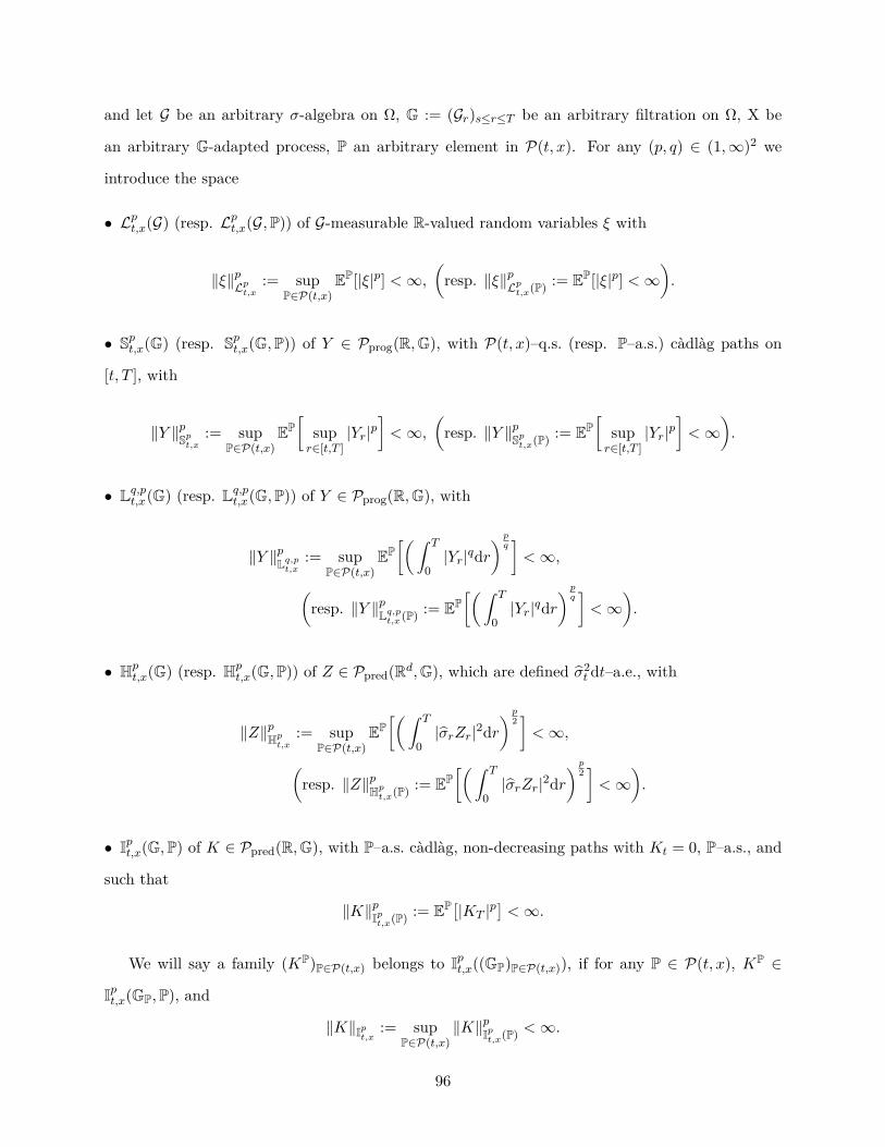
and let G be an arbitrary σ-algebra on Ω, G := (Gr)s≤r≤T be an arbitrary filtration on Ω, X be

an arbitrary G-adapted process, P an arbitrary element in P(t, x). For any (p, q) ∈ (1,∞)2 we

introduce the space

• Lpt,x(G) (resp. Lpt,x(G,P)) of G-measurable R-valued random variables ξ with

‖ξ‖pLpt,x := supP∈P(t,x)

EP[|ξ|p] <∞,(resp. ‖ξ‖pLpt,x(P) := EP[|ξ|p] <∞

).

• Spt,x(G) (resp. Spt,x(G,P)) of Y ∈ Pprog(R,G), with P(t, x)–q.s. (resp. P–a.s.) càdlàg paths on

[t, T ], with

‖Y ‖pSpt,x := supP∈P(t,x)

EP[

supr∈[t,T ]

|Yr|p]<∞,

(resp. ‖Y ‖pSpt,x(P) := EP

[supr∈[t,T ]

|Yr|p]<∞

).

• Lq,pt,x(G) (resp. Lq,pt,x(G,P)) of Y ∈ Pprog(R,G), with

‖Y ‖pLq,pt,x := supP∈P(t,x)

EP[( ∫ T

0|Yr|qdr

) pq]<∞,

(resp. ‖Y ‖pLq,pt,x(P) := EP

[( ∫ T

0|Yr|qdr

) pq]<∞

).

• Hpt,x(G) (resp. Hp

t,x(G,P)) of Z ∈ Ppred(Rd,G), which are defined σ2t dt–a.e., with

‖Z‖pHpt,x := supP∈P(t,x)

EP[( ∫ T

0|σrZr|2dr

) p2]<∞,

(resp. ‖Z‖pHpt,x(P) := EP

[( ∫ T

0|σrZr|2dr

) p2]<∞

).

• Ipt,x(G,P) of K ∈ Ppred(R,G), with P–a.s. càdlàg, non-decreasing paths with Kt = 0, P–a.s., and

such that

‖K‖pIpt,x(P) := EP[|KT |p]<∞.

We will say a family (KP)P∈P(t,x) belongs to Ipt,x((GP)P∈P(t,x)), if for any P ∈ P(t, x), KP ∈

Ipt,x(GP,P), and

‖K‖Ipt,x := supP∈P(t,x)

‖K‖pIpt,x(P) <∞.

96

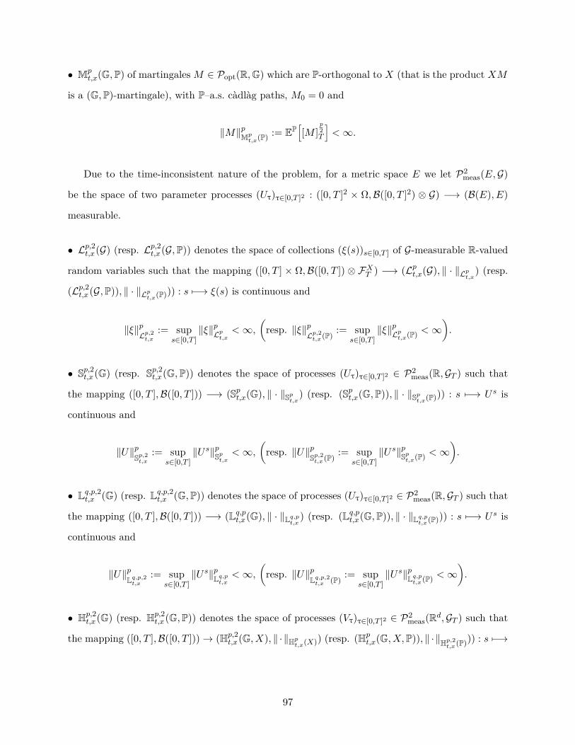
• Mpt,x(G,P) of martingalesM ∈ Popt(R,G) which are P-orthogonal to X (that is the product XM

is a (G,P)-martingale), with P–a.s. càdlàg paths, M0 = 0 and

‖M‖pMpt,x(P) := EP

[[M ]

p2T

]<∞.

Due to the time-inconsistent nature of the problem, for a metric space E we let P2meas(E,G)

be the space of two parameter processes (Uτ)τ∈[0,T ]2 : ([0, T ]2 × Ω,B([0, T ]2) ⊗ G) −→ (B(E), E)

measurable.

• Lp,2t,x(G) (resp. Lp,2t,x(G,P)) denotes the space of collections (ξ(s))s∈[0,T ] of G-measurable R-valued

random variables such that the mapping ([0, T ] × Ω,B([0, T ]) ⊗ FXT ) −→ (Lpt,x(G), ‖ · ‖Lpt,x) (resp.

(Lp,2t,x(G,P)), ‖ · ‖Lpt,x(P))) : s 7−→ ξ(s) is continuous and

‖ξ‖pLp,2t,x

:= sups∈[0,T ]

‖ξ‖pLpt,x <∞,(resp. ‖ξ‖p

Lp,2t,x(P):= sup

s∈[0,T ]‖ξ‖pLpt,x(P) <∞

).

• Sp,2t,x(G) (resp. Sp,2t,x(G,P)) denotes the space of processes (Uτ)τ∈[0,T ]2 ∈ P2meas(R,GT ) such that

the mapping ([0, T ],B([0, T ])) −→ (Spt,x(G), ‖ · ‖Spt,x) (resp. (Spt,x(G,P)), ‖ · ‖Spt,x(P))) : s 7−→ U s is

continuous and

‖U‖pSp,2t,x

:= sups∈[0,T ]

‖U s‖pSpt,x <∞,(resp. ‖U‖p

Sp,2t,x(P):= sup

s∈[0,T ]‖U s‖pSpt,x(P) <∞

).

• Lq,p,2t,x (G) (resp. Lq,p,2t,x (G,P)) denotes the space of processes (Uτ)τ∈[0,T ]2 ∈ P2meas(R,GT ) such that

the mapping ([0, T ],B([0, T ])) −→ (Lq,pt,x(G), ‖ · ‖Lq,pt,x ) (resp. (Lq,pt,x(G,P)), ‖ · ‖Lq,pt,x(P))) : s 7−→ U s is

continuous and

‖U‖pLq,p,2t,x

:= sups∈[0,T ]

‖U s‖pLq,pt,x <∞,(resp. ‖U‖p

Lq,p,2t,x (P):= sup

s∈[0,T ]‖U s‖pLq,pt,x(P) <∞

).

• Hp,2t,x(G) (resp. Hp,2

t,x(G,P)) denotes the space of processes (Vτ)τ∈[0,T ]2 ∈ P2meas(Rd,GT ) such that

the mapping ([0, T ],B([0, T ]))→ (Hp,2t,x(G, X), ‖ ·‖Hpt,x(X)) (resp. (Hp

t,x(G, X,P)), ‖ ·‖Hp,2t,x(P))) : s 7−→

97

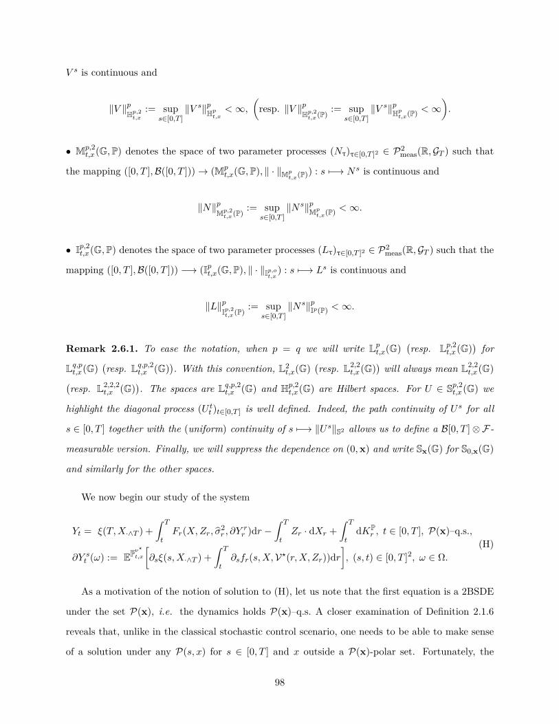
V s is continuous and

‖V ‖pHp,2t,x

:= sups∈[0,T ]

‖V s‖pHpt,x <∞,(resp. ‖V ‖p

Hp,2t,x(P):= sup

s∈[0,T ]‖V s‖pHpt,x(P) <∞

).

• Mp,2t,x(G,P) denotes the space of two parameter processes (Nτ)τ∈[0,T ]2 ∈ P2

meas(R,GT ) such that

the mapping ([0, T ],B([0, T ]))→ (Mpt,x(G,P), ‖ · ‖Mp

t,x(P)) : s 7−→ N s is continuous and

‖N‖pMp,2t,x(P)

:= sups∈[0,T ]

‖N s‖pMpt,x(P) <∞.

• Ip,2t,x(G,P) denotes the space of two parameter processes (Lτ)τ∈[0,T ]2 ∈ P2meas(R,GT ) such that the

mapping ([0, T ],B([0, T ])) −→ (Ipt,x(G,P), ‖ · ‖Ip,ot,x ) : s 7−→ Ls is continuous and

‖L‖pIp,2t,x(P)

:= sups∈[0,T ]

‖N s‖pIp(P) <∞.

Remark 2.6.1. To ease the notation, when p = q we will write Lpt,x(G)(resp. Lp,2t,x(G)

)for

Lq,pt,x(G)(resp. Lq,p,2t,x (G)

). With this convention, L2

t,x(G)(resp. L2,2

t,x(G))will always mean L2,2

t,x(G)(resp. L2,2,2

t,x (G)). The spaces are Lq,p,2t,x (G) and Hp,2

t,x(G) are Hilbert spaces. For U ∈ Sp,2t,x(G) we

highlight the diagonal process (U tt )t∈[0,T ] is well defined. Indeed, the path continuity of U s for all

s ∈ [0, T ] together with the (uniform) continuity of s 7−→ ‖U s‖S2 allows us to define a B[0, T ]⊗F-

measurable version. Finally, we will suppress the dependence on (0,x) and write Sx(G) for S0,x(G)

and similarly for the other spaces.

We now begin our study of the system

Yt = ξ(T,X·∧T ) +∫ T

tFr(X,Zr, σ2

r , ∂Yrr )dr −

∫ T

tZr · dXr +

∫ T

tdKP

r , t ∈ [0, T ], P(x)–q.s.,


?

t,x

[∂sξ(s,X·∧T ) +

∫ T

t∂sfr(s,X,V?(r,X,Zr))dr

], (s, t) ∈ [0, T ]2, ω ∈ Ω.

(H)

As a motivation of the notion of solution to (H), let us note that the first equation is a 2BSDE

under the set P(x), i.e. the dynamics holds P(x)–q.s. A closer examination of Definition 2.1.6

reveals that, unlike in the classical stochastic control scenario, one needs to be able to make sense

of a solution under any P(s, x) for s ∈ [0, T ] and x outside a P(x)-polar set. Fortunately, the

98

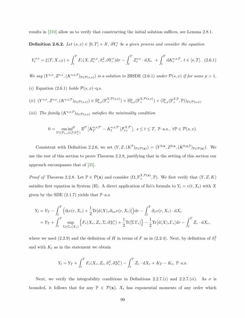
results in [210] allow us to verify that constructing the initial solution suffices, see Lemma 2.8.1.

Definition 2.6.2. Let (s, x) ∈ [0, T ]×X , ∂Y rr be a given process and consider the equation

Y s,xt = ξ(T,X·∧T ) +

∫ T

tFr(X,Zs,xr , σ2

r , ∂Yrr )dr −

∫ T

tZs,xr · dXr +

∫ T

tdKs,x,P

r , t ∈ [s, T ]. (2.6.1)

We say (Y s,x, Zs,x, (Ks,x,P)P∈P(s,x)) is a solution to 2BSDE (2.6.1) under P(s, x) if for some p > 1,

(i) Equation (2.6.1) holds P(s, x)–q.s.

(ii) (Y s,x, Zs,x, (Ks,x,P)P∈P(s,x)) ∈ Sps,x(FX,P(s,x)+ )×Hp

s,x(FX,P(s,x)+ )× (Ips,x(FX,P+ ,P))P∈P(s,x).

(iii) The family (Ks,x,P)P∈P(s,x) satisfies the minimality condition

0 = ess infPP′∈Ps,x(t,P,FX+ )

EP′[Ks,x,P′T −Ks,x,P′

t

∣∣FX,P′t+], s ≤ t ≤ T, P–a.s., ∀P ∈ P(s, x).

Consistent with Definition 2.2.6, we set (Y, Z, (KP)P∈P(x)) = (Y 0,x, Z0,x, (K0,x,P)P∈P(x)). We

use the rest of this section to prove Theorem 2.2.8, justifying that in the setting of this section our

approach encompasses that of [35].

Proof of Theorem 2.2.8. Let P ∈ P(x) and consider (Ω,FX,P(x)+ ,P). We first verify that (Y,Z,K)

satisfies first equation in System (H). A direct application of Itô’s formula to Yt = v(t,Xt) with X

given by the SDE (2.1.7) yields that P–a.s.

Yt = YT −∫ T

t

(∂tv(r,Xr) + 1

2Tr[d〈X〉r∂xxv(r,Xr)])dr −

∫ T

t∂xv(r,Xr) · dXr

= YT +∫ T

tsup

Σ∈Σr(Xr)

Fr(Xr, Zr,Σ, ∂Yrr ) + 1

2Tr[Σ Γr]− 1

2Tr[d〈X〉rΓr

]dr −

∫ T

tZr · dXr,

where we used (2.2.9) and the definition of H in terms of F as in (2.2.4). Next, by definition of σ2t

and with Kt as in the statement we obtain

Yt = YT +∫ T

tFr(Xr, Zr, σ

2r , ∂Yrr )−

∫ T

tZr · dXr +KT −Kt, P–a.s.

Next, we verify the integrability conditions in Definitions 2.2.7.(i) and 2.2.7.(ii). As σ is

bounded, it follows that for any P ∈ P(x), Xt has exponential moments of any order which

99

are bounded on [0, T ], i.e. ∃C, supt∈[0,T ] EP[exp(c|Xt|1)] ≤ C < ∞, ∀P ∈ P(x), ∀c > 0, where

C depends on T and the bound on σ.

The exponential grown assumption on v and de la Vallée-Poussin’s theorem yield that for p > 1

Y ∈ Spx(FX,P(x)+ ,P(x)). Similarly, we obtain (Z, ∂Y ) ∈ Hp

x(FX,P(x)+ ,P(x))×Sp,2x (FX,P(x)

+ ,P(x)). To

derive the integrability of K, let P ∈ P(x) and note that

EP[KpT ] ≤Cp

(‖Y ‖pSpx + sup

P∈P(x)EP[( ∫ T

0|Fr(Xr, Zr, σ

2r , 0)|dr

)p]+ ‖∂Y ‖p

Sp,2x+ ‖Z‖pHpx

)<∞,

where the inequality follows from the fact (t, x, z, a) 7−→ F (t, x, z, a, 0) is Lipschitz in z which follows

from the exponential growth assumption on f0 and the boundedness of the coefficients b and σ.

The constant Cp depends on the Lipschitz constant and the value of p as in Bouchard, Possamaï,

Tan, and Zhou [40, Lemma 2.1]. As the term on the right does not depend on P, we conclude

K ∈ Ipx((FX,P+ )P∈P(x)). Note that the previous estimate shows as a by-product that the 2BSDE in

(H) is well-posed, see [210, Theorem 4.1]. Therefore, provided K satisfies the minimality condition

by [210, Theorem 4.2], we conclude 2.2.7.(i), i.e. (Y, Z,K) is the solution to the 2BSDE in (H).

We now argue that K satisfies (2.2.8). Following [230, Theorem 5.2], we can exploit the fact

the σ is bounded and the continuity in time of X, Z and Γ for fixed x ∈ X , to show that for ε > 0,

(t, ν) ∈ [0, T ] × A(x,P) and τ ε,t := T ∧ infr > t : Kr ≥ Kt + ε, there exists Pνε ∈ Px(t,P,FX+ )

such that kt ≤ ε, dt⊗ dPνε on [τ ε,t, T ]×Ω. From this the minimality condition follows. Moreover,

by assumption, we know there exists Pν? ∈ P0(0,x, ν?) where ν? maximises the Hamiltonian, i.e.

σ2r = (σσ>)t(Xt, ν

?t ),dt ⊗ dP?–a.e. on [0, T ] × Ω, and kt = 0, Pν?–a.s. for all t ∈ [0, T ]. Thus the

minimality condition is attained under Pν? , i.e. 2.2.7.(iii) holds. Moreover, note that this implies

V?(t,Xt, Zt,Γt) = V?(t,Xt, Zt), Pν?–a.s. (2.6.2)

We are left to argue ∂Y satisfies the second equation in (H). Given the regularity of s 7−→

J(s, t, x), we can differentiate the second equation in (2.2.9). Using this, for s ∈ [0, T ] fixed and

ω = (x,w, q) ∈ Ω we can apply Itô’s formula to ∂Y st = ∂sJ(s, t,Xt) under Pν

?

t,x. This yields,

∂Y st (ω) = EPν

?

t,x

[∂sξ(s,XT ) +

∫ T

t∂sfr(s,Xr,V?(r,X,Zr))dr

],

100

where the stochastic integral term vanished in light of the growth assumption on ∂xJ(s, t, x) and

we used (2.6.2).


We recall that throughout this section, we let Assumptions A and B hold. To begin with, from

the definition of the set A(t, x), we can re-state the result of our dynamic programming principle

Theorem 2.2.2, by decomposing a control ν ∈ A(t, x) into a pair (P, ν) ∈ P(t, x)×A(t, x,P), where P

is the unique weak solution to (2.1.7) and ν. We remark that for any given P ∈ P(t, x), there could

be in general several admissible controls ν. With this we state Theorem 2.2.2 as, for ν? ∈ E(x),

σ, τ ∈ Tt,T , σ ≤ τ and P(x)–q.e. x ∈ X

v(σ, x) = supP∈P(σ,x)

supν∈A(σ,x,P)

EPν[v(τ,X) +

∫ τ

σfr(r,X, νr)dr

−∫ τ

σEP?,ν

?

r,·

[∂sξ(r,X·∧T ) +

∫ T


]dr].

(2.7.1)

The goal of this section is to show that given ν?, P?, unique solution to the martingale problem

asociated with ν?, and v(t, x), one can construct a solution to (H). To do so, we recall that given

a family of BSDEs (YP)P∈P(t,ω) indexed by P(t, ω) ⊆ Prob(Ω) with (t, ω) ∈ [0, T ] × Ω, a 2BSDE

is the supremum over P(t, ω) of the P-expectation of the afore mentioned family, see [230], [210].

This together with equation (2.7.1) reveals the road map we should take.

Let us begin by fixing an equilibrium ν? ∈ E(x). For (s, t, ω,P) ∈ [0, T ] × [0, T ] × Ω × P(t, x)

we consider the FX -adapted processes

YPt (ω) := sup

ν∈A(t,x,P)EPν

[ξ(T,X) +

∫ T

t

(fr(r,X, νr)− ∂Y r

r

)dr],


?

t,x

[∂sξ(s,X·∧T ) +

∫ T

t∂sfr(s,X, ν?r )dr

].

(2.7.2)

and on (Ω,FX,P+ ,P) the BSDE

YPt = ξ(T,X·∧T ) +

∫ T

tFr(X,ZP

r , σ2r , ∂Y

rr )dr −

(∫ T

tZPr · dXr

)P, 0 ≤ s ≤ t ≤ T. (2.7.3)

101

Note we specify the stochastic integral w.r.t X is under the probability P. Our first step is to relate

YP with the solution to the BSDE (2.7.3). Namely, Lemma 2.7.1 says that YP corresponds to the

first component of the solution to (2.7.3).

Lemma 2.7.1. Let Assumption B hold, (t, ω,P) ∈ [0, T ]×Ω×P(t, x) and (YP,ZP) be the solution

to the BSDE (2.7.3), as in Papapantoleon, Possamaï, and Saplaouras [200, Definition 3.2], and

ν?t := V?(t,X,ZPt ). Then

YPt (ω) = EPν? [YP

t ]. (2.7.4)

Proof. Let us consider on(Ω,FX,P+ ,P

), for t ≤ u ≤ T and ν ∈ A(t, x,P) the BSDE

YP,νu = ξ(T,X·∧T ) +

∫ T

u

(hr(r,X,ZP,ν

r , νr)− ∂Y rr

)dr −

(∫ T

uZP,νr · dXr

)P, P–a.s. (2.7.5)

Under Assumptions B.(ii) and B.(i), we know that z 7−→ ht(t, x, z, a) is Lipschitz-continuous, uni-

formly in (t, x, a), that there exists p > 1 such that ([0, T ] × Ω,FX) 3 (t, ω) 7−→ ht(t, x, 0, 0) ∈

Hp,2s,ω(FX,P+ ,P) is well defined, and that ∂Y ∈ Hp

s,x(FX,P+ ,P). Moreover, as for any ν, and ν in

A(s, x,P), (σσ>)t(X, νt) = σ2t = (σσ>)t(X, νt),dt⊗ dP–a.e., P is the unique solution to an uncon-

trolled martingale problem where (σσ>)t(X) := (σσ>)t(X, νt). Consequently, the martingale rep-

resentation property holds for any local martingale in (Ω,FP,P) relative to X, see Jacod and Shiry-

aev [142, Theorem 4.29]. Therefore, conditions (H1)–(H6) in [200, Theorem 3.23] hold and the above

BSDE is well defined. Its solution consists of a tuple (YP,ν ,ZP,ν) ∈ Dps,x(FX,P+ ,P) × Hps,x(FX,P+ ,P)

and for every ν ∈ A(t, x,P) and Pν is as in Remark 2.1.4 we have

EPν [YP,νt ] = EPν

[ξ(T,X) +

∫ T

t


r

)dr], t ∈ [0, T ].

In addition, the solution (YP,ZP) ∈ Dps,ω(FX,P+ ,P)×Hps,ω(FX,P+ ,P) to BSDE (2.7.3) is well defined,

by Assumption B.(iii) guarantees. Furthermore, conditions (Comp1)–(Comp3) in [200, Theorem

3.25] are fulfilled, ensuring a comparison theorem holds. Indeed, as X is continuous (Comp1) is

immediate, while (Comp2) and (Comp3) correspond in our setting to B.(ii) and B.(i), respectively.

By definition, ν?t satisfies (σσ>)t(X, ν?t ) = σ2t ,dt ⊗ dP–a.e. on [t, T ] × X , and so, ν? ∈ A(t, x,P).

102

By comparison, we obtain

YPt (x) = sup

ν∈A(t,x,P)EPν [YP,ν

t ] ≤ EPν?

[YPt ].

Remark 2.7.2. (i) In the literature on BSDEs one might find the additional term∫ Tt dN P

r in

(2.7.3), where N P is a P-martingale P-orthogonal to X. Yet, as noticed in the proof once (σσ>)t(X)

is fixed, uniqueness of the associated martingale problem guarantees the representation property

relative to X.

(ii) We remark that an alternative constructive approach to relate Y to a BSDE is to consider for

any ν ∈ A(s, x,P) and t ≥ s the process

NP,νt := J(t, t,X, ν?(P)) +

∫ t

0


r

)dr.

However, as the careful reader might have noticed, this requires that for a given P ∈ P(s, x) we

introduce ν?(P) the action process attaining the sup in (2.7.2). However, the existence of an ac-

tion with such property is not necessarily guaranteed for all P ∈ P(s, x), at least without further

assumptions, which we do not want to impose here.

Remark 2.7.3. At this point we are halfway from our goal in this section. For (t, ω) ∈ [0, T ]×Ω, the

previous lemma defines a family (YP)P∈P(t,ω) of FX,P+ -adapted processes. Recalling our discussion

at the beginning of this section, all we are left to do is to take sup over (P(t, x))(t,x)∈[0,T ]×X . In

other words, putting together (2.7.4) and (2.7.1), we now know


EPν? [YPt

]. (2.7.6)

In light of the previous remark and the characterisation in [210], we consider the following

2BSDE

Yt = ξ(T,X·∧T ) +∫ T

tFr(X,Zr, σ2

r , ∂Yrr )dr −

∫ T

tZr · dXr +KP

T −KPt , t ∈ [0, T ], P(x)–q.s. (2.7.7)

103

With this we are ready to prove the necessity of System (H).

Proof of Theorem 2.2.10. We begin by verifying the integrability of ∂Y , defined as in (2.7.2). From

Assumption B.(ii) we have that for any s ∈ [0, T ]

‖∂Y s‖Spx ≤ supP∈P(x)

EP[∣∣∂sξ(s,X·∧T )

∣∣p +∫ T

0

∣∣∂sfr(s,X, ν?r )∣∣pdr] <∞.

Therefore, as Assumption A.(i) guarantees the continuity of the map s 7−→ ‖∂Y s‖Sp0,x(FX ,P(x)) the

result follows.

Let us construct such a solution from ν? ∈ E(x). Under Assumption B.(ii), it follows from

(2.7.6) and [210, Lemma 3.2] that v is làdlàg outside a P(x)-polar set. Therefore the process v+

given by

v+t (x) := lim

r∈Q∩(t,T ],r↓tv(t, x),

is well defined in the P(x)–q.s. sense. Clearly v+ is càdlàg, FX,P(x)+ -adapted, and in light of [210,

Lemmata 2.2 and 3.6], which hold under Assumption B, we have that for any P ∈ P(x), there exist

(ZP,KP) ∈ Hp0,x(FX,P+ ,P)× Ip0,x(FX,P+ ,P) such that

v+t = ξ(T,X·∧T ) +

∫ T

tFr(X,ZP

r , σ2r , ∂Y

rr )dr −

(∫ T

tZPr · dXr

)P+KP

T −KPt , 0 ≤ t ≤ T, P–a.s.

Moreover, the process Zt := (σ2t )⊕

d[v+,X]tdt , where (σ2

t )⊕ denotes the Moore–Penrose pseudo-inverse

of σ2t , aggregates the family (ZP)P∈P(x). The proof that (KP)P∈P(x) satisfies the minimality condi-

tion (2.2.8) is argued as in [210, Section 4.4]. The result follows by well-posedness of (2.7.7).

Arguing as in [210, Lemma 3.5], we may obtain that for any P(x)–q.e. x ∈ X and P ∈ P(t, x)

v+t = ess supP

P∈P(t,P,FX+ )Y Pt ,

with Y P as in (2.7.3). Consequently


EP[v+t ].

104

Moreover, as for any t ∈ [0, T ] and P(x)–q.e. x ∈ X , Pν?

t,x attains equality in (2.7.6), see The-

orem 2.2.2, we deduce, in light of (2.1.4), Pν? attains the minimality condition. This is, under Pν? ,

the process KPν? equals 0. With this, we obtain (v+, Z, (K)PP∈P(x)) and ∂Y are a solution to (H).

Moreover, Lemma 2.7.1 implies

ν?t ∈ arg maxa∈At(x,σ2

t (x))ht(t,X,Zt, a), dt⊗ dPν?–a.e.., on [0, T ]×X .


This section is devoted to proof the verification Theorem 2.2.12. To do so we will need to obtain

a rigorous statement of how the processes defined by (H) relate. This is carried in the following

series of lemmata.

Lemma 2.8.1. For (x, x, s) ∈ X × X × (0, T ] consider the 2BSDEs

Yt = ξ(T,X) +∫ T

tFr(X,Zr, σ2

r , ∂Yrr )dr −

∫ T

tZr · dXr +

∫ T

tdKP

r , t ∈ [0, T ], P(x)–q.s.,

Y s,xt = ξ(T,X) +

∫ T

tFr(X,Zs,xr , σ2

r , ∂Yrr )dr −

∫ T

tZs,xr · dXr +

∫ T

tdKs,x,Q

r , t ∈ [s, T ], P(s, x)–q.s.

Suppose both 2BSDEs are well-posed. Then, for any s ∈ (0, T ],

Yt = Y s,xt , s ≤ t ≤ T, P(s, x)–q.s., for P(x)–q.e.x ∈ X ,

Zt = Zs,xt , σ2t dt⊗ dP(s, x)–q.e. on [s, T ]×X , for P(x)–q.e.x ∈ X ,

KPt = K

s,x,Ps,xt , s ≤ t ≤ T, Ps,x–a.s., for P–a.e. x ∈ X , ∀P ∈ P(x).

Proof. Following [210], we consider for (t, x) ∈ [0, T ]×X

Yt(x) := supP∈P(t,x)

EP[YPt

],

where for an arbitrary P ∈ P(s, x), YP corresponds to the first coordinate of the solution to the

105

BSDE

YPt = ξ(T,X·∧T ) +

∫ T

tFr(X,ZP

r , σ2r , ∂Y

rr )dr −

∫ T

tZPr · dXr, s ≤ t ≤ T, P–a.s.

It then follows by [210, Lemmata 3.2 and 3.6] that Y+, the right limit of Y, is FX,P(x)+ -measurable,

P(x)–q.s. càdlàg, and for every P ∈ P(x), there is (ZP, KP) ∈ Hpx(FX,P+ ,P)× Ipx(FX,P+ ,P) such that

for every P ∈ P(x)

Y+t = ξ(T,X·∧T ) +

∫ T

tFr(X, ZP

r , σ2r , ∂Y

rr )dr −

∫ T

tZPr · dXr +

∫ T

tdKP

r , 0 ≤ t ≤ T, P–a.s.

By [149], there exists a universal process [Y+, X] which coincides with the quadratic co-variation

of Y+ and X under each probability measure P ∈ P(x). Thus, one can define a universal FX,P(x)+ -

predictable process Z by

Zt := (σ2t )⊕

d[Y+, X]tdt , (2.8.1)

and obtain,

Y+t = ξ(T,X·∧T ) +

∫ T

tFr(X, Zr, σ2

r , ∂Yrr )dr −

∫ T

tZr · dXr + KP

T − KPt , 0 ≤ t ≤ T, P(x)–q.s.

By well-posedness, we have that

Y+t = Yt, 0 ≤ t ≤ T, P(x)–q.s.; Zt = Zt, σ

2dt⊗ dP(x)–q.e. on [0, T ]×X ;

KPt = KP

t , 0 ≤ t ≤ T, P–a.s., ∀P ∈ P(x),(2.8.2)

where the latter denotes the solution to the first 2BSDE in the statement of the lemma. Thus,

as Y+ is computed ω-by-ω, we can repeat the previous argument on the time interval [s, T ] and

Ωωs = ω ∈ Ω : xr = xr, 0 ≤ r ≤ s, i.e. fixing an initial trajectory. Reasoning as before, we

then find that on Ωωs , Y+ is FP(s,x)

+ -measurable and P(s, x)–q.s. càdlàg. By well-posedness of the

second 2BSDE in the statement of the lemma, this yields the analogous version of (2.8.2) between

106

(Y+, Z, (KP)P∈P(s,x)) and (Y s,x, Zs,x, (Ks,x)P∈P(s,x)). It is then clear that

Yt = Y s,xt , s ≤ t ≤ T,P(s, x)–q.s., for P(x)–q.e. x ∈ X , s ∈ (0, T ].

The corresponding result for Z follows from (2.8.1). The relation for the family (KP)P∈P(x) holds

P-by-P for every P ∈ P(x) in light of the weak uniqueness assumption for the drift-less dynamics

(2.1.7) and [56, Lemma 4.1], which guarantees that for any P ∈ P(x) and P–a.e. x ∈ X

(∫ T

tZr ·Xr

)P=(∫ T

tZr ·Xr

)Ps,x, 0 ≤ s ≤ t, Ps,x–a.s.

Lemma 2.8.2. Let (Pν , ν) ∈ M(x). For (s, x) ∈ [0, T ] × X consider the system, assumed to hold

Pνs,x–a.s.

∂Yrt = ∂sξ(r,X·∧T ) +∫ T

t∂hu(r,X, ∂Zru, νu)du−

∫ T

t∂Zru · dXu, s ≤ t ≤ T,

Yrt = ξ(r,X·∧T ) +∫ T

thu(r,X,Zru, νu)du−

∫ T

tZru · dXu, s ≤ t ≤ T.

(D)

Let (∂Y, ∂Z) ∈ Sp,2s,x(FX,Pνs,x

+ ,Pνs,x) × Hp,2s,x(FX,P

νs,x

+ ,Pνs,x, X) be the solution to the first BSDE in

(D). Then, the mapping [0, T ] 3 s 7−→ (∂Ys, ∂Zs) ∈ Sps,x(FX,Pνs,x

+ ,Pνs,x) × Hps,x(FX,P

νs,x

+ ,Pνs,x, X)

is Lebesgue-integrable with antiderivative (Y,Z), that is to say

(∫ T

s∂Yrdr,

∫ T

s∂Zrdr

)= (YT − Ys,ZT −Zs), Pνs,x–a.s.

Furthermore, letting

∂Y rt (ω) := EPνt,x

[∂sξ(r,X·∧T ) +

∫ T

t∂sfu(r,X, νu)du

], (s, t) ∈ [0, T ]2, ω ∈ Ω,

it holds that ∂Y ss = EPνs,x

[∂Yss

]and J(s, s, x, ν) = EPνs,x

[Yss]. If in addition ∂Y ∈ Sp,2x (FX,P

νs,x

+ ), for

any t ∈ [s, T ]

EPνs,x[ ∫ T

t∂Y r

r dr]

= EPνs,x[ ∫ T

t∂Yrrdr

].

107

Proof. We first prove the second part of the statement. Note that

Yst = ξ(s,X·∧T ) +∫ T

t

(fr(s,X, νr) + br(X, νr) · σ>r Zsr

)dr −

∫ T

tZsr · dXr, Pνs,x–a.s.,

= ξ(s,X·∧T ) +∫ T

tfr(s,X, νr)dr −

∫ T

tZsr · dXr, P

νs,x–a.s.

This implies

Yrt (x) = EPνs,x[ξ(r,X·∧T ) +

∫ T

tfu(r,X, νu)du

∣∣∣FX,Pνs,xt+

].

Therefore, by taking expectation

EPνs,x[Yss (ω)

]= EPνs,x

[ξ(s,X·∧T ) +

∫ T

sfr(s,X, νr)dr

]= J(s, s, x, ν).

The equality ∂Y ss = ∂Yss , is argued identically. Now, to obtain the last equality we use the fact

that ∂Y ∈ Sp,2s,x(FX,Pνs,x

+ ,Pνs,x). Indeed, the continuity of the mapping s 7−→ (∂Ys, ∂Zs) guarantees

the integral is well-defined. The equality follows from the tower property.

We now argue the first part of the statement. Again, we know the mapping [0, T ] 3 s 7−→

(∂Ys, ∂Zs) is continuous, in particular integrable. A formal integration with respect to s to the

first equation in (D) leads to

∫ T

s∂Yst ds =

∫ T

t

∫ T

s

∂fr∂s

(s,X, νr)ds+ br(X, νr) · σ>r∫ T

s∂Zsrdsdr

+∫ T

s∂sξ(s,X·∧T )ds−

∫ T

t

∫ T

s∂Zsrds · dXr.

Therefore, a natural candidate for solution to the second BSDE in (D) is (Ys,Zs,N s), solution of

the BSDE

Yst = ξ(s,X·∧T ) +∫ T

t

(fr(s,X, νr) + br(X, νr) · σ>r Zsr

)dr −

∫ T

tZsr · dXr.

Let (Π`)` be a properly chosen sequence of partitions of [s, T ], as in [240, Theorem 1], Π` =

(si)i=1,...,n` with ‖Π`‖ ≤ `. Recall ∆sì = sì − sì−1. For a generic family process X ∈ Hp,2s,x(G), and

108

mappings s 7−→ ∂sξ(s, x), s 7−→ ∂sf(s, x, a) for (s, x, a) ∈ [0, T ]×X ×A we define

I`(X) :=n∑i=0

∆sìXsì , δX := XT −Xs, I`(∂sξ(·, x)) :=n∑i=0

∆sì∂sξ(sì , x),

I`(∂sf)t(·, x, a) :=n∑i=0

∆sì∂sft(sì , x, a),

and notice that for any t ∈ [0, T ]

I`(∂Y )t − (δY )t

= I`(∂sξ(·, X·∧T ))− (ξ(T,X·∧T )− ξ(s,X·∧T ))−∫ T

t

(I`(∂Z)r − (δZ)r

)· dXr

+∫ T

t

[I`(∂sf)r(·, X, νr))− (fr(T,X, νr)− fr(s,X, νr)] + σrbr(X, ν)[I`(∂Z)r − (δZ)r]dr.

Thanks to the integrability of (∂Y, ∂Z) and (Y,Z), it follows that I`(∂Y )−(δY ) ∈ Hp,2s,x and similarly

for ∂Z and Z. Therefore, [40, Theorem 2.2] yields

‖I`(∂Y )− (δY )‖pHp,2s,x

+ ‖I`(∂Z)− (δZ)‖pHp,2s,x

≤ EPνs,x[∣∣∣I`(∂sξ(·, X·∧T )

)−(ξ(T,X·∧T )− ξ(s,X·∧T )

)∣∣∣p+∫ T

t

∣∣∣I`(∂sf)r(·, X, νr))−(fr(T,X, νr)− fr(s,X, νr)

)∣∣∣pdr].The uniform continuity of s 7−→ ∂sξ(s, x) and s 7−→ ∂sf(s, x, a), see Assumption C, justifies, via

bounded convergence, the convergence in Sps,x(FX,Pνs,x

+ ,Pνs,x) (resp Hps,x) of I`(∂Y s) to Y T −Y s (resp

I`(∂Zs) to ZT − Zs) as ` −→ 0.

Lemma 2.8.3. Let (Pν , ν) ∈M(x), (s, x) ∈ [0, T ]×X and (∂Y, ∂Z) and (Y,Z) as in (D). Then

Ytt = YTT +∫ T

thr(r,X,Zrr , νr)− ∂Yttdr −

∫ T

tZrr · dXr, s ≤ t ≤ T, Ps,x–a.s. (2.8.3)

Proof. By evaluating ∂Y at r = t in (D) we get

∂Ytt = ∂sξ(t,X·∧T ) +∫ T

t∂hr(t,X, ∂Ztr, νr)−

∫ T

t∂Ztr · dXr, Psx–a.s.

109

We will show that for s ≤ t ≤ T , Ps,x–a.s.

ξ(T,X·∧T )− ξ(t,X·∧T ) +∫ T

thr(r,X,Zrr , νr)dr −

∫ T

tZrrdXr

=∫ T

thr(t,X,Ztr, νr)dr −

∫ T

tZtr · dXr +

∫ T

t∂Yrrdr.

Indeed

∫ T

t∂Yrdr =

∫ T

t∂sξ(r,X·∧T )dr +

∫ T

t

∫ T

r∂hu(r,X, ∂Zru, νu)dudr −

∫ T

t

∫ T

r∂Zru · dXu dr.

Now, Assumption C.(ii) and ∂Z ∈ Hp,2s,x(FX,P

νs,x

+ ,Pνs,x, X) yield

∫ T

t

∫ T

r∂hu(r,X, ∂Zru, νu)du dr =

∫ T

t

∫ u

t

(∂sfu(r,X, νu) + σubu(X, νu) · ∂Zru

)dr du

=∫ T

t

(hu(u,X,Zuu , νu)− hu(t,X,Ztu, νu)

)du.

Moreover, ‖∂Z‖Hp,2s,x(X) < ∞ guarantees∫ T0 EPνs,x

[ ∫ T0∣∣σtZrt ∣∣2dt

] p2 dr < ∞ so a stochastic Fubini’s

theorem, see Da Prato and Zabczyk [66, Section I.4.5], justifies

∫ T

t

∫ T

r∂Zsu · dXudr =

∫ T

t[Zuu − Ztu] · dXu, Pνs,x–a.s.

Proof of Theorem 2.2.12. We will first show that with ν? as in the statement of the theorem Yt(x) =

J(t, t, x, ν?) for all t ∈ [0, T ] and P(x)–q.e. x ∈ X . To do so, let (s, x) ∈ [0, T ] × X and note that

Assumption C.(i) guarantees that the corresponding 2BSDE under P(s, x) is well-posed. Indeed,

it follows from Soner, Touzi, and Zhang [229, Lemma 6.2] that for any p > p′ > κ > 1,

supP∈P(s,x)

EP[

ess supP

s≤t≤T

(ess supP

P ′∈Ps,x(t,P,F+)EP′[|ξ(T,X·∧T )|κ +

∫ T

s|Fr(X, 0, σ2

r , ∂Yrr )|κdr

∣∣∣∣F+t

]) p′κ]<∞.

110

The well-posedness follows by [210, Theorem 4.1]. Now, in light of lemma 2.8.1, for any s ∈ [0, T ]

Yt = Y s,xt , s ≤ t ≤ T, P(s, x)–q.s., for P(x)–q.e. x ∈ X ,

Zt = Zs,xt , σ2t dt⊗ dP(s, x)–q.e. on [s, T ]×X , for P(x)–q.e. x ∈ X ,

KPt = K

s,x,Ps,xt , s ≤ t ≤ T, Ps,x–a.s., for P–a.e. x ∈ X , ∀P ∈ P(x).

(2.8.4)

We first claim that given a solution to (H) for any (s, x) ∈ (0, T ]×X , Pν?s,x attains the minimality

condition for the 2BSDE under P(s, x), see Definition 2.6.2. Indeed, by Definition 2.2.7.(iii)

EPν?0,x[K

Pν?0,xT −K

Pν?0,xt

]= 0, 0 ≤ t ≤ T.

As KPν?0,x is a non-decreasing process, this implies KPν?0,x = 0 and therefore Pν?0,x attains the min-

imality condition for the 2BSDE in (H) under P(x). This implies, together with (2.8.4), that for

P(x)–q.e. x ∈ X and s ∈ [0, T ]

EPν?s,x[EPν?s,x

[Ks,x,Pν?s,xT −Ks,x,Pν?s,x

s

∣∣∣FXs+]] = EPν?s,x[Ks,x,Pν?s,xT −Ks,x,Pν?s,x

s

]= 0, Pν?s,x-a.s.,

which proves the claim. Consequently, for P(x)–q.e. x ∈ X and s ∈ [0, T ]

Yt = Y s,xt = ξ(T,X·∧T ) +

∫ T

tFr(X,Zs,xr , σ2

r , ∂Yrr )dr −

∫ T

tZs,xr · dXr, s ≤ t ≤ T, Pν

?

s,x–a.s.

We note the equation on the right side prescribes a BSDE under Pν?s,x ∈ P(s, x). Moreover, given

that for P(x)–q.e. x ∈ X and s ∈ [0, T ], V?t (X,Zs,xt ) = V?t (X,Zt),dt⊗ dPν?s,x–a.e. on [s, T ]× X , we

obtain

Y s,xt = ξ(T,X·∧T ) +

∫ T

t

(hr(r,X,Zr, ν?r )− ∂Y r

r

)dr −

∫ T

tZs,xr · dXr, s ≤ t ≤ T, Pν

?

s,x–a.s.

In particular, at t = s we have that for P(x)–q.e. x ∈ X and t ∈ [0, T ]

EPν?t,x[Y t,xt

]= EPν?t,x

[ξ(T,X·∧T ) +

∫ T

t

(hr(r,X,Zr, ν?r )− ∂Y r

r

)dr]. (2.8.5)

Now, in light of Assumption D, there exists (∂Y, ∂Z) ∈ S2,2t,x(FX,P

ν?

t,x

+ ) × H2,2t,x(FX,P

ν?

t,x

+ , X) such

111

that for every s ∈ [0, T ]

∂Ysr = ∂sξ(s,X·∧T ) +∫ T

r∂hu(s,X, ∂Zsu, ν?u)du−

∫ T

r∂Zsu · dXu, t ≤ s ≤ r ≤ T, Pν

?

t,x–a.s.

In addition, Lemma 2.8.2 yields

EPν?t,x[ ∫ T

t∂Y r

r dr]

= EPν?t,x[ ∫ T

tEPν?t,·

[∂sξ(r,X·∧T ) +

∫ T


]dr]

= EPν?t,x[ ∫ T

t∂Yrrdr

].

Therefore, from Lemma 2.8.3 and (2.8.5) we have that for P(x)–q.e. x ∈ X and t ∈ [0, T ]

EPν?t,x[Y t,xt

]= EPν?t,x

[ξ(T,X·∧T ) +

∫ T

t

(hr(r,X,Zt,xr , ν?r )− ∂Yrr

)dr]

= J(t, t, x, ν?). (2.8.6)

Finally, arguing as in [64, Proposition 4.6], (2.8.6) yields that for P(x)–q.e. x ∈ X and t ∈ [0, T ]


EP[Y t,xt

].

It remains to show ν? ∈ E(x). Let (ε, `, t, x, ν) ∈ R?+ × (0, `ε) × [0, T ] × Ω × A(t, x), `ε to be

chosen, and ν ⊗t+` ν? as in (2.1.12). Recall we established that for P(x)–q.e. x ∈ X , t ∈ [0, T ]

J(t, t, x, ν?) = ξ(T,X) +∫ T

tFr(X,Zt,xr , σ2

r , ∂Yrr )dr −

∫ T

tZt,xr · dXr +Kt,x,P

T −Kt,x,Pt , P(t, x)–q.s.

By computing the expectation of the stochastic integral under Pν⊗t+`ν?

we obtain

J(t, t, x, ν?)− J(t, t, x, ν ⊗t+` ν?)

= EPν⊗t+`ν?[ξ(T,X) +

∫ T

t

(hr(r,X,Zt,xr , ν?r )− br(X, (ν ⊗t+` ν?)r) · σ>r Zt,xr

)dr

− ξ(t,X)−∫ T

t

(fr(t,X, (ν ⊗t+` ν?)r) + ∂Y r

r

)dr]

= EPν⊗t+`ν?[ξ(T,X)− ξ(t,X) +

∫ T

thr(r,X,Zt,xr , ν?r )− hr(t,X,Zt,xr , ν?r )− ∂Y r

r dr]

+∫ t+`

thr(r,X,Zt,xr , ν?r )− hr(t,X,Zt,xr , νr) + hr(t,X,Zt,xr , ν?r )− hr(r,X,Zt,xr , νr)dr

],

where the inequality follows from dropping the K term. Since for P(x)–q.e. x ∈ X , V?t (X,Zs,xt ) =

112

V?t (X,Zt),dt⊗ dP–a.e. on [s, T ]×X for all P ∈ P(s, x), we have the previous expression is greater

or equal than the sum of

I1 := EPν⊗t+`ν?[ξ(T,X)− ξ(t+ `,X) +

∫ T

t+`

(hr(r,X,Zt,xr , ν?r )− hr(t+ `,X,Zt,xr , ν?r )− ∂Y r

r

)dr],

I2 := EPν⊗t+`ν?[ξ(t+ `,X)− ξ(t,X)−

∫ T

tfr(t,X, ν?r )dr +

∫ T

t+`fr(t+ `,X, ν?r )dr

+∫ t+`

t

(fr(r,X, ν?r )− ∂Y r

r

)dr],

I3 := EPν⊗t+`ν?[ ∫ t+`

t

(fr(r,X, νr)− fr(t,X, νr) + fr(t,X, ν?r )− fr(r,X, ν?r )

)dr].

We now study each remaining terms separately. First, regarding I1, by conditioning we can

see this term equals 0. Indeed, this follows analogously to (2.8.5), by using the fact that(δω ⊗t+`

Pν?,t+`,x)

ω∈Ω is an r.c.p.d. of Pν⊗t+`ν?

|FXt+`, see Lemma 2.10.3.1, together with Lemma 2.8.3.

We can next use Fubini’s theorem and Φ as in Assumption C to express the term I2 as

I2 = EPν⊗t+`ν?[ ∫ t+`

t∂sξ(r,X)dr +

∫ T

t

∫ T

r∂sfu(r,X, ν?u)dudr

−∫ T

t+`

∫ T

r∂sfu(r,X, ν?u)dudr −

∫ t+`

t∂Y r

r dr]

= EPν[ ∫ t+`

tEPν

?

t+`,·[Φ(r,X)]− EPν

?

r,·[Φ(r,X)

]dr],

where the second equality follows by conditioning, see Lemma 2.10.3.1. Now, arguing as in the proof

of [232, Corollary 6.3.3], under the weak uniqueness assumption for fixed actions ,Pν?tn,xn −→ Pν?t,x

weakly, whenever (tn, xn) −→ (t, x).

By Assumption C.(iii), for every (r, t, x) ∈ [0, T ]2 × X , EPν?

t+`,x[Φ(r,X)] −→ EPν

?

t,x[Φ(r,X)],

` −→ 0. Moreover, as t 7−→ Φ(t, x) is clearly continuous and (r, t) ∈ [0, T ]2, the previous convergence

holds uniformly in (r, t). Together with bounded convergence we obtain that for P(x)–q.e. x ∈ X

and ν ∈ A(t, x), EPν⊗t+`ν? [

Φ(r,X)]−→ EPν⊗tν

? [Φ(r,X)

], ` −→ 0, uniformly in (t, r).

We now argue that the above convergence holds uniformly in ν. Indeed, Assumption C.(i)

guarantees that for P(x)–q.e. x ∈ X the family Mxt+`(x) := EPν

?

t+`,x [Φ(r,X)] − EPν?

t,x [Φ(r,X)], is

P(t, x)–uniformly integrable. Thus, provided P(t, x) is weakly compact, an application of the

non-dominated monotone convergence theorem, see [74, Theorem 31], yields the result. In order

113

to bypass the compactness assumption on P(t, x), we consider the compact set Arel(t, x), see [86,

Theorem 4.1], of solutions to the martingale problem for which relaxed action processes are allowed,

i.e. ignoring condition (iii) in the definition of P(t, x). By [86, Theorem 4.5], the supremum over

the two families coincide. With this we can find `ε such that for ` < `ε

∫ t+`

tsup

ν∈A(t,x)

∣∣∣EPν⊗t+`ν? [

Φ(r,X)]− EPν⊗tν

? [Φ(r,X)

]∣∣∣dr ≤ ε`.Finally, to control I3, we see that Assumption C.(ii) guarantees there is `ε such that for all (r, x, a) ∈

[0, T ]×X ×A, |fr(s, x, a)− fr(t, x, a)| < ε/2 whenever |s− t| < `ε, so that

EPν⊗t+`ν?[ ∫ t+`

t|fr(r,X, νr)dr − fr(t,X, νr)|+ |fr(t,X, ν?r )− fr(r,X, ν?r )|dr

]≤ ε`.

Combining the previous arguments, we obtain that for 0 < ` < `ε, P(x)–q.e. x ∈ X and (t, ν) ∈

[0, T ]×A(t, x)

J(t, t, x, ν?)− J(t, t, x, ν ⊗t+` ν?) ≥ −ε`.

2.9 Well-posedness: the uncontrolled volatility case

We start this section studying how System (H) reduces when no control on the volatility is

allowed. Intuitively speaking the first equation should reduce to a standard BSDE and under our

assumption of weak uniqueness for (2.1.7) we end up with only one probability measure which allows

a probabilistic representation of the second element in the system. We first study the reduction in

the next proposition.

Proposition 2.9.1. Suppose σt(x, a) = σt(x, a) =: σt(x) for all a ∈ A, i.e. the volatility is not

controlled, then System (H) reduces to the following system which for any s ∈ [0, T ], holds P–a.s.

for any t ∈ [0, T ]

Yt = ξ(T,X·∧T ) +∫ T

tHor (X,Zr, ∂Y r

r )dr −∫ T

tZr · dXr,

∂Y st = ∂sξ(s,X·∧T ) +

∫ T

t∂hor(s,X, ∂Zsr ,V?(r,X,Zr))dr −

∫ T

t∂Zsr · dXr.

(Ho)

114

Proof. As the volatility is not controlled there is a unique solution to the martingale problem

(2.1.6), i.e. P(x) = P. In addition, since (σσ>)t(x, a) = (σσ>)t(x) for all t ∈ [0, T ], then

Σt(x) = (σσ>)t(x) ∈ S+n (R), At(x, σt(x)) = A.

Let (Y, Z,K) be a solution to the 2BSDE in (H). As P(x) = P, the minimality condi-

tion implies that the process KP vanishes in the dynamics, thus (Y,Z) is a solution to the first

BSDE in (Ho). Now as the family ∂Y is defined P–a.s., Y is well-defined in the P–a.s. sense too.

Finally, P(x) = P guarantees that the predictable martingale representation holds for (FX,P+ ,P)-

martingales. With this, it follows that for s ∈ [0, T ], ∂Y s in (H) admits the representation in (Ho),

which holds up to a P-null set.

Remark 2.9.2 (HJB system exponential case). As a sanity check at this point we can check what

the above system leads to in the case of exponential discounting in a non-Markovian framework.

Defining f(s, t, x, a) and F (s, x) as in Remark 2.5.5, note that

J(t, x, ν) = EPν[ ∫ T

te−θ(r−t)f(r,X, νr)dr + e−θ(T−t)F (X·∧T )

]= Y t

t .

Notice that

∂Y st = θe−θ(T−s) +

∫ T

t

(θe−θ(r−s)f(r,X, ν?r ) + b(r,X, ν?r ) · σ(r,X)>Zsr

)dr −

∫ T

t∂Zsr · dXr,

and as it does turn out that Zrr = Zr, see Lemma 2.8.2 and Theorem 2.2.12, we get

∂Y tt = θe−θ(T−t) +

∫ T

t

(θe−θ(r−t)f(r,X, ν?r ) + b(r,X, ν?r ) · σ(r,X)>Ztr

)dr −

∫ T

t∂Ztr · dXr

= θEPν?[ ∫ T

te−θ(r−t)f(r,X, ν?r )dr + e−θ(T−t)F (X·∧T )

∣∣∣FX,Pt+

]= θY t

t .

Thus

Yt = ξ(T ) +∫ T

tHor (Xr, Z

ν?

r , θYr)dr −∫ T

tZν

?

r · dXr, ν?t (x, z, u) := arg max

a∈A

hot (t, x, z, a)

.

In the classic Brownian filtration set up, e.g. assuming σ is non-degenerate and n = d, the above

115

BSDE corresponds to the well known solution to an optimal stochastic control problem with expo-

nential discounting, see [273].

We would like to stress the fact that the existence of a solution to System (Ho) is in general

not guaranteed. Indeed, for a fixed ν one could try to find the family of BSDEs (∂Y s)s∈[0,T ],

determined by the second equation and use this solution to obtain Y . Nevertheless, this approach

becomes nonviable as a result of the coupling arising from the choice of ν in the first equation and

its appearance in the second one. The general treatment of systems as (Ho) is carried out in the

Appendix.

Proof of Theorem 2.2.15. The result is immediate from Theorem 3.3.5.

Remark 2.9.3. The general well-posedness result, i.e. in which both the drift and the volatility are

controlled remains open. In fact, as this requires to be able to guarantee the existence of a probability

measure P? under which the minimality condition (2.2.8) is attained, we believe a feasible direction

to attain this result is to go one level beyond the weak formulation, and consider and work in a

relaxed framework, see for example [86] for a precise formulation of control problems in relaxed

form.

2.10 Auxiliary results

2.10.1 Optimal investment and consumption for log utility

We provide the necessary results for Section 2.3. We start with expressions to determine the

functions a(·) and b(·). We introduce the quantities

p := 1η, q := 1− 1

η, α1(t) := r + 1

2β2p+ a(t)−p, α2(t) := (1− η)(α1(t) + β2

2η2 (1 + η)), t ∈ [0, T ].

Under the optimal policy (c?, γ?) we have that Pν?–a.s.

dXt = Xt(r + β2η−1 + a(r)−1η )dt+ βη−1XtdWt,

dXt1−η = (1− η)X1−η

t

[α1(t)dt+ pβdWt

],

116

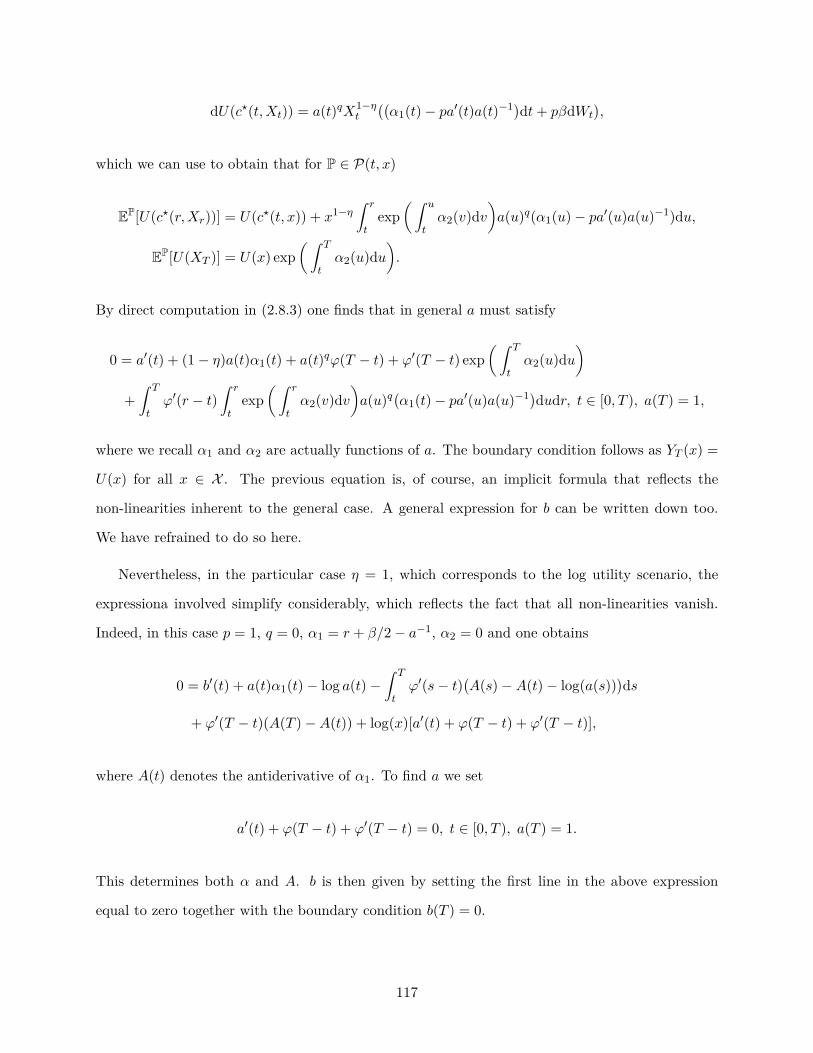
dU(c?(t,Xt)) = a(t)qX1−ηt

((α1(t)− pa′(t)a(t)−1)dt+ pβdWt

),

which we can use to obtain that for P ∈ P(t, x)

EP[U(c?(r,Xr))] = U(c?(t, x)) + x1−η∫ r

texp

(∫ u

tα2(v)dv

)a(u)q(α1(u)− pa′(u)a(u)−1)du,

EP[U(XT )] = U(x) exp(∫ T

tα2(u)du

).

By direct computation in (2.8.3) one finds that in general a must satisfy

0 = a′(t) + (1− η)a(t)α1(t) + a(t)qϕ(T − t) + ϕ′(T − t) exp(∫ T

tα2(u)du

)+∫ T

tϕ′(r − t)

∫ r

texp

(∫ r

tα2(v)dv

)a(u)q

(α1(t)− pa′(u)a(u)−1)dudr, t ∈ [0, T ), a(T ) = 1,

where we recall α1 and α2 are actually functions of a. The boundary condition follows as YT (x) =

U(x) for all x ∈ X . The previous equation is, of course, an implicit formula that reflects the

non-linearities inherent to the general case. A general expression for b can be written down too.

We have refrained to do so here.

Nevertheless, in the particular case η = 1, which corresponds to the log utility scenario, the

expressiona involved simplify considerably, which reflects the fact that all non-linearities vanish.

Indeed, in this case p = 1, q = 0, α1 = r + β/2− a−1, α2 = 0 and one obtains

0 = b′(t) + a(t)α1(t)− log a(t)−∫ T

tϕ′(s− t)

(A(s)−A(t)− log(a(s))

)ds

+ ϕ′(T − t)(A(T )−A(t)) + log(x)[a′(t) + ϕ(T − t) + ϕ′(T − t)],

where A(t) denotes the antiderivative of α1. To find a we set

a′(t) + ϕ(T − t) + ϕ′(T − t) = 0, t ∈ [0, T ), a(T ) = 1.

This determines both α and A. b is then given by setting the first line in the above expression

equal to zero together with the boundary condition b(T ) = 0.

117

2.10.2 Extensions

This section contain the proofs of the results in 2.4. We begin with the proof of Lemma 2.4.2

which verifies conditions under which the additional requirement in Assumption E is satisfied.

Proof of Lemma 2.4.2. In the case of uncontrolled volatility, the weak uniqueness assumption im-

plies that there exists a unique probability measure P and a P–Brownian motion W such that

Xt = x0 +∫ t

0σr(X·∧r) · dWr, t ∈ [0, T ], P–a.s.

In light of the regularity of f, we have

fr(X·∧r)− ft(X·∧t) =∫ r

tA(u,X·∧u, νu)dr +

∫ r

tσu(X·∧u)∇xfu(X·∧u) · dWr,

from which we obtain

EPν⊗t′ν?

[fr(Xr)|Ft] = ft(Xt) +∫ t′

tEP[A(u,X·∧u, νu)Eνt,T |Ft]du+

∫ r

t′EP[A(u,X·∧u, ν?u)Eν⊗t′ν

?

t,T |Ft]du.

Thus

EPν⊗t′ν?

[fr(Xr)|Ft]− EPν? [fr(Xr)|Ft] =∫ t′

tEP[A(u,X·∧u, νu)Eνt,T |Ft]− EP[A(u,X·∧u, ν?u)Eν?t,T |Ft]du

+ EP[(Eν⊗t′ν

?

t,T − Eν?t,T) ∫ r

t′A(u,X·∧u, ν?u)du

∣∣∣∣Ft].The result then follows in light of the integrability of the first term, applying Hölder intequality to

the second term and the estimate

EP[∣∣Eν⊗t′ν?t,T − Eν?t,T

∣∣2∣∣∣Ft] ≤ EP[( ∫ t′

t|νr − ν?r |dr

)2]≤ C|t′ − t|2.

To obtain the result in (ii), notice that by uniqueness of the strong solution Xx,ν we have

EP[fr(Xν⊗t′ν?r )|Ft] = ft(Xt) +

∫ t′

tEP[A(u,Xν

r , νu)|Ft]du+∫ r

t′EP[A(u,Xν⊗t′ν?

r , ν?u)|Ft]du

= ft(Xt) +∫ t′

tEP[A(u,Xν

r , νu)|Ft]du+∫ r

t′EP[A(u,Xν?

r , ν?u)|Ft]du.

118

Thus, the result follows from

EP[fr(Xν⊗t′ν?r )|Ft]− EP[fr(Xν?

r )|Ft] =∫ t′

tEP[A(u,Xν

r , νu)|Ft]− EP[A(u,Xν?

r , ν?u)|Ft]du.

The next sequence of results build up to the proof of Theorem 2.4.3, namely we wish to obtain the

corresponding extended version of the dynamic programming principle. We begin with a sequence

of lemmata that will allow us to study the local behaviour of the value of the game. These results

are true in great generality and require mere extra regularity of the running and terminal rewards

in the type variables (s, n,m). Our first result consists of a one step iteration of our equilibrium

definition.

Lemma 2.10.1. Let ν? ∈ E(x) and v the value associated to ν?. Then, for any (ε, `, t, σ, τ) ∈

(0,∞)× (0, `ε)× [0, T ]× Tt,t+` × Tt,t+` with σ ≤ τ, and P(x)–q.e. x ∈ X ,


EPν[v(τ,X) +

∫ τ

σfr(σ,X·∧r,EPν [fr(X)], νr)dr + EPν

?

τ,·

[G(σ,EPν [M?

τ ])−G(τ,M?τ )]

+ EPν?

τ,·

[ ∫ T

τfr(σ,X·∧r,EPν [N τ,?

r ], ν?r)− fr

(τ,X·∧r, N

τ,?r , ν?r

)dr]− ε`

+ EPν?

τ,·

[ξ(σ,X·∧T )− ξ(τ,X·∧T )

]− ε`.

Proof. To get the second inequality note that for (ε, `, t, σ, τ) ∈ R?+× (0, `ε)× [0, T ]×Tt,t+`×Tt,t+`

with σ ≤ τ, P(x)–q.e. x ∈ X and ν ∈ A(σ, x)

v(σ, x) = J(σ, σ, x, ν?) ≥ J(σ, σ, x, ν ⊗τ ν?)− ε`


σfr(σ,X,EPν⊗τ ν

?

[fr(X)], (ν ⊗τ ν?)r)dr

+∫ T

τfr(σ,X,EPν⊗τ ν

?

[fr(X)], (ν ⊗τ ν?)r)dr

+ ξ(σ,X·∧T ) +G(σ,EPν⊗τ ν?

[g(X·∧T )])]− ε`


σfr(σ,X,EPν [fr(X)], νr)dr +

∫ T

τfr(σ,X,EPν [N τ,?

r ], ν?r)dr]

+ EPν⊗τ ν?[ξ(σ,X·∧T ) +G(σ,EPν [M?

τ ])]− ε`

119

= EPν[v(τ,X) +

∫ τ

σfr(σ,X,EPν [fr(X)], νr)dr

+ EPν?

τ,·

[ ∫ T

τfr(σ,X,EPν [N τ,?

r ], ν?r)− fr

(τ,X,N τ,?

r , ν?r)dr

+ ξ(σ,X·∧T )− ξ(τ,X·∧T ) +G(σ,EPν [M?τ ])−G(τ,M?

τ )]]− ε`,

where the last equality follows by conditioning and the Fτ measurability of all the terms.

Indeed, in light of [232, Theorem 6.1.2], an r.c.p.d. of Pν⊗τν?

|Fτ evaluated at x agrees with

Pν?

τ(x),x, the weak solution to the martingale problem with initial condition (τ, x) and action ν?, for

Pν⊗τν?

–a.e. x ∈ X . As all the terms inside the second expectation are Fτ -measurable the previous

holds for Pν–a.e. x ∈ X .

From the previous result, we know that equilibrium models satisfy a form of ε-optimality in a

sufficiently small window of time. We now seek to gain more insight from iterating the previous

result. This will allow us to move forward the time window into consideration.

In the following, given (σ, τ) ∈ Tt,T × Tt,t+`, with σ ≤ τ , we denote by Π` := (τ ì )i=1,...,n` ⊆ Tt,T


⌉, σ =: τ `0 ≤ · · · ≤

τ `n`

:= τ, ∀`, and supi≤n` |τì − τ ì−1| ≤ `. We also let ∆τ ì := τ ì − τ ì−1. The previous definitions

hold ω–by–ω.

Proposition 2.10.2. Let ν? ∈ E(x) and σ, τ ⊂ Tt,T , with σ ≤ τ . Fix ε > 0 and some partition

Π` with ` < `ε. Then for P(x)–q.e. x ∈ X


EPν[v(τ,X) +

n`−1∑i=0

∫ τì+1

τì

fr(τ ì , X·∧r,EPντì,· [fr(X)], νr)dr

+n`−1∑i=0

EPν?

τì+1,·

[ ∫ T

τì+1

fr(τ ì , X·∧r,E

Pντì,· [N τì+1,?

r ], ν?r)− fr

(τ ì+1, X·∧r, N

τì+1,?r , ν?r

)dr]

+n`−1∑i=0

EPν?

τì+1,·

[G(τ ì ,E

Pντì,· [M?

τì+1])−G(τ ì+1,M

?τì+1

)]

+n`−1∑i=0

EPν?

τì+1,·

[ξ(τ ì , X·∧T )− ξ(τ ì+1, X·∧T )− n`ε`

]].

120

Proof. A straightforward iteration of Lemma 2.10.1 yields that for P(x)–q.e. x ∈ X


EPν[ ∫ τ`1

τ`0

fr(τ `0 , X,EPντ`0,x [fr(X)], νr)dr + E

Pν?

τ`1,X[G(τ `0 ,E

Pντ`0,x [M?τ`1

])−G(τ `1 ,M?τ`1

)]

+ EPν?

τ`1,X[ ∫ T

τ`1

fr(τ `0 , X,E

Pντ`0,x [N τ`1 ,?r ], ν?r

)− fr

(τ `1 , X,N

τ`1 ,?r , ν?r

)d]

+ EPν?

τ`1,X[ξ(τ `0 , X)− ξ(τ `1 , X) + v(τ1, X)

]− ε`

≥ supν∈A(σ,x)

∫Ω

∫ τ`1

τ`0

fr(τ `0 , X,EPντ`0,x [fr(X)], νr)dr + E

Pν?

τ`1,X[G(τ `0 ,E

Pντ`0,x [M?τ`1

])−G(τ `1 ,M?τ`1

)]

+ EPν?

τ`1,X[ ∫ T

τ`1

fr(τ `0 , X,E

Pντ`0,x [N τ`1 ,?r ], ν?r

)− fr

(τ `1 , X,N

τ`1 ,?r , ν?r

)dr + ξ(τ `0 , X)− ξ(τ `1 , X)

]

+ supν∈A(τ`1 ,x)

EPν[ ∫ τ`2

τ`1

fr(τ `1 , X,EPντ`1,x [fr(X)], νr)dr

+ EPν?

τ`2,X[ ∫ T

τ`2

fr(τ `1 , X,E

Pντ`1,x [N τ`2 ,?r ], ν?r

)− fr

(τ `2 , X,N

τ`2 ,?r , ν?r

)dr + ξ(τ `1 , X)− ξ(τ `2 , X)

]

+ EPν?

τ`2,X[G(τ `1 ,E

Pντ`1,x [M?τ`2

])−G(τ `2 ,M?τ`2

)]

+ v(τ2, X)]

Pν(dω)− 2ε`

= supν∈A(σ,x)

EPν[v(τ2, X) +

∫ τ`1

τ`0

fr(τ `0 , X,EPντ`0,x [fr(X)], νr)dr +

∫ τ`2

τ`1

fr(τ `1 , X,EPντ`1,· [fr(X)], νr)dr

+ EPν?

τ`1,·[ ∫ T

τ`1

fr(τ `0 , X,E

Pντ`0,x [N τ`1 ,?r ], ν?r

)− fr

(τ `1 , X,N

τ`1 ,?r , ν?r

)dr]

+ EPν?

τ`1,·[ξ(τ `0 , X)− ξ(τ `1 , X) +G(τ `0 ,E

Pντ`0,x [M?τ`1

])−G(τ `1 ,M?τ`1

)]

+ EPν?

τ`2,·[ ∫ T

τ`2

fr(τ `1 , X,E

Pντ`1,· [N τ`2 ,?r ], ν?r

)− fr

(τ `2 , X,N

τ`2 ,?r , ν?r

)dr]

+ EPν?

τ`2,·[ξ(τ `1 , X)− ξ(τ `2 , X) +G(τ `1 ,E

Pντ`1,· [M?τ`2

])−G(τ `2 ,M?τ`2

)]]− 2ε`,

where the second inequality follows by applying the definition of an equilibrium at (τ `1 , X). Now,

to justify the last step follows we first note that as we let the reward depend on EPt,x [fr(X·∧r)] and

EPt,x [g(X·∧T )] we need a dynamic programming result for McKean–Vlasov control. This result is

recently available in [76, Theorem 3.1]. The statement of the lemma follows directly by iterating

and the fact the iteration is countable.

To ease the readability of the next result, recall that for x ∈ X , σ, ζ, τ ⊂ T0,T with σ ≤ ζ ≤ τ ,

121

ν? ∈ A(x), ν ∈ A(σ, x), and any FXT -measurable random variable ξ, we introduce the notation

EPν ,Pν?

ζ [ξ] := EPν⊗ζPν?

ζ,X [ξ],

where Pν?ζ,X is given by ω 7−→ Pν?(ζ(ω),x·∧ζ(ω)) and denotes the Fζ-kernel prescribed by the family of

solutions to the martingale problem associated with ν?, see [232, Theorem 6.2.2]. Note in particular

EPν ,Pν?

σ [ξ] = EPν?

σ,X [ξ].

Proof of Theorem 2.4.3. Let ε > 0, 0 < ` < `ε and Π` be as in Proposition 2.10.2. It then follows



EPν[v(τ,X) +

n`−1∑i=0

∫ τì+1

τì

fr(τ ì , X,EPντì,· [fr(X)], νr)dr

+n`−1∑i=0

EPν?

τì+1,·

[ ∫ T

τì+1

fr(τ ì , X,E

Pντì,· [N τì+1,?

r ], ν?r)− fr

(τ ì+1, X,N

τì+1,?r , ν?r

)dr]

+n`−1∑i=0

EPν?

τì+1,·

[ξ(τ ì , X)− ξ(τ ì+1, X) +G(τ ì ,E

Pντì,· [M?

τì+1])−G(τ ì+1,M

?τì+1

)− n`ε`]]

= supν∈A(σ,x)

EPν[v(τ,X) +

n`−1∑i=0

∫ τì+1

τì


]

+n`−1∑i=0

EPν ,Pν?

τì+1

[ ∫ T

τì+1

fr(τ ì , X,E

Pντì,· [N τì+1,?

r ], ν?r)− fr

(τ ì+1, X,N

τì+1,?r , ν?r

)dr]

+n`−1∑i=0

EPν ,Pν?

τì+1

[ξ(τ ì , X)− ξ(τ ì+1, X) +G(τ ì ,E

Pντì,· [M?

τì+1])−G(τ ì+1,M

?τì+1

)− n`ε`].

For (t, x, ν) ∈ [0, T ] × X × A(t, x), let R(s) :=∫ sσ fr(s,X, fr(X), νr)dr, s ∈ [σ, T ], so that for

i = 0, . . . , n` − 1,

EPν[ ∫ τì+1

τì


]= EPν

[R(τ ì+1)− R(τ ì )

]+ EPν

[ ∫ τì+1

σ

(fr(τ ì , X,E

Pντì,· [fr(X)], νr)− fr(τ ì+1, X, fr(X), νr)

)dr],

122

where we used the fact that EPνζ,· [ft(X)] = ft(X) for t ∈ [σ, ζ]. Consequently, for P(x)–q.e. x ∈ X


EPν

[v(τ,X) +

n`−1∑i=0

R(τ ì+1)− R(τ ì )− n`ε`]

+n`−1∑i=0

EPν[ ∫ τì+1

σ

(fr(τ ì , X,E

Pντì,· [fr(X)], νr)− fr(τ ì+1, X, fr(X), νr)

)dr]

+n`−1∑i=0

EPν ,Pν?

τì+1

[ ∫ T

τì+1

fr(τ ì , X,E

Pντì,· [N τì+1,?

r ], ν?r)− fr

(τ ì+1, X,N

τì+1,?r , ν?r

)dr]

+n`−1∑i=0

EPν ,Pν?

τì+1

[ξ(τ ì , X)− ξ(τ ì+1, X) +G(τ ì ,E

Pντì,· [M?

τì+1])−G(τ ì+1,M

?τì+1

)].

(2.10.1)

The idea in the rest of the proof is to take the limit ` −→ 0 on both sides of (2.10.1). As v is

finite we can exchange the limit with the sup and study the limit inside. The analysis of all the

above terms, except the error term⌈τ − σ/`

⌉ε`, is carried out below. Regarding the error term,

we would like to make the following remarks as it is clear that simply letting ε go to zero will not

suffice for our purpose. As `ε is bounded and monotone in ε, we consider `0 given by `ε −→ `0 as

ε −→ 0. We must consider two cases for `0: when `0 = 0 the analysis in the next paragraph suffices

to obtain the result; in the case `0 > 0, we can then take at the beginning of this proof ` < `0 ≤ `ε,

in which case all the sums in (2.10.1) are independent of ε, we then first let ε go to zero so that⌈τ − σ/`

⌉ε` −→ 0 as ε −→ 0, and then study the limit ` −→ 0 as in the following. In both scenarii

the conclusion of the theorem holds.

We now carry out the analysis of the remaining terms. To this end, and in order to prevent enfor-

cing unnecessary time regularity on the action process, we will restrict our class of actions to piece-

wise constant actions, i.e. νt :=∑k≥1 νk1(%k−1,%k](t) for a sequence of non-decreasing F–stopping

times (%k)k≥0, and random variables (νk)k≥1, such that for any k ≥ 1, νk is FX%k−1-measurable. We

will denote by Apw(t, x) the corresponding subclass of actions. By [77] the supremum over A(t, x)

and Apw(t, x) coincide. Indeed, under Assumption E.(iv) and E.(v), we can apply [77, Theorem

3.1 and Lemma 4.3]. Assumption E.(iv), i.e. the Lipschitz-continuity of a 7−→ ft(t, x,n, a), ensures

the continuity of the drift coefficient when the space is extended to include the running reward, see

[86, Remark 3.8]. Without lost of generality we assume (%k)k≥0 ⊆ Π`, this is certainly the case as

we can always refine Π` so that νr = νi for τ ì ≤ r ≤ τ ì+1.

123

In the following, we fix ω ∈ Ω. A first-order Taylor expansion of the first summation term in

(2.10.1) guarantees the existence of γì ∈ (τ ì , τ ì+1), i ∈ 0, . . . , n` such that

∣∣∣∣∣n`−1∑i=0

R(τ ì+1)− R(τ ì )−∆τ ì+1

(fτì

(τ ì , X, fτì (X), νi) +∫ τì+1

σ∂sfr(τ ì+1, X, fr(X), νr)dr

)∣∣∣∣∣ (2.10.2)

=∣∣∣∣∣n`−1∑i=0

∆τ ì+1

(fγì

(γì , X, fγì (X), νi)− fτì (τ ì , X, fτì (X), νi)

+i∑

k=0

∫ τ`k+1∧γì

τ`k

∂sfr(γì , X, fγì (X), νk)dr −∫ τ`k+1

τ`k

∂sfr(τ ì+1, X, fr(X), νk)dr)∣∣∣∣∣

≤n`−1∑i=0|∆τ ì+1|

(ρf(|∆τ ì+1|

)+ Cρf

(|∆τ ì+1|

)+

i∑k=0

∫ τ`k+1

τ`k

ρ∂sf(|∆τ ì+1|

)+ Cρf

(|∆τ ì+1|

)dr)

≤ C(ρf (`) + ρf(`) + ρ∂sf (`)

) `→0−−→ 0.

The equality follows by replacing the expansion of the terms R(τ ì+1) and the fact ν is constant

between any two terms of the partition. The first inequality follows from Assumption E, where

ρf , ρf and ρ∂sf are the modulus of continuity of the maps t 7−→ ft(t, x, a), t 7−→ ft(x) and s 7−→

∂sfr(s, x, a). The limits follows by bounded convergence as in light of Assumption E the constant

in the last inequality and the last term are independent of ω. Thus, both expressions on the first

line have the same limit for every ω ∈ Ω. We claim that for a well chosen sequence of partitions of

the interval [σ, τ ]

EPν[ n`−1∑i=0

R(τ ì+1)− R(τ ì )]

`−→0−−−→ EPν[ ∫ τ

σfr(r,X, fr(X), νr)dr +

∫ τ

σEPν

?

r,X

[ ∫ r

σ∂sfu(r,X, fu(X), νu)du

]dr],

(2.10.3)

where the integrals on the right-hand side are w.r.t the Lebesgue measure on [0, T ], and we recall

the term inside EPν?

r,X is FXr -measurable. Indeed, following McShane [182], for ` > 0 fixed there

exists, ω-by-ω, Π` := (τ ì )i∈[n`] a partition of [σ, τ ] such that the Riemann sum in (2.10.2) evaluated

at Π` converges to the Lebesgue integral ω-by-ω. With this, we are left to argue (2.10.3). Recall

so far our analysis was for ω ∈ Ω fixed, therefore one has to be careful about, for instance, the

measurability of the partition (τ ì )1≤i≤n` . An application of Galmarino’s test, see Dellacherie and

Meyer [69, Ch. IV. 99–101], guarantees that τ ì ∈ T0,T for all i, i.e. the random times τ ì are in fact

124

stopping times. Finally, (2.10.3) follows by the bounded convergence theorem.

We now move to the second term in (2.10.1). Similarly, there are γì ∈ (τ ì , τ ì+1), [0, 1]-valued

random processes θi, i ∈ 0, . . . , n`, such that for ητì ,?t := θitft(X) + (1 − θit)E

Pντì,· [ft(X)], defined

dt⊗ dPν–a.e., it holds that

∣∣∣∣EPν[ n`−1∑i=0

∫ τì+1

σfr(τ ì , X,E

Pντì,· [fr(X)], νr)−fr(τ ì+1, X, fr(X), νr)+∆τ ì+1∂sfr(τ ì+1, X, fr(X), νr)dr

]∣∣∣∣=∣∣∣∣EPν

[ n`−1∑i=0

∫ τì+1

σ∆τ ì+1

(∂sfr(γì , X, fr(X), νr)− ∂sfr(τ ì+1, X, fr(X), νr)

)dr]

+ EPν[ n`−1∑i=0

∫ τì+1

σ∂nfr

(τ ì , X, η

τìr , νr)

(fr(X)− E

Pντì,· [fr(X)]

)dr]∣∣∣∣

≤ EPν[ n`−1∑i=0

∫ τì+1

σ|∆τ ì+1|ρ∂f (|`|)dr

]

+∣∣∣∣EPν

[ n`−1∑i=0

∫ τì+1

τì

∂nfr(τ ì , X, η

τìr , νr)

(fr(X)− E

Pντì,· [fr(X)]

)dr]∣∣∣∣

≤ Cρ∂f (|`|) + CEPν[ n`−1∑i=0

∫ τì+1

τì

∣∣∣EPντì+1,·

[fr(X)

]− E

Pντì,·[fr(X)

]∣∣∣dr] `→0−−→ 0,

where in the first inequality we used Assumption E and the fact that EPνζ,· [ft(X)] = ft(X) for t ∈

[σ, ζ]. The same argument together with the fact that n 7−→ ft(s, x,n, a) has bounded derivatives,

which holds by Assumption E, yields the second inequality. The limit follows in light of the

continuity of x 7−→ ft(x), and of (t, x) 7−→ Pνt,x for the weak topology. Since the limits agree, we

find the second term converges to

− EPν[ n`−1∑i=0

∆τ ì+1

∫ τì+1

σ∂sfr(τ ì+1, X, fr(X), νr)

)dr]

`−→0−−−→ − EPν[ ∫ τ

σEPν

?

r,X

[ ∫ r

σ∂sfu(r,X, fu(X), νu)du

]dr].

(2.10.4)

Similarly, we can write the third term in (2.10.1), namely

n`−1∑i=0

EPν ,Pν?

τì+1

[ ∫ T

τì+1

fr(τ ì , X,E

Pντì,· [N τì+1,?

r ], ν?r)− fr

(τ ì+1, X,N

τì+1,?r , ν?r

)dr],

125

as the sum of

I1 :=n`−1∑i=0

EPν ,Pν?

τì+1

[ ∫ T

τì+1

fr(τ ì , X,N

τì ,?r , ν?r

)− fr

(τ ì+1, X,N

τì+1,?r , ν?r

)dr],

I2 :=n`−1∑i=0

EPν ,Pν?

τì+1

[ ∫ T

τì+1

fr(τ ì , X,E

Pντì,· [N τì+1,?

r ], ν?r)− fr

(τ ì , X,N

τì ,?r , ν?r

)dr].

(2.10.5)

As for I1, we now there are γì ∈ (τ ì , τ ì+1), [0, 1]-valued random processes θi, i ∈ 0, . . . , n`, such

that for ητì+1,?t := θitN

τì ,?t + (1− θit)N

τì+1,?t

∣∣∣∣ n`−1∑i=0

EPν ,Pν?

τì+1

[ ∫ T

τì+1

(fr(τ ì , X,N

τì ,?r , ν?r )− fr(τ ì+1, X,N

τì+1,?r , ν?r )

)dr

+∫ T

τì+1

∆τ ì+1∂sfr(τ ì+1, X,Nτì+1,?r , ν?r )dr

+∫ T

τì+1

(∂nfr

(τ ì , N

τì ,?r )∆N τì+1,?

r + 12∂

2nnfr(τ ì , N

τì ,?r )

∣∣∆N τì+1,?r

∣∣2)dr]∣∣∣∣

(2.10.6)

=∣∣∣∣ n`−1∑i=0

EPν ,Pν?

τì+1

[ ∫ T

τì+1

∆τ ì+1

(∂sfr(τ ì+1, X,N

τì+1,?r , ν?r )− ∂sfr(γì , X,N

τì+1,?r , ν?r )

)dr

+ 12

∫ T

τì+1

∣∣∆N τì+1,?r

∣∣2(∂2nnfr(τ ì , N

τì ,?r )− ∂2

nnfr(τ ì , ητì+1,?r )

)dr]∣∣∣∣

≤ T 2ρ∂f (|`|) + CEPν[ ∫ T

σsupi

∣∣∆N τì+1,?r

∣∣ n`−1∑i=0

∣∣∆N τì+1,?r

∣∣2dr]`→0−−→ 0,

where in the first equality we used the fact that the first order term in the expansion for n cancels.

The inequality follows from Assumption E, the fact that θi ∈ [0, 1] and the FXτi+1-measurability of

∆N τì+1,?r . Lastly, the limit follows in light of the continuity of x 7−→ ft(x) and the continuity of

(t, x) 7−→ Pνt,x for the weak topology. Therefore the limits in (2.10.6) agree.

We now study the first order term, in n, in (2.10.6) together with I2, as defined in (2.10.5).

We claim the limit is zero. Indeed, for ητì ,?t := θìN

τì ,?t + (1− θì )E

Pντì,· [N τì+1,?

t ] we have that there

exists C > 0 such that

n`−1∑i=0

EPν ,Pν?

τì+1

[ ∫ T

τì+1

(fr(τ ì , X,E

Pντì,· [N τì+1,?

r ], ν?r)−fr

(τ ì , X,N

τì ,?r , ν?r

)−∂nfr

(τ ì , N

τì ,?r )∆N τì+1,?

r

)dr]∣∣∣∣

=n`−1∑i=0

EPν ,Pν?

τì+1

[ ∫ T

τì+1

(∂nfr

(τ ì , η

τìr )(EPντì,· [N τì+1,?

r ]−N τì ,?r

)− ∂nfr

(τ ì , N

τì ,?r )∆N τì+1,?

r

)dr]

126

=n`−1∑i=0

EPν[ ∫ T

τì+1

(∂nfr

(τ ì , η

τìr )(EPντì,· [N τì+1,?

r ]−N τì ,?r

)− ∂nfr

(τ ì , N

τì ,?r )∆N τì+1,?

r

)dr]

=n`−1∑i=0

EPν[ ∫ T

τì+1

(∂nfr

(τ ì , η

τìr )− ∂nfr

(τ ì , N

τì ,?r )

)(EPντì,· [N τì+1,?

r ]−N τì ,?r

)dr]

≤ Cn`−1∑i=0

EPν[ ∫ T

τì+1

∣∣∣EPντì,· [N τì+1,?

r ]−N τì ,?r

∣∣∣2dr]`−→0−−−→ 0,

where the inequality follows again from Assumption E.(i) and the fact that θi ∈ [0, 1]. The limit

follows from Assumption E.(iii).

We are only left left to compute the limit of

n`−1∑i=0

EPν ,Pν?

τì+1

[ ∫ T

τì+1

(∆τ ì+1∂sfr(τ ì+1, X,N

τì+1,?r , ν?r ) + 1

2∂2nnfr(τ ì , N

τì ,?r )

∣∣∆N τì+1,?r

∣∣2)dr].

Regarding the first term, note that for an appropriate choice of Π`, as in [182],

EPν[ n`−1∑i=0

∆τ ì+1EPν?

τi+1,·

[ ∫ T

τì+1

∂sfr(τ ì+1, X,Nτì+1,?r , ν?r )dr

]]`−→0−−−→ EPν

[ ∫ τ

σEPν

?

u

[ ∫ T

u∂sfr(u,X,Nu,?

r , ν?r )dr]du].

As for the second term let us note that, ignoring the factor 1/2,

n`−1∑i=0

EPν ,Pν?

τì+1

[ ∫ T

τì+1

∂2nnfr(τ ì , N

τì ,?r )

∣∣∆N τì+1,?r

∣∣2dr]

= EPν[ n`−1∑i=0

∫ T

τì+1

EPν?

τi+1,·

[∂2

nnfr(τ ì , Nτì ,?r )

∣∣∆N τì+1,?r

∣∣2]dr].Then, we can use the fact that ∆N τi+1,?

t = 0 for t ∈ [0, τi], to express it as the sum of

I3 := EPν[ ∫ T

σ

n`−1∑i=0

EPν?

τi+1,·

[∂2


∣∣∆N τì+1,?r

∣∣2]dr]

I4 := EPν[ n`−1∑i=0

∫ τi+1

τi

∂2nnfr(τ ì , N

τì ,?r )

∣∣∆N τì+1,?r

∣∣2dr].

127

In light of Assumption E.(i), we obtain that I4 converges to zero, whereas

EPν[ ∫ T

σ

n`−1∑i=0

EPν?

τi+1,·

[∂2


∣∣∆N τì+1,?r

∣∣2]dr]`−→0−−−→ EPν

[ ∫ T

σ

∫ τ

σEPν

?

u,·

[∂2

nnfr(u,Nu 2r )nu,?r

]dudr

],

at last we use the fact that, by definition, nu,?r = 0, dt⊗ dPν?

–a.e., whenever r ∈ [0, u] so that

EPν[ ∫ T

σ

∫ τ

σEPν

?

u,·

[∂2

nnfr(u,Nu,?r )nu 2

r

]dudr

]= EPν

[ ∫ τ

σEPν

?

u,·

[ ∫ T

u∂2

nnfr(u,X,Nu,?r , ν?r )nu 2

r dr]du].

The argument for the fourth term in (2.10.1) is analogous, but simpler, to that of the third

term in (2.10.1) exploiting the corresponding properties in Assumption E.(ii)–E.(iii).

We close this section with the proof of the necessity result in the extension section, namely

Theorem 2.4.4.

Proof of Theorem 2.4.4. This proof is analogous to the proof in the standard case. We just have

to verify the assumptions allow us to obtain the new version of the results. Indeed, let us result

that the proof of Theorem 2.2.10 in Section 2.7 is divided into two parts.

The first part consist of an application of the comparison theorem for the BSDE with terminal

condition ξ + G(T, g(X)) and generator h for every P ∈ P(t, x). Recall that as a function of z,

h is still Lipschitz. So all we are left to verify is that the term in F outside of the sup has the

appropriate integrability, i.e. that for every (t, x) ∈ [0, T ] × X , P ∈ P(t, x), ∂Y ∈ Hps,x(R,FX,P+ ,P)

and m2 ∈ Hps,x(R,FX,P+ ,P), recall that by assumption ∂2

nnG is bounded.The first result is immediate

from Assumption F.(i). The result for m2 follow from the integrability assumption on g(X).

The second part of the proof is argued in the same way by introducing the regularised version

of the value function v+.

2.10.3 Auxiliary lemmata

To being with we present a result that justifies our choice of the class A(t, x) in our definition

of equilibrium.

128

Lemma 2.10.3.1. Let τ ∈ Tt,T , ν ∈ A(x) and ν ∈ A(t, x). Then, Pν⊗τ ν = Pν ⊗τ Pντ,·, ν ⊗τ ν ∈

A(t, x), A(t, x, τ) = A(t, x).

Proof. The latter two results follows from the first. Let ν ∈ A(t, x), we claim that Pν ⊗τ Pντ,X is

well defined and solves the martingale problem associated with ν ⊗τ ν?. Indeed, by [232, Exercise

6.7.4, Theorem 6.2.2] we have that ω 7−→ Pν?τ(ω),X(τ(ω),ω)[A] is Fτ -measurable for any A ∈ F , and

Pν?τ(ω),X(τ(ω),ω)[Ωωτ ] = 1 for all ω ∈ Ω. Therefore, Theorem 2.1.1 guarantees Pν ⊗τ(·) Pντ(·),X(·) is well

defined and Pν ⊗τ(·) Pντ(·),X(·) equals Pν on Fτ and (δω ⊗τ(ω) Pν

?

τ(ω),x)ω∈Ω is an r.c.p.d. of Pν ⊗τ Pντ,X

given Fτ . In combination with [232, Theorem 1.2.10] this yields Mϕ is a (F,Pν ⊗τ Pν,τ,X)–local

martingale on [t, T ] with control ν ⊗τ ν?.

Lemma 2.10.3.2. Given (t, x) ∈ [0, T ] × X , τ ∈ Tt,T , (M, M) ∈ M(t, x) ×M(t, x) such that

ν ⊗τ ν ∈ A(t, x,P). Then Pν ⊗τ Pντ,· = Pν⊗τ ν .

Proof. This follows from Lemma 2.10.3.1 and the fact we can commute changes of measure and

concatenation.

Lemma 2.10.3.3. For ` > 0 let (γì )i∈[n`] be sample points as in Theorem 2.2.2. (γì )i∈[n`] are

F–stopping times.

Proof. We study (γì )i∈[n`] as the argument for the other sequences in the proof is similar. The

result follows from a direct application of Galmarino’s test, see [69, CH. IV. 99–101], we recall it

next for completeness: Let % be FT -measurable function with values in [0, T ]. % is a stopping time

if and only if for every t ∈ [0, T ] we have that %(ω) ≤ t, (Xr,Wr,∆r[ϕ])(ω) = (Xr,Wr,∆r[ϕ])(ω)

for all (r, ϕ) ∈ [0, t]× Cb([0, T ]×A) implies %(ω) = %(ω).

Now, in the context of Theorem 2.2.2 we are given Π` = (τ ì )i∈[n`] a collection of stopping times

that partitions the interval [σ, τ ] ⊆ [0, T ]. As ` > 0 is fixed we drop the dependence of the partition

on ` and write Π = (τi)i∈[n]. Without loss of generality we consider the case of a partition of [0, T ].

For ω ∈ Ω we can use [240, Theorem 1] to obtain a sequence of sample points (%i(ω))i∈[n] of the

intervals prescribed by Π, i.e. %i(ω) ∈ [τi−1(ω), τi(ω)] for all i. We want to show %i ∈ T0,T for all i.

A close inspection to the proof of [241, Theorem 1] allows us to see that for fixed ω ∈ Ω the

choice of %i(ω) depends solely on [τi−1(ω), τi(ω)] and the application t 7−→ ft(t, x, a) for (t, x, a) ∈

129

[0, T ] × X × A. We recall that as the supremum is taken over Apw(t, x) the action process is a

fix value a ∈ A over the interval [τi−1, τi]. We first note that for ω ∈ Ω as above the fact that

Π ⊂ T0,T , i.e. τi ≤ t ∈ Ft, implies Π(ω) = Π(ω). Next, we observe that ft(t,X, νi)(ω) =

ft(t, x·∧t, a) = ft(t,X, νi)(ω) as is ft(s, x, a) is optional for every (s, a) ∈ [0, T ]×A. These two facts

imply %i(ω) = %i(ω) and the result follows.

130

Part III

Backward stochastic Volterra integral

equations

Chapter 3

Lipschitz backward stochastic Volterra integral

equations

We saw in Chapter 2 that backward stochastic Volterra integral equations, BSVIEs for short,

appear naturally in the study of time-inconsistent stochastic control problems from a game theoretic

point of view, see Section 2.2.3 for details. This chapter is concerned with introducing a unified

method to address the well-posedness of these objects in the case of Lipschitz data.

In particular, we study a novel general class of multidimensional type-I backward stochastic

Volterra integral equations. Toward this goal, we introduce an infinite family of standard backward

SDEs and establish its well-posedness, and we show that it is equivalent to that of a type-I backward

stochastic Volterra integral equation. We also establish a representation formula in terms of non-

linear semi-linear partial differential equation of Hamilton–Jacobi–Bellman type. As an application,

we consider the study of time- inconsistent stochastic control from a game-theoretic point of view.

We show the equivalence of two current approaches to this problem from both a probabilistic and

an analytic point of view.

3.1 On Volterra BSDEs

In this chapter we want to build upon the strategy devised in Chapter 2 and address the well-

posedness of a general and novel class of type-I BSVIEs. We let X be the solution to a drift-less

stochastic differential equation (SDE, for short) under a probability measure P, and F be the P-

augmentation of the filtration generated by X, see Section 3.2 for details, and consider a tuple

132

(Y ·· , Z ·· , N ·· ), of appropriately F-adapted processes, satisfying for any s ∈ [0, T ]

Y st = ξ(s) +

∫ T

tgr(s,X, Y s

r , Zsr , Y

rr , Z

rr )dr −

∫ T

tZsrdXr −

∫ T

tdN s

r , t ∈ [0, T ], P–a.s. (3.1.1)

We remark that the additional process N corresponds to a martingale process which is P-

orthogonal to X. This is a consequence of the fact that we work with a general filtration F. To

the best of our knowledge, a theory for type-I BSVIEs, as general as the ones introduced above,

remains absent in the literature. Moreover, such class of type-I BSVIEs has only been mentioned

in [114, Remark 3.8] as an interesting generalisation of a classic type-I BSVIEs.

Our approach is based on the following class of infinite families of BSDEs

Yt = ξ(T,X·∧T ) +∫ T

thr(X·∧r,Yr,Zr, Y r

r , Zrr , ∂Y

rr )dr −

∫ T

tZ>r dXr, t ∈ [0, T ], P–a.s.,

Y st = η(s,X·∧T ) +

∫ T

tgr(s,X·∧r, Y s


∫ T

tV sr>dXr, t ∈ [0, T ], P–a.s.,

∂Y st = ∂sη(s,X·∧T ) +

∫ T

t∇gr(s,X·∧r, ∂Y s

r , ∂Zsr , Y

sr , Y

sr ,Yr,Zr)dr −

∫ T

t∂Zsr

>dXr, t ∈ [0, T ], P–a.s.

where (Y,Z,N , Y, Z,N, ∂Y, ∂Z, ∂N) are unknown, and required to have appropriate integrability,

see Section 3.3 and Equation (S).

We first establish the well-posedness of (S), see Theorem 3.3.5. For this it is important to

be able to identify the proper spaces to carry out the analyses, see Remark 3.3.3. Moreover, we

show that, for an appropriate choice of data for (S), its well-posedness is equivalent to that of the

type-I BSVIE (3.1.1), see Theorem 3.4.3. Noticeably, our approach can naturally be specialised to

obtain the well-posedness of previous BSVIEs considered in the literrature in the classic spaces, see

Remark 3.4.4. Moreover, as our results provide an alternative approach to BSVIEs, it may allow

for the future design of new numerical schemes to solve type-I BSVIEs, which to the best of our

knowledge, remain limited to [21]. In addition, we recover classical results for this general class of

multidimensional type-I BSVIEs. We provide a priori estimates, show the stability of solutions as

well as a representation formula in terms of a semilinear PDEs, see Proposition 3.5.1. Given our

multidimensional setting, we refrained from considering comparison results, see Wang and Yong

[254] for the one-dimensional case.

133

As an application of our results, we consider the game-theoretic approach to time-inconsistent

stochastic control problems. We recall this approach studies the problem faced by the, so-called,

sophisticated agent who aware of the inconsistency of its preferences seeks for consistent plans,

i.e. equilibria. We show that as a consequence of Theorem 3.4.3, one can reconcile two recent

probabilistic approaches to this problem. Moreover, we provide, see Proposition 3.5.3, an equivalent

result for two earlier analytic approaches, based on semi-linear PDEs. We believe this helps to

elucidate connections between the different takes on the problem available in the literature.

The rest of the chapter is structured as follows. Section 3.2 introduces the stochastic basis on

a canonical space as well as the integrability spaces necessary to our analysis. Section 3.3 precisely

formulates the class of infinite families of BSDEs (S), which is the crux of our approach, and

provides the statement of its well-posedness, while the proof is deferred to Section 3.6. Section 3.4

introduces the class of type-I BSVIEs which are the main object of this paper, and establishes

the equivalence of its well-posedness with that of (S) for a particular choice of data. Section 3.5

deals with the representation formula for the class of type-I BSVIEs considered, and presents the

application of our results in the context of time-inconsistent stochastic control. Finally, Section 3.6

includes the analysis of (S).

3.2 The stochastic basis on the canonical space

As a note to the reader, we mention that in the spirit of keeping the formulation of each chapter

self-contained we will present it at the beginning of each of the remaining chapter of the thesis.

This will create a modest level of repetition.

We fix two positive integers n and m, which represent respectively the dimension of the mar-

tingale which will drive our equations, and the dimension of the Brownian motion appearing in

the dynamics of the former. We consider the canonical space X = Cn, with canonical process

X. We let F be the Borel σ-algebra on X (for the topology of uniform convergence), and we

denote by FX := (FXt )t∈[0,T ] the natural filtration of X. We fix a bounded Borel-measurable map

σ : [0, T ]× X −→ Rn×m, σ·(X) ∈ Pmeas(Rn×m,FX), and an initial condition x0 ∈ Rn. We assume

there is P ∈ Prob(X ) such that P[X0 = x0] = 1 and X is martingale, whose quadratic variation,

134

〈X〉 = (〈X〉t)t∈[0,T ], is absolutely continuous with respect to Lebesgue measure, with density given

by σσ>. Enlarging the original probability space, see Stroock and Varadhan [232, Theorem 4.5.2],

there is an Rm-valued Brownian motion B with

Xt = x0 +∫ t

0σr(X·∧r)dBr, t ∈ [0, T ], P–a.s.

We now let F := (Ft)t∈[0,T ] be the (right-limit) of the P-augmentation of FX . We stress that we

will not assume P is unique. In particular, the predictable martingale representation property for

(F,P)-martingales in terms of stochastic integrals with respect to X might not hold.

Remark 3.2.1. We remark that the previous formulation on the canonical is by no means neces-

sary. Indeed, any probability space supporting a Brownian motion B and a process X satisfying the

previous SDE will do, and this can be found whenever that equation has a weak solution.


We now introduce our spaces. In the following, (Ω,FT ,F,P) is as in Section 3.2. We are given

a finite-dimensional Euclidean space, i.e. E = Rk for some non-negative integer k and | · | denotes

the Euclidean norm. For any (p, q) ∈ (1,∞)2, we introduce the spaces

• Lp(E) of FT -measurable, E-valued random variables ξ, with ‖ξ‖pLp := EP[|ξ|p] <∞;

• Sp(E) of Y ∈ Popt(E,F), with P–a.s. càdlàg paths on [0, T ], with ‖Y ‖pSp := EP[

supt∈[0,T ]

|Yt|p]<∞;

• Lq,p(E) of Y ∈ Popt(E,F), with ‖Y ‖pLq,p := EP[( ∫ T

0|Yr|qdr

) pq]<∞;

• Hp(E) of Z ∈ Ppred(E,F), defined σσ>t dt–a.e., with ‖Z‖pHp := EP[( ∫ T

0|σtZr|2dr

) p2]<∞;

• Mp(E) of martingales M ∈ Popt(E,F) which are P-orthogonal to X (that is the product XM is

an (F,P)-martingale), with P–a.s. càdlàg paths, M0 = 0 and ‖M‖pMp := EP[[M ]

p2T

]<∞;

• Lp,2(E) denotes the space of families (ξ(s))s∈[0,T ] of FT -measurable E-valued random variables

such that the mapping ([0, T ]× Ω,B([0, T ])⊗ F) −→ (Lp(E), ‖ · ‖Lp) : s 7−→ ξ(s) is continuous,

‖ξ‖pLp,2 := sups∈[0,T ] ‖ξ‖pLp <∞;

135

• P2meas(E,FT ) of two parameter processes (U st )(s,t)∈[0,T ]2 : ([0, T ]2 × Ω,B([0, T ]2) ⊗ FT ) −→

(E,B(E)) measurable.

Finally, given an arbitrary integrability space (Ip(E), ‖ · ‖I), we introduce the space

• Ip,2(E) of (U st )(s,t)∈[0,T ]2 ∈ P2meas(E,FT ) such that the mapping ([0, T ],B([0, T ])) −→ (Ip(E), ‖ ·

‖Ip) : s 7−→ U s is continuous and ‖U‖pIp,2 := sups∈[0,T ] ‖U s‖pIp <∞.

For example, Hp,2(E) denotes the space of (Zst )(s,t)∈[0,T ]2 ∈ P2meas(E,FT ), ([0, T ],B([0, T ])) −→

(Hp(E), ‖ · ‖Hp) : s 7−→ Zs is continuous and ‖Z‖pHp,2 := sups∈[0,T ] ‖Zs‖pHp <∞.

Lastly we introduce the space, see Remark 3.2.2 for further details,

• Hp,2(E) of (Zst )(s,t)∈[0,T ]2 ∈ P2meas(E,FT ) such that ([0, T ],B([0, T ])) −→ (Hp(E), ‖ · ‖Hp) : s 7−→

Zs is absolutely continuous with respect to the Lebesgue measure1, Z ∈ H2(E), where Z :=

(Ztt )t∈[0,T ] is given by

Ztt := ZTt −∫ T

tðZrt dr, and, ‖Z‖2Hp,2 := ‖Z‖2H2,2 + ‖Z‖2H2 <∞.

Remark 3.2.2. When p = q, we will write Lp(E)(resp. Lp,2(E)

)for Lq,p(E)

(resp. Lq,p,2(E)

).

With this convention, L2(E)(resp. L2,2(E)

)will be L2,2(E)

(resp. L2,2,2(E)

). Also, Sp,2(E),

Lq,p,2(E) and Hp,2(E) are Banach spaces.

In addition, we remark that the space H2(E) being closed implies Hp,2(E) is a closed subspace

of Hp,2(E) and thus a Banach space. The space Hp,2(E) allows us to define a good candidate for

(Ztt )t∈[0,T ] as an element of H2(E).2 Let Ω := [0, T ]×X and ω := (t, x) ∈ Ω. By the Radon–Nikodým

property and Fubini’s theorem, we may define

Zs(ω) := ZTt (x)−∫ T

sðZrt (x)dr, dt⊗ dP–a.e. ω ∈ Ω, s ∈ [0, T ],

1We recall that H2, being a Hilbert space and in particular a reflexive Banach space, has the so-called Radon–Nikodým property, see [216, Corollary 5.45]. Thus the absolute continuity of the H2-valued mapping s 7−→ Zs isequivalent to the existence of the density (ðZs)s∈[0,T ], which is unique for Lebesgue–a.e. s ∈ [0, T ]. The fact Z iswell-defined is argued in Remark 3.2.2

2This is based on [114, Section 2.1]. The mapping s 7−→ Zs is assumed absolutely continuous, as opposed tocontinuously differentiable. We are indebted to Yushi Hamaguchi for pointing out inconsistencies in the definition ofH2,2 on an earlier version of this chapter.

136

so that Zs = Zs, dt⊗ dP–a.e., s ∈ [0, T ]. Lastly, as ω ∈ Ω, s 7−→ Zs(ω) is continuous, we define

Ztt := ZTt −∫ T

tðZrt dr, for dt⊗ dP–a.e. (t, x) in [0, T ]×X .

3.3 An infinite family of Lipschitz BSDEs

We are given jointly measurable mappings h, g, ξ and η, such that for any (y, z, u, v,u) ∈

Rd1× Rn×d1× Rd2× Rn×d2× Rd2

h : [0, T ]×X × Rd1× Rn×d1× Rd2× Rn×d2× Rd2−→ Rd1 , h·(·, y, z, u, v, u) ∈ Pprog(Rd1 ,F),

g : [0, T ]2 ×X × Rd2× Rn×d2× Rd1× Rn×d1−→ Rd2 , g·(s, ·, u, v, y, z) ∈ Pprog(Rd2 ,F),

ξ : [0, T ]×X −→ Rd1 , η : [0, T ]×X −→ Rd2 .

Moreover, we work under the following set of assumptions.

Assumption G. (i) (s, u, v) 7−→ gt(s, x, u, v, y, z) (resp. s 7−→ η(s, x)) is continuously differenti-

able, uniformly in (t, x, y, z) (resp. in x). Moreover, the mapping ∇g : [0, T ]2×X ×(Rd2×Rn×d2)2×

Rd1× Rn×d1−→ Rd2 defined by

∇gt(s, x,u, v, u, v, y, z) := ∂sgt(s, x, u, v, y, z) + ∂ugt(s, x, u, v, y, z)u +n∑i=1

∂v:igt(s, x, u, v, y, z)vi:,

satisfies ∇g·(s, ·, u, v, u, v, y, z) ∈ Pprog(Rd2 ,F);

(ii) (y, z, u, v,u) 7−→ ht(x, y, z, u, v, u) is uniformly Lipschitz-continuous, i.e. ∃Lh > 0, such that

for all (t, x, y, y, z, z, u, u, v, v,u, u)

|ht(x, y, z, u, v, u)− ht(x, y, z, u, v, u)|

≤ Lh(|y − y|+ |σt(x)>(z − z)|+ |u− u|+ |σt(x)>(v − v)|+ |u− u|

);

(iii) for ϕ ∈ g, ∂sg, (u, v, y, z) 7−→ ϕt(s, x, u, v, y, z) is uniformly Lipschitz-continuous, i.e.

137

∃Lϕ > 0, such that for all (s, t, x, u, u, v, v, y, y, z, z)

|ϕt(s, x, u, v, y, z)− ϕt(s, x, u, v, y, z)| ≤ Lϕ(|u− u|+ |σt(x)>(v − v′)|+ |y − y|+ |σt(x)>(z − z)|

);

(iv) for 0 := (u, v, y, z)|(0,...,0),(h·, g·(s),∇g·(s)

):=(h·(·,0, 0), g·(s, ·,0), ∂sg·(s, ·,0)

)∈ L1,2(Rd1) ×(

L1,2,2(Rd2))2.

Remark 3.3.1. We comment on the set of requirements in Assumption G. Of particular interest

is Assumption G.(i), the other being the standard Lipschitz assumptions on the generators as well

as their integrability at zero. Anticipating the introduction of (S) below and the discussion in

Remark 3.3.3, Assumption G.(i) will allow us to identify the second BSDE in the system as the

antiderivative of the third one, see Remark 3.3.3.

We define the space (H, ‖ · ‖H), whose elements we denote h = (Y,Z,N , U, V,M, ∂U, ∂V, ∂M),

where

H := S2(Rd1)×H2(Rn×d1)×M2(Rd1)× S2,2(Rd2)×H2,2(Rn×d2)×M2,2(Rd2)

× S2,2(Rd2)×H2,2(Rn×d2)×M2,2(Rd2),

‖h‖2H := ‖Y‖2S2 + ‖Z‖2H2 + ‖N‖2M2 + ‖U‖2S2,2 + ‖V ‖2H2,2 + ‖M‖2M2,2

+ ‖∂U‖2S2,2 + ‖∂V ‖2H2,2 + ‖∂M‖2M2,2 .

We are now ready to precise the class of systems subject to our study. Given (ξ, η, ∂sη) ∈

L2(Rd1) × (L2,2(Rd2))2, ∂sη as in Assumption G, we consider the system, which for any s ∈ [0, T ]

holds, P–a.s., for every t ∈ [0, T ]

Yt = ξ(T,X·∧T ) +∫ T

thr(X,Yr,Zr, U rr , V r

r , ∂Urr )dr −

∫ T

tZ>r dXr −

∫ T

tdNr,

U st = η(s,X·∧T ) +∫ T

tgr(s,X,U sr , V s

r ,Yr,Zr)dr −∫ T

tV sr>dXr −

∫ T

tdM s

r , (S)

∂U st = ∂sη(s,X·∧T ) +∫ T

t∇gr(s,X, ∂U sr , ∂V s

r , Usr , V

sr ,Yr,Zr)dr −

∫ T

t∂V s

r>dXr −

∫ T

td∂M s

r .

Definition 3.3.2. We say h is a solution to (S) if h ∈ H and (S) holds.

Remark 3.3.3. We now expound on our choice for the set-up and the structure of (S).

138

(i) We first highlight two aspects which are crucial to establish the connection between (S) and

type-I BSVIE (3.1.1). The first is the presence of ∂U in the generator of the first equation. This

causes the system to be fully coupled but is nevertheless necessary in our methodology, this will be

clear from the proof of Theorem 3.4.3 in Section 3.4. The second relates to our choice to write

three equations instead of two. In fact, our approach is based on being able to identify ∂U as the

derivative with respect to the s variable of U in an appropriate sense and, at least formally, it is

clear that the third equation allows us to do so, see Lemma 3.6.1 for details. Alternatively, we could

have chosen not to write the third equation and consider the system which for any s ∈ [0, T ], holds

P–a.s. for any t ∈ [0, T ]

Yt = ξ(T,X·∧T ) +∫ T


r , ∂Urr )dr −

∫ T

tZ>r dXr −

∫ T

tdNr,

U st = η(s,X·∧T ) +∫ T

tgr(s,X,U sr , V s


tV sr>dXr −

∫ T

tdM s

r ,

∂U st := ddsU

s|(s,t) ,

where ddsU

s corresponds to the density with respect to the Lebesgue measure of s 7−→ U s. Never-

theless, for the proof of well-posedness of (S) that we present in Section 3.6, we have to derive

appropriate estimates for (∂U tt )t∈[0,T ], and for this it is advantageous to do the identification by

adding the third equation in (S) and work on the space (H, ‖ · ‖H).

(ii) We also emphasise that the presence of (V tt )t∈[0,T ] in the generator of the first equation requires

us to reduce the space of the solution from the classic (H, ‖ · ‖H) to (H, ‖ · ‖H) where

H := S2(Rd1)×H2(Rn×d1)×M2(Rd1)× S2,2(Rd2)×H2,2(Rn×d2)×M2,2(Rd2)

× S2,2(Rd2)×H2,2(Rn×d2)×M2,2(Rd2),

and ‖ · ‖H denotes the norm induced by H. Ultimately, this is due to the presence of (Ztt )t∈[0,T ] in

the type-I BSVIE (3.1.1). On this matter, we stress that to the best of our knowledge, our results

constitute the first comprehensive study of type-I BSVIEs as general as (3.1.1). We remark our

identification of the appropriate space to carry out the analysis is based on [114, Section 2.1]. In

the case where (V tt )t∈[0,T ] (resp. (Ztt )t∈[0,T ]

)does not appear in the generator of the first BSDE in

139

(S) (resp. type-I BSVIE (3.1.1)), Proposition 3.6.5 (resp. Remark 3.4.4) provide the arguments

for how one can adapt our approach to yield a solution in the classical space. This shows that

our methodology recovers existing results on type-I BSVIE (1.3.3) as well as the so-called extended

type-I BSVIE (1.3.5).

Remark 3.3.4. In addition, we highlight two features of (S) that will come into play in the setting

of type-I BSVIE (3.1.1), and differ from the one in the classic literature. They are related to the fact

we work under the general filtration F. The first is the fact that the stochastic integrals in (S) are

with respect to the canonical process X. Recall that σ is not assumed to be invertible (it is not even

a square matrix in general and can vanish), therefore the filtration generated by X is different from

the one generated by B. This yields more general results and it allows for extra flexibility necessary

in some applications, see Chapter 2 for an example. The second difference is the presence of the

processes (N,M, ∂M). As it was mentioned in Section 3.2, we work with a probability measure for

which the martingale representation property for F–local martingales in terms of stochastic integrals

with respect to X does not necessarily hold. Therefore, we need to allow for orthogonal martingales

in the representation. Certainly, there are known properties which are equivalent to the orthogonal

martingales vanishing, i.e. N = M = ∂M = 0, for example when P is an extremal point of the

convex hull of the probability measures that satisfy the properties in Section 3.2, see [142, Theorem

4.29].

Assumption G provides an appropriate framework to derive the well-posedness of (S). The

following is the main theorem of this section whose proof we postpone to Section 3.6.

Theorem 3.3.5. Let Assumption G hold. Then (S) admits a unique solution in (H, ‖ · ‖H). For

any h ∈ H solution to (S) there exists C > 0 such that

‖h‖2H ≤ C(‖ξ‖2L2 + ‖η‖2L2,2 + ‖∂sη‖2L2,2 + ‖h‖2L1,2 + ‖g‖2L1,2,2 + ‖∇g‖2L1,2,2

).

Moreover, if for i ∈ 1, 2 hi ∈ H denotes the solution to (S) with data (ξi, hi, ηi, gi, ∂sηi,∇gi),

then

‖δh‖2H ≤ C(‖δξ

∥∥2L2 + ‖δη

∥∥2L2,2 + ‖δ∂sη

∥∥2L2,2 + ‖δ1h‖2L1,2 + ‖δ1g‖2L1,2,2 + ‖δ1∇g‖L1,2,2

),

140

where for ϕ ∈ Y,Z,N , U, V,M, ∂U, ∂V, ∂M, ξ, η, ∂sη and Φ ∈ h, g,∇g

δϕ := ϕ1−ϕ2, and δ1Φt := Φ1t (Y1

r ,Z1t , U

1tt , V

1tt )−Φ2

t (Y 1r , Z

1t , U

1tt , V

1tt ), dt⊗ dP–a.e. on [0, T ]×X .

Remark 3.3.6. The reader may wonder about our choice to leave out the diagonal of ∂V in the

generator of the first equation in (S). As we will argue below, this would require us to consider

an auxiliary infinite family of quadratic BSDEs. Since the main purpose of this paper is to relate

the well-posedness of (S) to that of the type-I BSVIE (3.1.1), and inasmuch as we do not need

to consider this case to establish Theorem 3.4.3, we have refrained to pursue it in this document.

Nevertheless, this case is covered as part of the study of the extension of (S) to the quadratic case

in Chapter 4. If we were to study the system, which for any s ∈ [0, T ], holds P–a.s. for any t ∈ [0, T ]

Yt = ξ(T,X·∧T ) +∫ T


r , ∂Urr , ∂V

rr )dr −

∫ T

tZ>r dXr −

∫ T

tdNr,

U st = η(s,X·∧T ) +∫ T

tgr(s,X,U sr , V s


tV sr>dXr −

∫ T

tdM s

r ,

∂U st = ∂sη(s,X·∧T ) +∫ T


r , Usr , V

sr ,Yr,Zr)dr −

∫ T

t∂V s

r>dXr −

∫ T

td∂M s

r ,

and as it is clear from our analysis in Section 3.6, its well-posedness requires both having a

rigorous method to define the mapping t 7−→ ∂V tt , as well as deriving a priori estimates for the

norm of ∂V tt . In analogy with Lemma 3.6.1 and Remark 3.3.3, both tasks require us to make sense

of the family of BSDEs with terminal condition ∂ssη and generator

∇2gt(s, x, u, v, u, v, u, v, y, z) := ∇gt(s, x, u, v, u, v, y, z) +∑

(πi,πj ,πi,πj)∈Π2×Π2

π>i ∂2πiπjgt(s, x, u, v, y, z)πj ,

where Π :=(s, u, v1:, ..., vn:

), Π :=

(1,u, v1:, ..., vn:

)and ∂2

πiπjgt(s, x, u, v, y, z) denote the second

order derivatives of g. Even though we could add assumptions ensuring that the second order

derivatives are bounded, it is clear from the second term in the generator that we would necessarily

need to consider a quadratic framework.

141

3.4 Well-posedness of Lipschitz type-I BSVIEs

We now address the well-posedness of type-I BSVIEs. Let d be a non-negative integer, and f

and ξ be jointly measurable functionals such that for any (s, y, z, u, v) ∈ [0, T ]× (Rd × Rn×d)2

f : [0, T ]2 ×X × (Rd × Rn×d)2 −→ Rd, f·(s, ·, y, z, u, v) ∈ Pprog(Rd,F),

ξ : [0, T ]×X −→ Rd, ξ(s, ·) is F-measurable.

To derive the main result in this section, we will exploit the well-posedness of (S). Therefore,

we work under the following set of assumptions.

Assumption H. (i) (s, y, z) 7−→ ft(s, x, y, z, u, v) (resp. s 7−→ ξ(s, x)) is continuously differenti-

able, uniformly in (t, x, u, v) (resp. in x). Moreover, the mapping ∇f : [0, T ]2×X×(Rd×Rn×d)3 −→

Rd defined by

∇ft(s, x,u, v, y, z, u, v) := ∂sft(s, x, y, z, u, v) + ∂yft(s, x, y, z, u, v)u +n∑i=1

∂z:ift(s, x, y, z, u, v)vi:,

satisfies ∇f·(s, ·, y, z, u, v, u, v) ∈ Pprog(Rd,F) for all s ∈ [0, T ];

(ii) for ϕ ∈ f, ∂sf, (u, v, y, z) 7−→ ϕt(s, x, y, z, u, v) is uniformly Lipschitz-continuous, i.e. ∃Lϕ >

0, such that for all (s, t, x, y, y, z, z, u, u, v, v)

|ϕt(s, x, y, z, u, v)− ϕt(s, x, y, z, u, v)| ≤ Lϕ(|y − y|+ |σt(x)>(z − z)|+ |u− u|+ |σt(x)>(v − v)|

).

(iii)(f·, f·(s),∇f·(s)

):=(f·(·, ·,0), f·(s, ·,0), ∂sf·(s, ·,0)

)∈ L1,2(Rd)×

(L1,2,2(Rd)

)2.Let (H?, ‖ · ‖H?) denote the space of (Y, Z,N) ∈ H? such that ‖(Y,Z,N)‖H? <∞ where

H? := S2,2(Rd)×H2,2(Rn×d)×M2,2(Rd), ‖ · ‖H? := ‖Y ‖2S2,2 + ‖Z‖2H2,2 + ‖N‖2M2,2 .

We consider the n-dimensional type-I BSVIE on (H?, ‖ · ‖H?) which for any s ∈ [0, T ], holds

P–a.s. for any t ∈ [0, T ]

Y st = ξ(s,X) +

∫ T

tfr(s,X, Y s

r , Zsr , Y

rr , Z

rr )dr −

∫ T

tZsr>dXr −

∫ T

tdN s

r . (3.4.1)

142

We work under the following notion of solution.

Definition 3.4.1. We say (Y, Z,N) is a solution to the type-I BSVIE (3.4.1) if (Y,Z,N) ∈ H?

verifies (3.4.1).

Defining ht(x, y, z, u, v, u) := ft(t, x, y, z, u, v) − u, we may consider the system, which for any

s ∈ [0, T ], holds P–a.s. for any t ∈ [0, T ]

Yt = ξ(T,X) +∫ T

thr(X,Yr,Zr, Y r

r , Zrr , ∂Y

rr )dr −

∫ T

tZ>r dXr −

∫ T

tdNr,

Y st = ξ(s,X) +

∫ T

tfr(s,X, Y s


∫ T

tZsr>dXr −

∫ T

tdN s

r , (Sf )

∂Y st = ∂sξ(s,X) +

∫ T

t∇fr(s,X, ∂Y s

r , ∂Zsr , Y

sr , Z

sr ,Yr,Zr)dr −

∫ T

t∂Zsr

>dXr −∫ T

td∂N s

r .

Remark 3.4.2. We now make a few comments on our set-up for the study type-I BSVIE (3.4.1).

(i) The necessity of the set of assumptions in Assumption H to our approach, based on the systems

introduced in Section 3.3, is clear. Compared to the set of assumption made by recent works on

BSVIEs in the literature we notice the main difference is the regularity with respect to the s variable

we imposed on the data of the problem, i.e. Assumption H.(i). In particular, we highlight that type-

I BSVIE (1.3.5), in which the diagonal of Y , but not of Z is allowed in the generator, had been

considered in [114; 244]. In such a scenario, the authors assumed (ξ, f) ∈ L2,2(Rd) × L1,2,2(Rd),

and no additional condition is required to obtain the well-posedness of (1.3.5). As it will be clear

from Proposition 3.6.5 and Remark 3.4.4 our procedure can be adapted to work under such set of

assumptions provided the diagonal of Z is not considered in the generator.

(ii) Moreover, the spaces of the solution considered in [114; 244] also differ, echoing the absence

of the diagonal of Z in the generator. The authors work with the notion of C-solution, that is,

Y is assumed to be a jointly measurable process, such that s 7−→ Y s is continuous in L1,p(Rd),

p ≥ 2, and for every s ∈ [0, T ], Y s is F-adapted with P–a.s. continuous paths. This coincides with

our definition of the space L1,p,2(Rd). Similarly, Z belongs to the space H2,2(Rn×d). On the other

hand, [245] provides a representation formula for type-I BSVIEs for which the driver allows for

the diagonal of Z, but not of Y . More precisely, they introduce a PDE, similar to the one we will

introduce in Section 3.5, prove its well-posedness, and then a Feynman–Kac formula. Naturally, in

143

this case (Y, Z) inherits the regularity of the underlying PDE.

(iii) The main contribution of our methodology to the field of BSVIEs is to be able to accommodate

type-I BSVIEs for which the diagonal of Z appears in the generator. For this, the definition of the

space (H?, ‖ · ‖H?), notably the space H2,2(Rn×d), and Assumption H.(i) play a central role. As

first noticed in Chapter 2, see Lemma 3.6.1, under this assumption one can identify the density,

with respect to the Lebesgue measure, of the H2-valued mapping s 7−→ Zs, namely the H2-valued

mapping s 7−→ ∂Zs. This allows us to define the diagonal of Z following [114, Section 2.1], and

consequently, introduce the space H2,2(Rn×d).

(iv) We highlight that Theorem 3.4.3 below guarantees a unique solution to (3.4.1) in the space

H?, for which the mapping s 7−→ Zs is assumed to be absolutely continuous, cf. [114, Section

2.1]. This allows for extra generality compare to assuming such mapping is, a priori, continuously

differentiable. Nevertheless, as a by-product of Assumption H.(i), the unique solution ensured by

Theorem 3.4.3 is automatically C1 with derivative s 7−→ ∂Zs. Moreover, not only does our approach

identify the dynamics of (∂Y, ∂Z, ∂N), but also, in the terminology of [114, Section 2.1], it does

guarantee (Ztt )t∈[0,T ] is the unique process that satisfies the (D)-property with respect to Z.

(v) Let us remark that Assumption H.(i), being an assumption on the data of the BSVIE, is easier

to verify in practice compare to the regularity required in [114]. Certainly, our results would still

hold true if we require the differentiability of data (ξ, f) with respect to the parameter s in the L2

(resp. L1,2) sense, or, even better, absolute continuity,.

(vi) Lastly, we stress that the above type-I BSVIE is defined for (s, t) ∈ [0, T ]2, as opposed to

0 ≤ s ≤ t ≤ T . However, anticipating the result of Theorem 3.4.3, this could be handled by first

solving on (s, t) ∈ [0, T ]2 and then consider the restriction to 0 ≤ s ≤ t ≤ T .

We are now in position to prove the main result of this paper. The next result shows that under

the previous choice of data for (Sf ), its solution solves the type-I BSVIE with data (ξ, f) and vice

versa.

Theorem 3.4.3. Let Assumption H hold. Then

(i) the well-posedness of (Sf ) is equivalent to that of the type-I BSVIE (3.4.1);

144

(ii) the type-I BSVIE (3.4.1) is well-posed, and for any (Y, Z,N) ∈ H? solution to type-I BSVIE

(3.4.1) there exists C > 0 such that

‖(Y,Z,N)‖H? ≤ C(‖ξ‖2L2,2 + ‖∂sξ‖2L2,2 + ‖f‖2L1,2,2 + ‖∇f‖2L1,2,2

). (3.4.2)

Moreover, if (Y i, Zi, N i) ∈ H? denotes the solution to type-I BSVIE (3.4.1) with data (ξi, f i) for

i ∈ 1, 2, we have

‖(δY, δZ, δN)‖2H? ≤ C(‖δξ

∥∥2L2 + ‖δ∂sξ

∥∥2L2,2 + ‖δ1f‖2L1,2 + ‖δ1∇f‖2L1,2,2

).

Proof. (ii) is a consequence of (i). Indeed, (3.4.2) follows from Proposition 3.6.3, and the well-

posedness of type-I BSVIE (3.4.1) from that of (Sf ), which holds by Assumption H and The-

orem 3.3.5. We now argue (i).

Let (Y,Z,N , Y, Z,N, ∂Y, ∂Z, ∂N) ∈ H be a solution to (Sf ). It then follows from Lemma 3.6.2

that letting Nt := N tt −

∫ t0 ∂N

rr dr, t ∈ [0, T ], we have that P–a.s. for any t ∈ [0, T ]

Y tt = ξ(T,X) +

∫ T

thr(X,Y r

r , Zrr ,Yr,Zr, ∂Y r

r )dr −∫ T

tZrr>dXr −

∫ T

tdNr. (3.4.3)

This shows that((Y tt )t∈[0,T ], (Ztt )t∈[0,T ],Y·,Z·, (Nt)t∈[0,T ]

), solves the first BSDE in (Sf ). It then

follows from the well-posedness of (Sf ), which holds by Assumption H and Theorem 3.3.5, that((Y tt )t∈[0,T ], (Ztt )t∈[0,T ], (Nt)t∈[0,T ]

)= (Y·,Z·,N·) in S2(Rd)×H2(Rn×d)×M2(Rd). Consequently

Y st = ξ(s,X) +

∫ T

tfr(s,X, Y s

r , Zsr , Y

rr , Z

rr )dr −

∫ T

tZsr>dXr −

∫ T

tdN s

r , t ∈ [0, T ], P–a.s., s ∈ [0, T ].

We are left to show the converse result. Let (Y, Z,N) ∈ H? be a solution to type-I BSVIE

(3.4.1). We begin by noticing that the processes Y := (Y tt )t∈[0,T ],Z := (Ztt )t∈[0,T ],N := (N t

t )t∈[0,T ]

are well-defined. In particular, Z ∈ H2(Rn×d) is well-defined as Z ∈ H2,2(Rn×d). Moreover,

Y ∈ L2,2(Rd) follows from

‖Y‖2L2 = E[ ∫ T

0|Y rr |2dr

]≤ E

[ ∫ T

0supt∈[0,T ]

|Y rt |2dr

]=∫ T

0‖Y r‖S2dr <∞.

145

Then, since Assumption H holds and (Y,Z, Y, Z,N) ∈ L2(Rd)×H2(Rn×d)×S2,2(Rd)×H2,2(Rn×d)×

M2,2(Rd), we obtain, from Lemma 3.6.1, there is (∂Y, ∂Z, ∂N) ∈ S2,2(Rd)×H2,2(Rn×d)×M2,2(Rd)

such that for s ∈ [0, T ], P–a.s. for any t ∈ [0, T ]

∂Y st = ∂sξ(s,X) +

∫ T

t∇fr(s,X, ∂Y s

r , ∂Zsr , Y

sr , Z

sr , Y

rr , Z

rr )dr −

∫ T

t∂Zsr

>dXr −∫ T

td∂N s

r .

We claim that h := (Y,Z, N , Y, Z,N, ∂Y, ∂Z, ∂N) is a solution to (Sf ), where Nt := N tt −∫ t

0 ∂Nrr dr,

t ∈ [0, T ]. For this, we first note that in light of Lemmata 3.6.1 and 3.6.2 we have that P–a.s. for

any t ∈ [0, T ]

Yt = ξ(T,X) +∫ T

thr(X,Yr,Zr, Y r

r , Zrr , ∂Y

rr )dr −

∫ T

tZr>dXr −

∫ T

tdNr, (3.4.4)

and N ∈ M2,2(Rd). We are only left to argue Y ∈ S2(Rd). Note that by Assumption H and

Equation (I.1) there exists C > 0 such that

|Yt|2 ≤ C(|ξ|2 +

(∫ T

0|fr|dr

)2+∫ T

0

(|Yr|2 + |σ>r Zr|2 + |Y r

r |2 + |σ>r Zrr |2 + |∂Y rr |2)dr

+∣∣∣∣ ∫ T

tZ>r dXr

∣∣∣∣2 +∣∣∣∣ ∫ T

tdNr

∣∣∣∣2).

Moreover, by Doob’s inequality E[

supt∈[0,T ]

∣∣∣∣ ∫ t

0Z>dXr

∣∣∣∣2] ≤ 4‖Z‖2H2 and Equation (3.6.15) yields

‖Y‖2S2 ≤ C(‖ξ‖2L2,2 + ‖∂sξ‖2L2,2 + ‖f‖2L1,2,2 + ‖∇f‖2L1,2,2

+ ‖Y‖2L2 + ‖Y ‖2L2,2 + ‖Z‖2H2,2 + ‖∂Z‖2H2,2

)<∞.

We conclude ‖h‖H <∞, h ∈ H and thus h solves (Sf ).

Remark 3.4.4. There are two noticeable differences between Theorem 3.4.3 and the results in the

literature on type-I BSVIEs (1.3.3), (1.3.4) and (1.3.5), as previously studied in Chapter 2, [269],

[245] and [114; 244], respectively. The first is the additional terms, involving the derivative with

respect to the parameter s of the data, appearing in the a priori estimates and the stability. The

second one, is the space where the solution lives. Both differences are due to the fact that we are

146

handling the diagonal term for Z in the generator.

In fact, in light of Proposition 3.6.5 for the case of type-I BSVIEs (1.3.5), i.e. where only the

diagonal of Y is allowed in the generator, one can work in the more standard (compared to the

existing literature) space (H?, ‖ · ‖H?) given by

H? := S2,2(Rd)×H2,2(Rn×d)×M2,2(Rd), ‖(Y,Z,N)‖2H? := ‖Y ‖2S2,2 + ‖Z‖2H2,2 + ‖N‖2M2,2 .

Then, the a priori estimate (3.4.2) simplifies to

‖(Y,Z,N)‖H? ≤ C(‖ξ‖2L2,2 + ‖f‖2L1,2,2

),

and for (Y i, Zi, N i) the solution to type-I BSVIE (1.3.5) with data (ξi, f i) for i ∈ 1, 2, we obtain

‖(δY, δZ, δN)‖2H? ≤ C(‖δξ

∥∥2L2 + ‖δ1f‖2L1,2

).

3.5 Time-inconsistency, type-I BSVIEs and parabolic

PDEs

This section is devoted to the application of our results in Section 3.4 to the problem of time-

inconsistent control for sophisticated agents. Moreover, we also reconcile seemingly different ap-

proaches to the study of this problem.

3.5.1 A representation formula for adapted solutions of type-I BS-

VIEs

Building upon the fact that second-order, parabolic, semilinear PDEs of HJB type admit a

non-linear Feynman–Kac representation formula, we can identify the family of PDEs associated to

Type-I BSVIEs. This is similar to the representation of forward backward stochastic differential

equations, FBSDEs for short, see [255].

For (s, t, x, u, y, v, z,γ,Σ) ∈ [0, T ]2×X ×(Rd)2×(Rn×d)2×(Rn×n)d×Rn×m, define Tr[ΣΣ>γ

]∈

147

Rd by(Tr[ΣΣ>γ

])i

:= Tr[ΣΣ>γi

], i ∈ 1, . . . , d. Let f and σ be as in the preceding section, and

b : [0, T ]×X −→ Rm be bounded, b·(X) ∈ Pmeas(Rm,F) and

G(s, t, x, u, v, y, z, γ

):= v>σ(t, x)b(t, x) + 1

2Tr[σσ>(t, x)γ] + f(s, t, x, u, v, y, z).

Proposition 3.5.1. Suppose ϕt(X, ·) = ϕt(Xt, ·) for ϕ ∈ b, σ, f, ∂sf, and ϕ(s,X) = ϕ(s,XT ) for

ϕ ∈ ξ, ∂sξ. For (O := [0, T )× [0, T ]× Rn =, let V ∈ Cd1,1,2([0, T ]2 × Rn) be a classical solution to

∂tV(s, t, x) +G(s, t, x, V(s, t, x), ∂xV(s, t, x), V(t, t, x), ∂xV(t, t, x), ∂2

xxV(s, t, x))

= 0, (s, t, x) ∈ O,

V(s, T, x) = ξ(s, x), (s, x) ∈ [0, T ]× Rn,

for which V(s, t, x) and ∂xV(s, t, x) have uniform exponential growth in x3, i.e.

∃C > 0,∀(s, t, x) ∈ [0, T ]2 ×X , |V(t, x)|+ |∂xV(t, x)| ≤ C exp(C|x|1).

Then, Y st := V(s, t,Xt), and Zst := ∂xV(s, t,Xt) define a solution to the type-I BSVIE which for

every s ∈ [0, T ] holds P–a.s. for any t ∈ [0, T ]

Y st = Y s

T +∫ T

t

(fr(s,Xr, Y

sr , Z

sr , Y

rr , Z

rr ) + Zsr

>σr(Xr)br(Xr))dr −

∫ T

tZsr>dXr. (3.5.1)

Proof. Let s ∈ [0, T ] and P as in Section 3.2. Applying Itô’s formula to Y st we find that P–a.s.

Y st = Y s

T −∫ T

t

(∂tV(s, r,Xr) + 1

2Tr[σσ>r (Xr)∂2xxV(s, r,Xr)]

)dr −

∫ T

tZsr>dXr

= Y sT +

∫ T

t

(fr(s,Xr, Y

sr , Z

sr , Y

rr , Z

rr ) + Zsr

>σr(Xr)br(Xr))dr −

∫ T

tZsr>dXr.

We verify the integrability of (Y,Z). As σ is bounded, Xt has exponential moments of any

order which are bounded on [0, T ], i.e. ∃C > 0, such that supt∈[0,T ] EP[exp(c|Xt|1)] ≤ C < ∞, for

any c > 0, where C depends on T and the bound on σ. This together with the growth condition

on V(s, t, x) and ∂xV(s, t, x) yield the integrability.

Remark 3.5.2. In the previous result the type-I BSVIEs has an additional term linear in z. This3Here, | · |1 denotes the `1 norm in Rn as in Theorem 2.2.8

148

is a consequence of the dynamics of X under P, see Section 3.2. Nevertheless, as b is bounded, we

can define Pb ∈ Prob(X ), equivalent to P, given by

dPb

dP := exp(∫ T

0br(Xr) · dBr −

∫ T

0|br(Xr)|2dr

).

By Girsanov’s theorem Bb := B −∫ ·0 br(Xr)dr is a Pb–Brownian motion and

Xt = x0 +∫ t

0σr(Xr)br(Xr)dr +

∫ t

0σr(Xr)dBb

r, t ∈ [0, T ], Pb–a.s.,

and consequently

Y st = Y s

T +∫ T

tfr(s,Xr, Y

sr , Z

sr , Y

rr , Z

rr )dr −

∫ T

tZ>r dXr, t ∈ [0, T ], P–a.s., s ∈ [0, T ].

3.5.2 On equilibria and their value function in time-inconsistent

control problems

The game theoretic approach to time-inconsistent stochastic control problems in continuous-

time started with the Markovian setting, and is grounded in the notion of equilibrium first proposed

in Ekeland and Pirvu [82], Ekeland and Lazrak [81], and the infinite family of PDEs, or Hamilton–

Jacobi–Bellman equation, provided by Björk, Khapko, and Murgoci [38], see Equation (2.2.9)

below. Soon after, Wei, Yong, and Yu [260] presented a verification argument via a one dimensional

PDE, but over an extended domain, see Equation (3.5.3) below. Both approaches have generated

independent lines of research in the community, including both analytic and probabilistic methods,

but no compelling connections have been established, as far as we know.

BSDEs and BSVIEs appear naturally as part of the probabilistic study of these problems. This

approach allows extensions to a non-Markovian framework, and to reward functionals given by

recursive utilities. Indeed, the approaches in Chapter 2 and [245] address these directions, and

can be regarded as extensions of [38] and [260], respectively. As such, it is not surprising that in

order to characterise an equilibrium and its associated value function, both Chapter 2 and [245]

lay down an infinite family of BSDEs, and a type-I BSVIEs, respectively. In fact, Theorem 2.2.8

and [245, Theorem 5.1] establish representation formulae for the analytic, i.e. PDEs, counterparts.

149

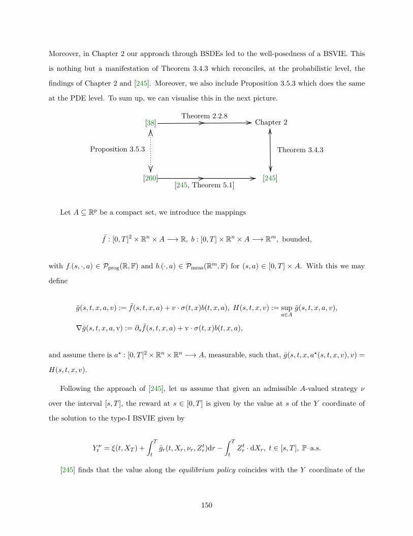
Moreover, in Chapter 2 our approach through BSDEs led to the well-posedness of a BSVIE. This

is nothing but a manifestation of Theorem 3.4.3 which reconciles, at the probabilistic level, the

findings of Chapter 2 and [245]. Moreover, we also include Proposition 3.5.3 which does the same

at the PDE level. To sum up, we can visualise this in the next picture.

[38]Theorem 2.2.8

Chapter 2

Proposition 3.5.3 Theorem 3.4.3

[260][245, Theorem 5.1]

[245]

Let A ⊆ Rp be a compact set, we introduce the mappings

f : [0, T ]2 × Rn ×A −→ R, b : [0, T ]× Rn ×A −→ Rm, bounded,

with f·(s, ·, a) ∈ Pprog(R,F) and b·(·, a) ∈ Pmeas(Rm,F) for (s, a) ∈ [0, T ] × A. With this we may

define

g(s, t, x, a, v) := f(s, t, x, a) + v · σ(t, x)b(t, x, a), H(s, t, x, v) := supa∈A

g(s, t, x, a, v),

∇g(s, t, x, a, v) := ∂sf(s, t, x, a) + v · σ(t, x)b(t, x, a),

and assume there is a? : [0, T ]2 ×Rn ×Rn −→ A, measurable, such that, g(s, t, x, a?(s, t, x, v), v) =

H(s, t, x, v).

Following the approach of [245], let us assume that given an admissible A-valued strategy ν

over the interval [s, T ], the reward at s ∈ [0, T ] is given by the value at s of the Y coordinate of

the solution to the type-I BSVIE given by

Y νt = ξ(t,XT ) +

∫ T

tgr(t,Xr, νr, Z

tr)dr −

∫ T

tZtr · dXr, t ∈ [s, T ], P–a.s.

[245] finds that the value along the equilibrium policy coincides with the Y coordinate of the

150

following type-I BSVIE

Yt = ξ(t,XT ) +∫ T

tgr(t,Xr, a

?(r, r,Xr, Zrr ), Ztr

)dr −

∫ T

tZtr · dXr, t ∈ [0, T ], P–a.s.,

where the diagonal of Z appears in the generator. However, decoupling the dependence between

the time variable and the variable source of time-inconsistency, we can define for any s ∈ [0, T ],

P–a.s., for any t ∈ [0, T ]

Y st := ξ(s,XT ) +

∫ T

tgr(s,Xr, a

?(r, r,Xr, Zrr ), Zsr

)dr −

∫ T

tZsr · dXr.

It then follows from Theorem 3.4.3 that this approach is equivalent to that of Chapter 2 based

on the system which for any s ∈ [0, T ], holds P–a.s. for any t ∈ [0, T ]

Yt = ξ(T,XT ) +∫ T

t

(Hr(r,Xr, Zr)− ∂Y r

r

)dr −

∫ T

tZr · dXr,

∂Y st = ∂sξ(s,XT ) +

∫ T

t∇gr(s,Xr, a

?(r, r,Xr, Zrr ), ∂Zsr )dr −

∫ T

t∂Zsr · dXr.

We now move on to establish the connection of the analyses at the PDE level. The original

result of [38] is based on the semi-linear PDE system of HJB type given for(V (t, x),J (s, t, x)

)∈

C1,2([0, T ]× Rn)× C1,1,2([0, T ]2 × Rn) and (s, t, x) ∈ O by

∂tV (t, x) + 12Tr[σσ>(t, x)∂xxV (t, x)] +H(t, t, x, ∂xV (t, x))− ∂sJ (t, t, x) = 0,

∂tJ (s, t, x) + 12Tr[σσ>(t, x)∂xxJ (s, t, x)] + g

(s, t, x, ∂xJ (s, t, x), a?

(t, t, x, ∂xV (t, x)

))= 0,

V (T, x) = ξ(T, x), J (s, T, x) = ξ(s, x), (s, x) ∈ [0, T ]× Rd.

(3.5.2)

On the other hand, [260] considers the equilibrium HJB equation for J (s, t, x) ∈ C1,1,2([0, T ]2×Rn)

and (s, t, x) ∈ O given by

∂tV(s, t, x) + 12Tr[σσ>(t, x)∂xxV(s, t, x)] + g

(s, t, x, ∂xV(t, t, x), a?

(t, t, x, ∂xV(t, t, x)

))= 0,

V(s, T, x) = ξ(s, x), (s, x) ∈ [0, T ]× Rd.(3.5.3)

By setting V(s, t, x) = J (s, t, x), it is immediate that a solution to (2.2.9) defines a solution to

151

(3.5.3). The next proposition establishes the converse result.

Proposition 3.5.3. Suppose (3.5.2) and (3.5.3) are well-posed.

(i) Let J (s, t, x) solve (3.5.2) Then V(s, t, x) := J (s, t, x) solves (3.5.3).

(ii) Let V(s, t, x) solve (3.5.3). Then(V (t, x),J (s, t, x)

):=(V(t, t, x),V(s, t, x)

)solves (3.5.2).

Proof. We are only left to argue (ii). It is clear(V (t, x),J (s, t, x)

)∈ C1,2([0, T ]×Rn)×C1,1,2([0, T ]2×

Rn), the results follows as −∂tV (t, x) + ∂sJ (t, t, x) = −∂tV(t, t, x).

3.6 Analysis of the BSDE system

In order to alleviate notations, and as it is standard in the literature, we suppress the dependence

on ω, i.e. on X, in the functionals, and, write E instead of EP as the underlying probability measure

P is fixed. Moreover, we will write I2 instead of I2(E) for any of the integrability spaces involved,

the specific space E is fixed and understood without ambiguity.

3.6.1 Regularity of the system and the diagonal processes

In preparation to the proof of Theorem 3.3.5, we present next a couple of lemmata from which

we will benefit in the following. As a historical remark, we mention the following is in the spirit of

the analysis in Protter [211, Section 3] and Pardoux and Protter [202] of forward Volterra integral

equations.

A technical detail in our analysis is to identify appropriate spaces so that given (∂U,U, V,M)

one can rigorously define the processes((U tt )t∈[0,T ], (V t

t )t∈[0,T ], (M tt )t∈[0,T ], (∂U tt )t∈[0,T ]

). It is known

that for U ∈ S2,2, the diagonal process (U tt )t∈[0,T ] is well-defined. Indeed, this follows from the

pathwise regularity of U s for s ∈ [0, T ] and has been noticed since [114; 256] and Chapter 2. The

same argument works for (∂U,M) ∈ S2,2 × M2,2. Unfortunately, the same reasoning cannot be

applied for arbitrary V ∈ H2,2 and motives the introduction of the space H2,2 , see Remark 3.3.3.

Lemma 3.6.1. Let Assumption G hold and (Y,Z) ∈ L2 ×H2. Let (U, V,M) ∈ L2,2 ×H2,2 ×M2,2

152

be a solution to

U st = η(s) +∫ T

tgr(s, U sr , V s


tV sr>dXr −

∫ T

tdM s

r , t ∈ [0, T ], P–a.s., s ∈ [0, T ];

(i) there exist (∂U, ∂V, ∂M) ∈ S2,2×H2,2×M2,2 unique solution to the equation, which for s ∈ [0, T ]

holds P–a.s. for any t ∈ [0, T ]

∂U st = ∂sη(s) +∫ T

t∇gr(s, ∂U sr , ∂V s

r , Usr , V

sr ,Yr,Zr)dr −

∫ T

t∂V s

r>dXr −

∫ T

td∂M s

r ; (3.6.1)

(ii) there exists C > 0, such that for all c > 4Lg and (s, t) ∈ [0, T ]2

E[ ∫ T

tecr|σ>r ∂V s

r |2dr]≤ CE

[ecT∣∣∂sη(s)

∣∣2 +(∫ T

tec2 r|∇gr(s)|dr

)2

+∫ T

tecr(|U sr |2 + |σ>r V s

r |2 + |Yr|2 + |σ>r Zr|2)dr];

(3.6.2)

(iii) for any s ∈ [0, T ], in S2 ×H2 ×M2,

(∫ T

s∂U rdr,

∫ T

s∂V rdr,

∫ T

s∂M rdr

)=(UT − U s, V T − V s,MT −M s); (3.6.3)

(iv) V ∈ H2,2. Moreover, for V := (V tt )t∈[0,T ] and ε > 0, P–a.s.

∫ T

t|σ>u Vu|2du ≤

∫ T

t|σ>u V t

u |2du+∫ T

t

∫ T

rε|σ>u V r

u |2 + ε−1|σ>u ∂V ru |2dudr, t ∈ [0, T ]. (3.6.4)

Proof. Note that in light of Assumption G.(i), for (t, s, x, u, v, y, z) ∈ [0, T ]2 × X × Rd2 × Rd2×n ×

Rd1 × Rd1×n, (u, v) 7−→ ∇gt(s, x,u, v, u, v, y, z) is linear. Therefore, for any s ∈ [0, T ] the second

equation defines a linear BSDE, in (∂U s, ∂V s), whose generator at zero, by Assumption G.(iii), is

in L1,2. Therefore, its solution (∂U s, ∂V s, ∂M s) ∈ S2×H2×M2 is well-defined from classic results,

see for instance Zhang [273] or [88]. The continuity of the applications s 7−→ (∂U s, ∂V s, ∂M s), e.g.

([0, T ],B([0, T ])) −→ (S2, ‖ · ‖S2) : s 7−→ ∂U s, follows from the classical stability results of BSDE,

and that by assumption (U, V, Y, Z) ∈ L2,2×H2,2×L2×H2 and s 7−→ (∂sη(s),∇g(s)) is continuous.

This establishes (∂U, ∂V, ∂M) ∈ S2,2 ×H2,2 ×M2,2.

153

(ii) follows from classic a priori estimates, but when the norms are considered over [t, T ] instead

of [0, T ]. Indeed, following the argument in [88, Proposition 2.1], applying Itô’s formula to ect|∂U st |2

we may find C > 0 such that for any c > 4Lg and (s, t) ∈ [0, T ]2

E[

supr∈[t,T ]

ecr∣∣∂U sr ∣∣2+

∫ T

tecr∣∣σ>r ∂V s

r

∣∣2dr +∫ T

tecr−d[∂M s]r

]

≤ CE[ecT∣∣∂sη(s)

∣∣2 +(∫ T

tec2 r∣∣∇gt(s, 0, 0, U sr , V s

r ,Yr,Zr)∣∣dr)2]

= CE[ecT∣∣∂sη(s)

∣∣2 +(∫ T

tec2 r∣∣∣∂sgr(s, U sr , V s

r ,Yr,Zr)∣∣∣dr)2]

≤ CE[ecT∣∣∂sη(s)

∣∣2 +(∫ T

tec2 r|∇gr(s)|dr

)2+∫ T

tecr(|U st |2 + |σ>t V s

t |2 + |Yt|2 + |σ>t Zt|2)dt],

where in the second inequality we exploited the fact (u, v, y, z) 7−→ ∂sg(t, s, x, u, v, y, z) is Lipschitz,

see Assumption G.(iii), and C > 0 was appropriately updated.

Next, we assume (iii) and show (iv). In light of (i) and (iii), s 7−→ ∂V s is the density of

s 7−→ V s with respect to the Lebesgue measure. Arguing as in Remark 3.2.2, we obtain that we

can define

V tt := V T

t −∫ T

t∂V r

t dr, dt⊗ dP–a.e. in [0, T ]×X . (3.6.5)

We now verify (3.6.4). By definition of V, Fubini’s theorem and Young’s inequality we have

that for ε > 0

∫ T

t|σ>u V u

u |2 − |σ>u V tu |2du =

∫ T

t

∫ u

t2Tr

[V ru>σuσ

>u ∂V

ru

]drdu

=∫ T

t

∫ T

r2Tr

[V ru>σuσ

>u ∂V

ru

]dudr

≤∫ T

t

∫ T

rε|σ>u V r

u |2 + ε−1|σ>u ∂V ru |2dudr.

Thus ‖V‖H2 <∞ and consequently V ∈ H2,2 . This proves (iv).

We now argue (iii). We also remark that a similar argument to the one in (i) shows that under

Assumption G U ∈ S2,2. We know the mapping [0, T ] 3 s 7−→ (∂Y s, ∂Zs, ∂M s) is continuous, in

154

particular integrable. A formal integration with respect to s to (3.6.1) leads to

∫ T

s∂U rt dr =

∫ T

s∂sη(r)dr +

∫ T

s

∫ T

t∂sgu(r, U ru, V r

u ,Yu,Zu) + ∂ygu(r, U ru, V ru ,Yu,Zu)∂U rududr

+∫ T

t

∫ T

s

n∑i=1

∂vigu(r, U ru, V ru ,Yu,Zu)(∂V r

u ):idudr

−∫ T

s

∫ T

t∂Zru

>dXudr −∫ T

t

∫ T

sd∂M r

udr.

Fix s ∈ [0, T ] and let (Π`)` be a properly chosen sequence of partitions of [s, T ], as in van

Neerven [240, Theorem 1], Π` = (si)i=1,...,n` with ‖Π`‖ := supi |si+1− si| ≤ `. To ease the notation,

we set ∆sì := sì−sì−1, and, for a generic family process (φs)s∈[0,T ], and a mapping s 7−→ ∂sη(s, x),

we define

I`(φ) :=n∑i=0

∆sìφsì , δφ := φT − φs, I`(∂sη(·, x)) :=

n∑i=0

∆sì∂sη(sì , x), δη(x) := η(T, x)− η(s, x).

We then notice that for any t ∈ [0, T ]

I`(∂U)t − (δU)t = I`(∂sη(·))− δη +∫ T

t

[I`(∂zgu(·, U ·u, V ·u,Yu,Zu)∂V ·u

)− δgu(·, U ·u, V ·u,Yu,Zu)

]du

+∫ T

t

[I`(∂sgu(·, U ·u, V ·u,Yu,Zu)

)+ I`

(∂ygu(·, U ·u, V ·u,Yu,Zu)∂U ·u

)]du

−∫ T

t

(I`(∂V )r − (δV )r

)>dXu − I`(∂M ·T − ∂M ·t)− δ(MT −Mt).

We now note that the integrability of (∂U, ∂V ) and (U, V ) yields I`(∂U)−(δU) ∈ S2,2 and I`(∂V )−

(δV ) ∈ H2,2. Therefore, Bouchard, Possamaï, Tan, and Zhou [40, Theorem 2.2] yields

‖I`(∂U)− (δU)‖2S2,2 + ‖I`(∂V )− (δV )‖2H2,2 + ‖I`(∂M)− (δM)‖2M2,2

≤ CE[∣∣I`(∂sη(·))− δη

∣∣2 +(∫ T

t

∣∣∣I`(∂sgu(·, U ·u, V ·u,Yu,Zu))− δgu(·, U ·u, V ·u,Yu,Zu)

∣∣∣du)2].

To conclude, we first note that by our choice of (Π`)`, I`(∂U) converges to the Lebesgue integral

of ∂U s. In addition, the uniform continuity of s 7−→ ∂sη(s, x) and s 7−→ ∂sg(s, x, u, v, y, z), see

Assumption G.(i), justifies, via bounded convergence, the convergence in S2,2 (resp. H2,2) of I`(∂U s)

to UT − U s (resp. I`(∂V s) to V T − V s) as ` −→ 0. The result follows in virtue of the uniqueness

155

of (U, V,M).

The next lemma identifies the dynamics of (U tt )t∈[0,T ].

Lemma 3.6.2. Let (Y,Z) ∈ L2×H2 and (U, ∂U, V, ∂V,M, ∂M) ∈ (L2,2)2×H2,2×H2,2×(M2,2)2

satisfy for any s ∈ [0, T ], P–a.s. for any t ∈ [0, T ]

U st = η(s,X·∧T ) +∫ T

tgr(s,X,U sr , V s


tV sr>dXr −

∫ T

tdM s

r ,

∂U st = ∂sη(s,X·∧T ) +∫ T


r , Usr , V

sr ,Yr,Zr)dr −

∫ T

t∂V s

r>dXr −

∫ T

td∂M s

r .

Then

U tt = UTT +∫ T

t

(gr(r, U rr , V r

r ,Yr,Zr)− ∂U rr)dr −

∫ T

tV rr dXr −

∫ T

tdMr, t ∈ [0, T ], P–a.s.,

where M := (Mt)t∈[0,T ] is given by Mt := M tt −

∫ t0 ∂M

rr dr. Moreover, M ∈M2.

Proof. We show that P–a.s., for any t ∈ [0, T ]

∫ T

t∂U rr dr = UTT − U tt +

∫ T

tgr(r, U rr , V r


tV rr dXr −

∫ T

tdMr.

Indeed, note that, P–a.s., for any t ∈ [0, T ]

∫ T

t∂U rr dr =

∫ T

t∂sη(r)dr +

∫ T

t

(∫ T

r∇gu(r, ∂U ru, ∂V r

u , Uru, V

ru ,Yu,Zu)du

)dr

−∫ T

t

(∫ T

r∂V r

u>dXu −

∫ T

rd∂M r

u

)dr.

By Fubini’s theorem, the change of variables formula for the Lebesgue integral, [212, Theorem

54], and Lemma 3.6.1 we have that, P–a.s., for any t ∈ [0, T ]

∫ T

t

∫ T

r∇gu(r, ∂U ru, ∂V r

u , Uru, V

ru ,Yu,Zu)dudr

=∫ T

t

∫ u

t∇gu(r, ∂U ru, ∂V r

u , Uru, V

ru ,Yu,Zu)drdu

=∫ T

tgu(u, Uuu , V u

u ,Yu,Zu)− gu(t, U tu, V tu ,Yu,Zu)du.

Similarly, given ∂V ∈ H2,2, the version of Fubini’s theorem for stochastic integration, see [212,

156

Theorem 65], yields

∫ T

t

∫ T

r∂V r

u>dXudr =

∫ T

t

∫ u

t∂V r

u>drdXu =

∫ T

t

(V uu − V t

u)>dXu.

Now, by Lemma 3.6.1 we have that, P–a.s., for any t ∈ [0, T ]

∫ T

t

∫ T

rd∂M r

udr =∫ T

t

(∂M r

T − ∂M rr

)dr = MT − Mt +M t

t −M tT .

We are left to verify M ∈M2. Indeed, note that M0 = 0 and

(i) M has càdlàg paths. This follows from the fact that, as F satisfies the usual conditions, there

exist a càdlàg modification of (M tt )t∈[0,T ], which, abusing notations, we still denote by (M t

t )t∈[0,T ].

Indeed for t ∈ [0, T ]

M tt = MT

t −∫ T

t∂M r

t dr, P–a.s.

(ii) M is a martingale. Indeed by Lemma 3.6.1, for 0 ≤ u ≤ t ≤ T , P–a.s.

E[Mt|Fu

]= E

[M tt |Fu

]−∫ u

0∂M r

r dr −∫ t

uE[∂M r

r

∣∣Fu]dr = M tu −

∫ u

0∂M r

r dr −∫ t

u∂M r

udr = Mu;

(iii) M is orthogonal to X. For 0 ≤ u ≤ t ≤ T , P–a.s.

E[XtMt

∣∣Fu] = E[XtM

tt

∣∣Fu]− E[Xt

∫ u

0∂M r

r dr∣∣∣Fu]− ∫ t

uE[E[Xt|Fr

]∂M r

r |Fu]dr

= XuMtu −Xu

∫ u

0∂M r

r dr −Xu

∫ t

u∂M r

udr

= XuMtu −Xu

∫ u

0∂M r

r dr −XuMtu +XuM

uu

= XuMu,

where in the second equality we used the fact∫ u

0 ∂Mrr dr is Fu-measurable, the tower property and

the orthogonality of M s and X and of ∂M s and X for s ∈ [0, T ]. The third equality follows from

Lemma 3.6.1.

157

(iv) ‖M‖M2 <∞,

‖M‖2M2 = E[∣∣∣∣MT

T −∫ T

0∂M r

r dr∣∣∣∣2]

≤ 2(E[[MT ]T

]+ T

∫ T

0E[[∂M r]r

]dr)≤ 2

[‖MT ‖2M2 + T 2‖∂M‖2M2,2

]<∞.

3.6.2 A priori estimates

We now establish a priori estimates for (S). To ease the readability, recall it holds for any

s ∈ [0, T ], holds P–a.s. for any t ∈ [0, T ]

Yt = ξ(T,X·∧T ) +∫ T


r , ∂Urr )dr −

∫ T

tZ>r dXr −

∫ T

tdNr,

U st = η(s,X·∧T ) +∫ T

tgr(s,X,U sr , V s


tV sr>dXr −

∫ T

tdM s

r (S)

∂U st = ∂sη(s,X·∧T ) +∫ T


r , Usr , V

sr ,Yr,Zr)dr −

∫ T

t∂V s

r>dXr −

∫ T

td∂M s

r .

Let us introduce (Ho, ‖ ·‖Ho) and (Ho, ‖ ·‖Ho) where ‖ ·‖Ho and ‖ ·‖Ho denote the norms induced

by

Ho := L2 ×H2 ×M2 × L2,2 ×H2,2 ×M2,2 × L2,2 ×H2,2 ×M2,2,

Ho := L2 ×H2 ×M2 ×(L2,2 ×H2,2 ×M2,2)2.

To obtain estimates between the difference of solutions, it is more convenient to work with

norms defined by adding exponential weights. We recall, for instance, that for c ∈ [0,∞) the norm

‖ · ‖H2,c is given by

‖Z‖2H2,c = E[ ∫ T

0ect|σ>t Zt|2dt

],

and they are equivalent for any two values of c, since [0, T ] is compact. With this, we define the

norm ‖ · ‖Ho,c . In the following, we take the customary approach of introducing arbitrary constants

C > 0 to our analysis. These constants will typically depend on the data of the problem, e.g. the

Lipschitz constants and T and on the value of c unless otherwise stated.

158

Proposition 3.6.3. Let Assumption G hold and (Y,Z,N , U, V,M, ∂U, ∂V, ∂M) ∈ Ho satisfy (S).

Then (Y, U, ∂U) ∈ S2 × S2,2 × S2,2. Furthermore, there exists a constant C > 0 such that for ‖ · ‖H

as in Section 3.3

‖h‖2H ≤ C(‖ξ‖2L2 + ‖η‖2L2,2 + ‖∂sη‖2L2,2 + ‖h‖2L1,2 + ‖g‖2L1,2,2 + ‖∇g‖2L1,2,2

)︸︷︷︸

=:I20

<∞.

Proof. We proceed in several steps. We recall that in light of Assumption G, dt⊗ dP–a.e.

|hr(Yr,Zr, U rr , V rr , ∂U

rr ))| ≤ |h|+ Lh

(|Yr|+ |σ>r Zr|+ |U rr |+ |σ>r V r

r |+ |∂U rr |),

|gr(s, U sr , V sr ,Yr,Zr))| ≤ |g(s)|+ Lg

(|U sr |+ |σ>r V s

r |+ |Yr|+ |σ>r Zr|), (3.6.6)

|∇gr(s, ∂U sr , ∂V sr , U

sr , V

sr ,Yr,Zr))| ≤ |∇gr(s)|+ L∂sg

(|U sr |+ |σ>r V s

r |+ |Yr|+ |σ>r Zr|)

+ Lg(|∂U sr |+ |σ>r ∂V s

r |).

Step 1: we start with auxiliary estimates. By Meyer–Itô’s formula for ec2 t|∂U st |, see Protter

[212, Theorem 70]

ec2 t|∂U st |+ L0

T −∫ T

tec2 r sgn(∂U sr ) · ∂V s

r>dXr −

∫ T

tec2 r− sgn(∂U sr−) · d∂M s

r

= ec2T |∂sη(s)|+

∫ T

tec2 r(

sgn(∂U sr ) · ∇gr(s, ∂U sr , ∂V sr , U

sr , V

sr ,Yr,Zr)−

c

2 |∂Usr |)

dr,(3.6.7)

where L0 := L0(∂U s) denotes the non-decreasing and pathwise-continuous local time of the semi-

martingale ∂U s at 0, see [212, Chapter IV, pp. 216]. We also notice that for any s ∈ [0, T ] the last

two terms on the left-hand side are martingales, recall that ∂V s ∈ H2.

We now take conditional expectation with respect to Ft in Equation (3.6.7). We may use (3.6.6)

and the fact L0 is non-decreasing to derive that for t ∈ [0, T ] and c > 2Lg

ec2 t|∂U st | ≤ Et

[ec2T |∂sη(s)|+

∫ T

tec2 r(|∂U sr |(Lg − c/2) + |∇gr(s)|+ Lg|σ>r ∂V s

r |)dr

+∫ T

tec2 rL∂sg

(|U sr |+ |σ>r V s

r |+ |Yr|+ |σ>r Zr|)dr]

159

≤ Et[ec2T |∂sη(s)|

+∫ T

tec2 r(|∇gr(s)|+ L

(|σ>r ∂V s

r |+ |U sr |+ |σ>r V sr |+ |Yr|+ |σ>r Zr|

))dr].

(3.6.8)

where L := maxLg, L∂sg. Squaring in (3.6.8), we may use (I.1) and Jensen’s inequality to

derive for t ∈ [0, T ]

ect

7 |∂Utt |2 ≤ Et

[ecT |∂sη(t)|2 + T L2

∫ T

tecr(|U tr |2 + |Yr|2 + |σ>r ∂V t

r |2 + |σ>r V tr |2 + |σ>r Zr|2

)dr]

+ Et[( ∫ T

tec2 r|∇gr(t)|dr

)2].

Integrating the previous expression and taking expectation, it follows from the tower property

that for any t ∈ [0, T ]

17E[ ∫ T

tecr|∂U rr |2dr

]≤ E

[ ∫ T

tecT |∂sη(r)|2dr

]+ E

[ ∫ T

t

(∫ T

rec2u|∇gu(r)|du

)2dr]

+ T L2E[ ∫ T

t

∫ T

recu(|U ru|2 + |Yu|2 + |σ>u ∂V r

u |2 + |σ>u V ru |2 + |σ>u Zu|2

)dudr

]≤ T sup

r∈[0,T ]

‖ecT |∂sη(r)|2]‖L2 + E

[( ∫ T

tec2u|∇gu(r)|du

)2]

+ T 2L2 supr∈[0,T ]

E[ ∫ T

tecu(|U ru|2 + |σ>u V r

u |2 + |σ>u ∂V ru |2)du]

+ T 2L2E[ ∫ T

tecu(|Yu|2 + |σ>u Zu|2

)du].

Thus, we obtain there is C∂u > 0 such that for any c > 2Lg and t ∈ [0, T ]

1C∂u

E[ ∫ T

tecr|∂U rr |2dr

]≤ ecT

(‖∂sη‖2L2,2 + ‖∇g‖2L1,2,2

)+ E

[ ∫ T

tecr(|Yr|2 + |σ>r Zr|2

)dr]

+ sups∈[0,T ]

E[ ∫ T


r |2 + |σ>r ∂V sr |2)dr].

(3.6.9)

Similarly, we may find Cu > 0 such that for any c > 2Lg and t ∈ [0, T ]

1Cu

E[ ∫ T

tecr|U rr |2dr

]≤ ecT

(‖η‖2L2,2 + ‖g‖2L1,2,2

)+ E

[ ∫ T


)dr]

+ sups∈[0,T ]

E[ ∫ T

tecr|σ>r V s

r |2dr].

(3.6.10)

160

We now estimate the term V tt . In light of (3.6.2) and (3.6.4), with ectσ>t instead of σ>t , there

exists C > 0 such that for any ε > 0, c > 4Lg and t ∈ [0, T ]

E[ ∫ T

tecu|σ>u V u

u |2du]

≤ E[ ∫ T

tecu|σ>u V t

u |2du]

+∫ T

tE[ ∫ T

recu(ε|σ>u V r

u |2 + ε−1|σ>u ∂V ru |2)du]dr

≤ supr∈[0,T ]

E[ ∫ T

tecu|σ>u V r

u |2du]

+ T supr∈[0,T ]

E[ ∫ T

tecu(ε|σ>u V r

u |2 + |σ>u ∂V ru |2/ε

)du]

≤ (1 + εT ) supr∈[0,T ]

E[ ∫ T

tecu|σ>u V r

u |2du]

+ TC/εE[ ∫ T

tecu(|Yu|2 + |σ>u Zu|2

)du]

+ TCε−1 supr∈[0,T ]

E[ ∫ T

tecu(|U ru|2 + |σ>u V r

u |2)du]

+ TCε−1ecT supr∈[0,T ]

E[∣∣∂sη(r)

∣∣2 +(∫ T

t|∇gu(r)|du

)2].

Thus, taking ε = TC we may find Cv > 0 such that for any c > 4Lg and t ∈ [0, T ]

1Cv

E[ ∫ T

tecu|σ>r V r

r |2dr]≤ ecT

(‖∂sη‖2L2,2 + ‖∇g‖2L1,2,2

)+ E

[ ∫ T


)dr]

+ sups∈[0,T ]

E[ ∫ T


r |2)dr].

(3.6.11)

We emphasise that the constants (C∂u, Cu, Cv) ∈ (0,∞)3 depend only of the data of the problem

and are universal for any value of c > 4Lg.

Step 2: Let s ∈ [0, T ], we show that (Y, U, ∂U) ∈ S2× S2,2× S2,2. To alleviate the notation we

introduce

Y := (Y, U s, ∂U s), Z := (Z, V s, ∂V s), N := (N ,M s, ∂M s),

whose elements we may denote with superscripts, e.g. Y1, Y2, Y3 correspond to Y, U s, ∂U s.

By (I.1) and (3.6.6), we obtain that there exists C > 0, which may change value from line to

line, such that

|U st |2 ≤ C

(|η(s)|2 +

(∫ T

0|gr(s)|dr

)2+∫ T

0

(|U sr |2 + |σ>r V s

r |2 + |Yr|2 + |σ>r Zr|2)dr

+∣∣∣∣ ∫ T

tV sr>dXr

∣∣∣∣2 +∣∣∣∣ ∫ T

tdM s

r

∣∣∣∣2).

161

We note that by Doob’s inequality

E[

supt∈[0,T ]

∣∣∣∣ ∫ t

0V sr>dXr

∣∣∣∣2]≤ 4‖V s‖2H2 . (3.6.12)

Taking supremum over t ∈ [0, T ] and expectation we obtain for s ∈ [0, T ]

‖U s‖2S2 ≤ C(‖η(s)‖2L2 + ‖g(s)‖2L1,2

+ ‖U s‖2L2 + ‖V s‖2H2 + ‖Y‖2L2 + ‖Z‖2H2 + ‖M s‖2M2)<∞.

(3.6.13)

Similarly, we obtain that there exists C > 0 such that for s ∈ [0, T ]

‖∂U s‖2S2 ≤ C(‖∂sη(s)‖2L2 + ‖∇g(s)‖2L1,2 +

3∑i=1‖Yi‖2L2 + ‖Zi‖2H2 + ‖∂M s‖2M2

)<∞. (3.6.14)

Given (η, ∂sη, g, ∂g) ∈ (L2,2)2 × (L1,2,2)2, (U, ∂U, V, ∂V,M, ∂M) ∈ (L2,2)2 × (H2,2)2 × (M2,2)2,

(3.6.13) and (3.6.14), the mapping

([0, T ],B([0, T ])) −→ (S2, ‖ · ‖S2) : s 7−→ Yis is continuous for i ∈ 2, 3,

and ‖Yi‖S2,2 <∞. Consequently, Yi ∈ S2,2 for i ∈ 2, 3. Arguing as above we may also derive,

|Yt|2 ≤ C(|ξ|2 +

(∫ T

0|hr|dr

)2+∫ T

0

(|Yr|2 + |σ>r Zr|2 + |U rr |2 + |σ>r V r

r |2 + |∂U rr |2)dr

+∣∣∣∣ ∫ T

tZ>r dXr

∣∣∣∣2 +∣∣∣∣ ∫ T

tdNr

∣∣∣∣2),which in turn yields, in combination with (3.6.9), (3.6.10) and (3.6.11),

‖Y‖2S2 ≤ C(I2

0 + ‖Y‖2L2 + ‖Z‖2H2 + ‖U‖2L2,2 + ‖V ‖2H2,2 + ‖∂V ‖2H2,2 + ‖N‖2M2)<∞. (3.6.15)

Finally, taking sup over s ∈ [0, T ] and adding together (3.6.15) (3.6.13) and (3.6.14) we obtain

‖Y‖2S2 + ‖U s‖2S2,2 + ‖∂U‖2S2,2 ≤ C(I2

0 + ‖(Y,Z,N , U, V,M, ∂U, ∂V, ∂M)‖Ho). (3.6.16)

162

Step 3: We obtain the estimate of the norm. To ease the notation we introduce

hr := hr(Yr,Zr, U rr , V rr , ∂U

rr ), gr(s) := gr(s, U sr , V s

r ,Yr,Zr),

∇gr(s) := ∇gr(s, ∂U sr , ∂V sr , U

sr , V

sr ,Yr,Zr).

By applying Itô’s formula to ect(|Yt|2 + |U st |2 + |∂U st |2

)we obtain, P–a.s.

3∑i=1

ect∣∣Yi

t

∣∣2 +∫ T

tecr∣∣σ>r Zir∣∣2dr +

∫ T

tecr−d

[Ni]

r+ Mt −MT

= ecT (|ξ(T )|2 + |η(s)|2 + |∂sη(s)|2)

+∫ T

tecr(2Yr · hr + 2U sr · gr(s) + 2∂U sr · ∇gr(s)− c(|Yr|2 + |U sr |2 + |∂U sr |2)

)dr,

where we used the orthogonality of X and both M s and N , and we introduced the martingale

Mt := 23∑i=1

∫ t

0ecrYi

r · Zir> dXr +

∫ t

0ecr−Yi

r− · dNir.

Indeed, the Burkholder–Davis–Gundy inequality together with the fact that (Y, U s, ∂U s) ∈

(S2)3 shows that M is uniformly integrable, and consequently a true martingale. Moreover, we

insist on the fact that the integrals with respect to N , M s and ∂M s account for possible jumps,

see [142, Lemma 4.24].

Moreover, as (Y, U, ∂U) ∈ S2× (S2,2)2, from (3.6.6) and with Young’s inequality we obtain that

for any (ε, ε) ∈ (0,∞)2, there is C(ε) ∈ (0,∞) such that the left-hand side above is smaller than

≤ ecT(|ξ|2 + |η(s)|2 + |∂sη(s)|2

)+∫ T

tecr(C(ε)− c)

(|Yr|2 + |U sr |2 + |∂U sr |2

)dr

+∫ T

tεecr

(|σ>r Zr|2 + |σ>r V s

r |2 + |σ>r ∂V sr |2 + 1

Cu|U rr |2 + 1

Cv|V rr |2 + 1

C∂u|∂U rr |2

)dr

+ ε3∑i=1

supr∈[0,T ]

ecr∣∣Yi

t

∣∣2 + 1ε

(∫ T

0ec2 r|hr|dr

)2+ 1ε

(∫ T

0ec2 r|gr(s)|dr

)2+ 1ε

(∫ T

0ec2 r|∇gr(s)|dr

)2,

with (C∂u, Cu, Cv) as in (3.6.9)-(3.6.11). Taking expectation and letting c > 4Lg, we find there

163

is C > 0 such that

E[ 3∑i=1

ect∣∣Yi

t

∣∣2 +∫ T

tecr∣∣σ>r Zir∣∣2dr +

∫ T

tecr−d

[Ni]

r

]

≤ E[ ∫ T

tecr|Yr|2(C(ε)− c)dr

]+ sups∈[0,T ]

E[ ∫ T

tecr|U sr |2(C(ε)− c)dr

]

+ sups∈[0,T ]

E[ ∫ T

tecr|∂U sr |2(C(ε)− c)dr

]+ εC

(‖Y‖2S2,c + ‖U‖2S2,2,c + ‖∂U‖2S2,2,c

)+ (1 + ε−1 + ε)CI2

0 + εC(‖Z‖2H2,c + ‖V ‖2H2,2,c + ‖∂V ‖2H2,2,c

).

We then let ε = 1/(24C), c ≥ max4Lg, C(ε), and take sup over t ∈ [0, T ] (resp. (s, t) ∈ [0, T ]2)

to each term on the left side separately. Adding these terms up we find there is C > 0, such that

for any ε > 0

1T‖h‖Ho ≤ sup

t∈[0,T ]E[ect|Yt|2

]+ sup

(s,t)∈[0,T ]2E[ect|U st |2

]+ sup

(s,t)∈[0,T ]2E[ect|∂U st |2

]+ ‖Z‖2H2 + ‖V ‖2H2,2 + ‖∂V ‖2H2,2 + ‖N‖2M2 + ‖M‖2M2,2 + ‖∂M‖2M2,2

≤ (1 + ε−1)CI20 + εC

(‖Y‖2S2 + ‖U‖2S2,2 + ‖∂U‖2S2,2

).

(3.6.17)

We can the use (3.6.17) back in (3.6.16) to find ε ∈ (0,∞) small enough so that4 ‖h‖2H ≤ CI20 .

The result in terms of the norm ‖ · ‖H follows from (3.6.11).

Proposition 3.6.4. Let (ξi, ηi, ∂sηi) ∈ L2 × (L2,2)2 and (hi, gi, ∂sgi) for i ∈ 1, 2 satisfy As-

sumption G and suppose that hi ∈ Ho is a solution to (S) with coefficients (ξi, hi, ηi, gi, ∂sηi,∇gi),

i ∈ 1, 2. Then

‖δh‖2H ≤ C(‖δξ

∥∥2L2 + ‖δη

∥∥2L2,2 + ‖δ∂η

∥∥2L2,2 + ‖δ1h‖2L1,2 + ‖δ1g‖2L1,2,2 + ‖δ1∇g‖L1,2,2

),

where for ϕ ∈ Y,Z,N , U, V,M, ∂U, ∂V, ∂M, ξ, η, ∂sη and Φ ∈ h, g,∇g

δϕ := ϕ1−ϕ2, and, δ1Φt := Φ1t (Y1

r ,Z1t , U

1tt , V

1tt )−Φ2

t (Y1r ,Z1

t , U1tt , V

1tt ), dt⊗dP–a.e. in [0, T ]×X .

Proof. Note that by the Lipschitz assumption on h and g there exist bounded processes with4Recall the norm ‖ · ‖H is the norm induced by the space H as defined in Remark 3.3.3.(ii)

164

appropriate dimensions (αi, βi, γi, εi), i ∈ 1, 2, 3, ρ and % such that for every s ∈ [0, T ], P–a.s.,

t ∈ [0, T ]

δYt = δξ(T )−∫ T

tδZ>r dXr −

∫ T

tdδNr,

+∫ T

t

(δ1hr + γ1

r δYr + α1>r σ>r δZr + β1

r δUrr + ε1>

r σ>r δVrr

)dr

δU st = δη(s)−∫ T

tδV s>

r dXr −∫ T

tdδM s

r

+∫ T

t

(δ1gr(s) + β2

r δUsr + ε2>

r σ>r δVsr + γ2

r δYr + α2>r σ>r δZr

)dr,

δ∂U st = δ∂sη(s)−∫ T

tδ∂V s

r>dXr −

∫ T

tdδ∂M s

r

+∫ T

t

(δ1∇gr(s) + ρrδ∂U

sr + %rδ∂V

sr + β3

r δUsr + ε3>

r σ>r δVsr + γ3

r δYr + α3>r σ>r δZr

)dr.

We can therefore apply Proposition 3.6.3 and the result follows.

When the data of the system is chosen so as to study the class of type-I BSVIEs considered in

Section 3.4, our approach can be specialised so as to enlarge the initial space and simplify the a

priori estimates obtained in Proposition 3.6.3. We let (H?,o, ‖ · ‖H?,o) be

H?,o := L2 ×H2 ×M2 × L2,2 ×H2,2 ×M2,2,

‖(Y,Z,N , Y, Z,N)‖2H?,o := ‖Y‖2L2 + ‖Z‖2H2 + ‖N‖2M2 + ‖Y ‖2L2,2 + ‖Z‖2H2,2 + ‖N‖2M2,2 .

Proposition 3.6.5. Let Assumption H hold and consider (Y,Z,N , Y, Z,N) ∈ H?,o solution to the

system which for any s ∈ [0, T ], holds P–a.s. for any t ∈ [0, T ]

Yt = ξ(T,X) +∫ T

t

(fr(r,X,Yr,Zr, Y r

r )− ∂Y rr

)dr −

∫ T

tZ>r Xr −

∫ T

tNr,

Y st = ξ(s,X) +

∫ T

tfr(s,X, Y s

r , Zsr ,Yr)dr −

∫ T

tZsr>dXr −

∫ T

tdN s

r , t ∈ [0, T ],(Sof )

with ∂Y given as in Lemma 3.6.1. Then (Y, Y ) ∈ S2 × S2,2 and there exist C > 0 such that

‖(Y,Z,N , Y, Z,N)‖2H? ≤ C(‖ξ‖2L2,2 + ‖f‖2L1,2,2

)<∞.

Proof. We first note that Y ∈ S2,2 follows as in Proposition 3.6.3. Thus, in light of Lemma 3.6.1,

165

there exists (∂Y, ∂Z, ∂N) ∈ S2,2 × H2,2 × M2,2 solution to the BSDE with data (∂sξ, ∂f), and,((Y tt )t∈[0,T ], (Ztt )t∈[0,T ]

)∈ S2 ×H2 are well-defined. Moreover, ∂Y r

r is well-defined as an element of

L1,2, i.e. dt ⊗ dP–a.e. on [0, T ] × X , as a consequence of the path-wise continuity of ∂Y s· . With

this, we conclude Y ∈ S2.

Let us now note that given (Y tt )t∈[0,T ], (Ztt )t∈[0,T ] and (∂Y t

t )t∈[0,T ], the first equation, being a

Lipschitz BSDE, admits a unique solution (Y,Z,N ). In addition, for N as in Lemma 3.6.2 we

obtain

Y tt = Y T

T +∫ T

t

(fr(r, Y r

r , Zrr ,Yr)− ∂Y r

r

)dr −

∫ T

tZrr>dXr −

∫ T

tdNr, t ∈ [0, T ], P–a.s. (3.6.18)

Thus,(Y·,Z·,N·

)=((Y tt )t∈[0,T ], (Ztt )t∈[0,T ], (Nt)t∈[0,T ]

)in S2 ×H2 ×M2 and we obtain

Yt = ξ(t) +∫ T

tfr(t, Y t

r , Ztr,Yr)dr −

∫ T

tZtr>dXr −

∫ T

tdN t

r , t ∈ [0, T ], P–a.s. (3.6.19)

With this equation we can simplify our estimates. Let us introduce the system

Yt = ξ(t) +∫ T

tfr(t, Y t

r , Ztr,Yr)dr −

∫ T

tZtr>dXr −

∫ T

tdN t

r , t ∈ [0, T ], P–a.s.,

Y st = ξ(s) +

∫ T

tfr(s, Y s

r , Zsr ,Yr)dr −

∫ T

tZsr>dXr −

∫ T

tdN s

r , t ∈ [0, T ], P–a.s., s ∈ [0, T ].(A)

Then, following the same reasoning of Proposition 3.6.3, i.e. applying Ito’s formula to ect(|Yt|+|Y s

t |)

in combination with Young’s inequality, we obtain there is C > 0 such that ‖(Y,Z,N , Y, Z,N)‖2H? ≤

C(‖ξ‖2L2,2 + ‖f‖2L1,2,2

)<∞.

3.6.3 Proof of Theorem 3.3.5

Before we present the proof of Theorem 3.3.5 we recall that in light of Proposition 3.6.3 and

Proposition 3.6.4 once the result is obtained for Ho the existence of a unique solution in H follows

immediately.

Proof of Theorem 3.3.5. Note that uniqueness follows from Proposition 3.6.4. To show existence,

166

let us define the map

T : Ho −→ Ho

(y, z, n, u, v,m,u, v,m) 7−→ (Y, Z,N,U, V,M, ∂U, ∂V, ∂M),

with (Y,Z,N , U, V,M, ∂U, ∂V, ∂M) given for any s ∈ [0, T ], P–a.s. for any t ∈ [0, T ] by

Yt = ξ(T,X·∧T ) +∫ T

thr(X, yr, zr, U rr , V r

r , ∂Urr )dr −

∫ T

tZ>r dXr −

∫ T

tdNr,

U st = η(s,X·∧,T ) +∫ T

tgr(s,X,U sr , V s

r , yr, zr)dr −∫ T

tV sr>dXr −

∫ T

tdM s

r ,

∂U st = ∂sη(s,X·∧,T ) +∫ T


r , Usr , V

sr , yr, zr)dr −

∫ T

t∂V s

r>dXr −

∫ T

td∂M s

r .

Step 1: We first show T is well defined. Let (y, z, n, u, v,m,u, v,m) ∈ Ho.

(i) Let us first consider the tuples (U, V,M) and (∂U, ∂V, ∂M). Let us first consider the second

equation. Given (y, z) ∈ S2 × H2 and Assumption G, this equation is a standard Lipschitz BSDE

whose well-posedness follows by classical arguments, see [273; 88]. This yields (U s, V s,M s) ∈

S2 ×H2 ×M2 for all s ∈ [0, T ].

Let us argue the continuity of ([0, T ],B([0, T ])) −→ (L2, ‖ · ‖L2) : s 7−→ U s. Let (sn)n ⊆

[0, T ], snn→∞−−−→ s0 ∈ [0, T ] and define for ϕ ∈ U, V, η, ∆ϕn := ϕsn − ϕs0 . From the classic

stability result for BSDEs we obtain that there is C > 0 such that

E[ ∫ T

0|∆Unt |2dr

]≤ 2T

(‖∆ηn‖2L2 + TL2

g

(ρ2g(|sn − s0|)

).

We conclude ‖U‖L2,2 <∞ and U ∈ L2,2. Given (U s, V s) ∈ L2×H2 together with (y, z) ∈ S2×H2,

the argument for (∂U s, ∂V s, ∂M s) for fixed s ∈ [0, T ] is identical.

(ii) We now show that (V, ∂V,M, ∂M) ∈ (H2,2)2 × (M2,2)2. Again, the argument for (∂V, ∂M) is

completely analogous. Applying Ito’s formula to |U sr |2 we obtain

|U st |2 +∫ T

t|σ>r V s

r |2dr +∫ T

td[M s]r = |η(s)|2 + 2

∫ T

tU sr · gr(s, U sr , V s

r , yr, zr)dr

167

− 2∫ T

tU sr · V s

r>dXr − 2

∫ T

tU sr− · dM s

r .

First note U s ∈ S2 guarantees that the last two terms are true martingale for any s ∈ [0, T ].

To show that ([0, T ],B([0, T ])) −→ (H2, ‖ · ‖H2)(resp. (M2, ‖ · ‖M2)

): s 7−→ V s

(resp. M s

)is

continuous, let (sn)n ⊆ [0, T ], snn→∞−−−→ s0 ∈ [0, T ]. We then deduce there is C > 0 such that

E[ ∫ T

0|σ>r ∆V n

r |2dr + [∆M s]T]≤ C

(‖∆η‖2L2 + ρ2

g(|sn − s0|)),

and, likewise, we obtain

sups∈[0,T ]

E[ ∫ T

0|σ>r V s

r |2dr + [M s]T]≤ C

(‖η‖2L2,2 + ‖g‖2L1,2

)<∞.

Since the first term on the right-hand side is finite from Assumption G, we obtain ‖V ‖H2,2 +

‖M‖M2,2 <∞.

We are left to argue V ∈ H2,2 . Applying Lemma 3.6.1 to the system, which for any s ∈ [0, T ]

satisfies P–a.s. for any t ∈ [0, T ]

U st = η(s,X·∧,T ) +∫ T

tgr(s,X,U sr , V s

r , yr, zr)dr −∫ T

tV sr>dXr −

∫ T

tdM s

r ,

∂U st = ∂sη(s,X·∧,T ) +∫ T


r , Usr , V

sr , yr, zr)dr −

∫ T

t∂V s

r>dXr −

∫ T

td∂M s

r ,

we obtain s 7−→ V s is absolutely continuous with density s 7−→ ∂V s. Consequently, we may define

the diagonal of V , denoted by V := (V tt )t∈[0,T ], as in Equation (3.6.5), with

V tt := V T

t −∫ T

t∂V r

t dr, dt⊗ dP–a.e. in [0, T ]×X .

The fact ‖V‖H2 <∞ follows as in Lemma 3.6.1.(iv). This yields V ∈ H2 and we conclude V ∈ H2,2 .

(iii) We derive an auxiliary estimate. Recall (U, V,M, ∂U, ∂V, ∂M) satisfy (3.6.3). Now, in light of

Assumption G and (ii), we may find, as in Step 1 in Proposition 3.6.3, a universal constant C > 0

168

such that for any c > 4Lg and t ∈ [0, T ]

1CE[ ∫ T

tecr(|U rr |2 + |∂U rr |2 + |σ>r V r

r |2)dr]

≤ ecT(‖η‖2L2,2 + ‖g‖2L1,2 + ‖∂sη‖2L2,2 + ‖∇g‖2L1,2,2

)+ E

[ ∫ T

tecr(|yr|2 + |σ>r zr|2

)dr].

(3.6.20)

(iv) We now argue for the tuple (Y,Z,N ). Notice that

Yt := E[ξ(T ) +

∫ T

0hr(yr, zr, U rr , V r

r , ∂Urr )dr

∣∣∣∣Ft], is a square integrable F-martingale.

Indeed, under Assumption G, h is uniformly Lipschitz in (y, z, u), so (3.6.20) yields for any

t ∈ [0, T ]

E[|Yt|2

]≤ 6

(‖ξ‖2L2 + ‖h‖2L1,2 + TL2

h

(‖y‖2H2 + ‖z‖2H2 + E

[ ∫ T

0

(|U rr |2 + |V r

r |2 + |∂U rr |2)dr]))

<∞.

Integrating the above expression, Fubini’s theorem implies that Y ∈ L2, thus the predictable

martingale representation property for local martingales guarantees the existence of a unique

(Z,N ) ∈ H2×M2 such that (Y,Z,N ) satisfies the correct dynamics and Doob’s inequality implies

Y ∈ S2, where

Y := Y − E[ ∫ ·

0hr(yr, zr, U rr , V r

r , ∂Urr )dr

].

All together, we have shown that T(y, z, n, u, v,m, ∂u, ∂v, ∂m) ∈ Ho.

Step 2: We show T is a contraction under the equivalent norm ‖ · ‖Ho,c , for some c > 0 large

enough. Let (yi, zi, ni, ui, vi,mi) ∈ Ho, hi = T(yi, zi, ni, ui, vi,mi, ∂ui, ∂vi, ∂mi) for i ∈ 1, 2. We

first note that by Lemma 3.6.2

U it = η(T ) +∫ T

t

(gr(r,U ir,V ir, yir, zir)− ∂U ir

)dr −

∫ T

tV irdXr −

∫ T

tdMi

r, t ∈ [0, T ], P–a.s.,

where

(U i,V i,Mi, ∂U i) :=((U itt )t∈[0,T ], (V it

t )t∈[0,T ], (M it )t∈[0,T ], (∂U itt )t∈[0,T ]

),

and M i as in Lemma 3.6.2 for i ∈ 1, 2.

169

To ease the readability we define dt⊗ dP–a.e.

δhr := hr(y1r , z

1r ,U1

r ,V1r , ∂U1

r )− hr(y2r , z

2r ,U2

r ,V2r , ∂U2

r ),

δgr := gr(r,U1r ,V1

r , y1r , z

1r )− ∂U1

r − gr(r,U2r ,V2

r , y2r , z

2r ) + ∂U2

r ,

δgr(s) := gr(s, U1sr , V

1sr , y1

r , z1r )− gr(s, U2s

r , V2sr , y2

r , z2r ),

δ∇gr(s) := ∇gr(s, ∂U sr 1, ∂V sr

1, U sr1, V s

r1, ysr

1, z1r )−∇gr(s, ∂U sr 2, ∂V s

r2, U sr

2, V sr

2, ysr2, z2

r ),

and

δY := (δY, δU , δU s, δ∂U s), δZ := (δZ, δV, δV s, δ∂V s), δN := (δN , δM, δM s, δ∂M s),

whose elements we may denote with superscripts, e.g. δY1, δY2, δY3, δY4 correspond to δY, δU ,

δU s, δ∂U s.

(i) In light of (3.6.3), as in Step 1 in Proposition 3.6.3, we may find that for c > 4Lg there exists

a universal constant C ∈ (0,∞) such that for t ∈ [0, T ]

E[ ∫ T

tecr(|δUr|2 + |δ∂Ur|2 + |σ>r δVr|2

)dr]≤ CE

[ ∫ T

tecr(|δyr|2 + |σ>r δzr|2

)dr]. (3.6.21)

(ii) Applying Itô’s formula to ecr(|δYr|2 + |δUr|2 + |δU sr |2 + |δ∂U sr |2

)and noticing that

(δYT , δUT , δUT , δ∂UT ) = (0, 0, 0, 0),

we obtain

4∑i=1

ect∣∣δYi

t

∣∣2 +∫ T

tecr∣∣σ>r δZir∣∣2dr +

∫ T

tecr−d

[δNi]

r+ Ms

T − Mst

=∫ T

tecr(2δYr · δhr + 2δU sr · δgr(s) + 2δ∂U sr · δ∇gr(s)− c

(|δYr|2 + |δU sr |2 + |δ∂U sr |2

))dr,

where

Mst = 2

4∑i=1

∫ t

0ecrδYi

r · δZir>dXr +

∫ t

0ecr−δYi

r− · d δNir.

Again, the fact that (δY, δU , δU, δ∂U) ∈ (S2)2 × (S2,2)2 guarantees, via the Burkholder–Davis–

170

Gundy inequality, that Ms is a uniformly integrable martingale, and thus a true martingale for all

s ∈ [0, T ].

Additionally, under Assumption G.(ii) and G.(iii), dt⊗ dP–a.e.

|δhr| ≤ Lh(|δyr|+ |σ>t δzr|+ |δUr|+ |σ>r δVr|+ |δ∂Urr |),

|δgr| ≤ Lg(|δyr|+ |σ>t δzr|+ |δUr|+ |σ>r δVr|) + |δ∂Urr |,

|δgr(s)| ≤ Lg(|δU sr |+ |σ>r δV s

r |+ |δyr|+ |σ>r δzr|),

|δ∇gr(s)| ≤ L∂sg(|δU sr |+ |σ>r δV s

r |+ |δyr|+ |σ>r δzr|)

+ Lg(|δ∂U sr |+ |σ>r δ∂V sr |).

In turn, this implies together with Young’s inequality and (3.6.21), that for any c > 4Lg there

exists a universal constant C > 0 such that for any ε > 0

E[ 4∑i=1

ect∣∣δYi

t

∣∣2 +∫ T


∫ T

tecr−d

[δNi]

r

]

≤ E[ ∫ T

tecr((|δYr|2 + |δUr|2 + |δU sr |2 + |δ∂U sr |2

)(Cε−1 − c)

)dr

+∫ T

tecr(ε(|δyr|2 + |σ>r δzr|2 + |δUr|+ |σ>r δVr|+ |δ∂Ur|

))dr

≤ E[ ∫ T

tecr(|δYr|2 + |δUr|2

)(Cε−1 − c)dr

]+ sups∈[0,T ]

E[ ∫ T

tecr|δU sr |2(Cε−1 − c)dr

]

+ sups∈[0,T ]

E[ ∫ T

tecr|δ∂U sr |2(Cε−1 − c)dr

]+ εCE

[ ∫ T

0ecr(|δyr|2 + |σ>r δzr|2

)dr],

where in the second inequality C is appropriately updated. Choosing ε = Cc−1 we obtain

E[ 4∑i=1

ect∣∣δYi

t

∣∣2 +∫ T


∫ T

tecr−d

[δNi]

r

]≤ C

c

(‖δy‖L2,c + ‖δz‖H2,c

),

which yields

‖δh‖2Ho,c ≤C

c

(‖δy‖L2,c + ‖δz‖H2,c

).

We conclude T has a fixed point as it is a contraction for c large enough.

171

Chapter 4

Quadratic backward stochastic Volterra integral

equations

We now want to build upon the strategy devised in Chapter 3 and address the well-posedness

of a general class of multidimensional type-I BSVIEs with quadratic generators.

The setting is, up to growth condition of the generator, identical to that of Chapter 3. Never-

theless, for the reader’s convience we briefly recall it. We let X be the solution to a drift-less SDE

under a probability measure P, and F be the P-augmentation of the filtration generated by X. We

consider a tuple (Y ·· , Z ·· , N ·· ), of appropriately F-adapted processes, which satisfy for any s ∈ [0, T ],

P–a.s. for any t ∈ [0, T ], the equation

Y st = ξ(s) +

∫ T

tgr(s,X, Y s

r , Zsr , Y

rr , Z

rr )dr −

∫ T

tZsrdXr −

∫ T

tdN s

r . (4.0.1)

We will consider both the case of linear (in Y ) quadratic (in Z) and fully quadratic generators.

To be able to cover type-I BSVIEs as general as (4.0.1), following the ideas in Chapter 3, our

approach is based on the following class of infinite families of BSDEs

Yt = ξ(T ) +∫ T

thr(X,Yr,Zr, Y r

r , Zrr , ∂Y

rr )dr −

∫ T

tZrdXr −

∫ T

tdNr,

Y st = η(s) +

∫ T

tgr(s,X, Y s


∫ T

tZsrdXr −

∫ T

tdN s

r ,

∂Y st = ∂sη(s) +

∫ T

t∇gr(s,X, ∂Y s

r , ∂Zsr , Y

sr , Z

sr ,Yr,Zr)dr −

∫ T

t∂ZsrdXr −

∫ T

td∂M s

r .

(4.0.2)

where (Y,Z,N , Y, Z,N, ∂Y, ∂Z, ∂N) are unknown, and required to have appropriate integrability.

172

4.1 Practical motivations

(i) The first motivation builds upon the treatment presented in [246] of scalar continuous-time

dynamic risk measures as introduced in [88]. By studying multidimensional type-BSVIEs one

could extend these ideas to the more realistic situation where the risky portfolio is vector-valued.

In the static case, Jouini, Meddeb, and Touzi [144] provides a notion of multidimensional coherent

risk measure that renders a convenient extension of the real-valued risk measures intially introduced

in Artzner, Delbaen, Eber, and Heath [13]. Building upon these ideas, Kulikov [160] presents a

model that takes into account risks of changing currency exchange rates and transaction costs. In

particular, exploiting the cone structure induced by a given partial ordering, the author introduces

multidimensional coherent risk measures tail V@R, and weighted V@R.

(ii) Systems of the nature of (4.0.2) are known to appear naturally in problems in behavioural

economics and applications in contract theory. An immediate practical motivation behind studying

systems of the form prescribed by (4.0.2) in a quadratic framework comes from the study of time-

inconsistent control problems. In this kind of problems the idea of optimal controls is incompatible

with the underlying agent’s preferences and thus one approach that leads to a successful concept

of solution is that of consistent plans or equilibria, as initially introduced in Ekeland and Lazrak

[80, 81]. In Chapter 2, we established this connection via a extended dynamic principle for the

problem faced by a sophisticated time-inconsistent agent, i.e. one seeking for an equilibria among

the players prescribed by her future preferences. However, their analysis was limited to a standard

Lipschitz assumptions on the data of the problem.

To motivate the results of this document, we specialised to the Markovian framework and precise

the dynamics of the controlled process X. This is, we let bt(x, a) := a−xt−T , σt(x) := σt bounded, and

A := [a1, a2] so that

Xt = x0 +∫ t

0σtαr −Xr

r − Tdr +

∫ t

0σrdWα

r , t ∈ [0, T ], Pα–a.s.

for some A-valued process α which the agent controls. Pα denotes a probability measure governing

the distribution of the canonical process X which the agent controls and for simplicity we assume

173

one dimensional. Wα denotes a Pα–Brownian motion. Let us recall that Pα is guaranteed to exists

as the previous Lipschitz SDE has a unique strong solution. Moreover, at t = T , we have that

XT = αT ∈ [a1, a2].

Now, for real valued k, F , and G with appropriate measurability, we let the reward of an agent

performing the A-valued action α from time t onwards, with initial condition x ∈ X , be given by

J(t, x, α) := EPα[ ∫ T

0kr(t,Xr, αr)dr + F (t,XT )

∣∣∣∣Ft]+G(t,EPα[XT

∣∣Ft]),where EPα [·|Ft] denote the classic conditional expectation operator under Pα. The noticeable

features of this type of rewards are: (i) the dependence of k, F and G on t which besides the case

of exponential discounting is a source of time-inconsistency; (ii) the possible non-linear dependence

of G on a conditional expectation of g(XT ), another source of time-inconsistency, which would allow

for mean–variance type of criteria. We remark that we have refrained ourselves to the Markovian

setting for the purpose of illustrating the result in this chapter.

Following the analysis in Chapter 2, let ξ(T, x) := F (T, x) + G(T, g(x)), η(s, x) := ∂sF (s, x),

gt(s, x, z, a) := kt(s, a) + bt(x, a) · σ>t z, ∇gt(s, x, v, a) := ∂skt(s, a) + bt(x, a) · σ>t v,

Ht(x, z, u, n, z) := supa∈A

gt(t, x, z, a)

− u− ∂sG(t, n)− 1

2 z>σtσ>t z ∂2nnG(t, n),

and denote by a?(t, x, z) the A-valued measurable mapping attaining the sup in H. Then, we

will find that agent’s value function associated to an equilibrium action α? correspond to Y and

a?(t,Xt,Zt), respectively, given by

Yt = ξ(T,XT ) +∫ T

tHr(Xr,Zr, ∂Y r

r , Nr, Zr)dr −∫ T

tZr · dXr,

∂Y st = ∂sη(s,XT ) +

∫ T

t∇gr(s,Xr, ∂Z

sr , a

?(r,Xr,Zr))dr −∫ T

t∂Zsr · dXr,

Nt = XT +∫ T

tbr(Xr, a

?(r,Xr,Zr)) · σ>r Zrdr −∫ T

tZr · dXr.

We highlight that it follows from the definition that H is quadratic in z and it is quadratic

in n if, for instance, G(s, n) = φ(s)n2. Moreover, having access to a well-posedness result for the

previous system would guarantee the uniqueness of the equilibrium. This becomes particularly

174

important in light of the recent results in [164], where the authors presents an example, stemming

from a mean–variance investment problem, in which uniqueness of the equilibrium fails. In light

of the dynamics specified above for X we have that terminal conditions of the previous system

are bounded. Morever, if in addition x 7−→ (ξ(t, x), ∂sη(s, x)) is monotone and continuous this

bound is determined by a1, a2. All in all, we will find that the previous system is well-posed and

therefore there is a unique equilibrium associated to the time-inconsistent control problem faced

by a sophisticated agent.

(iii) Lastly, even in the case G = 0 the reward of the agent can be represented via a standard

type-I BSVIE. This is due to the time-inconsistency arising from k and F . In complete analogy to

the case of a classic time-consistent agent, the need for the understanding of multidimensional BS-

VIEs such as (4.0.1) would arise in applications to nonzero-sum risk-sensitive stochastic differential

game, El Karoui and Hamadène [84] and [133]; financial market equilibrium problems for several

interacting agents, Bielagk, Lionnet, and Dos Reis [29], Espinosa and Touzi [96], [103], [102]; price

impact models, [158] [157]; and principal agent contracting problems with competitive interacting

agents in Élie and Possamaï [90] to mention just a few.

4.2 Preliminaries

4.2.1 The stochastic basis on the canonical space

For the reader’s convenience, we recall the formulation on the canonical space.

We take two positive integers n and m, which represent respectively the dimension of the

martingale which will drive our equations, and the dimension of the Brownian motion appearing in

the dynamics of the former. We consider the canonical space X = Cn, with canonical processX. We

let FX be the Borel σ-algebra on X (for the topology of uniform convergence), and FX = (FXt )t∈[0,T ]

is the natural filtration of X. We fix a bounded Borel-measurable map σ : [0, T ] × X −→ Rn×m,

σ·(X) ∈ Pmeas(Rn×m,FX), and an initial condition x0 ∈ Rn. We assume there is P ∈ Prob(X )

such that P[X0 = x0] = 1 and X is martingale, whose quadratic variation, 〈X〉 = (〈X〉t)t∈[0,T ], is

absolutely continuous with respect to Lebesgue measure, with density given by σσ>. Enlarging the

175

original probability space, see Stroock and Varadhan [232, Theorem 4.5.2], there is an Rm-valued

Brownian motion B with

Xt = x0 +∫ t

0σr(X·∧r)dBr, t ∈ [0, T ], P–a.s.

We now let F := (Ft)t∈[0,T ] be the (right-limit) of the P-augmentation of FX . We stress that we

will not assume P is unique. In particular, the predictable martingale representation property for

(F,P)-martingales in terms of stochastic integrals with respect to X might not hold.

Remark 4.2.1. We remark that the previous formulation on the canonical is by no means neces-

sary. Indeed, any probability space supporting a Brownian motion B and a process X satisfying the

previous SDE will do, and this can be found whenever that equation has a weak solution.


We now introduce the spaces of interest for our analysis. In the following, (Ω,FT ,F,P) denotes

the filtered probability space as defined in the introduction. We are given a non-negative real

number c and (E, | · |) a finite-dimensional Euclidean space, i.e. E = Rd for some non-negative

integer d and | · | denotes the L2-norm. We also introduce the L∞-norm which for an arbitrary

E-valued random variable ζ is given by ‖ζ‖∞ := infC ≥ 0 : |ζ| ≤ C, P–a.s. as well as the spaces

• L∞,c(E) of ξ ∈ Pmeas(E,FT ) P-essentially bounded, such that ‖ξ‖L∞,c := ‖ec2T ξ‖∞ <∞;

• S∞,c(E) of Y ∈ Popt(E,F), with P–a.s. càdlàg paths on [0, T ] and ‖Y ‖S∞,c :=∥∥∥∥ supt∈[0,T ]

ec2 t|Yt|

∥∥∥∥∞<

∞.;

• S2,c(E) of Y ∈ Popt(E,F), with P–a.s. càdlàg paths and ‖Y ‖2S2,c := E[

supt∈[0,T ]

ec2 t|Yt|2

]<∞.;

• L1,∞,c(E) of Y ∈ Popt(E,F) with ‖Y ‖L1,∞,c :=∥∥∥∥ ∫ T

0ec2 t|Yt|dt

∥∥∥∥∞<∞;

• H2,c(E) of Z ∈ Ppred(E,F), defined σσ>t dt–a.e., with ‖Z‖2H2,c := E[ ∫ T

0ecr|σrZr|2dr

]<∞;

• BMO2,c(E) of square integrable E-valued (F,P)-martingalesM with P–a.s. càdlàg paths on [0, T ]

and

‖M‖2BMO2,c := supτ∈T0,T

∥∥∥∥EP[∣∣∣∣ ∫ T

τ−ec2 r−dMr

∣∣∣∣2∣∣∣∣Fτ]∥∥∥∥∞<∞;

176

• H2,cBMO(E) of Z ∈ Ppred(E,F), defined σσ>t dt–a.e., with ‖Z‖2

H2,cBMO

:=∥∥∥∥ ∫ ·

0ZrdXr

∥∥∥∥2

BMO2,c<∞;

• M2,cBMO(E) of càdlàg martingales N ∈ Popt(E,F), P-orthogonal to X (that is the product XN is

an (F,P)-martingale), with N0 = 0 and ‖N‖2M2,c

BMO:=∥∥N∥∥2

BMO2,c <∞;

• M2,c(E) of càdlàg martingales N ∈ Popt(E,F), P-orthogonal to X, N0 = 0 and ‖N‖2M2,c :=

E[ ∫ T

0ecr−dTr[N ]r

]<∞1;

• P2meas(E,FT ) of two parameter processes (U st )(s,t)∈[0,T ]2 : ([0, T ]2 × Ω,B([0, T ]2) ⊗ FT ) −→

(E,B(E)) measurable.

• L∞,2,c(E) denotes the space of collections η := (η(s))s∈[0,T ] ∈ P2meas(E,F) such that the mapping

([0, T ]×Ω,B([0, T ])⊗F) −→ (L∞,c(F ,P)), ‖ · ‖∞,P)) : s 7−→ η(s) is continuous and ‖η‖L∞,2,c :=

sups∈[0,T ]

‖η(s)‖L∞,c <∞.

• Given a Banach space (Ic(E), ‖·‖Ic), we define (I2,c(E), ‖·‖I2,c) the space of U ∈ P2meas(E,FT ) such

that ([0, T ],B([0, T ])) −→ (Ic(E), ‖·‖Ic) : s 7−→ U s is continuous and ‖U‖I2,c := sups∈[0,T ]

‖U s‖I <∞.

For example, L1,∞,2,c(E) denotes the space of U ∈ P2meas(E,FT ) such that ([0, T ],B([0, T ])) −→

(L1,∞,c(E), ‖ · ‖L1,∞,c) : s 7−→ U s is continuous and ‖U‖L1,∞,2,c := sups∈[0,T ]

‖U s‖L1,∞,c <∞;

• H2,2(E) of (Zst )(s,t)∈[0,T ]2 ∈ P2meas(E,FT ) such that ([0, T ],B([0, T ])) −→ (Hp(E), ‖ · ‖Hp) : s 7−→

Zs is absolutely continuous with respect to the Lebesgue measure,2 Z ∈ H2,c(E), where Z :=

(Ztt )t∈[0,T ] is given by

Ztt := ZTt −∫ T

t∂Zrt dr, and, ‖Z‖2

H2,c,2 := ‖Z‖2H2,2 + ‖Z‖2H2 <∞.

• H2,2BMO(E) of (Zst )(s,t)∈[0,T ]2 ∈ P2

meas(E,FT ) such that ([0, T ],B([0, T ])) −→ (HpBMO(E), ‖·‖HpBMO

) :

s 7−→ Zs is absolutely continuous with respect to the Lebesgue measure, Z ∈ H2,cBMO(E), where

Z := (Ztt )t∈[0,T ] is given by

Ztt := ZTt −∫ T

t∂Zrt dr, and, ‖Z‖2

H2,c,2BMO

:= ‖Z‖2H2,c,2BMO

+ ‖Z‖2H2,cBMO

<∞.1We remark the use of [ · ] instead of 〈 · 〉 as N is only assumed to be càdlàg2We recall that H2, being a Hilbert space and in particular a reflexive Banach space, has the so-called Radon–

Nikodým property, see [216, Corollary 5.45]. Thus the absolute continuity of the H2-valued mapping s 7−→ Zs isequivalent to the existence of the density (ðZs)s∈[0,T ], which is unique for Lebesgue–a.e. s ∈ [0, T ]. The fact Z iswell-defined is argued in Remark 4.2.2

177

Remark 4.2.2. (i) We remark that the first set of spaces in the previous list, but M2,cBMO(E), are the

corresponding weighted version of the classic spaces in the literature for BSDEs, which are recovered

by taking c = 0. Such weighted spaces are known to be more suitable to handle existence results.

Moreover, given our assumption of finite time horizon these spaces are known to be isomorphic for

any value of c.

(ii) The second set of these spaces are weighted versions of suitable extensions of the classical ones,

whose norms are tailor-made to the analysis of the systems we will study. Some of these spaces

have been previously considered in the literature on BSVIEs, see Chapter 3 , [267] and [245].Of

particular interest are the spaces H2,2(E) and H2,2BMO(E). Indeed, the space H2,c(E) being closed

implies H2,2,c(E) is a closed subspace of H2,2,c(E) and thus a Banach space. Let us recall that the

space H2,2,c(E) allows us to define a good candidate for (Ztt )t∈[0,T ] as an element of H2,c(E). Let

Ω := [0, T ]×X , ω := (t, x) ∈ Ω and


s∂Zrt (x)dr, dt⊗ dP–a.e. ω ∈ Ω, s ∈ [0, T ],

so that the Radon–Nikodým property and Fubini’s theorem imply Zs = Zs,dt⊗ dP–a.e., s ∈ [0, T ].

Lastly, as for ω ∈ Ω, s 7−→ Zs(ω) is continuous, we may define

Ztt := ZTt −∫ T

t∂Zrt dr, for dt⊗ dP–a.e. (t, x) in [0, T ]×X .

(iii) Lastly, we comment on our choice to introduce the spaces M2,cBMO(E) and M2,2,c

BMO(E). Those

familiar with the theory of BSDEs would recognise the integrability in M2,c(E) as the typical one for

orthogonal martingales. However, given the setting of this paper, one might argue whether it would

be more natural to require a BMO-type of integrability, as the space M2,cBMO(E) does. This had been

noticed since [238]. Therefore, a natural question is how requiring one specific type of integrability

would quantitatively affect our well–posedness results.

178

4.2.3 Auxiliary inequalities

Finally, to ease the readability we recall a particularly useful inequality in our setting. It

is obtained from the so–called energy inequality, see Meyer [185, Chapter VII. Section 6]. For a

positive integer p and a potentialX, i.e. a positive right-continuous super-martingale s.t. E[Xt] −→

0, t −→∞, the pth-energy is defined by

ep(Xt) := 1p!E[(A∞)p],

where A is the increasing, right–continuous process appearing in the Doob–Meyer decomposition

of X. The p–energy inequality states that

ep(Xt) ≤ Cp, whenever |Xt| ≤ C.

In the context of this document, we can use it to obtain the following auxiliary inequalities, whose

proof is available in Section 4.7.1.

Lemma 4.2.3. Let d be a positive integer.

(i) Let Z ∈ H2BMO2,c(Rn×d). Then,

E[( ∫ T

0ecr|σ>r Zr|2dr

)p]≤ p!‖Z‖2p

H2,cBMO

. (4.2.1)

(ii) Let Z ∈ H2,2(Rn×d), Z = (Ztt )t∈[0,T ] and c > 0, ε > 0. Then, P–a.s.

∫ T

tecu|σ>u Zu|2du ≤

∫ T

tecu|σ>u Ztu|2du+

∫ T

t

∫ T

rεecu|σ>u Zru|2 + ε−1ecu|σ>u ∂Zru|2dudr, t ∈ [0, T ].

Moreover, for any t ∈ [0, T ]

Et[( ∫ T

tecu|σ>u Zu|2du

)2]≤ 6

((1 + T 2)‖Z‖4H2,2,c

BMO+ T 2‖∂Z‖4H2,2,c

BMO

),

Et[ ∫ T

tecu|σ>u Zu|2du

]≤ (1 + T )‖Z‖2H2,2,c

BMO+ T‖∂Z‖2H2,2,c

BMO.

179

4.3 The BSDE system

For a fixed integers d1 and d2 we are given jointly measurable mappings h, g, ξ and η, such that

for any (y, z, u, v,u) ∈ Rd1× Rn×d1× Rd2× Rn×d2× Rd2

h : [0, T ]×X × Rd1× Rn×d1× Rd2× Rn×d2× Rd2−→ Rd1 , h·(·, y, z, u, v, u) ∈ Pprog(Rd1 ,F),

g : [0, T ]2 ×X × Rd2× Rn×d2× Rd1× Rn×d1−→ Rd2 , g·(s, ·, u, v, y, z) ∈ Pprog(Rd2 ,F),

ξ : [0, T ]×X −→ Rd1 , η : [0, T ]×X −→ Rd2 .

Moreover, throughout this section we assume the following condition on (η, g).

Assumption I. (s, u, v) 7−→ gt(s, x, u, v, y, z) (resp. s 7−→ η(s, x)) is continuously differentiable,

uniformly in (t, x, y, z) (resp. in x). Moreover, ∇g·(s, ·,u, v, u, v, y, z) ∈ Pprog(Rd2 ,F), s ∈ [0, T ]

where the mapping ∇g : [0, T ]2 ×X × (Rd2× Rn×d2)2× Rd1× Rn×d1−→ Rd2 is defined by

∇gt(s, x,u, v, u, v, y, z) := ∂sgt(s, x, u, v, y, z) + ∂ugt(s, x, u, v, y, z)u +n∑i=1

∂v:igt(s, x, u, v, y, z)vi:.

Set(h·, g·(s),∇g·(s)

):=(h·(·,0, 0), g·(s, ·,0), ∂sg·(s, ·,0)

), for 0 := (u, v, y, z)|(0,...,0).

To ease the readability, in the rest of the document we will remove the dependence of the

previous spaces on the underlying Euclidean spaces where the processes take value, i.e. we will

write S∞,c for S∞,c(Rd1).

Given FT -measurable (ξ, η) and h and g, with ∂sη and ∇g given by Assumption I, which we

will refer as the data, we consider the following infinite family of BSDEs defined for s ∈ [0, T ],

P–a.s. for any t ∈ [0, T ] by

Yt = ξ(T,X·∧T ) +∫ T


r , ∂Urr )dr −

∫ T

tZ>r dXr −

∫ T

tdNr,

U st = η(s,X·∧T ) +∫ T

tgr(s,X,U sr , V s


tV sr>dXr −

∫ T

tdM s

r , (S)

∂U st = ∂sη(s,X·∧T ) +∫ T


r , Usr , V

sr ,Yr,Zr)dr −

∫ T

t∂V s

r>dXr −

∫ T

td∂M s

r ,

Under the above assumption, we are interested in studying the well-posedness of (S). For c > 0,

180

we define the space (Hc, ‖·‖Hc), whose elements we denote h = (Y,Z,N,U, V,M, ∂U, ∂V, ∂M), where

Hc := S∞,c ×H2,cBMO ×M2,c × S∞,2,c ×H2,2

BMO ×M2,2,c × S∞,2,c ×H2,2,cBMO ×M2,2,c

and ‖ · ‖Hc denotes the respective induced norm.

Remark 4.3.1. (i) We highlight that system (S) is fully coupled. This means that a solution to

the system has to be determined simultaneously. Moreover, the reader might notice our choice

to preven the generator of the first BSDE to depend on the diagonal of ∂V . This is due to

our interest, as in Chapter 3, to establish the connection between these systems and type-I

BSVIEs (4.0.1). For this, the presence of the diagonal ∂U plays a key role. It should be clear

from our arguments and Lemma 4.2.3 that these can be easily extended to accommodate this

case.

(ii) We remark that for any c ≥ 0, the space (Hc, ‖ · ‖Hc) is a Banach space. Indeed, it is clearly

a normed space. Moreover, the fact that the spaces S∞,c and M2,c are complete is classical

in the literature. The completeness of the spaces H2,cBMO and M2,c

BMO, which are endowed with

BMO-type norms, follows from Dellacherie and Meyer [70, CH. VII, Theorem 88]. Indeed, a

dual space is always complete. Finally, the completeness extends clearly to spaces of the form

S∞,2,c,H2,2,cBMO and M2,2,c

BMO.

(iii) We also remark that implicit in the definition of Hc is the fact that ∂V coincides, dt⊗dP–a.e.,

with the density with respect to the Lebesgue measure of the application s 7−→ V s which appears

in the definition of the space H2,2BMO. This is for any s ∈ [0, T ]

V s − V 0 =∫ s

0∂V rdr, in H2,c

BMO.

This contrasts with the result in the Lipschitz case obtained in Chapter 3 where this was a

consequence of the result, see also the remark after Definition 3.4.1. The reason for this is

that the quadratic growth of the generator is incompatible with the contraction specified in the

proof of Theorem 3.4.3.

We now state precisely what we mean by a solution to (S).

181

Definition 4.3.2. A tuple h = (Y,Z,N , U, V,M, ∂U, ∂V, ∂M) is said to be a solution to (S) with

terminal condition (ξ, η) and generators (f, g) under P, if h satisfies (S) P–a.s., and, h ∈ Hc for

some c > 0.

For c > 0 and R > 0, we define BR ⊆ Hc to be the subset of Hc of processes (Y,Z,N,U, V,M) ∈

Hc such that

‖(Y,Z,N,U, V,M)‖2Hc ≤ R2.

The need to introduce BR is inherent to the quadratic growth nature of (S). Systems of the type

of (S) were studied in a Lipschitz framework in Chapter 2. By choosing a weight c large enough,

and exploiting the fact that all weighted norms are equivalent, in Chapter 2 we obtained the well-

posedness of (S) in the space H2 := S2 × H2 ×M2 × S2,2 × H2,2 ×M2,2 × S2,2 × H2,2 ×M2,2. In

the setting of this paper, the Lipschitz assumption for the generators is replaced by some kind of

local quadratic growth. As a consequence, one cannot recover a contraction by simply choosing

a weight large enough. In fact, as noticed in [238] and [153], given our growth assumptions,

our candidate for providing a contractive map is no longer Lipschitz-continuous, but only locally

Lipschitz-continuous. The idea, initially proposed in [238], is then to localise the usual procedure

to a ball, thus making the application Lipschitz continuous again, and then to choose the radius

of such a ball so as to recover a contraction. The crucial contribution of [238] is to show that such

controls can be obtained by taking the data of the system small enough in norm.

Our procedure is inspired by this idea and incorporates it into the strategy devised in Chapter 3

to address the well–posedness of this kind of systems. We have decided to work on weighted spaces

as, in our opinion, it does significantly simplify the arguments in the proof. We also mention that we

tried to estimate the greatest ball, i.e. the largest radius R, for which such a localisation procedure

leads to a contraction. Details are found in the proof. As we work on weighted spaces, we will find

c > 0 large enough so that, given data with sufficiently small norm, (S) has a unique solution in

BR ⊆ Hc. In words, throughout the proof, we will accumulate conditions on any candidate value

for c that allows to verify the necessary steps to obtain the result. As such, an appropriate value

of c must satisfy all such conditions. This should be clear from the statement of the result.

182

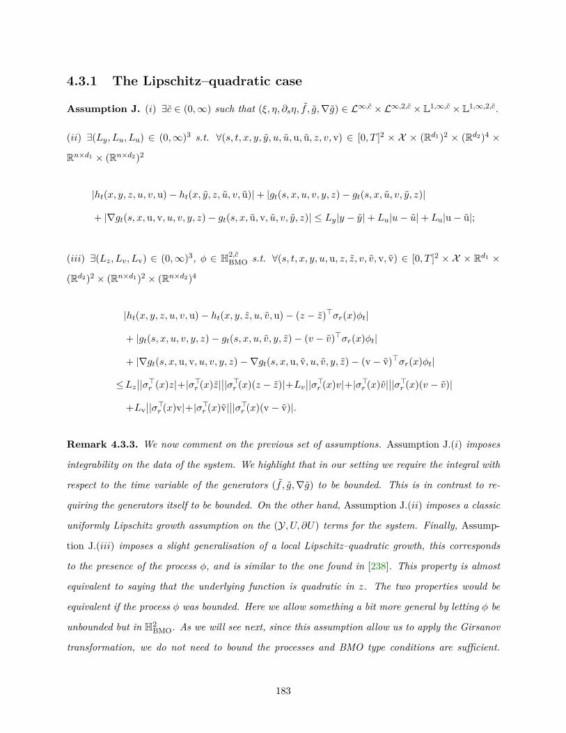
4.3.1 The Lipschitz–quadratic case

Assumption J. (i) ∃c ∈ (0,∞) such that (ξ, η, ∂sη, f , g,∇g) ∈ L∞,c × L∞,2,c × L1,∞,c × L1,∞,2,c.

(ii) ∃(Ly, Lu, Lu) ∈ (0,∞)3 s.t. ∀(s, t, x, y, y, u, u,u, u, z, v, v) ∈ [0, T ]2 × X × (Rd1)2 × (Rd2)4 ×

Rn×d1 × (Rn×d2)2

|ht(x, y, z, u, v, u)− ht(x, y, z, u, v, u)|+ |gt(s, x, u, v, y, z)− gt(s, x, u, v, y, z)|

+ |∇gt(s, x,u, v, u, v, y, z)− gt(s, x, u, v, u, v, y, z)| ≤ Ly|y − y|+ Lu|u− u|+ Lu|u− u|;

(iii) ∃(Lz, Lv, Lv) ∈ (0,∞)3, φ ∈ H2,cBMO s.t. ∀(s, t, x, y, u, u, z, z, v, v, v, v) ∈ [0, T ]2 × X × Rd1 ×

(Rd2)2 × (Rn×d1)2 × (Rn×d2)4

|ht(x, y, z, u, v, u)− ht(x, y, z, u, v,u)− (z − z)>σr(x)φt|

+ |gt(s, x, u, v, y, z)− gt(s, x, u, v, y, z)− (v − v)>σr(x)φt|

+ |∇gt(s, x,u, v, u, v, y, z)−∇gt(s, x,u, v, u, v, y, z)− (v− v)>σr(x)φt|

≤Lz∣∣|σ>r (x)z|+|σ>r (x)z|

∣∣|σ>r (x)(z − z)|+Lv∣∣|σ>r (x)v|+|σ>r (x)v|

∣∣|σ>r (x)(v − v)|

+Lv∣∣|σ>r (x)v|+|σ>r (x)v|

∣∣|σ>r (x)(v− v)|.

Remark 4.3.3. We now comment on the previous set of assumptions. Assumption J.(i) imposes

integrability on the data of the system. We highlight that in our setting we require the integral with

respect to the time variable of the generators (f , g,∇g) to be bounded. This is in contrast to re-

quiring the generators itself to be bounded. On the other hand, Assumption J.(ii) imposes a classic

uniformly Lipschitz growth assumption on the (Y, U, ∂U) terms for the system. Finally, Assump-

tion J.(iii) imposes a slight generalisation of a local Lipschitz–quadratic growth, this corresponds

to the presence of the process φ, and is similar to the one found in [238]. This property is almost

equivalent to saying that the underlying function is quadratic in z. The two properties would be

equivalent if the process φ was bounded. Here we allow something a bit more general by letting φ be

unbounded but in H2BMO. As we will see next, since this assumption allow us to apply the Girsanov

transformation, we do not need to bound the processes and BMO type conditions are sufficient.

183

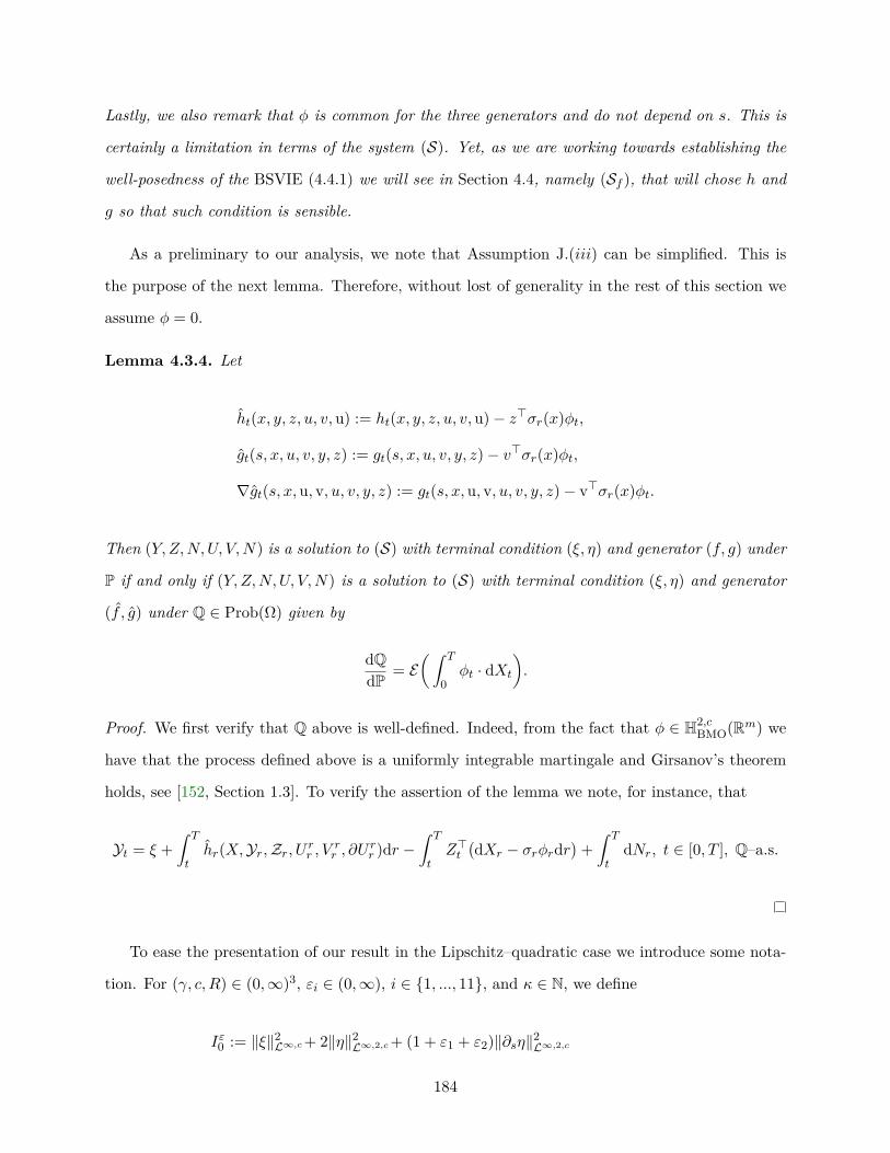
Lastly, we also remark that φ is common for the three generators and do not depend on s. This is

certainly a limitation in terms of the system (S). Yet, as we are working towards establishing the

well-posedness of the BSVIE (4.4.1) we will see in Section 4.4, namely (Sf ), that will chose h and

g so that such condition is sensible.

As a preliminary to our analysis, we note that Assumption J.(iii) can be simplified. This is

the purpose of the next lemma. Therefore, without lost of generality in the rest of this section we

assume φ = 0.

Lemma 4.3.4. Let

ht(x, y, z, u, v, u) := ht(x, y, z, u, v, u)− z>σr(x)φt,

gt(s, x, u, v, y, z) := gt(s, x, u, v, y, z)− v>σr(x)φt,

∇gt(s, x,u, v, u, v, y, z) := gt(s, x,u, v, u, v, y, z)− v>σr(x)φt.

Then (Y, Z,N,U, V,N) is a solution to (S) with terminal condition (ξ, η) and generator (f, g) under

P if and only if (Y, Z,N,U, V,N) is a solution to (S) with terminal condition (ξ, η) and generator

(f , g) under Q ∈ Prob(Ω) given by

dQdP = E

(∫ T

0φt · dXt

).

Proof. We first verify that Q above is well-defined. Indeed, from the fact that φ ∈ H2,cBMO(Rm) we

have that the process defined above is a uniformly integrable martingale and Girsanov’s theorem

holds, see [152, Section 1.3]. To verify the assertion of the lemma we note, for instance, that

Yt = ξ +∫ T


r , ∂Urr )dr −

∫ T

tZ>t(dXr − σrφrdr

)+∫ T

tdNr, t ∈ [0, T ], Q–a.s.

To ease the presentation of our result in the Lipschitz–quadratic case we introduce some nota-

tion. For (γ, c, R) ∈ (0,∞)3, εi ∈ (0,∞), i ∈ 1, ..., 11, and κ ∈ N, we define

Iε0 := ‖ξ‖2L∞,c+ 2‖η‖2L∞,2,c+ (1 + ε1 + ε2)‖∂sη‖2L∞,2,c

184

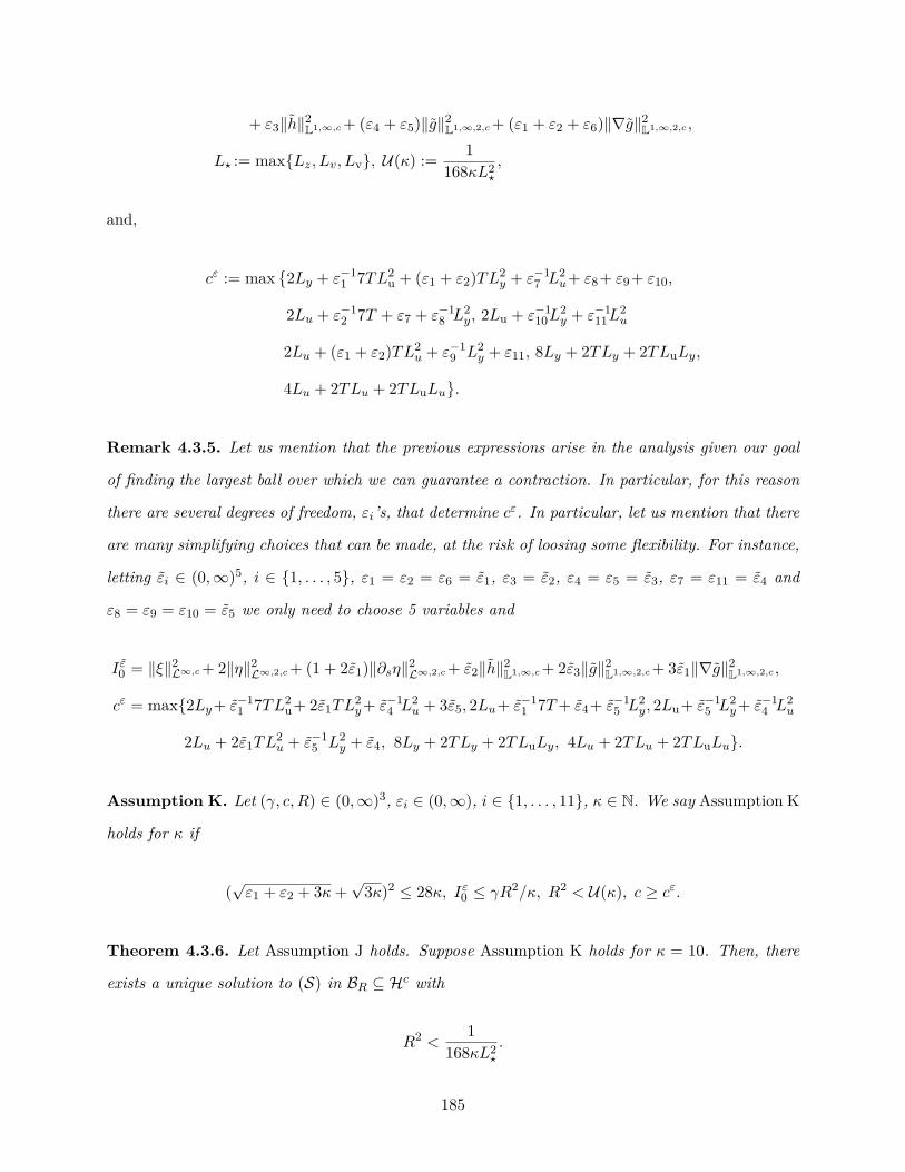
+ ε3‖h‖2L1,∞,c+ (ε4 + ε5)‖g‖2L1,∞,2,c+ (ε1 + ε2 + ε6)‖∇g‖2L1,∞,2,c ,

L? := maxLz, Lv, Lv, U(κ) := 1168κL2

?

,

and,

cε := max2Ly + ε−1

1 7TL2u + (ε1 + ε2)TL2

y + ε−17 L2

u+ ε8+ ε9+ ε10,

2Lu + ε−12 7T + ε7 + ε−1

8 L2y, 2Lu + ε−1

10L2y + ε−1

11L2u

2Lu + (ε1 + ε2)TL2u + ε−1

9 L2y + ε11, 8Ly + 2TLy + 2TLuLy,

4Lu + 2TLu + 2TLuLu.

Remark 4.3.5. Let us mention that the previous expressions arise in the analysis given our goal

of finding the largest ball over which we can guarantee a contraction. In particular, for this reason

there are several degrees of freedom, εi’s, that determine cε. In particular, let us mention that there

are many simplifying choices that can be made, at the risk of loosing some flexibility. For instance,

letting εi ∈ (0,∞)5, i ∈ 1, . . . , 5, ε1 = ε2 = ε6 = ε1, ε3 = ε2, ε4 = ε5 = ε3, ε7 = ε11 = ε4 and

ε8 = ε9 = ε10 = ε5 we only need to choose 5 variables and

I ε0 = ‖ξ‖2L∞,c+ 2‖η‖2L∞,2,c+ (1 + 2ε1)‖∂sη‖2L∞,2,c+ ε2‖h‖2L1,∞,c+ 2ε3‖g‖2L1,∞,2,c+ 3ε1‖∇g‖2L1,∞,2,c ,

cε = max2Ly+ ε−11 7TL2

u+ 2ε1TL2y+ ε−1

4 L2u + 3ε5, 2Lu+ ε−1

1 7T+ ε4+ ε−15 L2

y, 2Lu+ ε−15 L2

y+ ε−14 L2

u

2Lu + 2ε1TL2u + ε−1

5 L2y + ε4, 8Ly + 2TLy + 2TLuLy, 4Lu + 2TLu + 2TLuLu.

Assumption K. Let (γ, c, R) ∈ (0,∞)3, εi ∈ (0,∞), i ∈ 1, . . . , 11, κ ∈ N. We say Assumption K

holds for κ if

(√ε1 + ε2 + 3κ+

√3κ)2 ≤ 28κ, Iε0 ≤ γR2/κ, R2 < U(κ), c ≥ cε.

Theorem 4.3.6. Let Assumption J holds. Suppose Assumption K holds for κ = 10. Then, there

exists a unique solution to (S) in BR ⊆ Hc with

R2 <1

168κL2?

.

185

Remark 4.3.7. Before we proceed with the proof, we would like to comment on both the qualitative

and quantitative statements in Theorem 4.3.6.

(i) As a result of our procedure, and consistent with the results available in the literature, we require

the data of (S) to be sufficiently small in order to obtain the well–posedness of (S). We stress this

property on the data is influenced not only by the value of γ and R, but also, by the the value of c

which determines the norms.

(ii) In addition, we introduced Assumption K which depends on a parameter κ ∈ N. This parameter

is related with the number of processes for which we have to keep track of the integrability of. In

particular, we mention that, in the proof we present below, in addition to the 9 elements that

prescribe a solution to the system we control the norm of the diagonal process (V tt )t∈[0,T ] which

appears in the definition of H2,2. An alternative line of reasoning is available by leaving out the norm

of process (V tt )t∈[0,T ] in the definition of H2,2 and exploit the inequality derived in Lemma 4.2.3.

(iii) We also want to point out that we tried to obtain the largest ball for which the whole procedure

goes through. This can be appreciated in Equation (4.5.8) which introduces an upper bound on R

for which our candidate map is well-defined. A word of caution nonetheless, since our bound of R

cannot be directly compared to the ones obtained in [238] or [153]. Indeed, we recall that the norms

involved depend on our choice of c. As such, the radius of the ball, BR ⊆ Hc, in Theorem 4.3.6

depends on the choice of c. Consequently, if we were to exploit the equivalence between all the spaces

Hc the radius would have to be appropriately adjusted.

Remark 4.3.8. Alternative versions of Theorem 4.3.6 are available. These are related to the

orthogonal martingales.

(i) We first highlight that we are able to show, a posteriori, that the (N ,M, ∂M) part of the solution

to system (S) in Hc actually has a finite BMO-type norm. This is proved in Theorem 4.3.9. We

recall that in this quadratic setting with bounded terminal condition, this might be considered as a

more natural type of integrability for the martingale part of the solutions.

(ii) Furthermore, one could wonder about how the statement of Theorem 4.3.6 changes in the case

where (N ,M, ∂M) are required, a priori, to have finite BMO-norm. This would allow, for instance,

to keep a control on the BMO-norm inside the resulting ball. We cover this in Theorem 4.3.10.

186

(iii) Finally, we consider the case when the representation property for (F,P)-martingales in terms

of stochastic integrals with respect to X holds. This is the case, for example, if P is an extremal point

of the convex hull of the set of probability measures satisfying the requirements in Section 4.2.1, see

[142, Theorem 4.29]. In such a scenario, we have that N = M = ∂M = 0. This case is covered in

Theorem 4.3.10.

Theorem 4.3.9. Let Assumption J hold and h be a solution to (S) in the sense of Definition 4.3.2.

Then

‖N‖2M2,cBMO

+ ‖M‖2M2,2,cBMO

+ ‖∂M‖2M2,2,cBMO

<∞.

We now the address the well-posedness of (S) in the following two scenarii

(i) when (N ,M, ∂M) ∈ M2,cBMO ×M2,2,c

BMO ×M2,2,cBMO, i.e. (N ,M, ∂M) are required to have finite

BMO-norm;

(ii) when the predictable martingale representation property for (F,P)-martingales in term of

stochastic integral with respect to X hold, i.e. both N , M and ∂M vanish.

For this, let us introduce the spaces (Hc, ‖ · ‖Hc) and (Hc, ‖ · ‖Hc) for c > 0 where

Hc := S∞,c ×H2,cBMO ×M2,c

BMO × S∞,2,c ×H2,2,c

BMO ×M2,2,cBMO × S

∞,2,c ×H2,2,cBMO ×M2,2,c

BMO,

Hc := S∞,c ×H2,cBMO × S

∞,2,c ×H2,2,cBMO × S∞,2,c ×H2,2,c

BMO.

and ‖ · ‖Hc and ‖ · ‖Hc denote the associated norms. Moreover, BR ⊆ Hc(resp. BR ⊆ H

c ) denotesthe ball of radius R for the norm ‖ · ‖Hc

(resp. ‖ · ‖Hc

).

Theorem 4.3.10. Let Assumption J hold. If in addition

(i) Assumption K holds for κ = 11, then, there exists a unique solution to (S) in BR ⊆ (Hc, ‖·‖Hc);

(ii) Assumption K holds for κ = 8, and the predictable martingale representation property for

(F,P)-martingales in term of stochastic integral with respect to X hold. Then, there exists a unique

solution to (S) in BR ⊆ (Hc, ‖ · ‖Hc).

4.3.2 The quadratic case

Our approach allows us to consider also the case of quadratic generators as follows.

187

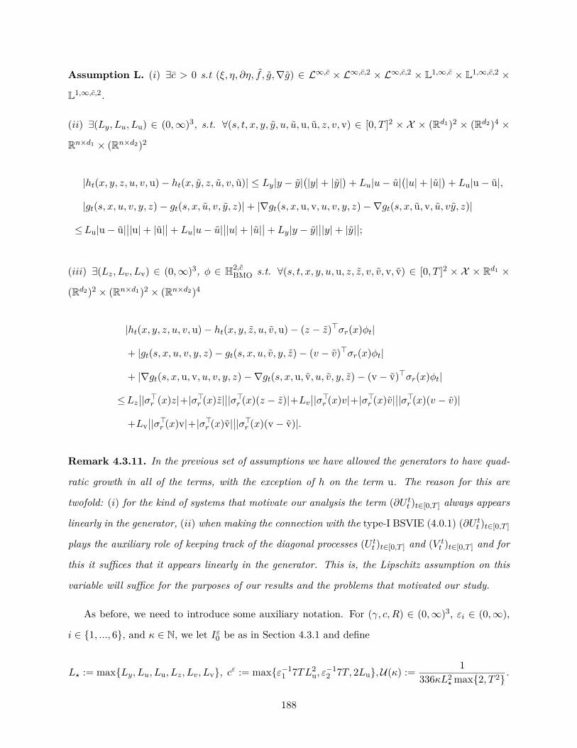
Assumption L. (i) ∃c > 0 s.t (ξ, η, ∂η, f , g,∇g) ∈ L∞,c × L∞,c,2 × L∞,c,2 × L1,∞,c × L1,∞,c,2 ×

L1,∞,c,2.

(ii) ∃(Ly, Lu, Lu) ∈ (0,∞)3, s.t. ∀(s, t, x, y, y, u, u,u, u, z, v, v) ∈ [0, T ]2 × X × (Rd1)2 × (Rd2)4 ×

Rn×d1 × (Rn×d2)2

|ht(x, y, z, u, v, u)− ht(x, y, z, u, v, u)| ≤ Ly|y − y|(|y|+ |y|

)+ Lu|u− u|

(|u|+ |u|

)+ Lu|u− u|,

|gt(s, x, u, v, y, z)− gt(s, x, u, v, y, z)|+ |∇gt(s, x,u, v, u, v, y, z)−∇gt(s, x, u, v, u, vy, z)|

≤Lu|u− u|∣∣|u|+ |u|∣∣+ Lu|u− u|

∣∣|u|+ |u|∣∣+ Ly|y − y|∣∣|y|+ |y|∣∣;

(iii) ∃(Lz, Lv, Lv) ∈ (0,∞)3, φ ∈ H2,cBMO s.t. ∀(s, t, x, y, u, u, z, z, v, v, v, v) ∈ [0, T ]2 × X × Rd1 ×

(Rd2)2 × (Rn×d1)2 × (Rn×d2)4

|ht(x, y, z, u, v, u)− ht(x, y, z, u, v,u)− (z − z)>σr(x)φt|

+ |gt(s, x, u, v, y, z)− gt(s, x, u, v, y, z)− (v − v)>σr(x)φt|

+ |∇gt(s, x,u, v, u, v, y, z)−∇gt(s, x,u, v, u, v, y, z)− (v− v)>σr(x)φt|

≤Lz∣∣|σ>r (x)z|+|σ>r (x)z|


∣∣|σ>r (x)(v − v)|

+Lv∣∣|σ>r (x)v|+|σ>r (x)v|

∣∣|σ>r (x)(v− v)|.

Remark 4.3.11. In the previous set of assumptions we have allowed the generators to have quad-

ratic growth in all of the terms, with the exception of h on the term u. The reason for this are

twofold: (i) for the kind of systems that motivate our analysis the term (∂U tt )t∈[0,T ] always appears

linearly in the generator, (ii) when making the connection with the type-I BSVIE (4.0.1) (∂U tt )t∈[0,T ]

plays the auxiliary role of keeping track of the diagonal processes (U tt )t∈[0,T ] and (V tt )t∈[0,T ] and for

this it suffices that it appears linearly in the generator. This is, the Lipschitz assumption on this

variable will suffice for the purposes of our results and the problems that motivated our study.

As before, we need to introduce some auxiliary notation. For (γ, c, R) ∈ (0,∞)3, εi ∈ (0,∞),

i ∈ 1, ..., 6, and κ ∈ N, we let Iε0 be as in Section 4.3.1 and define

L? := maxLy, Lu, Lu, Lz, Lv, Lv, cε := maxε−11 7TL2

u, ε−12 7T, 2Lu,U(κ) := 1

336κL2? max2, T 2

.

188

Assumption M. Let (γ, c, R) ∈ (0,∞)3, εi ∈ (0,∞), i ∈ 1, . . . , 6, and κ ∈ N. We say Assump-

tion M holds for κ if

(√ε1 + ε2 + 3κ+

√3κ)2 ≤ 56κ, Iε0 ≤ γR2/κ, R2 < U(κ), c ≥ cε.

Theorem 4.3.12. Let Assumption L holds. Suppose Assumption M holds for κ = 10. Then, there

exists a unique solution to (S) in BR ⊆ Hc with

R2 <1

336κL2? max2, T 2

.

Remark 4.3.13. We remark that the best way to appreciate the previous result is by contrasting

it with our well-posedness result in the linear–quadratic case. For simplicity, let us assume Ly =

Lu = Lu = Lz = Lv = Lv. Regarding the constraint on the weight parameter of the resulting

norm, the result is pretty much in the same order of magnitude. Nevertheless, the most noticeable

feature is that by allowing the system to have quadratic growth the greatest radius under which our

argument is able to guarantee the well-posedness of the solution decreases by a factor 2 max2, T 2.

This quantity can be significant in light of its dependence on the time horizon T .

4.4 Muldimensional quadratic type-I BSVIEs

We now address the well-posedness of multidimensional linear–quadratic and quadratic type-I

BSVIEs. Let d be a non-negative integer, and f and ξ be jointly measurable functionals such that

for any (s, y, z, u, v) ∈ [0, T ]× (Rd × Rn×d)2

f : [0, T ]2 ×X × (Rd × Rn×d)2 −→ Rd, f·(s, ·, y, z, u, v) ∈ Pprog(Rd,F),

ξ : [0, T ]×X −→ Rd, ξ(s, ·) is F-measurable.

The main result in this section follows exploiting the well-posedness of (S). Therefore, we work

under the following set of assumptions.

Assumption N. (s, y, z) 7−→ ft(s, x, y, z, u, v) (resp. s 7−→ ξ(s, x)) is continuously differentiable,

uniformly in (t, x, u, v) (resp. in x). Moreover, ∇f·(s, ·, y, z, u, v, u, v) ∈ Pprog(Rd,F), s ∈ [0, T ],

189

where the mapping ∇f : [0, T ]2 ×X × (Rd × Rn×d)3 −→ Rd is defined by

∇ft(s, x,u, v, y, z, u, v) := ∂sft(s, x, y, z, u, v) + ∂yft(s, x, y, z, u, v)u +n∑i=1

∂z:ift(s, x, y, z, u, v)vi:.

Set(f·, f·(s),∇f·(s)

):=(f·(·,0, 0), f·(s, ·,0), ∂sf·(s, ·,0)

), for 0 := (u, v, y, z)|(0,...,0).

Let (H?,c, ‖ · ‖H?,c) denote the space of (Y,Z,N) ∈ H?,c such that ‖(Y, Z,N)‖H?,c <∞ where

H?,c := S∞,2,c ×H2,2BMO ×M2,2,c

BMO, ‖ · ‖H?,c := ‖Y ‖2S∞,2,c + ‖Z‖2H2,2 + ‖N‖2M2,2BMO

.

We consider the n-dimensional type-I BSVIE on (H?, ‖ · ‖H?), which for any s ∈ [0, T ] satisfies

Y st = ξ(s,X) +

∫ T

tfr(s,X, Y s

r , Zsr , Y

rr , Z

rr )dr −

∫ T

tZsr>dXr −

∫ T

tdN s

r , t ∈ [0, T ], P–a.s. (4.4.1)

We work under the following notion of solution.

Definition 4.4.1. We say (Y,Z,N) is a solution to the type-I BSVIE (4.4.1) if (Y,Z,N) ∈ H?

verifies (4.4.1).

We may consider the system, given for any s ∈ [0, T ] by

Yt = ξ(T,X) +∫ T

t

(fr(r,X,Yr,Zr, Y r

r , Zrr )− ∂Y r

r

)dr −

∫ T

tZ>r dXr −

∫ T

tdNr,

Y st = ξ(s,X) +

∫ T

tfr(s,X, Y s


∫ T

tZsr>dXr −

∫ T

tdN s

r , (Sf )

∂Y st = ∂sξ(s,X) +

∫ T

t∇fr(s,X, ∂Y s

r , ∂Zsr , Y

sr , Z

sr ,Yr,Zr)dr −

∫ T

t∂Zsr

>dXr −∫ T

td∂N s

r .

Remark 4.4.2. Let us briefly comment that our set-up for the study type-I BSVIE (4.4.1) is

based on the systems introduced in Section 4.3. As such, the necessity of the set of assumptions in

Assumption N is clear.

We are now in position to prove the main result of this paper. The next result shows that under

the previous choice of data for (Sf ), its solution solves the type-I BSVIE with data (ξ, f) and vice

versa in both the linear–quadratic and quadratic case. For this we introduce the following set of

assumptions.

190

Assumption O. (i) ∃c ∈ (0,∞) such that (ξ, η, ∂sη, f , g,∇g) ∈ L∞,c ×L∞,2,c × L1,∞,c × L1,∞,2,c;

(ii) ∃(Ly, Lu, Lu) ∈ (0,∞)3 s.t. ∀(s, t, x, y, y, u, u,u, u, z, v, v) ∈ [0, T ]2×X×(Rd)6×Rn×d×(Rn×d)3

|ft(s, x, y, z, u, v)− ft(s, x, y, z, u, v)|+ |∇ft(s, x,u, v, y, z, u, v)−∇ft(s, x, u, v, y, z, u, v)|

≤Ly|y − y|+ Lu|u− u|+ Lu|u− u|;

(iii) ∃(Lz, Lv, Lv) ∈ (0,∞)3, φ ∈ H2,cBMO s.t. ∀(s, t, x, y, u, u, z, z, v, v, v, v) ∈ [0, T ]2 × X × (Rd)3 ×

(Rn×d)6

|ft(s, x, y, z, u, v)− ft(s, x, y, z, u, v)− (z − z)>σr(x)φt|

+ |∇ft(s, x,u, v, y, z, u, v)−∇ft(s, x,u, v, y, z, u, v)− (v− v)>σr(x)φt|

≤Lz∣∣|σ>r (x)z|+|σ>r (x)z|


∣∣|σ>r (x)(v − v)|

+Lv∣∣|σ>r (x)v|+|σ>r (x)v|

∣∣|σ>r (x)(v− v)|.

Assumption P. (i) ∃c ∈ (0,∞) such that (ξ, η, ∂sη, f , g,∇g) ∈ L∞,c ×L∞,2,c × L1,∞,c × L1,∞,2,c.

(ii) ∃(Ly, Lu, Lu) ∈ (0,∞)3 s.t. ∀(s, t, x, y, y, u, u,u, u, z, v, v) ∈ [0, T ]2×X×(Rd)6×Rn×d×(Rn×d2)3

|ft(s, x, y, z, u, v)− ft(s, x, y, z, u, v)|+ |∇ft(s, x,u, v, y, z, u, v)−∇ft(s, x, u, v, y, z, u, v)|

≤Ly|y − y|∣∣|y|+ |y|∣∣+ Lu|u− u|

∣∣|u|+ |u|∣∣+ Lu|u− u|∣∣|u|+ |u|∣∣;

(iii) ∃(Lz, Lv, Lv) ∈ (0,∞)3, φ ∈ H2,cBMO s.t. ∀(s, t, x, y, u, u, z, z, v, v, v, v) ∈ [0, T ]2 × X × (Rd)3 ×

(Rn×d)6

|ft(s, x, y, z, u, v)− ft(s, x, y, z, u, v)− (z − z)>σr(x)φt|

+ |∇ft(s, x,u, v, y, z, u, v)−∇ft(s, x,u, v, y, z, u, v)− (v− v)>σr(x)φt|

≤Lz∣∣|σ>r (x)z|+|σ>r (x)z|


∣∣|σ>r (x)(v − v)|

+Lv∣∣|σ>r (x)v|+|σ>r (x)v|

∣∣|σ>r (x)(v− v)|.

Theorem 4.4.3. Let Assumption N hold. Then, the well-posedness of (Sf ) is equivalent to that

191

of the type-I BSVIE (4.4.1) if either:

(i) Assumption O holds and Assumption K holds for κ = 7. In such case, there exists a unique

solution to the type-I BSVIE (4.4.1) in BR ⊆ H?,c with

R2 <1

168κL2?

.

(ii) Assumption P holds and Assumption M holds for κ = 7. In such case, there exists a unique

solution to the type-I BSVIE (4.4.1) in BR ⊆ H?,c with

R2 <1

336κL2? max2, T 2

.

Proof. Let us first note that the second part of the statements in (ii) and (iii) are a direct con-

sequente of Theorem 4.3.6 and Theorem 4.3.12, respectively.

Let us first argue why it suffices to have Assumption K and Assumption M hold for κ = 7

instead of 10. This follows from the specification of data for (Sf ). Indeed, following the notation

of the proof of Theorem 4.3.6 in this case we have that Y = U , Z = V and N =M so the auxiliary

equation introduced in step 1 (ii) is not necessary and, as from (4.5.6), the argument in the proof

holds with 7 instead on 10.

We are only left to argue the equivalence of the solutions. Let us argue (i), the argument for

(ii) is analogous. For this we follow Theorem 3.4.3. Let (Y,Z,N , Y, Z,N, ∂Y, ∂Z, ∂N) ∈ BR ⊆ Hc

be a solution to (Sf ). It then follows from Lemma 3.6.2 that

Y tt = ξ(T,X) +

∫ T

t

(fr(r,X, Y r

r , Zrr ,Yr,Zr)− ∂Y r

r

)dr −

∫ T

tZrr>dXr −

∫ T

tdNr, t ∈ [0, T ], P–a.s.,

where Nt := N tt −

∫ t0 ∂N

rr dr, t ∈ [0, T ], and N ∈ M2,c. As in Theorem 4.3.9, we obtain that

N ∈ M2,cBMO. This shows that

((Y tt )t∈[0,T ], (Ztt )t∈[0,T ],Y·,Z·, (Nt)t∈[0,T ]

), solves the first BSDE in

(Sf ). It then follows from the well-posedness of (Sf ), which holds by Assumption N, P, M and

Theorem 4.3.6, that((Y tt )t∈[0,T ], (Ztt )t∈[0,T ], (Nt)t∈[0,T ]

)= (Y·,Z·,N·) in S2,c ×H2,c

BMO ×M2,cBMO and

the result follows.

We show the converse result. Let (Y,Z,N) ∈ BR ⊆ H?,c be a solution to type-I BSVIE (4.4.1).

192

It is clear that the processes Y := (Y tt )t∈[0,T ],Z := (Ztt )t∈[0,T ],N := (N t

t )t∈[0,T ] are well-defined.

Then, since Assumption N holds and (Y,Z, Y, Z,N) ∈ L1,∞,c × H2,cBMO × S2,2,c × H2,2

BMO ×M2,2,cBMO,

we can apply Lemma 3.6.1 and obtain the existence of (∂Y, ∂Z, ∂N) ∈ S2,2,c ×H2,2,c ×M2,2,c such

that for s ∈ [0, T ]

∂Y st = ∂sξ(s,X) +

∫ T

t∇fr(s,X, ∂Y s

r , ∂Zsr , Y

sr , Z

sr , Y

rr , Z

rr )dr −

∫ T

t∂Zsr

>dXr −∫ T

td∂N s

r .

Moreover, from the fact that Assumption K holds for κ = 7 we obtain that ‖∂Y ‖2S2,2,c+‖∂Z‖2H2,2,c

BMO+

‖∂N‖2M2,2,c ≤ R2.

Let us claim that h := (Y,Z, N , Y, Z,N, ∂Y, ∂Z, ∂N) is a solution to (Sf ), where Nt := N tt −∫ t

0 ∂Nrr dr, t ∈ [0, T ]. For this, we first note that in light of Lemma 3.6.1 and 3.6.2 we have that

Yt = ξ(T,X) +∫ T

thr(X,Yr,Zr, Y r

r , Zrr , ∂Y

rr )dr −

∫ T

tZr>dXr −

∫ T

tdNr, t ∈ [0, T ], P–a.s.

Now, N ∈ M2,2,cBMO follows as in Theorem 4.3.9. As in step 1 (iii) in the proof of Theorem 4.3.6,

we obtain that Y ∈ S2,c. We are only left to argue ‖h‖ ≤ R. This follows readily following step 1

(iv) in the proof of Theorem 4.3.6 and the fact that ‖Z‖2H2,c + ‖Z‖2H2,2

BMO+ ‖∂Z‖2

H2,2,cBMO≤ R2.

4.5 Proof of the linear–quadratic case

Proof of Theorem 4.3.6. For c > 0, let us introduce the mapping

T : (BR, ‖ · ‖Hc) −→ (BR, ‖ · ‖Hc)

(y, z, n, u, v,m, ∂u, ∂v, ∂m) 7−→ (Y,Z,N,U, V,M, ∂U, ∂V, ∂M),

with (Y,Z,N , U, V,M, ∂U, ∂V, ∂M) given for any s ∈ [0, T ], P–a.s. for any t ∈ [0, T ] by

Yt = ξ(T,X·∧T ) +∫ T

thr(X,Yr, zr, U rr , vrr , ∂U rr )dr −

∫ T

tZ>r dXr −

∫ T

tdNr,

U st = η(s,X·∧,T ) +∫ T

tgr(s,X,U sr , vsr ,Yr, zr)dr −

∫ T

tV sr>dXr −

∫ T

tdM s

r ,

∂U st = ∂sη(s,X·∧,T ) +∫ T

t∇gr(s,X, ∂U sr , ∂vsr , U sr , vsr ,Yr, zr)dr −

∫ T

t∂V s

r>dXr −

∫ T

td∂M s

r .

193

Step 1: We first argue that T is well-defined.

(i) In light of Assumption J, there is c > 0 such that (ξ, η, ∂η, f , g,∇g) ∈ L∞,c×(L∞,2,c

)2×L1,∞,c×(L1,∞,2,c)2 and (z, v, ∂v) ∈ H2,c

BMO ×H2,2BMO ×H2,2,c

BMO, thus, we may use (4.2.1) to obtain

E[|ξ(T )|2 +

∣∣∣∣ ∫ T

0|ht(0, zt, 0, vtt, 0)|dt

∣∣∣∣2]+ sups∈[0,T ]

E[|η(s)|2 +

∣∣∣∣ ∫ T

0|gt(s, 0, vst , 0, zt)|dt

∣∣∣∣2]

+ sups∈[0,T ]

E[|∂η(s)|2 +

∣∣∣∣ ∫ T

0|∇gt(s, 0, ∂vst , 0, vst , 0, zt)|dt

∣∣∣∣2]

≤ E[|ξ(T )|2 + 3

∣∣∣∣ ∫ T

0|ht|dt

∣∣∣∣2 + 10L2z

∣∣∣∣ ∫ T

0|zt|2dt

∣∣∣∣2 + 3L2v

∣∣∣∣ ∫ T

0|vtt|2dt

∣∣∣∣2]+ sups∈[0,T ]

E[|η(s)|2 + 3

∣∣∣∣ ∫ T

0|gt(s)|dt

∣∣∣∣2 + 7L2v

∣∣∣∣ ∫ T

0|vst |2dt

∣∣∣∣2]

+ sups∈[0,T ]

E[|∂η(s)|2 + 4

∣∣∣∣ ∫ T

0|∇gt(s)|dt

∣∣∣∣2 + 4L2v

∣∣∣∣ ∫ T

0|∂vst |2dt

∣∣∣∣2]≤ ‖ξ‖2L∞,c + 3‖h‖2L1,∞,c + ‖η‖2L∞,2,c + 3‖g‖2L1,∞,2,c + ‖∂η‖2L∞,2,c + 4‖∇g‖2L1,∞,2,c

+ 20L2z‖z‖4H2,c

BMO+ 14L2

v‖v‖4H2,2,cBMO

+ 8L2v‖∂v‖4H2,2,c

BMO<∞.

Therefore, by Theorem 3.3.5, T defines a well-posed system of BSDEs with unique solution in the

space H2. We recall the spaces involved in the definition of H2, and their corresponding norms,

were introduced in Section 4.2.2.

(ii) Arguing as in Lemma 3.6.1 and 3.6.2, we may use Assumption J and v ∈ H2,2BMO, i.e. ∂v is the

density with respect to the Lebesgue measure of s 7−→ vs, to obtain that (U ,V,M) ∈ S2×H2×M2

given by

Ut := U tt , Vt := V tt , Mt := M t

t −∫ t

0∂M r

r dr, t ∈ [0, T ],

satisfy the equation

Ut = η(T,X·∧T ) +∫ T

t

(gr(r,X,Ur, vrr ,Yr, zr)− ∂U rr

)dr −

∫ T

tVr>dXr −

∫ T

tdMr, t ∈ [0, T ],P–a.s.

(iii) We show (Y,U) ∈ S∞,c × S∞,c and ‖U‖S∞,2,c + ‖∂U‖S∞,2,c <∞.

194

To alleviate the notation we introduce

hr := hr(Yr, zr,Ur, vrr , ∂U rr ), gr := gr(r,Ur, vrr ,Yr, zr)− ∂U rr ,

gr(s) := gr(s, U sr , vsr ,Yr, zr), ∇gr(s) := ∇gr(s, ∂U sr , ∂vsr , U sr , vsr ,Yr, zr),

and

Y := (Y,U , U s, ∂U s), Z := (Z,V, V s, ∂V s), Z := (N ,M,M s, ∂M s),

whose elements we may denote with superscripts, e.g. Y1,Y2,Y3,Y4 correspond to Y,U , U s, ∂U s.

In light of Assumption J, dr ⊗ dP–a.e.

|hr| ≤ Ly|Yr|+ Lz|σ>r zr|2 + Lu|Ur|+ Lv|σ>r vrr |2 + Lu|∂U rr |+ |hr|,

|gr| ≤ Lu|Ur|+ Lv|σ>r vrr |2 + Ly|Yr|+ Lz|σ>r zr|2 + |∂U rr |+ |gr|,

|gr(s)| ≤ Lu|U sr |+ Lv|σ>r vsr |2 + Ly|Yr|+ Lz|σ>r zr|2 + |gr(s)|,

|∇gr(s)| ≤ Lu|∂U sr |+ Lv|σ>r ∂vsr |2 + Lu|U sr |+ Lv|σ>r vsr |2 + Ly|Yr|+ Lz|σ>r zr|2 + |∇gr(s)|.

(4.5.1)

Applying Meyer–Itô’s formula to ec2 t(|Yt|+ |Ut|+ |U st |+ |∂U st |

)we obtain

ec2 t(|Yt|+ |Ut|+ |U st |+ |∂U st |

)+ Mt −MT + L0

T

= ec2T(|ξ|+ |η(T )|+ |η(s)|+ |∂η(s)|

)(4.5.2)

+∫ T

tec2 r(

sgn(Yr)·hr + sgn(Ur)·gr + sgn(U sr )·gr(s) + sgn(∂U sr )·∇gr(s)−c

2

4∑i=1|Yi

r|)

dr,

where L0t := L0

t (Y,U , U s, ∂U s) denotes the non-decreasing and pathwise-continuous local time of

the semimartingale (Y,U , U s, ∂U s) at 0, see [212, Theorem 70], and, we introduced the martingale

(recall that (i) and (ii) guarantee (Z,V,N ,M, V, ∂V,M, ∂M) ∈ (H2)2× (M2)2× (H2,2)2× (M2,2)2)

Mt :=4∑i=1

∫ t

0ec2 rZir sgn(Yi

r) · dXr +∫ t

0ec2 r− sgn(Yr−) · dZir, t ∈ [0, T ].

Again, we take conditional expectations with respect to Ft in Equation (4.5.2) and exploit the

fact L0T is non-decreasing. Moreover, in combination with (4.5.1) and Lemma 4.7.1, we obtain back

195

in (4.5.2) that for C1 := 4Ly +TLy +TLuLy, C2 := 2Lu, C3 := 2Lu +TLu +TLuLu, and C4 := Lu

ec2 t(|Yt|+ |Ut|+ |U st |+ |∂U st |

)+ Et

[ ∫ T

tec2 r|Yr|(c/2− C1)dr

]+ Et

[ ∫ T

tec2 r|Ur|(c/2− C2)dr

]+ sups∈[0,T ]

Et[ ∫ T

tec2 r|U sr |(c/2− C3)dr

]+ sups∈[0,T ]

Et[ ∫ T

tec2 r|∂U sr |(c/2− C4)

)dr]

≤ Et[ec2T(|ξ|+ |η(T )|+ |η(s)|+ |∂sη(s)|

)]+ Et

[ ∫ T

tec2 r(|hr|+ |gr|+ |gr(s)|+ |∇gr(s)|

)dr]

+ (T + LuT )(‖∂sη‖L∞,2,c + ‖∇g‖L1,∞,2,c + L?

(‖∂v‖2H2,2,c

BMO+ ‖v‖2H2,2,c

BMO+ ‖z‖2H2,c

BMO

))+ Et

[ ∫ T

tecr(4Lz|σ>r zr|2 + 2Lv|σ>r vrr |2 + 2Lv|σ>r vsr |2 + Lv|σ>r ∂vsr |2

)dr],

where we recall the notation L? = maxLz, Lv, Lv. Thus, for

c ≥ 2 max4Ly + TLy + TLuLy, 2Lu, 2Lu + TLu + TLuLu, Lu

= max8Ly + 2TLy + 2TLuLy, 4Lu + 2TLu + 2TLuLu, 2Lu, (4.5.3)

we obtain

maxec2 t|Yt|, e

c2 t|Ut|, e

c2 t|U st |, e

c2 t|∂U st |

≤ e

c2 t(|Yt|+ |Ut|+ |U st |+ |∂U st |

)≤ ‖ξ‖L∞,c + ‖h‖L1,∞,c + 2

(‖η‖L∞,2,c + ‖g‖L1,∞,2,c

)+ (1 + T + TLu)

(‖∂sη‖L∞,2,c + ‖∇g‖L1,∞,2,c

)+ (4 + T + LuT )L?

(‖∂v‖2H2,2,c

BMO+ ‖v‖2

H2,2,cBMO

+ ‖z‖2H2,cBMO

).

(iv) We show (Z,V,N ,M)∈(H2,c

BMO)2× (M2,c)2, ‖V ‖2

H2,2,cBMO

+‖M‖2M2,2,c+‖∂V ‖2H2,2,cBMO

+‖∂M‖2M2,2,c <

∞.

Applying Itô’s formula to ect(|Yt|2 + |Ut|2 + |U st |2 + |∂U st |2

)we obtain

4∑i=1

ect|Yit|2 +

∫ T

tecr|σ>r Zir|2dr +

∫ T

tecr−dTr[Zi]r + Mt − MT

= ecT(|ξ|2 + |η(T )|2 + |η(s)|2 + |∂sη(s)|2

)+∫ T

tecr(

2Yr · hr + 2Ur · gr + 2U sr · gr(s) + 2∂U sr · ∇gr(s)− c4∑i=1|Yi

r|2)

dr,

(4.5.4)

196

where for any s ∈ [0, T ] we introduced the martingale

Mt :=4∑i=1

∫ t

0ecrZirYi

r · dXr +∫ t

0ecr−Yi

r− · dZir, t ∈ [0, T ].

Indeed, Burkholder–Davis–Gundy’s inequality and the fact that (Y,U , Z,V, U, ∂U, V, ∂V ) ∈ (S2)2×

(H2)2 × (S2,2)2 × (H2,2)2, recall (i) and (ii), implies that there exists C > 0 such that

E[

supt∈[0,T ]

∣∣∣∣ ∫ t

0ecrZirYi

r · dXr

∣∣∣∣] ≤ CE[∣∣∣∣ ∫ T

0ecr|Yi

rσ>r Z

ir|2dr

∣∣∣∣12]≤ CecT ‖Yi‖S2‖Zi‖H2 , i ∈ 1, . . . , 4,

which guarantees each of the processes in M is an uniformly integrable martingale. Thus, taking

conditional expectations with respect to Ft in Equation (4.5.4), we obtain

4∑i=1

ect|Yit|2 + Et

[ ∫ T

tecr|σ>r Zir|2dr +

∫ T

tecr−dTr[Zi]r

]

= Et[ecT(|ξ|2 + |η(T )|2 + |η(s)|2 + |∂sη(s)|2

)]+ Et

[ ∫ T

tecr(

2Yr · hr + 2Ur · gr + 2U sr · gr(s) + 2∂U sr · ∇gr(s)− c4∑i=1|Yi

r|2)

dr], t ∈ [0, T ].

From (iii), Assumption J.(ii) and J.(iii), together with Young’s inequality, yield that, for any

εi > 0, and defining Cε1,7 := 2Ly + ε−11 7TL2

u + ε−17 L2

u, Cε2,8 := 2Lu + ε−12 7T + ε−1

8 L2y, Cε9 :=

2Lu + ε−19 L2

y, as well as, Cε10,11 := 2Lu + ε−111 L

2u + ε−1

10 L2y we have

2Yr · hr − c|Yr|2 ≤ (Cε1,7 − c)|Yr|2 + 2‖Y‖S∞,c(Lz|σ>r zr|2 + Lv|σ>r vrr |2 + |hr|

)+ ε1(7T )−1|∂U rr |2 + ε7|Ur|2,

2Ur · gr − c|Ur|2 ≤ (Cε2,8 − c)|Ur|2 + 2‖U‖S∞,c(Lz|σ>r zr|2 + Lv|σ>r vrr |2 + |gr|

)+ ε2(7T )−1|∂U rr |2 + ε8|Yr|2,

2U sr · gr(s)− c|U sr |2 ≤ (Cε9 − c)|U sr |2 + 2‖U‖S∞,2,c(Lv|σ>r vsr |2 + Lz|σ>r zr|2 + |gr(s)|

)+ ε9|Yr|2,

2∂U sr · ∇gr(s)− c|∂U sr |2 ≤ (Cε10,11 − c)|∂U sr |2 + ε11|U sr |2 + ε10|Yr|2

+ 2‖∂U‖S∞,c,2(Lv|σ>r ∂vsr |2 + Lv|σ>r vsr |2 + Lz|σ>r zr|2 + |∇gr(s)|

).

197

These inequalities in combination with Lemma 4.7.1, and Young’s inequality, show that if we

define Cε1 := Cε1,7 + ε8 + ε9 + ε10 + (ε1 + ε2)TL2y, Cε2 := Cε2,8 + ε7, Cε3 := Cε9 + ε11 + (ε1 + ε2)TL2

u,

Cε4 := Cε10,11 , then for any εi > 0, i ∈ 7, ..., 15

4∑i=1

ect|Yit|2 + Et

[ ∫ T

tecr|σ>r Zir|2dr +

∫ T

tecr−dTr[Zi]r +

∫ T

tecr(|Yr|2(c− Cε1) + |Ur|2(c− Cε2)

)dr]

+ sups∈[0,T ]

Et[ ∫ T

tecr|U sr |2(c− Cε3)dr

]+ sups∈[0,T ]

Et[ ∫ T

tecr|∂U sr |2(c− Cε4)dr

]= (ε1 + ε2)

(‖∂sη‖2L∞,2,c + ‖∇g‖2L1,∞,2,c + 2L2

?

(‖∂v‖4H2,2,c

BMO+ ‖v‖4H2,2,c

BMO+ ‖z‖4H2,c

BMO

))+ Et

[ecT(|ξ|2 + |η(T )|2 + |η(s)|2 + |∂sη(s)|2

)]+(ε−1

3 + ε−112 + ε−1

13)‖Y‖2S∞,c

+(ε−1

4 + ε−114 + ε−1

15)‖U‖2S∞,c +

(ε−1

5 + ε−116 + ε−1

17)‖U‖2S∞,c,2 +

(ε−1

6 + ε−118 + ε−1

19 + ε−120)‖∂U‖2S∞,c,2

+ ε3Et[∣∣∣∣ ∫ T

tecr|hr|dr

∣∣∣∣2]+ ε4Et[∣∣∣∣ ∫ T

tecr|gr|dr

∣∣∣∣2]+ ε5Et

[∣∣∣∣ ∫ T

tecr|gr(s)|dr

∣∣∣∣2]+ ε6Et[∣∣∣∣ ∫ T

tecr|∇gr|dr

∣∣∣∣2]+ (ε12 + ε14 + ε16 + ε18)L2

zEt[∣∣∣∣ ∫ T

tecr|σ>r zr|2dr

∣∣∣∣2]+ (ε13 + ε15)L2vEt[∣∣∣∣ ∫ T

tecr|σ>r vrr |2dr

∣∣∣∣2]+ (ε17 + ε19)L2

vEt[∣∣∣∣ ∫ T

tecr|σ>r vsr |2dr

∣∣∣∣2]+ ε20L2vEt

[∣∣∣∣ ∫ T

tecr|σ>r ∂vsr |2dr

∣∣∣∣2].We now let τ ∈ T0,T . In light of (4.5.3), for

c ≥ max 2Ly + ε−11 7TL2

u + ε1TL2y + ε2TL

2y + ε−1

7 L2u + ε8 + ε9 + ε10,

2Lu + ε−12 7T + ε7 + ε−1

8 L2y, 2Lu + ε1TL

2u + ε2TL

2u + ε−1

9 L2y + ε11,

2Lu + ε−111 L

2u + ε−1

10 L2y, 8Ly + 2TLy + 2TLuLy, 4Lu + 2TLu + 2TLuLu,

(4.5.5)

(4.2.1) yields

4∑i=1

ect|Yit|2 + Et

[ ∫ T

tecr|σ>r Zir|2dr +

∫ T

tecr−dTr[Zi]r

]

= Iε0 + 2L2?(ε1 + ε2 + ε12 + ε14 + ε16 + ε18)‖z‖4H2,c

BMO+(ε−1

3 + ε−112 + ε−1

13)‖Y ‖2S∞,c

+ 2L2?

((ε1 + ε2 + ε13 + ε15 + ε17 + ε19)‖v‖4

H2,2,cBMO

+ (ε1 + ε2 + ε20)‖∂v‖4H2,2,cBMO

)+(ε−1

4 + ε−114 + ε−1

15)‖U‖2S∞,c +

(ε−1

5 + ε−116 + ε−1

17)‖U‖2S∞,c,2 +

(ε−1

6 + ε−118 + ε−1

19 + ε−120)‖∂U‖2S∞,c,2 .

198

which in turn leads to

110(‖Y‖2S∞,c + ‖U‖2S∞,c + ‖U‖2S∞,2,c + ‖∂U‖2S∞,2,c + ‖Z‖2H2,c

BMO

+ ‖V ‖2H2,2,c

BMO+ ‖∂V ‖2H2,2,c

BMO+ ‖N‖2M2,c + ‖M‖2M2,2,c + ‖∂M‖2M2,2,c

)≤ ‖ξ‖2L∞,c + 2‖η‖2L∞,2,c + (1 + ε1 + ε2)‖∂sη‖2L∞,2,c + ε3‖h‖2L1,∞,c + (ε4 + ε5)‖g‖2L1,∞,2,c

+ (ε1 + ε2 + ε6)‖∇g‖2L1,∞,2,c + 2L2?(ε1 + ε2 + ε12 + ε14 + ε16 + ε18)‖z‖4H2,c

BMO

+ 2L2?(ε1 + ε2 + ε13 + ε15 + ε17 + ε19)‖v‖4

H2,2,cBMO

+ 2L2?(ε1 + ε2 + ε20)‖∂v‖4H2,2,c

BMO

+(ε−1

3 + ε−112 + ε−1

13)‖Y ‖2S∞,c +

(ε−1

4 + ε−114 + ε−1

15)‖U‖2S∞,c

+(ε−1

5 + ε−116 + ε−1

17)‖U‖2S∞,c,2 +

(ε−1

6 + ε−118 + ε−1

19 + ε−120)‖∂U‖2S∞,c,2 .

(4.5.6)

From (4.5.6) we conclude (Z,N) ∈ H2,cBMO ×M2,c,

‖V ‖2H2,2,c

BMO+ ‖∂V ‖2H2,2,c

BMO+ ‖M‖2M2,2,c + ‖∂M‖2M2,2,c <∞.

At this point, we can highlight a crucial step in this approach. It is clear from (4.5.6) that the

norm of T does not have a linear growth in the norm of the input. In the following, we will see

that choosing the data of the system small enough and localising T will bring us back to the linear

growth scenario. For this, we observe that if we define

Cε := min

1− 10(ε−13 + ε−1

12 + ε−113 ), 1− 10(ε−1

4 + ε−114 + ε−1

15 ),

1− 10(ε−15 + ε−1

16 + ε−117 ), 1− 10(ε−1

6 + ε−118 + ε−1

19 + ε−120 ),

for 1− 10(ε−13 + ε−1

12 + ε−113 ) ∈(0, 1], 1− 10(ε−1

4 + ε−114 + ε−1

15 ) ∈(0, 1], 1− 10(ε−15 + ε−1

16 + ε−117 ) ∈(0, 1],

1− 10(ε−16 + ε−1

18 + ε−119 + ε−1

20 ) ∈(0, 1], and for some γ ∈ (0,∞),

Iε0 ≤ γR2/10,

we obtain back in (4.5.6)

‖(Y,Z,N,U, V,M, ∂U, ∂V, ∂M)‖2Hc

199

≤ C−1ε

(10Iε0 + 20L2

?

((ε1 + ε2 + ε12 + ε14 + ε16 + ε18)‖z‖4H2,c

BMO

+ (ε1 + ε2 + ε13 + ε15 + ε17 + ε19)‖v‖4H2,2,c

BMO+ (ε1 + ε2 + ε20)‖∂v‖4H2,2,c

BMO

))≤ C−1

ε R2(γ + 20L2

?

((ε1 + ε2 + ε12 + ε14 + ε16 + ε18)‖z‖2H2,c

BMO

+ (ε1 + ε2 + ε13 + ε15 + ε17 + ε19)‖v‖2H2,2,c

BMO+ (ε1 + ε2 + ε20)‖∂v‖2H2,2,c

BMO

))≤ C−1

ε R2(γ + 20L2

?R2(ε1 + ε2 +

20∑i=12

εi

)).

Therefore, to obtain T(BR) ⊆ BR, that is to say that the image under T of the ball of radius

R is contained in the ball of radius R, it is necessary to find R2 such that the term in parentheses

above is less or equal than Cε, i.e.

R2 ≤ 120L2

?

Cε − γε1 + ε2 +

∑20i=12 εi

. (4.5.7)

Clearly, there are many choices of ε’s so that the above holds. Among such, we wish to choose

γ, εi, so that the expression to the right in (4.5.7) is maximal. In light of Lemma 4.7.2, we have

that ‖(Y, Z,N,U, V,M)‖Hc ≤ R provided that

R2 <1

25 · 3 · 52 · 7 · L2?

. (4.5.8)

(v) Lastly, we are left to argue (U, V,M, ∂U, ∂V, ∂M) ∈ S∞,2,c×H2,2,cBMO×M2,2,c×S∞,2,c×H2,2,c

BMO×

M2,2,c. The argument for (U, V,M) is analogous to that of (∂U, ∂V, ∂M), thus we argue the con-

tinuity of the applications ([0, T ],B([0, T ])) −→ (S∞,c, ‖ · ‖S∞,c)(resp. (H2,c

BMO, ‖ · ‖H2,cBMO

), (M2,c, ‖ ·

‖M2,c))

: s 7−→ ϕs for ϕ = U s (resp. V s,M s).

Recall ρg denotes the modulus of continuity of g. Let (sn)n ⊆ [0, T ], snn→∞−−−→ s0 ∈ [0, T ] and

define for ϕ ∈ U, V,M, u, v, η, ∆ϕn := ϕsn−ϕs0 . Applying Itô’s formula to ect|∆Unt |2, proceeding

as in Step 1 (iv) we obtain

‖∆Un‖2S∞,c + ‖∆V n‖2H2,cBMO

+ ‖∆Mn‖2M2,c ≤ 4(‖∆ηn‖2L∞,c + 4L2

v‖∆vn‖4H2,cBMO

+ ρg(|sn − s0|)2).

We conclude, T(BR) ⊆ BR for all R satisfying (4.5.8).

200

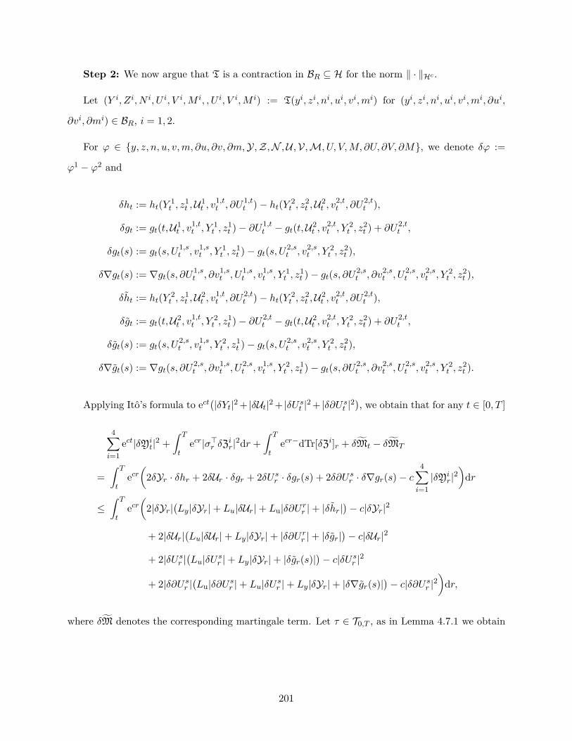
Step 2: We now argue that T is a contraction in BR ⊆ H for the norm ‖ · ‖Hc .

Let (Y i, Zi, N i, U i, V i,M i, , U i, V i,M i) := T(yi, zi, ni, ui, vi,mi) for (yi, zi, ni, ui, vi,mi, ∂ui,

∂vi, ∂mi) ∈ BR, i = 1, 2.

For ϕ ∈ y, z, n, u, v,m, ∂u, ∂v, ∂m,Y,Z,N ,U ,V,M, U, V,M, ∂U, ∂V, ∂M, we denote δϕ :=

ϕ1 − ϕ2 and

δht := ht(Y 1t , z

1t ,U1

t , v1,tt , ∂U1,t

t )− ht(Y 2t , z

2t ,U2

t , v2,tt , ∂U2,t

t ),

δgt := gt(t,U1t , v

1,tt , Y 1

t , z1t )− ∂U1,t

t − gt(t,U2t , v

2,tt , Y 2

t , z2t ) + ∂U2,t

t ,

δgt(s) := gt(s, U1,st , v1,s

t , Y 1t , z

1t )− gt(s, U2,s

t , v2,st , Y 2

t , z2t ),

δ∇gt(s) := ∇gt(s, ∂U1,st , ∂v1,s

t , U1,st , v1,s

t , Y 1t , z

1t )− gt(s, ∂U2,s

t , ∂v2,st , U2,s

t , v2,st , Y 2

t , z2t ),

δht := ht(Y 2t , z

1t ,U2

t , v1,tt , ∂U2,t

t )− ht(Y 2t , z

2t ,U2

t , v2,tt , ∂U2,t

t ),

δgt := gt(t,U2t , v

1,tt , Y 2

t , z1t )− ∂U2,t

t − gt(t,U2t , v

2,tt , Y 2

t , z2t ) + ∂U2,t

t ,

δgt(s) := gt(s, U2,st , v1,s

t , Y 2t , z

1t )− gt(s, U2,s

t , v2,st , Y 2

t , z2t ),

δ∇gt(s) := ∇gt(s, ∂U2,st , ∂v1,s

t , U2,st , v1,s

t , Y 2t , z

1t )− gt(s, ∂U2,s

t , ∂v2,st , U2,s

t , v2,st , Y 2

t , z2t ).

Applying Itô’s formula to ect(|δYt|2 + |δUt|2 + |δU st |2 + |δ∂U st |2

), we obtain that for any t ∈ [0, T ]

4∑i=1

ect|δYit|2 +

∫ T

tecr|σ>r δZir|2dr +

∫ T

tecr−dTr[δZi]r + δMt − δMT

=∫ T

tecr(

2δYr · δhr + 2δUr · δgr + 2δU sr · δgr(s) + 2δ∂U sr · δ∇gr(s)− c4∑i=1|δYi

r|2)

dr

≤∫ T

tecr(

2|δYr|(Ly|δYr|+ Lu|δUr|+ Lu|δ∂U rr |+ |δhr|

)− c|δYr|2

+ 2|δUr|(Lu|δUr|+ Ly|δYr|+ |δ∂U rr |+ |δgr|

)− c|δUr|2

+ 2|δU sr |(Lu|δU sr |+ Ly|δYr|+ |δgr(s)|

)− c|δU sr |2

+ 2|δ∂U sr |(Lu|δ∂U sr |+ Lu|δU sr |+ Ly|δYr|+ |δ∇gr(s)|

)− c|δ∂U sr |2

)dr,

where δM denotes the corresponding martingale term. Let τ ∈ T0,T , as in Lemma 4.7.1 we obtain

201

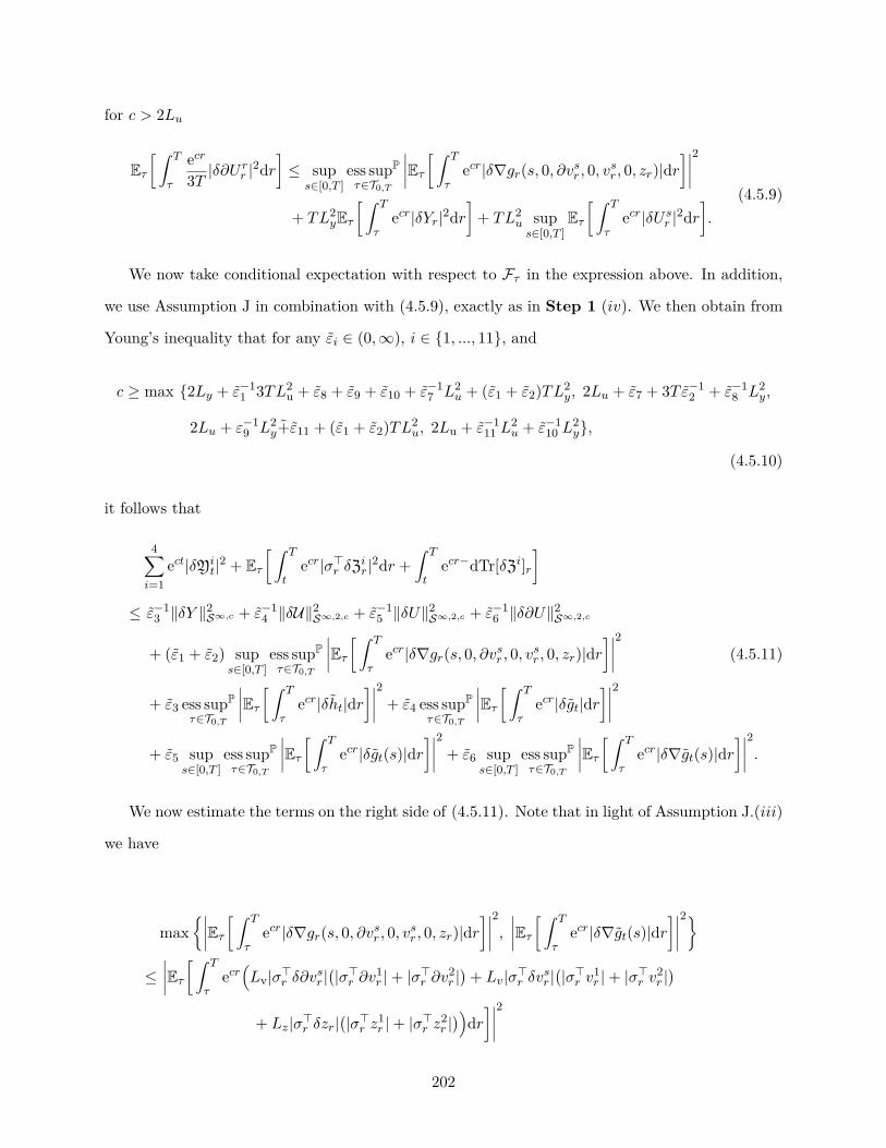
for c > 2Lu

Eτ[ ∫ T

τ

ecr

3T |δ∂Urr |2dr

]≤ sup

s∈[0,T ]ess supP

τ∈T0,T

∣∣∣∣Eτ[ ∫ T

τecr|δ∇gr(s, 0, ∂vsr , 0, vsr , 0, zr)|dr

]∣∣∣∣2+ TL2

yEτ[ ∫ T

τecr|δYr|2dr

]+ TL2

u sups∈[0,T ]

Eτ[ ∫ T

τecr|δU sr |2dr

].

(4.5.9)

We now take conditional expectation with respect to Fτ in the expression above. In addition,

we use Assumption J in combination with (4.5.9), exactly as in Step 1 (iv). We then obtain from

Young’s inequality that for any εi ∈ (0,∞), i ∈ 1, ..., 11, and

c ≥ max 2Ly + ε−11 3TL2

u + ε8 + ε9 + ε10 + ε−17 L2

u + (ε1 + ε2)TL2y, 2Lu + ε7 + 3T ε−1

2 + ε−18 L2

y,

2Lu + ε−19 L2

y+ε11 + (ε1 + ε2)TL2u, 2Lu + ε−1

11 L2u + ε−1

10 L2y,

(4.5.10)

it follows that

4∑i=1

ect|δYit|2 + Eτ

[ ∫ T


∫ T

tecr−dTr[δZi]r

]

≤ ε−13 ‖δY ‖

2S∞,c + ε−1

4 ‖δU‖2S∞,2,c + ε−1

5 ‖δU‖2S∞,2,c + ε−1

6 ‖δ∂U‖2S∞,2,c

+ (ε1 + ε2) sups∈[0,T ]

ess supP

τ∈T0,T

∣∣∣∣Eτ[ ∫ T


]∣∣∣∣2 (4.5.11)

+ ε3 ess supP

τ∈T0,T

∣∣∣∣Eτ[ ∫ T

τecr|δht|dr

]∣∣∣∣2 + ε4 ess supP

τ∈T0,T

∣∣∣∣Eτ[ ∫ T

τecr|δgt|dr

]∣∣∣∣2

+ ε5 sups∈[0,T ]

ess supP

τ∈T0,T

∣∣∣∣Eτ[ ∫ T

τecr|δgt(s)|dr

]∣∣∣∣2 + ε6 sups∈[0,T ]

ess supP

τ∈T0,T

∣∣∣∣Eτ[ ∫ T

τecr|δ∇gt(s)|dr

]∣∣∣∣2.We now estimate the terms on the right side of (4.5.11). Note that in light of Assumption J.(iii)

we have

max∣∣∣∣Eτ[ ∫ T


]∣∣∣∣2, ∣∣∣∣Eτ[ ∫ T

τecr|δ∇gt(s)|dr

]∣∣∣∣2≤∣∣∣∣Eτ[ ∫ T

τecr(Lv|σ>r δ∂vsr |

(|σ>r ∂v1

r |+ |σ>r ∂v2r |)

+ Lv|σ>r δvsr |(|σ>r v1

r |+ |σ>r v2r |)

+ Lz|σ>r δzr|(|σ>r z1

r |+ |σ>r z2r |))

dr]∣∣∣∣2

202

≤ 3L2?Eτ

[ ∫ T

τecr|σ>r δ∂vsr |2dr

]Eτ[ ∫ T

τecr(|σ>r ∂v1

r |+ |σ>r ∂v2r |)2dr

]+ 3L2

?Eτ[ ∫ T

τecr|σ>r δvsr |2dr

]Eτ[ ∫ T

τecr(|σ>r v1

r |+ |σ>r v2r |)2dr

]+ 3L2

?Eτ[ ∫ T

τecr|σ>r δzr|2dr

]Eτ[ ∫ T

τecr(|σ>r z1

r |+ |σ>r z2r |)2dr

]≤ 6L2

?R2(Eτ[ ∫ T


]+ Eτ

[ ∫ T


]+ Eτ

[ ∫ T

τecr|σ>r δzr|2dr

])≤ 6L2

?R2(‖δ∂v‖2H2,2,c

BMO+ ‖δv‖2

H2,2,cBMO

+ ‖δz‖2H2,cBMO

),

where in the second inequality we used (I.1) and Cauchy–Schwarz’s inequality. Similarly


τecr|δhr|dr

]∣∣∣∣2, ∣∣∣∣Eτ[ ∫ T

τecr|δgr(s)|dr

]∣∣∣∣2, ∣∣∣∣Eτ[ ∫ T

τecr|δgr|dr

]∣∣∣∣2≤ 4L2

?R2(‖δz‖2H2,c

BMO+ ‖δv‖2

H2,cBMO

).

Overall, we obtain back in (4.5.11) that

4∑i=1

ect|δYit|2 + Eτ

[ ∫ T


∫ T

tecr−dTr[δZi]r

]

≤ ε−13 ‖δY ‖

2S∞,c + ε−1

4 ‖δU‖2S∞,2,c + ε−1

5 ‖δU‖2S∞,2,c + ε−1

6 ‖δ∂U‖2S∞,2,c

+ 6L2?R

2(ε1 + ε2 + ε6)(‖δ∂v‖2H2,2,c

BMO+ ‖δv‖2

H2,2,cBMO

+ ‖δz‖2H2,cBMO

)+ 4L2

?R2(ε3 + ε4 + ε5)

(‖δz‖2H2,c

BMO+ ‖δv‖2

H2,cBMO

).

If we define, for εi > 10, i ∈ 3, 4, 5, 6, Cε := min1− 10/ε3, 1− 10/ε4, 1− 10/ε5, 1− 10/ε6

,

we deduce,

‖(δY, δZ, δN, δU, δV, δM, δ∂U, δ∂V, δ∂M)‖2Hc

≤ 10C−1ε L2

?R2(6(ε1 + ε2 + ε6)

(‖δ∂v‖2H2,2,c

BMO+ ‖δv‖2

H2,2,cBMO

+ ‖δz‖2H2,cBMO

)+ 4(ε3 + ε4 + ε5)

(‖δz‖2H2,c

BMO+ ‖δv‖2

H2,cBMO

)(4.5.12)

≤ 20C−1ε L2

?R2(3ε1 + 3ε2 + 2ε3 + 2ε4 + 2ε5 + 3ε6)

(‖δz‖2H2,c

BMO+ ‖δv‖2

H2,2,cBMO

+ ‖δ∂v‖2H2,2,cBMO

).

By minimising the previous upper bound for ε1 and ε2 fixed, see Lemma 4.7.3, and in light of

203

(4.5.8) and (4.5.10), we find that letting

R2 <1

25 · 3 · 52 · 7 · L2?

, and

c ≥ max2Ly + ε−11 3TL2

u + ε8 + ε9 + ε10 + ε−17 L2

u + (ε1 + ε2)TL2y, 2Lu + ε7 + 3T ε−1

2 + ε−18 L2

y,

2Lu + ε−19 L2

y+ε11 + (ε1 + ε2)TL2u, 2Lu + ε−1

11 L2u + ε−1

10 L2y,

we have that

‖(δY, δZ, δN, δU, δV, δM, δ∂U, δ∂V, δ∂M)‖2Hc

<20

23 · 3 · 7 · 102 3(√

30 + (ε1 + ε2) +√

30)2(‖δz‖2H2,c

BMO+ ‖δv‖2

H2,2,cBMO

+ ‖δv‖2H2,2,cBMO

)= (

√30 + (ε1 + ε2) +

√30)2

22 · 7 · 10(‖δz‖2H2,c

BMO+ ‖δv‖2

H2,2,cBMO

+ ‖δv‖2H2,2,cBMO

).

Thus, letting choosing (√

30 + (ε1 + ε2) +√

30)2 ≤ 22 · 7 · 10, T is contractive, i.e

‖(δY, δZ, δN, δU, δV, δM, δ∂U, δ∂V, δ∂M)‖2Hc < ‖δz‖2H2,cBMO

+ ‖δv‖2H2,2,c

BMO+ ‖δ∂v‖2H2,2,c

BMO.

Step 3: We consolidate our results. To begin with, we collect the constraints of the weight of

the norms. In light of (4.5.5) and (4.5.10), c must satisfy

c ≥ max 2Ly + ε−11 7TL2

u + ε1TL2y + ε2TL

2y + ε−1

7 L2u + ε8 + ε9 + ε10,

2Lu + ε−12 7T + ε7 + ε−1

8 L2y2Lu + ε1TL

2u + ε2TL

2u + ε−1

9 L2y + ε11,

2Lu + ε−111 L

2u + ε−1

10 L2y, , 2Lu + ε7 + 3T ε−1

2 + ε−18 L2

y,

2Ly + ε−11 3TL2

u + ε8 + ε9 + ε10 + ε−17 L2

u + (ε1 + ε2)TL2y,

2Lu + ε−19 L2

y+ε11 + (ε1 + ε2)TL2u, 2Lu + ε−1

11 L2u + ε−1

10 L2y,

8Ly + 2TLy + 2TLuLy, 4Lu + 2T 2Lu + 2T 2LuLu

= max 2Ly + ε−11 7TL2

u + (ε1 + ε2)TL2y + ε−1

7 L2u + ε8 + ε9 + ε10,

2Lu + ε−12 7T + ε7 + ε−1

8 L2y,

2Lu + ε1TL2u + ε2TL

2u + ε−1

9 L2y + ε11, 2Lu + ε−1

10 L2y + ε−1

11 L2u,

8Ly + 2TLy + 2TLuLy, 4Lu + 2TLu + 2TLuLu,

(4.5.13)

204

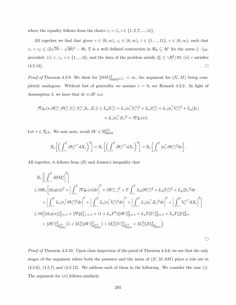
where the equality follows from the choice εi = εi, i ∈ 1, 2, 7, ..., 11.

All together we find that given γ ∈ (0,∞), εi ∈ (0,∞), i ∈ 1, ..., 11, c ∈ (0,∞), such that

ε1 + ε2 ≤ (2√

70 −√

30)2 − 30, T is a well–defined contraction in BR ⊆ Hc for the norm ‖ · ‖Hc

provided: (i) γ, εi, i ∈ 1, ..., 6, and the data of the problem satisfy Iε0 ≤ γR2/10; (ii) c satisfies

(4.5.13).

Proof of Theorem 4.3.9. We show for ‖∂M‖2BMO2,2,c < ∞, the argument for (N ,M) being com-

pletely analogous. Without lost of generality we assume c = 0, see Remark 4.2.2. In light of

Assumption J, we have that dr ⊗ dP–a.e.

|∇gr(s, ∂U sr , ∂V sr , U

sr , V

sr ,Yr,Zr)| ≤Lu|U sr |+ Lv|σ>r V s

r |2 + Lu|U sr |+ Lv|σ>r V sr |2 + Ly|Yr|

+ Lz|σ>r Zr|2 + |∇gr(s)|.

Let τ ∈ T0,T . We now note, recall ∂V ∈ H2,2BMO

Eτ[( ∫ T

τ−∂V s

r>dXr

)2]= Eτ

[( ∫ T

τ∂V s

r>dXr

)2]= Eτ

[ ∫ T

τ|σ>r ∂V s

r |2dr].

All together, it follows from (S) and Jensen’s inequality that

Eτ[∣∣∣∣ ∫ T

τ−d∂M s

r

∣∣∣∣2]≤ 10Eτ

[|∂sη(s)|2 +

∣∣∣∣ ∫ T

τ−|∇gr(s)|dr

∣∣∣∣2 + |∂U sτ−|2 + T

∫ T

τ−Lu|∂U sr |2 + Lu|U sr |2 + Ly|Yr|2dr

+∣∣∣∣ ∫ T

τ−Lv|σ>r ∂V s

r |2dr∣∣∣∣2 +

∣∣∣∣ ∫ T

τ−Lv|σ>r V s

r |2dr∣∣∣∣2 +

∣∣∣∣ ∫ T

τ−Lz|σ>r Zr|2dr

∣∣∣∣2 +∣∣∣∣ ∫ T

τ−V sr>dXr

∣∣∣∣2]≤ 10

(‖∂sη(s)‖2L∞,2 + ‖∇g‖2L1,∞,2 + (1 + LuT

2)‖∂U‖2S∞,2 + LuT‖U‖2S∞,2 + LyT‖Y‖2S∞

+ ‖∂V ‖2H2,2BMO

(1 + 2L2

v‖∂V ‖2H2,2BMO

)+ 2L2

v‖V ‖4H2,2BMO

+ 2L2z‖Z‖4H2

BMO

).

Proof of Theorem 4.3.10. Upon close inspection of the proof of Theorem 4.3.6, we see that the only

stages of the argument where both the presence and the norm of (N ,M, ∂M) plays a role are in

(4.5.6), (4.5.7) and (4.5.12). We address each of them in the following. We consider the case (i).

The argument for (ii) follows similarly.

205

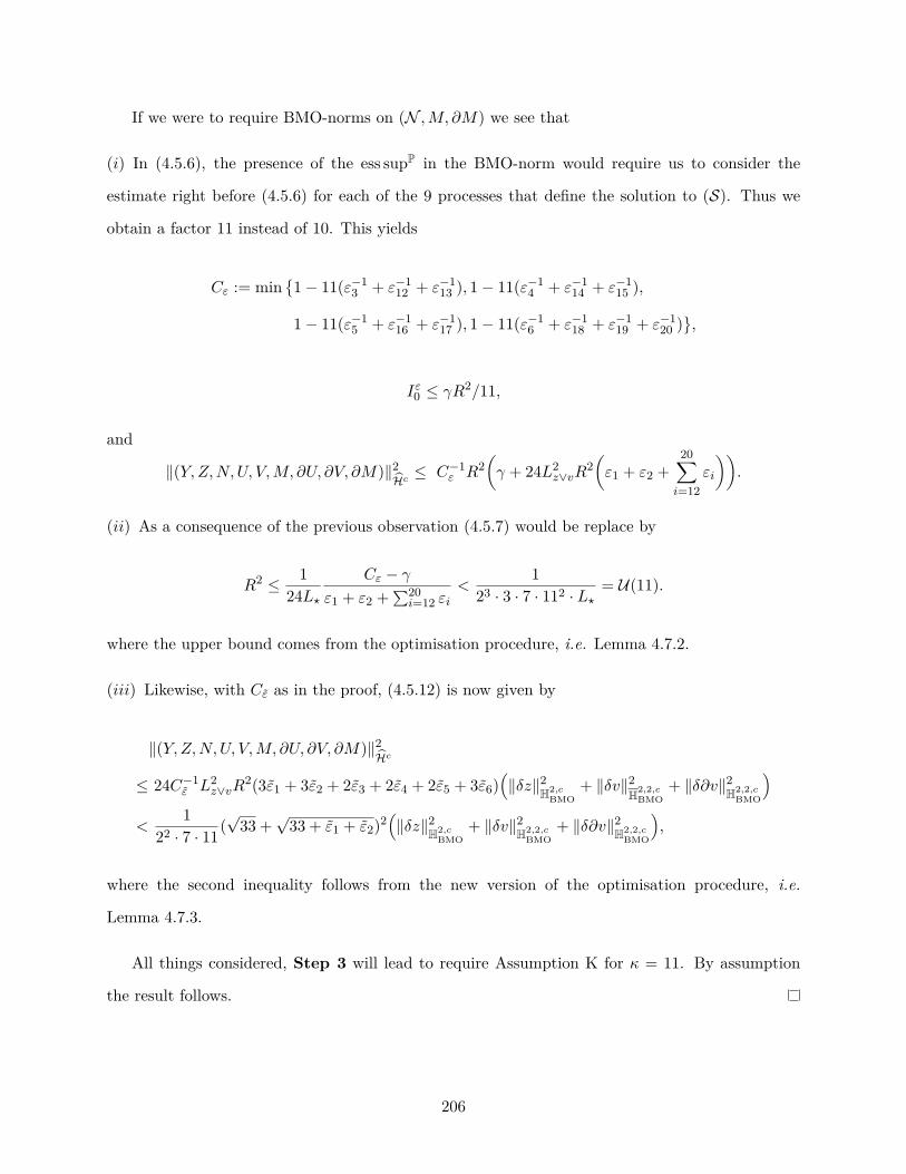
If we were to require BMO-norms on (N ,M, ∂M) we see that

(i) In (4.5.6), the presence of the ess supP in the BMO-norm would require us to consider the

estimate right before (4.5.6) for each of the 9 processes that define the solution to (S). Thus we

obtain a factor 11 instead of 10. This yields

Cε := min1− 11(ε−1

3 + ε−112 + ε−1

13 ), 1− 11(ε−14 + ε−1

14 + ε−115 ),

1− 11(ε−15 + ε−1

16 + ε−117 ), 1− 11(ε−1

6 + ε−118 + ε−1

19 + ε−120 ),

Iε0 ≤ γR2/11,

and

‖(Y, Z,N,U, V,M, ∂U, ∂V, ∂M)‖2Hc ≤ C−1ε R2

(γ + 24L2

z∨vR2(ε1 + ε2 +

20∑i=12

εi

)).

(ii) As a consequence of the previous observation (4.5.7) would be replace by

R2 ≤ 124L?

Cε − γε1 + ε2 +

∑20i=12 εi

<1

23 · 3 · 7 · 112 · L?= U(11).

where the upper bound comes from the optimisation procedure, i.e. Lemma 4.7.2.

(iii) Likewise, with Cε as in the proof, (4.5.12) is now given by

‖(Y,Z,N,U, V,M, ∂U, ∂V, ∂M)‖2Hc

≤ 24C−1ε L2

z∨vR2(3ε1 + 3ε2 + 2ε3 + 2ε4 + 2ε5 + 3ε6)

(‖δz‖2H2,c

BMO+ ‖δv‖2

H2,2,cBMO

+ ‖δ∂v‖2H2,2,cBMO

)<

122 · 7 · 11(

√33 +

√33 + ε1 + ε2)2

(‖δz‖2H2,c

BMO+ ‖δv‖2H2,2,c

BMO+ ‖δ∂v‖2H2,2,c

BMO

),

where the second inequality follows from the new version of the optimisation procedure, i.e.

Lemma 4.7.3.

All things considered, Step 3 will lead to require Assumption K for κ = 11. By assumption

the result follows.

206

4.6 Proof of the quadratic case

Proof of Theorem 4.3.12. For c > 0, let us introduce the mapping

T : (BR, ‖ · ‖Hc) −→ (BR, ‖ · ‖Hc)

(y, z, n, u, v,m, ∂u, ∂v, ∂m) 7−→ (Y,Z,N,U, V,M, ∂U, ∂V, ∂M),

with H = (Y,Z,N , U, V,M, ∂U, ∂V, ∂M) given for any s ∈ [0, T ], P–a.s. for any t ∈ [0, T ] by

Yt = ξ(T,X·∧T ) +∫ T

thr(X, yr, zr, urr, vrr , ∂U rr )dr −

∫ T

tZ>r dXr −

∫ T

tdNr,

U st = η(s,X·∧,T ) +∫ T

tgr(s,X, usr, vsr , yr, zr)dr −

∫ T

tV sr>dXr −

∫ T

tdM s

r ,

∂U st = ∂sη(s,X·∧,T ) +∫ T

t∇gr(s,X, ∂usr, ∂vsr , usr, vsr , yr, zr)dr −

∫ T

t∂V s

r>dXr −

∫ T

td∂M s

r .

Step 1: We first argue that T is well-defined.

(i) Let us first remark that for u ∈ S∞,2,c

E[ ∫ T

0|utt|2dr

]≤ T‖u‖2S∞,2,c . (4.6.1)

In light of Assumption L, there is c > 0 such that (ξ, η, ∂η, f , g,∇g) ∈ L∞,c×(L∞,2,c

)2×L1,∞,c×(L1,∞,2,c)2, thus, we may use (4.2.1) and (4.6.1) to obtain

E[|ξ(T )|2 +

∣∣∣∣ ∫ T

0|ht(yt, zt, utt, vtt, 0)|dt

∣∣∣∣2]+ sups∈[0,T ]

E[|η(s)|2 +

∣∣∣∣ ∫ T

0|gt(s, ust , vst , yt, zt)|dt

∣∣∣∣2]

+ sups∈[0,T ]

E[|∂η(s)|2 +

∣∣∣∣ ∫ T

0|∇gt(s, ∂ust , ∂vst , ust , vst , yst , zt)|dt

∣∣∣∣2]

≤ E[|ξ(T )|2 + 5

∣∣∣∣ ∫ T

0|ht|dt

∣∣∣∣2 + 17L2y

∣∣∣∣ ∫ T

0|yt|2dt

∣∣∣∣2 + 17L2z

∣∣∣∣ ∫ T

0|zt|2dt

∣∣∣∣2 + 5L2u

∣∣∣∣ ∫ T

0|utt|2dt

∣∣∣∣2+ 5L2

v

∣∣∣∣ ∫ T

0|vtt|2dt

∣∣∣∣2]+ sups∈[0,T ]

E[|η(s)|2+5

∣∣∣∣ ∫ T

0|gt(s)|dt

∣∣∣∣2+12L2u

∣∣∣∣ ∫ T

0|ust |2dt

∣∣∣∣2+12L2v

∣∣∣∣ ∫ T

0|vst |2dt

∣∣∣∣2]

+ sups∈[0,T ]

E[|∂η(s)|2 +7

∣∣∣∣ ∫ T

0|∇gt(s)|dt

∣∣∣∣2 +7L2u

∣∣∣∣ ∫ T

0|∂ust |2dt

∣∣∣∣2 + 7L2v

∣∣∣∣ ∫ T

0|∂vst |2dt

∣∣∣∣2]≤ ‖ξ‖2L∞,c + 5‖h‖2L1,∞,c + ‖η‖2L∞,2,c + 5‖g‖2L1,∞,2,c + ‖∂η‖2L∞,2,c + 7‖∇g‖2L1,∞,2,c

207

+ 17L2yT

2‖y‖4S∞,c + 34L2z‖z‖4H2,c

BMO+ 17L2

uT2‖u‖4S∞,2,c + 24L2

v‖v‖4H2,2,cBMO

+ 7L2uT

2‖∂u‖4S∞,2,c + 14L2v‖∂v‖4H2,2,c

BMO<∞.

Therefore, by Theorem 3.4.3, T defines a well-posed system of BSDEs with unique solution in the

space H2. We recall the spaces involved in the definition of H2, and their corresponding norms,

were introduced in Section 4.2.2.

(ii) For Ut := U tt , Vt := V tt , Mt := M t

t −∫ t

0 ∂Mrr dr, t ∈ [0, T ], (U ,V,M) ∈ S2 × H2 ×M2 and

satisfy the equation

Ut = η(T,X·∧T ) +∫ T

t

(gr(r,X, urr, vrr , yr, zr)− ∂U rr

)dr −

∫ T

tV>r dXr −

∫ T

tdMr, t ∈ [0, T ], P–a.s.

(iii) (Y,U) ∈ S∞,c × S∞,c and ‖U‖S∞,2,c + ‖∂U‖S∞,2,c <∞.

In light of Assumption L, dr ⊗ dP–a.e.

|hr| ≤ Ly|yr|2 + Lz|σ>r zr|2 + Lu|urr|2 + Lv|σ>r vrr |2 + Lu|∂U rr |+ |hr|,

|gr| ≤ Lu|urr|2 + Lv|σ>r vrr |2 + Ly|yr|2 + Lz|σ>r zr|2 + |∂U rr |+ |gr|,

|gr(s)| ≤ Lu|usr|2 + Lv|σ>r vsr |2 + Ly|yr|2 + Lz|σ>r zr|2 + |gr(s)|, (4.6.2)

|∇gr(s)| ≤ Lu|∂usr|2 + Lv|σ>r ∂vsr |2 + Lu|usr|2 + Lv|σ>r vsr |2 + Ly|yr|2 + Lz|σ>r zr|2 + |∇gr(s)|.

Again, we apply Meyer–Itô’s formula to ec2 t(|Yt| + |Ut| + |U st | + |∂U st |

)and take conditional

expectations with respect to Ft as in Equation (4.5.2). Moreover, in combination with (4.6.2) and

Lemma 4.7.1, we obtain back in (4.5.2) that

ec2 t(|Yt|+ |Ut|+ |U st |+ |∂U st |

)+ Et

[ ∫ T

t

c

2ec2 r|Yr|dr

]+ Et

[ ∫ T

t

c

2ec2 r|Ur|dr

]+ sups∈[0,T ]

Et[ ∫ T

t

c

2ec2 r|U sr |dr

]+ sups∈[0,T ]

Et[ ∫ T

t

c

2ec2 r|∂U sr |dr

]

≤ Et[ec2T(|ξ|+ |η(T )|+ |η(s)|+ |∂sη(s)|

)]+ Et

[ ∫ T

tec2 r(|hr|+ |gr|+ |gr(s)|+ |∇gr(s)|

)dr]

+ (T + LuT )(‖∂sη‖L∞,2,c + ‖∇g‖L1,∞,2,c + TL?

(‖y‖2S∞,c + ‖u‖2S∞,2,c + ‖∂u‖2S∞,2,c

))

208

+ (T + LuT )L?(‖z‖2H2,c

BMO+ ‖v‖2H2,2,c

BMO+ ‖∂v‖2H2,2,c

BMO

)+ Et

[ ∫ T

tecr(4Ly|σ>r yr|2 + 2Lu|σ>r urr|2 + 2Lu|σ>r usr|2

)dr]

+ Et[ ∫ T

tecr(Lu|σ>r ∂usr|2 + 4Lz|σ>r zr|2 + 2Lv|σ>r vrr |2 + 2Lv|σ>r vsr |2 + Lv|σ>r ∂vsr |2

)dr],

where we recall the notation L? = maxLy, Lu, Lu, Lz, Lv, Lv. Thus, for any c > 0 we obtain

maxec2 t|Yt|, e

c2 t|Ut|, e

c2 t|U st |, e

c2 t|∂U st |

≤ ‖ξ‖L∞,c + ‖h‖L1,∞,2,c + 2

(‖η‖L∞,2,c + ‖g‖L1,∞,2,c

)+ (1 + T + TLu)

(‖∂sη‖L∞,2,c + ‖∇g‖L1,∞,2,c

)+ (4 + T + LuT )L?T

(‖y‖2S2∞,c + ‖u‖2S∞,2,c + ‖∂u‖2S∞,2,c

)+ (4 + T + LuT )L?

(‖z‖2H2,c

BMO+ ‖v‖2

H2,2,cBMO

+ ‖∂v‖2H2,2,cBMO

),

(iv) We show (Z,V,N ,M)∈(H2,c

BMO)2×(M2,c)2, ‖V ‖2

H2,2,cBMO

+ ‖M‖2M2,2,c+ ‖∂V ‖2H2,2,cBMO

+ ‖∂M‖2M2,2,c <

∞.

From (iii), Assumption J.(ii) and J.(iii), together with Young’s inequality, yield that, for any

εi > 0, i ∈ 1, 2, and defining Cε1 := ε−11 7TL2

u, and Cε2 := ε−12 7T , we have

2Yr · hr − c|Yr|2 ≤ 2‖Y‖S∞,c(Ly|yr|2 + Lz|σ>r zr|2 + Lu|urr|2 + Lv|σ>r vrr |2 + |hr|

)+ ε1(7T )−1|∂U rr |2 + (Cε1 − c)|Yr|2,

2Ur · gr − c|Ur|2 ≤ 2‖U‖S∞,c(Ly|yr|2 + Lz|σ>r zr|2 + |urr|2 + Lv|σ>r vrr |2 + |gr|

)+ ε2(7T )−1|∂U rr |2 + (Cε2 − c)|Ur|2,

2U sr · gr(s)− c|U sr |2 ≤ 2‖U‖S∞,2,c(Lu|usr|2+Lv|σ>r vsr |2+Ly|yr|2+Lz|σ>r zr|2+|gr(s)|

)− c|U sr |2,

2∂U sr · ∇gr(s)− c|∂U sr |2 ≤ 2‖∂U‖S∞,c,2(Lu|∂usr|2 + Lv|σ>r ∂vsr |2 + Lu|usr|2 + Lv|σ>r vsr |2 + |∇gr(s)|

)+ 2‖∂U‖S∞,c,2

(Ly|yr|2 + Lz|σ>r zr|2

)− c|∂U sr |2.

These inequalities in combination with the analogous version of Lemma 4.7.1 (which holds for

209

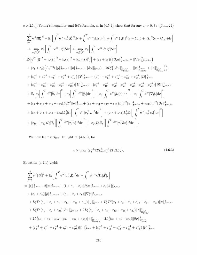
c > 2Lu), Young’s inequality, and Itô’s formula, as in (4.5.4), show that for any εi > 0, i ∈ 3, ..., 24

4∑i=1

ect|Yit|2 + Et

[ ∫ T

tecr|σ>r Zir|2dr +

∫ T

tecr−dTr[Zi]r +

∫ T

tecr(|Yr|2(c− Cε1) + |Ur|2(c− Cε2)

)dr]

+ sups∈[0,T ]

Et[ ∫ T

tcecr|U sr |2dr

]+ sups∈[0,T ]

Et[ ∫ T

tcecr|∂U sr |2dr

]=Et

[ecT(|ξ|2 + |η(T )|2 + |η(s)|2 + |∂sη(s)|2

)]+ (ε1 + ε2)

(‖∂sη‖2L∞,2,c + ‖∇g‖2L1,∞,2,c

)+ (ε1 + ε2)

(L?T

2(‖y‖4S∞,c+‖u‖4S∞,c + ‖∂u‖4S∞,c) + 2L2?

(‖∂v‖4H2,2,c

BMO+ ‖v‖4H2,2,c

BMO+ ‖z‖4H2,c

BMO

))+(ε−1

3 + ε−17 + ε−1

8 + ε−19 + ε−1

10)‖Y‖2S∞,c +

(ε−1

4 + ε−111 + ε−1

12 + ε−113 + ε−1

14)‖U‖2S∞,c

+(ε−1

5 + ε−115 + ε−1

16 + ε−117 + ε−1

18)‖U‖2S∞,c,2 +

(ε−1

6 + ε−119 + ε−1

20 + ε−121 + ε−1

22 + ε−123 + ε−1

24)‖∂U‖2S∞,c,2

+ Et[ε3

∣∣∣∣ ∫ T

tecr|hr|dr

∣∣∣∣2 + ε4

∣∣∣∣ ∫ T

tecr|gr|dr

∣∣∣∣2]+ ε5

∣∣∣∣ ∫ T

tecr|gr(s)|dr

∣∣∣∣2 + ε6

∣∣∣∣ ∫ T

tecr|∇gr|dr

∣∣∣∣2]+ (ε7 + ε11 + ε15 + ε19)L?T 2‖y‖4S∞,c+ (ε9 + ε13 + ε17 + ε21)L?T 2‖u‖4S∞,2,c+ ε23L?T

2‖∂u‖4S∞,2,c

+ (ε8 + ε12 + ε16 + ε20)L2zEt[∣∣∣∣ ∫ T

tecr|σ>r zr|2dr

∣∣∣∣2]+ (ε10 + ε14)L2vEt[∣∣∣∣ ∫ T

tecr|σ>r vrr |2dr

∣∣∣∣2]+ (ε18 + ε22)L2

vEt[∣∣∣∣ ∫ T

tecr|σ>r vsr |2dr

∣∣∣∣2]+ ε24L2vEt

[∣∣∣∣ ∫ T

tecr|σ>r ∂vsr |2dr

∣∣∣∣2].We now let τ ∈ T0,T . In light of (4.5.3), for

c ≥ max ε−11 7TL2

u, ε−12 7T, 2Lu, (4.6.3)

Equation (4.2.1) yields

4∑i=1

ect|Yit|2 + Et

[ ∫ T

tecr|σ>r Zir|2dr +

∫ T

tecr−dTr[Zi]r

]

= ‖ξ‖2L∞,c + 2‖η‖2L∞,2,c+ (1 + ε1 + ε2)‖∂sη‖2L∞,2,c+ ε3‖h‖2L1,∞,c

+ (ε4 + ε5)‖g‖2L1,∞,2,c+ (ε1 + ε2 + ε6)‖∇g‖2L1,∞,2,c

+ L2?T

2(ε1 + ε2 + ε7 + ε11 + ε15 + ε19)‖y‖4S∞,c + L2?T

2(ε1 + ε2 + ε9 + ε13 + ε17 + ε21)‖u‖4S∞,2,c

+ L2?T

2(ε1 + ε2 + ε23)‖∂u‖4S∞,2,c + 2L2?(ε1 + ε2 + ε8 + ε12 + ε16 + ε20)‖z‖4H2,c

BMO

+ 2L2?(ε1 + ε2 + ε10 + ε14 + ε18 + ε22)‖v‖4

H2,2,cBMO

+ 2L2?(ε1 + ε2 + ε24)‖∂v‖4H2,2,c

BMO

+(ε−1

3 + ε−17 + ε−1

8 + ε−19 + ε−1

10)‖Y‖2S∞,c +

(ε−1

4 + ε−111 + ε−1

12 + ε−113 + ε−1

14)‖U‖2S∞,c

210

+(ε−1

5 + ε−115 + ε−1

16 + ε−117 + ε−1

18)‖U‖2S∞,c,2

+(ε−1

6 + ε−119 + ε−1

20 + ε−121 + ε−1

22 + ε−123 + ε−1

24)‖∂U‖2S∞,c,2 ,

which in turn leads to

110(‖Y‖2S∞,c + ‖U‖2S∞,c + ‖U‖2S∞,2,c + ‖∂U‖2S∞,2,c + ‖Z‖2H2,c

BMO

+ ‖V ‖2H2,2,c

BMO+ ‖∂V ‖2H2,2,c

BMO+ ‖N‖2M2,c + ‖M‖2M2,2,c + ‖∂M‖2M2,2,c

)≤ ‖ξ‖2L∞,c + 2‖η‖2L∞,2,c+ (1 + ε1 + ε2)‖∂sη‖2L∞,2,c+ ε3‖h‖2L1,∞,c

+ (ε4 + ε5)‖g‖2L1,∞,2,c+ (ε1 + ε2 + ε6)‖∇g‖2L1,∞,2,c

+ L2?T

2(ε1 + ε2 + ε7 + ε11 + ε15 + ε19)‖y‖4S∞,c

+ L2?T

2(ε1 + ε2 + ε9 + ε13 + ε17 + ε21)‖u‖4S∞,2,c

+ L2?T

2(ε1 + ε2 + ε23)‖∂u‖4S∞,2,c + 2L2?(ε1 + ε2 + ε8 + ε12 + ε16 + ε20)‖z‖4H2,c

BMO

+ 2L2?(ε1 + ε2 + ε10 + ε14 + ε18 + ε22)‖v‖4

H2,2,cBMO

+ 2L2?(ε1 + ε2 + ε24)‖∂v‖4H2,2,c

BMO

+(ε−1

3 + ε−17 + ε−1

8 + ε−19 + ε−1

10)‖Y‖2S∞,c +

(ε−1

4 + ε−111 + ε−1

12 + ε−113 + ε−1

14)‖U‖2S∞,c

+(ε−1

5 + ε−115 + ε−1

16 + ε−117 + ε−1

18)‖U‖2S∞,c,2

+(ε−1

6 + ε−119 + ε−1

20 + ε−121 + ε−1

22 + ε−123 + ε−1

24)‖∂U‖2S∞,c,2 .

(4.6.4)

From (4.6.4) we conclude (Z,N) ∈ H2,cBMO ×M2,c,

‖V ‖2H2,2,c

BMO+ ‖∂V ‖2H2,2,c

BMO+ ‖M‖2M2,2,c + ‖∂M‖2M2,2,c <∞.

Defining Cε analogously and if for some γ ∈ (0,∞)

Iε0 ≤ γR2/10, (4.6.5)

we obtain back in (4.6.4)

‖(Y,Z,N,U, V,M, ∂U, ∂V, ∂M)‖2Hc

≤ C−1ε

(10Iε0 + 10L2

? max2, T 2((ε1 + ε2 + ε7 + ε11 + ε15 + ε19)‖y‖4S∞,c

211

+ (ε1 + ε2 + ε9 + ε13 + ε17 + ε21)‖u‖4S∞,2,c

+ (ε1 + ε2 + ε23)‖∂u‖4S∞,2,c + (ε1 + ε2 + ε8 + ε12 + ε16 + ε20)‖z‖4H2,cBMO

+ (ε1 + ε2 + ε10 + ε14 + ε18 + ε22)‖v‖4H2,2,c

BMO+ (ε1 + ε2 + ε24)‖∂v‖4H2,2,c

BMO

)≤ C−1

ε R2(γ + 10L2

? max2, T 2R2(ε1 + ε2 +

24∑i=7

εi

)).

Therefore, to obtain T(BR) ⊆ BR, that is to say that the image under T of the ball of radius

R is contained in the ball of radius R, it is necessary to find R2 such that the term in parentheses

above is less or equal than Cε, i.e.

R2 ≤ 110L2

? max2, T 2Cε − γ

ε1 + ε2 +∑24i=7 εi

,

which after optimising the choice of ε’s renders

R2 <1

26 · 3 · 52 · 7 · L2? ·max2, T 2

. (4.6.6)

(v) The continuity of the applications ([0, T ],B([0, T ])) −→ (S∞,c, ‖ · ‖S∞,c)(resp. (H2,c

BMO, ‖ ·

‖H2,cBMO

), (M2,c, ‖ · ‖M2,c))

: s 7−→ ϕs for ϕ = U s, ∂U s (resp. V s, ∂V s,M s, ∂M s) follows analogously

as in the proof Theorem 4.3.6.

We conclude, T(BR) ⊆ BR for all R satisfying (4.6.6).

Step 2: We now argue that T is a contraction in BR ⊆ H for the norm ‖ · ‖Hc . Let

δht := ht(y1t , z

1t , u

1,tt , v

1,tt , ∂U1,t

t )− ht(y2t , z

2t , u

2,tt , v

2,tt , ∂U2,t

t ),

δgt := gt(t, u1,tt , v

1,tt , y1

t , z1t )− ∂U1,t

t − gt(t, u2,tt , v

2,tt , y2

t , z2t ) + ∂U2,t

t ,

δht := ht(y1t , z

1t , u

1,tt , v

1,tt , ∂U2,t

t )− ht(y2t , z

2t , u

2,tt , v

2,tt , ∂U2,t

t ),

δgt := gt(t, u1,tt , v

1,tt , y1

t , z1t )− gt(t, u2,t

t , v2,tt , y2

t , z2t ),

δgt(s) := gt(s, u1,st , v1,s

t , y1t , z

1t )− gt(s, u2,s

t , v2,st , y2

t , z2t ),

δ∇gt(s) := ∇gt(s, ∂u1,st , ∂v1,s

t , u1,st , v1,s

t , y1t , z

1t )− gt(s, ∂u2,s

t , ∂v2,st , u2,s

t , v2,st , y2

t , z2t ).

212

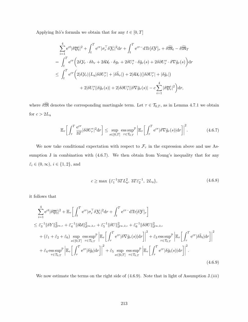
Applying Itô’s formula we obtain that for any t ∈ [0, T ]

4∑i=1

ect|δYit|2 +

∫ T


∫ T

tecr−dTr[δZi]r + δMt − δMT

=∫ T

tecr(

2δYr · δhr + 2δUr · δgr + 2δU sr · δgr(s) + 2δ∂U sr · δ∇gr(s))

dr

≤∫ T

tecr(

2|δYr|(Lu|δ∂U rr |+ |δhr|

)+ 2|δUr|

(|δ∂U rr |+ |δgr|

)+ 2|δU sr ||δgr(s)|+ 2|δ∂U sr ||δ∇gr(s)| − c

4∑i=1|δYi

r|2)

dr,

where δM denotes the corresponding martingale term. Let τ ∈ T0,T , as in Lemma 4.7.1 we obtain

for c > 2Lu

Eτ[ ∫ T

τ

ecr

3T |δ∂Urr |2dr

]≤ sup

s∈[0,T ]ess supP

τ∈T0,T

∣∣∣∣Eτ[ ∫ T

τecr|δ∇gr(s)|dr

]∣∣∣∣2. (4.6.7)

We now take conditional expectation with respect to Fτ in the expression above and use As-

sumption J in combination with (4.6.7). We then obtain from Young’s inequality that for any

εi ∈ (0,∞), i ∈ 1, 2, and

c ≥ max ε−11 3TL2

u, 3T ε−12 , 2Lu, (4.6.8)

it follows that

4∑i=1

ect|δYit|2 + Eτ

[ ∫ T


∫ T

tecr−dTr[δZi]r

]

≤ ε−13 ‖δY ‖

2S∞,c + ε−1

4 ‖δU‖2S∞,2,c + ε−1

5 ‖δU‖2S∞,2,c + ε−1

6 ‖δ∂U‖2S∞,2,c

+ (ε1 + ε2 + ε6) sups∈[0,T ]

ess supP

τ∈T0,T

∣∣∣∣Eτ[ ∫ T

τecr|δ∇gr(s)|dr

]∣∣∣∣2 + ε3 ess supP

τ∈T0,T

∣∣∣∣Eτ[ ∫ T

τecr|δht|dr

]∣∣∣∣2

+ ε4 ess supP

τ∈T0,T

∣∣∣∣Eτ[ ∫ T

τecr|δgt|dr

]∣∣∣∣2 + ε5 sups∈[0,T ]

ess supP

τ∈T0,T

∣∣∣∣Eτ[ ∫ T

τecr|δgt(s)|dr

]∣∣∣∣2.(4.6.9)

We now estimate the terms on the right side of (4.6.9). Note that in light of Assumption J.(iii)

213

we have

∣∣∣∣Eτ[ ∫ T

τecr|δ∇gt(s)|dr

]∣∣∣∣2≤∣∣∣∣Eτ[ ∫ T

τecr(Lu|δ∂usr|

(|∂u1,s

r |+ |∂u2,sr |)

+ Lv|σ>r δ∂vsr |(|σ>r ∂v1,s

r |+ |σ>r ∂v2,sr |)

+ Lu|δusr|(|u1,sr |+ |u2,s

r |)

+ Lv|σ>r δvsr |(|σ>r v1,s

r |+ |σ>r v2,sr |)

+ Ly|δyr|(|y1r |+ |y2

r |)

+ Lz|σ>r δzr|(|σ>r z1

r |+ |σ>r z2r |))

dr]∣∣∣∣2

≤ 6L2?Eτ

[ ∫ T

τecr|δ∂usr|2dr

]Eτ[ ∫ T

τecr(|∂u1,s

r |+ |∂u2,sr |)2dr

]+ 6L2

?Eτ[ ∫ T


]Eτ[ ∫ T

τecr(|σ>r ∂v1,s

r |+ |σ>r ∂v2,sr |)2dr

]+ 6L2

?Eτ[ ∫ T

τecr|δusr|2dr

]Eτ[ ∫ T

τecr(|u1,sr |+ |u2,s

r |)2dr

]+ 6L2

?Eτ[ ∫ T


]Eτ[ ∫ T

τecr(|σ>r v1,s

r |+ |σ>r v2,sr |)2dr

]+ 6L2

?Eτ[ ∫ T

τecr|δyr|2dr

]Eτ[ ∫ T

τecr(|y1r |+ |y2

r |)2dr

]+ 6L2

?Eτ[ ∫ T

τecr|σ>r δzr|2dr

]Eτ[ ∫ T

τecr(|σ>r z1

r |+ |σ>r z2r |)2dr

]≤ 6L2

?R2 max2, T

(Eτ[ ∫ T

τecr|δ∂usr|2dr

]+ Eτ

[ ∫ T


]+ Eτ

[ ∫ T

τecr|δusr|2dr

]+ Eτ

[ ∫ T


]+ Eτ

[ ∫ T

τecr|δyr|2dr

]+ Eτ

[ ∫ T

τecr|σ>r δzr|2dr

])≤ 6L2

?R2 max2, T 2

(‖δ∂u‖2S∞,2,c+ ‖δ∂v‖

2H2,2,c

BMO+ ‖δu‖2S∞,2,c+ ‖δv‖

2H2,2,c

BMO+ ‖δy‖2S∞,c+ ‖δz‖2H2,c

BMO

),

where in the second inequality we used (I.1) and Cauchy–Schwarz’s inequality. Similarly


τecr|δhr|dr

]∣∣∣∣2, ∣∣∣∣Eτ[ ∫ T

τecr|δgr(s)|dr

]∣∣∣∣2, ∣∣∣∣Eτ[ ∫ T

τecr|δgr|dr

]∣∣∣∣2≤ 4L2

?R2 max2, T 2

(‖δy‖2S∞,c + ‖δz‖2H2,c

BMO+ ‖δu‖2S∞,2,c + ‖δv‖2

H2,cBMO

).

Overall, we obtain back in (4.6.9) that

4∑i=1

ect|δYit|2 + Eτ

[ ∫ T


∫ T

tecr−dTr[δZi]r

]

≤ ε−13 ‖δY ‖

2S∞,c + ε−1

4 ‖δU‖2S∞,2,c + ε−1

5 ‖δU‖2S∞,2,c + ε−1

6 ‖δ∂U‖2S∞,2,c

214

+ 6(ε1 + ε2 + ε6)L2?R

2 max2, T 2(‖δ∂u‖2S∞,2,c + ‖δ∂v‖2H2,2,c

BMO+ ‖δu‖2S∞,2,c

)+ 6(ε1 + ε2 + ε6)L2

?R2 max2, T 2

(‖δv‖2

H2,2,cBMO

+ ‖δy‖2S∞,c + ‖δz‖2H2,cBMO

)+ 4(ε3 + ε4 + ε5)L2

?R2 max2, T 2

(‖δy‖2S∞,c + ‖δz‖2H2,c

BMO+ ‖δu‖2S∞,2,c + ‖δv‖2

H2,cBMO

).

If we define, for εi > 10, i ∈ 3, 4, 5, 6, Cε := min1− 10/ε3, 1− 10/ε4, 1− 10/ε5, 1− 10/ε6

,

we deduce,

‖δH‖2Hc ≤ 20C−1ε L2

?R2 max2, T 2(3ε1 + 3ε2 + 2ε3 + 2ε4 + 2ε5 + 3ε6)‖δh‖Hc . (4.6.10)

Minimising for ε1 and ε2 fixed, we find that letting

R2 <1

26 · 3 · 52 · 7 · L2? ·max2, T 2

, c ≥ maxε−11 7TL2

u, ε−12 7T, ε−1

1 3TL2u, 3T ε−1

2 , 2Lu,

we have that

‖δH‖2Hc <20

24 · 3 · 7 · 102 3(√

30 + (ε1 + ε2) +√

30)2‖δh‖Hc = (√

30 + (ε1 + ε2) +√

30)2

23 · 7 · 10 ‖δh‖Hc .

Thus, letting choosing (√

30 + (ε1 + ε2) +√

30)2 ≤ 23 · 7 · 10, T is contractive.

Step 3: We consolidate our results.. In light of (4.6.3) and (4.6.8), taking εi = εi, i ∈ 1, 2, c

must satisfy

c ≥ maxε−11 7TL2

u, ε−12 7T, ε−1

1 3TL2u, 3T ε−1

2 , 2Lu = maxε−11 7TL2

u, ε−12 7T, 2Lu (4.6.11)

All together we find that given γ ∈ (0,∞), εi ∈ (0,∞), i ∈ 1, 2, c ∈ (0,∞), such that

ε1 + ε2 ≤ (4√

35 −√

30)2 − 30, T is a well-defined contraction in BR ⊆ Hc for the norm ‖ · ‖Hc

provided: (i) γ, εi, i ∈ 1, 2, and the data of the problem satisfy (4.6.5); (ii) c satisfies (4.6.11).

215

4.7 Auxiliary results

4.7.1 Proofs of Section 4.2

Proof of Lemma 4.2.3. First note that for Z ∈ H2BMO(Rn×d), Z • Xt :=

∫ t0 ZdXr is a continuous

local martingale, thus we have that

‖Z •X‖BMO2,c = supτ∈T0,T

∥∥∥E[⟨e c2Z •X⟩T−⟨ec2Z •X

⟩τ

∣∣Fτ ]∥∥∥∞<∞.

Therefore, letting Xt := E[〈ec2Z •X〉T − 〈e

c2Z •X〉t|Ft], we have:

(i) |Xt| ≤ ‖Z •X‖BMO2,c = ‖Z‖2H2,c

BMO,

(ii) A = 〈ec2Z •X〉. Indeed, note Xt = E

[⟨ec2Z •X

⟩T

∣∣Ft]− ⟨e c2Z •X⟩t.The result then follows immediately from the energy inequality, i.e.

E[( ∫ T

0ecr|σ>r Zr|2dr

)p]= E[(A)p∞] ≤ p!‖Z‖2p

H2,cBMO

.

To obtain the second part of the statement, recall that by definition of H2,2(Rn×d), s 7−→ ∂Zs

is the density of s 7−→ Zs with respect to the Lebesgue measure and Z is given as in Remark 4.2.2.

By definition of Z, Fubini’s theorem and Young’s inequality we have that for ε > 0

∫ T

tecu|σ>u Zuu |2 − ecu|σ>u Ztu|2du =

∫ T

t

∫ u

t2ecuTr

[Zru>σuσ

>u ∂Z

ru

]drdu

=∫ T

t

∫ T

r2ecuTr

[Zru>σuσ

>u ∂Z

ru

]dudr

≤∫ T

t

∫ T

rεecu|σ>u Zru|2 + ε−1ecu|σ>u ∂Zru|2dudr.

This proves the first first statement. For the second claim, we may use (I.1) and (4.2.1) to obtain

Et[( ∫ T

tecu|σ>u Zu|2du

)2]≤ 3

(Et[( ∫ T

tecu|σ>u Ztu|2du

)2]

216

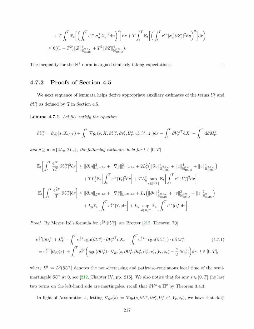
+ T

∫ T

tEt[( ∫ T

tecu|σ>u Zru|2du

)2]dr + T

∫ T

tEt[( ∫ T

tecu|σ>u ∂Zru|2du

)2]dr)

≤ 6((1 + T 2)‖Z‖4H2,2,cBMO

+ T 2‖∂Z‖4H2,2,cBMO

).

The inequality for the H2 norm is argued similarly taking expectations.

4.7.2 Proofs of Section 4.5

We next sequence of lemmata helps derive appropriate auxiliary estimates of the terms U tt and

∂U tt as defined by T in Section 4.5.

Lemma 4.7.1. Let ∂U satisfy the equation

∂U st = ∂sη(s,X·∧,T ) +∫ T

t∇gr(s,X, ∂U sr , ∂vsr , U sr , vsr ,Yr, zr)dr −

∫ T

t∂V s

r>dXr −

∫ T

td∂M s

r ,

and c ≥ max2Lu, 2Lu, the following estimates hold for t ∈ [0, T ]

Et[ ∫ T

t

ecr

7T |∂Urr |2dr

]≤ ‖∂sη‖2L∞,2,c + ‖∇g‖2L1,∞,2,c + 2L2

?

(‖∂v‖4H2,2,c

BMO+ ‖z‖4H2,c

BMO+ ‖v‖4H2,2,c

BMO

)+ TL2

yEt[ ∫ T

tecr|Yr|2dr

]+ TL2

u sups∈[0,T ]

Et[ ∫ T

tecr|U sr |2dr

],

Et[ ∫ T

t

ec2 r

T|∂U rr |dr

]≤ ‖∂sη‖L∞,2,c + ‖∇g‖L1,∞,2,c + L?

(‖∂v‖2H2,2,c

BMO+ ‖v‖2H2,2,c

BMO+ ‖z‖2H2,c

BMO

)+ LyEt

[ ∫ T

tec2 r|Yr|dr

]+ Lu sup

s∈[0,T ]Et[ ∫ T

tecr|U sr |dr

].

Proof. By Meyer–Itô’s formula for ec2 t|∂U st |, see Protter [212, Theorem 70]

ec2 t|∂U st |+ L0

T −∫ T

tec2 r sgn(∂U sr ) · ∂V s

r>dXr −

∫ T

tec2 r− sgn(∂U sr−) · d∂M s

r (4.7.1)

= ec2T |∂sη(s)|+

∫ T

tec2 r(

sgn(∂U sr ) · ∇gr(s, ∂U sr , ∂vsr , U sr , vsr ,Yr, zr)−c

2 |∂Usr |)

dr, t ∈ [0, T ],

where L0 := L0(∂U s) denotes the non-decreasing and pathwise-continuous local time of the semi-

martingale ∂U s at 0, see [212, Chapter IV, pp. 216]. We also notice that for any s ∈ [0, T ] the last

two terms on the left-hand side are martingales, recall that ∂V s ∈ H2 by Theorem 3.4.3.

In light of Assumption J, letting ∇gr(s) := ∇gr(s, ∂U sr , ∂vsr , U sr , vsr , Yr, zr), we have that dt ⊗

217

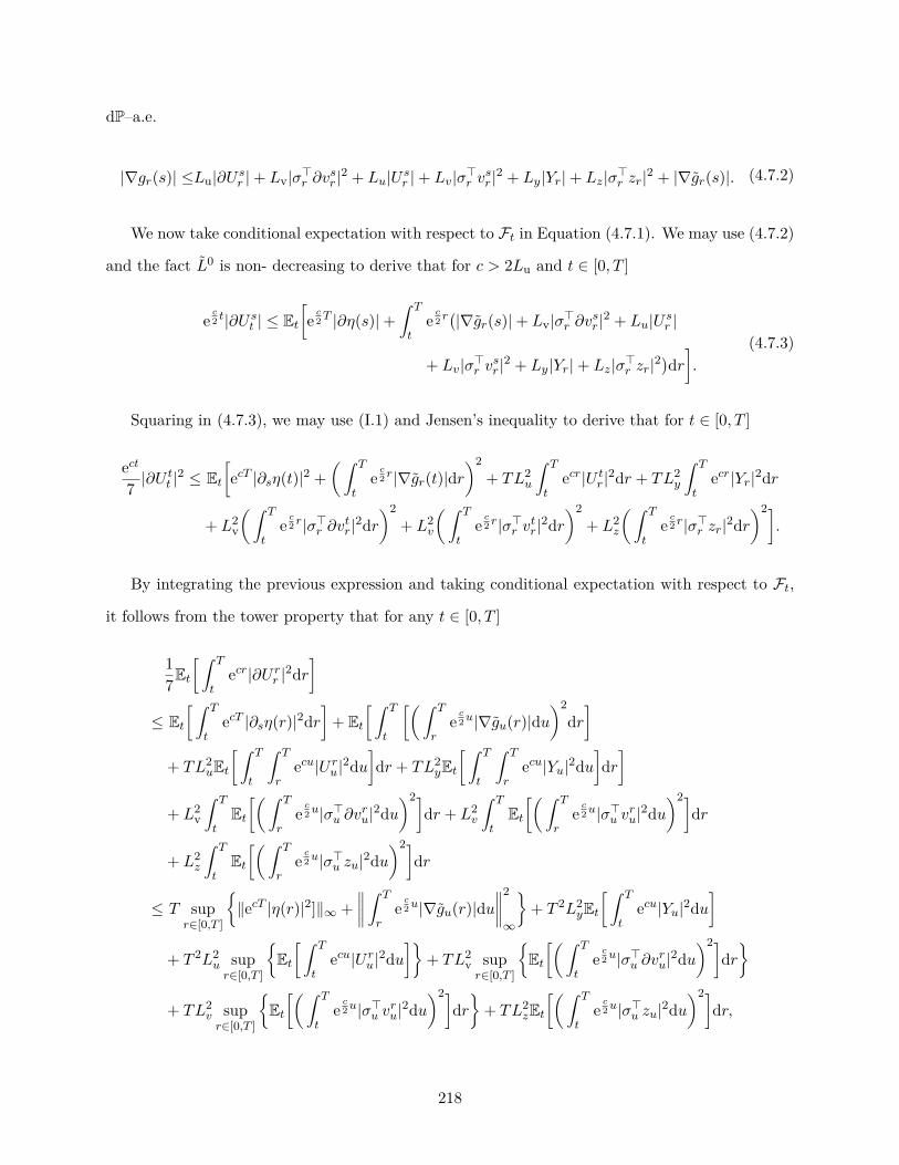
dP–a.e.

|∇gr(s)| ≤Lu|∂U sr |+ Lv|σ>r ∂vsr |2 + Lu|U sr |+ Lv|σ>r vsr |2 + Ly|Yr|+ Lz|σ>r zr|2 + |∇gr(s)|. (4.7.2)

We now take conditional expectation with respect to Ft in Equation (4.7.1). We may use (4.7.2)

and the fact L0 is non- decreasing to derive that for c > 2Lu and t ∈ [0, T ]

ec2 t|∂U st | ≤ Et

[ec2T |∂η(s)|+

∫ T

tec2 r(|∇gr(s)|+ Lv|σ>r ∂vsr |2 + Lu|U sr |

+ Lv|σ>r vsr |2 + Ly|Yr|+ Lz|σ>r zr|2)dr].

(4.7.3)

Squaring in (4.7.3), we may use (I.1) and Jensen’s inequality to derive that for t ∈ [0, T ]

ect

7 |∂Utt |2 ≤ Et

[ecT |∂sη(t)|2 +

(∫ T

tec2 r|∇gr(t)|dr

)2+ TL2

u

∫ T

tecr|U tr |2dr + TL2

y

∫ T

tecr|Yr|2dr

+ L2v

(∫ T

tec2 r|σ>r ∂vtr|2dr

)2+ L2

v

(∫ T

tec2 r|σ>r vtr|2dr

)2+ L2

z

(∫ T

tec2 r|σ>r zr|2dr

)2].

By integrating the previous expression and taking conditional expectation with respect to Ft,

it follows from the tower property that for any t ∈ [0, T ]

17Et

[ ∫ T

tecr|∂U rr |2dr

]≤ Et

[ ∫ T

tecT |∂sη(r)|2dr

]+ Et

[ ∫ T

t

[( ∫ T

rec2u|∇gu(r)|du

)2dr]

+ TL2uEt

[ ∫ T

t

∫ T

recu|U ru|2du

]dr + TL2

yEt[ ∫ T

t

∫ T

recu|Yu|2du

]dr]

+ L2v

∫ T

tEt[( ∫ T

rec2u|σ>u ∂vru|2du

)2]dr + L2

v

∫ T

tEt[( ∫ T

rec2u|σ>u vru|2du

)2]dr

+ L2z

∫ T

tEt[( ∫ T

rec2u|σ>u zu|2du

)2]dr

≤ T supr∈[0,T ]

‖ecT |η(r)|2]‖∞ +

∥∥∥∥ ∫ T

rec2u|∇gu(r)|du

∥∥∥∥2

∞

+ T 2L2

yEt[ ∫ T

tecu|Yu|2du

]

+ T 2L2u supr∈[0,T ]

Et[ ∫ T

tecu|U ru|2du

]+ TL2

v supr∈[0,T ]

Et[( ∫ T

tec2u|σ>u ∂vru|2du

)2]dr

+ TL2v supr∈[0,T ]

Et[( ∫ T

tec2u|σ>u vru|2du

)2]dr

+ TL2zEt[( ∫ T

tec2u|σ>u zu|2du

)2]dr,

218

and by (4.2.1) we obtain for c > 2Lu, and any t ∈ [0, T ]

Et[ ∫ T

t

ecr

7T |∂Urr |2dr

]≤ ‖∂sη‖2L∞,2,c + ‖∇g‖2L1,∞,2,c + 2L2

?

(‖∂v‖4H2,2,c

BMO+ ‖z‖4H2,c

BMO+ ‖v‖4H2,2,c

BMO

)+ TL2

yEt[ ∫ T

tecr|Yr|2dr

]+ +TL2

u supr∈[0,T ]

Et[ ∫ T

tecu|U ru|2du

].

Evaluating at s = t in (4.7.3) and integrating with respect to t we derive the second estimate.

Lemma 4.7.2 (Optimal upper bound for R). (OPT1) = 1/(245), where

supmin

α(ε3, ε12, ε13), α(ε4, ε14, ε15), α(ε5, ε16, ε17), α(ε6, ε18, ε19, ε20)

− γ

ε1 + ε2 +∑20i=12 εi

s.t. α(ε3, ε12, ε13) = 1− 10(ε−13 + ε−1

12 + ε−113 ) ∈ (0, 1],

α(ε4, ε14, ε15) = 1− 10(ε−14 + ε−1

14 + ε−115 ) ∈ (0, 1],

α(ε5, ε16, ε17) = 1− 10(ε−15 + ε−1

16 + ε−117 ) ∈ (0, 1],

α(ε6, ε18, ε19, ε20) = 1− 10(ε−16 + ε−1

18 + ε−119 + ε−1

20 ) ∈ (0, 1],

γ ∈ (0,∞); εi ∈ (0,∞),∀i ∈ 1, . . . , 6 ∪ 12, . . . , 20.

Proof. We begin by noticing that as a function of (γ, ε1, ε2, ε3, ε4, ε5, ε6) the objective is bounded

by the value when (γ, ε1, ε2, ε3, ε4, ε5, ε6) −→ (0, 0, 0,∞,∞,∞,∞). Thus, we will maximise

min1− 10(ε−112 + ε−1

13 ), 1− 10(ε−114 + ε−1

15 ), 1− 10(ε−116 + ε−1

17 ), 1− 10(ε−118 + ε−1

19 + ε−120 )∑20

i=12 εi.

From this we observe that the optimal value is positive. Indeed, one can find a feasible solution

with positive value, and the min in the objective function does not involve common εi terms, so

the minima is attained at one of the terms. Since the value function is symmetric in each of the

variables inside each term of the mean we can assume with out lost of generality

ε12 =ε13 = 2α1, ε14 = ε15 = 2α2, ε16 = ε17 = 2α3, ε18 = ε19 = ε20 = 3α4, α1, α2, α3, α4∈(0,∞)4.

219

So we can write the objective function as

min1− 10α−11 , 1− 10α−1

2 , 1− 10α−13 , 1− 10α−1

4 4α1 + 4α2 + 4α3 + 9α4

.

Now, without lost of generality the min is attained by the first quantity. This is, the optimisation

problem becomes

sup 1− 10α−11

4α1+4α2+4α3+9α4s.t. α1 ≤ minα2, α3, α4, 1− 10α−1

i ∈ (0, 1], αi ∈ (0,∞), i ∈ 1, . . . , 4.

Now, as the objective function is decreasing in α2, α3, α4, and α1 ≤ minα2, α3, α4,we must have

α1 = α2 = α3 = α4 and we are left with

sup 1− 10α−11

21α1s.t. 1− 10α−1

1 ∈ (0, 1], α1 ∈ (0,∞).

Let f(α1) := α1−1021α2

1. By first order analysis

∂α1f(α1) = −α1(α1 − 20)21α4

1= 0, yields, α1 ∈ 0, 20.

By inspecting the sign of the derivative, one sees that α1 = 0 corresponds to a minima and α1 = 20

is the maximum and it is feasible. Thus we obtain that

f(α?1)

= 123 · 3 · 5 · 7 .

We conclude the maxima happens when (ε12, ε13, ε14, ε15, ε16, ε17, ε18, ε19, ε20) = (40, 40, 40, 40,

40, 40, 60, 60, 60). Evaluating the value function in these values and letting (γ, ε1, ε3, ε8, ε9, ε10, ε11)

−→ (0, 0, 0,∞,∞,∞,∞), we obtain this bound. This is, f does not attain its maximum value, but

in the feasible region it can get as close as possible.

Lemma 4.7.3 (Minimal bound for Contraction). (OPT2) = 3(√

30 + (ε1 + ε2) +√

30)2, where

(OPT2) := inf(

3ε1 + 3ε2 + 2ε3 + 2ε4 + 2ε5 + 3ε6)

min

ε3ε3 − 10 ,

ε4ε4 − 10 ,

ε5ε5 − 10 ,

ε6ε6 − 10

,

s.t. 1− 10ε−1i ∈ (0, 1], εi ∈ (0,∞), i ∈ 3, 4, 5, 6.

220

Proof. Without lost of generality let us assume the min is attained by the first quantity, i.e. the

optimisation problem becomes

inf(3(ε1 + ε2) + 2ε3 + 2ε4 + 2ε5 + 3ε6

) ε3ε3 − 10 ,

s.t. ε8 ≤ minε4, ε5, ε6, 1− 10ε−13 ∈ (0, 1], εi ∈ (0,∞) i ∈ 3, 4, 5, 6.

As the value function is increasing in (ε4, ε5, ε6), ε3 ≤ minε4, ε5, ε6 implies we must have

ε3 = ε4 = ε5 = ε6. Thus, we minimise

f(ε) := 33ε2 + ε(ε1 + ε2)ε− 10 .

First order analysis gives

∂εf(ε) = 9ε− 180ε− 30(ε1 + ε2)ε− 10 = 0, yields, ε± = 10± 1

6

√602 + 120(ε1 + ε2).

The minimum occurs at ε? = 10 + 16√

602 + 120(ε1 + ε2), and

f(ε?) = 3(√

30 + (ε1 + ε2) +√

30)2.

We conclude the minima occurs when (ε3, ε4, ε5, ε6) = (20, 20, 20, 20). Evaluating the value

function in these values and letting (ε1, ε2) −→ (0, 0), we obtain this bound. This is, f does not

attain its minimum value, but in the feasible region it can get as close as possible.

221

Part IV

Time-inconsistent contract theory

Chapter 5

Time-inconsistent contract theory for sophisticated

agents

This chapter is devoted to put together all our efforts of Part II and Part III in order to address

the moral hazard problem in finite horizon with lump-sum payments, involving a time-inconsistent

sophisticated agent and a standard utility maximiser principal. Our main contribution consists

of a characterisation of the moral hazard problem faced by the principal. In particular, it shows

that under relatively mild technical conditions on the data of the problem, the supremum of the

principal’s expected utility over the restricted family of contracts is equal to the supremum over

all feasible contracts. Nevertheless, this characterisation yields, as far as we know, a novel class of

control problems that involve the control of a forward Volterra equation via constrained Volterra

type controls. Despite the inherent challenges of these class of problems, we study the solution

to this problem under three different specifications of utility functions for both the agent and the

principal and draw qualitative implications from the form of the optimal contract. The general

case remains the subject of future research.

5.1 Problem statement

Let us recall the formulation. We take two positive integers n and m, which represent respect-

ively the dimension of the process controlled by the agent, and the dimension of the Brownian

motion driving this controlled process. We consider the canonical space X = Cn, endowed with the

sup norm and with canonical process X, and whose generic elements we denote x. We reserve the

notation x and x to denote R-valued variables.

223

We let FX be the Borel σ-algebra on X (for the topology of uniform convergence), and FX =

(FXt )t∈[0,T ] is the natural filtration of X. We let A be a compact subspace of a finite-dimensional

Euclidean space (typically A is a subset of Rk for some positive integer k), where the controls will

take values.

5.1.1 Controlled state equation

We fix a bounded Borel-measurable map σ : [0, T ] × X −→ Rn×m, and an initial condition

x0 ∈ Rn, and assume that there is a unique solution, denoted by P, to the martingale problem

for which X is an (FX ,P)–local martingale, such that X0 = x0 with probability 1, and d〈X〉t =

σt(X·∧t)σ>t (X·∧t)dt. Enlarging the original probability space if necessary (see Stroock and Varadhan

[232, Theorem 4.5.2]), we can find an Rm-valued Brownian motion B such that

Xt = x0 +∫ t

0σs(X·∧r)dBr, t ∈ [0, T ].

We now let F := (Ft)t∈[0,T ] be the P–augmentation of FX which we assume is right-continuous.

We recall that uniqueness of the solution to the martingale problem implies that the predictable

martingale representation property holds for (F,P)-martingales, which can be represented as sto-

chastic integrals with respect to X (see Jacod and Shiryaev [142, Theorem III.4.29]). We also

mention that the right continuity assumption on F guarantees that (P,F) satisfies the Blumenthal

zero–one law.

We can then introduce our drift functional b : [0, T ] × X × A −→ Rm, which is assumed

to be Borel-measurable with respect to all its arguments. Let us recall that for any A-valued,

F-predictable process α such that

EP[

exp(∫ T

0br(X·∧r, αr

)dBr −

12

∫ T

0

∥∥bs(X·∧s, αr)∥∥2dr)]

<∞, (5.1.1)

we can define the probability measure Pα on (X ,FT ), whose density with respect to P is given by

dPα

dP := exp(∫ T

0br(X·∧r, αr

)dBr −

12

∫ T

0

∥∥br(X·∧r, αr)∥∥2dr).

224

Moreover, by Girsanov’s theorem, the process Bα := B−∫ ·

0 br(X·∧r, αr

)dr is an Rm-valued, (F,Pα)–

Brownian motion and we have

Xt = x0 +∫ t

0σr(X·∧r)br(X·∧r, αr)dr +

∫ t

0σr(X·∧r)dBα

r , t ∈ [0, T ], P–a.s.

Let us emphasise that we are working under the so-called weak formulation of the problem.

This means that the state process X is fixed and, in contrast to the typical strong formulation, the

Brownian motion and the probability measure are not fixed. Indeed, the choice of α corresponds

to the choice of probability measure Pα and thus the distribution of process X.

5.1.2 The agent’s problem

We aim to cover various specifications of time-inconsistent utility functions for the agent. To

motivate our formulation, let us start with an informal discussion on the typical nature of the

reward functionals assigned to the agent in contract theory. In general terms, and at the formal

level, given a contract ξ the value received by a time-inconsistent agent at the beginning of the

problem from choosing an action α typically takes the form

VA0 (ξ, α) := EPα[UA(0, ξ, Cα0,T )

], with Cαt,T :=

∫ T

tcr(t,X·∧r, αr)dr,

where UA : [0, T ]×R×R −→ R, (t, x, c) 7−→ UA(t, x, c) denotes the agent’s utility function, ξ is

a real-valued random variable representing the final payment prescribed by the contract and Cαt,T

denotes the cumulative cost functional. We highlight that the generic dependence of both UA and

c on t accounts for the sources of time-inconsistency. In the classic literature, utilities are usually

classified under two categories, namely

(i) separable utility functions, i.e. UA(t, x, c) = UA(t, x)− c,

(ii) non-separable utility functions, i.e. UA(t, x, c) = UA(t, x − c).

For instance, in the separable case the agent’s value takes the familiar form

VA0 (ξ, α) = EPα

[UA(0, ξ)−

∫ T

0cr(0, X·∧r, αr)dr

],

225

which we recall satisfies VA0 (ξ, α) = Y 0,α

0 , for Y 0,α0 the initial value of the first component of

(Y 0,α, Z0,α) solution to the BSDE

Y 0,αt = UA(0, ξ) +

∫ T

t

(σr(X·∧r)br(X·∧r, αr)Z0,α

r − cr(0, X·∧r, αr))dr −

∫ T

tZ0,αr · dXr, P–a.s.

Moreover, in the (time-consistent) case in which the agent discounts exponentially with constant

factor ρ, i.e. UA(t, x) = e−ρ(T−t)UA(x) and ct(s, x, a) = e−ρ(t−s)ct(x, a), it holds that

Y 0,αt = UA(ξ) +

∫ T

t

(σr(X·∧r)br(X·∧r, αr)Z0,α

r − cr(X·∧r, αr)− ρY 0,αr

)dr −

∫ T

tZ0,αr · dXr, P–a.s.

The previous representation corresponds to a so-called recursive utility particularly known as

standard additive utility, see Epstein and Zin [95]. Let us remark that an analogous argument holds

in the case of the non-separable exponential utility and refer to El Karoui, Peng, and Quenez [88] for

more examples on recursive utilities. Intuitively, a recursive utility can be viewed as an extension

of the classic separable or non-separable utilities in which the instantaneous utility depends on the

instantaneous action αt and the future utility via Y 0,αt . Extrapolating these ideas, we may arrive

at considering rewards functionals of the form VA0 (ξ, α) = Y 0,α

0 where the pair (Y α, Zα) satisfies

the BSVIE

Y t,αt = UA(t, ξ) +

∫ T

thr(t,X·∧r, Y

t,αr , Zt,αr , αr

)dr −

∫ T

tZt,αr · dXr, P–a.s., t ∈ [0, T ]. (5.1.2)

By letting both UA and h depend on t we allow for general discounting structures and incorpor-

ate time-inconsistency into the agent’s preferences. Moreover, the previous discussion shows that

this formulation encompasses time-inconsistent recursive utilities too.

Remark 5.1.1. In a Markovian framework, the game-theoretic approach to time-inconsistent

agents whose reward is given by (5.1.2) has been considered in Wei, Yong, and Yu [260], Wang

and Yong [245] and Hamaguchi [114]. In these works, the dynamics of the controlled state process

are given in strong formulation and each considered a refinement of the notion of equilibrium in

[82] that was suitable in their setting. In this work, we use BSVIEs to model the agent’s reward and

build upon the results in Part III to extend the non-Markovian framework proposed in Chapter 2.

226

Let us now present this formulation properly. We define the set of admissible actions, recall A

is compact, as

A := α ∈ Ppred(A,F) : (5.1.1) holds,

and assume we are given jointly measurable mappings h : [0, T ] × X × R × Rn × A −→

R, h·(·, y, z, a) ∈ Pprog(R,F) for any (y, z, a) ∈ R × Rn × A, and UA : [0, T ] × R −→ R satis-

fying the following set of assumptions.

Assumption Q. (i) For every s ∈ [0, T ], x 7−→ UA(s, x) is invertible, i.e. there exists a mapping

U(−1)A : [0, T ]× R −→ R such that U(−1)

A (s,UA(s, x)) = x;

(ii) (s, y, z) 7−→ ht(s, x, y, z, a) (resp. s 7−→ UA(s, x)) is continuously differentiable. Morevoer,

∇h·(s, ·, u, v, y, z, a) ∈ Pprog(R,F) for all s ∈ [0, T ], where ∇h : [0, T ]2 × X × (R × Rn)2 −→ R is

defined by

∇ht(s, x, u, v, y, z, a) := ∂sht(s, x, y, z, a) + ∂yht(s, x, y, z, a)u+n∑i=1

∂ziht(s, x, y, z, a)vi;

(iii) for ϕ ∈ h, ∂sh, (y, z, a) 7−→ ϕt(s, x, y, z, a) is uniformly Lipschitz-continuous with linear

growth, i.e. there exists some C > 0 such that ∀(s, t, x, y, y, z, z, a, a),

|ϕt(s, x, y, z, a)− ϕt(s, x, y, z, a)| ≤ C(|y − y|+ |σt(x)>(z − z)|+ |a− a|

),

|ϕt(s, x, y, z, a)| ≤ C(1 + |y|+ |σt(x)>z|

).

Remark 5.1.2. Let us comment of the previous assumptions. The first condition guarantees we can

identify units of utility with contract payments. Indeed, the utility UA(s, ξ) is sufficient to identify,

via U(−1)A , the contract payment ξ. The second assumption guarantees sufficient regularity, with

respect to the variable source of inconsistency, of the data prescribing the agent’s reward

We assume the agent has a reservation utility R0 ∈ R below which he refuses to take the

contract. The agent is hired at time t = 0, and the contracts ξ offered by the principal, for which

she can only access the information about the state process X, are assumed to provide the agent

with a compensation at the terminal time T . Thus, we specify the set of admissible contracts, see

227

Section 5.3.1 for the definition of the integrability spaces, as

C :=ξ : R-valued and FT -measurable,

((UA(s, ξ))s∈[0,T ], (∂sUA(s, ξ))s∈[0,T ]

)∈(L2,2)2. (5.1.3)

If hired, the agent chooses an effort strategy α ∈ A, and at any time t ∈ [0, T ], his value, from time

t onwards, from performing α is given by

VAt (ξ, α) := Y t,α

t

where the pair (Y α, Zα) satisfies the BSVIE (5.1.2). We recall VA(ξ, α) is commonly referred to in

the literature as the continuation utility. We always interpret VA(ξ, α) as a map from [0, T ] × X

to R.

Given the choice of reward, the problem of the agent is time-inconsistent. We, therefore, assume

the agent is a so-called sophisticated time-inconsistent agent who, aware of his inconsistency, can

anticipate it, thus making his strategy time-consistent. Consequently, the problem of the agent

can be interpreted as an intra-personal game in which he is trying to balance all of his preferences

searches for sub-game perfect Nash equilibria. We recall the definition of an equilibrium strategy

introduced in Chapter 2, see further comments in Remark 5.1.5. Let α?, α ⊆ A, t ∈ [0, T ], and

` ∈ (0, T − t], we define ν ⊗t+` ν? := ν1[t,t+`) + ν?1[t+`,T ].

Definition 5.1.3. Let α? ∈ A. For ε > 0, define

`ε := inf` > 0 : ∃α ∈ A, P

[x ∈ X : ∃t ∈ [0, T ], VA

t (ξ, α?) < VAt (ξ, α⊗t+` α?

)− ε`

]> 0

.

If for any ε > 0, `ε > 0 then α? is an equilibrium. Given ξ ∈ C, we call E(ξ) the set of all equilibria

associated to ξ.

As such, the agent’s goal is, given a contract ξ that is guaranteed by the principal, to choose

an effort that aligns with his sophisticated preferences, i.e. to find α? ∈ E(ξ). In contrast to the

case of a classic time-consistent utility maximiser, for a time-inconsistent sophisticated agent, there

could be more than one equilibria with potentially different rewards, see for instance [164]. In this

work, we will restrict our attention to the set for which all equilibria provide the same value to the

228

agent. See additional comments about this point in the following remark.

Definition 5.1.4. Co denotes the family of contracts ξ ∈ C such that for any α?, α∗ ⊆ E(ξ),

VAt (ξ, α?) = VA

t (ξ, α∗), t ∈ [0, T ].

All in all, for ξ ∈ Co we can now define

VAt (ξ) := VA

t (ξ, α?), α? ∈ E(ξ).

Remark 5.1.5. (i) In the non-Markovian framework, the strategy devised in Chapter 2 builds

upon the approach in [38] to study rewards given by conditional expectations of non-Markovian

functionals. This approach is based on decoupling the sources of inconsistency in the agent’s reward

and requires to introduce the terms ∂sUA and ∇h into the analysis, see Section 5.5 for details. We

also mention that Theorem 5.5.3 generalises the extended dynamic programming principle obtained

in Chapter 2 for the case of rewards given by (5.1.2) and equilibrium actions as in Definition 5.1.3.

(ii) The previous definition of equilibrium can be regarded as a reformulation of the classic defin-

ition, in [82], via the lim inf. Indeed, it follows from Definition 5.1.3 that given (ε, `) ∈ (0,∞) ×

(0, `ε), ∃X ⊆ X , P[X ] = 1, such that

VAt (ξ, α?)(x)−VA

t (ξ, α⊗t+` α?)(x) ≥ −ε`, ∀(t, x, α) ∈ [0, T ]× X × A.

(iii) Lastly, we also expand on the necessity to focus our attention on contracts for which all

equilibria provide the same value to the agent. The need for said restriction is inherent to contract

theory models involving a game-theoretic formulation at the level of the agent. Indeed, in either

the case of a finite number of competitive interacting agents seeking for a Nash equilibrium, see

Élie and Possamaï [90], or a continuum of players seeking for a mean-field equilibrium, see Élie,

Mastrolia, and Possamaï [91], it is generally possible for multiple equilibria to exist. In such cases,

the existence of a Pareto-dominating equilibrium, one for which all agents receive no worse reward if

deviating from a current equilibrium, is by no means guaranteed. In the context of contract theory,

this means that there is no clear rule, at the level of the problem of the agent, to decide which

equilibria should be taken for any two equilibria providing different values to different players. As

229

giving control on this decision to the principal makes little practical sense, one way to bypass this

is to assume that all possible equilibria yield the same value, as we did here.

Anticipating our analysis in Section 5.3.1, we highlight that, in the Lipschitz setting of this

paper, we can identify conditions on the data of the problem under which this is the case for any

ξ ∈ C, see Assumption R and Remark 5.3.2. As such, this is not such a stringent assumption in our

context. Moreover, in all the examples considered in Section 5.4 the agent’s participation constraint

is saturated, i.e. it is held to the reservation level R0. Hence, one suspects this might be a more

general phenomenon beyond this document’s scope.

5.1.3 The principal’s problem

We now present the principal’s problem. We therefore let Ξ ⊆ Co be the set of admissible

contracts, defined by

Ξ :=ξ ∈ Co : VA

0 (ξ) ≥ R0.

In such manner, any contract ξ ∈ Ξ is implementable, that is, there exists at least one equilibrium

strategy, namely α ∈ E(ξ), for the agent’s problem. Even though in the previous section we focused

our attention on equilibria for which the agent gets the same value, we still need a rule for whenever

there are more than one such equilibria. Following the standard convention in the literature, we

assume that if there is more than one such action, for which the agent is indifferent by assumption,

he implements the one that is best for the principal.

The principal has her own utility function UP : X × R −→ R and solves the problem

VP := supξ∈Ξ

supα∈E(ξ)


)].

Remark 5.1.6. We point out that we have assumed the principal is a standard utility maximiser.

This is because, in our opinion, the crux of the problem lies in identifying a proper description of

the problem of the principal when contracting a time-inconsistent sophisticated agent. In the case

of a time-consistent agent, [64] identifies this description as a standard stochastic control problem

with an additional state variable. Therefore, in the case of a classic time-consistent agent and a

time-inconsistent principal, following [64], one expects the problem of the principal to boil down to

230

a non-Markovian time-inconsistent control problem with an additional state variable. As studied in

Chapter 2, these problems are characterised by an infinite family of BSDEs, analogue to the PDE

system in [38] in the Markovian case.

5.2 The first-best problem

In the first-best, or risk-sharing, problem, the principal chooses both the effort and the con-

tract for the agent, and she is simply required to satisfy the participation constraint. To provide

appropriate characterisations of the solution to several examples, we will focus on a particular class

of reward functionals for the agent. We recall that our goal is to study the second-best problem

introduced in the previous section. As such, despite its inherent interest, the results in the cur-

rent section serve mainly as a reference point for the general analysis we conduct in Section 5.3.

Moreover, the following specification is covered by the general formulation presented in Section 5.1,

see Remark 5.2.1, and it is yet rich enough to cover examples of both separable and non-separable

utilities.

Let us assume the agent has a given increasing and concave utility function UoA : R −→ R

and Borel-measurable discount functions g, and f defined on [0, T ], taking values in (0,+∞), with

g(0) = f(0) = 1, which are assumed to be continuously differentiable with derivatives g′, and f ′.

Lastly, we have Borel-measurable functionals k and c, defined on [0, T ]×X ×A and taking values

in R+.

For any (t, α) ∈ [0, T ]×A, we then specify the agent’s continuation utility by

VAt (ξ, α) = EPα

[Kt,αt,T f(T − t)Uo

A(g(T − t)ξ)−∫ T

tKt,αt,r f(r − t)cr(X·∧r, αr)dr

∣∣∣∣Ft], (5.2.1)

where

Ks,αt,T := exp(∫ T

tg(r − s)kr(X·∧r, αr)dr

), (s, t, α) ∈ [0, T ]2 ×A.

Regarding the principal, we assume she has her own utility function UoP : R −→ R, which we

231

assume to be concave and strictly increasing so that

VP = sup(α,ξ)∈A×Ξ

EPα[UoP(Γ(XT )− ξ

)],

where Γ : Rn −→ R denotes a mechanism by which the principal collects the values of the n different

coordinates of the state process X.

Remark 5.2.1. (i) As commented above, the previous type of rewards are indeed covered by the

formulation via BSVIEs (5.1.2) and satisfy Assumption Q. Indeed, it corresponds to the choice

UA(s, x) = f(T − s)UoA(g(T − s)x), ∂sUA(s, x) = −f ′(T − s)Uo

A(g(T − s)x) − f(T − s)g′(T −

s)∂xUoA(g(T − s)x), and

ht(s, x, y, z, a) = σt(x)bt(x, a) · z − f(t− s)ct(x, a) + g(t− s)kt(x, a)y,

∇ht(s, x, u, v, y, z, a) = σt(x)bt(x, a) · v + f ′(t− s)ct(x, a)− g′(t− s)kt(x, a)y + g(t− s)kt(x, a)u.

Regarding the principal, our specification corresponds to UP(x, x) = UoP(Γ(xT )−x). Let us mention

that, to facilitate the resolution of the following examples, we assumed that UP depends only on

the terminal value of xT . This allow us to use the dynamics of X as given in Section 5.1.1. We

highlight this assumption is not necessary in general analysis for the second-best problem we present

in Section 5.3.

We now move on to characterise the solution to the first-best problem in the case of a time-

inconsistent agent with both separable and non-separable utility functions. Anticipating the result,

we highlight that in the first-best problem, the problem of the principal reduces to solving a standard

stochastic control problem.

5.2.1 Non-separable utility

We recall that the CARA utility function, commonly known as the exponential utility, consti-

tutes the stereotypical example of non-separable utility. We then consider (5.2.1) under the choice

c = 0,

UoP(x) = −e−γPx

γP, Uo

A(x) := −e−γAx

γA, x ∈ R, γA > 0, γP > 0,

232

kt(x, a) = γAkot (x, a) and assume a 7−→ kot (x, a) is convex for any (t, x) ∈ [0, T ]×X . We then have

that

VAt (ξ, α) := EPα

[f(T − t)Uo

A(g(T − t)ξ −Kt,α

t,T

)∣∣∣Ft], for Ks,αt,T :=

∫ T

tg(r − s)kor(X,αr)dr. (5.2.2)

The value of principal is thus obtained through the following constrained optimisation problem

VPFB := sup

(α,ξ)∈A×CEPα[Uo

P(Γ(XT )− ξ)], s.t. EPα

[f(T )UA

(g(T )ξ −

∫ T

0g(r)kor

(X·∧r, αr

)dr)]≥ R0.

Note that, the concavity (resp. convexity) of both UoA and Uo

P (resp. a 7−→ kot (x, a)) and the

fact (A, C) is a convex set, imply that VPFB is a concave optimisation problem. The Lagrangian

associated to this problem, where ρ ∈ R+ denotes the multiplier of the participation constraint, is

given, for any (α, ξ, ρ) ∈ A× C × R+, by

L(α, ξ, ρ) := EPα[Uo

P(Γ(XT )− ξ) + ρf(T )UoA

(g(T )ξ −

∫ T

0g(r)kor

(X·∧r, αr

)dr)]− ρR0.

For convenience of the reader, we recall that the dual problem VP,dFB , which is an unconstrained

control problem, is in general an upper bound of VPFb and is defined by

VPFB = sup

(α,ξ)∈A×Cinfρ∈R+

L(α, ξ, ρ) ≤ infρ∈R+

sup(α,ξ)∈A×C

L(α, ξ, ρ) =: VP,dFB , (5.2.3)

where we used the convention sup∅ = −∞. As it is commonplace for convex problems, the next

result exploits the absence of duality gap, i.e. VPFB = VP,d

FB , to compute the value of VPFB. It uses

the following notations

γ := γAγPg(T )γAg(T ) + γP

, Cy := − 1γP

exp(γPg(T )Uo

A(−1)(y)

).

Proposition 5.2.2. Let

Vcont := supα∈A

EPα[− 1γ

exp(− γΓ(XT ) +

∫ T

0

γg(r)korg(T )

(X·∧r, αr

)dr)],

ρ? := 1g(T )f(T )

(γf(T )γAR0

Vcont

)1+ γPγAg(T )

.

233

Suppose Vcont <∞ and for any (α, ρ) ∈ A× R+, ξ?(ρ, α) ∈ C where

ξ?(ρ, α) := 1g(T )γA + γP

(γPΓ(XT ) + γAK

0,α0,T + log

(ρ?g(T )f(T )

)).

Then

VPFB = C R0

f(T )VγPγ

cont.

Moreover, if α? is an optimal control for Vcont, then an optimal contract is given by ξ?(ρ?, α?).

Proof. Let (ρ, α) ∈ R+ ×A be fixed and optimise the mapping C 3 ξ 7−→ L(α, ξ, ρ) ∈ R. An upper

bound of this problem is given by optimising x-by-x. This leads us to define, for any (α, ρ) ∈ A×R+

fixed, the candidate

ξ?(ρ, α) = 1g(T )γA + γP

(γPΓ(XT ) + γAK

0,α0,T + log

(ρg(T )f(T )

)).

To show the upper bound induced by ξ?(ρ, α) is attained it suffices to note that ξ?(ρ, α) ∈ C by

assumption. Replacing in L(ρ, α, ξ) we obtain

VP,dFB = inf

ρ∈R+

− ρR0 −

1γ

(ρg(T )f(T ))γ

g(T )γA supα∈A

EPα[

exp(− γΓ(XT ) + γ

g(T )K0,α0,T

)].

If Vcont <∞, as the above function is a strictly convex function of ρ, first order conditions gives

ρ? as in the statement.

We are only left to show that VPFB = VP,d

FB , i.e. that there is no duality gap. For this, it suffices

to verify that (ξ?(ρ?, α?), α?) is primal feasible, i.e. that it satisfy the participation constraint.

Indeed

EPα?[Uo

A

(g(T )ξ −

∫ T

0g(r)kor

(X·∧r, α

?r

)dr)]

= −1γA

EPα?[

exp(− γΓ(XT )− γA

γPγK0,α?

0,T −γ

γPlog

(γf(T )γAR0

Vcont

)1+ γPγAg(T )

− γAK0,α?0,T

)]= −1γA

EPα?[

exp(− γΓ(XT )− γA

γPγK0,α?

0,T − γAK0,α?0,T

)](γ

γAVcont

)−1 R0f(T ) = R0

f(T ) .

234

5.2.2 Separable utility

We consider the case k = 0 and g = 1 in (5.2.1), and assume a 7−→ c(t, x, a) is convex for any

(t, x) ∈ [0, T ] × X . The agent’s reward from time t ∈ [0, T ] onwards is given, for any (t, α, ξ) ∈

[0, T ]×A× C, by

VAt (ξ, α) = EPα

[f(T − t)Uo

A(ξ)−∫ T

tf(s− t)cs

(X·∧s, αs

)ds∣∣∣∣Ft]. (5.2.4)

The value of principal is thus obtained through the following constrained optimisation problem

VPFB := sup

(α,ξ)∈A×CEPα[Uo

P(Γ(XT )− ξ)], s.t. EPα

[f(T )Uo

A(ξ)−∫ T

0f(r)cr

(X·∧r, αr

)dr]≥ R0.

The Lagrangian associated to this problem is given, for any (α, ξ, ρ) ∈ A× C × R+, by

L(α, ξ, ρ) := EPα[Uo

P(Γ(XT )− ξ) + ρf(T )UA(ξ)− ρ∫ T

0f(r)cr

(X·∧r, αr

)dr]− ρR0.

Proposition 5.2.3. (i) Suppose UoA and Uo

P are such that mapping ξ?(x, ρ) given as the solution

to

−∂xUoP(Γ(x)− ξ?(x, ρ)) + ρf(T )∂xUo

A(ξ?(x, ρ)) = 0, (x, ρ) ∈ Rn × R+,

is well-defined and ξ?(XT , ρ) ∈ C for any ρ ∈ R+. For ρ ∈ R+, let

Vcont(ρ) := supα∈A

EPα[Uo

P(Γ(XT )− ξ?(XT , ρ)

)+ ρf(T )Uo

A(ξ?(XT , ρ)

)− ρ

∫ T

0f(r)cr

(X·∧r, αr

)dr].

Then

VP,dFB = inf

ρ∈R+

− ρR0 + Vcont(ρ)

.

Moreover, suppose the pair(α?(ρ?), ξ?(XT , ρ

?))is feasible for the primal problem, where α?(ρ)

(resp. ρ?) denote the maximiser in Vcont(ρ) (resp. the above problem), which we assume to exist.

Then, there is no duality gap, i.e.

VPFB = VP,d

FB ,

235

the optimal contract is given by ξ?(XT , ρ?).

(ii) If UoP(x) = Uo

A(x) = x, for α ∈ A let

C(α) =ξ ∈ C : EPα [ξ?] = EPα

[ ∫ T

0

f(r)f(T )cr

(X·∧r, αr

)dr]

+ R0f(T )

.

Then, the problem of the principal is given by the solution to the standard control problem

VPFB = − R0

f(T ) + supα∈A

EPα[Γ(XT )−

∫ T

0f(r)cr

(X·∧r, αr

)dr].

Moreover, for α? ∈ A an optimal control of this problem, C(α?) contains all the optimal contracts

for the principal.e.g. the deterministic contract

ξ? := R0f(T ) + f(T )−1EPα?

[ ∫ T

0f(r)cr

(X·∧r, α

?r

)dr].

Proof. We argue (i). Let (ρ, α) ∈ R+×A be fixed and optimise the mapping C 3 ξ 7−→ L(α, ξ, ρ) ∈

R. An upper bound of this problem is given by optimising x-by-x. This defines the mapping

ξ?(x, ρ). As before, the fact that ξ?(ρ, α) ∈ C guarantees the upper bound is indeed attained.

Replacing in L(ρ, α, ξ) we obtain Vcont(ρ) and the corresponding equality for VP,dFB . Now, to obtain

the absence of duality gap we must verify that there exists a solution to the dual problem that is

primal feasible. This is exactly the additional assumption in the statement.

We now consider (ii). In this case, we can solve VPFB directly. In light of UP(x) = UA(x) = x,

VPFB = sup

(α,ξ)∈A×CEPα[Γ(XT )− ξ

], s.t. EPα

[f(T )ξ −

∫ T

0f(r)cr

(X·∧r, αr

)dr]≥ R0.

Let us note that for fixed α ∈ A the principal’s reward is linear and strictly decreasing in EPα [ξ]

and therefore she is indifferent between contracts that have the same expectation. Therefore, she

optimises over the feasible contracts that have the same expectation. Now, for fixed α ∈ A any

feasibility contract satisfies

EPα [ξ?] ≥ EPα[ ∫ T

0

f(r)f(T )cr

(X·∧r, αr

)dr]

+ R0f(T ) .

236

Therefore, our previous comment implies that for given α the principal is indifferent between

contracts in C(α). Note that C(α) 6= ∅. Indeed, take the deterministic contract ξ?(α) := R0f(T ) +

f(T )−1EPα[ ∫ T

0f(r)cr

(X·∧r, αr

)dr].

Plugging this back into the principal’s utility, we get the expression for VPFB in the statement.

Remark 5.2.4. We remark that the assumption on the utility functions in Proposition 5.2.3 is

relatively reasonable. Indeed, it is immediately satisfied, for instance, in either of the following

scenarii

(i) UoP(x) = x and Uo

A(x) is strictly increasing;

(ii) for ϕ ∈ UoA,Uo

P, x 7−→ ϕ(x) is concave, strictly increasing and satisfies the following condi-

tions

limx→−∞

∂xϕ(x) =∞, limx→∞

∂xϕ(x) = 0.

5.3 The second-best problem: general scenario

In this section, we bring back our attention to the second-best problem face by the principal

VP = supξ∈Ξ

supα∈E(ξ)


)].

We will exploit the theory of type-I BSVIEs, revisited in Part III. We first introduce suitable

integrability spaces.

5.3.1 Integrability spaces and Hamiltonian

Following Part III, to carry out the analysis we introduce the spaces

• L2 of ξ ∈ Pmeas(R,F), such that ‖ξ‖2L2 := E[|ξ|2

]<∞;

• S2 of càdlàg Y ∈ Pprog(R,F) such that ‖Y ‖2S2 := E[

supt∈[0,T ]

|Yt|2]<∞;

• L2 of Y ∈ Popt(R,F), with ‖Y ‖2L2 := E[( ∫ T

0|Yr|2dr

)]<∞;

237

• H2 of Z ∈ Ppred(Rn,F) such that ‖Z‖2H2 := E[ ∫ T

0|σrσ>r Zr|2dr

]<∞;

To make sense of the class of systems considered in this paper we introduce some extra spaces.

• Given a Banach space (I, ‖ · ‖I) of E-valued processes, we define (I2, ‖ · ‖I2) the space of U ∈

P2meas(E,F) such that ([0, T ],B([0, T ])) −→ (I2, ‖ · ‖I2) : s 7−→ U s is continuous and ‖U‖I2 :=

sups∈[0,T ]

‖U s‖I <∞;

e.g., S2,2 denotes the space of Y ∈ P2meas(R,F) such that ([0, T ],B([0, T ])) −→ (S2(R), ‖ · ‖S2) :

s 7−→ Y s is continuous and ‖Y ‖S2,2 := sups∈[0,T ]

‖Y s‖S2 <∞;

next, we introduce the space

• H2,2 of (Zτ)τ∈[0,T ]2 ∈ P2meas(Rn,F) such that ([0, T ],B([0, T ])) −→ (H2, ‖ · ‖H2) : s 7−→ Zs

is absolutely continuous with respect to the Lebesgue measure with density ∂Z, and ‖Z‖2H2,2 :=

‖Z‖2H2,2 + ‖Z‖2H2 <∞, where Z := (Ztt )t∈[0,T ] ∈ H2 is given by

Ztt := Z0t +

∫ t

0∂Zrt dr.

Lastly, we introduce the space H := S2 ×H2 × S2,2 ×H2,2 × S2,2 ×H2,2.

Remark 5.3.1. Building upon our analysis in Part II and Part III, we recall that the second

set of these spaces are suitable extensions of the classical ones, whose norms are tailor–made to

the analysis of the systems we will study. Some of these spaces have been previously considered

in the literature on BSVIEs, e.g. [245]. Of particular interest is the space H2,2, introduced in

Chapter 3, which allows us to define a good candidate for (Ztt )t∈[0,T ] as an element of H2. Indeed,

let Ω := [0, T ]×X , ω := (t, x) ∈ Ω and


s∂Zrt (x)dr, dt⊗ dP–a.e. ω ∈ Ω, s ∈ [0, T ],

so that the Radon–Nikodým property and Fubini’s theorem imply Zs = Zs,dt⊗ dP–a.e., s ∈ [0, T ].

Lastly, as for ω ∈ Ω, s 7−→ Zs(ω) is continuous, we may define

Ztt := ZTt −∫ T

t∂Zrt dr, for dt⊗ dP–a.e. (t, x) in [0, T ]×X .

238

5.3.2 Characterising equilibria and the BSDE system

Building upon the results in Chapter 2, where only the case of an agent with separable utility

was considered, we wish to obtain a characterisation of the equilibria that are associated to any

ξ ∈ Ξ. For this we must introduce the Hamiltonian functional H : [0, T ]×X ×R×Rn −→ R given

by

Ht(x, y, z) := supa∈A

ht(t, x, y, z, a), (t, x, y, z) ∈ [0, T ]×X × R× Rn.

Our standing assumptions on H are the following.

Assumption R. (i) For any (t, x) ∈ [0, T ] × X , the map R × Rn 3 (y, z) 7−→ Ht(x, y, z) is uni-

formly Lipschitz-continuous with linear growth, i.e. there is C > 0 such that for any (t, x, y, y, z, z) ∈

[0, T ]×X × R2 × (Rn)2

∣∣Ht(x, y, z)−Ht(x, y, z)∣∣ ≤ C(|y− y|+ |σt(x)>(z− z)|

),∣∣Ht(x, y, z)

∣∣ ≤ C(1 + |y|+ |σt(x)>z|);

(ii) there exists a unique Borel-measurable map a? : [0, T ]×X × R× Rn −→ A such that

Ht(x, y, z) = ht(t, x, y, z, a?(t, x, y, z)

), ∀(t, x, y, z) ∈ [0, T ]×X × R× Rn.

(iii) For any (t, x) ∈ [0, T ] × X , the map R × Rn 3 (y, z) 7−→ a?(t, x, y, z) is uniformly Lipschitz-

continuous with linear growth, i.e. there is C > 0 such that for any (t, x, y, y, z, z) ∈ [0, T ] × X ×

R2 × (Rn)2.

∣∣a?(t, x, y, z)− a?(t, x, y, z)∣∣ ≤ C(|y− y|+ |σt(x)>(z− z)|

),∣∣a?(t, x, y, z)

∣∣ ≤ C(1 + |y|+ |σt(x)>z|);

To ease the notation we also introduce b?t(x, y, z

):= bt

(x, a?(t, x, y, z)

),

h?r(s, x, y, z, y, z

):= hr

(s, x, y, z, a?(r, x, y, z)

),

∇h?r(s, x, u, v, y, z, y, z

):= ∇hr

(s, x, u, v, y, z, a?(r, x, y, z)

).

Remark 5.3.2. Let us comment on the previous set of assumptions. Even in the non-Markovian

239

setting of this document, the problem faced by a sophisticated agent is related to a system of equa-

tions instead of just one, see Chapter 2. This raises many issues, among which is the possibility

for multiplicity of equilibria with different values. Assumption R.(i), R.(iii) guarantee that for a

given ξ ∈ Ξ any equilibria α? ∈ E(ξ) provide the agent with the same value, and all correspond

to maximisers of the Hamiltonian. Ultimately, Assumption R.(ii) guarantees that there is only

one maximiser of the Hamiltonian. Let us mention that the existence of a? is guaranteed under

Assumption Q.(iii) by Schäl [221, Theorem 3]. This conciliates our focus on contracts for which

any equilibria provides the same value as we stated in Section 5.1.2.

Under this set of assumptions we are able to show, see Section 5.5, that for any ξ ∈ Ξ

E(ξ) =(a?(t,X·∧t, Yt(ξ), Zt(ξ)))t∈[0,T ]

,

where the processes(Y (ξ), Z(ξ)

)come from the solution to the following infinite family of

BSDEs which for any s ∈ [0, T ] satisfies, P–a.s.

Yt(ξ) = UA(T, ξ) +∫ T

t

(Hr(X,Yr(ξ), Zr(ξ)

)− ∂Y r

r (ξ))dr −

∫ T

tZr(ξ) · dXr,

Y st (ξ) = UA(s, ξ) +

∫ T

th?r(s,X, Y s

r (ξ), Zsr (ξ), Yr(ξ), Zr(ξ))dr −

∫ T

tZsr (ξ) · dXr, (5.3.1)

∂Y st (ξ) = ∂sUA(s, ξ) +

∫ T

t∇h?r

(s,X, ∂Y s

r (ξ), ∂Zsr (ξ), Y sr (ξ), Zsr (ξ), Yr(ξ), Zr(ξ)

)dr

−∫ T

t∂Zsr (ξ) · dXr.

Moreover, we have that

VAt

(ξ, a?(·, X·, Y·(ξ), Z·(ξ))

)= Yt(ξ) = Y t

t (ξ), t ∈ [0, T ], P–a.s.,

Zt(ξ) = Ztt (ξ), dt⊗ dP–a.e.(5.3.2)

Given that Assumption Q guarantees that x 7−→ UA(s, x) invertible for every s ∈ [0, T ], we also

have that

U(−1)A

(s, Y s

T (ξ))

= ξ = U(−1)A

(u, Y u

T (ξ)), P–a.s., (s, u) ∈ [0, T ]2. (5.3.3)

240

Remark 5.3.3. (i) We recall that the diagonal process (Ztt )t∈[0,T ] is well-defined for elements in

H2,2, see Section 5.3.1.

(ii) Links between time-inconsistent control problems and a broader class of BSVIEs have been

identified in the past. The first mention of this links appears, as far as we know, in the concluding

remarks of Wang and Yong [255]. The link was then made rigorous independently by Chapter 2

and Wang and Yong [245]. In our setting, in light of (5.3.2), such an equation appears as the one

satisfied by the reward of the agent along the equilibrium. As such, the pair(Y st (ξ), Zst (ξ)

)(s,t)∈[0,T ]2

solves a so-called extended Type-I BSVIE, which for any s ∈ [0, T ] satisfies

Y st (ξ) = UA(s, ξ) +

∫ T

th?r(s,X, Y s

r (ξ), Zsr (ξ), Y rr (ξ), Zrr (ξ)

)dr −

∫ T

tZsr (ξ) · dXr, P–a.s. (5.3.4)

We highlight that this BSVIE involves the diagonal processes(Y tt (ξ), Ztt (ξ)

)(s,t)∈[0,T ]2 and that in

light of Theorem 3.4.3 the well-posedness of (5.3.1) is equivalent to that of (5.3.4).

5.3.3 The family of restricted contracts

In light of our previous observation, namely (5.3.3), in the following, we will introduce a family

of restricted contract payments which we will denote Ξ. For any contract in this family, we can

solve the associate time-inconsistent control problem faced by the agent. Moreover, we will show

that any admissible contract available to the principal admits a representation as a contract in Ξ.

Consequently, the principal’s optimal expected utility is not reduced if she restricts herself to offer

contracts in this family and optimises.

In order to define the family of restricted contracts, we introduce next the process Y y0,Z which,

for a suitable process Z, will represent the value of the agent. This is a preliminary step based on

the observation, see (5.3.3), that the value of the agent at the terminal time T coincides with the

payment offered by the contract. To alleviate the notation let us set I := y0 ∈ C11 : y0

0 ≥ R0.

Definition 5.3.4. We denote by H2,2 the collection of processes Z ∈ H2,2 satisfying:

‖Y y0,Z‖S2,2 <∞, where for y0 ∈ I, Y y0,Z := (Y s,y0,Z)s∈[0,T ] satisfies for every s ∈ [0, T ],

Y s,y0,Zt = ys0 −

∫ t

0h?r(s,X·∧r, Y

s,y0,Zr , Zsr , Y

r,y0,Zr , Zrr

)dr +

∫ t

0Zsr · dXr, t ∈ [0, T ], P–a.s. (5.3.5)

241

U(−1)A

(s, Y s,y0,Z

T

)= U(−1)

A(u, Y u,y0,Z

T

), P–a.s., (s, u) ∈ [0, T ]2. (5.3.6)

With this, it is natural to consider the set Ξ of contracts of the form

U(−1)A

(T, Y T,y0,Z

T

), (y0, Z) ∈ I ×H2,2.

The main novelty of our argument, compared to that in the time-consistent case, is the fact

that (5.3.6) imposes a constraint on the elements Z ∈ H2,2. We note that in light of 3.4.3 we have

that H2,2 6= ∅.

Remark 5.3.5. (i) The process Y y0,Z denotes a solution to a so-called forward Volterra integral

equation (FSVIE, for short). These objects have been studied since Berger and Mizel [23, 24], Prot-

ter [211], Pardoux and Peng [201]. However, this is not a classic FSVIE in the sense that, in

addition to Y s,y0,Z , the diagonal processes(Y t,y0,Zt

)t∈[0,T ] appears in the generator. For complete-

ness, Proposition 5.6.4 below presents a suitable well-posedness result.

(ii) We also remark that in light of (5.3.6), for any ξ ∈ Ξ, it holds that ξ = U(−1)A

(s, Y s,y0,Z

T

),

P–a.s., s ∈ [0, T ].

(iii) As mentioned at the beginning of this section, we chose to work with a representation for the

agent’s value as opposed to the value of the contract itself. This determines the form of the contracts

in the definition of Ξ and provides a quite general and comprehensive approach. For instance,

one could have chosen to represent the value of the contract ξ directly for an agent with a time-

inconsistent exponential utility. This would have produced a version of (5.3.1) whose generators

have quadratic growth in Z and whose well-posedness is more delicate than in the Lipschitz case.

See for instance, Briand and Hu [42], Kobylanski [155] and Tevzadze [238] for the study of quadratic

BSDEs. We recall that in light of [42], taking that approach in the time-consistent scenario requires,

at the very least, to assume the contracts have exponential moments of sufficiently large order. Our

approach prevents this given our growth assumptions in Assumption Q. However, one cannot expect

to avoid such restrictions for problems that are inherently quadratic.

242

In light of our previous remark, as a preliminary step, we must verify that (5.3.5) uniquely defines

Y y0,Z . At the formal level, the following auxiliary lemma says that the integrability condition on

Y y0,Z guarantees this.

Lemma 5.3.6. Let Assumption Q and Assumption R hold. Given (y0, Z) ∈ I × H2,2 there exist

unique processes (Y Z , ∂Y ) ∈ S2,2 × S2,2 such that Y y0,Z satisfies (5.3.5) and ∂Y y0,Z satisfies

∂Y s,y0,Zt = ∂ys0 −

∫ t

0∇h?r

(s,X, ∂Y s,y0,Z

r , ∂Zsr , Ys,y0,Zr , Zsr , Y

r,y0,Zr , Zrr

)dr +

∫ t

0∂Zsr · dXr. (5.3.7)

Proof. Let us first argue the result for Y y0,Z . Note that the integrability of Z ∈ H2,2, Assump-

tion Q.(ii) and Assumption R.(iii) yields

sups∈[0,T ]

E[( ∫ T

0|h?·(s,X·∧r, 0, Zsr , 0, Zrr )

)|dr)2]

<∞.

The result follows from Proposition 5.6.4. The second part of the statement is a consequence of

Proposition 5.6.5.

We are now ready to state our main result, in words it guarantees that there is no loss of

generality for the principal in offering contracts of the form given by Ξ.

Theorem 5.3.7. (i) We have Ξ = Ξ. Moreover, for any contract ξ ∈ Ξ, associated to (y0, Z) ∈

I ×H2,2, we have

E(ξ) =a?(t,X·∧t, Y

t,y0,Zt , Ztt

)t∈[0,T ]

, VA

0 (ξ) = y00.

(ii) Let P?(Z) := Pa?(·,X·,Y·,y0,Z· ,Z·· ). The problem of the principal admits the following representa-

tion

VP = supy0∈I

V (y0), where V (y0) := supZ∈H2,2

EP?(Z)[UP

(X·∧T ,U(−1)

A

(T, Y T,y0,Z

T

))]. (5.3.8)

Proof. We first argue Ξ ⊆ Ξ. Let ξ ∈ Ξ. In light of Assumption Q, Theorem 3.3.5 guarantees

that for ξ ∈ C there exists (Y (ξ), Z(ξ)) ∈ S2,2 ×H2,2 solution to (5.3.4) and a process ∂Y (ξ) ∈ S2,2

satisfying that the mapping ([0, T ],B([0, T ])) −→ (S2, ‖ · ‖S2) : s 7−→ ∂Y s(ξ) is the derivative of

([0, T ],B([0, T ])) −→ (S2, ‖ · ‖S2) : s 7−→ Y s(ξ). Moreover, Assumption Q.(i) guarantees (5.3.6)

243

holds. Moreover, (5.3.2) implies Y0(ξ) = VA0(ξ, a?(·, X·, Y·(ξ), Z·(ξ))

)≥ R0, recall ξ ∈ Ξ. From this,

taking y0(ξ) = Y0(ξ) we have that (y0(ξ), Z(ξ)) ∈ I ×H2,2. Thus ξ ∈ Ξ.

To show the reverse inclusion, let ξ ∈ Ξ. This is, ξ = U(−1)A

(T, Y T,y0,Z

T

), where, in light

of Lemma 5.3.6, Y y0,Z denotes the unique process, induced by (y0, Z) ∈ I × H2,2, such that

‖Y y0,Z‖S2,2 <∞ and (5.3.6) holds. In particular,

Y s,y0,ZT = UA

(s, ξ), P–a.s., s ∈ [0, T ].

Therefore, for any s ∈ [0, T ]

Y s,y0,Zt = UA(s, ξ) +

∫ T

th?r(s,X·∧r, Y

s,y0,Zr , Zsr , Y

r,y0,Zr , Zrr

)dr −

∫ T

tZsr · dXr, P–a.s. (5.3.9)

We now show ξ ∈ C, as in Definition 5.1.4. We first show ξ ∈ C, recall (5.1.3). It is immediate

to see that

‖UA(·, ξ)‖2L2,2 = sups∈[0,T ]

E[∣∣UA(s, ξ)

∣∣2] = sups∈[0,T ]

E[∣∣Y s,y0,Z

T

∣∣2] ≤ ‖Y y0,Z‖2S2,2 <∞.

Now, given Y y0,Z solution to (5.3.5) and ∂Z by definition of Z ∈ H2,2 , Lemma 5.3.6 guarantees there

exists ∂Y y0,Z ∈ S2,2 such that the pair (∂Y Z , ∂Z) satisfies (5.3.7). Moreover, by Proposition 5.6.5

for any s ∈ [0, T ]

∂Y s,ZT = ∂sUA(s, ξ), P–a.s.

Thus, ‖∂sUA(·, ξ)‖2L2,2 ≤ ‖∂Y y0,Z‖2S2,2 <∞. This shows ξ ∈ C.

Let us argue ξ ∈ Co, i.e. that any α? ∈ E(ξ) provide the agent the same value. In light of

Theorem 5.5.4 and Theorem 5.5.5, it suffices to establish (5.3.1) has at most one solution. In light

of Assumption Q, ξ ∈ C,

‖h‖2L1,2,2 = sups∈[0,T ]

E[( ∫ T

0

∣∣h?r(s,X·∧r, 0, 0, 0, 0)∣∣dr)2]<∞,

‖∇h‖2L1,2,2 = sups∈[0,T ]

E[( ∫ T

0

∣∣∇h?r(s,X·∧r, 0, 0, 0, 0, 0, 0)∣∣dr)2]<∞,

244

and Theorem 3.3.5, (5.3.1) is well-posed with solution

((Y t,y0,Zt )t∈[0,T ], (Ztt )t∈[0,T ], Y

y0,Z , Z, ∂Y y0,Z , ∂Z).

Thus

E(ξ) =a?(t,X·∧t, Y

t,y0,Zt , Ztt

)t∈[0,T ]

.

To conclude ξ ∈ Ξ, note that by Theorem 5.5.5, VA0 (ξ) = y0

0, so that y00 ≥ R0 guarantees the

participation constraint is satisfied.

The problem of the principal involves controlling, via Z ∈ H2,2, of the processes (X,Y Z). The

dynamics of X are given, in weak formulation, by

Xt = x0 +∫ t

0σr(X·∧r)

(b?r(X·∧r, Y

r,y0,Zr , Zrr

)dr + dB?

r

), t ∈ [0, T ], P–a.s. (5.3.10)

where B? := B−∫ ·

0 b?r

(X·∧r, Y

r,y0,Zr , Zrr

)dr is a P?(Z)–Brownian motion. The second state variable,

(Y t,y0,Zt )t∈[0,T ], is the first component of the solution to the system

Y t,y0,Zt = y0

0 −∫ t

0

(Hr(X·∧r, Y

r,y0,Zr , Zrr

)− ∂Y r,y0,Z

r

)dr +

∫ t

0Zrr · dXr,

Y s,y0,Zt = ys0 −

∫ t

0h?r(s,X·∧r, Y

s,y0,Zr , Zsr , Y

r,y0,Zr , Zrr

)dr +

∫ t

0Zsr · dXr,

∂Y s,y0,Zt = ∂ys0 −

∫ t

0∇h?r

(s,X·∧r, ∂Y

s,y0,Zr , ∂Zsr , Y

s,y0,Zr , Zsr , Y

r,y0,Zr , Zrr

)dr +

∫ t

0∂Zsr · dXr.

In the general situation, it is unclear—at least to us—how to address this class of problems. In

fact, the previous system provides two possible representations for the term Y T,y0,ZT appearing in

the reward of the principal, each coming with its own challenges:

(i) If we choose to focus on the dynamics of Y t,y0,Zt as given by the first equation, one can ex-

ploit the fact that the action of the control Z is only through the diagonal (Ztt )t∈[0,T ]. Moreover,

given (∂Y t,y0,Zt )t∈[0,T ], the first equation implies (Y t,y0,Z

t )t∈[0,T ] is an Itô process. Nevertheless,

as (∂Y t,y0,Zt )t∈[0,T ] is not given, there is no direct access to the dynamics of (∂Y t,Z

t )t∈[0,T ] that is

amenable to the analysis, i.e. that would allow us to use Itô calculus. Moreover, this process is

245

neither Markov nor a semi-martingale and does not satisfy a flow property

∂Y s,y0,Zs 6= ∂Y t,y0,Z

t −∫ s

t∇h?r

(s,X·∧r, ∂Y


s,y0,Zr , Zsr , Y

r,y0,Zr , Zrr

)dr +

∫ s

tZsr · dXr

(ii) Alternatively, suppose we choose the representation through the second equation. In that

case, the problem of the principal involves the control of the family of FSVIEs Y s,y0,Zt , where

the controls consist of a constrained family of processes Z ∈ H2,2 that impacts the dynamics via

((Ztt )t∈[0,T ], (Zst )t∈[0,T ]). The fact that the dependence is through both arguments makes the recent

approach in Viens and Zhang [243] for controlled FSVIEs inoperable. Moreover, in general, this

seems to be quite a challenging problem. Therefore, we will for now concentrate our attention on

simpler examples.

As a motivation for our approach in the following examples, we recall that for classic separable

utilities, as in Chapter 2, it is known that in the case of exponential discounting with parameter

ρ, it holds that ∂Y = ρY , in which case the second and third equations are redundant. Indeed,

the first equation suffices to describe the dynamics of (Y tt )t∈[0,T ]. This motivates the study of H2,2

under particular specifications of utility functions for both the agent and the principal, hoping to

be able to

(a) reduce the complexity of the set H2,2;

(b) exploit its particular structure to formulate an ansatz to the problem of the principal.

This is exactly what we do in the following sections. The general case remains subject of further

research.

5.4 The second-best problem: examples

5.4.1 Agent with discounted utility reward

As an initial example, let us consider the scenario in Section 5.2.1 under the additional choice

g = 1, which implies Ks,αt,T does not depend on s ∈ [0, T ]. Thus, for any (t, α, ξ) ∈ [0, T ] × A × Ξ,

246

we have

VAt (ξ, α) = EPα

[f(T − t)Uo

A(ξ −Kα

t,T

)∣∣∣Ft], Kαt,T :=

∫ T

tkor(X·∧r, αr)dr. (5.4.1)

Under this specification, (5.3.1) reduces significantly. Indeed

ht(s, x, y, z, a) = σt(x)bt(x, a) · z + γAkot (x, a)y,

∇ht(s, x, u, v, y, z, a) = σt(x)bt(x, a) · v + γAkot (x, a)u,

UoA(s, x) = f(T − s)Uo

A(x), ∂sUoA(s, x) = −f ′(T − s)Uo

A(x).

Remark 5.4.1. (i) We highlight that the absence of accumulative cost in the agent’s reward func-

tional, i.e. c = 0, together with the choice g = 1 makes the driver in the second family of BSDEs

independent of the variable s, i.e. ∇h = h. Moreover, it coincides with the functional maximised

in the Hamiltonian H.

(ii) We remark that in this scenario, the non-exponential discount factor, i.e. the time-inconsistent

preferences, does not add much to the problem. Even though the agent’s continuation utility changes

by a factor, the optimal/equilibrium control state pair coincides for both problems. Our aim in

presenting it is to illustrate how the technique presented in Section 5.3.3 is compatible with the

results known in the case of a time-consistent agent.

The next result provides a drastic simplification of the infinite dimensional system introduced

in Section 5.3.2. This is due to the particular form of the reward of the agent (5.4.1).

Lemma 5.4.2. (i) Let ξ ∈ Ξ and the agent’s reward be given by (5.4.1). Then, (5.3.1) is equivalent

to the BSDE

Yt(ξ) = UoA(ξ)+

∫ T

t

(Hr(X·∧r, Yr(ξ), Zr(ξ)

)+ f ′(T − r)f(T − r) Yr(ξ)

)dr−

∫ T

tZr(ξ)·dXr, t ∈ [0, T ], P–a.s.

(ii) Let Z ∈ H2,2. Then (Y t,y0,Zt )t∈[0,T ] solves the BSDE

Y t,y0,Zt = Y T,y0,Z

T +∫ T

t

(Hr(X·∧r, Y

r,y0,Zr , Zrr

)+f ′(T − r)f(T − r) Y

r,y0,Zr

)dr−

∫ T

tZrr ·dXr, t ∈ [0, T ], P–a.s.

247

(iii) H2,2 = H2, where H2 denotes the family of Z ∈ H2 satisfying ‖Y y0,Z‖S2 <∞ where, for any

y0 ∈ (R0,∞),

Y y0,Zt = y0 −

∫ t

0

(Hr(X·∧r, Y

y0,Zr , Zr

)+ f ′(T − r)f(T − r) Y

y0,Zr

)dr +

∫ t

0Zr · dXr, t ∈ [0, T ], P–a.s.

(iv) Ξ =Uo

A(−1)(Y y0,Z

T ) : (y0, Z) ∈ (R0,∞)×H2. Moreover, for any ξ ∈ Ξ

E(ξ) =(a?(t,X·∧t, Y y0,Z

t , Zt)t∈[0,T ], VA

0 (ξ) = y0.

Proof. It is immediate from (5.3.1) that, P–a.s.

Y st (ξ) = EP?(ξ)

[f(T − s)Uo

A

(ξ −Ka?

t,T

)∣∣∣Ft],∂Y s

t (ξ) = −EP?(ξ)[f ′(T − s)Uo

A

(ξ −Ka?

t,T

)∣∣∣Ft], and,Y tt (ξ) = Yt(ξ).

Thus

Y st (ξ) = f(T − s)

f(T − t)Yt(ξ), P–a.s., s ∈ [0, T ], ∂Y tt (ξ) = −f

′(T − t)f(T − t) Y

tt (ξ) = −f

′(T − t)f(T − t) Yt(ξ), P–a.s.,

and, for any (s, u) ∈ [0, T ]2

U(−1)A

(s, Y s

T (ξ))

= UoA

(−1)(

Y sT (ξ)

f(T − s)

)= ξ = Uo

A(−1)

(Y uT (ξ)

f(T − u)

)= U(−1)

A(u, Y u

T (ξ)), P–a.s.

All together, this shows that (5.3.1) reduces to the equation in the statement. The result then

follows as we can trace back the argument and construct a solution to (5.3.1) starting from a

solution to the BSDE in the statement.

We now argue (ii). Let Z ∈ H2,2. Then, there is (ys0)s∈[0,T ] such that (5.3.6) holds and

Y s,y0,Zt = ys0 −

∫ t

0h?r(s,X·∧r, Y

s,y0,Zr , Zsr , Y

r,y0,Zr , Zrr

)dr +

∫ t

0Zsr · dXr.

248

Let us note that (5.3.6) implies Y s,y0,ZT = f(T − s)Y T,y0,Z

T . Since

ht(s, x, y, z, a) = ht(u, x, y, z, a), (s, u) ∈ [0, T ]2,

we obtain

Y s,y0,Zt = f(T − s)Y T,y0,Z

T +∫ T

th?r(r,X·∧r, Y

s,y0,Zr , Zsr , Y

r,y0,Zr , Zrr

)dr −

∫ T

tZsr · dXr,

so that

Y s,y0,Zt = EP?(Z)

[f(T − s)Y T,y0,Z

T exp(γA

∫ T

tkor?(X·∧r, Y r,y0,Z

r , Zrr )dr)∣∣∣∣Ft],

∂Y t,y0,Zt = −f

′(T − t)f(T − t) Y

t,y0,Zt .

Note that (Y t,y0,Zt )t∈[0,T ] ∈ S2. Thanks to Theorem 5.3.7, the result follows replacing ∂Y t,y0,Z

t in

the first equation of (5.3.1).

We are left to argue (iii) as (iv) is argued as in Theorem 5.3.7. H2,2 ⊆ H2 follows by (ii).

Indeed, there is y00 such that

Y t,y0,Zt = y0

0 −∫ t

0

(Hr(X·∧r, Y

r,y0,Zr , Zrr

)+ f ′(T − r)f(T − r) Y

r,y0,Zr

)dr +

∫ t

0Zrr · dXr.

Conversely, let (y0, Z) ∈ (R0,∞)×H2 and Y y0,Z ∈ S2 as in the statement. Then, letting

Y s,y0,Zt := f(T − s)

f(T − t)Yy0,Zt = EP?(Z)

[f(T − s)Y y0,Z

T exp(γA

∫ T

tkor?(X·∧r, Y y0,Z

r , Zr)dr)∣∣∣∣Ft],

∂Y s,y0,Zt := −f

′(T − s)f(T − t) Y

y0,Zt ,

the martingale representation theorem, which holds in light of (S) and the integrability of

(Y y0,Z , Z), guarantees the existence of (Z, ∂Z) ∈ H2,2 ×H2,2 such that, as elements of H2,

Zs = Z0 +∫ s

0∂Zrdr, and Ztt = Zt,dt⊗ dP–a.e.

It then follows that (Zs)s∈[0,T ] ∈ H2,2.

249

5.4.1.1 Principal’s second-best solution

In the following, we will exploit the so-called certainty equivalent, i.e. the relation ξ =

UoA

(−1)(V AT (ξ, α)

)between the the contract and the terminal value of the value function. The

benefits of this are twofold: it lays down an expression that can be replaced directly into the

principal’s criterion, and it removes Y y0,Z from the generator of the expression representing the

contract in exchange for a term which is quadratic in Z. For this we need to introduce some extra

notation.

Let H : [0, T ]×X × Rn −→ R be given by


ht(x, z, a), (t, x, z) ∈ [0, T ]×X × Rn,

with ht(x, z, a) := σt(x)bt(x, a) · z − kot (x, a). The mapping [0, T ] × X × Rn 7−→ a?(t, x, z) ∈ A

is defined, as before, by the relation Ht(x, z) = ht(x, z, a?(t, x, z)), and λ?t (x, z), ko?t (x, z) are also

defined.

Proposition 5.4.3. The problem of the principal can be represented as the following standard

control problem

VP = supy0≥R0

V (y0), with V (y0) = supZ∈H2

EP?(Z)[UP(X·∧T , Y

y0,ZT

)],

where P?(Z) := Pa?(·,X·,Z·) and Y y0,ZT is given by the terminal value of

Y y0,Zt := − 1

γAln(−γAy0

)−∫ t

0

(Hr(X·∧r, Zr)−

γA2 |σ

>r (X·∧r)Zr|2−

1γA

f ′(T − r)f(T − r)

)dr+

∫ t

0Zr ·dXr,

where,

Zt := − 1γA

Zt

Y y0,Zt

.

Proof. We first note that in light Lemma 5.4.2, we may replace the optimisation over H2,2 with H2.

Let Z ∈ H2. The result then follows from Lemma 5.4.2 by applying Itô’s formula to U(−1)A

(Y Zt

).

Remark 5.4.4. (i) Let us highlight the main message behind Proposition 5.4.3. When the agent’s

reward is given by (5.4.1), the principal’s second-best problem reduces to a standard control problem.

250

This is a drastic simplification of the result in Theorem 5.3.7 and a consequence of the particular

form of the agent’s reward.

(ii) In a Markovian setting in which the dependence of the data on the path X is via the current

value, we see from the controlled dynamics for X and Y y0,Z that the problem boilds down to solving

V . Employing the standard dynamic programming approach we obtain that the relevant term for

this problem is given for (t, x, y) ∈ [0, T ]× Rn × R by

∂tV (t, x, y) + H(t, x, y, ∂V (t, x, y), ∂2V (t, x, y)

)= 0,

where

H(t, x, y, p,M) := supz∈Rn

λ?t (x, z) · px +

(γA2 |σ

>r (x)z|2 − Hr(x, z) + 1

γA

f ′(T − t)f(T − t)

)py

+ 12Tr

[σσ>t (x)(Mxx + zz>Myy + 2z ·Mxy)

],

for p :=

px

py

∈ Rn × R, M :=

Mxx Mxy

Mxy Myy

∈ S+n+1(R), Mxx ∈ S+

n (R), Myy ∈ S+1 (R), and

Mxy ∈Mn,1(R).

In the following proposition, whose proof is available in Section 5.7, we study the case n = 1,

so that

V (y0) = supZ∈H2

EP?(Z)[UP(XT − Y y0,Z

T

))].

This result is equivalent to solving the HJB equation in Remark 5.4.4.

Proposition 5.4.5. Let principal and agent have exponential utility with parameters γP and γA,

respectively. Let Cy := − 1γP

e−γP(x0−y), R0 := UoA

(−1)(R0), and assume that

(i) the maps σ, λ? and ko? do not depend on the x variable;

(ii) for any t ∈ [0, T ], the map R 3 z g7−→ λ?t (z)− kot ?(z)−γA2 |σ

>t z|2 −

γP2 |σ

>t (1− z)|2 has a unique

maximiser z?(t), such that [0, T ] 3 t 7−→ z?(t) is square integrable.

Then

ξ? := U(−1)A

(R0f(T )

)−∫ T

0

(Hr(z?r )− γA

2 |σ>r z

?r |2)

dr +∫ T

0z?rdXr,

251

is an optimal solution to principal’s second-best problem and

VP = CR0f(T )

γPγA exp

(− γP

∫ T

0g(z?(t))dt

).

Remark 5.4.6. To close this section we present a few remarks:

(i) Comparing the results in Proposition 5.4.5 and Proposition 5.2.2 we see that, as expected, in

general the solution to the second-best and first-best problem are not equal.

(ii) If we bring ourselves back to the setting of [130], i.e. bt(x, a) = a/σ, σt(x) = σ, kot (x, a) =

ka2/2, we have

z?(t) = 1 + σ2γPk

1 + σ2k(γA + γP) , a?(t) = 1 + σ2γPk

c(1 + σ2k(γA + γP)

) .This recovers the result for the case of a risk-neutral principal, i.e. γP = 0, presented in [130]. The

optimal contract and the respective rewards differ by a factor which depends on the discount factor

and agent’s risk aversion parameter.

(iii) Following up on the previous comment, we add that the optimal contract takes the form of a

Markovian rule. Moreover, it is linear. This is consistent with the seminal work of [130] and the

conclusion of [45] in which the robustness of these policies was studied. Nevertheless, as we will see

in Section 5.4.3, this appears to be a consequence of the simplicity of the source of time-inconsistency

considered in this section.

5.4.2 Agent with separable utility

We consider the scenario in Section 5.2.2, i.e.

VAt (ξ, α) = EPα

[f(T − t)Uo

A(ξ)−∫ T

tf(s− t)cs

(X·∧s, αs

)ds∣∣∣∣Ft], (t, α, ξ) ∈ [0, T ]×A× Ξ,

and we have UA(s, x) = f(T − s)UoA(x), ∂sUA(s, x) = −f ′(T − s)Uo

A(x),

ht(s, x, z, a) = σt(x)bt(x, a) · z− f(t− s)ct(x, a), ∇ht(s, x, v, a) = σt(x)bt(x, a) · v+ f ′(t− s)ct(x, a).

252

The mappings Ht(x, z), a?(t, x, z), λ?t (x, z), c?t (x, z), and the probability P?(Z) = Pa?(·,X·,Z·· ) are

obtained accordingly.

In this section, we are trying to get a deeper understanding of the familyH2,2 under the previous

specification of preferences for the agent. In particular, we want to understand how the elements of

the family (Y s,Z , Zs)s∈[0,T ] are related to each other. In light of Assumption Q and Assumption R,

for any Z ∈ H2,2 we denote M s,Z the (F,P?(Z))-square integrable martingale

M s,Zt := EP?(Z)

[ ∫ T

0δ?r(s,X·∧r, Z

rr

)dr∣∣∣∣Ft], t ∈ [0, T ],

where

δ?r (s, x, z) := c?r(x, z)(f(r − s)− f(T − s)

f(T ) f(r)), (s, t, x, z) ∈ [0, T ]2 ×X × Rn.

We also recall that P?(Z) is the unique solution to the martingale problem for which X has char-

acteristic triplet (λ?, σσ>, 0). Thus, the representation property holds for (F,P?(Z))-martingales

(see [142, Theorem III.4.29]) and we can introduce the unique F-predictable process Zs,Z such that

sups∈[0,T ] EP?(Z)[ ∫ T

0|σrσ>r Zs,Zr |2dr

]<∞,1 and, in light of (5.3.10),

M s,Zt = M s,Z

0 +∫ t

0Zs,Zr ·

(dXr − λ?r

(X·∧r, Z

rr

)dr), t ∈ [0, T ], P–a.s.

The next lemma, proved in Section 5.7, presents relationships satisfied by the elements of family,

(Y s,Z , Zs)s∈[0,T ], and how we can use them to obtain another characterisation of H2,2 and Ξ.

Lemma 5.4.7. (i) Let Z ∈ H2,2, for any s ∈ [0, T ]

Y s,Zt = f(T − s)

f(T ) Y 0,Zt − EP?(Z)

[ ∫ T

tδ?r (s,X·∧r, Zrr )dr

∣∣∣∣Ft], t ∈ [0, T ], P–a.s.

(ii) Let Z ∈ H2,2, for any s ∈ [0, T ]

Zst = f(T − s)f(T ) Z0

t − Zs,Zt , dt⊗ dP–a.e.

1The integrability for s ∈ [0, T ] fixed is clear. The sup follows as in Theorem 3.3.5 as δ? is uniformly continuousin s.

253

(iii) H2,2 = H•, where H• denotes the class of Z ∈ H2,2(Rn) such that ‖Y Z‖S2 < ∞, where for

y0 ∈ (R0,∞)

Y y0,Zt := y0

f(T ) −∫ t

0f(T )−1h?r

(0, X·∧r, Z0

r , Zrr

)dr +

∫ t

0f(T )−1Z0

r · dXr, t ∈ [0, T ], P–a.s.

and

Zst = f(T − s)f(T ) Z0

t − Zs,Zt , dt⊗ dP–a.e. (5.4.2)

(iv) Ξ =Uo

A(−1)(Y y0,Z

T ) : (y0, Z) ∈ (R0,∞)×H•. For any ξ ∈ Ξ,

E(ξ) =(a?(t,X·∧t, Ztt )t∈[0,T ]

, VA

0 (ξ) = y0.

Remark 5.4.8. (i) In the exponential discounting case, i.e. f(t) := e−ρt for some ρ > 0, we have

f(r − s)− f(T − s)f(r − u)f(T − u) = e−ρ(r−s) − e−ρ(r−s) = 0. (r, s, u) ∈ [0, T ]3.

Thus, δ? = 0 and the result of Lemma 5.4.7 simplifies to

Y s,y0,Zt = f(T − s)

f(T ) Y 0,y0,Zt , t ∈ [0, T ], P–a.s. Zst = f(T − s)

f(T ) Z0t , dt⊗ dP–a.e., s ∈ [0, T ].

Therefore, this implies that in the non-exponential discounting case, the term

EP?(Z)[ ∫ T

tδ?r (s,X·∧r, Zrr )

∣∣∣∣Ft],is exactly the correction due to time-inconsistency.

(ii) We also remark that the choice Z0 in the constraint for the family Z is arbitrary. Indeed, it

could be replaced by any other element Zu of the family Z ∈ H2,2.


Thanks to Lemma 5.4.7, we have now proved that

254

Proposition 5.4.9. The problem of the principal can be represented as the following control problem

VP = supy0≥R0

V (y0), where V (y0) = supZ∈H•

EP?(Z)[UP(X·∧T ,U(−1)

A (Y y0,ZT )

)],

where P?(Z) = Pa?(·,X·,Z·· ) and

Y y0,Zt = y0

f(T ) −∫ t

0f(T )−1h?r

(0, X·∧r, Z0

r , Zrr

)dr +

∫ t

0f(T )−1Z0

r · dXr, t ∈ [0, T ], P–a.s.

We remark that contrary to the example in Section 5.4.1, Proposition 5.4.9 reduces the problem

of the principal to a non-standard control problem. Indeed, we have to optimise over H•, a family

of infinite-dimensional controls which has to satisfy a novel type of constraint, namely (5.4.2).

Nonetheless, under additional assumptions on the model, we can proceed with the resolution.

As in Section 5.4.1, we focus on the case n = 1 so that

V (y0) = supZ∈H•

EP?(Z)[Uo

P

(XT −Uo

A(−1)(Y y0,Z

T

))]. (5.4.3)

Proposition 5.4.10. Let n = 1, the principal and the agent be risk-neutral, i.e. UoA(x) = Uo

P(x) =

x, x ∈ R.

(i) Suppose there is a unique measurable map z? : [0, T ]×X × Rn −→ Rn satisfying

Ht(x, v) = vλ?t (x, z?(t, x, v)) + λ?t (x, z?(t, x, v))− f(r)f(T )c

?(x, z?(t, x, v)), for any (t, x) ∈ [0, T ]×X ,

where for any (t, x, v) ∈ [0, T ]×X × Rn

Ht(x, v) := supz∈R

vλ?(x, z) + λ?t (x, z)−

f(r)f(T )c

?(x, z),

Moreover, assume the mapping Rn 3 v 7−→ Ht(x, v) ∈ R is Lipschitz-continuous uniformly in (t, x)

with linear growth. Then, VP = x0 − R0f(T ) + U0 where the pair (U, V ) denotes a solution to the

BSDE

Ut =∫ T

tHr(X·∧r, Vr)dr −

∫ T

tVr · dXr.

255

In addition, let

y?0 := R0, Zt := z?(t,X·∧t, Vt), Z0,?t := f(T )

f(T − t)Zt, P?(Z) := Pa

?(·,X·,Z·),

and suppose EP?(Z)[ ∫ T0 |σrσ>r Zr|2dr

]< ∞. Then, there exists Z? ∈ H2,2, such that (y?0, Z?) ∈

[R0,∞)×H• define a solution to the second-best problem and the optimal contract is given by

ξ? := R0f(T ) − f(T )−1

∫ T

0h?r(0, X·∧r, Z0,?

r ,Zr)dr + f(T )−1

∫ T

0Z0,?r · dXr, t ∈ [0, T ], P–a.s.

(ii) Suppose the maps λ? and c? do not depend on the x variable and for any t ∈ [0, T ], the map

R 3 z g7−→ λ?t (z) − f(t)/f(T )c?t (z) has a unique maximiser z?(t), such that [0, T ] 3 t 7−→ z?(t) is

Lebesgue integrable.

Then, a solution (y?0, Z?) ∈ [R0,∞)×H• for the second-best problem is given by

y?0 = R0, Zst := f(T − s)

f(T − t) z?(t), Zst := 0, (s, t) ∈ [0, T ]2, and VP = x0 −

R0f(T ) +

∫ T

0gt(z?(t)

)dt.

Moreover, the associated optimal contract is given by

ξ? := R0f(T ) − f(T )−1

∫ T

0

(λ?t (z?(t))− f(t)c?t (z?(t))

)dt+

∫ T

0

z?(t)f(T − t)dXt.

Proof. Let us show (i). As both agent and principal are risk neutral, we have

V(y0) = supZ∈H•

EP?(Z)[ ∫ T

0

(λ?t (X·∧r, Zrr )− f(r)

f(T )c?r(X·∧r, Zrr )

)dr]

An upper bound V(y0) is obtained by ignoring (5.4.2). In such scenario, the mapping H in the

statement denotes the Hamiltonian and by classical arguments in control, see El Karoui, Peng, and

Quenez [88], its value is given by U0 where (U, V ) are as in the statement. We are left to show this

bound is attained. For this we must verify Z? ∈ H•.

On the one side, note that the integrability of Z together with Assumption Q guarantee

EP?(Z)[|ξ?|2] <∞.256

Therefore, by Theorem 3.3.5 and Theorem 3.4.3, there exists a unique solution (Y ?, Z?) ∈ S2,2×H2,2

to the BSVIE with data (ξ?, h?) given by

Y s,?t = f(T − s)ξ? +

∫ T

th?r(s,X·∧r, Z

s,?r , Zr,?r

)dr −

∫ T

tZs,?r · dXr, t ∈ [0, T ], P–a.s., s ∈ [0, T ].

On the other side, under the integrability assumption on Z we have that for every s ∈ [0, T ]

Y st := EP?(Z)

[f(T − s)ξ? −

∫ T

tf(r − s)c?(X·∧r,Zr)dr

∣∣∣∣Ft]

defines a P?(Z)-square integrable martingale. Thus, there exists a family of process (Zs)s∈[0,T ] such

that

Y st = f(T − s)ξ? +

∫ T

th?r(s,X·∧r, Z

sr ,Zr

)dr −

∫ T

tZsr · dXr t ∈ [0, T ], P–a.s., s ∈ [0, T ].

Moreover, in light of (Q) we have that Z ∈ H2,2 . Therefore, by uniqueness of the solution

(Y ?, Z?, (Zt,?t )t∈[0,T ]

)=(Y , Z,Z

), in S2,2 ×H2,2 ×H2

From this, arguing as in Lemma 5.4.7 we obtain that Z? satisfies (5.4.2).

We now argue (ii). Note that we can find an upper bound for VP. Indeed, we have

VP = x0 + supy0≥R0

supZ∈H•

EP?(Z)[− y0f(T ) +

∫ T

0

(λ?t (Ztt )−

f(t)f(T )c

?t (Ztt )

)dt]

≤ x0 −R0f(T ) +

∫ T

0gt(z?(t)

)dt =: VP,?.

We now show that the pair (y?0, Z?) given in the statement is a feasible solution that attains

VP,?. To verify feasibility note that, by assumption, z?(·) is deterministic, and so is Z?. Thus,

it is straightforward from the definition that Z? ∈ H•. Lastly, it follows by definition that under

(y?0, Z?) the upper bound VP,? is attained.

Remark 5.4.11. (i) Let us now present a formal argument regarding our choice UoA(x) = Uo

P(x) =

x in the previous result for solving (5.4.3). Suppose for simplicity the maps σ, λ? and c? do not

257

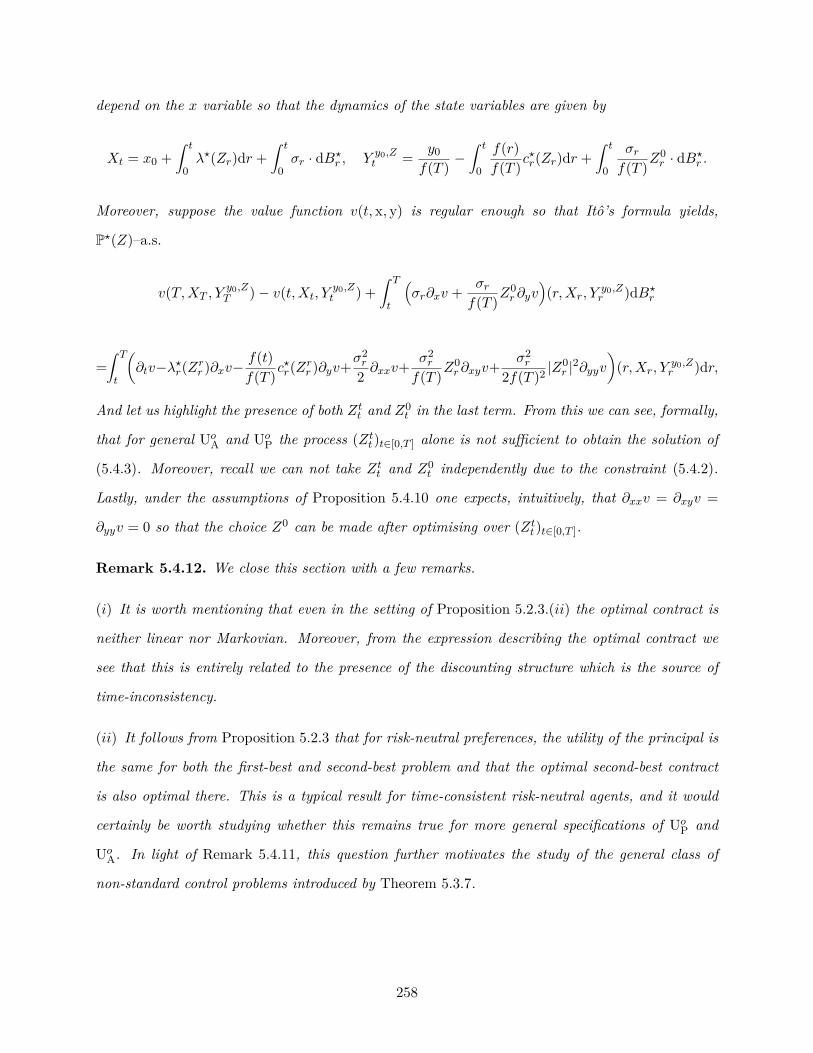
depend on the x variable so that the dynamics of the state variables are given by

Xt = x0 +∫ t

0λ?(Zr)dr +

∫ t

0σr · dB?

r , Y y0,Zt = y0

f(T ) −∫ t

0

f(r)f(T )c

?r(Zr)dr +

∫ t

0

σrf(T )Z

0r · dB?

r .

Moreover, suppose the value function v(t, x, y) is regular enough so that Itô’s formula yields,

P?(Z)–a.s.

v(T,XT , Yy0,ZT )− v(t,Xt, Y

y0,Zt ) +

∫ T

t

(σr∂xv + σr

f(T )Z0r∂yv

)(r,Xr, Y

y0,Zr )dB?

r

=∫ T

t

(∂tv−λ?r(Zrr )∂xv−

f(t)f(T )c

?r(Zrr )∂yv+σ2

r

2 ∂xxv+ σ2r

f(T )Z0r∂xyv+ σ2

r

2f(T )2 |Z0r |2∂yyv

)(r,Xr, Y

y0,Zr )dr,

And let us highlight the presence of both Ztt and Z0t in the last term. From this we can see, formally,

that for general UoA and Uo

P the process (Ztt )t∈[0,T ] alone is not sufficient to obtain the solution of

(5.4.3). Moreover, recall we can not take Ztt and Z0t independently due to the constraint (5.4.2).

Lastly, under the assumptions of Proposition 5.4.10 one expects, intuitively, that ∂xxv = ∂xyv =

∂yyv = 0 so that the choice Z0 can be made after optimising over (Ztt )t∈[0,T ].

Remark 5.4.12. We close this section with a few remarks.

(i) It is worth mentioning that even in the setting of Proposition 5.2.3.(ii) the optimal contract is

neither linear nor Markovian. Moreover, from the expression describing the optimal contract we

see that this is entirely related to the presence of the discounting structure which is the source of

time-inconsistency.

(ii) It follows from Proposition 5.2.3 that for risk-neutral preferences, the utility of the principal is

the same for both the first-best and second-best problem and that the optimal second-best contract

is also optimal there. This is a typical result for time-consistent risk-neutral agents, and it would

certainly be worth studying whether this remains true for more general specifications of UoP and

UoA. In light of Remark 5.4.11, this question further motivates the study of the general class of

non-standard control problems introduced by Theorem 5.3.7.

258

5.4.3 Agent with utility of discounted income

We now consider the scenario in Section 5.2.1 under the additional choice f = 1. We then have

VAt (ξ, α) := EPα

[Uo

A

(g(T − t)ξ −Kt,α

t,T

)∣∣∣Ft], where Ks,αt,T :=

∫ T

tg(r − s)kor(X,αr)dr. (5.4.4)

In the context of (5.3.1), this corresponds to

ht(s, x, y, z, a) = σt(x)bt(x, a) · z + γAg(t− s)kot (x, a)y,

∇ht(s, x, u, v, y, a) = σt(x)bt(x, a) · v − γAg′(t− s)kot (x, a)y + γAg(t− s)kot (x, a)u,

UA(s, ξ) = UoA(g(T − s)ξ), and ∂sUA(s, x) = −g′(T − s)∂xUo

A(g(T − s)ξ)UoA(g(T − s)ξ).

Remark 5.4.13. (i) The problem introduce by (5.4.4) is time-inconsistent even in the case of

exponential discounting, i.e. g(t) = e−ρt, t ∈ [0, T ], for some ρ > 0. This is due to the exponential

utility UA. Indeed, the BSDE representation allows us to interpret the reward of the agent as a

recursive utility in which the terminal value is discounted at a rate eg(T−s) whereas the generator

discounts at a rate g(t− s). It is known, see Marín-Solano and Navas [179, Section 4.5], that even

in the case of exponential discounting the problem becomes time-inconsistent as soon as the rates at

which the terminal value and the running reward are discounted differ. We also recall that the case

of no discounting, i.e. g(t) = 1, corresponds to the seminal work Holmström and Milgrom [130].

(ii) Let us note h exhibits both of the features of the examples in Sections 5.4.1 and 5.4.2, this is,

the second term includes the discount factor and the y variable.2 We highlight that a key element in

Proposition 5.4.10 was the fact that the dynamics of Y s,y0,Z were given by (y0, Z) without Y y0,Z on

the right hand side. Consequently, the presence of y in h forces us to begin by changing variables

to the certainty equivalent for the problem of the agent, i.e. from Z to Z as we denote below. In

this way, we remove y in the dynamics of Y y0,Z at the expense of the mapping δ?, which we use to

identify an auxiliary martingale, becoming quadratic in the new variable Z. On the one hand, this

creates a subtle issue when trying to establish a correspondence between the natural integrability of

the variables Z and Z. This will ultimately prevent us from obtaining a complete characterisation2In fact, (5.4.4) covers the situation in Section 5.4.2 in the particular case of a risk-neutral agent, recall 1/γA −

UA(x) −→ x, whenever γA → 0.

259

of the family H2,2. On the other hand, the quadratic term does not correspond to the diagonal values

of the control variable Z. This makes the approach in Section 5.4.2, namely Proposition 5.4.10,

inoperable and forces us to restrict ourselves to a suitable subclass that is amenable to the analysis.

As we may probably expect after our analysis in Section 5.4.1, the process Y y0,Z in the definition

of H2,2 becomes more amenable to the analysis by working in terms of the certainty equivalent.

For this, we introduce, for (t, s, x, z, z, v) ∈ [0, T ]2 ×X × (Rn)3,


ht(t, x, z, a), ht(s, x, z, a) := σt(x)bt(x, a) · z − g(t− s)kot (x, a),

∇ht(s, x, v, z, a) := σt(x)bt(x, a)) · v + g′(t− s)kor(x, a)− γAσ>t (x)z · σ>t (x)v.

The maps a?(t, x, z), λ?t (x, z), kot ?(x, z), h?t (s, x, z, z), ∇h?t (s, x, v, z, z), and the probability P?(z) are

defined accordingly.

Moreover, inspired by Section 5.4.2, we introduce the mapping δ? given, for (s, t, x, z, z, z) ∈

[0, T ]2 ×X × (Rn)3, by

δ?t (s, x, z, z, z) := kor?(x, z)

(g(r − s)− g(T − s)

g(T ) g(r))

+ γA2

(|σ>r (x)z|2 − g(T − s)

g(T − u) |σ>r (x)z|2

).

The following result is analogous to Lemma 5.4.7, we defer its proof to Section 5.7.

Lemma 5.4.14. Let Z ∈ H2,2.

(i) There exists family of processes (Y s,y0,Z , Zs)s∈[0,T ] such that for every s ∈ [0, T ]

Y s,y0,Zt = − 1

γAln(−γAy

s0)−∫ t

0

(h?r(s,X·∧r, Z

sr , Z

rr

)− γA

2 |σ>r Z

sr |2)dr+

∫ t

0Zsr ·dXr, t ∈ [0, T ], P–a.s.

(ii) If Z ∈ H2,2 then for every s ∈ [0, T ]

Y s,y0,Zt = g(T − s)

g(T ) Y 0,y0,Zt − EP?(Z)

[ ∫ T

tδ?r (s,X·∧r, Zrr , Zsr , Z0

r )dr∣∣∣∣Ft].

(iii) Moreover, if the process M s,Z given by

M s,Zt := EP?(Z)

[ ∫ T

0δ?r (s,X·∧r, Zrr , Zsr , Z0

r )dr∣∣∣∣Ft], P–a.s., (s, t) ∈ [0, T ]2,

260

is a square integrable (F,P?(Z))-martingale, then

Zst = g(T − s)g(T ) Z0

t − Zs,Zt ,dt⊗ dP–a.e.

where Zs,Z denotes the term in the representation of M s,Z .

Remark 5.4.15. (i) We highlight that in contrast to the analysis presented in Sections 5.4.1 and

5.4.2, the previous result does not provide an equivalent representation of the set H2,2. This is

intimately related to the square integrability condition on the process M s,Z required in (iii) above,

and the fact that (z, z) 7−→ δ?t (x, z, z, z) is quadratic for (t, s, x, z) ∈ [0, T ]2 ×X × Rm fixed.

(ii) As a sanity check at this point, let us verify the coherence of the previous system in terms of

the analysis of the previous section. In the following we omit the dependence on X and assume

Z ∈ H2,2(Rn). Let

(∆sg)(t) := g(t−s)−g(t), KZ,st,τ := exp

(γA

∫ τ

t

(k?r(Zr)(∆sg)(r)−γA|σrZ0

r |2+γAZs,>r σr ·Z0>

r σr)dr),

By applying Itô’s formula to Y sr := KZ,s

t,r UA(Y s,Zr − Y 0,y0,Z

r ), we have that for any s ∈ [0, T ], P–a.s.

UoA(Y s,y0,Zt − Y 0,y0,Z

t

)= EP?(Z)

[Uo

A

(ys0 − y0

0 −∫ t

0

((∆sg)(r)k?r(Zr)− γA|σrZ0

r |2 + γAZs,>r σr ·Z0>

r σr)dr)∣∣∣∣Ft].

As γ−1A −Uo

A(y) γA→0−−−−→ y, we see the previous equation induces the corresponding one in Lemma 5.4.7.


Let us highlight that in contrast to Section 5.4.2, the analysis in the previous section does not

provide a full characterisation of H2,2 in the context to rewards given by (5.2.4). This is principally

due to the integrability necessary on the variable Z, induced by the certainty equivalent, in order

to apply the methodology devised in 5.4.2, see Lemma 5.4.14. Nevertheless, given that current

example generalises the previous two, we build upon the structure of the optimal solution that was

obtained to propose a family over which the optimisation in the problem of the principal can be

carried out.

261

We will focus on the case n = 1 and we will pay special attention to the class H ⊆ H2,2 of

processes Z ∈ H2,2 for which given the pair (y0, Z) ∈ I0 ×H2,2, and Y y0,Z given by (5.3.5), there

exists a pair of predictable processes (η, ζ) such that

Zst = 1−γA

Zst

Y y0,s,Zt

= ηs,tζt, ηt,t = 1, t ∈ [0, T ].

Therefore, we have from Theorem 5.3.7 and (5.4.2) that

VP := supy00≥R0

supZ∈H

EP?(Z)[Uo

P

(XT − Y 0,y0,Z

T

)]≤ VP.

Remark 5.4.16. (i) We remark that the previous definition implicitly requires that for any t ∈

[0, T ] the mapping s 7−→ ηs,t is differentiable.

(ii) In addition, provided ko?(x, z) does not depend on x it is easy to verify that that H 6= ∅. In

light of the previous lemma, we have that for Z ∈ H

M s,Zt = EP?(Z)

[ ∫ T

0kor?(ζr)

(g(r−s)−g(T − s)

g(T ) g(r))

+γA2∣∣σ>r ζr∣∣2(|ηs,r|2−g(T − s)

g(T ) |η0,r|2∣∣∣2)dr

∣∣∣∣Ft],and

Zs,Zt =(g(T − s)g(T ) η0,t − ηs,t

)ζt,dt⊗ dP–a.e.

This implies that H includes, in particular, all the processes Z that are induced by deterministic

pairs (ζ, η). Indeed, for such class of processes we have that M s,Z is deterministic, Zs,Z = 0, and

consequently, ηs,t = g(T − s)/g(T − t) provides a non trivial element of H. The previous argument

also holds in the case of exponential discounting, in which we recall that the agent’s problem remains

time-inconsistent.

The following result characterises the solution to VP. Its proof is available in Section 5.7.

Proposition 5.4.17. Let principal and agent have exponential utility with parameters γP and γA,

respectively. Let Cy := − 1γP

e−γP(x0−y), R0 := UoA

(−1)(R0), and assume that:

(i) the maps σ, λ? and ko? do not depend on the x variable;

262

(ii) for any (t, η) ∈ [0, T ]× R, the map G : R −→ R given by

G(z) := λ?t (z)−g(t)g(T )k

ot?(z)− γA

2g(T )

∣∣∣η0σtη

∣∣∣2|z|2 − γP2 σ2

r

(1− η0

ηg(T )z)2,

has a unique maximiser z?(t, η), such that [0, T ] 3 t 7−→ z?(t, η) is square-integrable.

Then

VP = supZη∈H

CR0

EP[

exp(− γP

∫ T

0Gr(z?(r, ηr))dr

)], where, Zs,ηt := ηs

ηtz?(t, ηt).

Moreover

(i) let VP,o denote the restriction of VP to the subclass of H with deterministic η. Then the optimal

deterministic contract is given by the family

Zst := g(T − s)g(T − t) z

?(t, g(T − t)),

and

ξ = R0g(T ) −

1g(T )

∫ t

0h?r

(0, g(T )g(T − t)z

?(t, g(T − t)), z?(r, g(T − r)))

dr +∫ t

0

z?(t, g(T − t))g(T − t) dXr;

(ii) in the case (γA, γP) = (0, 0), i.e. the case of risk-neutral principal and agent, the solution to

VP, and consequently of VP, agrees with the value given by Proposition 5.4.10 and the optimal

family Z is deterministic.

Remark 5.4.18. We close this section with a few remarks.

(i) The solution to the problem of the principal for the general class of restricted contracts induced

by H2,2 escaped the analysis presented above. As detailed in Remark 5.4.13.(ii), this is due to subtle

integrability issues when trying to identify an appropriate reduction of H2,2, and the quadratic

nature of the generator when working in term of the certainty equivalent.We believe this echoes the

intricacies of the non-standard class of control problem introduced in Theorem 5.3.7.

(ii) If, as in Remark 5.4.6, we bring ourselves back to the setting of [130], i.e. bt(x, a) = a/σ,

263

σt(x) = σ, kt(x, a) = ka2/2, we have

Zst = g(T )g(T − s)(g(T − t) + γPσ2k)

g(t)g2(T − t) + σ2kg(T )(γAg(T ) + γP) .

We highlight that: (a) in contrast to [130], for any type of discounting structure (including expo-

nential discounting) the previous expression and consequently the optimal action is neither linear

nor Markovian. This corroborates our comment in Remark 5.4.13.(i), in the sense that even in

the case of exponential discounting the problem of the agent remains time-inconsistent; (b) in the

case of no discounting, i.e. g = 1, when we bring ourselves back to the model of Remark 5.4.6, the

previous expression coincides with the linear contract result specified by [130]. This shows that, even

if possibly not the best, the optimal contract in the class H at least captures the optimal contract

when the problem becomes time-consistent again.

5.5 On time-inconsistency for BSVIE-type rewards

Let us start by mentioning that in the context of rewards given by (5.1.2), the methodology

devised in Chapter 2, which builds on the approach in the Markovian framework of [38], is based

introducing the family of processes (Y s, Zs)s∈[0,T ] solution to the backward stochastic Volterra

integral equation (BSVIEs for short), which satisfies

Y s,αt = η(s, ξ) +

∫ T

thr(s,X·∧r, Y

s,αr , Zs,αr , αr

)dr −

∫ T

tZs,αr · dXr, P–a.s., s ∈ [0, T ]. (5.5.1)

Throughout this section we fix ξ ∈ C and α? ∈ E := E(ξ). Thus, we identify the agent’s reward

under α ∈ A via VAt (α) := VA

t (α, ξ) = Y t,αt . We write VA

t for the associated value function under

α?.

To establish an extended dynamic programming principle we need the following minimal set of

assumptions.

Assumption S. (i) (s, y, z) 7−→ ht(s, x, y, z, a) (resp. s 7−→ UA(s, x)) is continuously differenti-

able, uniformly in (t, x, a) (resp. in x). Moreover, the mapping ∇h : [0, T ]2×X × (R×Rn)2 −→ R

defined by

264

∇ht(s, x, u, v, y, z, a) := ∂sht(s, x, y, z, a) + ∂yht(s, x, y, z, a)u+n∑i=1

∂ziht(s, x, y, z, a)vi,

satisfies ∇h·(s, ·, u, v, y, z, a) ∈ Pprog(R,F); for all s ∈ [0, T ];

(ii) for ϕ ∈ h, ∂sh, (y, z, a) 7−→ ϕt(s, x, y, z, a) is uniformly Lipschitz-continuous with linear

growth, i.e. there exists some C > 0 such that ∀(s, t, x, y, y, z, z, a, a),

|ϕt(s, x, y, z, a)− ϕt(s, x, y, z, a)| ≤ C(|y − y|+ |σt(x)>(z − z)|+ |a− a|

);

(iii) let(h·(s),∇h·(s)

):=

(h·(s, ·, 0, 0, 0),∇h·(s, ·, 0, 0, 0, 0, 0)

), then

(h,∇h) :=

(h(·),∇h(·)

)∈

L1,2,2 × L1,2,2.

Remark 5.5.1. We remark that Assumption S.(iii) is satisfied if one assumes the classic linear

growth condition, i.e. there exists some C > 0 such that for all (s, t, x, y, z, u, v, a)

∣∣ht(s, x, y, z, a)∣∣ ≤ C(1 + |y|+ |σt(x)>z|

),∣∣∇ht(s, x, u, v, y, z, a)

∣∣ ≤ C(1 + |u|+ |σt(x)>v|+ |y|+ |σt(x)>z|).

Under Assumption S, Lemma 3.6.1 guarantees that for any α ∈ A there exists (∂Y α, ∂Zα) ∈

S2 ×H2,2 such that for every s ∈ [0, T ]

∂Y s,αt = ∂sη(s, ξ) +

∫ T

t∇hr(s,X·∧r, ∂Y s,α

r , ∂Zs,αr , Y s,αr Zs,αr , αr)dr

−∫ T

t∂Zs,αr · dXr, t ∈ [0, T ], P–a.s.,

(5.5.2)

which ultimately implies the absolute continuity of the mapping ([0, T ],B([0, T ])) −→ (H2, ‖ · ‖H2) :

s 7−→ Zs,α. With this, the process (Zt,αt )t∈[0,T ] is well-defined. Moreover, see Lemma 3.6.2, for any

265

α ∈ A

Y t,αt = η(T, ξ) +

∫ T

t

(hr(r,X·∧r, Y r,α

r , Zr,αr , αr)− ∂Y r,αr

)dr

−∫ T

tZr,αr · dXr, t ∈ [0, T ], P–a.s.

(5.5.3)

We begin stating the following auxiliary result.

Lemma 5.5.2. Let Assumption S hold. For any γ, γ′ ⊆ T0,T , γ ≤ γ′, and α ∈ A

EP[Y γ,αγ − Y γ′,α

γ′ +∫ γ′

γ∂Y r,α

r dr∣∣∣Fγ], depends only on the value of α on [γ, γ′].

Proof. This property is clear for BSDEs whose generator does not depend on (y, z). Indeed,

EP[Y γ,αγ − Y γ′,α

γ′ +∫ γ′

γ∂Y r,α

r dr∣∣∣Fγ] = EP

[ ∫ γ′

γhr(r,X·∧r, αr)dr

∣∣∣Fγ].To extend this result to the BSDEs (5.5.1)–(5.5.2) we consider the Picard iteration procedure

Y s,α,n+1t = η(s, ξ) +

∫ T

thr(s,X·∧r, Y

s,α,nr , Zs,α,nr , αr

)dr −

∫ T

tZs,α,n+1r · dXr,

∂Y s,α,n+1t = ∂sη(s, ξ) +

∫ T

t∇hr(s,X·∧r, ∂Y s,α,n

r , ∂Zs,α,nr , Y s,α,nr , Zs,α,nr , αr)dr

−∫ T

t∂Zs,α,n+1

r · dXr,

and note that, as in (5.5.3)

EP[Y γ,α,n+1γ − Y γ′,α,n+1

γ′ +∫ γ′

γ∂Y r,α,n+1

r dr∣∣∣∣Fγ]

=EP[ ∫ γ′

γhr(r,X·∧r, Y r,α,n

r , Zr,α,nr , αr)dr∣∣∣∣Fγ].

(5.5.4)

Then, from the fact that Y α,0 = Zα,0 = ∂Y α,0 = ∂Zα,0 = 0 we see that (5.5.4) implies the result

at the initial step. It is then also clear, again from (5.5.4), that this property is preserved at every

iteration and thus in the limit.

In the following, given (σ, τ) ∈ Tt,T × Tt,t+`, with σ ≤ τ , we denote by Π` := (τ ì )i=1,...,n` ⊆ Tt,T


⌉, σ =: τ `0 ≤ · · · ≤

266

τ `n`

:= τ, ∀`, and sup1≤i≤n` |τì − τ ì−1| ≤ `. We also let ∆τ ì := τ ì − τ ì−1. The previous definitions

hold x-by-x.

Theorem 5.5.3 (Dynamic programming principle). Let Assumption S hold. Let α? ∈ E(ξ) and

σ, τ ⊂ Tt,T , with σ ≤ τ . Then, P–a.s.

VAσ = ess supP

α∈AEP[VAτ +

∫ τ

σ

(hr(r,X·∧r, Y

r,αr , Zr,αr , αr

)− ∂Y r,α?

r

)dr∣∣∣∣Fσ],

where for every s ∈ [0, T ], ∂Y s,α? denotes the solution to (5.5.2) with α?. Moreover, α? attains the

ess supP.

Proof. We first show the inequality ≥. We proceed in 3 steps. Let ε > 0, 0 < ` < `ε, and Π` be a

partition of [σ, τ ].

Step 1: From the definition of equilibria we have that for any α ∈ A

VAσ ≥ VA

σ (α⊗τ1 α?)− ε` ≥ EP[Yσ,α⊗τ1α

?

σ − Y τ1,α⊗τ1α?

τ1 + Yτ1,α⊗τ1α

?

τ1

∣∣∣Fσ]− ε`.Recall that for any ρ ∈ T0,T , Y

ρ,α⊗ρα?ρ = Y ρ,α?

ρ . In light of the arbitrariness of α ∈ A we obtain

VAσ ≥ ess supP

α∈AEP[Yσ,α⊗τ1α

?


τ1 + VAτ1

∣∣∣Fσ]− ε`, P–a.s.Step 2: Let us note that in light of Step 1

VAσ ≥ ess supP


?


τ1 + VAτ1

∣∣∣Fσ]− ε`= ess supP


?


τ1

+ ess supP

α∈AEP[Yτ1,α⊗τ2α

?

τ1 − Y τ2,α⊗τ2α?


?

τ2

∣∣∣Fτ1]∣∣∣Fσ]− 2ε`

= ess supP

α∈AEP[VAτ2 + Y

σ,α⊗τ1α?



?

τ1 − Y τ2,α⊗τ2α?

τ2

∣∣∣Fσ]− 2ε`,

where the second equality holds in light of [210, Lemma 3.5] as [210, Assumption 1.1] holds under

267

Assumption Q. Iterating the previous argument we obtain that P–a.s.

VAσ ≥ ess supP

α∈AEP[VAτ +

n`−1∑i=0

Yτi,α⊗τi+1α

?

τi − Yτi+1,α⊗τi+1α

?

τi+1

∣∣∣∣Fσ]− n`ε`.Now, we use the fact that for any i ∈ 0, ..., n` − 1 and α⊗τi+1 α

?, Lemma 5.5.2 implies

EP[Yτi,α⊗τi+1α

?

τi − Yτi+1,α⊗τi+1α

?

τi+1 +∫ τi+1

τi

∂Yr,α⊗τi+1α

?

r dr∣∣∣Fσ]

= EP[ ∫ τi+1

τi

hr(r,X·∧r, Y r,αr , Zr,αr , αr)dr

∣∣∣∣Fσ].Replacing in the previous expression we obtain that P–a.s.

VAσ ≥ ess supP

α∈AEP[

VAτ +

∫ τ

σhr(r,X·∧r, Y r,α

r , Zr,αr , αr)dr

−n`−1∑i=0

∫ τi+1

τi

∂Yr,α⊗τi+1α

?

r dr − n`ε`∣∣∣∣Fσ].

(5.5.5)

Step 3: Let i ∈ 0, . . . , n` − 1. In light of Assumption Q, the stability of the system of BSDE

defined by (5.5.1) and (5.5.2), see Proposition 3.6.4, yields there exists a constant C > 0 such that

∥∥∥∥ ∫ τi+1

τi

∂Yr,α⊗τi+1α

?

r − ∂Y r,α?

r dr∥∥∥∥L2≤ `

∥∥∥∂Y α⊗τi+1α?

− ∂Y α?∥∥∥S2,2≤ `CE

[( ∫ τi+1

τi

|αr − α?r |dr)2]

,

which leads to

∥∥∥∥ n`−1∑i=0

∫ τi+1

τi

∂Yr,α⊗τi+1α

?

r − ∂Y r,α?

r dr∥∥∥∥L2≤ `CE

[( ∫ τ

σ|αr − α?r |dr

)2]`→0−−→ 0.

By choosing an appropriate partition Π` and dominated convergence we obtain that

I(n`) :=n`−1∑i=0

∫ τi+1

τi

∂Yr,α⊗τi+1α

?

r dr `ε→0−−−→∫ τ

σ∂Y r,α?

r dr, P–a.s.

Back in (5.5.5) we obtain

VAσ = ess supP

α∈AEP[VAτ +

∫ τ

σ

(hr(r,X·∧r, Y

r,αr , Zr,αr , αr

)− ∂Y r,α?

r

)dr∣∣∣∣Fσ], P–a.s.

268

Lastly, we show that the equality is attained by α? ∈ E . Indeed, note that (5.5.3) implies

VAσ = EP

[VAτ +

∫ τ

σ

(hr(r,X·∧r, Y

r,α?

r , Zr,α?

r , α?r)− ∂Y r,α?

r

)dr∣∣∣∣Fσ], P–a.s.

Let us recall that the Hamiltonian associated to h is given by

Ht(x, y, z) = supa∈A

ht(t, x, y, z, a), (t, x, y, z) ∈ [0, T ]×X × R× Rn.

Our standing assumptions on H are the following.

Assumption T. (i) For any (t, x) ∈ [0, T ]×X , the map R×Rn 3 (y, z) 7−→ Ht(x, y, z) is uniformly

Lipschitz-continuous, i.e. there is C > 0 such that for any (t, x, y, y, z, z) ∈ [0, T ]×X ×R2 × (Rn)2

∣∣Ht(x, y, z)−Ht(x, y, z)∣∣ ≤ C(|y− y|+ |σt(x)>(z− z)|

);

(ii) there exists a unique Borel-measurable map a? : [0, T ]×X × R× Rn −→ A such that

Ht(x, y, z) = ht(t, x, y, z, a?(t, x, y, z)

), ∀(t, x, y, z) ∈ [0, T ]×X × R× Rn;

(iii) for any (t, x) ∈ [0, T ] × X , the map R × Rn 3 (y, z) 7−→ a?(t, x, y, z) is uniformly Lipschitz-

continuous, i.e. there is C > 0 such that for any (t, x, y, y, z, z) ∈ [0, T ]×X × R2 × (Rn)2.

∣∣a?(t, x, y, z)− a?(t, x, y, z)∣∣ ≤ C(|y− y|+ |σt(x)>(z− z)|

);

(iv) (H, a?) ∈ L1,2(R)× L1,2(R), where(H·, a

?·)

:=(H·(·, 0, 0), a?· (·, 0, 0)

).

With this we introduce the system defined for any s ∈ [0, T ] by

Yt = η(T, ξ) +∫ T

t

(Hr(X·∧r, Yr, Zr)− ∂Y r

r

)dr −

∫ T

tZr · dXr, t ∈ [0, T ], P–a.s.

Y st = η(s, ξ) +

∫ T

th?r(s,X·∧r, Y

sr , Z

sr , Yr, Zr

)dr −

∫ T

tZsr · dXr, t ∈ [0, T ], P–a.s. (H)

∂Y st = ∂sη(s, ξ) +

∫ T

t∇h?r(s,X·∧r, ∂Y s

r , ∂Zsr , Y

sr Z

sr , Yr, Zr

)dr −

∫ T

t∂Zsr · dXr, t ∈ [0, T ], P–a.s.

269

We will say (Y,Z, Y, Z, ∂Y, ∂Z) ∈ H is a solution to the system whenever (H) is satisfied. In light

of Theorem 5.5.3, given α? ∈ E it is reasonable to associate the value along the equilibria with a

BSDE whose generator is given, partially, by H. This is the purpose of the next result.

Theorem 5.5.4 (Necessity). Let Assumptions S and T hold and α? ∈ E. Then, one can construct

a solution to (H).

Proof. Given α? ∈ E , Assumption S guarantees that the processes (Y α? , Zα?) and (∂Y α? , ∂Zα

?)

solution to (5.5.1) and (5.5.2), respectively, are well-defined. Moreover, the diagonal processes((Y t,α?

t )t∈[0,T ], (Zt,α?

t )t∈[0,T ])are well-defined as elements of S2 × H2, see Lemma 3.6.2. Given

(∂Y t,α?

t )t∈[0,T ] ∈ S2, for any α ∈ A, we can define the processes (Yα,Zα) ∈ S2 ×H2 solution to

Yαt = η(T, ξ) +∫ T

t

(hr(r,X·∧r,Yαr ,Zαr , αr)− ∂Y r,α?

r

)dr −

∫ T

tZαr · dXr, t ∈ [0, T ], P–a.s.

We now note that under Assumption S the classic comparison result for BSDEs, see for instance

[273, Theorem 4.4.1]. Then, it follows from Theorem 5.5.3 that the pair((Y t,α?

t )t∈[0,T ], (Zt,α?

t )t∈[0,T ])

solves the BSDE

Yt = η(T, ξ) +∫ T

t

(Hr(X·∧r, Yr, Zr)− ∂Y r,α?

r

)dr −

∫ T

tZr · dXr, t ∈ [0, T ], P–a.s.

Moreover, the second part of the statement of Theorem 5.5.3 implies that α? = a?(·, X, Y·, Z·),

dt⊗ dP–a.e. Consequently, (Y α? , Zα?) and (∂Y α? , ∂Zα

?) define a solution to the second and third

equations in (H), respectively.

We close this section with a verification theorem for equilibria.

Theorem 5.5.5 (Verification). Let Assumptions S and T hold. Let (Y,Z, Y, Z, ∂Y, ∂Z) ∈ H be a

solution to (H) with α? := a?(·, X,Y·,Z·). Then, α? ∈ E and

VAt = Yt, P–a.s.

Proof. We verify the definition of an equilibria. Let ε > 0, (t, `) ∈ [0, T ] × (0, `ε) with `ε to be

chosen. Let (Yα⊗t+`α? ,Zα⊗t+`α?) ∈ S2×H2 be the solution, which exists in light of Assumption S,

270

to (5.5.1) with action α⊗t+` α?, that is to say, P–a.s.

Ys,α⊗t+`α?

t = η(s, ξ) +∫ T

thr(s,X·∧r,Y

s,α⊗t+`α?r ,Zs,α⊗t+`α

?

r , (α⊗t+` α?)r)dr

−∫ T

tZs,α⊗t+`α

?

r · dXr, t ∈ [0, T ].

It then follows that

Yt,α⊗t+`α?

t = η(T, ξ) +∫ T

t

(hr(r,X·∧r,Y

α⊗t+`α?r ,Zα⊗t+`α

?

r , (α⊗t+` α?)r)− ∂Y r,α⊗t+`α?

r

)dr

−∫ T

tZr,α⊗t+`α

?

r · dXr.

Now

Yt − Yt,α⊗t+`α?t

=∫ T

t

(Hr(X·∧r, Yr, Zr)− hr(r,X·∧r,Y

α⊗t+`α?r ,Zα⊗t+`α

?

r , (α⊗t+` α?)r))

dr

−∫ T

t∂Y r,α?

r − ∂Y r,α⊗t+`α?r dr −

∫ T

t

(Zr −Z

r,α⊗t+`α?r

)· dXr

≥∫ T

t+`

(Hr(X·∧r, Yr, Zr)− ∂Y r,α?

r − hr(r,X·∧r,Yα⊗t+`α?r ,Zα⊗t+`α

?

r , α?r)

+ ∂Yr,α⊗t+`α?r

)dr

−∫ t+`

t∂Y r,α?

r − ∂Y r,α⊗t+`α?r dr −

∫ T

t

(Zr −Z

r,α⊗t+`α?r

)· dXr

=∫ t+`

t∂Y

r,α⊗t+`α?r − ∂Y r,α?

r dr −∫ T

t

(Zr −Z

r,α⊗t+`α?r

)· dXr,

where the inequality follows by definition of H and α? and Assumption T. The second equality

follows from the fact that the first term cancels on [t+ `, T ], see Lemma 5.5.2. Taking expectation

we find

VAt −VA

t (α⊗t+` α?) = E[Yt − Y

t,α⊗t+`α?t

∣∣∣Ft] ≥ E[ ∫ t+`

t∂Y


r dr∣∣∣∣Ft].

By Proposition 3.6.4 we find that

∥∥∥∥ ∫ t+`

t∂Y


r dr∥∥∥∥L2≤ `

∥∥∥∂Y α⊗t+`α? − ∂Y α?∥∥∥S2,2≤ `CE

[( ∫ t+`

t|αr − α?r |dr

)2].

271

By the boundedness of the action set, we may choose `ε such that the last term above is smaller

that `ε. With this, we conclude α? ∈ E . The second part of the statement follows from the fact

that Yt = Y t,α?

t , P–a.s.

5.6 On forward stochastic Volterra integral equations

We are given a jointly measurable mapping h, a processes Z, and a family (Y s0 )s∈[0,T ] ∈ I such

that for any (y, u) ∈ R2 × (Rn)2

h : [0, T ]2 ×X × R× Rn × R× Rn −→ R, h·(·, y, u) ∈ Pprog(R,F).

Moreover, we work under the following set of assumptions.

Assumption U. (i) (s, y) 7−→ ht(s, x, y, u) (resp. s 7−→ Y s0 (x)) is continuously differentiable,

uniformly in (t, x, u) (resp. in x). Moreover, the mapping ∇h : [0, T ]2 × X × (R × Rn)2 −→ R

defined by

∇ht(s, x,u, y, u) := ∂sht(s, x, y, u) + ∂yht(s, x, y, u)u, ∇h·(s, ·,u, y, u) ∈ Pprog(R,F);

(ii) for ϕ ∈ h, ∂sh, (y, u) 7−→ ∂sϕt(s, x, y, u) is uniformly Lipschitz-continuous, i.e. there exists

some C > 0 such that ∀(s, t, x, y, y, u, u),

|ϕt(s, x, y, u)− ϕt(s, x, y, u)| ≤ C(|y − y|+ |u− u|

);

(iii) (Y0, ∂sY0) ∈(I)2, Z ∈ H2,2, (h·(s),∇h·(s)) := (h·(s, ·,0), ∂sh·(s, ·,0)) ∈

(L1,2,2)2, for 0 :=

(y, u)|(0,0).

We are interested in establishing the well-posedness of the FSVIE

Y st = Y s

0 +∫ t

0hr(s,X·∧r, Y

sr , Y

rr

)dr +

∫ t

0Zsr · dXr, t ∈ [0, T ], P–a.s., s ∈ [0, T ]. (5.6.1)

To alleviate the notation we write Y instead of Y Z in the previous equation.

272

Definition 5.6.1. We say Y is a solution to the FSVIE (5.6.1) if Y satisfies equation (5.6.1) and

Y ∈ S2,2.

Remark 5.6.2. We remark that in light of the pathwise continuity of Y s for every s ∈ [0, T ] the

process (Y tt )t∈[0,T ] is well defined dt⊗ dP–a.e. on [0, T ]×X .

We begin presenting a priori estimates for solutions of (5.6.1). These can be recover from the

arguments in [273].

Lemma 5.6.3. Let Y be a solution to (5.6.1), there exists a constant C > 0 such that

‖Y ‖2S2,2 ≤ C(‖Y0‖2L2,2 + ‖h‖2L1,2,2 + ‖Z‖2H2,2

).

Moreover, for Y i solution to (5.6.1) with data (Y i0 , h

i, Zi) satisfying (U) for i ∈ 1, 2 there exists

C > 0 such that

‖Y 1 − Y 2‖2S2,2 ≤ C(‖Y 1

0 − Y 20 ‖2L2,2 + ‖h1 − h2‖2L1,2,2 + ‖Z1 − Z2‖2H2,2

).

Proof. Let us observe that the continuity of the application s 7−→ ‖∆Y s‖S2 implies

E[ ∫ T

0e−cr|∆Y r

r |2dr]≤∫ T

0E[

supu∈[0,T ]

e−cu|∆Y ru |2]dr ≤ T‖∆Y ‖2S2,2 . (5.6.2)

With this, the proof of both statements can obtained following the line of [273, Theorem 3.2.2 and

Theorem 3.2.4].

We are now ready to establish the well-posedness of (5.6.1).

Proposition 5.6.4. Let Assumption U hold. There is a unique solution to (5.6.1).

Proof. Uniqueness follows from Lemma 5.6.3. We use a Picard iteration argument. Let Y s,0· =

Y s0 , s ∈ [0, T ] and

Y s,n+1t = Y s

0 +∫ t

0hr(s,X·∧r, Y

s,nr , Y r,n

r

)dr +

∫ t

0Zsr · dXr, t ∈ [0, T ].

We note that Y n ∈ S2,2 for n ≥ 0. Indeed, the result holds for Y 0 and the process (Y t,0t )t∈[0,T ] ∈ L1,2

is well-defined. Inductively, in light of Assumption U, the fact that Z ∈ H2,2 and (Y t,nt )t∈[0,T ] ∈ L1,2,

273

see (5.6.2), yields Y s,n+1 ∈ S2 for every s ∈ [0, T ]. The continuity of s 7−→ ‖Y s,n‖S2 , Assumption U

together with Lemma 5.6.3 guarantees Y n+1 ∈ S2,2. Moreover, the pathwise continuity Y s,n+1 for

any s ∈ [0, T ] guarantees (Y t,n+1t )t∈[0,T ] is well-defined dt⊗ dP–a.e.

Let ∆Y n := Y n − Y n−1. Then, for any s ∈ [0, T ]

∆Y s,n+1t =

∫ t

0

(hr(s,X·∧r, Y s,n

r , Y r,nr )− hr(s,X·∧r, Y s,n−1

r , Y r,n−1r )

)dr.

The inequality 2ab ≤ ε−1a2 + εb2 for any ε > 0 yields that for any ε > 0 there exists C(ε) > 0 such

that

e−ct|∆Y s,n+1t |2

=∫ t

0e−cr

(2|∆Y s,n+1

r |(hr(s,X·∧r, Y s,nr , Y r,n

r )− hr(s,X·∧r, Y s,n−1r , Y r,n−1

r ))− c|∆Y s,n+1r |

)dr

≤∫ t

0e−cr

(|∆Y s,n+1

r |2(C(ε)− c) + ε|∆Y s,nr |2 + ε|∆Y r,n

r |2)dr,

we then find that for c > C(ε)

E[

supt∈[0,T ]

e−ct|∆Y s,n+1t |2

]≤ εE

[ ∫ T

0e−cr

(|∆Y s,n

r |2 + |∆Y r,nr |2

)dr]. (5.6.3)

Now, as ∆Y s,n ∈ S2,2 we may use (5.6.2) back in (5.6.3) and obtain that for ε = 18T , c > C(ε), we

have‖∆Y n+1‖2S2,2,c ≤ 4−1‖∆Y n‖2S2,2,c . Inductively, we find that for all n ≥ 1, ‖∆Y n‖2S2,2,c ≤ C4−n.

Thus, for m > n,

‖Y m − Y n‖S2,2,c ≤m∑

k=n+1‖∆Y k‖S2,2,c ≤

m∑k=n+1

C

2k ≤C

2n .

Hence there is Y ∈ S2,2 such that Y n n−→0−−−−→ Y .

We now establish a result regarding the differentiability of (5.6.1). Recall that for Z ∈ H2,2

there exists by definition, see Section 5.3.1, a process ∂Z which can be interpreted as the derivative

of the mapping ([0, T ],B([0, T ])) −→ (H2,2, ‖ · ‖H2) : s 7−→ Zs.

Proposition 5.6.5. Let Assumption U hold and Y ∈ S2 be the solution to (5.6.1). There is a

274

unique process ∂Y ∈ S2,2 that satisfies

∂Y st = ∂sY

s0 +

∫ t

0∇hr

(s,X·∧r, ∂Y

sr , Y

sr , Y

rr

)dr +

∫ t

0∂Zsr · dXr, t ∈ [0, T ], P–a.s., s ∈ [0, T ]. (5.6.4)

Moreover ∫ s

0∂Y udu = Y s − Y 0, in S2.

Proof. Note that given the pair (Y, Z) ∈ S2,2×H2,2 , Assumption U guarantees there is C > 0 such

that

sups∈[0,T ]

(∫ T

0

∣∣∇hr(s,X·∧r, 0, Y sr , Y

rr )∣∣dr)2

≤ C(‖∂sh‖2L1,2,2 + ‖Y ‖2S2,2

)<∞.

We now note that Assumption U.(ii) guarantees u 7−→ ∇ht(s, x,u, y, u) is Lipschitz uniformly in

(s, t, x, y, u). Therefore, Proposition 5.6.4 guarantees there is a unique solution ∂Y ∈ S2,2. The

second part of the statement, follows arguing as in Lemma 3.6.1 in light of the stability result in

Lemma 5.6.3 and the fact Z ∈ H2,2 .

5.7 Proofs of Section 5.4

5.7.1 Proof of Proposition 5.4.5

We first note that, P–a.s.

XT − Y y0,ZT

=x0 − Y0 +∫ T

0

(λ?r(X·∧r, Zr)(1− Zr) + Hr(X·∧r, Zr)−

γA2 |σ

>r (X·∧r)Zr|2 −

1γA

f ′(T − r)f(T − r)

)dr

+∫ T

0σ>r (X·∧r)(1− Zr)dBa?(Z)

r ,

so that,

UP(XT − Y y0,ZT ) = C

Y0MT exp

(− γP

∫ T

0Gr(X·∧r, Zr)dr

), P–a.s.,

275

where

Gt(x, z) := λ?r(x, z)− kor?(x, z)−γA2 |σ

>r (x)z|2 − γP

2 |σ>r (x)(1− z)|2 − 1

γA

f ′(T − r)f(T − r) ,

and M denotes the supermartingale

Mt := exp(− γP

∫ t

0σ>r (X·∧r)(1− Zr) · dBa?(Z)

r − γ2P2

∫ t

0|σ>r (X·∧r)(1− Zr)|2dr

), t ∈ [0, T ].

Indeed, M is a local martingale that is bounded from below and M0 = 1. Consequently,

EP?(Z)[UP(XT − Y y0,Z

T

)]≤ C

Y0EP[

exp(− γP

∫ T

0Gr(X·∧r, Zr)dr

)].

Now, under assumptions (i) and (ii) in the statement it is clear that

VP ≤ CR0f(T )

γPγA exp

(− γP

∫ T

0g(z?(t))dt

)=: VP,?,

where the upper bound is given by

supz∈R

λ?r(z)− kor?(z)−

γA2 |σ

>r z|2 −

γP2 |σ

>r (1− z)|2

.

Let us now show the upper bound is attained. Indeed, letting

Z?t := −γAUoA(Y R0,z?

t )z?(t),

Y R0,z?

t := R0 −∫ t

0

(Hr(z?r )− γA

2 |σ>r z

?r |2 −

1γA

f ′(T − r)f(T − r)

)dr +

∫ t

0z?rdXr, t ∈ [0, T ],

it is easy to verify that the integrability assumption on z? guarantees that Z? ∈ H2. We conclude

that ξ? ∈ Ξ, where ξ? denotes the contract induced by R0 and Z?, is optimal as it attains VP,?.

this concludes the proof.

276

5.7.2 Proof of Lemma 5.4.7

We argue (i). Let Z ∈ H2,2. Recall

Y s,y0,Zt = ys0 −

∫ t

0

(λ?r(X·∧r, Zrr )Zsr − f(r − s)c?r(X·∧r, Zrr )

)dr +

∫ t

0Zsr · dXr,

and, in light of (5.3.6), we have

UoA

(−1)(Y s,y0,ZT

f(T − s)

)= Uo

A(−1)

(Y u,y0,ZT

f(T − u)

), (s, u) ∈ [0, T ].

Therefore, for any s ∈ [0, T ]

0 = Y s,y0,Z0

f(T − s) −Y 0,y0,Z

0f(T )

−∫ T

0λ?r(X·∧r, Zrr )

(Zsr

f(T − s) −Z0r

f(T )

)− c?r

(X·∧r, Z

rr

)( f(r − s)f(T − s) −

f(r)f(T )

)dr

+∫ T

0

(Zsr

f(T − s) −Z0r

f(T )

)· dXr

= Y s,y0,Z0

f(T − s) −Y 0,y0,Z

0f(T − u) + 1

f(T − s)

∫ T

0δ?r (s,X·∧r, Zrr )dr

+∫ T

0

(Zsr

f(T − s) −Z0r

f(T )

)·(dXr − λ?r(X·∧r, Zrr )dr

)= Y s,y0,Z

t

f(T − s) −Y 0,y0,Zt

f(T ) + 1f(T − s)

∫ T


+∫ T

t

(Zsr

f(T − s) −Z0r

f(T )


).

The result then follows taking conditional expectation thanks to the integrability of Zs and Z0.

We now argue (ii). Let s ∈ [0, T ] be fixed. Note that

N s,Zt := EP?(Z)

[ ∫ T


∣∣∣∣Ft]= M s,Z

t −∫ t


= M s,Z0 +

∫ t

0Zs,Zr ·

(dXr − λ?r(X·∧r, Zrr )dr

)−∫ t

0δ?r (s,X·∧r, Zrr )dr. (5.7.1)

277

Therefore, in light of (i), we have that there exists a finite variation process A such that

Y s,y0,Zt = f(T − s)

f(T ) Y 0,y0,Zt − EP?(Z)

[ ∫ T


∣∣∣∣Ft]= At −

∫ t

0

(f(T − s)f(T ) Z0

t − Zs,Zt


), P–a.s.

The result then follows from the uniqueness of the Itô decomposition of Y s,y0,Zt .

We are only left to argue (iii) as (iv) is a direct consequence. The inclusion H2,2 ⊆ H• follows

from (ii) and taking Y Zt := Y 0,y0,Z

t /f(T ). Conversely, given Z ∈ H• we define for any s ∈ [0, T ]

Y 0,y0,Zt := f(T )Y y0,Z

t , Y s,y0,Zt := f(T − s)

f(T ) Y 0,y0,Zt −N s,Z

t , t ∈ [0, T ], P–a.s.

Let us note Y s,y0,Z0 is clearly differentiable and Y s,y0,Z satisfies (5.3.6). Indeed, as N s,Z

T = 0,

s ∈ [0, T ], we haveY s,y0,ZT

f(T − s) = Y y0,ZT = Y u,y0,Z

T

f(T − u) , (s, u) ∈ [0, T ]2.

We now verify Y y0,Z ∈ S2,2. Let us first note that ‖Z‖2H2,2 <∞. Indeed,

‖Zs‖2H2 = EP[ ∫ t


]= EP?(Z)

[Mt

∫ t


]≤ EP?(Z)

[ ∫ t


]<∞,

where M denotes the supermartingale given by

Mt := exp(−∫ t

0b?r(X·∧r, Zrr ) · dB?

r −12

∫ t

0|b?r(X·∧r, Zrr )|2dr

), t ∈ [0, T ].

From this, it follows by Assumption Q that

‖NZ‖2S2,2 ≤ C(EP[ ∫ T

0

∣∣λ?r(X,Zrr )∣∣2dr

]+ sups∈[0,T ]

EP[ ∫ T

0

∣∣δ?r (s,X,Zrr )∣∣2dr

]+ ‖Z‖2H2,2

)<∞.

We also note that the continuity of s 7−→ f(t−s) implies the continuity of s 7−→ ‖N s,Z‖S2 . Moreover,

278

‖Y 0,y0,Z‖2S2 <∞ guarantees, by definition, that ‖Y y0,Z‖2S2,2 <∞. Moreover, by definition

Y s,y0,Zt

= f(T − s)f(T )

(y0 +

∫ t

0c?r(X·∧rZrr )f(r)dr +

∫ t

0Z0r ·(dXr − λ?r(X·∧r, Zrr )dr

))−M s,Z

0 −∫ t

0Zs,Zr ·


)+∫ t


= f(T − s)f(T ) y0 −M s,Z

0 +∫ t

0c?r(X·∧rZrr )f(r − s)dr

+∫ t

0

(f(T − s)f(T ) Z0

r − Zs,Zr)·(dXr − λ?r(X·∧r, Zrr )dr

)= f(T − s)

f(T ) y0 −M s,Z0 +

∫ t

0c?r(X·∧rZrr )f(r − s)dr +

∫ t

0Zsr ·


)= ys0 −

∫ t

0h?r(s,X·∧r, Z

sr , Z

rr

)dr +

∫ t

0Zsr · dXr,

where the third inequality follows from the fact Z ∈ H•. We conclude Z ∈ H2,2.

5.7.3 Proof of Lemma 5.4.14

Let us note that (ii) and (iii) are argued as in Lemma 5.4.7. We now argue (i). Let (y0, Z) ∈

I × H2,2. Note that given Y s,y0,Z , in light of the regularity of ys0 and the generator, it is possible

to define ∂Y s,y0,Z such that

Y t,y0,Zt = y0

0 −∫ t

0

(Hr(X·∧r, Y

r,y0,Zr , Zrr

)− ∂Y r,Z

r

)dr +

∫ t

0Zrr · dXr,

Y s,y0,Zt = ys0 −

∫ t

0h?r(s,X·∧r, Y

s,y0,Zr , Zsr , Y

r,y0,Zr , Zrr

)dr +

∫ t

0Zsr · dXr,

∂Y s,y0,Zt = ∂ys0 −

∫ t

0∇h?r

(s,X·∧r, ∂Y


s,y0,Zr , Y r,y0,Z

r , Zrr)dr +

∫ t

0∂Zsr · dXr.

Letting

Zt := 1−γA

Ztt

Y t,y0,Zt

, and, Zst := 1−γA

Zst

Y s,y0,Zt

,

we obtain that

Y t,y0,Zt = y0

0 −∫ t

0

(− γAY

r,y0,Zr Hr

(X·∧r, Z

rr

)− ∂Y r,y0,Z

r

)dr +

∫ t

0Zrr · dXr,

Y s,y0,Zt = ys0 −

∫ t

0−γAY

s.y0,Zr h?r

(s,X·∧r, Z

sr , Z

rr

)dr +

∫ t

0Zsr · dXr,

279

∂Y s,Zt = ∂ys0 −

∫ t

0∇h?r

(s,X·∧r, ∂Y


s,y0,Zr , Zrr

)dr +

∫ t

0∂Zsr · dXr.

The result then follows by Itô’s formula introducing

Y s,y0,Zt := − 1

γAln(−γAY

s,y0,Zt ), ∂Y s,y0,Z

t := 1−γA

∂Y s,y0,Zt

Y s,y0,Zt

, and

∂Zst := 1−γA

(∂Zst

Y s,y0,Zt

+ γ2A∂Y

s,y0,Zt Zst

).

5.7.4 Proof of Proposition 5.4.17

Note that it always holds that, P?(Z)–a.s.

XT −UoA

(−1)(Y 0,ZT )/g(T )

=x0 −U(−1)

A (Y 00 )

g(T ) +∫ T

0

(λ?r(X·∧r, Zrr )− g(r)

g(T )kor?(X·∧r, Zrr )− γA

2g(T ) |σ>r (X·∧r)Z0

r |2)

dr

+∫ T

0

(1− Z0

r

g(T )


),

so that

UoP

(XT −Uo

A(−1)(Y 0,Z

T )/g(T ))

= CY 0

0MT exp

(− γP

∫ T

0Gr(X·∧r, Zr, Z0

r )dr), P–a.s.,

where

Gt(x, z, v) := λ?t (x, z)−g(t)g(T )k

ot?(x, z)− γA

2g(T ) |σ>t (x)v|2 − γP

2

∣∣∣∣σ>r (x)(

1− v

g(T )

)∣∣∣∣2,and M denotes the supermartingale

Mt := exp(−γP

∫ t

0σ>r (X·∧r)

(1− Z0

r

g(T )

)·dBa?(Z)

r − γ2P2

∫ t

0

∣∣∣∣σ>r (X·∧r)(

1− Z0r

g(T )

)∣∣∣∣2dr), t ∈ [0, T ].

Consequently

EP?(Z)[UoP(XT −Uo

A(−1)(Y 0,Z

T )/g(T ))]≤ C

Y 00EP[

exp(− γP

∫ T

0Gr(X·∧r, Zrr , Z0

r )dr)]. (5.7.2)

280

Now, under the additional assumptions, we have that for any Z ∈ H

EP?(Z)[UoP(XT −Uo

A(−1)(Y 0,Z

T )/g(T ))]≤ C

R0EP[

exp(− γP

∫ T

0Gr(ζr, η0,rζr

)dr)].

Therefore, as

z?(t, η) ∈ arg maxz∈R

λ?t (z)−

g(t)g(T )k

ot?(z)− γA

2g(T ) |σ>t z|2|η|2 −

γP2

∣∣∣∣σ>r (1− z

g(T )η)∣∣∣∣2,

as longs as η is chosen so that Zη ∈ H the upper bound is attained.

Let us argue the second part of the statement. Since we are now constrained to deterministic

choices of η the integrability of z? and the boundedness of [0, T ] 3 t 7−→ g(t) guarantee that

the constant process M s,Z in Lemma 5.4.2 is finite and thus square integrable. Therefore, as the

contract induced by the family

Zst := g(T − s)g(T − t) z

?(t, η?0,t), η?0,t = g(T )g(T − t) ,

attains the upper bound in (5.7.2), the result follows. The last statement follows letting (γA, γP) −→

(0, 0) and noticing the terms involving Z0 in (5.7.2) vanish. Therefore the upper bound is attained

by the maximiser of G(z) = λ?t (z) − g(t)kot ?(z)/g(T ), i.e. the deterministic contract given by

Zst = f(T − s)z?(t)/f(T − t).

281

Conclusion

This thesis studied the decision-making of agents exhibiting time-inconsistent preferences

and its implications in the context of contract theory. In particular, we studied the contracting

problem between a standard utility maximiser principal and a sophisticated time-inconsistent agent.

We showed that the contracting problem faced by the principal can be reformulated as a novel class

of control problems exposing the complications of the agent’s preferences. This corresponds to the

control of a forward Volterra equation via constrained Volterra type controls. The structure of this

problem is inherently related to the representation of the agent’s value function via extended type-I

backward stochastic differential equations. Despite the inherent challenges of this class of problems,

our reformulation allows us to study the solution for different specifications of preferences for the

principal and the agent. Regarding the implications of our results we can mention the following:

(i) from a methodological point of view, unlike in the time-consistent case, the solution to the

moral hazard problem does not reduce, in general, to a standard stochastic control problem. Nev-

ertheless, the solution to the risk-sharing problem between a utility maximiser principal and a

time-inconsistent sophisticated agent does, see Section 2. This suggest a dire difference between

the first-best and second-best problems as soon as the agent is allowed to have time-inconsistent

preferences;

(ii) a second takeaway from our analysis is associated with the so-called optimality of linear con-

tracts. These are contracts consisting of a constant part and a term proportional to the terminal

value of the state process as in the seminal work of [130]. We study two examples that can be

regarded as (time-inconsistent) variations of [130], which we refer to as discounted utility, and

utility of discounted income. In the former case, by virtue of the simplicity of the source of time-

inconsistency, we find that optimal contract is linear. In the latter case, we find that the optimal

contract is no longer linear unless there is no discounting (as in [130]). Our point here is that slight

deviations of the model in [130] seem to challenge the virtues attributed to linear contracts and

this suggests that would typically cease to be optimal in general for time-inconsistent agents;

282

(iii) lastly, we comment on the non-Markovian nature of the optimal contract. It is known that,

beyond the realm of the model in [130], the optimal contract in the time-consistent scenario is,

in general, non-Markovian in the state process X, see [64]. Indeed, we find the same result in

the case of an agent with separable time-inconsistent preferences. Moreover, in our context the

non-Markovian structure is also manifestation of the agent’s time-inconsistent preferences.

283

Bibliography

[1] T. Adrian and M.M. Westerfield. Disagreement and learning in a dynamic contracting model.Review of Financial Studies, 22(10):3873–3906, 2009.

[2] N. Agram. Dynamic risk measure for BSVIE with jumps and semimartingale issues. StochasticAnalysis and Applications, 37(3):361–376, 2019.

[3] N. Agram and B. Djehiche. Reflected backward stochastic Volterra integral equations andrelated time-inconsistent optimal stopping problems. ArXiv preprint arXiv:2004.11654, 2020.

[4] N. Agram, B. Øksendal, and S. Yakhlef. Optimal control of forward–backward stochasticVolterra equations. In F. Gesztesy, H. Hanche-Olsen, E.R. Jakobsen, Y.I. Lyubarskii, N.H.Risebro, and K. Seip, editors, Non–linear partial differential equations, mathematical physics,and stochastic analysis: the Helge Holden anniversary volume, number 250768 in EMS Seriesof Congress Reports, pages 3–35. European Mathematical Society Publishing House, Zürich,Switzerland, 2018.

[5] N. Agram, B. Øksendal, and S. Yakhlef. New approach to optimal control of stochastic Vol-terra integral equations. Stochastics: An International Journal of Probability and StochasticProcesses, 91(6):873–894, 2019.

[6] R. Aïd, D. Possamaï, and N. Touzi. Optimal electricity demand response contracting withresponsiveness incentives. ArXiv preprint arXiv:1810.09063, 2018.

[7] C. Alasseur, C. Chaton, and E. Hubert. Optimal insurance contract with benefits in kindunder adverse selection. ArXiv preprint arXiv:2001.02099, 2020.

[8] M. Allais. Le comportement de l’homme rationnel devant le risque : critique des postulats etaxiomes de l’école américaine. Econometrica, 21(4):503–546, 1953.

[9] M. Amador, I. Werning, and G.-M. Angeletos. Commitment vs. flexibility. Econometrica, 74(2):365–396, 2006.

[10] V.V. Anh and J. Yong. Backward stochastic Volterra integral equations in Hilbert spaces.In P.A. Ravi and P Kanishka, editors, Differential & difference equations and applications,pages 57–66. Hindawi, New York, 2006.

[11] V.V. Anh, W. Grecksch, and J. Yong. Regularity of backward stochastic Volterra integralequations in Hilbert spaces. Stochastic Analysis and Applications, 29(1):146–168, 2010.

[12] V.I. Arkin and M.T. Saksonov. Necessary conditions of optimality in the problems of controlof stochastic differential equations. Doklady Akademii Nauk SSSR, 244(1):11–15, 1979.

[13] P. Artzner, F. Delbaen, J.-M. Eber, and D. Heath. Coherent measures of risk. MathematicalFinance, 9(3):203–228, 1999.

[14] L. Balbus, K. Reffett, and L. Wozny. Time consistent equilibria in dynamic models withrecursive payoffs and behavioral discounting. SSRN preprint 3722808, 2020.

284

[15] B. Baldacci and D. Possamaï. Governmental incentives for green bonds investment. ArXivpreprint arXiv:2101.00648, 2021.

[16] B. Baldacci, D. Possamaï, and M. Rosenbaum. Optimal make-take fees in a multi market-maker environment. SIAM Journal on Financial Mathematics, 12(1):446–486, 2021.

[17] E.J. Balder. Generalized equilibrium results for games with incomplete information. Math-ematics of Operations Research, 13(2):265–276, 1988.

[18] R.J. Barro. Ramsey meets Laibson in the neoclassical growth model. The Quarterly Journalof Economics, 114(4):1125–1152, 1999.

[19] S. Basak and G. Chabakauri. Dynamic mean–variance asset allocation. Review of FinancialStudies, 23(8):2970–3016, 2010.

[20] E. Bayraktar, J. Zhang, and Z. Zhou. On the notions of equilibria for time-inconsistentstopping problems in continuous time. ArXiv preprint arXiv:1909.01112, 2019.

[21] C. Bender and S. Pokalyuk. Discretization of backward stochastic Volterra integral equations.In T. Gerstner and P. Kloeden, editors, Recent revelopments in computational finance—foundations, algorithms and applications, volume 14 of Interdisciplinary mathematical sci-ences, pages 245–278. World Scientific Publishing Company, 2013.

[22] A. Bensoussan. Maximum principle and dynamic programming approaches of the optimalcontrol of partially observed diffusions. Stochastics: An International Journal of Probabilityand Stochastic Processes, 9(3):169–222, 1983.

[23] M.A. Berger and V.J. Mizel. Volterra equations with Itô integrals–I. Journal of IntegralEquations, 2(3):187–245, 1980.

[24] M.A. Berger and V.J. Mizel. Volterra equations with Itô integrals–II. Journal of IntegralEquations, 2(4):319–337, 1980.

[25] D.P. Bertsekas and S.E. Shreve. Stochastic optimal control: the discrete time case, volume139 of Mathematics in science and engineering. Academic Press New York, 1978.

[26] B. Biais, T. Mariotti, G. Plantin, and J.-C. Rochet. Dynamic security design: convergenceto continuous time and asset pricing implications. The Review of Economic Studies, 74(2):345–390, 2007.

[27] B. Biais, T. Mariotti, J.-C. Rochet, and S. Villeneuve. Large risks, limited liability, anddynamic moral hazard. Econometrica, 78(1):73–118, 2010.

[28] B. Biais, T. Mariotti, and J.-C. Rochet. Dynamic financial contracting. In D. Acemoglu,M. Arellano, and E. Dekel, editors, Advances in economics and econometrics, 10th worldcongress of the Econometric Society, volume 1, economic theory, number 49 in EconometricSociety Monographs, pages 125–171. Cambridge University Press, 2013.

[29] J. Bielagk, A. Lionnet, and G. Dos Reis. Equilibrium pricing under relative performanceconcerns. SIAM Journal on Financial Mathematics, 8(1):435–482, 2017.

[30] A. Bisin, A. Lizzeri, and L. Yariv. Government policy with time inconsistent voters. AmericanEconomic Review, 105(6):1711–1737, 2015.

285

[31] J.-M. Bismut. Analyse convexe et probabilités. PhD thesis, Faculté des sciences de Paris,1973.

[32] J.-M. Bismut. Conjugate convex functions in optimal stochastic control. Journal of Math-ematical Analysis and Applications, 44(2):384–404, 1973.

[33] J.-M. Bismut. Contrôle des systèmes linéaires quadratiques : applications de l’intégralestochastique. Séminaire de probabilités de Strasbourg, XII:180–264, 1978.

[34] T. Björk and A. Murgoci. A general theory of Markovian time inconsistent stochastic controlproblems. SSRN preprint 1694759, 2010.

[35] T. Björk and A. Murgoci. A theory of Markovian time-inconsistent stochastic control indiscrete time. Finance and Stochastics, 18(3):545–592, 2014.

[36] T. Björk, A. Murgoci, and X.Y. Zhou. Mean–variance portfolio optimization with state–dependent risk aversion. Mathematical Finance, 24(1):1–24, 2014.

[37] T. Björk, M. Khapko, and A. Murgoci. Time inconsistent stochastic control in continuoustime: theory and examples. ArXiv preprint arXiv:1612.03650, 2016.

[38] T. Björk, M. Khapko, and A. Murgoci. On time-inconsistent stochastic control in continuoustime. Finance and Stochastics, 21(2):331–360, 2017.

[39] P. Bond and G. Sigurdsson. Commitment contracts. The Review of Economic Studies, 85(1):194–222, 07 2017.

[40] B. Bouchard, D. Possamaï, X. Tan, and C. Zhou. A unified approach to a priori estimatesfor supersolutions of BSDEs in general filtrations. Annales de l’institut Henri Poincaré,Probabilités et Statistiques (B), 54(1):154–172, 2018.

[41] P. Briand and Y. Hu. BSDE with quadratic growth and unbounded terminal value. ProbabilityTheory and Related Fields, 136(4):604–618, 2006.

[42] P. Briand and Y. Hu. Quadratic BSDEs with convex generators and unbounded terminalconditions. Probability Theory and Related Fields, 141(3-4):543–567, 2008.

[43] P.-B. Brutscher. Payment matters? An exploratory study into the pre-payment electricitymetering. Technical report, University of Cambridge, 2011.

[44] A. Capponi and C. Frei. Dynamic contracting: accidents lead to nonlinear contracts. SIAMJournal on Financial Mathematics, 6(1):959–983, 2015.

[45] G. Carroll. Robustness and linear contracts. American Economic Review, 105(2):536–63,2015.

[46] D. Cetemen, F. Feng, and C. Urgun. Renegotiation and dynamic inconsistency:contractingwith non-exponential discounting. Technical report, Collegio Carlo Alberto, University ofWashington and Princeton University, 2021.

[47] S. Chen and J. Yong. A linear quadratic optimal control problem for stochastic Volterraintegral equations. In S. Tang and J. Yong, editors, Control theory and related topics—inmemory of professor Xunjing Li, Fudan university, China, 3–5 June 2005, pages 44–66, 2007.

286

[48] X. Chen and J. Sung. Managerial compensation and outcome volatility. SSRN preprint3140205, 2018.

[49] P. Cheridito and K. Nam. Multidimensional quadratic and subquadratic BSDEs with specialstructure. Stochastics: An International Journal of Probability and Stochastic Processes, 87(5):871–884, 2015.

[50] R.J. Chitashvili. Martingale ideology in the theory of controlled stochastic processes. In J.V.Prokhorov and K. Itô, editors, Probability theory and mathematical statistics. Proceedings ofthe fourth USSR–Japan symposium, held at Tbilisi, USSR, August 23–29, 1982, volume 1021of Lecture notes in mathematics, pages 73–92. Springer, 1983.

[51] R.J. Chitashvili and M.G. Mania. Optimal locally absolutely continuous change of measure.Finite set of decisions. Part I. Stochastics: An International Journal of Probability andStochastic Processes, 21(2):131–185, 1987.

[52] R.J. Chitashvili and M.G. Mania. Optimal locally absolutely continuous change of measure.Finite set of decisions. Part II: optimization problems. Stochastics: An International Journalof Probability and Stochastic Processes, 21(3):187–229, 1987.

[53] S. Christensen and K. Lindensjö. Moment constrained optimal dividends: precommitment &consistent planning. ArXiv preprint arXiv:1909.10749, 2019.

[54] S. Christensen and K. Lindensjö. Time-inconsistent stopping, myopic adjustment & equilib-rium stability: with a mean–variance application. ArXiv preprint arXiv:1909.11921, 2019.

[55] S. Christensen and K. Lindensjö. On time-inconsistent stopping problems and mixed strategystopping times. Stochastic Processes and their Applications, 130(5):2886–2917, 2020.

[56] J. Claisse, D. Talay, and X. Tan. A pseudo-Markov property for controlled diffusion processes.SIAM Journal on Control and Optimization, 54(2):1017–1029, 2016.

[57] R. Cont and D.-A. Fournié. Change of variable formulas for non-anticipative functionals onpath space. Journal of Functional Analysis, 259(4):1043–1072, 2010.

[58] H. Coulibaly and A. Aman. Backward stochastic Volterra integral equations with time delayedgenerators. Journal of Mathematics Research, 11(3):94–102, 2019.

[59] J. Cvitanić and J. Zhang. Contract theory in continuous-time models. Springer, 2012.

[60] J. Cvitanić, X. Wan, and J. Zhang. Optimal contracts in continuous-time models. Interna-tional Journal of Stochastic Analysis, 2006(095203), 2006.

[61] J. Cvitanić, X. Wan, and J. Zhang. Principal–agent problems with exit options. The B.E.Journal of Theoretical Economics, 8(1):1–43, 2008.

[62] J. Cvitanić, X. Wan, and J. Zhang. Optimal compensation with hidden action and lump-sumpayment in a continuous-time model. Applied Mathematics and Optimization, 59(1):99–146,2009.

[63] J. Cvitanić, D. Possamaï, and N. Touzi. Moral hazard in dynamic risk management. Man-agement Science, 63(10):3328–3346, 2017.

287

[64] J. Cvitanić, D. Possamaï, and N. Touzi. Dynamic programming approach to principal–agentproblems. Finance and Stochastics, 22(1):1–37, 2018.

[65] C. Czichowsky. Time-consistent mean–variance portfolio selection in discrete and continuoustime. Finance and Stochastics, 17(2):227–271, 2013.

[66] G. Da Prato and J. Zabczyk. Stochastic equations in infinite dimensions, volume 45 ofEncyclopedia of mathematics and its applications. Cambridge University Press, 2014.

[67] M.H.A. Davis and P. Varaiya. Dynamic programming conditions for partially observablestochastic systems. SIAM Journal on Control and Optimization, 11(2):226–261, 1973.

[68] F. Delbaen, Y. Hu, and X. Bao. Backward SDEs with superquadratic growth. ProbabilityTheory and Related Fields, 150:145–192, 2011.

[69] C. Dellacherie and P.-A. Meyer. Probabilities and potential, volume 29 ofMathematics studies.North–Holland, 1978.

[70] C. Dellacherie and P.-A. Meyer. Probabilities and potential B: theory of martingales, volume 72of Mathematics studies. North–Holland, 1982.

[71] S. Dellavigna. Psychology and economics: evidence from the field. Journal of EconomicLiterature, 47(2):315–372, 2009.

[72] P.M. DeMarzo and Y. Sannikov. Optimal security design and dynamic capital structure in acontinuous-time agency model. The Journal of Finance, 61(6):2681–2724, 2006.

[73] P.M. DeMarzo, M.J. Fishman, Z. He, and N. Wang. Dynamic agency and the q theory ofinvestment. The Journal of Finance, 67(6):2295–2340, 2012.

[74] L. Denis, M. Hu, and S. Peng. Function spaces and capacity related to a sublinear expectation:application to G–Brownian motion paths. Potential Analysis, 34(2):139–161, 2011.

[75] B. Djehiche and P. Helgesson. The principal–agent problem with time inconsistent utilityfunctions. ArXiv preprint arXiv:1503.05416, 2015.

[76] M.F. Djete, D. Possamaï, and X. Tan. McKean–Vlasov optimal control: the dynamic pro-gramming principle. ArXiv preprint arXiv:1907.08860, 2019.

[77] M.F. Djete, D. Possamaï, and X. Tan. McKean–Vlasov optimal control: limit theory andequivalence between different formulations. ArXiv preprint arXiv:2001.00925, 2020.

[78] J. Djordjević and S. Janković. On a class of backward stochastic Volterra integral equations.Applied Mathematics Letters, 26(12):1192–1197, 2013.

[79] J. Djordjević and S. Janković. Backward stochastic Volterra integral equations with additiveperturbations. Applied Mathematics and Computation, 265:903–910, 2015.

[80] I. Ekeland and A. Lazrak. Being serious about non-commitment: subgame perfect equilibriumin continuous time. ArXiv preprint arXiv:0604264, 2006.

[81] I. Ekeland and A. Lazrak. The golden rule when preferences are time inconsistent. Mathem-atics and Financial Economics, 4(1):29–55, 2010.

288

[82] I. Ekeland and T.A. Pirvu. Investment and consumption without commitment. Mathematicsand Financial Economics, 2(1):57–86, 2008.

[83] O. El Euch, T. Mastrolia, M. Rosenbaum, and N. Touzi. Optimal make–take fees for marketmaking regulation. Mathematical Finance, 31(1):109–148, 2021.

[84] N. El Karoui and S. Hamadène. Bsdes and risk-sensitive control, zero-sum and nonzero-sumgame problems of stochastic functional differential equations. Stochastic Processes and theirApplications, 107(1):145–169, 2003.

[85] N. El Karoui and X. Tan. Capacities, measurable selection and dynamic programming partI: abstract framework. ArXiv preprint arXiv:1310.3363, 2013.

[86] N. El Karoui and X. Tan. Capacities, measurable selection and dynamic programming partII: application in stochastic control problems. ArXiv preprint arXiv:1310.3364, 2013.

[87] N. El Karoui, D.H. Nguyen, and M. Jeanblanc-Picqué. Compactification methods in thecontrol of degenerate diffusions: existence of an optimal control. Stochastics, 20(3):169–219,1987.

[88] N. El Karoui, S. Peng, and M.-C. Quenez. Backward stochastic differential equations infinance. Mathematical Finance, 7(1):1–71, 1997.

[89] K. Eliaz and R. Splieger. Contracting with diversely naive agents. The Review of EconomicStudies, 73(3):689–714, 2006.

[90] R. Élie and D. Possamaï. Contracting theory with competitive interacting agents. SIAMJournal on Control and Optimization, 57(2):1157–1188, 2019.

[91] R. Élie, T. Mastrolia, and D. Possamaï. A tale of a principal and many many agents. Math-ematics of Operations Research, 44(2):440–467, 2019.

[92] R. Élie, E. Hubert, T. Mastrolia, and D. Possamaï. Mean-field moral hazard for optimalenergy demand response management. Mathematical Finance, 31(1):399–473, 2021.

[93] D. Ellsberg. Risk, ambiguity and the Savage axioms. The Quarterly Journal of Economics,75(4):643–669, 1961.

[94] F. Englmaier, M. Fahn, and M.A. Schwarz. Long-term employment relations when agentsare present biased. Technical report, LMU Munich, JKU Linz and University of Innsbruck,2020.

[95] L.G. Epstein and S.E. Zin. Substitution, risk aversion, and the temporal behavior of con-sumption and asset returns: a theoretical framework. Econometrica, 57(4):937–969, 1989.

[96] G.-É. Espinosa and N. Touzi. Optimal investment under relative performance concerns.Mathematical Finance, 25(2):221–257, 2015.

[97] L.C. Evans, C.W. Miller, and I. Yang. Convexity and optimality conditions for continu-ous time principal–agent problems. Technical report, University of California, Berkeley andMassachusetts Institute of Technology, 2015.

[98] H. Fang and D. Silverman. Time-inconsistency and welfare program participation: evidencefrom the NLSY. International Economic Review, 50(4):1043–1077, 2009.

289

[99] W.H. Fleming and H.M. Soner. Controlled Markov processes and viscosity solutions,volume 25 of Stochastic modelling and applied probability. Springer–Verlag New York, 2ndedition, 2006.

[100] K. Fong. Evaluating skilled experts: optimal scoring rules for surgeons. Technical report,Stanford University, 2009.

[101] S. Frederick, G. Loewenstein, and T. O’Donoghue. Time discounting and time preference: acritical review. Journal of Economic Literature, 40(2):351–401, 2002.

[102] C. Frei. Splitting multidimensional BSDEs and finding local equilibria. Stochastic Processesand their Applications, 124(8):2654–2671, 2014.

[103] C. Frei and G. Dos Reis. A financial market with interacting investors: does an equilibriumexist? Mathematics and Financial Economics, 4(3):161–182, 2011.

[104] M. Friedman and L.J. Savage. The utility analysis of choices involving risk. Journal ofPolitical Economy, 56(4):279–304, 1948.

[105] D. Fudenberg and D.K. Levine. A dual-self model of impulse control. The American EconomicReview, 96(5):1449–1476, 2006.

[106] S. Galperti. Commitment, flexibility, and optimal screening of time inconsistency. Econo-metrica, 83(4):1425–1465, 2015.

[107] Steven M Goldman. Consistent plans. The Review of Economic Studies, 47(3):533–537, 1980.

[108] D. Gottlieb. Competition over time-inconsistent consumers. Journal of Public EconomicTheory, 10(4):673–684, 2008.

[109] D. Gottlieb and X. Zhang. Long-term contracting with time-inconsistent agents. Economet-rica, 89(2):793–824, 2021.

[110] F. Gul and W. Pesendorfer. Temptation and self-control. Econometrica, 69(6):1403–1435,2001.

[111] M. Halac and P. Yared. Fiscal rules and discretion under persistent shocks. Econometrica,82(5):1557–1614, 2014.

[112] Y. Hamaguchi. Small-time solvability of a flow of forward–backward stochastic differentialequations. Applied Mathematics and Optimization, 2020.

[113] Y. Hamaguchi. Infinite horizon backward stochastic Volterra integral equations and discoun-ted control problems. ArXiv preprint arXiv:2105.02438, 2020.

[114] Y. Hamaguchi. Extended backward stochastic Volterra integral equations and their applic-ations to time-inconsistent stochastic recursive control problems. Mathematical Control andRelated Fields, 11(3):433–478, 2021.

[115] Y. Hamaguchi. Time-inconsistent consumption–investment problems in incomplete marketsunder general discount functions. SIAM Journal on Control and Optimization, 59(3):2121–2146, 2021.

290

[116] B. Han and H.Y. Wong. Time-consistent feedback strategies with Volterra processes. ArXivpreprint arXiv:1907.11378, 2019.

[117] C. Harris and D. Laibson. Dynamic choices of hyperbolic consumers. Econometrica, 69(4):935–957, 2001.

[118] J. Harter and A. Richou. A stability approach for solving multidimensional quadratic BSDEs.Electronic Journal of Probability, 24(4):1–51, 2019.

[119] U.G. Haussmann and J.-P. Lepeltier. On the existence of optimal controls. SIAM Journalon Control and Optimization, 28(4):851–902, 1990.

[120] X.D. He and Z. Jiang. On the equilibrium strategies for time-inconsistent problems in con-tinuous time. SSRN preprint 3308274, 2019.

[121] X.D. He and X.Y. Zhou. Who are I: time inconsistency and intrapersonal conflict and recon-ciliation. ArXiv preprint arXiv:2105.01829, 2021.

[122] X.D. He, S. Hu, J. Obłój, and X.Y. Zhou. Optimal exit time from casino gambling: strategiesof precommitted and naive gamblers. SIAM Journal on Control and Optimization, 57(3):1845–1868, 2019.

[123] X.D. He, M.S. Strub, and T. Zariphopoulou. Forward rank-dependent performance criteria:time-consistent investment under probability distortion. ArXiv preprint arXiv:1904.01745,2019.

[124] Z. He. Optimal executive compensation when firm size follows geometric Brownian motion.Review of Financial Studies, 22(2):859–892, 2009.

[125] P. Heidhues. Exploiting naïveté about self-control in the credit market. The AmericanEconomic Review, 100(5):2279–2303, 2010.

[126] M.F. Hellwig. The role of boundary solutions in principal–agent problems of the Holmström–Milgrom type. Journal of Economic Theory, 136(1):446–475, 2007.

[127] M.F. Hellwig and K.M. Schmidt. Discrete-time approximations of the Holmström–MilgromBrownian-motion model of intertemporal incentive provision. Econometrica, 70(6):2225–2264,2002.

[128] N. Hernández Santibáñez and T. Mastrolia. Contract theory in a VUCA world. SIAM Journalon Control and Optimization, 57(4):3072–3100, 2019.

[129] F. Hoffmann and S. Pfeil. Reward for luck in a dynamic agency model. The Review ofFinancial Studies, 23(9):3329–3345, 2010.

[130] B. Holmström and P. Milgrom. Aggregation and linearity in the provision of intertemporalincentives. Econometrica, 55(2):303–328, 1987.

[131] Y. Hu and B. Øksendal. Linear Volterra backward stochastic integral equations. StochasticProcesses and their Applications, 129(2):626–633, 2019.

[132] Y. Hu and S. Peng. Adapted solution of a backward semilinear stochastic evolution equation.Stochastic Analysis and Applications, 9(4):445–459, 1991.

291

[133] Y. Hu and S. Tang. Multi-dimensional backward stochastic differential equations of diagonallyquadratic generators. Stochastic Processes and their Applications, 126(4):1066–1086, 2016.

[134] Y. Hu, P. Imkeller, and M. Müller. Utility maximization in incomplete markets. The Annalsof Applied Probability, 15(3):1691–1712, 2005.

[135] Y. Hu, H. Jin, and X.Y. Zhou. Time-inconsistent stochastic linear–quadratic control. SIAMJournal on Control and Optimization, 50(3):1548–1572, 2012.

[136] Y. Hu, H. Jin, and X.Y. Zhou. Time-inconsistent stochastic linear–quadratic control: char-acterization and uniqueness of equilibrium. SIAM Journal on Control and Optimization, 55(2):1261–1279, 2017.

[137] Y.-J. Huang and Z. Zhou. Strong and weak equilibria for time-inconsistent stochastic controlin continuous time. Mathematics of Operations Research, 46(2):405–833, 2018.

[138] Y.-J. Huang and Z. Zhou. Optimal equilibria for time-inconsistent stopping problems incontinuous time. Mathematical Finance, 30(3):1103–1134, 2020.

[139] Y.-J. Huang, A. Nguyen-Huu, and X.Y. Zhou. General stopping behaviors of naïve andnoncommitted sophisticated agents, with application to probability distortion. MathematicalFinance, 30(1):310–340, 2020.

[140] E. Hubert. Continuous-time incentives in hierarchies. ArXiv preprint arXiv:2007.10758, 2020.

[141] E. Hubert, T. Mastrolia, D. Possamaï, and Warin. Incentives, lockdown, and testing: fromThucydides’s analysis to the COVID-19 pandemic. ArXiv preprint arXiv:2009.00484, 2020.

[142] J. Jacod and A.N. Shiryaev. Limit theorems for stochastic processes, volume 288 ofGrundlehren der mathematischen Wissenschaften. Springer–Verlag Berlin Heidelberg, 2003.

[143] A. Jamneshan, M. Kupper, and P. Luo. Multidimensional quadratic BSDEs with separatedgenerators. Electronic Communications in Probability, 22(58):1–10, 2017.

[144] E. Jouini, M. Meddeb, and N. Touzi. Vector-valued coherent risk measures. Finance andStochastics, 8(4):531–552, 2004.

[145] N. Ju and X. Wan. Optimal compensation and pay-performance sensitivity in a continuous-time principal–agent model. Management Science, 58(3):641–657, 2012.

[146] Yu.M. Kabanov. On the Pontryiagin maximum principle for the linear stochastic differentialequations. In Probabilistic models and control of economic processes. TsEMI akademii naukSSSR, Moscow, 1978.

[147] O. Kadan, P. J Reny, and M. Swinkels, J. Existence of optimal mechanisms in principal–agentproblems. Econometrica, 85(3):769–823, 2017.

[148] A.K. Karaivanov and F.M. Martin. Markov-perfect risk sharing, moral hazard and limitedcommitment. Journal of Economic Dynamics and Control, 94:1–23, 2018.

[149] R.L. Karandikar. On pathwise stochastic integration. Stochastic Processes and their Applic-ations, 57(1):11–18, 1995.

292

[150] I. Karatzas and S.E. Shreve. Brownian motion and stochastic calculus, volume 113 ofGraduatetexts in mathematics. Springer–Verlag New York, 2nd edition, 1998.

[151] C. Karnam, J. Ma, and J. Zhang. Dynamic approaches for some time inconsistent problems.The Annals of Applied Probability, 27(6):3435–3477, 2017.

[152] N. Kazamaki. Continuous exponential martingales and BMO, volume 1579 of Lecture notesin mathematics. Springer–Verlag Berlin Heidelberg, 1994.

[153] N. Kazi-Tani, D. Possamaï, and C. Zhou. Quadratic BSDEs with jumps: a fixed-pointapproach. Electronic Journal of Probability, 20(66):1–28, 2015.

[154] K.L. Keiber. Overconfidence in the continuous-time principal–agent problem. Technicalreport, WHU Otto Beisheim Graduate School of Management, 2003.

[155] M. Kobylanski. Backward stochastic differential equations and partial differential equationswith quadratic growth. The Annals of Probability, 28(2):558–602, 2000.

[156] B. Kószegi. Behavioral contract theory. Journal of Economic Literature, 52(4):1075–1118,2014.

[157] D.O. Kramkov and S. Pulido. Stability and analytic expansions of local solutions of systemsof quadratic BSDEs with applications to a price impact model. SIAM Journal on FinancialMathematics, 7(1):567–587, 2016.

[158] D.O. Kramkov and S. Pulido. A system of quadratic BSDEs arising in a price impact model.The Annals of Applied Probability, 26(2):794–817, 2016.

[159] E. Kromer and L. Overbeck. Differentiability of BSVIEs and dynamic capital allocations.International Journal of Theoretical and Applied Finance, 20(7):1–26, 2017.

[160] A.V. Kulikov. Multidimensional coherent and convex risk measures. Theory of Probability &Its Applications, 52(4):614–635, 2008.

[161] M. Kupper, P. Luo, and L. Tangpi. Multidimensional Markovian FBSDEs with super-quadratic growth. Stochastic Processes and their Applications, 129(3):902–923, 2019.

[162] J.-J. Laffont and D. Martimort. The theory of incentives: the principal–agent model. Prin-ceton University Press, 2002.

[163] D. Laibson. Golden eggs and hyperbolic discounting. The Quarterly Journal of Economics,112(2):443–477, 1997.

[164] D. Landriault, B. Li, D. Li, and V.R. Young. Equilibrium strategies for the mean–varianceinvestment problem over a random horizon. SIAM Journal on Financial Mathematics, 9(3):1046–1073, 2018.

[165] J.-P. Lepeltier and J. San Martín. Existence for BSDE with superlinear–quadratic coefficient.Stochastics: An International Journal of Probability and Stochastic Processes, 63(3–4):227–240, 1998.

[166] R.C.W. Leung. Continuous-time principal–agent problem with drift and stochastic volatilitycontrol: with applications to delegated portfolio management. SSRN preprint 2482009, 2014.

293

[167] C. Li and Z. Qiu. A solvable time-inconsistent principal–agent problem. Discrete Dynamicsin Nature and Society, 2018(8512608):1–15, 2018.

[168] H. Li, C. Mu, and J. Yang. Optimal contract theory with time-inconsistent preferences.Economic Modelling, 52:519–530, 2016.

[169] W. Li, R. Wu, and K. Wang. Existence and uniqueness of M-solutions for backward stochasticVolterra integral equations. Electronic Journal of Differential Equations, 2014(178):1–16,2014.

[170] C.S.H. Lim and A. Yurukoglu. Dynamic natural monopoly regulation: time inconsistency,moral hazard, and political environments. Journal of Political Economy, 126(1):263–312,2018.

[171] J. Lin. Adapted solution of a backward stochastic nonlinear Volterra integral equation.Stochastic Analysis and Applications, 20(1):165–183, 2002.

[172] Y. Lin, Z. Ren, N. Touzi, and J. Yang. Random horizon principal–agent problem. ArXivpreprint arXiv:2002.10982, 2020.

[173] K. Lindensjö. A regular equilibrium solves the extended HJB system. Operations ResearchLetters, 47(5):427–432, 2019.

[174] B. Liu, C. Mu, and J. Yang. Dynamic agency and investment theory with time-inconsistentpreferences. Finance Research Letters, 20:88–95, 2017.

[175] W. Liu, W. Huang, B. Liu, and C. Mu. Optimal mortgage contracts with time-inconsistentpreferences. The European Journal of Finance, 25(18):1834–1855, 2019.

[176] W. Lu. Backward stochastic Volterra integral equations associated with a Lévy process andapplications. ArXiv preprint arXiv:1106.6129, 2016.

[177] C.-t.A. Ma. Adverse selection in dynamic moral hazard. The Quarterly Journal of Economics,106(1):255–275, 1991.

[178] J. Ma, T.-K.L. Wong, and J. Zhang. Time-consistent conditional expectation under probab-ility distortion. ArXiv preprint arXiv:1809.08262, 2018.

[179] J. Marín-Solano and J. Navas. Consumption and portfolio rules for time-inconsistent in-vestors. European Journal of Operational Research, 201(3):860–872, 2010.

[180] T. Mastrolia and D. Possamaï. Moral hazard under ambiguity. Journal of OptimizationTheory and Applications, 179(2):452–500, 2018.

[181] T. Mastrolia and Z. Ren. Principal–agent problem with common agency without communic-ation. SIAM Journal on Financial Mathematics, 9(2):775–799, 2018.

[182] E.J. McShane. Unified Integration. Pure and applied mathematics. Academic Press Orlando,1983.

[183] R. Mehra and E.C. Prescoot. The equity premium: a puzzle. Journal of Monetary Economics,15:145–161, 1985.

294

[184] H. Mei and C. Zhu. Closed-loop equilibrium for time-inconsistent McKean–Vlasov controlledproblem. ArXiv preprint arXiv:2002.06952, 2020.

[185] P.-A. Meyer. Probability and potentials. Blaisdell Publishing Company, 1966.

[186] J.A. Mirrlees and R.C. Raimondo. Strategies in the principal–agent model. Economic Theory,53(3):605–656, 2013.

[187] H.M. Müller. The first-best sharing rule in the continuous-time principal–agent problem withexponential utility. Journal of Economic Theory, 79(2):276–280, 1998.

[188] H.M. Müller. Asymptotic efficiency in dynamic principal–agent problems. Journal of Eco-nomic Theory, 91(2):292–301, 2000.

[189] R.B. Myerson. Leadership, trust, and power: dynamic moral hazard in high office. Technicalreport, University of Chicago, 2008.

[190] M. Nutz and R. van Handel. Constructing sublinear expectations on path space. StochasticProcesses and their Applications, 123(8):3100–3121, 2013.

[191] M. Nutz and Y. Zhang. Conditional optimal stopping: a time-inconsistent optimization.ArXiv preprint arXiv:1901.05802, 2019.

[192] T. O’Donoghue and M. Rabin. Doing it now or later. The American Economic Review, 89(1):103–124, 1999.

[193] T. O’Donoghue and M. Rabin. Incentives for procrastinators. The Quarterly Journal ofEconomics, 114(3):769–816, 1999.

[194] M.J. Osborne and A. Rubinstein. A course in game theory. MIT press, 1994.

[195] H. Ou-Yang. Optimal contracts in a continuous-time delegated portfolio management prob-lem. The Review of Financial Studies, 16(1):173–208, 2003.

[196] L. Overbeck and J.A.L. Röder. Path-dependent backward stochastic Volterra integral equa-tions with jumps, differentiability and duality principle. Probability, Uncertainty and Quant-itative Risk, 3(4):1–37, 2018.

[197] F.H. Page Jr. The existence of optimal contracts in the principal–agent model. Journal ofMathematical Economics, 16(2):157–167, 1987.

[198] H. Pagès. Bank monitoring incentives and optimal ABS. Journal of Financial Intermediation,22(1):30–54, 2013.

[199] H. Pagès and D. Possamaï. A mathematical treatment of bank monitoring incentives. Financeand Stochastics, 18(1):39–73, 2014.

[200] A. Papapantoleon, D. Possamaï, and A. Saplaouras. Existence and uniqueness for BSDEswith jumps: the whole nine yards. Electronic Journal of Probability, 23(121):1–68, 2018.

[201] É. Pardoux and S. Peng. Adapted solution of a backward stochastic differential equation.System and Control Letters, 14(1):55–61, 1990.

[202] É. Pardoux and P.E. Protter. Stochastic Volterra equations with anticipating coefficients.The Annals of Probability, 18(4):1635–1655, 1990.

295

[203] E.S. Phelps and R.A. Pollak. On second-best national saving and game-equilibrium growth.The Review of Economic Studies, 35(2):185–199, 1968.

[204] T. Piskorski and A. Tchistyi. Optimal mortgage design. Review of Financial Studies, 23(8):3098–3140, 2010.

[205] T. Piskorski and M.M. Westerfield. Optimal dynamic contracts with moral hazard and costlymonitoring. Journal of Economic Theory, 166:242–281, 2016.

[206] R.A. Pollak. Consistent planning. The Review of Economic Studies, 35(2):201–208, 1968.

[207] A. Popier. Backward stochastic Volterra integral equations with jumps in a general filtration.ESAIM: Probability and Statistics, 25:133–203, 2021.

[208] D. Possamaï and X. Tan. Weak approximation of second-order BSDEs. The Annals of AppliedProbability, 25(5):2535–2562, 2015.

[209] D. Possamaï and N. Touzi. Is there a golden parachute in Sannikov’s principal–agent problem?ArXiv preprint arXiv:2007.05529, 2020.

[210] D. Possamaï, X. Tan, and C. Zhou. Stochastic control for a class of nonlinear kernels andapplications. The Annals of Probability, 46(1):551–603, 2018.

[211] P.E. Protter. Volterra equations driven by semimartingales. The Annals of Probability, 13(2):519–530, 1985.

[212] P.E. Protter. Stochastic integration and differential equations, volume 21 of Stochastic mod-elling and applied probability. Springer–Verlag Berlin Heidelberg, 2nd edition, 2005.

[213] M. Rabin. Psychology and economics. Journal of Economic Literature, 36(1):11–46, 1998.

[214] Y. Ren. On solutions of backward stochastic Volterra integral equations with jumps in Hilbertspaces. Journal of Optimization Theory and Applications, 144(2):319–333, 2010.

[215] R. Rouge and N. El Karoui. Pricing via utility maximization and entropy. MathematicalFinance, 10(2):259–276, 2000.

[216] R.A. Ryan. Introduction to tensor products of Banach spaces. Springer monographs in math-ematics. Springer London, 2002.

[217] P.A. Samuelson. A note on measurement of utility. The Review of Economic Studies, 4(2):155–161, 1937.

[218] Y. Sannikov. Agency problems, screening and increasing credit lines. Technical report,Princeton University, 2007.

[219] Y. Sannikov. A continuous-time version of the principal–agent problem. The Review ofEconomic Studies, 75(3):957–984, 2008.

[220] Y. Sannikov. Contracts: the theory of dynamic principal–agent relationships and thecontinuous-time approach. In D. Acemoglu, M. Arellano, and E. Dekel, editors, Advancesin economics and econometrics, 10th world congress of the Econometric Society, volume 1,economic theory, number 49 in Econometric society monographs, pages 89–124. CambridgeUniversity Press, 2013.

296

[221] M. Schäl. A selection theorem for optimization problems. Archiv der Mathematik, 25(1):219–224, 1974.

[222] H. Schättler and J. Sung. The first-order approach to the continuous-time principal–agentproblem with exponential utility. Journal of Economic Theory, 61(2):331–371, 1993.

[223] H. Schättler and J. Sung. On optimal sharing rules in discrete- and continuous-time principal–agent problems with exponential utility. Journal of Economic Dynamics and Control, 21(2):551–574, 1997.

[224] M.D. Schroder, S. Sinha, and S. Levental. The continuous-time principal–agent problem withmoral hazard and recursive preferences. Technical report, Michigan State University, 2010.

[225] Y. Shi and T. Wang. Solvability of general backward stochastic Volterra integral equations.Journal of the Korean Mathematical Society, 49(6):1301–1321, 2012.

[226] Y. Shi, T. Wang, and J. Yong. Mean-field backward stochastic Volterra integral equation.Discrete and Continuous Dynamical Systems–Series B, 18(7):1929–1967, 2013.

[227] Y. Shi, T. Wang, and J. Yong. Optimal control problems of forward–backward stochasticVolterra integral equations. Mathematical Control and Related Fields, 5(3):613–649, 2015.

[228] Y. Shi, J. Wen, and J. Xiong. Optimal control problems of forward–backward stochasticVolterra integral equations. Journal of Differential Equations, 269(9):6492–6528, 2020.

[229] H.M. Soner, N. Touzi, and J. Zhang. Martingale representation theorem for the G-expectation. Stochastic Processes and their Applications, 121(2):265–287, 2011.

[230] H.M. Soner, N. Touzi, and J. Zhang. Wellposedness of second order backward SDEs. Prob-ability Theory and Related Fields, 153:149–190, 2012.

[231] S.E. Spear and S. Srivastava. On repeated moral hazard with discounting. The Review ofEconomic Studies, 54(4):599–617, 1987.

[232] D.W. Stroock and S.R.S. Varadhan. Multidimensional diffusion processes, volume 233 ofGrundlehren der mathematischen Wissenschaften. Springer–Verlag Berlin Heidelberg, 1997.

[233] R.H. Strotz. Myopia and inconsistency in dynamic utility maximization. The Review ofEconomic Studies, 23(3):165–180, 1955.

[234] J. Sung. Linearity with project selection and controllable diffusion rate in continuous-timeprincipal–agent problems. The RAND Journal of Economics, 26(4):720–743, 1995.

[235] J. Sung. Corporate insurance and managerial incentives. Journal of Economic Theory, 74(2):297–332, 1997.

[236] J. Sung. Optimal contracting under mean-volatility joint ambiguity uncertainties. EconomicTheory, to appear, 2021.

[237] K.S. Tan, W. Wei, and X.Y. Zhou. Failure of smooth pasting principle and nonexistenceof equilibrium stopping rules under time-inconsistency. ArXiv preprint arXiv: 1807.01785,2018.

297

[238] R. Tevzadze. Solvability of backward stochastic differential equations with quadratic growth.Stochastic Processes and their Applications, 118(3):503–515, 2008.

[239] N. Van Long and G. Sorger. A dynamic principal–agent problem as a feedback Stackelbergdifferential game. Central European Journal of Operations Research, 18(4):491–509, 2010.

[240] J. van Neerven. Approximating Bochner integrals by Riemann sums. Indagationes Mathem-aticae, 13(2):197–208, 2002.

[241] M. Veraar. The stochastic Fubini theorem revisited. Stochastics: An International Journalof Probability and Stochastic Processes, 84(4):1–9, 2011.

[242] N. Vieille and J.W. Weibull. Multiple solutions under quasi-exponential discounting. Eco-nomic Theory, 39(3):513–526, 2009.

[243] F. Viens and J. Zhang. A martingale approach for fractional Brownian motions and relatedpath dependent PDEs. The Annals of Applied Probability, 29(6):3489–3540, 2019.

[244] H. Wang. Extended backward stochastic Volterra integral equations, quasilinear parabolicequations, and Feynman–Kac formula. Stochastics and Dynamics, 21(01):215004, 2020.

[245] H. Wang and J. Yong. Time-inconsistent stochastic optimal control problems and back-ward stochastic Volterra integral equations. ESAIM: Control, Optimisation and Calculus ofVariations, 27(22):1–40, 2021.

[246] H. Wang, J. Sun, and J. Yong. Recursive utility processes, dynamic risk measures and quad-ratic backward stochastic Volterra integral equations. Applied Mathematics and Optimization,to appear, 2019.

[247] H. Wang, J. Yong, and J. Zhang. Path dependent Feynman–Kac formula for forward backwardstochastic Volterra integral equations. ArXiv preprint arXiv:2004.05825, 2020.

[248] T. Wang. Backward stochastic Volterra integral equation under local Lipschitz condition.Journal of Shandong University (Natural Science), 46(7):112–115, 2011.

[249] T. Wang. Lp solutions of backward stochastic Volterra integral equations. Acta MathematicaSinica, English Series, 28(9):1875–1882, 2012.

[250] T. Wang. Linear quadratic control problems of stochastic Volterra integral equation. Control,Optimisation and Calculus of Variations, 24:1849–1879, 2018.

[251] T. Wang and Y. Shi. A maximum principle for forward–backward stochastic Volterra integralequations and applications in finance. ArXiv preprint arXiv:1004.2206, 2010.

[252] T. Wang and Y. Shi. Symmetrical solutions of backward stochastic Volterra integral equationsand their applications. Discrete and Continuous Dynamical Systems–Series B, 14(1):251–274,2010.

[253] T. Wang and Y. Shi. A class of time inconsistent risk measures and backward stochasticVolterra integral equations. Risk and Decision Analysis, 4(1):17–24, 2013.

[254] T. Wang and J. Yong. Comparison theorems for some backward stochastic Volterra integralequations. Stochastic Processes and their Applications, 125(5):1756–1798, 2015.

298

[255] T. Wang and J. Yong. Backward stochastic Volterra integral equations—representation ofadapted solutions. Stochastic Processes and their Applications, 129(12):4926–4964, 2019.

[256] T. Wang and H. Zhang. Optimal control problems of forward–backward stochastic Volterraintegral equations with closed control regions. SIAM Journal on Control and Optimization,55(4):2574–2602, 2017.

[257] Y. Wang, W. Huang, B. Liu, and X. Zhang. Optimal effort in the principal–agent problemwith time-inconsistent preferences. The North American Journal of Economics and Finance,52(100909), 2020.

[258] Z. Wang and X. Zhang. Non-Lipschitz backward stochastic Volterra type equations withjumps. Stochastics and Dynamics, 7(4):479–496, 2007.

[259] Q. Wei and X. Xiao. An optimal control problem of forward–backward stochastic Volterraintegral equations with state constraints. Abstract and Applied Analysis, 2014(432718), 2014.

[260] Q. Wei, J. Yong, and Z. Yu. Time-inconsistent recursive stochastic optimal control problems.SIAM Journal on Control and Optimization, 55(6):4156–4201, 2017.

[261] M.M. Westerfield. Optimal dynamic contracts with hidden actions in continuous time. Tech-nical report, University of Southern California, 2006.

[262] N. Williams. On dynamic principal–agent problems in continuous time. Technical report,University of Wisconsin, Madison, 2009.

[263] N. Williams. Persistent private information. Econometrica, 79(4):1233–1275, 2011.

[264] N. Williams. A solvable continuous time dynamic principal–agent model. Journal of EconomicTheory, 159(part B):989–1015, 2015.

[265] H. Xing and G. Žitković. A class of globally solvable Markovian quadratic BSDE systemsand applications. The Annals of Probability, 46(1):491–550, 2018.

[266] T. Yamada and S. Watanabe. On the uniqueness of solutions of stochastic differential equa-tions. Journal of Mathematics of Kyoto University, 11(1):155–167, 1971.

[267] J. Yong. Backward stochastic Volterra integral equations and some related problems.Stochastic Processes and their Applications, 116(5):779–795, 2006.

[268] J. Yong. Continuous-time dynamic risk measures by backward stochastic Volterra integralequations. Applicable Analysis, 86(11):1429–1442, 2007.

[269] J. Yong. Well-posedness and regularity of backward stochastic Volterra integral equations.Probability Theory and Related Fields, 142(1–2):21–77, 2008.

[270] J. Yong. Time-inconsistent optimal control problems and the equilibrium HJB equation.Mathematical Control and Related Fields, 2(3):271–329, 2012.

[271] M. Yılmaz. Repeated moral hazard with a time-inconsistent agent. Journal of EconomicBehavior & Organization, 95:70–89, 2013.

[272] M. Yılmaz. Contracting with a naïve time-inconsistent agent: to exploit or not to exploit?Mathematical Social Sciences, 77:46–51, 2015.

299

[273] J. Zhang. Backward stochastic differential equations—from linear to fully nonlinear theory,volume 86 of Probability theory and stochastic modelling. Springer–Verlag New York, 2017.

[274] Y. Zhang. Dynamic contracting with persistent shocks. Journal of Economic Theory, 144(2):635–675, 2009.

[275] Y. Zhou. Principal–agent analysis in continuous-time. Technical report, The Chinese Uni-versity of Hong Kong, 2006.

[276] J.Y. Zhu. Sticky incentives and dynamic agency. PhD thesis, University of California Berkeley,2011.

300

Documents

Me, Myself and I: Time-Inconsistent Stochastic Control