ME - 733

Computational Fluid Mechanics

Fluent Lecture 2

Boundary Conditions

Dr./ Ahmed Nagib Elmekawy Oct 21, 2018

2

Outline

• Overview.

• Inlet and outlet boundaries.

– Velocity.

– Pressure boundaries and others.

• Wall, symmetry, periodic and axis boundaries.

• Internal cell zones.

– Fluid, porous media, moving cell zones.

– Solid.

• Internal face boundaries.

• Material properties.

• Proper specification.

3

Boundary conditions

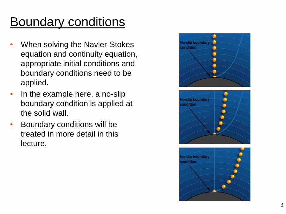
• When solving the Navier-Stokes

equation and continuity equation,

appropriate initial conditions and

boundary conditions need to be

applied.

• In the example here, a no-slip

boundary condition is applied at

the solid wall.

• Boundary conditions will be

treated in more detail in this

lecture.

4

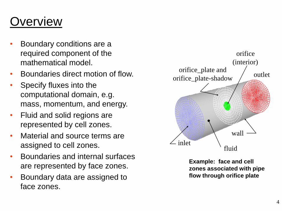
Example: face and cell

zones associated with pipe

flow through orifice plate

inlet

outlet

wall

orifice

(interior)orifice_plate and

orifice_plate-shadow

fluid

Overview

• Boundary conditions are a

required component of the

mathematical model.

• Boundaries direct motion of flow.

• Specify fluxes into the

computational domain, e.g.

mass, momentum, and energy.

• Fluid and solid regions are

represented by cell zones.

• Material and source terms are

assigned to cell zones.

• Boundaries and internal surfaces

are represented by face zones.

• Boundary data are assigned to

face zones.

5

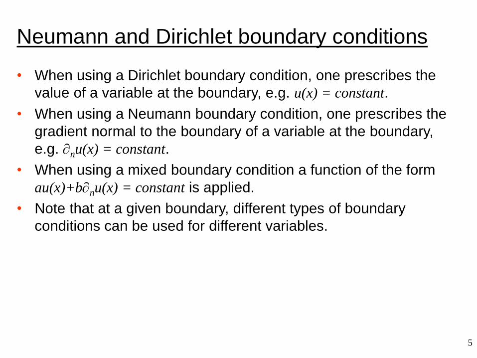
Neumann and Dirichlet boundary conditions

• When using a Dirichlet boundary condition, one prescribes the

value of a variable at the boundary, e.g. u(x) = constant.

• When using a Neumann boundary condition, one prescribes the

gradient normal to the boundary of a variable at the boundary,

e.g. nu(x) = constant.

• When using a mixed boundary condition a function of the form

au(x)+bnu(x) = constant is applied.

• Note that at a given boundary, different types of boundary

conditions can be used for different variables.

6

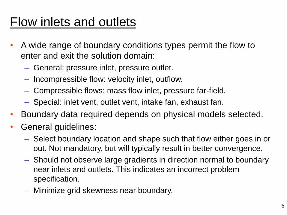
Flow inlets and outlets

• A wide range of boundary conditions types permit the flow to

enter and exit the solution domain:

– General: pressure inlet, pressure outlet.

– Incompressible flow: velocity inlet, outflow.

– Compressible flows: mass flow inlet, pressure far-field.

– Special: inlet vent, outlet vent, intake fan, exhaust fan.

• Boundary data required depends on physical models selected.

• General guidelines:

– Select boundary location and shape such that flow either goes in or

out. Not mandatory, but will typically result in better convergence.

– Should not observe large gradients in direction normal to boundary

near inlets and outlets. This indicates an incorrect problem

specification.

– Minimize grid skewness near boundary.

7

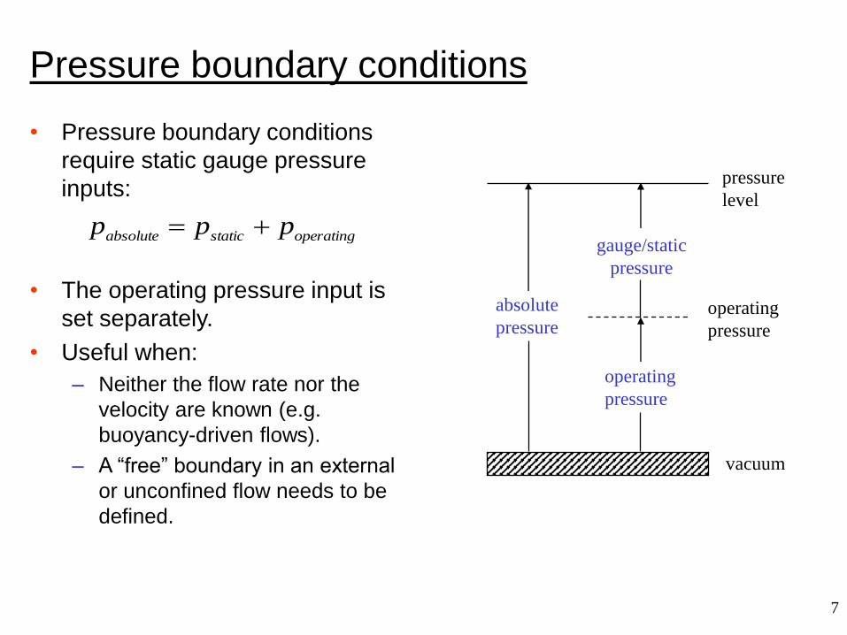
• Pressure boundary conditions

require static gauge pressure

inputs:

• The operating pressure input is

set separately.

• Useful when:

– Neither the flow rate nor the

velocity are known (e.g.

buoyancy-driven flows).

– A “free” boundary in an external

or unconfined flow needs to be

defined.

operatingstaticabsoluteppp +=

gauge/static

pressure

operating

pressure

pressure

level

operating

pressure

absolute

pressure

vacuum

Pressure boundary conditions

8

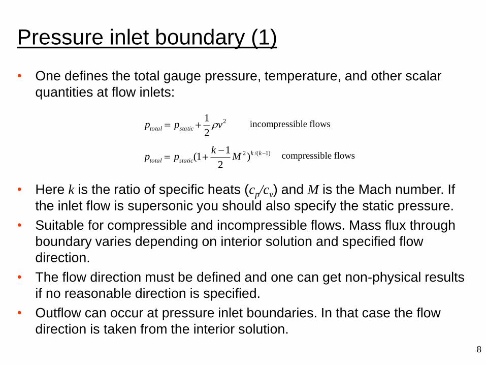
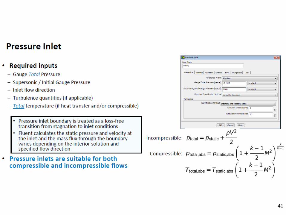
• One defines the total gauge pressure, temperature, and other scalar

quantities at flow inlets:

• Here k is the ratio of specific heats (cp/cv) and M is the Mach number. If

the inlet flow is supersonic you should also specify the static pressure.

• Suitable for compressible and incompressible flows. Mass flux through

boundary varies depending on interior solution and specified flow

direction.

• The flow direction must be defined and one can get non-physical results

if no reasonable direction is specified.

• Outflow can occur at pressure inlet boundaries. In that case the flow

direction is taken from the interior solution.

)1/(2)2

11( −−+= kk

statictotal Mk

pp

2

2

1vpp statictotal += incompressible flows

compressible flows

Pressure inlet boundary (1)

9

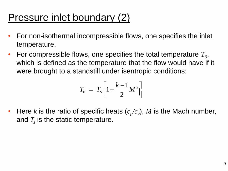
• For non-isothermal incompressible flows, one specifies the inlet

temperature.

• For compressible flows, one specifies the total temperature T0,

which is defined as the temperature that the flow would have if it

were brought to a standstill under isentropic conditions:

• Here k is the ratio of specific heats (cp/cv), M is the Mach number,

and Ts is the static temperature.

Pressure inlet boundary (2)

−+= 2

02

11 M

kTT

S

10

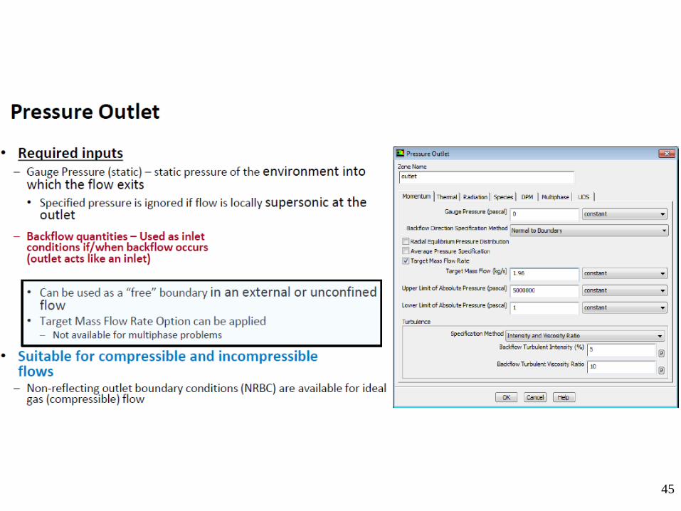
Pressure outlet boundary

• Here one defines the static/gauge pressure at the outlet boundary. This is interpreted as the static pressure of the environment into which the flow exhausts.

• Usually the static pressure is assumed to be constant over the outlet. A radial equilibrium pressure distribution option is available for cases where that is not appropriate, e.g. for strongly swirling flows.

• Backflow can occur at pressure outlet boundaries:

– During solution process or as part of solution.

– Backflow is assumed to be normal to the boundary.

– Convergence difficulties minimized by realistic values for backflow quantities.

– Value specified for static pressure used as total pressure wherever backflow occurs.

• Pressure outlet must always be used when model is set up with a pressure inlet.

11

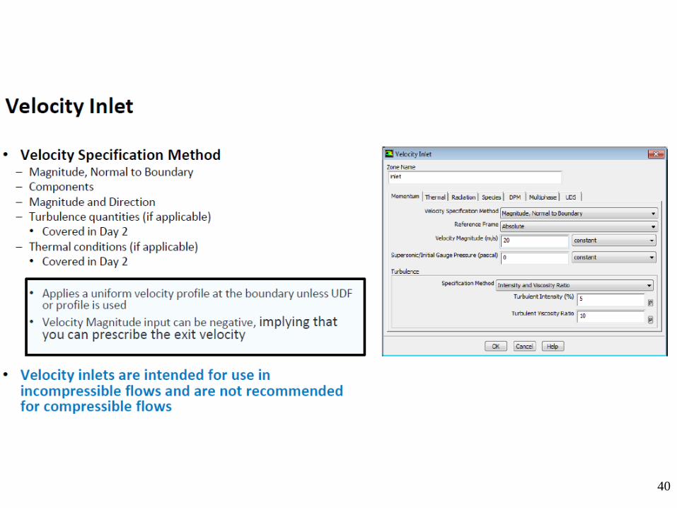
• Defines velocity vector and scalar properties of flow at inlet

boundaries.

• Useful when velocity profile is known at inlet. Uniform profile is

default but other profiles can be implemented too.

• Intended for incompressible flows. The total (stagnation)

properties of flow are not fixed. Stagnation properties vary to

accommodate prescribed velocity distribution. Using in

compressible flows can lead to non-physical results.

• Avoid placing a velocity inlet too close to a solid obstruction. This

can force the solution to be non-physical.

Velocity inlets

12

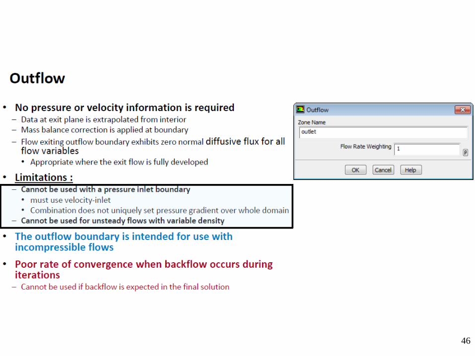
Outflow boundary

• Outflow boundary conditions are used to model flow exits where

the details of the flow velocity and pressure are not known prior to

solution of the flow problem.

• Appropriate where the exit flow is close to a fully developed

condition, as the outflow boundary condition assumes a zero

normal gradient for all flow variables except pressure. The solver

extrapolates the required information from interior.

• Furthermore, an overall mass balance correction is applied.

13

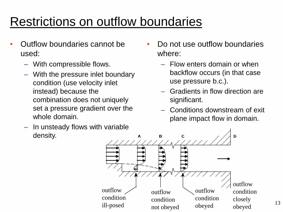
outflow

condition

ill-posed

outflow

condition

not obeyed

outflow

condition

obeyed

outflow

condition

closely

obeyed

Restrictions on outflow boundaries

• Outflow boundaries cannot be

used:

– With compressible flows.

– With the pressure inlet boundary

condition (use velocity inlet

instead) because the

combination does not uniquely

set a pressure gradient over the

whole domain.

– In unsteady flows with variable

density.

• Do not use outflow boundaries

where:

– Flow enters domain or when

backflow occurs (in that case

use pressure b.c.).

– Gradients in flow direction are

significant.

– Conditions downstream of exit

plane impact flow in domain.

14

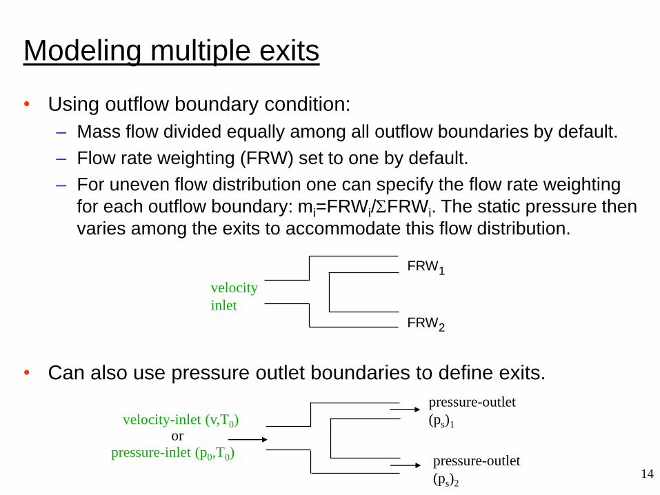
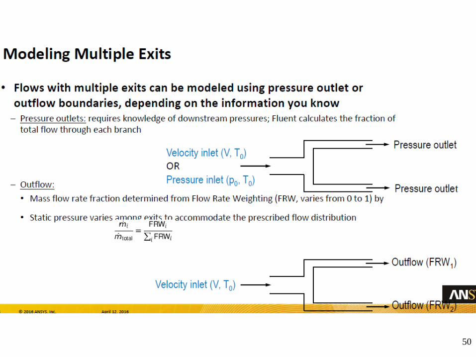
• Using outflow boundary condition:

– Mass flow divided equally among all outflow boundaries by default.

– Flow rate weighting (FRW) set to one by default.

– For uneven flow distribution one can specify the flow rate weighting

for each outflow boundary: mi=FRWi/FRWi. The static pressure then

varies among the exits to accommodate this flow distribution.

• Can also use pressure outlet boundaries to define exits.

pressure-inlet (p0,T0) pressure-outlet

(ps)2

velocity-inlet (v,T0)

pressure-outlet

(ps)1

or

FRW2

velocity

inlet

FRW1

Modeling multiple exits

15

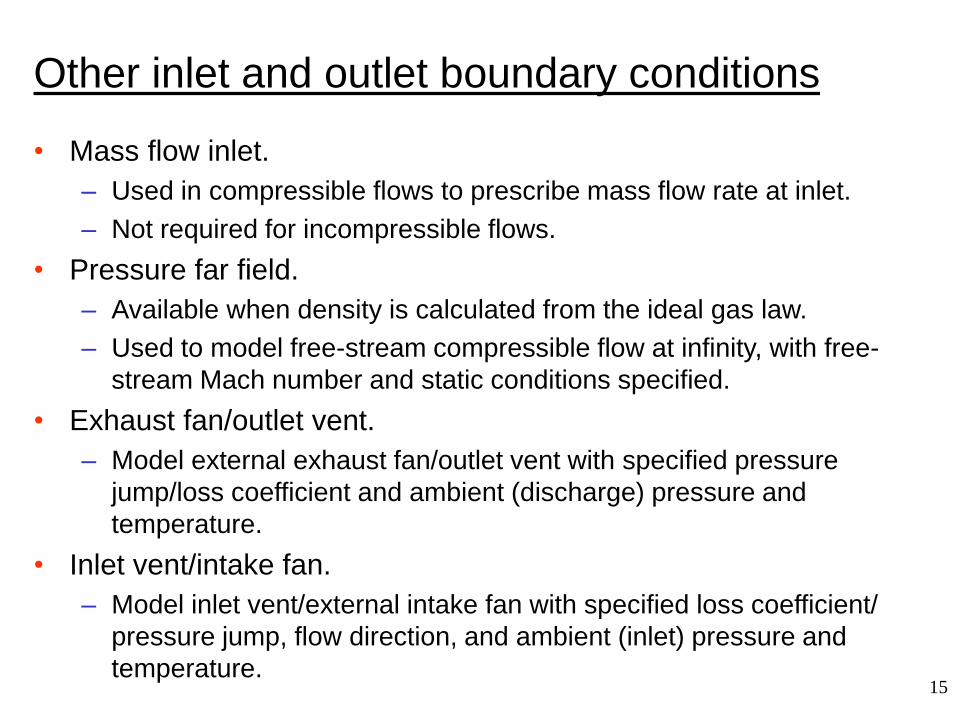
Other inlet and outlet boundary conditions

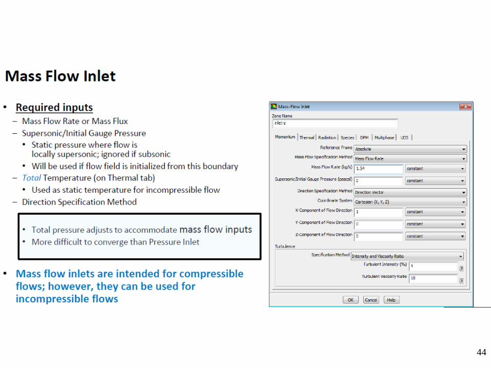
• Mass flow inlet.

– Used in compressible flows to prescribe mass flow rate at inlet.

– Not required for incompressible flows.

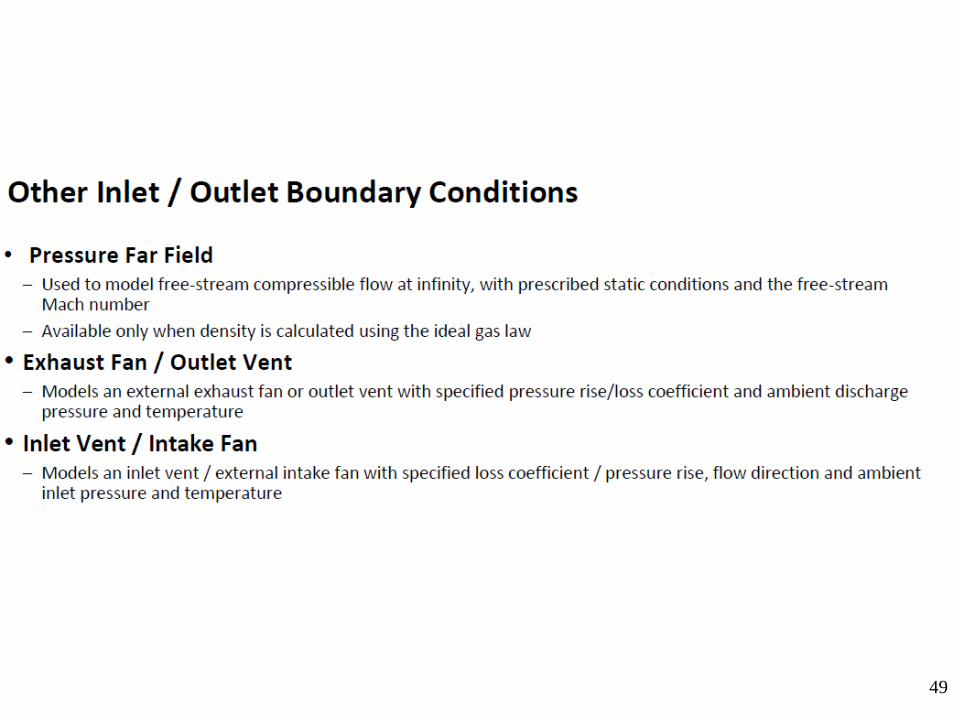
• Pressure far field.

– Available when density is calculated from the ideal gas law.

– Used to model free-stream compressible flow at infinity, with free-

stream Mach number and static conditions specified.

• Exhaust fan/outlet vent.

– Model external exhaust fan/outlet vent with specified pressure

jump/loss coefficient and ambient (discharge) pressure and

temperature.

• Inlet vent/intake fan.

– Model inlet vent/external intake fan with specified loss coefficient/

pressure jump, flow direction, and ambient (inlet) pressure and

temperature.

16

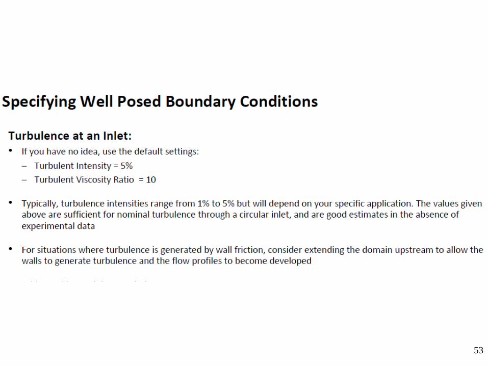
Determining turbulence parameters

• When turbulent flow enters domain at inlet, outlet, or at a far-field

boundary, boundary values are required for:

– Turbulent kinetic energy k.

– Turbulence dissipation rate .

• Four methods available for specifying turbulence parameters:

– Set k and explicitly.

– Set turbulence intensity and turbulence length scale.

– Set turbulence intensity and turbulent viscosity ratio.

– Set turbulence intensity and hydraulic diameter.

17

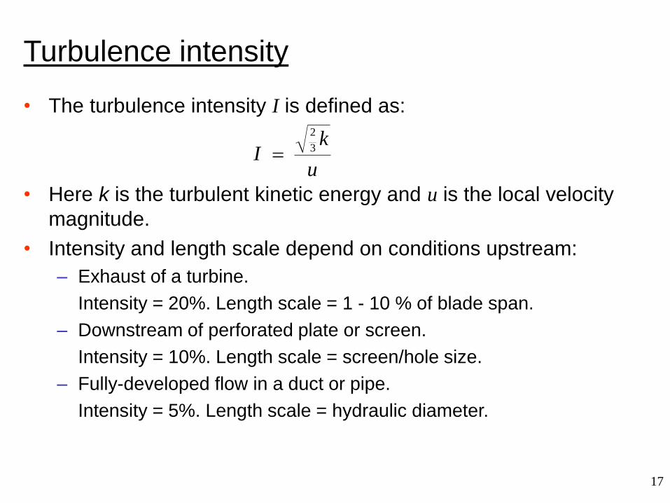
Turbulence intensity

• The turbulence intensity I is defined as:

• Here k is the turbulent kinetic energy and u is the local velocity

magnitude.

• Intensity and length scale depend on conditions upstream:

– Exhaust of a turbine.

Intensity = 20%. Length scale = 1 - 10 % of blade span.

– Downstream of perforated plate or screen.

Intensity = 10%. Length scale = screen/hole size.

– Fully-developed flow in a duct or pipe.

Intensity = 5%. Length scale = hydraulic diameter.

u

kI 3

2

=

18

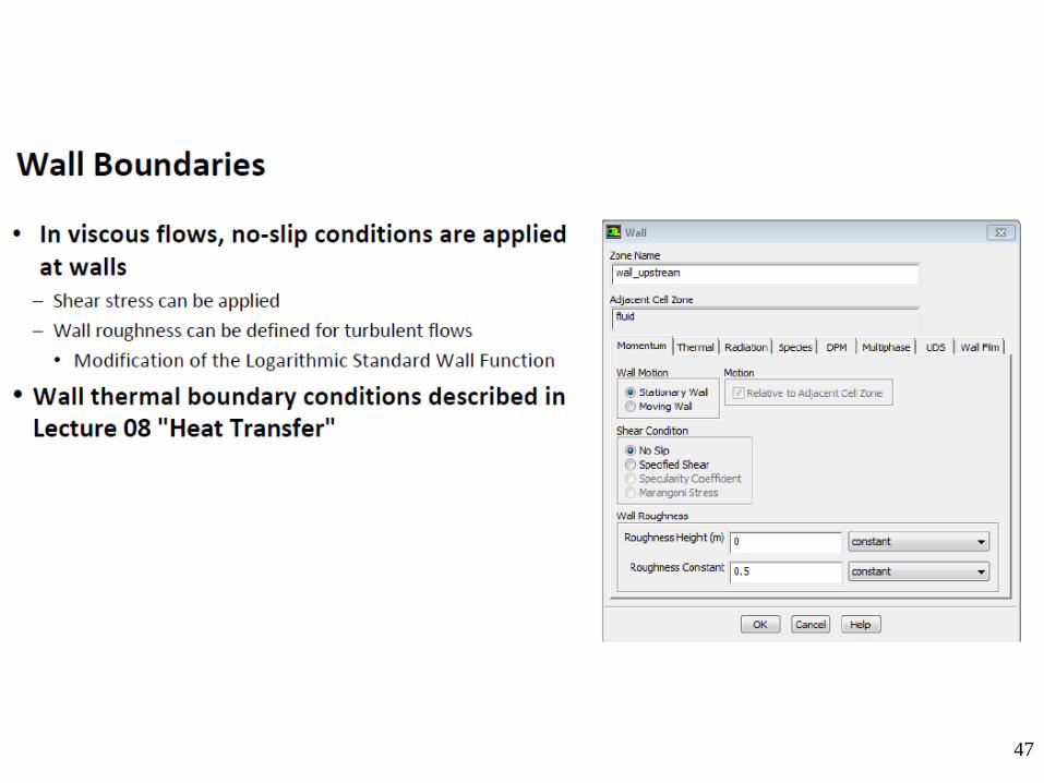
• Used to bound fluid and solid regions.

• In viscous flows, no-slip condition enforced at walls.

– Tangential fluid velocity equal to wall velocity.

– Normal velocity component is set to be zero.

• Alternatively one can specify the shear stress.

• Thermal boundary condition.

– Several types available.

– Wall material and thickness can be defined for 1-D or in-plane thin

plate heat transfer calculations.

• Wall roughness can be defined for turbulent flows.

– Wall shear stress and heat transfer based on local flow field.

• Translational or rotational velocity can be assigned to wall.

Wall boundaries

19

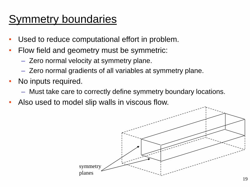
symmetry

planes

Symmetry boundaries

• Used to reduce computational effort in problem.

• Flow field and geometry must be symmetric:

– Zero normal velocity at symmetry plane.

– Zero normal gradients of all variables at symmetry plane.

• No inputs required.

– Must take care to correctly define symmetry boundary locations.

• Also used to model slip walls in viscous flow.

20

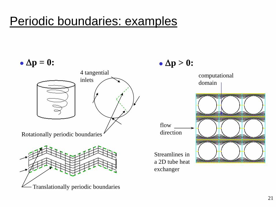
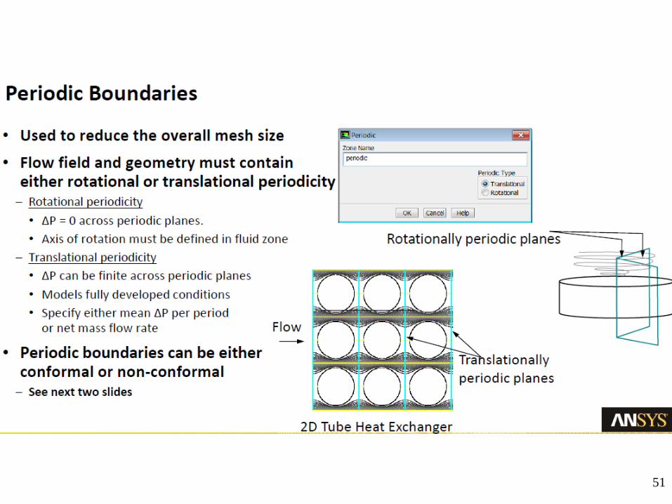
Periodic boundaries

• Used when physical geometry of interest and expected flow

pattern and the thermal solution are of a periodically repeating

nature.

– Reduces computational effort in problem.

• Two types available:

– p = 0 across periodic planes.

• Rotationally or translationally periodic.

• Rotationally periodic boundaries require axis of rotation be defined in

fluid zone.

– p is finite across periodic planes.

• Translationally periodic only.

• Models fully developed conditions.

• Specify either mean p per period or net mass flow rate.

21

computational

domain

Streamlines in

a 2D tube heat

exchanger

flow

direction

Translationally periodic boundaries

4 tangential

inlets

Rotationally periodic boundaries

⚫ p = 0: ⚫ p > 0:

Periodic boundaries: examples

22

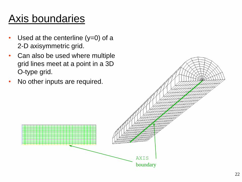
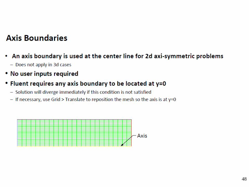
AXIS

boundary

Axis boundaries

• Used at the centerline (y=0) of a

2-D axisymmetric grid.

• Can also be used where multiple

grid lines meet at a point in a 3D

O-type grid.

• No other inputs are required.

23

24

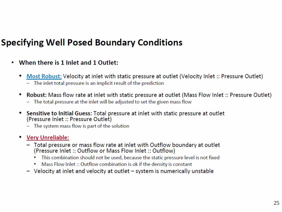
25

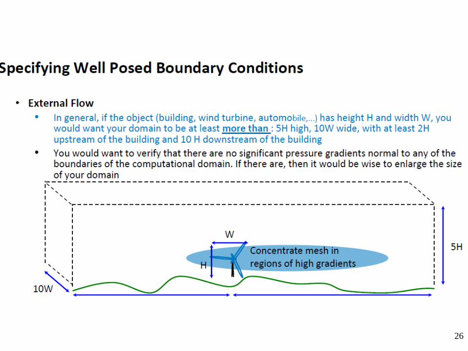
26

27

• A fluid zone is the group of cells for which all active equations are

solved.

• Fluid material input required.

– Single species, phase.

• Optional inputs allow setting of source terms:

– Mass, momentum, energy, etc.

• Define fluid zone as laminar flow region if modeling transitional

flow.

• Can define zone as porous media.

• Define axis of rotation for rotationally periodic flows.

• Can define motion for fluid zone.

Cell zones: fluid

28

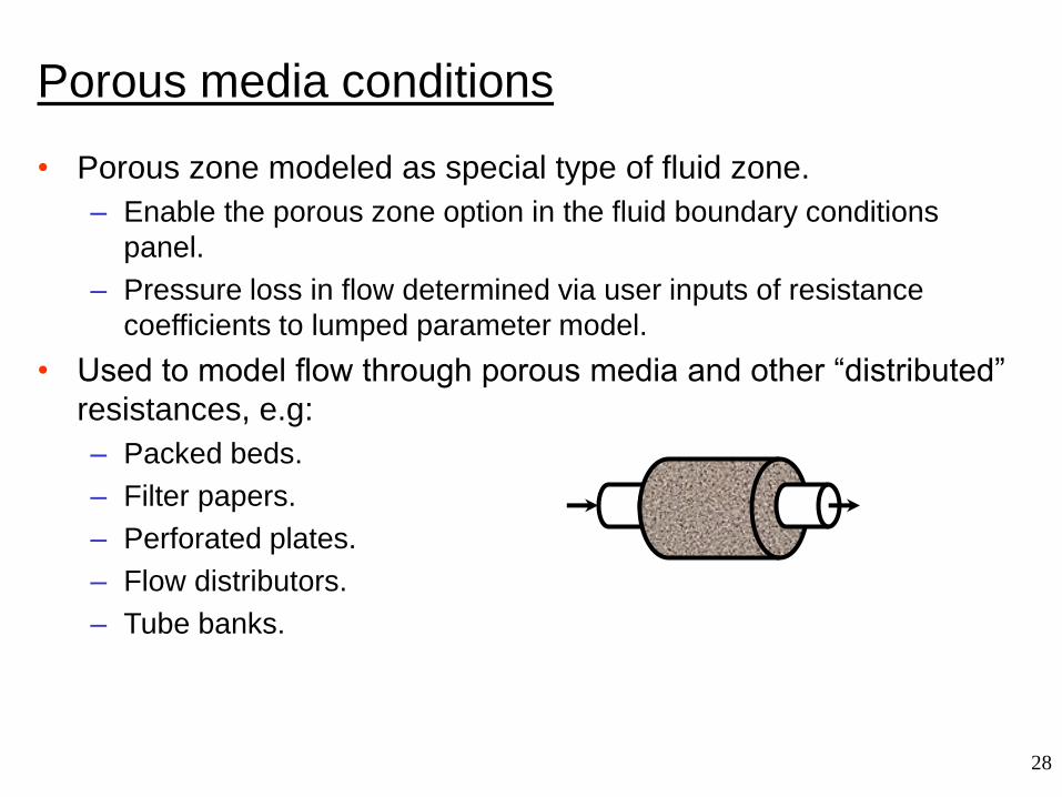
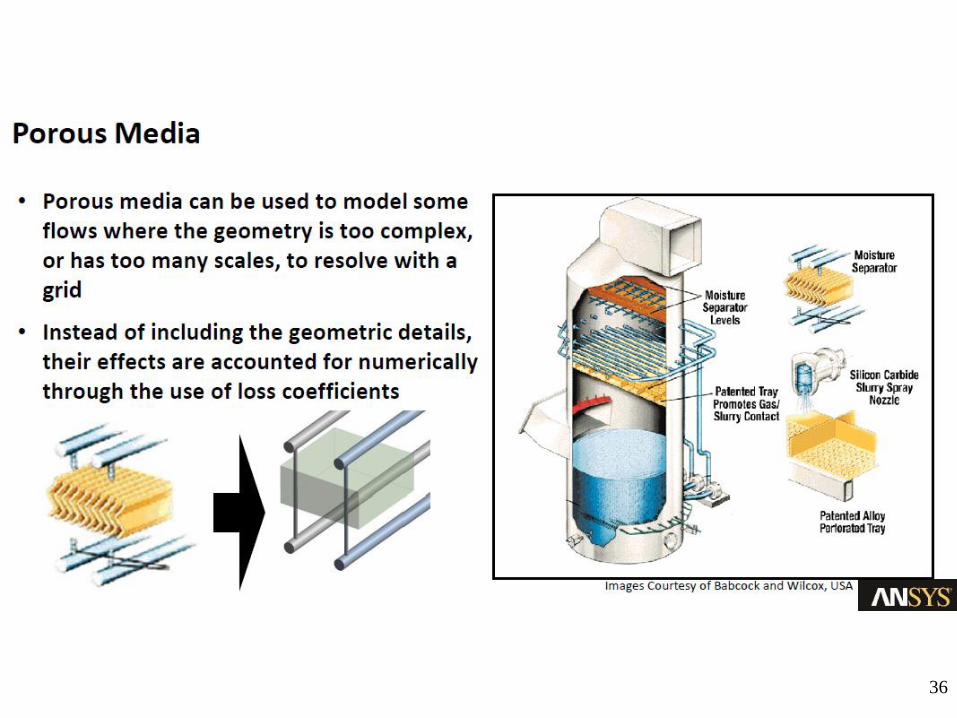
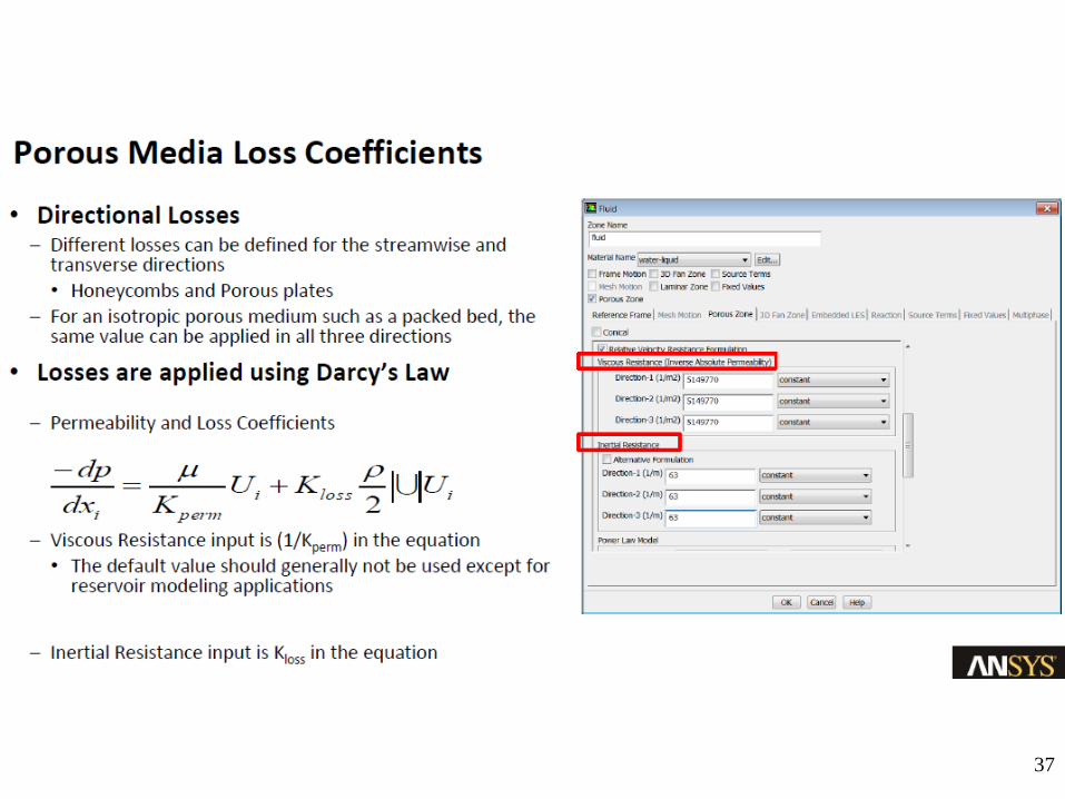
• Porous zone modeled as special type of fluid zone.

– Enable the porous zone option in the fluid boundary conditions

panel.

– Pressure loss in flow determined via user inputs of resistance

coefficients to lumped parameter model.

• Used to model flow through porous media and other “distributed”

resistances, e.g:

– Packed beds.

– Filter papers.

– Perforated plates.

– Flow distributors.

– Tube banks.

Porous media conditions

29

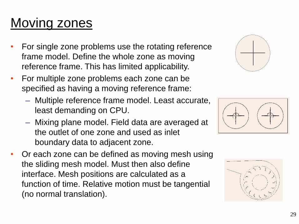
• For single zone problems use the rotating reference

frame model. Define the whole zone as moving

reference frame. This has limited applicability.

• For multiple zone problems each zone can be

specified as having a moving reference frame:

– Multiple reference frame model. Least accurate,

least demanding on CPU.

– Mixing plane model. Field data are averaged at

the outlet of one zone and used as inlet

boundary data to adjacent zone.

• Or each zone can be defined as moving mesh using

the sliding mesh model. Must then also define

interface. Mesh positions are calculated as a

function of time. Relative motion must be tangential

(no normal translation).

Moving zones

30

• A solid zone is a group of cells for which only heat conduction is

solved and no flow equations are solved.

• The material being treated as solid may actually be fluid, but it is

assumed that no convection takes place.

• The only required input is material type so that appropriate

material properties are being used.

• Optional inputs allow you to set a volumetric heat generation rate

(heat source).

• Need to specify rotation axis if rotationally periodic boundaries

adjacent to solid zone.

• Can define motion for solid zone.

Cell zones: solid

31

Internal face boundaries

• Defined on cell faces.

– Do not have finite thickness.

– Provide means of introducing step change in flow properties.

• Used to implement physical models representing:

– Fans.

– Radiators.

– Porous jumps.

– Interior walls. In that case also called “thin walls.”

32

Material properties

• For each zone, a material needs to be specified.

• For the material, relevant properties need to be specified:

– Density.

– Viscosity, may be non-Newtonian.

– Heat capacity.

– Molecular weight.

– Thermal conductivity.

– Diffusion coefficients.

• Which properties need to be specified depends on the model. Not

all properties are always required.

• For mixtures, properties may have to be specified as a function of

the mixture composition.

33

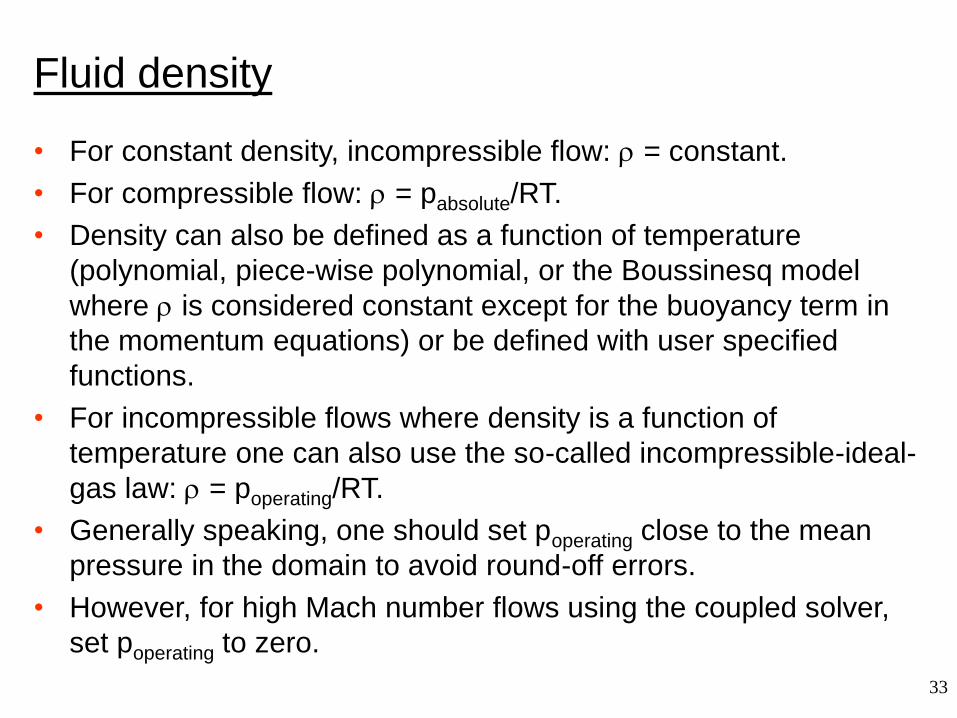
Fluid density

• For constant density, incompressible flow: = constant.

• For compressible flow: = pabsolute/RT.

• Density can also be defined as a function of temperature

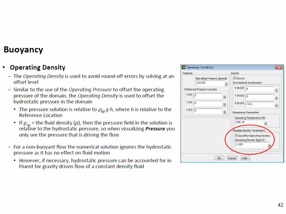
(polynomial, piece-wise polynomial, or the Boussinesq model

where is considered constant except for the buoyancy term in

the momentum equations) or be defined with user specified

functions.

• For incompressible flows where density is a function of

temperature one can also use the so-called incompressible-ideal-

gas law: = poperating/RT.

• Generally speaking, one should set poperating close to the mean

pressure in the domain to avoid round-off errors.

• However, for high Mach number flows using the coupled solver,

set poperating to zero.

34

When is a problem properly specified?

• Proper specification of boundary conditions is very important.

• Incorrect boundary conditions will lead to incorrect results.

• Boundary conditions may be overspecified or underspecified.

• Overspecification occurs when more boundary conditions are

specified than appropriate and not all conditions can hold at the

same time.

• Underspecification occurs when the problem is incompletely

specified, e.g. there are boundaries for which no condition is

specified.

• Commercially available CFD codes will usually perform a number

of checks on the boundary condition set-up to prevent obvious

errors from occurring.

35

36

37

38

39

40

41

42

43

44

45

46

47

48

49

50

51

52

53

54

Summary

• Zones are used to assign boundary conditions.

• Wide range of boundary conditions permit flow to enter and exit

solution domain.

• Wall boundary conditions used to bound fluid and solid regions.

• Repeating boundaries used to reduce computational effort.

• Internal cell zones used to specify fluid, solid, and porous regions.

• Internal face boundaries provide way to introduce step change in

flow properties.