ME 6000 COMPUTATIONAL METHODS IN ENGINEERING 3-0-0-3

Course Content:Approximations: Accuracy and precision, definitions ofround off and truncation errors, error propagation.Algebraic equations: Formulation and solution of linearalgebraic equations, Gauss elimination, LU decomposition,iteration methods (Gauss-Seidal), convergence of iterationmethods, eigen values and eigenvectors.Interpolation methods: Newton’s divided difference,interpolation polynomials, Lagrange interpolationpolynomials.Differentiation and Integration: High accuracydifferentiation formulae, extrapolation, derivatives ofunequally spaced data, Gauss quadrature and integration.

Transform techniques: Continuous Fourier series,frequency and time domains, Laplace transform, Fourierintegral and transform, Discrete Fourier Transform (DFT),Fast Fourier Transform (FFT).

Differential equations: Initial and boundary valueproblems, eigenvalue problems, solutions to elliptical andparabolic equations, partial differential equations.

Regression methods: Linear and non-linear regression,multiple linear regression, general linear least squares.

Statistical methods: Statistical representation of data,modeling and analysis of data, test of hypotheses.

Introduction to optimization methods: Local and globalminima, Line searches, Steepest descent method,Conjugate gradient method, Quasi Newton method,Penalty function.

Solution to practical engineering problems usingsoftware tools.

Books:

1. Schilling R.J and Harris S L, “Applied Numerical Methods for Engineering using MatLab and C”, Brooks/Cole Publishing Co., 2000.

2. Chapra S C and Canale R P, “Numerical Methods for Engineers”, McGraw Hill, 1989.

3. Hines, W.W and Montrogmery, “Probability and Statistics in Engineering and Management Studies”, John Willey, 1990.

4.Santhosh K.Gupta, “Numerical Methods for Engineers”, New age international publishers, 2005.

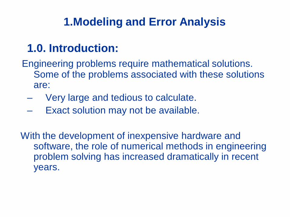
1.Modeling and Error Analysis

1.0. Introduction:Engineering problems require mathematical solutions.

Some of the problems associated with these solutions are:

– Very large and tedious to calculate.– Exact solution may not be available.

With the development of inexpensive hardware and software, the role of numerical methods in engineering problem solving has increased dramatically in recent years.

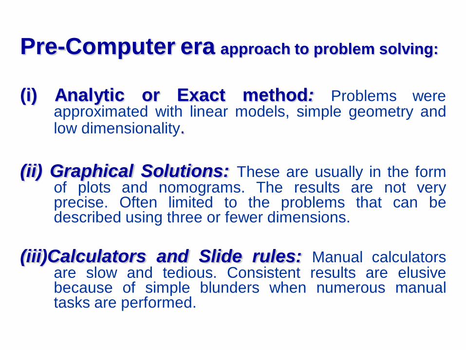
Pre-Computer era approach to problem solving:

(i) Analytic or Exact method: Problems wereapproximated with linear models, simple geometry andlow dimensionality.

(ii) Graphical Solutions: These are usually in the formof plots and nomograms. The results are not veryprecise. Often limited to the problems that can bedescribed using three or fewer dimensions.

(iii)Calculators and Slide rules: Manual calculatorsare slow and tedious. Consistent results are elusivebecause of simple blunders when numerous manualtasks are performed.

Computational Methods:Computers and Numerical methods provide an alternative forsuch complicated calculations. The following are theadvantages in using computational methods.

(i)They are extremely powerful problem solving tools. Capableof handling large system of equations, non-linearities,complicated geometries.

(ii) Computational methods reduce higher mathematics tobasic arithmetic operations.

(iii) Results can be seen dynamically at the designstage and possible to control the errors due tovarious approximations.

.

iv) Commercially available software packages involvenumerical method.

Caution while using commercial software:a) Intelligent use of these programs requires the

knowledge of basic theory underlying the methods.

b) Many problems cannot be approached using thepackage programs. Due to this limitation, developing ownprograms to solve problems may be preferred. In somecases spending on expensive software can be avoided.

1.1 Mathematical Modeling and Engineering problem solving:

A mathematical model can be broadly defined as aformulation or equation that expresses the essentialfeatures of a physical system or process in mathematicalterms. In general, it represents a functional relationshipform.

Dependent variable = f {independent variable, parameters, forcing functions} (1.1)

Where,Dependent variable: reflects the behavior or state of the system.Independent variable: dimensions (Ex: Time and space).Parameters: reflective of system’s properties.Forcing functions: External influences acting upon it.

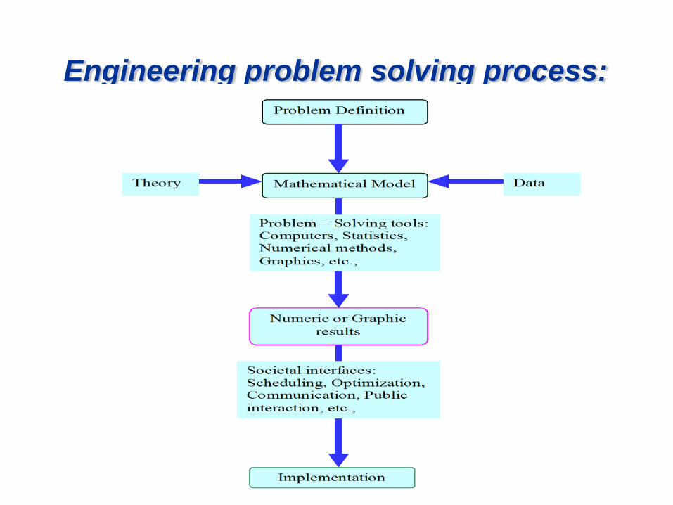
Engineering problem solving process:

The mathematical expression of Second law of NewtonF = m a (1.2)

Eq. (1.2) can be recast in the form of Eq.(1.1) asa = F/m (1.3)

Where ‘a’ is dependent variable reflecting the system’s behavior.‘F’ is forcing function.‘m’ is parameter representing a property of the system.

Eq. (1.2) has a number of characteristics of a typical mathematical model.

1. It describes a natural process or system in the mathematical term.

2. It represents an idealization and simplification of reality.3. It yields reproducible results.

Mathematical models ofphysical phenomena maybemore complex, and eithercannot be solved exactly orrequire more sophisticatedtechniques than simplealgebra for their solution.

This is illustrated in thefollowing example. Take acase of falling parachutist asshown in the Fig.1.2, and weare interested in the terminalvelocity.

A model of this case can be derived from Eq. (1.2) by expressing the acceleration in terms of rate of change of velocity as

(1.4)F has two components

FD : Downward pull of gravity.FU : Upward force of air resistance.

F = FD + FU (1.5)With a ‘+’ve sign for downward force, using Newton’s second

lawFD = m g (1.6)

Assuming air resistance is linearly proportional to velocity and it acts in upward direction.

FU = - c v (1.7)‘c’ is proportionality constant called drag co-efficient (kg/s).

dvm Fdt

=

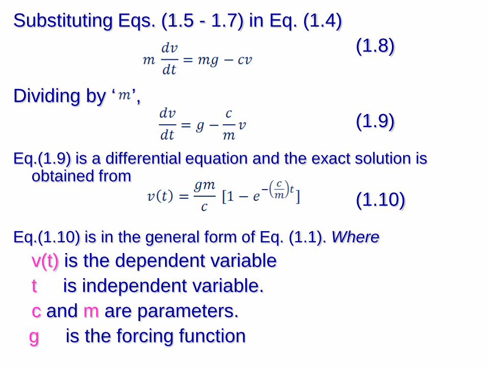
Substituting Eqs. (1.5 - 1.7) in Eq. (1.4)(1.8)

Dividing by ‘ ’,(1.9)

Eq.(1.9) is a differential equation and the exact solution is obtained from

(1.10)

Eq.(1.10) is in the general form of Eq. (1.1). Wherev(t) is the dependent variablet is independent variable.c and m are parameters.g is the forcing function

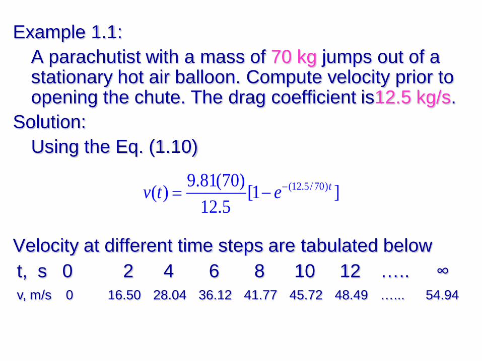
Example 1.1:A parachutist with a mass of 70 kg jumps out of a stationary hot air balloon. Compute velocity prior to opening the chute. The drag coefficient is12.5 kg/s.

Solution:Using the Eq. (1.10)

Velocity at different time steps are tabulated belowt, s 0 2 4 6 8 10 12 ….. ∞v, m/s 0 16.50 28.04 36.12 41.77 45.72 48.49 …... 54.94

(12.5/ 70)9.81(70)( ) [1 ]12.5

tv t e−= −

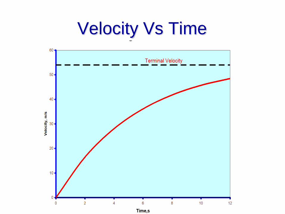
Velocity Vs Time

Eq. (1.10) is called analytical or exact solution. A numerical solution approximates the exact solution. The time rate of change of velocity can be approximated as

(1.11)

Where ∆v and ∆t are differences in velocity and time computed over finite interval. Substituting Eq.(1.11) in Eq.(1.9)

This equation can be rearranged to yield(1.12)

Eqn (1.12) is a transformation of differential equation (1.9) into an algebraic equation.

New value = Old value + Slope x Step Size.

1

1

( ) - ( ) ( ) -

ii

i

i

i

v t v t cg v tt t m+

+

= −

1 1( ) ( ) [ ( )]( )i i i i icv t v t g v t t tm

+ += + − −

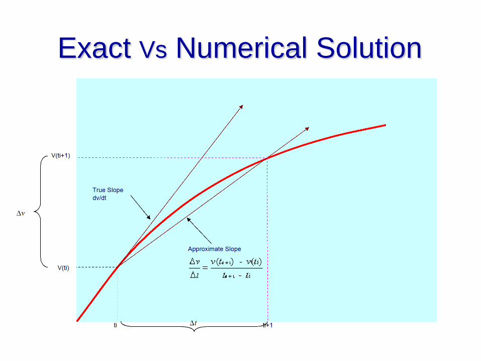
Exact Vs Numerical Solution

Example 1.2Develop a numerical solution to falling parachutist problem given in example 1.1. Employ a step size of 2 s.

Solution:At Initial time ( t i = 0), velocity of parachutist = 0Substituting in Eq. (1.12) to compute the velocity at ti+1 = 2s

For the next interval (from t = 2 to 4 s) the computation is repeated, resulting

The calculations are continued and tabulated below.

t, s 0 2 4 6 8 10 12 …. ∞

v,m/s,Exact 0 16.50 28.04 36.12 41.77 45.72 48.49 …. 54.94

v, m/s Numerical

0 19.62 32.23 40.34 45.55 48.90 51.06 ….

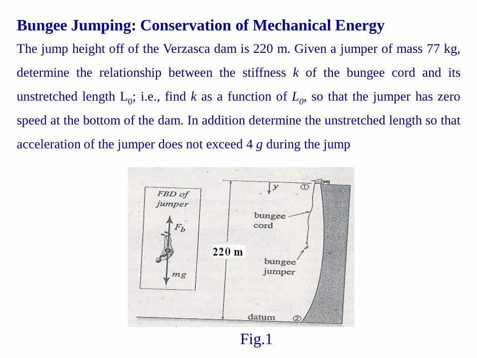
Bungee Jumping: Conservation of Mechanical EnergyThe jump height off of the Verzasca dam is 220 m. Given a jumper of mass 77 kg,

determine the relationship between the stiffness k of the bungee cord and its

unstretched length L0; i.e., find k as a function of L0, so that the jumper has zero

speed at the bottom of the dam. In addition determine the unstretched length so that

acceleration of the jumper does not exceed 4 g during the jump

Fig.1

SOLUTION

Referring to the FBD in Fig, we model the jumper as a particle subject to

gravity and the force Fb of the bungee cord, which we model as a linear elastic

spring. The jumper begins the jump at 1 with zero speed and ends the jump at 2

with zero speed (see Fig.1). Since we know the jumper’s speed at 1 and 2 and we

know all the forces doing work on the jumper, we can apply the work energy

principle to the jumper to determine the relationship between the bungee stiffness

and its unstretched length.

We will then apply Newton’s second law to the jumper to determine the

maximum acceleration so that we can find k and L0 for the bungee cord. Note that

all the forces acting on the jumper are conservative and that Fb is zero until the

jumper falls a distance equal to the unstretched length of the cord.

Governing Equations

Balance Principles Applying the work-energy principle between 1 and 2, we have

T1+V1 = T2 + V2 (1)

211 2

1 mvT = 222 2

1 mvT =and (2)where m is the jumper’s mass and v1 and v2 are the jumper’s speed at 1 and 2,respectively. Since we also need to determine the jumper’s acceleration, wewill write Newton’s second law for the jumper in the y direction as

∑ =− yby maFmgF : (3)

where we note that Fb = 0 until the bungee cord engages.

mghV =1 ( ) ,21 2

02 LhkV −=

Force Laws: If we place the datum line for gravitationalpotential energy at 2, then

and (4)

where h= 220 m, mg =756 N, and we have accounted for the

potential energy of the bungee cord in V2. We will also need

the force law for the bungee cord, which is given by

( ),0LykkFb −== δ (5)

where we note that Fb = 0 when y ≤ L0,

Kinematic Equations Since the jumper starts and ends thejump with zero speed, we have

.021 == vv (6)

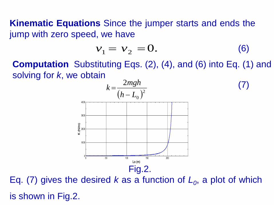
Computation Substituting Eqs. (2), (4), and (6) into Eq. (1) andsolving for k, we obtain

( )20

2Lh

mghk−

= (7)

Fig.2.Eq. (7) gives the desired k as a function of L0, a plot of which

is shown in Fig.2.

We now want to design the bungee system so that the

maximum acceleration of a jumper of mass 77 kg does not

exceed amax = 4 g. Referring to the FBD Fig.1, we know

that until the spring engages, the jumper will be in free fall

and his acceleration will be g downward. Once the spring

engages, the acceleration is determined by solving Eqs. (3)

and (5) for ay, which gives

( ).0Lymkgay −−= (8)

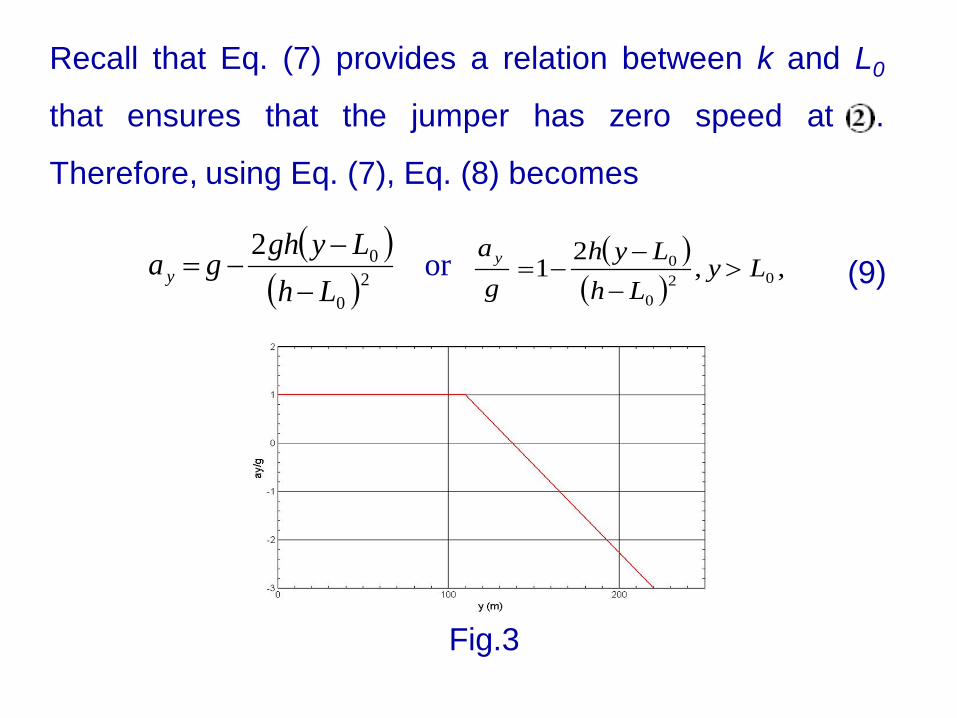
Recall that Eq. (7) provides a relation between k and L0

that ensures that the jumper has zero speed at 2.

Therefore, using Eq. (7), Eq. (8) becomes

( )( )2

0

02Lh

Lyghgay

−

−−= or ( )

( ),,

21 02

0

0 LyLh

Lyhgay >

−

−−= (9)

Fig.3

We will choose the following value of the unstretchedlength of the bungee cord:

(10)

We now need to verify that the design criterion requiring ay < 4 g

is always met. To do so, using the chosen L0 and referring to Fig.3,

we plot ay/g versus y. The plot shows that the chosen value of L0 is

such that our goal is met.