ME 309 Fluid Mechanics Honors

Computational Fluid Dynamics

Final Report

Instructor: Professor Ivan C. Christov

By: Patrick D. Tirtapraja

December 3, 2017

Page 2 of 15

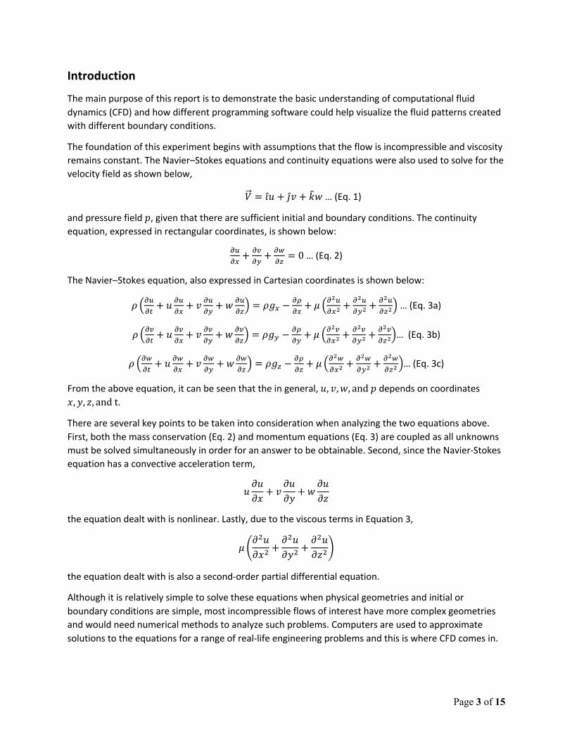
Abstract

The purpose of this experiment and report was to immerse myself in learning computational fluids dynamics (CFD) as part of the honors contract curriculum. The raw data of stream function values were given and this report analyzed its relationship with the flow’s velocity as well as its streamline patterns. Several software, such as the Excel Spreadsheet and MATLAB were used to compute and plot the streamlines and velocity vectors given the stream functions values. The Navier–Stokes equation was derived with the additional assumption of irrotational flow on top of its initial assumption of the flow being incompressible and its viscosity remaining constant. The equation of stream function, 𝜓, was derived and the velocities in the x and y-direction were calculated. With the use of MATLAB, the streamlines, velocity vectors, and velocity contour lines were plotted. Different scenarios depicting various boundary conditions were used to analyze the response of the flow with such changes. It was observed that as the flow approaches the boundary conditions placed, in this scenario, the wall, its stream function decreases and increases again as it distanced itself from the wall. Despite the various assumptions used for CFD in this report, these assumptions led to relatively accurate estimates as to how flows behave in reality. This honors assignment sparked an interest within me to learn more about the theories and concepts of CFD and pushed me to utilize different software programs to accomplish such tasks.

Page 3 of 15

Introduction

The main purpose of this report is to demonstrate the basic understanding of computational fluid dynamics (CFD) and how different programming software could help visualize the fluid patterns created with different boundary conditions.

The foundation of this experiment begins with assumptions that the flow is incompressible and viscosity remains constant. The Navier–Stokes equations and continuity equations were also used to solve for the velocity field as shown below,

𝑉#⃗ = 𝚤�̂� + 𝚥�̂� + 𝑘-𝑤 … (Eq. 1)

and pressure field 𝑝, given that there are sufficient initial and boundary conditions. The continuity equation, expressed in rectangular coordinates, is shown below:

0102+ 03

04+ 05

06= 0 … (Eq. 2)

The Navier–Stokes equation, also expressed in Cartesian coordinates is shown below:

𝜌 9010:+ 𝑢 01

02+ 𝑣 01

04+ 𝑤 01

06; = 𝜌𝑔2 −

0>02+ 𝜇 90

@102@

+ 0@104@

+ 0@106@; … (Eq. 3a)

𝜌 9030:+ 𝑢 03

02+ 𝑣 03

04+ 𝑤 03

06; = 𝜌𝑔4 −

0>04+ 𝜇 90

@302@

+ 0@304@

+ 0@306@;… (Eq. 3b)

𝜌 9050:+ 𝑢 05

02+ 𝑣 05

04+ 𝑤 05

06; = 𝜌𝑔6 −

0>06+ 𝜇 90

@502@

+ 0@504@

+ 0@506@

;… (Eq. 3c)

From the above equation, it can be seen that the in general, 𝑢, 𝑣, 𝑤, and𝑝 depends on coordinates 𝑥, 𝑦, 𝑧, andt.

There are several key points to be taken into consideration when analyzing the two equations above. First, both the mass conservation (Eq. 2) and momentum equations (Eq. 3) are coupled as all unknowns must be solved simultaneously in order for an answer to be obtainable. Second, since the Navier-Stokes equation has a convective acceleration term,

𝑢𝜕𝑢𝜕𝑥

+ 𝑣𝜕𝑢𝜕𝑦

+ 𝑤𝜕𝑢𝜕𝑧

the equation dealt with is nonlinear. Lastly, due to the viscous terms in Equation 3,

𝜇 K𝜕L𝑢𝜕𝑥L

+𝜕L𝑢𝜕𝑦L

+𝜕L𝑢𝜕𝑧L

M

the equation dealt with is also a second-order partial differential equation.

Although it is relatively simple to solve these equations when physical geometries and initial or boundary conditions are simple, most incompressible flows of interest have more complex geometries and would need numerical methods to analyze such problems. Computers are used to approximate solutions to the equations for a range of real-life engineering problems and this is where CFD comes in.

Page 4 of 15

The usage of CFD covers a variety of applications. CFD software packages are used to study the flow field around vehicles as shown in Fig. 1 below. This way the flow through the catalytic converter can be visualized and analyzed in order to develop more effective ones.

Figure 1: Pathlines around a Formula 1 Car as observed by a CFD Software

In this experiment, a basic application of the CFD was performed by using the Excel Spreadsheet to calculate the values and MATLAB to graphically plot the contours of the data, showing the streamlines and various velocity vectors. This basic application of a numerical method to fluid mechanics problem is when steady, incompressible, inviscid, and 2-D flow were assumed. Despite assuming a number of factors, these assumptions lead to reasonable estimates and flow predictions. The flows can be modeled with the following Laplace equation:

0@N02@

+ 0@N04@

= 0 … (Eq. 4)

where 𝜓 is the stream function. By approximating each differential with Taylor series, the following numerical approximation is derived:

NOPQ,RSNOTQ,RU@

+ NO,RPQSNO,RTQU@

− 4NO,RU@

= 0 … (Eq. 5)

where ℎ is the step size in either the 𝑖or𝑗 direction

𝜓\,] is the value of the stream function at the𝑖th and𝑗th location of x and y direction respectively

By simplifying the (Eq. 5), the following equation is obtained:

𝜓\,] =^_(𝜓\,S^] + 𝜓\a^,] + 𝜓\,]S^ + 𝜓\,]a^ … (Eq. 6)

which shows that a stream function at a specific location is the average of its four neighboring coordinates.

By implementing this concept with a given Excel spreadsheet containing the stream function data as well as boundary conditions, a graph was plotted and analyze. By analyzing the streamlines and flow separation location, velocity and pressure values at a specific location can be predicted and calculated. The relationship between the different factors was then able to be distinguished

Page 5 of 15

Methods and Materials

The materials used in this experiment were two software: Excel’s Spreadsheet and MATLAB.

The following data was given in an Excel Spreadsheet as shown below:

Figure 1: Excel Raw Data

Initially, the experiment would start with replicating the data above in MATLAB. However, certain functions, such as Excel’s ability to automatically iterate its tables’ values are not available in MATLAB and implementing the necessary partial differentials would take longer time deviating from the purpose of the experiment itself.

Page 6 of 15

As a trial and to get used to the features of Excel, the raw data was first remade onto a blank Excel Spreadsheet. The boundary conditions (0’s and 10’s) were then placed at the desired locations then each of the cells in the spreadsheet were equated to the average of its four neighboring cells. However, this will cause an error of circular calculation where one cell would be referring to a value that does not exist beforehand. This is where the Excel iterate feature comes in under Tools/Options/Calculation. The values were then iterated until the variations in values is zero or trivial. The surface plot was then plotted according to the attained data.

The data was then imported to MATLAB and the contour lines were plotted. The velocity vector was then calculated by first equation the velocity in the x-direction, denoted as 𝑉2, and the velocity in the y-direction, denoted as 𝑉4. Additional rows and columns were added if necessary for calculations of either velocities.

Given that the flow is incompressible, 2-D, and irrotational, the velocity components, 𝑉2 and 𝑉4 can be derived in terms of the stream function, 𝜓 as shown below:

𝑉2 =0N04

… (Eq. 7a)

𝑉4 = −0N02

… (Eq. 7b)

where 𝜕𝑥 and 𝜕𝑦 were initialized as equal to 0.1.

The velocity at a specific location was then calculated by using the following formula:

𝑉2,4 = b𝑉2L + 𝑉4L … (Eq. 8)

and for visualization purposes was then plotted by using the quiver function of MATLAB, representing its velocity directions.

Additional pathways and wall shapes and sizes were then analyzed by manipulating the boundary conditions.

Page 7 of 15

Results

This section will present the results obtained throughout this experiment. The figure below shows the completion of the duplicated data of the excel sheet.

Figure 2: Remade Raw Excel Data

The following is the MATLAB code to import the data and plot the contour plot.

%%MATLAB Code to plot streamline contours clear all %streamline plot psi = ... [8.97 8.93 8.89 8.84 8.77 8.69 8.59 8.48 8.35 8.23 8.13 8.06; 7.94 7.87 7.79 7.69 7.57 7.41 7.21 6.97 6.70 6.44 6.24 6.11; 6.91 6.82 6.71 6.57 6.39 6.16 5.86 5.48 5.03 4.58 4.29 4.12; 5.90 5.79 5.65 5.49 5.27 4.98 4.59 4.07 3.37 2.54 2.23 2.09; 4.89 4.77 4.63 4.45 4.22 3.91 3.47 2.83 1.83 0 0 0; 3.90 3.78 3.65 3.48 3.25 2.95 2.53 1.95 1.12 0 0 0; 2.91 2.82 2.70 2.56 2.37 2.11 1.77 1.31 0.719 0 0 0; 1.94 1.87 1.78 1.68 1.54 1.36 1.12 0.816 0.435 0 0 0; 0.966 0.929 0.886 0.831 0.759 0.666 0.546 0.392 0.207 0 0 0]; %adding a row of zero at the bottom for boundary condition psi = [psi; zeros(1,12)]; %additional column add_col = [8.00; 6.0; 4.0; 2.0; 0; 0; 0; 0; 0; 0]; psi = [psi add_col];

Page 8 of 15

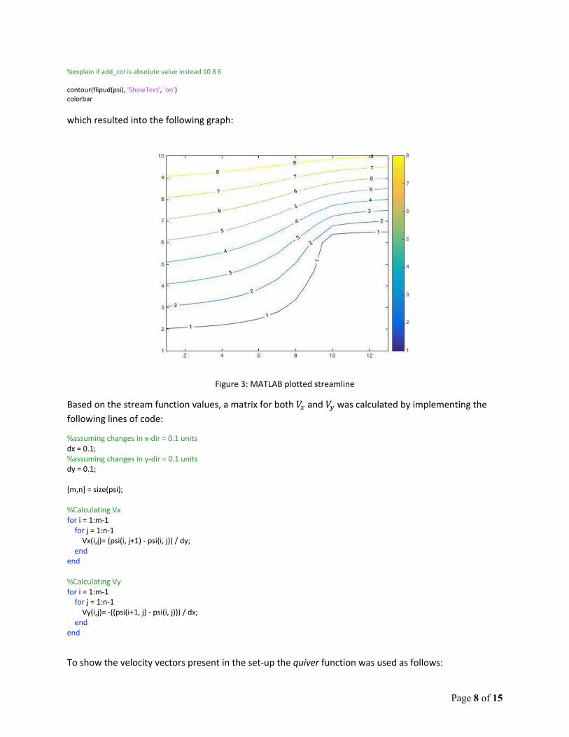
%explain if add_col is absolute value instead 10 8 6 contour(flipud(psi), 'ShowText', 'on') colorbar which resulted into the following graph:

Figure 3: MATLAB plotted streamline

Based on the stream function values, a matrix for both 𝑉2 and 𝑉4 was calculated by implementing the following lines of code:

%assuming changes in x-dir = 0.1 units dx = 0.1; %assuming changes in y-dir = 0.1 units dy = 0.1; [m,n] = size(psi); %Calculating Vx for i = 1:m-1 for j = 1:n-1 Vx(i,j)= (psi(i, j+1) - psi(i, j)) / dy; end end %Calculating Vy for i = 1:m-1 for j = 1:n-1 Vy(i,j)= -((psi(i+1, j) - psi(i, j))) / dx; end end

To show the velocity vectors present in the set-up the quiver function was used as follows:

Page 9 of 15

quiver(Vx, Vy)

Figure 3: Velocity vector plot by plotting 𝑉2 and 𝑉4

After the values of 𝑉2 and 𝑉4 were obtained, by using (Eq. 8), the velocity vector was calculated. The velocity was then plotted as a contour map to represent the speed of the system by using the following code:

%Calculating the veclocity at a given position for i = 1:m-1 for j = 1:n-1 V(i,j) = sqrt(Vx(i,j).^2 + Vy(i,j).^2); end end contour(flipud(V), 'ShowText', 'on') colorbar

The graph obtained was shown below:

Page 10 of 15

Figure 4: Velocity Contour Lines

With Figure 4 above, it is noticeable that the speeds decreased as it is closer to the wall (where it increases as the distance grew further away from the wall.

The following are some examples of different wall shapes used to analyze its streamlines and velocity contour lines. Additional Examples #1: A boulder located at the center.

Page 11 of 15

Figure 5 a, b, c shows the streamline, velocity vector, and velocity contour lines if there was a boulder located at the bottom center of the set-up as indicated by the white spaces in Figure 5a. Additional Examples #2: Two walls, one at the bottom left, the other one located at the top right.

Figure 5a: Streamline with a boulder at the center Figure 5b: Velocity vector

Figure 5c: Velocity Contour Lines

Page 12 of 15

Similarly, Figure 6 a, b, c also shows the streamline, velocity vector, and velocity contour lines if the wall placements changed to the specified description above. Discussion

Figure 6a: Streamline with a boulder at the center Figure 6b: Velocity vector

Figure 6c: Velocity Contour Lines

Page 13 of 15

The streamlines, velocity vectors, and velocity contour lines shown in Figures 5 and 6 were expected. It can be observed that as the flow travels closer to the wall, its velocity decreases. As the flow passed the obstruction, the further away the flow is to the object, the higher its velocity becomes until it reaches its free stream velocity.

By observing the individual set-ups contour lines, it can be seen that the velocity does not follow the streamlines’ path. The circular shaped contour lines in Figure 4 and 5c indicates that as the flow came in contact with an object, some of the flow may flowed backwards.

However, there are several limitations to take note of in this experiment. The raw data Excel Spreadsheet containing the stream function values assumed that the velocity will increase with increments of two up till 10 right after the flow reaches a specific distance from the first point of contact with the wall. However, in real life, this may not be the case as the values of the stream functions may not increment with such discrete values.

Furthermore, the same idea could lead to uncertainties and errors when calculating the velocities in subsequent example scenarios #1 and #2. It was assumed that the stream functions would achieve its initial max flow rate eventually. However, such assumptions could be incorrect as the velocity could indeed slow down to a stop after it came in contact with the object itself. To minimize this problem, more detailed in real life analysis should be conducted to obtain more accurate results.

Page 14 of 15

Conclusion

In conclusion, this experiment and report has been a great way to immersed myself in the basics of computation fluids dynamics. On top of the materials covered in the course, I managed to learn more about stream functions and its relationship with velocity, both magnitude and direction, alongside with its different interaction with boundary conditions. As the flow approaches the wall, the stream functions decreased until the flow distanced itself from the wall. Through this honors assignment, I was able to utilize the Excel Spreadsheet, MATLAB, and fluids concepts to learn about how a flow behaves through the use of CFD. I understood that CFD could be a relatively accurate estimate as to how flow will behave given that there are boundary conditions involved.

Page 15 of 15

References

[1] Fox, R. W., McDonald, A. T., & Pritchard, P. J. (2012). Introduction to fluid mechanics (8th ed.). New

Delhi, India: J. Wiley.