Embed Size (px)
Citation preview
Undergraduate Topics in Computer Science
Md. Saidur Rahman
Basic Graph Theory
Undergraduate Topics in Computer Science
Series editorIan Mackie
Advisory BoardSamson Abramsky, University of Oxford, Oxford, UKKarin Breitman, Pontifical Catholic University of Rio de Janeiro, Rio de Janeiro, BrazilChris Hankin, Imperial College London, London, UKDexter C. Kozen, Cornell University, Ithaca, USAAndrew Pitts, University of Cambridge, Cambridge, UKHanne Riis Nielson, Technical University of Denmark, Kongens Lyngby, DenmarkSteven S. Skiena, Stony Brook University, Stony Brook, USAIain Stewart, University of Durham, Durham, UK
Undergraduate Topics in Computer Science (UTiCS) delivers high-quality instructionalcontent for undergraduates studying in all areas of computing and information science.From core foundational and theoretical material to final-year topics and applications, UTiCSbooks take a fresh, concise, and modern approach and are ideal for self-study or for a one- ortwo-semester course. The texts are all authored by established experts in their fields,reviewed by an international advisory board, and contain numerous examples and problems.Many include fully worked solutions.
More information about this series at http://www.springer.com/series/7592
Md. Saidur Rahman
Basic Graph Theory
123
Md. Saidur RahmanDepartment of Computer Science and EngineeringBangladesh University of Engineering and Technology (BUET)DhakaBangladesh
ISSN 1863-7310 ISSN 2197-1781 (electronic)Undergraduate Topics in Computer ScienceISBN 978-3-319-49474-6 ISBN 978-3-319-49475-3 (eBook)DOI 10.1007/978-3-319-49475-3
Library of Congress Control Number: 2016961329
© Springer International Publishing AG 2017This work is subject to copyright. All rights are reserved by the Publisher, whether the whole or partof the material is concerned, specifically the rights of translation, reprinting, reuse of illustrations,recitation, broadcasting, reproduction on microfilms or in any other physical way, and transmissionor information storage and retrieval, electronic adaptation, computer software, or by similar or dissimilarmethodology now known or hereafter developed.The use of general descriptive names, registered names, trademarks, service marks, etc. in thispublication does not imply, even in the absence of a specific statement, that such names are exempt fromthe relevant protective laws and regulations and therefore free for general use.The publisher, the authors and the editors are safe to assume that the advice and information in thisbook are believed to be true and accurate at the date of publication. Neither the publisher nor theauthors or the editors give a warranty, express or implied, with respect to the material contained herein orfor any errors or omissions that may have been made. The publisher remains neutral with regard tojurisdictional claims in published maps and institutional affiliations.
Printed on acid-free paper
This Springer imprint is published by Springer NatureThe registered company is Springer International Publishing AGThe registered company address is: Gewerbestrasse 11, 6330 Cham, Switzerland
Preface
This book is written based on my class notes developed while teaching theundergraduate graph theory course “Basic Graph Theory” at the Department ofComputer Science and Engineering, Bangladesh University of Engineering andTechnology (BUET). Due to numerous applications in modeling problems inalmost every branch of science and technology, graph theory has appeared as a vitalcomponent of mathematics and computer science curricula of universities all overthe world.
There are several excellent books on graph theory. Harary’s book (GraphTheory, Addison-Wesley, Reading, Mass, 1969) is legendary while Wilson’s book(Introduction to Graph Theory, 4th edn, Longman, 1996) is an excellent intro-ductory textbook of graph theory. The book by West (Introduction to GraphTheory, 2nd edn, Prentice-Hall, 2001) is the most comprehensive book, whichcovers both introductory and advanced topics of graph theory. Agnarsson andGreenlaw in their book (Graph Theory: Modeling, Applications and Algorithms,Pearson Education, Inc., 2007) presented graph theory in a rigorous way usingpractical, intuitive, and algorithmic approaches. This list also includes many othernice books such as the book of Deo (Graph Theory with Applications toEngineering and Computer Science, 1974) and the book of Pirzada (AnIntroduction to Graph Theory, University Press, India, 2009). Since I have followedthose books in my classes, most of the contents of this book are taken from thosebooks. However, in this book all good features of those books are tied together withthe following features:
• terminologies are presented in simple language with illustrative examples,• proofs are presented with every details and illustrations for easy understanding,• constructive proofs are preferred to existential proofs so that students can easily
develop algorithms.
This book is primarily intended for use as a textbook at the undergraduate level.Topics are organized sequentially in such a way that an instructor can follow as it is.The organization of the book is as follows. In Chapter 1 historical background,motivation, and applications of graph theory are presented. Chapter 2 provides
v
basic graph theoretic terminologies. Chapter 3 deals with paths, cycles, and con-nectivity. Eulerian graphs and Hamiltonian cycles are also presented in this chapter.Chapter 4 deals with trees whereas Chapter 5 focuses on matchings and coverings.Planar graphs are treated in Chapter 6. Basic and fundamental results on graphcoloring are presented in Chapter 7. Chapter 8 deals with digraphs. Chapters 9 and10 exhibit the unique feature of this book; Chapter 9 presents some special classesof graphs, and some research topics are introduced in Chapter 10. While teachingthe graph theory course to undergraduate students of computer science and engi-neering, I have found many students who started their research career by doingresearch on graph theory and graph algorithms. Some special classes of graphs (onwhich many hard graph problems are efficiently solvable) together with someresearch topics can give direction to such students for selecting their first researchtopics.
While revising research articles of my students I often face difficulties, since theyare not familiar with formal mathematical writing. Thus I have used formalmathematical styles in writing this book so that the students can learn these styleswhile reading this book.
I would like to thank my undergraduate students of the Department of ComputerScience and Engineering, BUET, who took notes on my class lectures and handedthose to me. My undergraduate student Muhammad Jawaherul Alam started tocompile those lectures. I continued it and prepared a complete manuscript duringmy sabbatical leave at Military Institute of Science and Technology (MIST), Dhaka.I have used the manuscript in undergraduate courses at BUET and MIST forstudents’ feedback. I thank the students of Basic Graph Theory Course at BUETand MIST for pointing out several typos and inconsistencies. My heartfelt thanks goto Shin-ichi Nakano of Gunma University who read the manuscript thoroughly,pointed out several mistakes and suggested for improving the presentation of thebook. I must appreciate the useful feedback provided by my former Ph.D. studentMd. Rezaul Karim who used the manuscript in a course in Computer Science andEngineering Department of University of Dhaka. Some parts of this book are takenfrom our joint papers listed in bibliography; I thank all coauthors of those jointpapers. I would like to thank my students Afia, Aftab, Debajyoti, Iqbal, Jawaherul,Manzurul, Moon, Rahnuma, Rubaiyat, and Shaheena for their useful feedback.I would particularly like to express my gratitude to Mohammad Kaykobad for hiscontinuous encouragement. I thank Md. Afzal Hossain of MIST for providing me awonderful environment in MIST for completing this book. I sincerely appreciate theeditorial team of Springer for their nice work.
I am very much indebted to my Ph.D. supervisor Takao Nishizeki for hisenormous contribution in developing my academic and research career. I thank myparents for their blessings and good wishes. Of course, no word can express thesupport given by my family; my wife Anisa, son Atiq, and daughter Shuprova.
Dhaka, Bangladesh Md. Saidur Rahman2017
vi Preface
Contents
1 Graphs and Their Applications . . . . . . . . . . . . . . . . . . . . . . . . . . . . . 11.1 Introduction . . . . . . . . . . . . . . . . . . . . . . . . . . . . . . . . . . . . . . . . 11.2 Applications of Graphs . . . . . . . . . . . . . . . . . . . . . . . . . . . . . . . . 2
1.2.1 Map Coloring . . . . . . . . . . . . . . . . . . . . . . . . . . . . . . . . 21.2.2 Frequency Assignment . . . . . . . . . . . . . . . . . . . . . . . . . 31.2.3 Supply Gas to a Locality . . . . . . . . . . . . . . . . . . . . . . . . 41.2.4 Floorplanning . . . . . . . . . . . . . . . . . . . . . . . . . . . . . . . . 61.2.5 Web Communities . . . . . . . . . . . . . . . . . . . . . . . . . . . . . 71.2.6 Bioinformatics . . . . . . . . . . . . . . . . . . . . . . . . . . . . . . . . 71.2.7 Software Engineering . . . . . . . . . . . . . . . . . . . . . . . . . . 8
Exercises . . . . . . . . . . . . . . . . . . . . . . . . . . . . . . . . . . . . . . . . . . . . . . . . 8References. . . . . . . . . . . . . . . . . . . . . . . . . . . . . . . . . . . . . . . . . . . . . . . 9
2 Basic Graph Terminologies . . . . . . . . . . . . . . . . . . . . . . . . . . . . . . . . 112.1 Graphs and Multigraphs . . . . . . . . . . . . . . . . . . . . . . . . . . . . . . . 112.2 Adjacency, Incidence, and Degree . . . . . . . . . . . . . . . . . . . . . . . 13
2.2.1 Maximum and Minimum Degree. . . . . . . . . . . . . . . . . . 132.2.2 Regular Graphs . . . . . . . . . . . . . . . . . . . . . . . . . . . . . . . 14
2.3 Subgraphs . . . . . . . . . . . . . . . . . . . . . . . . . . . . . . . . . . . . . . . . . . 152.4 Some Important Trivial Classes of Graphs . . . . . . . . . . . . . . . . . 16
2.4.1 Null Graphs. . . . . . . . . . . . . . . . . . . . . . . . . . . . . . . . . . 172.4.2 Complete Graphs. . . . . . . . . . . . . . . . . . . . . . . . . . . . . . 172.4.3 Independent Set and Bipartite Graphs . . . . . . . . . . . . . . 172.4.4 Path Graphs. . . . . . . . . . . . . . . . . . . . . . . . . . . . . . . . . . 182.4.5 Cycle Graphs. . . . . . . . . . . . . . . . . . . . . . . . . . . . . . . . . 192.4.6 Wheel Graphs . . . . . . . . . . . . . . . . . . . . . . . . . . . . . . . . 19
2.5 Operations on Graphs . . . . . . . . . . . . . . . . . . . . . . . . . . . . . . . . . 192.5.1 Union and Intersection of Graphs . . . . . . . . . . . . . . . . . 192.5.2 Complement of a Graph . . . . . . . . . . . . . . . . . . . . . . . . 202.5.3 Subdivisions . . . . . . . . . . . . . . . . . . . . . . . . . . . . . . . . . 21
vii
2.5.4 Contraction of an Edge . . . . . . . . . . . . . . . . . . . . . . . . . 222.6 Graph Isomorphism . . . . . . . . . . . . . . . . . . . . . . . . . . . . . . . . . . 222.7 Degree Sequence . . . . . . . . . . . . . . . . . . . . . . . . . . . . . . . . . . . . 242.8 Data Structures and Graph Representation . . . . . . . . . . . . . . . . . 26
2.8.1 Adjacency Matrix . . . . . . . . . . . . . . . . . . . . . . . . . . . . . 262.8.2 Incidence Matrix . . . . . . . . . . . . . . . . . . . . . . . . . . . . . . 272.8.3 Adjacency List . . . . . . . . . . . . . . . . . . . . . . . . . . . . . . . 28
Exercises . . . . . . . . . . . . . . . . . . . . . . . . . . . . . . . . . . . . . . . . . . . . . . . . 28References. . . . . . . . . . . . . . . . . . . . . . . . . . . . . . . . . . . . . . . . . . . . . . . 29
3 Paths, Cycles, and Connectivity . . . . . . . . . . . . . . . . . . . . . . . . . . . . . 313.1 Walks, Trails, Paths, and Cycles. . . . . . . . . . . . . . . . . . . . . . . . . 313.2 Eulerian Graphs . . . . . . . . . . . . . . . . . . . . . . . . . . . . . . . . . . . . . 343.3 Hamiltonian Graphs . . . . . . . . . . . . . . . . . . . . . . . . . . . . . . . . . . 363.4 Connectivity . . . . . . . . . . . . . . . . . . . . . . . . . . . . . . . . . . . . . . . . 39
3.4.1 Connected Separable Graphs . . . . . . . . . . . . . . . . . . . . . 413.4.2 Block-Cutvertex Tree . . . . . . . . . . . . . . . . . . . . . . . . . . 423.4.3 2-Connected Graphs . . . . . . . . . . . . . . . . . . . . . . . . . . . 433.4.4 Ear Decomposition . . . . . . . . . . . . . . . . . . . . . . . . . . . . 44
Exercises . . . . . . . . . . . . . . . . . . . . . . . . . . . . . . . . . . . . . . . . . . . . . . . . 46References. . . . . . . . . . . . . . . . . . . . . . . . . . . . . . . . . . . . . . . . . . . . . . . 46
4 Trees . . . . . . . . . . . . . . . . . . . . . . . . . . . . . . . . . . . . . . . . . . . . . . . . . . 474.1 Introduction . . . . . . . . . . . . . . . . . . . . . . . . . . . . . . . . . . . . . . . . 474.2 Properties of a Tree . . . . . . . . . . . . . . . . . . . . . . . . . . . . . . . . . . 474.3 Rooted Trees . . . . . . . . . . . . . . . . . . . . . . . . . . . . . . . . . . . . . . . 504.4 Spanning Trees of a Graph . . . . . . . . . . . . . . . . . . . . . . . . . . . . . 514.5 Counting of Trees. . . . . . . . . . . . . . . . . . . . . . . . . . . . . . . . . . . . 544.6 Distances in Trees and Graphs . . . . . . . . . . . . . . . . . . . . . . . . . . 584.7 Graceful Labeling . . . . . . . . . . . . . . . . . . . . . . . . . . . . . . . . . . . . 59Exercises . . . . . . . . . . . . . . . . . . . . . . . . . . . . . . . . . . . . . . . . . . . . . . . . 60References. . . . . . . . . . . . . . . . . . . . . . . . . . . . . . . . . . . . . . . . . . . . . . . 62
5 Matching and Covering . . . . . . . . . . . . . . . . . . . . . . . . . . . . . . . . . . . 635.1 Matching . . . . . . . . . . . . . . . . . . . . . . . . . . . . . . . . . . . . . . . . . . 63
5.1.1 Perfect Matching . . . . . . . . . . . . . . . . . . . . . . . . . . . . . . 635.1.2 Maximum Matching . . . . . . . . . . . . . . . . . . . . . . . . . . . 635.1.3 Hall’s Matching Condition . . . . . . . . . . . . . . . . . . . . . . 66
5.2 Independent Set . . . . . . . . . . . . . . . . . . . . . . . . . . . . . . . . . . . . . 685.3 Covers . . . . . . . . . . . . . . . . . . . . . . . . . . . . . . . . . . . . . . . . . . . . 685.4 Dominating Set . . . . . . . . . . . . . . . . . . . . . . . . . . . . . . . . . . . . . . 695.5 Factor of a Graph . . . . . . . . . . . . . . . . . . . . . . . . . . . . . . . . . . . . 72Exercises . . . . . . . . . . . . . . . . . . . . . . . . . . . . . . . . . . . . . . . . . . . . . . . . 73References. . . . . . . . . . . . . . . . . . . . . . . . . . . . . . . . . . . . . . . . . . . . . . . 74
viii Contents
6 Planar Graphs . . . . . . . . . . . . . . . . . . . . . . . . . . . . . . . . . . . . . . . . . . . 776.1 Introduction . . . . . . . . . . . . . . . . . . . . . . . . . . . . . . . . . . . . . . . . 776.2 Characterization of Planar Graphs. . . . . . . . . . . . . . . . . . . . . . . . 776.3 Plane Graphs . . . . . . . . . . . . . . . . . . . . . . . . . . . . . . . . . . . . . . . 78
6.3.1 Euler’s Formula. . . . . . . . . . . . . . . . . . . . . . . . . . . . . . . 826.3.2 Dual Graph . . . . . . . . . . . . . . . . . . . . . . . . . . . . . . . . . . 84
6.4 Thickness of Graphs . . . . . . . . . . . . . . . . . . . . . . . . . . . . . . . . . . 856.5 Straight-Line Drawings of Planar Graphs . . . . . . . . . . . . . . . . . . 85Exercises . . . . . . . . . . . . . . . . . . . . . . . . . . . . . . . . . . . . . . . . . . . . . . . . 87References. . . . . . . . . . . . . . . . . . . . . . . . . . . . . . . . . . . . . . . . . . . . . . . 89
7 Graph Coloring . . . . . . . . . . . . . . . . . . . . . . . . . . . . . . . . . . . . . . . . . . 917.1 Introduction . . . . . . . . . . . . . . . . . . . . . . . . . . . . . . . . . . . . . . . . 917.2 Vertex Coloring . . . . . . . . . . . . . . . . . . . . . . . . . . . . . . . . . . . . . 917.3 Edge Coloring . . . . . . . . . . . . . . . . . . . . . . . . . . . . . . . . . . . . . . 947.4 Face Coloring (Map Coloring) . . . . . . . . . . . . . . . . . . . . . . . . . . 977.5 Chromatic Polynomials . . . . . . . . . . . . . . . . . . . . . . . . . . . . . . . . 977.6 Acyclic Coloring. . . . . . . . . . . . . . . . . . . . . . . . . . . . . . . . . . . . . 98Exercises . . . . . . . . . . . . . . . . . . . . . . . . . . . . . . . . . . . . . . . . . . . . . . . . 101References. . . . . . . . . . . . . . . . . . . . . . . . . . . . . . . . . . . . . . . . . . . . . . . 102
8 Digraphs. . . . . . . . . . . . . . . . . . . . . . . . . . . . . . . . . . . . . . . . . . . . . . . . 1038.1 Introduction . . . . . . . . . . . . . . . . . . . . . . . . . . . . . . . . . . . . . . . . 1038.2 Digraph Terminologies . . . . . . . . . . . . . . . . . . . . . . . . . . . . . . . . 1038.3 Eulerian Digraphs . . . . . . . . . . . . . . . . . . . . . . . . . . . . . . . . . . . . 1058.4 Hamiltonian Digraphs . . . . . . . . . . . . . . . . . . . . . . . . . . . . . . . . . 1068.5 Digraphs and Tournaments . . . . . . . . . . . . . . . . . . . . . . . . . . . . . 1068.6 Flow Networks . . . . . . . . . . . . . . . . . . . . . . . . . . . . . . . . . . . . . . 107Exercises . . . . . . . . . . . . . . . . . . . . . . . . . . . . . . . . . . . . . . . . . . . . . . . . 109References. . . . . . . . . . . . . . . . . . . . . . . . . . . . . . . . . . . . . . . . . . . . . . . 109
9 Special Classes of Graphs . . . . . . . . . . . . . . . . . . . . . . . . . . . . . . . . . . 1119.1 Introduction . . . . . . . . . . . . . . . . . . . . . . . . . . . . . . . . . . . . . . . . 1119.2 Outerplanar Graphs. . . . . . . . . . . . . . . . . . . . . . . . . . . . . . . . . . . 1119.3 Triangulated Plane Graphs . . . . . . . . . . . . . . . . . . . . . . . . . . . . . 114
9.3.1 Canonical Ordering . . . . . . . . . . . . . . . . . . . . . . . . . . . . 1149.3.2 Separating Triangles . . . . . . . . . . . . . . . . . . . . . . . . . . . 1169.3.3 Plane 3-Trees. . . . . . . . . . . . . . . . . . . . . . . . . . . . . . . . . 119
9.4 Chordal Graphs. . . . . . . . . . . . . . . . . . . . . . . . . . . . . . . . . . . . . . 1219.5 Interval Graphs . . . . . . . . . . . . . . . . . . . . . . . . . . . . . . . . . . . . . . 1249.6 Series-Parallel Graphs . . . . . . . . . . . . . . . . . . . . . . . . . . . . . . . . . 1259.7 Treewidth and Pathwidth . . . . . . . . . . . . . . . . . . . . . . . . . . . . . . 130Exercises . . . . . . . . . . . . . . . . . . . . . . . . . . . . . . . . . . . . . . . . . . . . . . . . 131References. . . . . . . . . . . . . . . . . . . . . . . . . . . . . . . . . . . . . . . . . . . . . . . 132
Contents ix
10 Some Research Topics . . . . . . . . . . . . . . . . . . . . . . . . . . . . . . . . . . . . 13510.1 Introduction . . . . . . . . . . . . . . . . . . . . . . . . . . . . . . . . . . . . . . . . 13510.2 Graph Representation . . . . . . . . . . . . . . . . . . . . . . . . . . . . . . . . . 13510.3 Graph Drawing . . . . . . . . . . . . . . . . . . . . . . . . . . . . . . . . . . . . . . 137
10.3.1 Drawings of Planar Graphs . . . . . . . . . . . . . . . . . . . . . . 13810.3.2 Simultaneous Embedding . . . . . . . . . . . . . . . . . . . . . . . 14510.3.3 Drawings of Nonplanar Graphs . . . . . . . . . . . . . . . . . . . 146
10.4 Graph Labeling. . . . . . . . . . . . . . . . . . . . . . . . . . . . . . . . . . . . . . 14810.5 Graph Partitioning . . . . . . . . . . . . . . . . . . . . . . . . . . . . . . . . . . . 15010.6 Graphs in Bioinformatics . . . . . . . . . . . . . . . . . . . . . . . . . . . . . . 152
10.6.1 Hamiltonian Path for DNA Sequencing. . . . . . . . . . . . . 15210.6.2 Cliques for Protein Structure Analysis. . . . . . . . . . . . . . 15310.6.3 Pairwise Compitability Graphs . . . . . . . . . . . . . . . . . . . 154
10.7 Graphs in Wireless Sensor Networks . . . . . . . . . . . . . . . . . . . . . 15610.7.1 Topology Control . . . . . . . . . . . . . . . . . . . . . . . . . . . . . 15710.7.2 Fault Tolerance . . . . . . . . . . . . . . . . . . . . . . . . . . . . . . . 15810.7.3 Clustering . . . . . . . . . . . . . . . . . . . . . . . . . . . . . . . . . . . 158
References. . . . . . . . . . . . . . . . . . . . . . . . . . . . . . . . . . . . . . . . . . . . . . . 159
Index . . . . . . . . . . . . . . . . . . . . . . . . . . . . . . . . . . . . . . . . . . . . . . . . . . . . . . 165
x Contents
Chapter 1Graphs and Their Applications
1.1 Introduction
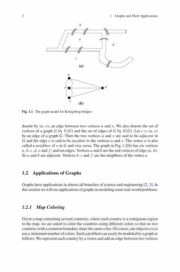
A graph consists of a set of vertices and set of edges, each joining two vertices.Usually an object is represented by a vertex and a relationship between two objectsis represented by an edge. Thus a graph may be used to represent any informationthat can bemodeled as objects and relationships between those objects. Graph theorydeals with study of graphs. The foundation stone of graph theory was laid by Euler in1736 by solving a puzzle called Königsberg seven-bridge problem [1]. Königsbergis an old city in Eastern Prussia lies on the Pregel River. The Pregel River surroundsan island called Kneiphof and separates into two branches as shown in Fig. 1.1(a)where four land areas are created: the island a, two river banks b and c, and the landd between two branches. Seven bridges connect the four land areas of the city. It issaid that the people of Königsberg used to entertain themselves by trying to devisea walk around the city which would cross each of the seven bridges just once. Sincetheir attempts had always failed, many of them believed that the task was impossible,but there was no proof until 1736. In that year, one of the leading mathematiciansof that time, Leonhard Euler published a solution to the problem that no such walkis possible. He not only dealt with this particular problem, but also gave a generalmethod for other problems of the same type. Euler constructed amathematical modelfor the problem in which each of the four lands a, b, c and d is represented by a pointand each of the seven bridges is represented by a curve or a line segment as illustratedin Fig. 1.2(b). The problem can now be stated as follows: Beginning at one of thepoints a, b, c and d , is it possible to trace the figure without traversing the same edgetwice? The mathematical model constructed for the problem is known as a graphmodel of the problem. The points a, b, c and d are called vertices, the line segmentsare called edges, and the whole diagram is called a graph.
Before presenting some applications of graphs, we need to know someterminologies. A graph G is a tuple (V, E) which consists of a finite set V ofvertices and a finite set E of edges; each edge is an unordered pair of vertices. Thetwo vertices associated with an edge e are called the end-vertices of e. We often
© Springer International Publishing AG 2017M.S. Rahman, Basic Graph Theory, Undergraduate Topics in Computer Science,DOI 10.1007/978-3-319-49475-3_1
1
2 1 Graphs and Their Applications
(b)
c
b
da
a d
(a)
b
c
Fig. 1.1 The graph model for Königsberg bridges
denote by (u, v), an edge between two vertices u and v. We also denote the set ofvertices of a graph G by V (G) and the set of edges of G by E(G). Let e = (u, v)be an edge of a graph G. Then the two vertices u and v are said to be adjacent inG and the edge e is said to be incident to the vertices u and v. The vertex u is alsocalled a neighbor of v in G and vice versa. The graph in Fig. 1.2(b) has six verticesa, b, c, d, e and f , and ten edges. Vertices a and b are the end vertices of edge (a, b).So a and b are adjacent. Vertices b, c and f are the neighbors of the vertex a.
1.2 Applications of Graphs
Graphs have applications in almost all branches of science and engineering [2, 3]. Inthis sectionwewill see applications of graphs inmodeling some real-world problems.
1.2.1 Map Coloring
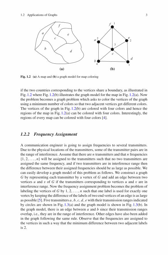
Given a map containing several countries, where each country is a contiguous regionin the map, we are asked to color the countries using different colors so that no twocountrieswith a commonboundary share the same color.Of course, our objective is touse a minimumnumber of colors. Such a problemcan easily bemodeled by a graph asfollows.We represent each country by a vertex and add an edge between two vertices
1.2 Applications of Graphs 3
(a) (b)
a
f
e
bd
a
f
e
db
c
c
1
2
4
2
3
1
Fig. 1.2 (a) A map and (b) a graph model for map coloring
if the two countries corresponding to the vertices share a boundary, as illustrated inFig. 1.2 where Fig. 1.2(b) illustrates the graph model for the map in Fig. 1.2(a). Nowthe problem becomes a graph problem which asks to color the vertices of the graphusing a minimum number of colors so that two adjacent vertices get different colors.The vertices of the graph in Fig. 1.2(b) are colored with four colors and hence theregions of the map in Fig. 1.2(a) can be colored with four colors. Interestingly, theregions of every map can be colored with four colors [4].
1.2.2 Frequency Assignment
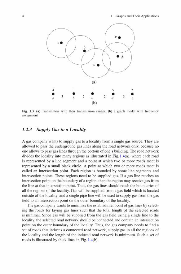
A communication engineer is going to assign frequencies to several transmitters.Due to the physical locations of the transmitters, some of the transmitter pairs are inthe range of interference. Assume that there are n transmitters and that n frequencies{1, 2, . . . , n} will be assigned to the transmitters such that no two transmitters areassigned the same frequency, and if two transmitters are in interference range thenthe difference between their assigned frequencies should be as large as possible. Wecan easily develop a graph model of this problem as follows. We construct a graphG by representing each transmitter by a vertex of G and add an edge between twovertices u and v of G if the transmitters corresponding to vertices u and v are ininterference range. Now the frequency assignment problem becomes the problem oflabeling the vertices of G by 1, 2, . . . , n such that one label is used for exactly onevertex by keeping the difference of the labels of two end vertices of an edge is as largeas possible [5]. Five transmitters a, b, c, d, ewith their transmission ranges indicatedby circles are shown in Fig. 1.3(a) and the graph model is shown in Fig. 1.3(b). Inthe graph model, there is an edge between a and b since their transmission rangesoverlap, i.e., they are in the range of interference. Other edges have also been addedin the graph following the same rule. Observe that the frequencies are assigned tothe vertices in such a way that the minimum difference between two adjacent labelsis 2.
4 1 Graphs and Their Applications
4 1 3 5 2
(b)
(a)
23 2 3
ab
c
e
d
a b c d e
Fig. 1.3 (a) Transmitters with their transmission ranges, (b) a graph model with frequencyassignment
1.2.3 Supply Gas to a Locality
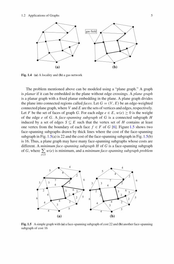
A gas company wants to supply gas to a locality from a single gas source. They areallowed to pass the underground gas lines along the road network only, because noone allows to pass gas lines through the bottom of one’s building. The road networkdivides the locality into many regions as illustrated in Fig. 1.4(a), where each roadis represented by a line segment and a point at which two or more roads meet isrepresented by a small black circle. A point at which two or more roads meet iscalled an intersection point. Each region is bounded by some line segments andintersection points. These regions need to be supplied gas. If a gas line reaches anintersection point on the boundary of a region, then the region may receive gas fromthe line at that intersection point. Thus, the gas lines should reach the boundaries ofall the regions of the locality. Gas will be supplied from a gas field which is locatedoutside of the locality, and a single pipe line will be used to supply gas from the gasfield to an intersection point on the outer boundary of the locality.
The gas company wants to minimize the establishment cost of gas lines by select-ing the roads for laying gas lines such that the total length of the selected roadsis minimal. Since gas will be supplied from the gas field using a single line to thelocality, the selected road network should be connected and contain an intersectionpoint on the outer boundary of the locality. Thus, the gas company needs to find aset of roads that induces a connected road network, supply gas in all the regions ofthe locality and the length of the induced road network is minimum. Such a set ofroads is illustrated by thick lines in Fig. 1.4(b).
1.2 Applications of Graphs 5
(a) (b)
gas field
Fig. 1.4 (a) A locality and (b) a gas network
The problem mentioned above can be modeled using a “plane graph.” A graphis planar if it can be embedded in the plane without edge crossings. A plane graphis a planar graph with a fixed planar embedding in the plane. A plane graph dividesthe plane into connected regions called faces. Let G = (V, E) be an edge-weightedconnected plane graph,where V and E are the sets of vertices and edges, respectively.Let F be the set of faces of graph G. For each edge e ∈ E , w(e) ≥ 0 is the weightof the edge e of G. A face-spanning subgraph of G is a connected subgraph Hinduced by a set of edges S ⊆ E such that the vertex set of H contains at leastone vertex from the boundary of each face f ∈ F of G [6]. Figure1.5 shows twoface-spanning subgraphs drawn by thick lines where the cost of the face-spanningsubgraph in Fig. 1.5(a) is 22 and the cost of the face-spanning subgraph in Fig. 1.5(b)is 16. Thus, a plane graph may have many face-spanning subgraphs whose costs aredifferent. A minimum face-spanning subgraph H of G is a face-spanning subgraphof G, where
∑
e∈Sw(e) is minimum, and a minimum face-spanning subgraph problem
2
3 3
4
4
35
5
6
6
2
24
5
6
3
4
4
2
3 3
4
4
35
5
6
6
2
24
5
6
3
4
4
4
3
(a) (b)
2
22
32
22
3
7 7
4 4
Fig. 1.5 Asimple graphwith (a) a face-spanning subgraph of cost 22 and (b) another face-spanningsubgraph of cost 16
6 1 Graphs and Their Applications
asks to find a minimum face-spanning subgraph of a plane graph. If we representeach road of the road network by an edge of G, each intersection point by a vertexof G, each region by a face of G, and assign the length of a road to the weightof the corresponding edge, then the problem of finding a minimum face-spanningsubgraph of G is the same as the problem of the gas company mentioned above[6]. A minimum face-spanning subgraph problem often arises in applications likeestablishing power transmission lines in a city, power wires layout in a complexcircuit, planning irrigation canal networks for irrigation systems, etc.
1.2.4 Floorplanning
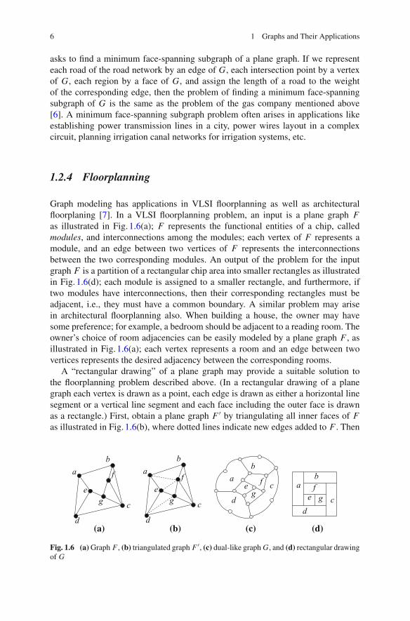
Graph modeling has applications in VLSI floorplanning as well as architecturalfloorplaning [7]. In a VLSI floorplanning problem, an input is a plane graph Fas illustrated in Fig. 1.6(a); F represents the functional entities of a chip, calledmodules, and interconnections among the modules; each vertex of F represents amodule, and an edge between two vertices of F represents the interconnectionsbetween the two corresponding modules. An output of the problem for the inputgraph F is a partition of a rectangular chip area into smaller rectangles as illustratedin Fig. 1.6(d); each module is assigned to a smaller rectangle, and furthermore, iftwo modules have interconnections, then their corresponding rectangles must beadjacent, i.e., they must have a common boundary. A similar problem may arisein architectural floorplanning also. When building a house, the owner may havesome preference; for example, a bedroom should be adjacent to a reading room. Theowner’s choice of room adjacencies can be easily modeled by a plane graph F , asillustrated in Fig. 1.6(a); each vertex represents a room and an edge between twovertices represents the desired adjacency between the corresponding rooms.
A “rectangular drawing” of a plane graph may provide a suitable solution tothe floorplanning problem described above. (In a rectangular drawing of a planegraph each vertex is drawn as a point, each edge is drawn as either a horizontal linesegment or a vertical line segment and each face including the outer face is drawnas a rectangle.) First, obtain a plane graph F ′ by triangulating all inner faces of Fas illustrated in Fig. 1.6(b), where dotted lines indicate new edges added to F . Then
b
c
d
eg
f ab
cfg
d
ab
c
d
eg
fa
b
cd
g
a
eef
(a) (b) (c) (d)
Fig. 1.6 (a)Graph F , (b) triangulated graph F ′, (c) dual-like graphG, and (d) rectangular drawingof G
1.2 Applications of Graphs 7
Fig. 1.7 Communities of common interests
obtain a “dual-like” graphG of F ′ as illustrated in Fig. 1.6(c), where the four verticesof degree 2 drawn by white circles correspond to the four corners of the rectangulararea. Finally, by finding a rectangular drawing of the plane graphG, obtain a possiblefloorplan for F as illustrated in Fig. 1.6(d).
1.2.5 Web Communities
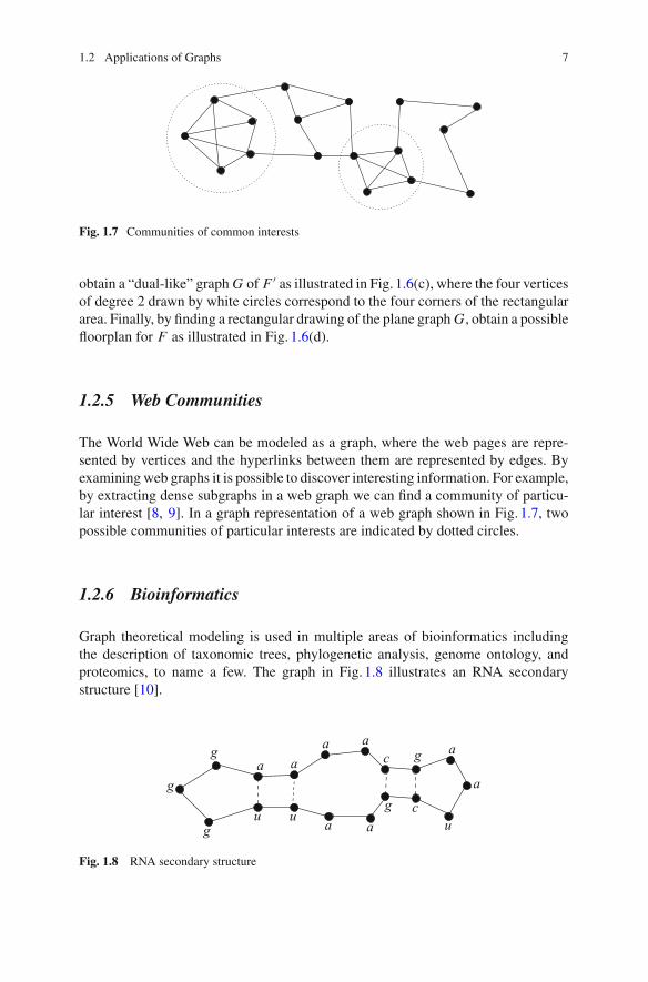
The World Wide Web can be modeled as a graph, where the web pages are repre-sented by vertices and the hyperlinks between them are represented by edges. Byexaminingweb graphs it is possible to discover interesting information. For example,by extracting dense subgraphs in a web graph we can find a community of particu-lar interest [8, 9]. In a graph representation of a web graph shown in Fig. 1.7, twopossible communities of particular interests are indicated by dotted circles.
1.2.6 Bioinformatics
Graph theoretical modeling is used in multiple areas of bioinformatics includingthe description of taxonomic trees, phylogenetic analysis, genome ontology, andproteomics, to name a few. The graph in Fig. 1.8 illustrates an RNA secondarystructure [10].
g
g
ga a
u ug
c
c
ga a
a a
a
u
a
Fig. 1.8 RNA secondary structure
8 1 Graphs and Their Applications
1.2.7 Software Engineering
There are enormous applications of graphs in various areas software engineering suchas project planning, dataflowanalysis, software testing, etc.Acontrol flowgraphusedin software testing describes how the control flows through the program. A controlflow graph is a directed graph where each vertex corresponds to a unique programstatement and each directed edge represents a control transfer from one statement tothe other. By analyzing a control flow graph one can understand the complexity ofthe program and can design a suitable test suite for software testing [11].
Exercises
1. Study your campus map and model the road network inside your campus by agraph.
2. Construct a graph to represent the adjacency relationship of rooms in a floor ofyour university building.
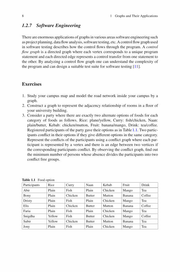
3. Consider a party where there are exactly two alternate options of foods for eachcategory of foods as follows. Rice: plane/yellow, Curry: fish/chicken, Naan:plain/butter, Kebab: chicken/mutton, Fruit: banana/mango, Drink: tea/coffee.Registered participants of the party gave their options as in Table1.1. Two partic-ipants conflict in their options if they give different options in the same category.Represent the conflicts of the participants using a conflict graph where each par-ticipant is represented by a vertex and there is an edge between two vertices ifthe corresponding participants conflict. By observing the conflict graph, find outthe minimum number of persons whose absence divides the participants into twoconflict free groups.
Table 1.1 Food option
Participants Rice Curry Naan Kebab Fruit Drink
Abir Plain Fish Plain Chicken Mango Tea
Bony Plain Chicken Butter Mutton Banana Coffee
Dristy Plain Fish Plain Chicken Mango Tea
Elis Plain Chicken Butter Mutton Banana Coffee
Faria Plain Fish Plain Chicken Mango Tea
Snigdha Yellow Fish Butter Chicken Mango Coffee
Subir Yellow Chicken Butter Mutton Banana Tea
Jony Plain Fish Plain Chicken Mango Tea
Exercise 9
4. There are five jobs {J1, J2, J3, J4, J5} in a company for which there are fiveworkers A, B,C, D and E to do those jobs. However, everybody does nothave expertise to do every job. Their expertise is as follows: A = {J1, J2, J3},B = {J2, J4},C = {J1, J3, J5}, D = {J3, J5}, E = {J1, J5}. Develop a graphmodel to represent the job expertise of the persons and find an assignment ofjobs to the workers such that every worker can do a job.
5. An industry has 600 square meter rectangular area on a floor of a building whereit needs to establish four processing units A, B,C , and D. Processing units A andD require 100 square meter area each whereas B and C require 200 square metereach. Furthermore, the following adjacency requirements must be satisfied: B,C ,and D should be adjacent to A; A and D should be adjacent to B; A and D shouldbe adjacent to C ; and A, B, and C should be adjacent to D. Can you construct afloor layout where the space for each processing unit will be a rectangle? Proposea suitable layout in your justification.
References
1. Biggs, N.L., Lloyd, E.K., Wilson, R.J.: Graph Theory: 1736–1936. Oxford University Press,Oxford (1976)
2. Bondy, J.A., Murty, U.S.R.: Graph Theory with Applications. Elsevier Science Ltd/North-Holland, New York (1976)
3. Gross, J.L., Yellen, J.: Graph Theory and Its Applications, 2nd edn. Chapman andHall, London(2005)
4. Appel, K., Haken, W.: Every map is four colourable. Bull. Am. Math. Soc. 82, 711–712 (1976)5. Calamoneri, T., Massini, A., Török, L., Vrt’o, I.: Antibandwidth of complete k-ary trees.
Discret. Math. 309(22), 6408–6414 (2009)6. Patwary, M.M.A., Rahman, M.S.: Minimum face-spanning subgraphs of plane graphs. AKCE
J. Graphs. Combin. 7(2), 133–150 (2010)7. Nishizeki, T., Rahman, M.S.: Planar Graph Drawing. World Scientific, Singapore (2004)8. Porter, M.A., Onnela, J.-P., Mucha, P.J.: Communities in networks. Not. Amer. Math. Soc. 56,
1082–1097, 1164–1166 (2009)9. Chen, J., Saad, Y.: Dense subgraph extraction with application to community detection, in
IEEE Trans. Knowl. Data Eng. 24(7), 1216–1230 (2012). doi:10.1109/TKDE.2010.27110. Sung, W.: Algorithms in Bioinformatics. CRC Press, London (2010)11. Mall, R.: Fundamentals of Software Engineering, 4th edn. Prentice-Hall of India Pvt. Ltd.
(2014)
Chapter 2Basic Graph Terminologies
In this chapter, we learn some definitions of basic graph theoretic terminologies andknow some preliminary results of graph theory.
2.1 Graphs and Multigraphs
A graph G is a tuple consisting of a finite set V of vertices and a finite set E of edgeswhere each edge is an unordered pair of vertices. The two vertices associated with anedge e are called the end-vertices of e. We often denote by (u, v), an edge betweentwo vertices u and v. We also denote the set of vertices of a graph G by V (G) andthe set of edges of G by E(G). A vertex of a graph is also called as a node of a graph.
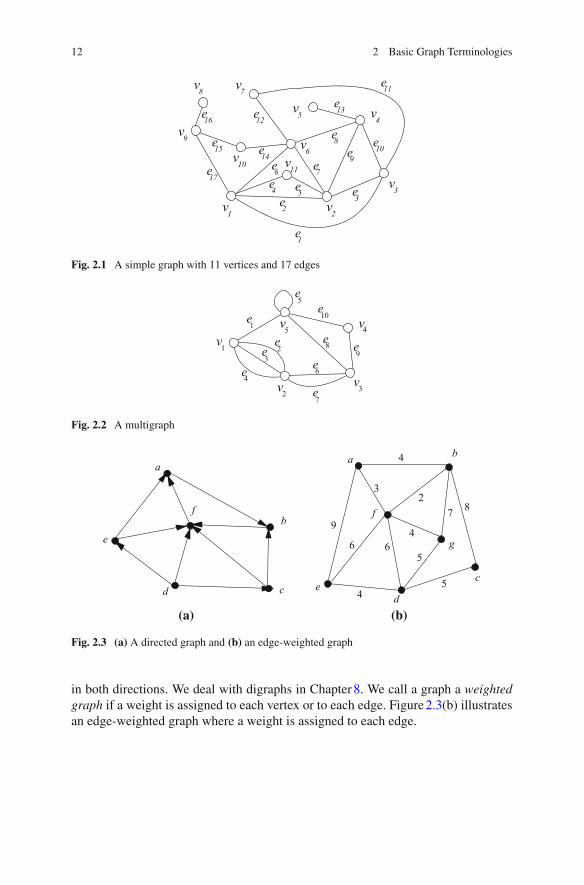
We generally draw a graph G by representing each vertex of G by a point or asmall circle and each edge of G by a line segment or a curve between its two end-vertices. For example, Fig. 2.1 represents a graphG where V (G) = {v1, v2, . . . , v11}and E(G) = {e1, e2, . . . , e17}. We often denote the number of vertices of a graphG by n and the number of edges of G by m; that is, n = |V (G)| and m = |E(G)|.We will use these two notations n and m to denote the number of vertices and thenumber of edges of a graph unless any confusion arises. Thus n = 11 and m = 17for the graph in Fig. 2.1.
A loop is an edge whose end-vertices are the same.Multiple edges are edges withthe same pair of end-vertices. If a graph G does not have any loop or multiple edge,then G is called a simple graph; otherwise, it is called a multigraph. The graph inFig. 2.1 is a simple graph since it has no loop or multiple edge. On the other hand,the graph in Fig. 2.2 contains a loop e5 and two sets of multiple edges {e2, e3, e4} and{e6, e7}. Hence the graph is a multigraph. In the remainder of the book, when we saya graph, we shall mean a simple graph unless there is any possibility of confusion.
We call a graph a directed graph or digraph if each edge is associated with adirection, as illustrated in Fig. 2.3(a). One can consider a directed edge as a one-waystreet. We thus can think an undirected graph as a graph where each edge is directed
© Springer International Publishing AG 2017M.S. Rahman, Basic Graph Theory, Undergraduate Topics in Computer Science,DOI 10.1007/978-3-319-49475-3_2
11
12 2 Basic Graph Terminologies
1v 2v3v
4v5v7v8v
9v
10v6v
e1
e2e3
e10e9
e8
e13
e11
e12e16
e15 e14e17
e711ve4 e5
e6
Fig. 2.1 A simple graph with 11 vertices and 17 edges
1v
e1
e5
e10
4v
e9
v3e7
2ve4
e3
e2
5ve8
e6
Fig. 2.2 A multigraph
b
c
e
f
(a) (b)
5
3
b
cd
4
g6
f
e
27
d
aa
4
9
8
4
56
Fig. 2.3 (a) A directed graph and (b) an edge-weighted graph
in both directions. We deal with digraphs in Chapter8. We call a graph a weightedgraph if a weight is assigned to each vertex or to each edge. Figure2.3(b) illustratesan edge-weighted graph where a weight is assigned to each edge.
2.2 Adjacency, Incidence, and Degree 13
2.2 Adjacency, Incidence, and Degree
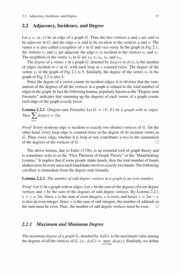
Let e = (u, v) be an edge of a graph G. Then the two vertices u and v are said tobe adjacent in G, and the edge e is said to be incident to the vertices u and v. Thevertex u is also called a neighbor of v in G and vice versa. In the graph in Fig. 2.1,the vertices v1 and v3 are adjacent; the edge e1 is incident to the vertices v1 and v3.The neighbors of the vertex v1 in G are v2, v3 v6, v9, and v11.
The degree of a vertex v in a graph G, denoted by deg(v) or d(v), is the numberof edges incident to v in G, with each loop at v counted twice. The degree of thevertex v1 in the graph of Fig. 2.1 is 5. Similarly, the degree of the vertex v5 in thegraph of Fig. 2.2 is also 5.
Since the degree of a vertex counts its incident edges, it is obvious that the sum-mation of the degrees of all the vertices in a graph is related to the total number ofedges in the graph. In fact the following lemma, popularly known as the “Degree-sumFormula,” indicates that summing up the degrees of each vertex of a graph countseach edge of the graph exactly twice.
Lemma 2.2.1 (Degree-sum Formula) Let G = (V, E) be a graph with m edges.Then
∑
v∈Vdeg(v) = 2m.
Proof Every nonloop edge is incident to exactly two distinct vertices of G. On theother hand, every loop edge is counted twice in the degree of its incident vertex inG. Thus, every edge, whether it is loop or not, contributes a two to the summationof the degrees of the vertices of G. �
The above lemma, due to Euler (1736), is an essential tool of graph theory andis sometimes refer to as the “First Theorem of Graph Theory” or the “HandshakingLemma.” It implies that if some people shake hands, then the total number of handsshakenmust be even since each handshake involves exactly two hands. The followingcorollary is immediate from the degree-sum formula.
Lemma 2.2.2 The number of odd degree vertices in a graph is an even number.
Proof LetG be a graph withm edges. Let x be the sum of the degrees of even degreevertices and y be the sum of the degrees of odd degree vertices. By Lemma 2.2.1x + y = 2m. Since x is the sum of even integers, x is even, and hence y = 2m − xis also an even integer. Since y is the sum of odd integers, the number of addends inthe sum must be even. Thus, the number of odd degree vertices must be even. �
2.2.1 Maximum and Minimum Degree
Themaximum degree of a graph G, denoted by �(G), is the maximum value amongthe degrees of all the vertices of G, i.e., �(G) = max
v∈V (G)deg(v). Similarly, we define
14 2 Basic Graph Terminologies
theminimum degree of a graph G and denote it by δ(G), i.e., δ(G) = minv∈V (G)
deg(v).
The maximum and the minimum degree of the graph in Fig. 2.1 are 5 and 1,respectively.
Let G be a graph with n vertices and m edges. Then by the degree-sum formula,the average degree of a vertex in G is 2m
n and hence δ(G) ≤ 2mn ≤ �(G).
2.2.2 Regular Graphs
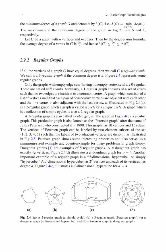
If all the vertices of a graph G have equal degrees, then we call G a regular graph.We call it a k-regular graph if the common degree is k. Figure2.4 represents someregular graphs.
Only the graphs with empty edge sets (having nonempty vertex sets) are 0-regular.These are called null graphs. Similarly, a 1-regular graph consists of a set of edgessuch that no two edges are incident to a common vertex. A graph which consists of alist of vertices such that each pair of consecutive vertices are adjacent with each otherand the first vertex is also adjacent with the last vertex, as illustrated in Fig. 2.4(a),is a 2-regular graph. Such a graph is called a cycle or a simple cycle. A graph whichis a collection of simple cycles is also a 2-regular graph.
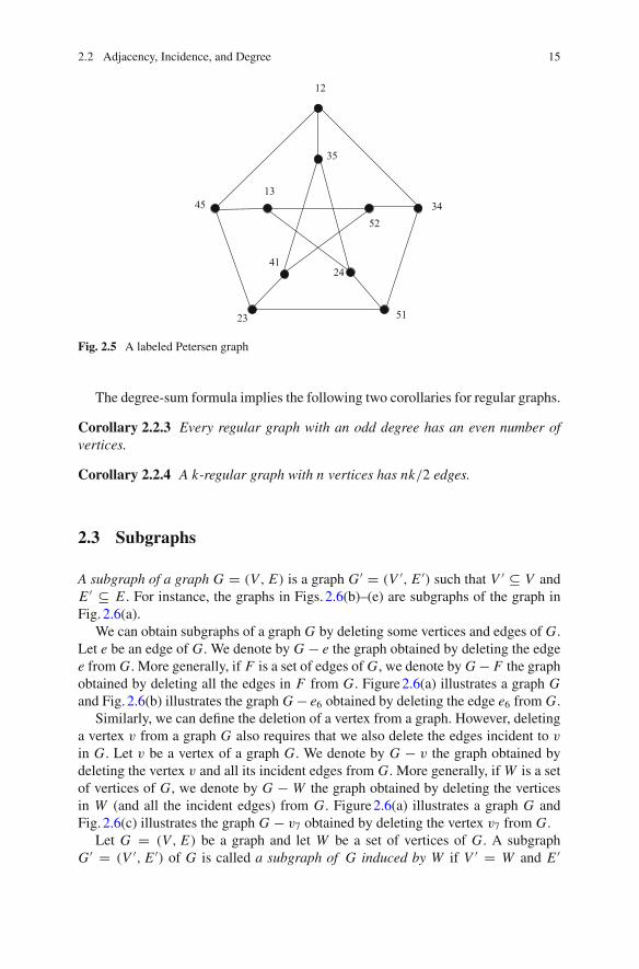
A 3-regular graph is also called a cubic graph. The graph in Fig. 2.4(b) is a cubicgraph. This particular graph is also known as the “Petersen graph” after the name ofJulius Petersen, who constructed it in 1898. This graph has 10 vertices and 15 edges.The vertices of Petersen graph can be labeled by two element subsets of the set{1, 2, 3, 4, 5} such that the labels of two adjacent vertices are disjoint, as illustratedin Fig. 2.5. Petersen graph shows some interesting properties and also serves as aminimum-sized example and counterexample for many problems in graph theory.Doughnut graphs [1] are examples of 5-regular graphs. A p-doughnut graph hasexactly 4p vertices. Figure2.4(d) illustrates a p-doughnut graph for p = 4. Anotherimportant example of a regular graph is a “d-dimensional hypercube” or simply“hypercube.” A d-dimensional hypercube has 2d vertices and each of its vertices hasdegree d. Figure2.4(c) illustrates a d-dimensional hypercube for d = 4.
(d)(a) (c)(b)
Fig. 2.4 (a) A 2-regular graph (a simple cycle), (b) a 3-regular graph (Petersen graph), (c) a4-regular graph (4-dimensional hypercube), and (d) a 5-regular graph (a doughnut graph)
2.2 Adjacency, Incidence, and Degree 15
12
34
5123
45
35
52
2441
13
Fig. 2.5 A labeled Petersen graph
The degree-sum formula implies the following two corollaries for regular graphs.
Corollary 2.2.3 Every regular graph with an odd degree has an even number ofvertices.
Corollary 2.2.4 A k-regular graph with n vertices has nk/2 edges.
2.3 Subgraphs
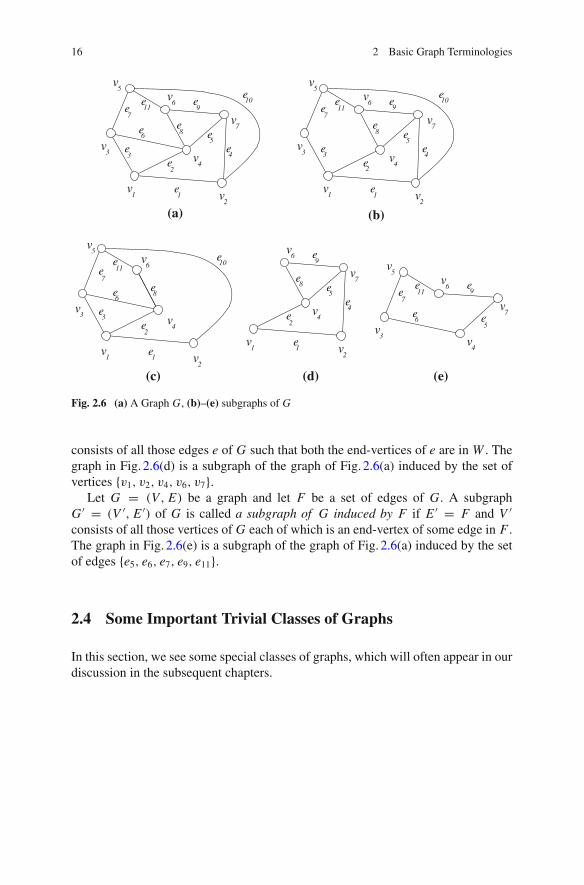
A subgraph of a graph G = (V, E) is a graph G ′ = (V ′, E ′) such that V ′ ⊆ V andE ′ ⊆ E . For instance, the graphs in Figs. 2.6(b)–(e) are subgraphs of the graph inFig. 2.6(a).
We can obtain subgraphs of a graph G by deleting some vertices and edges of G.Let e be an edge of G. We denote by G − e the graph obtained by deleting the edgee from G. More generally, if F is a set of edges of G, we denote by G − F the graphobtained by deleting all the edges in F from G. Figure2.6(a) illustrates a graph Gand Fig. 2.6(b) illustrates the graph G − e6 obtained by deleting the edge e6 from G.
Similarly, we can define the deletion of a vertex from a graph. However, deletinga vertex v from a graph G also requires that we also delete the edges incident to v
in G. Let v be a vertex of a graph G. We denote by G − v the graph obtained bydeleting the vertex v and all its incident edges from G. More generally, if W is a setof vertices of G, we denote by G − W the graph obtained by deleting the verticesin W (and all the incident edges) from G. Figure2.6(a) illustrates a graph G andFig. 2.6(c) illustrates the graph G − v7 obtained by deleting the vertex v7 from G.
Let G = (V, E) be a graph and let W be a set of vertices of G. A subgraphG ′ = (V ′, E ′) of G is called a subgraph of G induced by W if V ′ = W and E ′
16 2 Basic Graph Terminologies
1v
2v
3v
4v
6v
5v
e1
e2
e8e
6
e10
e7
e3
e11
1v
2v
3v
4v
7v
6v
5v
e1
e2
e5
e4
e9
e8e
6
e10
e7
e3
e11
1v
2v
3v
4v
7v
6v
5v
e1
e2
e5
e4
e9
e8
e10
e7
e3
e11
(c)
2v
4v
7v
6v
e1
e2
e5
e4
e9
e8
1v
(d)
e11
3v
4v
6v
5v
e5
e9
e6
e7
7v
(e)
(b)(a)
Fig. 2.6 (a) A Graph G, (b)–(e) subgraphs of G
consists of all those edges e of G such that both the end-vertices of e are in W . Thegraph in Fig. 2.6(d) is a subgraph of the graph of Fig. 2.6(a) induced by the set ofvertices {v1, v2, v4, v6, v7}.
Let G = (V, E) be a graph and let F be a set of edges of G. A subgraphG ′ = (V ′, E ′) of G is called a subgraph of G induced by F if E ′ = F and V ′consists of all those vertices of G each of which is an end-vertex of some edge in F .The graph in Fig. 2.6(e) is a subgraph of the graph of Fig. 2.6(a) induced by the setof edges {e5, e6, e7, e9, e11}.
2.4 Some Important Trivial Classes of Graphs
In this section, we see some special classes of graphs, which will often appear in ourdiscussion in the subsequent chapters.
2.4 Some Important Trivial Classes of Graphs 17
(b)(a)
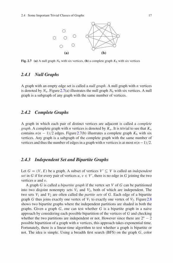
Fig. 2.7 (a) A null graph N6 with six vertices, (b) a complete graph K6 with six vertices
2.4.1 Null Graphs
A graph with an empty edge set is called a null graph. A null graph with n verticesis denoted by Nn . Figure2.7(a) illustrates the null graph N6 with six vertices. A nullgraph is a subgraph of any graph with the same number of vertices.
2.4.2 Complete Graphs
A graph in which each pair of distinct vertices are adjacent is called a completegraph. A complete graph with n vertices is denoted by Kn . It is trivial to see that Kn
contains n(n − 1)/2 edges. Figure2.7(b) illustrates a complete graph K6 with sixvertices. Any graph is a subgraph of the complete graph with the same number ofvertices and thus the number of edges in a graph with n vertices is at most n(n−1)/2.
2.4.3 Independent Set and Bipartite Graphs
Let G = (V, E) be a graph. A subset of vertices V ′ ⊆ V is called an independentset in G if for every pair of vertices u, v ∈ V ′, there is no edge in G joining the twovertices u and v.
A graph G is called a bipartite graph if the vertex set V of G can be partitionedinto two disjoint nonempty sets V1 and V2, both of which are independent. Thetwo sets V1 and V2 are often called the partite sets of G. Each edge of a bipartitegraph G thus joins exactly one vertex of V1 to exactly one vertex of V2. Figure2.8shows two bipartite graphs where the independent partitions are shaded in both thegraphs. Given a graph G, one can test whether G is a bipartite graph in a naiveapproach by considering each possible bipartition of the vertices of G and checkingwhether the two partitions are independent or not. However since there are 2n − 2possible bipartition of a graph with n vertices, this approach takes exponential time.Fortunately, there is a linear-time algorithm to test whether a graph is bipartite ornot. The idea is simple. Using a breadth first search (BFS) on the graph G, color
18 2 Basic Graph Terminologies
(a) (b)
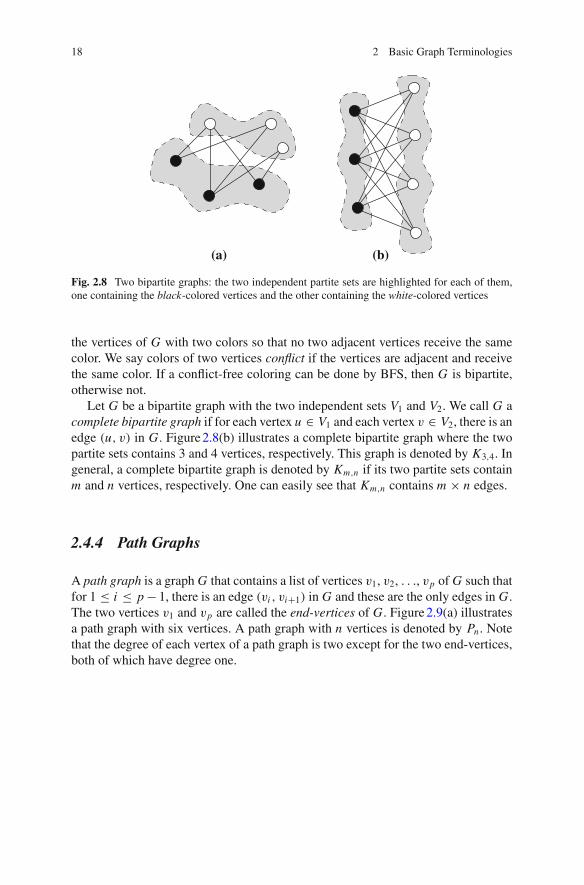
Fig. 2.8 Two bipartite graphs: the two independent partite sets are highlighted for each of them,one containing the black-colored vertices and the other containing the white-colored vertices
the vertices of G with two colors so that no two adjacent vertices receive the samecolor. We say colors of two vertices conflict if the vertices are adjacent and receivethe same color. If a conflict-free coloring can be done by BFS, then G is bipartite,otherwise not.
Let G be a bipartite graph with the two independent sets V1 and V2. We call G acomplete bipartite graph if for each vertex u ∈ V1 and each vertex v ∈ V2, there is anedge (u, v) in G. Figure2.8(b) illustrates a complete bipartite graph where the twopartite sets contains 3 and 4 vertices, respectively. This graph is denoted by K3,4. Ingeneral, a complete bipartite graph is denoted by Km,n if its two partite sets containm and n vertices, respectively. One can easily see that Km,n contains m × n edges.
2.4.4 Path Graphs
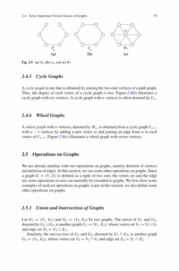
A path graph is a graph G that contains a list of vertices v1, v2, . . ., vp of G such thatfor 1 ≤ i ≤ p− 1, there is an edge (vi , vi+1) in G and these are the only edges in G.The two vertices v1 and vp are called the end-vertices of G. Figure2.9(a) illustratesa path graph with six vertices. A path graph with n vertices is denoted by Pn . Notethat the degree of each vertex of a path graph is two except for the two end-vertices,both of which have degree one.
2.4 Some Important Trivial Classes of Graphs 19
P6 C6(c)
W7
(a) (b)
w
Fig. 2.9 (a) P6, (b) C6, and (c) W7
2.4.5 Cycle Graphs
A cycle graph is one that is obtained by joining the two end-vertices of a path graph.Thus, the degree of each vertex of a cycle graph is two. Figure2.9(b) illustrates acycle graph with six vertices. A cycle graph with n vertices is often denoted by Cn .
2.4.6 Wheel Graphs
A wheel graph with n vertices, denoted by Wn , is obtained from a cycle graph Cn−1
with n − 1 vertices by adding a new vertex w and joining an edge from w to eachvertex of Cn−1. Figure 2.9(c) illustrates a wheel graph with seven vertices.
2.5 Operations on Graphs
We are already familiar with two operations on graphs, namely deletion of verticesand deletion of edges. In this section, we see some other operations on graphs. Sincea graph G = (V, E) is defined as a tuple of two sets; the vertex set and the edgeset, some operations on sets can naturally be extended to graphs. We first show someexamples of such set operations on graphs. Later in this section, we also define someother operations on graphs.
2.5.1 Union and Intersection of Graphs
Let G1 = (V1, E1) and G2 = (V2, E2) be two graphs. The union of G1 and G2,denoted by G1 ∪G2, is another graph G3 = (V3, E3), whose vertex set V3 = V1 ∪V2
and edge set E3 = E1 ∪ E2.Similarly, the intersection of G1 and G2, denoted by G1 ∩ G2, is another graph
G4 = (V4, E4), whose vertex set V4 = V1 ∩ V2 and edge set E4 = E1 ∩ E2.
20 2 Basic Graph Terminologies
a
b
c
d
f
e
d
e
f
g
h a
b
c
d
e
f
g
h
c
d
e
f
c
(a) (b) (c) (d)
Fig. 2.10 (a) G1, (b) G2, (c) G1 ∪ G2, and (d) G1 ∩ G2
K3,4
K4
(b)(a)
Fig. 2.11 (a) The graph representing handshakes, (b) K4 and K3,4
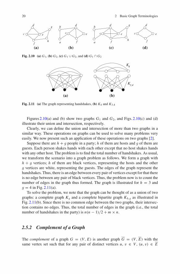
Figures2.10(a) and (b) show two graphs G1 and G2, and Figs. 2.10(c) and (d)illustrate their union and intersection, respectively.
Clearly, we can define the union and intersection of more than two graphs in asimilar way. These operations on graphs can be used to solve many problems veryeasily. We now present such an application of these operations on two graphs [2].
Suppose there are h + g people in a party; h of them are hosts and g of them areguests. Each person shakes hands with each other except that no host shakes handswith any other host. The problem is to find the total number of handshakes. As usual,we transform the scenario into a graph problem as follows. We form a graph withh + g vertices; h of them are black vertices, representing the hosts and the otherg vertices are white, representing the guests. The edges of the graph represent thehandshakes. Thus, there is an edge between every pair of vertices except for that thereis no edge between any pair of black vertices. Thus, the problem now is to count thenumber of edges in the graph thus formed. The graph is illustrated for h = 3 andg = 4 in Fig. 2.11(a).
To solve the problem, we note that the graph can be thought of as a union of twographs: a complete graph Kg and a complete bipartite graph Kh,g as illustrated inFig. 2.11(b). Since there is no common edge between the two graphs, their intersec-tion contains no edges. Thus, the total number of edges in the graph (i.e., the totalnumber of handshakes in the party) is n(n − 1)/2 + m × n.
2.5.2 Complement of a Graph
The complement of a graph G = (V, E) is another graph G = (V, E) with thesame vertex set such that for any pair of distinct vertices u, v ∈ V , (u, v) ∈ E
2.5 Operations on Graphs 21
c
d
a b
ec
d
a b
e
(b)(a)
Fig. 2.12 (a) A graph G, and (b) the complement G of G
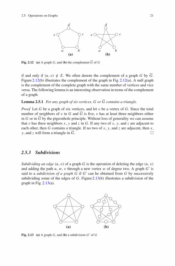
if and only if (u, v) /∈ E . We often denote the complement of a graph G by G.Figure2.12(b) illustrates the complement of the graph in Fig. 2.12(a). A null graphis the complement of the complete graph with the same number of vertices and viceversa. The following lemma is an interesting observation in terms of the complementof a graph.
Lemma 2.5.1 For any graph of six vertices, G or G contains a triangle.
Proof Let G be a graph of six vertices, and let v be a vertex of G. Since the totalnumber of neighbors of v in G and G is five, v has at least three neighbors eitherin G or in G by the pigeonhole principle. Without loss of generality we can assumethat v has three neighbors x , y and z in G. If any two of x , y, and z are adjacent toeach other, then G contains a triangle. If no two of x , y, and z are adjacent, then x ,y, and z will form a triangle in G. �
2.5.3 Subdivisions
Subdividing an edge (u, v) of a graph G is the operation of deleting the edge (u, v)
and adding the path u, w, v through a new vertex w of degree two. A graph G ′ issaid to a subdivision of a graph G if G ′ can be obtained from G by successivelysubdividing some of the edges of G. Figure2.13(b) illustrates a subdivision of thegraph in Fig. 2.13(a).
(a) (b)
Fig. 2.13 (a) A graph G, and (b) a subdivision G ′ of G
22 2 Basic Graph Terminologies
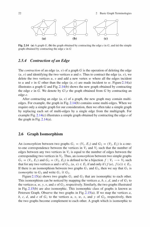
(b) (c)(a)
e
Fig. 2.14 (a) A graph G, (b) the graph obtained by contracting the edge e in G, and (c) the simplegraph obtained by contracting the edge e in G
2.5.4 Contraction of an Edge
The contraction of an edge (u, v) of a graph G is the operation of deleting the edge(u, v) and identifying the two vertices u and v. Thus to contract the edge (u, v), wedelete the two vertices u, v and add a new vertex w where all the edges incidentto u and v in G other than the edge (u, v) are made incident to w. Figure2.14(a)illustrates a graph G and Fig. 2.14(b) shows the new graph obtained by contractingthe edge e in G. We denote by G\e the graph obtained from G by contracting anedge e.
After contracting an edge (u, v) of a graph, the new graph may contain multi-edges. For example, the graph in Fig. 2.14(b) contains some multi-edges. When werequire only a simple graph for our consideration, then we often take a simple graphby replacing each set of multi-edges by a single edge from the multigraph. Forexample Fig. 2.14(c) illustrates a simple graph obtained by contracting the edge e ofthe graph in Fig. 2.14(a).
2.6 Graph Isomorphism
An isomorphism between two graphs G1 = (V1, E1) and G2 = (V2, E2) is a one-to-one correspondence between the vertices in V1 and V2 such that the number ofedges between any two vertices in V1 is equal to the number of edges between thecorresponding two vertices in V2. Thus, an isomorphism between two simple graphsG1 = (V1, E1) and G2 = (V2, E2) is defined to be a bijection f : V1 −→ V2 suchthat for any two vertices u and v ofG1, (u, v) ∈ E1 if and only if ( f (u), f (v)) ∈ E2.If there is an isomorphism between two graphs G1 and G2, then we say that G1 isisomorphic to G2 and write G1
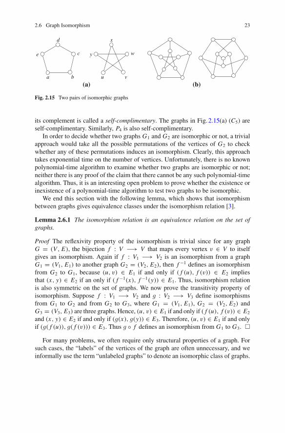
∼= G2.Figure2.15(a) shows two graphs G1 and G2 that are isomorphic to each other.
This isomorphism can be noticed by mapping the vertices a, b, c, d, and e of G1 tothe vertices u,w, y, v, and x of G2, respectively. Similarly, the two graphs illustratedin Fig. 2.15(b) are also isomorphic. This isomorphic class of graphs is known asPetersen Graph. Observe the two graphs in Fig. 2.15(a). If we map the vertices a,b, c, d, and e of G1 to the vertices u, v, w, x , and y of G2, respectively, thenthe two graphs become complement to each other. A graph which is isomorphic to
2.6 Graph Isomorphism 23
w
x
u
y
v
c
d
b
e
a
(a) (b)
Fig. 2.15 Two pairs of isomorphic graphs
its complement is called a self-complimentary. The graphs in Fig. 2.15(a) (C5) areself-complimentary. Similarly, P4 is also self-complimentary.
In order to decide whether two graphs G1 and G2 are isomorphic or not, a trivialapproach would take all the possible permutations of the vertices of G2 to checkwhether any of these permutations induces an isomorphism. Clearly, this approachtakes exponential time on the number of vertices. Unfortunately, there is no knownpolynomial-time algorithm to examine whether two graphs are isomorphic or not;neither there is any proof of the claim that there cannot be any such polynomial-timealgorithm. Thus, it is an interesting open problem to prove whether the existence orinexistence of a polynomial-time algorithm to test two graphs to be isomorphic.
We end this section with the following lemma, which shows that isomorphismbetween graphs gives equivalence classes under the isomorphism relation [3].
Lemma 2.6.1 The isomorphism relation is an equivalence relation on the set ofgraphs.
Proof The reflexivity property of the isomorphism is trivial since for any graphG = (V, E), the bijection f : V −→ V that maps every vertex v ∈ V to itselfgives an isomorphism. Again if f : V1 −→ V2 is an isomorphism from a graphG1 = (V1, E1) to another graph G2 = (V2, E2), then f −1 defines an isomorphismfrom G2 to G1, because (u, v) ∈ E1 if and only if ( f (u), f (v)) ∈ E2 impliesthat (x, y) ∈ E2 if an only if ( f −1(x), f −1(y)) ∈ E1. Thus, isomorphism relationis also symmetric on the set of graphs. We now prove the transitivity property ofisomorphism. Suppose f : V1 −→ V2 and g : V2 −→ V3 define isomorphismsfrom G1 to G2 and from G2 to G3, where G1 = (V1, E1), G2 = (V2, E2) andG3 = (V3, E3) are three graphs. Hence, (u, v) ∈ E1 if and only if ( f (u), f (v)) ∈ E2
and (x, y) ∈ E2 if and only if (g(x), g(y)) ∈ E3. Therefore, (u, v) ∈ E1 if and onlyif (g( f (u)), g( f (v))) ∈ E3. Thus g ◦ f defines an isomorphism from G1 to G3. �
For many problems, we often require only structural properties of a graph. Forsuch cases, the “labels” of the vertices of the graph are often unnecessary, and weinformally use the term “unlabeled graphs” to denote an isomorphic class of graphs.
24 2 Basic Graph Terminologies
2.7 Degree Sequence
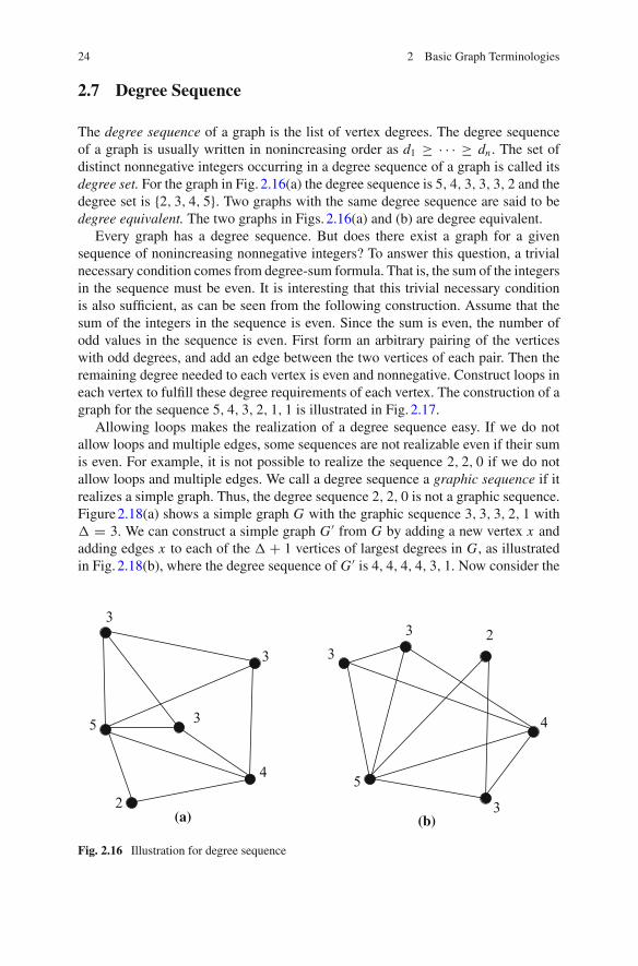
The degree sequence of a graph is the list of vertex degrees. The degree sequenceof a graph is usually written in nonincreasing order as d1 ≥ · · · ≥ dn . The set ofdistinct nonnegative integers occurring in a degree sequence of a graph is called itsdegree set. For the graph in Fig. 2.16(a) the degree sequence is 5, 4, 3, 3, 3, 2 and thedegree set is {2, 3, 4, 5}. Two graphs with the same degree sequence are said to bedegree equivalent. The two graphs in Figs. 2.16(a) and (b) are degree equivalent.
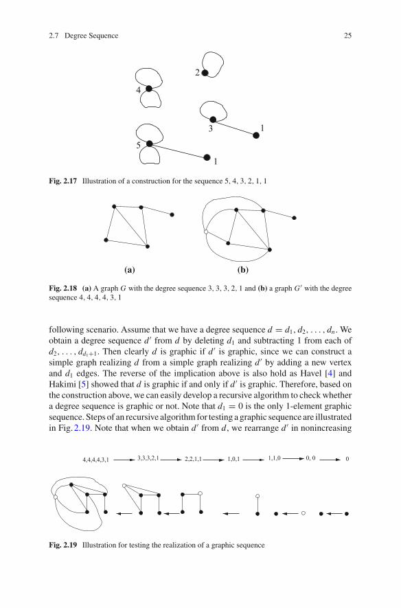
Every graph has a degree sequence. But does there exist a graph for a givensequence of nonincreasing nonnegative integers? To answer this question, a trivialnecessary condition comes from degree-sum formula. That is, the sum of the integersin the sequence must be even. It is interesting that this trivial necessary conditionis also sufficient, as can be seen from the following construction. Assume that thesum of the integers in the sequence is even. Since the sum is even, the number ofodd values in the sequence is even. First form an arbitrary pairing of the verticeswith odd degrees, and add an edge between the two vertices of each pair. Then theremaining degree needed to each vertex is even and nonnegative. Construct loops ineach vertex to fulfill these degree requirements of each vertex. The construction of agraph for the sequence 5, 4, 3, 2, 1, 1 is illustrated in Fig. 2.17.
Allowing loops makes the realization of a degree sequence easy. If we do notallow loops and multiple edges, some sequences are not realizable even if their sumis even. For example, it is not possible to realize the sequence 2, 2, 0 if we do notallow loops and multiple edges. We call a degree sequence a graphic sequence if itrealizes a simple graph. Thus, the degree sequence 2, 2, 0 is not a graphic sequence.Figure2.18(a) shows a simple graph G with the graphic sequence 3, 3, 3, 2, 1 with� = 3. We can construct a simple graph G ′ from G by adding a new vertex x andadding edges x to each of the � + 1 vertices of largest degrees in G, as illustratedin Fig. 2.18(b), where the degree sequence of G ′ is 4, 4, 4, 4, 3, 1. Now consider the
2
4
3
35
2
4
33
3
5
(a) (b)
3
Fig. 2.16 Illustration for degree sequence
2.7 Degree Sequence 25
2
13
4
1
5
Fig. 2.17 Illustration of a construction for the sequence 5, 4, 3, 2, 1, 1
(a) (b)
Fig. 2.18 (a) A graph G with the degree sequence 3, 3, 3, 2, 1 and (b) a graph G ′ with the degreesequence 4, 4, 4, 4, 3, 1
following scenario. Assume that we have a degree sequence d = d1, d2, . . . , dn . Weobtain a degree sequence d ′ from d by deleting d1 and subtracting 1 from each ofd2, . . . , dd1+1. Then clearly d is graphic if d ′ is graphic, since we can construct asimple graph realizing d from a simple graph realizing d ′ by adding a new vertexand d1 edges. The reverse of the implication above is also hold as Havel [4] andHakimi [5] showed that d is graphic if and only if d ′ is graphic. Therefore, based onthe construction above, we can easily develop a recursive algorithm to check whethera degree sequence is graphic or not. Note that d1 = 0 is the only 1-element graphicsequence. Steps of an recursive algorithm for testing a graphic sequence are illustratedin Fig. 2.19. Note that when we obtain d ′ from d , we rearrange d ′ in nonincreasing
3,3,3,2,1 1,0,1 1,1,0 0, 0 02,2,1,14,4,4,4,3,1
Fig. 2.19 Illustration for testing the realization of a graphic sequence
26 2 Basic Graph Terminologies
order if d ′ is not in nonincreasing order. For example, observe 1, 0, 1 → 1, 1, 0 inFig. 2.19.
2.8 Data Structures and Graph Representation
We are already accustomed with one way of representing a graph, i.e., by a diagramwhere each vertex is represented by a point or a small circle and each edge is repre-sented by a straight-line between the end-vertices. This graphical representation isconvenient for the visualization of a graph, yet it is unsuitable if we want to store agraph in a computer. However, there are other ways of representing a graph. In thissection, we first give a very brief account of some basic data structures and then weshow three methods for representing a graph in a computer.
A vector or a set of variables is usually stored as a (one-dimensional) array anda matrix is stored as a two-dimensional array. The main feature of an array is thatthe location of an entry can be uniquely determined by its index in the array and theentry can be accessed in constant time. A list is a data structure which consists ofhomogeneous records, linked together in a linear fashion. Each record contains oneor more items of data and one or more pointers. In a singly linked lists, each recordhas a single forwarding pointer indicating the address of the memory cell of thenext record. In a doubly linked list, each record has forward and backward pointersindicating the address of the memory cells of the next and the previous records,respectively.
We now present three different representations of graphs.
2.8.1 Adjacency Matrix
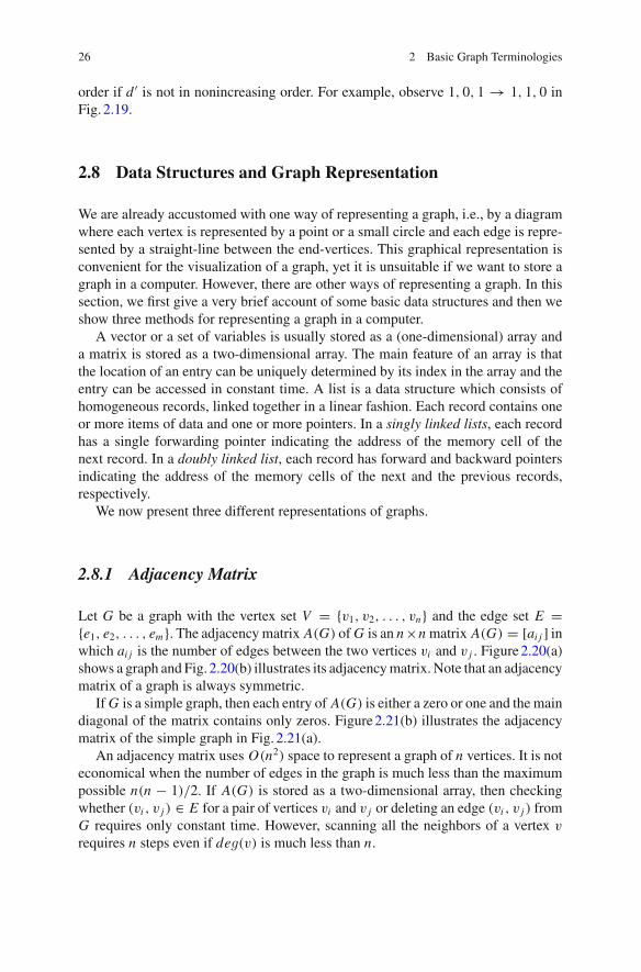
Let G be a graph with the vertex set V = {v1, v2, . . . , vn} and the edge set E ={e1, e2, . . . , em}. The adjacency matrix A(G) ofG is an n×nmatrix A(G) = [ai j ] inwhich ai j is the number of edges between the two vertices vi and v j . Figure2.20(a)shows a graph and Fig. 2.20(b) illustrates its adjacencymatrix. Note that an adjacencymatrix of a graph is always symmetric.
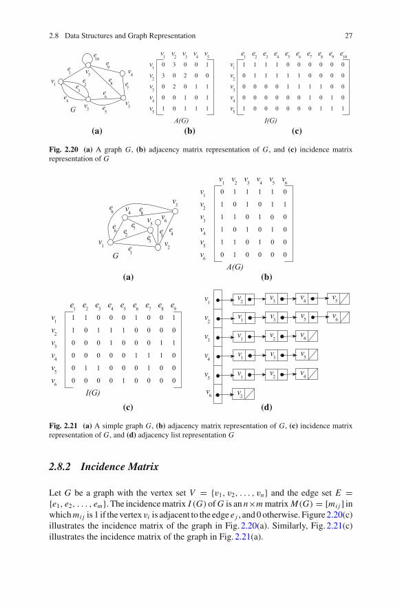
IfG is a simple graph, then each entry of A(G) is either a zero or one and the maindiagonal of the matrix contains only zeros. Figure2.21(b) illustrates the adjacencymatrix of the simple graph in Fig. 2.21(a).
An adjacency matrix uses O(n2) space to represent a graph of n vertices. It is noteconomical when the number of edges in the graph is much less than the maximumpossible n(n − 1)/2. If A(G) is stored as a two-dimensional array, then checkingwhether (vi , v j ) ∈ E for a pair of vertices vi and v j or deleting an edge (vi , v j ) fromG requires only constant time. However, scanning all the neighbors of a vertex v
requires n steps even if deg(v) is much less than n.
2.8 Data Structures and Graph Representation 27
(a) (b) (c)
Fig. 2.20 (a) A graph G, (b) adjacency matrix representation of G, and (c) incidence matrixrepresentation of G
1v 2v
5v 6v
e1
e4
e6
4v
e2e7
e3e5
e8
e9
v3
G
4v 5vv32v1v 6v
2vv34v
5v
1v
6v
0
1
1
1
1
11 1 1
0
1
0
1
1 0 1
0
1
1
0
0
01
1
0 1 0 0 0 0
0
0
0
1
0
A(G)
0
6v
5v
4v
v3
2v
1v v3 v4
v3 v5
v2
v3
v2
v2
v1
v1
v1
v1
v2
v5
v6
v4
v5
v4
2vv34v
5v
1v9ee87e6e4e 5ee32e1e
6v
1
0
1
1 1 1
1 11
1 1 1
11
1 1
1
0
0
0 0
0
0
0
0
0
0
0
0
0
0
0 0
0
0
0 0
0
0
0
0
0
0
0 0
0
0
0
0
0
0
0
1
1
I(G)
(a)
(d)(c)
(b)
Fig. 2.21 (a) A simple graph G, (b) adjacency matrix representation of G, (c) incidence matrixrepresentation of G, and (d) adjacency list representation G
2.8.2 Incidence Matrix
Let G be a graph with the vertex set V = {v1, v2, . . . , vn} and the edge set E ={e1, e2, . . . , em}. The incidencematrix I (G) ofG is an n×mmatrixM(G) = [mi j ] inwhichmi j is 1 if the vertex vi is adjacent to the edge e j , and 0 otherwise. Figure2.20(c)illustrates the incidence matrix of the graph in Fig. 2.20(a). Similarly, Fig. 2.21(c)illustrates the incidence matrix of the graph in Fig. 2.21(a).
28 2 Basic Graph Terminologies
The space requirement for the incidence matrix is n × m. For a graph whichcontains much more number of edges compared to n, this requirement is muchhigher than the adjacency matrix. Scanning all the neighbors of the graph also takesn steps even if deg(v) is much less than n. However, this representation is helpfulfor the query to know whether a vertex is incident to an edge or not and this querycan be responded in constant time from this representation.
If a graph G is a simple graph, then there is another representation of G, calledthe adjacency lists.
2.8.3 Adjacency List
Let G be a graph with the vertex set V = {v1, v2, . . . , vn} and the edge set E ={e1, e2, . . . , em}. The adjacency lists Ad j (G) of G is an array of n lists, where foreach vertex v ofG, there is a list corresponding to v, which contains a record for eachneighbor of v. Figure2.21(d) illustrates the adjacency lists of the graph in Fig. 2.21(a).
The space requirement for the adjacency lists is∑
v∈V(1 + deg(v)) = O(n + m).
Thus, this representation is much more economical than the adjacency matrix andthe incidence matrix, particularly if the number of edge in the graph is much lessthan n(n − 1)/2. Scanning the neighbors of a vertex v takes O(deg(v)) steps onlybut checking whether (vi , v j ) ∈ E requires O(deg(vi )) steps for a pair of verticesvi and v j of G.
Bibliographic Notes
The books [3, 6–9] were used in preparing this chapter.
Exercises
1. Show that every regular graph with an odd degree has an even number of vertices.2. Construct the complement of K3,3, W5, and C5.3. Can you construct a disconnected graph G of two or more vertices such that G is
also disconnected. Give a proof supporting your answer.4. Give two examples of self-complementary graphs.5. What is the necessary and sufficient condition for Km,n to be a regular graph?6. Is there a simple graph of n vertices such that the vertices all have distinct degrees?
Give a proof supporting your answer.7. Draw the graph G = (V, E) with vertex set V = {a, b, c, d, e, f, g, h} and edge
set {(a, b), (a, e), (b, c), (b, d), (c, d), (c, g), (d, e)(e, f ), ( f, g), ( f, h), (g, h)}.Draw G − (d, e). Draw the subgraph of G induced by {c, d, e, f }. Contract theedge (d, e) from G.
8. Show that two graphs are isomorphic if and only if their complements are iso-morphic.
References 29
References
1. Karim, M.R., Rahman, M.S.: On a class of planar graphs with straight-line grid drawings onlinear area. J. Graph Algorithms Appl. 13(2), 153–177 (2009)
2. Koshy, T.: Discrete Mathematics with Applications. Elsevier, Amsterdam (2004)3. West, D.B.: Introduction to Graph Theory, 2nd edn. Prentice Hall, New Jersey (2001)4. Havel, V.: A remark on the existence of finite graphs [Czec] Casopis. Pest. Mat. 80, 477–480
(1955)5. Hakimi, S.L.: On realizability of a set of integers as degrees of vertices of a linear graph. SIAM
J. Appl. Math. 10, 496–506 (1962)6. Nishizeki, T., Rahman, M.S.: Planar graph drawing. World Scientific, Singapore (2004)7. Wilson, R.J.: Introduction to Graph Theory, 4th edn. Longman, London (1996)8. Clark, J., Holton, D.A.: A First Look at Graph Theory. World Scientific, Singapore (1991)9. Pirzada, S.: An Introduction to Graph Theory. University Press, India (2009)
Chapter 3Paths, Cycles, and Connectivity
In this chapter, we study some important fundamental concepts of graph theory. InSection3.1 we start with the definitions of walks, trails, paths, and cycles. The well-known Eulerian graphs and Hamiltonian graphs are studied in Sections3.2 and 3.3,respectively. In Section3.4, we study the concepts of connectivity and connectivity-driven graph decompositions.
3.1 Walks, Trails, Paths, and Cycles
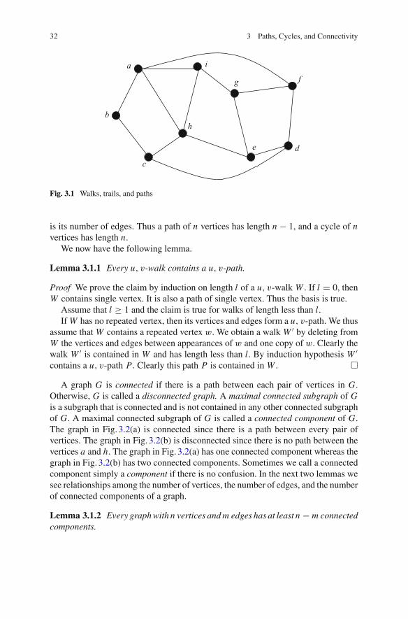
Let G be a graph. A walk in G is a nonempty list W = v0, e1, v1, . . ., v f −1, e f ,v f , whose elements are alternately vertices and edges of G where for 1 ≤ i ≤ f ,the edge ei has end vertices vi−1 and vi . The vertices v0 and v f are called the endvertices of W . If the end vertices of a walk W of a graph G are u and v respec-tively, W is also called an u, v-walk in G. For example in the graph G of Fig. 3.1,W = a, (a, i), i, (i, h), h, (h, c), c, (c, b), b is a walk. W is also an a, b-walk in Gsince the end vertices of W are a and b. Often for convenience, a walk in a simplegraph is represented by the sequence of its vertices only. Since the graphG of Fig. 3.1is simple, the walk W can also be represented by W = a, i, h, c, b.
A trail of a graphG is a walk inG with no repeated edges. That is, in a trail an edgecannot appearmore than once. In Fig. 3.1, thewalkW1 = a, (a, i), i, (i, h), h, (h, c),c, (c, b), b is a trail but thewalkW2 = a, (a, i), i, (i, h), h, (h, c), c, (c, b), b, (b, a),
a, (a, i) is not a trail since the edge (a, i) has appeared inW2 more than once. A trailis called a circuit when the two end vertices of the trail are the same.
A path is a walk with no repeated vertex (except end vertices). When the end ver-tices repeat, then it is called a closed path. In Fig. 3.1, a, (a, i), i, (i, h), h, (h, c), c,(c, b), b, (b, a), a is a closed path. A closed path is called a cycle. A u, v-path is apath whose end vertices are u and v. A vertex on a path P which is not an end vertexof P is called an internal vertex of P . The length of a walk, a trail, a path, or a cycle
© Springer International Publishing AG 2017M.S. Rahman, Basic Graph Theory, Undergraduate Topics in Computer Science,DOI 10.1007/978-3-319-49475-3_3
31
32 3 Paths, Cycles, and Connectivity
a
c
e d
fg
i
hb
Fig. 3.1 Walks, trails, and paths
is its number of edges. Thus a path of n vertices has length n − 1, and a cycle of nvertices has length n.
We now have the following lemma.
Lemma 3.1.1 Every u, v-walk contains a u, v-path.
Proof We prove the claim by induction on length l of a u, v-walk W . If l = 0, thenW contains single vertex. It is also a path of single vertex. Thus the basis is true.
Assume that l ≥ 1 and the claim is true for walks of length less than l.IfW has no repeated vertex, then its vertices and edges form a u, v-path. We thus
assume that W contains a repeated vertex w. We obtain a walk W ′ by deleting fromW the vertices and edges between appearances of w and one copy of w. Clearly thewalk W ′ is contained in W and has length less than l. By induction hypothesis W ′contains a u, v-path P . Clearly this path P is contained in W . �
A graph G is connected if there is a path between each pair of vertices in G.Otherwise, G is called a disconnected graph. A maximal connected subgraph of Gis a subgraph that is connected and is not contained in any other connected subgraphof G. A maximal connected subgraph of G is called a connected component of G.The graph in Fig. 3.2(a) is connected since there is a path between every pair ofvertices. The graph in Fig. 3.2(b) is disconnected since there is no path between thevertices a and h. The graph in Fig. 3.2(a) has one connected component whereas thegraph in Fig. 3.2(b) has two connected components. Sometimes we call a connectedcomponent simply a component if there is no confusion. In the next two lemmas wesee relationships among the number of vertices, the number of edges, and the numberof connected components of a graph.
Lemma 3.1.2 Every graphwith n vertices andm edges has at least n − m connectedcomponents.
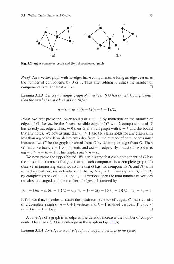
3.1 Walks, Trails, Paths, and Cycles 33
(a) (b)
a
b
c
d
e
f
e
a
bc
d
f
g
h
i
Fig. 3.2 (a) A connected graph and (b) a disconnected graph
Proof An n-vertex graphwith no edges has n components. Adding an edge decreasesthe number of components by 0 or 1. Thus after adding m edges the number ofcomponents is still at least n − m. �
Lemma 3.1.3 Let G be a simple graph of n vertices. If G has exactly k components,then the number m of edges of G satisfies
n − k ≤ m ≤ (n − k)(n − k + 1)/2.
Proof We first prove the lower bound m ≥ n − k by induction on the number ofedges of G. Let m0 be the fewest possible edges of G with k components and Ghas exactly m0 edges. If m0 = 0 then G is a null graph with n = k and the boundtrivially holds. We now assume that m0 ≥ 1 and the claim holds for any graph withless than m0 edges. If we delete any edge from G, the number of components mustincrease. Let G ′ be the graph obtained from G by deleting an edge from G. ThenG ′ has n vertices, k + 1 components and m0 − 1 edges. By induction hypothesism0 − 1 ≥ n − (k + 1). This implies m0 ≥ n − k.
We now prove the upper bound. We can assume that each component of G hasthe maximum number of edges, that is, each component is a complete graph. Toobserve an interesting scenario, assume that G has two components Hi and Hj withni and n j vertices, respectively, such that ni ≥ n j > 1. If we replace Hi and Hj
by complete graphs of ni + 1 and n j − 1 vertices, then the total number of verticesremains unchanged, and the number of edges is increased by
{(ni + 1)ni − ni (ni − 1)}/2 − {n j (n j − 1) − (n j − 1)(n j − 2)}/2 = ni − n j + 1.
It follows that, in order to attain the maximum number of edges, G must consistof a complete graph of n − k + 1 vertices and k − 1 isolated vertices. Thus m ≤(n − k)(n − k + 1)/2. �
A cut-edge of a graph is an edge whose deletion increases the number of compo-nents. The edge (d, f ) is a cut-edge in the graph in Fig. 3.2(b).
Lemma 3.1.4 An edge is a cut-edge if and only if it belongs to no cycle.
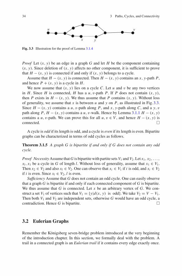
34 3 Paths, Cycles, and Connectivity
u v
x y
Fig. 3.3 Illustration for the proof of Lemma 3.1.4
Proof Let (x, y) be an edge in a graph G and let H be the component containing(x, y). Since deletion of (x, y) affects no other component, it is sufficient to provethat H − (x, y) is connected if and only if (x, y) belongs to a cycle.
Assume that H − (x, y) is connected. Then H − (x, y) contains an x, y-path P ,and hence P + (x, y) is a cycle in H .
We now assume that (x, y) lies on a cycle C . Let u and v be any two verticesin H . Since H is connected, H has a u, v-path P . If P does not contain (x, y),then P exists in H − (x, y). We thus assume that P contains (x, y). Without lossof generality, we assume that x is between u and y on P , as illustrated in Fig. 3.3.Since H − (x, y) contains a u, x-path along P , and x, y-path along C , and a y, vpath along P , H − (x, y) contains a u, v-walk. Hence by Lemma 3.1.1 H − (x, y)contains a u, v-path. We can prove this for all u, v ∈ V , and hence H − (x, y) isconnected. �
A cycle is odd if its length is odd, and a cycle is even if its length is even. Bipartitegraphs can be characterized in terms of odd cycles as follows.
Theorem 3.1.5 A graph G is bipartite if and only if G does not contain any oddcycle.
Proof NecessityAssume thatG is bipartitewith partite setsV1 andV2. Let x1, x2, . . . ,xl , x1 be a cycle in G of length l. Without loss of generality, assume that x1 ∈ V1.Then x2 ∈ V2 and also xl ∈ V2. One can observe that xi ∈ V1 if i is odd, and xi ∈ V2
if i is even. Since xl ∈ V2, l is even.Sufficiency Assume that G does not contain an odd cycle. One can easily observe
that a graph G is bipartite if and only if each connected component of G is bipartite.We thus assume that G is connected. Let x be an arbitrary vertex of G. We con-struct a set V1 of vertices such that V1 = {y|d(x, y) is odd}. We take V2 = V − V1.Then both V1 and V2 are independent sets, otherwise G would have an odd cycle, acontradiction. Hence G is bipartite. �
3.2 Eulerian Graphs
Remember the Königsberg seven-bridge problem introduced at the very beginningof the introduction chapter. In this section, we formally deal with the problem. Atrail in a connected graph is an Eulerian trail if it contains every edge exactly once.
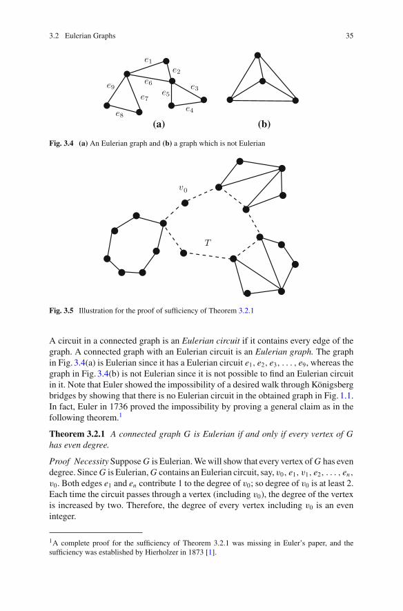
3.2 Eulerian Graphs 35
e1e2
e3
e4
e5
e6
e7
e8
e9
(a) (b)
Fig. 3.4 (a) An Eulerian graph and (b) a graph which is not Eulerian
v0
T
Fig. 3.5 Illustration for the proof of sufficiency of Theorem 3.2.1
A circuit in a connected graph is an Eulerian circuit if it contains every edge of thegraph. A connected graph with an Eulerian circuit is an Eulerian graph. The graphin Fig. 3.4(a) is Eulerian since it has a Eulerian circuit e1, e2, e3, . . . , e9, whereas thegraph in Fig. 3.4(b) is not Eulerian since it is not possible to find an Eulerian circuitin it. Note that Euler showed the impossibility of a desired walk through Königsbergbridges by showing that there is no Eulerian circuit in the obtained graph in Fig. 1.1.In fact, Euler in 1736 proved the impossibility by proving a general claim as in thefollowing theorem.1
Theorem 3.2.1 A connected graph G is Eulerian if and only if every vertex of Ghas even degree.
Proof Necessity SupposeG is Eulerian.Wewill show that every vertex ofG has evendegree. SinceG is Eulerian,G contains anEulerian circuit, say, v0, e1, v1, e2, . . . , en,v0. Both edges e1 and en contribute 1 to the degree of v0; so degree of v0 is at least 2.Each time the circuit passes through a vertex (including v0), the degree of the vertexis increased by two. Therefore, the degree of every vertex including v0 is an eveninteger.
1A complete proof for the sufficiency of Theorem 3.2.1 was missing in Euler’s paper, and thesufficiency was established by Hierholzer in 1873 [1].
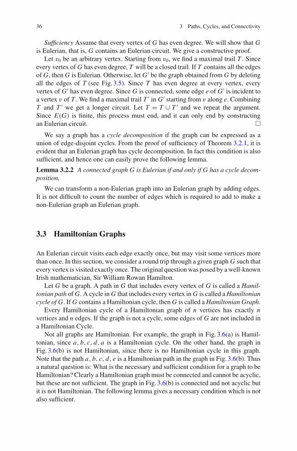
36 3 Paths, Cycles, and Connectivity
Sufficiency Assume that every vertex of G has even degree. We will show that Gis Eulerian, that is, G contains an Eulerian circuit. We give a constructive proof.
Let v0 be an arbitrary vertex. Starting from v0, we find a maximal trail T . Sinceevery vertex of G has even degree, T will be a closed trail. If T contains all the edgesof G, then G is Eulerian. Otherwise, let G ′ be the graph obtained from G by deletingall the edges of T (see Fig. 3.5). Since T has even degree at every vertex, everyvertex of G ′ has even degree. Since G is connected, some edge e of G ′ is incident toa vertex v of T . We find a maximal trail T ′ in G ′ starting from v along e. CombiningT and T ′ we get a longer circuit. Let T = T ∪ T ′ and we repeat the argument.Since E(G) is finite, this process must end, and it can only end by constructingan Eulerian circuit. �
We say a graph has a cycle decomposition if the graph can be expressed as aunion of edge-disjoint cycles. From the proof of sufficiency of Theorem 3.2.1, it isevident that an Eulerian graph has cycle decomposition. In fact this condition is alsosufficient, and hence one can easily prove the following lemma.
Lemma 3.2.2 A connected graph G is Eulerian if and only if G has a cycle decom-position.
We can transform a non-Eulerian graph into an Eulerian graph by adding edges.It is not difficult to count the number of edges which is required to add to make anon-Eulerian graph an Eulerian graph.
3.3 Hamiltonian Graphs
An Eulerian circuit visits each edge exactly once, but may visit some vertices morethan once. In this section, we consider a round trip through a given graph G such thatevery vertex is visited exactly once. The original questionwas posed by awell-knownIrish mathematician, Sir William Rowan Hamilton.
Let G be a graph. A path in G that includes every vertex of G is called a Hamil-tonian path ofG. A cycle inG that includes every vertex inG is called aHamiltoniancycle of G. IfG contains a Hamiltonian cycle, thenG is called aHamiltonian Graph.
Every Hamiltonian cycle of a Hamiltonian graph of n vertices has exactly nvertices and n edges. If the graph is not a cycle, some edges of G are not included ina Hamiltonian Cycle.
Not all graphs are Hamiltonian. For example, the graph in Fig. 3.6(a) is Hamil-tonian, since a, b, c, d, a is a Hamiltonian cycle. On the other hand, the graph inFig. 3.6(b) is not Hamiltonian, since there is no Hamiltonian cycle in this graph.Note that the path a, b, c, d, e is a Hamiltonian path in the graph in Fig. 3.6(b). Thusa natural question is: What is the necessary and sufficient condition for a graph to beHamiltonian? Clearly a Hamiltonian graph must be connected and cannot be acyclic,but these are not sufficient. The graph in Fig. 3.6(b) is connected and not acyclic butit is not Hamiltonian. The following lemma gives a necessary condition which is notalso sufficient.
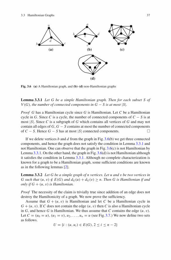
3.3 Hamiltonian Graphs 37
a
b cd
(a) (b)
a
c
b de
(c)
(d)
Fig. 3.6 (a) A Hamiltonian graph, and (b)–(d) non-Hamiltonian graphs
Lemma 3.3.1 Let G be a simple Hamiltonian graph. Then for each subset S ofV (G), the number of connected components in G − S is at most |S|.Proof G has a Hamiltonian cycle since G is Hamiltonian. Let C be a Hamiltoniancycle in G. Since C is a cycle, the number of connected components of C − S is atmost |S|. Since C is a subgraph of G which contains all vertices of G and may notcontain all edges ofG,G − S contains at most the number of connected componentsof C − S. Hence G − S has at most |S| connected components. �
If we delete vertices b and d from the graph in Fig. 3.6(b) we get three connectedcomponents, and hence the graph does not satisfy the condition in Lemma 3.3.1 andnot Hamiltonian. One can observe that the graph in Fig. 3.6(c) is not Hamiltonian byLemma 3.3.1. On the other hand, the graph in Fig. 3.6(d) is not Hamiltonian althoughit satisfies the condition in Lemma 3.3.1. Although no complete characterization isknown for a graph to be a Hamiltonian graph, some sufficient conditions are knownas in the following lemmas [2].
Lemma 3.3.2 Let G be a simple graph of n vertices. Let u and v be two vertices inG such that (u, v) /∈ E(G) and dG(u) + dG(v) ≥ n. Then G is Hamiltonian if andonly if G + (u, v) is Hamiltonian.
Proof The necessity of the claim is trivially true since addition of an edge does notdestroy the Hamiltonicity of a graph. We now prove the sufficiency.
Assume that G + (u, v) is Hamiltonian and let C be a Hamiltonian cycle inG + (u, v). If C does not contain the edge (u, v) then C is also a Hamiltonian cyclein G, and hence G is Hamiltonian. We thus assume that C contains the edge (u, v).Let C = (u0 = u), (u1 = v), u2, . . . , un = u (see Fig. 3.7.) We now define two setsas follows.
U = {i : (u, ui ) ∈ E(G), 2 ≤ i ≤ n − 2}
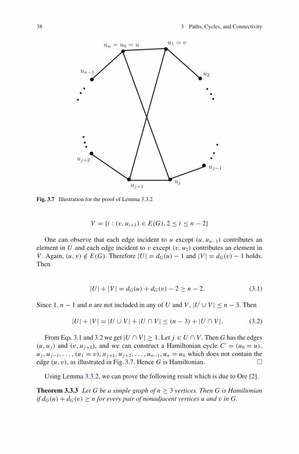
38 3 Paths, Cycles, and Connectivity
un = u0 = u u1 = v
u2
uj−1
ujuj+1
un−1
uj+2
Fig. 3.7 Illustration for the proof of Lemma 3.3.2
V = {i : (v, ui+1) ∈ E(G), 2 ≤ i ≤ n − 2}
One can observe that each edge incident to u except (u, un−1) contributes anelement in U and each edge incident to v except (v, u2) contributes an element inV . Again, (u, v) /∈ E(G). Therefore |U | = dG(u) − 1 and |V | = dG(v) − 1 holds.Then
|U | + |V | = dG(u) + dG(v) − 2 ≥ n − 2. (3.1)
Since 1, n − 1 and n are not included in any of U and V , |U ∪ V | ≤ n − 3. Then
|U | + |V | = |U ∪ V | + |U ∩ V | ≤ (n − 3) + |U ∩ V |. (3.2)
From Eqs. 3.1 and 3.2 we get |U ∩ V | ≥ 1. Let j ∈ U ∩ V . Then G has the edges(u, u j ) and (v, u j+1), and we can construct a Hamiltonian cycle C ′ = (u0 = u),
u j , u j−1, . . . , (u1 = v), u j+1, u j+2, . . . , un−1, un = u0 which does not contain theedge (u, v), as illustrated in Fig. 3.7. Hence G is Hamiltonian. �
Using Lemma 3.3.2, we can prove the following result which is due to Ore [2].
Theorem 3.3.3 Let G be a simple graph of n ≥ 3 vertices. Then G is Hamiltonianif dG(u) + dG(v) ≥ n for every pair of nonadjacent vertices u and v in G.
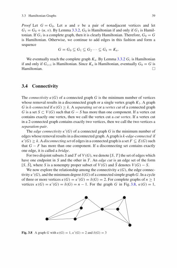
3.3 Hamiltonian Graphs 39
Proof Let G = G0. Let u and v be a pair of nonadjacent vertices and letG1 = G0 + (u, v). By Lemma 3.3.2, G0 is Hamiltonian if and only if G1 is Hamil-tonian. If G1 is a complete graph, then it is clearly Hamiltonian. Therefore, G0 = Gis Hamiltonian. Otherwise, we continue to add edges in this fashion and form asequence
G = G0 ⊆ G1 ⊆ G2 · · · ⊆ Gk = Kn.
We eventually reach the complete graph Kn . By Lemma 3.3.2 Gi is Hamiltonianif and only if Gi+1 is Hamiltonian. Since Kn is Hamiltonian, eventually G0 = G isHamiltonian. �
3.4 Connectivity
The connectivity κ(G) of a connected graph G is the minimum number of verticeswhose removal results in a disconnected graph or a single vertex graph K1. A graphG is k-connected if κ(G) ≥ k. A separating set or a vertex cut of a connected graphG is a set S ⊂ V (G) such that G − S has more than one component. If a vertex cutcontains exactly one vertex, then we call the vertex cut a cut vertex. If a vertex cutin a 2-connected graph contains exactly two vertices, then we call the two vertices aseparation-pair.
The edge connectivity κ ′(G) of a connected graph G is the minimum number ofedges whose removal results in a disconnected graph. A graph is k-edge-connected ifκ ′(G) ≥ k. A disconnecting set of edges in a connected graph is a set F ⊆ E(G) suchthat G − F has more than one component. If a disconnecting set contains exactlyone edge, it is called a bridge.
For two disjoint subsets S and T of V (G), we denote [S, T ] the set of edges whichhave one endpoint in S and the other in T . An edge cut is an edge set of the form[S, S], where S is a nonempty proper subset of V (G) and S denotes V (G) − S.
We now explore the relationship among the connectivity κ(G), the edge connec-tivity κ ′(G), and theminimum degree δ(G) of a connected simple graphG. In a cycleof three or more vertices κ(G) = κ ′(G) = δ(G) = 2. For complete graphs of n ≥ 1vertices κ(G) = κ ′(G) = δ(G) = n − 1. For the graph G in Fig. 3.8, κ(G) = 1,
Fig. 3.8 A graph G with κ(G) = 1, κ ′(G) = 2 and δ(G) = 3
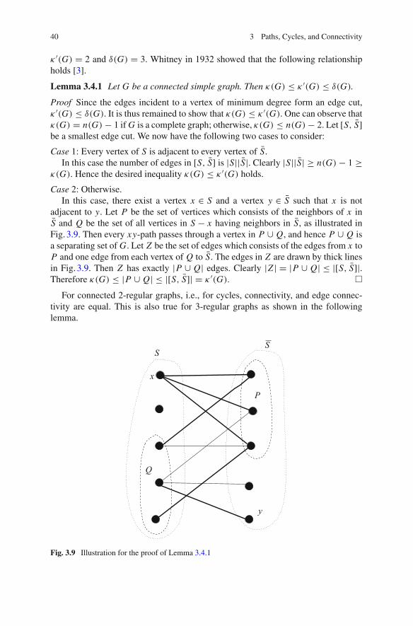
40 3 Paths, Cycles, and Connectivity
κ ′(G) = 2 and δ(G) = 3. Whitney in 1932 showed that the following relationshipholds [3].
Lemma 3.4.1 Let G be a connected simple graph. Then κ(G) ≤ κ ′(G) ≤ δ(G).
Proof Since the edges incident to a vertex of minimum degree form an edge cut,κ ′(G) ≤ δ(G). It is thus remained to show that κ(G) ≤ κ ′(G). One can observe thatκ(G) = n(G) − 1 ifG is a complete graph; otherwise, κ(G) ≤ n(G) − 2. Let [S, S]be a smallest edge cut. We now have the following two cases to consider:
Case 1: Every vertex of S is adjacent to every vertex of S.In this case the number of edges in [S, S] is |S||S|. Clearly |S||S| ≥ n(G) − 1 ≥
κ(G). Hence the desired inequality κ(G) ≤ κ ′(G) holds.
Case 2: Otherwise.In this case, there exist a vertex x ∈ S and a vertex y ∈ S such that x is not
adjacent to y. Let P be the set of vertices which consists of the neighbors of x inS and Q be the set of all vertices in S − x having neighbors in S, as illustrated inFig. 3.9. Then every xy-path passes through a vertex in P ∪ Q, and hence P ∪ Q isa separating set of G. Let Z be the set of edges which consists of the edges from x toP and one edge from each vertex of Q to S. The edges in Z are drawn by thick linesin Fig. 3.9. Then Z has exactly |P ∪ Q| edges. Clearly |Z | = |P ∪ Q| ≤ |[S, S]|.Therefore κ(G) ≤ |P ∪ Q| ≤ |[S, S]| = κ ′(G). �
For connected 2-regular graphs, i.e., for cycles, connectivity, and edge connec-tivity are equal. This is also true for 3-regular graphs as shown in the followinglemma.
P
Q
SS
x
y
Fig. 3.9 Illustration for the proof of Lemma 3.4.1
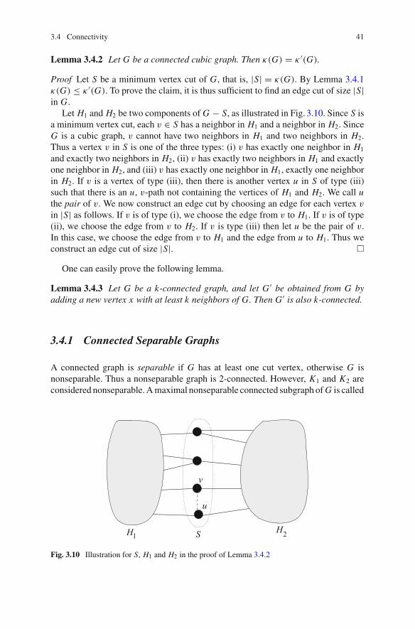
3.4 Connectivity 41
Lemma 3.4.2 Let G be a connected cubic graph. Then κ(G) = κ ′(G).
Proof Let S be a minimum vertex cut of G, that is, |S| = κ(G). By Lemma 3.4.1κ(G) ≤ κ ′(G). To prove the claim, it is thus sufficient to find an edge cut of size |S|in G.
Let H1 and H2 be two components of G − S, as illustrated in Fig. 3.10. Since S isa minimum vertex cut, each v ∈ S has a neighbor in H1 and a neighbor in H2. SinceG is a cubic graph, v cannot have two neighbors in H1 and two neighbors in H2.Thus a vertex v in S is one of the three types: (i) v has exactly one neighbor in H1
and exactly two neighbors in H2, (ii) v has exactly two neighbors in H1 and exactlyone neighbor in H2, and (iii) v has exactly one neighbor in H1, exactly one neighborin H2. If v is a vertex of type (iii), then there is another vertex u in S of type (iii)such that there is an u, v-path not containing the vertices of H1 and H2. We call uthe pair of v. We now construct an edge cut by choosing an edge for each vertex v
in |S| as follows. If v is of type (i), we choose the edge from v to H1. If v is of type(ii), we choose the edge from v to H2. If v is type (iii) then let u be the pair of v.In this case, we choose the edge from v to H1 and the edge from u to H1. Thus weconstruct an edge cut of size |S|. �
One can easily prove the following lemma.
Lemma 3.4.3 Let G be a k-connected graph, and let G ′ be obtained from G byadding a new vertex x with at least k neighbors of G. Then G ′ is also k-connected.
3.4.1 Connected Separable Graphs
A connected graph is separable if G has at least one cut vertex, otherwise G isnonseparable. Thus a nonseparable graph is 2-connected. However, K1 and K2 areconsidered nonseparable.Amaximal nonseparable connected subgraph ofG is called
SH H1 2
v
u
Fig. 3.10 Illustration for S, H1 and H2 in the proof of Lemma 3.4.2
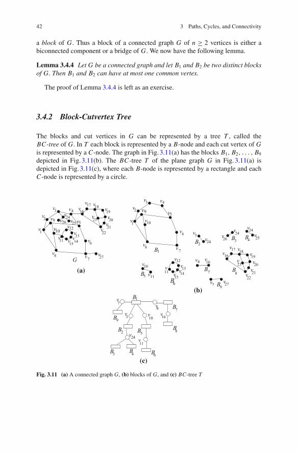
42 3 Paths, Cycles, and Connectivity
a block of G. Thus a block of a connected graph G of n ≥ 2 vertices is either abiconnected component or a bridge of G. We now have the following lemma.
Lemma 3.4.4 Let G be a connected graph and let B1 and B2 be two distinct blocksof G. Then B1 and B2 can have at most one common vertex.
The proof of Lemma 3.4.4 is left as an exercise.
3.4.2 Block-Cutvertex Tree
The blocks and cut vertices in G can be represented by a tree T , called theBC-tree of G. In T each block is represented by a B-node and each cut vertex of Gis represented by a C-node. The graph in Fig. 3.11(a) has the blocks B1, B2, . . . , B9
depicted in Fig. 3.11(b). The BC-tree T of the plane graph G in Fig. 3.11(a) isdepicted in Fig. 3.11(c), where each B-node is represented by a rectangle and eachC-node is represented by a circle.
vv
324B2
v2426v B3
v24
25
v
B4
vvv13
12
v11 14v15B6
11
10v
B v5
v v4 16
B7 vvv
vv v
v23
2221
20
191817
16v
B8
vv7 27B9
vvv24
2526
vv7 27G
v1
v2 v
v v615 14
v
v8
vvvv
v v
5v23
2221
20
191817
vvv13
12
11v10v
v3
9
v v4 16
(a)
v v10
v11
B B2
v B4v16
B
B B B3 4
5
6
8
7
B1
3
v
B
v
7
9
24
(c)
B1
v1
v vv2
3 4
v5
v
v7
9v
10v
v8
6
(b)
Fig. 3.11 (a) A connected graph G, (b) blocks of G, and (c) BC-tree T
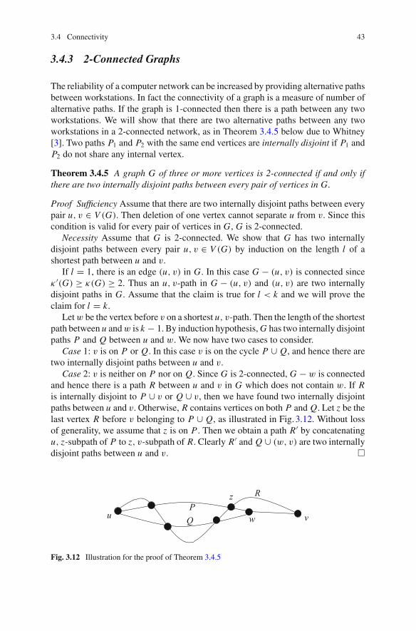
3.4 Connectivity 43
3.4.3 2-Connected Graphs
The reliability of a computer network can be increased by providing alternative pathsbetween workstations. In fact the connectivity of a graph is a measure of number ofalternative paths. If the graph is 1-connected then there is a path between any twoworkstations. We will show that there are two alternative paths between any twoworkstations in a 2-connected network, as in Theorem 3.4.5 below due to Whitney[3]. Two paths P1 and P2 with the same end vertices are internally disjoint if P1 andP2 do not share any internal vertex.
Theorem 3.4.5 A graph G of three or more vertices is 2-connected if and only ifthere are two internally disjoint paths between every pair of vertices in G.
Proof Sufficiency Assume that there are two internally disjoint paths between everypair u, v ∈ V (G). Then deletion of one vertex cannot separate u from v. Since thiscondition is valid for every pair of vertices in G, G is 2-connected.
Necessity Assume that G is 2-connected. We show that G has two internallydisjoint paths between every pair u, v ∈ V (G) by induction on the length l of ashortest path between u and v.
If l = 1, there is an edge (u, v) in G. In this case G − (u, v) is connected sinceκ ′(G) ≥ κ(G) ≥ 2. Thus an u, v-path in G − (u, v) and (u, v) are two internallydisjoint paths in G. Assume that the claim is true for l < k and we will prove theclaim for l = k.
Letw be the vertex before v on a shortest u, v-path. Then the length of the shortestpath between u andw is k − 1. By induction hypothesis,G has two internally disjointpaths P and Q between u and w. We now have two cases to consider.
Case 1: v is on P or Q. In this case v is on the cycle P ∪ Q, and hence there aretwo internally disjoint paths between u and v.
Case 2: v is neither on P nor on Q. Since G is 2-connected, G − w is connectedand hence there is a path R between u and v in G which does not contain w. If Ris internally disjoint to P ∪ v or Q ∪ v, then we have found two internally disjointpaths between u and v. Otherwise, R contains vertices on both P and Q. Let z be thelast vertex R before v belonging to P ∪ Q, as illustrated in Fig. 3.12. Without lossof generality, we assume that z is on P . Then we obtain a path R′ by concatenatingu, z-subpath of P to z, v-subpath of R. Clearly R′ and Q ∪ (w, v) are two internallydisjoint paths between u and v. �
u v
z RPQ w
Fig. 3.12 Illustration for the proof of Theorem 3.4.5
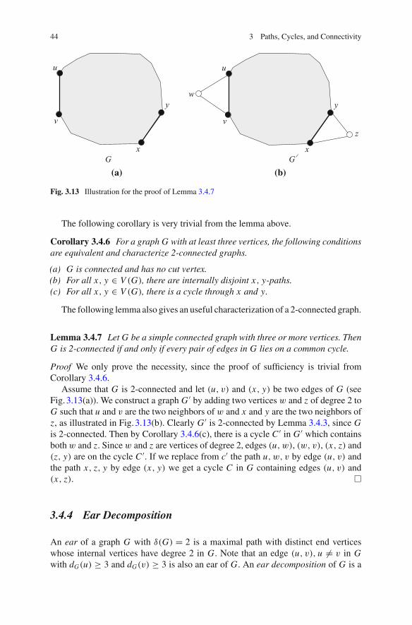
44 3 Paths, Cycles, and Connectivity
G G(a) (b)
u
v
x
yw
u
v
y
x
z
Fig. 3.13 Illustration for the proof of Lemma 3.4.7
The following corollary is very trivial from the lemma above.
Corollary 3.4.6 For a graph G with at least three vertices, the following conditionsare equivalent and characterize 2-connected graphs.
(a) G is connected and has no cut vertex.(b) For all x, y ∈ V (G), there are internally disjoint x, y-paths.(c) For all x, y ∈ V (G), there is a cycle through x and y.
The following lemma also gives an useful characterization of a 2-connected graph.
Lemma 3.4.7 Let G be a simple connected graph with three or more vertices. ThenG is 2-connected if and only if every pair of edges in G lies on a common cycle.
Proof We only prove the necessity, since the proof of sufficiency is trivial fromCorollary 3.4.6.
Assume that G is 2-connected and let (u, v) and (x, y) be two edges of G (seeFig. 3.13(a)). We construct a graph G ′ by adding two vertices w and z of degree 2 toG such that u and v are the two neighbors of w and x and y are the two neighbors ofz, as illustrated in Fig. 3.13(b). Clearly G ′ is 2-connected by Lemma 3.4.3, since Gis 2-connected. Then by Corollary 3.4.6(c), there is a cycle C ′ in G ′ which containsboth w and z. Since w and z are vertices of degree 2, edges (u, w), (w, v), (x, z) and(z, y) are on the cycle C ′. If we replace from c′ the path u, w, v by edge (u, v) andthe path x, z, y by edge (x, y) we get a cycle C in G containing edges (u, v) and(x, z). �
3.4.4 Ear Decomposition
An ear of a graph G with δ(G) = 2 is a maximal path with distinct end verticeswhose internal vertices have degree 2 in G. Note that an edge (u, v), u = v in Gwith dG(u) ≥ 3 and dG(v) ≥ 3 is also an ear of G. An ear decomposition of G is a
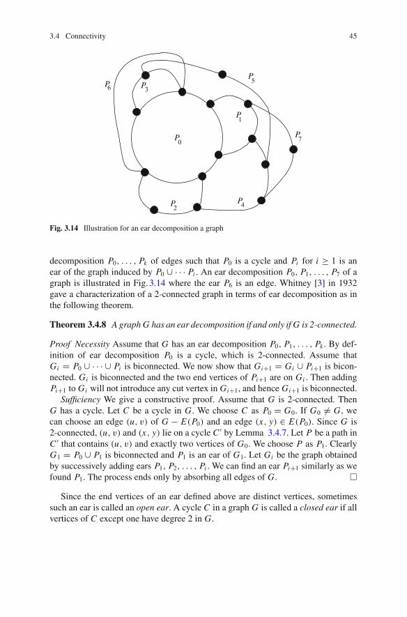
3.4 Connectivity 45
P
P
P
PP
P
0
1
2
35P6
4
P7
Fig. 3.14 Illustration for an ear decomposition a graph
decomposition P0, . . . , Pk of edges such that P0 is a cycle and Pi for i ≥ 1 is anear of the graph induced by P0 ∪ · · · Pi . An ear decomposition P0, P1, . . . , P7 of agraph is illustrated in Fig. 3.14 where the ear P6 is an edge. Whitney [3] in 1932gave a characterization of a 2-connected graph in terms of ear decomposition as inthe following theorem.
Theorem 3.4.8 A graph G has an ear decomposition if and only if G is 2-connected.
Proof Necessity Assume that G has an ear decomposition P0, P1, . . . , Pk . By def-inition of ear decomposition P0 is a cycle, which is 2-connected. Assume thatGi = P0 ∪ · · · ∪ Pi is biconnected. We now show that Gi+1 = Gi ∪ Pi+1 is bicon-nected. Gi is biconnected and the two end vertices of Pi+1 are on Gi . Then addingPi+1 to Gi will not introduce any cut vertex in Gi+1, and hence Gi+1 is biconnected.
Sufficiency We give a constructive proof. Assume that G is 2-connected. ThenG has a cycle. Let C be a cycle in G. We choose C as P0 = G0. If G0 = G, wecan choose an edge (u, v) of G − E(P0) and an edge (x, y) ∈ E(P0). Since G is2-connected, (u, v) and (x, y) lie on a cycle C ′ by Lemma 3.4.7. Let P be a path inC ′ that contains (u, v) and exactly two vertices of G0. We choose P as P1. ClearlyG1 = P0 ∪ P1 is biconnected and P1 is an ear of G1. Let Gi be the graph obtainedby successively adding ears P1, P2, . . . , Pi . We can find an ear Pi+1 similarly as wefound P1. The process ends only by absorbing all edges of G. �
Since the end vertices of an ear defined above are distinct vertices, sometimessuch an ear is called an open ear. A cycle C in a graph G is called a closed ear if allvertices of C except one have degree 2 in G.
46 3 Paths, Cycles, and Connectivity
Bibliographic Notes
For preparing this chapter several books [4–6] were used.
Exercises
1. Let G be a graph having exactly two vertices u and v of degree three and allother vertices have even degree. Then show that there is an u, v-path in G.
2. Write an algorithm to find a Eulerian circuit in an Eulerian graph based on thesufficiency proof of Lemma 3.2.1.
3. Give a proof of Lemma 3.2.2.4. Count the minimum number of edges required to add for making a non-Eulerian
graph an Eulerian graph.5. Let Kn be a complete graph of n vertices where n is odd and n ≥ 3. Show that
Kn has (n − 1)/2 edge-disjoint Hamiltonian cycles.6. Show that every k-regular graph on 2k + 1 vertices is Hamiltonian [7].7. Write an algorithm to find a pair of vertex disjoint paths between a pair of vertices
in a 2-connected graph.8. Write an algorithm to find an ear decomposition of a biconnected graph.9. Let s be a designated vertex in a connected graph G = (V, E). Design an
O(n +m) time algorithm to find a path between s and v with the minimumnumber of edges for all vertices v ∈ V .
10. Show that a 3-connected graph has at least six edges.
References
1. Biggs, N.L., Lloyd, E.K., Wilson, R.J.: Graph Theory: 1736–1936. Oxford University Press,Oxford (1976)
2. Ore, O.: Note on Hamiltonian circuits. Am. Mat. Mon. 67, 55 (1960)3. Whitney, H.: Congruent graphs and the connectivity of graphs. Am. J. Math. 54, 150–168 (1932)4. Agnarsson, G., Greenlaw, R.: Graph Theory: Modeling Applications and Algorithms. Pearson
Education Inc., London (2007)5. West, D.B.: Introduction to Graph Theory, 2nd edn. Prentice Hall, New Jersey (2001)6. Wilson, R.J.: Introduction to Graph Theory, 4th edn. Longman, London (1996)7. Nash-Williams, C.St.J.A.: Edge-disjoint Hamiltonian circuits in graphs with vertices of large
valency. Studies in Pure Mathematics. Academic Press, London (1971)
Chapter 4Trees
4.1 Introduction
A tree is a connected graph that contains no cycle. Figures4.1(a), (b), and (c) illus-trate trees with one, two, and three vertices, respectively. Figures4.1(d) and (e)illustrate two different trees with four vertices. A path is always a tree. The treesin Figs. 4.1(a)–(d) are all paths. Recall that a path with n vertices has n − 1 edges.In fact, every tree has n − 1 edges as we shall see later in this chapter. For example,Fig. 4.1(f) illustrates a tree with 14 vertices and 13 edges.
A vertex with degree one in a tree T is called a leaf of T . All the vertices of Tother than the leaves are called the internal vertices of T . The vertex d of the tree inFig. 4.1(f) is a leaf and the vertex a is an internal vertex.
A collection of trees is called a forest. In other words, a forest is a graph with nocycle. Such a graph is also called an acyclic graph. Each component of a forest is atree.
4.2 Properties of a Tree
There are many different sets of properties of trees; any of these sets of propertiescan be taken as a definition of a tree. In this section, we discuss these properties of atree. We first observe the following two trivial properties of a tree which play crucialroles while dealing with trees.
Lemma 4.2.1 Every tree with two or more vertices has at least two leaves.
Proof Let T be a tree of two or more vertices and let P be a maximal path in T . Thenthe end vertices u and v of P have degree 1 (see Fig. 4.1(f)), otherwise P would notbe a maximal path in T . �
© Springer International Publishing AG 2017M.S. Rahman, Basic Graph Theory, Undergraduate Topics in Computer Science,DOI 10.1007/978-3-319-49475-3_4
47
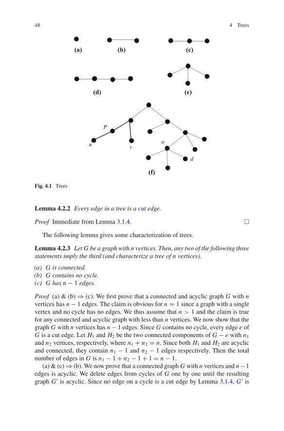
48 4 Trees
(a) (b) (c)
(d) (e)
(f)
d
au v
P
Fig. 4.1 Trees
Lemma 4.2.2 Every edge in a tree is a cut edge.
Proof Immediate from Lemma 3.1.4. �
The following lemma gives some characterization of trees.
Lemma 4.2.3 Let G be a graph with n vertices. Then, any two of the following threestatements imply the third (and characterize a tree of n vertices).
(a) G is connected.(b) G contains no cycle.(c) G has n − 1 edges.
Proof (a) & (b) ⇒ (c). We first prove that a connected and acyclic graph G with nvertices has n − 1 edges. The claim is obvious for n = 1 since a graph with a singlevertex and no cycle has no edges. We thus assume that n > 1 and the claim is truefor any connected and acyclic graph with less than n vertices. We now show that thegraph G with n vertices has n − 1 edges. Since G contains no cycle, every edge e ofG is a cut edge. Let H1 and H2 be the two connected components of G − e with n1and n2 vertices, respectively, where n1 + n2 = n. Since both H1 and H2 are acyclicand connected, they contain n1 − 1 and n2 − 1 edges respectively. Then the totalnumber of edges in G is n1 − 1 + n2 − 1 + 1 = n − 1.
(a) & (c)⇒ (b). We now prove that a connected graph G with n vertices and n−1edges is acyclic. We delete edges from cycles of G one by one until the resultinggraph G ′ is acyclic. Since no edge on a cycle is a cut edge by Lemma 3.1.4, G ′ is
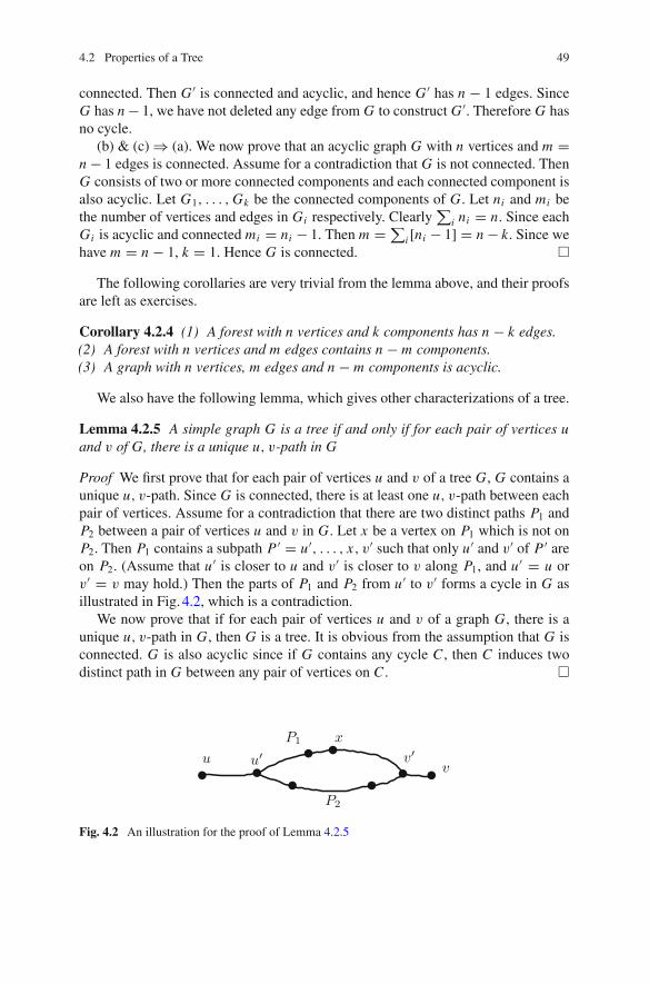
4.2 Properties of a Tree 49
connected. Then G ′ is connected and acyclic, and hence G ′ has n − 1 edges. SinceG has n − 1, we have not deleted any edge from G to construct G ′. Therefore G hasno cycle.
(b) & (c) ⇒ (a). We now prove that an acyclic graph G with n vertices and m =n − 1 edges is connected. Assume for a contradiction that G is not connected. ThenG consists of two or more connected components and each connected component isalso acyclic. Let G1, . . . ,Gk be the connected components of G. Let ni and mi bethe number of vertices and edges in Gi respectively. Clearly
∑i ni = n. Since each
Gi is acyclic and connected mi = ni − 1. Then m = ∑i [ni − 1] = n − k. Since we
have m = n − 1, k = 1. Hence G is connected. �
The following corollaries are very trivial from the lemma above, and their proofsare left as exercises.
Corollary 4.2.4 (1) A forest with n vertices and k components has n − k edges.(2) A forest with n vertices and m edges contains n − m components.(3) A graph with n vertices, m edges and n − m components is acyclic.
We also have the following lemma, which gives other characterizations of a tree.
Lemma 4.2.5 A simple graph G is a tree if and only if for each pair of vertices uand v of G, there is a unique u, v-path in G
Proof We first prove that for each pair of vertices u and v of a tree G, G contains aunique u, v-path. Since G is connected, there is at least one u, v-path between eachpair of vertices. Assume for a contradiction that there are two distinct paths P1 andP2 between a pair of vertices u and v in G. Let x be a vertex on P1 which is not onP2. Then P1 contains a subpath P ′ = u′, . . . , x, v′ such that only u′ and v′ of P ′ areon P2. (Assume that u′ is closer to u and v′ is closer to v along P1, and u′ = u orv′ = v may hold.) Then the parts of P1 and P2 from u′ to v′ forms a cycle in G asillustrated in Fig. 4.2, which is a contradiction.
We now prove that if for each pair of vertices u and v of a graph G, there is aunique u, v-path in G, then G is a tree. It is obvious from the assumption that G isconnected. G is also acyclic since if G contains any cycle C , then C induces twodistinct path in G between any pair of vertices on C . �
u u vv
x
P2
P1
Fig. 4.2 An illustration for the proof of Lemma 4.2.5
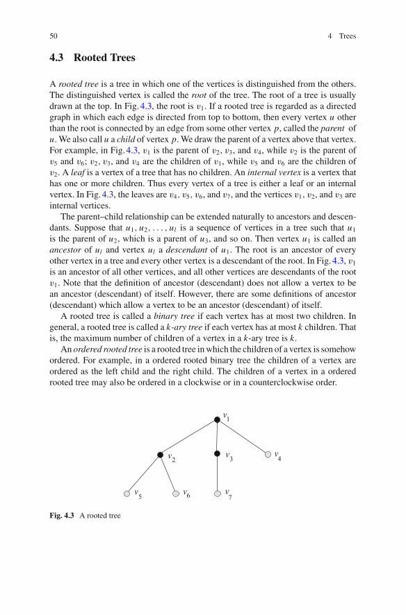
50 4 Trees
4.3 Rooted Trees
A rooted tree is a tree in which one of the vertices is distinguished from the others.The distinguished vertex is called the root of the tree. The root of a tree is usuallydrawn at the top. In Fig. 4.3, the root is v1. If a rooted tree is regarded as a directedgraph in which each edge is directed from top to bottom, then every vertex u otherthan the root is connected by an edge from some other vertex p, called the parent ofu. We also call u a child of vertex p. We draw the parent of a vertex above that vertex.For example, in Fig. 4.3, v1 is the parent of v2, v3, and v4, while v2 is the parent ofv5 and v6; v2, v3, and v4 are the children of v1, while v5 and v6 are the children ofv2. A leaf is a vertex of a tree that has no children. An internal vertex is a vertex thathas one or more children. Thus every vertex of a tree is either a leaf or an internalvertex. In Fig. 4.3, the leaves are v4, v5, v6, and v7, and the vertices v1, v2, and v3 areinternal vertices.
The parent–child relationship can be extended naturally to ancestors and descen-dants. Suppose that u1, u2, . . . , ul is a sequence of vertices in a tree such that u1is the parent of u2, which is a parent of u3, and so on. Then vertex u1 is called anancestor of ul and vertex ul a descendant of u1. The root is an ancestor of everyother vertex in a tree and every other vertex is a descendant of the root. In Fig. 4.3, v1is an ancestor of all other vertices, and all other vertices are descendants of the rootv1. Note that the definition of ancestor (descendant) does not allow a vertex to bean ancestor (descendant) of itself. However, there are some definitions of ancestor(descendant) which allow a vertex to be an ancestor (descendant) of itself.
A rooted tree is called a binary tree if each vertex has at most two children. Ingeneral, a rooted tree is called a k-ary tree if each vertex has at most k children. Thatis, the maximum number of children of a vertex in a k-ary tree is k.
An ordered rooted tree is a rooted tree inwhich the children of a vertex is somehowordered. For example, in a ordered rooted binary tree the children of a vertex areordered as the left child and the right child. The children of a vertex in a orderedrooted tree may also be ordered in a clockwise or in a counterclockwise order.
v5
v6 v7
v
v v v
1
2 3 4
Fig. 4.3 A rooted tree
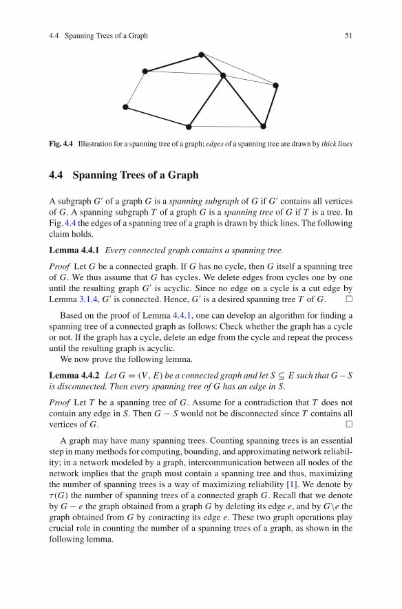
4.4 Spanning Trees of a Graph 51
Fig. 4.4 Illustration for a spanning tree of a graph; edges of a spanning tree are drawn by thick lines
4.4 Spanning Trees of a Graph
A subgraph G ′ of a graph G is a spanning subgraph of G if G ′ contains all verticesof G. A spanning subgraph T of a graph G is a spanning tree of G if T is a tree. InFig. 4.4 the edges of a spanning tree of a graph is drawn by thick lines. The followingclaim holds.
Lemma 4.4.1 Every connected graph contains a spanning tree.
Proof Let G be a connected graph. If G has no cycle, then G itself a spanning treeof G. We thus assume that G has cycles. We delete edges from cycles one by oneuntil the resulting graph G ′ is acyclic. Since no edge on a cycle is a cut edge byLemma 3.1.4, G ′ is connected. Hence, G ′ is a desired spanning tree T of G. �
Based on the proof of Lemma 4.4.1, one can develop an algorithm for finding aspanning tree of a connected graph as follows: Check whether the graph has a cycleor not. If the graph has a cycle, delete an edge from the cycle and repeat the processuntil the resulting graph is acyclic.
We now prove the following lemma.
Lemma 4.4.2 Let G = (V, E) be a connected graph and let S ⊆ E such that G− Sis disconnected. Then every spanning tree of G has an edge in S.
Proof Let T be a spanning tree of G. Assume for a contradiction that T does notcontain any edge in S. Then G − S would not be disconnected since T contains allvertices of G. �
A graph may have many spanning trees. Counting spanning trees is an essentialstep in manymethods for computing, bounding, and approximating network reliabil-ity; in a network modeled by a graph, intercommunication between all nodes of thenetwork implies that the graph must contain a spanning tree and thus, maximizingthe number of spanning trees is a way of maximizing reliability [1]. We denote byτ (G) the number of spanning trees of a connected graph G. Recall that we denoteby G − e the graph obtained from a graph G by deleting its edge e, and by G\e thegraph obtained from G by contracting its edge e. These two graph operations playcrucial role in counting the number of a spanning trees of a graph, as shown in thefollowing lemma.
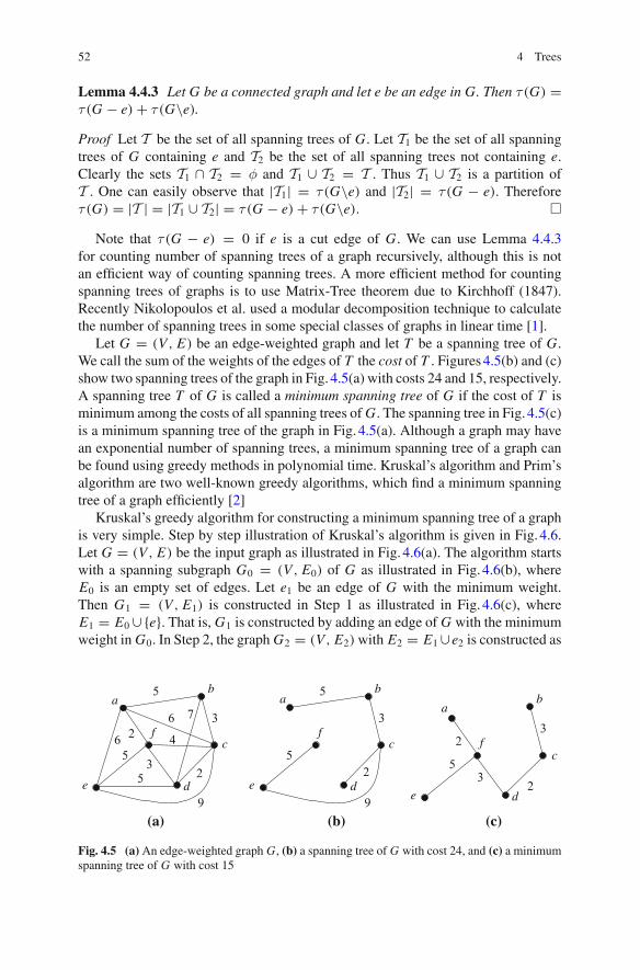
52 4 Trees
Lemma 4.4.3 Let G be a connected graph and let e be an edge in G. Then τ (G) =τ (G − e) + τ (G\e).Proof Let T be the set of all spanning trees of G. Let T1 be the set of all spanningtrees of G containing e and T2 be the set of all spanning trees not containing e.Clearly the sets T1 ∩ T2 = φ and T1 ∪ T2 = T . Thus T1 ∪ T2 is a partition ofT . One can easily observe that |T1| = τ (G\e) and |T2| = τ (G − e). Thereforeτ (G) = |T | = |T1 ∪ T2| = τ (G − e) + τ (G\e). �
Note that τ (G − e) = 0 if e is a cut edge of G. We can use Lemma 4.4.3for counting number of spanning trees of a graph recursively, although this is notan efficient way of counting spanning trees. A more efficient method for countingspanning trees of graphs is to use Matrix-Tree theorem due to Kirchhoff (1847).Recently Nikolopoulos et al. used a modular decomposition technique to calculatethe number of spanning trees in some special classes of graphs in linear time [1].
Let G = (V, E) be an edge-weighted graph and let T be a spanning tree of G.We call the sum of the weights of the edges of T the cost of T . Figures4.5(b) and (c)show two spanning trees of the graph in Fig. 4.5(a) with costs 24 and 15, respectively.A spanning tree T of G is called a minimum spanning tree of G if the cost of T isminimum among the costs of all spanning trees ofG. The spanning tree in Fig. 4.5(c)is a minimum spanning tree of the graph in Fig. 4.5(a). Although a graph may havean exponential number of spanning trees, a minimum spanning tree of a graph canbe found using greedy methods in polynomial time. Kruskal’s algorithm and Prim’salgorithm are two well-known greedy algorithms, which find a minimum spanningtree of a graph efficiently [2]
Kruskal’s greedy algorithm for constructing a minimum spanning tree of a graphis very simple. Step by step illustration of Kruskal’s algorithm is given in Fig. 4.6.Let G = (V, E) be the input graph as illustrated in Fig. 4.6(a). The algorithm startswith a spanning subgraph G0 = (V, E0) of G as illustrated in Fig. 4.6(b), whereE0 is an empty set of edges. Let e1 be an edge of G with the minimum weight.Then G1 = (V, E1) is constructed in Step 1 as illustrated in Fig. 4.6(c), whereE1 = E0 ∪{e}. That is, G1 is constructed by adding an edge of G with the minimumweight in G0. In Step 2, the graph G2 = (V, E2)with E2 = E1 ∪e2 is constructed as
b
3
d
f
e
2
53
a
2
c
(c)
e
5 b
3
c
9
6
(a)
d
f6
5
2
54
32
a7
b
3a
c
9
f
5
e d
(b)
5
2
Fig. 4.5 (a) An edge-weighted graph G, (b) a spanning tree of G with cost 24, and (c) a minimumspanning tree of G with cost 15
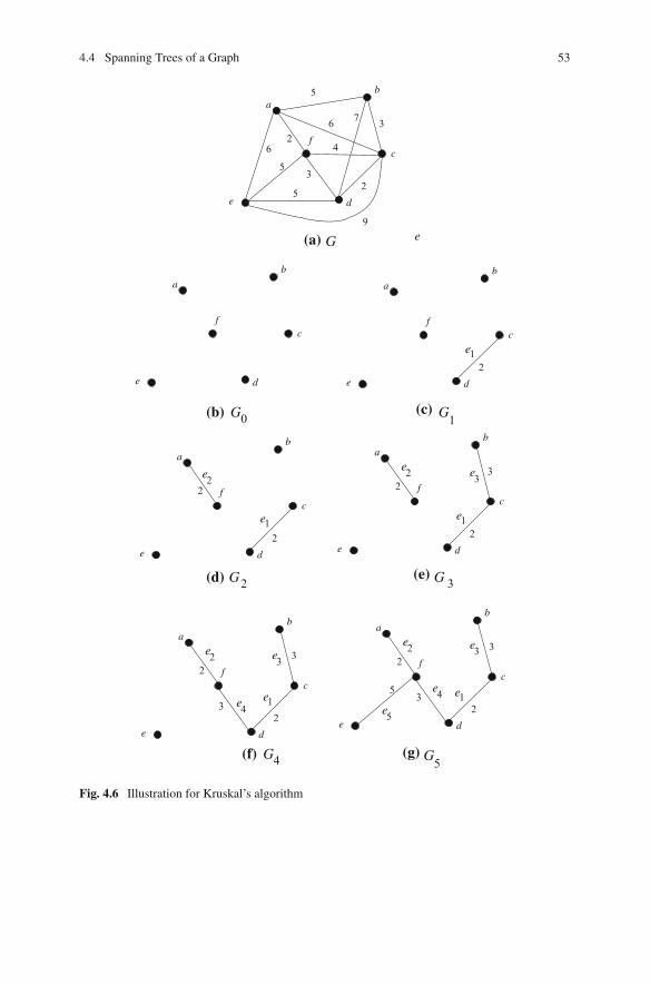
4.4 Spanning Trees of a Graph 53
a
b
c
d
f
e
4
3
5
2
9
762
a
b
c
d
f
35
5e
6
3
2
2
a
b
c
d
f
35
e
2
a
b
c
d
f
e
3
2
2
a
b
c
d
f
3
e
G4(f)
2
2
a
b
c
d
f
e
G2(d)
3
2
2
a
b
c
d
f
e
1e
1e 1e
1e1ee4
e4
3e
3e3e
e2
e2e2
e2
G
G G
G
G
0 1
3
5(g)
(e)
(a)
(c)(b)
e
e5
Fig. 4.6 Illustration for Kruskal’s algorithm
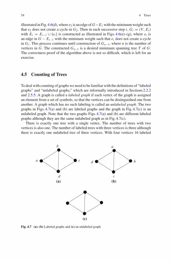
54 4 Trees
illustrated in Fig. 4.6(d), where e2 is an edge ofG−E1 with theminimumweight suchthat e2 does not create a cycle in G2. Then in each successive step i , Gi = (V, Ei )
with Ei = Ei−1 ∪ {ei } is constructed as illustrated in Figs. 4.6(e)–(g), where ei isan edge in G − Ei−1 with the minimum weight such that ei does not create a cyclein Gi . This process continues until construction of Gn−1, where n is the number ofvertices in G. The constructed Gn−1 is a desired minimum spanning tree T of G.The correctness proof of the algorithm above is not so difficult, which is left for anexercise.
4.5 Counting of Trees
To deal with counting of graphswe need to be familiar with the definitions of “labeledgraphs” and “unlabeled graphs,” which are informally introduced in Sections2.2.2and 2.5.5. A graph is called a labeled graph if each vertex of the graph is assignedan element from a set of symbols, so that the vertices can be distinguished one fromanother. A graph which has no such labeling is called an unlabeled graph. The twographs in Figs. 4.7(a) and (b) are labeled graphs and the graph in Fig. 4.7(c) is anunlabeled graph. Note that the two graphs Figs. 4.7(a) and (b) are different labeledgraphs although they are the same unlabeled graph as in Fig. 4.7(c).
There is exactly one tree with a single vertex. The number of trees with twovertices is also one. The number of labeled trees with three vertices is three althoughthere is exactly one unlabeled tree of three vertices. With four vertices 16 labeled
a
b
c
d c
b
a
d
(b)(a)
(c)
Fig. 4.7 (a)–(b) Labeled graphs and (c) an unlabeled graph
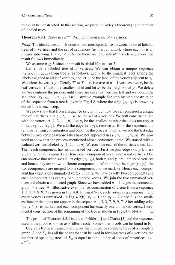
4.5 Counting of Trees 55
trees can be constructed. In this section, we present Cayley’s theorem [3] on numberof labeled trees.
Theorem 4.5.1 There are nn−2 distinct labeled trees of n vertices.
Proof The idea is to establish a one-to-one correspondence between the set of labeledtrees of n vertices and the set of sequences (a1, a2, . . . , an−2), where each ai is aninteger satisfying 1 ≤ ai ≤ n. Since there are precisely nn−2 such sequences, theresult follows immediately.
We assume n ≥ 3, since the result is trivial if n = 1 or 2.Let T be a labeled tree of n vertices. We can obtain a unique sequence
(x1, x2, . . . , xn−2) from tree T as follows. Let y1 be the smallest label among thelabels assigned to all leaf vertices, and let x1 be the label of the vertex adjacent to y1.We delete the vertex y1. Clearly T ′ = T − y1 is a tree of n− 1 vertices. Let y2 be theleaf vertex in T ′ with the smallest label and let x2 be the neighbor of y2. We deletey2. We continue the process until there are only two vertices left and we obtain thesequence (x1, x2, . . . , xn−2). An illustrative example for step by step constructionof the sequence from a tree is given in Fig. 4.8, where the edge (yi , xi ) is drawn bydotted line in each step.
We now show that from a sequence (x1, x2, . . . , xn−2) we can construct a uniquetree of n vertices. Let {1, 2, . . . , n} be the set of n vertices. We will construct a treewith the vertex set {1, 2, . . . , n}. Let y1 be the smallest number that does not appearin (x1, x2, . . . , xn−2). We add the edge (x1, y1), remove x1 from the sequence andremove y1 from consideration and continue the process. Finally, we add the last edgebetween two vertices whose label have not appeared in {y1, y2, . . . , yn−2}. We nowneed to show that the process mentioned above constructs a tree. We started with nisolated vertices labeled by {1, 2, . . . , n}.We consider each of the vertices unmarked.Then each component has an unmarked vertices. First we join edge (x1, y1), marky1, and x1 remains unmarked. Hence each component has an unmarked vertices. Onecan observe that when we add an edge (xi , yi ), both xi and yi are unmarked verticesand hence they are in two different components. After adding the edge (xi , yi ), thetwo components are merged to one component and we mark y1. Hence each compo-nent has exactly one unmarked vertex. Finally, we have exactly two components andeach component has exactly one unmarked vertex. We join the two unmarked ver-tices and obtain a connected graph. Since we have added n − 1 edges the connectedgraph is a tree. An illustrative example for construction of a tree from a sequence1, 3, 3, 7, 9, 9, 7 is given in Fig. 4.9. In Fig. 4.9(a), each vertex is a component andevery vertex is unmarked. In Fig. 4.9(b), x1 = 1 and y1 = 2 since 2 is the small-est integer that does not appear in the sequence 1, 3, 3, 7, 9, 9, 7. After adding edge(x1, y1), y1 is marked and each component has exactly one unmarked vertex. Incre-mental construction of the remaining of the tree is shown in Figs. 4.9(b)–(i). �
The proof of Theorem 4.5.1 is due to Prüffer [4] and Clarke [5] and the sequenceused in the proof is known as Prüffer’s code. Some other proofs can be found in [6].
Cayley’s formula immediately gives the number of spanning trees of a completegraph. Since Kn has all the edges that can be used in forming trees of n vertices, thenumber of spanning trees of Kn is equal to the number of trees of n vertices, i.e.,nn−2.
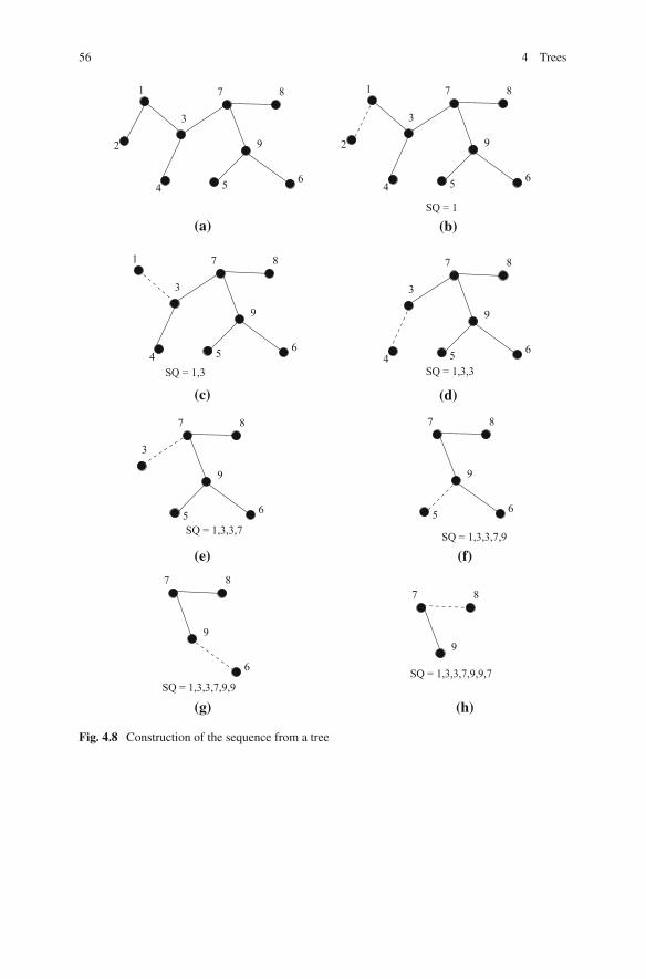
56 4 Trees
1
2
3
4 5 6
7 8
9
5 6
7 8
9
SQ = 1,3,3,7,9
7 8
9
SQ = 1,3,3,7,9,9,7
1
3
4 5 6
7 8
9
SQ = 1,3
3
5 6
7 8
9
SQ = 1,3,3,7
3
4 5 6
7 8
9
SQ = 1,3,3
1
2
3
4 5 6
7 8
9
SQ = 1
6
7 8
9
SQ = 1,3,3,7,9,9
(a)
(h)
(c)
(e) (f)
(b)
(d)
(g)
Fig. 4.8 Construction of the sequence from a tree
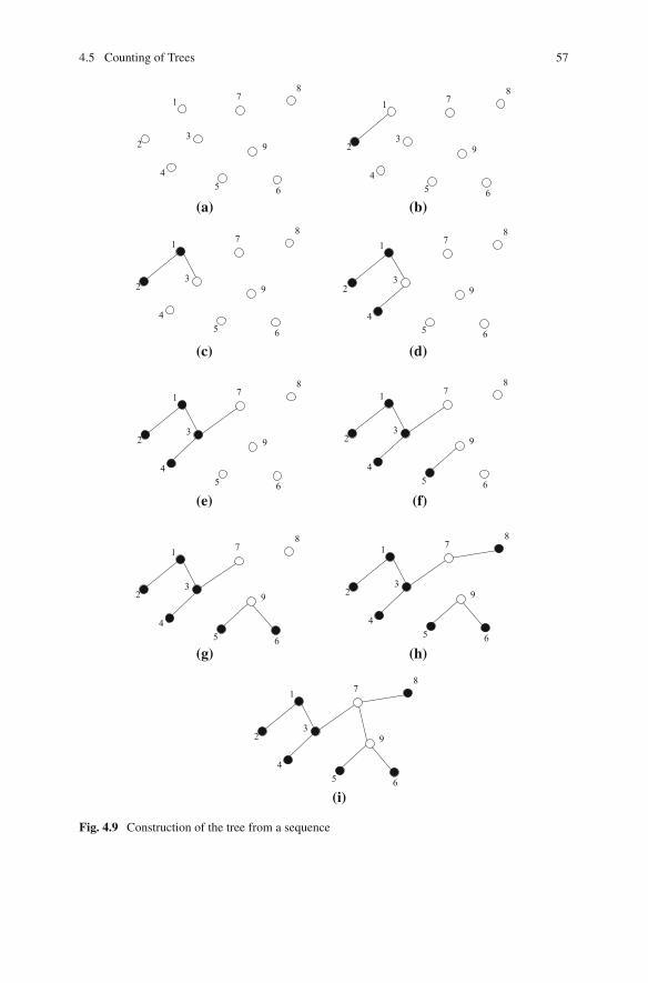
4.5 Counting of Trees 57
1
23
45 6
78
9
1
23
45 6
78
9
1
23
45 6
78
9
1
23
45 6
78
9
1
23
45 6
78
9
1
23
45 6
78
9
1
23
45 6
78
9
1
23
45 6
78
9
1
23
45 6
78
9
(a) (b)
(c) (d)
(e) (f)
(g) (h)
(i)
Fig. 4.9 Construction of the tree from a sequence
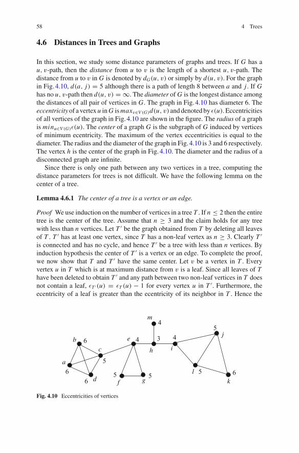
58 4 Trees
4.6 Distances in Trees and Graphs
In this section, we study some distance parameters of graphs and trees. If G has au, v-path, then the distance from u to v is the length of a shortest u, v-path. Thedistance from u to v in G is denoted by dG(u, v) or simply by d(u, v). For the graphin Fig. 4.10, d(a, j) = 5 although there is a path of length 8 between a and j . If Ghas no u, v-path then d(u, v) = ∞. The diameter of G is the longest distance amongthe distances of all pair of vertices in G. The graph in Fig. 4.10 has diameter 6. Theeccentricityof a vertexu inG ismaxv∈V (G)d(u, v) anddenoted by ε(u). Eccentricitiesof all vertices of the graph in Fig. 4.10 are shown in the figure. The radius of a graphis minu∈V (G)ε(u). The center of a graph G is the subgraph of G induced by verticesof minimum ecentricity. The maximum of the vertex eccentricities is equal to thediameter. The radius and the diameter of the graph in Fig. 4.10 is 3 and 6 respectively.The vertex h is the center of the graph in Fig. 4.10. The diameter and the radius of adisconnected graph are infinite.
Since there is only one path between any two vertices in a tree, computing thedistance parameters for trees is not difficult. We have the following lemma on thecenter of a tree.
Lemma 4.6.1 The center of a tree is a vertex or an edge.
Proof We use induction on the number of vertices in a tree T . If n ≤ 2 then the entiretree is the center of the tree. Assume that n ≥ 3 and the claim holds for any treewith less than n vertices. Let T ′ be the graph obtained from T by deleting all leavesof T . T ′ has at least one vertex, since T has a non-leaf vertex as n ≥ 3. Clearly T ′is connected and has no cycle, and hence T ′ be a tree with less than n vertices. Byinduction hypothesis the center of T ′ is a vertex or an edge. To complete the proof,we now show that T and T ′ have the same center. Let v be a vertex in T . Everyvertex u in T which is at maximum distance from v is a leaf. Since all leaves of Thave been deleted to obtain T ′ and any path between two non-leaf vertices in T doesnot contain a leaf, εT ′(u) = εT (u) − 1 for every vertex u in T ′. Furthermore, theecentricity of a leaf is greater than the ecentricity of its neighbor in T . Hence the
d
a
6
6b
c
5
e 4h
3i
4 j5
k6l 5
m
gf5 5
4
6
Fig. 4.10 Eccentricities of vertices
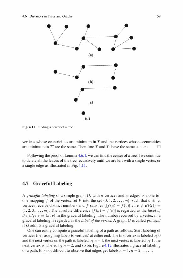
4.6 Distances in Trees and Graphs 59
(a)
(b)
(c)
(d)
Fig. 4.11 Finding a center of a tree
vertices whose ecentricities are minimum in T and the vertices whose ecentricitiesare minimum in T ′ are the same. Therefore T and T ′ have the same center. �
Following the proof of Lemma 4.6.1, we can find the center of a tree if we continueto delete all the leaves of the tree recursively until we are left with a single vertex ora single edge as illustrated in Fig. 4.11.
4.7 Graceful Labeling
A graceful labeling of a simple graph G, with n vertices and m edges, is a one-to-one mapping f of the vertex set V into the set {0, 1, 2, . . . ,m}, such that distinctvertices receive distinct numbers and f satisfies {| f (u) − f (v)| : uv ∈ E(G)} ={1, 2, 3, . . . ,m}. The absolute difference | f (u) − f (v)| is regarded as the label ofthe edge e = (u, v) in the graceful labeling. The number received by a vertex in agraceful labeling is regarded as the label of the vertex. A graph G is called gracefulif G admits a graceful labeling.
One can easily compute a graceful labeling of a path as follows. Start labeling ofvertices (i.e., assigning labels to vertices) at either end. The first vertex is labeled by 0and the next vertex on the path is labeled by n−1, the next vertex is labeled by 1, thenext vertex is labeled by n − 2, and so on. Figure4.12 illustrates a graceful labelingof a path. It is not difficult to observe that edges get labels n − 1, n − 2, . . . , 1.
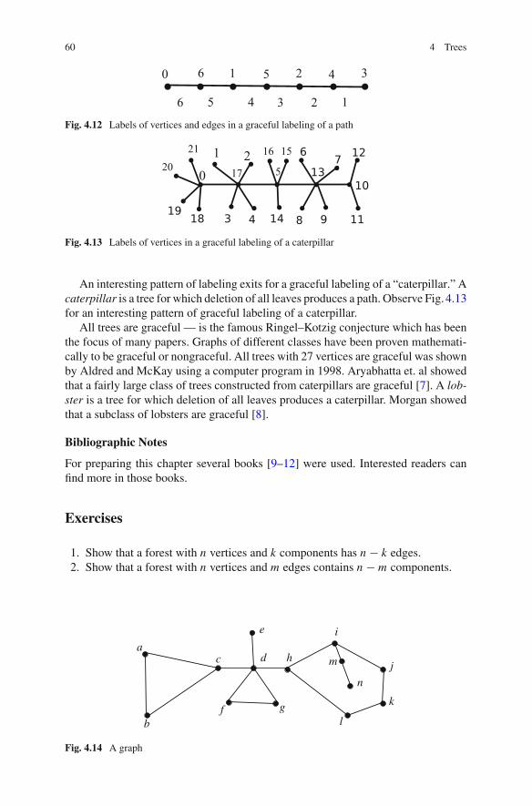
60 4 Trees
Fig. 4.12 Labels of vertices and edges in a graceful labeling of a path
Fig. 4.13 Labels of vertices in a graceful labeling of a caterpillar
An interesting pattern of labeling exits for a graceful labeling of a “caterpillar.” Acaterpillar is a tree for which deletion of all leaves produces a path. Observe Fig. 4.13for an interesting pattern of graceful labeling of a caterpillar.
All trees are graceful — is the famous Ringel–Kotzig conjecture which has beenthe focus of many papers. Graphs of different classes have been proven mathemati-cally to be graceful or nongraceful. All trees with 27 vertices are graceful was shownby Aldred and McKay using a computer program in 1998. Aryabhatta et. al showedthat a fairly large class of trees constructed from caterpillars are graceful [7]. A lob-ster is a tree for which deletion of all leaves produces a caterpillar. Morgan showedthat a subclass of lobsters are graceful [8].
Bibliographic Notes
For preparing this chapter several books [9–12] were used. Interested readers canfind more in those books.
Exercises
1. Show that a forest with n vertices and k components has n − k edges.2. Show that a forest with n vertices and m edges contains n − m components.
a
b
e
d
g
h
i
j
k
n
f
m
l
c
Fig. 4.14 A graph
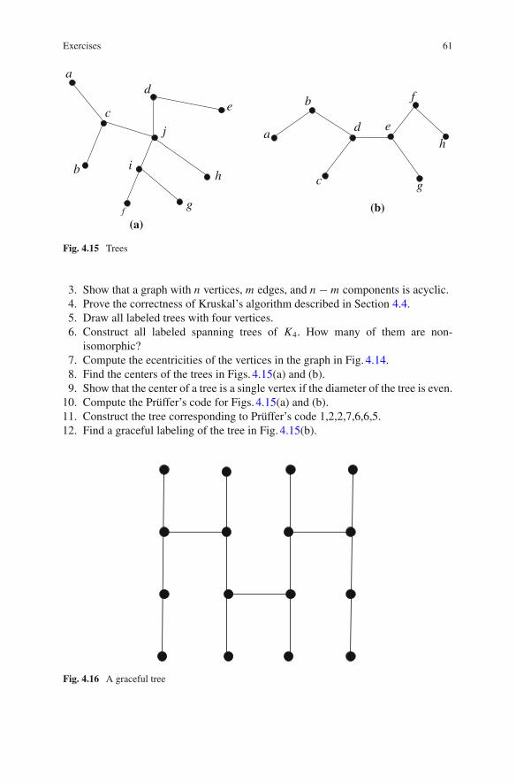
Exercises 61
f
a
c e
j
g
hi
b
a
c
d e
f
h
gb
d
(a)(b)
Fig. 4.15 Trees
3. Show that a graph with n vertices, m edges, and n − m components is acyclic.4. Prove the correctness of Kruskal’s algorithm described in Section 4.4.5. Draw all labeled trees with four vertices.6. Construct all labeled spanning trees of K4. How many of them are non-
isomorphic?7. Compute the ecentricities of the vertices in the graph in Fig. 4.14.8. Find the centers of the trees in Figs. 4.15(a) and (b).9. Show that the center of a tree is a single vertex if the diameter of the tree is even.
10. Compute the Prüffer’s code for Figs. 4.15(a) and (b).11. Construct the tree corresponding to Prüffer’s code 1,2,2,7,6,6,5.12. Find a graceful labeling of the tree in Fig. 4.15(b).
Fig. 4.16 A graceful tree
62 4 Trees
13. Develop an algorithm for computing a graceful labeling of a caterpillar.14. Find a graceful labeling of the tree in Fig. 4.16. Can you develop an algorithm
for finding graceful labelings of this type of trees?15. Show that every tree containing a vertex of degree k contains at least k leaves.
References
1. Nikolopoulos, S.D., Palios, L., Papadopoulos, C.: Counting spanning trees in graphs usingmod-ular decomposition. In: Proceedings of WALCOM 2011. Lecture Notes in Computer Science,vol. 6552, pp. 202–213. Springer, Berlin (2011)
2. Goodrich, M.T., Tamassia, R.: Algorithm Design: Foundations, Analysis, and Internet Exam-ples. Wiley, New York (2002)
3. Cayley, A.: A theorem on trees. Quart. J. Math. 23, 376–378 (1889)4. Prüfer, H.: Neuer beweis eines satzes über permutationen. Arch. Math. Phys. 27, 142–144
(1918)5. Clarke, L.E.: On Cayley’s formula for counting trees. J. LondonMath. Soc. 33, 471–474 (1958)6. Moon, J.W.: Counting Labeled Trees. Canadian Mathematical Congress, Montreal (1970)7. Arybhatta, S., Roy, T.G., Uddin, M., Rahman, M.S.: On graceful labeling of trees. In: Pro-
ceedings of WALCOM 2011. Lecture Notes in Computer Science, vol. 6552, pp. 214–220.Springer, Heidelberg (2011)
8. Morgan, D.: All lobsters with perfect matchings are graceful. Bull. Inst. Comb. Appl. 53, 82–85(2008)
9. Agnarsson, G., Greenlaw, R.: Graph Theory: Modeling, Applications and Algorithms. PearsonEducation Inc., New Jersey (2007)
10. Nishizeki, T., Rahman, M.S.: Planar Graph Drawing. World Scientific, Singapore (2004)11. West, D.B.: Introduction to Graph Theory, 2nd edn. Prentice Hall, New Jersey (2001)12. Wilson, R.J.: Introduction to Graph Theory, 4th edn. Longman, London (1996)
Chapter 5Matching and Covering
5.1 Matching
A matching in a graph is a set of non-loop edges with no common endpoints. Theset {(a, e), (b, c), (d, f )} of edges is a matching in graphs in Figs. 5.1(a) and (b).The vertices incident to the edges of a matching M are saturated by M ; the othersare unsaturated. In the graph in Fig. 5.1(a) vertices a, b, c, d, e, and f are saturated,whereas the vertex g is unsaturated.
5.1.1 Perfect Matching
A perfect matching in a graph is a matching that saturates every vertex. Thematching{(a, e), (b, c), (d, f )} is a perfect matching in the graph in Fig. 5.1(b), since allvertices are saturated. A complete graph of odd vertices does not have a perfectmatching, but a complete graph of even vertices always has a perfect matching. Agraphmay havemany perfectmatchings. For example, Kn,n has n! perfectmatchings.The bipartite graph in Fig. 5.2 has unique perfect matching.
5.1.2 Maximum Matching
A maximal matching in a graph is a matching that cannot be enlarged by adding anedge. A maximum matching is a matching of maximum size among all matchingsin the graph. The matching {(b, c)} in Fig. 5.3(a) is a maximal matching but not amaximum matching since there is a larger matching {(a, b), (c, d)} of this graph asshown in Fig. 5.3(b).
Given a matching M in a graph G, an M-alternating path is a path that alternatesbetween edges in M and edges not in M . An M-alternating path is an M-augmenting
© Springer International Publishing AG 2017M.S. Rahman, Basic Graph Theory, Undergraduate Topics in Computer Science,DOI 10.1007/978-3-319-49475-3_5
63
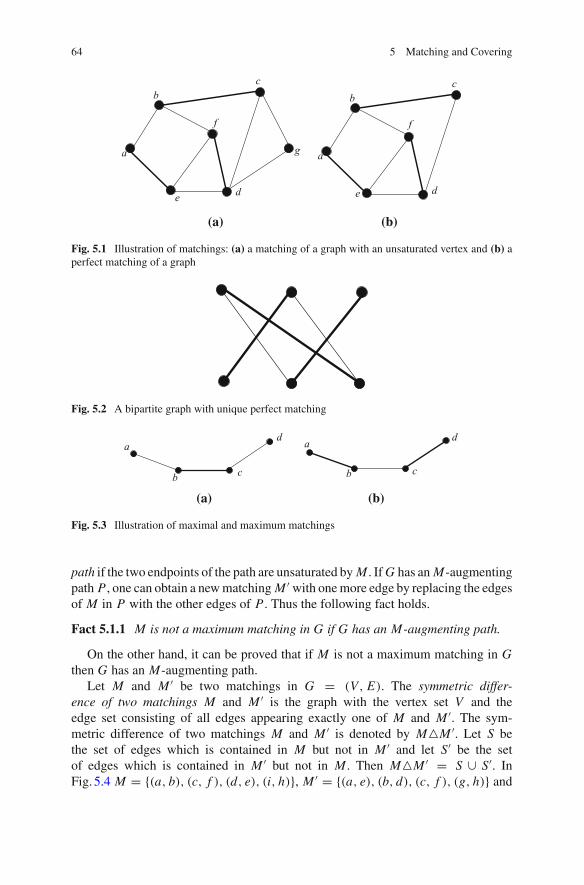
64 5 Matching and Covering
a
cb
de
f
a
cb
de
f
g
(a) (b)
Fig. 5.1 Illustration of matchings: (a) a matching of a graph with an unsaturated vertex and (b) aperfect matching of a graph
Fig. 5.2 A bipartite graph with unique perfect matching
(b)(a)
a
c
d a
b cb
d
Fig. 5.3 Illustration of maximal and maximum matchings
path if the two endpoints of the path are unsaturated byM . IfG has anM-augmentingpath P , one can obtain a newmatchingM ′ with onemore edge by replacing the edgesof M in P with the other edges of P . Thus the following fact holds.
Fact 5.1.1 M is not a maximum matching in G if G has an M-augmenting path.
On the other hand, it can be proved that if M is not a maximum matching in Gthen G has an M-augmenting path.
Let M and M ′ be two matchings in G = (V, E). The symmetric differ-ence of two matchings M and M ′ is the graph with the vertex set V and theedge set consisting of all edges appearing exactly one of M and M ′. The sym-metric difference of two matchings M and M ′ is denoted by M�M ′. Let S bethe set of edges which is contained in M but not in M ′ and let S′ be the setof edges which is contained in M ′ but not in M . Then M�M ′ = S ∪ S′. InFig. 5.4 M = {(a, b), (c, f ), (d, e), (i, h)}, M ′ = {(a, e), (b, d), (c, f ), (g, h)} and
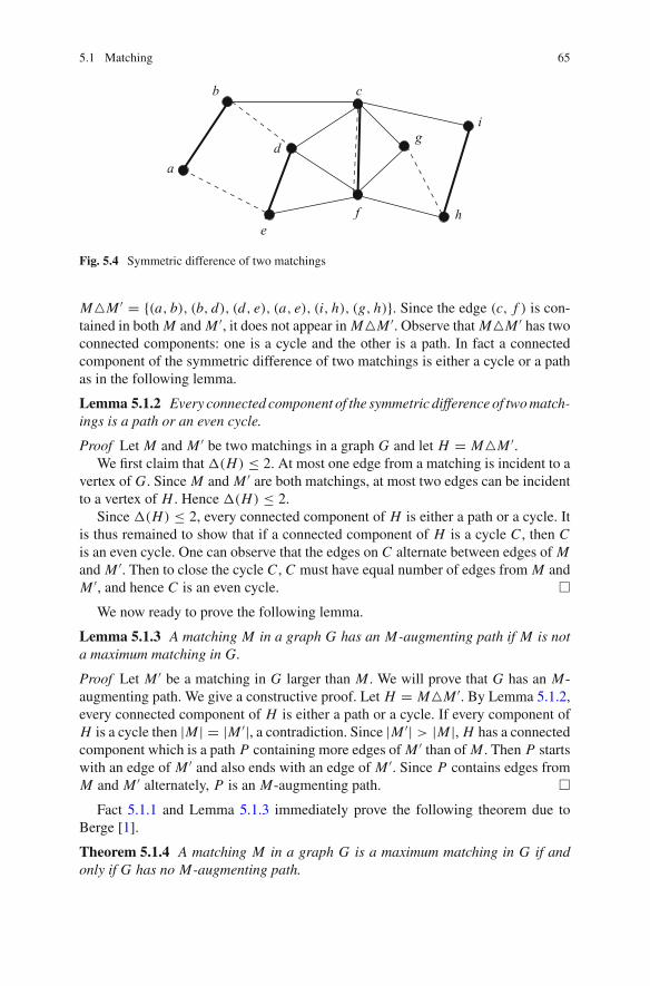
5.1 Matching 65
a
b c
d
ef
g
h
i
Fig. 5.4 Symmetric difference of two matchings
M�M ′ = {(a, b), (b, d), (d, e), (a, e), (i, h), (g, h)}. Since the edge (c, f ) is con-tained in both M and M ′, it does not appear in M�M ′. Observe that M�M ′ has twoconnected components: one is a cycle and the other is a path. In fact a connectedcomponent of the symmetric difference of two matchings is either a cycle or a pathas in the following lemma.
Lemma 5.1.2 Every connected component of the symmetric difference of twomatch-ings is a path or an even cycle.
Proof Let M and M ′ be two matchings in a graph G and let H = M�M ′.We first claim that �(H) ≤ 2. At most one edge from a matching is incident to a
vertex of G. Since M and M ′ are both matchings, at most two edges can be incidentto a vertex of H . Hence �(H) ≤ 2.
Since �(H) ≤ 2, every connected component of H is either a path or a cycle. Itis thus remained to show that if a connected component of H is a cycle C , then Cis an even cycle. One can observe that the edges on C alternate between edges of Mand M ′. Then to close the cycle C , C must have equal number of edges from M andM ′, and hence C is an even cycle. �
We now ready to prove the following lemma.
Lemma 5.1.3 A matching M in a graph G has an M-augmenting path if M is nota maximum matching in G.
Proof Let M ′ be a matching in G larger than M . We will prove that G has an M-augmenting path. We give a constructive proof. Let H = M�M ′. By Lemma 5.1.2,every connected component of H is either a path or a cycle. If every component ofH is a cycle then |M | = |M ′|, a contradiction. Since |M ′| > |M |, H has a connectedcomponent which is a path P containing more edges of M ′ than of M . Then P startswith an edge of M ′ and also ends with an edge of M ′. Since P contains edges fromM and M ′ alternately, P is an M-augmenting path. �
Fact 5.1.1 and Lemma 5.1.3 immediately prove the following theorem due toBerge [1].
Theorem 5.1.4 A matching M in a graph G is a maximum matching in G if andonly if G has no M-augmenting path.
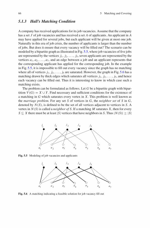
66 5 Matching and Covering
5.1.3 Hall’s Matching Condition
A company has received applications for its job vacancies. Assume that the companyhas a set J of job vacancies and has received a set A of applicants. An applicant in Amay have applied for several jobs, but each applicant will be given at most one job.Naturally in this era of job crisis, the number of applicants is larger than the numberof jobs. But does it ensure that every vacancy will be filled out? The scenario can bemodeled by a bipartite graph as illustrated in Fig. 5.5, where job vacancies of five jobsare represented by the vertices j1, j2, . . . , j5, seven applicants are represented by thevertices a1, a2, . . . , a7, and an edge between a job and an applicant represents thatthe corresponding applicant has applied for the corresponding job. In the examplein Fig. 5.5, it is impossible to fill out every vacancy since the graph has no matchingwhere all of vertices j1, j2, . . . , j5 are saturated. However, the graph in Fig. 5.6 has amatching drawn by thick edges which saturates all vertices j1, j2, . . . , j5, and henceeach vacancy can be filled out. Thus it is interesting to know in which case such amatching exists.
The problem can be formulated as follows. Let G be a bipartite graph with bipar-tition V (G) = X ∪ Y . Find necessary and sufficient conditions for the existence ofa matching in G which saturates every vertex in X . This problem is well known asthe marriage problem. For any set S of vertices in G, the neighbor set of S in G,denoted by N (S), is defined to be the set of all vertices adjacent to vertices in S. Avertex in N (S) is called a neighbor of S. If a matching M saturates X , then for everyS ⊆ X there must be at least |S| vertices that have neighbors in S. Thus |N (S)| ≥ |S|
a a a a a a a1 2 3 4 5 6 7
j1
j j j j2 3 4 5
Fig. 5.5 Modeling of job vacancies and applicants
a a a a a a a1 2 3 4 5 6 7
j1
j j j j2 3 4 5
Fig. 5.6 A matching indicating a feasible solution for job vacancy fill out
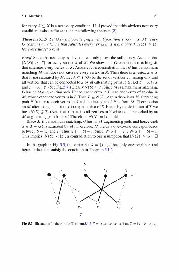
5.1 Matching 67
for every S ⊆ X is a necessary condition. Hall proved that this obvious necessarycondition is also sufficient as in the following theorem [2].
Theorem 5.1.5 Let G be a bipartite graph with bipartition V (G) = X ∪ Y . ThenG contains a matching that saturates every vertex in X if and only if |N (S)| ≥ |S|for every subset S of X.
Proof Since the necessity is obvious, we only prove the sufficiency. Assume that|N (S)| ≥ |S| for every subset S of X . We show that G contains a matching Mthat saturates every vertex in X . Assume for a contradiction that G has a maximummatching M that does not saturate every vertex in X . Then there is a vertex x ∈ Xthat is not saturated by M . Let A ⊆ V (G) be the set of vertices consisting of x andall vertices that can be connected to x by M-alternating paths in G. Let S = A ∩ Xand T = A∩Y . (See Fig. 5.7.) Clearly N (S) ⊆ Y . Since M is a maximummatching,G has no M-augmenting path. Hence, each vertex in T is an end vertex of an edge inM , whose other end vertex is in S. Then T ⊆ N (S). Again there is an M-alternatingpath P from x to each vertex in S and the last edge of P is from M . There is alsoan M-alternating path from x to any neighbor of S. Hence by the definition of T wehave N (S) ⊆ T . (Note that T contains all vertices in Y which can be reached by anM-augmenting path from x .) Therefore |N (S)| = |T | holds.
Since M is a maximum matching, G has no M-augmenting path, and hence eacha ∈ A − {x} is saturated by M . Therefore, M yields a one-to-one correspondencebetween S − {x} and T . Thus |T | = |S| − 1. Since |N (S)| = |T |, |N (S)| = |S| − 1.This implies |N (S)| < |S|, a contradiction to our assumption that |N (S)| ≥ |S|. �
In the graph in Fig. 5.5, the vertex set S = { j1, j4} has only one neighbor, andhence it does not satisfy the condition in Theorem 5.1.5.
1 2 3 4
1 2 3 4xX
Yy y y y
x x xx
S
T
Fig. 5.7 Illustration for the proof ofTheorem5.1.5; S = {x, x1, x2, x3, x4} and T = {y1, y2, y3, y4}
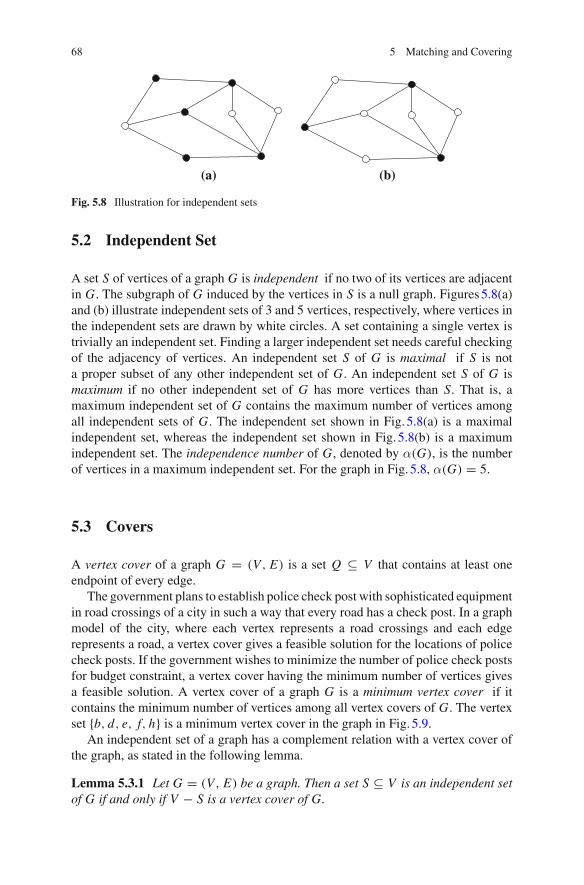
68 5 Matching and Covering
(b)(a)
Fig. 5.8 Illustration for independent sets
5.2 Independent Set
A set S of vertices of a graph G is independent if no two of its vertices are adjacentin G. The subgraph of G induced by the vertices in S is a null graph. Figures5.8(a)and (b) illustrate independent sets of 3 and 5 vertices, respectively, where vertices inthe independent sets are drawn by white circles. A set containing a single vertex istrivially an independent set. Finding a larger independent set needs careful checkingof the adjacency of vertices. An independent set S of G is maximal if S is nota proper subset of any other independent set of G. An independent set S of G ismaximum if no other independent set of G has more vertices than S. That is, amaximum independent set of G contains the maximum number of vertices amongall independent sets of G. The independent set shown in Fig. 5.8(a) is a maximalindependent set, whereas the independent set shown in Fig. 5.8(b) is a maximumindependent set. The independence number of G, denoted by α(G), is the numberof vertices in a maximum independent set. For the graph in Fig. 5.8, α(G) = 5.
5.3 Covers
A vertex cover of a graph G = (V, E) is a set Q ⊆ V that contains at least oneendpoint of every edge.
The government plans to establish police check post with sophisticated equipmentin road crossings of a city in such a way that every road has a check post. In a graphmodel of the city, where each vertex represents a road crossings and each edgerepresents a road, a vertex cover gives a feasible solution for the locations of policecheck posts. If the government wishes to minimize the number of police check postsfor budget constraint, a vertex cover having the minimum number of vertices givesa feasible solution. A vertex cover of a graph G is a minimum vertex cover if itcontains the minimum number of vertices among all vertex covers of G. The vertexset {b, d, e, f, h} is a minimum vertex cover in the graph in Fig. 5.9.
An independent set of a graph has a complement relation with a vertex cover ofthe graph, as stated in the following lemma.
Lemma 5.3.1 Let G = (V, E) be a graph. Then a set S ⊆ V is an independent setof G if and only if V − S is a vertex cover of G.
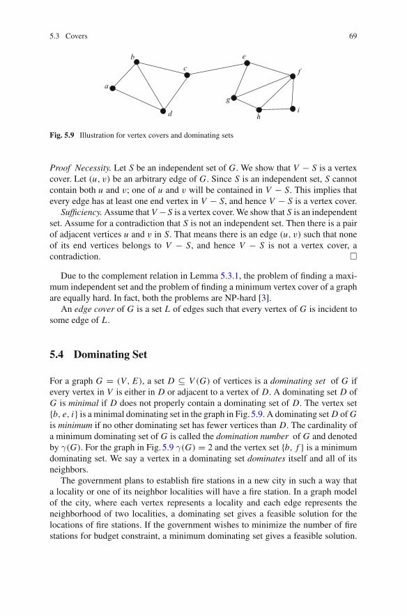
5.3 Covers 69
a
b
d
ce
g
hi
f
Fig. 5.9 Illustration for vertex covers and dominating sets
Proof Necessity. Let S be an independent set of G. We show that V − S is a vertexcover. Let (u, v) be an arbitrary edge of G. Since S is an independent set, S cannotcontain both u and v; one of u and v will be contained in V − S. This implies thatevery edge has at least one end vertex in V − S, and hence V − S is a vertex cover.
Sufficiency.Assume that V −S is a vertex cover.We show that S is an independentset. Assume for a contradiction that S is not an independent set. Then there is a pairof adjacent vertices u and v in S. That means there is an edge (u, v) such that noneof its end vertices belongs to V − S, and hence V − S is not a vertex cover, acontradiction. �
Due to the complement relation in Lemma 5.3.1, the problem of finding a maxi-mum independent set and the problem of finding a minimum vertex cover of a graphare equally hard. In fact, both the problems are NP-hard [3].
An edge cover of G is a set L of edges such that every vertex of G is incident tosome edge of L .
5.4 Dominating Set
For a graph G = (V, E), a set D ⊆ V (G) of vertices is a dominating set of G ifevery vertex in V is either in D or adjacent to a vertex of D. A dominating set D ofG is minimal if D does not properly contain a dominating set of D. The vertex set{b, e, i} is a minimal dominating set in the graph in Fig. 5.9. A dominating set D ofGis minimum if no other dominating set has fewer vertices than D. The cardinality ofa minimum dominating set of G is called the domination number of G and denotedby γ(G). For the graph in Fig. 5.9 γ(G) = 2 and the vertex set {b, f } is a minimumdominating set. We say a vertex in a dominating set dominates itself and all of itsneighbors.
The government plans to establish fire stations in a new city in such a way thata locality or one of its neighbor localities will have a fire station. In a graph modelof the city, where each vertex represents a locality and each edge represents theneighborhood of two localities, a dominating set gives a feasible solution for thelocations of fire stations. If the government wishes to minimize the number of firestations for budget constraint, a minimum dominating set gives a feasible solution.
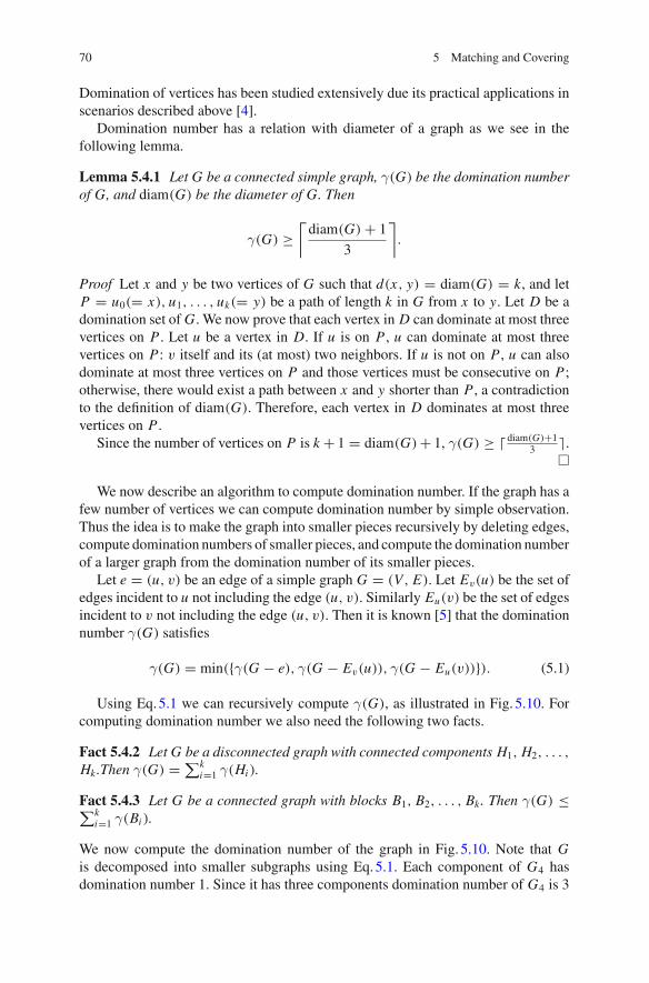
70 5 Matching and Covering
Domination of vertices has been studied extensively due its practical applications inscenarios described above [4].
Domination number has a relation with diameter of a graph as we see in thefollowing lemma.
Lemma 5.4.1 Let G be a connected simple graph, γ(G) be the domination numberof G, and diam(G) be the diameter of G. Then
γ(G) ≥⌈diam(G) + 1
3
⌉.
Proof Let x and y be two vertices of G such that d(x, y) = diam(G) = k, and letP = u0(= x), u1, . . . , uk(= y) be a path of length k in G from x to y. Let D be adomination set of G. We now prove that each vertex in D can dominate at most threevertices on P . Let u be a vertex in D. If u is on P , u can dominate at most threevertices on P: v itself and its (at most) two neighbors. If u is not on P , u can alsodominate at most three vertices on P and those vertices must be consecutive on P;otherwise, there would exist a path between x and y shorter than P , a contradictionto the definition of diam(G). Therefore, each vertex in D dominates at most threevertices on P .
Since the number of vertices on P is k + 1 = diam(G) + 1, γ(G) ≥ diam(G)+13 �.
�
We now describe an algorithm to compute domination number. If the graph has afew number of vertices we can compute domination number by simple observation.Thus the idea is to make the graph into smaller pieces recursively by deleting edges,compute domination numbers of smaller pieces, and compute the domination numberof a larger graph from the domination number of its smaller pieces.
Let e = (u, v) be an edge of a simple graph G = (V, E). Let Ev(u) be the set ofedges incident to u not including the edge (u, v). Similarly Eu(v) be the set of edgesincident to v not including the edge (u, v). Then it is known [5] that the dominationnumber γ(G) satisfies
γ(G) = min({γ(G − e), γ(G − Ev(u)), γ(G − Eu(v))}). (5.1)
Using Eq.5.1 we can recursively compute γ(G), as illustrated in Fig. 5.10. Forcomputing domination number we also need the following two facts.
Fact 5.4.2 Let G be a disconnected graph with connected components H1, H2, . . . ,
Hk.Then γ(G) = ∑ki=1 γ(Hi ).
Fact 5.4.3 Let G be a connected graph with blocks B1, B2, . . . , Bk. Then γ(G) ≤∑ki=1 γ(Bi ).
We now compute the domination number of the graph in Fig. 5.10. Note that Gis decomposed into smaller subgraphs using Eq.5.1. Each component of G4 hasdomination number 1. Since it has three components domination number of G4 is 3
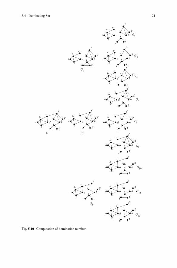
5.4 Dominating Set 71
G6ab
c
de
f
hg
jkl
i
G2
d
e
ab
cf
ghj
kl
ii
ab
c
ed
f
gh
kj
lG
G8ab
ed
cf
i ghj
kl
G9a
b
ed
cf
i ghj
kl
G10
f
gh
cb
ae
di
kj
l
G3
d
e
ab
cf
i gh
kj
l
f
G11ab
c
ed
i g
jkl
h
G12a
bc
f
de
i gh
kl
j
ab
ed
cf
hgi
l kj G7
e
ab
c
di
f
gh
kj
lG1
ab
c
ed
f
g
jkl
hi G5
ea
bc
d
f
g
l k
ihj
G4
Fig. 5.10 Computation of domination number
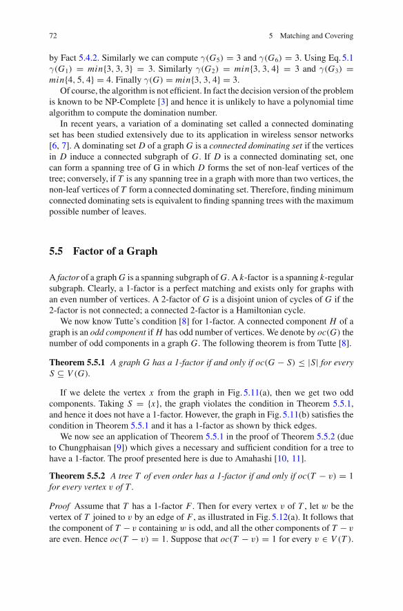
72 5 Matching and Covering
by Fact 5.4.2. Similarly we can compute γ(G5) = 3 and γ(G6) = 3. Using Eq.5.1γ(G1) = min{3, 3, 3} = 3. Similarly γ(G2) = min{3, 3, 4} = 3 and γ(G3) =min{4, 5, 4} = 4. Finally γ(G) = min{3, 3, 4} = 3.
Of course, the algorithm is not efficient. In fact the decision version of the problemis known to be NP-Complete [3] and hence it is unlikely to have a polynomial timealgorithm to compute the domination number.
In recent years, a variation of a dominating set called a connected dominatingset has been studied extensively due to its application in wireless sensor networks[6, 7]. A dominating set D of a graph G is a connected dominating set if the verticesin D induce a connected subgraph of G. If D is a connected dominating set, onecan form a spanning tree of G in which D forms the set of non-leaf vertices of thetree; conversely, if T is any spanning tree in a graph with more than two vertices, thenon-leaf vertices of T form a connected dominating set. Therefore, findingminimumconnected dominating sets is equivalent to finding spanning trees with the maximumpossible number of leaves.
5.5 Factor of a Graph
A factor of a graphG is a spanning subgraph ofG. A k-factor is a spanning k-regularsubgraph. Clearly, a 1-factor is a perfect matching and exists only for graphs withan even number of vertices. A 2-factor of G is a disjoint union of cycles of G if the2-factor is not connected; a connected 2-factor is a Hamiltonian cycle.
We now know Tutte’s condition [8] for 1-factor. A connected component H of agraph is an odd component if H has odd number of vertices. We denote by oc(G) thenumber of odd components in a graph G. The following theorem is from Tutte [8].
Theorem 5.5.1 A graph G has a 1-factor if and only if oc(G − S) ≤ |S| for everyS ⊆ V (G).
If we delete the vertex x from the graph in Fig. 5.11(a), then we get two oddcomponents. Taking S = {x}, the graph violates the condition in Theorem 5.5.1,and hence it does not have a 1-factor. However, the graph in Fig. 5.11(b) satisfies thecondition in Theorem 5.5.1 and it has a 1-factor as shown by thick edges.
We now see an application of Theorem 5.5.1 in the proof of Theorem 5.5.2 (dueto Chungphaisan [9]) which gives a necessary and sufficient condition for a tree tohave a 1-factor. The proof presented here is due to Amahashi [10, 11].
Theorem 5.5.2 A tree T of even order has a 1-factor if and only if oc(T − v) = 1for every vertex v of T .
Proof Assume that T has a 1-factor F . Then for every vertex v of T , let w be thevertex of T joined to v by an edge of F , as illustrated in Fig. 5.12(a). It follows thatthe component of T − v containing w is odd, and all the other components of T − v
are even. Hence oc(T − v) = 1. Suppose that oc(T − v) = 1 for every v ∈ V (T ).
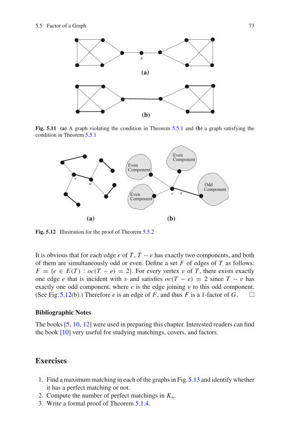
5.5 Factor of a Graph 73
(a)
(b)
x
Fig. 5.11 (a) A graph violating the condition in Theorem 5.5.1 and (b) a graph satisfying thecondition in Theorem 5.5.1
EvenComponent
EvenComponent
EvenComponent
OddComponent
(b)(a)
vw
v e
Fig. 5.12 Illustration for the proof of Theorem 5.5.2
It is obvious that for each edge e of T , T − e has exactly two components, and bothof them are simultaneously odd or even. Define a set F of edges of T as follows:F = {e ∈ E(T ) : oc(T − e) = 2}. For every vertex v of T , there exists exactlyone edge e that is incident with v and satisfies oc(T − e) = 2 since T − v hasexactly one odd component, where e is the edge joining v to this odd component.(See Fig. 5.12(b).) Therefore e is an edge of F , and thus F is a 1-factor of G. �
Bibliographic Notes
The books [5, 10, 12] were used in preparing this chapter. Interested readers can findthe book [10] very useful for studying matchings, covers, and factors.
Exercises
1. Find amaximummatching in each of the graphs in Fig.5.13 and identifywhetherit has a perfect matching or not.
2. Compute the number of perfect matchings in Kn .3. Write a formal proof of Theorem 5.1.4.
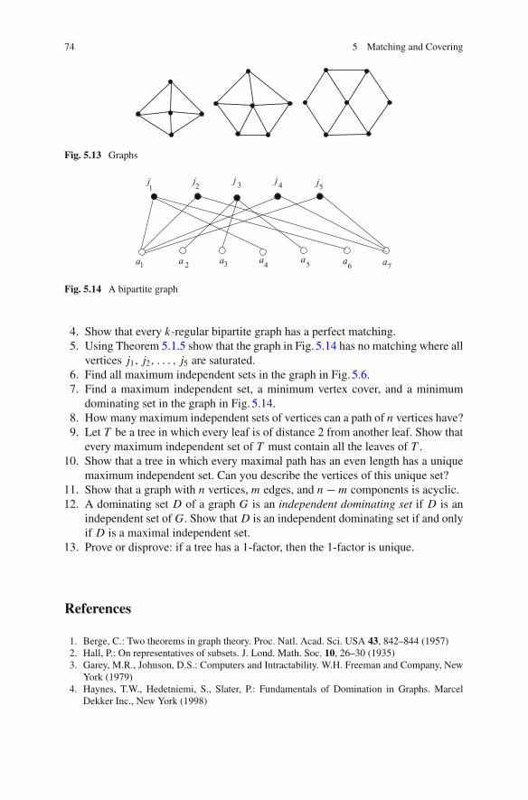
74 5 Matching and Covering
Fig. 5.13 Graphs
a a a a a a a1 2 3 4 5 6 7
j1
j j j j2 3 4 5
Fig. 5.14 A bipartite graph
4. Show that every k-regular bipartite graph has a perfect matching.5. Using Theorem 5.1.5 show that the graph in Fig. 5.14 has no matching where all
vertices j1, j2, . . . , j5 are saturated.6. Find all maximum independent sets in the graph in Fig. 5.6.7. Find a maximum independent set, a minimum vertex cover, and a minimum
dominating set in the graph in Fig. 5.14.8. How many maximum independent sets of vertices can a path of n vertices have?9. Let T be a tree in which every leaf is of distance 2 from another leaf. Show that
every maximum independent set of T must contain all the leaves of T .10. Show that a tree in which every maximal path has an even length has a unique
maximum independent set. Can you describe the vertices of this unique set?11. Show that a graph with n vertices, m edges, and n − m components is acyclic.12. A dominating set D of a graph G is an independent dominating set if D is an
independent set of G. Show that D is an independent dominating set if and onlyif D is a maximal independent set.
13. Prove or disprove: if a tree has a 1-factor, then the 1-factor is unique.
References
1. Berge, C.: Two theorems in graph theory. Proc. Natl. Acad. Sci. USA 43, 842–844 (1957)2. Hall, P.: On representatives of subsets. J. Lond. Math. Soc. 10, 26–30 (1935)3. Garey, M.R., Johnson, D.S.: Computers and Intractability. W.H. Freeman and Company, New
York (1979)4. Haynes, T.W., Hedetniemi, S., Slater, P.: Fundamentals of Domination in Graphs. Marcel
Dekker Inc., New York (1998)
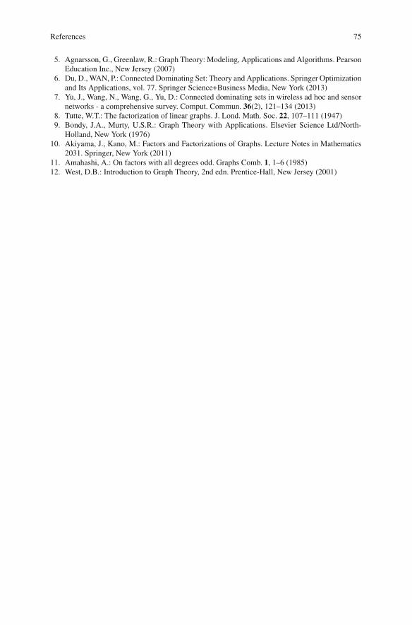
References 75
5. Agnarsson, G., Greenlaw, R.: Graph Theory: Modeling, Applications and Algorithms. PearsonEducation Inc., New Jersey (2007)
6. Du, D., WAN, P.: Connected Dominating Set: Theory and Applications. Springer Optimizationand Its Applications, vol. 77. Springer Science+Business Media, New York (2013)
7. Yu, J., Wang, N., Wang, G., Yu, D.: Connected dominating sets in wireless ad hoc and sensornetworks - a comprehensive survey. Comput. Commun. 36(2), 121–134 (2013)
8. Tutte, W.T.: The factorization of linear graphs. J. Lond. Math. Soc. 22, 107–111 (1947)9. Bondy, J.A., Murty, U.S.R.: Graph Theory with Applications. Elsevier Science Ltd/North-
Holland, New York (1976)10. Akiyama, J., Kano, M.: Factors and Factorizations of Graphs. Lecture Notes in Mathematics
2031. Springer, New York (2011)11. Amahashi, A.: On factors with all degrees odd. Graphs Comb. 1, 1–6 (1985)12. West, D.B.: Introduction to Graph Theory, 2nd edn. Prentice-Hall, New Jersey (2001)
Chapter 6Planar Graphs
6.1 Introduction
Consider a graph of six vertices and eight edges in Fig. 6.1(a) where some pairs ofedges cross each other. Is it possible to redraw the graph in such a way that there is noedge crossing in the drawing? Yes, it is possible to draw the graph without any edgecrossing as in Fig. 6.1(b). However, it is not possible to redraw the graph in Fig. 6.1(c)such that there is no edge crossing in the drawing. A graph is planar if it can be drawnor embedded in the plane so that no two edges intersect geometrically except at avertex to which they are both incident. The graph in Fig. 6.1(a) is a planar graphsince it has a planar embedding as in Fig. 6.1(b), whereas the graph in Fig. 6.1(c) isa nonplanar graph.
6.2 Characterization of Planar Graphs
Since not all graphs are planar, it is sometimes necessary to know whether a givengraph is planar or not. Consider the graph K5 in Fig. 6.2(a). Is it planar? We canproceed with simple observation as follows. Let p, q, r, s, and t be the five verticesof K5. There is a cycle C = p, q, r, s, t containing all the vertices of K5. We drawthe cycle as a pentagon as illustrated in Fig. 6.2(b). We can draw pr either inside thecycle C or outside C . We draw the edge (p, r) inside C , the other case is similar.Since (q, s) and (q, t) cross (p, r) if we draw them inside C , we must draw themoutside C . Since (p, s) cannot cross (q, t), we must draw (p, s) inside C . Now wecan draw (r, t) neither inside nor outside C without edge crossing. So K5 cannot bedrawn without edge crossings, and hence K5 is not a planar graph. Using a similarargument we can observe that K3,3 is also nonplanar. It is interesting that based onthis two forbidden graphs, Kuratowski gave a complete characterization of planargraphs as in the following theorem.
© Springer International Publishing AG 2017M.S. Rahman, Basic Graph Theory, Undergraduate Topics in Computer Science,DOI 10.1007/978-3-319-49475-3_6
77
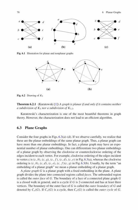
78 6 Planar Graphs
a
b
c
d
e
f
a
f
d
b
ec
a
b
c
d
e
f
(a) (b) (c)
Fig. 6.1 Illustration for planar and nonplanar graphs
t
p
q
rs
t
p
q
rs
(a) (b)
Fig. 6.2 Drawing of K5
Theorem 6.2.1 (Kuratowski [1]) A graph is planar if and only if it contains neithera subdivision of K5 nor a subdivision of K3,3.
Kuratowski’s characterization is one of the most beautiful theorems in graphtheory. However, the characterization does not lead to an efficient algorithm.
6.3 Plane Graphs
Consider the four graphs in Figs. 6.3(a)–(d). If we observe carefully, we realize thatthese are the planar embeddings of the same planar graph. Thus, a planar graph canhave more than one planar embeddings. In fact, a planar graph may have an expo-nential number of planar embeddings. One can differentiate two planar embeddingsof a planar graph by observing the clockwise or counterclockwise ordering of theedges incident to each vertex. For example, clockwise ordering of the edges incidentto vertex c is (c, b), (c, g), (c, f ), (c, d), (c, e) in Fig. 6.3(a), whereas the clockwiseordering is (c, b), (c, d), (c, e), (c, f )(c, g) in Fig. 6.3(b). Usually, by the term “anembedding of a planar graph” we mean a planar embedding of a planar graph.
A plane graph G is a planar graph with a fixed embedding in the plane. A planegraph divides the plane into connected regions called faces. The unbounded regionis called the outer face of G. The boundary of a face of a connected plane graph Gis a closed walk in general, and is a cycle if G is 2-connected and has at least threevertices. The boundary of the outer face of G is called the outer boundary of G anddenoted by Co(G). If Co(G) is a cycle, then Co(G) is called the outer cycle of G.
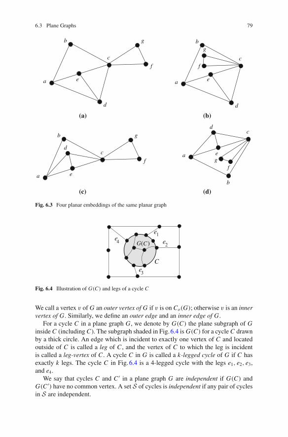
6.3 Plane Graphs 79
d
gb
a
c
f
e
gb
a
c
f
e
da
c
e
d
gf
b
d
b
a
c
g
f
e
(a) (b)
(d)(c)
Fig. 6.3 Four planar embeddings of the same planar graph
e2
e3
e4
e1
C
G( )C
Fig. 6.4 Illustration of G(C) and legs of a cycle C
We call a vertex v of G an outer vertex of G if v is on Co(G); otherwise v is an innervertex of G. Similarly, we define an outer edge and an inner edge of G.
For a cycle C in a plane graph G, we denote by G(C) the plane subgraph of Ginside C (including C). The subgraph shaded in Fig. 6.4 is G(C) for a cycle C drawnby a thick circle. An edge which is incident to exactly one vertex of C and locatedoutside of C is called a leg of C , and the vertex of C to which the leg is incidentis called a leg-vertex of C . A cycle C in G is called a k-legged cycle of G if C hasexactly k legs. The cycle C in Fig. 6.4 is a 4-legged cycle with the legs e1, e2, e3,and e4.
We say that cycles C and C ′ in a plane graph G are independent if G(C) andG(C ′) have no common vertex. A set S of cycles is independent if any pair of cyclesin S are independent.
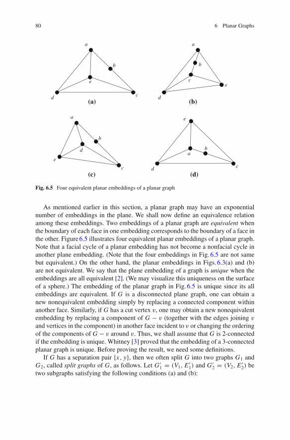
80 6 Planar Graphs
a
b
cd
e
a
b
c
e
d
cd
e
ab
a
d
e
b
c
(a) (b)
(d)(c)
Fig. 6.5 Four equivalent planar embeddings of a planar graph
As mentioned earlier in this section, a planar graph may have an exponentialnumber of embeddings in the plane. We shall now define an equivalence relationamong these embeddings. Two embeddings of a planar graph are equivalent whenthe boundary of each face in one embedding corresponds to the boundary of a face inthe other. Figure6.5 illustrates four equivalent planar embeddings of a planar graph.Note that a facial cycle of a planar embedding has not become a nonfacial cycle inanother plane embedding. (Note that the four embeddings in Fig. 6.5 are not samebut equivalent.) On the other hand, the planar embeddings in Figs. 6.3(a) and (b)are not equivalent. We say that the plane embedding of a graph is unique when theembeddings are all equivalent [2]. (We may visualize this uniqueness on the surfaceof a sphere.) The embedding of the planar graph in Fig. 6.5 is unique since its allembeddings are equivalent. If G is a disconnected plane graph, one can obtain anew nonequivalent embedding simply by replacing a connected component withinanother face. Similarly, if G has a cut vertex v, one may obtain a new nonequivalentembedding by replacing a component of G − v (together with the edges joining v
and vertices in the component) in another face incident to v or changing the orderingof the components of G − v around v. Thus, we shall assume that G is 2-connectedif the embedding is unique. Whitney [3] proved that the embedding of a 3-connectedplanar graph is unique. Before proving the result, we need some definitions.
If G has a separation pair {x, y}, then we often split G into two graphs G1 andG2, called split graphs of G, as follows. Let G ′
1 = (V1, E ′1) and G ′
2 = (V2, E ′2) be
two subgraphs satisfying the following conditions (a) and (b):
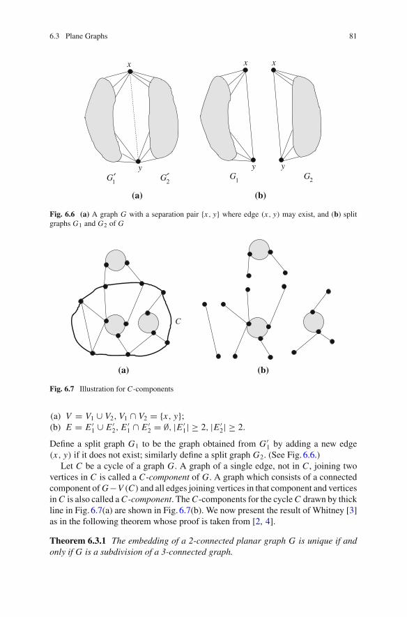
6.3 Plane Graphs 81
(a) (b)
x xx
y y yG G G G1 2 1 2
Fig. 6.6 (a) A graph G with a separation pair {x, y} where edge (x, y) may exist, and (b) splitgraphs G1 and G2 of G
C
(a) (b)
Fig. 6.7 Illustration for C-components
(a) V = V1 ∪ V2, V1 ∩ V2 = {x, y};(b) E = E ′
1 ∪ E ′2, E
′1 ∩ E ′
2 = ∅, |E ′1| ≥ 2, |E ′
2| ≥ 2.
Define a split graph G1 to be the graph obtained from G ′1 by adding a new edge
(x, y) if it does not exist; similarly define a split graph G2. (See Fig. 6.6.)Let C be a cycle of a graph G. A graph of a single edge, not in C , joining two
vertices in C is called a C-component of G. A graph which consists of a connectedcomponent ofG−V (C) and all edges joining vertices in that component and verticesinC is also called aC-component. TheC-components for the cycleC drawn by thickline in Fig. 6.7(a) are shown in Fig. 6.7(b). We now present the result of Whitney [3]as in the following theorem whose proof is taken from [2, 4].
Theorem 6.3.1 The embedding of a 2-connected planar graph G is unique if andonly if G is a subdivision of a 3-connected graph.
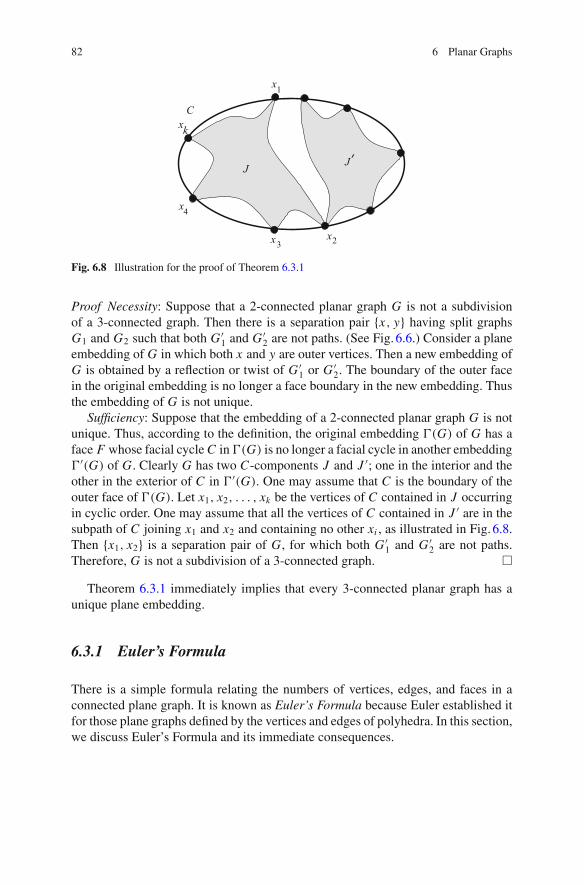
82 6 Planar Graphs
Fig. 6.8 Illustration for the proof of Theorem 6.3.1
Proof Necessity: Suppose that a 2-connected planar graph G is not a subdivisionof a 3-connected graph. Then there is a separation pair {x, y} having split graphsG1 and G2 such that both G ′
1 and G ′2 are not paths. (See Fig. 6.6.) Consider a plane
embedding of G in which both x and y are outer vertices. Then a new embedding ofG is obtained by a reflection or twist of G ′
1 or G′2. The boundary of the outer face
in the original embedding is no longer a face boundary in the new embedding. Thusthe embedding of G is not unique.
Sufficiency: Suppose that the embedding of a 2-connected planar graph G is notunique. Thus, according to the definition, the original embedding �(G) of G has aface F whose facial cycleC in�(G) is no longer a facial cycle in another embedding�′(G) of G. Clearly G has two C-components J and J ′; one in the interior and theother in the exterior of C in �′(G). One may assume that C is the boundary of theouter face of �(G). Let x1, x2, . . . , xk be the vertices of C contained in J occurringin cyclic order. One may assume that all the vertices of C contained in J ′ are in thesubpath of C joining x1 and x2 and containing no other xi , as illustrated in Fig. 6.8.Then {x1, x2} is a separation pair of G, for which both G ′
1 and G ′2 are not paths.
Therefore, G is not a subdivision of a 3-connected graph. �
Theorem 6.3.1 immediately implies that every 3-connected planar graph has aunique plane embedding.
6.3.1 Euler’s Formula
There is a simple formula relating the numbers of vertices, edges, and faces in aconnected plane graph. It is known as Euler’s Formula because Euler established itfor those plane graphs defined by the vertices and edges of polyhedra. In this section,we discuss Euler’s Formula and its immediate consequences.
6.3 Plane Graphs 83
Theorem 6.3.2 (Euler 1750) Let G be a connected plane graph, and let n, m,and f denote, respectively, the numbers of vertices, edges, and faces of G. Thenn − m + f = 2.
Proof We employ an induction on m, the result being obvious for m = 0 or 1.Assume that m ≥ 2 and the result is true for all connected plane graphs havingfewer than m edges, and suppose that G has m edges. Consider first the case Gis a tree. Then G has a vertex v of degree one. The connected plane graph G − v
has n − 1 vertices, m − 1 edges and f (=1) faces, so by the inductive hypothesis,(n − 1) − (m − 1) + f = 2, which implies that n − m + f = 2. Consider nextthe case when G is not a tree. Then G has an edge e on a cycle. In this case, theconnected plane graph G − e has n vertices, m − 1 edges, and f − 1 faces, so thatthe desired formula immediately follows from the inductive hypothesis. �
A maximal planar graph is one to which no edge can be added without losingplanarity. Thus in any embedding of a maximal planar graph G with n ≥ 3, theboundary of every face of G is a triangle, and hence the embedding is often calleda triangulated plane graph. Although a general graph may have up to n(n − 1)/2edges, it is not true for planar graphs.
Corollary 6.3.3 If G is a planar graph with n(≥3) vertices and m edges, thenm ≤ 3n − 6. Moreover the equality holds if G is maximal planar.
Proof We can assume without loss of generality that G is a maximal planar graph;otherwise add new edges without increasing n so that the resulting graph is maximalplanar. Consider a plane embedding of G. Every face is bounded by exactly threeedges, and each edge is on the boundaries of two faces. Therefore, counting up theedges around each face, we have 3 f = 2m. Applying Theorem 6.3.2, we obtainm = 3n − 6. �Corollary 6.3.4 Let G be a planar graph. Then G has a vertex of degree at most 5.
Proof The claim is trivially true for planar graph of six or less vertices. We thusconsider the case where G has more than six vertices. Assume that each vertex of Ghas degree at least 6. Then 6n ≤ 2m holds for G. This implies 3n ≤ m. By Corol-lary 6.3.3, m ≤ 3n − 6. Thus 3n ≤ 3n − 6 would hold, which is a contradiction. �
In fact, every planar graph of four or more vertices has at least four vertices ofdegree five or less as stated in the following lemma.
Lemma 6.3.5 Every maximal planar graph of four or more vertices has at leastfour vertices of degree five or less.
Proof By Euler’s Formula, every maximal planar graph G has 3n − 6 edges. Hencethe degree-sum for G is 6n − 12. Let v be a vertex of G. We define the deficiencyfor v by 6 − d(v). Then the total deficiency of the vertices of G is 12. Since Gis maximal planar and any embedding of G is triangulated, G is triconnected, andhence the degree of a vertex of G is at least 3. Then the deficiency of a vertex is atmost 3. Since the total deficiency is 12, there are at least four vertices of degree fiveor less. �
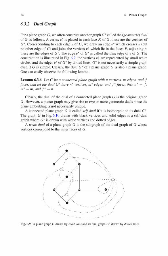
84 6 Planar Graphs
6.3.2 Dual Graph
For a plane graphG, we often construct another graphG∗ called the (geometric) dualof G as follows. A vertex v∗
i is placed in each face Fi of G; these are the vertices ofG∗. Corresponding to each edge e of G, we draw an edge e∗ which crosses e (butno other edge of G) and joins the vertices v∗
i which lie in the faces Fi adjoining e;these are the edges of G∗. The edge e∗ of G∗ is called the dual edge of e of G. Theconstruction is illustrated in Fig. 6.9; the vertices v∗
i are represented by small whitecircles, and the edges e∗ of G∗ by dotted lines. G∗ is not necessarily a simple grapheven if G is simple. Clearly, the dual G∗ of a plane graph G is also a plane graph.One can easily observe the following lemma.
Lemma 6.3.6 Let G be a connected plane graph with n vertices, m edges, and ffaces, and let the dual G∗ have n∗ vertices, m∗ edges, and f ∗ faces, then n∗ = f ,m∗ = m, and f ∗ = n.
Clearly, the dual of the dual of a connected plane graph G is the original graphG. However, a planar graph may give rise to two or more geometric duals since theplane embedding is not necessarily unique.
A connected plane graph G is called self-dual if it is isomorphic to its dual G∗.The graph G in Fig. 6.10 drawn with black vertices and solid edges is a self-dualgraph where G∗ is drawn with white vertices and dotted edges.
A weak dual of a plane graph G is the subgraph of the dual graph of G whosevertices correspond to the inner faces of G.
Fig. 6.9 A plane graph G drawn by solid lines and its dual graph G∗ drawn by dotted lines
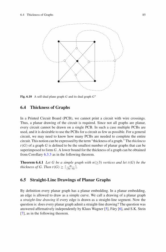
6.4 Thickness of Graphs 85
Fig. 6.10 A self-dual plane graph G and its dual graph G∗
6.4 Thickness of Graphs
In a Printed Circuit Board (PCB), we cannot print a circuit with wire crossings.Thus, a planar drawing of the circuit is required. Since not all graphs are planar,every circuit cannot be drawn on a single PCB. In such a case multiple PCBs areused, and it is desirable to use the PCBs for a circuit as few as possible. For a generalcircuit, we may need to know how many PCBs are needed to complete the entirecircuit. This notion can be expressed by the term “thickness of a graph.” The thicknesst (G) of a graph G is defined to be the smallest number of planar graphs that can besuperimposed to form G. A lower bound for the thickness of a graph can be obtainedfrom Corollary 6.3.3 as in the following theorem.
Theorem 6.4.1 Let G be a simple graph with n(≥3) vertices and let t (G) be thethickness of G. Then t (G) ≥ m
(3n−6).
6.5 Straight-Line Drawings of Planar Graphs
By definition every planar graph has a planar embedding. In a planar embedding,an edge is allowed to draw as a simple curve. We call a drawing of a planar grapha straight-line drawing if every edge is drawn as a straight-line segment. Now thequestion is: does every planar graph admit a straight-line drawing? The question wasanswered affirmatively independently by Klaus Wagner [5], Fáry [6], and S.K. Stein[7], as in the following theorem.
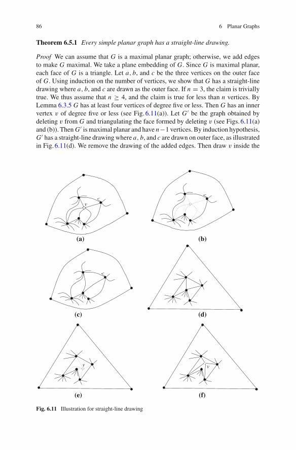
86 6 Planar Graphs
Theorem 6.5.1 Every simple planar graph has a straight-line drawing.
Proof We can assume that G is a maximal planar graph; otherwise, we add edgesto make G maximal. We take a plane embedding of G. Since G is maximal planar,each face of G is a triangle. Let a, b, and c be the three vertices on the outer faceof G. Using induction on the number of vertices, we show that G has a straight-linedrawing where a, b, and c are drawn as the outer face. If n = 3, the claim is triviallytrue. We thus assume that n ≥ 4, and the claim is true for less than n vertices. ByLemma 6.3.5 G has at least four vertices of degree five or less. Then G has an innervertex v of degree five or less (see Fig. 6.11(a)). Let G ′ be the graph obtained bydeleting v from G and triangulating the face formed by deleting v (see Figs. 6.11(a)and (b)). ThenG ′ is maximal planar and have n−1 vertices. By induction hypothesis,G ′ has a straight-line drawing where a, b, and c are drawn on outer face, as illustratedin Fig. 6.11(d). We remove the drawing of the added edges. Then draw v inside the
(a)
v
(c)
(e)
v
(b)
(d)
v
(f)
Fig. 6.11 Illustration for straight-line drawing
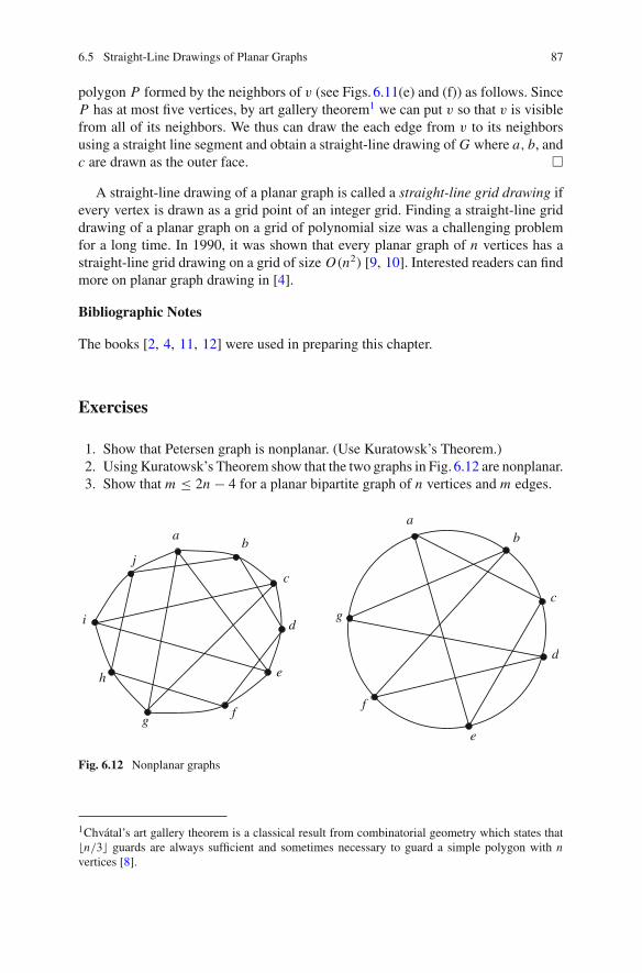
6.5 Straight-Line Drawings of Planar Graphs 87
polygon P formed by the neighbors of v (see Figs. 6.11(e) and (f)) as follows. SinceP has at most five vertices, by art gallery theorem1 we can put v so that v is visiblefrom all of its neighbors. We thus can draw the each edge from v to its neighborsusing a straight line segment and obtain a straight-line drawing of G where a, b, andc are drawn as the outer face. �
A straight-line drawing of a planar graph is called a straight-line grid drawing ifevery vertex is drawn as a grid point of an integer grid. Finding a straight-line griddrawing of a planar graph on a grid of polynomial size was a challenging problemfor a long time. In 1990, it was shown that every planar graph of n vertices has astraight-line grid drawing on a grid of size O(n2) [9, 10]. Interested readers can findmore on planar graph drawing in [4].
Bibliographic Notes
The books [2, 4, 11, 12] were used in preparing this chapter.
Exercises
1. Show that Petersen graph is nonplanar. (Use Kuratowsk’s Theorem.)2. UsingKuratowsk’s Theorem show that the two graphs in Fig. 6.12 are nonplanar.3. Show that m ≤ 2n − 4 for a planar bipartite graph of n vertices and m edges.
i
j
ab
c
d
e
fg
h
ab
c
d
g
e
f
Fig. 6.12 Nonplanar graphs
1Chvátal’s art gallery theorem is a classical result from combinatorial geometry which states that�n/3� guards are always sufficient and sometimes necessary to guard a simple polygon with nvertices [8].
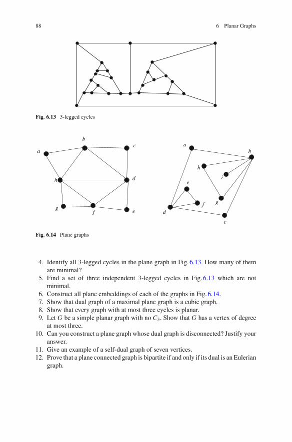
88 6 Planar Graphs
Fig. 6.13 3-legged cycles
a
bc
d
efg
h
ab
c
d
e
f g
h
i
Fig. 6.14 Plane graphs
4. Identify all 3-legged cycles in the plane graph in Fig. 6.13. How many of themare minimal?
5. Find a set of three independent 3-legged cycles in Fig. 6.13 which are notminimal.
6. Construct all plane embeddings of each of the graphs in Fig. 6.14.7. Show that dual graph of a maximal plane graph is a cubic graph.8. Show that every graph with at most three cycles is planar.9. Let G be a simple planar graph with no C3. Show that G has a vertex of degree
at most three.10. Can you construct a plane graph whose dual graph is disconnected? Justify your
answer.11. Give an example of a self-dual graph of seven vertices.12. Prove that a plane connected graph is bipartite if and only if its dual is an Eulerian
graph.
References 89
References
1. Kuratowski, K.: Sur le probleme des courbes gauches en topologie. Fund. Math. 15, 271–283(1930)
2. Nishizeki, T., Chiba, N.: Planar Graphs: Theory and Algorithms. North-Holland, Amsterdam(1988)
3. Whitney, H.: 2-isomorphic graphs. Amer. J. Math. 55, 245–254 (1933)4. Nishizeki, T., Rahman, M.S.: Planar Graph Drawing. World Scientific, Singapore (2004)5. Wagnar, K.: Bemerkungen zum vierfarbenproblem. Jahresbericht der Deutschen
Mathematiker-Vereinigung 46, 26–32 (1936)6. Fary, I.: On straight-line representation of planar graphs. Acta. Sci. Math. 11, 229–233 (1948)7. Stein, S.K.: Convex maps. Proc. of American Math. Society 2(3), 464–466 (1951)8. Chvátal, V.: A combinatorial theorem in plane geometry. J. Combin, Theory Ser. B 18, 39–41
(1975)9. de Fraysseix, H., Pach, J., Pollack, R.: How to draw a planar graph on a grid. Combinatorica
10, 41–51 (1990)10. Schnyder, W.: Embedding planar graphs on the grid. In: Proceedings of First ACM-SIAM
Symposium on Discrete Algorithms, San Francisco, pp. 138–148 (1990)11. Wilson, R.J.: Introduction to Graph Theory, 4th edn. Longman, London (1996)12. Clark, J., Holton, D.A.: A First Look at Graph Theory. World Scientific, Singapore (1991)
Chapter 7Graph Coloring
7.1 Introduction
Probably graph coloring concept naturally arose from its application inmap coloring:given amap containing several countries, we wish to color the countries in the map insuch a way that neighboring countries receive different colors to make the countriesdistinct. A map can be treated as a planar graph, and hence the problem was thoughton graphs. In addition to map coloring, coloring graphs has found its applicationsin many other areas and has become an active area of research in graph theory formany years.
7.2 Vertex Coloring
A vertex coloring of a graph is an assignment of colors to the vertices so that adja-cent vertices have distinct colors. A k-coloring of a graph uses at most k colors.A 5-coloring of a graph is illustrated in Fig. 7.1(a), where positive integer designatecolors. The vertex coloring of graph in Fig. 7.1(a) is not optimal since there is anothervertex coloring of the graph with three colors as illustrated in Fig. 7.1(b). The small-est integer k such that a graph G has a k-coloring is called the chromatic numberof G and is denoted by χ(G). If χ(G) = k, the graph G is said to be k-chromatic.Since the graph G in Fig. 7.1(a) has a triangle, one can observe that G cannot havea vertex coloring with less than three colors, and hence χ(G) = 3 for the graph inFig. 7.1(a). It is clear that χ(Kn) = n. On the other hand, if G is a null graph thenχ(G) = 1. Every bipartite graph is 2-chromatic since to color the vertices in an inde-pendent set, we need only one color. Since a tree is a bipartite graph, every treeis 2-chromatic. The definition of k-coloring implies that the k-coloring of a graphG = (V, E) partitions the vertex set V into k independent set V1, V2, . . . , Vk suchthat V = V1 ∪ V2 ∪ . . . Vk . The independent sets V1, V2, . . . , Vk are called the color
© Springer International Publishing AG 2017M.S. Rahman, Basic Graph Theory, Undergraduate Topics in Computer Science,DOI 10.1007/978-3-319-49475-3_7
91
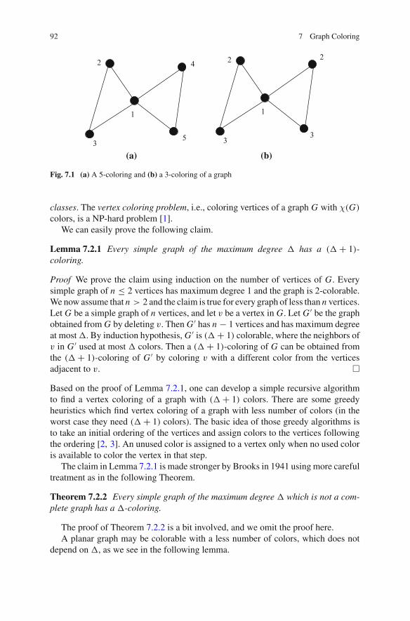
92 7 Graph Coloring
1
2
3
4
5
1
2
3
2
3
(b)(a)
Fig. 7.1 (a) A 5-coloring and (b) a 3-coloring of a graph
classes. The vertex coloring problem, i.e., coloring vertices of a graph G with χ(G)
colors, is a NP-hard problem [1].We can easily prove the following claim.
Lemma 7.2.1 Every simple graph of the maximum degree � has a (� + 1)-coloring.
Proof We prove the claim using induction on the number of vertices of G. Everysimple graph of n ≤ 2 vertices has maximum degree 1 and the graph is 2-colorable.We now assume that n > 2 and the claim is true for every graph of less than n vertices.Let G be a simple graph of n vertices, and let v be a vertex in G. Let G ′ be the graphobtained from G by deleting v. Then G ′ has n − 1 vertices and has maximum degreeat most�. By induction hypothesis, G ′ is (� + 1) colorable, where the neighbors ofv in G ′ used at most � colors. Then a (� + 1)-coloring of G can be obtained fromthe (� + 1)-coloring of G ′ by coloring v with a different color from the verticesadjacent to v. �
Based on the proof of Lemma 7.2.1, one can develop a simple recursive algorithmto find a vertex coloring of a graph with (� + 1) colors. There are some greedyheuristics which find vertex coloring of a graph with less number of colors (in theworst case they need (� + 1) colors). The basic idea of those greedy algorithms isto take an initial ordering of the vertices and assign colors to the vertices followingthe ordering [2, 3]. An unused color is assigned to a vertex only when no used coloris available to color the vertex in that step.
The claim in Lemma 7.2.1 is made stronger by Brooks in 1941 using more carefultreatment as in the following Theorem.
Theorem 7.2.2 Every simple graph of the maximum degree � which is not a com-plete graph has a �-coloring.
The proof of Theorem 7.2.2 is a bit involved, and we omit the proof here.A planar graph may be colorable with a less number of colors, which does not
depend on �, as we see in the following lemma.
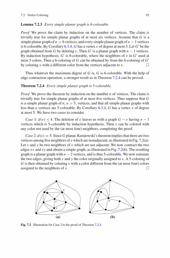
7.2 Vertex Coloring 93
Lemma 7.2.3 Every simple planar graph is 6-colorable.
Proof We prove the claim by induction on the number of vertices. The claim istrivially true for simple planar graphs of at most six vertices. Assume that G is asimple planar graph of n > 6 vertices, and every simple planar graph of n − 1 verticesis 6-colorable. By Corollary 6.3.4,G has a vertex v of degree at most 5. Let G ′ be thegraph obtained from G by deleting v. Then G ′ is a planar graph with n − 1 vertices.By induction hypothesis, G ′ is 6-colorable, where the neighbors of v in G ′ used atmost 5 colors. Then a 6-coloring of G can be obtained by from the 6-coloring of G ′by coloring v with a different color from the vertices adjacent to v. �
Thus whatever the maximum degree of G is, G is 6-colorable. With the help ofedge contraction operation, a stronger result as in Theorem 7.2.4 can be proved.
Theorem 7.2.4 Every simple planar graph is 5-colorable.
Proof We prove the theorem by induction on the number n of vertices. The claim istrivially true for simple planar graphs of at most five vertices. Thus suppose that Gis a simple planar graph of n, n > 5, vertices, and that all simple planar graphs withless than n vertices are 5-colorable. By Corollary 6.3.4, G has a vertex v of degreeat most 5. We have two cases to consider.
Case 1: d(v) ≤ 4. The deletion of v leaves us with a graph G − v having n − 1vertices which is 5-colorable by induction hypothesis. Then v can be colored withany color not used by the (at most four) neighbors, completing the proof.
Case 2: d(v) = 5. SinceG planar, Kuratowski’s theorem implies that there are twovertices among five neighbors of vwhich are nonadjacent, as illustrated in Fig. 7.2(a).Let x and y be two neighbors of v which are not adjacent. We now contract the twoedges vx and vy and obtain a simple graph, as illustrated in Fig. 7.2(b). The resultinggraph is a planar graph with n − 2 vertices, and is thus 5-colorable. We now reinstatethe two edges, giving both x and y the color originally assigned to v. A 5-coloring ofG is then obtained by coloring v with a color different from the (at most four) colorsassigned to the neighbors of v. �
(b)(a)
x
v
y
v
Fig. 7.2 Illustration for Case 2 in the proof of Theorem 7.2.4
94 7 Graph Coloring
Based on the proof of Theorem 7.2.4, one can easily design an O(n2) time recur-sive algorithm which finds a 5-coloring of a planar graph. Linear algorithms are alsoknown for 5-coloring of planar graphs [4–6].
In 1878, Cayley presented a conjecture that every plane graph is 4-colorable. Thisconjecture became a famous open problem for about a century. Apple, Haken, andKoch finally proved the conjecture in 1976 using a lengthy proof and the conjecturedturned into the 4-color theorem [7].
A graph G is called k-critical if χ(G) = k and χ(G − v) < k for each vertex v
of G. Thus a graph is k-critical if it needs k colors but each of its vertex deletedsubgraphs can be colored with less than k colors. Observe that K1 is the only one1-critical graph and K2 is the only one 2-critical graph. Every odd cycle is a 3-criticalgraph. However, there is no easy characterization of k-critical graphs for k ≥ 4. Thefollowing observation is due to Direc [8].
Lemma 7.2.5 Let G be a k-critical graph. Then G is connected.
Proof Assume for a contradiction that a k-critical graph G is not connected. Sinceχ(G) = k, there is a connected component H of G such that χ(H) = k. Let v be avertex of G not in H . Then H is also a connected component in G − v for whichχ(G) = k. Then χ(G − v) = χ(H) = k. This contradicts to the assumption that Gis a k-critical graph. �
A clique in a graph G is a subgraph of G that is a complete graph. The numberof vertices in a largest clique of G is called the clique number of G and denoted byω(G). Let G ′ be a vertex-induced subgraph of G. Then one can easily observe thatχ(G ′) ≥ ω(G ′). A simple graph G is called a perfect graph if χ(G ′) = ω(G ′) forevery vertex-induced subgraphs G ′ of G. Not all simple graphs are perfect graphs.For example, an odd cycle G of five or more vertices is not a perfect graph sinceχ(G) = 3 and ω(G) = 2. However, the class perfect graphs is a large class of graphsfor which greedy coloring algorithms work well.
7.3 Edge Coloring
An edge coloring of a graph is an assignment of colors to the edges so that the edgesincident to a vertex have distinct colors. A graph G is k-edge colorable if G has anedge coloring with k colors. The chromatic index of a graph G is k if G is k-edgecolorable but not (k − 1)-edge colorable. The chromatic index of a graph is denotedby χ′(G). The definition of k-edge coloring implies that the k-edge coloring of agraph G = (V, E) partitions the edge set E into k matchings E1, E2, . . . , Ek suchthat E = E1 ∪ E2 ∪ . . . Ek . The sets E1, E2, . . . , Ek are called the color classes.
It is trivial observation that χ′(G) ≥ �, where� is the maximum degree of graphG. The following theorem known as Vizing’s theorem [9] gives very sharp boundsfor the chromatic index of a simple graph G.
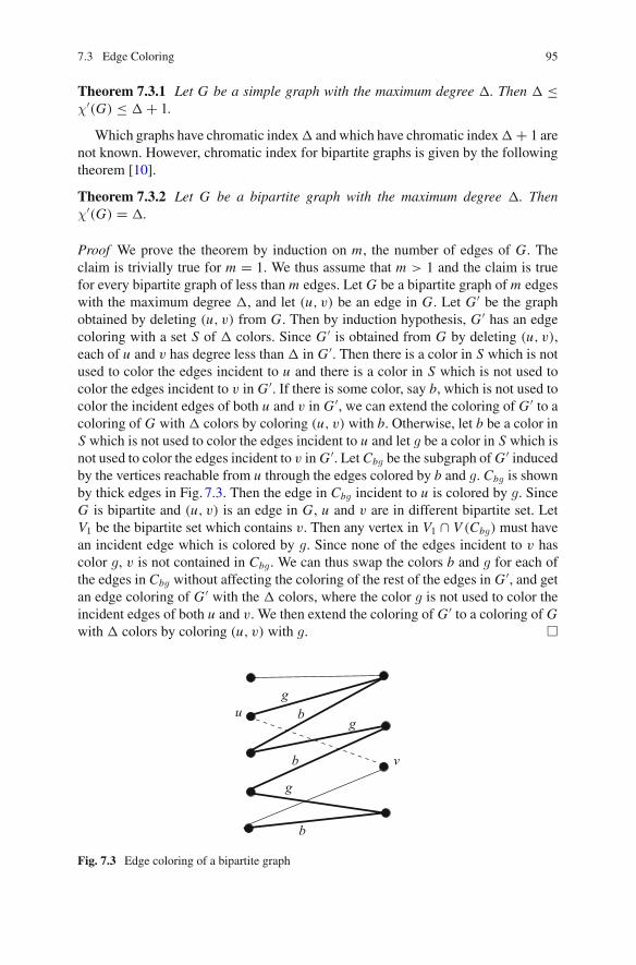
7.3 Edge Coloring 95
Theorem 7.3.1 Let G be a simple graph with the maximum degree �. Then � ≤χ′(G) ≤ � + 1.
Which graphs have chromatic index� and which have chromatic index� + 1 arenot known. However, chromatic index for bipartite graphs is given by the followingtheorem [10].
Theorem 7.3.2 Let G be a bipartite graph with the maximum degree �. Thenχ′(G) = �.
Proof We prove the theorem by induction on m, the number of edges of G. Theclaim is trivially true for m = 1. We thus assume that m > 1 and the claim is truefor every bipartite graph of less than m edges. Let G be a bipartite graph of m edgeswith the maximum degree �, and let (u, v) be an edge in G. Let G ′ be the graphobtained by deleting (u, v) from G. Then by induction hypothesis, G ′ has an edgecoloring with a set S of � colors. Since G ′ is obtained from G by deleting (u, v),each of u and v has degree less than � in G ′. Then there is a color in S which is notused to color the edges incident to u and there is a color in S which is not used tocolor the edges incident to v in G ′. If there is some color, say b, which is not used tocolor the incident edges of both u and v in G ′, we can extend the coloring of G ′ to acoloring of G with � colors by coloring (u, v) with b. Otherwise, let b be a color inS which is not used to color the edges incident to u and let g be a color in S which isnot used to color the edges incident to v in G ′. LetCbg be the subgraph of G ′ inducedby the vertices reachable from u through the edges colored by b and g. Cbg is shownby thick edges in Fig. 7.3. Then the edge in Cbg incident to u is colored by g. SinceG is bipartite and (u, v) is an edge in G, u and v are in different bipartite set. LetV1 be the bipartite set which contains v. Then any vertex in V1 ∩ V (Cbg) must havean incident edge which is colored by g. Since none of the edges incident to v hascolor g, v is not contained in Cbg . We can thus swap the colors b and g for each ofthe edges in Cbg without affecting the coloring of the rest of the edges in G ′, and getan edge coloring of G ′ with the � colors, where the color g is not used to color theincident edges of both u and v. We then extend the coloring of G ′ to a coloring of Gwith � colors by coloring (u, v) with g. �
ug
b
b
g
b
g
v
Fig. 7.3 Edge coloring of a bipartite graph
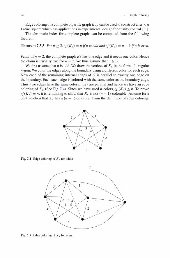
96 7 Graph Coloring
Edge coloring of a complete bipartite graph Kn,n can be used to construct an n × nLatine square which has applications in experimental design for quality control [11].
The chromatic index for complete graphs can be computed from the followingtheorem.
Theorem 7.3.3 For n ≥ 2, χ′(Kn) = n if n is odd and χ′(Kn) = n − 1 if n is even.
Proof If n = 2, the complete graph K2 has one edge and it needs one color. Hencethe claim is trivially true for n = 2. We thus assume that n ≥ 3.
We first assume that n is odd. We draw the vertices of Kn in the form of a regularn-gon. We color the edges along the boundary using a different color for each edge.Now each of the remaining internal edges of G is parallel to exactly one edge onthe boundary. Each such edge is colored with the same color as the boundary edge.Thus, two edges have the same color if they are parallel and hence we have an edgecoloring of Kn (See Fig. 7.4). Since we have used n colors, χ′(Kn) ≤ n. To proveχ′(Kn) = n, it is remaining to show that Kn is not (n − 1)-colorable. Assume for acontradiction that Kn has a (n − 1)-coloring. From the definition of edge coloring,
2
3
4
3
5 1
12
54
Fig. 7.4 Edge coloring of Kn for odd n
1
2
3
41
2 3 45
53
2
1
4
5
Fig. 7.5 Edge coloring of Kn for even n
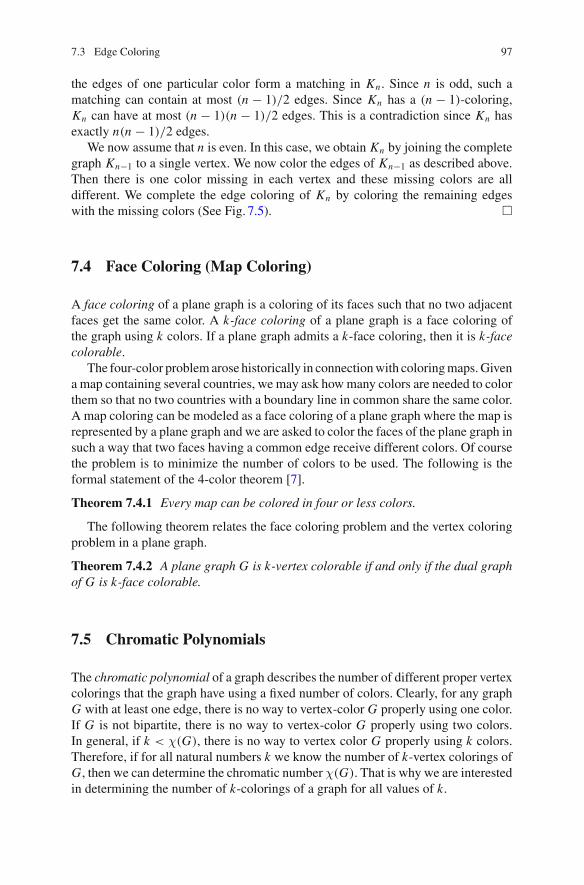
7.3 Edge Coloring 97
the edges of one particular color form a matching in Kn . Since n is odd, such amatching can contain at most (n − 1)/2 edges. Since Kn has a (n − 1)-coloring,Kn can have at most (n − 1)(n − 1)/2 edges. This is a contradiction since Kn hasexactly n(n − 1)/2 edges.
We now assume that n is even. In this case, we obtain Kn by joining the completegraph Kn−1 to a single vertex. We now color the edges of Kn−1 as described above.Then there is one color missing in each vertex and these missing colors are alldifferent. We complete the edge coloring of Kn by coloring the remaining edgeswith the missing colors (See Fig. 7.5). �
7.4 Face Coloring (Map Coloring)
A face coloring of a plane graph is a coloring of its faces such that no two adjacentfaces get the same color. A k-face coloring of a plane graph is a face coloring ofthe graph using k colors. If a plane graph admits a k-face coloring, then it is k-facecolorable.
The four-color problemarose historically in connectionwith coloringmaps.Givena map containing several countries, we may ask howmany colors are needed to colorthem so that no two countries with a boundary line in common share the same color.A map coloring can be modeled as a face coloring of a plane graph where the map isrepresented by a plane graph and we are asked to color the faces of the plane graph insuch a way that two faces having a common edge receive different colors. Of coursethe problem is to minimize the number of colors to be used. The following is theformal statement of the 4-color theorem [7].
Theorem 7.4.1 Every map can be colored in four or less colors.
The following theorem relates the face coloring problem and the vertex coloringproblem in a plane graph.
Theorem 7.4.2 A plane graph G is k-vertex colorable if and only if the dual graphof G is k-face colorable.
7.5 Chromatic Polynomials
The chromatic polynomial of a graph describes the number of different proper vertexcolorings that the graph have using a fixed number of colors. Clearly, for any graphG with at least one edge, there is no way to vertex-color G properly using one color.If G is not bipartite, there is no way to vertex-color G properly using two colors.In general, if k < χ(G), there is no way to vertex color G properly using k colors.Therefore, if for all natural numbers k we know the number of k-vertex colorings ofG, then we can determine the chromatic number χ(G). That is why we are interestedin determining the number of k-colorings of a graph for all values of k.
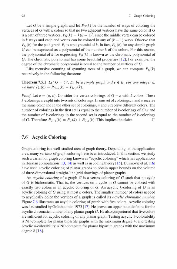
98 7 Graph Coloring
Let G be a simple graph, and let PG(k) be the number of ways of coloring thevertices of G with k colors so that no two adjacent vertices have the same color. If Gis a path of three vertices, PG(k) = k(k − 1)2, since the middle vertex can be coloredin k ways and each end vertex can be colored in any of (k − 1) ways. Observe thatPG(k) for the path graph P3 is a polynomial of k. In fact, PG(k) for any simple graphG can be expressed as a polynomial of the number k of the colors. For this reason,the polynomial of k for expressing PG(k) is known as the chromatic polynomial ofG. The chromatic polynomial has some beautiful properties [12]. For example, thedegree of the chromatic polynomial is equal to the number of vertices of G.
Like recursive counting of spanning trees of a graph, we can compute PG(k)recursively in the following theorem:
Theorem 7.5.1 Let G = (V, E) be a simple graph and e ∈ E. For any integer k,we have PG(k) = PG−e(k) − PG\e(k).
Proof Let e = (u, v). Consider the vertex colorings of G − e with k colors. Thesek-colorings are split into two sets of colorings. In one set of colorings, u and v receivethe same color and in the other set of colorings, u and v receive different colors. Thenumber of colorings in the first set is equal to the number of k-colorings of G\e andthe number of k-colorings in the second set is equal to the number of k-coloringsof G. Therefore PG−e(k) = PG(k) + PG\e(k). This implies the claim. �
7.6 Acyclic Coloring
Graph coloring is a well-studied area of graph theory. Depending on the applicationarea, many variants of graph coloring have been introduced. In this section, we studysuch a variant of graph coloring known as “acyclic coloring” which has applicationsin Hessian computation [13, 14] as well as in coding theory [15]. Dujmovic et al. [16]have used acyclic coloring of planar graphs to obtain upper bounds on the volumeof three-dimensional straight-line grid drawings of planar graphs.
An acyclic coloring of a graph G is a vertex coloring of G such that no cycleof G is bichromatic. That is, the vertices on a cycle in G cannot be colored withexactly two colors in an acyclic coloring of G. An acyclic k-coloring of G is anacyclic coloring of G using at most k colors. The smallest number of colors neededto acyclically color the vertices of a graph is called its acyclic chromatic number.Figure7.6 illustrates an acyclic coloring of graph with five colors. Acyclic coloringwas first studied byGrünbaum in 1973 [17]. He proved an upper bound of nine for theacyclic chromatic number of any planar graphG. He also conjectured that five colorsare sufficient for acyclic coloring of any planar graph. Testing acyclic 3-colorabilityis NP-complete for planar bipartite graphs with the maximum degree 4, and testingacyclic 4-colorability is NP-complete for planar bipartite graphs with the maximumdegree 8 [18].
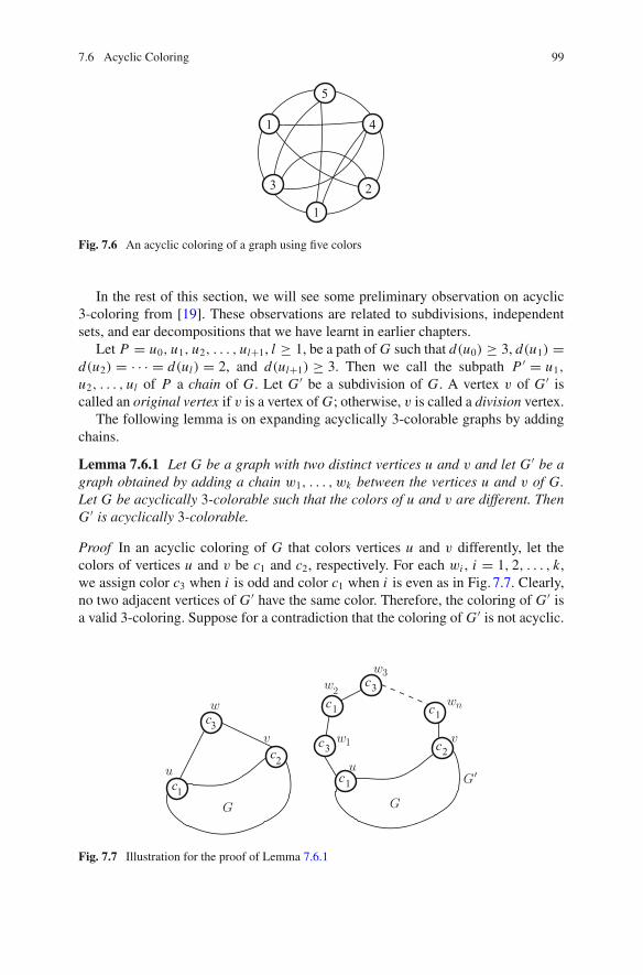
7.6 Acyclic Coloring 99
5
2
1
1
3
4
Fig. 7.6 An acyclic coloring of a graph using five colors
In the rest of this section, we will see some preliminary observation on acyclic3-coloring from [19]. These observations are related to subdivisions, independentsets, and ear decompositions that we have learnt in earlier chapters.
Let P = u0, u1, u2, . . . , ul+1, l ≥ 1, be a path of G such that d(u0) ≥ 3, d(u1) =d(u2) = · · · = d(ul) = 2, and d(ul+1) ≥ 3. Then we call the subpath P ′ = u1,u2, . . . , ul of P a chain of G. Let G ′ be a subdivision of G. A vertex v of G ′ iscalled an original vertex if v is a vertex of G; otherwise, v is called a division vertex.
The following lemma is on expanding acyclically 3-colorable graphs by addingchains.
Lemma 7.6.1 Let G be a graph with two distinct vertices u and v and let G ′ be agraph obtained by adding a chain w1, . . . , wk between the vertices u and v of G.Let G be acyclically 3-colorable such that the colors of u and v are different. ThenG ′ is acyclically 3-colorable.
Proof In an acyclic coloring of G that colors vertices u and v differently, let thecolors of vertices u and v be c1 and c2, respectively. For each wi , i = 1, 2, . . . , k,we assign color c3 when i is odd and color c1 when i is even as in Fig. 7.7. Clearly,no two adjacent vertices of G ′ have the same color. Therefore, the coloring of G ′ isa valid 3-coloring. Suppose for a contradiction that the coloring of G ′ is not acyclic.
c1
c1 c1
c3
c3
c2
c1
c2
c3v
uG
G
w1
w2
w3
wnw
v
u
G
Fig. 7.7 Illustration for the proof of Lemma 7.6.1
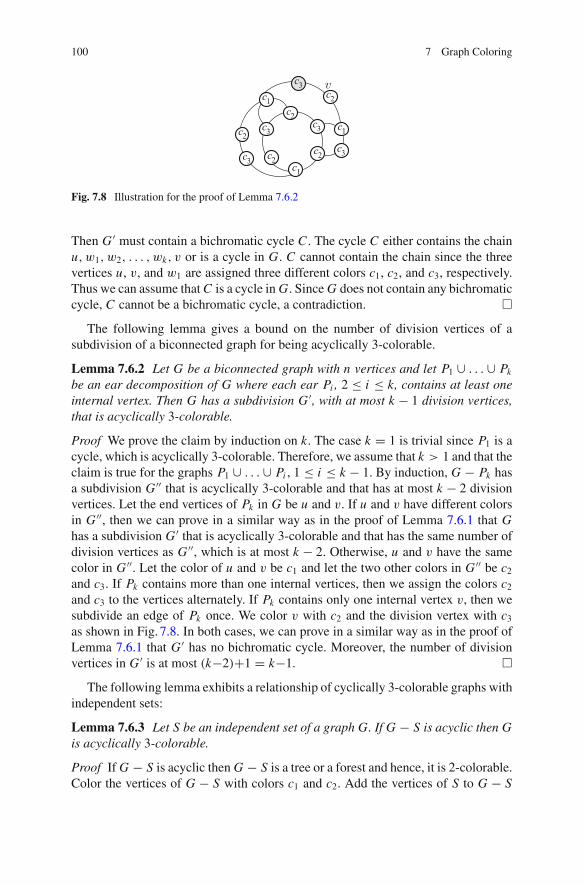
100 7 Graph Coloring
c3
c2c3
c2c1
c1
c3
c1
c2
c2c3
c2c3 v
Fig. 7.8 Illustration for the proof of Lemma 7.6.2
Then G ′ must contain a bichromatic cycle C . The cycle C either contains the chainu, w1, w2, . . . , wk, v or is a cycle in G. C cannot contain the chain since the threevertices u, v, and w1 are assigned three different colors c1, c2, and c3, respectively.Thus we can assume thatC is a cycle inG. SinceG does not contain any bichromaticcycle, C cannot be a bichromatic cycle, a contradiction. �
The following lemma gives a bound on the number of division vertices of asubdivision of a biconnected graph for being acyclically 3-colorable.
Lemma 7.6.2 Let G be a biconnected graph with n vertices and let P1 ∪ . . . ∪ Pkbe an ear decomposition of G where each ear Pi , 2 ≤ i ≤ k, contains at least oneinternal vertex. Then G has a subdivision G ′, with at most k − 1 division vertices,that is acyclically 3-colorable.
Proof We prove the claim by induction on k. The case k = 1 is trivial since P1 is acycle, which is acyclically 3-colorable. Therefore, we assume that k > 1 and that theclaim is true for the graphs P1 ∪ . . . ∪ Pi , 1 ≤ i ≤ k − 1. By induction, G − Pk hasa subdivision G ′′ that is acyclically 3-colorable and that has at most k − 2 divisionvertices. Let the end vertices of Pk in G be u and v. If u and v have different colorsin G ′′, then we can prove in a similar way as in the proof of Lemma 7.6.1 that Ghas a subdivision G ′ that is acyclically 3-colorable and that has the same number ofdivision vertices as G ′′, which is at most k − 2. Otherwise, u and v have the samecolor in G ′′. Let the color of u and v be c1 and let the two other colors in G ′′ be c2and c3. If Pk contains more than one internal vertices, then we assign the colors c2and c3 to the vertices alternately. If Pk contains only one internal vertex v, then wesubdivide an edge of Pk once. We color v with c2 and the division vertex with c3as shown in Fig. 7.8. In both cases, we can prove in a similar way as in the proof ofLemma 7.6.1 that G ′ has no bichromatic cycle. Moreover, the number of divisionvertices in G ′ is at most (k−2)+1 = k−1. �
The following lemma exhibits a relationship of cyclically 3-colorable graphs withindependent sets:
Lemma 7.6.3 Let S be an independent set of a graph G. If G − S is acyclic then Gis acyclically 3-colorable.
Proof If G − S is acyclic then G − S is a tree or a forest and hence, it is 2-colorable.Color the vertices of G − S with colors c1 and c2. Add the vertices of S to G − S
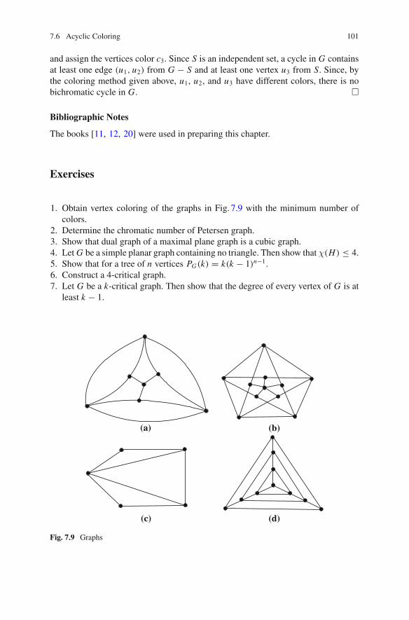
7.6 Acyclic Coloring 101
and assign the vertices color c3. Since S is an independent set, a cycle in G containsat least one edge (u1, u2) from G − S and at least one vertex u3 from S. Since, bythe coloring method given above, u1, u2, and u3 have different colors, there is nobichromatic cycle in G. �
Bibliographic Notes
The books [11, 12, 20] were used in preparing this chapter.
Exercises
1. Obtain vertex coloring of the graphs in Fig. 7.9 with the minimum number ofcolors.
2. Determine the chromatic number of Petersen graph.3. Show that dual graph of a maximal plane graph is a cubic graph.4. LetG be a simple planar graph containing no triangle. Then show that χ(H) ≤ 4.5. Show that for a tree of n vertices PG(k) = k(k − 1)n−1.6. Construct a 4-critical graph.7. Let G be a k-critical graph. Then show that the degree of every vertex of G is at
least k − 1.
(c) (d)
(b)(a)
Fig. 7.9 Graphs
102 7 Graph Coloring
References
1. Garey, M.R., Johnson, D.S.: Computers and Intractability. W.H. Freeman and Company, NewYork (1979)
2. Matula, D.W., Marble, G., Isaacson, J.D.: Graph colouring algorithms. In: Read, R.C. (ed.)Graph Theory and Computing, pp. 109–122. Academic Press, New York (1972)
3. Welsh, D.J.A., Powell, M.B.: An upper bound for chromatic number of a graph and its appli-cation to timetabling problem. Comput. J. 10, 85–86 (1967)
4. Chiba, N., Nishizeki, T., Saito, N.: A linear 5-coloring algorithm of planar graphs. J. Algorithms2(4), 317–327 (1981)
5. Matula, D.W., Schiloach, Y., Tarjan, R.E.: Two linear algorithms for five coloring of planargraphs. STAN-CS-80-830 (1980)
6. Frederickson, G.N.: On linear-time algorithms for five-coloring planar graphs. Inform. Process.Lett. 19(5), 219–224 (1984)
7. Appel, K., Haken, W.: Every map is four colourable. Bull. Am. Math. Soc. 82, 711–712 (1976)8. Dirac, G.A.: A property of 4-chromatic graph and some remarks on critical graphs. J. Lond.
Math. Soc. 27, 85–92 (1952)9. Vizing, V.G.: On an estimate of the chromatic class of a p-graph, Diskret. Analiz. 3, 25–30
(1964)10. Konig, D.: Uber graphen und ihre anwendung auf determinantentheorie und mengenlehre.
Math. Ann. 77(4), 453–465 (1916)11. Clark, J., Holton, D.A.: A First Look at Graph Theory. World Scientific, Singapore (1991)12. Agnarsson, G., Greenlaw, R.: Graph Theory: Modeling, Applications and Algorithms. Pearson
Education Inc., New Jersey (2007)13. Gebremedhin, A.H., Tarafdar, A., Manne, F., Pothen, A.: New acyclic and star coloring algo-
rithms with application to computing hessians. SIAM J. Sci. Comput. 29(3), 1042–1072 (2007)14. Gebremedhin, A.H., Tarafdar, A., Pothen, A., Walther, A.: Efficient computation of sparse
hessians using coloring and automatic differentiation. INFORMS J. Comput. 21(2), 209–223(2009)
15. Serra, O., Zémor, G.: Cycle codes of graphs and mds array codes. Electron. Notes Discret.Math. 34, 95–99 (2009)
16. Dujmovic, V., Morin, P., Wood, D.R.: Layout of graphs with bounded tree-width. SIAM J.Comput. 34, 553–579 (2005)
17. Grünbaum, B.: Acyclic colorings of planar graphs. Isr. J. Math. 14, 390–408 (1973)18. Ochem, P.: Negative results on acyclic improper colorings. In: Proceedings of European Con-
ference on Combinatorics (EuroComb 05), pp. 357–362 (2005)19. Mondal, D., Nishat, R.I., Whitesides, S., Rahman, M.S.: Acyclic colorings of graph subdivi-
sions revisited. J. Discret. Algorithms 16, 90–103 (2012)20. Wilson, R.J.: Introduction to Graph Theory, 4th edn. Longman, London (1996)
Chapter 8Digraphs
8.1 Introduction
Agraph is usually called a directed graph or a digraph if its edges have directions. Theconcept of directed graphs or digraphs has many applications in solving real-worldproblems. For example, flow networks as well as electrical networks are representedby digraphs.
8.2 Digraph Terminologies
A directed graph or digraph D = (V, A) consists of a nonempty finite set V (D) ofvertices and a (multi) set A(D) of ordered pairs of elements of V (D) called arcs ordirected edges. If A(D) is a multiset, then D is called a multidigraph. Figure8.1(a)illustrates a simple digraph whereas the graph in Fig. 8.1(b) is a multidigraph. Foru, v ∈ V , an arc a = (u, v) ∈ A is denoted by uv and implies that a is directed fromu to v. For an arc uv, u is called the tail of uv and v is called the head of uv. Forthe arc cd in Fig. 8.1(a), c is the tail and d is the head. We say the edge uv is leavingu and terminating at v. A digraph is represented by a diagram which is similar tothe representation of a graph where each arc contains an arrow directed from tail tohead, as illustrated in Fig. 8.1.
The concept of the degree of a vertex for graphs also extends to digraphs. Theindegree of a vertex v of a digraph is the number of directed edges terminating at v,and the outdegree of v is the number of directed edges leaving v. In the digraph inFig. 8.1(b), the indegree of e is 2 and the outdegree of e is 3; the indegree of c is 2and the outdegree of c is 3. The degree of v is the sum of its indegree and outdegree.A vertex with indegree 0 is a source and with outdegree 0 is a sink. In the digraph inFig. 8.1(a), a is a source and f is a sink. The digraph in Fig. 8.1(b) has no sink. Wenow have the following lemma which is analogous to Lemma 2.2.1.
© Springer International Publishing AG 2017M.S. Rahman, Basic Graph Theory, Undergraduate Topics in Computer Science,DOI 10.1007/978-3-319-49475-3_8
103
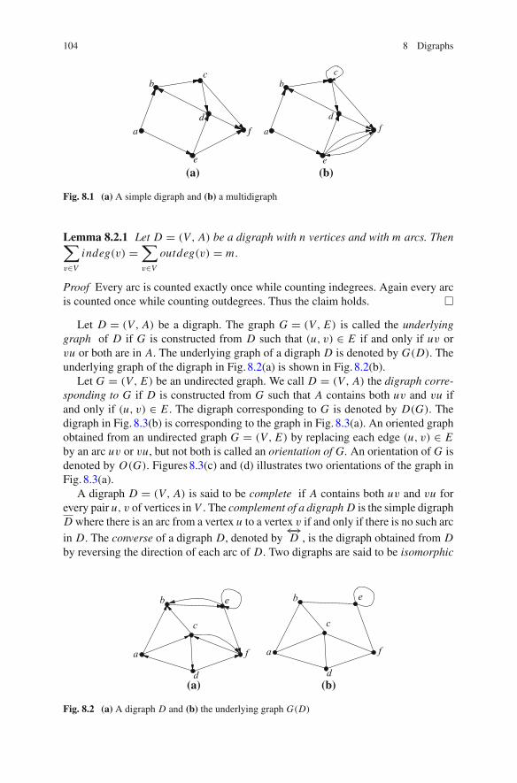
104 8 Digraphs
bc
f
e
a
d
b
a
e
c
d
(a) (b)
f
Fig. 8.1 (a) A simple digraph and (b) a multidigraph
Lemma 8.2.1 Let D = (V, A) be a digraph with n vertices and with m arcs. Then∑
v∈Vindeg(v) =
∑
v∈Voutdeg(v) = m.
Proof Every arc is counted exactly once while counting indegrees. Again every arcis counted once while counting outdegrees. Thus the claim holds. �
Let D = (V, A) be a digraph. The graph G = (V, E) is called the underlyinggraph of D if G is constructed from D such that (u, v) ∈ E if and only if uv orvu or both are in A. The underlying graph of a digraph D is denoted by G(D). Theunderlying graph of the digraph in Fig. 8.2(a) is shown in Fig. 8.2(b).
Let G = (V, E) be an undirected graph. We call D = (V, A) the digraph corre-sponding to G if D is constructed from G such that A contains both uv and vu ifand only if (u, v) ∈ E . The digraph corresponding to G is denoted by D(G). Thedigraph in Fig. 8.3(b) is corresponding to the graph in Fig. 8.3(a). An oriented graphobtained from an undirected graph G = (V, E) by replacing each edge (u, v) ∈ Eby an arc uv or vu, but not both is called an orientation of G. An orientation of G isdenoted by O(G). Figures8.3(c) and (d) illustrates two orientations of the graph inFig. 8.3(a).
A digraph D = (V, A) is said to be complete if A contains both uv and vu forevery pair u, v of vertices in V . The complement of a digraph D is the simple digraphD where there is an arc from a vertex u to a vertex v if and only if there is no such arcin D. The converse of a digraph D, denoted by
←→D , is the digraph obtained from D
by reversing the direction of each arc of D. Two digraphs are said to be isomorphic
(a) (b)
b e
f
d
a
b
c
d
e
a
c
f
Fig. 8.2 (a) A digraph D and (b) the underlying graph G(D)
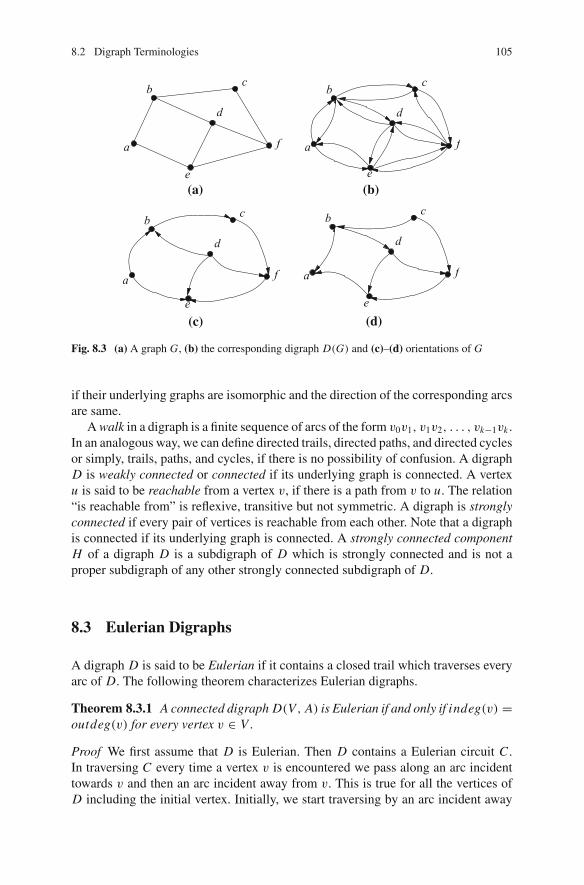
8.2 Digraph Terminologies 105
(a) (b)
(d)(c)
b c
f
e
a
d
b c
fa
e
d
b c
f
d
a
e
b c
d
fa
e
Fig. 8.3 (a) A graph G, (b) the corresponding digraph D(G) and (c)–(d) orientations of G
if their underlying graphs are isomorphic and the direction of the corresponding arcsare same.
Awalk in a digraph is a finite sequence of arcs of the form v0v1, v1v2, . . . , vk−1vk .In an analogous way, we can define directed trails, directed paths, and directed cyclesor simply, trails, paths, and cycles, if there is no possibility of confusion. A digraphD is weakly connected or connected if its underlying graph is connected. A vertexu is said to be reachable from a vertex v, if there is a path from v to u. The relation“is reachable from” is reflexive, transitive but not symmetric. A digraph is stronglyconnected if every pair of vertices is reachable from each other. Note that a digraphis connected if its underlying graph is connected. A strongly connected componentH of a digraph D is a subdigraph of D which is strongly connected and is not aproper subdigraph of any other strongly connected subdigraph of D.
8.3 Eulerian Digraphs
A digraph D is said to be Eulerian if it contains a closed trail which traverses everyarc of D. The following theorem characterizes Eulerian digraphs.
Theorem 8.3.1 A connected digraph D(V, A) is Eulerian if and only if indeg(v) =outdeg(v) for every vertex v ∈ V .
Proof We first assume that D is Eulerian. Then D contains a Eulerian circuit C .In traversing C every time a vertex v is encountered we pass along an arc incidenttowards v and then an arc incident away from v. This is true for all the vertices ofD including the initial vertex. Initially, we start traversing by an arc incident away
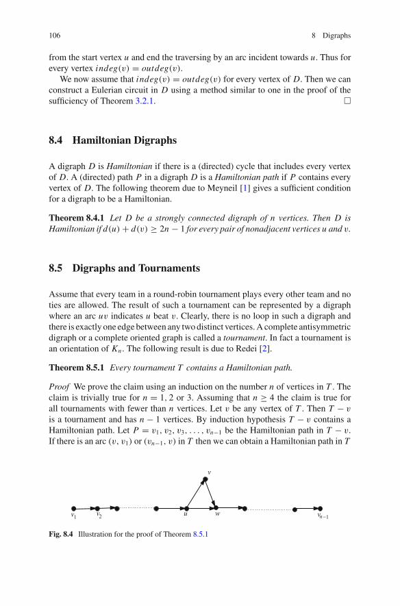
106 8 Digraphs
from the start vertex u and end the traversing by an arc incident towards u. Thus forevery vertex indeg(v) = outdeg(v).
We now assume that indeg(v) = outdeg(v) for every vertex of D. Then we canconstruct a Eulerian circuit in D using a method similar to one in the proof of thesufficiency of Theorem 3.2.1. �
8.4 Hamiltonian Digraphs
A digraph D is Hamiltonian if there is a (directed) cycle that includes every vertexof D. A (directed) path P in a digraph D is a Hamiltonian path if P contains everyvertex of D. The following theorem due to Meyneil [1] gives a sufficient conditionfor a digraph to be a Hamiltonian.
Theorem 8.4.1 Let D be a strongly connected digraph of n vertices. Then D isHamiltonian if d(u) + d(v) ≥ 2n − 1 for every pair of nonadjacent vertices u and v.
8.5 Digraphs and Tournaments
Assume that every team in a round-robin tournament plays every other team and noties are allowed. The result of such a tournament can be represented by a digraphwhere an arc uv indicates u beat v. Clearly, there is no loop in such a digraph andthere is exactly one edge between any twodistinct vertices.A complete antisymmetricdigraph or a complete oriented graph is called a tournament. In fact a tournament isan orientation of Kn . The following result is due to Redei [2].
Theorem 8.5.1 Every tournament T contains a Hamiltonian path.
Proof We prove the claim using an induction on the number n of vertices in T . Theclaim is trivially true for n = 1, 2 or 3. Assuming that n ≥ 4 the claim is true forall tournaments with fewer than n vertices. Let v be any vertex of T . Then T − v
is a tournament and has n − 1 vertices. By induction hypothesis T − v contains aHamiltonian path. Let P = v1, v2, v3, . . . , vn−1 be the Hamiltonian path in T − v.If there is an arc (v, v1) or (vn−1, v) in T then we can obtain a Hamiltonian path in T
−1nv wuv v1 2
v
Fig. 8.4 Illustration for the proof of Theorem 8.5.1
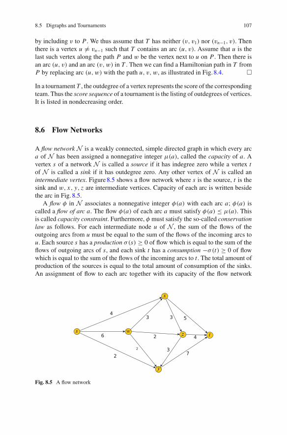
8.5 Digraphs and Tournaments 107
by including v to P . We thus assume that T has neither (v, v1) nor (vn−1, v). Thenthere is a vertex u �= vn−1 such that T contains an arc (u, v). Assume that u is thelast such vertex along the path P and w be the vertex next to u on P . Then there isan arc (u, v) and an arc (v,w) in T . Then we can find a Hamiltonian path in T fromP by replacing arc (u, w) with the path u, v, w, as illustrated in Fig. 8.4. �
In a tournament T , the outdegree of a vertex represents the score of the correspondingteam. Thus the score sequence of a tournament is the listing of outdegrees of vertices.It is listed in nondecreasing order.
8.6 Flow Networks
A flow network N is a weakly connected, simple directed graph in which every arca of N has been assigned a nonnegative integer μ(a), called the capacity of a. Avertex s of a network N is called a source if it has indegree zero while a vertex tof N is called a sink if it has outdegree zero. Any other vertex of N is called anintermediate vertex. Figure8.5 shows a flow network where s is the source, t is thesink and w, x, y, z are intermediate vertices. Capacity of each arc is written besidethe arc in Fig. 8.5.
A flow φ in N associates a nonnegative integer φ(a) with each arc a; φ(a) iscalled a flow of arc a. The flow φ(a) of each arc a must satisfy φ(a) ≤ μ(a). Thisis called capacity constraint. Furthermore, φ must satisfy the so-called conservationlaw as follows. For each intermediate node u of N , the sum of the flows of theoutgoing arcs from u must be equal to the sum of the flows of the incoming arcs tou. Each source s has a production σ(s) ≥ 0 of flow which is equal to the sum of theflows of outgoing arcs of s, and each sink t has a consumption −σ(t) ≥ 0 of flowwhich is equal to the sum of the flows of the incoming arcs to t . The total amount ofproduction of the sources is equal to the total amount of consumption of the sinks.An assignment of flow to each arc together with its capacity of the flow network
Fig. 8.5 A flow network
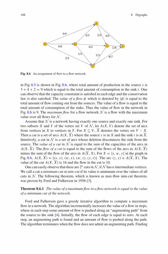
108 8 Digraphs
Fig. 8.6 An assignment of flow to a flow network
in Fig. 8.5 is shown in Fig. 8.6, where total amount of production in the source s is3 + 4 + 2 = 9 which is equal to the total amount of consumption in the sink t . Onecan observe that the capacity constraint is satisfied in each edge and the conservationlaw is also satisfied. The value of a flow φ which is denoted by |φ| is equal to thetotal amount of flow coming out from the sources. The value of a flow is equal to thetotal amount of consumption of the sinks. Thus the value of flow in the network inFig. 8.6 is 9. The maximum flow for a flow network N is a flow with the maximumvalue over all flows for N .
Assume thatN is a network having exactly one source and exactly one sink. Fortwo subsets X and Y of the vertex set V of N , let A(X, Y ) denote the set of arcsfrom vertices in X to vertices in Y . For X ⊆ V , X denotes the vertex set V − X .Then a cut is a set of arcs A(X, X) where the source s is in X and the sink t is in X .Intuitively, a cut in N is a set of arcs whose deletion disconnects the sink from thesource. The value of a cut in N is equal to the sum of the capacities of the arcs inA(X, X). The flow of a cut is equal to the sum of the flows of the arcs in A(X, X)
minus the sum of the flow of the arcs in A(X , X). For X = {s, w, y} in the graph inFig. 8.6, A(X, X) = {(s, x), (w, x), (w, z), (y, t)}. The arc (z, y) ∈ A(X , X). Thevalue of the cut A(X, X) is 16 and the flow in the cut is 10.
One can easily observe that there are 2n cuts inN , ifN has n intermediate vertices.We call a cut a minimum cut or min-cut if its value is minimum over the values of allcuts in N . The following theorem, which is known as max-flow min-cut theorem,was proven by Ford and Fulkerson in 1956 [3].
Theorem 8.6.1 The value of a maximum flow in a flow network is equal to the valueof a minimum cut of the network.
Ford and Fulkerson gave a greedy iterative algorithm to compute a maximumflow in a network. The algorithm incrementally increases the value of a flow in steps,where in each step some amount of flow is pushed along an “augmenting path” fromthe source to the sink [4]. Initially, the flow of each edge is equal to zero. At eachstep, an augmenting path is found and an amount of flow is pushed along the path.The algorithm terminates when the flow does not admit an augmenting path. Finding
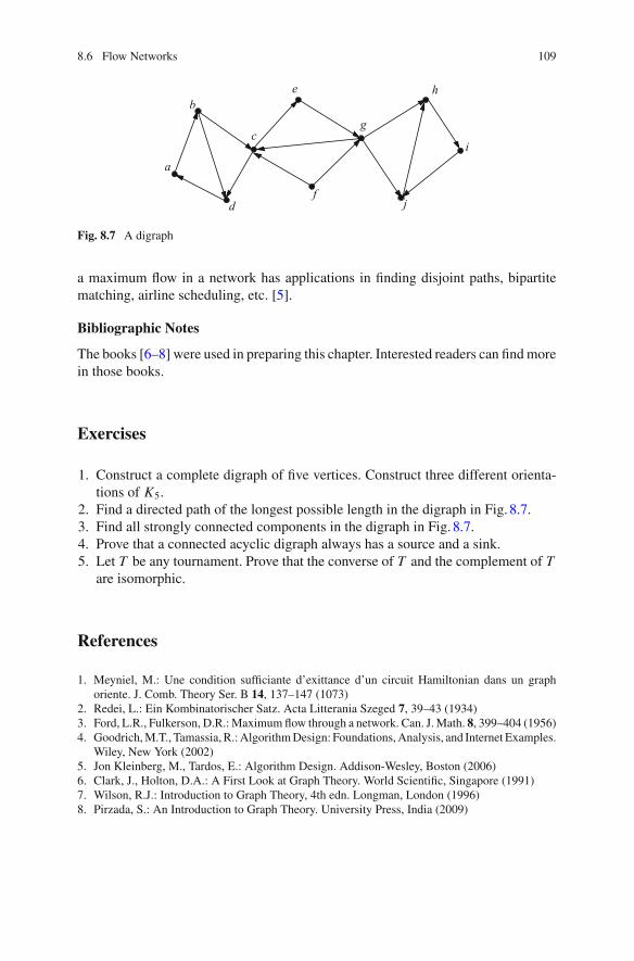
8.6 Flow Networks 109
a
b
c
d
e
f
g
h
i
j
Fig. 8.7 A digraph
a maximum flow in a network has applications in finding disjoint paths, bipartitematching, airline scheduling, etc. [5].
Bibliographic Notes
The books [6–8] were used in preparing this chapter. Interested readers can findmorein those books.
Exercises
1. Construct a complete digraph of five vertices. Construct three different orienta-tions of K5.
2. Find a directed path of the longest possible length in the digraph in Fig. 8.7.3. Find all strongly connected components in the digraph in Fig. 8.7.4. Prove that a connected acyclic digraph always has a source and a sink.5. Let T be any tournament. Prove that the converse of T and the complement of T
are isomorphic.
References
1. Meyniel, M.: Une condition sufficiante d’exittance d’un circuit Hamiltonian dans un graphoriente. J. Comb. Theory Ser. B 14, 137–147 (1073)
2. Redei, L.: Ein Kombinatorischer Satz. Acta Litterania Szeged 7, 39–43 (1934)3. Ford, L.R., Fulkerson, D.R.:Maximumflow through a network. Can. J.Math. 8, 399–404 (1956)4. Goodrich,M.T., Tamassia, R.:AlgorithmDesign: Foundations,Analysis, and Internet Examples.
Wiley, New York (2002)5. Jon Kleinberg, M., Tardos, E.: Algorithm Design. Addison-Wesley, Boston (2006)6. Clark, J., Holton, D.A.: A First Look at Graph Theory. World Scientific, Singapore (1991)7. Wilson, R.J.: Introduction to Graph Theory, 4th edn. Longman, London (1996)8. Pirzada, S.: An Introduction to Graph Theory. University Press, India (2009)
Chapter 9Special Classes of Graphs
9.1 Introduction
In this chapter, we know about some special classes of graphs. Special classes ofgraphs play important roles in graph algorithmic studies. When we find a computa-tionally hard problem for general graphs, we try to solve those problems for specialclasses of graphs.
9.2 Outerplanar Graphs
A graph is outerplanar if it has a planar embedding where all vertices are on theouter face. An outerplanar embedding of an outerplanar graph is called an outerplanegraph. The graph in Fig. 9.1(a) is an outerplanar graph since it has an outerplanarembedding as shown in Fig. 9.1(b). An outer edge of an outerplane graph is an edgeon the outer face of the outerplane graph and all other edges are inner edges.
Remember from Section6.3.2 that the weak dual of a plane graph G is a graph,where each vertex corresponds to each inner face of G and each edge corresponds toa common edge between two inner faces of G. Figure9.2 illustrates the weak dual ofan outerplane graph where the vertices of the weak dual are drawn by white circlesand the edges are drawn by dotted lines.
Lemma 9.2.1 The weak dual of a biconnected outerplane graph is a tree.
Proof Let G be a biconnected outerplane graph. Since G is biconnected, the outerboundary of G is a simple cycle C and all inner faces are inside C . Furthermore, twoneighboring faces share an inner edge. Therefore, the weak dual T is connected. Wenow show that T does not contain a cycle. Assume for a contradiction that T containsa cycle. Then G would have an inner vertex v, a contradiction to the definition of anouterplane graph. �
© Springer International Publishing AG 2017M.S. Rahman, Basic Graph Theory, Undergraduate Topics in Computer Science,DOI 10.1007/978-3-319-49475-3_9
111
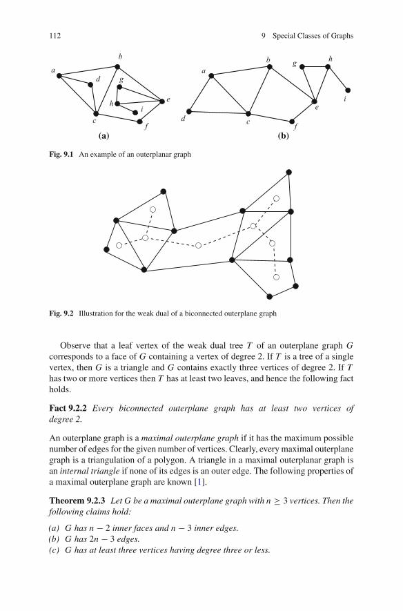
112 9 Special Classes of Graphs
(a) (b)
a
b
c
d
e
f
g
hi
ab
cde
f
g h
i
Fig. 9.1 An example of an outerplanar graph
Fig. 9.2 Illustration for the weak dual of a biconnected outerplane graph
Observe that a leaf vertex of the weak dual tree T of an outerplane graph Gcorresponds to a face of G containing a vertex of degree 2. If T is a tree of a singlevertex, then G is a triangle and G contains exactly three vertices of degree 2. If Thas two or more vertices then T has at least two leaves, and hence the following factholds.
Fact 9.2.2 Every biconnected outerplane graph has at least two vertices ofdegree 2.
An outerplane graph is a maximal outerplane graph if it has the maximum possiblenumber of edges for the given number of vertices. Clearly, every maximal outerplanegraph is a triangulation of a polygon. A triangle in a maximal outerplanar graph isan internal triangle if none of its edges is an outer edge. The following properties ofa maximal outerplane graph are known [1].
Theorem 9.2.3 Let G be a maximal outerplane graph with n ≥ 3 vertices. Then thefollowing claims hold:
(a) G has n − 2 inner faces and n − 3 inner edges.(b) G has 2n − 3 edges.(c) G has at least three vertices having degree three or less.
9.2 Outerplanar Graphs 113
Proof (a) We prove the claim using an induction on the number of vertices. Obvi-ously, the claim holds for n = 3. Assume that n > 3 and the claim holds for anymax-imal outerplane graph of less than n vertices. Let G be a maximal outerplane graphof n vertices. By Fact 9.2.2, G must have a vertex v of degree 2 on the outer face. Weobtain a graph G ′ from G by deleting v from G. Clearly, G ′ is a maximal outerplanegraph of n − 1 vertices. By induction hypothesis G ′ has (n − 1) − 2 inner faces and(n − 1) − 3 inner edges. In constructing G ′ by deleting v we reduced the number ofinner faces by1 andnumber of inner edges by1.ThenG has (n − 1) − 2 + 1 = n − 2inner faces and (n − 1) − 3 + 1 = n − 3 inner edges.
(b) Outer edges form a cycle of n vertices. Thus there are n outer edges. From (a),G has n − 3 inner edges. Then total number of edges in G is n + n − 3 = 2n − 3.
(c) By (b) G has 2n − 3 edges. Hence the degree sum for G is 4n − 6. Let v bea vertex of G with degree less than 4. We define the deficiency for v by 4 − d(v).Then the total deficiency of the vertices of G is 6. Since G is maximal planar, G isbiconnected and hence the degree of a vertex of G is at least 2. Then the deficiencyof a vertex is at most 2. Since the total deficiency is 6, there are at least three verticesof degree three or less. �
The following property is known from [2] whose proof is left as an exercise.
Lemma 9.2.4 Let n2 be the number of vertices of degree 2 and t be the numberof internal triangles in a maximal outerplane graph with n vertices. If n ≥ 4, thent = n2 − 2.
Sometimes we are interested in graphs of restricted degrees. The following inter-esting properties hold for maximal outerplane graphs of maximum degree 4 [3].
Theorem 9.2.5 Let G be a maximal outerplane graph of three or more verticeswith the maximum degree 4. Assume that G is not an outerplane graph as shown inFig.9.3. Then the following (a)–(d) hold.
(a) G has no internal triangle.(b) The inner dual of G is a path.(c) If G has four or more vertices, then G has exactly two pairs of adjacent vertices
x and y such that degree of x is 2 and degree of y is 3, and G has exactly n − 4vertices of degree 4.
(d) If G has more than four vertices, then every inner edge of G is incident to avertex of degree 4 in G.
Proof (a) Let v1, v2, . . . , vn be the consecutive vertices on the outer cycle of G inthis order. Assume for a contradiction that G has an internal triangle f consistingvx , vy , and vz and they are not consecutive on the outer cycle. In order to f be atriangle, each vx , vy, vz needs to have at least two inner edges incident to it. Sincetwo outer edges are incident to each of vx , vy, vz , the degree of each of these threevertices is 4 in G. Let fxy, fyz , and fzx be the three adjacent faces of f containing
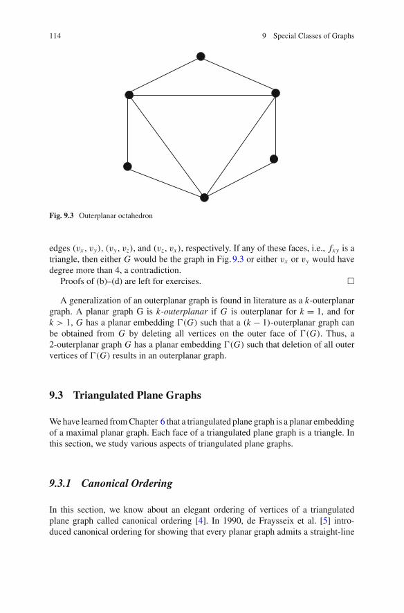
114 9 Special Classes of Graphs
Fig. 9.3 Outerplanar octahedron
edges (vx , vy), (vy, vz), and (vz, vx ), respectively. If any of these faces, i.e., fxy is atriangle, then either G would be the graph in Fig. 9.3 or either vx or vy would havedegree more than 4, a contradiction.
Proofs of (b)–(d) are left for exercises. �
A generalization of an outerplanar graph is found in literature as a k-outerplanargraph. A planar graph G is k-outerplanar if G is outerplanar for k = 1, and fork > 1, G has a planar embedding �(G) such that a (k − 1)-outerplanar graph canbe obtained from G by deleting all vertices on the outer face of �(G). Thus, a2-outerplanar graph G has a planar embedding �(G) such that deletion of all outervertices of �(G) results in an outerplanar graph.
9.3 Triangulated Plane Graphs
Wehave learned fromChapter 6 that a triangulated plane graph is a planar embeddingof a maximal planar graph. Each face of a triangulated plane graph is a triangle. Inthis section, we study various aspects of triangulated plane graphs.
9.3.1 Canonical Ordering
In this section, we know about an elegant ordering of vertices of a triangulatedplane graph called canonical ordering [4]. In 1990, de Fraysseix et al. [5] intro-duced canonical ordering for showing that every planar graph admits a straight-line
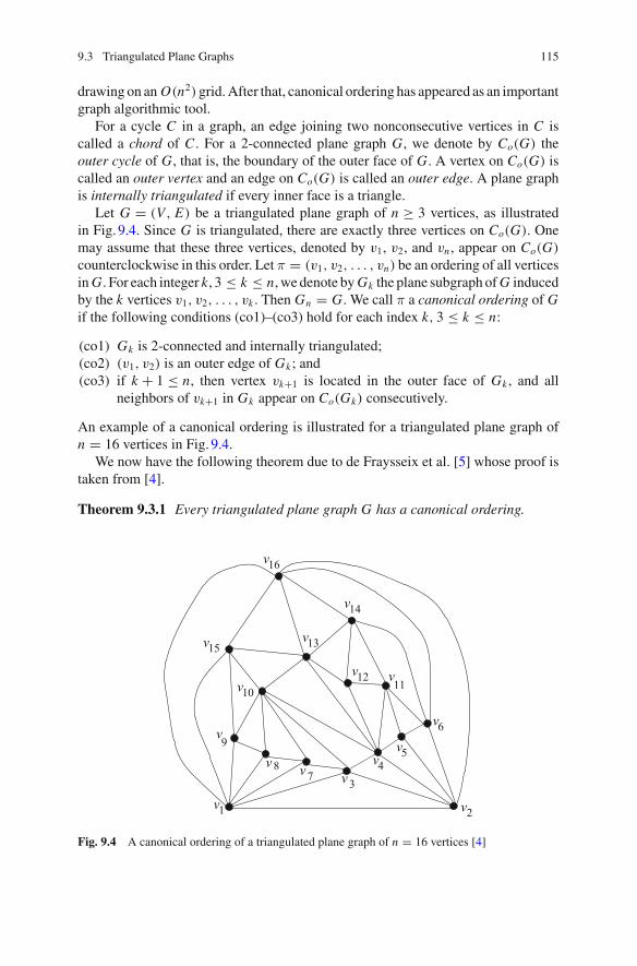
9.3 Triangulated Plane Graphs 115
drawing on anO(n2) grid.After that, canonical ordering has appeared as an importantgraph algorithmic tool.
For a cycle C in a graph, an edge joining two nonconsecutive vertices in C iscalled a chord of C . For a 2-connected plane graph G, we denote by Co(G) theouter cycle of G, that is, the boundary of the outer face of G. A vertex on Co(G) iscalled an outer vertex and an edge on Co(G) is called an outer edge. A plane graphis internally triangulated if every inner face is a triangle.
Let G = (V, E) be a triangulated plane graph of n ≥ 3 vertices, as illustratedin Fig. 9.4. Since G is triangulated, there are exactly three vertices on Co(G). Onemay assume that these three vertices, denoted by v1, v2, and vn , appear on Co(G)
counterclockwise in this order. Let π = (v1, v2, . . . , vn) be an ordering of all verticesinG. For each integer k, 3 ≤ k ≤ n, we denote byGk the plane subgraph ofG inducedby the k vertices v1, v2, . . . , vk . Then Gn = G. We call π a canonical ordering of Gif the following conditions (co1)–(co3) hold for each index k, 3 ≤ k ≤ n:
(co1) Gk is 2-connected and internally triangulated;(co2) (v1, v2) is an outer edge of Gk ; and(co3) if k + 1 ≤ n, then vertex vk+1 is located in the outer face of Gk , and all
neighbors of vk+1 in Gk appear on Co(Gk) consecutively.
An example of a canonical ordering is illustrated for a triangulated plane graph ofn = 16 vertices in Fig. 9.4.
We now have the following theorem due to de Fraysseix et al. [5] whose proof istaken from [4].
Theorem 9.3.1 Every triangulated plane graph G has a canonical ordering.
1
6
10
9
11
15
14
16v
v
v v13
12v v
v
v
v
87
34
5v v v
v
v2v
v
Fig. 9.4 A canonical ordering of a triangulated plane graph of n = 16 vertices [4]
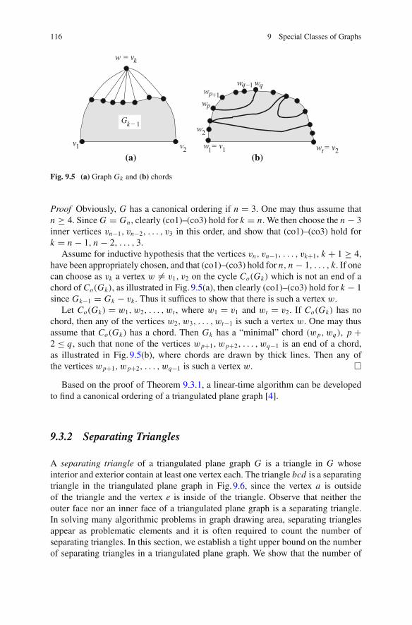
116 9 Special Classes of Graphs
w = v
w
w = v
wp
wq
2(b)
2
p+1q
1 1
ww
t
−1
w = v
vv1 2
Gk− 1
(a)
k
Fig. 9.5 (a) Graph Gk and (b) chords
Proof Obviously, G has a canonical ordering if n = 3. One may thus assume thatn ≥ 4. Since G = Gn , clearly (co1)–(co3) hold for k = n. We then choose the n − 3inner vertices vn−1, vn−2, . . . , v3 in this order, and show that (co1)–(co3) hold fork = n − 1, n − 2, . . . , 3.
Assume for inductive hypothesis that the vertices vn, vn−1, . . . , vk+1, k + 1 ≥ 4,have been appropriately chosen, and that (co1)–(co3) hold for n, n − 1, . . . , k. If onecan choose as vk a vertex w �= v1, v2 on the cycle Co(Gk) which is not an end of achord of Co(Gk), as illustrated in Fig. 9.5(a), then clearly (co1)–(co3) hold for k − 1since Gk−1 = Gk − vk . Thus it suffices to show that there is such a vertex w.
Let Co(Gk) = w1, w2, . . . , wt , where w1 = v1 and wt = v2. If Co(Gk) has nochord, then any of the vertices w2, w3, . . . , wt−1 is such a vertex w. One may thusassume that Co(Gk) has a chord. Then Gk has a “minimal” chord (wp, wq), p +2 ≤ q, such that none of the vertices wp+1, wp+2, . . . , wq−1 is an end of a chord,as illustrated in Fig. 9.5(b), where chords are drawn by thick lines. Then any ofthe vertices wp+1, wp+2, . . . , wq−1 is such a vertex w. �
Based on the proof of Theorem 9.3.1, a linear-time algorithm can be developedto find a canonical ordering of a triangulated plane graph [4].
9.3.2 Separating Triangles
A separating triangle of a triangulated plane graph G is a triangle in G whoseinterior and exterior contain at least one vertex each. The triangle bcd is a separatingtriangle in the triangulated plane graph in Fig. 9.6, since the vertex a is outsideof the triangle and the vertex e is inside of the triangle. Observe that neither theouter face nor an inner face of a triangulated plane graph is a separating triangle.In solving many algorithmic problems in graph drawing area, separating trianglesappear as problematic elements and it is often required to count the number ofseparating triangles. In this section, we establish a tight upper bound on the numberof separating triangles in a triangulated plane graph. We show that the number of
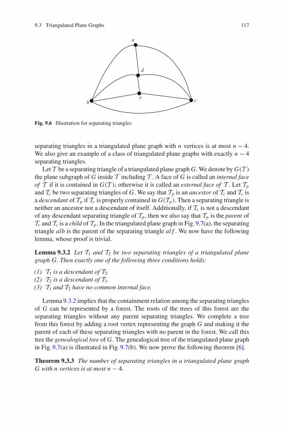
9.3 Triangulated Plane Graphs 117
a
eb
d
c
Fig. 9.6 Illustration for separating triangles
separating triangles in a triangulated plane graph with n vertices is at most n − 4.We also give an example of a class of triangulated plane graphs with exactly n − 4separating triangles.
Let T be a separating triangle of a triangulated plane graphG.We denote byG(T )
the plane subgraph of G inside T including T . A face of G is called an internal faceof T if it is contained in G(T ); otherwise it is called an external face of T . Let Tp
and Tc be two separating triangles of G. We say that Tp is an ancestor of Tc and Tc isa descendant of Tp if Tc is properly contained in G(Tp). Then a separating triangle isneither an ancestor nor a descendant of itself. Additionally, if Tc is not a descendantof any descendant separating triangle of Tp, then we also say that Tp is the parent ofTc and Tc is a child of Tp. In the triangulated plane graph in Fig. 9.7(a), the separatingtriangle alb is the parent of the separating triangle al f . We now have the followinglemma, whose proof is trivial.
Lemma 9.3.2 Let T1 and T2 be two separating triangles of a triangulated planegraph G. Then exactly one of the following three conditions holds:
(1) T1 is a descendant of T2.(2) T2 is a descendant of T1.(3) T1 and T2 have no common internal face.
Lemma 9.3.2 implies that the containment relation among the separating trianglesof G can be represented by a forest. The roots of the trees of this forest are theseparating triangles without any parent separating triangles. We complete a treefrom this forest by adding a root vertex representing the graph G and making it theparent of each of these separating triangles with no parent in the forest. We call thistree the genealogical tree of G. The genealogical tree of the triangulated plane graphin Fig. 9.7(a) is illustrated in Fig. 9.7(b). We now prove the following theorem [6].
Theorem 9.3.3 The number of separating triangles in a triangulated plane graphG with n vertices is at most n − 4.
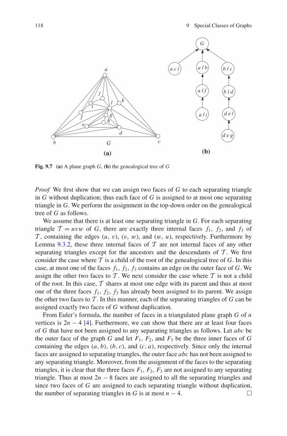
118 9 Special Classes of Graphs
b
ef
i
jk
h
l
G
g
d
a
c
G
a c l
d e g
d e l
a l b b l c
a l f b l d
a l i
(a) (b)
Fig. 9.7 (a) A plane graph G, (b) the genealogical tree of G
Proof We first show that we can assign two faces of G to each separating trianglein G without duplication; thus each face of G is assigned to at most one separatingtriangle in G. We perform the assignment in the top-down order on the genealogicaltree of G as follows.
We assume that there is at least one separating triangle in G. For each separatingtriangle T = uvw of G, there are exactly three internal faces f1, f2, and f3 ofT , containing the edges (u, v), (v, w), and (w, u), respectively. Furthermore byLemma 9.3.2, these three internal faces of T are not internal faces of any otherseparating triangles except for the ancestors and the descendants of T . We firstconsider the case where T is a child of the root of the genealogical tree of G. In thiscase, at most one of the faces f1, f2, f3 contains an edge on the outer face of G. Weassign the other two faces to T . We next consider the case where T is not a childof the root. In this case, T shares at most one edge with its parent and thus at mostone of the three faces f1, f2, f3 has already been assigned to its parent. We assignthe other two faces to T . In this manner, each of the separating triangles of G can beassigned exactly two faces of G without duplication.
From Euler’s formula, the number of faces in a triangulated plane graph G of nvertices is 2n − 4 [4]. Furthermore, we can show that there are at least four facesof G that have not been assigned to any separating triangles as follows. Let abc bethe outer face of the graph G and let F1, F2, and F3 be the three inner faces of Gcontaining the edges (a, b), (b, c), and (c, a), respectively. Since only the internalfaces are assigned to separating triangles, the outer face abc has not been assigned toany separating triangle. Moreover, from the assignment of the faces to the separatingtriangles, it is clear that the three faces F1, F2, F3 are not assigned to any separatingtriangle. Thus at most 2n − 8 faces are assigned to all the separating triangles andsince two faces of G are assigned to each separating triangle without duplication,the number of separating triangles in G is at most n − 4. �
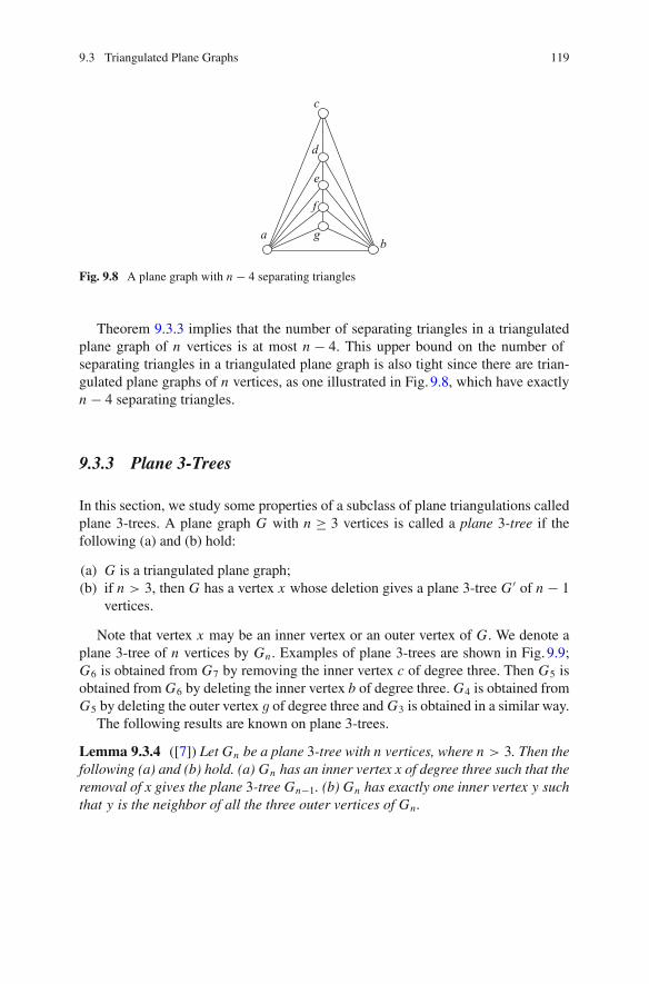
9.3 Triangulated Plane Graphs 119
c
d
gb
a
f
e
Fig. 9.8 A plane graph with n − 4 separating triangles
Theorem 9.3.3 implies that the number of separating triangles in a triangulatedplane graph of n vertices is at most n − 4. This upper bound on the number ofseparating triangles in a triangulated plane graph is also tight since there are trian-gulated plane graphs of n vertices, as one illustrated in Fig. 9.8, which have exactlyn − 4 separating triangles.
9.3.3 Plane 3-Trees
In this section, we study some properties of a subclass of plane triangulations calledplane 3-trees. A plane graph G with n ≥ 3 vertices is called a plane 3-tree if thefollowing (a) and (b) hold:
(a) G is a triangulated plane graph;(b) if n > 3, then G has a vertex x whose deletion gives a plane 3-tree G ′ of n − 1
vertices.
Note that vertex x may be an inner vertex or an outer vertex of G. We denote aplane 3-tree of n vertices by Gn . Examples of plane 3-trees are shown in Fig. 9.9;G6 is obtained from G7 by removing the inner vertex c of degree three. Then G5 isobtained from G6 by deleting the inner vertex b of degree three. G4 is obtained fromG5 by deleting the outer vertex g of degree three and G3 is obtained in a similar way.
The following results are known on plane 3-trees.
Lemma 9.3.4 ([7]) Let Gn be a plane 3-tree with n vertices, where n > 3. Then thefollowing (a) and (b) hold. (a) Gn has an inner vertex x of degree three such that theremoval of x gives the plane 3-tree Gn−1. (b) Gn has exactly one inner vertex y suchthat y is the neighbor of all the three outer vertices of Gn.
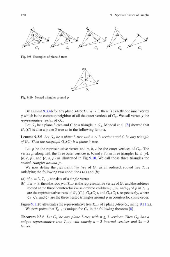
120 9 Special Classes of Graphs
G7 G6 G5 G4
caa
b gb ggaaa
dd d
fffff
eeee
G3
dd
Fig. 9.9 Examples of plane 3-trees
b
C
G
Cc
n
13
2C
p
a
Fig. 9.10 Nested triangles around p
By Lemma 9.3.4b for any plane 3-treeGn , n > 3, there is exactly one inner vertexy which is the common neighbor of all the outer vertices of Gn . We call vertex y therepresentative vertex of Gn .
Let Gn be a plane 3-tree and C be a triangle in Gn , Mondal et al. [8] showed thatGn(C) is also a plane 3-tree as in the following lemma.
Lemma 9.3.5 Let Gn be a plane 3-tree with n > 3 vertices and C be any triangleof Gn. Then the subgraph Gn(C) is a plane 3-tree.
Let p be the representative vertex and a, b, c be the outer vertices of Gn . Thevertex p, along with the three outer vertices a, b, and c, form three triangles {a, b, p},{b, c, p}, and {c, a, p} as illustrated in Fig. 9.10. We call those three triangles thenested triangles around p.
We now define the representative tree of Gn as an ordered, rooted tree Tn−3
satisfying the following two conditions (a) and (b):
(a) if n = 3, Tn−3 consists of a single vertex.(b) if n > 3, then the root p of Tn−3 is the representative vertex ofGn and the subtrees
rooted at the three counterclockwise ordered children q1, q2, and q3 of p in Tn−3
are the representative trees of Gn(C1), Gn(C2), and Gn(C3), respectively, whereC1,C2, andC3 are the three nested triangles around p in counterclockwise order.
Figure9.11(b) illustrates the representative treeTn−3 of a plane3-treeGn inFig. 9.11(a).We now prove that Tn−3 is unique for Gn in the following theorem [8].
Theorem 9.3.6 Let Gn be any plane 3-tree with n ≥ 3 vertices. Then Gn has aunique representative tree Tn−3 with exactly n − 3 internal vertices and 2n − 5leaves.
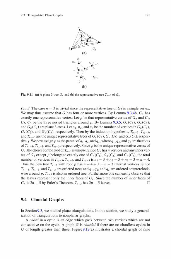
9.3 Triangulated Plane Graphs 121
p
Tn−3e
g
d f
Gnb
a
c
dp
egf
(a)
(b)
Fig. 9.11 (a) A plane 3-tree Gn and (b) the representative tree Tn−3 of Gn
Proof The case n = 3 is trivial since the representative tree of G3 is a single vertex.We may thus assume that G has four or more vertices. By Lemma 9.3.4b, Gn hasexactly one representative vertex. Let p be that representative vertex of Gn and C1,C2, C3 be the three nested triangles around p. By Lemma 9.3.5, Gn(C1), Gn(C2),andGn(C3) are plane 3-trees. Let n1, n2, and n3 be the number of vertices inGn(C1),Gn(C2), and Gn(C3), respectively. Then by the induction hypothesis, Tn1−3, Tn2−3,and Tn3−3 are the unique representative trees ofGn(C1),Gn(C2), andGn(C3), respec-tively.Wenowassign p as the parent ofq1,q2, andq3,whereq1,q2, andq3 are the rootsof Tn1−3, Tn2−3, and Tn3−3, respectively. Since p is the unique representative vertex ofGn , the choice for the root of Tn−3 is unique. SinceGn hasn vertices and any inner ver-tex of Gn except p belongs to exactly one of Gn(C1), Gn(C2), and Gn(C3), the totalnumber of vertices in Tn1−3, Tn2−3, and Tn3−3 is n1 − 3 + n2 − 3 + n3 − 3 = n − 4.Thus the new tree Tn−3 with root p has n − 4 + 1 = n − 3 internal vertices. SinceTn1−3, Tn2−3, and Tn3−3 are ordered trees and q1, q2, and q3 are ordered counterclock-wise around p, Tn−3 is also an ordered tree. Furthermore one can easily observe thatthe leaves represent only the inner faces of Gn . Since the number of inner faces ofGn is 2n − 5 by Euler’s Theorem, Tn−3 has 2n − 5 leaves. �
9.4 Chordal Graphs
In Section9.3, we studied plane triangulations. In this section, we study a general-ization of triangulations to nonplanar graphs.
A chord in a cycle is an edge which goes between two vertices which are notconsecutive on the cycle. A graph G is chordal if there are no chordless cycles inG of length greater than three. Figure9.12(a) illustrates a chordal graph of nine
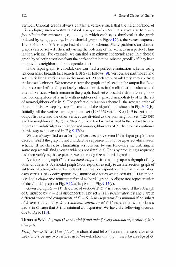
122 9 Special Classes of Graphs
vertices. Chordal graphs always contain a vertex v such that the neighborhood ofv is a clique; such a vertex is called a simplicial vertex. This gives rise to a per-fect elimination scheme v1, v2, . . . , vn in which each vi is simplicial in the graphinduced by vi , vi+1, . . . vn . In the chordal graph in Fig. 9.12(a), the vertex sequence1, 2, 3, 4, 5, 8, 6, 7, 9 is a perfect elimination scheme. Many problems on chordalgraphs can be solved efficiently using the ordering of the vertices in a perfect elim-ination scheme. For example, we can find a maximum independent set in a chordalgraph by selecting vertices from the perfect elimination scheme greedily if they haveno previous neighbor in the independent set.
If the input graph is chordal, one can find a perfect elimination scheme usinglexicographic breadth first search (LBFS) as follows [9]. Vertices are partitioned intosets; initially all vertices are in the same set. At each step, an arbitrary vertex x fromthe last set is chosen. We remove x from the graph and place it in the output list. Notethat x comes before all previously selected vertices in the elimination scheme, andafter all vertices which remain in the graph. Each set S is subdivided into neighborsand non-neighbors of x in S with neighbors of x placed immediately after the setof non-neighbors of x in S. The perfect elimination scheme is the reverse order ofthe output list. A step-by-step illustration of the algorithm is shown in Fig. 9.12(b).Initially, all the vertices are kept in one set (123456789). In Step 1, 9 is sent to theoutput list as x and the other vertices are divided as the non-neighbor set (123458)and the neighbor set (6, 7). In Step 2, 7 from the last set is sent to the output list andthe sets are subdivided as neighbor and non-neighbor sets of 7. The process continuesin this way as illustrated in Fig. 9.12(b).
We can always find an ordering of vertices above even if the input graph is notchordal. But if the graph is not chordal, the sequence will not be a perfect eliminationscheme. If we check by eliminating vertices one by one following the ordering, insome stepwewill find a vertex which is not simplicial. Thus by producing a sequenceand then verifying the sequence, we can recognize a chordal graph.
A clique in a graph G is a maximal clique if it is not a proper subgraph of anyother clique in G. A chordal graph G corresponds exactly to an intersection graph ofsubtrees of a tree, where the nodes of the tree correspond to maximal cliques of G,each vertex v of G corresponds to a subtree of cliques which contain v. This modelis called a clique tree representation of a chordal graph. A clique tree representationof the chordal graph in Fig. 9.12(a) is given in Fig. 9.12(c).
Given a graph G = (V, E), a set of vertices S ⊂ V is a separator if the subgraphof G induced by V − S is disconnected. The set S is a uv-separator if u and v are indifferent connected components of G − S. A uv-separator S is minimal if no subsetof S separates u and v. S is a minimal separator of G if there exist two vertices uand v in G such that S is a minimal uv-separator. We have the following theoremdue to Dirac [10].
Theorem 9.4.1 A graph G is chordal if and only if every minimal separator of G isa clique.
Proof Necessity Let G = (V, E) be chordal and let S be a minimal separator of G.Let x and y be any two vertices in S. We will show that (x, y) must be an edge of G.
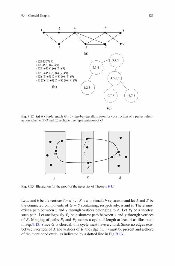
9.4 Chordal Graphs 123
(123456789)(123458) (67) (9)(123) (458) (6) (7) (9)(123) (45) (8) (6) (7) (9)(12) (3) (4) (5) (8) (6) (7) (9)(1) (2) (3) (4) (5) (8) (6) (7) (9)
1 2
3
4
5
6
7
8
9
6,7,9
4,5,6,7
6,7,8
2,3,4
1,2,3
(a)
(b)
(c)
3,4,5
Fig. 9.12 (a) A chordal graph G, (b) step-by-step illustration for construction of a perfect elimi-nation scheme of G and (c) a clique tree representation of G
y
x
a b
A S B
Fig. 9.13 Illustration for the proof of the necessity of Theorem 9.4.1
Let a and b be the vertices for which S is a minimal ab-separator, and let A and B bethe connected components of G − S containing, respectively, a and b. There mustexist a path between x and y through vertices belonging to A. Let P1 be a shortestsuch path. Let analogously P2 be a shortest path between x and y through verticesof B. Merging of paths P1 and P2 makes a cycle of length at least 4 as illustratedin Fig. 9.13. Since G is chordal, this cycle must have a chord. Since no edges existbetween vertices of A and vertices of B, the edge (x, y) must be present and a chordof the mentioned cycle, as indicated by a dotted line in Fig. 9.13.
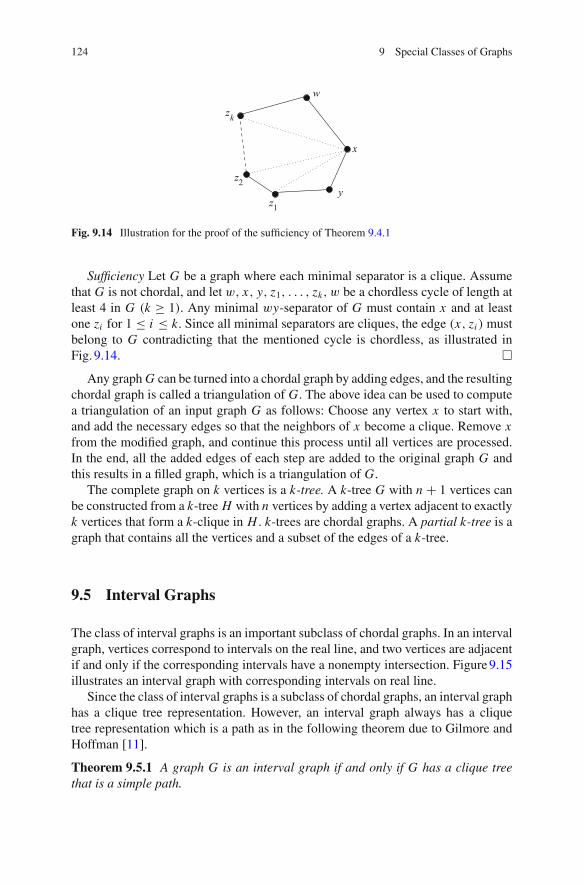
124 9 Special Classes of Graphs
w
x
yz
z
z
1
2
k
Fig. 9.14 Illustration for the proof of the sufficiency of Theorem 9.4.1
Sufficiency Let G be a graph where each minimal separator is a clique. Assumethat G is not chordal, and let w, x, y, z1, . . . , zk, w be a chordless cycle of length atleast 4 in G (k ≥ 1). Any minimal wy-separator of G must contain x and at leastone zi for 1 ≤ i ≤ k. Since all minimal separators are cliques, the edge (x, zi ) mustbelong to G contradicting that the mentioned cycle is chordless, as illustrated inFig. 9.14. �
Any graphG can be turned into a chordal graph by adding edges, and the resultingchordal graph is called a triangulation of G. The above idea can be used to computea triangulation of an input graph G as follows: Choose any vertex x to start with,and add the necessary edges so that the neighbors of x become a clique. Remove xfrom the modified graph, and continue this process until all vertices are processed.In the end, all the added edges of each step are added to the original graph G andthis results in a filled graph, which is a triangulation of G.
The complete graph on k vertices is a k-tree. A k-tree G with n + 1 vertices canbe constructed from a k-tree H with n vertices by adding a vertex adjacent to exactlyk vertices that form a k-clique in H . k-trees are chordal graphs. A partial k-tree is agraph that contains all the vertices and a subset of the edges of a k-tree.
9.5 Interval Graphs
The class of interval graphs is an important subclass of chordal graphs. In an intervalgraph, vertices correspond to intervals on the real line, and two vertices are adjacentif and only if the corresponding intervals have a nonempty intersection. Figure9.15illustrates an interval graph with corresponding intervals on real line.
Since the class of interval graphs is a subclass of chordal graphs, an interval graphhas a clique tree representation. However, an interval graph always has a cliquetree representation which is a path as in the following theorem due to Gilmore andHoffman [11].
Theorem 9.5.1 A graph G is an interval graph if and only if G has a clique treethat is a simple path.
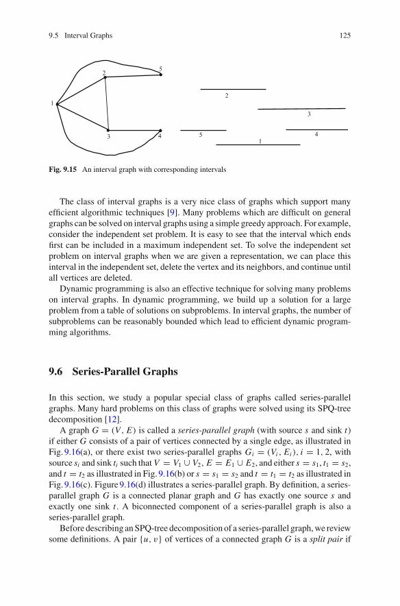
9.5 Interval Graphs 125
Fig. 9.15 An interval graph with corresponding intervals
The class of interval graphs is a very nice class of graphs which support manyefficient algorithmic techniques [9]. Many problems which are difficult on generalgraphs can be solved on interval graphs using a simple greedy approach. For example,consider the independent set problem. It is easy to see that the interval which endsfirst can be included in a maximum independent set. To solve the independent setproblem on interval graphs when we are given a representation, we can place thisinterval in the independent set, delete the vertex and its neighbors, and continue untilall vertices are deleted.
Dynamic programming is also an effective technique for solving many problemson interval graphs. In dynamic programming, we build up a solution for a largeproblem from a table of solutions on subproblems. In interval graphs, the number ofsubproblems can be reasonably bounded which lead to efficient dynamic program-ming algorithms.
9.6 Series-Parallel Graphs
In this section, we study a popular special class of graphs called series-parallelgraphs. Many hard problems on this class of graphs were solved using its SPQ-treedecomposition [12].
A graph G = (V, E) is called a series-parallel graph (with source s and sink t)if either G consists of a pair of vertices connected by a single edge, as illustrated inFig. 9.16(a), or there exist two series-parallel graphs Gi = (Vi , Ei ), i = 1, 2, withsource si and sink ti such that V = V1 ∪ V2, E = E1 ∪ E2, and either s = s1, t1 = s2,and t = t2 as illustrated in Fig. 9.16(b) or s = s1 = s2 and t = t1 = t2 as illustrated inFig. 9.16(c). Figure9.16(d) illustrates a series-parallel graph. By definition, a series-parallel graph G is a connected planar graph and G has exactly one source s andexactly one sink t . A biconnected component of a series-parallel graph is also aseries-parallel graph.
Before describing anSPQ-tree decomposition of a series-parallel graph,we reviewsome definitions. A pair {u, v} of vertices of a connected graph G is a split pair if
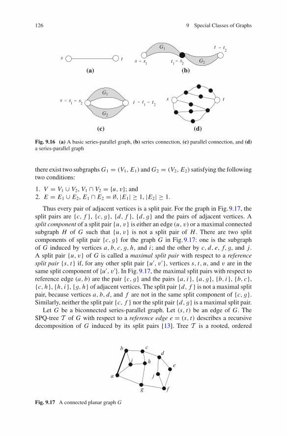
126 9 Special Classes of Graphs
s t1
=s s =s2t1
=t2
t
1
=s s =
2s 1
=t t =
2ts t
(a)
(c) (d)
(b)
G1
G2
G1
G2
Fig. 9.16 (a) A basic series-parallel graph, (b) series connection, (c) parallel connection, and (d)a series-parallel graph
there exist two subgraphsG1 = (V1, E1) andG2 = (V2, E2) satisfying the followingtwo conditions:
1. V = V1 ∪ V2, V1 ∩ V2 = {u, v}; and2. E = E1 ∪ E2, E1 ∩ E2 = ∅, |E1| ≥ 1, |E2| ≥ 1.
Thus every pair of adjacent vertices is a split pair. For the graph in Fig. 9.17, thesplit pairs are {c, f }, {c, g}, {d, f }, {d, g} and the pairs of adjacent vertices. Asplit component of a split pair {u, v} is either an edge (u, v) or a maximal connectedsubgraph H of G such that {u, v} is not a split pair of H . There are two splitcomponents of split pair {c, g} for the graph G in Fig. 9.17: one is the subgraphof G induced by vertices a, b, c, g, h, and i ; and the other by c, d, e, f, g, and j .A split pair {u, v} of G is called a maximal split pair with respect to a referencesplit pair {s, t} if, for any other split pair {u′, v′}, vertices s, t, u, and v are in thesame split component of {u′, v′}. In Fig. 9.17, the maximal split pairs with respect toreference edge (a, b) are the pair {c, g} and the pairs {a, i}, {a, g}, {b, i}, {b, c},{c, h}, {h, i}, {g, h} of adjacent vertices. The split pair {d, f } is not a maximal splitpair, because vertices a, b, d , and f are not in the same split component of {c, g}.Similarly, neither the split pair {c, f } nor the split pair {d, g} is a maximal split pair.
Let G be a biconnected series-parallel graph. Let (s, t) be an edge of G. TheSPQ-tree T of G with respect to a reference edge e = (s, t) describes a recursivedecomposition of G induced by its split pairs [13]. Tree T is a rooted, ordered
a
b
f
e
dc
i h
j
g
Fig. 9.17 A connected planar graph G
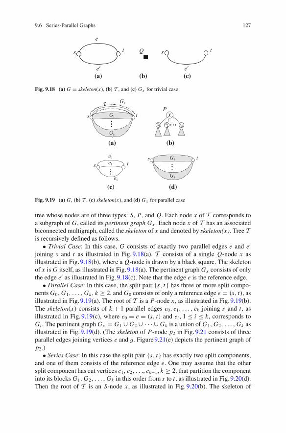
9.6 Series-Parallel Graphs 127
s ts t
e
e
Q
(a) (b) (c)e
Fig. 9.18 (a) G = skeleton(x), (b) T , and (c) Gx for trivial case
G0
G1
e1
e0
t
ek
sG1
s t
Gk
e
(c)
(a)
s t
Gk
(d)
P
(b)
xx x2 xk1
Fig. 9.19 (a) G, (b) T , (c) skeleton(x), and (d) Gx for parallel case
tree whose nodes are of three types: S, P , and Q. Each node x of T corresponds toa subgraph of G, called its pertinent graph Gx . Each node x of T has an associatedbiconnected multigraph, called the skeleton of x and denoted by skeleton(x). Tree Tis recursively defined as follows.
• Trivial Case: In this case, G consists of exactly two parallel edges e and e′joining s and t as illustrated in Fig. 9.18(a). T consists of a single Q-node x asillustrated in Fig. 9.18(b), where a Q-node is drawn by a black square. The skeletonof x is G itself, as illustrated in Fig. 9.18(a). The pertinent graph Gx consists of onlythe edge e′ as illustrated in Fig. 9.18(c). Note that the edge e is the reference edge.
• Parallel Case: In this case, the split pair {s, t} has three or more split compo-nents G0,G1, . . . ,Gk, k ≥ 2, and G0 consists of only a reference edge e = (s, t), asillustrated in Fig. 9.19(a). The root of T is a P-node x , as illustrated in Fig. 9.19(b).The skeleton(x) consists of k + 1 parallel edges e0, e1, . . . , ek joining s and t , asillustrated in Fig. 9.19(c), where e0 = e = (s, t) and ei , 1 ≤ i ≤ k, corresponds toGi . The pertinent graph Gx = G1 ∪ G2 ∪ · · · ∪ Gk is a union of G1,G2, . . . ,Gk asillustrated in Fig. 9.19(d). (The skeleton of P-node p2 in Fig. 9.21 consists of threeparallel edges joining vertices e and g. Figure9.21(e) depicts the pertinent graph ofp2.)
• Series Case: In this case the split pair {s, t} has exactly two split components,and one of them consists of the reference edge e. One may assume that the othersplit component has cut vertices c1, c2, . . ., ck−1, k ≥ 2, that partition the componentinto its blocks G1,G2, . . . ,Gk in this order from s to t , as illustrated in Fig. 9.20(d).Then the root of T is an S-node x , as illustrated in Fig. 9.20(b). The skeleton of
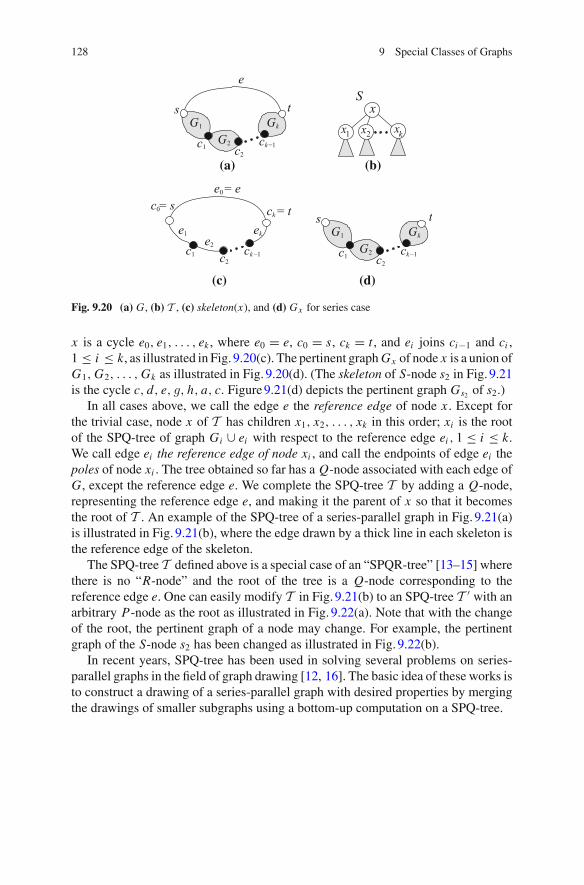
128 9 Special Classes of Graphs
G1 Gk
G21c2c
1c2c
2e1e
0e0c
G1 Gk
G21c2c
s t
−1kc
e
(a)
= e
−1kcke
= skc = t
(c)
s t
−1kc
(d)
S
(b)
xxkx2x1
Fig. 9.20 (a) G, (b) T , (c) skeleton(x), and (d) Gx for series case
x is a cycle e0, e1, . . . , ek , where e0 = e, c0 = s, ck = t , and ei joins ci−1 and ci ,1 ≤ i ≤ k, as illustrated in Fig. 9.20(c). The pertinent graphGx of node x is a union ofG1,G2, . . . ,Gk as illustrated in Fig. 9.20(d). (The skeleton of S-node s2 in Fig. 9.21is the cycle c, d, e, g, h, a, c. Figure9.21(d) depicts the pertinent graph Gs2 of s2.)
In all cases above, we call the edge e the reference edge of node x . Except forthe trivial case, node x of T has children x1, x2, . . . , xk in this order; xi is the rootof the SPQ-tree of graph Gi ∪ ei with respect to the reference edge ei , 1 ≤ i ≤ k.We call edge ei the reference edge of node xi , and call the endpoints of edge ei thepoles of node xi . The tree obtained so far has a Q-node associated with each edge ofG, except the reference edge e. We complete the SPQ-tree T by adding a Q-node,representing the reference edge e, and making it the parent of x so that it becomesthe root of T . An example of the SPQ-tree of a series-parallel graph in Fig. 9.21(a)is illustrated in Fig. 9.21(b), where the edge drawn by a thick line in each skeleton isthe reference edge of the skeleton.
The SPQ-tree T defined above is a special case of an “SPQR-tree” [13–15] wherethere is no “R-node” and the root of the tree is a Q-node corresponding to thereference edge e. One can easily modify T in Fig. 9.21(b) to an SPQ-tree T ′ with anarbitrary P-node as the root as illustrated in Fig. 9.22(a). Note that with the changeof the root, the pertinent graph of a node may change. For example, the pertinentgraph of the S-node s2 has been changed as illustrated in Fig. 9.22(b).
In recent years, SPQ-tree has been used in solving several problems on series-parallel graphs in the field of graph drawing [12, 16]. The basic idea of these works isto construct a drawing of a series-parallel graph with desired properties by mergingthe drawings of smaller subgraphs using a bottom-up computation on a SPQ-tree.
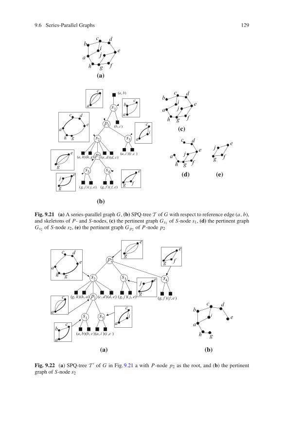
9.6 Series-Parallel Graphs 129
e d( , ) d c( , )
g j( , ) f e( , )
b c( , )
a h( , ) h g( , )a i( , ) i c( , )
j e( , ) g f( , )
(d)
(c)
(e)
(a)
a b( , )
(b)
s1
1p
s5s2
s3 s4
2p
c de
j
ha
g f
cb
di
g
je
a
h f
je
g f
c db
f
eji
a
ci
c
a
dc
a
gh
e
e
ge
j
g
e
g f
cb
a
ha
g
Fig. 9.21 (a) A series-parallel graph G, (b) SPQ-tree T of G with respect to reference edge (a, b),and skeletons of P- and S-nodes, (c) the pertinent graph Gs1 of S-node s1, (d) the pertinent graphGs2 of S-node s2, (e) the pertinent graph Gp2 of P-node p2
d e( , ) g f( , ) f e( , )
b c( , ) a i( , ) i c( , )
g h( , ) h a( , ) c d( , ) j e( , )g j( , )
(b)
a b( , )
(a)
2p
s2
1p
s1 s5
s4s3
i
cb
ea
d
h g
ah g
c
e
ge
g
c
a
cb
a
c
j
g
ia
e
d
e f
Fig. 9.22 (a) SPQ-tree T ′ of G in Fig. 9.21 a with P-node p2 as the root, and (b) the pertinentgraph of S-node s2
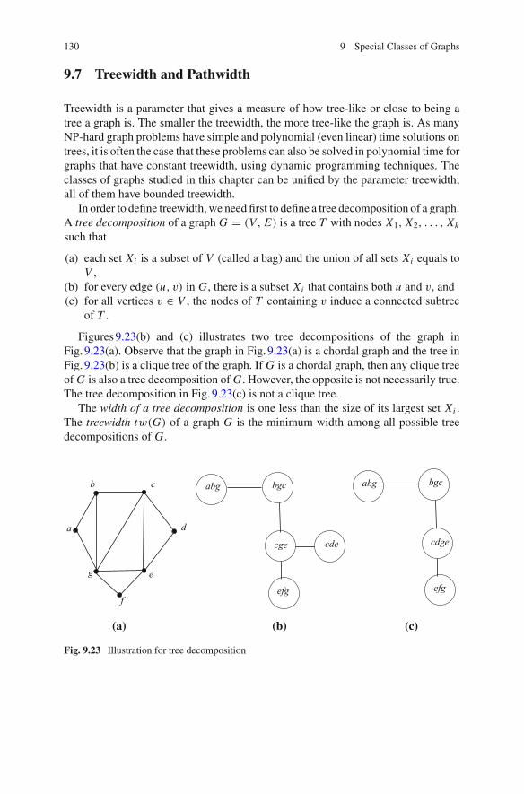
130 9 Special Classes of Graphs
9.7 Treewidth and Pathwidth
Treewidth is a parameter that gives a measure of how tree-like or close to being atree a graph is. The smaller the treewidth, the more tree-like the graph is. As manyNP-hard graph problems have simple and polynomial (even linear) time solutions ontrees, it is often the case that these problems can also be solved in polynomial time forgraphs that have constant treewidth, using dynamic programming techniques. Theclasses of graphs studied in this chapter can be unified by the parameter treewidth;all of them have bounded treewidth.
In order to define treewidth, we need first to define a tree decomposition of a graph.A tree decomposition of a graph G = (V, E) is a tree T with nodes X1, X2, . . . , Xk
such that
(a) each set Xi is a subset of V (called a bag) and the union of all sets Xi equals toV ,
(b) for every edge (u, v) in G, there is a subset Xi that contains both u and v, and(c) for all vertices v ∈ V , the nodes of T containing v induce a connected subtree
of T .
Figures9.23(b) and (c) illustrates two tree decompositions of the graph inFig. 9.23(a). Observe that the graph in Fig. 9.23(a) is a chordal graph and the tree inFig. 9.23(b) is a clique tree of the graph. If G is a chordal graph, then any clique treeof G is also a tree decomposition of G. However, the opposite is not necessarily true.The tree decomposition in Fig. 9.23(c) is not a clique tree.
The width of a tree decomposition is one less than the size of its largest set Xi .The treewidth tw(G) of a graph G is the minimum width among all possible treedecompositions of G.
a
b c
d
e
f
g
(a) (b)
abg bgc
cge
efg
cde
abg bgc
cdge
efg
(c)
Fig. 9.23 Illustration for tree decomposition
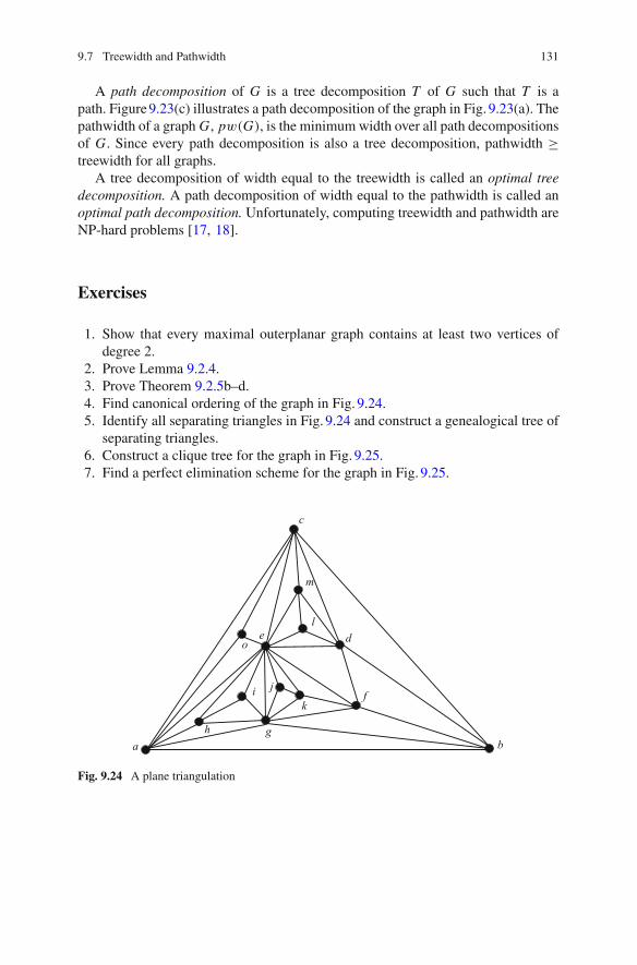
9.7 Treewidth and Pathwidth 131
A path decomposition of G is a tree decomposition T of G such that T is apath. Figure9.23(c) illustrates a path decomposition of the graph in Fig. 9.23(a). Thepathwidth of a graph G, pw(G), is the minimumwidth over all path decompositionsof G. Since every path decomposition is also a tree decomposition, pathwidth ≥treewidth for all graphs.
A tree decomposition of width equal to the treewidth is called an optimal treedecomposition. A path decomposition of width equal to the pathwidth is called anoptimal path decomposition. Unfortunately, computing treewidth and pathwidth areNP-hard problems [17, 18].
Exercises
1. Show that every maximal outerplanar graph contains at least two vertices ofdegree 2.
2. Prove Lemma 9.2.4.3. Prove Theorem 9.2.5b–d.4. Find canonical ordering of the graph in Fig. 9.24.5. Identify all separating triangles in Fig. 9.24 and construct a genealogical tree of
separating triangles.6. Construct a clique tree for the graph in Fig. 9.25.7. Find a perfect elimination scheme for the graph in Fig. 9.25.
a b
c
f
g
i
l
m
kj
h
oe d
Fig. 9.24 A plane triangulation
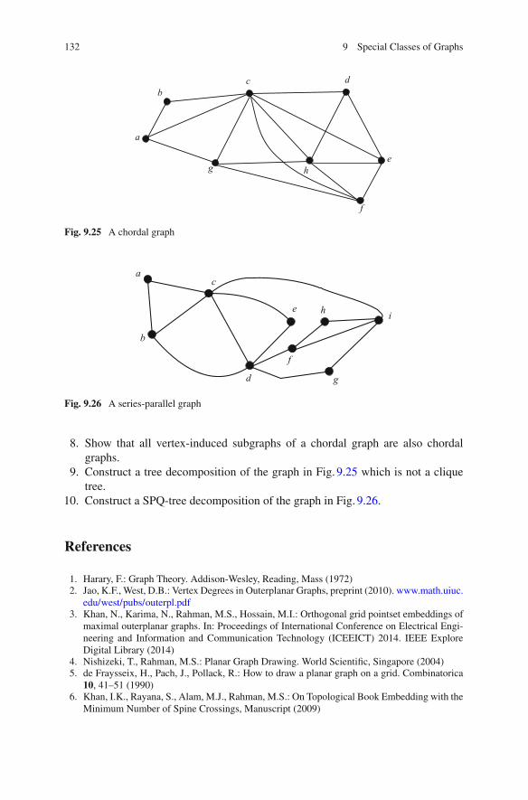
132 9 Special Classes of Graphs
bc d
e
f
hg
a
Fig. 9.25 A chordal graph
ac
e
g
h i
b
d
f
Fig. 9.26 A series-parallel graph
8. Show that all vertex-induced subgraphs of a chordal graph are also chordalgraphs.
9. Construct a tree decomposition of the graph in Fig. 9.25 which is not a cliquetree.
10. Construct a SPQ-tree decomposition of the graph in Fig. 9.26.
References
1. Harary, F.: Graph Theory. Addison-Wesley, Reading, Mass (1972)2. Jao, K.F., West, D.B.: Vertex Degrees in Outerplanar Graphs, preprint (2010). www.math.uiuc.
edu/west/pubs/outerpl.pdf3. Khan, N., Karima, N., Rahman, M.S., Hossain, M.I.: Orthogonal grid pointset embeddings of
maximal outerplanar graphs. In: Proceedings of International Conference on Electrical Engi-neering and Information and Communication Technology (ICEEICT) 2014. IEEE ExploreDigital Library (2014)
4. Nishizeki, T., Rahman, M.S.: Planar Graph Drawing. World Scientific, Singapore (2004)5. de Fraysseix, H., Pach, J., Pollack, R.: How to draw a planar graph on a grid. Combinatorica
10, 41–51 (1990)6. Khan, I.K., Rayana, S., Alam, M.J., Rahman, M.S.: On Topological Book Embedding with the
Minimum Number of Spine Crossings, Manuscript (2009)
References 133
7. Biedl, T., Velasquez, L.E.R.: Drawing planar 3-trees with given face-areas. In: Proceedings ofthe 17th International Symposium on Graph Drawing (GD 2009), Lecture Notes in ComputerScience, vol. 5849, pp. 316–322. Springer, Heidelberg (2010)
8. Mondal, D., Nishat, R.I., Rahman, M.S., Alam, M.J.: Minimum-area drawings of plane3-trees. J. Graph Algorithms Appl. 15(2), 177–204 (2011)
9. Spinrad, J.P.: Efficient Graph Representations. American Mathematical Society, Rhode Island(2003)
10. Dirac, G.A.: On rigid circuit graphs. Anh. Math. Sem. Univ. Hamburg 25, 71–76 (1961)11. Gilmore, P.C.,Hoffman,A.J.:A characterization of comparability graphs andof interval graphs.
Canadian J. Math. 16, 539548 (1964)12. Rahman, M.S., Egi, N., Nishizeki, T.: No-bend orthogonal drawings of series-parallel graphs.
In: Proceedings of the 13th International Conference on Graph Drawing (GD’05), LectureNotes in Computer Science, vol. 3843, pp. 409–420. Springer, Heidelberg (2006)
13. Garg, A., Liotta, G.: Almost bend-optimal planar orthogonal drawings of biconnected degree-3 planar graphs in quadratic time. In: Proceedings of Graph Drawing’99. Lecture Notes inComputer Science, vol. 1731, pp. 38–48. Springer, Heidelberg (1999)
14. Di Battista, G., Tamassia, R.: On-line maintenance of triconnected components with SPQR-trees. Algorithmica 15(4), 302–318 (1996)
15. Di Battista, G., Tamassia, R., Vismara, L.: Output-sensetive reporting of disjoint paths. Algo-rithmica 23, 302–340 (1999)
16. Hossain, M.I., Rahman, M.S.: Straight-line monotone grid drawings of series-parallel graphs.Discret. Math. Alg. Appl. 7(2) (2015)
17. Arnborg, S., Corneil, D., Proskurowski, A.: Complexity of finding embeddings in a k-tree.SIAM J. Matrix Anal. Appl. 8(2), 277–284 (1987)
18. Bodlaender, H.L.: A tourist guide through treewidth. In: Dassow, J., Kelemenová, A. (eds.)Developments in Theoretical Computer Science (Proc. 7th International Meeting of YoungComputer Scientists, Smolenice, 16–20 November 1992), Topics in Computer Mathematics,vol. 6, pp. 1–20. Gordon and Breach (1994)
Chapter 10Some Research Topics
10.1 Introduction
In this chapter, we introduce some research areas where the students learning graphtheory may find interest. As we have seen in Chapter1, graphs have applications inmodeling many real-world problems. So a researcher in graph theory can work onfundamental properties of graphs as well as developing graph models for practicalapplications and on devising efficient algorithms.
10.2 Graph Representation
In Chapter2, we have read adjacency matrix and adjacency list for graph represen-tation and learned that an adjacency matrix needs O(n2) space and an adjacency listtakes O(n + m) space to represent a graph of n vertices and m edges. Which one isbetter? The answer is not straightforward; it depends on which graph we are going torepresent. In this section, we focus on the space complexity of graph representationsin terms of the requirements of bits for storing the graph and see that different classesof graphs admit different forms of efficient representations [1].
We first address the space complexity of the two representationsmentioned above.Adjacency matrices use �(n2) bits to store a graph and the same amount of space isrequired for every graph. Adjacency lists take a total of 2m entries for an undirectedgraph, since each entry appears on two lists. Each entry holds a number in the range1 . . . n, and thus takes log n bits. Thus the total space complexity is �(m log n) bits.
Let a set has 2�( f (n)) elements. We call a representation of the members of theset by O( f (n)) bits an optimal representation. Using this definition, we call theadjacency matrix representation an optimal representation, since it uses O(n2) bitsto represent a set of 2n(n−1)/2 graphs of n vertices. On the other hand, adjacency listis not space optimal since it used �(n2 log n) bits to represent a complete graph.
© Springer International Publishing AG 2017M.S. Rahman, Basic Graph Theory, Undergraduate Topics in Computer Science,DOI 10.1007/978-3-319-49475-3_10
135
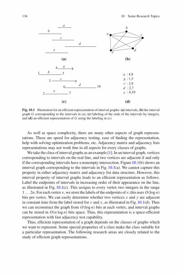
136 10 Some Research Topics
ab
c
d
e
ab
d
e
ab
e d
c
(d)(c)
(a) (b)
c1
9106
72
8
3
4
: 4,8a: 1,5b
cde : 6,10
: 2,7: 3,9
5
Fig. 10.1 Illustration for an efficient representation of interval graphs: (a) intervals, (b) the intervalgraph G corresponding to the intervals in (a), (c) labeling of the ends of the intervals by integers,and (d) an efficient representation of G using the labeling in (c)
As well as space complexity, there are many other aspects of graph represen-tations. These are speed for adjacency testing, ease of finding the representation,help with solving optimization problems, etc. Adjacency matrix and adjacency listsrepresentations may not work fine in all aspects for every classes of graphs.
We take the class of interval graphs as an example [1]. In an interval graph, verticescorresponding to intervals on the real line, and two vertices are adjacent if and onlyif the corresponding intervals have a nonempty intersection. Figure10.1(b) shows aninterval graph corresponding to the intervals in Fig. 10.1(a). We cannot capture thisproperty in either adjacency matrix and adjacency list data structure. However, thisinterval property of interval graphs leads to an efficient representation as follows.Label the endpoints of intervals in increasing order of their appearance on the line,as illustrated in Fig. 10.1(c). This assigns to every vertex two integers in the range1 . . . 2n. For each vertex v, we store the labels of the endpoints of v; this uses O(log n)
bits per vertex. We can easily determine whether two vertices x and y are adjacentin constant time from the label stored for x and y, as illustrated in Fig. 10.1(d). Thuswe can reconstruct the graph from O(log n) bits at each vertex, and interval graphscan be stored in O(n log n) bits space. Thus, this representation is a space-efficientrepresentation with fast adjacency test capability.
Thus, efficient representation of a graph depends on the classes of graphs whichwe want to represent. Some special properties of a class make the class suitable fora particular representation. The following research areas are closely related to thestudy of efficient graph representations.
10.2 Graph Representation 137
(a) Counting: The number of graphs in a particular class gives a lower bound on thespace complexity of its representation. Thus, counting the number of graphs ina special class of graphs is an interesting research problem.
(b) Representation: Finding space optimal representation with fast adjacency testingfor different classes of graphs is the main focus of the representation problem.Space optimal representation is motivated from the applications in smart devicesin recent years. Determining whether a particular form of representation existsfor a given class of graphs is an interesting problem.
(c) Constructing Representation: Some classes of graphs may have efficient repre-sentation, but they may not be constructed easily. Thus, efficient construction ofa representation is also an interesting research problem.
(d) Recognition: The recognition problem for a class of graphs is the problem ofdetermining whether a given graph is in some class. This problem is interestingnot only from the representation point of view, but also for other graph algorith-mic area. Say, some algorithm works for a particular class of graphs. If we candetermine whether the given graph is in that class, we can use the algorithm.
(e) Characterization: The problem of deriving necessary and sufficient conditionsfor a particular class of graphs is known as characterization problem. By derivingsuch conditions for the graphs in a class, we can develop efficient algorithms forrecognizing the graphs in the class.
Content of this section is based on the book of Spinrad [1], interested readers canfind more on graph classes and their representations in the book.
10.3 Graph Drawing
A drawing of a graph can be thought of as a diagram consisting of a collection ofobjects corresponding to the vertices of the graph together with some line segmentscorresponding to the edges connecting the objects. People are using diagrams fromancient time to represent abstract things like ideas, concepts, etc., as well as concretethings like maps, structures of machines, etc. A graph may be used to represent anyinformation which can bemodeled as objects and relationship between those objects.Adrawing of a graph is a sort of visualization of information represented by the graph.The graph in Fig. 10.2(a) represents eight components and their interconnections inan electronic circuit, and Fig. 10.2(b) depicts a drawing of the graph. Although thegraph in Fig. 10.2(a) correctly represents the circuit, the representation is messy andhard to trace the circuit for understanding and troubleshooting. Furthermore, in thisrepresentation one cannot lay the circuit on a single-layered PCB (Printed CircuitBoard) because of edge crossings. On the other hand, the drawing of the graphin Fig. 10.2(b) looks better and it is easily traceable. Furthermore one can use thedrawing to lay the circuit on a single-layered PCB, since it has no edge crossing.Thus, the objective of graph drawing is to obtain a nice representation of a graph such
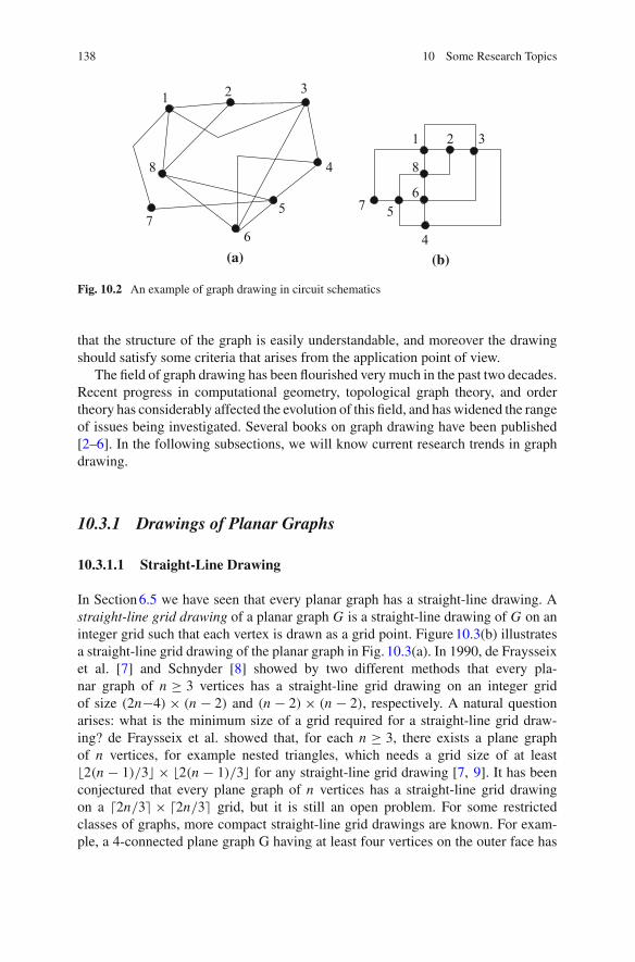
138 10 Some Research Topics
1 2 3
1 2 3
4
4
5 5
6
6
77
88
(b)(a)
Fig. 10.2 An example of graph drawing in circuit schematics
that the structure of the graph is easily understandable, and moreover the drawingshould satisfy some criteria that arises from the application point of view.
The field of graph drawing has been flourished very much in the past two decades.Recent progress in computational geometry, topological graph theory, and ordertheory has considerably affected the evolution of this field, and haswidened the rangeof issues being investigated. Several books on graph drawing have been published[2–6]. In the following subsections, we will know current research trends in graphdrawing.
10.3.1 Drawings of Planar Graphs
10.3.1.1 Straight-Line Drawing
In Section6.5 we have seen that every planar graph has a straight-line drawing. Astraight-line grid drawing of a planar graph G is a straight-line drawing of G on aninteger grid such that each vertex is drawn as a grid point. Figure10.3(b) illustratesa straight-line grid drawing of the planar graph in Fig. 10.3(a). In 1990, de Fraysseixet al. [7] and Schnyder [8] showed by two different methods that every pla-nar graph of n ≥ 3 vertices has a straight-line grid drawing on an integer gridof size (2n−4) × (n − 2) and (n − 2) × (n − 2), respectively. A natural questionarises: what is the minimum size of a grid required for a straight-line grid draw-ing? de Fraysseix et al. showed that, for each n ≥ 3, there exists a plane graphof n vertices, for example nested triangles, which needs a grid size of at least�2(n − 1)/3� × �2(n − 1)/3� for any straight-line grid drawing [7, 9]. It has beenconjectured that every plane graph of n vertices has a straight-line grid drawingon a �2n/3� × �2n/3� grid, but it is still an open problem. For some restrictedclasses of graphs, more compact straight-line grid drawings are known. For exam-ple, a 4-connected plane graph G having at least four vertices on the outer face has
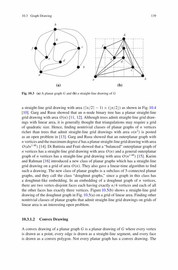
10.3 Graph Drawing 139
a
b
c
de
f
g
h
a b
c
(a) (b)
h
g
de
f
Fig. 10.3 (a) A planar graph G and (b) a straight-line drawing of G
a straight-line grid drawing with area (�n/2� − 1) × (�n/2�) as shown in Fig. 10.4[10]. Garg and Rusu showed that an n-node binary tree has a planar straight-linegrid drawing with area O(n) [11, 12]. Although trees admit straight-line grid draw-ings with linear area, it is generally thought that triangulations may require a gridof quadratic size. Hence, finding nontrivial classes of planar graphs of n verticesricher than trees that admit straight-line grid drawings with area o(n2) is postedas an open problem in [13]. Garg and Rusu showed that an outerplanar graph withn vertices and themaximumdegree d has a planar straight-line grid drawingwith areaO(dn1.48) [14]. Di Battista and Frati showed that a “balanced” outerplanar graph ofn vertices has a straight-line grid drawing with area O(n) and a general outerplanargraph of n vertices has a straight-line grid drawing with area O(n1.48) [15]. Karimand Rahman [16] introduced a new class of planar graphs which has a straight-linegrid drawing on a grid of area O(n). They also gave a linear-time algorithm to findsuch a drawing. The new class of planar graphs is a subclass of 5-connected planargraphs, and they call the class “doughnut graphs,” since a graph in this class hasa doughnut-like embedding. In an embedding of a doughnut graph of n vertices,there are two vertex-disjoint faces each having exactly n/4 vertices and each of allthe other faces has exactly three vertices. Figure10.5(b) shows a straight-line griddrawing of the doughnut graph in Fig. 10.5(a) on a grid of linear area. Finding othernontrivial classes of planar graphs that admit straight-line grid drawings on grids oflinear area is an interesting open problem.
10.3.1.2 Convex Drawing
A convex drawing of a planar graph G is a planar drawing of G where every vertexis drawn as a point, every edge is drawn as a straight-line segment, and every faceis drawn as a convex polygon. Not every planar graph has a convex drawing. The
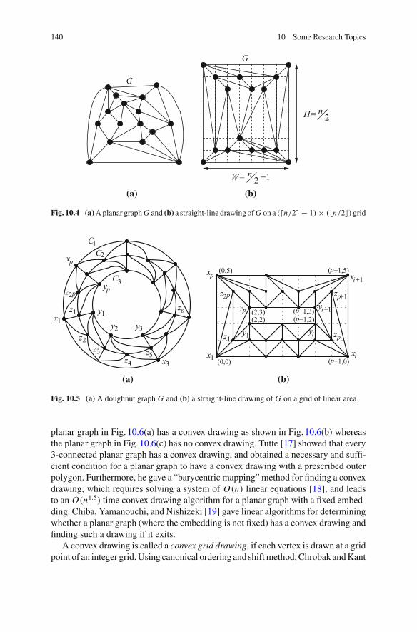
140 10 Some Research Topics
G
n2 −1
(b)(a)
G
W=
H= n2
Fig. 10.4 (a)Aplanar graphG and (b) a straight-line drawing ofG on a (�n/2� − 1) × (�n/2�) grid
y1zp
z2p py
px
C1
(p−1,3)
( +1,0)px1
px xi+1
z1 pz
+1zpz2p
y1 yi
i+1ypy
(0,0)
(0,5) ( +1,5)p
(p−1,2)(2,2)(2,3)
xi
x
xz
zz
z
z
3
11
23
45
y y2 3
C2
C3
(a) (b)
Fig. 10.5 (a) A doughnut graph G and (b) a straight-line drawing of G on a grid of linear area
planar graph in Fig. 10.6(a) has a convex drawing as shown in Fig. 10.6(b) whereasthe planar graph in Fig. 10.6(c) has no convex drawing. Tutte [17] showed that every3-connected planar graph has a convex drawing, and obtained a necessary and suffi-cient condition for a planar graph to have a convex drawing with a prescribed outerpolygon. Furthermore, he gave a “barycentric mapping” method for finding a convexdrawing, which requires solving a system of O(n) linear equations [18], and leadsto an O(n1.5) time convex drawing algorithm for a planar graph with a fixed embed-ding. Chiba, Yamanouchi, and Nishizeki [19] gave linear algorithms for determiningwhether a planar graph (where the embedding is not fixed) has a convex drawing andfinding such a drawing if it exits.
A convex drawing is called a convex grid drawing, if each vertex is drawn at a gridpoint of an integer grid.Using canonical ordering and shiftmethod,Chrobak andKant
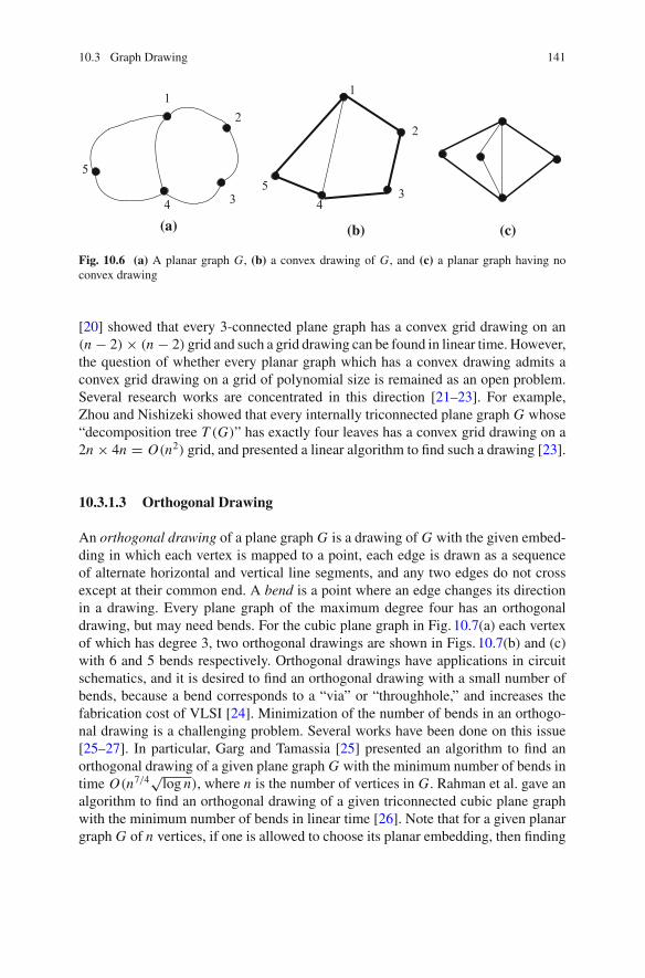
10.3 Graph Drawing 141
1
5
4 3
2
(b)(a)
1
34
2
5
(c)
Fig. 10.6 (a) A planar graph G, (b) a convex drawing of G, and (c) a planar graph having noconvex drawing
[20] showed that every 3-connected plane graph has a convex grid drawing on an(n − 2) × (n − 2) grid and such a grid drawing can be found in linear time. However,the question of whether every planar graph which has a convex drawing admits aconvex grid drawing on a grid of polynomial size is remained as an open problem.Several research works are concentrated in this direction [21–23]. For example,Zhou and Nishizeki showed that every internally triconnected plane graph G whose“decomposition tree T (G)” has exactly four leaves has a convex grid drawing on a2n × 4n = O(n2) grid, and presented a linear algorithm to find such a drawing [23].
10.3.1.3 Orthogonal Drawing
An orthogonal drawing of a plane graph G is a drawing of G with the given embed-ding in which each vertex is mapped to a point, each edge is drawn as a sequenceof alternate horizontal and vertical line segments, and any two edges do not crossexcept at their common end. A bend is a point where an edge changes its directionin a drawing. Every plane graph of the maximum degree four has an orthogonaldrawing, but may need bends. For the cubic plane graph in Fig. 10.7(a) each vertexof which has degree 3, two orthogonal drawings are shown in Figs. 10.7(b) and (c)with 6 and 5 bends respectively. Orthogonal drawings have applications in circuitschematics, and it is desired to find an orthogonal drawing with a small number ofbends, because a bend corresponds to a “via” or “throughhole,” and increases thefabrication cost of VLSI [24]. Minimization of the number of bends in an orthogo-nal drawing is a challenging problem. Several works have been done on this issue[25–27]. In particular, Garg and Tamassia [25] presented an algorithm to find anorthogonal drawing of a given plane graph G with the minimum number of bends intime O(n7/4
√log n), where n is the number of vertices in G. Rahman et al. gave an
algorithm to find an orthogonal drawing of a given triconnected cubic plane graphwith the minimum number of bends in linear time [26]. Note that for a given planargraph G of n vertices, if one is allowed to choose its planar embedding, then finding
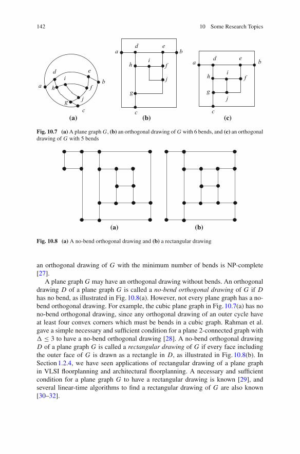
142 10 Some Research Topics
ab
c
d e
fi
j
b
c
d e
f
g
i
j
b
c
d e
fi
j
h
h
a
h
g
a
g
(b) (c)(a)
Fig. 10.7 (a)A plane graph G, (b) an orthogonal drawing of G with 6 bends, and (c) an orthogonaldrawing of G with 5 bends
(b)(a)
Fig. 10.8 (a) A no-bend orthogonal drawing and (b) a rectangular drawing
an orthogonal drawing of G with the minimum number of bends is NP-complete[27].
A plane graph G may have an orthogonal drawing without bends. An orthogonaldrawing D of a plane graph G is called a no-bend orthogonal drawing of G if Dhas no bend, as illustrated in Fig. 10.8(a). However, not every plane graph has a no-bend orthogonal drawing. For example, the cubic plane graph in Fig. 10.7(a) has nono-bend orthogonal drawing, since any orthogonal drawing of an outer cycle haveat least four convex corners which must be bends in a cubic graph. Rahman et al.gave a simple necessary and sufficient condition for a plane 2-connected graph with� ≤ 3 to have a no-bend orthogonal drawing [28]. A no-bend orthogonal drawingD of a plane graph G is called a rectangular drawing of G if every face includingthe outer face of G is drawn as a rectangle in D, as illustrated in Fig. 10.8(b). InSection1.2.4, we have seen applications of rectangular drawing of a plane graphin VLSI floorplanning and architectural floorplanning. A necessary and sufficientcondition for a plane graph G to have a rectangular drawing is known [29], andseveral linear-time algorithms to find a rectangular drawing of G are also known[30–32].
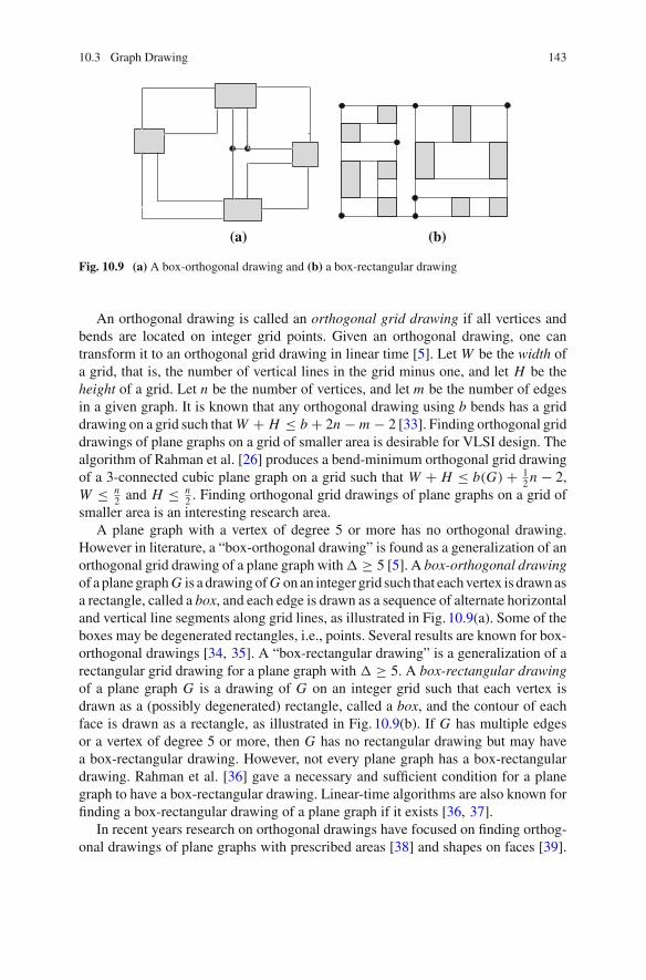
10.3 Graph Drawing 143
(a) (b)
Fig. 10.9 (a) A box-orthogonal drawing and (b) a box-rectangular drawing
An orthogonal drawing is called an orthogonal grid drawing if all vertices andbends are located on integer grid points. Given an orthogonal drawing, one cantransform it to an orthogonal grid drawing in linear time [5]. Let W be the width ofa grid, that is, the number of vertical lines in the grid minus one, and let H be theheight of a grid. Let n be the number of vertices, and let m be the number of edgesin a given graph. It is known that any orthogonal drawing using b bends has a griddrawing on a grid such thatW + H ≤ b + 2n − m − 2 [33]. Finding orthogonal griddrawings of plane graphs on a grid of smaller area is desirable for VLSI design. Thealgorithm of Rahman et al. [26] produces a bend-minimum orthogonal grid drawingof a 3-connected cubic plane graph on a grid such that W + H ≤ b(G) + 1
2n − 2,W ≤ n
2 and H ≤ n2 . Finding orthogonal grid drawings of plane graphs on a grid of
smaller area is an interesting research area.A plane graph with a vertex of degree 5 or more has no orthogonal drawing.
However in literature, a “box-orthogonal drawing” is found as a generalization of anorthogonal grid drawing of a plane graph with� ≥ 5 [5]. A box-orthogonal drawingof a planegraphG is a drawingofG onan integer grid such that eachvertex is drawnasa rectangle, called a box, and each edge is drawn as a sequence of alternate horizontaland vertical line segments along grid lines, as illustrated in Fig. 10.9(a). Some of theboxes may be degenerated rectangles, i.e., points. Several results are known for box-orthogonal drawings [34, 35]. A “box-rectangular drawing” is a generalization of arectangular grid drawing for a plane graph with � ≥ 5. A box-rectangular drawingof a plane graph G is a drawing of G on an integer grid such that each vertex isdrawn as a (possibly degenerated) rectangle, called a box, and the contour of eachface is drawn as a rectangle, as illustrated in Fig. 10.9(b). If G has multiple edgesor a vertex of degree 5 or more, then G has no rectangular drawing but may havea box-rectangular drawing. However, not every plane graph has a box-rectangulardrawing. Rahman et al. [36] gave a necessary and sufficient condition for a planegraph to have a box-rectangular drawing. Linear-time algorithms are also known forfinding a box-rectangular drawing of a plane graph if it exists [36, 37].
In recent years research on orthogonal drawings have focused on finding orthog-onal drawings of plane graphs with prescribed areas [38] and shapes on faces [39].
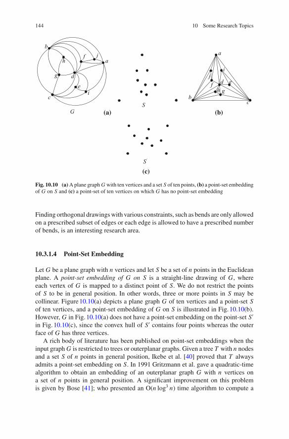
144 10 Some Research Topics
(b)(a)
(c)
G
/S
S
b
c
h
g d
a
ie
jf
b
a
gd ef
j
h
c
i
Fig. 10.10 (a)Aplane graphG with ten vertices and a set S of ten points, (b) a point-set embeddingof G on S and (c) a point-set of ten vertices on which G has no point-set embedding
Finding orthogonal drawingswith various constraints, such as bends are only allowedon a prescribed subset of edges or each edge is allowed to have a prescribed numberof bends, is an interesting research area.
10.3.1.4 Point-Set Embedding
Let G be a plane graph with n vertices and let S be a set of n points in the Euclideanplane. A point-set embedding of G on S is a straight-line drawing of G, whereeach vertex of G is mapped to a distinct point of S. We do not restrict the pointsof S to be in general position. In other words, three or more points in S may becollinear. Figure10.10(a) depicts a plane graph G of ten vertices and a point-set Sof ten vertices, and a point-set embedding of G on S is illustrated in Fig. 10.10(b).However, G in Fig. 10.10(a) does not have a point-set embedding on the point-set S′in Fig. 10.10(c), since the convex hull of S′ contains four points whereas the outerface of G has three vertices.
A rich body of literature has been published on point-set embeddings when theinput graphG is restricted to trees or outerplanar graphs. Given a tree T with n nodesand a set S of n points in general position, Ikebe et al. [40] proved that T alwaysadmits a point-set embedding on S. In 1991 Gritzmann et al. gave a quadratic-timealgorithm to obtain an embedding of an outerplanar graph G with n vertices ona set of n points in general position. A significant improvement on this problemis given by Bose [41]; who presented an O(n log3 n) time algorithm to compute a
10.3 Graph Drawing 145
straight-line embedding of an outerplanar graphG with n vertices on a set of n points.Cabello [42] proved that the problem is NP-complete for planar graphs in generaland even when the input graph is 2-connected and 2-outerplanar. Garcia et al. gavea characterization of a set S of points such that there exists a 3-connected cubicplane graph that admits a point-set embedding on S [43]. Recently, Nishat et al. [44]gave an O(n2) time algorithm that decides whether a plane 3-tree G with n verticesadmits a point-set embedding on a set S of n points or not; and computes a point-setembedding of G if such an embedding exists. They also showed that the problemis NP-complete for planar partial 3-trees. Durocher and Mondal [45] proved thatthe point-set embeddability problem remains NP-complete for 3-connected planegraphs.
Point-set embedding is an active area of research. Researchers are consideringthe problem from various point of views. A set P of points in R2 is n-universal, ifevery planar graph of n vertices admits a plane straight-line drawing on P . Finding ann-universal point-set of smaller size is an interesting area of research [46, 47]. Insteadof point-set, this problem has also been studied on line-sets [48, 49]. Interestingresearch problems can be formulated by combining other drawing styles like convexdrawing, orthogonal grid drawing with point-set embeddings [45, 50].
10.3.2 Simultaneous Embedding
Usually in a graph-drawing problemwe dealwith a drawing of a single graph. But in asimultaneous graph-drawing problem, we are concerned with the layout of a series ofgraphs that share all, or parts of the samevertex set. Figure10.11(b) illustrates a simul-taneous embedding of the two graphs in Fig. 10.11(a). In a drawing of such a series ofgraph readability of the individual graph aswell asmentalmap representation are twoimportant parameters [51]. Readability depends on some aesthetic criteria, whereasmental map preservation demands to make the position of the vertices in the draw-ing unchanged of the series of graphs. Simultaneous embedding finds applicationsin software engineering, database, in displaying phylogenetic trees etc. In evolu-tionary biology, phylogenetic trees are used to visualize the ancestral relationshipamong groups of species. Comparing two phylogenetic trees produced by differentmethods on the same set of species become easier if a simultaneous embedding ofthe two trees is constructed. Simultaneous embedding is an active area of researchand there are many interesting open problems on simultaneous embeddings [51].
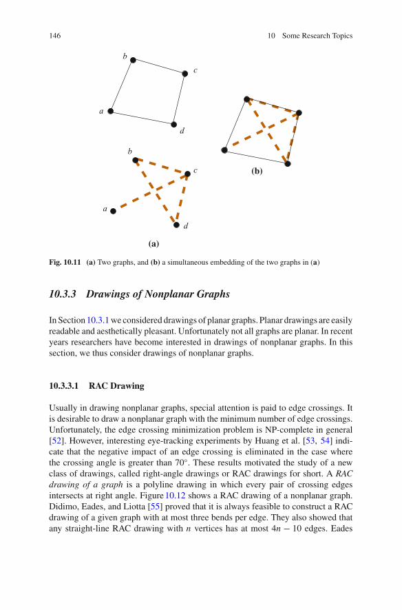
146 10 Some Research Topics
(a)
(b)
a
bc
d
a
b
c
d
Fig. 10.11 (a) Two graphs, and (b) a simultaneous embedding of the two graphs in (a)
10.3.3 Drawings of Nonplanar Graphs
In Section10.3.1we considered drawings of planar graphs. Planar drawings are easilyreadable and aesthetically pleasant. Unfortunately not all graphs are planar. In recentyears researchers have become interested in drawings of nonplanar graphs. In thissection, we thus consider drawings of nonplanar graphs.
10.3.3.1 RAC Drawing
Usually in drawing nonplanar graphs, special attention is paid to edge crossings. Itis desirable to draw a nonplanar graph with the minimum number of edge crossings.Unfortunately, the edge crossing minimization problem is NP-complete in general[52]. However, interesting eye-tracking experiments by Huang et al. [53, 54] indi-cate that the negative impact of an edge crossing is eliminated in the case wherethe crossing angle is greater than 70◦. These results motivated the study of a newclass of drawings, called right-angle drawings or RAC drawings for short. A RACdrawing of a graph is a polyline drawing in which every pair of crossing edgesintersects at right angle. Figure10.12 shows a RAC drawing of a nonplanar graph.Didimo, Eades, and Liotta [55] proved that it is always feasible to construct a RACdrawing of a given graph with at most three bends per edge. They also showed thatany straight-line RAC drawing with n vertices has at most 4n − 10 edges. Eades
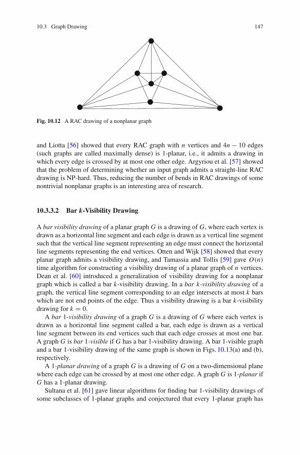
10.3 Graph Drawing 147
Fig. 10.12 A RAC drawing of a nonplanar graph
and Liotta [56] showed that every RAC graph with n vertices and 4n − 10 edges(such graphs are called maximally dense) is 1-planar, i.e., it admits a drawing inwhich every edge is crossed by at most one other edge. Argyriou et al. [57] showedthat the problem of determining whether an input graph admits a straight-line RACdrawing is NP-hard. Thus, reducing the number of bends in RAC drawings of somenontrivial nonplanar graphs is an interesting area of research.
10.3.3.2 Bar k-Visibility Drawing
A bar visibility drawing of a planar graph G is a drawing of G, where each vertex isdrawn as a horizontal line segment and each edge is drawn as a vertical line segmentsuch that the vertical line segment representing an edge must connect the horizontalline segments representing the end vertices. Otten and Wijk [58] showed that everyplanar graph admits a visibility drawing, and Tamassia and Tollis [59] gave O(n)
time algorithm for constructing a visibility drawing of a planar graph of n vertices.Dean et al. [60] introduced a generalization of visibility drawing for a nonplanargraph which is called a bar k-visibility drawing. In a bar k-visibility drawing of agraph, the vertical line segment corresponding to an edge intersects at most k barswhich are not end points of the edge. Thus a visibility drawing is a bar k-visibilitydrawing for k = 0.
A bar 1-visibility drawing of a graph G is a drawing of G where each vertex isdrawn as a horizontal line segment called a bar, each edge is drawn as a verticalline segment between its end vertices such that each edge crosses at most one bar.A graph G is bar 1-visible if G has a bar 1-visibility drawing. A bar 1-visible graphand a bar 1-visibility drawing of the same graph is shown in Figs. 10.13(a) and (b),respectively.
A 1-planar drawing of a graph G is a drawing of G on a two-dimensional planewhere each edge can be crossed by at most one other edge. A graph G is 1-planar ifG has a 1-planar drawing.
Sultana et al. [61] gave linear algorithms for finding bar 1-visibility drawings ofsome subclasses of 1-planar graphs and conjectured that every 1-planar graph has
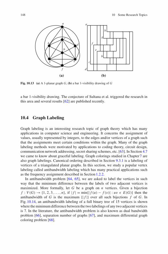
148 10 Some Research Topics
(a) (b)
a
h
g e
b
c
d
f
a
d
f
h
g
e
b
c
Fig. 10.13 (a) A 1-planar graph G, (b) a bar 1-visibility drawing of G
a bar 1-visibility drawing. The conjecture of Sultana et al. triggered the research inthis area and several results [62] are published recently.
10.4 Graph Labeling
Graph labeling is an interesting research topic of graph theory which has manyapplications in computer science and engineering. It concerns the assignment ofvalues, usually represented by integers, to the edges and/or vertices of a graph suchthat the assignments meet certain conditions within the graph. Many of the graphlabeling methods were motivated by applications to coding theory, circuit design,communication network addressing, secret sharing schemes, etc. [63]. In Section 4.7we came to know about graceful labeling. Graph colorings studied in Chapter 7 arealso graph labelings. Canonical ordering described in Section 9.3.1 is a labeling ofvertices of a triangulated planar graphs. In this section, we study a popular vertexlabeling called antibandwidth labeling which has many practical applications suchas the frequency assignment described in Section1.2.2.
In antibandwidth problem [64, 65], we are asked to label the vertices in suchway that the minimum difference between the labels of two adjacent vertices ismaximized. More formally, let G be a graph on n vertices. Given a bijectionf : V (G) → {1, 2, 3, . . . , n}, if | f | = min{| f (u) − f (v)| : uv ε E(G)} then theantibandwidth of G is the maximum {| f |} over all such bijections f of G. InFig. 10.14, an antibandwidth labeling of a full binary tree of 15 vertices is shownwhere theminimumdifference between the two labelings of any two adjacent verticesis 7. In the literature, the antibandwidth problem is also known as dual bandwidthproblem [66], separation number of graphs [67], and maximum differential graphcoloring problem [68].
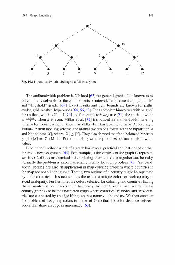
10.4 Graph Labeling 149
1 15
2
4 5 6 7 9 10 11 12
13 14 3
8
Fig. 10.14 Antibandwidth labeling of a full binary tree
The antibandwidth problem is NP-hard [67] for general graphs. It is known to bepolynomially solvable for the complements of interval, “arborescent comparability”and “threshold” graphs [69]. Exact results and tight bounds are known for paths,cycles, grid,meshes, hypercubes [64, 66, 68]. For a complete binary treewith height hthe antibandwidth is 2h − 1 [70] and for complete k-ary tree [71], the antibandwidthis n+1−k
2 , when k is even. Millar et al. [72] introduced an antibandwidth labelingscheme for forests, which is known asMillar–Pritikin labeling scheme. According toMillar–Pritikin labeling scheme, the antibandwidth of a forest with the bipartition Xand Y is at least |X |, where |X | ≤ |Y |. They also showed that for a balanced bipartitegraph (|X | = |Y |) Millar–Pritikin labeling scheme produces optimal antibandwidthvalue.
Finding the antibandwidth of a graph has several practical applications other thanthe frequency assignment [65]. For example, if the vertices of the graph G representsensitive facilities or chemicals, then placing them too close together can be risky.Formally the problem is known as enemy facility location problem [71]. Antiband-width labeling has also an application in map coloring problem where countries inthe map are not all contiguous. That is, two regions of a country might be separatedby other countries. This necessitates the use of a unique color for each country toavoid ambiguity. Furthermore, the colors selected for coloring two countries havingshared nontrivial boundary should be clearly distinct. Given a map, we define thecountry graph G to be the undirected graph where countries are nodes and two coun-tries are connected by an edge if they share a nontrivial boundary. We then considerthe problem of assigning colors to nodes of G so that the color distance betweennodes that share an edge is maximized [68].
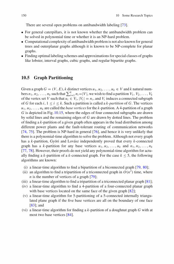
150 10 Some Research Topics
There are several open problems on antibandwidth labeling [73].
• For general caterpillars, it is not known whether the antibandwidth problem canbe solved in polynomial time or whether it is an NP-hard problem.
• Computational complexity of antibandwidth problem is not also known for generaltrees and outerplanar graphs although it is known to be NP-complete for planargraphs.
• Finding optimal labeling schemes and approximations for special classes of graphslike lobster, interval graphs, cubic graphs, and regular bipartite graphs.
10.5 Graph Partitioning
Given a graphG = (V, E), k distinct vertices u1, u2, . . . , uk ∈ V and k natural num-bers n1, n2, . . . , nk such that
∑ki=1 ni=|V |, wewish to find a partition V1, V2, . . . , Vk
of the vertex set V such that ui ∈ Vi , |Vi | = ni , and Vi induces a connected subgraphof G for each i , 1 ≤ i ≤ k. Such a partition is called a k-partition of G. The verticesu1, u2, . . . , uk are called the base vertices for the k-partition. A 4-partition of a graphG is depicted in Fig. 10.15, where the edges of four connected subgraphs are drawnby solid lines and the remaining edges of G are drawn by dotted lines. The problemof finding a k-partition of a given graph often appears in the load distribution amongdifferent power plants and the fault-tolerant routing of communication networks[74, 75]. The problem is NP-hard in general [76], and hence it is very unlikely thatthere is a polynomial-time algorithm to solve the problem. Although not every graphhas a k-partition, Györi and Lovász independently proved that every k-connectedgraph has a k-partition for any base vertices u1, u2, . . . , uk and n1, n2, . . . , nk[77, 78]. However, their proofs do not yield any polynomial-time algorithm for actu-ally finding a k-partition of a k-connected graph. For the case k ≤ 5, the followingalgorithms are known:
(i) a linear-time algorithm to find a bipartition of a biconnected graph [79, 80];(ii) an algorithm to find a tripartition of a triconnected graph in O(n2) time, where
n is the number of vertices of a graph [79];(iii) a linear-time algorithm to find a tripartition of a triconnected planar graph [81];(iv) a linear-time algorithm to find a 4-partition of a four-connected planar graph
with base vertices located on the same face of the given graph [82];(v) a linear-time algorithm for 5-partitioning of a 5-connected internally triangu-
lated plane graph if the five base vertices are all on the boundary of one face[83]; and
(vi) a linear-time algorithm for finding a k-partition of a doughnut graph G with atmost two base vertices [84].
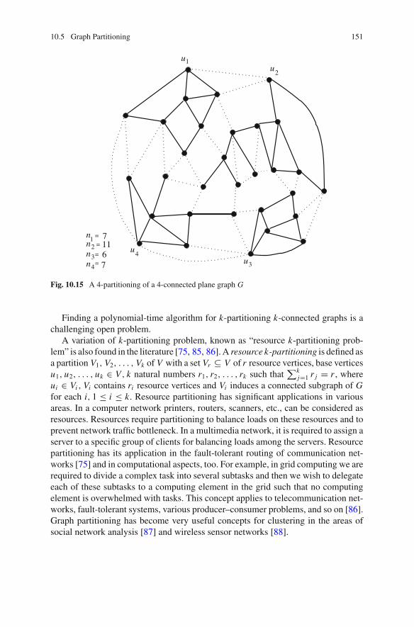
10.5 Graph Partitioning 151
uu
u
4
2
1u
3
nnnn
12
3
4
==
==
71167
Fig. 10.15 A 4-partitioning of a 4-connected plane graph G
Finding a polynomial-time algorithm for k-partitioning k-connected graphs is achallenging open problem.
A variation of k-partitioning problem, known as “resource k-partitioning prob-lem” is also found in the literature [75, 85, 86].A resource k-partitioning is defined asa partition V1, V2, . . . , Vk of V with a set Vr ⊆ V of r resource vertices, base verticesu1, u2, . . . , uk ∈ V, k natural numbers r1, r2, . . . , rk such that
∑kj=1 r j = r , where
ui ∈ Vi , Vi contains ri resource vertices and Vi induces a connected subgraph of Gfor each i, 1 ≤ i ≤ k. Resource partitioning has significant applications in variousareas. In a computer network printers, routers, scanners, etc., can be considered asresources. Resources require partitioning to balance loads on these resources and toprevent network traffic bottleneck. In a multimedia network, it is required to assign aserver to a specific group of clients for balancing loads among the servers. Resourcepartitioning has its application in the fault-tolerant routing of communication net-works [75] and in computational aspects, too. For example, in grid computing we arerequired to divide a complex task into several subtasks and then we wish to delegateeach of these subtasks to a computing element in the grid such that no computingelement is overwhelmed with tasks. This concept applies to telecommunication net-works, fault-tolerant systems, various producer–consumer problems, and so on [86].Graph partitioning has become very useful concepts for clustering in the areas ofsocial network analysis [87] and wireless sensor networks [88].
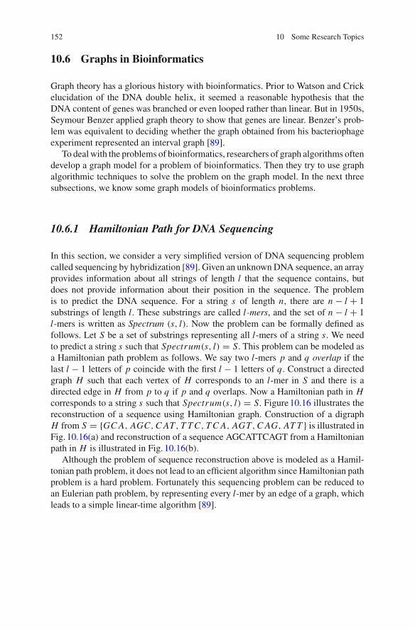
152 10 Some Research Topics
10.6 Graphs in Bioinformatics
Graph theory has a glorious history with bioinformatics. Prior to Watson and Crickelucidation of the DNA double helix, it seemed a reasonable hypothesis that theDNA content of genes was branched or even looped rather than linear. But in 1950s,Seymour Benzer applied graph theory to show that genes are linear. Benzer’s prob-lem was equivalent to deciding whether the graph obtained from his bacteriophageexperiment represented an interval graph [89].
To deal with the problems of bioinformatics, researchers of graph algorithms oftendevelop a graph model for a problem of bioinformatics. Then they try to use graphalgorithmic techniques to solve the problem on the graph model. In the next threesubsections, we know some graph models of bioinformatics problems.
10.6.1 Hamiltonian Path for DNA Sequencing
In this section, we consider a very simplified version of DNA sequencing problemcalled sequencing by hybridization [89]. Given an unknownDNA sequence, an arrayprovides information about all strings of length l that the sequence contains, butdoes not provide information about their position in the sequence. The problemis to predict the DNA sequence. For a string s of length n, there are n − l + 1substrings of length l. These substrings are called l-mers, and the set of n − l + 1l-mers is written as Spectrum (s, l). Now the problem can be formally defined asfollows. Let S be a set of substrings representing all l-mers of a string s. We needto predict a string s such that Spectrum(s, l) = S. This problem can be modeled asa Hamiltonian path problem as follows. We say two l-mers p and q overlap if thelast l − 1 letters of p coincide with the first l − 1 letters of q. Construct a directedgraph H such that each vertex of H corresponds to an l-mer in S and there is adirected edge in H from p to q if p and q overlaps. Now a Hamiltonian path in Hcorresponds to a string s such that Spectrum(s, l) = S. Figure10.16 illustrates thereconstruction of a sequence using Hamiltonian graph. Construction of a digraphH from S = {GCA, AGC,CAT, T TC, TC A, AGT,CAG, AT T } is illustrated inFig. 10.16(a) and reconstruction of a sequence AGCATTCAGT from a Hamiltonianpath in H is illustrated in Fig. 10.16(b).
Although the problem of sequence reconstruction above is modeled as a Hamil-tonian path problem, it does not lead to an efficient algorithm since Hamiltonian pathproblem is a hard problem. Fortunately this sequencing problem can be reduced toan Eulerian path problem, by representing every l-mer by an edge of a graph, whichleads to a simple linear-time algorithm [89].
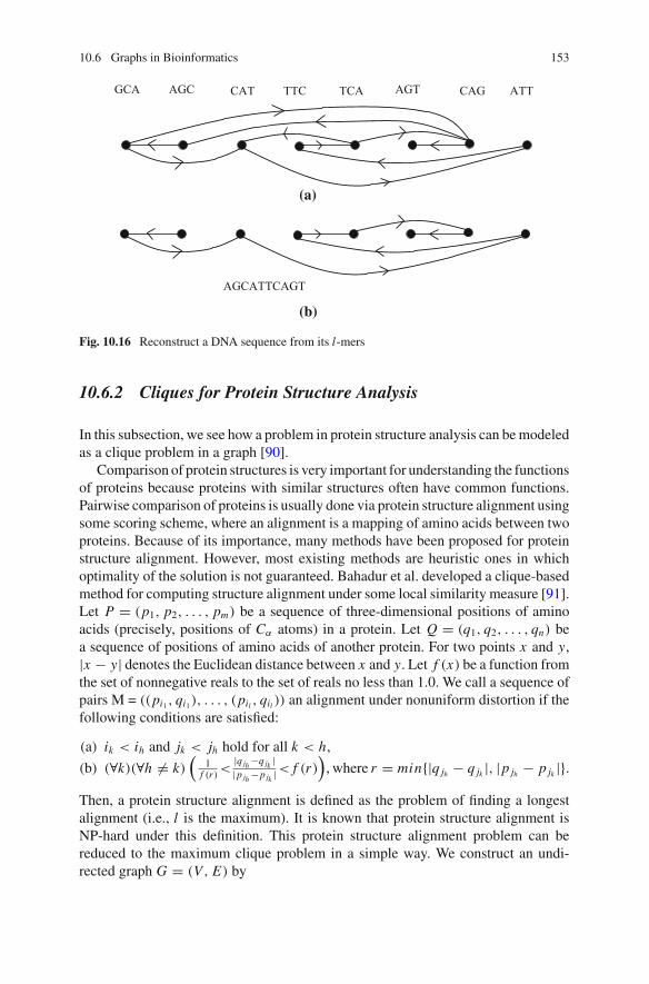
10.6 Graphs in Bioinformatics 153
GCA AGC CAT TTC TCA AGT ATTCAG
AGCATTCAGT
(a)
(b)
Fig. 10.16 Reconstruct a DNA sequence from its l-mers
10.6.2 Cliques for Protein Structure Analysis
In this subsection, we see how a problem in protein structure analysis can bemodeledas a clique problem in a graph [90].
Comparison of protein structures is very important for understanding the functionsof proteins because proteins with similar structures often have common functions.Pairwise comparison of proteins is usually done via protein structure alignment usingsome scoring scheme, where an alignment is a mapping of amino acids between twoproteins. Because of its importance, many methods have been proposed for proteinstructure alignment. However, most existing methods are heuristic ones in whichoptimality of the solution is not guaranteed. Bahadur et al. developed a clique-basedmethod for computing structure alignment under some local similarity measure [91].Let P = (p1, p2, . . . , pm) be a sequence of three-dimensional positions of aminoacids (precisely, positions of Cα atoms) in a protein. Let Q = (q1, q2, . . . , qn) bea sequence of positions of amino acids of another protein. For two points x and y,|x − y| denotes the Euclidean distance between x and y. Let f (x) be a function fromthe set of nonnegative reals to the set of reals no less than 1.0. We call a sequence ofpairs M = ((pi1 , qi1), . . . , (pil , qil )) an alignment under nonuniform distortion if thefollowing conditions are satisfied:
(a) ik < ih and jk < jh hold for all k < h,
(b) (∀k)(∀h �= k)(
1f (r)<
|q jh −q jk ||p jh −p jk |< f (r)
), where r = min{|q jh − q jk |, |p jh − p jk |}.
Then, a protein structure alignment is defined as the problem of finding a longestalignment (i.e., l is the maximum). It is known that protein structure alignment isNP-hard under this definition. This protein structure alignment problem can bereduced to the maximum clique problem in a simple way. We construct an undi-rected graph G = (V, E) by
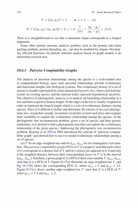
154 10 Some Research Topics
V = {(pi , q j )|i = 1, . . . ,m, j = 1, . . . , n},
E = {{(pi , q j ), (pk, qh)}|i < k, j < h,1
f (r)<
|qh − q j ||pk − pi | < f (r)}
Then, it is straightforward to see that a maximum clique corresponds to a longestalignment.
Some other protein structure analysis problem such as the protein side-chainpacking problem, protein threading, etc., can also be modeled by cliques. Develop-ing efficient heuristics for protein structure analysis based on graph models is aninteresting research area.
10.6.3 Pairwise Compitability Graphs
The analysis of ancestral relationships among the species is a well-studied areain computational biology since such ancestral relationships provide evolutionaryand functional insights into biological systems. The evolutionary history of a set ofspecies is usually represented by a tree named phylogenetic tree, where each leaf rep-resents an existing species and the internal nodes represent hypothetical ancestors.The objective of phylogenetic analysis is to analyze all branching relationship in atree and their respective branch length. So the edges of the tree is usually weighted inorder to represent the branch length which is a sort of evolutionary distance amongspecies. Since it is difficult to define and determine the criteria of an exact phyloge-netic tree, researchers usually reconstruct or predict several such trees and comparetheir suitability to explain the evolutionary relationship among the species. In thephylogenetic tree reconstruction problem, given a set of species and their geneticsimilarities, it is desired to find a phylogenetic tree that can explain the evolutionaryrelationship of the given species. Addressing the phylogenetic tree reconstructionproblem, Kearney et al. [92] in 2003 introduced the concept of “pairwise compati-bility graph” and showed how to use it to model evolutionary relationships among aset of species.
Let T be an edge-weighted tree and let dmin, dmax be two nonnegative real num-bers. The pairwise compatibility graph (PCG) of T is a graphG such that each vertexof G corresponds to a distinct leaf of T and two vertices are adjacent in G if and onlyif the weighted distance between their corresponding leaves in T is in the interval[dmin, dmax ]. Similarly, a given graphG is a PCG if there exist suitable T, dmin, dmax ,such that G is a PCG of T . Figure10.17(a) illustrates an edge-weighted tree T , andFig. 10.17(b) shows the corresponding PCG G, where dmin = 2 and dmax = 3.5.Figure10.17(c) shows another edge-weighted tree T ′ such that G is a PCG of T ′when dmin = 1.5 and dmax = 2.
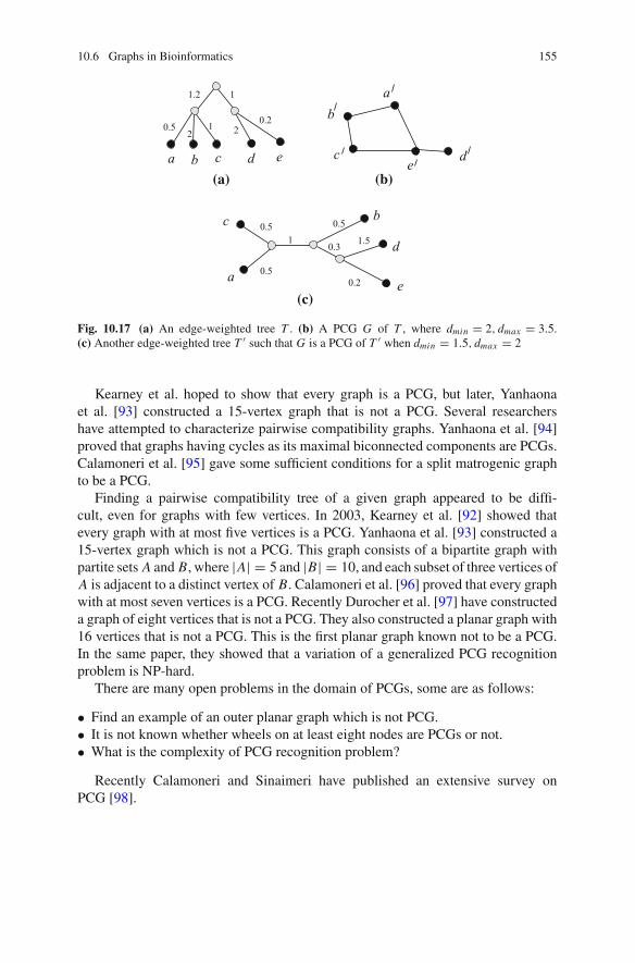
10.6 Graphs in Bioinformatics 155
d
ab
e(a) (b)
0.52
1 0.22
a cb d e
1.2 1
1
0.5
0.3
b
(c)
1.5 d
c
ae0.2
0.5
0.5
c
Fig. 10.17 (a) An edge-weighted tree T . (b) A PCG G of T , where dmin = 2, dmax = 3.5.(c) Another edge-weighted tree T ′ such that G is a PCG of T ′ when dmin = 1.5, dmax = 2
Kearney et al. hoped to show that every graph is a PCG, but later, Yanhaonaet al. [93] constructed a 15-vertex graph that is not a PCG. Several researchershave attempted to characterize pairwise compatibility graphs. Yanhaona et al. [94]proved that graphs having cycles as its maximal biconnected components are PCGs.Calamoneri et al. [95] gave some sufficient conditions for a split matrogenic graphto be a PCG.
Finding a pairwise compatibility tree of a given graph appeared to be diffi-cult, even for graphs with few vertices. In 2003, Kearney et al. [92] showed thatevery graph with at most five vertices is a PCG. Yanhaona et al. [93] constructed a15-vertex graph which is not a PCG. This graph consists of a bipartite graph withpartite sets A and B, where |A| = 5 and |B| = 10, and each subset of three vertices ofA is adjacent to a distinct vertex of B. Calamoneri et al. [96] proved that every graphwith at most seven vertices is a PCG. Recently Durocher et al. [97] have constructeda graph of eight vertices that is not a PCG. They also constructed a planar graph with16 vertices that is not a PCG. This is the first planar graph known not to be a PCG.In the same paper, they showed that a variation of a generalized PCG recognitionproblem is NP-hard.
There are many open problems in the domain of PCGs, some are as follows:
• Find an example of an outer planar graph which is not PCG.• It is not known whether wheels on at least eight nodes are PCGs or not.• What is the complexity of PCG recognition problem?
Recently Calamoneri and Sinaimeri have published an extensive survey onPCG [98].
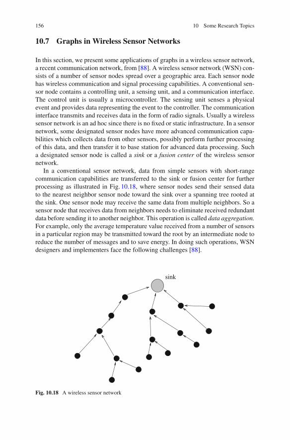
156 10 Some Research Topics
10.7 Graphs in Wireless Sensor Networks
In this section, we present some applications of graphs in a wireless sensor network,a recent communication network, from [88]. A wireless sensor network (WSN) con-sists of a number of sensor nodes spread over a geographic area. Each sensor nodehas wireless communication and signal processing capabilities. A conventional sen-sor node contains a controlling unit, a sensing unit, and a communication interface.The control unit is usually a microcontroller. The sensing unit senses a physicalevent and provides data representing the event to the controller. The communicationinterface transmits and receives data in the form of radio signals. Usually a wirelesssensor network is an ad hoc since there is no fixed or static infrastructure. In a sensornetwork, some designated sensor nodes have more advanced communication capa-bilities which collects data from other sensors, possibly perform further processingof this data, and then transfer it to base station for advanced data processing. Sucha designated sensor node is called a sink or a fusion center of the wireless sensornetwork.
In a conventional sensor network, data from simple sensors with short-rangecommunication capabilities are transferred to the sink or fusion center for furtherprocessing as illustrated in Fig. 10.18, where sensor nodes send their sensed datato the nearest neighbor sensor node toward the sink over a spanning tree rooted atthe sink. One sensor node may receive the same data from multiple neighbors. So asensor node that receives data from neighbors needs to eliminate received redundantdata before sending it to another neighbor. This operation is called data aggregation.For example, only the average temperature value received from a number of sensorsin a particular region may be transmitted toward the root by an intermediate node toreduce the number of messages and to save energy. In doing such operations, WSNdesigners and implementers face the following challenges [88].
sink
Fig. 10.18 A wireless sensor network
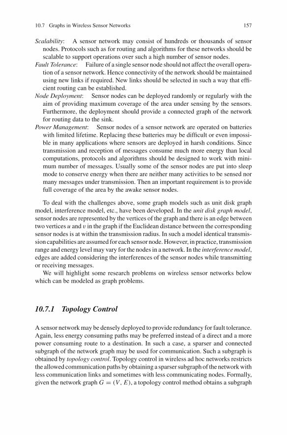
10.7 Graphs in Wireless Sensor Networks 157
Scalability: A sensor network may consist of hundreds or thousands of sensornodes. Protocols such as for routing and algorithms for these networks should bescalable to support operations over such a high number of sensor nodes.
Fault Tolerance: Failure of a single sensor node should not affect the overall opera-tion of a sensor network. Hence connectivity of the network should be maintainedusing new links if required. New links should be selected in such a way that effi-cient routing can be established.
Node Deployment: Sensor nodes can be deployed randomly or regularly with theaim of providing maximum coverage of the area under sensing by the sensors.Furthermore, the deployment should provide a connected graph of the networkfor routing data to the sink.
Power Management: Sensor nodes of a sensor network are operated on batterieswith limited lifetime. Replacing these batteries may be difficult or even impossi-ble in many applications where sensors are deployed in harsh conditions. Sincetransmission and reception of messages consume much more energy than localcomputations, protocols and algorithms should be designed to work with mini-mum number of messages. Usually some of the sensor nodes are put into sleepmode to conserve energy when there are neither many activities to be sensed normany messages under transmission. Then an important requirement is to providefull coverage of the area by the awake sensor nodes.
To deal with the challenges above, some graph models such as unit disk graphmodel, interference model, etc., have been developed. In the unit disk graph model,sensor nodes are represented by the vertices of the graph and there is an edge betweentwo vertices u and v in the graph if the Euclidean distance between the correspondingsensor nodes is at within the transmission radius. In such a model identical transmis-sion capabilities are assumed for each sensor node.However, in practice, transmissionrange and energy levelmay vary for the nodes in a network. In the interferencemodel,edges are added considering the interferences of the sensor nodes while transmittingor receiving messages.
We will highlight some research problems on wireless sensor networks belowwhich can be modeled as graph problems.
10.7.1 Topology Control
Asensor networkmay be densely deployed to provide redundancy for fault tolerance.Again, less energy consuming paths may be preferred instead of a direct and a morepower consuming route to a destination. In such a case, a sparser and connectedsubgraph of the network graph may be used for communication. Such a subgraph isobtained by topology control. Topology control in wireless ad hoc networks restrictsthe allowed communication paths by obtaining a sparser subgraph of the networkwithless communication links and sometimes with less communicating nodes. Formally,given the network graph G = (V, E), a topology control method obtains a subgraph
158 10 Some Research Topics
G ′ = (V ′, E ′) such that V ′ and/or E ′ satisfy some desired criterion. For example, achosen subset of the neighbors of a node are considered as connected neighbors, andthe rest are discarded inG ′.With the node failure for battery power outage, a subset ofedges are activated dynamically to maintain a shortest spanning tree over the activesensor nodes. A minimal subset of active nodes that induces connected subgraphand capable of performing special tasks of forwarding data of other active nodes toa sink is called the backbone of the wireless sensor network. Usually the backboneof an ad hoc wireless sensor network is called a virtual backbone, since there isno rigid (wired) connection among the nodes on the backbone and the backbonechanges dynamically with time. Backbone construction is an effective method fortopology control that provides a significant reduction in the number of messagescommunicated in an ad hoc wireless network. When a backbone is constructed, amessage from a source is first routed to the nearest neighbor backbone node, thenalong the backbone to the backbone node closest to the destination, and finally tothe destination. Finding a path in a graph of a given length such that the shortestdistance from each node to the path remains within a given bound is closely relatedto backbone construction problem. Finding minimum connecting domination sets(See Section5.4) has also applications in construction of the backbone networks.
10.7.2 Fault Tolerance
Failure of a single node or up to a certain number of nodes should not affect theoverall operation of a sensor network, and connectivity of the network should bemaintained using new links among active nodes if required. Since activating morelinks is costly from power consumption point of view, it is desirable to increaseconnectivity by activating a smaller number of new nodes. This problem is relatedto connectivity augmenting problems of graphs which asks to increase connectivityby adding the minimum number of edges [99, 100]. There are other constraints also.For example, increase the connectivity by adding smaller number of edges so thatthe maximum degree of the graph remains small.
10.7.3 Clustering
Clustering is a method for partitioning nodes of a network into groups, which canprovide a hierarchical architecture for efficient routing.
Given a graph G = (V, E), clustering divides the vertex set V into a collection ofsubsets {V1, V2, . . . , Vk}, where V = ∪k
i=1Vi , and each Vi ∈ V induces a connectedsubgraph Gi of G that may overlap. (Remember the Graph Partitioning problems inSection10.5 which have applications in clustering.) An elected node in each clusteracts as the cluster head or the leader of the cluster. The cluster heads dominate othernodes within the same cluster and hence they are responsible for cluster management
10.7 Graphs in Wireless Sensor Networks 159
functions and for providing hierarchical routing. The responsibility of the clusterhead may be rotated among the members of the cluster to provide load balancing,fault tolerance and power management. A gateway node is a node that connects twoclusters.
Graph partitioning as well as clustering is NP-hard in general. Hence variousheuristics may be used to form clusters. Clustering algorithms determine the clusterheads using some static properties of the graph such as the degrees of the nodes,eccentricities of the nodes, etc. and build a cluster around them. Themain advantagesto be gained by clustering an ad hoc wireless network are as follows. A virtualbackbone consisting of cluster heads and the gateway nodes provides an efficientmethod of hierarchical routing in ad hoc networks as it forms a simple topology tomaintain. This method of hierarchical routing results in smaller routing tables, whichare stored by the cluster heads and the gateway nodes only, and hence efficiency ofrouting is improved. Designing clustering (heuristics) algorithms for constructingclusters of desired properties for wireless sensor networks is a useful direction ofresearch.
References
1. Spinrad, J.P.: Efficient Graph Representations. American Mathematical Society, Providence(2003)
2. Di Battista, G., Eades, P., Tamassia, R., Tollis, I.G.: Graph Drawing: Algorithms for theVisualization of Graphs. Prentice-Hall Inc., Upper Saddle River (1999)
3. Kaufmann, M., Wagner, D. (eds.): Drawing Graphs: Methods and Models. Lecture Notes inComputer Science, vol. 2025. Springer, Berlin (2001)
4. Sugiyama, K.: Graph Drawing and Applications for Software and Knowledge Engineers.World Scientific, Singapore (2002)
5. Nishizeki, T., Rahman, M.S.: Planar Graph Drawing. World Scientific, Hackensack (2004)6. Tamassia, R. (Ed.): Handbook of Graph Drawing and Visualization, CRC Press (2014)7. de Fraysseix, H., Pach, J., Pollack, R.: How to draw a planar graph on a grid. Combinatorica
10, 41–51 (1990)8. Schnyder, W.: Embedding planar graphs on the grid. In: Proceedings of First ACM-SIAM
Symposium on Discrete Algorithms, San Francisco, pp. 138–148 (1990)9. Chrobak, M., Nakano, S.: Minimum-width grid drawings of plane graphs. Comp. Geom.
Theory Appl. 11, 29–54 (1998)10. Miura, K., Nakano, S., Nishizeki, T.: Grid drawings of 4-connected plane graphs. Discret.
Comput. Geom. 26(1), 73–87 (2001)11. Garg, A., Rusu, A.: Straight-line drawings of binary trees with linear area and arbitrary aspect
ration. Proceedings of Graph Drawing 2002. Lecture Notes in Computer Science, vol. 2528,pp. 320–331. Springer, Berlin (2002)
12. Garg, A., Rusu, A.: A more practical algorithm for drawing binary trees in linear area witharbitrary aspect ratio. In: Proceedings of Graph Drawing 2003, Lecture Notes in ComputerScience, vol. 2912, pp. 159–165. Springer (2003)
13. Brandenburg, F., Eppstein, D., Goodrich, M.T., Kobourov, S., Liotta, G., Mutzel, P.: Selectedopen problems in graph drawing. In: Proceedings of Graph Drawing 2003, Lecture Notes inComputer Science, vol. 2912, pp. 515–539. Springer (2003)
14. Garg, A., Rusu, A.: Area-efficient drawings of outerplanar graphs. In: Proceedings of GraphDrawing 2003, Lecture Notes in Computer Science, vol. 2912, pp. 129–134. Springer (2003)
160 10 Some Research Topics
15. Di Battista, G., Frati, F.: Small area drawings of outerplanar graphs. In: Proceedings of GraphDrawing 2005, Lecture Notes in Computer Science, vol. 3843, pp. 89–100. Springer (2005)
16. Karim, M.R., Rahman, M.S.: On a class of planar graphs with straight-line grid drawings onlinear area. J. Graph Algorithms Appl. 13(2), 153–177 (2009)
17. Tutte, W.T.: Convex representations of graphs. Proc. London Math. Soc. 10, 304–320 (1960)18. Tutte, W.T.: How to draw a graph. Proc. of London Math. Soc. 13, 743–768 (1963)19. Chiba, N., Yamanouchi, T., Nishizeki, T.: Linear algorithms for convex drawings of planar
graphs. In: Bondy, J.A., Murty, U.S.R. (eds.) Progress in Graph Theory, pp. 153–173. Acad-emic Press, Canada (1984)
20. Chrobak, M., Kant, G.: Convex grid drawings of 3-connected planar graphs. Inter. J. Comput.Geom. Appl. 7(3), 211–223 (1997)
21. Miura, K., Azuma, M., Nishizeki, T.: Convex drawings of plane graphs of minimum outerapices. Int. J. Found. Comput. Sci. 17, 1115–1127 (2006)
22. Miura, K., Nakano, S., Nishizeki, T.: Convex grid drawings of four connected plane graphs.Int. J. Found. Comput. Sci. 17, 1032–1060 (2006)
23. Zhou, X., Nishizeki, T.: Convex drawings of internally triconnected plane graphs on o(n2)grids. Discret. Math. Algorithms Appl. 2, 347–362 (2010)
24. Lengauer, T.: Combinatorial Algorithms for Integrated Circuit Layout. Wiley, Chichester(1990)
25. Garg, A., Tamassia, R.: A new minimum cost flow algorithm with applications to graphdrawing. In: Proceedings of Graph Drawing ’96, Lecture Notes in Computer Science, vol.1190, pp. 201–216. Springer (1997)
26. Rahman, M.S., Nakano, S., Nishizeki, T.: A linear algorithm for bend-optimal orthogonaldrawings of triconnected cubic plane graphs. J. Graph Alg. Appl. 3(4), 31–62 (1999). http://jgaa.info
27. Tamassia, R.: On embedding a graph in the grid with the minimum number of bends. SIAMJ. Comput. 16(3), 421–444 (1987)
28. Rahman,M.S.,Nishizeki, T., Naznin,M.:Orthogonal drawings of plane graphswithout bends.J. Graph Alg. Appl. 7(4), 335–362 (2003). http://jgaa.info
29. Thomassen, C.: Plane Representations of Graphs. In: Bondy, J.A., Murty, U.S.R. (eds.)Progress in Graph Theory, pp. 43–69. Academic Press, Canada (1984)
30. Bhasker, J., Sahni, S.: A linear algorithm to find a rectangular dual of a planar triangulatedgraph. Algorithmica 3, 247–278 (1988)
31. Kant, G., He, X.: Regular edge labeling of 4-connected plane graphs and its applications ingraph drawing problems. Theory Comput. Sci. 172, 175–193 (1997)
32. Rahman, M.S., Nakano, S., Nishizeki, T.: Rectangular grid drawings of plane graphs. Comp.Geom. Theory Appl. 10(3), 203–220 (1998)
33. Biedl, T.C.: Optimal orthogonal drawings of triconnected plane graphs. In: Proceedings ofSWAT’96, Lecture Notes in Computer Science, vol. 1097, pp. 333–344 (1996)
34. Biedl, T.C., Kaufmann, M.: Area-efficient static and incremental graph drawings. In: Pro-ceedings of 5th European Symposium on Algorithms, Lecture Notes in Computer Science,vol. 1284, pp. 37–52. Springer (1997)
35. Papakostas,A., Tollis, I.G.: Efficient orthogonal drawings of high degree graphs.Algorithmica26, 100–125 (2000)
36. Rahman, M.S., Nakano, S., Nishizeki, T.: Box-rectangular drawings of plane graphs. J. Algo-rithms 37, 363–398 (2000)
37. He, X.: A simple linear time algorithm for proper box rectangular drawings of plane graphs.J. Algorithms 40(1), 82–101 (2001)
38. Rahman, M.S., Miura, K., Nishizeki, T.: Octagonal drawings of plane graphs with prescribedface areas. Comput. Geom. 42(3), 214–230 (2009)
39. Alam,M.J., Kobourov, S.G., Mondal, D.: Orthogonal layout with optimal face complexity. In:Proceedings of SOFSEM 2016, Lecture Notes in Computer Science, vol. 9587, pp. 121–133(2016)
References 161
40. Ikebe, Y., Perles, M.A., Tamura, A., Tokunaga, S.: The rooted tree embedding problem intopoints in the plane. Discret. Comput. Geom. 11, 51–63 (1994)
41. Bose, P.: On embedding an outer-planar graph in a point set. Comput. Geom. Theory Appl.23(3), 303–312 (2002)
42. Cabello, S.: Planar embeddability of the vertices of a graph using a fixed point set is NP-hard.J. Graph Algorithms Appl. 10(2), 353–363 (2006)
43. Garcia, A., Hurtado, F., Huemer, C., Tejel, J., Valtr, P.: On embedding triconnected cubicgraphs on point sets. Electron. Notes Discret. Math. 29, 531–538 (2007)
44. Nishat, R.I., Mondal, D., Rahman, M.S.: Point-set embed dings of plane 3-trees. Comput.Geom. Theory Appl. 45(3), 88–98 (2012)
45. Durocher, S., Mondal, D.: On the hardness of point-set embeddability. In: Proceedings ofWALCOM 2012, Lecture Notes in Computer Science, vol. 7157, pp. 148–159. Springer(2012)
46. Cardinal, J., Hoffmann, M., Kusters, V.: On universal point sets for planar graphs. In: Pro-ceedings of Thailand-Japan Joint Conference onComputational Geometry andGraphs, LNCS8296, 30–41 (2013)
47. Dujmovic, V., Evans,W.S., Lazard, S., Lenhart, W., Liotta, G., Rappaport, D., Wismath, S.K.:On point-sets that support planar graphs. Comput. Geom. Theory Appl. 46(1), 29–50 (2013)
48. Dujmovic, V., Evans, W.S., Kobourov, S.G., Liotta, G., Weibel, C., Wismath, S.K.: On graphssupported by line sets In: Proceedings of Graph Drawing 2010, LNCS 6502, pp. 177–182(2011)
49. Hossain,M.I., Mondal, D., Rahman,M.S., Salma, S.A.: Universal line-sets for drawing planar3-trees. J. Graph Algorithms Appl. 17(2), 59–79 (2013)
50. Di Giacomo, E., Frati, F., Fulek, R., Grilli, L., Krug, M.: Orthogeodesic point-set embeddingof trees. In: Proceedings of Graph Drawing 2011, LNCS 7034, pp. 52–63 (2012)
51. Bläsius, T., Kobourov, S.G., Rutter, I.: Simultaneous embedding of planar graphs. In: Tamas-sia, R. (ed.) Handbook of Graph Drawing and Visualization, pp. 349–381. CRC press (2014)
52. Garey, M., Johnson, D.: Crossing number is NP-complete. SIAM J. Algebr. Discret. Methods4(3), 312–316 (1983)
53. Huang, W., Hong, S.-H., Eades, P.: Using eye tracking to investigate graph layout effects. In:Proceedings of 6thAsia-Pacific SymposiumonVisualisation 2007 (APVIS2007), pp. 97–100.IEEE (2007)
54. Huang,W., Hong, S.-H., Eades, P.: Effects of crossing angles. In: Proceedings of IEEEVGTCPacific Visualization Symposium 2008 (PacificVis 2008), pp. 41–46. IEEE (2008)
55. Didimo, W., Eades, P., Liotta, G.: Drawing graphs with right angle crossings. Theor. Comput.Sci. 412(39), 5156–5166 (2011)
56. Eades, P., Liotta, G.: Right angle crossing graphs and 1-planarity. Discret. Appl. Math.161(7–8), 961–969 (2013)
57. Argyriou, E.N., Bekos, M.A., Symvonis, A.: The straight-line RAC drawing problem is NP-Hard. J. Graph Algorithms Appl. 16(2), 569–597 (2012)
58. Otten, J., Wijk, J.G.V.: Graph representation in interactive layout design. In: Proceedings ofIEEE International Symposium On Circuits and Systems, pp. 914–918 (1978)
59. Tamassia, R., Tollis, I.G.: A unified approach to visibility representations of planar graphs.Discret. Comput. Geom. 1, 321–341 (1986)
60. Dean, A.M., Evans, W., Gethner, E., Laison, J.D., Safari, M.: Bar k-visibility graphs. J. GraphAlgorithms Appl. 11(1), 45–59 (2007)
61. Sultana, S., Rahman, M.S., Roy, A., Tairin, S.: Bar 1-visibility drawings of 1-planar graphs.In: Proceedings of ICAA 2014, LNCS 8321, pp. 62–76. Springer (2014)
62. Brandenburg, F.J.: 1-visibility representations of 1-planar graphs. J. Graph Algorithms Appl.18(3), 421–438 (2014)
63. Gallian, J.A.: A dynamic survey of graph labeling. Electron. J. Comb. DS6 (2015)64. Raspaud, A., Schroder, H., Sÿkora, O., Török, L.: Vrto, I.: Antibandwidth and cyclic antiband-
width of meshes and hypercubes. Discret. Math. 309(11), 3541–3552 (2009)
162 10 Some Research Topics
65. Rahaman, M.S., Eshan, T.A., Al Abdullah, S., Rahman, M.S.: Antibandwidth problem foritchy caterpillars. In: Proceeding of ICIEV 2014, IEEE Computer Society, pp. 1–6 (2014).doi:10.1109/ICIEV.2014.6850837
66. Yixun, L., Jinjiang, Y.: The dual bandwidth problem for graphs. J. Zhengzhou Univ. (NaturalScience Edition) 35, 1–5 (2003)
67. Leung, J.Y.-T., Vornberger, O., Witthoff, J.: On some variants of the bandwidth minimizationproblem. SIAM J. Comput. 13(3), 650–667 (1984)
68. Hun, Y., Kobourov, S., Veeramon, S.: On maximum differential graph coloring. In: GD’10Proceedings of the 18th International Conference on Graph Drawing, pp. 274–286 (2010)
69. Donnelly, S., Isaak, G.: Hamiltonian powers in threshold and arborescent comparabilitygraphs. Discret. Math. 202(1–3), 33–44 (1999)
70. Weili, Y., Ju, Z., Xiaoxu, L.: Dual bandwidth of some special trees. J. Zhengzhou Univ.(Natural Science Edition) 35, 16–19 (2003)
71. Calamoneri, T., Massini, A., Török, L.: Vrto, I.: Antibandwidth of complete k-ary trees.Discret. Math. 309(22), 6408–6414 (2009)
72. Miller, Z., Pritikin, D.: On separation number of a graph. Networks 19(6), 651–666 (1989)73. Bekos, M.A., Kaufmann, M., Kobourov, S., Veeramoni, S.: A note on maximum differential
coloring of planar graphs. J. Discret. Algorithms (2014). Published online74. Wada, K., Kawaguchi, K.: Efficient algorithms for triconnected graphs and 3-edge-connected
graphs. In: Proceedings of the 19th International Workshop on Graph Theoretic Conceptsin Computer Science (WG’93), Lecture Notes in Computer Science, vol. 790, pp. 132–143.Springer (1994)
75. Wada, K., Takaki, A., Kawaguchi, K.: Efficient algorithms for a mixed k-partition problem ofgraphswithout specifying bases. In: Proceedings of the 20th InternationalWorkshop onGraphTheoretic Concepts in Computer Science (WG’94), Lecture Notes in Computer Science, vol.903, pp. 319–330. Springer (1995)
76. Dyer, M.E., Frieze, A.M.: On the complexity of partitioning graphs into connected subgraphs.Discret. Appl. Math. 10, 139–153 (1985)
77. Györi, E.: On division of connected subgraphs. In: Proceedings of 5th Hungarian Combina-tional Coll., pp. 485–494 (1978)
78. Lovász, L.: A homology theory for spanning trees of a graph. Acta Math. Acad. Sci. Hunger30, 241–251 (1977)
79. Suzuki, H., Takahashi, N., Nishizeki, T.,Miyano,H., Ueno, S.: An algorithm for tripartitioning3-connected graphs. J. Inf. Process. Soc. Jpn. 31(5), 584–592 (1990)
80. Suzuki, H., Takahashi, N., Nishizeki, T.: A linear algorithm for bipartition of biconnectedgraphs. Inform. Process. Lett. 33(5), 227–232 (1990)
81. Jou, L., Suzuki, H., Nishizeki, T.: A linear algorithm for finding a nonseparating ear decom-position of triconnected planar graphs, Technical Report of Information Processing Societyof Japan, AL40-3 (1994)
82. Nakano, S., Rahman, M.S., Nishizeki, T.: A linear time algorithm for four-partitioning four-connected planar graphs. Inform. Process. Lett. 62, 315–322 (1997)
83. Nagai, S., Nakano, S.: A Linear-time algorithm for five-partitioning five-connected internallytriangulated plane graphs. IEICE Trans. Fundam. E84-A(9), 2330–2337 (2001)
84. Karim,M.R., Nahiduzzaman,K.M., Rahman,M.S.: A linear-time algorithm for k-PartitioningDoughnut Graphs. Infocomp J. Comput. Sci. 8(1), 8–13 (2009)
85. Awal, T., Rahman, M.S.: A linear algorithm for resource tripartitioning triconnected planargraphs. Infocomp J. Comput. Sci. 9(2), 39–48 (2010)
86. Awal, T., Rahman, M.S.: A linear algorithm for resource four-partitioning four-connectedplanar graphs. AKCE Int. J. Graphs Comb. 9(1), 11–20 (2012)
87. Furht, B. (ed.): Handbook of Social Network Technologies and Applications. Springer, Berlin(2010)
88. Erciyes, K.: Distributed Graph Algorithms for Computer Networks. Springer, London (2013)89. Jones, N.C., Pevzner, P.: An Introduction toBioinformaticsAlgorithms. TheMITPress (2004)
References 163
90. Tomita, E., Akutsu, T.,Matsunaga, T.: Efficient algorithms for findingmaximum andmaximalcliques: effective tools for bioinformatics. In: Laskovski, A.N. (ed.) Biomedical Engineering,pp. 625–638. Communications and Software, Trends in Electronics (2011)
91. Bahadur, D.K.C., Akutsu, T., Tomita, E., Seki, T., Fujiyama, A.: Point matching under non-uniform distortions and protein side chain packing based on an efficient maximum cliquealgorithm. Genome Informatics 13, 143–152 (2002)
92. Kearney, P.E.,Munro, J.I., Phillips, D.: Efficient generation of uniform samples from phyloge-netic trees. In: Proceedings of the 3rd InternationalWorkshop onAlgorithms inBioinformatics(WABI), LNCS 2812, pp. 177–189. Springer (2003)
93. Yanhaona, M.N., Bayzid, M.S., Rahman, M.S.: Discovering pairwise compatibility graphs.Discret. Math. Algorithms Appl. 2(4), 607–624 (2010)
94. Yanhaona, M.N., Hossain, K.S.M.T., Rahman, M.S.: Pairwise compatibility graphs. J. Appl.Math. Comput. 30, 479–503 (2009)
95. Calamoneri, T., Petreschi, R., Sinaimeri, B.: On relaxing the constraints in pairwise compati-bility graphs. In: Proceedings of the 6th International Workshop on Algorithms and Compu-tation (WALCOM), LNCS 7157, pp. 124–135. Springer (2012)
96. Calamoneri, T., Frascaria,D., Sinaimeri, B.:All graphswith atmost seven vertices are pairwisecompatibility graphs. Comput. J. (to appear) (2012). http://arxiv.org/abs/1202.4631
97. Durocher, S., Mondal, D., Rahman, M.S.: On graphs that are not PCGs, In: Proceedings ofthe 7th International Workshop on Algorithms and Computation (WALCOM), Lecture Notesin Computer Science, vol. 7748, pp. 310–321. Springer (2013)
98. Calamoneri, T., Sinaimeri, B.: Pairwise compatibility graphs: a survey. SIAM Rev. 58(3),445–460 (2016)
99. Kant, G.: Augmenting outerplanar graphs. J. Algorithms 21, 1–25 (1996)100. Abellanas, M., García, A., Hurtado, F., Tejel, J., Urrutia, J.: Augmenting the connectivity of
geometric graphs. Comput. Geom. Theory Appl. 40(3), 220–230 (2008)
Index
Symbols1-planar drawing, 1471-planar graph, 147C-component, 81Cn , 19Co(G), 78E(G), 11G(C), 79G − F , 15G − W , 15G − e, 15G − v, 15G\e, 22G1 ∩ G2, 19G1 ∪ G2, 19Kn , 17Km,n , 18M�M ′, 64Nn , 17PG(k), 98Pn , 18V (G), 11Wn , 19�(G), 13�(G), 82α(G), 68χ(G), 91χ ′(G), 94δ(G), 14γ (G), 70κ(G), 39κ ′(G), 39G, 21φ, 107τ(G), 51f , 83k-ary tree, 50
k-chromatic, 91k-factor, 72k-outerplanar, 114k-tree, 124m, 11, 83n, 11, 83u, v-walk, 312-outerplanar, 114
AAcyclic coloring, 98Adjacency list, 28, 135Adjacency matrix, 26, 135Adjacent, 2, 13Alternating path, 63Ancestor, 50, 117Antibandwidth labeling, 148Augmenting path, 64, 108
BBackbone construction, 158Bacteriophage experiment, 152Bar 1-visibility drawing, 147Bar k-visibility drawing, 147Bar visibility drawing, 147Base vertices, 150Binary tree, 50Bipartite graph, 17, 34
complete, 18Block, 42Block-cutvertex tree, 42Box-orthogonal drawing, 143Box-rectangular drawing, 143Bridge, 39
© Springer International Publishing AG 2017M.S. Rahman, Basic Graph Theory, Undergraduate Topics in Computer Science,DOI 10.1007/978-3-319-49475-3
165
166 Index
CCanonical ordering, 115, 148Capacity constraint, 107Caterpillar, 60, 150Cayley’s theorem, 55Center, 58Chain, 99Chord, 115, 121Chordal graph, 121Chromatic index, 94Chromatic number, 91Chromatic polynomial, 97Clique, 94Clique number, 94Clique tree representation, 122Clustering, 158Color class, 92, 94Complete graph, 17Connected, 32Connected component, 32Connected graph, 51Connectivity, 39Conservation law, 107Control flow graph, 8Convex drawing, 139Convex grid drawing, 140Cost, 52Critical graph, 94Cubic graph, 14Cut edge, 33, 48Cut vertex, 39Cycle, 14
chord, 115independent, 79k-legged cycle, 79leg, 79
Cycle decomposition, 36Cycle graph, 19
DData aggregation, 156Degree, 13, 103Degree sequence, 24Degree set, 24Degree-sum formula, 13Descendant, 50, 117Diameter, 58Differential graph coloring, 148Digraph, 11, 103
connected, 105degree, 103Hamiltonian, 106
indegree, 103isomorphic, 104outdegree, 103score sequence, 107strongly connected, 105tournament, 106walk, 105
Disconnecting set, 39Division vertex, 99DNA doublehelix, 152DNA sequencing, 152Dominating set, 69Domination number, 69Doughnut graph, 14, 139Dual bandwidth, 148Dual edge, 84Dual graph, 84
self-dual, 84weak dual, 84
EEar decomposition, 44Ecentricity, 58Edge
contraction, 22inner, 111outer, 111
Edge coloring, 94Edge connectivity, 39Edge cut, 39End-vertex
of an edge, 1, 11of a path graph, 18of a walk, 31
Equivalent embedding, 80Eulerian circuit, 35Eulerian graph, 35Eulerian trail, 34Euler’s formula, 82Even cycle, 34External face, 117
FFace, 5Face coloring, 97Face-spanning subgraph, 5Fault tolerance, 158Floorplanning, 6Flow network, 107
capacity, 107consumption, 107
Index 167
production, 107Forest, 47Frequency assignment, 3
GGenealogical tree, 117Graceful labeling, 59, 148Graph, 1, 11
acyclic, 47center, 58complement, 20connected, 32connected component, 32connectivity, 39diameter, 58ecentricity, 58edge, 1factor, 72intersection, 19isomorphism, 22k-regular, 14multigraph, 11planar, 77radius, 58regular, 14simple, 11thickness, 85union, 19vertex, 1
Graph coloring, 91, 148Graph drawing, 128, 137Graph labeling, 148Graph representation, 135Graphic sequence, 24Grid drawing, 87, 138
HHall’s matching condition, 66Hamiltonian cycle, 36Hamiltonian graph, 36Hamiltonian path, 36, 152Handshaking lemma, 13Hybridization, 152Hypercube, 14
IIncidence matrix, 26Incident, 2, 13Indegree, 103Independent set, 17, 68, 122Inner edge, 79, 111
Inner vertex, 79Interference model, 157Internal face, 117Internal triangle, 112Internal vertex, 47Internally triangulated, 115Interval graph, 124, 136, 150Isomorphic, 104Isomorphism, 22
KKönigsberg bridge, 1, 35Kruskal’s algorithm, 52Kuratowski’s theorem, 78
LLabeled graph, 54Leaf, 47Leg, 79Leg-vertex, 79Lobster, 60, 150Loop, 11
MMap coloring, 2, 97Marriage problem, 66Matching, 63
alternating path, 63augmenting path, 64maximal, 63maximum, 63perfect, 63symmetric difference, 64
Maximal clique, 122Maximal independent set, 68Maximal matching, 63Maximal outerplanar, 112Maximal planar graph, 83Maximum degree, 13Maximum flow, 108Maximum independent set, 68Maximum matching, 63Millar-Pritikin labeling scheme, 149Min-cut, 108Minimum degree, 14Minimum spanning tree, 52Minimum vertex cover, 68Modules, 6Multidigraph, 103Multiple edge, 11
168 Index
NNeighbor, 2, 13Nested triangle, 120Node, 11Nonplanar graphs, 146Null graph, 14, 17
OOdd cycle, 34Optimal representation, 135Ordered rooted tree, 50Orientation, 104Orthogonal drawing, 141Orthogonal grid drawing, 143Outdegree, 103Outer boundary, 78Outer cycle, 115Outer edge, 79, 111, 115Outer face, 78Outer vertex, 79, 115Outerplanar, 111Outerplane, 111
PPairwise compitability graph (PCG), 154Partial k-tree, 124Partite set, 17Path decomposition, 131Path graph, 18Pathwidth, 131Perfect elimination scheme, 122Perfect graph, 94Perfect matching, 63Pertinent graph, 127Petersen graph, 14Phylogenetic tree, 154Planar graph, 5, 77
straight-line drawing, 85Plane 3-tree, 119Plane graph, 5, 78Plane triangulation, 119Point-set embedding, 144Prüffer’s code, 55Prim’s algorithm, 52Protein structure analysis, 153
RRAC drawing, 146Radius, 58Rectangular drawing, 6, 142Representative tree, 120
Representative vertex, 120Ringel-Kotzig conjecture, 60RNA secondary structure, 7
SSaturated vertex, 63Score sequence, 107Self-dual, 84Separable, 41Separating set, 39Separating triangle, 116Separation number, 148Separation-pair, 39Separator, 122Series-parallel graphs, 125Simultaneous embedding, 145Sink, 103Skeleton, 127Software engineering, 8Software testing, 8Source, 103Spanning subgraph, 51Spanning tree, 51Split component, 126Split pair, 125SPQ-tree, 125Straight-line drawing, 85, 138Strongly connected, 105Subdivision
of an edge, 21Subgraph, 15
edge-induced, 16vertex-induced, 15
Symmetric difference, 64
TTaxonomic tree, 7Thickness, 85Topology control, 157Tournament, 106Trail, 31Tree, 47
ancestor, 50center, 58child, 50descendant, 50internal vertex, 50leaf, 47, 50parent, 50rooted, 50
Tree decomposition, 130
Index 169
Treewidth, 130Triangulated plane graph, 83
UUnderlying graph, 104Unique embedding, 80Unit disk graph model, 157Unlabeled graph, 54Unsaturated, 63
VVertex coloring, 91
Vertex cover, 68Vertex cut, 39VLSI floorplanning, 6
WWalk, 31, 105Weak dual, 84, 111Web community, 7Weighted graph, 12Wheel graph, 19Wireless sensor networks (WSN), 156