Embed Size (px)
Citation preview
User’s ManualCode Version 6.2
MCNP
MCNP® USER’S MANUAL Code Version 6.2
October 27, 2017 Manual Rev. 0
Edited by: Christopher J Werner1
Contributors: Jerawan Armstrong1
Forrest B. Brown1
Jeffrey S. Bull1 Laura Casswell1 Lawrence J. Cox1 David Dixon1
R. Arthur Forster1 John T. Goorley1 H. Grady Hughes1 Jeffrey Favorite1 Roger Martz1
Stepan G. Mashnik1 Michael E. Rising1
Clell(CJ) Solomon1
Avneet Sood1
Jeremy E. Sweezy1 Christopher J.Werner1 Anthony Zukaitis1 Casey Anderson2 Jay S. Elson2 Joe W. Durkee2 Russell C. Johns2
Gregg W. McKinney2 Garrett E. McMath2 John S. Hendricks3 Denise B. Pelowitz3
Richard E. Prael4 Thomas E. Booth4 Michael R. James5 Michael L. Fensin6 Trevor A. Wilcox7
Brian C. Kiedrowski8
1 XCP-3 Monte Carlo Methods, Codes, and Applications, Los Alamos National Laboratory 2 NEN-5 Systems Design and Analysis, Los Alamos National Laboratory 3 NEN-5 Systems Design and Analysis, Los Alamos National Laboratory, Guest Scientist 4 XCP-3 Monte Carlo Methods, Codes, and Applications, Los Alamos National Laboratory, contractor 5 C-NR Nuclear & Radiochemistry, Los Alamos National Laboratory 6 W-13 Advanced Engineering Analysis, Los Alamos National Laboratory 7XTD –SS Safety & Surety, Los Alamos National Laboratory 8XCP-3 Monte Carlo Methods, Codes, and Applications, Los Alamos National Laboratory, Guest Scientist

MCNP User’s Manual
TABLE OF CONTENTS
MCNP User’s Manual iii
Copyright Notice & Disclaimer
© Copyright (2018). Los Alamos National Security, LLC. All rights reserved.
This material was produced under U.S. Government contract DE-AC52-06NA25396 for Los Alamos National Laboratory, which is operated by Los Alamos National Security, LLC for the U.S. Department of Energy. The Government is granted for itself and others acting on its behalf a paid-up, nonexclusive, irrevocable worldwide license in this material to reproduce, prepare derivative works, and perform publicly and display publicly. Beginning five (5) years after February 14, 2018, subject to additional five-year worldwide renewals, the Government is granted for itself and others acting on its behalf a paid-up, nonexclusive, irrevocable worldwide license in this material to reproduce, prepare derivative works, distribute copies to the public, perform publicly and display publicly, and to permit others to do so. NEITHER THE UNITED STATES NOR THE UNITED STATES DEPARTMENT OF ENERGY, NOR LOS ALAMOS NATIONAL SECURITY, LLC, NOR ANY OF THEIR EMPLOYEES, MAKES ANY WARRANTY, EXPRESS OR IMPLIED, OR ASSUMES ANY LEGAL LIABILITY OR RESPONSIBILITY FOR THE ACCURACY, COMPLETENESS, OR USEFULNESS OF ANY INFORMATION, APPARATUS, PRODUCT, OR PROCESS DISCLOSED, OR REPRESENTS THAT ITS USE WOULD NOT INFRINGE PRIVATELY OWNED RIGHTS.
MCNP® and Monte Carlo N-Particle® are registered trademarks owned by Los Alamos National Security, LLC, manager and operator of Los Alamos National Laboratory. Any third party use of such registered marks should be properly attributed to Los Alamos National Security, LLC, including the use of the ® designation as appropriate. Any questions regarding licensing, proper use, and/or proper attribution of Los Alamos National Security, LLC marks should be directed to [email protected].
MCNP6, MCNPX, MCNP5, MCNP Version 5, LAHET, and LAHET Code System (LCS) are trademarks of Los Alamos National Security, LLC.
MCNP User’s Manual TABLE OF CONTENTS
iv MCNP User’s Manual
TABLE OF CONTENTS
1 MCNP6 INTRODUCTION AND PRIMER ........................................... 1-1 1.1 INTRODUCTION ......................................................... 1-1
1.1.1 New MCNP6.2 Features and Capabilities ......................... 1-1 1.1.2 MCNP6 Versatility ............................................. 1-2 1.1.3 User's Manual Organization .................................... 1-3
1.2 MCNP6 PRIMER: GETTING STARTED ......................................... 1-4 1.3 MCNP6 INPUT FOR SAMPLE PROBLEM .......................................... 1-4
1.3.1 INP File ...................................................... 1-6 1.3.2 Cell Cards .................................................... 1-7 1.3.3 Surface Cards ................................................. 1-8 1.3.4 Data Cards .................................................... 1-9
1.3.4.1 MODE Card ................................................. 1-9 1.3.4.2 Cell and Surface Parameter Cards ......................... 1-10 1.3.4.3 Source Specification Cards ............................... 1-10 1.3.4.4 Tally Specification Cards ................................ 1-11 1.3.4.5 Materials Specification .................................. 1-12 1.3.4.6 Problem Termination ...................................... 1-14
1.3.5 Sample Problem Input File .................................... 1-14 1.3.6 Running the Sample Problem ................................... 1-15
1.4 EXECUTING MCNP6 ..................................................... 1-15 1.4.1 Execution Line ............................................... 1-16 1.4.2 Interrupts ................................................... 1-20
1.5 TIPS FOR CORRECT AND EFFICIENT PROBLEMS .................................. 1-21 1.5.1 Problem Setup ................................................ 1-21 1.5.2 Preproduction ................................................ 1-22 1.5.3 Production ................................................... 1-22 1.5.4 Criticality .................................................. 1-22 1.5.5 Warnings and Limitations ..................................... 1-23
2 DESCRIPTION OF MCNP6 INPUT .............................................. 2-1 2.1 INITIATE-RUN ......................................................... 2-2 2.2 CONTINUE-RUN ......................................................... 2-3 2.3 CARD FORMAT .......................................................... 2-5 2.4 MESSAGE BLOCK ........................................................ 2-5 2.5 PROBLEM TITLE CARD .................................................... 2-6 2.6 COMMENT CARDS ........................................................ 2-6 2.7 AUXILIARY INPUT FILE CAPABILITY .......................................... 2-7 2.8 CELL, SURFACE, AND DATA CARDS ........................................... 2-7
2.8.1 Data Card Horizontal Input Format ............................. 2-7 2.8.2 Data Card Vertical Input Format ............................... 2-9
2.9 PARTICLE DESIGNATORS .................................................. 2-10 2.10 DEFAULT VALUES ...................................................... 2-13 2.11 INPUT ERROR MESSAGES ................................................. 2-13 2.12 GEOMETRY ERRORS...................................................... 2-13
3 INPUT CARDS ............................................................. 3-1 3.1 AUXILIARY INPUT FILE AND ENCRYPTION (READ) ................................ 3-1 3.2 GEOMETRY SPECIFICATION ................................................. 3-2
3.2.1 Cell Cards .................................................... 3-4
MCNP User’s Manual
TABLE OF CONTENTS
MCNP User’s Manual v
3.2.2 Surface Cards ................................................ 3-6 3.2.2.1 Surfaces Defined by Equations ............................ 3-7 3.2.2.2 Axisymmetric Surfaces Defined by Points ................. 3-12 3.2.2.3 General Plane Defined by Three Points ................... 3-14 3.2.2.4 Surfaces Defined by Macrobodies ......................... 3-15
3.2.2.4.1 BOX—ARBITRARILY ORIENTED ORTHOGONAL BOX ................... 3-15 3.2.2.4.2 RPP—RECTANGULAR PARALLELEPIPED .......................... 3-16 3.2.2.4.3 SPH—SPHERE .......................................... 3-16 3.2.2.4.4 RCC—RIGHT CIRCULAR CYLINDER ............................. 3-17 3.2.2.4.5 RHP OR HEX—RIGHT HEXAGONAL PRISM ........................ 3-17 3.2.2.4.6 REC—RIGHT ELLIPTICAL CYLINDER ........................... 3-18 3.2.2.4.7 TRC—TRUNCATED RIGHT-ANGLE CONE .......................... 3-18 3.2.2.4.8 ELL—ELLIPSOID ........................................ 3-19 3.2.2.4.9 WED—WEDGE ........................................... 3-19 3.2.2.4.10 ARB—ARBITRARY POLYHEDRON ............................... 3-20 3.2.2.4.11 MACROBODY FACETS ...................................... 3-21
3.3 DATA CARDS ......................................................... 3-23 3.3.1 Data Cards Related to Geometry............................... 3-23
3.3.1.1 VOL Cell Volume ......................................... 3-24 3.3.1.2 AREA Surface Area ....................................... 3-25 3.3.1.3 TR Surface Coordinate Transformation .................... 3-26 3.3.1.4 TRCL Cell Coordinate Transformation ..................... 3-28 3.3.1.5 Repeated Structures ..................................... 3-30
3.3.1.5.1 U UNIVERSE ........................................... 3-31 3.3.1.5.2 LAT LATTICE .......................................... 3-33 3.3.1.5.3 FILL FILL ........................................... 3-35 3.3.1.5.4 URAN STOCHASTIC GEOMETRY FOR HTGRS ...................... 3-38
3.3.1.6 Hybrid Geometries: Structured and Unstructured Meshes .. 3-40 3.3.1.6.1 CREATION OF A STRUCTURED DISCRETE-ORDINATES-STYLE GEOMETRY FILE 3-40 3.3.1.6.2 MESH IMPORTATION AND SPECIFICATION OF AN EMBEDDED GEOMETRY ..... 3-45
3.3.2 Data Cards Related to Materials.............................. 3-54 3.3.2.1 M Material Specification ................................ 3-55 3.3.2.2 MT S(α,β) Thermal Neutron Scattering .................... 3-59 3.3.2.3 MX Material Card Nuclide Substitution ................... 3-61 3.3.2.4 MPN Photonuclear Nuclide Selector ....................... 3-62 3.3.2.5 OTFDB On-The-Fly-Doppler Broadening ..................... 3-62 3.3.2.6 TOTNU Total Fission ..................................... 3-63 3.3.2.7 NONU Fission Turnoff .................................... 3-64 3.3.2.8 AWTAB Atomic Weight ..................................... 3-65 3.3.2.9 XS Cross-Section File ................................... 3-65 3.3.2.10 VOID Material Void ...................................... 3-66 3.3.2.11 MGOPT Multigroup Adjoint Transport Option ............... 3-66 3.3.2.12 DRXS Discrete-Reaction Cross Section .................... 3-68
3.3.3 Data Cards Related to Physics................................ 3-68 3.3.3.1 MODE Problem Type ....................................... 3-69 3.3.3.2 PHYS Particle Physics Options ........................... 3-70
3.3.3.2.1 NEUTRONS (PHYS:N) .................................... 3-70 3.3.3.2.2 PHOTONS (PHYS:P) ..................................... 3-74 3.3.3.2.3 ELECTRONS (PHYS:E) ................................... 3-76 3.3.3.2.4 PROTONS (PHYS:H) ..................................... 3-79
MCNP User’s Manual TABLE OF CONTENTS
vi MCNP User’s Manual
3.3.3.2.5 OTHER PARTICLES (PHYS:<PL>) ............................ 3-82 3.3.3.3 ACT Activation Control Card .............................. 3-84 3.3.3.4 Physics Cutoffs .......................................... 3-87
3.3.3.4.1 CUT:<PL> TIME, ENERGY, AND WEIGHT CUTOFFS ................. 3-87 3.3.3.4.2 ELPT CELL-BY-CELL ENERGY CUTOFF ......................... 3-90
3.3.3.5 TMP Free-Gas Thermal Temperature ......................... 3-91 3.3.3.6 THTME Thermal Times ...................................... 3-92 3.3.3.7 MODEL Physics ............................................ 3-93
3.3.3.7.1 MPHYS MODEL PHYSICS CONTROL ............................. 3-93 3.3.3.7.2 LCA ................................................. 3-94 3.3.3.7.3 LCB ................................................. 3-98 3.3.3.7.4 LCC ................................................. 3-99 3.3.3.7.5 LEA ................................................ 3-100 3.3.3.7.6 LEB ................................................ 3-102
3.3.3.8 FMULT Multiplicity Constants ............................ 3-102 3.3.3.9 Transport Options (TROPT Card) .......................... 3-108 3.3.3.10 Uncollided Secondaries (UNC Card) ....................... 3-117 3.3.3.11 Magnetic Field Tracking ................................. 3-118
3.3.3.11.1 TRANSFER MAPS (COSYP AND COSY CARDS) .................... 3-119 3.3.3.11.2 PARTICLE RAY TRACING (BFLD AND BFLCL CARDS) .............. 3-121
3.3.3.12 FIELD Gravitational Field ............................... 3-123 3.3.4 Data Cards Related to Source Specification .................. 3-124
3.3.4.1 SDEF General Source Definition .......................... 3-124 3.3.4.2 SI Source Information ................................... 3-140 3.3.4.3 SP Source Probability ................................... 3-142 3.3.4.4 SB Source Bias .......................................... 3-146 3.3.4.5 DS Dependent Source Distribution ........................ 3-146 3.3.4.6 SC Source Comment ....................................... 3-157 3.3.4.7 SSW Surface Source Write ................................ 3-158 3.3.4.8 SSR Surface Source Read ................................. 3-160 3.3.4.9 KCODE Criticality Source ................................ 3-165 3.3.4.10 KSRC Criticality Source Points .......................... 3-167 3.3.4.11 KOPTS Criticality Calculations Options .................. 3-168 3.3.4.12 HSRC Mesh for Shannon Entropy of Fission Source
Distribution ............................................ 3-170 3.3.4.13 BURN Depletion/Burnup (KCODE Problems ONLY) ............. 3-171 3.3.4.14 Subroutines SOURCE and SRCDX ............................ 3-181
3.3.5 Data Cards Related to Tally Specification ................... 3-183 3.3.5.1 F Standard Tallies ...................................... 3-184
3.3.5.1.1 SURFACE AND CELL TALLIES (TALLY TYPES 1, 2, 4, 6, AND 7) .... 3-186 3.3.5.1.2 DETECTOR TALLIES (TALLY TYPE 5) ......................... 3-189 3.3.5.1.3 PULSE-HEIGHT TALLY (TALLY TYPE 8) ....................... 3-197 3.3.5.1.4 REPEATED STRUCTURES TALLIES (TALLY TYPES 1, 2, 4, 6, 7, AND
8) ................................................. 3-203 3.3.5.2 FC Tally Comment ........................................ 3-207 3.3.5.3 E Tally Energy .......................................... 3-208 3.3.5.4 T Tally Time ............................................ 3-209 3.3.5.5 C Tally Cosine (Tally Type 1 and 2) ..................... 3-210 3.3.5.6 FQ Print Hierarchy ...................................... 3-212 3.3.5.7 FM Tally Multiplier ..................................... 3-213
MCNP User’s Manual
TABLE OF CONTENTS
MCNP User’s Manual vii
3.3.5.8 DE and DF Dose Energy and Dose Function ................ 3-220 3.3.5.9 EM Energy Multiplier ................................... 3-223 3.3.5.10 TM Time Multiplier ..................................... 3-224 3.3.5.11 CM Cosine Multiplier (tally types 1 and 2 only) ........ 3-225 3.3.5.12 CF Cell Flagging (Tally Types 1, 2, 4, 6, 7) ........... 3-225 3.3.5.13 SF Surface Flagging (Tally Types 1, 2, 4, 6, 7) ........ 3-226 3.3.5.14 FS Tally Segment (Tally Types 1, 2, 4, 6, 7) ........... 3-227 3.3.5.15 SD Segment Divisor (Tally Types 1, 2, 4, 6, 7) ......... 3-229 3.3.5.16 FU Special Tally or TALLYX Input ....................... 3-230 3.3.5.17 TALLYX User-supplied Subroutine ........................ 3-231 3.3.5.18 FT Special Treatments for Tallies ...................... 3-233 3.3.5.19 TF Tally Fluctuation ................................... 3-255 3.3.5.20 NOTRN Direct-ONLY NEUTRAL-PARTICLE POINT DETECTOR
Contributions .......................................... 3-257 3.3.5.21 PERT Tally Perturbations—Differential Operator ......... 3-257 3.3.5.22 KPERT Reactivity Perturbations—Adjoint Weighting ....... 3-263 3.3.5.23 KSEN KEFF Sensitivity Coefficients—Adjoint Weighting .... 3-265 3.3.5.24 TMESH Superimposed Mesh Tally A ........................ 3-272
3.3.5.24.1 SETTING UP THE TMESH TALLY IN THE INP FILE ............... 3-274 3.3.5.24.2 TRACK-AVERAGED TMESH MESH TALLY (TYPE 1) ................ 3-276 3.3.5.24.3 SOURCE TMESH MESH TALLY (TYPE 2) ....................... 3-279 3.3.5.24.4 ENERGY DEPOSITION TMESH MESH TALLY (TYPE 3) .............. 3-280 3.3.5.24.5 DXTRAN TMESH MESH TALLY (TYPE 4) ...................... 3-281 3.3.5.24.6 PROCESSING THE TMESH MESH TALLY RESULTS .................. 3-282
3.3.5.25 FMESH Superimposed Mesh Tally B ........................ 3-284 3.3.5.26 SPDTL Lattice Speed Tally Enhancement .................. 3-290
3.3.6 Data Cards Related to Variance Reduction .................... 3-291 3.3.6.1 IMP Cell Importance .................................... 3-292 3.3.6.2 VAR Variance Reduction Control ......................... 3-294 3.3.6.3 Weight-Window Cards .................................... 3-295
3.3.6.3.1 WWE WEIGHT-WINDOW ENERGIES (OR TIMES) ................... 3-296 3.3.6.3.2 WWT WEIGHT-WINDOW TIMES ............................... 3-296 3.3.6.3.3 WWN CELL-BASED WEIGHT-WINDOW BOUNDS ..................... 3-297 3.3.6.3.4 WWP WEIGHT-WINDOW PARAMETER ............................ 3-299
3.3.6.4 WEIGHT-WINDOW GENERATION CARDS ......................... 3-301 3.3.6.4.1 WWG WEIGHT-WINDOW GENERATION ........................... 3-301 3.3.6.4.2 WWGE WEIGHT-WINDOW GENERATION ENERGIES (OR TIMES) ......... 3-303 3.3.6.4.3 WWGT WEIGHT-WINDOW GENERATION TIMES ..................... 3-303 3.3.6.4.4 MESH SUPERIMPOSED IMPORTANCE MESH FOR MESH-BASED WEIGHT-WINDOW
GENERATOR ........................................... 3-304 3.3.6.5 ESPLT Energy Splitting and Roulette .................... 3-308 3.3.6.6 TSPLT Time Splitting and Roulette ...................... 3-311 3.3.6.7 EXT Exponential Transform .............................. 3-313 3.3.6.8 VECT Vector Input ...................................... 3-316 3.3.6.9 FCL Forced Collision ................................... 3-316 3.3.6.10 DXT DXTRAN Sphere ...................................... 3-317 3.3.6.11 DD Detector Diagnostics ................................ 3-320 3.3.6.12 PD Detector Contribution ............................... 3-322 3.3.6.13 DXC DXTRAN Contribution ................................ 3-323 3.3.6.14 BBREM Bremsstrahlung Biasing ........................... 3-324
MCNP User’s Manual TABLE OF CONTENTS
viii MCNP User’s Manual
3.3.6.15 PIKMT Photon-Production Biasing ......................... 3-325 3.3.6.16 SPABI Secondary Particle Biasing ........................ 3-327 3.3.6.17 PWT Photon Weight ....................................... 3-327
3.3.7 Problem Termination, Output Control, and Miscellaneous Data . 3-329 3.3.7.1 Problem Termination ..................................... 3-329
3.3.7.1.1 NPS HISTORY CUTOFF .................................... 3-330 3.3.7.1.2 CTME COMPUTER TIME CUTOFF .............................. 3-331 3.3.7.1.3 STOP PRECISION CUTOFF ................................. 3-331
3.3.7.2 Output Control .......................................... 3-332 3.3.7.2.1 PRINT OUTPUT PRINT TABLES ............................. 3-332 3.3.7.2.2 TALNP NEGATE PRINTING OF TALLIES ........................ 3-336 3.3.7.2.3 PRDMP PRINT AND DUMP CYCLE ............................. 3-336 3.3.7.2.4 PTRAC PARTICLE TRACK OUTPUT ............................ 3-338 3.3.7.2.5 MPLOT PLOT TALLY WHILE PROBLEM IS RUNNING ................. 3-344 3.3.7.2.6 HISTP CREATE LAHET-COMPATIBLE FILES ..................... 3-345
3.3.7.3 Miscellaneous data ...................................... 3-346 3.3.7.3.1 RAND RANDOM NUMBER GENERATION ........................... 3-346 3.3.7.3.2 DBCN DEBUG INFORMATION ................................ 3-347 3.3.7.3.3 LOST LOST PARTICLE CONTROL ............................. 3-354 3.3.7.3.4 IDUM INTEGER ARRAY ................................... 3-354 3.3.7.3.5 RDUM FLOATING-POINT ARRAY ............................. 3-355 3.3.7.3.6 ZA, ZB, ZC, AND ZD DEVELOPERS CARD PLACEHOLDERS .......... 3-355 3.3.7.3.7 FILES FILE CREATION .................................. 3-355
3.4 SUMMARY OF MCNP6 INPUT CARDS ......................................... 3-357 4 EXAMPLES ............................................................. 4-1
4.1 GEOMETRY EXAMPLES ..................................................... 4-1 4.1.1 Geometry Specification ........................................ 4-1 4.1.2 Coordinate Transformations ................................... 4-15 4.1.3 Repeated Structure and Lattice Examples ...................... 4-20 4.1.4 Embedded Meshes: Structured and Unstructured ................. 4-41
4.2 TALLY EXAMPLES ...................................................... 4-44 4.2.1 FM Examples (Simple Form) .................................... 4-44 4.2.2 FM Examples (General Form) ................................... 4-47 4.2.3 FMESH Tally Examples ......................................... 4-48 4.2.4 FS Examples .................................................. 4-51 4.2.5 FT Examples .................................................. 4-53 4.2.6 Repeated Structure/Lattice Tally Example ..................... 4-67 4.2.7 Miscellaneous Tally Examples ................................. 4-71
4.2.7.1 Light Ion Recoil (RECL) .................................. 4-71 4.2.7.2 Inline Generation of Double Differential Cross Sections and
Residual Nuclei .......................................... 4-72 4.2.7.3 Compton Image Tally Example .............................. 4-74
4.2.8 TALLYX Subroutine Examples ................................... 4-77 4.3 SOURCE EXAMPLES...................................................... 4-81
4.3.1 General Source ............................................... 4-81 4.3.2 Beam Sources ................................................. 4-86 4.3.3 Burning Multiple Materials In a Repeated Structure with Specified
Concentration Changes ........................................ 4-90 4.3.4 Source Subroutine ............................................ 4-94
MCNP User’s Manual
TABLE OF CONTENTS
MCNP User’s Manual ix
4.3.5 SRCDX Subroutine ............................................ 4-97 4.4 MATERIAL EXAMPLES .................................................. 4-103
4.4.1 Table Data/Model Physics Mix and Match ...................... 4-103 4.5 PHYSICS MODELS ..................................................... 4-104
4.5.1 Neutron Production from a Spallation Target ................. 4-104 5 MCNP6 GEOMETRY AND TALLY PLOTTING ...................................... 5-1
5.1 SYSTEM GRAPHICS INFORMATION ............................................ 5-1 5.2 THE GEOMETRY PLOTTER, PLOT ............................................ 5-2
5.2.1 PLOT Input and Execute Line Options ........................... 5-2 5.2.2 Geometry Plotting Basic Concepts .............................. 5-3 5.2.3 Interactive Geometry Plotting in Point-and-Click Mode ......... 5-5 5.2.4 Interactive Geometry Plotting in Command-Prompt Mode ......... 5-11 5.2.5 Plotting Embedded-Mesh Geometries ............................ 5-16 5.2.6 Geometry Debugging .......................................... 5-17 5.2.7 Geometry Plotting in Batch Mode.............................. 5-17
5.3 THE TALLY AND CROSS-SECTION PLOTTER, MCPLOT ............................. 5-17 5.3.1 Execution Line Options Related to MCPLOT Initiation .......... 5-19 5.3.2 Plot Conventions and Command Syntax .......................... 5-21
5.3.2.1 2D plot ................................................. 5-21 5.3.2.2 Contour plot ............................................ 5-21 5.3.2.3 Color-Wash Plot ......................................... 5-21 5.3.2.4 MCPLOT Command Syntax ................................... 5-21
5.3.3 Tally Plot Commands Grouped by Function ...................... 5-22 5.3.4 MCTAL Files ................................................. 5-29
5.4 TALLY PLOTTING EXAMPLES ............................................... 5-32 5.4.1 Example of Use of COPLOT .................................... 5-32 5.4.2 Tally Fluctuation Chart History Score Plotting ............... 5-33 5.4.3 Radiography Tally Contour Plot Example ....................... 5-34 5.4.4 TMESH Mesh Tally Plot Examples............................... 5-37
5.4.4.1 MCPLOT TMESH Mesh Tally ................................. 5-37 5.4.4.2 Superimposed Geometry Plot TMesh MESH Tally ............. 5-40
5.4.5 MCPLOT FREE Command Examples................................. 5-42 5.4.6 Photonuclear Cross-Section Plots ............................. 5-42 5.4.7 Lattice Tally Plot Example................................... 5-43 5.4.8 Weight-Window-Generator Superimposed Mesh Plots .............. 5-44
5.4.8.1 Cylindrical Mesh Example ................................ 5-44 5.4.8.2 Spherical Mesh Example .................................. 5-47
5.5 NORMALIZATION OF ENERGY-DEPENDENT TALLY PLOTS ............................. 5-49 5.5.1 MCNP6 Tally Values and Energy-Normalized Tallies ............. 5-49 5.5.2 Definition of Neutron Lethargy............................... 5-50 5.5.3 Lethargy-Normalized Tallies for a Logarithmic Energy Abscissa 5-51 5.5.4 Relation of Tally Lethargy Normalizing to Tally Energy
Normalizing ................................................. 5-51 5.5.5 Average Energy for a Lethargy-Normalized Tally ............... 5-52 5.5.6 MCNP6 LETHARGY Command for Lethargy Normalization ............ 5-52 5.5.7 Requirements for Producing a Visually Accurate Area (VAA) Tally
Plot ........................................................ 5-53 5.5.8 Comparisons of Energy and Lethargy Tally Normalizations for a Log
Energy Abscissa ............................................. 5-53
MCNP User’s Manual TABLE OF CONTENTS
x MCNP User’s Manual
5.5.9 Summary of Energy-Normalized and Lethargy-Normalized MCNP6 Tally Plots ........................................................ 5-63
6 REFERENCES ............................................................. 6-1 7 APPENDIX A — A SUMMARY OF MCNP6 COMMANDS ................................ 7-1
7.1 GENERAL INFORMATION, FILE NAMES, EXECUTION LINE, UNITS ...................... 7-1 7.1.1 Form of Input (INP) File: Required to Initiate & Run a Problem 7-1 7.1.2 Form of CONTINUE Input File: Requires a RUNPTE File .......... 7-2 7.1.3 MCNP6 File Names and Contents ................................. 7-2 7.1.4 MCNP6 Execution Line Options and Useful Combinations .......... 7-4 7.1.5 Execution Lines for Various Type of Problems .................. 7-5 7.1.6 MCNP6 Physical Units and Tally Units .......................... 7-6 7.1.7 MCNP6 Interrupts .............................................. 7-7 7.1.8 Example of an MCNP6 Fixed-Source INP File ..................... 7-7 7.1.9 Example of a keff Eigenvalue INP File .......................... 7-8
7.2 INPUT (INP) FILE COMMANDS ............................................. 7-9 7.2.1 Input Command Formats ......................................... 7-9
7.2.1.1 Horizontal 128-Character Input Format .................... 7-10 7.2.1.2 Vertical (Column) Input Format for Cell Parameters and Source
Distributions ............................................ 7-10 7.2.1.3 Particle Designators ..................................... 7-11
7.2.2 Input Commands (Alphabetical) ................................ 7-12 7.2.3 Input Commands (by Function) ................................. 7-18 7.2.4 Concise Input Command Descriptions ........................... 7-23
7.3 GEOMETRY PLOTTING COMMANDS ............................................. 7-71 7.3.1 Geometry Plotting Command Formats ............................ 7-71 7.3.2 Geometry Plotting Commands (Alphabetical) .................... 7-71 7.3.3 Geometry Plotting Commands (by Function) ..................... 7-72 7.3.4 Concise Geometry Plotting Command Descriptions ............... 7-73
7.4 TALLY AND CROSS-SECTION PLOTTING COMMANDS ................................ 7-79 7.4.1 Tally and Cross-Section Plotting Command Formats ............. 7-79 7.4.2 Tally and Cross-Sections Plotting Commands (Alphabetical) .... 7-79 7.4.3 Tally and Cross-Section Plotting Commands (by Function) ...... 7-81 7.4.4 Concise Tally and Cross-Section Plotting Command Description . 7-89
8 APPENDIX B - MESH-BASED WWINP, WWOUT, AND WWONE FILE FORMAT ............. 8-1 9 APPENDIX C - FISSION SPECTRA CONSTANTS AND FLUX-TO-DOSE FACTORS ......... 9-1
9.1 CONSTANTS FOR FISSION SPECTRA ........................................... 9-1 9.1.1 Constants for the Maxwell Fission Spectrum (neutron-induced) .. 9-1 9.1.2 Constants for the Watt Fission Spectrum ....................... 9-2
9.1.2.1 Neutron-Induced Fission ................................... 9-3 9.1.2.2 Spontaneous Fission ....................................... 9-3
10 APPENDIX D - PTRAC TABLES .............................................. 10-1 11 APPENDIX E - XSDIR DATA DIRECTORY FILE ................................. 11-1 12 APPENDIX F - SUPPLEMENTAL PHYSICS INFORMATION .......................... 12-1
CHAPTER 1 - MCNP INTRODUCTION AND PRIMER
INTRODUCTION
MCNP User’s Manual Chapter 1-1
1 MCNP INTRODUCTION AND PRIMER
1.1 INTRODUCTION
MCNP® is a general-purpose, continuous-energy, generalized-geometry, time-dependent, Monte Carlo radiation-transport code designed to track many particle types over broad ranges of energies. This MCNP Version 6.2 is a follow-on to the MCNP6.1.1 beta production version and has been released in order to provide the radiation transport community with the latest feature developments and bug fixes in the code.
MCNP6.2 has taken input from a group of people, residing in the Los Alamos National Laboratory's (LANL) X Computational Physics Division, Monte Carlo Methods, Codes, and Applications Group (XCP-3), and Nuclear Engineering and Nonproliferation Division, Systems Design and Analysis Group (NEN-5). This release of MCNP (v. 6.2) contains 31 new features. These new features are listed below.
1.1.1 New MCNP6.2 Features and Capabilities Below is a listing of major MCNP6 features that have been implemented since the release of version 6.1.1 beta. For more information on each feature or enhancement, please refer to the appropriate manual section or the references provided with the distribution.
Physics: • Improved correlated prompt secondary particle production (CGM) • Exact line emission treatment for delayed gamma production • Decay emission treatment • Charged particle delta-ray production • Correlated prompt fission neutron and gamma-ray emission models (CGMF & FREYA)
Sources: • New ACT card keywords for user control of spontaneous decay sources • Addition of spontaneous positrons decay sources • Improved cosmic-ray source:
o Inclusion of heavy ions o Updated solar modulation data
• Improved background source: o Updated cosmic and terrestrial background data file o Automatic elevation and data scaling
CHAPTER 1 - MCNP INTRODUCTION AND PRIMER INTRODUCTION
Chapter 1-2 MCNP User’s Manual
Data: • Revised nuclear data for hydrogen • SiO2 S(α,β) thermal scattering data updated • Zr-Hydride S(a,β) thermal scattering data updated at 1200K • New electron-photon relaxation library(EPRDATA14) added • Improved decay library data file, increasing radionuclides from 979 to 3475
Tallies: • Built-in physics-based neutron and photon response functions (FT PHL and DF cards) • Improved first-fission special tally option • Improved collision based cell-flag tally option • Surface flux tally improvements
Unstructured Mesh: • Improved tracking of all charged particles on unstructured mesh. • Selection of overlap model by part. • Ability to specify flux multipliers on the UM edits. • Ability to handle multiple UM’s in separate mesh universes.
Code Enhancements: • Filenames used by MCNP may now be up to 256 characters in length • Permit line lengths up to 128 chars in MCNP input files and xsdir files • Extend command line length to permit up to 4096 characters • Creation of installation log file recording each step in the installation • Ability to run analytic criticality benchmarks using continuous energy physics treatment • Remove limit on boundary-list entries for cell descriptions • The number of point detectors allowed increased from 100 to 1000
1.1.2 MCNP6 Versatility Application areas for the code among the thousands of MCNP users worldwide are quite broad and constantly developing. Examples include the following:
• Reactor design • Nuclear criticality safety • Nuclear safeguards • Medical physics, especially proton and neutron therapy • Design of accelerator spallation targets, particularly for neutron scattering facilities • Investigations for accelerator isotope production and destruction programs, including the
transmutation of nuclear waste • Research into accelerator-driven energy sources • Accelerator based imaging technology such as neutron and proton radiography
CHAPTER 1 - MCNP INTRODUCTION AND PRIMER
INTRODUCTION
MCNP User’s Manual Chapter 1-3
• Detection technology using charged particles via active interrogation • Design of shielding in accelerator facilities • Activation of accelerator components and surrounding groundwater and air • High-energy dosimetry and neutron detection • Investigations of cosmic-ray radiation backgrounds and shielding for high altitude aircraft
and spacecraft • Single-event upset in semiconductors from cosmic rays in spacecraft or from the neutron
component on the earth’s surface • Analysis of cosmo-chemistry experiments, such as Mars Odyssey • Charged-particle propulsion concepts for spaceflight • Investigation of fully coupled neutron and charged-particle transport for lower-energy
applications • Transmutation, activation, and burnup in reactor and other systems • Nuclear material detection • Design of neutrino experiments
1.1.3 User's Manual Organization MCNP6 documentation includes two primary volumes: the MCNP5 Theory Manual (Volume 1)[X-503a] and the MCNP6 User's Manual (Volume 2). Volume 1 contains an overview of the Monte Carlo method; a history of MCNP development; a discussion of program flow; details regarding the cross-section data, interaction physics, tally methodology, precision methods, variance-reduction techniques, and criticality computations that are available in MCNP6 (see the “Users Manual” section at http://mcnp.lanl.gov). The document you are reading is Volume 2, the comprehensive MCNP6 User’s Manual for MCNP6. This volume includes installation instructions, input card descriptions, geometry specifications, and tally plotting details.
There are certain limitations in code usage that the user must be made aware of. These items are listed in Section 1.5.5. Section 1 presents an overview of MCNP6 and provides a basic primer for new users. A general description of the MCNP6 input structure can be found in Chapter 2, while Chapter 3 provides detailed descriptions of each of the available input parameters. Numerous examples, both simple and complex, are presented in Chapter 4. Chapter 5 contains basic geometry, cross-section, and tally plotting instructions. Several appendices provide greater detail regarding various code aspects. For example, Appendix A discusses code installation and includes general notes on software management. Appendix B contains a summary of all MCNP6 options. Supplemental information for the user can be found in Appendices C through F.
In addition to this manual, classes on MCNP6 are also held on a regular basis (see http://mcnp.lanl.gov)

CHAPTER 1 - MCNP INTRODUCTION AND PRIMER PRIMER: SAMPLE PROBLEM
Chapter 1-4 MCNP User’s Manual
1.2 MCNP6 PRIMER: GETTING STARTED
The user sets up simulations in MCNP6 by creating a text file that is read by MCNP6. This file contains information about the problem such as:
• the geometry specification, • the description of problem materials and selection of cross-section evaluations, • the location and characteristics of the particle source, • the type of answers or tallies desired, and • any variance reduction techniques used to improve efficiency.
Each area will be discussed in the primer by use of a sample problem. Remember the five "rules" listed below when running a Monte Carlo calculation. These rules will become more meaningful as you read this manual and gain experience with MCNP6, but no matter how sophisticated a user you may become, never forget the following five points:
1. Define and sample the geometry and source well. 2. You cannot recover lost information. 3. Question the convergence of the results. 4. Be conservative and cautious with variance reduction biasing. 5. The number of histories run is not indicative of the quality of the answer.
1.3 MCNP6 INPUT FOR SAMPLE PROBLEM
The main input file for the user is the INP (the default name) file that contains the information to describe the problem. We present here only the subset of cards required to run the simple fixed source demonstration problem. All input cards are discussed in Section 3 and summarized in Table 3-150.
The basic constants used in MCNP6 are printed in an optional print table 98 in the output file. The MCNP6 units used in the sample problem that follows are length in centimeters (cm), energy in MeV, mass density in grams per cubic centimeter (g/cm3), and atomic density in atoms/barn-cm. Additional standard MCNP6 units are provided in Section 2.
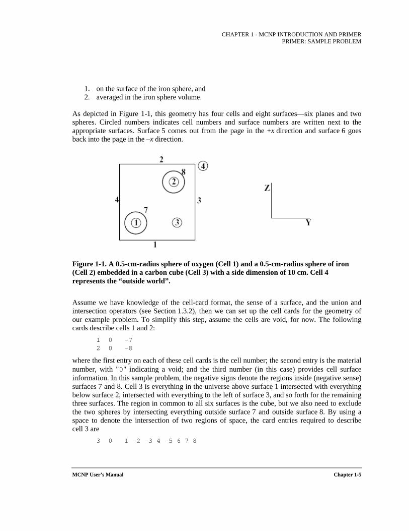
The simple sample problem is illustrated in Figure 1-1. A 0.5-cm-radius sphere of oxygen (Cell 1) and a 0.5-cm-radius sphere of iron (Cell 2) embedded in a carbon cube (Cell 3) with a side dimension of 10 cm. Cell 4 represents the “outside world”.The “outside world” is represented by Cell 4 and is referred to as such throughout the remainder of this section. We wish to start 14-MeV neutrons isotropically as a point source in the center of the small sphere of oxygen that is embedded in a cube of carbon. A small sphere of iron is also embedded in the carbon. The carbon is a cube 10 cm on each side; the spheres have a 0.5-cm radius and are centered between the front and back faces of the cube. We wish to calculate the total and energy-dependent flux in increments of 1 MeV from 1 to 14 MeV, where bin 1 will be the tally from 0 to 1 MeV
CHAPTER 1 - MCNP INTRODUCTION AND PRIMER
PRIMER: SAMPLE PROBLEM
MCNP User’s Manual Chapter 1-5
1. on the surface of the iron sphere, and 2. averaged in the iron sphere volume.
As depicted in Figure 1-1, this geometry has four cells and eight surfaces—six planes and two spheres. Circled numbers indicates cell numbers and surface numbers are written next to the appropriate surfaces. Surface 5 comes out from the page in the +x direction and surface 6 goes back into the page in the –x direction.
Figure 1-1. A 0.5-cm-radius sphere of oxygen (Cell 1) and a 0.5-cm-radius sphere of iron (Cell 2) embedded in a carbon cube (Cell 3) with a side dimension of 10 cm. Cell 4 represents the “outside world”.
Assume we have knowledge of the cell-card format, the sense of a surface, and the union and intersection operators (see Section 1.3.2), then we can set up the cell cards for the geometry of our example problem. To simplify this step, assume the cells are void, for now. The following cards describe cells 1 and 2:
1 0 –7 2 0 –8
where the first entry on each of these cell cards is the cell number; the second entry is the material number, with "0" indicating a void; and the third number (in this case) provides cell surface information. In this sample problem, the negative signs denote the regions inside (negative sense) surfaces 7 and 8. Cell 3 is everything in the universe above surface 1 intersected with everything below surface 2, intersected with everything to the left of surface 3, and so forth for the remaining three surfaces. The region in common to all six surfaces is the cube, but we also need to exclude the two spheres by intersecting everything outside surface 7 and outside surface 8. By using a space to denote the intersection of two regions of space, the card entries required to describe cell 3 are
3 0 1 –2 –3 4 –5 6 7 8
CHAPTER 1 - MCNP INTRODUCTION AND PRIMER PRIMER: SAMPLE PROBLEM
Chapter 1-6 MCNP User’s Manual
Optional
Cell 4 requires the use of the union operator, which is denoted by a colon (:). Cell 4 is the outside world and is defined as everything in the universe below surface 1, plus everything above surface 2, plus everything to the right of surface 3, and so forth. The cell card for cell 4 is
4 0 –1 : 2 : 3 : –4 : 5 : –6
Cell 4, the outside world, would usually have zero importance (not denoted here). You will learn more about cell importance in Section 1.3.4.2.
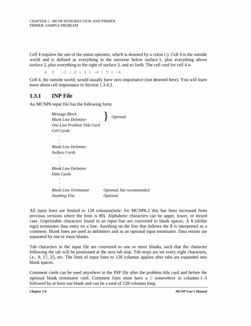
1.3.1 INP File An MCNP6 input file has the following form:
Message Block Blank Line Delimiter One Line Problem Title Card Cell Cards
.
.
. Blank Line Delimiter Surface Cards
.
.
. Blank Line Delimiter Data Cards
.
.
. Blank Line Terminator Optional, but recommended Anything Else Optional
All input lines are limited to 128 columns(note: for MCNP6.2 this has been increased from previous versions where the limit is 80). Alphabetic characters can be upper, lower, or mixed case. Unprintable characters found in an input line are converted to blank spaces. A $ (dollar sign) terminates data entry on a line. Anything on the line that follows the $ is interpreted as a comment. Blank lines are used as delimiters and as an optional input terminator. Data entries are separated by one or more blanks.
Tab characters in the input file are converted to one or more blanks, such that the character following the tab will be positioned at the next tab stop. Tab stops are set every eight characters, i.e., 9, 17, 25, etc. The limit of input lines to 128 columns applies after tabs are expanded into blank spaces.
Comment cards can be used anywhere in the INP file after the problem title card and before the optional blank terminator card. Comment lines must have a C somewhere in columns 1–5 followed by at least one blank and can be a total of 128 columns long.
CHAPTER 1 - MCNP INTRODUCTION AND PRIMER
PRIMER: SAMPLE PROBLEM
MCNP User’s Manual Chapter 1-7
Cell, surface, and data cards must all begin within the first five columns. Entries are separated by one or more blanks. Numbers can be integer or floating point. MCNP6 makes the appropriate conversion. A few entries on some cards are allowed to be 8-byte integers, i.e., integers larger than 2.147 billion but less than ~1E19. These entries are noted in their respective card description in Section 3. A data entry item, e.g., IMP:N or 1.1e2, must be completed on one line.
Blanks filling the first five columns indicate a continuation of the data from the last named card. An & (ampersand) ending a line indicates data will continue on the following card, where data on the continuation card can be in columns 1–128.
The optional message block, discussed in detail in Section 2.4, is used to change file names and specify running options such as a continue-run. On most systems these options and files may alternatively be specified with an execution line (see Section 1.4.1). If both an execution line and a message block are present and there is a conflict, the execution line entries supersede the message block entries. The blank line delimiter signals the end of the message block.
The first card in the file after the optional message block is the required problem title card. If there is no message block, this must be the first card in the INP file. It is limited to one 128-column line and is used as a title in various places in the MCNP6 output. It can contain any information you desire but usually contains information describing the particular problem.
MCNP6 makes extensive checks of the input file for user errors. A fatal error occurs if a basic constraint of the input specification is violated, and MCNP6 will terminate before running any particles. The first fatal error is real; subsequent error messages may or may not be real because of the nature of the first fatal message.
1.3.2 Cell Cards When populating the cell cards, the cell number is the first entry and must begin in the first five columns. The next entry is the cell material number, which is arbitrarily assigned by the user. The material is described on a material card (M) that has the same material number (see Section 1.3.4.5). If the cell is a void, a zero is entered for the material number. The cell and material numbers cannot exceed eight digits each. Following the material number is the cell material density. A positive entry is interpreted as atom density in units of 1024 atoms/cm3. A negative entry is interpreted as mass density in units of g/cm3. No density is entered for a void cell. After the material density, a complete specification of the geometry of the cell follows. This specification includes a list of the signed surfaces bounding the cell where the sign denotes the sense of the regions defined by the surfaces. The regions are combined with the Boolean intersection and union operators. A space indicates an intersection and a colon indicates a union.
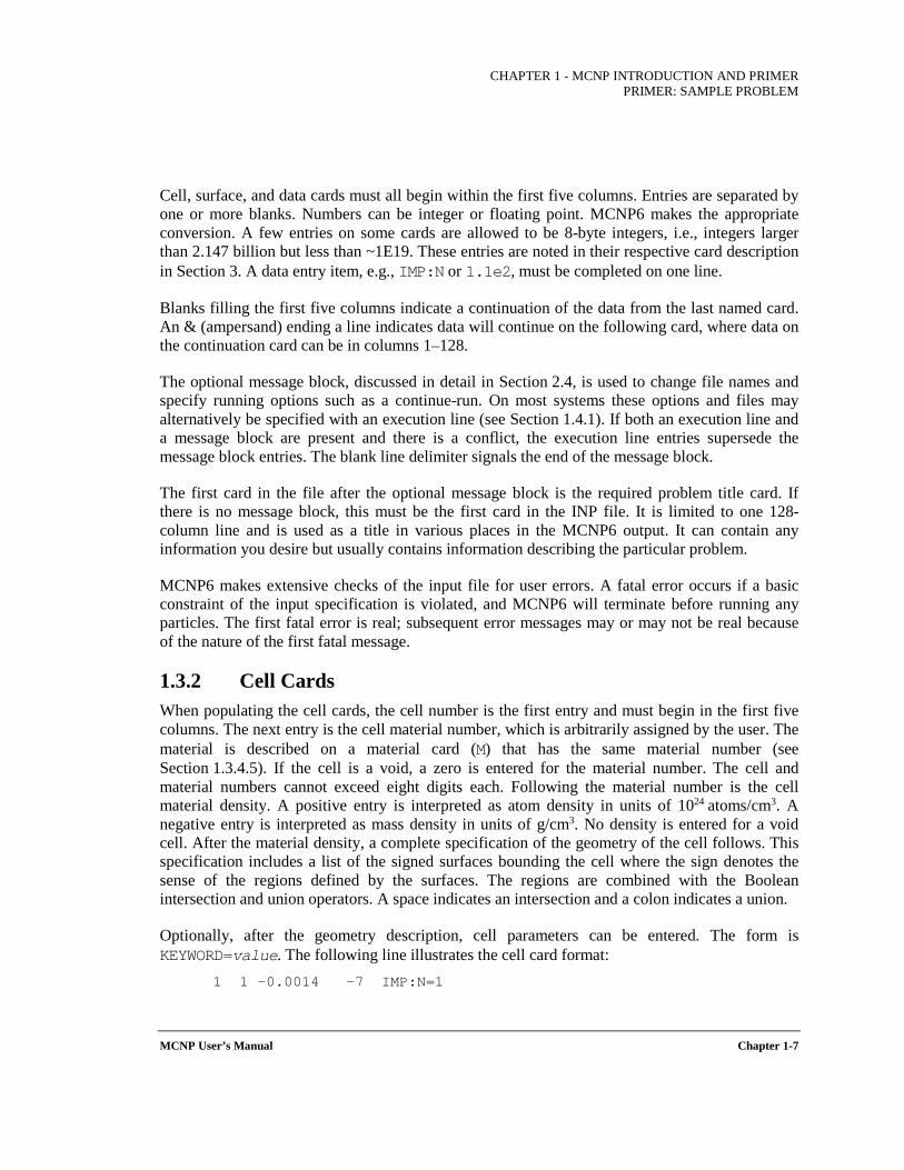
Optionally, after the geometry description, cell parameters can be entered. The form is KEYWORD=value. The following line illustrates the cell card format:
1 1 –0.0014 –7 IMP:N=1
CHAPTER 1 - MCNP INTRODUCTION AND PRIMER PRIMER: SAMPLE PROBLEM
Chapter 1-8 MCNP User’s Manual
Cell 1 contains material 1 with density 0.0014 g/cm3, is bounded only by one surface 7, and has a neutron importance of 1. If cell 1 were a void, the cell card would be
1 0 –7 IMP:N=1
The complete cell input for this problem (with two comment cards) is c cell cards for sample problem 1 1 –0.0014 –7 2 2 –7.86 –8 3 3 –1.60 1 –2 –3 4 –5 6 7 8 4 0 –1:2:3:–4:5:–6
c end of cell cards for sample problem blank line delimiter
The blank line at the end of the card terminates the cell-card section of the INP file. A complete explanation of the cell card input is found in Section 3.2.1.
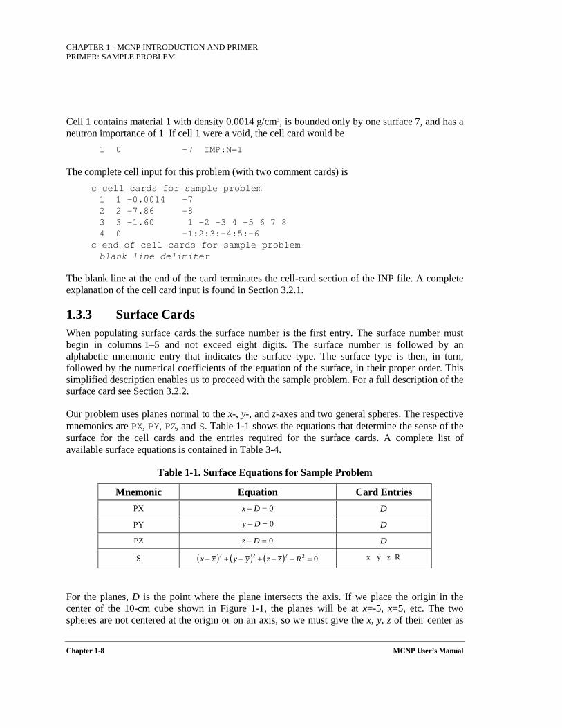
1.3.3 Surface Cards When populating surface cards the surface number is the first entry. The surface number must begin in columns 1–5 and not exceed eight digits. The surface number is followed by an alphabetic mnemonic entry that indicates the surface type. The surface type is then, in turn, followed by the numerical coefficients of the equation of the surface, in their proper order. This simplified description enables us to proceed with the sample problem. For a full description of the surface card see Section 3.2.2.
Our problem uses planes normal to the x-, y-, and z-axes and two general spheres. The respective mnemonics are PX, PY, PZ, and S. Table 1-1 shows the equations that determine the sense of the surface for the cell cards and the entries required for the surface cards. A complete list of available surface equations is contained in Table 3-4.
Table 1-1. Surface Equations for Sample Problem
Mnemonic Equation Card Entries PX
PY
PZ
S
For the planes, D is the point where the plane intersects the axis. If we place the origin in the center of the 10-cm cube shown in Figure 1-1, the planes will be at x=-5, x=5, etc. The two spheres are not centered at the origin or on an axis, so we must give the x, y, z of their center as
0=− Dx D
0=− Dy D
0=− Dz D
( ) ( ) ( ) 02222 =−−+−+− Rzzyyxx R z y x
CHAPTER 1 - MCNP INTRODUCTION AND PRIMER
PRIMER: SAMPLE PROBLEM
MCNP User’s Manual Chapter 1-9
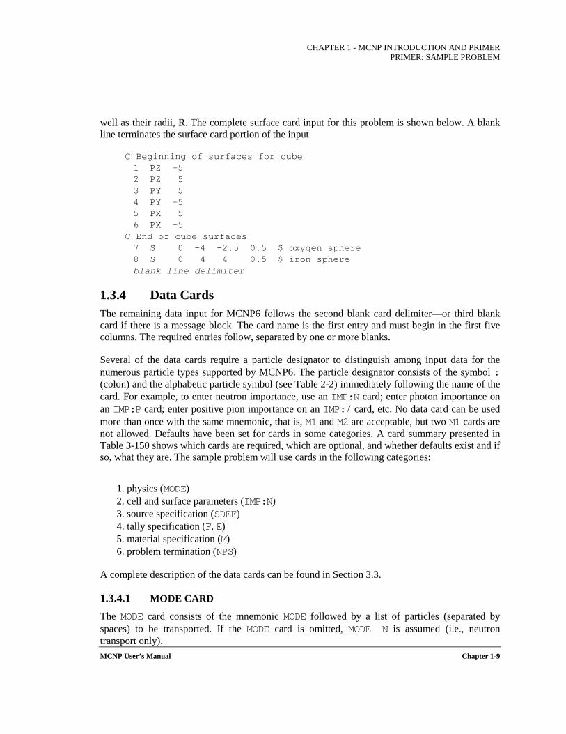
well as their radii, R. The complete surface card input for this problem is shown below. A blank line terminates the surface card portion of the input.
C Beginning of surfaces for cube 1 PZ −5 2 PZ 5 3 PY 5 4 PY −5 5 PX 5 6 PX −5
C End of cube surfaces 7 S 0 -4 -2.5 0.5 $ oxygen sphere 8 S 0 4 4 0.5 $ iron sphere blank line delimiter
1.3.4 Data Cards The remaining data input for MCNP6 follows the second blank card delimiter—or third blank card if there is a message block. The card name is the first entry and must begin in the first five columns. The required entries follow, separated by one or more blanks.
Several of the data cards require a particle designator to distinguish among input data for the numerous particle types supported by MCNP6. The particle designator consists of the symbol : (colon) and the alphabetic particle symbol (see Table 2-2) immediately following the name of the card. For example, to enter neutron importance, use an IMP:N card; enter photon importance on an IMP:P card; enter positive pion importance on an IMP:/ card, etc. No data card can be used more than once with the same mnemonic, that is, M1 and M2 are acceptable, but two M1 cards are not allowed. Defaults have been set for cards in some categories. A card summary presented in Table 3-150 shows which cards are required, which are optional, and whether defaults exist and if so, what they are. The sample problem will use cards in the following categories:
1. physics (MODE) 2. cell and surface parameters (IMP:N) 3. source specification (SDEF) 4. tally specification (F, E) 5. material specification (M) 6. problem termination (NPS)
A complete description of the data cards can be found in Section 3.3.
1.3.4.1 MODE CARD
The MODE card consists of the mnemonic MODE followed by a list of particles (separated by spaces) to be transported. If the MODE card is omitted, MODE N is assumed (i.e., neutron transport only).
CHAPTER 1 - MCNP INTRODUCTION AND PRIMER PRIMER: SAMPLE PROBLEM
Chapter 1-10 MCNP User’s Manual
By default, MODE N P does not account for photo-neutrons, but does account for neutron-induced photons. Photonuclear particle production can be turned on through an option on the PHYS:P card (see Section 3.3.3.2.2). Photon production cross sections do not exist for all nuclides. If they are not available for a MODE N P problem, MCNP6 will print out warning messages.
MODE P or MODE N P problems generate bremsstrahlung photons with a thick-target bremsstrahlung approximation. This approximation can be turned off with the PHYS:E card.
The sample problem is a neutron-only problem, so the MODE card can be omitted because MODE N is the default.
1.3.4.2 CELL AND SURFACE PARAMETER CARDS
Data related to individual cells can be entered either on the cell card or in the data card section of the input file, data related to individual surfaces can only be entered using the data card format. If entered on a card in the data block section, entries must be listed in the same order as the associated cell (or surface) cards that appear earlier in the INP file. The number of entries on a cell or surface data card must equal the number of cells or surfaces in the problem, otherwise MCNP6 prints out a warning or fatal error message. In the case of a warning, MCNP6 allows the problem to continue, but assumes that the value of the parameter for each cell or surface is zero. Cell parameters also can be defined on cell cards using the KEYWORD=value format. If a cell parameter is specified on any cell card, it must be specified only on cell cards and not at all in the data card section.
The only surface parameter card is AREA. A listing of available cell parameter cards appears in Table 3-2. Examples include importance cards (IMP:N, IMP:P) and weight-window cards (WWE:N, WWE:P, WWNi:N, WWNi:P), etc. Each problem requires some method of specifying relative cell importance, most of the other cell parameters are used to specify optional variance reduction techniques.
The IMP:N card is used to specify relative cell importance in the sample problem. There are four cells in the sample problem, so the IMP:N card will have four entries. The IMP:N card is used a) for terminating the particle’s history if the importance is zero and b) for geometry splitting and Russian roulette to help particles move more easily to important regions of the geometry. An IMP:N card for the sample problem is
IMP:N 1 1 1 0
1.3.4.3 SOURCE SPECIFICATION CARDS
A source definition card SDEF is one of four available methods of defining starting particles. Section 3.3.4 has a complete discussion of source specification. The SDEF card defines the basic source parameters, some of which are
POS= x y z Default = 0 0 0 CEL= starting cell number
CHAPTER 1 - MCNP INTRODUCTION AND PRIMER
PRIMER: SAMPLE PROBLEM
MCNP User’s Manual Chapter 1-11
ERG= starting energy Default = 14 MeV WGT= starting weight Default = 1 TME= time Default = 0 PAR= source particle type Symbol or number of the source particle type (N or 1
for neutron, P or 2 for photon, etc.)
MCNP6 will determine the starting cell number for a point isotropic source, so the CEL entry is not always required. The default starting direction for source particles is isotropic.
For the example problem, a fully specified source card is SDEF POS=0 –4 –2.5 CEL=1 ERG=14 WGT=1 TME=0 PAR=N
Neutron particles will start at the center of the oxygen sphere (0 –4 –2.5), in cell 1, with an energy of 14 MeV, and with weight of 1 at time 0. All these source parameters except the starting position are the default values, so the most concise source card is
SDEF POS=0 –4 –2.5
If all the default conditions applied to the problem, only the mnemonic SDEF would be required.
1.3.4.4 TALLY SPECIFICATION CARDS
The tally cards are used to specify what you want to learn from the Monte Carlo calculation, perhaps current across a surface, flux at a point, etc. You request this information with one or more tally cards. Tally specification cards are not required, but if none is supplied, no tallies will be printed when the problem is run and a warning message is issued. Many of the tally specification cards describe tally "bins." A few examples are energy (E), time (T), and cosine (C) bin cards.
MCNP6 provides seven different standard tally types, all normalized to be per starting particle. Some tallies in criticality calculations are normalized differently. Chapter 2 of the MCNP5 Theory Manual[X-503a] discusses tallies more completely, and Section 3.3.5 of this manual lists all the tally cards and fully describes each one.
Tally Mnemonic Description F1:<pl> Surface current F2:<pl> Surface flux F4:<pl> Track length estimate of cell flux F5a:N or F5a:P Flux at a point (point detector) F6:<pl> Track length estimate of energy deposition F7:N Track length estimate of fission energy deposition F8:<pl> Energy distribution of pulses created in a detector
The tallies are identified by tally type and particle type. Tallies are given the numbers 1, 2, 4, 5, 6, 7, 8, or increments of 10 thereof, and are given the particle designator :N for neutron, :\ for

CHAPTER 1 - MCNP INTRODUCTION AND PRIMER PRIMER: SAMPLE PROBLEM
Chapter 1-12 MCNP User’s Manual
pion, etc. You may have as many of any basic tally as you need, each with different energy bins or flagging or anything else. The tally designations F4:N, F14:N, F104:N, and F234:N are all legitimate neutron cell flux tallies; they could all be for the same cell(s) but with different energy or multiplier bins, for example. Similarly F5:P, F15:P, and F305:P are all photon point detector tallies. Having both an F1:N card and an F1:P card in the same INP file is not allowed. The tally number may not exceed 9999.
For our sample problem we will use F cards (tally type) and E cards (tally energy).
Tally (Fn) Cards: The sample problem has a surface flux tally and a track length cell flux tally. Thus, the tally cards for the sample problem shown in Figure 1-1 are
F2:N 8 $ flux across surface 8 F4:N 2 $ track length in cell 2
Printed out with each tally result is the uncertainty of the tally corresponding to one estimated standard deviation. Results are not reliable until they become stable as a function of the number of histories run. Much information is provided for a specified bin of each tally in the tally fluctuation charts at the end of the output file to help determine tally stability. The user is strongly encouraged to look at this information carefully.
Tally Energy (En) Cards: We wish to calculate flux in increments of 1 MeV from 1 to 14 MeV. Another tally specification card in the sample input deck establishes these energy bins.
The entries on the En card are the upper bounds in MeV of the energy bins for tally n. The entries must be given in order of increasing magnitude. If a particle has an energy greater than the last entry, it will not be tallied, and a warning is issued. MCNP6 automatically provides the total over all specified energy bins unless inhibited by putting the symbol NT as the last entry on the selected En card.
The following cards will create energy bins for the sample problem: E2 1 2 3 4 5 6 7 8 9 10 11 12 13 14 E4 1 12I 14
If no En card exists for tally n, a single bin over all energy will be used. To change this default, an E0 (zero) card can be used to set up a default energy bin structure for all tallies. A specific En card will override the default structure for tally n. We could replace the E2 and E4 cards with one E0 card for the sample problem, thus setting up identical bins for both tallies.
1.3.4.5 MATERIALS SPECIFICATION
The cards in this section specify both the isotopic composition of the materials and the cross-section evaluations to be used in the cells. For a comprehensive discussion of materials specification, see Section 3.3.2.
CHAPTER 1 - MCNP INTRODUCTION AND PRIMER
PRIMER: SAMPLE PROBLEM
MCNP User’s Manual Chapter 1-13
Material (Mm) Card: The following card is used to specify a material for all cells containing material m, where m cannot exceed five digits:
Mm ZAID1 fraction1 ZAID2 fraction2 ...
The m on a material card corresponds to the material number on the cell card (see Section 1.3.2). The consecutive pairs of entries on the material card consist of the identification number (ZAID) of the constituent element or nuclide followed by the atomic fraction (or weight fraction if entered as a negative number) of that element or nuclide, until all the elements and nuclides needed to define the material have been listed.
(1) Nuclide Identification Number (ZAID). This number is used to identify the element or nuclide desired. The form of the number is ZZZAAA.abx, where
ZZZ is the atomic number of the element or nuclide; AAA is the mass number of the nuclide, ignored for photons and electrons; ab is the cross-section evaluation identifier; and x is the class of data. Commonly used classes are: C is continuous energy neutron
cross sections, P is photon, E is electron, U is photonuclear, and H is proton.
For naturally occurring elements, AAA=000. Thus ZAID=74182 represents the isotope , and ZAID=74000 represents the element tungsten.
If .abx is omitted the first entry from the xsdir corresponding to the proper library class will be used. This same approach will be used for all libraries not specified. For example in a mode N P problem, if 1001.70c is specified the .70c library will be used for neutrons and the first photon library in the xsdir file will be used.
(2) Nuclide Fraction. The nuclide fractions may be normalized to 1 or left un-normalized. For example, if the material is H2O, the fractions can be entered as 0.667 and 0.333, or as 2 and 1 for H and O, respectively. If the fractions are entered with negative signs, they are weight fractions; otherwise they are atomic fractions. Weight fractions and atomic fractions cannot be mixed on the same Mm card.
Appropriate material cards for the sample problem are M1 8016 1 $ oxygen 16 M2 26000 1 $ natural iron M3 6000 1 $ carbon
VOID Card: The VOID card removes all materials and cross sections in a problem and sets all non-zero importance to unity. It is very effective for finding errors in the geometry description because many particles can be run in a short time. Flooding the geometry with many particles increases the chance of particles going to most parts of the geometry—in particular, to an incorrectly specified part of the geometry—and getting lost. The history of a lost particle often
W18274
CHAPTER 1 - MCNP INTRODUCTION AND PRIMER PRIMER: SAMPLE PROBLEM
Chapter 1-14 MCNP User’s Manual
helps locate the geometry error. The other actions of and uses for the VOID card are discussed in Section 3.3.2.10.
The sample input deck could have a VOID card while testing the geometry for errors. When you are satisfied that the geometry is error-free, remove the VOID card.
1.3.4.6 PROBLEM TERMINATION
Problem termination cards are used to specify parameters for some of the ways to terminate execution of MCNP6. The full list of available cards and a complete discussion of problem cutoffs is found in Section 3.3.7.1. For our problem we will use only the history cutoff (NPS) card. The mnemonic NPS is followed by an entry (npp) that specifies the number of histories to transport. MCNP6 will terminate after npp histories unless it has terminated earlier for some other reason.
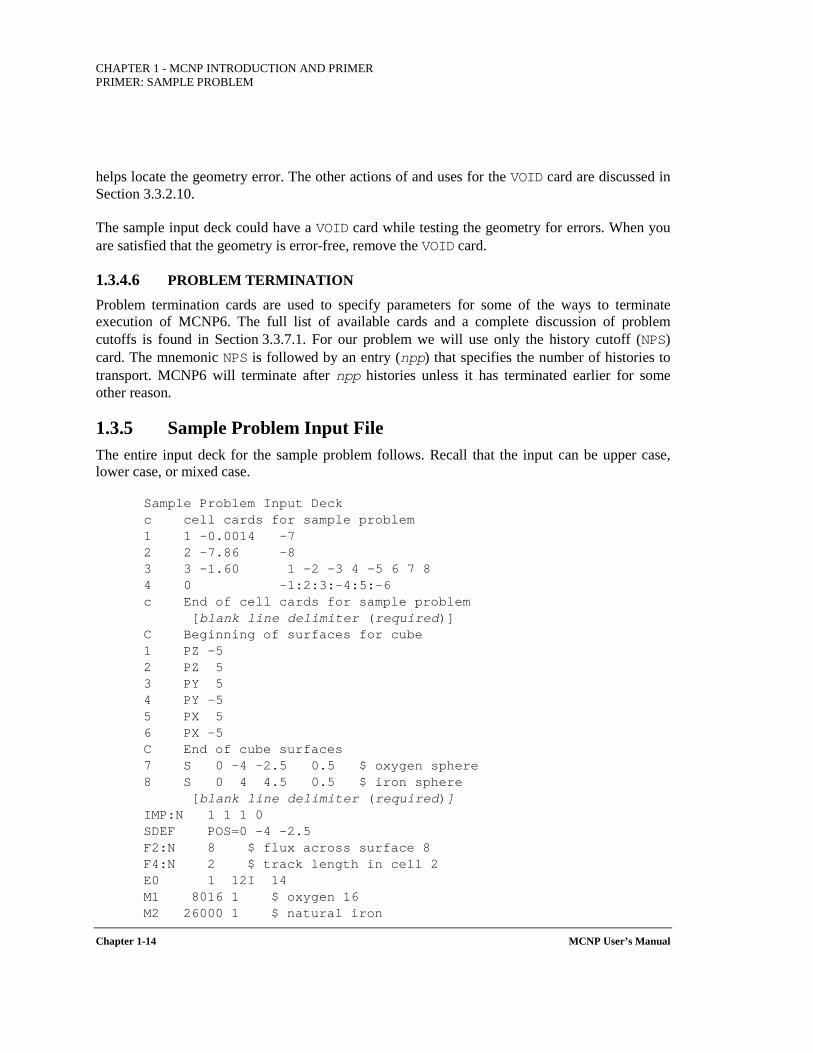
1.3.5 Sample Problem Input File The entire input deck for the sample problem follows. Recall that the input can be upper case, lower case, or mixed case.
Sample Problem Input Deck c cell cards for sample problem 1 1 -0.0014 -7 2 2 -7.86 -8 3 3 -1.60 1 -2 -3 4 -5 6 7 8 4 0 -1:2:3:-4:5:-6 c End of cell cards for sample problem
[blank line delimiter (required)] C Beginning of surfaces for cube 1 PZ -5 2 PZ 5 3 PY 5 4 PY -5 5 PX 5 6 PX -5 C End of cube surfaces 7 S 0 -4 -2.5 0.5 $ oxygen sphere 8 S 0 4 4.5 0.5 $ iron sphere
[blank line delimiter (required)] IMP:N 1 1 1 0 SDEF POS=0 -4 -2.5 F2:N 8 $ flux across surface 8 F4:N 2 $ track length in cell 2 E0 1 12I 14 M1 8016 1 $ oxygen 16 M2 26000 1 $ natural iron
CHAPTER 1 - MCNP INTRODUCTION AND PRIMER
PRIMER: SAMPLE PROBLEM
MCNP User’s Manual Chapter 1-15
M3 6000 1 $ carbon NPS 100000
[blank line delimiter (optional)]
1.3.6 Running the Sample Problem To run the example problem, place the input file in your current directory. Let’s assume the file is called SAMPLE. Type
mcnp6 N=SAMPLE
where N is an abbreviation for the keyword NAME. MCNP6 will produce an output file SAMPLEo that you can examine at your terminal, send to a printer, or both. To look at the geometry with the PLOT module using an interactive graphics terminal, type
mcnp6 IP N=SAMPLE
After the plot window appears, click anywhere in the picture to get the default plot. This plot will show an intersection of the surfaces of the problem by the plane x=0 with an extent in the x direction of 100 cm on either side of the origin. If you want to do more with PLOT, see the instructions in Section 5. Otherwise click "end" to terminate the session.
MCNP6 does extensive input checking but is not foolproof. A geometry should be checked by looking at several different views with the geometry plotting option. You should also surround the entire geometry with a sphere and flood the geometry with particles from a source that has an inward cosine distribution on the spherical surface, using a VOID card to remove all materials specified in the problem. If there are any incorrectly specified places in your geometry, this procedure will usually find them. Make sure the importance of the cell just inside the source sphere is not zero. Then run a short job and study the output to see if you are calculating what you think you are calculating.
1.4 EXECUTING MCNP6
This section assumes a basic knowledge of UNIX. Lines the user will type are shown in lower case typewriter style type. Press the ENTER key after each input line. The file mcnp6 is the executable binary file and the file xsdir_mcnp6.2 contains the cross-section directory for MCNP6, Version 2. If xsdir_mcnp6.2 is not in your current directory, you may need to set the DATAPATH environmental variable. The c-shell (csh) syntax for this is
setenv DATAPATH /ab/cd
and the bash syntax is export DATAPATH=/ab/cd
where /ab/cd is the directory containing both the file xsdir_mcnp6.2 and the data libraries.
CHAPTER 1 - MCNP INTRODUCTION AND PRIMER Executing MCNP
Chapter 1-16 MCNP User’s Manual
1.4.1 Execution Line The MCNP6 execution line has the following form:
mcnp6 KEYWORD=value ... KEYWORD=value execution_option(s) other_options
where each KEYWORD is an MCNP6 default file name to which the user may assign a specific value (i.e., file name or path); execution_options is a character or string of characters that informs MCNP6 which of five execution module(s) to run; and other_option(s) provides the user with additional execution control. The execute line message may be up to 240 characters long. The order of the entries on the MCNP6 execution line is irrelevant. If no changes are desired to the default names and options, no entries to the MCNP6 execution line are necessary.
The execution-line keywords (i.e., default file names), execution options, and other options are summarized in Table 1-2. Let us examine each of these execution-line inputs.
a) KEYWORD=value (where KEYWORD is any of a list of default MCNP6 file names)
MCNP6 uses several files for input and output. The file names can include full paths to the files (e.g., /mydir/problem-x/jobs/problem_1a.inp), but the path cannot be longer than 256 characters. In the simplest case, in which the MCNP6 execution command has no arguments, a file named INP must be present in the local directory; then, during problem execution, MCNP6 will create two output files: OUTP and RUNTPE.
The default name of any of the files in Table 1-2 can be changed on the MCNP6 execution line by entering
KEYWORD=newname
For example, if you have an input file called MCIN and want the output file to be MCOUT and the restart file to be MCRUNTPE, the appropriate execution line would read
mcnp6 INP=MCIN OUTP=MCOUT RUNTPE=MCRUNTPE
Only enough letters of the default name are required to identify it uniquely. For example, mcnp6 I=MCIN O=MCOUT RU=MCRUNTPE
also works. If a file in your local file space has the same name as a file MCNP6 needs to create, the file is created with a different unique name by changing the last letter of the name of the new file to the next letter in the alphabet. For example, if you already have a file named OUTP in the directory, MCNP6 will create OUTQ. However, if the file includes an extension, such as ".txt" or ".inp", the last character before the extension will be checked and changed if necessary.
Sometimes it is useful for all files from one run to have similar names. If your input file is called JOB1, the following line
mcnp6 NAME=JOB1
CHAPTER 1 - MCNP INTRODUCTION AND PRIMER
Executing MCNP
MCNP User’s Manual Chapter 1-17
will create an OUTP file called JOB1O and a RUNTPE file called JOB1R. If these files already exist, MCNP6 will not overwrite them or modify the last letter, but will issue a message that JOB1O already exists and then will terminate.
b) execution_option
MCNP6 consists of six distinct execution modules: IMCN, PLOT, XACT, MCRUN, MCPLOT, and PARTISN_INPUT. A description of these modules, including a one-letter mnemonic assigned to each, appears in Table 1-2.
Given no other instructions, MCNP6 will process the input (I), process the cross-section data (X), and then perform the particle transport (R). Thus, the default execution input is IXR. Entering the proper mnemonic on the execution line controls the execution of the modules. If more than one operation is desired, combine the single characters (in any order) to form a string. To look for input errors only, specify I; to debug a geometry by plotting, use IP; to plot cross-section data, enter IXZ; to plot tally results from the RUNTPE or MCTAL files, specify Z; and to create a LNK3DNT geometry file for use in PARTISN, specify M on the execution line as the execution_option.
After a job has been run, the print file OUTP can be examined with an editor on the computer and/or sent to a printer. Numerous messages about the problem execution and statistical quality of the results are displayed at the terminal. These are repeated in the OUTP file.
c) other_options
The "other" options add more flexibility when running MCNP6 and also are shown in Table 1-2.
MCNP6 may be compiled for MPI and then executed in the same fashion as other parallel programs on a given system. The parallel operation is a master-slave algorithm with one master process accumulating total statistics and a group of slave processes tracking particles. When shared memory processors are used, MCNP6 may also be compiled for OpenMP threading, either independently or in combination with MPI.
Generally, the MPI execution line will look like this example from a Linux system, using OpenMPI:
MPIRUN -NP <m> MCNP.MPI I=input ...
where <m> is the total number of MPI processes, including the master, and <m>-1 slave processes will track the particles. On other systems, or other MPI implementations, the syntax of the MPI command may differ. Note that the minimum number of slaves accepted by MCNP6 is two, so at least three MPI processes must be initiated. That is, <m> can equal 1 or be greater than or equal to 3.

CHAPTER 1 - MCNP INTRODUCTION AND PRIMER Executing MCNP
Chapter 1-18 MCNP User’s Manual
If MCNP6 is compiled with OpenMP on a multiprocessor SMP machine, then it is possible to optionally thread each slave by setting the TASKS option
MPIRUN -NP <m> MCNP.MPI I=input TASKS <n>
making (m-1)×n processors available to track particles. The syntax required to allocate enough resources for the threading varies by system.
An MCNP6 executable built with combined MPI and OpenMP options can be utilized as follows: sequentially, all MPI, threads only, or hybrid. To perform the combined executable in sequential or threads-only mode (for example, in early testing of a problem or for plotting geometry), the system will likely require MPIRUN -NP 1.
The simplest parallel run would be to build one shared memory node and run OpenMP threading. Then, use build option "OMP" and execute with just the TASKS option on the command line:
mcnp6 I=input TASKS <n>
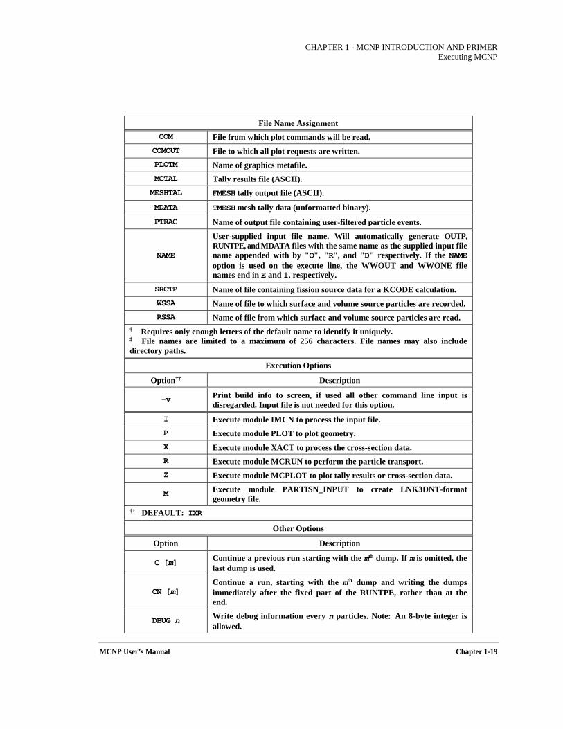
Table 1-2. MCNP6 Execution Line Input
File Name Assignment
Keyword†
(Default File Name) Value‡
INP User-supplied input file name. This is the name of the file that contains the problem input specification and must be present as a local file.
OUTP File name to which results are written. This file may be viewed and/or printed. Created by MCNP6 during problem execution.
RUNTPE Name of file containing binary start/restart data. Created by MCNP6 during initial problem execution and added to by MCNP6 during continued problem execution.
XSDIR Name of cross-section directory (XSDIR) file. Note: The default name for the XSDIR file in MCNP6 (Version 2) is xsdir_mcnp6.2.
WWINP Name of weight-window generator input file containing either cell- or mesh-based lower weight-window bounds.
WWOUT Name of weight-window generator output file containing either cell- or mesh-based lower weight-window bounds.
WWONE Name of weight-window generator output file containing cell- or mesh-based time- and/or energy-integrated weight windows.
PARTINP PARTISN input file for MCNP6 to output. LINKIN Name of LNK3DNT file to input. LINKOUT Name of LNK3DNT-format geometry file created by MCNP6. KSENTAL Name of ASCII results file KCODE for sensitivity profiles. HISTP History tape file. See Section 3.3.7.2.6.
DUMN1 and DUMN2 See Section 3.3.7.3.6, File creation card.
CHAPTER 1 - MCNP INTRODUCTION AND PRIMER
Executing MCNP
MCNP User’s Manual Chapter 1-19
File Name Assignment COM File from which plot commands will be read.
COMOUT File to which all plot requests are written. PLOTM Name of graphics metafile. MCTAL Tally results file (ASCII). MESHTAL FMESH tally output file (ASCII).
MDATA TMESH mesh tally data (unformatted binary).
PTRAC Name of output file containing user-filtered particle events.
NAME
User-supplied input file name. Will automatically generate OUTP, RUNTPE, and MDATA files with the same name as the supplied input file name appended with by "O", "R", and "D" respectively. If the NAME option is used on the execute line, the WWOUT and WWONE file names end in E and 1, respectively.
SRCTP Name of file containing fission source data for a KCODE calculation. WSSA Name of file to which surface and volume source particles are recorded. RSSA Name of file from which surface and volume source particles are read.
† Requires only enough letters of the default name to identify it uniquely. ‡ File names are limited to a maximum of 256 characters. File names may also include directory paths.
Execution Options
Option†† Description
-v Print build info to screen, if used all other command line input is disregarded. Input file is not needed for this option.
I Execute module IMCN to process the input file. P Execute module PLOT to plot geometry. X Execute module XACT to process the cross-section data. R Execute module MCRUN to perform the particle transport. Z Execute module MCPLOT to plot tally results or cross-section data.
M Execute module PARTISN_INPUT to create LNK3DNT-format geometry file.
†† DEFAULT: IXR
Other Options
Option Description
C [m] Continue a previous run starting with the mth dump. If m is omitted, the last dump is used.
CN [m] Continue a run, starting with the mth dump and writing the dumps immediately after the fixed part of the RUNTPE, rather than at the end.
DBUG n Write debug information every n particles. Note: An 8-byte integer is allowed.
CHAPTER 1 - MCNP INTRODUCTION AND PRIMER Executing MCNP
Chapter 1-20 MCNP User’s Manual
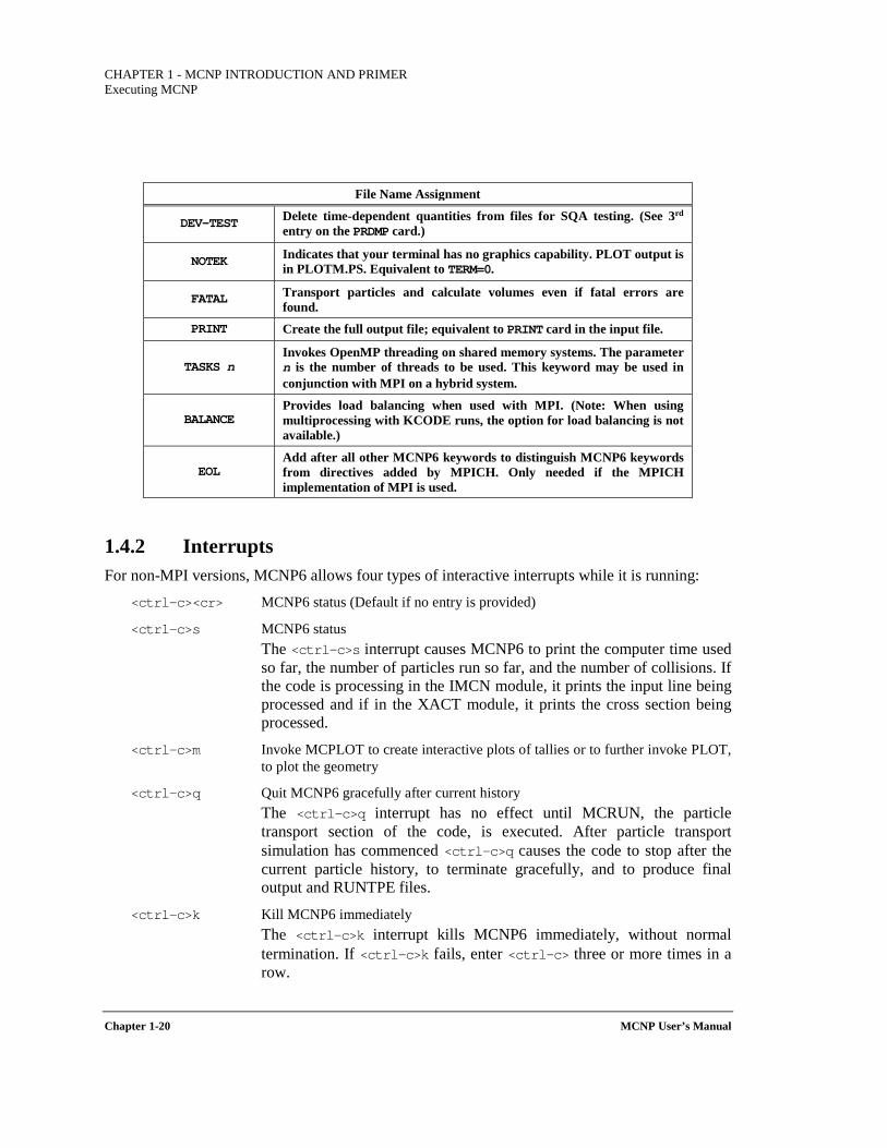
File Name Assignment
DEV-TEST Delete time-dependent quantities from files for SQA testing. (See 3rd entry on the PRDMP card.)
NOTEK Indicates that your terminal has no graphics capability. PLOT output is in PLOTM.PS. Equivalent to TERM=0.
FATAL Transport particles and calculate volumes even if fatal errors are found.
PRINT Create the full output file; equivalent to PRINT card in the input file.
TASKS n Invokes OpenMP threading on shared memory systems. The parameter n is the number of threads to be used. This keyword may be used in conjunction with MPI on a hybrid system.
BALANCE Provides load balancing when used with MPI. (Note: When using multiprocessing with KCODE runs, the option for load balancing is not available.)
EOL Add after all other MCNP6 keywords to distinguish MCNP6 keywords from directives added by MPICH. Only needed if the MPICH implementation of MPI is used.
1.4.2 Interrupts For non-MPI versions, MCNP6 allows four types of interactive interrupts while it is running:
<ctrl-c><cr> MCNP6 status (Default if no entry is provided)
<ctrl-c>s MCNP6 status The <ctrl-c>s interrupt causes MCNP6 to print the computer time used
so far, the number of particles run so far, and the number of collisions. If the code is processing in the IMCN module, it prints the input line being processed and if in the XACT module, it prints the cross section being processed.
<ctrl-c>m Invoke MCPLOT to create interactive plots of tallies or to further invoke PLOT, to plot the geometry
<ctrl-c>q Quit MCNP6 gracefully after current history The <ctrl-c>q interrupt has no effect until MCRUN, the particle
transport section of the code, is executed. After particle transport simulation has commenced <ctrl-c>q causes the code to stop after the current particle history, to terminate gracefully, and to produce final output and RUNTPE files.
<ctrl-c>k Kill MCNP6 immediately The <ctrl-c>k interrupt kills MCNP6 immediately, without normal
termination. If <ctrl-c>k fails, enter <ctrl-c> three or more times in a row.
CHAPTER 1 - MCNP INTRODUCTION AND PRIMER
Executing MCNP
MCNP User’s Manual Chapter 1-21
Batch jobs, run in sequential or multiprocessing mode, may be interrupted and stopped with the creation of a file in the directory where the job was started. The name of the file must be "STOPinp" where inp is the name of the original input file that initiated the run. On a computer system that is case sensitive (e.g., Linux), the "stop" must be in lower case and "INP" must match the case of the input file name. The contents of this file are meaningless. Once this file is created, MCNP6 will terminate the job during the next output rendezvous (see 5th entry on PRDMP card, Section 3.3.7.2.3) as if a <ctrl-c>q interrupt had been issued.
Caution: If one uses the <ctrl-c>q interrupt during a KCODE multiple-processor MPI run in Linux, MCNP6 does not finish writing the OUTP file before the code exits. This failure appears to be an MPI error in the MPI_FINALIZE call, where the last processor kills all subtasks and the master. Also, the <ctrl-c> interrupt does not function properly when using the MPI executable on Windows systems.
On some computer systems (e.g., SGI), MPI versions, even when run sequentially, do not allow the interactive interrupts because the MPI daemon catches the signal and aborts the MCNP6 run.
1.5 TIPS FOR CORRECT AND EFFICIENT PROBLEMS
Provided in this section are checklists of helpful hints that apply to three phases of your calculation: defining and setting up the problem, preparing for the long computer runs that you may require, and making the runs that will give you results. A fourth checklist is provided for KCODE calculations. The list can serve as a springboard for further reading in preparation for tackling more difficult problems.
1.5.1 Problem Setup 1. Draw a picture of your geometry to help you with geometry setup. 2. Always plot the geometry to see if it is defined correctly and that it is what was intended. 3. Model the geometry and source distribution in enough detail as needed for accurate
particle tracking. 4. Use simple cells. 5. Use the simplest surfaces, including macrobodies. 6. Avoid excessive use of the complement operator, #. 7. Do not set up all the geometry at one time. 8. Put commonly used cards in a separate file and add them to your input file via the READ
card. 9. Know and compare calculated mass, cell volumes, and surface areas. 10. Use the VOID card when checking the geometry. 11. Look at print tables 10, 110, and 170 to check the source. 12. Check your source with a mesh tally. 13. Be aware of physics approximations, problem cutoffs, and default cross sections. 14. Cross-section sets matter! Check the listing of datasets in the output file. 15. Use separate tallies for the fluctuation chart.
CHAPTER 1 - MCNP INTRODUCTION AND PRIMER Tips for Running MCNP
Chapter 1-22 MCNP User’s Manual
16. Use the most conservative variance-reduction techniques. 17. Do not use too many variance-reduction techniques. 18. Balance user time with computer time. 19. Study all warning messages. 20. Generate the best output (consider the PRINT card). 21. Recheck the INP file (materials, densities, masses, sources, etc.). 22. Remember that garbage into MCNP6 equals garbage out of MCNP6.
1.5.2 Preproduction 1. Do not use MCNP6 as a black box. Become familiar with the theory and methods. 2. Run some short jobs. 3. Examine the outputs carefully. 4. Study the summary tables. 5. Study the statistical checks on tally quality and the sources of variance. 6. Compare the figures of merit and variance of the variance. 7. Consider the collisions per source particle. 8. Examine the track populations by cell. 9. Scan the mean-free-path column. 10. Check detector diagnostic tables. 11. Understand large tally contributions (with event logs). 12. Strive to reduce the number of unimportant tracks. 13. Check secondary particle production. 14. Do a back-of-the-envelope check of the results.
1.5.3 Production 1. Save RUNTPE file for expanded output printing, continue-run, and tally plotting. 2. Limit the size of the RUNTPE file with the PRDMP card. 3. Look at figure of merit stability. 4. Make sure answers seem reasonable. 5. Examine and understand the 10 statistical checks provided by MCNP6. 6. Form valid confidence intervals. 7. Make continue-runs if necessary. 8. See if stable errors decrease by . 9. Remember, accuracy is only as good as the nuclear data, modeling, MCNP6 sampling
approximations, etc. 10. Adequately sample all cells.
1.5.4 Criticality 1. Determine how many inactive cycles are needed by using the MCNP6 plotter to examine
the behavior of keff and the Shannon entropy of the source distribution with cycle number. 2. Run a large number of histories per cycle. For production runs, at least 5000 or 10000
neutrons per cycle are recommended. More neutrons per cycle are better.
N1

CHAPTER 1 - MCNP INTRODUCTION AND PRIMER
Tips for Running MCNP
MCNP User’s Manual Chapter 1-23
3. Examine the behavior of keff with cycle number and continue calculations if trends are noticed.
4. Use at least 100 cycles after source convergence. 5. After a production run, use the MCNP6 plotter again to examine the behavior of keff and
the Shannon entropy of the source distribution with cycle number. Ensure that a sufficient number of inactive cycles were used so that keff and the source distribution are both properly converged.
1.5.5 Warnings and Limitations All computer simulation codes must be validated for specific uses, and the needs of one project may not overlap completely with the needs of other projects. It is the responsibility of the user to ensure that his or her needs are adequately identified, and that benchmarking activities are performed to ascertain how accurately the code will perform. The benchmarking done by code developers for the MCNP6 sponsors may or may not be adequate for a user’s particular requirements. We make our benchmarking efforts public as they are completed, but the user must also develop a rigorous benchmarking program for his/her own application. Such benchmarking efforts by the user also ensures that the user understands how to use MCNP6 for his/her application.
The following warnings and known bugs apply to the energies and particles beyond MCNP, version 4C [BRI00]:
1. Perturbation methods used in MCNP4C have not been extended yet to the non-tabular models present in MCNP6. MCNP6 gives a fatal error if it is run for problems that invoke the perturbation capabilities above the MCNP4C energy range or beyond the MCNP4C particle set.
2. KCODE criticality calculations work only with available actinide nuclear data libraries and have not been extended to the model energy regions of the code.
3. Charged-particle reaction products are not generated for some neutron reactions below 20 MeV in the LA150N library. In calculating total particle-production cross sections, the library processing routines include only those reactions for which complete angular and energy information is given for secondary products. Most 150-MeV evaluations are built "on top" of existing ENDF and JENDL evaluations which typically go to 20 MeV. Although the 150-MeV evaluations do include the detailed secondary information in the 20–150-MeV range, the <20-MeV data typically do not. Therefore secondary production is generally ignored when processing interactions in that energy range. Table 2-2 lists the actual secondary particle-production thresholds in LA150N. Fixing this situation is non-trivial, and involves a re-evaluation of the low-energy data. Improved libraries will be issued, but on an isotope-by-isotope basis.
4. Beware of the results of an F6:P tally in small cells when running a photon or photon/electron problem. Photon heating numbers include the energy deposited by electrons generated during photon collisions, but assume that the electron energy is deposited locally. In a cell where the majority of the electrons lose all of their energy
CHAPTER 1 - MCNP INTRODUCTION AND PRIMER Warnings and Limitations
Chapter 1-24 MCNP User’s Manual
before exiting that cell, this is a good approximation. However, if the cell is thin and/or a large number of electrons are created near the cell boundary, these electrons could carry significant energy into the neighboring cell. For this situation, the F6:P tally for the cell in which the electrons were created would be too large. The user is encouraged to consider use of the F6:E tally instead, which provides an accurate tally of electron energy deposition within a cell.
5. The FLUKA [FAS94] physics module that was in MCNPX is not present in MCNP6. We recommend using the Los Alamos Quark-Gluon String Model (LAQGSM03.03) [GUD75, GUD83, GUD01, GUD06, MAS74, MAS01, MAS05, MAS05a, MAS05b, MAS06, MAS07, MAS07a, MAS08, MAS11, MAS11a, MAS11b, MAS12] for very high-energy calculations.
6. Specifying different densities for the same material produces a warning. MCNP6 performs a material density correction for charged-particle energy deposition that is not a strict linear function. MCNP6 searches through all cells, finds the first one with the material of interest, and uses the associated material density to determine the correction factor for all cells using that material. For MCNP4C applications the effect is typically small; therefore this is an adequate procedure. For MCNP6 applications that utilize more charged particles and a greatly expanded energy range, this formerly "small" correction becomes increasingly important, and the usual way of handling it is not sufficient. A suggested practice in such instances is to specify a unique material identifier for each density.
7. "Next-event estimators," i.e., point and ring detectors, DXTRAN, and radiography tallies, use an assumption of isotropic scatter for contributions from collisions within the model regime. These estimators require the angular distribution data for particles produced in an interaction to predict the "next event." Information on these distributions is available in tabular form in the libraries; however, this information is not available in the required form from physics models used to produce secondary particles above the tabular region.
8. A numerical problem occurs in the straggling routines with densities less than about 1E-9 g/cm3 for heavier charged particles and with densities less than about 1E-15 g/cm3 for electrons. Users should avoid such low densities.
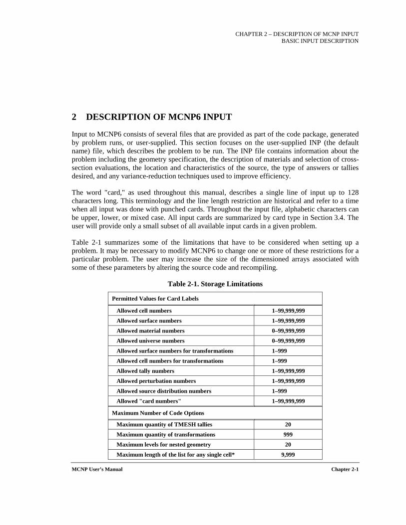
CHAPTER 2 – DESCRIPTION OF MCNP INPUT
BASIC INPUT DESCRIPTION
MCNP User’s Manual Chapter 2-1
2 DESCRIPTION OF MCNP6 INPUT
Input to MCNP6 consists of several files that are provided as part of the code package, generated by problem runs, or user-supplied. This section focuses on the user-supplied INP (the default name) file, which describes the problem to be run. The INP file contains information about the problem including the geometry specification, the description of materials and selection of cross-section evaluations, the location and characteristics of the source, the type of answers or tallies desired, and any variance-reduction techniques used to improve efficiency.
The word "card," as used throughout this manual, describes a single line of input up to 128 characters long. This terminology and the line length restriction are historical and refer to a time when all input was done with punched cards. Throughout the input file, alphabetic characters can be upper, lower, or mixed case. All input cards are summarized by card type in Section 3.4. The user will provide only a small subset of all available input cards in a given problem.
Table 2-1 summarizes some of the limitations that have to be considered when setting up a problem. It may be necessary to modify MCNP6 to change one or more of these restrictions for a particular problem. The user may increase the size of the dimensioned arrays associated with some of these parameters by altering the source code and recompiling.
Table 2-1. Storage Limitations
Permitted Values for Card Labels
Allowed cell numbers 1–99,999,999
Allowed surface numbers 1–99,999,999
Allowed material numbers 0–99,999,999
Allowed universe numbers 0–99,999,999
Allowed surface numbers for transformations 1–999
Allowed cell numbers for transformations 1–999
Allowed tally numbers 1–99,999,999
Allowed perturbation numbers 1–99,999,999
Allowed source distribution numbers 1–999
Allowed "card numbers" 1–99,999,999
Maximum Number of Code Options
Maximum quantity of TMESH tallies 20
Maximum quantity of transformations 999
Maximum levels for nested geometry 20
Maximum length of the list for any single cell* 9,999

CHAPTER 2 – DESCRIPTION OF MCNP INPUT BASIC INPUT DESCRIPTION
Chapter 2-2 MCNP User’s Manual
Maximum length of file names 256 characters
Maximum file name path length, including file name
256 characters
Maximum quantity of different tallies 9,999
Maximum quantity of detector tallies 1,000
Quantity of DXTRAN spheres per particle type 10
Quantity of URAN universes unlimited
Entries on IDUM and RDUM cards 2,000
* MCNP6 allocates a generous amount of array space to store the surfaces bounding the cells. Occasionally, the use of macrobodies, surface unions, and complement operators can cause a cell specification to overflow the array. If not enough storage is allocated, MCNP6 will output a fatal error message instructing the user how to increase the array to the proper size.
Total storage requirements can be significantly reduced by turning off model physics for neutron problems (see PHYS:N card, Section 3.3.3.2.1)
All features of MCNP6 should be used with caution and knowledge. This is especially true of detectors and variance-reduction schemes. Read and understand the relevant sections of the manual before using them.
The units of measurement used throughout MCNP6 are the following: • length in centimeters, • energy in MeV, • time in shakes (10-8 sec), • temperature in MeV (kT), • atomic density in atoms/barn-cm, • mass density in g/cm3, • cross sections in barns (10-24 cm2), • heating numbers in MeV/collision, and • atomic weight ratio based on a neutron mass of 1.008664967 amu. In these units,
Avogadro’s number is 0.59703109 × 1024 per amu.
The INP file can have two forms, initiate-run and continue-run. Either form can contain an optional message block that replaces or supplements the MCNP6 execution-line information.
2.1 INITIATE-RUN
This form is used to set up a Monte Carlo problem (describe geometry, materials, tallies, etc.) and to run it using information from either the message block or the execution line. The initiate-run file has the following form:
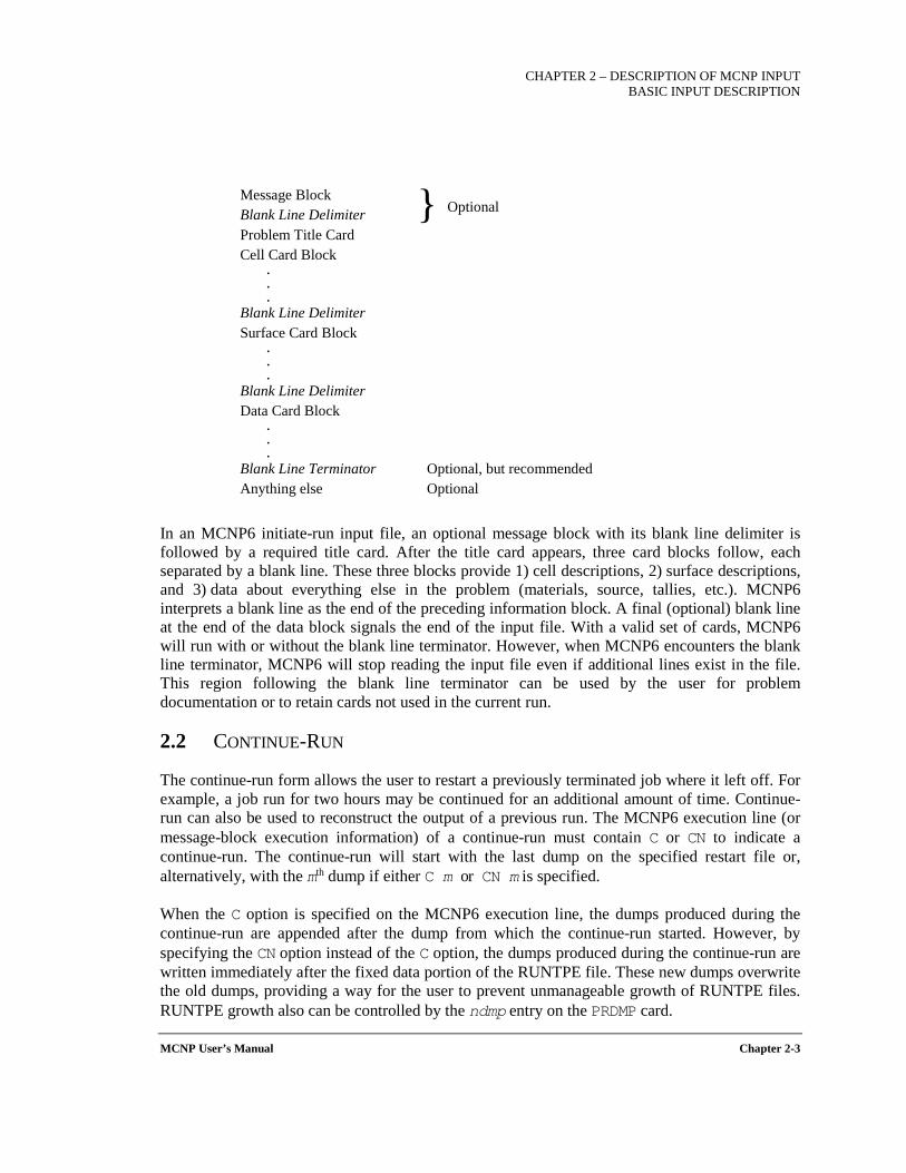
CHAPTER 2 – DESCRIPTION OF MCNP INPUT
BASIC INPUT DESCRIPTION
MCNP User’s Manual Chapter 2-3
Optional
Message Block Blank Line Delimiter Problem Title Card Cell Card Block
.
.
. Blank Line Delimiter Surface Card Block
.
.
. Blank Line Delimiter Data Card Block
.
.
. Blank Line Terminator Optional, but recommended Anything else Optional
In an MCNP6 initiate-run input file, an optional message block with its blank line delimiter is followed by a required title card. After the title card appears, three card blocks follow, each separated by a blank line. These three blocks provide 1) cell descriptions, 2) surface descriptions, and 3) data about everything else in the problem (materials, source, tallies, etc.). MCNP6 interprets a blank line as the end of the preceding information block. A final (optional) blank line at the end of the data block signals the end of the input file. With a valid set of cards, MCNP6 will run with or without the blank line terminator. However, when MCNP6 encounters the blank line terminator, MCNP6 will stop reading the input file even if additional lines exist in the file. This region following the blank line terminator can be used by the user for problem documentation or to retain cards not used in the current run.
2.2 CONTINUE-RUN
The continue-run form allows the user to restart a previously terminated job where it left off. For example, a job run for two hours may be continued for an additional amount of time. Continue-run can also be used to reconstruct the output of a previous run. The MCNP6 execution line (or message-block execution information) of a continue-run must contain C or CN to indicate a continue-run. The continue-run will start with the last dump on the specified restart file or, alternatively, with the mth dump if either C m or CN m is specified.
When the C option is specified on the MCNP6 execution line, the dumps produced during the continue-run are appended after the dump from which the continue-run started. However, by specifying the CN option instead of the C option, the dumps produced during the continue-run are written immediately after the fixed data portion of the RUNTPE file. These new dumps overwrite the old dumps, providing a way for the user to prevent unmanageable growth of RUNTPE files. RUNTPE growth also can be controlled by the ndmp entry on the PRDMP card.
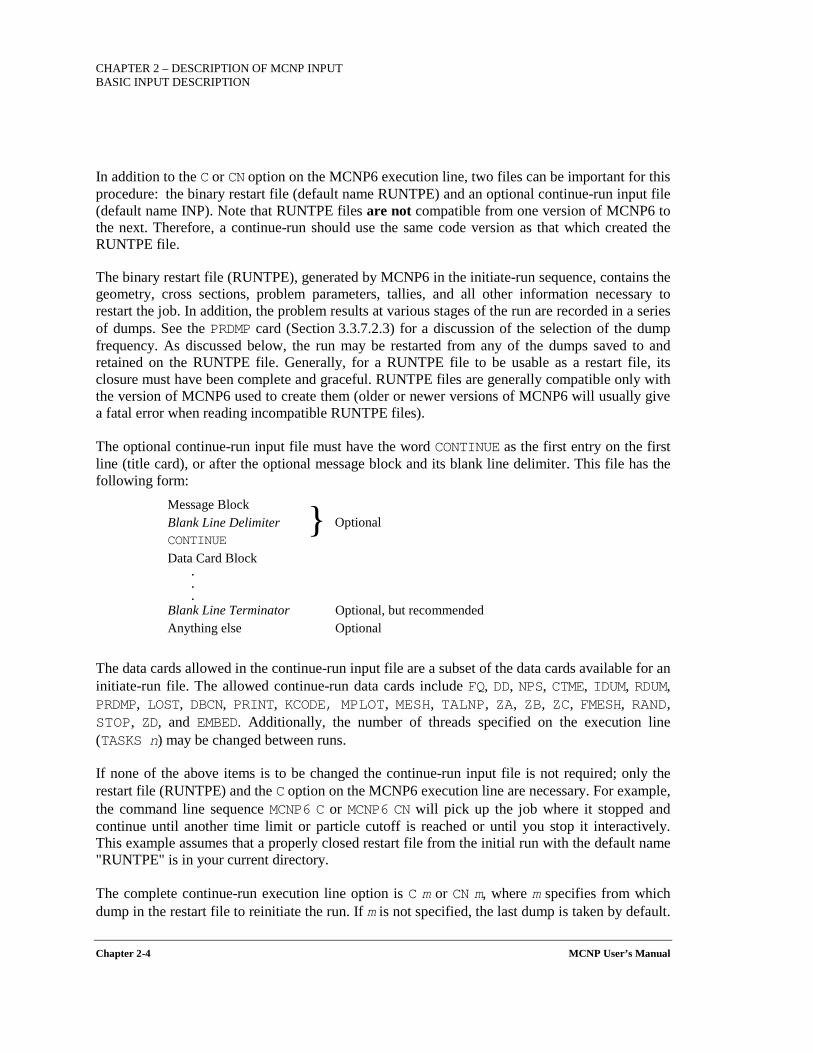
CHAPTER 2 – DESCRIPTION OF MCNP INPUT BASIC INPUT DESCRIPTION
Chapter 2-4 MCNP User’s Manual
Optional
In addition to the C or CN option on the MCNP6 execution line, two files can be important for this procedure: the binary restart file (default name RUNTPE) and an optional continue-run input file (default name INP). Note that RUNTPE files are not compatible from one version of MCNP6 to the next. Therefore, a continue-run should use the same code version as that which created the RUNTPE file.
The binary restart file (RUNTPE), generated by MCNP6 in the initiate-run sequence, contains the geometry, cross sections, problem parameters, tallies, and all other information necessary to restart the job. In addition, the problem results at various stages of the run are recorded in a series of dumps. See the PRDMP card (Section 3.3.7.2.3) for a discussion of the selection of the dump frequency. As discussed below, the run may be restarted from any of the dumps saved to and retained on the RUNTPE file. Generally, for a RUNTPE file to be usable as a restart file, its closure must have been complete and graceful. RUNTPE files are generally compatible only with the version of MCNP6 used to create them (older or newer versions of MCNP6 will usually give a fatal error when reading incompatible RUNTPE files).
The optional continue-run input file must have the word CONTINUE as the first entry on the first line (title card), or after the optional message block and its blank line delimiter. This file has the following form:
Message Block Blank Line Delimiter CONTINUE Data Card Block
.
.
. Blank Line Terminator Optional, but recommended Anything else Optional
The data cards allowed in the continue-run input file are a subset of the data cards available for an initiate-run file. The allowed continue-run data cards include FQ, DD, NPS, CTME, IDUM, RDUM, PRDMP, LOST, DBCN, PRINT, KCODE, MPLOT, MESH, TALNP, ZA, ZB, ZC, FMESH, RAND, STOP, ZD, and EMBED. Additionally, the number of threads specified on the execution line (TASKS n) may be changed between runs.
If none of the above items is to be changed the continue-run input file is not required; only the restart file (RUNTPE) and the C option on the MCNP6 execution line are necessary. For example, the command line sequence MCNP6 C or MCNP6 CN will pick up the job where it stopped and continue until another time limit or particle cutoff is reached or until you stop it interactively. This example assumes that a properly closed restart file from the initial run with the default name "RUNTPE" is in your current directory.
The complete continue-run execution line option is C m or CN m, where m specifies from which dump in the restart file to reinitiate the run. If m is not specified, the last dump is taken by default.
CHAPTER 2 – DESCRIPTION OF MCNP INPUT
BASIC INPUT DESCRIPTION
MCNP User’s Manual Chapter 2-5
If the initial run producing the restart file was stopped because of particle cutoff (NPS card, Section 3.3.7.1.1), the value of npp on the NPS card must be increased for a continue-run via a continue-run file. The parameter npp represents the cumulative histories to be run, including preceding continue-runs and the initial run. On the other hand, the tme parameter on the CTME card in a continue-run is the number of minutes more to run, not cumulative total time. To run more KCODE cycles, only the fourth entry on the KCODE card, kct, must be changed. Like npp, kct refers to total cycles to be run, including previous ones.
In a continue-run, a negative number entered for npp on the NPS card produces a print output file at the time of the requested dump. No more histories will be run. This can be useful when the printed output has been lost or you want to alter the content of the output with the PRINT or FQ cards.
Continue-runs do not produce identical results to initial-runs for delayed particle calculations (see the ACT card, Section 3.3.3.3).
Be cautious if you use a FILES card in the initial run. See Section 3.3.7.3.6.
2.3 CARD FORMAT
Most input is entered in horizontal format; however, a vertical input format is allowed for data cards. Comment cards (Section 2.6) can be inserted throughout the input file. Additionally, a comment can be added to any input card: a $ (dollar sign) terminates data entry on a card and anything that follows the $ is interpreted as a comment. (One exception is that you cannot use a $ within a TMESH tally block. See Section 3.3.5.24.) Blank lines are used as delimiters between input blocks and as a terminator after the data block to indicate the end of the input file. Individual data entries are separated by one or more blanks.
If the first five columns of a card are blank, the entries on the card are interpreted as a continuation of the data from the last named card. The user also can continue data on the following card by ending the line with an & (ampersand) preceded by at least one blank space. In this case, the data on the continuation card can reside in columns 1–128. Remember that completely blank cards are reserved as delimiters between major sections of the input file.
2.4 MESSAGE BLOCK
In computer environments where there are no execution line messages, the optional message block is the only means for providing MCNP6 with execution information. Optionally, it is a convenient way to avoid retyping an often-repeated message. Both initiate-run and continue-run input files can contain a message block that replaces or supplements the MCNP6 execution line information. If used, the message block is located before the problem title card in the INP file. The message block starts with the string, MESSAGE: and is limited to columns 1–128. The message block ends with a blank line delimiter before the title card. All cards before the blank
CHAPTER 2 – DESCRIPTION OF MCNP INPUT BASIC INPUT DESCRIPTION
Chapter 2-6 MCNP User’s Manual
line delimiter are continuation cards. The $ symbol (which indicates an end-of-line comment follows) and the & symbol (which indicates that the information continues on the next line) are permitted in message blocks and act as end-of-line markers. The syntax and components of the message are the same as for the regular execution line message. Any file name substitution, program module execution option, or keyword entry on the execution line takes precedence over conflicting information in the message block. Renaming of the input file default file name, INP=filename, is not a legitimate entry in the message block. The name INP can be changed on the execution line only.
For example, assume the MCNP6 execution line required to run the input file, sphere.i, and to assign user-designated names to the output files is
mcnp6 i=sphere.i o=sphere.o r=sphere.r mctal=sphere.m .
The following simplified execution line mcnp6 i=sphere.i
can provide the same file name assignments through the message block feature: message: o=sphere.o r= sphere.r mctal= sphere.m
Title: bare uranium sphere .
The three lines above show the message block and the input-file title card separated by a blank line delimiter.
2.5 PROBLEM TITLE CARD
The first card in the file after the optional message block is the required problem title card. If there is no message block, this must be the first card in the INP file. It is limited to one 128-column line and is used as a title in various places in the MCNP6 output. It can contain any information the user desires (or can even be blank) and often contains information describing the particular problem. Note that a blank card elsewhere is used as a delimiter or as a terminator.
2.6 COMMENT CARDS
General comment cards can be used anywhere in the INP file after the problem title card and before the last blank terminator card. (The TMESH tally format is an exception. See Section 3.3.5.24.) These cards must have a C anywhere in columns 1–5 followed by at least one blank. Comments can be up to a total of128 columns long. General comment cards are printed only with the input file listing and not anywhere else in the MCNP6 output file.
Additionally, specific comment cards are provided for tallies (the FCn card, Section 3.3.5.2) and for sources (the SCn card, Section 3.3.4.6). User-provided text on these cards are printed in the output as a tally title and as a heading for a source probability distribution, n, respectively.
CHAPTER 2 – DESCRIPTION OF MCNP INPUT
BASIC INPUT DESCRIPTION
MCNP User’s Manual Chapter 2-7
2.7 AUXILIARY INPUT FILE CAPABILITY
Subsections of the input file may be inserted using the READ card (Section 3.1). The text of these insertions will be expanded in the output file unless disabled by the READ NOECHO keyword.
2.8 CELL, SURFACE, AND DATA CARDS
Detailed specifications for the cell, surface, and data cards are provided in Chapter 3. A general description of these card types is provided in this section to orient the user.
The first entry on any cell card is the user-assigned cell number, which must begin in the first five columns of the card. The second entry is a cell material number that corresponds to a material card number (m on the Mm card) in the data card input block. If the cell is void, a zero is entered for the material number. For a cell with a non-zero material number, the material density follows the material number. The next entries include a list of signed surfaces that provide a complete specification of the geometry of the cell. Optionally, after the geometry description, cell parameters can be entered.
Similarly, the first entry on any surface card is the user-assigned surface number, which must begin in the first five columns of the card. The second entry is typically an alphabetic mnemonic indicating the surface type. Following the surface mnemonic are the numerical coefficients of the equation of the surface in the proper order.
The remaining data input for MCNP6 follows the second blank card delimiter (or third blank card if there is a message block). Although a horizontal input format for data cards is most commonly used, a vertical format option permitted by MCNP6 is particularly useful for some cell parameters and source distributions. Both formats are described in the sections that follow.
2.8.1 Data Card Horizontal Input Format Like cell and surface cards, data cards all must begin within the first five columns. The card name or number and particle designator are followed by data entries separated by one or more blanks. An individual entry cannot be split between two lines. There can be only one card of any given type for a given particle designation. (See Section 2.9.) Integers must be entered where integer input is required. Other numerical data can be entered as integer or floating point and will be read properly by MCNP6. (In fact, non-integer numerical data can be entered in any form acceptable to a Fortran E-edit descriptor.)
MCNP6 allows five shortcuts to facilitate data input:
1. nR means repeat the immediately preceding entry on the card n times. For example, 2 4R is the same as 2 2 2 2 2.
2. nI means insert n linear interpolates between the entries immediately preceding and following this feature. For example, 1.5 2I 3.0 on a card is the same as

CHAPTER 2 – DESCRIPTION OF MCNP INPUT BASIC INPUT DESCRIPTION
Chapter 2-8 MCNP User’s Manual
1.5 2.0 2.5 3.0. In the construct X nI Y, if X and Y are integers, and if Y-X is an exact multiple of n+1, then correct integer interpolates will be created. Otherwise, only real interpolates will be created, but Y will be stored directly in all cases. In the above example, the 2.0 value may not be exact, but in the example 1 4I 6, all interpolates are exact and the entry is equivalent to 1 2 3 4 5 6.
3. xM means multiply the previous entry on the card by the value x. For example, 1 1 2M 2M 2M 2M 4M 2M 2M is equivalent to 1 1 2 4 8 16 64 128 256.
4. nJ means jump over the entry and take the default value. As an example, the following two cards are identical in their effect:
DD 0.1 1000 DD J 1000
J J J is also equivalent to 3J. Also using this shortcut, you can jump to a particular entry on a card without having to specify explicitly previous items on the card. This feature is convenient if you know you want to use a default value but cannot remember it. Another example of this capability is DBCN 2J 10 15.
5. nLOG or, equivalently, nILOG means insert n (base-10) logarithmic interpolates between the entries immediately preceding and following this feature. For example, 0.01 2ILOG 10 is equivalent to 0.01 0.1 1 10. In the construct X nILOG Y, X and Y must be non-zero and have the same sign—otherwise a fatal error is produced.
These features apply to both integer and floating-point quantities. If n (an integer) is omitted in the constructs nR, nI, nLOG, nILOG, and nJ, then n is assumed to be 1. If x (integer or floating point) is omitted in xM, it is a fatal error. The rules for dealing with adjacent special input items are as follows:
1. nR must be preceded by a number or by an item created by R or M.
2. nI, nLOG, and nILOG must be preceded by a number or by an item created by R or M, and must be followed by a number. The preceding number cannot be 0.0 for nLOG or nILOG.
3. xM must be preceded by a number or by an item created by R or M.
4. nJ may be preceded by anything except I and may begin the card input list.
Several examples follow: 1 3M 2R is equivalent to 1 3 3 3 1 3M I 4 is equivalent to 1 3 3.5 4 1 3M 3M is equivalent to 1 3 9 1 2R 2I 2.5 is equivalent to 1 1 1 1.5 2.0 2.5 1 R 2M is equivalent to 1 1 2 1 R R is equivalent to 1 1 1
CHAPTER 2 – DESCRIPTION OF MCNP INPUT
BASIC INPUT DESCRIPTION
MCNP User’s Manual Chapter 2-9
1 2I 4 3M is equivalent to 1 2 3 4 12 1 2I 4 2I 10 is equivalent to 1 2 3 4 6 8 10 3J 4R is illegal 1 4I 3M is illegal 1 4I J is illegal
2.8.2 Data Card Vertical Input Format Column input is particularly useful for cell parameters and source distributions. Cell importance or volumes strung out on horizontal input lines are not very readable and often lead to errors when users add or delete cells. In vertical format, all the cell parameters for one cell can be on a single line, labeled with the name of the cell. If a cell is deleted, the user deletes just one line of cell parameters instead of hunting for the data item that belongs to the cell in each of several multi-line cell-parameter cards. For source distributions, corresponding SI, SP, and SB values are side by side. Source options, other than defaults, are on the next line and must all be entered explicitly. The & continuation symbol is not needed and is ignored if it is present.
In column format, card names are put side by side on one input line and the data values are listed in columns under the card names. To indicate that vertical input format is being used, a # is put somewhere in columns 1–5 on the line with the card names. The card names must be all cell parameters, all surface parameters, or all something else. If a card name appears on a # card, there must not be a regular horizontal card by that name in the same input file. If there are more entries on data value lines than card names on the # line, the first data entry is assumed to be a cell or surface number. If any cell names are entered, all must be entered. If cell names are entered, the cells do not have to be in the same order as they are in the cell cards block. If cell names are omitted, the default order is the order of the cells in the cell card block. The same rules apply to surface parameters, but because we presently have only one surface parameter (AREA), column input of surface parameters is less useful.
There can be more than one block of column data in an input file. Typically, there would be one block for cell parameters and one for each source distribution. If a lot of cell parameter options are being used, additional blocks of column data would be needed.
We strongly suggest keeping columns reasonably neat for user readability. The column format is intended for input data that naturally fit into columns of equal length, but less tidy data are not prohibited. If a longer column is to the right of a shorter column, the shorter column must be filled with enough J entries to eliminate any ambiguity about which columns the data items are in.
Special syntax items (R, M, I, LOG, ILOG, and J) are not as appropriate in column format as they are on horizontal lines, but they are not prohibited. They are, of course, interpreted vertically instead of horizontally. Multiple special syntax items, such as 9R, are not allowed if cell or surface names are present.

CHAPTER 2 – DESCRIPTION OF MCNP INPUT BASIC INPUT DESCRIPTION
Chapter 2-10 MCNP User’s Manual
The form of a column input block is # S1 S2 ... Sm k1 d11 d12 ... d1m k2 d21 d22 ... d2m . . . ... . . . . ... . . . . ... . kN dN1 dN2 ... dNm
1. The # is somewhere in columns 1–5.
2. Each line can be only 128 columns wide.
3. Each column, Si through dli, where l may be less than N, represents a regular input card.
4. The Si must be valid MCNP6 card names. They must be all cell parameters, all surface parameters, or all something else.
5. d1i through dNi must be valid entries for an Si card, except that dl+1,i through dNi may be some Js possibly followed by some blanks.
6. If dji is non-blank, dj,i-1 must also be non-blank. A J may be used if necessary to make dj,i-1 non-blank.
7. The Si must not appear anywhere else in the input file.
8. The kj are optional integers. If any are non-blank, all must be non-blank.
9. If the Si are cell parameter card names, the kj, if present, must be valid cell names. The same is true with surface parameters.
10. If the kj is present, the dji must not be multiple special syntax items, such as 9R or 9M.
2.9 PARTICLE DESIGNATORS
Numerous input cards require a particle designator to distinguish between input data for tracked particles. Refer to the pertinent card information for instructions. The particle designator consists of a colon (:) followed by the particle symbol(s) immediately after the name of the card. These particle designations are presented in Table 2-2. At least one blank must follow the particle designator. For example, IMP:N signifies neutron importance values follow while IMP:P signifies photon importance values follow. To specify the same value for more than one kind of particle, a single card can be used instead of several. For example, if the designation IMP:E,P,N 1 1 0 appears on a cell card, the electron importance for that cell is 1, the photon importance is 1, and the neutron importance is 0. With a tally card, the particle designator follows the card name including tally number. For example, *F5:N indicates a neutron point-detector energy tally. In the heating tally case, two particle designators may appear. The syntax F6:N,P indicates the combined heating tally for both neutrons and photons.
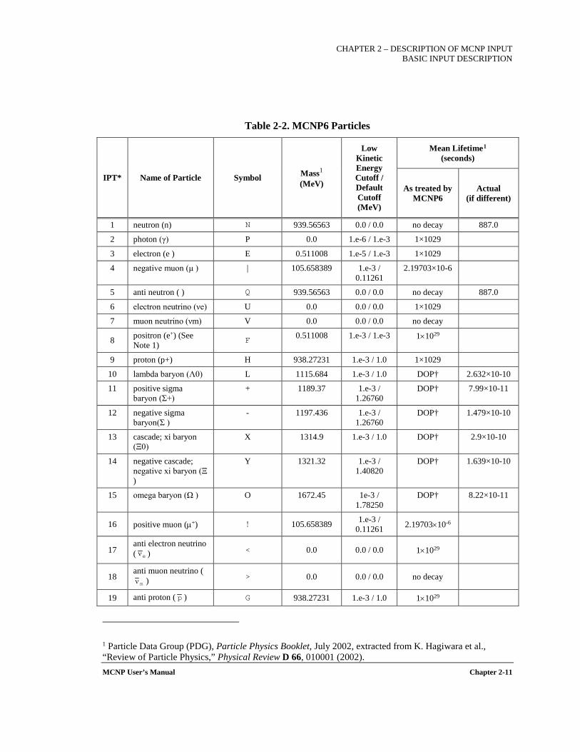
CHAPTER 2 – DESCRIPTION OF MCNP INPUT
BASIC INPUT DESCRIPTION
MCNP User’s Manual Chapter 2-11
Table 2-2. MCNP6 Particles
IPT* Name of Particle Symbol Mass1 (MeV)
Low Kinetic Energy Cutoff / Default Cutoff (MeV)
Mean Lifetime1 (seconds)
As treated by MCNP6
Actual (if different)
1 neutron (n) N 939.56563 0.0 / 0.0 no decay 887.0
2 photon (γ) P 0.0 1.e-6 / 1.e-3 1×1029
3 electron (e ) E 0.511008 1.e-5 / 1.e-3 1×1029
4 negative muon (μ ) | 105.658389 1.e-3 / 0.11261
2.19703×10⁻⁶
5 anti neutron ( ) Q 939.56563 0.0 / 0.0 no decay 887.0
6 electron neutrino (νe) U 0.0 0.0 / 0.0 1×1029
7 muon neutrino (νm) V 0.0 0.0 / 0.0 no decay
8 positron (e+) (See Note 1) F 0.511008 1.e-3 / 1.e-3 1×1029
9 proton (p+) H 938.27231 1.e-3 / 1.0 1×1029
10 lambda baryon (Λ0) L 1115.684 1.e-3 / 1.0 DOP† 2.632×10⁻¹⁰
11 positive sigma baryon (Σ+)
+ 1189.37 1.e-3 / 1.26760
DOP† 7.99×10⁻¹¹
12 negative sigma baryon(Σ )
- 1197.436 1.e-3 / 1.26760
DOP† 1.479×10⁻¹⁰
13 cascade; xi baryon (Ξ0)
X 1314.9 1.e-3 / 1.0 DOP† 2.9×10⁻¹⁰
14 negative cascade; negative xi baryon (Ξ )
Y 1321.32 1.e-3 / 1.40820
DOP† 1.639×10⁻¹⁰
15 omega baryon (Ω ) O 1672.45 1e-3 / 1.78250
DOP† 8.22×10⁻¹¹
16 positive muon (µ+) ! 105.658389 1.e-3 / 0.11261 2.19703×10⁻⁶
17 anti electron neutrino ( ) < 0.0 0.0 / 0.0 1×1029
18 anti muon neutrino (
) > 0.0 0.0 / 0.0 no decay
19 anti proton ( ) G 938.27231 1.e-3 / 1.0 1×1029
1 Particle Data Group (PDG), Particle Physics Booklet, July 2002, extracted from K. Hagiwara et al., “Review of Particle Physics,” Physical Review D 66, 010001 (2002).
eν
mν
p
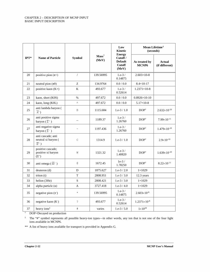
CHAPTER 2 – DESCRIPTION OF MCNP INPUT BASIC INPUT DESCRIPTION
Chapter 2-12 MCNP User’s Manual
IPT* Name of Particle Symbol Mass1 (MeV)
Low Kinetic Energy Cutoff / Default Cutoff (MeV)
Mean Lifetime1 (seconds)
As treated by MCNP6
Actual (if different)
20 positive pion (π+) / 139.56995 1.e-3 / 0.14875
2.603×10⁻⁸
21 neutral pion (π0) Z 134.9764 0.0 / 0.0 8.4×10⁻¹⁷
22 positive kaon (K+) K 493.677 1.e-3 / 0.52614
1.2371×10⁻⁸
23 kaon, short (K0S) % 497.672 0.0 / 0.0 0.8926×10⁻¹⁰
24 kaon, long (K0L) ^ 497.672 0.0 / 0.0 5.17×10⁻⁸
25 anti lambda baryon (
) B 1115.684 1.e-3 / 1.0 DOP† 2.632×10⁻¹⁰
26 anti positive sigma baryon ( )
_ 1189.37 1.e-3 / 1.26760 DOP† 7.99×10⁻¹¹
27 anti negative sigma baryon ( )
~ 1197.436 1.e-3 / 1.26760 DOP† 1.479×10⁻¹⁰
28 anti cascade; anti neutral xi baryon (
) C 1314.9 1.e-3 / 1.0 DOP† 2.9×10⁻¹⁰
29 positive cascade; positive xi baryon (Ξ+)
W 1321.32 1.e-3 / 1.40820 DOP† 1.639×10⁻¹⁰
30 anti omega ( ) @ 1672.45 1e-3 / 1.78250 DOP† 8.22×10⁻¹¹
31 deuteron (d) D 1875.627 1.e-3 / 2.0 1×1029
32 triton (t) T 2808.951 1.e-3 / 3.0 12.3 years
33 helion (3He) S 2808.421 1.e-3 / 3.0 1×1029
34 alpha particle (α) A 3727.418 1.e-3 / 4.0 1×1029
35 negative pion (π-) * 139.56995 1.e-3 / 0.14875 2.603×10⁻⁸
36 negative kaon (K-) ? 493.677 1.e-3 / 0.52614 1.2371×10⁻⁸
37 heavy ions‡ # varies 1.e-3 / 5.0 1×1029 † DOP=Decayed on production ‡ The “#” symbol represents all possible heavy-ion types—in other words, any ion that is not one of the four light
ions available in MCNP6. ** A list of heavy ions available for transport is provided in Appendix G.
0Λ
+Σ
−Σ
0Ξ
−Ω

CHAPTER 2 – DESCRIPTION OF MCNP INPUT
BASIC INPUT DESCRIPTION
MCNP User’s Manual Chapter 2-13
Note 1: Positrons are treated identical to electrons in transport (outside magnetic field effects), and need to be used with the electron transport option (particle e) enabled. Please refer to the MODE section (3.3.3.1) to see the exceptions for positron labels.
2.10 DEFAULT VALUES
Many MCNP6 input parameters have default values that are summarized in Section 3.4. Therefore, you do not always have to specify explicitly every input parameter every time if the defaults match your needs. If an input card is left out, the default values for all parameters on the card are used. However, if you want to change a particular default parameter on a card where others precede that parameter, you have to specify the others or use the nJ jump feature to jump over the parameters for which you still want the defaults. For example, the input CUT:P 3J -0.10 is a convenient way to use the defaults for the first three parameters on the photon cutoff card but change the fourth.
2.11 INPUT ERROR MESSAGES
MCNP6 makes over 800 checks of the input file for user errors. If the user violates a basic constraint of the input specification, a fatal error message is printed, both at the terminal and in the OUTP file. If a fatal input error is detected, MCNP6 will terminate before running any particles. The first fatal error is real; subsequent error messages may or may not be real because of the nature of the first fatal message. The FATAL option on the MCNP6 execution line instructs MCNP6 to ignore fatal errors and run particles, but the user should be extremely cautious when doing this.
Most MCNP6 error messages are either warnings or comments that are not fatal. Warnings are intended to inform the user about unconventional input parameters or running conditions and may need further attention. Comments relay useful additional information to the user. The user should not ignore these messages but should understand their significance before making important calculations.
In addition to fatal, warning, and comment messages, MCNP6 issues BAD TROUBLE messages immediately before any impending catastrophe, such as a divide by zero, which would otherwise cause the program to "crash." MCNP6 terminates as soon as the BAD TROUBLE message is issued. User input errors in the INP file are the most common reason for issuing a BAD TROUBLE message. These error messages indicate what corrective action is required.
2.12 GEOMETRY ERRORS
There is one important kind of input error that MCNP6 will not detect while processing data from the INP file. MCNP6 cannot detect overlapping cells or gaps between cells until a particle track actually gets lost. Even then the precise nature of the error may remain unclear. However, there is much that you can and should do to check your geometry before starting a long computer run.

CHAPTER 2 – DESCRIPTION OF MCNP INPUT BASIC INPUT DESCRIPTION
Chapter 2-14 MCNP User’s Manual
Use the geometry-plotting feature of MCNP6 to look at the system from several directions and at various scales. Be sure that what you see is what you intend. Any gaps or overlaps in the geometry will probably show up as dashed lines. The intersection of a surface with the plot plane is drawn as a dashed line if there is not exactly one cell on each side of the surface at each point. Dashed lines can also appear if the plot plane happens to coincide with a plane of the problem, there are any cookie-cutter cells in the source, or there are DXTRAN spheres in the problem.
One way to check your geometry is to set up and run a short problem in which your system is flooded with particle tracks from an external source. The changes required in the INP file to perform this test follow:
1. Add a VOID card to override some of the other specifications in the problem and make all the cells voids, turn heating tallies into flux tallies, and turn off any tally multiplication (FM) cards.
2. Add another cell and a large spherical surface to the problem such that the surface surrounds the system and the old outside world cell is split by the new surface into two cells: the space between the system and the new surface, which is the new cell, and the space outside the new surface, which is now the outside world cell. Be sure that the new cell has non-zero importance. Actually, it is best to make all non-zero importance equal. If the system is infinite in one or two dimensions, use one or more planes instead of a sphere.
3. Replace the source specifications by an inward directed surface source to flood the geometry with particles. To do this, you can use the command
SDEF SUR=m NRM=-1 ,
where m is the number of the new spherical surface added in Step 2. If the new surface is a plane, you must specify the portion to be used by means of POS and RAD or possibly X, Y, and Z source distributions.
Because there are no collisions, a short run will generate a great many tracks through your system. If there are any geometry errors, they should cause some of the particles to get lost.
When a particle first gets lost, whether in a special run with the VOID card or in a regular production run, the history is rerun to produce some special output on the OUTP file. Event-log printing is turned on during the rerun. The event log will show all surface crossings and will tell you the path the particle took to the bad spot in the geometry. When the particle again gets lost, a description of the situation at that point is printed. You can usually deduce the cause of the lost particle from this output. It is not possible to rerun lost particles in a multitasking run.
If the cause of the lost particle is still obscure, try plotting the geometry with the origin of the plot at the point where the particle got lost and with the horizontal axis of the plot plane along the direction the particle was moving. You might also consider turning COLOR OFF using the interactive geometry plotter. A wire drawing then appears, reducing the complexity of the visual representation caused by the color. The cause of the trouble is likely to appear as a dashed line

CHAPTER 2 – DESCRIPTION OF MCNP INPUT
BASIC INPUT DESCRIPTION
MCNP User’s Manual Chapter 2-15
somewhere in the plot or as some discrepancy between the plot and your idea of what it should look like.


CHAPTER 3 – INPUT CARDS
AUXILIARY INPUT FILE
MCNP User’s Manual Chapter 3-1
3 INPUT CARDS
MCNP6 input cards other than those that define cells (Section 3.2.1) and surfaces (Section 3.2.2) typically are entered after the blank card delimiter following the cell-card and surface-card blocks. The mnemonic that specifies the type of data card must begin within the first five columns of the input file.
No data card can be used more than once with the same number or particle type designations. For example, M1 and M2 are acceptable, as are CUT:N and CUT:P, but two M1 cards or two CUT:N cards are disallowed.
Note that when values are assigned to keywords, the equals sign (=) is optional.
3.1 AUXILIARY INPUT FILE AND ENCRYPTION (READ)
The MCNP6 READ card enables (1) the reading of parts of the input file from other (auxiliary) files, (2) the suppression of the printing of the auxiliary input files to shorten output files and protect proprietary information, and (3) the encryption of auxiliary input files to protect proprietary information. Unlike most MCNP6 input cards, there may be as many READ cards and auxiliary input files as desired. The READ card may appear anywhere after the title card of an MCNP6 input file but not in the middle of a card continuation. READ cards may appear in auxiliary files, allowing the nesting of READ cards to multiple levels. The encryption capability may be applied to any or all of the READ levels. There is no limit to the number of nested levels.
The encryption capability can be used to protect proprietary designs of tools and other systems modeled with MCNP6. The encryption capability is localized in subroutine ENCRYPT. The MCNP6 scheme is very simple; therefore, it protects nothing. To protect input, the subroutine should be modified to a more sophisticated scheme known only to those producing the data and only executable MCNP6 versions should be provided to users of the encrypted files.
Form: READ KEYWORD=value(s) ...
Table 3-1. Auxiliary Input and Encryption (READ)
Keyword Value
FILE=filename Causes input from the file filename to be inserted after the READ card in the MCNP6 input deck.
NOECHO Suppresses printing in the output file of the input cards that follow the READ card.
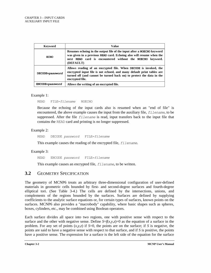
CHAPTER 3 – INPUT CARDS AUXILIARY INPUT FILE
Chapter 3-2 MCNP User’s Manual
Keyword Value
ECHO
Resumes echoing in the output file of the input after a NOECHO keyword was given in a previous READ card. Echoing also will resume when the next READ card is encountered without the NOECHO keyword. (DEFAULT)
DECODE=password
Allows reading of an encrypted file. When DECODE is invoked, the encrypted input file is not echoed, and many default print tables are turned off (and cannot be turned back on) to protect the data in the encrypted file.
ENCODE=password Allows the writing of an encrypted file.
Example 1: READ FILE=filename NOECHO
Because the echoing of the input cards also is resumed when an "end of file" is encountered, the above example causes the input from the auxiliary file, filename, to be suppressed. After the file filename is read, input transfers back to the input file that contains the READ card and printing is no longer suppressed.
Example 2: READ DECODE password FILE=filename
This example causes the reading of the encrypted file, filename.
Example 3: READ ENCODE password FILE=filename
This example causes an encrypted file, filename, to be written.
3.2 GEOMETRY SPECIFICATION
The geometry of MCNP6 treats an arbitrary three-dimensional configuration of user-defined materials in geometric cells bounded by first- and second-degree surfaces and fourth-degree elliptical tori. (See Table 3-4.) The cells are defined by the intersections, unions, and complements of the regions bounded by the surfaces. Surfaces are defined by supplying coefficients to the analytic surface equations or, for certain types of surfaces, known points on the surfaces. MCNP6 also provides a "macrobody" capability, where basic shapes such as spheres, boxes, cylinders, etc., may be combined using Boolean operators.
Each surface divides all space into two regions, one with positive sense with respect to the surface and the other with negative sense. Define S=f(x,y,z)=0 as the equation of a surface in the problem. For any set of points (x,y,z) if S=0, the points are on the surface; if S is negative, the points are said to have a negative sense with respect to that surface, and if S is positive, the points have a positive sense. The expression for a surface is the left side of the equation for the surface
CHAPTER 3 – INPUT CARDS
GEOMETRY SPECIFICATION
MCNP User’s Manual Chapter 3-3
in Table 3-4. For the sphere, cylinder, cone, and torus, this definition is identical to defining the sense to be positive outside the figure. With planes normal to axes (PX, PY, or PZ), the definition gives positive sense for points with x, y, or z values exceeding the intercept of the plane. For the P, SQ and GQ surfaces, the user supplies all of the coefficients for the expression and thus can determine the sense of the surface at will. This is different from the other cases where the sense, though arbitrary, is uniquely determined by the form of the expression. Therefore, in a surface transformation (see the TRn card in Section 3.3.1.3) a PX, PY, or PZ surface will sometimes be replaced by a P surface just to prevent the sense of the surface from getting reversed.
The geometry of each cell is described on a cell card by a list of operators and signed surfaces that bound the cell. (If the sense is positive, the + sign can be omitted.) This geometry description defines the cell to be the intersection, union, and/or complement of the listed regions. The intersection operator in MCNP6 is implicit; it is simply the blank space between two signed surface numbers on the cell card. The union operator, signified by a colon (:), allows concave corners in cells and also cells that are completely disjoint. Because the intersection and union operators are binary Boolean operators, their use follows Boolean algebra methodology; unions and intersections can be used in combination in any cell description. Spaces on either side of the union operator are irrelevant, but a space without the colon signifies an intersection.
The complement operator, signified by the # symbol1, provides no new capability over the intersection and union operators. It is just a shorthand cell-specifying method that implicitly uses the intersection and union operators. The complement operator can be thought of as standing for not in. The notation #n, where n is a previously defined cell number, means that the description of the current cell is the complement of the description of cell n. In other words, a number immediately after a complement operator, without parentheses, is interpreted as a cell number and is shorthand for the geometry specification of that cell number. The notation #(...), where (...) is usually a list of surfaces describing another cell, means to complement the portion of the cell description in parentheses.
The default order of operations is complement first, intersection second, and unions third. There is no right-to-left ordering. Parentheses can be used to clarify operations and in some cases are required to force a certain order of operations. Innermost parentheses are cleared first. Spaces are optional on either side of a parenthesis. A parenthesis is equivalent to a space and signifies an intersection. Parentheses and operator symbols also function as delimiters; where they are present, blank delimiters are not necessary.
1 The symbol "#" is also used to denote heavy ions. The meaning of the symbol in the input file should be obvious from context.
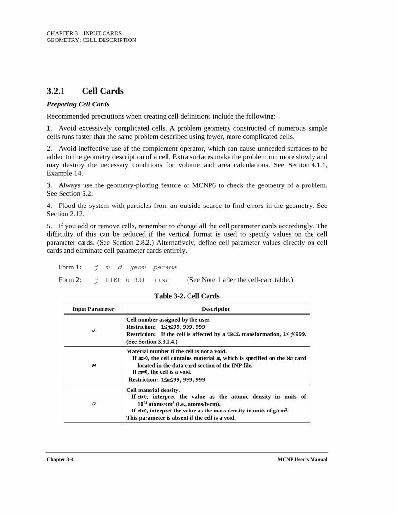
CHAPTER 3 – INPUT CARDS GEOMETRY: CELL DESCRIPTION
Chapter 3-4 MCNP User’s Manual
3.2.1 Cell Cards Preparing Cell Cards
Recommended precautions when creating cell definitions include the following:
1. Avoid excessively complicated cells. A problem geometry constructed of numerous simple cells runs faster than the same problem described using fewer, more complicated cells.
2. Avoid ineffective use of the complement operator, which can cause unneeded surfaces to be added to the geometry description of a cell. Extra surfaces make the problem run more slowly and may destroy the necessary conditions for volume and area calculations. See Section 4.1.1, Example 14.
3. Always use the geometry-plotting feature of MCNP6 to check the geometry of a problem. See Section 5.2.
4. Flood the system with particles from an outside source to find errors in the geometry. See Section 2.12.
5. If you add or remove cells, remember to change all the cell parameter cards accordingly. The difficulty of this can be reduced if the vertical format is used to specify values on the cell parameter cards. (See Section 2.8.2.) Alternatively, define cell parameter values directly on cell cards and eliminate cell parameter cards entirely.
Form 1: j m d geom params
Form 2: j LIKE n BUT list (See Note 1 after the cell-card table.)
Table 3-2. Cell Cards
Input Parameter Description
J
Cell number assigned by the user. Restriction: 1≤j≤99,999,999 Restriction: If the cell is affected by a TRCL transformation, 1≤j≤999. (See Section 3.3.1.4.)
M
Material number if the cell is not a void. If m>0, the cell contains material m, which is specified on the Mm card
located in the data card section of the INP file. If m=0, the cell is a void.
Restriction: 1≤m≤99,999,999
D
Cell material density. If d>0, interpret the value as the atomic density in units of
1024 atoms/cm3 (i.e., atoms/b-cm). If d<0, interpret the value as the mass density in units of g/cm3.
This parameter is absent if the cell is a void.
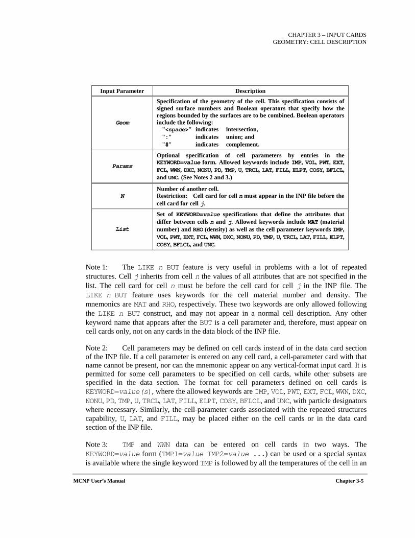
CHAPTER 3 – INPUT CARDS
GEOMETRY: CELL DESCRIPTION
MCNP User’s Manual Chapter 3-5
Input Parameter Description
Geom
Specification of the geometry of the cell. This specification consists of signed surface numbers and Boolean operators that specify how the regions bounded by the surfaces are to be combined. Boolean operators include the following:
"<space>" indicates intersection, ":" indicates union; and "#" indicates complement.
Params
Optional specification of cell parameters by entries in the KEYWORD=value form. Allowed keywords include IMP, VOL, PWT, EXT, FCL, WWN, DXC, NONU, PD, TMP, U, TRCL, LAT, FILL, ELPT, COSY, BFLCL, and UNC. (See Notes 2 and 3.)
N Number of another cell. Restriction: Cell card for cell n must appear in the INP file before the cell card for cell j.
List
Set of KEYWORD=value specifications that define the attributes that differ between cells n and j. Allowed keywords include MAT (material number) and RHO (density) as well as the cell parameter keywords IMP, VOL, PWT, EXT, FCL, WWN, DXC, NONU, PD, TMP, U, TRCL, LAT, FILL, ELPT, COSY, BFLCL, and UNC.
Note 1: The LIKE n BUT feature is very useful in problems with a lot of repeated structures. Cell j inherits from cell n the values of all attributes that are not specified in the list. The cell card for cell n must be before the cell card for cell j in the INP file. The LIKE n BUT feature uses keywords for the cell material number and density. The mnemonics are MAT and RHO, respectively. These two keywords are only allowed following the LIKE n BUT construct, and may not appear in a normal cell description. Any other keyword name that appears after the BUT is a cell parameter and, therefore, must appear on cell cards only, not on any cards in the data block of the INP file.
Note 2: Cell parameters may be defined on cell cards instead of in the data card section of the INP file. If a cell parameter is entered on any cell card, a cell-parameter card with that name cannot be present, nor can the mnemonic appear on any vertical-format input card. It is permitted for some cell parameters to be specified on cell cards, while other subsets are specified in the data section. The format for cell parameters defined on cell cards is KEYWORD=value(s), where the allowed keywords are IMP, VOL, PWT, EXT, FCL, WWN, DXC, NONU, PD, TMP, U, TRCL, LAT, FILL, ELPT, COSY, BFLCL, and UNC, with particle designators where necessary. Similarly, the cell-parameter cards associated with the repeated structures capability, U, LAT, and FILL, may be placed either on the cell cards or in the data card section of the INP file.
Note 3: TMP and WWN data can be entered on cell cards in two ways. The KEYWORD=value form (TMP1=value TMP2=value ...) can be used or a special syntax is available where the single keyword TMP is followed by all the temperatures of the cell in an
CHAPTER 3 – INPUT CARDS GEOMETRY: CELL DESCRIPTION
Chapter 3-6 MCNP User’s Manual
order corresponding to the times on the THTME card. The form for the WWN card is analogous: WWN1:n=value or WWN:n followed by all the lower weight bounds for the energy intervals of the cell.
Example 1: 3 0 -1 2 -4 $ definition of cell 3 5 0 #3 $ equivalent to each of the next 2 lines or 5 0 #(-1 2 -4) or 5 0 (+1 : -2 : +4)
Cell 3 is defined as the region in space with negative sense with respect to surface 1, positive sense with respect to surface 2, and negative sense with respect to surface 4. Cell 5 is the region of space not including cell 3. In the second and third lines of the example, it is specified using the complement operator; in the fourth line, the same region is specified using the union operator.
Example 2: 2 3 -3.7 -1 IMP:N=2 IMP:P=4 3 LIKE 2 BUT IMP:N=10 TRCL=1
This second example says that cell 3 is the same as cell 2 in every respect except that cell 3 has a different location (TRCL=1) and a different neutron importance. The material in cell 3, the density, and the definition are the same as cell 2 and the photon importance is the same.
Example 3: 10 16 -4.2 1 -2 3 IMP:N=4 IMP:P=8 EXT:N=-0.4X
This says that cell 10 is to be filled with material 16 at a density of 4.2 g/cm3. The cell consists of the intersections of the regions on the positive side of surface 1, the negative side of surface 2, and the positive side of surface 3. The neutron importance in cell 10 is 4 and the photon importance is 8. Neutrons in cell 10 are subject to an exponential transform in the minus X direction with stretching parameter 0.4.
3.2.2 Surface Cards Surfaces can be defined by equations (Section 3.2.2.1), points (Sections 3.2.2.2 and 3.2.2.3), or macrobodies (Section 3.2.2.4). Each of these methods is discussed in the sections that follow.
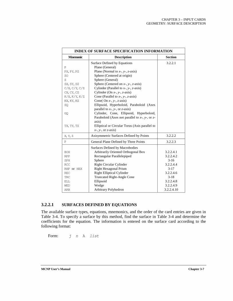
CHAPTER 3 – INPUT CARDS
GEOMETRY: SURFACE DESCRIPTION
MCNP User’s Manual Chapter 3-7
INDEX OF SURFACE SPECIFICATION INFORMATION Mnemonic Description Section
P PX, PY, PZ SO S SX, SY, SZ C/X, C/Y, C/Z CX, CY, CZ K/X, K/Y, K/Z KX, KY, KZ SQ GQ TX, TY, TZ
Surface Defined by Equations Plane (General) Plane (Normal to x-, y-, z-axis) Sphere (Centered at origin) Sphere (General) Sphere (Centered on x-, y-, z-axis) Cylinder (Parallel to x-, y-, z-axis) Cylinder (On x-, y-, z-axis) Cone (Parallel to x-, y-, z-axis) Cone( On x-, y-, z-axis) Ellipsoid, Hyperboloid, Paraboloid (Axes parallel to x-, y-, or z-axis) Cylinder, Cone, Ellipsoid, Hyperboloid, Paraboloid (Axes not parallel to x-, y-, or z-axis) Elliptical or Circular Torus (Axis parallel to x-, y-, or z-axis)
3.2.2.1
X, Y, Z Axisymmetric Surfaces Defined by Points 3.2.2.2
P General Plane Defined by Three Points 3.2.2.3
BOX RPP SPH RCC RHP or HEX REC TRC ELL WED ARB
Surfaces Defined by Macrobodies Arbitrarily Oriented Orthogonal Box Rectangular Parallelepiped Sphere Right Circular Cylinder Right Hexagonal Prism Right Elliptical Cylinder Truncated Right-Angle Cone Ellipsoid Wedge Arbitrary Polyhedron
3.2.2.4.1 3.2.2.4.2
3-16 3.2.2.4.4
3-17 3.2.2.4.6
3-18 3.2.2.4.8 3.2.2.4.9 3.2.2.4.10
3.2.2.1 SURFACES DEFINED BY EQUATIONS
The available surface types, equations, mnemonics, and the order of the card entries are given in Table 3-4. To specify a surface by this method, find the surface in Table 3-4 and determine the coefficients for the equation. The information is entered on the surface card according to the following format:
Form: j n A list
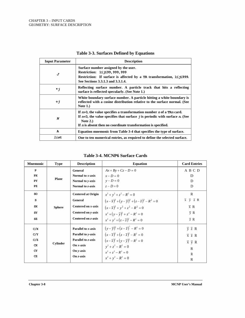
CHAPTER 3 – INPUT CARDS GEOMETRY: SURFACE DESCRIPTION
Chapter 3-8 MCNP User’s Manual
Table 3-3. Surfaces Defined by Equations
Input Parameter Description
J
Surface number assigned by the user. Restriction: 1≤j≤99,999,999 Restriction: If surface is affected by a TR transformation, 1≤j≤999. See Sections 3.3.1.3 and 3.3.1.4.
*j Reflecting surface number. A particle track that hits a reflecting surface is reflected specularly. (See Note 1.)
+j White boundary surface number. A particle hitting a white boundary is reflected with a cosine distribution relative to the surface normal. (See Note 1.)
N
If n>0, the value specifies a transformation number n of a TRn card. If n<0, the value specifies that surface j is periodic with surface n. (See
Note 2.) If n is absent then no coordinate transformation is specified.
A Equation mnemonic from Table 3-4 that specifies the type of surface. list One to ten numerical entries, as required to define the selected surface.
Table 3-4. MCNP6 Surface Cards
Mnemonic Type Description Equation Card Entries
P
PX
PY
PZ
Plane
General Normal to x-axis Normal to y-axis Normal to z-axis
SO
S
SX
SY
SZ
Sphere
Centered at Origin
General
Centered on x-axis
Centered on y-axis
Centered on z-axis
C/X
C/Y
C/Z
CX
CY
CZ
Cylinder
Parallel to x-axis
Parallel to y-axis
Parallel to z-axis
On x-axis
On y-axis
On z-axis
0=−++ DCzByAx0=− Dx0=− Dy0=− Dz
D C BA DDD
02222 =−++ Rzyx
( ) ( ) ( ) 02222 =−−+−+− Rzzyyxx
( ) 02222 =−++− Rzyxx
( ) 02222 =−+−+ Rzyyx
( ) 02222 =−−++ Rzzyx
RR z y x
R xR y
R z
( ) ( ) 022 2
=−−+− Rzzyy
( ) ( ) 0222 =−−+− Rzzxx
( ) ( ) 0222 =−−+− Ryyxx0222 =−+ Rzy0222 =−+ Rzx0222 =−+ Ryx
R z y
R z x
R y x
RRR
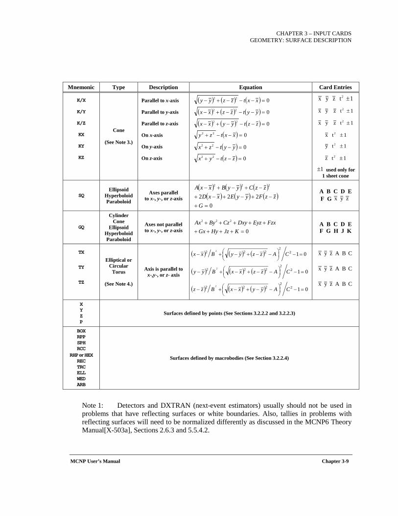
CHAPTER 3 – INPUT CARDS
GEOMETRY: SURFACE DESCRIPTION
MCNP User’s Manual Chapter 3-9
Mnemonic Type Description Equation Card Entries
K/X
K/Y
K/Z
KX
KY
KZ
Cone
(See Note 3.)
Parallel to x-axis
Parallel to y-axis
Parallel to z-axis
On x-axis
On y-axis
On z-axis
used only for 1 sheet cone
SQ Ellipsoid
Hyperboloid Paraboloid
Axes parallel to x-, y-, or z-axis
A B C D E F G
GQ
Cylinder Cone
Ellipsoid Hyperboloid Paraboloid
Axes not parallel to x-, y-, or z-axis A B C D E
F G H J K
TX
TY
TZ
Elliptical or Circular
Torus
(See Note 4.)
Axis is parallel to x-,y-, or z- axis
X Y Z P
Surfaces defined by points (See Sections 3.2.2.2 and 3.2.2.3)
BOX RPP SPH RCC
RHP or HEX REC TRC ELL WED ARB
Surfaces defined by macrobodies (See Section 3.2.2.4)
Note 1: Detectors and DXTRAN (next-event estimators) usually should not be used in problems that have reflecting surfaces or white boundaries. Also, tallies in problems with reflecting surfaces will need to be normalized differently as discussed in the MCNP6 Theory Manual[X-503a], Sections 2.6.3 and 5.5.4.2.
( ) ( ) ( ) 022 =−−−+− xxtzzyy
( ) ( ) ( ) 022 =−−−+− yytzzxx
( ) ( ) ( ) 022 =−−−+− zztyyxx
( ) 022 =−−+ xxtzy
( ) 022 =−−+ yytzx
( ) 022 =−−+ zztyx
1 tz y x 2 ±
1 tz y x 2 ±
1 tz y x 2 ±
1 tx 2 ±
1 ty 2 ±
1 tz 2 ±
1±
( ) ( ) ( )( ) ( ) ( )
0222
222
=+−+−+−+
−+−+−
GzzFyyExxD
zzCyyBxxA
z y x
0
222
=+++++++++
KJzHyGxFzxEyzDxyCzByAx
( ) ( ) ( ) 0122
222 2
=−
−−+−+− CAzzyyBxx
( ) ( ) ( ) 0122
222 2
=−
−−+−+− CAzzxxByy
( ) ( ) ( ) 0122
222 2
=−
−−+−+− CAyyxxBzz
C BA z y x
C BA z y x
C BA z y x

CHAPTER 3 – INPUT CARDS GEOMETRY: SURFACE DESCRIPTION
Chapter 3-10 MCNP User’s Manual
Note 2: If periodic boundaries are specified (i.e., n<0) such that surface j is periodic with surface n, the following restrictions apply:
1. Surfaces j and n must be planes. 2. No surface transformation is allowed for the periodic planes. 3. The periodic cell(s) can be infinite or bounded by planes on the top and bottom that
can be reflecting or white, but cannot be periodic. 4. Periodic planes can bound only other periodic planes or top and bottom planes. 5. A single zero-importance cell must be on one side of each periodic plane. 6. All periodic planes must have a common rotational vector normal to the geometry top
and bottom. 7. Next-event estimators such as detectors and DXTRAN should not be used.
Note 3: The quadratic equation for a cone describes a cone of two sheets—one sheet is a cone of positive slope, and the other has a negative slope. MCNP6 provides the option to select either of the two sheets. The +1 or the -1 entry on the cone surface card causes the one sheet cone treatment to be used. If the sign of the entry is positive, the specified sheet is the one that extends to infinity in the positive direction of the coordinate axis to which the cone axis is parallel. The converse is true for a negative entry. A cell whose description contains a two-sheeted cone may require an additional surface specification to help distinguish between the two sheets. This ambiguity surface helps to eliminate any ambiguities as to which region of space is included in the cell.
Note 4: The TX, TY, and TZ input cards represent elliptical tori (fourth degree surfaces) rotationally symmetric about axes parallel to the x-, y-, and z-axes, respectively. A TY torus is illustrated in Figure 3-1a. Note that the input parameters a b c specify the ellipse
rotated about the s–axis in the (r,s) cylindrical coordinate system (Figure 3-1b) whose origin is at in the x, y, z system. In the case of a TY torus,
and
A torus is degenerate if |a |<c where 0<a<c produces the outer surface (Figure 3-1c), and -c<a<0 produces the inner surface (Figure 3-1d).
x y z
( ) 12
2
2
2
=−
+c
arbs
( )yys −=
( ) ( )22 zzxxr −+−=
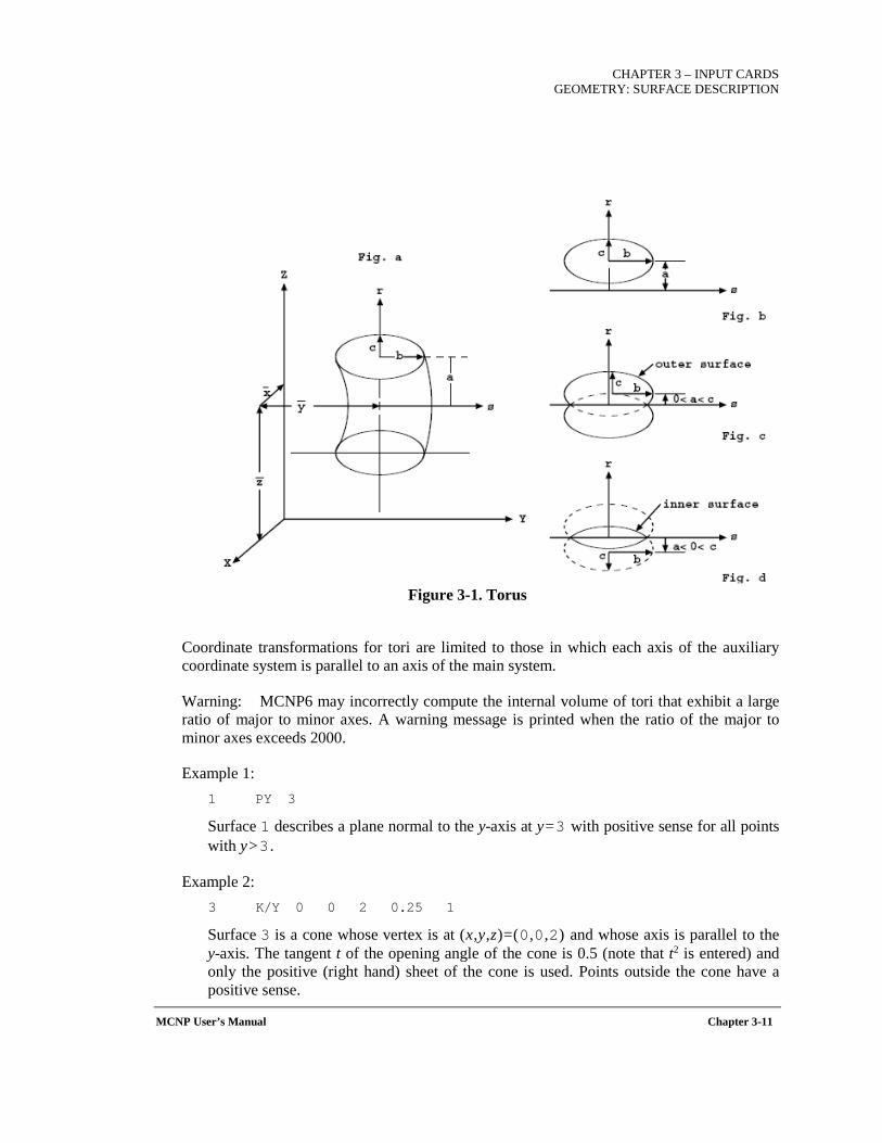
CHAPTER 3 – INPUT CARDS
GEOMETRY: SURFACE DESCRIPTION
MCNP User’s Manual Chapter 3-11
Figure 3-1. Torus
Coordinate transformations for tori are limited to those in which each axis of the auxiliary coordinate system is parallel to an axis of the main system.
Warning: MCNP6 may incorrectly compute the internal volume of tori that exhibit a large ratio of major to minor axes. A warning message is printed when the ratio of the major to minor axes exceeds 2000.
Example 1: 1 PY 3
Surface 1 describes a plane normal to the y-axis at y=3 with positive sense for all points with y>3 .
Example 2: 3 K/Y 0 0 2 0.25 1
Surface 3 is a cone whose vertex is at (x,y,z)=(0,0,2) and whose axis is parallel to the y-axis. The tangent t of the opening angle of the cone is 0.5 (note that t2 is entered) and only the positive (right hand) sheet of the cone is used. Points outside the cone have a positive sense.
CHAPTER 3 – INPUT CARDS GEOMETRY: SURFACE DESCRIPTION
Chapter 3-12 MCNP User’s Manual
Example 3: 11 GQ 1 0.25 0.75 0 –0.866 0 –12 –2 3.464 39
This is a cylinder of radius 1 cm whose axis is in a plane normal to the x-axis at x=6, displaced 2 cm from the x-axis and rotated 30 degrees about the x-axis off the y-axis toward the z-axis. The sense is positive for points outside the cylinder. Such a cylinder would be much easier to specify by first defining it in an auxiliary coordinate system where it is symmetric about a coordinate axis and then using the TRn card (see Section 3.3.1.3) to define the relationship between the basic and auxiliary coordinate systems. The input would then be 11 7 CX 1 *TR7 6 1 –1.732 0 30 60
3.2.2.2 AXISYMMETRIC SURFACES DEFINED BY POINTS
Surface cards of the type X, Y, and Z can be used to describe surfaces by coordinate points rather than by equation coefficients as in the previous section. The surfaces described by these cards must be symmetric about the x-, y-, or z-axis, respectively, and, if the surface consists of more than one sheet, the specified coordinate points must all be on the same sheet.
Each of the coordinate pairs defines a geometrical point on the surface. On the Y card, for example, the entries may be
j Y y1 r1 y2 r2
where and yi is the coordinate of point i. If one coordinate pair is used, a plane (PX, PY, or PZ) is defined. If two coordinate pairs are used, a linear surface (PX, PY, PZ, CX, CY, CZ, KX, KY, or KZ) is defined. If three coordinate pairs are used, a quadratic surface (PX, PY, PZ, SO, SX, SY, SZ, CX, CY, CZ, KX, KY, KZ, or SQ) is defined.
When a cone is specified by two points, a cone of only one sheet is generated.
The senses of these surfaces (except SQ) are determined by the code to be identical to the senses one would obtain by specifying the surface by equations. For SQ, the sense is defined so that points sufficiently far from the axis of symmetry have positive sense. Note that this is different from the equation-defined SQ, where the user could choose the sense freely.
Form: j n A list
( )22iii zxr +=
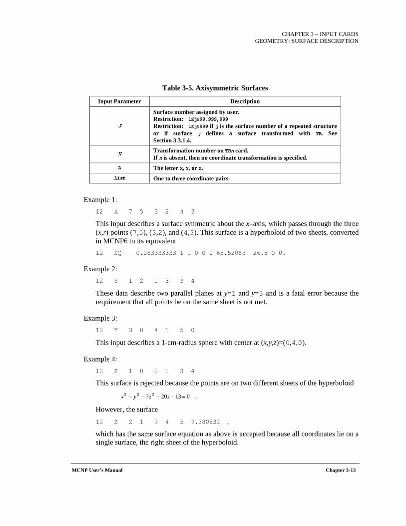
CHAPTER 3 – INPUT CARDS
GEOMETRY: SURFACE DESCRIPTION
MCNP User’s Manual Chapter 3-13
Table 3-5. Axisymmetric Surfaces
Input Parameter Description
J
Surface number assigned by user. Restriction: 1≤j≤99,999,999 Restriction: 1≤j≤999 if j is the surface number of a repeated structure or if surface j defines a surface transformed with TR. See Section 3.3.1.4.
N Transformation number on TRn card. If n is absent, then no coordinate transformation is specified.
A The letter X, Y, or Z. List One to three coordinate pairs.
Example 1: 12 X 7 5 3 2 4 3
This input describes a surface symmetric about the x–axis, which passes through the three (x,r) points (7,5), (3,2), and (4,3). This surface is a hyperboloid of two sheets, converted in MCNP6 to its equivalent 12 SQ −0.083333333 1 1 0 0 0 68.52083 −26.5 0 0.
Example 2: 12 Y 1 2 1 3 3 4
These data describe two parallel planes at y=1 and y=3 and is a fatal error because the requirement that all points be on the same sheet is not met.
Example 3: 12 Y 3 0 4 1 5 0
This input describes a 1-cm-radius sphere with center at (x,y,z)=(0,4,0).
Example 4: 12 Z 1 0 2 1 3 4
This surface is rejected because the points are on two different sheets of the hyperboloid
.
However, the surface 12 Z 2 1 3 4 5 9.380832 ,
which has the same surface equation as above is accepted because all coordinates lie on a single surface, the right sheet of the hyperboloid.
013207 222 =−+−+ zzyx
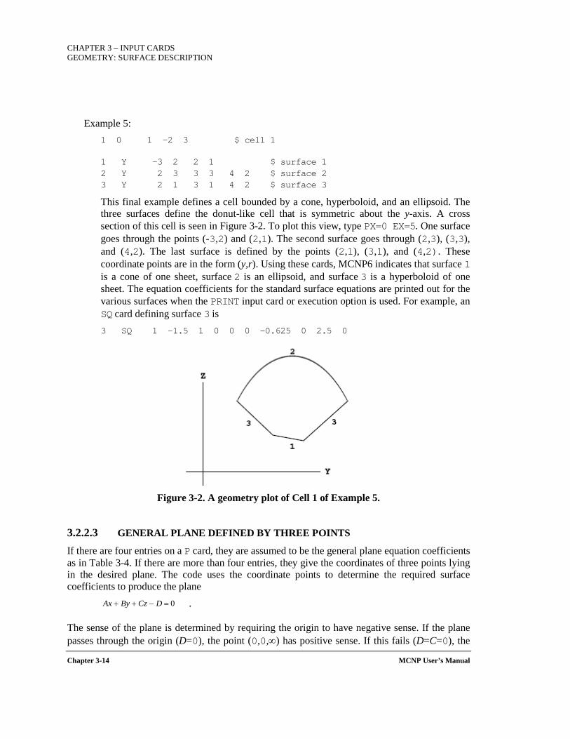
CHAPTER 3 – INPUT CARDS GEOMETRY: SURFACE DESCRIPTION
Chapter 3-14 MCNP User’s Manual
Example 5: 1 0 1 −2 3 $ cell 1
1 Y −3 2 2 1 $ surface 1 2 Y 2 3 3 3 4 2 $ surface 2 3 Y 2 1 3 1 4 2 $ surface 3
This final example defines a cell bounded by a cone, hyperboloid, and an ellipsoid. The three surfaces define the donut-like cell that is symmetric about the y-axis. A cross section of this cell is seen in Figure 3-2. To plot this view, type PX=0 EX=5. One surface goes through the points (-3,2) and (2,1). The second surface goes through (2,3), (3,3), and (4,2). The last surface is defined by the points (2,1), (3,1), and (4,2). These coordinate points are in the form (y,r). Using these cards, MCNP6 indicates that surface 1 is a cone of one sheet, surface 2 is an ellipsoid, and surface 3 is a hyperboloid of one sheet. The equation coefficients for the standard surface equations are printed out for the various surfaces when the PRINT input card or execution option is used. For example, an SQ card defining surface 3 is 3 SQ 1 -1.5 1 0 0 0 −0.625 0 2.5 0
Figure 3-2. A geometry plot of Cell 1 of Example 5.
3.2.2.3 GENERAL PLANE DEFINED BY THREE POINTS
If there are four entries on a P card, they are assumed to be the general plane equation coefficients as in Table 3-4. If there are more than four entries, they give the coordinates of three points lying in the desired plane. The code uses the coordinate points to determine the required surface coefficients to produce the plane
.
The sense of the plane is determined by requiring the origin to have negative sense. If the plane passes through the origin (D=0), the point (0,0,∞) has positive sense. If this fails (D=C=0), the
0=−++ DCzByAx
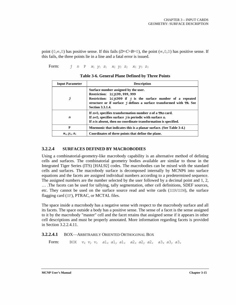
CHAPTER 3 – INPUT CARDS
GEOMETRY: SURFACE DESCRIPTION
MCNP User’s Manual Chapter 3-15
point (0,∞,0) has positive sense. If this fails (D=C=B=0), the point (∞,0,0) has positive sense. If this fails, the three points lie in a line and a fatal error is issued.
Form: j n P x1 y1 z1 x2 y2 z2 x3 y3 z3
Table 3-6. General Plane Defined by Three Points
Input Parameter Description
j
Surface number assigned by the user. Restriction: 1≤j≤99,999,999 Restriction: 1≤j≤999 if j is the surface number of a repeated structure or if surface j defines a surface transformed with TR. See Section 3.3.1.4.
n If n>0, specifies transformation number n of a TRn card. If n<0, specifies surface j is periodic with surface n. If n is absent, then no coordinate transformation is specified.
P Mnemonic that indicates this is a planar surface. (See Table 3-4.) xi,yi,zi Coordinates of three points that define the plane.
3.2.2.4 SURFACES DEFINED BY MACROBODIES
Using a combinatorial-geometry-like macrobody capability is an alternative method of defining cells and surfaces. The combinatorial geometry bodies available are similar to those in the Integrated Tiger Series (ITS) [HAL92] codes. The macrobodies can be mixed with the standard cells and surfaces. The macrobody surface is decomposed internally by MCNP6 into surface equations and the facets are assigned individual numbers according to a predetermined sequence. The assigned numbers are the number selected by the user followed by a decimal point and 1, 2, … .The facets can be used for tallying, tally segmentation, other cell definitions, SDEF sources, etc. They cannot be used on the surface source read and write cards (SSR/SSW), the surface flagging card (SF), PTRAC, or MCTAL files.
The space inside a macrobody has a negative sense with respect to the macrobody surface and all its facets. The space outside a body has a positive sense. The sense of a facet is the sense assigned to it by the macrobody "master" cell and the facet retains that assigned sense if it appears in other cell descriptions and must be properly annotated. More information regarding facets is provided in Section 3.2.2.4.11.
3.2.2.4.1 BOX—ARBITRARILY ORIENTED ORTHOGONAL BOX
Form: BOX vx vy vz a1x a1y a1z a2x a2y a2z a3x a3y a3z
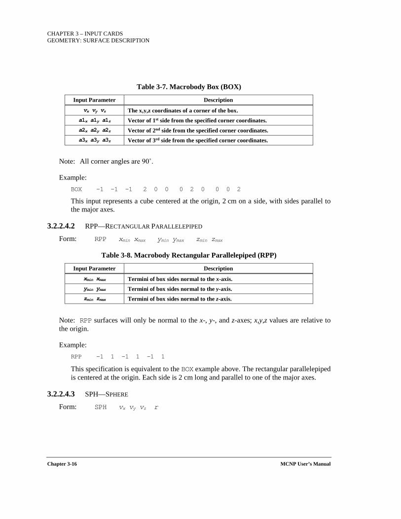
CHAPTER 3 – INPUT CARDS GEOMETRY: SURFACE DESCRIPTION
Chapter 3-16 MCNP User’s Manual
Table 3-7. Macrobody Box (BOX)
Input Parameter Description
vx vy vz The x,y,z coordinates of a corner of the box. a1x a1y a1z Vector of 1st side from the specified corner coordinates. a2x a2y a2z Vector of 2nd side from the specified corner coordinates. a3x a3y a3z Vector of 3rd side from the specified corner coordinates.
Note: All corner angles are 90˚.
Example: BOX -1 -1 -1 2 0 0 0 2 0 0 0 2
This input represents a cube centered at the origin, 2 cm on a side, with sides parallel to the major axes.
3.2.2.4.2 RPP—RECTANGULAR PARALLELEPIPED
Form: RPP xmin xmax ymin ymax zmin zmax
Table 3-8. Macrobody Rectangular Parallelepiped (RPP)
Input Parameter Description
xmin xmax Termini of box sides normal to the x-axis. ymin ymax Termini of box sides normal to the y-axis. zmin zmax Termini of box sides normal to the z-axis.
Note: RPP surfaces will only be normal to the x-, y-, and z-axes; x,y,z values are relative to the origin.
Example: RPP -1 1 -1 1 -1 1
This specification is equivalent to the BOX example above. The rectangular parallelepiped is centered at the origin. Each side is 2 cm long and parallel to one of the major axes.
3.2.2.4.3 SPH—SPHERE
Form: SPH vx vy vz r

CHAPTER 3 – INPUT CARDS
GEOMETRY: SURFACE DESCRIPTION
MCNP User’s Manual Chapter 3-17
Table 3-9. Macrobody Sphere (SPH)
Input Parameter Description vx vy vz The x,y,z coordinates of the center of the sphere.
r Radius of sphere.
3.2.2.4.4 RCC—RIGHT CIRCULAR CYLINDER
Form: RCC vx vy vz hx hy hz r
Table 3-10. Macrobody Right Circular Cylinder (RCC)
Input Parameter Description
vx vy vz The x,y,z coordinates at the center of the base for the right circular cylinder.
hx hy hz Right circular cylinder axis vector, which provides both the orientation and the height of the cylinder.
r Radius of right circular cylinder.
Example: RCC 0 -5 0 0 10 0 4
This input specification represents a 10-cm-high can about the y-axis with its base plane at y=-5 and having a radius of 4 cm.
3.2.2.4.5 RHP OR HEX—RIGHT HEXAGONAL PRISM
Form: RHP v1 v2 v3 h1 h2 h3 r1 r2 r3 s1 s2 s3 t1 t2 t3
Table 3-11. Macrobody Right Hexagonal Prism (HEX or RHP)
Input Parameter Description
v1 v2 v3 The x,y,z coordinates of the bottom of the hexagonal prism.
h1 h2 h3 Vector from the bottom to the top of the hexagonal prism. For a z-hex with height h, h1, h2, and h3= 0 0 h .
r1 r2 r3 Vector from the axis to the center of the 1st facet. For a pitch 2p facet normal to y-axis, r1, r2, and r3= 0 p 0 .
s1 s2 s3 Vector to center of the 2nd facet. t1 t2 t3 Vector to center of the 3rd facet.
Note: Differs from ITS-ACCEPT [HAL92] format.
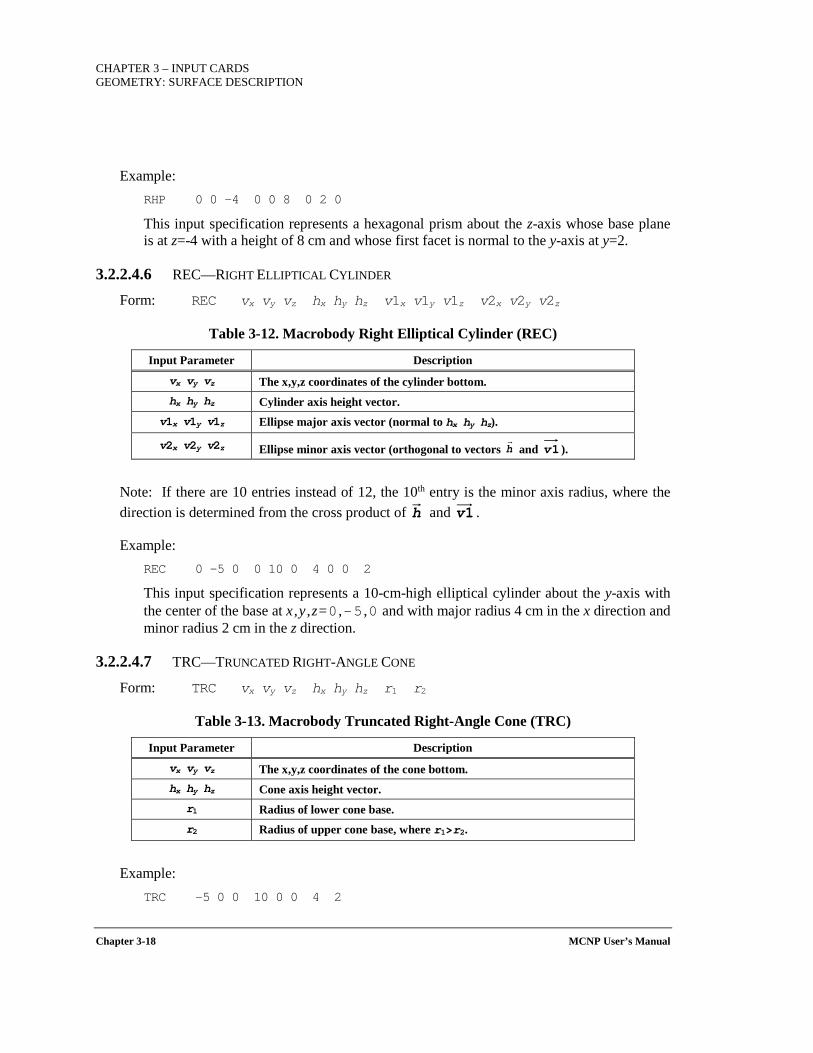
CHAPTER 3 – INPUT CARDS GEOMETRY: SURFACE DESCRIPTION
Chapter 3-18 MCNP User’s Manual
Example: RHP 0 0 -4 0 0 8 0 2 0
This input specification represents a hexagonal prism about the z-axis whose base plane is at z=-4 with a height of 8 cm and whose first facet is normal to the y-axis at y=2.
3.2.2.4.6 REC—RIGHT ELLIPTICAL CYLINDER
Form: REC vx vy vz hx hy hz v1x v1y v1z v2x v2y v2z
Table 3-12. Macrobody Right Elliptical Cylinder (REC)
Input Parameter Description
vx vy vz The x,y,z coordinates of the cylinder bottom. hx hy hz Cylinder axis height vector.
v1x v1y v1z Ellipse major axis vector (normal to hx hy hz).
v2x v2y v2z Ellipse minor axis vector (orthogonal to vectors and ).
Note: If there are 10 entries instead of 12, the 10th entry is the minor axis radius, where the direction is determined from the cross product of and .
Example: REC 0 -5 0 0 10 0 4 0 0 2
This input specification represents a 10-cm-high elliptical cylinder about the y-axis with the center of the base at x ,y ,z=0 ,-5 ,0 and with major radius 4 cm in the x direction and minor radius 2 cm in the z direction.
3.2.2.4.7 TRC—TRUNCATED RIGHT-ANGLE CONE
Form: TRC vx vy vz hx hy hz r1 r2
Table 3-13. Macrobody Truncated Right-Angle Cone (TRC)
Input Parameter Description
vx vy vz The x,y,z coordinates of the cone bottom. hx hy hz Cone axis height vector.
r1 Radius of lower cone base. r2 Radius of upper cone base, where r1>r2.
Example: TRC -5 0 0 10 0 0 4 2
h
1v
h 1v
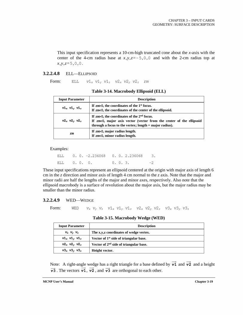
CHAPTER 3 – INPUT CARDS
GEOMETRY: SURFACE DESCRIPTION
MCNP User’s Manual Chapter 3-19
This input specification represents a 10-cm-high truncated cone about the x-axis with the center of the 4-cm radius base at x ,y ,z=-5 ,0 ,0 and with the 2-cm radius top at x ,y ,z=5 ,0 ,0 .
3.2.2.4.8 ELL—ELLIPSOID
Form: ELL v1x v1y v1z v2x v2y v2z rm
Table 3-14. Macrobody Ellipsoid (ELL)
Input Parameter Description
v1x v1y v1z If rm>0, the coordinates of the 1st focus. If rm<0, the coordinates of the center of the ellipsoid.
v2x v2y v2z If rm>0, the coordinates of the 2nd focus. If rm<0, major axis vector (vector from the center of the ellipsoid through a focus to the vertex; length = major radius).
rm If rm>0, major radius length. If rm<0, minor radius length.
Examples: ELL 0. 0. -2.236068 0. 0. 2.236068 3.
ELL 0. 0. 0. 0. 0. 3. -2
These input specifications represent an ellipsoid centered at the origin with major axis of length 6 cm in the z direction and minor axis of length 4 cm normal to the z axis. Note that the major and minor radii are half the lengths of the major and minor axes, respectively. Also note that the ellipsoid macrobody is a surface of revolution about the major axis, but the major radius may be smaller than the minor radius.
3.2.2.4.9 WED—WEDGE
Form: WED vx vy vz v1x v1y v1z v2x v2y v2z v3x v3y v3z
Table 3-15. Macrobody Wedge (WED)
Input Parameter Description
vx vy vz The x,y,z coordinates of wedge vertex. v1x v1y v1z Vector of 1st side of triangular base. v2x v2y v2z Vector of 2nd side of triangular base. v3x v3y v3z Height vector.
Note: A right-angle wedge has a right triangle for a base defined by and and a height . The vectors , , and are orthogonal to each other.
1v 2v3v 1v 2v 3v
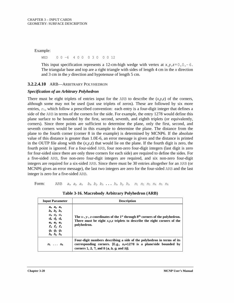
CHAPTER 3 – INPUT CARDS GEOMETRY: SURFACE DESCRIPTION
Chapter 3-20 MCNP User’s Manual
Example: WED 0 0 -6 4 0 0 0 3 0 0 0 12
This input specification represents a 12-cm-high wedge with vertex at x ,y ,z=0 ,0 ,-6 . The triangular base and top are a right triangle with sides of length 4 cm in the x direction and 3 cm in the y direction and hypotenuse of length 5 cm.
3.2.2.4.10 ARB—ARBITRARY POLYHEDRON
Specification of an Arbitrary Polyhedron
There must be eight triplets of entries input for the ARB to describe the (x,y,z) of the corners, although some may not be used (just use triplets of zeros). These are followed by six more entries, ni, which follow a prescribed convention: each entry is a four-digit integer that defines a side of the ARB in terms of the corners for the side. For example, the entry 1278 would define this plane surface to be bounded by the first, second, seventh, and eighth triplets (or equivalently, corners). Since three points are sufficient to determine the plane, only the first, second, and seventh corners would be used in this example to determine the plane. The distance from the plane to the fourth corner (corner 8 in the example) is determined by MCNP6. If the absolute value of this distance is greater than 1.0E-6, an error message is given and the distance is printed in the OUTP file along with the (x,y,z) that would lie on the plane. If the fourth digit is zero, the fourth point is ignored. For a four-sided ARB, four non-zero four-digit integers (last digit is zero for four-sided since there are only three corners for each side) are required to define the sides. For a five-sided ARB, five non-zero four-digit integers are required, and six non-zero four-digit integers are required for a six-sided ARB. Since there must be 30 entries altogether for an ARB (or MCNP6 gives an error message), the last two integers are zero for the four-sided ARB and the last integer is zero for a five-sided ARB.
Form: ARB ax ay az bx by bz ... hx hy hz n1 n2 n3 n4 n5 n6
Table 3-16. Macrobody Arbitrary Polyhedron (ARB)
Input Parameter Description
ax ay az bx by bz cx cy cz dx dy dz ex ey ez fx fy fz gx gy gz hx hy hz
The x-, y-, z-coordinates of the 1st through 8th corners of the polyhedron. There must be eight x,y,z triplets to describe the eight corners of the polyhedron.
n1 ... n6 Four-digit numbers describing a side of the polyhedron in terms of its corresponding corners. [E.g., n1=1278 is a plane/side bounded by corners 1, 2, 7, and 8 (a, b, g, and h)].
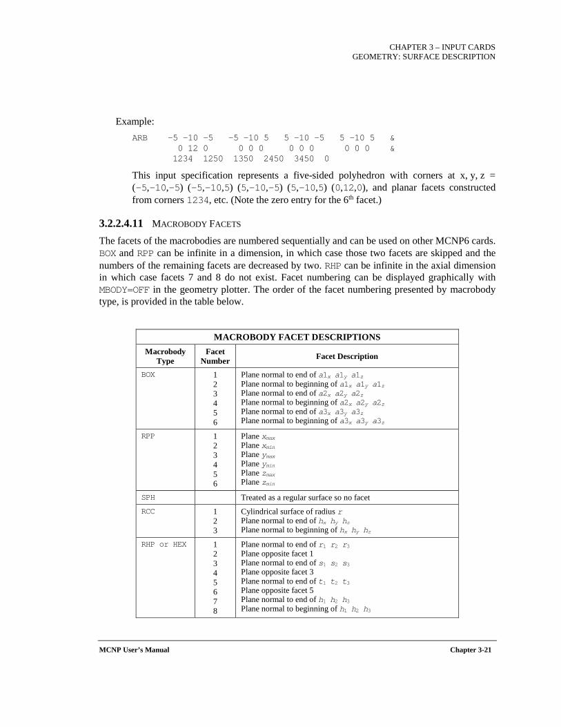
CHAPTER 3 – INPUT CARDS
GEOMETRY: SURFACE DESCRIPTION
MCNP User’s Manual Chapter 3-21
Example: ARB -5 -10 -5 -5 -10 5 5 -10 -5 5 -10 5 & 0 12 0 0 0 0 0 0 0 0 0 0 & 1234 1250 1350 2450 3450 0
This input specification represents a five-sided polyhedron with corners at x, y, z = (-5,-10,-5) (-5,-10,5) (5,-10,-5) (5,-10,5) (0,12,0), and planar facets constructed from corners 1234, etc. (Note the zero entry for the 6th facet.)
3.2.2.4.11 MACROBODY FACETS
The facets of the macrobodies are numbered sequentially and can be used on other MCNP6 cards. BOX and RPP can be infinite in a dimension, in which case those two facets are skipped and the numbers of the remaining facets are decreased by two. RHP can be infinite in the axial dimension in which case facets 7 and 8 do not exist. Facet numbering can be displayed graphically with MBODY=OFF in the geometry plotter. The order of the facet numbering presented by macrobody type, is provided in the table below.
MACROBODY FACET DESCRIPTIONS Macrobody
Type Facet
Number Facet Description
BOX 1 2 3 4 5 6
Plane normal to end of a1x a1y a1z Plane normal to beginning of a1x a1y a1z Plane normal to end of a2x a2y a2z Plane normal to beginning of a2x a2y a2z Plane normal to end of a3x a3y a3z Plane normal to beginning of a3x a3y a3z
RPP 1 2 3 4 5 6
Plane xmax Plane xmin Plane ymax Plane ymin Plane zmax Plane zmin
SPH Treated as a regular surface so no facet RCC 1
2 3
Cylindrical surface of radius r Plane normal to end of hx hy hz Plane normal to beginning of hx hy hz
RHP or HEX 1 2 3 4 5 6 7 8
Plane normal to end of r1 r2 r3 Plane opposite facet 1 Plane normal to end of s1 s2 s3 Plane opposite facet 3 Plane normal to end of t1 t2 t3 Plane opposite facet 5 Plane normal to end of h1 h2 h3 Plane normal to beginning of h1 h2 h3
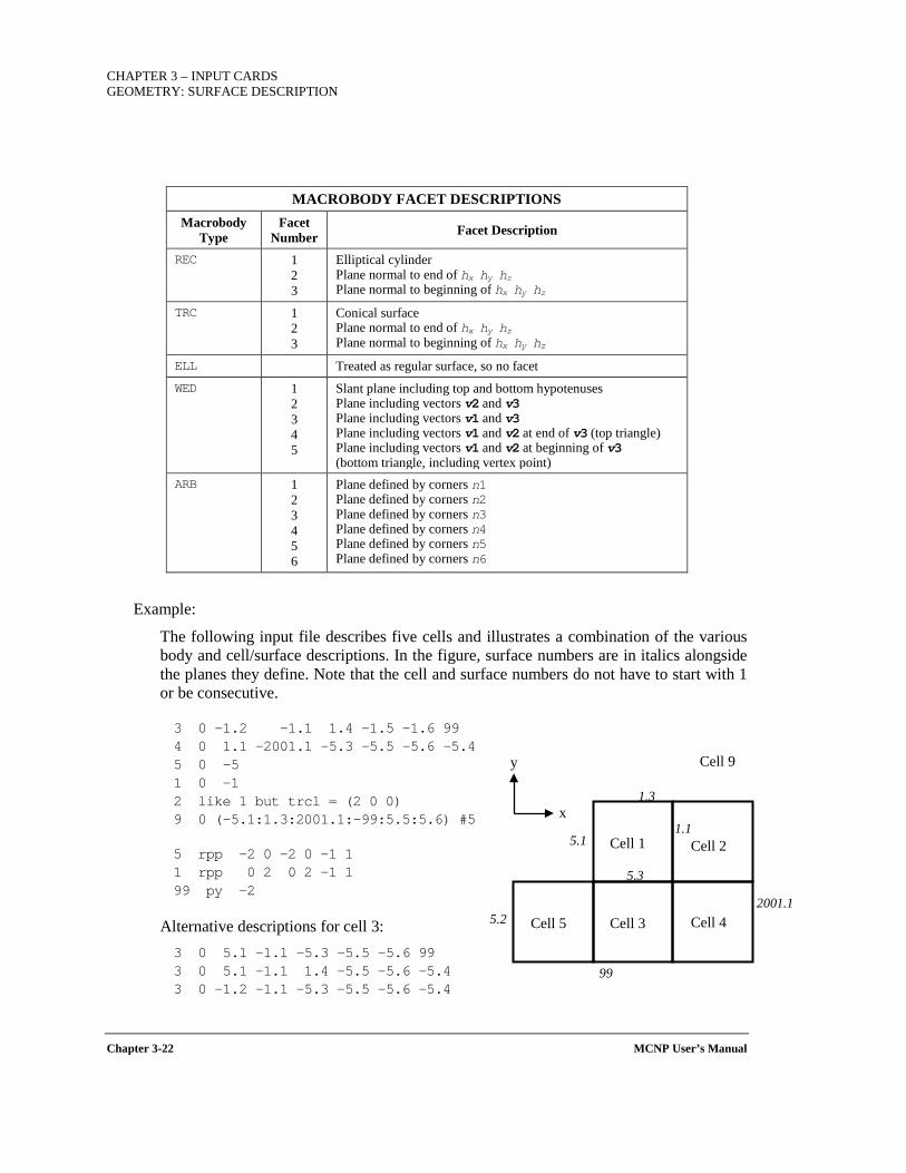
CHAPTER 3 – INPUT CARDS GEOMETRY: SURFACE DESCRIPTION
Chapter 3-22 MCNP User’s Manual
Cell 9
Cell 1 Cell 2
Cell 3 Cell 4 Cell 5
x
y
5.1
5.2
5.3
99
1.3
1.1
2001.1
MACROBODY FACET DESCRIPTIONS Macrobody
Type Facet
Number Facet Description
REC 1 2 3
Elliptical cylinder Plane normal to end of hx hy hz Plane normal to beginning of hx hy hz
TRC 1 2 3
Conical surface Plane normal to end of hx hy hz Plane normal to beginning of hx hy hz
ELL Treated as regular surface, so no facet WED 1
2 3 4 5
Slant plane including top and bottom hypotenuses Plane including vectors v2 and v3 Plane including vectors v1 and v3 Plane including vectors v1 and v2 at end of v3 (top triangle) Plane including vectors v1 and v2 at beginning of v3 (bottom triangle, including vertex point)
ARB 1 2 3 4 5 6
Plane defined by corners n1 Plane defined by corners n2 Plane defined by corners n3 Plane defined by corners n4 Plane defined by corners n5 Plane defined by corners n6
Example:
The following input file describes five cells and illustrates a combination of the various body and cell/surface descriptions. In the figure, surface numbers are in italics alongside the planes they define. Note that the cell and surface numbers do not have to start with 1 or be consecutive.
3 0 –1.2 –1.1 1.4 –1.5 –1.6 99 4 0 1.1 –2001.1 –5.3 –5.5 –5.6 –5.4 5 0 –5 1 0 –1 2 like 1 but trcl = (2 0 0) 9 0 (–5.1:1.3:2001.1:–99:5.5:5.6) #5
5 rpp –2 0 –2 0 –1 1 1 rpp 0 2 0 2 –1 1 99 py –2
Alternative descriptions for cell 3: 3 0 5.1 –1.1 –5.3 –5.5 –5.6 99 3 0 5.1 –1.1 1.4 –5.5 –5.6 –5.4 3 0 –1.2 –1.1 –5.3 –5.5 –5.6 –5.4
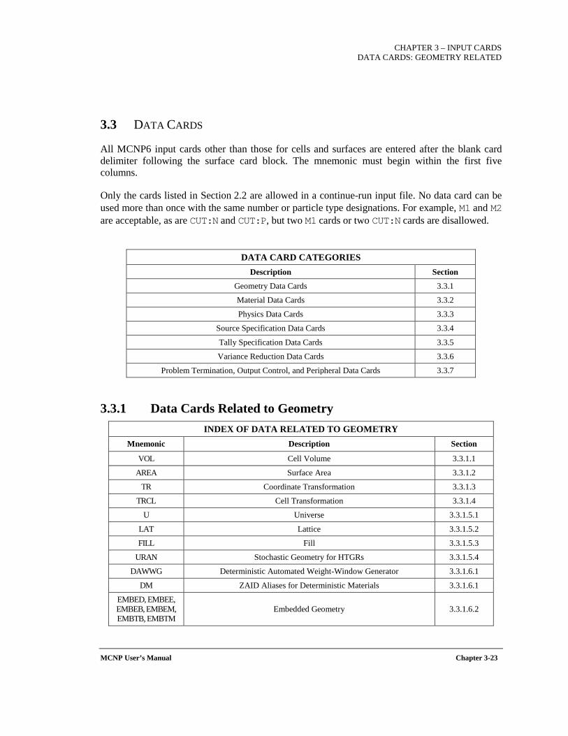
CHAPTER 3 – INPUT CARDS
DATA CARDS: GEOMETRY RELATED
MCNP User’s Manual Chapter 3-23
3.3 DATA CARDS
All MCNP6 input cards other than those for cells and surfaces are entered after the blank card delimiter following the surface card block. The mnemonic must begin within the first five columns.
Only the cards listed in Section 2.2 are allowed in a continue-run input file. No data card can be used more than once with the same number or particle type designations. For example, M1 and M2 are acceptable, as are CUT:N and CUT:P, but two M1 cards or two CUT:N cards are disallowed.
DATA CARD CATEGORIES
Description Section
Geometry Data Cards 3.3.1
Material Data Cards 3.3.2
Physics Data Cards 3.3.3
Source Specification Data Cards 3.3.4
Tally Specification Data Cards 3.3.5
Variance Reduction Data Cards 3.3.6
Problem Termination, Output Control, and Peripheral Data Cards 3.3.7
3.3.1 Data Cards Related to Geometry INDEX OF DATA RELATED TO GEOMETRY
Mnemonic Description Section
VOL Cell Volume 3.3.1.1
AREA Surface Area 3.3.1.2
TR Coordinate Transformation 3.3.1.3
TRCL Cell Transformation 3.3.1.4
U Universe 3.3.1.5.1
LAT Lattice 3.3.1.5.2
FILL Fill 3.3.1.5.3
URAN Stochastic Geometry for HTGRs 3.3.1.5.4
DAWWG Deterministic Automated Weight-Window Generator 3.3.1.6.1
DM ZAID Aliases for Deterministic Materials 3.3.1.6.1
EMBED, EMBEE, EMBEB, EMBEM, EMBTB, EMBTM
Embedded Geometry 3.3.1.6.2
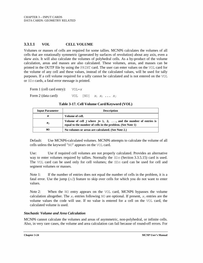
CHAPTER 3 – INPUT CARDS DATA CARDS: GEOMETRY RELATED
Chapter 3-24 MCNP User’s Manual
3.3.1.1 VOL CELL VOLUME
Volumes or masses of cells are required for some tallies. MCNP6 calculates the volumes of all cells that are rotationally symmetric (generated by surfaces of revolution) about any axis, even a skew axis. It will also calculate the volumes of polyhedral cells. As a by-product of the volume calculation, areas and masses are also calculated. These volumes, areas, and masses can be printed in the OUTP file by using the PRINT card. The user can enter values on the VOL card for the volume of any cell and these values, instead of the calculated values, will be used for tally purposes. If a cell volume required for a tally cannot be calculated and is not entered on the VOL or SDn cards, a fatal error message is printed.
Form 1 (cell card entry): VOL=x
Form 2 (data card): VOL [NO] x1 x2 ... xj
Table 3-17. Cell Volume Card/Keyword (VOL)
Input Parameter Description
x Volume of cell.
xj Volume of cell j where j= 1, 2, ..., and the number of entries is equal to the number of cells in the problem. (See Note 1)
NO No volumes or areas are calculated. (See Note 2.)
Default: Use MCNP6-calculated volumes. MCNP6 attempts to calculate the volume of all cells unless the keyword "NO" appears on the VOL card.
Use: Use if required cell volumes are not properly calculated. Provides an alternative way to enter volumes required by tallies. Normally the SDn (Section 3.3.5.15) card is used. The VOL card can be used only for cell volumes; the SDn card can be used for cell and segment volumes or masses.
Note 1: If the number of entries does not equal the number of cells in the problem, it is a fatal error. Use the jump (nJ) feature to skip over cells for which you do not want to enter values.
Note 2: When the NO entry appears on the VOL card, MCNP6 bypasses the volume calculation altogether. The xj entries following NO are optional. If present, xj entries are the volume values the code will use. If no value is entered for a cell on the VOL card, the calculated volume is used.
Stochastic Volume and Area Calculation
MCNP6 cannot calculate the volumes and areas of asymmetric, non-polyhedral, or infinite cells. Also, in very rare cases, the volume and area calculation can fail because of round-off errors. For

CHAPTER 3 – INPUT CARDS
DATA CARDS: GEOMETRY RELATED
MCNP User’s Manual Chapter 3-25
these cases, when neither MCNP6 nor the user can calculate the volume or area, a stochastic estimation is possible by ray tracing. The procedure follows:
1. Void out all materials in the problem by inserting a VOID card into the data card portion of the input.
2. Set all nonzero importance to one and all positive weight windows to zero.
3. Use a planar source with a source weight equal to the surface area to flood the geometry with particles. This setup will cause the particle flux throughout the geometry to statistically approach unity. Perhaps the best way to do a stochastic volume estimation is to use an inward-directed, biased cosine source on a spherical surface with weight equal to πr2 [CAS53].
4. Use the cell flux tally (F4) to tabulate volumes and the surface flux tally (F2) to tabulate areas. The cell flux tally is inversely proportional to cell volume. Thus in cells whose volumes are known, the unit flux will result in a tally of unity and, in cells whose volumes are uncalculated, the unit flux will result in a tally of volumes. Similarly, the surface flux tally is inversely proportional to area so that the unit flux will result in a tally of unity wherever the area is known and a tally of area wherever it is unknown.
5. For any tally volume or area that MCNP6 cannot calculate, use the AREA, VOL, or SD card to assign a value of 1.0 to the area(s) and/or volume(s) of the surface(s) or cell(s) of interest.
3.3.1.2 AREA SURFACE AREA
MCNP6 calculates the area of surfaces as a by-product of the volume calculation. If the volume of all cells on either side of the surface can be calculated, the area of the surface will be calculated. Otherwise, the area calculation will fail.
Form (data card only): AREA x1 x2 ... xj ...
where xj is the area of surface j where j= 1, 2, ..., and the number of entries equals the total number of surfaces in the problem. (See Notes 1 and 2.)
Default: MCNP6 attempts to calculate the area of all surfaces.
Use: Use if required surface areas for F2 tallies are not properly calculated. Provides an alternative way to enter areas required by tallies. Normally the SDn (Section 3.3.5.15) card is used. The AREA card can be used only for areas of whole surfaces; the SDn card can be used for area of surface segments as well as whole surfaces.
Note 1: If the number of entries does not equal the number of surfaces in the problem, it is a fatal error. Use the jump (nJ) feature to skip over surfaces for which you do not want to enter values.
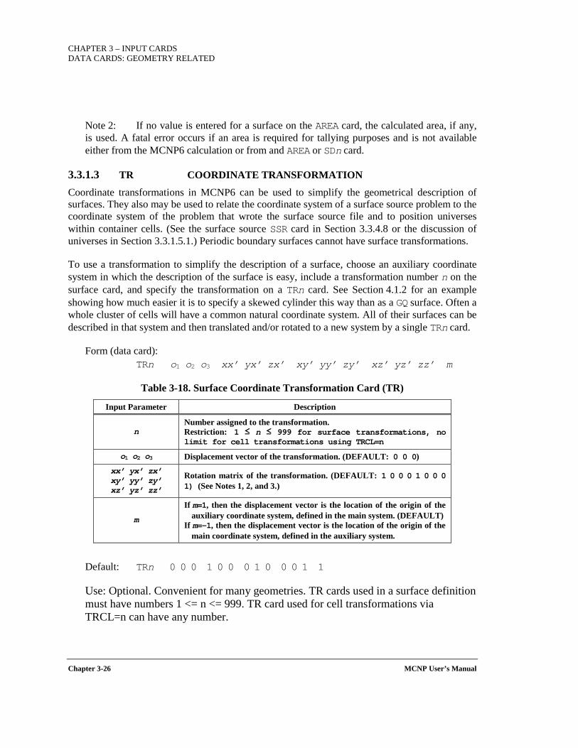
CHAPTER 3 – INPUT CARDS DATA CARDS: GEOMETRY RELATED
Chapter 3-26 MCNP User’s Manual
Note 2: If no value is entered for a surface on the AREA card, the calculated area, if any, is used. A fatal error occurs if an area is required for tallying purposes and is not available either from the MCNP6 calculation or from and AREA or SDn card.
3.3.1.3 TR COORDINATE TRANSFORMATION
Coordinate transformations in MCNP6 can be used to simplify the geometrical description of surfaces. They also may be used to relate the coordinate system of a surface source problem to the coordinate system of the problem that wrote the surface source file and to position universes within container cells. (See the surface source SSR card in Section 3.3.4.8 or the discussion of universes in Section 3.3.1.5.1.) Periodic boundary surfaces cannot have surface transformations.
To use a transformation to simplify the description of a surface, choose an auxiliary coordinate system in which the description of the surface is easy, include a transformation number n on the surface card, and specify the transformation on a TRn card. See Section 4.1.2 for an example showing how much easier it is to specify a skewed cylinder this way than as a GQ surface. Often a whole cluster of cells will have a common natural coordinate system. All of their surfaces can be described in that system and then translated and/or rotated to a new system by a single TRn card.
Form (data card): TRn o1 o2 o3 xx’ yx’ zx’ xy’ yy’ zy’ xz’ yz’ zz’ m
Table 3-18. Surface Coordinate Transformation Card (TR)
Input Parameter Description
n Number assigned to the transformation. Restriction: 1 ≤ n ≤ 999 for surface transformations, no limit for cell transformations using TRCL=n
o1 o2 o3 Displacement vector of the transformation. (DEFAULT: 0 0 0) xx’ yx’ zx’ xy’ yy’ zy’ xz’ yz’ zz’
Rotation matrix of the transformation. (DEFAULT: 1 0 0 0 1 0 0 0 1) (See Notes 1, 2, and 3.)
m
If m=1, then the displacement vector is the location of the origin of the auxiliary coordinate system, defined in the main system. (DEFAULT)
If m=-1, then the displacement vector is the location of the origin of the main coordinate system, defined in the auxiliary system.
Default: TRn 0 0 0 1 0 0 0 1 0 0 0 1 1
Use: Optional. Convenient for many geometries. TR cards used in a surface definition must have numbers 1 <= n <= 999. TR card used for cell transformations via TRCL=n can have any number.

CHAPTER 3 – INPUT CARDS
DATA CARDS: GEOMETRY RELATED
MCNP User’s Manual Chapter 3-27
Reminder: When a transformation is applied to a cell, MCNP6 generates a set of new unique surface numbers based on the original surface numbers. The number of the generated surface is equal to the number of original surface plus 1000 times the number of the cell. This formula creates generated surface numbers that are predictable and can be used on other cell cards and on tally cards. This method, however, limits cell numbers to no more than 6 digits and the original surface numbers to no more than 3 digits.
Note 1: If the symbol *TR is used, the rotation matrix entries are angles in degrees instead of cosines of the angles.
Note 2: The rotation matrix entries specify the relationship between the directions of the axes of the two coordinate systems. For example, the value of xx’ is the cosine of the angle (or, if the optional asterisk is used, the angle in degrees ranging from 0° to 180°) between the x-axis of the main coordinate system and the x′-axis of the auxiliary coordinate system. Similarly, yx’ is the cosine of the angle between the y-axis of the main coordinate system and the x′-axis of the auxiliary system.
The meaning of the rotation matrix entries do not depend on the value of m. It is usually not necessary to enter all of the elements of the matrix. The following patterns are acceptable:
1. All nine elements. (Required if one of the systems is right-handed and the other is left-handed.)
2. Two of the three vectors either way in the matrix (6 values). MCNP6 will create the third vector by cross product.
3. One vector each way in the matrix (5 values). The component in common must be less than 1. MCNP6 will fill out the matrix by the Eulerian angles scheme.
4. One vector (3 values). MCNP6 will create the other two vectors in some arbitrary way. (Appropriate when the auxiliary coordinate system is being used to describe a set of surfaces that are all surfaces of rotation about a common skew axis.)
5. None. MCNP6 will create the identity matrix. (Appropriate when the transformation is a pure translation.)
A vector consists of the three elements in either a row or a column in the matrix. In all cases, MCNP6 cleans up any small non-orthogonality and normalizes the matrix. In this process, exact vectors like (1,0,0) are left unchanged. A warning message is issued if the non-orthogonality is more than about 0.001 radian.
Note 3: A cone of one sheet can be rotated only from being on or parallel to one coordinate axis to being on or parallel to another coordinate axis (multiples of 90°). A cone of one sheet can have any origin displacement vector appropriate to the problem. A cone of two sheets can be transformed anywhere. A cone of two sheets with an ambiguity surface in the cell description to cut the two-sheet cone in half (so that the cell appears as one sheet) can be transformed. The ambiguity surface must have the same transformation number as the cone
CHAPTER 3 – INPUT CARDS DATA CARDS: GEOMETRY RELATED
Chapter 3-28 MCNP User’s Manual
of two sheets. Ambiguity surfaces are described in Section 2.6.2 of the MCNP5 Theory Manual[X-503a].
Example 1: 17 4 RCC 0 0 0 0 12 0 5 *TR4 20 0 0 45 -45 90 135 45 90 90 90 0
In this example, surface 17 is transformed via transformation 4 causing it to be displaced to x ,y ,z=20 ,0 ,0 and rotated 45° counter-clockwise with respect to x and y. If the rotational matrix is left incomplete, MCNP6 will calculate what it should be, but completeness is the only way to be sure you get what you want and get error messages if you are wrong.
Example 2: 11 4 PX 5 TR4 7 0.9 1.3 0 −1 0 0 0 1 −1 0 0
Surface 11 is set up in an auxiliary coordinate system that is related to the main coordinate system by transformation number 4. MCNP6 will produce coefficients in the main coordinate system as if surface 11 had been entered as 11 P 0 -1.0 4.1
It will not produce
11 PY 4.1 .
This surface, represented by PY as shown in the line above, has the wrong sense. More examples of the transformation capability appear in Section 4.1.2.
3.3.1.4 TRCL CELL COORDINATE TRANSFORMATION
A cell transformation (TRCL cell parameter) may be applied to a cell using either of two formats. The first TRCL entry form is an integer that is interpreted as the number of a TRn card that contains transformation information for all of the surfaces defining the cell. The associated TRn card is located in the data card section of the INP file. An alternate entry form for TRCL allows the actual transformation to be entered on the cell card following the TRCL mnemonic, enclosed by parentheses. If the actual transformation is entered, all the rules applying to the TR card (Section 3.3.1.3) are valid.
Although a cell transformation can be applied to a standard cell, the utility of the TRCL parameter becomes most evident when applied to repeated structures. (See Section 3.3.1.5.) Assume your analysis model contains several cells identical in size and shape but located at multiple places in the geometry. You can describe the surfaces that describe these cells once and then use the TRCL keyword to position the identical cells in various locations and/or orientations. The TRCL feature is especially valuable when these cells are filled with the same universe. If the surfaces of these filled cells and the surfaces of the cells belonging to the universe that fills them are all described
CHAPTER 3 – INPUT CARDS
DATA CARDS: GEOMETRY RELATED
MCNP User’s Manual Chapter 3-29
in the same auxiliary coordinate system, then a single transformation will completely define the interior of all these filled cells. That is, the cells of the universe will inherit the transformation of the cells they fill.
Form 1 (cell card entry): TRCL=n
Form 2 (cell card entry): TRCL=(o1 o2 o3 xx’ yx’ zx’ xy’ yy’ zy’ xz’ yz’ zz’ m)
Table 3-19. Cell Transformation Keyword (TRCL)
Input Parameter Description
n Number of the transformation corresponding to a TRn card in the data section of the input file. (DEFAULT: n=0)
o1 o2 o3 Displacement vector of the transformation. (DEFAULT: 0 0 0)
xx’ yx’ zx’ xy’ yy’ zy’ xz’ yz’ zz’
Rotation matrix of the transformation. (DEFAULT: 1 0 0 0 1 0 0 0 1) (See the description of the rotation matrix in Note 2 of Section 3.3.1.3.) (See Note 1.)
m
If m=1, then the displacement vector is the location of the origin of the auxiliary coordinate system, defined in the main system. (DEFAULT)
If m=-1, then the displacement vector is the location of the origin of the main coordinate system, defined in the auxiliary system.
Default: No transformation if TRCL card is absent. This is equivalent to TRCL=0 or TRCL 0 0 0 1 0 0 0 1 0 0 0 1 1
Use: Optional. Convenient for many geometries. Use with the LIKE BUT cell description. To transform a standard cell description it is recommended that the TR parameter associated with the surface cards be used.
Reminder: Coordinate transformations using TRCL can be applied only to cells with surface numbers <1000. When a transformation is applied to a cell, MCNP6 generates a set of new unique surface numbers based on the original surface numbers. The number of the generated surface is equal to the number of the original surface plus 1000 times the number of the cell. This formula creates generated surface numbers that are predictable and can be used on other cell cards and on tally cards. This method, however, limits cell numbers to 6 digits and original surface numbers to no more than three digits. These generated surfaces are only the bounding surfaces of the transformed cell, not the surfaces of any universe that fills it. MCNP6 requires only one full description of each universe, no matter how many times that universe is referenced in the problem
Note 1: If the symbol *TRCL is used, the rotation matrix entries are angles in degrees instead of cosines of the angles.
CHAPTER 3 – INPUT CARDS DATA CARDS: GEOMETRY RELATED
Chapter 3-30 MCNP User’s Manual
Example: 1 0 -17 $ rcc can 21 like 1 but *trcl=(20 0 0 45 -45 90 135 45 90 90 90 0)
Cell 21 is like cell 1 but is translated to x ,y ,z=20 ,0 ,0 and rotated 45° counter-clockwise with respect to x and y. If the rotational matrix is left incomplete, MCNP6 will calculate what it should be, but completeness is the only way to be sure you get what you want and get error messages if you are wrong.
3.3.1.5 REPEATED STRUCTURES
The primary goal of the repeated-structures capability is to make it possible to describe only once the cells and surfaces of any structure that appears more than once in a geometry. Obvious examples of geometry models constructed from repeated structures include a reactor core with dozens of nearly identical fuel modules or a room containing complicated, nearly identical objects arranged in an irregular order. Although the repeated-structures feature reduces input and memory use, problems will not run any faster than with any other description. Examples of the use of repeated structures cards appear in Section 4.1.3.
The repeated structures capability extends the concept of an MCNP6 cell. Four input cards are used exclusively to define repeated-structure features of a geometry: universe (U); fill (FILL); lattice (LAT); and, for stochastic geometries, URAN. Additionally, the cell transformation keyword (TRCL) is a supportive companion to the repeated-structures capability and the LIKE n BUT cell-description construct provides a convenient way to create multiple cells with similar attributes.
The user can specify that a cell is to be filled with something called a universe. The U card identifies the universe, if any, to which a cell belongs, and the FILL card specifies with which universe a cell is to be filled. A universe is either a lattice (LAT card) or a user-specified collection of cells. A single universe, described only once, can be designated to fill each of any number of cells in the geometry. Some or all of the cells in a universe may themselves be filled with universes. To use the repeated-structures capability effectively, keep in mind the following information:
• Cell parameters (IMP, VOL, PWT, EXT, FCL, WWN, DXC, NONU, PD, TMP, U, TRCL, LAT, FILL, ELPT, COSY, BFLCL, and UNC) can be defined on cell cards.
• "LIKE n BUT" is a shorthand method to describe easily one cell as equivalent to another except for a limited list of attributes. See Section 3.2.1.
• The universe (U) card specifies to what universe a cell belongs. • The fill (FILL) card specifies with which universe a cell is to be filled. • The cell transformation (TRCL) keyword allows the user to define only once the surfaces
that bound several cells identical in size and shape but located at different places in the geometry. The TRCL keyword follows the transformation rules established for the surface transformation (TR) card. See Section 3.3.1.3.
CHAPTER 3 – INPUT CARDS
DATA CARDS: GEOMETRY RELATED
MCNP User’s Manual Chapter 3-31
• The lattice (LAT) card defines an infinite array of hexahedra or hexagonal prisms. Lattice cell indexing is determined by the user-specified order of the surfaces that describe the (0,0,0) lattice cell.
• A general source description can be defined in a repeated structures part of the geometry. Surface source surfaces must be regular MCNP6 surfaces, not surfaces associated with a repeated structures part of the geometry. No check is made that this requirement is met.
• An importance assigned to a cell that is in a universe is interpreted as a multiplier of the importance of the filled cell. Weight-window lower bounds are not multipliers. Mesh-based weight windows (MESH card) automatically address this issue.
3.3.1.5.1 U UNIVERSE
Think of a universe as either a lattice cell or a collection of ordinary cells that you want to treat in a common manner. For example, perhaps this collection of cells appears multiple times in your model, but in varying orientations. You can use the repeated structures capability to simplify the setup of your model.
By assigning a non-zero universe number to one or more cells, the user creates a geometry unit that can be manipulated or referenced as a group. This assignment is accomplished by using the universe (U) card or, equivalently, the U cell-parameter keyword. If a cell lacks a universe assignment or is assigned to universe zero (U=0), then the cell does not belong to any universe and is a member of the real world. By using the FILL card (Section 3.3.1.5.3), a cell can be filled with a collection of cells that are assigned to the same universe. Note that the cells of a universe may be geometrically finite or infinite, but they must fill all of the space inside any cell that the universe is specified to fill.
One way to think about the connection between a filled cell and the filling universe is that the filled cell is a "window" that looks into a second level, like a window in a wall provides a view of the outdoors. Cells in the second level can be infinite because they will be (virtually) truncated when they bump into or intersect the surfaces of the window. The second level can have its own origin, in a primed coordinate system, unrelated to the upper level origin. However, if the filled cell and filling universe have all their surfaces in the same coordinate system, one TRCL card (Section 3.3.1.4) defines the coordinate system of both filled and filling cells.
A cell in a universe can be filled by another universe, in which case a third level is introduced. Up to 20 levels are permitted, more than most problems will need. The nomenclature chosen to address these hierarchical levels uses the following convention: the highest to lowest level is in inverse order to the associated numerical value. That is, the highest level is level zero (also known as the real world), lower is level one, lower still is level two, etc.
Every cell in the problem is either part of the real world (universe level 0) or part of some universe, but the surfaces of a problem are less restricted. A single planar surface can be used to describe cells in more than one universe. Coincident surfaces cannot be reflecting or periodic,
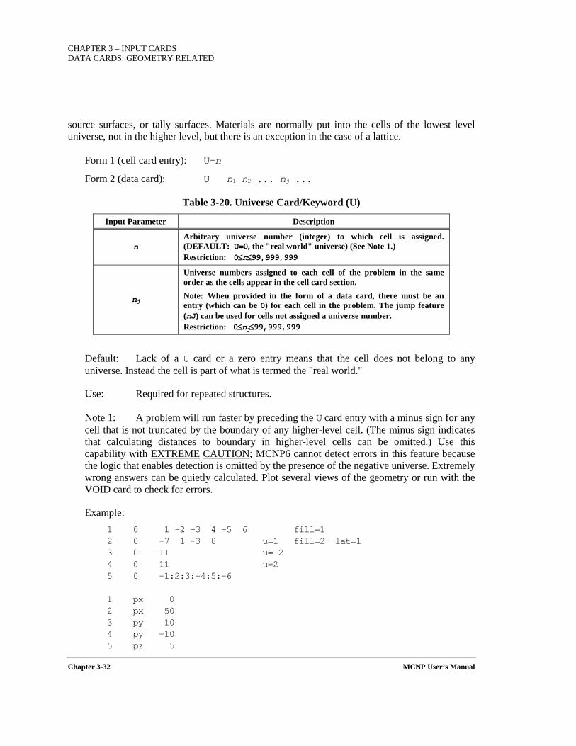
CHAPTER 3 – INPUT CARDS DATA CARDS: GEOMETRY RELATED
Chapter 3-32 MCNP User’s Manual
source surfaces, or tally surfaces. Materials are normally put into the cells of the lowest level universe, not in the higher level, but there is an exception in the case of a lattice.
Form 1 (cell card entry): U=n
Form 2 (data card): U n1 n2 ... nj ...
Table 3-20. Universe Card/Keyword (U)
Input Parameter Description
n Arbitrary universe number (integer) to which cell is assigned. (DEFAULT: U=0, the "real world" universe) (See Note 1.) Restriction: 0≤n≤99,999,999
nj
Universe numbers assigned to each cell of the problem in the same order as the cells appear in the cell card section. Note: When provided in the form of a data card, there must be an entry (which can be 0) for each cell in the problem. The jump feature (nJ) can be used for cells not assigned a universe number. Restriction: 0≤nj≤99,999,999
Default: Lack of a U card or a zero entry means that the cell does not belong to any universe. Instead the cell is part of what is termed the "real world."
Use: Required for repeated structures.
Note 1: A problem will run faster by preceding the U card entry with a minus sign for any cell that is not truncated by the boundary of any higher-level cell. (The minus sign indicates that calculating distances to boundary in higher-level cells can be omitted.) Use this capability with EXTREME CAUTION; MCNP6 cannot detect errors in this feature because the logic that enables detection is omitted by the presence of the negative universe. Extremely wrong answers can be quietly calculated. Plot several views of the geometry or run with the VOID card to check for errors.
Example: 1 0 1 -2 -3 4 -5 6 fill=1 2 0 -7 1 -3 8 u=1 fill=2 lat=1 3 0 -11 u=-2 4 0 11 u=2 5 0 -1:2:3:-4:5:-6 1 px 0 2 px 50 3 py 10 4 py -10 5 pz 5
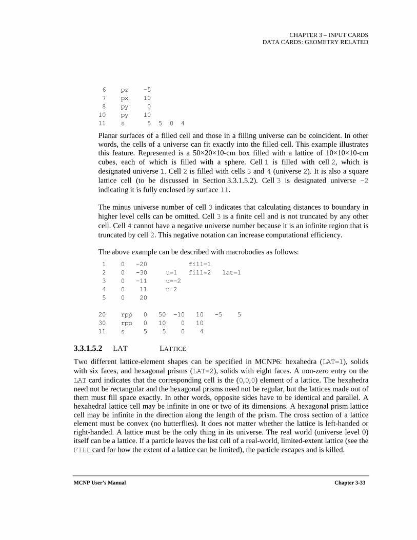
CHAPTER 3 – INPUT CARDS
DATA CARDS: GEOMETRY RELATED
MCNP User’s Manual Chapter 3-33
6 pz -5 7 px 10 8 py 0 10 py 10 11 s 5 5 0 4
Planar surfaces of a filled cell and those in a filling universe can be coincident. In other words, the cells of a universe can fit exactly into the filled cell. This example illustrates this feature. Represented is a 50×20×10-cm box filled with a lattice of 10×10×10-cm cubes, each of which is filled with a sphere. Cell 1 is filled with cell 2, which is designated universe 1. Cell 2 is filled with cells 3 and 4 (universe 2). It is also a square lattice cell (to be discussed in Section 3.3.1.5.2). Cell 3 is designated universe -2 indicating it is fully enclosed by surface 11.
The minus universe number of cell 3 indicates that calculating distances to boundary in higher level cells can be omitted. Cell 3 is a finite cell and is not truncated by any other cell. Cell 4 cannot have a negative universe number because it is an infinite region that is truncated by cell 2. This negative notation can increase computational efficiency.
The above example can be described with macrobodies as follows: 1 0 -20 fill=1 2 0 -30 u=1 fill=2 lat=1 3 0 -11 u=-2 4 0 11 u=2 5 0 20 20 rpp 0 50 -10 10 -5 5 30 rpp 0 10 0 10 11 s 5 5 0 4
3.3.1.5.2 LAT LATTICE
Two different lattice-element shapes can be specified in MCNP6: hexahedra (LAT=1), solids with six faces, and hexagonal prisms (LAT=2), solids with eight faces. A non-zero entry on the LAT card indicates that the corresponding cell is the (0,0,0) element of a lattice. The hexahedra need not be rectangular and the hexagonal prisms need not be regular, but the lattices made out of them must fill space exactly. In other words, opposite sides have to be identical and parallel. A hexahedral lattice cell may be infinite in one or two of its dimensions. A hexagonal prism lattice cell may be infinite in the direction along the length of the prism. The cross section of a lattice element must be convex (no butterflies). It does not matter whether the lattice is left-handed or right-handed. A lattice must be the only thing in its universe. The real world (universe level 0) itself can be a lattice. If a particle leaves the last cell of a real-world, limited-extent lattice (see the FILL card for how the extent of a lattice can be limited), the particle escapes and is killed.

CHAPTER 3 – INPUT CARDS DATA CARDS: GEOMETRY RELATED
Chapter 3-34 MCNP User’s Manual
The cell description of a lattice cell not only provides the standard MCNP6 cell description for the base lattice element, but, through the order of the surface specification for the lattice cell, it identifies which lattice element lies beyond each surface. The first two surfaces listed on the cell card define the direction of the first lattice index; the third and fourth surfaces listed in the cell description define the direction of the second lattice element, etc. This concept is further explained in the following discussion.
After designing your lattice, decide which element you want to be the (0,0,0) element and in which directions you want the three lattice indices to increase. In the case of a hexagonal prism lattice you have two constraints: the first and second indices must increase across adjacent surfaces and the third index must increase in one or the other direction along the length of the prism. Enter the bounding surfaces of the (0,0,0) element on the cell card in the appropriate order, in accordance with the following conventions. For a hexahedral lattice cell, beyond the first surface listed is the (1,0,0) element, beyond the second surface listed is the (-1,0,0) element. Similarly, the (0,1,0), (0,-1,0), (0,0,1), and (0,0,-1) lattice elements are beyond the 3rd, 4th, 5th, and 6th surfaces in that order. This method provides the order of arrangement of the lattice to the code so that when you specify element (7,9,3), the code knows to which element you are referring.
For a hexagonal prism lattice cell, on the opposite side of the first surface listed is element (1,0,0), opposite the second listed surface is (-1,0,0), followed by the lattice elements (0,1,0), (0,-1,0), (-1,1,0), (1,-1,0), (0,0,1), and (0,0,-1), which are opposite the 3rd through 8th surfaces defining the hexagonal prism (0,0,0) lattice cell. These last two surfaces must be the base surfaces of the prism. You can use the MCNP6 geometry plotter to label the lattice cells with their indices. This provides an easy way to verify the lattice index arrangement. Example 7 in Section 4.1.3 illustrates a hexagonal prism lattice cell.
Each cell containing a lattice, whether specified using a LAT keyword or a LAT data card, must have an associated FILL keyword.
Form 1 (cell card entry): LAT=n
Form 2 (data card): LAT n1 n2 ... nj ...
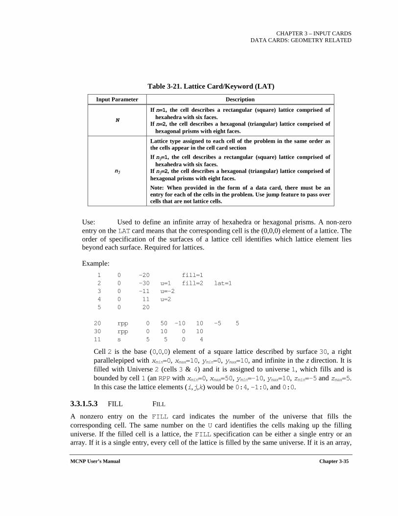
CHAPTER 3 – INPUT CARDS
DATA CARDS: GEOMETRY RELATED
MCNP User’s Manual Chapter 3-35
Table 3-21. Lattice Card/Keyword (LAT)
Input Parameter Description
N
If n=1, the cell describes a rectangular (square) lattice comprised of hexahedra with six faces.
If n=2, the cell describes a hexagonal (triangular) lattice comprised of hexagonal prisms with eight faces.
nj
Lattice type assigned to each cell of the problem in the same order as the cells appear in the cell card section If nj=1, the cell describes a rectangular (square) lattice comprised of
hexahedra with six faces. If nj=2, the cell describes a hexagonal (triangular) lattice comprised of hexagonal prisms with eight faces. Note: When provided in the form of a data card, there must be an entry for each of the cells in the problem. Use jump feature to pass over cells that are not lattice cells.
Use: Used to define an infinite array of hexahedra or hexagonal prisms. A non-zero entry on the LAT card means that the corresponding cell is the (0,0,0) element of a lattice. The order of specification of the surfaces of a lattice cell identifies which lattice element lies beyond each surface. Required for lattices.
Example: 1 0 -20 fill=1 2 0 -30 u=1 fill=2 lat=1 3 0 -11 u=-2 4 0 11 u=2 5 0 20 20 rpp 0 50 -10 10 -5 5 30 rpp 0 10 0 10 11 s 5 5 0 4
Cell 2 is the base (0,0,0) element of a square lattice described by surface 30, a right parallelepiped with xmin=0, xmax=10, ymin=0, ymax=10, and infinite in the z direction. It is filled with Universe 2 (cells 3 & 4) and it is assigned to universe 1, which fills and is bounded by cell 1 (an RPP with xmin=0, xmax=50, ymin=-10, ymax=10, zmin=-5 and zmax=5. In this case the lattice elements (i,j,k) would be 0:4, -1:0, and 0:0.
3.3.1.5.3 FILL FILL
A nonzero entry on the FILL card indicates the number of the universe that fills the corresponding cell. The same number on the U card identifies the cells making up the filling universe. If the filled cell is a lattice, the FILL specification can be either a single entry or an array. If it is a single entry, every cell of the lattice is filled by the same universe. If it is an array,
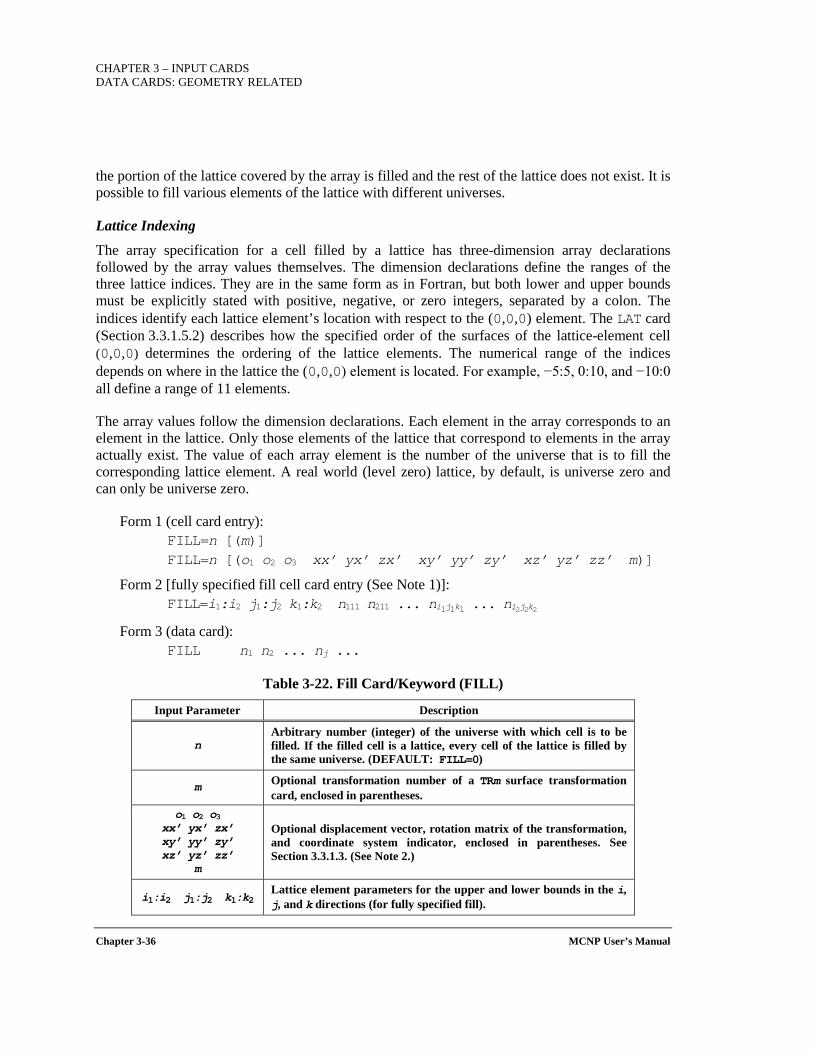
CHAPTER 3 – INPUT CARDS DATA CARDS: GEOMETRY RELATED
Chapter 3-36 MCNP User’s Manual
the portion of the lattice covered by the array is filled and the rest of the lattice does not exist. It is possible to fill various elements of the lattice with different universes.
Lattice Indexing
The array specification for a cell filled by a lattice has three-dimension array declarations followed by the array values themselves. The dimension declarations define the ranges of the three lattice indices. They are in the same form as in Fortran, but both lower and upper bounds must be explicitly stated with positive, negative, or zero integers, separated by a colon. The indices identify each lattice element’s location with respect to the (0,0,0) element. The LAT card (Section 3.3.1.5.2) describes how the specified order of the surfaces of the lattice-element cell (0,0,0) determines the ordering of the lattice elements. The numerical range of the indices depends on where in the lattice the (0,0,0) element is located. For example, −5:5, 0:10, and −10:0 all define a range of 11 elements.
The array values follow the dimension declarations. Each element in the array corresponds to an element in the lattice. Only those elements of the lattice that correspond to elements in the array actually exist. The value of each array element is the number of the universe that is to fill the corresponding lattice element. A real world (level zero) lattice, by default, is universe zero and can only be universe zero.
Form 1 (cell card entry): FILL=n [(m)] FILL=n [(o1 o2 o3 xx’ yx’ zx’ xy’ yy’ zy’ xz’ yz’ zz’ m)]
Form 2 [fully specified fill cell card entry (See Note 1)]: FILL=i1:i2 j1:j2 k1:k2 n111 n211 ... ni1j1k1 ... ni2j2k2
Form 3 (data card): FILL n1 n2 ... nj ...
Table 3-22. Fill Card/Keyword (FILL)
Input Parameter Description
n Arbitrary number (integer) of the universe with which cell is to be filled. If the filled cell is a lattice, every cell of the lattice is filled by the same universe. (DEFAULT: FILL=0)
m Optional transformation number of a TRm surface transformation card, enclosed in parentheses.
o1 o2 o3 xx’ yx’ zx’ xy’ yy’ zy’ xz’ yz’ zz’
m
Optional displacement vector, rotation matrix of the transformation, and coordinate system indicator, enclosed in parentheses. See Section 3.3.1.3. (See Note 2.)
i1:i2 j1:j2 k1:k2 Lattice element parameters for the upper and lower bounds in the i, j, and k directions (for fully specified fill).
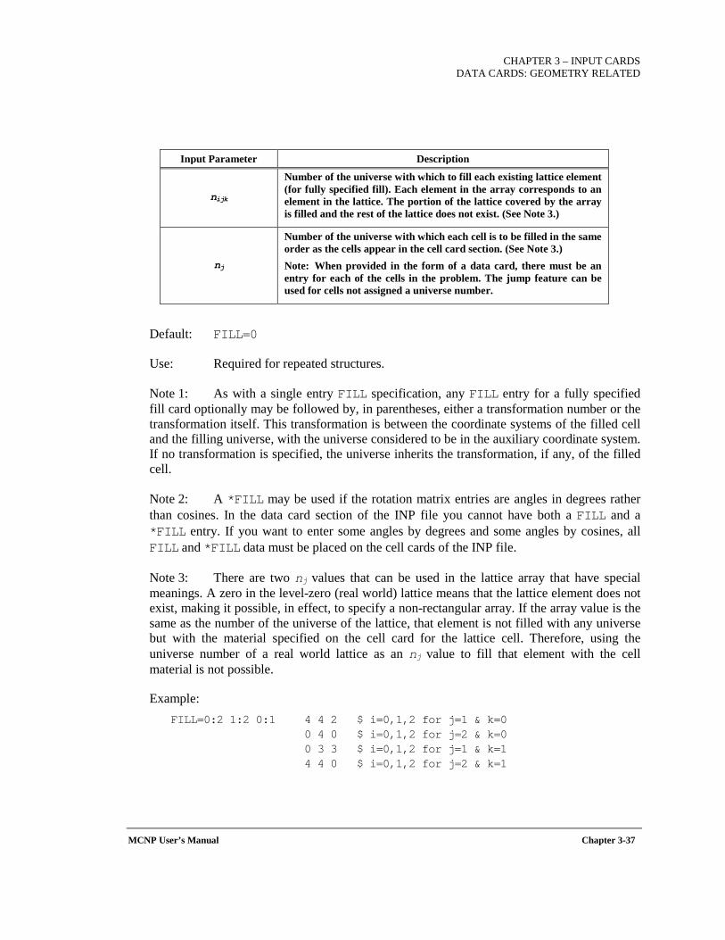
CHAPTER 3 – INPUT CARDS
DATA CARDS: GEOMETRY RELATED
MCNP User’s Manual Chapter 3-37
Input Parameter Description
nijk
Number of the universe with which to fill each existing lattice element (for fully specified fill). Each element in the array corresponds to an element in the lattice. The portion of the lattice covered by the array is filled and the rest of the lattice does not exist. (See Note 3.)
nj
Number of the universe with which each cell is to be filled in the same order as the cells appear in the cell card section. (See Note 3.) Note: When provided in the form of a data card, there must be an entry for each of the cells in the problem. The jump feature can be used for cells not assigned a universe number.
Default: FILL=0
Use: Required for repeated structures.
Note 1: As with a single entry FILL specification, any FILL entry for a fully specified fill card optionally may be followed by, in parentheses, either a transformation number or the transformation itself. This transformation is between the coordinate systems of the filled cell and the filling universe, with the universe considered to be in the auxiliary coordinate system. If no transformation is specified, the universe inherits the transformation, if any, of the filled cell.
Note 2: A *FILL may be used if the rotation matrix entries are angles in degrees rather than cosines. In the data card section of the INP file you cannot have both a FILL and a *FILL entry. If you want to enter some angles by degrees and some angles by cosines, all FILL and *FILL data must be placed on the cell cards of the INP file.
Note 3: There are two nj values that can be used in the lattice array that have special meanings. A zero in the level-zero (real world) lattice means that the lattice element does not exist, making it possible, in effect, to specify a non-rectangular array. If the array value is the same as the number of the universe of the lattice, that element is not filled with any universe but with the material specified on the cell card for the lattice cell. Therefore, using the universe number of a real world lattice as an nj value to fill that element with the cell material is not possible.
Example: FILL=0:2 1:2 0:1 4 4 2 $ i=0,1,2 for j=1 & k=0
0 4 0 $ i=0,1,2 for j=2 & k=0 0 3 3 $ i=0,1,2 for j=1 & k=1 4 4 0 $ i=0,1,2 for j=2 & k=1
CHAPTER 3 – INPUT CARDS DATA CARDS: GEOMETRY RELATED
Chapter 3-38 MCNP User’s Manual
Only eight elements of this lattice exist. Elements (0,1,0), (1,1,0), (1,2,0), (0,2,1) and (1,2,1) are filled with universe 4. Element (2,1,0) is filled with universe 2. Elements (1,1,1) and (2,1,1) are filled with universe 3.
3.3.1.5.4 URAN STOCHASTIC GEOMETRY FOR HTGRS
Randomization of HTGR Fuel-Kernel Geometry
The URAN card provides a limited means of modeling stochastic geometry in MCNP6 for both fixed-source and eigenvalue problems. It is primarily intended for modeling the randomly located fuel kernels in high-temperature gas-cooled reactor (HTGR) geometries. (Although this feature may have other possible applications, users should proceed carefully and perform their own verification calculations to ensure that the feature adequately represents the physical problem they are modeling.)
MCNP6 has been used frequently to model HTGRs with explicit geometric representation of fuel compacts or pebbles, including the microscopic fuel kernels within them. [(BRO05) (BRO04)] Each fuel kernel typically has a spherical (~0.5-mm-diameter) uranium oxycarbide region surrounded by layers of graphite, pyrolytic graphite, and silicon carbide. Modular HTGRs contain cylindrical fuel compacts filled with randomly located fuel kernels in a graphite matrix. Pebble bed HTGRs contain spherical fuel pebbles filled with randomly located fuel kernels in a graphite matrix.
Modeling these geometries in multigroup deterministic codes requires the implementation of shielding factors to account for double heterogeneities (i.e., fuel kernels and fuel particles). Monte Carlo codes that permit hierarchical geometry models, such as MCNP6 with its embedded lattices and universes, can explicitly model the pebble bed double heterogeneities. The random locations of fuel kernels within each fuel compact or pebble are typically modeled in MCNP6 using a regular lattice arrangement, ignoring any randomness.
To provide a limited form of randomness to the locations of fuel kernels in HTGR models, the URAN card may be used to flag selected universes in a lattice as stochastic. This feature provides an additional, random transformation to the geometry each time a neutron enters the lattice element. That is, when a neutron enters a lattice element containing an embedded universe flagged as stochastic, the universe coordinates are transformed randomly according to
where ξ1, ξ2, ξ3 are random numbers uniformly distributed on (0,1), and δx, δy, δz are user-defined parameters supplied on the URAN card. Different translation parameters can be declared for different levels of the geometry, and the random translations are performed only when entering lattice elements containing universes that the user declares as stochastic on the URAN card. To preserve mass and packing fractions, the translation parameters should be chosen such that fuel
( ) xxx δξ ⋅−+= 12 1
( ) yyy δξ ⋅−+= 12 2
( ) zzz δξ ⋅−+= 12 3

CHAPTER 3 – INPUT CARDS
DATA CARDS: GEOMETRY RELATED
MCNP User’s Manual Chapter 3-39
kernels or other objects are not displaced beyond the edges of the enclosing cell or lattice element.
In addition to the random translation applied to a neutron entering a stochastic universe, special treatment is needed to save the fission sites in an eigenvalue calculation. When a fission occurs and the site parameters are saved in the fission bank, the current values of the random translation parameters must be saved along with the normal fission-site data. In the next cycle of the calculation, these saved translation parameters are used for the neutron starting at that fission site. This ensures that the flight continues from the same stochastic realization in effect when the site was saved.
This stochastic geometry treatment has been verified for several realistic HTGR problems. [(BRO05) (BRO04)]
Form (data card): URAN n1 dx1 dy1 dz1 nj dxj dyj dzj
Table 3-23. Stochastic Geometry Card (URAN)
Input Parameter Description
ni Universe number to which to apply stochastic transformation. (Only applied when used to fill a lattice element.)
dxi Maximum translation in the ±x direction for stochastic transformation applied to universe ni.
dyi Maximum translation in the ±y direction for stochastic transformation applied to universe ni.
dzi Maximum translation in the ±z direction for stochastic transformation applied to universe ni.
Default: None.
Use: To model random nature of HTGR or similar geometries.
Caution: There is no stochastic geometry plotting capability associated with the URAN card. Users should be extremely cautious in supplying information using the URAN card because MCNP6 has no means of checking whether the supplied parameters properly represent the physical model being simulated.
CHAPTER 3 – INPUT CARDS DATA CARDS: GEOMETRY RELATED
Chapter 3-40 MCNP User’s Manual
3.3.1.6 HYBRID GEOMETRIES: STRUCTURED AND UNSTRUCTURED MESHES
A geometry mesh from an external file can be embedded into a MCNP6 constructive solid geometry model using the "universe" construct from the repeated structures capability. The embedded geometry mesh may be structured or unstructured.1
A structured mesh, such as that defined by the geometry/materials block of the PARTISN discrete ordinates (SN) code [ALC08], can be embedded into an MCNP6 geometry. The resultant hybrid geometry can then be used for Monte Carlo calculations. It is also possible to convert a standard MCNP6 geometry to a PARTISN-style mesh. The only structured-mesh geometry file format accommodated at this time is LNK3DNT, used by the LANL discrete-ordinates deterministic-transport code PARTISN. With this capability, Monte Carlo vs. discrete-ordinates comparisons can be accomplished directly, thus separating geometry, cross-section data, and methodology effects. This initial capability takes MCNP6's constructive solid geometry, creates a homogenized regular mesh of materials in 1D (r), 2D (rz), or 3D (xyz or rzθ), and writes a PARTISN-style geometry file in the LNK3DNT file format. MCNP6 can also import a geometry description from an existing LNK3DNT geometry file for continuous-energy neutron transport.
Unstructured meshes, such as those created by the finite-element code Abaqus/CAE [DES09], also can be embedded in a hybrid arrangement. Only the format output by Abaqus is recognized at this time. However, many other computer-aided engineering (CAE) tools have the ability to generate a mesh from a solid model that can be converted easily to the Abaqus format. Meshes consisting of four-, five-, or six-sided finite elements, with linear, bi-linear, or quadratic faces are allowed.
Before creating or incorporating structured or unstructured meshes, it is highly recommended that the interested user become familiar with external references, as appropriate. [MAR12a, MAR12b, MAR12c, MAR17, COX11] This section is not meant to provide information regarding PARTISN or Abaqus file formats nor provide a primer on how to run or interact with these codes.
3.3.1.6.1 CREATION OF A STRUCTURED DISCRETE-ORDINATES-STYLE GEOMETRY FILE
LNK3DNT-format files, used by the LANL PARTISN code, can be created from a standard MCNP6 input deck. [COX11] Two cards are required to accomplish this task: the MESH card (discussed in Section 3.3.6.4.4) and the DAWWG card.
MESH: Superimposed Importance Mesh for Mesh-Based Weight-Window Generator
The MESH card (see Section 3.3.6.4.4) specifies the layout and orientation of the geometry to be generated with respect to the cell-based coordinate system. For this application, the supported coordinate-system options include XYZ (3D Cartesian), CYL [in either 2D (rz) or 3D (rzθ)], and SPH (1D spherical). The optional ORG, AXS, and VEC keywords of the MESH card can be used to 1 Currently, the file of a structured mesh to be embedded in MCNP6 must be in PARTISN-style format and that of a unstructured mesh must be in Abaqus-style format.

CHAPTER 3 – INPUT CARDS
DATA CARDS: GEOMETRY RELATED
MCNP User’s Manual Chapter 3-41
align the mesh with the MCNP6 geometry from which the discrete-ordinates geometry will be generated.
Note that the geometry orientation is not transferred to the resultant LNK3DNT file. Regarding the MESH orientation parameters, the generated homogenized geometry will have a geometrical center at (0,0,0) and will be aligned with the standard MCNP6 Cartesian coordinate system. For cylindrical geometries, the defaults are that the cylinder axis is aligned with the positive z-axis and the azimuthal plane (θ=0) is aligned with the positive x-axis.
DM ZAID Aliases for Deterministic Materials
Form: DMn zaid1 zaid2 zaid3 ...
(See external documentation [COX11]).
DAWWG Deterministic Adjoint Weight-Window Generator
Note: The DAWWG card must appear after the MESH card in the input file's data section.
The DAWWG card specifies the number of points to sample in each element of the mesh. This sampling is used to estimate the volume fraction of different materials within each element. From this information a homogenized material definition with its associated density can be generated for each element. DAWWG may also be used to pass information directly to PARTISN.
Form: DAWWG KEYWORD=value(s) ...
Table 3-24. Deterministic Adjoint Weight-Window Generator Card (DAWWG)
Keyword Value
POINTS=n
Randomly sample the material within each element of the defined mesh using n sample points in each coordinate direction for each mesh element, where n is an integer. This sampling is used to estimate material volume fractions and thereby estimate the composition of each geometry element. (DEFAULT: POINTS=1) (See Note 1.) (Required)
XSEC=<name> Declares that cross-section library <name> will be passed to the discrete-ordinates code for weight-window generation. This information is not explicitly used in the generation of the mesh. (Required)†
TALLY=i (Optional)†
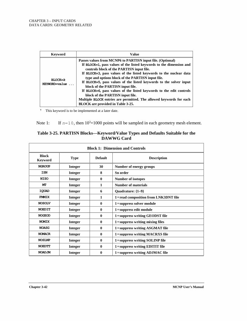
CHAPTER 3 – INPUT CARDS DATA CARDS: GEOMETRY RELATED
Chapter 3-42 MCNP User’s Manual
Keyword Value
BLOCK=k KEYWORD=value ...
Passes values from MCNP6 to PARTISN input file. (Optional) If BLOCK=1, pass values of the listed keywords to the dimension and
controls block of the PARTISN input file. If BLOCK=3, pass values of the listed keywords to the nuclear data
type and options block of the PARTISN input file. If BLOCK=5, pass values of the listed keywords to the solver input
block of the PARTISN input file. If BLOCK=6, pass values of the listed keywords to the edit controls
block of the PARTISN input file. Multiple BLOCK entries are permitted. The allowed keywords for each BLOCK are provided in Table 3-25.
† This keyword is to be implemented at a later date.
Note 1: If n=10, then 103=1000 points will be sampled in each geometry mesh element.
Table 3-25. PARTISN Blocks—Keyword/Value Types and Defaults Suitable for the DAWWG Card
Block 1: Dimension and Controls
Block Keyword Type Default Description
NGROUP Integer 30 Number of energy groups ISN Integer 8 Sn order NISO Integer 0 Number of isotopes MT Integer 1 Number of materials
IQUAD Integer 6 Quadrature: 1–9 FMMIX Integer 1 1=read composition from LNK3DNT file NOSOLV Integer 0 1=suppress solver module NOEDIT Integer 0 1=suppress edit module NOGEOD Integer 0 1=suppress writing GEODST file NOMIX Integer 0 1=suppress writing mixing files NOASG Integer 0 1=suppress writing ASGMAT file NOMACR Integer 0 1=suppress writing MACRXS file NOSLNP Integer 0 1=suppress writing SOLINP file NOEDTT Integer 0 1=suppress writing EDITIT file NOADJM Integer 0 1=suppress writing ADJMAC file
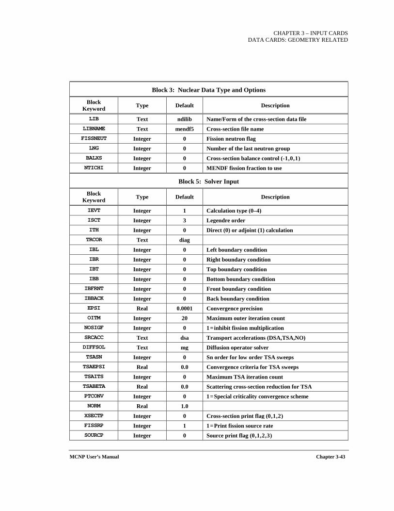
CHAPTER 3 – INPUT CARDS
DATA CARDS: GEOMETRY RELATED
MCNP User’s Manual Chapter 3-43
Block 3: Nuclear Data Type and Options
Block Keyword Type Default Description
LIB Text ndilib Name/Form of the cross-section data file LIBNAME Text mendf5 Cross-section file name FISSNEUT Integer 0 Fission neutron flag
LNG Integer 0 Number of the last neutron group BALXS Integer 0 Cross-section balance control (-1,0,1) NTICHI Integer 0 MENDF fission fraction to use
Block 5: Solver Input
Block Keyword Type Default Description
IEVT Integer 1 Calculation type (0–4) ISCT Integer 3 Legendre order ITH Integer 0 Direct (0) or adjoint (1) calculation TRCOR Text diag IBL Integer 0 Left boundary condition IBR Integer 0 Right boundary condition IBT Integer 0 Top boundary condition IBB Integer 0 Bottom boundary condition
IBFRNT Integer 0 Front boundary condition IBBACK Integer 0 Back boundary condition EPSI Real 0.0001 Convergence precision OITM Integer 20 Maximum outer iteration count NOSIGF Integer 0 1=inhibit fission multiplication SRCACC Text dsa Transport accelerations (DSA,TSA,NO) DIFFSOL Text mg Diffusion operator solver TSASN Integer 0 Sn order for low order TSA sweeps TSAEPSI Real 0.0 Convergence criteria for TSA sweeps TSAITS Integer 0 Maximum TSA iteration count TSABETA Real 0.0 Scattering cross-section reduction for TSA PTCONV Integer 0 1=Special criticality convergence scheme NORM Real 1.0 XSECTP Integer 0 Cross-section print flag (0,1,2) FISSRP Integer 1 1=Print fission source rate SOURCP Integer 0 Source print flag (0,1,2,3)
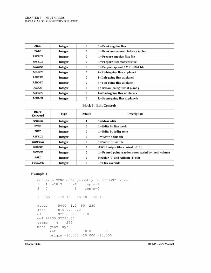
CHAPTER 3 – INPUT CARDS DATA CARDS: GEOMETRY RELATED
Chapter 3-44 MCNP User’s Manual
ANGP Integer 0 1=Print angular flux BALP Integer 0 1=Print coarse-mesh balance tables RAFLUX Integer 0 1=Prepare angular flux file RMFLUX Integer 0 1=Prepare flux moments file AVATAR Integer 0 1=Prepare special XMFLUXA file ASLEFT Integer 0 i=Right-going flux at plane i ASRITE Integer 0 i=Left-going flux at plane i ASBOTT Integer 0 j=Top-going flux at plane j ASTOP Integer 0 j=Bottom-going flux at plane j ASFRNT Integer 0 k=Back-going flux at plane k ASBACK Integer 0 k=Front-going flux at plane k
Block 6: Edit Controls
Block Keyword Type Default Description
MASSED Integer 1 1=Mass edits PTED Integer 0 1=Edits by fine mesh ZNED Integer 0 1=Edits by (edit) zone RZFLUX Integer 0 1=Write a-flux file RZMFLUX Integer 0 1=Write b-flux file EDOUTF Integer 3 ASCII output files control [-3:3] BYVOLP Integer 0 1=Printed point reaction rates scaled by mesh volume AJED Integer 0 Regular (0) and Adjoint (1) edit
FLUXONE Integer 0 1=Flux override
Example 1: Converts MCNP cube geometry to LNK3DNT format 1 1 -18.7 -1 imp:n=1 2 0 1 imp:n=0 1 rpp -10 10 -10 10 -10 10 kcode 5000 1.0 50 250 ksrc 0.0 0.0 0.0 m1 92235.69c 1.0 dm1 92235 92235.50 prdmp j 275 mesh geom xyz ref 0.0 -0.0 -0.0 origin -10.000 -10.000 -10.000
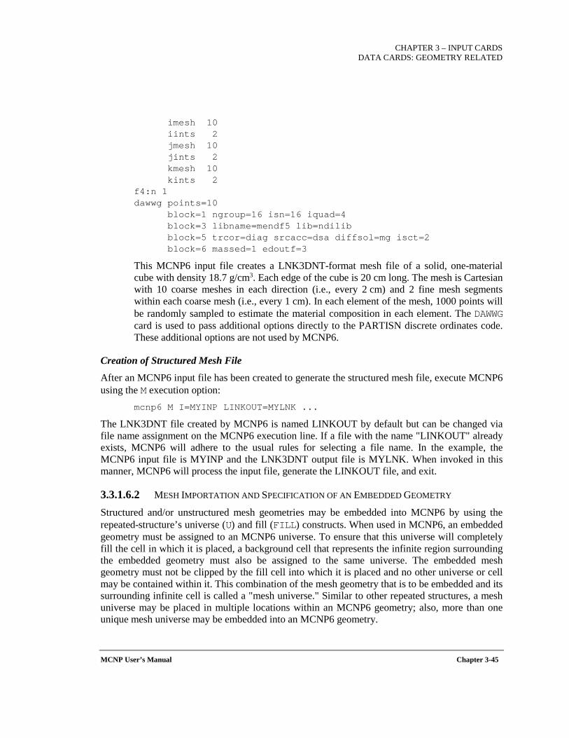
CHAPTER 3 – INPUT CARDS
DATA CARDS: GEOMETRY RELATED
MCNP User’s Manual Chapter 3-45
imesh 10 iints 2 jmesh 10 jints 2 kmesh 10 kints 2 f4:n 1 dawwg points=10 block=1 ngroup=16 isn=16 iquad=4 block=3 libname=mendf5 lib=ndilib block=5 trcor=diag srcacc=dsa diffsol=mg isct=2 block=6 massed=1 edoutf=3
This MCNP6 input file creates a LNK3DNT-format mesh file of a solid, one-material cube with density 18.7 g/cm3. Each edge of the cube is 20 cm long. The mesh is Cartesian with 10 coarse meshes in each direction (i.e., every 2 cm) and 2 fine mesh segments within each coarse mesh (i.e., every 1 cm). In each element of the mesh, 1000 points will be randomly sampled to estimate the material composition in each element. The DAWWG card is used to pass additional options directly to the PARTISN discrete ordinates code. These additional options are not used by MCNP6.
Creation of Structured Mesh File
After an MCNP6 input file has been created to generate the structured mesh file, execute MCNP6 using the M execution option:
mcnp6 M I=MYINP LINKOUT=MYLNK ...
The LNK3DNT file created by MCNP6 is named LINKOUT by default but can be changed via file name assignment on the MCNP6 execution line. If a file with the name "LINKOUT" already exists, MCNP6 will adhere to the usual rules for selecting a file name. In the example, the MCNP6 input file is MYINP and the LNK3DNT output file is MYLNK. When invoked in this manner, MCNP6 will process the input file, generate the LINKOUT file, and exit.
3.3.1.6.2 MESH IMPORTATION AND SPECIFICATION OF AN EMBEDDED GEOMETRY
Structured and/or unstructured mesh geometries may be embedded into MCNP6 by using the repeated-structure’s universe (U) and fill (FILL) constructs. When used in MCNP6, an embedded geometry must be assigned to an MCNP6 universe. To ensure that this universe will completely fill the cell in which it is placed, a background cell that represents the infinite region surrounding the embedded geometry must also be assigned to the same universe. The embedded mesh geometry must not be clipped by the fill cell into which it is placed and no other universe or cell may be contained within it. This combination of the mesh geometry that is to be embedded and its surrounding infinite cell is called a "mesh universe." Similar to other repeated structures, a mesh universe may be placed in multiple locations within an MCNP6 geometry; also, more than one unique mesh universe may be embedded into an MCNP6 geometry.

CHAPTER 3 – INPUT CARDS DATA CARDS: GEOMETRY RELATED
Chapter 3-46 MCNP User’s Manual
In MCNP6, space is defined by a collection of cells using surfaces, lattices, universes, fills, etc. Building on this cell-geometry concept, incorporation of an embedded geometry into MCNP6 requires defining cells to represent the embedded geometry and its composition. There are three special MCNP6 cell categories for specifying the use of an embedded geometry: geometry cells, background cells, and fill cells. Geometry cells and background cells are instances of a special cell-type category called pseudo-cells, meaning cell-like. The treatment of these cells differs depending on the type of embedded mesh; this concept is explained in great detail below. Each embedded mesh universe consists of one or more pseudo-cell geometry cells and a single pseudo-cell background cell.
Pseudo-cells are defined in the MCNP6 cell block by a null surface—with a surface number of "0." These pseudo-cells are used to communicate normal MCNP6 cell properties from the external mesh to the MCNP6 code. The cell-card format for pseudo-cells exhibits the following properties that differ from those of regular MCNP6 cells:
• Pseudo-cells have a single null-surface entry (i.e., "0") instead of a list of signed surfaces. • Pseudo-cells are assigned to a universe (e.g., U=10 or U=e10 where the “e”
prefix to the universe is optional and signifies a mesh universe).
• The universe number of the pseudo-cell must match the n specified on its associated EMBEDn card.
• Pseudo-cells cannot be filled by another universe or lattice (i.e., a pseudo-cell cannot have a FILL or LAT entry).
Pseudo cells cards may contain material, density, importance, and other cell properties. All cell-card fields that typically are required by regular MCNP6 cells also are required by pseudo cells. How the user should think about these cells differs slightly depending on the type of embedded mesh.
For the PARTISN mesh, a pseudo-cell geometry cell must exist for each material defined in an embedded geometry mesh input file. If void elements exist, a separate pseudo-cell is required to represent them. Pure elements, i.e., those that contain only one material or void, belong to only one pseudo-cell. Multi-material elements, however, belong to each pseudo-cell that is associated with a material contained in the element. As will be seen in the next section, the geometry cells are connected to an embedded geometry through the MATCELL entries on the associated EMBED card.
Material information (i.e., density, composition) is assigned to each mesh element within the external mesh geometry file. The materials within the LNK3DNT geometry file must be numbered consecutively, starting with 1. The material information in the external mesh file is transferred to MCNP6 through the pseudo-cells and the MCNP6 EMBED card; each unique material in the external mesh file must have an associated pseudo-cell.

CHAPTER 3 – INPUT CARDS
DATA CARDS: GEOMETRY RELATED
MCNP User’s Manual Chapter 3-47
For the Abaqus unstructured mesh, the unstructured mesh library that handles all of the details of unstructured meshes for MCNP6 establishes pseudo-cells (unique combinations of materials and element sets) from the information contained in the Abaqus input file. The user is referred to "The MCNP6 Book on Unstructured Mesh Geometry: User's Guide" [MAR17] for details on this topic. A pseudo-cell cross-reference table is printed to the MCNP6 outp file. Among other things, this table lists the known pseudo-cells and the associated material assignments that are expected. For each pseudo-cell entry in this table, there must be a pair of values for the MATCELL parameter on the EMBED card. This association connects the MCNP6 pseudo-cell with the unstructured mesh pseudo-cell. This association is essential to establish the material properties for the unstructured mesh pseudo-cells because the only required material property in the mesh file is the material numbers. It is up to the user to ensure that this information is input correctly through the MATCELL entries on the associated EMBED card. For large and complex geometries, this can be a tedious process. To help with this input setup, users should take advantage of the unstructured mesh pre-processor program, um_pre_op. For details, see "The MCNP6 Book on Unstructured Mesh Geometry: User's Guide" [MAR17].
Mesh element assignment to each MCNP6 pseudo-cell is determined by the data as it appears in the external geometry mesh file. For a given geometry mesh, if the element sets of the mesh are built in a different order, then the mapping to the associated MCNP6 pseudo-cells will also be different. The user is directed to the previous list of references to decipher the cross-reference mapping data provided in the external geometry mesh file.
To make a mesh universe infinite in extent, it must have a background pseudo-cell that consists of all space outside the associated embedded geometry. The background cell is connected to the mesh universe through the BACKGROUND entry on the EMBED card.
The third cell type required to embed a mesh geometry into a MCNP6 input is the fill cell. The fill cell is a regular MCNP6 cell into which the mesh universe is placed. (Note: Mesh surfaces should not be coincident with fill-cell surfaces, else lost particles may result.) The cell card for a cell filled with a mesh universe has the following properties that differ from those of other MCNP6 fill cells:
• A mesh universe cannot be an pseudo-cell. • Mesh universe fill cells have a fill entry of the form FILL=En or FILL=n, where n is the
MCNP6 universe number of the mesh universe. This universe number, n, also appears as the n on the EMBEDn card. The FILL entry may have a transformation (TR) to permit realignment of the embedded geometry within the fill cell. Recall that LNK3DNT geometries are always defined relative to the MCNP6 origin.
• Mesh universe fill cells cannot have a lattice entry.
Eight MCNP6 data cards are available to support mesh importation. The EMBED card is required for both structured and unstructured mesh importation. Seven additional cards (EMBEE, EMBEB, EMBEM, EMBTB, EMBTM, EMBDE, and EMBDF) are optional and only valid for unstructured meshes. These seven cards provide for elemental edits, i.e., results accumulated on the
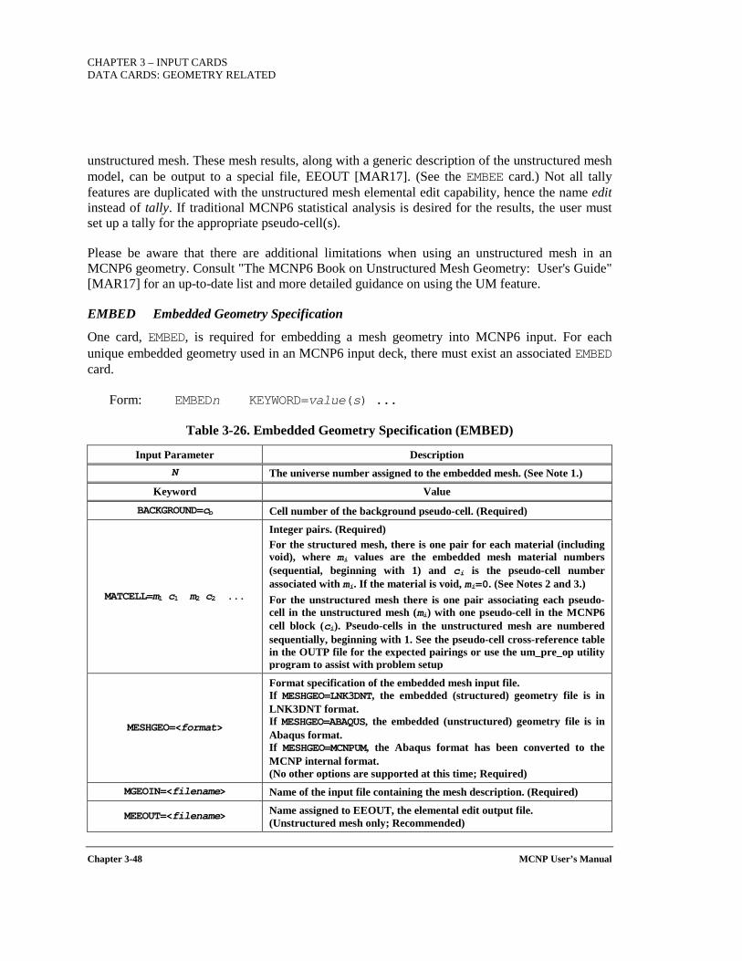
CHAPTER 3 – INPUT CARDS DATA CARDS: GEOMETRY RELATED
Chapter 3-48 MCNP User’s Manual
unstructured mesh. These mesh results, along with a generic description of the unstructured mesh model, can be output to a special file, EEOUT [MAR17]. (See the EMBEE card.) Not all tally features are duplicated with the unstructured mesh elemental edit capability, hence the name edit instead of tally. If traditional MCNP6 statistical analysis is desired for the results, the user must set up a tally for the appropriate pseudo-cell(s).
Please be aware that there are additional limitations when using an unstructured mesh in an MCNP6 geometry. Consult "The MCNP6 Book on Unstructured Mesh Geometry: User's Guide" [MAR17] for an up-to-date list and more detailed guidance on using the UM feature.
EMBED Embedded Geometry Specification
One card, EMBED, is required for embedding a mesh geometry into MCNP6 input. For each unique embedded geometry used in an MCNP6 input deck, there must exist an associated EMBED card.
Form: EMBEDn KEYWORD=value(s) ...
Table 3-26. Embedded Geometry Specification (EMBED)
Input Parameter Description N The universe number assigned to the embedded mesh. (See Note 1.)
Keyword Value
BACKGROUND=cb Cell number of the background pseudo-cell. (Required)
MATCELL=m1 c1 m2 c2 ...
Integer pairs. (Required) For the structured mesh, there is one pair for each material (including void), where mi values are the embedded mesh material numbers (sequential, beginning with 1) and ci is the pseudo-cell number associated with mi. If the material is void, mi=0. (See Notes 2 and 3.) For the unstructured mesh there is one pair associating each pseudo-cell in the unstructured mesh (mi) with one pseudo-cell in the MCNP6 cell block (ci). Pseudo-cells in the unstructured mesh are numbered sequentially, beginning with 1. See the pseudo-cell cross-reference table in the OUTP file for the expected pairings or use the um_pre_op utility program to assist with problem setup
MESHGEO=<format>
Format specification of the embedded mesh input file. If MESHGEO=LNK3DNT, the embedded (structured) geometry file is in LNK3DNT format. If MESHGEO=ABAQUS, the embedded (unstructured) geometry file is in Abaqus format. If MESHGEO=MCNPUM, the Abaqus format has been converted to the MCNP internal format. (No other options are supported at this time; Required)
MGEOIN=<filename> Name of the input file containing the mesh description. (Required)
MEEOUT=<filename> Name assigned to EEOUT, the elemental edit output file. (Unstructured mesh only; Recommended)
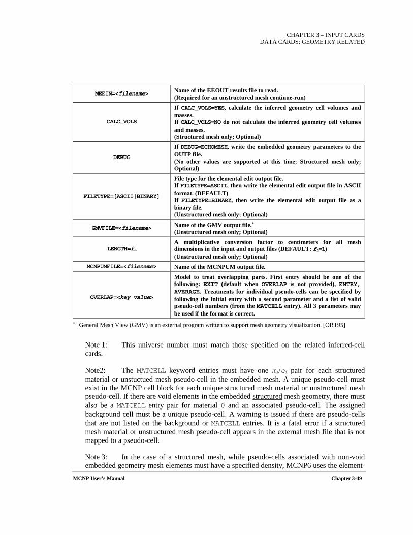
CHAPTER 3 – INPUT CARDS
DATA CARDS: GEOMETRY RELATED
MCNP User’s Manual Chapter 3-49
MEEIN=<filename> Name of the EEOUT results file to read. (Required for an unstructured mesh continue-run)
CALC_VOLS
If CALC_VOLS=YES, calculate the inferred geometry cell volumes and masses. If CALC_VOLS=NO do not calculate the inferred geometry cell volumes and masses. (Structured mesh only; Optional)
DEBUG
If DEBUG=ECHOMESH, write the embedded geometry parameters to the OUTP file. (No other values are supported at this time; Structured mesh only; Optional)
FILETYPE=[ASCII|BINARY]
File type for the elemental edit output file. If FILETYPE=ASCII, then write the elemental edit output file in ASCII format. (DEFAULT) If FILETYPE=BINARY, then write the elemental edit output file as a binary file. (Unstructured mesh only; Optional)
GMVFILE=<filename> Name of the GMV output file.* (Unstructured mesh only; Optional)
LENGTH=fL A multiplicative conversion factor to centimeters for all mesh dimensions in the input and output files (DEFAULT: fL=1) (Unstructured mesh only; Optional)
MCNPUMFILE=<filename> Name of the MCNPUM output file.
OVERLAP=<key value>
Model to treat overlapping parts. First entry should be one of the following: EXIT (default when OVERLAP is not provided), ENTRY, AVERAGE. Treatments for individual pseudo-cells can be specified by following the initial entry with a second parameter and a list of valid pseudo-cell numbers (from the MATCELL entry). All 3 parameters may be used if the format is correct.
* General Mesh View (GMV) is an external program written to support mesh geometry visualization. [ORT95]
Note 1: This universe number must match those specified on the related inferred-cell cards.
Note2: The MATCELL keyword entries must have one mi/ci pair for each structured material or unstuctued mesh pseudo-cell in the embedded mesh. A unique pseudo-cell must exist in the MCNP cell block for each unique structured mesh material or unstructured mesh pseudo-cell. If there are void elements in the embedded structured mesh geometry, there must also be a MATCELL entry pair for material 0 and an associated pseudo-cell. The assigned background cell must be a unique pseudo-cell. A warning is issued if there are pseudo-cells that are not listed on the background or MATCELL entries. It is a fatal error if a structured mesh material or unstructured mesh pseudo-cell appears in the external mesh file that is not mapped to a pseudo-cell.
Note 3: In the case of a structured mesh, while pseudo-cells associated with non-void embedded geometry mesh elements must have a specified density, MCNP6 uses the element-
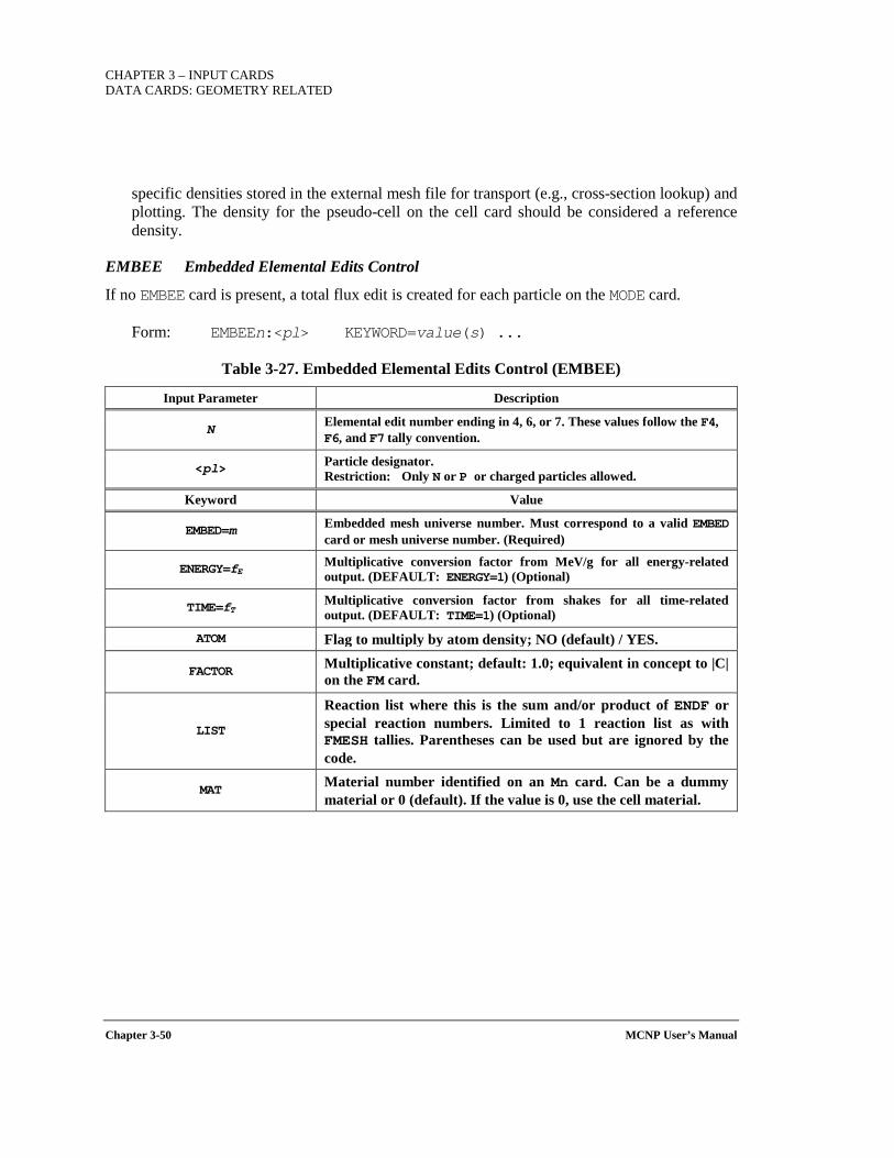
CHAPTER 3 – INPUT CARDS DATA CARDS: GEOMETRY RELATED
Chapter 3-50 MCNP User’s Manual
specific densities stored in the external mesh file for transport (e.g., cross-section lookup) and plotting. The density for the pseudo-cell on the cell card should be considered a reference density.
EMBEE Embedded Elemental Edits Control
If no EMBEE card is present, a total flux edit is created for each particle on the MODE card.
Form: EMBEEn:<pl> KEYWORD=value(s) ...
Table 3-27. Embedded Elemental Edits Control (EMBEE)
Input Parameter Description
N Elemental edit number ending in 4, 6, or 7. These values follow the F4, F6, and F7 tally convention.
<pl> Particle designator. Restriction: Only N or P or charged particles allowed.
Keyword Value
EMBED=m Embedded mesh universe number. Must correspond to a valid EMBED card or mesh universe number. (Required)
ENERGY=fE Multiplicative conversion factor from MeV/g for all energy-related output. (DEFAULT: ENERGY=1) (Optional)
TIME=fT Multiplicative conversion factor from shakes for all time-related output. (DEFAULT: TIME=1) (Optional)
ATOM Flag to multiply by atom density; NO (default) / YES.
FACTOR Multiplicative constant; default: 1.0; equivalent in concept to |C| on the FM card.
LIST
Reaction list where this is the sum and/or product of ENDF or special reaction numbers. Limited to 1 reaction list as with FMESH tallies. Parentheses can be used but are ignored by the code.
MAT Material number identified on an Mn card. Can be a dummy material or 0 (default). If the value is 0, use the cell material.
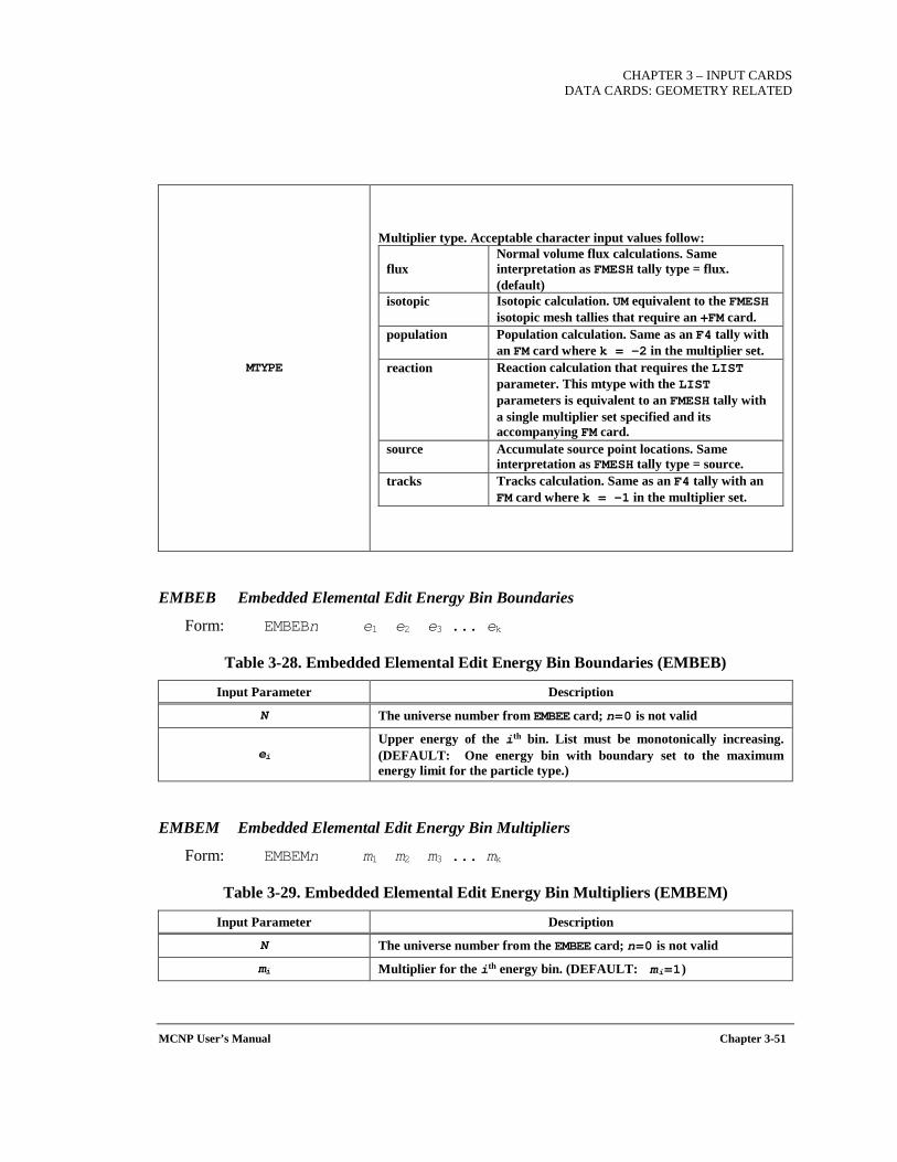
CHAPTER 3 – INPUT CARDS
DATA CARDS: GEOMETRY RELATED
MCNP User’s Manual Chapter 3-51
MTYPE
Multiplier type. Acceptable character input values follow: flux
Normal volume flux calculations. Same interpretation as FMESH tally type = flux. (default)
isotopic Isotopic calculation. UM equivalent to the FMESH isotopic mesh tallies that require an +FM card.
population Population calculation. Same as an F4 tally with an FM card where k = -2 in the multiplier set.
reaction Reaction calculation that requires the LIST parameter. This mtype with the LIST parameters is equivalent to an FMESH tally with a single multiplier set specified and its accompanying FM card.
source Accumulate source point locations. Same interpretation as FMESH tally type = source.
tracks Tracks calculation. Same as an F4 tally with an FM card where k = -1 in the multiplier set.
EMBEB Embedded Elemental Edit Energy Bin Boundaries
Form: EMBEBn e1 e2 e3 ... ek
Table 3-28. Embedded Elemental Edit Energy Bin Boundaries (EMBEB)
Input Parameter Description
N The universe number from EMBEE card; n=0 is not valid
ei Upper energy of the ith bin. List must be monotonically increasing. (DEFAULT: One energy bin with boundary set to the maximum energy limit for the particle type.)
EMBEM Embedded Elemental Edit Energy Bin Multipliers
Form: EMBEMn m1 m2 m3 ... mk
Table 3-29. Embedded Elemental Edit Energy Bin Multipliers (EMBEM)
Input Parameter Description
N The universe number from the EMBEE card; n=0 is not valid
mi Multiplier for the ith energy bin. (DEFAULT: mi=1)
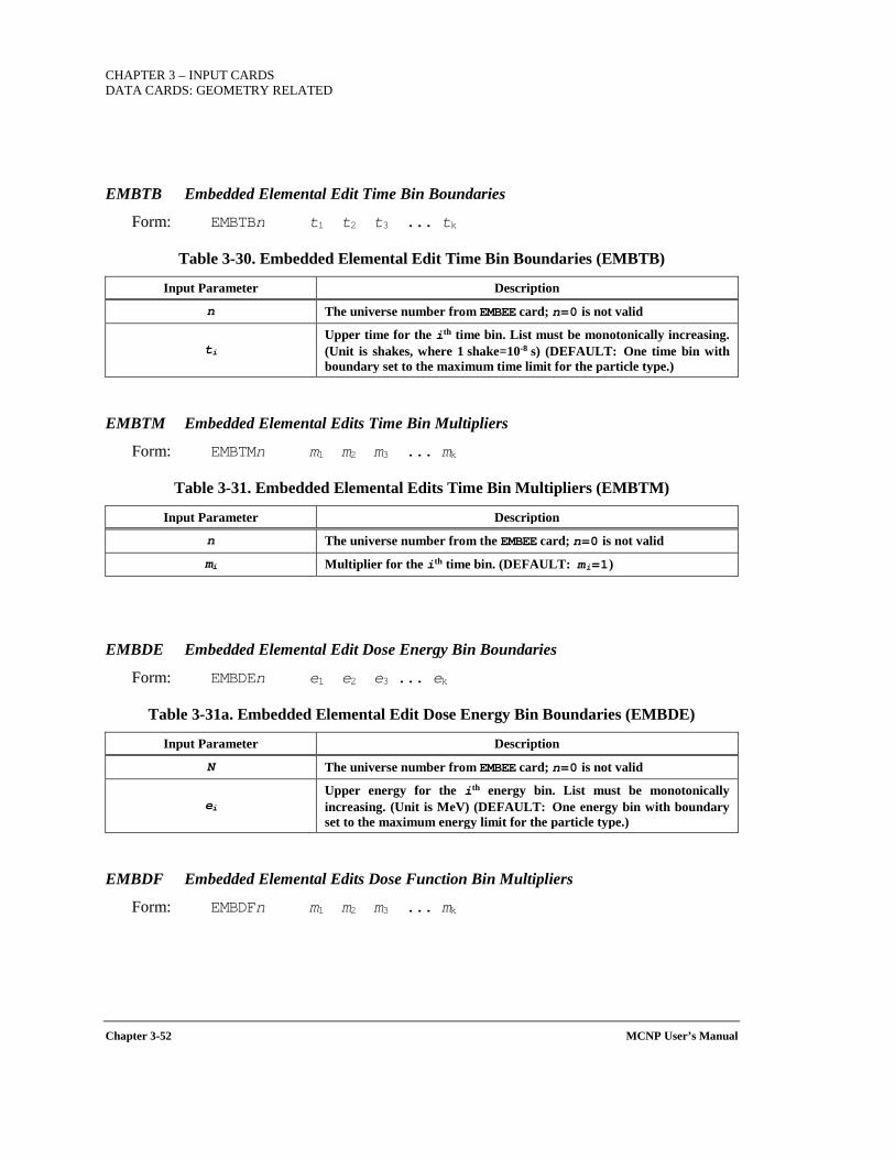
CHAPTER 3 – INPUT CARDS DATA CARDS: GEOMETRY RELATED
Chapter 3-52 MCNP User’s Manual
EMBTB Embedded Elemental Edit Time Bin Boundaries
Form: EMBTBn t1 t2 t3 ... tk
Table 3-30. Embedded Elemental Edit Time Bin Boundaries (EMBTB)
Input Parameter Description
n The universe number from EMBEE card; n=0 is not valid
ti Upper time for the ith time bin. List must be monotonically increasing. (Unit is shakes, where 1 shake=10-8 s) (DEFAULT: One time bin with boundary set to the maximum time limit for the particle type.)
EMBTM Embedded Elemental Edits Time Bin Multipliers
Form: EMBTMn m1 m2 m3 ... mk
Table 3-31. Embedded Elemental Edits Time Bin Multipliers (EMBTM)
Input Parameter Description
n The universe number from the EMBEE card; n=0 is not valid
mi Multiplier for the ith time bin. (DEFAULT: mi=1)
EMBDE Embedded Elemental Edit Dose Energy Bin Boundaries
Form: EMBDEn e1 e2 e3 ... ek
Table 3-31a. Embedded Elemental Edit Dose Energy Bin Boundaries (EMBDE)
Input Parameter Description
N The universe number from EMBEE card; n=0 is not valid
ei Upper energy for the ith energy bin. List must be monotonically increasing. (Unit is MeV) (DEFAULT: One energy bin with boundary set to the maximum energy limit for the particle type.)
EMBDF Embedded Elemental Edits Dose Function Bin Multipliers
Form: EMBDFn m1 m2 m3 ... mk
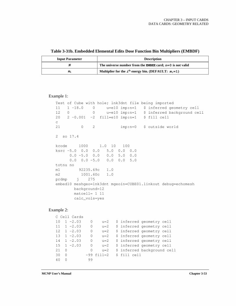
CHAPTER 3 – INPUT CARDS
DATA CARDS: GEOMETRY RELATED
MCNP User’s Manual Chapter 3-53
Table 3-31b. Embedded Elemental Edits Dose Function Bin Multipliers (EMBDF)
Input Parameter Description
N The universe number from the EMBEE card; n=0 is not valid
mi Multiplier for the ith energy bin. (DEFAULT: mi=1)
Example 1: Test of Cube with hole; lnk3dnt file being imported 11 1 -18.0 0 u=e10 imp:n=1 $ inferred geometry cell 12 0 0 u=e10 imp:n=1 $ inferred background cell 20 2 -0.001 -2 fill=e10 imp:n=1 $ fill cell c 21 0 2 imp:n=0 $ outside world 2 so 17.4 kcode 1000 1.0 10 100 ksrc -5.0 0.0 0.0 5.0 0.0 0.0 0.0 -5.0 0.0 0.0 5.0 0.0 0.0 0.0 -5.0 0.0 0.0 5.0 totnu no m1 92235.69c 1.0 m2 1001.60c 1.0 prdmp j 275 embed10 meshgeo=lnk3dnt mgeoin=CUBE01.linkout debug=echomesh background=12 matcell= 1 11 calc_vols=yes
Example 2: C Cell Cards 10 1 -2.03 0 u=2 $ inferred geometry cell 11 1 -2.03 0 u=2 $ inferred geometry cell 12 1 -2.03 0 u=2 $ inferred geometry cell 13 1 -2.03 0 u=2 $ inferred geometry cell 14 1 -2.03 0 u=2 $ inferred geometry cell 15 1 -2.03 0 u=2 $ inferred geometry cell 21 0 0 u=2 $ inferred background cell 30 0 -99 fill=2 $ fill cell 40 0 99
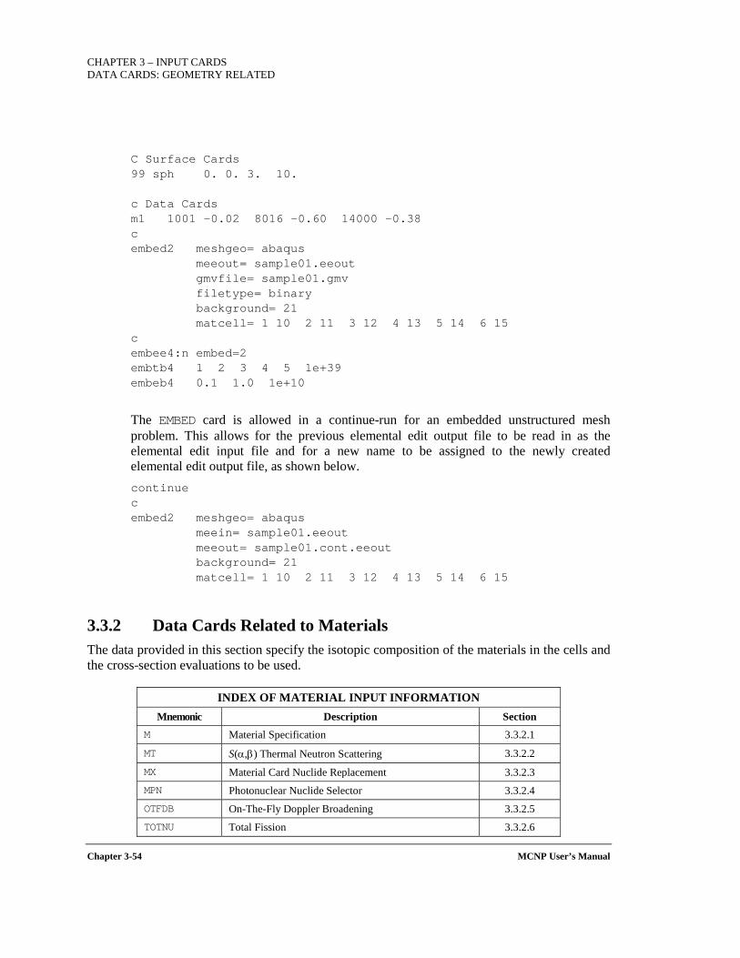
CHAPTER 3 – INPUT CARDS DATA CARDS: GEOMETRY RELATED
Chapter 3-54 MCNP User’s Manual
C Surface Cards 99 sph 0. 0. 3. 10. c Data Cards m1 1001 -0.02 8016 -0.60 14000 -0.38 c embed2 meshgeo= abaqus meeout= sample01.eeout gmvfile= sample01.gmv filetype= binary background= 21 matcell= 1 10 2 11 3 12 4 13 5 14 6 15 c embee4:n embed=2 embtb4 1 2 3 4 5 1e+39 embeb4 0.1 1.0 1e+10
The EMBED card is allowed in a continue-run for an embedded unstructured mesh problem. This allows for the previous elemental edit output file to be read in as the elemental edit input file and for a new name to be assigned to the newly created elemental edit output file, as shown below. continue c embed2 meshgeo= abaqus meein= sample01.eeout meeout= sample01.cont.eeout background= 21 matcell= 1 10 2 11 3 12 4 13 5 14 6 15
3.3.2 Data Cards Related to Materials The data provided in this section specify the isotopic composition of the materials in the cells and the cross-section evaluations to be used.
INDEX OF MATERIAL INPUT INFORMATION Mnemonic Description Section
M Material Specification 3.3.2.1
MT S(α,β) Thermal Neutron Scattering 3.3.2.2
MX Material Card Nuclide Replacement 3.3.2.3
MPN Photonuclear Nuclide Selector 3.3.2.4 OTFDB On-The-Fly Doppler Broadening 3.3.2.5 TOTNU Total Fission 3.3.2.6
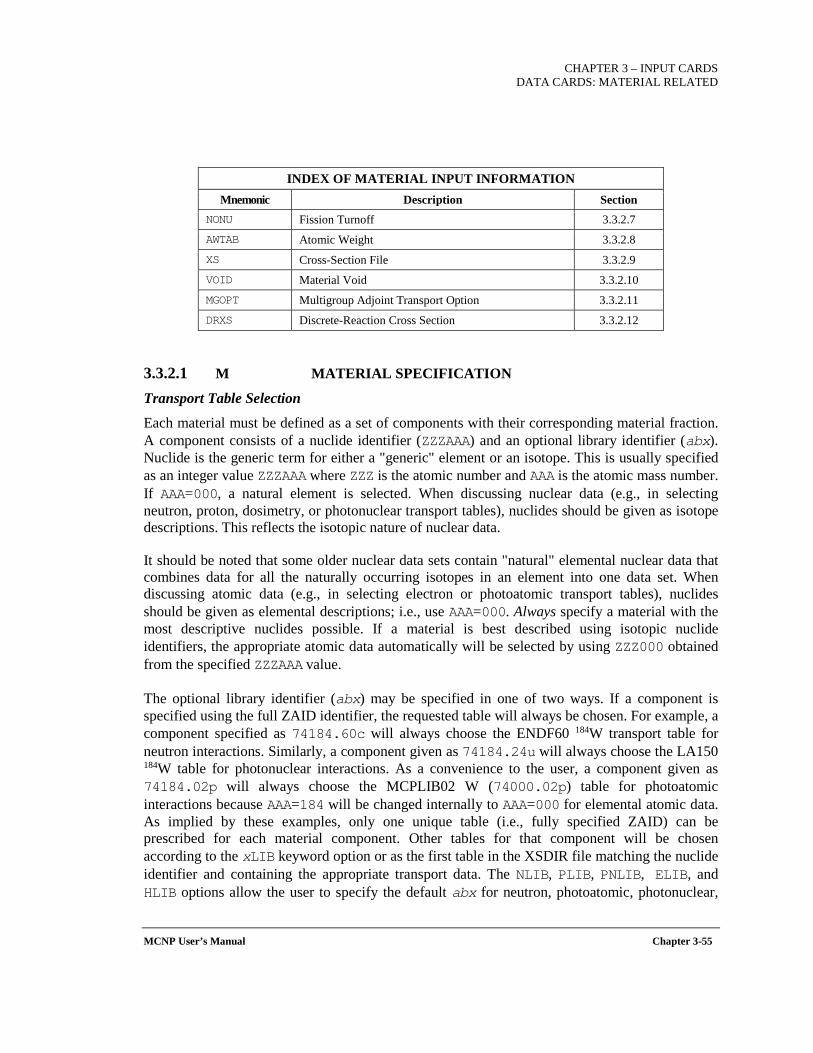
CHAPTER 3 – INPUT CARDS
DATA CARDS: MATERIAL RELATED
MCNP User’s Manual Chapter 3-55
INDEX OF MATERIAL INPUT INFORMATION Mnemonic Description Section
NONU Fission Turnoff 3.3.2.7
AWTAB Atomic Weight 3.3.2.8
XS Cross-Section File 3.3.2.9
VOID Material Void 3.3.2.10
MGOPT Multigroup Adjoint Transport Option 3.3.2.11
DRXS Discrete-Reaction Cross Section 3.3.2.12
3.3.2.1 M MATERIAL SPECIFICATION
Transport Table Selection
Each material must be defined as a set of components with their corresponding material fraction. A component consists of a nuclide identifier (ZZZAAA) and an optional library identifier (abx). Nuclide is the generic term for either a "generic" element or an isotope. This is usually specified as an integer value ZZZAAA where ZZZ is the atomic number and AAA is the atomic mass number. If AAA=000, a natural element is selected. When discussing nuclear data (e.g., in selecting neutron, proton, dosimetry, or photonuclear transport tables), nuclides should be given as isotope descriptions. This reflects the isotopic nature of nuclear data.
It should be noted that some older nuclear data sets contain "natural" elemental nuclear data that combines data for all the naturally occurring isotopes in an element into one data set. When discussing atomic data (e.g., in selecting electron or photoatomic transport tables), nuclides should be given as elemental descriptions; i.e., use AAA=000. Always specify a material with the most descriptive nuclides possible. If a material is best described using isotopic nuclide identifiers, the appropriate atomic data automatically will be selected by using ZZZ000 obtained from the specified ZZZAAA value.
The optional library identifier (abx) may be specified in one of two ways. If a component is specified using the full ZAID identifier, the requested table will always be chosen. For example, a component specified as 74184.60c will always choose the ENDF60 184W transport table for neutron interactions. Similarly, a component given as 74184.24u will always choose the LA150 184W table for photonuclear interactions. As a convenience to the user, a component given as 74184.02p will always choose the MCPLIB02 W (74000.02p) table for photoatomic interactions because AAA=184 will be changed internally to AAA=000 for elemental atomic data. As implied by these examples, only one unique table (i.e., fully specified ZAID) can be prescribed for each material component. Other tables for that component will be chosen according to the xLIB keyword option or as the first table in the XSDIR file matching the nuclide identifier and containing the appropriate transport data. The NLIB, PLIB, PNLIB, ELIB, and HLIB options allow the user to specify the default abx for neutron, photoatomic, photonuclear,
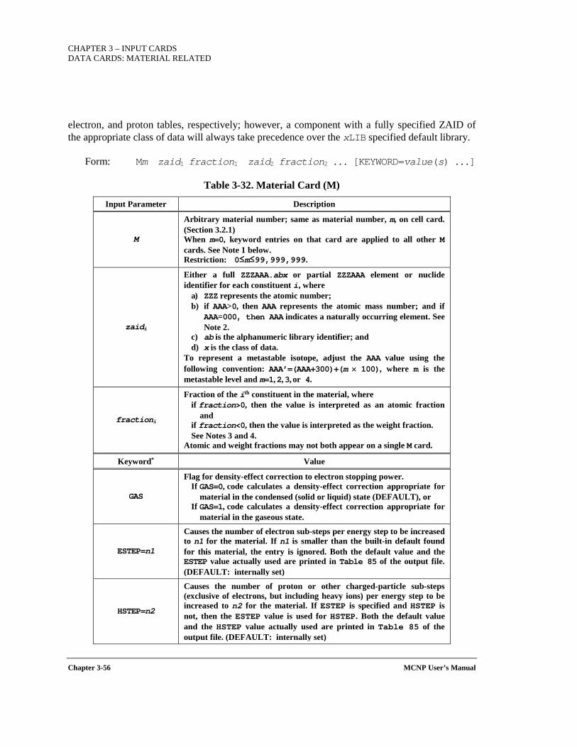
CHAPTER 3 – INPUT CARDS DATA CARDS: MATERIAL RELATED
Chapter 3-56 MCNP User’s Manual
electron, and proton tables, respectively; however, a component with a fully specified ZAID of the appropriate class of data will always take precedence over the xLIB specified default library.
Form: Mm zaid1 fraction1 zaid2 fraction2 ... [KEYWORD=value(s) ...]
Table 3-32. Material Card (M)
Input Parameter Description
M
Arbitrary material number; same as material number, m, on cell card. (Section 3.2.1) When m=0, keyword entries on that card are applied to all other M cards. See Note 1 below. Restriction: 0≤m≤99,999,999.
zaidi
Either a full ZZZAAA.abx or partial ZZZAAA element or nuclide identifier for each constituent i, where
a) ZZZ represents the atomic number; b) if AAA>0, then AAA represents the atomic mass number; and if
AAA=000, then AAA indicates a naturally occurring element. See Note 2.
c) ab is the alphanumeric library identifier; and d) x is the class of data.
To represent a metastable isotope, adjust the AAA value using the following convention: AAA’=(AAA+300)+(m × 100), where m is the metastable level and m=1, 2, 3, or 4.
fractioni
Fraction of the ith constituent in the material, where if fraction>0, then the value is interpreted as an atomic fraction
and if fraction<0, then the value is interpreted as the weight fraction. See Notes 3 and 4.
Atomic and weight fractions may not both appear on a single M card.
Keyword* Value
GAS
Flag for density-effect correction to electron stopping power. If GAS=0, code calculates a density-effect correction appropriate for
material in the condensed (solid or liquid) state (DEFAULT), or If GAS=1, code calculates a density-effect correction appropriate for
material in the gaseous state.
ESTEP=n1
Causes the number of electron sub-steps per energy step to be increased to n1 for the material. If n1 is smaller than the built-in default found for this material, the entry is ignored. Both the default value and the ESTEP value actually used are printed in Table 85 of the output file. (DEFAULT: internally set)
HSTEP=n2
Causes the number of proton or other charged-particle sub-steps (exclusive of electrons, but including heavy ions) per energy step to be increased to n2 for the material. If ESTEP is specified and HSTEP is not, then the ESTEP value is used for HSTEP. Both the default value and the HSTEP value actually used are printed in Table 85 of the output file. (DEFAULT: internally set)
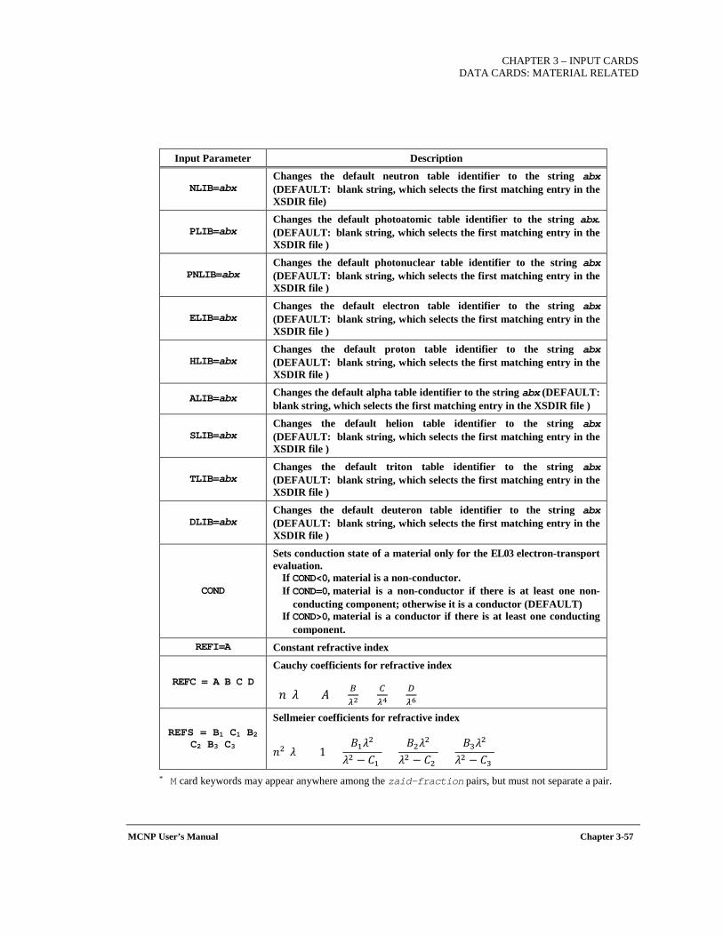
CHAPTER 3 – INPUT CARDS
DATA CARDS: MATERIAL RELATED
MCNP User’s Manual Chapter 3-57
Input Parameter Description
NLIB=abx Changes the default neutron table identifier to the string abx (DEFAULT: blank string, which selects the first matching entry in the XSDIR file)
PLIB=abx Changes the default photoatomic table identifier to the string abx. (DEFAULT: blank string, which selects the first matching entry in the XSDIR file )
PNLIB=abx Changes the default photonuclear table identifier to the string abx (DEFAULT: blank string, which selects the first matching entry in the XSDIR file )
ELIB=abx Changes the default electron table identifier to the string abx (DEFAULT: blank string, which selects the first matching entry in the XSDIR file )
HLIB=abx Changes the default proton table identifier to the string abx (DEFAULT: blank string, which selects the first matching entry in the XSDIR file )
ALIB=abx Changes the default alpha table identifier to the string abx (DEFAULT: blank string, which selects the first matching entry in the XSDIR file )
SLIB=abx Changes the default helion table identifier to the string abx (DEFAULT: blank string, which selects the first matching entry in the XSDIR file )
TLIB=abx Changes the default triton table identifier to the string abx (DEFAULT: blank string, which selects the first matching entry in the XSDIR file )
DLIB=abx Changes the default deuteron table identifier to the string abx (DEFAULT: blank string, which selects the first matching entry in the XSDIR file )
COND
Sets conduction state of a material only for the EL03 electron-transport evaluation.
If COND<0, material is a non-conductor. If COND=0, material is a non-conductor if there is at least one non-
conducting component; otherwise it is a conductor (DEFAULT) If COND>0, material is a conductor if there is at least one conducting
component. REFI=A Constant refractive index
REFC = A B C D
Cauchy coefficients for refractive index
𝑛𝑛(𝜆𝜆) = 𝐴𝐴 + 𝐵𝐵𝜆𝜆2
+ 𝐶𝐶𝜆𝜆4
+ 𝐷𝐷𝜆𝜆6
REFS = B1 C1 B2 C2 B3 C3
Sellmeier coefficients for refractive index
𝑛𝑛2(𝜆𝜆) = 1 + 𝐵𝐵1𝜆𝜆2
𝜆𝜆2 − 𝐶𝐶1 +
𝐵𝐵2𝜆𝜆2
𝜆𝜆2 − 𝐶𝐶2 +
𝐵𝐵3𝜆𝜆2
𝜆𝜆2 − 𝐶𝐶3
* M card keywords may appear anywhere among the zaid-fraction pairs, but must not separate a pair.

CHAPTER 3 – INPUT CARDS DATA CARDS: MATERIAL RELATED
Chapter 3-58 MCNP User’s Manual
Use: Required if you want materials in cells. Recall that an equals sign (=) following a keyword, such as the xLIB keywords, is optional. Inclusion of the decimal point in the library abx designation (e.g., .70c) is permitted, but not required.
Note 1: An M0 card may be specified to select default cross-section library identifiers via the library keywords NLIB, HLIB, PLIB, PNLIB, and ELIB, for all materials specified in the input file. Default cross-section library identifiers also may be specified for an individual material Mm. (m≠0). Fully specified ZAIDs on an Mm card override the default structure library selections for material m..
Note 2: For naturally occurring elements, AAA=000. Very few natural-element libraries exist within the isotopic data libraries (i.e., neutron, proton, and photonuclear); examine the XSDIR library directory file to determine availability. Natural elements not available from among those listed in the XSDIR file must be constructed on an M card by adding together the individual isotopes if they are available. The value of AAA for photons and electrons is always 000, providing no distinction between isotope and element.
Note 3: The nuclide fractions can be normalized to 1.0 or left un-normalized, in which case the code will perform the normalization.
Note 4: The code uses the atomic weight ratio values from the transport table to convert mass fractions to atom fractions. To avoid this conversion and therefore ensure the most accurate material representation, it is recommended that atom fractions be specified.
Example 1: M1 6012.50c 1 8016.01p 2 NLIB=60c PNLIB=24u PLIB=02p
This material definition will cause the data tables 6012.50c and 8016.60c to be used for neutron transport. The component 6012.50c is a fully specified neutron transport table that takes precedence over the NLIB default abx specifier. The 02p portion of the component 8016.02p is ignored because it specifies the wrong class of table; therefore the NLIB default 60c is used to choose the 8016.60c neutron transport table.
Similarly, the material definition will invoke the photoatomic transport tables 6000.02p and 8000.01p by ignoring the mass number (AAA) and using the PLIB specified abx 02p for carbon and the component specified 01p for oxygen. Because neither component abx is appropriate for specification of photonuclear tables, the data tables 6012.24u and 8016.24u will be chosen based on the PNLIB default abx 24u. Because no abx is specified for electron or proton tables via the component description or by the ELIB or HLIB options, the first matching entries in the XSDIR file will determine the selection of electron and proton tables.
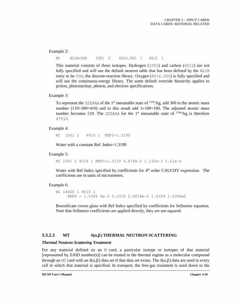
CHAPTER 3 – INPUT CARDS
DATA CARDS: MATERIAL RELATED
MCNP User’s Manual Chapter 3-59
Example 2: M1 NLIB=50D 1001 2 8016.50C 1 6012 1
This material consists of three isotopes. Hydrogen (1001) and carbon (6012) are not fully specified and will use the default neutron table that has been defined by the NLIB entry to be 50D, the discrete-reaction library. Oxygen (8016.50C) is fully specified and will use the continuous-energy library. The same default override hierarchy applies to proton, photonuclear, photon, and electron specifications.
Example 3:
To represent the ZZZAAA of the 1st metastable state of 110mAg, add 300 to the atomic mass number (110+300=410) and to this result add 1×100=100. The adjusted atomic mass number becomes 510. The ZZZAAA for the 1st metastable state of 110mAg is therefore 47510.
Example 4: M1 1001 2 8016 1 REFI=1.3199
Water with a constant Ref. Index=1.3199
Example 5: M1 1001 2 8016 1 REFC=1.3119 6.878e-2 1.132e-3 1.11e-4
Water with Ref Index specified by coefficients for 4th order CAUCHY expression. The coefficients are in units of micrometers.
Example 6: M1 14028 1 8016 2 REFS = 1.0396 6e-3 0.2318 2.0018e-2 1.0104 1.0356e2 Borosilicate crown glass with Ref Index specified by coefficients for Sellmeier equation. Note that Sellmeier coefficients are applied directly, they are not squared.
3.3.2.2 MT S(α,β) THERMAL NEUTRON SCATTERING
Thermal Neutron Scattering Treatment
For any material defined on an M card, a particular isotope or isotopes of that material [represented by ZAID number(s)] can be treated in the thermal regime as a molecular compound through an MT card with an S(α,β) data set if that data set exists. The S(α,β) data are used in every cell in which that material is specified. In transport, the free-gas treatment is used down to the

CHAPTER 3 – INPUT CARDS DATA CARDS: MATERIAL RELATED
Chapter 3-60 MCNP User’s Manual
energy where S(α,β) data are available. At that point, the S(α,β) treatment automatically overrides the free-gas treatment (that is, there is no mixing of the two treatments for the same isotope in the same material at a given energy). Typically the free-gas model is used for each isotope of a material down to a few electron volts and then the S(α,β) treatment takes over for the isotope(s) comprising the substance specified on the MT card. In general, S(α,β) effects are most significant below 2 eV. The appearance of an MT card will cause the loading of the corresponding S(α,β) data from the thermal data file. Multiple S(α,β) libraries can be specified on one MT card, but only if the libraries treat different isotopes—otherwise, the first S(α,β) treatment is used.
Form: MTm x1 x2 ...
Table 3-33. S(α,β) Card (MT)
Input Parameter Description
m Material identifier, same as m on the corresponding material (Mm) card.
xi S(α,β) identifier corresponding to a particular component on the Mm card. See Note 1.
Default: None.
Use: Essential for problems with thermal neutron scattering.
Note 1: S(α,β) contributions to detectors of DXTRAN spheres are approximate.
Example 1: M1 1001 2 8016 1 $ light water MT1 LWTR.02T
Example 2: M8 6012 1 $ graphite MT8 GRPH.06T
Example 3:
When a particle is within the energy regime at which the S(α,β) treatment applies, the specification
M1 1001 2 8016 1 4009 1e-3 $ light water w/ small amt of Be MT1 LWTR.01t BE.01t
will substitute the light-water S(α,β) library for the hydrogen (1001) and the beryllium metal library for the beryllium (4009).
However, the specification

CHAPTER 3 – INPUT CARDS
DATA CARDS: MATERIAL RELATED
MCNP User’s Manual Chapter 3-61
M1 4009 2 8016 1 $ Be oxide MT1 BE.60T BEO.60T
will not work as desired because both libraries will try to substitute for the beryllium (4009) in the problem. Only the first S(α,β) specification (for be.60t) will be used.
3.3.2.3 MX MATERIAL CARD NUCLIDE SUBSTITUTION
Mixing of Nuclide Physics Models and Data Tables
The MCNP6 nuclide substitution capability [HEN03] enables mixing of physics models and data tables for individual isotopes. Different nuclides can be substituted for different particle types. For example, natural carbon and calcium can be used for neutrons, whereas 12C and 40Ca can be used for protons and photonuclear reactions.
Above tabular data limits, models are automatically called in MCNP6. The model to be used depends on values set on the LCA card (Section 3.3.3.7.2). The sole exception is photonuclear interactions, for which CEM03.03 [MAS12, MAS08, MAS05b, MAS05a,GUD83] is always used regardless of whether CEM03.03 is used for other particles (see the LCA card). Using the term "MODEL" on an MX card will substitute model physics for the entire energy range of a particle—no tabular data will be used. This option should be carefully considered before use. The parameter '0' on an MX card eliminates all interaction physics, whether model or table-based. This makes sense in the case of photonuclear interactions on hydrogen, which do not exist in nature, but should be avoided for other cases.
Form: MXm:<pl> zaid1 zaid2 ...
Table 3-34. Nuclide Substitution (MX)
Input Parameter Description
m Material number of an associated Mm material card. See Note 1.
<pl> Particle designator (see Table 2-2); allowed values are neutron (N), photonuclear (P), proton (H), deuteron (D), triton (T), hellion (S), and alpha (A).
zaidi
If zaidi is set to the full library identifier, ZZZAAA.abx, substitute the specified library for the ith nuclide identifier on the M card.
If zaidi is set to, ZZZAAA, replace the ith nuclide on the M card with the nuclide ZZZAAA.
If zaidi=MODEL, substitute model physics for the ith nuclide on the M card. A mixture of models and tabular data may be specified for nuclides on a single M card.
If zaidi=0 on a photonuclear substitution card (MXm:P), then omit photonuclear reactions for zaidi. This option is only available for photonuclear particles.
No substitutions are allowed for photoatomic (P) and electron (E) data because these data depend only on Z and are not isotope-specific.
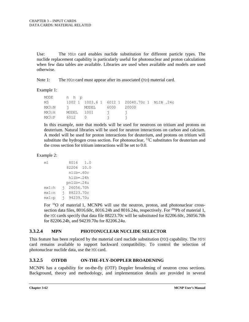
CHAPTER 3 – INPUT CARDS DATA CARDS: MATERIAL RELATED
Chapter 3-62 MCNP User’s Manual
Use: The MXm card enables nuclide substitution for different particle types. The nuclide replacement capability is particularly useful for photonuclear and proton calculations when few data tables are available. Libraries are used when available and models are used otherwise.
Note 1: The MXm card must appear after its associated (Mm) material card.
Example 1: MODE n h p M3 1002 1 1003.6 1 6012 1 20040.70c 1 NLIB .24c MX3:N j MODEL 6000 20000 MX3:H MODEL 1001 j j MX3:P 6012 0 j j
In this example, note that models will be used for neutrons on tritium and protons on deuterium. Natural libraries will be used for neutron interactions on carbon and calcium. A model will be used for proton interactions for deuterium, and protons on tritium will substitute the hydrogen cross section. For photonuclear, 12C substitutes for deuterium and the cross section for tritium interactions will be set to 0.0.
Example 2: m1 8016 1.0 82206 10.0 nlib=.60c hlib=.24h pnlib=.24u mx1:h j 26056.70h mx1:n j 88223.70c mx1:p j 94239.70u
For 16O of material 1, MCNP6 will use the neutron, proton, and photonuclear cross-section data files, 8016.60c, 8016.24h and 8016.24u, respectively. For 206Pb of material 1, the MX cards specify that data file 88223.70c will be substituted for 82206.60c, 26056.70h for 82206.24h, and 94239.70u for 82206.24u.
3.3.2.4 MPN PHOTONUCLEAR NUCLIDE SELECTOR
This feature has been replaced by the material card nuclide substitution (MX) capability. The MPN card remains available to support backward compatibility. To control the selection of photonuclear nuclide data, use the MX card.
3.3.2.5 OTFDB ON-THE-FLY-DOPPLER BROADENING
MCNP6 has a capability for on-the-fly (OTF) Doppler broadening of neutron cross sections. Background, theory and methodology, and implementation details are provided in several
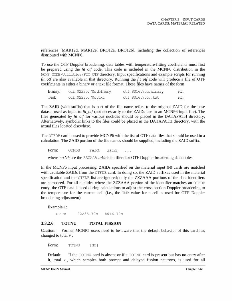
CHAPTER 3 – INPUT CARDS
DATA CARDS: MATERIAL RELATED
MCNP User’s Manual Chapter 3-63
references [MAR12d, MAR12e, BRO12a, BRO12b], including the collection of references distributed with MCNP6.
To use the OTF Doppler broadening, data tables with temperature-fitting coefficients must first be prepared using the fit_otf code. This code is included in the MCNP6 distribution in the MCNP_CODE/Utilities/FIT_OTF directory. Input specifications and example scripts for running fit_otf are also available in that directory. Running the fit_otf code will produce a file of OTF coefficients in either a binary or a text file format. These files have names of the form
Binary: otf_92235.70c.binary otf_8016.70c.binary etc. Test: otf.92235.70c.txt otf_8016.70c..txt etc.
The ZAID (with suffix) that is part of the file name refers to the original ZAID for the base dataset used as input to fit_otf (not necessarily to the ZAIDs use in an MCNP6 input file). The files generated by fit_otf for various nuclides should be placed in the DATAPATH directory. Alternatively, symbolic links to the files could be placed in the DATAPATH directory, with the actual files located elsewhere.
The OTFDB card is used to provide MCNP6 with the list of OTF data files that should be used in a calculation. The ZAID portion of the file names should be supplied, including the ZAID suffix.
Form: OTFDB zaid1 zaid2 ...
where zaidi are the ZZZAAA.abx identifiers for OTF Doppler broadening data tables.
In the MCNP6 input processing, ZAIDs specified on the material input (M) cards are matched with available ZAIDs from the OTFDB card. In doing so, the ZAID suffixes used in the material specification and the OTFDB list are ignored; only the ZZZAAA portions of the data identifiers are compared. For all nuclides where the ZZZAAA portion of the identifier matches an OTFDB entry, the OTF data is used during calculations to adjust the cross-section Doppler broadening to the temperature for the current cell (i.e., the TMP value for a cell is used for OTF Doppler broadening adjustment).
Example 1: OTFDB 92235.70c 8016.70c
3.3.2.6 TOTNU TOTAL FISSION
Caution: Former MCNP5 users need to be aware that the default behavior of this card has changed to total .
Form: TOTNU [NO]
Default: If the TOTNU card is absent or if a TOTNU card is present but has no entry after it, total , which samples both prompt and delayed fission neutrons, is used for all
ν
ν
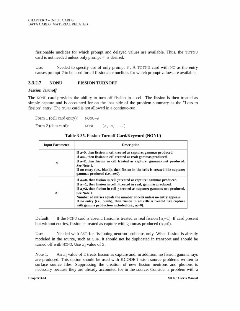
CHAPTER 3 – INPUT CARDS DATA CARDS: MATERIAL RELATED
Chapter 3-64 MCNP User’s Manual
fissionable nuclides for which prompt and delayed values are available. Thus, the TOTNU card is not needed unless only prompt is desired.
Use: Needed to specify use of only prompt . A TOTNU card with NO as the entry causes prompt to be used for all fissionable nuclides for which prompt values are available.
3.3.2.7 NONU FISSION TURNOFF
Fission Turnoff
The NONU card provides the ability to turn off fission in a cell. The fission is then treated as simple capture and is accounted for on the loss side of the problem summary as the "Loss to fission" entry. The NONU card is not allowed in a continue-run.
Form 1 (cell card entry): NONU=a
Form 2 (data card): NONU [a1 a2 ...]
Table 3-35. Fission Turnoff Card/Keyword (NONU)
Input Parameter Description
a
If a=0, then fission in cell treated as capture; gammas produced. If a=1, then fission in cell treated as real; gammas produced. If a=2, then fission in cell treated as capture; gammas not produced. See Note 1. If no entry (i.e., blank), then fission in the cells is treated like capture; gammas produced (i.e., a=0).
aj
If aj=0, then fission in cell j treated as capture; gammas produced. If aj=1, then fission in cell j treated as real; gammas produced. If aj=2, then fission in cell j treated as capture; gammas not produced. See Note 1. Number of entries equals the number of cells unless no entry appears. If no entry (i.e., blank), then fission in all cells is treated like capture with gamma production included (i.e., aj=0).
Default: If the NONU card is absent, fission is treated as real fission (aj=1). If card present but without entries, fission is treated as capture with gammas produced (aj=0).
Use: Needed with SSR for fissioning neutron problems only. When fission is already modeled in the source, such as SSR, it should not be duplicated in transport and should be turned off with NONU. Use aj value of 2.
Note 1: An aj value of 2 treats fission as capture and, in addition, no fission gamma rays are produced. This option should be used with KCODE fission source problems written to surface source files. Suppressing the creation of new fission neutrons and photons is necessary because they are already accounted for in the source. Consider a problem with a
ν
νν
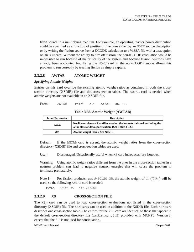
CHAPTER 3 – INPUT CARDS
DATA CARDS: MATERIAL RELATED
MCNP User’s Manual Chapter 3-65
fixed source in a multiplying medium. For example, an operating reactor power distribution could be specified as a function of position in the core either by an SDEF source description or by writing the fission source from a KCODE calculation to a WSSA file with a CEL option on an SSW card. Without the ability to turn off fission, the non-KCODE calculation would be impossible to run because of the criticality of the system and because fission neutrons have already been accounted for. Using the NONU card in the non-KCODE mode allows this problem to run correctly by treating fission as simple capture.
3.3.2.8 AWTAB ATOMIC WEIGHT
Specifying Atomic Weights
Entries on this card override the existing atomic weight ratios as contained in both the cross-section directory (XSDIR) file and the cross-section tables. The AWTAB card is needed when atomic weights are not available in an XSDIR file.
Form: AWTAB zaid1 aw1 zaid2 aw2 ...
Table 3-36. Atomic Weight (AWTAB)
Input Parameter Description
zaidi Nuclide or element identifier used on the Mm material card excluding the x for class of data specification. (See Table 3-32.)
awi Atomic weight ratios. See Note 1.
Default: If the AWTAB card is absent, the atomic weight ratios from the cross-section directory (XSDIR) file and cross-section tables are used.
Use: Discouraged. Occasionally useful when XS card introduces rare isotopes.
Warning: Using atomic weight ratios different from the ones in the cross-section tables in a neutron problem can lead to negative neutron energies that will cause the problem to terminate prematurely.
Note 1: For fission products, zaid=50120.35, the atomic weight of tin ( ) will be used, so the following AWTAB card is needed:
AWTAB 50120.35 116.490609
3.3.2.9 XS CROSS-SECTION FILE
The XSn card can be used to load cross-section evaluations not listed in the cross-section directory (XSDIR) file. The XSn cards can be used in addition to the XSDIR file. Each XSn card describes one cross-section table. The entries for the XSn card are identical to those that appear in the default cross-section directory file (xsdir_mcnp6.2) provided with MCNP6, Version 2, except that the "+" is not used for continuation..
Sn12050
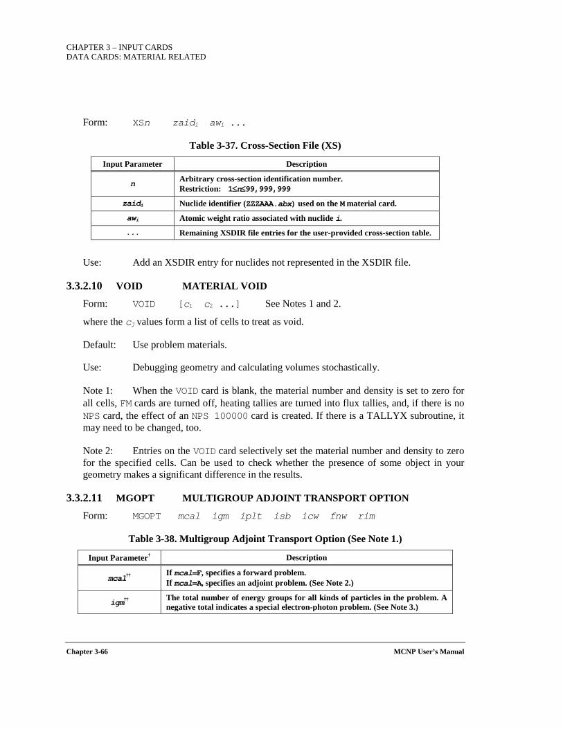
CHAPTER 3 – INPUT CARDS DATA CARDS: MATERIAL RELATED
Chapter 3-66 MCNP User’s Manual
Form: XSn zaidi awi ...
Table 3-37. Cross-Section File (XS)
Input Parameter Description
n Arbitrary cross-section identification number. Restriction: 1≤n≤99,999,999
zaidi Nuclide identifier (ZZZAAA.abx) used on the M material card.
awi Atomic weight ratio associated with nuclide i.
... Remaining XSDIR file entries for the user-provided cross-section table.
Use: Add an XSDIR entry for nuclides not represented in the XSDIR file.
3.3.2.10 VOID MATERIAL VOID
Form: VOID [c1 c2 ...] See Notes 1 and 2.
where the cj values form a list of cells to treat as void.
Default: Use problem materials.
Use: Debugging geometry and calculating volumes stochastically.
Note 1: When the VOID card is blank, the material number and density is set to zero for all cells, FM cards are turned off, heating tallies are turned into flux tallies, and, if there is no NPS card, the effect of an NPS 100000 card is created. If there is a TALLYX subroutine, it may need to be changed, too.
Note 2: Entries on the VOID card selectively set the material number and density to zero for the specified cells. Can be used to check whether the presence of some object in your geometry makes a significant difference in the results.
3.3.2.11 MGOPT MULTIGROUP ADJOINT TRANSPORT OPTION
Form: MGOPT mcal igm iplt isb icw fnw rim
Table 3-38. Multigroup Adjoint Transport Option (See Note 1.)
Input Parameter† Description
mcal†† If mcal=F, specifies a forward problem. If mcal=A, specifies an adjoint problem. (See Note 2.)
igm†† The total number of energy groups for all kinds of particles in the problem. A negative total indicates a special electron-photon problem. (See Note 3.)
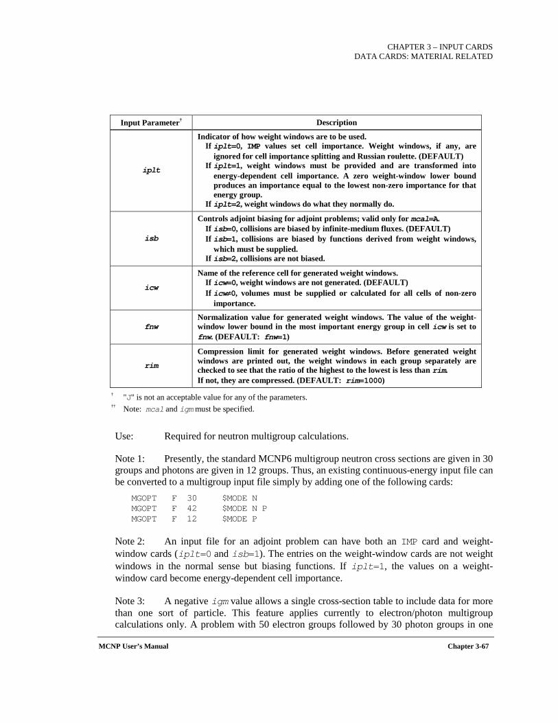
CHAPTER 3 – INPUT CARDS
DATA CARDS: MATERIAL RELATED
MCNP User’s Manual Chapter 3-67
Input Parameter† Description
iplt
Indicator of how weight windows are to be used. If iplt=0, IMP values set cell importance. Weight windows, if any, are
ignored for cell importance splitting and Russian roulette. (DEFAULT) If iplt=1, weight windows must be provided and are transformed into
energy-dependent cell importance. A zero weight-window lower bound produces an importance equal to the lowest non-zero importance for that energy group.
If iplt=2, weight windows do what they normally do.
isb
Controls adjoint biasing for adjoint problems; valid only for mcal=A. If isb=0, collisions are biased by infinite-medium fluxes. (DEFAULT) If isb=1, collisions are biased by functions derived from weight windows,
which must be supplied. If isb=2, collisions are not biased.
icw
Name of the reference cell for generated weight windows. If icw=0, weight windows are not generated. (DEFAULT) If icw≠0, volumes must be supplied or calculated for all cells of non-zero
importance.
fnw Normalization value for generated weight windows. The value of the weight-window lower bound in the most important energy group in cell icw is set to fnw. (DEFAULT: fnw=1)
rim
Compression limit for generated weight windows. Before generated weight windows are printed out, the weight windows in each group separately are checked to see that the ratio of the highest to the lowest is less than rim. If not, they are compressed. (DEFAULT: rim=1000)
† "J" is not an acceptable value for any of the parameters. †† Note: mcal and igm must be specified.
Use: Required for neutron multigroup calculations.
Note 1: Presently, the standard MCNP6 multigroup neutron cross sections are given in 30 groups and photons are given in 12 groups. Thus, an existing continuous-energy input file can be converted to a multigroup input file simply by adding one of the following cards:
MGOPT F 30 $MODE N MGOPT F 42 $MODE N P MGOPT F 12 $MODE P
Note 2: An input file for an adjoint problem can have both an IMP card and weight-window cards (iplt=0 and isb=1). The entries on the weight-window cards are not weight windows in the normal sense but biasing functions. If iplt=1, the values on a weight-window card become energy-dependent cell importance.
Note 3: A negative igm value allows a single cross-section table to include data for more than one sort of particle. This feature applies currently to electron/photon multigroup calculations only. A problem with 50 electron groups followed by 30 photon groups in one
CHAPTER 3 – INPUT CARDS DATA CARDS: MATERIAL RELATED
Chapter 3-68 MCNP User’s Manual
table would have igm=-80. Also, all tables must have the same group structure. A negative igm value will use the energy variable on the source or tally card as groups index unless it is associated with a distribution. For an energy distribution on the source card, there should be igm increasing integer entries for each group on the SI card. On a tally energy card, if there are fewer than igm entries, they will be taken as energies in MeV; otherwise, the bins will be according to group index. The particles can be separated in tallies by using the PTT keyword on the FTn tally special treatment card.
3.3.2.12 DRXS DISCRETE-REACTION CROSS SECTION
Discrete Energy Treatment
If the necessary discrete data are available, nuclides listed on the optional DRXS card are given a discrete energy treatment instead of the regular fully continuous-energy cross-section treatment.
All discrete reaction libraries are based on a 262-energy-group structure. Groups below 1 eV make the discrete treatment appropriate for thermal neutron problems near room temperature. All discrete reaction libraries have photon production data given in expanded format.
Form: DRXS [zaid1 zaid2 ... zaidi...] See Note 1.
where zaidi is an identifying number of the form ZZZAAA.ab, where ZZZ is the atomic number, AAA the atomic mass number, and ab the neutron library identifier.
Default: Continuous-energy cross-section treatment if DRXS is absent. If the DRXS card is present but has no entries after the mnemonic, discrete cross sections will be used for every nuclide, if available.
Use: Discouraged. Applies only to neutron cross sections. It is not recommended that this card be used unless you are transporting neutrons in an energy region where resonances and hence self-shielding are of little importance. If the problem under consideration meets this criterion, using the DRXS card can reduce computer storage requirements and enhance timesharing.
Note 1: Use of these discrete cross sections will not result in the calculation being what is commonly referred to as a multigroup Monte Carlo calculation because the only change is that the cross sections are represented in a histogram form rather than a continuous-energy form. The angular treatment used for scattering, energy sampling after scattering, etc., is performed using identical procedures and data as in the continuous-energy treatment. The user wanting to make a truly multigroup Monte Carlo calculation should use the MGOPT card multigroup capability.
3.3.3 Data Cards Related to Physics The data provided in this section describe the physics options that can be selected.
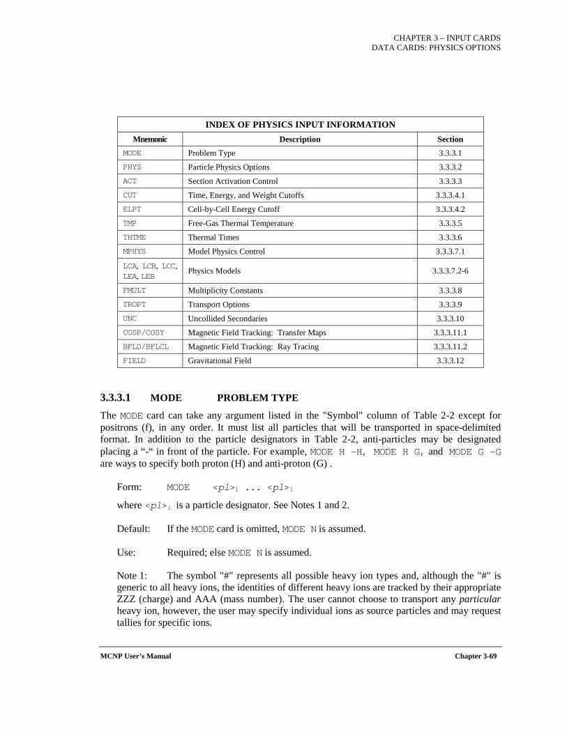
CHAPTER 3 – INPUT CARDS DATA CARDS: PHYSICS OPTIONS
MCNP User’s Manual Chapter 3-69
INDEX OF PHYSICS INPUT INFORMATION Mnemonic Description Section
MODE Problem Type 3.3.3.1 PHYS Particle Physics Options 3.3.3.2 ACT Section Activation Control 3.3.3.3 CUT Time, Energy, and Weight Cutoffs 3.3.3.4.1 ELPT Cell-by-Cell Energy Cutoff 3.3.3.4.2 TMP Free-Gas Thermal Temperature 3.3.3.5 THTME Thermal Times 3.3.3.6 MPHYS Model Physics Control 3.3.3.7.1
LCA, LCB, LCC, LEA, LEB Physics Models 3.3.3.7.2-6
FMULT Multiplicity Constants 3.3.3.8 TROPT Transport Options 3.3.3.9 UNC Uncollided Secondaries 3.3.3.10 COSP/COSY Magnetic Field Tracking: Transfer Maps 3.3.3.11.1 BFLD/BFLCL Magnetic Field Tracking: Ray Tracing 3.3.3.11.2 FIELD Gravitational Field 3.3.3.12
3.3.3.1 MODE PROBLEM TYPE
The MODE card can take any argument listed in the "Symbol" column of Table 2-2 except for positrons (f), in any order. It must list all particles that will be transported in space-delimited format. In addition to the particle designators in Table 2-2, anti-particles may be designated placing a “-“ in front of the particle. For example, MODE H –H, MODE H G, and MODE G -G are ways to specify both proton (H) and anti-proton (G) .
Form: MODE <pl>1 ... <pl>i
where <pl>i is a particle designator. See Notes 1 and 2.
Default: If the MODE card is omitted, MODE N is assumed.
Use: Required; else MODE N is assumed.
Note 1: The symbol "#" represents all possible heavy ion types and, although the "#" is generic to all heavy ions, the identities of different heavy ions are tracked by their appropriate ZZZ (charge) and AAA (mass number). The user cannot choose to transport any particular heavy ion, however, the user may specify individual ions as source particles and may request tallies for specific ions.
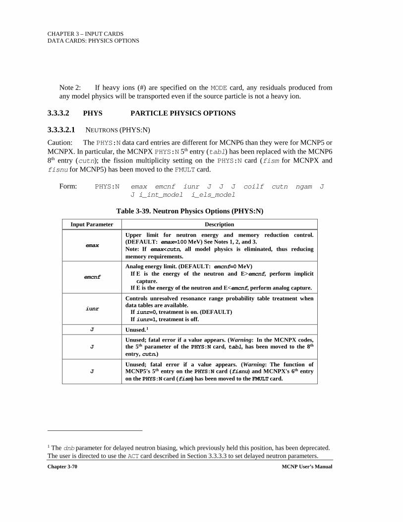
CHAPTER 3 – INPUT CARDS DATA CARDS: PHYSICS OPTIONS
Chapter 3-70 MCNP User’s Manual
Note 2: If heavy ions (#) are specified on the MODE card, any residuals produced from any model physics will be transported even if the source particle is not a heavy ion.
3.3.3.2 PHYS PARTICLE PHYSICS OPTIONS
3.3.3.2.1 NEUTRONS (PHYS:N)
Caution: The PHYS:N data card entries are different for MCNP6 than they were for MCNP5 or MCNPX. In particular, the MCNPX PHYS:N 5th entry (tabl) has been replaced with the MCNP6 8th entry (cutn); the fission multiplicity setting on the PHYS:N card (fism for MCNPX and fisnu for MCNP5) has been moved to the FMULT card.
Form: PHYS:N emax emcnf iunr J J J coilf cutn ngam J J i_int_model i_els_model
Table 3-39. Neutron Physics Options (PHYS:N)
Input Parameter Description
emax
Upper limit for neutron energy and memory reduction control. (DEFAULT: emax=100 MeV) See Notes 1, 2, and 3. Note: If emax<cutn, all model physics is eliminated, thus reducing memory requirements.
emcnf
Analog energy limit. (DEFAULT: emcnf=0 MeV) If E is the energy of the neutron and E>emcnf, perform implicit
capture. If E is the energy of the neutron and E<emcnf, perform analog capture.
iunr
Controls unresolved resonance range probability table treatment when data tables are available.
If iunr=0, treatment is on. (DEFAULT) If iunr=1, treatment is off.
J Unused.1
J Unused; fatal error if a value appears. (Warning: In the MCNPX codes, the 5th parameter of the PHYS:N card, tabl, has been moved to the 8th entry, cutn.)
J Unused; fatal error if a value appears. (Warning: The function of MCNP5's 5th entry on the PHYS:N card (fisnu) and MCNPX's 6th entry on the PHYS:N card (fism) has been moved to the FMULT card.
1 The dnb parameter for delayed neutron biasing, which previously held this position, has been deprecated. The user is directed to use the ACT card described in Section 3.3.3.3 to set delayed neutron parameters.
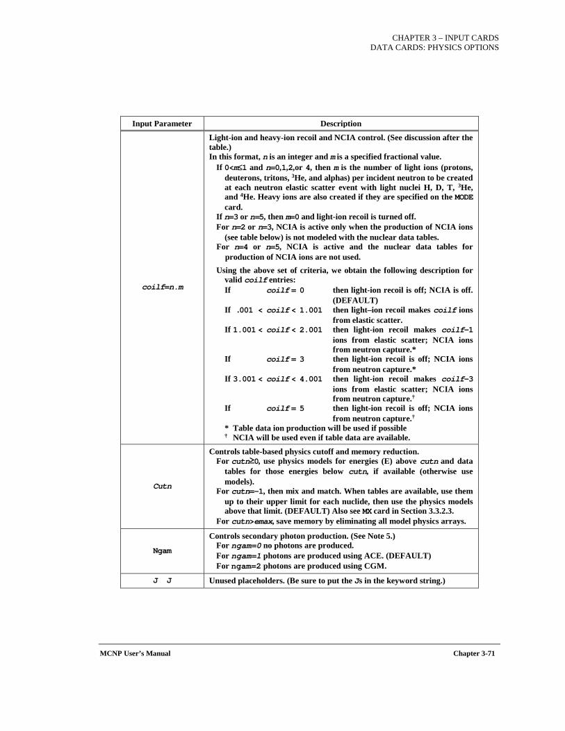
CHAPTER 3 – INPUT CARDS DATA CARDS: PHYSICS OPTIONS
MCNP User’s Manual Chapter 3-71
Input Parameter Description
coilf=n.m
Light-ion and heavy-ion recoil and NCIA control. (See discussion after the table.) In this format, n is an integer and m is a specified fractional value.
If 0<m≤1 and n=0,1,2,or 4, then m is the number of light ions (protons, deuterons, tritons, 3He, and alphas) per incident neutron to be created at each neutron elastic scatter event with light nuclei H, D, T, 3He, and 4He. Heavy ions are also created if they are specified on the MODE card.
If n=3 or n=5, then m=0 and light-ion recoil is turned off. For n=2 or n=3, NCIA is active only when the production of NCIA ions
(see table below) is not modeled with the nuclear data tables. For n=4 or n=5, NCIA is active and the nuclear data tables for
production of NCIA ions are not used. Using the above set of criteria, we obtain the following description for
valid coilf entries: If coilf = 0 then light-ion recoil is off; NCIA is off.
(DEFAULT) If .001 < coilf < 1.001 then light–ion recoil makes coilf ions
from elastic scatter. If 1.001 < coilf < 2.001 then light-ion recoil makes coilf-1
ions from elastic scatter; NCIA ions from neutron capture.*
If coilf = 3 then light-ion recoil is off; NCIA ions from neutron capture.*
If 3.001 < coilf < 4.001 then light-ion recoil makes coilf-3 ions from elastic scatter; NCIA ions from neutron capture.†
If coilf = 5 then light-ion recoil is off; NCIA ions from neutron capture.†
* Table data ion production will be used if possible † NCIA will be used even if table data are available.
Cutn
Controls table-based physics cutoff and memory reduction. For cutn≥0, use physics models for energies (E) above cutn and data
tables for those energies below cutn, if available (otherwise use models).
For cutn=-1, then mix and match. When tables are available, use them up to their upper limit for each nuclide, then use the physics models above that limit. (DEFAULT) Also see MX card in Section 3.3.2.3.
For cutn>emax, save memory by eliminating all model physics arrays.
Ngam
Controls secondary photon production. (See Note 5.) For ngam=0 no photons are produced. For ngam=1 photons are produced using ACE. (DEFAULT) For ngam=2 photons are produced using CGM.
J J Unused placeholders. (Be sure to put the Js in the keyword string.)

CHAPTER 3 – INPUT CARDS DATA CARDS: PHYSICS OPTIONS
Chapter 3-72 MCNP User’s Manual
Input Parameter Description
i_int_model
Controls treatment of nuclear interactions. If i_int_model=-1, no interactions. (Equivalent to setting the inelastic
cross section to zero.). If i_int_model=0, process all interactions. (DEFAULT) If i_int_model=1, no secondaries, inelastic collisions treated as weight
reduction. If i_int_model=2, no secondaries, inelastic collisions treated as
removal.
i_els_model
Controls treatment of nuclear elastic scattering. (See Note 4.) If i_els_model=-1, no elastic scattering (i.e., treat as pseudo collision) If i_els_model=0,elastic scattering by Prael/Liu/Striganov model.
(DEFAULT)
Default: PHYS:N 100 0 0 J J J 0 -1 J J J 0 0
Use: Encouraged. Also see FMULT card, Section 3.3.3.8. Continue-runs are not supported for delayed-neutron calculations that use model physics.
Note 1: Memory allocation can be reduced significantly for MODE N P E problems that do not invoke the photonuclear option. By setting the neutron table/model cutoff energy, cutn, greater than the maximum neutron energy, emax, physics models are disabled, storage requirements for secondary particles are greatly reduced, and, consequently, the amount of memory that must be allocated to several MCNP6 arrays is decreased. The reduction of memory usage is helpful particularly for burnup problems. Use of this memory reduction option (i.e., setting emax<cutn) is confirmed by the following OUTP file message: "memory reduction option specified, models disabled".
Note 2: The parameter emax must be higher than the highest energy in the problem or the physics is wrong. For problems with energies above 100 MeV, emax should be chosen carefully; the default is appropriate for problems with energies below 100 MeV.
Note 3: Neutron data above emax are expunged, as are neutron data below e, the lower energy cutoff, which is entered via the second entry on the CUT:N card (Section 3.3.3.4.1).
Note 4: Elastic scattering will be ignored if nuclear interactions are turned off.
Note 5: Correlated neutron and gamma emission is provided by CGM (unlike use of the ACE libraries) [WIL13], although execution times will increase. CGM/CGMF currently treats neutron interactions with targets of Z>9, except elastic scatter which continues to be treated by ACE libraries.
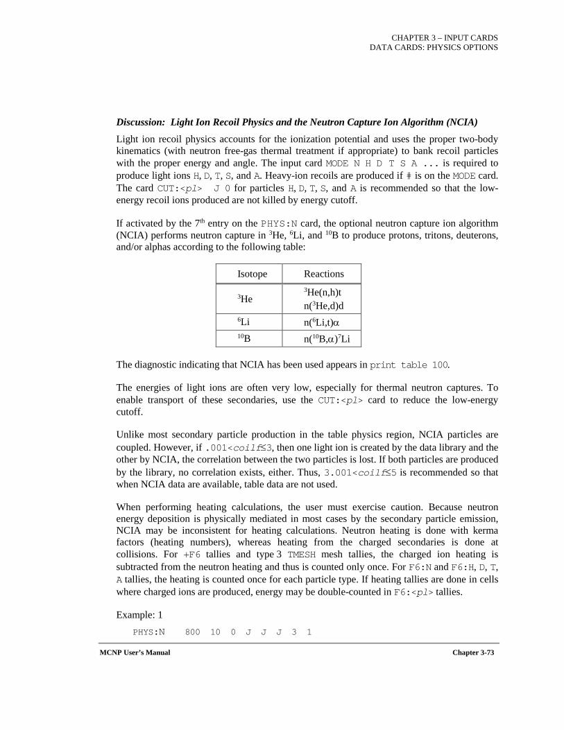
CHAPTER 3 – INPUT CARDS DATA CARDS: PHYSICS OPTIONS
MCNP User’s Manual Chapter 3-73
Discussion: Light Ion Recoil Physics and the Neutron Capture Ion Algorithm (NCIA)
Light ion recoil physics accounts for the ionization potential and uses the proper two-body kinematics (with neutron free-gas thermal treatment if appropriate) to bank recoil particles with the proper energy and angle. The input card MODE N H D T S A ... is required to produce light ions H, D, T, S, and A. Heavy-ion recoils are produced if # is on the MODE card. The card CUT:<pl> J 0 for particles H, D, T, S, and A is recommended so that the low-energy recoil ions produced are not killed by energy cutoff.
If activated by the 7th entry on the PHYS:N card, the optional neutron capture ion algorithm (NCIA) performs neutron capture in 3He, 6Li, and 10B to produce protons, tritons, deuterons, and/or alphas according to the following table:
Isotope Reactions
3He 3He(n,h)t n(3He,d)d
6Li n(6Li,t)α 10B n(10B,α)7Li
The diagnostic indicating that NCIA has been used appears in print table 100.
The energies of light ions are often very low, especially for thermal neutron captures. To enable transport of these secondaries, use the CUT:<pl> card to reduce the low-energy cutoff.
Unlike most secondary particle production in the table physics region, NCIA particles are coupled. However, if .001<coilf≤3, then one light ion is created by the data library and the other by NCIA, the correlation between the two particles is lost. If both particles are produced by the library, no correlation exists, either. Thus, 3.001<coilf≤5 is recommended so that when NCIA data are available, table data are not used.
When performing heating calculations, the user must exercise caution. Because neutron energy deposition is physically mediated in most cases by the secondary particle emission, NCIA may be inconsistent for heating calculations. Neutron heating is done with kerma factors (heating numbers), whereas heating from the charged secondaries is done at collisions. For +F6 tallies and type 3 TMESH mesh tallies, the charged ion heating is subtracted from the neutron heating and thus is counted only once. For F6:N and F6:H, D, T, A tallies, the heating is counted once for each particle type. If heating tallies are done in cells where charged ions are produced, energy may be double-counted in F6:<pl> tallies.
Example: 1 PHYS:N 800 10 0 J J J 3 1
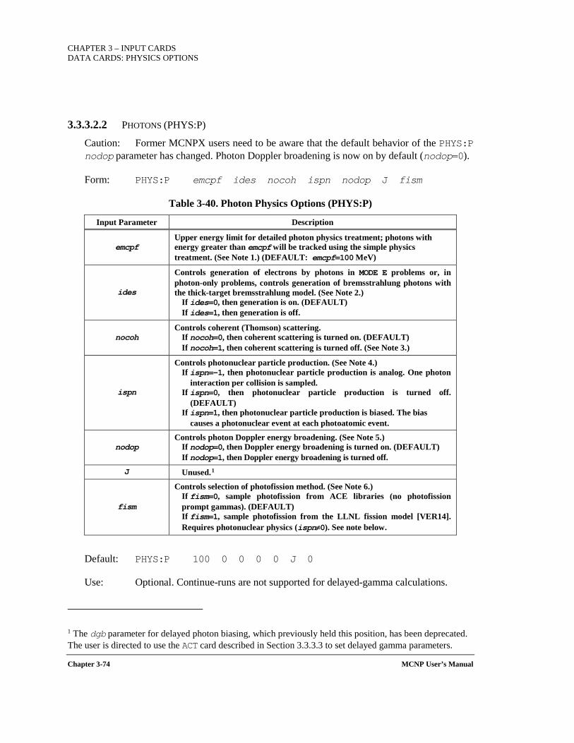
CHAPTER 3 – INPUT CARDS DATA CARDS: PHYSICS OPTIONS
Chapter 3-74 MCNP User’s Manual
3.3.3.2.2 PHOTONS (PHYS:P)
Caution: Former MCNPX users need to be aware that the default behavior of the PHYS:P nodop parameter has changed. Photon Doppler broadening is now on by default (nodop=0).
Form: PHYS:P emcpf ides nocoh ispn nodop J fism
Table 3-40. Photon Physics Options (PHYS:P)
Input Parameter Description
emcpf Upper energy limit for detailed photon physics treatment; photons with energy greater than emcpf will be tracked using the simple physics treatment. (See Note 1.) (DEFAULT: emcpf=100 MeV)
ides
Controls generation of electrons by photons in MODE E problems or, in photon-only problems, controls generation of bremsstrahlung photons with the thick-target bremsstrahlung model. (See Note 2.)
If ides=0, then generation is on. (DEFAULT) If ides=1, then generation is off.
nocoh Controls coherent (Thomson) scattering.
If nocoh=0, then coherent scattering is turned on. (DEFAULT) If nocoh=1, then coherent scattering is turned off. (See Note 3.)
ispn
Controls photonuclear particle production. (See Note 4.) If ispn=-1, then photonuclear particle production is analog. One photon
interaction per collision is sampled. If ispn=0, then photonuclear particle production is turned off.
(DEFAULT) If ispn=1, then photonuclear particle production is biased. The bias
causes a photonuclear event at each photoatomic event.
nodop Controls photon Doppler energy broadening. (See Note 5.)
If nodop=0, then Doppler energy broadening is turned on. (DEFAULT) If nodop=1, then Doppler energy broadening is turned off.
J Unused.1
fism
Controls selection of photofission method. (See Note 6.) If fism=0, sample photofission from ACE libraries (no photofission prompt gammas). (DEFAULT) If fism=1, sample photofission from the LLNL fission model [VER14]. Requires photonuclear physics (ispn≠0). See note below.
Default: PHYS:P 100 0 0 0 0 J 0
Use: Optional. Continue-runs are not supported for delayed-gamma calculations.
1 The dgb parameter for delayed photon biasing, which previously held this position, has been deprecated. The user is directed to use the ACT card described in Section 3.3.3.3 to set delayed gamma parameters.
CHAPTER 3 – INPUT CARDS DATA CARDS: PHYSICS OPTIONS
MCNP User’s Manual Chapter 3-75
Note 1: If emax on the PHYS:E card is less than emcpf on the PHYS:P card, MCNP6 will internally reset empcf to be equal to emax.
If wc1=0 on the CUT:P card, analog capture is used in the energy region above emcpf. Otherwise capture is simulated by weight reduction with Russian roulette on weight cutoff. Photons with energy less than emcpf will be treated with the more detailed physics that always includes analog capture. For a detailed discussion of the simple and detailed photon physics treatments, see the MCNP5 Theory Manual[X-503a], Section 4.4.
The simple physics treatment, intended primarily for higher energy photons, considers the following physical processes: photoelectric effect without fluorescence, Compton scattering, and pair production. The highly forward peaked coherent Thomson scattering is ignored. In the detailed physics treatment, photoelectric absorption can result in fluorescent emission, the Thomson and Klein-Nishina differential cross sections are modified by appropriate form factors [HEN11] and Compton profiles taking electron binding effects into account, and coherent scattering is included.
Note 2: To turn off the production of secondary electrons generated by photons, the switch ides can be set, either on the PHYS:P or on the PHYS:E card. If either of these cards sets ides=1, photons will not produce electrons, even if ides=0 is set on the other. In a photon-only problem, turning off secondary electrons causes the thick-target bremsstrahlung model to be bypassed. This option should be exercised only with great care because it alters the physics of the electron-photon cascade and will give erroneously low photon results when bremsstrahlung and electron transport are significant.
Note 3: When nocoh=1, the cross section for coherent scattering will be set to zero. This approximation can be useful in problems with bad point detector variances.
Note 4: Photonuclear physics models enable (γ,n) and other photonuclear reactions when photonuclear data tables are unavailable. When some photonuclear data tables are available, MCNP6 will mix and match, using tables when available and physics models when no tables are available. Consider using an MX:P card to override this default behavior.
Note 5: When photon Doppler broadening is turned on (nodop=0), there is no effect unless photon Doppler broadening momentum profile data are available in the photon library. These data are available in the MCPLIB03 and later photon libraries.
Note 6: When fism=1, photofission secondaries are sampled only when a photofission event occurs (unlike fism=0). This enables coincidence counting of photofission secondaries. The LLNL fission model for photofission is the only way to produce prompt photofission gammas; these gammas are correlated with the photofission neutrons with appropriate multiplicities. When fism=1 on the PHYS:P card, photonuclear physics must be turned on (ispn≠0) and the LLNL fission model should be used also for neutrons (METHOD=5 on the FMULT card).
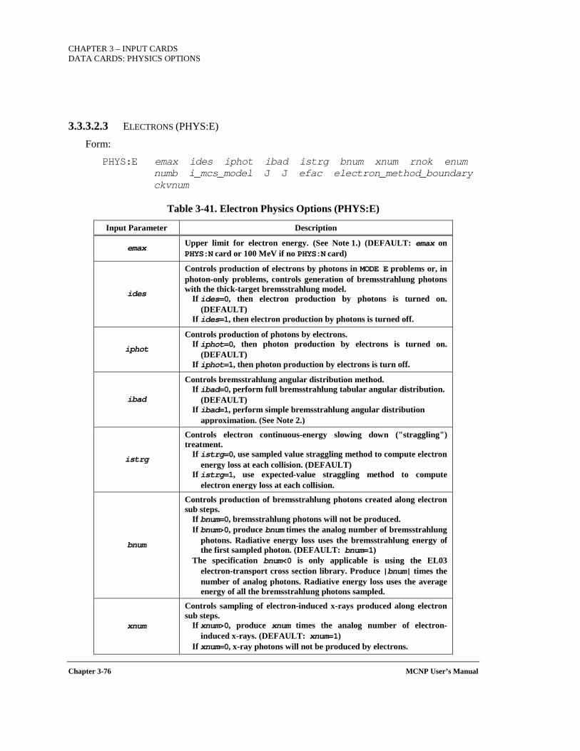
CHAPTER 3 – INPUT CARDS DATA CARDS: PHYSICS OPTIONS
Chapter 3-76 MCNP User’s Manual
3.3.3.2.3 ELECTRONS (PHYS:E)
Form: PHYS:E emax ides iphot ibad istrg bnum xnum rnok enum
numb i_mcs_model J J efac electron_method_boundary ckvnum
Table 3-41. Electron Physics Options (PHYS:E)
Input Parameter Description
emax Upper limit for electron energy. (See Note 1.) (DEFAULT: emax on PHYS:N card or 100 MeV if no PHYS:N card)
ides
Controls production of electrons by photons in MODE E problems or, in photon-only problems, controls generation of bremsstrahlung photons with the thick-target bremsstrahlung model.
If ides=0, then electron production by photons is turned on. (DEFAULT)
If ides=1, then electron production by photons is turned off.
iphot
Controls production of photons by electrons. If iphot=0, then photon production by electrons is turned on.
(DEFAULT) If iphot=1, then photon production by electrons is turn off.
ibad
Controls bremsstrahlung angular distribution method. If ibad=0, perform full bremsstrahlung tabular angular distribution.
(DEFAULT) If ibad=1, perform simple bremsstrahlung angular distribution
approximation. (See Note 2.)
istrg
Controls electron continuous-energy slowing down ("straggling") treatment.
If istrg=0, use sampled value straggling method to compute electron energy loss at each collision. (DEFAULT)
If istrg=1, use expected-value straggling method to compute electron energy loss at each collision.
bnum
Controls production of bremsstrahlung photons created along electron sub steps.
If bnum=0, bremsstrahlung photons will not be produced. If bnum>0, produce bnum times the analog number of bremsstrahlung
photons. Radiative energy loss uses the bremsstrahlung energy of the first sampled photon. (DEFAULT: bnum=1)
The specification bnum<0 is only applicable is using the EL03 electron-transport cross section library. Produce |bnum| times the number of analog photons. Radiative energy loss uses the average energy of all the bremsstrahlung photons sampled.
xnum
Controls sampling of electron-induced x-rays produced along electron sub steps.
If xnum>0, produce xnum times the analog number of electron-induced x-rays. (DEFAULT: xnum=1)
If xnum=0, x-ray photons will not be produced by electrons.
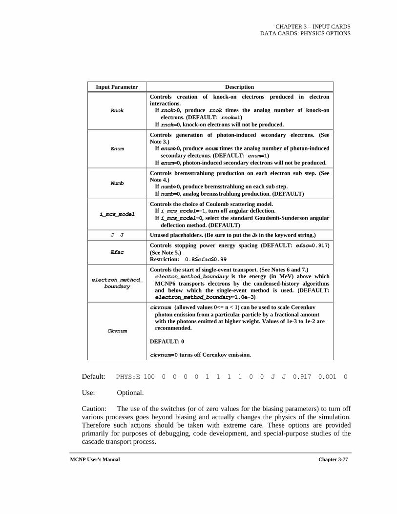
CHAPTER 3 – INPUT CARDS DATA CARDS: PHYSICS OPTIONS
MCNP User’s Manual Chapter 3-77
Input Parameter Description
Rnok
Controls creation of knock-on electrons produced in electron interactions.
If rnok>0, produce rnok times the analog number of knock-on electrons. (DEFAULT: rnok=1)
If rnok=0, knock-on electrons will not be produced.
Enum
Controls generation of photon-induced secondary electrons. (See Note 3.)
If enum>0, produce enum times the analog number of photon-induced secondary electrons. (DEFAULT: enum=1)
If enum=0, photon-induced secondary electrons will not be produced.
Numb
Controls bremsstrahlung production on each electron sub step. (See Note 4.)
If numb>0, produce bremsstrahlung on each sub step. If numb=0, analog bremsstrahlung production. (DEFAULT)
i_mcs_model
Controls the choice of Coulomb scattering model. If i_mcs_model=-1, turn off angular deflection. If i_mcs_model=0, select the standard Goudsmit-Sunderson angular
deflection method. (DEFAULT) J J Unused placeholders. (Be sure to put the Js in the keyword string.)
Efac Controls stopping power energy spacing (DEFAULT: efac=0.917) (See Note 5.) Restriction: 0.8≤efac≤0.99
electron_method_boundary
Controls the start of single-event transport. (See Notes 6 and 7.) electon_method_boundary is the energy (in MeV) above which MCNP6 transports electrons by the condensed-history algorithms and below which the single-event method is used. (DEFAULT: electron_method_boundary=1.0e-3)
Ckvnum
ckvnum (allowed values 0<= n < 1) can be used to scale Cerenkov photon emission from a particular particle by a fractional amount with the photons emitted at higher weight. Values of 1e-3 to 1e-2 are recommended.
DEFAULT: 0 ckvnum=0 turns off Cerenkov emission.
Default: PHYS:E 100 0 0 0 0 1 1 1 1 0 0 J J 0.917 0.001 0
Use: Optional.
Caution: The use of the switches (or of zero values for the biasing parameters) to turn off various processes goes beyond biasing and actually changes the physics of the simulation. Therefore such actions should be taken with extreme care. These options are provided primarily for purposes of debugging, code development, and special-purpose studies of the cascade transport process.
CHAPTER 3 – INPUT CARDS DATA CARDS: PHYSICS OPTIONS
Chapter 3-78 MCNP User’s Manual
Note 1: The parameter emax should be set to the highest electron energy encountered in your problem.
Note 2: Point detectors and DXTRAN spheres use the simple bremsstrahlung angular distribution approximation. Always use(ibad=1).
Note 3: The specification enum=0 differs from ides=1. If enum=0, pair production is totally turned off. If ides=1, the pair production-produced annihilation photons are still produced.
Note 4: Only a real event, i.e., one that has been sampled to have a bremsstrahlung interaction, causes energy loss. The weights of the bremsstrahlung photons are multiplied by the probability of interaction in a substep. If two or more photons are produced in a real event, the weight of the second or more photons is the unadjusted value because there is no Poisson sampling, except for real events.
Note 5: When efac is specified, the energy spacing for multiple-scattering tables (stopping power, range, etc.) is determined by
En+1 = En * F
where E1 is the highest energy and
F = (1/2) ** (1/D)
with D=real(nint(ln(1/2) / ln(efac)))
This means that on average, the energy of the particle will decrease by a factor of two in D energy steps and that a larger value of efac results in more points in the multiple-scattering tables. The default value, 0.917, leads to the traditional choice of eight energy steps for a factor-of-two energy loss.
Note 6: To invoke the single-event electron-transport method, the problem must have access to photon data, even if the user is not interested in the photon transport. Therefore, the MODE card must included the specification for both photons (P) and electrons (E). Access to the EPRDATA14 library data is required to transport electrons below 1 keV. This library, which is denoted by the cross-section identifier ".14p", is not the default in the xsdir_mcnp6.2 cross-section directory file provided with the MCNP6 (Version 2) distribution; therefore the EPRDATA14 library may need to be requested on the material cards explicitly. This low-energy (<1 keV) data are only for zero-temperature atomic targets, so temperature, condensed state, and molecular effects are not yet treated for electrons in this regime.
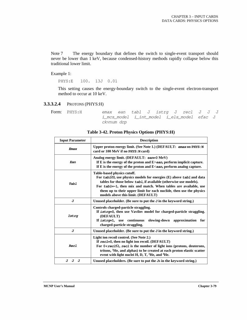
CHAPTER 3 – INPUT CARDS DATA CARDS: PHYSICS OPTIONS
MCNP User’s Manual Chapter 3-79
Note 7 The energy boundary that defines the switch to single-event transport should never be lower than 1 keV, because condensed-history methods rapidly collapse below this traditional lower limit.
Example 1: PHYS:E 100. 13J 0.01
This setting causes the energy-boundary switch to the single-event electron-transport method to occur at 10 keV.
3.3.3.2.4 PROTONS (PHYS:H)
Form: PHYS:H emax ean tabl J istrg J recl J J J i_mcs_model i_int_model i_els_model efac J
ckvnum drp
Table 3-42. Proton Physics Options (PHYS:H)
Input Parameter Description
Emax Upper proton energy limit. (See Note 1.) (DEFAULT: emax on PHYS:N card or 100 MeV if no PHYS:N card)
Ean Analog energy limit. (DEFAULT: ean=0 MeV)
If E is the energy of the proton and E>ean, perform implicit capture. If E is the energy of the proton and E<ean, perform analog capture.
Tabl
Table-based physics cutoff. For tabl≥0, use physics models for energies (E) above tabl and data
tables for those below tabl, if available (otherwise use models). For tabl=-1, then mix and match. When tables are available, use
them up to their upper limit for each nuclide, then use the physics models above this limit. (DEFAULT)
J Unused placeholder. (Be sure to put the J in the keyword string.)
Istrg
Controls charged-particle straggling. If istrg=0, then use Vavilov model for charged-particle straggling.
(DEFAULT) If istrg=1, use continuous slowing-down approximation for
charged-particle straggling. J Unused placeholder. (Be sure to put the J in the keyword string.)
Recl
Light ion recoil control. (See Note 2.) If recl=0, then no light ion recoil. (DEFAULT) For 0<recl≤1, recl is the number of light ions (protons, deuterons,
tritons, 3He, and alphas) to be created at each proton elastic scatter event with light nuclei H, D, T, 3He, and 4He.
J J J Unused placeholders. (Be sure to put the Js in the keyword string.)
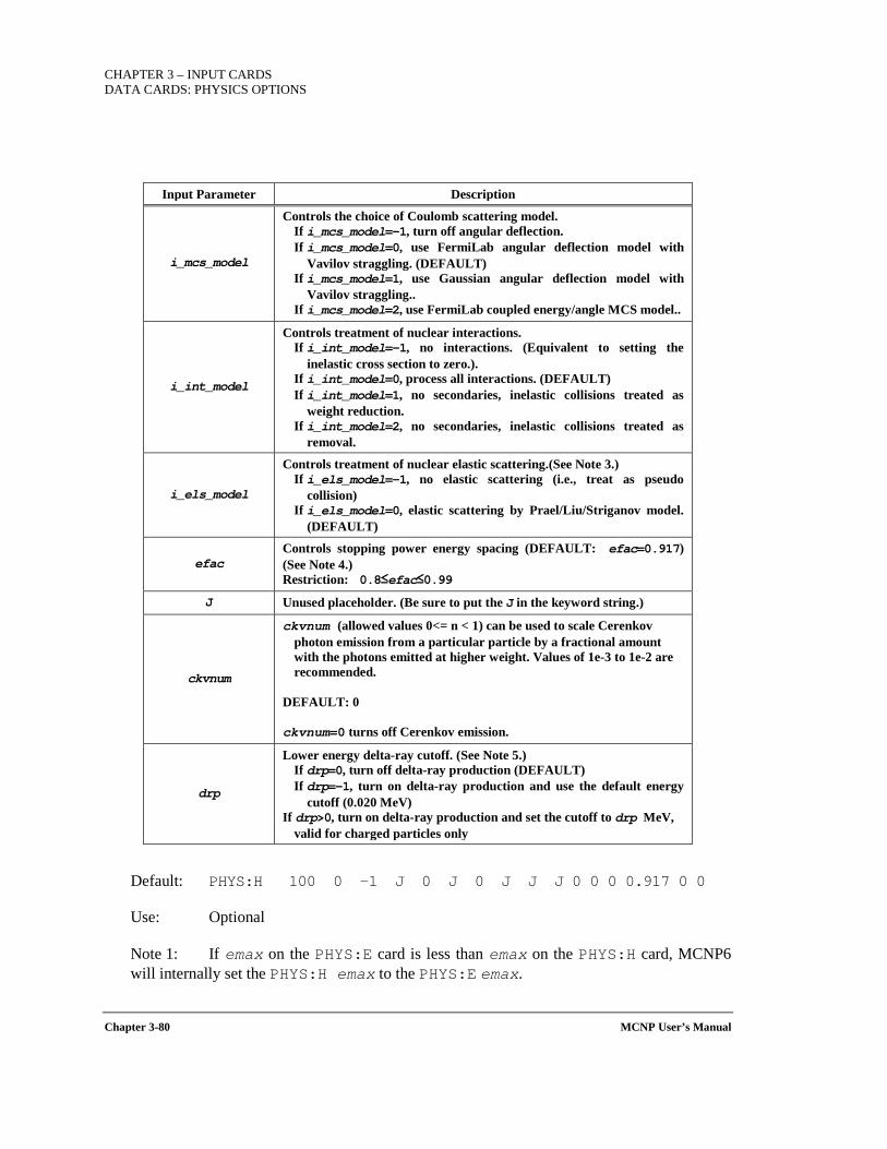
CHAPTER 3 – INPUT CARDS DATA CARDS: PHYSICS OPTIONS
Chapter 3-80 MCNP User’s Manual
Input Parameter Description
i_mcs_model
Controls the choice of Coulomb scattering model. If i_mcs_model=-1, turn off angular deflection. If i_mcs_model=0, use FermiLab angular deflection model with
Vavilov straggling. (DEFAULT) If i_mcs_model=1, use Gaussian angular deflection model with
Vavilov straggling.. If i_mcs_model=2, use FermiLab coupled energy/angle MCS model..
i_int_model
Controls treatment of nuclear interactions. If i_int_model=-1, no interactions. (Equivalent to setting the
inelastic cross section to zero.). If i_int_model=0, process all interactions. (DEFAULT) If i_int_model=1, no secondaries, inelastic collisions treated as
weight reduction. If i_int_model=2, no secondaries, inelastic collisions treated as
removal.
i_els_model
Controls treatment of nuclear elastic scattering.(See Note 3.) If i_els_model=-1, no elastic scattering (i.e., treat as pseudo
collision) If i_els_model=0, elastic scattering by Prael/Liu/Striganov model.
(DEFAULT)
efac Controls stopping power energy spacing (DEFAULT: efac=0.917) (See Note 4.) Restriction: 0.8≤efac≤0.99
J Unused placeholder. (Be sure to put the J in the keyword string.)
ckvnum
ckvnum (allowed values 0<= n < 1) can be used to scale Cerenkov photon emission from a particular particle by a fractional amount with the photons emitted at higher weight. Values of 1e-3 to 1e-2 are recommended.
DEFAULT: 0 ckvnum=0 turns off Cerenkov emission.
drp
Lower energy delta-ray cutoff. (See Note 5.) If drp=0, turn off delta-ray production (DEFAULT) If drp=-1, turn on delta-ray production and use the default energy
cutoff (0.020 MeV) If drp>0, turn on delta-ray production and set the cutoff to drp MeV,
valid for charged particles only
Default: PHYS:H 100 0 -1 J 0 J 0 J J J 0 0 0 0.917 0 0
Use: Optional
Note 1: If emax on the PHYS:E card is less than emax on the PHYS:H card, MCNP6 will internally set the PHYS:H emax to the PHYS:E emax.
CHAPTER 3 – INPUT CARDS DATA CARDS: PHYSICS OPTIONS
MCNP User’s Manual Chapter 3-81
The parameter emax must be higher than the highest energy in the problem or the physics is wrong. For problems with energies above 100 MeV, emax should be chosen carefully; the default is appropriate for problems with energies below 100 MeV.
Note 2: Light ion recoil physics accounts for the ionization potential and uses the proper two-body kinematics (with neutron free-gas thermal treatment if appropriate) to bank recoil particles with the proper energy and angle. The input card MODE N H D T S A ... is required to produce light ions H, D, T, S, and A. The card CUT:<pl> J 0 for particles H, D, T, S, and A is recommended so that the low-energy recoil ions produced are not killed by energy cutoff. Note that protons colliding with hydrogen to produce more protons can produce an overwhelming number of protons. Therefore, caution is required, and recl<1 may be needed. This capability is the same for incident neutrons as controlled by the recl keyword on the PHYS:N card.
Note 3: Elastic scattering will be ignored if nuclear interactions are turned off.
Note 4: When efac is specified, the energy spacing for multiple-scattering tables (stopping power, range, etc.) is determined by
En+1 = En * F
where E1 is the highest energy and
F = (1/2) ** (1/D)
with D=real(nint(ln(1/2) / ln(efac)))
This means that on average, the energy of the particle will decrease by a factor of two in D energy steps and that a larger value of efac results in more points in the multiple-scattering tables. The default value, 0.917, leads to the traditional choice of eight energy steps for a factor-of-two energy loss.
Note 5: Delta-ray production is according to the formulation by B. Rossi, as found in ICRU Report 37. The 1/E2 differential spectrum is truncated by the drp parameter, which should be greater than 1 keV, with a default value of 20 keV and a maximum of 1,022 keV. To increase execution speed, this parameter should be set as large as possible, while retaining important effects to tallies of interest.
Example: PHYS:H 800 10 150 J 0 J 2
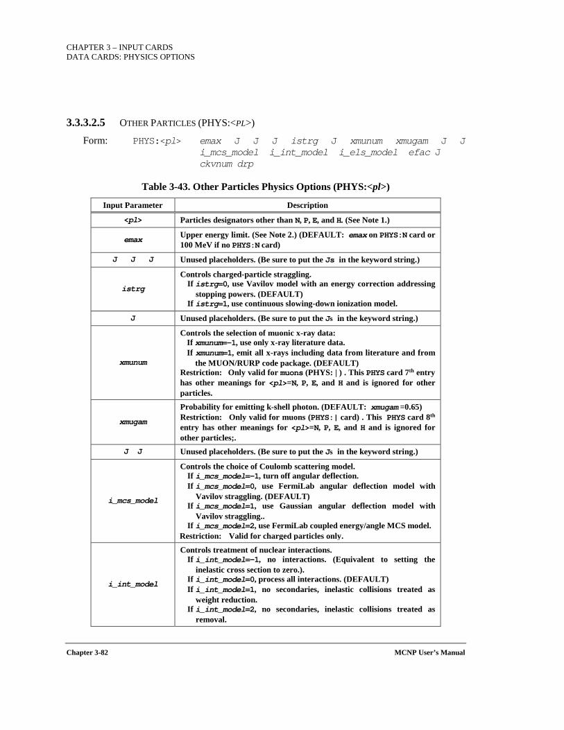
CHAPTER 3 – INPUT CARDS DATA CARDS: PHYSICS OPTIONS
Chapter 3-82 MCNP User’s Manual
3.3.3.2.5 OTHER PARTICLES (PHYS:<PL>)
Form: PHYS:<pl> emax J J J istrg J xmunum xmugam J J i_mcs_model i_int_model i_els_model efac J ckvnum drp
Table 3-43. Other Particles Physics Options (PHYS:<pl>)
Input Parameter Description
<pl> Particles designators other than N, P, E, and H. (See Note 1.)
emax Upper energy limit. (See Note 2.) (DEFAULT: emax on PHYS:N card or 100 MeV if no PHYS:N card)
J J J Unused placeholders. (Be sure to put the Js in the keyword string.)
istrg
Controls charged-particle straggling. If istrg=0, use Vavilov model with an energy correction addressing
stopping powers. (DEFAULT) If istrg=1, use continuous slowing-down ionization model.
J Unused placeholders. (Be sure to put the Js in the keyword string.)
xmunum
Controls the selection of muonic x-ray data: If xmunum=-1, use only x-ray literature data. If xmunum=1, emit all x-rays including data from literature and from
the MUON/RURP code package. (DEFAULT) Restriction: Only valid for muons (PHYS: | ) . This PHYS card 7th entry has other meanings for <pl>=N, P, E, and H and is ignored for other particles.
xmugam
Probability for emitting k-shell photon. (DEFAULT: xmugam =0.65) Restriction: Only valid for muons (PHYS:| card) . This PHYS card 8th entry has other meanings for <pl>=N, P, E, and H and is ignored for other particles;.
J J Unused placeholders. (Be sure to put the Js in the keyword string.)
i_mcs_model
Controls the choice of Coulomb scattering model. If i_mcs_model=-1, turn off angular deflection. If i_mcs_model=0, use FermiLab angular deflection model with
Vavilov straggling. (DEFAULT) If i_mcs_model=1, use Gaussian angular deflection model with
Vavilov straggling.. If i_mcs_model=2, use FermiLab coupled energy/angle MCS model.
Restriction: Valid for charged particles only.
i_int_model
Controls treatment of nuclear interactions. If i_int_model=-1, no interactions. (Equivalent to setting the
inelastic cross section to zero.). If i_int_model=0, process all interactions. (DEFAULT) If i_int_model=1, no secondaries, inelastic collisions treated as
weight reduction. If i_int_model=2, no secondaries, inelastic collisions treated as
removal.
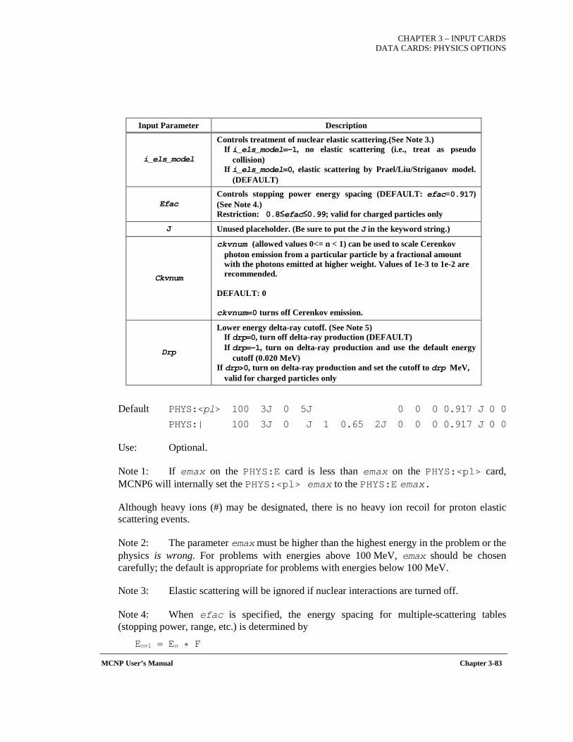
CHAPTER 3 – INPUT CARDS DATA CARDS: PHYSICS OPTIONS
MCNP User’s Manual Chapter 3-83
Input Parameter Description
i_els_model
Controls treatment of nuclear elastic scattering.(See Note 3.) If i_els_model=-1, no elastic scattering (i.e., treat as pseudo
collision) If i_els_model=0, elastic scattering by Prael/Liu/Striganov model.
(DEFAULT)
Efac Controls stopping power energy spacing (DEFAULT: efac=0.917) (See Note 4.) Restriction: 0.8≤efac≤0.99; valid for charged particles only
J Unused placeholder. (Be sure to put the J in the keyword string.)
Ckvnum
ckvnum (allowed values 0<= n < 1) can be used to scale Cerenkov photon emission from a particular particle by a fractional amount with the photons emitted at higher weight. Values of 1e-3 to 1e-2 are recommended.
DEFAULT: 0 ckvnum=0 turns off Cerenkov emission.
Drp
Lower energy delta-ray cutoff. (See Note 5) If drp=0, turn off delta-ray production (DEFAULT) If drp=-1, turn on delta-ray production and use the default energy
cutoff (0.020 MeV) If drp>0, turn on delta-ray production and set the cutoff to drp MeV,
valid for charged particles only
Default PHYS:<pl> 100 3J 0 5J 0 0 0 0.917 J 0 0
PHYS:| 100 3J 0 J 1 0.65 2J 0 0 0 0.917 J 0 0
Use: Optional.
Note 1: If emax on the PHYS:E card is less than emax on the PHYS:<pl> card, MCNP6 will internally set the PHYS:<pl> emax to the PHYS:E emax.
Although heavy ions (#) may be designated, there is no heavy ion recoil for proton elastic scattering events.
Note 2: The parameter emax must be higher than the highest energy in the problem or the physics is wrong. For problems with energies above 100 MeV, emax should be chosen carefully; the default is appropriate for problems with energies below 100 MeV.
Note 3: Elastic scattering will be ignored if nuclear interactions are turned off.
Note 4: When efac is specified, the energy spacing for multiple-scattering tables (stopping power, range, etc.) is determined by
En+1 = En * F
CHAPTER 3 – INPUT CARDS DATA CARDS: PHYSICS OPTIONS
Chapter 3-84 MCNP User’s Manual
where E1 is the highest energy and
F = (1/2) ** (1/D)
with D=real(nint(ln(1/2) / ln(efac)))
This means that on average, the energy of the particle will decrease by a factor of two in D energy steps and that a larger value of efac results in more points in the multiple-scattering tables. The default value, 0.917, leads to the traditional choice of eight energy steps for a factor-of-two energy loss.
Note 5: Delta-ray production is according to the formulation by B. Rossi, as found in ICRU Report 37. The 1/E2 differential spectrum is truncated by the drp parameter, which should be greater than 1 keV, with a default value of 20 keV and a maximum of 1,022 keV. To increase execution speed, this parameter should be set as large as possible, while retaining important effects to tallies of interest.
Example: PHYS:D 800 3J 1
3.3.3.3 ACT ACTIVATION CONTROL CARD
Available delayed particles are: neutrons, gammas, betas, alphas, and positrons. Delayed-neutron emission can be calculated using library (DN=LIBRARY) or model (DN=MODEL) treatments. The library treatment uses ACE data and produces delayed neutrons only for fission. The model treatment uses data from the DELAY_LIBRARY_V5.dat library and produces delayed neutrons for fission and, if requested, activation. Delayed-gamma emission is calculated by line emission data (DG=LINES), from ENDF/B-VII.1 data contained in CINDERGL.dat and augmented by model data contained in DELAY_LIBRARY_V5.dat, or only model data (DG=MG). Delayed betas, alphas, and positrons are sampled solely from DELAY_LIBRARY_V5.dat data.
The DELAY_LIBRARY_V5.dat delayed-particle library provides unique delayed neutron, gamma, beta, alpha, and positron spectra to be sampled for each radionuclide. Delayed neutron spectra are sampled from 750 bins ranging from 0-7.5 MeV for 298 nuclides. Delayed gamma spectra are sampled from 500 bins ranging from 0-10 MeV for 1865 nuclides, (see Note 3 & 4). Delayed beta spectra are sampled from 100 bins ranging from 0-10 MeV for 1891 nuclides. Delayed positron spectra are sampled from 100 bins ranging from 0-10 MeV for 531 nuclides. Delayed alpha spectra are sampled from 100 bins ranging from 0-10 MeV for 248 nuclides. A warning is issued when no delayed particle data is available and a nuclide with a non-zero delayed-particle probability is sampled.
Delayed-gamma emission is limited to fixed source (SDEF) problems.
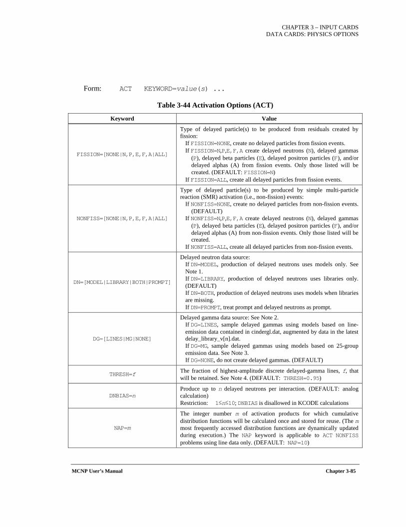
CHAPTER 3 – INPUT CARDS DATA CARDS: PHYSICS OPTIONS
MCNP User’s Manual Chapter 3-85
Form: ACT KEYWORD=value(s) ...
Table 3-44 Activation Options (ACT)
Keyword Value
FISSION=[NONE|N,P,E,F,A|ALL]
Type of delayed particle(s) to be produced from residuals created by fission:
If FISSION=NONE, create no delayed particles from fission events. If FISSION=N,P,E,F,A create delayed neutrons (N), delayed gammas
(P), delayed beta particles (E), delayed positron particles (F), and/or delayed alphas (A) from fission events. Only those listed will be created. (DEFAULT: FISSION=N)
If FISSION=ALL, create all delayed particles from fission events.
NONFISS=[NONE|N,P,E,F,A|ALL]
Type of delayed particle(s) to be produced by simple multi-particle reaction (SMR) activation (i.e., non-fission) events:
If NONFISS=NONE, create no delayed particles from non-fission events. (DEFAULT)
If NONFISS=N,P,E,F,A create delayed neutrons (N), delayed gammas (P), delayed beta particles (E), delayed positron particles (F), and/or delayed alphas (A) from non-fission events. Only those listed will be created.
If NONFISS=ALL, create all delayed particles from non-fission events.
DN=[MODEL|LIBRARY|BOTH|PROMPT]
Delayed neutron data source: If DN=MODEL, production of delayed neutrons uses models only. See Note 1. If DN=LIBRARY, production of delayed neutrons uses libraries only. (DEFAULT) If DN=BOTH, production of delayed neutrons uses models when libraries are missing. If DN=PROMPT, treat prompt and delayed neutrons as prompt.
DG=[LINES|MG|NONE]
Delayed gamma data source: See Note 2. If DG=LINES, sample delayed gammas using models based on line-emission data contained in cindergl.dat, augmented by data in the latest delay_library_v[n].dat. If DG=MG, sample delayed gammas using models based on 25-group emission data. See Note 3. If DG=NONE, do not create delayed gammas. (DEFAULT)
THRESH=f The fraction of highest-amplitude discrete delayed-gamma lines, f, that will be retained. See Note 4. (DEFAULT: THRESH=0.95)
DNBIAS=n Produce up to n delayed neutrons per interaction. (DEFAULT: analog calculation) Restriction: 1≤n≤10; DNBIAS is disallowed in KCODE calculations
NAP=m
The integer number m of activation products for which cumulative distribution functions will be calculated once and stored for reuse. (The m most frequently accessed distribution functions are dynamically updated during execution.) The NAP keyword is applicable to ACT NONFISS problems using line data only. (DEFAULT: NAP=10)
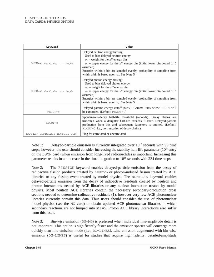
CHAPTER 3 – INPUT CARDS DATA CARDS: PHYSICS OPTIONS
Chapter 3-86 MCNP User’s Manual
Keyword Value
DNEB=w1,e1,w2,e2, ... wn,en
Delayed neutron energy biasing: Used to bias delayed neutron energy wm = weight for the mth energy bin em = upper energy for the mth energy bin (initial lower bin bound of 0 assumed) Energies within a bin are sampled evenly; probability of sampling from within a bin is based upon wm. See Note 5.
DGEB=w1,e1,w2,e2, ... wn,en
Delayed photon energy biasing: Used to bias delayed photon energy wm = weight for the mth energy bin em = upper energy for the mth energy bin (initial lower bin bound of 0 assumed) Energies within a bin are sampled evenly; probability of sampling from within a bin is based upon wm. See Note 5.
PECUT=e Delayed-gamma energy cutoff (MeV). Gamma lines below PECUT will be expunged. (Default: PECUT=0)
HLCUT=t
Spontaneous-decay half-life threshold (seconds). Decay chains are truncated when a daughter half-life exceeds HLCUT. Delayed-particle production from this and subsequent daughters is omitted. (Default: HLCUT=0, i.e., no truncation of decay chains).
SAMPLE=[CORRELATE|NONFISS_COR] Flag for correlated or uncorrelated
Note 1: Delayed-particle emission is currently integrated over 1010 seconds with 99 time steps; however, the user should consider increasing the stability half-life parameter (10th entry on the DBCN card) when emission from long-lived radionuclides is important. Increasing this parameter results in an increase in the time integration to 1019 seconds with 234 time steps.
Note 2: The FISSION keyword enables delayed-particle emission from the decay of radioactive fission products created by neutron- or photon-induced fission treated by ACE libraries or any fission event treated by model physics. The NONFISS keyword enables delayed-particle emission from the decay of radioactive residuals created by neutron and photon interactions treated by ACE libraries or any nuclear interaction treated by model physics. Most neutron ACE libraries contain the necessary secondary-production cross sections needed to determine radioactive residuals (1), however very few ACE photonuclear libraries currently contain this data. Thus users should consider the use of photonuclear model physics (see the MX card) or obtain updated ACE photonuclear libraries in which secondary reactions are not lumped into MT=5. Proton ACE library interactions also suffer from this issue.
Note 3: Bin-wise emission (DG=MG) is preferred when individual line-amplitude detail is not important. This option is significantly faster and the emission spectra will converge more quickly than line emission mode (i.e., DG=LINES). Line emission augmented with bin-wise emission (DG=LINES) is useful for studies that require high fidelity, detailed-amplitude

CHAPTER 3 – INPUT CARDS DATA CARDS: PHYSICS OPTIONS
MCNP User’s Manual Chapter 3-87
emission spectra. This option is significantly slower and can require the execution of large numbers of histories to suitably converge low probability delayed-gamma emission lines.
Note 4: Set THRESH=1.0 to retain all lines in the CINDERGL.dat file. Caution: For some problems (e.g., fission), the calculation with THRESH=1.0 will either run slowly or exceed memory limits and fail.
Note 5: A weight of “0” should not be set for any of the energy bins with DGEB/DNEB. Instead, a small value (0.001) is recommended. More information on the Delayed Neutron and Photon Energy Biasing is available in “Delayed Neutron and Photon Energy Biasing in MCNP6” LA-UR-13-23368.
3.3.3.4 PHYSICS CUTOFFS
3.3.3.4.1 CUT:<PL> TIME, ENERGY, AND WEIGHT CUTOFFS
Form: CUT:<pl> t e wc1 wc2 swtm
Table 3-45. Time, Energy, and Weight Cutoff Card (CUT:<pl>)
Input Parameter Description
<pl> Particle designator. t Time cutoff in shakes, 1 shake=10-8 second. (See Notes 1 and 2.) e Lower energy cutoff in MeV. (See Note 1.)
wc1, wc2 Weight cutoffs. If weight goes below wc2 roulette is played to restore weight to wc1. Setting wc1=wc2=0 invokes analog capture. (See Notes 3, 4, and 5.)
swtm Minimum source weight. (See Note 6.)
Neutron default: t=very large, e=0.0 MeV, wc1=-0.50, wc2=-0.25, swtm=minimum source weight if the general source is used
Photon default: t=neutron cutoff, e=0.001 MeV, wc1=-0.50, wc2=-0.25, swtm= minimum source weight if the general source is used; if there are pulse-height tallies, wc1=wc2=0, unless forced collisions are also used; if pulse-height tallies exist with forced collisions, the default values are wc1=-0.50 and wc2=-0.25
Electron default: t=neutron cutoff, e=0.001 MeV, wc1=0, wc2=0, swtm=minimum source weight if the general source is used; if there are pulse-height tallies, wc1=wc2=0, unless forced collisions are also used; if pulse-height tallies exist with forced collisions, the default values are wc1=-0.50 and wc2=-0.25

CHAPTER 3 – INPUT CARDS DATA CARDS: PHYSICS OPTIONS
Chapter 3-88 MCNP User’s Manual
With the exception of photon energy and electron/positron energy (see "Additional Photon Cutoff Notes" and "Additional Electron/Positron Cutoff Notes" below), the default energy cutoff values for all particles appear in Table 2-2. All other particle time and weight default cutoffs are the same as for electrons.
Use: Optional, as needed. Analog capture is highly recommended when using weight windows and for many other applications.
Note 1: If a particle’s time becomes greater than t as specified for that particle, its transport is stopped and the particle is killed. Although MCNP6 is time dependent, particle decay is not considered. Any particle with energy lower than the e specified for that particle is killed.
Note 2: The default (and maximum) emission time for delayed particle emission is 1010 s. By using the CUT card(s), the maximum emission time becomes 1) the particle’s time cutoff if time cutoff is specified or 2) the minimum of time cutoff if multiple time cutoffs are provided.
Note 3: For non-analog capture, if a particle’s weight WGT falls below wc2 times the ratio R of the source cell importance to the current cell importance, then with probability WGT/(wc1∗R), the particle survives and is assigned WGT=wc1∗R. If negative values are entered for the weight cutoffs, the values |wc1|∗Ws and |wc2|∗Ws will be used for wc1 and wc2, respectively, where Ws is the minimum starting weight assigned to a source particle from an MCNP6 general source. These negative entries are recommended over positive entries for most problems. If only wc1 is specified, then wc2=0.5∗wc1.
Note 4: If wc1 is set to zero, capture is treated explicitly by analog rather than implicitly by reducing the particles’ weight according to the capture probability. If ean or emcnf =emax on the PHYS:<pl> card (i.e., applies to neutrons or protons), analog capture is used regardless of the value of wc1 except for particles leaving a DXTRAN sphere.
Note 5: To generate delayed particles from non-fissioning isotopes, wc1 must be set to zero on both the photon and neutron CUT:<pl> cards so that analog capture is invoked.
Note 6: The parameter swtm can be used to make the weight cutoffs relative to the minimum starting weight of a source particle for a user source, as is done automatically for the general source. The entry will in general be the minimum starting weight of all source particles, including the effects of energy and direction biasing. The entry is also effective for the general source. Then swtm is multiplied by the WGT entry on the SDEF card, but is unaffected by any directional or energy biasing. This entry is ignored for a KCODE calculation.

CHAPTER 3 – INPUT CARDS DATA CARDS: PHYSICS OPTIONS
MCNP User’s Manual Chapter 3-89
Additional Photon Cutoff Notes
The CUT:P weight cutoffs are analogous to those on the CUT:N card except that they are used only for energies above the emcpf entry on the PHYS:P card. If wc1=0, analog capture is specified for photons of energy greater than emcpf. For energies below emcpf, analog capture is the only choice with one exception: photons leaving a DXTRAN sphere. Their weight is always checked against the CUT:P weight cutoff upon exiting. If only wc1 is specified, then wc2=0.5∗wc1.
In a coupled neutron/photon problem, the photon weight cutoffs are the same as the neutron weight cutoffs unless overridden by a CUT:P card.
In a coupled neutron/photon problem, photons are generated before the neutron weight cutoff game is played.
Although the default photon energy cutoff is 1 keV, a user may explicitly specify a lower cutoff down to 1 eV. The required photoatomic cross sections from ENDF/B-VI, release 8, are included in the new data library EPRDATA14 (Electron-Photon-Relaxation DATA). The tables in this library are presented in a newly developed ACE format specifically designed for use with MCNP6. (They cannot be used correctly with the earlier codes MCNP5 or MCNPX.) The proper tables can be requested on material cards using the cross-section identifier ".14p". Users are cautioned that at very low energies, molecular and other effects become important for scattering and absorption, and these more complex effects are not yet included in the photon transport methods. Also, note that although electron transport has been extended down to 10 eV, electron energies have not been extended as low as photon energies.
MCNP6 allows only analog capture below 0.001 MeV. Because the photoelectric cross section is virtually 100% of the total cross section below that energy for all isotopes, tracks will be quickly captured and terminated.
Additional Electron/Positron Cutoff Notes
Positron physics in MCNP6 is identical to electron physics, except for tracking directions in magnetic fields and consideration of positron annihilation. Whereas electrons below the energy cutoff are terminated, positrons below the energy cutoff produce annihilation photons. The positrons have a positive charge and may be tallied using the FT card ELC option (Section 3.3.5.18). Electron transport, which has a default cutoff of 1 keV, may be explicitly specified down to 10 eV.
To transport electrons at energies below 1 keV, the EPRDATA14 library is required. As with low-energy photon transport, the proper tables can be requested with the cross-section identifier ".14p". Also as with photons, the same cautions regarding temperature, molecular, solid-state, and other low-energy phenomena apply to low-energy electrons.
For very low-energy electrons, a physics-based practical difficulty can arise: the lack of energy-loss-inducing processes. Although bremsstrahlung is still present, it is completely
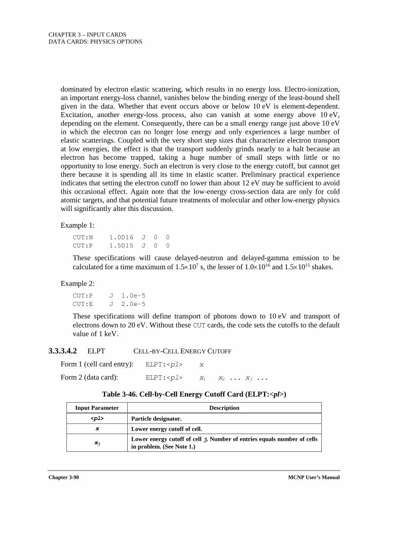
CHAPTER 3 – INPUT CARDS DATA CARDS: PHYSICS OPTIONS
Chapter 3-90 MCNP User’s Manual
dominated by electron elastic scattering, which results in no energy loss. Electro-ionization, an important energy-loss channel, vanishes below the binding energy of the least-bound shell given in the data. Whether that event occurs above or below 10 eV is element-dependent. Excitation, another energy-loss process, also can vanish at some energy above 10 eV, depending on the element. Consequently, there can be a small energy range just above 10 eV in which the electron can no longer lose energy and only experiences a large number of elastic scatterings. Coupled with the very short step sizes that characterize electron transport at low energies, the effect is that the transport suddenly grinds nearly to a halt because an electron has become trapped, taking a huge number of small steps with little or no opportunity to lose energy. Such an electron is very close to the energy cutoff, but cannot get there because it is spending all its time in elastic scatter. Preliminary practical experience indicates that setting the electron cutoff no lower than about 12 eV may be sufficient to avoid this occasional effect. Again note that the low-energy cross-section data are only for cold atomic targets, and that potential future treatments of molecular and other low-energy physics will significantly alter this discussion.
Example 1: CUT:N 1.0D16 J 0 0 CUT:P 1.5D15 J 0 0
These specifications will cause delayed-neutron and delayed-gamma emission to be calculated for a time maximum of 1.5×10⁷ s, the lesser of 1.0×10¹⁶ and 1.5×10¹⁵ shakes.
Example 2: CUT:P J 1.0e-5 CUT:E J 2.0e-5
These specifications will define transport of photons down to 10 eV and transport of electrons down to 20 eV. Without these CUT cards, the code sets the cutoffs to the default value of 1 keV.
3.3.3.4.2 ELPT CELL-BY-CELL ENERGY CUTOFF
Form 1 (cell card entry): ELPT:<pl> x
Form 2 (data card): ELPT:<pl> x1 x2 ... xj ...
Table 3-46. Cell-by-Cell Energy Cutoff Card (ELPT:<pl>)
Input Parameter Description
<pl> Particle designator. x Lower energy cutoff of cell.
xj Lower energy cutoff of cell j. Number of entries equals number of cells in problem. (See Note 1.)
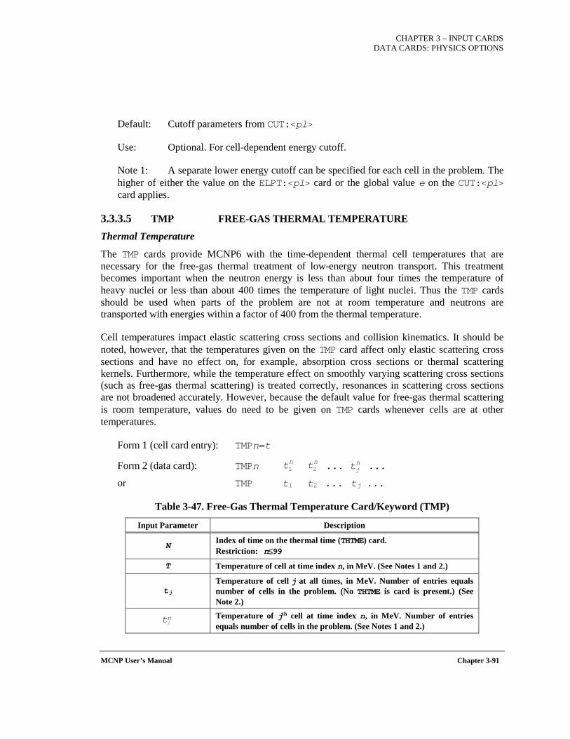
CHAPTER 3 – INPUT CARDS DATA CARDS: PHYSICS OPTIONS
MCNP User’s Manual Chapter 3-91
Default: Cutoff parameters from CUT:<pl>
Use: Optional. For cell-dependent energy cutoff.
Note 1: A separate lower energy cutoff can be specified for each cell in the problem. The higher of either the value on the ELPT:<pl> card or the global value e on the CUT:<pl> card applies.
3.3.3.5 TMP FREE-GAS THERMAL TEMPERATURE
Thermal Temperature
The TMP cards provide MCNP6 with the time-dependent thermal cell temperatures that are necessary for the free-gas thermal treatment of low-energy neutron transport. This treatment becomes important when the neutron energy is less than about four times the temperature of heavy nuclei or less than about 400 times the temperature of light nuclei. Thus the TMP cards should be used when parts of the problem are not at room temperature and neutrons are transported with energies within a factor of 400 from the thermal temperature.
Cell temperatures impact elastic scattering cross sections and collision kinematics. It should be noted, however, that the temperatures given on the TMP card affect only elastic scattering cross sections and have no effect on, for example, absorption cross sections or thermal scattering kernels. Furthermore, while the temperature effect on smoothly varying scattering cross sections (such as free-gas thermal scattering) is treated correctly, resonances in scattering cross sections are not broadened accurately. However, because the default value for free-gas thermal scattering is room temperature, values do need to be given on TMP cards whenever cells are at other temperatures.
Form 1 (cell card entry): TMPn=t
Form 2 (data card): TMPn ... ...
or TMP t1 t2 ... tj ...
Table 3-47. Free-Gas Thermal Temperature Card/Keyword (TMP)
Input Parameter Description
N Index of time on the thermal time (THTME) card. Restriction: n≤99
T Temperature of cell at time index n, in MeV. (See Notes 1 and 2.)
tj Temperature of cell j at all times, in MeV. Number of entries equals number of cells in the problem. (No THTME is card is present.) (See Note 2.)
Temperature of jth cell at time index n, in MeV. Number of entries equals number of cells in the problem. (See Notes 1 and 2.)
nt1nt2
njt
njt
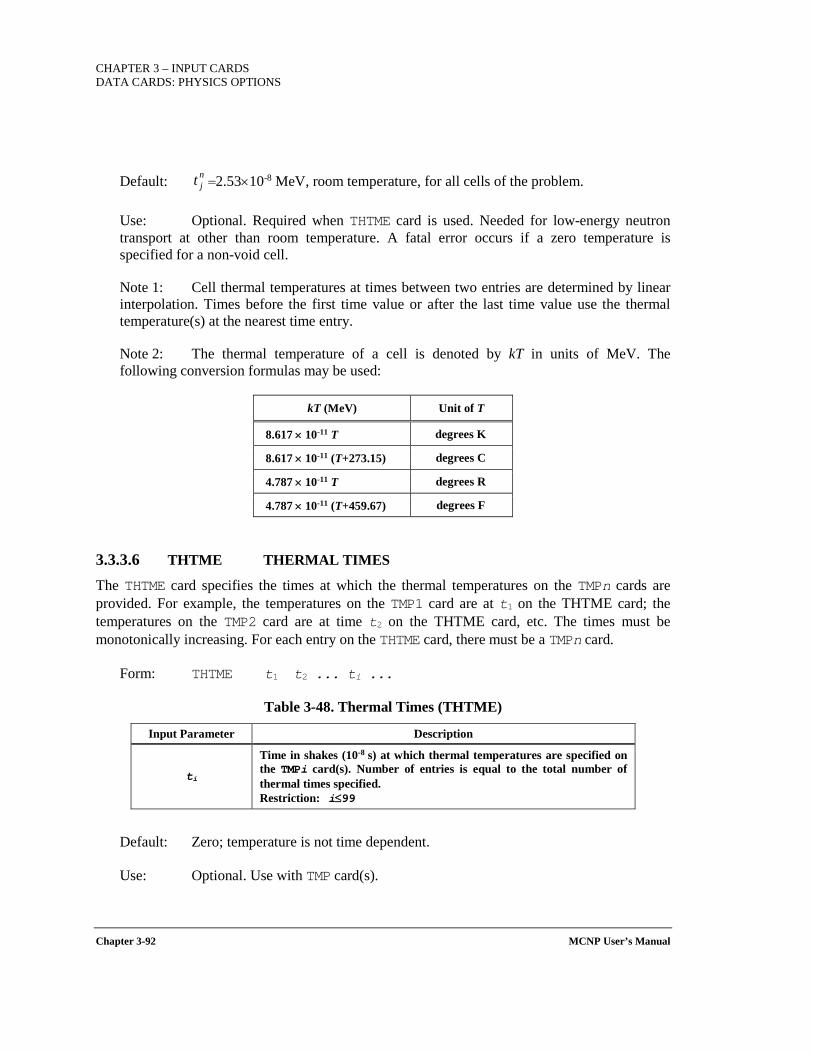
CHAPTER 3 – INPUT CARDS DATA CARDS: PHYSICS OPTIONS
Chapter 3-92 MCNP User’s Manual
Default: =2.53×10⁻⁸ MeV, room temperature, for all cells of the problem.
Use: Optional. Required when THTME card is used. Needed for low-energy neutron transport at other than room temperature. A fatal error occurs if a zero temperature is specified for a non-void cell.
Note 1: Cell thermal temperatures at times between two entries are determined by linear interpolation. Times before the first time value or after the last time value use the thermal temperature(s) at the nearest time entry.
Note 2: The thermal temperature of a cell is denoted by kT in units of MeV. The following conversion formulas may be used:
kT (MeV) Unit of T
8.617 × 10⁻¹¹ T degrees K
8.617 × 10⁻¹¹ (T+273.15) degrees C
4.787 × 10⁻¹¹ T degrees R
4.787 × 10⁻¹¹ (T+459.67) degrees F
3.3.3.6 THTME THERMAL TIMES
The THTME card specifies the times at which the thermal temperatures on the TMPn cards are provided. For example, the temperatures on the TMP1 card are at t1 on the THTME card; the temperatures on the TMP2 card are at time t2 on the THTME card, etc. The times must be monotonically increasing. For each entry on the THTME card, there must be a TMPn card.
Form: THTME t1 t2 ... ti ...
Table 3-48. Thermal Times (THTME)
Input Parameter Description
ti
Time in shakes (10-8 s) at which thermal temperatures are specified on the TMPi card(s). Number of entries is equal to the total number of thermal times specified. Restriction: i≤99
Default: Zero; temperature is not time dependent.
Use: Optional. Use with TMP card(s).
njt

CHAPTER 3 – INPUT CARDS DATA CARDS: PHYSICS OPTIONS
MCNP User’s Manual Chapter 3-93
3.3.3.7 MODEL PHYSICS
3.3.3.7.1 MPHYS MODEL PHYSICS CONTROL
The use of physics models is controlled with the MPHYS card.
Form: MPHYS [ON/OFF]
Default: All MODE N P E problems (and subsets) run with physics models off (MPHYS OFF) by default. Any particle on the MODE card other than N, P, or E will automatically activate the use of physics models (MPHYS ON).
Use: To disable the use of physics models, set MPHYS OFF. To enable the use of physics models, set MPHYS ON or include the MPHYS card with no entries.
Note: When isotopes that are missing cross-section libraries in a problem or when reactions exceed a libraries' maximum energy, MCNP6's behavior can change whether models are being used or not.
Physics Models Options:
Five cards (LCA, LCB, LCC, LEA, and LEB) control physics parameters for the Bertini [BER63a, BER69], ISABEL [YAR79, YAR81], CEM03.03 and LAQGSM03.03 [GUD75, GUD83, GUD01, GUD06, MAS74, MAS01, MAS05, MAS05a, MAS05b, MAS06, MAS07, MAS07a, MAS08, MAS11, MAS11a, MAS11b, MAS12], and INCL4 [BOU02] with ABLA [GAI91, JUN98] options. All of the input values on the five cards have defaults, which will be taken in the absence of the cards, or with the use of the J input option.
These MCNP6 input cards provide the user control of physics options. A summary of the cards follows. The options controlling the Bertini and ISABEL physics modules are taken from the User Guide to LCSTM [PRA89]. The user is referred to that document for further information.
The table that follows shows how different combinations of physics models are possible using the third and ninth entries on the LCA card, iexisa and icem, and the seventh entry on the LEA card, ievap.
Caution: Combinations of options for the physics models should be chosen with careful consideration. Although many combinations are allowed, inappropriate choices can lead to incorrect results.
LCA(3) LCA(9) LEA(7)
Bertini/Dresner 1 0 0
ISABEL/Dresner 2 0 0
Bertini/ABLA 1 0 2
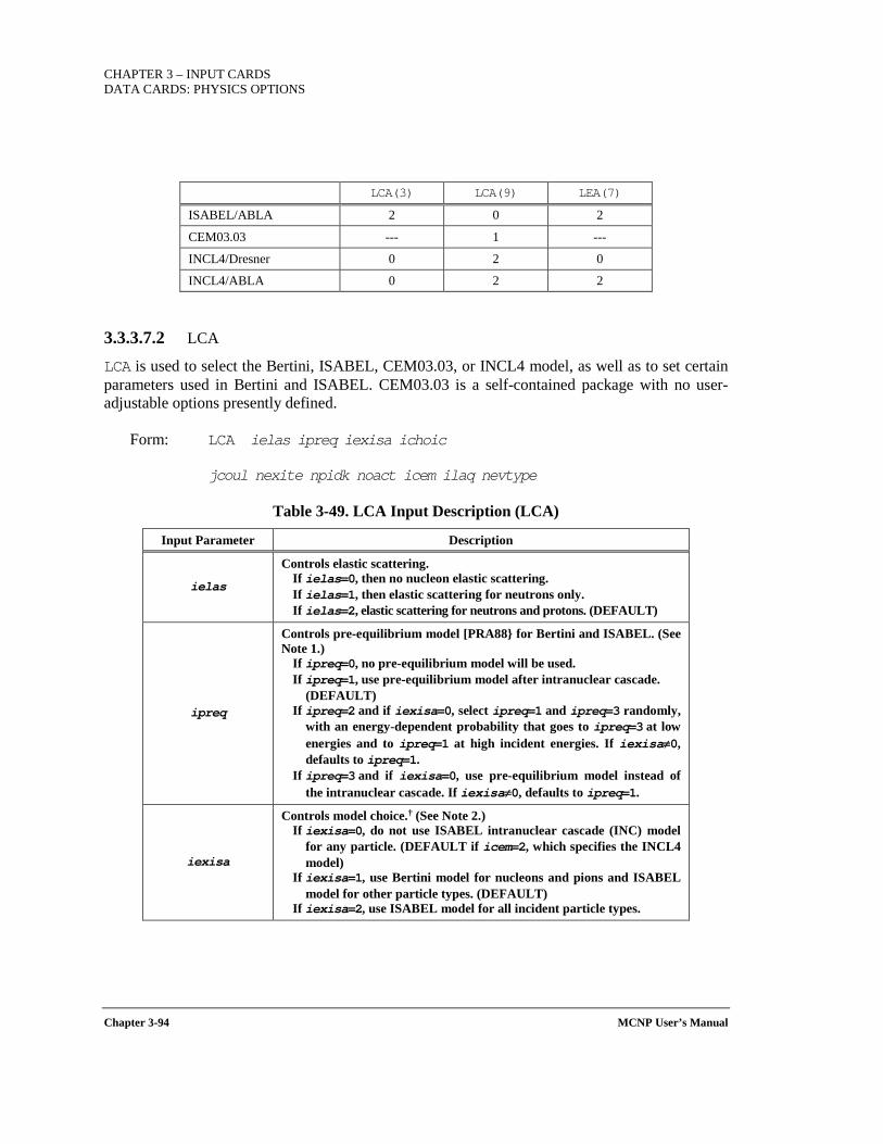
CHAPTER 3 – INPUT CARDS DATA CARDS: PHYSICS OPTIONS
Chapter 3-94 MCNP User’s Manual
LCA(3) LCA(9) LEA(7)
ISABEL/ABLA 2 0 2
CEM03.03 --- 1 ---
INCL4/Dresner 0 2 0
INCL4/ABLA 0 2 2
3.3.3.7.2 LCA
LCA is used to select the Bertini, ISABEL, CEM03.03, or INCL4 model, as well as to set certain parameters used in Bertini and ISABEL. CEM03.03 is a self-contained package with no user-adjustable options presently defined.
Form: LCA ielas ipreq iexisa ichoic
jcoul nexite npidk noact icem ilaq nevtype
Table 3-49. LCA Input Description (LCA)
Input Parameter Description
ielas
Controls elastic scattering. If ielas=0, then no nucleon elastic scattering. If ielas=1, then elastic scattering for neutrons only. If ielas=2, elastic scattering for neutrons and protons. (DEFAULT)
ipreq
Controls pre-equilibrium model [PRA88 for Bertini and ISABEL. (See Note 1.)
If ipreq=0, no pre-equilibrium model will be used. If ipreq=1, use pre-equilibrium model after intranuclear cascade.
(DEFAULT) If ipreq=2 and if iexisa=0, select ipreq=1 and ipreq=3 randomly,
with an energy-dependent probability that goes to ipreq=3 at low energies and to ipreq=1 at high incident energies. If iexisa≠0, defaults to ipreq=1.
If ipreq=3 and if iexisa=0, use pre-equilibrium model instead of the intranuclear cascade. If iexisa≠0, defaults to ipreq=1.
iexisa
Controls model choice.† (See Note 2.) If iexisa=0, do not use ISABEL intranuclear cascade (INC) model
for any particle. (DEFAULT if icem=2, which specifies the INCL4 model)
If iexisa=1, use Bertini model for nucleons and pions and ISABEL model for other particle types. (DEFAULT)
If iexisa=2, use ISABEL model for all incident particle types.
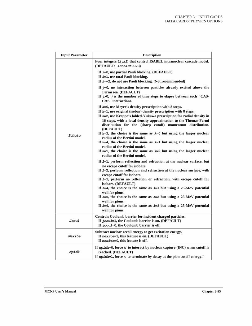
CHAPTER 3 – INPUT CARDS DATA CARDS: PHYSICS OPTIONS
MCNP User’s Manual Chapter 3-95
Input Parameter Description
Ichoic
Four integers (ijkl) that control ISABEL intranuclear cascade model. (DEFAULT: ichoic=0023)
If i=0, use partial Pauli blocking. (DEFAULT) If i=1, use total Pauli blocking. If i=-2, do not use Pauli blocking. (Not recommended)
If j=0, no interaction between particles already excited above the Fermi sea. (DEFAULT)
If j>0, j is the number of time steps to elapse between such "CAS-CAS" interactions.
If k=0, use Meyer’s density prescription with 8 steps. If k=1, use original (isobar) density prescription with 8 steps. If k=2, use Krappe’s folded-Yukawa prescription for radial density in
16 steps, with a local density approximation to the Thomas-Fermi distribution for the (sharp cutoff) momentum distribution. (DEFAULT)
If k=3, the choice is the same as k=0 but using the larger nuclear radius of the Bertini model.
If k=4, the choice is the same as k=1 but using the larger nuclear radius of the Bertini model.
If k=5, the choice is the same as k=2 but using the larger nuclear radius of the Bertini model.
If l=1, perform reflection and refraction at the nuclear surface, but no escape cutoff for isobars.
If l=2, perform reflection and refraction at the nuclear surface, with escape cutoff for isobars.
If l=3, perform no reflection or refraction, with escape cutoff for isobars. (DEFAULT)
If l=4, the choice is the same as l=1 but using a 25-MeV potential well for pions.
If l=5, the choice is the same as l=2 but using a 25-MeV potential well for pions.
If l=6, the choice is the same as l=3 but using a 25-MeV potential well for pions.
Jcoul Controls Coulomb barrier for incident charged particles.
If jcoul=1, the Coulomb barrier is on. (DEFAULT) If jcoul=0, the Coulomb barrier is off.
Nexite Subtract nuclear recoil energy to get excitation energy.
If nexite=1, this feature is on. (DEFAULT) If nexite=0, this feature is off.
Npidk If npidk=0, force π- to interact by nuclear capture (INC) when cutoff is
reached. (DEFAULT) If npidk=1, force π- to terminate by decay at the pion cutoff energy.‡
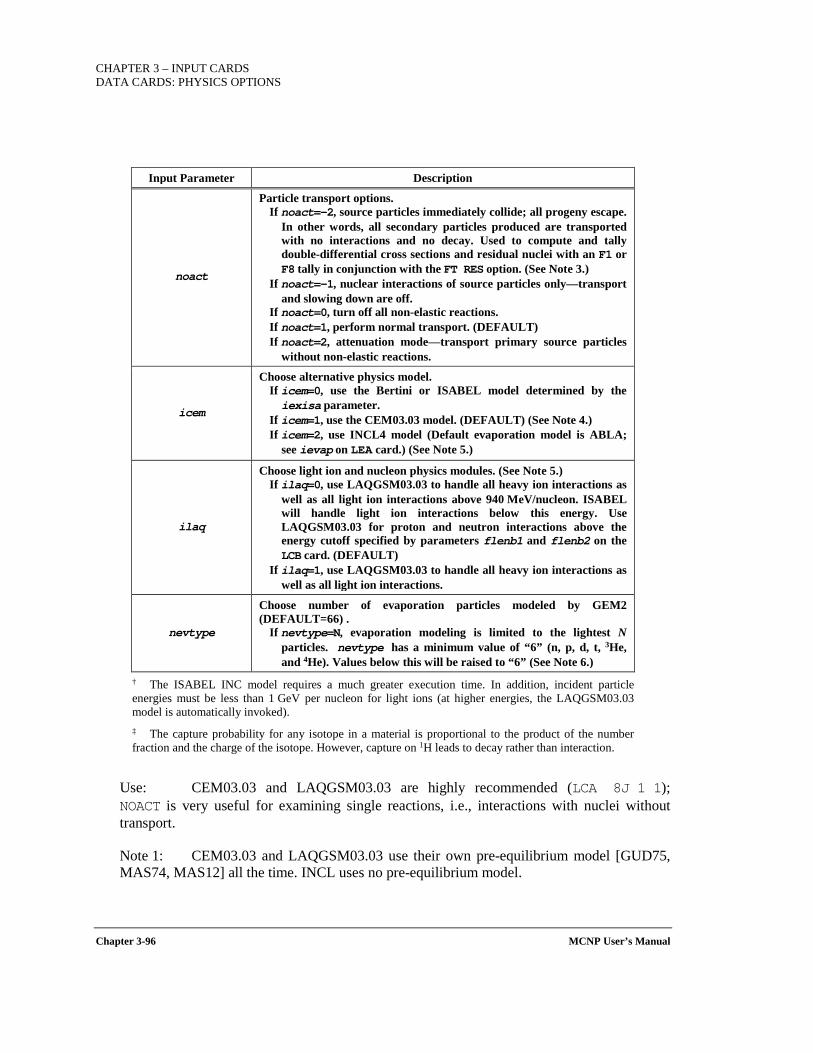
CHAPTER 3 – INPUT CARDS DATA CARDS: PHYSICS OPTIONS
Chapter 3-96 MCNP User’s Manual
Input Parameter Description
noact
Particle transport options. If noact=-2, source particles immediately collide; all progeny escape.
In other words, all secondary particles produced are transported with no interactions and no decay. Used to compute and tally double-differential cross sections and residual nuclei with an F1 or F8 tally in conjunction with the FT RES option. (See Note 3.)
If noact=-1, nuclear interactions of source particles only—transport and slowing down are off.
If noact=0, turn off all non-elastic reactions. If noact=1, perform normal transport. (DEFAULT) If noact=2, attenuation mode—transport primary source particles
without non-elastic reactions.
icem
Choose alternative physics model. If icem=0, use the Bertini or ISABEL model determined by the iexisa parameter.
If icem=1, use the CEM03.03 model. (DEFAULT) (See Note 4.) If icem=2, use INCL4 model (Default evaporation model is ABLA;
see ievap on LEA card.) (See Note 5.)
ilaq
Choose light ion and nucleon physics modules. (See Note 5.) If ilaq=0, use LAQGSM03.03 to handle all heavy ion interactions as
well as all light ion interactions above 940 MeV/nucleon. ISABEL will handle light ion interactions below this energy. Use LAQGSM03.03 for proton and neutron interactions above the energy cutoff specified by parameters flenb1 and flenb2 on the LCB card. (DEFAULT)
If ilaq=1, use LAQGSM03.03 to handle all heavy ion interactions as well as all light ion interactions.
nevtype
Choose number of evaporation particles modeled by GEM2 (DEFAULT=66) .
If nevtype=N, evaporation modeling is limited to the lightest N particles. nevtype has a minimum value of “6” (n, p, d, t, 3He, and 4He). Values below this will be raised to “6” (See Note 6.)
† The ISABEL INC model requires a much greater execution time. In addition, incident particle energies must be less than 1 GeV per nucleon for light ions (at higher energies, the LAQGSM03.03 model is automatically invoked). ‡ The capture probability for any isotope in a material is proportional to the product of the number fraction and the charge of the isotope. However, capture on 1H leads to decay rather than interaction.
Use: CEM03.03 and LAQGSM03.03 are highly recommended (LCA 8J 1 1); NOACT is very useful for examining single reactions, i.e., interactions with nuclei without transport.
Note 1: CEM03.03 and LAQGSM03.03 use their own pre-equilibrium model [GUD75, MAS74, MAS12] all the time. INCL uses no pre-equilibrium model.
CHAPTER 3 – INPUT CARDS DATA CARDS: PHYSICS OPTIONS
MCNP User’s Manual Chapter 3-97
Note 2: The antinucleons and kaons are unaffected by the choice of physics models. They always choose ISABEL below the flenb5 (see LCB card) and LAQGSM03.03 above the flenb6. At energies intermediate to these two, a weighted random choice is made between the two models.
Note 3: If noact=-2 on the LCA card, table physics will be used whenever possible to get the differential data actually used in a given problem. To get the differential data with models only, table data can be turned off by setting the cutn parameter on the PHYS:N card and the tabl parameter on the PHYS:H card.
Note 4: CEM03.03 allows neutrons, protons, pions, and photons to initiate nuclear reactions. We recommend when possible using CEM03.03 for target-nuclei energies up to about 5 GeV for reactions induced by nucleons and pions on heavy nuclei-targets, up to about 1.2 GeV for photonuclear reactions, and up to about 1 GeV for reactions on light nuclei-targets. Although results from CEM03.03 are expected to be more reliable in these energy regions, CEM03.03 is expected also to work quite reliably for all target-nuclei at energies up to about 5 GeV. CEM03.03 consists of an IntraNuclear Cascade (INC) model [BAR72, BAR73, MAS12], followed by its own pre-equilibrium model [GUD75, MAS74, MAS12] and an evaporation model (see details in reference MAS12 and references therein). Possible fission events are initiated in the equilibrium stage for compound nuclei with a charge number greater than 65. The evaporation/fission is handled by a modification of the Generalized Evaporation/Fission Model (GEM2) [FUR00]. Fission fragments undergo an evaporation stage that depends on their excitation energy. When the mass number of excited nuclei produced after INC, as well as after and during the preequilibrium and evaporation/fission stages of reactions, is below 13 (i.e., A<13), CEM03.03 uses the Fermi break-up model to calculate the following de-excitation, instead of using the preequilibrium and/or the evaporation/fission models. After the last stage of a reaction calculated by CEM03.03 (usually, the evaporation), a de-excitation of the residual nucleus follows in MCNP6 (but not in CEM03.03 when used as a stand-alone code [MAS12]), generating gammas with the PHT code adopted from LAHET [PRA89].
Note 5: By default, light ions (d, t, 3He, alpha) are handled by ISABEL below 940 MeV/nucleon and LAQGSM03.03 above 940 MeV/nucleon. Specifying ilaq=1 will send them to LAQGSM03.03 at all energies. Specifying icem=2 will instead send them to INCL for all energies.
Note 6: By default, GEM2 models the evaporation of 66 types of particles (up to 28Mg). As heavier nuclei often have negligible fission/evaporation probabilities, specifying nevtype=N, limits evaporation modeling to the lightest N particles. A minimum number of 6 particle types (n, p, d, t, 3He, and 4He) is needed, and will default to “6” when nevtype<6. It is recommended that users of CEM03.03 and LAQGSM03.01 use a nevtype value of “66” only when evaporation of fragments heavier than 4He are desired; otherwise the value of “6” is recommended to save computational performance.
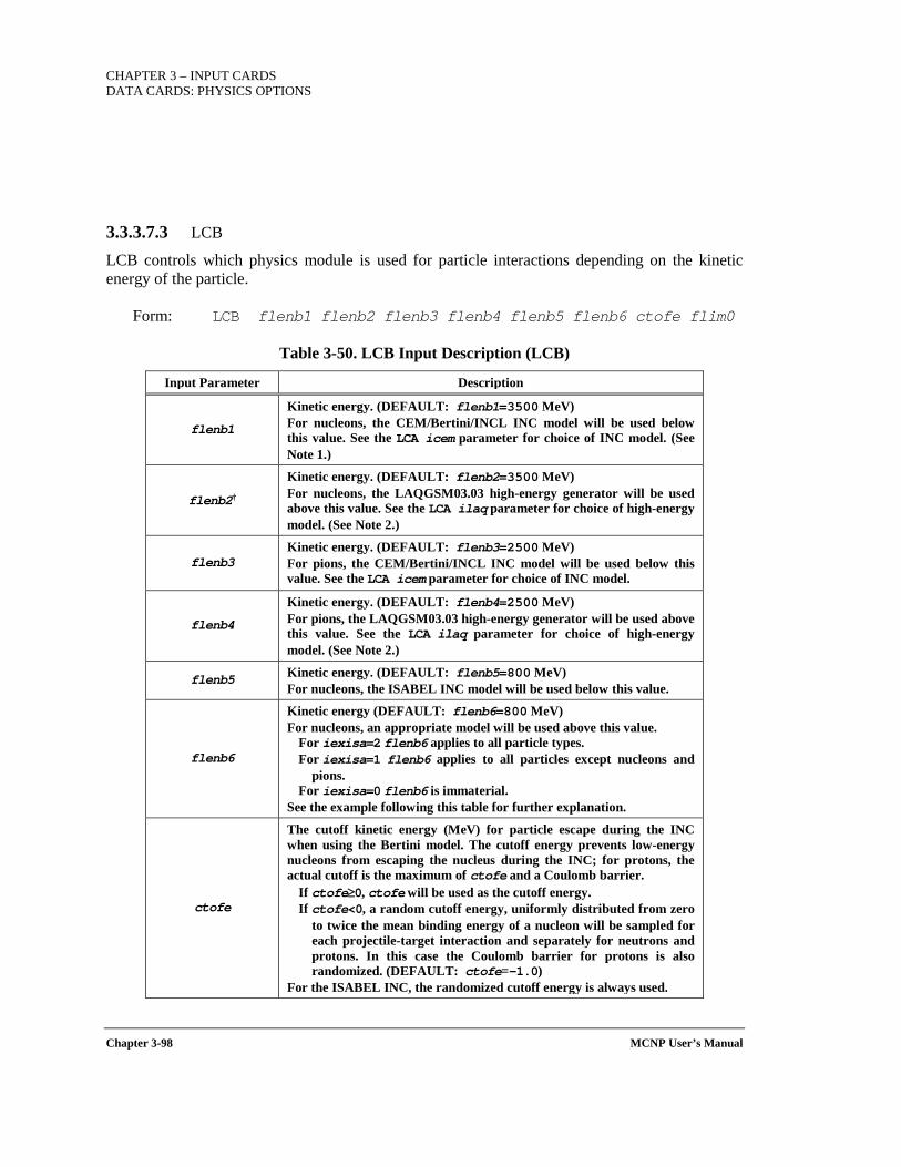
CHAPTER 3 – INPUT CARDS DATA CARDS: PHYSICS OPTIONS
Chapter 3-98 MCNP User’s Manual
3.3.3.7.3 LCB
LCB controls which physics module is used for particle interactions depending on the kinetic energy of the particle.
Form: LCB flenb1 flenb2 flenb3 flenb4 flenb5 flenb6 ctofe flim0
Table 3-50. LCB Input Description (LCB)
Input Parameter Description
flenb1
Kinetic energy. (DEFAULT: flenb1=3500 MeV) For nucleons, the CEM/Bertini/INCL INC model will be used below this value. See the LCA icem parameter for choice of INC model. (See Note 1.)
flenb2†
Kinetic energy. (DEFAULT: flenb2=3500 MeV) For nucleons, the LAQGSM03.03 high-energy generator will be used above this value. See the LCA ilaq parameter for choice of high-energy model. (See Note 2.)
flenb3 Kinetic energy. (DEFAULT: flenb3=2500 MeV) For pions, the CEM/Bertini/INCL INC model will be used below this value. See the LCA icem parameter for choice of INC model.
flenb4
Kinetic energy. (DEFAULT: flenb4=2500 MeV) For pions, the LAQGSM03.03 high-energy generator will be used above this value. See the LCA ilaq parameter for choice of high-energy model. (See Note 2.)
flenb5 Kinetic energy. (DEFAULT: flenb5=800 MeV) For nucleons, the ISABEL INC model will be used below this value.
flenb6
Kinetic energy (DEFAULT: flenb6=800 MeV) For nucleons, an appropriate model will be used above this value.
For iexisa=2 flenb6 applies to all particle types. For iexisa=1 flenb6 applies to all particles except nucleons and
pions. For iexisa=0 flenb6 is immaterial.
See the example following this table for further explanation.
ctofe
The cutoff kinetic energy (MeV) for particle escape during the INC when using the Bertini model. The cutoff energy prevents low-energy nucleons from escaping the nucleus during the INC; for protons, the actual cutoff is the maximum of ctofe and a Coulomb barrier.
If ctofe≥0, ctofe will be used as the cutoff energy. If ctofe<0, a random cutoff energy, uniformly distributed from zero
to twice the mean binding energy of a nucleon will be sampled for each projectile-target interaction and separately for neutrons and protons. In this case the Coulomb barrier for protons is also randomized. (DEFAULT: ctofe=-1.0)
For the ISABEL INC, the randomized cutoff energy is always used.
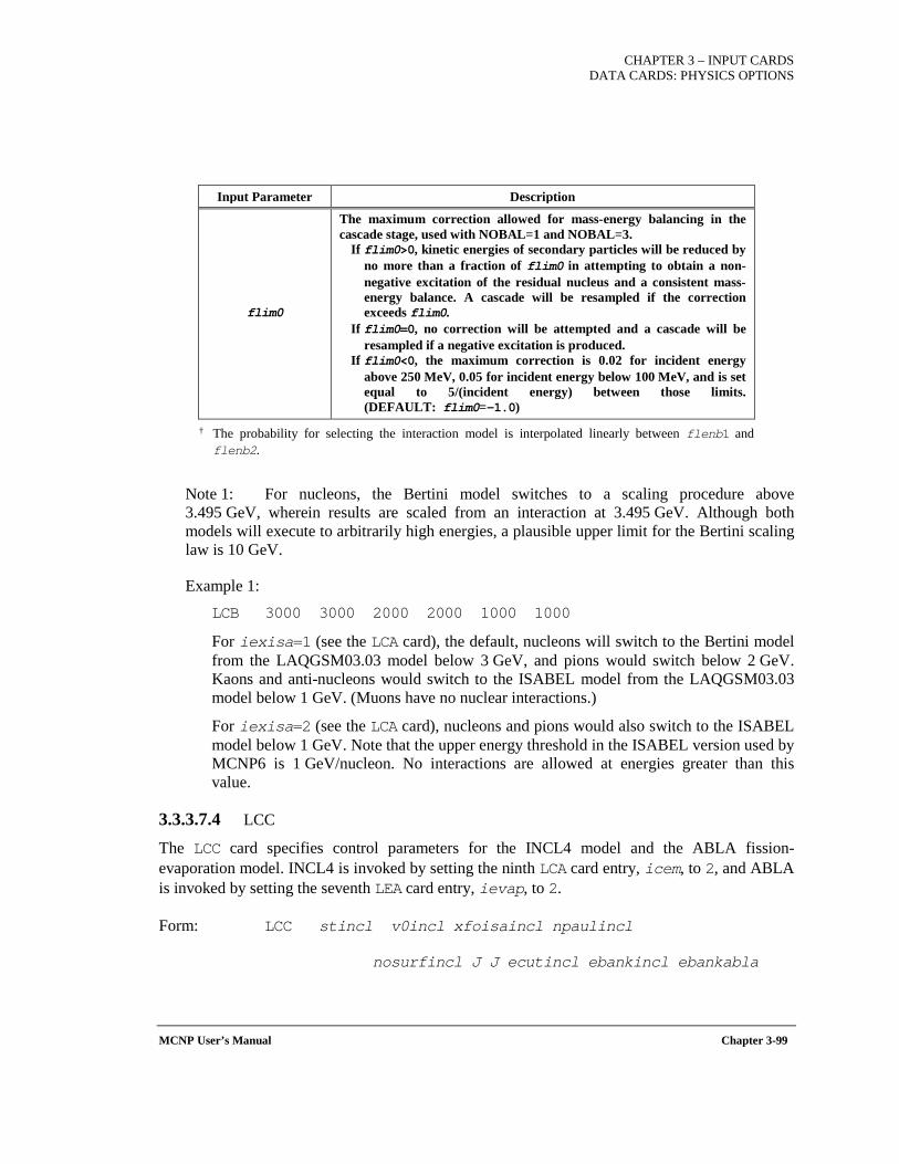
CHAPTER 3 – INPUT CARDS DATA CARDS: PHYSICS OPTIONS
MCNP User’s Manual Chapter 3-99
Input Parameter Description
flim0
The maximum correction allowed for mass-energy balancing in the cascade stage, used with NOBAL=1 and NOBAL=3.
If flim0>0, kinetic energies of secondary particles will be reduced by no more than a fraction of flim0 in attempting to obtain a non-negative excitation of the residual nucleus and a consistent mass-energy balance. A cascade will be resampled if the correction exceeds flim0.
If flim0=0, no correction will be attempted and a cascade will be resampled if a negative excitation is produced.
If flim0<0, the maximum correction is 0.02 for incident energy above 250 MeV, 0.05 for incident energy below 100 MeV, and is set equal to 5/(incident energy) between those limits. (DEFAULT: flim0=-1.0)
† The probability for selecting the interaction model is interpolated linearly between flenb1 and flenb2.
Note 1: For nucleons, the Bertini model switches to a scaling procedure above 3.495 GeV, wherein results are scaled from an interaction at 3.495 GeV. Although both models will execute to arbitrarily high energies, a plausible upper limit for the Bertini scaling law is 10 GeV.
Example 1: LCB 3000 3000 2000 2000 1000 1000
For iexisa=1 (see the LCA card), the default, nucleons will switch to the Bertini model from the LAQGSM03.03 model below 3 GeV, and pions would switch below 2 GeV. Kaons and anti-nucleons would switch to the ISABEL model from the LAQGSM03.03 model below 1 GeV. (Muons have no nuclear interactions.)
For iexisa=2 (see the LCA card), nucleons and pions would also switch to the ISABEL model below 1 GeV. Note that the upper energy threshold in the ISABEL version used by MCNP6 is 1 GeV/nucleon. No interactions are allowed at energies greater than this value.
3.3.3.7.4 LCC
The LCC card specifies control parameters for the INCL4 model and the ABLA fission-evaporation model. INCL4 is invoked by setting the ninth LCA card entry, icem, to 2, and ABLA is invoked by setting the seventh LEA card entry, ievap, to 2.
Form: LCC stincl v0incl xfoisaincl npaulincl
nosurfincl J J ecutincl ebankincl ebankabla
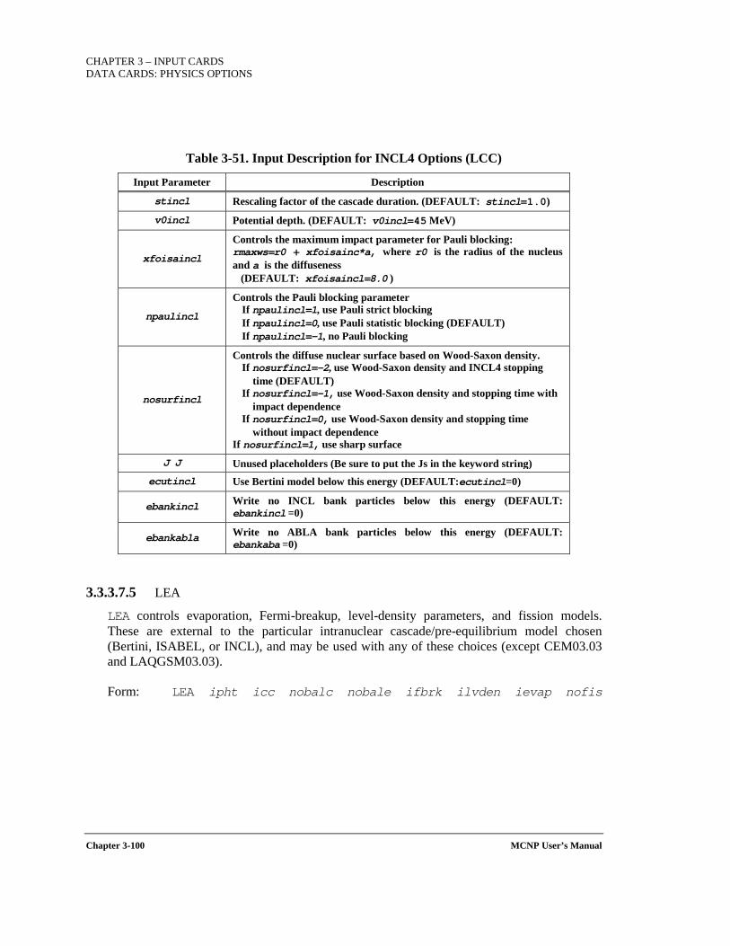
CHAPTER 3 – INPUT CARDS DATA CARDS: PHYSICS OPTIONS
Chapter 3-100 MCNP User’s Manual
Table 3-51. Input Description for INCL4 Options (LCC)
Input Parameter Description
stincl Rescaling factor of the cascade duration. (DEFAULT: stincl=1.0)
v0incl Potential depth. (DEFAULT: v0incl=45 MeV)
xfoisaincl
Controls the maximum impact parameter for Pauli blocking: rmaxws=r0 + xfoisainc*a, where r0 is the radius of the nucleus and a is the diffuseness (DEFAULT: xfoisaincl=8.0 )
npaulincl
Controls the Pauli blocking parameter If npaulincl=1, use Pauli strict blocking If npaulincl=0, use Pauli statistic blocking (DEFAULT) If npaulincl=-1, no Pauli blocking
nosurfincl
Controls the diffuse nuclear surface based on Wood-Saxon density. If nosurfincl=-2, use Wood-Saxon density and INCL4 stopping
time (DEFAULT) If nosurfincl=-1, use Wood-Saxon density and stopping time with
impact dependence If nosurfincl=0, use Wood-Saxon density and stopping time
without impact dependence If nosurfincl=1, use sharp surface
J J Unused placeholders (Be sure to put the Js in the keyword string) ecutincl Use Bertini model below this energy (DEFAULT:ecutincl=0)
ebankincl Write no INCL bank particles below this energy (DEFAULT: ebankincl =0)
ebankabla Write no ABLA bank particles below this energy (DEFAULT: ebankaba =0)
3.3.3.7.5 LEA
LEA controls evaporation, Fermi-breakup, level-density parameters, and fission models. These are external to the particular intranuclear cascade/pre-equilibrium model chosen (Bertini, ISABEL, or INCL), and may be used with any of these choices (except CEM03.03 and LAQGSM03.03).
Form: LEA ipht icc nobalc nobale ifbrk ilvden ievap nofis
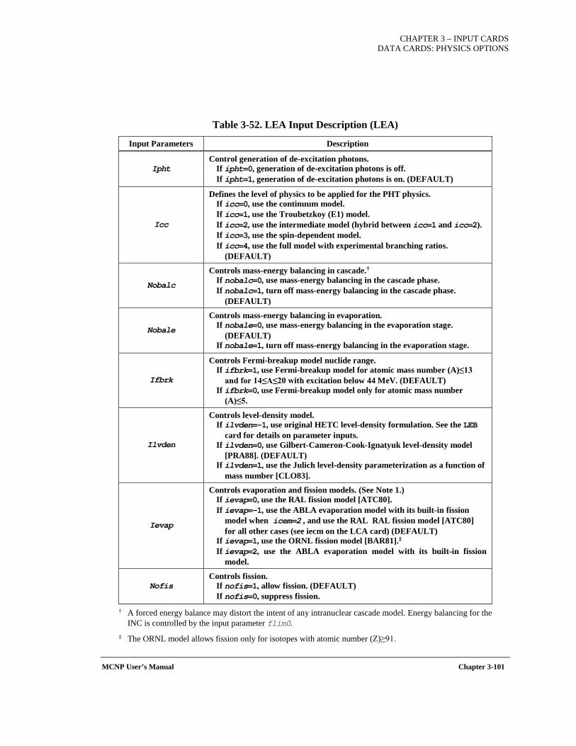
CHAPTER 3 – INPUT CARDS DATA CARDS: PHYSICS OPTIONS
MCNP User’s Manual Chapter 3-101
Table 3-52. LEA Input Description (LEA)
Input Parameters Description
Ipht Control generation of de-excitation photons.
If ipht=0, generation of de-excitation photons is off. If ipht=1, generation of de-excitation photons is on. (DEFAULT)
Icc
Defines the level of physics to be applied for the PHT physics. If icc=0, use the continuum model. If icc=1, use the Troubetzkoy (E1) model. If icc=2, use the intermediate model (hybrid between icc=1 and icc=2). If icc=3, use the spin-dependent model. If icc=4, use the full model with experimental branching ratios.
(DEFAULT)
Nobalc
Controls mass-energy balancing in cascade.† If nobalc=0, use mass-energy balancing in the cascade phase. If nobalc=1, turn off mass-energy balancing in the cascade phase.
(DEFAULT)
Nobale
Controls mass-energy balancing in evaporation. If nobale=0, use mass-energy balancing in the evaporation stage.
(DEFAULT) If nobale=1, turn off mass-energy balancing in the evaporation stage.
Ifbrk
Controls Fermi-breakup model nuclide range. If ifbrk=1, use Fermi-breakup model for atomic mass number (A)≤13
and for 14≤A≤20 with excitation below 44 MeV. (DEFAULT) If ifbrk=0, use Fermi-breakup model only for atomic mass number
(A)≤5.
Ilvden
Controls level-density model. If ilvden=-1, use original HETC level-density formulation. See the LEB
card for details on parameter inputs. If ilvden=0, use Gilbert-Cameron-Cook-Ignatyuk level-density model
[PRA88]. (DEFAULT) If ilvden=1, use the Julich level-density parameterization as a function of
mass number [CLO83].
Ievap
Controls evaporation and fission models. (See Note 1.) If ievap=0, use the RAL fission model [ATC80]. If ievap=-1, use the ABLA evaporation model with its built-in fission
model when icem=2 , and use the RAL RAL fission model [ATC80] for all other cases (see iecm on the LCA card) (DEFAULT)
If ievap=1, use the ORNL fission model [BAR81].‡ If ievap=2, use the ABLA evaporation model with its built-in fission
model.
Nofis Controls fission.
If nofis=1, allow fission. (DEFAULT) If nofis=0, suppress fission.
† A forced energy balance may distort the intent of any intranuclear cascade model. Energy balancing for the INC is controlled by the input parameter flim0.
‡ The ORNL model allows fission only for isotopes with atomic number (Z)≥91.
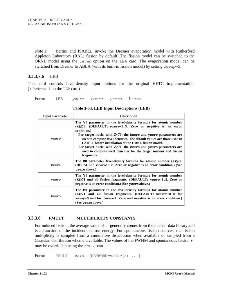
CHAPTER 3 – INPUT CARDS DATA CARDS: PHYSICS OPTIONS
Chapter 3-102 MCNP User’s Manual
Note 1: Bertini and ISABEL invoke the Dresner evaporation model with Rutherford Appleton Laboratory (RAL) fission by default. The fission model can be switched to the ORNL model using the ievap option on the LEA card. The evaporation model can be switched from Dresner to ABLA (with its built-in fission model) by setting ievap=2.
3.3.3.7.6 LEB
This card controls level-density input options for the original HETC implementation. (ilvden=-1 on the LEA card)
Form: LEB yzere bzere yzero bzero
Table 3-53. LEB Input Descriptions (LEB)
Input Parameter Description
yzere
The Y0 parameter in the level-density formula for atomic number (Z)≤70. (DEFAULT: yzere=1.5. Zero or negative is an error condition.)
For target nuclei with Z≤70, the bzere and yzere parameters are used to compute level densities. The default values are those used in LAHET before installation of the ORNL fission model.
For target nuclei with Z≥71, the bzero and yzero parameters are used to compute level densities for the target nucleus and fission fragments.
bzere The B0 parameter level-density formula for atomic number (Z)≤70. (DEFAULT: bzere=8.0. Zero or negative is an error condition.) (See yzere above.)
yzero The Y0 parameter in the level-density formula for atomic number (Z)≥71 and all fission fragments. (DEFAULT: yzero=1.5. Zero or negative is an error condition.) (See yzere above.)
bzero
The B0 parameter in the level-density formula for atomic number (Z)≥71 and all fission fragments. (DEFAULT: bzero=10.0 for ievap=0 and for ievap=1. Zero and negative is an error condition.) (See yzere above.)
3.3.3.8 FMULT MULTIPLICITY CONSTANTS
For induced fission, the average value of generally comes from the nuclear data library and is a function of the incident neutron energy. For spontaneous fission sources, the fission multiplicity is sampled from a cumulative distribution when available or sampled from a Gaussian distribution when unavailable. The values of the FWHM and spontaneous fission may be overridden using the FMULT card.
Form: FMULT zaid [KEYWORD=value(s) ...]
ν
ν
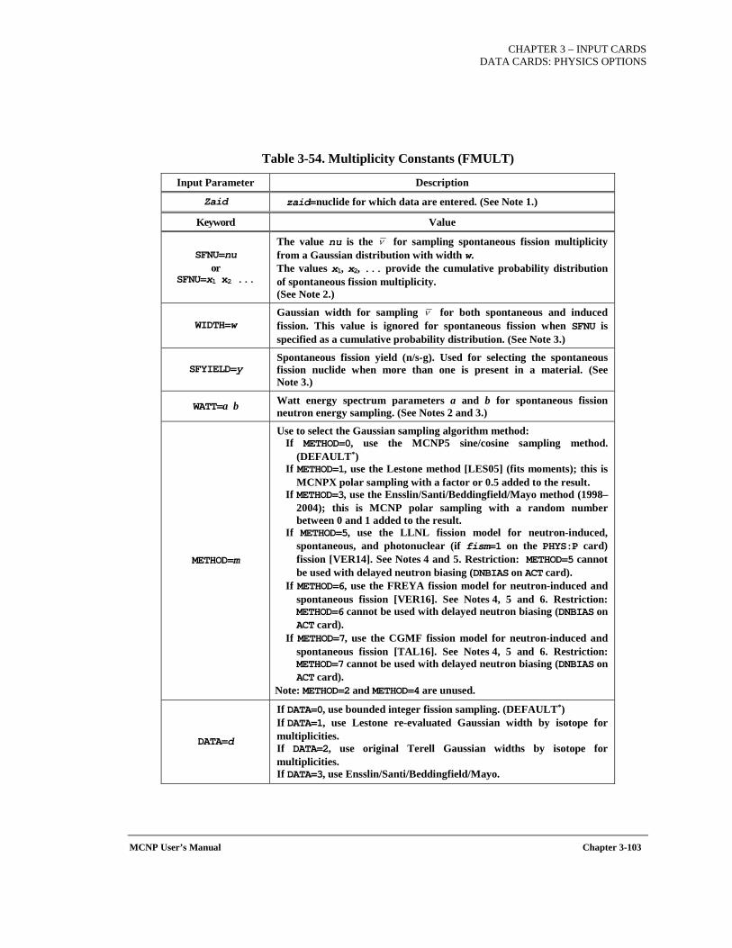
CHAPTER 3 – INPUT CARDS DATA CARDS: PHYSICS OPTIONS
MCNP User’s Manual Chapter 3-103
Table 3-54. Multiplicity Constants (FMULT)
Input Parameter Description
Zaid zaid=nuclide for which data are entered. (See Note 1.)
Keyword Value
SFNU=nu or
SFNU=x1 x2 ...
The value nu is the for sampling spontaneous fission multiplicity from a Gaussian distribution with width w. The values x1, x2, ... provide the cumulative probability distribution of spontaneous fission multiplicity. (See Note 2.)
WIDTH=w Gaussian width for sampling for both spontaneous and induced fission. This value is ignored for spontaneous fission when SFNU is specified as a cumulative probability distribution. (See Note 3.)
SFYIELD=y Spontaneous fission yield (n/s-g). Used for selecting the spontaneous fission nuclide when more than one is present in a material. (See Note 3.)
WATT=a b Watt energy spectrum parameters a and b for spontaneous fission neutron energy sampling. (See Notes 2 and 3.)
METHOD=m
Use to select the Gaussian sampling algorithm method: If METHOD=0, use the MCNP5 sine/cosine sampling method.
(DEFAULT*) If METHOD=1, use the Lestone method [LES05] (fits moments); this is
MCNPX polar sampling with a factor or 0.5 added to the result. If METHOD=3, use the Ensslin/Santi/Beddingfield/Mayo method (1998–
2004); this is MCNP polar sampling with a random number between 0 and 1 added to the result.
If METHOD=5, use the LLNL fission model for neutron-induced, spontaneous, and photonuclear (if fism=1 on the PHYS:P card) fission [VER14]. See Notes 4 and 5. Restriction: METHOD=5 cannot be used with delayed neutron biasing (DNBIAS on ACT card).
If METHOD=6, use the FREYA fission model for neutron-induced and spontaneous fission [VER16]. See Notes 4, 5 and 6. Restriction: METHOD=6 cannot be used with delayed neutron biasing (DNBIAS on ACT card).
If METHOD=7, use the CGMF fission model for neutron-induced and spontaneous fission [TAL16]. See Notes 4, 5 and 6. Restriction: METHOD=7 cannot be used with delayed neutron biasing (DNBIAS on ACT card).
Note: METHOD=2 and METHOD=4 are unused.
DATA=d
If DATA=0, use bounded integer fission sampling. (DEFAULT*) If DATA=1, use Lestone re-evaluated Gaussian width by isotope for multiplicities. If DATA=2, use original Terell Gaussian widths by isotope for multiplicities. If DATA=3, use Ensslin/Santi/Beddingfield/Mayo.
ν
ν

CHAPTER 3 – INPUT CARDS DATA CARDS: PHYSICS OPTIONS
Chapter 3-104 MCNP User’s Manual
SHIFT=s
Designate method to decrease ν to preserve : If SHIFT=0, use the MCNP5 treatment, which assumes an integer
number of neutrons per fission. For example, if =2.7, then the number of neutrons will be two 30% of the time and three 70% of the time. (DEFAULT*)
If SHIFT>0, sample from an isotope-dependent Gaussian distribution. The full-width at half-maximum (FWHM) values are displayed in print table 38. The following values are allowed:
If SHIFT=1, correct the sampled to preserve the average multiplicity (MCNPX-style adjustment). This method uses a reevaluated Gaussian width to sample fission neutron multiplicities for all fissionable isotopes.
If SHIFT=2, preserve the multiplicity by increasing the threshold. If SHIFT=3, sample the Gaussian distribution without correction.
(This will over predict ν.) If SHIFT=4, use MCNP4C integer sampling method in the presence of
spontaneous fission. * Default if no METHOD, DATA, or SHIFT keywords are specified. If any of these keywords appear, the
code will automatically assign values for the unspecified keywords. The default assignments are METHOD=3, DATA=3, and SHIFT=1.
Use: Enables users to override or add additional fission multiplicity data.
Table 3-55. Mapping from MCNP5 and MCNPX PHYS:N Settings to New FMULT Settings*
MCNPX: PHYS:N 6th entry (fism)
FMULT Keyword: METHOD
FMULT Keyword: DATA
FMULT Keyword: SHIFT
0 (sample fission neutron multiplicity using bounded integers)
0 0 0
-1, 1 (correct the sampled to preserve the average multiplicity)
3 3 1
2 (preserve the multiplicity by increasing the threshold)
3 3 2
3 (sample the Gaussian distribution without correction)
3 3 3
4 (use the bounded integer method in the presence of spontaneous fission)
3 3 4
5 (use the LLNL fission model for neutron-induced, spontaneous, and photonuclear fission)
5 unused unused
ν
ν
ν
ν
ν
ν
ν
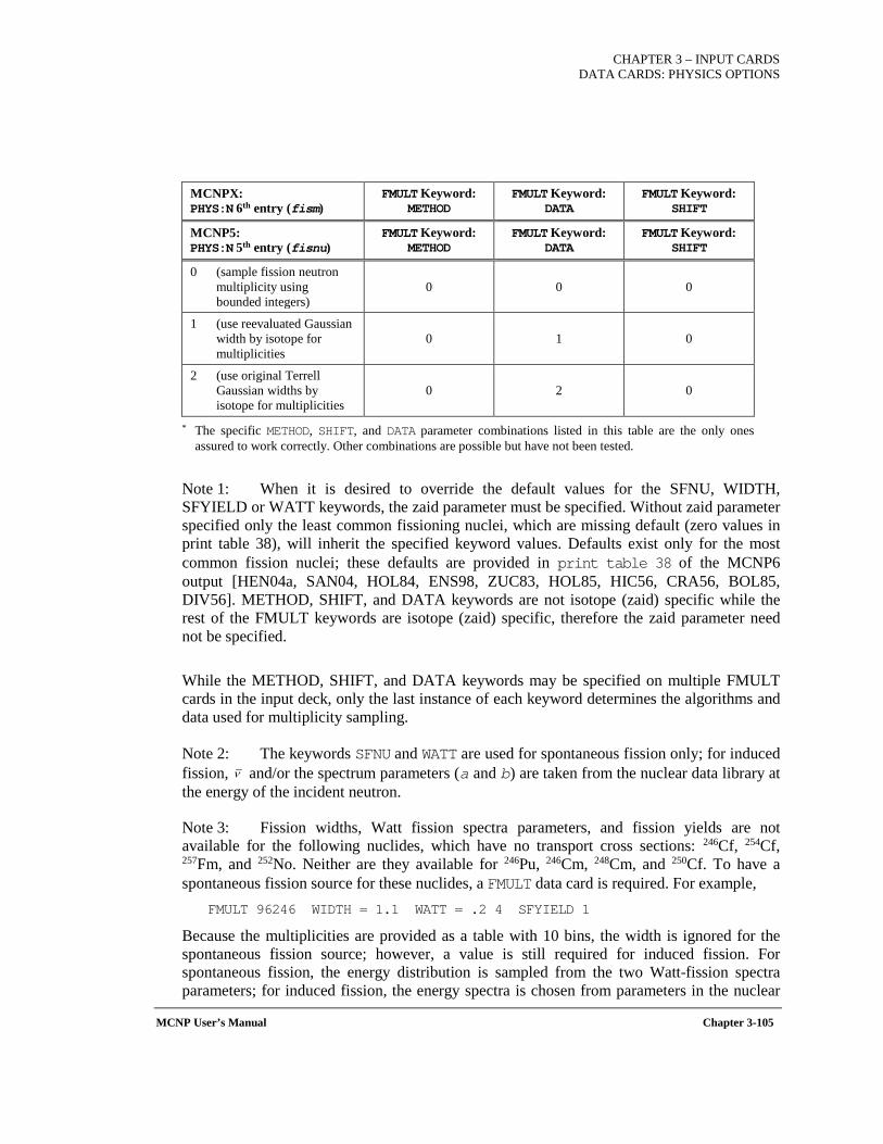
CHAPTER 3 – INPUT CARDS DATA CARDS: PHYSICS OPTIONS
MCNP User’s Manual Chapter 3-105
MCNPX: PHYS:N 6th entry (fism)
FMULT Keyword: METHOD
FMULT Keyword: DATA
FMULT Keyword: SHIFT
MCNP5: PHYS:N 5th entry (fisnu)
FMULT Keyword: METHOD
FMULT Keyword: DATA
FMULT Keyword: SHIFT
0 (sample fission neutron multiplicity using bounded integers)
0 0 0
1 (use reevaluated Gaussian width by isotope for multiplicities
0 1 0
2 (use original Terrell Gaussian widths by isotope for multiplicities
0 2 0
* The specific METHOD, SHIFT, and DATA parameter combinations listed in this table are the only ones assured to work correctly. Other combinations are possible but have not been tested.
Note 1: When it is desired to override the default values for the SFNU, WIDTH, SFYIELD or WATT keywords, the zaid parameter must be specified. Without zaid parameter specified only the least common fissioning nuclei, which are missing default (zero values in print table 38), will inherit the specified keyword values. Defaults exist only for the most common fission nuclei; these defaults are provided in print table 38 of the MCNP6 output [HEN04a, SAN04, HOL84, ENS98, ZUC83, HOL85, HIC56, CRA56, BOL85, DIV56]. METHOD, SHIFT, and DATA keywords are not isotope (zaid) specific while the rest of the FMULT keywords are isotope (zaid) specific, therefore the zaid parameter need not be specified.
While the METHOD, SHIFT, and DATA keywords may be specified on multiple FMULT cards in the input deck, only the last instance of each keyword determines the algorithms and data used for multiplicity sampling.
Note 2: The keywords SFNU and WATT are used for spontaneous fission only; for induced fission, and/or the spectrum parameters (a and b) are taken from the nuclear data library at the energy of the incident neutron.
Note 3: Fission widths, Watt fission spectra parameters, and fission yields are not available for the following nuclides, which have no transport cross sections: 246Cf, 254Cf, 257Fm, and 252No. Neither are they available for 246Pu, 246Cm, 248Cm, and 250Cf. To have a spontaneous fission source for these nuclides, a FMULT data card is required. For example,
FMULT 96246 WIDTH = 1.1 WATT = .2 4 SFYIELD 1
Because the multiplicities are provided as a table with 10 bins, the width is ignored for the spontaneous fission source; however, a value is still required for induced fission. For spontaneous fission, the energy distribution is sampled from the two Watt-fission spectra parameters; for induced fission, the energy spectra is chosen from parameters in the nuclear
ν

CHAPTER 3 – INPUT CARDS DATA CARDS: PHYSICS OPTIONS
Chapter 3-106 MCNP User’s Manual
data tables of the transport cross sections. Finally, the spontaneous fission yield must be specified if more than one spontaneous fission source nuclide occurs. The yield is used to determine the relative sampling among spontaneous fission source nuclides. These parameters have no default values; if the FMULT card is missing, a fatal error message is issued.
Note 4: The LLNL fission model (METHOD=5), the FREYA fission model (METHOD=6), and the CGMF fission model (METHOD=7) are the only ways in MCNP6 to produce prompt fission photons at low energies. (At high energies, use of event generators followed by the PHT code produces photons from fission fragments.) Both fission neutrons and photons are correlated to the fission event and have multiplicities. When photofission is also turned on (ispn≠0 and fism=1 on the PHYS:P card), prompt photofission gammas are generated using the LLNL fission model with appropriate photofission neutron correlation and multiplicities. Use of the fission models is confirmed by the following example OUTP file message: "Using LLNL Fission Multiplicity Model". Delayed fission gammas are independent of the fission model and are controlled by the ACT card.
When any one of the fission models is selected (METHOD=5,6,7), the prompt fission photons are correlated with the fission event. Furthermore, for PAR=SF, the fission models are the only MCNP6 method emitting spontaneous fission prompt gamma rays. These are neglected in the MCNP6 default FMULT spontaneous fission source.
Note 5: If the LLNL, FREYA, or CGMF fission model is used, then only the spontaneous fission yield (SFYIELD) is used for nuclides in the respective model. For fissioning nuclides not in the LLNL model, the FMULT parameters are used.
Note 6: If either the FREYA or CGMF fission model is used, and the fission nuclide is unavailable, the LLNL fission model is used to emit correlated neutrons and photons.
Multiplicity Parameters Default Values
The data that follow are the default values [SAN04] of the multiplicity parameters in MCNP6; these can be modified with the FMULT card. The spontaneous fission multiplicity table values are displayed in print table 38 to three-digits, but are accurate to seven digits in MCNP6.
1fission multiplicity data. print table 38 zaid width watt1 watt2 yield sfnu 90232 1.079 .800000 4.00000 6.00E-08 2.140 92232 1.079 .892204 3.72278 1.30E+00 1.710 92233 1.041 .854803 4.03210 8.60E-04 1.760 92234 1.079 .771241 4.92449 5.02E-03 1.810 92235 1.072 .774713 4.85231 2.99E-04 1.860 92236 1.079 .735166 5.35746 5.49E-03 1.910
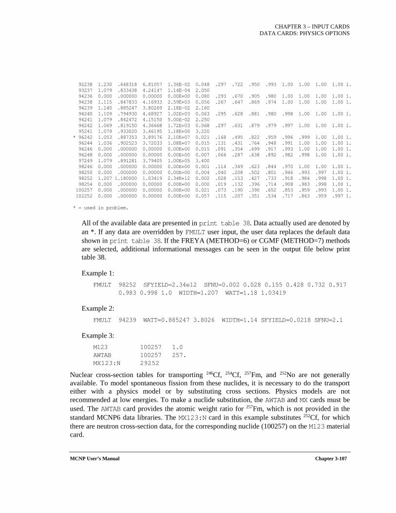
CHAPTER 3 – INPUT CARDS DATA CARDS: PHYSICS OPTIONS
MCNP User’s Manual Chapter 3-107
92238 1.230 .648318 6.81057 1.36E-02 0.048 .297 .722 .950 .993 1.00 1.00 1.00 1.00 1. 93237 1.079 .833438 4.24147 1.14E-04 2.050 94236 0.000 .000000 0.00000 0.00E+00 0.080 .293 .670 .905 .980 1.00 1.00 1.00 1.00 1. 94238 1.115 .847833 4.16933 2.59E+03 0.056 .267 .647 .869 .974 1.00 1.00 1.00 1.00 1. 94239 1.140 .885247 3.80269 2.18E-02 2.160 94240 1.109 .794930 4.68927 1.02E+03 0.063 .295 .628 .881 .980 .998 1.00 1.00 1.00 1. 94241 1.079 .842472 4.15150 5.00E-02 2.250 94242 1.069 .819150 4.36668 1.72E+03 0.068 .297 .631 .879 .979 .997 1.00 1.00 1.00 1. 95241 1.079 .933020 3.46195 1.18E+00 3.220 * 96242 1.053 .887353 3.89176 2.10E+07 0.021 .168 .495 .822 .959 .996 .999 1.00 1.00 1. 96244 1.036 .902523 3.72033 1.08E+07 0.015 .131 .431 .764 .948 .991 1.00 1.00 1.00 1. 96246 0.000 .000000 0.00000 0.00E+00 0.015 .091 .354 .699 .917 .993 1.00 1.00 1.00 1. 96248 0.000 .000000 0.00000 0.00E+00 0.007 .066 .287 .638 .892 .982 .998 1.00 1.00 1. 97249 1.079 .891281 3.79405 1.00E+05 3.400 98246 0.000 .000000 0.00000 0.00E+00 0.001 .114 .349 .623 .844 .970 1.00 1.00 1.00 1. 98250 0.000 .000000 0.00000 0.00E+00 0.004 .040 .208 .502 .801 .946 .993 .997 1.00 1. 98252 1.207 1.180000 1.03419 2.34E+12 0.002 .028 .153 .427 .733 .918 .984 .998 1.00 1. 98254 0.000 .000000 0.00000 0.00E+00 0.000 .019 .132 .396 .714 .908 .983 .998 1.00 1. 100257 0.000 .000000 0.00000 0.00E+00 0.021 .073 .190 .390 .652 .853 .959 .993 1.00 1. 102252 0.000 .000000 0.00000 0.00E+00 0.057 .115 .207 .351 .534 .717 .863 .959 .997 1. * = used in problem.
All of the available data are presented in print table 38. Data actually used are denoted by an *. If any data are overridden by FMULT user input, the user data replaces the default data shown in print table 38. If the FREYA (METHOD=6) or CGMF (METHOD=7) methods are selected, additional informational messages can be seen in the output file below print table 38.
Example 1: FMULT 98252 SFYIELD=2.34e12 SFNU=0.002 0.028 0.155 0.428 0.732 0.917 0.983 0.998 1.0 WIDTH=1.207 WATT=1.18 1.03419
Example 2: FMULT 94239 WATT=0.885247 3.8026 WIDTH=1.14 SFYIELD=0.0218 SFNU=2.1
Example 3: M123 100257 1.0 AWTAB 100257 257. MX123:N 29252
Nuclear cross-section tables for transporting 246Cf, 254Cf, 257Fm, and 252No are not generally available. To model spontaneous fission from these nuclides, it is necessary to do the transport either with a physics model or by substituting cross sections. Physics models are not recommended at low energies. To make a nuclide substitution, the AWTAB and MX cards must be used. The AWTAB card provides the atomic weight ratio for 257Fm, which is not provided in the standard MCNP6 data libraries. The MX123:N card in this example substitutes 252Cf, for which there are neutron cross-section data, for the corresponding nuclide (100257) on the M123 material card.
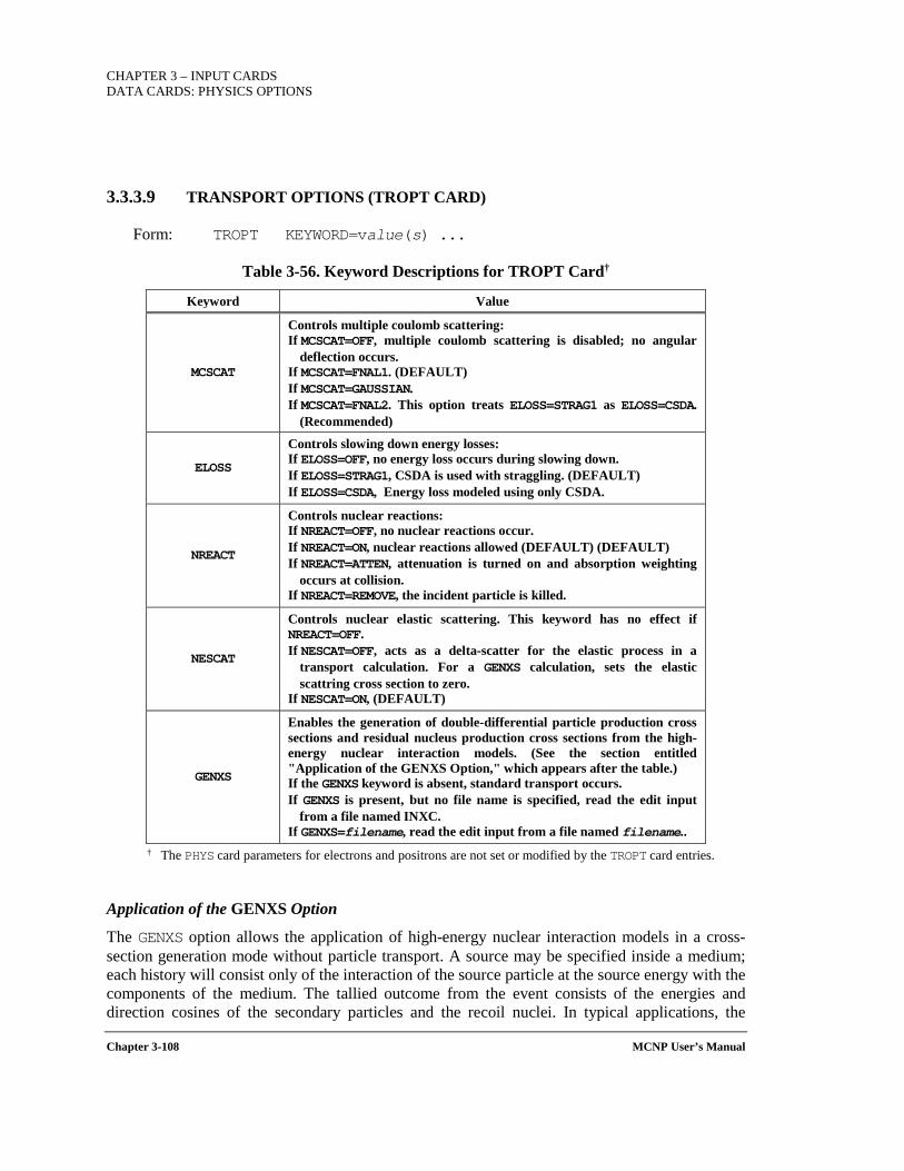
CHAPTER 3 – INPUT CARDS DATA CARDS: PHYSICS OPTIONS
Chapter 3-108 MCNP User’s Manual
3.3.3.9 TRANSPORT OPTIONS (TROPT CARD)
Form: TROPT KEYWORD=value(s) ...
Table 3-56. Keyword Descriptions for TROPT Card†
Keyword Value
MCSCAT
Controls multiple coulomb scattering: If MCSCAT=OFF, multiple coulomb scattering is disabled; no angular
deflection occurs. If MCSCAT=FNAL1. (DEFAULT) If MCSCAT=GAUSSIAN. If MCSCAT=FNAL2. This option treats ELOSS=STRAG1 as ELOSS=CSDA.
(Recommended)
ELOSS
Controls slowing down energy losses: If ELOSS=OFF, no energy loss occurs during slowing down. If ELOSS=STRAG1, CSDA is used with straggling. (DEFAULT) If ELOSS=CSDA, Energy loss modeled using only CSDA.
NREACT
Controls nuclear reactions: If NREACT=OFF, no nuclear reactions occur. If NREACT=ON, nuclear reactions allowed (DEFAULT) (DEFAULT) If NREACT=ATTEN, attenuation is turned on and absorption weighting
occurs at collision. If NREACT=REMOVE, the incident particle is killed.
NESCAT
Controls nuclear elastic scattering. This keyword has no effect if NREACT=OFF. If NESCAT=OFF, acts as a delta-scatter for the elastic process in a
transport calculation. For a GENXS calculation, sets the elastic scattring cross section to zero.
If NESCAT=ON, (DEFAULT)
GENXS
Enables the generation of double-differential particle production cross sections and residual nucleus production cross sections from the high-energy nuclear interaction models. (See the section entitled "Application of the GENXS Option," which appears after the table.) If the GENXS keyword is absent, standard transport occurs. If GENXS is present, but no file name is specified, read the edit input
from a file named INXC. If GENXS=filename, read the edit input from a file named filename..
† The PHYS card parameters for electrons and positrons are not set or modified by the TROPT card entries.
Application of the GENXS Option
The GENXS option allows the application of high-energy nuclear interaction models in a cross-section generation mode without particle transport. A source may be specified inside a medium; each history will consist only of the interaction of the source particle at the source energy with the components of the medium. The tallied outcome from the event consists of the energies and direction cosines of the secondary particles and the recoil nuclei. In typical applications, the

CHAPTER 3 – INPUT CARDS DATA CARDS: PHYSICS OPTIONS
MCNP User’s Manual Chapter 3-109
material composition will be a single isotope; however, averaged results may be obtained for a natural multi-isotopic element or a complex composition. A GENXS calculation is independent of the material density specification.
The GENXS option requires two input files: the standard MCNP6 INP file and an accompanying auxiliary INXC file. To invoke the GENXS cross-section-generating option, specify “GENXS” or “GENXS filename” on the TROPT card. The content and format of the edited output are determined by the content of the auxiliary input file associated with the GENXS option. If GENXS is specified on the TROPT card without a user-provided file name, by default the output tally edit information will be read from a file named "INXC." If a file name is provided with the GENXS keyword, the output tally edit information will be read from the user-specified filename. In either case, the absence of the required file will produce a fatal error. A description of the INXC file structure and an example follow this discussion.
To calculate inelastic secondary particle production only, turn off the elastic scattering by setting NESCAT=OFF on the TROPT card. Isotopic elastic scattering cross sections will be set to zero and the total cross section will equal the nonelastic cross section. All histories will sample the nonelastic interaction model. [Note that this applies only to the GENXS option; in a transport calculation, NESCAT=OFF implies a delta-scatter for the elastic process.]
To examine only elastic scattering, use NREACT=ATTEN on the TROPT card. All histories will sample the elastic scattering model and produce results for the scattered projectile and the recoil nucleus.
In the output data for a multi-isotopic composition, quoted cross sections are a weighted average of the isotopic cross sections, weighted by the input atom fractions. Thus, the cross-section output represents average cross sections per atom in the composition. Results will reflect the variance introduced by sampling for the target isotope.
Energy- and angle-integrated results are provided as yield as well as cross section. The term “yield” might be better defined as “multiplicity”. The nonelastic yield for a given particle type is the number of secondary particles of that type produced per nonelastic event. The elastic yield is per elastic event and is always unity. The "iyield" input option allows single- and double-differential results to be provided as yield rather than cross section, with the above normalization.
INXC File Structure: The INXC input is based on an128-column "card" format and each requested case may require as many as seven cards. With the exception of the formatted title cards, all data provided in the INXC file are entered as list-directed input. Repeat counts are allowed. A forward slash (/) may be used to terminate an input line; unread variables following a slash are assigned the default value(s). A description of the seven input cards follows:
Card 1: 80-character problem title
Card 2: ncase kplot l_res

CHAPTER 3 – INPUT CARDS DATA CARDS: PHYSICS OPTIONS
Chapter 3-110 MCNP User’s Manual
ncase Defines the number of desired double-differential cross-section edits. (DEFAULT=0)
kplot If nonzero, write cross-section edits to the MCNP6 MCTAL file. (DEFAULT=0) Note: Plotting is available only with the MCTAL file.
l_res If l_res=0, no residual nuclei are calculated; if l_res≠0, perform a residual nuclei edit. (DEFAULT=0)
For each of the ncase cases, repeat the following cards 3 through 7, as required.
Card 3: 128-character case title
Card 4: nerg nang ntype fnorm imom iyield
nerg The number of energy (momentum) bin boundaries. (DEFAULT=0, i.e., produce only energy-integrated values)
nang The absolute value, |nang|, provides the number of angle bin boundaries. For nang>0, cosine bins are specified; for nang<0, degree bins are specified. (DEFAULT=0, i.e., produce only angle-integrated energy spectra values)
ntype The number of particle types to be tallied, including elastic scattering as a special case. If ntype=0, all allowed particle types are included in the tally, including elastic scattering and elastic recoil. (DEFAULT=0)
fnorm A normalization factor for the double-differential cross-section edit. (DEFAULT=1) Note: Use fnorm=1000.0 to convert output to millibarns.
imom If nonzero, treat the input energy bins as momentum bins (MeV/c) rather than energy bins (MeV). The output double-differential cross-section edits will be per unit momentum. (DEFAULT=0)
iyield If nonzero, the output will be differential multiplicities or yields rather than differential cross sections. Multiplicities for nonelastic reactions are defined with respect to the nonelastic cross section; for elastic scattering, the differential multiplicity is with respect to the elastic cross section. (DEFAULT=0)
Card 5: Energy (momentum) bin boundaries (present if nerg>0).
Four modes of input are allowed. The values are energy in MeV or, if imom≠0, momentum in MeV/c:
1) All bins Ei for i=1,. . . ,nerg may be specified in increasing order.
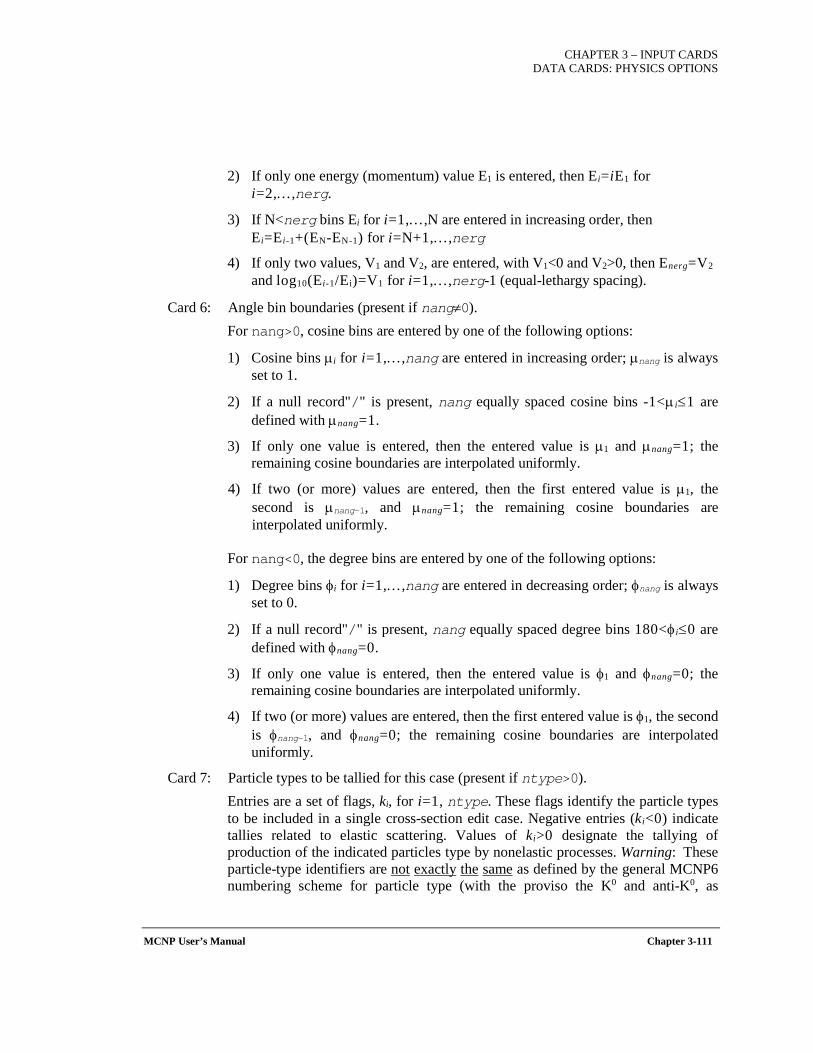
CHAPTER 3 – INPUT CARDS DATA CARDS: PHYSICS OPTIONS
MCNP User’s Manual Chapter 3-111
2) If only one energy (momentum) value E1 is entered, then Ei=iE1 for i=2,. . . ,nerg.
3) If N<nerg bins Ei for i=1,. . . ,N are entered in increasing order, then Ei=Ei-1+(EN-EN-1) for i=N+1,. . . ,nerg
4) If only two values, V1 and V2, are entered, with V1<0 and V2>0, then Energ=V2 and log10(Ei-1/Ei)=V1 for i=1,. . . ,nerg-1 (equal-lethargy spacing).
Card 6: Angle bin boundaries (present if nang≠0). For nang>0, cosine bins are entered by one of the following options:
1) Cosine bins µi for i=1,. . . ,nang are entered in increasing order; µnang is always set to 1.
2) If a null record"/" is present, nang equally spaced cosine bins -1<µi≤1 are defined with µnang=1.
3) If only one value is entered, then the entered value is µ1 and µnang=1; the remaining cosine boundaries are interpolated uniformly.
4) If two (or more) values are entered, then the first entered value is µ1, the second is µnang-1, and µnang=1; the remaining cosine boundaries are interpolated uniformly.
For nang<0, the degree bins are entered by one of the following options:
1) Degree bins φi for i=1,. . . ,nang are entered in decreasing order; φnang is always set to 0.
2) If a null record"/" is present, nang equally spaced degree bins 180<φi≤0 are defined with φnang=0.
3) If only one value is entered, then the entered value is φ1 and φnang=0; the remaining cosine boundaries are interpolated uniformly.
4) If two (or more) values are entered, then the first entered value is φ1, the second is φnang-1, and φnang=0; the remaining cosine boundaries are interpolated uniformly.
Card 7: Particle types to be tallied for this case (present if ntype>0). Entries are a set of flags, ki, for i=1, ntype. These flags identify the particle types to be included in a single cross-section edit case. Negative entries (ki<0) indicate tallies related to elastic scattering. Values of ki>0 designate the tallying of production of the indicated particles type by nonelastic processes. Warning: These particle-type identifiers are not exactly the same as defined by the general MCNP6 numbering scheme for particle type (with the proviso the K0 and anti-K0, as
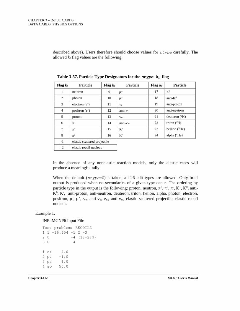
CHAPTER 3 – INPUT CARDS DATA CARDS: PHYSICS OPTIONS
Chapter 3-112 MCNP User’s Manual
described above). Users therefore should choose values for ntype carefully. The allowed ki flag values are the following:
Table 3-57. Particle Type Designators for the ntype ki flag
Flag ki Particle Flag ki Particle Flag ki Particle
1 neutron 9 µ– 17 Κ0
2 photon 10 µ+ 18 anti-Κ0
3 electron (e–) 11 νe 19 anti-proton
4 positron (e+) 12 anti-νe 20 anti-neutron
5 proton 13 νm 21 deuteron (2H)
6 π+ 14 anti-νm 22 triton (3H)
7 π– 15 Κ+ 23 hellion (3He)
8 π0 16 Κ– 24 alpha (4He)
-1 elastic scattered projectile
-2 elastic recoil nucleus
In the absence of any nonelastic reaction models, only the elastic cases will produce a meaningful tally.
When the default (ntype=0) is taken, all 26 edit types are allowed. Only brief output is produced when no secondaries of a given type occur. The ordering by particle type in the output is the following: proton, neutron, π+, π0, π-, Κ+, Κ0, anti-Κ0, Κ-, anti-proton, anti-neutron, deuteron, triton, helion, alpha, photon, electron, positron, µ-, µ+, νe, anti-νe, νm, anti-νm, elastic scattered projectile, elastic recoil nucleus.
Example 1:
INP: MCNP6 Input File Test problem: RECOIL2 1 1 -16.654 -1 2 -3 2 0 -4 (1:-2:3) 3 0 4 1 cz 4.0 2 pz -1.0 3 pz 1.0 4 so 50.0
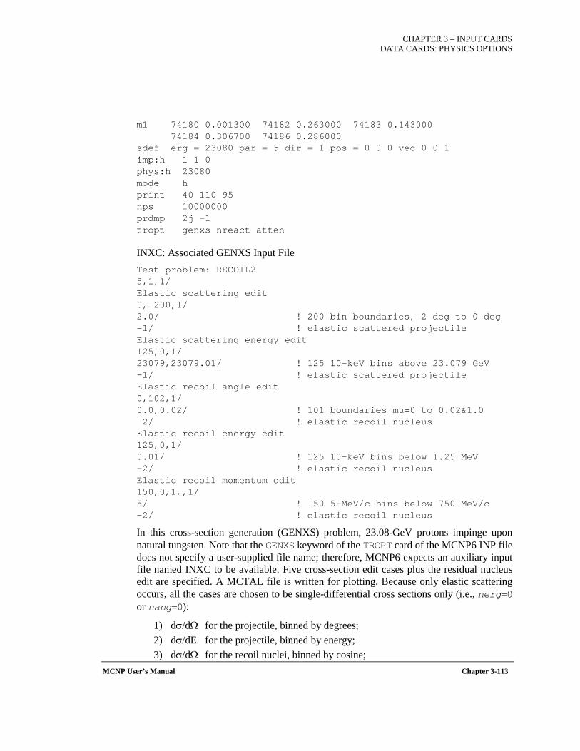
CHAPTER 3 – INPUT CARDS DATA CARDS: PHYSICS OPTIONS
MCNP User’s Manual Chapter 3-113
m1 74180 0.001300 74182 0.263000 74183 0.143000 74184 0.306700 74186 0.286000 sdef erg = 23080 par = 5 dir = 1 pos = 0 0 0 vec 0 0 1 imp:h 1 1 0 phys:h 23080 mode h print 40 110 95 nps 10000000 prdmp 2j -1 tropt genxs nreact atten
INXC: Associated GENXS Input File Test problem: RECOIL2 5,1,1/ Elastic scattering edit 0,-200,1/ 2.0/ ! 200 bin boundaries, 2 deg to 0 deg -1/ ! elastic scattered projectile Elastic scattering energy edit 125,0,1/ 23079,23079.01/ ! 125 10-keV bins above 23.079 GeV -1/ ! elastic scattered projectile Elastic recoil angle edit 0,102,1/ 0.0,0.02/ ! 101 boundaries mu=0 to 0.02&1.0 -2/ ! elastic recoil nucleus Elastic recoil energy edit 125,0,1/ 0.01/ ! 125 10-keV bins below 1.25 MeV -2/ ! elastic recoil nucleus Elastic recoil momentum edit 150,0,1,,1/ 5/ ! 150 5-MeV/c bins below 750 MeV/c -2/ ! elastic recoil nucleus
In this cross-section generation (GENXS) problem, 23.08-GeV protons impinge upon natural tungsten. Note that the GENXS keyword of the TROPT card of the MCNP6 INP file does not specify a user-supplied file name; therefore, MCNP6 expects an auxiliary input file named INXC to be available. Five cross-section edit cases plus the residual nucleus edit are specified. A MCTAL file is written for plotting. Because only elastic scattering occurs, all the cases are chosen to be single-differential cross sections only (i.e., nerg=0 or nang=0):
1) dσ/dΩ for the projectile, binned by degrees; 2) dσ/dE for the projectile, binned by energy; 3) dσ/dΩ for the recoil nuclei, binned by cosine;
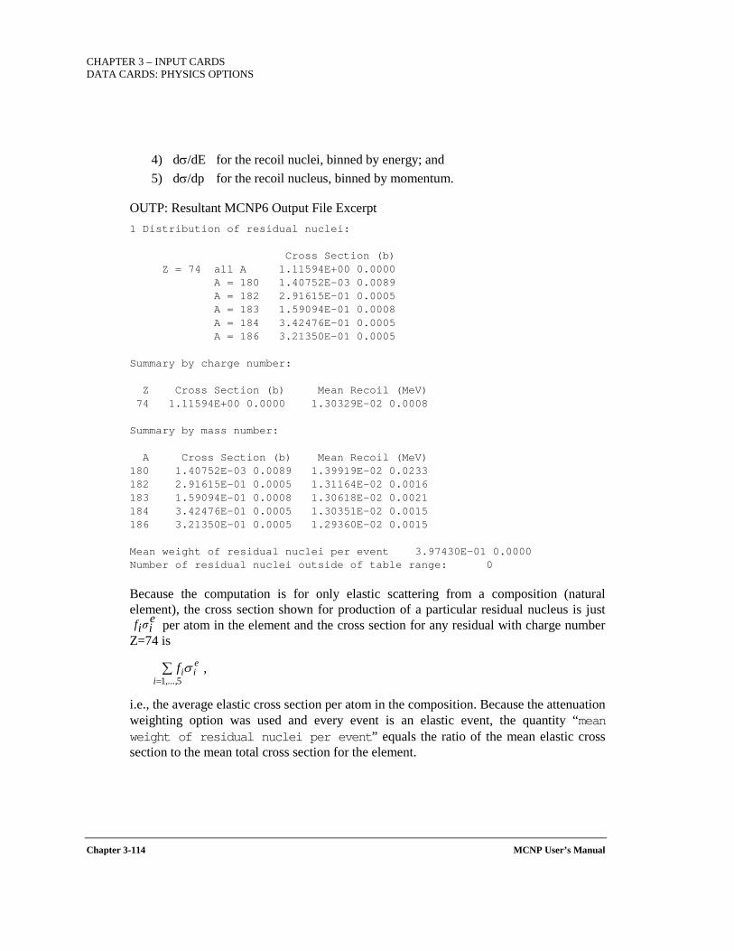
CHAPTER 3 – INPUT CARDS DATA CARDS: PHYSICS OPTIONS
Chapter 3-114 MCNP User’s Manual
4) dσ/dE for the recoil nuclei, binned by energy; and 5) dσ/dp for the recoil nucleus, binned by momentum.
OUTP: Resultant MCNP6 Output File Excerpt 1 Distribution of residual nuclei: Cross Section (b) Z = 74 all A 1.11594E+00 0.0000 A = 180 1.40752E-03 0.0089 A = 182 2.91615E-01 0.0005 A = 183 1.59094E-01 0.0008 A = 184 3.42476E-01 0.0005 A = 186 3.21350E-01 0.0005 Summary by charge number: Z Cross Section (b) Mean Recoil (MeV) 74 1.11594E+00 0.0000 1.30329E-02 0.0008 Summary by mass number: A Cross Section (b) Mean Recoil (MeV) 180 1.40752E-03 0.0089 1.39919E-02 0.0233 182 2.91615E-01 0.0005 1.31164E-02 0.0016 183 1.59094E-01 0.0008 1.30618E-02 0.0021 184 3.42476E-01 0.0005 1.30351E-02 0.0015 186 3.21350E-01 0.0005 1.29360E-02 0.0015 Mean weight of residual nuclei per event 3.97430E-01 0.0000 Number of residual nuclei outside of table range: 0
Because the computation is for only elastic scattering from a composition (natural element), the cross section shown for production of a particular residual nucleus is just
per atom in the element and the cross section for any residual with charge number Z=74 is
,
i.e., the average elastic cross section per atom in the composition. Because the attenuation weighting option was used and every event is an elastic event, the quantity “mean weight of residual nuclei per event” equals the ratio of the mean elastic cross section to the mean total cross section for the element.
eiσif
∑= 51,...,i
eiif σ
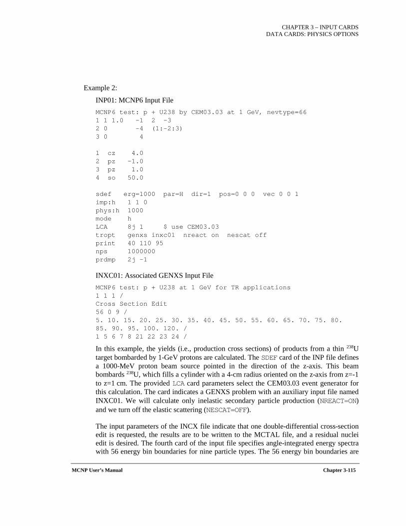
CHAPTER 3 – INPUT CARDS DATA CARDS: PHYSICS OPTIONS
MCNP User’s Manual Chapter 3-115
Example 2:
INP01: MCNP6 Input File MCNP6 test: p + U238 by CEM03.03 at 1 GeV, nevtype=66 1 1 1.0 -1 2 -3 2 0 -4 (1:-2:3) 3 0 4 1 cz 4.0 2 pz -1.0 3 pz 1.0 4 so 50.0 sdef erg=1000 par=H dir=1 pos=0 0 0 vec 0 0 1 imp:h 1 1 0 phys:h 1000 mode h LCA 8j 1 $ use CEM03.03 tropt genxs inxc01 nreact on nescat off print 40 110 95 nps 1000000 prdmp 2j -1
INXC01: Associated GENXS Input File MCNP6 test: p + U238 at 1 GeV for TR applications 1 1 1 / Cross Section Edit 56 0 9 / 5. 10. 15. 20. 25. 30. 35. 40. 45. 50. 55. 60. 65. 70. 75. 80. 85. 90. 95. 100. 120. / 1 5 6 7 8 21 22 23 24 /
In this example, the yields (i.e., production cross sections) of products from a thin 238U target bombarded by 1-GeV protons are calculated. The SDEF card of the INP file defines a 1000-MeV proton beam source pointed in the direction of the z-axis. This beam bombards 238U, which fills a cylinder with a 4-cm radius oriented on the z-axis from z=-1 to z=1 cm. The provided LCA card parameters select the CEM03.03 event generator for this calculation. The card indicates a GENXS problem with an auxiliary input file named INXC01. We will calculate only inelastic secondary particle production (NREACT=ON) and we turn off the elastic scattering (NESCAT=OFF).
The input parameters of the INCX file indicate that one double-differential cross-section edit is requested, the results are to be written to the MCTAL file, and a residual nuclei edit is desired. The fourth card of the input file specifies angle-integrated energy spectra with 56 energy bin boundaries for nine particle types. The 56 energy bin boundaries are
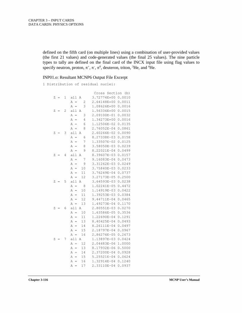
CHAPTER 3 – INPUT CARDS DATA CARDS: PHYSICS OPTIONS
Chapter 3-116 MCNP User’s Manual
defined on the fifth card (on multiple lines) using a combination of user-provided values (the first 21 values) and code-generated values (the final 25 values). The nine particle types to tally are defined on the final card of the INCX input file using flag values to specify neutron, proton, π+, π-, π0, deuteron, triton, 3He, and 4He.
INP01.o: Resultant MCNP6 Output File Excerpt 1 Distribution of residual nuclei: Cross Section (b) Z = 1 all A 3.72774E+00 0.0010 A = 2 2.64148E+00 0.0011 A = 3 1.08626E+00 0.0016 Z = 2 all A 1.56336E+00 0.0015 A = 3 2.09100E-01 0.0032 A = 4 1.34273E+00 0.0016 A = 6 1.12506E-02 0.0135 A = 8 2.76052E-04 0.0861 Z = 3 all A 2.60266E-02 0.0090 A = 6 8.27338E-03 0.0158 A = 7 1.33507E-02 0.0125 A = 8 3.58050E-03 0.0239 A = 9 8.22021E-04 0.0499 Z = 4 all A 8.39607E-03 0.0157 A = 7 9.16083E-04 0.0473 A = 9 3.31262E-03 0.0249 A = 10 3.75840E-03 0.0233 A = 11 3.76249E-04 0.0737 A = 12 3.27173E-05 0.2500 Z = 5 all A 3.64593E-03 0.0238 A = 8 1.02241E-05 0.4472 A = 10 1.14919E-03 0.0422 A = 11 1.39253E-03 0.0384 A = 12 9.44711E-04 0.0465 A = 13 1.49273E-04 0.1170 Z = 6 all A 2.80551E-03 0.0270 A = 10 1.63586E-05 0.3536 A = 11 1.22690E-04 0.1291 A = 13 8.40425E-04 0.0493 A = 14 8.26111E-04 0.0497 A = 15 2.18797E-04 0.0967 A = 16 2.86276E-05 0.2673 Z = 7 all A 1.13897E-03 0.0424 A = 12 2.04483E-06 1.0000 A = 13 8.17932E-06 0.5000 A = 14 2.37200E-04 0.0928 A = 15 5.25521E-04 0.0624 A = 16 1.32914E-04 0.1240 A = 17 2.33110E-04 0.0937
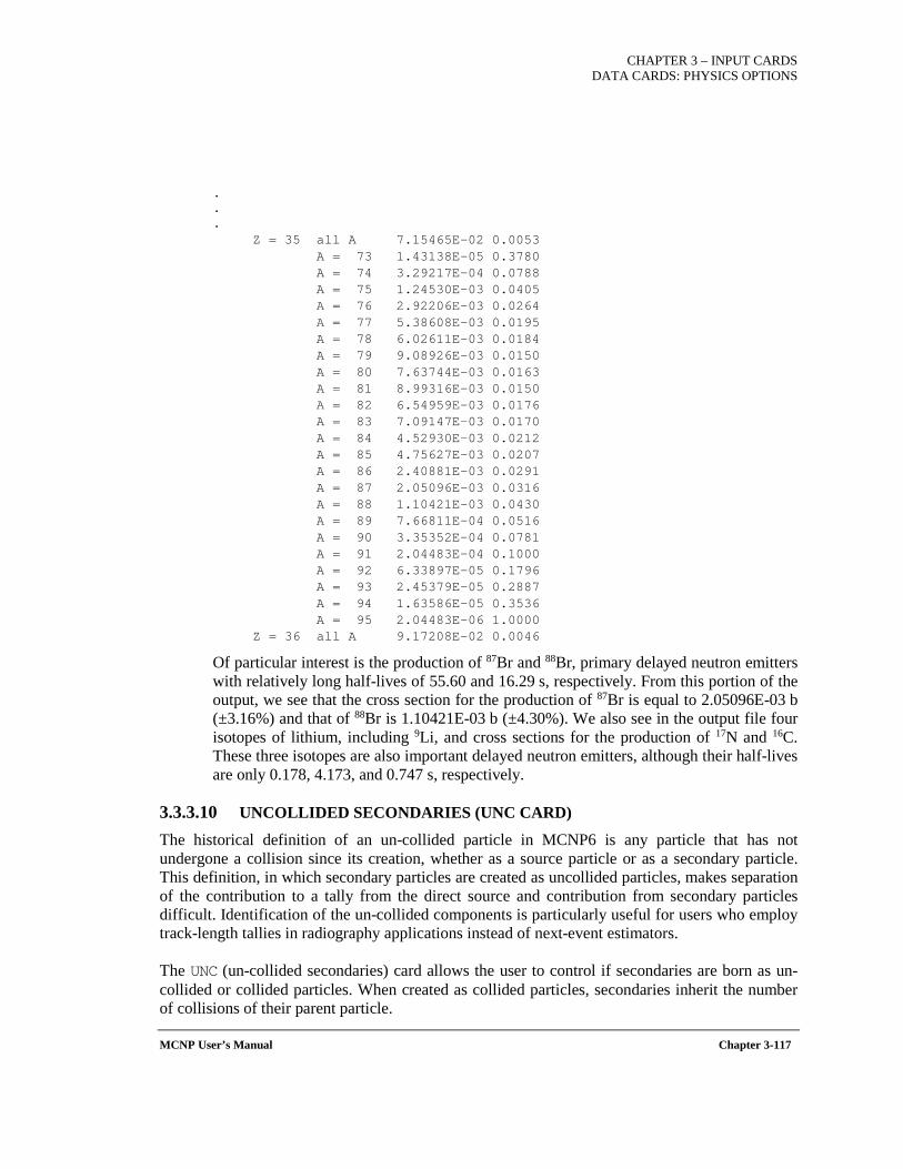
CHAPTER 3 – INPUT CARDS DATA CARDS: PHYSICS OPTIONS
MCNP User’s Manual Chapter 3-117
.
.
. Z = 35 all A 7.15465E-02 0.0053 A = 73 1.43138E-05 0.3780 A = 74 3.29217E-04 0.0788 A = 75 1.24530E-03 0.0405 A = 76 2.92206E-03 0.0264 A = 77 5.38608E-03 0.0195 A = 78 6.02611E-03 0.0184 A = 79 9.08926E-03 0.0150 A = 80 7.63744E-03 0.0163 A = 81 8.99316E-03 0.0150 A = 82 6.54959E-03 0.0176 A = 83 7.09147E-03 0.0170 A = 84 4.52930E-03 0.0212 A = 85 4.75627E-03 0.0207 A = 86 2.40881E-03 0.0291 A = 87 2.05096E-03 0.0316 A = 88 1.10421E-03 0.0430 A = 89 7.66811E-04 0.0516 A = 90 3.35352E-04 0.0781 A = 91 2.04483E-04 0.1000 A = 92 6.33897E-05 0.1796 A = 93 2.45379E-05 0.2887 A = 94 1.63586E-05 0.3536 A = 95 2.04483E-06 1.0000 Z = 36 all A 9.17208E-02 0.0046
Of particular interest is the production of 87Br and 88Br, primary delayed neutron emitters with relatively long half-lives of 55.60 and 16.29 s, respectively. From this portion of the output, we see that the cross section for the production of 87Br is equal to 2.05096E-03 b (±3.16%) and that of 88Br is 1.10421E-03 b (±4.30%). We also see in the output file four isotopes of lithium, including 9Li, and cross sections for the production of 17N and 16C. These three isotopes are also important delayed neutron emitters, although their half-lives are only 0.178, 4.173, and 0.747 s, respectively.
3.3.3.10 UNCOLLIDED SECONDARIES (UNC CARD)
The historical definition of an un-collided particle in MCNP6 is any particle that has not undergone a collision since its creation, whether as a source particle or as a secondary particle. This definition, in which secondary particles are created as uncollided particles, makes separation of the contribution to a tally from the direct source and contribution from secondary particles difficult. Identification of the un-collided components is particularly useful for users who employ track-length tallies in radiography applications instead of next-event estimators.
The UNC (un-collided secondaries) card allows the user to control if secondaries are born as un-collided or collided particles. When created as collided particles, secondaries inherit the number of collisions of their parent particle.
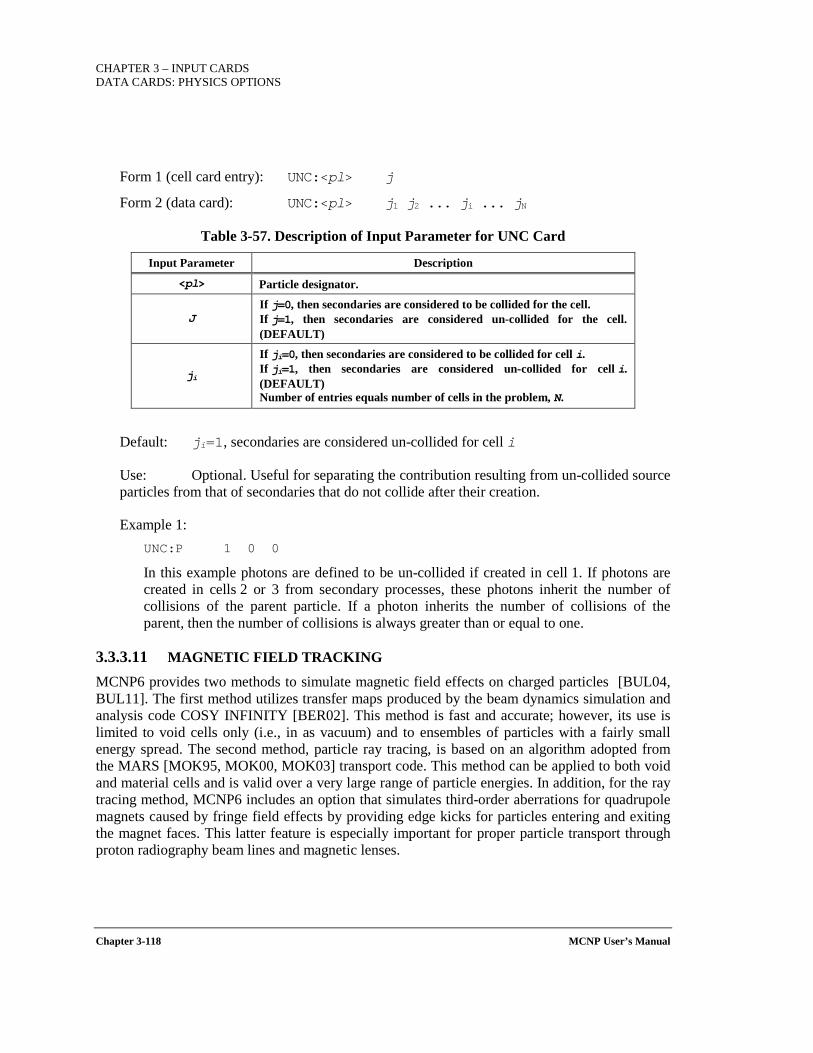
CHAPTER 3 – INPUT CARDS DATA CARDS: PHYSICS OPTIONS
Chapter 3-118 MCNP User’s Manual
Form 1 (cell card entry): UNC:<pl> j
Form 2 (data card): UNC:<pl> j1 j2 ... ji ... jN
Table 3-57. Description of Input Parameter for UNC Card
Input Parameter Description
<pl> Particle designator.
J If j=0, then secondaries are considered to be collided for the cell. If j=1, then secondaries are considered un-collided for the cell. (DEFAULT)
ji
If ji=0, then secondaries are considered to be collided for cell i. If ji=1, then secondaries are considered un-collided for cell i. (DEFAULT) Number of entries equals number of cells in the problem, N.
Default: ji=1, secondaries are considered un-collided for cell i
Use: Optional. Useful for separating the contribution resulting from un-collided source particles from that of secondaries that do not collide after their creation.
Example 1: UNC:P 1 0 0
In this example photons are defined to be un-collided if created in cell 1. If photons are created in cells 2 or 3 from secondary processes, these photons inherit the number of collisions of the parent particle. If a photon inherits the number of collisions of the parent, then the number of collisions is always greater than or equal to one.
3.3.3.11 MAGNETIC FIELD TRACKING
MCNP6 provides two methods to simulate magnetic field effects on charged particles [BUL04, BUL11]. The first method utilizes transfer maps produced by the beam dynamics simulation and analysis code COSY INFINITY [BER02]. This method is fast and accurate; however, its use is limited to void cells only (i.e., in as vacuum) and to ensembles of particles with a fairly small energy spread. The second method, particle ray tracing, is based on an algorithm adopted from the MARS [MOK95, MOK00, MOK03] transport code. This method can be applied to both void and material cells and is valid over a very large range of particle energies. In addition, for the ray tracing method, MCNP6 includes an option that simulates third-order aberrations for quadrupole magnets caused by fringe field effects by providing edge kicks for particles entering and exiting the magnet faces. This latter feature is especially important for proper particle transport through proton radiography beam lines and magnetic lenses.
CHAPTER 3 – INPUT CARDS DATA CARDS: PHYSICS OPTIONS
MCNP User’s Manual Chapter 3-119
3.3.3.11.1 TRANSFER MAPS (COSYP AND COSY CARDS)
COSY INFINITY is a beam optics code that utilizes numerical integration and differential algebraic techniques to generate transfer maps based on a Taylor series expansion of a particle's canonical variables [FAV99]. These transfer maps represent the functional relation between the phase-space coordinates of a particle that has passed through a region of magnetic field and its phase-space coordinates before entering the field region. In the transfer map approach to particle transport, the actual trajectories that the particles follow through the field region do not appear explicitly; in applying precomputed maps, charged particles are transported from an initial location to a final location in one step by applying the transfer maps to the initial phase space coordinates.
Although the COSY map method provides a fast and accurate method for transporting charged particles in magnetic fields, the transfer map method has several limitations. First, map methods can only be used in void regions. Also, the COSY maps are limited to only one particle type. In addition, the Taylor expansions used in applying the maps have a finite volume of convergence in phase space. The convergence volume has a very complicated shape in five dimensions (x, y, dx, dy, p), requiring that the shape of the phase-space volume and the order of the Taylor series needed in order to get a given accuracy in final particle position is not easily predicted in practice and can be checked only by particle tracking. For example, a map to fifth order in energy deviation might be applied with good accuracy to particles with energies within 10% of the reference energy, but not to those with 50% deviation. In other words, COSY maps are specific to particle momentum; therefore, a particle with significantly different energy or mass than what was used to create the map will not be transported correctly.
Summary of known limitations of transfer map method:
• COSY maps can only be applied to void cells. • COSY maps are specific to particle momentum. Therefore, a particle with significantly
different energy or mass than what was used to create the map will not be transported correctly.
• No information about the magnetic fields is written to the output file.
• COSY maps are limited to only one particle type
The following COSYP card describes the COSY map parameters:
Form: COSYP prefix axsh axsv emap1 emap2 ... emapN
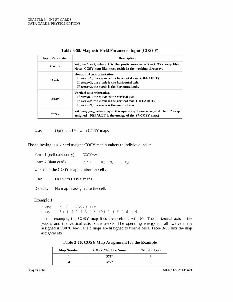
CHAPTER 3 – INPUT CARDS DATA CARDS: PHYSICS OPTIONS
Chapter 3-120 MCNP User’s Manual
Table 3-58. Magnetic Field Parameter Input (COSYP)
Input Parameter Description
Prefix Set prefix=k, where k is the prefix number of the COSY map files. Note: COSY map files must reside in the working directory.
Axsh
Horizontal axis orientation If axsh=1, the x-axis is the horizontal axis. (DEFAULT) If axsh=2, the y-axis is the horizontal axis. If axsh=3, the z-axis is the horizontal axis.
Axsv
Vertical axis orientation If axsv=1, the x-axis is the vertical axis. If axsv=2, the y-axis is the vertical axis. (DEFAULT) If axsv=3, the z-axis is the vertical axis.
emapi Set emapi=ei, where ei is the operating beam energy of the ith map assigned. (DEFAULT is the energy of the ith COSY map.)
Use: Optional. Use with COSY maps.
The following COSY card assigns COSY map numbers to individual cells:
Form 1 (cell card entry): COSY=m
Form 2 (data card): COSY m1 m2 ... mK
where mi=the COSY map number for cell i.
Use: Use with COSY maps.
Default: No map is assigned to the cell.
Example 1: cosyp 57 2 1 23070 11r cosy 3j 1 j 2 j 3 j 4 10j 5 j 5 j 6 j 6
In this example, the COSY map files are prefixed with 57. The horizontal axis is the y-axis, and the vertical axis is the x-axis. The operating energy for all twelve maps assigned is 23070 MeV. Field maps are assigned to twelve cells. Table 3-60 lists the map assignments.
Table 3-60. COSY Map Assignment for the Example
Map Number COSY Map File Name Cell Numbers
1 571* 4 2 572* 6
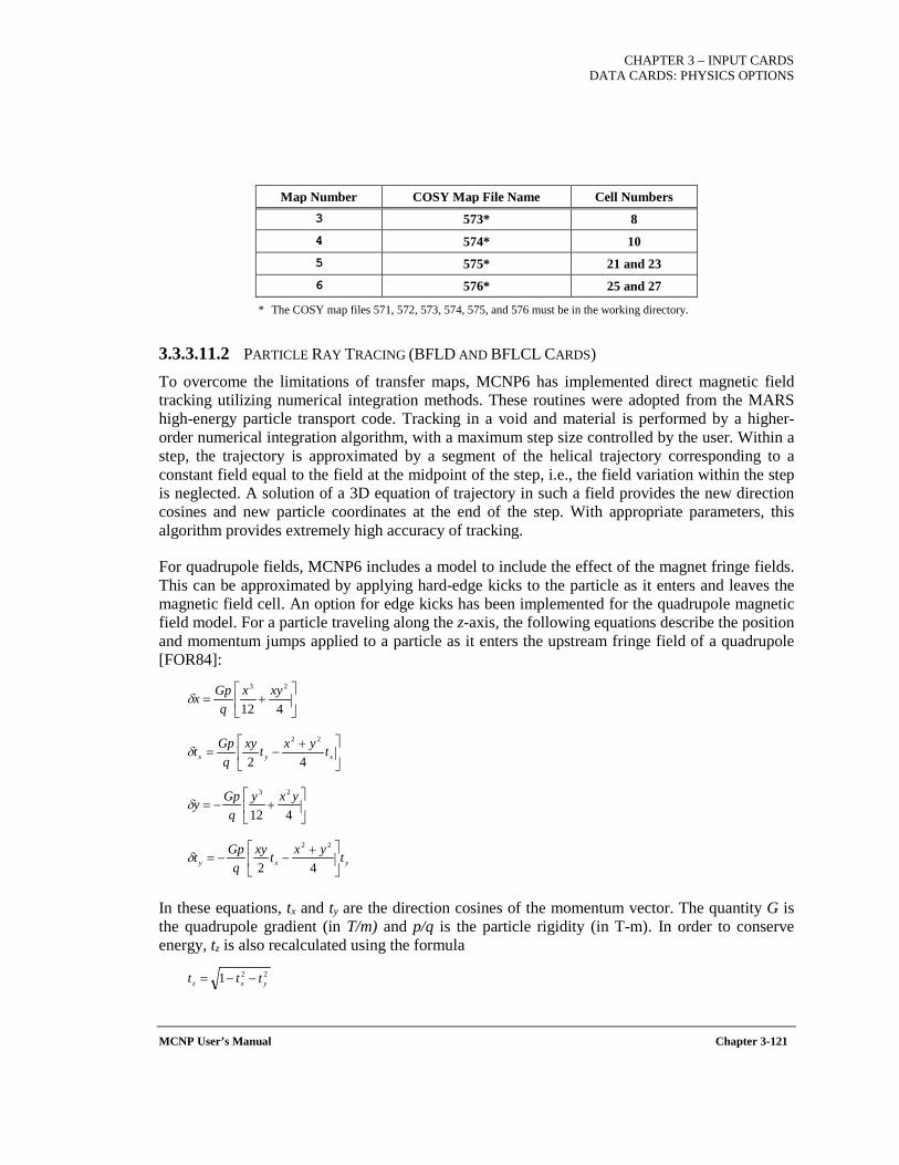
CHAPTER 3 – INPUT CARDS DATA CARDS: PHYSICS OPTIONS
MCNP User’s Manual Chapter 3-121
Map Number COSY Map File Name Cell Numbers 3 573* 8 4 574* 10 5 575* 21 and 23 6 576* 25 and 27
* The COSY map files 571, 572, 573, 574, 575, and 576 must be in the working directory.
3.3.3.11.2 PARTICLE RAY TRACING (BFLD AND BFLCL CARDS)
To overcome the limitations of transfer maps, MCNP6 has implemented direct magnetic field tracking utilizing numerical integration methods. These routines were adopted from the MARS high-energy particle transport code. Tracking in a void and material is performed by a higher-order numerical integration algorithm, with a maximum step size controlled by the user. Within a step, the trajectory is approximated by a segment of the helical trajectory corresponding to a constant field equal to the field at the midpoint of the step, i.e., the field variation within the step is neglected. A solution of a 3D equation of trajectory in such a field provides the new direction cosines and new particle coordinates at the end of the step. With appropriate parameters, this algorithm provides extremely high accuracy of tracking.
For quadrupole fields, MCNP6 includes a model to include the effect of the magnet fringe fields. This can be approximated by applying hard-edge kicks to the particle as it enters and leaves the magnetic field cell. An option for edge kicks has been implemented for the quadrupole magnetic field model. For a particle traveling along the z-axis, the following equations describe the position and momentum jumps applied to a particle as it enters the upstream fringe field of a quadrupole [FOR84]:
In these equations, tx and ty are the direction cosines of the momentum vector. The quantity G is the quadrupole gradient (in T/m) and p/q is the particle rigidity (in T-m). In order to conserve energy, tz is also recalculated using the formula
+=
412
23 xyxq
Gpxδ
+−= xyx tyxtxy
qGpt
42
22
δ
+−=
412
23 yxyq
Gpyδ
yxy tyxtxyq
Gpt
+−−=
42
22
δ
221 yxz ttt −−=
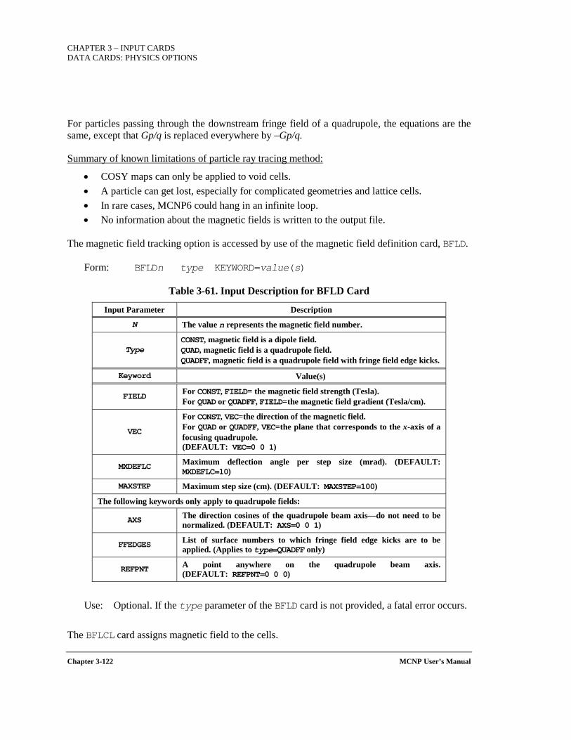
CHAPTER 3 – INPUT CARDS DATA CARDS: PHYSICS OPTIONS
Chapter 3-122 MCNP User’s Manual
For particles passing through the downstream fringe field of a quadrupole, the equations are the same, except that Gp/q is replaced everywhere by –Gp/q.
Summary of known limitations of particle ray tracing method:
• COSY maps can only be applied to void cells. • A particle can get lost, especially for complicated geometries and lattice cells. • In rare cases, MCNP6 could hang in an infinite loop. • No information about the magnetic fields is written to the output file.
The magnetic field tracking option is accessed by use of the magnetic field definition card, BFLD.
Form: BFLDn type KEYWORD=value(s)
Table 3-61. Input Description for BFLD Card
Input Parameter Description
N The value n represents the magnetic field number.
Type CONST, magnetic field is a dipole field. QUAD, magnetic field is a quadrupole field. QUADFF, magnetic field is a quadrupole field with fringe field edge kicks.
Keyword Value(s)
FIELD For CONST, FIELD= the magnetic field strength (Tesla). For QUAD or QUADFF, FIELD=the magnetic field gradient (Tesla/cm).
VEC
For CONST, VEC=the direction of the magnetic field. For QUAD or QUADFF, VEC=the plane that corresponds to the x-axis of a focusing quadrupole. (DEFAULT: VEC=0 0 1)
MXDEFLC Maximum deflection angle per step size (mrad). (DEFAULT: MXDEFLC=10)
MAXSTEP Maximum step size (cm). (DEFAULT: MAXSTEP=100)
The following keywords only apply to quadrupole fields:
AXS The direction cosines of the quadrupole beam axis—do not need to be normalized. (DEFAULT: AXS=0 0 1)
FFEDGES List of surface numbers to which fringe field edge kicks are to be applied. (Applies to type=QUADFF only)
REFPNT A point anywhere on the quadrupole beam axis. (DEFAULT: REFPNT=0 0 0)
Use: Optional. If the type parameter of the BFLD card is not provided, a fatal error occurs.
The BFLCL card assigns magnetic field to the cells.
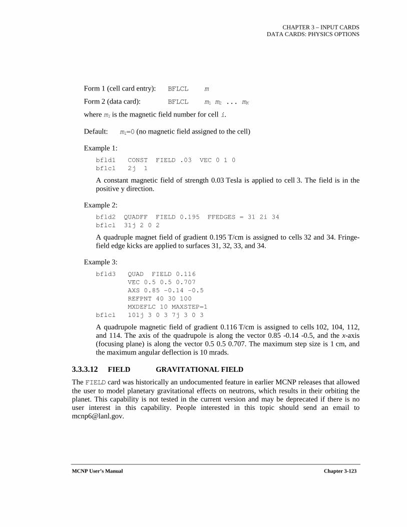
CHAPTER 3 – INPUT CARDS DATA CARDS: PHYSICS OPTIONS
MCNP User’s Manual Chapter 3-123
Form 1 (cell card entry): BFLCL m
Form 2 (data card): BFLCL m1 m2 ... mK
where mi is the magnetic field number for cell i.
Default: mi=0 (no magnetic field assigned to the cell)
Example 1: bfld1 CONST FIELD .03 VEC 0 1 0 bflcl 2j 1
A constant magnetic field of strength 0.03 Tesla is applied to cell 3. The field is in the positive y direction.
Example 2: bfld2 QUADFF FIELD 0.195 FFEDGES = 31 2i 34 bflcl 31j 2 0 2
A quadruple magnet field of gradient 0.195 T/cm is assigned to cells 32 and 34. Fringe-field edge kicks are applied to surfaces 31, 32, 33, and 34.
Example 3: bfld3 QUAD FIELD 0.116 VEC 0.5 0.5 0.707 AXS 0.85 -0.14 -0.5 REFPNT 40 30 100 MXDEFLC 10 MAXSTEP=1 bflcl 101j 3 0 3 7j 3 0 3
A quadrupole magnetic field of gradient 0.116 T/cm is assigned to cells 102, 104, 112, and 114. The axis of the quadrupole is along the vector 0.85 -0.14 -0.5, and the x-axis (focusing plane) is along the vector 0.5 0.5 0.707. The maximum step size is 1 cm, and the maximum angular deflection is 10 mrads.
3.3.3.12 FIELD GRAVITATIONAL FIELD
The FIELD card was historically an undocumented feature in earlier MCNP releases that allowed the user to model planetary gravitational effects on neutrons, which results in their orbiting the planet. This capability is not tested in the current version and may be deprecated if there is no user interest in this capability. People interested in this topic should send an email to [email protected].
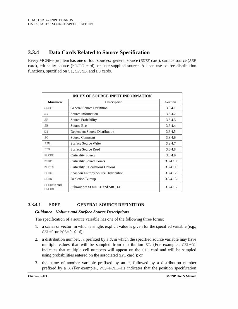
CHAPTER 3 – INPUT CARDS DATA CARDS: SOURCE SPECIFICATION
Chapter 3-124 MCNP User’s Manual
3.3.4 Data Cards Related to Source Specification Every MCNP6 problem has one of four sources: general source (SDEF card), surface source (SSR card), criticality source (KCODE card), or user-supplied source. All can use source distribution functions, specified on SI, SP, SB, and DS cards.
INDEX OF SOURCE INPUT INFORMATION Mnemonic Description Section
SDEF General Source Definition 3.3.4.1 SI Source Information 3.3.4.2 SP Source Probability 3.3.4.3 SB Source Bias 3.3.4.4 DS Dependent Source Distribution 3.3.4.5 SC Source Comment 3.3.4.6 SSW Surface Source Write 3.3.4.7 SSR Surface Source Read 3.3.4.8 KCODE Criticality Source 3.3.4.9 KSRC Criticality Source Points 3.3.4.10 KOPTS Criticality Calculations Options 3.3.4.11 HSRC Shannon Entropy Source Distribution 3.3.4.12 BURN Depletion/Burnup 3.3.4.13
SOURCE and SRCDX Subroutines SOURCE and SRCDX 3.3.4.13
3.3.4.1 SDEF GENERAL SOURCE DEFINITION
Guidance: Volume and Surface Source Descriptions
The specification of a source variable has one of the following three forms:
1. a scalar or vector, in which a single, explicit value is given for the specified variable (e.g., CEL=1 or POS=0 0 6);
2. a distribution number, n, prefixed by a D, in which the specified source variable may have multiple values that will be sampled from distribution SI. (For example., CEL=D1 indicates that multiple cell numbers will appear on the SI1 card and will be sampled using probabilities entered on the associated SP1 card.); or
3. the name of another variable prefixed by an F, followed by a distribution number prefixed by a D. (For example., POS=FCEL=D1 indicates that the position specification
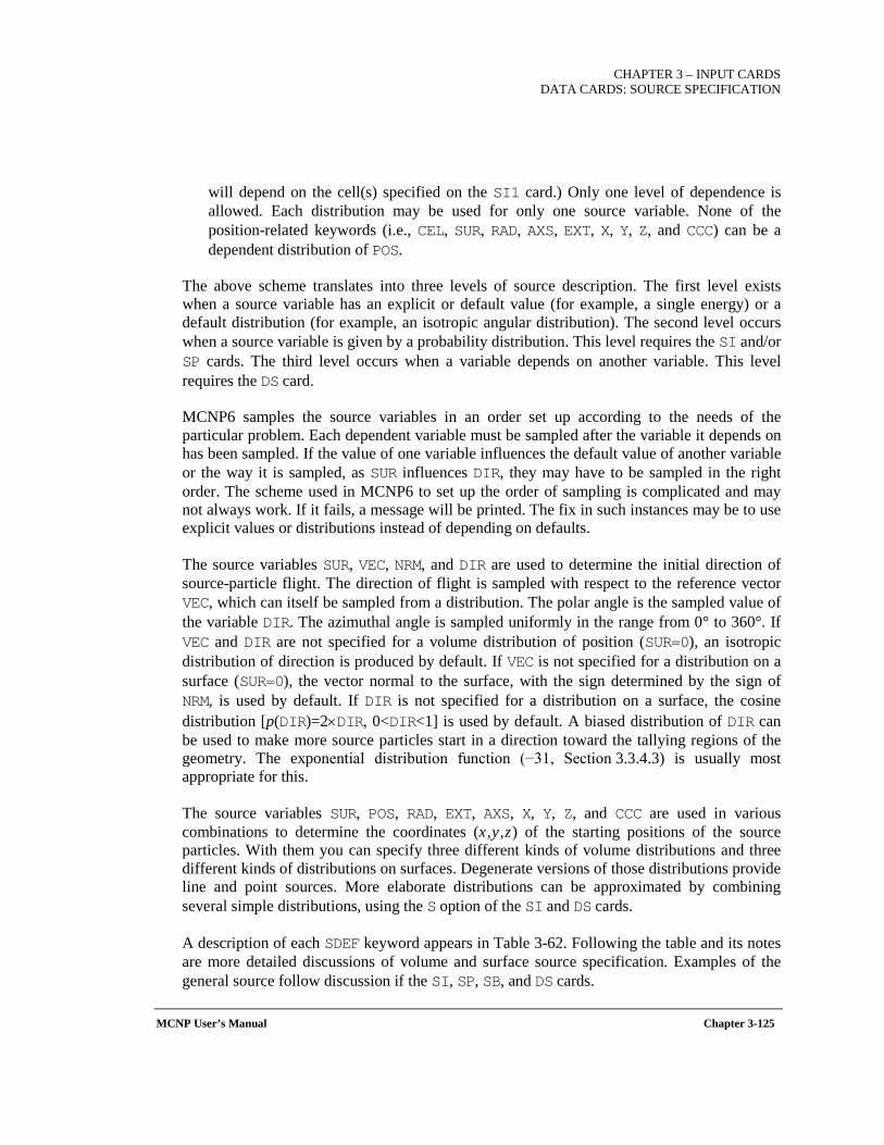
CHAPTER 3 – INPUT CARDS
DATA CARDS: SOURCE SPECIFICATION
MCNP User’s Manual Chapter 3-125
will depend on the cell(s) specified on the SI1 card.) Only one level of dependence is allowed. Each distribution may be used for only one source variable. None of the position-related keywords (i.e., CEL, SUR, RAD, AXS, EXT, X, Y, Z, and CCC) can be a dependent distribution of POS.
The above scheme translates into three levels of source description. The first level exists when a source variable has an explicit or default value (for example, a single energy) or a default distribution (for example, an isotropic angular distribution). The second level occurs when a source variable is given by a probability distribution. This level requires the SI and/or SP cards. The third level occurs when a variable depends on another variable. This level requires the DS card.
MCNP6 samples the source variables in an order set up according to the needs of the particular problem. Each dependent variable must be sampled after the variable it depends on has been sampled. If the value of one variable influences the default value of another variable or the way it is sampled, as SUR influences DIR, they may have to be sampled in the right order. The scheme used in MCNP6 to set up the order of sampling is complicated and may not always work. If it fails, a message will be printed. The fix in such instances may be to use explicit values or distributions instead of depending on defaults.
The source variables SUR, VEC, NRM, and DIR are used to determine the initial direction of source-particle flight. The direction of flight is sampled with respect to the reference vector VEC, which can itself be sampled from a distribution. The polar angle is the sampled value of the variable DIR. The azimuthal angle is sampled uniformly in the range from 0° to 360°. If VEC and DIR are not specified for a volume distribution of position (SUR=0), an isotropic distribution of direction is produced by default. If VEC is not specified for a distribution on a surface (SUR=0), the vector normal to the surface, with the sign determined by the sign of NRM, is used by default. If DIR is not specified for a distribution on a surface, the cosine distribution [p(DIR)=2×DIR, 0<DIR<1] is used by default. A biased distribution of DIR can be used to make more source particles start in a direction toward the tallying regions of the geometry. The exponential distribution function (−31, Section 3.3.4.3) is usually most appropriate for this.
The source variables SUR, POS, RAD, EXT, AXS, X, Y, Z, and CCC are used in various combinations to determine the coordinates (x,y,z) of the starting positions of the source particles. With them you can specify three different kinds of volume distributions and three different kinds of distributions on surfaces. Degenerate versions of those distributions provide line and point sources. More elaborate distributions can be approximated by combining several simple distributions, using the S option of the SI and DS cards.
A description of each SDEF keyword appears in Table 3-62. Following the table and its notes are more detailed discussions of volume and surface source specification. Examples of the general source follow discussion if the SI, SP, SB, and DS cards.
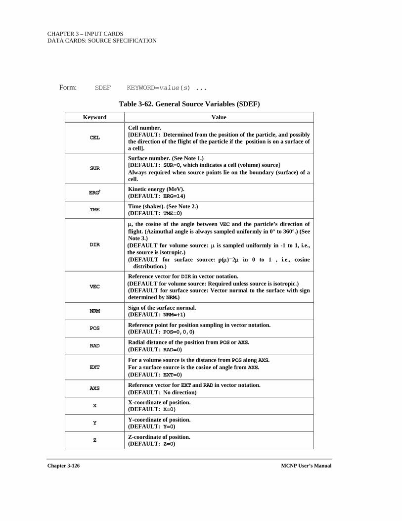
CHAPTER 3 – INPUT CARDS DATA CARDS: SOURCE SPECIFICATION
Chapter 3-126 MCNP User’s Manual
Form: SDEF KEYWORD=value(s) ...
Table 3-62. General Source Variables (SDEF)
Keyword Value
CEL
Cell number. [DEFAULT: Determined from the position of the particle, and possibly the direction of the flight of the particle if the position is on a surface of a cell].
SUR
Surface number. (See Note 1.) [DEFAULT: SUR=0, which indicates a cell (volume) source] Always required when source points lie on the boundary (surface) of a cell.
ERG† Kinetic energy (MeV). (DEFAULT: ERG=14)
TME Time (shakes). (See Note 2.) (DEFAULT: TME=0)
DIR
µ, the cosine of the angle between VEC and the particle’s direction of flight. (Azimuthal angle is always sampled uniformly in 0° to 360°.) (See Note 3.) (DEFAULT for volume source: µ is sampled uniformly in -1 to 1, i.e., the source is isotropic.) (DEFAULT for surface source: p(µ)=2µ in 0 to 1 , i.e., cosine
distribution.)
VEC
Reference vector for DIR in vector notation. (DEFAULT for volume source: Required unless source is isotropic.) (DEFAULT for surface source: Vector normal to the surface with sign determined by NRM.)
NRM Sign of the surface normal. (DEFAULT: NRM=+1)
POS Reference point for position sampling in vector notation. (DEFAULT: POS=0,0,0)
RAD Radial distance of the position from POS or AXS. (DEFAULT: RAD=0)
EXT For a volume source is the distance from POS along AXS. For a surface source is the cosine of angle from AXS. (DEFAULT: EXT=0)
AXS Reference vector for EXT and RAD in vector notation. (DEFAULT: No direction)
X X-coordinate of position. (DEFAULT: X=0)
Y Y-coordinate of position. (DEFAULT: Y=0)
Z Z-coordinate of position. (DEFAULT: Z=0)
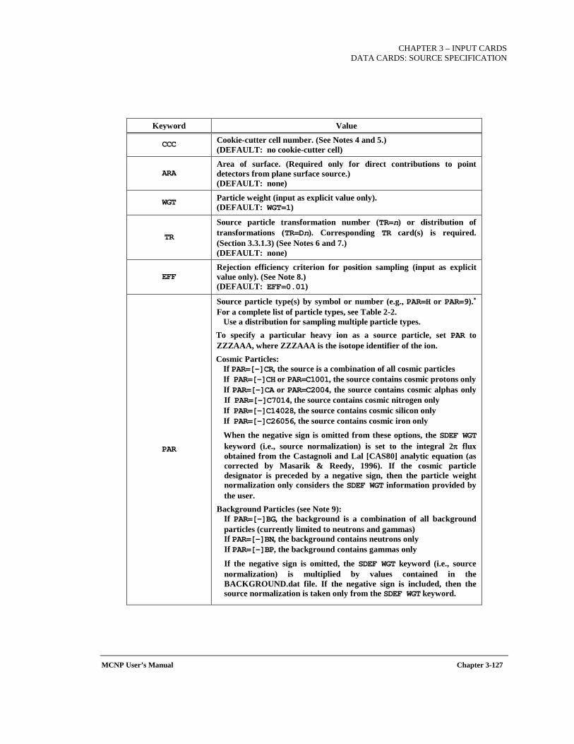
CHAPTER 3 – INPUT CARDS
DATA CARDS: SOURCE SPECIFICATION
MCNP User’s Manual Chapter 3-127
Keyword Value
CCC Cookie-cutter cell number. (See Notes 4 and 5.) (DEFAULT: no cookie-cutter cell)
ARA Area of surface. (Required only for direct contributions to point detectors from plane surface source.) (DEFAULT: none)
WGT Particle weight (input as explicit value only). (DEFAULT: WGT=1)
TR
Source particle transformation number (TR=n) or distribution of transformations (TR=Dn). Corresponding TR card(s) is required. (Section 3.3.1.3) (See Notes 6 and 7.) (DEFAULT: none)
EFF Rejection efficiency criterion for position sampling (input as explicit value only). (See Note 8.) (DEFAULT: EFF=0.01)
PAR
Source particle type(s) by symbol or number (e.g., PAR=H or PAR=9).* For a complete list of particle types, see Table 2-2.
Use a distribution for sampling multiple particle types. To specify a particular heavy ion as a source particle, set PAR to ZZZAAA, where ZZZAAA is the isotope identifier of the ion. Cosmic Particles:
If PAR=[-]CR, the source is a combination of all cosmic particles If PAR=[-]CH or PAR=C1001, the source contains cosmic protons only If PAR=[-]CA or PAR=C2004, the source contains cosmic alphas only If PAR=[-]C7014, the source contains cosmic nitrogen only If PAR=[-]C14028, the source contains cosmic silicon only If PAR=[-]C26056, the source contains cosmic iron only
When the negative sign is omitted from these options, the SDEF WGT keyword (i.e., source normalization) is set to the integral 2π flux obtained from the Castagnoli and Lal [CAS80] analytic equation (as corrected by Masarik & Reedy, 1996). If the cosmic particle designator is preceded by a negative sign, then the particle weight normalization only considers the SDEF WGT information provided by the user.
Background Particles (see Note 9): If PAR=[-]BG, the background is a combination of all background particles (currently limited to neutrons and gammas) If PAR=[-]BN, the background contains neutrons only If PAR=[-]BP, the background contains gammas only
If the negative sign is omitted, the SDEF WGT keyword (i.e., source normalization) is multiplied by values contained in the BACKGROUND.dat file. If the negative sign is included, then the source normalization is taken only from the SDEF WGT keyword.
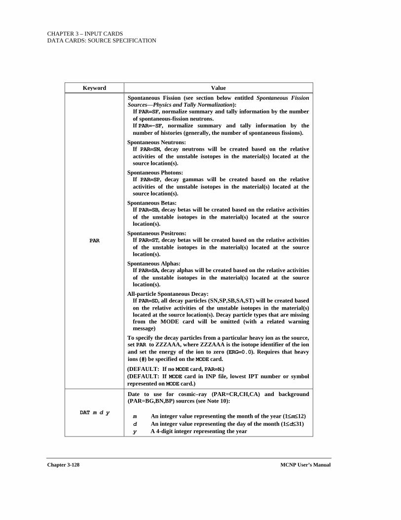
CHAPTER 3 – INPUT CARDS DATA CARDS: SOURCE SPECIFICATION
Chapter 3-128 MCNP User’s Manual
Keyword Value
PAR
Spontaneous Fission (see section below entitled Spontaneous Fission Sources—Physics and Tally Normalization):
If PAR=SF, normalize summary and tally information by the number of spontaneous-fission neutrons. If PAR=-SF, normalize summary and tally information by the number of histories (generally, the number of spontaneous fissions).
Spontaneous Neutrons: If PAR=SN, decay neutrons will be created based on the relative activities of the unstable isotopes in the material(s) located at the source location(s).
Spontaneous Photons: If PAR=SP, decay gammas will be created based on the relative activities of the unstable isotopes in the material(s) located at the source location(s).
Spontaneous Betas: If PAR=SB, decay betas will be created based on the relative activities of the unstable isotopes in the material(s) located at the source location(s).
Spontaneous Positrons: If PAR=ST, decay betas will be created based on the relative activities of the unstable isotopes in the material(s) located at the source location(s).
Spontaneous Alphas: If PAR=SA, decay alphas will be created based on the relative activities of the unstable isotopes in the material(s) located at the source location(s).
All-particle Spontaneous Decay: If PAR=SD, all decay particles (SN,SP,SB,SA,ST) will be created based on the relative activities of the unstable isotopes in the material(s) located at the source location(s). Decay particle types that are missing from the MODE card will be omitted (with a related warning message)
To specify the decay particles from a particular heavy ion as the source, set PAR to ZZZAAA, where ZZZAAA is the isotope identifier of the ion and set the energy of the ion to zero (ERG=0.0). Requires that heavy ions (#) be specified on the MODE card.
(DEFAULT: If no MODE card, PAR=N.) (DEFAULT: If MODE card in INP file, lowest IPT number or symbol represented on MODE card.)
DAT m d y
Date to use for cosmic–ray (PAR=CR,CH,CA) and background (PAR=BG,BN,BP) sources (see Note 10): m An integer value representing the month of the year (1≤m≤12) d An integer value representing the day of the month (1≤d≤31) y A 4-digit integer representing the year
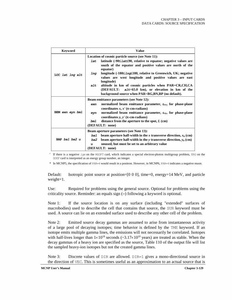
CHAPTER 3 – INPUT CARDS
DATA CARDS: SOURCE SPECIFICATION
MCNP User’s Manual Chapter 3-129
Keyword Value
LOC lat lng alt
Location of cosmic particle source (see Note 11): lat latitude (-90≤lat≤90, relative to equator; negative values are
south of the equator and positive values are north of the equator)
lng longitude (-180≤lng≤180, relative to Greenwich, UK; negative values are west longitude and positive values are east longitude)
alt altitude in km of cosmic particles when PAR=CR,CH,CA (DEFAULT: alt=65.0 km), or elevation in km of the background source when PAR=BG,BN,BP (no default).
BEM exn eyn bml
Beam emittance parameters (see Note 12): exn normalized beam emittance parameter, εnx, for phase-plane
coordinates x, x' (π-cm-radians) eyn normalized beam emittance parameter, εny, for phase-plane
coordinates y, y' (π-cm-radians) bml distance from the aperture to the spot, L (cm)
(DEFAULT: none)
BAP ba1 ba2 u
Beam aperture parameters (see Note 13): ba1 beam aperture half-width in the x transverse direction, x0 (cm) ba2 beam aperture half-width in the y transverse direction, y0 (cm) u unused, but must be set to an arbitrary value
(DEFAULT: none) † If there is a negative igm on the MGOPT card, which indicates a special electron-photon multigroup problem, ERG on the SDEF card is interpreted as an energy group number, an integer.
* In MCNP5, the specification of PAR=4 would result in a positron. However, in MCNP6, PAR=4 indicates a negative muon.
Default: Isotropic point source at position=[0 0 0], time=0, energy=14 MeV, and particle weight=1.
Use: Required for problems using the general source. Optional for problems using the criticality source. Reminder: an equals sign (=) following a keyword is optional.
Note 1: If the source location is on any surface (including "extended" surfaces of macrobodies) used to describe the cell that contains that source, the SUR keyword must be used. A source can lie on an extended surface used to describe any other cell of the problem.
Note 2: Emitted source decay gammas are assumed to arise from instantaneous activity of a large pool of decaying isotopes; time behavior is defined by the TME keyword. If an isotope emits multiple gamma lines, the emissions will not necessarily be correlated. Isotopes with half-lives longer than 1×10¹⁸ seconds (~3.17×10¹⁰ years) are treated as stable. When the decay gammas of a heavy ion are specified as the source, Table 110 of the output file will list the sampled heavy-ion isotopes but not the created gamma lines.
Note 3: Discrete values of DIR are allowed. DIR=1 gives a mono-directional source in the direction of VEC. This is sometimes useful as an approximation to an actual source that is

CHAPTER 3 – INPUT CARDS DATA CARDS: SOURCE SPECIFICATION
Chapter 3-130 MCNP User’s Manual
at a large distance from the geometry of the problem. In most cases discrete values of DIR will prevent direct contributions to point detectors from being scored. The direct contribution will be scored only if the source is on a plane surface, is sampled uniformly in area within a circle (using RAD sampled from SP −21 1), VEC is perpendicular to the surface (the default), and DIR=1. A cookie-cutter cell is allowed and a value of ARA is necessary. Discrete values of DIR with DXTRAN are generally wrong because p(μ)=0.5 is assumed.
Note 4: Cookie-cutter rejection is available for both cell and surface sources. If CCC is present, the sampled position is accepted if it is within cell CCC and is resampled if it is not. It is recommended that cookie-cutter cells be bounded by surfaces used for no other purpose in the problem and that the cookie-cutter cell cards appear at the end of the list of cell cards. Also, keep the cookie-cutter cell as simple as possible. For example, for a surface source, the intersection of the cookie-cutter cell with the source surface is what matters. For a plane surface source, an infinitely long cell of uniform cross section bounded by planes and cylinders is usually adequate.
Note 5: Warning! The combination of either CEL or CCC rejection with biased sampling of the position is nearly always an unfair game. If the user employs this combination, he must ensure that the game is fair; MCNP6 cannot detect this error.
Note 6: A general transformation of the generated source may be specified with a single transformation TR=n or with a distribution of transformations TR=Dm. In either case, all SDEF parameters relating to particle position or direction are interpreted as being in an auxiliary coordinate system in which the source specification is simpler. A general transformation is applied to a source particle after its coordinates and direction cosines have been determined in the auxiliary coordinate system. Particle coordinates are modified by both rotation and translation, while direction cosines are modified only by rotation. The source after transformation is treated as a volume source (i.e., surface number not defined); the cell for the source particle is determined after transformation. (SUR and CEL are used only in the initial generation procedure.) To avoid the possibility of lost particles, do not place the transformed source exactly on a surface of the physical geometry. With the form TR=n, a transformation card TRn must be specified. With the form TR=Dm, in addition to the TR cards, the user must provide SIm, SPm, and possibly SBm cards. If a distribution of transformations is specified, the option parameter on the corresponding SIm card must be L. The option parameter on the SPm and SBm cards may be blank, D, or C.
Note 7: Sources may be translated to different locations with the TR option. For example, the source transformation capability allows the user to rotate the direction of an accelerator beam or move the entire beam of particles in space. In addition, this capability is useful for setting up the source as an accelerator beam and then using the translation as a distribution to repeat the accelerator source at different locations and orientations. The TR option can be dependent on other source variables. For example, the particle type can depend on the translated source location:
CHAPTER 3 – INPUT CARDS
DATA CARDS: SOURCE SPECIFICATION
MCNP User’s Manual Chapter 3-131
SDEF CEL=FTR=D3 PAR=FTR=D1 TR=D2 ,
or the translated source location can be a dependent distribution function of cell: SDEF CEL=D2 TR=FCEL=D5
Note 8: The efficiency criterion EFF applies to both CCC and CEL rejection. If in any source cell or cookie-cutter cell the acceptance rate is too low (the default value of EFF is 0.01), the problem is terminated for inefficiency. To increase efficiency, the user is encouraged to revise the source description. If a source efficiency lower than 0.01 is unavoidable, specify a lower value for EFF.
Note 9: The BG, BN, and BP options require that the user: (1) properly normalize the source in a spherical volume (WGT = sphere surface area/3.0), cylindrical volume (WGT = cylindrical surface area/3.4), cube volume (WGT = cube surface area/3.7), spherical surface (WGT=πr2), or some other enclosed surface (WGT set to a central cell tally that has unit flux); (2) use the appropriate SDEF keywords to specify an isotropic uniform spatial distribution within these volumes or a cosine-weighted uniform distribution on any enclosing surface; (3) ensure that the background source volume is large compared to the geometry of interest (i.e., a radius or diameter that is 10 times that of the interior geometry); and (4) ensure that the BACKGROUND.dat file is in the local directory or in the DATAPATH directory. When the "-" sign is omitted from these options, the WGT normalization will be further modified by the neutron and/or gamma flux normalization provided in the BACKGROUND.dat file, as well as being multiplied by the neutron/cosmic-photon elevation scaling factor (see LA-UR-14-21331). The elevation scaling is only performed when the LOC elevation (3rd entry) differs from that of the selected BACKGROUND.dat grid-point elevation. This scaling will be omitted when the LOC elevation is specified as “-1” or when the grid-point location is over seawater. These background source options require use of the LOC keyword and the sampling of this source ignores any specification for the ERG keyword. The LOC keyword identifies the normalization and energy spectrum to be sampled from the BACKGROUND.dat file. Note 10: The DAT keyword is used with the PAR=BG,BN,BP option to scale the background fluxes from the date specified in the background.dat file to the date specified by the DAT keyword. It can be used with the PAR=BG,BN,BP option when the cosmic source is intended for use within the Earth's atmosphere (in which case solar modulation effects are included). When the keyword DAT specifies a date between 1936 and 2014, linear interpolation of the yearly solar modulation values determines the appropriate modulation. Specified dates prior to 1936 or after 2014 use a sine wave fit to approximate the solar modulation based on the measured data available for 1936-2014.
Note 11: The keyword LOC is used only the PAR=CR, CH, CA, BG, BN, or BP options and should be specified when the cosmic or background source is intended for use within the Earth's atmosphere. Omission of the LOC keyword with the PAR=CR, CH, or CA option provides a cosmic source appropriate for interplanetary analysis. The 47th entry on the DBCN card (see Section 3.3.7.3.2) can be used to switch between the default Clem formulation [CLE04] and the

CHAPTER 3 – INPUT CARDS DATA CARDS: SOURCE SPECIFICATION
Chapter 3-132 MCNP User’s Manual
Lal formation [CAS80]. When the LOC keyword is used, the SKYMAP.dat file must be available in the local directory or in the DATAPATH directory. The skymap data file contains rigidity data on an approximate 5° latitude resolution (non-uniform spacing) and 20° longitude resolution (uniform spacing). Based on the LOC keyword, the algorithm uses a closest-match approach, first finding the closest longitude match followed by the closest latitude match. Fractional values are allowed after the LOC keyword—however, these are converted to the nearest integer degree for comparison to the skymap data. The PAR=CR, CH, CA option will automatically include heavy ions if they are included on the MODE card, unless the Lal source is specified.
Note 12: The PAR=SD, SN, SP, SB, ST, SA, and ZZZAAA (with ERG=0) options require time integration of daughter production at each level within a decay chain. This is facilitated by setting all decay constants to unity and uniformly spacing all time bins within 20 s (or ~20 decay levels), which will include all decay particle production within most decay chains (i.e., an equilibrium production). The user can adjust the integration time, and thus the number of decay levels, by modifying the 55th entry on the DBCN card. For example, setting this to ~1.0 s will result in daughter production and related decay particle production from just the precursor. If long-lived radionuclides are included (HL<1.5768E16 s) the user must increase the 10th entry on the DBCN card to obtain related decay particle production. This will also increase the fidelity of the time integration by increasing the number of time steps from 99 to 234. Note 13: In a multiple-source-particle problem, the "energy per source particle" given in the summary tables is normalized to the source particle weight for each source particle type. If the particle type is not a source particle (listed on the MODE card, but not on SDEF), then the "energy per source particle" is normalized to the source particle weight of the lowest particle type.
Note 14: To simplify the description of the beam parameters BEM and BAP, the beam is referenced to the z-axis and the aperture is described as if it lies in the x-y plane. Other SDEF keywords, namely POS, AXS, and VEC, are employed to describe the location and orientation of the beam. These three keywords specify the center of the aperture, the beam direction, and the azimuthal orientation of the beam, respectively. The Figure 3-3 caption explains further the keyword relationships.
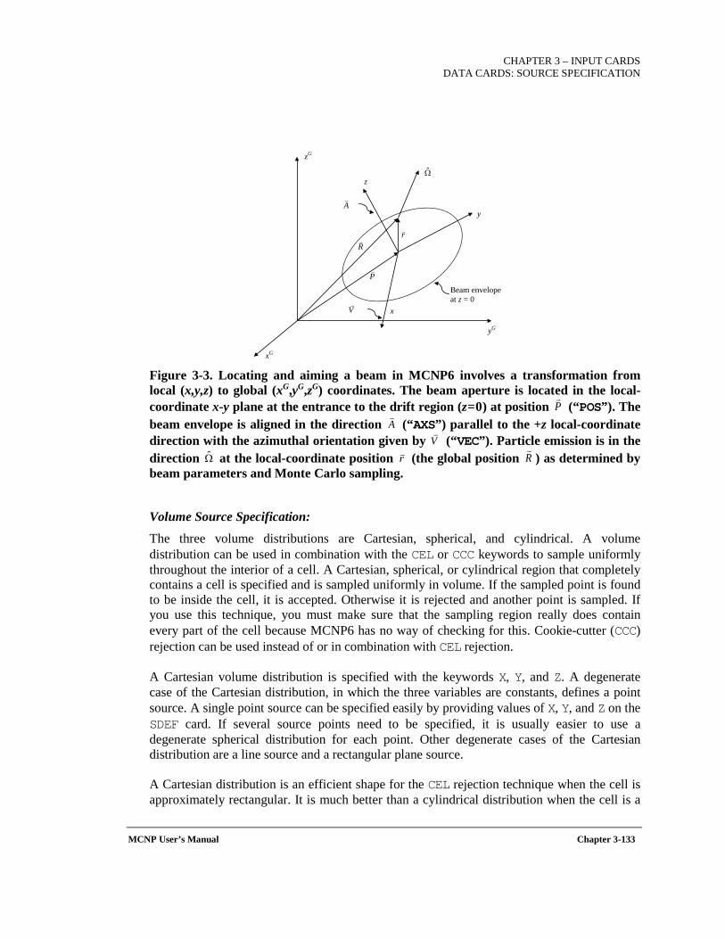
CHAPTER 3 – INPUT CARDS
DATA CARDS: SOURCE SPECIFICATION
MCNP User’s Manual Chapter 3-133
Figure 3-3. Locating and aiming a beam in MCNP6 involves a transformation from local (x,y,z) to global (xG,yG,zG) coordinates. The beam aperture is located in the local-coordinate x-y plane at the entrance to the drift region (z=0) at position (“POS”). The beam envelope is aligned in the direction (“AXS”) parallel to the +z local-coordinate direction with the azimuthal orientation given by (“VEC”). Particle emission is in the direction at the local-coordinate position (the global position ) as determined by beam parameters and Monte Carlo sampling.
Volume Source Specification:
The three volume distributions are Cartesian, spherical, and cylindrical. A volume distribution can be used in combination with the CEL or CCC keywords to sample uniformly throughout the interior of a cell. A Cartesian, spherical, or cylindrical region that completely contains a cell is specified and is sampled uniformly in volume. If the sampled point is found to be inside the cell, it is accepted. Otherwise it is rejected and another point is sampled. If you use this technique, you must make sure that the sampling region really does contain every part of the cell because MCNP6 has no way of checking for this. Cookie-cutter (CCC) rejection can be used instead of or in combination with CEL rejection.
A Cartesian volume distribution is specified with the keywords X, Y, and Z. A degenerate case of the Cartesian distribution, in which the three variables are constants, defines a point source. A single point source can be specified easily by providing values of X, Y, and Z on the SDEF card. If several source points need to be specified, it is usually easier to use a degenerate spherical distribution for each point. Other degenerate cases of the Cartesian distribution are a line source and a rectangular plane source.
A Cartesian distribution is an efficient shape for the CEL rejection technique when the cell is approximately rectangular. It is much better than a cylindrical distribution when the cell is a
z
x
y
zG
xG
yG
P
R
r
Ω
Beam envelope at z = 0
A
V
P
A
V
Ω r R

CHAPTER 3 – INPUT CARDS DATA CARDS: SOURCE SPECIFICATION
Chapter 3-134 MCNP User’s Manual
long thin slab. The Cartesian distribution is limited in that the faces can only be perpendicular to the coordinate axes.
A spherical volume distribution is specified with the keywords POS and RAD. The keywords X, Y, Z, and AXS must not be specified or the distribution will be assumed to be Cartesian or cylindrical. The sampled value of the vector POS defines the center of the sphere. The sampled value of RAD defines the distance from the center of the sphere to the position of the particle. The position is then sampled uniformly on the surface of the sphere of radius RAD. Uniform sampling in volume is obtained if the distribution of RAD is a power law with a=2, which is the default case. If RAD is not specified, the default is zero. This is useful because it specifies a point source at the position POS. A distribution for POS, with an L on the SI card, is the easiest way to specify a set of point sources in a problem.
A common use of the spherical volume distribution is to sample uniformly in the volume between two concentric spherical surfaces. The two radii are specified on the SI card for RAD and the effect of an SPn -21 2 card is obtained by default.
A cylindrical volume distribution is specified with the keywords POS, AXS, RAD, and EXT. The axis of the cylinder passes through the point POS in the direction AXS. The position of the particles is sampled uniformly on a circle whose radius is the sampled value of RAD, centered on the axis of the cylinder. The circle lies in a plane perpendicular to AXS at a distance from POS which is the sampled value of EXT. A useful degenerate case is EXT=0, which provides a source with circular symmetry on a plane (i.e., a thin disk source).
A common use of the cylindrical distribution is to sample uniformly in volume within a cylindrical shell. The distances of the ends of the cylinder from POS are entered on the SIn card for EXT and the inner and outer radii are entered on the SIn card for RAD. Uniform sampling between the two values of EXT and power law sampling between the two values of RAD, with a= 1 which gives sampling uniform in volume, are provided by default.
Caution: Never position any kind of degenerate volume distribution so that it lies on a defined surface of the problem geometry. Even a bounding surface that extends into the interior of a cell can cause trouble. If possible, use one of the surface distributions instead. Else, move to a position a small distance from the surface. This positioning will make no detectable difference in the answers, but will prevent particles from getting lost.
Surface Source Specification:
The value of the keyword SUR is non-zero for a distribution on a surface. The shape of the surface can be a spheroid, sphere, cylinder, or plane. (A spheroid is an ellipse revolved around one of its axes.) If X, Y, and Z are specified, their sampled values determine the position. The user must in this case make sure that the point really is on the surface because MCNP6 does not check. If X, Y, and Z are not specified, the position is sampled on the surface SUR. With the exception of a spherical surface, the SUR keyword does not
CHAPTER 3 – INPUT CARDS
DATA CARDS: SOURCE SPECIFICATION
MCNP User’s Manual Chapter 3-135
automatically provide source points on the listed surface. The user must still use the X, Y, Z, POS, AXS, RAD, and EXT keywords to ensure the source points actually lay on the prescribed surface. For a surface source, sampling using CEL rejection is not an option; however, cookie-cutter rejection can be used.
If the value of SUR is the name of a spheroidal surface, the position of the particle is sampled uniformly in area on the surface. A spheroid for this purpose must have its axis parallel to one of the coordinate axes. Although there is no provision for easy non-uniform or biased sampling on a spheroidal surface, a distribution of cookie-cutter cells could be used to produce a crude non-uniform distribution of position.
If the value of SUR is the name of a spherical surface, the position of the particle is sampled on that surface. A spherical surface source does not have to be on a cell-bounding problem surface. If the vector AXS is not specified, the position is sampled uniformly in area on the surface. If AXS is specified, the sampled value of EXT is used for the cosine of the angle between the direction AXS and the vector from the center of the sphere to the position point. The azimuthal angle is sampled uniformly in the range from 0° to 360°. A non-uniform distribution of position, in polar angle only, is available through a non-uniform distribution of EXT. A biased distribution of EXT can be used to start more particles from the side of the sphere nearest the tallying regions of the geometry. The exponential distribution function (-31, Section 3.3.4.3) usually is the most appropriate way to specify this behavior. The keyword DIR may be specified without VEC, allowing VEC to default to the outward surface normal.
Cylindrical surface sources must be specified as degenerate volume sources. For a cylindrical surface source, the cylindrical surface can be, but does not have to be, a cell-bounding problem surface specified by the keyword SUR. If the cylindrical surface is a problem surface, then the surface number must be specified on the SDEF card with the SUR keyword. The default of VEC is the surface normal. If both DIR and VEC are specified, then particle directions are relative to VEC rather than to the cylindrical surface normal. DIR may be specified without VEC, causing VEC to default to the outward surface normal.
If the value of SUR is the name of a plane, the position is sampled on that plane. The sampled value of POS must be a point on the plane. The user must make sure that POS really is on the plane because MCNP6 does not check. The sampled position of the particle is at a distance from POS equal to the sampled value of RAD. The position is sampled uniformly on the circle of radius RAD centered on POS. Uniform sampling in area is obtained if the distribution of RAD is a power law with a=1, which is the default in this case.
Guidance: Defining Embedded Source Distribution Information
Source distributions may be embedded within each other to describe accelerator micro-pulses and other phenomena. The format to specify an embedded source is
SDEF TME=( D11 < D12 < D13 )
CHAPTER 3 – INPUT CARDS DATA CARDS: SOURCE SPECIFICATION
Chapter 3-136 MCNP User’s Manual
or, for distributions of distributions, the following form may be used: SDEF TME=D41 SI41 S 51 ( D11 < D12 < D13 ) 52
In both cases, distributions 11, 12, 13 are all for the same variable, time. Distribution 11 covers a small time range that is repeated as often as needed to fill exactly the larger time range of distribution 12. Similarly, distribution 12 is repeated as often as needed to fill exactly the even larger time range of distribution 13. (See Example 20.)
Note that the parentheses are optional and that the designator “D” on the SI card with “S” option is also optional. Thus
SDEF TME=( D11 < D12 < D13 ) and SDEF TME= D11 < D12 < D13 are equivalent.
Also,
SI41 S 51 ( D11 < D12 < D13 ) 52 , SI41 S 51 D11 < D12 < D13 52 , SI41 S 51 ( 11 < 12 < 13 ) 52 , and SI41 S 51 11 < 12 < 13 52 are all equivalent.
The embedded distributions must start at zero or a fatal error message is issued. For (D11<D12<D13) the lowest value on the SI11 and SI12 cards must be zero. The embedding distribution, D13, can have any range.
The embedded distributions should fit within each other (nearly) exactly. If they do not there the fatal error message, “embedded distribution nn has improper range” is issued and the distribution will spill into the next bin and have a strange normalization for values in its last bin.
Only continuous source distributions such as ERG, TME, X, Y, Z, DIR, RAD and EXT may use embedded distributions.
Guidance: Defining a Source in a Repeated Structures or Lattice Geometry
Hint: Carefully study print table 110 in the MCNP6 output file to ensure that the proper source path and position are being sampled when repeated structures are used in a source description.
When the source is specified in a repeated structure part of the geometry, the CEL parameter on the SDEF card must have a value that is a path, enclosed in parentheses, from level n to level 0 (i.e., the highest level), where n is not necessarily the bottom level:
CEL=(cn<cn-1<...<c0)
CHAPTER 3 – INPUT CARDS
DATA CARDS: SOURCE SPECIFICATION
MCNP User’s Manual Chapter 3-137
In this specification ci is either zero or a cell in the universe that fills cell ci-1, or is Dm for a distribution of cells in the repeated structure case. A distribution of cells (i.e., Dm ) is not valid for a lattice; however, a range of lattice elements may be specified. (Cell designator ci can have a minus sign, but Dm cannot. This is discussed below.) If ci=0, the cell at that level is searched for. If ci is one specific element in a lattice, it is indicated as
...<ci[i j k]<...
The coordinate system for position and direction sampling (PDS) is the coordinate system of the first negative or zero ci in the source path starting from the right and proceeding left. Each entry in the source path represents a geometry level, where level zero is the last specified source path entry, level one is the second entry to the left, and so forth. Level zero is above level one and level two is below level one. The PDS level is the level associated with the PDS cell or PDS coordinate system. All levels above the PDS level must be included in the source path. Levels below the PDS level need not be specified, and when given, may include one or more zero entries. When the path has no negative or zero entry, the default PDS level is the first (i.e., lowest) entry in the source path.
Position rejection is done in cells at all levels where ci≠0, but if any ci has a negative universe number on its cell card and is at or above the PDS level, higher level cells are not checked.
The following chart illustrates the concept of the PDS level:
CEL Source Path Cell of PDS Level PDS Level
(5<6<7<8) 5 3 (6<-7<8) 7 1 (0<4<0<-6<7<8) 6 2 (0<6[0 0 0]<-7[1 0 0]<8) 7 1 (0<6[0 0 0]<7[1 0 0]<8) Will be determined 3
A range of lattice indices may be specified to produce a uniform sampling among those lattice elements. The ability to sample source points from a range of lattice indices requires the use of a fully specified FILL card for the listed lattice cell. The sampling is accomplished using rejection on all possible lattice elements. Note that the SDEF keyword EFF may need to be decreased to accommodate sampling of a small portion of a large lattice. A lattice cell without indices results in uniform sampling in all elements if a fully specified FILL card is provided. Uniform sampling is applied to lattice cell entries in the source path that lack an explicit lattice index and that are at or above the PDS level. Lattice cells not defined by the expanded FILL card must include an explicit lattice index when at or above the PDS level. Rejection of automatically sampled lattice elements depends on the entry before the lattice cell number in the source path.
Assume the following cell descriptions:
CHAPTER 3 – INPUT CARDS DATA CARDS: SOURCE SPECIFICATION
Chapter 3-138 MCNP User’s Manual
Cell 7 is a 3-element lattice defined using the following data entries: lat=1 u=1 fill=0:2 0:0 0:0 1 2 3
Cells 8 and 9 are members of universe 2 Cells 10 and 11 are members of universe 3
Cell 7 is a lattice with three existing elements: [0 0 0], which is filled by itself [u=1]; [1 0 0], which is filled by cells 8 and 9 [u=2]; and [2 0 0], which is filled by cells 10 and 11 [u=3]. The following combinations show which elements are accepted and which are rejected.
CEL Source Path Accepted Rejected
7 All elements None (0<7) All elements None (8<7) [1 0 0] [0 0 0], [2 0 0] (10<7) [2 0 0] [0 0 0], [1 0 0]
The sampling efficiency for cell 7 in the OUTP file will reflect the element rejections. Lattice cell entries that lack an explicit lattice index and are below the PDS level are not sampled. Instead, the appropriate lattice element is determined by the input source position.
Lattice element sampling is independent from position sampling. First a lattice element is chosen, then a position is chosen. If the sampled position is not in the sampled lattice element, the position is resampled until it is in the specified source path and in the lattice element chosen or until an efficiency error occurs. The lattice elements will not be resampled to accommodate the sampled position. Lattice element rejection is done only as described above.
Using the previous description of lattice cell 7, add that cell 6 is filled by cell 7. The source path becomes (0<7<6). Three elements of the lattice exist [fill=0:2 0:0 0:0] but element [0 0 0] now is cut off by cell 6. Lattice element [0 0 0] still will be sampled one-third of the time. The first time element [0 0 0] is sampled a fatal error will occur because the sampled position, no matter what it is, will be rejected because element [0 0 0] does not exist. Caution: Implement automatic lattice sampling carefully and ensure that all of the lattice elements specified on the expanded FILL card really do exist.
Note that the format of the CEL source path is the same as for tally cards. See Section 3.3.5.1.4 for more information about specifying the path for repeated structures or lattices for tallies.
Shorthand: Specifying Multiple Cell Paths for Repeated Structures or Lattices
The source cell path input format also allows a shorthand notation for one source cell path to represent a number of source paths, similar to the way that one "tally 4" path sequence
CHAPTER 3 – INPUT CARDS
DATA CARDS: SOURCE SPECIFICATION
MCNP User’s Manual Chapter 3-139
enclosed in parentheses can represent a number of separate tallies. For example, the input source path (5<7 8 9 10 11<1) is interpreted by MCNP6 as the five paths (5<7<1), (5<8<1), (5<9<1), (5<10<1), and(5<11<1). The sequence order of these paths is determined from left to right in the original input master path. Similarly, single or multiple lattice indexes within the square brackets of path (5<3[...]<2) can have the following four optional input forms for the ijk index data for lattice cell element(s) with the FILL array defined on the cell 3 card:
i Indicates the ith lattice element of cell 3 as defined by the FILL array using only one count index; e.g., i=1 is the first element.
i j k Indicates a lattice element from the FILL array using the three indexes.
i1:i2 j1:j2 k1:k2 Indicates a range of one or more lattice elements, where the ":" and last entry of any of the three pairs can be omitted if that lattice element does not vary.
U=m Specifies all of the lattice elements that have universe "m".
For the third specification form listed above, MCNP6 will create "n" source paths, where
n=(i2-i1+1)×(j2-j1+1)×(k2-k1+1)
with the order of these "n" paths being the order of the indexes changing from left to right with the left index varying most rapidly. For the fourth specification, the "n" source paths are the number of lattice elements with universe "m," where the order of the source paths is the order in the FILL matrix for cell 3. Since the SP card must specify the corresponding probabilities, this sequence order may be important. This sequence of the split paths is shown in the "cell" column of print table 10 of the OUTP file.
When more than one cell (or lattice cell) is specified on more than one level in the source input path, MCNP6 splits into multiple paths with the variation most rapid from the left. However, the first level (level n) and the last level (level 0) entered in the source input path can only have one entry. The path in this new format must always be enclosed in parentheses, but there must not be any inner parentheses in the path.
Spontaneous Fission Sources—Physics and Tally Normalization:
Note: Eighteen nuclides are available for a spontaneous fission source (PAR=SF):232Th, 232U, 233U, 234U, 235U, 236U, 238U, 237Np, 238Pu, 239Pu, 240Pu, 241Pu, 242Pu, 241Am, 242Cm, 244Cm, 249Bk, and 252Cf.
If more than one spontaneous-fission nuclide is present in a source cell, the fissioning nuclide will be chosen proportionately to the product of its atom fraction and the spontaneous-fission yield for each nuclide. If no spontaneous-fission nuclide is found in a specified source cell, the code exits with a BAD TROUBLE error, "spontaneous fission impossible."
CHAPTER 3 – INPUT CARDS DATA CARDS: SOURCE SPECIFICATION
Chapter 3-140 MCNP User’s Manual
The number of spontaneous-fission neutrons then is sampled. The spontaneous-fission multiplicity data of Santi [SAN04] and references cited by him are used by default. Alternatively, the LLNL FREYA or CGMF fission model can be used (see the FMULT card for more details). The energies are sampled from a Watt spectrum with appropriate spontaneous-fission parameters for the selected nuclide. Only the first spontaneous-fission neutron from each history is printed. If the spontaneous fission samples a multiplicity of zero—that is, no neutrons for a given spontaneous fission—then the history is omitted from the first 50 history lists of print table 110. The number of source particles is the number of spontaneous-fission neutrons, which will be times the requested number of source histories on the NPS card.
The spontaneous fission source is different from most other SDEF fixed sources. Let
N = the number of source-particle histories run in the problem, W = the average source particle weight, and = the average number of spontaneous fission neutrons per fission.
For most other fixed-source (SDEF) problems,
summary table source tracks = N, summary table source weight = W, and summary tables and tallies are normalized by N.
For the spontaneous fission source, SDEF PAR=SF,
summary table source tracks = ·N, summary table source weight = W, and summary tables and tallies are normalized by ·N, the number of spontaneous fission
neutrons.
For the spontaneous fission source, SDEF PAR=-SF,
summary table source tracks = ·N summary table source weight = ·W, and summary tables and tallies are normalized by N, the number of spontaneous fissions.
3.3.4.2 SI SOURCE INFORMATION
Form: SIn option i1 ... ik
ν
ν
ν
ν
νν
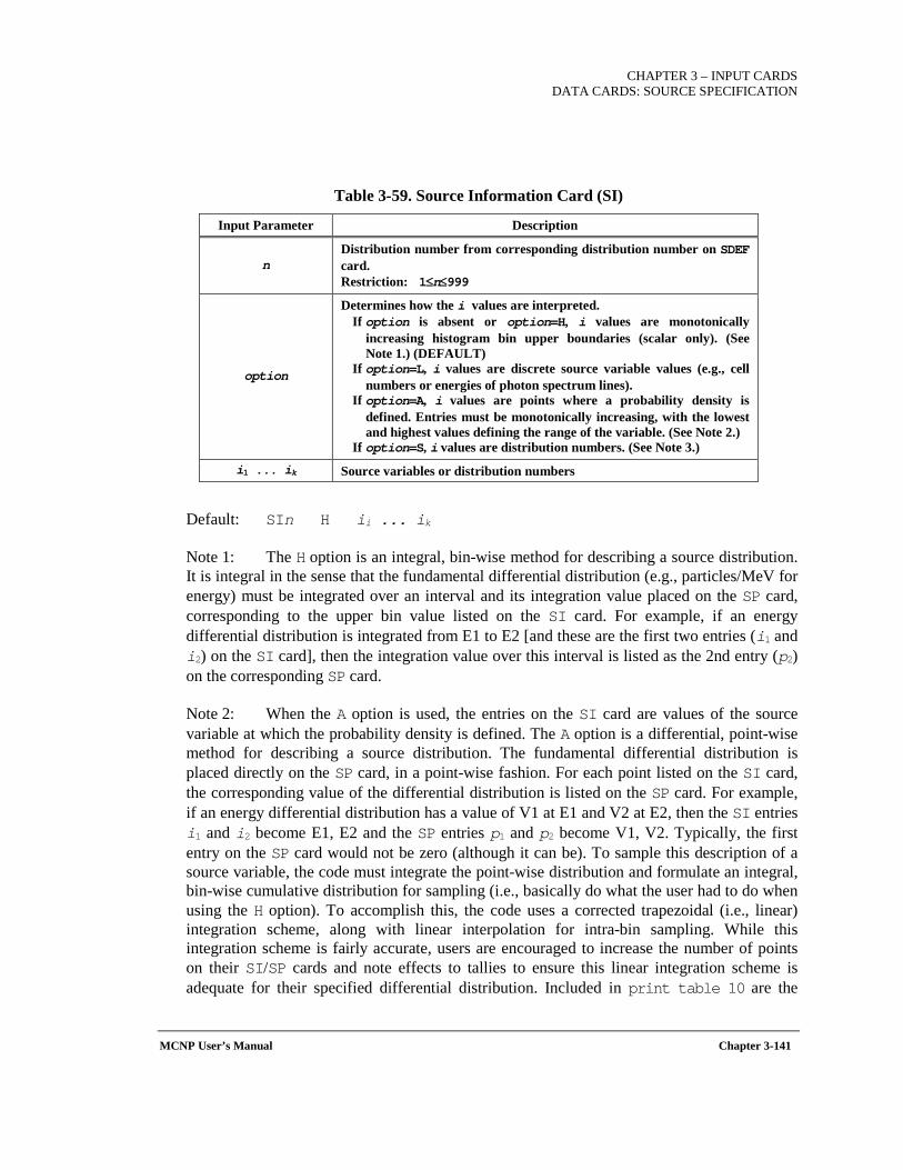
CHAPTER 3 – INPUT CARDS
DATA CARDS: SOURCE SPECIFICATION
MCNP User’s Manual Chapter 3-141
Table 3-59. Source Information Card (SI)
Input Parameter Description
n Distribution number from corresponding distribution number on SDEF card. Restriction: 1≤n≤999
option
Determines how the i values are interpreted. If option is absent or option=H, i values are monotonically
increasing histogram bin upper boundaries (scalar only). (See Note 1.) (DEFAULT)
If option=L, i values are discrete source variable values (e.g., cell numbers or energies of photon spectrum lines).
If option=A, i values are points where a probability density is defined. Entries must be monotonically increasing, with the lowest and highest values defining the range of the variable. (See Note 2.)
If option=S, i values are distribution numbers. (See Note 3.)
i1 ... ik Source variables or distribution numbers
Default: SIn H ii ... ik
Note 1: The H option is an integral, bin-wise method for describing a source distribution. It is integral in the sense that the fundamental differential distribution (e.g., particles/MeV for energy) must be integrated over an interval and its integration value placed on the SP card, corresponding to the upper bin value listed on the SI card. For example, if an energy differential distribution is integrated from E1 to E2 [and these are the first two entries (i1 and i2) on the SI card], then the integration value over this interval is listed as the 2nd entry (p2) on the corresponding SP card.
Note 2: When the A option is used, the entries on the SI card are values of the source variable at which the probability density is defined. The A option is a differential, point-wise method for describing a source distribution. The fundamental differential distribution is placed directly on the SP card, in a point-wise fashion. For each point listed on the SI card, the corresponding value of the differential distribution is listed on the SP card. For example, if an energy differential distribution has a value of V1 at E1 and V2 at E2, then the SI entries i1 and i2 become E1, E2 and the SP entries p1 and p2 become V1, V2. Typically, the first entry on the SP card would not be zero (although it can be). To sample this description of a source variable, the code must integrate the point-wise distribution and formulate an integral, bin-wise cumulative distribution for sampling (i.e., basically do what the user had to do when using the H option). To accomplish this, the code uses a corrected trapezoidal (i.e., linear) integration scheme, along with linear interpolation for intra-bin sampling. While this integration scheme is fairly accurate, users are encouraged to increase the number of points on their SI/SP cards and note effects to tallies to ensure this linear integration scheme is adequate for their specified differential distribution. Included in print table 10 are the
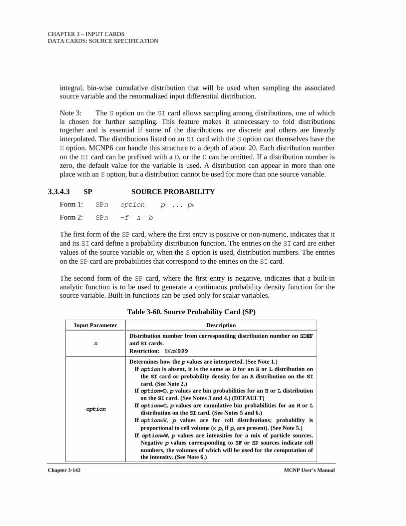
CHAPTER 3 – INPUT CARDS DATA CARDS: SOURCE SPECIFICATION
Chapter 3-142 MCNP User’s Manual
integral, bin-wise cumulative distribution that will be used when sampling the associated source variable and the renormalized input differential distribution.
Note 3: The S option on the SI card allows sampling among distributions, one of which is chosen for further sampling. This feature makes it unnecessary to fold distributions together and is essential if some of the distributions are discrete and others are linearly interpolated. The distributions listed on an SI card with the S option can themselves have the S option. MCNP6 can handle this structure to a depth of about 20. Each distribution number on the SI card can be prefixed with a D, or the D can be omitted. If a distribution number is zero, the default value for the variable is used. A distribution can appear in more than one place with an S option, but a distribution cannot be used for more than one source variable.
3.3.4.3 SP SOURCE PROBABILITY
Form 1: SPn option p1 ... pk
Form 2: SPn -f a b
The first form of the SP card, where the first entry is positive or non-numeric, indicates that it and its SI card define a probability distribution function. The entries on the SI card are either values of the source variable or, when the S option is used, distribution numbers. The entries on the SP card are probabilities that correspond to the entries on the SI card.
The second form of the SP card, where the first entry is negative, indicates that a built-in analytic function is to be used to generate a continuous probability density function for the source variable. Built-in functions can be used only for scalar variables.
Table 3-60. Source Probability Card (SP)
Input Parameter Description
n Distribution number from corresponding distribution number on SDEF and SI cards. Restriction: 1≤n≤999
option
Determines how the p values are interpreted. (See Note 1.) If option is absent, it is the same as D for an H or L distribution on
the SI card or probability density for an A distribution on the SI card. (See Note 2.)
If option=D, p values are bin probabilities for an H or L distribution on the SI card. (See Notes 3 and 4.) (DEFAULT)
If option=C, p values are cumulative bin probabilities for an H or L distribution on the SI card. (See Notes 5 and 6.)
If option=V, p values are for cell distributions; probability is proportional to cell volume (× pi if pi are present). (See Note 5.)
If option=W, p values are intensities for a mix of particle sources. Negative p values corresponding to SF or SP sources indicate cell numbers, the volumes of which will be used for the computation of the intensity. (See Note 6.)
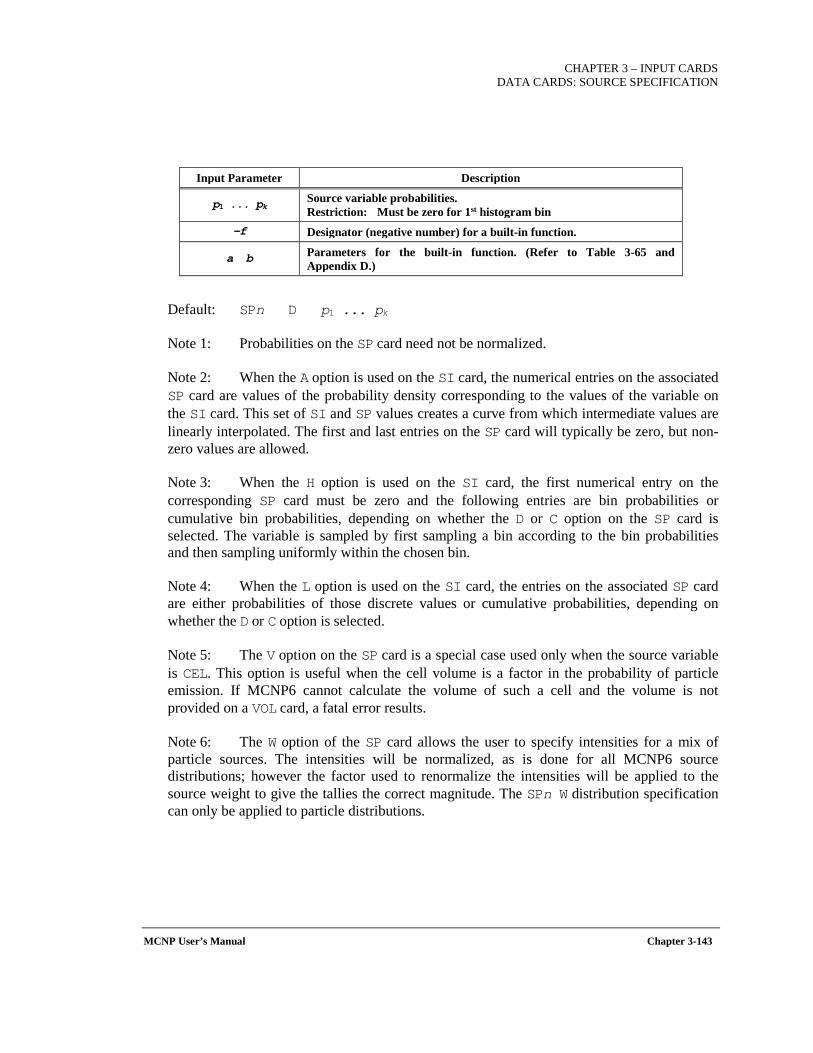
CHAPTER 3 – INPUT CARDS
DATA CARDS: SOURCE SPECIFICATION
MCNP User’s Manual Chapter 3-143
Input Parameter Description
p1 ... pk Source variable probabilities. Restriction: Must be zero for 1st histogram bin
-f Designator (negative number) for a built-in function.
a b Parameters for the built-in function. (Refer to Table 3-65 and Appendix D.)
Default: SPn D p1 ... pk
Note 1: Probabilities on the SP card need not be normalized.
Note 2: When the A option is used on the SI card, the numerical entries on the associated SP card are values of the probability density corresponding to the values of the variable on the SI card. This set of SI and SP values creates a curve from which intermediate values are linearly interpolated. The first and last entries on the SP card will typically be zero, but non-zero values are allowed.
Note 3: When the H option is used on the SI card, the first numerical entry on the corresponding SP card must be zero and the following entries are bin probabilities or cumulative bin probabilities, depending on whether the D or C option on the SP card is selected. The variable is sampled by first sampling a bin according to the bin probabilities and then sampling uniformly within the chosen bin.
Note 4: When the L option is used on the SI card, the entries on the associated SP card are either probabilities of those discrete values or cumulative probabilities, depending on whether the D or C option is selected.
Note 5: The V option on the SP card is a special case used only when the source variable is CEL. This option is useful when the cell volume is a factor in the probability of particle emission. If MCNP6 cannot calculate the volume of such a cell and the volume is not provided on a VOL card, a fatal error results.
Note 6: The W option of the SP card allows the user to specify intensities for a mix of particle sources. The intensities will be normalized, as is done for all MCNP6 source distributions; however the factor used to renormalize the intensities will be applied to the source weight to give the tallies the correct magnitude. The SPn W distribution specification can only be applied to particle distributions.
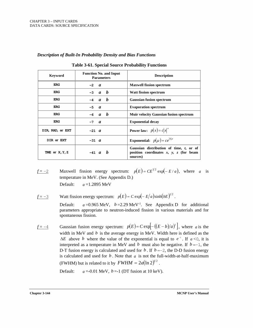
CHAPTER 3 – INPUT CARDS DATA CARDS: SOURCE SPECIFICATION
Chapter 3-144 MCNP User’s Manual
Description of Built-In Probability Density and Bias Functions
Table 3-61. Special Source Probability Functions
Keyword Function No. and Input Parameters Description
ERG -2 a Maxwell fission spectrum
ERG -3 a b Watt fission spectrum
ERG -4 a b Gaussian fusion spectrum
ERG -5 a Evaporation spectrum
ERG -6 a b Muir velocity Gaussian fusion spectrum
ERG -7 a Exponential decay
DIR, RAD, or EXT -21 a Power law:
DIR or EXT -31 a Exponential:
TME or X,Y,Z -41 a b Gaussian distribution of time, t, or of position coordinates x, y, z (for beam sources)
f = -2 Maxwell fission energy spectrum: , where is temperature in MeV. (See Appendix D.)
Default: =1.2895 MeV
f = -3 Watt fission energy spectrum: .
Default: =0.965 MeV, =2.29 MeV-1. See Appendix D for additional parameters appropriate to neutron-induced fission in various materials and for spontaneous fission.
f = -4 Gaussian fusion energy spectrum: , where is the width in MeV and is the average energy in MeV. Width here is defined as the
above where the value of the exponential is equal to . If <0, it is interpreted as a temperature in MeV and must also be negative. If =-1, the D-T fusion energy is calculated and used for . If =-2, the D-D fusion energy is calculated and used for . Note that is not the full-width-at-half-maximum (FWHM) but is related to it by .
Default: =-0.01 MeV, =-1 (DT fusion at 10 keV).
( ) axcxp =
( ) µµ acep =
( ) ( )aECEEp /exp21 −= a
a
( ) ( ) ( ) 21sinhexp bEaECEp −=
a b
( ) ( )( )[ ]2exp abECEp −−= ab
E∆ b 1−e ab b
b bb a
( ) 212ln2aFWHM =
a b
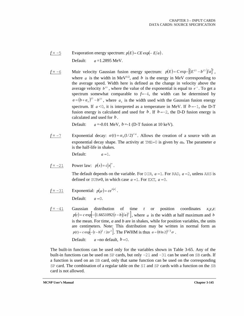
CHAPTER 3 – INPUT CARDS
DATA CARDS: SOURCE SPECIFICATION
MCNP User’s Manual Chapter 3-145
f = -5 Evaporation energy spectrum: .
Default: =1.2895 MeV.
f = -6 Muir velocity Gaussian fusion energy spectrum: , where is the width in MeV1/2, and is the energy in MeV corresponding to the average speed. Width here is defined as the change in velocity above the average velocity , where the value of the exponential is equal to . To get a spectrum somewhat comparable to f=-4, the width can be determined by
, where is the width used with the Gaussian fusion energy spectrum. If <0, it is interpreted as a temperature in MeV. If =-1, the D-T fusion energy is calculated and used for . If =-2, the D-D fusion energy is calculated and used for .
Default: =-0.01 MeV, =-1 (D-T fusion at 10 keV).
f = -7 Exponential decay: . Allows the creation of a source with an exponential decay shape. The activity at TME=0 is given by α0. The parameter a is the half-life in shakes.
Default: =1.
f = -21 Power law: .
The default depends on the variable. For DIR, =1. For RAD, =2, unless AXS is defined or SUR≠0, in which case =1. For EXT, =0.
f = -31 Exponential: .
Default: =0.
f = -41 Gaussian distribution of time t or position coordinates x,y,z: , where is the width at half maximum and
is the mean. For time, a and b are in shakes, while for position variables, the units are centimeters. Note: This distribution may be written in normal form as
. The FWHM is thus .
Default: =no default, =0.
The built-in functions can be used only for the variables shown in Table 3-65. Any of the built-in functions can be used on SP cards, but only -21 and -31 can be used on SB cards. If a function is used on an SB card, only that same function can be used on the corresponding SP card. The combination of a regular table on the SI and SP cards with a function on the SB card is not allowed.
( ) ( )aECEEp −= exp
a
( ) ( )[ ]22121exp abECEp −−=
a b
21b 1−e
( ) 21214 baba −+=
4aa b
b bb
a b
att /0 )2/1()( αα =
a
( ) axcxp =
a aa a
( ) µµ acep =
a
( ) ( )( )[ ]26651092.1exp abtctp −−= a b
( )[ ]22 2/exp)( σbtctp −−= ( ) σ2/12ln8=a
a b
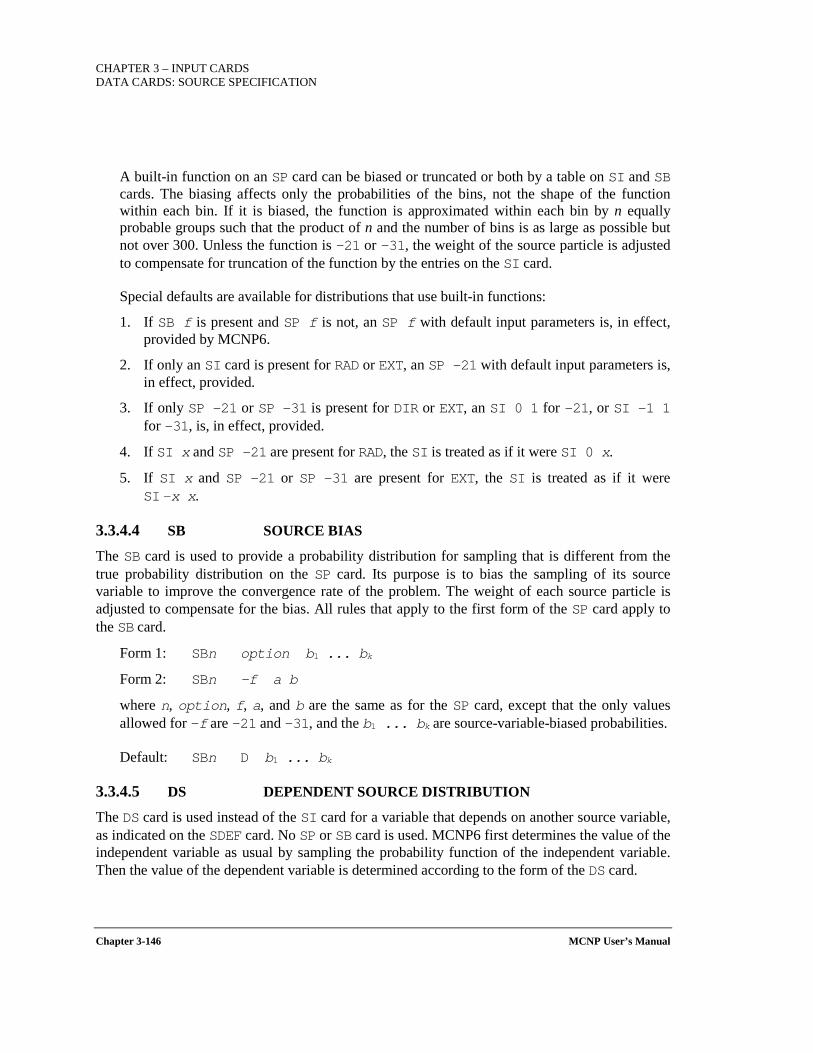
CHAPTER 3 – INPUT CARDS DATA CARDS: SOURCE SPECIFICATION
Chapter 3-146 MCNP User’s Manual
A built-in function on an SP card can be biased or truncated or both by a table on SI and SB cards. The biasing affects only the probabilities of the bins, not the shape of the function within each bin. If it is biased, the function is approximated within each bin by n equally probable groups such that the product of n and the number of bins is as large as possible but not over 300. Unless the function is -21 or -31, the weight of the source particle is adjusted to compensate for truncation of the function by the entries on the SI card.
Special defaults are available for distributions that use built-in functions:
1. If SB f is present and SP f is not, an SP f with default input parameters is, in effect, provided by MCNP6.
2. If only an SI card is present for RAD or EXT, an SP -21 with default input parameters is, in effect, provided.
3. If only SP -21 or SP -31 is present for DIR or EXT, an SI 0 1 for -21, or SI -1 1 for -31, is, in effect, provided.
4. If SI x and SP -21 are present for RAD, the SI is treated as if it were SI 0 x.
5. If SI x and SP -21 or SP -31 are present for EXT, the SI is treated as if it were SI -x x.
3.3.4.4 SB SOURCE BIAS
The SB card is used to provide a probability distribution for sampling that is different from the true probability distribution on the SP card. Its purpose is to bias the sampling of its source variable to improve the convergence rate of the problem. The weight of each source particle is adjusted to compensate for the bias. All rules that apply to the first form of the SP card apply to the SB card.
Form 1: SBn option b1 ... bk
Form 2: SBn -f a b
where n, option, f, a, and b are the same as for the SP card, except that the only values allowed for -f are -21 and -31, and the b1 ... bk are source-variable-biased probabilities.
Default: SBn D b1 ... bk
3.3.4.5 DS DEPENDENT SOURCE DISTRIBUTION
The DS card is used instead of the SI card for a variable that depends on another source variable, as indicated on the SDEF card. No SP or SB card is used. MCNP6 first determines the value of the independent variable as usual by sampling the probability function of the independent variable. Then the value of the dependent variable is determined according to the form of the DS card.
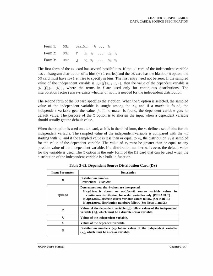
CHAPTER 3 – INPUT CARDS
DATA CARDS: SOURCE SPECIFICATION
MCNP User’s Manual Chapter 3-147
Form 1: DSn option j1 ... jk
Form 2: DSn T i1 j1 ... ik jk
Form 3: DSn Q v1 s1 ... vk sk
The first form of the DS card has several possibilities. If the SI card of the independent variable has a histogram distribution of m bins (m+1 entries) and the DS card has the blank or H option, the DS card must have m+1 entries to specify m bins. The first entry need not be zero. If the sampled value of the independent variable is ii+[f(ii+1-ii)], then the value of the dependent variable is ji+[f(ji+1-ji)], where the terms in f are used only for continuous distributions. The interpolation factor f always exists whether or not it is needed for the independent distribution.
The second form of the DS card specifies the T option. When the T option is selected, the sampled value of the independent variable is sought among the ii, and if a match is found, the independent variable gets the value ji. If no match is found, the dependent variable gets its default value. The purpose of the T option is to shorten the input when a dependent variable should usually get the default value.
When the Q option is used on a DS card, as it is in the third form, the vi define a set of bins for the independent variable. The sampled value of the independent variable is compared with the vi, starting with v1, and if the sampled value is less than or equal to vi, the distribution si is sampled for the value of the dependent variable. The value of vi must be greater than or equal to any possible value of the independent variable. If a distribution number si is zero, the default value for the variable is used. The Q option is the only form of the DS card that can be used when the distribution of the independent variable is a built-in function.
Table 3-62. Dependent Source Distribution Card (DS)
Input Parameter Description
N Distribution number. Restriction: 1≤n≤999
Option
Determines how the j values are interpreted. If option is absent or option=H, source variable values in
continuous distribution, for scalar variables only. (DEFAULT) If option=L, discrete source variable values follow. (See Note 1.) If option=S, distribution numbers follow. (See Notes 1 and 2.)
T Values of the dependent variable (ji) follow values of the independent variable (ii), which must be a discrete scalar variable.
ii Values of the independent variable. ji Values of the dependent variable.
Q Distribution numbers (si) follow values of the independent variable (vi), which must be a scalar variable.
CHAPTER 3 – INPUT CARDS DATA CARDS: SOURCE SPECIFICATION
Chapter 3-148 MCNP User’s Manual
Input Parameter Description vi Monotonically increasing set of values of the independent variable. si Distribution numbers for the dependent variable.
Default: DSn H j1 ... jk
Note 1: If the L or S option is used on the DS card, m entries are required to specify m discrete values (for all options on the independent variable except H). (See the note that follows for a histogrammed independent variable.) It is not necessary for the distributions of the independent and dependent variables to be both discrete or both continuous. All combinations work correctly.
Note 2: If the S option is used on the DS card and the independent variable has a histogram defined by m+1 SI entries, then m numbers must appear on the DS card. Recall that the first bin of a histogram distribution must have an SP value of 0.0. The code will assume that the first independent histogram bin is ignored. A fatal error will result if a dependent source value is assigned to the first histogram bin.
Examples of the General Source (SDEF) with SI, SP, and SB
Example 1: SDEF
This card specifies a 14-MeV isotropic point source at position 0,0,0 at time 0 with weight 1 (all defaults).
Example 2: SDEF ERG=D1 POS=x y z WGT=w SI1 H e1 e2 ... ek SP1 D 0 p2 ... pk SB1 D 0 b2 ... bk
This is a point isotropic source at x,y,z with a biased histogram energy distribution and average source particle weight w. The starting cell is not specified. MCNP6 will determine it from the value of x, y, and z.
Example 3: SDEF SUR=m AXS=i j k EXT=D6 SB6 −31 1.5
This is a source on surface m. The presence of AXS and EXT implies that surface m is a sphere because AXS and EXT are not otherwise used together for sources on a surface. By default, the particles are emitted in a cosine distribution. They are emitted outward if the positive normal to the sphere is outward, which it is for all the spherical surface types but
CHAPTER 3 – INPUT CARDS
DATA CARDS: SOURCE SPECIFICATION
MCNP User’s Manual Chapter 3-149
might not be if the sphere is specified as type SQ. The position on the surface is biased toward the direction i,j,k by an exponential bias (specified by -31). Table 2.8 of the MCNP5 Theory Manual[X-503a] shows the effect of the biasing parameter on the maximum and minimum source particle weights and the cumulative probability distribution. By default, MCNP6 provides the effect of two cards: SI6 −1 1 and SP6 -31 0.
Example 4: SDEF SUR=999 NRM=−1 DIR=D1 WGT=1.13097e6 SB1 −21 2 void f4:n 1 2 3 4 vol 1 5r imp:n 1.0 4r 0.0
These data cards illustrate how an inward-directed (NRM=-1), biased cosine source on a spherical surface can be used to stochastically calculate the volume of MCNP6 cells. All materials are voided in the problem (VOID card) and all non-zero importance are set to 1 (IMP:N card). In this example, the surface source is placed on the surface of a 600-cm-radius sphere (SUR=999) that surrounds the cells of interest and the source weight (WGT) is set to 1.13097e6 cm2 (πr2). All volumes are forced to unity (VOL card). Type 2 and type 4 flux tallies will provide estimates of the areas and volumes of the cells, respectively. By default, MCNP6 provides the effect of two cards: SI1 0 1 and SP1 −21 1. The directional bias by the SB1 card causes higher track density toward the center of the sphere, where presumably the cells of greatest interest lie, than it would be if the unbiased cosine distribution were used. This bias, incidentally, provides a zero-variance estimate of the (known) volume of the sphere 999..
Example 5: SDEF CEL=D3 POS=0 6 0 EXT=D1 RAD=D2 AXS= 0 1 0 SI3 L (1<10[0 0 0]<11) (1<10[1 0 0]<11) (1<10[2 0 0]<11) (1<10[0 1 0]<11) (1<10[1 1 0]<11) (1<10[2 1 0]<11)
The SDEF card creates a cylindrical volume source oriented along the y-axis with radius specified by the SI2 source information and SP2 source probability cards and extent given by SI1 and SP1. This CEL source specification for repeated-structures geometries is consistent with the repeated-structures tally format. The old-style format (listing cells in the opposite order separated by ":") is no longer recognized and will produce a fatal error.
CHAPTER 3 – INPUT CARDS DATA CARDS: SOURCE SPECIFICATION
Chapter 3-150 MCNP User’s Manual
Example 6: SDEF POS=0 0 0 RAD=1 EXT=D1 AXS=1 0 0 SUR=5
SDEF POS=0 0 0 RAD=1 EXT=D1 AXS=1 0 0 SUR=5 DIR=D2
SDEF POS=0 0 0 RAD=1 EXT=D1 AXS=1 0 0 DIR=D2
The first SDEF card specifies a cylindrical source on surface 5 with default cosine distribution relative to the surface normal. The second SDEF card specifies a cylindrical source on surface 5 with a specified angular distribution that is relative to the cylindrical surface normal. The third SDEF source specification is similar except that a degenerate volume source is used to specify the cylindrical surface source (i.e., omitting the SUR keyword) with a specified angular distribution relative to the surface normal.
Example 7: SDEF DIR=1 VEC=0 0 1 X=D1 Y=D2 Z=0 CCC=99 TR=1 SP1 -41 fx 0 SP2 -41 fy 0 TR1 x0 y0 z0 cosθ -sinθ 0 sinθ cosθ 0 0 0 1
The SDEF card sets up an initial beam of particles traveling along the z-axis (DIR=1, VEC=0 0 1). Information on the x- and y-coordinates of particle position is detailed in the two SP cards. The z-coordinate is left unchanged. The first entry on the SP cards is -41, indicating sampling from a built-in Gaussian distribution. The second SP card entry is the full width half maximum (FWHM) of the Gaussian in either the xor y direction. This value must be computed for the x- and y-axes by the user as follows:
and , where a and b are the standard deviations of the Gaussian in the x and y directions, respectively. (More details are provided in Section 4.3.2.) The third entry represents the centroid of the Gaussian in either the x or y direction. It is recommended the user input zero for this third entry and handle any transformations of the source with a TR card. The specification of the cookie-cutter cell 99 for source rejection prevents the beam Gaussian from extending infinitely. The TR card performs a rotation of the major axis of the source distribution. Other beam examples appear in Section 4.3.2.
Example 8: SDEF ERG=D1 POS=x y z CEL=m RAD=D2 EXT=D3 AXS=i j k SP1 −3 SI2 r1 r2 SI3 l
This source is distributed uniformly in volume throughout cell m, which presumably approximates a cylinder. The cell is enclosed by a sampling volume centered at x,y,z. The axis of the sampling volume is the line through x,y,z in the direction i,j,k. The inner and outer radii of the sampling volume are r1 and r2, and it extends along i,j,k for
( ) aaf x 35482.22ln8 21 == ( ) bbf y 35482.22ln8 21 ==
CHAPTER 3 – INPUT CARDS
DATA CARDS: SOURCE SPECIFICATION
MCNP User’s Manual Chapter 3-151
a distance from x,y,z. The user has to make sure that the sampling volume totally encloses cell m. The energies of the source particles are sampled from the Watt fission spectrum using the default values of the two parameters, making it a Cranberg spectrum. By default, MCNP6 interprets SI3 l as if it was actually SI3 −l +l and provides the effect of two cards: SP2 −21 1 and SP3 −21 0.
Example 9: SDEF SUR=m POS=x y z RAD=D1 DIR=1 CCC=n SI1 r
This is a mono-directional source emitted from surface m in the direction of the positive normal to the surface. The presence of POS and RAD implies that surface m is a plane because POS and RAD are not otherwise used together for sources on a surface. The position is sampled uniformly in area on the surface within radius r of point x,y,z. The user must make sure that point x,y,z actually lies on surface m.. The sampled position is rejected and resampled if it is not within cookie-cutter cell n. The starting cell is found from the position and the direction of the particle. By default, MCNP6 interprets SI1 r as if it were actually SI1 0 r and provides the effect of card SP1 −21 1.
Example 10: SDEF PAR=SF CEL=D1 POS=D2 RAD=FPOS=D3
Spontaneous-fission source in which source points will be started from within defined spheres (POS, RAD) and limited to fission cells by CEL. Each sampled source point will be a spontaneous-fission site (PAR=SF) producing the appropriate number of spontaneous-fission neutrons per fission at the appropriate energy with isotropic direction.
Example 11: SDEF PAR=D1 SI1 L 1 9 3006 26056 92238 SP1 1 1 0.1 0.3 0.5
Five different source particles are sampled in this example: neutrons; protons; and the three heavy ions—6Li, 56Fe, and 238U. The relative sampling frequency is given by the probability parameters on the SP1 card.
CHAPTER 3 – INPUT CARDS DATA CARDS: SOURCE SPECIFICATION
Chapter 3-152 MCNP User’s Manual
*************************************************************************** ASIDE: PAR=Dn
Note the following when using a distribution specification for the PAR keyword:
1. The characters L, A, H, S, Q, and T are reserved as SI and DS card options. L=discrete source variables, S=distribution numbers, etc. If the first entry on the SI or DS card is L, A, H, S, Q, or T, it will be interpreted as a distribution option. To list source particles types L, A, H, S, Q, or T, either the corresponding particle numbers (10,34,9,33,5,32) must be used or L, A, H, S, Q, or T must appear as the second or later particle type. Generally, it is best to specify the discrete source variable option; therefore, L will be the first entry, followed by the particle types. A second L will be interpreted correctly as particle type L. For example,
SI99 L -H N L Q F T S
2. Antiparticles may be designated, as usual, with negative entries: SI77 L -E N -H
3. Either characters (N, P, E, H, D, T,S, A, etc.) or numbers (1, 2, 3, 9, 31, 32, 33, 34, etc.) may be used. For example, SI98 L -H 3 -32 N
4. Spontaneous fission may be used as a particle type. For example, SI87 L SF N
5. Particle types may be listed multiple times to give them different energy distributions, angular distributions, etc., in different parts of the problem. For example: SI23 L N n 1 n N
6. Heavy ions may be specified using the appropriate ZZZAAA identifier for individual ions. Multiple heavy ions may be specified for the source using a distribution. Dependent distributions can be used to specify different energies for different heavy ions. Heavy ion particle energy should be input as total energy, not energy/nucleon.
7. Tallies are normalized by dividing the total source weight by the number of source histories. Note that weight (WGT on the SDEF card) cannot be a source distribution (either independent or dependent). The weight of particles in the summary tables is controlled by the SI, SP, SB, and DS cards for the particle distribution. This normalization procedure is described in Example 12 below:
***************************************************************************
CHAPTER 3 – INPUT CARDS
DATA CARDS: SOURCE SPECIFICATION
MCNP User’s Manual Chapter 3-153
Example 12: SDEF PAR=D1 POS FPAR D2 ERG FPAR D3 SI1 L H N SP1 2 1 SB1 1 2 DS2 L 0 0 0 15 0 0 DS3 L 2 3
SDEF PAR=FPOS D2 POS=D1 ERG FPOS D3 SI1 L 0 0 0 15 0 0 SP1 2 1 SB1 1 2 DS2 L h n DS3 L 2 3
The first source definition above defines the source particle type, PAR, as the independent variable; while in the second source definition, the source particles specified by PAR depend on the source positions (POS). Both approaches result in the same source distributions.
The total source weight is WGT=1.0 by default. From the SP1 card, the weight of the neutrons that are produced is 0.3333 and the weight of protons that are produced is 0.6667. From the SB1 card, the total number of neutron tracks is 0.6667 × N for neutrons and 0.333 × N for protons (where N is the number of source histories actually run). The energy per source particle is normalized to the source particle weight for each source particle type. If the particle type is not a source particle (e.g., photons in the above problem), then the energy per source particle is normalized to the source particle weight of the lowest particle type. In this example, photon source energy would be normalized in the photon creation-and-loss table by 0.3333, which is the weight of the source neutrons produced.
Example 13: SDEF POS D1 ERG FPOS D2 SI1 L 5 3.3 6 75 3.3 6 SP1 0.3 0.7 DS2 S 3 4 SI3 H 2 10 14 SP3 D 0 1 2 SI4 −3 a b
This is a point isotropic source in two locations, shown by two x,y,z’s on the SI1 card. The code will determine the starting cell. With probability 0.3 the first location will be picked, and with probability 0.7 the second location will be chosen. Each location has a different energy spectrum pointed to by the DS2 card. All other needed source variables will use their default values.
CHAPTER 3 – INPUT CARDS DATA CARDS: SOURCE SPECIFICATION
Chapter 3-154 MCNP User’s Manual
Example 14: SDEF DIR=1 VEC=0 0 1 X=D1 Y=0 Z=−2 TR=1 SI1 0.0 0.5 SP1 0.0 1.0 TR1 0.5 0.5 0.0 0.4 0.3 0.0 −0.3 0.4 0.0
This example generates a source uniform on a straight line from (x,y,z)=(0.5,0.5,-2.0) to (x,y,z)=(0.9,0.8,-2.0) in the +z direction. In the auxiliary coordinate system, the source is easily created as uniform from (0.0,0.0,−2.0) to (0.5,0.0,-2.0) and then transformed.
Example 15: SDEF TR=D1 SI1 L 1 3 5 SP1 D 1.0 1.0 1.0 SB1 C 0.2 0.5 1.0
In this example, a distribution of transformations is specified using TR=D1 on the SDEF card. Three transformations are assigned: TR1, TR3, and TR5. The L option on the SI card is required so that MCNP6 interprets the values as discrete transformation numbers. The option on the SP and SB cards may be blank, D, or C. For this problem, the transformations are equally probable, but are biased to sample TR1 20% of the time, TR3 30% of the time, and TR5 50% of the time.
Example 16: SDEF TME=D1 SP1 -7 2e8 $ 2e8 shakes=2 seconds
The source shape will be represented by exponential decay with a half-life of 2 s.
Example 17: 999 0 -999 $ cookie cutter cell CCC ...
999 SQ 25 100 0 0 0 0 -4 0 0 0 $ surface for cell CCC ...
SDEF DIR=1 VEC=0 0 1 X=D1 Y=D2 Z=0 CCC=999 TR=D3 SP1 −41 0.470964 0 SP2 −41 0.235482 0 SI3 L 11 22 33 SP3 1 2 3 SB3 1 1 1 TR11 0 0 −2 1 0 0 0 1 0 0 0 1 TR22 −2 0 0 0 1 0 0 0 1 1 0 0 TR33 0 -2 0 0.707107 0 0.707107 0.707107 0 −0.707107 0 1 0
CHAPTER 3 – INPUT CARDS
DATA CARDS: SOURCE SPECIFICATION
MCNP User’s Manual Chapter 3-155
In this example, the source particle coordinates are generated in an auxiliary coordinate system in the (x′,y′,0) plane around the origin with a Gaussian profile (FWHM=0.470964) in the x′-coordinate and a Gaussian profile (FWHM=0.235482) in the y′-coordinate. The beam is truncated by "cookie cutter cell" CCC, which restricts the source to an ellipse corresponding to two standard deviations of the Gaussian distributions in the x′- and y′-coordinates. The subsequent application of the transformation TR=D3 results in three intersecting beams with the following characteristics:
− Beam 1 is centered at (0,0,-2) with the major axis of the beam distribution along the x-axis, emitted in the +z direction, with relative intensity 1;
− Beam 2 is centered at (-2,0,0) with the major axis of the beam distribution along the y-axis, emitted in the +x direction, with relative intensity 2; and
− Beam 3 is centered at (0,-2,0) with the major axis of the beam distribution along the line x=z, emitted in the +y direction, with relative intensity 3.
Example 18: m1 1001 1 8016 1 7016 1e-4 $ Unstable isotope N-16 25054 1e-2 $ Unstable isotope Mn-54 c sdef par=sp pos= 0 0 0 $ Location of material 1 ACT DG=LINES
The source is defined as decay gammas from the unstable isotopes 16N and 54Mn in material 1, which is the material located at the user-provided source position coordinates (0,0,0). The two unstable isotopes will be sampled based on their relative activities within material 1. The default time (TME=0) is assumed.
Example 19: mode p # sdef par=7016 erg=0 pos= 0 0 0 ACT DG=LINES
Setting the source particle to the heavy ion 16N (PAR=7016) and specifying the energy of the ion as zero (ERG=0) defines the source as the decay gammas of 16N. The heavy ions will not be transported. Notice that the heavy-ion symbol, #, appears on the MODE card.
Example 20: sdef erg d21 cel=d11 tme=d41 si41 S 52<51 (D31<32<d33) 61 sp41 .1 .8 .1 si51 A -26 -16
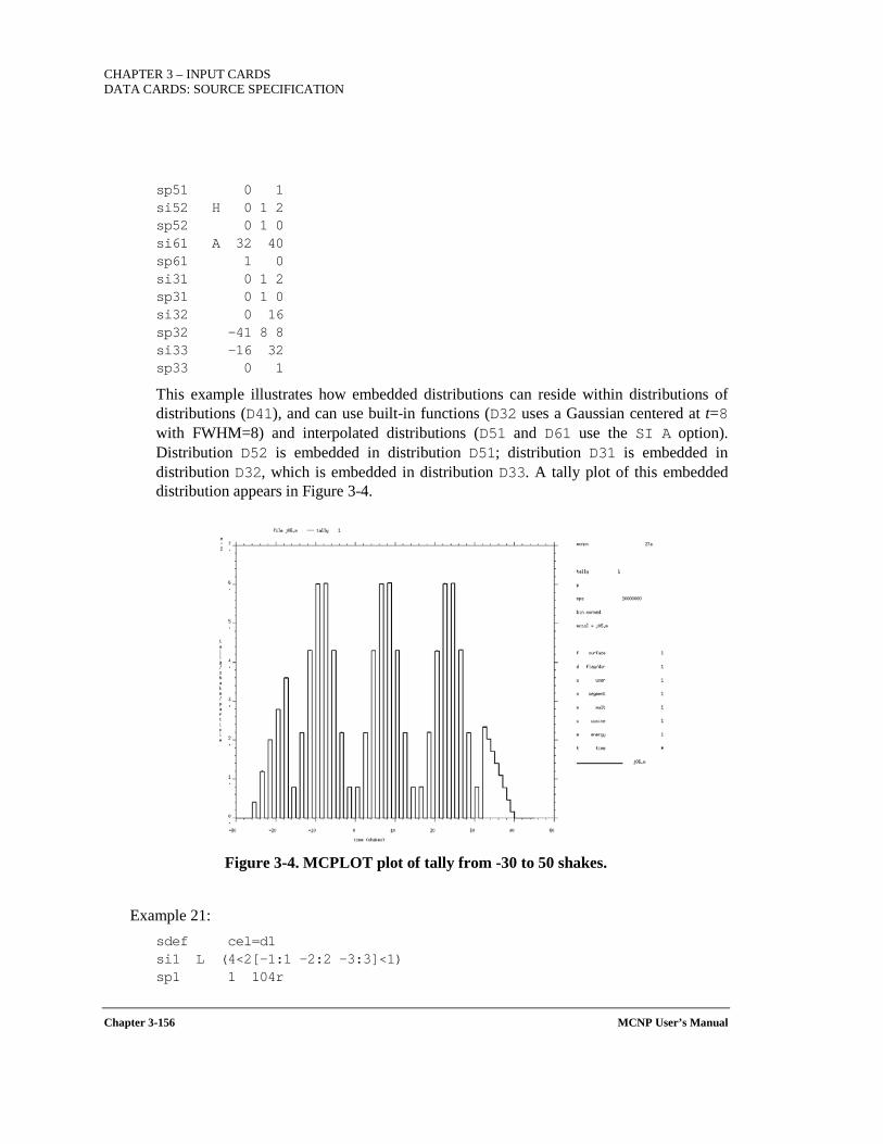
CHAPTER 3 – INPUT CARDS DATA CARDS: SOURCE SPECIFICATION
Chapter 3-156 MCNP User’s Manual
sp51 0 1 si52 H 0 1 2 sp52 0 1 0 si61 A 32 40 sp61 1 0 si31 0 1 2 sp31 0 1 0 si32 0 16 sp32 -41 8 8 si33 -16 32 sp33 0 1
This example illustrates how embedded distributions can reside within distributions of distributions (D41), and can use built-in functions (D32 uses a Gaussian centered at t=8 with FWHM=8) and interpolated distributions (D51 and D61 use the SI A option). Distribution D52 is embedded in distribution D51; distribution D31 is embedded in distribution D32, which is embedded in distribution D33. A tally plot of this embedded distribution appears in Figure 3-4.
Figure 3-4. MCPLOT plot of tally from -30 to 50 shakes.
Example 21: sdef cel=d1 si1 L (4<2[-1:1 -2:2 -3:3]<1) sp1 1 104r
CHAPTER 3 – INPUT CARDS
DATA CARDS: SOURCE SPECIFICATION
MCNP User’s Manual Chapter 3-157
This source definition creates source particles in a subset of a lattice using ranges specified for the lattice elements. The lattice must have been defined using a fully specified FILL card.
Example 22: si1 L n p h sp1 W 3e9 5e9 2e9
The source shown here mixes contributions from three source particles and samples them according to their relative magnitudes (neutrons 30%, photons 50%, and protons 20%). The weight assigned to each particle will be the sum of the non-normalized values, 3E9+5E9+2E9=1E10.
Example 23: si1 L sp sf n sp1 W -10 -15 3e9
The spontaneous photon source will look to cell 10 and use the material and volume to calculate the overall activity that will be substituted into the SP1 distribution. Correspondingly, the SF source will look to the material and volume in cell 15 for the intensity of the spontaneous fission source. (Note that a +SF normalizes per spontaneous fission neutron, a -SF normalizes per spontaneous fission.) The neutron source is unchanged. After the overall activity is computed, the source distribution normalization will be done as described above and the weight adjustment value passed into the weight parameter.
Example 24: sdef par=d1 wgt=264 si1 L sf sp1 w -35
If the cell specified in the SPn W option is a lattice cell, then the code may not know the correct volume for this cell. If the user does not wish to correct the volume using the VOL card or cell keyword, a WGT keyword can be used with the source as a multiplicative factor. In this example, the spontaneous fission source is weighted by the activity from cell 35, which has been duplicated 264 times in the geometry. The final source weight will be the activity from cell 35×264.
3.3.4.6 SC SOURCE COMMENT
Form: SCn comment (See Note.)
where n is a distribution number such that 1≤n≤999, and comment is user-supplied text describing the source.
Default: No comment.

CHAPTER 3 – INPUT CARDS DATA CARDS: SOURCE SPECIFICATION
Chapter 3-158 MCNP User’s Manual
Note: The comment is printed as part of the header of distribution n in the source distribution table and in the source distribution frequency table. The & continuation symbol is considered to be part of the comment, not a continuation command.
3.3.4.7 SSW SURFACE SOURCE WRITE
This card is used to write a surface source file or KCODE fission volume source file for use in a subsequent MCNP6 calculation. Include enough geometry beyond the specified surfaces to account for albedo effects.
During execution, surface source information is written to the scratch file WXXA. Upon normal completion, WXXA becomes WSSA. If the run terminates abnormally, the WXXA file will appear instead of WSSA and must be saved along with the RUNTPE file. The job must be continued for at least one more history. At the subsequent normal termination, WXXA disappears and the correct surface source file WSSA is properly written.
Form: SSW s1 s2 (c1 ... ck) s3 ... sk KEYWORD=value(s) ...
Table 3-63. Surface Source Write Card
Input Parameter Description
si
Problem surface number, with the appropriate sign to indicate sense of inward or outward particle direction, for which particle-crossing information is to be written to the surface source file WSSA. Macrobody facets are allowed.
cj
Problem cell number. A positive entry denotes a cell the particle is entering. A negative entry specifies a cell that particle is leaving. This option provides a means to include only a portion of tracks crossing a certain surface. (See Notes 1 and 2.)
Keyword Values
SYM
Symmetry option flag. If SYM=0, no symmetry assumed. (DEFAULT) If SYM=1, spherical symmetry assumed. The list of problem surface
numbers must contain only one surface and it must be a sphere. (See Note 3.)
If SYM=2, write particles to a surface bidirectionally. Otherwise, only particles going out of a positive surface and into a negative surface are recorded.
PTY=<pl>1 <pl>2 ...
Controls tracks to record. If PTY is absent, record all tracks for all particle types. (DEFAULT) Each <pl>i entry is a particle type selected from those listed in Table
2-2.
CEL=cf1 cf2 ... List of names of all the cells from which KCODE fission source neutrons are to be written, active cycles only. (See Notes 4 and 5.)
Default: SYM=0; no PTY keyword (record tracks for all particle types)
CHAPTER 3 – INPUT CARDS
DATA CARDS: SOURCE SPECIFICATION
MCNP User’s Manual Chapter 3-159
Use: Optional.
Note 1: The SSW card allows a list of one or more cell names, positive or negative, after any of the surface names. The list of cell names must be enclosed in parentheses. If the list of cells is absent, any track that crosses the surface in the "correct direction" (as specified by the positive or negative sign on the surface number) will be recorded. If the list of cells is present, a track will be recorded if it crosses the surface in the correct direction and is either entering a cell in the list whose entry is positive or leaving a cell in the list whose entry is negative.
Note 2: Problem cell numbers, ci, cannot include chain information; i.e., all cells listed must be at the lowest level. Lattice cells should not be listed because in most cases other cells are filled into a lattice cell. In the rare case that a lattice cell is filled with itself, simply list the lattice cell without any reference to a specific element.
Note 3: If the SYM=1 option is used, the geometry inside the surface must be spherically symmetric and the materials must be symmetric. This symmetric situation only occurs rarely and it is the responsibility of the user to determine whether SYM=1 is appropriate for the problem. If the SYM=1 option is invoked, fewer words per particle need to be written to the surface source file and certain biasing options become available when reading the surface source file. The SYM=1 option cannot be used if CEL is specified.
Note 4: Fission volume sources from a KCODE calculation can be written from active cycles only. The fission neutrons and prompt photons can then be transported in a subsequent calculation using the SSR surface source read fixed-source capability. In a KCODE criticality calculation the fission neutron sources and prompt photons produced from fission during each cycle are written to the WSSA surface source file if the SSW card has the CEL keyword followed by the names of all the cells from which fission source neutrons are to be written. Particles crossing specified surfaces can also be written by specifying si.
Note 5: Fission neutrons and photons written to the surface source file in a KCODE calculation can be used as a volume-distributed source in a subsequent calculation. A NONU card should be used so that fission neutrons and photons are not counted twice. Generally a TOTNU card is not required. Total is the default for both KCODE and non-KCODE sources. Prompt may be invoked by specifying TOTNU NO.
Example 1: SSW 4 -7 19 (45 -46) 16 -83 (49)
A track that crosses surface 19 in the correct direction will be recorded only if it is either entering cell 45 or leaving cell 46. A track that crosses surface 83 in the correct direction will be recorded only if it is entering cell 49. A track that crosses surface 4, 7, or 16 in the correct direction will be recorded regardless of what cells it happens to be leaving or entering.
νν
CHAPTER 3 – INPUT CARDS DATA CARDS: SOURCE SPECIFICATION
Chapter 3-160 MCNP User’s Manual
Example 2: SSW 1 2 (3 4) CEL 8 9
A track that crosses surface 2 in the correct direction will be recorded only if it enters cell 3 or 4. A track crossing surface 1 in the correct direction always will be recorded. Particles created from fission events in cells 8 and 9 will be recorded.
3.3.4.8 SSR SURFACE SOURCE READ
This card is used to read a surface source file or KCODE fission volume source file that was created in a previous MCNP6 calculation. The file WSSA must have previously been created using the SSW card; the file must be renamed to RSSA before it can be read by the SSR feature.
The number of particle histories reported in the output file for an SSR calculation is related to the number written to the WSSA file during the SSW procedure, so that proper normalization is preserved. However, a user may specify a different value on the NPS card in the SSR input file than that used in the initial SSW calculation. If the value of the npp parameter of the NPS card is smaller than that used in the initial calculation, an appropriate ratio of tracks will be rejected. If the npp value is larger than that of the initial calculation, an appropriate duplication of tracks will be sampled. For example, if the SSW calculation used an npp value of 100 and the SSR calculation uses an npp of 200, then every track is duplicated, each with a different random number seed and each with half the original weight. Note that a larger value of npp on the SSR calculation will indeed lower the tally errors until the weight variance contained on the RSSA file dominates. (Therefore, a user should maximize the number of tracks on the RSSA file.) Because the npp value can readjust particle weights as described above, some variance reduction parameters (e.g., weight-window bounds) may need to be renormalized for SSR applications.
The problem summary tables for a surface source problem represent the weights of the particles read from the RSSA file, not the weights in the original problem that wrote the surface source. To understand the resultant Problem Summary Tables for an SSR problem, consider the following example:
Run 1: MODE N E SSW $ neutrons and electrons written to WSSA file
Run 2: MODE N P E SSR $ no photons available on RSSA to read
The weight creation and loss columns for all particles are normalized by the number of histories run in the problem. For this example, the neutron and electron average energies are determined by normalizing by the respective starting source weights from the RSSA file. Because no photons were available to be read, the photon summary table average energies will be normalized by the first particle source weight from RSSA in the problem, where neutrons have first priority (as in this example), then photons, then electrons, etc.

CHAPTER 3 – INPUT CARDS
DATA CARDS: SOURCE SPECIFICATION
MCNP User’s Manual Chapter 3-161
For the general SSR problem, one or more particle types will have source weights. The average energies in a particle Problem Summary Table are obtained in the following order: 1) if source particles are read from the RSSA file, then the average energies are determined by normalizing by the starting source weight; else 2) the first particle type with source weight will be used for obtaining average summary table energies.
Any variance-reduction technique that requires the input of normalized weight parameters (e.g., weight-window bounds, negative entries on the DD card, etc.) may need to be renormalized for SSW/SSR applications. Consider the following observations and comments:
1) In general, weight-window bounds generated in a SSW calculation are not useful in the SSR calculation, unless the tally identified on the WWG card of the SSW calculation is the same as that desired for the SSR calculation and plenty of tracks contributed to that tally during the SSW calculation.
2) A window generated in an SSR calculation will likely have to be renormalized in subsequent runs that use those windows, unless the value on the NPS card remains unchanged. If the value on the NPS card is changed, the WGT keyword on the SSR card can be used to renormalize the source weights to ensure weights are within the window in the source region. Whenever the WGT keyword is used in this fashion, tallies must be properly normalized by using this value on the SD card or the inverse of this value as a multiplier on the FM card.
Form: SSR KEYWORD=value(s) ...
Table 3-64. Surface Source Read Card
Keyword Value
OLD=s1 s2 ... sk
List of k problem surface numbers that are a subset of the surfaces on the SSW card that created the file WSSA, now called RSSA. Negative entries are not allowed as filtering is not available based on crossing direction. A positive value (as on the SSW card) simply means to accept all tracks that have crossed that surface regardless of direction. (DEFAULT: All surfaces in original run.) Restriction: Macrobody surfaces are allowed.
CEL=c1 c2 ... ck
List of k cells numbers that represent a subset of the cells on the SSW card that created the file WSSA, now called RSSA. This subset specifies which fission cells to accept of those from the KCODE calculation that wrote the RSSA file. (See Note 1.) (DEFAULT: All cells in original run.)
NEW= sa1 sa2 ... sak sb1 sb2 ... sbk ... sm1 sm2 ... smk
Problem surface numbers on which the surface source is to start particles in this run. The k entries may be repeated to start the surface source in multiple (m) transformed locations. In other words, for m=1, each particle written from surface si in the OLD list will start on surface s1i. For m=2, each particle written on surface si in the OLD list will start on surface s2i, etc. (See the TR keyword below.) (DEFAULT: Surfaces in the OLD list.)
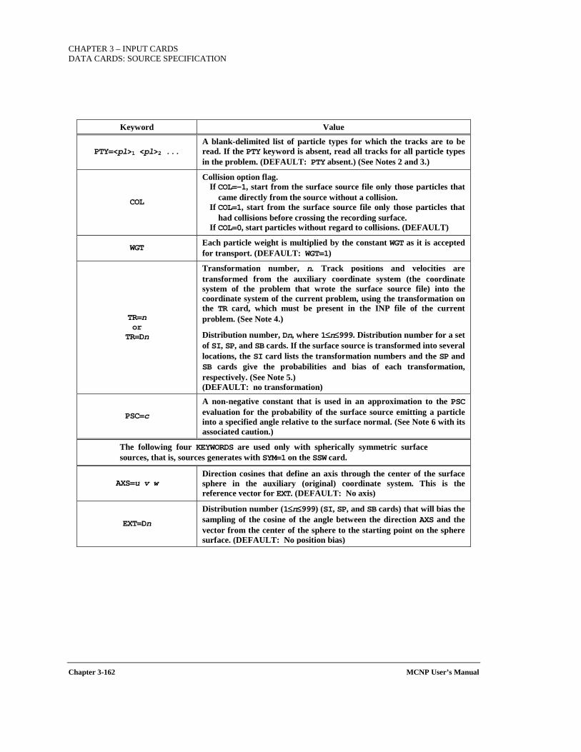
CHAPTER 3 – INPUT CARDS DATA CARDS: SOURCE SPECIFICATION
Chapter 3-162 MCNP User’s Manual
Keyword Value
PTY=<pl>1 <pl>2 ... A blank-delimited list of particle types for which the tracks are to be read. If the PTY keyword is absent, read all tracks for all particle types in the problem. (DEFAULT: PTY absent.) (See Notes 2 and 3.)
COL
Collision option flag. If COL=-1, start from the surface source file only those particles that
came directly from the source without a collision. If COL=1, start from the surface source file only those particles that
had collisions before crossing the recording surface. If COL=0, start particles without regard to collisions. (DEFAULT)
WGT Each particle weight is multiplied by the constant WGT as it is accepted for transport. (DEFAULT: WGT=1)
TR=n or
TR=Dn
Transformation number, n. Track positions and velocities are transformed from the auxiliary coordinate system (the coordinate system of the problem that wrote the surface source file) into the coordinate system of the current problem, using the transformation on the TR card, which must be present in the INP file of the current problem. (See Note 4.)
Distribution number, Dn, where 1≤n≤999. Distribution number for a set of SI, SP, and SB cards. If the surface source is transformed into several locations, the SI card lists the transformation numbers and the SP and SB cards give the probabilities and bias of each transformation, respectively. (See Note 5.) (DEFAULT: no transformation)
PSC=c
A non-negative constant that is used in an approximation to the PSC evaluation for the probability of the surface source emitting a particle into a specified angle relative to the surface normal. (See Note 6 with its associated caution.)
The following four KEYWORDS are used only with spherically symmetric surface sources, that is, sources generates with SYM=1 on the SSW card.
AXS=u v w Direction cosines that define an axis through the center of the surface sphere in the auxiliary (original) coordinate system. This is the reference vector for EXT. (DEFAULT: No axis)
EXT=Dn
Distribution number (1≤n≤999) (SI, SP, and SB cards) that will bias the sampling of the cosine of the angle between the direction AXS and the vector from the center of the sphere to the starting point on the sphere surface. (DEFAULT: No position bias)
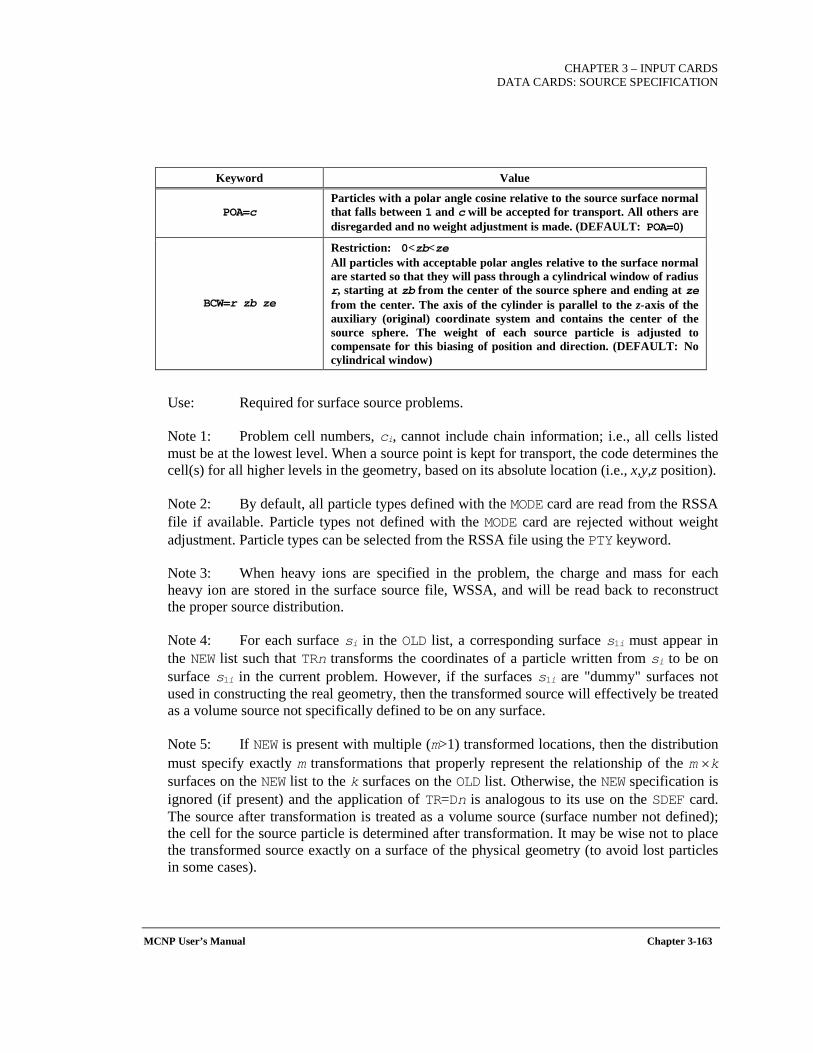
CHAPTER 3 – INPUT CARDS
DATA CARDS: SOURCE SPECIFICATION
MCNP User’s Manual Chapter 3-163
Keyword Value
POA=c Particles with a polar angle cosine relative to the source surface normal that falls between 1 and c will be accepted for transport. All others are disregarded and no weight adjustment is made. (DEFAULT: POA=0)
BCW=r zb ze
Restriction: 0<zb<ze All particles with acceptable polar angles relative to the surface normal are started so that they will pass through a cylindrical window of radius r, starting at zb from the center of the source sphere and ending at ze from the center. The axis of the cylinder is parallel to the z-axis of the auxiliary (original) coordinate system and contains the center of the source sphere. The weight of each source particle is adjusted to compensate for this biasing of position and direction. (DEFAULT: No cylindrical window)
Use: Required for surface source problems.
Note 1: Problem cell numbers, ci, cannot include chain information; i.e., all cells listed must be at the lowest level. When a source point is kept for transport, the code determines the cell(s) for all higher levels in the geometry, based on its absolute location (i.e., x,y,z position).
Note 2: By default, all particle types defined with the MODE card are read from the RSSA file if available. Particle types not defined with the MODE card are rejected without weight adjustment. Particle types can be selected from the RSSA file using the PTY keyword.
Note 3: When heavy ions are specified in the problem, the charge and mass for each heavy ion are stored in the surface source file, WSSA, and will be read back to reconstruct the proper source distribution.
Note 4: For each surface si in the OLD list, a corresponding surface s1i must appear in the NEW list such that TRn transforms the coordinates of a particle written from si to be on surface s1i in the current problem. However, if the surfaces s1i are "dummy" surfaces not used in constructing the real geometry, then the transformed source will effectively be treated as a volume source not specifically defined to be on any surface.
Note 5: If NEW is present with multiple (m>1) transformed locations, then the distribution must specify exactly m transformations that properly represent the relationship of the m ×k surfaces on the NEW list to the k surfaces on the OLD list. Otherwise, the NEW specification is ignored (if present) and the application of TR=Dn is analogous to its use on the SDEF card. The source after transformation is treated as a volume source (surface number not defined); the cell for the source particle is determined after transformation. It may be wise not to place the transformed source exactly on a surface of the physical geometry (to avoid lost particles in some cases).
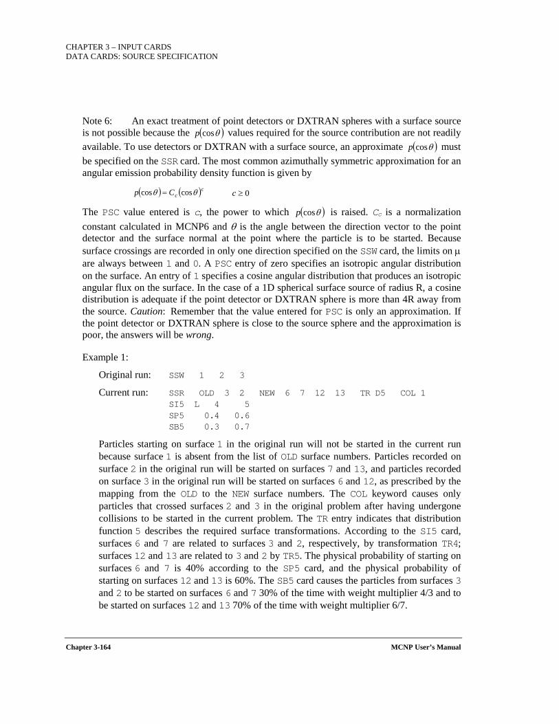
CHAPTER 3 – INPUT CARDS DATA CARDS: SOURCE SPECIFICATION
Chapter 3-164 MCNP User’s Manual
Note 6: An exact treatment of point detectors or DXTRAN spheres with a surface source is not possible because the values required for the source contribution are not readily available. To use detectors or DXTRAN with a surface source, an approximate must be specified on the SSR card. The most common azimuthally symmetric approximation for an angular emission probability density function is given by
The PSC value entered is c, the power to which is raised. Cc is a normalization constant calculated in MCNP6 and θ is the angle between the direction vector to the point detector and the surface normal at the point where the particle is to be started. Because surface crossings are recorded in only one direction specified on the SSW card, the limits on µ are always between 1 and 0. A PSC entry of zero specifies an isotropic angular distribution on the surface. An entry of 1 specifies a cosine angular distribution that produces an isotropic angular flux on the surface. In the case of a 1D spherical surface source of radius R, a cosine distribution is adequate if the point detector or DXTRAN sphere is more than 4R away from the source. Caution: Remember that the value entered for PSC is only an approximation. If the point detector or DXTRAN sphere is close to the source sphere and the approximation is poor, the answers will be wrong.
Example 1:
Original run: SSW 1 2 3
Current run: SSR OLD 3 2 NEW 6 7 12 13 TR D5 COL 1 SI5 L 4 5 SP5 0.4 0.6 SB5 0.3 0.7
Particles starting on surface 1 in the original run will not be started in the current run because surface 1 is absent from the list of OLD surface numbers. Particles recorded on surface 2 in the original run will be started on surfaces 7 and 13, and particles recorded on surface 3 in the original run will be started on surfaces 6 and 12, as prescribed by the mapping from the OLD to the NEW surface numbers. The COL keyword causes only particles that crossed surfaces 2 and 3 in the original problem after having undergone collisions to be started in the current problem. The TR entry indicates that distribution function 5 describes the required surface transformations. According to the SI5 card, surfaces 6 and 7 are related to surfaces 3 and 2, respectively, by transformation TR4; surfaces 12 and 13 are related to 3 and 2 by TR5. The physical probability of starting on surfaces 6 and 7 is 40% according to the SP5 card, and the physical probability of starting on surfaces 12 and 13 is 60%. The SB5 card causes the particles from surfaces 3 and 2 to be started on surfaces 6 and 7 30% of the time with weight multiplier 4/3 and to be started on surfaces 12 and 13 70% of the time with weight multiplier 6/7.
( )θcosp( )θcosp
( ) ( )ccCp θθ coscos = 0≥c
( )θcosp
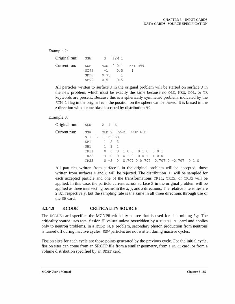
CHAPTER 3 – INPUT CARDS
DATA CARDS: SOURCE SPECIFICATION
MCNP User’s Manual Chapter 3-165
Example 2:
Original run: SSW 3 SYM 1
Current run: SSR AXS 0 0 1 EXT D99 SI99 -1 0.5 1 SP99 0.75 1 SB99 0.5 0.5
All particles written to surface 3 in the original problem will be started on surface 3 in the new problem, which must be exactly the same because no OLD, NEW, COL, or TR keywords are present. Because this is a spherically symmetric problem, indicated by the SYM 1 flag in the original run, the position on the sphere can be biased. It is biased in the z direction with a cone bias described by distribution 99.
Example 3:
Original run: SSW 2 4 6
Current run: SSR OLD 2 TR=D1 WGT 6.0 SI1 L 11 22 33 SP1 1 2 3 SB1 1 1 1 TR11 0 0 −3 1 0 0 0 1 0 0 0 1 TR22 −3 0 0 0 1 0 0 0 1 1 0 0 TR33 0 −3 0 0.707 0 0.707 0.707 0 −0.707 0 1 0
All particles written from surface 2 in the original problem will be accepted; those written from surfaces 4 and 6 will be rejected. The distribution D1 will be sampled for each accepted particle and one of the transformations TR11, TR22, or TR33 will be applied. In this case, the particle current across surface 2 in the original problem will be applied as three intersecting beams in the x, y, and z directions. The relative intensities are 2:3:1 respectively, but the sampling rate is the same in all three directions through use of the SB card.
3.3.4.9 KCODE CRITICALITY SOURCE
The KCODE card specifies the MCNP6 criticality source that is used for determining keff. The criticality source uses total fission values unless overridden by a TOTNU NO card and applies only to neutron problems. In a MODE N,P problem, secondary photon production from neutrons is turned off during inactive cycles. SSW particles are not written during inactive cycles.
Fission sites for each cycle are those points generated by the previous cycle. For the initial cycle, fission sites can come from an SRCTP file from a similar geometry, from a KSRC card, or from a volume distribution specified by an SDEF card.
ν

CHAPTER 3 – INPUT CARDS DATA CARDS: SOURCE SPECIFICATION
Chapter 3-166 MCNP User’s Manual
Since the mid-2000s, there have been many detailed studies on the theory and practice of performing Monte Carlo criticality calculations. These studies have resulted in a set of “best practices” for performing KCODE calculations with MCNP, and are fully described in a section of the MCNP Reference Collection on the MCNP website, “Best Practices - Convergence, Bias, Statistics.” To summarize:
Convergence of the fission source shape should be assessed with plots of the Shannon entropy vs. cycle. To avoid bias from the renormalization of the fission source each cycle, it is very strongly recommended that at least 10,000 neutrons/cycle should be specified on the KCODE card, with even larger numbers for large reactor problems. The initial guess for the source distribution (via KSRC, srctp, or SDEF) should be a reasonable representation covering the fissionable regions of a problem.
Form: KCODE nsrck rkk ikz kct msrk knrm mrkp kc8
Table 3-69 Criticality Source Card (KCODE)
Input Parameter Description
nsrck Number of source histories per cycle. (DEFAULT: nsrck=1000)
rkk Initial guess for keff. (See Note 1.) (DEFAULT: rkk=1.0)
ikz Number of cycles to be skipped before beginning tally accumulation. (DEFAULT: ikz=30)
kct Total number of cycles to be done. If kct=0, never terminate on the number of cycles, but terminate on time. (DEFAULT: kct=ikz+100)
msrk Number of source points for which to allocate storage. (See Note 2.) (DEFAULT: msrk=maximum of 4500 or 2 × nsrck)
knrm Controls normalization of tallies.
If knrm=0, normalize tallies by weight. (DEFAULT) If knrm=1, normalize tallies by number of histories.
mrkp Maximum number of cycle values on MCTAL or RUNTPE files. (DEFAULT: mrkp=6500)
kc8
Controls the number of cycles over which summary and tally information are averaged.
If kc8=0, average over all cycles. (See Note 3.) If kc8=1, average over active cycles only. (DEFAULT)
Defaults: See Table 3-69.
Use: Required for criticality calculations.
Note 1: If in the first cycle the source being generated overruns the current source, the initial guess (rkk) is probably too low. The code then proceeds to print a comment, continues without writing a new source, calculates , reads the initial source back in, and begins the effk ′
CHAPTER 3 – INPUT CARDS
DATA CARDS: SOURCE SPECIFICATION
MCNP User’s Manual Chapter 3-167
problem using instead of rkk. If the generated source again overruns the current source after the first cycle, the job terminates and either a better initial guess (rkk) or more source space (msrk) should be specified on the next try.
Note 2: If an SRCTP file with a larger value of msrk is read for the initial source, the larger value is used.
Note 3: Setting the parameter kc8 to zero causes tallies and summary table information to be for both active and inactive cycles and should not be used. Setting kc8=0 also results in strange MCTAL file normalization.
3.3.4.10 KSRC CRITICALITY SOURCE POINTS
This card contains up to nsrck (x,y,z) triplets that are locations of initial source points for a KCODE calculation. At least one point must be in a cell containing fissile material and points must be away from cell boundaries. It is not necessary to input all nsrck coordinate points. MCNP6 will start approximately (nsrck/number of points) particles at each point. Usually one point in each fissile region is adequate, because MCNP6 will quickly calculate and use the new fission source distribution. The energy of each particle in the initial source is sampled from a Watt fission spectrum hardwired into MCNP6, with =0.965 MeV, =2.29 MeV-1.
An SRCTP file from a previous criticality calculation can be used instead of a KSRC card. If the current problem has a lot in common with the previous problem, using the SRCTP file may save some computer time. Even if the problems are quite different, the SRCTP file may still be usable if some of the points in the SRCTP file are in cells containing fissile material in the current problem. Points in void or zero importance cells will be deleted. The number of particles actually started at each point will be such as to produce approximately nsrck initial source particles.
An SDEF card also can be used to sample initial source points in fissile material regions. The SDEF card parameters applicable to volume sampling can be used: CEL, POS, RAD, EXT, AXS, X, Y, Z; and CCC, ERG, and EFF. If a uniform volume distribution is chosen, the early values of keff will likely be low because too many particles are put near where they can escape, just the opposite of the usual situation with the KSRC card. Do not change the default value of WGT for a KCODE calculation.
Form: KSRC x1 y1 z1 x2 y2 z2 ...
where xi, yi, and zi are the locations of the initial source points.
Default: None. If this card is absent, an SRCTP source file or SDEF card must be supplied to provide initial source points for a criticality calculation.
Use: Optional card for use with criticality calculations.
effk ′
a b
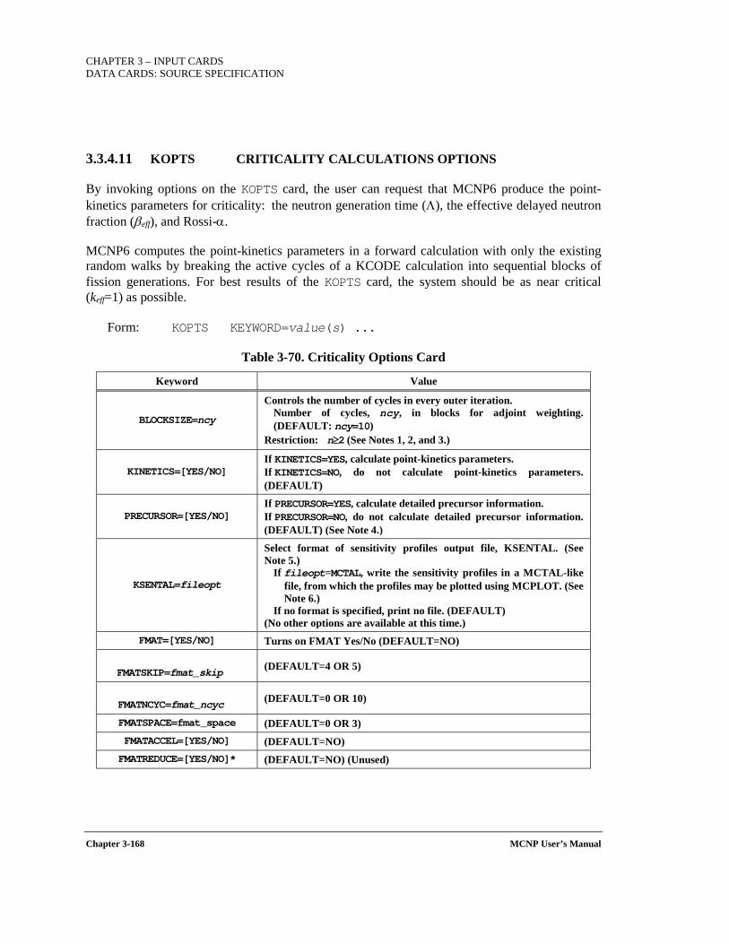
CHAPTER 3 – INPUT CARDS DATA CARDS: SOURCE SPECIFICATION
Chapter 3-168 MCNP User’s Manual
3.3.4.11 KOPTS CRITICALITY CALCULATIONS OPTIONS
By invoking options on the KOPTS card, the user can request that MCNP6 produce the point-kinetics parameters for criticality: the neutron generation time (Λ), the effective delayed neutron fraction (βeff), and Rossi-α.
MCNP6 computes the point-kinetics parameters in a forward calculation with only the existing random walks by breaking the active cycles of a KCODE calculation into sequential blocks of fission generations. For best results of the KOPTS card, the system should be as near critical (keff=1) as possible.
Form: KOPTS KEYWORD=value(s) ...
Table 3-70. Criticality Options Card
Keyword Value
BLOCKSIZE=ncy
Controls the number of cycles in every outer iteration. Number of cycles, ncy, in blocks for adjoint weighting. (DEFAULT: ncy=10)
Restriction: n≥2 (See Notes 1, 2, and 3.)
KINETICS=[YES/NO] If KINETICS=YES, calculate point-kinetics parameters. If KINETICS=NO, do not calculate point-kinetics parameters. (DEFAULT)
PRECURSOR=[YES/NO] If PRECURSOR=YES, calculate detailed precursor information. If PRECURSOR=NO, do not calculate detailed precursor information. (DEFAULT) (See Note 4.)
KSENTAL=fileopt
Select format of sensitivity profiles output file, KSENTAL. (See Note 5.)
If fileopt=MCTAL, write the sensitivity profiles in a MCTAL-like file, from which the profiles may be plotted using MCPLOT. (See Note 6.)
If no format is specified, print no file. (DEFAULT) (No other options are available at this time.)
FMAT=[YES/NO] Turns on FMAT Yes/No (DEFAULT=NO)
FMATSKIP=fmat_skip (DEFAULT=4 OR 5)
FMATNCYC=fmat_ncyc (DEFAULT=0 OR 10)
FMATSPACE=fmat_space (DEFAULT=0 OR 3) FMATACCEL=[YES/NO] (DEFAULT=NO) FMATREDUCE=[YES/NO]* (DEFAULT=NO) (Unused)

CHAPTER 3 – INPUT CARDS
DATA CARDS: SOURCE SPECIFICATION
MCNP User’s Manual Chapter 3-169
Keyword Value
FMATNX=fmat_nx (DEFAULT=0)
FMATNY=fmat_ny (DEFAULT=0)
FMATNZ=fmat_nz (DEFAULT=0)
Note 1: Specification of BLOCKSIZE without setting KINETICS=YES is allowed, but MCNP6 will try to do adjoint weighting without tallying anything.
Note 2: The default block size of 10 cycles produces results with sufficient accuracy for most problems of interest. Using fewer cycles per block introduces greater bias from truncation, but provides a more statistically efficient calculation. Larger blocks are more accurate, but the accuracy gained for larger block sizes is often small relative to the increased computer time required to preserve the statistical precision. Users are encouraged to check whether the selected block size is sufficient for their application by running a larger block size and comparing the results. For small, leakage-dominated systems, the block size can often be reduced to 5.
Note 3: Because sensitivity coefficients (see the KSEN card, Section 3.3.5.23) are adjoint weighted, they theoretically require infinitely many cycles before a tally may be performed. In practice, the default BLOCKSIZE value of 10 generations is usually more than sufficient to get accurate results.
Note 4: If PRECURSOR=YES, then KINETICS must be set to YES.
Note 5: The KSENTAL keyword requires there be at least one KSEN card (see Section 3.3.5.23) specified in the MCNP6 input file.
Note 6: The MCTAL format of the sensitivity profiles is much like the standard MCTAL file except that the symbols for bins have different meanings: F=cells (with 0 denoting all cells); D=unused; U=unused; S=isotopes; M=reaction numbers; C=cosine bins; E=energy bins; and T=incident energy bins (for fission chi or scattering laws). The tally plotter, MCPLOT, may be loaded to plot these results. The results should be normalized to be per unit lethargy with the "LETHARGY" option and plotted on a semi log-x scale for visually accurate area plots.
Example 1: KOPTS BLOCKSIZE=15 KINETICS=YES PRECURSOR=YES
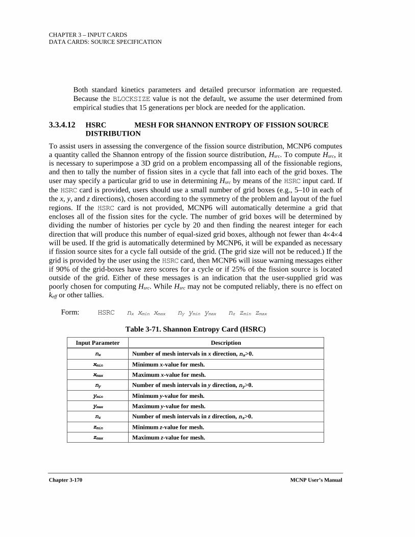
CHAPTER 3 – INPUT CARDS DATA CARDS: SOURCE SPECIFICATION
Chapter 3-170 MCNP User’s Manual
Both standard kinetics parameters and detailed precursor information are requested. Because the BLOCKSIZE value is not the default, we assume the user determined from empirical studies that 15 generations per block are needed for the application.
3.3.4.12 HSRC MESH FOR SHANNON ENTROPY OF FISSION SOURCE DISTRIBUTION
To assist users in assessing the convergence of the fission source distribution, MCNP6 computes a quantity called the Shannon entropy of the fission source distribution, Hsrc. To compute Hsrc, it is necessary to superimpose a 3D grid on a problem encompassing all of the fissionable regions, and then to tally the number of fission sites in a cycle that fall into each of the grid boxes. The user may specify a particular grid to use in determining Hsrc by means of the HSRC input card. If the HSRC card is provided, users should use a small number of grid boxes (e.g., 5–10 in each of the x, y, and z directions), chosen according to the symmetry of the problem and layout of the fuel regions. If the HSRC card is not provided, MCNP6 will automatically determine a grid that encloses all of the fission sites for the cycle. The number of grid boxes will be determined by dividing the number of histories per cycle by 20 and then finding the nearest integer for each direction that will produce this number of equal-sized grid boxes, although not fewer than 4×4×4 will be used. If the grid is automatically determined by MCNP6, it will be expanded as necessary if fission source sites for a cycle fall outside of the grid. (The grid size will not be reduced.) If the grid is provided by the user using the HSRC card, then MCNP6 will issue warning messages either if 90% of the grid-boxes have zero scores for a cycle or if 25% of the fission source is located outside of the grid. Either of these messages is an indication that the user-supplied grid was poorly chosen for computing Hsrc. While Hsrc may not be computed reliably, there is no effect on keff or other tallies.
Form: HSRC nx xmin xmax ny ymin ymax nz zmin zmax
Table 3-71. Shannon Entropy Card (HSRC)
Input Parameter Description
nx Number of mesh intervals in x direction, nx>0.
xmin Minimum x-value for mesh. xmax Maximum x-value for mesh. ny Number of mesh intervals in y direction, ny>0.
ymin Minimum y-value for mesh. ymax Maximum y-value for mesh. nz Number of mesh intervals in z direction, nz>0.
zmin Minimum z-value for mesh. zmax Maximum z-value for mesh.
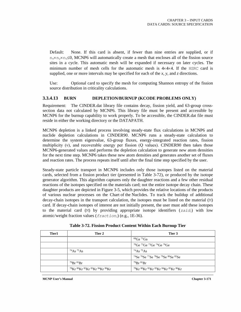
CHAPTER 3 – INPUT CARDS
DATA CARDS: SOURCE SPECIFICATION
MCNP User’s Manual Chapter 3-171
Default: None. If this card is absent, if fewer than nine entries are supplied, or if nx×ny×nz≤0, MCNP6 will automatically create a mesh that encloses all of the fission source sites in a cycle. This automatic mesh will be expanded if necessary on later cycles. The minimum number of mesh cells for the automatic mesh is 4×4×4. If the HSRC card is supplied, one or more intervals may be specified for each of the x, y, and z directions.
Use: Optional card to specify the mesh for computing Shannon entropy of the fission source distribution in criticality calculations.
3.3.4.13 BURN DEPLETION/BURNUP (KCODE PROBLEMS ONLY)
Requirement: The CINDER.dat library file contains decay, fission yield, and 63-group cross-section data not calculated by MCNP6. This library file must be present and accessible by MCNP6 for the burnup capability to work properly. To be accessible, the CINDER.dat file must reside in either the working directory or the DATAPATH.
MCNP6 depletion is a linked process involving steady-state flux calculations in MCNP6 and nuclide depletion calculations in CINDER90. MCNP6 runs a steady-state calculation to determine the system eigenvalue, 63-group fluxes, energy-integrated reaction rates, fission multiplicity (ν), and recoverable energy per fission (Q values). CINDER90 then takes those MCNP6-generated values and performs the depletion calculation to generate new atom densities for the next time step. MCNP6 takes these new atom densities and generates another set of fluxes and reaction rates. The process repeats itself until after the final time step specified by the user.
Steady-state particle transport in MCNP6 includes only those isotopes listed on the material cards, selected from a fission product tier (presented in Table 3-72), or produced by the isotope generator algorithm. This algorithm captures only the daughter reactions and a few other residual reactions of the isotopes specified on the materials card; not the entire isotope decay chain. These daughter products are depicted in Figure 3-5, which provides the relative locations of the products of various nuclear processes on the Chart of the Nuclides. To track the buildup of additional decay-chain isotopes in the transport calculation, the isotopes must be listed on the material (M) card. If decay-chain isotopes of interest are not initially present, the user must add these isotopes to the material card (M) by providing appropriate isotope identifiers (zaidi) with low atomic/weight fraction values (fractioni) (e.g., 1E-36).
Table 3-72. Fission Product Content Within Each Burnup Tier
Tier1 Tier 2 Tier 3 69Ga 71Ga
70Ge 72Ge 73Ge 74Ge 76Ge
74As 75As 74As 75As
74Se 76Se 77Se 78Se 79Se 80Se 82Se
79Br 81Br 79Br 81Br
78Kr 80Kr 82Kr 83Kr 84Kr 86Kr 78Kr 80Kr 82Kr 83Kr 84Kr 85Kr 86Kr
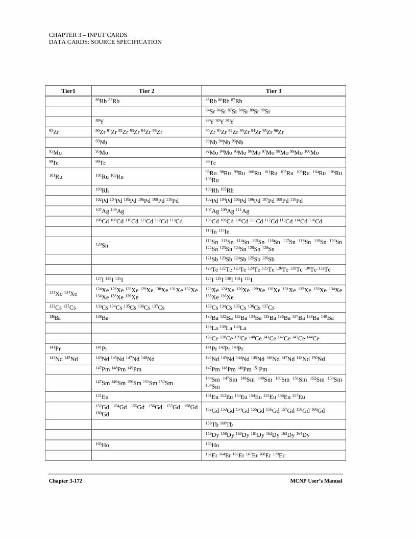
CHAPTER 3 – INPUT CARDS DATA CARDS: SOURCE SPECIFICATION
Chapter 3-172 MCNP User’s Manual
Tier1 Tier 2 Tier 3 85Rb 87Rb 85Rb 86Rb 87Rb
84Sr 86Sr 87Sr 88Sr 89Sr 90Sr
89Y 89Y 90Y 91Y 93Zr 90Zr 91Zr 92Zr 93Zr 94Zr 96Zr 90Zr 91Zr 92Zr 93Zr 94Zr 95Zr 96Zr
93Nb 93Nb 94Nb 95Nb 95Mo 95Mo 92Mo 94Mo 95Mo 96Mo 97Mo 98Mo 99Mo 100Mo 99Tc 99Tc 99Tc
101Ru 101Ru 103Ru 96Ru 98Ru 99Ru 100Ru 101Ru 102Ru 103Ru 104Ru 105Ru 106Ru
103Rh 103Rh 105Rh
102Pd 104Pd 105Pd 106Pd 108Pd 110Pd 102Pd 104Pd 105Pd 106Pd 107Pd 108Pd 110Pd
107Ag 109Ag 107Ag 109Ag 111Ag
106Cd 108Cd 110Cd 111Cd 112Cd 113Cd 106Cd 108Cd 110Cd 111Cd 112Cd 113Cd 114Cd 116Cd
113In 115In
120Sn 112Sn 113Sn 114Sn 115Sn 116Sn 117Sn 118Sn 119Sn 120Sn 122Sn 123Sn 124Sn 125Sn 126Sn
121Sb 123Sb 124Sb 125Sb 126Sb
120Te 122Te 123Te 124Te 125Te 126Te 128Te 130Te 132Te
127I 129I 135I 127I 129I 130I 131I 135I
131Xe 134Xe 124Xe 126Xe 128Xe 129Xe 130Xe 131Xe 132Xe 134Xe 135Xe 136Xe
123Xe 124Xe 126Xe 129Xe 130Xe 131Xe 132Xe 133Xe 134Xe 135Xe 136Xe
133Cs 137Cs 133Cs 134Cs 135Cs 136Cs 137Cs 133Cs 134Cs 135Cs 136Cs 137Cs 138Ba 138Ba 130Ba 132Ba 133Ba 134Ba 135Ba 136Ba 137Ba 138Ba 140Ba
138La 139La 140La
136Ce 138Ce 139Ce 140Ce 141Ce 142Ce 143Ce 144Ce 141Pr 141Pr 141Pr 142Pr 143Pr 143Nd 145Nd 143Nd 145Nd 147Nd 148Nd 142Nd 143Nd 144Nd 145Nd 146Nd 147Nd 148Nd 150Nd
147Pm 148Pm 149Pm 147Pm 148Pm 149Pm 151Pm
147Sm 149Sm 150Sm 151Sm 152Sm 144Sm 147Sm 148Sm 149Sm 150Sm 151Sm 152Sm 153Sm 154Sm
151Eu 151Eu 152Eu 153Eu 154Eu 155Eu 156Eu 157Eu
152Gd 154Gd 155Gd 156Gd 157Gd 158Gd 160Gd
152Gd 153Gd 154Gd 155Gd 156Gd 157Gd 158Gd 160Gd
159Tb 160Tb
156Dy 158Dy 160Dy 161Dy 162Dy 163Dy 164Dy
165Ho 165Ho
162Er 164Er 166Er 167Er 168Er 170Er
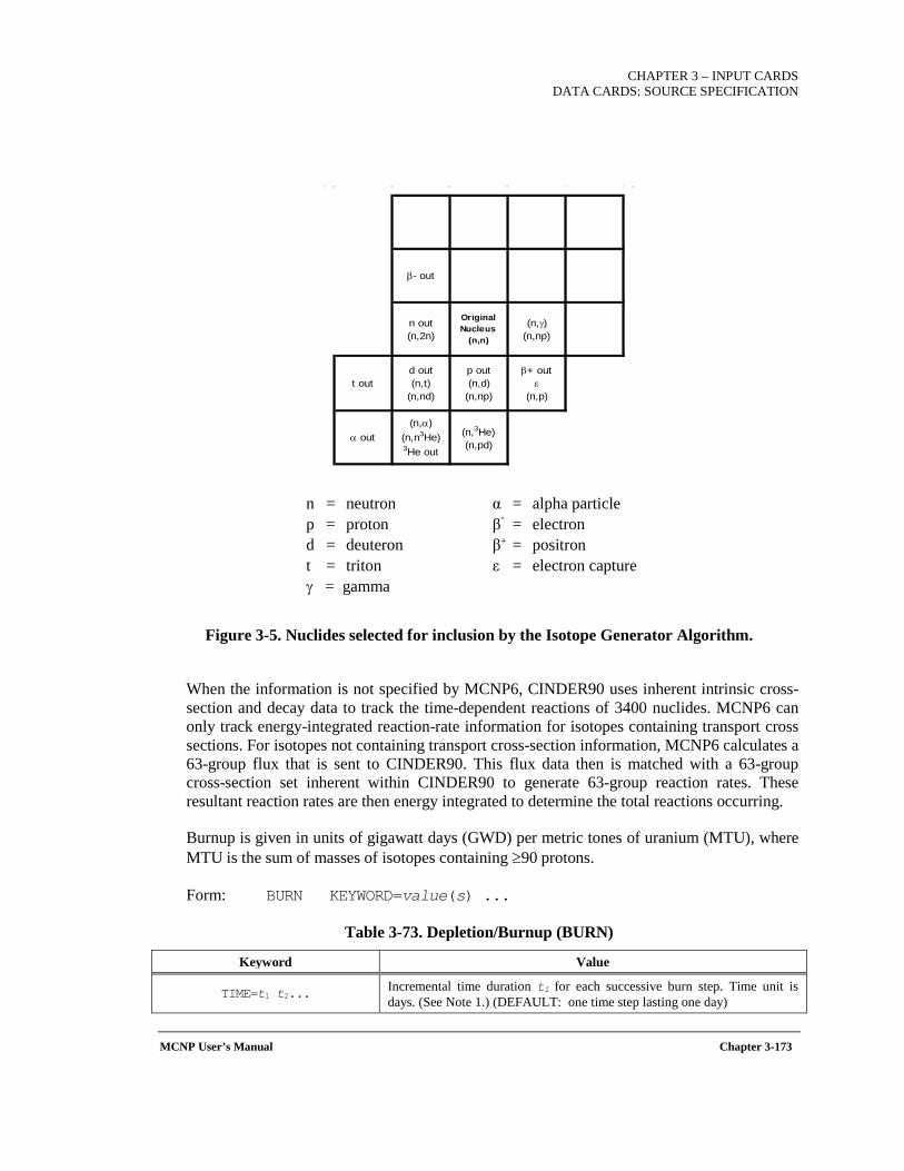
CHAPTER 3 – INPUT CARDS
DATA CARDS: SOURCE SPECIFICATION
MCNP User’s Manual Chapter 3-173
n = neutron α = alpha particle p = proton β- = electron d = deuteron β+ = positron t = triton ε = electron capture γ = gamma
Figure 3-5. Nuclides selected for inclusion by the Isotope Generator Algorithm.
When the information is not specified by MCNP6, CINDER90 uses inherent intrinsic cross-section and decay data to track the time-dependent reactions of 3400 nuclides. MCNP6 can only track energy-integrated reaction-rate information for isotopes containing transport cross sections. For isotopes not containing transport cross-section information, MCNP6 calculates a 63-group flux that is sent to CINDER90. This flux data then is matched with a 63-group cross-section set inherent within CINDER90 to generate 63-group reaction rates. These resultant reaction rates are then energy integrated to determine the total reactions occurring.
Burnup is given in units of gigawatt days (GWD) per metric tones of uranium (MTU), where MTU is the sum of masses of isotopes containing ≥90 protons.
Form: BURN KEYWORD=value(s) ...
Table 3-73. Depletion/Burnup (BURN)
Keyword Value
TIME=t1 t2... Incremental time duration ti for each successive burn step. Time unit is days. (See Note 1.) (DEFAULT: one time step lasting one day)
β- out
n out (n,2n)
Original Nucleus
(n,n)
(n,γ) (n,np)
t outd out (n,t)
(n,nd)
p out (n,d)
(n,np)
β+ out ε
(n,p)
α out(n,α)
(n,n3He) 3He out
(n,3He) (n,pd)
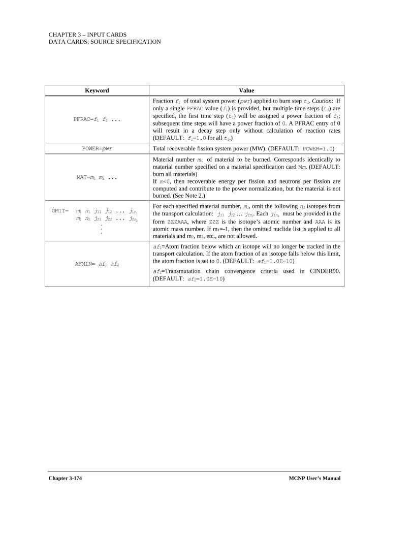
CHAPTER 3 – INPUT CARDS DATA CARDS: SOURCE SPECIFICATION
Chapter 3-174 MCNP User’s Manual
Keyword Value
PFRAC=f1 f2 ...
Fraction fi of total system power (pwr) applied to burn step ti. Caution: If only a single PFRAC value (f1) is provided, but multiple time steps (ti) are specified, the first time step (t1) will be assigned a power fraction of f1; subsequent time steps will have a power fraction of 0. A PFRAC entry of 0 will result in a decay step only without calculation of reaction rates (DEFAULT: fi=1.0 for all ti.)
POWER=pwr Total recoverable fission system power (MW). (DEFAULT: POWER=1.0)
MAT=m1 m2 ...
Material number mi of material to be burned. Corresponds identically to material number specified on a material specification card Mm. (DEFAULT: burn all materials) If m<0, then recoverable energy per fission and neutrons per fission are computed and contribute to the power normalization, but the material is not burned. (See Note 2.)
OMIT= m1 n1 j11 j12 ... j1n1 m2 n2 j21 j22 ... j2n2
.
.
.
For each specified material number, mi, omit the following ni isotopes from the transport calculation: ji1 ji2 … jini. Each jink must be provided in the form ZZZAAA, where ZZZ is the isotope’s atomic number and AAA is its atomic mass number. If m1=-1, then the omitted nuclide list is applied to all materials and m2, m3, etc., are not allowed.
AFMIN= af1 af2
af1=Atom fraction below which an isotope will no longer be tracked in the transport calculation. If the atom fraction of an isotope falls below this limit, the atom fraction is set to 0. (DEFAULT: af1=1.0E-10)
af2=Transmutation chain convergence criteria used in CINDER90. (DEFAULT: af2=1.0E-10)
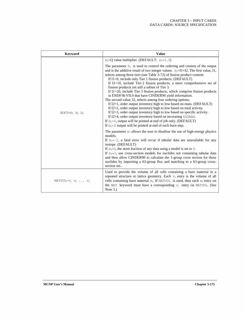
CHAPTER 3 – INPUT CARDS
DATA CARDS: SOURCE SPECIFICATION
MCNP User’s Manual Chapter 3-175
Keyword Value
BOPT=b1 b2 b3
b1=Q value multiplier. (DEFAULT: b1=1.0)
The parameter b2 is used to control the ordering and content of the output and is the additive result of two integer values: b2=I1+I2. The first value, I1, selects among three tiers (see Table 3-72) of fission product content:
If I1=0, include only Tier 1 fission products. (DEFAULT) If I1=10, include Tier 2 fission products, a more comprehensive set of fission products yet still a subset of Tier 3. If I1=20, include Tier 3 fission products, which comprise fission products in ENDF/B-VII.0 that have CINDER90 yield information.
The second value, I2, selects among four ordering options: If I2=1, order output inventory high to low based on mass. (DEFAULT) If I2=2, order output inventory high to low based on total activity. If I2=3, order output inventory high to low based on specific activity. If I2=4, order output inventory based on increasing ZZZAAA.
If b2>0, output will be printed at end of job only. (DEFAULT) If b2<0 output will be printed at end of each burn step.
The parameter b3 allows the user to disallow the use of high-energy physics models. If b3=-1, a fatal error will occur if tabular data are unavailable for any isotope. (DEFAULT) If b3=0, the atom fraction of any data using a model is set to 0. If b3=1, use cross-section models for nuclides not containing tabular data and then allow CINDER90 to calculate the 1-group cross section for these nuclides by importing a 63-group flux and matching to a 63-group cross-section set..
MATVOL=v1 v2 ... vn
Used to provide the volume of all cells containing a burn material in a repeated structure or lattice geometry. Each vi entry is the volume of all cells containing burn material mi. If MATVOL is used, then each mi entry on the MAT keyword must have a corresponding vi entry on MATVOL. (See Note 3.)
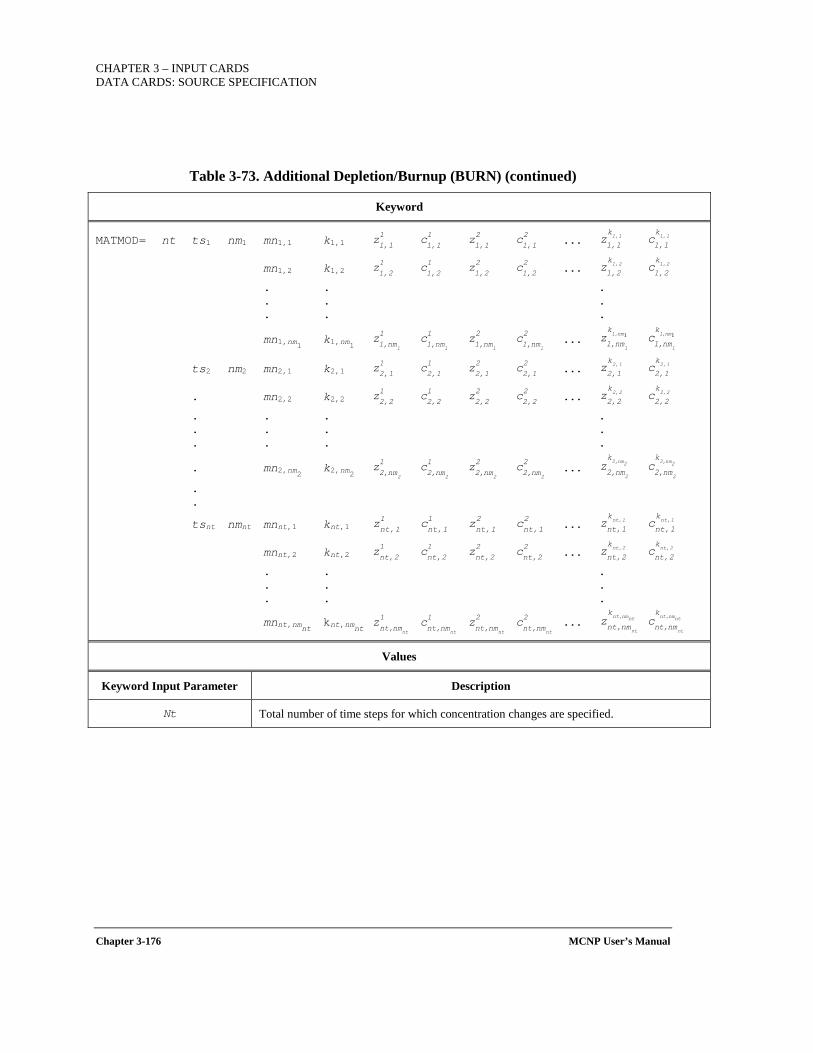
CHAPTER 3 – INPUT CARDS DATA CARDS: SOURCE SPECIFICATION
Chapter 3-176 MCNP User’s Manual
Table 3-73. Additional Depletion/Burnup (BURN) (continued)
Keyword
MATMOD= nt ts1 nm1 mn1,1 k1,1 . . .
mn1,2 k1,2 . . .
. . . . . . . . .
mn1,nm1 k1,nm1 . . .
ts2 nm2 mn2,1 k2,1 . . .
. mn2,2 k2,2 . . .
. . . . . . . . . . . .
. mn2,nm2 k2,nm2 . . .
. .
tsnt nmnt mnnt,1 knt,1 . . .
mnnt,2 knt,2 . . .
. . . . . . . . .
mnnt,nmnt knt,nmnt . . .
Values
Keyword Input Parameter Description
Nt Total number of time steps for which concentration changes are specified.
11,1z 1
1,1c 2
1,1z 2
1,1c 1,1
k
1,1z 1,1
k
1,1c
11,2z 1
1,2c 2
1,2z 2
1,2c 1,2
k
1,2z 1,2
k
1,2c
1nm1,
1
z 1nm1,
1
c 2nm1,
1
z 2nm1,
1
c 1nm1,
1
k
nm1,z 1nm1,
1
k
nm1,c
12,1z 1
2,1c 2
2,1z 2
2,1c 2,1
k
2,1z 2,1
k
2,1c
12,2z 1
2,2c 2
2,2z 2
2,2c 2,2
k
2,2z 2,2
k
2,2c
1nm2,
2
z 1nm2,
2
c 2nm2,
2
z 2nm2,
2
c 2nm2,
2
k
nm2,z 2nm2,
2
k
nm2,c
1nt,1z 1
nt,1c 2
nt,1z 2
nt,1c nt,1
k
nt,1z nt,1
k
nt,1c
1nt,2z 1
nt,2c 2
nt,2z 2
nt,2c nt,2
k
nt,2z nt,2
k
nt,2c
1nmnt,
nt
z 1nmnt,
nt
c 2nmnt,
nt
z 2nmnt,
nt
c ntnmnt,
nt
k
nmnt,z ntnmnt,
nt
k
nmnt,c
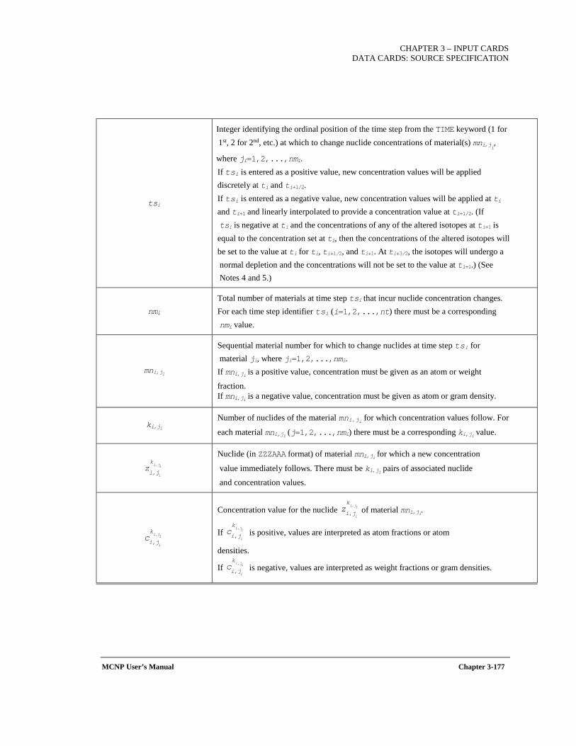
CHAPTER 3 – INPUT CARDS
DATA CARDS: SOURCE SPECIFICATION
MCNP User’s Manual Chapter 3-177
tsi
Integer identifying the ordinal position of the time step from the TIME keyword (1 for 1st, 2 for 2nd, etc.) at which to change nuclide concentrations of material(s) mni,ji,
where ji=1,2,...,nmi. If tsi is entered as a positive value, new concentration values will be applied discretely at ti and ti+1/2. If tsi is entered as a negative value, new concentration values will be applied at ti and ti+1 and linearly interpolated to provide a concentration value at ti+1/2. (If tsi is negative at ti and the concentrations of any of the altered isotopes at ti+1 is equal to the concentration set at ti, then the concentrations of the altered isotopes will be set to the value at ti for ti, ti+1/2, and ti+1. At ti+3/2, the isotopes will undergo a normal depletion and the concentrations will not be set to the value at ti+1.) (See Notes 4 and 5.)
nmi
Total number of materials at time step tsi that incur nuclide concentration changes. For each time step identifier tsi (i=1,2,...,nt) there must be a corresponding nmi value.
mni,ji
Sequential material number for which to change nuclides at time step tsi for material ji, where ji=1,2,...,nmi. If mni,ji is a positive value, concentration must be given as an atom or weight
fraction. If mni,ji is a negative value, concentration must be given as atom or gram density.
ki,ji Number of nuclides of the material mni,ji for which concentration values follow. For
each material mni,ji (j=1,2,...,nmi) there must be a corresponding ki,ji value.
Nuclide (in ZZZAAA format) of material mni,ji for which a new concentration
value immediately follows. There must be ki,ji pairs of associated nuclide
and concentration values.
Concentration value for the nuclide of material mni,ji.
If is positive, values are interpreted as atom fractions or atom
densities.
If is negative, values are interpreted as weight fractions or gram densities.
iji,
i
k
ji,z
iji,
i
k
ji,c
iji,
i
k
ji,z
iji,
i
k
ji,c
iji,
i
k
ji,c
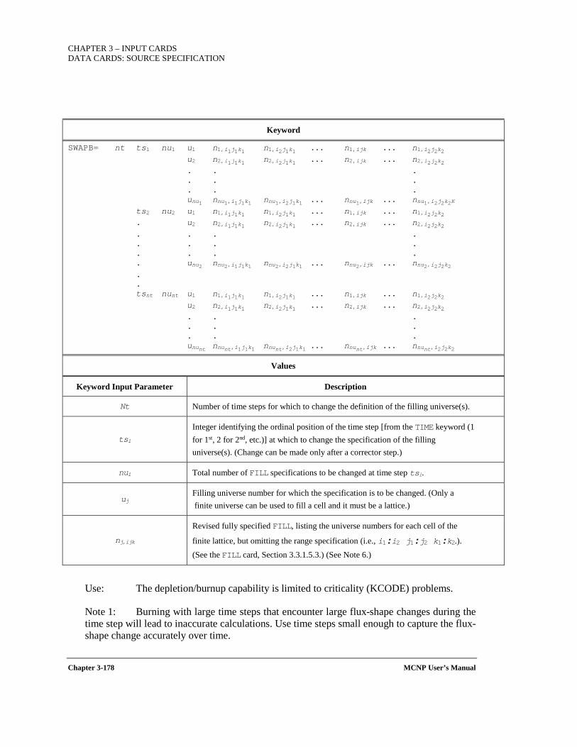
CHAPTER 3 – INPUT CARDS DATA CARDS: SOURCE SPECIFICATION
Chapter 3-178 MCNP User’s Manual
Keyword
SWAPB= nt ts1 nu1 u1 n1,i1j1k1 n1,i2j1k1 . . . n1,ijk . . . n1,i2j2k2 u2 n2,i1j1k1 n2,i2j1k1 . . . n2,ijk . . . n2,i2j2k2 . . . . . . . . . unu1 nnu1,i1j1k1 nnu1,i2j1k1 . . . nnu1,ijk . . . nnu1,i2j2k2K ts2 nu2 u1 n1,i1j1k1 n1,i2j1k1 . . . n1,ijk . . . n1,i2j2k2 . u2 n2,i1j1k1 n2,i2j1k1 . . . n2,ijk . . . n2,i2j2k2 . . . . . . . . . . . . . unu2 nnu2,i1j1k1 nnu2,i2j1k1 . . . nnu2,ijk . . . nnu2,i2j2k2 . . tsnt nunt u1 n1,i1j1k1 n1,i2j1k1 . . . n1,ijk . . . n1,i2j2k2 u2 n2,i1j1k1 n2,i2j1k1 . . . n2,ijk . . . n2,i2j2k2 . . . . . . . . . ununt nnunt,i1j1k1 nnunt,i2j1k1 . . . nnunt,ijk . . . nnunt,i2j2k2
Values
Keyword Input Parameter Description
Nt Number of time steps for which to change the definition of the filling universe(s).
tsi
Integer identifying the ordinal position of the time step [from the TIME keyword (1 for 1st, 2 for 2nd, etc.)] at which to change the specification of the filling universe(s). (Change can be made only after a corrector step.)
nui Total number of FILL specifications to be changed at time step tsi.
uj Filling universe number for which the specification is to be changed. (Only a finite universe can be used to fill a cell and it must be a lattice.)
nj,ijk
Revised fully specified FILL, listing the universe numbers for each cell of the
finite lattice, but omitting the range specification (i.e., i1:i2 j1:j2 k1:k2.). (See the FILL card, Section 3.3.1.5.3.) (See Note 6.)
Use: The depletion/burnup capability is limited to criticality (KCODE) problems.
Note 1: Burning with large time steps that encounter large flux-shape changes during the time step will lead to inaccurate calculations. Use time steps small enough to capture the flux-shape change accurately over time.
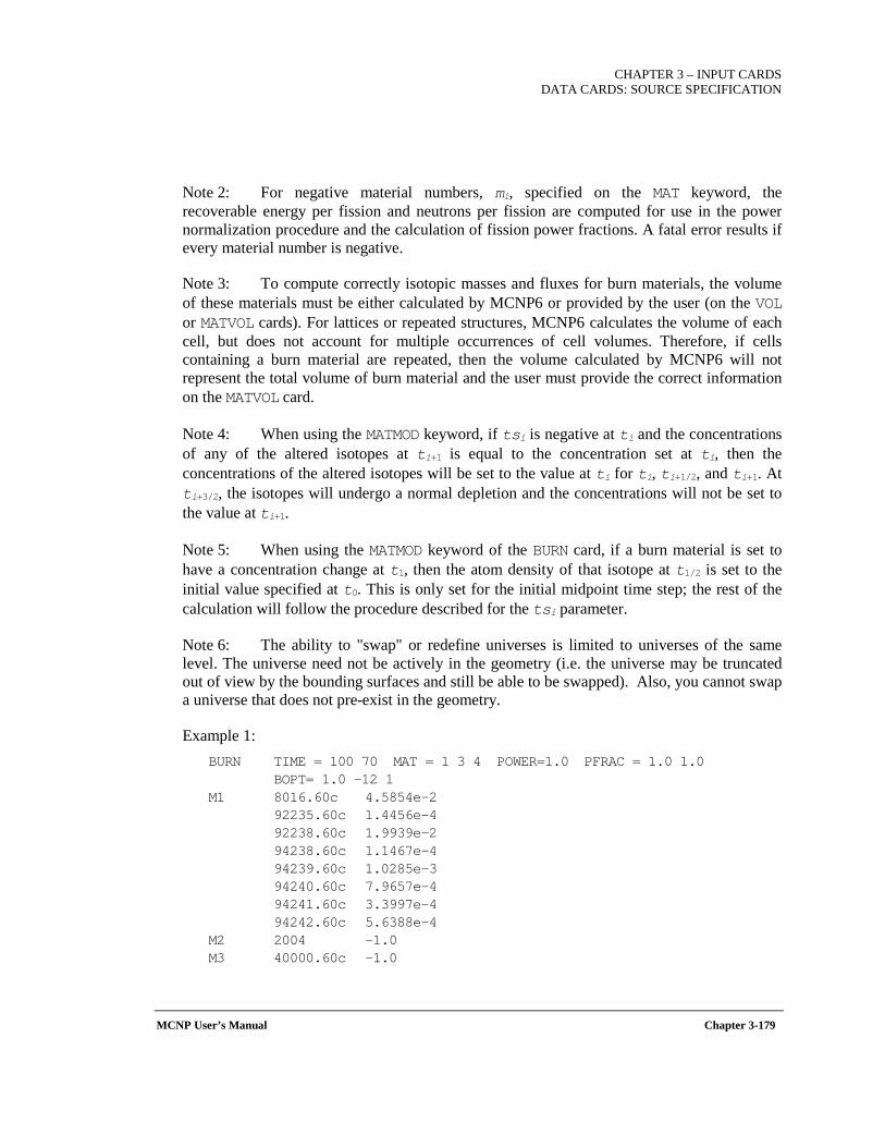
CHAPTER 3 – INPUT CARDS
DATA CARDS: SOURCE SPECIFICATION
MCNP User’s Manual Chapter 3-179
Note 2: For negative material numbers, mi, specified on the MAT keyword, the recoverable energy per fission and neutrons per fission are computed for use in the power normalization procedure and the calculation of fission power fractions. A fatal error results if every material number is negative.
Note 3: To compute correctly isotopic masses and fluxes for burn materials, the volume of these materials must be either calculated by MCNP6 or provided by the user (on the VOL or MATVOL cards). For lattices or repeated structures, MCNP6 calculates the volume of each cell, but does not account for multiple occurrences of cell volumes. Therefore, if cells containing a burn material are repeated, then the volume calculated by MCNP6 will not represent the total volume of burn material and the user must provide the correct information on the MATVOL card.
Note 4: When using the MATMOD keyword, if tsi is negative at ti and the concentrations of any of the altered isotopes at ti+1 is equal to the concentration set at ti, then the concentrations of the altered isotopes will be set to the value at ti for ti, ti+1/2, and ti+1. At ti+3/2, the isotopes will undergo a normal depletion and the concentrations will not be set to the value at ti+1.
Note 5: When using the MATMOD keyword of the BURN card, if a burn material is set to have a concentration change at t1, then the atom density of that isotope at t1/2 is set to the initial value specified at t0. This is only set for the initial midpoint time step; the rest of the calculation will follow the procedure described for the tsi parameter.
Note 6: The ability to "swap" or redefine universes is limited to universes of the same level. The universe need not be actively in the geometry (i.e. the universe may be truncated out of view by the bounding surfaces and still be able to be swapped). Also, you cannot swap a universe that does not pre-exist in the geometry.
Example 1: BURN TIME = 100 70 MAT = 1 3 4 POWER=1.0 PFRAC = 1.0 1.0 BOPT= 1.0 -12 1 M1 8016.60c 4.5854e-2 92235.60c 1.4456e-4 92238.60c 1.9939e-2 94238.60c 1.1467e-4 94239.60c 1.0285e-3 94240.60c 7.9657e-4 94241.60c 3.3997e-4 94242.60c 5.6388e-4 M2 2004 -1.0 M3 40000.60c -1.0
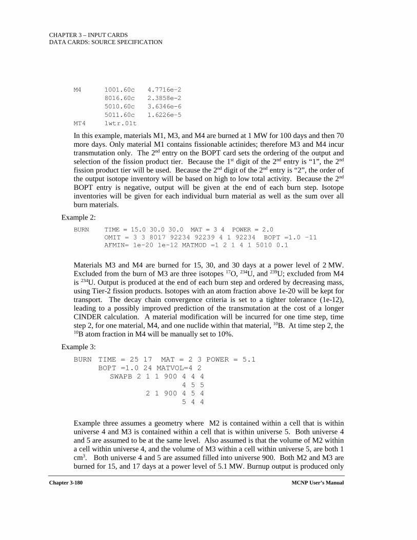
CHAPTER 3 – INPUT CARDS DATA CARDS: SOURCE SPECIFICATION
Chapter 3-180 MCNP User’s Manual
M4 1001.60c 4.7716e-2 8016.60c 2.3858e-2 5010.60c 3.6346e-6 5011.60c 1.6226e-5 MT4 lwtr.01t
In this example, materials M1, M3, and M4 are burned at 1 MW for 100 days and then 70 more days. Only material M1 contains fissionable actinides; therefore M3 and M4 incur transmutation only. The 2nd entry on the BOPT card sets the ordering of the output and selection of the fission product tier. Because the 1st digit of the 2nd entry is “1”, the 2nd fission product tier will be used. Because the 2nd digit of the 2nd entry is “2”, the order of the output isotope inventory will be based on high to low total activity. Because the 2nd BOPT entry is negative, output will be given at the end of each burn step. Isotope inventories will be given for each individual burn material as well as the sum over all burn materials.
Example 2: BURN TIME = 15.0 30.0 30.0 MAT = 3 4 POWER = 2.0 OMIT = 3 3 8017 92234 92239 4 1 92234 BOPT =1.0 -11 AFMIN= 1e-20 1e-12 MATMOD =1 2 1 4 1 5010 0.1
Materials M3 and M4 are burned for 15, 30, and 30 days at a power level of 2 MW. Excluded from the burn of M3 are three isotopes 17O, 234U, and 239U; excluded from M4 is 234U. Output is produced at the end of each burn step and ordered by decreasing mass, using Tier-2 fission products. Isotopes with an atom fraction above 1e-20 will be kept for transport. The decay chain convergence criteria is set to a tighter tolerance (1e-12), leading to a possibly improved prediction of the transmutation at the cost of a longer CINDER calculation. A material modification will be incurred for one time step, time step 2, for one material, M4, and one nuclide within that material, 10B. At time step 2, the 10B atom fraction in M4 will be manually set to 10%.
Example 3: BURN TIME = 25 17 MAT = 2 3 POWER = 5.1 BOPT =1.0 24 MATVOL=4 2 SWAPB 2 1 1 900 4 4 4 4 5 5 2 1 900 4 5 4 5 4 4
Example three assumes a geometry where M2 is contained within a cell that is within universe 4 and M3 is contained within a cell that is within universe 5. Both universe 4 and 5 are assumed to be at the same level. Also assumed is that the volume of M2 within a cell within universe 4, and the volume of M3 within a cell within universe 5, are both 1 cm3. Both universe 4 and 5 are assumed filled into universe 900. Both M2 and M3 are burned for 15, and 17 days at a power level of 5.1 MW. Burnup output is produced only
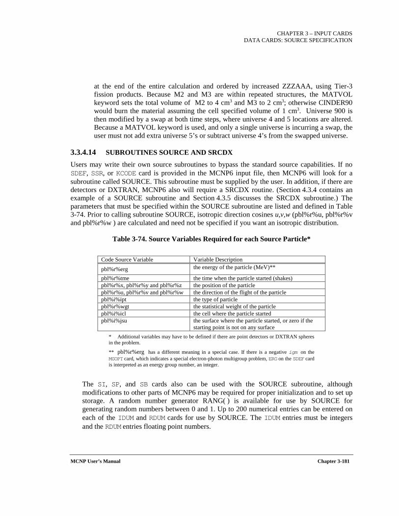
CHAPTER 3 – INPUT CARDS
DATA CARDS: SOURCE SPECIFICATION
MCNP User’s Manual Chapter 3-181
at the end of the entire calculation and ordered by increased ZZZAAA, using Tier-3 fission products. Because M2 and M3 are within repeated structures, the MATVOL keyword sets the total volume of M2 to 4 cm3 and M3 to 2 cm3; otherwise CINDER90 would burn the material assuming the cell specified volume of 1 cm3. Universe 900 is then modified by a swap at both time steps, where universe 4 and 5 locations are altered. Because a MATVOL keyword is used, and only a single universe is incurring a swap, the user must not add extra universe 5’s or subtract universe 4’s from the swapped universe.
3.3.4.14 SUBROUTINES SOURCE AND SRCDX
Users may write their own source subroutines to bypass the standard source capabilities. If no SDEF, SSR, or KCODE card is provided in the MCNP6 input file, then MCNP6 will look for a subroutine called SOURCE. This subroutine must be supplied by the user. In addition, if there are detectors or DXTRAN, MCNP6 also will require a SRCDX routine. (Section 4.3.4 contains an example of a SOURCE subroutine and Section 4.3.5 discusses the SRCDX subroutine.) The parameters that must be specified within the SOURCE subroutine are listed and defined in Table 3-74. Prior to calling subroutine SOURCE, isotropic direction cosines u,v,w (pbl%r%u, pbl%r%v and pbl%r%w ) are calculated and need not be specified if you want an isotropic distribution.
Table 3-74. Source Variables Required for each Source Particle*
Code Source Variable Variable Description pbl%r%erg the energy of the particle (MeV)**
pbl%r%tme the time when the particle started (shakes) pbl%r%x, pbl%r%y and pbl%r%z the position of the particle pbl%r%u, pbl%r%v and pbl%r%w the direction of the flight of the particle pbl%i%ipt the type of particle pbl%r%wgt the statistical weight of the particle pbl%i%icl the cell where the particle started pbl%i%jsu the surface where the particle started, or zero if the
starting point is not on any surface * Additional variables may have to be defined if there are point detectors or DXTRAN spheres in the problem.
** pbl%r%erg has a different meaning in a special case. If there is a negative igm on the MGOPT card, which indicates a special electron-photon multigroup problem, ERG on the SDEF card is interpreted as an energy group number, an integer.
The SI, SP, and SB cards also can be used with the SOURCE subroutine, although modifications to other parts of MCNP6 may be required for proper initialization and to set up storage. A random number generator RANG( ) is available for use by SOURCE for generating random numbers between 0 and 1. Up to 200 numerical entries can be entered on each of the IDUM and RDUM cards for use by SOURCE. The IDUM entries must be integers and the RDUM entries floating point numbers.
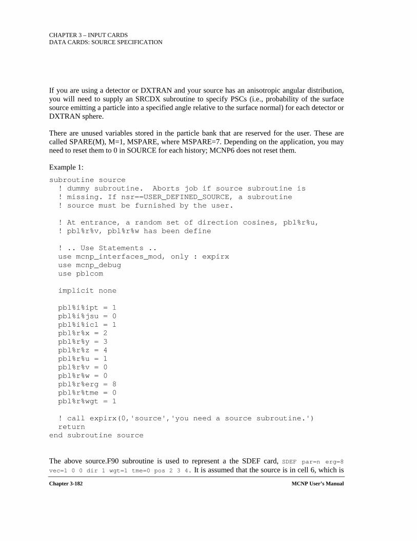
CHAPTER 3 – INPUT CARDS DATA CARDS: SOURCE SPECIFICATION
Chapter 3-182 MCNP User’s Manual
If you are using a detector or DXTRAN and your source has an anisotropic angular distribution, you will need to supply an SRCDX subroutine to specify PSCs (i.e., probability of the surface source emitting a particle into a specified angle relative to the surface normal) for each detector or DXTRAN sphere.
There are unused variables stored in the particle bank that are reserved for the user. These are called SPARE(M), M=1, MSPARE, where MSPARE=7. Depending on the application, you may need to reset them to 0 in SOURCE for each history; MCNP6 does not reset them.
Example 1: subroutine source ! dummy subroutine. Aborts job if source subroutine is ! missing. If nsr==USER_DEFINED_SOURCE, a subroutine ! source must be furnished by the user. ! At entrance, a random set of direction cosines, pbl%r%u, ! pbl%r%v, pbl%r%w has been define ! .. Use Statements .. use mcnp_interfaces_mod, only : expirx use mcnp_debug use pblcom implicit none pbl%i%ipt = 1 pbl%i%jsu = 0 pbl%i%icl = 1 pbl%r%x = 2 pbl%r%y = 3 pbl%r%z = 4 pbl%r%u = 1 pbl%r%v = 0 pbl%r%w = 0 pbl%r%erg = 8 pbl%r%tme = 0 pbl%r%wgt = 1 ! call expirx(0,'source','you need a source subroutine.') return end subroutine source
The above source.F90 subroutine is used to represent a the SDEF card, SDEF par=n erg=8 vec=1 0 0 dir 1 wgt=1 tme=0 pos 2 3 4. It is assumed that the source is in cell 6, which is
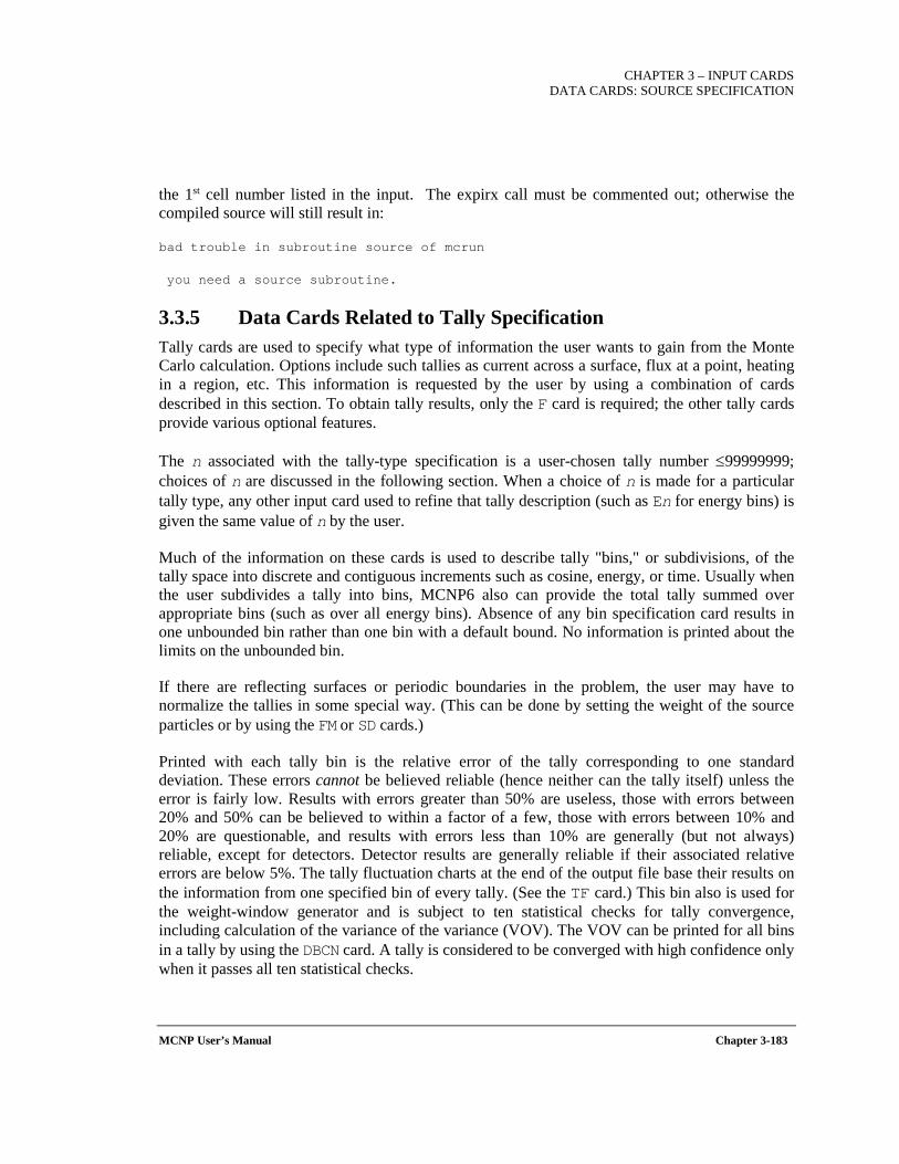
CHAPTER 3 – INPUT CARDS
DATA CARDS: SOURCE SPECIFICATION
MCNP User’s Manual Chapter 3-183
the 1st cell number listed in the input. The expirx call must be commented out; otherwise the compiled source will still result in:
bad trouble in subroutine source of mcrun
you need a source subroutine.
3.3.5 Data Cards Related to Tally Specification Tally cards are used to specify what type of information the user wants to gain from the Monte Carlo calculation. Options include such tallies as current across a surface, flux at a point, heating in a region, etc. This information is requested by the user by using a combination of cards described in this section. To obtain tally results, only the F card is required; the other tally cards provide various optional features.
The n associated with the tally-type specification is a user-chosen tally number ≤99999999; choices of n are discussed in the following section. When a choice of n is made for a particular tally type, any other input card used to refine that tally description (such as En for energy bins) is given the same value of n by the user.
Much of the information on these cards is used to describe tally "bins," or subdivisions, of the tally space into discrete and contiguous increments such as cosine, energy, or time. Usually when the user subdivides a tally into bins, MCNP6 also can provide the total tally summed over appropriate bins (such as over all energy bins). Absence of any bin specification card results in one unbounded bin rather than one bin with a default bound. No information is printed about the limits on the unbounded bin.
If there are reflecting surfaces or periodic boundaries in the problem, the user may have to normalize the tallies in some special way. (This can be done by setting the weight of the source particles or by using the FM or SD cards.)
Printed with each tally bin is the relative error of the tally corresponding to one standard deviation. These errors cannot be believed reliable (hence neither can the tally itself) unless the error is fairly low. Results with errors greater than 50% are useless, those with errors between 20% and 50% can be believed to within a factor of a few, those with errors between 10% and 20% are questionable, and results with errors less than 10% are generally (but not always) reliable, except for detectors. Detector results are generally reliable if their associated relative errors are below 5%. The tally fluctuation charts at the end of the output file base their results on the information from one specified bin of every tally. (See the TF card.) This bin also is used for the weight-window generator and is subject to ten statistical checks for tally convergence, including calculation of the variance of the variance (VOV). The VOV can be printed for all bins in a tally by using the DBCN card. A tally is considered to be converged with high confidence only when it passes all ten statistical checks.
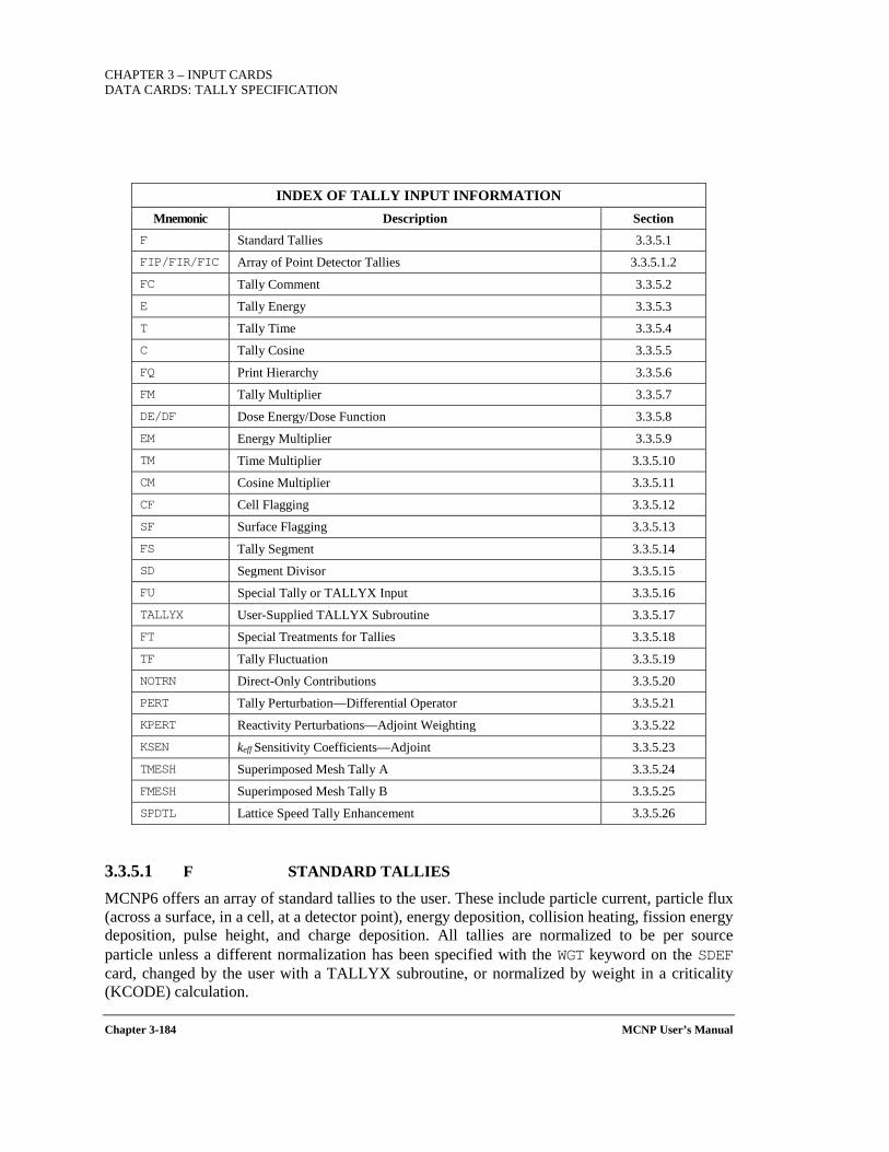
CHAPTER 3 – INPUT CARDS DATA CARDS: TALLY SPECIFICATION
Chapter 3-184 MCNP User’s Manual
INDEX OF TALLY INPUT INFORMATION Mnemonic Description Section
F Standard Tallies 3.3.5.1 FIP/FIR/FIC Array of Point Detector Tallies 3.3.5.1.2 FC Tally Comment 3.3.5.2 E Tally Energy 3.3.5.3 T Tally Time 3.3.5.4 C Tally Cosine 3.3.5.5 FQ Print Hierarchy 3.3.5.6 FM Tally Multiplier 3.3.5.7 DE/DF Dose Energy/Dose Function 3.3.5.8 EM Energy Multiplier 3.3.5.9 TM Time Multiplier 3.3.5.10 CM Cosine Multiplier 3.3.5.11 CF Cell Flagging 3.3.5.12 SF Surface Flagging 3.3.5.13 FS Tally Segment 3.3.5.14 SD Segment Divisor 3.3.5.15 FU Special Tally or TALLYX Input 3.3.5.16 TALLYX User-Supplied TALLYX Subroutine 3.3.5.17 FT Special Treatments for Tallies 3.3.5.18 TF Tally Fluctuation 3.3.5.19 NOTRN Direct-Only Contributions 3.3.5.20 PERT Tally Perturbation—Differential Operator 3.3.5.21 KPERT Reactivity Perturbations—Adjoint Weighting 3.3.5.22 KSEN keff Sensitivity Coefficients—Adjoint 3.3.5.23 TMESH Superimposed Mesh Tally A 3.3.5.24 FMESH Superimposed Mesh Tally B 3.3.5.25 SPDTL Lattice Speed Tally Enhancement 3.3.5.26
3.3.5.1 F STANDARD TALLIES
MCNP6 offers an array of standard tallies to the user. These include particle current, particle flux (across a surface, in a cell, at a detector point), energy deposition, collision heating, fission energy deposition, pulse height, and charge deposition. All tallies are normalized to be per source particle unless a different normalization has been specified with the WGT keyword on the SDEF card, changed by the user with a TALLYX subroutine, or normalized by weight in a criticality (KCODE) calculation.
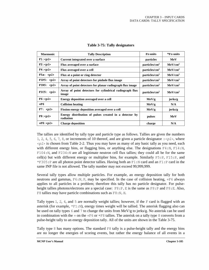
CHAPTER 3 – INPUT CARDS
DATA CARDS: TALLY SPECIFICATION
MCNP User’s Manual Chapter 3-185
Table 3-75: Tally designators
Mnemonic Tally Description Fn units *Fn units
F1:<pl> Current integrated over a surface particles MeV F2:<pl> Flux averaged over a surface particles/cm2 MeV/cm2 F4:<pl> Flux averaged over a cell particles/cm2 MeV/cm2 F5a: <pl> Flux at a point or ring detector particles/cm2 MeV/cm2 FIP5: <pl> Array of point detectors for pinhole flux image particles/cm2 MeV/cm2 FIR5: <pl> Array of point detectors for planar radiograph flux image particles/cm2 MeV/cm2
FIC5: <pl> Array of point detectors for cylindrical radiograph flux image particles/cm2 MeV/cm2
F6:<pl> Energy deposition averaged over a cell MeV/g jerks/g +F6 Collision heating MeV/g N/A F7: <pl> Fission energy deposition averaged over a cell MeV/g jerks/g
F8:<pl> Energy distribution of pulses created in a detector by radiation pulses MeV
+F8:<pl> Charge deposition charge N/A
The tallies are identified by tally type and particle type as follows. Tallies are given the numbers 1, 2, 4, 5, 6, 7, 8, or increments of 10 thereof, and are given a particle designator :<pl>, where <pl> is chosen from Table 2-2. Thus you may have as many of any basic tally as you need, each with different energy bins, or flagging bins, or anything else. The designations F4:N, F14:N, F104:N, and F234:N are all legitimate neutron cell flux tallies; they could all be for the same cell(s) but with different energy or multiplier bins, for example. Similarly F5:P, F15:P, and *F305:P are all photon point detector tallies. Having both an F1:N card and an F1:P card in the same INP file is not allowed. The tally number may not exceed 99,999,999.
Several tally types allow multiple particles. For example, an energy deposition tally for both neutrons and gammas, F6:N,P, may be specified. In the case of collision heating, +F6 always applies to all particles in a problem; therefore this tally has no particle designator. For pulse-height tallies photons/electrons are a special case: F8:P,E is the same as F8:P and F8:E. Also, F8 tallies may have particle combinations such as F8:N,H.
Tally types 1, 2, 4, and 5 are normally weight tallies; however, if the F card is flagged with an asterisk (for example, *F1:N), energy times weight will be tallied. The asterisk flagging also can be used on tally types 6 and 7 to change the units from MeV/g to jerks/g. No asterisk can be used in combination with the + on the +F6 or +F8 tallies. The asterisk on a tally type 8 converts from a pulse-height tally to an energy deposition tally. All of the units are shown in the Table 3-75.
Tally type 8 has many options. The standard F8 tally is a pulse-height tally and the energy bins are no longer the energies of scoring events, but rather the energy balance of all events in a
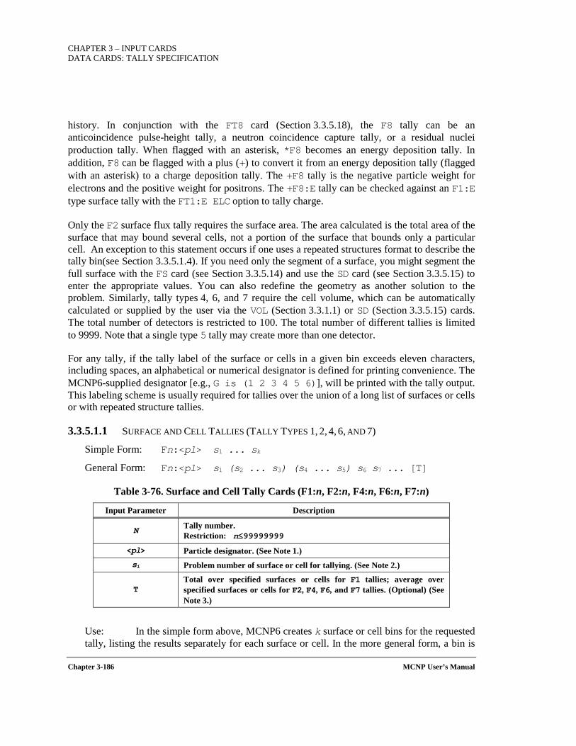
CHAPTER 3 – INPUT CARDS DATA CARDS: TALLY SPECIFICATION
Chapter 3-186 MCNP User’s Manual
history. In conjunction with the FT8 card (Section 3.3.5.18), the F8 tally can be an anticoincidence pulse-height tally, a neutron coincidence capture tally, or a residual nuclei production tally. When flagged with an asterisk, *F8 becomes an energy deposition tally. In addition, F8 can be flagged with a plus (+) to convert it from an energy deposition tally (flagged with an asterisk) to a charge deposition tally. The +F8 tally is the negative particle weight for electrons and the positive weight for positrons. The +F8:E tally can be checked against an F1:E type surface tally with the FT1:E ELC option to tally charge.
Only the F2 surface flux tally requires the surface area. The area calculated is the total area of the surface that may bound several cells, not a portion of the surface that bounds only a particular cell. An exception to this statement occurs if one uses a repeated structures format to describe the tally bin(see Section 3.3.5.1.4). If you need only the segment of a surface, you might segment the full surface with the FS card (see Section 3.3.5.14) and use the SD card (see Section 3.3.5.15) to enter the appropriate values. You can also redefine the geometry as another solution to the problem. Similarly, tally types 4, 6, and 7 require the cell volume, which can be automatically calculated or supplied by the user via the VOL (Section 3.3.1.1) or SD (Section 3.3.5.15) cards. The total number of detectors is restricted to 100. The total number of different tallies is limited to 9999. Note that a single type 5 tally may create more than one detector.
For any tally, if the tally label of the surface or cells in a given bin exceeds eleven characters, including spaces, an alphabetical or numerical designator is defined for printing convenience. The MCNP6-supplied designator [e.g., G is (1 2 3 4 5 6)], will be printed with the tally output. This labeling scheme is usually required for tallies over the union of a long list of surfaces or cells or with repeated structure tallies.
3.3.5.1.1 SURFACE AND CELL TALLIES (TALLY TYPES 1, 2, 4, 6, AND 7)
Simple Form: Fn:<pl> s1 ... sk
General Form: Fn:<pl> s1 (s2 ... s3) (s4 ... s5) s6 s7 ... [T]
Table 3-76. Surface and Cell Tally Cards (F1:n, F2:n, F4:n, F6:n, F7:n)
Input Parameter Description
N Tally number. Restriction: n≤99999999
<pl> Particle designator. (See Note 1.) si Problem number of surface or cell for tallying. (See Note 2.)
T Total over specified surfaces or cells for F1 tallies; average over specified surfaces or cells for F2, F4, F6, and F7 tallies. (Optional) (See Note 3.)
Use: In the simple form above, MCNP6 creates k surface or cell bins for the requested tally, listing the results separately for each surface or cell. In the more general form, a bin is
CHAPTER 3 – INPUT CARDS
DATA CARDS: TALLY SPECIFICATION
MCNP User’s Manual Chapter 3-187
created for each surface or cell listed separately and for each collection of surfaces or cells enclosed within a set of parentheses. Entries within parentheses also can appear separately or in other combinations. Parentheses indicate that the tally is for the union of the items within the parentheses. For unnormalized tallies (tally type 1), the union of tallies is a sum, but for normalized tallies (types 2, 4, 6, and 7), the union results in an average. See Section 3.3.5.1.4 for an explanation of the repeated structure and lattice tally format.
Note 1: Tally type 7 allows N only.
Note 2: Only surfaces that define cell boundaries and that are listed in a cell card description can be used on F1 and F2 tallies.
Note 3: The symbol T entered on surface or cell F cards is shorthand for a region that is the union of all of the other entries on the card. A tally is made for the individual entries on the F card plus the union of all the entries. The entry is optional.
Note 4: Surface flux tallies require an approximation when counting grazing contributions, that is, for contributions where the dot product of the particle direction and the surface normal are between -0.001 and 0.001 (the current default, new in MCNP6.2). The grazing angle cutoff can be reset using the 24th entry on the DBCN card; i.e., “DBCN 23j 0.1” changes the grazing angle cutoff from the MCNP6.2 value of ±0.001 to the historic MCNP value of ±0.1.
Aside: Surface Flux Tally (F2) For particles grazing the surface, 1/|μ| (where μ is the cosine of the angle that the particle track makes with the surface normal) is very large and MCNP approximates the surface flux estimator in order to satisfy the requirement of one central limit theorem. An unmodified surface flux estimator has an infinite variance, and thus confidence intervals could not be formed via the central limit theorem, because the central limit theorem requires a finite variance. For this reason, MCNP sets |μ| = 0.0005 when |μ| < 0.001; because of this approximation, the F2 tally is not an exact estimate of the surface flux. . (The grazing angle cutoff cosine can be changed using the 24th entry on the DBCN card.) While the numeric values may vary, this is the standard approximation used in Monte Carlo codes. This approximation is accurate when the angular flux is isotropic or linearly anisotropic with respect to μ on the surface and the limits of the flux integral with respect to μ are symmetric. However, these assumptions may become invalid on external surfaces or in other cases of one-way surface crossings; when exactly tangent crossing is not possible because of the geometry of the problem; or when cosine bins are used. Users should be especially careful in these cases. More details may be found in FAV11a and FAV11b.
CHAPTER 3 – INPUT CARDS DATA CARDS: TALLY SPECIFICATION
Chapter 3-188 MCNP User’s Manual
Aside: Energy Deposition Tally (F6)
In the energy range where nuclear data tables are available, the neutron, photon, and proton energy deposition is determined using the heating numbers from the nuclear data tables. These heating numbers are estimates of the energy deposited per unit track length. In addition, the de/dx ionization contribution for electrons and/or protons is added in for MODE E or MODE H.
Above that tabular energy limit, or when no tabular data is available, energy deposition is determined by summing several factors. For charged particles, ionization (de/dx) energy is deposited uniformly along the track length (which is important to keep in mind when doing a mesh tally). All other energy deposition is calculated at the time of a nuclear interaction. The energies of secondary particles, if they are not to be tracked (i.e., not included on the MODE card) will be deposited at the point of the interaction. Nuclear recoil energy will be deposited at the point of interaction unless heavy ion transport is specified (i.e., MODE #).1
To obtain the most accurate energy deposition tallies possible, the user must include all potential secondary particles on the MODE card. (Users may wish to omit electrons, provided they fully understands how energy deposition for photons is done.) The energy deposition for non-tracked secondary particles generally assumes all energy is deposited locally at the collision site. The exception is for neutral particles (photons, neutrinos, etc.), which generally travel far from the collision site. Heating is included for these secondary particles only if they are listed on the MODE card and F6 card. The assumption of local energy deposition for non-tracked secondary particles is poor, especially when the energies of the secondaries are high, or when the user is simulating thin volumes. When secondary particles are indicated on the MODE card, MCNP6 will subtract their energies from the heating values, and energy deposition will be handled in the regular process of tracking those particles.2
When there are no library heating data available, de/dx, nuclear recoil, and the energies of some non-tracked secondary particles are added to the F6 collision estimator. A secondary particle can be produced either by collision or by particle decay.3 In MCNP6, the energies of neutral particles will never be added to the collision estimator (this includes neutrons, photons, neutrinos, π0, and neutral kaons). Therefore, it is especially important for the user to
1 Tracking of residual nuclei is important in small volumes where the recoil nucleus might leave the cell.
This is especially important in light ion recoils (such as a scattered hydrogen nucleus). Light ion recoil from elastic collisions is an option on the PHYS:N and PHYS:H cards.
2 Energies of particles that fall below minimum energy cutoffs will also be deposited locally. The user must be certain that the value of these cutoff energies will not cause the results of the F6 tally to be in error.
3 Note that the π0, if included on the MODE card, will be transported before it decays, even though its lifetime is 8.4×10⁻¹⁷ seconds. This allows the user to use MCNP6 tallies for that particle.
CHAPTER 3 – INPUT CARDS
DATA CARDS: TALLY SPECIFICATION
MCNP User’s Manual Chapter 3-189
include all possible secondary particles on the MODE card (especially photons and neutrinos), in order to get the most accurate energy deposition tally.
MCNP6 has the track-length heating (F6:<pl>) tally, where <pl> can be any particle or combination of particles. In addition, MCNP6 also has a collision heating (+F6) tally, which contains energy deposition from all particles in the problem. Note that the PEDEP keyword in a Type 1 mesh tally is analogous to the F6:<pl> tally, and the Type 3 mesh tally is analogous to the +F6 tally, although the normalizations will be different. Since the mesh tallies score energy deposition within a mesh cell, which may contain more than one material, normalization is per unit volume. The units of this tally are MeV/source-particle. In the F6 and +F6 tallies, material density is available for the chosen cells, and normalization is MeV/gm/source-particle.
Example 1: F2:N 1 3 6 T
This card specifies four neutron flux tallies, one across each of the surfaces 1, 3, and 6 and one which is the average of the flux across all three of the surfaces.
Example 2: F1:P (1 2) (3 4 5) 6
This card provides three photon current tallies, one for the sum over surfaces 1 and 2; one for the sum over surfaces 3, 4, and 5; and one for surface 6 alone.
Example 3: F371:N (1 2 3) (1 4) T
This card provides three neutron current tallies, one for the sum over surfaces 1, 2, and 3; one for the sum over surfaces 1 and 4; and one for the sum over surfaces 1, 2, 3, and 4. The point of this example is that the T bin is not confused by the repetition of surface 1.
Example 4: +F6 2
This card produces energy deposition (MeV/g) from all particles averaged over cell 2. This will include heating values and/or de/dx energy from particles undergoing library interactions (e.g., neutrons, photons, electrons, protons) and de/dx, recoil, and non-tracked secondary particle energy from all model interactions.
3.3.5.1.2 DETECTOR TALLIES (TALLY TYPE 5)
Point detectors, ring detectors, and radiography tallies use an assumption of isotropic scatter for contributions from collisions within the model regime (i.e., generally E>150 MeV). These estimators require the angular distribution data for particles produced in an interaction to predict
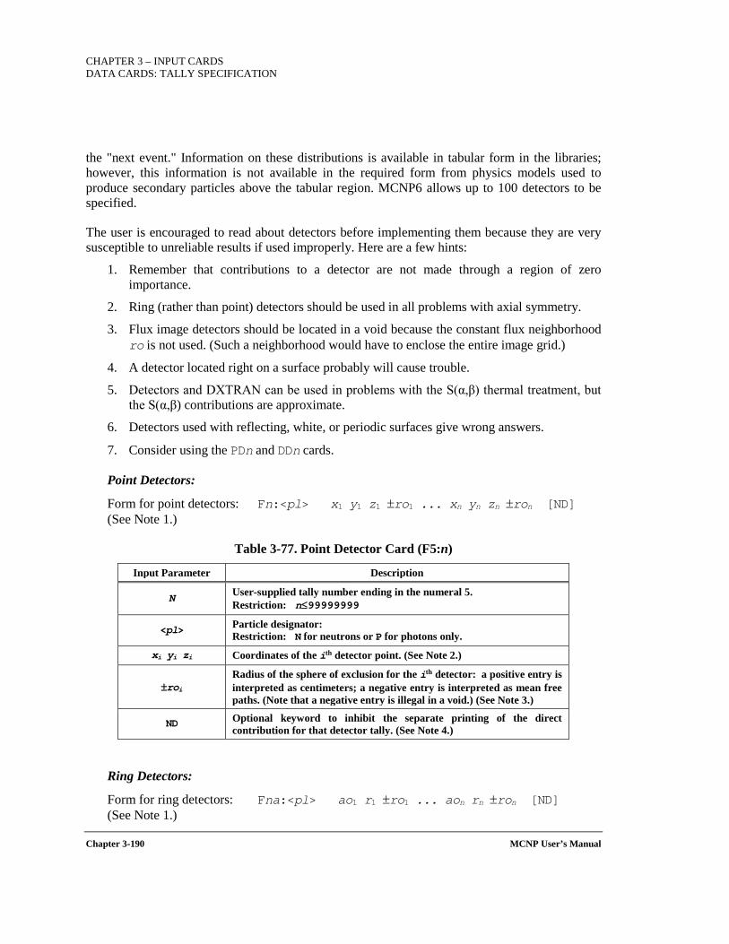
CHAPTER 3 – INPUT CARDS DATA CARDS: TALLY SPECIFICATION
Chapter 3-190 MCNP User’s Manual
the "next event." Information on these distributions is available in tabular form in the libraries; however, this information is not available in the required form from physics models used to produce secondary particles above the tabular region. MCNP6 allows up to 100 detectors to be specified.
The user is encouraged to read about detectors before implementing them because they are very susceptible to unreliable results if used improperly. Here are a few hints:
1. Remember that contributions to a detector are not made through a region of zero importance.
2. Ring (rather than point) detectors should be used in all problems with axial symmetry.
3. Flux image detectors should be located in a void because the constant flux neighborhood ro is not used. (Such a neighborhood would have to enclose the entire image grid.)
4. A detector located right on a surface probably will cause trouble.
5. Detectors and DXTRAN can be used in problems with the S(α,β) thermal treatment, but the S(α,β) contributions are approximate.
6. Detectors used with reflecting, white, or periodic surfaces give wrong answers.
7. Consider using the PDn and DDn cards.
Point Detectors:
Form for point detectors: Fn:<pl> x1 y1 z1 ±ro1 ... xn yn zn ±ron [ND] (See Note 1.)
Table 3-77. Point Detector Card (F5:n)
Input Parameter Description
N User-supplied tally number ending in the numeral 5. Restriction: n≤99999999
<pl> Particle designator: Restriction: N for neutrons or P for photons only.
xi yi zi Coordinates of the ith detector point. (See Note 2.)
±roi Radius of the sphere of exclusion for the ith detector: a positive entry is interpreted as centimeters; a negative entry is interpreted as mean free paths. (Note that a negative entry is illegal in a void.) (See Note 3.)
ND Optional keyword to inhibit the separate printing of the direct contribution for that detector tally. (See Note 4.)
Ring Detectors:
Form for ring detectors: Fna:<pl> ao1 r1 ±ro1 ... aon rn ±ron [ND] (See Note 1.)
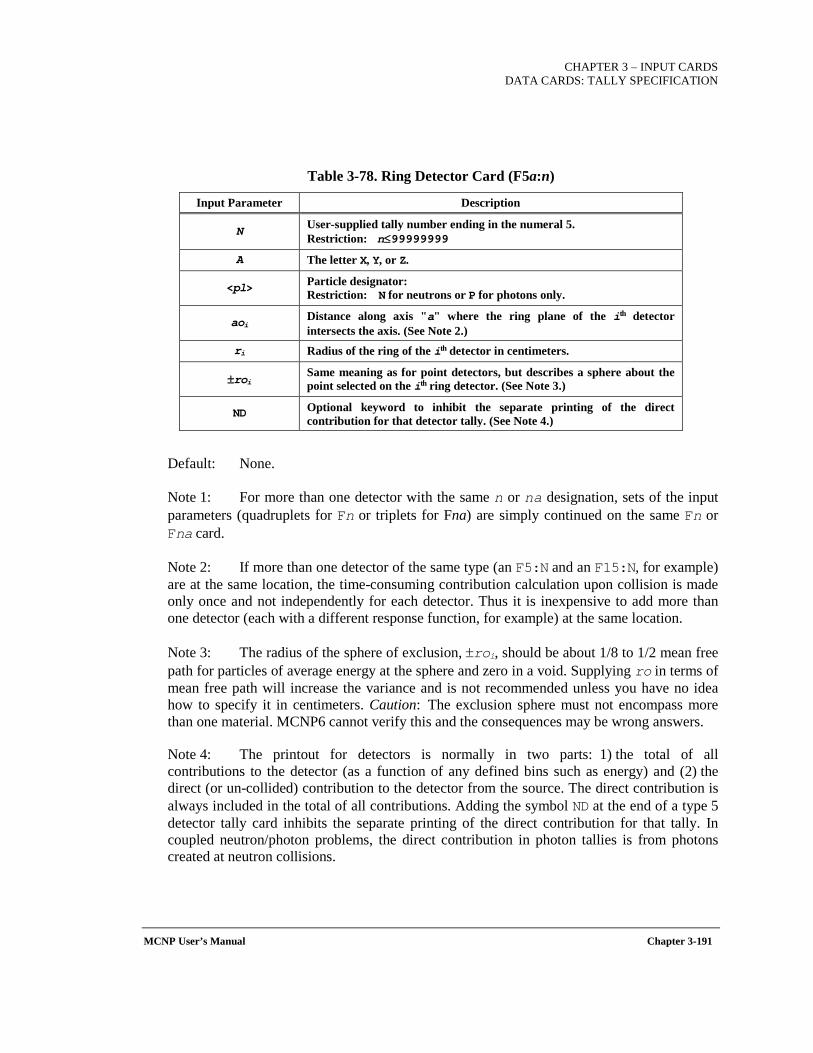
CHAPTER 3 – INPUT CARDS
DATA CARDS: TALLY SPECIFICATION
MCNP User’s Manual Chapter 3-191
Table 3-78. Ring Detector Card (F5a:n)
Input Parameter Description
N User-supplied tally number ending in the numeral 5. Restriction: n≤99999999
A The letter X, Y, or Z.
<pl> Particle designator: Restriction: N for neutrons or P for photons only.
aoi Distance along axis "a" where the ring plane of the ith detector intersects the axis. (See Note 2.)
ri Radius of the ring of the ith detector in centimeters.
±roi Same meaning as for point detectors, but describes a sphere about the point selected on the ith ring detector. (See Note 3.)
ND Optional keyword to inhibit the separate printing of the direct contribution for that detector tally. (See Note 4.)
Default: None.
Note 1: For more than one detector with the same n or na designation, sets of the input parameters (quadruplets for Fn or triplets for Fna) are simply continued on the same Fn or Fna card.
Note 2: If more than one detector of the same type (an F5:N and an F15:N, for example) are at the same location, the time-consuming contribution calculation upon collision is made only once and not independently for each detector. Thus it is inexpensive to add more than one detector (each with a different response function, for example) at the same location.
Note 3: The radius of the sphere of exclusion, ±roi, should be about 1/8 to 1/2 mean free path for particles of average energy at the sphere and zero in a void. Supplying ro in terms of mean free path will increase the variance and is not recommended unless you have no idea how to specify it in centimeters. Caution: The exclusion sphere must not encompass more than one material. MCNP6 cannot verify this and the consequences may be wrong answers.
Note 4: The printout for detectors is normally in two parts: 1) the total of all contributions to the detector (as a function of any defined bins such as energy) and (2) the direct (or un-collided) contribution to the detector from the source. The direct contribution is always included in the total of all contributions. Adding the symbol ND at the end of a type 5 detector tally card inhibits the separate printing of the direct contribution for that tally. In coupled neutron/photon problems, the direct contribution in photon tallies is from photons created at neutron collisions.
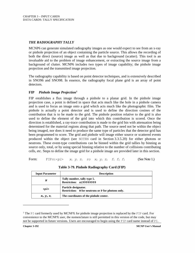
CHAPTER 3 – INPUT CARDS DATA CARDS: TALLY SPECIFICATION
Chapter 3-192 MCNP User’s Manual
THE RADIOGRAPHY TALLY
MCNP6 can generate simulated radiography images as one would expect to see from an x-ray or pinhole projection of an object containing the particle source. This allows the recording of both the direct (source) image as well as that due to background (scatter). This tool is an invaluable aid to the problem of image enhancement, or extracting the source image from a background of clutter. MCNP6 includes two types of image capability; the pinhole image projection and the transmitted image projection.
The radiography capability is based on point detector techniques, and is extensively described in SNO96 and SNO98. In essence, the radiography focal plane grid is an array of point detectors.
FIP Pinhole Image Projection1
FIP establishes a flux image through a pinhole to a planar grid. In the pinhole image projection case, a point is defined in space that acts much like the hole in a pinhole camera and is used to focus an image onto a grid which acts much like the photographic film. The pinhole is actually a point detector and is used to define the direction cosines of the contribution that is to be made to the grid. The pinhole position relative to the grid is also used to define the element of the grid into which this contribution is scored. Once the direction is established, a ray-trace contribution is made to the grid bin with attenuation being determined for the material regions along that path. The source need not be within the object being imaged, nor does it need to produce the same type of particles that the detector grid has been programmed to score. The grid and pinhole will image either source or scattered events produced within the object (see NOTRN card in Section 3.3.5.20) for either photons or neutrons. These event-type contributions can be binned within the grid tallies by binning as source only, total, or by using special binning relative to the number of collisions contributing cells, etc. Steps to define the image grid for a pinhole image are provided later in this section.
Form: FIPn:<pl> x1 y1 z1 ro x2 y2 z2 f1 f2 f3 (See Note 1.)
Table 3-79. Pinhole Radiography Card (FIP)
Input Parameter Description
N Tally number, tally type 5. Restriction: n≤99999999
<pl> Particle designator. Restriction: N for neutrons or P for photons only.
x1, y1, z1 The coordinates of the pinhole center.
1 The PI card formerly used by MCNPX for pinhole image projection is replaced by the FIP card. For convenience to the MCNPX user, the nomenclature is still permitted in this version of the code, but may not be supported in future versions. Users are encouraged to begin using the FIP card name instead of PI.

CHAPTER 3 – INPUT CARDS
DATA CARDS: TALLY SPECIFICATION
MCNP User’s Manual Chapter 3-193
Ro Always 0 (zero) for this application. Note: Neither the pinhole nor the grid should be located within a highly scattering media.
x2, y2, z2 The reference coordinates (center of object) that establish the reference direction cosines for the normal to the detector grid. This direction is defined as being from x2, y2, z2 to the pinhole at x1, y1, z1.
f1
If f1>0, this value is the radius of a cylindrical collimator, centered on and parallel to the reference direction, which establishes a radial field of view through the object and surrounding materials and onto the image grid. If f1=0, the value of the radius is "large." (DEFAULT)
f2
The radius of the pinhole perpendicular to the reference direction. If f2=0, this represents a perfect pinhole. If f2>0, the point within the pinhole through which the particle flux
contribution will pass is picked randomly (i.e., uniformly in area) for each source and scatter event. This simulates a less-than-perfect pinhole.
f3 The distance from the pinhole at x1, y1, z1 to the center of the detector grid along the direction established from x2, y2, z2 to x1, y1, z1,. The image grid is perpendicular to this reference vector.
Note 1: Only one pinhole image tally per FIP card is allowed. The point detector Russian roulette game is not used with the FIP tally. Consider use of the NOTRN card for only direct contributions and the TALNP card to reduce the size of the OUTP file for large-image grids. The image grid should not be in a scattering material because the point detector average flux neighborhood is not used for flux image tallies.
FIR and FIC Transmitted Image Projection1
FIR establishes a flux image on a rectangular radiograph planar grid, and FIC establishes a flux image on a cylindrical radiograph grid.
In the transmitted image projection case, the grid acts like a film pack in an x-ray type image, or transmitted image projection. In both cases, for every source or scatter event a ray-trace contribution is made to every bin in the detector grid. This eliminates statistical fluctuations across the grid that would occur if the grid location of the contribution from each event were to be picked randomly, as would be the case if one used a DXTRAN sphere and a segmented surface tally. For each event, source or scatter, the direction to each of the grid points is determined, and an attenuated ray-trace contribution is made. As in pinhole image projection, there are no restrictions as to location or type of source used. These tallies automatically bin
1 The TIR and TIC cards formerly used by MCNPX for pinhole image projection is replaced by the FIR and FIC cards. For convenience to the MCNPX user, the nomenclature is still permitted in this version of the code, but may not be supported in future versions. Users are encouraged to begin using the FIR and FIC cards name instead of TIR and TIC.

CHAPTER 3 – INPUT CARDS DATA CARDS: TALLY SPECIFICATION
Chapter 3-194 MCNP User’s Manual
in a source-only and a total contribution. Steps to define the image grid for transmitted images are provided later in this section.
When this type of detector is being used in a problem, if a contribution is required from a source or scatter event, an attenuated contribution is made to each and every detector grid bin. Because for some types of source distributions very few histories are required to image the direct or source contributions, an additional entry has been added to the NPS card to eliminate unwanted duplication of information from the source. (See Section 3.3.7.1.)
Rectangular grid:
Form: FIRn:<pl> x1 y1 z1 ro x2 y2 z2 f1 f2 f3 (See Note 1.)
Cylindrical grid:
Form: FICn:<pl> x1 y1 z1 ro x2 y2 z2 f1 f2 f3 (See Note 1.)
Table 3-80. Transmitted Image Projection Cards (FIR and FIC)
Input Parameter Description
N Tally number, tally type 5. Restriction: n≤99999999
<pl> Particle designator. Restriction: N for neutrons or P for photons only.
x1, y1, z1
The coordinates of the center of the detector flux image grid, the extent and spacing of which are defined by the entries on the tally segment (FS) and cosine (C) cards. In the planar rectangular grid case, this point defines the center of the grid. In the cylindrical grid case, this point defines the center of the cylinder on which the grid is established.
Ro Always 0 (zero) in this application. Note: Do not locate the image grid in a scattering material.
x2, y2, z2
The reference coordinates (center of object) that establish the reference direction cosines for the outward normal to the detector grid plane, as from x2, y2, z2 to x1, y1, z1. This direction is used as the outward normal to the detector grid plane for the FIR case, and as the centerline of the cylinder for the FIC case.
f1 If f1=0, both the direct (source) and scattered contributions will be
scored at the detector grid. If f1=-1, only the scattered contributions will be scored. (See Note 2.)
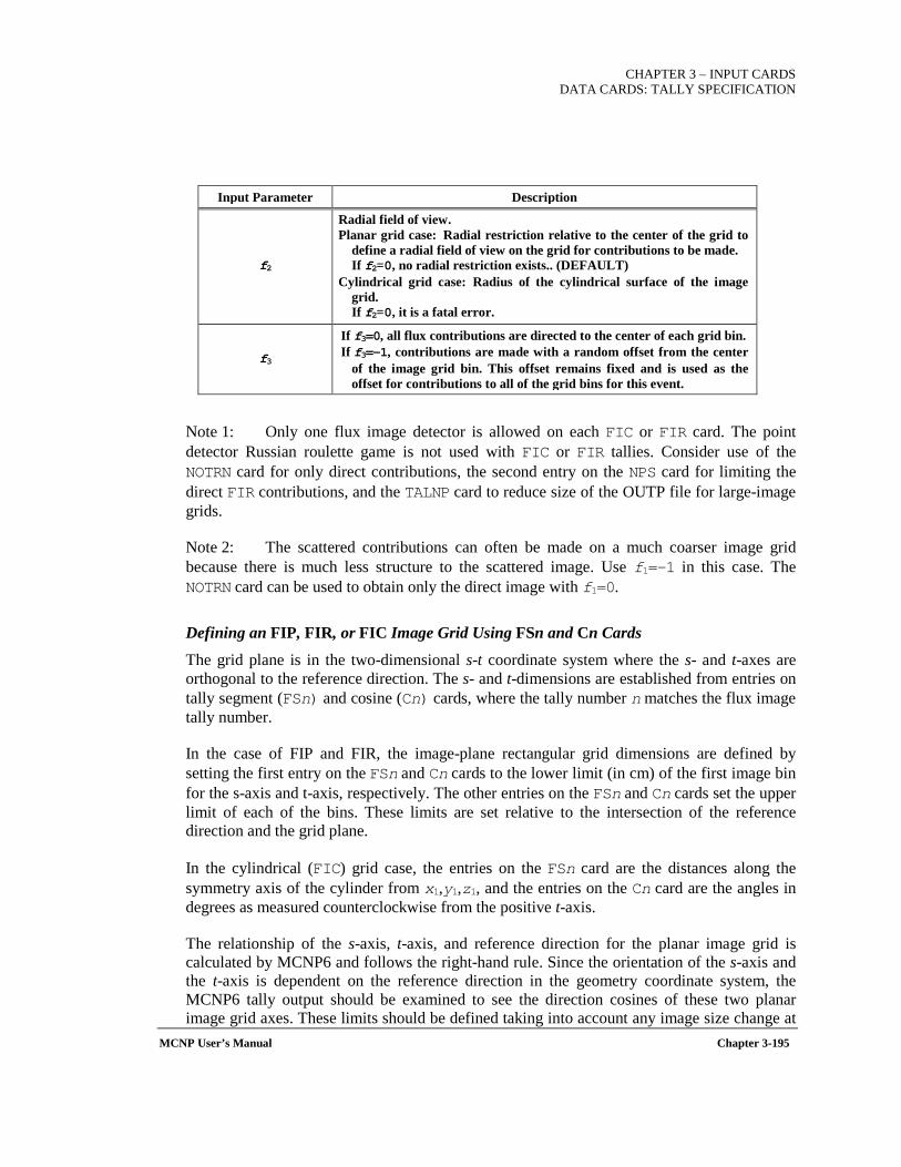
CHAPTER 3 – INPUT CARDS
DATA CARDS: TALLY SPECIFICATION
MCNP User’s Manual Chapter 3-195
Input Parameter Description
f2
Radial field of view. Planar grid case: Radial restriction relative to the center of the grid to
define a radial field of view on the grid for contributions to be made. If f2=0, no radial restriction exists.. (DEFAULT)
Cylindrical grid case: Radius of the cylindrical surface of the image grid. If f2=0, it is a fatal error.
f3
If f3=0, all flux contributions are directed to the center of each grid bin. If f3=-1, contributions are made with a random offset from the center
of the image grid bin. This offset remains fixed and is used as the offset for contributions to all of the grid bins for this event.
Note 1: Only one flux image detector is allowed on each FIC or FIR card. The point detector Russian roulette game is not used with FIC or FIR tallies. Consider use of the NOTRN card for only direct contributions, the second entry on the NPS card for limiting the direct FIR contributions, and the TALNP card to reduce size of the OUTP file for large-image grids.
Note 2: The scattered contributions can often be made on a much coarser image grid because there is much less structure to the scattered image. Use f1=-1 in this case. The NOTRN card can be used to obtain only the direct image with f1=0.
Defining an FIP, FIR, or FIC Image Grid Using FSn and Cn Cards
The grid plane is in the two-dimensional s-t coordinate system where the s- and t-axes are orthogonal to the reference direction. The s- and t-dimensions are established from entries on tally segment (FSn) and cosine (Cn) cards, where the tally number n matches the flux image tally number.
In the case of FIP and FIR, the image-plane rectangular grid dimensions are defined by setting the first entry on the FSn and Cn cards to the lower limit (in cm) of the first image bin for the s-axis and t-axis, respectively. The other entries on the FSn and Cn cards set the upper limit of each of the bins. These limits are set relative to the intersection of the reference direction and the grid plane.
In the cylindrical (FIC) grid case, the entries on the FSn card are the distances along the symmetry axis of the cylinder from x1,y1,z1, and the entries on the Cn card are the angles in degrees as measured counterclockwise from the positive t-axis.
The relationship of the s-axis, t-axis, and reference direction for the planar image grid is calculated by MCNP6 and follows the right-hand rule. Since the orientation of the s-axis and the t-axis is dependent on the reference direction in the geometry coordinate system, the MCNP6 tally output should be examined to see the direction cosines of these two planar image grid axes. These limits should be defined taking into account any image size change at
CHAPTER 3 – INPUT CARDS DATA CARDS: TALLY SPECIFICATION
Chapter 3-196 MCNP User’s Manual
the grid caused by magnification. The image grid should not be in a scattering material because the point detector average flux neighborhood is not used for flux image tallies.
There is no limit to the number of image grid bins that can be defined by FSn and Cn. However, it is easy to define a tally with a huge number of point detectors. For example, a 1000 by 1000 grid is the equivalent of 1 million point detectors, which could take a long time to run. Fatal errors will result if the FSn and Cn card bin specifications are not each monotonically increasing. The default tally fluctuation chart bin is the last FSn and Cn bin in the total (direct plus scattered) detector tally. FS0 and C0 cards for these image tallies are not allowed. The T (total) and C (cumulative) options for the FSn and Cn cards are not available for flux image tallies.
The directions of the t-axis and s-axis of the grid are set up such that if the reference direction (the outward normal to the grid plane) is not parallel to the z-axis of the geometry, the t-axis of the grid is defined by the intersection of the grid plane and plane formed by the z-axis and the point where the reference direction would intersect the grid plane. If the reference direction is parallel to the z-axis of the geometry, then the t-axis of the grid is defined to be parallel to the y-axis of the geometry. The s-axis of the grid is defined as the cross product of a unit vector in the "t" direction and a unit vector in the reference direction. If the reference direction is not parallel to the z-axis, MCNP6 calculates the orthogonal axes. The s and t image axes direction cosines are printed in the OUTP file.
Example 1: FSn -20. 99i 15. Cn -25. 99i 10.
These two cards set up a 100×100 grid that extends from -20 cm to 15 cm along the s-axis, from -25 cm to 10 cm along the t-axis, and has 10,000 equal sized bins. These bins need not be equal in size nor do they need to be symmetric about the reference direction.
Reading or Plotting the Radiography Tally Output
The output of the two radiography tally options is contained in the MCTAL file. It can be formatted for use with external graphics programs with the GRIDCONV1 routine. The user is referred to Section 3.3.5.24.6 for information on how to use GRIDCONV. Pinhole and radiography tallies can also be plotted directly in the MCNP6 tally plotter from RUNTPE or MCTAL files using the "FREE SC" command to give a 2D contour plot of the s- and t-axes. They can also be plotted during the course of a calculation by incorporating an MPLOT card into the input file or by using the TTY interrupt capability to invoke MCPLOT.
1 GRIDCONV is not packaged with MCNP6. However, the MCNPX version should be able to read and process most of the output files from MCNP6.
CHAPTER 3 – INPUT CARDS
DATA CARDS: TALLY SPECIFICATION
MCNP User’s Manual Chapter 3-197
3.3.5.1.3 PULSE-HEIGHT TALLY (TALLY TYPE 8)
The pulse-height tally is a radical departure from other MCNP6 tallies. All other tallies are estimates of macroscopic variables, such as flux, whose values are determined by very large numbers of microscopic events. The pulse-height tally records the energy or charge deposited in a cell by each source particle and its secondary particles. For other tallies it is not necessary to model microscopic events realistically as long as the expectation values of macroscopic variables are correct. For the pulse-height tally, microscopic events must be modeled much more realistically.
The departures from microscopic realism in MCNP6 are everywhere. The number, energies, and directions of the secondary neutrons and photons from a neutron collision are sampled without any correlation between the particles and with no regard for the conservation of energy. The fluctuations in the energy loss rate of an electron are not correlated with the production of knock-on electrons and x-rays. The variance reduction schemes in MCNP6 distort the natural random walk process in various ways; nevertheless, they give correct results for macroscopic tallies when appropriate weighting factors are used.
Problems that give correct pulse height tallies are severely limited. For example, the pulse-height tally does not work well with neutrons because of the non-analog nature of neutron transport that departs from microscopic realism at every turn. One can have a neutron source in a MODE N P or N P E problem, but only the photons and electrons can be tallied on the F8 card. The F8 tally can be used effectively in photon problems. Electron problems may give correct results as long as the tally cells are thick enough for the errors in the energy loss rate to average out. Combining F8 tallies with a photonuclear bias is a fatal error. MCNP6 tries to detect conditions in a problem that would invalidate pulse height tallies, but it is not able to catch all of them. The user must ascertain that his problem does not violate the necessary conditions for obtaining correct answers.
Scoring the pulse-height tally is done at the end of each history. In the absence of variance reduction, the scoring is reasonably easy to describe. For example, consider a unit weight source and an F8 tally in cell 7. Suppose that on a given particle history that there are K entries into cell 7 and L departures from cell 7. The tally energy associated with an F8 tally is the kinetic energy of the particle plus 1.022016 MeV if it is a positron. Particles can enter cell 7 either by crossing a boundary into cell 7 or entering cell 7 as a source event. Particles depart cell 7 either by capture in cell 7 or by crossing a boundary out of cell 7. Let Ei be the ith tally energy of a particle entering cell 7 and let Dj be the jth tally energy of a particle departing cell 7. The total energy deposited in cell 7 is
.
Suppose the pulse height bins are specified on the E8 card as: E8 T1 T2 T3 T4 T5
∑−∑===
L
jj
K
ii DET
11

CHAPTER 3 – INPUT CARDS DATA CARDS: TALLY SPECIFICATION
Chapter 3-198 MCNP User’s Manual
If Tm-1<T<Tm, then MCNP6 will post a unit tally in the mth bin. If the problem is analog but the source weight is ws, then ws would be posted in the mth bin. If there is an asterisk on the F8 card, then MCNP6 tallies ws*T in the mth bin. If there is a plus on the F8 card, then MCNP6 posts the net charge change times the ws into the mth bin. That is, an entering electron or a departing positron constitutes a charge change of -1, whereas a departing electron or an entering positron constitutes a charge change of +1.
The scoring details are more complex with pulse-height tally variance reduction. (BOO02)
One common application of the F8 tally is simulation of the energy distribution of pulses created in a detector by radiation. The union of tallies produces a tally sum, not an average. Cell, user, and energy bin cards are allowed. Flagging and multiplier bins are not allowed. Segment, time, and cosine bins are permitted with certain FT options (see Section 3.3.5.18). Use of the dose energy (DE) and dose function (DF) cards is also disallowed with the F8 tally.
The energy bins in the F8 pulse-height tally are different from those of all other tallies. Rather than tally the particle energy at the time of scoring, the number of pulses depositing energy within the bins are tallied. That is, the meaning of the energy bins of a pulse-height tally is the energy deposited in a cell bin by all the physically associated tracks of a history. Care must be taken when selecting energy bins for a pulse-height tally. It is recommended that a zero bin and an epsilon bin be included such as
E8 0 1E-5 1E-3 1E-1 ...
The zero bin will catch non-analog knock-on electron negative scores. The epsilon (1E-5) bin will catch scores from particles that travel through the cell without depositing energy.
With the FT8 special tally treatments card (Section 3.3.5.18) the F8 tally can become an anticoincidence pulse-height tally (FT8 PHL) or a different kind of tally altogether. For example, FT8 CAP is a neutron coincidence capture tally, and FT8 RES tallies the residual nuclides from physics-model evaporation and fission models. These variations have special rules regarding possible variance reduction, time bins, and other issues.
Pulse-Height Tally Variance Reduction
Variance reduction for F8 tallies is implemented for electrons and photons; however, not a lot of experience exists to guide the user. Experience suggests that weight windows be used instead of geometry splitting for F8 tallies. Many of the variance-reduction techniques that were designed for lowering the variance on other tally types may be used with the F8 tally. Allowed variance reduction techniques include
• Splitting/roulette (IMP card) • Implicit capture and weight cutoff (CUT card) • Weight window (WWN card) • Forced collisions (FCL card)
CHAPTER 3 – INPUT CARDS
DATA CARDS: TALLY SPECIFICATION
MCNP User’s Manual Chapter 3-199
• Exponential transform (EXT card) • DXTRAN (DXT card) • Weight roulette on DXTRAN particle (DD card) • DXTRAN cell probabilities (DXC card) • Source biasing (SB card) • Energy splitting (ESPLT card) • Time splitting (TSPLT card)
The roulette associated with splitting/roulette (IMP card) and weight windows (WWN card) may be less useful than it is for non-F8 tallies; roulette may be turned off by setting the keyword RR=OFF on the VAR card. Although implicit capture and weight cutoff have been implemented, in most cases these games are turned off by default if an F8 tally is in the problem. An exception occurs if forced collisions also are used in the problem.
Note that the weight-window generator was designed for non-F8 tallies; the generator should not be used for F8 tallies. The generator estimates the importance of a single particle at a phase-space point P. The generator cannot estimate the importance of a collection of K particles at phase-space points P1, P2, ..., Pk. (To see what is involved with making a generator work with F8, see BOO94.) Instead, a useful window often can be generated using a tally such as an F4 tally in the same cell as the F8 tally.
Pulse-Height Tally Variance Reduction: Discussion Using Examples
The MCNP6 pulse height variance-reduction theory is described in detail in BOO92 and BOO02. Two simple examples are given in this manual to give the reader an idea of how MCNP6 does variance reduction with pulse height tallies. The essential idea is that MCNP6's deconvolution method reconstructs physically possible random walks and assigns an appropriate tally weight based on how much the variance reduction has distorted the frequency of obtaining the walks. For example, if a random walk has been made twice as likely to occur in the simulation as it would naturally, then this random walk will be assigned at weight of 1/2 so that the expected tallies are preserved.
Let’s suppose, as depicted in Figure 3-6, that there is a pair annihilation event and an exponential transform is applied to both 0.511-MeV branches. (Assume this is the only variance reduction used.) Because the exponential transform samples a non-analog density, there will be a weight multiplication to account for this. The left branch has a track weight of 1/5 indicating that the left branch's random walk was made 5 times more likely to occur as it would have without applying the exponential transform. Similarly, the right branch has a track weight of 1/3 indicating that the right branch's random walk was made 3 times more likely to occur as it would have without applying the exponential transform. Assuming that none of the Ei is in the same bin, the tally for the total current into the cell is tallied as
1/5 in the energy bin around E5 1/5 in the energy bin around E7
CHAPTER 3 – INPUT CARDS DATA CARDS: TALLY SPECIFICATION
Chapter 3-200 MCNP User’s Manual
1/3 in the energy bin around E1 1/3 in the energy bin around E3
and the total current leaving the cell is tallied as
1/5 in the energy bin around E6 1/5 in the energy bin around E7 1/3 in the energy bin around E2 1/3 in the energy bin around E4
By contrast, as explained below, the F8 tally for this history is
(1/5)(1/3) in the energy bin around E5 - E6 + E7 - E7 + E1 - E2 + E3 - E4
Note that the F8 tally depends on the energy deposited collectively by both branches of the pair annihilation event. If the history above had been sampled without the exponential transforms, then the F8 tally would have been
1 in the energy bin around E5 - E6 + E7 - E7 + E1 - E2 + E3 - E4.
Note that the physical walk contributes E5 - E6 + E7 - E7 + E1 - E2 + E3 - E4 regardless of how often the walk is sampled. With the variance reduction applied here, the particular walk sampled occurred 5*3=15 times as often as it would in an analog calculation. Thus, the F8 tally credits the physical energy bin with a weight factor of 1/15, correcting for the fact that the annihilation pair has been made 15 times as likely to execute the walk that contributes E5 - E6 + E7 - E7 + E1 - E2 + E3 - E4 as it should have. Note that it is a physical collection of particles that now carries the tally modification weight because it is the physical collection that tallies to the F8 tally rather than just the individual tracks as with other tallies in MCNP6.
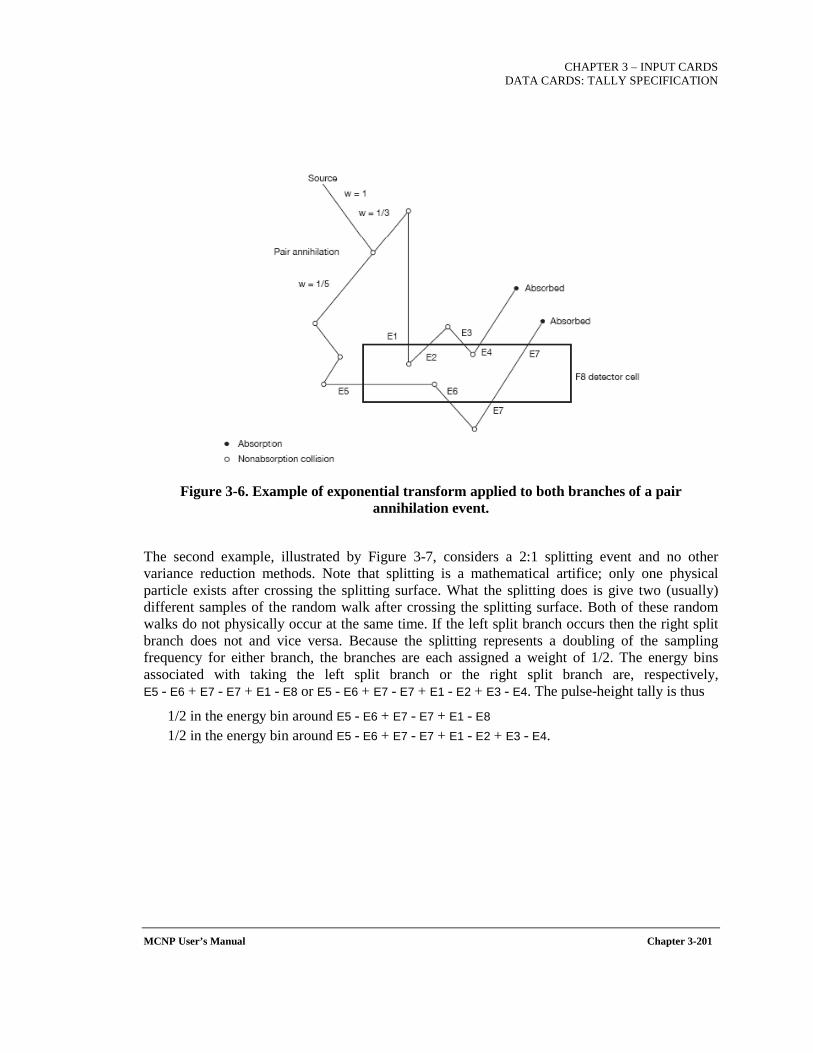
CHAPTER 3 – INPUT CARDS
DATA CARDS: TALLY SPECIFICATION
MCNP User’s Manual Chapter 3-201
Figure 3-6. Example of exponential transform applied to both branches of a pair
annihilation event.
The second example, illustrated by Figure 3-7, considers a 2:1 splitting event and no other variance reduction methods. Note that splitting is a mathematical artifice; only one physical particle exists after crossing the splitting surface. What the splitting does is give two (usually) different samples of the random walk after crossing the splitting surface. Both of these random walks do not physically occur at the same time. If the left split branch occurs then the right split branch does not and vice versa. Because the splitting represents a doubling of the sampling frequency for either branch, the branches are each assigned a weight of 1/2. The energy bins associated with taking the left split branch or the right split branch are, respectively, E5 - E6 + E7 - E7 + E1 - E8 or E5 - E6 + E7 - E7 + E1 - E2 + E3 - E4. The pulse-height tally is thus
1/2 in the energy bin around E5 - E6 + E7 - E7 + E1 - E8 1/2 in the energy bin around E5 - E6 + E7 - E7 + E1 - E2 + E3 - E4.

CHAPTER 3 – INPUT CARDS DATA CARDS: TALLY SPECIFICATION
Chapter 3-202 MCNP User’s Manual
Figure 3-7. Splitting example.
Simple Form: Fn:<pl> s1 ... sk ... T (See Note 1.)
General Form: Fn:<pl> s1 (s2 ... s3) (s4 ... s5) s6 s7 ... T (See Note 1.)
Table 3-81. Pulse-Height Tally Card (F8)
Input Parameter Description
N User-supplied tally number, ending in the numeral 8. Restriction: n≤99999999
<pl> Particle designator. Standard F8 tallies support only “P,E” (if only one of these is specified, it is expanded to include both). Other particle types should only be specified with the FT PHL or CAP options. (See Note 2.)
sj Problem number of cell for tallying, or T for the total across all listed cells..
T Provide average of tally over specified cells.
Note 1: An asterisk on the F8 card converts the tally from a pulse-height tally to an energy deposition tally. A plus on the F8 card converts the tally from a pulse-height tally to a charge deposition tally in units of charge. Energy binning is not recommended with the +F8 tally.
Note 2: Both photons and electrons will be tallied if present, even if only E or only P is on the F8 card. In other words, F8:P, F8:E, and F8:P,E are all equivalent tallies.
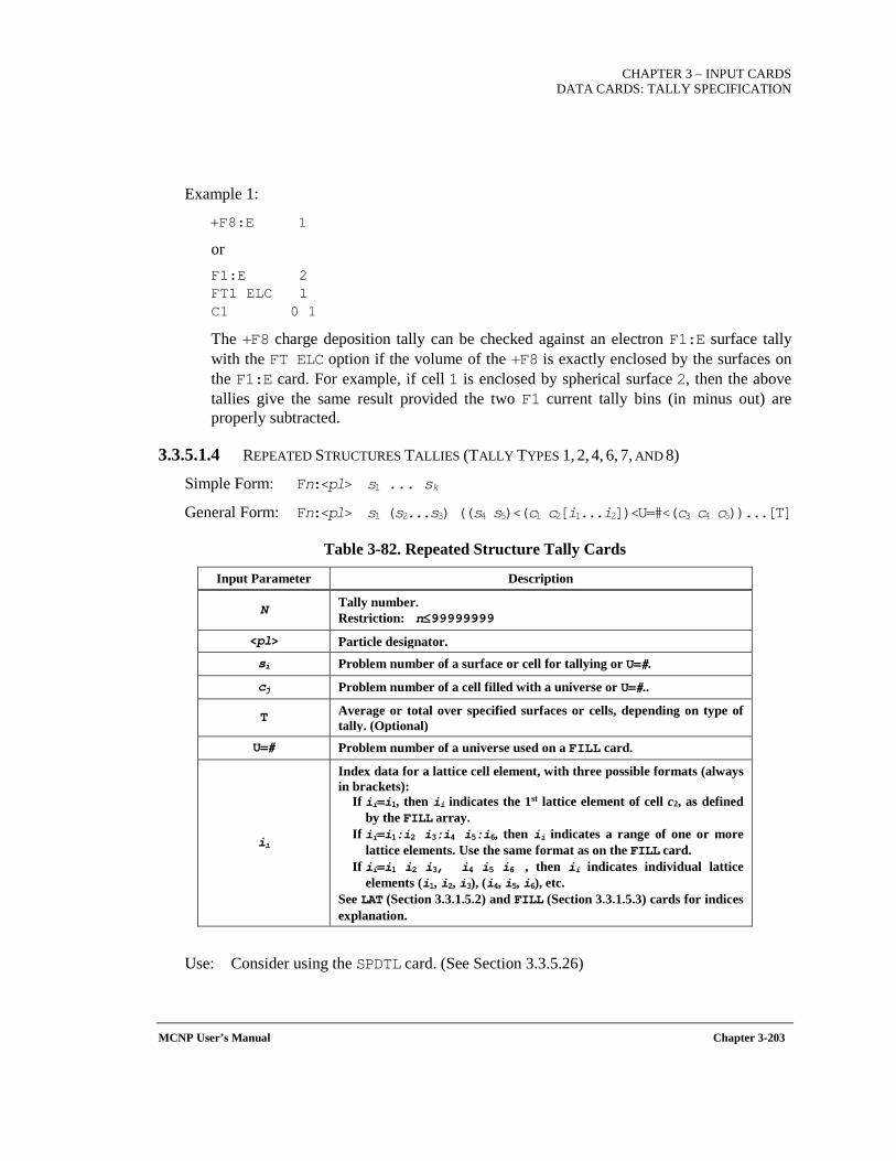
CHAPTER 3 – INPUT CARDS
DATA CARDS: TALLY SPECIFICATION
MCNP User’s Manual Chapter 3-203
Example 1:
+F8:E 1
or F1:E 2 FT1 ELC 1 C1 0 1
The +F8 charge deposition tally can be checked against an electron F1:E surface tally with the FT ELC option if the volume of the +F8 is exactly enclosed by the surfaces on the F1:E card. For example, if cell 1 is enclosed by spherical surface 2, then the above tallies give the same result provided the two F1 current tally bins (in minus out) are properly subtracted.
3.3.5.1.4 REPEATED STRUCTURES TALLIES (TALLY TYPES 1, 2, 4, 6, 7, AND 8)
Simple Form: Fn:<pl> s1 ... sk
General Form: Fn:<pl> s1 (s2...s3) ((s4 s5)<(c1 c2[i1...i2])<U=#<(c3 c4 c5))...[T]
Table 3-82. Repeated Structure Tally Cards
Input Parameter Description
N Tally number. Restriction: n≤99999999
<pl> Particle designator. si Problem number of a surface or cell for tallying or U=#.
cj Problem number of a cell filled with a universe or U=#..
T Average or total over specified surfaces or cells, depending on type of tally. (Optional)
U=# Problem number of a universe used on a FILL card.
ii
Index data for a lattice cell element, with three possible formats (always in brackets):
If ii=i1, then ii indicates the 1st lattice element of cell c2, as defined by the FILL array.
If ii=i1:i2 i3:i4 i5:i6, then ii indicates a range of one or more lattice elements. Use the same format as on the FILL card.
If ii=i1 i2 i3, i4 i5 i6 , then ii indicates individual lattice elements (i1, i2, i3), (i4, i5, i6), etc.
See LAT (Section 3.3.1.5.2) and FILL (Section 3.3.1.5.3) cards for indices explanation.
Use: Consider using the SPDTL card. (See Section 3.3.5.26)
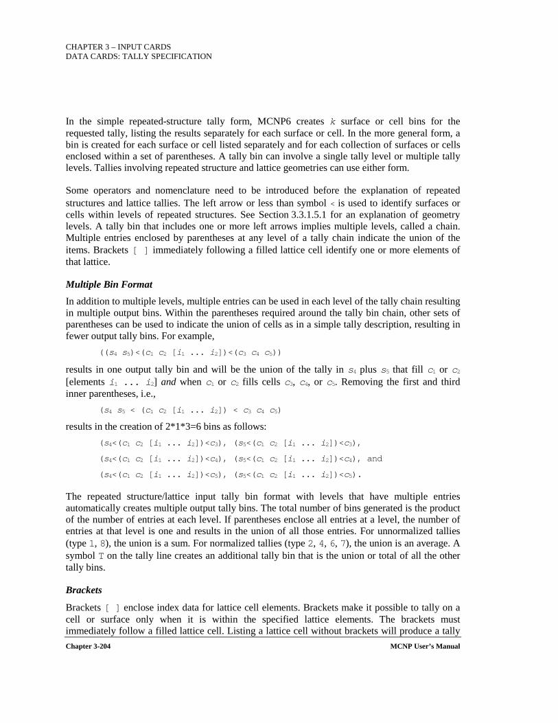
CHAPTER 3 – INPUT CARDS DATA CARDS: TALLY SPECIFICATION
Chapter 3-204 MCNP User’s Manual
In the simple repeated-structure tally form, MCNP6 creates k surface or cell bins for the requested tally, listing the results separately for each surface or cell. In the more general form, a bin is created for each surface or cell listed separately and for each collection of surfaces or cells enclosed within a set of parentheses. A tally bin can involve a single tally level or multiple tally levels. Tallies involving repeated structure and lattice geometries can use either form.
Some operators and nomenclature need to be introduced before the explanation of repeated structures and lattice tallies. The left arrow or less than symbol < is used to identify surfaces or cells within levels of repeated structures. See Section 3.3.1.5.1 for an explanation of geometry levels. A tally bin that includes one or more left arrows implies multiple levels, called a chain. Multiple entries enclosed by parentheses at any level of a tally chain indicate the union of the items. Brackets [ ] immediately following a filled lattice cell identify one or more elements of that lattice.
Multiple Bin Format
In addition to multiple levels, multiple entries can be used in each level of the tally chain resulting in multiple output bins. Within the parentheses required around the tally bin chain, other sets of parentheses can be used to indicate the union of cells as in a simple tally description, resulting in fewer output tally bins. For example,
((s4 s5)<(c1 c2 [i1 ... i2])<(c3 c4 c5))
results in one output tally bin and will be the union of the tally in s4 plus s5 that fill c1 or c2 [elements i1 ... i2] and when c1 or c2 fills cells c3, c4, or c5. Removing the first and third inner parentheses, i.e.,
(s4 s5 < (c1 c2 [i1 ... i2]) < c3 c4 c5)
results in the creation of 2*1*3=6 bins as follows: (s4<(c1 c2 [i1 ... i2])<c3), (s5<(c1 c2 [i1 ... i2])<c3),
(s4<(c1 c2 [i1 ... i2])<c4), (s5<(c1 c2 [i1 ... i2])<c4), and
(s4<(c1 c2 [i1 ... i2])<c5), (s5<(c1 c2 [i1 ... i2])<c5).
The repeated structure/lattice input tally bin format with levels that have multiple entries automatically creates multiple output tally bins. The total number of bins generated is the product of the number of entries at each level. If parentheses enclose all entries at a level, the number of entries at that level is one and results in the union of all those entries. For unnormalized tallies (type 1, 8), the union is a sum. For normalized tallies (type 2, 4, 6, 7), the union is an average. A symbol T on the tally line creates an additional tally bin that is the union or total of all the other tally bins.
Brackets
Brackets [ ] enclose index data for lattice cell elements. Brackets make it possible to tally on a cell or surface only when it is within the specified lattice elements. The brackets must immediately follow a filled lattice cell. Listing a lattice cell without brackets will produce a tally

CHAPTER 3 – INPUT CARDS
DATA CARDS: TALLY SPECIFICATION
MCNP User’s Manual Chapter 3-205
when the tally cell or surface is in any element of the lattice, provided the tally cell or surface fills an entry at all other levels in the chain. The use of brackets is limited to levels after the first "<" symbol in the tally specification.
To tally within lattice elements of a real world (level zero) lattice cell, use the special syntax that follows. Cell 3 contains material 1 and is bounded by four surfaces. The F4 card specifies a tally only in lattice element (0,0,0). This syntax is required because brackets can only follow a < symbol:
3 1 -1.0 -1234 lat=1 . . .
F4:N (3 < 3 [0 0 0])
Universe Format
The universe format, U=#, is a shorthand method of including all cells and lattice elements filled by universe #. This format can be used in any level of the tally chain. The following example illustrates valid shorthand U=# descriptions in the left column. The right column shows the tally after the shorthand has been expanded. Cells 4 and 5 are filled with universe 1.
shorthand expanded F4:N u = 1 4 5 (u = 1) (4 5) (u = 1 < 2 < 3) (4 5 < 2 < 3) ((u = 1) < 2 < 3) ((4 5) < 2 < 3) (1 < u = 1 < 2 < 3) (1 < 4 5 < 2 < 3) (1 < (u = 1) < 2 < 3) (1 < (4 5) < 2 < 3)
In complex geometries, the U=# format should be used sparingly, especially with the multiple bin format. If 100 cells are filled by universe 1 and 10 cells are filled by universe 2, then the tally
F4:N (u = 1 < u = 2) will create 1000 output tally bins.
However,
F4:N ((u = 1) < (u = 2)) will create only one output tally bin.
Example 1: F4:N (5 < 4 < 2 [1 0 0])
This example could specify an F4 tally in cell 5 when it is in cell 4, when cell 4 is in cell 2, which is a lattice, and only in lattice element [1,0,0]. While any cell (lattice, filled, or simple) can be entered as a tally cell (e.g., s1 through s5), only cells filled with a universe can be used in higher levels (e.g., c1 through c5).
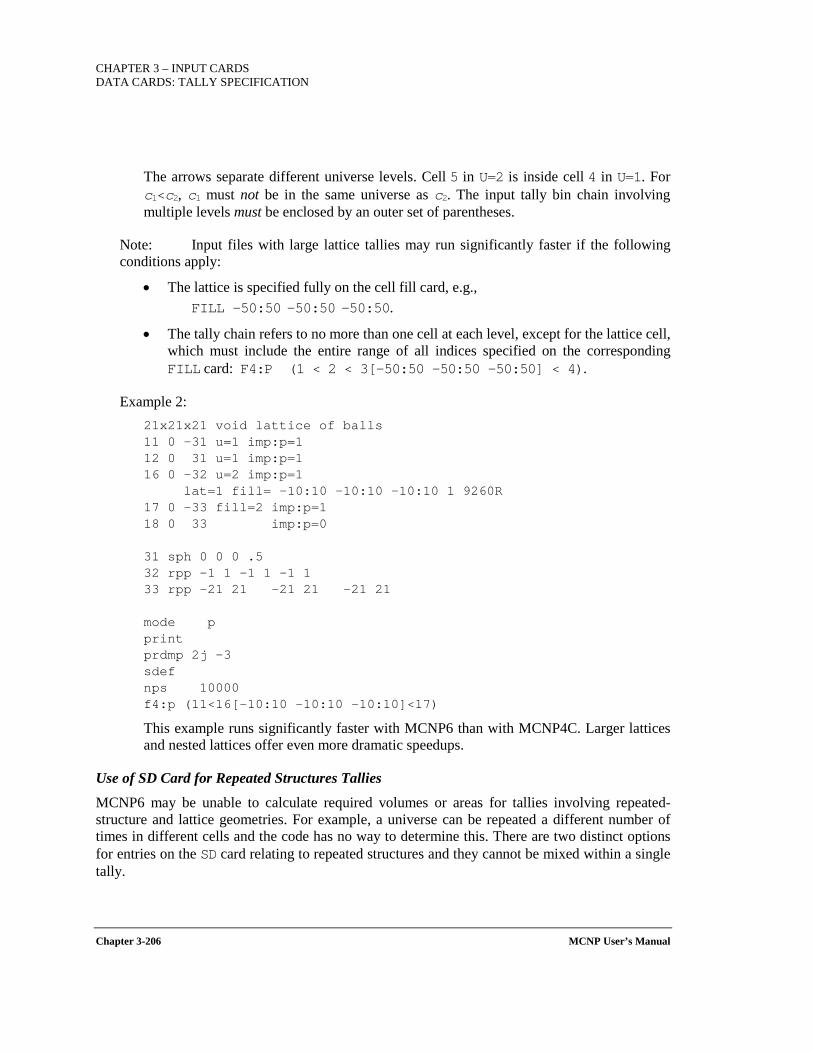
CHAPTER 3 – INPUT CARDS DATA CARDS: TALLY SPECIFICATION
Chapter 3-206 MCNP User’s Manual
The arrows separate different universe levels. Cell 5 in U=2 is inside cell 4 in U=1. For c1<c2, c1 must not be in the same universe as c2. The input tally bin chain involving multiple levels must be enclosed by an outer set of parentheses.
Note: Input files with large lattice tallies may run significantly faster if the following conditions apply:
• The lattice is specified fully on the cell fill card, e.g., FILL -50:50 -50:50 -50:50.
• The tally chain refers to no more than one cell at each level, except for the lattice cell, which must include the entire range of all indices specified on the corresponding FILL card: F4:P (1 < 2 < 3[-50:50 -50:50 -50:50] < 4).
Example 2: 21x21x21 void lattice of balls 11 0 -31 u=1 imp:p=1 12 0 31 u=1 imp:p=1 16 0 -32 u=2 imp:p=1 lat=1 fill= -10:10 -10:10 -10:10 1 9260R 17 0 -33 fill=2 imp:p=1 18 0 33 imp:p=0 31 sph 0 0 0 .5 32 rpp -1 1 -1 1 -1 1 33 rpp -21 21 -21 21 -21 21 mode p print prdmp 2j -3 sdef nps 10000 f4:p (11<16[-10:10 -10:10 -10:10]<17)
This example runs significantly faster with MCNP6 than with MCNP4C. Larger lattices and nested lattices offer even more dramatic speedups.
Use of SD Card for Repeated Structures Tallies
MCNP6 may be unable to calculate required volumes or areas for tallies involving repeated-structure and lattice geometries. For example, a universe can be repeated a different number of times in different cells and the code has no way to determine this. There are two distinct options for entries on the SD card relating to repeated structures and they cannot be mixed within a single tally.
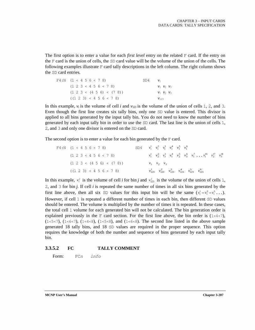
CHAPTER 3 – INPUT CARDS
DATA CARDS: TALLY SPECIFICATION
MCNP User’s Manual Chapter 3-207
The first option is to enter a value for each first level entry on the related F card. If the entry on the F card is the union of cells, the SD card value will be the volume of the union of the cells. The following examples illustrate F card tally descriptions in the left column. The right column shows the SD card entries.
F4:N (1 < 4 5 6 < 7 8) SD4 v1 (1 2 3 < 4 5 6 < 7 8) v1 v2 v3 (1 2 3 < (4 5 6) < (7 8)) v1 v2 v3 ((1 2 3) < 4 5 6 < 7 8) v123
In this example, vi is the volume of cell i and v123 is the volume of the union of cells 1, 2, and 3. Even though the first line creates six tally bins, only one SD value is entered. This divisor is applied to all bins generated by the input tally bin. You do not need to know the number of bins generated by each input tally bin in order to use the SD card. The last line is the union of cells 1, 2, and 3 and only one divisor is entered on the SD card.
The second option is to enter a value for each bin generated by the F card.
F4:N (1 < 4 5 6 < 7 8) SD4
(1 2 3 < 4 5 6 < 7 8) ...
(1 2 3 < (4 5 6) < (7 8))
((1 2 3) < 4 5 6 < 7 8)
In this example, is the volume of cell i for bin j and is the volume of the union of cells 1, 2, and 3 for bin j. If cell i is repeated the same number of times in all six bins generated by the first line above, then all six SD values for this input bin will be the same ( = = ...). However, if cell 1 is repeated a different number of times in each bin, then different SD values should be entered. The volume is multiplied by the number of times it is repeated. In these cases, the total cell 1 volume for each generated bin will not be calculated. The bin generation order is explained previously in the F card section. For the first line above, the bin order is (1<4<7), (1<5<7), (1<6<7), (1<4<8), (1<5<8), and (1<6<8). The second line listed in the above sample generated 18 tally bins, and 18 SD values are required in the proper sequence. This option requires the knowledge of both the number and sequence of bins generated by each input tally bin.
3.3.5.2 FC TALLY COMMENT
Form: FCn info
11v 2
1v 31v 4
1v 51v 6
1v11v 2
2v 33v 4
1v 52v 6
3v 71v 16
1v 172v 18
3v
1v 2v 3v1123v 2
123v 3123v 4
123v 5123v 6
123v
jiv jv123
11v 2
1v 31v
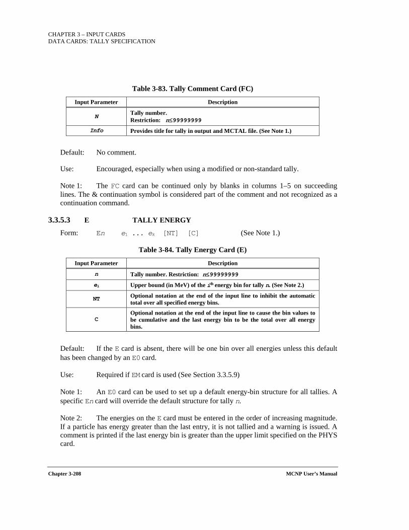
CHAPTER 3 – INPUT CARDS DATA CARDS: TALLY SPECIFICATION
Chapter 3-208 MCNP User’s Manual
Table 3-83. Tally Comment Card (FC)
Input Parameter Description
N Tally number. Restriction: n≤99999999
Info Provides title for tally in output and MCTAL file. (See Note 1.)
Default: No comment.
Use: Encouraged, especially when using a modified or non-standard tally.
Note 1: The FC card can be continued only by blanks in columns 1–5 on succeeding lines. The & continuation symbol is considered part of the comment and not recognized as a continuation command.
3.3.5.3 E TALLY ENERGY
Form: En e1 ... ek [NT] [C] (See Note 1.)
Table 3-84. Tally Energy Card (E)
Input Parameter Description
n Tally number. Restriction: n≤99999999
ei Upper bound (in MeV) of the ith energy bin for tally n. (See Note 2.)
NT Optional notation at the end of the input line to inhibit the automatic total over all specified energy bins.
C Optional notation at the end of the input line to cause the bin values to be cumulative and the last energy bin to be the total over all energy bins.
Default: If the E card is absent, there will be one bin over all energies unless this default has been changed by an E0 card.
Use: Required if EM card is used (See Section 3.3.5.9)
Note 1: An E0 card can be used to set up a default energy-bin structure for all tallies. A specific En card will override the default structure for tally n.
Note 2: The energies on the E card must be entered in the order of increasing magnitude. If a particle has energy greater than the last entry, it is not tallied and a warning is issued. A comment is printed if the last energy bin is greater than the upper limit specified on the PHYS card.
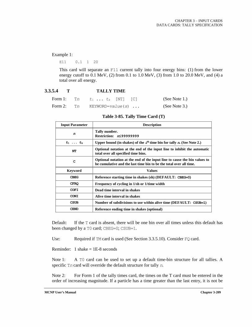
CHAPTER 3 – INPUT CARDS
DATA CARDS: TALLY SPECIFICATION
MCNP User’s Manual Chapter 3-209
Example 1: E11 0.1 1 20
This card will separate an F11 current tally into four energy bins: (1) from the lower energy cutoff to 0.1 MeV, (2) from 0.1 to 1.0 MeV, (3) from 1.0 to 20.0 MeV, and (4) a total over all energy.
3.3.5.4 T TALLY TIME
Form 1: Tn t1 ... tk [NT] [C] (See Note 1.) Form 2: Tn KEYWORD=value(s) ... (See Note 3.)
Table 3-85. Tally Time Card (T)
Input Parameter Description
n Tally number. Restriction: n≤99999999
t1 ... tk Upper bound (in shakes) of the ith time bin for tally n. (See Note 2.)
NT Optional notation at the end of the input line to inhibit the automatic total over all specified time bins.
C Optional notation at the end of the input line to cause the bin values to be cumulative and the last time bin to be the total over all time.
Keyword Values
CBEG Reference starting time in shakes (sh) (DEFAULT: CBEG=0)
CFRQ Frequency of cycling in 1/sh or 1/time width COFI Dead time interval in shakes CONI Alive time interval in shakes CSUB Number of subdivisions to use within alive time (DEFAULT: CSUB=1)
CEND Reference ending time in shakes (optional)
Default: If the T card is absent, there will be one bin over all times unless this default has been changed by a T0 card; CBEG=0; CSUB=1.
Use: Required if TM card is used (See Section 3.3.5.10). Consider FQ card.
Reminder: 1 shake = 1E-8 seconds
Note 1: A T0 card can be used to set up a default time-bin structure for all tallies. A specific Tn card will override the default structure for tally n.
Note 2: For Form 1 of the tally times card, the times on the T card must be entered in the order of increasing magnitude. If a particle has a time greater than the last entry, it is not be
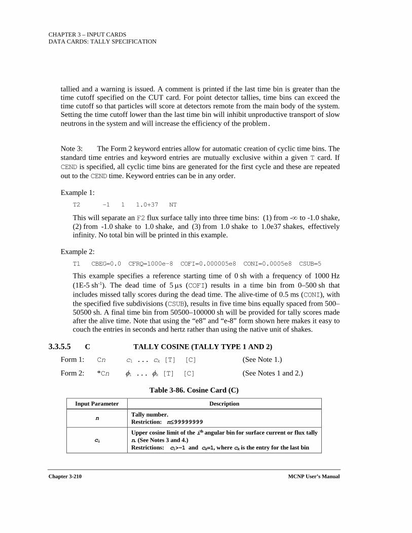
CHAPTER 3 – INPUT CARDS DATA CARDS: TALLY SPECIFICATION
Chapter 3-210 MCNP User’s Manual
tallied and a warning is issued. A comment is printed if the last time bin is greater than the time cutoff specified on the CUT card. For point detector tallies, time bins can exceed the time cutoff so that particles will score at detectors remote from the main body of the system. Setting the time cutoff lower than the last time bin will inhibit unproductive transport of slow neutrons in the system and will increase the efficiency of the problem.
Note 3: The Form 2 keyword entries allow for automatic creation of cyclic time bins. The standard time entries and keyword entries are mutually exclusive within a given T card. If CEND is specified, all cyclic time bins are generated for the first cycle and these are repeated out to the CEND time. Keyword entries can be in any order.
Example 1: T2 -1 1 1.0+37 NT
This will separate an F2 flux surface tally into three time bins: (1) from -∞ to -1.0 shake, (2) from -1.0 shake to 1.0 shake, and (3) from 1.0 shake to 1.0e37 shakes, effectively infinity. No total bin will be printed in this example.
Example 2: T1 CBEG=0.0 CFRQ=1000e-8 COFI=0.000005e8 CONI=0.0005e8 CSUB=5
This example specifies a reference starting time of 0 sh with a frequency of 1000 Hz (1E-5 sh-1). The dead time of 5 µs (COFI) results in a time bin from 0–500 sh that includes missed tally scores during the dead time. The alive-time of 0.5 ms (CONI), with the specified five subdivisions (CSUB), results in five time bins equally spaced from 500–50500 sh. A final time bin from 50500–100000 sh will be provided for tally scores made after the alive time. Note that using the “e8” and “e-8” form shown here makes it easy to couch the entries in seconds and hertz rather than using the native unit of shakes.
3.3.5.5 C TALLY COSINE (TALLY TYPE 1 AND 2)
Form 1: Cn c1 ... ck [T] [C] (See Note 1.)
Form 2: *Cn φ1 ... φk [T] [C] (See Notes 1 and 2.)
Table 3-86. Cosine Card (C)
Input Parameter Description
n Tally number. Restriction: n≤99999999
ci Upper cosine limit of the ith angular bin for surface current or flux tally n. (See Notes 3 and 4.) Restrictions: c1>-1 and ck=1, where ck is the entry for the last bin

CHAPTER 3 – INPUT CARDS
DATA CARDS: TALLY SPECIFICATION
MCNP User’s Manual Chapter 3-211
φi Upper angular limit of the ith angular bin for surface current or flux tally n. expressed in degrees. (See Notes 3 and 4.) Restrictions: φ1<180 and φk=0, where φk is the entry for the last bin
T Optional notation at the end of the input line to provide the total over all specified angular bins.
C Optional notation at the end of the input line to cause the bin values to be cumulative and the last angular bin to be the total over all angles.
Default: If the C card is absent, there will be one bin over all angles unless this default has been changed by a C0 card.
Use: For use with tally types 1 and 2 only. Required if CM card is used. Consider FQ card.
Note 1: A C0 card can be used to set up a default angular bin structure for all tallies. A specific Cn card will override the default structure for tally n. The selection of a single cosine bin for an F1 tally gives the total and not the net current crossing a surface.
Note 2: The asterisk (*) on the Cn card causes the entries to be interpreted as degrees.
Note 3: Whether entered as degrees or cosines, the entries on the C card must be such that the cosine is monotonically increasing, beginning with the cosine of the largest angle less than 180° to the normal and ending with the normal (i.e., cos=1). A lower cosine bound of -1 is set in the code and should not be entered on the card.
Note 4: The angular limits described by the C card are defined with respect to the positive normal to the surface at the particle point of entry. An FT card with an FRV v1 v2 v3 option can be used to make the cosine bins relative to the vector u,v,w. The positive normal to the surface is always in the direction of a cell that has positive sense with respect to that surface.
Example 1: C1 -0.866 -0.5 0 0.5 0.866 1
*C1 150 120 90 60 30 0
Either card will tally currents within the following angular limits (1) 180° to 150°, (2) 150° to 120°, (3) 120° to 90°, (4) 90° to 60°, (5) 60° to 30°, and (6) 30° to 0° with respect to the positive normal. No total will be provided.
Example 2:
As an example of the relationship between a surface normal and sense for the C1 card, consider a source at the origin of a coordinate system and a plane (PY) intersecting the +y axis. An entry of 0 and 1 on the C1 card will tally all source particles transmitted through the plane in the 0 to 1 cosine bin (0° to 90°) and all particles scattered back across the
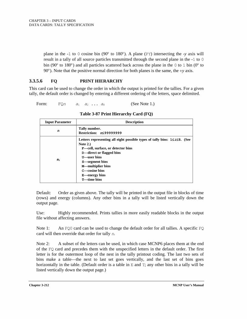
CHAPTER 3 – INPUT CARDS DATA CARDS: TALLY SPECIFICATION
Chapter 3-212 MCNP User’s Manual
plane in the -1 to 0 cosine bin (90° to 180°). A plane (PY) intersecting the -y axis will result in a tally of all source particles transmitted through the second plane in the -1 to 0 bin (90° to 180°) and all particles scattered back across the plane in the 0 to 1 bin (0° to 90°). Note that the positive normal direction for both planes is the same, the +y axis.
3.3.5.6 FQ PRINT HIERARCHY
This card can be used to change the order in which the output is printed for the tallies. For a given tally, the default order is changed by entering a different ordering of the letters, space delimited.
Form: FQn a1 a2 ... a8 (See Note 1.)
Table 3-87 Print Hierarchy Card (FQ)
Input Parameter Description
n Tally number. Restriction: n≤99999999
ai
Letters representing all eight possible types of tally bins: 1≤i≤8. (See Note 2.) F—cell, surface, or detector bins D—direct or flagged bins U—user bins S—segment bins M—multiplier bins C—cosine bins E—energy bins T—time bins
Default: Order as given above. The tally will be printed in the output file in blocks of time (rows) and energy (columns). Any other bins in a tally will be listed vertically down the output page.
Use: Highly recommended. Prints tallies in more easily readable blocks in the output file without affecting answers.
Note 1: An FQ0 card can be used to change the default order for all tallies. A specific FQ card will then override that order for tally n.
Note 2: A subset of the letters can be used, in which case MCNP6 places them at the end of the FQ card and precedes them with the unspecified letters in the default order. The first letter is for the outermost loop of the nest in the tally printout coding. The last two sets of bins make a table—the next to last set goes vertically, and the last set of bins goes horizontally in the table. (Default order is a table in E and T; any other bins in a tally will be listed vertically down the output page.)
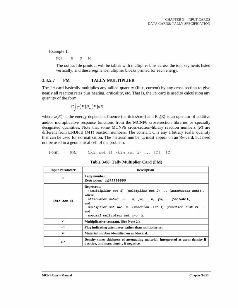
CHAPTER 3 – INPUT CARDS
DATA CARDS: TALLY SPECIFICATION
MCNP User’s Manual Chapter 3-213
Example 1: FQ4 E S M
The output file printout will be tables with multiplier bins across the top, segments listed vertically, and these segment-multiplier blocks printed for each energy.
3.3.5.7 FM TALLY MULTIPLIER
The FM card basically multiplies any tallied quantity (flux, current) by any cross section to give nearly all reaction rates plus heating, criticality, etc. That is, the FM card is used to calculation any quantity of the form
,
where is the energy-dependent fluence (particles/cm2) and Rm(E) is an operator of additive and/or multiplicative response functions from the MCNP6 cross-section libraries or specially designated quantities. Note that some MCNP6 cross-section-library reaction numbers (R) are different from ENDF/B (MT) reaction numbers. The constant C is any arbitrary scalar quantity that can be used for normalization. The material number m must appear on an Mm card, but need not be used in a geometrical cell of the problem.
Form: FMn (bin set 1) (bin set 2) ... [T] [C]
Table 3-88. Tally Multiplier Card (FM)
Input Parameter Description
n Tally number. Restriction: n≤99999999
(bin set i)
Represents ((multiplier set 1) (multiplier set 2) ... (attenuator set)) ,
where attenuator set=c -1 m1 px1 m2 px2 ... (See Note 1.)
and multiplier set i=c m (reaction list 1) (reaction list 2) ...
and special multiplier set i=c k.
c Multiplicative constant. (See Note 2.) -1 Flag indicating attenuator rather than multiplier set. m Material number identified on an Mm card.
px Density times thickness of attenuating material; interpreted as atom density if positive, and mass density if negative.
( ) ( )∫ dEEREC mϕ
( )Eϕ
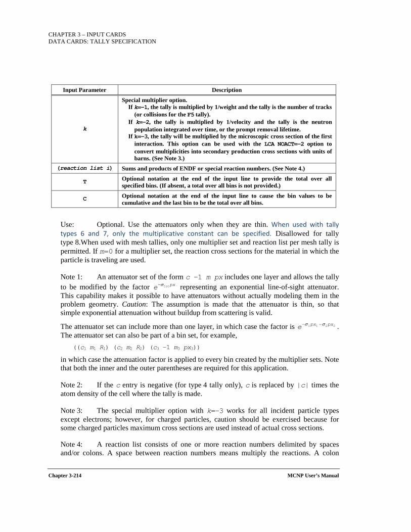
CHAPTER 3 – INPUT CARDS DATA CARDS: TALLY SPECIFICATION
Chapter 3-214 MCNP User’s Manual
Input Parameter Description
k
Special multiplier option. If k=-1, the tally is multiplied by 1/weight and the tally is the number of tracks
(or collisions for the F5 tally). If k=-2, the tally is multiplied by 1/velocity and the tally is the neutron
population integrated over time, or the prompt removal lifetime. If k=-3, the tally will be multiplied by the microscopic cross section of the first
interaction. This option can be used with the LCA NOACT=-2 option to convert multiplicities into secondary production cross sections with units of barns. (See Note 3.)
(reaction list i) Sums and products of ENDF or special reaction numbers. (See Note 4.)
T Optional notation at the end of the input line to provide the total over all specified bins. (If absent, a total over all bins is not provided.)
C Optional notation at the end of the input line to cause the bin values to be cumulative and the last bin to be the total over all bins.
Use: Optional. Use the attenuators only when they are thin. When used with tally types 6 and 7, only the multiplicative constant can be specified. Disallowed for tally type 8.When used with mesh tallies, only one multiplier set and reaction list per mesh tally is permitted. If m=0 for a multiplier set, the reaction cross sections for the material in which the particle is traveling are used.
Note 1: An attenuator set of the form c −1 m px includes one layer and allows the tally to be modified by the factor representing an exponential line-of-sight attenuator. This capability makes it possible to have attenuators without actually modeling them in the problem geometry. Caution: The assumption is made that the attenuator is thin, so that simple exponential attenuation without buildup from scattering is valid.
The attenuator set can include more than one layer, in which case the factor is . The attenuator set can also be part of a bin set, for example,
((c1 m1 R1) (c2 m2 R2) (c3 −1 m3 px3))
in which case the attenuation factor is applied to every bin created by the multiplier sets. Note that both the inner and the outer parentheses are required for this application.
Note 2: If the c entry is negative (for type 4 tally only), c is replaced by |c| times the atom density of the cell where the tally is made.
Note 3: The special multiplier option with k=-3 works for all incident particle types except electrons; however, for charged particles, caution should be exercised because for some charged particles maximum cross sections are used instead of actual cross sections.
Note 4: A reaction list consists of one or more reaction numbers delimited by spaces and/or colons. A space between reaction numbers means multiply the reactions. A colon
pxtote σ−
2211 pxpxe σσ −−

CHAPTER 3 – INPUT CARDS
DATA CARDS: TALLY SPECIFICATION
MCNP User’s Manual Chapter 3-215
means add the reactions. The hierarchy of operation is multiply first and then add. One bin is created for each reaction list. No parentheses are allowed within the reaction list.
The reaction cross sections are microscopic (with units of barns) and not macroscopic. Therefore, if the constant c is the atomic density (in atoms/barn-cm), the results will include the normalization "per cm3."
Any number of ENDF/B (MT) or special (R) reactions can be used in a multiplier set as long as they are present in the MCNP6 cross-section libraries, or in special libraries of dosimetry data. If neither a material number nor any reactions are given, the tally simply is multiplied by the constant c.
Use of Parentheses:
1. If a given multiplier set contains only one reaction list, the parentheses surrounding the reaction list can be omitted. Parentheses within a reaction list are forbidden.
2. If a given bin set consists of more than a single multiplier or attenuator set, each multiplier or attenuator set must be surrounded by parentheses, and the combination must also be surrounded by parentheses.
3. If the FM card consists only of a single bin set, and that bin set consists only of a single multiplier or attenuator bin, surrounding parentheses can be omitted.
Special Reaction Numbers:
In addition to the standard ENDF reaction numbers (e.g., MT=1, 2, and 16, representing σtot, σel, and σn,2n, respectively), Table 3-89 lists the non-standard special R numbers that may be used.
Table 3-89. ENDF/B Special Reaction Numbers
Reaction Type Special Reaction Number (R) Microscopic Cross-Section Description
Neutron -1 Total cross section without thermal
-2 Absorption cross section
-3 Elastic cross section without thermal
-4 Average neutron heating number (MeV/collision)
-5 Gamma-ray production cross section , barns
-6 Total fission cross section
-7 Fission , prompt or total
-8 Fission Q (MeV/fission)
Many Nuclides -4 Average heating numbers (MeV/collision)
-5 Gamma-ray production cross section, barns
ν
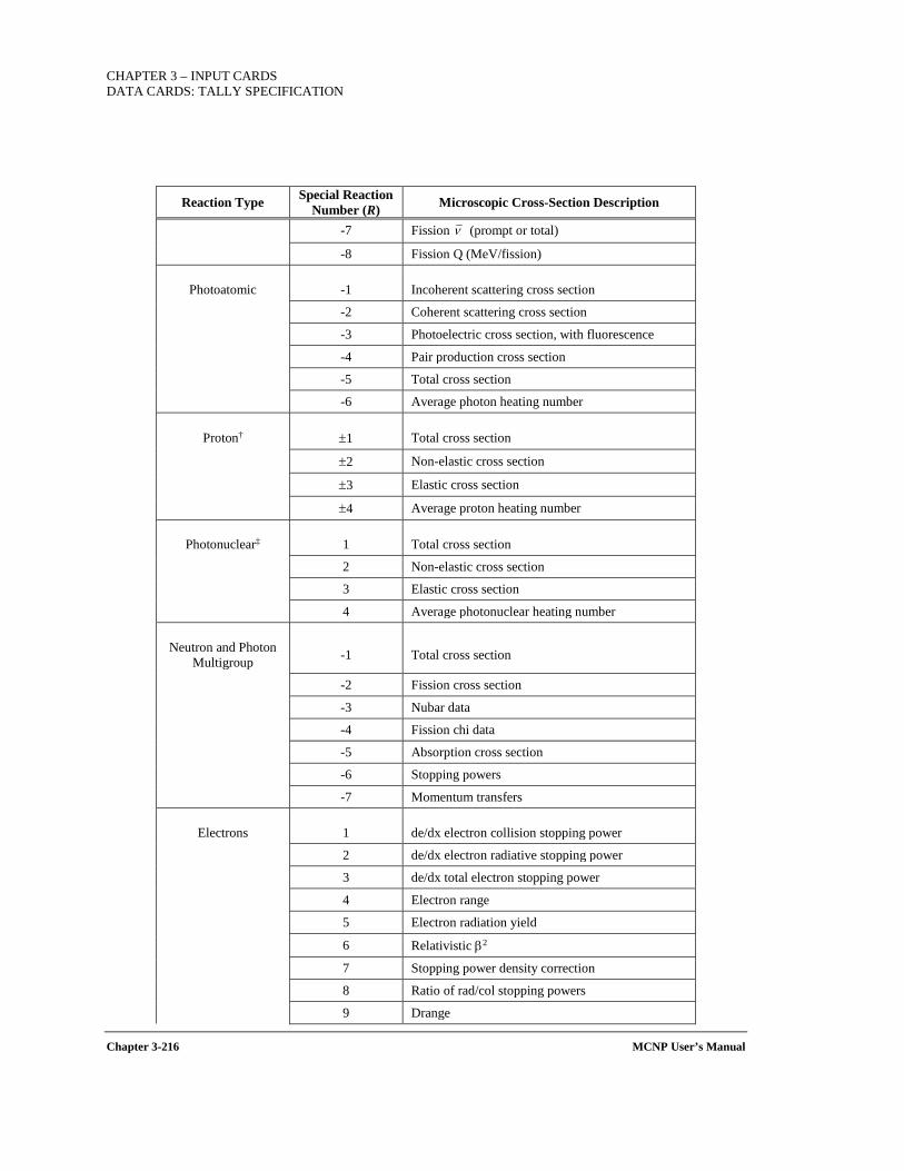
CHAPTER 3 – INPUT CARDS DATA CARDS: TALLY SPECIFICATION
Chapter 3-216 MCNP User’s Manual
Reaction Type Special Reaction Number (R) Microscopic Cross-Section Description
-7 Fission (prompt or total)
-8 Fission Q (MeV/fission)
Photoatomic -1 Incoherent scattering cross section
-2 Coherent scattering cross section
-3 Photoelectric cross section, with fluorescence
-4 Pair production cross section
-5 Total cross section
-6 Average photon heating number
Proton† ±1 Total cross section
±2 Non-elastic cross section
±3 Elastic cross section
±4 Average proton heating number
Photonuclear‡ 1 Total cross section
2 Non-elastic cross section
3 Elastic cross section
4 Average photonuclear heating number
Neutron and Photon Multigroup -1 Total cross section
-2 Fission cross section
-3 Nubar data
-4 Fission chi data
-5 Absorption cross section
-6 Stopping powers
-7 Momentum transfers
Electrons 1 de/dx electron collision stopping power
2 de/dx electron radiative stopping power
3 de/dx total electron stopping power
4 Electron range
5 Electron radiation yield
6 Relativistic β2
7 Stopping power density correction
8 Ratio of rad/col stopping powers
9 Drange
ν
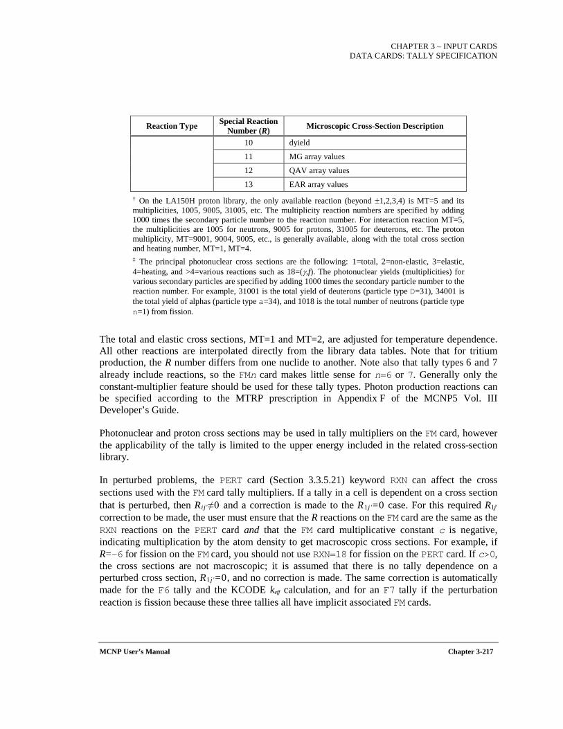
CHAPTER 3 – INPUT CARDS
DATA CARDS: TALLY SPECIFICATION
MCNP User’s Manual Chapter 3-217
Reaction Type Special Reaction Number (R) Microscopic Cross-Section Description
10 dyield
11 MG array values
12 QAV array values
13 EAR array values † On the LA150H proton library, the only available reaction (beyond ±1,2,3,4) is MT=5 and its multiplicities, 1005, 9005, 31005, etc. The multiplicity reaction numbers are specified by adding 1000 times the secondary particle number to the reaction number. For interaction reaction MT=5, the multiplicities are 1005 for neutrons, 9005 for protons, 31005 for deuterons, etc. The proton multiplicity, MT=9001, 9004, 9005, etc., is generally available, along with the total cross section and heating number, MT=1, MT=4. ‡ The principal photonuclear cross sections are the following: 1=total, 2=non-elastic, 3=elastic, 4=heating, and >4=various reactions such as 18=(γ,f). The photonuclear yields (multiplicities) for various secondary particles are specified by adding 1000 times the secondary particle number to the reaction number. For example, 31001 is the total yield of deuterons (particle type D=31), 34001 is the total yield of alphas (particle type a=34), and 1018 is the total number of neutrons (particle type n=1) from fission.
The total and elastic cross sections, MT=1 and MT=2, are adjusted for temperature dependence. All other reactions are interpolated directly from the library data tables. Note that for tritium production, the R number differs from one nuclide to another. Note also that tally types 6 and 7 already include reactions, so the FMn card makes little sense for n=6 or 7. Generally only the constant-multiplier feature should be used for these tally types. Photon production reactions can be specified according to the MTRP prescription in Appendix F of the MCNP5 Vol. III Developer’s Guide.
Photonuclear and proton cross sections may be used in tally multipliers on the FM card, however the applicability of the tally is limited to the upper energy included in the related cross-section library.
In perturbed problems, the PERT card (Section 3.3.5.21) keyword RXN can affect the cross sections used with the FM card tally multipliers. If a tally in a cell is dependent on a cross section that is perturbed, then Rij'≠0 and a correction is made to the R1 j '=0 case. For this required R1j′ correction to be made, the user must ensure that the R reactions on the FM card are the same as the RXN reactions on the PERT card and that the FM card multiplicative constant c is negative, indicating multiplication by the atom density to get macroscopic cross sections. For example, if R=–6 for fission on the FM card, you should not use RXN=18 for fission on the PERT card. If c>0, the cross sections are not macroscopic; it is assumed that there is no tally dependence on a perturbed cross section, R1 j '=0, and no correction is made. The same correction is automatically made for the F6 tally and the KCODE keff calculation, and for an F7 tally if the perturbation reaction is fission because these three tallies all have implicit associated FM cards.
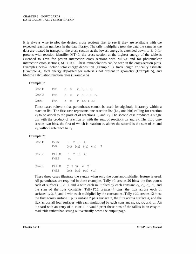
CHAPTER 3 – INPUT CARDS DATA CARDS: TALLY SPECIFICATION
Chapter 3-218 MCNP User’s Manual
It is always wise to plot the desired cross sections first to see if they are available with the expected reaction numbers in the data library. The tally multipliers treat the data the same as the data are treated in transport: the cross section at the lowest energy is extended down to E=0 for protons with reaction identifier MT<0; the cross section at the highest energy of the table is extended to E=∞ for proton interaction cross sections with MT<0; and for photonuclear interaction cross sections, MT<1000. These extrapolations can be seen in the cross-section plots. Examples below include total energy deposition (Example 3), track length criticality estimate (Example 4), total energy deposited for materials not present in geometry (Example 5), and lifetime calculation/reaction rates (Example 6).
Example 1:
Case 1: FMn c m r1 r2 : r3
Case 2: FMn c m r1 r2 : r1 r3
Case3: FMn c m r1 (r2 : r3)
These cases reiterate that parentheses cannot be used for algebraic hierarchy within a reaction list. The first case represents one reaction list (i.e., one bin) calling for reaction r3 to be added to the product of reactions r1 and r2. The second case produces a single bin with the product of reaction r1 with the sum of reactions r2 and r3. The third case creates two bins, the first of which is reaction r1 alone; the second is the sum of r2 and r3, without reference to r1.
Example 2: Case 1: F2:N 1 2 3 4 FM2 (c1) (c2) (c3) (c4) T
Case 2: F12:N 1 2 3 4 FM12 c1
Case 3: F22:N (1 2 3) 4 T FM22 (c1) (c2) (c3) (c4)
These three cases illustrate the syntax when only the constant-multiplier feature is used. All parentheses are required in these examples. Tally F2 creates 20 bins: the flux across each of surfaces 1, 2, 3, and 4 with each multiplied by each constant c1, c2, c3, c4, and the sum of the four constants. Tally F12 creates 4 bins: the flux across each of surfaces 1, 2, 3, and 4 with each multiplied by the constant c1. Tally F22 creates 12 bins: the flux across surface 1 plus surface 2 plus surface 3, the flux across surface 4, and the flux across all four surfaces with each multiplied by each constant c1, c2, c3, and c4. An FQ card with an entry of F M or M F would print these bins of the tallies in an easy-to-read table rather than strung out vertically down the output page.
CHAPTER 3 – INPUT CARDS
DATA CARDS: TALLY SPECIFICATION
MCNP User’s Manual Chapter 3-219
Example 3 (Total Energy Deposition): F4:P 1 FM4 -1 2 -5 -6 SD4 1 F6:P 1 SD6 1
Multiplying the photon flux by volume (SD4 1) times the atom density (-1) for material 2 times the photon total cross section (-5) times the photon heating number (-6) is the same as the F6:P photon heating tally multiplied by mass (SD6 1), namely the total energy deposition in cell 1. Note that positive photon reaction numbers are photonuclear reactions. Note also that the SD card replaces the normal divisor (volume for F4 and mass for F6) with new values (both 1 in this example). By overriding the MCNP6-computed cell volume and mass with values of 1, you effectively multiply the unmodified F4 and F6 tallies by the volume and mass, respectively, yielding the score for the entire cell.
Example 4 (Track Length Criticality Estimate): F4:n 1 FM4 -1 3 -6 -7 SD4 1
Multiplying the neutron flux by volume (SD4 1) times the atom density (-1) for material 3 times the fission multiplicity, (-7), times the fission cross section (-6) gives the track-length estimate of criticality for cell 1.
Example 5 (Total Energy Deposited for Materials Not Present in Geometry):
Using MCNP6 tallies, there are two ways to obtain the energy deposited in a material in terms of rads (1 rad=100 ergs/g). When the actual material of interest is present in the MCNP6 model, the simplest way is to use the heating tally with units MeV/g in conjunction with c=1.602E-08 on the companion FM card, where c=(1.602E-06 ergs/MeV)/(100 ergs/g). When the material is not present in the model, rads can be obtained from type 1, 2, 4, and 5 tallies by using an FM card where c is equal to the factor above times Noη×10-24/A, where No is Avogadro’s number and η and A are the number of atoms/molecule and the atomic weight, respectively, of the material of interest. This value of c equals ρa/ρg as discussed in Section 5.3.4 of the MCNP5 Theory Manual[X-503a]. The implicit assumption when the material is not present is that it does not affect the radiation transport significantly. In the reaction list on the FM card, you must enter -4 1 for neutron heating and -5 -6 for photon heating. For both F4 and F6, if a heating number from the data library is negative, it is set to zero by the code.
ν
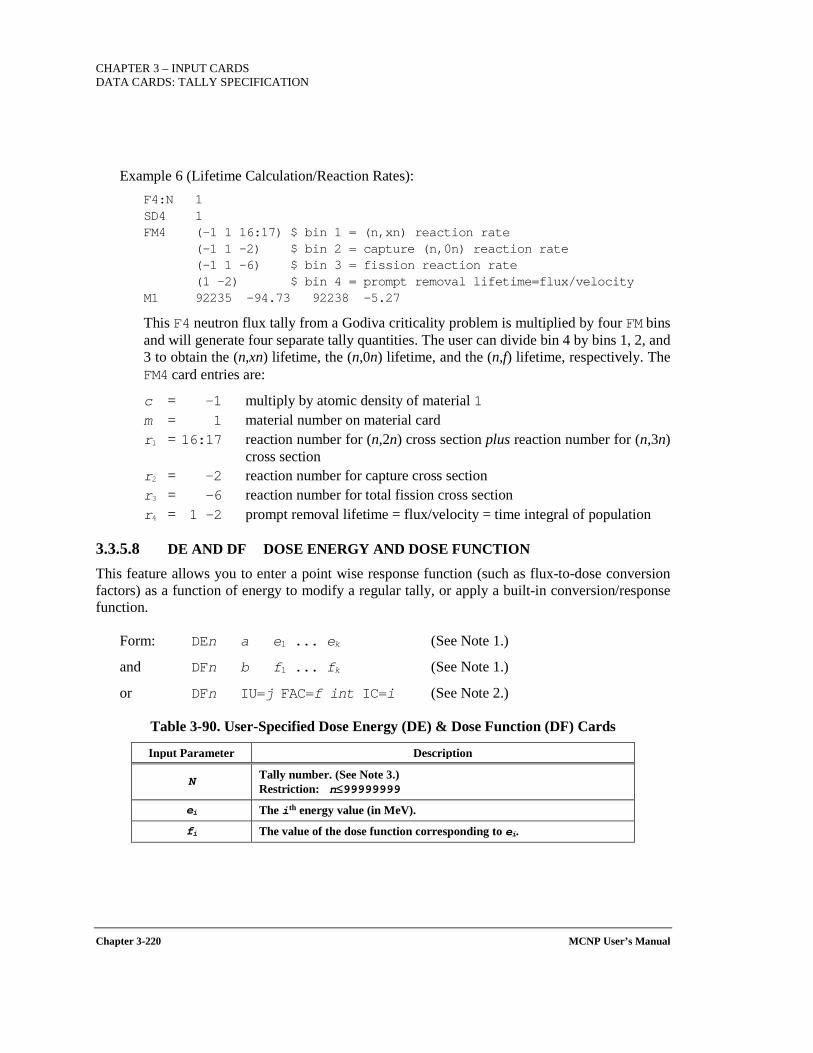
CHAPTER 3 – INPUT CARDS DATA CARDS: TALLY SPECIFICATION
Chapter 3-220 MCNP User’s Manual
Example 6 (Lifetime Calculation/Reaction Rates): F4:N 1 SD4 1 FM4 (-1 1 16:17) $ bin 1 = (n,xn) reaction rate (-1 1 -2) $ bin 2 = capture (n,0n) reaction rate (-1 1 -6) $ bin 3 = fission reaction rate (1 -2) $ bin 4 = prompt removal lifetime=flux/velocity M1 92235 –94.73 92238 –5.27
This F4 neutron flux tally from a Godiva criticality problem is multiplied by four FM bins and will generate four separate tally quantities. The user can divide bin 4 by bins 1, 2, and 3 to obtain the (n,xn) lifetime, the (n,0n) lifetime, and the (n,f) lifetime, respectively. The FM4 card entries are:
c = −1 multiply by atomic density of material 1 m = 1 material number on material card r1 = 16:17 reaction number for (n,2n) cross section plus reaction number for (n,3n)
cross section r2 = −2 reaction number for capture cross section r3 = –6 reaction number for total fission cross section r4 = 1 -2 prompt removal lifetime = flux/velocity = time integral of population
3.3.5.8 DE AND DF DOSE ENERGY AND DOSE FUNCTION
This feature allows you to enter a point wise response function (such as flux-to-dose conversion factors) as a function of energy to modify a regular tally, or apply a built-in conversion/response function.
Form: DEn a e1 ... ek (See Note 1.)
and DFn b f1 ... fk (See Note 1.)
or DFn IU=j FAC=f int IC=i (See Note 2.)
Table 3-90. User-Specified Dose Energy (DE) & Dose Function (DF) Cards
Input Parameter Description
N Tally number. (See Note 3.) Restriction: n≤99999999
ei The ith energy value (in MeV).
fi The value of the dose function corresponding to ei.
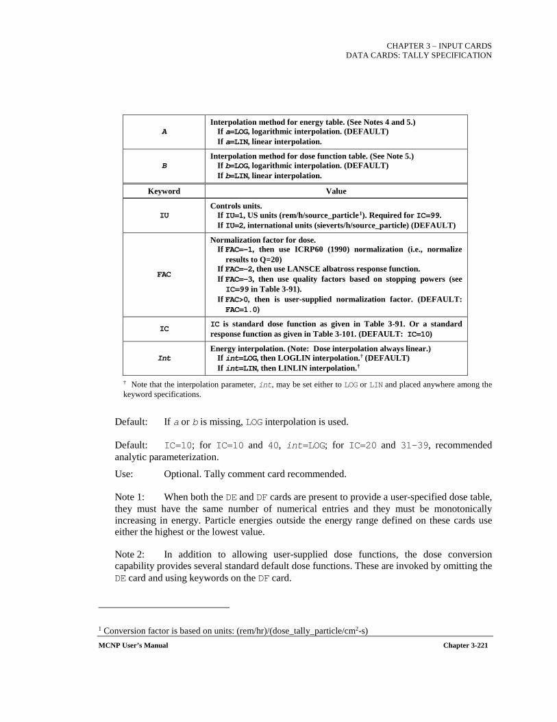
CHAPTER 3 – INPUT CARDS
DATA CARDS: TALLY SPECIFICATION
MCNP User’s Manual Chapter 3-221
A Interpolation method for energy table. (See Notes 4 and 5.)
If a=LOG, logarithmic interpolation. (DEFAULT) If a=LIN, linear interpolation.
B Interpolation method for dose function table. (See Note 5.)
If b=LOG, logarithmic interpolation. (DEFAULT) If b=LIN, linear interpolation.
Keyword Value
IU Controls units.
If IU=1, US units (rem/h/source_particle1). Required for IC=99. If IU=2, international units (sieverts/h/source_particle) (DEFAULT)
FAC
Normalization factor for dose. If FAC=-1, then use ICRP60 (1990) normalization (i.e., normalize
results to Q=20) If FAC=-2, then use LANSCE albatross response function. If FAC=-3, then use quality factors based on stopping powers (see IC=99 in Table 3-91).
If FAC>0, then is user-supplied normalization factor. (DEFAULT: FAC=1.0)
IC IC is standard dose function as given in Table 3-91. Or a standard response function as given in Table 3-101. (DEFAULT: IC=10)
Int Energy interpolation. (Note: Dose interpolation always linear.)
If int=LOG, then LOGLIN interpolation.† (DEFAULT) If int=LIN, then LINLIN interpolation.†
† Note that the interpolation parameter, int, may be set either to LOG or LIN and placed anywhere among the keyword specifications.
Default: If a or b is missing, LOG interpolation is used.
Default: IC=10; for IC=10 and 40, int=LOG; for IC=20 and 31–39, recommended analytic parameterization.
Use: Optional. Tally comment card recommended.
Note 1: When both the DE and DF cards are present to provide a user-specified dose table, they must have the same number of numerical entries and they must be monotonically increasing in energy. Particle energies outside the energy range defined on these cards use either the highest or the lowest value.
Note 2: In addition to allowing user-supplied dose functions, the dose conversion capability provides several standard default dose functions. These are invoked by omitting the DE card and using keywords on the DF card.
1 Conversion factor is based on units: (rem/hr)/(dose_tally_particle/cm2-s)
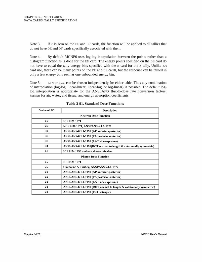
CHAPTER 3 – INPUT CARDS DATA CARDS: TALLY SPECIFICATION
Chapter 3-222 MCNP User’s Manual
Note 3: If n is zero on the DE and DF cards, the function will be applied to all tallies that do not have DE and DF cards specifically associated with them.
Note 4: By default MCNP6 uses log-log interpolation between the points rather than a histogram function as is done for the EM card. The energy points specified on the DE card do not have to equal the tally energy bins specified with the E card for the F tally. Unlike EM card use, there can be many points on the DE and DF cards, but the response can be tallied in only a few energy bins such as one unbounded energy bin.
Note 5: LIN or LOG can be chosen independently for either table. Thus any combination of interpolation (log-log, linear-linear, linear-log, or log-linear) is possible. The default log-log interpolation is appropriate for the ANSI/ANS flux-to-dose rate conversion factors; kermas for air, water, and tissue; and energy absorption coefficients.
Table 3-91. Standard Dose Functions
Value of IC Description
Neutron Dose Function
10 ICRP-21 1971 20 NCRP-38 1971, ANSI/ANS-6.1.1-1977 31 ANSI/ANS-6.1.1-1991 (AP anterior-posterior) 32 ANSI/ANS-6.1.1-1991 (PA posterior-anterior) 33 ANSI/ANS-6.1.1-1991 (LAT side exposure) 34 ANSI/ANS-6.1.1-1991(ROT normal to length & rotationally symmetric) 40 ICRP-74 1996 ambient dose equivalent
Photon Dose Function
10 ICRP-21 1971 20 Claiborne & Trubey, ANSI/ANS 6.1.1-1977 31 ANSI/ANS-6.1.1-1991 (AP anterior-posterior) 32 ANSI/ANS-6.1.1-1991 (PA posterior-anterior) 33 ANSI/ANS-6.1.1-1991 (LAT side exposure) 34 ANSI/ANS-6.1.1-1991 (ROT normal to length & rotationally symmetric) 35 ANSI/ANS-6.1.1-1991 (ISO isotropic)
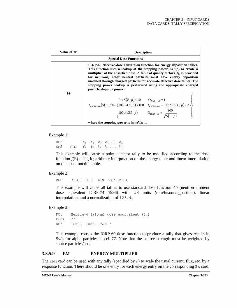
CHAPTER 3 – INPUT CARDS
DATA CARDS: TALLY SPECIFICATION
MCNP User’s Manual Chapter 3-223
Value of IC Description
Special Dose Functions
99
ICRP-60 effective-dose conversion function for energy deposition tallies. This function uses a lookup of the stopping power, S(E,p) to create a multiplier of the absorbed dose. A table of quality factors, Q, is provided for neutrons; other neutral particles must have energy deposition modeled through charged particles for accurate effective dose tallies. The stopping power lookup is performed using the appropriate charged particle stopping power:
where the stopping power is in keV/µm.
Example 1: DE5 e1 e2 e3 e4 ... ek DF5 LIN f1 f2 f3 f4 ... fk
This example will cause a point detector tally to be modified according to the dose function f(E) using logarithmic interpolation on the energy table and linear interpolation on the dose function table.
Example 2: DF0 IC 40 IU 1 LIN FAC 123.4
This example will cause all tallies to use standard dose function 40 (neutron ambient dose equivalent ICRP-74 1996) with US units (rem/h/source_particle), linear interpolation, and a normalization of 123.4.
Example 3: FC6 Helium-4 (alpha) dose equivalent (Sv) F6:A 77 DF6 IC=99 IU=2 FAC=-3 This example causes the ICRP-60 dose function to produce a tally that gives results in Sv/h for alpha particles in cell 77. Note that the source strength must be weighted by source particles/sec.
3.3.5.9 EM ENERGY MULTIPLIER
The EMn card can be used with any tally (specified by n) to scale the usual current, flux, etc. by a response function. There should be one entry for each energy entry on the corresponding En card.
( )( )( )( ) ( )
( )( )
=>
−×=≤<=≤<
=
−
−
−
−
pES
QpES
pES QpESQpES
pESQ
ICRP
ICRP
ICRP
ICRP
,300,100
2.2,32.0100,10110,0
,
60
60
60
60

CHAPTER 3 – INPUT CARDS DATA CARDS: TALLY SPECIFICATION
Chapter 3-224 MCNP User’s Manual
When a tally is being recorded within a certain energy bin, the regular contribution is multiplied by the entry on the EMn card corresponding to that bin. For example, a dose rate can be tallied with the appropriate response function entries. Tallies can also be changed to be per unit energy if the entries are 1/ΔE for each bin, where ΔE is the width of the corresponding energy bin. Note that this card modifies the tally by an energy-dependent function that has the form of a histogram and not a continuous function. It also requires the tally to have as many energy bins as there are histograms on the EMn card. If neither of these two effects is desired, see the DE and DF cards.
Form: EMn m1 ... mk (See Note 1.)
Table 3-92. Energy Multiplier Card (EM)
Input Parameter Description
n Tally number. Restriction: n≤99999999
mi Multiplier to be applied to the ith energy bin.
Default: None.
Use: Requires E card (See Section 3.3.5.3). Tally comment recommended.
Note 1: A set of energy multipliers can be specified on an EM0 card that will be used for all tallies for which there is not a specific EM card.
3.3.5.10 TM TIME MULTIPLIER
The TM card can be used with any tally to scale the usual current, flux, etc. by a response function. There should be one entry for each time entry on the corresponding T card. Note that this card modifies the tally by a time-dependent function that has the form of a histogram and not a continuous function. For example, tallies can be changed to be per unit time if the entries are
for each bin, where is the width or the corresponding time bin.
Form: TMn m1 ... mk (See Note 1.)
Table 3-93. Time Multiplier Card (TM)
Input Parameter Description
N Tally number. Restriction: n≤99999999
mi Multiplier to be applied to the ith time bin.
Default: None.
T∆1 T∆

CHAPTER 3 – INPUT CARDS
DATA CARDS: TALLY SPECIFICATION
MCNP User’s Manual Chapter 3-225
Use: Requires T card (See Section 3.3.5.4). Tally comment recommended.
Note 1: A set of time multipliers can be specified on a TM0 card that will be used for all tallies for which there is not a specific TM card.
3.3.5.11 CM COSINE MULTIPLIER (TALLY TYPES 1 AND 2 ONLY)
The CM card can be used with an F1 or F2 tally to scale the usual current by a response function. There should be one entry for each cosine entry on the corresponding C card. Note that this card modifies the tally by an angular-dependent function that has the form of a histogram and not a continuous function. For example, To get the directionally dependent F1 tally results to be per steradian, the ith entry on the CM1 card is where is 180º.
Form: CMn m1 ... mk (See Note 1.)
Table 3-94. Cosine Multiplier Card (CM)
Input Parameter Description
n Tally number. Restriction: n≤99999999
mi Multiplier to be applied to the ith cosine bin.
Default: None.
Use: Tally types 1 and 2. Requires Cn card (See Section 3.3.5.5). Tally comment recommended.
Note 1: A set of cosine multipliers can be specified on a CM0 card that will be used for all F1 or F2 tallies for which there is not a specific CM card.
3.3.5.12 CF CELL FLAGGING (TALLY TYPES 1, 2, 4, 6, 7)
Particle tracks can be "flagged" when they leave designated cells and the contributions of these flagged tracks to a tally are listed separately in addition to the normal total tally. This method can determine the tally contribution from tracks that have passed through an area of interest.
The cell flag is turned on only upon leaving a cell. A source particle born in a flagged cell does not turn the flag on until it leaves the cell.
The flagged tallies are the contribution to the tally made by a particle or it’s progeny that ever had it’s cell flag set by leaving the flagged cell or cells designated on the CF card. For example, a flagged photon tally can be scored in by either a photon leaving the flagged cell or a neutron leaving a flagged cell, which leads to a photon that is tallied. Caution, a particle that is killed on a surface will have it’s surface flag set but not have it’s cell flag.
( )[ ]1coscos21 −− ii θθπ 0θ
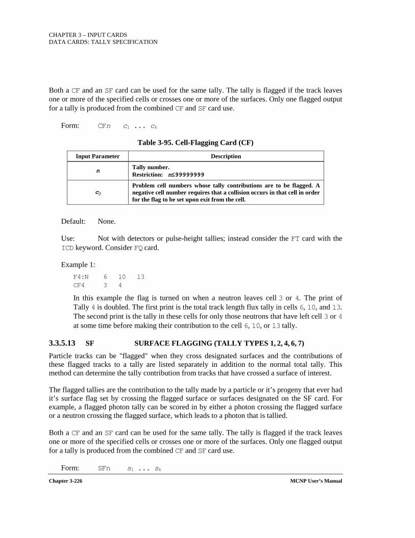
CHAPTER 3 – INPUT CARDS DATA CARDS: TALLY SPECIFICATION
Chapter 3-226 MCNP User’s Manual
Both a CF and an SF card can be used for the same tally. The tally is flagged if the track leaves one or more of the specified cells or crosses one or more of the surfaces. Only one flagged output for a tally is produced from the combined CF and SF card use.
Form: CFn c1 ... ck
Table 3-95. Cell-Flagging Card (CF)
Input Parameter Description
n Tally number. Restriction: n≤99999999
cj Problem cell numbers whose tally contributions are to be flagged. A negative cell number requires that a collision occurs in that cell in order for the flag to be set upon exit from the cell.
Default: None.
Use: Not with detectors or pulse-height tallies; instead consider the FT card with the ICD keyword. Consider FQ card.
Example 1: F4:N 6 10 13 CF4 3 4
In this example the flag is turned on when a neutron leaves cell 3 or 4. The print of Tally 4 is doubled. The first print is the total track length flux tally in cells 6, 10, and 13. The second print is the tally in these cells for only those neutrons that have left cell 3 or 4 at some time before making their contribution to the cell 6, 10, or 13 tally.
3.3.5.13 SF SURFACE FLAGGING (TALLY TYPES 1, 2, 4, 6, 7)
Particle tracks can be "flagged" when they cross designated surfaces and the contributions of these flagged tracks to a tally are listed separately in addition to the normal total tally. This method can determine the tally contribution from tracks that have crossed a surface of interest.
The flagged tallies are the contribution to the tally made by a particle or it’s progeny that ever had it’s surface flag set by crossing the flagged surface or surfaces designated on the SF card. For example, a flagged photon tally can be scored in by either a photon crossing the flagged surface or a neutron crossing the flagged surface, which leads to a photon that is tallied.
Both a CF and an SF card can be used for the same tally. The tally is flagged if the track leaves one or more of the specified cells or crosses one or more of the surfaces. Only one flagged output for a tally is produced from the combined CF and SF card use.
Form: SFn s1 ... sk
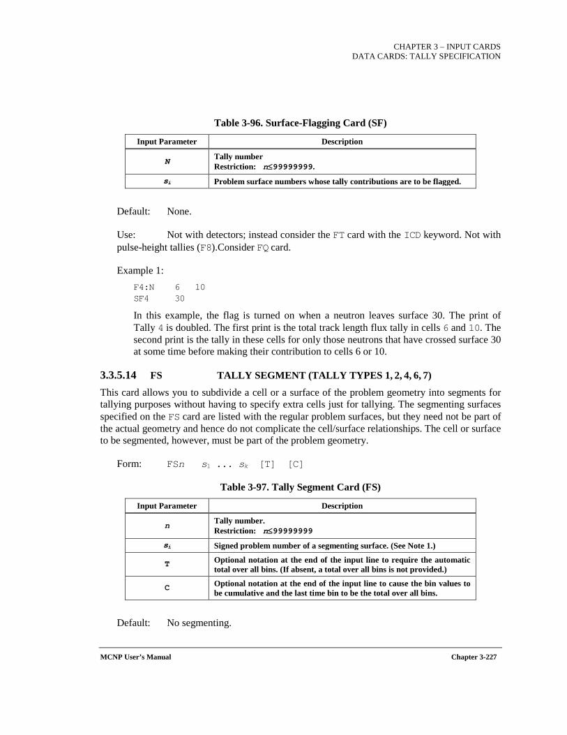
CHAPTER 3 – INPUT CARDS
DATA CARDS: TALLY SPECIFICATION
MCNP User’s Manual Chapter 3-227
Table 3-96. Surface-Flagging Card (SF)
Input Parameter Description
N Tally number Restriction: n≤99999999.
si Problem surface numbers whose tally contributions are to be flagged.
Default: None.
Use: Not with detectors; instead consider the FT card with the ICD keyword. Not with pulse-height tallies (F8).Consider FQ card.
Example 1: F4:N 6 10 SF4 30
In this example, the flag is turned on when a neutron leaves surface 30. The print of Tally 4 is doubled. The first print is the total track length flux tally in cells 6 and 10. The second print is the tally in these cells for only those neutrons that have crossed surface 30 at some time before making their contribution to cells 6 or 10.
3.3.5.14 FS TALLY SEGMENT (TALLY TYPES 1, 2, 4, 6, 7)
This card allows you to subdivide a cell or a surface of the problem geometry into segments for tallying purposes without having to specify extra cells just for tallying. The segmenting surfaces specified on the FS card are listed with the regular problem surfaces, but they need not be part of the actual geometry and hence do not complicate the cell/surface relationships. The cell or surface to be segmented, however, must be part of the problem geometry.
Form: FSn s1 ... sk [T] [C]
Table 3-97. Tally Segment Card (FS)
Input Parameter Description
n Tally number. Restriction: n≤99999999
si Signed problem number of a segmenting surface. (See Note 1.)
T Optional notation at the end of the input line to require the automatic total over all bins. (If absent, a total over all bins is not provided.)
C Optional notation at the end of the input line to cause the bin values to be cumulative and the last time bin to be the total over all bins.
Default: No segmenting.
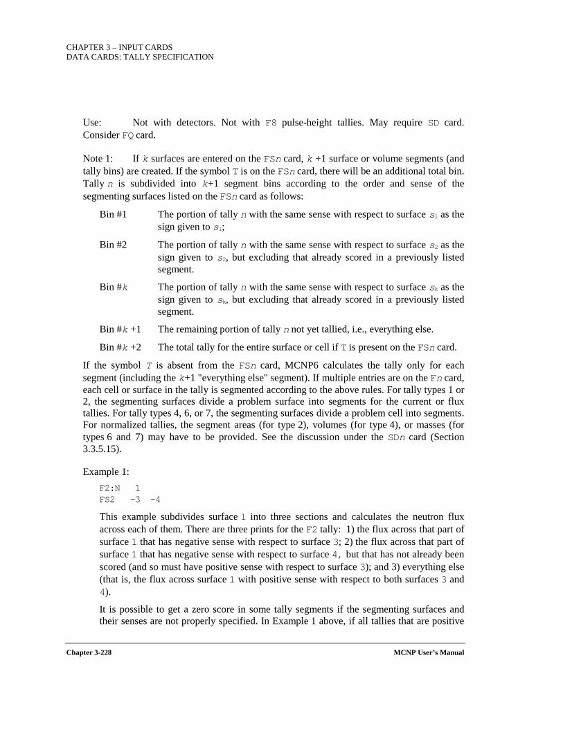
CHAPTER 3 – INPUT CARDS DATA CARDS: TALLY SPECIFICATION
Chapter 3-228 MCNP User’s Manual
Use: Not with detectors. Not with F8 pulse-height tallies. May require SD card. Consider FQ card.
Note 1: If k surfaces are entered on the FSn card, k +1 surface or volume segments (and tally bins) are created. If the symbol T is on the FSn card, there will be an additional total bin. Tally n is subdivided into k+1 segment bins according to the order and sense of the segmenting surfaces listed on the FSn card as follows:
Bin #1 The portion of tally n with the same sense with respect to surface s1 as the sign given to s1;
Bin #2 The portion of tally n with the same sense with respect to surface s2 as the sign given to s2, but excluding that already scored in a previously listed segment.
Bin #k The portion of tally n with the same sense with respect to surface sk as the sign given to sk, but excluding that already scored in a previously listed segment.
Bin #k +1 The remaining portion of tally n not yet tallied, i.e., everything else.
Bin #k +2 The total tally for the entire surface or cell if T is present on the FSn card.
If the symbol T is absent from the FSn card, MCNP6 calculates the tally only for each segment (including the k+1 "everything else" segment). If multiple entries are on the Fn card, each cell or surface in the tally is segmented according to the above rules. For tally types 1 or 2, the segmenting surfaces divide a problem surface into segments for the current or flux tallies. For tally types 4, 6, or 7, the segmenting surfaces divide a problem cell into segments. For normalized tallies, the segment areas (for type 2), volumes (for type 4), or masses (for types 6 and 7) may have to be provided. See the discussion under the SDn card (Section 3.3.5.15).
Example 1: F2:N 1 FS2 -3 -4
This example subdivides surface 1 into three sections and calculates the neutron flux across each of them. There are three prints for the F2 tally: 1) the flux across that part of surface 1 that has negative sense with respect to surface 3; 2) the flux across that part of surface 1 that has negative sense with respect to surface 4, but that has not already been scored (and so must have positive sense with respect to surface 3); and 3) everything else (that is, the flux across surface 1 with positive sense with respect to both surfaces 3 and 4).
It is possible to get a zero score in some tally segments if the segmenting surfaces and their senses are not properly specified. In Example 1 above, if all tallies that are positive
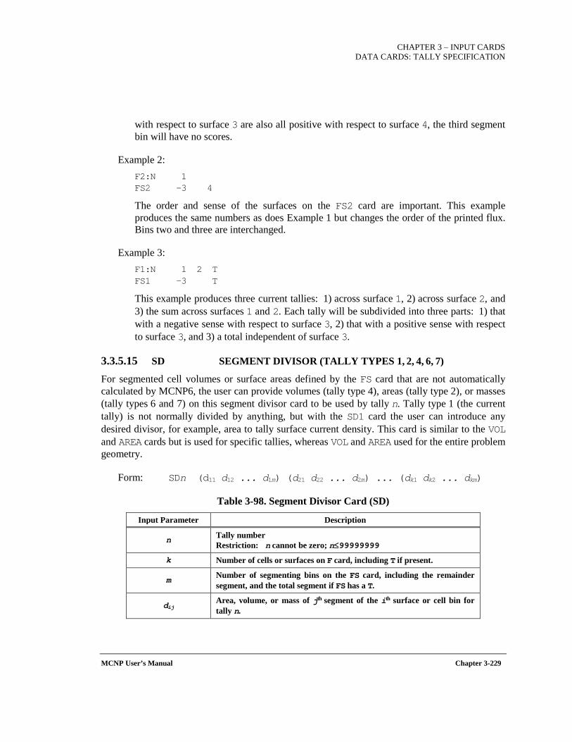
CHAPTER 3 – INPUT CARDS
DATA CARDS: TALLY SPECIFICATION
MCNP User’s Manual Chapter 3-229
with respect to surface 3 are also all positive with respect to surface 4, the third segment bin will have no scores.
Example 2: F2:N 1 FS2 -3 4
The order and sense of the surfaces on the FS2 card are important. This example produces the same numbers as does Example 1 but changes the order of the printed flux. Bins two and three are interchanged.
Example 3: F1:N 1 2 T FS1 -3 T
This example produces three current tallies: 1) across surface 1, 2) across surface 2, and 3) the sum across surfaces 1 and 2. Each tally will be subdivided into three parts: 1) that with a negative sense with respect to surface 3, 2) that with a positive sense with respect to surface 3, and 3) a total independent of surface 3.
3.3.5.15 SD SEGMENT DIVISOR (TALLY TYPES 1, 2, 4, 6, 7)
For segmented cell volumes or surface areas defined by the FS card that are not automatically calculated by MCNP6, the user can provide volumes (tally type 4), areas (tally type 2), or masses (tally types 6 and 7) on this segment divisor card to be used by tally n. Tally type 1 (the current tally) is not normally divided by anything, but with the SD1 card the user can introduce any desired divisor, for example, area to tally surface current density. This card is similar to the VOL and AREA cards but is used for specific tallies, whereas VOL and AREA used for the entire problem geometry.
Form: SDn (d11 d12 ... d1m) (d21 d22 ... d2m) ... (dk1 dk2 ... dkm)
Table 3-98. Segment Divisor Card (SD)
Input Parameter Description
n Tally number Restriction: n cannot be zero; n≤99999999
k Number of cells or surfaces on F card, including T if present.
m Number of segmenting bins on the FS card, including the remainder segment, and the total segment if FS has a T.
dij Area, volume, or mass of jth segment of the ith surface or cell bin for tally n.

CHAPTER 3 – INPUT CARDS DATA CARDS: TALLY SPECIFICATION
Chapter 3-230 MCNP User’s Manual
Use: Not with detectors. The parentheses [( )] are optional. May be required with FS card. Can be used without FS card.
MCNP6 uses the following hierarchy for determining the volume, area, or mass:
For cell or surface without segmenting (tally types 2, 4, 6, and 7): a) non-zero entry on SD card b) non-zero entry on VOL or AREA card c) volume, area, or mass calculated by MCNP6 d) fatal error
For cell or surface with segmenting (tally types 2, 4, 6, and 7): a) non-zero entry on SD card b) volume, area, or mass calculated by MCNP6 c) fatal error
For surface in a type 1 tally: a) non-zero entry on SD card b) no divisor
Example: F4:N 1 2 3 T SD4 1 1 1 1
Note that the SD card can be used to define tally divisors even if the tally is not segmented. In this example the tally calculates the flux in the three cells plus the union of the three cells. The VOL card can be used to set the volume divisor of the three cells (to unity, for example), but it cannot do anything about the divisor for the union. Its divisor is the sum of the volumes (whether MCNP6-calculated or user-entered) of the three cells. However, the divisors for all four of the cell bins can be set to unity by means of the SD card. These entries override entries on the VOL and AREA cards. See Section 3.3.5.1.4 for use with repeated structure tallies.
3.3.5.16 FU SPECIAL TALLY OR TALLYX INPUT
This card is used with a user-supplied tally modification subroutine TALLYX and some cases of the FT card. If the FU card has no input parameters, TALLYX will be called but no user bins will be created. The k entries on the FU card serve three purposes: 1) each entry establishes a separate user tally bin for tally n, 2) each entry can be used as an input parameter for TALLYX to define the user bin it establishes, and 3) the entries appear in the output as labels for the user bins.
Form: FUn [x1 x2 ... xk] [NT] [C]
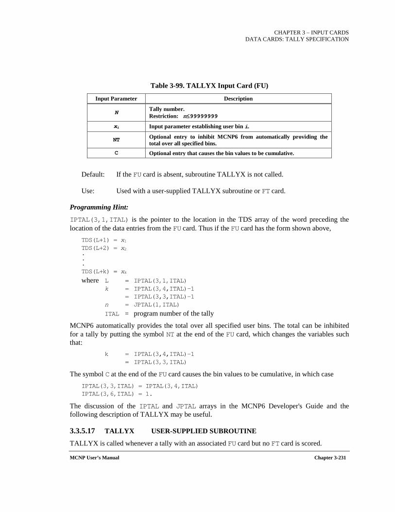
CHAPTER 3 – INPUT CARDS
DATA CARDS: TALLY SPECIFICATION
MCNP User’s Manual Chapter 3-231
Table 3-99. TALLYX Input Card (FU)
Input Parameter Description
N Tally number. Restriction: n≤99999999
xi Input parameter establishing user bin i.
NT Optional entry to inhibit MCNP6 from automatically providing the total over all specified bins.
C Optional entry that causes the bin values to be cumulative.
Default: If the FU card is absent, subroutine TALLYX is not called.
Use: Used with a user-supplied TALLYX subroutine or FT card.
Programming Hint:
IPTAL(3,1,ITAL) is the pointer to the location in the TDS array of the word preceding the location of the data entries from the FU card. Thus if the FU card has the form shown above,
TDS(L+1) = x1 TDS(L+2) = x2 . . . TDS(L+k) = xk
where L = IPTAL(3,1,ITAL) k = IPTAL(3,4,ITAL)−1 = IPTAL(3,3,ITAL)−1 n = JPTAL(1,ITAL)
ITAL = program number of the tally
MCNP6 automatically provides the total over all specified user bins. The total can be inhibited for a tally by putting the symbol NT at the end of the FU card, which changes the variables such that:
k = IPTAL(3,4,ITAL)−1 = IPTAL(3,3,ITAL)
The symbol C at the end of the FU card causes the bin values to be cumulative, in which case IPTAL(3,3,ITAL) = IPTAL(3,4,ITAL) IPTAL(3,6,ITAL) = 1.
The discussion of the IPTAL and JPTAL arrays in the MCNP6 Developer's Guide and the following description of TALLYX may be useful.
3.3.5.17 TALLYX USER-SUPPLIED SUBROUTINE
TALLYX is called whenever a tally with an associated FU card but no FT card is scored.
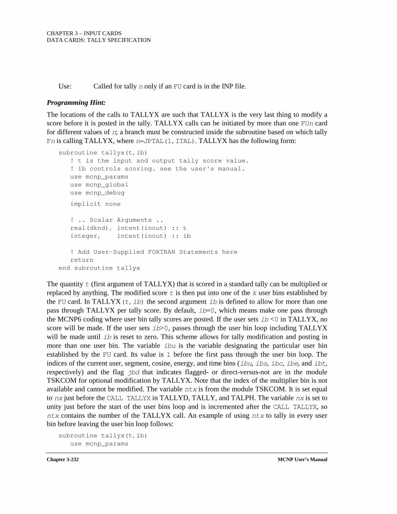
CHAPTER 3 – INPUT CARDS DATA CARDS: TALLY SPECIFICATION
Chapter 3-232 MCNP User’s Manual
Use: Called for tally n only if an FU card is in the INP file.
Programming Hint:
The locations of the calls to TALLYX are such that TALLYX is the very last thing to modify a score before it is posted in the tally. TALLYX calls can be initiated by more than one FUn card for different values of n; a branch must be constructed inside the subroutine based on which tally Fn is calling TALLYX, where n=JPTAL(1,ITAL). TALLYX has the following form:
subroutine tallyx(t,ib) ! t is the input and output tally score value. ! ib controls scoring. see the user's manual. use mcnp_params use mcnp_global use mcnp_debug
implicit none ! .. Scalar Arguments .. real(dknd), intent(inout) :: t integer, intent(inout) :: ib ! Add User-Supplied FORTRAN Statements here return
end subroutine tallyx
The quantity t (first argument of TALLYX) that is scored in a standard tally can be multiplied or replaced by anything. The modified score t is then put into one of the k user bins established by the FU card. In TALLYX(t,ib) the second argument ib is defined to allow for more than one pass through TALLYX per tally score. By default, ib=0, which means make one pass through the MCNP6 coding where user bin tally scores are posted. If the user sets ib <0 in TALLYX, no score will be made. If the user sets ib>0, passes through the user bin loop including TALLYX will be made until ib is reset to zero. This scheme allows for tally modification and posting in more than one user bin. The variable ibu is the variable designating the particular user bin established by the FU card. Its value is 1 before the first pass through the user bin loop. The indices of the current user, segment, cosine, energy, and time bins (ibu, ibs, ibc, ibe, and ibt, respectively) and the flag jbd that indicates flagged- or direct-versus-not are in the module TSKCOM for optional modification by TALLYX. Note that the index of the multiplier bin is not available and cannot be modified. The variable ntx is from the module TSKCOM. It is set equal to nx just before the CALL TALLYX in TALLYD, TALLY, and TALPH. The variable nx is set to unity just before the start of the user bins loop and is incremented after the CALL TALLYX, so ntx contains the number of the TALLYX call. An example of using ntx to tally in every user bin before leaving the user bin loop follows:
subroutine tallyx(t,ib) use mcnp_params
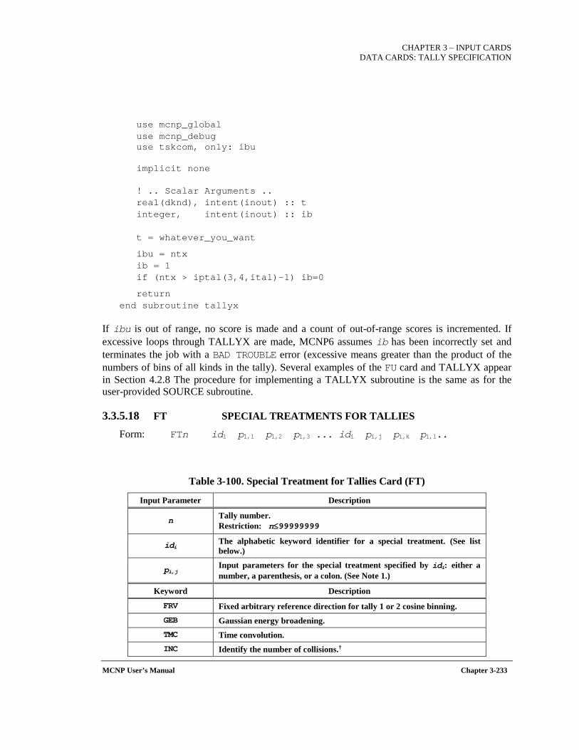
CHAPTER 3 – INPUT CARDS
DATA CARDS: TALLY SPECIFICATION
MCNP User’s Manual Chapter 3-233
use mcnp_global use mcnp_debug use tskcom, only: ibu implicit none ! .. Scalar Arguments .. real(dknd), intent(inout) :: t integer, intent(inout) :: ib t = whatever_you_want
ibu = ntx ib = 1 if (ntx > iptal(3,4,ital)-1) ib=0
return end subroutine tallyx
If ibu is out of range, no score is made and a count of out-of-range scores is incremented. If excessive loops through TALLYX are made, MCNP6 assumes ib has been incorrectly set and terminates the job with a BAD TROUBLE error (excessive means greater than the product of the numbers of bins of all kinds in the tally). Several examples of the FU card and TALLYX appear in Section 4.2.8 The procedure for implementing a TALLYX subroutine is the same as for the user-provided SOURCE subroutine.
3.3.5.18 FT SPECIAL TREATMENTS FOR TALLIES
Form: FTn id1 p1,1 p1,2 p1,3 ... idi pi,j pi,k pi,l..
Table 3-100. Special Treatment for Tallies Card (FT)
Input Parameter Description
n Tally number. Restriction: n≤99999999
idi The alphabetic keyword identifier for a special treatment. (See list below.)
pi,j Input parameters for the special treatment specified by idi: either a number, a parenthesis, or a colon. (See Note 1.)
Keyword Description
FRV Fixed arbitrary reference direction for tally 1 or 2 cosine binning. GEB Gaussian energy broadening. TMC Time convolution. INC Identify the number of collisions.†
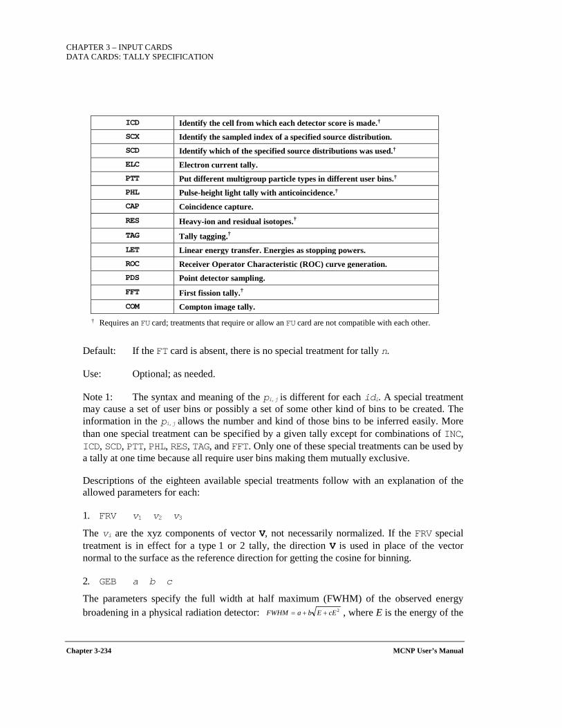
CHAPTER 3 – INPUT CARDS DATA CARDS: TALLY SPECIFICATION
Chapter 3-234 MCNP User’s Manual
ICD Identify the cell from which each detector score is made.† SCX Identify the sampled index of a specified source distribution. SCD Identify which of the specified source distributions was used.† ELC Electron current tally. PTT Put different multigroup particle types in different user bins.† PHL Pulse-height light tally with anticoincidence.† CAP Coincidence capture. RES Heavy-ion and residual isotopes.† TAG Tally tagging.† LET Linear energy transfer. Energies as stopping powers. ROC Receiver Operator Characteristic (ROC) curve generation. PDS Point detector sampling. FFT First fission tally.† COM Compton image tally.
† Requires an FU card; treatments that require or allow an FU card are not compatible with each other.
Default: If the FT card is absent, there is no special treatment for tally n.
Use: Optional; as needed.
Note 1: The syntax and meaning of the pi,j is different for each idi. A special treatment may cause a set of user bins or possibly a set of some other kind of bins to be created. The information in the pi,j allows the number and kind of those bins to be inferred easily. More than one special treatment can be specified by a given tally except for combinations of INC, ICD, SCD, PTT, PHL, RES, TAG, and FFT. Only one of these special treatments can be used by a tally at one time because all require user bins making them mutually exclusive.
Descriptions of the eighteen available special treatments follow with an explanation of the allowed parameters for each:
1. FRV v1 v2 v3
The vi are the xyz components of vector V, not necessarily normalized. If the FRV special treatment is in effect for a type 1 or 2 tally, the direction V is used in place of the vector normal to the surface as the reference direction for getting the cosine for binning.
2. GEB a b c
The parameters specify the full width at half maximum (FWHM) of the observed energy broadening in a physical radiation detector: , where E is the energy of the 2cEEbaFWHM ++=
CHAPTER 3 – INPUT CARDS
DATA CARDS: TALLY SPECIFICATION
MCNP User’s Manual Chapter 3-235
particle. The units of a, b, and c are MeV, MeV1/2, and 1/MeV, respectively. The energy actually scored is sampled from a Gaussian with that FWHM.
3. TMC a b
All particles should be started at time zero. The tally scores are made as if the source was actually a square pulse starting at time a and ending at time b.
4. INC
No parameters follow the INC keyword but an FU card is required (see Section 3.3.5.16). Its bin boundaries are the number of collisions that have occurred in the track. The user can control if secondary particles are considered un-collided (default) or collided at their creation with use of the UNC card (see Section 3.3.3.10). If the INC special treatment is in effect, the call to TALLYX that the presence of the FU card would normally trigger does not occur. Instead ibu is set by calling JBIN with the number of collisions as the argument. To capture all particles, the last FU bin value should be a very large number.
5. ICD
No parameters follow the keyword ICD but an FU card is required (see Section 3.3.5.16). Its bins are the names of some or all of the cells in the problem. If the cell from which a detector score is about to be made is not in the list on the FU card, the score is not made. The result is that the detector tally is subdivided into bins according to which cell had the source or collision resulting in the detector score. TALLYX is not called. The selection of the user bin is done in TALLYD.
6. SCX k
The parameter k is the name of one of the source distributions and is the k that appears on the SIk card. One user bin is created for each bin of source distribution k plus a total bin. The scores for tally n are then binned according to which bin of source distribution k the source particle came from. The score of the total bin is the score you would see for tally n without the special treatment, if source distribution k is not a dependent distribution.
Caution: For a dependent distribution, the score in the total bin is the subtotal portion of the score from dependent distribution k.
7. SCD
No parameters follow the keyword SCD but an FU card is required (see Section 3.3.5.16). Its bins are a list of source distribution numbers from SIk cards. The scores for tally n are then binned according to which distribution listed on the FU card was sampled. This feature might be used to identify which of several source nuclides emitted the source particle. In this case, the source distributions listed on the FU card would presumably be energy distributions. Each energy distribution is the correct energy distribution for some nuclide known to the user and

CHAPTER 3 – INPUT CARDS DATA CARDS: TALLY SPECIFICATION
Chapter 3-236 MCNP User’s Manual
the probability of that distribution being sampled from is proportional to the activity of that nuclide in the source. The user might want to include an FC card that tells to what nuclide each energy distribution number corresponds.
Caution: If more than one of the source distributions listed on the FU card is used for a given history, only the first one used will score.
8. ELC c
The single parameter c of ELC specifies how the charge of a particle is to affect the scoring of an F1 tally. Normally, an F1 tally gives particle current without regard for the charge of the particles. Additionally, this treatment can create separate bins for particles and antiparticles. There are three possible values for c:
• specify c=1 to cause negatively charged particles to make negative scores, • specify c=2 to put charged particles and antiparticles into separate user bins, and • specify c=3 for the effect of both c=1 and c=2.
If c= 2 or 3, three user bins (e.g., positrons, electrons, and total) are created.
9. PTT
No parameters follow the keyword PTT but an FU card is required (see Section 3.3.5.16). Its bins are a list of atomic weights in units of MeV of particles masquerading as neutrons in a multigroup data library. The scores for tally n are then binned according to the particle type as differentiated from the masses in the multigroup data library. For example, 0.511 0 would be for electrons and photons masquerading as neutrons.
10. PHL [n ta1 ba1 ta2 ba2 ... tan ban] [det1] [m tb1 bb1 tb2 bb2 ... tbm bbm] [det2] [j tc1 bc1 tc2 bc2 ... tcj bcj] [det3] [k td1 bd1 td2 bd2 ... tdk bdk] [det4] [0] [TDEP tg tt]
The PHL option models a pulse-height tally with anticoincidence. This option allows the F8 tally to be based on energy/light deposition in up to four regions as specified via F6 tallies. Requires an FU card (see Section 3.3.5.16).
The parameters for keyword PHL are the following:
n is the number of F6 tallies for the first detector region, tai bai are the pairings of tally number and F-bin number (see Table 3-102) for
the n F6 tallies of the first detector region, det1 is an optional detector descriptor chosen from Table 3-101 for the first
detector region,

CHAPTER 3 – INPUT CARDS
DATA CARDS: TALLY SPECIFICATION
MCNP User’s Manual Chapter 3-237
m is the number of F6 tallies for the second detector region, tbi bbi are the pairings of tally number and F-bin number for the m F6 tallies of
the second detector region, det2 is an optional detector descriptor chosen from Table 3-101 for the second
detector region, j is the number of F6 tallies for the third detector region, tci bci are the pairings of tally number and F-bin number for the j F6 tallies of
the third detector region, det3 is an optional detector descriptor chosen from Table 3-101 for the third
detector region, k is the number of F6 tallies for the fourth detector region, tdi bdi are the pairings of tally number and F-bin number for the k F6 tallies of
the fourth detector region, det4 is an optional detector descriptor chosen from Table 3-101 for the fourth
detector region, 0 a zero entry terminates input for PHL detectors entries and allows for other FT
options to follow, TDEP tg tt is a keyword option that specifies a tally that will be used as a trigger for
the related T8 card. The first optional TDEP entry (tg) specifies the trigger tally number and the second optional TDEP entry (tt) specifies an energy threshold (MeV).
The F-bin descriptor specified after each tally, bai or bbi, may be “0”, indicating that the referenced tally includes a lattice description of multiple lattice elements. When this option is specified, all tallies within that PHL region must also include the “0” descriptor for bai or bbi and all tallies must be over the same lattice cell and elements. When this option is used in both PHL regions, the related F8 F-bins are modified, with an appropriate warning message, to include J x K bins, where J is the number of lattice elements included in PHL Region 1 and K is the number of lattice elements included in PHL Region 2. The output of Tally 8 will include coincidence results for all J x K bins, along with appropriate cell labels (e.g., 1[0 1 1]+2[0 0 0], which is the combination of lattice cell 1, element [0 1 1], with lattice cell 2, element [0 0 0]). This special F-bin descriptor is typically used with the FT COM option to create a Compton image of a radiation source.
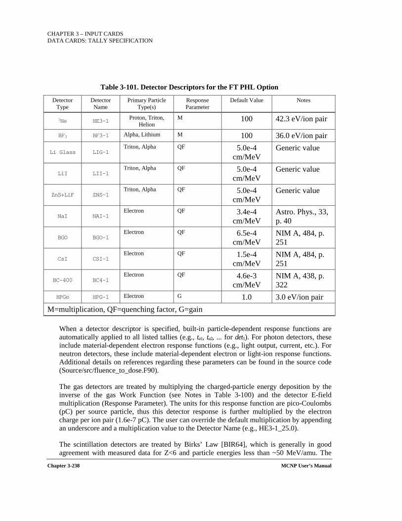
CHAPTER 3 – INPUT CARDS DATA CARDS: TALLY SPECIFICATION
Chapter 3-238 MCNP User’s Manual
Table 3-101. Detector Descriptors for the FT PHL Option
Detector Type
Detector Name
Primary Particle Type(s)
Response Parameter
Default Value Notes
3He HE3-1 Proton, Triton, Helion
M 100 42.3 eV/ion pair
BF3 BF3-1 Alpha, Lithium M 100 36.0 eV/ion pair
Li Glass LIG-1 Triton, Alpha QF 5.0e-4
cm/MeV Generic value
LiI LII-1 Triton, Alpha QF 5.0e-4
cm/MeV Generic value
ZnS+LiF ZNS-1 Triton, Alpha QF 5.0e-4
cm/MeV Generic value
NaI NAI-1 Electron QF 3.4e-4
cm/MeV Astro. Phys., 33, p. 40
BGO BGO-1 Electron QF 6.5e-4
cm/MeV NIM A, 484, p. 251
CsI CSI-1 Electron QF 1.5e-4
cm/MeV NIM A, 484, p. 251
BC-400 BC4-1 Electron QF 4.6e-3
cm/MeV NIM A, 438, p. 322
HPGe HPG-1 Electron G 1.0 3.0 eV/ion pair M=multiplication, QF=quenching factor, G=gain
When a detector descriptor is specified, built-in particle-dependent response functions are automatically applied to all listed tallies (e.g., ta1, ta2, ... for det1). For photon detectors, these include material-dependent electron response functions (e.g., light output, current, etc.). For neutron detectors, these include material-dependent electron or light-ion response functions. Additional details on references regarding these parameters can be found in the source code (Source/src/fluence_to_dose.F90).
The gas detectors are treated by multiplying the charged-particle energy deposition by the inverse of the gas Work Function (see Notes in Table 3-100) and the detector E-field multiplication (Response Parameter). The units for this response function are pico-Coulombs (pC) per source particle, thus this detector response is further multiplied by the electron charge per ion pair (1.6e-7 pC). The user can override the default multiplication by appending an underscore and a multiplication value to the Detector Name (e.g., HE3-1_25.0).
The scintillation detectors are treated by Birks’ Law [BIR64], which is generally in good agreement with measured data for Z<6 and particle energies less than ~50 MeV/amu. The
CHAPTER 3 – INPUT CARDS
DATA CARDS: TALLY SPECIFICATION
MCNP User’s Manual Chapter 3-239
stopping powers used in Birks’ Law are the total stopping powers calculated by MCNP for each particle type. The units for this response function are 1-MeVee photons per source particle (MeVee=MeV electron-equivalent). For absolute visible light photons per source particle, one must multiply this response by the number of visible light photons produced by a 1-MeV electron (which is typically given by the detector manufacturer or can be found in the literature). The default Birks’ quenching factors (QF) are given in Table 3-101, however the user may override these values by appending an underscore and a QF value to the detector name (e.g., LIG-1_2.5e-3).
The semi-conductor detector is treated similarly to a gas detector, except the Work Function is typically much lower (~3 eV/ion pair) and the multiplication is replaced by the gain. The units for this response are also pC per source particle. The user can override the default gain by appending an underscore and new gain value to the detector name (e.g., HPG-1_2.5).
When m is non-zero, indicating the use of two or more detector regions, an FU card is required for the F8 tally. The entries on the FU card are presented in units of MeV (unless modified by DE/DF cards associated with the specified F6 tallies) and must increase monotonically. Similarly, if j or k is non-zero, the energy bins must be specified with C (tally cosine) and FS (tally segment) cards, respectively. The particle type indicated on the F8 tally does not matter because this tally allows a combination of light output from various particle types. If ban is zero, then the number of cell bins on the F8 card must match that on the corresponding tan tally card, which is useful for a lattice pulse-height PHL tally.
The TDEP keyword allows the T8 values to be relative to the first contribution to any FT8 PHL tally. Invoking TDEP allows pulse distributions from different histories to be relative to the same start time rather than distributed in absolute time with significant variation based on when a particle reaches the detector. TDEP can also be followed by one or two entries, where the first entry (tg) is a tally number and the second (tt) is an energy threshold. If an energy threshold value is provided, the reference time on the T8 card is whenever the specified tally has a value greater than the specified threshold. The specified tally can be the same number as the F8 tally, in which case TDEP depends on the sum of the PHL F6 tallies, or it can be a single F6 tally that is specified in any region of the FT PHL option. If the tally number has a format of 8.3, for example, then the trigger tally is the sum of all F6 tallies that are specified for region 3 of the FT PHL option. The default TDEP tally number is the corresponding F8 tally number and the default energy threshold is 0 MeV.
Time-Dependent F8 Tallies Using the Pulse Height Light (PHL) Option.
The T (time bin) card is allowed with pulse-height tallies (F8), but only when used in conjunction with the FT PHL option. In this case, the time-dependent energy deposition is taken from the associated F6 tally(s). If the time entries on the F8 card do not match those provided for the various F6 tallies, a fatal error is issued. If the associated F6 tallies do not have T cards, then one matching the F8 tally will be created automatically.
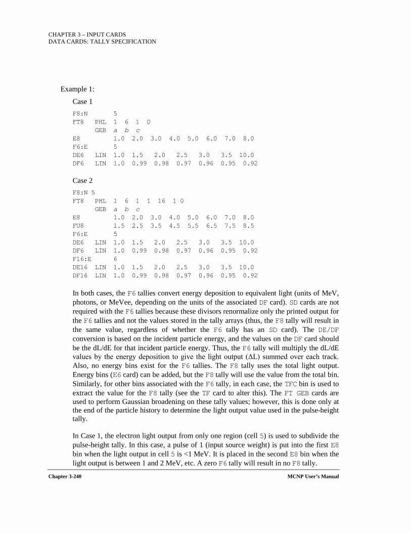
CHAPTER 3 – INPUT CARDS DATA CARDS: TALLY SPECIFICATION
Chapter 3-240 MCNP User’s Manual
Example 1:
Case 1 F8:N 5 FT8 PHL 1 6 1 0 GEB a b c E8 1.0 2.0 3.0 4.0 5.0 6.0 7.0 8.0 F6:E 5 DE6 LIN 1.0 1.5 2.0 2.5 3.0 3.5 10.0 DF6 LIN 1.0 0.99 0.98 0.97 0.96 0.95 0.92 Case 2 F8:N 5 FT8 PHL 1 6 1 1 16 1 0 GEB a b c E8 1.0 2.0 3.0 4.0 5.0 6.0 7.0 8.0 FU8 1.5 2.5 3.5 4.5 5.5 6.5 7.5 8.5 F6:E 5 DE6 LIN 1.0 1.5 2.0 2.5 3.0 3.5 10.0 DF6 LIN 1.0 0.99 0.98 0.97 0.96 0.95 0.92 F16:E 6 DE16 LIN 1.0 1.5 2.0 2.5 3.0 3.5 10.0 DF16 LIN 1.0 0.99 0.98 0.97 0.96 0.95 0.92
In both cases, the F6 tallies convert energy deposition to equivalent light (units of MeV, photons, or MeVee, depending on the units of the associated DF card). SD cards are not required with the F6 tallies because these divisors renormalize only the printed output for the F6 tallies and not the values stored in the tally arrays (thus, the F8 tally will result in the same value, regardless of whether the F6 tally has an SD card). The DE/DF conversion is based on the incident particle energy, and the values on the DF card should be the dL/dE for that incident particle energy. Thus, the F6 tally will multiply the dL/dE values by the energy deposition to give the light output (ΔL) summed over each track. Also, no energy bins exist for the F6 tallies. The F8 tally uses the total light output. Energy bins (E6 card) can be added, but the F8 tally will use the value from the total bin. Similarly, for other bins associated with the F6 tally, in each case, the TFC bin is used to extract the value for the F8 tally (see the TF card to alter this). The FT GEB cards are used to perform Gaussian broadening on these tally values; however, this is done only at the end of the particle history to determine the light output value used in the pulse-height tally.
In Case 1, the electron light output from only one region (cell 5) is used to subdivide the pulse-height tally. In this case, a pulse of 1 (input source weight) is put into the first E8 bin when the light output in cell 5 is <1 MeV. It is placed in the second E8 bin when the light output is between 1 and 2 MeV, etc. A zero F6 tally will result in no F8 tally.
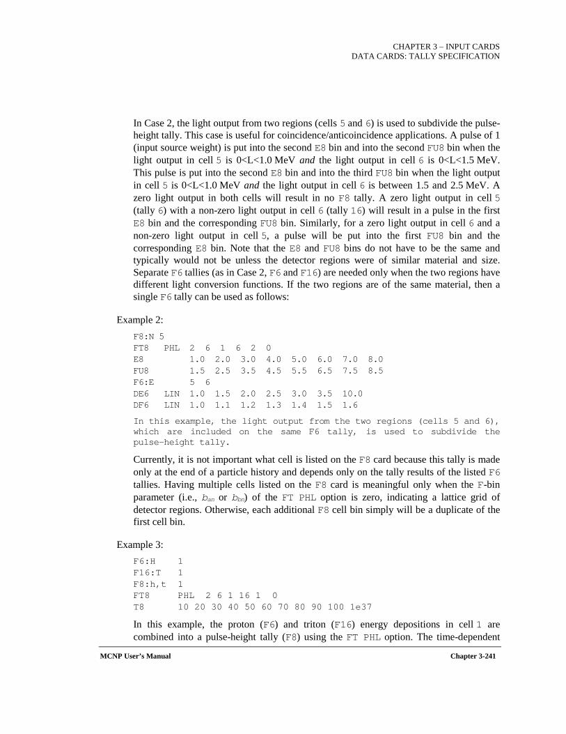
CHAPTER 3 – INPUT CARDS
DATA CARDS: TALLY SPECIFICATION
MCNP User’s Manual Chapter 3-241
In Case 2, the light output from two regions (cells 5 and 6) is used to subdivide the pulse-height tally. This case is useful for coincidence/anticoincidence applications. A pulse of 1 (input source weight) is put into the second E8 bin and into the second FU8 bin when the light output in cell 5 is 0<L<1.0 MeV and the light output in cell 6 is 0<L<1.5 MeV. This pulse is put into the second E8 bin and into the third FU8 bin when the light output in cell 5 is 0<L<1.0 MeV and the light output in cell 6 is between 1.5 and 2.5 MeV. A zero light output in both cells will result in no F8 tally. A zero light output in cell 5 (tally 6) with a non-zero light output in cell 6 (tally 16) will result in a pulse in the first E8 bin and the corresponding FU8 bin. Similarly, for a zero light output in cell 6 and a non-zero light output in cell 5, a pulse will be put into the first FU8 bin and the corresponding E8 bin. Note that the E8 and FU8 bins do not have to be the same and typically would not be unless the detector regions were of similar material and size. Separate F6 tallies (as in Case 2, F6 and F16) are needed only when the two regions have different light conversion functions. If the two regions are of the same material, then a single F6 tally can be used as follows:
Example 2: F8:N 5 FT8 PHL 2 6 1 6 2 0 E8 1.0 2.0 3.0 4.0 5.0 6.0 7.0 8.0 FU8 1.5 2.5 3.5 4.5 5.5 6.5 7.5 8.5 F6:E 5 6 DE6 LIN 1.0 1.5 2.0 2.5 3.0 3.5 10.0 DF6 LIN 1.0 1.1 1.2 1.3 1.4 1.5 1.6
In this example, the light output from the two regions (cells 5 and 6), which are included on the same F6 tally, is used to subdivide the pulse-height tally.
Currently, it is not important what cell is listed on the F8 card because this tally is made only at the end of a particle history and depends only on the tally results of the listed F6 tallies. Having multiple cells listed on the F8 card is meaningful only when the F-bin parameter (i.e., ban or bbn) of the FT PHL option is zero, indicating a lattice grid of detector regions. Otherwise, each additional F8 cell bin simply will be a duplicate of the first cell bin.
Example 3: F6:H 1 F16:T 1 F8:h,t 1 FT8 PHL 2 6 1 16 1 0 T8 10 20 30 40 50 60 70 80 90 100 1e37
In this example, the proton (F6) and triton (F16) energy depositions in cell 1 are combined into a pulse-height tally (F8) using the FT PHL option. The time-dependent
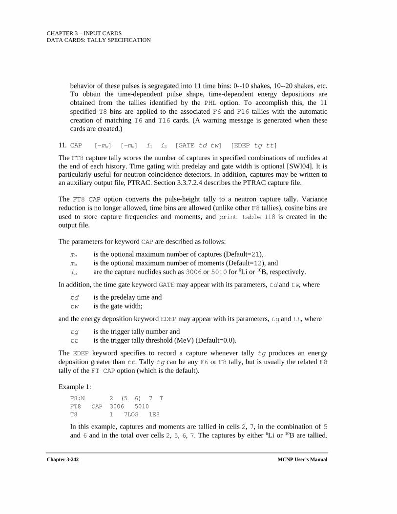
CHAPTER 3 – INPUT CARDS DATA CARDS: TALLY SPECIFICATION
Chapter 3-242 MCNP User’s Manual
behavior of these pulses is segregated into 11 time bins: 0--10 shakes, 10--20 shakes, etc. To obtain the time-dependent pulse shape, time-dependent energy depositions are obtained from the tallies identified by the PHL option. To accomplish this, the 11 specified T8 bins are applied to the associated F6 and F16 tallies with the automatic creation of matching T6 and T16 cards. (A warning message is generated when these cards are created.)
11. CAP [-mc] [-mo] i1 i2 [GATE td tw] [EDEP tg tt]
The FT8 capture tally scores the number of captures in specified combinations of nuclides at the end of each history. Time gating with predelay and gate width is optional [SWI04]. It is particularly useful for neutron coincidence detectors. In addition, captures may be written to an auxiliary output file, PTRAC. Section 3.3.7.2.4 describes the PTRAC capture file.
The FT8 CAP option converts the pulse-height tally to a neutron capture tally. Variance reduction is no longer allowed, time bins are allowed (unlike other F8 tallies), cosine bins are used to store capture frequencies and moments, and print table 118 is created in the output file.
The parameters for keyword CAP are described as follows:
mc is the optional maximum number of captures (Default=21), mo is the optional maximum number of moments (Default=12), and in are the capture nuclides such as 3006 or 5010 for 6Li or 10B, respectively.
In addition, the time gate keyword GATE may appear with its parameters, td and tw, where
td is the predelay time and tw is the gate width;
and the energy deposition keyword EDEP may appear with its parameters, tg and tt, where
tg is the trigger tally number and tt is the trigger tally threshold (MeV) (Default=0.0).
The EDEP keyword specifies to record a capture whenever tally tg produces an energy deposition greater than tt. Tally tg can be any F6 or F8 tally, but is usually the related F8 tally of the FT CAP option (which is the default).
Example 1: F8:N 2 (5 6) 7 T FT8 CAP 3006 5010 T8 1 7LOG 1E8
In this example, captures and moments are tallied in cells 2, 7, in the combination of 5 and 6 and in the total over cells 2, 5, 6, 7. The captures by either 6Li or 10B are tallied.
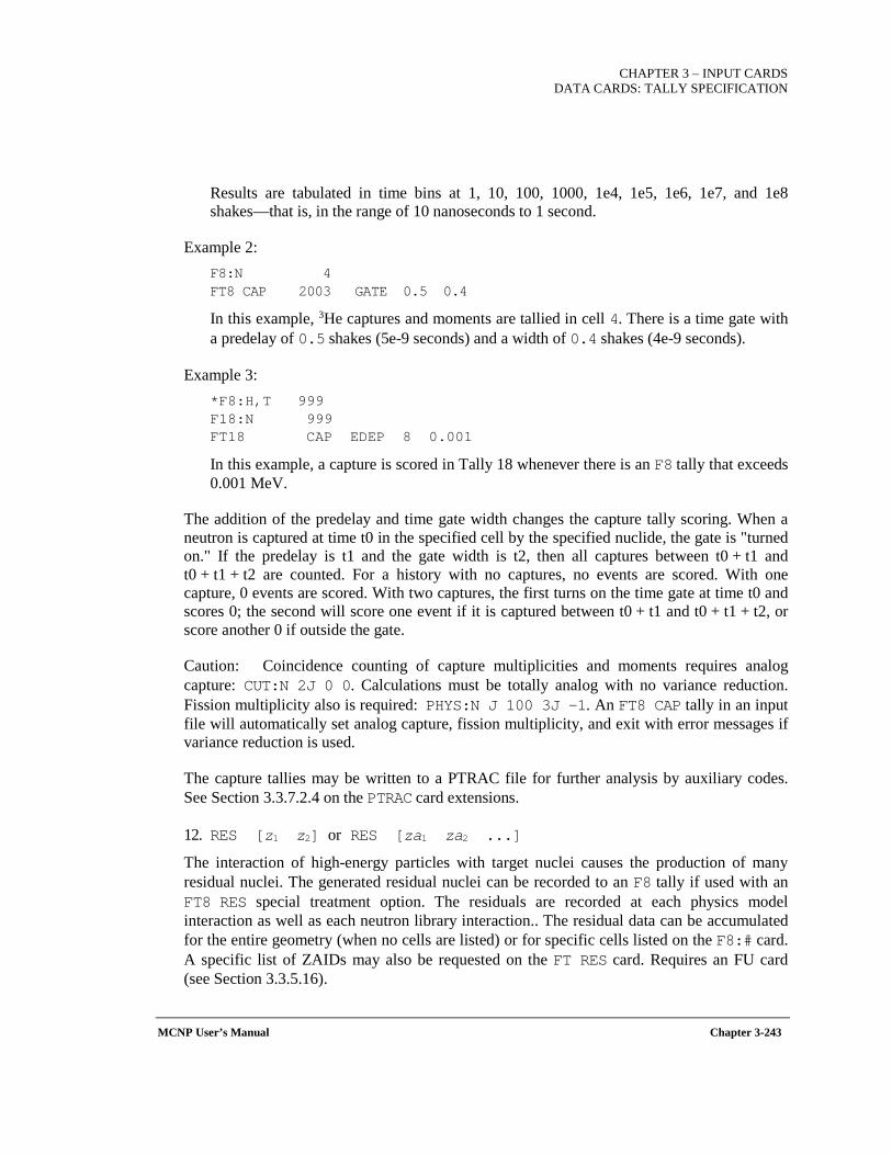
CHAPTER 3 – INPUT CARDS
DATA CARDS: TALLY SPECIFICATION
MCNP User’s Manual Chapter 3-243
Results are tabulated in time bins at 1, 10, 100, 1000, 1e4, 1e5, 1e6, 1e7, and 1e8 shakes—that is, in the range of 10 nanoseconds to 1 second.
Example 2: F8:N 4 FT8 CAP 2003 GATE 0.5 0.4
In this example, 3He captures and moments are tallied in cell 4. There is a time gate with a predelay of 0.5 shakes (5e-9 seconds) and a width of 0.4 shakes (4e-9 seconds).
Example 3: *F8:H,T 999 F18:N 999 FT18 CAP EDEP 8 0.001
In this example, a capture is scored in Tally 18 whenever there is an F8 tally that exceeds 0.001 MeV.
The addition of the predelay and time gate width changes the capture tally scoring. When a neutron is captured at time t0 in the specified cell by the specified nuclide, the gate is "turned on." If the predelay is t1 and the gate width is t2, then all captures between t0 + t1 and t0 + t1 + t2 are counted. For a history with no captures, no events are scored. With one capture, 0 events are scored. With two captures, the first turns on the time gate at time t0 and scores 0; the second will score one event if it is captured between t0 + t1 and t0 + t1 + t2, or score another 0 if outside the gate.
Caution: Coincidence counting of capture multiplicities and moments requires analog capture: CUT:N 2J 0 0. Calculations must be totally analog with no variance reduction. Fission multiplicity also is required: PHYS:N J 100 3J -1. An FT8 CAP tally in an input file will automatically set analog capture, fission multiplicity, and exit with error messages if variance reduction is used.
The capture tallies may be written to a PTRAC file for further analysis by auxiliary codes. See Section 3.3.7.2.4 on the PTRAC card extensions.
12. RES [z1 z2] or RES [za1 za2 ...]
The interaction of high-energy particles with target nuclei causes the production of many residual nuclei. The generated residual nuclei can be recorded to an F8 tally if used with an FT8 RES special treatment option. The residuals are recorded at each physics model interaction as well as each neutron library interaction.. The residual data can be accumulated for the entire geometry (when no cells are listed) or for specific cells listed on the F8:# card. A specific list of ZAIDs may also be requested on the FT RES card. Requires an FU card (see Section 3.3.5.16).
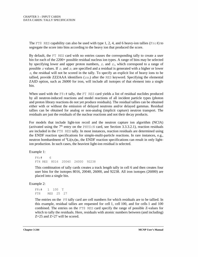
CHAPTER 3 – INPUT CARDS DATA CARDS: TALLY SPECIFICATION
Chapter 3-244 MCNP User’s Manual
The FT8 RES capability can also be used with type 1, 2, 4, and 6 heavy-ion tallies (Fn:#) to segregate the score into bins according to the heavy ion that produced the score.
By default, the FT RES card with no entries causes the corresponding tally to create a user bin for each of the 2200+ possible residual nucleus ion types. A range of bins may be selected by specifying lower and upper proton numbers, z1 and z2, which correspond to a range of possible z values. If z1 and z2 are specified and a residual is generated with a higher or lower z, the residual will not be scored in the tally. To specify an explicit list of heavy ions to be tallied, provide ZZZAAA identifiers (zai) after the RES keyword. Specifying the elemental ZAID option, such as 26000 for iron, will include all isotopes of that element into a single bin.
When used with the F8:# tally, the FT RES card yields a list of residual nuclides produced by all neutron-induced reactions and model reactions of all incident particle types (photon and proton library reactions do not yet produce residuals). The residual tallies can be obtained either with or without the emission of delayed neutrons and/or delayed gammas. Residual tallies can be obtained for analog or non-analog (implicit capture) neutron transport. The residuals are just the residuals of the nuclear reactions and not their decay products.
For models that include light-ion recoil and the neutron capture ion algorithm (NCIA) (activated using the 7th entry on the PHYS:N card, see Section 3.3.3.2.1), reaction residuals are included in the FT8 RES tally. In most instances, reaction residuals are determined using the ENDF reaction specifications for simple-multi-particle reactions. In rare instances, e.g., neutron bombardment of 6Li(n,t)α, the ENDF reaction specifications can result in only light-ion production. In such cases, the heaviest light-ion residual is selected.
Example 1: F4:# 6 FT4 RES 8016 20040 26000 92238
This combination of tally cards creates a track length tally in cell 6 and then creates four user bins for the isotopes 8016, 20040, 26000, and 92238. All iron isotopes (26000) are placed into a single bin.
Example 2: F8:# 1 100 T FT8 RES 25 27
The entries on the F8 tally card are cell numbers for which residuals are to be tallied. In this example, residual tallies are requested for cell 1, cell 100, and for cells 1 and 100 combined. The entries on the FT8 RES card specify the range of possible Z-values for which to tally the residuals. Here, residuals with atomic numbers between (and including) Z=25 and Z=27 will be scored.
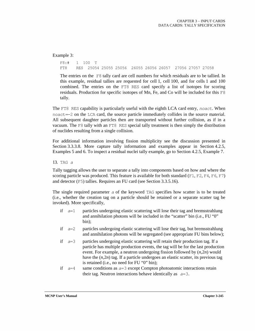
CHAPTER 3 – INPUT CARDS
DATA CARDS: TALLY SPECIFICATION
MCNP User’s Manual Chapter 3-245
Example 3: F8:# 1 100 T FT8 RES 25054 25055 25056 26055 26056 26057 27056 27057 27058
The entries on the F8 tally card are cell numbers for which residuals are to be tallied. In this example, residual tallies are requested for cell 1, cell 100, and for cells 1 and 100 combined. The entries on the FT8 RES card specify a list of isotopes for scoring residuals. Production for specific isotopes of Mn, Fe, and Co will be included for this F8 tally.
The FT8 RES capability is particularly useful with the eighth LCA card entry, noact. When noact=−2 on the LCA card, the source particle immediately collides in the source material. All subsequent daughter particles then are transported without further collision, as if in a vacuum. The F8 tally with an FT8 RES special tally treatment is then simply the distribution of nuclides resulting from a single collision.
For additional information involving fission multiplicity see the discussion presented in Section 3.3.3.8. More capture tally information and examples appear in Section 4.2.5, Examples 5 and 6. To inspect a residual nuclei tally example, go to Section 4.2.5, Example 7.
13. TAG a
Tally tagging allows the user to separate a tally into components based on how and where the scoring particle was produced. This feature is available for both standard (F1, F2, F4, F6, F7) and detector (F5) tallies. Requires an FU card (see Section 3.3.5.16).
The single required parameter a of the keyword TAG specifies how scatter is to be treated (i.e., whether the creation tag on a particle should be retained or a separate scatter tag be invoked). More specifically,
if a=1 particles undergoing elastic scattering will lose their tag and bremsstrahlung and annihilation photons will be included in the “scatter” bin (i.e., FU “0” bin);
if a=2 particles undergoing elastic scattering will lose their tag, but bremsstrahlung and annihilation photons will be segregated (see appropriate FU bins below);
if a=3 particles undergoing elastic scattering will retain their production tag. If a particle has multiple production events, the tag will be for the last production event. For example, a neutron undergoing fission followed by (n,2n) would have the (n,2n) tag. If a particle undergoes an elastic scatter, its previous tag is retained (i.e., no need for FU “0” bin);
if a=4 same conditions as a=3 except Compton photoatomic interactions retain their tag. Neutron interactions behave identically as a=3.

CHAPTER 3 – INPUT CARDS DATA CARDS: TALLY SPECIFICATION
Chapter 3-246 MCNP User’s Manual
Binning specifications for the tagged tally must be provided on the FU special tally card. Each bini entry on the card requests three distinct pieces of tagging information:
1) a cell of interest where particles are produced; 2) a target nuclide from which the particle is emitted; and 3) a reaction MT identifier, or, in the case of spallation, a residual nuclide of interest, or
a special designator (see below).
The format on the FU card when used in association with the tagging treatment is
FUn bin1 bin2 ... binN [NT]
where each tagging bini has the form CCCCCZZAAA.RRRRR and
CCCCC represents a user cell number (Note: Leading zeros are not required.) ZZAAA represents a 5-digit isotope identifier for a target nuclide where ZZ is the
atomic number and AAA is the atomic mass number (Note: ZZ is limited to two characters, therefore nuclides with Z>99 cannot be tagged.)
RRRRR specifies a reaction identifier for library interactions or a residual nuclide ZZAAA identifier for high-energy model interactions or a special designator.
By default, a total over all specified bins is provided for the FU special tally; add the NT parameter after the last specified bin to suppress this total. A list of special cases for the CCCCCZZAAA.RRRRR FU card entries appears later in this section.
If cell tagging is not desired, the CCCCC portion of the tag should be omitted or, alternatively, set to “00000”. In either case, tally contributions will be accumulated for all cells for that FU bin, provided the ZZAAA.RRRRR portion of the tag is satisfied. In the case of particle production from electrons, which are material based (not nuclide specific), the CCCCC input should be used to identify the cell and the ZZAAA input should be set to “00000”. The suffix RRRRR refers to a standard ENDF reaction number for library interactions [e.g., “00102” stipulates (n,γ)] or, in the case of high-energy model interactions, RRRRR refers to a residual nuclide ZZAAA identifier (e.g., “06012” for 12C).
In general, a zero input for any portion of the tag results in the sum of all contributions related to the entry. For example, the tag “0000092000.00000” will collect all tally contributions for which any isotope of uranium (z=92) produced the particle making the tally. However, the tag “0000000000.00000” is reserved for elastic-scattered particles. Note that each tally contribution is made only to the first FU bin that satisfies the tag description (i.e., those that have not already been tallied). If no appropriate FU bin is found, the tally contribution is not made; however a special “everything else” bini (i.e., “1e10”) can be specified to collect any portion of the tally that falls into no other bin. When the “everything else” bin is used, then the user is assured that the “user-bin total” bin will reproduce the original tally as if the FTn TAG option had not been used.
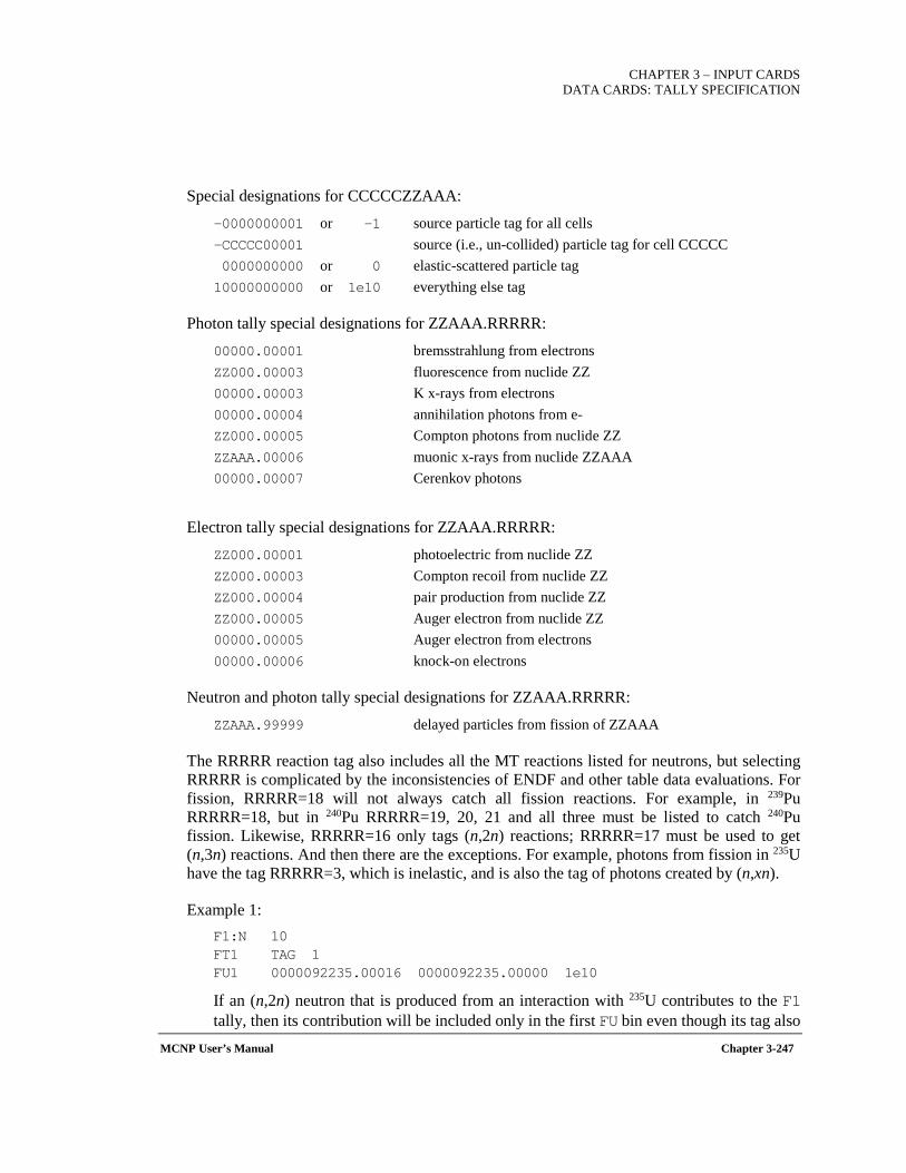
CHAPTER 3 – INPUT CARDS
DATA CARDS: TALLY SPECIFICATION
MCNP User’s Manual Chapter 3-247
Special designations for CCCCCZZAAA: -0000000001 or -1 source particle tag for all cells -CCCCC00001 source (i.e., un-collided) particle tag for cell CCCCC 0000000000 or 0 elastic-scattered particle tag 10000000000 or 1e10 everything else tag
Photon tally special designations for ZZAAA.RRRRR: 00000.00001 bremsstrahlung from electrons ZZ000.00003 fluorescence from nuclide ZZ 00000.00003 K x-rays from electrons 00000.00004 annihilation photons from e- ZZ000.00005 Compton photons from nuclide ZZ ZZAAA.00006 muonic x-rays from nuclide ZZAAA 00000.00007 Cerenkov photons
Electron tally special designations for ZZAAA.RRRRR: ZZ000.00001 photoelectric from nuclide ZZ ZZ000.00003 Compton recoil from nuclide ZZ ZZ000.00004 pair production from nuclide ZZ ZZ000.00005 Auger electron from nuclide ZZ 00000.00005 Auger electron from electrons 00000.00006 knock-on electrons
Neutron and photon tally special designations for ZZAAA.RRRRR: ZZAAA.99999 delayed particles from fission of ZZAAA
The RRRRR reaction tag also includes all the MT reactions listed for neutrons, but selecting RRRRR is complicated by the inconsistencies of ENDF and other table data evaluations. For fission, RRRRR=18 will not always catch all fission reactions. For example, in 239Pu RRRRR=18, but in 240Pu RRRRR=19, 20, 21 and all three must be listed to catch 240Pu fission. Likewise, RRRRR=16 only tags (n,2n) reactions; RRRRR=17 must be used to get (n,3n) reactions. And then there are the exceptions. For example, photons from fission in 235U have the tag RRRRR=3, which is inelastic, and is also the tag of photons created by (n,xn).
Example 1: F1:N 10 FT1 TAG 1 FU1 0000092235.00016 0000092235.00000 1e10
If an (n,2n) neutron that is produced from an interaction with 235U contributes to the F1 tally, then its contribution will be included only in the first FU bin even though its tag also
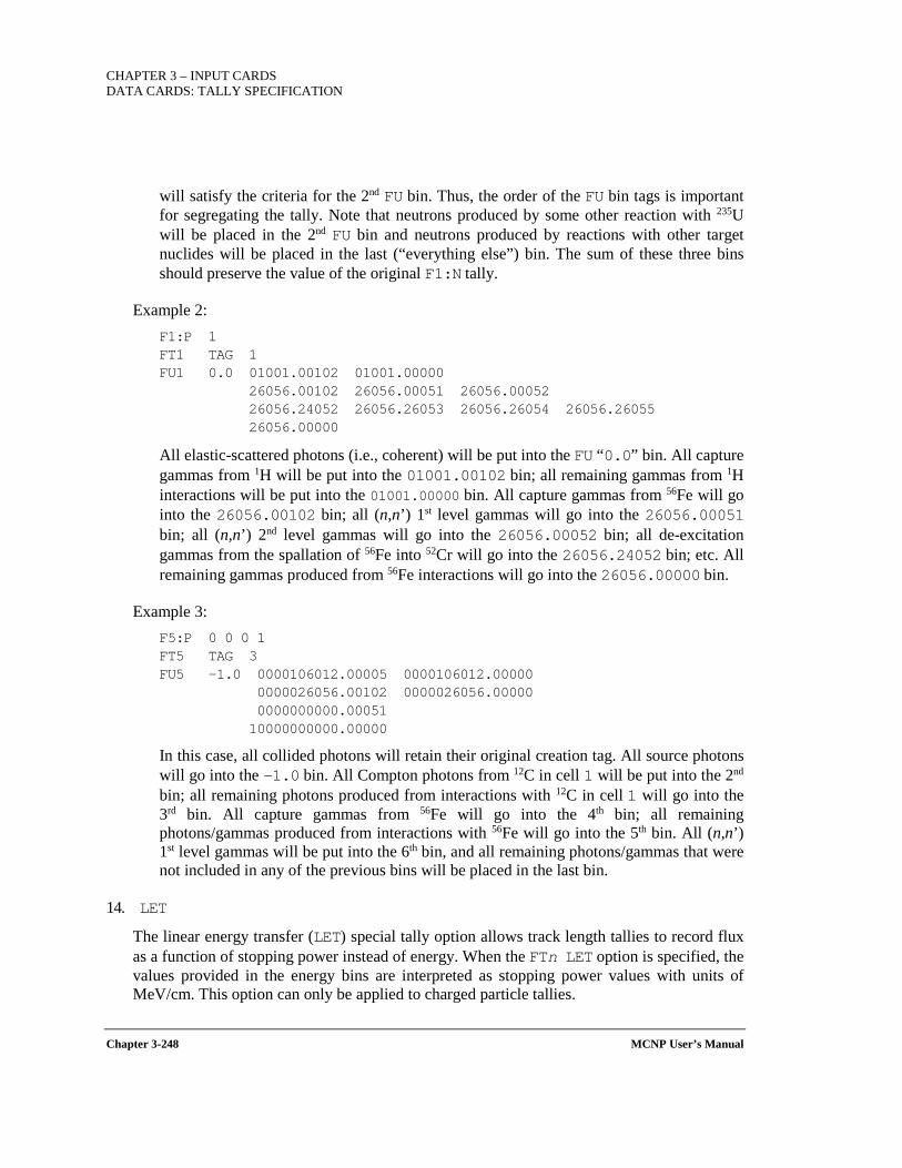
CHAPTER 3 – INPUT CARDS DATA CARDS: TALLY SPECIFICATION
Chapter 3-248 MCNP User’s Manual
will satisfy the criteria for the 2nd FU bin. Thus, the order of the FU bin tags is important for segregating the tally. Note that neutrons produced by some other reaction with 235U will be placed in the 2nd FU bin and neutrons produced by reactions with other target nuclides will be placed in the last (“everything else”) bin. The sum of these three bins should preserve the value of the original F1:N tally.
Example 2: F1:P 1 FT1 TAG 1 FU1 0.0 01001.00102 01001.00000 26056.00102 26056.00051 26056.00052 26056.24052 26056.26053 26056.26054 26056.26055 26056.00000
All elastic-scattered photons (i.e., coherent) will be put into the FU “0.0” bin. All capture gammas from 1H will be put into the 01001.00102 bin; all remaining gammas from 1H interactions will be put into the 01001.00000 bin. All capture gammas from 56Fe will go into the 26056.00102 bin; all (n,n’) 1st level gammas will go into the 26056.00051 bin; all (n,n’) 2nd level gammas will go into the 26056.00052 bin; all de-excitation gammas from the spallation of 56Fe into 52Cr will go into the 26056.24052 bin; etc. All remaining gammas produced from 56Fe interactions will go into the 26056.00000 bin.
Example 3: F5:P 0 0 0 1 FT5 TAG 3 FU5 -1.0 0000106012.00005 0000106012.00000 0000026056.00102 0000026056.00000 0000000000.00051 10000000000.00000
In this case, all collided photons will retain their original creation tag. All source photons will go into the -1.0 bin. All Compton photons from 12C in cell 1 will be put into the 2nd bin; all remaining photons produced from interactions with 12C in cell 1 will go into the 3rd bin. All capture gammas from 56Fe will go into the 4th bin; all remaining photons/gammas produced from interactions with 56Fe will go into the 5th bin. All (n,n’) 1st level gammas will be put into the 6th bin, and all remaining photons/gammas that were not included in any of the previous bins will be placed in the last bin.
14. LET
The linear energy transfer (LET) special tally option allows track length tallies to record flux as a function of stopping power instead of energy. When the FTn LET option is specified, the values provided in the energy bins are interpreted as stopping power values with units of MeV/cm. This option can only be applied to charged particle tallies.
CHAPTER 3 – INPUT CARDS
DATA CARDS: TALLY SPECIFICATION
MCNP User’s Manual Chapter 3-249
Example 1: fc4 Proton flux LET f4:h 77 e4 1e-2 99ilog 6e4 ft4 LET
This example is a tally that records the proton flux in cell 77 for a LET tally. The tally results are recorded in 100 bins of stopping power from 0.01 to 60000 MeV/cm.
15. ROC nhb [m]
The ROC special tally option separates tallies into two components, signal and noise. During a calculation, the signal and noise tally values are saved for each specified batch of histories. These distributions of tally values are formed into signal and noise probability distribution functions (PDFs). Integration of the signal PDF (labeled as the Probability of Detection, PD) is plotted as a function of the integral of the noise PDF (labeled as the Probability of False Alarm, PFA), resulting in the printed Receiver-Operator Characteristic (ROC) curve. A table of the PDF values is provided in Table 163 of the OUTP file.
To specify the “signal” portion of a tally, use entries 1–8 on an associated TF card; to specify the "noise" portion, use TF entries 9–16. The ROC keyword parameter nhb sets the number of histories per batch. This parameter sets the 5th entry (the TFC frequency) on the PRDMP card. The nhb value should represent the total number of source particles emitted over the time interval of interest. The npp value on the NPS card should be set to a multiple of nhb; the npp value will then be used to determine the number of sampled batches. We recommend that npp should be 50–100 times the value of nhb. The optional parameter m specifies the maximum number of batches that will be kept and analyzed. The default value is 100. We recommend m be greater than 50 and perhaps two times the number of batches planned, even considering possible continue-runs. (This value cannot be increased in a continue-run file.) If there are multiple tallies with ROC entries, the maximum m value is used. The WGT keyword on the SDEF card should be set to the default value of unity.
Example 1: f1:n 1 t1 1e8 1e37 tf1 j j j j j j j 2 j j j j j j j 1 ft1 ROC 1000
In this example, tally F1 scores the current of neutrons crossing surface 1. This tally is divided into two time bins, neutrons arriving before 1 second (i.e., 1×10⁸ shakes) and those arriving after 1 second (i.e., 1e37 shakes). The TF card associates the second time bin as the “signal” and the first as the “noise.” The signal and noise currents are accumulated for each batch of 1000 particle histories. The resulting tally values are formed into signal and noise PDFs that are integrated and plotted in Table 163 as a ROC curve for this tally.
CHAPTER 3 – INPUT CARDS DATA CARDS: TALLY SPECIFICATION
Chapter 3-250 MCNP User’s Manual
Another ROC curve example is provided in Section 4.2.5 Example 42.
16. PDS c
This pre-collision estimator augments the post-collision next-event estimator that has historically been used for point flux estimation in MCNP6. The pre-collision next-event estimator includes the contribution of all possible reactions before the collision isotope and resulting reaction are sampled. This procedure has the advantage of providing an improved expected estimate per collision, but with a significant increase in computational costs per collision. This improved sampling technique removes the requirement to suppress coherent scattering for photon transport problems that include photon next-event estimators. The sampling of all possible scattering reactions generally provides an increase in the Figure of Merit (FOM) for most photon problems. This increase in the FOM can be significant when the contribution to a photon next-event estimator is primarily from forward scattering. For most neutron problems there is not typically a large increase in the FOM. However, for both photons and neutrons the pre-collision next-event estimator increases the convergence rate as measured by the time to pass MCNP6's ten statistical checks.
The single parameter, c, specifies how the sampling of the collision is performed for the next-event estimator:
if c=-1 Next-event estimator sampling is performed post-collision; only a single reaction and isotope is sampled (historic MCNP4 and MCNP5 behavior)
if c=0 Same as c=-1 (DEFAULT)
if c=1 Next-event estimator sampling is performed using post-collision sampling of the collision isotope and pre-collision sampling of all reaction channels. (Recommended for photons.)
if c=2 Next-event estimator sampling is performed using pre-collision sampling of all collision isotopes and pre-collision sampling of all reaction channels.
Recommendation: Using either PDS 1 or PDS 2 allows the user to perform next-event estimator tallies with photon coherent scattering enabled.
For neutron next-event estimator tallies the user should perform scoping calculations with PDS=-1, 1, and 2. The user should check the 10 statistical tests of the three runs to assess which parameter provides the best compromise between convergence and FOM. Using a pre-collision estimator for neutrons will typically reduce the computational time needed to pass the 10 statistical checks but result in a lower FOM.
Example 1: f5p 100.0 50.0 25.0 0.0 $ post-collision next-event estimator ft5 pds -1 $ F5 tally is post-collision c
CHAPTER 3 – INPUT CARDS
DATA CARDS: TALLY SPECIFICATION
MCNP User’s Manual Chapter 3-251
f15p 100.0 50.0 25.0 0.0 $ pre-collision next-event estimator ft15 pds 1 $ F15 tally is pre-collision
In this example the pre-collision next-event estimator and the post-collision next-event estimator are compared for a photon tally located at x=100 cm, y=50 cm, and z=25 cm.
17. FFT [LKJI]
A single parameter may follow the FFT keyword and an FU card is required (see Section 3.3.5.16).. The optional LKJI parameter toggles on/off the first-fission treatment for the various physics packages, as explained below. The related FU card segregates the tally into contributions according to which fission occurred first. FU entries should be ZZZAAAs of fissionable nuclides. Additionally, an FU entry of "0" should be included to score all contributions that are not associated with any other FU bin, an FU entry of "16" will score (n,xn) reactions instead of fission if they occur before any fission, and an entry of "18" will score first fissions from any nuclide that is not listed on the FU card. The bins may be entered in any order. The LKJI parameter combines four binary toggles that specify which physics packages should be included with the FFT treatment, such that:
I = 0/1 Omit/include neutron-induced fissions treated by library physics (E<~20 MeV) J = 0/1 Omit/include photon-induced fissions treated by library physics K = 0/1 Omit/include neutron spontaneous fissions (PAR=SF source particles) L = 0/1 Omit/include neutron and photon-induced fissions treated by model physics
The default value for LKJI=0001, which is equivalent to LKJI=1 and is the default action if LKJI is omitted. To turn on the full FFT treatment, one would specify LKJI=1111.
Cell flagging (CF card, Section 3.3.5.12) and surface tally segmenting (FS card, Section 3.3.5.14) have somewhat different meanings when the FFT special tally treatment is used. Unlike the standard tally segmenting, in which the segment identifies where the score is made, FFT tally segmenting identifies where the first fission occurs. Unlike the standard tally flagging, which flags cells through which the track has passed before scoring, FFT cell flagging flags cells in which the first fission occurred. Cell flagging and surface segmenting work for cells and surfaces at the lowest level so when FFT is specified, these lowest-level cells/surfaces will be the location of the first fission. If a CF card is used with the FFT option on any tally, then the use of a CF card without the FFT option is prohibited on any other tally, and the related CF card is ignored and a warning is issued.
Example 1: FT1 FFT FU1 92238 0 16 18 94241 92235 94239
If an (n,xn) reaction occurs before a fission, then the 16 bin records a score. If the particle has its first fission in a listed nuclide (92235, 92238, 94239, 94241), then that nuclide bin records a score provided 16 has no score. If the first fission is not a listed nuclide, the 18
CHAPTER 3 – INPUT CARDS DATA CARDS: TALLY SPECIFICATION
Chapter 3-252 MCNP User’s Manual
bin records a score provided 16 has no score. The 0 bin records a score if no other bin has a score.
18. COM t a
The FT8 COM tally option produces a Compton image stored in an associated FIR radiography tally t using algorithm a (optional, currently there is one algorithm so a=1). The Compton image is formed from a FT8 PHL specification of dual-region coincidences of planar lattice tallies. At the end of each particle history, Compton/photoelectric energy deposition in the front/back of these dual-panel detectors is used to create a circular “image” of the incident photon on a specified image plane. The FT8 PHL enhancement is used to obtain coincidences of front-panel energy deposition with back-panel energy deposition, on a voxel-by-voxel (or element-by-element) basis. For example, if the front-panel detector consists of a 5x5 lattice and the back-panel detector consists of a 10x10 lattice, then the FT8 PHL option produces coincident pulses for 25x100=2500 voxel combinations. The Compton electron energy deposition scored in a front-panel voxel (Ef) is correlated to the photoelectric energy deposition in a back-panel voxel (Eb), via the Compton Equation, to produce the Compton angle of scatter and thus determine a conical angle of incidence. Here is the form of the Compton Equation that is used to obtain the conical angle of incidence: cos (θ) = 1 – me [1/Eb – 1/(Ef+Eb)] , where me is taken as 0.511 MeV. Restrictions on Ef and Eb include: (1) Ef < Eb, and (2) Ef > Eft and Eb < Ebt, where Eft and Ebt are threshold energies set by the user on the corresponding E8 and FU8 cards. The first of these is required to formulate a backward conical image (and helps ensure a Compton/photoelectric reaction occurred), while the latter is needed to reduce image clutter from voxel leakage (electron escape, Brems., etc.). The FT8 COM processing algorithm is currently quite simple in that it takes the center-point of the front-panel voxel and that of the back-panel voxel to form a line which is then intersected with the image plane (at point P). Using the equation above, a radial distance from point P is determined and scores are made to various grid elements intersected by the circle about P (see Fig. 3-8). A simple algorithm is used, based on the size of the grid elements, to determine the number of sample points to score around the circle. A pulse of the source weight is scored in each image-plane grid element that overlaps a circular sample point.
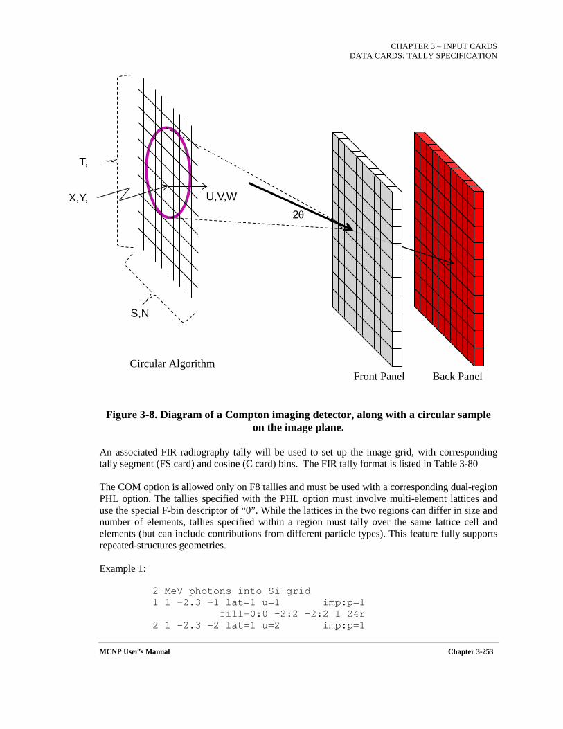
CHAPTER 3 – INPUT CARDS
DATA CARDS: TALLY SPECIFICATION
MCNP User’s Manual Chapter 3-253
X,Y,
U,V,W
T,
S,N
2θ
Circular Algorithm Front Panel Back Panel
Figure 3-8. Diagram of a Compton imaging detector, along with a circular sample on the image plane.
An associated FIR radiography tally will be used to set up the image grid, with corresponding tally segment (FS card) and cosine (C card) bins. The FIR tally format is listed in Table 3-80 The COM option is allowed only on F8 tallies and must be used with a corresponding dual-region PHL option. The tallies specified with the PHL option must involve multi-element lattices and use the special F-bin descriptor of “0”. While the lattices in the two regions can differ in size and number of elements, tallies specified within a region must tally over the same lattice cell and elements (but can include contributions from different particle types). This feature fully supports repeated-structures geometries. Example 1:
2-MeV photons into Si grid 1 1 -2.3 -1 lat=1 u=1 imp:p=1 fill=0:0 -2:2 -2:2 1 24r 2 1 -2.3 -2 lat=1 u=2 imp:p=1
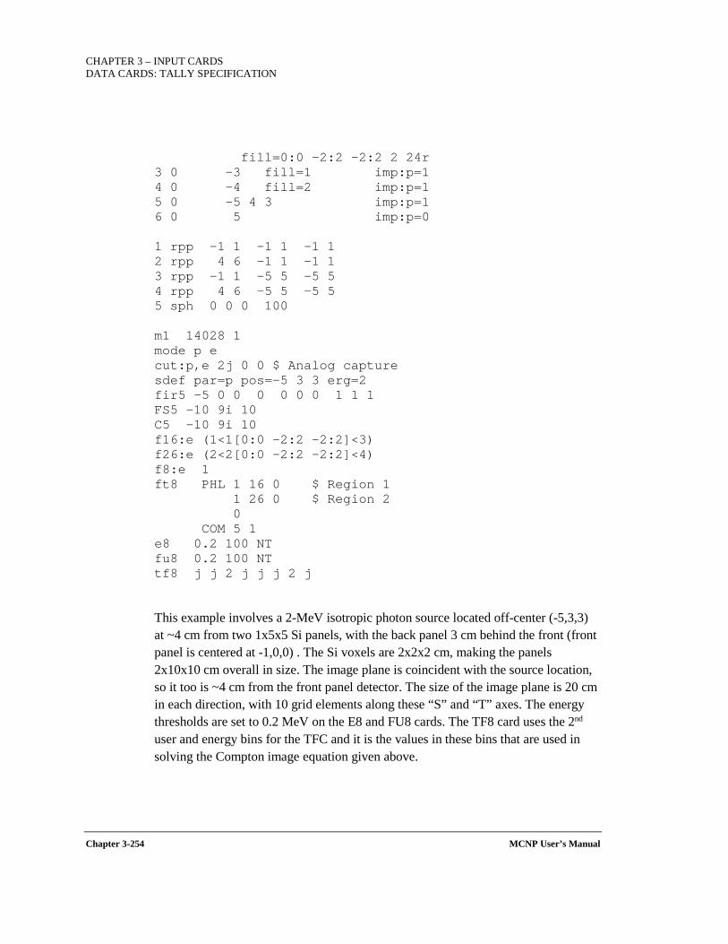
CHAPTER 3 – INPUT CARDS DATA CARDS: TALLY SPECIFICATION
Chapter 3-254 MCNP User’s Manual
fill=0:0 -2:2 -2:2 2 24r 3 0 -3 fill=1 imp:p=1 4 0 -4 fill=2 imp:p=1 5 0 -5 4 3 imp:p=1 6 0 5 imp:p=0 1 rpp -1 1 -1 1 -1 1 2 rpp 4 6 -1 1 -1 1 3 rpp -1 1 -5 5 -5 5 4 rpp 4 6 -5 5 -5 5 5 sph 0 0 0 100 m1 14028 1 mode p e cut:p,e 2j 0 0 $ Analog capture sdef par=p pos=-5 3 3 erg=2 fir5 -5 0 0 0 0 0 0 1 1 1 FS5 -10 9i 10 C5 -10 9i 10 f16:e (1<1[0:0 -2:2 -2:2]<3) f26:e (2<2[0:0 -2:2 -2:2]<4) f8:e 1 ft8 PHL 1 16 0 $ Region 1 1 26 0 $ Region 2 0 COM 5 1 e8 0.2 100 NT fu8 0.2 100 NT tf8 j j 2 j j j 2 j
This example involves a 2-MeV isotropic photon source located off-center (-5,3,3) at ~4 cm from two 1x5x5 Si panels, with the back panel 3 cm behind the front (front panel is centered at -1,0,0) . The Si voxels are 2x2x2 cm, making the panels 2x10x10 cm overall in size. The image plane is coincident with the source location, so it too is ~4 cm from the front panel detector. The size of the image plane is 20 cm in each direction, with 10 grid elements along these “S” and “T” axes. The energy thresholds are set to 0.2 MeV on the E8 and FU8 cards. The TF8 card uses the 2nd user and energy bins for the TFC and it is the values in these bins that are used in solving the Compton image equation given above.
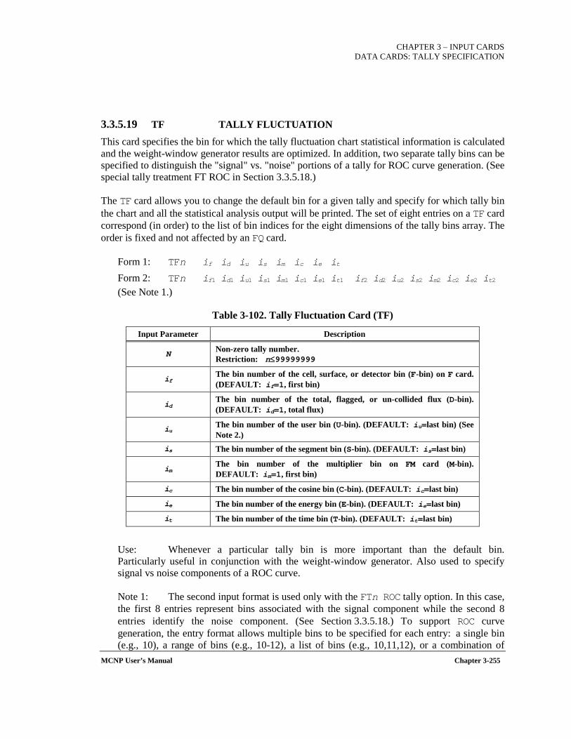
CHAPTER 3 – INPUT CARDS
DATA CARDS: TALLY SPECIFICATION
MCNP User’s Manual Chapter 3-255
3.3.5.19 TF TALLY FLUCTUATION
This card specifies the bin for which the tally fluctuation chart statistical information is calculated and the weight-window generator results are optimized. In addition, two separate tally bins can be specified to distinguish the "signal" vs. "noise" portions of a tally for ROC curve generation. (See special tally treatment FT ROC in Section 3.3.5.18.)
The TF card allows you to change the default bin for a given tally and specify for which tally bin the chart and all the statistical analysis output will be printed. The set of eight entries on a TF card correspond (in order) to the list of bin indices for the eight dimensions of the tally bins array. The order is fixed and not affected by an FQ card.
Form 1: TFn if id iu is im ic ie it
Form 2: TFn if1 id1 iu1 is1 im1 ic1 ie1 it1 if2 id2 iu2 is2 im2 ic2 ie2 it2 (See Note 1.)
Table 3-102. Tally Fluctuation Card (TF)
Input Parameter Description
N Non-zero tally number. Restriction: n≤99999999
if The bin number of the cell, surface, or detector bin (F-bin) on F card. (DEFAULT: if=1, first bin)
id The bin number of the total, flagged, or un-collided flux (D-bin). (DEFAULT: id=1, total flux)
iu The bin number of the user bin (U-bin). (DEFAULT: iu=last bin) (See Note 2.)
is The bin number of the segment bin (S-bin). (DEFAULT: is=last bin)
im The bin number of the multiplier bin on FM card (M-bin). DEFAULT: im=1, first bin)
ic The bin number of the cosine bin (C-bin). (DEFAULT: ic=last bin)
ie The bin number of the energy bin (E-bin). (DEFAULT: ie=last bin)
it The bin number of the time bin (T-bin). (DEFAULT: it=last bin)
Use: Whenever a particular tally bin is more important than the default bin. Particularly useful in conjunction with the weight-window generator. Also used to specify signal vs noise components of a ROC curve.
Note 1: The second input format is used only with the FTn ROC tally option. In this case, the first 8 entries represent bins associated with the signal component while the second 8 entries identify the noise component. (See Section 3.3.5.18.) To support ROC curve generation, the entry format allows multiple bins to be specified for each entry: a single bin (e.g., 10), a range of bins (e.g., 10-12), a list of bins (e.g., 10,11,12), or a combination of
CHAPTER 3 – INPUT CARDS DATA CARDS: TALLY SPECIFICATION
Chapter 3-256 MCNP User’s Manual
these formats (e.g., 10-12,13,14). However, only the first bin listed in each entry is used for generating the TFC output, weight-window generation, and statistical analysis.
Note 2: You may find the J feature useful to jump over last entries. Remember that totals are calculated for energy, time, and user bins (unless inhibited by using NT), so that last for eight energy bins is 9. If one segmenting surface divides a cell or surface into two segments, last in that case is 2, unless T is used on the FS card, in which case last is 3. If there are no user bins or cosine bins, for example, last is 1 for each; last is never less than 1.
The Tally Fluctuation Chart:
At the end of the output, one chart for each tally is printed to give an indication of tally fluctuations; that is, how well the tally has converged. The tally mean, relative error, variance of the variance, Pareto slope (see Section 6.9.7 of the MCNP5 Theory Manual[X-503a]), and figure of merit (FOM=1/(σ2t), where σ is the relative error printed with the tally and t is computer time in minutes) are printed as functions of the number of histories run. The FOM should be roughly constant. The TFn card determines for which bin in tally n the fluctuations are printed. It also determines which tally bin is optimized by the weight-window generator (WWE or WWT and WWG or WWGT cards).
The mean printed in a chart will correspond to some number in the regular tally print. If you have more than one surface listed on an F2 card, for example, the default chart will be for the first surface only; charts can be obtained for all surfaces by having a separate tally for each surface.
Example 1:
Suppose an F2 tally has four surface entries, is segmented into two segments (the segment plus everything else) by one segmenting surface, and has eight energy bins. By default one chart will be produced for the first surface listed, for the part outside the segment, and totaled over energy. If we wish a chart for the fifth energy bin of the third surface in the first segment, we would use TF2 3 2J 1 2J 5
Example 1: TF2 3 2J 1 2J 5 J
In this example, statistics will be calculated based on the 3rd surface, 1st segment, and 5th energy bin provided in Tally 2. Without this card, statistics will be performed on the 1st surface, 1st segment, and the total of all energy bins.
Example 2: TF1 2 j 10-12,13,88 1-2 j 7,8,9 1-99 2 j 1 j j 2 j j j
Note that spaces are not allowed within a comma-delimited list of bins and/or bin ranges. Spaces continue to be used to delimit the eight bin-type entries. The first eight entries
CHAPTER 3 – INPUT CARDS
DATA CARDS: TALLY SPECIFICATION
MCNP User’s Manual Chapter 3-257
specify the bins that constitute the signal component of the tally, while the second eight entries specify the bins that constitute the noise component of the tally.
3.3.5.20 NOTRN DIRECT-ONLY NEUTRAL-PARTICLE POINT DETECTOR CONTRIBUTIONS
Form: NOTRN
Default: None.
Use: This option works with point-detector tallies as well as pinhole or transmitted image tallies. If the NOTRN card appears in the INP file, no transport of the neutral particle source particles takes place, and only the direct neutral particle source contributions are made to the detectors and the detector grid. This is especially useful for checking the problem setup or doing a fast calculation to generate the direct source image. (A NOTRN card is not allowed in a continue run.)
TALLY PERTURBATIONS AND REACTIVITY SENSITIVITIES
MCNP6 offers two flavors of perturbation theory, one based on the differential operator (PERT card) and two others based on adjoint weighting (KPERT and KSEN cards). Both methods offer advantages and disadvantages. The differential operator technique is based on a Taylor series expansion and works very well for generalized responses in fixed-source problems. In eigenvalue problems, however, the differential operator methodology may produce inaccurate results because the MCNP6 implementation does not account for the perturbation of the fission source distribution. The adjoint-based methodology implicitly captures the perturbation in the fission source; however, it is only capable of finding the change in reactivity resulting from perturbations in cross sections and not other responses.
Should a user desire estimates of changes in reactivity for reactor physics applications or sensitivity coefficients to the k-eigenvalue, then the adjoint-based methodology is appropriate. An important limitation of the adjoint-based methods as implemented in MCNP6 is that they do not consider perturbations that may arise from scattering laws or from fission emission spectra; this limitation has been shown to lead to spurious results. For perturbations where the dominant effects are from absorption or the scattering is mostly isotopic, the results tend to agree well with those from direct cross-section substitutions and from the adjoint-methodology code TSUNAMI-3D [REA09], which employs multigroup cross-section data rather than continuous-energy data.
3.3.5.21 PERT TALLY PERTURBATIONS—DIFFERENTIAL OPERATOR
This card allows perturbations in cell material density, composition, or reaction cross-section data. The perturbation analysis uses the first and second order differential operator technique. Perturbation estimates are made without actually changing the input material specifications. Multiple perturbations can be applied in the same run, each specified by a separate PERT card.
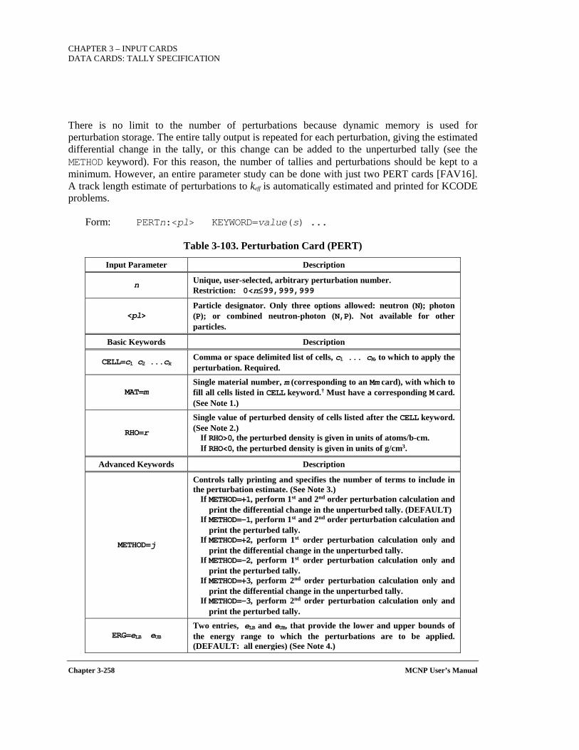
CHAPTER 3 – INPUT CARDS DATA CARDS: TALLY SPECIFICATION
Chapter 3-258 MCNP User’s Manual
There is no limit to the number of perturbations because dynamic memory is used for perturbation storage. The entire tally output is repeated for each perturbation, giving the estimated differential change in the tally, or this change can be added to the unperturbed tally (see the METHOD keyword). For this reason, the number of tallies and perturbations should be kept to a minimum. However, an entire parameter study can be done with just two PERT cards [FAV16]. A track length estimate of perturbations to keff is automatically estimated and printed for KCODE problems.
Form: PERTn:<pl> KEYWORD=value(s) ...
Table 3-103. Perturbation Card (PERT)
Input Parameter Description
n Unique, user-selected, arbitrary perturbation number. Restriction: 0<n≤99,999,999
<pl> Particle designator. Only three options allowed: neutron (N); photon (P); or combined neutron-photon (N,P). Not available for other particles.
Basic Keywords Description
CELL=c1 c2 ...ck Comma or space delimited list of cells, c1 ... cK, to which to apply the perturbation. Required.
MAT=m Single material number, m (corresponding to an Mm card), with which to fill all cells listed in CELL keyword.† Must have a corresponding M card. (See Note 1.)
RHO=r
Single value of perturbed density of cells listed after the CELL keyword. (See Note 2.)
If RHO>0, the perturbed density is given in units of atoms/b-cm. If RHO<0, the perturbed density is given in units of g/cm3.
Advanced Keywords Description
METHOD=j
Controls tally printing and specifies the number of terms to include in the perturbation estimate. (See Note 3.)
If METHOD=+1, perform 1st and 2nd order perturbation calculation and print the differential change in the unperturbed tally. (DEFAULT)
If METHOD=-1, perform 1st and 2nd order perturbation calculation and print the perturbed tally.
If METHOD=+2, perform 1st order perturbation calculation only and print the differential change in the unperturbed tally.
If METHOD=-2, perform 1st order perturbation calculation only and print the perturbed tally.
If METHOD=+3, perform 2nd order perturbation calculation only and print the differential change in the unperturbed tally.
If METHOD=-3, perform 2nd order perturbation calculation only and print the perturbed tally.
ERG=eLB eUB Two entries, eLB and eUB, that provide the lower and upper bounds of the energy range to which the perturbations are to be applied. (DEFAULT: all energies) (See Note 4.)
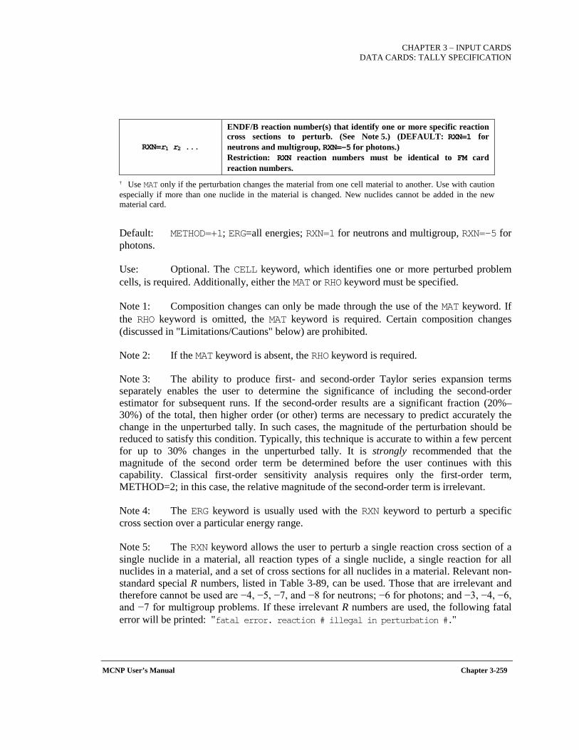
CHAPTER 3 – INPUT CARDS
DATA CARDS: TALLY SPECIFICATION
MCNP User’s Manual Chapter 3-259
RXN=r1 r2 ...
ENDF/B reaction number(s) that identify one or more specific reaction cross sections to perturb. (See Note 5.) (DEFAULT: RXN=1 for neutrons and multigroup, RXN=-5 for photons.) Restriction: RXN reaction numbers must be identical to FM card reaction numbers.
† Use MAT only if the perturbation changes the material from one cell material to another. Use with caution especially if more than one nuclide in the material is changed. New nuclides cannot be added in the new material card.
Default: METHOD=+1; ERG=all energies; RXN=1 for neutrons and multigroup, RXN=-5 for photons.
Use: Optional. The CELL keyword, which identifies one or more perturbed problem cells, is required. Additionally, either the MAT or RHO keyword must be specified.
Note 1: Composition changes can only be made through the use of the MAT keyword. If the RHO keyword is omitted, the MAT keyword is required. Certain composition changes (discussed in "Limitations/Cautions" below) are prohibited.
Note 2: If the MAT keyword is absent, the RHO keyword is required.
Note 3: The ability to produce first- and second-order Taylor series expansion terms separately enables the user to determine the significance of including the second-order estimator for subsequent runs. If the second-order results are a significant fraction (20%–30%) of the total, then higher order (or other) terms are necessary to predict accurately the change in the unperturbed tally. In such cases, the magnitude of the perturbation should be reduced to satisfy this condition. Typically, this technique is accurate to within a few percent for up to 30% changes in the unperturbed tally. It is strongly recommended that the magnitude of the second order term be determined before the user continues with this capability. Classical first-order sensitivity analysis requires only the first-order term, METHOD=2; in this case, the relative magnitude of the second-order term is irrelevant.
Note 4: The ERG keyword is usually used with the RXN keyword to perturb a specific cross section over a particular energy range.
Note 5: The RXN keyword allows the user to perturb a single reaction cross section of a single nuclide in a material, all reaction types of a single nuclide, a single reaction for all nuclides in a material, and a set of cross sections for all nuclides in a material. Relevant non-standard special R numbers, listed in Table 3-89, can be used. Those that are irrelevant and therefore cannot be used are −4, −5, −7, and −8 for neutrons; −6 for photons; and −3, −4, −6, and −7 for multigroup problems. If these irrelevant R numbers are used, the following fatal error will be printed: "fatal error. reaction # illegal in perturbation #."
CHAPTER 3 – INPUT CARDS DATA CARDS: TALLY SPECIFICATION
Chapter 3-260 MCNP User’s Manual
RXN reaction numbers must be consistent with FM card reaction numbers (see Section 3.3.5.7) if the perturbation affects the tally cross section. The specification RXN=-6 is most efficient for fission, although MT=18, MT=19, or MT=-2 (multigroup) also work for keff and F7 tallies.
PERT Card Limitations/Cautions:
1. The perturbation method is limited to the 1st and 2nd order terms of a Taylor series expansion. Examine the 1st and 2nd order terms separately for large (>30%) perturbations to determine the significance of the 2nd order terms. If 2nd order terms are a significant fraction (20%–30%) of the total perturbation, inaccurate tallies can result. (Warning message is generated.) See Note 3 above.
2. Nuclide fraction changes (MAT keyword) are assumed to be independent and, consequently, differential cross terms are ignored. Stated another way, when multiple isotopes are perturbed at once, the perturbation estimate is the sum of the independent nuclide perturbations and does not include the 2nd-order differential term. Therefore, it is very important to change only one isotope density in each PERT card, or to change all isotope densities the same relative amount [FAV16].
3. FM tallies in perturbed cells can be wrong. Surface tallies and tallies in perturbed cells are safe. (Warning message is generated.)
4. Detector (F5) and pulse-height tallies (F8) are not compatible with the PERT card. (i.e., give zero perturbation).
5. DXTRAN is not compatible with the PERT card. (Fatal error message is generated.)
6. You cannot un-void a region. That is, if you take a region originally specified as void and put in a material in that region with the perturbation technique, a fatal error message is generated. However, you can specify a region as containing a material and use the PERT card to make it void by setting RHO=0.
7. You cannot introduce a new nuclide into a material composition. (A fatal error message is generated.) However, you can set up the problem with a mixture of all nuclides of interest and use PERT cards to remove one or more nuclides.
8. Although there is no limit to the number of perturbations, each perturbation increases running time by 10%–20%.
9. Some perturbations (those with small changes) converge slowly.
10. The track length estimate of keff in criticality calculations assumes the fundamental eigenvector (fission distribution) is unchanged in the perturbed configuration. This approximation can lead to serious errors [FAV02]. For the effect of a perturbation on keff, use the KPERT card (Sec. 3.3.5.22)
11. Use caution when selecting the multiplicative constant and reaction number on FM cards used with F4 tallies in perturbation problems. The track length correction term R1j’ is made only if the multiplicative constant on the FM card is negative (indicating macroscopic cross sections with multiplication by the atom density of the cell). If the multiplicative constant on the FM
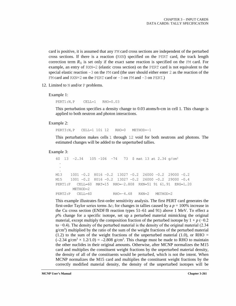
CHAPTER 3 – INPUT CARDS
DATA CARDS: TALLY SPECIFICATION
MCNP User’s Manual Chapter 3-261
card is positive, it is assumed that any FM card cross sections are independent of the perturbed cross sections. If there is a reaction (RXN) specified on the PERT card, the track length correction term R1j is set only if the exact same reaction is specified on the FM card. For example, an entry of RXN=2 (elastic cross section) on the PERT card is not equivalent to the special elastic reaction -3 on the FM card (the user should either enter 2 as the reaction of the FM card and RXN=2 on the PERT card or -3 on FM and -3 on PERT.)
12. Limited to N and/or P problems.
Example 1: PERT1:N,P CELL=1 RHO=0.03
This perturbation specifies a density change to 0.03 atoms/b-cm in cell 1. This change is applied to both neutron and photon interactions.
Example 2: PERT3:N,P CELL=1 10i 12 RHO=0 METHOD=-1
This perturbation makes cells 1 through 12 void for both neutrons and photons. The estimated changes will be added to the unperturbed tallies.
Example 3: 60 13 -2.34 105 -106 -74 73 $ mat 13 at 2.34 g/cm3 . . .
M13 1001 -0.2 8016 -0.2 13027 -0.2 26000 -0.2 29000 -0.2 M15 1001 -0.2 8016 -0.2 13027 -0.2 26000 -0.2 29000 -0.4 PERT1:P CELL=60 MAT=15 RHO=-2.808 RXN=51 9i 61,91 ERG=1,20 METHOD=2 PERT2:P CELL=60 RHO=-4.68 RXN=2 METHOD=2
This example illustrates first-order sensitivity analysis. The first PERT card generates the first-order Taylor series terms Δc1 for changes in tallies caused by a p = 100% increase in the Cu cross section (ENDF/B reaction types 51–61 and 91) above 1 MeV. To effect a p% change for a specific isotope, set up a perturbed material mimicking the original material, except multiply the composition fraction of the perturbed isotope by 1 + p (−0.2 to −0.4). The density of the perturbed material is the density of the original material (2.34 g/cm3) multiplied by the ratio of the sum of the weight fractions of the perturbed material (1.2) to the sum of the weight fractions of the unperturbed material (1.0), or RHO = (–2.34 g/cm3 × 1.2/1.0) = –2.808 g/cm3. This change must be made to RHO to maintain the other nuclides in their original amounts. Otherwise, after MCNP normalizes the M15 card and multiplies the constituent weight fractions by the unperturbed material density, the density of all of the constituents would be perturbed, which is not the intent. When MCNP normalizes the M15 card and multiplies the constituent weight fractions by the correctly modified material density, the density of the unperturbed isotopes will be
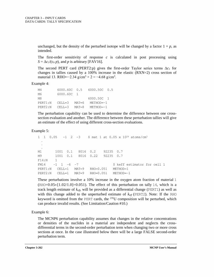
CHAPTER 3 – INPUT CARDS DATA CARDS: TALLY SPECIFICATION
Chapter 3-262 MCNP User’s Manual
unchanged, but the density of the perturbed isotope will be changed by a factor 1 + p, as intended.
The first-order sensitivity of response c is calculated in post processing using S = Δc1/(c0 p), and p is arbitrary [FAV16].
The second PERT card (PERT2:p) gives the first-order Taylor series terms Δc1 for changes in tallies caused by a 100% increase in the elastic (RXN=2) cross section of material 13. RHO=−2.34 g/cm3 × 2 = −4.68 g/cm3.
Example 4: M4 6000.60C 0.5 6000.50C 0.5 M6 6000.60C 1 M8 6000.50C 1 PERT1:N CELL=3 MAT=6 METHOD=-1 PERT2:N CELL=3 MAT=8 METHOD=-1
The perturbation capability can be used to determine the difference between one cross-section evaluation and another. The difference between these perturbation tallies will give an estimate of the effect of using different cross-section evaluations.
Example 5: 1 1 0.05 -1 2 -3 $ mat 1 at 0.05 x 1024 atoms/cm3 . . .
M1 1001 0.1 8016 0.2 92235 0.7 M9 1001 0.1 8016 0.22 92235 0.7 F14:N 1 FM14 -1 1 -6 -7 $ keff estimator for cell 1 PERT1:N CELL=1 MAT=9 RHO=0.051 METHOD=1 PERT2:N CELL=1 MAT=9 RHO=0.051 METHOD=-1
These perturbations involve a 10% increase in the oxygen atom fraction of material 1 (RHO=0.05×[1.02/1.0]=0.051). The effect of this perturbation on tally 14, which is a track length estimate of keff, will be provided as a differential change (PERT1) as well as with this change added to the unperturbed estimate of keff (PERT2). Note: If the RHO keyword is omitted from the PERT cards, the 235U composition will be perturbed, which can produce invalid results. (See Limitation/Caution #10.)
Example 6:
The MCNP6 perturbation capability assumes that changes in the relative concentrations or densities of the nuclides in a material are independent and neglects the cross-differential terms in the second-order perturbation term when changing two or more cross sections at once. In the case illustrated below there will be a large FALSE second-order perturbation term.
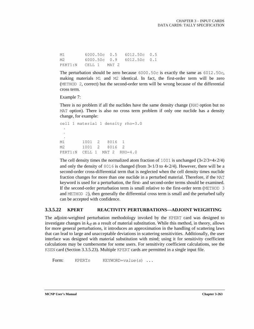
CHAPTER 3 – INPUT CARDS
DATA CARDS: TALLY SPECIFICATION
MCNP User’s Manual Chapter 3-263
M1 6000.50c 0.5 6012.50c 0.5 M2 6000.50c 0.9 6012.50c 0.1 PERT1:N CELL 1 MAT 2
The perturbation should be zero because 6000.50c is exactly the same as 6012.50c, making materials M1 and M2 identical. In fact, the first-order term will be zero (METHOD 2, correct) but the second-order term will be wrong because of the differential cross term.
Example 7:
There is no problem if all the nuclides have the same density change (RHO option but no MAT option). There is also no cross term problem if only one nuclide has a density change, for example: cell 1 material 1 density rho=3.0 . . .
M1 1001 2 8016 1 M2 1001 2 8016 2 PERT1:N CELL 1 MAT 2 RHO=4.0
The cell density times the normalized atom fraction of 1001 is unchanged (3×2/3=4×2/4) and only the density of 8016 is changed (from 3×1/3 to 4×2/4). However, there will be a second-order cross-differential term that is neglected when the cell density times nuclide fraction changes for more than one nuclide in a perturbed material. Therefore, if the MAT keyword is used for a perturbation, the first- and second-order terms should be examined. If the second-order perturbation term is small relative to the first-order term (METHOD 3 and METHOD 2), then generally the differential cross term is small and the perturbed tally can be accepted with confidence.
3.3.5.22 KPERT REACTIVITY PERTURBATIONS—ADJOINT WEIGHTING
The adjoint-weighted perturbation methodology invoked by the KPERT card was designed to investigate changes in keff as a result of material substitution. While this method, in theory, allows for more general perturbations, it introduces an approximation in the handling of scattering laws that can lead to large and unacceptable deviations in scattering sensitivities. Additionally, the user interface was designed with material substitution with mind; using it for sensitivity coefficient calculations may be cumbersome for some users. For sensitivity coefficient calculations, see the KSEN card (Section 3.3.5.23). Multiple KPERT cards are permitted in a single input file.
Form: KPERTn KEYWORD=value(s) ...
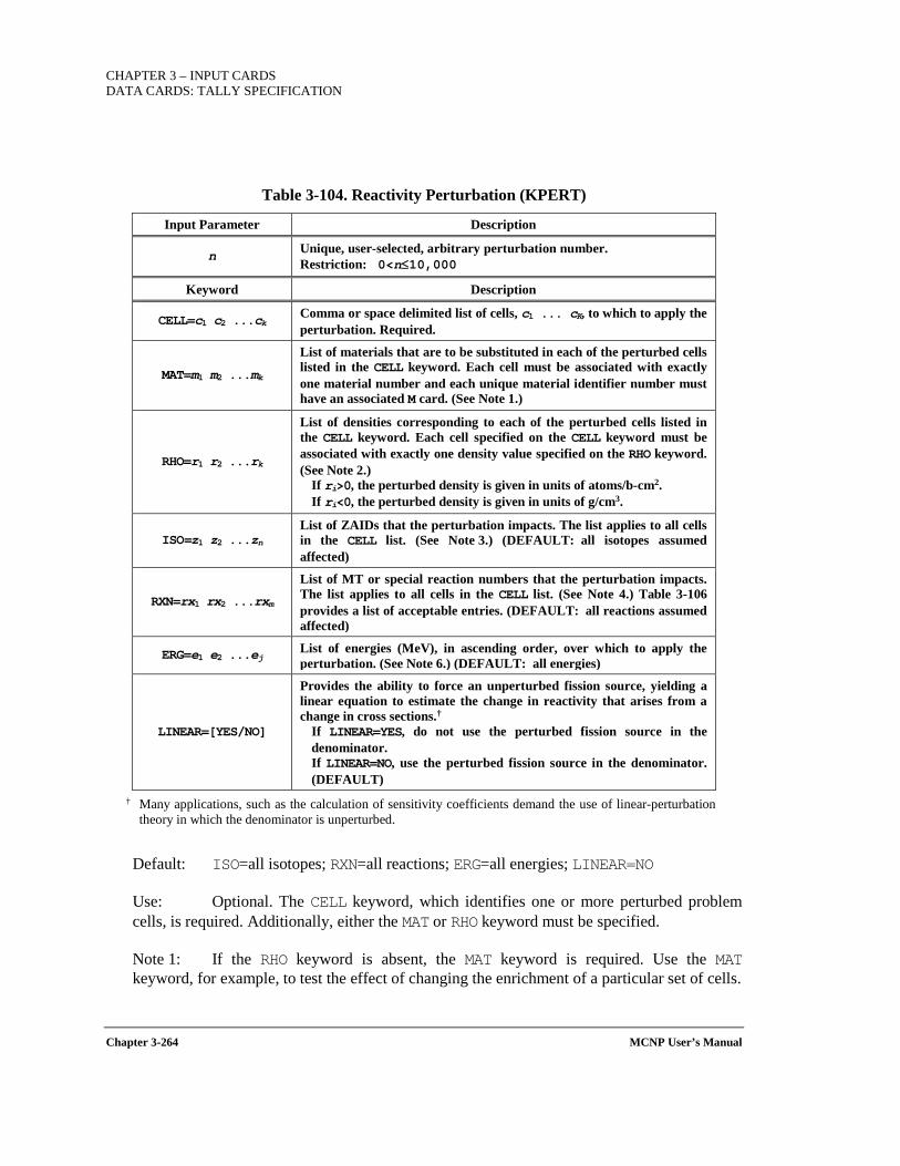
CHAPTER 3 – INPUT CARDS DATA CARDS: TALLY SPECIFICATION
Chapter 3-264 MCNP User’s Manual
Table 3-104. Reactivity Perturbation (KPERT)
Input Parameter Description
n Unique, user-selected, arbitrary perturbation number. Restriction: 0<n≤10,000
Keyword Description
CELL=c1 c2 ...ck Comma or space delimited list of cells, c1 ... cK, to which to apply the perturbation. Required.
MAT=m1 m2 ...mk
List of materials that are to be substituted in each of the perturbed cells listed in the CELL keyword. Each cell must be associated with exactly one material number and each unique material identifier number must have an associated M card. (See Note 1.)
RHO=r1 r2 ...rk
List of densities corresponding to each of the perturbed cells listed in the CELL keyword. Each cell specified on the CELL keyword must be associated with exactly one density value specified on the RHO keyword. (See Note 2.)
If ri>0, the perturbed density is given in units of atoms/b-cm2. If ri<0, the perturbed density is given in units of g/cm3.
ISO=z1 z2 ...zn List of ZAIDs that the perturbation impacts. The list applies to all cells in the CELL list. (See Note 3.) (DEFAULT: all isotopes assumed affected)
RXN=rx1 rx2 ...rxm
List of MT or special reaction numbers that the perturbation impacts. The list applies to all cells in the CELL list. (See Note 4.) Table 3-106 provides a list of acceptable entries. (DEFAULT: all reactions assumed affected)
ERG=e1 e2 ...ej List of energies (MeV), in ascending order, over which to apply the perturbation. (See Note 6.) (DEFAULT: all energies)
LINEAR=[YES/NO]
Provides the ability to force an unperturbed fission source, yielding a linear equation to estimate the change in reactivity that arises from a change in cross sections.†
If LINEAR=YES, do not use the perturbed fission source in the denominator. If LINEAR=NO, use the perturbed fission source in the denominator. (DEFAULT)
† Many applications, such as the calculation of sensitivity coefficients demand the use of linear-perturbation theory in which the denominator is unperturbed.
Default: ISO=all isotopes; RXN=all reactions; ERG=all energies; LINEAR=NO
Use: Optional. The CELL keyword, which identifies one or more perturbed problem cells, is required. Additionally, either the MAT or RHO keyword must be specified.
Note 1: If the RHO keyword is absent, the MAT keyword is required. Use the MAT keyword, for example, to test the effect of changing the enrichment of a particular set of cells.
CHAPTER 3 – INPUT CARDS
DATA CARDS: TALLY SPECIFICATION
MCNP User’s Manual Chapter 3-265
Note 2: If the MAT keyword is absent, the RHO keyword is required. This keyword allows the user to perform density perturbations. RHO may be used in addition to the MAT keyword to perturb both the material and the density of the cells specified in the CELL keyword list.
Note 3: The ISO keyword is useful for testing the effect of individual nuclides.
Note 4: The RXN keyword is useful for testing the effect of individual reactions.
Note 5: The ERG keyword is similar to energy binning with tallies, except that there is no implied lower bound of 0 MeV.
Example 1: KPERT5 CELL=1 4 MAT=2 2 RHO=-19.1 -19.1
This perturbation takes whatever materials are in cells 1 and 4 and makes them both material 2 with a mass density of 19.1 g/cm3.
Example 2: KPERT98 CELL=10 RHO=-18.6 RXN=18
This perturbation looks at the effect on the fission reaction (MT=18) when the mass density of the material in cell 10 is changed to 18.6 g/cm3.
Example 3: KPERT1 CELL=22 26 MAT=92 92 ISO=92238.70c RXN=51 39i 91 ERG=0 2 5 20 LINEAR=YES
This perturbation judges the impact of 238U inelastic scattering in cells 22 and 26 by a change to material 92. The perturbation is further broken down by energy, with regions of less than 2 MeV, between 2 and 5 MeV, and between 5 and 20 MeV. The perturbation is also linear.
3.3.5.23 KSEN KEFF SENSITIVITY COEFFICIENTS—ADJOINT WEIGHTING
The KSEN card [KIE12, KIE13] provides the ability to compute sensitivity coefficients of the effective multiplication k (i.e., keff) for nuclear data. These types of calculations are useful for code validation and the development of benchmark suites applicable to specific sets of applications, for the design of critical (integral) experiments, and for uncertainty quantification. This computation is done in a KCODE calculation using the KSEN card; fixed-source problems are not appropriate for KSEN. Multiple KSEN cards are permitted in a single input file.
The methods employed are based upon linear-perturbation theory using adjoint weighting, the same as those used by TSUNAMI-3D for this purpose. The adjoint weighting is performed in a single forward calculation using the Iterated Fission Probability method. The capability is
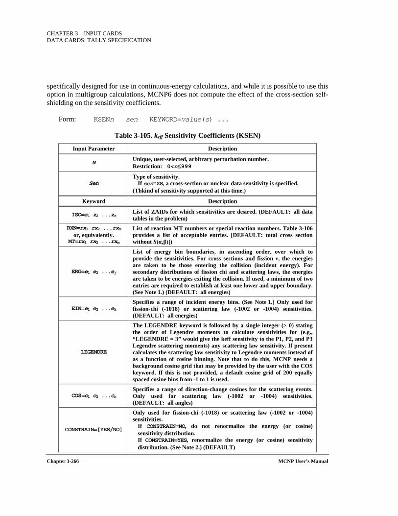
CHAPTER 3 – INPUT CARDS DATA CARDS: TALLY SPECIFICATION
Chapter 3-266 MCNP User’s Manual
specifically designed for use in continuous-energy calculations, and while it is possible to use this option in multigroup calculations, MCNP6 does not compute the effect of the cross-section self-shielding on the sensitivity coefficients.
Form: KSENn sen KEYWORD=value(s) ...
Table 3-105. keff Sensitivity Coefficients (KSEN)
Input Parameter Description
N Unique, user-selected, arbitrary perturbation number. Restriction: 0<n≤999
Sen Type of sensitivity.
If sen=XS, a cross-section or nuclear data sensitivity is specified. (Thkind of sensitivity supported at this time.)
Keyword Description
ISO=z1 z2 ...zn List of ZAIDs for which sensitivities are desired. (DEFAULT: all data tables in the problem)
RXN=rx1 rx2 ...rxm or, equivalently.
MT=rx1 rx2 ...rxm
List of reaction MT numbers or special reaction numbers. Table 3-106 provides a list of acceptable entries. [DEFAULT: total cross section without S(α,β)])
ERG=e1 e2 ...ej
List of energy bin boundaries, in ascending order, over which to provide the sensitivities. For cross sections and fission ν, the energies are taken to be those entering the collision (incident energy). For secondary distributions of fission chi and scattering laws, the energies are taken to be energies exiting the collision. If used, a minimum of two entries are required to establish at least one lower and upper boundary. (See Note 1.) (DEFAULT: all energies)
EIN=e1 e2 ...ek Specifies a range of incident energy bins. (See Note 1.) Only used for fission-chi (-1018) or scattering law (-1002 or -1004) sensitivities. (DEFAULT: all energies)
LEGENDRE
The LEGENDRE keyword is followed by a single integer (> 0) stating the order of Legendre moments to calculate sensitivities for (e.g., “LEGENDRE = 3” would give the keff sensitivity to the P1, P2, and P3 Legendre scattering moments) any scattering law sensitivity. If present calculates the scattering law sensitivity to Legendre moments instead of as a function of cosine binning. Note that to do this, MCNP needs a background cosine grid that may be provided by the user with the COS keyword. If this is not provided, a default cosine grid of 200 equally spaced cosine bins from -1 to 1 is used.
COS=c1 c2 ...cn Specifies a range of direction-change cosines for the scattering events. Only used for scattering law (-1002 or -1004) sensitivities. (DEFAULT: all angles)
CONSTRAIN=[YES/NO]
Only used for fission-chi (-1018) or scattering law (-1002 or -1004) sensitivities.
If CONSTRAIN=NO, do not renormalize the energy (or cosine) sensitivity distribution. If CONSTRAIN=YES, renormalize the energy (or cosine) sensitivity distribution. (See Note 2.) (DEFAULT)

CHAPTER 3 – INPUT CARDS
DATA CARDS: TALLY SPECIFICATION
MCNP User’s Manual Chapter 3-267
Default: ISO=all isotopes in the problem; RXN=total cross section without S(α,β); ERG=all energies; EIN=all energies, COS=all angles; CONSTRAIN=YES
Use: Optional. If the KSEN card is used, the KOPTS card is recommended (see Section 3.3.4.11) .
Note 1: Unlike tallies, there is no implied zero lower-energy-bin boundary.
Note 2: Increasing a distribution in one region of energy (or cosine) space needs to be offset by decreases elsewhere to preserve the condition that the distribution be normalized to a constant value, typically one. For most applications, users should use the default, i.e., renormalize the sensitivities. Full normat\lization [FAV17] is applied.
Note 3: For cross sections and fission nu, the energies listed on ERG are taken to be those entering the collision, whereas for secondary distributions of fission chi and scattering laws they are taken to be energies exiting the collision.
MCNP6 has the ability to subdivide sensitivities by spatial zone. These can be done either as a collection of cells or materials. The keywords on the KSEN card to do this are:
CELL = C1 (C2 C3) … MAT = M1 (M2 M3) …
Each entry defines a spatial zone, and like with tally specifications, cells or materials may be grouped by parentheses. Duplicate cells or materials are allowed. A KSEN card may not have both the CELL and the MAT; doing this both ways requires multiple instances of KSEN. To summarize:
CELL List of cell numbers of the problem for spatial zoning. Each entry defines a spatial zone and multiple cells may be grouped into a single spatial zone with parentheses. Duplicate cells are allowed.
MAT Like the CELL keyword except material numbers are used as opposed to cell
numbers. Zones are defined to encompass all cells containing that material.
Table 3-106. Allowed Reaction Numbers for KSEN with Continuous-Energy Physics
Nuclear Data MT Number Special Reaction Number
Total 1 --
Total+S(α,β) -- -1
Capture -- -2
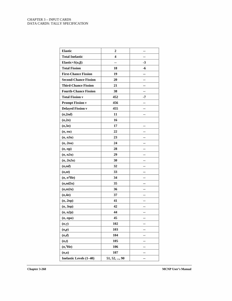
CHAPTER 3 – INPUT CARDS DATA CARDS: TALLY SPECIFICATION
Chapter 3-268 MCNP User’s Manual
Elastic 2 --
Total Inelastic 4 --
Elastic+S(α,β) -- -3
Total Fission 18 -6
First-Chance Fission 19 --
Second-Chance Fission 20 --
Third-Chance Fission 21 --
Fourth-Chance Fission 38 --
Total Fission ν 452 -7
Prompt Fission ν 456 --
Delayed Fission ν 455 --
(n,2nd) 11 --
(n,2n) 16
(n,3n) 17 --
(n, nα) 22 --
(n, n3α) 23 --
(n, 2nα) 24 --
(n, np) 28 --
(n, n2α) 29 --
(n, 2n2α) 30 --
(n,nd) 32 --
(n,nt) 33 --
(n, n3He) 34 --
(n,nd2α) 35 --
(n,nt2α) 36 --
(n,4n) 37 --
(n, 2np) 41 --
(n, 3np) 42 --
(n, n2p) 44 --
(n, npα) 45 --
(n,γ) 102 --
(n,p) 103 --
(n,d) 104 --
(n,t) 105 --
(n,3He) 106 --
(n,α) 107 --
Inelastic Levels (1–40) 51, 52, ..., 90 --
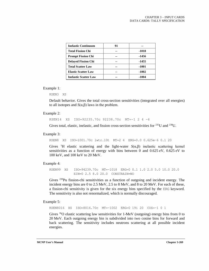
CHAPTER 3 – INPUT CARDS
DATA CARDS: TALLY SPECIFICATION
MCNP User’s Manual Chapter 3-269
Inelastic Continuum 91 --
Total Fission Chi -- -1018
Prompt Fission Chi -- -1456
Delayed Fission Chi -- -1455
Total Scatter Law -- -1001
Elastic Scatter Law -- -1002
Inelastic Scatter Law -- -1004
Example 1: KSEN3 XS
Default behavior. Gives the total cross-section sensitivities (integrated over all energies) to all isotopes and S(α,β) laws in the problem.
Example 2: KSEN14 XS ISO=92235.70c 92238.70c MT=-1 2 4 -6
Gives total, elastic, inelastic, and fission cross-section sensitivities for 235U and 238U.
Example 3: KSEN8 XS ISO=1001.70c lwtr.10t MT=2 4 ERG=0.0 0.625e-6 0.1 20
Gives 1H elastic scattering and the light-water S(α,β) inelastic scattering kernel sensitivities as a function of energy with bins between 0 and 0.625 eV, 0.625 eV to 100 keV, and 100 keV to 20 MeV.
Example 4: KSEN99 XS ISO=94239.70c MT=-1018 ERG=0 0.1 1.0 2.0 5.0 10.0 20.0 EIN=0 2.5 8.0 20.0 CONSTRAIN=NO
Gives 239Pu fission-chi sensitivities as a function of outgoing and incident energy. The incident energy bins are 0 to 2.5 MeV, 2.5 to 8 MeV, and 8 to 20 MeV. For each of these, a fission-chi sensitivity is given for the six energy bins specified by the ERG keyword. The sensitivity is also not renormalized, which is normally discouraged.
Example 5: KSEN8016 XS ISO=8016.70c MT=-1002 ERG=0 19i 20 COS=-1 0 1
Gives 16O elastic scattering law sensitivities for 1-MeV (outgoing) energy bins from 0 to 20 MeV. Each outgoing energy bin is subdivided into two cosine bins for forward and back scattering. The sensitivity includes neutrons scattering at all possible incident energies.

CHAPTER 3 – INPUT CARDS DATA CARDS: TALLY SPECIFICATION
Chapter 3-270 MCNP User’s Manual
Example 6: KSEN101 XS CELL=10 20 (10 20) ERG=SCALE-238 Gives total cross section sensitivities for all isotopes in the problem with an energy binning defined by SCALE’s 238-group library. Three energy-resolved sensitivity profiles are given: one for cell 10, another for cell 20, and a third for both (the sum of the sensitivities for cells 10 and 20).
Example 7: KSEN101 XS RXN=-1002 -1004 LEGENDRE=5 ISO=26056.70c MAT=20 Gives the sensitivities for the first five Legendre moments of elastic and inelastic scattering of 56Fe, but only for cells with material 20. The default cosine grid of 200 equally spaced intervals from -1 to 1 is used for computing the Legendre moment sensitivities because the COS keyword is not specified.
Other options may be controlled by use of the KOPTS card, which contains various options for KCODE calculations. The two options are BLOCKSIZE, which controls the number of cycles in every outer iteration, and KSENTAL, which controls output printing of a results file for sensitivity profiles. The format for these is as follows:
KOPTS BLOCKSIZE = NCY KSENTAL = FILEOPT The NCY argument denotes the number of cycles. A greater number leads to better accuracy of the answer, but the results will be less statistically resolved. The default is 10 cycles, which has been shown to be conservative for almost all cases and still preserves a reasonable about of statistical precision. For small, leakage dominated systems, this can often be reduced to 5. The FILEOPT argument gives a file format for printing the sensitivity profiles. The default is to print no file. In MCNP6, two file formats are available: MCTAL and TSUNAMI-B. The MCTAL format has MCNP print the sensitivity profiles in a special file called ksental which is similar to an mctal file for tallies, and can be plotted by MCPLOT. The TSUNAMI-B format is defined in the SCALE6 Manual. The concepts used by MCNP and SCALE are not necessarily compatible depending on the sensitivity profile options in either code, so the TSUNAMI-B format may not be able to capture everything that MCNP can compute. A description of the formats are given below. An example illustrating these concepts: KOPTS BLOCKSIZE = 5 KSENTAL = TSUNAMI-B By default MCNP prints the sensitivity profiles to the output file. These are located below “the box” with the k results with the heading “nuclear data sensitivity profiles”. The ordering of results
CHAPTER 3 – INPUT CARDS
DATA CARDS: TALLY SPECIFICATION
MCNP User’s Manual Chapter 3-271
changes depending upon the requested information. Regardless, the sensitivities are presented as the sensitivity result (integrated over an energy bin) and its associated relative uncertainty. Note that because sensitivities may either be positive or negative, those near zero may have a very large (greater than one) relative uncertainty, but the absolute uncertainty may be quite small. If no energy bins are requested, then the sensitivities will be presented as: ZAID REACTION SENS REL UNC If energy bins are requested, then the sensitivities will be presented as a function of energy for each isotope and reaction: ELOW EHIGH SENS REL UNC Here ELOW and EHIGH denote the energy bin boundaries. These energy-resolved results may be plotted for visualization in various plotting programs (GNUPLOT, MS Excel, etc.). When doing so, it is usually recommended to plot the profiles per unit lethargy (divide each sensitivity by the logarithm of the ratio of EHIGH to ELOW) on a semi log-x scale. Doing so makes it visually accurate in that areas under curves are visually representative of magnitudes of sensitivity coefficients integrated over energy ranges. If incident energy grids for secondary distributions are requested, then an energy-resolved profile in the above format is given for each incident energy bin. For cosine bins, if an ERG card is specified, then additional grids in the above format is given for each cosine bin. If no ERG card is specified, but COS bins are, then the following results are given for all outgoing energies: CLOW CHIGH SENS REL UNC Here CLOW and CHIGH are the lower and upper cosine bounds. It is also possible to have the results printed to a special MCTAL-formatted file called “ksental”. This is done with the KOPTS keyword and a discussion of its use may be found in Section III. The MCTAL file format is very much like the standard MCTAL file except that the symbols for bins have different meanings. These are:
F = spatial zones as cells or materials (0 denoting all cells) D = unused U = unused S = isotopes M = reaction MTs C = cosine bins E = energy bins T = incident energy bins (for fission chi or scattering laws)

CHAPTER 3 – INPUT CARDS DATA CARDS: TALLY SPECIFICATION
Chapter 3-272 MCNP User’s Manual
The MCNP tally plotter, MCPLOT may be loaded to plot these results. Again, the results should be normalized to be per unit lethargy with the “lethargy” option and plotted on a semi log-x scale for visually accurate area plots. The TSUNAMI-B format is given in the SCALE6 Manual (See Table M18.A.2 in the SCALE6.1 Manual for a full description). Since the SCALE and MCNP6 sensitivity capabilities are different, not all concepts in each code perfectly translate. In writing the TSUNAMI-B file format, MCNP will do the following:
• Multiple energy grids, which is possible in MCNP by multiple uses of the KSEN card, are not supported by TSUNAMI-B. To handle this, each instance of the KSEN card is listed in the file one after the other. For use in SCALE plotting tools, these will need to be split into multiple files.
• Unlike MCNP, energy units in SCALE are in eV, not MeV. The TSUNAMI-B format gives the energies in eV.
• The concept of a unit is not defined in MCNP, and the portion of the header that reports a unit number will give a 0 if no spatial zoning is involved, 1 if the zoning is by cell, and 2 if it is by material. The entry that follows (normally the region within the unit) is an enumeration of each spatial zone (the first zone has a “1”, the second a “2”, and so on).
• MCNP may not be able to compute the volume of a region. In this case, MCNP prints zero to the TSUNAMI-B file.
• In the place where TSUNAMI-B reports the number of uses of the region, MCNP reports the number of spatial zones on this instance of KSEN.
• For fission chi sensitivities, the ones reported are automatically summed over all incident energy grids as the TSUNAMI-B format does not support this.
• The TSUNAMI-B format does not support scattering laws, so these are omitted.
SUPERIMPOSED MESH TALLIES: TWO VERSIONS MCNP6 offers two different mesh tallies to the user. The TMESH tally (Section 3.3.5.24) was developed for the MCNPX code, while the FMESH tally (Section 3.3.5.25) was developed for MCNP5. Although similar, each method is characterized by its own syntax, card format, and output files. The user is encouraged to read about both methods and choose the one that is most appropriate for his or her problem.
3.3.5.24 TMESH SUPERIMPOSED MESH TALLY A
Form: (See Section 3.3.5.24.1)

CHAPTER 3 – INPUT CARDS
DATA CARDS: TALLY SPECIFICATION
MCNP User’s Manual Chapter 3-273
The TMESH tally is a method of graphically displaying particle flux, dose, or other quantities on a rectangular, cylindrical, or spherical grid overlaid on top of the standard problem geometry. Particles are tracked through the independent mesh as part of the regular transport problem. The contents of each mesh cell are written to the RUNTPE file and can be plotted with the MCNP6 geometry plotter superimposed over a plot of the problem geometry. The TMESH tally data are also written to the MCTAL file and can be plotted with the MCNP6 tally plotter, MCPLOT.
Further, the TMESH tally data are written to the MDATA file at the end of each initial-run or continue-run. The MDATA file can be converted into a number of standard formats suitable for reading by various graphical analysis packages. Although the conversion program, GRIDCONV (Section 3.3.5.24.6), is not supplied as part of the overall MCNP6 package, the MCNPX version should be able to read and process most of the output files from MCNP6. Analysis of this data is limited only by the capabilities of the graphical program being used.
Four different mesh-tally types are provided by TMESH:, depending on the information the user wishes to view.
Type 1: Track-Averaged Mesh Tally (Section 3.3.5.24.2) Type 2: Source Mesh Tally (Section 3.3.5.24.3) Type 3 Energy Deposition Mesh Tally (Section 3.3.5.24.4) Type 4: DXTRAN Mesh Tally (Section 3.3.5.24.5)
Each of the four types has its own associated keywords and input values.
For additional information involving the superimposed geometry TMESH tally see Section 5.4.4.
DESCRIPTION OF GENERAL TMESH INPUT CARDS
Card Mnemonic Description TMESH Block Initiation Card CORA Data Card for Mesh Coordinate Direction #1 CORB Data Card for Mesh Coordinate Direction #2 CORC Data Card for Mesh Coordinate Direction #3 ERGSH Mesh Tally Energy or Time Boundary Card MSHMF Response Function RMESH Rectangular Mesh Control Card CMESH Cylindrical Mesh Control Card
SMESH Spherical Mesh Control Card ENDMD Block Termination Card
CHAPTER 3 – INPUT CARDS DATA CARDS: TALLY SPECIFICATION
Chapter 3-274 MCNP User’s Manual
3.3.5.24.1 SETTING UP THE TMESH TALLY IN THE INP FILE
All of the input for TMESH tallies must be in a dedicated block of cards in the INP file data card section. This block must start with a card containing the word TMESH in the first five columns and end with a card containing the word ENDMD in the first five columns. For each requested mesh tally (a maximum of 20 TMESH tallies are permitted), a minimum of four cards must exist between the TMESH and ENDMD cards: an RMESH, CMESH, or SMESH control card, and CORA, CORB, and CORC cards. Optional cards within the mesh-tally block include ERGSH and MSHMF. An FM tally multiplier card may be specified only for Type 1 mesh tallies (Section 3.3.5.24.2); however, if an FM card is associated with a Type 1 mesh tally, it must appear outside of the TMESH/ENDMD card block. Each of these cards is described in the discussion that follows.
The basic structure of the desired mesh as well as what quantities are to be stored to the mesh tally are determined by a mesh control card (RMESH, CMESH, or SMESH). The general form of the control cards follow:
RMESHn:<pl> KEYWORD=value(s) ... CMESHn:<pl> KEYWORD=value(s) ... SMESHn:<pl> KEYWORD=value(s) ...
where
RMESH specifies a rectangular mesh; CMESH specifies a cylindrical mesh; SMESH specifies a spherical mesh; <pl> is the particle type to be tallied—this parameter may or may not be required, depending on the mesh-tally type; n is a user-defined mesh-tally number for which the last digit of n , defines the type (1, 2, 3, or 4) of mesh tally and, consequently, the type of information to be stored in the mesh; and KEYWORD options vary depending on the mesh-tally type.
The notation (R/C/S)MESH will be used in subsequent sections to indicate any of the three mesh geometries. Input keywords for the four mesh-tally types are described in sections that follow. Note that the chosen mesh-tally number must be different from all other tallies in the problem. For example, an F1:N tally will conflict with a RMESH1:N tally.
In addition to the (R/C/S)MESH control card, the following set of cards provides details about the TMESH mesh characteristics and must be present for each requested mesh tally:
CORAn corran,1 corran,2 ... CORBn corrbn,1 corrbn,2 ... CORCn corrcn,1 corrcn,2 ...
where n is the same user-defined mesh-tally number as that on the associated (R/C/S)MESH control card. The mesh tally number must end in 1, 2, 3, or 4 corresponding to the mesh tally type. The entries on the CORA, CORB, and CORC cards describe a mesh in three coordinate directions as defined by the mesh type (rectangular, cylindrical, or spherical), prior to any
CHAPTER 3 – INPUT CARDS
DATA CARDS: TALLY SPECIFICATION
MCNP User’s Manual Chapter 3-275
transformation. (Each tally type supports an optional TRANS keyword to allow the application of a coordinate transformation to the mesh.)
To describe a rectangular mesh, the entries on the CORA card represent planes perpendicular to the x-axis, CORB entries are planes perpendicular to the y-axis, and CORC entries are planes perpendicular to the z-axis. Bins do not have to be equally spaced.
To describe a cylindrical mesh, the middle coordinate, CORB, is the untransformed z-axis, which is the symmetry axis of the cylinder, with radial meshes defined on the CORA input line. The first smallest radius must be equal to zero. The values following CORB define planes perpendicular to the untransformed z-axis. The values following CORC are positive angles relative to a counter-clockwise rotation about the untransformed z-axis. These angles, in degrees, are measured from the positive x-axis and must have at least one entry of 360, which is also required to be the last entry. The lower limit of zero degrees is implicit and never appears on the CORC card.
For spherical meshes, scoring will happen within a spherical volume, and can also be further defined to fall within a conical section defined by a polar angle (relative to the +z-axis) and azimuthal angle. The CORA card entries are sphere radii; inner and outer radii are required. The CORB entries define the polar angle meshing in which the polar angle ranges from 0 to 180 degrees, the 1st bin must be greater than 0 degrees, and the last bin must be 180. The CORC entries are the same as in the cylindrical case, with the 1st bin greater than 0 degrees and the last bin equal to 360. It is helpful in setting up spherical problems to think of the longitude-latitude coordinates on a globe.
The "I" data-input notation (Section 2.8.1) is allowed, enabling a large number of regularly spaced mesh points to be defined with a minimum of entries on the coordinate lines. All of the coordinate entries must be monotonically increasing for the tally mesh features to work properly, but do not need to be equally spaced. It should be noted that the size of these meshes scales with the product of the number of entries for the three coordinates. Machine memory could become a problem for very large meshes with fine spacing.
Additional cards that can be used with TMESH mesh tallies include the following:
ERGSHn e1 e2 , MSHMFm e1 f1 e2 f2 ... ei fi , and FMn ... ,
where positive values on the ERGSH card, e1 and e2, are the lower and upper energy limits for information to be stored to mesh tally n. On the other hand, negative values of e1 and e2 represent lower and upper time limits (in shakes) for information to be stored to mesh tally n. The default is to consider all energies and all times. The value of m on the MSHMF card does not refer to a corresponding mesh tally; instead, m is an arbitrary user-assigned value between 1 and 9. The entries on the MSHMF card, ei and fi, are pairs of energies and the corresponding response
CHAPTER 3 – INPUT CARDS DATA CARDS: TALLY SPECIFICATION
Chapter 3-276 MCNP User’s Manual
functions; as many pairs as needed can be designated. Use of the FM card is limited to Type 1 mesh tallies (Section 3.3.5.24.2) and the card must not appear inside the TMESH card block..
Note that the type 1 (particle track) and type 3 (energy deposition) mesh tallies work with heavy ions although there is no capability to separate out contributions from particular heavy ion species. Also, in void regions, electron mesh tallies will generate zeros; to circumvent this issue, a material of very low density (but ≥1E-15 g/cm3) may be specified in these regions.
For additional examples involving the mesh tally see Section 5.4.4.
3.3.5.24.2 TRACK-AVERAGED TMESH MESH TALLY (TYPE 1)
The first TMESH mesh type scores track averaged data: flux, fluence, or current. The values can be weighted by an MSHMF card, through a dose conversion-coefficient function, or for energy deposition.
Form: (R/C/S)MESHn:<pl> KEYWORD=value(s) ...
where n= 1, 11, 21, 31, ..., and <pl> is the particle type. (See Table 2-2.) (Note: The mesh tally number, n, must not duplicate one used for an F1 tally.) There is no default. The allowed keywords for the Type 1 TMESH are presented in Table 3-107.
Table 3-107. Track-Averaged TMESH Mesh Tally (Type 1)
Keyword Description
TRAKS If TRAKS appears on the input line, tally the number of tracks through each mesh volume. No values accompany the keyword.
FLUX
If FLUX appears on the input line, then the average fluence is particle weight times track length divided by volume in units of number/cm2. If the source is considered to be steady state in particles per second, then the value becomes flux in number/cm2/second. No values accompany the keyword. (DEFAULT)
DOSE
Causes the average flux to be modified by an energy-dependent dose function. The DOSE keyword may be followed by up to four entries, where
If the first entry is 1 to 9, an energy-dependent dose function must be supplied by the user on an MSHMF card.
If the first entry is 10, 20, 31–35, 40, or 99, the dose function is an ANSI standard dose as on the DF card. The next three optional entries define additional standard dose options: int, iu, and fac. See the dose conversion coefficients discussion below and Section 3.3.5.8—DF card.
If no entries follow the DOSE keyword, the default entries are 10, 1, 1, and 1.0, which form inputs into the dose conversion-coefficient function. Results are in rem/hour/source_particle. These functions are described in Table 3-108.
POPUL If POPUL appears on the input line, tally the population (i.e., weight times the track length) in each volume.
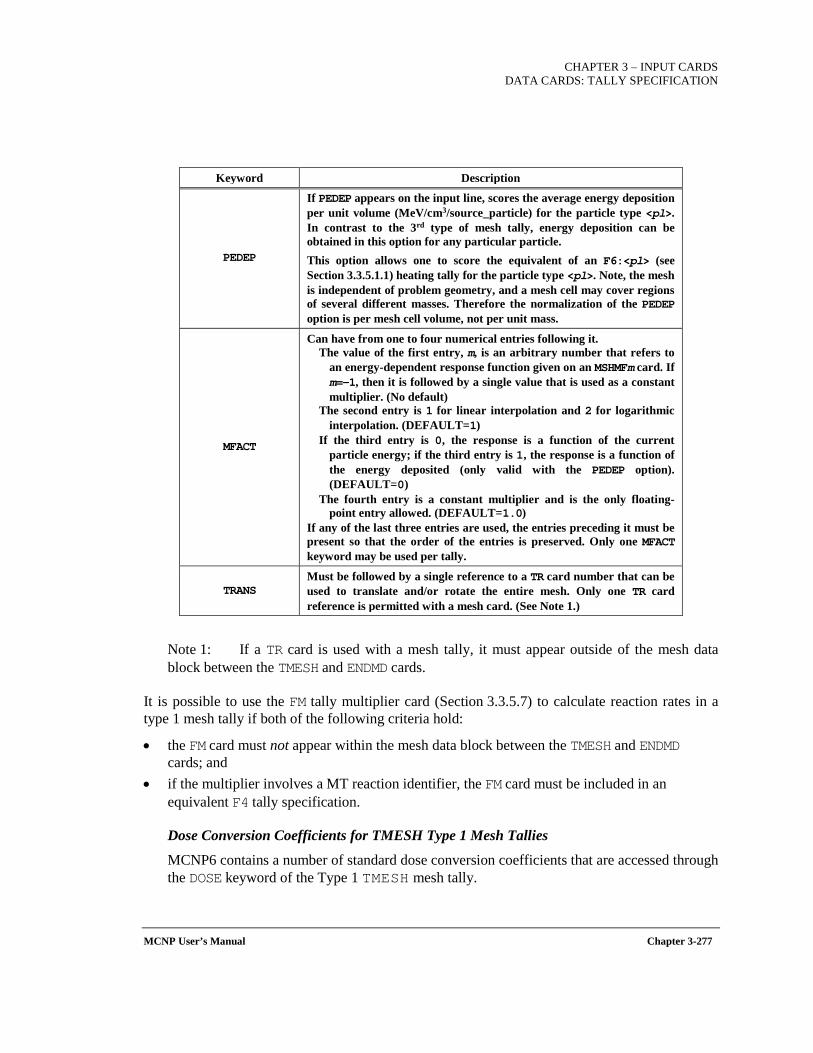
CHAPTER 3 – INPUT CARDS
DATA CARDS: TALLY SPECIFICATION
MCNP User’s Manual Chapter 3-277
Keyword Description
PEDEP
If PEDEP appears on the input line, scores the average energy deposition per unit volume (MeV/cm3/source_particle) for the particle type <pl>. In contrast to the 3rd type of mesh tally, energy deposition can be obtained in this option for any particular particle. This option allows one to score the equivalent of an F6:<pl> (see Section 3.3.5.1.1) heating tally for the particle type <pl>. Note, the mesh is independent of problem geometry, and a mesh cell may cover regions of several different masses. Therefore the normalization of the PEDEP option is per mesh cell volume, not per unit mass.
MFACT
Can have from one to four numerical entries following it. The value of the first entry, m, is an arbitrary number that refers to
an energy-dependent response function given on an MSHMFm card. If m=-1, then it is followed by a single value that is used as a constant multiplier. (No default)
The second entry is 1 for linear interpolation and 2 for logarithmic interpolation. (DEFAULT=1)
If the third entry is 0, the response is a function of the current particle energy; if the third entry is 1, the response is a function of the energy deposited (only valid with the PEDEP option). (DEFAULT=0)
The fourth entry is a constant multiplier and is the only floating-point entry allowed. (DEFAULT=1.0)
If any of the last three entries are used, the entries preceding it must be present so that the order of the entries is preserved. Only one MFACT keyword may be used per tally.
TRANS Must be followed by a single reference to a TR card number that can be used to translate and/or rotate the entire mesh. Only one TR card reference is permitted with a mesh card. (See Note 1.)
Note 1: If a TR card is used with a mesh tally, it must appear outside of the mesh data block between the TMESH and ENDMD cards.
It is possible to use the FM tally multiplier card (Section 3.3.5.7) to calculate reaction rates in a type 1 mesh tally if both of the following criteria hold:
• the FM card must not appear within the mesh data block between the TMESH and ENDMD cards; and
• if the multiplier involves a MT reaction identifier, the FM card must be included in an equivalent F4 tally specification.
Dose Conversion Coefficients for TMESH Type 1 Mesh Tallies
MCNP6 contains a number of standard dose conversion coefficients that are accessed through the DOSE keyword of the Type 1 TMESH mesh tally.
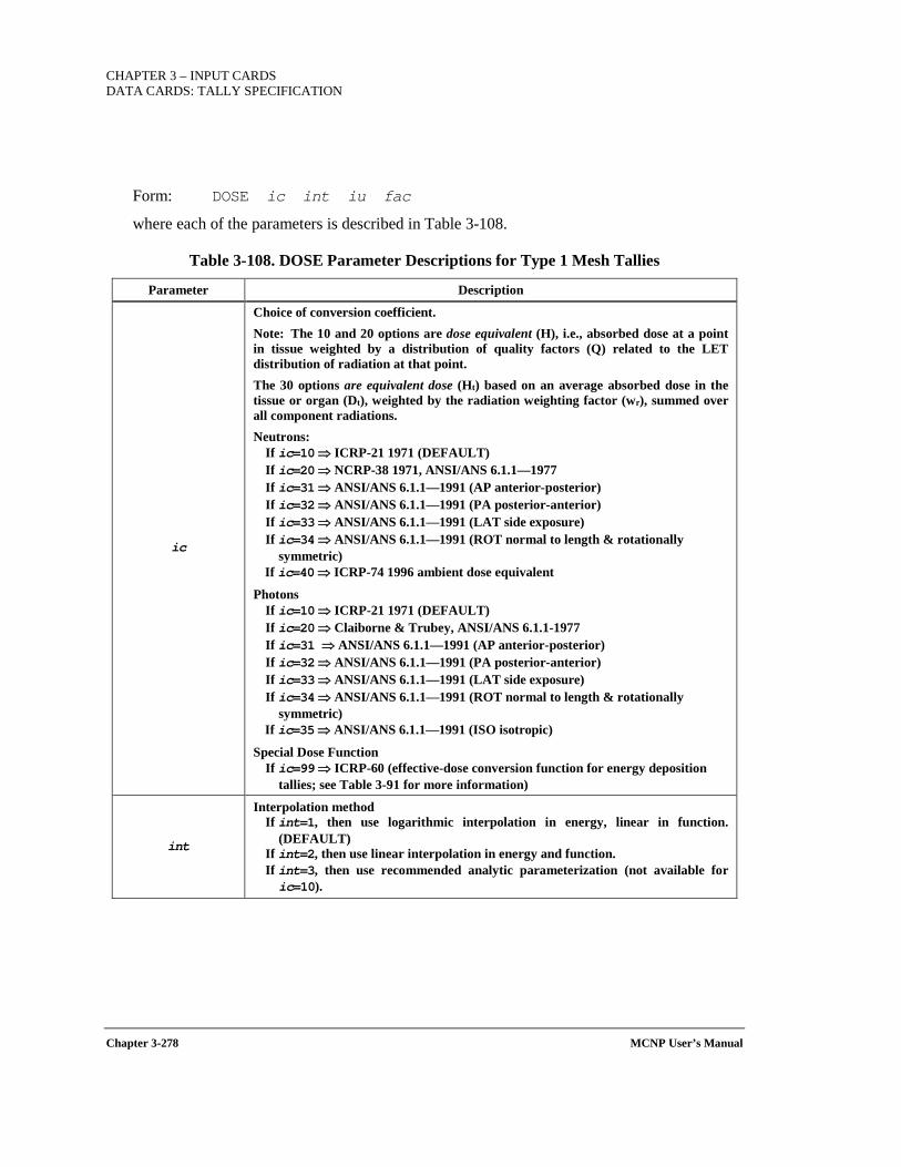
CHAPTER 3 – INPUT CARDS DATA CARDS: TALLY SPECIFICATION
Chapter 3-278 MCNP User’s Manual
Form: DOSE ic int iu fac
where each of the parameters is described in Table 3-108.
Table 3-108. DOSE Parameter Descriptions for Type 1 Mesh Tallies
Parameter Description
ic
Choice of conversion coefficient. Note: The 10 and 20 options are dose equivalent (H), i.e., absorbed dose at a point in tissue weighted by a distribution of quality factors (Q) related to the LET distribution of radiation at that point. The 30 options are equivalent dose (Ht) based on an average absorbed dose in the tissue or organ (Dt), weighted by the radiation weighting factor (wr), summed over all component radiations. Neutrons:
If ic=10 ⇒ ICRP-21 1971 (DEFAULT) If ic=20 ⇒ NCRP-38 1971, ANSI/ANS 6.1.1—1977 If ic=31 ⇒ ANSI/ANS 6.1.1—1991 (AP anterior-posterior) If ic=32 ⇒ ANSI/ANS 6.1.1—1991 (PA posterior-anterior) If ic=33 ⇒ ANSI/ANS 6.1.1—1991 (LAT side exposure) If ic=34 ⇒ ANSI/ANS 6.1.1—1991 (ROT normal to length & rotationally
symmetric) If ic=40 ⇒ ICRP-74 1996 ambient dose equivalent
Photons If ic=10 ⇒ ICRP-21 1971 (DEFAULT) If ic=20 ⇒ Claiborne & Trubey, ANSI/ANS 6.1.1-1977 If ic=31 ⇒ ANSI/ANS 6.1.1—1991 (AP anterior-posterior) If ic=32 ⇒ ANSI/ANS 6.1.1—1991 (PA posterior-anterior) If ic=33 ⇒ ANSI/ANS 6.1.1—1991 (LAT side exposure) If ic=34 ⇒ ANSI/ANS 6.1.1—1991 (ROT normal to length & rotationally
symmetric) If ic=35 ⇒ ANSI/ANS 6.1.1—1991 (ISO isotropic)
Special Dose Function If ic=99 ⇒ ICRP-60 (effective-dose conversion function for energy deposition
tallies; see Table 3-91 for more information)
int
Interpolation method If int=1, then use logarithmic interpolation in energy, linear in function.
(DEFAULT) If int=2, then use linear interpolation in energy and function. If int=3, then use recommended analytic parameterization (not available for ic=10).
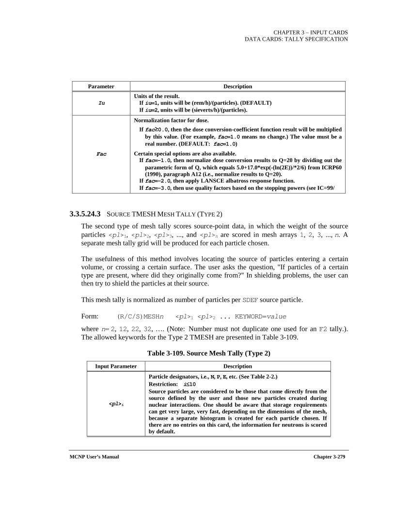
CHAPTER 3 – INPUT CARDS
DATA CARDS: TALLY SPECIFICATION
MCNP User’s Manual Chapter 3-279
Parameter Description
Iu Units of the result.
If iu=1, units will be (rem/h)/(particles). (DEFAULT) If iu=2, units will be (sieverts/h)/(particles).
Fac
Normalization factor for dose. If fac≥0.0, then the dose conversion-coefficient function result will be multiplied
by this value. (For example, fac=1.0 means no change.) The value must be a real number. (DEFAULT: fac=1.0)
Certain special options are also available. If fac=-1.0, then normalize dose conversion results to Q=20 by dividing out the
parametric form of Q, which equals 5.0+17.0*exp(-(ln(2E))/*2/6) from ICRP60 (1990), paragraph A12 (i.e., normalize results to Q=20).
If fac=-2.0, then apply LANSCE albatross response function. If fac=-3.0, then use quality factors based on the stopping powers (see IC=99/
3.3.5.24.3 SOURCE TMESH MESH TALLY (TYPE 2)
The second type of mesh tally scores source-point data, in which the weight of the source particles <pl>1, <pl>2, <pl>3, ..., and <pl>n are scored in mesh arrays 1, 2, 3, ..., n. A separate mesh tally grid will be produced for each particle chosen.
The usefulness of this method involves locating the source of particles entering a certain volume, or crossing a certain surface. The user asks the question, "If particles of a certain type are present, where did they originally come from?" In shielding problems, the user can then try to shield the particles at their source.
This mesh tally is normalized as number of particles per SDEF source particle.
Form: (R/C/S)MESHn <pl>1 <pl>2 ... KEYWORD=value
where n= 2, 12, 22, 32, …. (Note: Number must not duplicate one used for an F2 tally.). The allowed keywords for the Type 2 TMESH are presented in Table 3-109.
Table 3-109. Source Mesh Tally (Type 2)
Input Parameter Description
<pl>i
Particle designators, i.e., N, P, E, etc. (See Table 2-2.) Restriction: i≤10 Source particles are considered to be those that come directly from the source defined by the user and those new particles created during nuclear interactions. One should be aware that storage requirements can get very large, very fast, depending on the dimensions of the mesh, because a separate histogram is created for each particle chosen. If there are no entries on this card, the information for neutrons is scored by default.
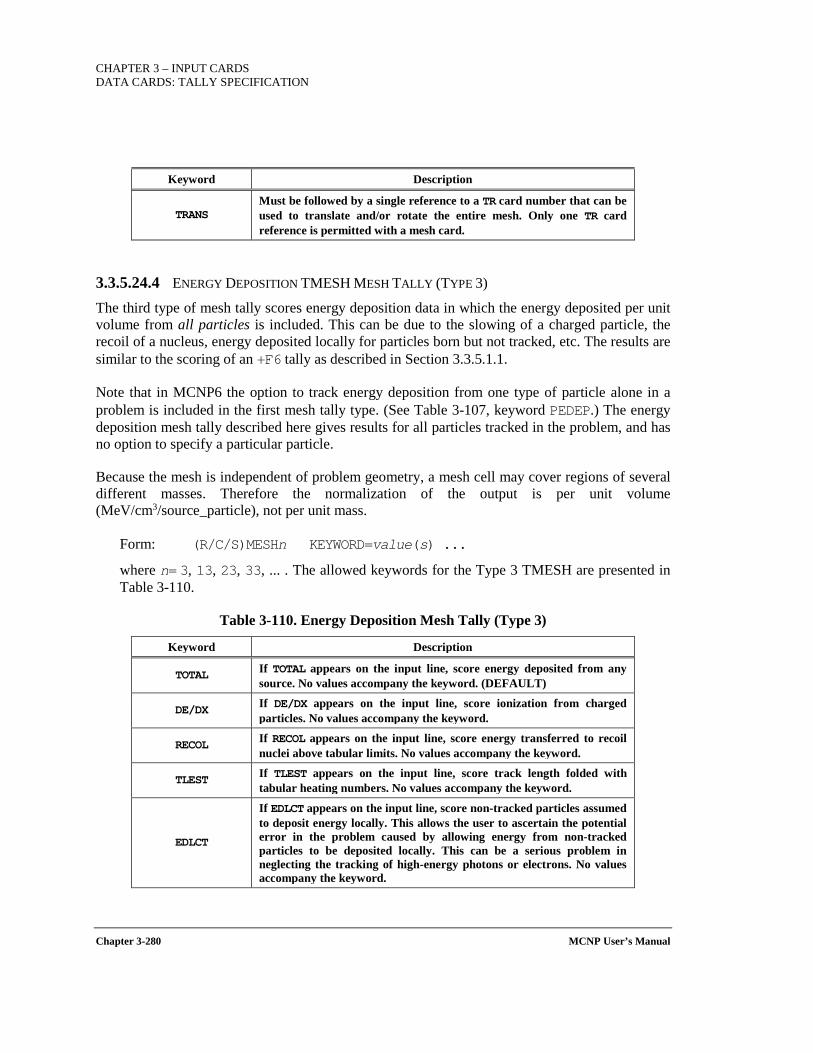
CHAPTER 3 – INPUT CARDS DATA CARDS: TALLY SPECIFICATION
Chapter 3-280 MCNP User’s Manual
Keyword Description
TRANS Must be followed by a single reference to a TR card number that can be used to translate and/or rotate the entire mesh. Only one TR card reference is permitted with a mesh card.
3.3.5.24.4 ENERGY DEPOSITION TMESH MESH TALLY (TYPE 3)
The third type of mesh tally scores energy deposition data in which the energy deposited per unit volume from all particles is included. This can be due to the slowing of a charged particle, the recoil of a nucleus, energy deposited locally for particles born but not tracked, etc. The results are similar to the scoring of an +F6 tally as described in Section 3.3.5.1.1.
Note that in MCNP6 the option to track energy deposition from one type of particle alone in a problem is included in the first mesh tally type. (See Table 3-107, keyword PEDEP.) The energy deposition mesh tally described here gives results for all particles tracked in the problem, and has no option to specify a particular particle.
Because the mesh is independent of problem geometry, a mesh cell may cover regions of several different masses. Therefore the normalization of the output is per unit volume (MeV/cm3/source_particle), not per unit mass.
Form: (R/C/S)MESHn KEYWORD=value(s) ...
where n= 3, 13, 23, 33, ... . The allowed keywords for the Type 3 TMESH are presented in Table 3-110.
Table 3-110. Energy Deposition Mesh Tally (Type 3)
Keyword Description
TOTAL If TOTAL appears on the input line, score energy deposited from any source. No values accompany the keyword. (DEFAULT)
DE/DX If DE/DX appears on the input line, score ionization from charged particles. No values accompany the keyword.
RECOL If RECOL appears on the input line, score energy transferred to recoil nuclei above tabular limits. No values accompany the keyword.
TLEST If TLEST appears on the input line, score track length folded with tabular heating numbers. No values accompany the keyword.
EDLCT
If EDLCT appears on the input line, score non-tracked particles assumed to deposit energy locally. This allows the user to ascertain the potential error in the problem caused by allowing energy from non-tracked particles to be deposited locally. This can be a serious problem in neglecting the tracking of high-energy photons or electrons. No values accompany the keyword.
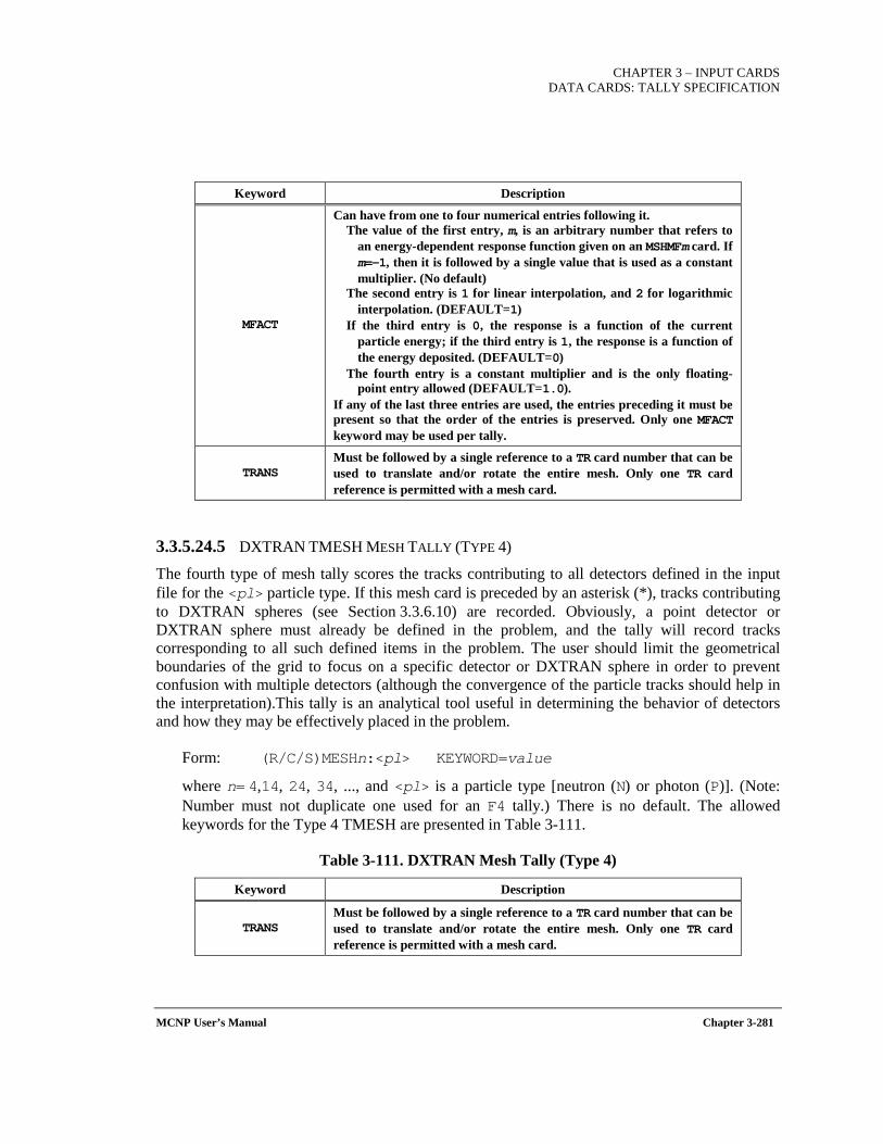
CHAPTER 3 – INPUT CARDS
DATA CARDS: TALLY SPECIFICATION
MCNP User’s Manual Chapter 3-281
Keyword Description
MFACT
Can have from one to four numerical entries following it. The value of the first entry, m, is an arbitrary number that refers to
an energy-dependent response function given on an MSHMFm card. If m=-1, then it is followed by a single value that is used as a constant multiplier. (No default)
The second entry is 1 for linear interpolation, and 2 for logarithmic interpolation. (DEFAULT=1)
If the third entry is 0, the response is a function of the current particle energy; if the third entry is 1, the response is a function of the energy deposited. (DEFAULT=0)
The fourth entry is a constant multiplier and is the only floating-point entry allowed (DEFAULT=1.0).
If any of the last three entries are used, the entries preceding it must be present so that the order of the entries is preserved. Only one MFACT keyword may be used per tally.
TRANS Must be followed by a single reference to a TR card number that can be used to translate and/or rotate the entire mesh. Only one TR card reference is permitted with a mesh card.
3.3.5.24.5 DXTRAN TMESH MESH TALLY (TYPE 4)
The fourth type of mesh tally scores the tracks contributing to all detectors defined in the input file for the <pl> particle type. If this mesh card is preceded by an asterisk (*), tracks contributing to DXTRAN spheres (see Section 3.3.6.10) are recorded. Obviously, a point detector or DXTRAN sphere must already be defined in the problem, and the tally will record tracks corresponding to all such defined items in the problem. The user should limit the geometrical boundaries of the grid to focus on a specific detector or DXTRAN sphere in order to prevent confusion with multiple detectors (although the convergence of the particle tracks should help in the interpretation).This tally is an analytical tool useful in determining the behavior of detectors and how they may be effectively placed in the problem.
Form: (R/C/S)MESHn:<pl> KEYWORD=value
where n= 4,14, 24, 34, ..., and <pl> is a particle type [neutron (N) or photon (P)]. (Note: Number must not duplicate one used for an F4 tally.) There is no default. The allowed keywords for the Type 4 TMESH are presented in Table 3-111.
Table 3-111. DXTRAN Mesh Tally (Type 4)
Keyword Description
TRANS Must be followed by a single reference to a TR card number that can be used to translate and/or rotate the entire mesh. Only one TR card reference is permitted with a mesh card.

CHAPTER 3 – INPUT CARDS DATA CARDS: TALLY SPECIFICATION
Chapter 3-282 MCNP User’s Manual
3.3.5.24.6 PROCESSING THE TMESH MESH TALLY RESULTS
The values of the coordinates, the tally quantity within each mesh bin, and the relative errors are all written by MCNP6 to the RUNTPE file, the optional MCTAL file, and an unformatted binary file named MDATA.
The mesh tallies may be plotted with the MCNP6 geometry plotter either during the course of a run (by placing an MPLOT card in the input file or by using the TTY interrupt capability to invoke MCPLOT) or after a run using the RUNTPE file and the MCNP6 geometry plotter. These plots are superimposed over 2D views of the problem geometry. Note that the geometry plotter must be accessed via the tally plotter. For example,
MCNP6 Z MCPLOT>RUNTPE=<filename> MCPLOT>PLOT PLOT>py 4 ex 40 or 0 4 0 la 0 1 tal12 color on la 0 0 con 0 100 %
After the PLOT command, the MCNP6 interactive geometry plotter appears. If the Plot> button (bottom center) is clicked, then the above command after the PLOT> prompt can be entered. Alternatively, the mesh tally superimposed on the geometry can be viewed by clicking buttons (tal, etc.) of the interactive tally plot. Note that the command tal12 has no space between tal and 12 and that the cell labels (la 0 1 tal12) must be turned on to set the color (color on) and then be turned off (la 0 0).
The second mesh tally processing option is to use the MCNP6 tally plotter (MCPLOT) after a run with the optional MCTAL file (see PRDMP card). For example,
MCNP6 Z MCPLOT>RMCTAL=<filename> tal 12 free ik
Note that there is a space between tal and 12 and that the mesh tally dimensionality (i,j,k) corresponding to CORA, CORB, and CORC) must be specified.
The third mesh tally processing option is to post-process the MDATA (or MCTAL) file with GRIDCONV and then use an external graphics package.
The GRIDCONV program is a post-processing code used with the MDATA output file. It can also be used with the MCTAL output file from the radiography tally as described in Section 3.3.5.1.2. GRIDCONV converts the data arrays in MDATA to forms compatible with various external graphics packages. Those supported in MCNP6 include the following:
PAW PAW (Physics Analysis Workstation) is distributed through the CERN Program Library.
(http://wwwasd.web.cern.ch.wwwasd/paw/index.html)
CHAPTER 3 – INPUT CARDS
DATA CARDS: TALLY SPECIFICATION
MCNP User’s Manual Chapter 3-283
IDL IDL (Interactive Data Language) is a product of ITT Visual Information Solutions, 4990 Pearl East Circle, Boulder, CO 80301
(http://www.ittvis.com/idl/index.asp)
Tecplot Tecplot is a product of Amtec Engineering, Inc., 13920 SE Eastgate Way, Ste. 220, Bellevue, WA 98005 (http://www.amtec.com)
GNUPLOT Freeware. (http://www.gnuplot.info). Only 1D and 2D plots supported.
Like MCNP6, GRIDCONV will compile on several platforms. However, currently the PAW part of the code will not compile on the Linux operating system, since some of the PAW subroutines needed by the code are not Linux compatible. GRIDCONV may be compiled with a ‘NOPAW’ option.
After GRIDCONV is compiled, one need type only the word ‘GRIDCONV‘ to execute the code. The code will then prompt the user for information that is required such as file type, file names, etc. In most cases the default value is used and a return is all that is necessary.
Once the header information from MDATA has been read from the file, GRIDCONV can either produce an ASCII file from a binary or generate the required graphics input files as requested by the user. (Note that the ASCII file contains raw data not normalized to the number of source particles.) The reason for the option to write an ASCII file is that sometimes users will want to look at the numbers in the MDATA file before doing any plotting, or check the numerical results for a test case. The ASCII option is also very useful for porting the MDATA file to another computer platform, and for reading the data into graphics packages not currently supported by GRIDCONV.
GRIDCONV is currently set up to generate one-, two-, or three-dimensional graphics input files with any combination of binning choices. Once the input file has been generated, GRIDCONV gives the user the option of producing another file from the currently selected mesh tally, selecting a different mesh tally available on this MDATA file, or reading information from a different file. Of course there is always the option to exit the program.
The capabilities of GRIDCONV have recently been expanded so that any and all tallies written to MCTAL can be processed. The code is still interactive, but now shows all tallies in the problem, from which any may be selected. The user has the option of generating one- or two-dimensional output. The user is then told about the bin structure so the one or two free variables may be selected. The energy is the default independent variable in the one-dimensional case. There is no default for the two-dimensional case. The order in which the two-dimensional bin variables are selected does not make any difference to the output, in that the order of the processing will be as it appears on the MCTAL file.
For additional information involving superimposed geometry mesh tallies, see Section 5.4.4.

CHAPTER 3 – INPUT CARDS DATA CARDS: TALLY SPECIFICATION
Chapter 3-284 MCNP User’s Manual
3.3.5.25 FMESH SUPERIMPOSED MESH TALLY B
The FMESH card allows the user to define a mesh tally superimposed over the problem geometry. Results are written to a separate output file with the default name MESHTAL. By default, the mesh tally calculates the track length estimate of the particle flux averaged over a mesh cell in units of particles/cm2. If an asterisk precedes the FMESH card, energy times particle weight will be tallied in units of MeV/cm2. Other mesh-tally types include source points and isotopic reaction rates.
FMESH mesh tallies can be used in combination with the DE, DF, FC, FM, and TR cards. FMESH mesh tallies can be used in combination with the surface (SF) and cell (CF) flagging tally cards. However, unlike the regular tallies, only one mesh tally, the flagged tally, is created. A separate mesh tally will need to be provided for un-flagged tally results.
Form: FMESHn:<pl> KEYWORD=value(s)
where n is a tally number ending in the numeral 4 (only type 4 volume flux tallies are permitted) and <pl>=N or P or E. The allowed FMESH keywords are presented in Table 3-112.
Table 3-65. Superimposed FMESH Mesh Tally
Keyword Description
GEOM Mesh geometry, either Cartesian (XYZ or REC) or cylindrical (RZT or CYL) coordinates. (DEFAULT: GEOM=XYZ)
ORIGIN
Coordinates x,y,z of the origin of the mesh in terms of MCNP6 cell geometry. This position is the bottom center for cylindrical coordinates or the bottom, left, behind for rectangular coordinates. (DEFAULT: ORIGIN=0.,0.,0.) (See Note 1.)
AXS Vector giving the direction of the axis of the cylindrical mesh. (DEFAULT: AXS=0.,0.,1.) (See Note 2.)
VEC Vector defining, along with AXS, the plane for θ=0. (DEFAULT: VEC=1.,0.,0.) (See Note 2.)
IMESH Locations of the coarse mesh points in the x direction for rectangular geometry or in the r direction for cylindrical geometry. (DEFAULT: none) (See Note 3.)
IINTS Number of fine mesh points within each corresponding coarse mesh in the x direction for rectangular geometry or in the r direction for cylindrical geometry. (DEFAULT: IINTS=1)
JMESH Locations of the coarse mesh points in the y direction for rectangular geometry or in the z direction for cylindrical geometry. (DEFAULT: none) (See Note 3.)
JINTS Number of fine mesh points within each corresponding coarse mesh in the y direction for rectangular geometry or in the z direction for cylindrical geometry. (DEFAULT: JINTS=1)
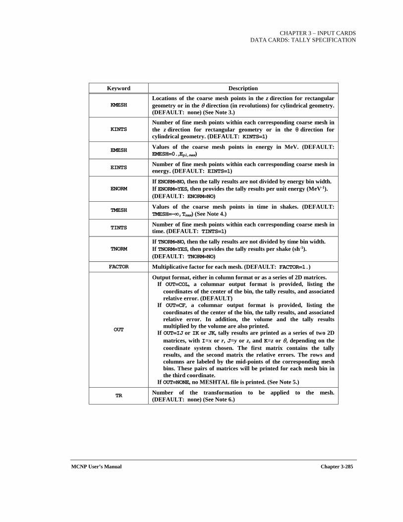
CHAPTER 3 – INPUT CARDS
DATA CARDS: TALLY SPECIFICATION
MCNP User’s Manual Chapter 3-285
Keyword Description
KMESH Locations of the coarse mesh points in the z direction for rectangular geometry or in the θ direction (in revolutions) for cylindrical geometry. (DEFAULT: none) (See Note 3.)
KINTS Number of fine mesh points within each corresponding coarse mesh in the z direction for rectangular geometry or in the θ direction for cylindrical geometry. (DEFAULT: KINTS=1)
EMESH Values of the coarse mesh points in energy in MeV. (DEFAULT: EMESH=0.,Epl,max)
EINTS Number of fine mesh points within each corresponding coarse mesh in energy. (DEFAULT: EINTS=1)
ENORM If ENORM=NO, then the tally results are not divided by energy bin width. If ENORM=YES, then provides the tally results per unit energy (MeV-1). (DEFAULT: ENORM=NO)
TMESH Values of the coarse mesh points in time in shakes. (DEFAULT: TMESH=-∞,Tmax) (See Note 4.)
TINTS Number of fine mesh points within each corresponding coarse mesh in time. (DEFAULT: TINTS=1)
TNORM If TNORM=NO, then the tally results are not divided by time bin width. If TNORM=YES, then provides the tally results per shake (sh-1). (DEFAULT: TNORM=NO)
FACTOR Multiplicative factor for each mesh. (DEFAULT: FACTOR=1.)
OUT
Output format, either in column format or as a series of 2D matrices. If OUT=COL, a columnar output format is provided, listing the
coordinates of the center of the bin, the tally results, and associated relative error. (DEFAULT)
If OUT=CF, a columnar output format is provided, listing the coordinates of the center of the bin, the tally results, and associated relative error. In addition, the volume and the tally results multiplied by the volume are also printed.
If OUT=IJ or IK or JK, tally results are printed as a series of two 2D matrices, with I=x or r, J=y or z, and K=z or θ, depending on the coordinate system chosen. The first matrix contains the tally results, and the second matrix the relative errors. The rows and columns are labeled by the mid-points of the corresponding mesh bins. These pairs of matrices will be printed for each mesh bin in the third coordinate.
If OUT=NONE, no MESHTAL file is printed. (See Note 5.)
TR Number of the transformation to be applied to the mesh. (DEFAULT: none) (See Note 6.)
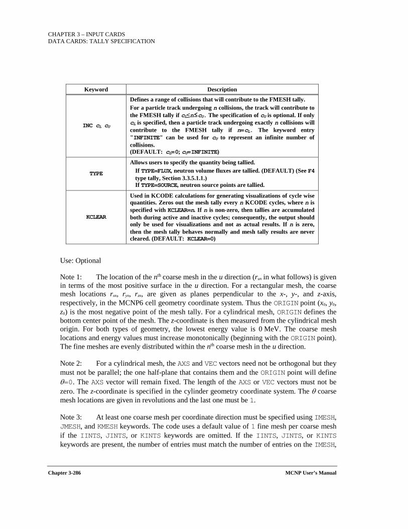
CHAPTER 3 – INPUT CARDS DATA CARDS: TALLY SPECIFICATION
Chapter 3-286 MCNP User’s Manual
Keyword Description
INC cL cU
Defines a range of collisions that will contribute to the FMESH tally. For a particle track undergoing n collisions, the track will contribute to the FMESH tally if cL≤n≤cU. The specification of cU is optional. If only cL is specified, then a particle track undergoing exactly n collisions will contribute to the FMESH tally if n=cL. The keyword entry "INFINITE" can be used for cU to represent an infinite number of collisions. (DEFAULT: cL=0; cU=INFINITE)
TYPE
Allows users to specify the quantity being tallied. If TYPE=FLUX, neutron volume fluxes are tallied. (DEFAULT) (See F4 type tally, Section 3.3.5.1.1.) If TYPE=SOURCE, neutron source points are tallied.
KCLEAR
Used in KCODE calculations for generating visualizations of cycle wise quantities. Zeros out the mesh tally every n KCODE cycles, where n is specified with KCLEAR=n. If n is non-zero, then tallies are accumulated both during active and inactive cycles; consequently, the output should only be used for visualizations and not as actual results. If n is zero, then the mesh tally behaves normally and mesh tally results are never cleared. (DEFAULT: KCLEAR=0)
Use: Optional
Note 1: The location of the nth coarse mesh in the u direction (run in what follows) is given in terms of the most positive surface in the u direction. For a rectangular mesh, the coarse mesh locations rxn, ryn, rzn, are given as planes perpendicular to the x-, y-, and z-axis, respectively, in the MCNP6 cell geometry coordinate system. Thus the ORIGIN point (x0, y0, z0) is the most negative point of the mesh tally. For a cylindrical mesh, ORIGIN defines the bottom center point of the mesh. The z-coordinate is then measured from the cylindrical mesh origin. For both types of geometry, the lowest energy value is 0 MeV. The coarse mesh locations and energy values must increase monotonically (beginning with the ORIGIN point). The fine meshes are evenly distributed within the nth coarse mesh in the u direction.
Note 2: For a cylindrical mesh, the AXS and VEC vectors need not be orthogonal but they must not be parallel; the one half-plane that contains them and the ORIGIN point will define θ=0. The AXS vector will remain fixed. The length of the AXS or VEC vectors must not be zero. The z-coordinate is specified in the cylinder geometry coordinate system. The θ coarse mesh locations are given in revolutions and the last one must be 1.
Note 3: At least one coarse mesh per coordinate direction must be specified using IMESH, JMESH, and KMESH keywords. The code uses a default value of 1 fine mesh per coarse mesh if the IINTS, JINTS, or KINTS keywords are omitted. If the IINTS, JINTS, or KINTS keywords are present, the number of entries must match the number of entries on the IMESH,
CHAPTER 3 – INPUT CARDS
DATA CARDS: TALLY SPECIFICATION
MCNP User’s Manual Chapter 3-287
JMESH, and KMESH keywords, respectively. Entries on the IINTS, JINTS, and KINTS keywords must be greater than zero.
Note 4: Because the lower time bound is minus infinity, users are encouraged to specify the first bin as a dummy bin with the smallest time of interest (usually zero shakes). The user should then ignore the first time bin when plotting.
Note 5: If the FMESH card is present in a continue-run, only the OUT keyword is permitted.
Note 6: Any FMESH mesh can be transformed using the TR keyword followed by a transformation number. The transformation is defined on the associated TR card. (See Section 3.3.1.3.)
Special Cases of the FM Tally Multiplier Used in Conjunction with the FMESH Mesh Tally
Default Materials: When the FMESH capability is associated with a tally multiplier (FM) card, then the material number specified on the FM card determines the cross sections that are used to calculate the mesh bin values. That is, the cross sections of the specified material are used for the entire mesh, even if the mesh covers several different materials. If instead, a "0" is entered as the material number on the FM card, then MCNP6 will use the reaction data of the material through which the particle travels to calculate the bin values. Thus, material-dependent quantities that are computed with the use of the FM card (e.g., neutron heating) can be calculated using mesh tallies that cover more than one material.
Example 1: FC4 Mesh tally energy deposition (in MeV/cm^3) FMESH4:n GEOM=xyz ORIGIN= -5 -5 -5 IMESH= 5 IINTS=100 JMESH= 5 JINTS= 1 KMESH= 5 KINTS=100 FM4 -1 0 -5
This example describes an energy-deposition rectangular-mesh tally covering a 10 cm × 10 cm × 10 cm box centered on the origin. The tally is divided into 100 bins in both the x and z directions and one bin in the y direction.
Isotopic Reaction Rate Tallies: Individual isotopic reaction rates can be obtained throughout the mesh tally geometry. To invoke this capability, define a new dummy material card containing only the isotope(s) of interest. This dummy material card should be specified in exactly the same way as a standard Mm card; however, the dummy material number should not appear in the problem geometry—instead the material number is used exclusively by the FM card. Note that for these dummy materials, the isotopic densities are not used by MCNP6 but values must be provided as placeholders. Instead, the required isotopic atom fractions will be extracted from the appropriate material data used during transport.
CHAPTER 3 – INPUT CARDS DATA CARDS: TALLY SPECIFICATION
Chapter 3-288 MCNP User’s Manual
To specify a reaction-rate mesh tally based on isotopic fractions, place a "+" symbol in front of the FM card associated with the mesh tally. The rest of the FM card is set up the regular way, with a multiplicative constant followed by the dummy material number and the ENDF reaction numbers of interest.
When calculating the mesh tally, MCNP6 will multiply the particle flux times the cross sections for the isotopes defined on the material card. This value is then multiplied by the atom fraction of the dummy material isotope(s) which are present in the material in which the particle is traveling to calculate the isotopic reaction rate. The units of the results will be (number of reactions/cm3) *c (atoms/b-cm) (multiplicative constant) or (number or reactions/cm3/shake) *c (atoms/b-cm) depending on the units of the source. Recall that placing a minus sign in front of the multiplicative constant will multiply the results by the atom density of the cell. Therefore using c=-1 will return units of (number of reactions/cm3) or (number of reactions/cm3/shake) for the specific isotopes. For isotopic reaction rate tallies, multiplication by this factor usually is undesired.
Example 2: FMESH4:n GEOM=CYL ORIGIN= –100 0 0 IMESH= 5 10 IINTS= 5 2 JMESH= 100 200 JINTS 10 5 KMESH 0.5 1 KINTS= 1 2 AXS= 1 0 0 VEC=0 1 0 OUT=IJ
This example describes a cylindrical mesh tally along the x-axis, with base at x=-100 and θ=0 along the +y-axis. The tally is divided into five bins from r=0 to r=5, two bins from r=5 to r=10, ten bins from z=0 to 100, five bins from z=100 to z=200, one bin from θ=0° to θ=180°, and two bins from θ=180° to 360°.
Special Case of Leakage Tallies using the FMESH Mesh Tally All normal applications of the FMESH tallies make use of pathlength estimates of flux, dose, or reaction rates over each mesh element volume. For these normal applications, the FMESH tally number must end in the numeral 4, e.g., Fmesh74:n. As a very special and limited extension of the FMESH mesh tallies, FMESH cards with a tally number ending in the two numerals 01 can be used to obtain the outgoing leakage (or outgoing partial current) across each of the 6 faces of each mesh element.
• Outgoing partial current FMESH tallies defined in the problem input must end in "01"
• Specifying Fmesh901:n in the problem input will result in the following
FMESH tallies being created internally:

CHAPTER 3 – INPUT CARDS
DATA CARDS: TALLY SPECIFICATION
MCNP User’s Manual Chapter 3-289
o Fmesh911:n - outgoing partial current in the +x or +r direction o Fmesh921:n - outgoing partial current in the -x or -r direction o Fmesh931:n - outgoing partial current in the +y or +z direction o Fmesh941:n - outgoing partial current in the -y or -z direction o Fmesh951:n - outgoing partial current in the +z or +t direction o Fmesh961:n - outgoing partial current in the -z or -t direction
All 6 of the partial current tallies will have the same specifications that are supplied for Fmesh901:n. The specific tally Fmesh901:n will not actually be stored or be available for referencing with FM, DE/DF, SC, or SF cards.
• These tallies are not divided by volume or area. They produce the total particle
weight crossing each surface of a mesh cell in the outward direction, normalized to be per unit source particle.
• The incoming partial currents to a mesh element can be obtained from the outgoing partial currents of neighboring elements. Since the partial current FMESH tally only tallies outward currents for each mesh element, it is necessary to specify the mesh to include a “halo” of inactive elements surrounding the active problem domain in order to properly capture incoming current at the boundary of the problem domain.
• Use of the “*” prefix, as in *Fmesh901:n, is permitted. This will result in the
FMESH partial current tallies providing the energy crossing each mesh element surface in the outward direction.
• The tally modifier cards, such as FM, DE/DF, CF, or SF may be used with the
partial current tallies (although most modifiers don't make physical sense). To do so, however, the tally number for only the first of the created FMESH tallies must be used. For example, if Fmesh901:n is specified, then tally number 911 should be used on any FM, DE/DF, CF, or SF cards. Those cards will be also be applied to the Fmesh912:n, …, Fmesh916:n partial current mesh tallies. Note that using DE/DF cards, for example, is not appropriate with these tallies, since “flux-to-dose” conversion factors are not the same as “current-to-dose” factors. Similarly, FM modifiers that are typically used with flux tallies may not be appropriate with partial currents.
• The partial current tallies can be plotted, using the tally numbers for the 6 created
mesh tallies. For example, in the plotter one can specify “fmesh 911” for the example above.

CHAPTER 3 – INPUT CARDS DATA CARDS: TALLY SPECIFICATION
Chapter 3-290 MCNP User’s Manual
• The tallies appear in the standard format in the meshtal file, with the 6 names of tallies created, e.g., Fmesh911, and can be combined using merge_meshtal
• There can be as many FMESH "01" tallies as desired.
The FMESH partial current tallies are deliberately limited in scope and usage. They are provided primarily so that users can obtain a complete particle balance for individual mesh elements. That is, using FMESH4 tallies for particle production and particle capture, the FMESH01 tallies provide the leakage across mesh element surfaces.
3.3.5.26 SPDTL LATTICE SPEED TALLY ENHANCEMENT
The SPDTL card allows the user to force or prevent the use of the lattice speed tally enhancement. [GOO04] This feature allows the user to run a short test case with and without the enhancements to verify they are appropriate by comparing the tally results of the two runs.
Form: SPDTL KEYWORD
Table 3-113. Lattice Speed Tally Enhancement (SPDTL)
Keyword Description
FORCE Force the use of the lattice speed tally enhancement feature. No values accompany the keyword.* (See Note 1.)
OFF Prevent the use of the lattice speed tally enhancement feature. No values accompany the keyword.*
* Only one keyword may be specified for SPDTL.
Default: Lattice speed tally enhancement is enabled by default if strict criteria are met.
Use: Optional.
Note 1: Using SPDTL FORCE also causes comments to be printed about lattice speed tally enhancement conflicts with other cards.
Conditions Required for Lattice Speed Tally Enhancements:
The lattice speed tally enhancements greatly reduce the runtime of certain problems, namely large lattices used for voxel phantoms. This enhancement will only work under certain conditions, which MCNP6 will try to detect. If any of the following criteria are not met, then the lattice speed tally enhancement will not be used unless the SPDTL FORCE card is used. Using the SPDTL FORCE card to run the lattice speed tally enhancement is discouraged, since it may result in a program crash, tally values that are all zeros, or silent wrong answers.
CHAPTER 3 – INPUT CARDS
DATA CARDS: TALLY SPECIFICATION
MCNP User’s Manual Chapter 3-291
Criteria that must be met for MCNP6 to automatically (and appropriately) use the lattice speed tally enhancement include the following:
a. A hexagonal lattice must be present in the geometry. b. All F4 tallies contain a hexahedral lattice. c. None of the following cards are used: DXT, DXC, F1, F2, *F4, F6, F7, F8, +F8, PERT,
WWG, WWGE, WWGT. d. None of the following cards are used to modify an F4 tally: FT, E, EM, T, TM, CF, SF, FS,
C. e. All F4 tallies have an associated FM4 card that contains only a single digit multiplier. f. All F4 tallies have associated DE/DF cards.
The following criteria are not checked by MCNP6. The user must verify that the input deck meets these criteria:
g. Nested lattices are not tallied over. h. The entries for a cell's FILL card do not include that cell's own universe number. i. The full lattice index range is given on every lattice on each F4 tally card.
For more information, see GOO04.
.
3.3.6 Data Cards Related to Variance Reduction Many of these variance-reduction cards require knowledge of both the Monte Carlo method and the particular variance reduction technique employed. The MCNP5 Theory Manual[X-503a] and its references are a good place to start learning more about these topics.
INDEX OF VARIANCE REDUCTION INPUT INFORMATION Mnemonic Description Section
IMP Cell Importance 3.3.6.1 VAR Variance Reduction Control 3.3.6.2 WWE Weight-Window Energies 3.3.6.3.1 WWT Weight-Window Times 3.3.6.3.2 WWN Cell-Based Weight-Window Bounds 3.3.6.3.3 WWP Weight-Window Parameter 3.3.6.3.4 WWG Weight-Window Generation 3.3.6.4.1 WWGE Weight-Window Generation Energies 3.3.6.4.2 WWGT Weight-Window Generation Times 3.3.6.4.3
CHAPTER 3 – INPUT CARDS DATA CARDS: VARIANCE REDUCTION
Chapter 3-292 MCNP User’s Manual
INDEX OF VARIANCE REDUCTION INPUT INFORMATION Mnemonic Description Section
MESH Superimposed Importance Mesh for Mesh-Based Weight-Window Generator 3.3.6.4.4
ESPLT Energy Splitting and Roulette 3.3.6.5 TSPLT Time Splitting and Roulette 3.3.6.6 EXT Exponential Transform 3.3.6.7 VECT Vector Input 3.3.6.8 FCL Forced Collision 3.3.6.9 DXT DXTRAN Sphere 3.3.6.10 DD Detector Diagnostics 3.3.6.11 PD Detector Contribution 3.3.6.12 DXC DXTRAN Contribution 3.3.6.13 BBREM Bremsstrahlung Biasing 3.3.6.14 PIKMT Photon-Production Biasing 3.3.6.15 SPABI Secondary Particle Biasing 3.3.6.16 PWT Photon Weight 3.3.6.17
Only two variance reduction games in MCNP6 are set "on" by default: implicit capture/weight cutoff and Russian roulette for point detectors and DXTRAN spheres. All other variance reduction games must be applied explicitly and therefore are considered optional. In spite of this statement, the code does require that either (1) the IMP card be present in the data-card section of the INP file (or, equivalently, an IMP parameter be specified on each cell card) or (2) weight windows be supplied through WWN cards (or, equivalently, read from a WWINP file). Otherwise, a fatal error will occur during the input-checking process.
Some variance reduction cards (e.g., IMP) in the data section require the number of entries to equal the number of cells or surfaces in the problem; otherwise, a fatal error results. For other cards (e.g., EXT) no fatal error results if the number of entries does not equal the number of cells or surfaces, but a warning may be issued. The order of the cells or surfaces on these cards correspond in order to the cell or surface cards that appear in the INP file. The nR repeat or nJ jump features may help in supplying the desired values. Note that the nJ feature relies on the presence of a default value. Users should refer to the individual cards to learn about their defaults.
3.3.6.1 IMP CELL IMPORTANCE
A cell's importance is used (1) to terminate the particle’s history when a particle enters a cell with importance zero, (2) for playing geometry splitting and Russian roulette as a means to control the particle population upon entering a cell, and (3) for scaling the cutoffs in the weight cutoff game.

CHAPTER 3 – INPUT CARDS
DATA CARDS: VARIANCE REDUCTION
MCNP User’s Manual Chapter 3-293
An importance assigned to a cell that is in a universe is interpreted as a multiplier of the importance of the filled cell.
Form 1 (cell card entry): IMP:<pl>=x
Form 2 (data card): IMP:<pl> x1 x2 ... xj ...
Table 3-114. Cell Importance Card (IMP:<pl>)
Input Parameter Description
<pl>
Any particle symbol from Table 2-2. May also be a list of particle symbols separated by commas as long as the importance are the same for the desired importance are the same for the different listed particle types.
X Cell importance. One entry must appear on each cell card for each particle type that has non-default values.
xj Importance of cell j. Number of entries must equal number of cells in the problem.
Default: Default IMP values are variable and depend on the presence or absence of other cards as illustrated below. For this reason, it is highly recommended that the user explicitly specify IMP values for all particle types or verify from print table 60 the values used in the calculation are those intended.
If no WWN card is present: IMP values are explicitly required for one of the requested particle types on the MODE card, otherwise a fatal error occurs. Additionally, if (1) one particle is explicitly assigned IMP values and (2) IMP values are not supplied for the other particle types, then the default IMP values for the remaining particles are 1 where the explicitly assigned importance are greater than 0 and 0 where the explicitly assigned importance are 0.
If a WWN card is present: IMP values are not required when using cell-based weight windows. However, one set of IMP values is required when using mesh-based weight windows. The default IMP values for the particle(s) on the WWN card are set to 1 where the weight-window lower bounds are not -1, otherwise they are set to 0. IMP values for all other particles not having a WWN card are set to 0. If IMP values are explicitly provided along with the WWN card(s), they are retained and IMP values not explicitly provided for any other particles are set to 1 where the explicitly set IMP values are not 0; otherwise, they are set to 0.
If a cell importance is set to 0 for any particle, all particle importance for that cell will be set to 0 (default implicit value) unless specified otherwise. However, if the nJ feature is used to specify importance, the values jumped over are given a default importance value of 0. Particles entering a cell with an importance value of 0 are immediately terminated as are contributions to detectors and DXTRAN spheres. The outside world cell (surrounding the
CHAPTER 3 – INPUT CARDS DATA CARDS: VARIANCE REDUCTION
Chapter 3-294 MCNP User’s Manual
geometry of interest) should be such a cell; problems without such a cell will experience lost particles.
Use: Use IMP when weight windows are not desired. See details in the default discussion above.
Different particle types can be split differently by having separate IMP:<pl> cards. When using the data card entry format, it is a fatal error if the number of entries on any IMP:<pl> card is not equal to the number of cells in the problem. Similarly, if an IMP:<pl> parameter appears on one cell card, a fatal error occurs if a comparable entry does not appear on all cell cards. The nR repeat and nM multiply features are especially useful with this card in the data-card section. Be careful when using these shorthand notations together—R does not duplicate the M, but rather the value that the M notation creates..
A track will neither be split nor rouletted when it enters a void cell even if the importance ratio of the adjacent cells would normally call for a split or roulette. However, the importance of the non-void cell that a particle exits is remembered and splitting or Russian roulette will be played when the particle next enters a non-void cell. As an example of the benefit of not splitting into a void, consider a long cylindrical void (or pipe) surrounded by a material like concrete where the importance are decreasing radially away from the pipe. Considerable computer time can be wasted by tracks bouncing back and forth across the pipe and doing nothing but splitting, then immediately undergoing roulette. Splitting into a void increases the time per history but has no counterbalancing effect on the expected history variance. Thus, the figure of merit (FOM) is reduced by the increased time per history.
If a superimposed weight-window mesh is used, the IMP card is required. Cell importance are only used for the weight cutoff game in zero-window meshes.
Example: IMP:N 1 2 2M 0 1 20R
The neutron importance of cell 1 is 1, cell 2 is 2, cell 3 is 4, and cell 4 is 0. The importance for cells 5 through 25 are 1. A track will be split 2 for 1 going from cell 2 into cell 3, each new track having half the weight of the original track before splitting. A track moving in the opposite direction will be terminated in half the cases (that is, with probability=0.5), but it will be followed in the remaining cases with twice the weight.
3.3.6.2 VAR VARIANCE REDUCTION CONTROL
The VAR card is used to control variance-reduction methods across several variance-reduction techniques. In particular, it allows the roulette game for weight windows and cell/energy/time importance to be turned off. Turning off roulette can be helpful for F8 tallies using variance reduction. (See Note 1.)

CHAPTER 3 – INPUT CARDS
DATA CARDS: VARIANCE REDUCTION
MCNP User’s Manual Chapter 3-295
Form: VAR KEYWORD=value
where, if the keyword RR is set to either OFF or NO (RR=OFF or RR=NO), then the roulette game for weight windows and cell/energy/time importance is turned off.
Default: No modifications of variance reduction methods.
Use: Optional
Note 1: For a pulse-height tally (that uses the de-branching method), Russian rouletting a particle produces zero tallies for all collections of particles that include the rouletted particle. This procedure results in no bias, but adds computational effort. In this circumstance, roulette is contraindicated.
3.3.6.3 WEIGHT-WINDOW CARDS
Weight windows can be either cell-based or mesh-based. Mesh-based windows eliminate the need to subdivide geometries finely enough for importance functions.
Weight windows provide an alternative means to importance (IMP values), energy splitting (ESPLT cards), and time splitting (TSPLT cards) for specifying space-, energy-, and time-dependent importance functions. The advantages of weight windows are that they 1) provide an importance function in space, time, space-energy, space-time, or space-energy-time; 2) attempt to control particle weights; 3) are more compatible with other variance-reduction features such as the exponential transform (EXT card); 4) can be applied at surface crossings, collisions, or both; 5) control the severity of splitting or Russian roulette; 6) can be turned off in selected space, time, or energy regions; and 7) can be automatically generated by the weight-window generator. The disadvantages are that 1) weight windows are not as straightforward as importance and 2) when the source weight is changed, the weight windows may have to be renormalized (see the 7th entry on the WWP card, Section 3.3.6.3.4). (The novice user is strongly advised to read the section on weight windows in the MCNP5 Theory Manual[X-503a].)
In repeated structures, an additional difference between cell importance and weight windows exists. For cell importance (IMP card), an importance in a cell that is in a universe is interpreted as a multiplier of the importance of the filled cell (see Section 3.3.6.1) and action (i.e., splitting or roulette) is taken based on the ratio of importance. The weight-window bounds are absolute bounds, not multipliers. The lower window bound in cell j and energy bin k is unaffected by the repeated structures. Mesh based windows are recommended for use with repeated structures.
A cell-based weight-window lower bound of a cell that is in a universe is interpreted as a multiplier of the weight-window lower bound of the filled cell.

CHAPTER 3 – INPUT CARDS DATA CARDS: VARIANCE REDUCTION
Chapter 3-296 MCNP User’s Manual
3.3.6.3.1 WWE WEIGHT-WINDOW ENERGIES (OR TIMES1)
The WWE card defines the energy (or time) intervals for which weight-window bounds will be specified on the WWN card. The minimum energy is not entered on the WWE card, but is defined to be zero. Similarly, the minimum time is -∞. Whether energy or time is specified is determined by the 6th entry on the WWP card. (See Section 3.3.6.3.4.) For time-dependent weight windows, the WWT card is now recommended. (See Section 3.3.6.3.2.)
Form: WWE:<pl> e1 e2 ... ei ...
where i≤99.
Table 3-115 Weight-Window Energies (or Times) Card (WWE)
Input Parameter Description
<pl> Particle designator.
ei
Upper energy (or time) bound of ith window. Restriction: 1≤i≤99 (Note: Parameter ei accepts time entries to allow backward compatibility. See WWT card for time-dependent weight windows.)
ei-1 Lower energy (or time) bound of ith window.
Default: If the WWE card is omitted and weight windows are used, one energy (or time) interval is established corresponding to the energy (or time) limits of the problem.
Use: Optional. Use only with WWN card. See the WWGE card for use with the weight-window generator
3.3.6.3.2 WWT WEIGHT-WINDOW TIMES
The WWT card defines the time intervals in shakes for which weight-window bounds will be specified on the WWN card. The minimum time is not entered on the WWT card, but is defined to be -∞.
Form: WWT:<pl> t1 t2 ... ti ...
where i≤99.
1 Times are allowed on the WWE card to preserve backward compatibility. The user is directed now to use the WWT card for time-dependent weight windows.

CHAPTER 3 – INPUT CARDS
DATA CARDS: VARIANCE REDUCTION
MCNP User’s Manual Chapter 3-297
Table 3-66. Weight-Window Times Card (WWT)
Input Parameter Description
<pl> Particle designator.
ti Upper time bound of ith window. Restriction: 1≤i≤99
ti-1 Lower time bound of ith window.
Default: One weight-window time interval.
Use: Optional. Use only with WWN card. See WWGT card for use with the weight-window generator.
3.3.6.3.3 WWN CELL-BASED WEIGHT-WINDOW BOUNDS
The WWN card specifies the lower weight bound of the space-, time-, and energy-dependent weight windows in cells. It must be used with the WWP card and, if the weight windows are energy and/or time dependent, with the WWE and/or WWT card. For a particular particle type, both IMP and WWN cards should not be used with one exception: mesh-based weight windows require the presence of IMP cards (see the IMP card default value discussion). The weight-window game turns off the IMP card game unless the weight-window phase-space region has a lower bound of 0—then the weight cutoff game, which uses the IMP values to scale the cutoff values, is played.
In terms of the weight window, particle weight bounds are always absolute and not relative; the user must explicitly account for weight changes from any other variance reduction techniques such as source biasing. The user must specify one lower weight bound per cell per energy per time interval. There must be no holes in the specification; that is, if WWNi is specified, WWNk for 1<k<i must also be specified.
Form 1 (cell card entry): WWNi:<pl>=wij
Form 2 (data card): WWNi:<pl> wi1 wi2 ... wij ...
Table 3-117. Cell-Based Weight-Window Bounds Card (WWNi)
Input Parameter Description
<pl> Particle designator. i Energy or time index.
wi
If wi>0, then value is the lower weight bound in the cell for energy (or time) interval ei-1<e<ei, where e0=0, or time interval ti-1<t<ti, where t0=-∞. If no WWE or WWT card is included in INP file, then i=1. (See Note 1.)
If wi=0, then no weight-window game is played. (See Note 2.) If wi=-1, then any particle entering the cell is killed (equivalent to zero
importance). (See Note 3.)

CHAPTER 3 – INPUT CARDS DATA CARDS: VARIANCE REDUCTION
Chapter 3-298 MCNP User’s Manual
wij
If wij>0, then value is the lower weight bound in cell j for energy (or time) interval ei-1<e<ei, where e0=0, or time interval ti-1<t<ti, where t0=-∞. If no WWE or WWT card is included in INP file, then i=1. (See Note 1.)
If wij=0 then no weight-window game is played. (See Note 2.) If wij=-1, then any particle entering cell j is killed (equivalent to zero importance).
(See Note 3.) Note: The number of entries equals the number of cells in the problem.
Default: None.
Use: Either cell importance (Section 3.3.6.1) or weight windows (3.3.6.3.3) must be supplied to MCNP6.
Note 1: If wij>0, particles entering or colliding in the cell are split or rouletted based on the conditions setup by the WWP card parameters. (See Section 3.3.6.3.4.)
Note 2: If wij=0, the weight-window game is turned off in cell j for energy or time bin i and the weight cutoff game is turned on with a 1-for-2 roulette limit. Sometimes it is useful to specify the weight cutoffs on the CUT card as the lowest permissible weights desired in the problem. Otherwise, too many particles entering cells with wij=0 may be killed by the weight cutoff. Usually, the 1-for-2 roulette limitation is sufficient to use the default weight cutoffs, but caution is needed and the problem output file should be examined carefully. The capability to turn the weight-window game off in various phase-space regions is useful when these regions cannot be characterized by a single importance function or set of weight-window bounds.
Note 3: Caution should be exercised when one energy (or time) group out of many groups is set to -1. If the intent is to kill only low-energy particles, this may be okay; otherwise, it may be better to set all groups to -1.
Example 1: WWE:N e1 e2 e3 WWN1:N w11 w12 w13 w14 WWN2:N w21 w22 w23 w24 WWN3:N w31 w32 w33 w34
These cards define three energy intervals and the weight-window bounds for a four-cell neutron problem.
Example 2: WWN1:P w11 w12 w13
This card, without an accompanying WWE card, defines an energy- or time-independent photon weight window for a three-cell problem.
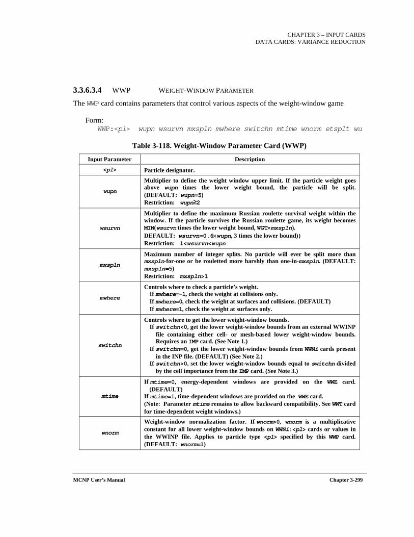
CHAPTER 3 – INPUT CARDS
DATA CARDS: VARIANCE REDUCTION
MCNP User’s Manual Chapter 3-299
3.3.6.3.4 WWP WEIGHT-WINDOW PARAMETER
The WWP card contains parameters that control various aspects of the weight-window game
Form: WWP:<pl> wupn wsurvn mxspln mwhere switchn mtime wnorm etsplt wu
Table 3-118. Weight-Window Parameter Card (WWP)
Input Parameter Description
<pl> Particle designator.
wupn
Multiplier to define the weight window upper limit. If the particle weight goes above wupn times the lower weight bound, the particle will be split. (DEFAULT: wupn=5) Restriction: wupn≥2
wsurvn
Multiplier to define the maximum Russian roulette survival weight within the window. If the particle survives the Russian roulette game, its weight becomes MIN(wsurvn times the lower weight bound, WGT×mxspln). DEFAULT: wsurvn=0.6×wupn, 3 times the lower bound)) Restriction: 1<wsurvn<wupn
mxspln
Maximum number of integer splits. No particle will ever be split more than mxspln-for-one or be rouletted more harshly than one-in-mxspln. (DEFAULT: mxspln=5) Restriction: mxspln>1
mwhere
Controls where to check a particle’s weight. If mwhere=-1, check the weight at collisions only. If mwhere=0, check the weight at surfaces and collisions. (DEFAULT) If mwhere=1, check the weight at surfaces only.
switchn
Controls where to get the lower weight-window bounds. If switchn<0, get the lower weight-window bounds from an external WWINP
file containing either cell- or mesh-based lower weight-window bounds. Requires an IMP card. (See Note 1.)
If switchn=0, get the lower weight-window bounds from WWNi cards present in the INP file. (DEFAULT) (See Note 2.)
If switchn>0, set the lower weight-window bounds equal to switchn divided by the cell importance from the IMP card. (See Note 3.)
mtime
If mtime=0, energy-dependent windows are provided on the WWE card. (DEFAULT)
If mtime=1, time-dependent windows are provided on the WWE card. (Note: Parameter mtime remains to allow backward compatibility. See WWT card for time-dependent weight windows.)
wnorm
Weight-window normalization factor. If wnorm>0, wnorm is a multiplicative constant for all lower weight-window bounds on WWNi:<pl> cards or values in the WWINP file. Applies to particle type <pl> specified by this WWP card. (DEFAULT: wnorm=1)
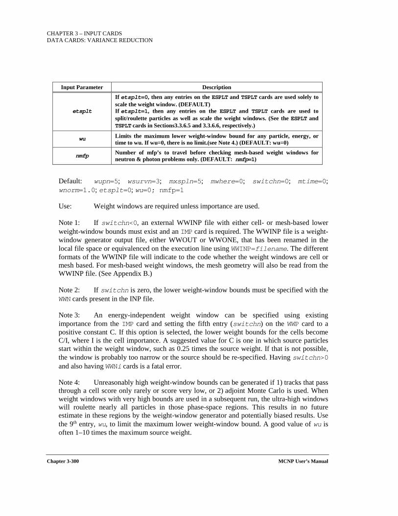
CHAPTER 3 – INPUT CARDS DATA CARDS: VARIANCE REDUCTION
Chapter 3-300 MCNP User’s Manual
Input Parameter Description
etsplt
If etsplt=0, then any entries on the ESPLT and TSPLT cards are used solely to scale the weight window. (DEFAULT) If etsplt=1, then any entries on the ESPLT and TSPLT cards are used to split/roulette particles as well as scale the weight windows. (See the ESPLT and TSPLT cards in Sections3.3.6.5 and 3.3.6.6, respectively.)
wu Limits the maximum lower weight-window bound for any particle, energy, or time to wu. If wu=0, there is no limit.(see Note 4.) (DEFAULT: wu=0)
nmfp Number of mfp’s to travel before checking mesh-based weight windows for neutron & photon problems only. (DEFAULT: nmfp=1)
Default: wupn=5; wsurvn=3; mxspln=5; mwhere=0; switchn=0; mtime=0; wnorm=1.0; etsplt=0; wu=0; nmfp=1
Use: Weight windows are required unless importance are used.
Note 1: If switchn<0, an external WWINP file with either cell- or mesh-based lower weight-window bounds must exist and an IMP card is required. The WWINP file is a weight-window generator output file, either WWOUT or WWONE, that has been renamed in the local file space or equivalenced on the execution line using WWINP=filename. The different formats of the WWINP file will indicate to the code whether the weight windows are cell or mesh based. For mesh-based weight windows, the mesh geometry will also be read from the WWINP file. (See Appendix B.)
Note 2: If switchn is zero, the lower weight-window bounds must be specified with the WWN cards present in the INP file.
Note 3: An energy-independent weight window can be specified using existing importance from the IMP card and setting the fifth entry (switchn) on the WWP card to a positive constant C. If this option is selected, the lower weight bounds for the cells become C/I, where I is the cell importance. A suggested value for C is one in which source particles start within the weight window, such as 0.25 times the source weight. If that is not possible, the window is probably too narrow or the source should be re-specified. Having switchn>0 and also having WWNi cards is a fatal error.
Note 4: Unreasonably high weight-window bounds can be generated if 1) tracks that pass through a cell score only rarely or score very low, or 2) adjoint Monte Carlo is used. When weight windows with very high bounds are used in a subsequent run, the ultra-high windows will roulette nearly all particles in those phase-space regions. This results in no future estimate in these regions by the weight-window generator and potentially biased results. Use the 9th entry, wu, to limit the maximum lower weight-window bound. A good value of wu is often 1–10 times the maximum source weight.

CHAPTER 3 – INPUT CARDS
DATA CARDS: VARIANCE REDUCTION
MCNP User’s Manual Chapter 3-301
3.3.6.4 WEIGHT-WINDOW GENERATION CARDS
The weight-window generator estimates the importance of the space-energy-time regions of phase space specified by the user. The space-energy-time weight-window lower bounds are then calculated inversely proportional to the importance.
The cell–based generator estimates the average importance of a phase-space cell. Inadequately sized (i.e., large) geometry cells often lead to inappropriate weight windows because of a large variation in the importance inside the cell. An appropriate user action is to refine the cell definitions or use the mesh-based weight window. Inadequate geometry specification for weight-window purposes also results when there are large importance differences between adjacent cells. Fortunately, the code provides information about whether the geometry specification is adequate for sampling purposes by printing to the OUTP file a list of neighboring cells that differ by a factor of 4 or more. If geometries are inadequately subdivided by the geometry cells, mesh-based weight windows should be used.
The user is advised to become familiar with the section on the weight windows in The MCNP5 Theory Manual[X-503a], before trying to use the weight-window generator.
3.3.6.4.1 WWG WEIGHT-WINDOW GENERATION
The WWG card allows the code to generate an importance function for a user-specified tally (input parameter it). In many cases, a window using the adjoint function will not be too far from optimal.
For the cell-based weight-window generator, the code creates WWE and WWNi cards that are printed, evaluated, and summarized in the OUTP file and written to the weight-window generator output file WWOUT.
For the mesh-based weight-window generator, the code writes the weight-window lower bounds and a mesh description only to the WWOUT file. (The format of the mesh-based WWOUT file is provided in Appendix B.)
In either case, the generated weight-window information can be easily used in subsequent runs using switchn<0 on the WWP card. For many problems, the weight-window generator results are superior to anything an experienced user can guess and then input on an IMP card. To generate energy- and/or time-dependent weight windows, use the WWGE and/or WWGT cards described below.
Form: WWG it ic wg J J J J iE

CHAPTER 3 – INPUT CARDS DATA CARDS: VARIANCE REDUCTION
Chapter 3-302 MCNP User’s Manual
Table 3-119. Weight-Window Generator Card (WWG)
Input Parameter Description
it Problem tally number (n of the Fn card). The particular tally bin for which the weight-window generator is optimized is defined by the TFn card. (See Note 1.)
ic
Invokes cell- or mesh-based weight-window generator. If ic>0, then invoke the cell-based weight-window generator with ic
as the reference cell (typically a source cell). If ic=0, then invoke the mesh-based weight-window generator. (MESH
card required.) (See Note 2.)
wg Value of the generated lower weight-window bound for cell ic or for the reference mesh. (See MESH card.) (See Note 3.) If wg=0, then the lower bound will be half the average source weight.
J J J J Unused placeholders.
iE
Toggles energy- or time-dependent weight windows. If iE=0, then interpret WWGE card entries as energy bins. If iE=1, then interpret WWGE card entries as time bins.
(Note: Parameter iE remains to allow backward compatibility. See WWGT card for time-dependent weight windows.)
Default: No weight-window values are generated.
Use: Optional.
Note 1: Weight-window generation relies on scores being made by the primary source particle to or near (so secondary particles can score) the reference tally, it. The primary source particle is typically specified by PAR on the SDEF card. If PAR is a distribution or unspecified, then the primary source particle is the particle with the lowest number on the MODE card.
Note 2: For mesh-based weight windows, a reference point (REF) is required instead of a cell number. (See MESH card, Section 3.3.6.4.4.)
Note 3: The value wg of the lower weight-window bound for reference cell ic or reference mesh location is chosen so that the source weight will start within the weight window, when possible. The reference cell ic is often chosen as the source cell and the reference mesh location is often chosen in or near the source cell.
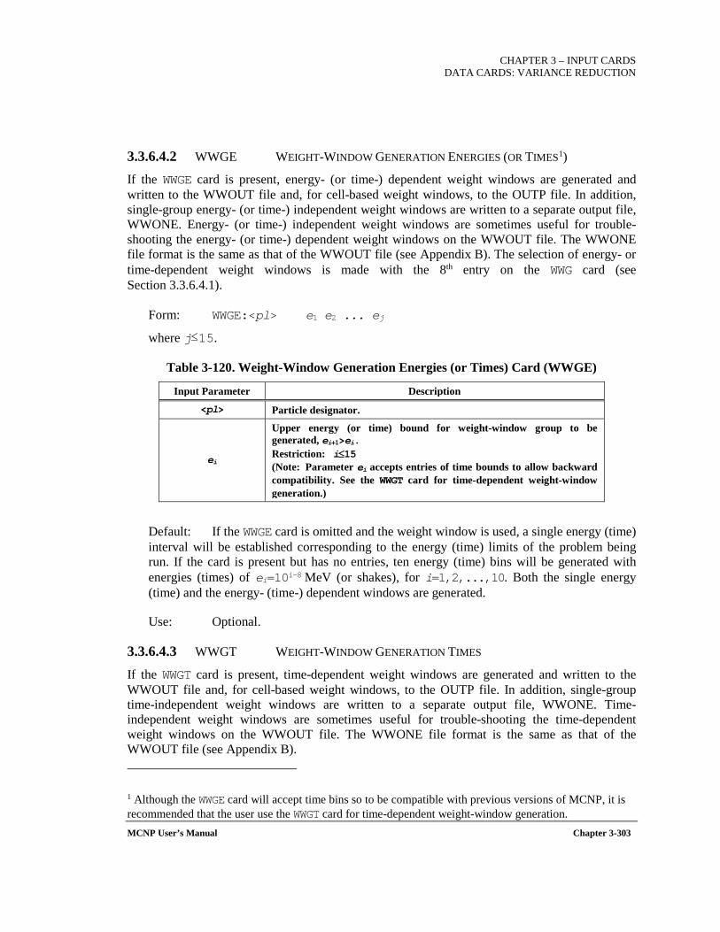
CHAPTER 3 – INPUT CARDS
DATA CARDS: VARIANCE REDUCTION
MCNP User’s Manual Chapter 3-303
3.3.6.4.2 WWGE WEIGHT-WINDOW GENERATION ENERGIES (OR TIMES1)
If the WWGE card is present, energy- (or time-) dependent weight windows are generated and written to the WWOUT file and, for cell-based weight windows, to the OUTP file. In addition, single-group energy- (or time-) independent weight windows are written to a separate output file, WWONE. Energy- (or time-) independent weight windows are sometimes useful for trouble-shooting the energy- (or time-) dependent weight windows on the WWOUT file. The WWONE file format is the same as that of the WWOUT file (see Appendix B). The selection of energy- or time-dependent weight windows is made with the 8th entry on the WWG card (see Section 3.3.6.4.1).
Form: WWGE:<pl> e1 e2 ... ej
where j≤15.
Table 3-120. Weight-Window Generation Energies (or Times) Card (WWGE)
Input Parameter Description
<pl> Particle designator.
ei
Upper energy (or time) bound for weight-window group to be generated, ei+1>ei. Restriction: i≤15 (Note: Parameter ei accepts entries of time bounds to allow backward compatibility. See the WWGT card for time-dependent weight-window generation.)
Default: If the WWGE card is omitted and the weight window is used, a single energy (time) interval will be established corresponding to the energy (time) limits of the problem being run. If the card is present but has no entries, ten energy (time) bins will be generated with energies (times) of ei=10i-8 MeV (or shakes), for i=1,2,...,10. Both the single energy (time) and the energy- (time-) dependent windows are generated.
Use: Optional.
3.3.6.4.3 WWGT WEIGHT-WINDOW GENERATION TIMES
If the WWGT card is present, time-dependent weight windows are generated and written to the WWOUT file and, for cell-based weight windows, to the OUTP file. In addition, single-group time-independent weight windows are written to a separate output file, WWONE. Time-independent weight windows are sometimes useful for trouble-shooting the time-dependent weight windows on the WWOUT file. The WWONE file format is the same as that of the WWOUT file (see Appendix B). 1 Although the WWGE card will accept time bins so to be compatible with previous versions of MCNP, it is recommended that the user use the WWGT card for time-dependent weight-window generation.
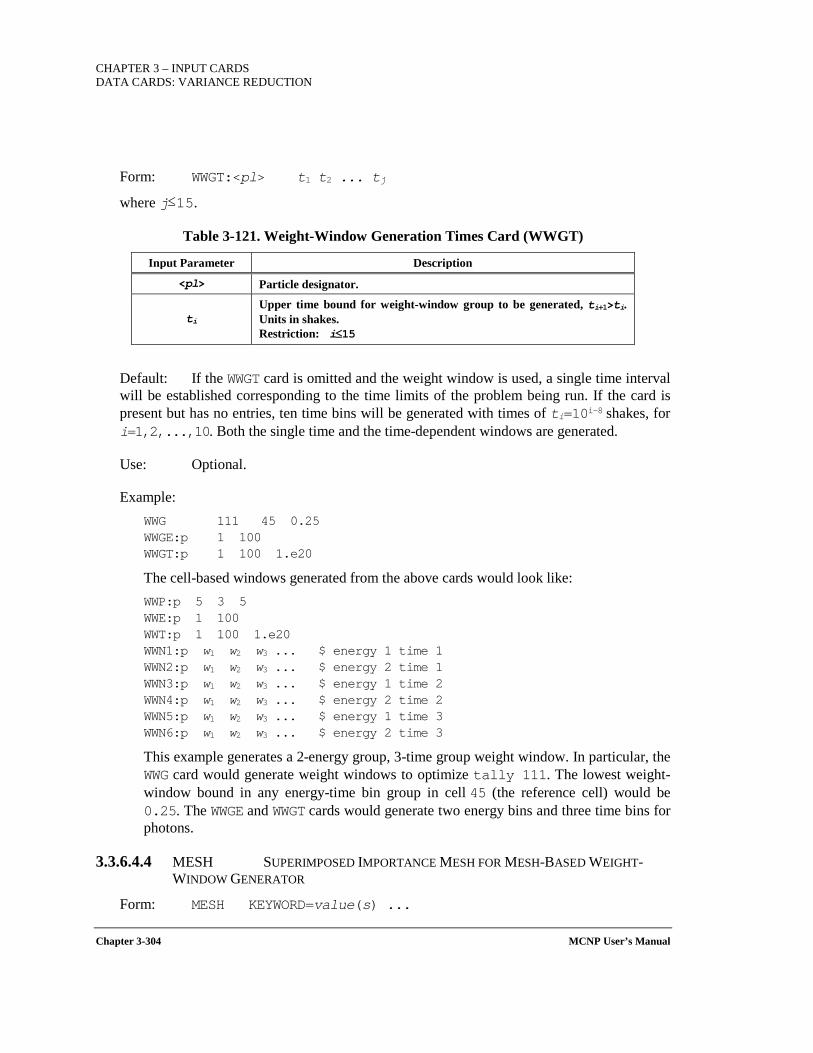
CHAPTER 3 – INPUT CARDS DATA CARDS: VARIANCE REDUCTION
Chapter 3-304 MCNP User’s Manual
Form: WWGT:<pl> t1 t2 ... tj
where j≤15.
Table 3-121. Weight-Window Generation Times Card (WWGT)
Input Parameter Description
<pl> Particle designator.
ti Upper time bound for weight-window group to be generated, ti+1>ti. Units in shakes. Restriction: i≤15
Default: If the WWGT card is omitted and the weight window is used, a single time interval will be established corresponding to the time limits of the problem being run. If the card is present but has no entries, ten time bins will be generated with times of ti=10i-8 shakes, for i=1,2,...,10. Both the single time and the time-dependent windows are generated.
Use: Optional.
Example: WWG 111 45 0.25 WWGE:p 1 100 WWGT:p 1 100 1.e20
The cell-based windows generated from the above cards would look like: WWP:p 5 3 5 WWE:p 1 100 WWT:p 1 100 1.e20 WWN1:p w1 w2 w3 ... $ energy 1 time 1 WWN2:p w1 w2 w3 ... $ energy 2 time 1 WWN3:p w1 w2 w3 ... $ energy 1 time 2 WWN4:p w1 w2 w3 ... $ energy 2 time 2 WWN5:p w1 w2 w3 ... $ energy 1 time 3 WWN6:p w1 w2 w3 ... $ energy 2 time 3
This example generates a 2-energy group, 3-time group weight window. In particular, the WWG card would generate weight windows to optimize tally 111. The lowest weight-window bound in any energy-time bin group in cell 45 (the reference cell) would be 0.25. The WWGE and WWGT cards would generate two energy bins and three time bins for photons.
3.3.6.4.4 MESH SUPERIMPOSED IMPORTANCE MESH FOR MESH-BASED WEIGHT-WINDOW GENERATOR
Form: MESH KEYWORD=value(s) ...
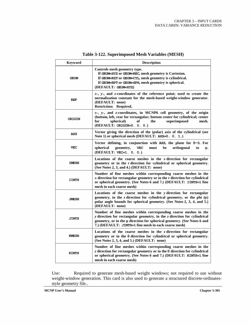
CHAPTER 3 – INPUT CARDS
DATA CARDS: VARIANCE REDUCTION
MCNP User’s Manual Chapter 3-305
Table 3-122. Superimposed Mesh Variables (MESH)
Keyword Description
GEOM
Controls mesh geometry type. If GEOM=XYZ or GEOM=REC, mesh geometry is Cartesian. If GEOM=RZT or GEOM=CYL, mesh geometry is cylindrical. If GEOM=RPT or GEOM=SPH, mesh geometry is spherical.
(DEFAULT: GEOM=XYZ)
REF
x-, y-, and z-coordinates of the reference point; used to create the normalization constant for the mesh-based weight-window generator. (DEFAULT: none) Restriction: Required.
ORIGIN
x-, y-, and z-coordinates, in MCNP6 cell geometry, of the origin (bottom, left, rear for rectangular; bottom center for cylindrical; center for spherical) of the superimposed mesh. (DEFAULT: ORIGIN=0. 0. 0.)
AXS Vector giving the direction of the (polar) axis of the cylindrical (see Note 1) or spherical mesh (DEFAULT: AXS=0. 0. 1.)
VEC Vector defining, in conjunction with AXS, the plane for θ=0. For spherical geometry, VEC must be orthogonal to ϕ. (DEFAULT: VEC=1. 0. 0.)
IMESH Locations of the coarse meshes in the x direction for rectangular geometry or in the r direction for cylindrical or spherical geometry. (See Notes 2, 3, and 4.) (DEFAULT: none)
IINTS
Number of fine meshes within corresponding coarse meshes in the x direction for rectangular geometry or in the r direction for cylindrical or spherical geometry. (See Notes 6 and 7.) (DEFAULT: IINTS=1 fine mesh in each coarse mesh)
JMESH
Locations of the coarse meshes in the y direction for rectangular geometry, in the z direction for cylindrical geometry, or the phi (ϕ) polar angle bounds for spherical geometry. (See Notes 2, 3, 4, and 5.) (DEFAULT: none)
JINTS
Number of fine meshes within corresponding coarse meshes in the y direction for rectangular geometry, in the z direction for cylindrical geometry, or in the ϕ direction for spherical geometry. (See Notes 6 and 7.) (DEFAULT: JINTS=1 fine mesh in each coarse mesh)
KMESH Locations of the coarse meshes in the z direction for rectangular geometry or in the θ direction for cylindrical or spherical geometry. (See Notes 2, 3, 4, and 5.) (DEFAULT: none)
KINTS
Number of fine meshes within corresponding coarse meshes in the z direction for rectangular geometry or in the θ direction for cylindrical or spherical geometry. (See Notes 6 and 7.) (DEFAULT: KINTS=1 fine mesh in each coarse mesh)
Use: Required to generate mesh-based weight windows; not required to use without weight-window generation. This card is also used to generate a structured discrete-ordinates-style geometry file..

CHAPTER 3 – INPUT CARDS DATA CARDS: VARIANCE REDUCTION
Chapter 3-306 MCNP User’s Manual
Note 1: For a cylindrical mesh, the AXS and VEC vectors need not be orthogonal but they must not be parallel; the one half-plane that contains them and the ORIGIN point will define θ=0. The AXS vector will remain fixed. The length of the AXS or VEC vectors must not be zero.
Note 2: For both the cylindrical and spherical meshes, the lower radial and angular mesh bounds (R-ϕ-θ) are implicitly zero.
Note 3: The location of the nth coarse mesh in the u direction (run in what follows) is given in terms of the most positive surface in the u direction. For a rectangular mesh, the coarse mesh locations rxn, ryn, and rzn are given as planes perpendicular to the x-, y-, and z-axes, respectively, in the MCNP6 cell coordinate system; thus, the ORIGIN point (x0,y0,z0) is the most negative point of the mesh. For a cylindrical mesh, ORIGIN (r0,z0,θ0) corresponds to the bottom center point and, for a spherical mesh, ORIGIN (r0,ϕ0,θ0) corresponds the sphere center. The coarse mesh locations must increase monotonically.
Note 4: In the XYZ (REC) mesh, the IMESH, JMESH, and KMESH are the actual x,y,z coordinates. In the RZT (CYL) mesh, IMESH (radius) and JMESH (height) are relative to ORIGIN and KMESH (θ) is relative to VEC. In the RPT (SPH) mesh, IMESH (radius) is relative to ORIGIN, JMESH (ϕ) is relative to AXS, and KMESH (θ) is relative to VEC.
Note 5: Polar and azimuthal angles may be specified in revolutions (0≤ϕ≤0.5 and 0≤θ≤1), radians, or degrees. MCNP6 recognizes the appropriate units by looking for 0.5, 3.14, or 180 for the last spherical geometry JMESH entry and for 1, 6.28, or 360 for the last spherical or cylindrical KMESH entry.
Note 6: The fine meshes are evenly distributed within the nth coarse mesh in the u direction. The mesh in which the reference point lies becomes the reference mesh cell for the mesh-based weight-window generator; this reference mesh cell is analogous to the reference cell used by the cell-based weight-window generator. The mesh cell containing the REF point will have its (over energy) weight-window lower bound equal to the third entry on the WWG card.
Note 7: The code uses a default value of 1 fine mesh per coarse mesh if IINTS, JINTS, or KINTS keywords are omitted. If IINTS, JINTS, or KINTS keywords are present, the number of entries must match the number of entries on the IMESH, JMESH, and KMESH keywords, respectively. Entries on the IINTS, JINTS, and KINTS keywords must be greater than zero.
Using an Existing Superimposed Mesh
A second method of providing a superimposed mesh is to use one that already exists, written either to the WWOUT file or to the WWONE file. To implement this method, use the WWG card
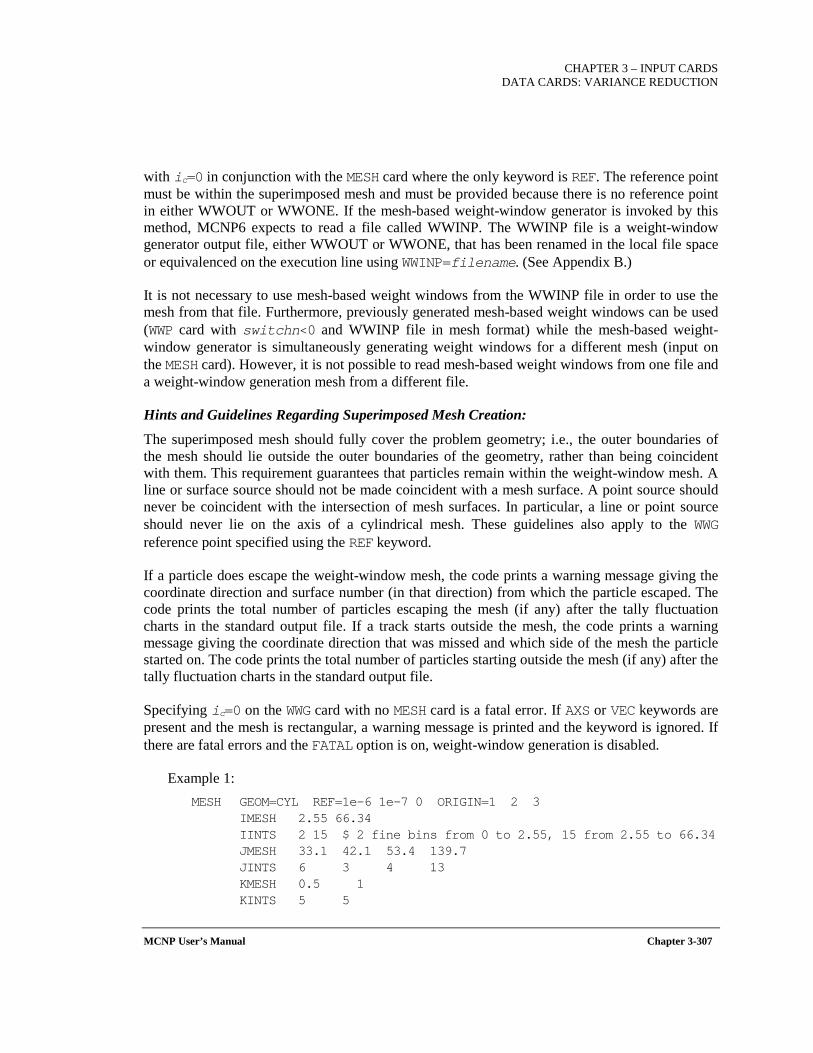
CHAPTER 3 – INPUT CARDS
DATA CARDS: VARIANCE REDUCTION
MCNP User’s Manual Chapter 3-307
with ic=0 in conjunction with the MESH card where the only keyword is REF. The reference point must be within the superimposed mesh and must be provided because there is no reference point in either WWOUT or WWONE. If the mesh-based weight-window generator is invoked by this method, MCNP6 expects to read a file called WWINP. The WWINP file is a weight-window generator output file, either WWOUT or WWONE, that has been renamed in the local file space or equivalenced on the execution line using WWINP=filename. (See Appendix B.)
It is not necessary to use mesh-based weight windows from the WWINP file in order to use the mesh from that file. Furthermore, previously generated mesh-based weight windows can be used (WWP card with switchn<0 and WWINP file in mesh format) while the mesh-based weight-window generator is simultaneously generating weight windows for a different mesh (input on the MESH card). However, it is not possible to read mesh-based weight windows from one file and a weight-window generation mesh from a different file.
Hints and Guidelines Regarding Superimposed Mesh Creation:
The superimposed mesh should fully cover the problem geometry; i.e., the outer boundaries of the mesh should lie outside the outer boundaries of the geometry, rather than being coincident with them. This requirement guarantees that particles remain within the weight-window mesh. A line or surface source should not be made coincident with a mesh surface. A point source should never be coincident with the intersection of mesh surfaces. In particular, a line or point source should never lie on the axis of a cylindrical mesh. These guidelines also apply to the WWG reference point specified using the REF keyword.
If a particle does escape the weight-window mesh, the code prints a warning message giving the coordinate direction and surface number (in that direction) from which the particle escaped. The code prints the total number of particles escaping the mesh (if any) after the tally fluctuation charts in the standard output file. If a track starts outside the mesh, the code prints a warning message giving the coordinate direction that was missed and which side of the mesh the particle started on. The code prints the total number of particles starting outside the mesh (if any) after the tally fluctuation charts in the standard output file.
Specifying ic=0 on the WWG card with no MESH card is a fatal error. If AXS or VEC keywords are present and the mesh is rectangular, a warning message is printed and the keyword is ignored. If there are fatal errors and the FATAL option is on, weight-window generation is disabled.
Example 1: MESH GEOM=CYL REF=1e-6 1e-7 0 ORIGIN=1 2 3 IMESH 2.55 66.34 IINTS 2 15 $ 2 fine bins from 0 to 2.55, 15 from 2.55 to 66.34 JMESH 33.1 42.1 53.4 139.7 JINTS 6 3 4 13 KMESH 0.5 1 KINTS 5 5
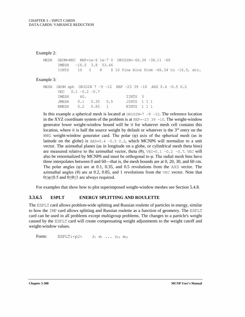
CHAPTER 3 – INPUT CARDS DATA CARDS: VARIANCE REDUCTION
Chapter 3-308 MCNP User’s Manual
Example 2: MESH GEOM=REC REF=1e-6 1e-7 0 ORIGIN=-66.34 -38.11 -60 IMESH -16.5 3.8 53.66 IINTS 10 3 8 $ 10 fine bins from -66.34 to -16.5, etc.
Example 3: MESH GEOM sph ORIGIN 7 -9 -12 REF -23 39 -10 AXS 0.4 -0.5 0.2 VEC 0.1 -0.2 -0.7 IMESH 60. IINTS 3 JMESH 0.1 0.35 0.5 JINTS 1 1 1 KMESH 0.2 0.85 1 KINTS 1 1 1
In this example a spherical mesh is located at ORIGIN=7 -9 -12. The reference location in the XYZ coordinate system of the problem is at REF=-23 39 -10. The weight-window generator lower weight-window bound will be W for whatever mesh cell contains this location, where W is half the source weight by default or whatever is the 3rd entry on the WWG weight-window generator card. The polar (φ) axis of the spherical mesh (as in latitude on the globe) is AXS=0.4 -0.5 0.2, which MCNP6 will normalize to a unit vector. The azimuthal planes (as in longitude on a globe, or cylindrical mesh theta bins) are measured relative to the azimuthal vector, theta (θ), VEC=0.1 -0.2 -0.7. VEC will also be renormalized by MCNP6 and must be orthogonal to φ. The radial mesh bins have three interpolates between 0 and 60—that is, the mesh bounds are at 0, 20, 30, and 60 cm. The polar angles (φ) are at 0.1, 0.35, and 0.5 revolutions from the AXS vector. The azimuthal angles (θ) are at 0.2, 0.85, and 1 revolutions from the VEC vector. Note that 0≤φ≤0.5 and 0≤θ≤1 are always required.
For examples that show how to plot superimposed weight-window meshes see Section 5.4.8.
3.3.6.5 ESPLT ENERGY SPLITTING AND ROULETTE
The ESPLT card allows problem-wide splitting and Russian roulette of particles in energy, similar to how the IMP card allows splitting and Russian roulette as a function of geometry. The ESPLT card can be used in all problems except multigroup problems. The changes to a particle's weight caused by the ESPLT card will create compensating weight adjustments to the weight cutoff and weight-window values.
Form: ESPLT:<pl> r1 e1 ... r20 e20
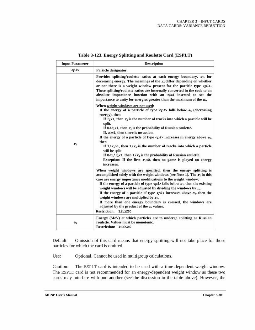
CHAPTER 3 – INPUT CARDS
DATA CARDS: VARIANCE REDUCTION
MCNP User’s Manual Chapter 3-309
Table 3-123. Energy Splitting and Roulette Card (ESPLT)
Input Parameter Description
<pl> Particle designator.
ri
Provides splitting/roulette ratios at each energy boundary, ei, for decreasing energy. The meanings of the ri differ depending on whether or not there is a weight window present for the particle type <pl>. These splitting/roulette ratios are internally converted in the code to an absolute importance function with an r0=1 inserted to set the importance to unity for energies greater than the maximum of the ei.
When weight windows are not used: If the energy of a particle of type <pl> falls below ei (decreasing energy), then
If ri>1, then ri is the number of tracks into which a particle will be split. If 0<ri<1, then ri is the probability of Russian roulette. If, ri=1, then there is no action.
If the energy of a particle of type <pl> increases in energy above ei, then
If 1/ri>1, then 1/ri is the number of tracks into which a particle will be split. If 0<1/ri<1, then 1/ri is the probability of Russian roulette. Exception: If the first r1<0, then no game is played on energy increases.
When weight windows are specified, then the energy splitting is accomplished solely with the weight windows (see Note 1). The ri in this case are energy importance modifications to the weight window:
If the energy of a particle of type <pl> falls below ei, then the existing weight windows will be adjusted by dividing the windows by ri. If the energy of a particle of type <pl> increases above ei, then the weight windows are multiplied by ri. If more than one energy boundary is crossed, the windows are adjusted by the product of the ri values.
Restriction: 1≤i≤20
ei Energy (MeV) at which particles are to undergo splitting or Russian roulette. Values must be monotonic. Restriction: 1≤i≤20
Default: Omission of this card means that energy splitting will not take place for those particles for which the card is omitted.
Use: Optional. Cannot be used in multigroup calculations.
Caution: The ESPLT card is intended to be used with a time-dependent weight window. The ESPLT card is not recommended for an energy-dependent weight window as these two cards may interfere with one another (see the discussion in the table above). However, the
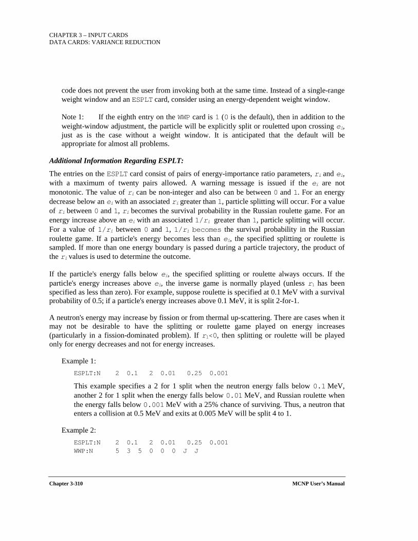
CHAPTER 3 – INPUT CARDS DATA CARDS: VARIANCE REDUCTION
Chapter 3-310 MCNP User’s Manual
code does not prevent the user from invoking both at the same time. Instead of a single-range weight window and an ESPLT card, consider using an energy-dependent weight window.
Note 1: If the eighth entry on the WWP card is 1 (0 is the default), then in addition to the weight-window adjustment, the particle will be explicitly split or rouletted upon crossing ei, just as is the case without a weight window. It is anticipated that the default will be appropriate for almost all problems.
Additional Information Regarding ESPLT:
The entries on the ESPLT card consist of pairs of energy-importance ratio parameters, ri and ei, with a maximum of twenty pairs allowed. A warning message is issued if the ei are not monotonic. The value of ri can be non-integer and also can be between 0 and 1. For an energy decrease below an ei with an associated ri greater than 1, particle splitting will occur. For a value of ri between 0 and 1, ri becomes the survival probability in the Russian roulette game. For an energy increase above an ei with an associated 1/ri greater than 1, particle splitting will occur. For a value of 1/ri between 0 and 1, 1/ri becomes the survival probability in the Russian roulette game. If a particle's energy becomes less than ei, the specified splitting or roulette is sampled. If more than one energy boundary is passed during a particle trajectory, the product of the ri values is used to determine the outcome.
If the particle's energy falls below ei, the specified splitting or roulette always occurs. If the particle's energy increases above ei, the inverse game is normally played (unless r1 has been specified as less than zero). For example, suppose roulette is specified at 0.1 MeV with a survival probability of 0.5; if a particle's energy increases above 0.1 MeV, it is split 2-for-1.
A neutron's energy may increase by fission or from thermal up-scattering. There are cases when it may not be desirable to have the splitting or roulette game played on energy increases (particularly in a fission-dominated problem). If r1<0, then splitting or roulette will be played only for energy decreases and not for energy increases.
Example 1: ESPLT:N 2 0.1 2 0.01 0.25 0.001
This example specifies a 2 for 1 split when the neutron energy falls below 0.1 MeV, another 2 for 1 split when the energy falls below 0.01 MeV, and Russian roulette when the energy falls below 0.001 MeV with a 25% chance of surviving. Thus, a neutron that enters a collision at 0.5 MeV and exits at 0.005 MeV will be split 4 to 1.
Example 2: ESPLT:N 2 0.1 2 0.01 0.25 0.001 WWP:N 5 3 5 0 0 0 J J
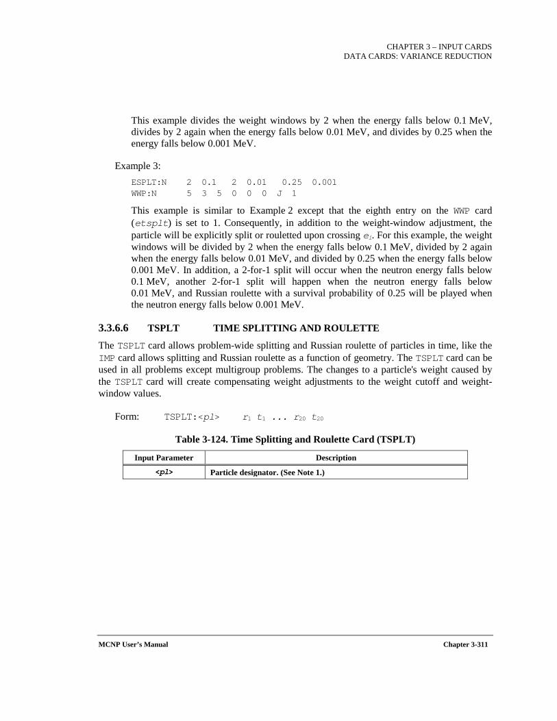
CHAPTER 3 – INPUT CARDS
DATA CARDS: VARIANCE REDUCTION
MCNP User’s Manual Chapter 3-311
This example divides the weight windows by 2 when the energy falls below 0.1 MeV, divides by 2 again when the energy falls below 0.01 MeV, and divides by 0.25 when the energy falls below 0.001 MeV.
Example 3: ESPLT:N 2 0.1 2 0.01 0.25 0.001 WWP:N 5 3 5 0 0 0 J 1
This example is similar to Example 2 except that the eighth entry on the WWP card (etsplt) is set to 1. Consequently, in addition to the weight-window adjustment, the particle will be explicitly split or rouletted upon crossing ei. For this example, the weight windows will be divided by 2 when the energy falls below 0.1 MeV, divided by 2 again when the energy falls below 0.01 MeV, and divided by 0.25 when the energy falls below 0.001 MeV. In addition, a 2-for-1 split will occur when the neutron energy falls below 0.1 MeV, another 2-for-1 split will happen when the neutron energy falls below 0.01 MeV, and Russian roulette with a survival probability of 0.25 will be played when the neutron energy falls below 0.001 MeV.
3.3.6.6 TSPLT TIME SPLITTING AND ROULETTE
The TSPLT card allows problem-wide splitting and Russian roulette of particles in time, like the IMP card allows splitting and Russian roulette as a function of geometry. The TSPLT card can be used in all problems except multigroup problems. The changes to a particle's weight caused by the TSPLT card will create compensating weight adjustments to the weight cutoff and weight-window values.
Form: TSPLT:<pl> r1 t1 ... r20 t20
Table 3-124. Time Splitting and Roulette Card (TSPLT)
Input Parameter Description
<pl> Particle designator. (See Note 1.)
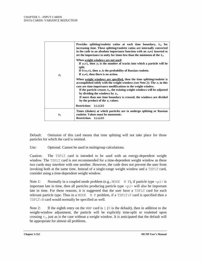
CHAPTER 3 – INPUT CARDS DATA CARDS: VARIANCE REDUCTION
Chapter 3-312 MCNP User’s Manual
Default: Omission of this card means that time splitting will not take place for those particles for which the card is omitted.
Use: Optional. Cannot be used in multigroup calculations.
Caution: The TSPLT card is intended to be used with an energy-dependent weight window. The TSPLT card is not recommended for a time-dependent weight window as these two cards may interfere with one another. However, the code does not prevent the user from invoking both at the same time. Instead of a single-range weight window and a TSPLT card, consider using a time-dependent weight window.
Note 1: Normally in a coupled mode problem (e.g., MODE N P), if particle type <pl> is important late in time, then all particles producing particle type <pl> will also be important late in time. For these reasons, it is suggested that the user have a TSPLT card for each relevant particle type. Thus in a MODE N P problem, if a TSPLT:P card is specified then a TSPLT:N card would normally be specified as well.
Note 2: If the eighth entry on the WWP card is 1 (0 is the default), then in addition to the weight-window adjustment, the particle will be explicitly time-split or rouletted upon crossing ti, just as is the case without a weight window. It is anticipated that the default will be appropriate for almost all problems.
ri
Provides splitting/roulette ratios at each time boundary, ti, for increasing time. These splitting/roulette ratios are internally converted in the code to an absolute importance function with an r0=1 inserted to set the importance to unity for times less than the minimum of the ti.
When weight windows are not used: If ri>1, then ri is the number of tracks into which a particle will be split. If 0<ri<1, then ri is the probability of Russian roulette. If ri=1, then there is no action.
When weight windows are specified, then the time splitting/roulette is accomplished solely with the weight windows (see Note 2): The ri in this case are time importance modifications to the weight window.
If the particle crosses ti, the existing weight windows will be adjusted by dividing the windows by ri. If more than one time boundary is crossed, the windows are divided by the product of the ri values.
Restriction: 1≤i≤20
ti Times (shakes) at which particles are to undergo splitting or Russian roulette. Values must be monotonic. Restriction: 1≤i≤20
CHAPTER 3 – INPUT CARDS
DATA CARDS: VARIANCE REDUCTION
MCNP User’s Manual Chapter 3-313
Additional Information Regarding TSPLT:
The entries on the TSPLT card consist of pairs of time-importance ratio parameters, ri and ti, with a maximum of twenty pairs allowed. A warning message is issued if the ti are not monotonic. The value of ri can be non-integer and also can be between 0 and 1. For an ri greater than 1, particle splitting will occur. For a value of ri between 0 and 1, ri becomes the survival probability in the Russian roulette game. If a particle's time becomes greater than ti, the specified splitting or roulette is sampled. If more than one time boundary is passed during a particle trajectory, the product of the ri values is used to determine the outcome. The ti are in units of shakes.
Example 1: TSPLT:N 2 100 2 1000 0.2 10000
This example specifies a-2 for-1 split when the neutron time exceeds 100 shakes, another 2-for-1 split when the time exceeds 1000 shakes, and Russian roulette with a survival probability of 0.2 when the time exceeds 10000 shakes. A neutron that crosses both 1000 and 10000 shakes will have a survival probability of 0.4.
Example 2: TSPLT:N 2 100 2 1000 0.2 10000 WWP:N 5 3 5 0 0 0 J J
This example divides the weight windows by 2 when the neutron time exceeds 100 shakes, divides by 2 again when the time exceeds 1000 shakes, and divides by 0.2 when the time exceeds 10000 shakes. Thus the weight window will be divided by a factor of 4 for a particle whose time at the start of the transport step was 90 shakes and whose time at the end of the transport step was 1010 shakes.
Example 3: TSPLT:N 2 100 2 1000 0.2 10000 WWP:N 5 3 5 0 0 0 J 1
This example is similar to Example 2 except that the eighth entry on the WWP card (etsplt) is set to 1. Consequently, in addition to the weight-window adjustment, the particle will be explicitly split or rouletted when it exceeds ti. For this example the weight windows will be divided by 2 when the neutron time exceeds 100 shakes, divided by 2 again when the time exceeds 1000 shakes, and divided by 0.2 when the time exceeds 10000 shakes. In addition, this example specifies a 2-for-1 split when the neutron time exceeds 100 shakes, another 2-for-1 split when the time exceeds 1000 shakes, and a Russian roulette survival probability of 0.2 when the time exceeds 10000 shakes.
3.3.6.7 EXT EXPONENTIAL TRANSFORM
The exponential transform method stretches the path length between collisions in a preferred direction by adjusting the total cross section.
CHAPTER 3 – INPUT CARDS DATA CARDS: VARIANCE REDUCTION
Chapter 3-314 MCNP User’s Manual
Form 1 (cell card entry): EXT:<pl>=a
Form 2 (data card): EXT:<pl> a1 a2 ... aj ...
Table 3-125. Exponential Transform Card (EXT)
Input Parameter Description
<pl> Particle designator.
A Each entry a is of the form a=QVm, where Q describes the amount of stretching and Vm defines the stretching direction for the cell. (See Table 3-126 of Example 1.)
aj
Each entry aj is of the form aj=QVm, where Q describes the amount of stretching and Vm defines the stretching direction for cell j. (See Table 3-126 of Example 1.) The number of entries need not equal the number of cells in the problem, but a warning message is printed if they are not equal..
Default: No transform, aj=0.
Use: Optional. Use cautiously. Weight windows are strongly recommended. A warning message is given if weight windows are not present when the exponential transform is used. The exponential transform should not be used in the same cell as forced collisions or without good weight control. The transform works best when the particle flux has an exponential attenuation, such as in problems with highly absorbing media.
Additional Information Regarding the Exponential Transform:
The exponential transform method stretches the path length between collisions in a preferred direction by adjusting the total cross section as follows:
where is the artificially adjusted total cross section, is the true total cross section,
p is the stretching parameter, and µ is the cosine of the angle between the particle direction and the stretching direction.
The stretching parameter, p, can be specified by the stretching entry, Q, in three ways:
If p=0, then Q=0 and the exponential transform is not used. If 0<p<1, then Q=p and a constant stretching parameter is specified. If p=Σc/Σt, then Q=S where Σc is the capture cross section (as defined by nuclear
engineers).
Letting p=Σc/Σt can be used for implicit capture along a flight path, as described in the MCNP5 Theory Manual[X-503a].
( )µpt*t −Σ=Σ 1
*tΣ
tΣ
CHAPTER 3 – INPUT CARDS
DATA CARDS: VARIANCE REDUCTION
MCNP User’s Manual Chapter 3-315
The stretching direction is defined by the Vm part of each aj entry on the EXT card with three available options:
1. If the Vm part of the aj entry is omitted (i.e., aj=Q for a given cell), then the stretching is in the particle direction (µ=1), independent of the particle direction (and therefore independent of any direction). This is not recommended unless you want to do implicit capture along a flight path, in which case aj=Q=S and the distance to scatter rather than the distance to collision is sampled.
2. The stretching direction may be specified as Vm, where m is a unique integer that is associated with the vector entry provided on the VECT card (Section 3.3.6.8). The stretching direction is defined as the line from the collision point to the point (xm,ym,zm), where (xm,ym,zm) is provided on the VECT card. The direction cosine µ is now the cosine of the angle between the particle direction and the line drawn from the collision point to point (xm,ym,zm). The sign of aj governs whether stretching is toward or away from (xm,ym,zm).
3. The stretching direction may also be specified as Vm=X or Y or Z, so the direction cosine µ is the cosine of the angle between the particle direction and the x−, y−, or z−axis, respectively. The sign of aj governs whether stretching is toward or away from the x−, y−, or z−axis.
Example 1: EXT:N 0 0 0.7V2 S -SV2 -0.6V9 0 0.5V9 SZ -0.4X VECT V9 0 0 0 V2 1 1 1
The 10 entries are for the 10 cells in this problem. Path length stretching is not turned on for photons or for cells 1, 2, and 7. Table 3-126 is a summary of path length stretching in the other cells.
Table 3-126 Exponential Transform Stretching Parameter
Cell ai Q Vm Stretching Parameter Stretching Direction
3 0.7V2 0.7 V2 p = 0.7 Toward point (1,1,1)
4 S S p = Σc/Σt Particle direction 5 -SV2 S -V2 p = Σc/Σt Away from point (1,1,1)
6 -0.6V9 0.6 -V9 p = 0.6 Away from origin 8 0.5V9 0.5 V9 p = 0.5 Toward origin 9 SZ S Z p = Σc/Σt Along +z-axis
10 -0.4X 0.4 -X p = 0.4 Along -x-axis

CHAPTER 3 – INPUT CARDS DATA CARDS: VARIANCE REDUCTION
Chapter 3-316 MCNP User’s Manual
3.3.6.8 VECT VECTOR INPUT
The entries on the VECT card are quadruplets that may define any number of vectors for either the exponential transform or user patches. See the EXT card (Section 3.3.6.7) for a usage example
Form: VECT Vm xm ym zm ... Vn xn yn zn ...
Table 3-127. Vector Input Card (VECT)
Input Parameter Description
m, n Any number to uniquely identify vectors Vm, Vn, ...
xm ym zm Coordinate triplets to define vector Vm.
Default: None.
Use: Optional.
3.3.6.9 FCL FORCED COLLISION
The FCL card controls the forcing of neutron or photon collisions in each cell. This is particularly useful for generating contributions to point detectors or DXTRAN spheres. The weight-window game at surfaces is not played when entering forced-collision cells.
Because the forced-collision variance reduction method can produce several very low-weight particles, the weight cutoff game is turned on by default when using pulse-height tallies and forced collisions together. Any of the default settings can be overridden by explicitly setting the weight cutoffs on the CUT card (see Section 3.3.3.4.1).
Form 1 (cell card entry): FCL:<pl>=x
Form 2 (data card): FCL:<pl> x1 x2 ... xj ...
Table 3-128. Forced-Collision Card (FCL)
Input Parameter Description
<pl> Particle designator. Restriction: Only neutrons (N) and photons (P) are permitted.
x
Forced-collision control for cell. (See Notes 1, 2 and 3.) Restriction: -1≤x≤1
If x>0, forced collision applies to particles entering the cell and to those surviving weight cutoff/weight-window games in the cell. (See Note 4.)
If x<0, forced collision applies only to particles entering the cell. (See Note 5.)
If x=0, no forced collision in the cell. (DEFAULT)
CHAPTER 3 – INPUT CARDS
DATA CARDS: VARIANCE REDUCTION
MCNP User’s Manual Chapter 3-317
xj
Forced-collision control for cell j. (See Notes 1, 2 and 3.) Restriction: -1≤xj≤1
If xj>0, forced collision applies to particles entering the cell j and to those surviving weight cutoff/weight-window games in the cell. (See Note 4.)
If xj<0, forced collision applies only to particles entering the cell j. (See Note 5.)
If xj=0, no forced collision in the cell j. (DEFAULT) The number of entries need not equal the number of cells in the problem, but a warning message is printed if they are not equal.
Default: xj=0, no forced collisions.
Use: Optional. Exercise caution.
Note 1: If xj≠0, all particles entering cell j are split into collided and un-collided parts with the appropriate weight adjustment. If |xj|<1, Russian roulette is played on the collided parts with survival probability |xj| to keep the number of collided histories from getting too large. Fractional xj entries, rather than values of -1 or 1, are recommended if a number of forced-collision cells are adjacent to each other.
Note 2: When cell-based weight-window bounds bracket the typical weight entering the cell, choose xj>0. When cell-based weight-window bounds bracket the weight typical of forced-collision particles, choose xj<0. For mesh-based windows, xj>0 usually is recommended. When using importance, xj>0 because xj<0 turns off the weight cutoff game.
Note 3: Let xj=1 or -1 unless a number of forced collision cells are adjacent to each other or the number of forced collision particles produced is higher than desired. Then fractional values are usually needed.
Note 4: If xj>0, the forced collision process applies both to particles entering cell j and to the collided particles surviving the weight cutoff or weight-window games. Particles will continue to be split into un-collided and (with probability |xi|) collided parts until killed by either weight cutoff or weight windows.
Note 5: If xj<0, the forced collision process applies only to particles entering the cell. After the forced collision, the weight cutoff is ignored and all subsequent collisions are handled in the usual analog manner. Weight windows are not ignored and are applied after contributions are made to detectors and DXTRAN spheres.
3.3.6.10 DXT DXTRAN SPHERE
DXTRAN (deterministic transport) spheres are used to improve the particle sampling in a given region of phase-space, a type of angle biasing, or, conversely, to block high-weight particles from reaching a given region. Primarily, the DXT card specifies the spheres needed to define a spherical
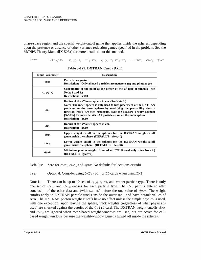
CHAPTER 3 – INPUT CARDS DATA CARDS: VARIANCE REDUCTION
Chapter 3-318 MCNP User’s Manual
phase-space region and the special weight-cutoff game that applies inside the spheres, depending upon the presence or absence of other variance reduction games specified in the problem. See the MCNP5 Theory Manual[X-503a] for more details about this method.
Form: DXT:<pl> x1 y1 z1 ri1 ro1 x2 y2 z2 ri2 ro2 ... dwc1 dwc2 dpwt
Table 3-129. DXTRAN Card (DXT)
Input Parameter Description
<pl> Particle designator. Restriction: Only allowed particles are neutrons (N) and photons (P).
xi yi zi Coordinates of the point at the center of the ith pair of spheres. (See Notes 1 and 2.) Restriction: i≤10
rii
Radius of the ith inner sphere in cm. (See Note 3.) Note: The inner sphere is only used to bias placement of the DXTRAN particles on the outer sphere by modifying the probability density function into a two-step histogram. (See the MCNP6 Theory Manual [X-503a] for more details.) All particles start on the outer sphere. Restriction: i≤10
roi Radius of the ith outer sphere in cm. Restriction: i≤10
dwc1 Upper weight cutoff in the spheres for the DXTRAN weight-cutoff game inside the sphere. (DEFAULT: dwc1=0)
dwc2 Lower weight cutoff in the spheres for the DXTRAN weight-cutoff game inside the sphere.. (DEFAULT: dwc2=0)
dpwt Minimum photon weight. Entered on DXT:N card only. (See Note 4.) (DEFAULT: dpwt=0)
Defaults: Zero for dwc1, dwc2, and dpwt. No defaults for locations or radii.
Use: Optional. Consider using DXC:<pl> or DD cards when using DXT.
Note 1: There can be up to 10 sets of x, y, z, ri, and ro per particle type. There is only one set of dwc1 and dwc2 entries for each particle type. The dwc pair is entered after conclusion of the other data and (with DXT:N) before the one value of dpwt. The weight cutoffs apply to DXTRAN particle tracks inside the outer radii and have default values of zero. The DXTRAN photon weight cutoffs have no effect unless the simple physics is used, with one exception: upon leaving the sphere, track weights (regardless of what physics is used) are checked against the cutoffs of the CUT:P card. The DXTRAN weight cutoffs dwc1 and dwc2 are ignored when mesh-based weight windows are used, but are active for cell-based weight windows because the weight-window game is turned off inside the spheres.
CHAPTER 3 – INPUT CARDS
DATA CARDS: VARIANCE REDUCTION
MCNP User’s Manual Chapter 3-319
Note 2: DXTRAN spheres can be nested inside one another. [BOO09] The allowed nesting is reasonably general: more than one DXTRAN sphere may be nested inside a larger DXTRAN sphere and the centers of the nested DXTRAN spheres need not be concentric. Also, the spherical surfaces must not intersect. This nesting mitigates weight fluctuation problems as the particles approach the region(s) of interest.
Note 3: When the DXTRAN method is used as a means to produce a higher particle population near a tally, the inner radius ri should be at least as large as the tally region. The purpose of the inner sphere is for biasing placement of DXTRAN particles on the outer sphere; there is no problem making the two radii the same.
Note 4: The minimum photon weight limit dpwt on the DXT:N card parallels almost exactly the minimum photon weight entries on the PWT card. One slight difference is that in Russian roulette during photon production inside DXTRAN spheres, the factor for relating current cell importance to source cell importance is not applied. Thus, the user must have some knowledge of the weight distribution of the DXTRAN particles (from a short run with the DD card, for example) inside the DXTRAN sphere, so the lower weight limit for photon production may be specified intelligently. As in the case of the PWT entries, a negative entry will make the minimum photon weight relative to the source particle starting weight. The default value is zero, which means photon production will occur at each neutron DXTRAN particle collision in a material with non-zero photon production cross section inside the DXTRAN sphere.
Additional Information Regarding DXTRAN Spheres:
One use of DXTRAN is to improve the particle sample in the vicinity of a tally (see the MCNP6 Theory Manual[X-503a]. It should not be misconstrued as a tally itself, such as a point detector; it is used in conjunction with tallies as a variance reduction technique. DXTRAN spheres must not overlap. The spheres should normally cover the tally region if possible. Specifying a tally cell or surface partly inside and partly outside a DXTRAN sphere usually will make the mean of the tally erratic and the variance huge.
The technique is most effective when the geometry inside the spheres is very simple and can be costly if the inside geometry is complicated, involving several surfaces. However, the nested DXTRAN treatment should alleviate some of these complicated geometry issues. The inner sphere is intended to surround the region of interest. The outer sphere should surround neighboring regions that may scatter into the region of interest. In MCNP6, the relative importance of the two regions is five. That is, the probability density for scattering toward the inner sphere region is five times as high as the probability density for scattering between the inner and outer spheres. This position biasing is only one of several factors that affect the weights of the DXTRAN particles; see the MCNP5 Theory Manual[X-503a] on this topic for more information.
All collisions producing neutrons and photons contribute to DXTRAN, including model physics interactions. When the secondary neutron/photon angular scattering distribution function is
CHAPTER 3 – INPUT CARDS DATA CARDS: VARIANCE REDUCTION
Chapter 3-320 MCNP User’s Manual
unknown, isotropic scattering, which may be a poor approximation, is assumed. Although the extension to higher energies often is approximate, a tally with an appropriate energy structure can provide the user with insight regarding the contributions at these energies. This approximation is superior to neglecting charged-particle and high-energy neutron collisions altogether.
As mentioned above, DXTRAN uses an assumption of isotropic scatter for contributions from collisions within the model regime. These estimators require the angular distribution data for particles produced in an interaction to predict scattering toward the sphere(s). Information on these distributions is available in tabular form in the libraries; however, this information is not available in the required form from physics models used to produce secondary particles above the tabular region.
DXTRAN can be used in a problem with the S(α,β) thermal treatment, but contributions to the DXTRAN spheres are approximate. DXTRAN should not be used with reflecting surfaces, white boundaries, or periodic boundaries (see the MCNP6 Theory Manual[X-503a]). DXTRAN can be used with mono-direction sources, but the user should understand that no contributions from sources occur unless the source is directed at the DXTRAN sphere.
DXTRAN spheres can be used around point detectors (F5 tallies), but the combination may be very sensitive to reliable sampling.
If more than one set of DXTRAN spheres is used in the same problem, they can "talk" to each other in the sense that collisions of DXTRAN particles in one set of spheres cause contributions to another set of spheres. The contributions to the second set have, in general, extremely low weights but can be numerous with an associated large increase in computer time. In this case the DXTRAN weight cutoffs probably will be required to kill the very-low-weight particles, provided mesh-based weight windows are not used. The DD card (Section 3.3.6.11) can give you an indication of the weight distribution of DXTRAN particles.
Remember that the DD card roulette game is on by default and the reference weight is a moving average for the first dmmp histories unless this Russian roulette game is turned off or a fixed level is input (as a -ki on the DD card). It is highly recommended that the user make a short exploratory run to establish a value to input; a value that is 10% of the average contributed weight to the sphere is a good place to start. See Section 3.3.6.11 for the DD card input requirements and more details regarding the number of histories used to find the average contribution. If the user were to rely on the default behavior, then running a single history after the first dmmp histories (perhaps for the sake of debugging or dealing with a lost particle) will not yield the same result as before.
3.3.6.11 DD DETECTOR DIAGNOSTICS
The DD card (1) can speed up calculations significantly by using a Russian roulette game to limit small contributions that are less than some fraction k of the average contribution per history to detectors or DXTRAN spheres and (2) can provide more information about the origin of large contributions or the lack of a sufficient number of collisions close to the detector or DXTRAN
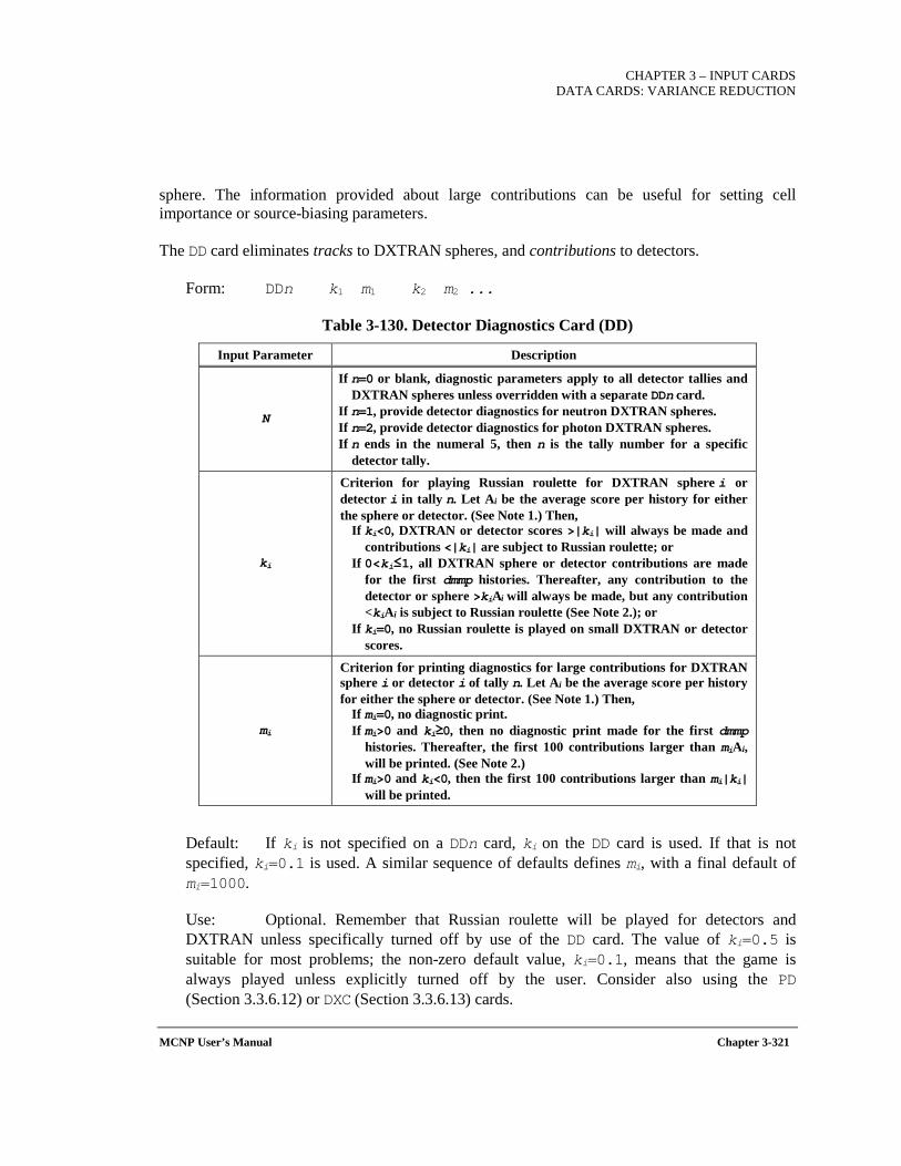
CHAPTER 3 – INPUT CARDS
DATA CARDS: VARIANCE REDUCTION
MCNP User’s Manual Chapter 3-321
sphere. The information provided about large contributions can be useful for setting cell importance or source-biasing parameters.
The DD card eliminates tracks to DXTRAN spheres, and contributions to detectors.
Form: DDn k1 m1 k2 m2 ...
Table 3-130. Detector Diagnostics Card (DD)
Input Parameter Description
N
If n=0 or blank, diagnostic parameters apply to all detector tallies and DXTRAN spheres unless overridden with a separate DDn card.
If n=1, provide detector diagnostics for neutron DXTRAN spheres. If n=2, provide detector diagnostics for photon DXTRAN spheres. If n ends in the numeral 5, then n is the tally number for a specific
detector tally.
ki
Criterion for playing Russian roulette for DXTRAN sphere i or detector i in tally n. Let Ai be the average score per history for either the sphere or detector. (See Note 1.) Then,
If ki<0, DXTRAN or detector scores >|ki| will always be made and contributions <|ki| are subject to Russian roulette; or
If 0<ki≤1, all DXTRAN sphere or detector contributions are made for the first dmmp histories. Thereafter, any contribution to the detector or sphere >kiAi will always be made, but any contribution <kiAi is subject to Russian roulette (See Note 2.); or
If ki=0, no Russian roulette is played on small DXTRAN or detector scores.
mi
Criterion for printing diagnostics for large contributions for DXTRAN sphere i or detector i of tally n. Let Ai be the average score per history for either the sphere or detector. (See Note 1.) Then,
If mi=0, no diagnostic print. If mi>0 and ki≥0, then no diagnostic print made for the first dmmp
histories. Thereafter, the first 100 contributions larger than miAi, will be printed. (See Note 2.)
If mi>0 and ki<0, then the first 100 contributions larger than mi|ki| will be printed.
Default: If ki is not specified on a DDn card, ki on the DD card is used. If that is not specified, ki=0.1 is used. A similar sequence of defaults defines mi, with a final default of mi=1000.
Use: Optional. Remember that Russian roulette will be played for detectors and DXTRAN unless specifically turned off by use of the DD card. The value of ki=0.5 is suitable for most problems; the non-zero default value, ki=0.1, means that the game is always played unless explicitly turned off by the user. Consider also using the PD (Section 3.3.6.12) or DXC (Section 3.3.6.13) cards.
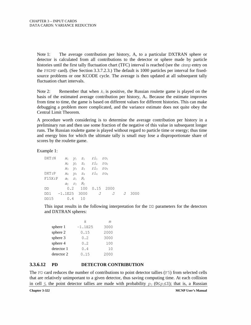
CHAPTER 3 – INPUT CARDS DATA CARDS: VARIANCE REDUCTION
Chapter 3-322 MCNP User’s Manual
Note 1: The average contribution per history, A, to a particular DXTRAN sphere or detector is calculated from all contributions to the detector or sphere made by particle histories until the first tally fluctuation chart (TFC) interval is reached (see the dmmp entry on the PRDMP card). (See Section 3.3.7.2.3.) The default is 1000 particles per interval for fixed-source problems or one KCODE cycle. The average is then updated at all subsequent tally fluctuation chart intervals.
Note 2: Remember that when ki is positive, the Russian roulette game is played on the basis of the estimated average contribution per history, Ai. Because the estimate improves from time to time, the game is based on different values for different histories. This can make debugging a problem more complicated, and the variance estimate does not quite obey the Central Limit Theorem.
A procedure worth considering is to determine the average contribution per history in a preliminary run and then use some fraction of the negative of this value in subsequent longer runs. The Russian roulette game is played without regard to particle time or energy; thus time and energy bins for which the ultimate tally is small may lose a disproportionate share of scores by the roulette game.
Example 1: DXT:N x1 y1 z1 ri1 ro1 x2 y2 z2 ri2 ro2 x3 y3 z3 ri3 ro3 DXT:P x4 y4 z4 ri4 ro4 F15X:P a1 r1 R1 a2 r2 R2 DD 0.2 100 0.15 2000 DD1 -1.1E25 3000 J J J 3000 DD15 0.4 10
This input results in the following interpretation for the DD parameters for the detectors and DXTRAN spheres:
k m sphere 1 -1.1E25 3000 sphere 2 0.15 2000 sphere 3 0.2 3000 sphere 4 0.2 100 detector 1 0.4 10 detector 2 0.15 2000
3.3.6.12 PD DETECTOR CONTRIBUTION
The PD card reduces the number of contributions to point detector tallies (F5) from selected cells that are relatively unimportant to a given detector, thus saving computing time. At each collision in cell j, the point detector tallies are made with probability pj (0≤pj≤1); that is, a Russian

CHAPTER 3 – INPUT CARDS
DATA CARDS: VARIANCE REDUCTION
MCNP User’s Manual Chapter 3-323
roulette game is played in which the survival probability is pj to determine if the contribution should take place. When the contribution survives the roulette game, the tally is then increased by the factor 1/pj to obtain unbiased results for all cells except those where pj=0. This enables the user to decrease the problem runtime by setting pj<1 for cells many mean free paths from the detectors. It also selectively eliminates detector contributions from cells by setting the pj values for those cells to zero. This card is analogous to the DXC card (Section 3.3.6.13), but is used for contributions to point detector tallies (F5).
Form 1 (cell card entry): PDn=p
Form 2 (data card): PDn p1 p2 ... pj ...
Table 3-131. Detector Contribution Card (PD)
Input Parameter Description
N Tally number. (See Note 1.) Restriction: n≤9999
P Probability of contribution to detector n from cell. (DEFAULT: p=1)
pj Probability of contribution to detector n from cell j. (DEFAULT: pj=1) Number of entries is equal to the number of cells in the problem.
Default: pj=1
Use: Optional. Consider also using the DD card, Section 3.3.6.11.
Note 1 A default set of probabilities can be established for all tallies by use of a PD0 card. These default values will be overridden for a specific tally n by values entered on a PD card.
3.3.6.13 DXC DXTRAN CONTRIBUTION
The DXC card is analogous to the PD card for detector contributions except it is used for contributions to DXTRAN spheres.
Form 1 (cell card entry): DXCm:<pl>=p
Form 2 (data card): DXCm:<pl> p1 p2 ... pj ...
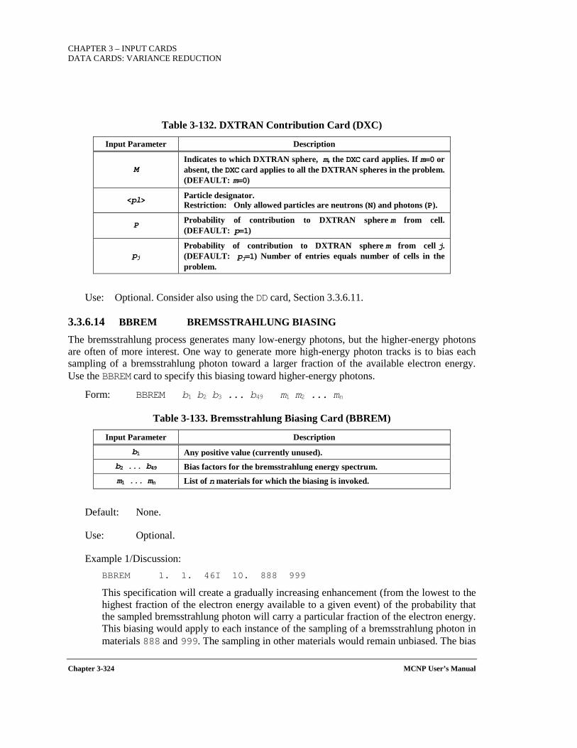
CHAPTER 3 – INPUT CARDS DATA CARDS: VARIANCE REDUCTION
Chapter 3-324 MCNP User’s Manual
Table 3-132. DXTRAN Contribution Card (DXC)
Input Parameter Description
M Indicates to which DXTRAN sphere, m, the DXC card applies. If m=0 or absent, the DXC card applies to all the DXTRAN spheres in the problem. (DEFAULT: m=0)
<pl> Particle designator. Restriction: Only allowed particles are neutrons (N) and photons (P).
P Probability of contribution to DXTRAN sphere m from cell. (DEFAULT: p=1)
pj Probability of contribution to DXTRAN sphere m from cell j. (DEFAULT: pj=1) Number of entries equals number of cells in the problem.
Use: Optional. Consider also using the DD card, Section 3.3.6.11.
3.3.6.14 BBREM BREMSSTRAHLUNG BIASING
The bremsstrahlung process generates many low-energy photons, but the higher-energy photons are often of more interest. One way to generate more high-energy photon tracks is to bias each sampling of a bremsstrahlung photon toward a larger fraction of the available electron energy. Use the BBREM card to specify this biasing toward higher-energy photons.
Form: BBREM b1 b2 b3 ... b49 m1 m2 ... mn
Table 3-133. Bremsstrahlung Biasing Card (BBREM)
Input Parameter Description
b1 Any positive value (currently unused). b2 ... b49 Bias factors for the bremsstrahlung energy spectrum. m1 ... mn List of n materials for which the biasing is invoked.
Default: None.
Use: Optional.
Example 1/Discussion: BBREM 1. 1. 46I 10. 888 999
This specification will create a gradually increasing enhancement (from the lowest to the highest fraction of the electron energy available to a given event) of the probability that the sampled bremsstrahlung photon will carry a particular fraction of the electron energy. This biasing would apply to each instance of the sampling of a bremsstrahlung photon in materials 888 and 999. The sampling in other materials would remain unbiased. The bias

CHAPTER 3 – INPUT CARDS
DATA CARDS: VARIANCE REDUCTION
MCNP User’s Manual Chapter 3-325
factors are normalized by the code in a manner that depends both on material and on electron energy, so that although the ratios of the photon weight adjustments among the different groups are known, the actual number of photons produced in any group is not easily predictable. For the EL03 treatment, there are more than 49 relative photon energy ratios so the lower energy bins have a linear interpolation between b1 and b2 for their values.
In most problems the above prescription will increase the total number of bremsstrahlung photons produced because there will be more photon tracks generated at higher energies. The secondary electrons created by these photons will tend to have higher energies as well, and will therefore be able to create more bremsstrahlung tracks than they would at lower energies. This increase in the population of the electron-photon cascade will make the problem run more slowly. The benefits of better sampling of the high-energy domain must be balanced against this increase in run time.
3.3.6.15 PIKMT PHOTON-PRODUCTION BIASING
Photon-Production Biasing
For several classes of coupled neutron-photon calculations, the desired result is the intensity of a small subset of the entire photon energy spectrum. Two examples are discrete-energy (line) photons and the high-energy tail of a continuum spectrum. In such cases, it may be beneficial to bias the spectrum of neutron-induced photons to produce only those that are of interest.
Be careful. Use of the PIKMT card can cause non-zero probability events to be excluded completely, resulting in a biasing game that may not be fair. While neutron tallies will be unaffected (within statistics), the only reliable photon tallies will be those with energy bins immediately around the energies of the discrete photons produced.
To use this feature, users will likely need information about the MT identifiers of the reactions that produce discrete energy photons. The user is encouraged to consult Appendix B of the ENDF-6 Formats Manual (CSEWG Document ENDF-102, Report BNL-90365-2009) for a list of all MT identifiers and look through Chapters 12 and 13 (i.e., Files 12 and 13) for a better understanding of ENDF neutron-induced photon production.
This photon-production biasing feature is also useful for biasing the neutron-induced photon spectrum to produce very high-energy photons (for example, Eγ ≥ 10 MeV). Without biasing, these high-energy photons are produced very infrequently; therefore, it is difficult to extract reliable statistical information about them. An energy cutoff can be used to terminate a track when it falls below the energy range of interest.1
1 LANL users interested in using the PIKMT card for this application should contact XCP-3 regarding an internal code (NIPE) that is useful for optimizing such problems.
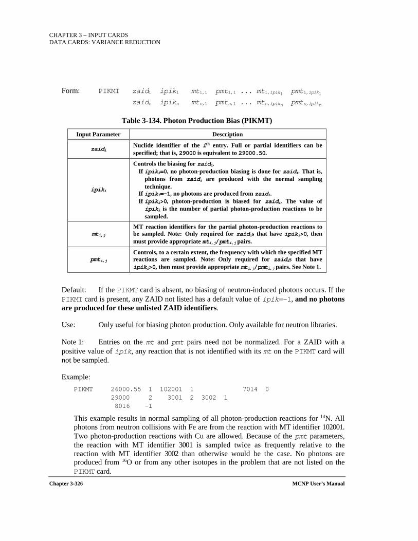
CHAPTER 3 – INPUT CARDS DATA CARDS: VARIANCE REDUCTION
Chapter 3-326 MCNP User’s Manual
Form: PIKMT zaid1 ipik1 mt1,1 pmt1,1 ... mt1,ipik1 pmt1,ipik1 zaidn ipikn mtn,1 pmtn,1 ... mtn,ipikn pmtn,ipikn
Table 3-134. Photon Production Bias (PIKMT)
Input Parameter Description
zaidi Nuclide identifier of the ith entry. Full or partial identifiers can be specified; that is, 29000 is equivalent to 29000.50.
ipiki
Controls the biasing for zaidi. If ipiki=0, no photon-production biasing is done for zaidi. That is,
photons from zaidi are produced with the normal sampling technique.
If ipiki=-1, no photons are produced from zaidi. If ipiki>0, photon-production is biased for zaidi. The value of ipiki is the number of partial photon-production reactions to be sampled.
mti,j MT reaction identifiers for the partial photon-production reactions to be sampled. Note: Only required for zaidis that have ipiki>0, then must provide appropriate mti,j/pmti,j pairs.
pmti,j Controls, to a certain extent, the frequency with which the specified MT reactions are sampled. Note: Only required for zaidis that have ipiki>0, then must provide appropriate mti,j/pmti,j pairs. See Note 1.
Default: If the PIKMT card is absent, no biasing of neutron-induced photons occurs. If the PIKMT card is present, any ZAID not listed has a default value of ipik=-1, and no photons are produced for these unlisted ZAID identifiers.
Use: Only useful for biasing photon production. Only available for neutron libraries.
Note 1: Entries on the mt and pmt pairs need not be normalized. For a ZAID with a positive value of ipik, any reaction that is not identified with its mt on the PIKMT card will not be sampled.
Example: PIKMT 26000.55 1 102001 1 7014 0 29000 2 3001 2 3002 1 8016 -1
This example results in normal sampling of all photon-production reactions for 14N. All photons from neutron collisions with Fe are from the reaction with MT identifier 102001. Two photon-production reactions with Cu are allowed. Because of the pmt parameters, the reaction with MT identifier 3001 is sampled twice as frequently relative to the reaction with MT identifier 3002 than otherwise would be the case. No photons are produced from 16O or from any other isotopes in the problem that are not listed on the PIKMT card.
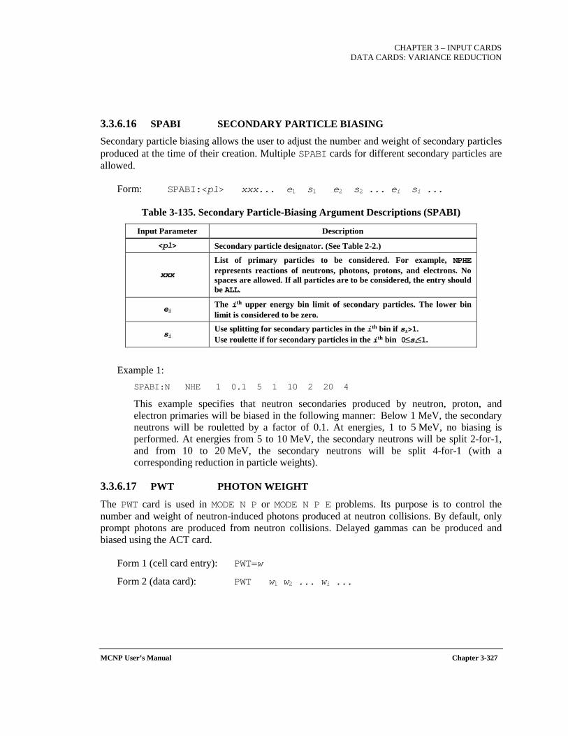
CHAPTER 3 – INPUT CARDS
DATA CARDS: VARIANCE REDUCTION
MCNP User’s Manual Chapter 3-327
3.3.6.16 SPABI SECONDARY PARTICLE BIASING
Secondary particle biasing allows the user to adjust the number and weight of secondary particles produced at the time of their creation. Multiple SPABI cards for different secondary particles are allowed.
Form: SPABI:<pl> xxx... e1 s1 e2 s2 ... ei si ...
Table 3-135. Secondary Particle-Biasing Argument Descriptions (SPABI)
Input Parameter Description
<pl> Secondary particle designator. (See Table 2-2.)
xxx
List of primary particles to be considered. For example, NPHE represents reactions of neutrons, photons, protons, and electrons. No spaces are allowed. If all particles are to be considered, the entry should be ALL.
ei The ith upper energy bin limit of secondary particles. The lower bin limit is considered to be zero.
si Use splitting for secondary particles in the ith bin if si>1. Use roulette if for secondary particles in the ith bin 0≤si≤1.
Example 1: SPABI:N NHE 1 0.1 5 1 10 2 20 4
This example specifies that neutron secondaries produced by neutron, proton, and electron primaries will be biased in the following manner: Below 1 MeV, the secondary neutrons will be rouletted by a factor of 0.1. At energies, 1 to 5 MeV, no biasing is performed. At energies from 5 to 10 MeV, the secondary neutrons will be split 2-for-1, and from 10 to 20 MeV, the secondary neutrons will be split 4-for-1 (with a corresponding reduction in particle weights).
3.3.6.17 PWT PHOTON WEIGHT
The PWT card is used in MODE N P or MODE N P E problems. Its purpose is to control the number and weight of neutron-induced photons produced at neutron collisions. By default, only prompt photons are produced from neutron collisions. Delayed gammas can be produced and biased using the ACT card.
Form 1 (cell card entry): PWT=w
Form 2 (data card): PWT w1 w2 ... wi ...
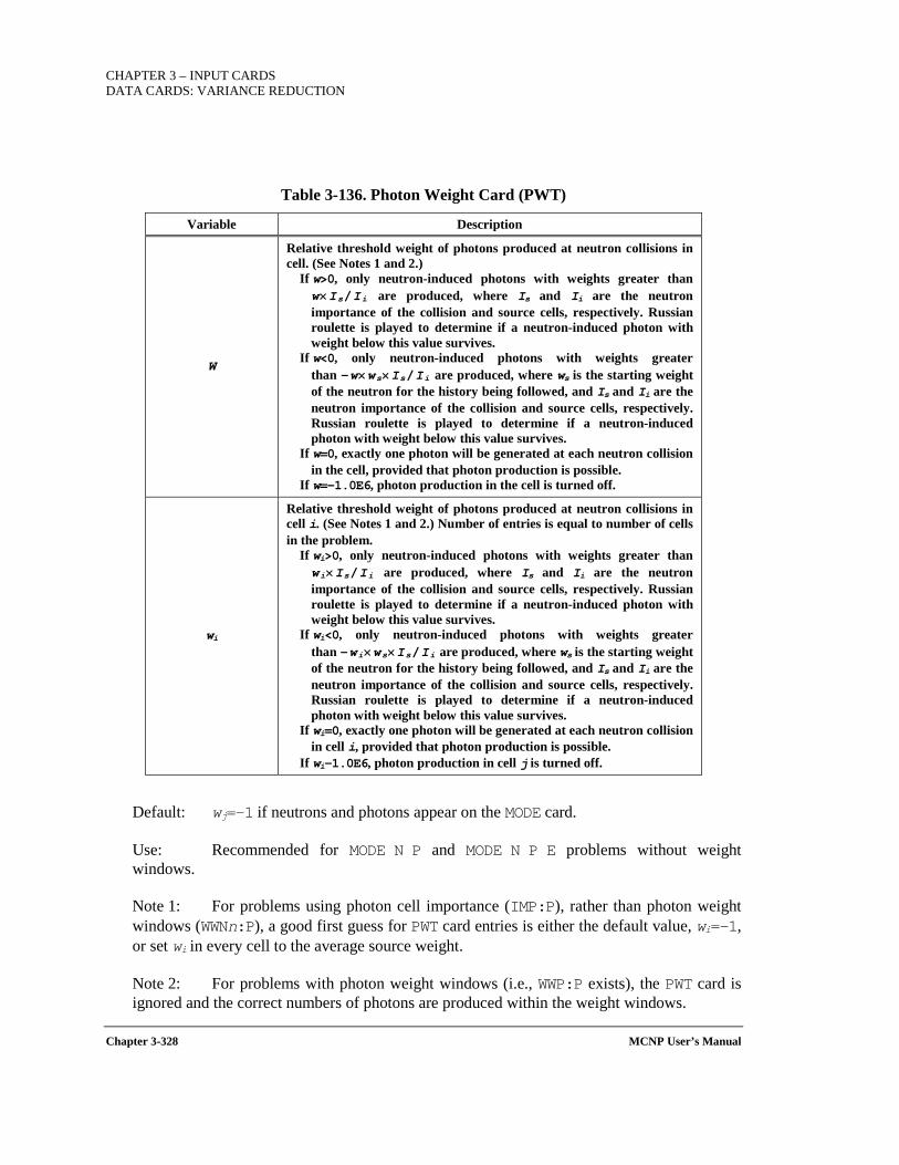
CHAPTER 3 – INPUT CARDS DATA CARDS: VARIANCE REDUCTION
Chapter 3-328 MCNP User’s Manual
Table 3-136. Photon Weight Card (PWT)
Variable Description
W
Relative threshold weight of photons produced at neutron collisions in cell. (See Notes 1 and 2.)
If w>0, only neutron-induced photons with weights greater than w×Is/Ii are produced, where Is and Ii are the neutron importance of the collision and source cells, respectively. Russian roulette is played to determine if a neutron-induced photon with weight below this value survives.
If w<0, only neutron-induced photons with weights greater than -w×ws×Is/Ii are produced, where ws is the starting weight of the neutron for the history being followed, and Is and Ii are the neutron importance of the collision and source cells, respectively. Russian roulette is played to determine if a neutron-induced photon with weight below this value survives.
If w=0, exactly one photon will be generated at each neutron collision in the cell, provided that photon production is possible.
If w=-1.0E6, photon production in the cell is turned off.
wi
Relative threshold weight of photons produced at neutron collisions in cell i. (See Notes 1 and 2.) Number of entries is equal to number of cells in the problem.
If wi>0, only neutron-induced photons with weights greater than wi×Is/Ii are produced, where Is and Ii are the neutron importance of the collision and source cells, respectively. Russian roulette is played to determine if a neutron-induced photon with weight below this value survives.
If wi<0, only neutron-induced photons with weights greater than -wi×ws×Is/Ii are produced, where ws is the starting weight of the neutron for the history being followed, and Is and Ii are the neutron importance of the collision and source cells, respectively. Russian roulette is played to determine if a neutron-induced photon with weight below this value survives.
If wi=0, exactly one photon will be generated at each neutron collision in cell i, provided that photon production is possible.
If wi-1.0E6, photon production in cell j is turned off.
Default: wj=-1 if neutrons and photons appear on the MODE card.
Use: Recommended for MODE N P and MODE N P E problems without weight windows.
Note 1: For problems using photon cell importance (IMP:P), rather than photon weight windows (WWNn:P), a good first guess for PWT card entries is either the default value, wi=−1, or set wi in every cell to the average source weight.
Note 2: For problems with photon weight windows (i.e., WWP:P exists), the PWT card is ignored and the correct numbers of photons are produced within the weight windows.
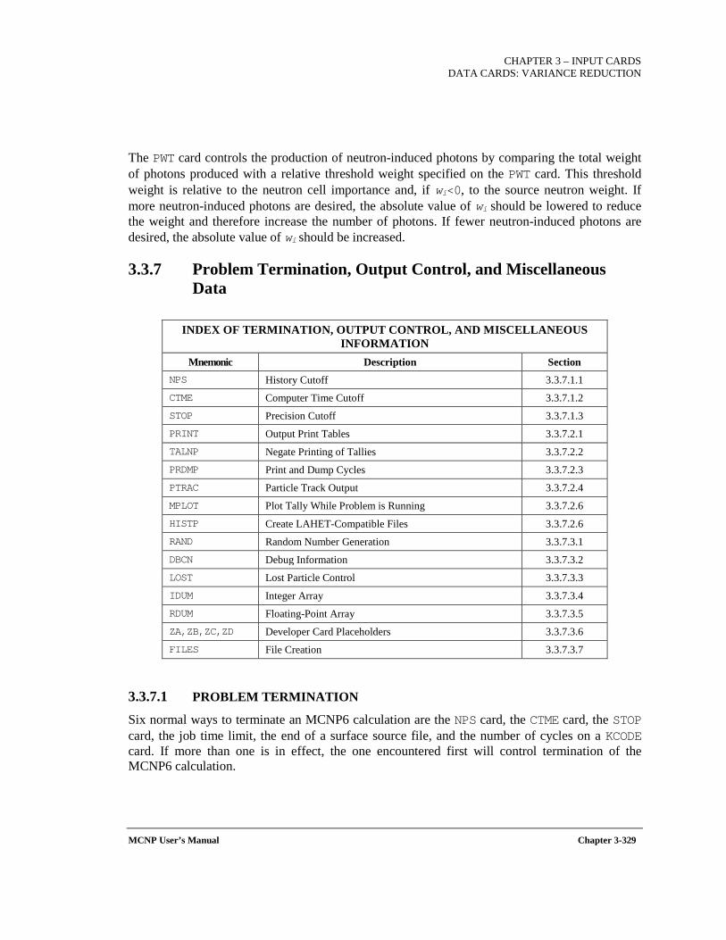
CHAPTER 3 – INPUT CARDS
DATA CARDS: VARIANCE REDUCTION
MCNP User’s Manual Chapter 3-329
The PWT card controls the production of neutron-induced photons by comparing the total weight of photons produced with a relative threshold weight specified on the PWT card. This threshold weight is relative to the neutron cell importance and, if wi<0, to the source neutron weight. If more neutron-induced photons are desired, the absolute value of wi should be lowered to reduce the weight and therefore increase the number of photons. If fewer neutron-induced photons are desired, the absolute value of wi should be increased.
3.3.7 Problem Termination, Output Control, and Miscellaneous Data
INDEX OF TERMINATION, OUTPUT CONTROL, AND MISCELLANEOUS
INFORMATION Mnemonic Description Section
NPS History Cutoff 3.3.7.1.1 CTME Computer Time Cutoff 3.3.7.1.2 STOP Precision Cutoff 3.3.7.1.3 PRINT Output Print Tables 3.3.7.2.1 TALNP Negate Printing of Tallies 3.3.7.2.2 PRDMP Print and Dump Cycles 3.3.7.2.3 PTRAC Particle Track Output 3.3.7.2.4 MPLOT Plot Tally While Problem is Running 3.3.7.2.6 HISTP Create LAHET-Compatible Files 3.3.7.2.6 RAND Random Number Generation 3.3.7.3.1 DBCN Debug Information 3.3.7.3.2 LOST Lost Particle Control 3.3.7.3.3 IDUM Integer Array 3.3.7.3.4 RDUM Floating-Point Array 3.3.7.3.5 ZA,ZB,ZC,ZD Developer Card Placeholders 3.3.7.3.6 FILES File Creation 3.3.7.3.7
3.3.7.1 PROBLEM TERMINATION
Six normal ways to terminate an MCNP6 calculation are the NPS card, the CTME card, the STOP card, the job time limit, the end of a surface source file, and the number of cycles on a KCODE card. If more than one is in effect, the one encountered first will control termination of the MCNP6 calculation.
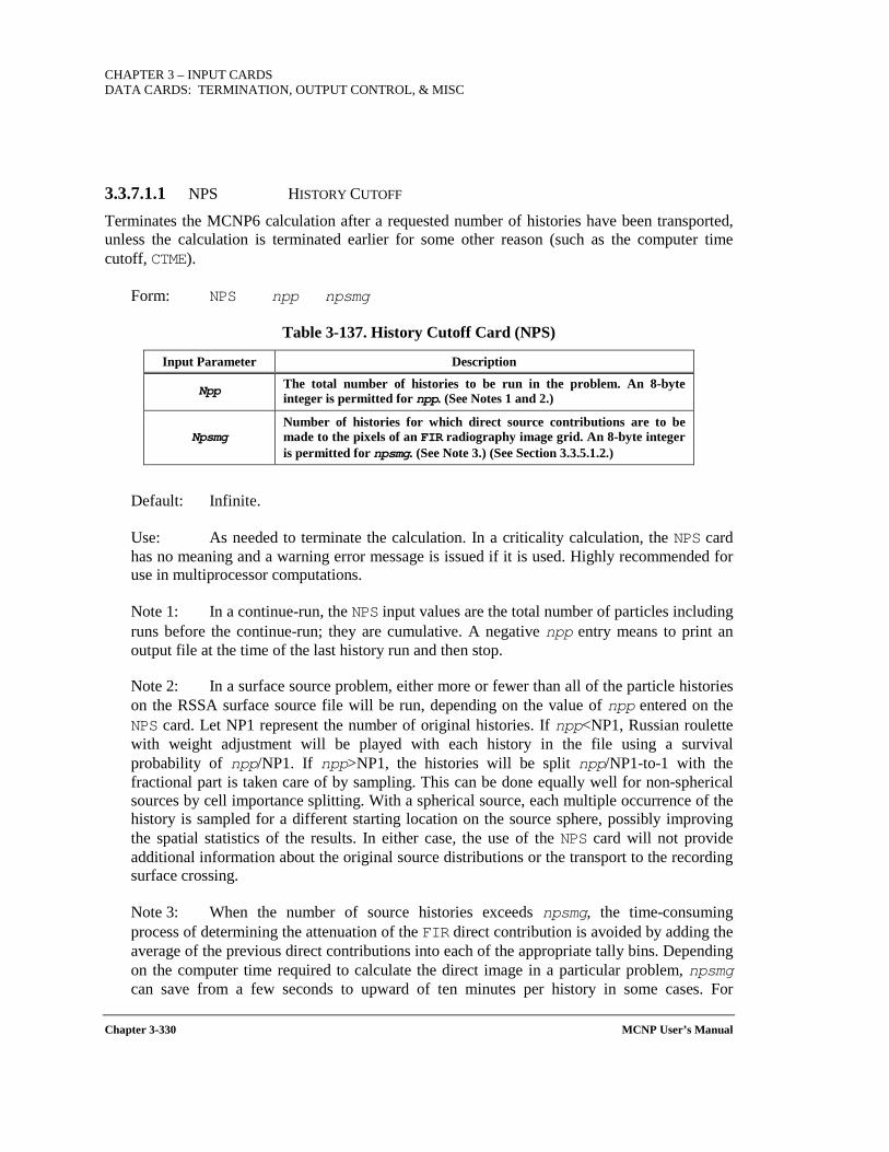
CHAPTER 3 – INPUT CARDS DATA CARDS: TERMINATION, OUTPUT CONTROL, & MISC
Chapter 3-330 MCNP User’s Manual
3.3.7.1.1 NPS HISTORY CUTOFF
Terminates the MCNP6 calculation after a requested number of histories have been transported, unless the calculation is terminated earlier for some other reason (such as the computer time cutoff, CTME).
Form: NPS npp npsmg
Table 3-137. History Cutoff Card (NPS)
Input Parameter Description
Npp The total number of histories to be run in the problem. An 8-byte integer is permitted for npp. (See Notes 1 and 2.)
Npsmg Number of histories for which direct source contributions are to be made to the pixels of an FIR radiography image grid. An 8-byte integer is permitted for npsmg. (See Note 3.) (See Section 3.3.5.1.2.)
Default: Infinite.
Use: As needed to terminate the calculation. In a criticality calculation, the NPS card has no meaning and a warning error message is issued if it is used. Highly recommended for use in multiprocessor computations.
Note 1: In a continue-run, the NPS input values are the total number of particles including runs before the continue-run; they are cumulative. A negative npp entry means to print an output file at the time of the last history run and then stop.
Note 2: In a surface source problem, either more or fewer than all of the particle histories on the RSSA surface source file will be run, depending on the value of npp entered on the NPS card. Let NP1 represent the number of original histories. If npp<NP1, Russian roulette with weight adjustment will be played with each history in the file using a survival probability of npp/NP1. If npp>NP1, the histories will be split npp/NP1-to-1 with the fractional part is taken care of by sampling. This can be done equally well for non-spherical sources by cell importance splitting. With a spherical source, each multiple occurrence of the history is sampled for a different starting location on the source sphere, possibly improving the spatial statistics of the results. In either case, the use of the NPS card will not provide additional information about the original source distributions or the transport to the recording surface crossing.
Note 3: When the number of source histories exceeds npsmg, the time-consuming process of determining the attenuation of the FIR direct contribution is avoided by adding the average of the previous direct contributions into each of the appropriate tally bins. Depending on the computer time required to calculate the direct image in a particular problem, npsmg can save from a few seconds to upward of ten minutes per history in some cases. For

CHAPTER 3 – INPUT CARDS
DATA CARDS: TERMINATION, OUTPUT CONTROL, & MISC
MCNP User’s Manual Chapter 3-331
example, a mono-energetic isotropic point source or a mono-energetic mono-directional surface source requires only one history to determine completely the direct image. For this case, npsmg=1 is adequate.
3.3.7.1.2 CTME COMPUTER TIME CUTOFF
Allows the user to specify minutes of computer time after which MCNP6 will terminate the calculation. MCNP6 checks the computer time remaining in a running problem and will terminate the job itself, allowing enough time to wrap up and terminate gracefully.
Form: CTME tme
where tme=maximum amount of computer time (in minutes) to be spent in the Monte Carlo calculation. (See Notes 1 and 2.)
Default: Infinite.
Use: As needed.
Note 1: For a continue-run job the time on the CTME card is the time relative to the start of the continue-run; it is not cumulative.
Note 2: For multiprocessor runs, it is highly recommended that the NPS card (Section 3.3.7.1.1) be used to limit the run time.
3.3.7.1.3 STOP PRECISION CUTOFF
Enables termination of calculations based on the number of particle histories run, the computer time expended, or the desired precision for a specified tally.
Form: STOP KEYWORD=value(s) ...
Table 3-138. Precision Cutoff (STOP)
Keyword Description
NPS npp [npsmg] Stop calculation after npp particle histories. (See Note 1.) (See NPS card, Section 3.3.7.1.1.)
CTME tme Stop calculation after m minutes of computer time. (See Note 2.) (See CTME card, Section 3.3.7.1.2.)
Fk e Stop calculation when the tally fluctuation chart of tally k has a relative error less than e. (See Note 3.)
Use: If values for any (or all) of the keywords are supplied, MCNP6 will terminate the problem at the first met criteria.
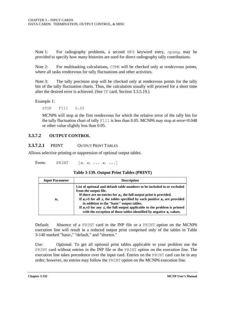
CHAPTER 3 – INPUT CARDS DATA CARDS: TERMINATION, OUTPUT CONTROL, & MISC
Chapter 3-332 MCNP User’s Manual
Note 1: For radiography problems, a second NPS keyword entry, npsmg, may be provided to specify how many histories are used for direct radiography tally contributions.
Note 2: For multitasking calculations, CTME will be checked only at rendezvous points, where all tasks rendezvous for tally fluctuations and other activities.
Note 3: The tally precision stop will be checked only at rendezvous points for the tally bin of the tally fluctuation charts. Thus, the calculation usually will proceed for a short time after the desired error is achieved. (See TF card, Section 3.3.5.19.)
Example 1: STOP F111 0.05
MCNP6 will stop at the first rendezvous for which the relative error of the tally bin for the tally fluctuation chart of tally F111 is less than 0.05. MCNP6 may stop at error=0.048 or other value slightly less than 0.05.
3.3.7.2 OUTPUT CONTROL
3.3.7.2.1 PRINT OUTPUT PRINT TABLES
Allows selective printing or suppression of optional output tables.
Form: PRINT [x1 x2 ... xi ...]
Table 3-139. Output Print Tables (PRINT)
Input Parameter Description
xi
List of optional and default table numbers to be included in or excluded from the output file.
If there are no entries for xi, the full output print is provided. If xi>0 for all i, the tables specified by each positive xi are provided
in addition to the "basic" output tables. If xi<0 for any i, the full output applicable to the problem is printed
with the exception of those tables identified by negative xi values.
Default: Absence of a PRINT card in the INP file or a PRINT option on the MCNP6 execution line will result in a reduced output print comprised only of the tables in Table 3-140 marked "basic," "default," and "shorten."
Use: Optional. To get all optional print tables applicable to your problem use the PRINT card without entries in the INP file or the PRINT option on the execution line. The execution line takes precedence over the input card. Entries on the PRINT card can be in any order; however, no entries may follow the PRINT option on the MCNP6 execution line.
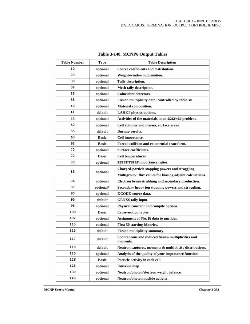
CHAPTER 3 – INPUT CARDS
DATA CARDS: TERMINATION, OUTPUT CONTROL, & MISC
MCNP User’s Manual Chapter 3-333
Table 3-140. MCNP6 Output Tables
Table Number Type Table Description
10 optional Source coefficients and distribution. 20 optional Weight-window information. 30 optional Tally description. 32 optional Mesh tally description. 35 optional Coincident detectors. 38 optional Fission multiplicity data; controlled by table 30. 40 optional Material composition. 41 default LAHET physics options. 44 optional Activities of the materials in an SDEF=SP problem.
50 optional Cell volumes and masses, surface areas. 55 default Burnup results. 60 Basic Cell importance. 62 Basic Forced collision and exponential transform. 70 optional Surface coefficients. 72 Basic Cell temperatures. 80 optional ESPLT/TSPLT importance ratios.
85 optional Charged-particle stopping powers and straggling.
Multigroup: flux values for biasing adjoint calculations. 86 optional Electron bremsstrahlung and secondary production. 87 optional* Secondary heavy ion stopping powers and straggling. 90 optional KCODE source data. 95 default GENXS tally input. 98 optional Physical constant and compile options. 100 Basic Cross-section tables. 102 optional Assignment of S(α, β) data to nuclides. 110 optional First 50 starting histories. 115 default Fission multiplicity summary.
117 default Spontaneous and induced fission multiplicities and moments.
118 default Neutron captures, moments & multiplicity distributions. 120 optional Analysis of the quality of your importance function. 126 Basic Particle activity in each cell. 128 optional Universe map. 130 optional Neutron/photon/electron weight balance. 140 optional Neutron/photon nuclide activity.

CHAPTER 3 – INPUT CARDS DATA CARDS: TERMINATION, OUTPUT CONTROL, & MISC
Chapter 3-334 MCNP User’s Manual
Table Number Type Table Description 150 optional DXTRAN diagnostics. 160 default TFC bin tally analysis.
161 default f(x) tally density plot. 162 default Cumulative f(x) and tally density plot. 163 optional Receiver-Operator Characterization (ROC) curve data. 170 optional Source distribution frequency tables, surface source. 175 shorten Estimated keff results by cycle. 178 optional Estimated keff results by batch size.
180 optional Weight-window generator bookkeeping summary controlled by WWG(7), not print card.
190 basic Weight-window generator summary. 198 optional Weight windows from multigroup fluxes. 200 basic Weight-window-generated windows. 210 default Burnup summary table. 220 default Burnup summary table summed over all materials.
* The printing of table 87 does not follow the standard default convention. To print table 87, specify the table number on the PRINT card.
The following output will be printed automatically, as applicable:
• a listing of the input file, • the problem summary of particle creation and loss, • KCODE cycle summaries, • tallies, • tally fluctuation charts, • the tables listed in Table 3-140 as basic, and • the tables listed in Table 3-140 as default, provided they are not turned off explicitly with
the PRINT card.
In an MCNP6 output file, a table number appears in the upper right-hand corner of each table, providing a convenient pattern when scanning the output file with an editor. The pattern is "print table n," where n, the table number, is always preceded by one space and is a two- or three-digit number. The table numbers, titles, and type are summarized in Table 3-140 above. "Basic" tables cannot be controlled by the PRINT card." "Default" tables are automatically printed but can be turned off. "Optional" tables with can be turned off and on with the PRINT card or option.
With one exception, the PRINT control can be used in a continue-run to recover all or any applicable print tables, even if they were not requested in the original run. The following continue-run input file:
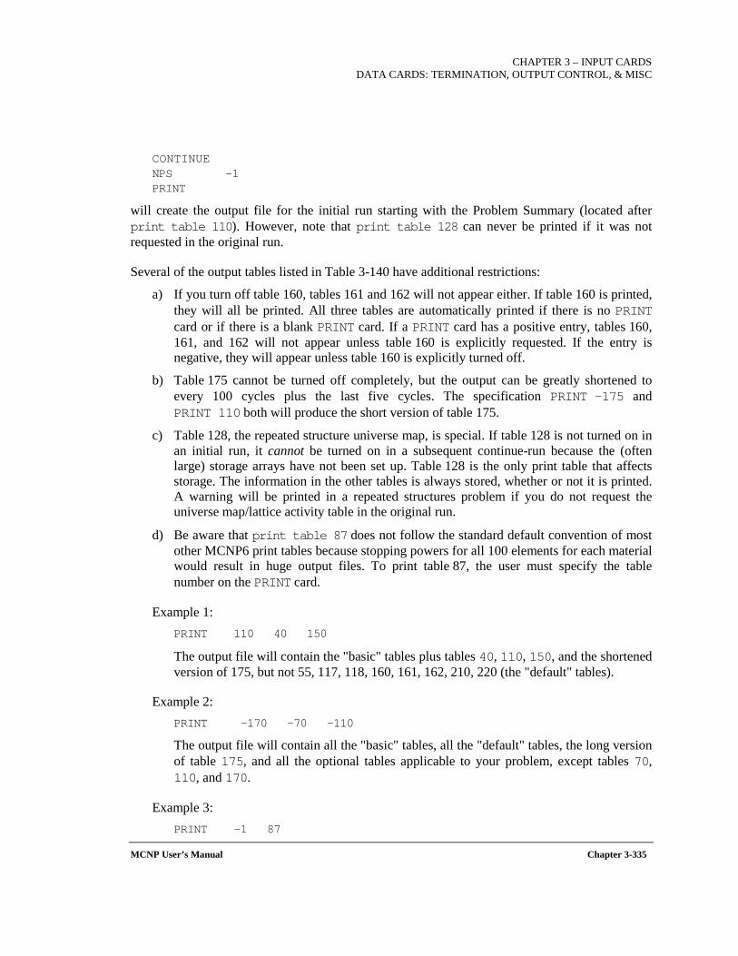
CHAPTER 3 – INPUT CARDS
DATA CARDS: TERMINATION, OUTPUT CONTROL, & MISC
MCNP User’s Manual Chapter 3-335
CONTINUE NPS -1 PRINT
will create the output file for the initial run starting with the Problem Summary (located after print table 110). However, note that print table 128 can never be printed if it was not requested in the original run.
Several of the output tables listed in Table 3-140 have additional restrictions:
a) If you turn off table 160, tables 161 and 162 will not appear either. If table 160 is printed, they will all be printed. All three tables are automatically printed if there is no PRINT card or if there is a blank PRINT card. If a PRINT card has a positive entry, tables 160, 161, and 162 will not appear unless table 160 is explicitly requested. If the entry is negative, they will appear unless table 160 is explicitly turned off.
b) Table 175 cannot be turned off completely, but the output can be greatly shortened to every 100 cycles plus the last five cycles. The specification PRINT −175 and PRINT 110 both will produce the short version of table 175.
c) Table 128, the repeated structure universe map, is special. If table 128 is not turned on in an initial run, it cannot be turned on in a subsequent continue-run because the (often large) storage arrays have not been set up. Table 128 is the only print table that affects storage. The information in the other tables is always stored, whether or not it is printed. A warning will be printed in a repeated structures problem if you do not request the universe map/lattice activity table in the original run.
d) Be aware that print table 87 does not follow the standard default convention of most other MCNP6 print tables because stopping powers for all 100 elements for each material would result in huge output files. To print table 87, the user must specify the table number on the PRINT card.
Example 1: PRINT 110 40 150
The output file will contain the "basic" tables plus tables 40, 110, 150, and the shortened version of 175, but not 55, 117, 118, 160, 161, 162, 210, 220 (the "default" tables).
Example 2: PRINT -170 -70 -110
The output file will contain all the "basic" tables, all the "default" tables, the long version of table 175, and all the optional tables applicable to your problem, except tables 70, 110, and 170.
Example 3: PRINT -1 87
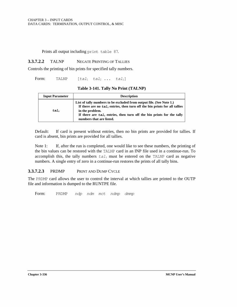
CHAPTER 3 – INPUT CARDS DATA CARDS: TERMINATION, OUTPUT CONTROL, & MISC
Chapter 3-336 MCNP User’s Manual
Prints all output including print table 87.
3.3.7.2.2 TALNP NEGATE PRINTING OF TALLIES
Controls the printing of bin prints for specified tally numbers.
Form: TALNP [tal1 tal2 ... tali]
Table 3-141. Tally No Print (TALNP)
Input Parameter Description
tali
List of tally numbers to be excluded from output file. (See Note 1.) If there are no tali entries, then turn off the bin prints for all tallies in the problem. If there are tali entries, then turn off the bin prints for the tally numbers that are listed.
Default: If card is present without entries, then no bin prints are provided for tallies. If card is absent, bin prints are provided for all tallies.
Note 1: If, after the run is completed, one would like to see these numbers, the printing of the bin values can be restored with the TALNP card in an INP file used in a continue-run. To accomplish this, the tally numbers tali must be entered on the TALNP card as negative numbers. A single entry of zero in a continue-run restores the prints of all tally bins.
3.3.7.2.3 PRDMP PRINT AND DUMP CYCLE
The PRDMP card allows the user to control the interval at which tallies are printed to the OUTP file and information is dumped to the RUNTPE file.
Form: PRDMP ndp ndm mct ndmp dmmp
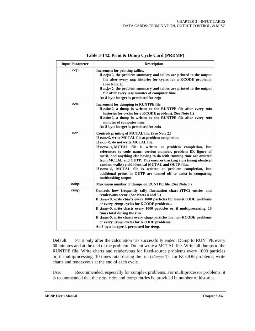
CHAPTER 3 – INPUT CARDS
DATA CARDS: TERMINATION, OUTPUT CONTROL, & MISC
MCNP User’s Manual Chapter 3-337
Table 3-142. Print & Dump Cycle Card (PRDMP)
Input Parameter Description
ndp Increment for printing tallies. If ndp>0, the problem summary and tallies are printed to the output
file after every ndp histories (or cycles for a KCODE problem). (See Note 1.)
If ndp<0, the problem summary and tallies are printed to the output file after every ndp minutes of computer time.
An 8-byte integer is permitted for ndp. ndm Increment for dumping to RUNTPE file.
If ndm>0, a dump is written to the RUNTPE file after every ndm histories (or cycles for a KCODE problem). (See Note 1.)
If ndm<0, a dump is written to the RUNTPE file after every ndm minutes of computer time.
An 8-byte integer is permitted for ndm.
mct Controls printing of MCTAL file. (See Note 2.) If mct>0, write MCTAL file at problem completion. If mct=0, do not write MCTAL file. If mct=-1, MCTAL file is written at problem completion, but
references to code name, version number, problem ID, figure of merit, and anything else having to do with running time are omitted from MCTAL and OUTP. This ensures tracking runs (using identical random walks) yield identical MCTAL and OUTP files.
If mct=-2, MCTAL file is written at problem completion, but additional prints in OUTP are turned off to assist in comparing multitasking output.
ndmp Maximum number of dumps on RUNTPE file. (See Note 3.) dmmp Controls how frequently tally fluctuation chart (TFC) entries and
rendezvous occur. (See Notes 4 and 5.) If dmmp<0, write charts every 1000 particles for non-KCODE problems
or every |dmmp| cycles for KCODE problems.. If dmmp=0, write charts every 1000 particles or, if multiprocessing, 10
times total during the run. If dmmp>0, write charts every dmmp particles for non-KCODE problems
or every |dmmp| cycles for KCODE problems. An 8-byte integer is permitted for dmmp.
Default: Print only after the calculation has successfully ended. Dump to RUNTPE every 60 minutes and at the end of the problem. Do not write a MCTAL file. Write all dumps to the RUNTPE file. Write charts and rendezvous for fixed-source problems every 1000 particles or, if multiprocessing, 10 times total during the run (dmmp=0); for KCODE problems, write charts and rendezvous at the end of each cycle.
Use: Recommended, especially for complex problems. For multiprocessor problems, it is recommended that the ndp, ndm, and dmmp entries be provided in number of histories.
CHAPTER 3 – INPUT CARDS DATA CARDS: TERMINATION, OUTPUT CONTROL, & MISC
Chapter 3-338 MCNP User’s Manual
Note 1: If ndp or ndm is set to time on a parallel job, it will be time used by one processor, approximately elapsed wall time. The scheduled print or dump will be delayed to the next rendezvous or cycle to assure consistent data. For parallel (i.e., multiprocessor) runs, is highly recommended that the ndp and ndm values be set in terms of particles or cycles, instead of minutes,
Note 2: The MCTAL file is an ASCII file of tallies that can be subsequently plotted with the MCNP6 MCPLOT option. The MCTAL file is also a convenient way to store tally information in a format that is stable for use in the user’s own auxiliary programs. For example, if the user is on a system that cannot use the MCNP6 MCPLOT option, the MCTAL file can be manipulated into whatever format is required by the user’s own local plotting algorithms.
Note 3: Using the parameter ndmp, the PRDMP card allows the user to control the size of the RUNTPE file. The RUNTPE file will contain the last ndmp dumps that were written. For example, if ndmp=4, after dump 20 is written only dumps 17, 18, 19, and 20 will be on the RUNTPE file. In all cases, the fixed data and cross-section data at the front of the RUNTPE file are preserved.
Note 4: The fifth entry dmmp has several possible meanings. For sequential non-KCODE MCNP6, a value of dmmp≤0 results in TFC entries every 1000 particles initially. This value doubles to 2000 after 20 TFC entries. A positive value of dmmp produces TFC entries every dmmp particles initially. For non-KCODE distributed memory multiprocessing, dmmp<0 produces TFC entries and task rendezvous every 1000 particles initially, the same as does the sequential version. The default value, dmmp=0, produces ten TFC entries and task rendezvous, rounded to the nearest 1000 particles, based on other cutoffs such as NPS, CTME, etc. This selection optimizes speedup in conjunction with TFC entries. If detectors/DXTRAN are used with default Russian roulette criteria (DD card default), the dmmp=0 entry is changed by MCNP6 to dmmp<0, ensuring tracking with the sequential version (i.e., TFC entries and rendezvous every 1000 particles). As with the sequential non-KCODE version, dmmp>0 produces TFC entries and task rendezvous every dmmp particles, even with detectors/DXTRAN with default Russian roulette criteria. Setting dmmp to a large positive number minimizes communication time and maximizes speedup. However, the TFC may not have many entries, possibly only one, if dmmp=npp.
Note 5: The rendezvous frequency of a multiprocessor run is the minimum interval of parameters or ndp, ndm, and dmmp.
3.3.7.2.4 PTRAC PARTICLE TRACK OUTPUT
The PTRAC card generates an output file, default name PTRAC, of user-filtered particle events. (See Appendix E.) The file name PTRAC can be changed on the execution line or within the message block.
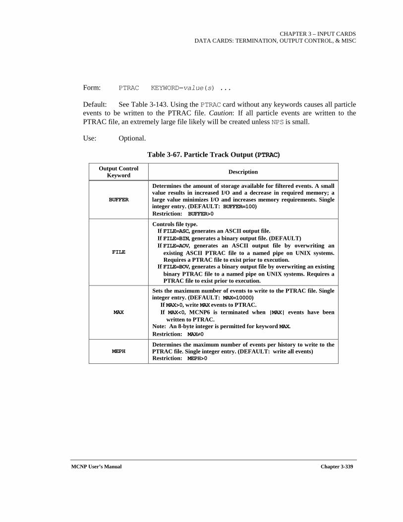
CHAPTER 3 – INPUT CARDS
DATA CARDS: TERMINATION, OUTPUT CONTROL, & MISC
MCNP User’s Manual Chapter 3-339
Form: PTRAC KEYWORD=value(s) ...
Default: See Table 3-143. Using the PTRAC card without any keywords causes all particle events to be written to the PTRAC file. Caution: If all particle events are written to the PTRAC file, an extremely large file likely will be created unless NPS is small.
Use: Optional.
Table 3-67. Particle Track Output (PTRAC)
Output Control Keyword Description
BUFFER
Determines the amount of storage available for filtered events. A small value results in increased I/O and a decrease in required memory; a large value minimizes I/O and increases memory requirements. Single integer entry. (DEFAULT: BUFFER=100) Restriction: BUFFER>0
FILE
Controls file type. If FILE=ASC, generates an ASCII output file. If FILE=BIN, generates a binary output file. (DEFAULT) If FILE=AOV, generates an ASCII output file by overwriting an
existing ASCII PTRAC file to a named pipe on UNIX systems. Requires a PTRAC file to exist prior to execution.
If FILE=BOV, generates a binary output file by overwriting an existing binary PTRAC file to a named pipe on UNIX systems. Requires a PTRAC file to exist prior to execution.
MAX
Sets the maximum number of events to write to the PTRAC file. Single integer entry. (DEFAULT: MAX=10000)
If MAX>0, write MAX events to PTRAC. If MAX<0, MCNP6 is terminated when |MAX| events have been
written to PTRAC. Note: An 8-byte integer is permitted for keyword MAX. Restriction: MAX≠0
MEPH Determines the maximum number of events per history to write to the PTRAC file. Single integer entry. (DEFAULT: write all events) Restriction: MEPH>0
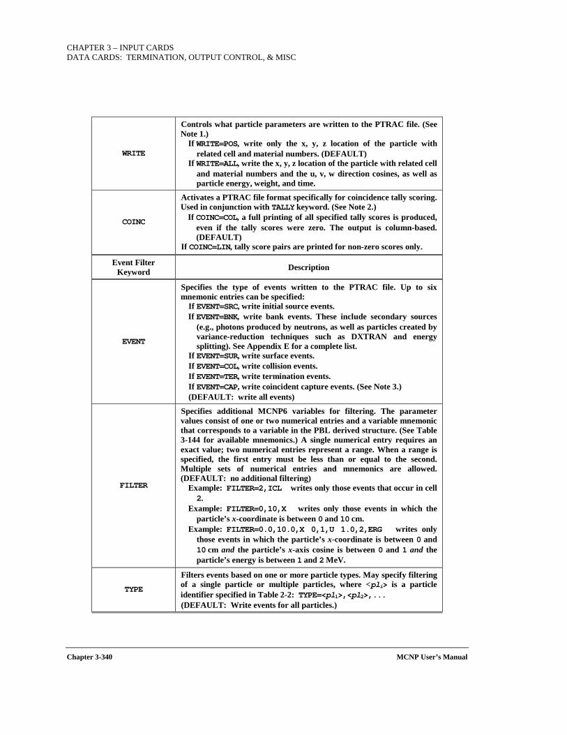
CHAPTER 3 – INPUT CARDS DATA CARDS: TERMINATION, OUTPUT CONTROL, & MISC
Chapter 3-340 MCNP User’s Manual
WRITE
Controls what particle parameters are written to the PTRAC file. (See Note 1.)
If WRITE=POS, write only the x, y, z location of the particle with related cell and material numbers. (DEFAULT)
If WRITE=ALL, write the x, y, z location of the particle with related cell and material numbers and the u, v, w direction cosines, as well as particle energy, weight, and time.
COINC
Activates a PTRAC file format specifically for coincidence tally scoring. Used in conjunction with TALLY keyword. (See Note 2.)
If COINC=COL, a full printing of all specified tally scores is produced, even if the tally scores were zero. The output is column-based. (DEFAULT)
If COINC=LIN, tally score pairs are printed for non-zero scores only.
Event Filter Keyword Description
EVENT
Specifies the type of events written to the PTRAC file. Up to six mnemonic entries can be specified:
If EVENT=SRC, write initial source events. If EVENT=BNK, write bank events. These include secondary sources
(e.g., photons produced by neutrons, as well as particles created by variance-reduction techniques such as DXTRAN and energy splitting). See Appendix E for a complete list.
If EVENT=SUR, write surface events. If EVENT=COL, write collision events. If EVENT=TER, write termination events. If EVENT=CAP, write coincident capture events. (See Note 3.) (DEFAULT: write all events)
FILTER
Specifies additional MCNP6 variables for filtering. The parameter values consist of one or two numerical entries and a variable mnemonic that corresponds to a variable in the PBL derived structure. (See Table 3-144 for available mnemonics.) A single numerical entry requires an exact value; two numerical entries represent a range. When a range is specified, the first entry must be less than or equal to the second. Multiple sets of numerical entries and mnemonics are allowed. (DEFAULT: no additional filtering)
Example: FILTER=2,ICL writes only those events that occur in cell 2.
Example: FILTER=0,10,X writes only those events in which the particle’s x-coordinate is between 0 and 10 cm.
Example: FILTER=0.0,10.0,X 0,1,U 1.0,2,ERG writes only those events in which the particle’s x-coordinate is between 0 and 10 cm and the particle’s x-axis cosine is between 0 and 1 and the particle’s energy is between 1 and 2 MeV.
TYPE
Filters events based on one or more particle types. May specify filtering of a single particle or multiple particles, where <pli> is a particle identifier specified in Table 2-2: TYPE=<pl1>,<pl2>,... (DEFAULT: Write events for all particles.)
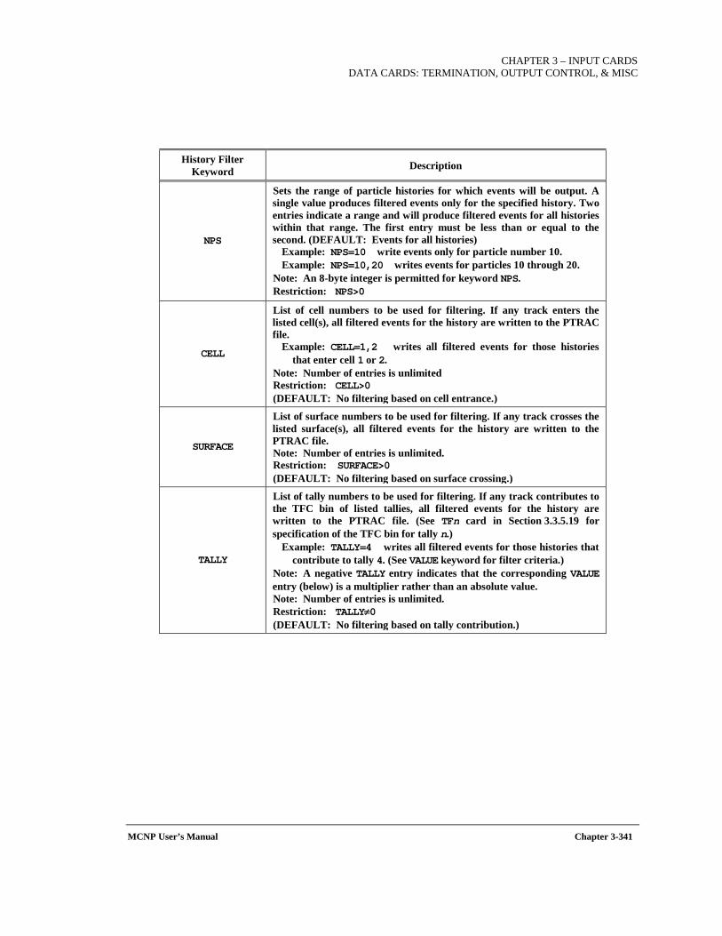
CHAPTER 3 – INPUT CARDS
DATA CARDS: TERMINATION, OUTPUT CONTROL, & MISC
MCNP User’s Manual Chapter 3-341
History Filter Keyword Description
NPS
Sets the range of particle histories for which events will be output. A single value produces filtered events only for the specified history. Two entries indicate a range and will produce filtered events for all histories within that range. The first entry must be less than or equal to the second. (DEFAULT: Events for all histories)
Example: NPS=10 write events only for particle number 10. Example: NPS=10,20 writes events for particles 10 through 20.
Note: An 8-byte integer is permitted for keyword NPS. Restriction: NPS>0
CELL
List of cell numbers to be used for filtering. If any track enters the listed cell(s), all filtered events for the history are written to the PTRAC file.
Example: CELL=1,2 writes all filtered events for those histories that enter cell 1 or 2.
Note: Number of entries is unlimited Restriction: CELL>0 (DEFAULT: No filtering based on cell entrance.)
SURFACE
List of surface numbers to be used for filtering. If any track crosses the listed surface(s), all filtered events for the history are written to the PTRAC file. Note: Number of entries is unlimited. Restriction: SURFACE>0 (DEFAULT: No filtering based on surface crossing.)
TALLY
List of tally numbers to be used for filtering. If any track contributes to the TFC bin of listed tallies, all filtered events for the history are written to the PTRAC file. (See TFn card in Section 3.3.5.19 for specification of the TFC bin for tally n.)
Example: TALLY=4 writes all filtered events for those histories that contribute to tally 4. (See VALUE keyword for filter criteria.)
Note: A negative TALLY entry indicates that the corresponding VALUE entry (below) is a multiplier rather than an absolute value. Note: Number of entries is unlimited. Restriction: TALLY≠0 (DEFAULT: No filtering based on tally contribution.)
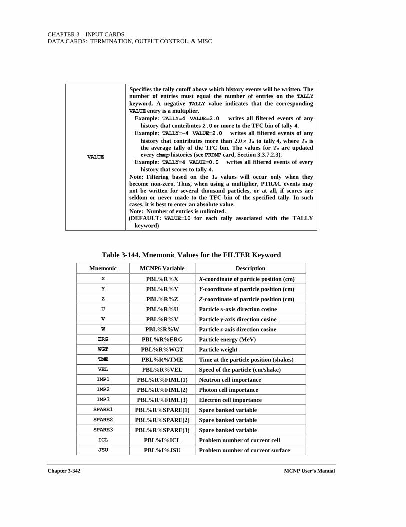
CHAPTER 3 – INPUT CARDS DATA CARDS: TERMINATION, OUTPUT CONTROL, & MISC
Chapter 3-342 MCNP User’s Manual
VALUE
Specifies the tally cutoff above which history events will be written. The number of entries must equal the number of entries on the TALLY keyword. A negative TALLY value indicates that the corresponding VALUE entry is a multiplier.
Example: TALLY=4 VALUE=2.0 writes all filtered events of any history that contributes 2.0 or more to the TFC bin of tally 4.
Example: TALLY=-4 VALUE=2.0 writes all filtered events of any history that contributes more than 2.0 × Ta to tally 4, where Ta is the average tally of the TFC bin. The values for Ta are updated every dmmp histories (see PRDMP card, Section 3.3.7.2.3).
Example: TALLY=4 VALUE=0.0 writes all filtered events of every history that scores to tally 4.
Note: Filtering based on the Ta values will occur only when they become non-zero. Thus, when using a multiplier, PTRAC events may not be written for several thousand particles, or at all, if scores are seldom or never made to the TFC bin of the specified tally. In such cases, it is best to enter an absolute value. Note: Number of entries is unlimited. (DEFAULT: VALUE=10 for each tally associated with the TALLY
keyword)
Table 3-144. Mnemonic Values for the FILTER Keyword
Mnemonic MCNP6 Variable Description
X PBL%R%X X-coordinate of particle position (cm) Y PBL%R%Y Y-coordinate of particle position (cm) Z PBL%R%Z Z-coordinate of particle position (cm) U PBL%R%U Particle x-axis direction cosine V PBL%R%V Particle y-axis direction cosine W PBL%R%W Particle z-axis direction cosine ERG PBL%R%ERG Particle energy (MeV) WGT PBL%R%WGT Particle weight TME PBL%R%TME Time at the particle position (shakes) VEL PBL%R%VEL Speed of the particle (cm/shake) IMP1 PBL%R%FIML(1) Neutron cell importance IMP2 PBL%R%FIML(2) Photon cell importance IMP3 PBL%R%FIML(3) Electron cell importance SPARE1 PBL%R%SPARE(1) Spare banked variable SPARE2 PBL%R%SPARE(2) Spare banked variable SPARE3 PBL%R%SPARE(3) Spare banked variable ICL PBL%I%ICL Problem number of current cell JSU PBL%I%JSU Problem number of current surface
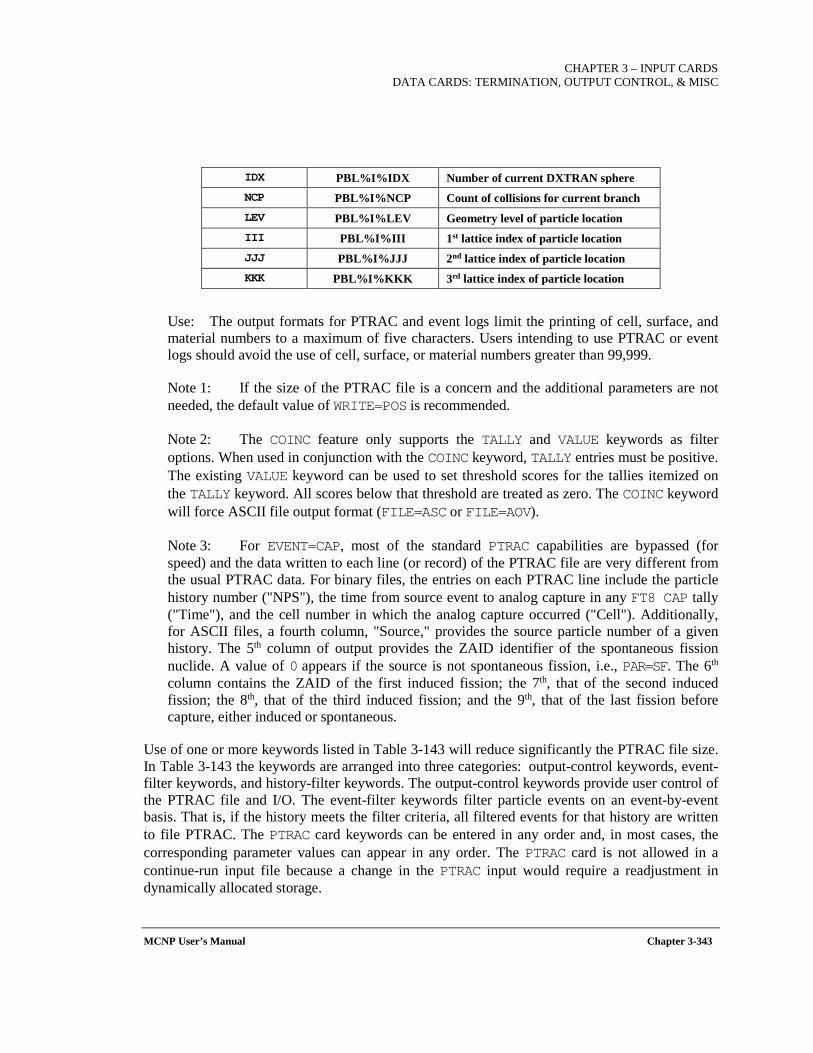
CHAPTER 3 – INPUT CARDS
DATA CARDS: TERMINATION, OUTPUT CONTROL, & MISC
MCNP User’s Manual Chapter 3-343
IDX PBL%I%IDX Number of current DXTRAN sphere NCP PBL%I%NCP Count of collisions for current branch LEV PBL%I%LEV Geometry level of particle location III PBL%I%III 1st lattice index of particle location JJJ PBL%I%JJJ 2nd lattice index of particle location KKK PBL%I%KKK 3rd lattice index of particle location
Use: The output formats for PTRAC and event logs limit the printing of cell, surface, and material numbers to a maximum of five characters. Users intending to use PTRAC or event logs should avoid the use of cell, surface, or material numbers greater than 99,999.
Note 1: If the size of the PTRAC file is a concern and the additional parameters are not needed, the default value of WRITE=POS is recommended.
Note 2: The COINC feature only supports the TALLY and VALUE keywords as filter options. When used in conjunction with the COINC keyword, TALLY entries must be positive. The existing VALUE keyword can be used to set threshold scores for the tallies itemized on the TALLY keyword. All scores below that threshold are treated as zero. The COINC keyword will force ASCII file output format (FILE=ASC or FILE=AOV).
Note 3: For EVENT=CAP, most of the standard PTRAC capabilities are bypassed (for speed) and the data written to each line (or record) of the PTRAC file are very different from the usual PTRAC data. For binary files, the entries on each PTRAC line include the particle history number ("NPS"), the time from source event to analog capture in any FT8 CAP tally ("Time"), and the cell number in which the analog capture occurred ("Cell"). Additionally, for ASCII files, a fourth column, "Source," provides the source particle number of a given history. The 5th column of output provides the ZAID identifier of the spontaneous fission nuclide. A value of 0 appears if the source is not spontaneous fission, i.e., PAR=SF. The 6th column contains the ZAID of the first induced fission; the 7th, that of the second induced fission; the 8th, that of the third induced fission; and the 9th, that of the last fission before capture, either induced or spontaneous.
Use of one or more keywords listed in Table 3-143 will reduce significantly the PTRAC file size. In Table 3-143 the keywords are arranged into three categories: output-control keywords, event-filter keywords, and history-filter keywords. The output-control keywords provide user control of the PTRAC file and I/O. The event-filter keywords filter particle events on an event-by-event basis. That is, if the history meets the filter criteria, all filtered events for that history are written to file PTRAC. The PTRAC card keywords can be entered in any order and, in most cases, the corresponding parameter values can appear in any order. The PTRAC card is not allowed in a continue-run input file because a change in the PTRAC input would require a readjustment in dynamically allocated storage.
CHAPTER 3 – INPUT CARDS DATA CARDS: TERMINATION, OUTPUT CONTROL, & MISC
Chapter 3-344 MCNP User’s Manual
The PTRAC file will contain the heavy ion particles and their track information, but not individual heavy ion identities (ZZZAAAs).
Example: PTRAC FILTER=8,9,ERG EVENT=SUR NPS=1,50 TYPE=E CELL=3,4
When multiple keywords are entered on the PTRAC card, the filter criteria for each keyword must be satisfied to obtain an output event. This input line will write only surface crossing events for 8–9-MeV electrons generated by histories 1–50 that have entered cells 3 or 4.
3.3.7.2.5 MPLOT PLOT TALLY WHILE PROBLEM IS RUNNING
The MPLOT card specifies a plot of intermediate tally results that is to be produced periodically during the run.
Form: MPLOT KEYWORD=value(s)
Default: None.
Use: Optional. The specification of 8-byte integer values is allowed for FREQ.
The entries on the MPLOT card are MCPLOT commands (see Table 5-5) for one picture. During the run, as determined by the FREQ n keyword entry, MCRUN will call MCPLOT to display the current status of one or more of the tallies in the problem. If a FREQ n command is not included on the MPLOT card, n will be set to 5000. The following MCPLOT commands cannot appear on the MPLOT card: RMCTAL, RUNTPE, DUMP, and END. All of the commands on the MPLOT card are executed for each displayed picture, so coplots of more than one bin or tally are possible. No output is sent to a COMOUT file. MCPLOT will not take plot requests from the terminal; it returns to MCRUN after each plot is displayed. See Section 5.3.2 for a complete list of MCPLOT commands available.
A second way to plot intermediate tally results is to use the TTY interrupt <ctrl-c>MCPLOT or <ctrl-c>M that allows interactive plotting during the run. At the end of the history that is running when the interrupt occurs, MCRUN will call MCPLOT, which will take plot requests from the terminal. No output is sent to the COMOUT file. The following commands can not be used: RMCTAL, RUNTPE, DUMP, and END.
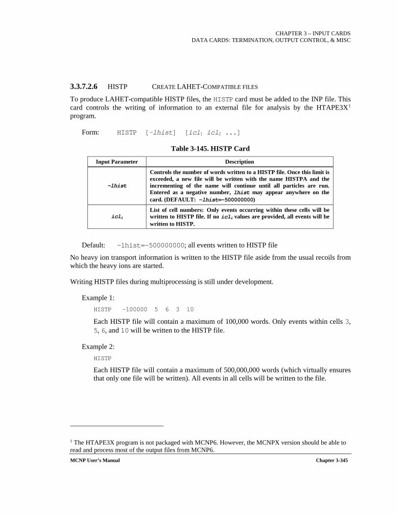
CHAPTER 3 – INPUT CARDS
DATA CARDS: TERMINATION, OUTPUT CONTROL, & MISC
MCNP User’s Manual Chapter 3-345
3.3.7.2.6 HISTP CREATE LAHET-COMPATIBLE FILES
To produce LAHET-compatible HISTP files, the HISTP card must be added to the INP file. This card controls the writing of information to an external file for analysis by the HTAPE3X1 program.
Form: HISTP [-lhist] [icl1 icl2 ...]
Table 3-145. HISTP Card
Input Parameter Description
-lhist
Controls the number of words written to a HISTP file. Once this limit is exceeded, a new file will be written with the name HISTPA and the incrementing of the name will continue until all particles are run. Entered as a negative number, lhist may appear anywhere on the card. (DEFAULT: -lhist=-500000000)
icli List of cell numbers: Only events occurring within these cells will be written to HISTP file. If no icli values are provided, all events will be written to HISTP.
Default: -lhist=-500000000; all events written to HISTP file
No heavy ion transport information is written to the HISTP file aside from the usual recoils from which the heavy ions are started.
Writing HISTP files during multiprocessing is still under development.
Example 1: HISTP -100000 5 6 3 10
Each HISTP file will contain a maximum of 100,000 words. Only events within cells 3, 5, 6, and 10 will be written to the HISTP file.
Example 2: HISTP
Each HISTP file will contain a maximum of 500,000,000 words (which virtually ensures that only one file will be written). All events in all cells will be written to the file.
1 The HTAPE3X program is not packaged with MCNP6. However, the MCNPX version should be able to read and process most of the output files from MCNP6.
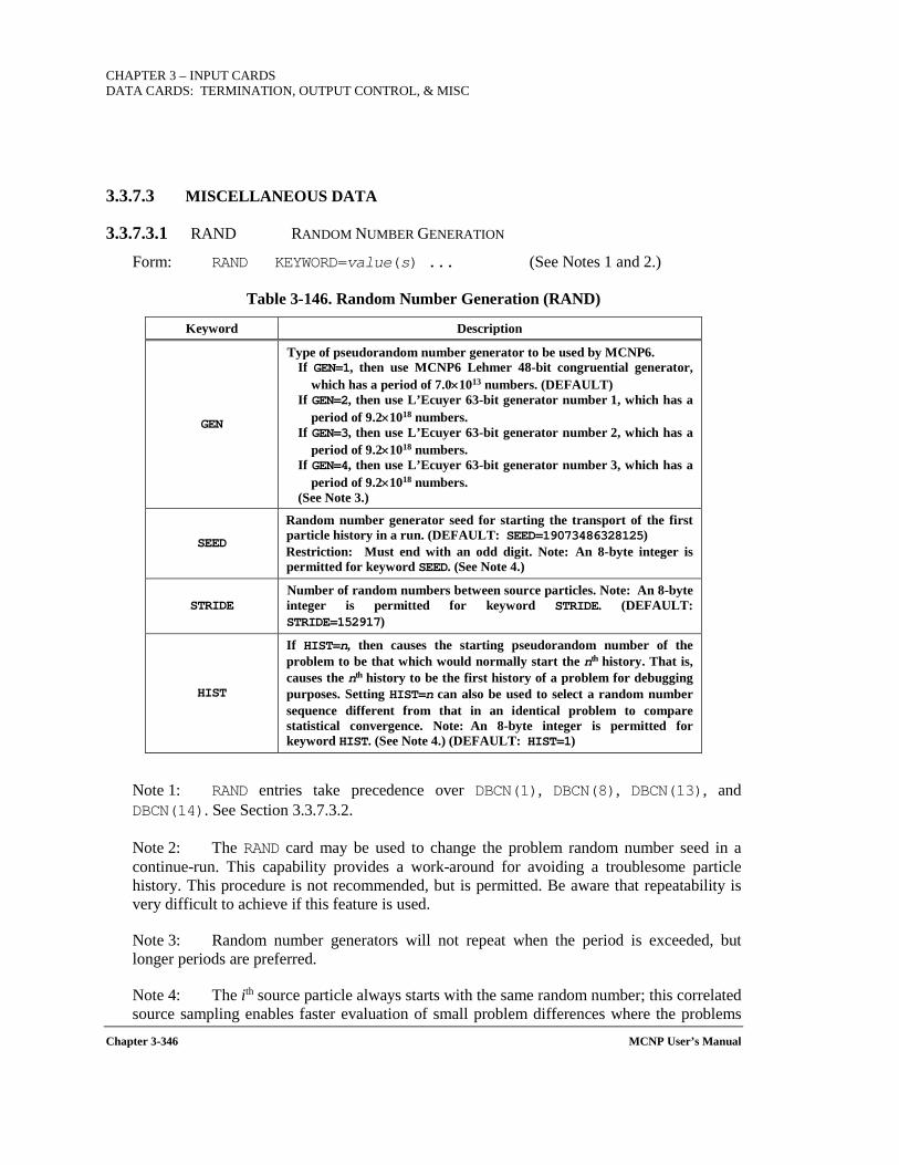
CHAPTER 3 – INPUT CARDS DATA CARDS: TERMINATION, OUTPUT CONTROL, & MISC
Chapter 3-346 MCNP User’s Manual
3.3.7.3 MISCELLANEOUS DATA
3.3.7.3.1 RAND RANDOM NUMBER GENERATION
Form: RAND KEYWORD=value(s) ... (See Notes 1 and 2.)
Table 3-146. Random Number Generation (RAND)
Keyword Description
GEN
Type of pseudorandom number generator to be used by MCNP6. If GEN=1, then use MCNP6 Lehmer 48-bit congruential generator,
which has a period of 7.0×10¹³ numbers. (DEFAULT) If GEN=2, then use L’Ecuyer 63-bit generator number 1, which has a
period of 9.2×10¹⁸ numbers. If GEN=3, then use L’Ecuyer 63-bit generator number 2, which has a
period of 9.2×10¹⁸ numbers. If GEN=4, then use L’Ecuyer 63-bit generator number 3, which has a
period of 9.2×10¹⁸ numbers. (See Note 3.)
SEED
Random number generator seed for starting the transport of the first particle history in a run. (DEFAULT: SEED=19073486328125) Restriction: Must end with an odd digit. Note: An 8-byte integer is permitted for keyword SEED. (See Note 4.)
STRIDE Number of random numbers between source particles. Note: An 8-byte integer is permitted for keyword STRIDE. (DEFAULT: STRIDE=152917)
HIST
If HIST=n, then causes the starting pseudorandom number of the problem to be that which would normally start the nth history. That is, causes the nth history to be the first history of a problem for debugging purposes. Setting HIST=n can also be used to select a random number sequence different from that in an identical problem to compare statistical convergence. Note: An 8-byte integer is permitted for keyword HIST. (See Note 4.) (DEFAULT: HIST=1)
Note 1: RAND entries take precedence over DBCN(1), DBCN(8), DBCN(13), and DBCN(14). See Section 3.3.7.3.2.
Note 2: The RAND card may be used to change the problem random number seed in a continue-run. This capability provides a work-around for avoiding a troublesome particle history. This procedure is not recommended, but is permitted. Be aware that repeatability is very difficult to achieve if this feature is used.
Note 3: Random number generators will not repeat when the period is exceeded, but longer periods are preferred.
Note 4: The ith source particle always starts with the same random number; this correlated source sampling enables faster evaluation of small problem differences where the problems
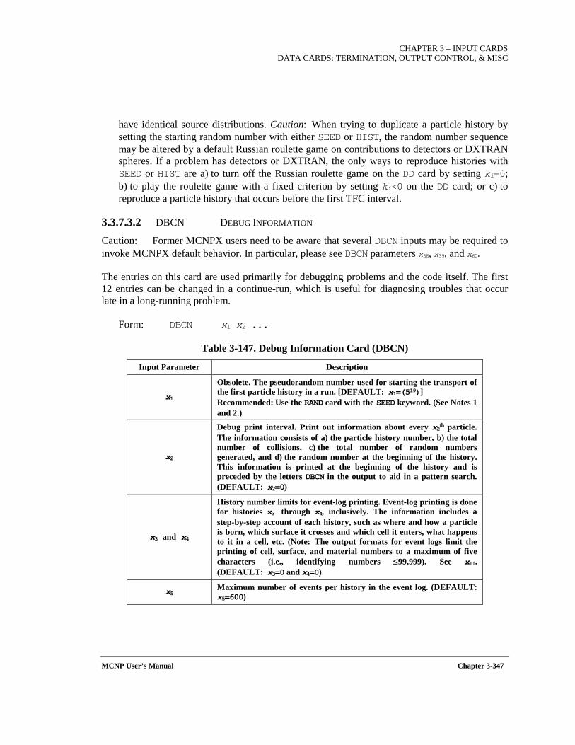
CHAPTER 3 – INPUT CARDS
DATA CARDS: TERMINATION, OUTPUT CONTROL, & MISC
MCNP User’s Manual Chapter 3-347
have identical source distributions. Caution: When trying to duplicate a particle history by setting the starting random number with either SEED or HIST, the random number sequence may be altered by a default Russian roulette game on contributions to detectors or DXTRAN spheres. If a problem has detectors or DXTRAN, the only ways to reproduce histories with SEED or HIST are a) to turn off the Russian roulette game on the DD card by setting ki=0; b) to play the roulette game with a fixed criterion by setting ki<0 on the DD card; or c) to reproduce a particle history that occurs before the first TFC interval.
3.3.7.3.2 DBCN DEBUG INFORMATION
Caution: Former MCNPX users need to be aware that several DBCN inputs may be required to invoke MCNPX default behavior. In particular, please see DBCN parameters x38, x39, and x60.
The entries on this card are used primarily for debugging problems and the code itself. The first 12 entries can be changed in a continue-run, which is useful for diagnosing troubles that occur late in a long-running problem.
Form: DBCN x1 x2 ...
Table 3-147. Debug Information Card (DBCN)
Input Parameter Description
x1
Obsolete. The pseudorandom number used for starting the transport of the first particle history in a run. [DEFAULT: x1=(519)] Recommended: Use the RAND card with the SEED keyword. (See Notes 1 and 2.)
x2
Debug print interval. Print out information about every x2th particle. The information consists of a) the particle history number, b) the total number of collisions, c) the total number of random numbers generated, and d) the random number at the beginning of the history. This information is printed at the beginning of the history and is preceded by the letters DBCN in the output to aid in a pattern search. (DEFAULT: x2=0)
x3 and x4
History number limits for event-log printing. Event-log printing is done for histories x3 through x4, inclusively. The information includes a step-by-step account of each history, such as where and how a particle is born, which surface it crosses and which cell it enters, what happens to it in a cell, etc. (Note: The output formats for event logs limit the printing of cell, surface, and material numbers to a maximum of five characters (i.e., identifying numbers ≤99,999). See x11. (DEFAULT: x3=0 and x4=0)
x5 Maximum number of events per history in the event log. (DEFAULT: x5=600)
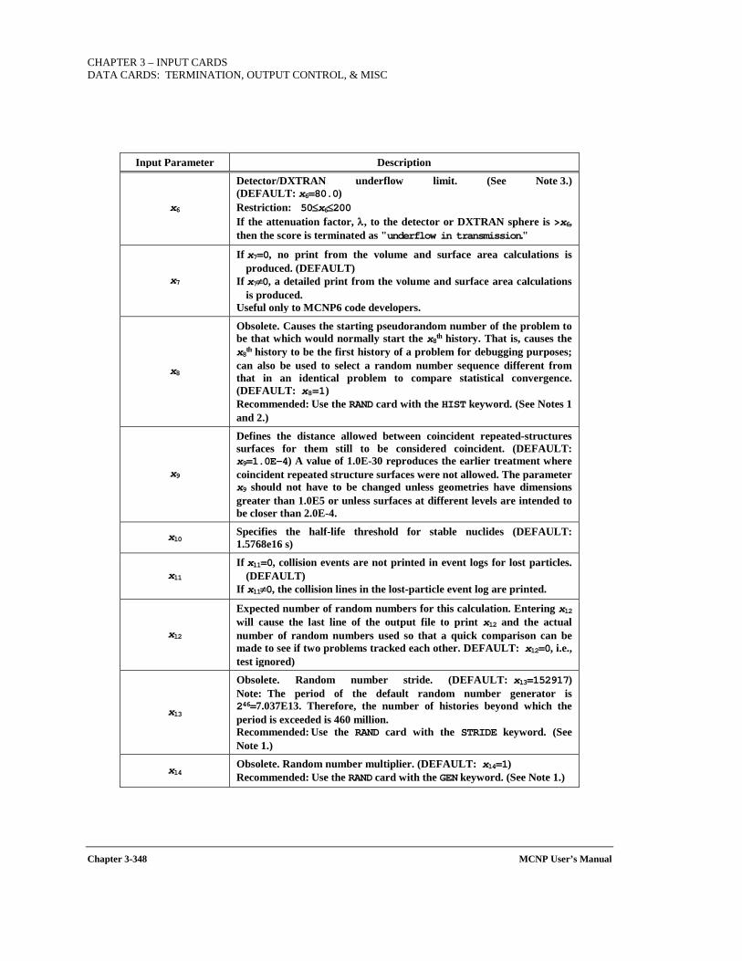
CHAPTER 3 – INPUT CARDS DATA CARDS: TERMINATION, OUTPUT CONTROL, & MISC
Chapter 3-348 MCNP User’s Manual
Input Parameter Description
x6
Detector/DXTRAN underflow limit. (See Note 3.) (DEFAULT: x6=80.0) Restriction: 50≤x6≤200 If the attenuation factor, λ, to the detector or DXTRAN sphere is >x6, then the score is terminated as "underflow in transmission."
x7
If x7=0, no print from the volume and surface area calculations is produced. (DEFAULT)
If x7≠0, a detailed print from the volume and surface area calculations is produced.
Useful only to MCNP6 code developers.
x8
Obsolete. Causes the starting pseudorandom number of the problem to be that which would normally start the x8th history. That is, causes the x8th history to be the first history of a problem for debugging purposes; can also be used to select a random number sequence different from that in an identical problem to compare statistical convergence. (DEFAULT: x8=1) Recommended: Use the RAND card with the HIST keyword. (See Notes 1 and 2.)
x9
Defines the distance allowed between coincident repeated-structures surfaces for them still to be considered coincident. (DEFAULT: x9=1.0E-4) A value of 1.0E-30 reproduces the earlier treatment where coincident repeated structure surfaces were not allowed. The parameter x9 should not have to be changed unless geometries have dimensions greater than 1.0E5 or unless surfaces at different levels are intended to be closer than 2.0E-4.
x10 Specifies the half-life threshold for stable nuclides (DEFAULT: 1.5768e16 s)
x11 If x11=0, collision events are not printed in event logs for lost particles.
(DEFAULT) If x11≠0, the collision lines in the lost-particle event log are printed.
x12
Expected number of random numbers for this calculation. Entering x12 will cause the last line of the output file to print x12 and the actual number of random numbers used so that a quick comparison can be made to see if two problems tracked each other. DEFAULT: x12=0, i.e., test ignored)
x13
Obsolete. Random number stride. (DEFAULT: x13=152917) Note: The period of the default random number generator is 246=7.037E13. Therefore, the number of histories beyond which the period is exceeded is 460 million. Recommended: Use the RAND card with the STRIDE keyword. (See Note 1.)
x14 Obsolete. Random number multiplier. (DEFAULT: x14=1) Recommended: Use the RAND card with the GEN keyword. (See Note 1.)
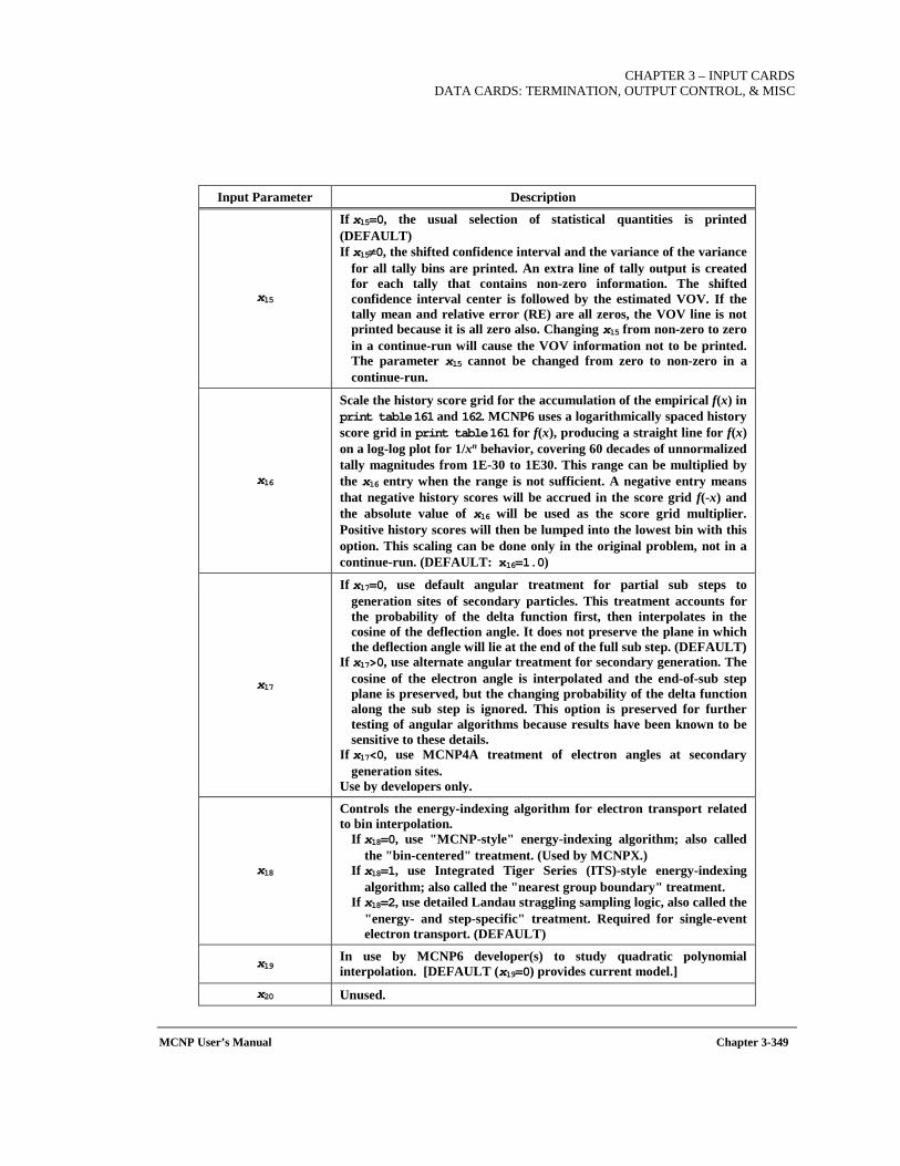
CHAPTER 3 – INPUT CARDS
DATA CARDS: TERMINATION, OUTPUT CONTROL, & MISC
MCNP User’s Manual Chapter 3-349
Input Parameter Description
x15
If x15=0, the usual selection of statistical quantities is printed (DEFAULT) If x15≠0, the shifted confidence interval and the variance of the variance
for all tally bins are printed. An extra line of tally output is created for each tally that contains non-zero information. The shifted confidence interval center is followed by the estimated VOV. If the tally mean and relative error (RE) are all zeros, the VOV line is not printed because it is all zero also. Changing x15 from non-zero to zero in a continue-run will cause the VOV information not to be printed. The parameter x15 cannot be changed from zero to non-zero in a continue-run.
x16
Scale the history score grid for the accumulation of the empirical f(x) in print table 161 and 162. MCNP6 uses a logarithmically spaced history score grid in print table 161 for f(x), producing a straight line for f(x) on a log-log plot for 1/xn behavior, covering 60 decades of unnormalized tally magnitudes from 1E-30 to 1E30. This range can be multiplied by the x16 entry when the range is not sufficient. A negative entry means that negative history scores will be accrued in the score grid f(-x) and the absolute value of x16 will be used as the score grid multiplier. Positive history scores will then be lumped into the lowest bin with this option. This scaling can be done only in the original problem, not in a continue-run. (DEFAULT: x16=1.0)
x17
If x17=0, use default angular treatment for partial sub steps to generation sites of secondary particles. This treatment accounts for the probability of the delta function first, then interpolates in the cosine of the deflection angle. It does not preserve the plane in which the deflection angle will lie at the end of the full sub step. (DEFAULT)
If x17>0, use alternate angular treatment for secondary generation. The cosine of the electron angle is interpolated and the end-of-sub step plane is preserved, but the changing probability of the delta function along the sub step is ignored. This option is preserved for further testing of angular algorithms because results have been known to be sensitive to these details.
If x17<0, use MCNP4A treatment of electron angles at secondary generation sites.
Use by developers only.
x18
Controls the energy-indexing algorithm for electron transport related to bin interpolation.
If x18=0, use "MCNP-style" energy-indexing algorithm; also called the "bin-centered" treatment. (Used by MCNPX.)
If x18=1, use Integrated Tiger Series (ITS)-style energy-indexing algorithm; also called the "nearest group boundary" treatment.
If x18=2, use detailed Landau straggling sampling logic, also called the "energy- and step-specific" treatment. Required for single-event electron transport. (DEFAULT)
x19 In use by MCNP6 developer(s) to study quadratic polynomial interpolation. [DEFAULT (x19=0) provides current model.]
x20 Unused.
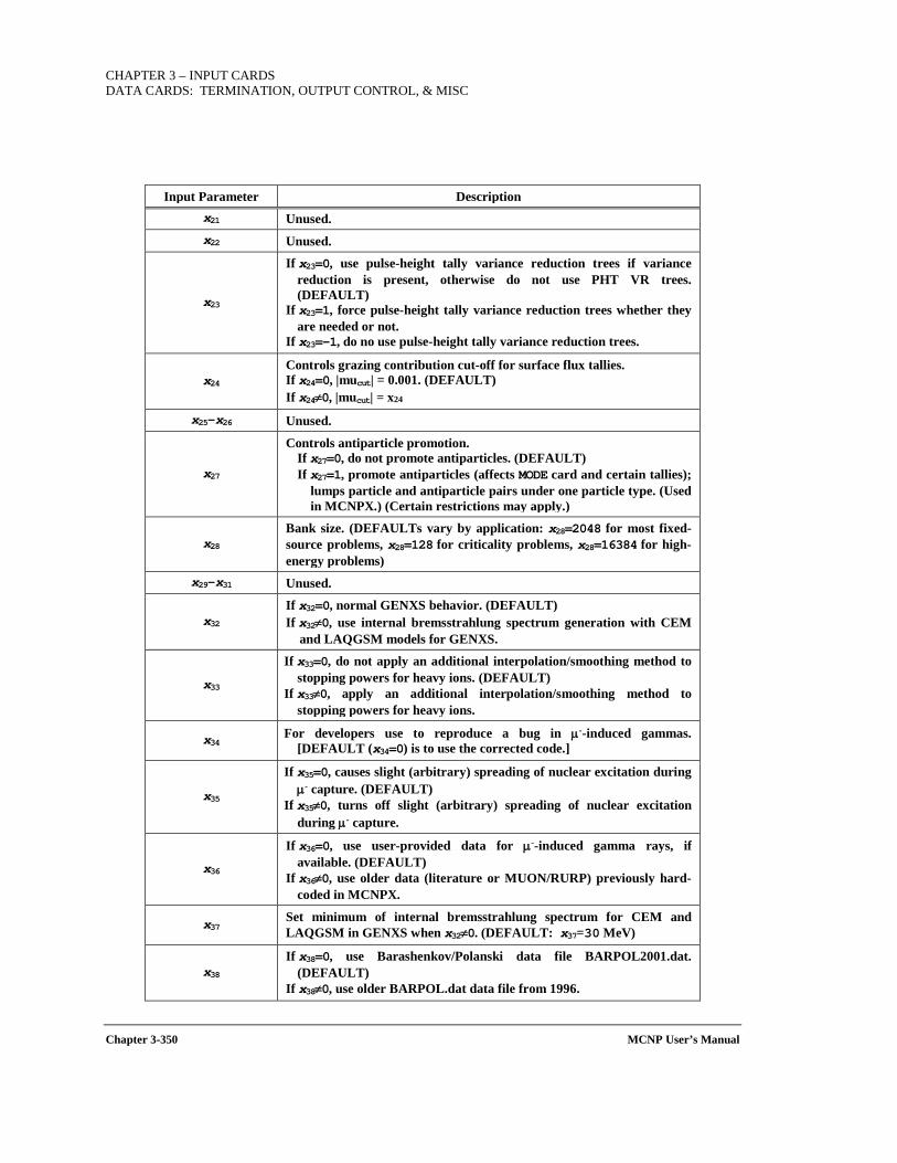
CHAPTER 3 – INPUT CARDS DATA CARDS: TERMINATION, OUTPUT CONTROL, & MISC
Chapter 3-350 MCNP User’s Manual
Input Parameter Description x21 Unused. x22 Unused.
x23
If x23=0, use pulse-height tally variance reduction trees if variance reduction is present, otherwise do not use PHT VR trees. (DEFAULT)
If x23=1, force pulse-height tally variance reduction trees whether they are needed or not.
If x23=-1, do no use pulse-height tally variance reduction trees.
x24 Controls grazing contribution cut-off for surface flux tallies. If x24=0, |mucut| = 0.001. (DEFAULT) If x24≠0, |mucut| = x24
x25–x26 Unused.
x27
Controls antiparticle promotion. If x27=0, do not promote antiparticles. (DEFAULT) If x27=1, promote antiparticles (affects MODE card and certain tallies);
lumps particle and antiparticle pairs under one particle type. (Used in MCNPX.) (Certain restrictions may apply.)
x28 Bank size. (DEFAULTs vary by application: x28=2048 for most fixed-source problems, x28=128 for criticality problems, x28=16384 for high-energy problems)
x29–x31 Unused.
x32 If x32=0, normal GENXS behavior. (DEFAULT) If x32≠0, use internal bremsstrahlung spectrum generation with CEM
and LAQGSM models for GENXS.
x33
If x33=0, do not apply an additional interpolation/smoothing method to stopping powers for heavy ions. (DEFAULT)
If x33≠0, apply an additional interpolation/smoothing method to stopping powers for heavy ions.
x34 For developers use to reproduce a bug in µ--induced gammas. [DEFAULT (x34=0) is to use the corrected code.]
x35
If x35=0, causes slight (arbitrary) spreading of nuclear excitation during µ- capture. (DEFAULT)
If x35≠0, turns off slight (arbitrary) spreading of nuclear excitation during µ- capture.
x36
If x36=0, use user-provided data for µ--induced gamma rays, if available. (DEFAULT)
If x36≠0, use older data (literature or MUON/RURP) previously hard-coded in MCNPX.
x37 Set minimum of internal bremsstrahlung spectrum for CEM and LAQGSM in GENXS when x32≠0. (DEFAULT: x37=30 MeV)
x38 If x38=0, use Barashenkov/Polanski data file BARPOL2001.dat.
(DEFAULT) If x38≠0, use older BARPOL.dat data file from 1996.
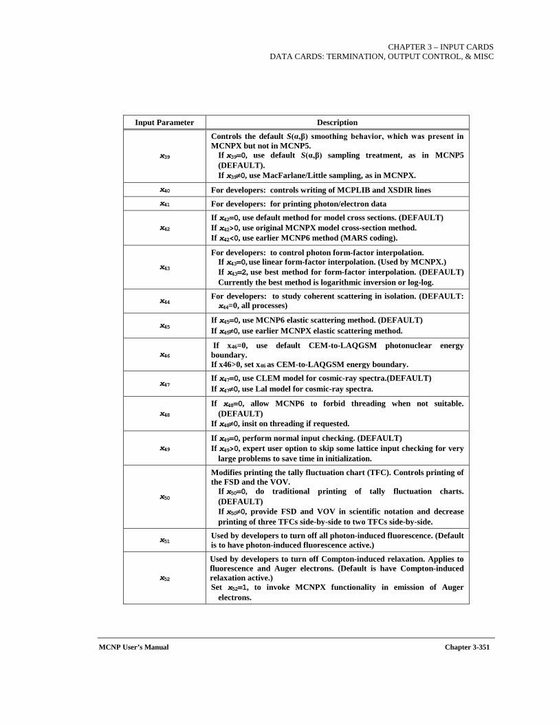
CHAPTER 3 – INPUT CARDS
DATA CARDS: TERMINATION, OUTPUT CONTROL, & MISC
MCNP User’s Manual Chapter 3-351
Input Parameter Description
x39
Controls the default S(α,β) smoothing behavior, which was present in MCNPX but not in MCNP5.
If x39=0, use default S(α,β) sampling treatment, as in MCNP5 (DEFAULT). If x39≠0, use MacFarlane/Little sampling, as in MCNPX.
x40 For developers: controls writing of MCPLIB and XSDIR lines x41 For developers: for printing photon/electron data
x42 If x42=0, use default method for model cross sections. (DEFAULT) If x42>0, use original MCNPX model cross-section method. If x42<0, use earlier MCNP6 method (MARS coding).
x43
For developers: to control photon form-factor interpolation. If x43=0, use linear form-factor interpolation. (Used by MCNPX.) If x43=2, use best method for form-factor interpolation. (DEFAULT) Currently the best method is logarithmic inversion or log-log.
x44 For developers: to study coherent scattering in isolation. (DEFAULT: x44=0, all processes)
x45 If x45=0, use MCNP6 elastic scattering method. (DEFAULT) If x45≠0, use earlier MCNPX elastic scattering method.
x46 If x46=0, use default CEM-to-LAQGSM photonuclear energy boundary. If x46>0, set x46 as CEM-to-LAQGSM energy boundary.
x47 If x47=0, use CLEM model for cosmic-ray spectra.(DEFAULT) If x47≠0, use Lal model for cosmic-ray spectra.
x48 If x48=0, allow MCNP6 to forbid threading when not suitable.
(DEFAULT) If x48≠0, insit on threading if requested.
x49 If x49=0, perform normal input checking. (DEFAULT) If x49>0, expert user option to skip some lattice input checking for very
large problems to save time in initialization.
x50
Modifies printing the tally fluctuation chart (TFC). Controls printing of the FSD and the VOV.
If x50=0, do traditional printing of tally fluctuation charts. (DEFAULT) If x50≠0, provide FSD and VOV in scientific notation and decrease printing of three TFCs side-by-side to two TFCs side-by-side.
x51 Used by developers to turn off all photon-induced fluorescence. (Default is to have photon-induced fluorescence active.)
x52
Used by developers to turn off Compton-induced relaxation. Applies to fluorescence and Auger electrons. (Default is have Compton-induced relaxation active.) Set x52=1, to invoke MCNPX functionality in emission of Auger
electrons.
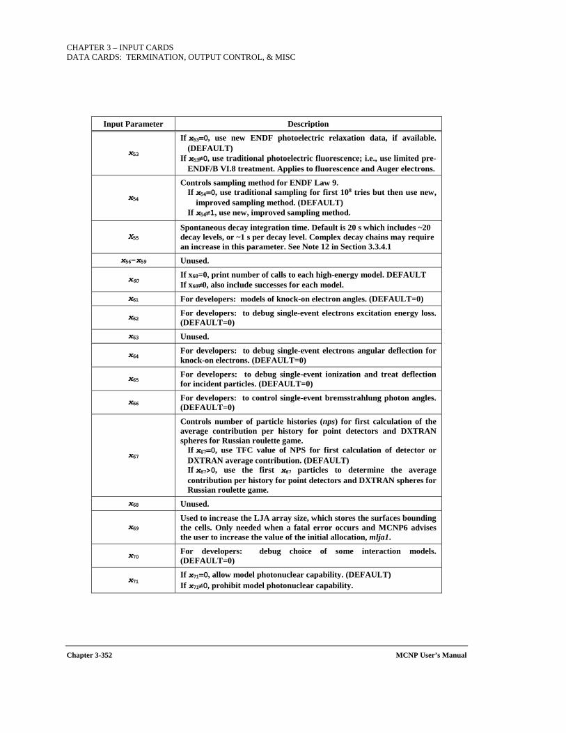
CHAPTER 3 – INPUT CARDS DATA CARDS: TERMINATION, OUTPUT CONTROL, & MISC
Chapter 3-352 MCNP User’s Manual
Input Parameter Description
x53
If x53=0, use new ENDF photoelectric relaxation data, if available. (DEFAULT)
If x53≠0, use traditional photoelectric fluorescence; i.e., use limited pre-ENDF/B VI.8 treatment. Applies to fluorescence and Auger electrons.
x54
Controls sampling method for ENDF Law 9. If x54=0, use traditional sampling for first 108 tries but then use new,
improved sampling method. (DEFAULT) If x54≠1, use new, improved sampling method.
X55 Spontaneous decay integration time. Default is 20 s which includes ~20 decay levels, or ~1 s per decay level. Complex decay chains may require an increase in this parameter. See Note 12 in Section 3.3.4.1
x56–x59 Unused.
x60 If x60=0, print number of calls to each high-energy model. DEFAULT If x60≠0, also include successes for each model.
x61 For developers: models of knock-on electron angles. (DEFAULT=0)
x62 For developers: to debug single-event electrons excitation energy loss. (DEFAULT=0)
x63 Unused.
x64 For developers: to debug single-event electrons angular deflection for knock-on electrons. (DEFAULT=0)
x65 For developers: to debug single-event ionization and treat deflection for incident particles. (DEFAULT=0)
x66 For developers: to control single-event bremsstrahlung photon angles. (DEFAULT=0)
x67
Controls number of particle histories (nps) for first calculation of the average contribution per history for point detectors and DXTRAN spheres for Russian roulette game.
If x67=0, use TFC value of NPS for first calculation of detector or DXTRAN average contribution. (DEFAULT) If x67>0, use the first x67 particles to determine the average contribution per history for point detectors and DXTRAN spheres for Russian roulette game.
x68 Unused.
x69 Used to increase the LJA array size, which stores the surfaces bounding the cells. Only needed when a fatal error occurs and MCNP6 advises the user to increase the value of the initial allocation, mlja1.
x70 For developers: debug choice of some interaction models. (DEFAULT=0)
x71 If x71=0, allow model photonuclear capability. (DEFAULT) If x71≠0, prohibit model photonuclear capability.
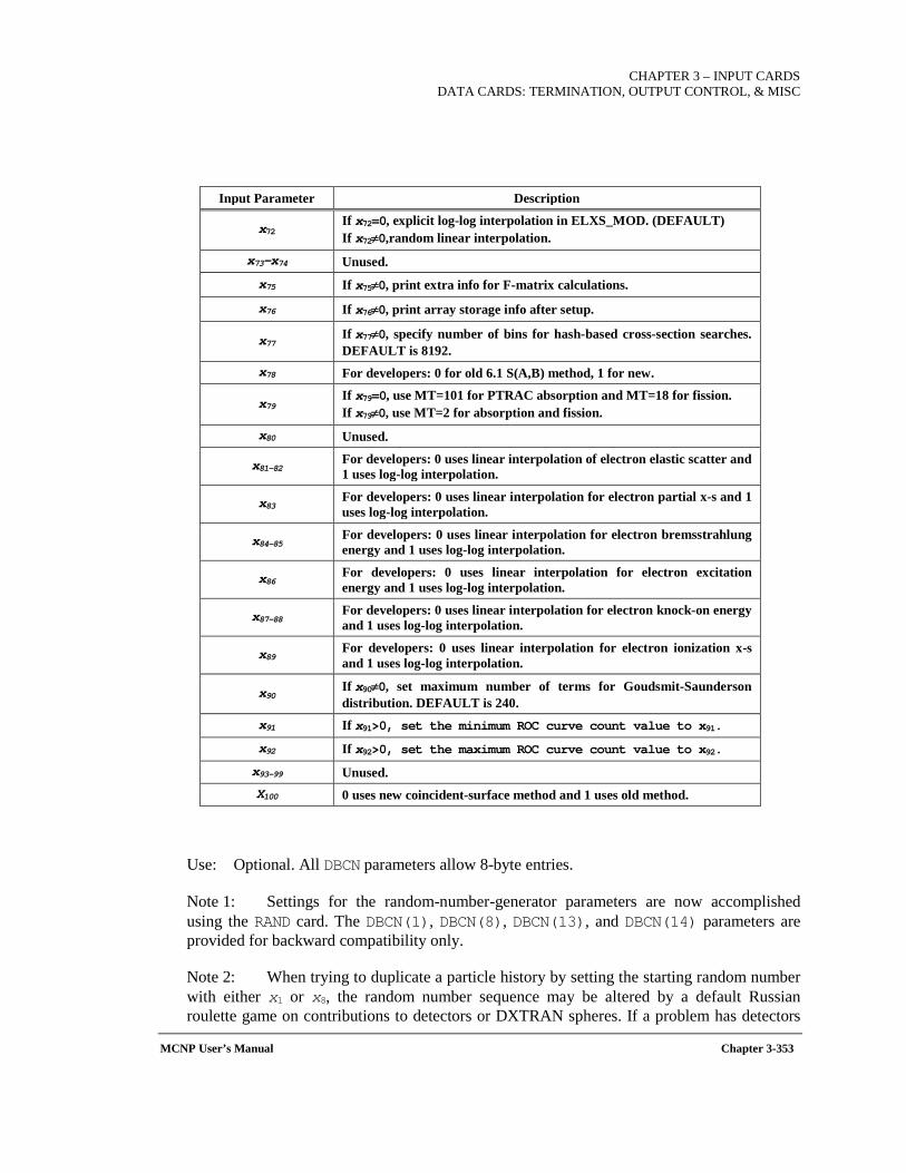
CHAPTER 3 – INPUT CARDS
DATA CARDS: TERMINATION, OUTPUT CONTROL, & MISC
MCNP User’s Manual Chapter 3-353
Input Parameter Description
x72 If x72=0, explicit log-log interpolation in ELXS_MOD. (DEFAULT) If x72≠0,random linear interpolation.
x73-x74 Unused. x75 If x75≠0, print extra info for F-matrix calculations.
x76 If x76≠0, print array storage info after setup.
x77 If x77≠0, specify number of bins for hash-based cross-section searches. DEFAULT is 8192.
x78 For developers: 0 for old 6.1 S(A,B) method, 1 for new.
x79 If x79=0, use MT=101 for PTRAC absorption and MT=18 for fission. If x79≠0, use MT=2 for absorption and fission.
x80 Unused.
x81-82 For developers: 0 uses linear interpolation of electron elastic scatter and 1 uses log-log interpolation.
x83 For developers: 0 uses linear interpolation for electron partial x-s and 1 uses log-log interpolation.
x84-85 For developers: 0 uses linear interpolation for electron bremsstrahlung energy and 1 uses log-log interpolation.
x86 For developers: 0 uses linear interpolation for electron excitation energy and 1 uses log-log interpolation.
x87-88 For developers: 0 uses linear interpolation for electron knock-on energy and 1 uses log-log interpolation.
x89 For developers: 0 uses linear interpolation for electron ionization x-s and 1 uses log-log interpolation.
x90 If x90≠0, set maximum number of terms for Goudsmit-Saunderson distribution. DEFAULT is 240.
x91 If x91>0, set the minimum ROC curve count value to x91.
x92 If x92>0, set the maximum ROC curve count value to x92.
x93-99 Unused. X100 0 uses new coincident-surface method and 1 uses old method.
Use: Optional. All DBCN parameters allow 8-byte entries.
Note 1: Settings for the random-number-generator parameters are now accomplished using the RAND card. The DBCN(1), DBCN(8), DBCN(13), and DBCN(14) parameters are provided for backward compatibility only.
Note 2: When trying to duplicate a particle history by setting the starting random number with either x1 or x8, the random number sequence may be altered by a default Russian roulette game on contributions to detectors or DXTRAN spheres. If a problem has detectors
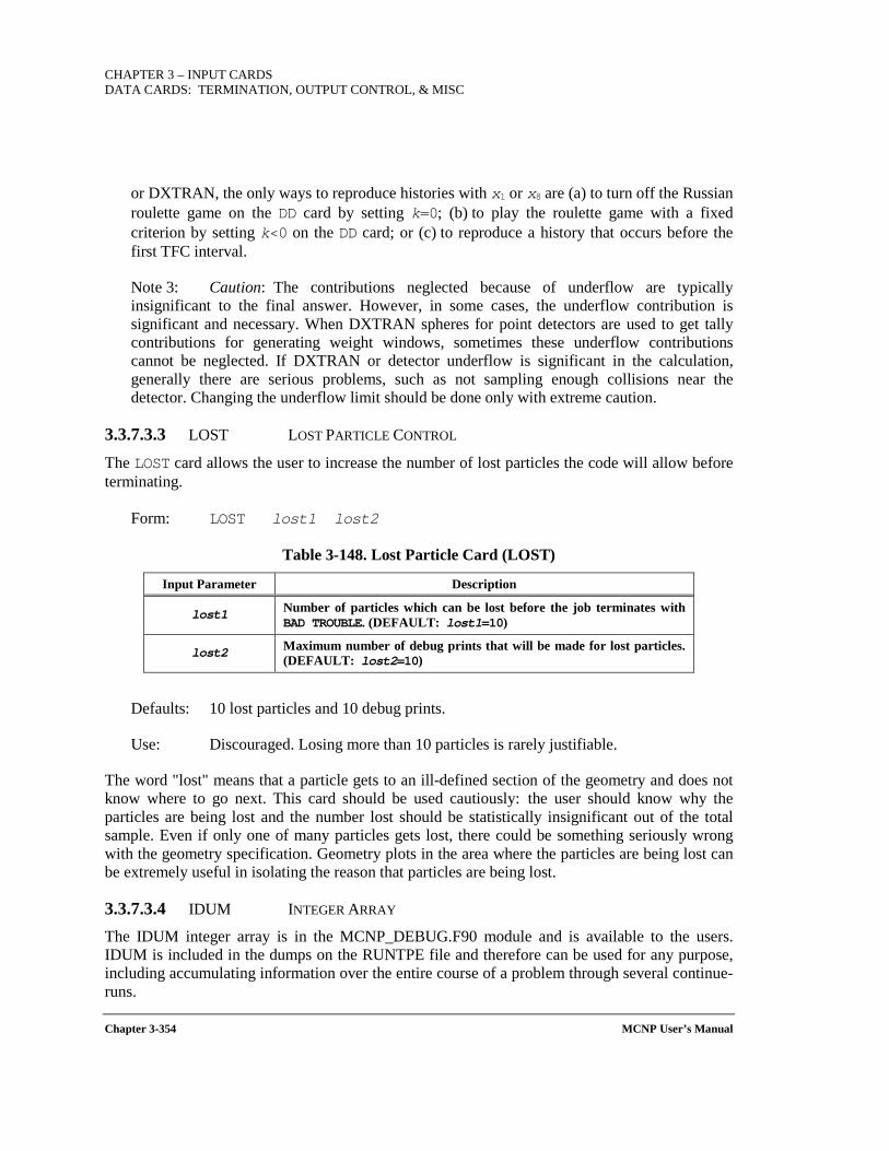
CHAPTER 3 – INPUT CARDS DATA CARDS: TERMINATION, OUTPUT CONTROL, & MISC
Chapter 3-354 MCNP User’s Manual
or DXTRAN, the only ways to reproduce histories with x1 or x8 are (a) to turn off the Russian roulette game on the DD card by setting k=0; (b) to play the roulette game with a fixed criterion by setting k<0 on the DD card; or (c) to reproduce a history that occurs before the first TFC interval.
Note 3: Caution: The contributions neglected because of underflow are typically insignificant to the final answer. However, in some cases, the underflow contribution is significant and necessary. When DXTRAN spheres for point detectors are used to get tally contributions for generating weight windows, sometimes these underflow contributions cannot be neglected. If DXTRAN or detector underflow is significant in the calculation, generally there are serious problems, such as not sampling enough collisions near the detector. Changing the underflow limit should be done only with extreme caution.
3.3.7.3.3 LOST LOST PARTICLE CONTROL
The LOST card allows the user to increase the number of lost particles the code will allow before terminating.
Form: LOST lost1 lost2
Table 3-148. Lost Particle Card (LOST)
Input Parameter Description
lost1 Number of particles which can be lost before the job terminates with BAD TROUBLE. (DEFAULT: lost1=10)
lost2 Maximum number of debug prints that will be made for lost particles. (DEFAULT: lost2=10)
Defaults: 10 lost particles and 10 debug prints.
Use: Discouraged. Losing more than 10 particles is rarely justifiable.
The word "lost" means that a particle gets to an ill-defined section of the geometry and does not know where to go next. This card should be used cautiously: the user should know why the particles are being lost and the number lost should be statistically insignificant out of the total sample. Even if only one of many particles gets lost, there could be something seriously wrong with the geometry specification. Geometry plots in the area where the particles are being lost can be extremely useful in isolating the reason that particles are being lost.
3.3.7.3.4 IDUM INTEGER ARRAY
The IDUM integer array is in the MCNP_DEBUG.F90 module and is available to the users. IDUM is included in the dumps on the RUNTPE file and therefore can be used for any purpose, including accumulating information over the entire course of a problem through several continue-runs.

CHAPTER 3 – INPUT CARDS
DATA CARDS: TERMINATION, OUTPUT CONTROL, & MISC
MCNP User’s Manual Chapter 3-355
Form: IDUM i1 ... in
where 1≤n≤2000 and ii is an integer.
Default: All array values zero.
Use: Useful only in user-modified versions of MCNP6.
Note: Up to 2000 entries can be provided to fill the IDUM array with integer numbers. If floating-point numbers are entered, they will be truncated and converted to integers.
3.3.7.3.5 RDUM FLOATING-POINT ARRAY
The RDUM floating-point array is in the MCNP_DEBUG.F90 module and is available to the users. RDUM is included in the dumps on the RUNTPE file and therefore can be used for any purpose, including accumulating information over the entire course of a problem through several continue-runs.
Form: RDUM r1 ... rn
where 1≤n≤2000 and ri is a real number.
Default: All array values zero.
Use: Useful only in user-modified versions of MCNP6.
Note: Up to 2000 entries can be provided to fill the RDUM array with floating-point (real) numbers.
3.3.7.3.6 ZA, ZB, ZC, AND ZD DEVELOPERS CARD PLACEHOLDERS
The ZA, ZB, ZC, and ZD cards are made available to advanced user-developers who wish to construct their own input cards in MCNP6. Similar to the use of IDUM and RDUM, source code that is modified by users to create a modified version of MCNP6 no longer carries the extensive validation and verification the original LANL-created source and executables do. Users must perform their own verification and validation to ensure their modifications have not had adverse effects on existing capabilities.
3.3.7.3.7 FILES FILE CREATION
Form: FILES unit_no. filename access form record_length ...
(See Note 1.)
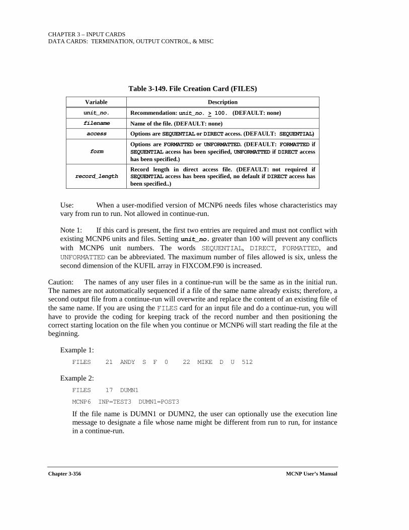
CHAPTER 3 – INPUT CARDS DATA CARDS: TERMINATION, OUTPUT CONTROL, & MISC
Chapter 3-356 MCNP User’s Manual
Table 3-149. File Creation Card (FILES)
Variable Description
unit_no. Recommendation: unit_no. > 100. (DEFAULT: none)
filename Name of the file. (DEFAULT: none) access Options are SEQUENTIAL or DIRECT access. (DEFAULT: SEQUENTIAL)
form Options are FORMATTED or UNFORMATTED. (DEFAULT: FORMATTED if SEQUENTIAL access has been specified, UNFORMATTED if DIRECT access has been specified.)
record_length Record length in direct access file. (DEFAULT: not required if SEQUENTIAL access has been specified, no default if DIRECT access has been specified..)
Use: When a user-modified version of MCNP6 needs files whose characteristics may vary from run to run. Not allowed in continue-run.
Note 1: If this card is present, the first two entries are required and must not conflict with existing MCNP6 units and files. Setting unit_no. greater than 100 will prevent any conflicts with MCNP6 unit numbers. The words SEQUENTIAL, DIRECT, FORMATTED, and UNFORMATTED can be abbreviated. The maximum number of files allowed is six, unless the second dimension of the KUFIL array in FIXCOM.F90 is increased.
Caution: The names of any user files in a continue-run will be the same as in the initial run. The names are not automatically sequenced if a file of the same name already exists; therefore, a second output file from a continue-run will overwrite and replace the content of an existing file of the same name. If you are using the FILES card for an input file and do a continue-run, you will have to provide the coding for keeping track of the record number and then positioning the correct starting location on the file when you continue or MCNP6 will start reading the file at the beginning.
Example 1: FILES 21 ANDY S F 0 22 MIKE D U 512
Example 2: FILES 17 DUMN1
MCNP6 INP=TEST3 DUMN1=POST3
If the file name is DUMN1 or DUMN2, the user can optionally use the execution line message to designate a file whose name might be different from run to run, for instance in a continue-run.
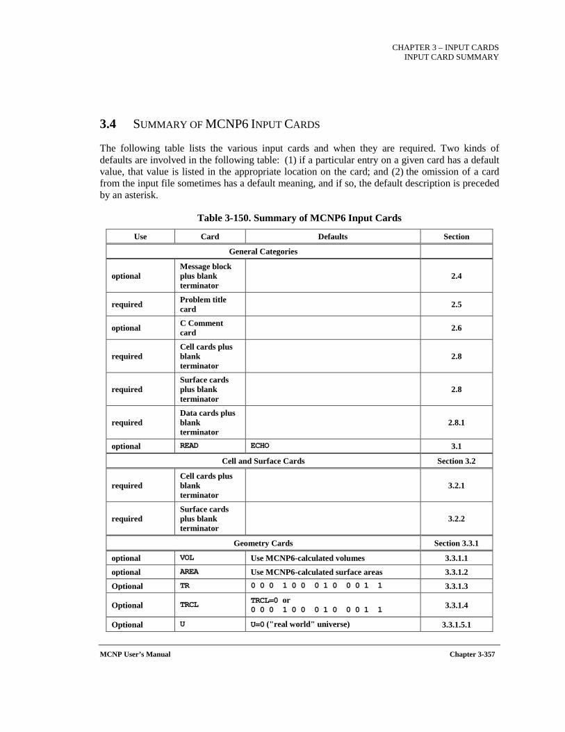
CHAPTER 3 – INPUT CARDS
INPUT CARD SUMMARY
MCNP User’s Manual Chapter 3-357
3.4 SUMMARY OF MCNP6 INPUT CARDS
The following table lists the various input cards and when they are required. Two kinds of defaults are involved in the following table: (1) if a particular entry on a given card has a default value, that value is listed in the appropriate location on the card; and (2) the omission of a card from the input file sometimes has a default meaning, and if so, the default description is preceded by an asterisk.
Table 3-150. Summary of MCNP6 Input Cards
Use Card Defaults Section
General Categories
optional Message block plus blank terminator
2.4
required Problem title card 2.5
optional C Comment card 2.6
required Cell cards plus blank terminator
2.8
required Surface cards plus blank terminator
2.8
required Data cards plus blank terminator
2.8.1
optional READ ECHO 3.1
Cell and Surface Cards Section 3.2
required Cell cards plus blank terminator
3.2.1
required Surface cards plus blank terminator
3.2.2
Geometry Cards Section 3.3.1
optional VOL Use MCNP6-calculated volumes 3.3.1.1
optional AREA Use MCNP6-calculated surface areas 3.3.1.2
Optional TR 0 0 0 1 0 0 0 1 0 0 0 1 1 3.3.1.3
Optional TRCL TRCL=0 or 0 0 0 1 0 0 0 1 0 0 0 1 1 3.3.1.4
Optional U U=0 ("real world" universe) 3.3.1.5.1
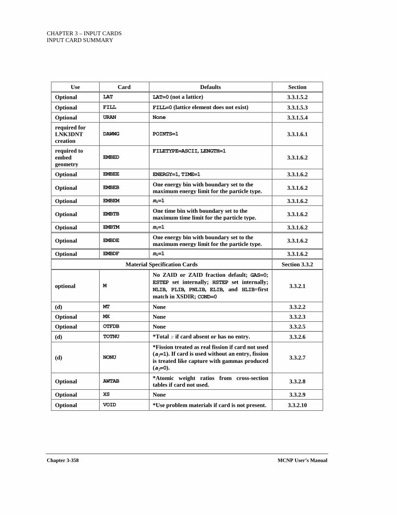
CHAPTER 3 – INPUT CARDS INPUT CARD SUMMARY
Chapter 3-358 MCNP User’s Manual
Use Card Defaults Section
Optional LAT LAT=0 (not a lattice) 3.3.1.5.2
Optional FILL FILL=0 (lattice element does not exist) 3.3.1.5.3
Optional URAN None 3.3.1.5.4
required for LNK3DNT creation
DAWWG POINTS=1 3.3.1.6.1
required to embed geometry
EMBED FILETYPE=ASCII, LENGTH=1
3.3.1.6.2
Optional EMBEE ENERGY=1, TIME=1 3.3.1.6.2
Optional EMBEB One energy bin with boundary set to the maximum energy limit for the particle type. 3.3.1.6.2
Optional EMBEM mi=1 3.3.1.6.2
Optional EMBTB One time bin with boundary set to the maximum time limit for the particle type. 3.3.1.6.2
Optional EMBTM mi=1 3.3.1.6.2
Optional EMBDE One energy bin with boundary set to the maximum energy limit for the particle type. 3.3.1.6.2
Optional EMBDF mi=1 3.3.1.6.2
Material Specification Cards Section 3.3.2
optional M
No ZAID or ZAID fraction default; GAS=0; ESTEP set internally; HSTEP set internally; NLIB, PLIB, PNLIB, ELIB, and HLIB=first match in XSDIR; COND=0
3.3.2.1
(d) MT None 3.3.2.2
Optional MX None 3.3.2.3
Optional OTFDB None 3.3.2.5
(d) TOTNU *Total if card absent or has no entry. 3.3.2.6
(d) NONU
*Fission treated as real fission if card not used (aj=1). If card is used without an entry, fission is treated like capture with gammas produced (aj=0).
3.3.2.7
Optional AWTAB *Atomic weight ratios from cross-section tables if card not used. 3.3.2.8
Optional XS None 3.3.2.9
Optional VOID *Use problem materials if card is not present. 3.3.2.10
ν
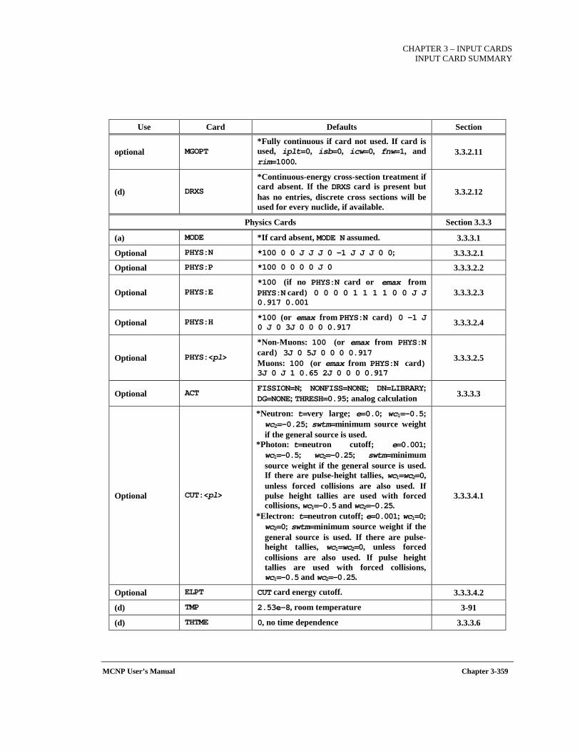
CHAPTER 3 – INPUT CARDS
INPUT CARD SUMMARY
MCNP User’s Manual Chapter 3-359
Use Card Defaults Section
optional MGOPT *Fully continuous if card not used. If card is used, iplt=0, isb=0, icw=0, fnw=1, and rim=1000.
3.3.2.11
(d) DRXS
*Continuous-energy cross-section treatment if card absent. If the DRXS card is present but has no entries, discrete cross sections will be used for every nuclide, if available.
3.3.2.12
Physics Cards Section 3.3.3
(a) MODE *If card absent, MODE N assumed. 3.3.3.1
Optional PHYS:N *100 0 0 J J J 0 -1 J J J 0 0; 3.3.3.2.1
Optional PHYS:P *100 0 0 0 0 J 0 3.3.3.2.2
Optional PHYS:E *100 (if no PHYS:N card or emax from PHYS:N card) 0 0 0 0 1 1 1 1 0 0 J J 0.917 0.001
3.3.3.2.3
Optional PHYS:H *100 (or emax from PHYS:N card) 0 -1 J 0 J 0 3J 0 0 0 0.917 3.3.3.2.4
Optional PHYS:<pl>
*Non-Muons: 100 (or emax from PHYS:N card) 3J 0 5J 0 0 0 0.917 Muons: 100 (or emax from PHYS:N card) 3J 0 J 1 0.65 2J 0 0 0 0.917
3.3.3.2.5
Optional ACT FISSION=N; NONFISS=NONE; DN=LIBRARY; DG=NONE; THRESH=0.95; analog calculation 3.3.3.3
Optional CUT:<pl>
*Neutron: t=very large; e=0.0; wc1=-0.5; wc2=-0.25; swtm=minimum source weight if the general source is used.
*Photon: t=neutron cutoff; e=0.001; wc1=-0.5; wc2=-0.25; swtm=minimum source weight if the general source is used. If there are pulse-height tallies, wc1=wc2=0, unless forced collisions are also used. If pulse height tallies are used with forced collisions, wc1=-0.5 and wc2=-0.25.
*Electron: t=neutron cutoff; e=0.001; wc1=0; wc2=0; swtm=minimum source weight if the general source is used. If there are pulse-height tallies, wc1=wc2=0, unless forced collisions are also used. If pulse height tallies are used with forced collisions, wc1=-0.5 and wc2=-0.25.
3.3.3.4.1
Optional ELPT CUT card energy cutoff. 3.3.3.4.2
(d) TMP 2.53e-8, room temperature 3-91
(d) THTME 0, no time dependence 3.3.3.6
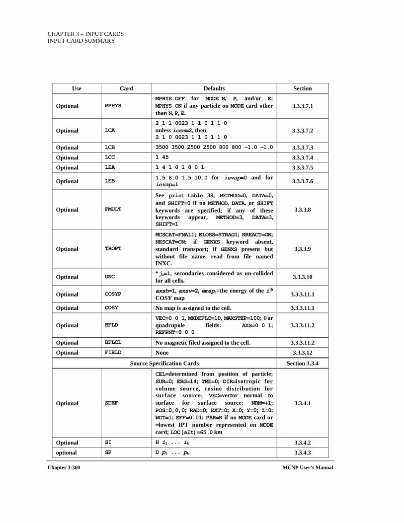
CHAPTER 3 – INPUT CARDS INPUT CARD SUMMARY
Chapter 3-360 MCNP User’s Manual
Use Card Defaults Section
Optional MPHYS MPHYS OFF for MODE N, P, and/or E; MPHYS ON if any particle on MODE card other than N, P, E.
3.3.3.7.1
Optional LCA 2 1 1 0023 1 1 0 1 1 0 unless icem=2, then 2 1 0 0023 1 1 0 1 1 0
3.3.3.7.2
Optional LCB 3500 3500 2500 2500 800 800 -1.0 -1.0 3.3.3.7.3
Optional LCC 1 45 3.3.3.7.4
Optional LEA 1 4 1 0 1 0 0 1 3.3.3.7.5
Optional LEB 1.5 8.0 1.5 10.0 for ievap=0 and for ievap=1 3.3.3.7.6
Optional FMULT
See print table 38; METHOD=0, DATA=0, and SHIFT=0 if no METHOD, DATA, or SHIFT keywords are specified; if any of these keywords appear, METHOD=3, DATA=3, SHIFT=1
3.3.3.8
Optional TROPT
MCSCAT=FNAL1; ELOSS=STRAG1; NREACT=ON; NESCAT=ON; if GENXS keyword absent, standard transport; if GENXS present but without file name, read from file named INXC.
3.3.3.9
Optional UNC *ji=1, secondaries considered as un-collided for all cells. 3.3.3.10
Optional COSYP axsh=1, axsv=2, emapi=the energy of the ith COSY map 3.3.3.11.1
Optional COSY No map is assigned to the cell. 3.3.3.11.1
Optional BFLD VEC=0 0 1, MXDEFLC=10, MAXSTEP=100; For quadrupole fields: AXS=0 0 1; REFPNT=0 0 0
3.3.3.11.2
Optional BFLCL No magnetic filed assigned to the cell. 3.3.3.11.2
Optional FIELD None 3.3.3.12
Source Specification Cards Section 3.3.4
Optional SDEF
CEL=determined from position of particle; SUR=0; ERG=14; TME=0; DIR=isotropic for volume source, cosine distribution for surface source; VEC=vector normal to surface for surface source; NRM=+1; POS=0,0,0; RAD=0; EXT=0; X=0; Y=0; Z=0; WGT=1; EFF=0.01; PAR=N if no MODE card or =lowest IPT number represented on MODE card; LOC(alt)=65.0 km
3.3.4.1
Optional SI H i1 ... ik 3.3.4.2
optional SP D p1 ... pk 3.3.4.3
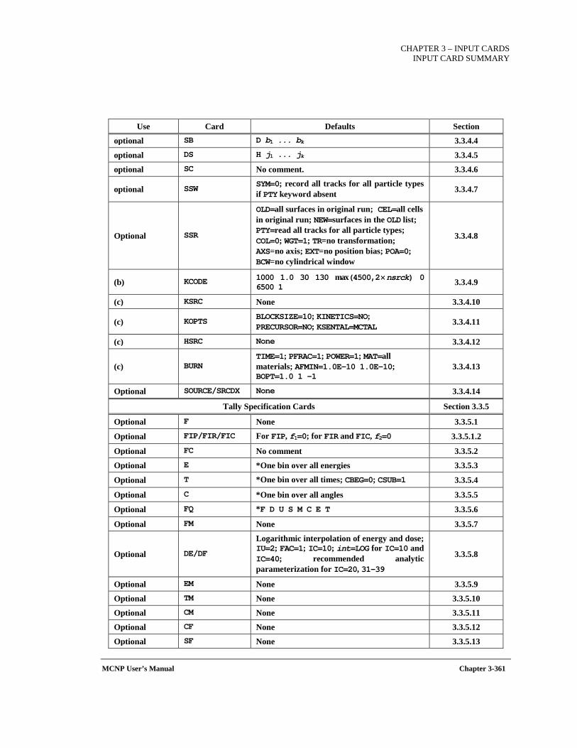
CHAPTER 3 – INPUT CARDS
INPUT CARD SUMMARY
MCNP User’s Manual Chapter 3-361
Use Card Defaults Section
optional SB D b1 ... bk 3.3.4.4
optional DS H j1 ... jk 3.3.4.5
optional SC No comment. 3.3.4.6
optional SSW SYM=0; record all tracks for all particle types if PTY keyword absent 3.3.4.7
Optional SSR
OLD=all surfaces in original run; CEL=all cells in original run; NEW=surfaces in the OLD list; PTY=read all tracks for all particle types; COL=0; WGT=1; TR=no transformation; AXS=no axis; EXT=no position bias; POA=0; BCW=no cylindrical window
3.3.4.8
(b) KCODE 1000 1.0 30 130 max(4500,2 × nsrck) 0 6500 1 3.3.4.9
(c) KSRC None 3.3.4.10
(c) KOPTS BLOCKSIZE=10; KINETICS=NO; PRECURSOR=NO; KSENTAL=MCTAL 3.3.4.11
(c) HSRC None 3.3.4.12
(c) BURN TIME=1; PFRAC=1; POWER=1; MAT=all materials; AFMIN=1.0E-10 1.0E-10; BOPT=1.0 1 -1
3.3.4.13
Optional SOURCE/SRCDX None 3.3.4.14
Tally Specification Cards Section 3.3.5
Optional F None 3.3.5.1
Optional FIP/FIR/FIC For FIP, f1=0; for FIR and FIC, f2=0 3.3.5.1.2
Optional FC No comment 3.3.5.2
Optional E *One bin over all energies 3.3.5.3
Optional T *One bin over all times; CBEG=0; CSUB=1 3.3.5.4
Optional C *One bin over all angles 3.3.5.5
Optional FQ *F D U S M C E T 3.3.5.6
Optional FM None 3.3.5.7
Optional DE/DF
Logarithmic interpolation of energy and dose; IU=2; FAC=1; IC=10; int=LOG for IC=10 and IC=40; recommended analytic parameterization for IC=20, 31–39
3.3.5.8
Optional EM None 3.3.5.9
Optional TM None 3.3.5.10
Optional CM None 3.3.5.11
Optional CF None 3.3.5.12
Optional SF None 3.3.5.13
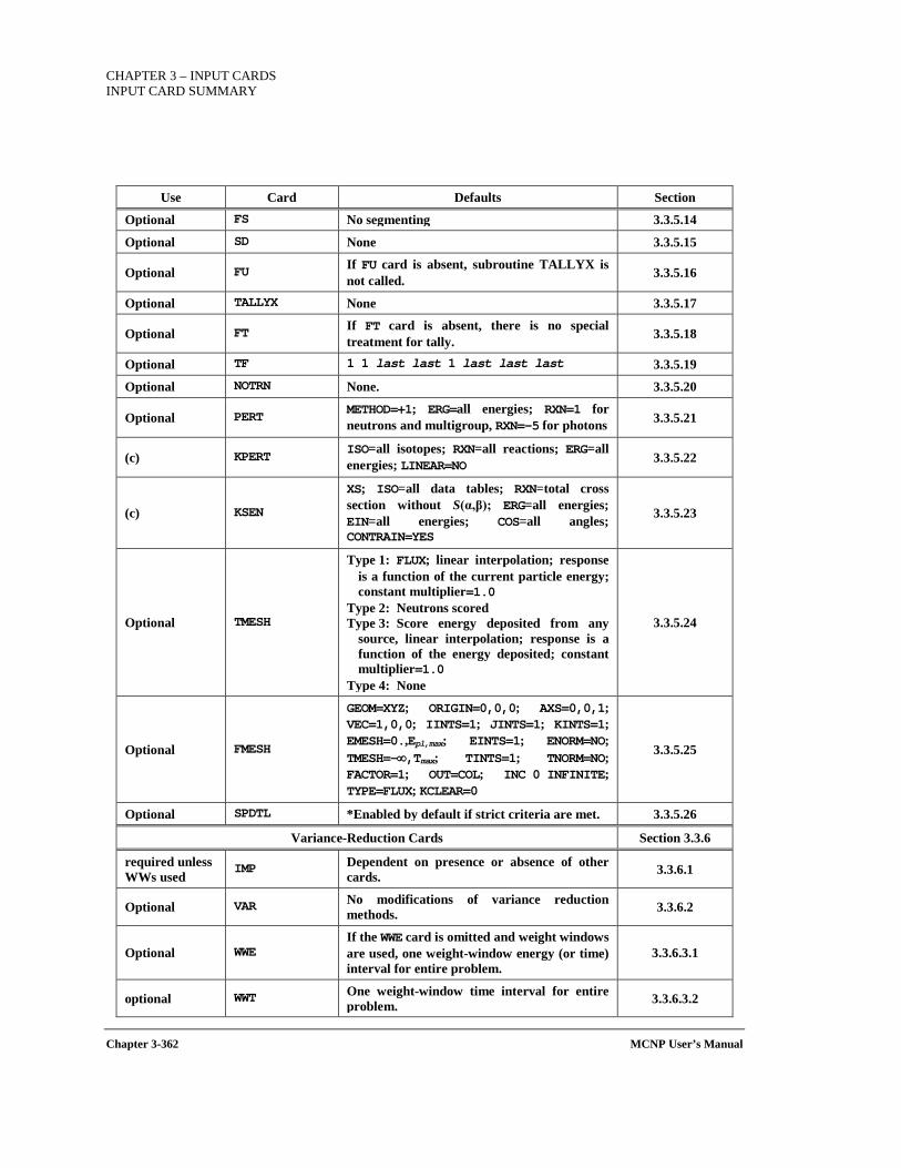
CHAPTER 3 – INPUT CARDS INPUT CARD SUMMARY
Chapter 3-362 MCNP User’s Manual
Use Card Defaults Section
Optional FS No segmenting 3.3.5.14
Optional SD None 3.3.5.15
Optional FU If FU card is absent, subroutine TALLYX is not called. 3.3.5.16
Optional TALLYX None 3.3.5.17
Optional FT If FT card is absent, there is no special treatment for tally. 3.3.5.18
Optional TF 1 1 last last 1 last last last 3.3.5.19
Optional NOTRN None. 3.3.5.20
Optional PERT METHOD=+1; ERG=all energies; RXN=1 for neutrons and multigroup, RXN=-5 for photons 3.3.5.21
(c) KPERT ISO=all isotopes; RXN=all reactions; ERG=all energies; LINEAR=NO 3.3.5.22
(c) KSEN
XS; ISO=all data tables; RXN=total cross section without S(α,β); ERG=all energies; EIN=all energies; COS=all angles; CONTRAIN=YES
3.3.5.23
Optional TMESH
Type 1: FLUX; linear interpolation; response is a function of the current particle energy; constant multiplier=1.0
Type 2: Neutrons scored Type 3: Score energy deposited from any
source, linear interpolation; response is a function of the energy deposited; constant multiplier=1.0
Type 4: None
3.3.5.24
Optional FMESH
GEOM=XYZ; ORIGIN=0,0,0; AXS=0,0,1; VEC=1,0,0; IINTS=1; JINTS=1; KINTS=1; EMESH=0.,Epl,max; EINTS=1; ENORM=NO; TMESH=-∞,Tmax; TINTS=1; TNORM=NO; FACTOR=1; OUT=COL; INC 0 INFINITE; TYPE=FLUX; KCLEAR=0
3.3.5.25
Optional SPDTL *Enabled by default if strict criteria are met. 3.3.5.26
Variance-Reduction Cards Section 3.3.6
required unless WWs used
IMP Dependent on presence or absence of other cards. 3.3.6.1
Optional VAR No modifications of variance reduction methods. 3.3.6.2
Optional WWE If the WWE card is omitted and weight windows are used, one weight-window energy (or time) interval for entire problem.
3.3.6.3.1
optional WWT One weight-window time interval for entire problem. 3.3.6.3.2
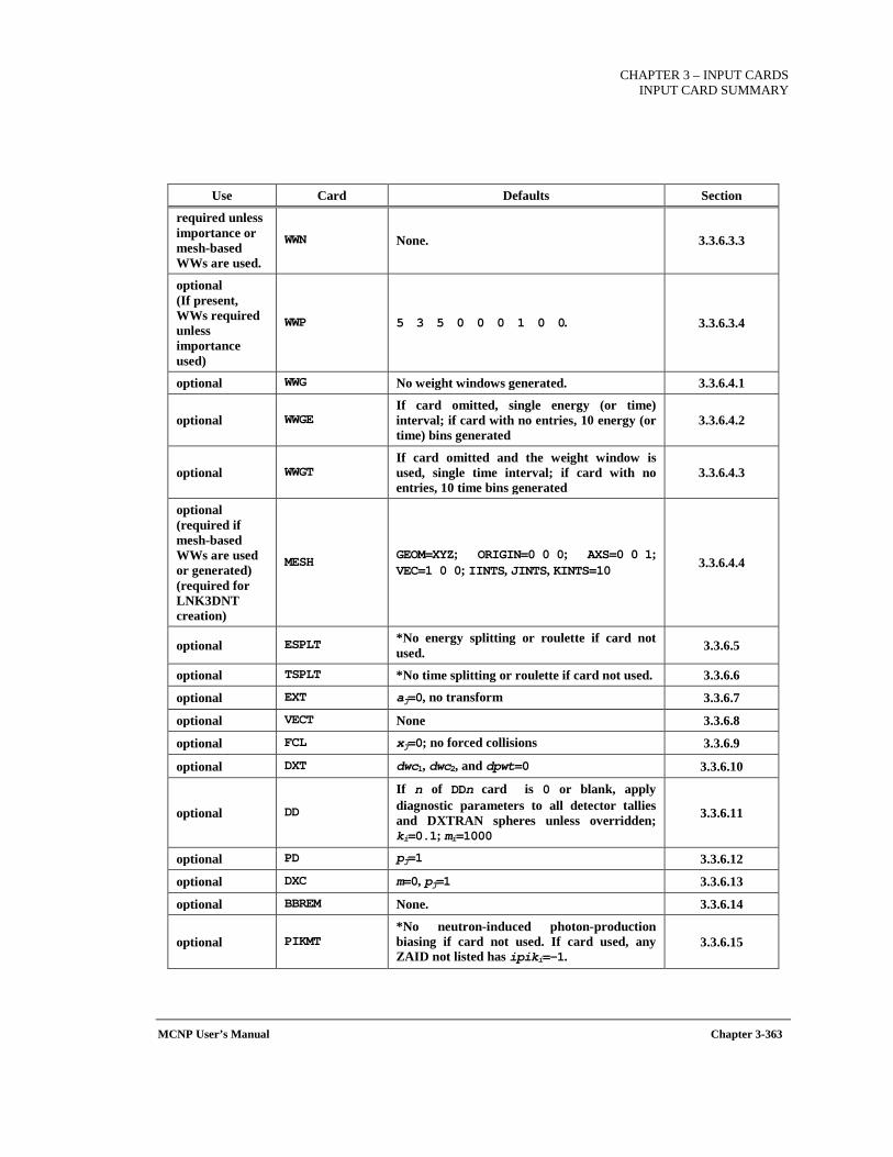
CHAPTER 3 – INPUT CARDS
INPUT CARD SUMMARY
MCNP User’s Manual Chapter 3-363
Use Card Defaults Section
required unless importance or mesh-based WWs are used.
WWN None. 3.3.6.3.3
optional (If present, WWs required unless importance used)
WWP 5 3 5 0 0 0 1 0 0. 3.3.6.3.4
optional WWG No weight windows generated. 3.3.6.4.1
optional WWGE If card omitted, single energy (or time) interval; if card with no entries, 10 energy (or time) bins generated
3.3.6.4.2
optional WWGT If card omitted and the weight window is used, single time interval; if card with no entries, 10 time bins generated
3.3.6.4.3
optional (required if mesh-based WWs are used or generated) (required for LNK3DNT creation)
MESH GEOM=XYZ; ORIGIN=0 0 0; AXS=0 0 1; VEC=1 0 0; IINTS, JINTS, KINTS=10 3.3.6.4.4
optional ESPLT *No energy splitting or roulette if card not used. 3.3.6.5
optional TSPLT *No time splitting or roulette if card not used. 3.3.6.6
optional EXT aj=0, no transform 3.3.6.7
optional VECT None 3.3.6.8
optional FCL xj=0; no forced collisions 3.3.6.9
optional DXT dwc1, dwc2, and dpwt=0 3.3.6.10
optional DD
If n of DDn card is 0 or blank, apply diagnostic parameters to all detector tallies and DXTRAN spheres unless overridden; ki=0.1; mi=1000
3.3.6.11
optional PD pj=1 3.3.6.12
optional DXC m=0, pj=1 3.3.6.13
optional BBREM None. 3.3.6.14
optional PIKMT *No neutron-induced photon-production biasing if card not used. If card used, any ZAID not listed has ipiki=-1.
3.3.6.15
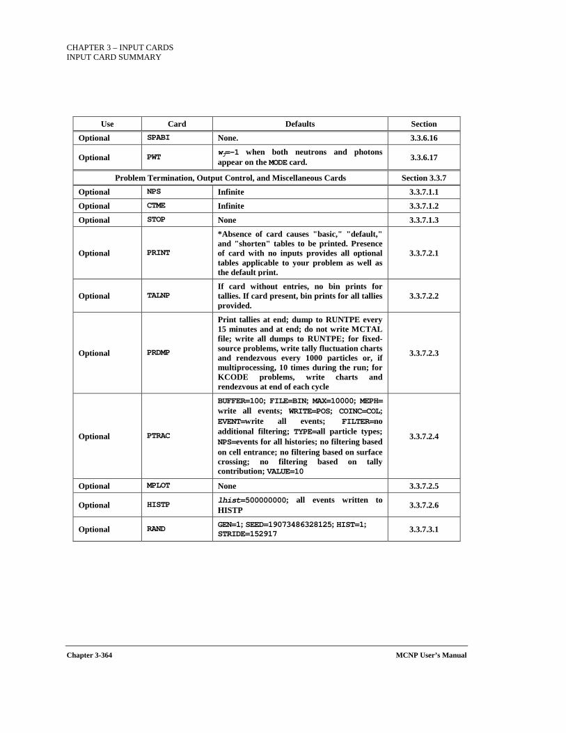
CHAPTER 3 – INPUT CARDS INPUT CARD SUMMARY
Chapter 3-364 MCNP User’s Manual
Use Card Defaults Section
Optional SPABI None. 3.3.6.16
Optional PWT wj=-1 when both neutrons and photons appear on the MODE card. 3.3.6.17
Problem Termination, Output Control, and Miscellaneous Cards Section 3.3.7
Optional NPS Infinite 3.3.7.1.1
Optional CTME Infinite 3.3.7.1.2
Optional STOP None 3.3.7.1.3
Optional PRINT
*Absence of card causes "basic," "default," and "shorten" tables to be printed. Presence of card with no inputs provides all optional tables applicable to your problem as well as the default print.
3.3.7.2.1
Optional TALNP If card without entries, no bin prints for tallies. If card present, bin prints for all tallies provided.
3.3.7.2.2
Optional PRDMP
Print tallies at end; dump to RUNTPE every 15 minutes and at end; do not write MCTAL file; write all dumps to RUNTPE; for fixed-source problems, write tally fluctuation charts and rendezvous every 1000 particles or, if multiprocessing, 10 times during the run; for KCODE problems, write charts and rendezvous at end of each cycle
3.3.7.2.3
Optional PTRAC
BUFFER=100; FILE=BIN; MAX=10000; MEPH= write all events; WRITE=POS; COINC=COL; EVENT=write all events; FILTER=no additional filtering; TYPE=all particle types; NPS=events for all histories; no filtering based on cell entrance; no filtering based on surface crossing; no filtering based on tally contribution; VALUE=10
3.3.7.2.4
Optional MPLOT None 3.3.7.2.5
Optional HISTP lhist=500000000; all events written to HISTP 3.3.7.2.6
Optional RAND GEN=1; SEED=19073486328125; HIST=1; STRIDE=152917 3.3.7.3.1
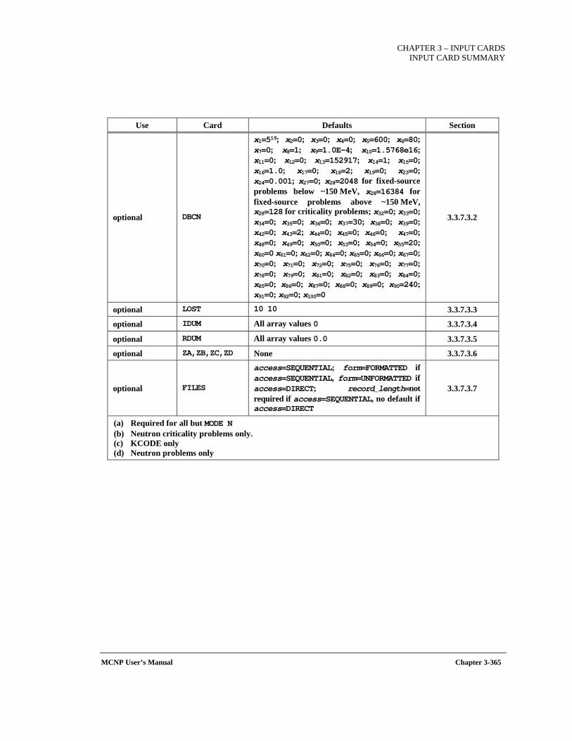
CHAPTER 3 – INPUT CARDS
INPUT CARD SUMMARY
MCNP User’s Manual Chapter 3-365
Use Card Defaults Section
optional DBCN
x1=519; x2=0; x3=0; x4=0; x5=600; x6=80; x7=0; x8=1; x9=1.0E-4; x10=1.5768e16; x11=0; x12=0; x13=152917; x14=1; x15=0; x16=1.0; x17=0; x18=2; x19=0; x23=0; x24=0.001; x27=0; x28=2048 for fixed-source problems below ~150 MeV, x28=16384 for fixed-source problems above ~150 MeV, x28=128 for criticality problems; x32=0; x33=0; x34=0; x35=0; x36=0; x37=30; x38=0; x39=0; x42=0; x43=2; x44=0; x45=0; x46=0; x47=0; x48=0; x49=0; x50=0; x53=0; x54=0; x55=20; x60=0 x61=0; x62=0; x64=0; x65=0; x66=0; x67=0; x70=0; x71=0; x72=0; x75=0; x76=0; x77=0; x78=0; x79=0; x81=0; x82=0; x83=0; x84=0; x85=0; x86=0; x87=0; x88=0; x89=0; x90=240; x91=0; x92=0; x100=0
3.3.7.3.2
optional LOST 10 10 3.3.7.3.3
optional IDUM All array values 0 3.3.7.3.4
optional RDUM All array values 0.0 3.3.7.3.5
optional ZA,ZB,ZC,ZD None 3.3.7.3.6
optional FILES
access=SEQUENTIAL; form=FORMATTED if access=SEQUENTIAL, form=UNFORMATTED if access=DIRECT; record_length=not required if access=SEQUENTIAL, no default if access=DIRECT
3.3.7.3.7
(a) Required for all but MODE N (b) Neutron criticality problems only. (c) KCODE only (d) Neutron problems only

CHAPTER 4 – EXAMPLES
GEOMETRY
MCNP User’s Manual Chapter 4-1
4 EXAMPLES
Instructive examples of several topics are included in this section. Some of the examples are simplistic while others illustrate more complex features of the MCNP6 code. They should be studied in conjunction with the theory, instructions, and previous examples provided in Sections 1, 2, and 3 of this manual. Following the simple geometry specification examples are related geometry examples that exercise coordinate transformations, repeated structure and lattice geometries, and embedded meshes. After the geometry-related examples are those related to tally options, including the FM, FMESH, FS, and FT cards as well as the TALLYX subroutine for user-defined tallies using the FU card. Next are source specification examples for the generalized source, beam sources, and a burnup case followed by example SOURCE and SRCDX subroutines for point detectors and/or DXTRAN spheres. Finally, a materials example of table and model-data mix-and-match and a physics model example complete the section.
4.1 GEOMETRY EXAMPLES
The geometry discussions in Sections 1 and 2 must be understood before studying the following examples. The concept of combining regions of space bounded by surfaces to make a cell must be fully appreciated; the following examples should help solidify this concept. The use of macrobodies will simplify many geometry definition situations.
4.1.1 Geometry Specification Several examples of the union and complement operators follow. These should help you better understand how cells are defined. In the illustrations, cell numbers will be circled; surface numbers will not be circled but will appear next to the surface they represent. For simplicity, all cells are void of material.
The next several examples become progressively more difficult and usually take advantage of what you learned in the preceding ones. Remember that unless altered by parentheses, the hierarchy of operations is that intersections are performed first and then unions.
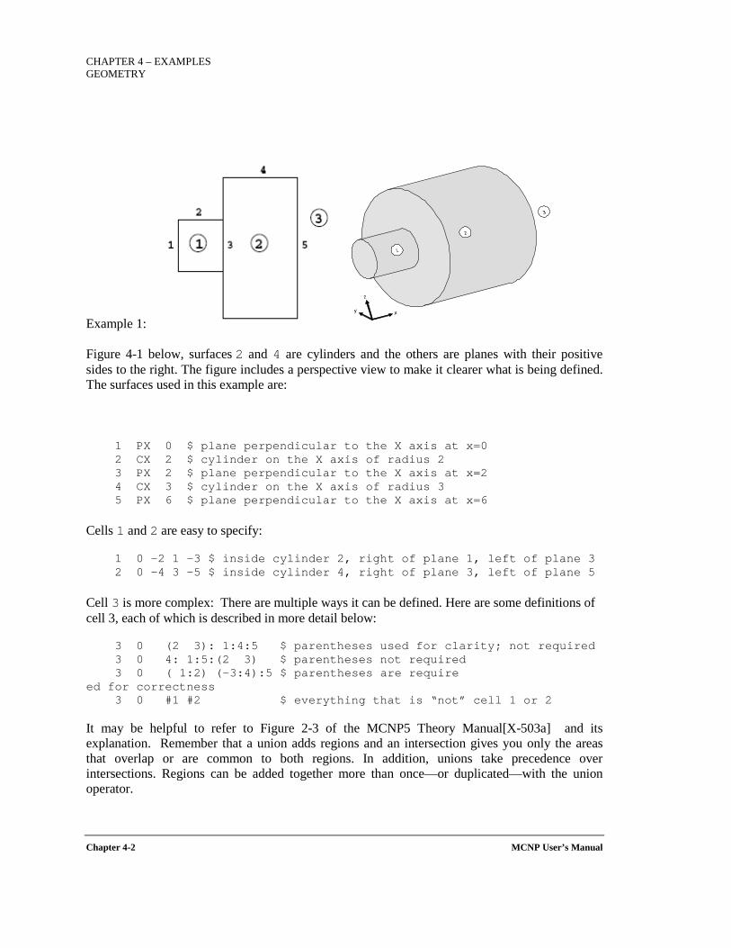
CHAPTER 4 – EXAMPLES GEOMETRY
Chapter 4-2 MCNP User’s Manual
Example 1:
Figure 4-1 below, surfaces 2 and 4 are cylinders and the others are planes with their positive sides to the right. The figure includes a perspective view to make it clearer what is being defined. The surfaces used in this example are:
1 PX 0 $ plane perpendicular to the X axis at x=0 2 CX 2 $ cylinder on the X axis of radius 2 3 PX 2 $ plane perpendicular to the X axis at x=2 4 CX 3 $ cylinder on the X axis of radius 3 5 PX 6 $ plane perpendicular to the X axis at x=6 Cells 1 and 2 are easy to specify: 1 0 −2 1 −3 $ inside cylinder 2, right of plane 1, left of plane 3 2 0 −4 3 −5 $ inside cylinder 4, right of plane 3, left of plane 5 Cell 3 is more complex: There are multiple ways it can be defined. Here are some definitions of cell 3, each of which is described in more detail below: 3 0 (2 3): 1:4:5 $ parentheses used for clarity; not required 3 0 4: 1:5:(2 3) $ parentheses not required 3 0 ( 1:2) (-3:4):5 $ parentheses are require ed for correctness 3 0 #1 #2 $ everything that is “not” cell 1 or 2 It may be helpful to refer to Figure 2-3 of the MCNP5 Theory Manual[X-503a] and its explanation. Remember that a union adds regions and an intersection gives you only the areas that overlap or are common to both regions. In addition, unions take precedence over intersections. Regions can be added together more than once—or duplicated—with the union operator.
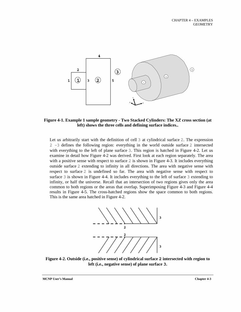
CHAPTER 4 – EXAMPLES
GEOMETRY
MCNP User’s Manual Chapter 4-3
Figure 4-1. Example 1 sample geometry - Two Stacked Cylinders: The XZ cross section (at left) shows the three cells and defining surface indices..
Let us arbitrarily start with the definition of cell 3 at cylindrical surface 2. The expression 2 -3 defines the following region: everything in the world outside surface 2 intersected with everything to the left of plane surface 3. This region is hatched in Figure 4-2. Let us examine in detail how Figure 4-2 was derived. First look at each region separately. The area with a positive sense with respect to surface 2 is shown in Figure 4-3. It includes everything outside surface 2 extending to infinity in all directions. The area with negative sense with respect to surface 2 is undefined so far. The area with negative sense with respect to surface 3 is shown in Figure 4-4. It includes everything to the left of surface 3 extending to infinity, or half the universe. Recall that an intersection of two regions gives only the area common to both regions or the areas that overlap. Superimposing Figure 4-3 and Figure 4-4 results in Figure 4-5. The cross-hatched regions show the space common to both regions. This is the same area hatched in Figure 4-2.
Figure 4-2. Outside (i.e., positive sense) of cylindrical surface 2 intersected with region to
left (i.e., negative sense) of plane surface 3.
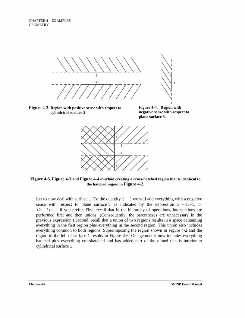
CHAPTER 4 – EXAMPLES GEOMETRY
Chapter 4-4 MCNP User’s Manual
Figure 4-3. Region with positive sense with respect to
cylindrical surface 2 Figure 4-4. Region with negative sense with respect to plane surface 3.
Figure 4-5. Figure 4-3 and Figure 4-4 overlaid creating a cross-hatched region that is identical to
the hatched region in Figure 4-2.
Let us now deal with surface 1. To the quantity 2 -3 we will add everything with a negative sense with respect to plane surface 1 as indicated by the expression 2 -3:-1, or (2 -3):-1 if you prefer. First, recall that in the hierarchy of operations, intersections are performed first and then unions. (Consequently, the parentheses are unnecessary in the previous expression.) Second, recall that a union of two regions results in a space containing everything in the first region plus everything in the second region. This union also includes everything common to both regions. Superimposing the region shown in Figure 4-2 and the region to the left of surface 1 results in Figure 4-6. Our geometry now includes everything hatched plus everything crosshatched and has added part of the tunnel that is interior to cylindrical surface 2.
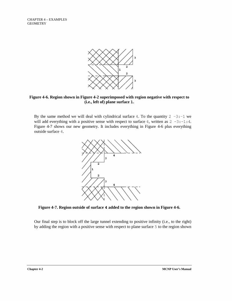
CHAPTER 4 – EXAMPLES GEOMETRY
Chapter 4-2 MCNP User’s Manual
Figure 4-6. Region shown in Figure 4-2 superimposed with region negative with respect to
(i.e., left of) plane surface 1.
By the same method we will deal with cylindrical surface 4. To the quantity 2 -3:-1 we will add everything with a positive sense with respect to surface 4, written as 2 -3:-1:4. Figure 4-7 shows our new geometry. It includes everything in Figure 4-6 plus everything outside surface 4.
Figure 4-7. Region outside of surface 4 added to the region shown in Figure 4-6.
Our final step is to block off the large tunnel extending to positive infinity (i.e., to the right) by adding the region with a positive sense with respect to plane surface 5 to the region shown
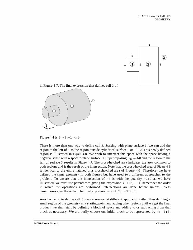
CHAPTER 4 – EXAMPLES
GEOMETRY
MCNP User’s Manual Chapter 4-3
in Figure 4-7. The final expression that defines cell 3 of
Figure 4-1 is 2 -3:-1:4:5.
There is more than one way to define cell 3. Starting with plane surface 1, we can add the region to the left of 1 to the region outside cylindrical surface 2 or -1:2. This newly defined region is illustrated in Figure 4-8. We wish to intersect this space with the space having a negative sense with respect to plane surface 3. Superimposing Figure 4-8 and the region to the left of surface 3 results in Figure 4-9. The cross-hatched area indicates the area common to both regions and is the result of the intersection. Note that the cross-hatched area of Figure 4-9 is identical to the entire hatched plus crosshatched area of Figure 4-6. Therefore, we have defined the same geometry in both figures but have used two different approaches to the problem. To ensure that the intersection of -3 is with the quantity -1:2 as we have illustrated, we must use parentheses giving the expression (-1:2) −3. Remember the order in which the operations are performed. Intersections are done before unions unless parentheses alter the order. The final expression is (-1:2) -3:4:5.
Another tactic to define cell 3 uses a somewhat different approach. Rather than defining a small region of the geometry as a starting point and adding other regions until we get the final product, we shall start by defining a block of space and adding to or subtracting from that block as necessary. We arbitrarily choose our initial block to be represented by 4: 1:5,
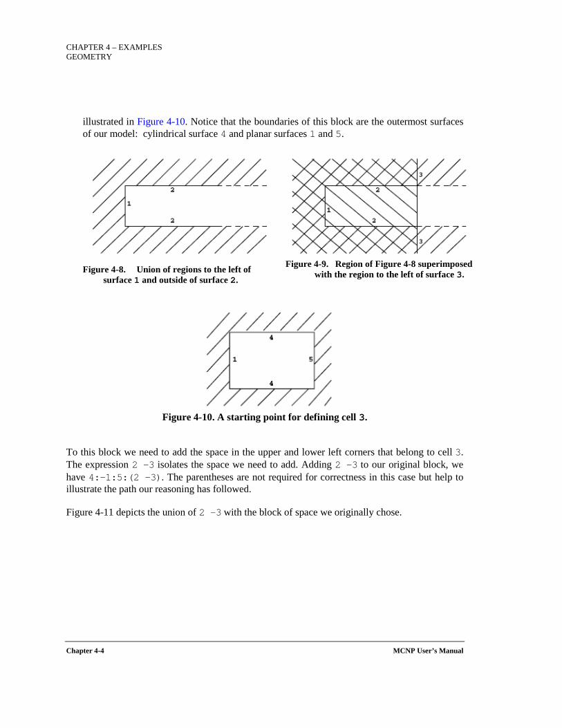
CHAPTER 4 – EXAMPLES GEOMETRY
Chapter 4-4 MCNP User’s Manual
illustrated in Figure 4-10. Notice that the boundaries of this block are the outermost surfaces of our model: cylindrical surface 4 and planar surfaces 1 and 5.
Figure 4-8. Union of regions to the left of
surface 1 and outside of surface 2. Figure 4-9. Region of Figure 4-8 superimposed
with the region to the left of surface 3.
Figure 4-10. A starting point for defining cell 3.
To this block we need to add the space in the upper and lower left corners that belong to cell 3. The expression 2 −3 isolates the space we need to add. Adding 2 -3 to our original block, we have 4:-1:5:(2 -3). The parentheses are not required for correctness in this case but help to illustrate the path our reasoning has followed.
Figure 4-11 depicts the union of 2 -3 with the block of space we originally chose.
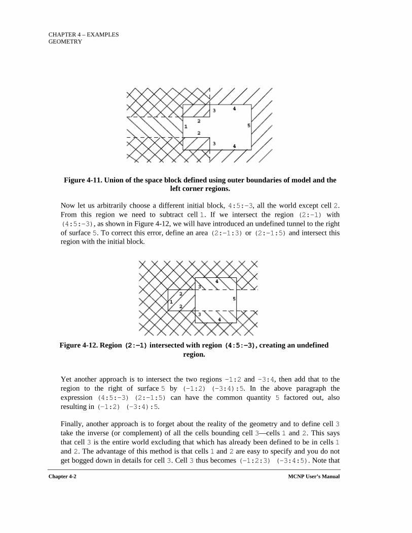
CHAPTER 4 – EXAMPLES GEOMETRY
Chapter 4-2 MCNP User’s Manual
Figure 4-11. Union of the space block defined using outer boundaries of model and the left corner regions.
Now let us arbitrarily choose a different initial block, 4:5:-3, all the world except cell 2. From this region we need to subtract cell 1. If we intersect the region (2:-1) with (4:5:-3), as shown in Figure 4-12, we will have introduced an undefined tunnel to the right of surface 5. To correct this error, define an area (2:-1:3) or (2:-1:5) and intersect this region with the initial block.
Figure 4-12. Region (2:−1) intersected with region (4:5:−3), creating an undefined
region.
Yet another approach is to intersect the two regions -1:2 and -3:4, then add that to the region to the right of surface 5 by (-1:2) (-3:4):5. In the above paragraph the expression (4:5:-3) (2:-1:5) can have the common quantity 5 factored out, also resulting in (-1:2) (-3:4):5.
Finally, another approach is to forget about the reality of the geometry and to define cell 3 take the inverse (or complement) of all the cells bounding cell 3—cells 1 and 2. This says that cell 3 is the entire world excluding that which has already been defined to be in cells 1 and 2. The advantage of this method is that cells 1 and 2 are easy to specify and you do not get bogged down in details for cell 3. Cell 3 thus becomes (-1:2:3) (-3:4:5). Note that
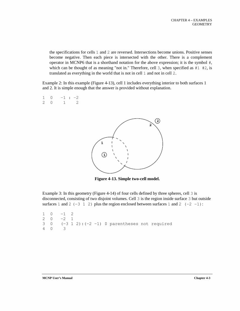
CHAPTER 4 – EXAMPLES
GEOMETRY
MCNP User’s Manual Chapter 4-3
the specifications for cells 1 and 2 are reversed. Intersections become unions. Positive senses become negative. Then each piece is intersected with the other. There is a complement operator in MCNP6 that is a shorthand notation for the above expression; it is the symbol #, which can be thought of as meaning "not in." Therefore, cell 3, when specified as #1 #2, is translated as everything in the world that is not in cell 1 and not in cell 2.
Example 2: In this example (Figure 4-13), cell 1 includes everything interior to both surfaces 1 and 2. It is simple enough that the answer is provided without explanation. 1 0 −1 : −2 2 0 1 2
Figure 4-13. Simple two-cell model.
Example 3: In this geometry (Figure 4-14) of four cells defined by three spheres, cell 3 is disconnected, consisting of two disjoint volumes. Cell 3 is the region inside surface 3 but outside surfaces 1 and 2 (−3 1 2) plus the region enclosed between surfaces 1 and 2 (−2 −1): 1 0 −1 2 2 0 −2 1 3 0 (−3 1 2):(−2 −1) $ parentheses not required 4 0 3
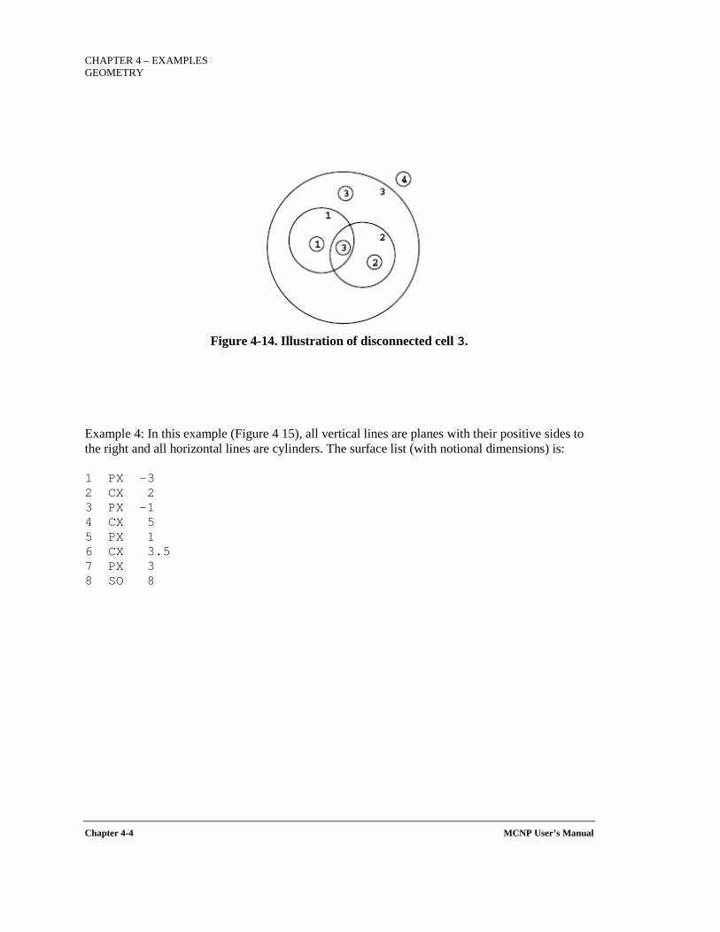
CHAPTER 4 – EXAMPLES GEOMETRY
Chapter 4-4 MCNP User’s Manual
Figure 4-14. Illustration of disconnected cell 3.
Example 4: In this example (Figure 4 15), all vertical lines are planes with their positive sides to the right and all horizontal lines are cylinders. The surface list (with notional dimensions) is: 1 PX -3 2 CX 2 3 PX -1 4 CX 5 5 PX 1 6 CX 3.5 7 PX 3 8 SO 8
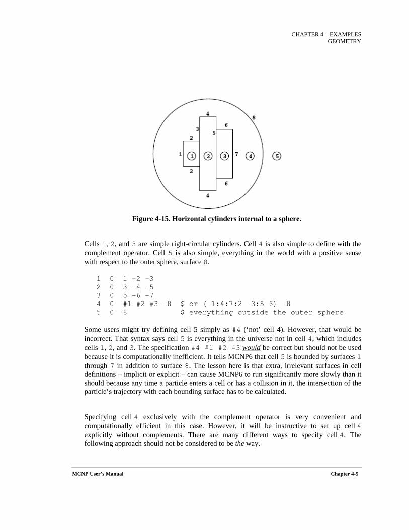
CHAPTER 4 – EXAMPLES
GEOMETRY
MCNP User’s Manual Chapter 4-5
Figure 4-15. Horizontal cylinders internal to a sphere.
Cells 1, 2, and 3 are simple right-circular cylinders. Cell 4 is also simple to define with the complement operator. Cell 5 is also simple, everything in the world with a positive sense with respect to the outer sphere, surface 8.
1 0 1 -2 -3 2 0 3 -4 -5 3 0 5 -6 -7 4 0 #1 #2 #3 -8 $ or (−1:4:7:2 −3:5 6) −8 5 0 8 $ everything outside the outer sphere
Some users might try defining cell 5 simply as #4 (‘not’ cell 4). However, that would be incorrect. That syntax says cell 5 is everything in the universe not in cell 4, which includes cells 1, 2, and 3. The specification #4 #1 #2 #3 would be correct but should not be used because it is computationally inefficient. It tells MCNP6 that cell 5 is bounded by surfaces 1 through 7 in addition to surface 8. The lesson here is that extra, irrelevant surfaces in cell definitions – implicit or explicit – can cause MCNP6 to run significantly more slowly than it should because any time a particle enters a cell or has a collision in it, the intersection of the particle’s trajectory with each bounding surface has to be calculated.
Specifying cell 4 exclusively with the complement operator is very convenient and computationally efficient in this case. However, it will be instructive to set up cell 4 explicitly without complements. There are many different ways to specify cell 4, The following approach should not be considered to be the way.

CHAPTER 4 – EXAMPLES GEOMETRY
Chapter 4-6 MCNP User’s Manual
First consider cell 4 to be everything outside the big cylinder of surface 4 that is bounded on each end by surfaces 1 and 7. This is specified by (-1:4:7). The parentheses are not necessary but may add clarity. Now all that remains is to add the corners outside cylinders 2 and 6. The corner outside cylinder 2 is (2 -3), whereas it is (5 6) outside cylinder 6. Again the parentheses are optional. These corners are then added to what we already have outside cylinder 4 to get
(−1:4:7):(2 −3):(5 6)
The region described so far does not include cells 1, 2, or 3 but extends to infinity in all directions. This region needs to be terminated at the spherical surface 8. In other words, cell 4 is everything we have defined so far that is also common with everything inside surface 8 (that is, everything so far intersected with -8). So as a final result,
((−1:4:7):(2 −3):(5 6)) −8
The inner parentheses can be removed, but the outer ones are necessary (remember the hierarchy of operations) to give us
(−1:4:7:2 −3:5 6) −8
If the outer parentheses are removed, the intersection of -8 will occur only with 5 and 6, an event that is clearly incorrect.
Example 5:
Figure 4-16. Horizontal and vertical cylinders in a sphere.
This example (Figure 4-16) is similar to the previous one except that a vertical cylinder (surface 4) is added to one side of the horizontal cylinder (surface 3).
Cell 1 is (1 -3 -2), cell 3 is #1 #2 #4, and cell 4 is just 6.
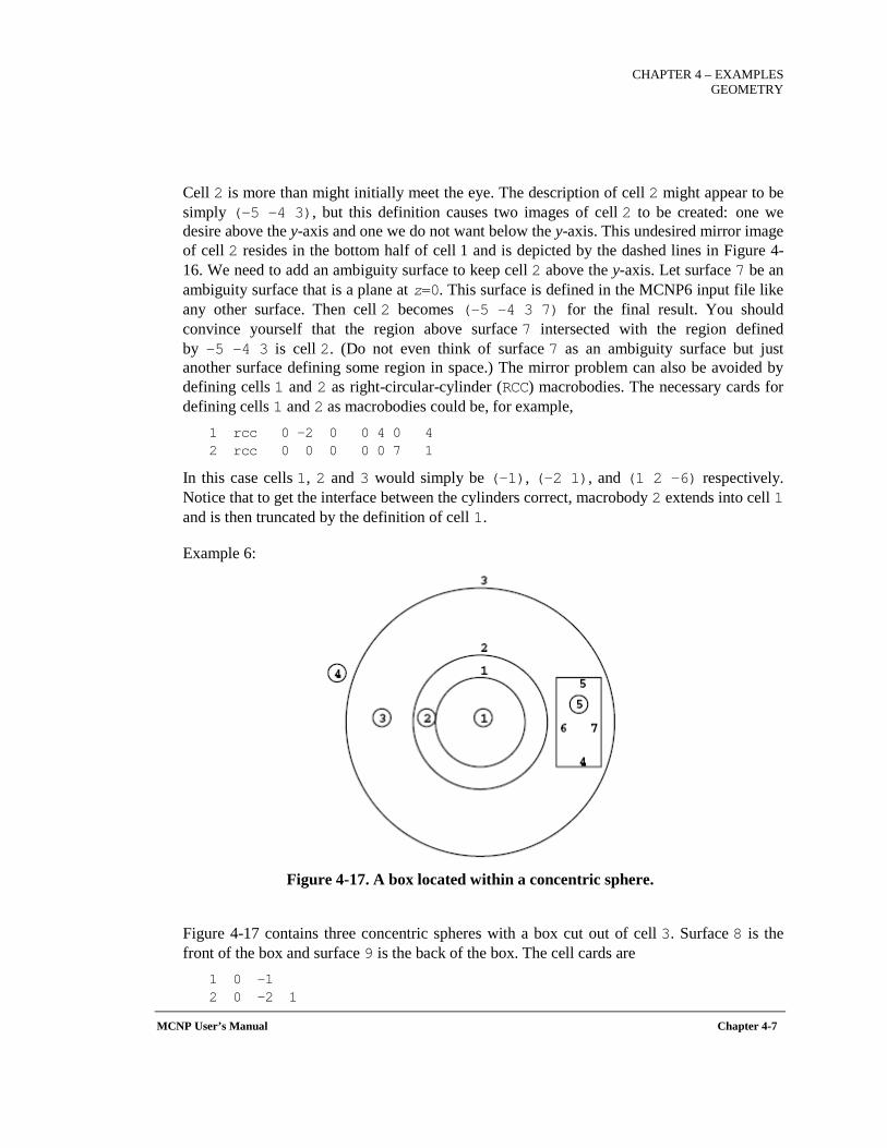
CHAPTER 4 – EXAMPLES
GEOMETRY
MCNP User’s Manual Chapter 4-7
Cell 2 is more than might initially meet the eye. The description of cell 2 might appear to be simply (-5 -4 3), but this definition causes two images of cell 2 to be created: one we desire above the y-axis and one we do not want below the y-axis. This undesired mirror image of cell 2 resides in the bottom half of cell 1 and is depicted by the dashed lines in Figure 4-16. We need to add an ambiguity surface to keep cell 2 above the y-axis. Let surface 7 be an ambiguity surface that is a plane at z=0. This surface is defined in the MCNP6 input file like any other surface. Then cell 2 becomes (-5 -4 3 7) for the final result. You should convince yourself that the region above surface 7 intersected with the region defined by -5 -4 3 is cell 2. (Do not even think of surface 7 as an ambiguity surface but just another surface defining some region in space.) The mirror problem can also be avoided by defining cells 1 and 2 as right-circular-cylinder (RCC) macrobodies. The necessary cards for defining cells 1 and 2 as macrobodies could be, for example,
1 rcc 0 -2 0 0 4 0 4 2 rcc 0 0 0 0 0 7 1
In this case cells 1, 2 and 3 would simply be (-1), (-2 1), and (1 2 -6) respectively. Notice that to get the interface between the cylinders correct, macrobody 2 extends into cell 1 and is then truncated by the definition of cell 1.
Example 6:
Figure 4-17. A box located within a concentric sphere.
Figure 4-17 contains three concentric spheres with a box cut out of cell 3. Surface 8 is the front of the box and surface 9 is the back of the box. The cell cards are
1 0 −1 2 0 −2 1
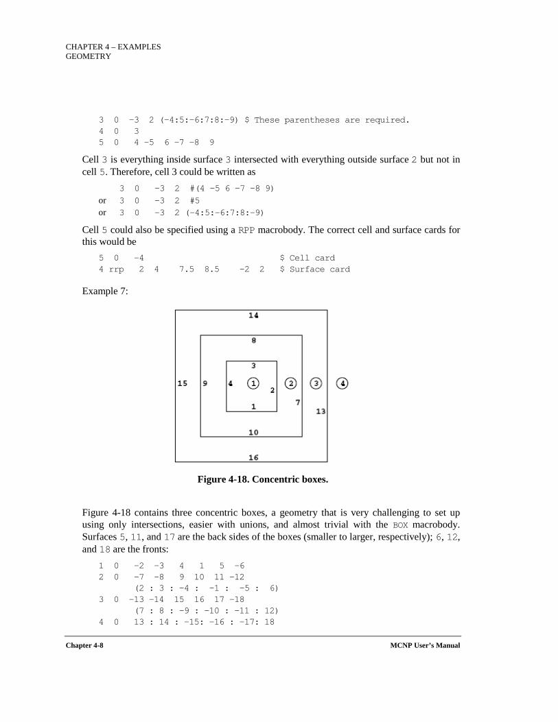
CHAPTER 4 – EXAMPLES GEOMETRY
Chapter 4-8 MCNP User’s Manual
3 0 −3 2 (−4:5:−6:7:8:−9) $ These parentheses are required. 4 0 3 5 0 4 −5 6 −7 −8 9
Cell 3 is everything inside surface 3 intersected with everything outside surface 2 but not in cell 5. Therefore, cell 3 could be written as
3 0 −3 2 #(4 −5 6 −7 −8 9) or 3 0 −3 2 #5 or 3 0 −3 2 (−4:5:−6:7:8:−9)
Cell 5 could also be specified using a RPP macrobody. The correct cell and surface cards for this would be
5 0 -4 $ Cell card 4 rrp 2 4 7.5 8.5 -2 2 $ Surface card
Example 7:
Figure 4-18. Concentric boxes.
Figure 4-18 contains three concentric boxes, a geometry that is very challenging to set up using only intersections, easier with unions, and almost trivial with the BOX macrobody. Surfaces 5, 11, and 17 are the back sides of the boxes (smaller to larger, respectively); 6, 12, and 18 are the fronts:
1 0 −2 −3 4 1 5 −6 2 0 −7 −8 9 10 11 −12 (2 : 3 : −4 : −1 : −5 : 6) 3 0 −13 −14 15 16 17 −18 (7 : 8 : −9 : −10 : −11 : 12) 4 0 13 : 14 : −15: −16 : −17: 18

CHAPTER 4 – EXAMPLES
GEOMETRY
MCNP User’s Manual Chapter 4-9
Example 8:
Figure 4-19. Torus attached to a concentric sphere.
Figure 4-19 contains two concentric spheres with a torus attached to cell 2 and cut out of cell 1:
1 0 −1 4 2 0 −2 (1 : −4) 3 0 2
If the torus were attached to cell 1 and cut out of cell 2, this bug-eyed geometry would be: 1 0 −1 : −4 2 0 −2 1 4 3 0 2
Example 9:
Figure 4-20. Disconnected cell.

CHAPTER 4 – EXAMPLES GEOMETRY
Chapter 4-10 MCNP User’s Manual
Notice that cell 17 is disconnected, having two pieces. Cell 9 in Figure 4-20 is a box cut out of the left part of spherical cell 17; surface 9 is the front of the box and surface 8 is the rear. The right part of cell 17 is the space interior to spheres 6 and 7. An F4 tally in cell 17 would be the average flux in all parts of cell 17. An F2 surface tally on surface 7 would be the flux across only the solid portion of surface 7 in the figure. The cell specifications are:
9 0 −3 −2 4 1 8 −9 17 0 −5 (3 : −4 : −1 : 2 : 9 : −8) : −6 : −7 22 0 5 6 7
A variation on this problem is for the right portion of cell 17 to be the intersection of the interiors of surfaces 6 and 7 (the region bounded by the dashed lines in Figure 4-20):
9 0 −3 −2 4 1 8 −9 17 0 −5 (3 : −4 : −1 : 2 : 9 : −8) : −6 −7 22 0 5 (6 : 7)
Example 10:
Figure 4-21. Box with an upside-down cone.
Figure 4-21 contains a box with a cone sitting on top of it. Surface 6 is the front of the box and 7 is the rear. You should understand this example before going on to the next one.
1 0 1 2 −3 (-4 : −5) −6 7 2 0 −1 : −2 : 3 : 4 5 : 6 : −7
This problem could be simplified by replacing surfaces 1–6 with a BOX macrobody. To specify individual macrobody surfaces, the resulting cell and surface definitions must use macrobody facet notation. Typical cell and surface cards would look like
c cell cards 1 0 -8:(-5 8.5) 2 0 #1 $ or -8.4:-8.6:8.3:(8.5 5):8.1:-8.2
c surface cards 5 kz 8 0.25 -1 8 box -2.5 -2.5 0 5 0 0 0 5 0 0 0 5
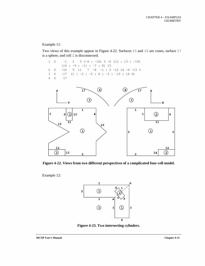
CHAPTER 4 – EXAMPLES
GEOMETRY
MCNP User’s Manual Chapter 4-11
Example 11:
Two views of this example appear in Figure 4-22. Surfaces 15 and 16 are cones, surface 17 is a sphere, and cell 2 is disconnected.
1 0 −1 2 3 (−4 : −16) 5 −6 (12 : 13 : −14) (10 : −9 : −11 : −7 : 8) 15 2 0 −10 9 11 7 −8 −1 : 2 −12 14 −6 −13 3 3 0 −17 (1 : −2 : −5 : 6 : −3 : −15 : 16 4) 4 0 17
Figure 4-22. Views from two different perspectives of a complicated four-cell model.
Example 12:
Figure 4-23. Two intersecting cylinders.
CHAPTER 4 – EXAMPLES GEOMETRY
Chapter 4-12 MCNP User’s Manual
In Figure 4-23, cell 1 consists of two cylinders joined at a 45-degree angle. Cell 2 is a disk consisting of a cylinder (surface 8) bounded by two planes. Surface 5 is a diagonal plane representing the intersection of the two cylinders. The problem is to specify the disk (cell 2) in one cell formed by the two cylinders (cell 1). A conflict arises in specifying cell 1 since, from the outside of cell 3, corner a between surfaces 1 and 3 is convex, but on the other side of the cell the same two surfaces form a concave corner at b. The dilemma is solved by composing cell 1 of two disconnected cells, each bounded by surface 5 between corners a and b. Surface 5 must be included in the list of surface cards in the MCNP6 input file. When the two parts are joined to make cell 1, surface 5 does not appear. Convince yourself by plotting it using an origin of 0 0 24 and basis vectors 0 1 1 0 -1 1. See Section 5 for an explanation of plotting commands.
1 0 (2 −1 −5 (7:8:−6)):(4 −3 5(−6:8:7)) 2 0 −8 6 −7 3 0 (−2:1:5) (−4:3:−5)
A more efficient expression for cell 1 is 1 0 (2 −1 −5:4 −3 5) (−6:8:7)
Example 13:
This example (Figure 4-24) has the most complicated geometry so far, but it can be described very simply.
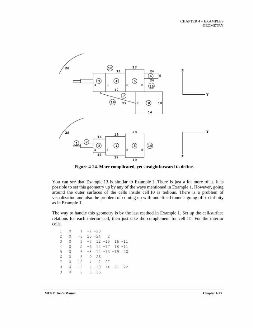
CHAPTER 4 – EXAMPLES
GEOMETRY
MCNP User’s Manual Chapter 4-13
Figure 4-24. More complicated, yet straightforward to define.
You can see that Example 13 is similar to Example 1. There is just a lot more of it. It is possible to set this geometry up by any of the ways mentioned in Example 1. However, going around the outer surfaces of the cells inside cell 10 is tedious. There is a problem of visualization and also the problem of coming up with undefined tunnels going off to infinity as in Example 1.
The way to handle this geometry is by the last method in Example 1. Set up the cell/surface relations for each interior cell, then just take the complement for cell 10. For the interior cells,
1 0 1 −2 −23 2 0 −3 25 −24 2 3 0 3 −5 12 −15 16 −11 4 0 5 −6 12 −17 18 −11 5 0 6 −8 12 −13 −19 20 6 0 8 −9 −26 7 0 −12 4 −7 −27 8 0 −12 7 −10 14 −21 22 9 0 2 −3 −25
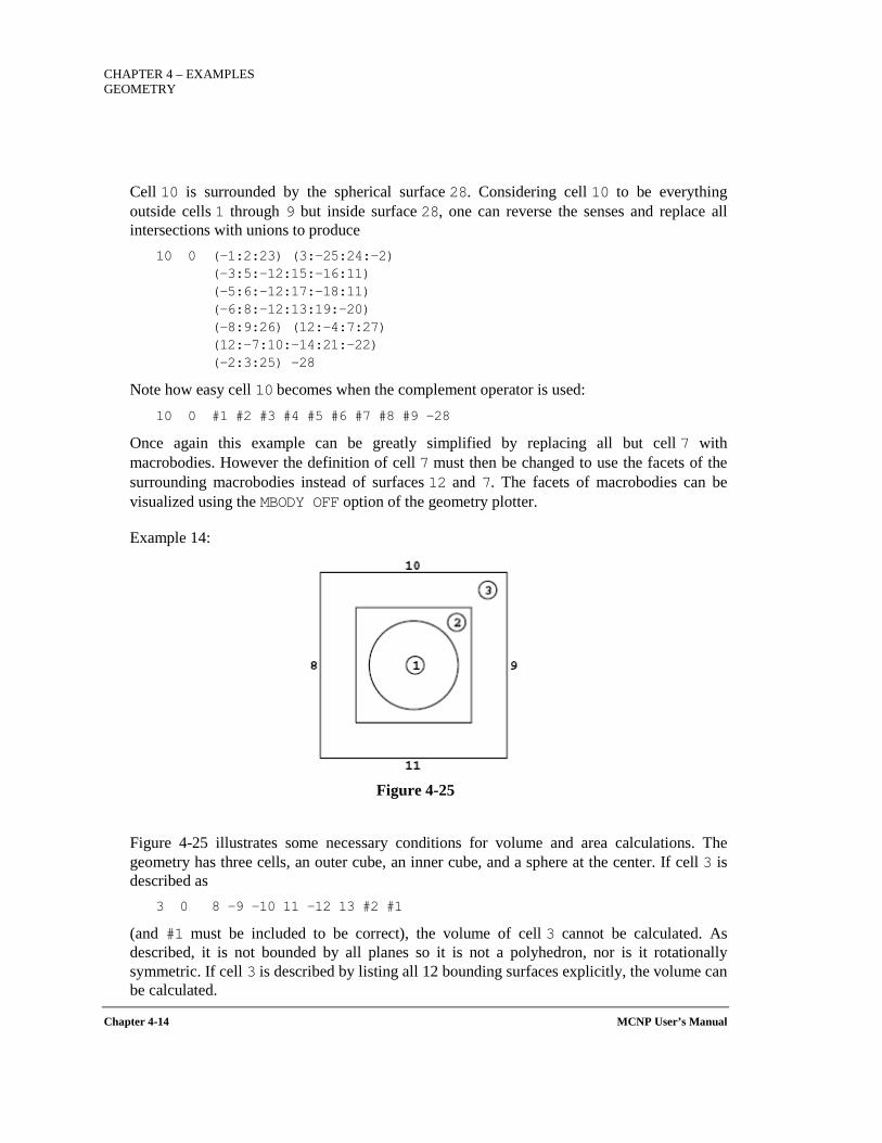
CHAPTER 4 – EXAMPLES GEOMETRY
Chapter 4-14 MCNP User’s Manual
Cell 10 is surrounded by the spherical surface 28. Considering cell 10 to be everything outside cells 1 through 9 but inside surface 28, one can reverse the senses and replace all intersections with unions to produce
10 0 (−1:2:23) (3:−25:24:−2) (−3:5:−12:15:−16:11) (−5:6:−12:17:−18:11) (−6:8:−12:13:19:−20) (−8:9:26) (12:−4:7:27) (12:−7:10:−14:21:−22) (−2:3:25) −28
Note how easy cell 10 becomes when the complement operator is used: 10 0 #1 #2 #3 #4 #5 #6 #7 #8 #9 −28
Once again this example can be greatly simplified by replacing all but cell 7 with macrobodies. However the definition of cell 7 must then be changed to use the facets of the surrounding macrobodies instead of surfaces 12 and 7. The facets of macrobodies can be visualized using the MBODY OFF option of the geometry plotter.
Example 14:
Figure 4-25
Figure 4-25 illustrates some necessary conditions for volume and area calculations. The geometry has three cells, an outer cube, an inner cube, and a sphere at the center. If cell 3 is described as
3 0 8 −9 −10 11 −12 13 #2 #1
(and #1 must be included to be correct), the volume of cell 3 cannot be calculated. As described, it is not bounded by all planes so it is not a polyhedron, nor is it rotationally symmetric. If cell 3 is described by listing all 12 bounding surfaces explicitly, the volume can be calculated.
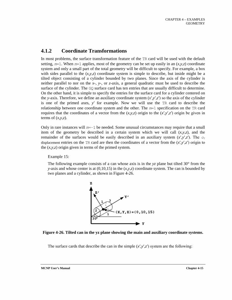
CHAPTER 4 – EXAMPLES
GEOMETRY
MCNP User’s Manual Chapter 4-15
4.1.2 Coordinate Transformations In most problems, the surface transformation feature of the TR card will be used with the default setting, m=1. When m=1 applies, most of the geometry can be set up easily in an (x,y,z) coordinate system and only a small part of the total geometry will be difficult to specify. For example, a box with sides parallel to the (x,y,z) coordinate system is simple to describe, but inside might be a tilted object consisting of a cylinder bounded by two planes. Since the axis of the cylinder is neither parallel to nor on the x-, y-, or z-axis, a general quadratic must be used to describe the surface of the cylinder. The GQ surface card has ten entries that are usually difficult to determine. On the other hand, it is simple to specify the entries for the surface card for a cylinder centered on the y-axis. Therefore, we define an auxiliary coordinate system (x′,y′,z′) so the axis of the cylinder is one of the primed axes, y′ for example. Now we will use the TR card to describe the relationship between one coordinate system and the other. The m=1 specification on the TR card requires that the coordinates of a vector from the (x,y,z) origin to the (x′,y′,z′) origin be given in terms of (x,y,z).
Only in rare instances will m=-1 be needed. Some unusual circumstances may require that a small item of the geometry be described in a certain system which we will call (x,y,z), and the remainder of the surfaces would be easily described in an auxiliary system (x′,y′,z′). The oi displacement entries on the TR card are then the coordinates of a vector from the (x′,y′,z′) origin to the (x,y,z) origin given in terms of the primed system.
Example 15:
The following example consists of a can whose axis is in the yz plane but tilted 30° from the y-axis and whose center is at (0,10,15) in the (x,y,z) coordinate system. The can is bounded by two planes and a cylinder, as shown in Figure 4-26.
Figure 4-26. Tilted can in the yz plane showing the main and auxiliary coordinate systems.
The surface cards that describe the can in the simple (x′,y′,z′) system are the following:
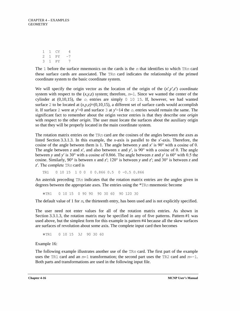
CHAPTER 4 – EXAMPLES GEOMETRY
Chapter 4-16 MCNP User’s Manual
1 1 CY 4 2 1 PY −7 3 1 PY 7
The 1 before the surface mnemonics on the cards is the n that identifies to which TRn card these surface cards are associated. The TRn card indicates the relationship of the primed coordinate system to the basic coordinate system.
We will specify the origin vector as the location of the origin of the (x′,y′,z′) coordinate system with respect to the (x,y,z) system; therefore, m=1. Since we wanted the center of the cylinder at (0,10,15), the oi entries are simply 0 10 15. If, however, we had wanted surface 2 to be located at (x,y,z)=(0,10,15), a different set of surface cards would accomplish it. If surface 2 were at y′=0 and surface 3 at y′=14 the oi entries would remain the same. The significant fact to remember about the origin vector entries is that they describe one origin with respect to the other origin. The user must locate the surfaces about the auxiliary origin so that they will be properly located in the main coordinate system.
The rotation matrix entries on the TRn card are the cosines of the angles between the axes as listed Section 3.3.1.3. In this example, the x-axis is parallel to the x′-axis. Therefore, the cosine of the angle between them is 1. The angle between y and x′ is 90° with a cosine of 0. The angle between z and x′, and also between x and y′, is 90° with a cosine of 0. The angle between y and y′ is 30° with a cosine of 0.866. The angle between z and y′ is 60° with 0.5 the cosine. Similarly, 90° is between x and z′; 120° is between y and z′; and 30° is between z and z′. The complete TRn card is
TR1 0 10 15 1 0 0 0 0.866 0.5 0 −0.5 0.866
An asterisk preceding TRn indicates that the rotation matrix entries are the angles given in degrees between the appropriate axes. The entries using the *TRn mnemonic become
∗TR1 0 10 15 0 90 90 90 30 60 90 120 30
The default value of 1 for m, the thirteenth entry, has been used and is not explicitly specified.
The user need not enter values for all of the rotation matrix entries. As shown in Section 3.3.1.3, the rotation matrix may be specified in any of five patterns. Pattern #1 was used above, but the simplest form for this example is pattern #4 because all the skew surfaces are surfaces of revolution about some axis. The complete input card then becomes
∗TR1 0 10 15 3J 90 30 60
Example 16:
The following example illustrates another use of the TRn card. The first part of the example uses the TR1 card and an m=1 transformation; the second part uses the TR2 card and m=-1. Both parts and transformations are used in the following input file.
CHAPTER 4 – EXAMPLES
GEOMETRY
MCNP User’s Manual Chapter 4-17
EXAMPLE OF SURFACE TRANSFORMATIONS 2 0 -4 3 -5 6 0 -14 -13 : -15 41 -42
3 1 PX -14 4 1 X -14 10 0 12 14 10 5 1 PX 14 13 2 SX -15 70 14 2 CX 30 15 2 Y 75 0 30 16 41 2 PY 0 42 2 PY 75
TR1 20 31 37 0.223954 0.358401 0.906308 TR2 -250 -100 -65 0.675849 0.669131 0.309017 J J 0.918650 J J -0.246152 -1 imp:n 1 1 SDEF PRINT NPS 50
Case 1: TR1 and m=1
Cell 2 is bounded by the plane surfaces 3 and 5 and the spheroid surface 4, which is a surface of revolution about the skew axis x′ in Figure 4-27.
CHAPTER 4 – EXAMPLES GEOMETRY
Chapter 4-18 MCNP User’s Manual
Figure 4-27. A tilted barrel as seen from three views.
To get the coefficients of surfaces 3, 4, and 5, define the x′-axis as shown in the drawings. (Because the surfaces are surfaces of revolution about the x′-axis, the orientation of the y′- and z′-axes does not matter.) Then set up cell 2 and its surfaces with coefficients defined in the x′y′z′ coordinate system.
On the TR1 card, the origin vector is the location of the origin of the x′y′z′ coordinate system with respect to the main xyz system of the problem. The pattern #4 in Section 3.3.1.3 is appropriate since the surfaces are all surfaces of revolution about the x′-axis. The components of one vector of the transformation matrix are the cosines of the angles between x′ and the x-, y-, and z-axes. They are obtained from spherical trigonometry as shown in Figure 4-28.
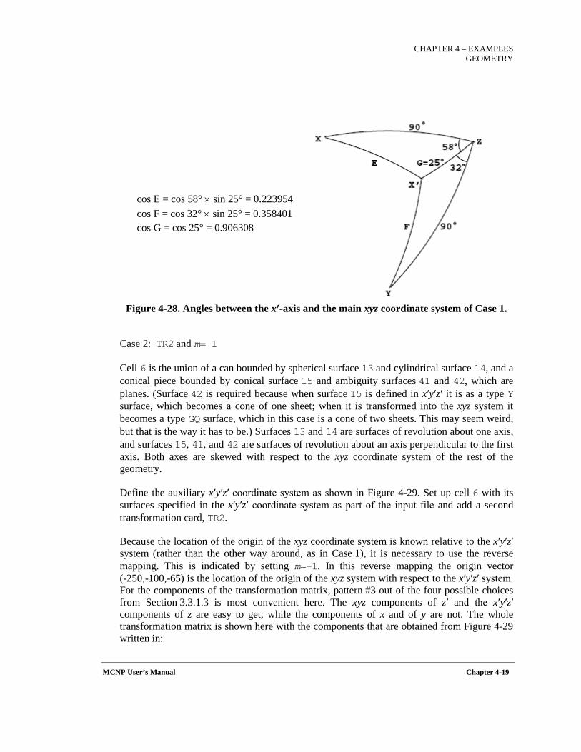
CHAPTER 4 – EXAMPLES
GEOMETRY
MCNP User’s Manual Chapter 4-19
cos E = cos 58° × sin 25° = 0.223954 cos F = cos 32° × sin 25° = 0.358401 cos G = cos 25° = 0.906308
Figure 4-28. Angles between the x′-axis and the main xyz coordinate system of Case 1.
Case 2: TR2 and m=-1
Cell 6 is the union of a can bounded by spherical surface 13 and cylindrical surface 14, and a conical piece bounded by conical surface 15 and ambiguity surfaces 41 and 42, which are planes. (Surface 42 is required because when surface 15 is defined in x′y′z′ it is as a type Y surface, which becomes a cone of one sheet; when it is transformed into the xyz system it becomes a type GQ surface, which in this case is a cone of two sheets. This may seem weird, but that is the way it has to be.) Surfaces 13 and 14 are surfaces of revolution about one axis, and surfaces 15, 41, and 42 are surfaces of revolution about an axis perpendicular to the first axis. Both axes are skewed with respect to the xyz coordinate system of the rest of the geometry.
Define the auxiliary x′y′z′ coordinate system as shown in Figure 4-29. Set up cell 6 with its surfaces specified in the x′y′z′ coordinate system as part of the input file and add a second transformation card, TR2.
Because the location of the origin of the xyz coordinate system is known relative to the x′y′z′ system (rather than the other way around, as in Case 1), it is necessary to use the reverse mapping. This is indicated by setting m=-1. In this reverse mapping the origin vector (-250,-100,-65) is the location of the origin of the xyz system with respect to the x′y′z′ system. For the components of the transformation matrix, pattern #3 out of the four possible choices from Section 3.3.1.3 is most convenient here. The xyz components of z′ and the x′y′z′ components of z are easy to get, while the components of x and of y are not. The whole transformation matrix is shown here with the components that are obtained from Figure 4-29 written in:
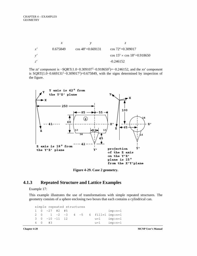
CHAPTER 4 – EXAMPLES GEOMETRY
Chapter 4-20 MCNP User’s Manual
x y z
x′ 0.675849 cos 48°=0.669131 cos 72°=0.309017
y′ cos 15° × cos 18°=0.918650
z′ -0.246152
The zz′ component is −SQRT(1.0−0.3091072−0.9186502)=−0.246152, and the xx′ component is SQRT(1.0−0.6691312−0.3090172)=0.675849, with the signs determined by inspection of the figure.
Figure 4-29. Case 2 geometry.
4.1.3 Repeated Structure and Lattice Examples
Example 17:
This example illustrates the use of transformations with simple repeated structures. The geometry consists of a sphere enclosing two boxes that each contains a cylindrical can.
simple repeated structures 1 0 -27 #2 #5 imp:n=1 2 0 1 -2 -3 4 -5 6 fill=1 imp:n=1 3 0 -10 -11 12 u=1 imp:n=1 4 0 #3 u=1 imp:n=1
CHAPTER 4 – EXAMPLES
GEOMETRY
MCNP User’s Manual Chapter 4-21
5 like 2 but trcl=3 7 0 27 imp:n=0
1 px -3 2 px 3 3 py 3 4 py -3 5 pz 4.7 6 pz -4.7 10 cz 1 11 pz 4.5 12 pz -4.5 27 s 3.5 3.5 0 11
sdef pos 3.5 3.5 0 f2:n 1 tr3* 7 7 0 40 130 90 50 40 90 90 90 0 nps 10000
The geometric structure of this example can be displayed using the plot feature in MCNP6. Specifically, Figure 4-30 can be obtained by launching the plotter:
mcnp6 ip i=<input file name>
clicking the lower left hand corner of the plot window (“click here or picture or window”) and entering the following three settings:
b 1 0 0 0 1 0
ex 11
or 3.5 3.5 0
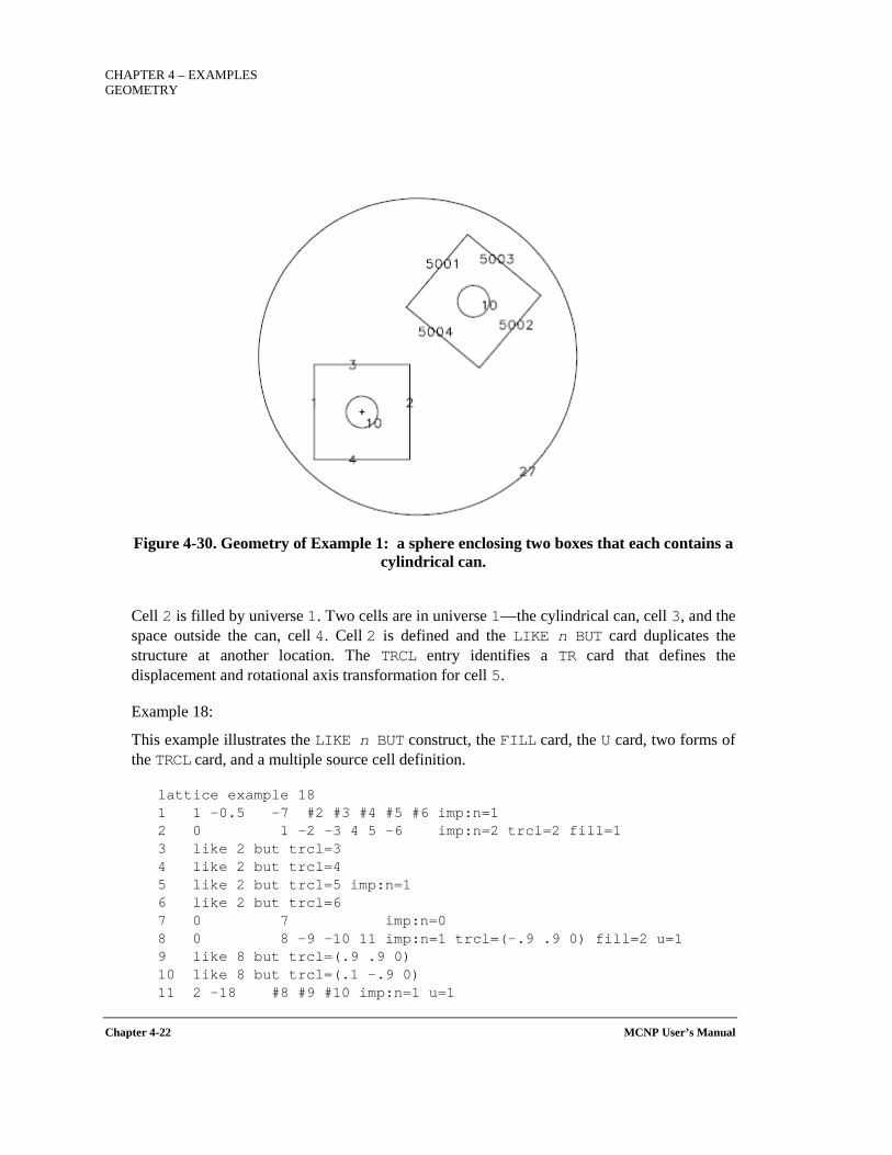
CHAPTER 4 – EXAMPLES GEOMETRY
Chapter 4-22 MCNP User’s Manual
Figure 4-30. Geometry of Example 1: a sphere enclosing two boxes that each contains a
cylindrical can.
Cell 2 is filled by universe 1. Two cells are in universe 1—the cylindrical can, cell 3, and the space outside the can, cell 4. Cell 2 is defined and the LIKE n BUT card duplicates the structure at another location. The TRCL entry identifies a TR card that defines the displacement and rotational axis transformation for cell 5.
Example 18:
This example illustrates the LIKE n BUT construct, the FILL card, the U card, two forms of the TRCL card, and a multiple source cell definition.
lattice example 18 1 1 -0.5 -7 #2 #3 #4 #5 #6 imp:n=1 2 0 1 -2 -3 4 5 -6 imp:n=2 trcl=2 fill=1 3 like 2 but trcl=3 4 like 2 but trcl=4 5 like 2 but trcl=5 imp:n=1 6 like 2 but trcl=6 7 0 7 imp:n=0 8 0 8 -9 -10 11 imp:n=1 trcl=(-.9 .9 0) fill=2 u=1 9 like 8 but trcl=(.9 .9 0) 10 like 8 but trcl=(.1 -.9 0) 11 2 -18 #8 #9 #10 imp:n=1 u=1
CHAPTER 4 – EXAMPLES
GEOMETRY
MCNP User’s Manual Chapter 4-23
12 2 -18 -12 imp:n=1 trcl=(-.3 .3 0) u=2 13 like 12 but trcl=( .3 .3 0) 14 like 12 but trcl=( .3 -.3 0) 15 like 12 but trcl=(-.3 -.3 0) 16 1 -0.5 #12 #13 #14 #15 u=2 imp:n=1
1 px -2 2 py 2 3 px 2 4 py -2 5 pz -2 6 pz 2 7 so 15 8 px -0.7 9 py 0.7 10 px 0.7 11 py -0.7 12 cz 0.1
sdef erg=d1 cel=d2:d3:0 rad=d5 ext=d6 axs=0 0 1 pos=d7 # si1 sp1 sb1 1 0 0 3 0.22 0.05 4 0.08 0.05 5 0.25 0.1 6 0.18 0.1 7 0.07 0.2 8 0.1 0.2 9 0.05 0.1 11 0.05 0.2 si2 L 2 3 4 5 6 sp2 1 1 1 1 1 si3 L 8 9 10 sp3 1 1 1 si5 0 0.1 sp5 -21 1 si6 -2 2 sp6 0 1 si7 L 0.3 0.3 0 0.3 -0.3 0 -0.3 0.3 0 -0.3 -0.3 0 sp7 1 1 1 1 m1 6000 1 m2 92235 1 drxs tr2 -6 7 1.2 tr3 7 6 1.1 tr4 8 -5 1.4
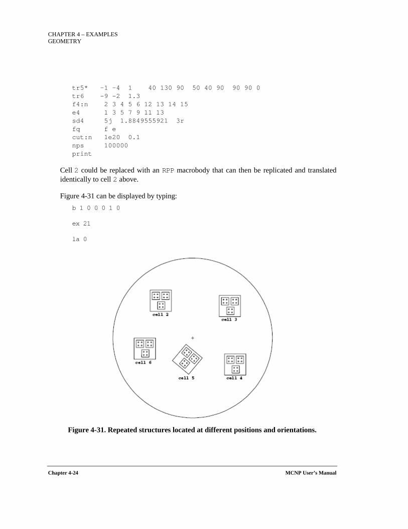
CHAPTER 4 – EXAMPLES GEOMETRY
Chapter 4-24 MCNP User’s Manual
tr5* -1 -4 1 40 130 90 50 40 90 90 90 0 tr6 -9 -2 1.3 f4:n 2 3 4 5 6 12 13 14 15 e4 1 3 5 7 9 11 13 sd4 5j 1.8849555921 3r fq f e cut:n 1e20 0.1 nps 100000 print
Cell 2 could be replaced with an RPP macrobody that can then be replicated and translated identically to cell 2 above.
Figure 4-31 can be displayed by typing: b 1 0 0 0 1 0
ex 21
la 0
Figure 4-31. Repeated structures located at different positions and orientations.
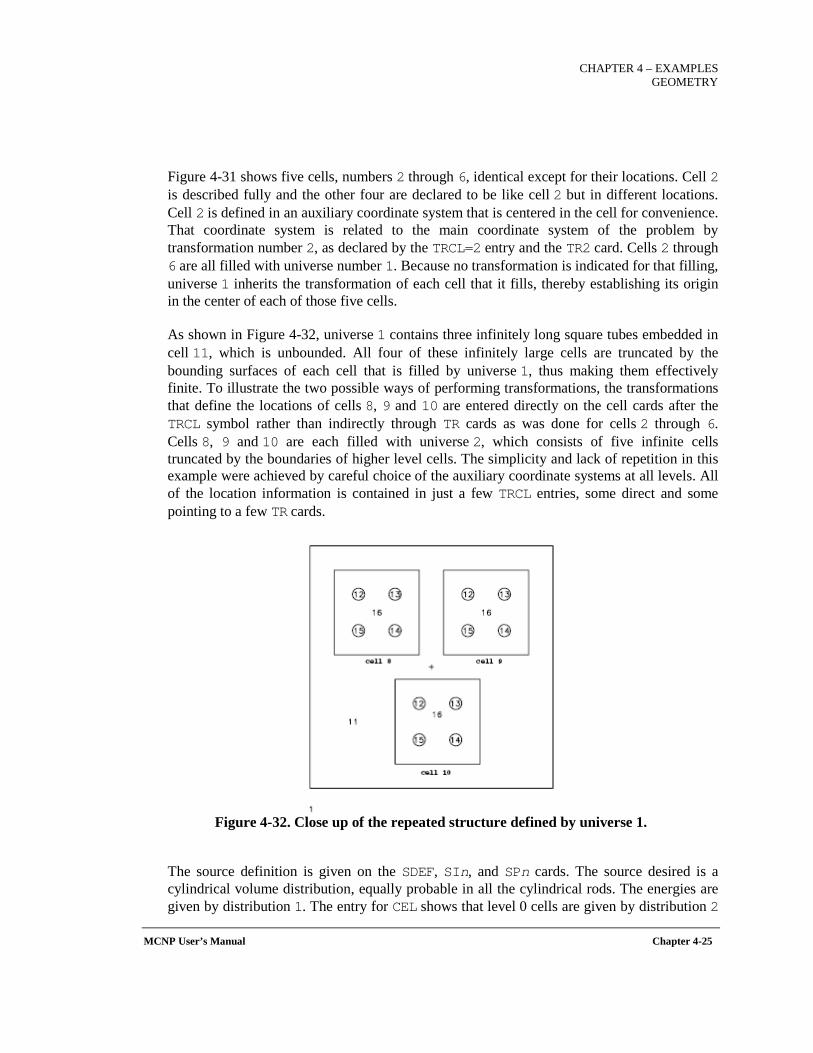
CHAPTER 4 – EXAMPLES
GEOMETRY
MCNP User’s Manual Chapter 4-25
Figure 4-31 shows five cells, numbers 2 through 6, identical except for their locations. Cell 2 is described fully and the other four are declared to be like cell 2 but in different locations. Cell 2 is defined in an auxiliary coordinate system that is centered in the cell for convenience. That coordinate system is related to the main coordinate system of the problem by transformation number 2, as declared by the TRCL=2 entry and the TR2 card. Cells 2 through 6 are all filled with universe number 1. Because no transformation is indicated for that filling, universe 1 inherits the transformation of each cell that it fills, thereby establishing its origin in the center of each of those five cells.
As shown in Figure 4-32, universe 1 contains three infinitely long square tubes embedded in cell 11, which is unbounded. All four of these infinitely large cells are truncated by the bounding surfaces of each cell that is filled by universe 1, thus making them effectively finite. To illustrate the two possible ways of performing transformations, the transformations that define the locations of cells 8, 9 and 10 are entered directly on the cell cards after the TRCL symbol rather than indirectly through TR cards as was done for cells 2 through 6. Cells 8, 9 and 10 are each filled with universe 2, which consists of five infinite cells truncated by the boundaries of higher level cells. The simplicity and lack of repetition in this example were achieved by careful choice of the auxiliary coordinate systems at all levels. All of the location information is contained in just a few TRCL entries, some direct and some pointing to a few TR cards.
Figure 4-32. Close up of the repeated structure defined by universe 1.
The source definition is given on the SDEF, SIn, and SPn cards. The source desired is a cylindrical volume distribution, equally probable in all the cylindrical rods. The energies are given by distribution 1. The entry for CEL shows that level 0 cells are given by distribution 2
CHAPTER 4 – EXAMPLES GEOMETRY
Chapter 4-26 MCNP User’s Manual
and level 1 cells by distribution 3. The zero means that cells are searched for at level 2 and also that the sampled position and direction will apply to the universe indicated by the entry just preceding the first entry that is ≤0. In this case the position and direction will be defined in the coordinate system of the cell sampled by distribution 3 at level 1. The SI2 card lists all the cells at level 0 that will contain the source. The SP2 entries indicate equally probable source distributions. The values in SI3 are the cells in level 1, and the positions on the SI7 card are given in the coordinates of this level. A cylindrical volume distribution is specified by RAD, EXT, AXS, and POS. The cylinder is centered about the origin, with a radius of 0.1 (SI5) and a length of 4 (SI6, from -2 to 2). The four sets of entries on the SI7 card are the origins of the four cylinders of cells 12–15. These parameters describe exactly the four cells 12–15.
Example 19:
This simple example illustrates the use of the FILL, U, and LAT cards to create an object within several cells of a lattice. A cylinder contains a square lattice and the cells in the inner 3×3 array of that lattice each contain a small cylinder.
simple lattice 1 0 -1 fill=1 imp:n=1 2 0 -301 302 -303 304 lat=1 u=1 imp:n=1 fill -2:2 -2:2 0:0 1 1 1 1 1 1 2 2 2 1 1 2 2 2 1 1 2 2 2 1 1 1 1 1 1 3 0 -10 u=2 imp:n=1 4 0 #3 u=2 imp:n=1 5 0 1 imp:n=0
1 cz 45 10 cz 8 301 px 10 302 px -10 303 py 10 304 py -10
sdef mode n nps 5000
The resulting geometry is shown in Figure 4-33. Cell 1 is the interior of the cylinder, and cell 5 is everything outside (all surfaces are infinite in the z direction). Cell 1 is filled by universe 1. Cell 2 is defined to be in universe 1. Surfaces 301–304 define the dimensions of the square lattice:
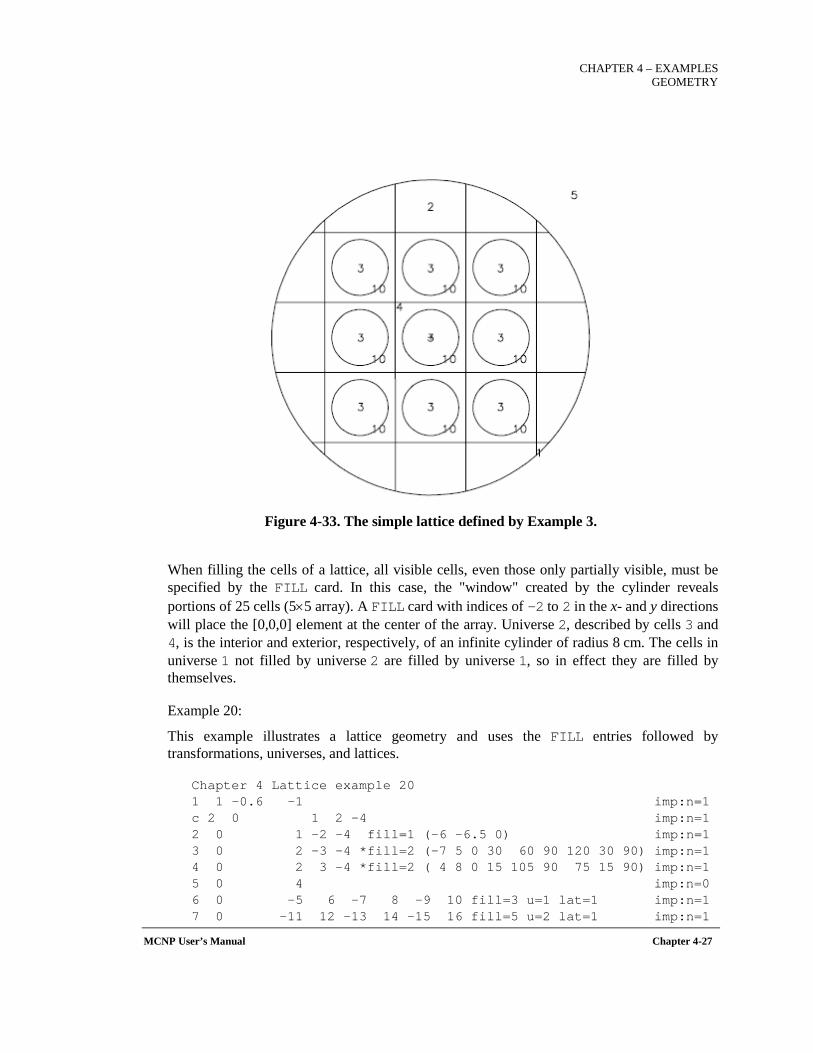
CHAPTER 4 – EXAMPLES
GEOMETRY
MCNP User’s Manual Chapter 4-27
Figure 4-33. The simple lattice defined by Example 3.
When filling the cells of a lattice, all visible cells, even those only partially visible, must be specified by the FILL card. In this case, the "window" created by the cylinder reveals portions of 25 cells (5×5 array). A FILL card with indices of -2 to 2 in the x- and y directions will place the [0,0,0] element at the center of the array. Universe 2, described by cells 3 and 4, is the interior and exterior, respectively, of an infinite cylinder of radius 8 cm. The cells in universe 1 not filled by universe 2 are filled by universe 1, so in effect they are filled by themselves.
Example 20:
This example illustrates a lattice geometry and uses the FILL entries followed by transformations, universes, and lattices.
Chapter 4 Lattice example 20 1 1 -0.6 -1 imp:n=1 c 2 0 1 2 -4 imp:n=1 2 0 1 -2 -4 fill=1 (-6 -6.5 0) imp:n=1 3 0 2 -3 -4 *fill=2 (-7 5 0 30 60 90 120 30 90) imp:n=1 4 0 2 3 -4 *fill=2 ( 4 8 0 15 105 90 75 15 90) imp:n=1 5 0 4 imp:n=0 6 0 -5 6 -7 8 -9 10 fill=3 u=1 lat=1 imp:n=1 7 0 -11 12 -13 14 -15 16 fill=5 u=2 lat=1 imp:n=1
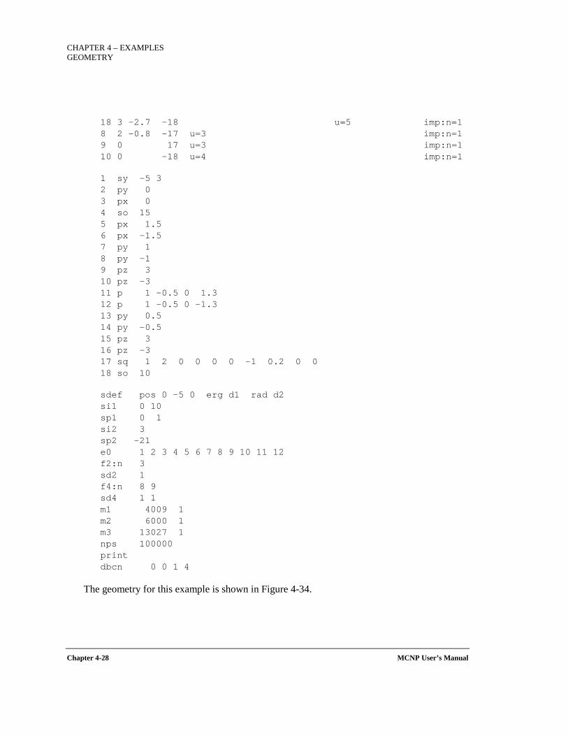
CHAPTER 4 – EXAMPLES GEOMETRY
Chapter 4-28 MCNP User’s Manual
18 3 -2.7 -18 u=5 imp:n=1 8 2 -0.8 -17 u=3 imp:n=1 9 0 17 u=3 imp:n=1 10 0 -18 u=4 imp:n=1
1 sy -5 3 2 py 0 3 px 0 4 so 15 5 px 1.5 6 px -1.5 7 py 1 8 py -1 9 pz 3 10 pz -3 11 p 1 -0.5 0 1.3 12 p 1 -0.5 0 -1.3 13 py 0.5 14 py -0.5 15 pz 3 16 pz -3 17 sq 1 2 0 0 0 0 -1 0.2 0 0 18 so 10
sdef pos 0 -5 0 erg d1 rad d2 si1 0 10 sp1 0 1 si2 3 sp2 -21 e0 1 2 3 4 5 6 7 8 9 10 11 12 f2:n 3 sd2 1 f4:n 8 9 sd4 1 1 m1 4009 1 m2 6000 1 m3 13027 1 nps 100000 print dbcn 0 0 1 4
The geometry for this example is shown in Figure 4-34.
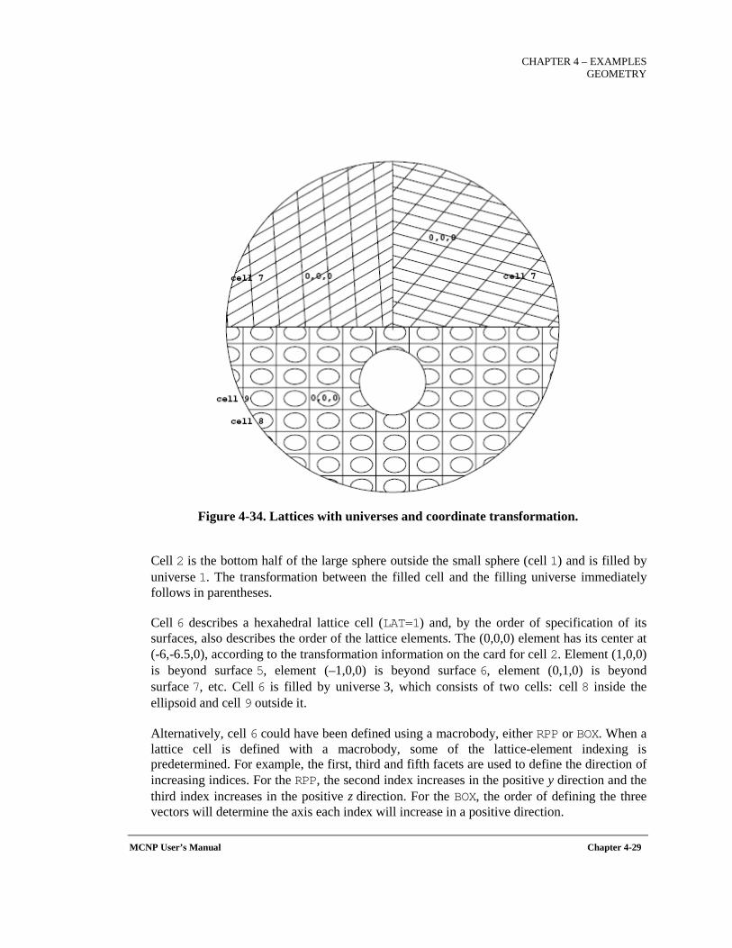
CHAPTER 4 – EXAMPLES
GEOMETRY
MCNP User’s Manual Chapter 4-29
Figure 4-34. Lattices with universes and coordinate transformation.
Cell 2 is the bottom half of the large sphere outside the small sphere (cell 1) and is filled by universe 1. The transformation between the filled cell and the filling universe immediately follows in parentheses.
Cell 6 describes a hexahedral lattice cell (LAT=1) and, by the order of specification of its surfaces, also describes the order of the lattice elements. The (0,0,0) element has its center at (-6,-6.5,0), according to the transformation information on the card for cell 2. Element (1,0,0) is beyond surface 5, element (–1,0,0) is beyond surface 6, element (0,1,0) is beyond surface 7, etc. Cell 6 is filled by universe 3, which consists of two cells: cell 8 inside the ellipsoid and cell 9 outside it.
Alternatively, cell 6 could have been defined using a macrobody, either RPP or BOX. When a lattice cell is defined with a macrobody, some of the lattice-element indexing is predetermined. For example, the first, third and fifth facets are used to define the direction of increasing indices. For the RPP, the second index increases in the positive y direction and the third index increases in the positive z direction. For the BOX, the order of defining the three vectors will determine the axis each index will increase in a positive direction.
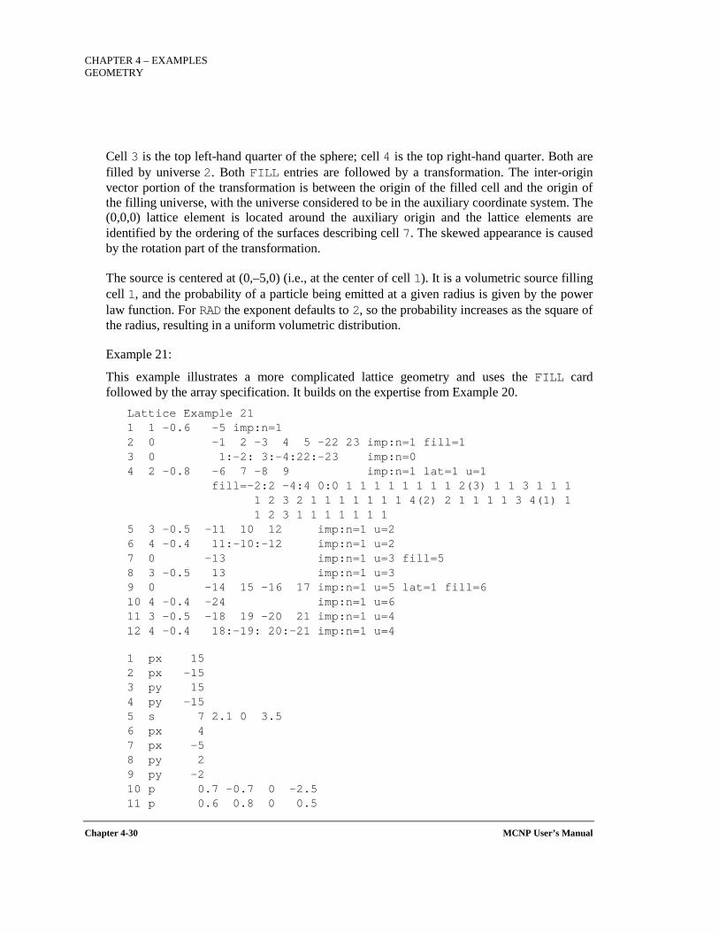
CHAPTER 4 – EXAMPLES GEOMETRY
Chapter 4-30 MCNP User’s Manual
Cell 3 is the top left-hand quarter of the sphere; cell 4 is the top right-hand quarter. Both are filled by universe 2. Both FILL entries are followed by a transformation. The inter-origin vector portion of the transformation is between the origin of the filled cell and the origin of the filling universe, with the universe considered to be in the auxiliary coordinate system. The (0,0,0) lattice element is located around the auxiliary origin and the lattice elements are identified by the ordering of the surfaces describing cell 7. The skewed appearance is caused by the rotation part of the transformation.
The source is centered at (0,–5,0) (i.e., at the center of cell 1). It is a volumetric source filling cell 1, and the probability of a particle being emitted at a given radius is given by the power law function. For RAD the exponent defaults to 2, so the probability increases as the square of the radius, resulting in a uniform volumetric distribution.
Example 21:
This example illustrates a more complicated lattice geometry and uses the FILL card followed by the array specification. It builds on the expertise from Example 20.
Lattice Example 21 1 1 -0.6 -5 imp:n=1 2 0 -1 2 -3 4 5 -22 23 imp:n=1 fill=1 3 0 1:-2: 3:-4:22:-23 imp:n=0 4 2 -0.8 -6 7 -8 9 imp:n=1 lat=1 u=1 fill=-2:2 -4:4 0:0 1 1 1 1 1 1 1 1 2(3) 1 1 3 1 1 1 1 2 3 2 1 1 1 1 1 1 1 4(2) 2 1 1 1 1 3 4(1) 1 1 2 3 1 1 1 1 1 1 1 5 3 -0.5 -11 10 12 imp:n=1 u=2 6 4 -0.4 11:-10:-12 imp:n=1 u=2 7 0 -13 imp:n=1 u=3 fill=5 8 3 -0.5 13 imp:n=1 u=3 9 0 -14 15 -16 17 imp:n=1 u=5 lat=1 fill=6 10 4 -0.4 -24 imp:n=1 u=6 11 3 -0.5 -18 19 -20 21 imp:n=1 u=4 12 4 -0.4 18:-19: 20:-21 imp:n=1 u=4
1 px 15 2 px -15 3 py 15 4 py -15 5 s 7 2.1 0 3.5 6 px 4 7 px -5 8 py 2 9 py -2 10 p 0.7 -0.7 0 -2.5 11 p 0.6 0.8 0 0.5
CHAPTER 4 – EXAMPLES
GEOMETRY
MCNP User’s Manual Chapter 4-31
12 py -1 13 x -4.5 0 -0.5 1.7 3.5 0 14 px 1.6 15 px -1.4 16 py 1 17 py -1.2 18 px 3 19 px -3 20 py 0.5 21 py -0.6 22 pz 6 23 pz -7 24 so 10
sdef erg d1 pos 7 2 0 cel=1 rad d2 si2 3.6 si1 0 10 sp1 0 1 f4:n 10 e4 1 3 5 7 9 11 m1 4009 1 m2 6000 1 m3 13027 1 m4 1001 2 8016 1 nps 100000 dbcn 0 0 1 4 *tr1 0 0 0 10 80 90 100 10 90 *tr2 1 0 0 2 88 90 92 2 90 tr3 3 0 0 vol 1 11r print
This example has three "main" cells: cell 1 is inside surface 5, cell 3 is the outside world, and cell 2 is the large square (excluding cell 1) that is filled with a lattice, some of whose elements are filled with three different universes. A schematic of the geometry is given in Figure 4-35.
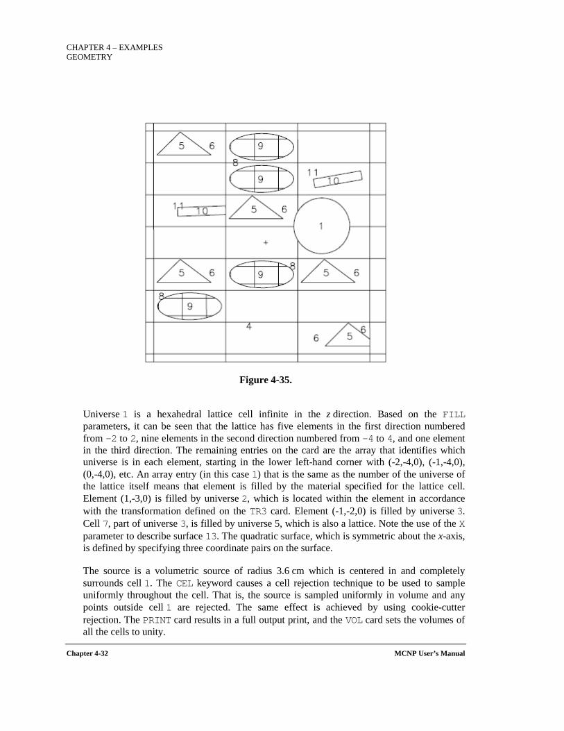
CHAPTER 4 – EXAMPLES GEOMETRY
Chapter 4-32 MCNP User’s Manual
Figure 4-35.
Universe 1 is a hexahedral lattice cell infinite in the z direction. Based on the FILL parameters, it can be seen that the lattice has five elements in the first direction numbered from -2 to 2, nine elements in the second direction numbered from -4 to 4, and one element in the third direction. The remaining entries on the card are the array that identifies which universe is in each element, starting in the lower left-hand corner with (-2,-4,0), (-1,-4,0), (0,-4,0), etc. An array entry (in this case 1) that is the same as the number of the universe of the lattice itself means that element is filled by the material specified for the lattice cell. Element (1,-3,0) is filled by universe 2, which is located within the element in accordance with the transformation defined on the TR3 card. Element (-1,-2,0) is filled by universe 3. Cell 7, part of universe 3, is filled by universe 5, which is also a lattice. Note the use of the X parameter to describe surface 13. The quadratic surface, which is symmetric about the x-axis, is defined by specifying three coordinate pairs on the surface.
The source is a volumetric source of radius 3.6 cm which is centered in and completely surrounds cell 1. The CEL keyword causes a cell rejection technique to be used to sample uniformly throughout the cell. That is, the source is sampled uniformly in volume and any points outside cell 1 are rejected. The same effect is achieved by using cookie-cutter rejection. The PRINT card results in a full output print, and the VOL card sets the volumes of all the cells to unity.
CHAPTER 4 – EXAMPLES
GEOMETRY
MCNP User’s Manual Chapter 4-33
Example 22:
This example primarily illustrates a fairly complex source description in a lattice geometry. The geometry consists of two "main" cells, each filled with a different lattice.
Lattice Example 22 1 0 1:-3:-4:5:6:-7 imp:n=0 2 0 -2 3 4 -5 -6 7 imp:n=1 fill=1 (-25 0 0) 3 0 -1 2 4 -5 -6 7 imp:n=1 fill=2 (0 -20 0) 4 0 -11 12 -14 13 imp:n=1 lat=1 u=1 fill=-1:1 -1:1 0:0 3 8r 5 3 -1.0 -15 2 -18 17 imp:n=1 lat=1 u=2 fill=0:1 0:3 0:0 4 4 4(5 0 0) 4 0 5 4 4 6 1 -0.9 21:-22:-23:24 imp:n=1 u=3 7 1 -0.9 19 imp:n=1 u=4 8 2 -18 -21 22 23 -24 imp:n=1 u=3 9 1 -0.9 20(31:-32:-33:34) imp:n=1 u=5 11 2 -18 -19 imp:n=1 u=4 13 2 -18 -20 imp:n=1 u=5 15 2 -18 -31 32 33 -34 imp:n=1 u=5
1 px 50 2 px 0 3 px -50 4 py -20 5 py 20 6 pz 60 7 pz -60 11 px 8.334 12 px -8.334 13 py -6.67 14 py 6.67 15 px 25 17 py 0 18 py 10 19 c/z 10 5 3 20 c/z 10 5 3 21 px 4 22 px -4 23 py -3 24 py 3 31 px 20 32 px 16 33 py 3 34 py 6
m1 6000 0.4 8016 0.2 11023 0.2 29000 0.2 m2 92238 0.98 92235 0.02
CHAPTER 4 – EXAMPLES GEOMETRY
Chapter 4-34 MCNP User’s Manual
m3 1001 1 sdef erg fcel d1 x fcel d11 y fcel d13 z fcel d15 cel d6 rad fcel d17 ext fcel d19 pos fcel d21 axs fcel d23 ds1 s d2 d3 d4 d5 sp2 -2 1.2 sp3 -2 1.3 sp4 -2 1.4 sp5 -2 1.42 si6 s d7 d8 d9 d10 sp6 0.65 0.2 0.1 0.05 si7 l 2:4:8 sp7 1 si8 l 3:5(0 0 0):11 3:5(1 0 0):11 3:5(0 1 0):11 3:5(1 1 0):11 3:5(0 2 0):11 3:5(0 3 0):11 3:5(1 3 0):11 sp8 1 1 1 1 1 1 1 si9 l 3:5(1 2 0):13 sp9 1 si10 l 3:5(1 2 0):15 sp10 1 ds11 s d12 0 0 d25 si12 -4 4 sp12 0 1 ds13 s d14 0 0 d26 si14 -3 3 sp14 0 1 ds15 s d16 0 0 d16 si16 -60 60 sp16 0 1 ds17 s 0 d18 d18 0 si18 0 3 sp18 -21 1 ds19 s 0 d20 d20 0 si20 -60 60 sp20 0 1 ds21 s 0 d22 d22 0 si22 l 10 5 0 sp22 1 ds23 s 0 d24 d24 0 si24 l 0 0 1 sp24 1 si25 16 20 sp25 0 1 si26 3 6 sp26 0 1 f2:n 1 e2 0.1 1 20
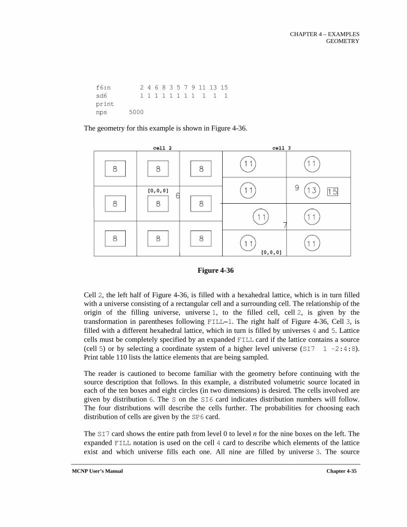
CHAPTER 4 – EXAMPLES
GEOMETRY
MCNP User’s Manual Chapter 4-35
f6:n 2 4 6 8 3 5 7 9 11 13 15 sd6 1 1 1 1 1 1 1 1 1 1 1 print nps 5000
The geometry for this example is shown in Figure 4-36.
Figure 4-36
Cell 2, the left half of Figure 4-36, is filled with a hexahedral lattice, which is in turn filled with a universe consisting of a rectangular cell and a surrounding cell. The relationship of the origin of the filling universe, universe 1, to the filled cell, cell 2, is given by the transformation in parentheses following FILL=1. The right half of Figure 4-36, Cell 3, is filled with a different hexahedral lattice, which in turn is filled by universes 4 and 5. Lattice cells must be completely specified by an expanded FILL card if the lattice contains a source (cell 5) or by selecting a coordinate system of a higher level universe (SI7 1 –2:4:8). Print table 110 lists the lattice elements that are being sampled.
The reader is cautioned to become familiar with the geometry before continuing with the source description that follows. In this example, a distributed volumetric source located in each of the ten boxes and eight circles (in two dimensions) is desired. The cells involved are given by distribution 6. The S on the SI6 card indicates distribution numbers will follow. The four distributions will describe the cells further. The probabilities for choosing each distribution of cells are given by the SP6 card.
The SI7 card shows the entire path from level 0 to level n for the nine boxes on the left. The expanded FILL notation is used on the cell 4 card to describe which elements of the lattice exist and which universe fills each one. All nine are filled by universe 3. The source
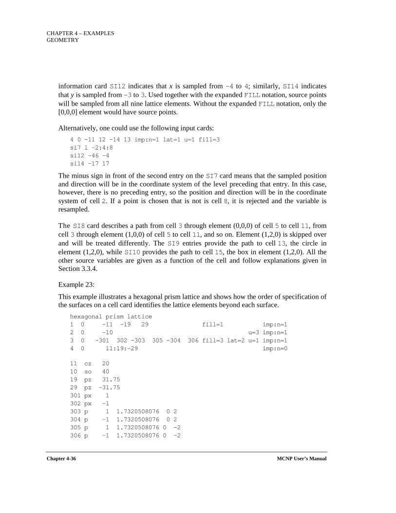
CHAPTER 4 – EXAMPLES GEOMETRY
Chapter 4-36 MCNP User’s Manual
information card SI12 indicates that x is sampled from -4 to 4; similarly, SI14 indicates that y is sampled from -3 to 3. Used together with the expanded FILL notation, source points will be sampled from all nine lattice elements. Without the expanded FILL notation, only the [0,0,0] element would have source points.
Alternatively, one could use the following input cards: 4 0 -11 12 –14 13 imp:n=1 lat=1 u=1 fill=3 si7 l –2:4:8 si12 –46 –4 si14 –17 17
The minus sign in front of the second entry on the SI7 card means that the sampled position and direction will be in the coordinate system of the level preceding that entry. In this case, however, there is no preceding entry, so the position and direction will be in the coordinate system of cell 2. If a point is chosen that is not is cell 8, it is rejected and the variable is resampled.
The SI8 card describes a path from cell 3 through element (0,0,0) of cell 5 to cell 11, from cell 3 through element (1,0,0) of cell 5 to cell 11, and so on. Element (1,2,0) is skipped over and will be treated differently. The SI9 entries provide the path to cell 13, the circle in element (1,2,0), while SI10 provides the path to cell 15, the box in element (1,2,0). All the other source variables are given as a function of the cell and follow explanations given in Section 3.3.4.
Example 23:
This example illustrates a hexagonal prism lattice and shows how the order of specification of the surfaces on a cell card identifies the lattice elements beyond each surface.
hexagonal prism lattice 1 0 -11 -19 29 fill=1 imp:n=1 2 0 -10 u=3 imp:n=1 3 0 -301 302 -303 305 -304 306 fill=3 lat=2 u=1 imp:n=1 4 0 11:19:-29 imp:n=0
11 cz 20 10 so 40 19 pz 31.75 29 pz -31.75 301 px 1 302 px -1 303 p 1 1.7320508076 0 2 304 p -1 1.7320508076 0 2 305 p 1 1.7320508076 0 -2 306 p -1 1.7320508076 0 -2
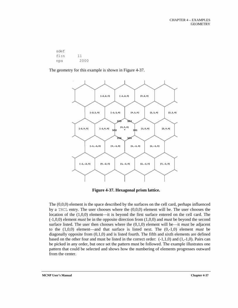
CHAPTER 4 – EXAMPLES
GEOMETRY
MCNP User’s Manual Chapter 4-37
sdef f1:n 11 nps 2000
The geometry for this example is shown in Figure 4-37.
Figure 4-37. Hexagonal prism lattice.
The (0,0,0) element is the space described by the surfaces on the cell card, perhaps influenced by a TRCL entry. The user chooses where the (0,0,0) element will be. The user chooses the location of the (1,0,0) element—it is beyond the first surface entered on the cell card. The (-1,0,0) element must be in the opposite direction from (1,0,0) and must be beyond the second surface listed. The user then chooses where the (0,1,0) element will be—it must be adjacent to the (1,0,0) element—and that surface is listed next. The (0,-1,0) element must be diagonally opposite from (0,1,0) and is listed fourth. The fifth and sixth elements are defined based on the other four and must be listed in the correct order: (-1,1,0) and (1,-1,0). Pairs can be picked in any order, but once set the pattern must be followed. The example illustrates one pattern that could be selected and shows how the numbering of elements progresses outward from the center.
CHAPTER 4 – EXAMPLES GEOMETRY
Chapter 4-38 MCNP User’s Manual
One of the most powerful uses of macrobodies is for the specification of hexagonal prisms. The example above can be simplified by using the RHP (also called HEX) macrobody as follows:
hexagonal prism lattice using macrobodies C Cell Cards 1 0 -2 fill=1 imp:n=1 2 0 -10 u=3 imp:n=1 3 0 -1 fill=3 lat=2 u=1 imp:n=1 4 0 2 imp:n=0
C Surface Cards 1 rhp 0 0 -31.75 0 0 63.5 2 0 0 2 rcc 0 0 -31.75 0 0 63.5 20 10 sph 0 0 0 40
sdef f1:n 2.1 nps 2000
Example 24:
This example demonstrates how the LIKE n BUT and TRCL cards can be used to create an array of non-identical objects within each cell of a lattice.
Lattice/Rotation example of pwrlat 1 0 -1 -19 29 fill=1 imp:n=1 2 2 -1 -301 302 -303 304 lat=1 u=1 imp:n=1 fill=-3:3 -3:3 0:0 1 1 1 1 1 1 1 1 1 2 2 2 1 1 1 2 2 2 2 2 1 1 2 2 2 2 2 1 1 2 2 2 2 2 1 1 1 2 2 2 1 1 1 1 1 1 1 1 1 3 1 -18 -10 u=2 imp:n=1 4 2 -1 #3 #5 #6 #7 #8 #9 #10 #11 #12 #13 #14 #15 #16 #17 #18 #19 #20 #21 #22 #23 #24 #25 #26 #27 #28 imp:n=1 u=2 5 like 3 but trcl=(-6 6 0) 6 like 3 but trcl=(-3 6 0) 7 like 3 but trcl=(0 6 0) 8 like 3 but trcl=(3 6 0) 9 like 3 but trcl=(6 6 0) 10 like 3 but trcl=(-6 3 0) 11 like 3 but trcl=(0 3 0) 12 like 3 but trcl=(6 3 0) 13 like 3 but trcl=(-6 0 0) 14 like 3 but trcl=(-3 0 0) 15 like 3 but trcl=(3 0 0) 16 like 3 but trcl=(6 0 0) 17 like 3 but trcl=(-6 -3 0) 18 like 3 but trcl=(0 -3 0)
CHAPTER 4 – EXAMPLES
GEOMETRY
MCNP User’s Manual Chapter 4-39
19 like 3 but trcl=(6 -3 0) 20 like 3 but trcl=(-6 -6 0) 21 like 3 but trcl=(-3 -6 0) 22 like 3 but trcl=(0 -6 0) 23 like 3 but trcl=(3 -6 0) 24 like 3 but trcl=(6 -6 0) 25 like 3 but mat=3 rho=-9 trcl=(-3 3 0) 26 like 25 but trcl=(3 3 0) 27 like 25 but trcl=(-3 -3 0) 28 like 25 but trcl=(3 -3 0) 50 0 1:19:-29 imp:n=0
1 cz 60 10 cz 1.4 19 pz 60 29 pz -60 301 px 10 302 px -10 303 py 10 304 py -10
kcode 1000 1 5 10 ksrc 0 0 0 m1 92235 0.02 92238 0.98 m2 1001 2 8016 1 m3 48000 1
A horizontal slice through this configuration is shown in Figure 4-38.
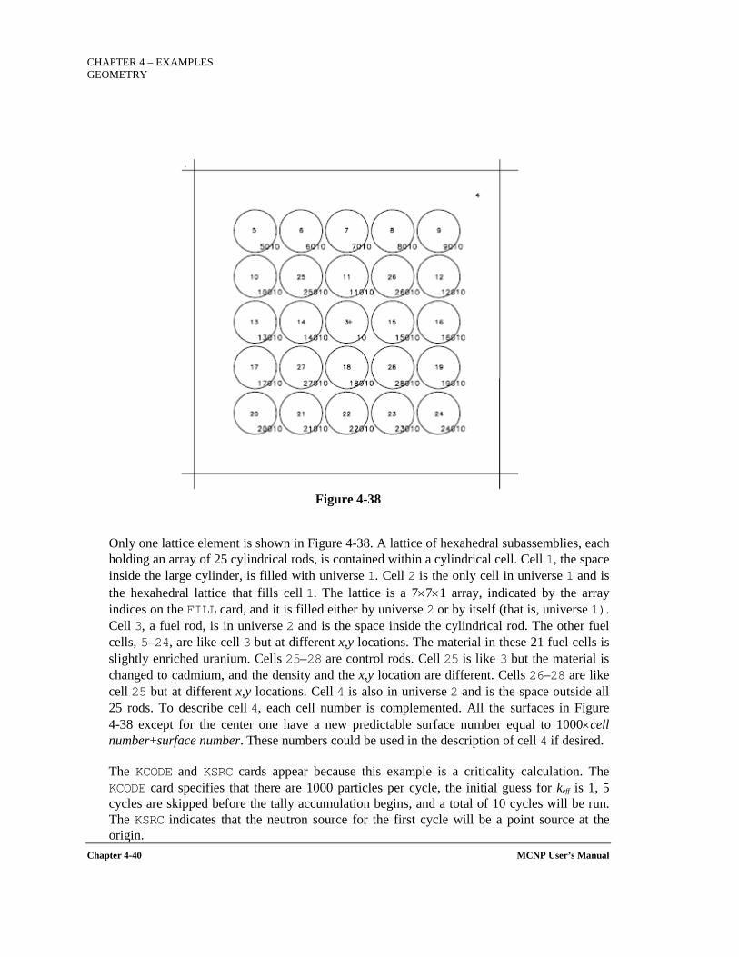
CHAPTER 4 – EXAMPLES GEOMETRY
Chapter 4-40 MCNP User’s Manual
Figure 4-38
Only one lattice element is shown in Figure 4-38. A lattice of hexahedral subassemblies, each holding an array of 25 cylindrical rods, is contained within a cylindrical cell. Cell 1, the space inside the large cylinder, is filled with universe 1. Cell 2 is the only cell in universe 1 and is the hexahedral lattice that fills cell 1. The lattice is a 7×7×1 array, indicated by the array indices on the FILL card, and it is filled either by universe 2 or by itself (that is, universe 1). Cell 3, a fuel rod, is in universe 2 and is the space inside the cylindrical rod. The other fuel cells, 5–24, are like cell 3 but at different x,y locations. The material in these 21 fuel cells is slightly enriched uranium. Cells 25–28 are control rods. Cell 25 is like 3 but the material is changed to cadmium, and the density and the x,y location are different. Cells 26–28 are like cell 25 but at different x,y locations. Cell 4 is also in universe 2 and is the space outside all 25 rods. To describe cell 4, each cell number is complemented. All the surfaces in Figure 4-38 except for the center one have a new predictable surface number equal to 1000×cell number+surface number. These numbers could be used in the description of cell 4 if desired.
The KCODE and KSRC cards appear because this example is a criticality calculation. The KCODE card specifies that there are 1000 particles per cycle, the initial guess for keff is 1, 5 cycles are skipped before the tally accumulation begins, and a total of 10 cycles will be run. The KSRC indicates that the neutron source for the first cycle will be a point source at the origin.
CHAPTER 4 – EXAMPLES
GEOMETRY
MCNP User’s Manual Chapter 4-41
4.1.4 Embedded Meshes: Structured and Unstructured In the following example, we first create a structured PARTISN-style geometry mesh and save it in LNK3DNT format. The cylindrical mesh consists of two materials in a checkerboard pattern that appears radially, axially, and azimuthally. After the LNK3DNT-format mesh file is created, we then embed the mesh in a new MCNP6 file.
Example 25 (Part 1): Generate a LNK3DNT rzt mesh w/ multiple materials c upper-inner 1 1 -18.7 -11 1 2 3 imp:n=1 2 2 -0.001 -11 1 -2 3 imp:n=1 3 1 -18.7 -11 -1 -2 3 imp:n=1 4 2 -0.001 -11 -1 2 3 imp:n=1 c upper-outer 6 2 -0.001 -10 11 1 2 3 imp:n=1 7 1 -18.7 -10 11 1 -2 3 imp:n=1 8 2 -0.001 -10 11 -1 -2 3 imp:n=1 9 1 -18.7 -10 11 -1 2 3 imp:n=1 c lower-inner 11 2 -0.001 -11 1 2 -3 imp:n=1 12 1 -18.7 -11 1 -2 -3 imp:n=1 13 2 -0.001 -11 -1 -2 -3 imp:n=1 14 1 -18.7 -11 -1 2 -3 imp:n=1 c lower-outer 16 1 -18.7 -10 11 1 2 -3 imp:n=1 17 2 -0.001 -10 11 1 -2 -3 imp:n=1 18 1 -18.7 -10 11 -1 -2 -3 imp:n=1 19 2 -0.001 -10 11 -1 2 -3 imp:n=1 c c outer void 20 0 10 imp:n=0 10 rcc 0. 0. -10. 0. 0. 20. 10. $ outer rcc 11 rcc 0 0 -10 0 0 20 5 $ inner rcc 1 py 0.0 2 px 0.0 3 pz 0.0 kcode 5000 1.0 50 250 ksrc 0.0 0.0 0.0 m1 92235.69c 1.0 m2 6012 1.0 dm1 92235 92235.50
CHAPTER 4 – EXAMPLES GEOMETRY
Chapter 4-42 MCNP User’s Manual
mesh geom cyl ref 0.0 0.0 0.0 origin 0.0 0.0 -10.0 $ bottom center of cylinder axs 0.0 0.0 1.0 vec 1.0 0.0 0.0 imesh 10 $ cylinder radius iints 2 $ 2 radial divisions jmesh 20 $ axial (z) length jints 2 $ 2 axial divisions kmesh 1 $ azimuth-single rotation (0-2pi) kints 4 $ 4 azimuthal divisions (0, pi/2, pi, 3pi/2, 2pi) dawwg xsec=ndilib points=10
In this example the MESH and DAWWG cards specify a cylindrical geometry with diameter and length of 20 cm. The cylinder mesh has two radial, two axial, and four azimuthal divisions, creating a total of eight mesh elements. The materials in each of the elements alternate, creating a checkerboard-like pattern throughout the cylinder. The use of the MESH keywords ORIGIN, AXS, and VEC ensure that the mesh aligns with the geometry —the bottom center of the mesh at (0,0,-10), the cylinder oriented along the z-axis, and the azimuthal plane along the positive x-axis. To create the LNK3DNT file, run MCNP6 with the M execution-line option using the example file above as the MCNP6 input and assign the LINKOUT file the arbitrary name "cyl.linkout."
Example 25 (Part 2):
Now we embed the mesh geometry into an MCNP6 input using inferred geometry cells (one for each material in the cyl.linkout file) and one inferred background cell.
RZT Test of checkerboard cylinder with lnk3dnt 11 3 -18.7 0 u=e10 imp:n=1 $ inferred geometry cell 12 4 -0.001 0 u=e10 imp:n=1 $ inferred geometry cell 13 0 0 u=e10 imp:n=1 $ inferred background cell 20 0 -1 fill=e10 imp:n=1 $ embedded mesh fill cell 99 0 1 imp:n=0 $ outside world 1 so 20 kcode 500 1.0 50 100 ksrc 1 1 5 1 -1 5 -1 -1 5 -1 1 5 5 5 5 5 -5 5 -5 -5 5 -5 5 5 1 1 -5 1 -1 -5 -1 -1 -5 -1 1 -5 5 5 -5 5 -5 -5 -5 -5 -5 -5 5 -5 m3 92235.69c 1.0 m4 6012 1.0 dm1 92235 92235.50
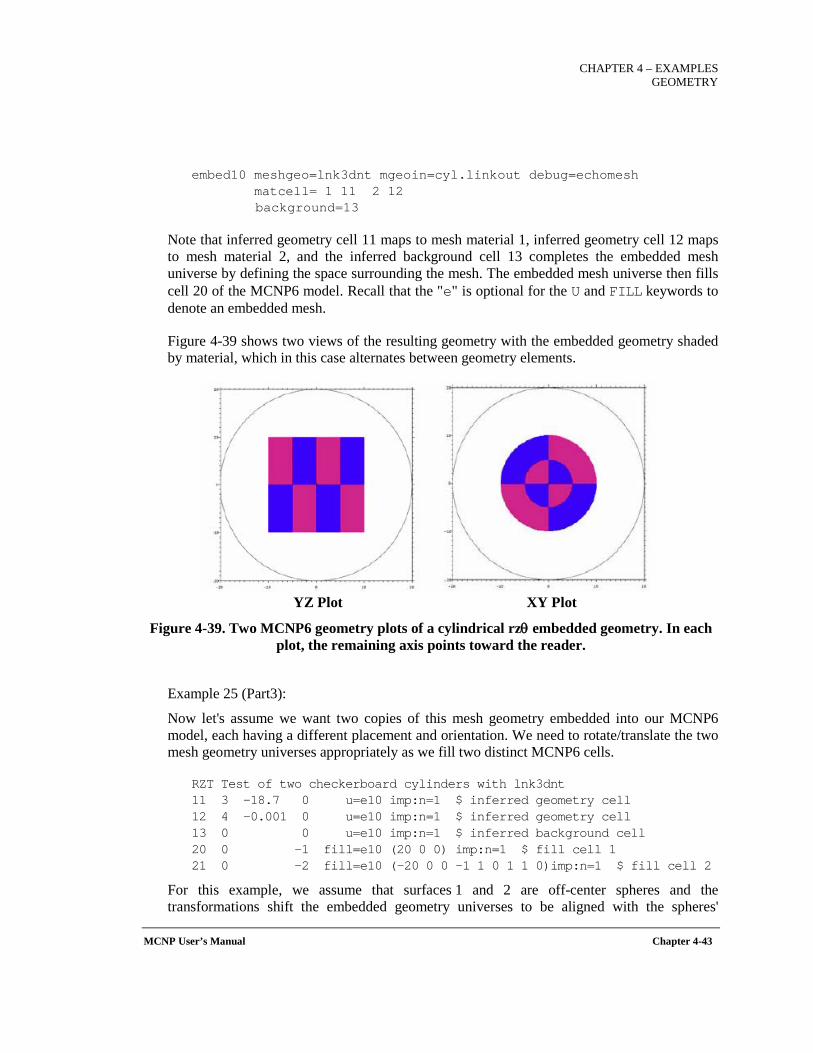
CHAPTER 4 – EXAMPLES
GEOMETRY
MCNP User’s Manual Chapter 4-43
embed10 meshgeo=lnk3dnt mgeoin=cyl.linkout debug=echomesh matcell= 1 11 2 12 background=13
Note that inferred geometry cell 11 maps to mesh material 1, inferred geometry cell 12 maps to mesh material 2, and the inferred background cell 13 completes the embedded mesh universe by defining the space surrounding the mesh. The embedded mesh universe then fills cell 20 of the MCNP6 model. Recall that the "e" is optional for the U and FILL keywords to denote an embedded mesh.
Figure 4-39 shows two views of the resulting geometry with the embedded geometry shaded by material, which in this case alternates between geometry elements.
YZ Plot XY Plot
Figure 4-39. Two MCNP6 geometry plots of a cylindrical rzθ embedded geometry. In each plot, the remaining axis points toward the reader.
Example 25 (Part3):
Now let's assume we want two copies of this mesh geometry embedded into our MCNP6 model, each having a different placement and orientation. We need to rotate/translate the two mesh geometry universes appropriately as we fill two distinct MCNP6 cells.
RZT Test of two checkerboard cylinders with lnk3dnt 11 3 -18.7 0 u=e10 imp:n=1 $ inferred geometry cell 12 4 -0.001 0 u=e10 imp:n=1 $ inferred geometry cell 13 0 0 u=e10 imp:n=1 $ inferred background cell 20 0 -1 fill=e10 (20 0 0) imp:n=1 $ fill cell 1 21 0 -2 fill=e10 (-20 0 0 -1 1 0 1 1 0)imp:n=1 $ fill cell 2
For this example, we assume that surfaces 1 and 2 are off-center spheres and the transformations shift the embedded geometry universes to be aligned with the spheres'
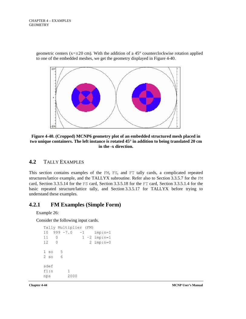
CHAPTER 4 – EXAMPLES GEOMETRY
Chapter 4-44 MCNP User’s Manual
geometric centers (x=±20 cm). With the addition of a 45° counterclockwise rotation applied to one of the embedded meshes, we get the geometry displayed in Figure 4-40.
Figure 4-40. (Cropped) MCNP6 geometry plot of an embedded structured mesh placed in
two unique containers. The left instance is rotated 45° in addition to being translated 20 cm in the -x direction.
4.2 TALLY EXAMPLES
This section contains examples of the FM, FS, and FT tally cards, a complicated repeated structures/lattice example, and the TALLYX subroutine. Refer also to Section 3.3.5.7 for the FM card, Section 3.3.5.14 for the FS card, Section 3.3.5.18 for the FT card, Section 3.3.5.1.4 for the basic repeated structure/lattice tally, and Section 3.3.5.17 for TALLYX before trying to understand these examples.
4.2.1 FM Examples (Simple Form) Example 26:
Consider the following input cards. Tally Multiplier (FM) 10 999 -7.0 -1 imp:n=1 11 0 1 -2 imp:n=1 12 0 2 imp:n=0
1 so 5 2 so 6
sdef f1:n 1 nps 2000
CHAPTER 4 – EXAMPLES
TALLIES
MCNP User’s Manual Chapter 4-45
f4:n 10 fm4 0.04786 999 102 m999 92238.80c 1.0
The F4 neutron tally is the track length estimate of the average fluence in cell 10. Material 999 is 238U with an atomic fraction of 100%.
c= 0.04786 normalization factor (such as atom/barn-cm) m=999 material number for 238U as defined on the material card (with an atom
density of 0.04786 atom/barn-cm) r1=102 ENDF reaction number for radiative capture cross-section (microscopic)
The average fluence is multiplied by the microscopic (n,γ) cross section of 238U (with an atomic fraction of 1.0) and then by the constant 0.04786 (atom/barn−cm). Thus the tally 4 printout will indicate the number of 239U atoms/cm3 produced as a result of (n, γ) capture with 238U.
Standard F6 and F7 tallies can be duplicated by F4 tallies with appropriate FM4 cards. The FM4 card to duplicate F6 is
FM4 c m 1 –4
where
c = 10−24 × number of atoms per gram r1 = 1 ENDF reaction number for total cross section (barns) r2 = −4 reaction number for average heating number (MeV/collision)
and for F7 it is FM4 c m –6 –8
where
c = 10−24 × number of atoms per gram r1 = −6 reaction number for total fission cross section (barns) r2 = −8 reaction number for fission Q (MeV/fission)
This technique applied to F2 tallies can be used to estimate the average heating over a surface rather than over a volume. It provides the surface equivalents of F6 and F7 tallies, which are not available as standard tallies in MCNP6.
Example 27:
Consider a point detector.
CHAPTER 4 – EXAMPLES TALLIES
Chapter 4-46 MCNP User’s Manual
Point Detector Tally 10 999 -1.0 -1 imp:n=1 11 1001 -5.0 1 -2 imp:n=1 12 0 2 imp:n=0
1 so 5 2 so 6
sdef f1:n 1 nps 2000 m999 1001.80c 2 8016.80c 1 F25:N 0 0 0 0 FM25 0.00253 1001 -6 -8 M1001 92238.80c 0.9 92235.80c 0.1
This F25 neutron tally is the fission heating per unit volume of material 1001 at the origin. Material 1001 does not actually have to be in a cell at the origin. The FM25 card constants are:
c = 0.00253 atoms per barn−cm (atomic density) of material 1001 m = 1001 material number for material being heated r1 = -6 reaction number for total fission cross section (barn) r2 = -8 reaction number for fission Q (MeV/fission)
More Simple Form Fm Examples:
(Remember c=–1=ρ⟩ for type 4 tally) F5:N 0 0 0 0 Neutron heating per cm3 with an atom density FM5 ρ m 1 -4 of ρ of material m at a point detector
F5Y:P 10 5 0 Photon heating per cm3 of material m with FM5 ρ m -5 -6 an atom density ρ at a ring detector
F1:N 1 2 3 Number of neutron tracks crossing surfaces 1, FM1 1 0 2, and 3 per neutron started
F35:P 0 0 0 0 Number of photon collisions per source particle FM35 1 0 that contribute to point detector
M99 3007 1 7Li tritium production per cm3 in cell 10 F4:N 10 FM4 -1 99 91
F104:N 8 Number of reactions per cm3 of type r in cell 8 FM104 ρ m r of material m of atom density ρ
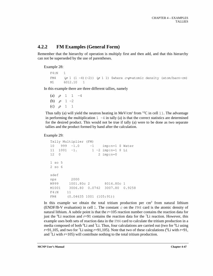
CHAPTER 4 – EXAMPLES
TALLIES
MCNP User’s Manual Chapter 4-47
4.2.2 FM Examples (General Form) Remember that the hierarchy of operation is multiply first and then add, and that this hierarchy can not be superseded by the use of parentheses.
Example 28: F4:N 1 FM4 (ρ 1 (1 –4)(–2)) (ρ 1 1) $where c=ρ=atomic density (atom/barn-cm) M1 6012.10 1
In this example there are three different tallies, namely
(a) ρ 1 1 -4 (b) ρ 1 -2 (c) ρ 1 1
Thus tally (a) will yield the neutron heating in MeV/cm3 from 12C in cell 11. The advantage in performing the multiplication 1 -4 in tally (a) is that the correct statistics are determined for the desired product. This would not be true if tally (a) were to be done as two separate tallies and the product formed by hand after the calculation.
Example 29: Tally Multiplier (FM) 10 999 -1.0 -1 imp:n=1 $ Water 11 1001 -1. 1 -2 imp:n=1 $ Li 12 0 2 imp:n=0
1 so 5 2 so 6
sdef nps 2000 M999 1001.80c 2 8016.80c 1 M1001 3006.80 0.0742 3007.80 0.9258 F4:N 11 FM4 (0.04635 1001 (105:91))
In this example we obtain the total tritium production per cm3 from natural lithium (ENDF/B-V evaluation) in cell 1. The constant c on the FM4 card is the atomic density of natural lithium. A subtle point is that the r=105 reaction number contains the reaction data for just the 6Li reaction and r=91 contains the reaction data for the 7Li reaction. However, this example uses both sets of reaction data in the FM4 card to calculate the tritium production in a media composed of both 6Li and 7Li. Thus, four calculations are carried out (two for 6Li using r=91,105, and two for 7Li using r=91,105). Note that two of these calculations (6Li with r=91, and 7Li with r=105) will contribute nothing to the total tritium production.
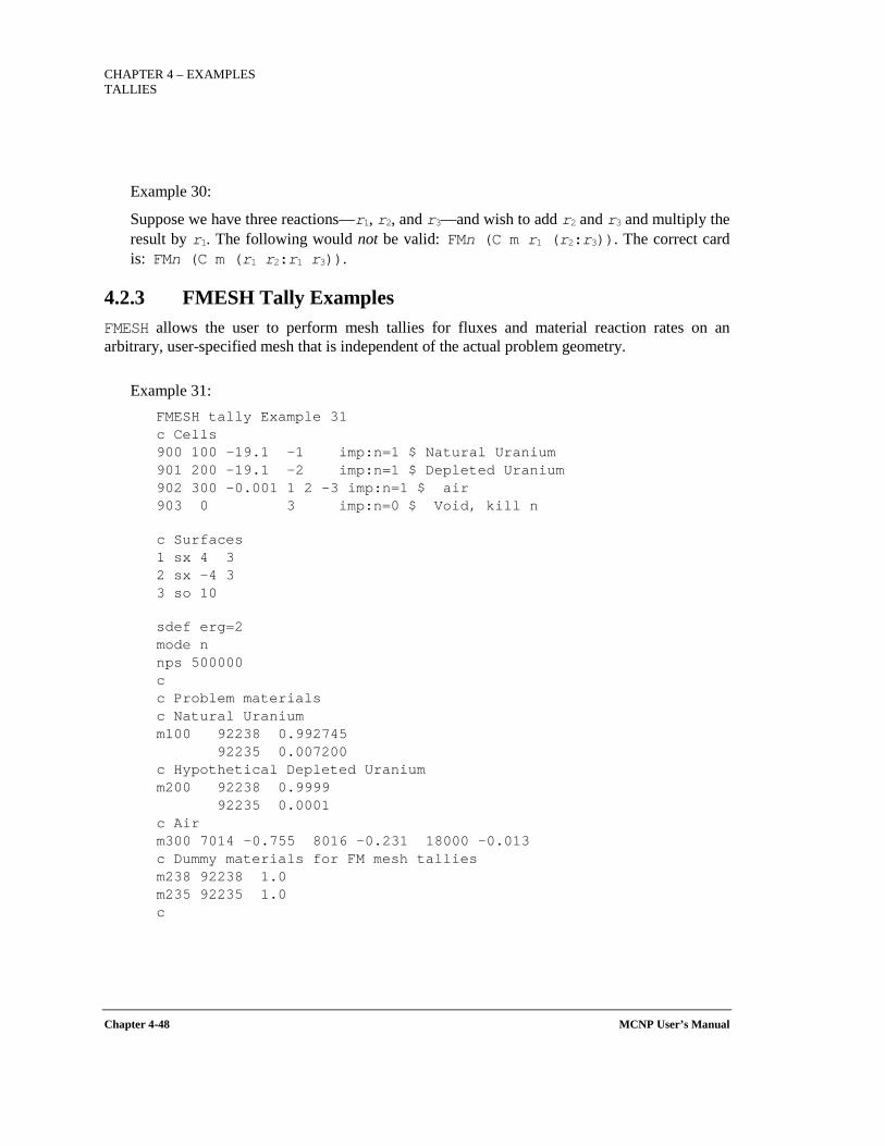
CHAPTER 4 – EXAMPLES TALLIES
Chapter 4-48 MCNP User’s Manual
Example 30:
Suppose we have three reactions—r1, r2, and r3—and wish to add r2 and r3 and multiply the result by r1. The following would not be valid: FMn (C m r1 (r2:r3)). The correct card is: FMn (C m (r1 r2:r1 r3)).
4.2.3 FMESH Tally Examples FMESH allows the user to perform mesh tallies for fluxes and material reaction rates on an arbitrary, user-specified mesh that is independent of the actual problem geometry.
Example 31: FMESH tally Example 31 c Cells 900 100 -19.1 -1 imp:n=1 $ Natural Uranium 901 200 -19.1 -2 imp:n=1 $ Depleted Uranium 902 300 -0.001 1 2 -3 imp:n=1 $ air 903 0 3 imp:n=0 $ Void, kill n
c Surfaces 1 sx 4 3 2 sx -4 3 3 so 10
sdef erg=2 mode n nps 500000 c c Problem materials c Natural Uranium m100 92238 0.992745 92235 0.007200 c Hypothetical Depleted Uranium m200 92238 0.9999 92235 0.0001 c Air m300 7014 -0.755 8016 -0.231 18000 -0.013 c Dummy materials for FM mesh tallies m238 92238 1.0 m235 92235 1.0 c
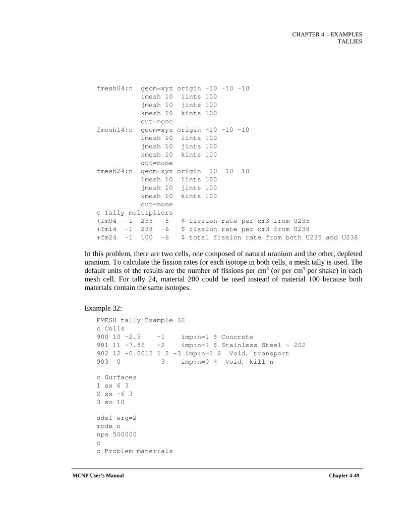
CHAPTER 4 – EXAMPLES
TALLIES
MCNP User’s Manual Chapter 4-49
fmesh04:n geom=xyz origin -10 -10 -10 imesh 10 iints 100 jmesh 10 jints 100 kmesh 10 kints 100 out=none fmesh14:n geom=xyz origin -10 -10 -10 imesh 10 iints 100 jmesh 10 jints 100 kmesh 10 kints 100 out=none fmesh24:n geom=xyz origin -10 -10 -10 imesh 10 iints 100 jmesh 10 jints 100 kmesh 10 kints 100 out=none c Tally multipliers +fm04 -1 235 -6 $ fission rate per cm3 from U235 +fm14 -1 238 -6 $ fission rate per cm3 from U238 +fm24 -1 100 -6 $ total fission rate from both U235 and U238
In this problem, there are two cells, one composed of natural uranium and the other, depleted uranium. To calculate the fission rates for each isotope in both cells, a mesh tally is used. The default units of the results are the number of fissions per cm3 (or per cm3 per shake) in each mesh cell. For tally 24, material 200 could be used instead of material 100 because both materials contain the same isotopes.
Example 32: FMESH tally Example 32 c Cells 900 10 -2.5 -1 imp:n=1 $ Concrete 901 11 -7.86 -2 imp:n=1 $ Stainless Steel - 202 902 12 -0.0012 1 2 -3 imp:n=1 $ Void, transport 903 0 3 imp:n=0 $ Void, kill n
c Surfaces 1 sx 6 3 2 sx -6 3 3 so 10
sdef erg=2 mode n nps 500000 c c Problem materials
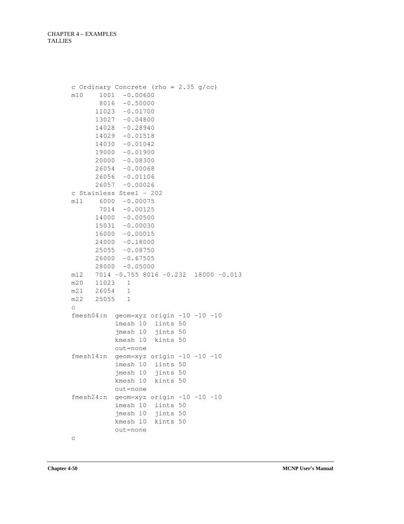
CHAPTER 4 – EXAMPLES TALLIES
Chapter 4-50 MCNP User’s Manual
c Ordinary Concrete (rho = 2.35 g/cc) m10 1001 -0.00600 8016 -0.50000 11023 -0.01700 13027 -0.04800 14028 -0.28940 14029 -0.01518 14030 -0.01042 19000 -0.01900 20000 -0.08300 26054 -0.00068 26056 -0.01106 26057 -0.00026 c Stainless Steel - 202 m11 6000 -0.00075 7014 -0.00125 14000 -0.00500 15031 -0.00030 16000 -0.00015 24000 -0.18000 25055 -0.08750 26000 -0.67505 28000 -0.05000 m12 7014 -0.755 8016 -0.232 18000 -0.013 m20 11023 1 m21 26054 1 m22 25055 1 c fmesh04:n geom=xyz origin -10 -10 -10 imesh 10 iints 50 jmesh 10 jints 50 kmesh 10 kints 50 out=none fmesh14:n geom=xyz origin -10 -10 -10 imesh 10 iints 50 jmesh 10 jints 50 kmesh 10 kints 50 out=none fmesh24:n geom=xyz origin -10 -10 -10 imesh 10 iints 50 jmesh 10 jints 50 kmesh 10 kints 50 out=none c
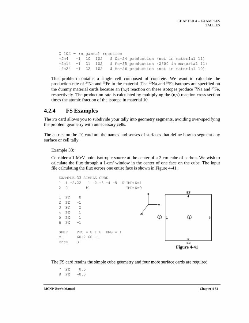
CHAPTER 4 – EXAMPLES
TALLIES
MCNP User’s Manual Chapter 4-51
C 102 = (n,gamma) reaction +fm4 -1 20 102 $ Na-24 production (not in material 11) +fm14 -1 21 102 $ Fe-55 production (2600 in material 11) +fm24 -1 22 102 $ Mn-56 production (not in material 10)
This problem contains a single cell composed of concrete. We want to calculate the production rate of 24Na and 55Fe in the material. The 23Na and 54Fe isotopes are specified on the dummy material cards because an (n,γ) reaction on these isotopes produce 24Na and 55Fe, respectively. The production rate is calculated by multiplying the (n,γ) reaction cross section times the atomic fraction of the isotope in material 10.
4.2.4 FS Examples The FS card allows you to subdivide your tally into geometry segments, avoiding over-specifying the problem geometry with unnecessary cells.
The entries on the FS card are the names and senses of surfaces that define how to segment any surface or cell tally.
Example 33:
Consider a 1-MeV point isotropic source at the center of a 2-cm cube of carbon. We wish to calculate the flux through a 1-cm2 window in the center of one face on the cube. The input file calculating the flux across one entire face is shown in Figure 4-41.
EXAMPLE 33 SIMPLE CUBE 1 1 -2.22 1 2 -3 -4 -5 6 IMP:N=1 2 0 #1 IMP:N=0
1 PY 0 2 PZ -1 3 PY 2 4 PZ 1 5 PX 1 6 PX –1
SDEF POS = 0 1 0 ERG = 1 M1 6012.60 –1 F2:N 3
Figure 4-41
The FS card retains the simple cube geometry and four more surface cards are required, 7 PX 0.5 8 PX -0.5
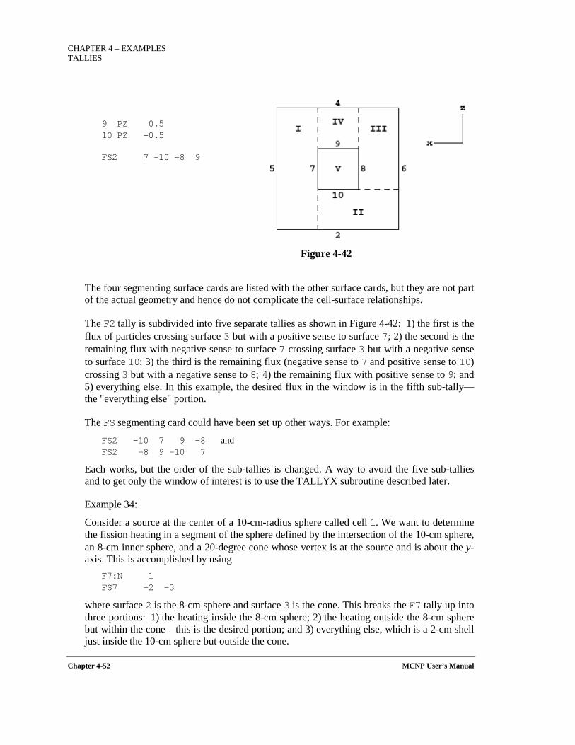
CHAPTER 4 – EXAMPLES TALLIES
Chapter 4-52 MCNP User’s Manual
9 PZ 0.5 10 PZ -0.5
FS2 7 -10 -8 9
Figure 4-42
The four segmenting surface cards are listed with the other surface cards, but they are not part of the actual geometry and hence do not complicate the cell-surface relationships.
The F2 tally is subdivided into five separate tallies as shown in Figure 4-42: 1) the first is the flux of particles crossing surface 3 but with a positive sense to surface 7; 2) the second is the remaining flux with negative sense to surface 7 crossing surface 3 but with a negative sense to surface 10; 3) the third is the remaining flux (negative sense to 7 and positive sense to 10) crossing 3 but with a negative sense to 8; 4) the remaining flux with positive sense to 9; and 5) everything else. In this example, the desired flux in the window is in the fifth sub-tally—the "everything else" portion.
The FS segmenting card could have been set up other ways. For example:
FS2 -10 7 9 -8 and FS2 -8 9 -10 7
Each works, but the order of the sub-tallies is changed. A way to avoid the five sub-tallies and to get only the window of interest is to use the TALLYX subroutine described later.
Example 34:
Consider a source at the center of a 10-cm-radius sphere called cell 1. We want to determine the fission heating in a segment of the sphere defined by the intersection of the 10-cm sphere, an 8-cm inner sphere, and a 20-degree cone whose vertex is at the source and is about the y-axis. This is accomplished by using
F7:N 1 FS7 -2 -3
where surface 2 is the 8-cm sphere and surface 3 is the cone. This breaks the F7 tally up into three portions: 1) the heating inside the 8-cm sphere; 2) the heating outside the 8-cm sphere but within the cone—this is the desired portion; and 3) everything else, which is a 2-cm shell just inside the 10-cm sphere but outside the cone.
CHAPTER 4 – EXAMPLES
TALLIES
MCNP User’s Manual Chapter 4-53
4.2.5 FT Examples
Example 35:
Consider the following input cards. F1:N 2 FT1 FRV v1 v2 v3
The FTn card is the special treatment for tallies card. Various tally treatments are available for certain specific tally requirements. The FTn tally with the FRV card used in conjunction with tally type 1 will redefine the vector normal to the tally surface. In this case, the current over surface 2 (tally type 1) uses the vector V as its reference vector for getting the cosine for binning.
Example 36: F5:P 4 5 6 FT5 ICD FU5 1 3
In this example the photon flux at detector 5 is being tallied. However, only the contributions to the detector tally from cells 1 and 3 are of interest. The ICD keyword allows the user to create a separate bin for each cell, and only contributions from one of the specified cells are scored. The FUn card specifies the cells from which tallies are to be made, but TALLYX is not called.
Example 37:
When keeping track of charged particle current across a surface, it is sometimes desirable to track both positive and negative score contributions, applicable in cases that include charged particles. Consider a photon source that is enclosed in a spherical shell of lead. If a surface current tally is taken over the sphere and it is desirable to tally both the positron and electron current separately, then the special treatment card option is invoked.
1 1 −0.001124 −11 imp:e=1 imp:p=1 2 2 −11.0 11 −21 imp:e=1 imp:p=1 3 0 21 imp:e=0 imp:p=0
11 so 30 21 so 32
m1 6012 0.000125 7014 0.6869 8016 0.301248 18040 0.011717 m2 82000 1. mode p e sdef pos = 0. 0. 0. erg = 2.5 f1:e 21 ft1 elc 2
CHAPTER 4 – EXAMPLES TALLIES
Chapter 4-54 MCNP User’s Manual
f2:p 21 e2 1e-3 1e-2 0.1 0.5 1.0 1.5 2.0 2.5 C nps 10000
The input deck shown above models a sphere filled with dry air surrounded by a spherical shell of lead. The centrally located source emits 2.5-MeV photons that travel through the air into the lead shell. The F1 surface current tally has been modified with the ELC special tally option. The parameter value of 2 that follows the ELC keyword specifies that positrons and electrons be placed into separate tally user bins. Once this option has been invoked, the user can inspect the output tally bins for the respective scoring of either particle.
The F2 tally scores photon flux crossing surface 21, scored into energy bins defined on the E2 card. The C at the end of the energy bin card indicates that the bins are cumulative. For instance, the bin with an upper limit of 1 MeV would contain scores from particles that cross surface 21 with energy less than or equal to 1 MeV.
Example 38:
Consider the following two point sources, each with a different energy distribution: sdef pos=d1 erg=fpos d2 si1 L 5 3 6 75 3 6 sp1 0.3 0.7 ds2 S 3 4 si3 H 2 10 14 sp3 D 0 1 2 si4 H 5 2 8 sp4 D 0 3 1 f2:n 2 ft2 scd fu2 3 4
The SCD option causes tallies to be binned according to which source distribution was sampled. The FUn card is used to list the distribution numbers of interest. Thus, the tallies in this example are placed in one of two bins, depending on which of the two sources emitted the particle. The two sources may represent two nuclides with different energy distributions. In this case use of the SCD option allows the user to determine each nuclide’s contribution to the final tally.
Example 39: Capture Tallies: Interpreting Capture Tally Output
The FT8 CAP coincidence capture tally option produces both a standard tally, which is generally unreadable, and a coincidence capture table, print table 118. An example is provided to help in the interpretation of this table:
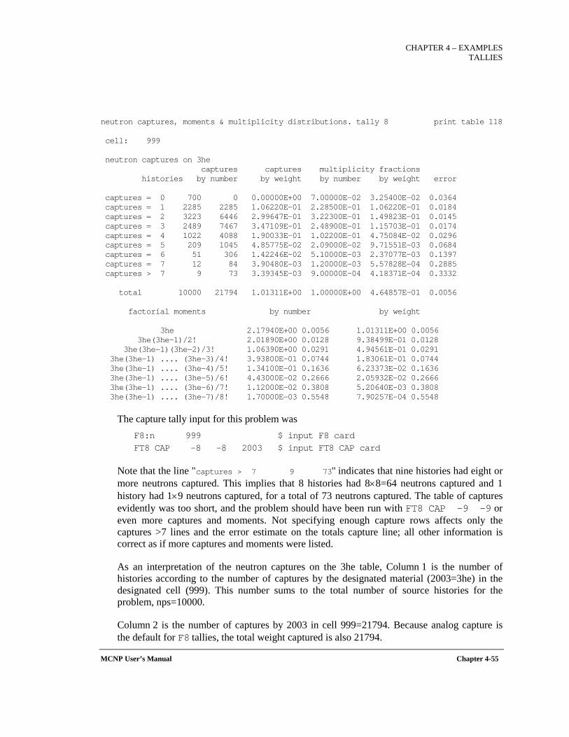
CHAPTER 4 – EXAMPLES
TALLIES
MCNP User’s Manual Chapter 4-55
neutron captures, moments & multiplicity distributions. tally 8 print table 118 cell: 999 neutron captures on 3he captures captures multiplicity fractions histories by number by weight by number by weight error captures = 0 700 0 0.00000E+00 7.00000E-02 3.25400E-02 0.0364 captures = 1 2285 2285 1.06220E-01 2.28500E-01 1.06220E-01 0.0184 captures = 2 3223 6446 2.99647E-01 3.22300E-01 1.49823E-01 0.0145 captures = 3 2489 7467 3.47109E-01 2.48900E-01 1.15703E-01 0.0174 captures = 4 1022 4088 1.90033E-01 1.02200E-01 4.75084E-02 0.0296 captures = 5 209 1045 4.85775E-02 2.09000E-02 9.71551E-03 0.0684 captures = 6 51 306 1.42246E-02 5.10000E-03 2.37077E-03 0.1397 captures = 7 12 84 3.90480E-03 1.20000E-03 5.57828E-04 0.2885 captures > 7 9 73 3.39345E-03 9.00000E-04 4.18371E-04 0.3332 total 10000 21794 1.01311E+00 1.00000E+00 4.64857E-01 0.0056 factorial moments by number by weight 3he 2.17940E+00 0.0056 1.01311E+00 0.0056 3he(3he-1)/2! 2.01890E+00 0.0128 9.38499E-01 0.0128 3he(3he-1)(3he-2)/3! 1.06390E+00 0.0291 4.94561E-01 0.0291 3he(3he-1) .... (3he-3)/4! 3.93800E-01 0.0744 1.83061E-01 0.0744 3he(3he-1) .... (3he-4)/5! 1.34100E-01 0.1636 6.23373E-02 0.1636 3he(3he-1) .... (3he-5)/6! 4.43000E-02 0.2666 2.05932E-02 0.2666 3he(3he-1) .... (3he-6)/7! 1.12000E-02 0.3808 5.20640E-03 0.3808 3he(3he-1) .... (3he-7)/8! 1.70000E-03 0.5548 7.90257E-04 0.5548
The capture tally input for this problem was F8:n 999 $ input F8 card FT8 CAP -8 -8 2003 $ input FT8 CAP card
Note that the line "captures > 7 9 73" indicates that nine histories had eight or more neutrons captured. This implies that 8 histories had 8×8=64 neutrons captured and 1 history had 1×9 neutrons captured, for a total of 73 neutrons captured. The table of captures evidently was too short, and the problem should have been run with FT8 CAP -9 -9 or even more captures and moments. Not specifying enough capture rows affects only the captures >7 lines and the error estimate on the totals capture line; all other information is correct as if more captures and moments were listed.
As an interpretation of the neutron captures on the 3he table, Column 1 is the number of histories according to the number of captures by the designated material (2003=3he) in the designated cell (999). This number sums to the total number of source histories for the problem, nps=10000.
Column 2 is the number of captures by 2003 in cell 999=21794. Because analog capture is the default for F8 tallies, the total weight captured is also 21794.
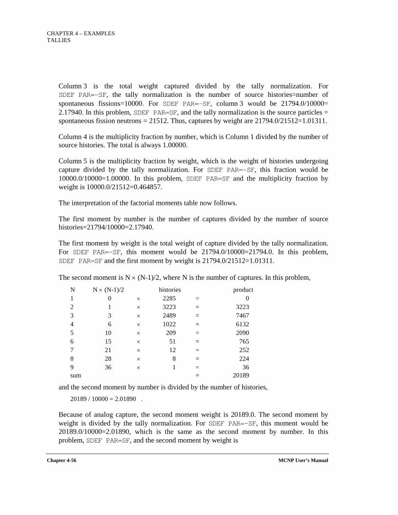
CHAPTER 4 – EXAMPLES TALLIES
Chapter 4-56 MCNP User’s Manual
Column 3 is the total weight captured divided by the tally normalization. For SDEF PAR=-SF, the tally normalization is the number of source histories=number of spontaneous fissions=10000. For SDEF PAR=-SF, column 3 would be 21794.0/10000= 2.17940. In this problem, SDEF PAR=SF, and the tally normalization is the source particles = spontaneous fission neutrons = 21512. Thus, captures by weight are 21794.0/21512=1.01311.
Column 4 is the multiplicity fraction by number, which is Column 1 divided by the number of source histories. The total is always 1.00000.
Column 5 is the multiplicity fraction by weight, which is the weight of histories undergoing capture divided by the tally normalization. For SDEF PAR=-SF, this fraction would be 10000.0/10000=1.00000. In this problem, SDEF PAR=SF and the multiplicity fraction by weight is 10000.0/21512=0.464857.
The interpretation of the factorial moments table now follows.
The first moment by number is the number of captures divided by the number of source histories=21794/10000=2.17940.
The first moment by weight is the total weight of capture divided by the tally normalization. For SDEF PAR=-SF, this moment would be 21794.0/10000=21794.0. In this problem, SDEF PAR=SF and the first moment by weight is 21794.0/21512=1.01311.
The second moment is N × (N-1)/2, where N is the number of captures. In this problem,
N N × (N-1)/2 histories product 1 0 × 2285 = 0 2 1 × 3223 = 3223 3 3 × 2489 = 7467 4 6 × 1022 = 6132 5 10 × 209 = 2090 6 15 × 51 = 765 7 21 × 12 = 252 8 28 × 8 = 224 9 36 × 1 = 36 sum = 20189
and the second moment by number is divided by the number of histories, 20189 / 10000 = 2.01890 .
Because of analog capture, the second moment weight is 20189.0. The second moment by weight is divided by the tally normalization. For SDEF PAR=-SF, this moment would be 20189.0/10000=2.01890, which is the same as the second moment by number. In this problem, SDEF PAR=SF, and the second moment by weight is
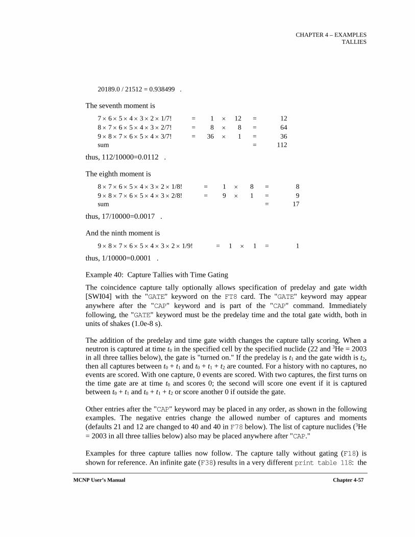
CHAPTER 4 – EXAMPLES
TALLIES
MCNP User’s Manual Chapter 4-57
20189.0 / 21512 = 0.938499 .
The seventh moment is
7 × 6 × 5 × 4 × 3 × 2 × 1/7! = 1 × 12 = 12 8 × 7 × 6 × 5 × 4 × 3 × 2/7! = 8 × 8 = 64 9 × 8 × 7 × 6 × 5 × 4 × 3/7! = 36 × 1 = 36 sum = 112
thus, 112/10000=0.0112 .
The eighth moment is
8 × 7 × 6 × 5 × 4 × 3 × 2 × 1/8! = 1 × 8 = 8 9 × 8 × 7 × 6 × 5 × 4 × 3 × 2/8! = 9 × 1 = 9 sum = 17
thus, 17/10000=0.0017 .
And the ninth moment is
9 × 8 × 7 × 6 × 5 × 4 × 3 × 2 × 1/9! = 1 × 1 = 1
thus, 1/10000=0.0001 .
Example 40: Capture Tallies with Time Gating
The coincidence capture tally optionally allows specification of predelay and gate width [SWI04] with the "GATE" keyword on the FT8 card. The "GATE" keyword may appear anywhere after the "CAP" keyword and is part of the "CAP" command. Immediately following, the "GATE" keyword must be the predelay time and the total gate width, both in units of shakes (1.0e-8 s).
The addition of the predelay and time gate width changes the capture tally scoring. When a neutron is captured at time t0 in the specified cell by the specified nuclide (22 and 3He = 2003 in all three tallies below), the gate is "turned on." If the predelay is t1 and the gate width is t2, then all captures between t0 + t1 and t0 + t1 + t2 are counted. For a history with no captures, no events are scored. With one capture, 0 events are scored. With two captures, the first turns on the time gate are at time t0 and scores 0; the second will score one event if it is captured between t0 + t1 and t0 + t1 + t2 or score another 0 if outside the gate.
Other entries after the "CAP" keyword may be placed in any order, as shown in the following examples. The negative entries change the allowed number of captures and moments (defaults 21 and 12 are changed to 40 and 40 in F78 below). The list of capture nuclides (3He = 2003 in all three tallies below) also may be placed anywhere after "CAP."
Examples for three capture tallies now follow. The capture tally without gating (F18) is shown for reference. An infinite gate (F38) results in a very different print table 118: the
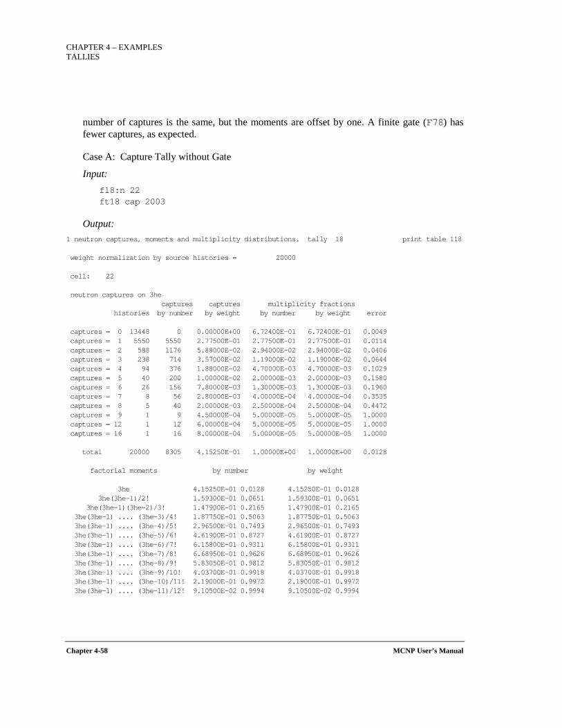
CHAPTER 4 – EXAMPLES TALLIES
Chapter 4-58 MCNP User’s Manual
number of captures is the same, but the moments are offset by one. A finite gate (F78) has fewer captures, as expected.
Case A: Capture Tally without Gate
Input: f18:n 22 ft18 cap 2003
Output: 1 neutron captures, moments and multiplicity distributions. tally 18 print table 118 weight normalization by source histories = 20000 cell: 22 neutron captures on 3he captures captures multiplicity fractions histories by number by weight by number by weight error captures = 0 13448 0 0.00000E+00 6.72400E-01 6.72400E-01 0.0049 captures = 1 5550 5550 2.77500E-01 2.77500E-01 2.77500E-01 0.0114 captures = 2 588 1176 5.88000E-02 2.94000E-02 2.94000E-02 0.0406 captures = 3 238 714 3.57000E-02 1.19000E-02 1.19000E-02 0.0644 captures = 4 94 376 1.88000E-02 4.70000E-03 4.70000E-03 0.1029 captures = 5 40 200 1.00000E-02 2.00000E-03 2.00000E-03 0.1580 captures = 6 26 156 7.80000E-03 1.30000E-03 1.30000E-03 0.1960 captures = 7 8 56 2.80000E-03 4.00000E-04 4.00000E-04 0.3535 captures = 8 5 40 2.00000E-03 2.50000E-04 2.50000E-04 0.4472 captures = 9 1 9 4.50000E-04 5.00000E-05 5.00000E-05 1.0000 captures = 12 1 12 6.00000E-04 5.00000E-05 5.00000E-05 1.0000 captures = 16 1 16 8.00000E-04 5.00000E-05 5.00000E-05 1.0000 total 20000 8305 4.15250E-01 1.00000E+00 1.00000E+00 0.0128 factorial moments by number by weight 3he 4.15250E-01 0.0128 4.15250E-01 0.0128 3he(3he-1)/2! 1.59300E-01 0.0651 1.59300E-01 0.0651 3he(3he-1)(3he-2)/3! 1.47900E-01 0.2165 1.47900E-01 0.2165 3he(3he-1) .... (3he-3)/4! 1.87750E-01 0.5063 1.87750E-01 0.5063 3he(3he-1) .... (3he-4)/5! 2.96500E-01 0.7493 2.96500E-01 0.7493 3he(3he-1) .... (3he-5)/6! 4.61900E-01 0.8727 4.61900E-01 0.8727 3he(3he-1) .... (3he-6)/7! 6.15800E-01 0.9311 6.15800E-01 0.9311 3he(3he-1) .... (3he-7)/8! 6.68950E-01 0.9626 6.68950E-01 0.9626 3he(3he-1) .... (3he-8)/9! 5.83050E-01 0.9812 5.83050E-01 0.9812 3he(3he-1) .... (3he-9)/10! 4.03700E-01 0.9918 4.03700E-01 0.9918 3he(3he-1) .... (3he-10)/11! 2.19000E-01 0.9972 2.19000E-01 0.9972 3he(3he-1) .... (3he-11)/12! 9.10500E-02 0.9994 9.10500E-02 0.9994
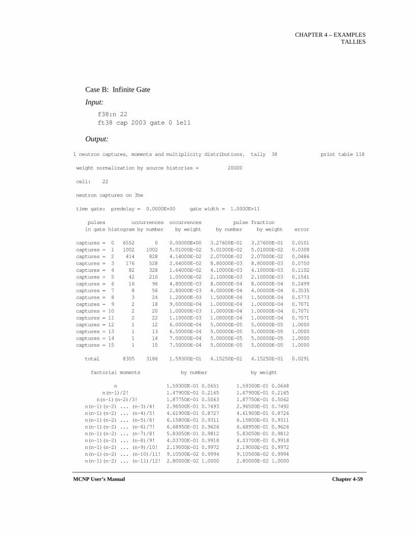
CHAPTER 4 – EXAMPLES
TALLIES
MCNP User’s Manual Chapter 4-59
Case B: Infinite Gate
Input: f38:n 22 ft38 cap 2003 gate 0 1e11
Output:
1 neutron captures, moments and multiplicity distributions. tally 38 print table 118 weight normalization by source histories = 20000 cell: 22 neutron captures on 3he time gate: predelay = 0.0000E+00 gate width = 1.0000E+11 pulses occurrences occurrences pulse fraction in gate histogram by number by weight by number by weight error captures = 0 6552 0 0.00000E+00 3.27600E-01 3.27600E-01 0.0101 captures = 1 1002 1002 5.01000E-02 5.01000E-02 5.01000E-02 0.0308 captures = 2 414 828 4.14000E-02 2.07000E-02 2.07000E-02 0.0486 captures = 3 176 528 2.64000E-02 8.80000E-03 8.80000E-03 0.0750 captures = 4 82 328 1.64000E-02 4.10000E-03 4.10000E-03 0.1102 captures = 5 42 210 1.05000E-02 2.10000E-03 2.10000E-03 0.1541 captures = 6 16 96 4.80000E-03 8.00000E-04 8.00000E-04 0.2499 captures = 7 8 56 2.80000E-03 4.00000E-04 4.00000E-04 0.3535 captures = 8 3 24 1.20000E-03 1.50000E-04 1.50000E-04 0.5773 captures = 9 2 18 9.00000E-04 1.00000E-04 1.00000E-04 0.7071 captures = 10 2 20 1.00000E-03 1.00000E-04 1.00000E-04 0.7071 captures = 11 2 22 1.10000E-03 1.00000E-04 1.00000E-04 0.7071 captures = 12 1 12 6.00000E-04 5.00000E-05 5.00000E-05 1.0000 captures = 13 1 13 6.50000E-04 5.00000E-05 5.00000E-05 1.0000 captures = 14 1 14 7.00000E-04 5.00000E-05 5.00000E-05 1.0000 captures = 15 1 15 7.50000E-04 5.00000E-05 5.00000E-05 1.0000 total 8305 3186 1.59300E-01 4.15250E-01 4.15250E-01 0.0291 factorial moments by number by weight n 1.59300E-01 0.0651 1.59300E-01 0.0648 n(n-1)/2! 1.47900E-01 0.2165 1.47900E-01 0.2165 n(n-1)(n-2)/3! 1.87750E-01 0.5063 1.87750E-01 0.5062 n(n-1)(n-2) ... (n-3)/4! 2.96500E-01 0.7493 2.96500E-01 0.7492 n(n-1)(n-2) ... (n-4)/5! 4.61900E-01 0.8727 4.61900E-01 0.8726 n(n-1)(n-2) ... (n-5)/6! 6.15800E-01 0.9311 6.15800E-01 0.9311 n(n-1)(n-2) ... (n-6)/7! 6.68950E-01 0.9626 6.68950E-01 0.9626 n(n-1)(n-2) ... (n-7)/8! 5.83050E-01 0.9812 5.83050E-01 0.9812 n(n-1)(n-2) ... (n-8)/9! 4.03700E-01 0.9918 4.03700E-01 0.9918 n(n-1)(n-2) ... (n-9)/10! 2.19000E-01 0.9972 2.19000E-01 0.9972 n(n-1)(n-2) ... (n-10)/11! 9.10500E-02 0.9994 9.10500E-02 0.9994 n(n-1)(n-2) ... (n-11)/12! 2.80000E-02 1.0000 2.80000E-02 1.0000
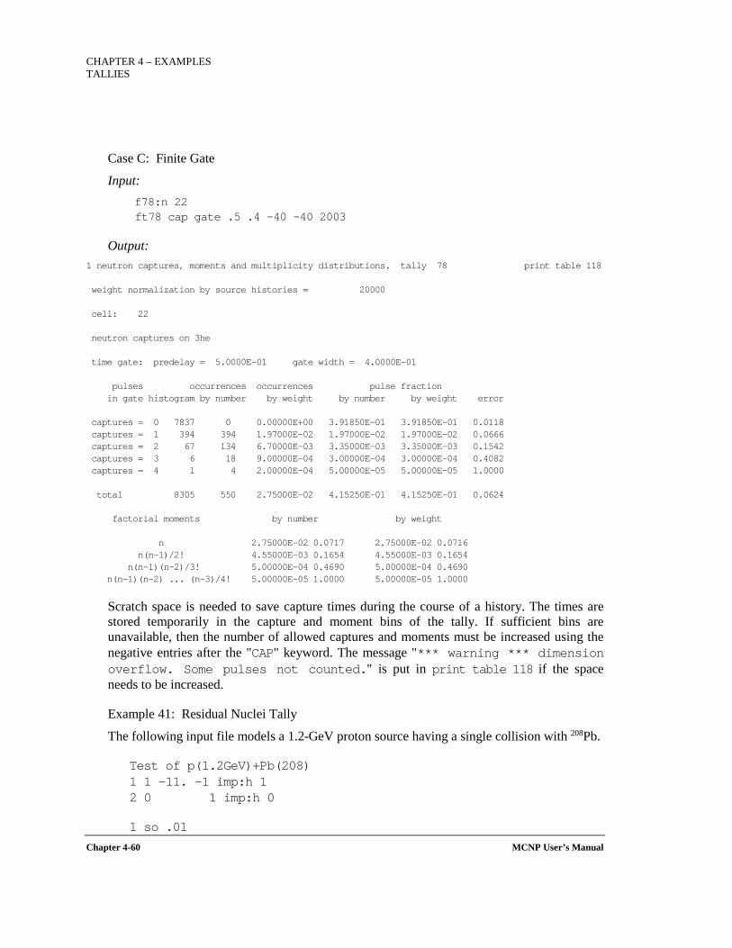
CHAPTER 4 – EXAMPLES TALLIES
Chapter 4-60 MCNP User’s Manual
Case C: Finite Gate
Input: f78:n 22 ft78 cap gate .5 .4 -40 -40 2003
Output: 1 neutron captures, moments and multiplicity distributions. tally 78 print table 118 weight normalization by source histories = 20000 cell: 22 neutron captures on 3he time gate: predelay = 5.0000E-01 gate width = 4.0000E-01 pulses occurrences occurrences pulse fraction in gate histogram by number by weight by number by weight error captures = 0 7837 0 0.00000E+00 3.91850E-01 3.91850E-01 0.0118 captures = 1 394 394 1.97000E-02 1.97000E-02 1.97000E-02 0.0666 captures = 2 67 134 6.70000E-03 3.35000E-03 3.35000E-03 0.1542 captures = 3 6 18 9.00000E-04 3.00000E-04 3.00000E-04 0.4082 captures = 4 1 4 2.00000E-04 5.00000E-05 5.00000E-05 1.0000 total 8305 550 2.75000E-02 4.15250E-01 4.15250E-01 0.0624 factorial moments by number by weight n 2.75000E-02 0.0717 2.75000E-02 0.0716 n(n-1)/2! 4.55000E-03 0.1654 4.55000E-03 0.1654 n(n-1)(n-2)/3! 5.00000E-04 0.4690 5.00000E-04 0.4690 n(n-1)(n-2) ... (n-3)/4! 5.00000E-05 1.0000 5.00000E-05 1.0000
Scratch space is needed to save capture times during the course of a history. The times are stored temporarily in the capture and moment bins of the tally. If sufficient bins are unavailable, then the number of allowed captures and moments must be increased using the negative entries after the "CAP" keyword. The message "*** warning *** dimension overflow. Some pulses not counted." is put in print table 118 if the space needs to be increased.
Example 41: Residual Nuclei Tally
The following input file models a 1.2-GeV proton source having a single collision with 208Pb.
Test of p(1.2GeV)+Pb(208) 1 1 -11. -1 imp:h 1 2 0 1 imp:h 0
1 so .01
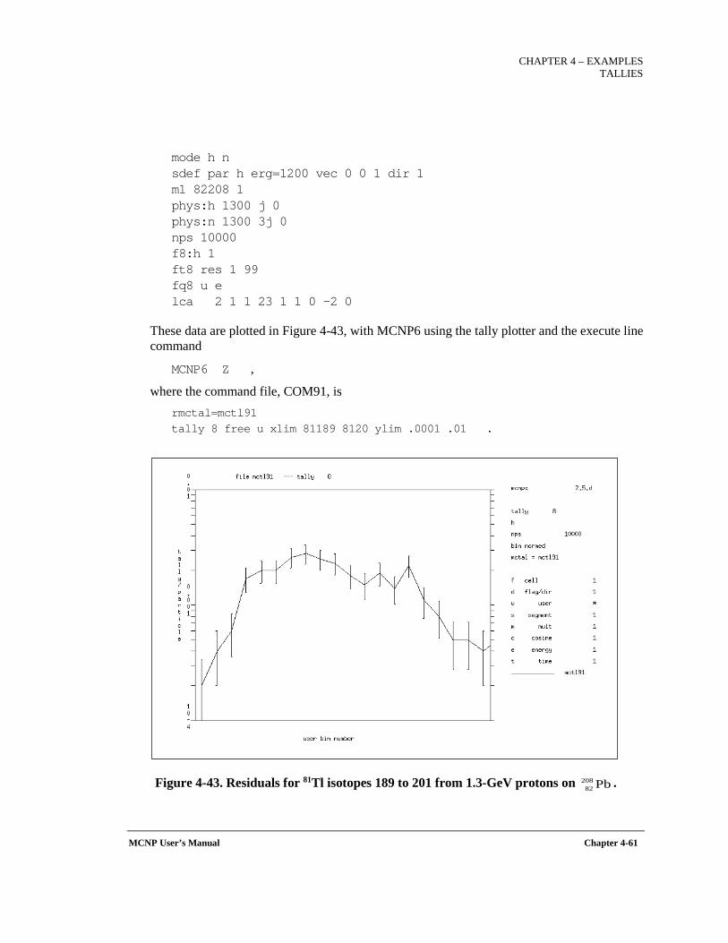
CHAPTER 4 – EXAMPLES
TALLIES
MCNP User’s Manual Chapter 4-61
mode h n sdef par h erg=1200 vec 0 0 1 dir 1 m1 82208 1 phys:h 1300 j 0 phys:n 1300 3j 0 nps 10000 f8:h 1 ft8 res 1 99 fq8 u e lca 2 1 1 23 1 1 0 -2 0
These data are plotted in Figure 4-43, with MCNP6 using the tally plotter and the execute line command
MCNP6 Z ,
where the command file, COM91, is rmctal=mctl91 tally 8 free u xlim 81189 8120 ylim .0001 .01 .
Figure 4-43. Residuals for 81Tl isotopes 189 to 201 from 1.3-GeV protons on . Pb20882
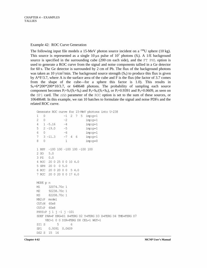
CHAPTER 4 – EXAMPLES TALLIES
Chapter 4-62 MCNP User’s Manual
Example 42: ROC Curve Generation
The following input file models a 15-MeV photon source incident on a 238U sphere (10 kg). This source is represented as a single 10 µs pulse of 107 photons (Si). A 1/E background source is specified in the surrounding cube (200 cm each side), and the FT PHL option is used to generate a ROC curve from the signal and noise components tallied in a Ge detector for 60 s. The Ge detector is surrounded by 2 cm of Pb. The flux of the background photons was taken as 10 γ/cm2/min. The background source strength (Sb) to produce this flux is given by A*F/3.7, where A is the surface area of the cube and F is the flux (the factor of 3.7 comes from the shape of the cube—for a sphere this factor is 1.0). This results in Sb=6*200*200*10/3.7, or 648648 photons. The probability of sampling each source component becomes Pi=Si/(Si+Sb) and Pb=Sb/(Si+Sb), or Pi=0.9391 and Pb=0.0609, as seen on the SP1 card. The nhb parameter of the ROC option is set to the sum of these sources, or 10648648. In this example, we ran 10 batches to formulate the signal and noise PDFs and the related ROC curve.
Generate ROC curve for 15-MeV photons into U-238 1 0 -1 2 7 5 imp:p=1 2 0 -2 imp:p=1 4 1 -5.16 -4 imp:p=1 5 2 -19.0 -5 imp:p=1 6 0 -6 imp:p=1 7 3 -11.3 -7 4 6 imp:p=1 8 0 1 imp:p=0 1 RPP -100 100 -100 100 -100 100 2 SO 5.0 3 PZ 0.0 4 RCC 20 0 25 0 0 10 4.0 5 SPH 20 0 0 5.0 6 RCC 20 0 20 0 0 5 4.0 7 RCC 20 0 20 0 0 17 6.0 MODE p n M1 32074.70c 1 M2 92238.70c 1 M3 82208.70c 1 MX2:P model CUT:N 60e8 CUT:P 60e8 PHYS:P j 1 j -1 j -101 SDEF PAR=P ERG=D1 X=FERG D2 Y=FERG D3 Z=FERG D4 TME=FERG D7 VEC=1 0 0 DIR=FERG D8 CEL=1 WGT=1 SI1 S 5 6 SP1 0.9391 0.0609 DS2 S 15 16
CHAPTER 4 – EXAMPLES
TALLIES
MCNP User’s Manual Chapter 4-63
DS3 S 25 26 DS4 S 35 36 DS7 S 45 46 DS8 S 55 56 SI15 L 5.1 SP15 1 SI25 L 0.0 SP25 1 SI35 L 0.0 SP35 1 SI16 -100 100 SP16 0 1 SI26 -100 100 SP26 0 1 SI36 -100 100 SP36 0 1 SI45 0 0.000010e8 SP45 0 1 SI46 0 60e8 SP46 0 1 SI55 L 1 SP55 1 SI56 -1 1 SP56 0 1 SI5 L 15.0 SP5 1 C 1/E for background source SI6 A .100 1.0 2.0 3.0 4.0 5.0 6.0 7.0 8.0 9.0 10.0 SP6 10.0 1.0 0.5 0.333 0.250 0.200 0.167 0.143 0.125 0.111 0.100 c f4:p 2 f1:p 4.3 e1 1.0 100.0 t1 0.001e8 60e8 ft1 scx 1 roc 10648648 tf1 1 1 1 1 1 1 2 2 1 1 2 1 1 1 2 2 $ signal bins, noise bins nps 106486480l
The ROC output for Tally 1 is provided in print table 163, shown below. The first printed plot is the ROC curve itself, plotting the noise PDF (usually referred to as the probability of false alarm) versus the signal PDF (usually referred to as the probability of detection). The data for the signal and noise PDFs is provided in the subsequent table. The jagged behavior of the ROC curve can be significantly refined by increasing the number of batches (say from 10 to 100, or by running 1064864800 particle histories).
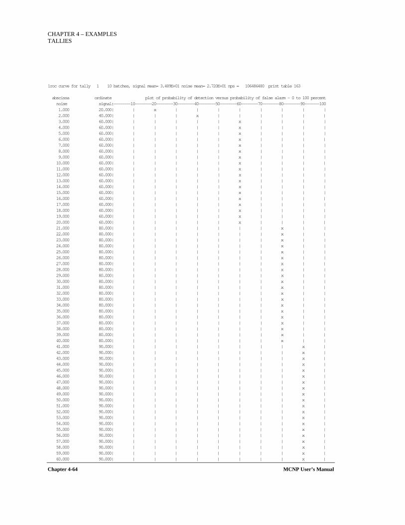
CHAPTER 4 – EXAMPLES TALLIES
Chapter 4-64 MCNP User’s Manual
1roc curve for tally 1 10 batches, signal mean= 3.489E+01 noise mean= 2.720E+01 nps = 106486480 print table 163 abscissa ordinate plot of probability of detection versus probability of false alarm - 0 to 100 percent noise signal:--------10--------20--------30--------40--------50--------60--------70--------80--------90-------100 1.000 20.000| | x | | | | | | | | 2.000 40.000| | | | x | | | | | | 3.000 60.000| | | | | | x | | | | 4.000 60.000| | | | | | x | | | | 5.000 60.000| | | | | | x | | | | 6.000 60.000| | | | | | x | | | | 7.000 60.000| | | | | | x | | | | 8.000 60.000| | | | | | x | | | | 9.000 60.000| | | | | | x | | | | 10.000 60.000| | | | | | x | | | | 11.000 60.000| | | | | | x | | | | 12.000 60.000| | | | | | x | | | | 13.000 60.000| | | | | | x | | | | 14.000 60.000| | | | | | x | | | | 15.000 60.000| | | | | | x | | | | 16.000 60.000| | | | | | x | | | | 17.000 60.000| | | | | | x | | | | 18.000 60.000| | | | | | x | | | | 19.000 60.000| | | | | | x | | | | 20.000 60.000| | | | | | x | | | | 21.000 80.000| | | | | | | | x | | 22.000 80.000| | | | | | | | x | | 23.000 80.000| | | | | | | | x | | 24.000 80.000| | | | | | | | x | | 25.000 80.000| | | | | | | | x | | 26.000 80.000| | | | | | | | x | | 27.000 80.000| | | | | | | | x | | 28.000 80.000| | | | | | | | x | | 29.000 80.000| | | | | | | | x | | 30.000 80.000| | | | | | | | x | | 31.000 80.000| | | | | | | | x | | 32.000 80.000| | | | | | | | x | | 33.000 80.000| | | | | | | | x | | 34.000 80.000| | | | | | | | x | | 35.000 80.000| | | | | | | | x | | 36.000 80.000| | | | | | | | x | | 37.000 80.000| | | | | | | | x | | 38.000 80.000| | | | | | | | x | | 39.000 80.000| | | | | | | | x | | 40.000 80.000| | | | | | | | x | | 41.000 90.000| | | | | | | | | x | 42.000 90.000| | | | | | | | | x | 43.000 90.000| | | | | | | | | x | 44.000 90.000| | | | | | | | | x | 45.000 90.000| | | | | | | | | x | 46.000 90.000| | | | | | | | | x | 47.000 90.000| | | | | | | | | x | 48.000 90.000| | | | | | | | | x | 49.000 90.000| | | | | | | | | x | 50.000 90.000| | | | | | | | | x | 51.000 90.000| | | | | | | | | x | 52.000 90.000| | | | | | | | | x | 53.000 90.000| | | | | | | | | x | 54.000 90.000| | | | | | | | | x | 55.000 90.000| | | | | | | | | x | 56.000 90.000| | | | | | | | | x | 57.000 90.000| | | | | | | | | x | 58.000 90.000| | | | | | | | | x | 59.000 90.000| | | | | | | | | x | 60.000 90.000| | | | | | | | | x |
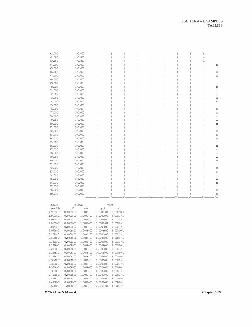
CHAPTER 4 – EXAMPLES
TALLIES
MCNP User’s Manual Chapter 4-65
61.000 90.000| | | | | | | | | x | 62.000 90.000| | | | | | | | | x | 63.000 90.000| | | | | | | | | x | 64.000 100.000| | | | | | | | | | x 65.000 100.000| | | | | | | | | | x 66.000 100.000| | | | | | | | | | x 67.000 100.000| | | | | | | | | | x 68.000 100.000| | | | | | | | | | x 69.000 100.000| | | | | | | | | | x 70.000 100.000| | | | | | | | | | x 71.000 100.000| | | | | | | | | | x 72.000 100.000| | | | | | | | | | x 73.000 100.000| | | | | | | | | | x 74.000 100.000| | | | | | | | | | x 75.000 100.000| | | | | | | | | | x 76.000 100.000| | | | | | | | | | x 77.000 100.000| | | | | | | | | | x 78.000 100.000| | | | | | | | | | x 79.000 100.000| | | | | | | | | | x 80.000 100.000| | | | | | | | | | x 81.000 100.000| | | | | | | | | | x 82.000 100.000| | | | | | | | | | x 83.000 100.000| | | | | | | | | | x 84.000 100.000| | | | | | | | | | x 85.000 100.000| | | | | | | | | | x 86.000 100.000| | | | | | | | | | x 87.000 100.000| | | | | | | | | | x 88.000 100.000| | | | | | | | | | x 89.000 100.000| | | | | | | | | | x 90.000 100.000| | | | | | | | | | x 91.000 100.000| | | | | | | | | | x 92.000 100.000| | | | | | | | | | x 93.000 100.000| | | | | | | | | | x 94.000 100.000| | | | | | | | | | x 95.000 100.000| | | | | | | | | | x 96.000 100.000| | | | | | | | | | x 97.000 100.000| | | | | | | | | | x 98.000 100.000| | | | | | | | | | x 99.000 100.000| | | | | | | | | | x |--------10--------20--------30--------40--------50--------60--------70--------80--------90-------100 tally signal noise upper bin pdf cum. pdf cum. 1.929E+01 0.000E+00 1.000E+00 1.000E-01 1.000E+00 1.958E+01 0.000E+00 1.000E+00 0.000E+00 9.000E-01 1.987E+01 0.000E+00 1.000E+00 0.000E+00 9.000E-01 2.015E+01 0.000E+00 1.000E+00 1.000E-01 9.000E-01 2.044E+01 0.000E+00 1.000E+00 0.000E+00 8.000E-01 2.073E+01 0.000E+00 1.000E+00 0.000E+00 8.000E-01 2.102E+01 0.000E+00 1.000E+00 0.000E+00 8.000E-01 2.131E+01 0.000E+00 1.000E+00 0.000E+00 8.000E-01 2.160E+01 0.000E+00 1.000E+00 0.000E+00 8.000E-01 2.188E+01 0.000E+00 1.000E+00 0.000E+00 8.000E-01 2.217E+01 0.000E+00 1.000E+00 0.000E+00 8.000E-01 2.246E+01 0.000E+00 1.000E+00 0.000E+00 8.000E-01 2.275E+01 0.000E+00 1.000E+00 0.000E+00 8.000E-01 2.304E+01 0.000E+00 1.000E+00 0.000E+00 8.000E-01 2.333E+01 0.000E+00 1.000E+00 0.000E+00 8.000E-01 2.361E+01 0.000E+00 1.000E+00 0.000E+00 8.000E-01 2.390E+01 0.000E+00 1.000E+00 0.000E+00 8.000E-01 2.419E+01 0.000E+00 1.000E+00 0.000E+00 8.000E-01 2.448E+01 0.000E+00 1.000E+00 0.000E+00 8.000E-01 2.477E+01 0.000E+00 1.000E+00 0.000E+00 8.000E-01 2.506E+01 1.000E-01 1.000E+00 2.000E-01 8.000E-01
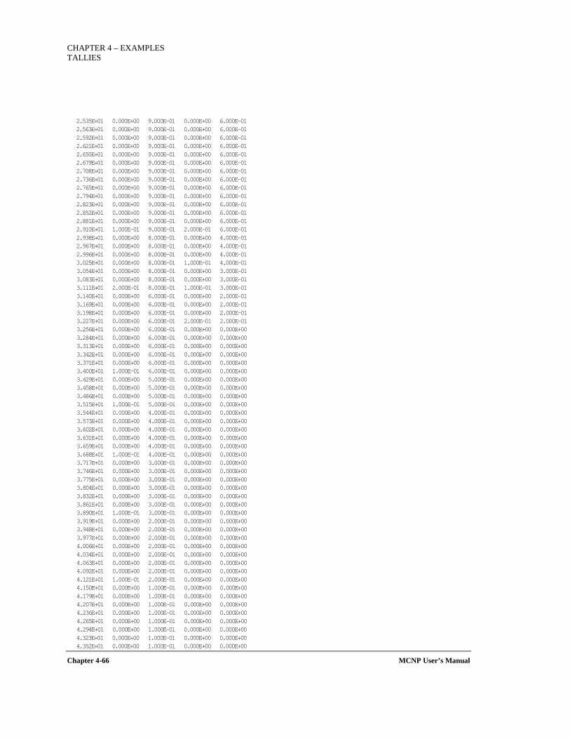
CHAPTER 4 – EXAMPLES TALLIES
Chapter 4-66 MCNP User’s Manual
2.535E+01 0.000E+00 9.000E-01 0.000E+00 6.000E-01 2.563E+01 0.000E+00 9.000E-01 0.000E+00 6.000E-01 2.592E+01 0.000E+00 9.000E-01 0.000E+00 6.000E-01 2.621E+01 0.000E+00 9.000E-01 0.000E+00 6.000E-01 2.650E+01 0.000E+00 9.000E-01 0.000E+00 6.000E-01 2.679E+01 0.000E+00 9.000E-01 0.000E+00 6.000E-01 2.708E+01 0.000E+00 9.000E-01 0.000E+00 6.000E-01 2.736E+01 0.000E+00 9.000E-01 0.000E+00 6.000E-01 2.765E+01 0.000E+00 9.000E-01 0.000E+00 6.000E-01 2.794E+01 0.000E+00 9.000E-01 0.000E+00 6.000E-01 2.823E+01 0.000E+00 9.000E-01 0.000E+00 6.000E-01 2.852E+01 0.000E+00 9.000E-01 0.000E+00 6.000E-01 2.881E+01 0.000E+00 9.000E-01 0.000E+00 6.000E-01 2.910E+01 1.000E-01 9.000E-01 2.000E-01 6.000E-01 2.938E+01 0.000E+00 8.000E-01 0.000E+00 4.000E-01 2.967E+01 0.000E+00 8.000E-01 0.000E+00 4.000E-01 2.996E+01 0.000E+00 8.000E-01 0.000E+00 4.000E-01 3.025E+01 0.000E+00 8.000E-01 1.000E-01 4.000E-01 3.054E+01 0.000E+00 8.000E-01 0.000E+00 3.000E-01 3.083E+01 0.000E+00 8.000E-01 0.000E+00 3.000E-01 3.111E+01 2.000E-01 8.000E-01 1.000E-01 3.000E-01 3.140E+01 0.000E+00 6.000E-01 0.000E+00 2.000E-01 3.169E+01 0.000E+00 6.000E-01 0.000E+00 2.000E-01 3.198E+01 0.000E+00 6.000E-01 0.000E+00 2.000E-01 3.227E+01 0.000E+00 6.000E-01 2.000E-01 2.000E-01 3.256E+01 0.000E+00 6.000E-01 0.000E+00 0.000E+00 3.284E+01 0.000E+00 6.000E-01 0.000E+00 0.000E+00 3.313E+01 0.000E+00 6.000E-01 0.000E+00 0.000E+00 3.342E+01 0.000E+00 6.000E-01 0.000E+00 0.000E+00 3.371E+01 0.000E+00 6.000E-01 0.000E+00 0.000E+00 3.400E+01 1.000E-01 6.000E-01 0.000E+00 0.000E+00 3.429E+01 0.000E+00 5.000E-01 0.000E+00 0.000E+00 3.458E+01 0.000E+00 5.000E-01 0.000E+00 0.000E+00 3.486E+01 0.000E+00 5.000E-01 0.000E+00 0.000E+00 3.515E+01 1.000E-01 5.000E-01 0.000E+00 0.000E+00 3.544E+01 0.000E+00 4.000E-01 0.000E+00 0.000E+00 3.573E+01 0.000E+00 4.000E-01 0.000E+00 0.000E+00 3.602E+01 0.000E+00 4.000E-01 0.000E+00 0.000E+00 3.631E+01 0.000E+00 4.000E-01 0.000E+00 0.000E+00 3.659E+01 0.000E+00 4.000E-01 0.000E+00 0.000E+00 3.688E+01 1.000E-01 4.000E-01 0.000E+00 0.000E+00 3.717E+01 0.000E+00 3.000E-01 0.000E+00 0.000E+00 3.746E+01 0.000E+00 3.000E-01 0.000E+00 0.000E+00 3.775E+01 0.000E+00 3.000E-01 0.000E+00 0.000E+00 3.804E+01 0.000E+00 3.000E-01 0.000E+00 0.000E+00 3.832E+01 0.000E+00 3.000E-01 0.000E+00 0.000E+00 3.861E+01 0.000E+00 3.000E-01 0.000E+00 0.000E+00 3.890E+01 1.000E-01 3.000E-01 0.000E+00 0.000E+00 3.919E+01 0.000E+00 2.000E-01 0.000E+00 0.000E+00 3.948E+01 0.000E+00 2.000E-01 0.000E+00 0.000E+00 3.977E+01 0.000E+00 2.000E-01 0.000E+00 0.000E+00 4.006E+01 0.000E+00 2.000E-01 0.000E+00 0.000E+00 4.034E+01 0.000E+00 2.000E-01 0.000E+00 0.000E+00 4.063E+01 0.000E+00 2.000E-01 0.000E+00 0.000E+00 4.092E+01 0.000E+00 2.000E-01 0.000E+00 0.000E+00 4.121E+01 1.000E-01 2.000E-01 0.000E+00 0.000E+00 4.150E+01 0.000E+00 1.000E-01 0.000E+00 0.000E+00 4.179E+01 0.000E+00 1.000E-01 0.000E+00 0.000E+00 4.207E+01 0.000E+00 1.000E-01 0.000E+00 0.000E+00 4.236E+01 0.000E+00 1.000E-01 0.000E+00 0.000E+00 4.265E+01 0.000E+00 1.000E-01 0.000E+00 0.000E+00 4.294E+01 0.000E+00 1.000E-01 0.000E+00 0.000E+00 4.323E+01 0.000E+00 1.000E-01 0.000E+00 0.000E+00 4.352E+01 0.000E+00 1.000E-01 0.000E+00 0.000E+00
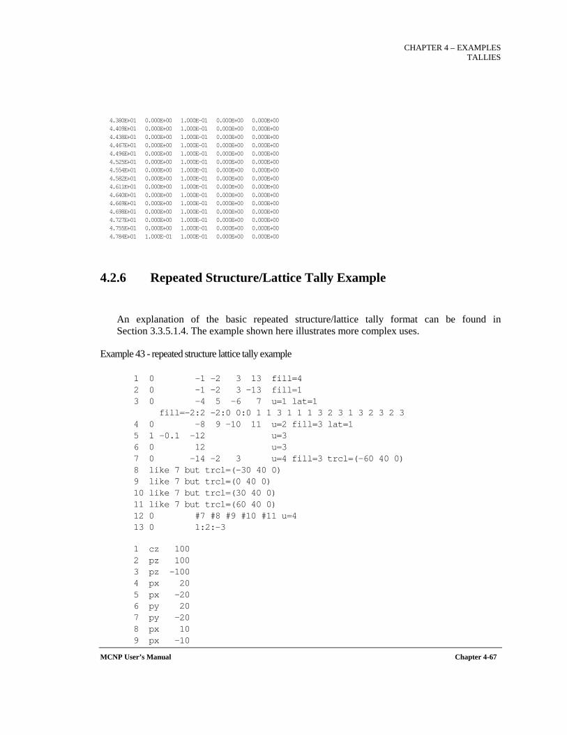
CHAPTER 4 – EXAMPLES
TALLIES
MCNP User’s Manual Chapter 4-67
4.380E+01 0.000E+00 1.000E-01 0.000E+00 0.000E+00 4.409E+01 0.000E+00 1.000E-01 0.000E+00 0.000E+00 4.438E+01 0.000E+00 1.000E-01 0.000E+00 0.000E+00 4.467E+01 0.000E+00 1.000E-01 0.000E+00 0.000E+00 4.496E+01 0.000E+00 1.000E-01 0.000E+00 0.000E+00 4.525E+01 0.000E+00 1.000E-01 0.000E+00 0.000E+00 4.554E+01 0.000E+00 1.000E-01 0.000E+00 0.000E+00 4.582E+01 0.000E+00 1.000E-01 0.000E+00 0.000E+00 4.611E+01 0.000E+00 1.000E-01 0.000E+00 0.000E+00 4.640E+01 0.000E+00 1.000E-01 0.000E+00 0.000E+00 4.669E+01 0.000E+00 1.000E-01 0.000E+00 0.000E+00 4.698E+01 0.000E+00 1.000E-01 0.000E+00 0.000E+00 4.727E+01 0.000E+00 1.000E-01 0.000E+00 0.000E+00 4.755E+01 0.000E+00 1.000E-01 0.000E+00 0.000E+00 4.784E+01 1.000E-01 1.000E-01 0.000E+00 0.000E+00
4.2.6 Repeated Structure/Lattice Tally Example
An explanation of the basic repeated structure/lattice tally format can be found in Section 3.3.5.1.4. The example shown here illustrates more complex uses.
Example 43 - repeated structure lattice tally example 1 0 –1 –2 3 13 fill=4 2 0 –1 –2 3 –13 fill=1 3 0 –4 5 –6 7 u=1 lat=1 fill=–2:2 –2:0 0:0 1 1 3 1 1 1 3 2 3 1 3 2 3 2 3 4 0 –8 9 –10 11 u=2 fill=3 lat=1 5 1 –0.1 –12 u=3 6 0 12 u=3 7 0 –14 –2 3 u=4 fill=3 trcl=(-60 40 0) 8 like 7 but trcl=(-30 40 0) 9 like 7 but trcl=(0 40 0) 10 like 7 but trcl=(30 40 0) 11 like 7 but trcl=(60 40 0) 12 0 #7 #8 #9 #10 #11 u=4 13 0 1:2:-3
1 cz 100 2 pz 100 3 pz -100 4 px 20 5 px -20 6 py 20 7 py -20 8 px 10 9 px -10
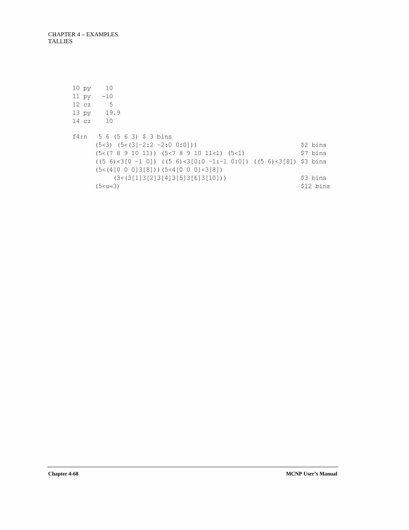
CHAPTER 4 – EXAMPLES TALLIES
Chapter 4-68 MCNP User’s Manual
10 py 10 11 py -10 12 cz 5 13 py 19.9 14 cz 10
f4:n 5 6 (5 6 3) $ 3 bins (5<3) (5<(3[–2:2 –2:0 0:0])) $2 bins (5<(7 8 9 10 11)) (5<7 8 9 10 11<1) (5<1) $7 bins ((5 6)<3[0 –1 0]) ((5 6)<3[0:0 –1:-1 0:0]) ((5 6)<3[8]) $3 bins (5<(4[0 0 0]3[8]))(5<4[0 0 0]<3[8]) (3<(3[1]3[2]3[4]3[5]3[6]3[10])) $3 bins (5<u=3) $12 bins
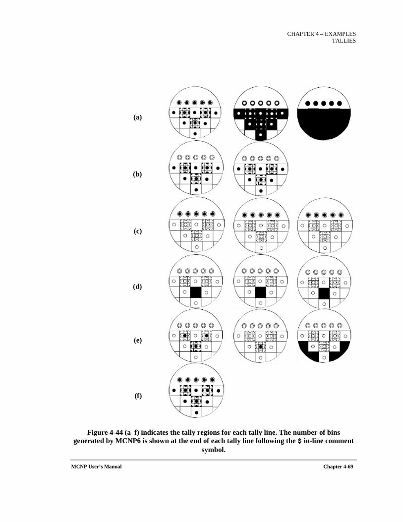
CHAPTER 4 – EXAMPLES
TALLIES
MCNP User’s Manual Chapter 4-69
(a)
(b)
(c)
(d)
(e)
(f)
Figure 4-44 (a–f) indicates the tally regions for each tally line. The number of bins generated by MCNP6 is shown at the end of each tally line following the $ in-line comment
symbol.
CHAPTER 4 – EXAMPLES TALLIES
Chapter 4-70 MCNP User’s Manual
Tally line 1: This first line creates three tally output bins: cell 5, cell 6, and the union of cells 5, 6, and 3, as indicated in Figure 4-44a. Because cell 3 is filled entirely by cells 5 and 6, a tally over cell 5 plus cell 6 is the same as a tally over cell 3. If a particle is tallied in cell 5 and tallied in cell 3, it will be tallied twice in the bin (5 6 3).
Caution: A true union is performed when first level cells overlap (or fill) another cell. This is not a tally that is normally desired. If an average of cell 3 and region (5 6) outside cell 3 is desired, separate bins must be defined and properly combined using correct volume weighting.
Tally line 2: These two input tally bins result in identical output tallies, as shown in Figure 4-44b. The use of lattice index brackets that include all existing lattice elements makes the two tallies equivalent. The simpler format will execute faster.
Tally line 3: This line illustrates omission of geometry levels and a single output bin versus multiple bins. All three input bins tally cell 5 within cells 7 through 11. The second bin specifies the entire path explicitly. Because the only place cell 5 exists within cell 1 is in cells 7–11, the 7–11 specification can be omitted, as in the third input bin. In the second input bin, the parentheses around cells 7–11 are omitted, creating multiple output bins. Five tally bins are produced: (5<7<1), (5<8<1), (5<9<1), (5<10<1), and (5<11<1). The sum of these five bins should equal the tally in the first and last output bins on this line. The tally regions are shown in Figure 4-44c.
Tally line 4: This line illustrates the union of multiple tally cells, (5 6), and various ways of specifying lattice index data. The three input tally bins create three output tally bins with identical values because the three different lattice descriptions refer to the same lattice element, the eighth entry on the FILL array. If the parentheses around (5 6) were removed, two output bins would be created for each input bin, namely (5<3[0 -1 0]) and (6<3[0 -1 0]), etc. The tally regions are shown in Figure 4-44d.
Tally line 5: This line illustrates tallies in overlapping regions in repeated structures in a lattice and a tally in lattice elements filled with themselves. Three tally output bins are produced. In the first input bin, a particle is tallied only once when it is in cell 5 and in 4[0 0 0] or when it is in cell 5 and in 3[0 -1 0]. Figure 4-44e shows all the cell 5 instances included in this tally bin. This tally is probably more useful than the overlapping regions in tally line 1. Input bin 2 demonstrates a tally for a nested lattice. A tally is made when a particle is in cell 5 and in cell 4, element [0 0 0] and in cell 3, element [0 -1 0]. Note that 3[0 -1 0] is indeed filled with cell 4 (u=2). If that were not true, a zero tally would result in this bin. The final input tally bin demonstrated a tally in lattice elements that are filled with their own universe number. This method is the only way to tally in these elements separate from the rest of cell 3.
Tally line 6: This line illustrates the universe format. The single input bin includes all possible chains involving cell 5. Because u=3 is not within parentheses, the input is expanded into twelve output bins: (5<3[3], etc.). The format 3[3] indicates the third lattice element of
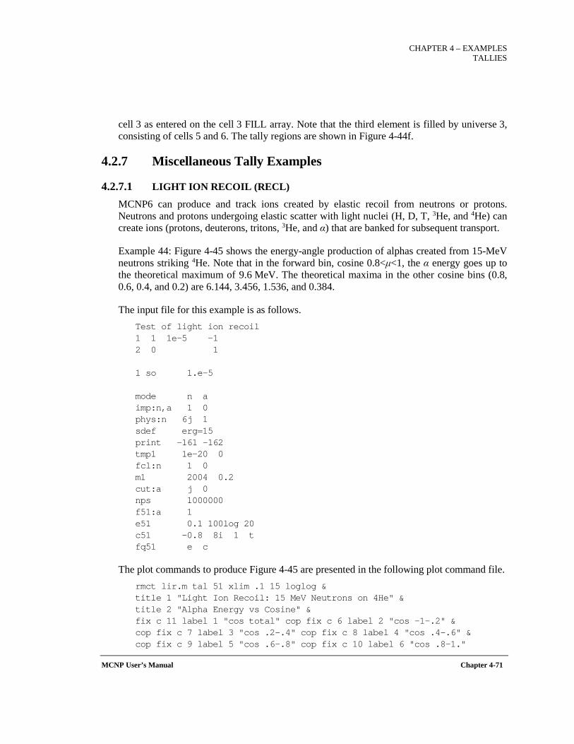
CHAPTER 4 – EXAMPLES
TALLIES
MCNP User’s Manual Chapter 4-71
cell 3 as entered on the cell 3 FILL array. Note that the third element is filled by universe 3, consisting of cells 5 and 6. The tally regions are shown in Figure 4-44f.
4.2.7 Miscellaneous Tally Examples
4.2.7.1 LIGHT ION RECOIL (RECL)
MCNP6 can produce and track ions created by elastic recoil from neutrons or protons. Neutrons and protons undergoing elastic scatter with light nuclei (H, D, T, 3He, and 4He) can create ions (protons, deuterons, tritons, 3He, and α) that are banked for subsequent transport.
Example 44: Figure 4-45 shows the energy-angle production of alphas created from 15-MeV neutrons striking 4He. Note that in the forward bin, cosine 0.8<μ<1, the α energy goes up to the theoretical maximum of 9.6 MeV. The theoretical maxima in the other cosine bins (0.8, 0.6, 0.4, and 0.2) are 6.144, 3.456, 1.536, and 0.384.
The input file for this example is as follows. Test of light ion recoil 1 1 1e-5 -1 2 0 1 1 so 1.e-5 mode n a imp:n,a 1 0 phys:n 6j 1 sdef erg=15 print -161 -162 tmp1 1e-20 0 fcl:n 1 0 m1 2004 0.2 cut:a j 0 nps 1000000 f51:a 1 e51 0.1 100log 20 c51 -0.8 8i 1 t fq51 e c
The plot commands to produce Figure 4-45 are presented in the following plot command file. rmct lir.m tal 51 xlim .1 15 loglog & title 1 "Light Ion Recoil: 15 MeV Neutrons on 4He" & title 2 "Alpha Energy vs Cosine" & fix c 11 label 1 "cos total" cop fix c 6 label 2 "cos -1-.2" & cop fix c 7 label 3 "cos .2-.4" cop fix c 8 label 4 "cos .4-.6" & cop fix c 9 label 5 "cos .6-.8" cop fix c 10 label 6 "cos .8-1."

CHAPTER 4 – EXAMPLES TALLIES
Chapter 4-72 MCNP User’s Manual
Figure 4-45. Light ion recoil.
4.2.7.2 INLINE GENERATION OF DOUBLE DIFFERENTIAL CROSS SECTIONS AND RESIDUAL NUCLEI
The double differential cross sections and distributions of residual nuclei for a single nuclear interaction thus may be calculated directly in MCNP6. Tallying of the residual nuclei is discussed in the FT8 RES tally description (see Section 3.3.5.18). Tallying of the differential cross section can be done with standard F1 surface tallies, as shown in the following example. The input file models a 1.2-GeV proton source having a single collision with 208Pb.
Test of p(1.2GeV)+Pb(208) 1 1 -11. -1 imp:h 1 2 0 1 imp:h 0 1 so .01 mode h n sdef par h erg=1200 vec 0 0 1 dir 1
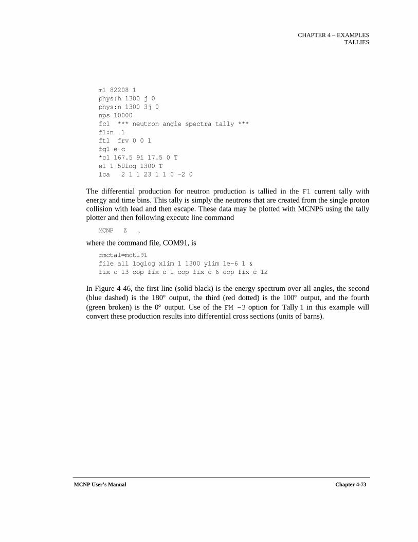
CHAPTER 4 – EXAMPLES
TALLIES
MCNP User’s Manual Chapter 4-73
m1 82208 1 phys:h 1300 j 0 phys:n 1300 3j 0 nps 10000 fc1 *** neutron angle spectra tally *** f1:n 1 ft1 frv 0 0 1 fq1 e c *c1 167.5 9i 17.5 0 T e1 1 50log 1300 T lca 2 1 1 23 1 1 0 -2 0
The differential production for neutron production is tallied in the F1 current tally with energy and time bins. This tally is simply the neutrons that are created from the single proton collision with lead and then escape. These data may be plotted with MCNP6 using the tally plotter and then following execute line command
MCNP Z ,
where the command file, COM91, is rmctal=mctl91 file all loglog xlim 1 1300 ylim 1e-6 1 & fix c 13 cop fix c 1 cop fix c 6 cop fix c 12
In Figure 4-46, the first line (solid black) is the energy spectrum over all angles, the second (blue dashed) is the 180° output, the third (red dotted) is the 100° output, and the fourth (green broken) is the 0° output. Use of the FM -3 option for Tally 1 in this example will convert these production results into differential cross sections (units of barns).
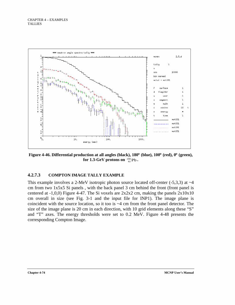
CHAPTER 4 – EXAMPLES TALLIES
Chapter 4-74 MCNP User’s Manual
Figure 4-46. Differential production at all angles (black), 180° (blue), 100° (red), 0° (green),
for 1.3-GeV protons on .
4.2.7.3 COMPTON IMAGE TALLY EXAMPLE
This example involves a 2-MeV isotropic photon source located off-center (-5,3,3) at ~4 cm from two 1x5x5 Si panels , with the back panel 3 cm behind the front (front panel is centered at -1,0,0) Figure 4-47. The Si voxels are 2x2x2 cm, making the panels 2x10x10 cm overall in size (see Fig. 3-1 and the input file for INP1). The image plane is coincident with the source location, so it too is ~4 cm from the front panel detector. The size of the image plane is 20 cm in each direction, with 10 grid elements along these “S” and “T” axes. The energy thresholds were set to 0.2 MeV. Figure 4-48 presents the corresponding Compton Image.
Pb20882
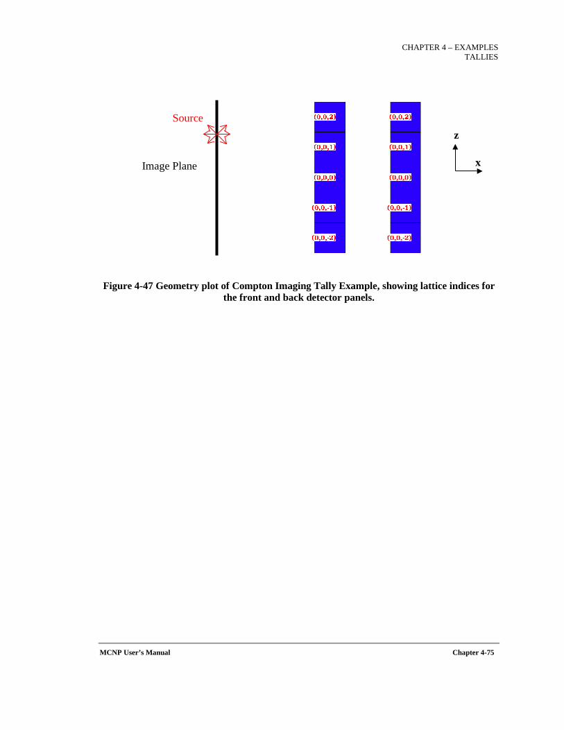
CHAPTER 4 – EXAMPLES
TALLIES
MCNP User’s Manual Chapter 4-75
Figure 4-47 Geometry plot of Compton Imaging Tally Example, showing lattice indices for the front and back detector panels.
Source
Image Plane
z
x
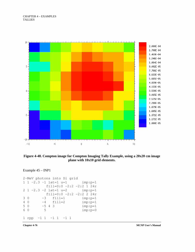
CHAPTER 4 – EXAMPLES TALLIES
Chapter 4-76 MCNP User’s Manual
Figure 4-48. Compton image for Compton Imaging Tally Example, using a 20x20 cm image plane with 10x10 grid elements.
Example 45 – INP1 2-MeV photons into Si grid 1 1 -2.3 -1 lat=1 u=1 imp:p=1 fill=0:0 -2:2 -2:2 1 24r 2 1 -2.3 -2 lat=1 u=2 imp:p=1 fill=0:0 -2:2 -2:2 2 24r 3 0 -3 fill=1 imp:p=1 4 0 -4 fill=2 imp:p=1 5 0 -5 4 3 imp:p=1 6 0 5 imp:p=0 1 rpp -1 1 -1 1 -1 1
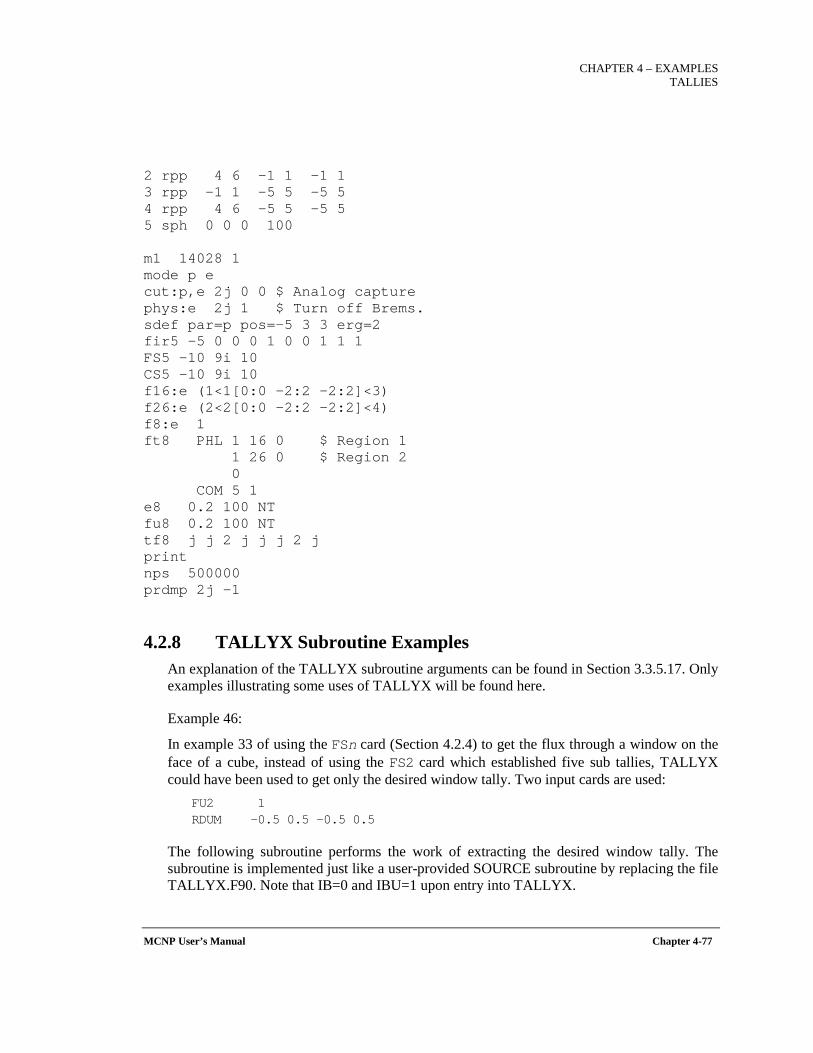
CHAPTER 4 – EXAMPLES
TALLIES
MCNP User’s Manual Chapter 4-77
2 rpp 4 6 -1 1 -1 1 3 rpp -1 1 -5 5 -5 5 4 rpp 4 6 -5 5 -5 5 5 sph 0 0 0 100 m1 14028 1 mode p e cut:p,e 2j 0 0 $ Analog capture phys:e 2j 1 $ Turn off Brems. sdef par=p pos=-5 3 3 erg=2 fir5 -5 0 0 0 1 0 0 1 1 1 FS5 -10 9i 10 CS5 -10 9i 10 f16:e (1<1[0:0 -2:2 -2:2]<3) f26:e (2<2[0:0 -2:2 -2:2]<4) f8:e 1 ft8 PHL 1 16 0 $ Region 1 1 26 0 $ Region 2 0 COM 5 1 e8 0.2 100 NT fu8 0.2 100 NT tf8 j j 2 j j j 2 j print nps 500000 prdmp 2j -1
4.2.8 TALLYX Subroutine Examples An explanation of the TALLYX subroutine arguments can be found in Section 3.3.5.17. Only examples illustrating some uses of TALLYX will be found here.
Example 46:
In example 33 of using the FSn card (Section 4.2.4) to get the flux through a window on the face of a cube, instead of using the FS2 card which established five sub tallies, TALLYX could have been used to get only the desired window tally. Two input cards are used:
FU2 1 RDUM -0.5 0.5 -0.5 0.5
The following subroutine performs the work of extracting the desired window tally. The subroutine is implemented just like a user-provided SOURCE subroutine by replacing the file TALLYX.F90. Note that IB=0 and IBU=1 upon entry into TALLYX.
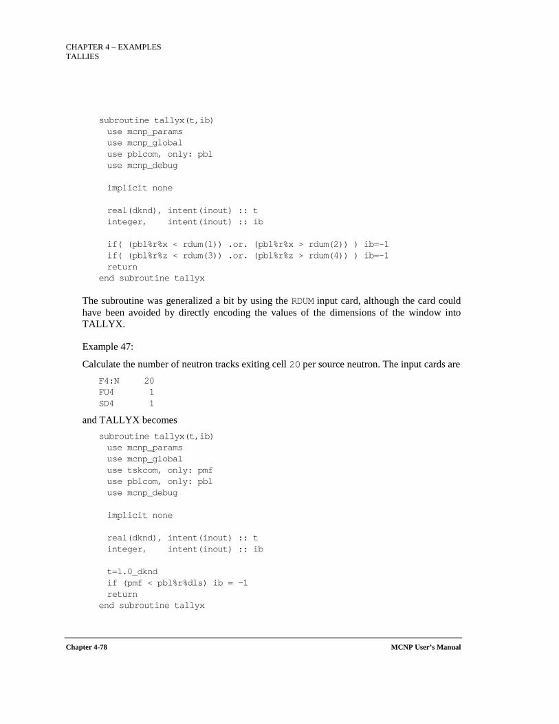
CHAPTER 4 – EXAMPLES TALLIES
Chapter 4-78 MCNP User’s Manual
subroutine tallyx(t,ib) use mcnp_params use mcnp_global use pblcom, only: pbl use mcnp_debug implicit none real(dknd), intent(inout) :: t integer, intent(inout) :: ib if( (pbl%r%x < rdum(1)) .or. (pbl%r%x > rdum(2)) ) ib=-1 if( (pbl%r%z < rdum(3)) .or. (pbl%r%z > rdum(4)) ) ib=-1 return
end subroutine tallyx
The subroutine was generalized a bit by using the RDUM input card, although the card could have been avoided by directly encoding the values of the dimensions of the window into TALLYX.
Example 47:
Calculate the number of neutron tracks exiting cell 20 per source neutron. The input cards are F4:N 20 FU4 1 SD4 1
and TALLYX becomes subroutine tallyx(t,ib) use mcnp_params use mcnp_global use tskcom, only: pmf use pblcom, only: pbl use mcnp_debug implicit none real(dknd), intent(inout) :: t integer, intent(inout) :: ib t=1.0_dknd if (pmf < pbl%r%dls) ib = -1 return
end subroutine tallyx
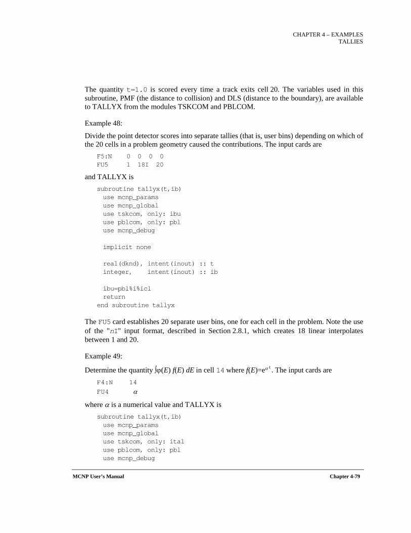
CHAPTER 4 – EXAMPLES
TALLIES
MCNP User’s Manual Chapter 4-79
The quantity t=1.0 is scored every time a track exits cell 20. The variables used in this subroutine, PMF (the distance to collision) and DLS (distance to the boundary), are available to TALLYX from the modules TSKCOM and PBLCOM.
Example 48:
Divide the point detector scores into separate tallies (that is, user bins) depending on which of the 20 cells in a problem geometry caused the contributions. The input cards are
F5:N 0 0 0 0 FU5 1 18I 20
and TALLYX is subroutine tallyx(t,ib) use mcnp_params use mcnp_global use tskcom, only: ibu use pblcom, only: pbl use mcnp_debug implicit none real(dknd), intent(inout) :: t integer, intent(inout) :: ib ibu=pbl%i%icl return
end subroutine tallyx
The FU5 card establishes 20 separate user bins, one for each cell in the problem. Note the use of the "nI" input format, described in Section 2.8.1, which creates 18 linear interpolates between 1 and 20.
Example 49:
Determine the quantity ∫ϕ(E) f(E) dE in cell 14 where f(E)=eα t . The input cards are F4:N 14 FU4 α
where α is a numerical value and TALLYX is subroutine tallyx(t,ib) use mcnp_params use mcnp_global use tskcom, only: ital use pblcom, only: pbl use mcnp_debug
CHAPTER 4 – EXAMPLES TALLIES
Chapter 4-80 MCNP User’s Manual
implicit none real(dknd), intent(inout) :: t integer, intent(inout) :: ib t=t*exp(tds(iptal(3,1,ital)+1)*pbl%r%tme) return
end subroutine tallyx
The FU4 card establishes a single user bin, and the value of α is stored in TDS(IPTAL(3,1,ITAL)+1) and used for the tally label.
Example 50:
Tally the number of neutrons passing through cell 16 that have had 0, 1, 2, 3, or 4 collisions. The input cards are
F4:N 16 FU4 0 1 2 3 4 SD4 1
and TALLYX is subroutine tallyx(t,ib) use mcnp_params use mcnp_global use tskcom, only: ibu use pblcom, only: pbl use mcnp_debug implicit none real(dknd), intent(inout) :: t integer, intent(inout) :: ib ibu = pbl%i%ncp if(ibu > 5 ) ib=-1 t=pbl%r%wgt return
end subroutine tallyx
If the IF statement in this TALLYX is omitted, a count will be made of the cases of five or more collisions, and in these cases no score will be tallied but a count will be printed of the times that the tally was unable to be made because IBU was a value where no bin existed.
CHAPTER 4 – EXAMPLES
TALLIES
MCNP User’s Manual Chapter 4-81
In the five user bins, t is the number of neutrons per source neutron passing through cell 16 that have undergone 0, 1, 2, 3, or 4 collisions, respectively. Note that the FU4 card has five entries to establish the five user bins and provide labels. Note also that in this example, the neutrons are calculated so that t=t × renormalization factor (which preserves the weight associated with the tracks), where in TALLYX subroutine Example 3 the neutron tracks are calculated so that t=1. Finally, note that if pbl%i%ncp>5 (six or more collisions) no tally is made because IB is set to be less than zero. If an E4 card was added, the neutrons would be tallied as a function of energy for each user bin.
4.3 SOURCE EXAMPLES
4.3.1 General Source Some examples of the general source are given here to illustrate the power and complexity of this feature. Refer to Section 3.3.4 for a more complete explanation and other examples.
The following example is of the general source that illustrates two levels of dependency. Let us assume a duct streaming problem where the source at the duct opening has been obtained from a reactor calculation. Energies above 13.5 MeV have one angular distribution and energies below 13.5 MeV have a different angular distribution. The source has a uniform spatial distribution on a circular disk of radius 37 cm centered at x,y,z on planar surface 1 going into cell 2.
Example 51: SDEF ERG = D1 DIR FERG D2 SUR = 1 CEL = 2 POS = x y z RAD D5 AXS u v w VEC u v w c Source Definition Card. c In this example, AXS is needed to define a vector which c defines the source plane of a disk source. c In this example, POS defines the location of the center c of the disk. c VEC is the direction that source particles will be c travelling once created. c AXS and VEC can be different. c For this duct streaming problem, they should be the same. c SI1 H 1E-7 1E-5 ... 13.5 14 ... 20 c Source Information 1 (SI1) corresponds to D1. c H indicates histogram values follow. c SP1 D 0 10E-4 ... 10E-2 10E-1 ... 0.3 c Source Probability 1 (SP1) augments SI1. c D indicates discrete values. c Probability of each bin on SI1. c The probability a source particle will be between 10E-7 c and 10E-5 MeV is 10E-4.
CHAPTER 4 – EXAMPLES SOURCE
Chapter 4-82 MCNP User’s Manual
c DS2 S 3 3 ... 3 4 ... 4 c Dependent Source 2 (Depends as a function of ERG). c S indicates numbers following are themselves other c distributions. c In this example, if a particle has an energy in bin 10E-7 to c 10E-5, then it will have a direction associated with source c distribution 3. c SI3 0 0.2 ... 1 c Source Information 3 (Second Level) c Default is histogram values. c SP3 D 0 1E-4 ... 0.1 c Source Probability 3 (Second Level). c Probability of each bin on SI3. c SI4 0 0.1 ... 1 c Source Information 4 (Second Level). c Default is histogram values. c SP4 D 0 1E-2 ... 0.1 c Source Probability 4 (Second Level). c Probability of each bin on SI4. c SI5 37 c Source Information 5. c Default is histogram values. c There is one bin from 0 to 37. c When used with the RAD keyword on the SDEF card, it indicates c a circular distribution from 0 to 37 cm. c SP5 -21 1 c Source Probability 5. c The -21 indicates a sampling scheme based on a power of the c variable. c In this case, the sampling is a function of radius^1, c which results in a uniform spatial distribution over the disk. c Since a uniform spatial distribution is the default for disk c sources, this card is optional. c
This example can be expanded by having the source in two ducts instead of one (with the same energy and angular distribution as before). The SI1, SP1, DS2, SI3, SP3, SI4, and SP4 cards remain unchanged, but the SI5 and SP5 cards are no longer valid. The SDEF card is changed as shown below and the other cards are added.
CHAPTER 4 – EXAMPLES
SOURCE
MCNP User’s Manual Chapter 4-83
SDEF ERG = D1 DIR FERG D2 SUR = D6 CEL FSUR D7 POS FSUR D8 RAD FSUR D9 AXS FSUR D10 VEC FSUR D10 SI6 L 1 7 c Source Information 6. c L indicates discrete values, in this case surface 1 or 7 c SP6 D 0.6 0.4 c Source Probability 6. c Probability of each value on SI6. c DS7 L 2 8 c Dependent Source 7 (Depends as a function of SUR). c L indicates discrete value, in this case cell 2 or 8, c depending on whether surface 1 or 7, respectively, was chosen. c DS8 L x1 y1 z1 x2 y2 z2 c Dependent Source 8 (Depends as a function of SUR). c L indicates discrete values, in this case the respective centers, c of two disks, depending on whether surface 1 or 7 was chosen. c DS9 S 11 12 c Dependent Source 9 (Depends as a function of SUR). c S indicates other distributions, in this case the respective radii, c of two disks, depending on whether surface 1 or 7 was chosen. c DS10 L u1 v1 w1 u2 v2 w2 c Dependent Source 10 (Depends as a function of SUR). c L indicates discrete values, in this case the vectors that define a c plane that the disk is on and the vector from which DIR is measured. c In this streaming problem, AXS=VEC, and both depend on whether c surface 1 or 7 was chosen. SI11 0 37 SP11 −21 1 SI12 0 25 SP12 −21 1 c In this problem, the radius of the duct depends on which c duct was chosen.
Example 52:
This example is a two-source-cell problem where the material in one cell is uranium and in the other is thorium. The uranium cell has two isotopes, 235Uand 238U, and the thorium has one, 232Th. Each isotope has many photon lines from radioactive decay. The following input cards describe this source.
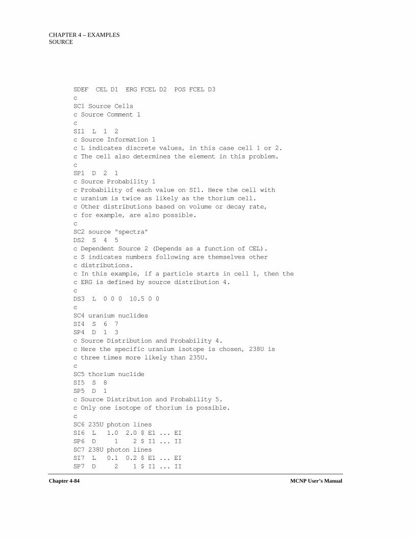
CHAPTER 4 – EXAMPLES SOURCE
Chapter 4-84 MCNP User’s Manual
SDEF CEL D1 ERG FCEL D2 POS FCEL D3 c SC1 Source Cells c Source Comment 1 c SI1 L 1 2 c Source Information 1 c L indicates discrete values, in this case cell 1 or 2. c The cell also determines the element in this problem. c SP1 D 2 1 c Source Probability 1 c Probability of each value on SI1. Here the cell with c uranium is twice as likely as the thorium cell. c Other distributions based on volume or decay rate, c for example, are also possible. c SC2 source "spectra" DS2 S 4 5 c Dependent Source 2 (Depends as a function of CEL). c S indicates numbers following are themselves other c distributions. c In this example, if a particle starts in cell 1, then the c ERG is defined by source distribution 4. c DS3 L 0 0 0 10.5 0 0 c SC4 uranium nuclides SI4 S 6 7 SP4 D 1 3 c Source Distribution and Probability 4. c Here the specific uranium isotope is chosen, 238U is c three times more likely than 235U. c SC5 thorium nuclide SI5 S 8 SP5 D 1 c Source Distribution and Probability 5. c Only one isotope of thorium is possible. c SC6 235U photon lines SI6 L 1.0 2.0 $ E1 ... EI SP6 D 1 2 $ I1 ... II SC7 238U photon lines SI7 L 0.1 0.2 $ E1 ... EI SP7 D 2 1 $ I1 ... II
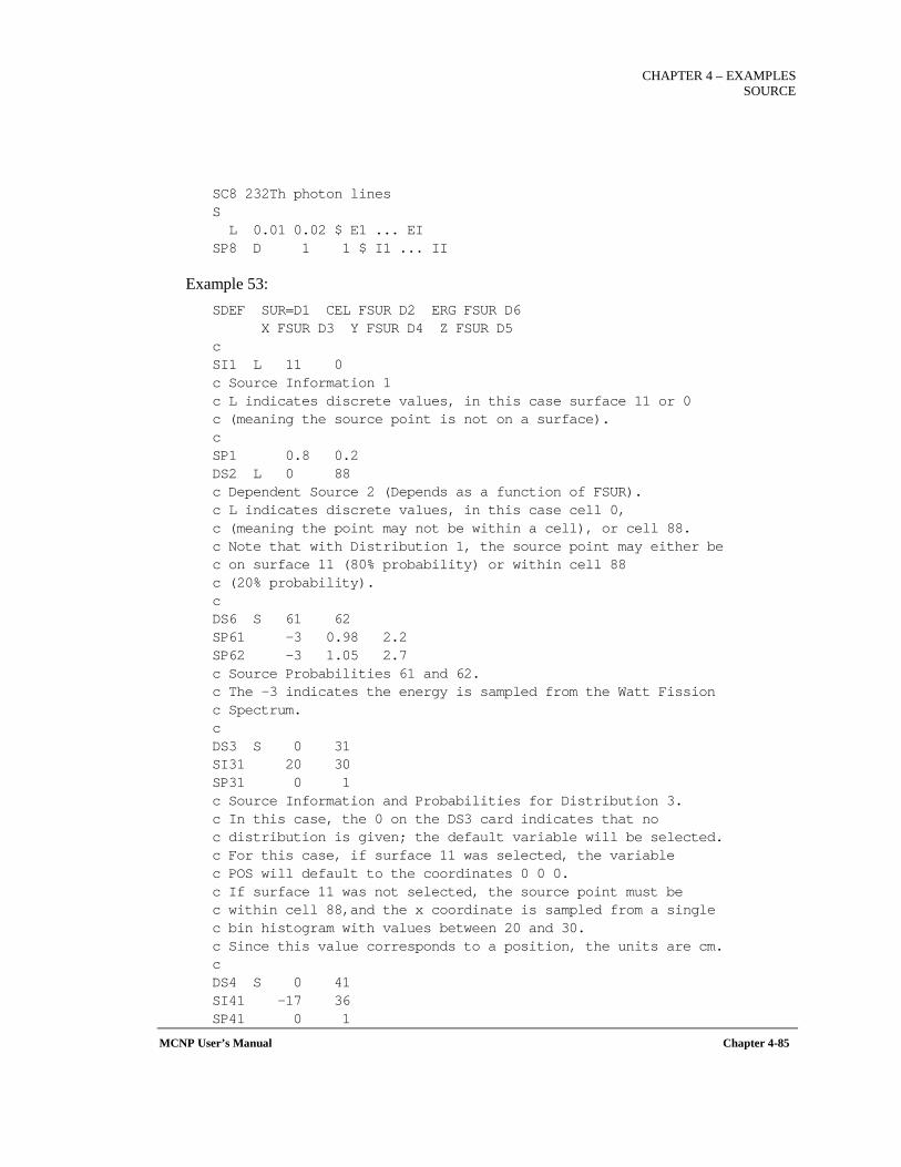
CHAPTER 4 – EXAMPLES
SOURCE
MCNP User’s Manual Chapter 4-85
SC8 232Th photon lines S L 0.01 0.02 $ E1 ... EI SP8 D 1 1 $ I1 ... II
Example 53: SDEF SUR=D1 CEL FSUR D2 ERG FSUR D6 X FSUR D3 Y FSUR D4 Z FSUR D5 c SI1 L 11 0 c Source Information 1 c L indicates discrete values, in this case surface 11 or 0 c (meaning the source point is not on a surface). c SP1 0.8 0.2 DS2 L 0 88 c Dependent Source 2 (Depends as a function of FSUR). c L indicates discrete values, in this case cell 0, c (meaning the point may not be within a cell), or cell 88. c Note that with Distribution 1, the source point may either be c on surface 11 (80% probability) or within cell 88 c (20% probability). c DS6 S 61 62 SP61 -3 0.98 2.2 SP62 -3 1.05 2.7 c Source Probabilities 61 and 62. c The -3 indicates the energy is sampled from the Watt Fission c Spectrum. c DS3 S 0 31 SI31 20 30 SP31 0 1 c Source Information and Probabilities for Distribution 3. c In this case, the 0 on the DS3 card indicates that no c distribution is given; the default variable will be selected. c For this case, if surface 11 was selected, the variable c POS will default to the coordinates 0 0 0. c If surface 11 was not selected, the source point must be c within cell 88,and the x coordinate is sampled from a single c bin histogram with values between 20 and 30. c Since this value corresponds to a position, the units are cm. c DS4 S 0 41 SI41 -17 36 SP41 0 1
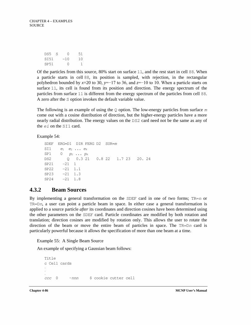
CHAPTER 4 – EXAMPLES SOURCE
Chapter 4-86 MCNP User’s Manual
DS5 S 0 51 SI51 -10 10 SP51 0 1
Of the particles from this source, 80% start on surface 11, and the rest start in cell 88. When a particle starts in cell 88, its position is sampled, with rejection, in the rectangular polyhedron bounded by x=20 to 30, y=−17 to 36, and z=−10 to 10. When a particle starts on surface 11, its cell is found from its position and direction. The energy spectrum of the particles from surface 11 is different from the energy spectrum of the particles from cell 88. A zero after the S option invokes the default variable value.
The following is an example of using the Q option. The low-energy particles from surface m come out with a cosine distribution of direction, but the higher-energy particles have a more nearly radial distribution. The energy values on the DS2 card need not be the same as any of the ei on the SI1 card.
Example 54: SDEF ERG=D1 DIR FERG D2 SUR=m SI1 e1 e2 ... ek SP1 0 p2 ... pk DS2 Q 0.3 21 0.8 22 1.7 23 20. 24 SP21 -21 1 SP22 -21 1.1 SP23 -21 1.3 SP24 -21 1.8
4.3.2 Beam Sources By implementing a general transformation on the SDEF card in one of two forms; TR=n or TR=Dn, a user can point a particle beam in space. In either case a general transformation is applied to a source particle after its coordinates and direction cosines have been determined using the other parameters on the SDEF card. Particle coordinates are modified by both rotation and translation; direction cosines are modified by rotation only. This allows the user to rotate the direction of the beam or move the entire beam of particles in space. The TR=Dn card is particularly powerful because it allows the specification of more than one beam at a time.
Example 55: A Single Beam Source
An example of specifying a Gaussian beam follows:
Title c Cell cards . . .
ccc 0 -nnn $ cookie cutter cell
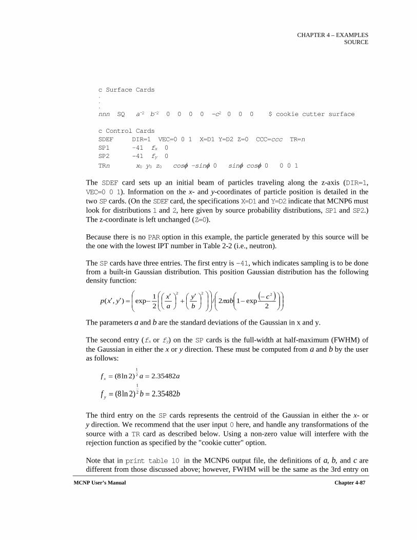
CHAPTER 4 – EXAMPLES
SOURCE
MCNP User’s Manual Chapter 4-87
c Surface Cards . . .
nnn SQ a-2 b-2 0 0 0 0 -c2 0 0 0 $ cookie cutter surface c Control Cards SDEF DIR=1 VEC=0 0 1 X=D1 Y=D2 Z=0 CCC=ccc TR=n SP1 -41 fx 0 SP2 -41 fy 0 TRn x0 y0 z0 cosφ -sinφ 0 sinφ cosφ 0 0 0 1
The SDEF card sets up an initial beam of particles traveling along the z-axis (DIR=1, VEC=0 0 1). Information on the x- and y-coordinates of particle position is detailed in the two SP cards. (On the SDEF card, the specifications X=D1 and Y=D2 indicate that MCNP6 must look for distributions 1 and 2, here given by source probability distributions, SP1 and SP2.) The z-coordinate is left unchanged (Z=0).
Because there is no PAR option in this example, the particle generated by this source will be the one with the lowest IPT number in Table 2-2 (i.e., neutron).
The SP cards have three entries. The first entry is -41, which indicates sampling is to be done from a built-in Gaussian distribution. This position Gaussian distribution has the following density function:
The parameters a and b are the standard deviations of the Gaussian in x and y.
The second entry (fx or fy) on the SP cards is the full-width at half-maximum (FWHM) of the Gaussian in either the x or y direction. These must be computed from a and b by the user as follows:
The third entry on the SP cards represents the centroid of the Gaussian in either the x- or y direction. We recommend that the user input 0 here, and handle any transformations of the source with a TR card as described below. Using a non-zero value will interfere with the rejection function as specified by the "cookie cutter" option.
Note that in print table 10 in the MCNP6 output file, the definitions of a, b, and c are different from those discussed above; however, FWHM will be the same as the 3rd entry on
( )
−−
′
+
′
−=′′2
exp12/21exp),(
222 cabby
axyxp π
aaf x 35482.2)2ln8( 21
==
bbf y 35482.2)2ln8( 21
==
CHAPTER 4 – EXAMPLES SOURCE
Chapter 4-88 MCNP User’s Manual
the SP cards. The parameter ‘a’ in Table 10 differs from the parameter ‘a’ above by a factor of the square root of two. This is a legacy item from the conversion of the -41 function from time to space, and will be corrected in a future version.
The user generally does not want the beam Gaussian to extend infinitely in x and y, therefore a cookie cutter option has been included to keep the distribution to a reasonable size. CCC=ccc tells MCNP6 to look at the card labeled ccc (ccc is a user-specified cell number) to define the cutoff volume. The first entry on the ccc card is 0, which indicates a void cell. The second number, -nnn (nnn again is a user-specified number), indicates a surface card within which to accept particles. In the example, this is a SQ surface (a 2-sheet hyperboloid) that is defined as follows:
Any particle generated within this cell is accepted; any outside of the cell is rejected. Any well defined surface may be selected, and it is common to use a simple cylinder to represent the extent of a beam pipe.
In this example, a source is generated in an (x′,y′)-coordinate system with the distribution centered at the origin and the particles traveling in the z′ direction. The particle coordinates can be modified to an (x,y)-coordinate system by translation and rotation according to the following equations, where
Thus the angle is the angle of rotation of the major axis of the source distribution from the positive y direction in the laboratory coordinate system. If , the angle is 90° and the major axis lies along the x-axis. The TRn card in the example above implements this rotation matrix, however the user should note that in the TRn card is equal to .
Example 56: Defining Multiple Beams
The opportunity to specify a probability distribution of transformations on the SDEF card allows the formation of multiple beams which differ only in orientation and intensity. This feature may have applications in radiography or in the distribution of point sources of arbitrary intensity.
The use of a distribution of transformations is invoked by specifying TR=Dn on the SDEF card. The cards SI, SP, and, optionally, SB are used as specified for the SSR card, which is discussed in Section 3.3.4.8.
222
cby
ax
≤
′
+
′
:0 πφ ≤≤ L
0cossin xyxx LL +′−′= φφ
0sincos yysxy LL +′+′= φφ
Lφ0.0cos =Lφ
Lφ2πφ −L
CHAPTER 4 – EXAMPLES
SOURCE
MCNP User’s Manual Chapter 4-89
SIn L i1 ... ik SPn option p1 ... pk SBn option b1 ... bk
The L option on the SI card is required; input checking ensures this usage for both the SDEF and SSR applications. The "option" on the SP and SB cards may be blank, D, or C. The values i1 ... ik identify k transformations which must be supplied. The content of the SP and SB cards then follows the general MCNP6 rules.
The following example shows a case of three intersecting Gaussian parallel beams, each defined with the parameters a=0.2 cm, b=0.1 cm and c=2 in the notation previously discussed in Example 1. For each, the beam is normal to the plane of definition.
Beam 1 is centered at (0,0,-2). The major axis of the beam distribution is along the x-axis. The beam is emitted in the +z direction and has relative intensity 1.
Beam 2 is centered at (-2,0,0). The major axis of the beam distribution is along the y-axis. The beam is emitted in the +x direction and has relative intensity 2.
Beam 3 is centered at (0,-2,0). The major axis of the beam distribution is along the line defined by x=z. The beam is emitted in the +y direction and has relative intensity 3.
The card SBn is used to provide equal sampling from each of the three beams, independent of the relative intensities. The input cards are as follows:
Title c Cell cards . . .
999 0 -999 $ cookie cutter cell c Surface Cards . . .
999 SQ 25 100 0 0 0 0 -4 0 0 0 $ cookie cutter surface c Control Cards SDEF DIR=1 VEC=0 0 1 X=D1 Y=D2 Z=0 CCC=999 TR=D3 SP1 -41 0.4709640 SP2 -41 0.23584820 SI3 L 1 2 3 SP3 1 2 3 SB3 1 1 1 TR1 0 0 -2 1 0 0 0 1 0 0 0 1 TR2 -2 0 0 0 1 0 0 0 1 1 0 0 TR3 0 -2 0 0.707 0 0.707 0.707 0 -0.707 0 1 0
CHAPTER 4 – EXAMPLES SOURCE
Chapter 4-90 MCNP User’s Manual
4.3.3 Burning Multiple Materials In a Repeated Structure with Specified Concentration Changes
Example 57:
In the following example, a 4×4 fuel pin array (created using repeated structures) is burned while material concentration changes are made at various time steps. Portions of the input and output files are provided below to illustrate various BURN card features;:
burn example 1 1 6.87812e-2 -1 u=2 imp:n=1 vol=192.287 $ fuel 3 2 4.5854e-2 1 -2 u=2 imp:n=1 vol=66.43 $ clad 4 3 7.1594e-2 2 u=2 imp:n=1 vol=370.82 $ water 6 4 6.87812e-2 -1 u=3 imp:n=1 vol=192.287 $ fuel 7 5 4.5854e-2 1 -2 u=3 imp:n=1 vol=66.43 $ clad 8 6 7.1594e-2 2 u=3 imp:n=1 vol=370.82 $ water 10 0 -3 4 -5 6 u=1 imp:n=1 lat=1 fill=0:1 0:1 0:0 2 3 2 3 ... ... BURN TIME=50,10,500 MAT=1 4 POWER=1.0 PFRAC=1.0 0 0.2 OMIT= 1,8,6014,7016,8018,9018,90234,91232,95240,95244 4,8,6014,7016,8018,9018,90234,91232,95240,95244 BOPT= 1.0, -4 AFMIN= 1e-32 MATVOL= 384.57 384.57 MATMOD= 2 1 1 -4 1 94238 1e-6 2 2 -1 2 94238 1e-6 94241 1e-6 -4 1 94238 1e-6 ...
A 4×4 lattice contains universes 2 and 3, which are both repeated twice in the lattice. Universe 2 comprises cells 1, 3, and 4, where cell 1 contains material 1; universe 3 comprises cells 6, 7, and 8, where cell 6 contains material 4. The MAT keyword specifies that both materials 1 and 4 will be burned. The combination of the TIME, POWER and PFRAC keywords specify that these materials will be burned first for 50 days at 100% of 1 MW, then decayed for 10 days, and then finally burned for 500 days at 20% of 1 MW.
CHAPTER 4 – EXAMPLES
SOURCE
MCNP User’s Manual Chapter 4-91
The BOPT keyword specifies that the following options will be invoked: the Q-value multiplier will be set to a value of 1.0, only Tier 1 fission products will be included, the output will be ordered by ZAID and printed at the end of each KCODE run, and only tabular transport cross sections will be used. Because tabular transport cross sections do not exist for every isotope that is generated, an OMIT card is required to omit these isotopes from the transport process. The transmutation of these isotopes is accounted for by sending a 63-group flux from MCNP6 to be matched to a 63-group cross-section set within CINDER90. These are energy integrated to determine a total collision rate. The OMIT card in the example omits eight isotopes from material 1 and eight isotopes from material 4. The AFMIN card states that only isotopes possessing an atom fraction below 1E-32 will be omitted from the transport calculation.
Because there are repeated structures in the example a MATVOL keyword is required to calculate the track-length-estimated reaction rates in each repeated structure. Because material 1 and 4 are repeated twice and each material possesses a volume of 192.287 cm3, MATVOL keyword entries of 384.57 (192.287×2) are required for each material being burned.
A MATMOD keyword is used to manually change the concentration of certain isotopes at specified time steps. In this example, manual isotope concentration changes are to be completed at two time steps. At time step 1, material 4 will have the atom density of isotope 94238 changed to 1E-6 atoms/b-cm. At time step 2, the atom densities of isotopes 94238 and 94241 in material 1 both will be revised to 1E-6 atoms/b-cm. Also in step 2, the atom density of isotope 94238 in material 4 will be set to 1E-6 atoms/b-cm.
Print table 210 contains the burnup summary table: 1burnup summary table by material print table 210 neutronics and burnup data step duration time power keff flux ave. nu ave. q burnup source (days) (days) (MW) (GWd/MTU) (nts/sec) 0 0.000E+00 0.000E+00 1.000E+00 1.54021 7.715E+14 2.452 200.979 0.000E+00 7.616E+16 1 5.000E+01 5.000E+01 1.000E+00 1.50987 7.945E+14 2.473 201.411 7.183E+00 7.664E+16 2 1.000E+01 6.000E+01 0.000E+00 1.51150 0.000E+00 2.474 201.448 7.183E+00 0.000E+00 3 5.000E+02 5.600E+02 2.000E-01 1.43413 1.699E+14 2.510 202.199 2.155E+01 1.550E+16 ...
The burnup summary table contains information regarding the entire burn system. Each time step is listed with the corresponding time duration and actual specified time. The next six columns list the power used for the flux normalization, keff, energy integrated system averaged flux, system averaged neutrons per fission and recoverable energy per fission, and burnup. Finally, the production rate is listed in the source column.
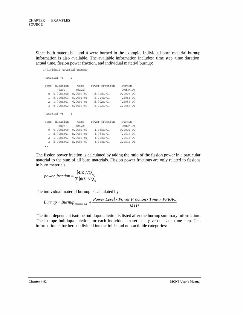
CHAPTER 4 – EXAMPLES SOURCE
Chapter 4-92 MCNP User’s Manual
Since both materials 1 and 4 were burned in the example, individual burn material burnup information is also available. The available information includes: time step, time duration, actual time, fission power fraction, and individual material burnup:
Individual Material Burnup Material #: 1 step duration time power fraction burnup (days) (days) (GWd/MTU) 0 0.000E+00 0.000E+00 5.015E-01 0.000E+00 1 5.000E+01 5.000E+01 5.016E-01 7.205E+00 2 1.000E+01 6.000E+01 5.002E-01 7.205E+00 3 5.000E+02 5.600E+02 5.002E-01 2.158E+01 Material #: 4 step duration time power fraction burnup (days) (days) (GWd/MTU) 0 0.000E+00 0.000E+00 4.985E-01 0.000E+00 1 5.000E+01 5.000E+01 4.984E-01 7.161E+00 2 1.000E+01 6.000E+01 4.998E-01 7.161E+00 3 5.000E+02 5.600E+02 4.998E-01 2.152E+01 ...
The fission power fraction is calculated by taking the ratio of the fission power in a particular material to the sum of all burn materials. Fission power fractions are only related to fissions in burn materials.
The individual material burnup is calculated by
The time-dependent isotope buildup/depletion is listed after the burnup summary information. The isotope buildup/depletion for each individual material is given at each time step. The information is further subdivided into actinide and non-actinide categories:
( )( )∑ ΦΣ
ΦΣ=
i if
if
VQVQ
fractionpower
MTUPFRACTimeFractionPowerLevelPowerBurnupBurnup stepprevious
×××+=
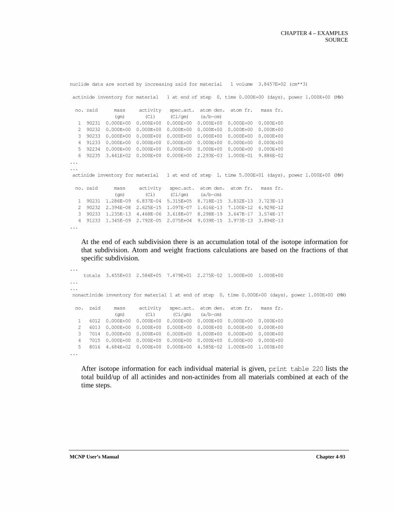
CHAPTER 4 – EXAMPLES
SOURCE
MCNP User’s Manual Chapter 4-93
nuclide data are sorted by increasing zaid for material 1 volume 3.8457E+02 (cm**3) actinide inventory for material 1 at end of step 0, time 0.000E+00 (days), power 1.000E+00 (MW) no. zaid mass activity spec.act. atom den. atom fr. mass fr. (gm) (Ci) (Ci/gm) (a/b-cm) 1 90231 0.000E+00 0.000E+00 0.000E+00 0.000E+00 0.000E+00 0.000E+00 2 90232 0.000E+00 0.000E+00 0.000E+00 0.000E+00 0.000E+00 0.000E+00 3 90233 0.000E+00 0.000E+00 0.000E+00 0.000E+00 0.000E+00 0.000E+00 4 91233 0.000E+00 0.000E+00 0.000E+00 0.000E+00 0.000E+00 0.000E+00 5 92234 0.000E+00 0.000E+00 0.000E+00 0.000E+00 0.000E+00 0.000E+00 6 92235 3.441E+02 0.000E+00 0.000E+00 2.293E-03 1.000E-01 9.886E-02 ... ... actinide inventory for material 1 at end of step 1, time 5.000E+01 (days), power 1.000E+00 (MW) no. zaid mass activity spec.act. atom den. atom fr. mass fr. (gm) (Ci) (Ci/gm) (a/b-cm) 1 90231 1.286E-09 6.837E-04 5.315E+05 8.718E-15 3.832E-13 3.723E-13 2 90232 2.394E-08 2.625E-15 1.097E-07 1.616E-13 7.100E-12 6.929E-12 3 90233 1.235E-13 4.468E-06 3.618E+07 8.298E-19 3.647E-17 3.574E-17 4 91233 1.345E-09 2.792E-05 2.075E+04 9.039E-15 3.973E-13 3.894E-13 ...
At the end of each subdivision there is an accumulation total of the isotope information for that subdivision. Atom and weight fractions calculations are based on the fractions of that specific subdivision.
... totals 3.455E+03 2.584E+05 7.479E+01 2.275E-02 1.000E+00 1.000E+00 ... ... nonactinide inventory for material 1 at end of step 0, time 0.000E+00 (days), power 1.000E+00 (MW) no. zaid mass activity spec.act. atom den. atom fr. mass fr. (gm) (Ci) (Ci/gm) (a/b-cm) 1 6012 0.000E+00 0.000E+00 0.000E+00 0.000E+00 0.000E+00 0.000E+00 2 6013 0.000E+00 0.000E+00 0.000E+00 0.000E+00 0.000E+00 0.000E+00 3 7014 0.000E+00 0.000E+00 0.000E+00 0.000E+00 0.000E+00 0.000E+00 4 7015 0.000E+00 0.000E+00 0.000E+00 0.000E+00 0.000E+00 0.000E+00 5 8016 4.684E+02 0.000E+00 0.000E+00 4.585E-02 1.000E+00 1.000E+00 ...
After isotope information for each individual material is given, print table 220 lists the total build/up of all actinides and non-actinides from all materials combined at each of the time steps.
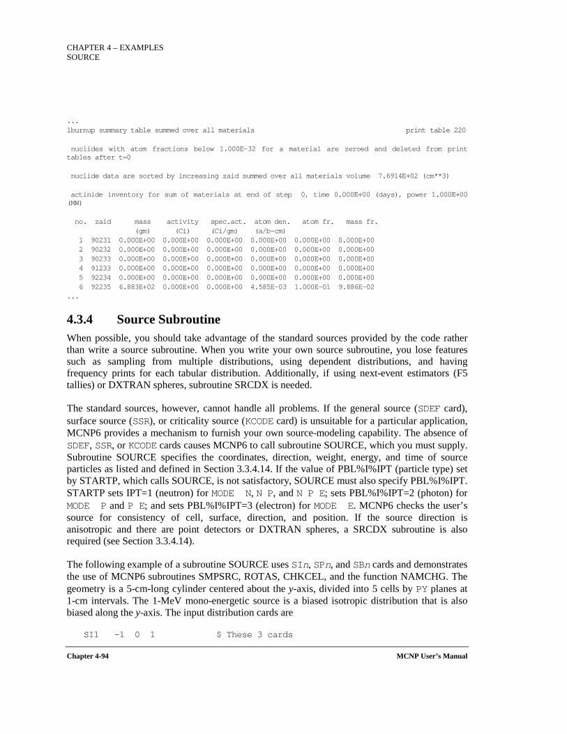
CHAPTER 4 – EXAMPLES SOURCE
Chapter 4-94 MCNP User’s Manual
... 1burnup summary table summed over all materials print table 220 nuclides with atom fractions below 1.000E-32 for a material are zeroed and deleted from print tables after t=0 nuclide data are sorted by increasing zaid summed over all materials volume 7.6914E+02 (cm**3) actinide inventory for sum of materials at end of step 0, time 0.000E+00 (days), power 1.000E+00 (MW) no. zaid mass activity spec.act. atom den. atom fr. mass fr. (gm) (Ci) (Ci/gm) (a/b-cm) 1 90231 0.000E+00 0.000E+00 0.000E+00 0.000E+00 0.000E+00 0.000E+00 2 90232 0.000E+00 0.000E+00 0.000E+00 0.000E+00 0.000E+00 0.000E+00 3 90233 0.000E+00 0.000E+00 0.000E+00 0.000E+00 0.000E+00 0.000E+00 4 91233 0.000E+00 0.000E+00 0.000E+00 0.000E+00 0.000E+00 0.000E+00 5 92234 0.000E+00 0.000E+00 0.000E+00 0.000E+00 0.000E+00 0.000E+00 6 92235 6.883E+02 0.000E+00 0.000E+00 4.585E-03 1.000E-01 9.886E-02 ...
4.3.4 Source Subroutine When possible, you should take advantage of the standard sources provided by the code rather than write a source subroutine. When you write your own source subroutine, you lose features such as sampling from multiple distributions, using dependent distributions, and having frequency prints for each tabular distribution. Additionally, if using next-event estimators (F5 tallies) or DXTRAN spheres, subroutine SRCDX is needed.
The standard sources, however, cannot handle all problems. If the general source (SDEF card), surface source (SSR), or criticality source (KCODE card) is unsuitable for a particular application, MCNP6 provides a mechanism to furnish your own source-modeling capability. The absence of SDEF, SSR, or KCODE cards causes MCNP6 to call subroutine SOURCE, which you must supply. Subroutine SOURCE specifies the coordinates, direction, weight, energy, and time of source particles as listed and defined in Section 3.3.4.14. If the value of PBL%I%IPT (particle type) set by STARTP, which calls SOURCE, is not satisfactory, SOURCE must also specify PBL%I%IPT. STARTP sets IPT=1 (neutron) for MODE N, N P, and N P E; sets PBL%I%IPT=2 (photon) for MODE P and P E; and sets PBL%I%IPT=3 (electron) for MODE E. MCNP6 checks the user’s source for consistency of cell, surface, direction, and position. If the source direction is anisotropic and there are point detectors or DXTRAN spheres, a SRCDX subroutine is also required (see Section 3.3.4.14).
The following example of a subroutine SOURCE uses SIn, SPn, and SBn cards and demonstrates the use of MCNP6 subroutines SMPSRC, ROTAS, CHKCEL, and the function NAMCHG. The geometry is a 5-cm-long cylinder centered about the y-axis, divided into 5 cells by PY planes at 1-cm intervals. The 1-MeV mono-energetic source is a biased isotropic distribution that is also biased along the y-axis. The input distribution cards are
SI1 –1 0 1 $ These 3 cards
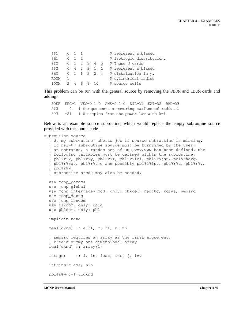
CHAPTER 4 – EXAMPLES
SOURCE
MCNP User’s Manual Chapter 4-95
SP1 0 1 1 $ represent a biased SB1 0 1 2 $ isotropic distribution. SI2 0 1 2 3 4 5 $ These 3 cards SP2 0 4 2 2 1 1 $ represent a biased SB2 0 1 1 2 2 4 $ distribution in y. RDUM 1 $ cylindrical radius IDUM 2 4 6 8 10 $ source cells
This problem can be run with the general source by removing the RDUM and IDUM cards and adding:
SDEF ERG=1 VEC=0 1 0 AXS=0 1 0 DIR=D1 EXT=D2 RAD=D3 SI3 0 1 $ represents a covering surface of radius 1 SP3 −21 1 $ samples from the power law with k=1
Below is an example source subroutine, which would replace the empty subroutine source provided with the source code. subroutine source ! dummy subroutine. aborts job if source subroutine is missing. ! if nsr=0, subroutine source must be furnished by the user. ! at entrance, a random set of uuu,vvv,www has been defined. the ! following variables must be defined within the subroutine: ! pbl%r%x, pbl%r%y, pbl%r%z, pbl%r%icl, pbl%r%jsu, pbl%r%erg, ! pbl%r%wgt, pbl%r%tme and possibly pbl%i%ipt, pbl%r%u, pbl%r%v, ! pbl%r%w. ! subroutine srcdx may also be needed. use mcnp_params use mcnp_global use mcnp_interfaces_mod, only: chkcel, namchg, rotas, smpsrc use mcnp_debug use mcnp_random use tskcom, only: uold use pblcom, only: pbl implicit none real(dknd) :: a(3), c, fi, r, th ! smpsrc requires an array as the first arguement. ! create dummy one dimensional array real(dknd) :: array(1) integer :: i, ib, imax, itr, j, lev intrinsic cos, sin pbl%r%wgt=1.0_dknd
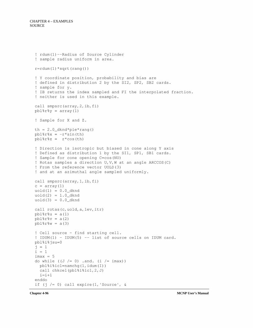
CHAPTER 4 – EXAMPLES SOURCE
Chapter 4-96 MCNP User’s Manual
! rdum(1)--Radius of Source Cylinder ! sample radius uniform in area. r=rdum(1)*sqrt(rang()) ! Y coordinate position, probability and bias are ! defined in distribution 2 by the SI2, SP2, SB2 cards. ! sample for y. ! IB returns the index sampled and FI the interpolated fraction. ! neither is used in this example. call smpsrc(array,2,ib,fi) pbl%r%y = array(1) ! Sample for X and Z. th = 2.0_dknd*pie*rang() pbl%r%x = -r*sin(th) pbl%r%z = r*cos(th) ! Direction is isotropic but biased in cone along Y axis ! Defined as distribution 1 by the SI1, SP1, SB1 cards. ! Sample for cone opening C=cos(NU) ! Rotas samples a direction U,V,W at an angle ARCCOS(C) ! From the reference vector UOLD(3) ! and at an azimuthal angle sampled uniformly. call smpsrc(array,1,ib,fi) c = array(1) uold(1) = 0.0_dknd uold(2) = 1.0_dknd uold(3) = 0.0_dknd call rotas(c,uold,a,lev,itr) pbl%r%u = a(1) pbl%r%v = a(2) pbl%r%w = a(3) ! Cell source - find starting cell. ! IDUM(1) - IDUM(5) -- list of source cells on IDUM card. pbl%i%jsu=0 j = 1 i = 1 imax = 5 do while ((J /= 0) .and. (i /= imax)) pbl%i%icl=namchg(1,idum(I)) call chkcel(pbl%i%icl,2,J) i=i+1 enddo if (j /= 0) call expire(1,'Source', &
CHAPTER 4 – EXAMPLES
SOURCE
MCNP User’s Manual Chapter 4-97
& 'Source is not in any cells on the idum card.') pbl%r%erg = 1.0_dknd pbl%r%tme = 0.0_dknd return end subroutine source
4.3.5 SRCDX Subroutine If a user has supplied a subroutine SOURCE that does not emit particles isotropically (uniform emission in all directions) and is using either a detector tally or DXTRAN in the calculations, then subroutine SRCDX must also be supplied to MCNP6. The structure of this subroutine is the same as for subroutine SOURCE, except that usually only a single parameter, PSC, needs to be specified for each detector or set of DXTRAN spheres. PSC as defined in SRCDX is used to calculate the direct contribution from the source to a point detector, to the point selected for the ring detector or DXTRAN sphere. Other parameters may also be specified in SRCDX. For example, if a quantity such as particle energy and/or weight is directionally dependent, its value must be specified in both subroutines SOURCE and SRCDX. When using detectors and a subroutine SOURCE with an anisotropic distribution, check the direct source contribution to the detectors carefully to see if it is close to the expected result.
In general, it is best to have as few directionally dependent parameters as possible in subroutine SOURCE. Directionally dependent parameters must also be dealt with in subroutine SRCDX.
The most general function for emitting a particle from the source in the laboratory system can be expressed as p(µ,ϕ), where µ is the cosine of the polar angle and ϕ is the azimuthal angle in the coordinate system of the problem. Most anisotropic sources are azimuthally symmetric and p(µ,ϕ)=p(µ)/2π. The quantity p(µ) is the probability density function for the µ variable only (that is, ∫ p(µ) dµ=1, p(µ)≥0). PSC is p(µ0), where µ0 is the cosine of the angle between the direction defining the polar angle for the source and the direction to a detector or DXTRAN sphere point in the laboratory system. (MCNP6 includes the 2π in the calculation automatically.) Note that p(µ0) and hence PSC may have a value greater than unity and must be non-negative. It is valuable to point out that every source must have a cumulative distribution function based on p(µ,ϕ) from which to sample angular dependence. The probability density function p(µ,ϕ) needs only to be considered explicitly for those problems with detectors or DXTRAN.
Table 4-1 gives the equations for PSC for six continuous source probability density functions. More discussion of probability density functions is given in the detector theory section of Section 5.5.4.6 of the MCNP5 Theory Manual [X-503a]. The isotropic case is assumed in MCNP6; therefore SRCDX is required only for the anisotropic case.
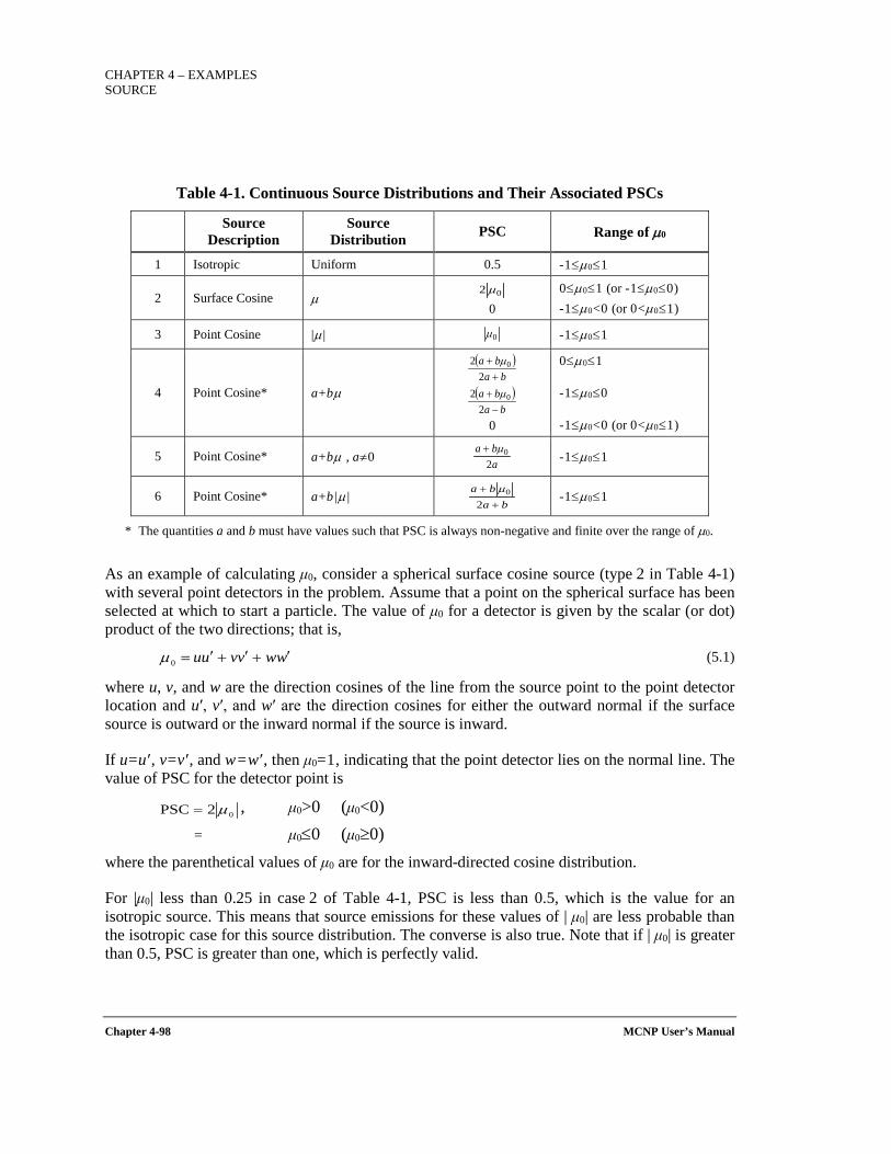
CHAPTER 4 – EXAMPLES SOURCE
Chapter 4-98 MCNP User’s Manual
Table 4-1. Continuous Source Distributions and Their Associated PSCs
Source Description
Source Distribution PSC Range of µ0
1 Isotropic Uniform 0.5 -1≤µ0≤1
2 Surface Cosine µ
0 0≤µ0≤1 (or -1≤µ0≤0) -1≤µ0<0 (or 0<µ0≤1)
3 Point Cosine |µ | -1≤µ0≤1
4 Point Cosine* a+bµ
0
0≤µ0≤1
-1≤µ0≤0
-1≤µ0<0 (or 0<µ0≤1)
5 Point Cosine* a+bµ , a≠0 -1≤µ0≤1
6 Point Cosine* a+b|µ| -1≤µ0≤1
* The quantities a and b must have values such that PSC is always non-negative and finite over the range of µ0.
As an example of calculating μ0, consider a spherical surface cosine source (type 2 in Table 4-1) with several point detectors in the problem. Assume that a point on the spherical surface has been selected at which to start a particle. The value of μ0 for a detector is given by the scalar (or dot) product of the two directions; that is,
(5.1)
where u, v, and w are the direction cosines of the line from the source point to the point detector location and u′, v′, and w′ are the direction cosines for either the outward normal if the surface source is outward or the inward normal if the source is inward.
If u=u′, v=v′, and w=w′, then μ0=1, indicating that the point detector lies on the normal line. The value of PSC for the detector point is
, μ0>0 (μ0<0) = μ0≤0 (μ0≥0)
where the parenthetical values of μ0 are for the inward-directed cosine distribution.
For |μ0| less than 0.25 in case 2 of Table 4-1, PSC is less than 0.5, which is the value for an isotropic source. This means that source emissions for these values of | μ0| are less probable than the isotropic case for this source distribution. The converse is also true. Note that if | μ0| is greater than 0.5, PSC is greater than one, which is perfectly valid.
02 µ
0µ
( )ba
ba+
+2
2 0µ
( )ba
ba−
+2
2 0µ
aba
20µ+
baba+
+
20µ
wwvvuu ′+′+′=0µ
02PSC µ=
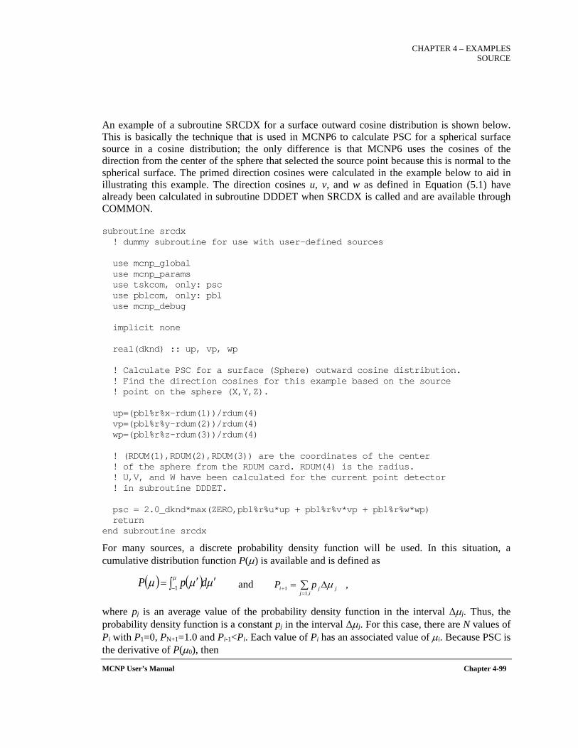
CHAPTER 4 – EXAMPLES
SOURCE
MCNP User’s Manual Chapter 4-99
An example of a subroutine SRCDX for a surface outward cosine distribution is shown below. This is basically the technique that is used in MCNP6 to calculate PSC for a spherical surface source in a cosine distribution; the only difference is that MCNP6 uses the cosines of the direction from the center of the sphere that selected the source point because this is normal to the spherical surface. The primed direction cosines were calculated in the example below to aid in illustrating this example. The direction cosines u, v, and w as defined in Equation (5.1) have already been calculated in subroutine DDDET when SRCDX is called and are available through COMMON.
subroutine srcdx ! dummy subroutine for use with user-defined sources use mcnp_global use mcnp_params use tskcom, only: psc use pblcom, only: pbl use mcnp_debug implicit none real(dknd) :: up, vp, wp ! Calculate PSC for a surface (Sphere) outward cosine distribution. ! Find the direction cosines for this example based on the source ! point on the sphere (X,Y,Z). up=(pbl%r%x-rdum(1))/rdum(4) vp=(pbl%r%y-rdum(2))/rdum(4) wp=(pbl%r%z-rdum(3))/rdum(4) ! (RDUM(1),RDUM(2),RDUM(3)) are the coordinates of the center ! of the sphere from the RDUM card. RDUM(4) is the radius. ! U,V, and W have been calculated for the current point detector ! in subroutine DDDET. psc = 2.0_dknd*max(ZERO,pbl%r%u*up + pbl%r%v*vp + pbl%r%w*wp) return end subroutine srcdx
For many sources, a discrete probability density function will be used. In this situation, a cumulative distribution function P(µ) is available and is defined as
and ,
where pj is an average value of the probability density function in the interval Δµj. Thus, the probability density function is a constant pj in the interval Δµj. For this case, there are N values of Pi with P1=0, PN+1=1.0 and Pi-1<Pi. Each value of Pi has an associated value of µi. Because PSC is the derivative of P(µ0), then
( ) ( ) µµµ µ ′′= ∫− dpP 1 ∑=
+ ∆=ij
jji pP,1
1 µ
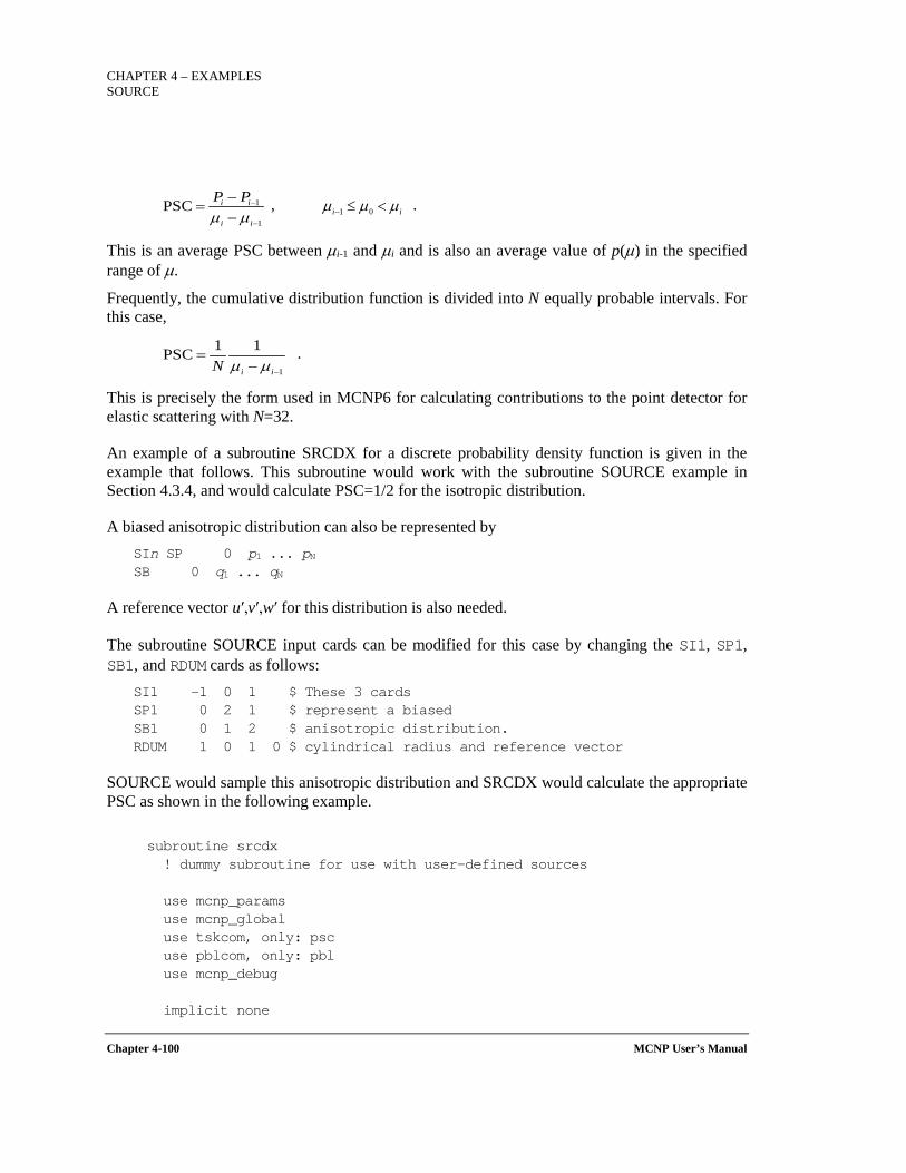
CHAPTER 4 – EXAMPLES SOURCE
Chapter 4-100 MCNP User’s Manual
, .
This is an average PSC between µi-1 and µi and is also an average value of p(µ) in the specified range of µ.
Frequently, the cumulative distribution function is divided into N equally probable intervals. For this case,
.
This is precisely the form used in MCNP6 for calculating contributions to the point detector for elastic scattering with N=32.
An example of a subroutine SRCDX for a discrete probability density function is given in the example that follows. This subroutine would work with the subroutine SOURCE example in Section 4.3.4, and would calculate PSC=1/2 for the isotropic distribution.
A biased anisotropic distribution can also be represented by SIn SP 0 p1 ... pN SB 0 q1 ... qN
A reference vector u′,v′,w′ for this distribution is also needed.
The subroutine SOURCE input cards can be modified for this case by changing the SI1, SP1, SB1, and RDUM cards as follows:
SI1 -1 0 1 $ These 3 cards SP1 0 2 1 $ represent a biased SB1 0 1 2 $ anisotropic distribution. RDUM 1 0 1 0 $ cylindrical radius and reference vector
SOURCE would sample this anisotropic distribution and SRCDX would calculate the appropriate PSC as shown in the following example.
subroutine srcdx ! dummy subroutine for use with user-defined sources use mcnp_params use mcnp_global use tskcom, only: psc use pblcom, only: pbl use mcnp_debug implicit none
1
1PSC−
−
−−
=ii
ii PPµµ ii µµµ <≤− 01
1
11PSC−−
=iiN µµ
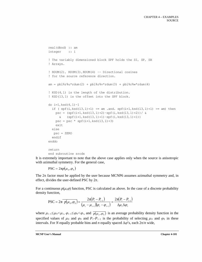
CHAPTER 4 – EXAMPLES
SOURCE
MCNP User’s Manual Chapter 4-101
real(dknd) :: am integer :: i ! The variably dimensioned block SPF holds the SI, SP, SB ! Arrays. ! RDUM(2), RDUM(3),RDUM(4) -- Directional cosines ! for the source reference direction. am = pbl%r%u*rdum(2) + pbl%r%v*rdum(3) + pbl%r%w*rdum(4) ! KSD(4,1) is the length of the distribution. ! KSD(13,1) is the offset into the SPF block. do i=1,ksd(4,1)-1 if ( spf(i,ksd(13,1)+1) <= am .and. spf(i+1,ksd(13,1)+1) >= am) then psc = (spf(i+1,ksd(13,1)+2)-spf(i,ksd(13,1)+2))/ & & (spf(i+1,ksd(13,1)+1)-spf(i,ksd(13,1)+1)) psc = psc * spf(i+1,ksd(13,1)+3) exit else psc = ZERO endif enddo return end subroutine srcdx
It is extremely important to note that the above case applies only when the source is anisotropic with azimuthal symmetry. For the general case,
The 2π factor must be applied by the user because MCNP6 assumes azimuthal symmetry and, in effect, divides the user-defined PSC by 2π.
For a continuous p(µ,ϕ) function, PSC is calculated as above. In the case of a discrete probability density function,
where µ i - 1≤µ0<µ i , ϕ i - 1≤ϕ0<ϕ i , and is an average probability density function in the specified values of µ0 and ϕ0 and Pi-Pi - 1 is the probability of selecting µ0 and ϕ0 in these intervals. For N equally probable bins and n equally spaced Δϕ’s, each 2π/n wide,
( )00 ,π2PSC ϕµp=
( ) ( )( )( )
( )ii
ii
iii
ii PPPPp
ϕµϕϕµµϕµ
∆∆−
=−−
−=⋅= −
−−
− 1
11i
100
π2π2,π2PSC
( )0,ϕµop
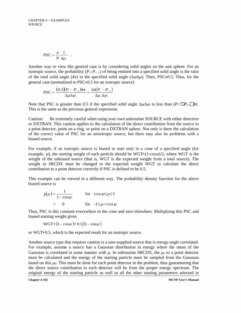
CHAPTER 4 – EXAMPLES SOURCE
Chapter 4-102 MCNP User’s Manual
.
Another way to view this general case is by considering solid angles on the unit sphere. For an isotropic source, the probability (Pi-Pi - 1) of being emitted into a specified solid angle is the ratio of the total solid angle (4π) to the specified solid angle (ΔϕΔµ). Then, PSC≡0.5. Thus, for the general case (normalized to PSC≡0.5 for an isotropic source)
Note that PSC is greater than 0.5 if the specified solid angle ΔµΔϕi is less than (Pi−Pi-14π. This is the same as the previous general expression.
Caution: Be extremely careful when using your own subroutine SOURCE with either detectors or DXTRAN. This caution applies to the calculation of the direct contribution from the source to a point detector, point on a ring, or point on a DXTRAN sphere. Not only is there the calculation of the correct value of PSC for an anisotropic source, but there may also be problems with a biased source.
For example, if an isotropic source is biased to start only in a cone of a specified angle (for example, ψ), the starting weight of each particle should be WGT∗(1-cosψ)/2, where WGT is the weight of the unbiased source (that is, WGT is the expected weight from a total source). The weight in SRCDX must be changed to the expected weight WGT to calculate the direct contribution to a point detector correctly if PSC is defined to be 0.5.
This example can be viewed in a different way. The probability density function for the above biased source is
for cosψ≤µ≤1
= 0 for -1≤µ<cosψ
Thus, PSC is this constant everywhere in the cone and zero elsewhere. Multiplying this PSC and biased starting weight gives
or WGT∗0.5, which is the expected result for an isotropic source.
Another source type that requires caution is a user-supplied source that is energy-angle correlated. For example, assume a source has a Gaussian distribution in energy where the mean of the Gaussian is correlated in some manner with µ. In subroutine SRCDX, the µ0 to a point detector must be calculated and the energy of the starting particle must be sampled from the Gaussian based on this µ0. This must be done for each point detector in the problem, thus guaranteeing that the direct source contribution to each detector will be from the proper energy spectrum. The original energy of the starting particle as well as all the other starting parameters selected in
iNn
µ∆=
1PSC
( )( ) ( )ii
ii
i
ii PPPPϕµϕµ ∆∆
−=
∆∆−
= −− 11 π2π45.0PSC
( )ψ
µcos11
−=p
( ) ( )ψψ cos15.0cos1WGT −∗−∗
CHAPTER 4 – EXAMPLES
SOURCE
MCNP User’s Manual Chapter 4-103
subroutine SOURCE are automatically restored after the direct source contribution to detectors is made. Thus, the subroutine SOURCE is still sampled correctly.
4.4 MATERIAL EXAMPLES
4.4.1 Table Data/Model Physics Mix and Match Consider a neutron problem with deuterium and tritium. The available deuterium library contains values valid up to 150 MeV, but the tritium library goes up to only 20 MeV. Previously, either neutron physics models above 20 MeV (neglecting the deuterium table data up to 150 MeV) or nuclear data tables below 150 MeV (using the 20-MeV tritium data throughout the entire 20- to 150-MeV range) had to be used. Using the mix-and-match capability available through the tabl parameter of the PHYS:<pl> card, the user can specify that deuterium use tables up to 150 MeV and use physics models above 150 MeV and that tritium use data tables up to 20 MeV and use physics models above 20 MeV.
Figure 4-49 shows an example of the energy-matching capability. The 100-MeV neutrons are incident on an 8.433-cm-long, 3.932-cm-radius BGO crystal. The crystal contains 21% bismuth, 16% germanium, and 63% oxygen. Assume no germanium libraries are available. The solid line represents flux in the crystal with the full mix-and-match capability, which uses all libraries up to their energy limits and physics models above those limits and for germanium. The dashed-line calculation uses the old method of substituting arsenic for the missing germanium library, using the libraries up to 20 MeV and using physics models above. The dotted line uses bismuth and oxygen libraries up to their limits of 150 MeV; the arsenic library is used up to its limit of 20 MeV, and then the 20-MeV data are used from 20 to 150 MeV; above 150 MeV, physics models are used for all three nuclides. This last option is least desirable but often was used in past code versions to take advantage of the 150-MeV libraries, even though many data libraries go only to 20 MeV.
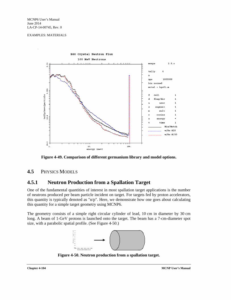
MCNP6 User’s Manual June 2014 LA-CP-14-00745, Rev. 0 EXAMPLES: MATERIALS
Chapter 4-104 MCNP User’s Manual
Figure 4-49. Comparison of different germanium library and model options.
4.5 PHYSICS MODELS
4.5.1 Neutron Production from a Spallation Target One of the fundamental quantities of interest in most spallation target applications is the number of neutrons produced per beam particle incident on target. For targets fed by proton accelerators, this quantity is typically denoted as "n/p". Here, we demonstrate how one goes about calculating this quantity for a simple target geometry using MCNP6.
The geometry consists of a simple right circular cylinder of lead, 10 cm in diameter by 30 cm long. A beam of 1-GeV protons is launched onto the target. The beam has a 7-cm-diameter spot size, with a parabolic spatial profile. (See Figure 4-50.)
Figure 4-50. Neutron production from a spallation target.
-4
-3
-2
-1
0
1
2
3
4
0.00 0.01 0.02 0.03 0.04 0.05
bea
m r
adi
us
beam current density (a.u.)
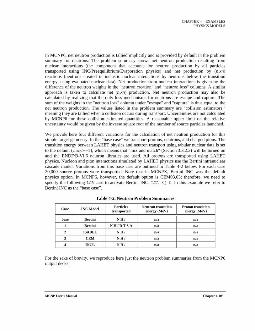
CHAPTER 4 – EXAMPLES
PHYSICS MODELS
MCNP User’s Manual Chapter 4-105
In MCNP6, net neutron production is tallied implicitly and is provided by default in the problem summary for neutrons. The problem summary shows net neutron production resulting from nuclear interactions (the component that accounts for neutron production by all particles transported using INC/Preequilibrium/Evaporation physics) and net production by (n,xn) reactions (neutrons created in inelastic nuclear interactions by neutrons below the transition energy, using evaluated nuclear data). Net production from nuclear interactions is given by the difference of the neutron weights in the "neutron creation" and "neutron loss" columns. A similar approach is taken to calculate net (n,xn) production. Net neutron production may also be calculated by realizing that the only loss mechanisms for neutrons are escape and capture. The sum of the weights in the "neutron loss" column under "escape" and "capture" is thus equal to the net neutron production. The values listed in the problem summary are "collision estimators," meaning they are tallied when a collision occurs during transport. Uncertainties are not calculated by MCNP6 for these collision-estimated quantities. A reasonable upper limit on the relative uncertainty would be given by the inverse square root of the number of source particles launched.
We provide here four different variations for the calculation of net neutron production for this simple target geometry. In the "base case" we transport protons, neutrons, and charged pions. The transition energy between LAHET physics and neutron transport using tabular nuclear data is set to the default (tabl=-1), which means that "mix and match" (Section 3.3.2.3) will be turned on and the ENDF/B-VI.6 neutron libraries are used. All protons are transported using LAHET physics. Nucleon and pion interactions simulated by LAHET physics use the Bertini intranuclear cascade model. Variations from this base case are outlined in Table 4-2 below. For each case 20,000 source protons were transported. Note that in MCNPX, Bertini INC was the default physics option. In MCNP6, however, the default option is CEM03.03; therefore, we need to specify the following LCA card to activate Bertini INC: LCA 8j 0. In this example we refer to Bertini INC as the “base case”.
Table 4-2. Neutron Problem Summaries
Case INC Model Particles transported
Neutron transition energy (MeV)
Proton transition energy (MeV)
base Bertini N H / n/a n/a
1 Bertini N H / D T S A n/a n/a
2 ISABEL N H / n/a n/a
3 CEM N H / n/a n/a
4 INCL N H / n/a n/a
For the sake of brevity, we reproduce here just the neutron problem summaries from the MCNP6 output decks.
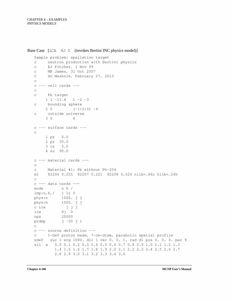
CHAPTER 4 – EXAMPLES PHYSICS MODELS
Chapter 4-106 MCNP User’s Manual
Base Case [LCA 8J 0 (invokes Bertini INC physics model)] Sample problem: spallation target c neutron production with Bertini physics c EJ Pitcher, 1 Nov 99 c MR James, 31 Oct 2007 C SG Mashnik, February 27, 2013 c c --- cell cards --- c c Pb target 1 1 -11.4 1 -2 -3 c bounding sphere 2 0 (-1:2:3) -4 c outside universe 3 0 4
c --- surface cards --- c 1 pz 0.0 2 pz 30.0 3 cz 5.0 4 so 90.0
c --- material cards --- c c Material #1: Pb without Pb-204 m1 82206 0.255 82207 0.221 82208 0.524 nlib=.66c hlib=.24h c c --- data cards --- mode n h / imp:n,h,/ 1 1r 0 phys:n 1000. j j phys:h 1000. j j c lca j j j lca 8j 0 nps 20000 prdmp j -30 j 1 c c --- source definition --- c 1-GeV proton beam, 7-cm-diam, parabolic spatial profile sdef sur 1 erg 1000. dir 1 vec 0. 0. 1. rad d1 pos 0. 0. 0. par 9 si1 a 0.0 0.1 0.2 0.3 0.4 0.5 0.6 0.7 0.8 0.9 1.0 1.1 1.2 1.3 1.4 1.5 1.6 1.7 1.8 1.9 2.0 2.1 2.2 2.3 2.4 2.5 2.6 2.7 2.8 2.9 3.0 3.1 3.2 3.3 3.4 3.5
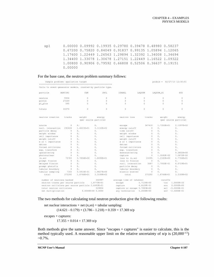
CHAPTER 4 – EXAMPLES
PHYSICS MODELS
MCNP User’s Manual Chapter 4-107
sp1 0.00000 0.09992 0.19935 0.29780 0.39478 0.48980 0.58237 0.67200 0.75820 0.84049 0.91837 0.99135 1.05894 1.12065 1.17600 1.22449 1.26563 1.29894 1.32392 1.34008 1.34694 1.34400 1.33078 1.30678 1.27151 1.22449 1.16522 1.09322 1.00800 0.90906 0.79592 0.66808 0.52506 0.36637 0.19151 0.00000
For the base case, the neutron problem summary follows: Sample problem: spallation target probid = 02/27/13 12:30:01 ********************************************************** Calls to event-generator models, counted by particle type. particle BERTINI CEM INCL ISABEL LAQGSM LAQGSM_H1 HYD neutron 5506 0 0 0 0 0 0 proton 27269 0 0 0 0 0 0 pi_plus 595 0 0 0 0 0 0 totals 33370 0 0 0 0 0 0 neutron creation tracks weight energy neutron loss tracks weight energy (per source particle) (per source particle) source 0 0. 0. escape 347410 1.7355E+01 2.1397E+02 nucl. interaction 292426 1.4621E+01 3.1152E+02 energy cutoff 0 0. 0. particle decay 0 0. 0. time cutoff 0 0. 0. weight window 0 0. 0. weight window 0 0. 0. cell importance 0 0. 0. cell importance 0 0. 0. weight cutoff 0 0. 0. weight cutoff 0 0. 0. e or t importance 0 0. 0. e or t importance 0 0. 0. dxtran 0 0. 0. dxtran 0 0. 0. forced collisions 0 0. 0. forced collisions 0 0. 0. exp. transform 0 0. 0. exp. transform 0 0. 0. upscattering 0 0. 0. downscattering 0 0. 9.3802E+00 photonuclear 0 0. 0. capture 0 1.3592E-02 7.2872E-02 (n,xn) 75783 3.7856E+00 1.8490E+01 loss to (n,xn) 24395 1.2182E+00 4.7746E+01 prompt fission 0 0. 0. loss to fission 0 0. 0. delayed fission 0 0. 0. nucl. interaction 3587 1.7935E-01 6.0729E+01 prompt photofis 0 0. 0. particle decay 0 0. 0. tabular boundary 0 0. 0. tabular boundary 0 0. 0. tabular sampling 7183 3.5915E-01 1.8827E+00 elastic scatter 0 0. 0. total 375392 1.8766E+01 3.3189E+02 total 375392 1.8766E+01 3.3189E+02 number of neutrons banked 350997 average time of (shakes) cutoffs neutron tracks per source particle 1.8770E+01 escape 5.7124E+00 tco 1.0000E+33 neutron collisions per source particle 2.6493E+01 capture 4.6539E-01 eco 0.0000E+00 total neutron collisions 529856 capture or escape 5.7083E+00 wc1 -5.0000E-01 net multiplication 0.0000E+00 0.0000 any termination 5.2838E+00 wc2 -2.5000E-01
The two methods for calculating total neutron production give the following results: net nuclear interactions + net (n,xn) + tabular sampling: (14.621 - 0.179) + (3.786 - 1.218) + 0.359 = 17.369 n/p
escapes + captures: 17.355 + 0.014 = 17.369 n/p
Both methods give the same answer. Since "escapes + captures" is easier to calculate, this is the method typically used. A reasonable upper limit on the relative uncertainty of n/p is (20,000-1/2) ~0.7%.
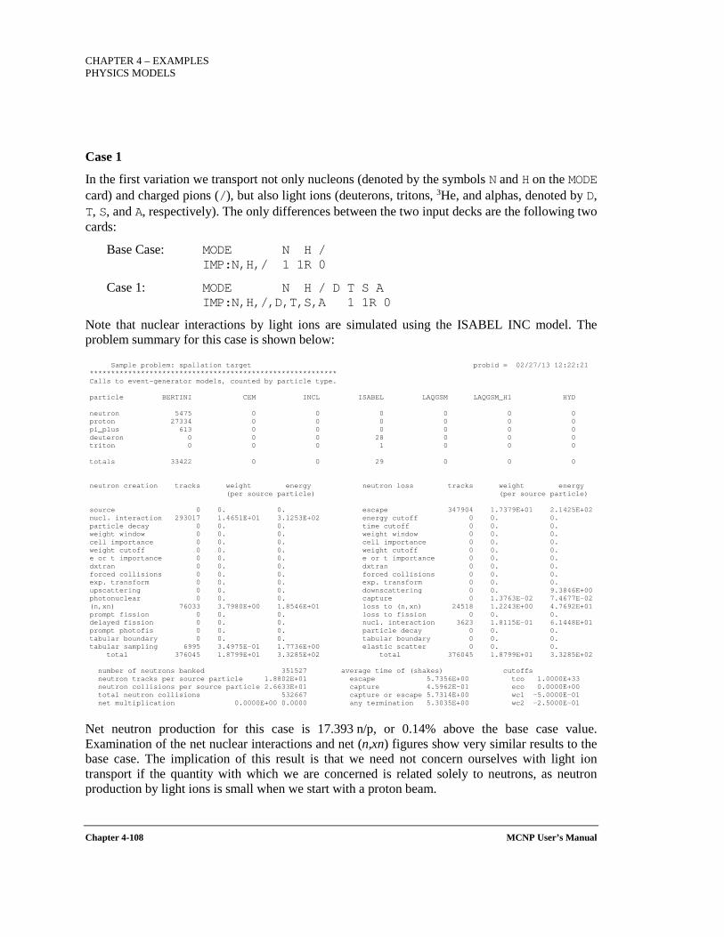
CHAPTER 4 – EXAMPLES PHYSICS MODELS
Chapter 4-108 MCNP User’s Manual
Case 1
In the first variation we transport not only nucleons (denoted by the symbols N and H on the MODE card) and charged pions (/), but also light ions (deuterons, tritons, 3He, and alphas, denoted by D, T, S, and A, respectively). The only differences between the two input decks are the following two cards:
Base Case: MODE N H / IMP:N,H,/ 1 1R 0
Case 1: MODE N H / D T S A IMP:N,H,/,D,T,S,A 1 1R 0
Note that nuclear interactions by light ions are simulated using the ISABEL INC model. The problem summary for this case is shown below:
Sample problem: spallation target probid = 02/27/13 12:22:21 ********************************************************** Calls to event-generator models, counted by particle type. particle BERTINI CEM INCL ISABEL LAQGSM LAQGSM_H1 HYD neutron 5475 0 0 0 0 0 0 proton 27334 0 0 0 0 0 0 pi_plus 613 0 0 0 0 0 0 deuteron 0 0 0 28 0 0 0 triton 0 0 0 1 0 0 0 totals 33422 0 0 29 0 0 0 neutron creation tracks weight energy neutron loss tracks weight energy (per source particle) (per source particle) source 0 0. 0. escape 347904 1.7379E+01 2.1425E+02 nucl. interaction 293017 1.4651E+01 3.1253E+02 energy cutoff 0 0. 0. particle decay 0 0. 0. time cutoff 0 0. 0. weight window 0 0. 0. weight window 0 0. 0. cell importance 0 0. 0. cell importance 0 0. 0. weight cutoff 0 0. 0. weight cutoff 0 0. 0. e or t importance 0 0. 0. e or t importance 0 0. 0. dxtran 0 0. 0. dxtran 0 0. 0. forced collisions 0 0. 0. forced collisions 0 0. 0. exp. transform 0 0. 0. exp. transform 0 0. 0. upscattering 0 0. 0. downscattering 0 0. 9.3846E+00 photonuclear 0 0. 0. capture 0 1.3763E-02 7.4677E-02 (n,xn) 76033 3.7980E+00 1.8546E+01 loss to (n,xn) 24518 1.2243E+00 4.7692E+01 prompt fission 0 0. 0. loss to fission 0 0. 0. delayed fission 0 0. 0. nucl. interaction 3623 1.8115E-01 6.1448E+01 prompt photofis 0 0. 0. particle decay 0 0. 0. tabular boundary 0 0. 0. tabular boundary 0 0. 0. tabular sampling 6995 3.4975E-01 1.7736E+00 elastic scatter 0 0. 0. total 376045 1.8799E+01 3.3285E+02 total 376045 1.8799E+01 3.3285E+02 number of neutrons banked 351527 average time of (shakes) cutoffs neutron tracks per source particle 1.8802E+01 escape 5.7356E+00 tco 1.0000E+33 neutron collisions per source particle 2.6633E+01 capture 4.5962E-01 eco 0.0000E+00 total neutron collisions 532667 capture or escape 5.7314E+00 wc1 -5.0000E-01 net multiplication 0.0000E+00 0.0000 any termination 5.3035E+00 wc2 -2.5000E-01
Net neutron production for this case is 17.393 n/p, or 0.14% above the base case value. Examination of the net nuclear interactions and net (n,xn) figures show very similar results to the base case. The implication of this result is that we need not concern ourselves with light ion transport if the quantity with which we are concerned is related solely to neutrons, as neutron production by light ions is small when we start with a proton beam.
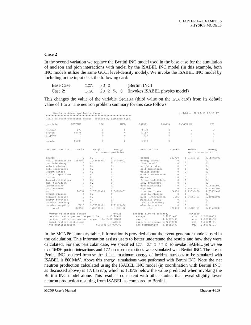
CHAPTER 4 – EXAMPLES
PHYSICS MODELS
MCNP User’s Manual Chapter 4-109
Case 2
In the second variation we replace the Bertini INC model used in the base case for the simulation of nucleon and pion interactions with nuclei by the ISABEL INC model (in this example, both INC models utilize the same GCCI level-density model). We invoke the ISABEL INC model by including in the input deck the following card:
Base Case: LCA 8J 0 (Bertini INC) Case 2: LCA 2J 2 5J 0 (invokes ISABEL physics model)
This changes the value of the variable iexisa (third value on the LCA card) from its default value of 1 to 2. The neutron problem summary for this case follows:
Sample problem: spallation target probid = 02/27/13 12:18:17 ********************************************************** Calls to event-generator models, counted by particle type. particle BERTINI CEM INCL ISABEL LAQGSM LAQGSM_H1 HYD neutron 172 0 0 6138 0 0 0 proton 16436 0 0 12155 0 0 0 pi_plus 0 0 0 706 0 0 0 totals 16608 0 0 18999 0 0 0 neutron creation tracks weight energy neutron loss tracks weight energy (per source particle) (per source particle) source 0 0. 0. escape 342730 1.7121E+01 2.1554E+02 nucl. interaction 288164 1.4408E+01 3.1428E+02 energy cutoff 0 0. 0. particle decay 0 0. 0. time cutoff 0 0. 0. weight window 0 0. 0. weight window 0 0. 0. cell importance 0 0. 0. cell importance 0 0. 0. weight cutoff 0 0. 0. weight cutoff 0 0. 0. e or t importance 0 0. 0. e or t importance 0 0. 0. dxtran 0 0. 0. dxtran 0 0. 0. forced collisions 0 0. 0. forced collisions 0 0. 0. exp. transform 0 0. 0. exp. transform 0 0. 0. upscattering 0 0. 0. downscattering 0 0. 9.1966E+00 photonuclear 0 0. 0. capture 0 1.3422E-02 7.2094E-02 (n,xn) 74854 3.7392E+00 1.8478E+01 loss to (n,xn) 24008 1.1989E+00 4.7368E+01 prompt fission 0 0. 0. loss to fission 0 0. 0. delayed fission 0 0. 0. nucl. interaction 3695 1.8475E-01 6.2501E+01 prompt photofis 0 0. 0. particle decay 0 0. 0. tabular boundary 0 0. 0. tabular boundary 0 0. 0. tabular sampling 7415 3.7075E-01 1.9142E+00 elastic scatter 0 0. 0. total 370433 1.8518E+01 3.3468E+02 total 370433 1.8518E+01 3.3468E+02 number of neutrons banked 346425 average time of (shakes) cutoffs neutron tracks per source particle 1.8522E+01 escape 5.7255E+00 tco 1.0000E+33 neutron collisions per source particle 2.6117E+01 capture 4.8478E-01 eco 0.0000E+00 total neutron collisions 522349 capture or escape 5.7214E+00 wc1 -5.0000E-01 net multiplication 0.0000E+00 0.0000 any termination 5.2945E+00 wc2 -2.5000E-01
In the MCNP6 summary table, information is provided about the event-generator models used in the calculation. This information assists users to better understand the results and how they were calculated. For this particular case, we specified LCA 2J 2 5J 0 to invoke ISABEL, yet we see that 16436 proton interactions and 172 neutron interactions were simulated with Bertini INC. The use of Bertini INC occurred because the default maximum energy of incident nucleons to be simulated with ISABEL is 800 MeV. Above this energy simulations were performed with Bertini INC. Note the net neutron production calculated using the ISABEL INC model (in coordination with Bertini INC, as discussed above) is 17.135 n/p, which is 1.35% below the value predicted when invoking the Bertini INC model alone. This result is consistent with other studies that reveal slightly lower neutron production resulting from ISABEL as compared to Bertini.
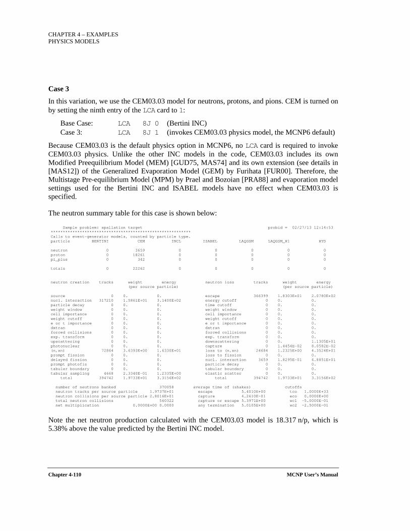
CHAPTER 4 – EXAMPLES PHYSICS MODELS
Chapter 4-110 MCNP User’s Manual
Case 3
In this variation, we use the CEM03.03 model for neutrons, protons, and pions. CEM is turned on by setting the ninth entry of the LCA card to 1:
Base Case: LCA 8J 0 (Bertini INC) Case 3: LCA 8J 1 (invokes CEM03.03 physics model, the MCNP6 default)
Because CEM03.03 is the default physics option in MCNP6, no LCA card is required to invoke CEM03.03 physics. Unlike the other INC models in the code, CEM03.03 includes its own Modified Preequilibrium Model (MEM) [GUD75, MAS74] and its own extension (see details in [MAS12]) of the Generalized Evaporation Model (GEM) by Furihata [FUR00]. Therefore, the Multistage Pre-equilibrium Model (MPM) by Prael and Bozoian [PRA88] and evaporation model settings used for the Bertini INC and ISABEL models have no effect when CEM03.03 is specified.
The neutron summary table for this case is shown below:
Sample problem: spallation target probid = 02/27/13 12:14:53 ********************************************************** Calls to event-generator models, counted by particle type. particle BERTINI CEM INCL ISABEL LAQGSM LAQGSM_H1 HYD neutron 0 3659 0 0 0 0 0 proton 0 18261 0 0 0 0 0 pi_plus 0 342 0 0 0 0 0 totals 0 22262 0 0 0 0 0 neutron creation tracks weight energy neutron loss tracks weight energy (per source particle) (per source particle) source 0 0. 0. escape 366399 1.8303E+01 2.0780E+02 nucl. interaction 317210 1.5861E+01 3.1400E+02 energy cutoff 0 0. 0. particle decay 0 0. 0. time cutoff 0 0. 0. weight window 0 0. 0. weight window 0 0. 0. cell importance 0 0. 0. cell importance 0 0. 0. weight cutoff 0 0. 0. weight cutoff 0 0. 0. e or t importance 0 0. 0. e or t importance 0 0. 0. dxtran 0 0. 0. dxtran 0 0. 0. forced collisions 0 0. 0. forced collisions 0 0. 0. exp. transform 0 0. 0. exp. transform 0 0. 0. upscattering 0 0. 0. downscattering 0 0. 1.1305E+01 photonuclear 0 0. 0. capture 0 1.4454E-02 8.0582E-02 (n,xn) 72864 3.6393E+00 1.6330E+01 loss to (n,xn) 24684 1.2325E+00 4.3524E+01 prompt fission 0 0. 0. loss to fission 0 0. 0. delayed fission 0 0. 0. nucl. interaction 3659 1.8295E-01 6.8851E+01 prompt photofis 0 0. 0. particle decay 0 0. 0. tabular boundary 0 0. 0. tabular boundary 0 0. 0. tabular sampling 4668 2.3340E-01 1.2335E+00 elastic scatter 0 0. 0. total 394742 1.9733E+01 3.3156E+02 total 394742 1.9733E+01 3.3156E+02 number of neutrons banked 370058 average time of (shakes) cutoffs neutron tracks per source particle 1.9737E+01 escape 5.4010E+00 tco 1.0000E+33 neutron collisions per source particle 2.8016E+01 capture 4.2610E-01 eco 0.0000E+00 total neutron collisions 560322 capture or escape 5.3971E+00 wc1 -5.0000E-01 net multiplication 0.0000E+00 0.0000 any termination 5.0105E+00 wc2 -2.5000E-01
Note the net neutron production calculated with the CEM03.03 model is 18.317 n/p, which is 5.38% above the value predicted by the Bertini INC model.
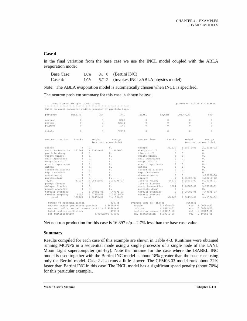
CHAPTER 4 – EXAMPLES
PHYSICS MODELS
MCNP User’s Manual Chapter 4-111
Case 4
In the final variation from the base case we use the INCL model coupled with the ABLA evaporation mode:
Base Case: LCA 8J 0 (Bertini INC) Case 4: LCA 8J 2 (invokes INCL/ABLA physics model)
Note: The ABLA evaporation model is automatically chosen when INCL is specified.
The neutron problem summary for this case is shown below:
Sample problem: spallation target probid = 02/27/13 12:08:25 ********************************************************** Calls to event-generator models, counted by particle type. particle BERTINI CEM INCL ISABEL LAQGSM LAQGSM_H1 HYD neutron 0 0 8583 0 0 0 0 proton 0 0 42531 0 0 0 0 pi_plus 0 0 1080 0 0 0 0 totals 0 0 52194 0 0 0 0 neutron creation tracks weight energy neutron loss tracks weight energy (per source particle) (per source particle) source 0 0. 0. escape 332230 1.6597E+01 2.2404E+02 nucl. interaction 271669 1.3583E+01 3.1917E+02 energy cutoff 0 0. 0. particle decay 0 0. 0. time cutoff 0 0. 0. weight window 0 0. 0. weight window 0 0. 0. cell importance 0 0. 0. cell importance 0 0. 0. weight cutoff 0 0. 0. weight cutoff 0 0. 0. e or t importance 0 0. 0. e or t importance 0 0. 0. dxtran 0 0. 0. dxtran 0 0. 0. forced collisions 0 0. 0. forced collisions 0 0. 0. exp. transform 0 0. 0. exp. transform 0 0. 0. upscattering 0 0. 0. downscattering 0 0. 9.2580E+00 photonuclear 0 0. 0. capture 0 1.2528E-02 6.6701E-02 (n,xn) 81138 4.0537E+00 2.0529E+01 loss to (n,xn) 25210 1.2591E+00 5.2600E+01 prompt fission 0 0. 0. loss to fission 0 0. 0. delayed fission 0 0. 0. nucl. interaction 3524 1.7620E-01 5.5785E+01 prompt photofis 0 0. 0. particle decay 0 0. 0. tabular boundary 1 5.0000E-05 7.4999E-03 tabular boundary 1 5.0000E-05 7.4999E-03 tabular sampling 8157 4.0785E-01 2.0521E+00 elastic scatter 0 0. 0. total 360965 1.8045E+01 3.4176E+02 total 360965 1.8045E+01 3.4176E+02 number of neutrons banked 335755 average time of (shakes) cutoffs neutron tracks per source particle 1.8048E+01 escape 5.4378E+00 tco 1.0000E+33 neutron collisions per source particle 2.4996E+01 capture 4.6562E-01 eco 0.0000E+00 total neutron collisions 499914 capture or escape 5.4341E+00 wc1 -5.0000E-01 net multiplication 0.0000E+00 0.0000 any termination 5.0024E+00 wc2 -2.5000E-01
Net neutron production for this case is 16.897 n/p—2.7% less than the base case value.
Summary
Results compiled for each case of this example are shown in Table 4-3. Runtimes were obtained running MCNP6 in a sequential mode using a single processor of a single node of the LANL Moon Light supercomputer (ml-fey). Note the runtime for the case where the ISABEL INC model is used together with the Bertini INC model is about 18% greater than the base case using only the Bertini model. Case 2 also runs a little slower. The CEM03.03 model runs about 22% faster than Bertini INC in this case. The INCL model has a significant speed penalty (about 70%) for this particular example..
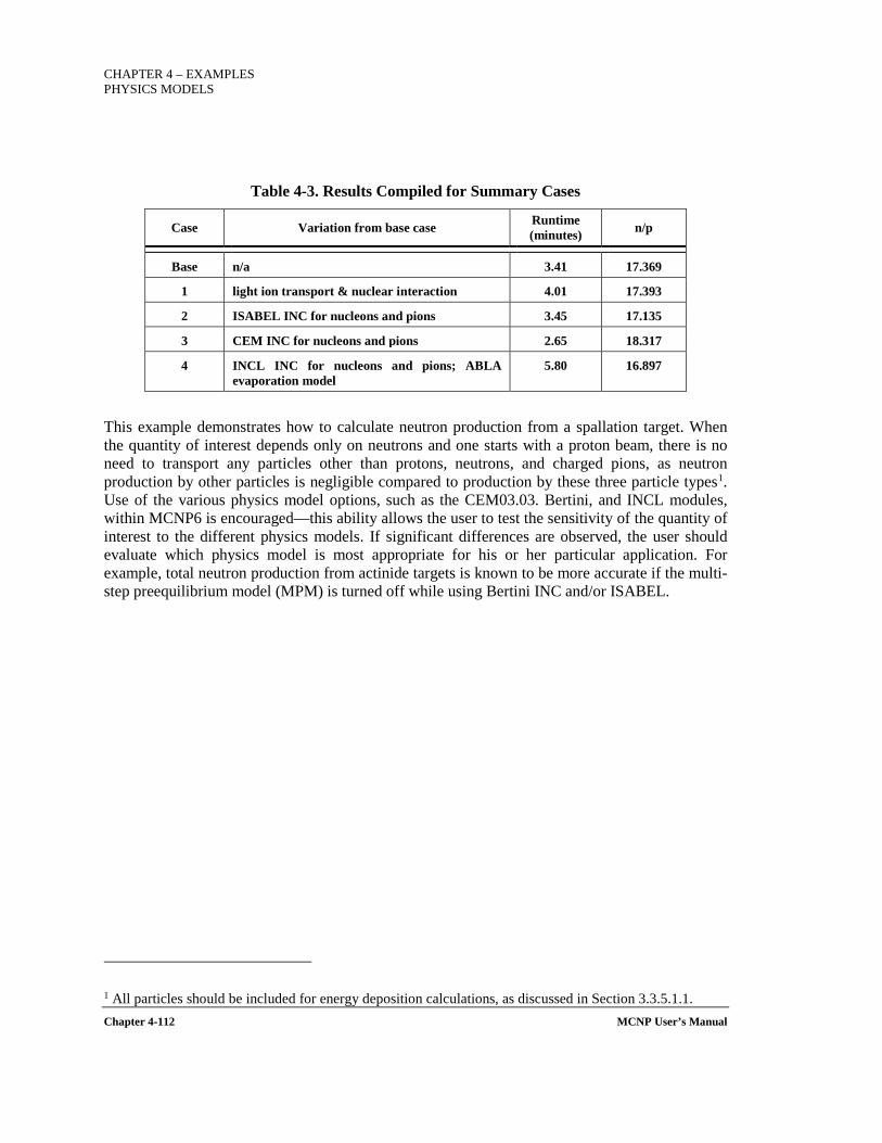
CHAPTER 4 – EXAMPLES PHYSICS MODELS
Chapter 4-112 MCNP User’s Manual
Table 4-3. Results Compiled for Summary Cases
Case Variation from base case Runtime (minutes) n/p
Base n/a 3.41 17.369
1 light ion transport & nuclear interaction 4.01 17.393
2 ISABEL INC for nucleons and pions 3.45 17.135
3 CEM INC for nucleons and pions 2.65 18.317
4 INCL INC for nucleons and pions; ABLA evaporation model
5.80 16.897
This example demonstrates how to calculate neutron production from a spallation target. When the quantity of interest depends only on neutrons and one starts with a proton beam, there is no need to transport any particles other than protons, neutrons, and charged pions, as neutron production by other particles is negligible compared to production by these three particle types1. Use of the various physics model options, such as the CEM03.03. Bertini, and INCL modules, within MCNP6 is encouraged—this ability allows the user to test the sensitivity of the quantity of interest to the different physics models. If significant differences are observed, the user should evaluate which physics model is most appropriate for his or her particular application. For example, total neutron production from actinide targets is known to be more accurate if the multi-step preequilibrium model (MPM) is turned off while using Bertini INC and/or ISABEL.
1 All particles should be included for energy deposition calculations, as discussed in Section 3.3.5.1.1.
CHAPTER 5 – MCNP GEOMETRY AND TALLY PLOTTING
GENERAL PLOTTER INFORMATION
MCNP User’s Manual Chapter 5-1
5 MCNP GEOMETRY AND TALLY PLOTTING
MCNP6 has two plotting capabilities. The first, PLOT, is used to plot two-dimensional slices of a problem geometry specified in the INP file. The user can perform interactive geometry plotting in two ways: either "point-and-click" mode or "command-prompt" mode. In addition, generation of plot files can be done in batch mode using a command file. The second plotting capability, MCPLOT, plots tally results produced by MCNP6 and cross-section data used by MCNP6. Mesh tallies may be plotted either in MCPLOT from MCTAL files or superimposed over geometry plots in PLOT from RUNTPE files.
Section 5.1 addresses system issues external to MCNP6 related to graphics. Section 5.2 discusses how to invoke the PLOT features, whereas Section 5.3 discusses the MCPLOT features. An explanation of each set of input commands is given. Lines the user will type are shown in typewriter font. The <ENTER> key must be pressed after each input line. Although in this section plot options and keywords are shown in UPPER CASE, they are usually typed by the user in lower case.
5.1 SYSTEM GRAPHICS INFORMATION
X Windows is the only graphics system supported by MCNP6. This graphics library is device-independent in general and gives considerable flexibility in processing graphical output.
The X-window graphics library (http://www.x.org) allows the user to send/receive graphics output to/from remote hosts as long as the window manager on the display device supports the X protocol [e.g., OpenLook window manager, MOTIF window manager, Cygwin (PC Windows), etc.]. Before running MCNP6, perform the following steps to use these capabilities. Note that these steps use UNIX C-shell commands. Other shells may require different syntax.
1. On the host that will execute MCNP6, enter: setenv DISPLAY displayhost:0
where displayhost is the name of the host that will receive the graphics. If the displayhost is the same as the execution host (executehost), set DISPLAY to
‘localhost:0’ or just ‘:0’.
2. If the two hosts are different, in a CONSOLE window of the display host enter: xhost executehost
where executehost is the name of the host that will execute MCNP6.
CHAPTER 5 – MCNP GEOMETRY AND TALLY PLOTTING GENERAL PLOTTER INFORMATION
Chapter 5-2 MCNP User’s Manual
With the setenv or the xhost command, the host IP address can be used in place of the host name. For example,
setenv DISPLAY 128.10.1:0
This option is useful when one remote system does not recognize the host name of another.
Note to LANL Users: On some systems, including the Los Alamos Integrated Computing Network (ICN) and other LANL local area networks, use of the ‘xhost’ command is strongly discouraged. This is because it creates a security problem. In place of using the xhost, the secure shell (SSH) can be used to log into remote hosts and provide X Windows forwarding. This is considered to be more secure, and it handles setting the DISPLAY variable for the user. If SSH is used, do not manually set DISPLAY as this will interfere with the secure forwarding. On local systems (where displayhost and executehost are the same), this warning does not apply.
5.2 THE GEOMETRY PLOTTER, PLOT
The geometry plotter is used to plot two-dimensional slices of a problem geometry specified in the INP file. This feature of MCNP6 is invaluable for debugging geometries. You should first verify your geometry model with the MCNP6 geometry plotter before running the transport part of MCNP6, especially with a complicated geometry in which it is easy to make mistakes. The time that is required to plot the geometry model is small compared with the potential time lost working with an erroneous geometry.
5.2.1 PLOT Input and Execute Line Options To plot geometries with MCNP6, enter the following command:
MCNP6 IP INP=filename KEYWORD[=value(s)]
where IP stands for initiate and plot. The allowed keywords are explained in Table 5-1. The most common method of plotting is with an interactive graphics terminal. First, MCNP6 will read the input file and perform the normal checks for consistency, then the interactive point-and-click interactive geometry plotting window will appear on the terminal screen.
When X Windows is in use, the plot window supports a variety of interactive features that assist the user in selecting the plot. The interactive options are discussed after the discussion of the command-line plot options.
The four plot options described in Table 5-1 can be entered on the execution line in addition to the standard MCNP6 execution options:
CHAPTER 5 – MCNP GEOMETRY AND TALLY PLOTTING
GEOMETRY PLOTTER
MCNP User’s Manual Chapter 5-3
Table 5-1. PLOT Execution Line Keywords
Keyword Options Description
NOTEK Suppress plotting at the terminal and send all plots to the graphics metafile, PLOTM. The keyword NOTEK is for production and batch situations and is used when the user’s terminal has no graphics capability.
COM=filename
Use file filename as the source of plot requests. When an end-of-file (EOF) is read, control is transferred to the terminal. In a production or batch situation, end the file with an END command to prevent transfer of control. Never end the COM file with a blank line. If COM is absent, the terminal is used as the source of plot requests.
PLOTM=filename
Name the graphics metafile filename. The default name is PLOTM. For some systems this metafile is a standard postscript file and is named PLOTM.PS. When CGS is being used, there can be no more than six characters in filename. Unique names for the output file, PLOTM, will be chosen by MCNP6 to avoid overwriting existing files.
COMOUT=filename
Write all plot requests to file filename. The default name is COMOUT. PLOT writes the COMOUT file in order to give the user the opportunity to do the same plotting at some later time, using all or part of the old COMOUT file as the COM file in the second run. Unique names for the output file, COMOUT, will be chosen by MCNP6 to avoid overwriting existing files.
When names are defaulted, unique names for the output files, PLOTM and COMOUT, will be chosen by MCNP6 to avoid overwriting existing files. Unique names are created by changing the last letter of the default name until the next available name is found. For example, if the file PLOTM.PS already exists, MCNP6 tries the name PLOTN.PS, etc., until it finds an available name.
MCNP6 can be run in a batch environment without much difficulty, but the user interaction with the plotter is significantly reduced. When not using an interactive graphics terminal, use the NOTEK option on the MCNP6 execution line or set TERM=0 along with other PLOT commands when first prompted by PLOT. (Note: For geometry plotting with X Windows, a plot window will appear before the first plot request as the interactive plot window is created. To prevent this, use the NOTEK option.) Every view plotted will be put in a postscript file called PLOTn where n begins at M and goes to the next letter in the alphabet if PLOTM exists. In the interactive mode, plots can be sent to this graphics metafile with the FILE keyword. (See the keyword description in Table 5-3 for a complete explanation.) The PLOTN.PS file is a postscript file that can be sent to a postscript printer.
5.2.2 Geometry Plotting Basic Concepts A plot request consists of a sequence of commands terminated by pressing the <ENTER> key. A command consists of a keyword, usually followed by some parameters. Lines can be continued by typing an & (ampersand) before pressing the <ENTER> key, but each keyword and its parameters must be complete on one line. The & character can be used in the COM file as well as at the plot prompt. Keywords and parameters are blank-delimited. A plot request line cannot have more than128 characters on a single line. Use the & to enter more complex commands. Commas and equal signs are interpreted as blanks. Keywords can be shortened to any degree as long as

CHAPTER 5 – MCNP GEOMETRY AND TALLY PLOTTING GEOMETRY PLOTTER
Chapter 5-4 MCNP User’s Manual
they are not ambiguous and are spelled correctly. Parameters following the keywords cannot be abbreviated. Numbers can be entered in free-form format and do not require a decimal point for floating point data. Keywords and parameters remain in effect until you change them. Note: If a shortened, ambiguous keyword is used, the entire command line will be rejected and a message to that effect will be printed to the terminal. The commands OPTIONS, HELP, and ‘?’ display a list of the keywords to help the user recall the correct keyword.
Before describing the individual plotting commands, it may help to explain the mechanics of two-dimensional (2D) plotting. To obtain a 2D slice of a geometry, you must decide where the slice should be taken and how much of the slice should be viewed on the terminal screen. The slice is actually a 2D plane that may be arbitrarily oriented in space; therefore, the first problem is to decide the plane position and orientation. In an orthogonal three-dimensional coordinate system the three axes are perpendicular to each other. An orthogonal axis system is defined with a set of BASIS vectors on the 2D plane used to slice the geometry to determine the plot orientation. The first BASIS vector is the horizontal direction on the screen. The second BASIS vector is the vertical direction on the screen. The surface normal for the plane being viewed is perpendicular to the two BASIS vectors.
How much of the slice to view is determined next. The center of the view plane is set with the ORIGIN command, which serves two purposes. First, for planes not corresponding to simple coordinate planes, it determines the position of the plane being viewed. Second, the origin becomes the center of the cross-sectional slice being viewed. For example, for a y-z plot, the x-coordinate given with the PX command determines the location of the PX plane. The ORIGIN is given as an x-, y-, and z-coordinate and is the center of the plot displayed. Because planes are infinite and only a finite area can be displayed at any given time, you must limit the extent of the cross-sectional plane being displayed with the EXTENT command. For instance, a plane defined with PX=x1 at an ORIGIN of x1, y1, and z1 would produce a y-z plane at x=x1, centered at y1 and z1 using the default BASIS vectors for a PX plane of 0 1 0 and 0 0 1. If the EXTENT entered is y2 and z2, the plot displayed would have a horizontal extent from y1-y2 to y1+y2 and a vertical extent of z1-z2 to z1+z2.
The BASIS vectors are arbitrary vectors in space. This may seem confusing to the new user, but the majority of plots are PX, PY, or PZ planes where the BASIS vectors are defaulted. For the majority of geometry plots, these simple planes are sufficient and you do not have to enter BASIS vectors. The flexibility of the BASIS option can also be used to examine the geometry from more obscure views.
The ORIGIN, EXTENT, and BASIS vectors all define a space called the plot window (in particular, the window that appears on the terminal screen). The window is a rectangular plane twice the length and width of EXTENT, centered about the point defined by ORIGIN. The first BASIS vector is along the horizontal axis of the plot window and points toward the right side of the window. The second BASIS vector is along the vertical axis of the plot window and points toward the top of the window.
CHAPTER 5 – MCNP GEOMETRY AND TALLY PLOTTING
GEOMETRY PLOTTER
MCNP User’s Manual Chapter 5-5
The signs are determined by the direction of the vectors; in particular, do the vector components point in the ±x, ±y, or ±z direction? After signs have been fixed, determine the magnitudes of the vector components. Assume the vector is parallel to the x-axis. It has no y-component and no z-component so the vector would be 1 0 0. If there is no x-component but both y- and z-components, and y and z have equal magnitudes, the vector would be 0 1 1. The vector does not have to be normalized. If the angle between the vector and the axes is known, the user can use the sine and cosine of the angle to determine the magnitude of the components. A rough approximation will probably be sufficient.
All the plot parameters for the MCNP6 plotter have defaults. If you are in command-line mode, respond to the first MCNP6 prompt with a carriage return to obtain a default plot; if you are in interactive mode, click on the plot area of the interactive screen. The default geometry plot is a PX plane centered at 0,0,0 with an extent of -100 to +100 on y and -100 to +100 on z. The y-axis will be the horizontal axis of the plot, and the z-axis will be the vertical axis. Surface labels are printed. In command-prompt mode, this default is the equivalent of entering the command line:
ORIGIN 0 0 0 EXTENT 100 100 BASIS 0 1 0 0 0 1 LABEL 1 0
By resetting selected plot parameters, you can obtain any desired 2D plot. Most parameters remain set until you change them, either by the same command with new values or by a conflicting command.
Warning: Placing the plot plane exactly on a surface of the geometry is not a good idea. For example, if the input geometry has a PX plane at x=0, that plane coincides with the default plot plane. Several things can result. Some portion of the geometry may be displayed in dotted lines, which usually indicates a geometry error. Some portion of the geometry may simply not show up at all. Very infrequently the code may crash with an error. To prevent all these un-pleasantries, move the plot plane some tiny amount away from surfaces.
5.2.3 Interactive Geometry Plotting in Point-and-Click Mode The geometry plotter supports interactive point and click plotting for all systems with X11 graphics. Figure 5-1 shows an example geometry plot window with the interactive controls outlined. The controls are separated into left, right, top, and bottom menus. The plot area itself is also active. An explanation of the point-and-click commands in each control menu is provided in Table 5-2.
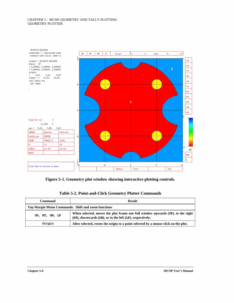
CHAPTER 5 – MCNP GEOMETRY AND TALLY PLOTTING GEOMETRY PLOTTER
Chapter 5-6 MCNP User’s Manual
Figure 5-1. Geometry plot window showing interactive plotting controls.
Table 5-2. Point-and-Click Geometry Plotter Commands
Command Result
Top Margin Menu Commands: Shift and zoom functions
UP, RT, DN, LF When selected, moves the plot frame one full window upwards (UP), to the right (RT), downwards (DN), or to the left (LF), respectively.
Origin After selected, resets the origin to a point selected by a mouse click on the plot.
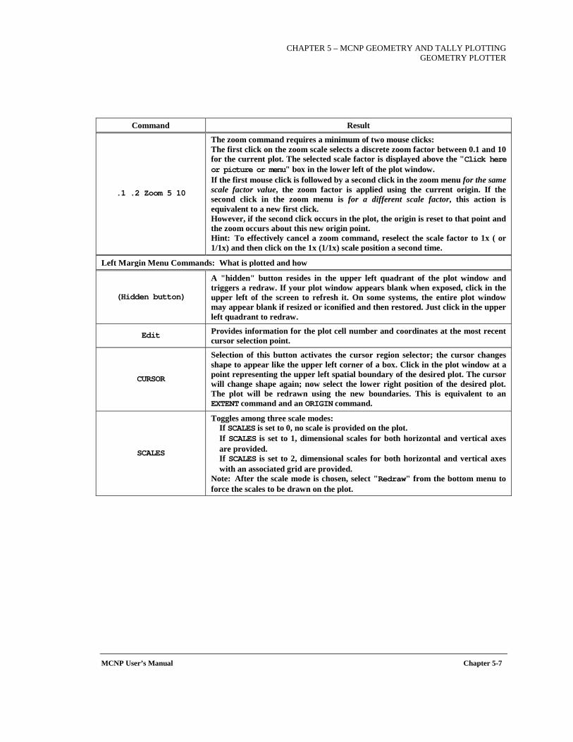
CHAPTER 5 – MCNP GEOMETRY AND TALLY PLOTTING
GEOMETRY PLOTTER
MCNP User’s Manual Chapter 5-7
Command Result
.1 .2 Zoom 5 10
The zoom command requires a minimum of two mouse clicks: The first click on the zoom scale selects a discrete zoom factor between 0.1 and 10 for the current plot. The selected scale factor is displayed above the "Click here or picture or menu" box in the lower left of the plot window. If the first mouse click is followed by a second click in the zoom menu for the same scale factor value, the zoom factor is applied using the current origin. If the second click in the zoom menu is for a different scale factor, this action is equivalent to a new first click. However, if the second click occurs in the plot, the origin is reset to that point and the zoom occurs about this new origin point. Hint: To effectively cancel a zoom command, reselect the scale factor to 1x ( or 1/1x) and then click on the 1x (1/1x) scale position a second time.
Left Margin Menu Commands: What is plotted and how
(Hidden button)
A "hidden" button resides in the upper left quadrant of the plot window and triggers a redraw. If your plot window appears blank when exposed, click in the upper left of the screen to refresh it. On some systems, the entire plot window may appear blank if resized or iconified and then restored. Just click in the upper left quadrant to redraw.
Edit Provides information for the plot cell number and coordinates at the most recent cursor selection point.
CURSOR
Selection of this button activates the cursor region selector; the cursor changes shape to appear like the upper left corner of a box. Click in the plot window at a point representing the upper left spatial boundary of the desired plot. The cursor will change shape again; now select the lower right position of the desired plot. The plot will be redrawn using the new boundaries. This is equivalent to an EXTENT command and an ORIGIN command.
SCALES
Toggles among three scale modes: If SCALES is set to 0, no scale is provided on the plot. If SCALES is set to 1, dimensional scales for both horizontal and vertical axes are provided. If SCALES is set to 2, dimensional scales for both horizontal and vertical axes with an associated grid are provided.
Note: After the scale mode is chosen, select "Redraw" from the bottom menu to force the scales to be drawn on the plot.
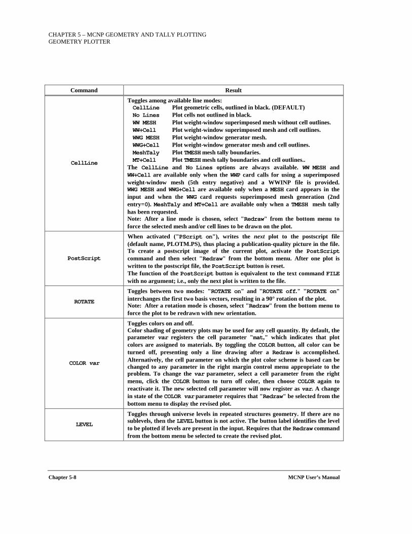
CHAPTER 5 – MCNP GEOMETRY AND TALLY PLOTTING GEOMETRY PLOTTER
Chapter 5-8 MCNP User’s Manual
Command Result
CellLine
Toggles among available line modes: CellLine Plot geometric cells, outlined in black. (DEFAULT) No Lines Plot cells not outlined in black. WW MESH Plot weight-window superimposed mesh without cell outlines. WW+Cell Plot weight-window superimposed mesh and cell outlines. WWG MESH Plot weight-window generator mesh. WWG+Cell Plot weight-window generator mesh and cell outlines. MeshTaly Plot TMESH mesh tally boundaries. MT+Cell Plot TMESH mesh tally boundaries and cell outlines..
The CellLine and No Lines options are always available. WW MESH and WW+Cell are available only when the WWP card calls for using a superimposed weight-window mesh (5th entry negative) and a WWINP file is provided. WWG MESH and WWG+Cell are available only when a MESH card appears in the input and when the WWG card requests superimposed mesh generation (2nd entry=0). MeshTaly and MT+Cell are available only when a TMESH mesh tally has been requested. Note: After a line mode is chosen, select "Redraw" from the bottom menu to force the selected mesh and/or cell lines to be drawn on the plot.
PostScript
When activated ("PScript on"), writes the next plot to the postscript file (default name, PLOTM.PS), thus placing a publication-quality picture in the file. To create a postscript image of the current plot, activate the PostScript command and then select "Redraw" from the bottom menu. After one plot is written to the postscript file, the PostScript button is reset. The function of the PostScript button is equivalent to the text command FILE with no argument; i.e., only the next plot is written to the file.
ROTATE
Toggles between two modes: "ROTATE on" and "ROTATE off." "ROTATE on" interchanges the first two basis vectors, resulting in a 90° rotation of the plot. Note: After a rotation mode is chosen, select "Redraw" from the bottom menu to force the plot to be redrawn with new orientation.
COLOR var
Toggles colors on and off. Color shading of geometry plots may be used for any cell quantity. By default, the parameter var registers the cell parameter "mat," which indicates that plot colors are assigned to materials. By toggling the COLOR button, all color can be turned off, presenting only a line drawing after a Redraw is accomplished. Alternatively, the cell parameter on which the plot color scheme is based can be changed to any parameter in the right margin control menu appropriate to the problem. To change the var parameter, select a cell parameter from the right menu, click the COLOR button to turn off color, then choose COLOR again to reactivate it. The new selected cell parameter will now register as var. A change in state of the COLOR var parameter requires that "Redraw" be selected from the bottom menu to display the revised plot.
LEVEL
Toggles through universe levels in repeated structures geometry. If there are no sublevels, then the LEVEL button is not active. The button label identifies the level to be plotted if levels are present in the input. Requires that the Redraw command from the bottom menu be selected to create the revised plot.
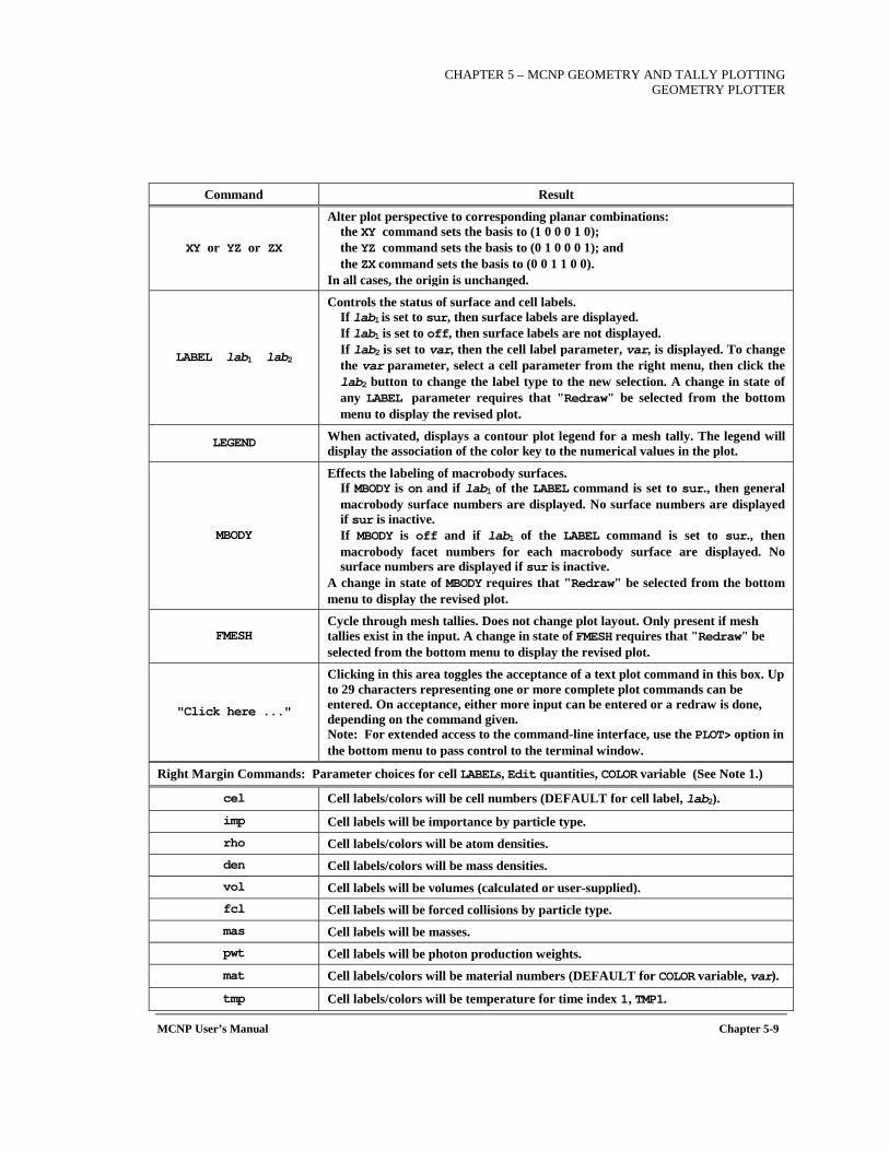
CHAPTER 5 – MCNP GEOMETRY AND TALLY PLOTTING
GEOMETRY PLOTTER
MCNP User’s Manual Chapter 5-9
Command Result
XY or YZ or ZX
Alter plot perspective to corresponding planar combinations: the XY command sets the basis to (1 0 0 0 1 0); the YZ command sets the basis to (0 1 0 0 0 1); and the ZX command sets the basis to (0 0 1 1 0 0).
In all cases, the origin is unchanged.
LABEL lab1 lab2
Controls the status of surface and cell labels. If lab1 is set to sur, then surface labels are displayed. If lab1 is set to off, then surface labels are not displayed. If lab2 is set to var, then the cell label parameter, var, is displayed. To change the var parameter, select a cell parameter from the right menu, then click the lab2 button to change the label type to the new selection. A change in state of any LABEL parameter requires that "Redraw" be selected from the bottom menu to display the revised plot.
LEGEND When activated, displays a contour plot legend for a mesh tally. The legend will display the association of the color key to the numerical values in the plot.
MBODY
Effects the labeling of macrobody surfaces. If MBODY is on and if lab1 of the LABEL command is set to sur., then general macrobody surface numbers are displayed. No surface numbers are displayed if sur is inactive. If MBODY is off and if lab1 of the LABEL command is set to sur., then macrobody facet numbers for each macrobody surface are displayed. No surface numbers are displayed if sur is inactive.
A change in state of MBODY requires that "Redraw" be selected from the bottom menu to display the revised plot.
FMESH Cycle through mesh tallies. Does not change plot layout. Only present if mesh tallies exist in the input. A change in state of FMESH requires that "Redraw" be selected from the bottom menu to display the revised plot.
"Click here ..."
Clicking in this area toggles the acceptance of a text plot command in this box. Up to 29 characters representing one or more complete plot commands can be entered. On acceptance, either more input can be entered or a redraw is done, depending on the command given. Note: For extended access to the command-line interface, use the PLOT> option in the bottom menu to pass control to the terminal window.
Right Margin Commands: Parameter choices for cell LABELs, Edit quantities, COLOR variable (See Note 1.)
cel Cell labels/colors will be cell numbers (DEFAULT for cell label, lab2).
imp Cell labels will be importance by particle type. rho Cell labels/colors will be atom densities. den Cell labels/colors will be mass densities. vol Cell labels will be volumes (calculated or user-supplied). fcl Cell labels will be forced collisions by particle type. mas Cell labels will be masses. pwt Cell labels will be photon production weights. mat Cell labels/colors will be material numbers (DEFAULT for COLOR variable, var).
tmp Cell labels/colors will be temperature for time index 1, TMP1.
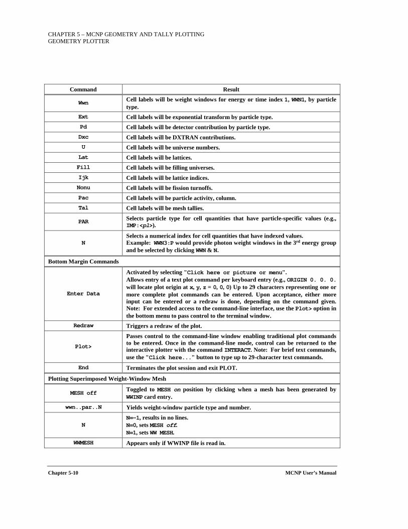
CHAPTER 5 – MCNP GEOMETRY AND TALLY PLOTTING GEOMETRY PLOTTER
Chapter 5-10 MCNP User’s Manual
Command Result
Wwn Cell labels will be weight windows for energy or time index 1, WWN1, by particle type.
Ext Cell labels will be exponential transform by particle type. Pd Cell labels will be detector contribution by particle type. Dxc Cell labels will be DXTRAN contributions. U Cell labels will be universe numbers. Lat Cell labels will be lattices. Fill Cell labels will be filling universes. Ijk Cell labels will be lattice indices. Nonu Cell labels will be fission turnoffs. Pac Cell labels will be particle activity, column. Tal Cell labels will be mesh tallies.
PAR Selects particle type for cell quantities that have particle-specific values (e.g., IMP:<pl>).
N Selects a numerical index for cell quantities that have indexed values. Example: WWN3:P would provide photon weight windows in the 3rd energy group and be selected by clicking WWN & N.
Bottom Margin Commands
Enter Data
Activated by selecting "Click here or picture or menu". Allows entry of a text plot command per keyboard entry (e.g., ORIGIN 0. 0. 0. will locate plot origin at x, y, z = 0, 0, 0) Up to 29 characters representing one or more complete plot commands can be entered. Upon acceptance, either more input can be entered or a redraw is done, depending on the command given. Note: For extended access to the command-line interface, use the Plot> option in the bottom menu to pass control to the terminal window.
Redraw Triggers a redraw of the plot.
Plot>
Passes control to the command-line window enabling traditional plot commands to be entered. Once in the command-line mode, control can be returned to the interactive plotter with the command INTERACT. Note: For brief text commands, use the "Click here..." button to type up to 29-character text commands.
End Terminates the plot session and exit PLOT.
Plotting Superimposed Weight-Window Mesh
MESH off Toggled to MESH on position by clicking when a mesh has been generated by WWINP card entry.
wwn..par..N Yields weight-window particle type and number.
N N=-1, results in no lines. N=0, sets MESH off. N=1, sets WW MESH.
WWMESH Appears only if WWINP file is read in.
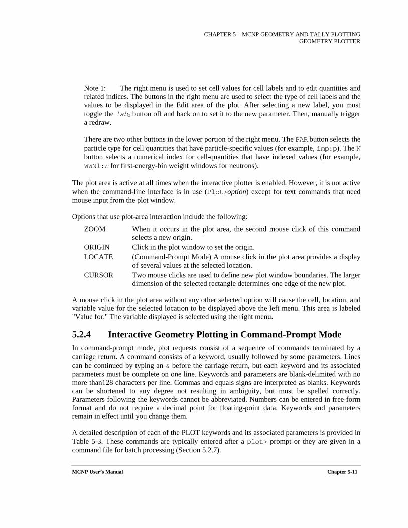
CHAPTER 5 – MCNP GEOMETRY AND TALLY PLOTTING
GEOMETRY PLOTTER
MCNP User’s Manual Chapter 5-11
Note 1: The right menu is used to set cell values for cell labels and to edit quantities and related indices. The buttons in the right menu are used to select the type of cell labels and the values to be displayed in the Edit area of the plot. After selecting a new label, you must toggle the lab2 button off and back on to set it to the new parameter. Then, manually trigger a redraw.
There are two other buttons in the lower portion of the right menu. The PAR button selects the particle type for cell quantities that have particle-specific values (for example, imp:p). The N button selects a numerical index for cell-quantities that have indexed values (for example, WWN1:n for first-energy-bin weight windows for neutrons).
The plot area is active at all times when the interactive plotter is enabled. However, it is not active when the command-line interface is in use (Plot>option) except for text commands that need mouse input from the plot window.
Options that use plot-area interaction include the following:
ZOOM When it occurs in the plot area, the second mouse click of this command selects a new origin.
ORIGIN Click in the plot window to set the origin. LOCATE (Command-Prompt Mode) A mouse click in the plot area provides a display
of several values at the selected location. CURSOR Two mouse clicks are used to define new plot window boundaries. The larger
dimension of the selected rectangle determines one edge of the new plot.
A mouse click in the plot area without any other selected option will cause the cell, location, and variable value for the selected location to be displayed above the left menu. This area is labeled "Value for." The variable displayed is selected using the right menu.
5.2.4 Interactive Geometry Plotting in Command-Prompt Mode In command-prompt mode, plot requests consist of a sequence of commands terminated by a carriage return. A command consists of a keyword, usually followed by some parameters. Lines can be continued by typing an & before the carriage return, but each keyword and its associated parameters must be complete on one line. Keywords and parameters are blank-delimited with no more than128 characters per line. Commas and equals signs are interpreted as blanks. Keywords can be shortened to any degree not resulting in ambiguity, but must be spelled correctly. Parameters following the keywords cannot be abbreviated. Numbers can be entered in free-form format and do not require a decimal point for floating-point data. Keywords and parameters remain in effect until you change them.
A detailed description of each of the PLOT keywords and its associated parameters is provided in Table 5-3. These commands are typically entered after a plot> prompt or they are given in a command file for batch processing (Section 5.2.7).
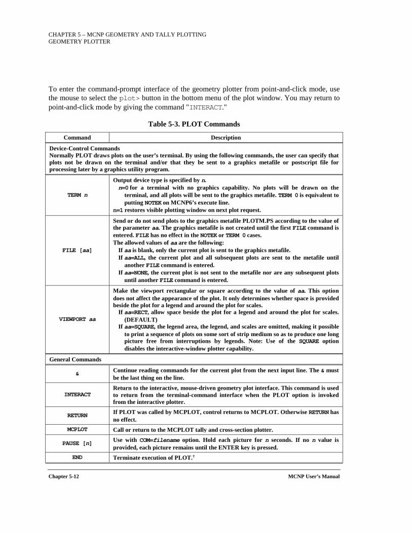
CHAPTER 5 – MCNP GEOMETRY AND TALLY PLOTTING GEOMETRY PLOTTER
Chapter 5-12 MCNP User’s Manual
To enter the command-prompt interface of the geometry plotter from point-and-click mode, use the mouse to select the plot> button in the bottom menu of the plot window. You may return to point-and-click mode by giving the command "INTERACT."
Table 5-3. PLOT Commands
Command Description
Device-Control Commands Normally PLOT draws plots on the user’s terminal. By using the following commands, the user can specify that plots not be drawn on the terminal and/or that they be sent to a graphics metafile or postscript file for processing later by a graphics utility program.
TERM n
Output device type is specified by n. n=0 for a terminal with no graphics capability. No plots will be drawn on the
terminal, and all plots will be sent to the graphics metafile. TERM 0 is equivalent to putting NOTEK on MCNP6’s execute line.
n=1 restores visible plotting window on next plot request.
FILE [aa]
Send or do not send plots to the graphics metafile PLOTM.PS according to the value of the parameter aa. The graphics metafile is not created until the first FILE command is entered. FILE has no effect in the NOTEK or TERM 0 cases. The allowed values of aa are the following:
If aa is blank, only the current plot is sent to the graphics metafile. If aa=ALL, the current plot and all subsequent plots are sent to the metafile until
another FILE command is entered. If aa=NONE, the current plot is not sent to the metafile nor are any subsequent plots
until another FILE command is entered.
VIEWPORT aa
Make the viewport rectangular or square according to the value of aa. This option does not affect the appearance of the plot. It only determines whether space is provided beside the plot for a legend and around the plot for scales.
If aa=RECT, allow space beside the plot for a legend and around the plot for scales. (DEFAULT)
If aa=SQUARE, the legend area, the legend, and scales are omitted, making it possible to print a sequence of plots on some sort of strip medium so as to produce one long picture free from interruptions by legends. Note: Use of the SQUARE option disables the interactive-window plotter capability.
General Commands
& Continue reading commands for the current plot from the next input line. The & must be the last thing on the line.
INTERACT Return to the interactive, mouse-driven geometry plot interface. This command is used to return from the terminal-command interface when the PLOT option is invoked from the interactive plotter.
RETURN If PLOT was called by MCPLOT, control returns to MCPLOT. Otherwise RETURN has no effect.
MCPLOT Call or return to the MCPLOT tally and cross-section plotter.
PAUSE [n] Use with COM=filename option. Hold each picture for n seconds. If no n value is provided, each picture remains until the ENTER key is pressed.
END Terminate execution of PLOT.†
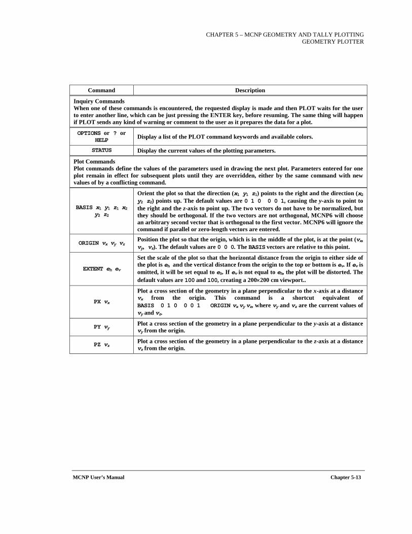
CHAPTER 5 – MCNP GEOMETRY AND TALLY PLOTTING
GEOMETRY PLOTTER
MCNP User’s Manual Chapter 5-13
Command Description
Inquiry Commands When one of these commands is encountered, the requested display is made and then PLOT waits for the user to enter another line, which can be just pressing the ENTER key, before resuming. The same thing will happen if PLOT sends any kind of warning or comment to the user as it prepares the data for a plot.
OPTIONS or ? or HELP Display a list of the PLOT command keywords and available colors.
STATUS Display the current values of the plotting parameters.
Plot Commands Plot commands define the values of the parameters used in drawing the next plot. Parameters entered for one plot remain in effect for subsequent plots until they are overridden, either by the same command with new values of by a conflicting command.
BASIS x1 y1 z1 x2 y2 z2
Orient the plot so that the direction (x1 y1 z1) points to the right and the direction (x2 y2 z2) points up. The default values are 0 1 0 0 0 1, causing the y-axis to point to the right and the z-axis to point up. The two vectors do not have to be normalized, but they should be orthogonal. If the two vectors are not orthogonal, MCNP6 will choose an arbitrary second vector that is orthogonal to the first vector. MCNP6 will ignore the command if parallel or zero-length vectors are entered.
ORIGIN vx vy vz Position the plot so that the origin, which is in the middle of the plot, is at the point (vx, vy, vz). The default values are 0 0 0. The BASIS vectors are relative to this point.
EXTENT eh ev
Set the scale of the plot so that the horizontal distance from the origin to either side of the plot is eh and the vertical distance from the origin to the top or bottom is ev. If ev is omitted, it will be set equal to eh. If ev is not equal to eh, the plot will be distorted. The default values are 100 and 100, creating a 200×200 cm viewport..
PX vx
Plot a cross section of the geometry in a plane perpendicular to the x-axis at a distance vx from the origin. This command is a shortcut equivalent of BASIS 0 1 0 0 0 1 ORIGIN vx vy vz, where vy and vz are the current values of vy and vz.
PY vy Plot a cross section of the geometry in a plane perpendicular to the y-axis at a distance vy from the origin.
PZ vz Plot a cross section of the geometry in a plane perpendicular to the z-axis at a distance vz from the origin.
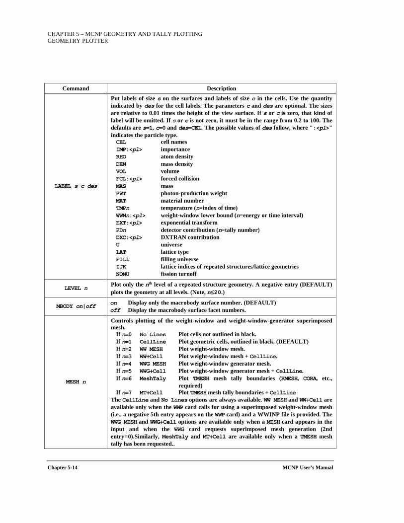
CHAPTER 5 – MCNP GEOMETRY AND TALLY PLOTTING GEOMETRY PLOTTER
Chapter 5-14 MCNP User’s Manual
Command Description
LABEL s c des
Put labels of size s on the surfaces and labels of size c in the cells. Use the quantity indicated by des for the cell labels. The parameters c and des are optional. The sizes are relative to 0.01 times the height of the view surface. If s or c is zero, that kind of label will be omitted. If s or c is not zero, it must be in the range from 0.2 to 100. The defaults are s=1, c=0 and des=CEL. The possible values of des follow, where ":<pl>" indicates the particle type. CEL cell names IMP:<pl> importance RHO atom density DEN mass density VOL volume FCL:<pl> forced collision MAS mass PWT photon-production weight MAT material number TMPn temperature (n=index of time) WWNn:<pl> weight-window lower bound (n=energy or time interval) EXT:<pl> exponential transform PDn detector contribution (n=tally number) DXC:<pl> DXTRAN contribution U universe LAT lattice type FILL filling universe IJK lattice indices of repeated structures/lattice geometries NONU fission turnoff
LEVEL n Plot only the nth level of a repeated structure geometry. A negative entry (DEFAULT) plots the geometry at all levels. (Note, n≤20.)
MBODY on|off on Display only the macrobody surface number. (DEFAULT) off Display the macrobody surface facet numbers.
MESH n
Controls plotting of the weight-window and weight-window-generator superimposed mesh.
If n=0 No Lines Plot cells not outlined in black. If n=1 CellLine Plot geometric cells, outlined in black. (DEFAULT) If n=2 WW MESH Plot weight-window mesh. If n=3 WW+Cell Plot weight-window mesh + CellLine. If n=4 WWG MESH Plot weight-window generator mesh. If n=5 WWG+Cell Plot weight-window generator mesh + CellLine. If n=6 MeshTaly Plot TMESH mesh tally boundaries (RMESH, CORA, etc.,
required) If n=7 MT+Cell Plot TMESH mesh tally boundaries + CellLine
The CellLine and No Lines options are always available. WW MESH and WW+Cell are available only when the WWP card calls for using a superimposed weight-window mesh (i.e., a negative 5th entry appears on the WWP card) and a WWINP file is provided. The WWG MESH and WWG+Cell options are available only when a MESH card appears in the input and when the WWG card requests superimposed mesh generation (2nd entry=0).Similarly, MeshTaly and MT+Cell are available only when a TMESH mesh tally has been requested..
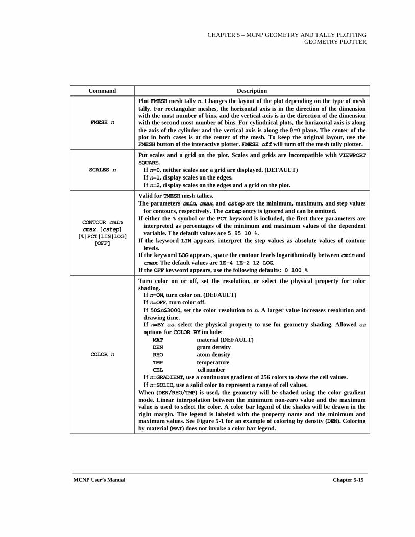
CHAPTER 5 – MCNP GEOMETRY AND TALLY PLOTTING
GEOMETRY PLOTTER
MCNP User’s Manual Chapter 5-15
Command Description
FMESH n
Plot FMESH mesh tally n. Changes the layout of the plot depending on the type of mesh tally. For rectangular meshes, the horizontal axis is in the direction of the dimension with the most number of bins, and the vertical axis is in the direction of the dimension with the second most number of bins. For cylindrical plots, the horizontal axis is along the axis of the cylinder and the vertical axis is along the θ=0 plane. The center of the plot in both cases is at the center of the mesh. To keep the original layout, use the FMESH button of the interactive plotter. FMESH off will turn off the mesh tally plotter.
SCALES n
Put scales and a grid on the plot. Scales and grids are incompatible with VIEWPORT SQUARE.
If n=0, neither scales nor a grid are displayed. (DEFAULT) If n=1, display scales on the edges. If n=2, display scales on the edges and a grid on the plot.
CONTOUR cmin cmax [cstep]
[%|PCT|LIN|LOG] [OFF]
Valid for TMESH mesh tallies. The parameters cmin, cmax, and cstep are the minimum, maximum, and step values
for contours, respectively. The cstep entry is ignored and can be omitted. If either the % symbol or the PCT keyword is included, the first three parameters are
interpreted as percentages of the minimum and maximum values of the dependent variable. The default values are 5 95 10 %.
If the keyword LIN appears, interpret the step values as absolute values of contour levels.
If the keyword LOG appears, space the contour levels logarithmically between cmin and cmax. The default values are 1E-4 1E-2 12 LOG.
If the OFF keyword appears, use the following defaults: 0 100 %
COLOR n
Turn color on or off, set the resolution, or select the physical property for color shading.
If n=ON, turn color on. (DEFAULT) If n=OFF, turn color off. If 50≤n≤3000, set the color resolution to n. A larger value increases resolution and drawing time. If n=BY aa, select the physical property to use for geometry shading. Allowed aa options for COLOR BY include:
MAT material (DEFAULT) DEN gram density RHO atom density TMP temperature CEL cell number
If n=GRADIENT, use a continuous gradient of 256 colors to show the cell values. If n=SOLID, use a solid color to represent a range of cell values.
When (DEN/RHO/TMP) is used, the geometry will be shaded using the color gradient mode. Linear interpolation between the minimum non-zero value and the maximum value is used to select the color. A color bar legend of the shades will be drawn in the right margin. The legend is labeled with the property name and the minimum and maximum values. See Figure 5-1 for an example of coloring by density (DEN). Coloring by material (MAT) does not invoke a color bar legend.
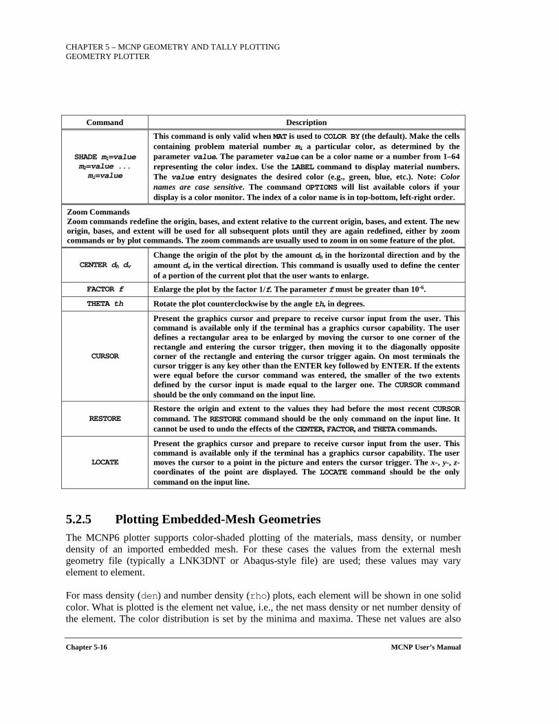
CHAPTER 5 – MCNP GEOMETRY AND TALLY PLOTTING GEOMETRY PLOTTER
Chapter 5-16 MCNP User’s Manual
Command Description
SHADE m1=value m2=value ... mi=value
This command is only valid when MAT is used to COLOR BY (the default). Make the cells containing problem material number mi a particular color, as determined by the parameter value. The parameter value can be a color name or a number from 1–64 representing the color index. Use the LABEL command to display material numbers. The value entry designates the desired color (e.g., green, blue, etc.). Note: Color names are case sensitive. The command OPTIONS will list available colors if your display is a color monitor. The index of a color name is in top-bottom, left-right order.
Zoom Commands Zoom commands redefine the origin, bases, and extent relative to the current origin, bases, and extent. The new origin, bases, and extent will be used for all subsequent plots until they are again redefined, either by zoom commands or by plot commands. The zoom commands are usually used to zoom in on some feature of the plot.
CENTER dh dv Change the origin of the plot by the amount dh in the horizontal direction and by the amount dv in the vertical direction. This command is usually used to define the center of a portion of the current plot that the user wants to enlarge.
FACTOR f Enlarge the plot by the factor 1/f. The parameter f must be greater than 10-6.
THETA th Rotate the plot counterclockwise by the angle th, in degrees.
CURSOR
Present the graphics cursor and prepare to receive cursor input from the user. This command is available only if the terminal has a graphics cursor capability. The user defines a rectangular area to be enlarged by moving the cursor to one corner of the rectangle and entering the cursor trigger, then moving it to the diagonally opposite corner of the rectangle and entering the cursor trigger again. On most terminals the cursor trigger is any key other than the ENTER key followed by ENTER. If the extents were equal before the cursor command was entered, the smaller of the two extents defined by the cursor input is made equal to the larger one. The CURSOR command should be the only command on the input line.
RESTORE Restore the origin and extent to the values they had before the most recent CURSOR command. The RESTORE command should be the only command on the input line. It cannot be used to undo the effects of the CENTER, FACTOR, and THETA commands.
LOCATE
Present the graphics cursor and prepare to receive cursor input from the user. This command is available only if the terminal has a graphics cursor capability. The user moves the cursor to a point in the picture and enters the cursor trigger. The x-, y-, z-coordinates of the point are displayed. The LOCATE command should be the only command on the input line.
5.2.5 Plotting Embedded-Mesh Geometries The MCNP6 plotter supports color-shaded plotting of the materials, mass density, or number density of an imported embedded mesh. For these cases the values from the external mesh geometry file (typically a LNK3DNT or Abaqus-style file) are used; these values may vary element to element.
For mass density (den) and number density (rho) plots, each element will be shown in one solid color. What is plotted is the element net value, i.e., the net mass density or net number density of the element. The color distribution is set by the minima and maxima. These net values are also
CHAPTER 5 – MCNP GEOMETRY AND TALLY PLOTTING
GEOMETRY PLOTTER
MCNP User’s Manual Chapter 5-17
the values reported for plot queries when "den" or "rho" is selected from the right-hand-side interactive menu.
For material plots, multi-material zones may appear striped as the color to plot is chosen randomly based on the material mass fraction. This means that redrawing a color-by-mat plot may give a slightly different striping. For example, in a two-material element with a 50/50 mass –fraction mix, approximately 50/50 color striping will display horizontally. If "mat" is selected from the right-hand-side interactive menu, clicking on a spot containing multiple materials will randomly select which material to report. Repeated clicking on such a spot may show different materials on different clicks. Void elements in the mesh are not shaded (i.e., shown as white) on material plots.
5.2.6 Geometry Debugging Surfaces appearing on a plot as red dashed lines usually indicate that adjoining space is improperly defined. Dashed lines caused by a geometry error can indicate space that has been defined in more than one cell or space that has never been defined. These geometry errors need to be corrected. Dashed lines also can occur because the plot plane corresponds to a bounding planar surface. The plot plane should be moved so it is not coincident with a problem surface. Dashed lines can indicate a cookie cutter cell or a DXTRAN sphere. These are not errors. The reason for the presence of dashed lines on an MCNP6 plot should be understood before running a problem.
When checking a geometry model, errors may not appear on the two-dimensional slice chosen, but one or more particles will get lost in tracking. To find the modeling error, use the coordinates and trajectory of the particle when it got lost. Entering the particle coordinates as the ORIGIN and the particle trajectory as the first basis vector will result in a plot displaying the problem space.
5.2.7 Geometry Plotting in Batch Mode Although MCNP6 can be run in a batch environment without much difficulty, user interaction with the plotter is significantly reduced. If you are not using an interactive graphics terminal, use the NOTEK option on the MCNP6 execution line or set TERM=0 along with other PLOT keywords when first prompted by PLOT. Every view you plot will be put in a local graphics metafile or postscript file called PLOTn where n begins at M and goes to the next letter in the alphabet if PLOTM exists. In the interactive mode, plots can be sent to this graphics metafile with the FILE keyword. (See the keyword description in Table 5-3 for a complete explanation.) For some graphics systems, the PLOTn.PS file is a postscript file that can be sent to a postscript printer.
5.3 THE TALLY AND CROSS-SECTION PLOTTER, MCPLOT
MCPLOT plots tally results produced by MCNP6 as well as cross-section data used by MCNP6. It can draw ordinary two-dimensional x-y plots and contour or color-filled tally plots of three-dimensional data. MCPLOT supports a wide variety of plot options. More than one curve can be plotted on a single x-y plot. Tally plots can be created from tally data that exists within a MCTAL
CHAPTER 5 – MCNP GEOMETRY AND TALLY PLOTTING TALLY AND CROSS-SECTION PLOTTER
Chapter 5-18 MCNP User’s Manual
or RUNTPE file. However, if one is plotting from a MCTAL file, not all options are available because not all the information is available in that format.
In addition to plotting tally results, MCPLOT also plots cross-section data specified in an INP file—either individual nuclides or the complete material composed of constituent nuclei properly weighted by atomic fraction. The data plotted reflect adjustments to the cross sections made by MCNP6 such as energy cutoffs, neutron cross-section temperatures, S(α,β) treatment, summation of photon reactions to provide a total photon cross section, simple physics treatment for photon data, generation of electron stopping powers and other electron data, and more. Cross-section plots cannot be made from a RUNTPE file.
MCNP6 can plot proton cross sections. The reaction numbers are similar to the neutron reaction numbers: all positive. The principal proton cross sections are the following: ±1=total, ±2=non-elastic, ±3=elastic, ±4=heating, and >4=various reactions. On the LA150H proton library, the only available reaction is MT=5 with its multiplicities, 1005, 9005, 31,005, etc. The multiplicity reaction numbers for interaction reaction MT=5 are 1005 for neutrons, 9005 for protons, 31,005 for deuterons, etc. To find out which reactions are available for a particular nuclide or material, enter an invalid reaction number, such as MT=99, and MCNP6 will list the available proton reactions and the available yields, such as 1005, 32,001, and 34,002. The proton multiplicity, MT=9001, 9004, 9005, etc., generally is available, along with the total cross section and heating number, MT=1, MT=4. Entering a bad nuclide, e.g., XS=12345.67H, will cause MCNP6 to list the available proton nuclides.
Final tally results can be plotted after particle transport has finished. The temporary status of one or more tallies can be displayed during the run as transport is ongoing. (Note: This capability is not always possible in parallel computations.) After transport is finished, MCPLOT is invoked by typing a Z on the MCNP6 execution line, either as a separate procedure using existing RUNTPE or MCTAL files:
MCNP6 Z RMCTAL=<mctal_filename> or MCNP6 Z RUNTPE=<runtpe_filename> ,
or as part of a regular uninterrupted MCNP6 run. To superimpose mesh tally contours with problem geometries, initiate MCPLOT using one of the two execute lines above and then enter the geometry plotter using the PLOT command.
There are two ways to request that a plot be produced periodically during the run: use an MPLOT card (Section 3.3.7.2.5) in the INP file or use the TTY interrupt feature (Section 1.4.2). (Note: This capability is not always possible during parallel computations.) The TTY interrupt <ctrl-c>m causes MCNP6 to pause at the end of the history that is running when the interrupt occurs and allows plots to be made by calling MCPLOT, which takes plot requests from the terminal. During run-time plotting, no output is sent to the COMOUT file. In addition, the following commands can not be used after invoking MCPLOT with an interrupt: RMCTAL, RUNTPE, and DUMP. The END or RETURN commands are used to exit MCPLOT or return MCNP6
CHAPTER 5 – MCNP GEOMETRY AND TALLY PLOTTING
TALLY AND CROSS-SECTION PLOTTER
MCNP User’s Manual Chapter 5-19
to transport mode. Cross-section data cannot be displayed after a TTY interrupt or by use of the MPLOT card.
Color contour plots may be created of mesh tally, radiography tally, and lattice tally results. Mesh tallies also can be plotted superimposed over problem geometries. All of these plots are done in MCNP6 without the need of auxiliary post-processing codes; the plots can be made either at the end of a calculation or while a calculation proceeds by using the MPLOT card.
MCPLOT can make tally plots on a machine different from the one on which the problem was run by using the MCTAL file. When the INP file has a PRDMP card with a non-zero third entry, a MCTAL file is created at the end of the run. The MCTAL file contains all the tally data in the last RUNTPE dump. MCTAL is a coded ASCII file that can be converted and moved from one kind of machine to another. When the MCTAL file is created, its name can be specified in the execute line using the following format:
MCNP6 I=inpfile MCTAL=filename
The default filename is a unique name based on MCTAL.
The MCPLOT “HELP” command provides an alphabetized four-column listing of options [DUR09]. At the bottom of the four-column list are instructions describing how to
1) invoke a listing of all HELP commands with an explanation of their function and use syntax (“HELP ALL”),
2) provide a listing of function and syntax for a single HELP command (“HELP <command>”), 3) request an overview of the MCPLOT capability (“HELP OVERVIEW”), and 4) summarize input and execution-line options (“HELP EXECUTE”).
For examples of using MCPLOT, see Section 5.4.
5.3.1 Execution Line Options Related to MCPLOT Initiation To run only MCPLOT and plot tallies upon termination of the job by MCNP6, enter the following command:
MCNP6 Z KEYWORD[=value(s)]
where Z invokes MCPLOT. The allowed keywords are explained in Table 5-4. Cross-section data cannot be plotted by this method.
The execute line command MCNP6 INP=filename IXRZ KEYWORD[=value(s)]
causes MCNP6 to run the problem specified in filename, following which the prompt mcplot> appears for MCPLOT commands. Both cross-section data and tallies can be plotted using this method after the run is complete. Cross-section data cannot be plotted after a TTY interrupt or by use of the MPLOT card.
CHAPTER 5 – MCNP GEOMETRY AND TALLY PLOTTING TALLY AND CROSS-SECTION PLOTTER
Chapter 5-20 MCNP User’s Manual
The execute line command MCNP6 INP=filename IXZ KEYWORD[=value(s)]
provides the most common way to plot cross-section data. The problem cross sections are read in, but no transport occurs. When using this method to plot cross sections, the following commands cannot be used: BAR, CONTOUR, DUMP, FREQ, HIST, PLOT, RETURN, RMCTAL, RUNTPE, SPLINE, WASH, and WMCTAL.
Table 5-4. MCPLOT Execution Line Options
Keyword Options Description
NOTEK Suppress plotting at the terminal and send all plots to the graphics metafile, PLOTM. The keyword NOTEK is for production and batch situations and is used when the user’s terminal has no graphics capability.
COM=filename
Use file filename as the source of plot requests. When an end-of-file (EOF) is read, control is transferred to the terminal. In a production or batch situation, end the file with an END command to prevent transfer of control. Never end the COM file with a blank line. If COM is absent, the terminal is used as the source of plot requests.
RUNTPE=filename
Read file filename as the source of MCNP6 tally data. The default file name is RUNTPE, if it exists. If the default RUNTPE file does not exist, the user will be prompted for an RMCTAL or RUNTPE command. The name for the RUNTPE can be specified on the execution line via the RUNTPE=filename execute-line option.
RMCTAL=filename Read the MCTAL file, filename, as the source of the MCNP6 tally data. The default is MCTAL, if it exists.
PLOTM=filename
Name the graphics metafile filename. The default name is PLOTM. For some systems this metafile is a standard postscript file and is named PLOTM.PS. When CGS is being used, there can be no more than six characters in filename. Unique names for the output file, PLOTM, will be chosen by MCNP6 to avoid overwriting existing files.
COMOUT=filename
Write all plot requests to file filename. The default name is COMOUT. MCPLOT writes the COMOUT file in order to give the user the opportunity to do the same plotting at some later time, using all or part of the old COMOUT file as the COM file in the second run. Unique names for the output file, COMOUT, will be chosen by MCNP6 to avoid overwriting existing files.
Plot requests are normally entered from the keyboard of a terminal; alternatively, they can be entered from a file. A plot is requested by entering a sequence of plot commands following a prompt character. The request is terminated by the ENTER key not immediately preceded by an & or by a COPLOT command. Commands consist of keywords usually followed by some parameters, either space or comma delimited.
Defaults are available for nearly everything. If MCNP6 is run with Z as the execute line message, and if file RUNTPE is present with more than one energy bin in the first tally, and if the ENTER key is pressed in response to the MCPLOT prompt, a lin-log histogram plot of tally/MeV vs. energy, with error bars and suitable labels, will appear on the screen.
CHAPTER 5 – MCNP GEOMETRY AND TALLY PLOTTING
TALLY AND CROSS-SECTION PLOTTER
MCNP User’s Manual Chapter 5-21
5.3.2 Plot Conventions and Command Syntax
5.3.2.1 2D PLOT
The origin of coordinates for the MCPLOT 2D option is at the lower left corner of the picture. The horizontal axis is called the x-axis. It is the axis of the independent variable such as user bin or cell number or energy. The vertical axis is called the y-axis. It is the axis of the dependent variable such as flux or current or dose. Each axis can be either linear or logarithmic.
5.3.2.2 CONTOUR PLOT
Similarly, the origin of coordinates for MCPLOT’s contour plot option is at the lower left corner of the picture. The horizontal axis is called the x-axis. It is the axis of the first of the two independent variables. The vertical axis is called the y-axis. It is the axis of the second independent variable. The contours represent the values of the dependent variable. Only linear axes are available. Each contour is drawn in a different color depending on its value with respect to the z-value extrema. Extensions to the FREE and CONTOUR commands allow for shaded contour plots of tally and mesh data.
For additional examples involving contour plots see Section 5.4.3 and Section 5.4.4.
5.3.2.3 COLOR-WASH PLOT
This plot option is similar to contour plotting, but instead of drawing contours of z(x,y) data, each tally bin is filled with a color selected by the tally value in the bin. The axis conventions are the same as in contour plotting. This option is selected with the command WASH. If two free variables have been selected (with the FREE command), a color-filled plot is drawn. This is a useful option for radiography tallies. A palette of 64 colors ranging from red to yellow to green to blue is used. The color index is selected by linear interpolation between the z-minimum and the z-maximum values.
5.3.2.4 MCPLOT COMMAND SYNTAX
Like the geometry plotter, each MCPLOT command consists of a command keyword that in most cases is followed by some parameters. Keywords and parameters are entered space delimited with no more than128 characters per line. Commas and equals signs are interpreted as spaces. A plot request can be continued onto another line by typing an & before the ENTER key, but each command (the keyword and its parameters) must be complete on one line. Command keywords, but not parameters, can be abbreviated to any degree not resulting in ambiguity, but they must be correctly spelled. The term "current plot" means the plot that is being defined by the commands currently being typed in, which might not be the plot that is showing on the screen. Only those commands marked with a dagger (†) in the list presented in Table 5-5 can be used after the first COPLOT command in a plot request because the others all affect the framework of the plot or are for contour or 3D plots only.
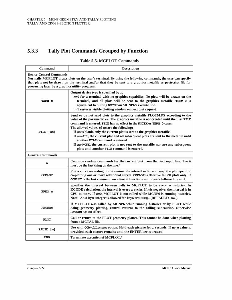
CHAPTER 5 – MCNP GEOMETRY AND TALLY PLOTTING TALLY AND CROSS-SECTION PLOTTER
Chapter 5-22 MCNP User’s Manual
5.3.3 Tally Plot Commands Grouped by Function
Table 5-5. MCPLOT Commands
Command Description
Device-Control Commands Normally MCPLOT draws plots on the user’s terminal. By using the following commands, the user can specify that plots not be drawn on the terminal and/or that they be sent to a graphics metafile or postscript file for processing later by a graphics utility program.
TERM n
Output device type is specified by n. n=0 for a terminal with no graphics capability. No plots will be drawn on the
terminal, and all plots will be sent to the graphics metafile. TERM 0 is equivalent to putting NOTEK on MCNP6’s execute line.
n=1 restores visible plotting window on next plot request.
FILE [aa]
Send or do not send plots to the graphics metafile PLOTM.PS according to the value of the parameter aa. The graphics metafile is not created until the first FILE command is entered. FILE has no effect in the NOTEK or TERM 0 cases. The allowed values of aa are the following:
If aa is blank, only the current plot is sent to the graphics metafile. If aa=ALL, the current plot and all subsequent plots are sent to the metafile until
another FILE command is entered. If aa=NONE, the current plot is not sent to the metafile nor are any subsequent
plots until another FILE command is entered.
General Commands
& Continue reading commands for the current plot from the next input line. The & must be the last thing on the line.†
COPLOT Plot a curve according to the commands entered so far and keep the plot open for co-plotting one or more additional curves. COPLOT is effective for 2D plots only. If COPLOT is the last command on a line, it functions as if it were followed by an &.
FREQ n
Specifies the interval between calls to MCPLOT to be every n histories. In KCODE calculation, the interval is every n cycles. If n is negative, the interval is in CPU minutes. If n=0, MCPLOT is not called while MCNP6 is running histories. Note: An 8-byte integer is allowed for keyword FREQ.. (DEFAULT: n=0)
RETURN If MCPLOT was called by MCNP6 while running histories or by PLOT while doing geometry plotting, control returns to the calling subroutine. Otherwise RETURN has no effect.
PLOT Call or return to the PLOT geometry plotter. This cannot be done when plotting from a MCTAL file.
PAUSE [n] Use with COM=filename option. Hold each picture for n seconds. If no n value is provided, each picture remains until the ENTER key is pressed.
END Terminate execution of MCPLOT.†
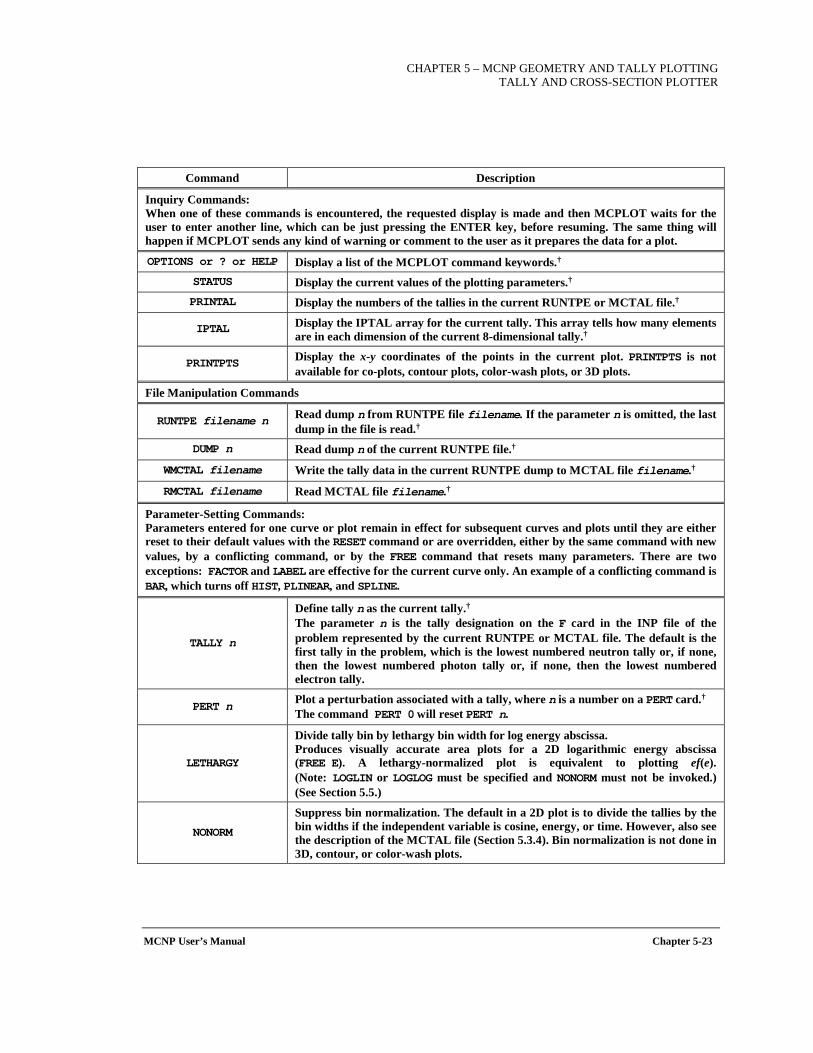
CHAPTER 5 – MCNP GEOMETRY AND TALLY PLOTTING
TALLY AND CROSS-SECTION PLOTTER
MCNP User’s Manual Chapter 5-23
Command Description
Inquiry Commands: When one of these commands is encountered, the requested display is made and then MCPLOT waits for the user to enter another line, which can be just pressing the ENTER key, before resuming. The same thing will happen if MCPLOT sends any kind of warning or comment to the user as it prepares the data for a plot.
OPTIONS or ? or HELP Display a list of the MCPLOT command keywords.† STATUS Display the current values of the plotting parameters.† PRINTAL Display the numbers of the tallies in the current RUNTPE or MCTAL file.†
IPTAL Display the IPTAL array for the current tally. This array tells how many elements are in each dimension of the current 8-dimensional tally.†
PRINTPTS Display the x-y coordinates of the points in the current plot. PRINTPTS is not available for co-plots, contour plots, color-wash plots, or 3D plots.
File Manipulation Commands
RUNTPE filename n Read dump n from RUNTPE file filename. If the parameter n is omitted, the last dump in the file is read.†
DUMP n Read dump n of the current RUNTPE file.†
WMCTAL filename Write the tally data in the current RUNTPE dump to MCTAL file filename.†
RMCTAL filename Read MCTAL file filename.†
Parameter-Setting Commands: Parameters entered for one curve or plot remain in effect for subsequent curves and plots until they are either reset to their default values with the RESET command or are overridden, either by the same command with new values, by a conflicting command, or by the FREE command that resets many parameters. There are two exceptions: FACTOR and LABEL are effective for the current curve only. An example of a conflicting command is BAR, which turns off HIST, PLINEAR, and SPLINE.
TALLY n
Define tally n as the current tally.† The parameter n is the tally designation on the F card in the INP file of the problem represented by the current RUNTPE or MCTAL file. The default is the first tally in the problem, which is the lowest numbered neutron tally or, if none, then the lowest numbered photon tally or, if none, then the lowest numbered electron tally.
PERT n Plot a perturbation associated with a tally, where n is a number on a PERT card.† The command PERT 0 will reset PERT n.
LETHARGY
Divide tally bin by lethargy bin width for log energy abscissa. Produces visually accurate area plots for a 2D logarithmic energy abscissa (FREE E). A lethargy-normalized plot is equivalent to plotting ef(e). (Note: LOGLIN or LOGLOG must be specified and NONORM must not be invoked.) (See Section 5.5.)
NONORM
Suppress bin normalization. The default in a 2D plot is to divide the tallies by the bin widths if the independent variable is cosine, energy, or time. However, also see the description of the MCTAL file (Section 5.3.4). Bin normalization is not done in 3D, contour, or color-wash plots.
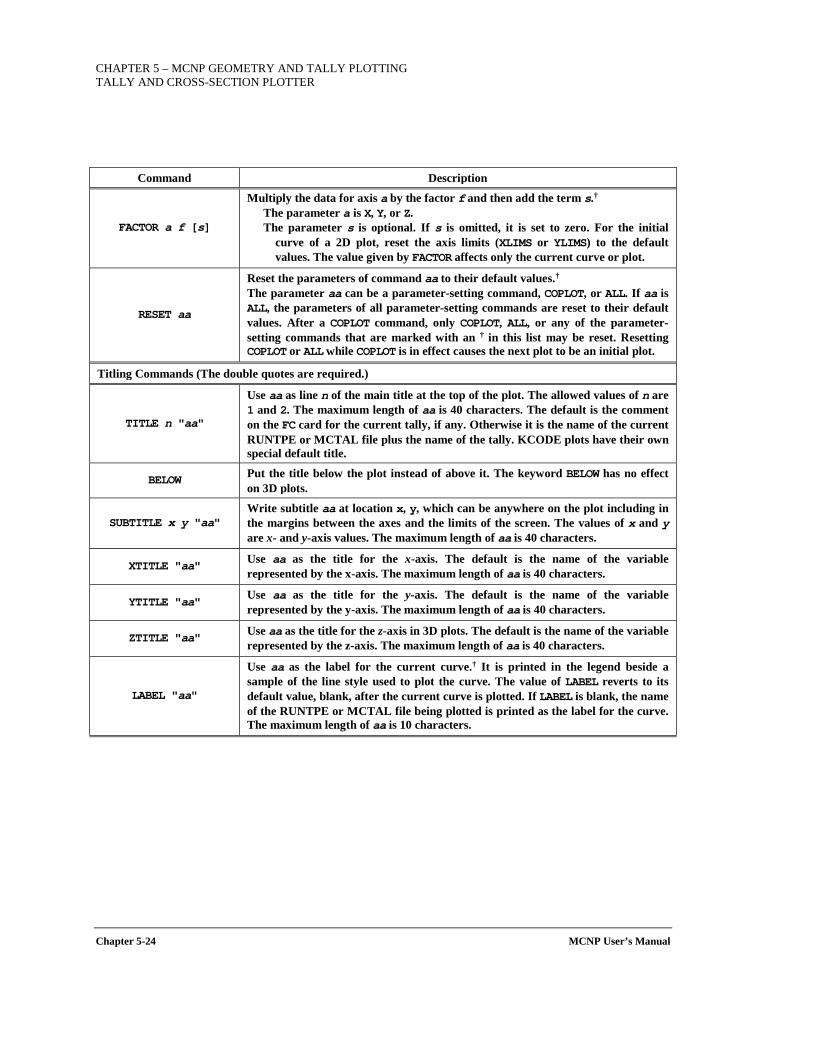
CHAPTER 5 – MCNP GEOMETRY AND TALLY PLOTTING TALLY AND CROSS-SECTION PLOTTER
Chapter 5-24 MCNP User’s Manual
Command Description
FACTOR a f [s]
Multiply the data for axis a by the factor f and then add the term s.† The parameter a is X, Y, or Z. The parameter s is optional. If s is omitted, it is set to zero. For the initial
curve of a 2D plot, reset the axis limits (XLIMS or YLIMS) to the default values. The value given by FACTOR affects only the current curve or plot.
RESET aa
Reset the parameters of command aa to their default values.† The parameter aa can be a parameter-setting command, COPLOT, or ALL. If aa is ALL, the parameters of all parameter-setting commands are reset to their default values. After a COPLOT command, only COPLOT, ALL, or any of the parameter-setting commands that are marked with an † in this list may be reset. Resetting COPLOT or ALL while COPLOT is in effect causes the next plot to be an initial plot.
Titling Commands (The double quotes are required.)
TITLE n "aa"
Use aa as line n of the main title at the top of the plot. The allowed values of n are 1 and 2. The maximum length of aa is 40 characters. The default is the comment on the FC card for the current tally, if any. Otherwise it is the name of the current RUNTPE or MCTAL file plus the name of the tally. KCODE plots have their own special default title.
BELOW Put the title below the plot instead of above it. The keyword BELOW has no effect on 3D plots.
SUBTITLE x y "aa" Write subtitle aa at location x, y, which can be anywhere on the plot including in the margins between the axes and the limits of the screen. The values of x and y are x- and y-axis values. The maximum length of aa is 40 characters.
XTITLE "aa" Use aa as the title for the x-axis. The default is the name of the variable represented by the x-axis. The maximum length of aa is 40 characters.
YTITLE "aa" Use aa as the title for the y-axis. The default is the name of the variable represented by the y-axis. The maximum length of aa is 40 characters.
ZTITLE "aa" Use aa as the title for the z-axis in 3D plots. The default is the name of the variable represented by the z-axis. The maximum length of aa is 40 characters.
LABEL "aa"
Use aa as the label for the current curve.† It is printed in the legend beside a sample of the line style used to plot the curve. The value of LABEL reverts to its default value, blank, after the current curve is plotted. If LABEL is blank, the name of the RUNTPE or MCTAL file being plotted is printed as the label for the curve. The maximum length of aa is 10 characters.
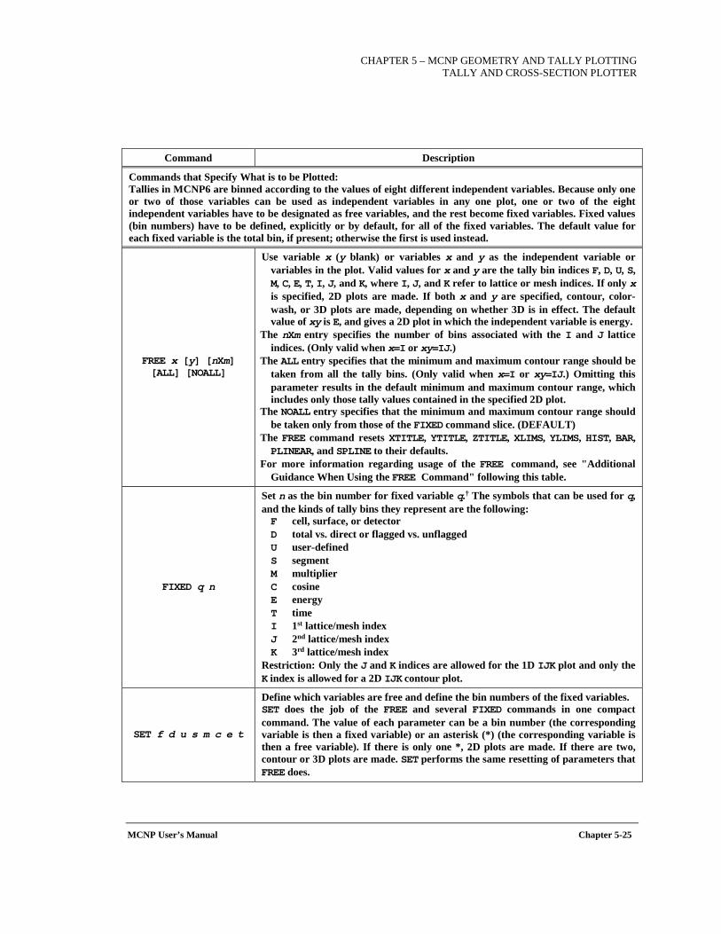
CHAPTER 5 – MCNP GEOMETRY AND TALLY PLOTTING
TALLY AND CROSS-SECTION PLOTTER
MCNP User’s Manual Chapter 5-25
Command Description
Commands that Specify What is to be Plotted: Tallies in MCNP6 are binned according to the values of eight different independent variables. Because only one or two of those variables can be used as independent variables in any one plot, one or two of the eight independent variables have to be designated as free variables, and the rest become fixed variables. Fixed values (bin numbers) have to be defined, explicitly or by default, for all of the fixed variables. The default value for each fixed variable is the total bin, if present; otherwise the first is used instead.
FREE x [y] [nXm] [ALL] [NOALL]
Use variable x (y blank) or variables x and y as the independent variable or variables in the plot. Valid values for x and y are the tally bin indices F, D, U, S, M, C, E, T, I, J, and K, where I, J, and K refer to lattice or mesh indices. If only x is specified, 2D plots are made. If both x and y are specified, contour, color-wash, or 3D plots are made, depending on whether 3D is in effect. The default value of xy is E, and gives a 2D plot in which the independent variable is energy.
The nXm entry specifies the number of bins associated with the I and J lattice indices. (Only valid when x=I or xy=IJ.)
The ALL entry specifies that the minimum and maximum contour range should be taken from all the tally bins. (Only valid when x=I or xy=IJ.) Omitting this parameter results in the default minimum and maximum contour range, which includes only those tally values contained in the specified 2D plot.
The NOALL entry specifies that the minimum and maximum contour range should be taken only from those of the FIXED command slice. (DEFAULT)
The FREE command resets XTITLE, YTITLE, ZTITLE, XLIMS, YLIMS, HIST, BAR, PLINEAR, and SPLINE to their defaults.
For more information regarding usage of the FREE command, see "Additional Guidance When Using the FREE Command" following this table.
FIXED q n
Set n as the bin number for fixed variable q.† The symbols that can be used for q, and the kinds of tally bins they represent are the following: F cell, surface, or detector D total vs. direct or flagged vs. unflagged U user-defined S segment M multiplier C cosine E energy T time I 1st lattice/mesh index J 2nd lattice/mesh index K 3rd lattice/mesh index
Restriction: Only the J and K indices are allowed for the 1D IJK plot and only the K index is allowed for a 2D IJK contour plot.
SET f d u s m c e t
Define which variables are free and define the bin numbers of the fixed variables. SET does the job of the FREE and several FIXED commands in one compact command. The value of each parameter can be a bin number (the corresponding variable is then a fixed variable) or an asterisk (*) (the corresponding variable is then a free variable). If there is only one *, 2D plots are made. If there are two, contour or 3D plots are made. SET performs the same resetting of parameters that FREE does.
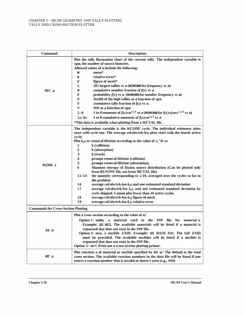
CHAPTER 5 – MCNP GEOMETRY AND TALLY PLOTTING TALLY AND CROSS-SECTION PLOTTER
Chapter 5-26 MCNP User’s Manual
Command Description
TFC x
Plot the tally fluctuation chart of the current tally. The independent variable is nps, the number of source histories. Allowed values of x include the following: M mean* E relative error* F figure of merit* L 201 largest tallies vs x (NONORM for frequency vs x) N cumulative number fraction of f(x) vs x P probability f(x) vs x (NONORM for number frequency vs x) S SLOPE of the high tallies as a function of nps T cumulative tally fraction of f(x) vs x V VOV as a function of nps 1–8 1 to 8 moments of f(x)*x1 to 8 vs x (NONORM for f(x)*∆x*x1 to 8 vs x) 1c–8c 1 to 8 cumulative moments of f(x)*x1 to 8 vs x
*This data is available when plotting from a MCTAL file.
KCODE i
The independent variable is the KCODE cycle. The individual estimator plots start with cycle one. The average col/abs/trk-len plots start with the fourth active cycle. Plot keff or removal lifetime according to the value of i.† If i= 1 k (collision) 2 k (absorption) 3 k (track) 4 prompt removal lifetime (collision) 5 prompt removal lifetime (absorption) 6 Shannon entropy of fission source distribution (Can be plotted only
from RUNTPE file, not from MCTAL file) 11–15 the quantity corresponding to i-10, averaged over the cycles so far in
the problem. 16 average col/abs/trk-len keff and one estimated standard deviation 17 average col/abs/trk-len keff and one estimated standard deviation by
cycle skipped. Cannot plot fewer than 10 active cycles. 18 average col/abs/trk-len keff figure of merit 19 average col/abs/trk-len keff relative error
Commands for Cross-Section Plotting
XS m
Plot a cross section according to the value of m.† Option 1: m=Mn, a material card in the INP file for material n.
Example: XS M15. The available materials will be listed if a material is requested that does not exist in the INP file.
Option 2: m=z, a nuclide ZAID. Example: XS 92235.50C. The full ZAID must be provided. The available nuclides will be listed if a nuclide is requested that does not exist in the INP file.
Option 3: m=?. Print out a cross-section plotting primer.
MT n Plot reaction n of material or nuclide specified by XS m.† The default is the total cross section. The available reaction numbers in the data file will be listed if one enters a reaction number that is invalid or doesn’t exist (e.g., 999)
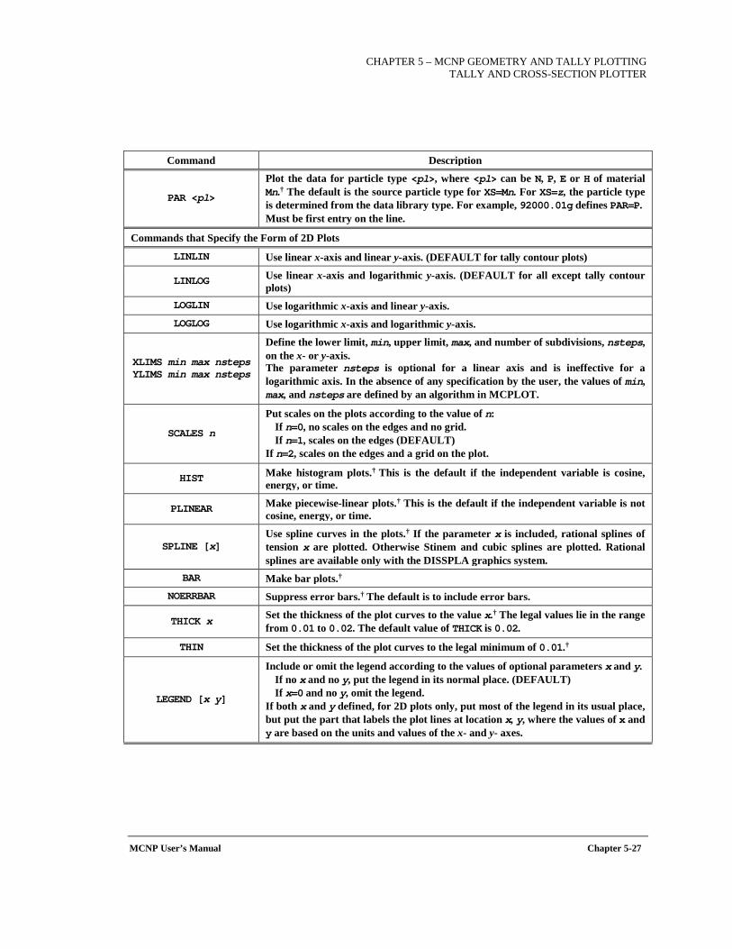
CHAPTER 5 – MCNP GEOMETRY AND TALLY PLOTTING
TALLY AND CROSS-SECTION PLOTTER
MCNP User’s Manual Chapter 5-27
Command Description
PAR <pl>
Plot the data for particle type <pl>, where <pl> can be N, P, E or H of material Mn.† The default is the source particle type for XS=Mn. For XS=z, the particle type is determined from the data library type. For example, 92000.01g defines PAR=P. Must be first entry on the line.
Commands that Specify the Form of 2D Plots
LINLIN Use linear x-axis and linear y-axis. (DEFAULT for tally contour plots)
LINLOG Use linear x-axis and logarithmic y-axis. (DEFAULT for all except tally contour plots)
LOGLIN Use logarithmic x-axis and linear y-axis. LOGLOG Use logarithmic x-axis and logarithmic y-axis.
XLIMS min max nsteps YLIMS min max nsteps
Define the lower limit, min, upper limit, max, and number of subdivisions, nsteps, on the x- or y-axis. The parameter nsteps is optional for a linear axis and is ineffective for a logarithmic axis. In the absence of any specification by the user, the values of min, max, and nsteps are defined by an algorithm in MCPLOT.
SCALES n
Put scales on the plots according to the value of n: If n=0, no scales on the edges and no grid. If n=1, scales on the edges (DEFAULT)
If n=2, scales on the edges and a grid on the plot.
HIST Make histogram plots.† This is the default if the independent variable is cosine, energy, or time.
PLINEAR Make piecewise-linear plots.† This is the default if the independent variable is not cosine, energy, or time.
SPLINE [x] Use spline curves in the plots.† If the parameter x is included, rational splines of tension x are plotted. Otherwise Stinem and cubic splines are plotted. Rational splines are available only with the DISSPLA graphics system.
BAR Make bar plots.† NOERRBAR Suppress error bars.† The default is to include error bars.
THICK x Set the thickness of the plot curves to the value x.† The legal values lie in the range from 0.01 to 0.02. The default value of THICK is 0.02.
THIN Set the thickness of the plot curves to the legal minimum of 0.01.†
LEGEND [x y]
Include or omit the legend according to the values of optional parameters x and y. If no x and no y, put the legend in its normal place. (DEFAULT) If x=0 and no y, omit the legend.
If both x and y defined, for 2D plots only, put most of the legend in its usual place, but put the part that labels the plot lines at location x, y, where the values of x and y are based on the units and values of the x- and y- axes.
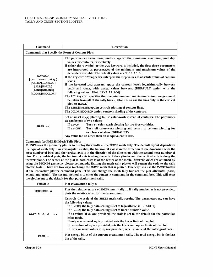
CHAPTER 5 – MCNP GEOMETRY AND TALLY PLOTTING TALLY AND CROSS-SECTION PLOTTER
Chapter 5-28 MCNP User’s Manual
Command Description
Commands that Specify the Form of Contour Plots
CONTOUR [cmin cmax cstep] [%|PCT|LIN|LOG] [ALL|NOALL] [LINE|NOLINE] [COLOR|NOCOLOR]
The parameters cmin, cmax, and cstep are the minimum, maximum, and step values for contours, respectively.
If either the % symbol or the PCT keyword is included, the first three parameters are interpreted as percentages of the minimum and maximum values of the dependent variable. The default values are 5 95 10 %.
If the keyword LIN appears, interpret the step values as absolute values of contour levels.
If the keyword LOG appears, space the contour levels logarithmically between cmin and cmax, with cstep values between. (DEFAULT option with the following values: 1E-4 1E-2 12 LOG)
The ALL keyword specifies that the minimum and maximum contour range should be taken from all of the tally bins. (Default is to use the bins only in the current plot, or NOALL.)
The LINE|NOLINE option controls plotting of contour lines. The COLOR|NOCOLOR option controls shading of the contours.
WASH aa
Set or unset z(x,y) plotting to use color-wash instead of contours. The parameter aa can be one of two values:
If aa=ON Turn on color-wash plotting for two free variables. If aa=OFF Turn off color-wash plotting and return to contour plotting for
two free variables. (DEFAULT) Any value for aa other than on is equivalent to OFF.
Commands for FMESH Mesh Tally Plots MCNP6 uses the geometry plotter to display the results of the FMESH mesh tally. The default layout depends on the type of mesh tally. For rectangular meshes, the horizontal axis is in the direction of the dimension with the most number of bins, and the vertical axis is in the direction of the dimension with the second most number of bins. For cylindrical plots, the horizontal axis is along the axis of the cylinder and the vertical axis is along the theta=0 plane. The center of the plot in both cases is at the center of the mesh. Different views are obtained by using the MCNP6 geometry plotter commands. Exiting the mesh tally plotter will return the code to the tally plotter. Note: There are two ways to change the FMESH mesh that is plotted. One way is to use the FMESH button of the interactive plotter command panel. This will change the mesh tally but not the plot attributes (basis, extent, and origin). The second method is to enter the FMESH n command in the command box. This will reset the plot layout to the default for that particular mesh tally.
FMESH n Plot FMESH mesh tally n.
FMRELERR n Plot the relative errors of FMESH mesh tally n. If tally number n is not provided, plots the relative error for the current mesh.
ZLEV n1 n2 n3 ...
Controls the scale of the FMESH mesh tally results. The parameters ni, can have the following values:
If ni=LOG, the tally data scaling is set to logarithmic. (DEFAULT) If ni=LIN, the tally data scaling is set to linear numeric value. If no values of ni are provided, the scale is set to the default for the particular color mode. If only one value of ni is provided, sets the lower limit of the plot. If two values of ni are provided, sets the lower and upper limits of the plot. If three or more values of ni are provided, sets the value of the color gradients.
EBIN n Plot energy bin n of the current FMESH mesh tally. The total energy bin is the last bin of the tally.

CHAPTER 5 – MCNP GEOMETRY AND TALLY PLOTTING
TALLY AND CROSS-SECTION PLOTTER
MCNP User’s Manual Chapter 5-29
Command Description
TBIN n Plot time bin n of the current FMESH mesh tally. The total time bin is the last bin of the tally.
† available with COPLOT
Additional Guidance When Using the FREE Command:
• For TMESH mesh tallies, the i, j, and k parameters of the FREE command refer to the CORA, CORB, and CORC mesh-tally dimensions.
• For lattice tallies, the i, j, and k parameters of the FREE command refer to i, j, and k lattice indices.
• For radiography tallies, the command FREE S C is used to make a contour plot of the s- and t- radiography axes.
• For lattice tallies that are not specified fully, the [nXm] dimensions must be provided. Mesh and radiography tallies are always specified fully, so [nXm] is never required for them.
• One-dimensional mesh, radiography, and lattice tallies may be specified by giving the free dimension of the FREE command and fixing the other two dimensions:
FREE I FIXED J=10 FIXED K=12
5.3.4 MCTAL Files A MCTAL file contains the tally data of one dump of a RUNTPE file. It can be written by the MCRUN module of MCNP6 or by the MCPLOT module, by other codes, or even by hand in order to send data to MCPLOT for co-plotting with MCNP6 tally data. Data from TMESH mesh tallies are written to the MCTAL file; however, data from FMESH mesh tallies are not.
As written by MCNP6, a MCTAL file has the format shown below, but only as much of it as is essential to contain the information of real substance is necessary. Furthermore the numerical items do not need to be in the columns implied by the formats as long as they are in the right order, are blank delimited, and have no embedded blanks. For example, to give MCPLOT a table of something versus energy, the user might write a file as simple as the following:
E 7 1 .2 .4 .7 1 3 8 12 VALS 4.00E-5 .022 5.78E-4 .054 3.70E-5 .079 1.22E-5 .122 7.60E-6 .187 2.20E-6 .245 9.10E-7 .307
If more than one independent variable is wanted, other lines such as a T line followed by a list of time values would be needed and the table of tally/error values would need to be expanded. If more than one table of tally/error values is wanted, the file would have to include an NTAL line
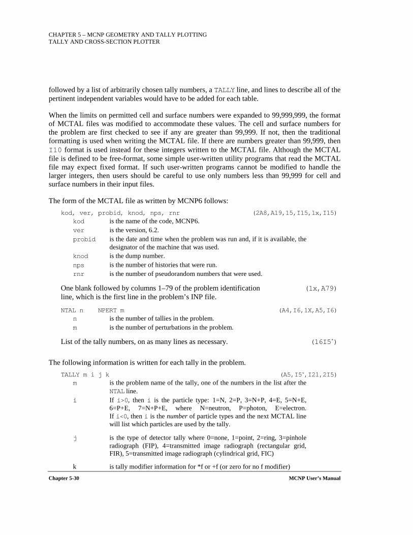
CHAPTER 5 – MCNP GEOMETRY AND TALLY PLOTTING TALLY AND CROSS-SECTION PLOTTER
Chapter 5-30 MCNP User’s Manual
followed by a list of arbitrarily chosen tally numbers, a TALLY line, and lines to describe all of the pertinent independent variables would have to be added for each table.
When the limits on permitted cell and surface numbers were expanded to 99,999,999, the format of MCTAL files was modified to accommodate these values. The cell and surface numbers for the problem are first checked to see if any are greater than 99,999. If not, then the traditional formatting is used when writing the MCTAL file. If there are numbers greater than 99,999, then I10 format is used instead for these integers written to the MCTAL file. Although the MCTAL file is defined to be free-format, some simple user-written utility programs that read the MCTAL file may expect fixed format. If such user-written programs cannot be modified to handle the larger integers, then users should be careful to use only numbers less than 99,999 for cell and surface numbers in their input files.
The form of the MCTAL file as written by MCNP6 follows: kod, ver, probid, knod, nps, rnr (2A8,A19,15,I15,1x,I15)
kod is the name of the code, MCNP6. ver is the version, 6.2. probid is the date and time when the problem was run and, if it is available, the
designator of the machine that was used. knod is the dump number. nps is the number of histories that were run. rnr is the number of pseudorandom numbers that were used.
One blank followed by columns 1–79 of the problem identification (1x,A79) line, which is the first line in the problem’s INP file.
NTAL n NPERT m (A4,I6,1X,A5,I6) n is the number of tallies in the problem. m is the number of perturbations in the problem.
List of the tally numbers, on as many lines as necessary. (16I5*)
The following information is written for each tally in the problem. TALLY m i j k (A5,I5*,I21,2I5)
m is the problem name of the tally, one of the numbers in the list after the NTAL line.
i If i>0, then i is the particle type: 1=N, 2=P, 3=N+P, 4=E, 5=N+E, 6=P+E, 7=N+P+E, where N=neutron, P=photon, E=electron. If i<0, then i is the number of particle types and the next MCTAL line will list which particles are used by the tally.
j is the type of detector tally where 0=none, 1=point, 2=ring, 3=pinhole radiograph (FIP), 4=transmitted image radiograph (rectangular grid, FIR), 5=transmitted image radiograph (cylindrical grid, FIC)
k is tally modifier information for *f or +f (or zero for no f modifier)
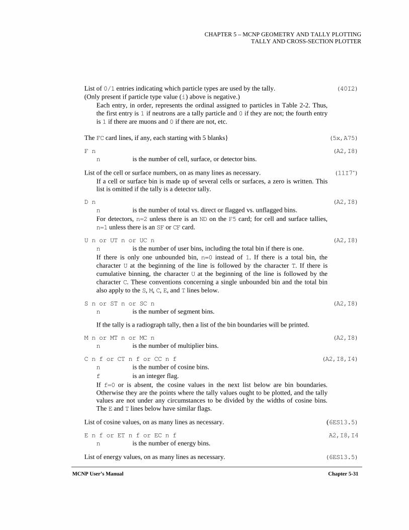
CHAPTER 5 – MCNP GEOMETRY AND TALLY PLOTTING
TALLY AND CROSS-SECTION PLOTTER
MCNP User’s Manual Chapter 5-31
List of 0/1 entries indicating which particle types are used by the tally. (40I2) (Only present if particle type value (i) above is negative.)
Each entry, in order, represents the ordinal assigned to particles in Table 2-2. Thus, the first entry is 1 if neutrons are a tally particle and 0 if they are not; the fourth entry is 1 if there are muons and 0 if there are not, etc.
The FC card lines, if any, each starting with 5 blanks (5x,A75)
F n (A2,I8) n is the number of cell, surface, or detector bins.
List of the cell or surface numbers, on as many lines as necessary. (11I7*) If a cell or surface bin is made up of several cells or surfaces, a zero is written. This list is omitted if the tally is a detector tally.
D n (A2,I8) n is the number of total vs. direct or flagged vs. unflagged bins. For detectors, n=2 unless there is an ND on the F5 card; for cell and surface tallies, n=1 unless there is an SF or CF card.
U n or UT n or UC n (A2,I8) n is the number of user bins, including the total bin if there is one. If there is only one unbounded bin, n=0 instead of 1. If there is a total bin, the character U at the beginning of the line is followed by the character T. If there is cumulative binning, the character U at the beginning of the line is followed by the character C. These conventions concerning a single unbounded bin and the total bin also apply to the S, M, C, E, and T lines below.
S n or ST n or SC n (A2,I8) n is the number of segment bins.
If the tally is a radiograph tally, then a list of the bin boundaries will be printed.
M n or MT n or MC n (A2,I8) n is the number of multiplier bins.
C n f or CT n f or CC n f (A2,I8,I4) n is the number of cosine bins. f is an integer flag. If f=0 or is absent, the cosine values in the next list below are bin boundaries. Otherwise they are the points where the tally values ought to be plotted, and the tally values are not under any circumstances to be divided by the widths of cosine bins. The E and T lines below have similar flags.
List of cosine values, on as many lines as necessary. (6ES13.5)
E n f or ET n f or EC n f A2,I8,I4 n is the number of energy bins.
List of energy values, on as many lines as necessary. (6ES13.5)
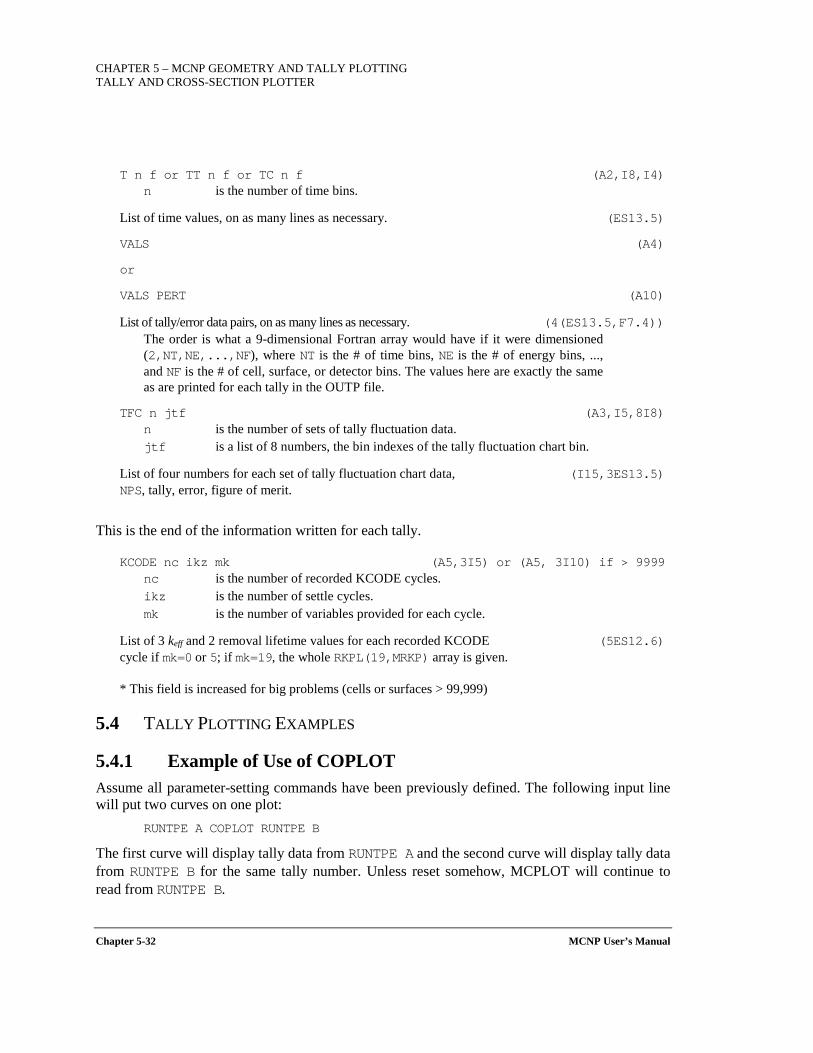
CHAPTER 5 – MCNP GEOMETRY AND TALLY PLOTTING TALLY AND CROSS-SECTION PLOTTER
Chapter 5-32 MCNP User’s Manual
T n f or TT n f or TC n f (A2,I8,I4) n is the number of time bins.
List of time values, on as many lines as necessary. (ES13.5)
VALS (A4)
or
VALS PERT (A10)
List of tally/error data pairs, on as many lines as necessary. (4(ES13.5,F7.4)) The order is what a 9-dimensional Fortran array would have if it were dimensioned (2,NT,NE,...,NF), where NT is the # of time bins, NE is the # of energy bins, ..., and NF is the # of cell, surface, or detector bins. The values here are exactly the same as are printed for each tally in the OUTP file.
TFC n jtf (A3,I5,8I8) n is the number of sets of tally fluctuation data. jtf is a list of 8 numbers, the bin indexes of the tally fluctuation chart bin.
List of four numbers for each set of tally fluctuation chart data, (I15,3ES13.5) NPS, tally, error, figure of merit.
This is the end of the information written for each tally.
KCODE nc ikz mk (A5,3I5) or (A5, 3I10) if > 9999 nc is the number of recorded KCODE cycles. ikz is the number of settle cycles. mk is the number of variables provided for each cycle.
List of 3 keff and 2 removal lifetime values for each recorded KCODE (5ES12.6) cycle if mk=0 or 5; if mk=19, the whole RKPL(19,MRKP) array is given.
* This field is increased for big problems (cells or surfaces > 99,999)
5.4 TALLY PLOTTING EXAMPLES
5.4.1 Example of Use of COPLOT Assume all parameter-setting commands have been previously defined. The following input line will put two curves on one plot:
RUNTPE A COPLOT RUNTPE B
The first curve will display tally data from RUNTPE A and the second curve will display tally data from RUNTPE B for the same tally number. Unless reset somehow, MCPLOT will continue to read from RUNTPE B.
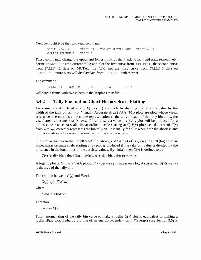
CHAPTER 5 – MCNP GEOMETRY AND TALLY PLOTTING
TALLY PLOTTING EXAMPLES
MCNP User’s Manual Chapter 5-33
Next we might type the following command: XLIMS min max TALLY 11 COPLOT RMCTAL AUX TALLY 41 & COPLOT RUNTPE A TALLY 1
These commands change the upper and lower limits of the x-axis to max and min, respectively; define TALLY 11 as the current tally; and plot the first curve from RUNTPE B, the second curve from TALLY 41 data on MCTAL file AUX, and the third curve from TALLY 1 data on RUNTPE A. Future plots will display data from RUNTPE A unless reset.
The command TALLY 24 NONORM FILE COPLOT TALLY 44
will send a frame with two curves to the graphics metafile.
5.4.2 Tally Fluctuation Chart History Score Plotting Two-dimensional plots of a tally F(x)=xf(x) are made by dividing the tally bin value by the width of the tally bin xi+1−xi. Visually Accurate Area (VAA) F(x) plots are plots whose visual area under the curve is an accurate representation of the tally in each of the tally bins; i.e., the visual area represents F(x)(xi+1−xi) for all abscissa values. A VAA plot will be produced for a linlin0 (linear abscissa scale, linear ordinate scale starting at 0) F(x) plot; i.e., the area of F(x) from xi to xi+1 correctly represents the bin tally value visually for all x when both the abscissa and ordinate scales are linear and the smallest ordinate value is zero.
In a similar manner to the linlin0 VAA plot above, a VAA plot of F(x) on a loglin0 (log abscissa scale, linear ordinate scale starting at 0) plot is produced if the tally bin value is divided by the difference in the logarithms of the abscissa values. If y=ln(x), then G(y) is defined to be
G(y)=(tally bin value)/(ln(xi+1)−ln(xi))=(tally bin value)/(yi+1−yi).
A loglin0 plot of G(y) is a VAA plot of F(x) because y is linear on a log abscissa and G(y)(yi+1−yi) is the area of the tally bin.
The relation between G(y) and F(x) is
G(y)|dy|=F(x)|dx|,
where
dy=dln(x)=dx/x.
Therefore
G(y)=xF(x).
This y normalizing of the tally bin value to make a loglin G(y) plot is equivalent to making a loglin xF(x) plot. Lethargy plotting of an energy-dependent tally F(energy) (see Section 5.5) is
CHAPTER 5 – MCNP GEOMETRY AND TALLY PLOTTING TALLY PLOTTING EXAMPLES
Chapter 5-34 MCNP User’s Manual
the equivalent of plotting G(ln(energy))=energy×F(energy) on a loglin0 scale to produce a VAA plot for the tally F(energy).
These normalizing statements can be generalized to any function h(x). The VAA interpretation of a 2D plot therefore depends on the abscissa axis scale. A linlin0 plot of h(x) is a VAA h(x) plot and a loglin0 h(x) plot is a VAA plot for h(x)/x. If h(x)/x is a useful quantity, then the VAA plot of h(x)/x is also useful.
Two-dimensional plots from a RUNTPE (not a MCTAL) file of the empirical history score probability density function f(x) moments can be made using the Tally Fluctuation Chart (TFC) tally plot commands (see Table 5-5, under the section entitled, "Commands that Specify What is to be Plotted"). The tally F(x)=xf(x). From the discussion above, a loglin0 F(x) plot can be interpreted as a VAA plot for f(x); i.e., the area under the curve on a loglin0 scale represents where the f(x) sampling has occurred. A linlin0 F(x) plot can be interpreted as a VAA plot for the tally F(x).
Based on these observations, the following statements can be made about TFC commands to create f(x) moment plots for the TFC bin of a tally (without the NONORM option):
• f(x) TFC bin plots are VAA plots when 1) TFC P [f(x)] is on a linlin0 scale; and 2) TFC 1 [xf(x)] is on a loglin0 scale.
• xf(x)=F(x) TFC bin tally plots are VAA plots when 1) TFC 1 [xf(x)=F(x)] is on a linlin0 scale; and 2) TFC 2 [x2f(x)=xF(x)] is on a loglin0 scale.
• xnf(x) TFC bin tally moment plots are VAA plots when 1) TFC n [xnf(x)] is on a linlin0 scale; and 2) TFC n+1 [xn+1f(x)] is on a loglin0 scale.
The VAA contributions to the nth f(x) moment can be viewed with an xnf(x) linlin0 plot or an xn+1f(x) loglin0 plot. The empirical f(x) slope result can be checked by viewing a TFC n plot. If the high-score f(x) tail for a long-tailed distribution (not a finite distribution) is proportional to 1/xn, then the TFC n plot will be a statistical constant at the high x scores. A large score f(x) slope of at least n exists if the high-score TFC n [xnf(x)] values are decreasing. VAA f(x) moment plots can be a useful tool in studying the detailed impact of variance reduction techniques on f(x) (not the history sampling time as function of x) and the efficiency of a calculation.
5.4.3 Radiography Tally Contour Plot Example Tally output may be plotted as 2D color contours from either MCTAL or RUNTPE files. For example, a radiography tally with s- and t-axes specified on FS and C cards can be plotted with the MCNP6 Z execute option, as illustrated below.

CHAPTER 5 – MCNP GEOMETRY AND TALLY PLOTTING
TALLY PLOTTING EXAMPLES
MCNP User’s Manual Chapter 5-35
The following example is a radiograph of a 4-cm-radius, 1-cm-thick 238U disc with an embedded 4-mm-void sphere and skew-oriented 1-cm × 1-cm × 8-mm box. The input file is
Radiography Tally 1 5 -25.0 -1 4 5 imp:p=1 2 0 1 -2 imp:p=1 3 0 2 imp:p=0 4 0 -4 imp:p=1 5 0 -5 imp:p=1 1 RCC 0 0 0 0 0 1 4 2 RPP -100 100 -100 100 -100 100 4 SPH 3 0 0.5 0.4 5 BOX -1 1 0.1 0.6 0.8 0 -0.8 0.6 0 0 0 0.8 mode p nps 100 5 sdef pos=0 0 -20 axs=0 0 1 rad=d1 ext=0 vec=0 0 1 dir=d2 erg=6 si1 0 0.1 sp1 -21 1 si2 -1 1 sp2 -31 1 m5 92238 1 print prdmp 2j 1 tir5:p 0 0 10 0 0 0 -100 0 100 0 fs5 -10. 99i 10. c5 -10. 99i 10.
The x-y geometry plot of this geometry is given in Figure 5-2.
To get the contour plot, type the following MCNP6 execution line command: MCNP6 Z RUNTPE=filename
The contour plots also may be read from a MCTAL file instead of the RUNTPE file. When the code gives you the MCPLOT prompt, enter two dimensions with the FREE command (Table 5-5); for example, S and C:
MCPLOT>FREE SC .
Recall that the possible tally dimensions are
F surface / cell / detector F card bin D total / direct or flagged bin U user bin S segment or radiography s-axis bin M multiplier bin
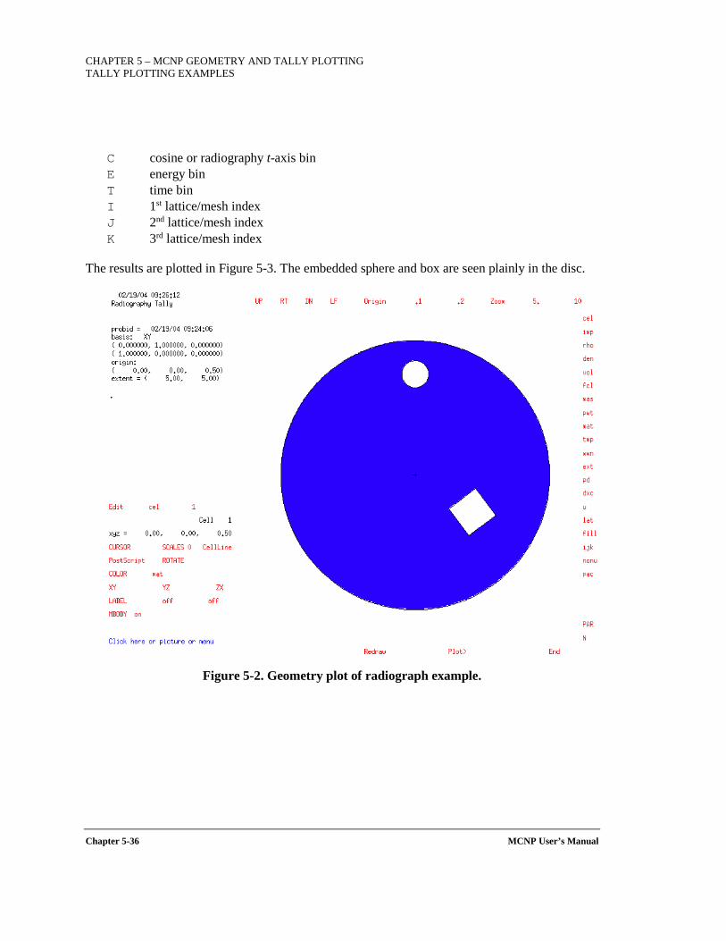
CHAPTER 5 – MCNP GEOMETRY AND TALLY PLOTTING TALLY PLOTTING EXAMPLES
Chapter 5-36 MCNP User’s Manual
C cosine or radiography t-axis bin E energy bin T time bin I 1st lattice/mesh index J 2nd lattice/mesh index K 3rd lattice/mesh index
The results are plotted in Figure 5-3. The embedded sphere and box are seen plainly in the disc.
Figure 5-2. Geometry plot of radiograph example.
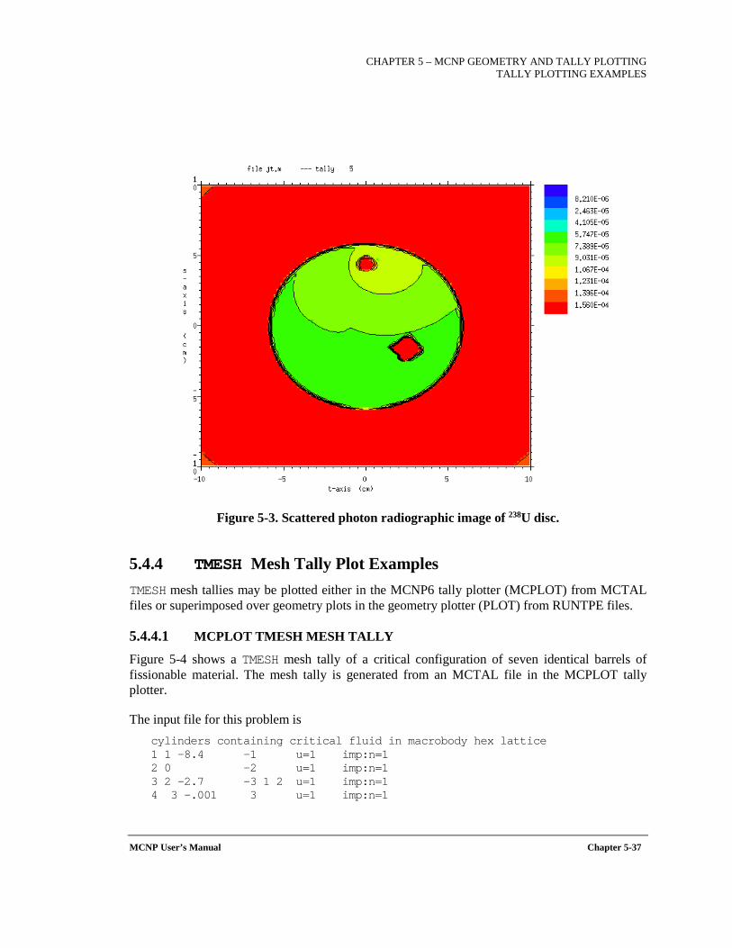
CHAPTER 5 – MCNP GEOMETRY AND TALLY PLOTTING
TALLY PLOTTING EXAMPLES
MCNP User’s Manual Chapter 5-37
Figure 5-3. Scattered photon radiographic image of 238U disc.
5.4.4 TMESH Mesh Tally Plot Examples TMESH mesh tallies may be plotted either in the MCNP6 tally plotter (MCPLOT) from MCTAL files or superimposed over geometry plots in the geometry plotter (PLOT) from RUNTPE files.
5.4.4.1 MCPLOT TMESH MESH TALLY
Figure 5-4 shows a TMESH mesh tally of a critical configuration of seven identical barrels of fissionable material. The mesh tally is generated from an MCTAL file in the MCPLOT tally plotter.
The input file for this problem is cylinders containing critical fluid in macrobody hex lattice 1 1 -8.4 -1 u=1 imp:n=1 2 0 -2 u=1 imp:n=1 3 2 -2.7 -3 1 2 u=1 imp:n=1 4 3 -.001 3 u=1 imp:n=1
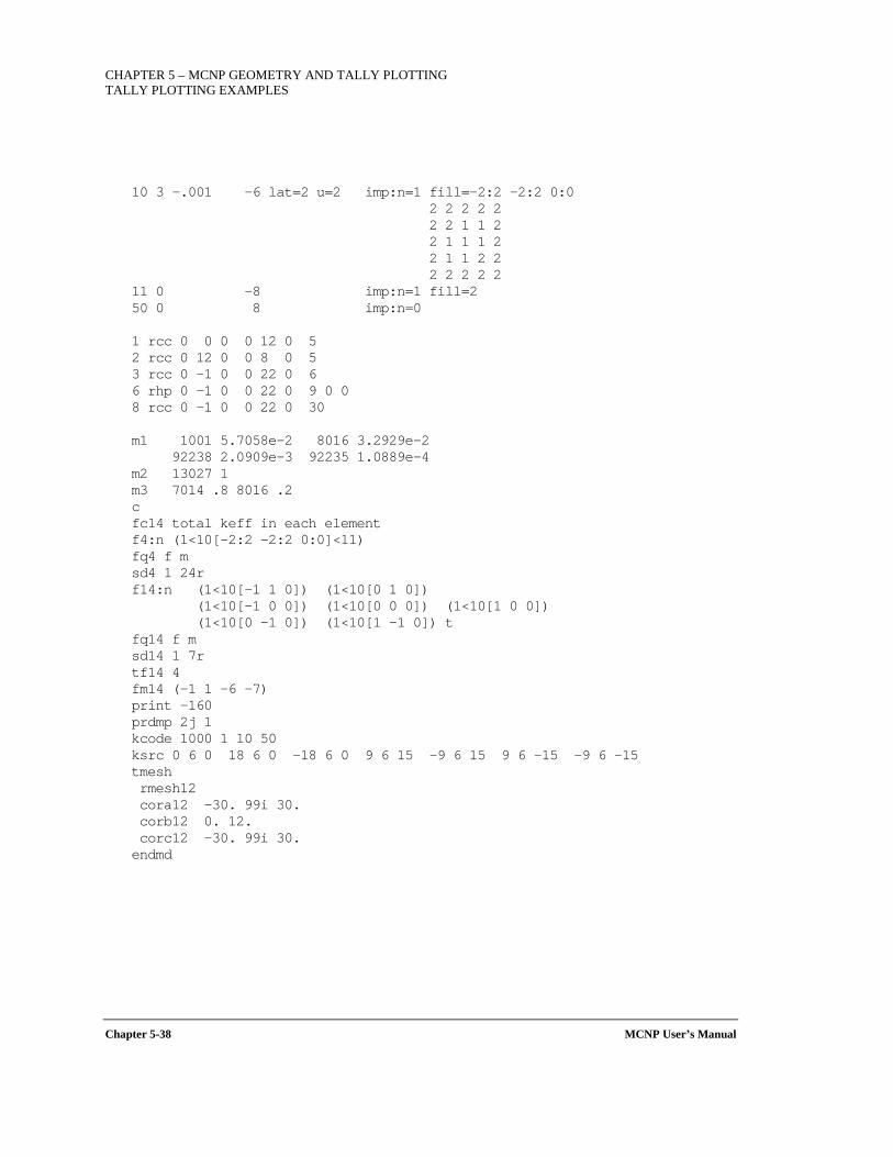
CHAPTER 5 – MCNP GEOMETRY AND TALLY PLOTTING TALLY PLOTTING EXAMPLES
Chapter 5-38 MCNP User’s Manual
10 3 -.001 -6 lat=2 u=2 imp:n=1 fill=-2:2 -2:2 0:0 2 2 2 2 2 2 2 1 1 2 2 1 1 1 2 2 1 1 2 2 2 2 2 2 2 11 0 -8 imp:n=1 fill=2 50 0 8 imp:n=0 1 rcc 0 0 0 0 12 0 5 2 rcc 0 12 0 0 8 0 5 3 rcc 0 -1 0 0 22 0 6 6 rhp 0 -1 0 0 22 0 9 0 0 8 rcc 0 -1 0 0 22 0 30 m1 1001 5.7058e-2 8016 3.2929e-2 92238 2.0909e-3 92235 1.0889e-4 m2 13027 1 m3 7014 .8 8016 .2 c fc14 total keff in each element f4:n (1<10[-2:2 -2:2 0:0]<11) fq4 f m sd4 1 24r f14:n (1<10[-1 1 0]) (1<10[0 1 0]) (1<10[-1 0 0]) (1<10[0 0 0]) (1<10[1 0 0]) (1<10[0 -1 0]) (1<10[1 -1 0]) t fq14 f m sd14 1 7r tf14 4 fm14 (-1 1 -6 -7) print -160 prdmp 2j 1 kcode 1000 1 10 50 ksrc 0 6 0 18 6 0 -18 6 0 9 6 15 -9 6 15 9 6 -15 -9 6 -15 tmesh rmesh12 cora12 -30. 99i 30. corb12 0. 12. corc12 -30. 99i 30. endmd
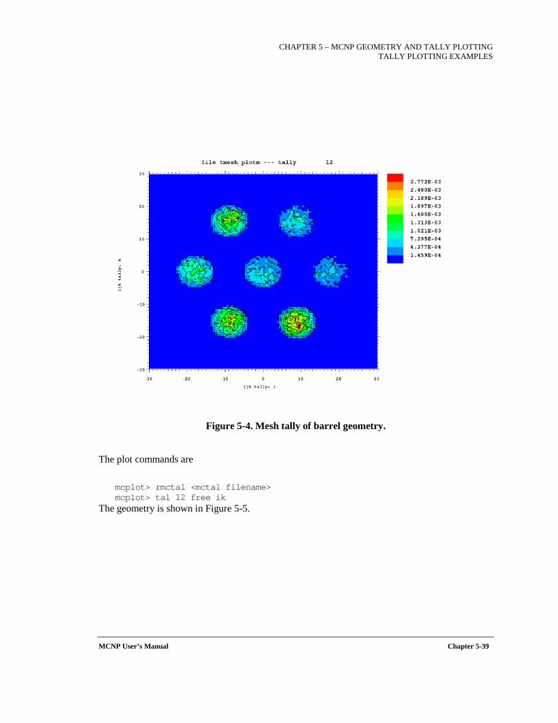
CHAPTER 5 – MCNP GEOMETRY AND TALLY PLOTTING
TALLY PLOTTING EXAMPLES
MCNP User’s Manual Chapter 5-39
Figure 5-4. Mesh tally of barrel geometry.
The plot commands are
mcplot> rmctal <mctal filename> mcplot> tal 12 free ik
The geometry is shown in Figure 5-5.
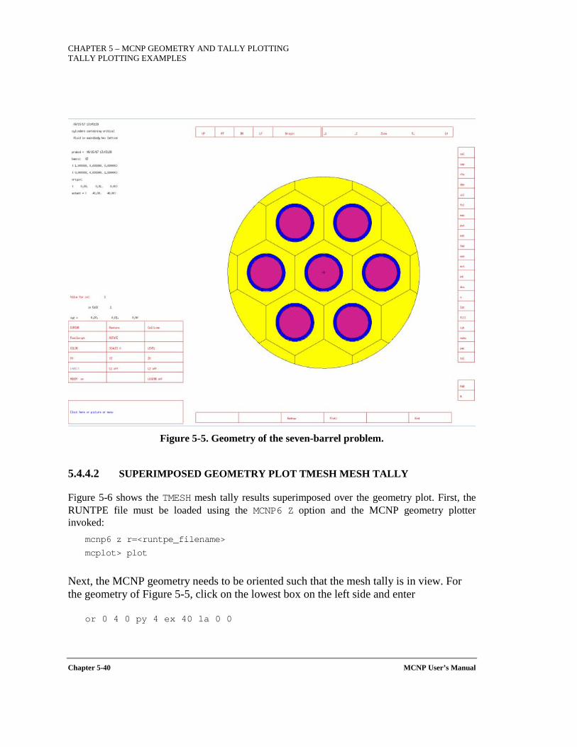
CHAPTER 5 – MCNP GEOMETRY AND TALLY PLOTTING TALLY PLOTTING EXAMPLES
Chapter 5-40 MCNP User’s Manual
Figure 5-5. Geometry of the seven-barrel problem.
5.4.4.2 SUPERIMPOSED GEOMETRY PLOT TMESH MESH TALLY
Figure 5-6 shows the TMESH mesh tally results superimposed over the geometry plot. First, the RUNTPE file must be loaded using the MCNP6 Z option and the MCNP geometry plotter invoked:
mcnp6 z r=<runtpe_filename>
mcplot> plot
Next, the MCNP geometry needs to be oriented such that the mesh tally is in view. For the geometry of Figure 5-5, click on the lowest box on the left side and enter or 0 4 0 py 4 ex 40 la 0 0
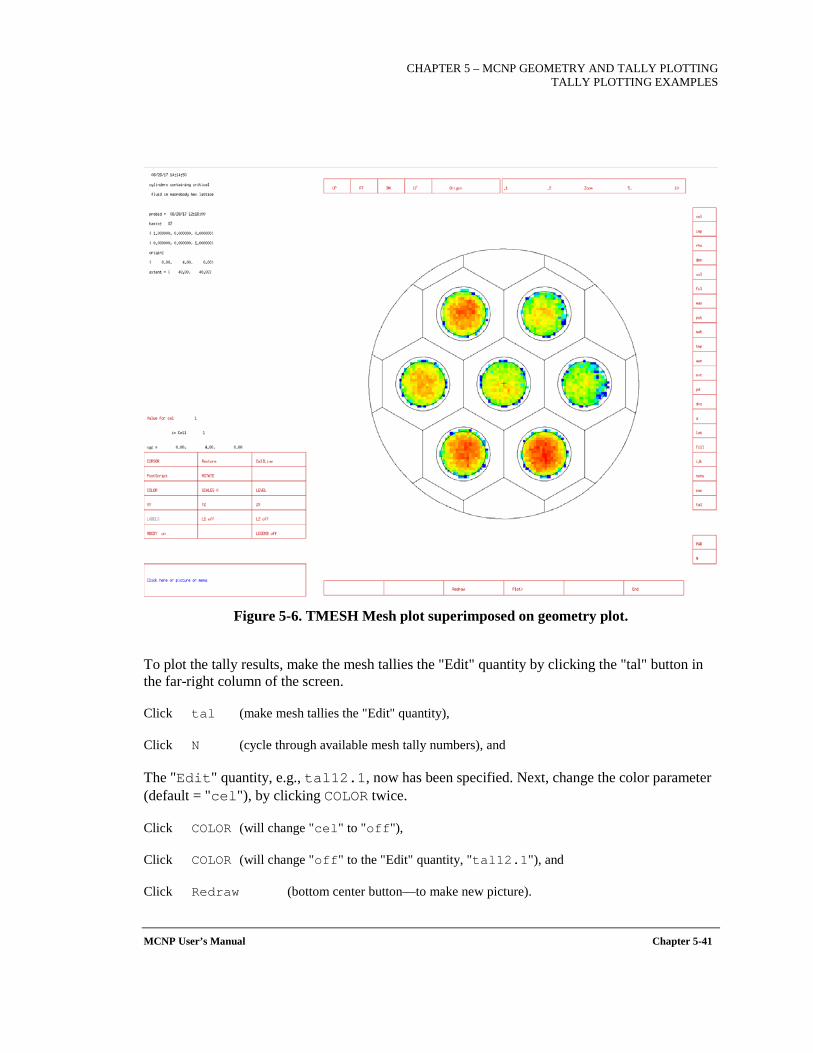
CHAPTER 5 – MCNP GEOMETRY AND TALLY PLOTTING
TALLY PLOTTING EXAMPLES
MCNP User’s Manual Chapter 5-41
Figure 5-6. TMESH Mesh plot superimposed on geometry plot.
To plot the tally results, make the mesh tallies the "Edit" quantity by clicking the "tal" button in the far-right column of the screen. Click tal (make mesh tallies the "Edit" quantity), Click N (cycle through available mesh tally numbers), and The "Edit" quantity, e.g., tal12.1, now has been specified. Next, change the color parameter (default = "cel"), by clicking COLOR twice. Click COLOR (will change "cel" to "off"), Click COLOR (will change "off" to the "Edit" quantity, "tal12.1"), and Click Redraw (bottom center button—to make new picture).
CHAPTER 5 – MCNP GEOMETRY AND TALLY PLOTTING TALLY PLOTTING EXAMPLES
Chapter 5-42 MCNP User’s Manual
In addition, the actual mesh tally grid can be displayed by clicking "CellLine" and cycling through the options to get either "MeshTaly" (which draws mesh tally grid lines over the plot) or "MT+Cell" (which draws mesh tally grid lines and cell surface lines over the plot).
5.4.5 MCPLOT FREE Command Examples Example 1:
The following command FREE I 64x64 FIXED J=38 FIXED K=30 .
specifies a 1D lattice tally plot of the cell bins, which should correspond to a lattice tally with 64 "I" index bins, 64 "J" index bins, and at least 30 "K" index bins. With the "K" index set to 30 and the "J" index to 38, the offset into the F-bins will be 29 × 64 × 64 + 37 × 64 = 121,152. The minimum and maximum values will be determined from the 64 "I" bin values included in the plot. If the "J" and "K" indices are not specified, their default value of 1 is assumed, which results in an offset of 0.
Example 2:
The following command FREE IJ 10x30 ALL FIXED K=60
specifies a 10 × 30 2D contour plot, which should correspond to a lattice tally with 10 "I" bins, 30 "J" bins, and at least 60 "K" bins. Note that the "K" index is specified using the FIXED command, which sets the offset into the F-bins as 60 × 10 × 30 = 18,000. In this case, the contour range is taken from all of the F-bin tally values.
For additional information involving lattice tally plots see Section 5.4.7.
5.4.6 Photonuclear Cross-Section Plots MCNP6 can plot photonuclear data in addition to the photoatomic data of MCNP6.
Photoatomic reaction numbers are all negative: -1=incoherent, -2=coherent, -3=photoelectric, -4=pair production, -5=total, and -6=heating. For the MCNP6 photonuclear cross-section plotting, the reaction numbers all are positive. The principal photonuclear cross sections are as follows: 1=total, 2=non-elastic, 3=elastic, 4=heating, and >4=various reactions such as 18, which is (γ,f). The photonuclear yields (multiplicities) for various secondary particles are specified by adding 1000 times the secondary particle number to the reaction number. For example, 31,001 is the total yield of deuterons (particle type D=31), 34,001 is the total yield of alphas (particle type A=34), and 1018 is the total number of neutrons (particle type N=1) from fission. To find out which reactions are available for a particular nuclide or material, enter an invalid reaction number, such as MT=99 and MCNP6 will list the available photonuclear reactions and the available yields, such as 1018, 31,018, and 34,018. Entering a bad nuclide, XS=12345.67U, will cause MCNP6 to list the available nuclides.
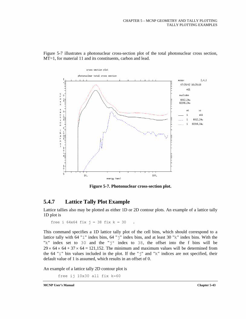
CHAPTER 5 – MCNP GEOMETRY AND TALLY PLOTTING
TALLY PLOTTING EXAMPLES
MCNP User’s Manual Chapter 5-43
Figure 5-7 illustrates a photonuclear cross-section plot of the total photonuclear cross section, MT=1, for material 11 and its constituents, carbon and lead.
Figure 5-7. Photonuclear cross-section plot.
5.4.7 Lattice Tally Plot Example Lattice tallies also may be plotted as either 1D or 2D contour plots. An example of a lattice tally 1D plot is
free i 64x64 fix j = 38 fix k = 30 .
This command specifies a 1D lattice tally plot of the cell bins, which should correspond to a lattice tally with 64 "i" index bins, 64 "j" index bins, and at least 30 "k" index bins. With the "k" index set to 30 and the "j" index to 38, the offset into the f bins will be 29 × 64 × 64 + 37 × 64 = 121,152. The minimum and maximum values will be determined from the 64 "i" bin values included in the plot. If the "j" and "k" indices are not specified, their default value of 1 is assumed, which results in an offset of 0.
An example of a lattice tally 2D contour plot is free ij 10x30 all fix k=60
CHAPTER 5 – MCNP GEOMETRY AND TALLY PLOTTING TALLY PLOTTING EXAMPLES
Chapter 5-44 MCNP User’s Manual
This example specifies a 10 × 30 2D contour plot, which should correspond to a lattice tally with 10 "i" bins, 30 "j" bins, and at least 60 "k" bins. Note that the "k" index is specified using the "fix" command, which sets the offset into the f bins as 60 × 10 × 30 = 18,000. In this case, the contour range is taken from all of the f-bin tally values.
5.4.8 Weight-Window-Generator Superimposed Mesh Plots MCNP6 can plot the WWG superimposed mesh specified on the MESH card in an input file. MCNP4C3 and older MCNPX versions could plot only the weight-window superimposed mesh used in a problem, and a WWINP file had to be provided. In the MCNP6 geometry plotter, toggle CellLine for the following options:
No Lines Plot cells not outlined in black CellLine Plot geometric cells, outlined in black WW MESH Plot the weight-window superimposed mesh (WWINP required) WW+Cell Plot superimposed mesh and cells, outlined in black WWG MESH Plot MESH card WWG mesh WWG+Cell Plot WWG mesh and cells, outlined in black MeshTaly Plot mesh tally boundaries MT+Cell Plot mesh tally boundaries + CellLine
The CellLine and No Lines options are always available. WW Mesh and WW+Cell are available only when the WWP card calls for using a superimposed weight-window mesh (fifth entry negative) and a WWINP file is provided. WWG MESH and WWG+Cell are available only when a MESH card is in the input file and when the WWG requests superimposed mesh generation (WWG card second entry equals 0). In all cases, the cells may be outlined in black (CellLine, WW+Cell, WWG+Cell) or the cells simply may be colored without outlining (WW MESH, WWG MESH, No Lines).
5.4.8.1 CYLINDRICAL MESH EXAMPLE
Example:
Input file: inp10 Demonstration of WWG Plot 1 1 1.0 -1 imp:p 1 2 0 1 imp:p 0 1 rcc 0 0 0 0 10 0 5 mode p sdef sur 1.3 vec 0 1 0 dir 1 erg 100 m1 1001 2 8016 1 nps 1000
CHAPTER 5 – MCNP GEOMETRY AND TALLY PLOTTING
TALLY PLOTTING EXAMPLES
MCNP User’s Manual Chapter 5-45
f1:p 1.2 wwg 1 0 mesh geom=cyl origin=0 -1 0 ref=0 .1 0 axs=0 1 0 vec=1 0 0 imesh 6 iints 7 jmesh 12 jints 7 kmesh 1 kints 3
Com file: com10 ex 10 lab 0 0 px 0 mesh 4 pause py 5 pause
Execution line:
mcnp6 i=inp10 com=com10 ip .
Or, instead of using the command file (with plot commands in command mode), the interactive plotter can be used:
mcnp6 i=inp10 ip ,
click CellLine to get WWG+Cell label sur to turn off surface labels XY to get px=0 view (axial view, Fig. 12) Zoom 10 to get 10 × magnification (click twice) Origin click in the center of material to center picture ZX to get py=5 view (radial view, Fig. 13)
The above COM file or plot commands in the command mode generate the two plots shown in Figure 5-8 and Figure 5-9.
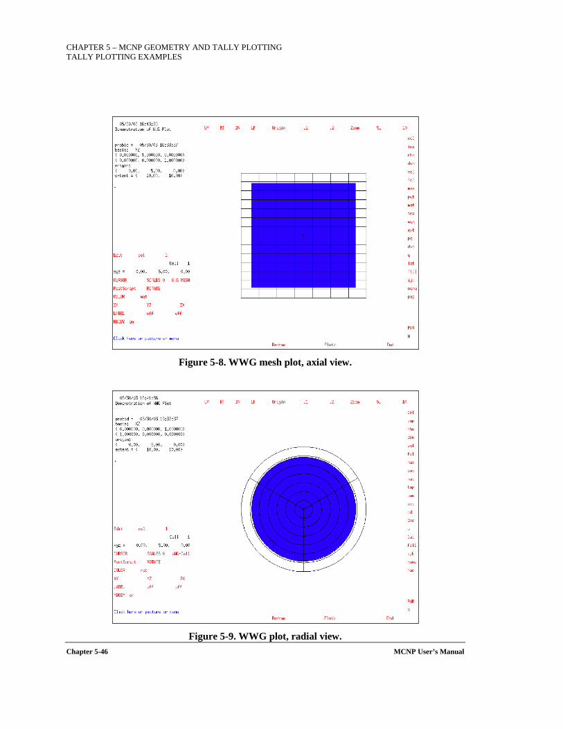
CHAPTER 5 – MCNP GEOMETRY AND TALLY PLOTTING TALLY PLOTTING EXAMPLES
Chapter 5-46 MCNP User’s Manual
Figure 5-8. WWG mesh plot, axial view.
Figure 5-9. WWG plot, radial view.
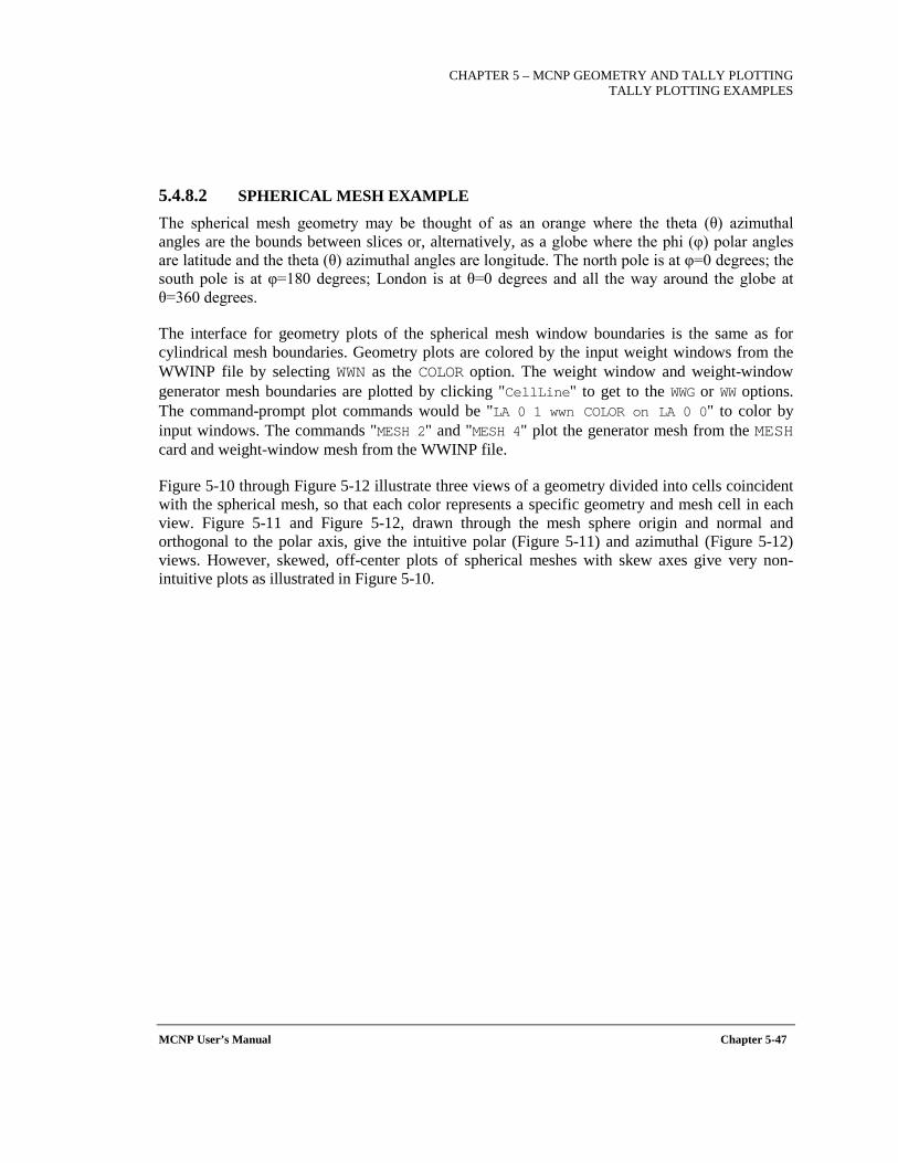
CHAPTER 5 – MCNP GEOMETRY AND TALLY PLOTTING
TALLY PLOTTING EXAMPLES
MCNP User’s Manual Chapter 5-47
5.4.8.2 SPHERICAL MESH EXAMPLE
The spherical mesh geometry may be thought of as an orange where the theta (θ) azimuthal angles are the bounds between slices or, alternatively, as a globe where the phi (φ) polar angles are latitude and the theta (θ) azimuthal angles are longitude. The north pole is at φ=0 degrees; the south pole is at φ=180 degrees; London is at θ=0 degrees and all the way around the globe at θ=360 degrees.
The interface for geometry plots of the spherical mesh window boundaries is the same as for cylindrical mesh boundaries. Geometry plots are colored by the input weight windows from the WWINP file by selecting WWN as the COLOR option. The weight window and weight-window generator mesh boundaries are plotted by clicking "CellLine" to get to the WWG or WW options. The command-prompt plot commands would be "LA 0 1 wwn COLOR on LA 0 0" to color by input windows. The commands "MESH 2" and "MESH 4" plot the generator mesh from the MESH card and weight-window mesh from the WWINP file.
Figure 5-10 through Figure 5-12 illustrate three views of a geometry divided into cells coincident with the spherical mesh, so that each color represents a specific geometry and mesh cell in each view. Figure 5-11 and Figure 5-12, drawn through the mesh sphere origin and normal and orthogonal to the polar axis, give the intuitive polar (Figure 5-11) and azimuthal (Figure 5-12) views. However, skewed, off-center plots of spherical meshes with skew axes give very non-intuitive plots as illustrated in Figure 5-10.
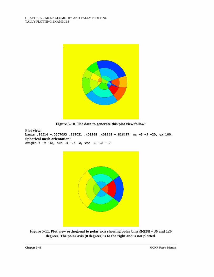
CHAPTER 5 – MCNP GEOMETRY AND TALLY PLOTTING TALLY PLOTTING EXAMPLES
Chapter 5-48 MCNP User’s Manual
Figure 5-10. The data to generate this plot view follow:
Plot view: basis .84514 -.0507093 .169031 .408248 .408248 -.816497, or -3 -9 -20, ex 100. Spherical mesh orientation: origin 7 -9 -12, axs .4 -.5 .2, vec .1 -.2 -.7
Figure 5-11. Plot view orthogonal to polar axis showing polar bins JMESH = 36 and 126
degrees. The polar axis (0 degrees) is to the right and is not plotted.
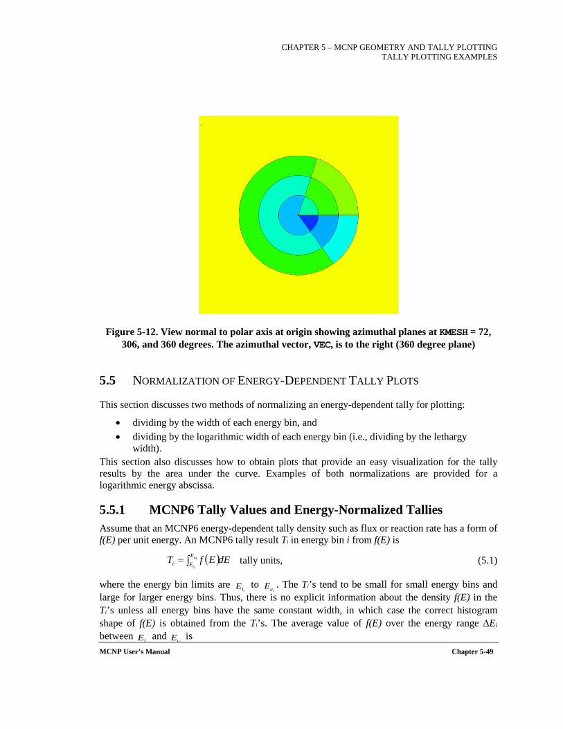
CHAPTER 5 – MCNP GEOMETRY AND TALLY PLOTTING
TALLY PLOTTING EXAMPLES
MCNP User’s Manual Chapter 5-49
Figure 5-12. View normal to polar axis at origin showing azimuthal planes at KMESH = 72, 306, and 360 degrees. The azimuthal vector, VEC, is to the right (360 degree plane)
5.5 NORMALIZATION OF ENERGY-DEPENDENT TALLY PLOTS
This section discusses two methods of normalizing an energy-dependent tally for plotting:
• dividing by the width of each energy bin, and • dividing by the logarithmic width of each energy bin (i.e., dividing by the lethargy
width). This section also discusses how to obtain plots that provide an easy visualization for the tally results by the area under the curve. Examples of both normalizations are provided for a logarithmic energy abscissa.
5.5.1 MCNP6 Tally Values and Energy-Normalized Tallies Assume that an MCNP6 energy-dependent tally density such as flux or reaction rate has a form of f(E) per unit energy. An MCNP6 tally result Ti in energy bin i from f(E) is
tally units, (5.1)
where the energy bin limits are to . The Ti’s tend to be small for small energy bins and large for larger energy bins. Thus, there is no explicit information about the density f(E) in the Ti’s unless all energy bins have the same constant width, in which case the correct histogram shape of f(E) is obtained from the Ti’s. The average value of f(E) over the energy range ∆Ei between and is
( )dEEfT iu
il
EEi ∫=
ilE
iuE
ilE
iuE
CHAPTER 5 – MCNP GEOMETRY AND TALLY PLOTTING NORMALIZATION OF TALLY PLOTS
Chapter 5-50 MCNP User’s Manual
(tally units)/(unit energy). (5.2)
The fi(E)'s are the bin-wise histogram representations of the tally of f(E) because they are the average values of f(E) in each energy bin. Note that fi(E) is a constant between El and Eu.
This Eu−El normalizing of Ti, the default for a 2D MCNP6 energy-dependent tally spectral plot, is generally agreed to be the proper way to display the fi(E)’s when the abscissa E of a 2D plot is linear. When a LINLIN (linear abscissa and linear ordinate) plot of fi(E)’s is made with the ordinate starting at zero, the visual area under each histogram represents Ti. This type of visually correct area plot will be termed a Visually Accurate Area (VAA) plot. A VAA plot provides correct visual information about the tally by the area under the histogram.
The average energy for each fi(E) bin is
, (5.3)
where the fi(E) histogram approximation to f(E) cancels out. is used as the average energy for plotting the statistical error bars for tally bin i.
5.5.2 Definition of Neutron Lethargy The lethargy U of a neutron with energy E is defined to be
, (5.4)
where E0 is the upper neutron energy for the problem. On the average, neutrons lose a fixed fraction of their energy in each elastic collision with a specific isotope above thermal energies. The lethargy U is used in nuclear reactor analysis to assess the average logarithmic energy loss of these elastically scattered neutrons.
A neutron with energy E0 has zero lethargy. As the neutron loses energy, its lethargy increases (hence the name "lethargy" because the neutron becomes more lethargic) and is always positive because no energy is greater than E0. A neutron with zero energy has infinite lethargy.
For eigenvalue problems, MCNP6 calculates the Energy of the Average neutron Lethargy causing Fission (EALF):
, (5.5)
( )( )
ii
iu
il
iu
il
lu
iEE
EE
i EET
dE
dEEfEf
−==
∫
∫
iE
( )( )
( )( ) 2
ii
iu
il
iu
il
iu
il
iu
il luEE i
EE i
EE
EE
iEE
dEEf
dEEEf
dEEf
dEEEfE
+=≈=
∫
∫
∫
∫
iE
( ) ( )EEEEU lnlnln 0
0 −=
=
( ) ( ) ( ) ( ) ( ) ∫∫ ΣΦΣΦ= dEEEdEEEE fflnexpEALF
CHAPTER 5 – MCNP GEOMETRY AND TALLY PLOTTING NORMALIZATION OF TALLY PLOTS
MCNP User’s Manual Chapter 5-51
where Φ(E) is the neutron flux and Σf(E) is the fission cross section (the E0’s cancel). MCNP6 can plot energy-dependent tallies versus a logarithmic energy scale using lethargy for tally bin normalization.
5.5.3 Lethargy-Normalized Tallies for a Logarithmic Energy Abscissa
When the abscissa E is logarithmic, the Ti normalizing procedure often preferred involves the differences in the natural logs (ln) of the energy instead of the differences in the energies. It is useful to relate the differences in the logs of the bin energies to the often used neutron lethargy U:
, (5.6)
where is the lethargy at and is the lethargy at (the ln(E0) terms cancel: see Eqn. (5.4)).
The tally Ti can be converted to an average bin i lethargy-normalized value Fi(U) by
(tally units)/(unit lethargy). (5.7)
The Fi(U)’s are the histogram approximation to F(U) per unit lethargy. MCNP6 plots the Fi(U)'s instead of the fi(E)'s for a ln(E) abscissa when the LETHARGY plot command is used. The Fi(U)'s are not plotted when the energy abscissa is linear. Only the fi(E)'s and Ti’s can be plotted for a linear E abscissa. A LOGLIN (log abscissa and linear ordinate) plot of the Fi(U)’s is a VAA plot because the ln(E) abscissa is linear in U and the area under the histogram is visually correct.
5.5.4 Relation of Tally Lethargy Normalizing to Tally Energy Normalizing
To determine the functional form of F(U) in terms of f(E), equate the U and E density function areas to produce
. (5.8)
The negative sign is required because E decreases as U increases. Integrating the left hand side of Eqn. (5.8) from to is equal to Ti, as is the integral of the right hand side from to .
The differential dU can be written in terms of energy E from Eqn. (5.4) as
. (5.9)
Substituting Eqn. (5.9) for dU into Eqn. (5.8) gives
. (5.10)
( ) ( )iiii ullu UUEE −=− lnln
ilU
ilE
iuUiuE
( ) ( )iiii ul
i
lu
ii UU
TEE
TUF−
==ln
( ) ( )dEEfdUUF −=
iuUil
UiuE
ilE
( ) EdEEddU −
=−= ln
( ) ( )EEfUF =
CHAPTER 5 – MCNP GEOMETRY AND TALLY PLOTTING NORMALIZATION OF TALLY PLOTS
Chapter 5-52 MCNP User’s Manual
Eqn. (5.10) shows that F(U) can be thought of as the energy E times f(E). Thus, besides producing VAA LOGLIN plots, lethargy-normalized plots have the additional virtue of flattening the 1/E neutron flux shape that often occurs in neutron spectra. For an f(E) that has a 1/E shape everywhere, Fi(U) is a constant for all i (as opposed to the widely varying fi(E)'s), which produces a VAA plot for the 1/E shape. Lethargy-normalized plots remove many of the decades of fi(E) change, represent the 1/E portions of the spectrum as a constant, and make understanding and comparing the Fi(U) results easier.
5.5.5 Average Energy for a Lethargy-Normalized Tally The lethargy-averaged energy <Ei> for energy bin i is defined as
. (5.11)
For the histogram approximation of F(U) by Fi(U), the Fi(U)’s cancel, and changing variables using Eqn. (5.9) gives
. (5.12)
In the limit as becomes small, in Eqn. (6.3) as expected. This average <Ei> is considered to be the centroid energy for a lethargy-normalized bin and is used in MCNP6 to plot statistical error bars, BAR plots, and PLINEAR plots, as well as printing the plotted points using the PRINTPTS command.
5.5.6 MCNP6 LETHARGY Command for Lethargy Normalization Lethargy-normalized plots of energy-dependent tallies with a log energy abscissa are made with the LETHARGY plotting command. This command cannot be used for cross-section plots. For this command to apply, "FREE E" must be active, "LOGLIN" or "LOGLOG" axes must be used, and the "NONORM" command must not be invoked. The LETHARGY command cannot be used after a COPLOT command and can be disabled to return to energy-bin-width tally normalization for a log energy abscissa by using RESET LETHARGY. Switching from a logarithmic energy to a linear energy abscissa with LETHARGY in use will automatically change a plot of the Fi(U)’s to the fi(E)’s. Switching back to the log energy abscissa will again plot the Fi(U)’s.
If an E0 were specified for a log abscissa plot, a linear lethargy abscissa could be specified starting at the right with a value of zero at E0 and linearly increasing to the left in steps of about 2.3 per energy decade decrease. MCNP6 does not label the abscissa as lethargy because of the difficult energy interpretation. The logarithmic energy decades are plotted instead to allow easier
∫
∫>=<
il
iu
il
iu
UU
UU
i dUUF
dUUEFE
)(
)(
−==>≈<
∫
∫
∫
∫
i
i
ii
iu
il
iu
il
il
iu
il
iu
l
u
lu
EE
EE
UU
UU
i
EE
EE
EdEdE
dU
EdUE
ln
ii lu EE − ii EE >≈<
CHAPTER 5 – MCNP GEOMETRY AND TALLY PLOTTING NORMALIZATION OF TALLY PLOTS
MCNP User’s Manual Chapter 5-53
interpretation of the areas under the lethargy-normalized histogram. For this reason, there is neither a need nor a provision to specify E0.
5.5.7 Requirements for Producing a Visually Accurate Area (VAA) Tally Plot
Consider the characteristics of a function of one variable, such as an MCNP6 2D tally histogram plot. One important quantity for this histogram is the integral over the tally range, which is the total MCNP6 tally. Another important characteristic is the shape of this histogram that provides information about where the largest regions of the tally have occurred. The area of a tally range under the plotted curve is a measure of the contribution of each range to the total.
The area under this curve is best visualized with both the abscissa and the ordinate having a linear scale. The ordinate usually has a lower value of zero to represent correctly the curve area. A LINLIN plot of the fi(E)’s fits these criteria and therefore is a VAA plot. Often linear scales do not allow complete display of a tally, so logarithmic scales must be used. A logarithmic axis scale typically changes by decades. Each decade change on the abscissa changes a ΔE for a specified length along the abscissa by a decade. The area under the LOGLIN fi(E) curve is proportional to ΔE, which is not reflected in the visual area representation on the log abscissa plot. A logarithmic ordinate does not visually display the correct tally contribution under the curve because this area in the plot is proportional to the number of ordinate decades. When both axes are logarithmic, the visual interpretation in the plot of the area under the curve is further obscured.
The lethargy variable U is linear in the logarithm of the energy as defined in Eqn. (5.4). U values for decreasing energy E values of E0, E0/10, and E0/100 are 0, 2.3, and 4.6. Therefore, a LOGLIN plot of the Fi(U)'s instead of the fi(E)'s satisfies the VAA plot linear scale criterion for visually examining the area under a curve. The area under each histogram Fi(U) is , which is exactly the bin i tally Ti as defined in Eqn. (5.7). Similarly, the area under all the Fi(U)'s is the sum of the Ti's, which is the total MCNP6 tally. A LOGLIN plot of the Fi(U)’s is a VAA plot; a LOGLIN plot of the fi(E)’s is not a VAA plot.
5.5.8 Comparisons of Energy and Lethargy Tally Normalizations for a Log Energy Abscissa
Energy-normalized and lethargy-normalized log energy abscissa tally plots for two analytic and two critical uranium assembly problems are discussed to show which are VAA plots. The two analytic f(E) examples will be accurate to three significant figures in the text.
Example 1: A Constant f(E)=0.100 from 0.0001 to 10 MeV
The first example is the tally of a uniform energy source between 0.0001 and 10 MeV. The expected value of all fi(E)'s is 0.100. Figure 5-13 shows a plot of the five energy-normalized fi(E)'s, each with an energy bin width of a decade. The tally Ti in the energy bin from 1 to 10 MeV is . The next lowest energy bin tally is . The tally
( ) ( )ii uli UUUF −∗
( ) 9.01.0110 =∗− ( ) 09.01.01.01 =∗−
CHAPTER 5 – MCNP GEOMETRY AND TALLY PLOTTING NORMALIZATION OF TALLY PLOTS
Chapter 5-54 MCNP User’s Manual
bin Ti's are decreasing by a decade per decade decrease in energy, but the fi(E)'s are a statistically constant 0.1. Visually interpreting this LOGLIN plot of the fi(E)'s by the area under the curve is not useful because the energies are changing by decades along the logarithmic energy abscissa.
Figure 5-14 shows a LOGLIN lethargy-normalized plot of the corresponding five Fi(U)'s. (The "f(u) = ef(e) bin normed" text on the right hand side of the plot is a reminder that this is a lethargy-normalized plot.) The shapes of the fi(E)’s in Figure 5-13 and the Fi(U)’s in Figure 5-14 are completely different. Fi(U) for the 1 to 10 MeV tally bin is . The area in the plot of this bin is , which is the correct Ti for this bin. The tally bin area from 0.1 to 1 MeV is . The visual areas of each of the tally bins represent the tally for that bin because of the linear lethargy abscissa obtained by the lethargy normalization. The LOGLIN lethargy-normalized plot in Figure 5-14 clearly displays the relative contribution of each of the five tally bins by the area under the histogram. Figure B-3 is a VAA plot.
Figure 5-15 shows the same plot as in Figure 5-14, except the ordinate is now logarithmic. The five Fi(U)'s are the same in both plots, but the visual area interpretation in Figure 5-15 is misleading because the ordinate scale is logarithmic. Nevertheless, Figure 5-15 is useful for assessing the behavior of the Fi(U)'s that are small and cannot be seen in Figure 5-14 with the linear ordinate.
( ) 391.0110ln9.0 =( ) 900.0391.0110ln =∗
( ) 0900.0391.01.01ln =∗
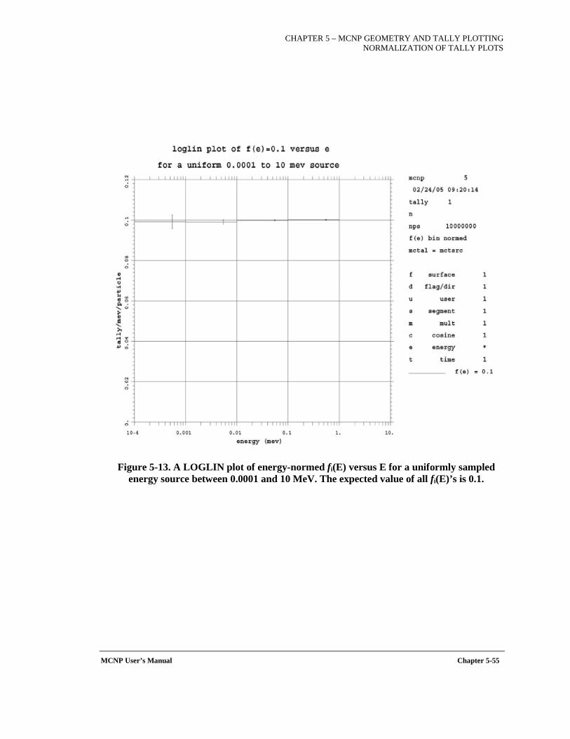
CHAPTER 5 – MCNP GEOMETRY AND TALLY PLOTTING NORMALIZATION OF TALLY PLOTS
MCNP User’s Manual Chapter 5-55
Figure 5-13. A LOGLIN plot of energy-normed fi(E) versus E for a uniformly sampled energy source between 0.0001 and 10 MeV. The expected value of all fi(E)’s is 0.1.
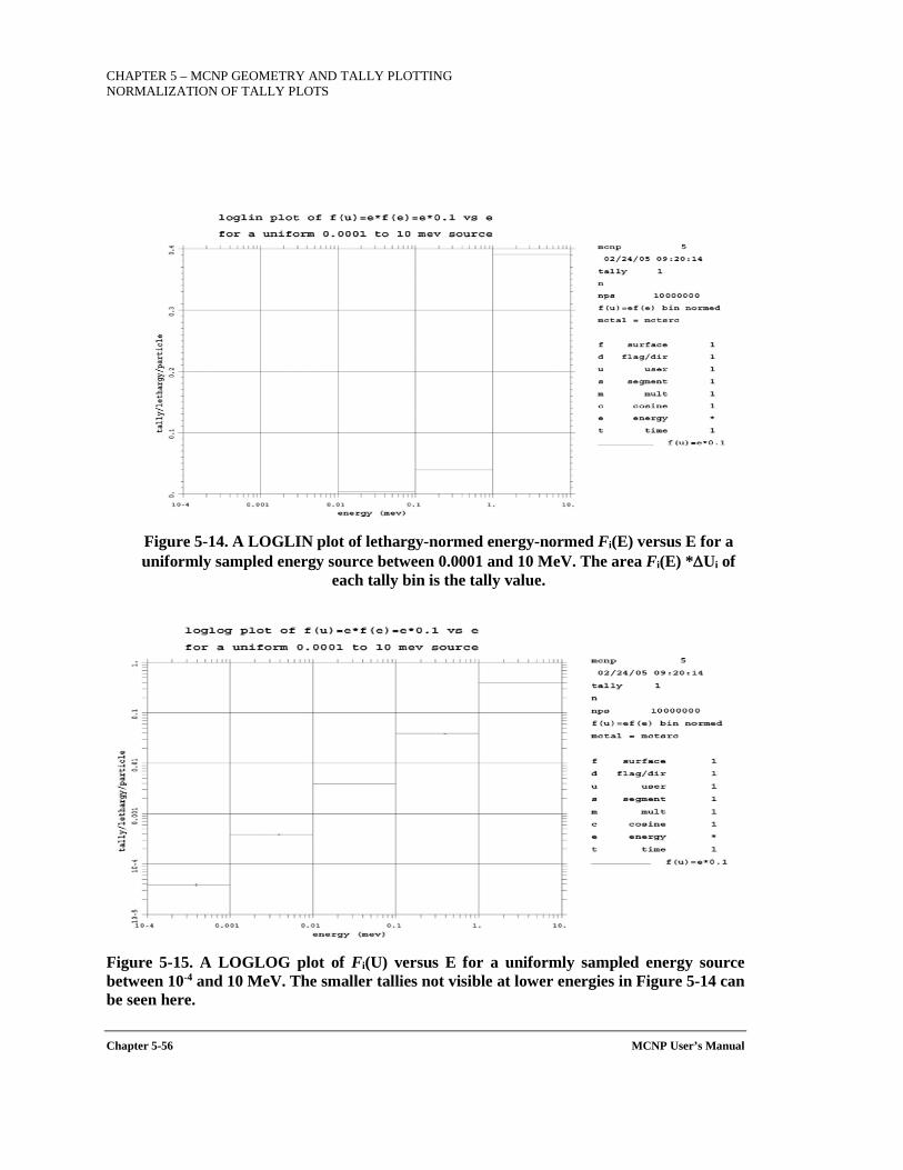
CHAPTER 5 – MCNP GEOMETRY AND TALLY PLOTTING NORMALIZATION OF TALLY PLOTS
Chapter 5-56 MCNP User’s Manual
Figure 5-14. A LOGLIN plot of lethargy-normed energy-normed Fi(E) versus E for a uniformly sampled energy source between 0.0001 and 10 MeV. The area Fi(E) *∆Ui of
each tally bin is the tally value.
Figure 5-15. A LOGLOG plot of Fi(U) versus E for a uniformly sampled energy source between 10-4 and 10 MeV. The smaller tallies not visible at lower energies in Figure 5-14 can be seen here.
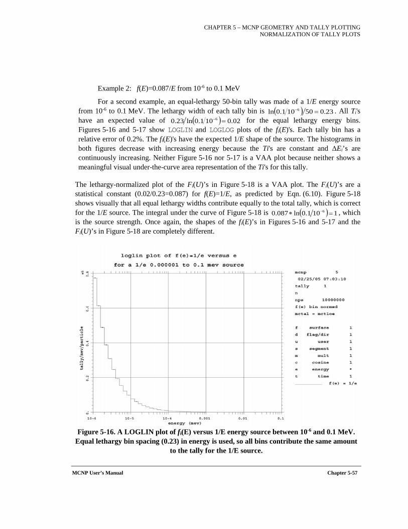
CHAPTER 5 – MCNP GEOMETRY AND TALLY PLOTTING NORMALIZATION OF TALLY PLOTS
MCNP User’s Manual Chapter 5-57
Example 2: f(E)=0.087/E from 10-6 to 0.1 MeV
For a second example, an equal-lethargy 50-bin tally was made of a 1/E energy source from 10-6 to 0.1 MeV. The lethargy width of each tally bin is . All Ti's have an expected value of for the equal lethargy energy bins. Figures 5-16 and 5-17 show LOGLIN and LOGLOG plots of the fi(E)'s. Each tally bin has a relative error of 0.2%. The fi(E)'s have the expected 1/E shape of the source. The histograms in both figures decrease with increasing energy because the Ti's are constant and ΔEi’s are continuously increasing. Neither Figure 5-16 nor 5-17 is a VAA plot because neither shows a meaningful visual under-the-curve area representation of the Ti's for this tally.
The lethargy-normalized plot of the Fi(U)’s in Figure 5-18 is a VAA plot. The Fi(U)’s are a statistical constant (0.02/0.23=0.087) for f(E)=1/E, as predicted by Eqn. (6.10). Figure 5-18 shows visually that all equal lethargy widths contribute equally to the total tally, which is correct for the 1/E source. The integral under the curve of Figure 5-18 is , which is the source strength. Once again, the shapes of the fi(E)’s in Figures 5-16 and 5-17 and the Fi(U)’s in Figure 5-18 are completely different.
Figure 5-16. A LOGLIN plot of fi(E) versus 1/E energy source between 10-6 and 0.1 MeV. Equal lethargy bin spacing (0.23) in energy is used, so all bins contribute the same amount
to the tally for the 1/E source.
( ) 23.050101.0ln 6 =−
( ) 02.0101.0ln23.0 6 =−
( ) 1101.0ln087.0 6 =∗ −
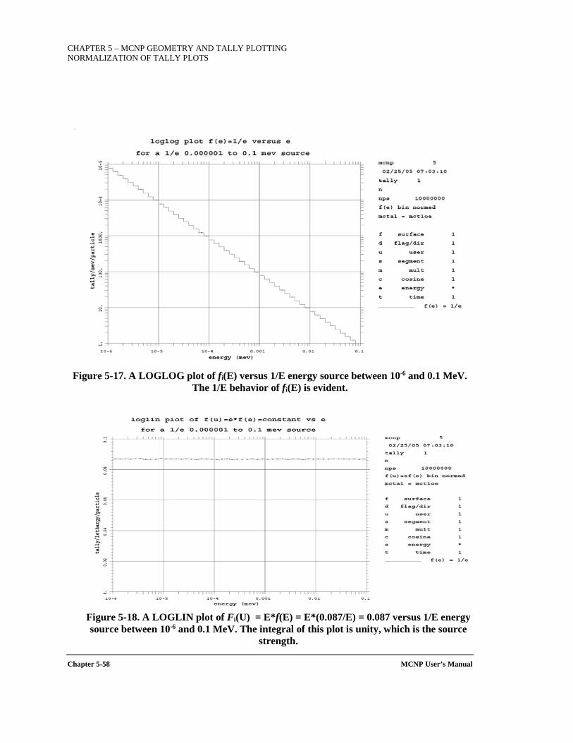
CHAPTER 5 – MCNP GEOMETRY AND TALLY PLOTTING NORMALIZATION OF TALLY PLOTS
Chapter 5-58 MCNP User’s Manual
Figure 5-17. A LOGLOG plot of fi(E) versus 1/E energy source between 10-6 and 0.1 MeV.
The 1/E behavior of fi(E) is evident.
Figure 5-18. A LOGLIN plot of Fi(U) = E*f(E) = E*(0.087/E) = 0.087 versus 1/E energy source between 10-6 and 0.1 MeV. The integral of this plot is unity, which is the source
strength.
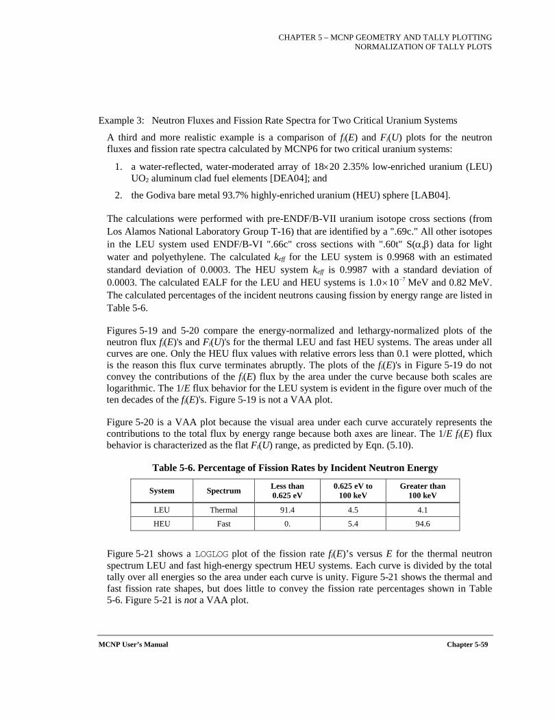
CHAPTER 5 – MCNP GEOMETRY AND TALLY PLOTTING NORMALIZATION OF TALLY PLOTS
MCNP User’s Manual Chapter 5-59
Example 3: Neutron Fluxes and Fission Rate Spectra for Two Critical Uranium Systems
A third and more realistic example is a comparison of fi(E) and Fi(U) plots for the neutron fluxes and fission rate spectra calculated by MCNP6 for two critical uranium systems:
1. a water-reflected, water-moderated array of 18×20 2.35% low-enriched uranium (LEU) UO2 aluminum clad fuel elements [DEA04]; and
2. the Godiva bare metal 93.7% highly-enriched uranium (HEU) sphere [LAB04].
The calculations were performed with pre-ENDF/B-VII uranium isotope cross sections (from Los Alamos National Laboratory Group T-16) that are identified by a ".69c." All other isotopes in the LEU system used ENDF/B-VI ".66c" cross sections with ".60t" S(α,β) data for light water and polyethylene. The calculated keff for the LEU system is 0.9968 with an estimated standard deviation of 0.0003. The HEU system keff is 0.9987 with a standard deviation of 0.0003. The calculated EALF for the LEU and HEU systems is MeV and 0.82 MeV. The calculated percentages of the incident neutrons causing fission by energy range are listed in Table 5-6.
Figures 5-19 and 5-20 compare the energy-normalized and lethargy-normalized plots of the neutron flux fi(E)'s and Fi(U)'s for the thermal LEU and fast HEU systems. The areas under all curves are one. Only the HEU flux values with relative errors less than 0.1 were plotted, which is the reason this flux curve terminates abruptly. The plots of the fi(E)'s in Figure 5-19 do not convey the contributions of the fi(E) flux by the area under the curve because both scales are logarithmic. The 1/E flux behavior for the LEU system is evident in the figure over much of the ten decades of the fi(E)'s. Figure 5-19 is not a VAA plot.
Figure 5-20 is a VAA plot because the visual area under each curve accurately represents the contributions to the total flux by energy range because both axes are linear. The 1/E fi(E) flux behavior is characterized as the flat Fi(U) range, as predicted by Eqn. (5.10).
Table 5-6. Percentage of Fission Rates by Incident Neutron Energy
System Spectrum Less than 0.625 eV
0.625 eV to 100 keV
Greater than 100 keV
LEU Thermal 91.4 4.5 4.1
HEU Fast 0. 5.4 94.6
Figure 5-21 shows a LOGLOG plot of the fission rate fi(E)’s versus E for the thermal neutron spectrum LEU and fast high-energy spectrum HEU systems. Each curve is divided by the total tally over all energies so the area under each curve is unity. Figure 5-21 shows the thermal and fast fission rate shapes, but does little to convey the fission rate percentages shown in Table 5-6. Figure 5-21 is not a VAA plot.
7100.1 −×
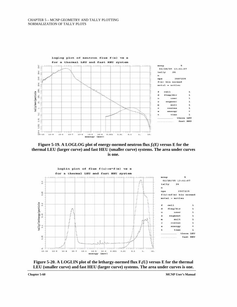
CHAPTER 5 – MCNP GEOMETRY AND TALLY PLOTTING NORMALIZATION OF TALLY PLOTS
Chapter 5-60 MCNP User’s Manual
Figure 5-19. A LOGLOG plot of energy-normed neutron flux fi(E) versus E for the thermal LEU (larger curve) and fast HEU (smaller curve) systems. The area under curves
is one.
Figure 5-20. A LOGLIN plot of the lethargy-normed flux Fi(U) versus E for the thermal LEU (smaller curve) and fast HEU (larger curve) systems. The area under curves is one.
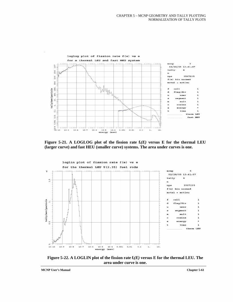
CHAPTER 5 – MCNP GEOMETRY AND TALLY PLOTTING NORMALIZATION OF TALLY PLOTS
MCNP User’s Manual Chapter 5-61
Figure 5-21. A LOGLOG plot of the fission rate fi(E) versus E for the thermal LEU (larger curve) and fast HEU (smaller curve) systems. The area under curves is one.
Figure 5-22. A LOGLIN plot of the fission rate fi(E) versus E for the thermal LEU. The area under curve is one.
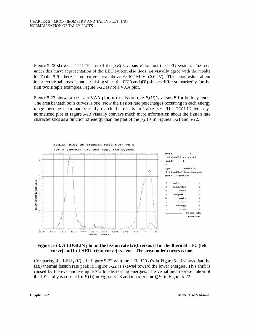
CHAPTER 5 – MCNP GEOMETRY AND TALLY PLOTTING NORMALIZATION OF TALLY PLOTS
Chapter 5-62 MCNP User’s Manual
Figure 5-22 shows a LOGLIN plot of the fi(E)’s versus E for just the LEU system. The area under this curve representation of the LEU system also does not visually agree with the results in Table 5-6: there is no curve area above 6×10⁻⁷ MeV (0.6 eV). This conclusion about incorrect visual areas is not surprising since the F(U) and f(E) shapes differ so markedly for the first two simple examples. Figure 5-22 is not a VAA plot.
Figure 5-23 shows a LOGLIN VAA plot of the fission rate Fi(U)’s versus E for both systems. The area beneath both curves is one. Now the fission rate percentages occurring in each energy range become clear and visually match the results in Table 5-6. The LOGLIN lethargy-normalized plot in Figure 5-23 visually conveys much more information about the fission rate characteristics as a function of energy than the plot of the fi(E)’s in Figures 5-21 and 5-22.
Figure 5-23. A LOGLIN plot of the fission rate fi(E) versus E for the thermal LEU (left curve) and fast HEU (right curve) systems. The area under curves is one.
Comparing the LEU fi(E)’s in Figure 5-22 with the LEU Fi(U)’s in Figure 5-23 shows that the fi(E) thermal fission rate peak in Figure 5-22 is skewed toward the lower energies. This shift is caused by the ever-increasing 1/ΔEi for decreasing energies. The visual area representation of the LEU tally is correct for Fi(U) in Figure 5-23 and incorrect for fi(E) in Figure 5-22.
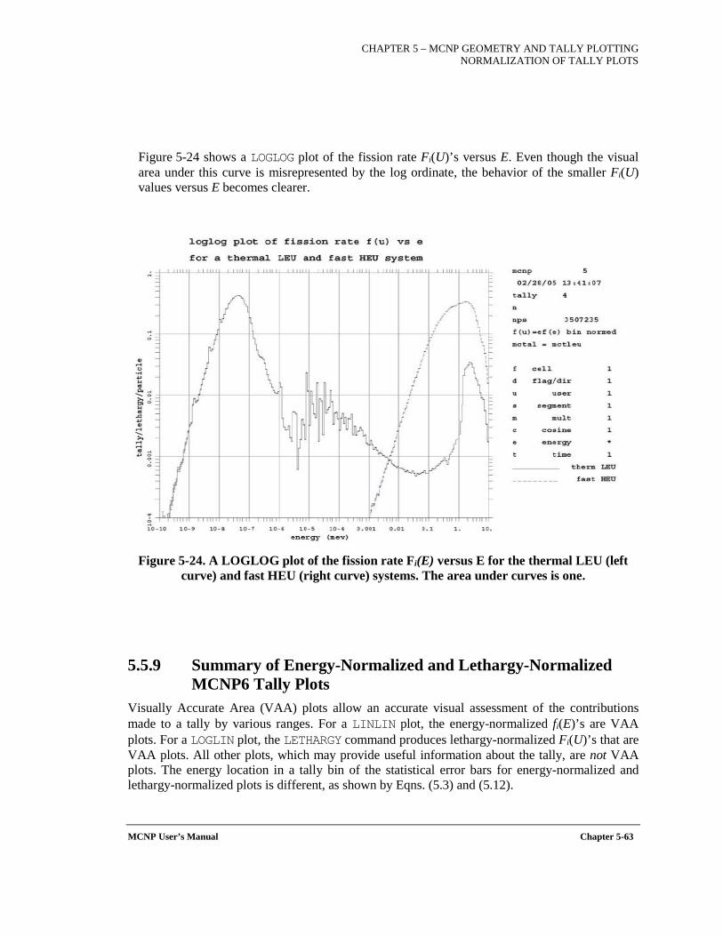
CHAPTER 5 – MCNP GEOMETRY AND TALLY PLOTTING NORMALIZATION OF TALLY PLOTS
MCNP User’s Manual Chapter 5-63
Figure 5-24 shows a LOGLOG plot of the fission rate Fi(U)’s versus E. Even though the visual area under this curve is misrepresented by the log ordinate, the behavior of the smaller Fi(U) values versus E becomes clearer.
Figure 5-24. A LOGLOG plot of the fission rate Fi(E) versus E for the thermal LEU (left curve) and fast HEU (right curve) systems. The area under curves is one.
5.5.9 Summary of Energy-Normalized and Lethargy-Normalized MCNP6 Tally Plots
Visually Accurate Area (VAA) plots allow an accurate visual assessment of the contributions made to a tally by various ranges. For a LINLIN plot, the energy-normalized fi(E)’s are VAA plots. For a LOGLIN plot, the LETHARGY command produces lethargy-normalized Fi(U)’s that are VAA plots. All other plots, which may provide useful information about the tally, are not VAA plots. The energy location in a tally bin of the statistical error bars for energy-normalized and lethargy-normalized plots is different, as shown by Eqns. (5.3) and (5.12).

CHAPTER 5 – MCNP GEOMETRY AND TALLY PLOTTING NORMALIZATION OF TALLY PLOTS
Chapter 5-64 MCNP User’s Manual
VAA plots are useful tools that allow visual assessment of the characteristics of the tally by examining the area under the curve. Equal abscissa bin spacing is not required for VAA plots. The more uniform the abscissa intervals are, however, the easier the area visualization becomes; e.g., it may be hard to estimate the area for a narrow bin that is much higher than other bins. If the abscissa intervals are all the same length, then the shape of a plot is identical to a NONORM plot where the bin Ti's themselves are plotted. The magnitude of the two curves will differ by the bin-width normalization. MCNP6 can create lethargy-normalized plots for ln(E) abscissas for all particle types when the LETHARGY plotting command is used.
The Bottom-line: Both the LINLIN energy-normalized and LOGLIN lethargy-normalized plots of energy-dependent tallies allow a direct tally contribution visualization by the area under the histogram.
CHAPTER 6 - REFERENCES
MCNP User’s Manual Chapter 6-1
6 REFERENCES
ALC08 R. E. Alcouffe, et al., "PARTISN: A Time-Dependent, Parallel Neutral Particle Transport Code System, Los Alamos National Laboratory report LA-UR-08-07258 (November 2008).
ANS85 "American National Standard for Information Systems—Computer Graphics—Graphical Kernel System (GKS) Functional Description," ANSI X3.124-1985, ANSI, INC (1985).
ARM73 T. W. Armstrong and K. C. Chandler, "SPAR, A FORTRAN Program for Computing Stopping Powers and Ranges for Muons, Charged Pions, and Heavy Ions," Oak Ridge National Laboratory report ORNL-4869 (May 1973).
ART80 E. D. Arthur and P. G. Young, “Evaluated Neutron-Induced Cross Sections for 54,56Fe to 40 MeV,” Los Alamos Scientific Laboratory report LA-8626-MS (ENDF-304) (December 1980).
ART81 E. D. Arthur, P. G. Young, A. B. Smith, and C. A. Philis, “New Tungsten Isotope Evaluations for Neutron Energies Between 0.1 and 20 MeV,” Trans. Am. Nucl. Soc. 39, 793 (1981).
ART88 E. D. Arthur, "The GNASH Preequilibrium-Statistical Model Code," Los Alamos National Laboratory report LA-UR-88-382 (February 1988).
ATC80 F. Atchison, "Spallation and Fission in Heavy Metal Nuclei under Medium Energy Proton Bombardment," in Targets for Neutron Beam Spallation Sources, Jul-Conf-34, Kernforschungsanlage Julich GmbH (January 1980).
BAR72 V. S. Barashenkov and V. D. Toneev, Interaction of Particles and Nuclei with Atomic Nuclei [in Russian], Atomizdat, Moscow (1972).
BAR73 V. S. Barashenkov, A. S. Iljinov, N. M. Sobolevskii, and V. D. Toneev, "Interaction of Particles and Nuclei of High and Ultrahigh Energy with Nuclei," Usp. Fiz. Nauk 109, 91 (1973) [Sov. Phys. Usp. 16, 31 (1973)].
BAR81 J. Barish, T. A. Gabriel, F. S. Alsmiller, and R. G. Alsmiller, Jr., "HETFIS High-Energy Nucleon-Meson Transport Code with Fission," Oak Ridge National Laboratory Report ORNL-TM-7882 (July 1981).
BAR94 V. S. Barashenkov and A. Polanski, "Electronic Guide for Nuclear Cross Sections," Comm. JINR E2-94-417, Dubna (1994).
BER63 M. J. Berger, "Monte Carlo Calculation of Penetration and Diffusion of Fast Charged Particles," in Methods in Computational Physics, B. Alder, S. Fernbach, and M. Rotenberg, Eds., (Academic Press, New York, 1963) Vol 1, p. 135.
BER63a H. W. Bertini, "Low-Energy Intranuclear Cascade Calculation," Phys. Rev 131, 1801 (1963).
CHAPTER 6 - REFERENCES
Chapter 6-2 MCNP User’s Manual
BER69 H. W. Bertini, "Intranuclear Cascade Calculation of the Secondary Nucleon Spectra from Nucleon-Nucleus Interations in the Energy Range 340 to 2900 MeV and Comparison with Experiment," Phys. Rev. 188, 1711 (1969).
BER70 M. J. Berger and S. M. Seltzer, "Bremsstrahlung and Photoneutrons from Thick Target and Tantalum Targets," Phys. Rev. C2, 621 (1970).
BER02 M. Berz, K. Makino, COSY INFINITY Version 8.1—user’s guide and reference manual, Tech. Rep. MSUHEP-20704, Department of Physics and Astronomy, Michigan State University, East Lansing, MI 48824 (2002). Also see http://cosy.pa.msu.edu..
BET34 H. A. Bethe and W. Heitler, "On Stopping of Fast Particles and on the Creation of Positive Electrons," Proc. Roy. Soc. (London) A146, 83 (1934).
BEV69 Phillip R. Bevington, Data Reduction and Error Analysis for the Physical Sciences (McGraw-Hill Book Company, New York, NY, 1969).
BIE89 Alex F Bielajew, Rahde Mohan, and Chen-Shou Chui, “Improved Bremsstrahlung Photon Angular Sampling in the EGS4 Code System,” National Research Council of Canada report, PIRS-0203 (November 1989). Also see http://www.irs.inms.nrc.ca/inms/irs/papers /irs_www/irs_www.html.
BIR64 J. B. Birks, The Theory and Practice of Scintillation Counting, Macmillan, New York (1964).
BLU50 O. Blunck and S. Leisegang, "Zum Energieverlust schneller Elektronen in dunnen Schichten," Z. Physik 128, 500 (1950).
BLU51 O. Blunck and R. Westphal, "Zum Energieverlust energiereicher Elektronen in dunnen Schichten," Z. Physik 130, 641 (1951).
BOL85 J. W. Boldeman and M. G. Hines, “Prompt Neutron Emission Probabilities Following Spontaneous and Thermal Neutron Fission,” Nucl. Sci. Eng. 91, 114 (1985).
BOO92 Thomas E. Booth, “Monte Carlo Variance Reduction Approaches for Non-Boltzmann Tallies,” Los Alamos National Laboratory report, LA-12433 (December 1992).
BOO94 Thomas E. Booth, “A Supertrack Importance Generator for Pulse Height Tallies,” Transactions of the American Nuclear Society, Vol. 71, 400 (1994).
BOO02 Thomas E. Booth, “Pulse Height Tally Variance Reduction in MCNP,” Los Alamos National Laboratory report, LA-13955 (2002).
BOO09 T. E. Booth, K. C. Kelley, and S. S. McCready, "Monte Carlo Variance Reduction Using Nested DXTRAN Spheres," Nuc. Tech., 168, 765–767 (December 2009).
BOU02 A. Boudard, J. Cugnon, S. Leray, and C. Volant, "Intranuclear cascade model for a comprehensive description of spallation reaction data," Phys. Rev. C 66, 044615 (2002).
CHAPTER 6 - REFERENCES
MCNP User’s Manual Chapter 6-3
BRE81 D. J. Brenner, R. E. Prael, J. F. Dicello, and M. Zaider, "Improved Calculations of Energy Deposition from Fast Neutrons," in Proceedings, Fourth Symposium on Neutron Dosimetry, EUR-7448, Munich-Neuherberg (1981).
BRE89 D. J. Brenner and R. E. Prael, "Calculated Differential Secondary-Particle Production Cross Sections after Nonelastic Neutron Interactions with Carbon and Oxygen between 10 and 60 MeV," Atomic and Nuclear Data Tables 41, 71–130 (1989).
BRI00 J. F. Briesmeister, ed., "MCNP™—A General Monte Carlo N-Particle Transport Code, Version 4C," Los Alamos National Laboratory report LA-13709-M (March 2000).
BRO04 F. B. Brown and W. R. Martin, “Stochastic Geometry Capability in MCNP5 for the Analysis of Particle Fuel,” Annals of Nuclear Energy, Vol. 31, Issue 17, pp. 2039-2047 (2004), and Los Alamos National Laboratory report LA-UR-04-5362 (November 2004).
BRO05 F. B. Brown, W. R. Martin, W. Ji, J. L. Conlin, and J. C. Lee, “Stochastic Geometry and HTGR Modeling for MCNP5,” ANS Monte Carlo 2005 Topical Meeting, Chattanooga TN, (April 2005), and Los Alamos National Laboratory report LA-UR-04-8668 (April 2005).
BRO06 F. B. Brown, "The makxsf Code with Doppler Broadening", Los Alamos National Laboratory report LA-UR-06-7002 (2006). See also http://mcnp.lanl.gov.
BRO12a F. B. Brown, W. R. Martin, G. Yesilyurt, S. Wilderman, "Progress with On-The-Fly Neutron Doppler Broadening in MCNP," Trans. Am. Nuc. Soc. 106 (2012); paper, Los Alamos National Laboratory report LA-UR-12-00423 (2012); presentation, Los Alamos National Laboratory report LA-UR-12-22277 (2012). See also http://mcnp.lanl.gov.
BRO12b F. B. Brown, W. R. Martin, G. Yesilyurt, S. Wilderman,"On-th-Fly Neutron Doppler Broadening for MCNP," Los Alamos National Laboratory report LA-UR-12-20338 (2012). See also http://mcnp.lanl.gov.
BUL04 Jeffrey S. Bull, H. Grady Hughes, Peter L. Walstrom, John D. Zumbro, and Nikolai V. Mokhov, "Magnetic Field Tracking with MCNP5," Los Alamos National Laboratory report LA-UR-04-2125 (2004).
BUL11 Jeffrey S. Bull, "Magnetic Field Tracking Features in MCNP6," Los Alamos National Laboratory report LA-UR-11-00872 (2011).
CAR98 L. L. Carter, R. C. Little, and J. S. Hendricks, "New Probability Table Treatment in MCNP for Unresolved Resonances,'' 1998 Radiation Protection and Shielding Division Topical Conference on Technologies for the New Century, Sheraton Music City, Nashville, TN, Vol. II, p. 341, April 19–23 (1998).
CAS53 K. M. Case, F. de Hoffmann, and G. Placzek, Introduction to the Theory of Neutron Diffusion, Volume I, Los Alamos Scientific Laboratory report (June 1953).
CAS80 G. C. Castagnoli and D. Lal, "Solar Modulation Effects in Terrestrial Production of Carbon-14," Radiocarbon, 22, No. 2, pp. 133–158 (1980).
CHAPTER 6 - REFERENCES
Chapter 6-4 MCNP User’s Manual
CED05 P. Cederqvist, et al., "Version Management with CVS," Version 1.11.19, Free Software Foundation, Inc. (2005).
CHA98 M. B. Chadwick, et al., "Reference Input Parameter Library: Handbook for Calculations of Nuclear Reaction Data", IAEA-TECDOC-Draft, IAEA, Vienna (March 1998).
CHA99a M. B. Chadwick, P. G. Young, S. Chiba, S. C. Frankle, G. M. Hale, H. G. Hughes, A. J. Koning, R. C. Little, R. E. MacFarlane, R. E. Prael, and L. S. Waters, "Cross Section Evaluations to 150 MeV for Accelerator-Driven Systems and Implementation in MCNPX," Nuclear Science and Engineering 131 (3), 293 (March 1999).
CHA99b M. B. Chadwick, P. G. Young, R. E. MacFarlane, P. Moller, G. M. Hale, R. C. Little, A. J. Koning, and S. Chiba, "LA150 Documentation of Cross Sections, Heating, and Damage: Part A (Incident Neutrons) and Part B (Incident Protons)," Los Alamos National Laboratory report LA-UR-99-1222 (1999).
CHE76 V. A. Chechin and V. C. Ermilova, "The Ionization-Loss Distribution at Very Small Absorber Thickness," Nucl Instr. Meth. 136, 551 (1976).
CLE04 M. Clem, G. de Angelis, P. Goldhagen, and J. W. Wilson, "New Calculations of the Atmospheric Cosmic Radiation Field—Results for Neutron Spectra," Radiation Protection Dosimetry, 110, pp. 423–428 (2004).
CLO83 P. Cloth, et al., "The KFA-Version of the High-Energy Transport Code HETC and the Generalized Evaluation Code SIMPEL," Jul-Spez-196, Kernforschungsanlage Julich GmbH (March 1983).
CLO88 P. Cloth et al., "HERMES—A Monte Carlo Program System for Beam-Materials Interaction Studies," Jul-2203, Kernforschungsanlage Julich GmbH (May 1988).
CMU94 The Capability Maturity Model, Guidelines for Improving the Software Process (Carnegie Mellon University Software Engineering Institute, Addison Wesley, 1994).
COL00 G. Collazuol, A. Ferrari, A. Guglielmi, and P. R. Sala, "Hadronic Models and Experimental Data for the Neutrino Beam Production," Nuclear Instruments & Methods A 449, 609–623 (2000).
COU97 J. D. Court, "Combining the Results of Multiple LCS Runs," Los Alamos National Laboratory memorandum LANSCE-12-97-43 (May 8, 1997).
COU97a J. D. Court, "More Derivations: Combining Multiple Bins in a MCNP or LAHET Tally," Los Alamos National Laboratory memorandum LANSCE-12-97-66 (July 16, 1997).
COX11 L. J. Cox, "LNK3DNT Geometry Support: User Guidance for Creating and Embedding," Los Alamos National Laboratory report LA-UR-11-01654 (2011).
CRA56 W. W. T. Crane, G. H. Higgins, and H. R. Bowman, "Average Number of Neutrons per Fission for Several Heavy-Element Nuclides," Phys. Rev. 101, 1804 (1956).
CHAPTER 6 - REFERENCES
MCNP User’s Manual Chapter 6-5
CUL89 D. E. Cullen, M. H. Chen, J. H. Hubbell, S. T. Perkins, E. F. Plechaty, J. A. Rathkopf, and J. H. Scofield, "Tables and Graphs of Photon Interaction Cross Sections from 10 eV to 100 GeV Derived from the LLNL Evaluated Photon Data Library (EPDL)," Lawrence Livermore National Laboratory report UCRL-50400, Volume 6, Rev. 4, Part A: Z = 1 to 50 and Part B: Z = 51 to 100 (1989).
DEA04 V. F. Dean, C. A. Atkinson, and N. R. Smith, "Water Moderated U(2.35)O2 Fuel Rods in 2.032-cm Square-Pitched Arrays," International Handbook of Evaluated Criticality Safety Experiments, LEU-COMP-THERM-001, Nuclear Energy Agency, Organization for Economic Co-Operation and Development (September 2004).
DES09 Dessault Systemes Simulia, Inc., "ABAQUS USER MANUALS, Version 6.9," Providence, RI (2009).
DIV56 B. C. Diven, et al., "Multiplicities of Fission Neutrons," Phys. Rev. 101, 1012 (1956)
DRE81 L. Dresner, "EVAP-A Fortran Program for Calculating the Evaporation of Various Particles from Excited Compound Nuclei," Oak Ridge National Laboratory report ORNL-TM-7882 (July 1981).
DUR09 J. W. Durkee, et al., "MCNPX Graphics and Arithmetic Tally Upgrades," International Conference on Mathematics, Computational Methods, & Reactor Physics (M&C 2009), Saratoga Springs, New York, May 3–7 (2009).
DUR12 J. W. Durkee, et al., "The MCNP6 Delayed-Particle Feature," Nuc. Tech., 180, 336–354 (December 2012).
EGD01 H. W. Egdorf and T. L. Roberts, "Component Architectures and the Future Structure of Physics Codes," Los Alamos National Laboratory report LA-UR-01-4750 (2001).
ENS98 N. Ensslin, et al., "Application Guide to Neutron Multiplicity Counting," Los Alamos National Laboratory report LA-13422-M (November 1998).
EVA55 R. D. Evans, The Atomic Nucleus (Robert E. Krieger Publishing Co., 1955).
EVA98 T. M. Evans and J. S. Hendricks, "An Enhanced Geometry-Independent Mesh Weight Window Generator for MCNP,'' 1998 Radiation Protection and Shielding Division Topical Conference on Technologies for the New Century, Sheraton Music City, Nashville, TN, Vol. I, p. 165 (April 19–23, 1998).
FAS94 A. Fasso, A. Ferrari, J. Ranft, P. R. Sala, G. R. Stevenson, and J. M. Zazula, "FLUKA92," in Proceedings of the Workshop on Simulating Accelerator Radiation Environments, SARE1, Santa Fe, New Mexico, January 11–15, 1993, A. Palounek, Ed., p 134–144 (1994), Los Alamos National Laboratory report LA-12835-C (1994).
FAV01 J. A. Favorite and D. K. Parsons, “Second-Order Cross Terms in Monte Carlo Differential Operator Perturbation Estimates,” Proceedings of the International Conference on Mathematical Methods for Nuclear Applications, CD-ROM, Salt Lake City, Utah, September 9-13 (2001).
CHAPTER 6 - REFERENCES
Chapter 6-6 MCNP User’s Manual
FAV02 J. A. Favorite, “An Alternative Implementation of the Differential Operator (Taylor Series)
Perturbation Method for Monte Carlo Criticality Problems,” Nuclear Science and Engineering, 142, 3, 327-341 (2002).
FAV11a J. A. Favorite, A. D. Thomas, and T. E. Booth, “On the Accuracy of a Common Monte Carlo Surface Flux Grazing Approximation,” Nuclear Science and Engineering, 168, 2, 115-127 (2011).
FAV11b J. A. Favorite , “Monte Carlo Surface Flux Tallies,” Proceedings of the International
Conference on Mathematics and Computational Methods Applied to Nuclear Science and Engineering, Rio de Janeiro, Brazil, May 8-12, CD-ROM (2011).
FAV16 J. A. Favorite, “Using the MCNP Taylor Series Perturbation Feature (Efficiently) for Shielding Problems,” Proceedings of the 13th International Conference on Radiation Shielding (ICRS-13) & 19th Topical Meeting of the Radiation Protection and Shielding Division of the American Nuclear Society (RPSD-2016), CD-ROM <Oral/T6/T6_S7/000197_FP.pdf>, Paris, France, October 3-6 (2016).
FAV17 J. A. Favorite, Z. Perkó, B. C. Kiedrowski, and C. M. Perfetti, “Adjoint-Based Sensitivity and
Uncertainty Analysis for Density and Composition: A User’s Guide,” Nuclear Science and Engineering, 185, 3, 384-405 (2017).
FAV99 J. A. Favorite and K. Adams, "Tracking Charged Particles Through a Magnetic Field Using
MCNPX (U)," Los Alamos National Laboratory (X-Division) research note XCI-RN(U)99-002 (February 5, 1999).
FEN06a M. L. Fensin, J. S. Hendricks, and S. Anghaie, "Enhanced Monte Carlo Linked Depletion Capabilities in MCNPX," 2006 International Congress on Advances in Nuclear Power Plants, Embedded International Topical Meeting at the 2006 ANS Annual Meeting, ICAPP '06, Reno, NV, June 4–8, 2006, Los Alamos National Laboratory report LA-UR-06-0363 (2006).
FEN06b M. L. Fensin, J. S. Hendricks, H. R. Trellue, and S. Anghaie, "Incorporation of a Predictor-Corrector Methodology and 1-Group Reaction Rate Reporting Scheme for the MCNPX Depletion Capability," ANS 2006 Annual Meeting, Albuquerque, NM, November 12–16, 2006, Los Alamos National Laboratory report LA-UR-06-3925 (2006).
FEN08 M. L. Fensin, J. S. Hendricks, and S. Anghaie, "The Enhancements and Testing of the MCNPX Depletion Capability," 2008 International Congress on Advances in Nuclear Power Plants, Embedded International Topical Meeting at the 2008 ANS Annual Meeting, ICAPP '08, Anaheim, CA, June 8–12, 2008, Los Alamos National Laboratory report: LA-UR-08-0305 (2008).
FIR96 R. B. Firestone and V. S. Shirley, Table of Isotopes: 8th Edition (John Wiley, New York, 1996).
FOR82 D. G. Foster, Jr. and E. D. Arthur, “Average Neutronic Properties of “Prompt” Fission Products,” Los Alamos National Laboratory report LA-9168-MS (February 1982).
CHAPTER 6 - REFERENCES
MCNP User’s Manual Chapter 6-7
FOR84 E. Forest, "Lie algebraic methods for charged particle beams and light options," unpublished Ph.D. thesis, University of Maryland (1984).
FOR90 R. A. Forster, R. C. Little, J. F. Briesmeister, and J. S. Hendricks, “MCNP Capabilities For Nuclear Well Logging Calculations,” IEEE Transactions on Nuclear Science, 37 (3), 1378 (June 1990)
FUR00 S. Furihata, "Statistical Analysis of Light Fragment Production from Medium Energy Proton-Induced Reactions," Nucl. Instrum. Methods B 171 (2000), pp. 252-258; PhD thesis, Tohoku University (March 2003).
GAI91 J. J. Gaimard and K. H. Schmidt, "A reexamination of the abrasion ablation model for the description of the nuclear fragmentation reaction," Nucl. Phys. A 531, pp. 709–745 (1991).
GAR78 M. A. Gardner and R. J. Howerton, “ACTL: Evaluated Neutron Activation Cross–Section Library-Evaluation Techniques and Reaction Index,” Lawrence Livermore National Laboratory report UCRL-50400, Vol. 18 (October 1978).
GOO04 Tim Goorley, “MCNP5 Tally Enhancements for Lattices (aka Lattice Speed Tally Patch),” Los Alamos National Laboratory report LA-UR-04-3400 (June 2004).
GOU40 S. Goudsmit and J. L. Saunderson, "Multiple Scattering of Electrons," Phys. Rev. 57, 24 (1940).
GUD75 K. K. Gudima, G. A. Osokov, and V. D. Toneev, "Model for Pre-Equilibrium Decay of Excited Nuclei," Yad. Fiz 21, 260(1975). [Sov. J. Nucl. Phys. 21, 138 (1975)].
GUD83 K. K. Gudima, S. G. Mashnik, and V. D. Toneev, "Cascade-Exciton Model of Nuclear Reactions," Nucl. Phys. A 401, 329 (1983).
GUD01 K. K. Gudima, S. G. Mashnik, and A. J. Sierk, “User Manual for the code LAQGSM,” Los Alamos National Laboratory report LA-UR-01-6804 (2001). Also see http://lib-www.lanl.gov/la-pubs/00818645.pdf and http://mcnp.lanl.gov/.
GUD06 K. K. Gudima and S. G. Mashnik, “Extension of the LAQGSM03 Code to Describe Photo-Nuclear Reactions up to Tens of GeV,” Proc. 11th Int. Conf. on Nucl. Reaction Mechanisms, Varenna, Italy, June 12–16, 2006, edited by Ettore Gadioli, Universita degli Studi di Milano, Ricerca Scientifica ed Educazione Permanente, Supplemento 126, 525–534, 2006; Los Alamos National Laboratory report LA-UR-06-4693 (2006); E-print arXiv:nucl-th/0607007.
HAL92 J. A. Halbleib, R. P. Kensek, T. A. Mehlhorn, G. D. Valdez, S. M. Seltzer, and M. J. Berger, “The Integrated TIGER Series of Coupled Electron/Photon Monte Carlo Transport Codes,” Sandia National Laboratories report SAND91-1634, Albuquerque, New Mexico and Livermore, California (March 1992).
HEN00a J. S. Hendricks, "Advances in MCNP4C,'' Radiation Protection for Our National Priorities Spokane, Washington, September 17–21, 2000, Los Alamos National Laboratory report LA-UR-00-2643 (2000).
CHAPTER 6 - REFERENCES
Chapter 6-8 MCNP User’s Manual
HEN00b J. S. Hendricks, "Point-and-Click Plotting with MCNP,'' Radiation Protection for Our National Priorities, Spokane, Washington, September 17–21, 2000, Los Alamos National Laboratory report LA-UR-00-2642 (2000).
HEN01 J. S. Hendricks, "Superimposed Mesh Plotting in MCNP,'' International Meeting on Mathematical Methods for Nuclear Applications, M&C 2001, American Nuclear Society, Salt Lake City, Utah (September 9–13, 2001).
HEN02a J. S. Hendricks, G. W. McKinney, L. S. Waters, H. G. Hughes, and E. C. Snow, "New MCNPX Developments," 12th Biennial Radiation Protection and Shielding Division Topical Meeting, Santa Fe, NM, American Nuclear Society, ISBN:8-89448-667-5, ANS Order No. 700293, April 14–18, 2002, Los Alamos National Laboratory report LA-UR-02-2181 (2002).
HEN03 J. S. Hendricks, "MCNPX Model/Table Comparison," Los Alamos National Laboratory report LA-14030 (March 2003).
HEN04a J. S. Hendricks, "New Spontaneous Fission Data," Los Alamos National Laboratory internal memorandum D-5:JSH-2005-064 (December 14, 2004).
HEN04c J. S. Hendricks, "Monte Carlo Sampling of Fission Multiplicity," Los Alamos National Laboratory report LA-UR-04-6967 (2004).
HEN05 J. S. Hendricks and J. M. Burward-Hoy, "Monte Carlo Radiation Detector Modeling in Space Systems," Los Alamos National Laboratory report LA-UR-05-0278 (2005).
HEN11 J. S. Hendricks and B. Quiter, "MCNP/X Form Factor Upgrade for Improved Photon Transport," Nuc. Tech., 175, 150–161 (2011).
HIC56 D. A. Hicks, J. Ise, Jr., and R. V. Pyle, "Probabilities of Prompt-Neutron Emission from Spontaneous Fission," Phys. Rev. 101, 1016 (1956).
HOL84 N. E. Holden and M. S. Zucker, Brookhaven National Laboratory report BNL-NCS-35513-R. IAEA Advisory Group Meeting on Neutron Standard Reference Data, Geel, Belgium, November 12–16 (1984).
HOL85 N. E. Holden and M. S. Zucker, "Prompt Neutron Multiplicity for the Transplutonium Nuclides," Brookhaven National Laboratory report BNL-NCS-36379. Proc. Int. Conf. Nucl. Data for Basic and Applied Science, Santa Fe, New Mexico, May 13–17 (1985).
HOW75 R. J. Howerton, D. E. Cullen, R. C. Haight, M. H. MacGregor, S. T. Perkins, and E. F. Plechaty, “The LLL Evaluated Nuclear Data Library (ENDL): Evaluation Techniques, Reaction Index, and Descriptions of Individual Reactions,” Lawrence Livermore National Laboratory report UCRL-50400, Vol. 15, Part A (September 1975).
HOW81 R. J. Howerton, "ENSL and CDRL: Evaluated nuclear Structure Libraries," Lawrence Livermore National Laboratory report UCRL-50400, Vol. 23 (February 1981).
HUG95 H. G. Hughes and L. S. Waters, "Energy Straggling Module Prototype," Los Alamos National Laboratory memorandum XTM:95-305 (U) (November 29, 1995).
CHAPTER 6 - REFERENCES
MCNP User’s Manual Chapter 6-9
HUG98a H. G. Hughes, K. J. Adams, M. B. Chadwick, J. C. Comly, L. J. Cox, H. W. Egdorf, S. C. Frankle, F. X. Gallmeier, J. S. Hendricks, R. C. Little, R. E. MacFarlane, R. E. Prael, E. C. Snow, L. S. Waters, and P. G. Young, Jr., "Status of the MCNP™/LCS™ Merger Project," American Nuclear Society Radiation Protection and Shielding Topical Conference, Nashville, TN (April 19–23, 1998).
HUG98b H. G. Hughes, et al., "Recent Developments in MCNPX," American Nuclear Society, Topical Meeting on Nuclear Applications of Accelerator Technology, Gatlinburg, TN (September 20–23, 1998).
HUG98c H. G. Hughes, et al., "MCNPX Code Development," 4th Workshop on Simulating Accelerator Radiation Environments, Knoxville, TN (September 14, 1998).
HUG99 H. G. Hughes, et al., "MCNPX™ for Neutron-Proton Transport," International Conference on Mathematics & Computation, Reactor Physics & Environmental. Analysis in Nuclear Applications, American Nuclear Society, Madrid, Spain (September 27–30, 1999).
ICR84 "Stopping Powers for Electrons and Positrons," International Commission on Radiation Units and Measurements (ICRU) report 37 (October 1984).
IGN75 A. V. Ignatyuk, G. N. Smirenkin, and A. S. Tishin, Sov. J. Nucl. Phys. 21, 256 (1975).
JAM06a M. R. James, G. W. McKinney, J. S. Hendricks, and M. Moyers, "Heavy-Ion Transport in MCNPX," The American Nuclear Society’s 14th Biennial Topical Meeting of the Radiation Protection and Shielding Division, Carlsbad, New Mexico, USA (April 3–6, 2006).
JAM06b M. R. James, G. W. McKinney, J. S. Hendricks, and M. Moyers, "Recent enhancements in MCNPX: heavy-ion transport and the LAQGSM physics model," Nuclear Instruments and Methods in Physics Research, Section A, 562(2), pp. 819-822 (June 23, 2006).
JAN82 J. F. Janni, "Proton Range-Energy Tables, 1 keV–10 GeV," Atomic Data and Nuclear Data Tables 27, 2/3 (1982).
JUN98 A. R. Junghans, M. de Jong, H.-G. Clerc, A. V. Ignatyuk, G. A. Kudyaev, and K.-H. Schmidt, “Projectile-Fragment Yields as a Probe for the Collective Enhancement in the Nuclear Level Density,” Nucl. Phys. A 629, 635–655 (1998).
KAL85 "PRECO-D2: Program for Calculating Preequilibrium and Direct Reaction Double Differential Cross Sections," Los Alamos National Laboratory report LA-10248-MS (1985).
KIE12 B. C. Kiedrowski and F. B Brown, "Continuous-Energy Sensitivity Coefficient Capability in MCNP6," Los Alamos National Laboratory report LA-UR-12-21010 (2012); 2012 ANS Winter Meeting, Dec. 11–15, 2012, San Diego, California. (2012). See also http://mcnp. lanl.gov/
KIE13 B. C. Kiedrowski, "MCNP6.1 k-Eigenvalue Sensitivity Capability: A User's Guide," Los Alamos National Laboratory report LA-UR-13-22251 (2013). See also http://mcnp. lanl.gov/
CHAPTER 6 - REFERENCES
Chapter 6-10 MCNP User’s Manual
KOC59 H. W. Koch and J. W. Motz, "Bremsstrahlung Cross-Section Formulas and Related Data," Rev. Mod. Phys. 31, 920 (1959).
LAB02 R. J. LaBauve, “Highly Enriched Uranium Systems,” in International Handbook of Evaluated Criticality, HEU-MET-FAST-001 (NEA/NSC/DOC(95)03/II, Volume II, Revision 2 (September 30, 2002).
LAB04 R. J. LaBauve, J. Sapir, and C. A. Atkinson, "Bare, Highly Enriched Uranium Sphere (GODIVA)," International Handbook of Evaluated Criticality Safety Experiments, HEUMET- FAST-001, Nuclear Energy Agency, Organization for Economic Co-Operation and Development (September 2004).
LAN44 L. Landau, "On the Energy Loss of Fast Particles by Ionization," J. Phys. USSR 8, 201 (1944).
LES05 J. P. Lestone,"Energy and Isotope Dependence of Neutron Multiplicity Distributions," Los Alamos National Laboratory report, LA-UR-05-0288 (2005).
LIT00 R. C. Little, J. M. Campbell, M. B. Chadwick, S. C. Frankle, J. S. Hendricks, H. G. Hughes, R. E. MacFarlane, C. J. Werner, M. C. White, and P. G. Young, "Modern Nuclear Data for Monte Carlo Codes,'' MC2000: International Conference on Advanced Monte Carlo for Radiation Physics, Particle Transport Simulation and Applications, Lisbon, Portugal, October 23–26, 2000, Los Alamos National Laboratory report LA-UR-00-4979 (2000).
MAC82a R. E. MacFarlane, D. W. Muir, and R. M. Boicourt, “The NJOY Nuclear Data Processing System, Volume I: User’s Manual,” Los Alamos National Laboratory report LA-9303-M, Vol. I (ENDF-324) (May 1982).
MAC82b R. E. MacFarlane, D. W. Muir, and R. M. Boicourt, “The NJOY Nuclear Data Processing System, Volume II: The NJOY, RECONR, BROADR, HEATR, and THERMR Modules,” Los Alamos National Laboratory report LA-9303-M, Vol. II (ENDF-324) (May 1982).
MAC94 R. E. MacFarlane and D. W. Muir, "The NJOY Nuclear Data Processing System version 91," Los Alamos National Laboratory report LA-12740-M (October 1994).
MAD88 D. G. Madland, "Recent Results in the Development of a Global Medium-Energy Nucleon-Nucleus Optical-Model Potential," in Proceedings of a Specialist’s Meeting on Preequilibrium Reactions, Semmering, Austria, February 10–12, 1988, B. Strohmaier, Ed. (OECD, Paris), pp. 103–116 (1988).
MAR12a R. L. Martz and D. L. Crane,"The MCNP6 Book on Unstructured Mesh Geometry: Foundations," Los Alamos National Laboratory report LA-UR-12-25478 (November 2012).
MAR12b R. L. Martz, "The MCNP6 Book on Unstructured Mesh Geometry: User's Guide," Los Alamos National Laboratory report LA-UR-11-05668 (Rev. 5) (May 2012).
MAR12c R. L. Martz, "Unstructured Mesh User's Startup Guide," Los Alamos National Laboratory presentation slides, LA-UR-12-00795 (February 2012).
CHAPTER 6 - REFERENCES
MCNP User’s Manual Chapter 6-11
MAR12d W. R. Martin, S. Wilderman, F. B. Brown, G. Yesilyurt, "Implementation of On-The-Fly Doppler Broadening in MCNP," Mathematics & Computation 2013, Sun Valley, ID (2012); Los Alamos National Laboratory report LA-UR-13-20662 (2013). See also http://mcnp. lanl.gov.
MAR12e W. R. Martin, G. Yesilyurt, F. B. Brown, S. J. Wilderman, "Implementation of On-The-Fly Doppler Broadening in MCNP5 for Multiphysics Simulation of Nuclear Reactors," final report for Project No. 10-897, DE-AC07-05ID14517, US DOE Nuclear Energy University Programs (November 2012). See also http://mcnp.lanl.gov.
MAR17 R. L. Martz, "The MCNP6 Book on Unstructured Mesh Geometry: User's Guide," Los Alamos National Laboratory report LA-UR-17-2242 (March 2017).
MAS74 S. G. Mashnik and V. D. Toneev, “MODEX—The Program for Calculation of the Energy Spectra of Particles Emitted in the Reactions of Pre-Equilibrium and Equilibrium Statistical Decays” [in Russian], Communication JINR P4-8417, Dubna, 25 pp. (1974); Los Alamos National Laboratory report LA-UR-12-20390 (2012). See also http://mcnp.lanl.gov/.
MAS01 S. G. Mashnik and A. J. Sierk, “Recent Developments of the Cascade-Exciton Model of Nuclear Reactions,” Los Alamos National Laboratory report LA-UR-01-5390; Proc. Int. Conf. on Nucl. Data for Sci. and Technol. (ND2001), October 7–12, 2001, Tsukuba, Ibaraki, Japan, J. Nucl. Sci. and Technol., Supplement 2, 720–725 (2002). See also http://mcnp. lanl.gov/.
MAS05 S. G. Mashnik, K. K. Gudima, A. J. Sierk, and R. E. Prael, “Improved Intranuclear Cascade Models for the Codes CEM2k and LAQGSM,” Los Alamos National Laboratory report LA-UR-05-0711 (2005); E-print arXiv: nucl-th/0502019; Proc. Int. Conf. on Nuclear Data for Sci. & Technol. (ND2004), September 26–October 1, 2004, Santa Fe, New Mexico, USA, edited by R. C. Haight, M. B. Chadwick, T. Kawano, and P. Talou, AIP Conf. Proc., pp. 1188–1192, 769 (2005). See also http://mcnp.lanl.gov/.
MAS05a S. G. Mashnik, K. K. Gudima, M. I. Baznat, A. J. Sierk, R. E. Prael, and N. V. Mokhov, “CEM03.01 and LAQGSM03.01 Versions of the Improved Cascade-Exciton Model (CEM) and Los Alamos Quark-Gluon String Model (LAQGSM) Codes,” Los Alamos National Laborabory research note X-5-RN (U) 05-11, Los Alamos National Laboratory report LA-UR-05-2686 (2005). See also http://mcnp.lanl.gov/.
MAS05b S. G. Mashnik, M. I. Baznat, K. K. Gudima, A. J. Sierk, and R. E. Prael, “CEM03 and LAQGSM03: Extension of the CEM2k+GEM2 and LAQGSM Codes to Describe Photo-Nuclear Reactions at Intermediate Energies (30 MeV to 1. GeV),” J. Nucl. Radiochem. Sci., 6, No. 2, pp. A1–A19, 2005. (http://www.radiochem.org/j-online.html); Los Alamos National Laboratory report LA-UR-05-2013 (2005); E-print arXiv:nucl-th/0503061. See also http://mcnp.lanl.gov/.
MAS06 S. G. Mashnik, A. J. Sierk, K. K. Gudima, M. I. Baznat, "CEM03 and LAQGSM03—New Modeling Tools for Nuclear Applications," Los Alamos National Laboratory report LA-UR-05-8130 (2005); E-print arXiv:nucl-th/0510070; Journal of Physics: Conference Series, 41(1), pp. 340–351 (2006). See also http://mcnp.lanl.gov/.
CHAPTER 6 - REFERENCES
Chapter 6-12 MCNP User’s Manual
MAS07 S. G. Mashnik, R. E. Prael, and K. K. Gudima, “Implementation of CEM03.01 into MCNP6 and its Verification and Validation Running through MCNP6. CEM03.02 Upgrade,” Los Alamos National Laboratory research note X-3-RN(U) 07-03; Los Alamos National Laboratory report LA-UR-06-8652 (2007). See also http://mcnp.lanl.gov/.
MAS07a S. G. Mashnik, K. K. Gudima, N. V. Mokhov, and R. E. Prael, “LAQGSM03.03 Upgrade and Its Validation,” Los Alamos National Laboratory research note X-3-RN(U) 07-15, August 27, 2007; Los Alamos National Laboratory report LA-UR-07-6198 (2007); E-print arXiv:0709.1736. See also http://mcnp.lanl.gov/.
MAS08 S. G. Mashnik, K. K. Gudima, R. E. Prael, A. J. Sierk, M. I. Baznat, and N. V. Mokhov, "CEM03.03 and LAQGSM03.03 Event Generators for the MCNP6, MCNPX, and MARS15 Transport Codes," invited lectures presented at the Joint ICTP-IAEA Advanced Workshop on Model Codes for Spallation Reactions, February 4–8, 2008, ICTP, Trieste, Italy, Los Alamos National Laboratory report LA-UR-08-2931 (2008); E-print: arXiv:0805.0751; IAEA report INDC(NDS)-0530, Vienna, Austria, p. 53 (August 2008). See also http://mcnp.lanl.gov/.
MAS11 S. G. Mashnik, “Validation and Verification of MCNP6 Against Intermediate and High-Energy Experimental Data and Results by Other Codes,” Los Alamos National Laboratory report LA-UR-10-07847 (2010); E-print arXiv:1011.4978; Eur. Phys. J. Plus 126, 49 (2011). See also http://mcnp.lanl.gov/.
MAS11a S. G. Mashnik, “Validation and Verification of MCNP6 Against High-Energy Experimental Data and Calculations by Other Codes. I. The CEM Testing Primer,” Los Alamos National Laboratory report LA-UR-11-05129 (2011). See also http://mcnp.lanl.gov/.
MAS11b S. G. Mashnik, “Validation and Verification of MCNP6 Against High-Energy Experimental Data and Calculations by Other Codes. II. The LAQGSM Testing Primer,” Los Alamos National Laboratory report LA-UR-11-05627 (2011). See also http://mcnp.lanl.gov/.
MAS12 S. G. Mashnik and A. J. Sierk, “CEM03.03 User Manual,” Los Alamos National Laboratory report LA-UR-12-01364 (2012). See also http://www-rsicc.ornl.gov/codes/psr/psr5 /psr-532.html and http://mcnp.lanl.gov/)
MCK00 G. W. McKinney, T. E. Booth, J. F. Briesmeister, L. J. Cox, R. A. Forster, J. S. Hendricks, R. D. Mosteller, R. E. Prael, and A. Sood, "MCNP Applications for the 21st Century,'' Proceedings of the 4th International Conference on Supercomputing in Nuclear Applications, Tokyo, Japan, September 4–7 (2000).
MCK02 G. W. McKinney, J. S. Hendricks, L. S. Waters, and T. H. Prettyman, "Using MCNPX for Space Applications,'' 12th Biennial Radiation Protection and Shielding Division Topical Meeting, Santa Fe, NM, American Nuclear Society, ISBN:8-89448-667-5, ANS Order No. 700293, April 14–18, 2002, Los Alamos National Laboratory report LA-UR-02-2179 (2002).
MOH83 H. J. Moehring, "Hadron-nucleus Inelastic Cross-sections for Use in Hadron-cascade Calculations at High Energies," CERN/TIS-RP/116 (October 1983).
CHAPTER 6 - REFERENCES
MCNP User’s Manual Chapter 6-13
MOK95 Mokhov, N.V., "The MARS code system user's guide,"Fermilab-FN-628, Fermi National Accelerator Laboratory (1995).
MOK00 Mokhov, N.V. and Krivosheev, O.E., "MARS code status," Conference Proceedings—International Conference on Advanced Monte Carlo for Radiation Physics, Particle Transport Simulation and Applications, Lisbon, October 2000. (Berlin: Springer-Verlag) (2001).
MOK03 Mokhov, N.V. "Status of MARS code," Fermilab-Conf-03/053, Fermi National Accelerator Laboratory (2003). Also see http://www-ap.fnal.giv/MARS
MOL48 G. Moliere, "Theorie der Streuung schneller geladener Teilchen II: Mehrfachund Vielfachstreuung," Z. Naturforsch. 3a, 78 (1948).
MOT29 N. F. Mott, "The Scattering of Fast Electrons by Atomic Nuclei," Proc. Roy. Soc. (London) A125, 425 (1929).
ORT95 Frank A. Ortega, "General Mesh Viewer User's Manual GMV Version 3.8," Los Alamos National Laboratory report, LA-UR-95-2986 (1995).
PEL08 D. B. Pelowitz, ed., "MCNPXTM User’s Manual," Version 2.6.0, Los Alamos National Laboratory report LA-CP-07-1473 (April, 2008).
PEL11 D. B. Pelowitz, ed., "MCNPXTM User’s Manual," Version 2.7.0, Los Alamos National Laboratory report LA-CP-11-0438 (April, 2011).
PRA88 R. E. Prael and M. Bozoian, "Adaptation of the Multistage Pre-equilibrium Model for the Monte Carlo Method (I)," Los Alamos National Laboratory report LA-UR-88-3238 (September 1988). See also http://mcnp.lanl.gov/.
PRA89 R. E. Prael and H.Lichtenstein, "User Guide to LCS: The LAHET Code System," Los Alamos National Laboratory report LA-UR-89-3014, Revised (September 15, 1989). See also http://www-xdiv.lanl.gov/XCI/PROJECTS/LCS/lahet-doc.html and http://mcnp. lanl.gov/.
PRA94 R. E. Prael, "A Review of Physics Models in the LAHET™ Code," Los Alamos National Laboratory report LA-UR-94-1817 (1994).
PRA95 R. E. Prael and D. G. Madland, "LAHET Code System Modifications for LAHET 2.8," Los Alamos National Laboratory report LA-UR-95-3605 (September 1995).
PRA96 R. E. Prael, D. G. Madland, "A Nucleon-Nucleus Elastic Scattering Model for LAHET," in Proceedings of the 1996 Topical Meeting on Radiation Protection and Shielding, April 21–25, 1996, No. Falmouth, Mass., (American Nuclear Society, 1996), pp. 251–257.
PRA98a R. E. Prael, A. Ferrari, R. K. Tripathi, and A. Polanski, "Comparison of Nucleon Cross Section Parameterization Methods for Medium and High Energies," in Proceedings of the Fourth Workshop on Simulating Accelerator Radiation Environments (SARE4), September 14–16, Knoxville, TN, Tony A. Gabriel, Ed., ORNL, pp. 171–181 (1998).
CHAPTER 6 - REFERENCES
Chapter 6-14 MCNP User’s Manual
PRA98b R. E. Prael, "Upgrading Physics Packages for LAHET/MCNPX," in Proceedings of the American Nuclear Society Topical Meeting on Nuclear Applications of Accelerator Technology, Gatlinburg, TN, Sept. 20–23 (1998).
PRA98c R. E. Prael and W. B. Wilson, "Nuclear Structure Libraries for LAHET and MCNPX," Proceedings of the Fourth Workshop on Simulating Accelerator Radiation Environments (SARE4), September 14–16, Knoxville, TN, Tony A. Gabriel, Ed., ORNL, pp. 183 (1998).
PRA99 R. E. Prael, "Primary Beam Transport methods in LAHET," in Transactions of the June ANS Meeting, Boston, June 6–10 (1999).
PRA00a R. E. Prael, "Proposed Modification to the Charged Hadron Tracking Algorithm in MCNPX," Los Alamos National Laboratory research note X-5-RN (U) (August 23, 2000), Los Alamos National Laboratory report LA-UR-00-4027 (2000).
PRA00b R. E. Prael, "A New Nuclear Structure Library for MCNPX and LAHET3," in Proceedings of the Fourth International Topical Meeting on Nuclear Applications of Accelerator Technology, Washington DC, pp. 350–352, Nov. 12–15 (2000).
RAD77 Radiation Shielding Information Center, "HETC Monte Carlo High-Energy Nucleon-Meson Transport Code," Oak Ridge National Laboratory report CCC-178 (August 1977).
REA09 B. T. Rearden, "TSUNAMI-3D: Control Module for Three-Dimensional Cross-Section Sensitivity and Uncertainty Analysis for Criticality," ORNL/TM-2005/39 Version 6, Oak Ridge National Laboratory (2009).
RIL75 M. E. Riley, C. J. MacCallum, and F. Biggs, "Theoretical Electron-Atom Elastic Scattering Cross Sections, Selected Elements, 1 keV to 256 keV," Atom. Data and Nucl. Data Tables 15, 443 (1975).
ROS91 P. F. Rose, Compiler and Editor, “ENDF-201, ENDF/B-VI Summary Documentation,” BNL-NCS-17541, Brookhaven National Laboratory (October 1991).
RUT11 E. Rutherford, "The Scattering of a and b Particles by Matter and the Structure of the Atom," Philos. Mag 21, 669 (1911).
SAN04 P. Santi, D. Beddingford, and D. Mayo, "Revised Prompt Neutron Emission Multiplicity Distributions for 236, 238-Pu," Los Alamos National Laboratory report LA-UR-04-8040 (December 2004).
SEL88 S. M. Seltzer, "An Overview of ETRAN Monte Carlo Methods," in Monte Carlo Transport of Electrons and Photons, T. M. Jenkins, W. R. Nelson, and A. Rindi, Eds. (Plenum Press, New York, 1988), p. 153.
SEL91 S. M. Seltzer, "Electron-Photon Monte Carlo Calculations: The ETRAN Code," Appl. Radiat. Isot. Vol. 42 (10), pp. 917–941 (1991).
SNO96 E. C. Snow, "Radiography Image Detector Patch for MCNP," private communication (1996).
CHAPTER 6 - REFERENCES
MCNP User’s Manual Chapter 6-15
SNO98 E. C. Snow, "Mesh Tallies and Radiography Images for MCNPX," Proceedings of the Fourth Workshop on Simulating Accelerator Radiation Environments (SARE4), T. A. Gabriel, ed., p. 113 (1998).
SWI04 M. T. Swinhoe, J. S. Hendricks, and D. R. Mayo, "MCNPX for Neutron Multiplicity Detector Simulation," Los Alamos National Laboratory report LA-UR-04-8025 (2004).
TAL16 P. Talou, I. Stetcu, and T. Kawano “CGMF Documentation,” LA-UR-14-24031.
TRI97a R. K. Tripathi, F. A. Cucinotta, and J. W. Wilson, "Universal Parameterization of Absorption Cross Sections," NASA Technical Paper 3621 (January 1997).
TRI97b R. K. Tripathi, J. W. Wilson, and F. A. Cucinotta, "New Parameterization of Neutron Absorption Cross Sections," NASA Technical Paper 3656 (June 1997).
VAV57 P. V. Vavilov, "Ionization Losses of High-Energy Heavy Particles," Soviet Physics JETP 5 (5), 749 (1957).
VER10 Jerome M. Verbeke, Chris Hagmann, Doug Wright, “Simulation of Neutron and Gamma Ray Emission from Fission and Photofission,” Lawrence Livermore National Laboratory report UCRL-AR-228518 (May 11, 2010). See also http://nuclear.llnl.gov/simulation/.
VER14 J. M. Verbeke, C. Hagmann, and D. Wright, “Simulation of Neutron and Gamma Ray Emission from Fission and Photofission,” Lawrence Livermore National Laboratory report UCRL-AR-228518 (2014). Also see http://nuclear.llnl.gov/simulation/.
VER16 J. M. Verbeke, J. Randrup, and R. Vogt, “Fission Reaction Yield Algorithm FREYA User Manual 2.0,” Lawrence Livermore National Laboratory report LLNL-SM-705798 (2016).
WAT02c L. S. Waters, ed., "MCNPX™ User’s Manual, Version 2.3.0, Los Alamos National Laboratory report LA-UR-02-2607 (April 2002).
WHI99 M. C. White, R. C. Little, and M. B. Chadwick, "Photonuclear Physics in MCNP(X)," Proceedings of the ANS meeting on Nuclear Applications of Accelerator Technology, Long Beach, California, November 14–18 (1999).
WHI00 M. C. White, "User Interface for Photonuclear Physics in MCNP(X)," Los Alamos National Laboratory memorandum X5-MCW-00-88(U), revised (March 21, 2001).
WIL97 W. B. Wilson, et al., "CINDER’90 code for Transmutation Calculations," Proceedings of the International Conference on Nuclear Data for Science and Technology, Trieste, May 19–24, 1997, Italian Physical Society, Bologna, p. 1454 (1997).
WIL13 T. A. Wilcox et al., “Correlated Gammas Using CGM and MCNPX,”, PNE, 63, pp. 1-6 ( March 2013)
CHAPTER 6 - REFERENCES
Chapter 6-16 MCNP User’s Manual
X-503 X-5 Monte Carlo Team, "MCNP—A General Monte Carlo N-Particle Transport Code, Version 5, Volume II: User’s Guide," Los Alamos National Laboratory report LA-CP-03-0245 (April 24, 2003), revised October 3, 2005 and February 1, 2008..
X-503a X-5 Monte Carlo Team, "MCNP—A General Monte Carlo N-Particle Transport Code, Version 5, Volume I: Overview and Theory," Los Alamos National Laboratory report LA-UR-03-1987 (April 24, 2003), revised February 1, 2008.
YAR79 Y. Yariv and Z. Fraenkel, “Intranuclear Cascade Calculation of High-Energy Heavy-Ion Interactions,” Phys Rev C 20 2227 (1979).
YAR81 Y. Yariv and Z. Fraenkel, “Inclusive Cascade Calculation of High Energy Heavy Ion Collisions: Effect of Interactions between Cascade Particles,” Phys Rev C 24, 488 (1981).
YOU98 P. G. Young, E. D. Arthur, and M. B. Chadwick, "Comprehensive Nuclear Model Calculations: Theory and Use of the GNASH Code," Proceedings of the IAEA Workshop on Nuclear Reaction Data and Nuclear Reactors—Physics Design, and Safety, Trieste, Italy, April 15–May 17, 1996.
ZUC83 M. S. Zucker and N. E. Holden, "Californium-252 and 238U Nuclear Parameters of Safeguards Interest," Brookhaven National Laboratory report BNL-34804 (1983).
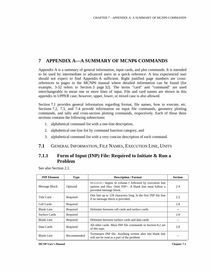
CHAPTER 7 - APPENDIX A: A SUMMARY OF MCNP6 COMMANDS
MCNP User’s Manual Chapter 7-1
7 APPENDIX A—A SUMMARY OF MCNP6 COMMANDS
Appendix A is a summary of general information, input cards, and plot commands. It is intended to be used by intermediate to advanced users as a quick reference. A less experienced user should not expect to find Appendix A sufficient. Right justified page numbers are cross-references to pages in the MCNP6 manual where detailed information can be found (for example, 3-32 refers to Section 3 page 32). The terms "card" and "command" are used interchangeably to mean one or more lines of input. File and card names are shown in this appendix in UPPER case; however, upper, lower, or mixed case is also allowed.
Section 7.1 provides general information regarding format, file names, how to execute, etc. Sections 7.2, 7.3, and 7.4 provide information on input file commands, geometry plotting commands, and tally and cross-section plotting commands, respectively. Each of these three sections contains the following subsections:
1. alphabetical command list with a one-line description,
2. alphabetical one-line list by command function category, and
3. alphabetical command list with a very concise description of each command.
7.1 GENERAL INFORMATION, FILE NAMES, EXECUTION LINE, UNITS
7.1.1 Form of Input (INP) File: Required to Initiate & Run a Problem
See also Section 2.1.
INP Element Type Description / Format Section
Message Block Optional MESSAGE: begins in column 1 followed by execution line options and files. Omit INP=. A blank line must follow a provided message block.
2.4
Title Card Required One line up to 128 characters long. Is the first INP file line if no message block is provided. 2.5
Cell Cards Required 2.8
Blank Line Required Delimiter between cell cards and surface cards. --
Surface Cards Required 2.8
Blank Line Required Delimiter between surface cards and data cards --
Data Cards Required All other cards. Most INP file commands in Section 8.2 are of this type. 2.8
Blank Line Recommended Terminates INP file. Anything written after last blank line will not be read as a part of the problem --

CHAPTER 7 - APPENDIX A: A SUMMARY OF MCNP6 COMMANDS
Chapter 7-2 MCNP User’s Manual
7.1.2 Form of CONTINUE Input File: Requires a RUNPTE File (Recap of Section 2.2.) CONTINUE and RUNTPE files are needed for continuation if the prior run finished all NPS histories or KCODE cycles. An unfinished problem requires only RUNTPE for continuation.
In a CONTINUE input file the number of histories or cycles can be increased as follows:
1. Change NPS to new total (not increment) number of histories.
2. Change the fourth KCODE card entry to new total number of cycles.
3. Change CTME to the number of additional minutes for the continue-run.
4. Use NPS=–1 to reprint the results portion of the OUTP file.
The word CONTINUE begins in column 1 of line one followed by data cards on subsequent lines. The following data cards are allowed in a continue-run after the CONTINUE line:
CTME, DBCN, DD, EMBED, FQ, IDUM, KCODE, LOST, FMESH, MESH, MPLOT, NPS, PRDMP, PRINT, RAND, RDUM, STOP, TALNP, ZA, ZB, ZC, and ZD.
A blank line terminator is recommended. Anything else can be put after the blank line terminator.
7.1.3 MCNP6 File Names and Contents (Recap of Table 1-2 of Section 1.4.1.) File path names must be ≤256 characters or ≤255 characters with the NAME option. All files can be renamed on the execute line or in the MESSAGE block except WXXA. Only enough of the default file name needs to be typed so that it is unique:
MCNP6 i=infile o=outfile mc=mcfile wwi=wwifile
MCNP6 Default File Name File Description
COM Plotter command input file name.
COMOUT Plotter command output file name.
DUMN1, DUMN2 Dummy file names 1 and 2. Used with FILE, the file creation card (See Section 3.3.7.3.6)
HISTP History tape file.
INP Original problem input file (cannot be renamed in the message block).
KSENTAL ASCII KCODE sensitivity output file.
LINKIN LNK3DNT file name to be input into MCNP6. Used with embedded structures.
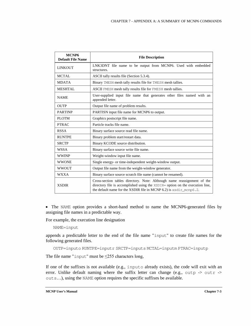
CHAPTER 7 - APPENDIX A: A SUMMARY OF MCNP6 COMMANDS
MCNP User’s Manual Chapter 7-3
MCNP6 Default File Name File Description
LINKOUT LNK3DNT file name to be output from MCNP6. Used with embedded structures.
MCTAL ASCII tally results file (Section 5.3.4).
MDATA Binary TMESH mesh tally results file for TMESH mesh tallies.
MESHTAL ASCII FMESH mesh tally results file for FMESH mesh tallies.
NAME User-supplied input file name that generates other files named with an appended letter.
OUTP Output file name of problem results.
PARTINP PARTISN input file name for MCNP6 to output.
PLOTM Graphics postscript file name.
PTRAC Particle tracks file name.
RSSA Binary surface source read file name.
RUNTPE Binary problem start/restart data.
SRCTP Binary KCODE source distribution.
WSSA Binary surface source write file name.
WWINP Weight-window input file name.
WWONE Single energy- or time-independent weight-window output.
WWOUT Output file name from the weight-window generator.
WXXA Binary surface source scratch file name (cannot be renamed).
XSDIR Cross-section tables directory. Note: Although name reassignment of the directory file is accomplished using the XSDIR= option on the execution line, the default name for the XSDIR file in MCNP 6.2) is xsdir_mcnp6.2.
• The NAME option provides a short-hand method to name the MCNP6-generated files by assigning file names in a predictable way.
For example, the execution line designation NAME=input
appends a predictable letter to the end of the file name "input" to create file names for the following generated files.
OUTP=inputo RUNTPE=inputr SRCTP=inputs MCTAL=inputm PTRAC=inputp
The file name "input" must be ≤255 characters long,
If one of the suffixes is not available (e.g., inputo already exists), the code will exit with an error. Unlike default naming where the suffix letter can change (e.g., outp -> outr -> outs…), using the NAME option requires the specific suffixes be available.
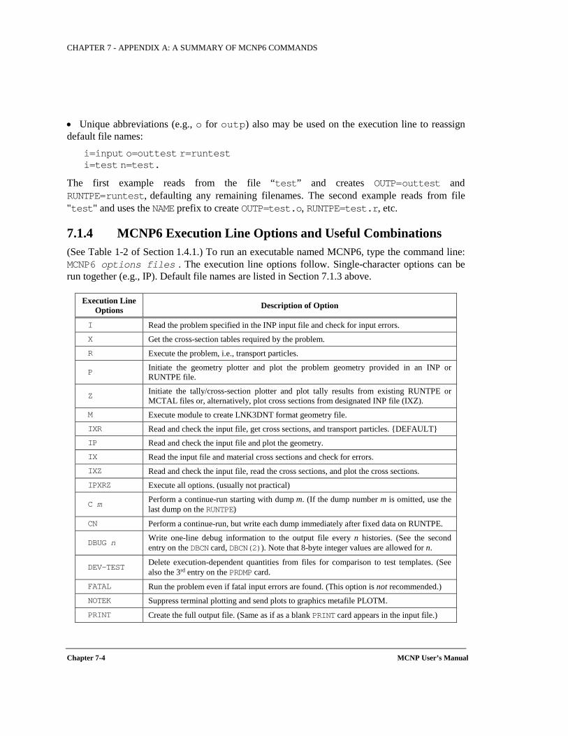
CHAPTER 7 - APPENDIX A: A SUMMARY OF MCNP6 COMMANDS
Chapter 7-4 MCNP User’s Manual
• Unique abbreviations (e.g., o for outp) also may be used on the execution line to reassign default file names:
i=input o=outtest r=runtest i=test n=test.
The first example reads from the file “test” and creates OUTP=outtest and RUNTPE=runtest, defaulting any remaining filenames. The second example reads from file "test" and uses the NAME prefix to create OUTP=test.o, RUNTPE=test.r, etc.
7.1.4 MCNP6 Execution Line Options and Useful Combinations (See Table 1-2 of Section 1.4.1.) To run an executable named MCNP6, type the command line: MCNP6 options files . The execution line options follow. Single-character options can be run together (e.g., IP). Default file names are listed in Section 7.1.3 above.
Execution Line Options Description of Option
I Read the problem specified in the INP input file and check for input errors. X Get the cross-section tables required by the problem. R Execute the problem, i.e., transport particles.
P Initiate the geometry plotter and plot the problem geometry provided in an INP or RUNTPE file.
Z Initiate the tally/cross-section plotter and plot tally results from existing RUNTPE or MCTAL files or, alternatively, plot cross sections from designated INP file (IXZ).
M Execute module to create LNK3DNT format geometry file. IXR Read and check the input file, get cross sections, and transport particles. DEFAULT IP Read and check the input file and plot the geometry. IX Read the input file and material cross sections and check for errors. IXZ Read and check the input file, read the cross sections, and plot the cross sections. IPXRZ Execute all options. (usually not practical)
C m Perform a continue-run starting with dump m. (If the dump number m is omitted, use the last dump on the RUNTPE)
CN Perform a continue-run, but write each dump immediately after fixed data on RUNTPE.
DBUG n Write one-line debug information to the output file every n histories. (See the second entry on the DBCN card, DBCN(2)). Note that 8-byte integer values are allowed for n.
DEV-TEST Delete execution-dependent quantities from files for comparison to test templates. (See also the 3rd entry on the PRDMP card.
FATAL Run the problem even if fatal input errors are found. (This option is not recommended.) NOTEK Suppress terminal plotting and send plots to graphics metafile PLOTM.
PRINT Create the full output file. (Same as if as a blank PRINT card appears in the input file.)
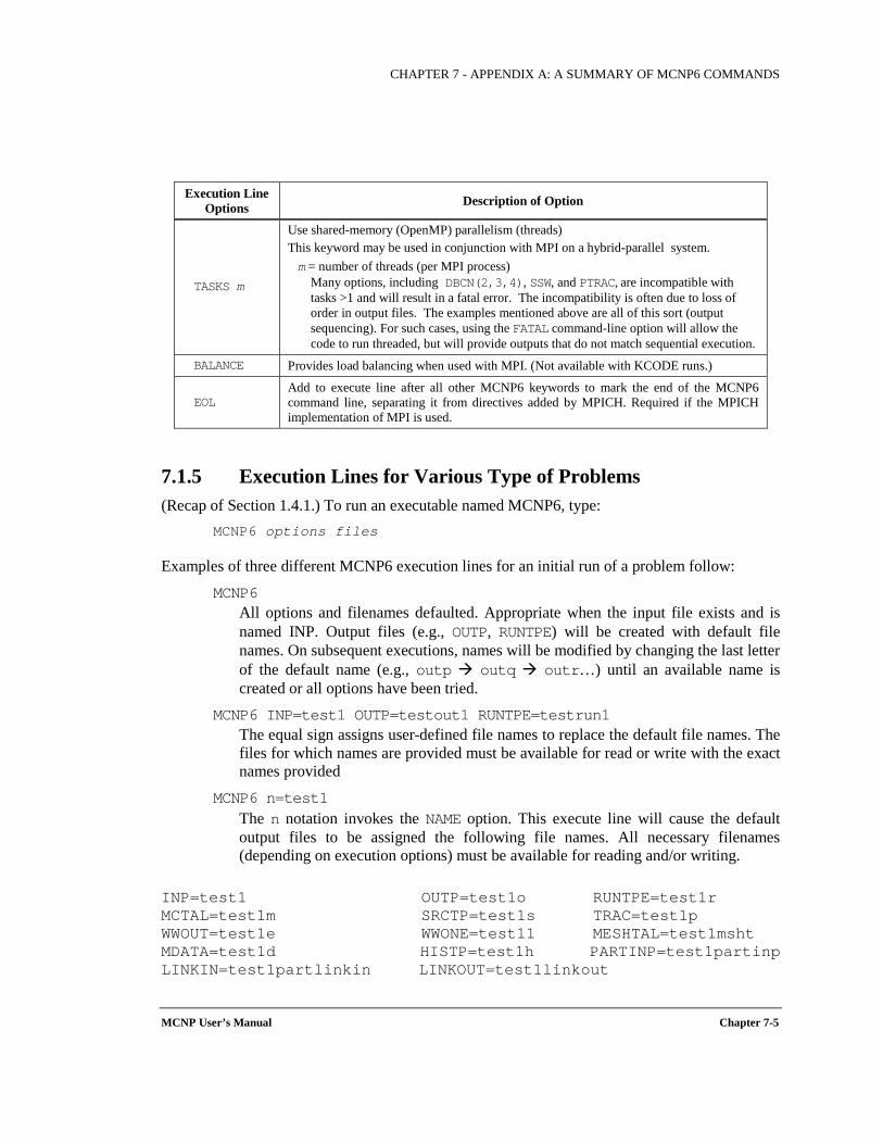
CHAPTER 7 - APPENDIX A: A SUMMARY OF MCNP6 COMMANDS
MCNP User’s Manual Chapter 7-5
Execution Line Options Description of Option
TASKS m
Use shared-memory (OpenMP) parallelism (threads) This keyword may be used in conjunction with MPI on a hybrid-parallel system. m = number of threads (per MPI process)
Many options, including DBCN(2,3,4), SSW, and PTRAC, are incompatible with tasks >1 and will result in a fatal error. The incompatibility is often due to loss of order in output files. The examples mentioned above are all of this sort (output sequencing). For such cases, using the FATAL command-line option will allow the code to run threaded, but will provide outputs that do not match sequential execution.
BALANCE Provides load balancing when used with MPI. (Not available with KCODE runs.)
EOL Add to execute line after all other MCNP6 keywords to mark the end of the MCNP6 command line, separating it from directives added by MPICH. Required if the MPICH implementation of MPI is used.
7.1.5 Execution Lines for Various Type of Problems (Recap of Section 1.4.1.) To run an executable named MCNP6, type:
MCNP6 options files
Examples of three different MCNP6 execution lines for an initial run of a problem follow:
MCNP6 All options and filenames defaulted. Appropriate when the input file exists and is named INP. Output files (e.g., OUTP, RUNTPE) will be created with default file names. On subsequent executions, names will be modified by changing the last letter of the default name (e.g., outp outq outr…) until an available name is created or all options have been tried.
MCNP6 INP=test1 OUTP=testout1 RUNTPE=testrun1 The equal sign assigns user-defined file names to replace the default file names. The files for which names are provided must be available for read or write with the exact names provided
MCNP6 n=test1 The n notation invokes the NAME option. This execute line will cause the default output files to be assigned the following file names. All necessary filenames (depending on execution options) must be available for reading and/or writing.
INP=test1 OUTP=test1o RUNTPE=test1r MCTAL=test1m SRCTP=test1s TRAC=test1p WWOUT=test1e WWONE=test11 MESHTAL=test1msht MDATA=test1d HISTP=test1h PARTINP=test1partinp LINKIN=test1partlinkin LINKOUT=test1linkout

CHAPTER 7 - APPENDIX A: A SUMMARY OF MCNP6 COMMANDS
Chapter 7-6 MCNP User’s Manual
Many command line entries can be placed, instead, in the input file within the MESSAGE BLOCK. This approach can be used to simplify the command line for problem setups with complicated options.
Continuation Runs: To continue (restart) an MCNP6 run, type: mcnp6 c run=file inp=continue_file to append to the RUNTPE file mcnp6 cn run=file inp=continue_file to begin writing after the RUNTPE fixed data
If the initial problem did not complete, a continue input file is not needed. A problem can be continued as many times as desired (see PRDMP card to control the number of dumps stored on the RUNTPE).
Geometry Plotting: To plot problem geometry, type: mcnp6 ip inp=filename ... or mcnp6 p runtpe=filename ...
Cross Section Plotting: To plot problem cross-sections, type: mcnp6 ixz inp=filename ...
Type "XS?" for cross-section plotting printer at the command prompt.
Tally Plotting: To plot problem tally results, type: mcnp6 z runtpe=filename ... or mcnp6 z mctal=mctal_filename ...
At the plotter command prompt, type "?" for a list of available plot commands. Typing "HELP <command>" will provide a description of a specific command.
7.1.6 MCNP6 Physical Units and Tally Units (See Section 2.)
Length = centimeters (cm) Temperature = MeV (kT: see TMP card) Area = cm2 Atom Density = atoms/barn-cm Volume = cm3 Heating Numbers = MeV/collision Mass = grams (g) Mass Density = g/cm3 Energy = MeV Cross Sections = barn (10-24 cm2) Time = shakes (10-8 s)
Source weight (see SDEF card, WGT entry) are in particles (pulse) or particles/unit time(steady state).
Tally units: All tallies below have additional units of “per unit source time” for steady state simulations. Units can be modified by tally multipliers. (See Section 3.3.5.7)
Type Description Units F1 current tally = particle weight (WGT) particles F2 surface flux tally = WGT / (cosine of surface crossing angle) / area particles/cm2 F4 volume flux (path length) tally = WGT * (track length) / (cell volume) particles/cm2

CHAPTER 7 - APPENDIX A: A SUMMARY OF MCNP6 COMMANDS
MCNP User’s Manual Chapter 7-7
Type Description Units F5, FIP, FIC, FIP point detector(s) = WGT * exp(-mean free paths) * p(u) / (2*π*radius2) particles/cm2
F6 heating tally = (F4 tally)*(total macro xsec) * (heating #) / (gram density) MeV/gram F7 fission heating = (F4 tally)*(total macro fission xsec)*Q/(gram density) MeV/gram F8 pulse-height tally = collective history weight deposited in the detector pulses Note: *F converts weight to energy*weight or other energy-deposition tally units
7.1.7 MCNP6 Interrupts You can send a query, request to stop or request to abort to MCNP6 during execution with the following keyboard interrupts. (See Section 1.4.2.) Press <ENTER> after each entry:
<ctrl c> problem status (run mode gives time, current history, and collisions) <ctrl c>s problem status (run mode gives time, current history, and collisions) <ctrl c>m make interactive tally plots (enter END or RETURN to return to calculation) <ctrl c>q quit and terminate gracefully after current history <ctrl c>k kill immediately (all files created for the problem are incomplete)
Note that these interrupts do not work with MPI-enabled compilations. This is because MPI catches the interrupts and (usually) aborts ungracefully upon any <ctrl c>. Interrupts may also not work as specified on non-Linux operating systems.
7.1.8 Example of an MCNP6 Fixed-Source INP File Steps to Run a Fixed-Source MCNP6 Problem Section
Fixed source requires: SDEF, SSR (with RSSA file), or user-defined source subroutine. 3.3.4
Always plot the geometry and inspect OUTP file cell volumes and masses. 1.5.1
Use tips in manual for correct and efficient problems. 1.5
Inspect ten statistical check results for tally fluctuation chart bin (see TFn card). 3.3.5.19
Form valid statistical confidence intervals for result precision using statistical checks. 3.3.5
Example: The following is an INP file for a Cf-252 SDEF fixed point source in a water cylinder. This example has no MESSAGE block:
point Cf-252 fission source in a cylinder of water (required title card) c begin cell cards for fixed source sample problem 1 1 -1. -1 -2 3 $ cylinder of water 2 0 1:2:-3 $ all space outside the cylinder c end cell cards; next line is required blank line delimiter
c begin surface specifications after blank line delimiter 1 cy 20. $ cylinder about the y axis 2 py 10. $ top plane of water cylinder 3 py -10. $ bottom plane of water cylinder
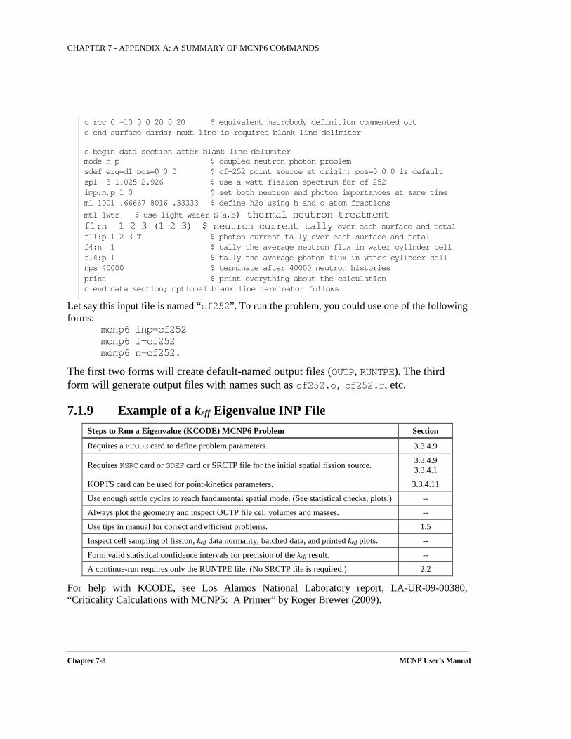
CHAPTER 7 - APPENDIX A: A SUMMARY OF MCNP6 COMMANDS
Chapter 7-8 MCNP User’s Manual
c rcc 0 –10 0 0 20 0 20 $ equivalent macrobody definition commented out c end surface cards; next line is required blank line delimiter c begin data section after blank line delimiter mode n p $ coupled neutron-photon problem sdef erg=d1 pos=0 0 0 $ cf-252 point source at origin; pos=0 0 0 is default sp1 -3 1.025 2.926 $ use a watt fission spectrum for cf-252 imp:n,p 1 0 $ set both neutron and photon importances at same time m1 1001 .66667 8016 .33333 $ define h2o using h and o atom fractions
mt1 lwtr $ use light water S(a,b) thermal neutron treatment f1:n 1 2 3 (1 2 3) $ neutron current tally over each surface and total f11:p 1 2 3 T $ photon current tally over each surface and total f4:n 1 $ tally the average neutron flux in water cylinder cell f14:p 1 $ tally the average photon flux in water cylinder cell nps 40000 $ terminate after 40000 neutron histories print $ print everything about the calculation c end data section; optional blank line terminator follows
Let say this input file is named “cf252”. To run the problem, you could use one of the following forms: mcnp6 inp=cf252 mcnp6 i=cf252 mcnp6 n=cf252.
The first two forms will create default-named output files (OUTP, RUNTPE). The third form will generate output files with names such as cf252.o, cf252.r, etc.
7.1.9 Example of a keff Eigenvalue INP File Steps to Run a Eigenvalue (KCODE) MCNP6 Problem Section
Requires a KCODE card to define problem parameters. 3.3.4.9
Requires KSRC card or SDEF card or SRCTP file for the initial spatial fission source. 3.3.4.9 3.3.4.1
KOPTS card can be used for point-kinetics parameters. 3.3.4.11
Use enough settle cycles to reach fundamental spatial mode. (See statistical checks, plots.) --
Always plot the geometry and inspect OUTP file cell volumes and masses. --
Use tips in manual for correct and efficient problems. 1.5
Inspect cell sampling of fission, keff data normality, batched data, and printed keff plots. --
Form valid statistical confidence intervals for precision of the keff result. --
A continue-run requires only the RUNTPE file. (No SRCTP file is required.) 2.2
For help with KCODE, see Los Alamos National Laboratory report, LA-UR-09-00380, “Criticality Calculations with MCNP5: A Primer” by Roger Brewer (2009).
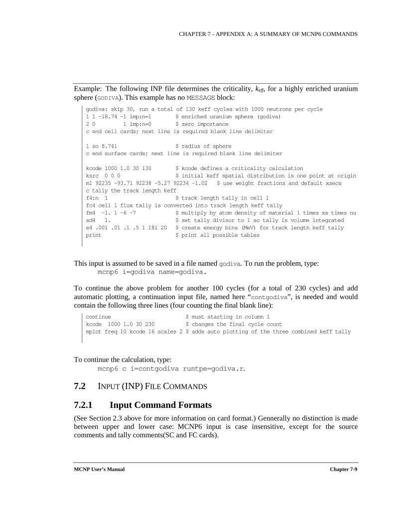
CHAPTER 7 - APPENDIX A: A SUMMARY OF MCNP6 COMMANDS
MCNP User’s Manual Chapter 7-9
Example: The following INP file determines the criticality, keff, for a highly enriched uranium sphere (GODIVA). This example has no MESSAGE block:
godiva: skip 30, run a total of 130 keff cycles with 1000 neutrons per cycle 1 1 -18.74 -1 imp:n=1 $ enriched uranium sphere (godiva) 2 0 1 imp:n=0 $ zero importance c end cell cards; next line is required blank line delimiter
1 so 8.741 $ radius of sphere c end surface cards; next line is required blank line delimiter
kcode 1000 1.0 30 130 $ kcode defines a criticality calculation ksrc 0 0 0 $ initial keff spatial distribution is one point at origin m1 92235 -93.71 92238 -5.27 92234 -1.02 $ use weight fractions and default xsecs c tally the track length keff f4:n 1 $ track length tally in cell 1 fc4 cell 1 flux tally is converted into track length keff tally fm4 -1. 1 -6 -7 $ multiply by atom density of material 1 times xs times nu sd4 1. $ set tally divisor to 1 so tally is volume integrated e4 .001 .01 .1 .5 1 18i 20 $ create energy bins (MeV) for track length keff tally print $ print all possible tables
This input is assumed to be saved in a file named godiva. To run the problem, type: mcnp6 i=godiva name=godiva.
To continue the above problem for another 100 cycles (for a total of 230 cycles) and add automatic plotting, a continuation input file, named here “contgodiva”, is needed and would contain the following three lines (four counting the final blank line):
continue $ must starting in column 1 kcode 1000 1.0 30 230 $ changes the final cycle count mplot freq 10 kcode 16 scales 2 $ adds auto plotting of the three combined keff tally
To continue the calculation, type: mcnp6 c i=contgodiva runtpe=godiva.r.
7.2 INPUT (INP) FILE COMMANDS
7.2.1 Input Command Formats (See Section 2.3 above for more information on card format.) Gennerally no distinction is made between upper and lower case: MCNP6 input is case insensitive, except for the source comments and tally comments(SC and FC cards).
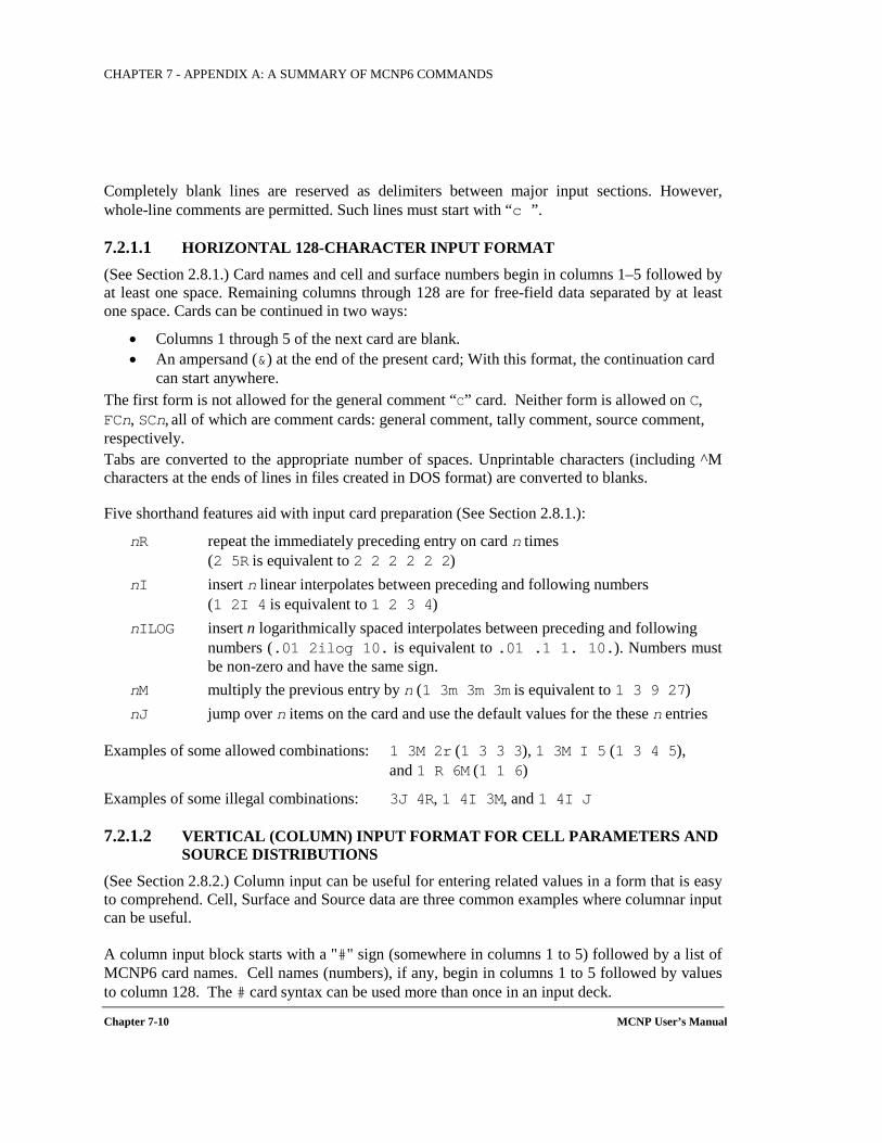
CHAPTER 7 - APPENDIX A: A SUMMARY OF MCNP6 COMMANDS
Chapter 7-10 MCNP User’s Manual
Completely blank lines are reserved as delimiters between major input sections. However, whole-line comments are permitted. Such lines must start with “c ”.
7.2.1.1 HORIZONTAL 128-CHARACTER INPUT FORMAT
(See Section 2.8.1.) Card names and cell and surface numbers begin in columns 1–5 followed by at least one space. Remaining columns through 128 are for free-field data separated by at least one space. Cards can be continued in two ways:
• Columns 1 through 5 of the next card are blank. • An ampersand (&) at the end of the present card; With this format, the continuation card
can start anywhere. The first form is not allowed for the general comment “C” card. Neither form is allowed on C, FCn, SCn, all of which are comment cards: general comment, tally comment, source comment, respectively. Tabs are converted to the appropriate number of spaces. Unprintable characters (including ^M characters at the ends of lines in files created in DOS format) are converted to blanks.
Five shorthand features aid with input card preparation (See Section 2.8.1.):
nR repeat the immediately preceding entry on card n times (2 5R is equivalent to 2 2 2 2 2 2) nI insert n linear interpolates between preceding and following numbers (1 2I 4 is equivalent to 1 2 3 4) nILOG insert n logarithmically spaced interpolates between preceding and following numbers (.01 2ilog 10. is equivalent to .01 .1 1. 10.). Numbers must
be non-zero and have the same sign. nM multiply the previous entry by n (1 3m 3m 3m is equivalent to 1 3 9 27) nJ jump over n items on the card and use the default values for the these n entries
Examples of some allowed combinations: 1 3M 2r (1 3 3 3), 1 3M I 5 (1 3 4 5), and 1 R 6M (1 1 6)
Examples of some illegal combinations: 3J 4R, 1 4I 3M, and 1 4I J
7.2.1.2 VERTICAL (COLUMN) INPUT FORMAT FOR CELL PARAMETERS AND SOURCE DISTRIBUTIONS
(See Section 2.8.2.) Column input can be useful for entering related values in a form that is easy to comprehend. Cell, Surface and Source data are three common examples where columnar input can be useful.
A column input block starts with a "#" sign (somewhere in columns 1 to 5) followed by a list of MCNP6 card names. Cell names (numbers), if any, begin in columns 1 to 5 followed by values to column 128. The # card syntax can be used more than once in an input deck.
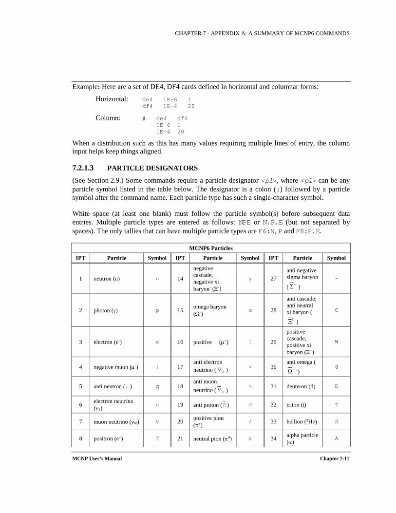
CHAPTER 7 - APPENDIX A: A SUMMARY OF MCNP6 COMMANDS
MCNP User’s Manual Chapter 7-11
Example: Here are a set of DE4, DF4 cards defined in horizontal and columnar forms:
Horizontal: de4 1E-6 1 df4 1E-4 20
Column: # de4 df4 1E-6 1 1E-4 20
When a distribution such as this has many values requiring multiple lines of entry, the column input helps keep things aligned.
7.2.1.3 PARTICLE DESIGNATORS
(See Section 2.9.) Some commands require a particle designator <pl>, where <pl> can be any particle symbol listed in the table below. The designator is a colon (:) followed by a particle symbol after the command name. Each particle type has such a single-character symbol.
White space (at least one blank) must follow the particle symbol(s) before subsequent data entries. Multiple particle types are entered as follows: NPE or N,P,E (but not separated by spaces). The only tallies that can have multiple particle types are F6:N,P and F8:P,E.
MCNP6 Particles
IPT Particle Symbol IPT Particle Symbol IPT Particle Symbol
1 neutron (n) n 14
negative cascade; negative xi baryon- (Ξ-)
y 27 anti negative sigma baryon
( ) ~
2 photon (γ) p 15 omega baryon (Ω-)
o 28
anti cascade; anti neutral xi baryon (
)
C
3 electron (e-) e 16 positive (µ+) ! 29
positive cascade; positive xi baryon (Ξ+)
W
4 negative muon (µ-) | 17 anti electron neutrino ( ) < 30
anti omega (-)
@
5 anti neutron ( ) q 18 anti muon neutrino ( )
> 31 deuteron (d) D
6 electron neutrino (νe)
u 19 anti proton ( ) g 32 triton (t) T
7 muon neutrino (νm) v 20 positive pion (π+)
/ 33 hellion (3He) S
8 positron (e+) f 21 neutral pion (π0) z 34 alpha particle (α)
A
−Σ
0Ξ
eν −Ω
nmν
p
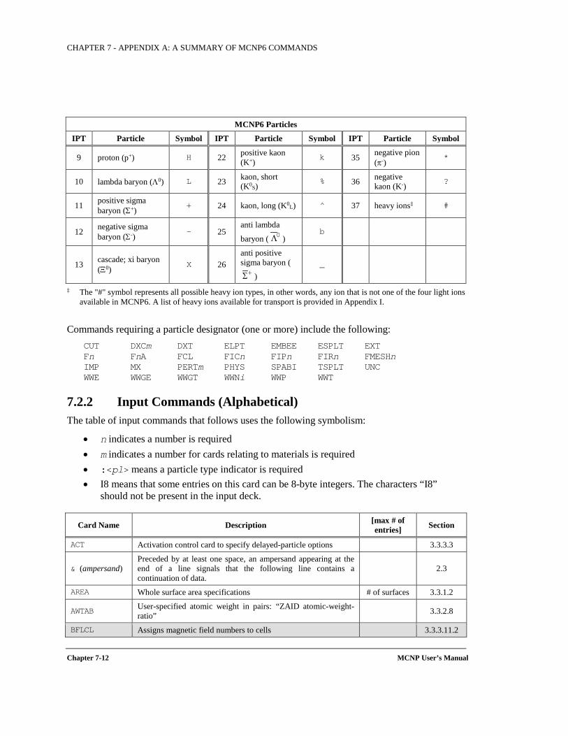
CHAPTER 7 - APPENDIX A: A SUMMARY OF MCNP6 COMMANDS
Chapter 7-12 MCNP User’s Manual
MCNP6 Particles
IPT Particle Symbol IPT Particle Symbol IPT Particle Symbol
9 proton (p+) H 22 positive kaon (K+) k 35 negative pion
(π-) *
10 lambda baryon (Λ0) L 23 kaon, short (K0S) % 36 negative
kaon (K-) ?
11 positive sigma baryon (Σ+) + 24 kaon, long (K0L) ^ 37 heavy ions‡ #
12 negative sigma baryon (Σ-)
- 25 anti lambda
baryon ( ) b
13 cascade; xi baryon (Ξ0) X 26
anti positive sigma baryon (
) _
‡ The "#" symbol represents all possible heavy ion types, in other words, any ion that is not one of the four light ions available in MCNP6. A list of heavy ions available for transport is provided in Appendix I.
Commands requiring a particle designator (one or more) include the following: CUT DXCm DXT ELPT EMBEE ESPLT EXT Fn FnA FCL FICn FIPn FIRn FMESHn IMP MX PERTm PHYS SPABI TSPLT UNC WWE WWGE WWGT WWNi WWP WWT
7.2.2 Input Commands (Alphabetical) The table of input commands that follows uses the following symbolism:
• n indicates a number is required • m indicates a number for cards relating to materials is required • :<pl> means a particle type indicator is required • I8 means that some entries on this card can be 8-byte integers. The characters “I8”
should not be present in the input deck.
Card Name Description [max # of entries] Section
ACT Activation control card to specify delayed-particle options 3.3.3.3
& (ampersand) Preceded by at least one space, an ampersand appearing at the end of a line signals that the following line contains a continuation of data.
2.3
AREA Whole surface area specifications # of surfaces 3.3.1.2
AWTAB User-specified atomic weight in pairs: “ZAID atomic-weight-ratio” 3.3.2.8
BFLCL Assigns magnetic field numbers to cells 3.3.3.11.2
0Λ
+Σ
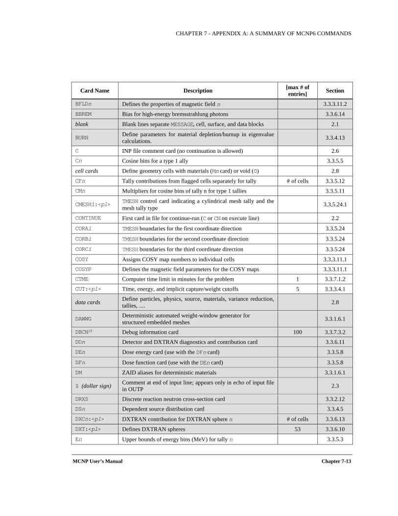
CHAPTER 7 - APPENDIX A: A SUMMARY OF MCNP6 COMMANDS
MCNP User’s Manual Chapter 7-13
Card Name Description [max # of entries] Section
BFLDn Defines the properties of magnetic field n 3.3.3.11.2
BBREM Bias for high-energy bremsstrahlung photons 3.3.6.14
blank Blank lines separate MESSAGE, cell, surface, and data blocks 2.1
BURN Define parameters for material depletion/burnup in eigenvalue calculations. 3.3.4.13
C INP file comment card (no continuation is allowed) 2.6 Cn Cosine bins for a type 1 ally 3.3.5.5
cell cards Define geometry cells with materials (Mm card) or void (0) 2.8
CFn Tally contributions from flagged cells separately for tally # of cells 3.3.5.12 CMn Multipliers for cosine bins of tally n for type 1 tallies 3.3.5.11
CMESHi:<pl> TMESH control card indicating a cylindrical mesh tally and the mesh tally type 3.3.5.24.1
CONTINUE First card in file for continue-run (C or CN on execute line) 2.2
CORAi TMESH boundaries for the first coordinate direction 3.3.5.24
CORBi TMESH boundaries for the second coordinate direction 3.3.5.24
CORCi TMESH boundaries for the third coordinate direction 3.3.5.24
COSY Assigns COSY map numbers to individual cells 3.3.3.11.1 COSYP Defines the magnetic field parameters for the COSY maps 3.3.3.11.1 CTME Computer time limit in minutes for the problem 1 3.3.7.1.2 CUT:<pl> Time, energy, and implicit capture/weight cutoffs 5 3.3.3.4.1
data cards Define particles, physics, source, materials, variance reduction, tallies, .... 2.8
DAWWG Deterministic automated weight-window generator for structured embedded meshes 3.3.1.6.1
DBCNI8 Debug information card 100 3.3.7.3.2 DDn Detector and DXTRAN diagnostics and contribution card 3.3.6.11
DEn Dose energy card (use with the DFn card) 3.3.5.8
DFn Dose function card (use with the DEn card) 3.3.5.8
DM ZAID aliases for deterministic materials 3.3.1.6.1
$ (dollar sign) Comment at end of input line; appears only in echo of input file in OUTP 2.3
DRXS Discrete reaction neutron cross-section card 3.3.2.12 DSn Dependent source distribution card 3.3.4.5
DXCn:<pl> DXTRAN contribution for DXTRAN sphere n # of cells 3.3.6.13
DXT:<pl> Defines DXTRAN spheres 53 3.3.6.10
En Upper bounds of energy bins (MeV) for tally n 3.3.5.3
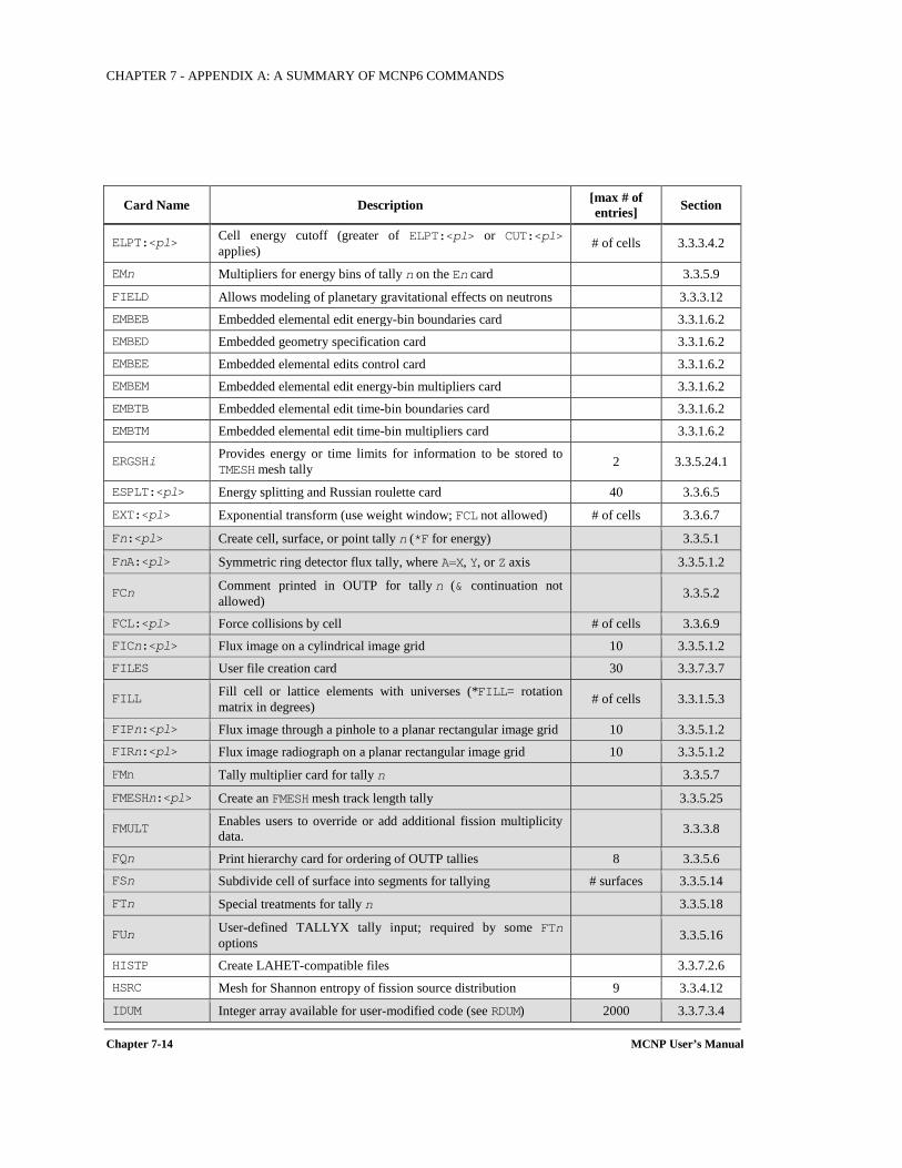
CHAPTER 7 - APPENDIX A: A SUMMARY OF MCNP6 COMMANDS
Chapter 7-14 MCNP User’s Manual
Card Name Description [max # of entries] Section
ELPT:<pl> Cell energy cutoff (greater of ELPT:<pl> or CUT:<pl> applies) # of cells 3.3.3.4.2
EMn Multipliers for energy bins of tally n on the En card 3.3.5.9
FIELD Allows modeling of planetary gravitational effects on neutrons 3.3.3.12 EMBEB Embedded elemental edit energy-bin boundaries card 3.3.1.6.2 EMBED Embedded geometry specification card 3.3.1.6.2 EMBEE Embedded elemental edits control card 3.3.1.6.2 EMBEM Embedded elemental edit energy-bin multipliers card 3.3.1.6.2 EMBTB Embedded elemental edit time-bin boundaries card 3.3.1.6.2 EMBTM Embedded elemental edit time-bin multipliers card 3.3.1.6.2
ERGSHi Provides energy or time limits for information to be stored to TMESH mesh tally 2 3.3.5.24.1
ESPLT:<pl> Energy splitting and Russian roulette card 40 3.3.6.5
EXT:<pl> Exponential transform (use weight window; FCL not allowed) # of cells 3.3.6.7
Fn:<pl> Create cell, surface, or point tally n (*F for energy) 3.3.5.1
FnA:<pl> Symmetric ring detector flux tally, where A=X, Y, or Z axis 3.3.5.1.2
FCn Comment printed in OUTP for tally n (& continuation not allowed) 3.3.5.2
FCL:<pl> Force collisions by cell # of cells 3.3.6.9 FICn:<pl> Flux image on a cylindrical image grid 10 3.3.5.1.2 FILES User file creation card 30 3.3.7.3.7
FILL Fill cell or lattice elements with universes (*FILL= rotation matrix in degrees) # of cells 3.3.1.5.3
FIPn:<pl> Flux image through a pinhole to a planar rectangular image grid 10 3.3.5.1.2 FIRn:<pl> Flux image radiograph on a planar rectangular image grid 10 3.3.5.1.2
FMn Tally multiplier card for tally n 3.3.5.7
FMESHn:<pl> Create an FMESH mesh track length tally 3.3.5.25
FMULT Enables users to override or add additional fission multiplicity data. 3.3.3.8
FQn Print hierarchy card for ordering of OUTP tallies 8 3.3.5.6 FSn Subdivide cell of surface into segments for tallying # surfaces 3.3.5.14
FTn Special treatments for tally n 3.3.5.18
FUn User-defined TALLYX tally input; required by some FTn options 3.3.5.16
HISTP Create LAHET-compatible files 3.3.7.2.6 HSRC Mesh for Shannon entropy of fission source distribution 9 3.3.4.12
IDUM Integer array available for user-modified code (see RDUM) 2000 3.3.7.3.4
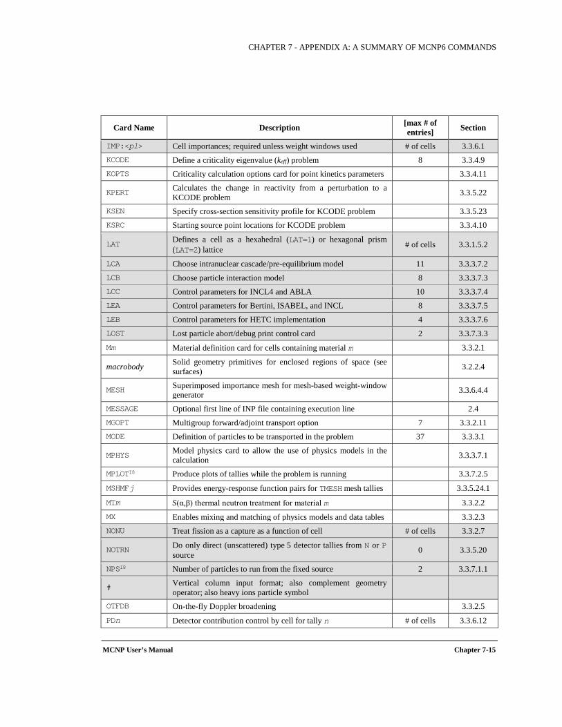
CHAPTER 7 - APPENDIX A: A SUMMARY OF MCNP6 COMMANDS
MCNP User’s Manual Chapter 7-15
Card Name Description [max # of entries] Section
IMP:<pl> Cell importances; required unless weight windows used # of cells 3.3.6.1 KCODE Define a criticality eigenvalue (keff) problem 8 3.3.4.9 KOPTS Criticality calculation options card for point kinetics parameters 3.3.4.11
KPERT Calculates the change in reactivity from a perturbation to a KCODE problem 3.3.5.22
KSEN Specify cross-section sensitivity profile for KCODE problem 3.3.5.23 KSRC Starting source point locations for KCODE problem 3.3.4.10
LAT Defines a cell as a hexahedral (LAT=1) or hexagonal prism (LAT=2) lattice # of cells 3.3.1.5.2
LCA Choose intranuclear cascade/pre-equilibrium model 11 3.3.3.7.2 LCB Choose particle interaction model 8 3.3.3.7.3 LCC Control parameters for INCL4 and ABLA 10 3.3.3.7.4 LEA Control parameters for Bertini, ISABEL, and INCL 8 3.3.3.7.5 LEB Control parameters for HETC implementation 4 3.3.3.7.6 LOST Lost particle abort/debug print control card 2 3.3.7.3.3
Mm Material definition card for cells containing material m 3.3.2.1
macrobody Solid geometry primitives for enclosed regions of space (see surfaces) 3.2.2.4
MESH Superimposed importance mesh for mesh-based weight-window generator 3.3.6.4.4
MESSAGE Optional first line of INP file containing execution line 2.4 MGOPT Multigroup forward/adjoint transport option 7 3.3.2.11 MODE Definition of particles to be transported in the problem 37 3.3.3.1
MPHYS Model physics card to allow the use of physics models in the calculation 3.3.3.7.1
MPLOTI8 Produce plots of tallies while the problem is running 3.3.7.2.5
MSHMFj Provides energy-response function pairs for TMESH mesh tallies 3.3.5.24.1
MTm S(α,β) thermal neutron treatment for material m 3.3.2.2
MX Enables mixing and matching of physics models and data tables 3.3.2.3 NONU Treat fission as a capture as a function of cell # of cells 3.3.2.7
NOTRN Do only direct (unscattered) type 5 detector tallies from N or P source 0 3.3.5.20
NPSI8 Number of particles to run from the fixed source 2 3.3.7.1.1
# Vertical column input format; also complement geometry operator; also heavy ions particle symbol
OTFDB On-the-fly Doppler broadening 3.3.2.5
PDn Detector contribution control by cell for tally n # of cells 3.3.6.12
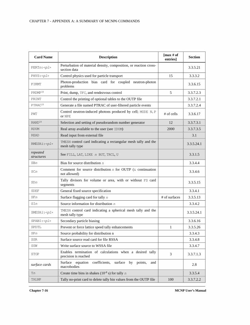
CHAPTER 7 - APPENDIX A: A SUMMARY OF MCNP6 COMMANDS
Chapter 7-16 MCNP User’s Manual
Card Name Description [max # of entries] Section
PERTn:<pl> Perturbation of material density, composition, or reaction cross-section data 3.3.5.21
PHYS:<pl> Control physics used for particle transport 15 3.3.3.2
PIKMT Photon-production bias card for coupled neutron-photon problems 3.3.6.15
PRDMPI8 Print, dump, TFC, and rendezvous control 5 3.3.7.2.3
PRINT Control the printing of optional tables to the OUTP file 3.3.7.2.1 PTRACI8 Generate a file named PTRAC of user-filtered particle events 3.3.7.2.4
PWT Control neutron-induced photons produced by cell; MODE N,P or NPE # of cells 3.3.6.17
RANDI8 Selection and setting of pseudorandom number generator 12 3.3.7.3.1
RDUM Real array available to the user (see IDUM) 2000 3.3.7.3.5
READ Read input from external file 3.1
RMESHi:<pl> TMESH control card indicating a rectangular mesh tally and the mesh tally type 3.3.5.24.1
repeated structures See FILL, LAT, LIKE n BUT, TRCL, U 3.3.1.5
SBn Bias for source distribution n 3.3.4.4
SCn Comment for source distribution n for OUTP (& continuation not allowed) 3.3.4.6
SDn Tally divisors for volume or area, with or without FS card segments 3.3.5.15
SDEF General fixed source specification 3.3.4.1
SFn Surface flagging card for tally n # of surfaces 3.3.5.13
SIn Source information for distribution n 3.3.4.2
SMESHi:<pl> TMESH control card indicating a spherical mesh tally and the mesh tally type 3.3.5.24.1
SPABI:<pl> Secondary particle biasing 3.3.6.16 SPDTL Prevent or force lattice speed tally enhancements 1 3.3.5.26 SPn Source probability for distribution n 3.3.4.3 SSR Surface source read card for file RSSA 3.3.4.8 SSW Write surface source to WSSA file 3.3.4.7
STOP Enables termination of calculations when a desired tally precision is reached 3 3.3.7.1.3
surface cards Surface equation coefficients, surface by points, and macrobodies 2.8
Tn Create time bins in shakes (10-8 s) for tally n 3.3.5.4
TALNP Tally no-print card to delete tally bin values from the OUTP file 100 3.3.7.2.2
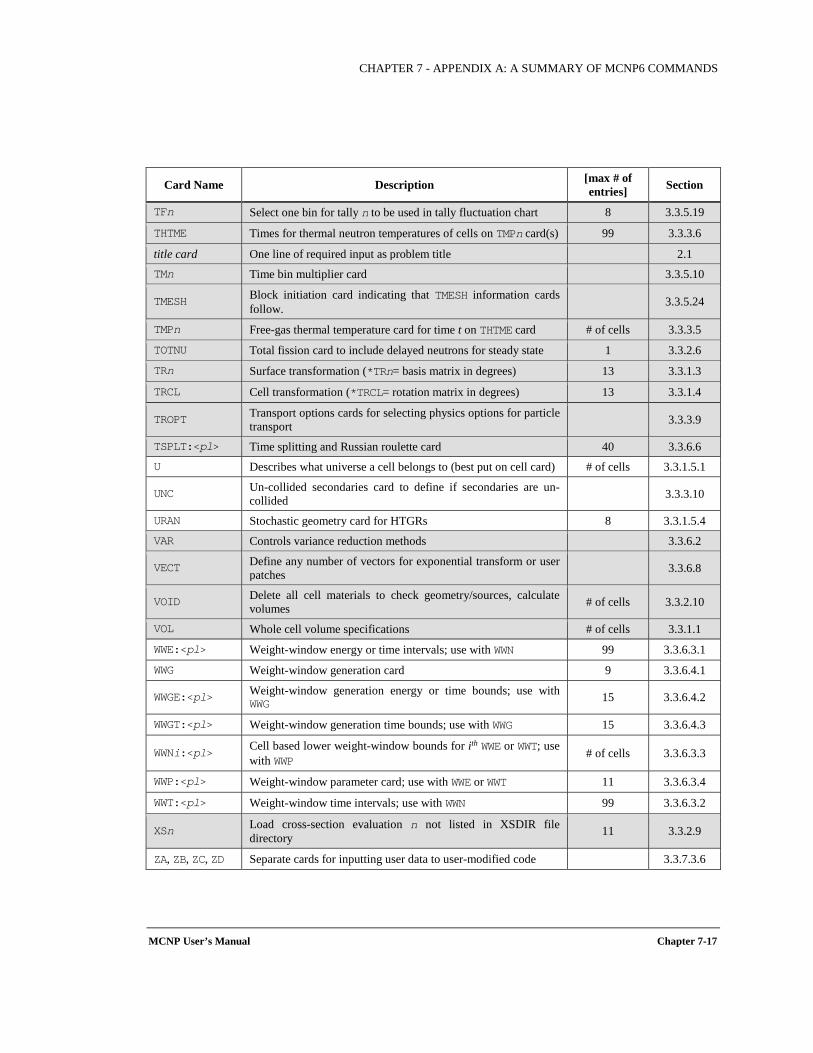
CHAPTER 7 - APPENDIX A: A SUMMARY OF MCNP6 COMMANDS
MCNP User’s Manual Chapter 7-17
Card Name Description [max # of entries] Section
TFn Select one bin for tally n to be used in tally fluctuation chart 8 3.3.5.19
THTME Times for thermal neutron temperatures of cells on TMPn card(s) 99 3.3.3.6
title card One line of required input as problem title 2.1 TMn Time bin multiplier card 3.3.5.10
TMESH Block initiation card indicating that TMESH information cards follow. 3.3.5.24
TMPn Free-gas thermal temperature card for time t on THTME card # of cells 3.3.3.5
TOTNU Total fission card to include delayed neutrons for steady state 1 3.3.2.6
TRn Surface transformation (*TRn= basis matrix in degrees) 13 3.3.1.3
TRCL Cell transformation (*TRCL= rotation matrix in degrees) 13 3.3.1.4
TROPT Transport options cards for selecting physics options for particle transport 3.3.3.9
TSPLT:<pl> Time splitting and Russian roulette card 40 3.3.6.6 U Describes what universe a cell belongs to (best put on cell card) # of cells 3.3.1.5.1
UNC Un-collided secondaries card to define if secondaries are un-collided 3.3.3.10
URAN Stochastic geometry card for HTGRs 8 3.3.1.5.4 VAR Controls variance reduction methods 3.3.6.2
VECT Define any number of vectors for exponential transform or user patches 3.3.6.8
VOID Delete all cell materials to check geometry/sources, calculate volumes # of cells 3.3.2.10
VOL Whole cell volume specifications # of cells 3.3.1.1
WWE:<pl> Weight-window energy or time intervals; use with WWN 99 3.3.6.3.1
WWG Weight-window generation card 9 3.3.6.4.1
WWGE:<pl> Weight-window generation energy or time bounds; use with WWG 15 3.3.6.4.2
WWGT:<pl> Weight-window generation time bounds; use with WWG 15 3.3.6.4.3
WWNi:<pl> Cell based lower weight-window bounds for ith WWE or WWT; use with WWP # of cells 3.3.6.3.3
WWP:<pl> Weight-window parameter card; use with WWE or WWT 11 3.3.6.3.4
WWT:<pl> Weight-window time intervals; use with WWN 99 3.3.6.3.2
XSn Load cross-section evaluation n not listed in XSDIR file directory 11 3.3.2.9
ZA, ZB, ZC, ZD Separate cards for inputting user data to user-modified code 3.3.7.3.6
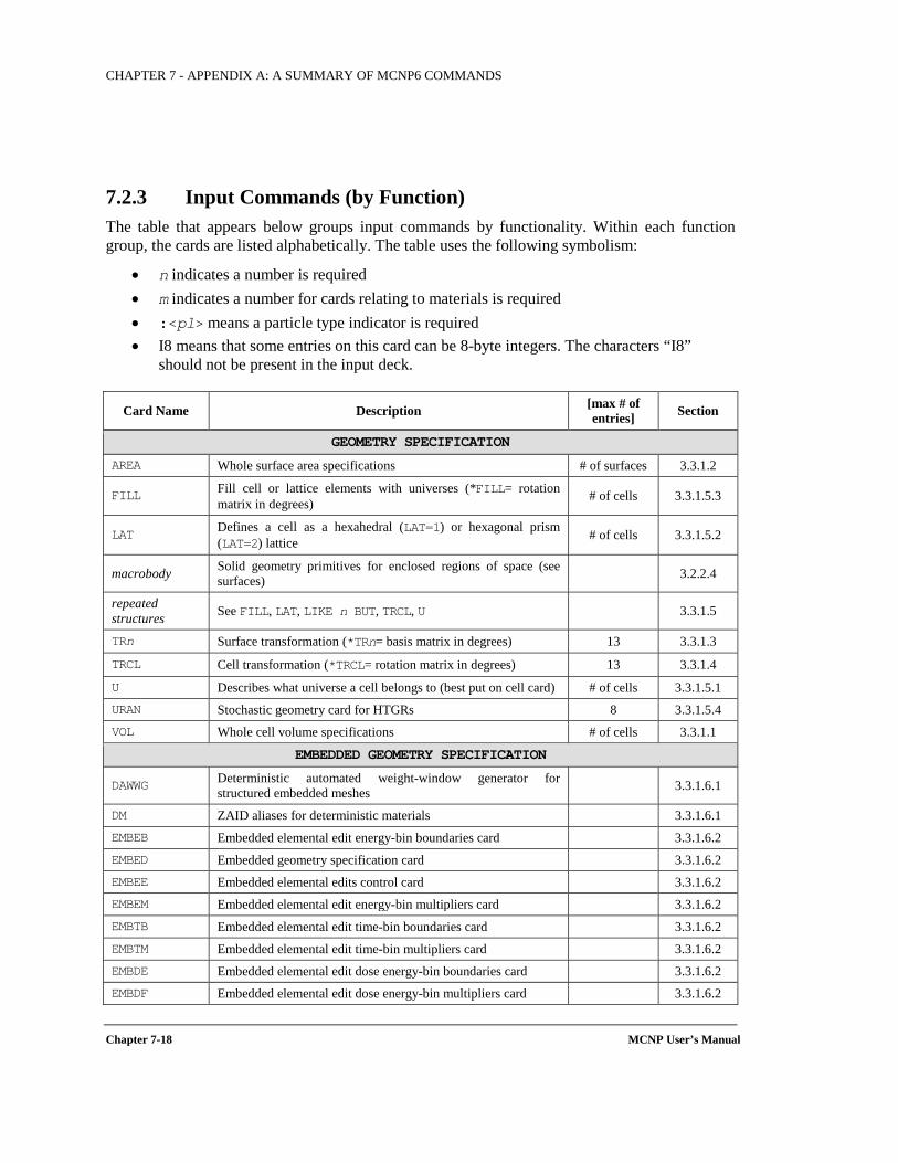
CHAPTER 7 - APPENDIX A: A SUMMARY OF MCNP6 COMMANDS
Chapter 7-18 MCNP User’s Manual
7.2.3 Input Commands (by Function) The table that appears below groups input commands by functionality. Within each function group, the cards are listed alphabetically. The table uses the following symbolism:
• n indicates a number is required • m indicates a number for cards relating to materials is required • :<pl> means a particle type indicator is required • I8 means that some entries on this card can be 8-byte integers. The characters “I8”
should not be present in the input deck.
Card Name Description [max # of entries] Section
GEOMETRY SPECIFICATION AREA Whole surface area specifications # of surfaces 3.3.1.2
FILL Fill cell or lattice elements with universes (*FILL= rotation matrix in degrees) # of cells 3.3.1.5.3
LAT Defines a cell as a hexahedral (LAT=1) or hexagonal prism (LAT=2) lattice # of cells 3.3.1.5.2
macrobody Solid geometry primitives for enclosed regions of space (see surfaces) 3.2.2.4
repeated structures See FILL, LAT, LIKE n BUT, TRCL, U 3.3.1.5
TRn Surface transformation (*TRn= basis matrix in degrees) 13 3.3.1.3
TRCL Cell transformation (*TRCL= rotation matrix in degrees) 13 3.3.1.4
U Describes what universe a cell belongs to (best put on cell card) # of cells 3.3.1.5.1 URAN Stochastic geometry card for HTGRs 8 3.3.1.5.4 VOL Whole cell volume specifications # of cells 3.3.1.1
EMBEDDED GEOMETRY SPECIFICATION
DAWWG Deterministic automated weight-window generator for structured embedded meshes 3.3.1.6.1
DM ZAID aliases for deterministic materials 3.3.1.6.1 EMBEB Embedded elemental edit energy-bin boundaries card 3.3.1.6.2 EMBED Embedded geometry specification card 3.3.1.6.2 EMBEE Embedded elemental edits control card 3.3.1.6.2 EMBEM Embedded elemental edit energy-bin multipliers card 3.3.1.6.2 EMBTB Embedded elemental edit time-bin boundaries card 3.3.1.6.2 EMBTM Embedded elemental edit time-bin multipliers card 3.3.1.6.2 EMBDE Embedded elemental edit dose energy-bin boundaries card 3.3.1.6.2 EMBDF Embedded elemental edit dose energy-bin multipliers card 3.3.1.6.2
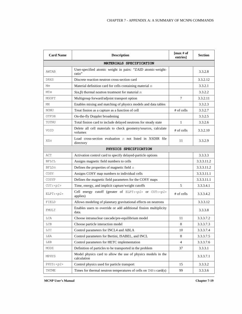
CHAPTER 7 - APPENDIX A: A SUMMARY OF MCNP6 COMMANDS
MCNP User’s Manual Chapter 7-19
Card Name Description [max # of entries] Section
MATERIALS SPECIFICATION
AWTAB User-specified atomic weight in pairs: “ZAID atomic-weight-ratio” 3.3.2.8
DRXS Discrete reaction neutron cross-section card 3.3.2.12
Mm Material definition card for cells containing material m 3.3.2.1
MTm S(α,β) thermal neutron treatment for material m 3.3.2.2
MGOPT Multigroup forward/adjoint transport option 7 3.3.2.11 MX Enables mixing and matching of physics models and data tables 3.3.2.3 NONU Treat fission as a capture as a function of cell # of cells 3.3.2.7 OTFDB On-the-fly Doppler broadening 3.3.2.5 TOTNU Total fission card to include delayed neutrons for steady state 1 3.3.2.6
VOID Delete all cell materials to check geometry/sources, calculate volumes # of cells 3.3.2.10
XSn Load cross-section evaluation n not listed in XSDIR file directory 11 3.3.2.9
PHYSICS SPECIFICATION ACT Activation control card to specify delayed-particle options 3.3.3.3 BFLCL Assigns magnetic field numbers to cells 3.3.3.11.2
BFLDn Defines the properties of magnetic field n 3.3.3.11.2
COSY Assigns COSY map numbers to individual cells 3.3.3.11.1 COSYP Defines the magnetic field parameters for the COSY maps 3.3.3.11.1 CUT:<pl> Time, energy, and implicit capture/weight cutoffs 5 3.3.3.4.1
ELPT:<pl> Cell energy cutoff (greater of ELPT:<pl> or CUT:<pl> applies) # of cells 3.3.3.4.2
FIELD Allows modeling of planetary gravitational effects on neutrons 3.3.3.12
FMULT Enables users to override or add additional fission multiplicity data. 3.3.3.8
LCA Choose intranuclear cascade/pre-equilibrium model 11 3.3.3.7.2 LCB Choose particle interaction model 8 3.3.3.7.3 LCC Control parameters for INCL4 and ABLA 10 3.3.3.7.4 LEA Control parameters for Bertini, ISABEL, and INCL 8 3.3.3.7.5 LEB Control parameters for HETC implementation 4 3.3.3.7.6 MODE Definition of particles to be transported in the problem 37 3.3.3.1
MPHYS Model physics card to allow the use of physics models in the calculation 3.3.3.7.1
PHYS:<pl> Control physics used for particle transport 15 3.3.3.2
THTME Times for thermal neutron temperatures of cells on TMPn card(s) 99 3.3.3.6
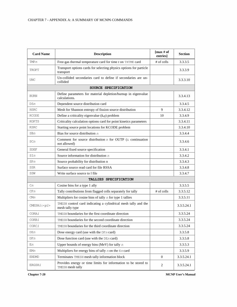
CHAPTER 7 - APPENDIX A: A SUMMARY OF MCNP6 COMMANDS
Chapter 7-20 MCNP User’s Manual
Card Name Description [max # of entries] Section
TMPn Free-gas thermal temperature card for time t on THTME card # of cells 3.3.3.5
TROPT Transport options cards for selecting physics options for particle transport 3.3.3.9
UNC Un-collided secondaries card to define if secondaries are un-collided 3.3.3.10
SOURCE SPECIFICATION
BURN Define parameters for material depletion/burnup in eigenvalue calculations. 3.3.4.13
DSn Dependent source distribution card 3.3.4.5 HSRC Mesh for Shannon entropy of fission source distribution 9 3.3.4.12 KCODE Define a criticality eigenvalue (keff) problem 10 3.3.4.9 KOPTS Criticality calculation options card for point kinetics parameters 3.3.4.11 KSRC Starting source point locations for KCODE problem 3.3.4.10
SBn Bias for source distribution n 3.3.4.4
SCn Comment for source distribution n for OUTP (& continuation not allowed) 3.3.4.6
SDEF General fixed source specification 3.3.4.1
SIn Source information for distribution n 3.3.4.2
SPn Source probability for distribution n 3.3.4.3 SSR Surface source read card for file RSSA 3.3.4.8 SSW Write surface source to l file 3.3.4.7
TALLIES SPECIFICATION Cn Cosine bins for a type 1 ally 3.3.5.5 CFn Tally contributions from flagged cells separately for tally # of cells 3.3.5.12
CMn Multipliers for cosine bins of tally n for type 1 tallies 3.3.5.11
CMESHi:<pl> TMESH control card indicating a cylindrical mesh tally and the mesh tally type 3.3.5.24.1
CORAi TMESH boundaries for the first coordinate direction 3.3.5.24 CORBi TMESH boundaries for the second coordinate direction 3.3.5.24 CORCi TMESH boundaries for the third coordinate direction 3.3.5.24 DEn Dose energy card (use with the DFn card) 3.3.5.8
DFn Dose function card (use with the DEn card) 3.3.5.8
En Upper bounds of energy bins (MeV) for tally n 3.3.5.3
EMn Multipliers for energy bins of tally n on the En card 3.3.5.9
ENDMD Terminates TMESH mesh tally information block 0 3.3.5.24.1
ERGSHi Provides energy or time limits for information to be stored to TMESH mesh tally 2 3.3.5.24.1
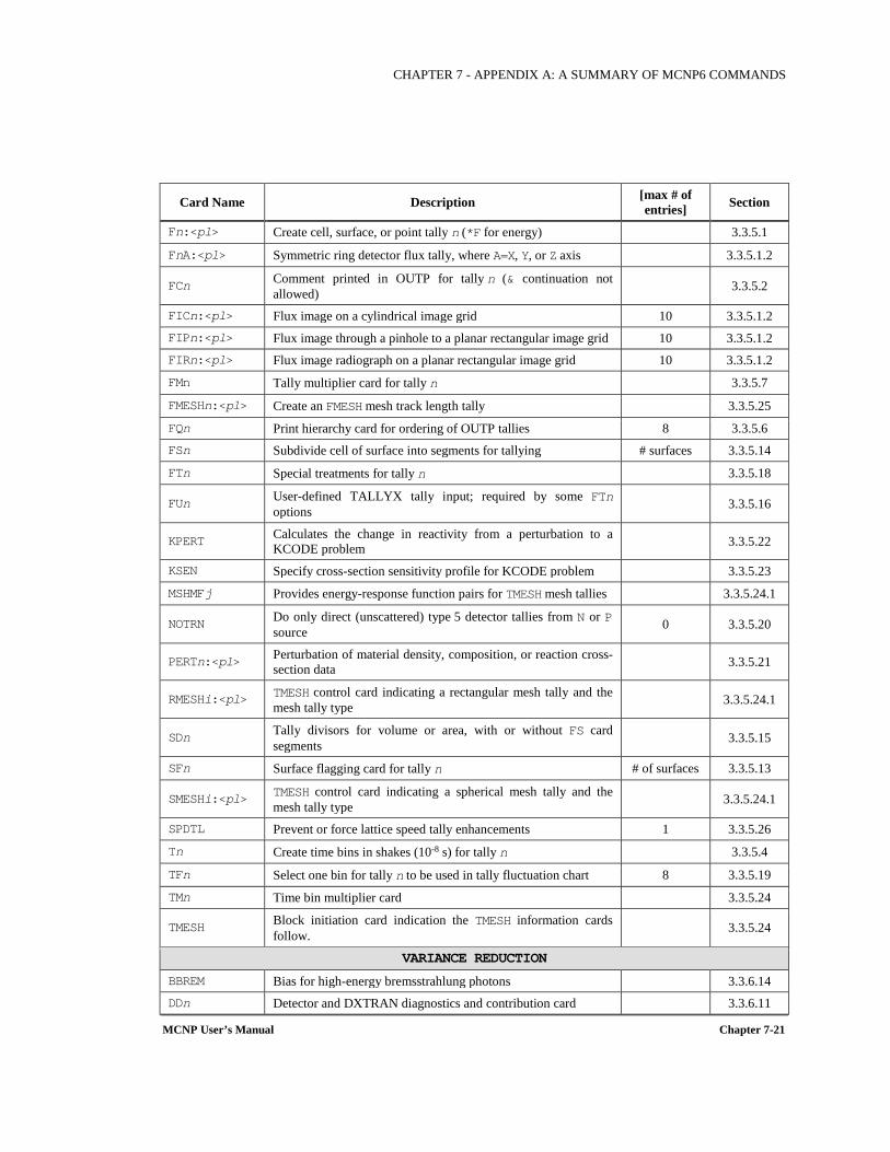
CHAPTER 7 - APPENDIX A: A SUMMARY OF MCNP6 COMMANDS
MCNP User’s Manual Chapter 7-21
Card Name Description [max # of entries] Section
Fn:<pl> Create cell, surface, or point tally n (*F for energy) 3.3.5.1
FnA:<pl> Symmetric ring detector flux tally, where A=X, Y, or Z axis 3.3.5.1.2
FCn Comment printed in OUTP for tally n (& continuation not allowed) 3.3.5.2
FICn:<pl> Flux image on a cylindrical image grid 10 3.3.5.1.2 FIPn:<pl> Flux image through a pinhole to a planar rectangular image grid 10 3.3.5.1.2 FIRn:<pl> Flux image radiograph on a planar rectangular image grid 10 3.3.5.1.2 FMn Tally multiplier card for tally n 3.3.5.7
FMESHn:<pl> Create an FMESH mesh track length tally 3.3.5.25
FQn Print hierarchy card for ordering of OUTP tallies 8 3.3.5.6 FSn Subdivide cell of surface into segments for tallying # surfaces 3.3.5.14
FTn Special treatments for tally n 3.3.5.18
FUn User-defined TALLYX tally input; required by some FTn options 3.3.5.16
KPERT Calculates the change in reactivity from a perturbation to a KCODE problem 3.3.5.22
KSEN Specify cross-section sensitivity profile for KCODE problem 3.3.5.23
MSHMFj Provides energy-response function pairs for TMESH mesh tallies 3.3.5.24.1
NOTRN Do only direct (unscattered) type 5 detector tallies from N or P source 0 3.3.5.20
PERTn:<pl> Perturbation of material density, composition, or reaction cross-section data 3.3.5.21
RMESHi:<pl> TMESH control card indicating a rectangular mesh tally and the mesh tally type 3.3.5.24.1
SDn Tally divisors for volume or area, with or without FS card segments 3.3.5.15
SFn Surface flagging card for tally n # of surfaces 3.3.5.13
SMESHi:<pl> TMESH control card indicating a spherical mesh tally and the mesh tally type 3.3.5.24.1
SPDTL Prevent or force lattice speed tally enhancements 1 3.3.5.26
Tn Create time bins in shakes (10-8 s) for tally n 3.3.5.4
TFn Select one bin for tally n to be used in tally fluctuation chart 8 3.3.5.19
TMn Time bin multiplier card 3.3.5.24
TMESH Block initiation card indication the TMESH information cards follow. 3.3.5.24
VARIANCE REDUCTION BBREM Bias for high-energy bremsstrahlung photons 3.3.6.14 DDn Detector and DXTRAN diagnostics and contribution card 3.3.6.11
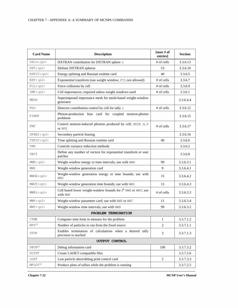
CHAPTER 7 - APPENDIX A: A SUMMARY OF MCNP6 COMMANDS
Chapter 7-22 MCNP User’s Manual
Card Name Description [max # of entries] Section
DXCn:<pl> DXTRAN contribution for DXTRAN sphere n # of cells 3.3.6.13
DXT:<pl> Defines DXTRAN spheres 53 3.3.6.10 ESPLT:<pl> Energy splitting and Russian roulette card 40 3.3.6.5
EXT:<pl> Exponential transform (use weight window; FCL not allowed) # of cells 3.3.6.7
FCL:<pl> Force collisions by cell # of cells 3.3.6.9 IMP:<pl> Cell importances; required unless weight windows used # of cells 3.3.6.1
MESH Superimposed importance mesh for mesh-based weight-window generator 3.3.6.4.4
PDn Detector contribution control by cell for tally n # of cells 3.3.6.12
PIKMT Photon-production bias card for coupled neutron-photon problems 3.3.6.15
PWT Control neutron-induced photons produced by cell; MODE N,P or NPE # of cells 3.3.6.17
SPABI:<pl> Secondary particle biasing 3.3.6.16 TSPLT:<pl> Time splitting and Russian roulette card 40 3.3.6.6 VAR Controls variance reduction methods 3.3.6.2
VECT Define any number of vectors for exponential transform or user patches 3.3.6.8
WWE:<pl> Weight-window energy or time intervals; use with WWN 99 3.3.6.3.1
WWG Weight-window generation card 9 3.3.6.4.1
WWGE:<pl> Weight-window generation energy or time bounds; use with WWG 15 3.3.6.4.2
WWGT:<pl> Weight-window generation time bounds; use with WWG 15 3.3.6.4.3
WWNi:<pl> Cell based lower weight-window bounds for ith WWE or WWT; use with WWP # of cells 3.3.6.3.3
WWP:<pl> Weight-window parameter card; use with WWE or WWT 11 3.3.6.3.4
WWT:<pl> Weight-window time intervals; use with WWN 99 3.3.6.3.2
PROBLEM TERMINATION CTME Computer time limit in minutes for the problem 1 3.3.7.1.2 NPSI8 Number of particles to run from the fixed source 2 3.3.7.1.1
STOP Enables termination of calculations when a desired tally precision is reached 3 3.3.7.1.3
OUTPUT CONTROL DBCNI8 Debug information card 100 3.3.7.3.2 HISTP Create LAHET-compatible files 3.3.7.2.6 LOST Lost particle abort/debug print control card 2 3.3.7.3.3 MPLOTI8 Produce plots of tallies while the problem is running 3.3.7.2.5
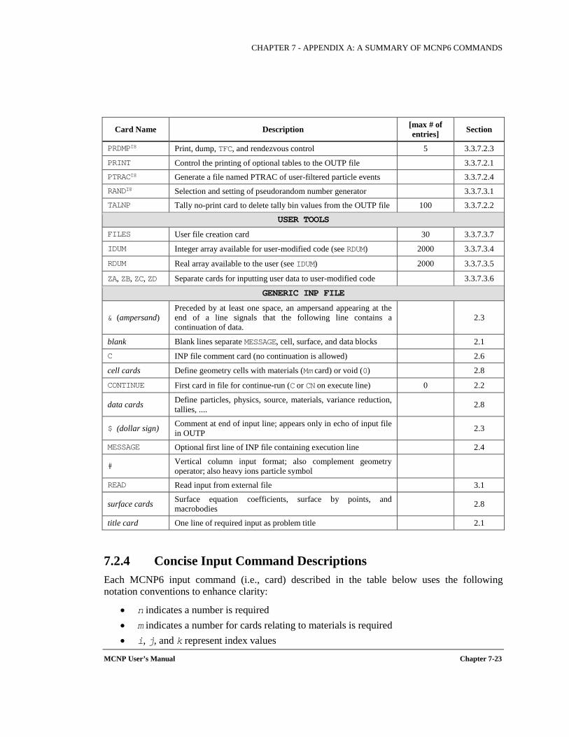
CHAPTER 7 - APPENDIX A: A SUMMARY OF MCNP6 COMMANDS
MCNP User’s Manual Chapter 7-23
Card Name Description [max # of entries] Section
PRDMPI8 Print, dump, TFC, and rendezvous control 5 3.3.7.2.3
PRINT Control the printing of optional tables to the OUTP file 3.3.7.2.1 PTRACI8 Generate a file named PTRAC of user-filtered particle events 3.3.7.2.4 RANDI8 Selection and setting of pseudorandom number generator 3.3.7.3.1 TALNP Tally no-print card to delete tally bin values from the OUTP file 100 3.3.7.2.2
USER TOOLS FILES User file creation card 30 3.3.7.3.7
IDUM Integer array available for user-modified code (see RDUM) 2000 3.3.7.3.4
RDUM Real array available to the user (see IDUM) 2000 3.3.7.3.5
ZA, ZB, ZC, ZD Separate cards for inputting user data to user-modified code 3.3.7.3.6
GENERIC INP FILE
& (ampersand) Preceded by at least one space, an ampersand appearing at the end of a line signals that the following line contains a continuation of data.
2.3
blank Blank lines separate MESSAGE, cell, surface, and data blocks 2.1
C INP file comment card (no continuation is allowed) 2.6
cell cards Define geometry cells with materials (Mm card) or void (0) 2.8
CONTINUE First card in file for continue-run (C or CN on execute line) 0 2.2
data cards Define particles, physics, source, materials, variance reduction, tallies, .... 2.8
$ (dollar sign) Comment at end of input line; appears only in echo of input file in OUTP 2.3
MESSAGE Optional first line of INP file containing execution line 2.4
# Vertical column input format; also complement geometry operator; also heavy ions particle symbol
READ Read input from external file 3.1
surface cards Surface equation coefficients, surface by points, and macrobodies 2.8
title card One line of required input as problem title 2.1
7.2.4 Concise Input Command Descriptions Each MCNP6 input command (i.e., card) described in the table below uses the following notation conventions to enhance clarity:
• n indicates a number is required • m indicates a number for cards relating to materials is required • i, j, and k represent index values
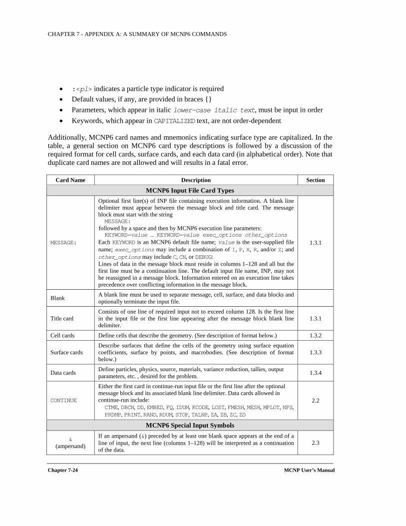
CHAPTER 7 - APPENDIX A: A SUMMARY OF MCNP6 COMMANDS
Chapter 7-24 MCNP User’s Manual
• :<pl> indicates a particle type indicator is required • Default values, if any, are provided in braces • Parameters, which appear in italic lower-case italic text, must be input in order • Keywords, which appear in CAPITALIZED text, are not order-dependent
Additionally, MCNP6 card names and mnemonics indicating surface type are capitalized. In the table, a general section on MCNP6 card type descriptions is followed by a discussion of the required format for cell cards, surface cards, and each data card (in alphabetical order). Note that duplicate card names are not allowed and will results in a fatal error.
Card Name Description Section
MCNP6 Input File Card Types
MESSAGE:
Optional first line(s) of INP file containing execution information. A blank line delimiter must appear between the message block and title card. The message block must start with the string MESSAGE:
followed by a space and then by MCNP6 execution line parameters: KEYWORD=value … KEYWORD=value exec_options other_options
Each KEYWORD is an MCNP6 default file name; value is the user-supplied file name; exec_options may include a combination of I, P, X, R, and/or Z; and other_options may include C, CN, or DEBUG: Lines of data in the message block must reside in columns 1–128 and all but the first line must be a continuation line. The default input file name, INP, may not be reassigned in a message block. Information entered on an execution line takes precedence over conflicting information in the message block.
1.3.1
Blank A blank line must be used to separate message, cell, surface, and data blocks and optionally terminate the input file.
Title card Consists of one line of required input not to exceed column 128. Is the first line in the input file or the first line appearing after the message block blank line delimiter.
1.3.1
Cell cards Define cells that describe the geometry. (See description of format below.) 1.3.2
Surface cards Describe surfaces that define the cells of the geometry using surface equation coefficients, surface by points, and macrobodies. (See description of format below.)
1.3.3
Data cards Define particles, physics, source, materials, variance reduction, tallies, output parameters, etc. , desired for the problem. 1.3.4
CONTINUE
Either the first card in continue-run input file or the first line after the optional message block and its associated blank line delimiter. Data cards allowed in continue-run include: CTME, DBCN, DD, EMBED, FQ, IDUM, KCODE, LOST, FMESH, MESH, MPLOT, NPS, PRDMP, PRINT, RAND, RDUM, STOP, TALNP, ZA, ZB, ZC, ZD
2.2
MCNP6 Special Input Symbols
& (ampersand)
If an ampersand (&) preceded by at least one blank space appears at the end of a line of input, the next line (columns 1–128) will be interpreted as a continuation of the data.
2.3
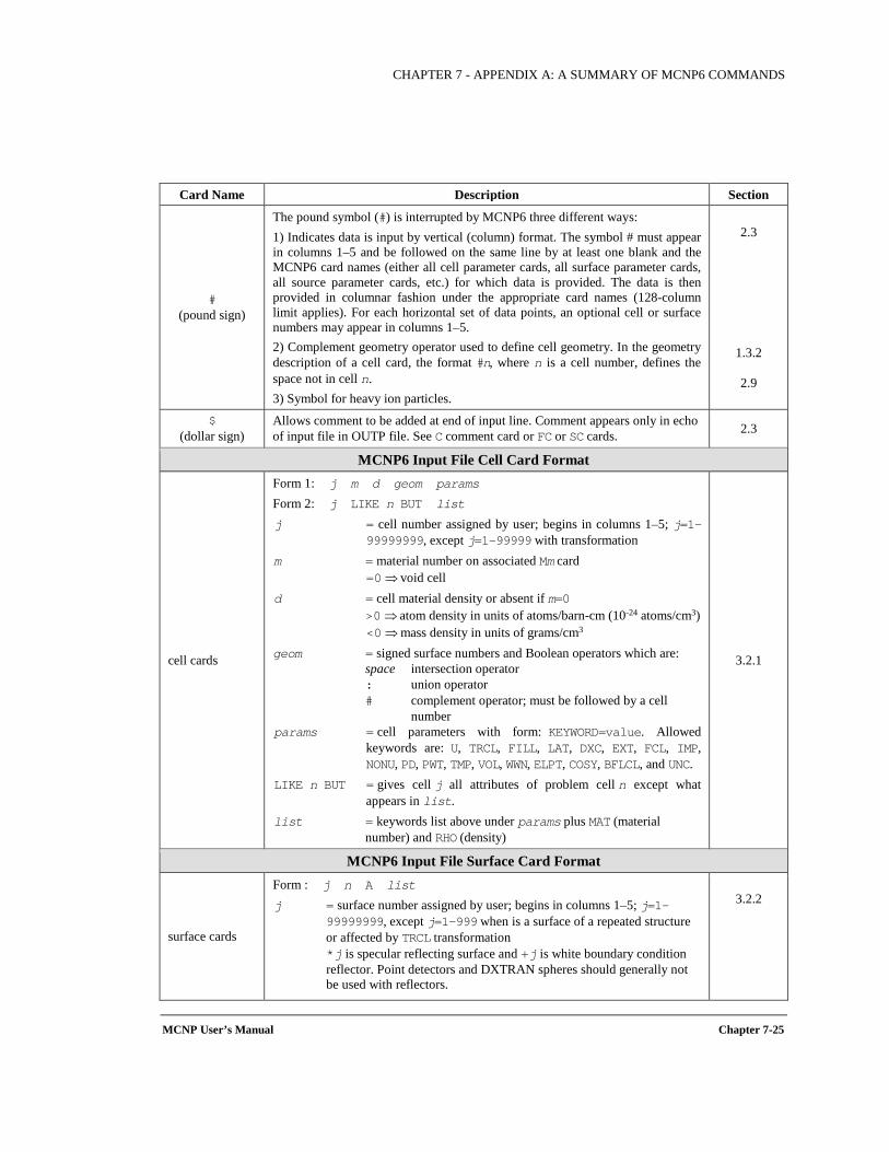
CHAPTER 7 - APPENDIX A: A SUMMARY OF MCNP6 COMMANDS
MCNP User’s Manual Chapter 7-25
Card Name Description Section
# (pound sign)
The pound symbol (#) is interrupted by MCNP6 three different ways: 1) Indicates data is input by vertical (column) format. The symbol # must appear in columns 1–5 and be followed on the same line by at least one blank and the MCNP6 card names (either all cell parameter cards, all surface parameter cards, all source parameter cards, etc.) for which data is provided. The data is then provided in columnar fashion under the appropriate card names (128-column limit applies). For each horizontal set of data points, an optional cell or surface numbers may appear in columns 1–5. 2) Complement geometry operator used to define cell geometry. In the geometry description of a cell card, the format #n, where n is a cell number, defines the space not in cell n. 3) Symbol for heavy ion particles.
2.3
1.3.2
2.9
$ (dollar sign)
Allows comment to be added at end of input line. Comment appears only in echo of input file in OUTP file. See C comment card or FC or SC cards. 2.3
MCNP6 Input File Cell Card Format
cell cards
Form 1: j m d geom params Form 2: j LIKE n BUT list j = cell number assigned by user; begins in columns 1–5; j=1–
99999999, except j=1–99999 with transformation m = material number on associated Mm card =0 ⇒ void cell d = cell material density or absent if m=0 >0 ⇒ atom density in units of atoms/barn-cm (10-24 atoms/cm3) <0 ⇒ mass density in units of grams/cm3 geom = signed surface numbers and Boolean operators which are:
space intersection operator : union operator # complement operator; must be followed by a cell
number params = cell parameters with form: KEYWORD=value. Allowed
keywords are: U, TRCL, FILL, LAT, DXC, EXT, FCL, IMP, NONU, PD, PWT, TMP, VOL, WWN, ELPT, COSY, BFLCL, and UNC.
LIKE n BUT = gives cell j all attributes of problem cell n except what appears in list.
list = keywords list above under params plus MAT (material number) and RHO (density)
3.2.1
MCNP6 Input File Surface Card Format
surface cards
Form : j n A list j = surface number assigned by user; begins in columns 1–5; j=1–
99999999, except j=1–999 when is a surface of a repeated structure or affected by TRCL transformation *j is specular reflecting surface and +j is white boundary condition reflector. Point detectors and DXTRAN spheres should generally not be used with reflectors.
3.2.2
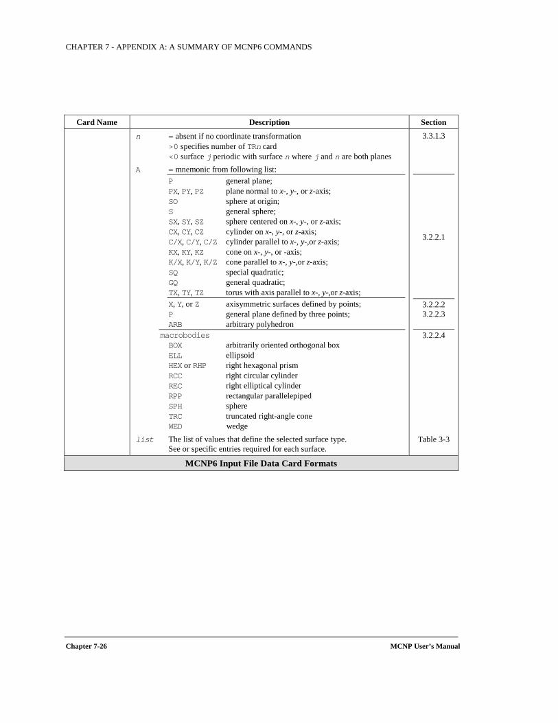
CHAPTER 7 - APPENDIX A: A SUMMARY OF MCNP6 COMMANDS
Chapter 7-26 MCNP User’s Manual
Card Name Description Section
n = absent if no coordinate transformation >0 specifies number of TRn card <0 surface j periodic with surface n where j and n are both planes A = mnemonic from following list:
P general plane; PX, PY, PZ plane normal to x-, y-, or z-axis; SO sphere at origin; S general sphere; SX, SY, SZ sphere centered on x-, y-, or z-axis; CX, CY, CZ cylinder on x-, y-, or z-axis; C/X, C/Y, C/Z cylinder parallel to x-, y-,or z-axis; KX, KY, KZ cone on x-, y-, or -axis; K/X, K/Y, K/Z cone parallel to x-, y-,or z-axis; SQ special quadratic; GQ general quadratic; TX, TY, TZ torus with axis parallel to x-, y-,or z-axis; X, Y, or Z axisymmetric surfaces defined by points; P general plane defined by three points; ARB arbitrary polyhedron
macrobodies BOX arbitrarily oriented orthogonal box ELL ellipsoid HEX or RHP right hexagonal prism RCC right circular cylinder REC right elliptical cylinder RPP rectangular parallelepiped SPH sphere TRC truncated right-angle cone WED wedge
list The list of values that define the selected surface type. See or specific entries required for each surface.
3.3.1.3
3.2.2.1
3.2.2.2 3.2.2.3
3.2.2.4
Table 3-3
MCNP6 Input File Data Card Formats
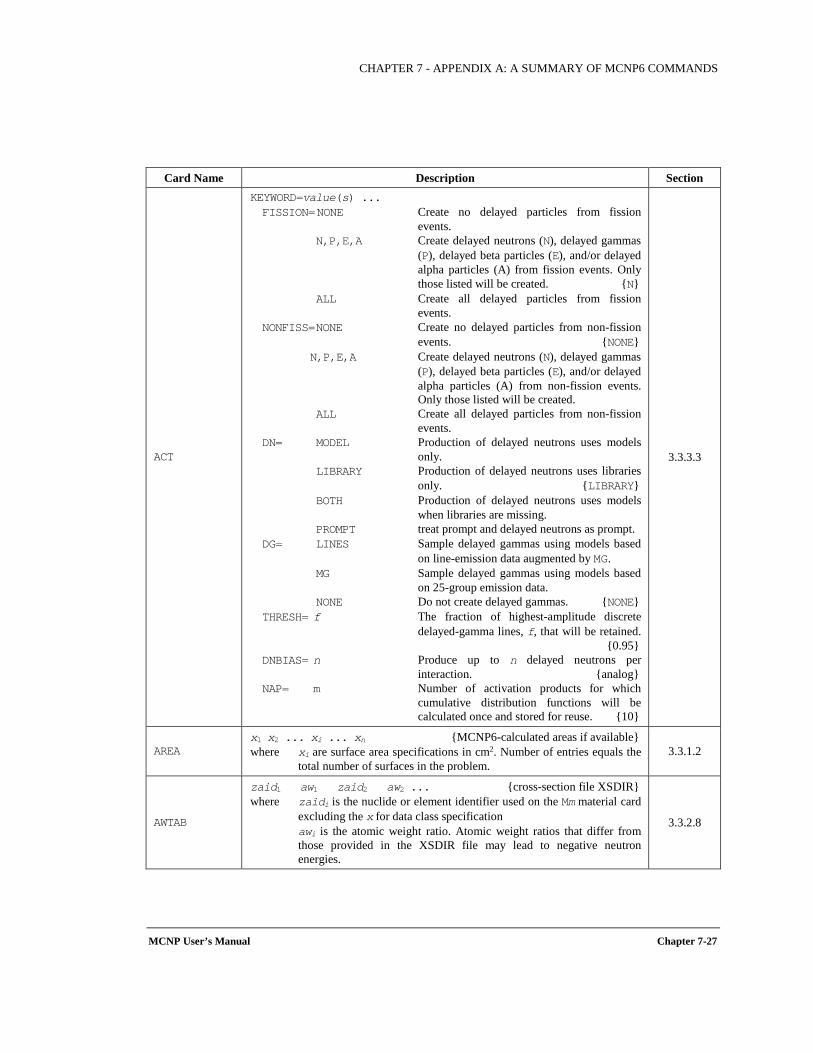
CHAPTER 7 - APPENDIX A: A SUMMARY OF MCNP6 COMMANDS
MCNP User’s Manual Chapter 7-27
Card Name Description Section
ACT
KEYWORD=value(s) ... FISSION= NONE Create no delayed particles from fission
events. N,P,E,A Create delayed neutrons (N), delayed gammas
(P), delayed beta particles (E), and/or delayed alpha particles (A) from fission events. Only those listed will be created. N
ALL Create all delayed particles from fission events.
NONFISS= NONE Create no delayed particles from non-fission events. NONE
N,P,E,A Create delayed neutrons (N), delayed gammas (P), delayed beta particles (E), and/or delayed alpha particles (A) from non-fission events. Only those listed will be created.
ALL Create all delayed particles from non-fission events.
DN= MODEL Production of delayed neutrons uses models only.
LIBRARY Production of delayed neutrons uses libraries only. LIBRARY
BOTH Production of delayed neutrons uses models when libraries are missing.
PROMPT treat prompt and delayed neutrons as prompt. DG= LINES Sample delayed gammas using models based
on line-emission data augmented by MG. MG Sample delayed gammas using models based
on 25-group emission data. NONE Do not create delayed gammas. NONE THRESH= f The fraction of highest-amplitude discrete
delayed-gamma lines, f, that will be retained. 0.95
DNBIAS= n Produce up to n delayed neutrons per interaction. analog
NAP= m Number of activation products for which cumulative distribution functions will be calculated once and stored for reuse. 10
3.3.3.3
AREA x1 x2 ... xi ... xn MCNP6-calculated areas if available where xi are surface area specifications in cm2. Number of entries equals the
total number of surfaces in the problem. 3.3.1.2
AWTAB
zaid1 aw1 zaid2 aw2 ... cross-section file XSDIR where zaidi is the nuclide or element identifier used on the Mm material card
excluding the x for data class specification awi is the atomic weight ratio. Atomic weight ratios that differ from
those provided in the XSDIR file may lead to negative neutron energies.
3.3.2.8
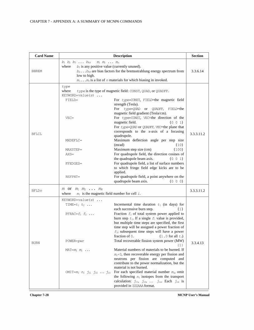
CHAPTER 7 - APPENDIX A: A SUMMARY OF MCNP6 COMMANDS
Chapter 7-28 MCNP User’s Manual
Card Name Description Section
BBREM
b1 b2 b3 ... b49 m1 m2 ... mn where b1 is any positive value (currently unused). b2...b49 are bias factors for the bremsstrahlung energy spectrum from
low to high. m1...mn is a list of n materials for which biasing in invoked.
3.3.6.14
BFLCL
type where type is the type of magnetic field: CONST, QUAD, or QUADFF. KEYWORD=value(s) ... FIELD= For type=CONST, FIELD=the magnetic field
strength (Tesla). For type=QUAD or QUADFF, FIELD=the
magnetic field gradient (Tesla/cm). VEC= For type=CONST, VEC=the direction of the
magnetic field. 0 0 1 For type=QUAD or QUADFF, VEC=the plane that
corresponds to the x-axis of a focusing quadrupole.
MXDEFLC= Maximum deflection angle per step size (mrad) 10
MAXSTEP= Maximum step size (cm) 100 AXS= For quadrupole field, the direction cosines of
the quadrupole beam axis. 0 0 1 FFEDGES= For quadrupole field, a list of surface numbers
to which fringe field edge kicks are to be applied.
REFPNT= For quadrupole field, a point anywhere on the quadrupole beam axis. 0 0 0
3.3.3.11.2
BFLDn m or m1 m2 ... mK where mi is the magnetic field number for cell i.
3.3.3.11.2
BURN
KEYWORD=value(s) ... TIME=t1 t2 ... Incremental time duration t1 (in days) for
each successive burn step. 1 PFRAC=f1 f2 ... Fraction fi of total system power applied to
burn step ti. If a single f1 value is provided, but multiple time steps are specified, the first time step will be assigned a power fraction of f1; subsequent time steps will have a power fraction of 0. 1.0 for all ti)
POWER=pwr Total recoverable fission system power (MW) 1
MAT=m1 m2 ... Material numbers of materials to be burned. If mi<0, then recoverable energy per fission and neutrons per fission are computed and contribute to the power normalization, but the material is not burned.
OMIT=mi ni ji1 ji2 ... jin For each specified material number mi, omit the following ni isotopes from the transport calculation: ji1, ji2, … jin. Each jik is provided in ZZZAAA format.
3.3.4.13
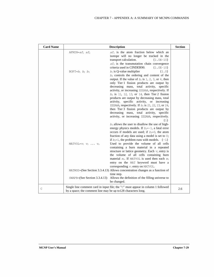
CHAPTER 7 - APPENDIX A: A SUMMARY OF MCNP6 COMMANDS
MCNP User’s Manual Chapter 7-29
Card Name Description Section
AFMIN=af1 af2 af1 is the atom fraction below which an isotope will no longer be tracked in the transport calculation. 1.0E-10
af2 is the transmutation chain convergence criteria used in CINDER90. 1.0E-10
BOPT=b1 b2 b3 b1 is Q-value multiplier 1.0 b2 controls the ordering and content of the
output. If the value of b2 is 1, 2, 3, or 4, then only Tier 1 fission products are output by decreasing mass, total activity, specific activity, or increasing ZZZAAA, respectively. If b2 is 11, 12, 13, or 14, then Tier 2 fission products are output by decreasing mass, total activity, specific activity, or increasing ZZZAAA, respectively. If b2 is 21, 22, 23, or 24, then Tier 3 fission products are output by decreasing mass, total activity, specific activity, or increasing ZZZAAA, respectively. 1
b3 allows the user to disallow the use of high-energy physics models. If b3=-1, a fatal error occurs if models are used; if b3=0, the atom fraction of any data using a model is set to 0; if b3=1, the problem runs with models. -1
MATVOL=v1 v2 ... vn Used to provide the volume of all cells containing a burn material in a repeated structure or lattice geometry. Each vi entry is the volume of all cells containing burn material mi. If MATVOL is used then each mi entry on the MAT keyword must have a corresponding vi entry on MATVOL.
MATMOD=(See Section 3.3.4.13) Allows concentration changes as a function of time step.
SWAPB=(See Section 3.3.4.13) Allows the definition of the filling universe to be changed.
C Single line comment card in input file; the "C" must appear in column 1 followed by a space; the comment line may be up to128 characters long. 2.6
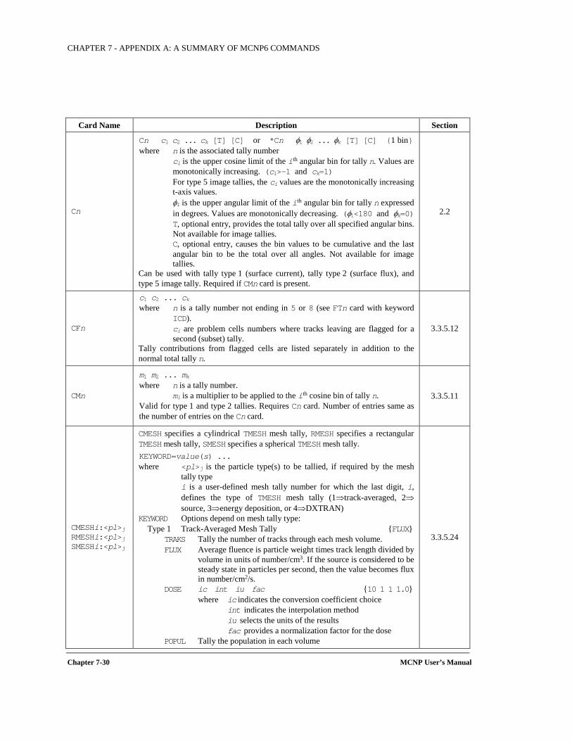
CHAPTER 7 - APPENDIX A: A SUMMARY OF MCNP6 COMMANDS
Chapter 7-30 MCNP User’s Manual
Card Name Description Section
Cn
Cn c1 c2 ... ck [T] [C] or *Cn φ1 φ2 ... φk [T] [C] 1 bin where n is the associated tally number ci is the upper cosine limit of the ith angular bin for tally n. Values are
monotonically increasing. (c1>-1 and ck=1) For type 5 image tallies, the ci values are the monotonically increasing
t-axis values. φi is the upper angular limit of the ith angular bin for tally n expressed
in degrees. Values are monotonically decreasing. (φ1<180 and φk=0) T, optional entry, provides the total tally over all specified angular bins.
Not available for image tallies. C, optional entry, causes the bin values to be cumulative and the last
angular bin to be the total over all angles. Not available for image tallies.
Can be used with tally type 1 (surface current), tally type 2 (surface flux), and type 5 image tally. Required if CMn card is present.
2.2
CFn
c1 c2 ... ck where n is a tally number not ending in 5 or 8 (see FTn card with keyword
ICD). ci are problem cells numbers where tracks leaving are flagged for a
second (subset) tally. Tally contributions from flagged cells are listed separately in addition to the normal total tally n.
3.3.5.12
CMn
m1 m2 ... mk where n is a tally number. mi is a multiplier to be applied to the ith cosine bin of tally n. Valid for type 1 and type 2 tallies. Requires Cn card. Number of entries same as the number of entries on the Cn card.
3.3.5.11
CMESHi:<pl>j RMESHi:<pl>j SMESHi:<pl>j
CMESH specifies a cylindrical TMESH mesh tally, RMESH specifies a rectangular TMESH mesh tally, SMESH specifies a spherical TMESH mesh tally. KEYWORD=value(s) ... where <pl>j is the particle type(s) to be tallied, if required by the mesh
tally type i is a user-defined mesh tally number for which the last digit, i,
defines the type of TMESH mesh tally (1⇒track-averaged, 2⇒ source, 3⇒energy deposition, or 4⇒DXTRAN)
KEYWORD Options depend on mesh tally type: Type 1 Track-Averaged Mesh Tally FLUX
TRAKS Tally the number of tracks through each mesh volume. FLUX Average fluence is particle weight times track length divided by
volume in units of number/cm3. If the source is considered to be steady state in particles per second, then the value becomes flux in number/cm2/s.
DOSE ic int iu fac 10 1 1 1.0 where ic indicates the conversion coefficient choice int indicates the interpolation method iu selects the units of the results fac provides a normalization factor for the dose
POPUL Tally the population in each volume
3.3.5.24
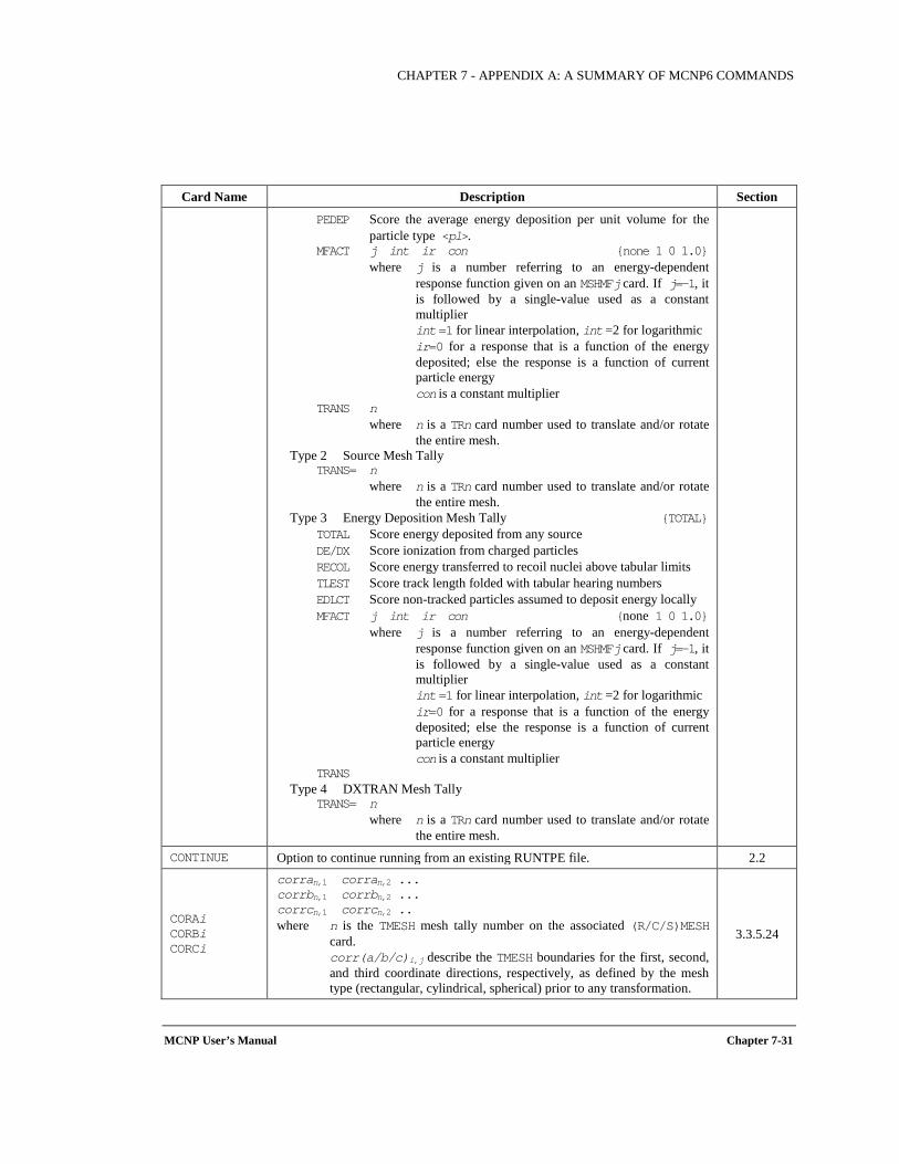
CHAPTER 7 - APPENDIX A: A SUMMARY OF MCNP6 COMMANDS
MCNP User’s Manual Chapter 7-31
Card Name Description Section
PEDEP Score the average energy deposition per unit volume for the particle type <pl>.
MFACT j int ir con none 1 0 1.0 where j is a number referring to an energy-dependent
response function given on an MSHMFj card. If j=-1, it is followed by a single-value used as a constant multiplier
int =1 for linear interpolation, int =2 for logarithmic ir=0 for a response that is a function of the energy
deposited; else the response is a function of current particle energy
con is a constant multiplier TRANS n
where n is a TRn card number used to translate and/or rotate the entire mesh.
Type 2 Source Mesh Tally TRANS= n
where n is a TRn card number used to translate and/or rotate the entire mesh.
Type 3 Energy Deposition Mesh Tally TOTAL TOTAL Score energy deposited from any source DE/DX Score ionization from charged particles RECOL Score energy transferred to recoil nuclei above tabular limits TLEST Score track length folded with tabular hearing numbers EDLCT Score non-tracked particles assumed to deposit energy locally MFACT j int ir con none 1 0 1.0
where j is a number referring to an energy-dependent response function given on an MSHMFj card. If j=-1, it is followed by a single-value used as a constant multiplier
int =1 for linear interpolation, int =2 for logarithmic ir=0 for a response that is a function of the energy
deposited; else the response is a function of current particle energy
con is a constant multiplier TRANS
Type 4 DXTRAN Mesh Tally TRANS= n
where n is a TRn card number used to translate and/or rotate the entire mesh.
CONTINUE Option to continue running from an existing RUNTPE file. 2.2
CORAi CORBi CORCi
corran,1 corran,2 ... corrbn,1 corrbn,2 ... corrcn,1 corrcn,2 .. where n is the TMESH mesh tally number on the associated (R/C/S)MESH
card. corr(a/b/c)i,j describe the TMESH boundaries for the first, second,
and third coordinate directions, respectively, as defined by the mesh type (rectangular, cylindrical, spherical) prior to any transformation.
3.3.5.24
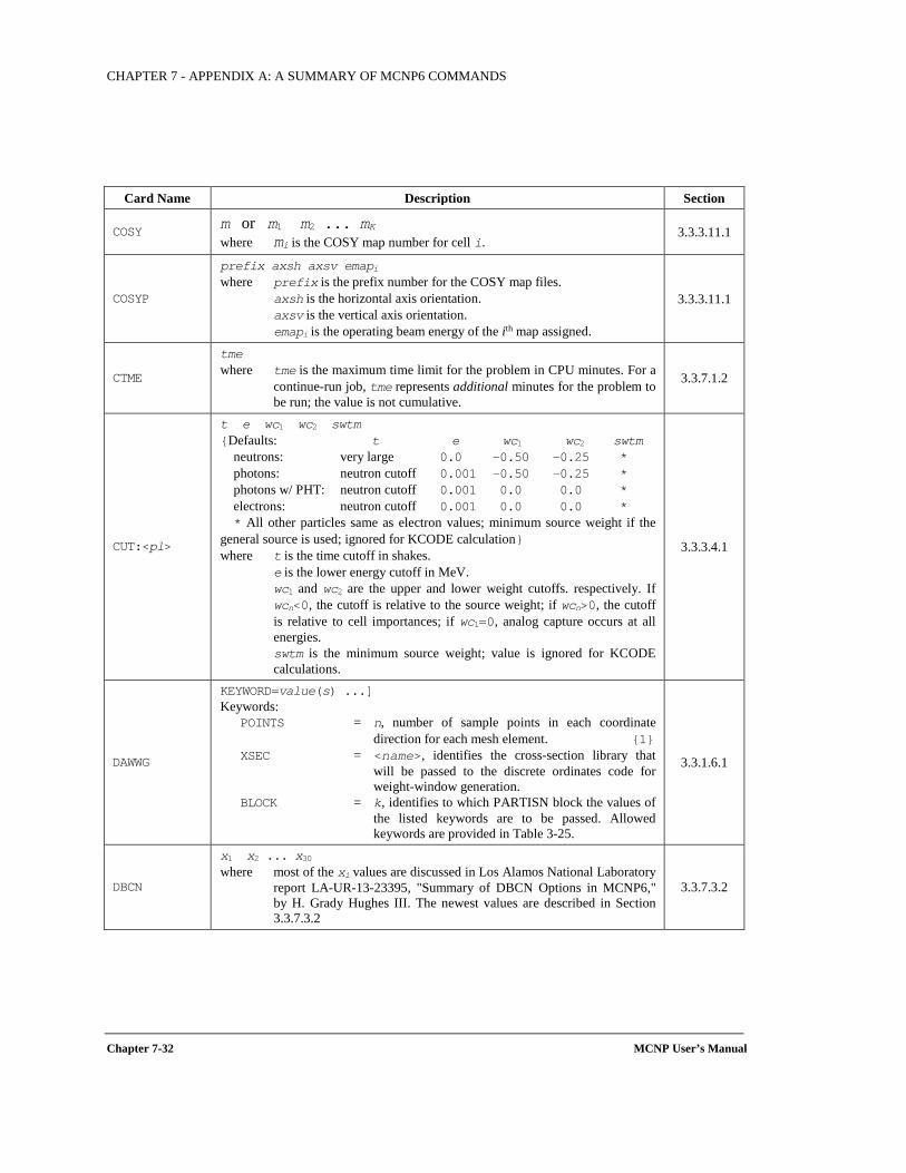
CHAPTER 7 - APPENDIX A: A SUMMARY OF MCNP6 COMMANDS
Chapter 7-32 MCNP User’s Manual
Card Name Description Section
COSY m or m1 m2 ... mK where mi is the COSY map number for cell i.
3.3.3.11.1
COSYP
prefix axsh axsv emapi where prefix is the prefix number for the COSY map files. axsh is the horizontal axis orientation. axsv is the vertical axis orientation. emapi is the operating beam energy of the ith map assigned.
3.3.3.11.1
CTME
tme where tme is the maximum time limit for the problem in CPU minutes. For a
continue-run job, tme represents additional minutes for the problem to be run; the value is not cumulative.
3.3.7.1.2
CUT:<pl>
t e wc1 wc2 swtm Defaults: t e wc1 wc2 swtm neutrons: very large 0.0 -0.50 -0.25 * photons: neutron cutoff 0.001 -0.50 -0.25 * photons w/ PHT: neutron cutoff 0.001 0.0 0.0 * electrons: neutron cutoff 0.001 0.0 0.0 * * All other particles same as electron values; minimum source weight if the general source is used; ignored for KCODE calculation where t is the time cutoff in shakes. e is the lower energy cutoff in MeV. wc1 and wc2 are the upper and lower weight cutoffs. respectively. If
wcn<0, the cutoff is relative to the source weight; if wcn>0, the cutoff is relative to cell importances; if wc1=0, analog capture occurs at all energies.
swtm is the minimum source weight; value is ignored for KCODE calculations.
3.3.3.4.1
DAWWG
KEYWORD=value(s) ...] Keywords: POINTS = n, number of sample points in each coordinate
direction for each mesh element. 1 XSEC = <name>, identifies the cross-section library that
will be passed to the discrete ordinates code for weight-window generation.
BLOCK = k, identifies to which PARTISN block the values of the listed keywords are to be passed. Allowed keywords are provided in Table 3-25.
3.3.1.6.1
DBCN
x1 x2 ... x30 where most of the xi values are discussed in Los Alamos National Laboratory
report LA-UR-13-23395, "Summary of DBCN Options in MCNP6," by H. Grady Hughes III. The newest values are described in Section 3.3.7.3.2
3.3.7.3.2
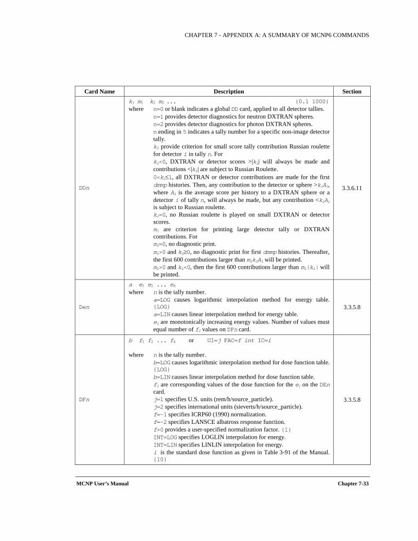
CHAPTER 7 - APPENDIX A: A SUMMARY OF MCNP6 COMMANDS
MCNP User’s Manual Chapter 7-33
Card Name Description Section
DDn
k1 m1 k2 m2 ... 0.1 1000 where n=0 or blank indicates a global DD card, applied to all detector tallies. n=1 provides detector diagnostics for neutron DXTRAN spheres. n=2 provides detector diagnostics for photon DXTRAN spheres. n ending in 5 indicates a tally number for a specific non-image detector
tally. ki provide criterion for small score tally contribution Russian roulette
for detector i in tally n. For ki<0, DXTRAN or detector scores >|ki| will always be made and
contributions <|ki| are subject to Russian Roulette. 0<ki≤1, all DXTRAN or detector contributions are made for the first
dmmp histories. Then, any contribution to the detector or sphere >kiAi, where Ai is the average score per history to a DXTRAN sphere or a detector i of tally n, will always be made, but any contribution <kiAi is subject to Russian roulette.
ki=0, no Russian roulette is played on small DXTRAN or detector scores.
mi are criterion for printing large detector tally or DXTRAN contributions. For
mi=0, no diagnostic print. mi>0 and ki≥0, no diagnostic print for first dmmp histories. Thereafter,
the first 600 contributions larger than mikiAi will be printed. mi>0 and ki<0, then the first 600 contributions larger than mi|ki| will
be printed.
3.3.6.11
Den
a e1 e2 ... ek where n is the tally number. a=LOG causes logarithmic interpolation method for energy table.
LOG a=LIN causes linear interpolation method for energy table. ei are monotonically increasing energy values. Number of values must
equal number of fi values on DFn card.
3.3.5.8
DFn
b f1 f2 ... fk or UI=j FAC=f int IC=i where n is the tally number. b=LOG causes logarithmic interpolation method for dose function table.
LOG b=LIN causes linear interpolation method for dose function table. fi are corresponding values of the dose function for the ei on the DEn
card. j=1 specifies U.S. units (rem/h/source_particle). j=2 specifies international units (sieverts/h/source_particle). f=-1 specifies ICRP60 (1990) normalization. f=-2 specifies LANSCE albatross response function. f>0 provides a user-specified normalization factor. 1 INT=LOG specifies LOGLIN interpolation for energy. INT=LIN specifies LINLIN interpolation for energy. i is the standard dose function as given in Table 3-91 of the Manual.
10
3.3.5.8
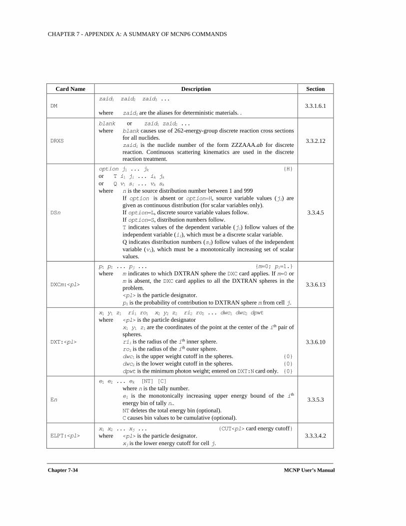
CHAPTER 7 - APPENDIX A: A SUMMARY OF MCNP6 COMMANDS
Chapter 7-34 MCNP User’s Manual
Card Name Description Section
DM zaid1 zaid2 zaid3 ... where zaidi are the aliases for deterministic materials. .
3.3.1.6.1
DRXS
blank or zaid1 zaid2 ... where blank causes use of 262-energy-group discrete reaction cross sections
for all nuclides. zaidi is the nuclide number of the form ZZZAAA.ab for discrete
reaction. Continuous scattering kinematics are used in the discrete reaction treatment.
3.3.2.12
DSn
option j1 ... jk H or T i1 ji ... ik jk or Q v1 si ... vk sk where n is the source distribution number between 1 and 999 If option is absent or option=H, source variable values (ji) are
given as continuous distribution (for scalar variables only). If option=L, discrete source variable values follow. If option=S, distribution numbers follow. T indicates values of the dependent variable (ji) follow values of the
independent variable (ii), which must be a discrete scalar variable. Q indicates distribution numbers (si) follow values of the independent
variable (vi), which must be a monotonically increasing set of scalar values.
3.3.4.5
DXCm:<pl>
p1 p2 ... pj ... m=0; pi=1. where m indicates to which DXTRAN sphere the DXC card applies. If m=0 or
m is absent, the DXC card applies to all the DXTRAN spheres in the problem.
<pl> is the particle designator. pi is the probability of contribution to DXTRAN sphere m from cell j.
3.3.6.13
DXT:<pl>
x1 y1 z1 ri1 ro1 x2 y2 z2 ri2 ro2 ... dwc1 dwc2 dpwt where <pl> is the particle designator x1 y1 z1 are the coordinates of the point at the center of the ith pair of
spheres. rii is the radius of the ith inner sphere. roi is the radius of the ith outer sphere. dwc1 is the upper weight cutoff in the spheres. 0 dwc2 is the lower weight cutoff in the spheres. 0 dpwt is the minimum photon weight; entered on DXT:N card only. 0
3.3.6.10
En
e1 e2 ... ek [NT] [C] where n is the tally number. ei is the monotonically increasing upper energy bound of the ith
energy bin of tally n.. NT deletes the total energy bin (optional). C causes bin values to be cumulative (optional).
3.3.5.3
ELPT:<pl> x1 x2 ... xj ... CUT<pl> card energy cutoff where <pl> is the particle designator. xj is the lower energy cutoff for cell j.
3.3.3.4.2
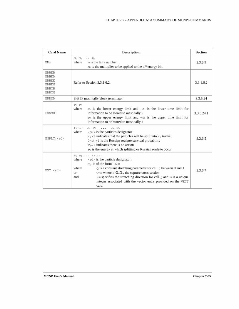
CHAPTER 7 - APPENDIX A: A SUMMARY OF MCNP6 COMMANDS
MCNP User’s Manual Chapter 7-35
Card Name Description Section
EMn m1 m2 ... mk where n is the tally number. mi is the multiplier to be applied to the ith energy bin.
3.3.5.9
EMBEB EMBED EMBEE EMBEM EMBTB EMBTM
Refer to Section 3.3.1.6.2. 3.3.1.6.2
ENDMD TMESH mesh tally block terminator 3.3.5.24
ERGSHi
e1 e2 where e1 is the lower energy limit and –e1 is the lower time limit for
information to be stored to mesh tally i e2 is the upper energy limit and –e2 is the upper time limit for
information to be stored to mesh tally i
3.3.5.24.1
ESPLT:<pl>
ri ei r2 e2 ... rk ek where <pl> is the particles designator ri>1 indicates that the particles will be split into ri tracks 0<ri<1 is the Russian roulette survival probability ri=1 indicates there is no action ei is the energy at which splitting or Russian roulette occur
3.3.6.5
EXT:<pl>
a1 a2 ... aj ... where <pl> is the particle designator. aj.is of the form QVm where Q is a constant stretching parameter for cell j between 0 and 1 or Q=S where S=Σc/Σt, the capture cross section and Vm specifies the stretching direction for cell j and m is a unique
integer associated with the vector entry provided on the VECT card.
3.3.6.7
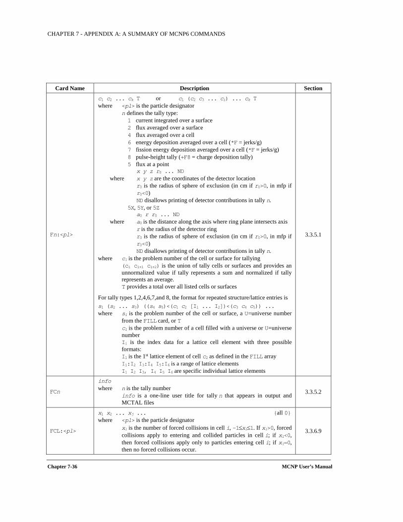
CHAPTER 7 - APPENDIX A: A SUMMARY OF MCNP6 COMMANDS
Chapter 7-36 MCNP User’s Manual
Card Name Description Section
Fn:<pl>
c1 c2 ... ck T or c1 (c2 c3 ... ci) ... ck T where <pl> is the particle designator n defines the tally type: 1 current integrated over a surface 2 flux averaged over a surface 4 flux averaged over a cell 6 energy deposition averaged over a cell (*F = jerks/g) 7 fission energy deposition averaged over a cell (*F = jerks/g) 8 pulse-height tally (+F8 = charge deposition tally) 5 flux at a point x y z r0 ... ND
where x y z are the coordinates of the detector location r0 is the radius of sphere of exclusion (in cm if r0>0, in mfp if
r0<0) ND disallows printing of detector contributions in tally n.
5X, 5Y, or 5Z a0 r r0 ... ND where a0 is the distance along the axis where ring plane intersects axis r is the radius of the detector ring r0 is the radius of sphere of exclusion (in cm if r0>0, in mfp if
r0<0) ND disallows printing of detector contributions in tally n.
where ci is the problem number of the cell or surface for tallying (ci ci+1 ci+2) is the union of tally cells or surfaces and provides an
unnormalized value if tally represents a sum and normalized if tally represents an average.
T provides a total over all listed cells or surfaces
For tally types 1,2,4,6,7,and 8, the format for repeated structure/lattice entries is s1 (s2 ... s3) ((s4 s5)<(c1 c2 [I1 ... I2])<(c3 c4 c5)) ... where si is the problem number of the cell or surface, a U=universe number
from the FILL card, or T ci is the problem number of a cell filled with a universe or U=universe
number Ii is the index data for a lattice cell element with three possible
formats: I1 is the 1st lattice element of cell c2 as defined in the FILL array I1:I2 I3:I4 I5:I6 is a range of lattice elements I1 I2 I3, I4 I5 I6 are specific individual lattice elements
3.3.5.1
FCn
info where n is the tally number info is a one-line user title for tally n that appears in output and
MCTAL files
3.3.5.2
FCL:<pl>
x1 x2 ... xj ... all 0 where <pl> is the particle designator xi is the number of forced collisions in cell i, -1≤xi≤1. If xi>0, forced
collisions apply to entering and collided particles in cell i; if xi<0, then forced collisions apply only to particles entering cell i; if xi=0, then no forced collisions occur.
3.3.6.9
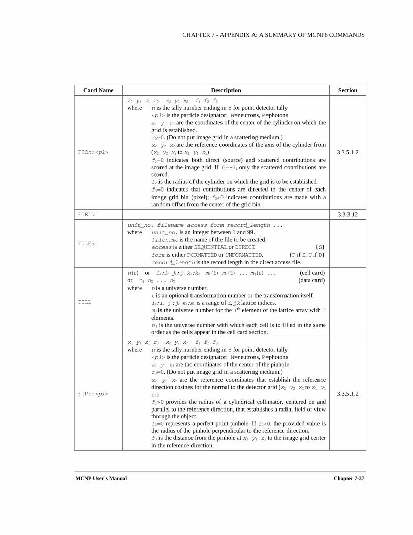
CHAPTER 7 - APPENDIX A: A SUMMARY OF MCNP6 COMMANDS
MCNP User’s Manual Chapter 7-37
Card Name Description Section
FICn:<pl>
x1 y1 z1 r0 x2 y2 x2 f1 f2 f3 where n is the tally number ending in 5 for point detector tally <pl> is the particle designator: N=neutrons, P=photons x1 y1 z1 are the coordinates of the center of the cylinder on which the
grid is established. r0=0. (Do not put image grid in a scattering medium.) x2 y2 x2 are the reference coordinates of the axis of the cylinder from
(x2 y2 x2 to x1 y1 z1) f1=0 indicates both direct (source) and scattered contributions are
scored at the image grid. If f1=-1, only the scattered contributions are scored.
f2 is the radius of the cylinder on which the grid is to be established. f3=0 indicates that contributions are directed to the center of each
image grid bin (pixel); f3≠0 indicates contributions are made with a random offset from the center of the grid bin.
3.3.5.1.2
FIELD 3.3.3.12
FILES
unit_no. filename access form record_length ... where unit_no. is an integer between 1 and 99. filename is the name of the file to be created. access is either SEQUENTIAL or DIRECT. S form is either FORMATTED or UNFORMATTED. F if S, U if D record_length is the record length in the direct access file.
FILL
n(t) or i1:i2 j1:j2 k1:k2 m1(t) m2(t) ... mj(t) ... (cell card) or n1 n2 ... nT (data card) where n is a universe number. t is an optional transformation number or the transformation itself. i1:i2 j1:j2 k1:k2 is a range of i,j,k lattice indices. mj is the universe number for the ith element of the lattice array with T
elements. nj is the universe number with which each cell is to filled in the same
order as the cells appear in the cell card section.
FIPn:<pl>
x1 y1 z1 r0 x2 y2 x2 f1 f2 f3 where n is the tally number ending in 5 for point detector tally <pl> is the particle designator: N=neutrons, P=photons x1 y1 z1 are the coordinates of the center of the pinhole. r0=0. (Do not put image grid in a scattering medium.) x2 y2 x2 are the reference coordinates that establish the reference
direction cosines for the normal to the detector grid (x2 y2 x2 to x1 y1 z1)
f1>0 provides the radius of a cylindrical collimator, centered on and parallel to the reference direction, that establishes a radial field of view through the object.
f2=0 represents a perfect point pinhole. If f2>0, the provided value is the radius of the pinhole perpendicular to the reference direction.
f3 is the distance from the pinhole at x1 y1 z1 to the image grid center in the reference direction.
3.3.5.1.2
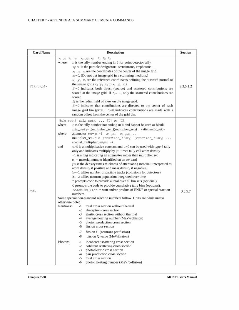
CHAPTER 7 - APPENDIX A: A SUMMARY OF MCNP6 COMMANDS
Chapter 7-38 MCNP User’s Manual
Card Name Description Section
FIRn:<pl>
x1 y1 z1 r0 x2 y2 x2 f1 f2 f3 where n is the tally number ending in 5 for point detector tally <pl> is the particle designator: N=neutrons, P=photons x1 y1 z1 are the coordinates of the center of the image grid. r0=0. (Do not put image grid in a scattering medium.) x2 y2 x2 are the reference coordinates defining the outward normal to
the image grid (x2 y2 x2 to x1 y1 z1). f1=0 indicates both direct (source) and scattered contributions are
scored at the image grid. If f1=-1, only the scattered contributions are scored.
f2 is the radial field of view on the image grid. f3=0 indicates that contributions are directed to the center of each
image grid bin (pixel); f3≠0 indicates contributions are made with a random offset from the center of the grid bin.
3.3.5.1.2
FMn
(bin_set1) (bin_set2) ... [T] or [C] where n is the tally number not ending in 8 and cannot be zero or blank. bin_seti= ((multiplier_set1)(multiplier_set2) ... (attenuator_set)) where attenuator_set= c –1 m1 px1 m2 px2 ... multiplier_seti=c m (reaction_list1) (reaction_list2) ... special_multiplier_seti=c –k and c>0 is a multiplicative constant and c<0 can be used with type 4 tally
only and indicates multiply by |c| times tally cell atom density –1 is a flag indicating an attenuator rather than multiplier set. mi = material number identified on an Mm card px is the density times thickness of attenuating material; interpreted as
atom density if positive and mass density if negative. k=–1 tallies number of particle tracks (collisions for detectors) k=–2 tallies neutron population integrated over time T prompts code to provide a total over all bin sets (optional). C prompts the code to provide cumulative tally bins (optional). reaction_listi = sum and/or product of ENDF or special reaction
numbers. Some special non-standard reaction numbers follow. Units are barns unless otherwise noted. Neutrons: -1 total cross section without thermal -2 absorption cross section -3 elastic cross section without thermal -4 average hearing number (MeV/collision) -5 photon production cross section -6 fission cross section -7 fission (neutrons per fission) -8 fission Q value (MeV/fission) Photons: -1 incoherent scattering cross section -2 coherent scattering cross section -3 photoelectric cross section -4 pair production cross section -5 total cross section -6 photon heating number (MeV/collision)
3.3.5.7
ν
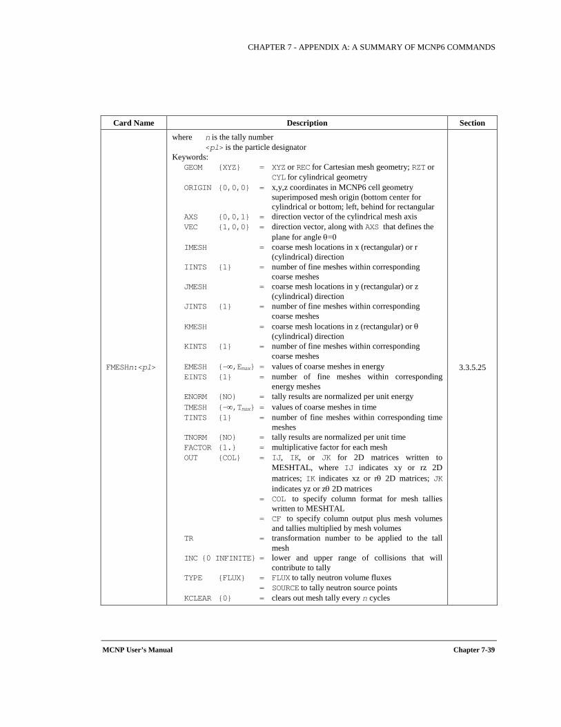
CHAPTER 7 - APPENDIX A: A SUMMARY OF MCNP6 COMMANDS
MCNP User’s Manual Chapter 7-39
Card Name Description Section
FMESHn:<pl>
where n is the tally number <pl> is the particle designator Keywords: GEOM XYZ = XYZ or REC for Cartesian mesh geometry; RZT or
CYL for cylindrical geometry ORIGIN 0,0,0 = x,y,z coordinates in MCNP6 cell geometry
superimposed mesh origin (bottom center for cylindrical or bottom; left, behind for rectangular
AXS 0,0,1 = direction vector of the cylindrical mesh axis VEC 1,0,0 = direction vector, along with AXS that defines the
plane for angle θ=0 IMESH = coarse mesh locations in x (rectangular) or r
(cylindrical) direction IINTS 1 = number of fine meshes within corresponding
coarse meshes JMESH = coarse mesh locations in y (rectangular) or z
(cylindrical) direction JINTS 1 = number of fine meshes within corresponding
coarse meshes KMESH = coarse mesh locations in z (rectangular) or θ
(cylindrical) direction KINTS 1 = number of fine meshes within corresponding
coarse meshes EMESH -∞,Emax = values of coarse meshes in energy EINTS 1 = number of fine meshes within corresponding
energy meshes ENORM NO = tally results are normalized per unit energy TMESH -∞,Tmax = values of coarse meshes in time TINTS 1 = number of fine meshes within corresponding time
meshes TNORM NO = tally results are normalized per unit time FACTOR 1. = multiplicative factor for each mesh OUT COL = IJ, IK, or JK for 2D matrices written to
MESHTAL, where IJ indicates xy or rz 2D matrices; IK indicates xz or rθ 2D matrices; JK indicates yz or zθ 2D matrices
= COL to specify column format for mesh tallies written to MESHTAL
= CF to specify column output plus mesh volumes and tallies multiplied by mesh volumes
TR = transformation number to be applied to the tall mesh
INC 0 INFINITE = lower and upper range of collisions that will contribute to tally
TYPE FLUX = FLUX to tally neutron volume fluxes = SOURCE to tally neutron source points KCLEAR 0 = clears out mesh tally every n cycles
3.3.5.25
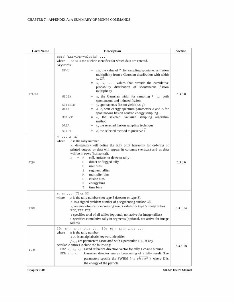
CHAPTER 7 - APPENDIX A: A SUMMARY OF MCNP6 COMMANDS
Chapter 7-40 MCNP User’s Manual
Card Name Description Section
FMULT
zaid [KEYWORD=value(s) ...] where zaid is the nuclide identifier for which data are entered. Keywords: SFNU = nu, the value of for sampling spontaneous fission
multiplicity from a Gaussian distribution with width w, OR
= x1 x2 ..., values that provide the cumulative probability distribution of spontaneous fission multiplicity
WIDTH = w, the Gaussian width for sampling for both spontaneous and induced fission.
SFYIELD = y, spontaneous fission yield (n/s-g). WATT = a b, watt energy spectrum parameters a and b for
spontaneous fission neutron energy sampling. METHOD = m, the selected Gaussian sampling algorithm
method. DATA = d, the selected fission sampling technique. . SHIFT = d, the selected method to preserve .
3.3.3.8
FQn
a1 ... a7 a8 where n is the tally number ai designators will define the tally print hierarchy for ordering of
printed output; a7 data will appear in columns (vertical) and a8 data will be in rows (horizontal).
ai = F cell, surface, or detector tally D direct or flagged tally U user bins S segment tallies M multiplier bins C cosine bins E energy bins T time bins
3.3.5.6
FSn
s1 s2 ... [T] or [C] where n is the tally number (not type 5 detector or type 8). si is a signed problem number of a segmenting surface OR. si are monotonically increasing s-axis values for type 5 image tallies
FIC, FIP, FIR T specifies total of all tallies (optional, not active for image tallies) C specifies cumulative tally in segments (optional, not active for image
tallies)
3.3.5.14
FTn
ID1 p1,1 p1,2 p1,3 ... ID2 p2,1 p2,2 p2,3 ... where n is the tally number IDi is an alphabetic keyword identifier pi,j are parameters associated with a particular IDi, if any Available entries include the following: FRV v1 v2 v3 Fixed reference direction vector for tally 1 cosine binning GEB a b c Gaussian detector energy broadening of a tally result. The
parameters specify the FWHM (= ), where E is the energy of the particle.
3.3.5.18
ν
ν
ν
2cEEba ++
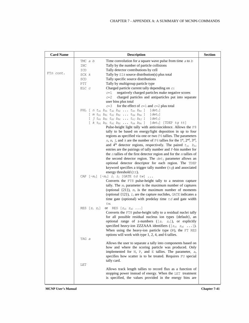
CHAPTER 7 - APPENDIX A: A SUMMARY OF MCNP6 COMMANDS
MCNP User’s Manual Chapter 7-41
Card Name Description Section FTn cont.
TMC a b Time convolution for a square wave pulse from time a to b INC Tally by the number of particle collisions ICD Tally detector contributions by cell SCX k Tally by SIk source distribution(s) plus total SCD Tally specific source distributions PTT Tally by multigroup particle type ELC c Charged particle current tally depending on c: c=1 negatively charged particles make negative scores c=2 charged particles and antiparticles put into separate
user bins plus total c=3 for the effect of c=1 and c=2 plus total PHL [ n ta1 ba1 ta2 ba2 ... tbn bbn ] [det1] [ m tb1 bb1 tb2 bb2 ... tbm bbm ] [det2] [ j tb1 bb1 tb2 bb2 ... tbj bbj ] [det3] [ k tb1 bb1 tb2 bb2 ... tbk bbk ] [det4] [TDEP tg tt] Pulse-height light tally with anticoincidence. Allows the F8
tally to be based on energy/light deposition in up to four regions as specified via one or two F6 tallies. The parameters n, m, j, and k are the number of F6 tallies for the 1st, 2nd, 3rd, and 4th detector regions, respectively. The paired txi bxi entries are the pairings of tally number and F-bin number for the n tallies of the first detector region and for the m tallies of the second detector region. The deti parameter allows an optional detector descriptor for each region. The TDEP keyword specifies a trigger tally number (tg) and associated energy threshold (tt).
CAP [-mc] [-mo] i1 i2 [GATE td tw] ... Converts the FT8 pulse-height tally to a neutron capture
tally. The mc parameter is the maximum number of captures (optional 21), mo is the maximum number of moments (optional 12), in are the capture nuclides, GATE indicates a time gate (optional) with predelay time td and gate width tw.
RES [z1 z2] or RES [za1 za2 ...] Converts the FT8 pulse-height tally to a residual nuclei tally
for all possible residual nucleus ion types default, an optional range of z-numbers ([z1 z2]), or explicitly specified heavy-ion ZZZAAA identifiers ([za1 za2 ...]). When using the heavy-ion particle type (#), the FT RES options will work with type 1, 2, 4, and 6 tallies.
TAG a Allows the user to separate a tally into components based on
how and where the scoring particle was produced. Only implemented for N, P, and E tallies. The parameter, a, specifies how scatter is to be treated. Requires FU special tally card.
LET Allows track length tallies to record flux as a function of
stopping power instead of energy. When the LET treatment is specified, the values provided in the energy bins are
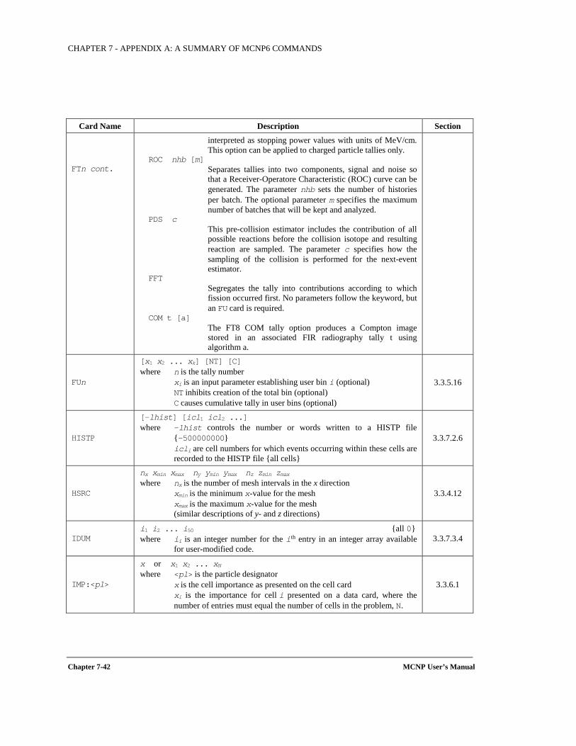
CHAPTER 7 - APPENDIX A: A SUMMARY OF MCNP6 COMMANDS
Chapter 7-42 MCNP User’s Manual
Card Name Description Section FTn cont.
interpreted as stopping power values with units of MeV/cm. This option can be applied to charged particle tallies only.
ROC nhb [m] Separates tallies into two components, signal and noise so
that a Receiver-Operatore Characteristic (ROC) curve can be generated. The parameter nhb sets the number of histories per batch. The optional parameter m specifies the maximum number of batches that will be kept and analyzed.
PDS c This pre-collision estimator includes the contribution of all
possible reactions before the collision isotope and resulting reaction are sampled. The parameter c specifies how the sampling of the collision is performed for the next-event estimator.
FFT Segregates the tally into contributions according to which
fission occurred first. No parameters follow the keyword, but an FU card is required.
COM t [a] The FT8 COM tally option produces a Compton image
stored in an associated FIR radiography tally t using algorithm a.
FUn
[x1 x2 ... xk] [NT] [C] where n is the tally number xi is an input parameter establishing user bin i (optional) NT inhibits creation of the total bin (optional) C causes cumulative tally in user bins (optional)
3.3.5.16
HISTP
[-lhist] [icl1 icl2 ...] where -lhist controls the number or words written to a HISTP file
-500000000 icli are cell numbers for which events occurring within these cells are
recorded to the HISTP file all cells
3.3.7.2.6
HSRC
nx xmin xmax ny ymin ymax nz zmin zmax where nx is the number of mesh intervals in the x direction xmin is the minimum x-value for the mesh xmax is the maximum x-value for the mesh (similar descriptions of y- and z directions)
3.3.4.12
IDUM i1 i2 ... i50 all 0 where ii is an integer number for the ith entry in an integer array available
for user-modified code. 3.3.7.3.4
IMP:<pl>
x or x1 x2 ... xN where <pl> is the particle designator x is the cell importance as presented on the cell card xi is the importance for cell i presented on a data card, where the
number of entries must equal the number of cells in the problem, N.
3.3.6.1
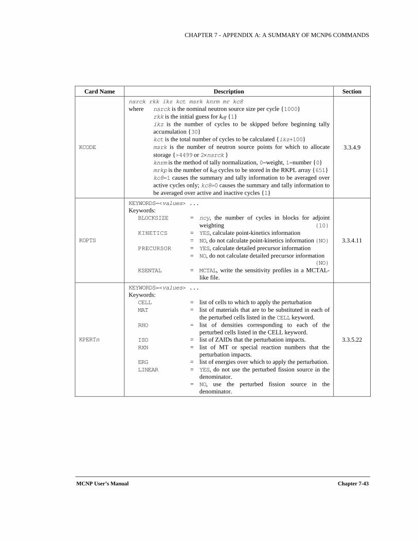
CHAPTER 7 - APPENDIX A: A SUMMARY OF MCNP6 COMMANDS
MCNP User’s Manual Chapter 7-43
Card Name Description Section
KCODE
nsrck rkk ikz kct msrk knrm mr kc8 where nsrck is the nominal neutron source size per cycle 1000 rkk is the initial guess for keff 1 ikz is the number of cycles to be skipped before beginning tally
accumulation 30 kct is the total number of cycles to be calculated ikz+100 msrk is the number of neutron source points for which to allocate
storage >4499 or 2×nsrck knrm is the method of tally normalization, 0=weight, 1=number 0 mrkp is the number of keff cycles to be stored in the RKPL array 651 kc8=1 causes the summary and tally information to be averaged over
active cycles only; kc8=0 causes the summary and tally information to be averaged over active and inactive cycles 1
3.3.4.9
KOPTS
KEYWORDS=<values> ... Keywords: BLOCKSIZE = ncy, the number of cycles in blocks for adjoint
weighting 10 KINETICS = YES, calculate point-kinetics information = NO, do not calculate point-kinetics information NO PRECURSOR = YES, calculate detailed precursor information = NO, do not calculate detailed precursor information NO KSENTAL = MCTAL, write the sensitivity profiles in a MCTAL-
like file.
3.3.4.11
KPERTn
KEYWORDS=<values> ... Keywords: CELL = list of cells to which to apply the perturbation MAT = list of materials that are to be substituted in each of
the perturbed cells listed in the CELL keyword. RHO = list of densities corresponding to each of the
perturbed cells listed in the CELL keyword. ISO = list of ZAIDs that the perturbation impacts. RXN = list of MT or special reaction numbers that the
perturbation impacts. ERG = list of energies over which to apply the perturbation. LINEAR = YES, do not use the perturbed fission source in the
denominator. = NO, use the perturbed fission source in the
denominator.
3.3.5.22
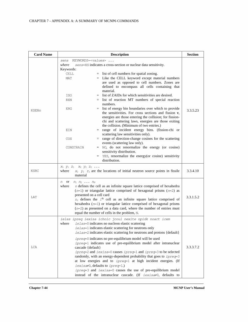
CHAPTER 7 - APPENDIX A: A SUMMARY OF MCNP6 COMMANDS
Chapter 7-44 MCNP User’s Manual
Card Name Description Section
KSENn
sens KEYWORDS=<values> ... where sens=XS indicates a cross-section or nuclear data sensitivity. Keywords: CELL = list of cell numbers for spatial zoning. MAT = Like the CELL keyword except material numbers
are used as opposed to cell numbers. Zones are defined to encompass all cells containing that material.
ISO = list of ZAIDs for which sensitivities are desired. RXN = list of reaction MT numbers of special reaction
numbers. ERG = list of energy bin boundaries over which to provide
the sensitivities. For cross sections and fission ν, energies are those entering the collision; for fission-chi and scattering laws, energies are those exiting the collision. (Minimum of two entries.)
EIN = range of incident energy bins. (fission-chi or scattering law sensitivities only).
COS = range of direction-change cosines for the scattering events (scattering law only).
CONSTRAIN = NO, do not renormalize the energy (or cosine) sensitivity distribution.
= YES, renormalize the energy(or cosine) sensitivity distribution.
3.3.5.23
KSRC x1 y1 z1 x2 y2 z2 ... where xi yi zi are the locations of initial neutron source points in fissile
material 3.3.4.10
LAT
n or n1 n2 ... nN where n defines the cell as an infinite square lattice comprised of hexahedra
(n=1) or triangular lattice comprised of hexagonal prisms (n=2) as presented on a cell card
ni defines the ith cell as an infinite square lattice comprised of hexahedra (n=1) or triangular lattice comprised of hexagonal prisms (n=2) as presented on a data card, where the number of entries must equal the number of cells in the problem, N.
3.3.1.5.2
LCA
ielas ipreq iexisa ichoic jcoul nexite npidk noact icem where ielas=0 indicates no nucleon elastic scattering ielas=1 indicates elastic scattering for neutrons only ielas=2 indicates elastic scattering for neutrons and protons default
ipreq=0 indicates no pre-equilibrium model will be used ipreq=1 indicates use of pre-equilibrium model after intranuclear
cascade default ipreq=2 and iexisa=0 causes ipreq=1 and ipreq=3 to be selected
randomly, with an energy-dependent probability that goes to ipreq=3 at low energies and to ipreq=1 at high incident energies. (If iexisa≠0, defaults to ipreq=1.)
ipreq=3 and iexisa=0 causes the use of pre-equilibrium model instead of the intranuclear cascade. (If iexisa≠0, defaults to
3.3.3.7.2
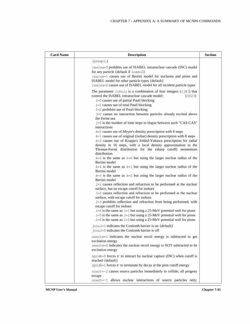
CHAPTER 7 - APPENDIX A: A SUMMARY OF MCNP6 COMMANDS
MCNP User’s Manual Chapter 7-45
Card Name Description Section
ipreq=1.)
iexisa=0 prohibits use of ISABEL intranuclear cascade (INC) model for any particle default if icem=2
iexisa=1 causes use of Bertini model for nucleons and pions and ISABEL model for other particle types default
iexisa=2 causes use of ISABEL model for all incident particle types
The parameter ichoic is a combination of four integers (ijkl) that control the ISABEL intranuclear cascade model: 0023
i=0 causes use of partial Pauli blocking i=1 causes use of total Pauli blocking i=2 prohibits use of Pauli blocking j=0 causes no interaction between particles already excited above
the Fermi sea j>0 is the number of time steps to elapse between such "CAS-CAS"
interactions k=0 causes use of Meyer's density prescription with 8 steps k=1 causes use of original (isobar) density prescription with 8 steps k=2 causes use of Krappe's folded-Yukawa prescription for radial
density in 16 steps, with a local density approximation to the Thomas-Fermi distribution for the (sharp cutoff) momentum distribution.
k=3 is the same as k=0 but using the larger nuclear radius of the Bertini model
k=4 is the same as k=1 but using the larger nuclear radius of the Bertini model
k=5 is the same as k=2 but using the larger nuclear radius of the Bertini model
l=1 causes reflection and refraction to be performed at the nuclear surface, but no escape cutoff for isobars
l=2 causes reflection and refraction to be performed at the nuclear surface, with escape cutoff for isobars
l=3 prohibits reflection and refraction from being performed, with escape cutoff for isobars
l=4 is the same as l=1 but using a 25-MeV potential well for pions l=5 is the same as l=2 but using a 25-MeV potential well for pions l=6 is the same as l=3 but using a 25-MeV potential well for pions
jcoul=1 indicates the Coulomb barrier is on default jcoul=0 indicates the Coulomb barrier is off
nexite=1 indicates the nuclear recoil energy is subtracted to get excitation energy
nexite=0 indicates the nuclear recoil energy is NOT subtracted to be excitation energy
npidk=0 forces π- to interact by nuclear capture (INC) when cutoff is reached default
npidk=1 forces π- to terminate by decay at the pion cutoff energy
noact=-2 causes source particles immediately to collide; all progeny escape
noact=-1 allows nuclear interactions of source particles only;

CHAPTER 7 - APPENDIX A: A SUMMARY OF MCNP6 COMMANDS
Chapter 7-46 MCNP User’s Manual
Card Name Description Section transport and slowing down are turned off
noact=0 turns off all non-elastic reactions noact=1 performs normal transport default) noact=2 indicates attenuation mode—transport primary source
particles without non-elastic reactions icem=0 causes use of the Bertini or ISABEL model determined by the
iexisa parameter icem=1 causes use of the CEM03.03 model default icem=2 causes use of the INCL4 model (default evaporation model is
ABLA) ilaq=0 causes use of LAQGSM03.03 to handle all heavy-ion
interactions as well as all light-ion interactions above 940 MeV/nucleon. ISABEL will handle light-ion interactions below this energy. Use LAQGSM03.03 for protons and neutrons above the energy cutoff specified by parameters flenb1 and flenb2 on the LCB card
ilaq=1 causes use of LAQGSM03.03 to handle all heavy-ion interactions as well as all light-ion interactions.
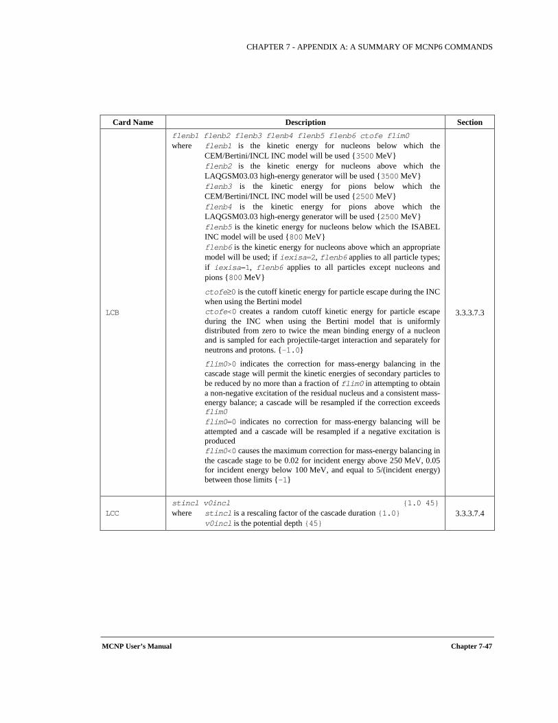
CHAPTER 7 - APPENDIX A: A SUMMARY OF MCNP6 COMMANDS
MCNP User’s Manual Chapter 7-47
Card Name Description Section
LCB
flenb1 flenb2 flenb3 flenb4 flenb5 flenb6 ctofe flim0 where flenb1 is the kinetic energy for nucleons below which the
CEM/Bertini/INCL INC model will be used 3500 MeV flenb2 is the kinetic energy for nucleons above which the
LAQGSM03.03 high-energy generator will be used 3500 MeV flenb3 is the kinetic energy for pions below which the
CEM/Bertini/INCL INC model will be used 2500 MeV flenb4 is the kinetic energy for pions above which the
LAQGSM03.03 high-energy generator will be used 2500 MeV flenb5 is the kinetic energy for nucleons below which the ISABEL
INC model will be used 800 MeV flenb6 is the kinetic energy for nucleons above which an appropriate
model will be used; if iexisa=2, flenb6 applies to all particle types; if iexisa=1, flenb6 applies to all particles except nucleons and pions 800 MeV
ctofe≥0 is the cutoff kinetic energy for particle escape during the INC when using the Bertini model
ctofe<0 creates a random cutoff kinetic energy for particle escape during the INC when using the Bertini model that is uniformly distributed from zero to twice the mean binding energy of a nucleon and is sampled for each projectile-target interaction and separately for neutrons and protons. -1.0
flim0>0 indicates the correction for mass-energy balancing in the cascade stage will permit the kinetic energies of secondary particles to be reduced by no more than a fraction of flim0 in attempting to obtain a non-negative excitation of the residual nucleus and a consistent mass-energy balance; a cascade will be resampled if the correction exceeds flim0
flim0=0 indicates no correction for mass-energy balancing will be attempted and a cascade will be resampled if a negative excitation is produced
flim0<0 causes the maximum correction for mass-energy balancing in the cascade stage to be 0.02 for incident energy above 250 MeV, 0.05 for incident energy below 100 MeV, and equal to 5/(incident energy) between those limits -1
3.3.3.7.3
LCC stincl v0incl 1.0 45 where stincl is a rescaling factor of the cascade duration 1.0 v0incl is the potential depth 45
3.3.3.7.4
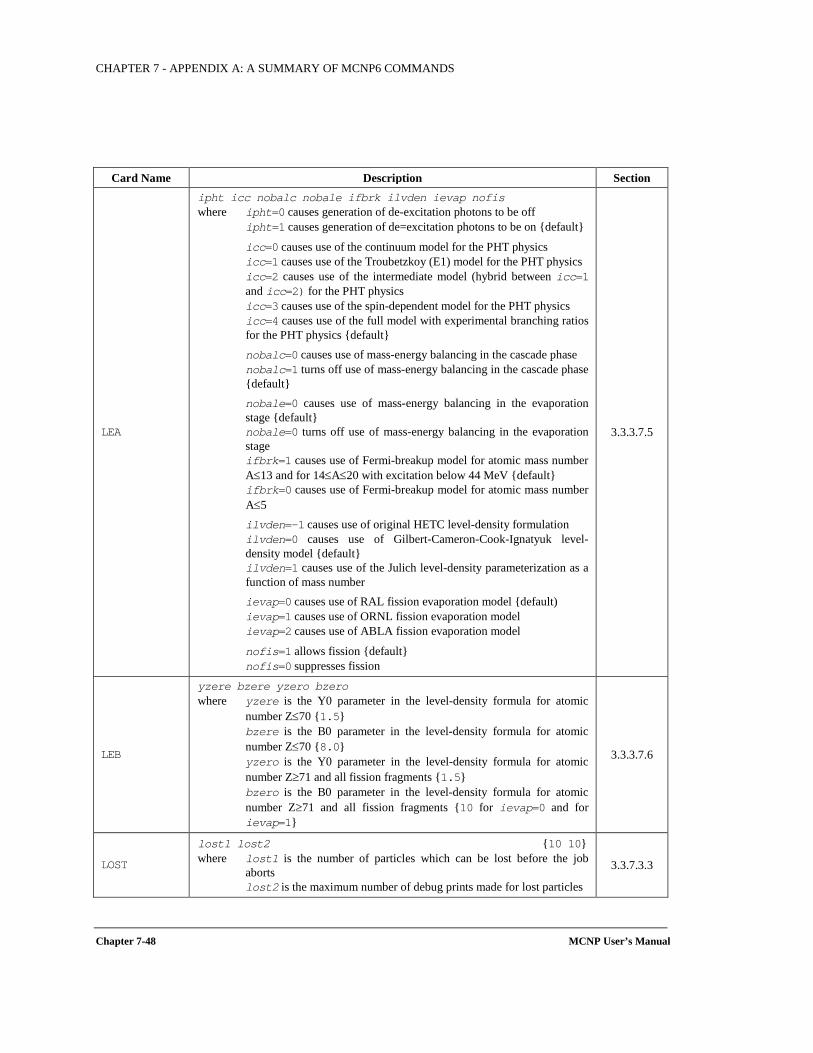
CHAPTER 7 - APPENDIX A: A SUMMARY OF MCNP6 COMMANDS
Chapter 7-48 MCNP User’s Manual
Card Name Description Section
LEA
ipht icc nobalc nobale ifbrk ilvden ievap nofis where ipht=0 causes generation of de-excitation photons to be off ipht=1 causes generation of de=excitation photons to be on default
icc=0 causes use of the continuum model for the PHT physics icc=1 causes use of the Troubetzkoy (E1) model for the PHT physics icc=2 causes use of the intermediate model (hybrid between icc=1
and icc=2) for the PHT physics icc=3 causes use of the spin-dependent model for the PHT physics icc=4 causes use of the full model with experimental branching ratios
for the PHT physics default nobalc=0 causes use of mass-energy balancing in the cascade phase nobalc=1 turns off use of mass-energy balancing in the cascade phase
default nobale=0 causes use of mass-energy balancing in the evaporation
stage default nobale=0 turns off use of mass-energy balancing in the evaporation
stage ifbrk=1 causes use of Fermi-breakup model for atomic mass number
A≤13 and for 14≤A≤20 with excitation below 44 MeV default ifbrk=0 causes use of Fermi-breakup model for atomic mass number
A≤5 ilvden=-1 causes use of original HETC level-density formulation ilvden=0 causes use of Gilbert-Cameron-Cook-Ignatyuk level-
density model default ilvden=1 causes use of the Julich level-density parameterization as a
function of mass number ievap=0 causes use of RAL fission evaporation model default) ievap=1 causes use of ORNL fission evaporation model ievap=2 causes use of ABLA fission evaporation model
nofis=1 allows fission default nofis=0 suppresses fission
3.3.3.7.5
LEB
yzere bzere yzero bzero where yzere is the Y0 parameter in the level-density formula for atomic
number Z≤70 1.5 bzere is the B0 parameter in the level-density formula for atomic
number Z≤70 8.0 yzero is the Y0 parameter in the level-density formula for atomic
number Z≥71 and all fission fragments 1.5 bzero is the B0 parameter in the level-density formula for atomic
number Z≥71 and all fission fragments 10 for ievap=0 and for ievap=1
3.3.3.7.6
LOST
lost1 lost2 10 10 where lost1 is the number of particles which can be lost before the job
aborts lost2 is the maximum number of debug prints made for lost particles
3.3.7.3.3
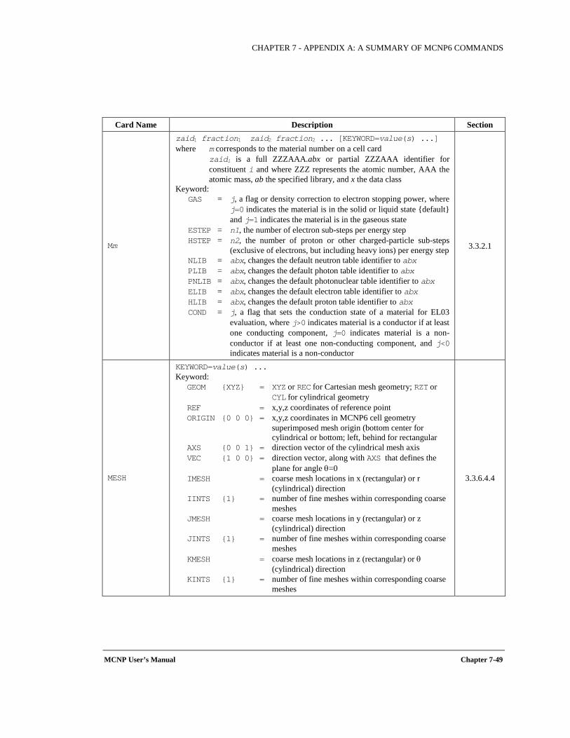
CHAPTER 7 - APPENDIX A: A SUMMARY OF MCNP6 COMMANDS
MCNP User’s Manual Chapter 7-49
Card Name Description Section
Mm
zaid1 fraction1 zaid2 fraction2 ... [KEYWORD=value(s) ...] where m corresponds to the material number on a cell card zaidi is a full ZZZAAA.abx or partial ZZZAAA identifier for
constituent i and where ZZZ represents the atomic number, AAA the atomic mass, ab the specified library, and x the data class
Keyword: GAS = j, a flag or density correction to electron stopping power, where
j=0 indicates the material is in the solid or liquid state default and j=1 indicates the material is in the gaseous state
ESTEP = n1, the number of electron sub-steps per energy step HSTEP = n2, the number of proton or other charged-particle sub-steps
(exclusive of electrons, but including heavy ions) per energy step NLIB = abx, changes the default neutron table identifier to abx PLIB = abx, changes the default photon table identifier to abx PNLIB = abx, changes the default photonuclear table identifier to abx ELIB = abx, changes the default electron table identifier to abx HLIB = abx, changes the default proton table identifier to abx COND = j, a flag that sets the conduction state of a material for EL03
evaluation, where j>0 indicates material is a conductor if at least one conducting component, j=0 indicates material is a non-conductor if at least one non-conducting component, and j<0 indicates material is a non-conductor
3.3.2.1
MESH
KEYWORD=value(s) ... Keyword: GEOM XYZ = XYZ or REC for Cartesian mesh geometry; RZT or
CYL for cylindrical geometry REF = x,y,z coordinates of reference point ORIGIN 0 0 0 = x,y,z coordinates in MCNP6 cell geometry
superimposed mesh origin (bottom center for cylindrical or bottom; left, behind for rectangular
AXS 0 0 1 = direction vector of the cylindrical mesh axis VEC 1 0 0 = direction vector, along with AXS that defines the
plane for angle θ=0 IMESH = coarse mesh locations in x (rectangular) or r
(cylindrical) direction IINTS 1 = number of fine meshes within corresponding coarse
meshes JMESH = coarse mesh locations in y (rectangular) or z
(cylindrical) direction JINTS 1 = number of fine meshes within corresponding coarse
meshes KMESH = coarse mesh locations in z (rectangular) or θ
(cylindrical) direction KINTS 1 = number of fine meshes within corresponding coarse
meshes
3.3.6.4.4
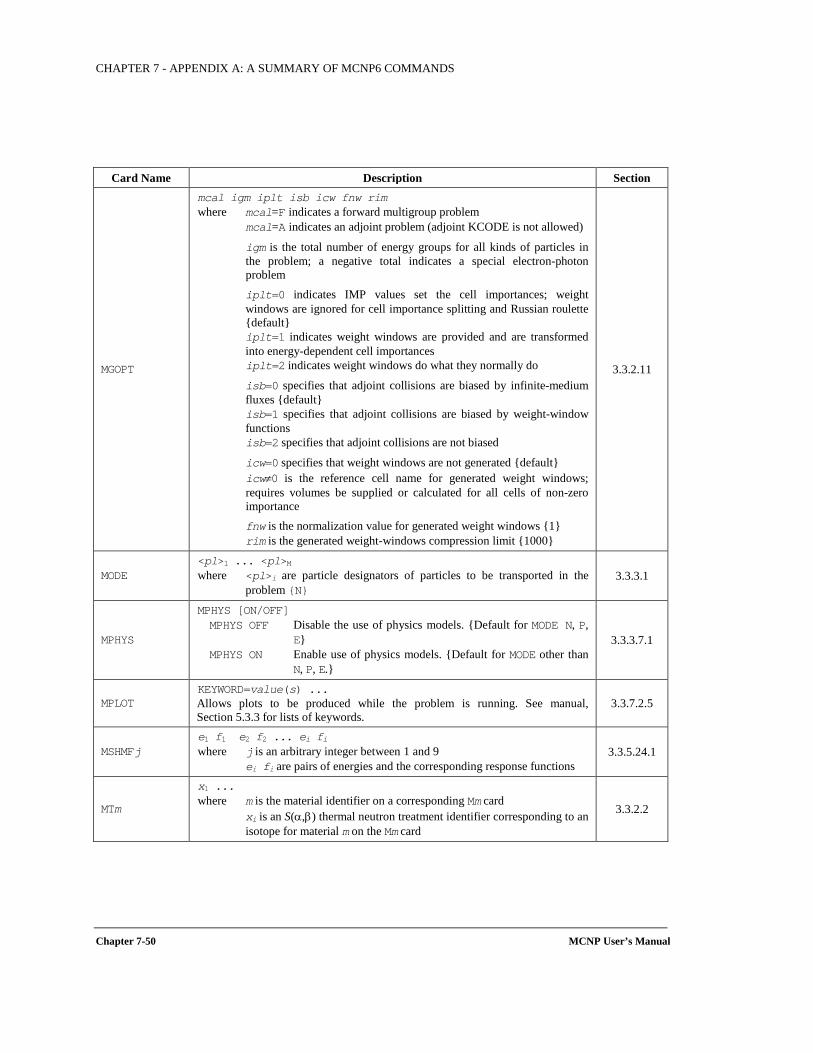
CHAPTER 7 - APPENDIX A: A SUMMARY OF MCNP6 COMMANDS
Chapter 7-50 MCNP User’s Manual
Card Name Description Section
MGOPT
mcal igm iplt isb icw fnw rim where mcal=F indicates a forward multigroup problem mcal=A indicates an adjoint problem (adjoint KCODE is not allowed)
igm is the total number of energy groups for all kinds of particles in the problem; a negative total indicates a special electron-photon problem
iplt=0 indicates IMP values set the cell importances; weight windows are ignored for cell importance splitting and Russian roulette default
iplt=1 indicates weight windows are provided and are transformed into energy-dependent cell importances
iplt=2 indicates weight windows do what they normally do
isb=0 specifies that adjoint collisions are biased by infinite-medium fluxes default
isb=1 specifies that adjoint collisions are biased by weight-window functions
isb=2 specifies that adjoint collisions are not biased
icw=0 specifies that weight windows are not generated default icw≠0 is the reference cell name for generated weight windows;
requires volumes be supplied or calculated for all cells of non-zero importance
fnw is the normalization value for generated weight windows 1 rim is the generated weight-windows compression limit 1000
3.3.2.11
MODE <pl>1 ... <pl>M where <pl>i are particle designators of particles to be transported in the
problem N 3.3.3.1
MPHYS
MPHYS [ON/OFF] MPHYS OFF Disable the use of physics models. Default for MODE N, P,
E MPHYS ON Enable use of physics models. Default for MODE other than
N, P, E.
3.3.3.7.1
MPLOT KEYWORD=value(s) ... Allows plots to be produced while the problem is running. See manual, Section 5.3.3 for lists of keywords.
3.3.7.2.5
MSHMFj e1 f1 e2 f2 ... ei fi where j is an arbitrary integer between 1 and 9 ei fi are pairs of energies and the corresponding response functions
3.3.5.24.1
MTm
x1 ... where m is the material identifier on a corresponding Mm card xi is an S(α,β) thermal neutron treatment identifier corresponding to an
isotope for material m on the Mm card
3.3.2.2
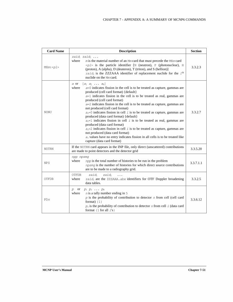
CHAPTER 7 - APPENDIX A: A SUMMARY OF MCNP6 COMMANDS
MCNP User’s Manual Chapter 7-51
Card Name Description Section
MXm:<pl>
zaid1 zaid2 ... where m is the material number of an Mm card that must precede the MXm card <pl> is the particle identifier [N (neutron), P (photonuclear), H
(proton), A (alpha), D (deuteron), T (triton), and S (hellion)] zaidi is the ZZZAAA identifier of replacement nuclide for the ith
nuclide on the Mm card.
3.3.2.3
NONU
a or [a1 a2 ... aN] where a=0 indicates fission in the cell is to be treated as capture, gammas are
produced (cell card format) default a=1 indicates fission in the cell is to be treated as real, gammas are
produced (cell card format) a=2 indicates fission in the cell is to be treated as capture, gammas are
not produced (cell card format) ai=0 indicates fission in cell i is to be treated as capture, gammas are
produced (data card format) default ai=1 indicates fission in cell i is to be treated as real, gammas are
produced (data card format) ai=2 indicates fission in cell i is to be treated as capture, gammas are
not produced (data card format) ai values have no entry indicates fission in all cells is to be treated like
capture (data card format)
3.3.2.7
NOTRN If the NOTRN card appears in the INP file, only direct (unscattered) contributions are made to point detectors and the detector grid 3.3.5.20
NPS
npp npsmg where npp is the total number of histories to be run in the problem npsmg is the number of histories for which direct source contributions
are to be made to a radiography grid.
3.3.7.1.1
OTFDB OTFDB zaid1 zaid2 ... where zaidi are the ZZZAAA.abx identifiers for OTF Doppler broadening
data tables. 3.3.2.5
PDn
p or p1 p2 ... pN where n is a tally number ending in 5 p is the probability of contribution to detector n from cell (cell card
format) 1 pi is the probability of contribution to detector n from cell i (data card
format 1 for all i's
3.3.6.12

CHAPTER 7 - APPENDIX A: A SUMMARY OF MCNP6 COMMANDS
Chapter 7-52 MCNP User’s Manual
Card Name Description Section
PERTn:<pl>
KEYWORD=value(s) ... where n is a unique arbitrary perturbation number ≤99999999 <pl> is the particle designator [N (neutron), P (photon), or N,P
(combined neutron-photon)] Keywords:
CELL c1 ... ck = comma or space delimited list of cells to which to apply perturbation
MAT m = single material number of an existing Mm card with which to fill all cells listed in CELL keyword
RHO rho = single value of perturbed density of cells listed after CELL keyword
METHOD 1 = 1 performs 1st and 2nd order perturbation calculation and prints the differential change in the tally
= 2 performs 1st order perturbation calculation only and prints the differential change in the tally
= 3 performs 2nd order perturbation calculation only and prints the differential change in the tally
= -1, -2, or -3 same as above except the perturbed tally is printed rather than the differential
ERG eLB eUB = lower and upper energy entries to specify energy range for perturbation
RXN rx1 ... = ENDF/B reaction numbers to which to apply perturbation
3.3.5.21
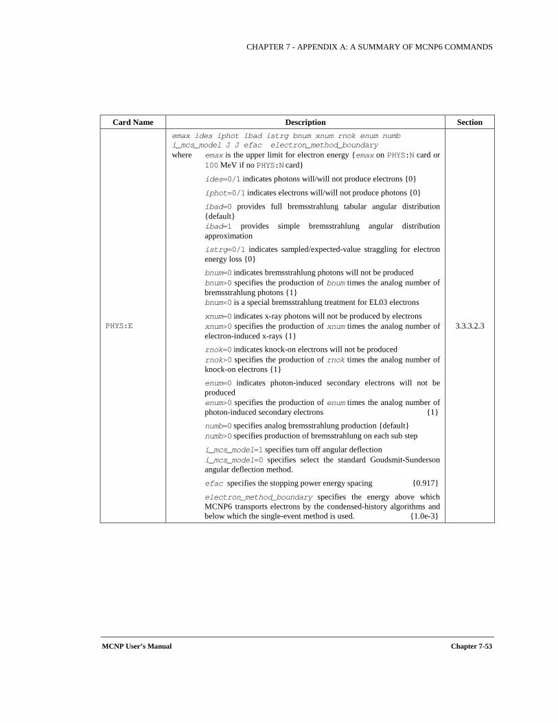
CHAPTER 7 - APPENDIX A: A SUMMARY OF MCNP6 COMMANDS
MCNP User’s Manual Chapter 7-53
Card Name Description Section
PHYS:E
emax ides iphot ibad istrg bnum xnum rnok enum numb i_mcs_model J J efac electron_method_boundary where emax is the upper limit for electron energy emax on PHYS:N card or
100 MeV if no PHYS:N card
ides=0/1 indicates photons will/will not produce electrons 0
iphot=0/1 indicates electrons will/will not produce photons 0
ibad=0 provides full bremsstrahlung tabular angular distribution default
ibad=1 provides simple bremsstrahlung angular distribution approximation
istrg=0/1 indicates sampled/expected-value straggling for electron energy loss 0
bnum=0 indicates bremsstrahlung photons will not be produced bnum>0 specifies the production of bnum times the analog number of
bremsstrahlung photons 1 bnum<0 is a special bremsstrahlung treatment for EL03 electrons
xnum=0 indicates x-ray photons will not be produced by electrons xnum>0 specifies the production of xnum times the analog number of
electron-induced x-rays 1 rnok=0 indicates knock-on electrons will not be produced rnok>0 specifies the production of rnok times the analog number of
knock-on electrons 1 enum=0 indicates photon-induced secondary electrons will not be
produced enum>0 specifies the production of enum times the analog number of
photon-induced secondary electrons 1 numb=0 specifies analog bremsstrahlung production default numb>0 specifies production of bremsstrahlung on each sub step
i_mcs_model=1 specifies turn off angular deflection i_mcs_model=0 specifies select the standard Goudsmit-Sunderson
angular deflection method.
efac specifies the stopping power energy spacing 0.917
electron_method_boundary specifies the energy above which MCNP6 transports electrons by the condensed-history algorithms and below which the single-event method is used. 1.0e-3
3.3.3.2.3
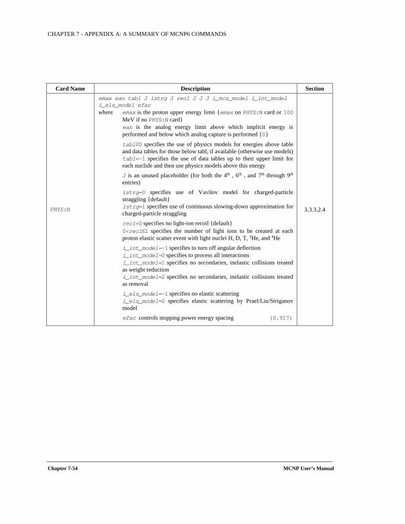
CHAPTER 7 - APPENDIX A: A SUMMARY OF MCNP6 COMMANDS
Chapter 7-54 MCNP User’s Manual
Card Name Description Section
PHYS:H
emax ean tabl J istrg J recl J J J i_mcs_model i_int_model i_els_model efac where emax is the proton upper energy limit emax on PHYS:N card or 100
MeV if no PHYS:N card ean is the analog energy limit above which implicit energy is
performed and below which analog capture is performed 0
tabl≥0 specifies the use of physics models for energies above table and data tables for those below tabl, if available (otherwise use models)
tabl=-1 specifies the use of data tables up to their upper limit for each nuclide and then use physics models above this energy
J is an unused placeholder (for both the 4th , 6th , and 7th through 9th entries)
istrg=0 specifies use of Vavilov model for charged-particle straggling default
istrg=1 specifies use of continuous slowing-down approximation for charged-particle straggling
recl=0 specifies no light-ion recoil default 0<recl≤1 specifies the number of light ions to be created at each
proton elastic scatter event with light nuclei H, D, T, 3He, and 4He i_int_model=-1 specifies to turn off angular deflection i_int_model=0 specifies to process all interactions i_int_model=1 specifies no secondaries, inelastic collisions treated
as weight reduction i_int_model=2 specifies no secondaries, inelastic collisions treated
as removal i_els_model=-1 specifies no elastic scattering i_els_model=0 specifies elastic scattering by Prael/Liu/Striganov
model efac controls stopping power energy spacing 0.917
3.3.3.2.4
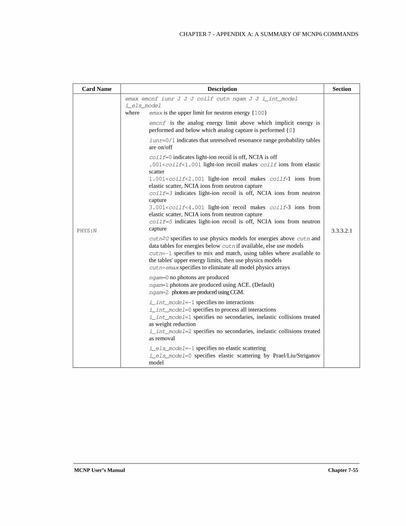
CHAPTER 7 - APPENDIX A: A SUMMARY OF MCNP6 COMMANDS
MCNP User’s Manual Chapter 7-55
Card Name Description Section
PHYS:N
emax emcnf iunr J J J coilf cutn ngam J J i_int_model i_els_model where emax is the upper limit for neutron energy 100
emcnf is the analog energy limit above which implicit energy is performed and below which analog capture is performed 0
iunr=0/1 indicates that unresolved resonance range probability tables are on/off
coilf=0 indicates light-ion recoil is off, NCIA is off .001<coilf<1.001 light-ion recoil makes coilf ions from elastic
scatter 1.001<coilf<2.001 light-ion recoil makes coilf-1 ions from
elastic scatter, NCIA ions from neutron capture coilf=3 indicates light-ion recoil is off, NCIA ions from neutron
capture 3.001<coilf<4.001 light-ion recoil makes coilf-3 ions from
elastic scatter, NCIA ions from neutron capture coilf=5 indicates light-ion recoil is off, NCIA ions from neutron
capture cutn≥0 specifies to use physics models for energies above cutn and
data tables for energies below cutn if available, else use models cutn=-1 specifies to mix and match, using tables where available to
the tables' upper energy limits, then use physics models cutn>emax specifies to eliminate all model physics arrays
ngam=0 no photons are produced ngam=1 photons are produced using ACE. (Default) ngam=2 photons are produced using CGM.
i_int_model=-1 specifies no interactions i_int_model=0 specifies to process all interactions i_int_model=1 specifies no secondaries, inelastic collisions treated
as weight reduction i_int_model=2 specifies no secondaries, inelastic collisions treated
as removal i_els_model=-1 specifies no elastic scattering i_els_model=0 specifies elastic scattering by Prael/Liu/Striganov
model
3.3.3.2.1

CHAPTER 7 - APPENDIX A: A SUMMARY OF MCNP6 COMMANDS
Chapter 7-56 MCNP User’s Manual
Card Name Description Section
PHYS:P
emcpf ides nocoh ispn nodop J fism where emcpf is the upper energy limit for detailed photon physics treatment
emax on PHYS:N card or 100 MeV if no PHYS:N card
ides=0 indicates that generation of electrons in MODE E problems or bremsstrahlung photons with the thick-target bremsstrahlung model is turned on default
ides=1 indicates that generation of electrons in MODE E problems or bremsstrahlung photons with the thick-target bremsstrahlung model is turned off
nocoh=0/1 specifies coherent scattering will/will not occur 0
ispn=1/0/-1 specifies biased/none/analog photonuclear production is turned on 0
nodop=0/1 indicates photon Doppler energy broadening will/will not occur 0
fism=0/1 indicates to sample fission from ACE libraries/LLNL fission model
3.3.3.2.2
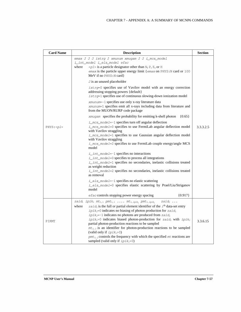
CHAPTER 7 - APPENDIX A: A SUMMARY OF MCNP6 COMMANDS
MCNP User’s Manual Chapter 7-57
Card Name Description Section
PHYS:<pl>
emax J J J istrg J xmunum xmugam J J i_mcs_model i_int_model i_els_model efac where <pl> is a particle designator other than N, P, E, or H emax is the particle upper energy limit emax on PHYS:N card or 100
MeV if no PHYS:N card
J is an unused placeholder
istrg=0 specifies use of Vavilov model with an energy correction addressing stopping powers default
istrg=1 specifies use of continuous slowing-down ionization model
xmunum=-1 specifies use only x-ray literature data xmunum=1 specifies emit all x-rays including data from literature and
from the MUON/RURP code package xmugam specifies the probability for emitting k-shell photon 0.65
i_mcs_model=-1 specifies turn off angular deflection i_mcs_model=0 specifies to use FermiLab angular deflection model
with Vavilov straggling i_mcs_model=1 specifies to use Gaussian angular deflection model
with Vavilov straggling i_mcs_model=2 specifies to use FermiLab couple energy/angle MCS
model i_int_model=-1 specifies no interactions i_int_model=0 specifies to process all integrations i_int_model=1 specifies no secondaries, inelastic collisions treated
as weight reduction i_int_model=2 specifies no secondaries, inelastic collisions treated
as removal i_els_model=-1 specifies no elastic scattering i_els_model=0 specifies elastic scattering by Prael/Liu/Striganov
model efac controls stopping power energy spacing 0.917
3.3.3.2.5
PIKMT
zaid1 ipik1 mt1,1 pmt1,1 .... mt1,ipik1 pmt1,ipik1 zaid2 ... where zaidi is the full or partial element identifier of the ith data-set entry ipiki=0 indicates no biasing of photon production for zaidi ipiki=-1 indicates no photons are produced from zaidi ipiki>0 indicates biased photon-production for zaidi with ipiki
partial photon-production reactions to be sampled mti,j is an identifier for photon-production reactions to be sampled
(valid only if ipiki>0) pmti,j controls the frequency with which the specified mt reactions are
sampled (valid only if ipiki>0)
3.3.6.15

CHAPTER 7 - APPENDIX A: A SUMMARY OF MCNP6 COMMANDS
Chapter 7-58 MCNP User’s Manual
Card Name Description Section
PRDMP
ndp ndm mct ndmp dmmp end of problem -60 0 large 0 where ndp>0 specifies to print tallies every ndp histories or kcode cycles
end of problem ndp<0 specifies to print tallies every ndp minutes of running time
ndm>0 specifies to dump to the RUNTPE file every ndm histories or criticality cycles
ndm<0 specifies to dump to the RUNTPE file every ndm minutes of running time -60
mct>0 specifies to write a MCTAL file at problem completion mct=0 suppresses the printing of a MCTAL file DEFAULT mct=-1 specifies to write a MCTAL file at problem completion, but
references to code name, version number, problem ID, figure of merit, and anything else having to do with running time are omitted from MCTAL and OUTP
mct=-2 specifies that additional prints in OUTP are turned off to assist in comparing multitasking output
ndmp specifies the maximum number of dumps to be kept on the RUNTPE file large
dmmp>0 specifies to write the tally fluctuation charts every dmmp histories or number of KCODE cycles
dmmp=0 specifies to write the tally fluctuation charts every 1000 particles or, if multiprocessing, 10 times total during the run
dmmp<0 specifies to write the tally fluctuation charts every 1000 particles
3.3.7.2.3
[x1 x2 ... xi ...] or blank or ALL where no entries causes the basic output to be printed DEFAULT xi>0 prints the basic output plus tables x1, x2 ... xi<0 prints the full output except tables x1, x2 ... ALL produces the full output print of all tables
3.3.7.2.1
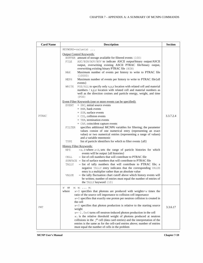
CHAPTER 7 - APPENDIX A: A SUMMARY OF MCNP6 COMMANDS
MCNP User’s Manual Chapter 7-59
Card Name Description Section
PTRAC
KEYWORD=value(s) ...
Output Control Keywords: BUFFER amount of storage available for filtered events 100 FILE ASC/BIN/AOV/BOV to indicate ASCII output/binary output/ASCII
output, overwriting existing ASCII PTRAC file/binary output, overwriting existing binary PTRAC file BIN
MAX Maximum number of events per history to write to PTRAC file 10000
MEPH Maximum number of events per history to write to PTRAC fileall events
WRITE POS/ALL to specify only x,y,z location with related cell and material numbers / x,y,z location with related cell and material numbers as well as the direction cosines and particle energy, weight, and time POS
Event Filter Keywords (one or more events can be specified): EVENT = SRC, initial source events = BNK, bank events = SUR, surface events = COL, collision events = TER, termination events = CAP, coincident capture events FILTER specifies additional MCNP6 variables for filtering; the parameter
values consist of one numerical entry (representing an exact value) or two numerical entries (representing a range of values) and a variable mnemonic
TYPE list of particle identifiers for which to filter events all History Filter Keywords: NPS =a,b where a<b, sets the range of particle histories for which
events will be output all histories CELL = list of cell numbers that will contribute to PTRAC file SURFACE = list of surface numbers that will contribute to PTRAC file TALLY = list of tally numbers that will contribute to PTRAC file; a
negative TALLY entry indicates that the corresponding VALUE entry is a multiplier rather than an absolute value
VALUE = the tally fluctuation chart cutoff above which history events will be written; number of entries must equal the number of entries of the TALLY keyword 10
3.3.7.2.4
PWT
w or w1 w2 ... wj where w>0 specifies that photons are produced with weights>w times the
ratio of the source cell importance to collision cell importance w=0 specifies that exactly one proton per neutron collision is created in
the cell w<0 specifies that photon production is relative to the starting source
weight w=-1.0e6 turns off neutron-induced photon production in the cell wj is the relative threshold weight of photons produced at neutron
collisions in the jth cell (data card entries) and the interpretation of the entries is the same as for the cell-card entries above; number of entries must equal the number of cells in the problem
3.3.6.17
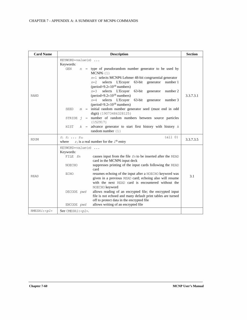
CHAPTER 7 - APPENDIX A: A SUMMARY OF MCNP6 COMMANDS
Chapter 7-60 MCNP User’s Manual
Card Name Description Section
RAND
KEYWORD=value(s) ... Keywords:
GEN n = type of pseudorandom number generator to be used by MCNP6 1 n=1 selects MCNP6 Lehmer 48-bit congruential generator n=2 selects L'Ecuyer 63-bit generator number 1 (period=9.2×10¹⁸ numbers) n=3 selects L'Ecuyer 63-bit generator number 2 (period=9.2×10¹⁸ numbers) n=4 selects L'Ecuyer 63-bit generator number 3 (period=9.2×10¹⁸ numbers)
SEED m = initial random number generator seed (must end in odd digit) 19073486328125
STRIDE j = number of random numbers between source particles 152917
HIST k = advance generator to start first history with history k random number 1
3.3.7.3.1
RDUM r1 r2 ... r50 all 0 where ri is a real number for the ith entry 3.3.7.3.5
READ
KEYWORD=value(s) ... Keywords:
FILE fn causes input from the file fn to be inserted after the READ card in the MCNP6 input deck
NOECHO suppresses printing of the input cards following the READ card
ECHO resumes echoing of the input after a NOECHO keyword was given in a previous READ card; echoing also will resume with the next READ card is encountered without the NOECHO keyword
DECODE pwd allows reading of an encrypted file; the encrypted input file is not echoed and many default print tables are turned off to protect data in the encrypted file
ENCODE pwd allows writing of an encrypted file
3.1
RMESHi:<pl> See CMESHi:<pl>.
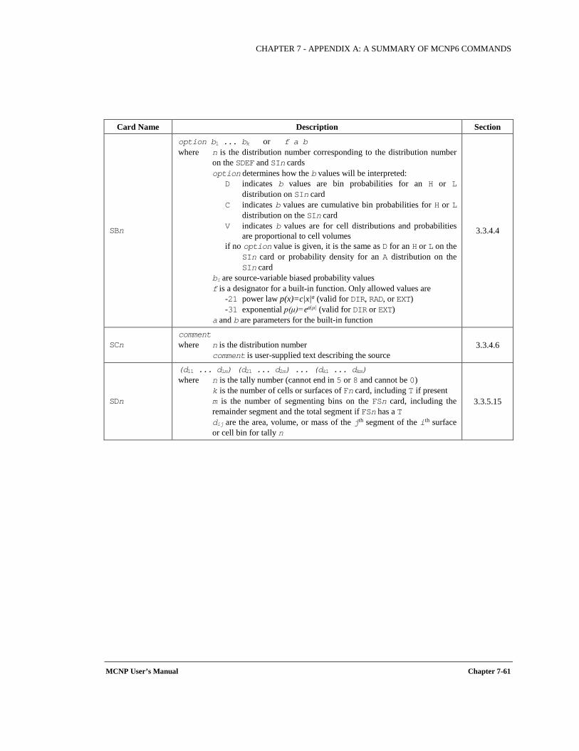
CHAPTER 7 - APPENDIX A: A SUMMARY OF MCNP6 COMMANDS
MCNP User’s Manual Chapter 7-61
Card Name Description Section
SBn
option b1 ... bk or f a b where n is the distribution number corresponding to the distribution number
on the SDEF and SIn cards option determines how the b values will be interpreted:
D indicates b values are bin probabilities for an H or L distribution on SIn card
C indicates b values are cumulative bin probabilities for H or L distribution on the SIn card
V indicates b values are for cell distributions and probabilities are proportional to cell volumes
if no option value is given, it is the same as D for an H or L on the SIn card or probability density for an A distribution on the SIn card
bi are source-variable biased probability values f is a designator for a built-in function. Only allowed values are
-21 power law p(x)=c|x|a (valid for DIR, RAD, or EXT) -31 exponential p(μ)=ea|μ| (valid for DIR or EXT)
a and b are parameters for the built-in function
3.3.4.4
SCn comment where n is the distribution number comment is user-supplied text describing the source
3.3.4.6
SDn
(d11 ... d1m) (d21 ... d2m) ... (dk1 ... dkm) where n is the tally number (cannot end in 5 or 8 and cannot be 0) k is the number of cells or surfaces of Fn card, including T if present m is the number of segmenting bins on the FSn card, including the
remainder segment and the total segment if FSn has a T dij are the area, volume, or mass of the jth segment of the ith surface
or cell bin for tally n
3.3.5.15
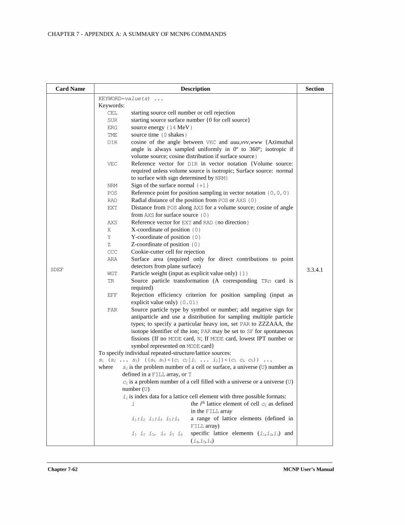
CHAPTER 7 - APPENDIX A: A SUMMARY OF MCNP6 COMMANDS
Chapter 7-62 MCNP User’s Manual
Card Name Description Section
SDEF
KEYWORD=value(s) ... Keywords:
CEL starting source cell number or cell rejection SUR starting source surface number 0 for cell source ERG source energy 14 MeV TME source time 0 shakes DIR cosine of the angle between VEC and uuu,vvv,www Azimuthal
angle is always sampled uniformly in 0º to 360º; isotropic if volume source; cosine distribution if surface source
VEC Reference vector for DIR in vector notation Volume source: required unless volume source is isotropic; Surface source: normal to surface with sign determined by NRM
NRM Sign of the surface normal +1 POS Reference point for position sampling in vector notation 0,0,0 RAD Radial distance of the position from POS or AXS 0 EXT Distance from POS along AXS for a volume source; cosine of angle
from AXS for surface source 0 AXS Reference vector for EXT and RAD no direction X X-coordinate of position 0 Y Y-coordinate of position 0 Z Z-coordinate of position 0 CCC Cookie-cutter cell for rejection ARA Surface area (required only for direct contributions to point
detectors from plane surface) WGT Particle weight (input as explicit value only) 1 TR Source particle transformation (A corresponding TRn card is
required) EFF Rejection efficiency criterion for position sampling (input as
explicit value only) 0.01 PAR Source particle type by symbol or number; add negative sign for
antiparticle and use a distribution for sampling multiple particle types; to specify a particular heavy ion, set PAR to ZZZAAA, the isotope identifier of the ion; PAR may be set to SF for spontaneous fissions If no MODE card, N; If MODE card, lowest IPT number or symbol represented on MODE card
To specify individual repeated-structure/lattice sources: s1 (s2 ... s3) ((s4 s5)<(c1 c2[i1 ... i2])<(c3 c4 c5)) ... where si is the problem number of a cell or surface, a universe (U) number as
defined in a FILL array, or T ci is a problem number of a cell filled with a universe or a universe (U)
number (U) ii is index data for a lattice cell element with three possible formats:
i the ith lattice element of cell c2 as defined in the FILL array
i1:i2 i3:i4 i5:i6 a range of lattice elements (defined in FILL array)
i1 i2 i3, i4 i5 i6 specific lattice elements (i1,i2,i3) and (i4,i5,i6)
3.3.4.1
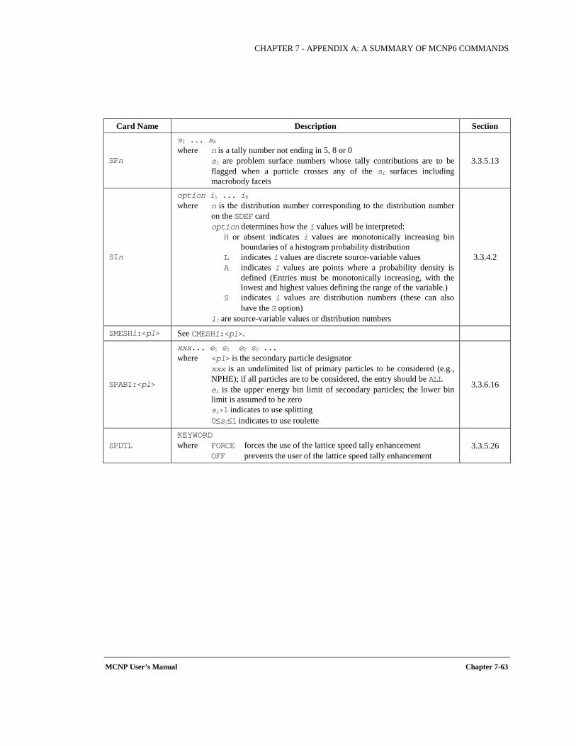
CHAPTER 7 - APPENDIX A: A SUMMARY OF MCNP6 COMMANDS
MCNP User’s Manual Chapter 7-63
Card Name Description Section
SFn
s1 ... sk where n is a tally number not ending in 5, 8 or 0 si are problem surface numbers whose tally contributions are to be
flagged when a particle crosses any of the si surfaces including macrobody facets
3.3.5.13
SIn
option i1 ... ik where n is the distribution number corresponding to the distribution number
on the SDEF card option determines how the i values will be interpreted:
H or absent indicates i values are monotonically increasing bin boundaries of a histogram probability distribution
L indicates i values are discrete source-variable values A indicates i values are points where a probability density is
defined (Entries must be monotonically increasing, with the lowest and highest values defining the range of the variable.)
S indicates i values are distribution numbers (these can also have the S option)
ii are source-variable values or distribution numbers
3.3.4.2
SMESHi:<pl> See CMESHi:<pl>.
SPABI:<pl>
xxx... e1 s1 e2 s2 ... where <pl> is the secondary particle designator xxx is an undelimited list of primary particles to be considered (e.g.,
NPHE); if all particles are to be considered, the entry should be ALL ei is the upper energy bin limit of secondary particles; the lower bin
limit is assumed to be zero si>1 indicates to use splitting 0≤si≤1 indicates to use roulette
3.3.6.16
SPDTL KEYWORD where FORCE forces the use of the lattice speed tally enhancement OFF prevents the user of the lattice speed tally enhancement
3.3.5.26
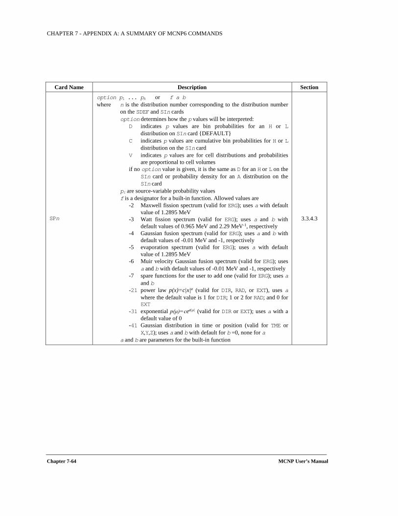
CHAPTER 7 - APPENDIX A: A SUMMARY OF MCNP6 COMMANDS
Chapter 7-64 MCNP User’s Manual
Card Name Description Section
SPn
option p1 ... pk or f a b where n is the distribution number corresponding to the distribution number
on the SDEF and SIn cards option determines how the p values will be interpreted:
D indicates p values are bin probabilities for an H or L distribution on SIn card DEFAULT
C indicates p values are cumulative bin probabilities for H or L distribution on the SIn card
V indicates p values are for cell distributions and probabilities are proportional to cell volumes
if no option value is given, it is the same as D for an H or L on the SIn card or probability density for an A distribution on the SIn card
pi are source-variable probability values f is a designator for a built-in function. Allowed values are
-2 Maxwell fission spectrum (valid for ERG); uses a with default value of 1.2895 MeV
-3 Watt fission spectrum (valid for ERG); uses a and b with default values of 0.965 MeV and 2.29 MeV-1, respectively
-4 Gaussian fusion spectrum (valid for ERG); uses a and b with default values of -0.01 MeV and -1, respectively
-5 evaporation spectrum (valid for ERG); uses a with default value of 1.2895 MeV
-6 Muir velocity Gaussian fusion spectrum (valid for ERG); uses a and b with default values of -0.01 MeV and -1, respectively
-7 spare functions for the user to add one (valid for ERG); uses a and b
-21 power law p(x)=c|x|a (valid for DIR, RAD, or EXT), uses a where the default value is 1 for DIR; 1 or 2 for RAD; and 0 for EXT
-31 exponential p(μ)=cea|μ| (valid for DIR or EXT); uses a with a default value of 0
-41 Gaussian distribution in time or position (valid for TME or X,Y,Z); uses a and b with default for b =0, none for a
a and b are parameters for the built-in function
3.3.4.3
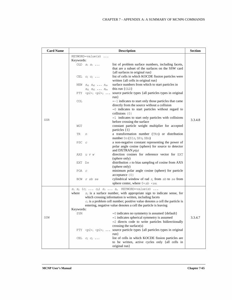
CHAPTER 7 - APPENDIX A: A SUMMARY OF MCNP6 COMMANDS
MCNP User’s Manual Chapter 7-65
Card Name Description Section
SSR
KEYWORD=value(s) ... Keywords:
OLD s1 s2 ... list of problem surface numbers, including facets, that are a subset of the surfaces on the SSW card all surfaces in original run
CEL c1 c2 ... list of cells in which KOCDE fission particles were written all cells in original run
NEW sa1 sa2 ... san surface numbers from which to start particles in sb1 sb2 ... sbn this run OLD PTY <pl>1 <pl>2 ... source particle types all particles types in original
run COL =-1 indicates to start only those particles that came
directly from the source without a collision =0 indicates to start particles without regard to
collisions 0 =1 indicates to start only particles with collisions
before crossing the surface WGT constant particle weight multiplier for accepted
particles 1 TR n a transformation number (TRn) or distribution
number Dn (SIn, SPn, SBn) PSC c a non-negative constant representing the power of
polar angle cosine (sphere) for source to detector and DXTRAN p(μ)
AXS u v w direction cosines for reference vector for EXT (sphere only)
EXT Dn distribution n to bias sampling of cosine from AXS (sphere only)
POA c minimum polar angle cosine (sphere) for particle acceptance 0
BCW r zb ze cylindrical window of rad r, from zb to ze from sphere center, where 0<zb <ze.
3.3.4.8
SSW
s1 s2 (c1 ... ck) s3 ... sn KEYWORD=value(s) ... where si is a surface number, with appropriate sign to indicate sense, for
which crossing information is written, including facets ci is a problem cell number; positive value denotes a cell the particle is
entering, negative value denotes a cell the particle is leaving Keywords:
SYM =0 indicates no symmetry is assumed default =1 indicates spherical symmetry is assumed =2 directs code to write particles bidirectionally
crossing the surface(s) PTY <pl>1 <pl>2 ... source particle types all particles types in original
run CEL c1 c2 ... list of cells in which KOCDE fission particles are
to be written, active cycles only all cells in original run
3.3.4.7
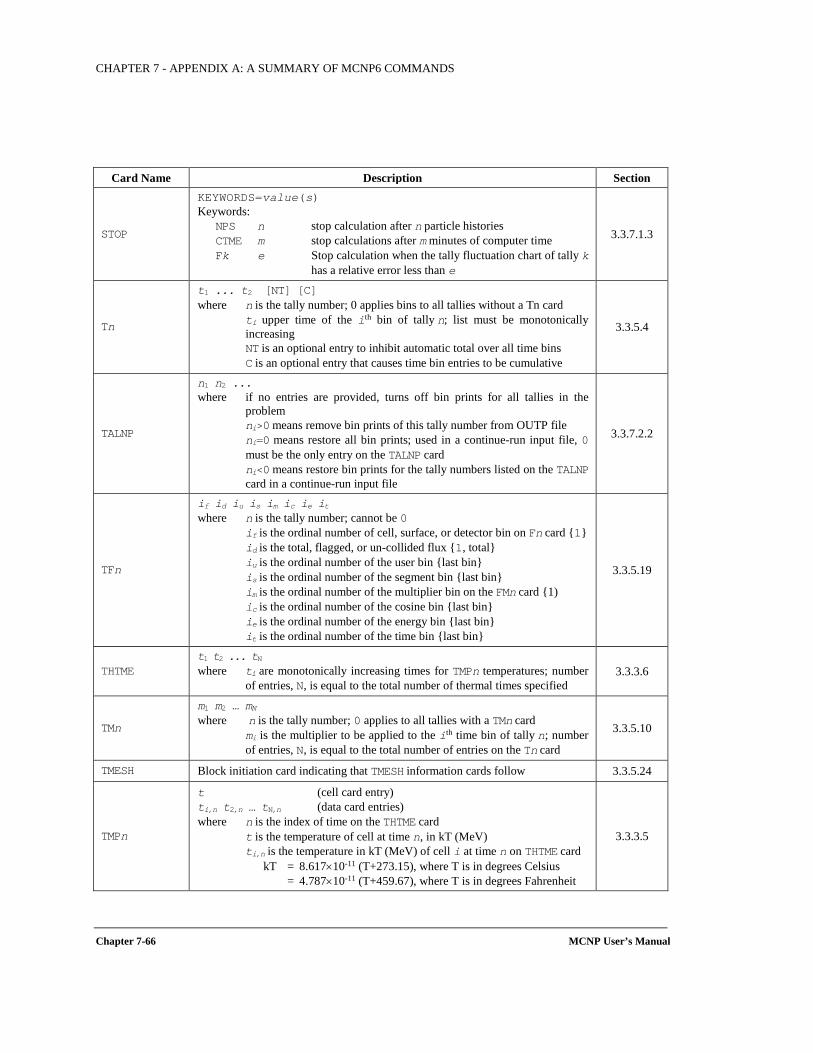
CHAPTER 7 - APPENDIX A: A SUMMARY OF MCNP6 COMMANDS
Chapter 7-66 MCNP User’s Manual
Card Name Description Section
STOP
KEYWORDS=value(s) Keywords:
NPS n stop calculation after n particle histories CTME m stop calculations after m minutes of computer time Fk e Stop calculation when the tally fluctuation chart of tally k
has a relative error less than e
3.3.7.1.3
Tn
t1 ... t2 [NT] [C] where n is the tally number; 0 applies bins to all tallies without a Tn card ti upper time of the ith bin of tally n; list must be monotonically
increasing NT is an optional entry to inhibit automatic total over all time bins C is an optional entry that causes time bin entries to be cumulative
3.3.5.4
TALNP
n1 n2 ... where if no entries are provided, turns off bin prints for all tallies in the
problem ni>0 means remove bin prints of this tally number from OUTP file ni=0 means restore all bin prints; used in a continue-run input file, 0
must be the only entry on the TALNP card ni<0 means restore bin prints for the tally numbers listed on the TALNP
card in a continue-run input file
3.3.7.2.2
TFn
if id iu is im ic ie it where n is the tally number; cannot be 0 if is the ordinal number of cell, surface, or detector bin on Fn card 1 id is the total, flagged, or un-collided flux 1, total iu is the ordinal number of the user bin last bin is is the ordinal number of the segment bin last bin im is the ordinal number of the multiplier bin on the FMn card 1) ic is the ordinal number of the cosine bin last bin ie is the ordinal number of the energy bin last bin it is the ordinal number of the time bin last bin
3.3.5.19
THTME t1 t2 ... tN where ti are monotonically increasing times for TMPn temperatures; number
of entries, N, is equal to the total number of thermal times specified 3.3.3.6
TMn
m1 m2 … mN where n is the tally number; 0 applies to all tallies with a TMn card mi is the multiplier to be applied to the ith time bin of tally n; number
of entries, N, is equal to the total number of entries on the Tn card
3.3.5.10
TMESH Block initiation card indicating that TMESH information cards follow 3.3.5.24
TMPn
t (cell card entry) ti,n t2,n … tN,n (data card entries) where n is the index of time on the THTME card t is the temperature of cell at time n, in kT (MeV) ti,n is the temperature in kT (MeV) of cell i at time n on THTME card
kT = 8.617×10⁻¹¹ (T+273.15), where T is in degrees Celsius = 4.787×10⁻¹¹ (T+459.67), where T is in degrees Fahrenheit
3.3.3.5
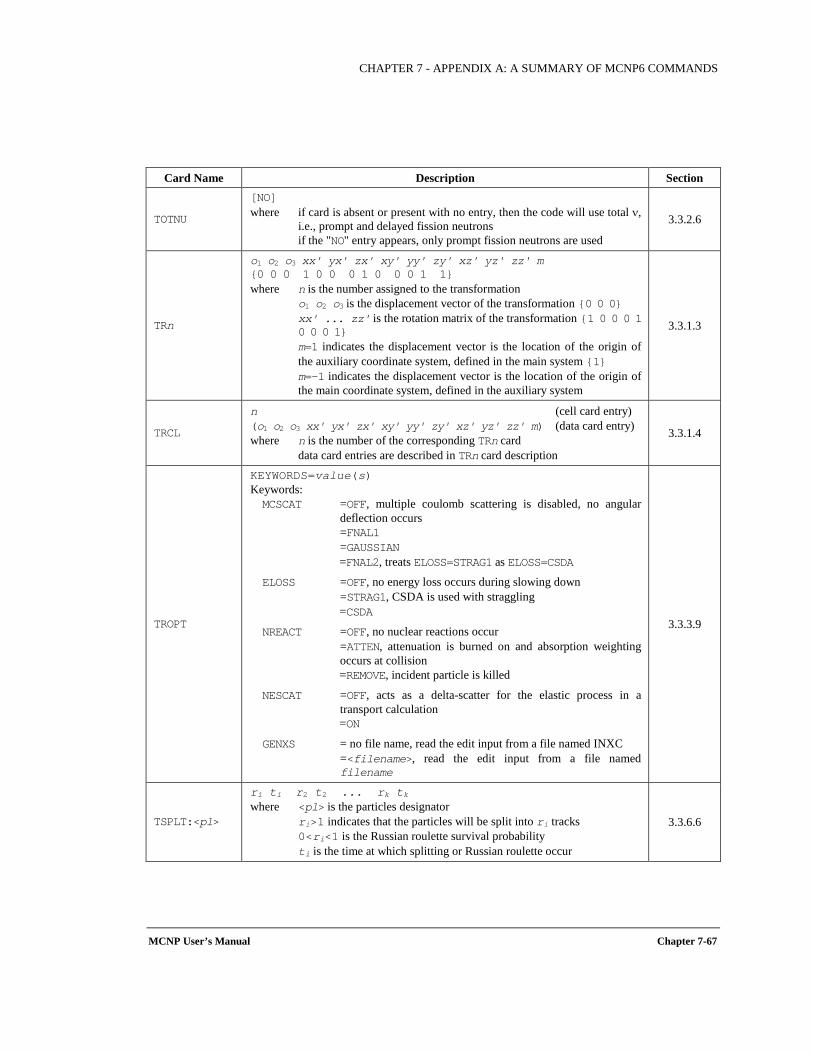
CHAPTER 7 - APPENDIX A: A SUMMARY OF MCNP6 COMMANDS
MCNP User’s Manual Chapter 7-67
Card Name Description Section
TOTNU
[NO] where if card is absent or present with no entry, then the code will use total ν,
i.e., prompt and delayed fission neutrons if the "NO" entry appears, only prompt fission neutrons are used
3.3.2.6
TRn
o1 o2 o3 xx' yx' zx' xy' yy' zy' xz' yz' zz' m 0 0 0 1 0 0 0 1 0 0 0 1 1 where n is the number assigned to the transformation o1 o2 o3 is the displacement vector of the transformation 0 0 0 xx' ... zz' is the rotation matrix of the transformation 1 0 0 0 1
0 0 0 1 m=1 indicates the displacement vector is the location of the origin of
the auxiliary coordinate system, defined in the main system 1 m=-1 indicates the displacement vector is the location of the origin of
the main coordinate system, defined in the auxiliary system
3.3.1.3
TRCL
n (cell card entry) (o1 o2 o3 xx' yx' zx' xy' yy' zy' xz' yz' zz' m) (data card entry) where n is the number of the corresponding TRn card data card entries are described in TRn card description
3.3.1.4
TROPT
KEYWORDS=value(s) Keywords: MCSCAT =OFF, multiple coulomb scattering is disabled, no angular
deflection occurs =FNAL1 =GAUSSIAN =FNAL2, treats ELOSS=STRAG1 as ELOSS=CSDA
ELOSS =OFF, no energy loss occurs during slowing down =STRAG1, CSDA is used with straggling =CSDA
NREACT =OFF, no nuclear reactions occur =ATTEN, attenuation is burned on and absorption weighting
occurs at collision =REMOVE, incident particle is killed
NESCAT =OFF, acts as a delta-scatter for the elastic process in a transport calculation
=ON
GENXS = no file name, read the edit input from a file named INXC =<filename>, read the edit input from a file named
filename
3.3.3.9
TSPLT:<pl>
ri ti r2 t2 ... rk tk where <pl> is the particles designator ri>1 indicates that the particles will be split into ri tracks 0<ri<1 is the Russian roulette survival probability ti is the time at which splitting or Russian roulette occur
3.3.6.6
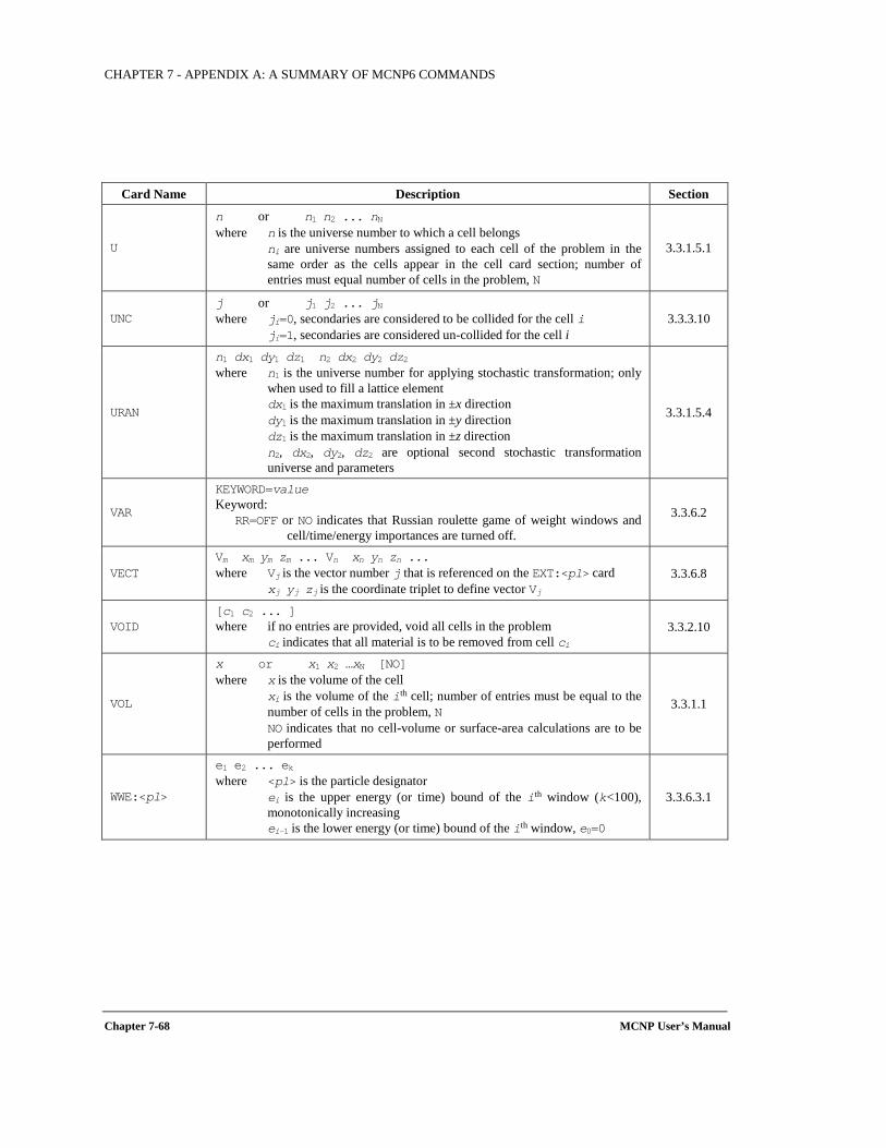
CHAPTER 7 - APPENDIX A: A SUMMARY OF MCNP6 COMMANDS
Chapter 7-68 MCNP User’s Manual
Card Name Description Section
U
n or n1 n2 ... nN where n is the universe number to which a cell belongs ni are universe numbers assigned to each cell of the problem in the
same order as the cells appear in the cell card section; number of entries must equal number of cells in the problem, N
3.3.1.5.1
UNC j or j1 j2 ... jN where ji=0, secondaries are considered to be collided for the cell i ji=1, secondaries are considered un-collided for the cell i
3.3.3.10
URAN
n1 dx1 dy1 dz1 n2 dx2 dy2 dz2 where n1 is the universe number for applying stochastic transformation; only
when used to fill a lattice element dx1 is the maximum translation in ±x direction dy1 is the maximum translation in ±y direction dz1 is the maximum translation in ±z direction n2, dx2, dy2, dz2 are optional second stochastic transformation
universe and parameters
3.3.1.5.4
VAR
KEYWORD=value Keyword:
RR=OFF or NO indicates that Russian roulette game of weight windows and cell/time/energy importances are turned off.
3.3.6.2
VECT Vm xm ym zm ... Vn xn yn zn ... where Vj is the vector number j that is referenced on the EXT:<pl> card xj yj zj is the coordinate triplet to define vector Vj
3.3.6.8
VOID [c1 c2 ... ] where if no entries are provided, void all cells in the problem ci indicates that all material is to be removed from cell ci
3.3.2.10
VOL
x or x1 x2 …xN [NO] where x is the volume of the cell xi is the volume of the ith cell; number of entries must be equal to the
number of cells in the problem, N NO indicates that no cell-volume or surface-area calculations are to be
performed
3.3.1.1
WWE:<pl>
e1 e2 ... ek where <pl> is the particle designator ei is the upper energy (or time) bound of the ith window (k<100),
monotonically increasing ei-1 is the lower energy (or time) bound of the ith window, e0=0
3.3.6.3.1
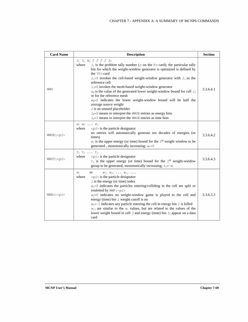
CHAPTER 7 - APPENDIX A: A SUMMARY OF MCNP6 COMMANDS
MCNP User’s Manual Chapter 7-69
Card Name Description Section
WWG
it ic wg J J J J iE where it is the problem tally number (n on the Fn card); the particular tally
bin for which the weight-window generator is optimized is defined by the TFn card
ic>0 invokes the cell-based weight-window generator with ic as the reference cell
ic=0 invokes the mesh-based weight-window generator wg is the value of the generated lower weight-window bound for cell ic
or for the reference mesh wg=0 indicates the lower weight-window bound will be half the
average source weight J is an unused placeholder iE=0 means to interpret the WWGE entries as energy bins iE=1 means to interpret the WWGE entries as time bins
3.3.6.4.1
WWGE:<pl>
e1 e2 ... ej where <pl> is the particle designator no entries will automatically generate ten decades of energies (or
times) ei is the upper energy (or time) bound for the ith weight window to be
generated , monotonically increasing; e0=0
3.3.6.4.2
WWGT:<pl>
t1 t2 ... tj where <pl> is the particle designator ti is the upper energy (or time) bound for the ith weight-window
group to be generated, monotonically increasing; t0=-∞
3.3.6.4.3
WWNi:<pl>
wi or wi1 wi2 ... wij ... where <pl> is the particle designator i is the energy (or time) index wi>0 indicates the particles entering/colliding in the cell are split or
rouletted by WWP:<pl> wi=0 indicates no weight-window game is played in the cell and
energy (time) bin i weight cutoff is on wi=-1 indicates any particle entering the cell in energy bin i is killed wij are similar to the wi values, but are related to the values of the
lower weight bound in cell j and energy (time) bin i; appear on a data card
3.3.6.3.3
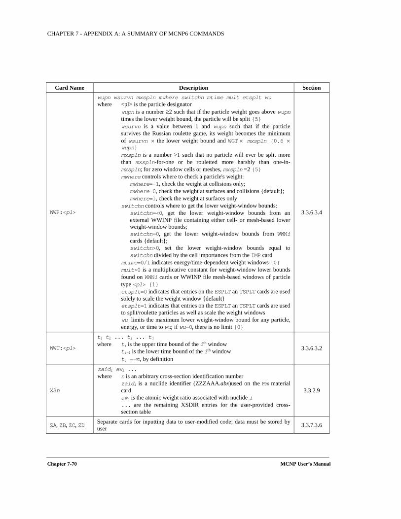
CHAPTER 7 - APPENDIX A: A SUMMARY OF MCNP6 COMMANDS
Chapter 7-70 MCNP User’s Manual
Card Name Description Section
WWP:<pl>
wupn wsurvn mxspln mwhere switchn mtime mult etsplt wu where <pl> is the particle designator wupn is a number ≥2 such that if the particle weight goes above wupn
times the lower weight bound, the particle will be split 5 wsurvn is a value between 1 and wupn such that if the particle
survives the Russian roulette game, its weight becomes the minimum of wsurvn × the lower weight bound and WGT × mxspln 0.6 × wupn
mxspln is a number >1 such that no particle will ever be split more than mxspln-for-one or be rouletted more harshly than one-in-mxspln; for zero window cells or meshes, mxspln =2 5
mwhere controls where to check a particle's weight: mwhere=-1, check the weight at collisions only; mwhere=0, check the weight at surfaces and collisions default; mwhere=1, check the weight at surfaces only
switchn controls where to get the lower weight-window bounds: switchn=<0, get the lower weight-window bounds from an external WWINP file containing either cell- or mesh-based lower weight-window bounds; switchn=0, get the lower weight-window bounds from WWNi cards default; switchn>0, set the lower weight-window bounds equal to switchn divided by the cell importances from the IMP card
mtime=0/1 indicates energy/time-dependent weight windows 0 mult>0 is a multiplicative constant for weight-window lower bounds
found on WWNi cards or WWINP file mesh-based windows of particle type <pl> 1
etsplt=0 indicates that entries on the ESPLT an TSPLT cards are used solely to scale the weight window default
etsplt=1 indicates that entries on the ESPLT an TSPLT cards are used to split/roulette particles as well as scale the weight windows
wu limits the maximum lower weight-window bound for any particle, energy, or time to wu; if wu=0, there is no limit 0
3.3.6.3.4
WWT:<pl>
t1 t2 ... ti ... tj where ti is the upper time bound of the ith window ti-1 is the lower time bound of the ith window t0 =-∞, by definition
3.3.6.3.2
XSn
zaidi awi ... where n is an arbitrary cross-section identification number zaidi is a nuclide identifier (ZZZAAA.abx)used on the Mm material
card awi is the atomic weight ratio associated with nuclide i ... are the remaining XSDIR entries for the user-provided cross-
section table
3.3.2.9
ZA, ZB, ZC, ZD Separate cards for inputting data to user-modified code; data must be stored by user 3.3.7.3.6
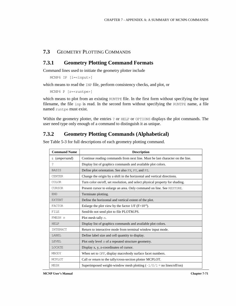
CHAPTER 7 - APPENDIX A: A SUMMARY OF MCNP6 COMMANDS
MCNP User’s Manual Chapter 7-71
7.3 GEOMETRY PLOTTING COMMANDS
7.3.1 Geometry Plotting Command Formats Command lines used to initiate the geometry plotter include
MCNP6 IP [i=<input>]
which means to read the INP file, perform consistency checks, and plot, or MCNP6 P [r=<runtpe>]
which means to plot from an existing RUNTPE file. In the first form without specifying the input filename, the file inp is read. In the second form without specifying the RUNTPE name, a file named runtpe must exist.
Within the geometry plotter, the entries ? or HELP or OPTIONS displays the plot commands. The user need type only enough of a command to distinguish it as unique.
7.3.2 Geometry Plotting Commands (Alphabetical) See Table 5-3 for full descriptions of each geometry plotting command.
Command Name Description
& (ampersand) Continue reading commands from next line. Must be last character on the line.
? Display list of graphics commands and available plot colors.
BASIS Define plot orientation. See also PX, PY, and PZ.
CENTER Change the origin by a shift in the horizontal and vertical directions. COLOR Turn color on/off, set resolution, and select physical property for shading.
CURSOR Present cursor to enlarge an area. Only command on line. See RESTORE.
END Terminate plotting. EXTENT Define the horizontal and vertical extent of the plot. FACTOR Enlarge the plot view by the factor 1/F (F>10-6). FILE Send/do not send plot to file PLOTM.PS.
FMESH n Plot mesh tally n.
HELP Display list of graphics commands and available plot colors. INTERACT Return to interactive mode from terminal window input mode. LABEL Define label size and cell quantity to display.
LEVEL Plot only level n of a repeated structure geometry.
LOCATE Display x, y, z-coordinates of cursor.
MBODY When set to OFF, display macrobody surface facet numbers.
MCPLOT Call or return to the tally/cross-section plotter MCPLOT.
MESH Superimposed weight-window mesh plotting (-1/0/1 = no lines/off/on)
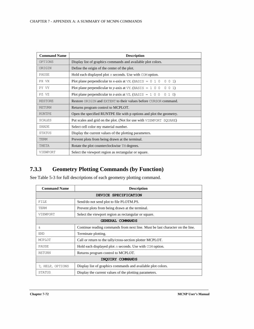
CHAPTER 7 - APPENDIX A: A SUMMARY OF MCNP6 COMMANDS
Chapter 7-72 MCNP User’s Manual
Command Name Description OPTIONS Display list of graphics commands and available plot colors. ORIGIN Define the origin of the center of the plot.
PAUSE Hold each displayed plot n seconds. Use with COM option.
PX VX Plot plane perpendicular to x-axis at VX. (BASIS = 0 1 0 0 0 1)
PY VY Plot plane perpendicular to y-axis at VY. (BASIS = 1 0 0 0 0 1)
PZ VZ Plot plane perpendicular to z-axis at VZ. (BASIS = 1 0 0 0 1 0)
RESTORE Restore ORIGIN and EXTENT to their values before CURSOR command.
RETURN Returns program control to MCPLOT. RUNTPE Open the specified RUNTPE file with p options and plot the geometry.
SCALES Put scales and grid on the plot. (Not for use with VIEWPORT SQUARE)
SHADE Select cell color my material number. STATUS Display the current values of the plotting parameters. TERM Prevent plots from being drawn at the terminal.
THETA Rotate the plot counterclockwise TH degrees.
VIEWPORT Select the viewport region as rectangular or square.
7.3.3 Geometry Plotting Commands (by Function) See Table 5-3 for full descriptions of each geometry plotting command.
Command Name Description
DEVICE SPECIFICATION FILE Send/do not send plot to file PLOTM.PS. TERM Prevent plots from being drawn at the terminal. VIEWPORT Select the viewport region as rectangular or square.
GENERAL COMMANDS & Continue reading commands from next line. Must be last character on the line. END Terminate plotting. MCPLOT Call or return to the tally/cross-section plotter MCPLOT.
PAUSE Hold each displayed plot n seconds. Use with COM option.
RETURN Returns program control to MCPLOT.
INQUIRY COMMANDS ?, HELP, OPTIONS Display list of graphics commands and available plot colors.
STATUS Display the current values of the plotting parameters.
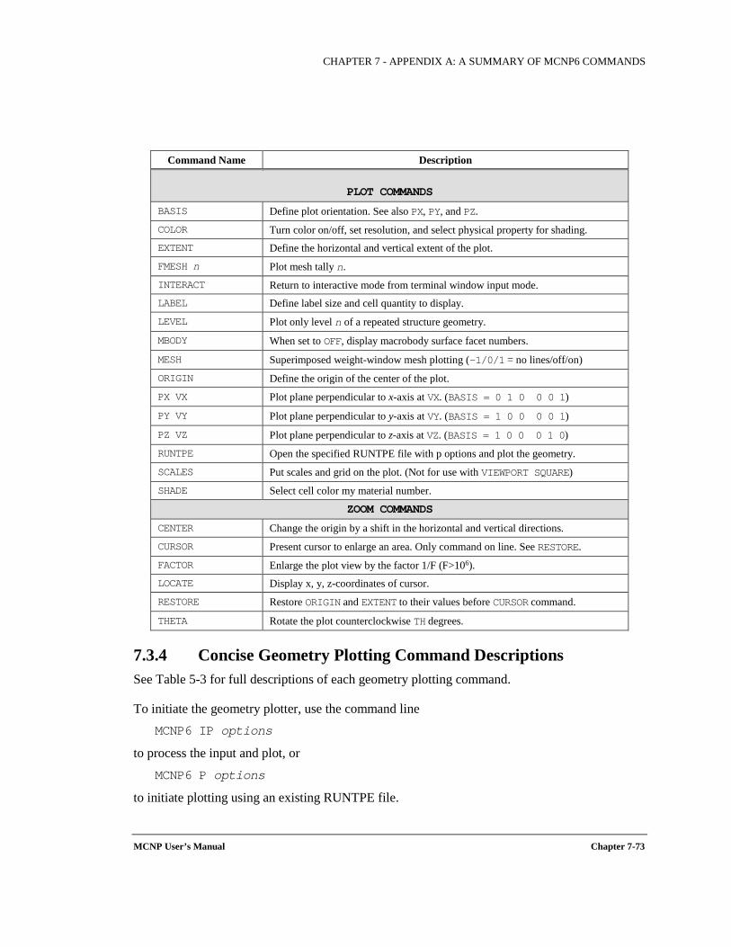
CHAPTER 7 - APPENDIX A: A SUMMARY OF MCNP6 COMMANDS
MCNP User’s Manual Chapter 7-73
Command Name Description
PLOT COMMANDS
BASIS Define plot orientation. See also PX, PY, and PZ.
COLOR Turn color on/off, set resolution, and select physical property for shading. EXTENT Define the horizontal and vertical extent of the plot.
FMESH n Plot mesh tally n.
INTERACT Return to interactive mode from terminal window input mode. LABEL Define label size and cell quantity to display.
LEVEL Plot only level n of a repeated structure geometry.
MBODY When set to OFF, display macrobody surface facet numbers.
MESH Superimposed weight-window mesh plotting (-1/0/1 = no lines/off/on)
ORIGIN Define the origin of the center of the plot.
PX VX Plot plane perpendicular to x-axis at VX. (BASIS = 0 1 0 0 0 1)
PY VY Plot plane perpendicular to y-axis at VY. (BASIS = 1 0 0 0 0 1)
PZ VZ Plot plane perpendicular to z-axis at VZ. (BASIS = 1 0 0 0 1 0)
RUNTPE Open the specified RUNTPE file with p options and plot the geometry.
SCALES Put scales and grid on the plot. (Not for use with VIEWPORT SQUARE)
SHADE Select cell color my material number.
ZOOM COMMANDS
CENTER Change the origin by a shift in the horizontal and vertical directions.
CURSOR Present cursor to enlarge an area. Only command on line. See RESTORE.
FACTOR Enlarge the plot view by the factor 1/F (F>106). LOCATE Display x, y, z-coordinates of cursor.
RESTORE Restore ORIGIN and EXTENT to their values before CURSOR command.
THETA Rotate the plot counterclockwise TH degrees.
7.3.4 Concise Geometry Plotting Command Descriptions See Table 5-3 for full descriptions of each geometry plotting command.
To initiate the geometry plotter, use the command line MCNP6 IP options
to process the input and plot, or MCNP6 P options
to initiate plotting using an existing RUNTPE file.

CHAPTER 7 - APPENDIX A: A SUMMARY OF MCNP6 COMMANDS
Chapter 7-74 MCNP User’s Manual
The options that are available on the execution line include
NOTEK to suppress terminal plotting and send plots to file PLOTM.PS COM=fn1 to input commands contained in file fn1 PLOTM=fn2 to assign the file name fn2 to a graphics postscript file PLOTM.PS COMOUT=fn3 to create the file fn3 of terminal plot commands COMOUT RUNTPE=fn4 to open a specified RUNTPE file, fn4, and plot with the P (not IP)
execution option RUNTPE
The following table of commands is a copy of Table 5-3
Geometry Plotting Commands
Command Description
Device-Control Commands
TERM n
Output device type is specified by n. n=0 for a terminal with no graphics capability. No plots will be drawn on the terminal,
and all plots will be sent to the graphics metafile. TERM 0 is equivalent to putting NOTEK on MCNP6’s execute line.
n=1 restores visible plotting window on next plot request.
FILE [aa]
Send or do not send plots to the graphics metafile PLOTM.PS according to the value of the parameter aa. The graphics metafile is not created until the first FILE command is entered. FILE has no effect in the NOTEK or TERM 0 cases. The allowed values of aa are the following:
If aa is blank, only the current plot is sent to the graphics metafile. If aa=ALL, the current plot and all subsequent plots are sent to the metafile until another FILE command is entered.
If aa=NONE, the current plot is not sent to the metafile nor are any subsequent plots until another FILE command is entered.
VIEWPORT aa
Make the viewport rectangular or square according to the value of aa. This option does not affect the appearance of the plot. It only determines whether space is provided beside the plot for a legend and around the plot for scales.
If aa=RECT, allow space beside the plot for a legend and around the plot for scales. (DEFAULT)
If aa=SQUARE, the legend area, the legend, and scales are omitted, making it possible to print a sequence of plots on some sort of strip medium so as to produce one long picture free from interruptions by legends. Note: Use of the SQUARE option disables the interactive-window plotter capability.
General Commands
& Continue reading commands for the current plot from the next input line. The & must be the last thing on the line.
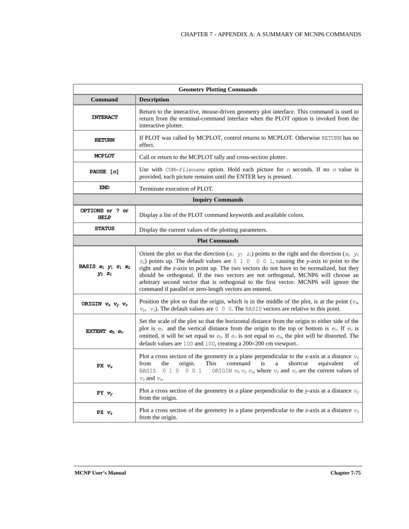
CHAPTER 7 - APPENDIX A: A SUMMARY OF MCNP6 COMMANDS
MCNP User’s Manual Chapter 7-75
Geometry Plotting Commands
Command Description
INTERACT Return to the interactive, mouse-driven geometry plot interface. This command is used to return from the terminal-command interface when the PLOT option is invoked from the interactive plotter.
RETURN If PLOT was called by MCPLOT, control returns to MCPLOT. Otherwise RETURN has no effect.
MCPLOT Call or return to the MCPLOT tally and cross-section plotter.
PAUSE [n] Use with COM=filename option. Hold each picture for n seconds. If no n value is provided, each picture remains until the ENTER key is pressed.
END Terminate execution of PLOT.
Inquiry Commands
OPTIONS or ? or HELP Display a list of the PLOT command keywords and available colors.
STATUS Display the current values of the plotting parameters.
Plot Commands
BASIS x1 y1 z1 x2 y2 z2
Orient the plot so that the direction (x1 y1 z1) points to the right and the direction (x2 y2 z2) points up. The default values are 0 1 0 0 0 1, causing the y-axis to point to the right and the z-axis to point up. The two vectors do not have to be normalized, but they should be orthogonal. If the two vectors are not orthogonal, MCNP6 will choose an arbitrary second vector that is orthogonal to the first vector. MCNP6 will ignore the command if parallel or zero-length vectors are entered.
ORIGIN vx vy vz Position the plot so that the origin, which is in the middle of the plot, is at the point (vx, vy, vz). The default values are 0 0 0. The BASIS vectors are relative to this point.
EXTENT eh ev
Set the scale of the plot so that the horizontal distance from the origin to either side of the plot is eh and the vertical distance from the origin to the top or bottom is ev. If ev is omitted, it will be set equal to eh. If ev is not equal to eh, the plot will be distorted. The default values are 100 and 100, creating a 200×200 cm viewport..
PX vx
Plot a cross section of the geometry in a plane perpendicular to the x-axis at a distance vx from the origin. This command is a shortcut equivalent of BASIS 0 1 0 0 0 1 ORIGIN vx vy vz, where vy and vz are the current values of vy and vz.
PY vy Plot a cross section of the geometry in a plane perpendicular to the y-axis at a distance vy from the origin.
PZ vz Plot a cross section of the geometry in a plane perpendicular to the z-axis at a distance vz from the origin.
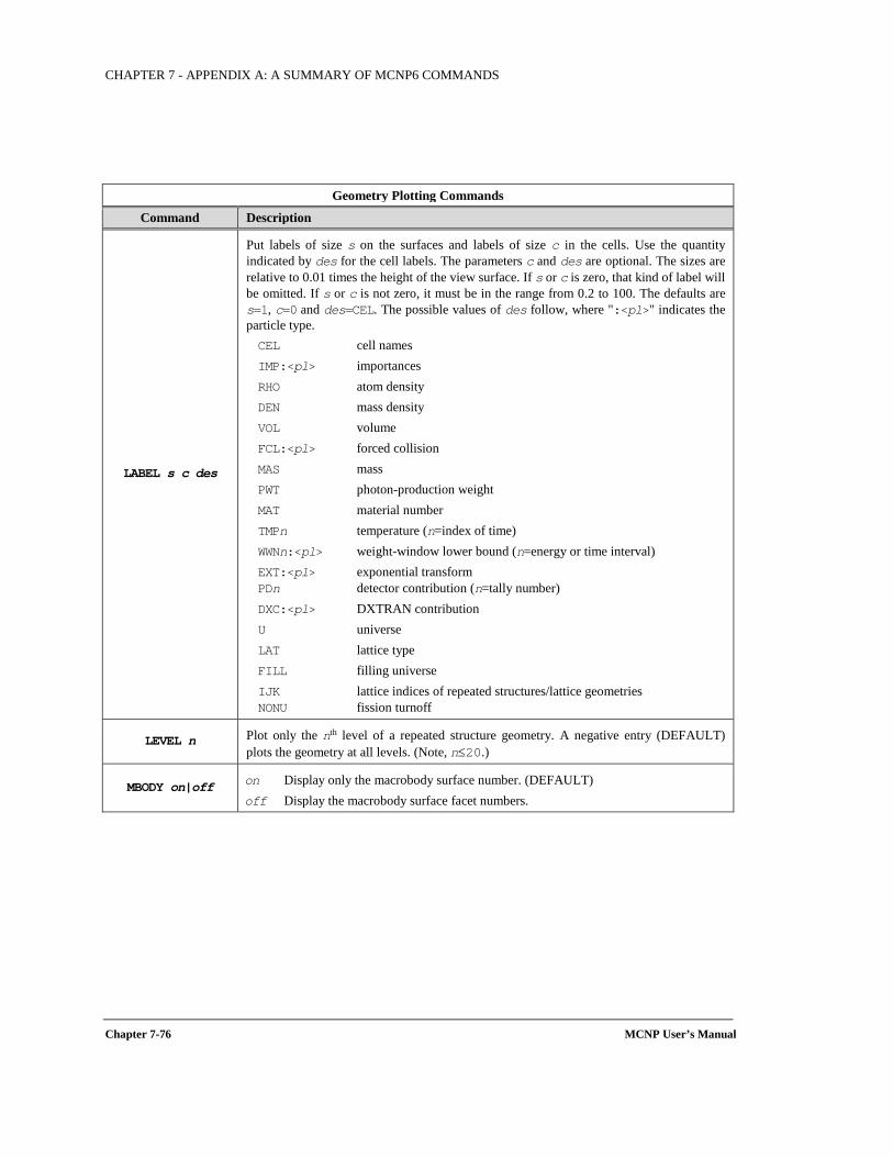
CHAPTER 7 - APPENDIX A: A SUMMARY OF MCNP6 COMMANDS
Chapter 7-76 MCNP User’s Manual
Geometry Plotting Commands
Command Description
LABEL s c des
Put labels of size s on the surfaces and labels of size c in the cells. Use the quantity indicated by des for the cell labels. The parameters c and des are optional. The sizes are relative to 0.01 times the height of the view surface. If s or c is zero, that kind of label will be omitted. If s or c is not zero, it must be in the range from 0.2 to 100. The defaults are s=1, c=0 and des=CEL. The possible values of des follow, where ":<pl>" indicates the particle type. CEL cell names IMP:<pl> importances RHO atom density DEN mass density VOL volume FCL:<pl> forced collision MAS mass PWT photon-production weight MAT material number TMPn temperature (n=index of time) WWNn:<pl> weight-window lower bound (n=energy or time interval) EXT:<pl> exponential transform PDn detector contribution (n=tally number) DXC:<pl> DXTRAN contribution U universe LAT lattice type FILL filling universe IJK lattice indices of repeated structures/lattice geometries NONU fission turnoff
LEVEL n Plot only the nth level of a repeated structure geometry. A negative entry (DEFAULT) plots the geometry at all levels. (Note, n≤20.)
MBODY on|off on Display only the macrobody surface number. (DEFAULT) off Display the macrobody surface facet numbers.
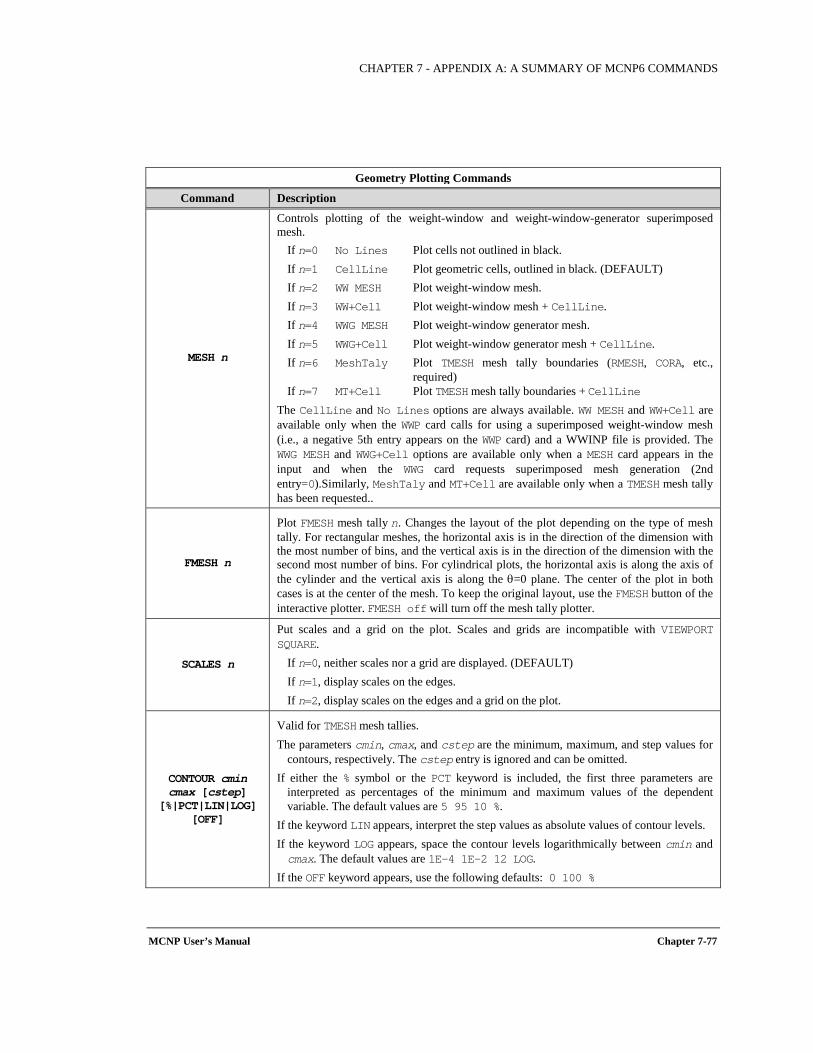
CHAPTER 7 - APPENDIX A: A SUMMARY OF MCNP6 COMMANDS
MCNP User’s Manual Chapter 7-77
Geometry Plotting Commands
Command Description
MESH n
Controls plotting of the weight-window and weight-window-generator superimposed mesh.
If n=0 No Lines Plot cells not outlined in black. If n=1 CellLine Plot geometric cells, outlined in black. (DEFAULT) If n=2 WW MESH Plot weight-window mesh. If n=3 WW+Cell Plot weight-window mesh + CellLine. If n=4 WWG MESH Plot weight-window generator mesh. If n=5 WWG+Cell Plot weight-window generator mesh + CellLine. If n=6 MeshTaly Plot TMESH mesh tally boundaries (RMESH, CORA, etc.,
required) If n=7 MT+Cell Plot TMESH mesh tally boundaries + CellLine
The CellLine and No Lines options are always available. WW MESH and WW+Cell are available only when the WWP card calls for using a superimposed weight-window mesh (i.e., a negative 5th entry appears on the WWP card) and a WWINP file is provided. The WWG MESH and WWG+Cell options are available only when a MESH card appears in the input and when the WWG card requests superimposed mesh generation (2nd entry=0).Similarly, MeshTaly and MT+Cell are available only when a TMESH mesh tally has been requested..
FMESH n
Plot FMESH mesh tally n. Changes the layout of the plot depending on the type of mesh tally. For rectangular meshes, the horizontal axis is in the direction of the dimension with the most number of bins, and the vertical axis is in the direction of the dimension with the second most number of bins. For cylindrical plots, the horizontal axis is along the axis of the cylinder and the vertical axis is along the θ=0 plane. The center of the plot in both cases is at the center of the mesh. To keep the original layout, use the FMESH button of the interactive plotter. FMESH off will turn off the mesh tally plotter.
SCALES n
Put scales and a grid on the plot. Scales and grids are incompatible with VIEWPORT SQUARE.
If n=0, neither scales nor a grid are displayed. (DEFAULT) If n=1, display scales on the edges. If n=2, display scales on the edges and a grid on the plot.
CONTOUR cmin cmax [cstep]
[%|PCT|LIN|LOG] [OFF]
Valid for TMESH mesh tallies. The parameters cmin, cmax, and cstep are the minimum, maximum, and step values for
contours, respectively. The cstep entry is ignored and can be omitted. If either the % symbol or the PCT keyword is included, the first three parameters are
interpreted as percentages of the minimum and maximum values of the dependent variable. The default values are 5 95 10 %.
If the keyword LIN appears, interpret the step values as absolute values of contour levels. If the keyword LOG appears, space the contour levels logarithmically between cmin and cmax. The default values are 1E-4 1E-2 12 LOG.
If the OFF keyword appears, use the following defaults: 0 100 %
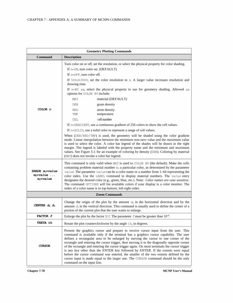
CHAPTER 7 - APPENDIX A: A SUMMARY OF MCNP6 COMMANDS
Chapter 7-78 MCNP User’s Manual
Geometry Plotting Commands
Command Description
COLOR n
Turn color on or off, set the resolution, or select the physical property for color shading. If n=ON, turn color on. (DEFAULT) If n=OFF, turn color off. If 50≤n≤3000, set the color resolution to n. A larger value increases resolution and drawing time. If n=BY aa, select the physical property to use for geometry shading. Allowed aa options for COLOR BY include:
MAT material (DEFAULT) DEN gram density RHO atom density TMP temperature CEL cell number
If n=GRADIENT, use a continuous gradient of 256 colors to show the cell values. If n=SOLID, use a solid color to represent a range of cell values.
When (DEN/RHO/TMP) is used, the geometry will be shaded using the color gradient mode. Linear interpolation between the minimum non-zero value and the maximum value is used to select the color. A color bar legend of the shades will be drawn in the right margin. The legend is labeled with the property name and the minimum and maximum values. See Figure 5-1 for an example of coloring by density (DEN). Coloring by material (MAT) does not invoke a color bar legend.
SHADE m1=value m2=value ... mi=value
This command is only valid when MAT is used to COLOR BY (the default). Make the cells containing problem material number mi a particular color, as determined by the parameter value. The parameter value can be a color name or a number from 1–64 representing the color index. Use the LABEL command to display material numbers. The value entry designates the desired color (e.g., green, blue, etc.). Note: Color names are case sensitive. The command OPTIONS will list available colors if your display is a color monitor. The index of a color name is in top-bottom, left-right order.
Zoom Commands
CENTER dh dv Change the origin of the plot by the amount dh in the horizontal direction and by the amount dv in the vertical direction. This command is usually used to define the center of a portion of the current plot that the user wants to enlarge.
FACTOR f Enlarge the plot by the factor 1/f. The parameter f must be greater than 10-6.
THETA th Rotate the plot counterclockwise by the angle th, in degrees.
CURSOR
Present the graphics cursor and prepare to receive cursor input from the user. This command is available only if the terminal has a graphics cursor capability. The user defines a rectangular area to be enlarged by moving the cursor to one corner of the rectangle and entering the cursor trigger, then moving it to the diagonally opposite corner of the rectangle and entering the cursor trigger again. On most terminals the cursor trigger is any key other than the ENTER key followed by ENTER. If the extents were equal before the cursor command was entered, the smaller of the two extents defined by the cursor input is made equal to the larger one. The CURSOR command should be the only command on the input line.

CHAPTER 7 - APPENDIX A: A SUMMARY OF MCNP6 COMMANDS
MCNP User’s Manual Chapter 7-79
Geometry Plotting Commands
Command Description
RESTORE Restore the origin and extent to the values they had before the most recent CURSOR command. The RESTORE command should be the only command on the input line. It cannot be used to undo the effects of the CENTER, FACTOR, and THETA commands.
LOCATE
Present the graphics cursor and prepare to receive cursor input from the user. This command is available only if the terminal has a graphics cursor capability. The user moves the cursor to a point in the picture and enters the cursor trigger. The x-, y-, z-coordinates of the point are displayed. The LOCATE command should be the only command on the input line.
7.4 TALLY AND CROSS-SECTION PLOTTING COMMANDS
7.4.1 Tally and Cross-Section Plotting Command Formats Tally plotting and cross-section plotting are each initiated using a specific form of the MCNP6 execute line. The form
MCNP6 Z [options]
provides tally plots from RUNTPE and MCTAL files, while MCNP6 IXZ [options]
provides cross-section plots from an INP file only, not from a RUNTPE file.
While plotting tallies or cross-section, remember the following hints:
• You only need enough letters of a command to identify it uniquely (e.g., cop=coplot) • Enter "?" at a prompt to display a list of tally and cross-section plotting commands • Enter "xs ?" at a prompt to see a primer in cross-section plotting • The <ctrl_c>m interrupt allows interactive tally plots during a run; use RETURN or END
to exit
7.4.2 Tally and Cross-Sections Plotting Commands (Alphabetical) See Table 5-5 for full descriptions of these commands.
Command Name Description
& Continue reading commands from next line. Must be last character on the line. ? Display list of tally and cross-section plotting commands. BAR Make bar plots of tally data. BELOW Put the main title below the plot instead of above it. CONTOUR Specify the form of contour plots.
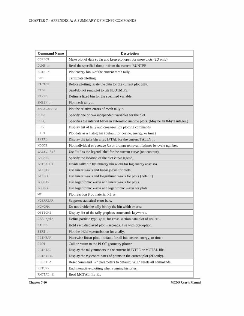
CHAPTER 7 - APPENDIX A: A SUMMARY OF MCNP6 COMMANDS
Chapter 7-80 MCNP User’s Manual
Command Name Description COPLOT Make plot of data so far and keep plot open for more plots (2D only)
DUMP n Read the specified dump n from the current RUNTPE
EBIN n Plot energy bin n of the current mesh tally.
END Terminate plotting. FACTOR Before plotting, scale the data for the current plot only. FILE Send/do not send plot to file PLOTM.PS. FIXED Define a fixed bin for the specified variable.
FMESH n Plot mesh tally n.
FMRELERR n Plot the relative errors of mesh tally n.
FREE Specify one or two independent variables for the plot. FREQ Specifies the interval between automatic runtime plots. (May be an 8-byte integer.) HELP Display list of tally and cross-section plotting commands. HIST Plot data as a histogram default for cosine, energy, or time
IPTAL Display the tally bin array IPTAL for the current TALLY n.
KCODE Plot individual or average keff or prompt removal lifetimes by cycle number.
LABEL "a" Use "a " as the legend label for the current curve (not contour).
LEGEND Specify the location of the plot curve legend. LETHARGY Divide tally bin by lethargy bin width for log energy abscissa. LINLIN Use linear x-axis and linear y-axis for plots. LINLOG Use linear x-axis and logarithmic y-axis for plots default LOGLIN Use logarithmic x-axis and linear y-axis for plots. LOGLOG Use logarithmic x-axis and logarithmic y-axis for plots.
MT Plot reaction R of material XS m
NOERRBAR Suppress statistical error bars. NONORM Do not divide the tally bin by the bin width or area OPTIONS Display list of the tally graphics commands keywords.
PAR <pl> Define particle type <pl> for cross-section data plot of XS, MT.
PAUSE Hold each displayed plot n seconds. Use with COM option.
PERT n Plot the PERTn perturbation for a tally.
PLINEAR Piecewise linear plots default for all but cosine, energy, or time PLOT Call or return to the PLOT geometry plotter. PRINTAL Display the tally numbers in the current RUNTPE or MCTAL file. PRINTPTS Display the x-y coordinates of points in the current plot (2D only).
RESET a Reset command "a " parameters to default; "ALL" resets all commands.
RETURN End interactive plotting when running histories.
RMCTAL fn Read MCTAL file fn.
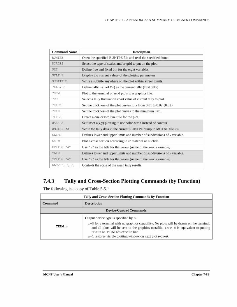
CHAPTER 7 - APPENDIX A: A SUMMARY OF MCNP6 COMMANDS
MCNP User’s Manual Chapter 7-81
Command Name Description RUNTPE Open the specified RUNTPE file and read the specified dump. SCALES Select the type of scales and/or grid to put on the plot. SET Define free and fixed bin for the eight variables. STATUS Display the current values of the plotting parameters. SUBTITLE Write a subtitle anywhere on the plot within screen limits.
TALLY n Define tally n (n of Fn) as the current tally first tally
TERM Plot to the terminal or send plots to a graphics file. TFC Select a tally fluctuation chart value of current tally to plot.
THICK Set the thickness of the plot curves to x from 0.01 to 0.02 0.02
THIN Set the thickness of the plot curves to the minimum 0.01. TITLE Create a one or two line title for the plot. WASH a Set/unset z(x,y) plotting to use color-wash instead of contour.
WMCTAL fn Write the tally data in the current RUNTPE dump to MCTAL file fn.
XLIMS Defines lower and upper limits and number of subdivisions of x variable.
XS m Plot a cross section according to m: material or nuclide.
XTITLE "a" Use "a" as the title for the x-axis name of the x-axis variable.
YLIMS Defines lower and upper limits and number of subdivisions of y variable.
YTITLE "a" Use "a" as the title for the y-axis name of the y-axis variable.
ZLEV n1 n2 n3 Controls the scale of the mesh tally results.
7.4.3 Tally and Cross-Section Plotting Commands (by Function) The following is a copy of Table 5-5. †
Tally and Cross-Section Plotting Commands By Function
Command Description
Device-Control Commands
TERM n
Output device type is specified by n. n=0 for a terminal with no graphics capability. No plots will be drawn on the terminal,
and all plots will be sent to the graphics metafile. TERM 0 is equivalent to putting NOTEK on MCNP6’s execute line.
n=1 restores visible plotting window on next plot request.
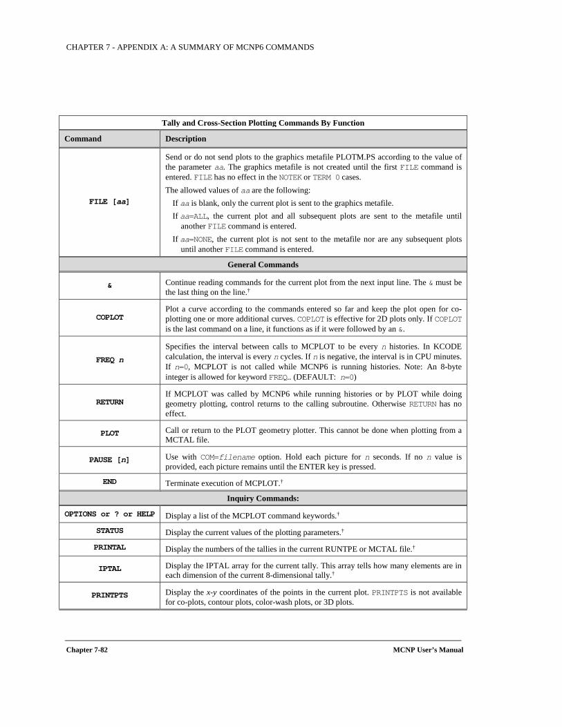
CHAPTER 7 - APPENDIX A: A SUMMARY OF MCNP6 COMMANDS
Chapter 7-82 MCNP User’s Manual
Tally and Cross-Section Plotting Commands By Function
Command Description
FILE [aa]
Send or do not send plots to the graphics metafile PLOTM.PS according to the value of the parameter aa. The graphics metafile is not created until the first FILE command is entered. FILE has no effect in the NOTEK or TERM 0 cases. The allowed values of aa are the following:
If aa is blank, only the current plot is sent to the graphics metafile. If aa=ALL, the current plot and all subsequent plots are sent to the metafile until
another FILE command is entered. If aa=NONE, the current plot is not sent to the metafile nor are any subsequent plots
until another FILE command is entered.
General Commands
& Continue reading commands for the current plot from the next input line. The & must be the last thing on the line.†
COPLOT Plot a curve according to the commands entered so far and keep the plot open for co-plotting one or more additional curves. COPLOT is effective for 2D plots only. If COPLOT is the last command on a line, it functions as if it were followed by an &.
FREQ n
Specifies the interval between calls to MCPLOT to be every n histories. In KCODE calculation, the interval is every n cycles. If n is negative, the interval is in CPU minutes. If n=0, MCPLOT is not called while MCNP6 is running histories. Note: An 8-byte integer is allowed for keyword FREQ.. (DEFAULT: n=0)
RETURN If MCPLOT was called by MCNP6 while running histories or by PLOT while doing geometry plotting, control returns to the calling subroutine. Otherwise RETURN has no effect.
PLOT Call or return to the PLOT geometry plotter. This cannot be done when plotting from a MCTAL file.
PAUSE [n] Use with COM=filename option. Hold each picture for n seconds. If no n value is provided, each picture remains until the ENTER key is pressed.
END Terminate execution of MCPLOT.†
Inquiry Commands:
OPTIONS or ? or HELP Display a list of the MCPLOT command keywords.†
STATUS Display the current values of the plotting parameters.†
PRINTAL Display the numbers of the tallies in the current RUNTPE or MCTAL file.†
IPTAL Display the IPTAL array for the current tally. This array tells how many elements are in each dimension of the current 8-dimensional tally.†
PRINTPTS Display the x-y coordinates of the points in the current plot. PRINTPTS is not available for co-plots, contour plots, color-wash plots, or 3D plots.
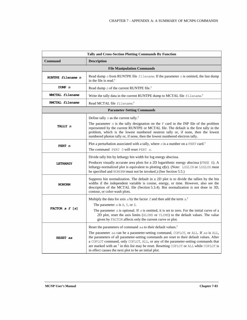
CHAPTER 7 - APPENDIX A: A SUMMARY OF MCNP6 COMMANDS
MCNP User’s Manual Chapter 7-83
Tally and Cross-Section Plotting Commands By Function
Command Description
File Manipulation Commands
RUNTPE filename n Read dump n from RUNTPE file filename. If the parameter n is omitted, the last dump in the file is read.†
DUMP n Read dump n of the current RUNTPE file.†
WMCTAL filename Write the tally data in the current RUNTPE dump to MCTAL file filename.†
RMCTAL filename Read MCTAL file filename.†
Parameter-Setting Commands
TALLY n
Define tally n as the current tally.† The parameter n is the tally designation on the F card in the INP file of the problem represented by the current RUNTPE or MCTAL file. The default is the first tally in the problem, which is the lowest numbered neutron tally or, if none, then the lowest numbered photon tally or, if none, then the lowest numbered electron tally.
PERT n Plot a perturbation associated with a tally, where n is a number on a PERT card.† The command PERT 0 will reset PERT n.
LETHARGY
Divide tally bin by lethargy bin width for log energy abscissa. Produces visually accurate area plots for a 2D logarithmic energy abscissa (FREE E). A lethargy-normalized plot is equivalent to plotting ef(e). (Note: LOGLIN or LOGLOG must be specified and NONORM must not be invoked.) (See Section 5.5.)
NONORM Suppress bin normalization. The default in a 2D plot is to divide the tallies by the bin widths if the independent variable is cosine, energy, or time. However, also see the description of the MCTAL file (Section 5.3.4). Bin normalization is not done in 3D, contour, or color-wash plots.
FACTOR a f [s]
Multiply the data for axis a by the factor f and then add the term s.† The parameter a is X, Y, or Z. The parameter s is optional. If s is omitted, it is set to zero. For the initial curve of a
2D plot, reset the axis limits (XLIMS or YLIMS) to the default values. The value given by FACTOR affects only the current curve or plot.
RESET aa
Reset the parameters of command aa to their default values.† The parameter aa can be a parameter-setting command, COPLOT, or ALL. If aa is ALL, the parameters of all parameter-setting commands are reset to their default values. After a COPLOT command, only COPLOT, ALL, or any of the parameter-setting commands that are marked with an † in this list may be reset. Resetting COPLOT or ALL while COPLOT is in effect causes the next plot to be an initial plot.
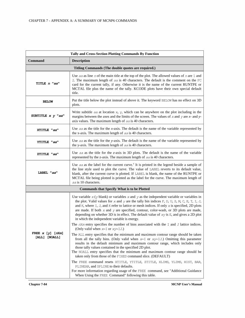
CHAPTER 7 - APPENDIX A: A SUMMARY OF MCNP6 COMMANDS
Chapter 7-84 MCNP User’s Manual
Tally and Cross-Section Plotting Commands By Function
Command Description
Titling Commands (The double quotes are required.)
TITLE n "aa"
Use aa as line n of the main title at the top of the plot. The allowed values of n are 1 and 2. The maximum length of aa is 40 characters. The default is the comment on the FC card for the current tally, if any. Otherwise it is the name of the current RUNTPE or MCTAL file plus the name of the tally. KCODE plots have their own special default title.
BELOW Put the title below the plot instead of above it. The keyword BELOW has no effect on 3D plots.
SUBTITLE x y "aa" Write subtitle aa at location x, y, which can be anywhere on the plot including in the margins between the axes and the limits of the screen. The values of x and y are x- and y-axis values. The maximum length of aa is 40 characters.
XTITLE "aa" Use aa as the title for the x-axis. The default is the name of the variable represented by the x-axis. The maximum length of aa is 40 characters.
YTITLE "aa" Use aa as the title for the y-axis. The default is the name of the variable represented by the y-axis. The maximum length of aa is 40 characters.
ZTITLE "aa" Use aa as the title for the z-axis in 3D plots. The default is the name of the variable represented by the z-axis. The maximum length of aa is 40 characters.
LABEL "aa"
Use aa as the label for the current curve.† It is printed in the legend beside a sample of the line style used to plot the curve. The value of LABEL reverts to its default value, blank, after the current curve is plotted. If LABEL is blank, the name of the RUNTPE or MCTAL file being plotted is printed as the label for the curve. The maximum length of aa is 10 characters.
Commands that Specify What is to be Plotted
FREE x [y] [nXm] [ALL] [NOALL]
Use variable x (y blank) or variables x and y as the independent variable or variables in the plot. Valid values for x and y are the tally bin indices F, D, U, S, M, C, E, T, I, J, and K, where I, J, and K refer to lattice or mesh indices. If only x is specified, 2D plots are made. If both x and y are specified, contour, color-wash, or 3D plots are made, depending on whether 3D is in effect. The default value of xy is E, and gives a 2D plot in which the independent variable is energy.
The nXm entry specifies the number of bins associated with the I and J lattice indices. (Only valid when x=I or xy=IJ.)
The ALL entry specifies that the minimum and maximum contour range should be taken from all the tally bins. (Only valid when x=I or xy=IJ.) Omitting this parameter results in the default minimum and maximum contour range, which includes only those tally values contained in the specified 2D plot.
The NOALL entry specifies that the minimum and maximum contour range should be taken only from those of the FIXED command slice. (DEFAULT)
The FREE command resets XTITLE, YTITLE, ZTITLE, XLIMS, YLIMS, HIST, BAR, PLINEAR, and SPLINE to their defaults.
For more information regarding usage of the FREE command, see "Additional Guidance When Using the FREE Command" following this table.
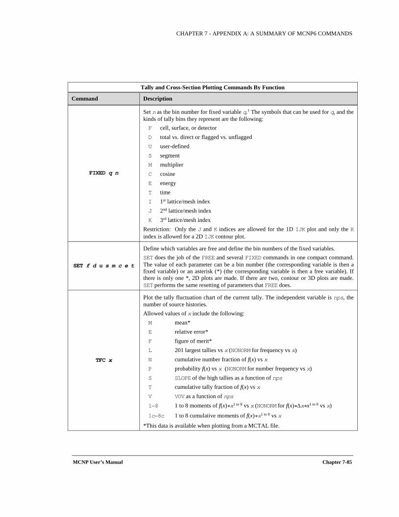
CHAPTER 7 - APPENDIX A: A SUMMARY OF MCNP6 COMMANDS
MCNP User’s Manual Chapter 7-85
Tally and Cross-Section Plotting Commands By Function
Command Description
FIXED q n
Set n as the bin number for fixed variable q.† The symbols that can be used for q, and the kinds of tally bins they represent are the following: F cell, surface, or detector D total vs. direct or flagged vs. unflagged U user-defined S segment M multiplier C cosine E energy T time I 1st lattice/mesh index J 2nd lattice/mesh index K 3rd lattice/mesh index
Restriction: Only the J and K indices are allowed for the 1D IJK plot and only the K index is allowed for a 2D IJK contour plot.
SET f d u s m c e t
Define which variables are free and define the bin numbers of the fixed variables. SET does the job of the FREE and several FIXED commands in one compact command. The value of each parameter can be a bin number (the corresponding variable is then a fixed variable) or an asterisk (*) (the corresponding variable is then a free variable). If there is only one *, 2D plots are made. If there are two, contour or 3D plots are made. SET performs the same resetting of parameters that FREE does.
TFC x
Plot the tally fluctuation chart of the current tally. The independent variable is nps, the number of source histories. Allowed values of x include the following: M mean* E relative error* F figure of merit* L 201 largest tallies vs x (NONORM for frequency vs x) N cumulative number fraction of f(x) vs x P probability f(x) vs x (NONORM for number frequency vs x) S SLOPE of the high tallies as a function of nps T cumulative tally fraction of f(x) vs x V VOV as a function of nps 1–8 1 to 8 moments of f(x)*x1 to 8 vs x (NONORM for f(x)*∆x*x1 to 8 vs x)
1c–8c 1 to 8 cumulative moments of f(x)*x1 to 8 vs x
*This data is available when plotting from a MCTAL file.
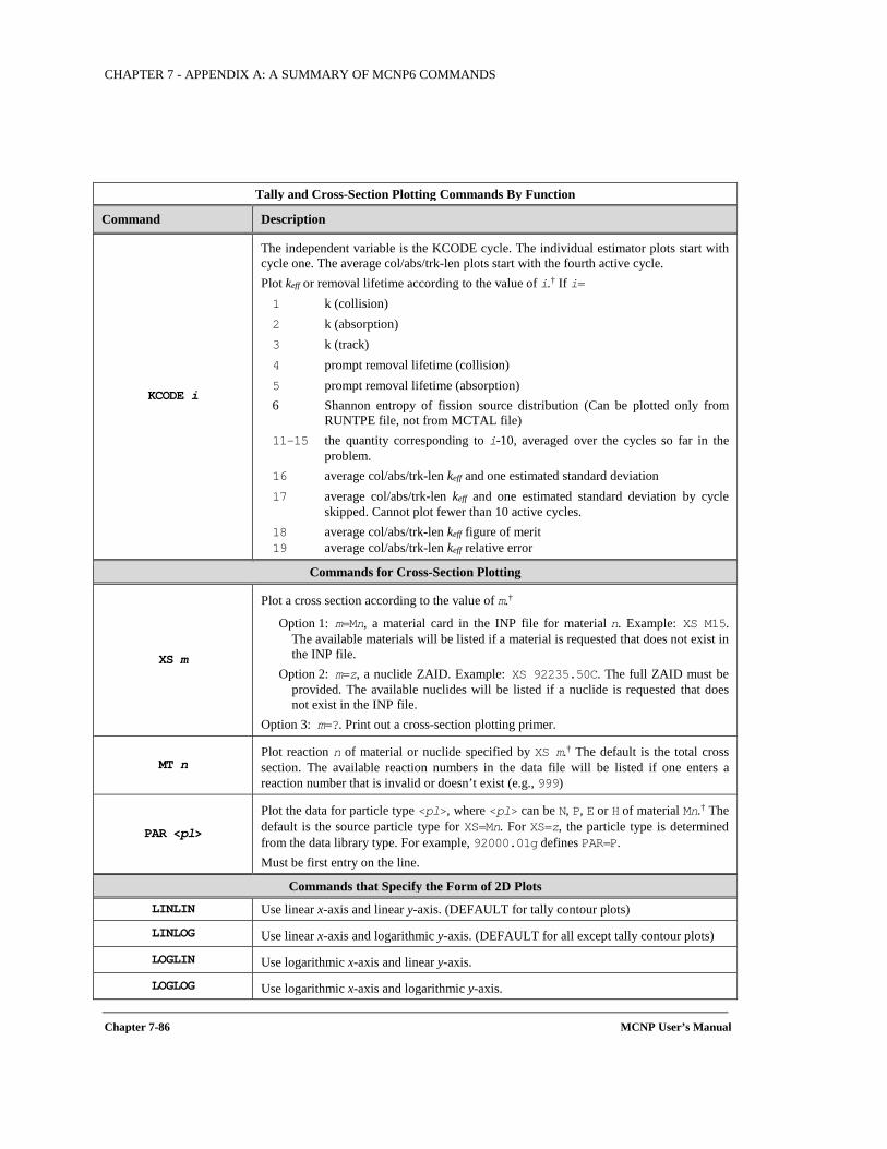
CHAPTER 7 - APPENDIX A: A SUMMARY OF MCNP6 COMMANDS
Chapter 7-86 MCNP User’s Manual
Tally and Cross-Section Plotting Commands By Function
Command Description
KCODE i
The independent variable is the KCODE cycle. The individual estimator plots start with cycle one. The average col/abs/trk-len plots start with the fourth active cycle. Plot keff or removal lifetime according to the value of i.† If i= 1 k (collision) 2 k (absorption) 3 k (track) 4 prompt removal lifetime (collision) 5 prompt removal lifetime (absorption) 6 Shannon entropy of fission source distribution (Can be plotted only from
RUNTPE file, not from MCTAL file) 11–15 the quantity corresponding to i-10, averaged over the cycles so far in the
problem. 16 average col/abs/trk-len keff and one estimated standard deviation 17 average col/abs/trk-len keff and one estimated standard deviation by cycle
skipped. Cannot plot fewer than 10 active cycles. 18 average col/abs/trk-len keff figure of merit 19 average col/abs/trk-len keff relative error
Commands for Cross-Section Plotting
XS m
Plot a cross section according to the value of m.†
Option 1: m=Mn, a material card in the INP file for material n. Example: XS M15. The available materials will be listed if a material is requested that does not exist in the INP file.
Option 2: m=z, a nuclide ZAID. Example: XS 92235.50C. The full ZAID must be provided. The available nuclides will be listed if a nuclide is requested that does not exist in the INP file.
Option 3: m=?. Print out a cross-section plotting primer.
MT n Plot reaction n of material or nuclide specified by XS m.† The default is the total cross section. The available reaction numbers in the data file will be listed if one enters a reaction number that is invalid or doesn’t exist (e.g., 999)
PAR <pl>
Plot the data for particle type <pl>, where <pl> can be N, P, E or H of material Mn.† The default is the source particle type for XS=Mn. For XS=z, the particle type is determined from the data library type. For example, 92000.01g defines PAR=P. Must be first entry on the line.
Commands that Specify the Form of 2D Plots
LINLIN Use linear x-axis and linear y-axis. (DEFAULT for tally contour plots)
LINLOG Use linear x-axis and logarithmic y-axis. (DEFAULT for all except tally contour plots)
LOGLIN Use logarithmic x-axis and linear y-axis.
LOGLOG Use logarithmic x-axis and logarithmic y-axis.
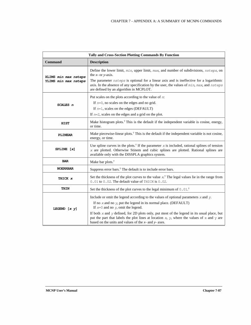
CHAPTER 7 - APPENDIX A: A SUMMARY OF MCNP6 COMMANDS
MCNP User’s Manual Chapter 7-87
Tally and Cross-Section Plotting Commands By Function
Command Description
XLIMS min max nsteps YLIMS min max nsteps
Define the lower limit, min, upper limit, max, and number of subdivisions, nsteps, on the x- or y-axis. The parameter nsteps is optional for a linear axis and is ineffective for a logarithmic axis. In the absence of any specification by the user, the values of min, max, and nsteps are defined by an algorithm in MCPLOT.
SCALES n
Put scales on the plots according to the value of n: If n=0, no scales on the edges and no grid. If n=1, scales on the edges (DEFAULT)
If n=2, scales on the edges and a grid on the plot.
HIST Make histogram plots.† This is the default if the independent variable is cosine, energy, or time.
PLINEAR Make piecewise-linear plots.† This is the default if the independent variable is not cosine, energy, or time.
SPLINE [x] Use spline curves in the plots.† If the parameter x is included, rational splines of tension x are plotted. Otherwise Stinem and cubic splines are plotted. Rational splines are available only with the DISSPLA graphics system.
BAR Make bar plots.†
NOERRBAR Suppress error bars.† The default is to include error bars.
THICK x Set the thickness of the plot curves to the value x.† The legal values lie in the range from 0.01 to 0.02. The default value of THICK is 0.02.
THIN Set the thickness of the plot curves to the legal minimum of 0.01.†
LEGEND [x y]
Include or omit the legend according to the values of optional parameters x and y. If no x and no y, put the legend in its normal place. (DEFAULT) If x=0 and no y, omit the legend.
If both x and y defined, for 2D plots only, put most of the legend in its usual place, but put the part that labels the plot lines at location x, y, where the values of x and y are based on the units and values of the x- and y- axes.
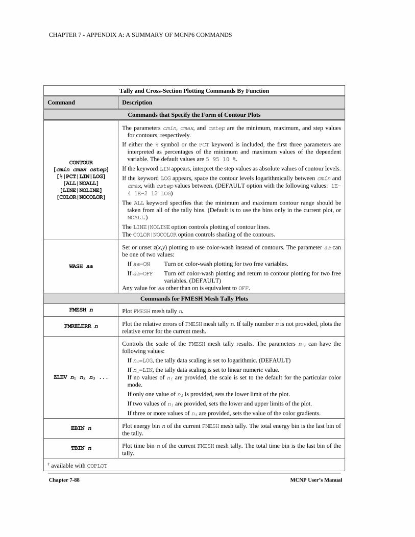
CHAPTER 7 - APPENDIX A: A SUMMARY OF MCNP6 COMMANDS
Chapter 7-88 MCNP User’s Manual
Tally and Cross-Section Plotting Commands By Function
Command Description
Commands that Specify the Form of Contour Plots
CONTOUR [cmin cmax cstep] [%|PCT|LIN|LOG] [ALL|NOALL] [LINE|NOLINE] [COLOR|NOCOLOR]
The parameters cmin, cmax, and cstep are the minimum, maximum, and step values for contours, respectively.
If either the % symbol or the PCT keyword is included, the first three parameters are interpreted as percentages of the minimum and maximum values of the dependent variable. The default values are 5 95 10 %.
If the keyword LIN appears, interpret the step values as absolute values of contour levels. If the keyword LOG appears, space the contour levels logarithmically between cmin and cmax, with cstep values between. (DEFAULT option with the following values: 1E-4 1E-2 12 LOG)
The ALL keyword specifies that the minimum and maximum contour range should be taken from all of the tally bins. (Default is to use the bins only in the current plot, or NOALL.)
The LINE|NOLINE option controls plotting of contour lines. The COLOR|NOCOLOR option controls shading of the contours.
WASH aa
Set or unset z(x,y) plotting to use color-wash instead of contours. The parameter aa can be one of two values:
If aa=ON Turn on color-wash plotting for two free variables. If aa=OFF Turn off color-wash plotting and return to contour plotting for two free
variables. (DEFAULT) Any value for aa other than on is equivalent to OFF.
Commands for FMESH Mesh Tally Plots
FMESH n Plot FMESH mesh tally n.
FMRELERR n Plot the relative errors of FMESH mesh tally n. If tally number n is not provided, plots the relative error for the current mesh.
ZLEV n1 n2 n3 ...
Controls the scale of the FMESH mesh tally results. The parameters ni, can have the following values:
If ni=LOG, the tally data scaling is set to logarithmic. (DEFAULT) If ni=LIN, the tally data scaling is set to linear numeric value. If no values of ni are provided, the scale is set to the default for the particular color mode. If only one value of ni is provided, sets the lower limit of the plot. If two values of ni are provided, sets the lower and upper limits of the plot. If three or more values of ni are provided, sets the value of the color gradients.
EBIN n Plot energy bin n of the current FMESH mesh tally. The total energy bin is the last bin of the tally.
TBIN n Plot time bin n of the current FMESH mesh tally. The total time bin is the last bin of the tally.
† available with COPLOT
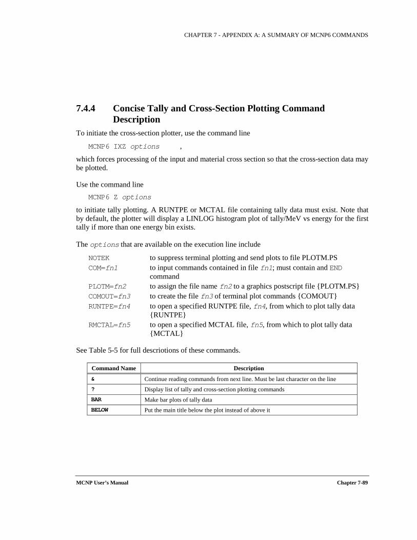
CHAPTER 7 - APPENDIX A: A SUMMARY OF MCNP6 COMMANDS
MCNP User’s Manual Chapter 7-89
7.4.4 Concise Tally and Cross-Section Plotting Command Description
To initiate the cross-section plotter, use the command line
MCNP6 IXZ options ,
which forces processing of the input and material cross section so that the cross-section data may be plotted.
Use the command line MCNP6 Z options
to initiate tally plotting. A RUNTPE or MCTAL file containing tally data must exist. Note that by default, the plotter will display a LINLOG histogram plot of tally/MeV vs energy for the first tally if more than one energy bin exists.
The options that are available on the execution line include
NOTEK to suppress terminal plotting and send plots to file PLOTM.PS COM=fn1 to input commands contained in file fn1; must contain and END
command PLOTM=fn2 to assign the file name fn2 to a graphics postscript file PLOTM.PS COMOUT=fn3 to create the file fn3 of terminal plot commands COMOUT RUNTPE=fn4 to open a specified RUNTPE file, fn4, from which to plot tally data
RUNTPE RMCTAL=fn5 to open a specified MCTAL file, fn5, from which to plot tally data
MCTAL
See Table 5-5 for full descriotions of these commands.
Command Name Description
& Continue reading commands from next line. Must be last character on the line ? Display list of tally and cross-section plotting commands BAR Make bar plots of tally data BELOW Put the main title below the plot instead of above it
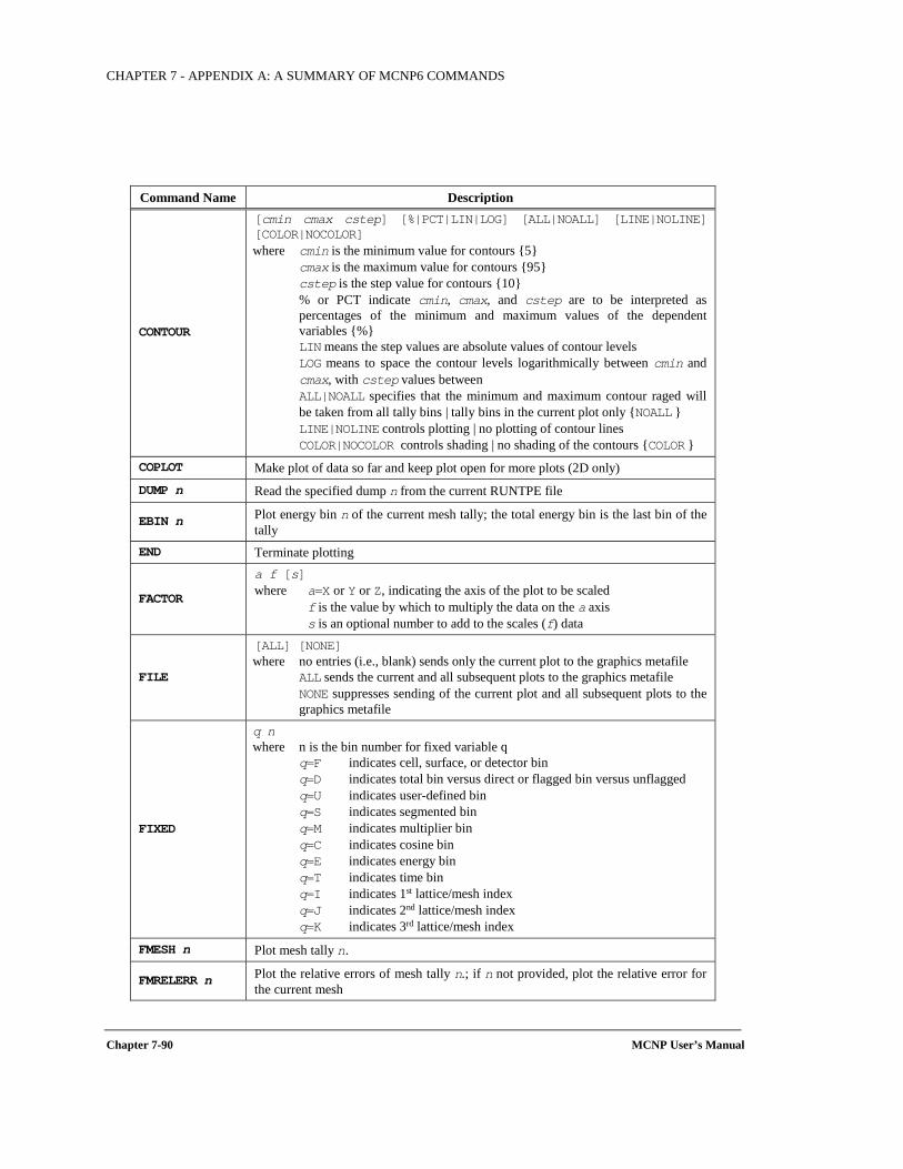
CHAPTER 7 - APPENDIX A: A SUMMARY OF MCNP6 COMMANDS
Chapter 7-90 MCNP User’s Manual
Command Name Description
CONTOUR
[cmin cmax cstep] [%|PCT|LIN|LOG] [ALL|NOALL] [LINE|NOLINE] [COLOR|NOCOLOR] where cmin is the minimum value for contours 5 cmax is the maximum value for contours 95 cstep is the step value for contours 10 % or PCT indicate cmin, cmax, and cstep are to be interpreted as
percentages of the minimum and maximum values of the dependent variables %
LIN means the step values are absolute values of contour levels LOG means to space the contour levels logarithmically between cmin and
cmax, with cstep values between ALL|NOALL specifies that the minimum and maximum contour raged will
be taken from all tally bins | tally bins in the current plot only NOALL LINE|NOLINE controls plotting | no plotting of contour lines COLOR|NOCOLOR controls shading | no shading of the contours COLOR
COPLOT Make plot of data so far and keep plot open for more plots (2D only) DUMP n Read the specified dump n from the current RUNTPE file
EBIN n Plot energy bin n of the current mesh tally; the total energy bin is the last bin of the tally
END Terminate plotting
FACTOR
a f [s] where a=X or Y or Z, indicating the axis of the plot to be scaled f is the value by which to multiply the data on the a axis s is an optional number to add to the scales (f) data
FILE
[ALL] [NONE] where no entries (i.e., blank) sends only the current plot to the graphics metafile ALL sends the current and all subsequent plots to the graphics metafile NONE suppresses sending of the current plot and all subsequent plots to the
graphics metafile
FIXED
q n where n is the bin number for fixed variable q q=F indicates cell, surface, or detector bin q=D indicates total bin versus direct or flagged bin versus unflagged q=U indicates user-defined bin q=S indicates segmented bin q=M indicates multiplier bin q=C indicates cosine bin q=E indicates energy bin q=T indicates time bin q=I indicates 1st lattice/mesh index q=J indicates 2nd lattice/mesh index q=K indicates 3rd lattice/mesh index
FMESH n Plot mesh tally n.
FMRELERR n Plot the relative errors of mesh tally n.; if n not provided, plot the relative error for the current mesh
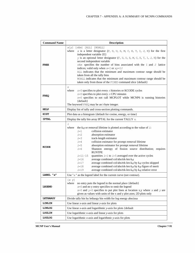
CHAPTER 7 - APPENDIX A: A SUMMARY OF MCNP6 COMMANDS
MCNP User’s Manual Chapter 7-91
Command Name Description
FREE
x[y] [nXm] [ALL] [NOALL] where x is a letter designator (F, D, U, S, M, C, E, T, I, J, K) for the first
independent variable E y is an optional letter designator (F, D, U, S, M, C, E, T, I, J, K) for the
second independent variable nXm specifies the number of bins associated with the I and J lattice
indices; valid only when x=I or xy=IJ ALL indicates that the minimum and maximum contour range should be
taken from all the tally bins NOALL indicates that the minimum and maximum contour range should be
taken only from those of the FIXED command slice default
FREQ
n where n>0 specifies to plot every n histories or KCODE cycles n<0 specifies to plot every n CPU minutes n=0 specifies to not call MCPLOT while MCNP6 is running histories
default The keyword FREQ may be an i-byte integer.
HELP Display list of tally and cross-section plotting commands. HIST Plot data as a histogram default for cosine, energy, or time IPTAL Display the tally bin array IPTAL for the current TALLY n.
KCODE
i where the keff or removal lifetime is plotted according to the value of i:
i=1 collision estimator i=2 absorption estimator i=3 track-length estimator i=4 collision estimator for prompt removal lifetime i=5 absorption estimator for prompt removal lifetime i=6 Shannon entropy of fission source distribution; requires
RUNTPE i=11-15 quantities i=1 to i=5 averaged over the active cycles i=16 average combined col/abs/trk-len keff i=17 average combined col/abs/trk-len keff by keff cycles skipped i=18 average combined col/abs/trk-len keff by keff figure of merit i=19 average combined col/abs/trk-len keff by keff relative error
LABEL "a" Use "a " as the legend label for the current curve (not contour).
LEGEND
[x y] where no entry puts the legend in the normal place default x=0 and no y entry specifies to omit the legend x>0 and y>0 specifies to put plot lines at location x,y where x and y are
given as values with units of the x and y plot axes; 2D plots only LETHARGY Divide tally bin by lethargy bin width for log energy abscissa LINLIN Use linear x-axis and linear y-axis for plots LINLOG Use linear x-axis and logarithmic y-axis for plots default LOGLIN Use logarithmic x-axis and linear y-axis for plots LOGLOG Use logarithmic x-axis and logarithmic y-axis for plots
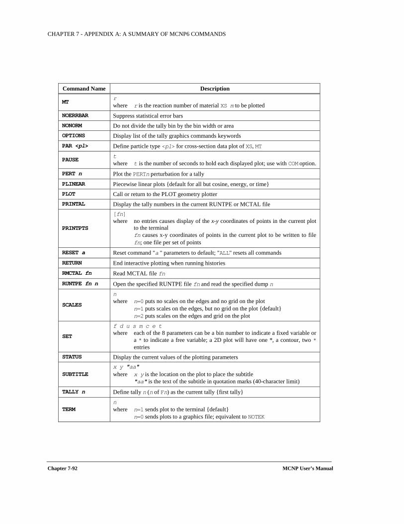
CHAPTER 7 - APPENDIX A: A SUMMARY OF MCNP6 COMMANDS
Chapter 7-92 MCNP User’s Manual
Command Name Description
MT r where r is the reaction number of material XS m to be plotted
NOERRBAR Suppress statistical error bars NONORM Do not divide the tally bin by the bin width or area OPTIONS Display list of the tally graphics commands keywords PAR <pl> Define particle type <pl> for cross-section data plot of XS, MT
PAUSE t where t is the number of seconds to hold each displayed plot; use with COM option.
PERT n Plot the PERTn perturbation for a tally PLINEAR Piecewise linear plots default for all but cosine, energy, or time PLOT Call or return to the PLOT geometry plotter PRINTAL Display the tally numbers in the current RUNTPE or MCTAL file
PRINTPTS
[fn] where no entries causes display of the x-y coordinates of points in the current plot
to the terminal fn causes x-y coordinates of points in the current plot to be written to file
fn; one file per set of points
RESET a Reset command "a " parameters to default; "ALL" resets all commands
RETURN End interactive plotting when running histories RMCTAL fn Read MCTAL file fn
RUNTPE fn n Open the specified RUNTPE file fn and read the specified dump n
SCALES
n where n=0 puts no scales on the edges and no grid on the plot n=1 puts scales on the edges, but no grid on the plot default n=2 puts scales on the edges and grid on the plot
SET
f d u s m c e t where each of the 8 parameters can be a bin number to indicate a fixed variable or
a * to indicate a free variable; a 2D plot will have one *, a contour, two * entries
STATUS Display the current values of the plotting parameters
SUBTITLE x y "aa" where x y is the location on the plot to place the subtitle "aa" is the text of the subtitle in quotation marks (40-character limit)
TALLY n Define tally n (n of Fn) as the current tally first tally
TERM n where n=1 sends plot to the terminal default n=0 sends plots to a graphics file; equivalent to NOTEK
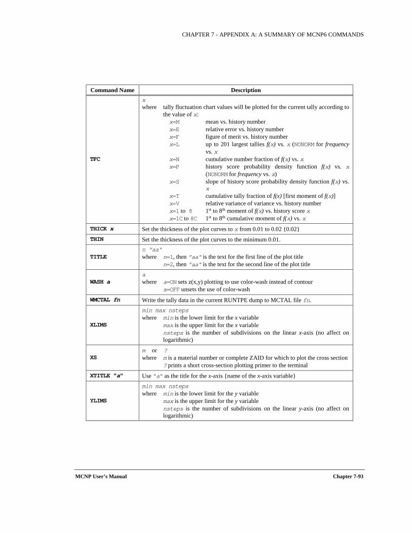
CHAPTER 7 - APPENDIX A: A SUMMARY OF MCNP6 COMMANDS
MCNP User’s Manual Chapter 7-93
Command Name Description
TFC
x where tally fluctuation chart values will be plotted for the current tally according to
the value of x: x=M mean vs. history number x=E relative error vs. history number x=F figure of merit vs. history number x=L up to 201 largest tallies f(x) vs. x (NONORM for frequency
vs. x x=N cumulative number fraction of f(x) vs. x x=P history score probability density function f(x) vs. x
(NONORM for frequency vs. x) x=S slope of history score probability density function f(x) vs.
x x=T cumulative tally fraction of f(x) [first moment of f(x)] x=V relative variance of variance vs. history number x=1 to 8 1st to 8th moment of f(x) vs. history score x x=1C to 8C 1st to 8th cumulative moment of f(x) vs. x
THICK x Set the thickness of the plot curves to x from 0.01 to 0.02 0.02 THIN Set the thickness of the plot curves to the minimum 0.01.
TITLE n "aa" where n=1, then "aa" is the text for the first line of the plot title n=2, then "aa" is the text for the second line of the plot title
WASH a a where a=ON sets z(x,y) plotting to use color-wash instead of contour a=OFF unsets the use of color-wash
WMCTAL fn Write the tally data in the current RUNTPE dump to MCTAL file fn.
XLIMS
min max nsteps where min is the lower limit for the x variable max is the upper limit for the x variable nsteps is the number of subdivisions on the linear x-axis (no affect on
logarithmic)
XS m or ? where m is a material number or complete ZAID for which to plot the cross section ? prints a short cross-section plotting primer to the terminal
XTITLE "a" Use "a" as the title for the x-axis name of the x-axis variable
YLIMS
min max nsteps where min is the lower limit for the y variable max is the upper limit for the y variable nsteps is the number of subdivisions on the linear y-axis (no affect on
logarithmic)
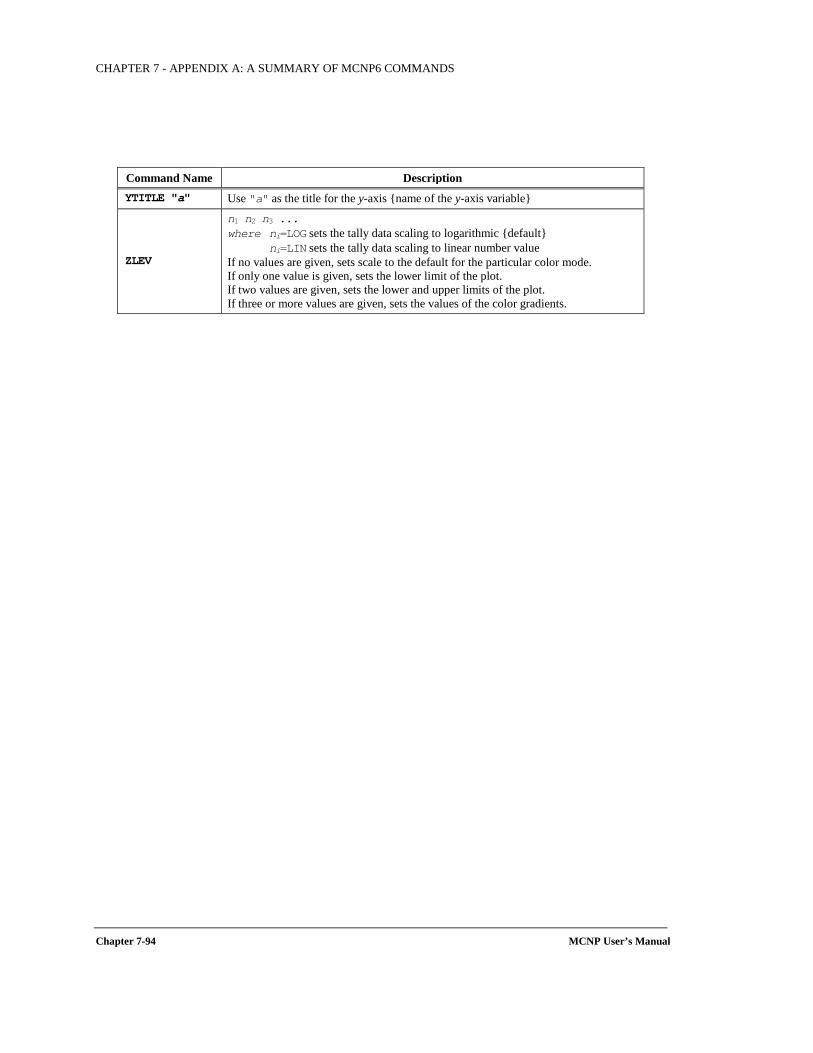
CHAPTER 7 - APPENDIX A: A SUMMARY OF MCNP6 COMMANDS
Chapter 7-94 MCNP User’s Manual
Command Name Description YTITLE "a" Use "a" as the title for the y-axis name of the y-axis variable
ZLEV
n1 n2 n3 ... where ni=LOG sets the tally data scaling to logarithmic default ni=LIN sets the tally data scaling to linear number value If no values are given, sets scale to the default for the particular color mode. If only one value is given, sets the lower limit of the plot. If two values are given, sets the lower and upper limits of the plot. If three or more values are given, sets the values of the color gradients.
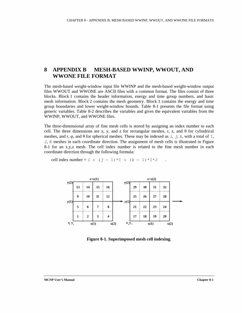
CHAPTER 8 - APPENDIX B: MESH BASED WWINP, WWOUT, AND WWONE FILE FORMATS
MCNP User’s Manual Chapter 8-1
8 APPENDIX B MESH-BASED WWINP, WWOUT, AND WWONE FILE FORMAT
The mesh-based weight-window input file WWINP and the mesh-based weight-window output files WWOUT and WWONE are ASCII files with a common format. The files consist of three blocks. Block 1 contains the header information, energy and time group numbers, and basic mesh information. Block 2 contains the mesh geometry. Block 3 contains the energy and time group boundaries and lower weight-window bounds. Table 8-1 presents the file format using generic variables. Table 8-2 describes the variables and gives the equivalent variables from the WWINP, WWOUT, and WWONE files.
The three-dimensional array of fine mesh cells is stored by assigning an index number to each cell. The three dimensions are x, y, and z for rectangular meshes, r, z, and θ for cylindrical meshes, and r, φ, and θ for spherical meshes. These may be indexed as i, j, k, with a total of I, J, K meshes in each coordinate direction. The assignment of mesh cells is illustrated in Figure 8-1 for an x,y,z mesh. The cell index number is related to the fine mesh number in each coordinate direction through the following formula:
cell index number = i + (j − 1)*I + (k − 1)*I*J .
Figure 8-1. Superimposed mesh cell indexing.
13 14 15 16
9 10 1 1 12
5 6 7 8
1 2 3 4
29 30 31 32
25 26 27 28
21 22 23 24
17 18 19 20
x 0 y 0
y(1)
y(2) z=z(1) z=z(2)
x(1) x(2)
y(1)
y(2)
x(1) x(2) x 0 y
0
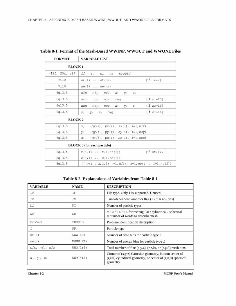
CHAPTER 8 - APPENDIX B: MESH BASED WWINP, WWOUT, AND WWONE FILE FORMATS
Chapter 8-2 MCNP User’s Manual
Table 8-1. Format of the Mesh-Based WWINP, WWOUT and WWONE Files
FORMAT VARIABLE LIST
BLOCK 1
4i10, 20x, a19 if iv ni nr probid
7i10 nt(1) ... nt(ni) [if iv=2]
7i10 ne(1) ... ne(ni)
6g13.5 nfx nfy nfz x0 y0 z0
6g13.5 ncx ncy ncz nwg [if nr=10]
6g13.5 ncx ncy ncz x1 y1 z1 [if nr=16]
6g13.5 x2 y2 z2 nwg [if nr=16]
BLOCK 2
6g13.5 x0 (qx(i), px(i), sx(i), i=1,ncx)
6g13.5 y0 (qy(i), py(i), sy(i), i=1,ncy)
6g13.5 z0 (qz(i), pz(i), sz(i), i=1,ncz)
BLOCK 3 (for each particle)
6g13.5 t(i,1) ... t(i,nt(i)) [if nt(i)>1]
6g13.5 e(i,1) ... e(i,ne(i))
6g13.5 (((w(i,j,k,l,1) j=1,nft), k=1,ne(i)), l=1,nt(i))
Table 8-2. Explanations of Variables from Table 8-1
VARIABLE NAME DESCRIPTION If IF File type. Only 1 is supported. Unused.
Iv IV Time-dependent windows flag (1 / 2 = no / yes)
Ni NI Number of particle types
Nr NR = 10 / 16 / 16 for rectangular / cylindrical / spherical = number of words to describe mesh
Probed PROBID Problem identification description
I KP Particle type
nt(i) NWW(KP) Number of time bins for particle type i
ne(i) NGWW(KP) Number of energy bins for particle type i
nfx, nfy, nfz WWM(1:3) Total number of fine (x,y,z), (r,z,θ), or (r,ϕ,θ) mesh bins
x0, y0, z0 WWM(4:6) Corner of (x,y,z) Cartesian geometry, bottom center of (r,z,θ) cylindrical geometry, or center of (r,ϕ,θ) spherical geometry
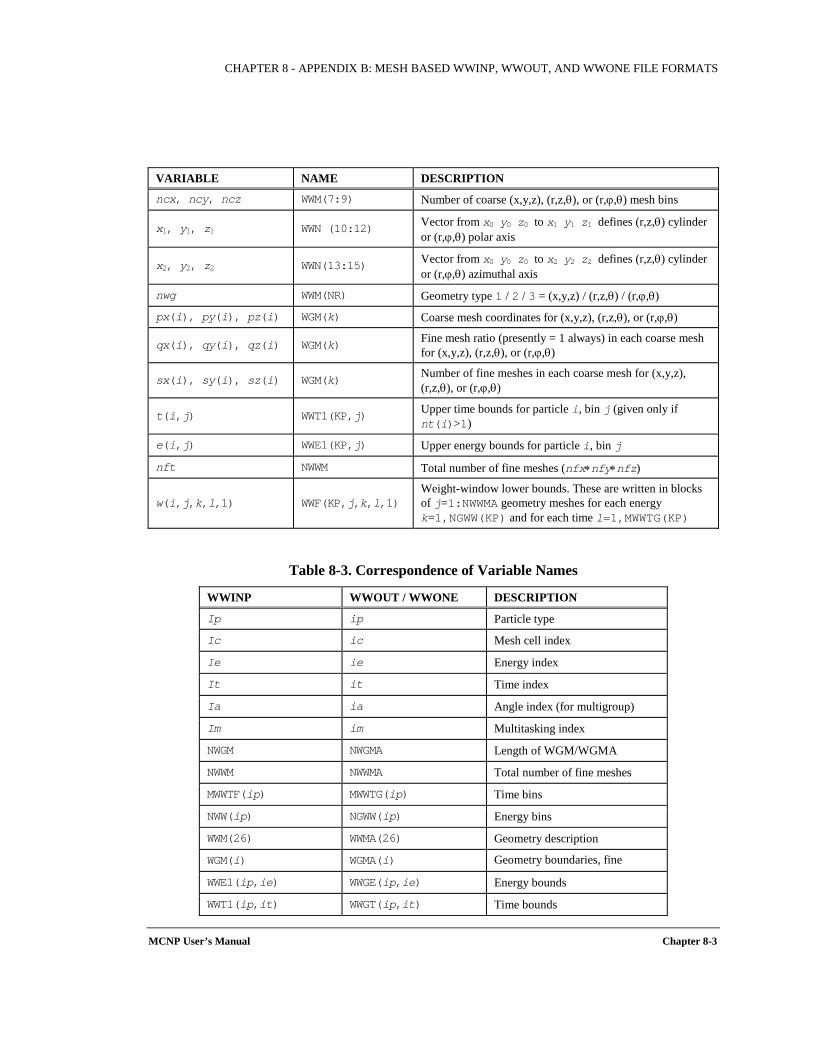
CHAPTER 8 - APPENDIX B: MESH BASED WWINP, WWOUT, AND WWONE FILE FORMATS
MCNP User’s Manual Chapter 8-3
VARIABLE NAME DESCRIPTION ncx, ncy, ncz WWM(7:9) Number of coarse (x,y,z), (r,z,θ), or (r,ϕ,θ) mesh bins
x1, y1, z1 WWN (10:12) Vector from x0 y0 z0 to x1 y1 z1 defines (r,z,θ) cylinder or (r,ϕ,θ) polar axis
x2, y2, z2 WWN(13:15) Vector from x0 y0 z0 to x2 y2 z2 defines (r,z,θ) cylinder or (r,ϕ,θ) azimuthal axis
nwg WWM(NR) Geometry type 1 / 2 / 3 = (x,y,z) / (r,z,θ) / (r,ϕ,θ)
px(i), py(i), pz(i) WGM(k) Coarse mesh coordinates for (x,y,z), (r,z,θ), or (r,ϕ,θ)
qx(i), qy(i), qz(i) WGM(k) Fine mesh ratio (presently = 1 always) in each coarse mesh for (x,y,z), (r,z,θ), or (r,ϕ,θ)
sx(i), sy(i), sz(i) WGM(k) Number of fine meshes in each coarse mesh for (x,y,z), (r,z,θ), or (r,ϕ,θ)
t(i,j) WWT1(KP,j) Upper time bounds for particle i, bin j (given only if nt(i)>1)
e(i,j) WWE1(KP,j) Upper energy bounds for particle i, bin j
nft NWWM Total number of fine meshes (nfx∗nfy∗nfz)
w(i,j,k,l,1) WWF(KP,j,k,l,1) Weight-window lower bounds. These are written in blocks of j=1:NWWMA geometry meshes for each energy k=1,NGWW(KP) and for each time l=1,MWWTG(KP)
Table 8-3. Correspondence of Variable Names
WWINP WWOUT / WWONE DESCRIPTION
Ip ip Particle type
Ic ic Mesh cell index
Ie ie Energy index
It it Time index
Ia ia Angle index (for multigroup)
Im im Multitasking index
NWGM NWGMA Length of WGM/WGMA
NWWM NWWMA Total number of fine meshes
MWWTF(ip) MWWTG(ip) Time bins
NWW(ip) NGWW(ip) Energy bins
WWM(26) WWMA(26) Geometry description
WGM(i) WGMA(i) Geometry boundaries, fine
WWE1(ip,ie) WWGE(ip,ie) Energy bounds
WWT1(ip,it) WWGT(ip,it) Time bounds
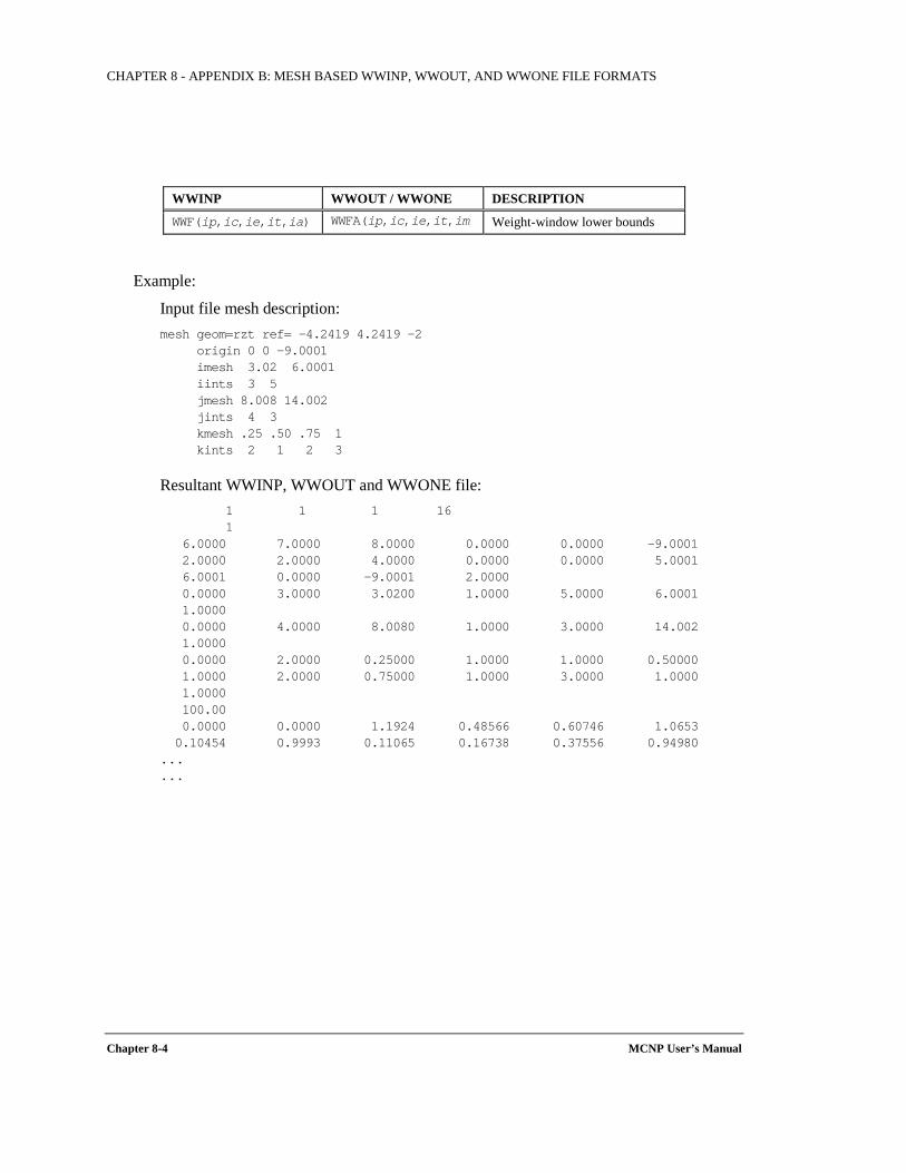
CHAPTER 8 - APPENDIX B: MESH BASED WWINP, WWOUT, AND WWONE FILE FORMATS
Chapter 8-4 MCNP User’s Manual
WWINP WWOUT / WWONE DESCRIPTION WWF(ip,ic,ie,it,ia) WWFA(ip,ic,ie,it,im
Weight-window lower bounds
Example:
Input file mesh description: mesh geom=rzt ref= -4.2419 4.2419 -2 origin 0 0 -9.0001 imesh 3.02 6.0001 iints 3 5 jmesh 8.008 14.002 jints 4 3 kmesh .25 .50 .75 1 kints 2 1 2 3
Resultant WWINP, WWOUT and WWONE file: 1 1 1 16 1 6.0000 7.0000 8.0000 0.0000 0.0000 -9.0001 2.0000 2.0000 4.0000 0.0000 0.0000 5.0001 6.0001 0.0000 -9.0001 2.0000 0.0000 3.0000 3.0200 1.0000 5.0000 6.0001 1.0000 0.0000 4.0000 8.0080 1.0000 3.0000 14.002 1.0000 0.0000 2.0000 0.25000 1.0000 1.0000 0.50000 1.0000 2.0000 0.75000 1.0000 3.0000 1.0000 1.0000 100.00 0.0000 0.0000 1.1924 0.48566 0.60746 1.0653 0.10454 0.9993 0.11065 0.16738 0.37556 0.94980 ... ...
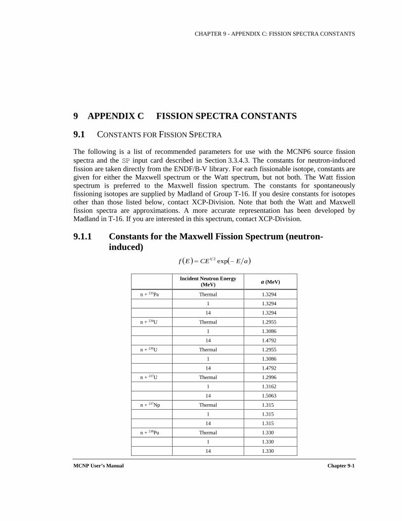
CHAPTER 9 - APPENDIX C: FISSION SPECTRA CONSTANTS
MCNP User’s Manual Chapter 9-1
9 APPENDIX C FISSION SPECTRA CONSTANTS
9.1 CONSTANTS FOR FISSION SPECTRA
The following is a list of recommended parameters for use with the MCNP6 source fission spectra and the SP input card described in Section 3.3.4.3. The constants for neutron-induced fission are taken directly from the ENDF/B-V library. For each fissionable isotope, constants are given for either the Maxwell spectrum or the Watt spectrum, but not both. The Watt fission spectrum is preferred to the Maxwell fission spectrum. The constants for spontaneously fissioning isotopes are supplied by Madland of Group T-16. If you desire constants for isotopes other than those listed below, contact XCP-Division. Note that both the Watt and Maxwell fission spectra are approximations. A more accurate representation has been developed by Madland in T-16. If you are interested in this spectrum, contact XCP-Division.
9.1.1 Constants for the Maxwell Fission Spectrum (neutron-induced)
Incident Neutron Energy (MeV) a (MeV)
n + 233Pa Thermal 1.3294
1 1.3294
14 1.3294
n + 234U Thermal 1.2955
1 1.3086
14 1.4792
n + 236U Thermal 1.2955
1 1.3086
14 1.4792
n + 237U Thermal 1.2996
1 1.3162
14 1.5063
n + 237Np Thermal 1.315
1 1.315
14 1.315
n + 238Pu Thermal 1.330
1 1.330
14 1.330
( ) ( )aECEEf −= exp21
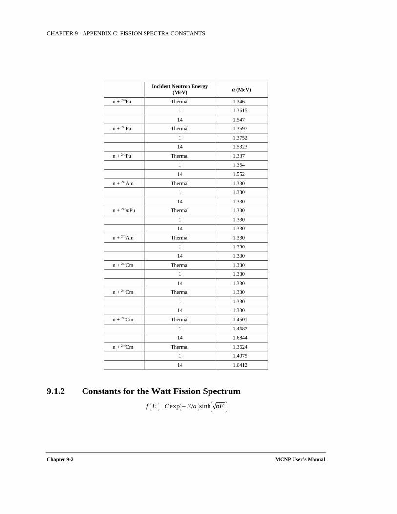
CHAPTER 9 - APPENDIX C: FISSION SPECTRA CONSTANTS
Chapter 9-2 MCNP User’s Manual
Incident Neutron Energy (MeV) a (MeV)
n + 240Pu Thermal 1.346
1 1.3615
14 1.547
n + 241Pu Thermal 1.3597
1 1.3752
14 1.5323
n + 242Pu Thermal 1.337
1 1.354
14 1.552
n + 241Am Thermal 1.330
1 1.330
14 1.330
n + 242mPu Thermal 1.330
1 1.330
14 1.330
n + 243Am Thermal 1.330
1 1.330
14 1.330
n + 242Cm Thermal 1.330
1 1.330
14 1.330
n + 244Cm Thermal 1.330
1 1.330
14 1.330
n + 245Cm Thermal 1.4501
1 1.4687
14 1.6844
n + 246Cm Thermal 1.3624
1 1.4075
14 1.6412
9.1.2 Constants for the Watt Fission Spectrum
−= bEaECEf sinhexp
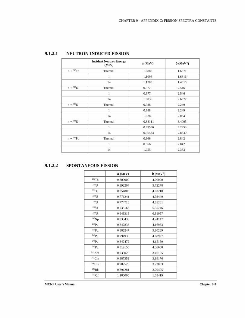
CHAPTER 9 - APPENDIX C: FISSION SPECTRA CONSTANTS
MCNP User’s Manual Chapter 9-3
9.1.2.1 NEUTRON-INDUCED FISSION
Incident Neutron Energy (MeV) a (MeV) b (MeV-1)
n + 232Th Thermal 1.0888 1.6871
1 1.1096 1.6316
14 1.1700 1.4610
n + 233U Thermal 0.977 2.546
1 0.977 2.546
14 1.0036 2.6377
n + 235U Thermal 0.988 2.249
1 0.988 2.249
14 1.028 2.084
n + 238U Thermal 0.88111 3.4005
1 0.89506 3.2953
14 0.96534 2.8330
n + 239Pu Thermal 0.966 2.842
1 0.966 2.842
14 1.055 2.383
9.1.2.2 SPONTANEOUS FISSION
a (MeV) b (MeV-1) 232Th 0.800000 4.00000 232U 0.892204 3.72278 233 U 0.854803 4.03210 234U 0.771241 4.92449 235U 0.774713 4.85231 236U 0.735166 5.35746 238U 0.648318 6.81057
237Np 0.833438 4.24147 238Pu 0.847833 4.16933 239Pu 0.885247 3.80269 240Pu 0.794930 4.68927 241Pu 0.842472 4.15150 242Pu 0.819150 4.36668
241Am 0.933020 3.46195 242Cm 0.887353 3.89176 244Cm 0.902523 3.72033 249Bk 0.891281 3.79405 252Cf 1.180000 1.03419

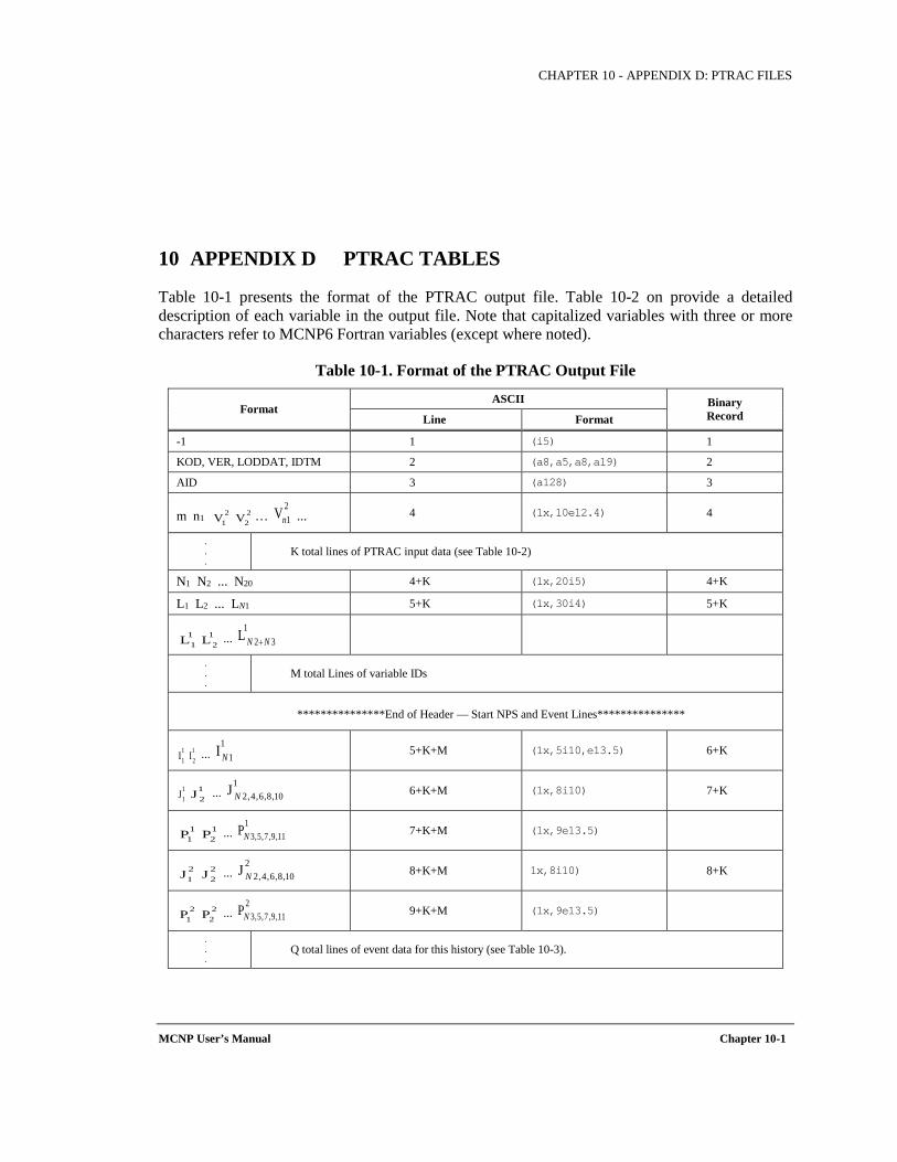
CHAPTER 10 - APPENDIX D: PTRAC FILES
MCNP User’s Manual Chapter 10-1
10 APPENDIX D PTRAC TABLES
Table 10-1 presents the format of the PTRAC output file. Table 10-2 on provide a detailed description of each variable in the output file. Note that capitalized variables with three or more characters refer to MCNP6 Fortran variables (except where noted).
Table 10-1. Format of the PTRAC Output File
Format ASCII Binary
Record Line Format
-1 1 (i5) 1
KOD, VER, LODDAT, IDTM 2 (a8,a5,a8,a19) 2
AID 3 (a128) 3
m n1 … ... 4 (1x,10e12.4) 4
.
.
. K total lines of PTRAC input data (see Table 10-2)
N1 N2 ... N20 4+K (1x,20i5) 4+K
L1 L2 ... LN1 5+K (1x,30i4) 5+K
...
.
.
. M total Lines of variable IDs
***************End of Header — Start NPS and Event Lines***************
... 5+K+M (1x,5i10,e13.5) 6+K
... 6+K+M (1x,8i10) 7+K
... 7+K+M (1x,9e13.5)
... 8+K+M 1x,8i10) 8+K
... 9+K+M (1x,9e13.5)
.
.
. Q total lines of event data for this history (see Table 10-3).
21V 2
2V21Vn
11L 1
2L1
32L NN +
11I
12I
11I N
11J 1
2J1
10,8,6,4,2J N
11P 1
2P1
11,9,7,5,3PN
21J 2
2J2
10,8,6,4,2J N
21P 2
2P2
11,9,7,5,3PN
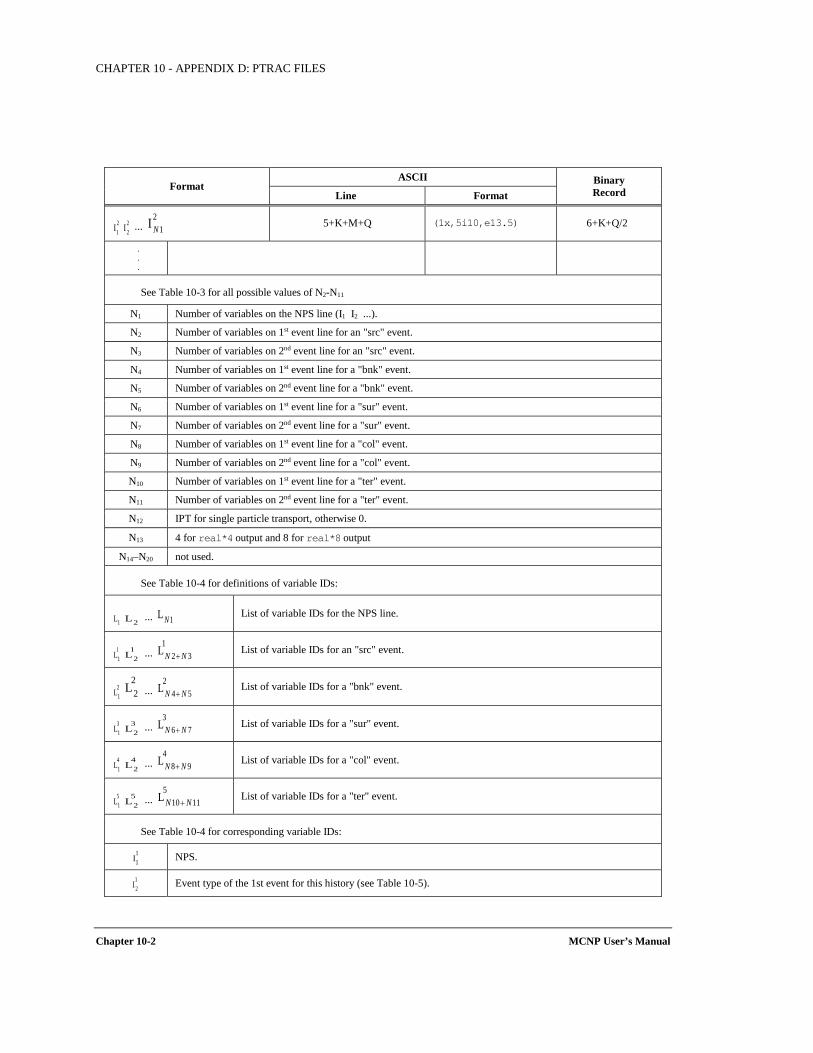
CHAPTER 10 - APPENDIX D: PTRAC FILES
Chapter 10-2 MCNP User’s Manual
Format ASCII Binary
Record Line Format
... 5+K+M+Q (1x,5i10,e13.5) 6+K+Q/2
.
.
.
See Table 10-3 for all possible values of N2-N11
N1 Number of variables on the NPS line (I1 I2 ...).
N2 Number of variables on 1st event line for an "src" event.
N3 Number of variables on 2nd event line for an "src" event.
N4 Number of variables on 1st event line for a "bnk" event.
N5 Number of variables on 2nd event line for a "bnk" event.
N6 Number of variables on 1st event line for a "sur" event.
N7 Number of variables on 2nd event line for a "sur" event.
N8 Number of variables on 1st event line for a "col" event.
N9 Number of variables on 2nd event line for a "col" event.
N10 Number of variables on 1st event line for a "ter" event.
N11 Number of variables on 2nd event line for a "ter" event.
N12 IPT for single particle transport, otherwise 0.
N13 4 for real*4 output and 8 for real*8 output
N14–N20 not used.
See Table 10-4 for definitions of variable IDs:
... List of variable IDs for the NPS line.
... List of variable IDs for an "src" event.
... List of variable IDs for a "bnk" event.
... List of variable IDs for a "sur" event.
... List of variable IDs for a "col" event.
... List of variable IDs for a "ter" event.
See Table 10-4 for corresponding variable IDs:
NPS.
Event type of the 1st event for this history (see Table 10-5).
21I
22I
21I N
1L 2L 1L N
11L
12L
132L NN +
21L
22L 2
54L NN +
31L
32L
376L NN +
41L
42L
498L NN +
51L
52L
51110L NN +
11I
12I
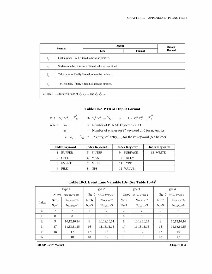
CHAPTER 10 - APPENDIX D: PTRAC FILES
MCNP User’s Manual Chapter 10-3
Format ASCII Binary
Record Line Format
Cell number if cell filtered, otherwise omitted.
Surface number if surface filtered, otherwise omitted.
Tally number if tally filtered, otherwise omitted.
TFC bin tally if tally filtered, otherwise omitted.
See Table 10-4 for definitions of , , ..., and , , ... .
Table 10-2. PTRAC Input Format
m n1 … n2 … ... n13 …
where m = Number of PTRAC keywords = 13 ni = Number of entries for ith keyword or 0 for no entries
… = 1st entry, 2nd entry, ..., for the ith keyword (see below).
Index Keyword Index Keyword Index Keyword Index Keyword
1 BUFFER 5 FILTER 9 SURFACE 13 WRITE
2 CELL 6 MAX 10 TALLY
3 EVENT 7 MENP 11 TYPE
4 FILE 8 NPS 12 VALUE
Table 10-3. Event Line Variable IDs (See Table 10-4)†
Index
Type 1 Type 2 Type 3 Type 4
N12≠0 WRITE=pos N12=0 WRITE=pos N12≠0 WRITE=all N12=0 WRITE=all
N2=5 N4,6,8,10=6 N2=6 N4,6,8,10=7 N2=6 N4,6,8,10=7 N2=7 N4,6,8,10=8
N3=3 N5,7,9,11=3 N3=3 N5,7,9,11=3 N3=9 N5,7,9,11=9 N3=9 N5,7,9,11=9
J1 7 7 7 7 7 7 7 7
J2 8 8 8 8 8 8 8 8
J3 9 10,12,10,14 9 10,12,10,14 9 10,12,10,14 9 10,12,10,14
J4 17 11,13,11,15 16 11,13,11,15 17 11,13,11,15 16 11,13,11,15
J5 18 17 17 16 18 17 17 16
J6 18 18 17 19 18 18 17
13I
14I
15I
16I
11J
12J
11P
12P
11V 1
2V11Vn
21V 2
2V22Vn
131V 13
2V131Vn
1V 2V niV
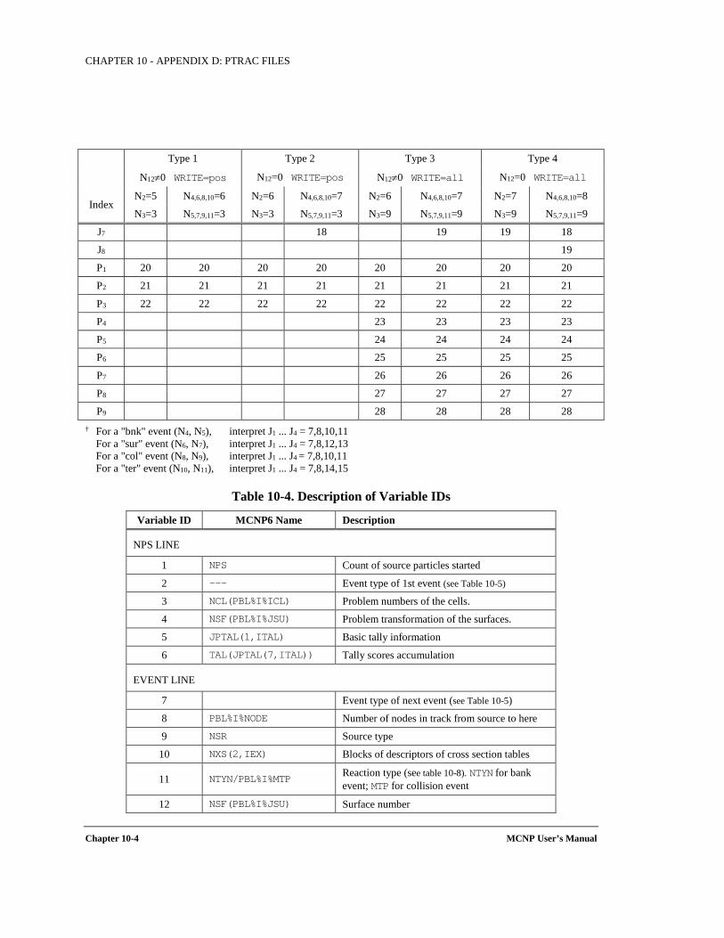
CHAPTER 10 - APPENDIX D: PTRAC FILES
Chapter 10-4 MCNP User’s Manual
Index
Type 1 Type 2 Type 3 Type 4
N12≠0 WRITE=pos N12=0 WRITE=pos N12≠0 WRITE=all N12=0 WRITE=all
N2=5 N4,6,8,10=6 N2=6 N4,6,8,10=7 N2=6 N4,6,8,10=7 N2=7 N4,6,8,10=8
N3=3 N5,7,9,11=3 N3=3 N5,7,9,11=3 N3=9 N5,7,9,11=9 N3=9 N5,7,9,11=9
J7 18 19 19 18
J8 19
P1 20 20 20 20 20 20 20 20
P2 21 21 21 21 21 21 21 21
P3 22 22 22 22 22 22 22 22
P4 23 23 23 23
P5 24 24 24 24
P6 25 25 25 25
P7 26 26 26 26
P8 27 27 27 27
P9 28 28 28 28 † For a "bnk" event (N4, N5), interpret J1 ... J4 = 7,8,10,11 For a "sur" event (N6, N7), interpret J1 ... J4 = 7,8,12,13 For a "col" event (N8, N9), interpret J1 ... J4 = 7,8,10,11 For a "ter" event (N10, N11), interpret J1 ... J4 = 7,8,14,15
Table 10-4. Description of Variable IDs
Variable ID MCNP6 Name Description
NPS LINE
1 NPS Count of source particles started
2 --- Event type of 1st event (see Table 10-5)
3 NCL(PBL%I%ICL) Problem numbers of the cells.
4 NSF(PBL%I%JSU) Problem transformation of the surfaces.
5 JPTAL(1,ITAL) Basic tally information
6 TAL(JPTAL(7,ITAL)) Tally scores accumulation
EVENT LINE
7 Event type of next event (see Table 10-5)
8 PBL%I%NODE Number of nodes in track from source to here
9 NSR Source type
10 NXS(2,IEX) Blocks of descriptors of cross section tables
11 NTYN/PBL%I%MTP Reaction type (see table 10-8). NTYN for bank event; MTP for collision event
12 NSF(PBL%I%JSU) Surface number
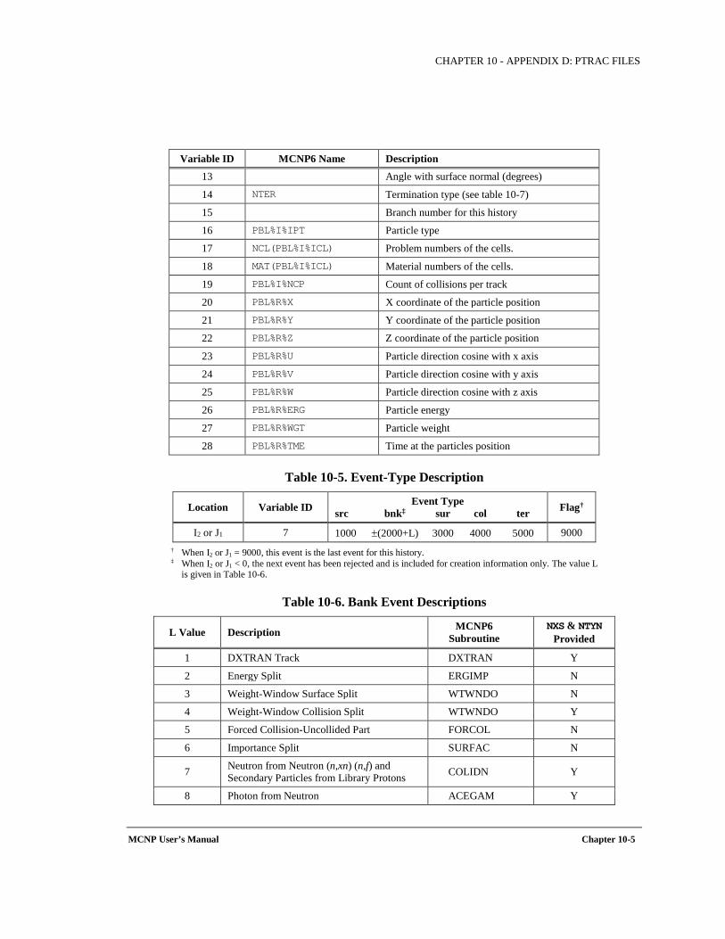
CHAPTER 10 - APPENDIX D: PTRAC FILES
MCNP User’s Manual Chapter 10-5
Variable ID MCNP6 Name Description 13 Angle with surface normal (degrees)
14 NTER Termination type (see table 10-7)
15 Branch number for this history
16 PBL%I%IPT Particle type
17 NCL(PBL%I%ICL) Problem numbers of the cells.
18 MAT(PBL%I%ICL) Material numbers of the cells.
19 PBL%I%NCP Count of collisions per track
20 PBL%R%X X coordinate of the particle position
21 PBL%R%Y Y coordinate of the particle position
22 PBL%R%Z Z coordinate of the particle position
23 PBL%R%U Particle direction cosine with x axis
24 PBL%R%V Particle direction cosine with y axis
25 PBL%R%W Particle direction cosine with z axis
26 PBL%R%ERG Particle energy
27 PBL%R%WGT Particle weight
28 PBL%R%TME Time at the particles position
Table 10-5. Event-Type Description
Location Variable ID Event Type src bnk‡ sur col ter Flag†
I2 or J1 7 1000 ±(2000+L) 3000 4000 5000 9000 † When I2 or J1 = 9000, this event is the last event for this history. ‡ When I2 or J1 < 0, the next event has been rejected and is included for creation information only. The value L
is given in Table 10-6.
Table 10-6. Bank Event Descriptions
L Value Description MCNP6 Subroutine
NXS & NTYN Provided
1 DXTRAN Track DXTRAN Y
2 Energy Split ERGIMP N
3 Weight-Window Surface Split WTWNDO N
4 Weight-Window Collision Split WTWNDO Y
5 Forced Collision-Uncollided Part FORCOL N
6 Importance Split SURFAC N
7 Neutron from Neutron (n,xn) (n,f) and Secondary Particles from Library Protons COLIDN Y
8 Photon from Neutron ACEGAM Y
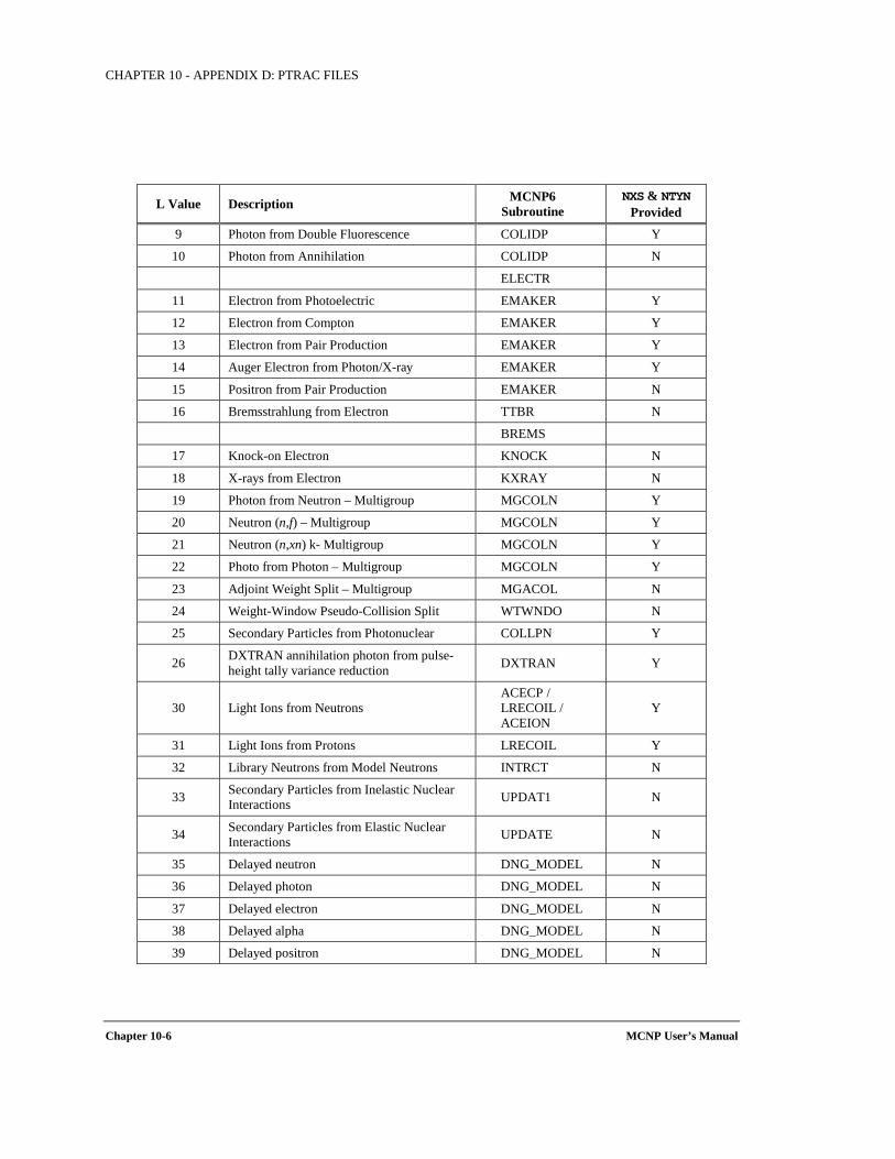
CHAPTER 10 - APPENDIX D: PTRAC FILES
Chapter 10-6 MCNP User’s Manual
L Value Description MCNP6 Subroutine
NXS & NTYN Provided
9 Photon from Double Fluorescence COLIDP Y
10 Photon from Annihilation COLIDP N
ELECTR
11 Electron from Photoelectric EMAKER Y
12 Electron from Compton EMAKER Y
13 Electron from Pair Production EMAKER Y
14 Auger Electron from Photon/X-ray EMAKER Y
15 Positron from Pair Production EMAKER N
16 Bremsstrahlung from Electron TTBR N
BREMS 17 Knock-on Electron KNOCK N
18 X-rays from Electron KXRAY N
19 Photon from Neutron – Multigroup MGCOLN Y
20 Neutron (n,f) – Multigroup MGCOLN Y
21 Neutron (n,xn) k- Multigroup MGCOLN Y
22 Photo from Photon – Multigroup MGCOLN Y
23 Adjoint Weight Split – Multigroup MGACOL N
24 Weight-Window Pseudo-Collision Split WTWNDO N
25 Secondary Particles from Photonuclear COLLPN Y
26 DXTRAN annihilation photon from pulse-height tally variance reduction DXTRAN Y
30 Light Ions from Neutrons ACECP / LRECOIL / ACEION
Y
31 Light Ions from Protons LRECOIL Y
32 Library Neutrons from Model Neutrons INTRCT N
33 Secondary Particles from Inelastic Nuclear Interactions UPDAT1 N
34 Secondary Particles from Elastic Nuclear Interactions UPDATE N
35 Delayed neutron DNG_MODEL N
36 Delayed photon DNG_MODEL N
37 Delayed electron DNG_MODEL N
38 Delayed alpha DNG_MODEL N
39 Delayed positron DNG_MODEL N
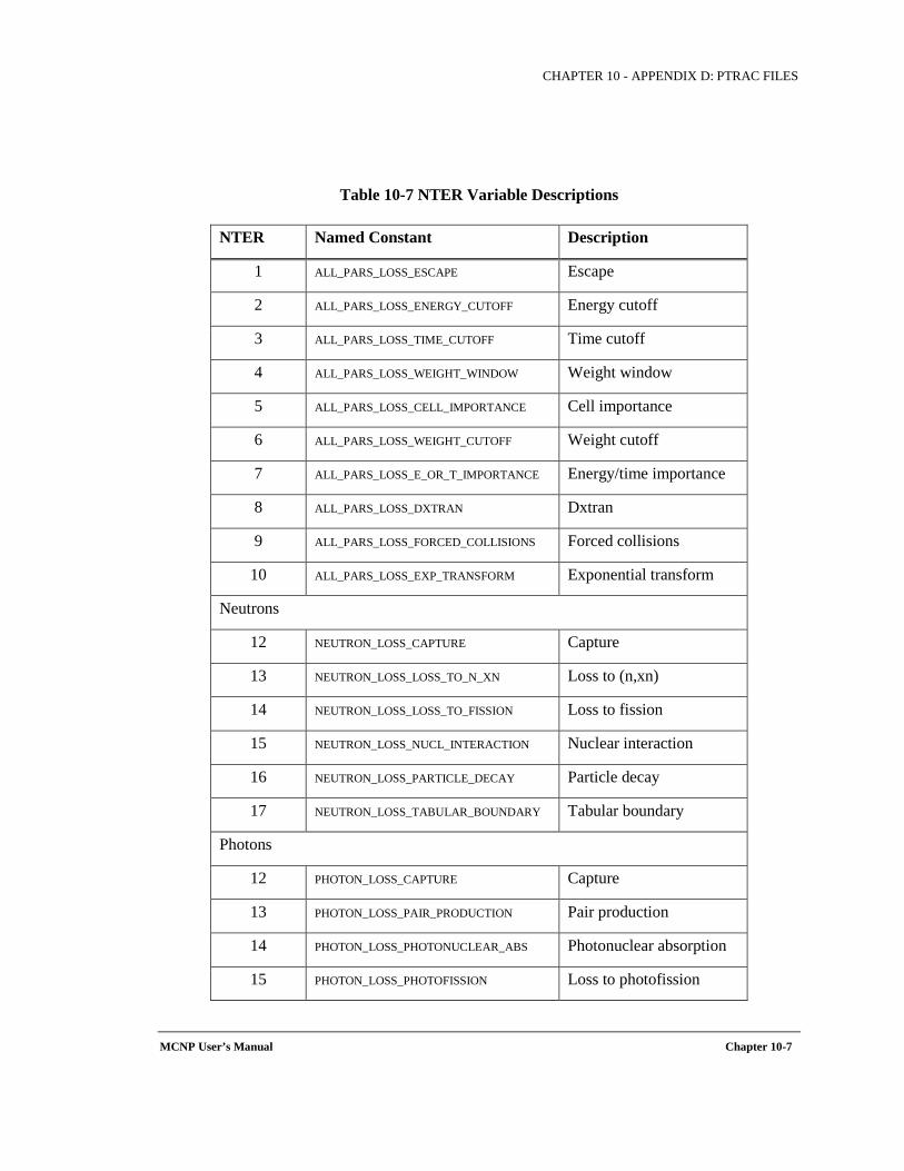
CHAPTER 10 - APPENDIX D: PTRAC FILES
MCNP User’s Manual Chapter 10-7
Table 10-7 NTER Variable Descriptions
NTER Named Constant Description
1 ALL_PARS_LOSS_ESCAPE Escape
2 ALL_PARS_LOSS_ENERGY_CUTOFF Energy cutoff
3 ALL_PARS_LOSS_TIME_CUTOFF Time cutoff
4 ALL_PARS_LOSS_WEIGHT_WINDOW Weight window
5 ALL_PARS_LOSS_CELL_IMPORTANCE Cell importance
6 ALL_PARS_LOSS_WEIGHT_CUTOFF Weight cutoff
7 ALL_PARS_LOSS_E_OR_T_IMPORTANCE Energy/time importance
8 ALL_PARS_LOSS_DXTRAN Dxtran
9 ALL_PARS_LOSS_FORCED_COLLISIONS Forced collisions
10 ALL_PARS_LOSS_EXP_TRANSFORM Exponential transform
Neutrons
12 NEUTRON_LOSS_CAPTURE Capture
13 NEUTRON_LOSS_LOSS_TO_N_XN Loss to (n,xn)
14 NEUTRON_LOSS_LOSS_TO_FISSION Loss to fission
15 NEUTRON_LOSS_NUCL_INTERACTION Nuclear interaction
16 NEUTRON_LOSS_PARTICLE_DECAY Particle decay
17 NEUTRON_LOSS_TABULAR_BOUNDARY Tabular boundary
Photons
12 PHOTON_LOSS_CAPTURE Capture
13 PHOTON_LOSS_PAIR_PRODUCTION Pair production
14 PHOTON_LOSS_PHOTONUCLEAR_ABS Photonuclear absorption
15 PHOTON_LOSS_PHOTOFISSION Loss to photofission
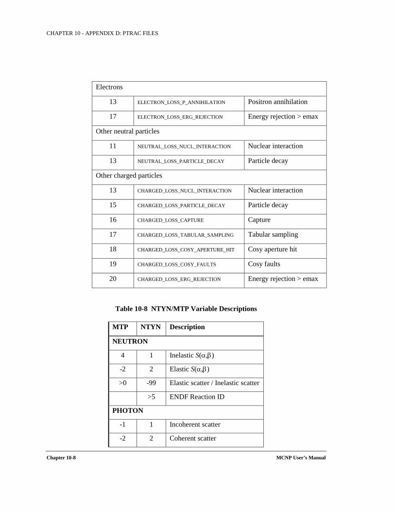
CHAPTER 10 - APPENDIX D: PTRAC FILES
Chapter 10-8 MCNP User’s Manual
Table 10-8 NTYN/MTP Variable Descriptions
MTP NTYN Description
NEUTRON
4 1 Inelastic S(α,β)
-2 2 Elastic S(α,β)
>0 -99 Elastic scatter / Inelastic scatter
>5 ENDF Reaction ID
PHOTON
-1 1 Incoherent scatter
-2 2 Coherent scatter
Electrons
13 ELECTRON_LOSS_P_ANNIHILATION Positron annihilation
17 ELECTRON_LOSS_ERG_REJECTION Energy rejection > emax
Other neutral particles
11 NEUTRAL_LOSS_NUCL_INTERACTION Nuclear interaction
13 NEUTRAL_LOSS_PARTICLE_DECAY Particle decay
Other charged particles
13 CHARGED_LOSS_NUCL_INTERACTION Nuclear interaction
15 CHARGED_LOSS_PARTICLE_DECAY Particle decay
16 CHARGED_LOSS_CAPTURE Capture
17 CHARGED_LOSS_TABULAR_SAMPLING Tabular sampling
18 CHARGED_LOSS_COSY_APERTURE_HIT Cosy aperture hit
19 CHARGED_LOSS_COSY_FAULTS Cosy faults
20 CHARGED_LOSS_ERG_REJECTION Energy rejection > emax
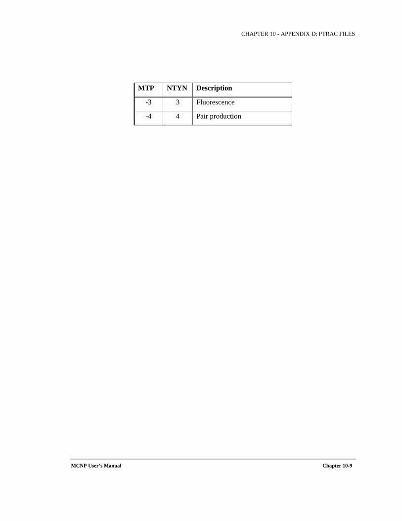
CHAPTER 10 - APPENDIX D: PTRAC FILES
MCNP User’s Manual Chapter 10-9
MTP NTYN Description
-3 3 Fluorescence
-4 4 Pair production


CHAPTER 11 - APPENDIX E: MCNP6 DATA LIBRARIES
MCNP User’s Manual Chapter 10-1

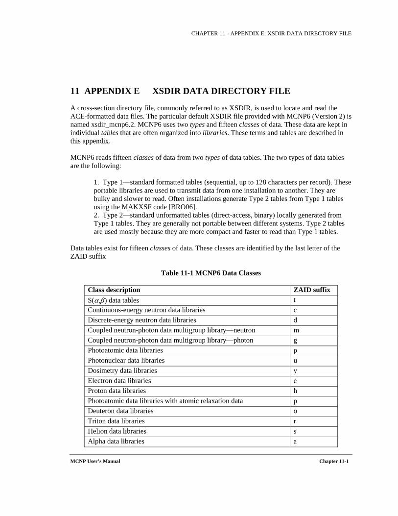
CHAPTER 11 - APPENDIX E: XSDIR DATA DIRECTORY FILE
MCNP User’s Manual Chapter 11-1
11 APPENDIX E XSDIR DATA DIRECTORY FILE
A cross-section directory file, commonly referred to as XSDIR, is used to locate and read the ACE-formatted data files. The particular default XSDIR file provided with MCNP6 (Version 2) is named xsdir_mcnp6.2. MCNP6 uses two types and fifteen classes of data. These data are kept in individual tables that are often organized into libraries. These terms and tables are described in this appendix. MCNP6 reads fifteen classes of data from two types of data tables. The two types of data tables are the following:
1. Type 1—standard formatted tables (sequential, up to 128 characters per record). These portable libraries are used to transmit data from one installation to another. They are bulky and slower to read. Often installations generate Type 2 tables from Type 1 tables using the MAKXSF code [BRO06]. 2. Type 2—standard unformatted tables (direct-access, binary) locally generated from Type 1 tables. They are generally not portable between different systems. Type 2 tables are used mostly because they are more compact and faster to read than Type 1 tables.
Data tables exist for fifteen classes of data. These classes are identified by the last letter of the ZAID suffix
Table 11-1 MCNP6 Data Classes
Class description ZAID suffix S(α,β) data tables t Continuous-energy neutron data libraries c Discrete-energy neutron data libraries d Coupled neutron-photon data multigroup library—neutron m Coupled neutron-photon data multigroup library—photon g Photoatomic data libraries p Photonuclear data libraries u Dosimetry data libraries y Electron data libraries e Proton data libraries h Photoatomic data libraries with atomic relaxation data p Deuteron data libraries o Triton data libraries r Helion data libraries s Alpha data libraries a

CHAPTER 11 - APPENDIX E: XSDIR DATA DIRECTORY FILE
Chapter 11-2 MCNP User’s Manual
A user should think of a data table as an entity that contains evaluation-dependent information about one of the fifteen classes of data for a specific target isotope, isomer, element, or material. For how the data are used in MCNP6, a user does not need to know whether a particular table is in Type 1 or Type 2. For a given ZAID, the data contained on Type 1 and Type 2 tables are identical. Problems run with one data type will track problems run with the same data in another format type. When we refer to data libraries, we are talking about a series of data tables concatenated into one file. All tables on a single library must be of the same type but not necessarily of the same class. There is no reason, other than convenience, for having data libraries; MCNP6 could read exclusively from individual data tables not in libraries. MCNP6 determines where to find data tables for each ZAID in a problem based on information contained in a system-dependent cross-section directory (or XSDIR) file. (The specific directory file supplied with the MCNP6 (Version 2) distribution is named xsdir_mcnp6.2.) The directory file is a sequentially formatted ASCII file containing free-field entries delimited by blanks. The XSDIR file has three sections. In the first section, the first line is an optional entry of the form
DATAPATH = datapath where the word DATAPATH (case insensitive) must start in columns 1–5. The "=" sign is optional. The directory where the data libraries are stored is named datapath. The XSDIR directory file can be renamed on the MCNP6 execution line (see Table 1-2). The search hierarchy to find XSDIR and/or the data libraries is the following:
1. XSDIR=file_name on the MCNP6 execution line, where "file_name " is the name of a cross-section directory file
2. DATAPATH = datapath in the INP file message block,
3. the current working directory,
4. the DATAPATH entry on the first line of the XSDIR file,
5. the system environment variable DATAPATH, or
the individual data table line in the XSDIR file (see below under Access Route).The second section of the XSDIR file is the atomic weight ratios. This section starts with the words “ATOMIC WEIGHT RATIOS” (case insensitive) beginning in columns 1–5. The following lines are free-format pairs of ZAID AWR, where ZAID is an integer of the form ZZAAA and AWR is the atomic weight ratio. These atomic weight ratios are used for converting from weight fractions to atom fractions and for getting the average Z in computing electron stopping powers. If the atomic weight ratio is missing for any nuclide requested on an Mm card, it must be provided on the AWTAB card.

CHAPTER 11 - APPENDIX E: XSDIR DATA DIRECTORY FILE
MCNP User’s Manual Chapter 11-3
The third section of the XSDIR file is the listing of available data tables. This section starts with the word “DIRECTORY” (case insensitive) beginning in columns 1–5. The lines following consist of the seven– to ten–entry description of each table. The ZAID of each table must be the first entry. If a table requires more than one line, the continuation is indicated by a at the end of the line. A zero indicates the entry is not applicable. Unneeded entries at the end of the line can be omitted. The directory file has seven to eleven entries for each table. They are the following:
1. Name of the Table character * 10 2. Atomic Weight Ratio real 3. File Name character * 60 4. Access Route character * 70 5. File Type integer 6. Address integer 7. Table Length integer 8. Record Length integer 9. Number of Entries per Record integer 10. Temperature real 11. Probability Table Flag character * 6
1. Name of the Table. This is usually the 10-character ZAID with 3 characters for Z, 3 characters for A, a decimal point, 2 characters for evaluation identification, and a tenth character to identify the class. For the S(α,β) tables, the first 6 characters contain a mnemonic character string, such as LWTR.01T. 2. Atomic Weight Ratio. This is the atomic mass divided by the mass of a neutron. The atomic weight ratio here is used only for neutron kinematics and should be the same as it appears in the cross-section table so that threshold reactions are correct. It is the quantity A used in all the neutron interaction equations of Section 2. This entry is used only for neutron tables. 3. File Name. The file name is the name of the library that contains the table. The file name can include a directory path. 4. Access Route. The access route is a string of up to 70 characters that tells how to access the file if it is not already accessible, such as a directory path. If there is no access route, this entry is zero 5. File Type. Either 1 for Type 1 files or 2.for Type 2. 6. Address. For Type 1 files, the address is the line number in the file where the table starts. For Type 2 files, it is the record number of the first record of the table. 7. Table Length. A data table consists of two blocks of information. The first block is a collection of pointers, counters, and character information. The second block is a solid sequence of numbers. For Type 1 and Type 2 tables, the table length is the length (total number of words) of the second block.

CHAPTER 11 - APPENDIX E: XSDIR DATA DIRECTORY FILE
Chapter 11-4 MCNP User’s Manual
8. Record Length. This entry is unused for Type 1 files and therefore is zero. For Type 2 direct access files, it is a compiler-dependent attribute. 9. Number of Entries per Record. This is unused for Type 1 files and therefore is zero. For Type 2 files it is the number of entries per record. Usually this entry is set to 512. 10. Temperature. This is the temperature in MeV at which a neutron table is processed. This entry is used only for neutron data. 11. Probability Table Flag. The character word “ptable” indicates a continuous-energy neutron nuclide has unresolved resonance range probability tables.
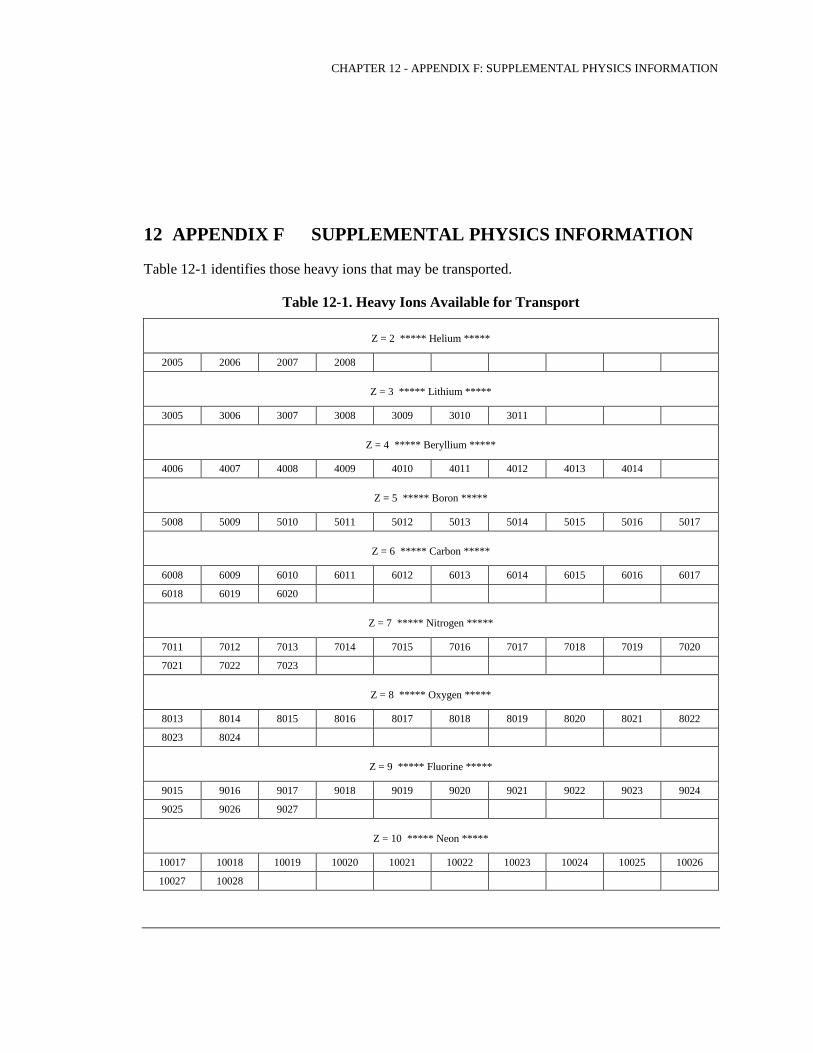
CHAPTER 12 - APPENDIX F: SUPPLEMENTAL PHYSICS INFORMATION
12 APPENDIX F SUPPLEMENTAL PHYSICS INFORMATION
Table 12-1 identifies those heavy ions that may be transported.
Table 12-1. Heavy Ions Available for Transport
Z = 2 ***** Helium *****
2005 2006 2007 2008
Z = 3 ***** Lithium *****
3005 3006 3007 3008 3009 3010 3011
Z = 4 ***** Beryllium *****
4006 4007 4008 4009 4010 4011 4012 4013 4014
Z = 5 ***** Boron *****
5008 5009 5010 5011 5012 5013 5014 5015 5016 5017
Z = 6 ***** Carbon *****
6008 6009 6010 6011 6012 6013 6014 6015 6016 6017
6018 6019 6020
Z = 7 ***** Nitrogen *****
7011 7012 7013 7014 7015 7016 7017 7018 7019 7020
7021 7022 7023
Z = 8 ***** Oxygen *****
8013 8014 8015 8016 8017 8018 8019 8020 8021 8022
8023 8024
Z = 9 ***** Fluorine *****
9015 9016 9017 9018 9019 9020 9021 9022 9023 9024
9025 9026 9027
Z = 10 ***** Neon *****
10017 10018 10019 10020 10021 10022 10023 10024 10025 10026
10027 10028
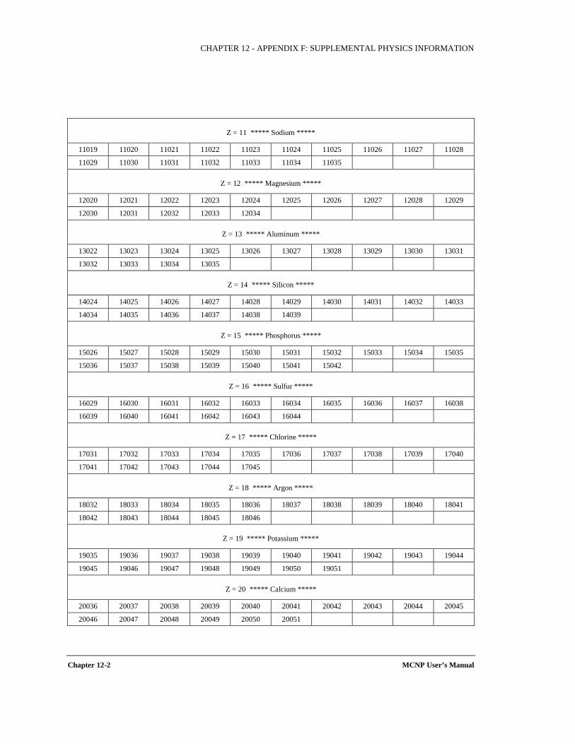
CHAPTER 12 - APPENDIX F: SUPPLEMENTAL PHYSICS INFORMATION
Chapter 12-2 MCNP User’s Manual
Z = 11 ***** Sodium *****
11019 11020 11021 11022 11023 11024 11025 11026 11027 11028
11029 11030 11031 11032 11033 11034 11035
Z = 12 ***** Magnesium *****
12020 12021 12022 12023 12024 12025 12026 12027 12028 12029
12030 12031 12032 12033 12034
Z = 13 ***** Aluminum *****
13022 13023 13024 13025 13026 13027 13028 13029 13030 13031
13032 13033 13034 13035
Z = 14 ***** Silicon *****
14024 14025 14026 14027 14028 14029 14030 14031 14032 14033
14034 14035 14036 14037 14038 14039
Z = 15 ***** Phosphorus *****
15026 15027 15028 15029 15030 15031 15032 15033 15034 15035
15036 15037 15038 15039 15040 15041 15042
Z = 16 ***** Sulfur *****
16029 16030 16031 16032 16033 16034 16035 16036 16037 16038
16039 16040 16041 16042 16043 16044
Z = 17 ***** Chlorine *****
17031 17032 17033 17034 17035 17036 17037 17038 17039 17040
17041 17042 17043 17044 17045
Z = 18 ***** Argon *****
18032 18033 18034 18035 18036 18037 18038 18039 18040 18041
18042 18043 18044 18045 18046
Z = 19 ***** Potassium *****
19035 19036 19037 19038 19039 19040 19041 19042 19043 19044
19045 19046 19047 19048 19049 19050 19051
Z = 20 ***** Calcium *****
20036 20037 20038 20039 20040 20041 20042 20043 20044 20045
20046 20047 20048 20049 20050 20051

CHAPTER 12 - APPENDIX F: SUPPLEMENTAL PHYSICS INFORMATION
Z = 21 ***** Scandium *****
21040 21041 21042 21043 21044 21045 21046 21047 21048 21049
21050 21051
Z = 22 ***** Titanium *****
22041 22042 22043 22044 22045 22046 22047 22048 22049 22050
22051 22052 22053 22054
Z = 23 ***** Vanadium *****
23044 23045 23046 23047 23048 23049 23050 23051 23052 23053
23054 23055 23056
Z = 24 ***** Chromium *****
24045 24046 24047 24048 24049 24050 24051 24052 24053 24054
24055 24056 24057 24058 24059
Z = 25 ***** Manganese *****
25049 25050 25051 25052 25053 25054 25055 25056 25057 25058
25059 25060 25061 25062
Z = 26 ***** Iron *****
26049 26050 26051 26052 26053 26054 26055 26056 26057 26058
26059 26060 26061 26062 26063 26064
Z = 27 ***** Cobalt *****
27053 27054 27055 27056 27057 27058 27059 27060 27061 27062
27063 27064
Z = 28 ***** Nickel *****
28053 28054 28055 28056 28057 28058 28059 28060 28061 28062
28063 28064 28065 28066 28067 28068
Z = 29 ***** Copper *****
29057 29058 29059 29060 29061 29062 29063 29064 29065 29066
29067 29068 29069 29070 29071 29072 29073
Z = 30 ***** Zinc *****
30057 30058 30059 30060 30061 30062 30063 30064 30065 30066
30067 30068 30069 30070 30071 30072 30073 30074 30075 30076
30077 30078
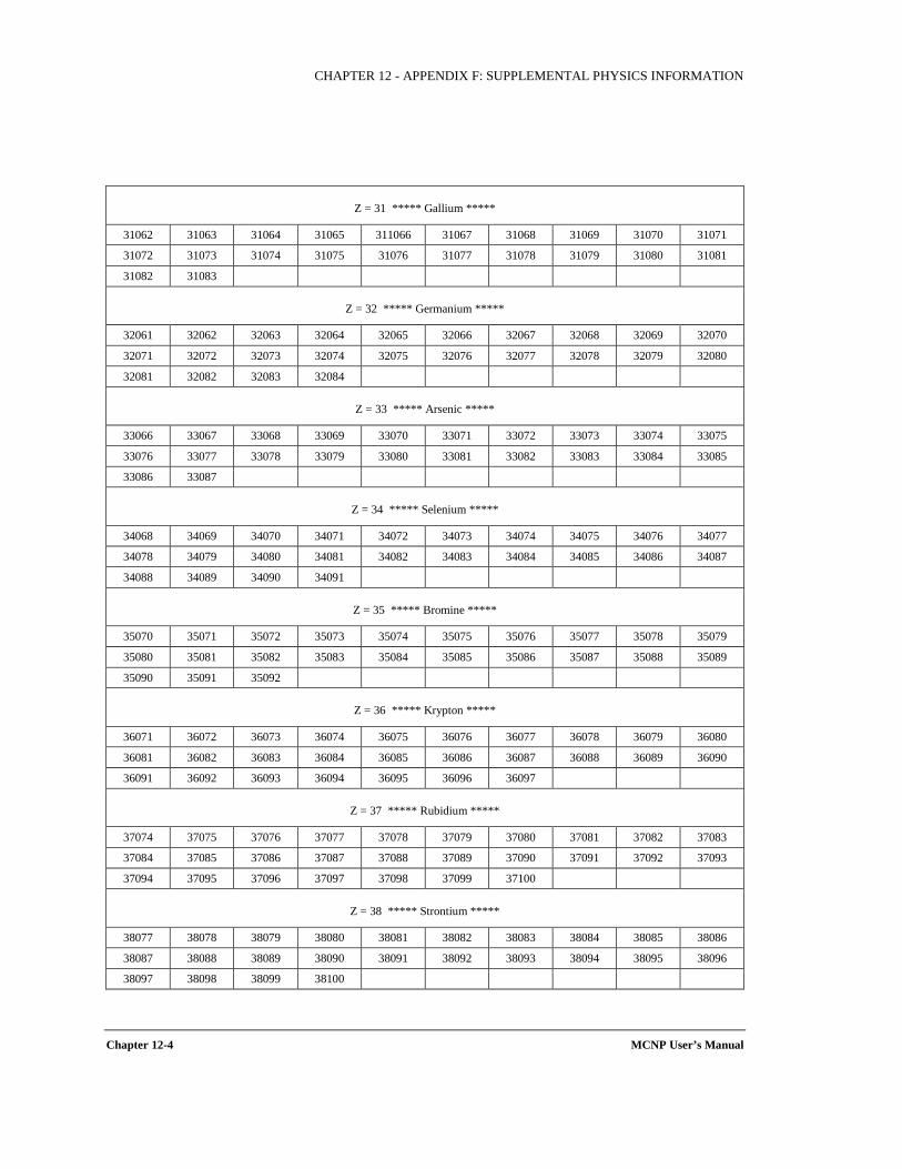
CHAPTER 12 - APPENDIX F: SUPPLEMENTAL PHYSICS INFORMATION
Chapter 12-4 MCNP User’s Manual
Z = 31 ***** Gallium *****
31062 31063 31064 31065 311066 31067 31068 31069 31070 31071
31072 31073 31074 31075 31076 31077 31078 31079 31080 31081
31082 31083
Z = 32 ***** Germanium *****
32061 32062 32063 32064 32065 32066 32067 32068 32069 32070
32071 32072 32073 32074 32075 32076 32077 32078 32079 32080
32081 32082 32083 32084
Z = 33 ***** Arsenic *****
33066 33067 33068 33069 33070 33071 33072 33073 33074 33075
33076 33077 33078 33079 33080 33081 33082 33083 33084 33085
33086 33087
Z = 34 ***** Selenium *****
34068 34069 34070 34071 34072 34073 34074 34075 34076 34077
34078 34079 34080 34081 34082 34083 34084 34085 34086 34087
34088 34089 34090 34091
Z = 35 ***** Bromine *****
35070 35071 35072 35073 35074 35075 35076 35077 35078 35079
35080 35081 35082 35083 35084 35085 35086 35087 35088 35089
35090 35091 35092
Z = 36 ***** Krypton *****
36071 36072 36073 36074 36075 36076 36077 36078 36079 36080
36081 36082 36083 36084 36085 36086 36087 36088 36089 36090
36091 36092 36093 36094 36095 36096 36097
Z = 37 ***** Rubidium *****
37074 37075 37076 37077 37078 37079 37080 37081 37082 37083
37084 37085 37086 37087 37088 37089 37090 37091 37092 37093
37094 37095 37096 37097 37098 37099 37100
Z = 38 ***** Strontium *****
38077 38078 38079 38080 38081 38082 38083 38084 38085 38086
38087 38088 38089 38090 38091 38092 38093 38094 38095 38096
38097 38098 38099 38100
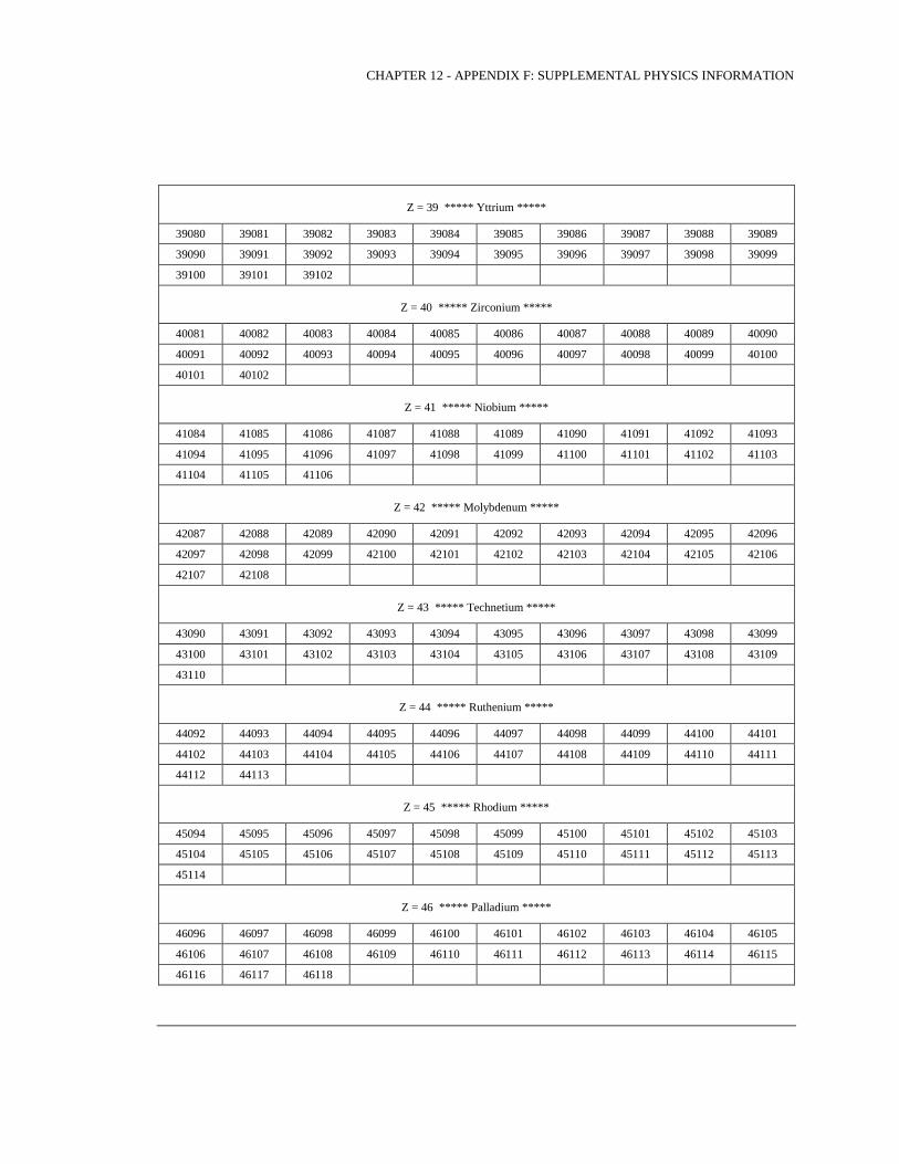
CHAPTER 12 - APPENDIX F: SUPPLEMENTAL PHYSICS INFORMATION
Z = 39 ***** Yttrium *****
39080 39081 39082 39083 39084 39085 39086 39087 39088 39089
39090 39091 39092 39093 39094 39095 39096 39097 39098 39099
39100 39101 39102
Z = 40 ***** Zirconium *****
40081 40082 40083 40084 40085 40086 40087 40088 40089 40090
40091 40092 40093 40094 40095 40096 40097 40098 40099 40100
40101 40102
Z = 41 ***** Niobium *****
41084 41085 41086 41087 41088 41089 41090 41091 41092 41093
41094 41095 41096 41097 41098 41099 41100 41101 41102 41103
41104 41105 41106
Z = 42 ***** Molybdenum *****
42087 42088 42089 42090 42091 42092 42093 42094 42095 42096
42097 42098 42099 42100 42101 42102 42103 42104 42105 42106
42107 42108
Z = 43 ***** Technetium *****
43090 43091 43092 43093 43094 43095 43096 43097 43098 43099
43100 43101 43102 43103 43104 43105 43106 43107 43108 43109
43110
Z = 44 ***** Ruthenium *****
44092 44093 44094 44095 44096 44097 44098 44099 44100 44101
44102 44103 44104 44105 44106 44107 44108 44109 44110 44111
44112 44113
Z = 45 ***** Rhodium *****
45094 45095 45096 45097 45098 45099 45100 45101 45102 45103
45104 45105 45106 45107 45108 45109 45110 45111 45112 45113
45114
Z = 46 ***** Palladium *****
46096 46097 46098 46099 46100 46101 46102 46103 46104 46105
46106 46107 46108 46109 46110 46111 46112 46113 46114 46115
46116 46117 46118
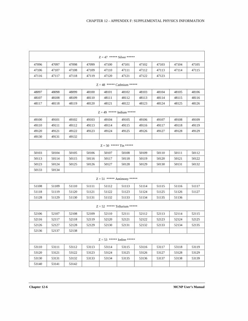
CHAPTER 12 - APPENDIX F: SUPPLEMENTAL PHYSICS INFORMATION
Chapter 12-6 MCNP User’s Manual
Z = 47 ***** Silver *****
47096 47097 47098 47099 47100 47101 47102 47103 47104 47105
47106 47107 47108 47109 47110 47111 47112 47113 47114 47115
47116 47117 47118 47119 47120 47121 47122 47123
Z = 48 ***** Cadmium *****
48097 48098 48099 48100 48101 48102 48103 48104 48105 48106
48107 48108 48109 48110 48111 48112 48113 48114 48115 48116
48117 48118 48119 48120 48121 48122 48123 48124 48125 48126
Z = 49 ***** Indium *****
49100 49101 49102 49103 49104 49105 49106 49107 49108 49109
49110 49111 49112 49113 49114 49115 49116 49117 49118 49119
49120 49121 49122 49123 49124 49125 49126 49127 49128 49129
49130 49131 49132
Z = 50 ***** Tin *****
50103 50104 50105 50106 50107 50108 50109 50110 50111 50112
50113 50114 50115 50116 50117 50118 50119 50120 50121 50122
50123 50124 50125 50126 50127 50128 50129 50130 50131 50132
50133 50134
Z = 51 ***** Antimony *****
51108 51109 51110 51111 51112 51113 51114 51115 51116 51117
51118 51119 51120 51121 51122 51123 51124 51125 51126 51127
51128 51129 51130 51131 51132 51133 51134 51135 51136
Z = 52 ***** Tellurium *****
52106 52107 52108 52109 52110 52111 52112 52113 52114 52115
52116 52117 52118 52119 52120 52121 52122 52123 52124 52125
52126 52127 52128 52129 52130 52131 52132 52133 52134 52135
52136 52137 52138
Z = 53 ***** Iodine *****
53110 53111 53112 53113 53114 53115 53116 53117 53118 53119
53120 53121 53122 53123 53124 53125 53126 53127 53128 53129
53130 53131 53132 53133 53134 53135 53136 53137 53138 53139
53140 53141 53142
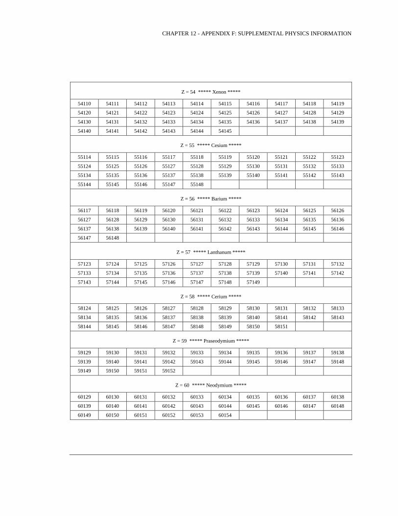
CHAPTER 12 - APPENDIX F: SUPPLEMENTAL PHYSICS INFORMATION
Z = 54 ***** Xenon *****
54110 54111 54112 54113 54114 54115 54116 54117 54118 54119
54120 54121 54122 54123 54124 54125 54126 54127 54128 54129
54130 54131 54132 54133 54134 54135 54136 54137 54138 54139
54140 54141 54142 54143 54144 54145
Z = 55 ***** Cesium *****
55114 55115 55116 55117 55118 55119 55120 55121 55122 55123
55124 55125 55126 55127 55128 55129 55130 55131 55132 55133
55134 55135 55136 55137 55138 55139 55140 55141 55142 55143
55144 55145 55146 55147 55148
Z = 56 ***** Barium *****
56117 56118 56119 56120 56121 56122 56123 56124 56125 56126
56127 56128 56129 56130 56131 56132 56133 56134 56135 56136
56137 56138 56139 56140 56141 56142 56143 56144 56145 56146
56147 56148
Z = 57 ***** Lanthanum *****
57123 57124 57125 57126 57127 57128 57129 57130 57131 57132
57133 57134 57135 57136 57137 57138 57139 57140 57141 57142
57143 57144 57145 57146 57147 57148 57149
Z = 58 ***** Cerium *****
58124 58125 58126 58127 58128 58129 58130 58131 58132 58133
58134 58135 58136 58137 58138 58139 58140 58141 58142 58143
58144 58145 58146 58147 58148 58149 58150 58151
Z = 59 ***** Praseodymium *****
59129 59130 59131 59132 59133 59134 59135 59136 59137 59138
59139 59140 59141 59142 59143 59144 59145 59146 59147 59148
59149 59150 59151 59152
Z = 60 ***** Neodymium *****
60129 60130 60131 60132 60133 60134 60135 60136 60137 60138
60139 60140 60141 60142 60143 60144 60145 60146 60147 60148
60149 60150 60151 60152 60153 60154
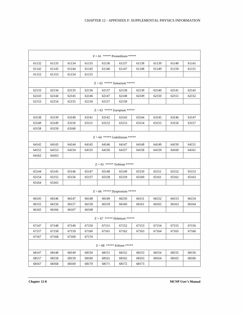
CHAPTER 12 - APPENDIX F: SUPPLEMENTAL PHYSICS INFORMATION
Chapter 12-8 MCNP User’s Manual
Z = 61 ***** Promethium *****
61132 61133 61134 61135 61136 61137 61138 61139 61140 61141
61142 61143 61144 61145 61146 61147 61148 61149 61150 61151
61152 61153 61154 61155
Z = 62 ***** Samarium *****
62133 62134 62135 62136 62137 62138 62139 62140 62141 62142
62143 62144 62145 62146 62147 62148 62149 62150 62151 62152
62153 62154 62155 62156 62157 62158
Z = 63 ***** Europium *****
63138 63139 63140 63141 63142 63143 63144 63145 63146 63147
63148 63149 63150 63151 63152 63153 63154 63155 63156 63157
63158 63159 63160
Z = 64 ***** Gadolinium *****
64142 64143 64144 64145 64146 64147 64148 64149 64150 64151
64152 64153 64154 64155 64156 64157 64158 64159 64160 64161
64162 64163
Z = 65 ***** Terbium *****
65144 65145 65146 65147 65148 65149 65150 65151 65152 65153
65154 65155 65156 65157 65158 65159 65160 65161 65162 65163
65164 65165
Z = 66 ***** Dysprosium *****
66145 66146 66147 66148 66149 66150 66151 66152 66153 66154
66155 66156 66157 66158 66159 66160 66161 66162 66163 66164
66165 66166 66167 66168
Z = 67 ***** Holmium *****
67147 67148 67149 67150 67151 67152 67153 67154 67155 67156
67157 67158 67159 67160 67161 67162 67163 67164 67165 67166
67167 67168 67169 67170
Z = 68 ***** Erbium *****
68147 68148 68149 68150 68151 68152 68153 68154 68155 68156
68157 68158 68159 68160 68161 68162 68163 68164 68165 68166
68167 68168 68169 68170 68171 68172 68173
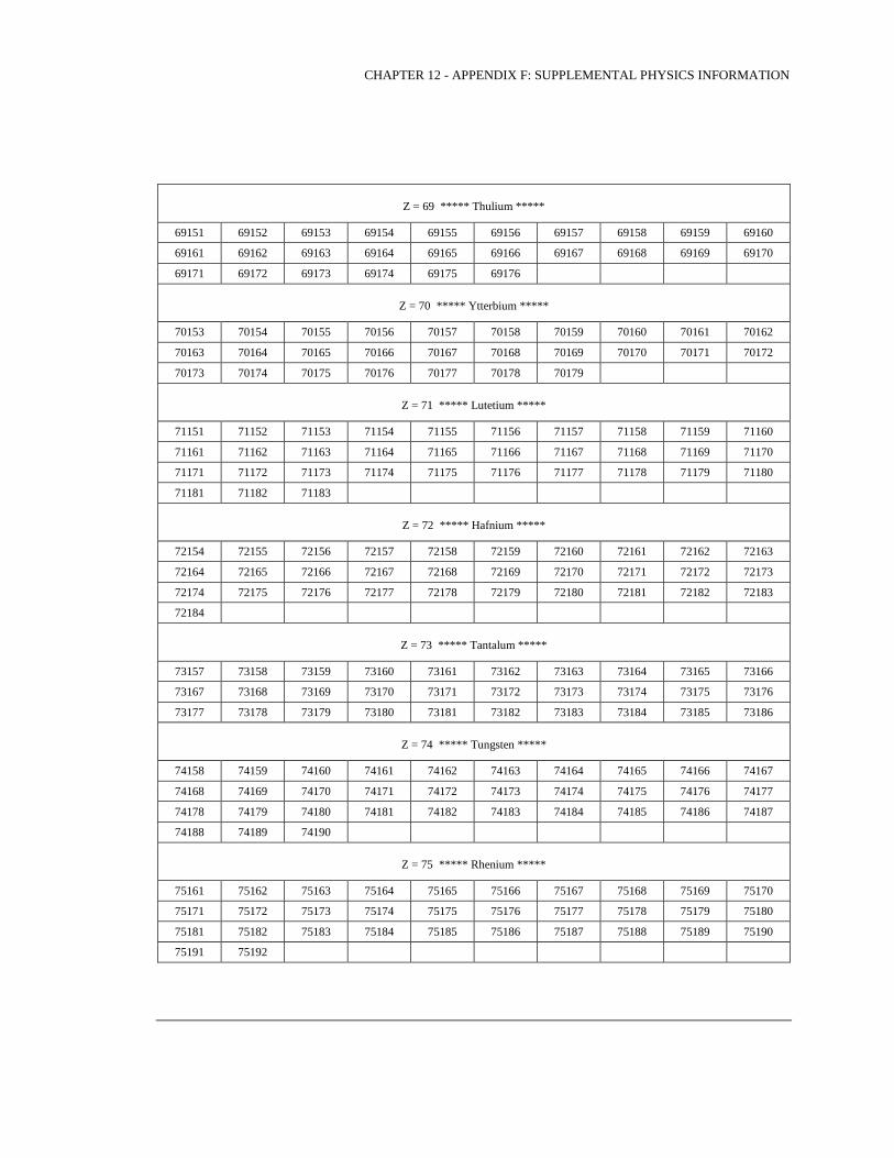
CHAPTER 12 - APPENDIX F: SUPPLEMENTAL PHYSICS INFORMATION
Z = 69 ***** Thulium *****
69151 69152 69153 69154 69155 69156 69157 69158 69159 69160
69161 69162 69163 69164 69165 69166 69167 69168 69169 69170
69171 69172 69173 69174 69175 69176
Z = 70 ***** Ytterbium *****
70153 70154 70155 70156 70157 70158 70159 70160 70161 70162
70163 70164 70165 70166 70167 70168 70169 70170 70171 70172
70173 70174 70175 70176 70177 70178 70179
Z = 71 ***** Lutetium *****
71151 71152 71153 71154 71155 71156 71157 71158 71159 71160
71161 71162 71163 71164 71165 71166 71167 71168 71169 71170
71171 71172 71173 71174 71175 71176 71177 71178 71179 71180
71181 71182 71183
Z = 72 ***** Hafnium *****
72154 72155 72156 72157 72158 72159 72160 72161 72162 72163
72164 72165 72166 72167 72168 72169 72170 72171 72172 72173
72174 72175 72176 72177 72178 72179 72180 72181 72182 72183
72184
Z = 73 ***** Tantalum *****
73157 73158 73159 73160 73161 73162 73163 73164 73165 73166
73167 73168 73169 73170 73171 73172 73173 73174 73175 73176
73177 73178 73179 73180 73181 73182 73183 73184 73185 73186
Z = 74 ***** Tungsten *****
74158 74159 74160 74161 74162 74163 74164 74165 74166 74167
74168 74169 74170 74171 74172 74173 74174 74175 74176 74177
74178 74179 74180 74181 74182 74183 74184 74185 74186 74187
74188 74189 74190
Z = 75 ***** Rhenium *****
75161 75162 75163 75164 75165 75166 75167 75168 75169 75170
75171 75172 75173 75174 75175 75176 75177 75178 75179 75180
75181 75182 75183 75184 75185 75186 75187 75188 75189 75190
75191 75192
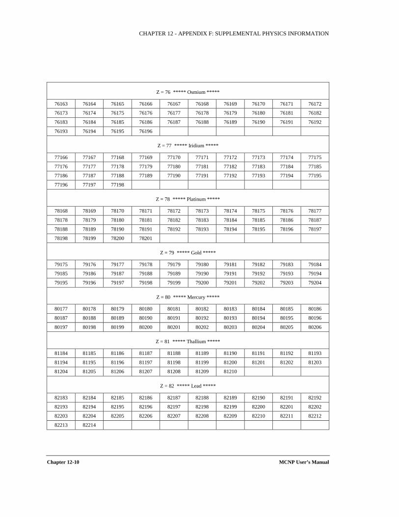
CHAPTER 12 - APPENDIX F: SUPPLEMENTAL PHYSICS INFORMATION
Chapter 12-10 MCNP User’s Manual
Z = 76 ***** Osmium *****
76163 76164 76165 76166 76167 76168 76169 76170 76171 76172
76173 76174 76175 76176 76177 76178 76179 76180 76181 76182
76183 76184 76185 76186 76187 76188 76189 76190 76191 76192
76193 76194 76195 76196
Z = 77 ***** Iridium *****
77166 77167 77168 77169 77170 77171 77172 77173 77174 77175
77176 77177 77178 77179 77180 77181 77182 77183 77184 77185
77186 77187 77188 77189 77190 77191 77192 77193 77194 77195
77196 77197 77198
Z = 78 ***** Platinum *****
78168 78169 78170 78171 78172 78173 78174 78175 78176 78177
78178 78179 78180 78181 78182 78183 78184 78185 78186 78187
78188 78189 78190 78191 78192 78193 78194 78195 78196 78197
78198 78199 78200 78201
Z = 79 ***** Gold *****
79175 79176 79177 79178 79179 79180 79181 79182 79183 79184
79185 79186 79187 79188 79189 79190 79191 79192 79193 79194
79195 79196 79197 79198 79199 79200 79201 79202 79203 79204
Z = 80 ***** Mercury *****
80177 80178 80179 80180 80181 80182 80183 80184 80185 80186
80187 80188 80189 80190 80191 80192 80193 80194 80195 80196
80197 80198 80199 80200 80201 80202 80203 80204 80205 80206
Z = 81 ***** Thallium *****
81184 81185 81186 81187 81188 81189 81190 81191 81192 81193
81194 81195 81196 81197 81198 81199 81200 81201 81202 81203
81204 81205 81206 81207 81208 81209 81210
Z = 82 ***** Lead *****
82183 82184 82185 82186 82187 82188 82189 82190 82191 82192
82193 82194 82195 82196 82197 82198 82199 82200 82201 82202
82203 82204 82205 82206 82207 82208 82209 82210 82211 82212
82213 82214
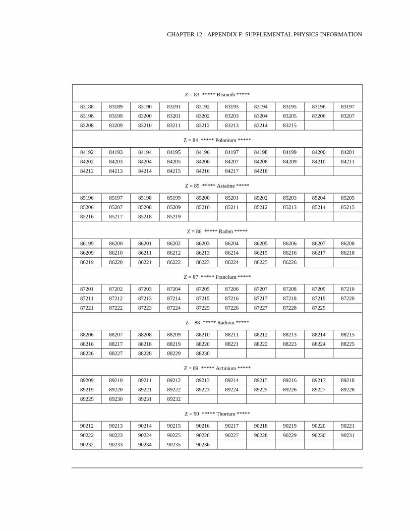
CHAPTER 12 - APPENDIX F: SUPPLEMENTAL PHYSICS INFORMATION
Z = 83 ***** Bismuth *****
83188 83189 83190 83191 83192 83193 83194 83195 83196 83197
83198 83199 83200 83201 83202 83203 83204 83205 83206 83207
83208 83209 83210 83211 83212 83213 83214 83215
Z = 84 ***** Polonium *****
84192 84193 84194 84195 84196 84197 84198 84199 84200 84201
84202 84203 84204 84205 84206 84207 84208 84209 84210 84211
84212 84213 84214 84215 84216 84217 84218
Z = 85 ***** Astatine *****
85196 85197 85198 85199 85200 85201 85202 85203 85204 85205
85206 85207 85208 85209 85210 85211 85212 85213 85214 85215
85216 85217 85218 85219
Z = 86 ***** Radon *****
86199 86200 86201 86202 86203 86204 86205 86206 86207 86208
86209 86210 86211 86212 86213 86214 86215 86216 86217 86218
86219 86220 86221 86222 86223 86224 86225 86226
Z = 87 ***** Francium *****
87201 87202 87203 87204 87205 87206 87207 87208 87209 87210
87211 87212 87213 87214 87215 87216 87217 87218 87219 87220
87221 87222 87223 87224 87225 87226 87227 87228 87229
Z = 88 ***** Radium *****
88206 88207 88208 88209 88210 88211 88212 88213 88214 88215
88216 88217 88218 88219 88220 88221 88222 88223 88224 88225
88226 88227 88228 88229 88230
Z = 89 ***** Actinium *****
89209 89210 89211 89212 89213 89214 89215 89216 89217 89218
89219 89220 89221 89222 89223 89224 89225 89226 89227 89228
89229 89230 89231 89232
Z = 90 ***** Thorium *****
90212 90213 90214 90215 90216 90217 90218 90219 90220 90221
90222 90223 90224 90225 90226 90227 90228 90229 90230 90231
90232 90233 90234 90235 90236
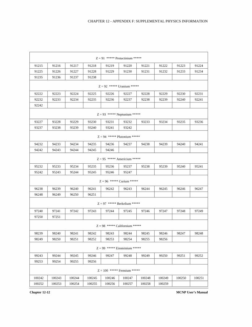
CHAPTER 12 - APPENDIX F: SUPPLEMENTAL PHYSICS INFORMATION
Chapter 12-12 MCNP User’s Manual
Z = 91 ***** Protactinium *****
91215 91216 91217 91218 91219 91220 91221 91222 91223 91224
91225 91226 91227 91228 91229 91230 91231 91232 91233 91234
91235 91236 91237 91238
Z = 92 ***** Uranium *****
92222 92223 92224 92225 92226 92227 92228 92229 92230 92231
92232 92233 92234 92235 92236 92237 92238 92239 92240 92241
92242
Z = 93 ***** Neptunium *****
93227 93228 93229 93230 93231 93232 93233 93234 93235 93236
93237 93238 93239 93240 93241 93242
Z = 94 ***** Plutonium *****
94232 94233 94234 94235 94236 94237 94238 94239 94240 94241
94242 94243 94244 94245 94246
Z = 95 ***** Americium *****
95232 95233 95234 95235 95236 95237 95238 95239 95240 95241
95242 95243 95244 95245 95246 95247
Z = 96 ***** Curium *****
96238 96239 96240 96241 96242 96243 96244 96245 96246 96247
96248 96249 96250 96251
Z = 97 ***** Berkelium *****
97240 97241 97242 97243 97244 97245 97246 97247 97248 97249
97250 97251
Z = 98 ***** Californium *****
98239 98240 98241 98242 98243 98244 98245 98246 98247 98248
98249 98250 98251 98252 98253 98254 98255 98256
Z = 99 ***** Einsteinium *****
99243 99244 99245 99246 99247 99248 99249 99250 99251 99252
99253 99254 99255 99256
Z = 100 ***** Fermium *****
100242 100243 100244 100245 100246 100247 100248 100249 100250 100251
100252 100253 100254 100255 100256 100257 100258 100259