MCMC Methods in Harmonic Models

Simon Godsill

Signal Processing Laboratory

Cambridge University Engineering Department

sjg@eng.cam.ac.uk

www-sigproc.eng.cam.ac.uk/~sjg

Overview MCMC Methods Metropolis-Hastings and Gibbs Samplers Design Considerations Case Study: Gabor Regression Models

MCMC Methods

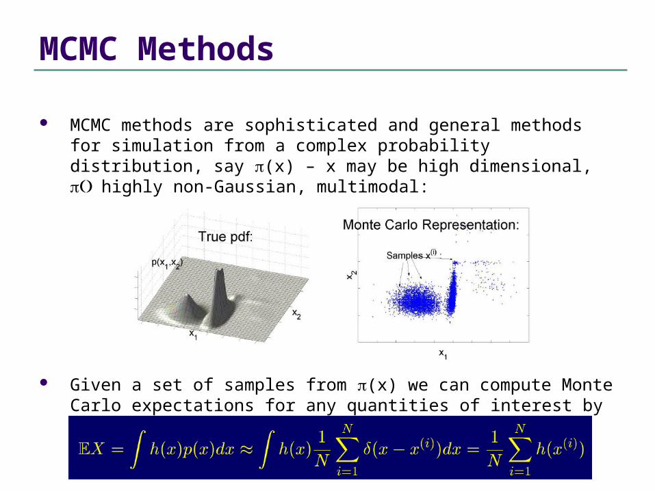
MCMC methods are sophisticated and general methods for simulation from a complex probability distribution, say (x) – x may be high dimensional, highly non-Gaussian, multimodal:

Given a set of samples from (x) we can compute Monte Carlo expectations for any quantities of interest by ergodic averages:

MCMC Contd.

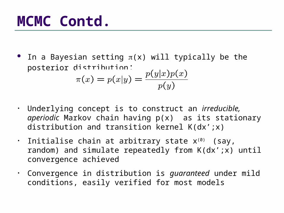
In a Bayesian setting (x) will typically be the posterior distribution:

• Underlying concept is to construct an irreducible, aperiodic Markov chain having p(x) as its stationary distribution and transition kernel K(dx’;x)

• Initialise chain at arbitrary state x(0) (say, random) and simulate repeatedly from K(dx’;x) until convergence achieved

• Convergence in distribution is guaranteed under mild conditions, easily verified for most models

MCMC, contd. Rates of convergence are hard to compute – lots of

theory, but not typically applicable in practice. However, many models, e.g. many harmonic modelling

cases, can be proven to have geometric convergence rates.

MCMC Algorithms

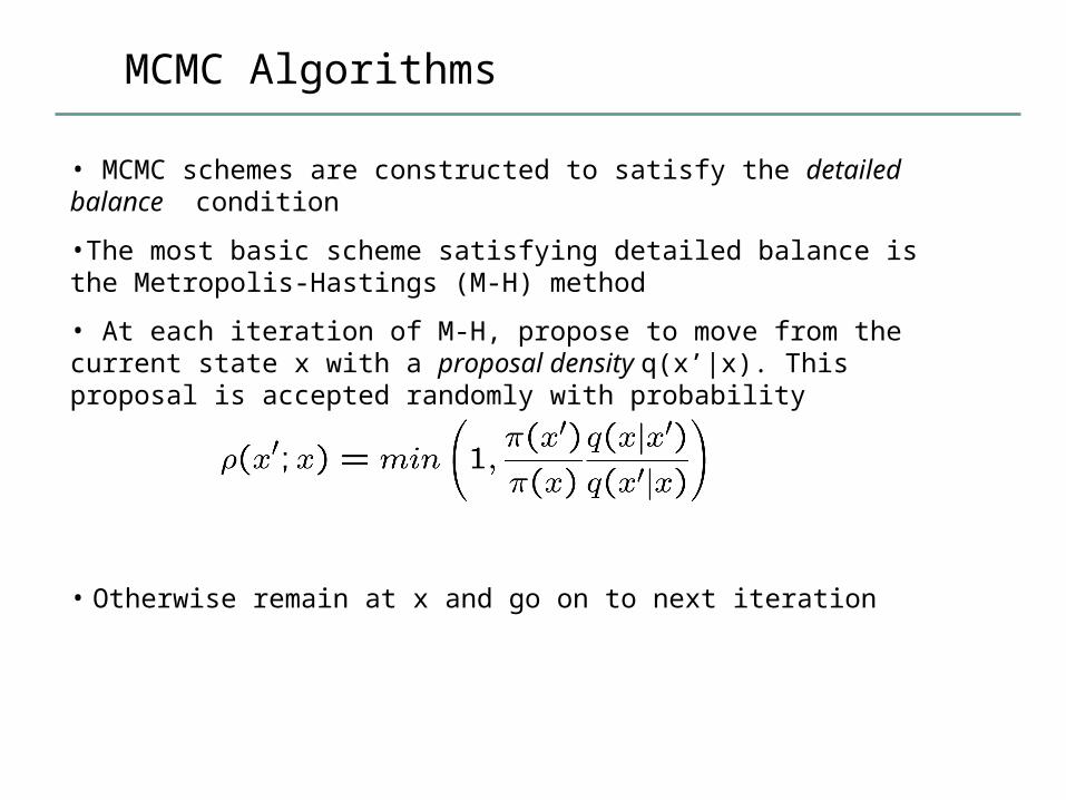
• MCMC schemes are constructed to satisfy the detailed balance condition

•The most basic scheme satisfying detailed balance is the Metropolis-Hastings (M-H) method

• At each iteration of M-H, propose to move from the current state x with a proposal density q(x’|x). This proposal is accepted randomly with probability

• Otherwise remain at x and go on to next iteration

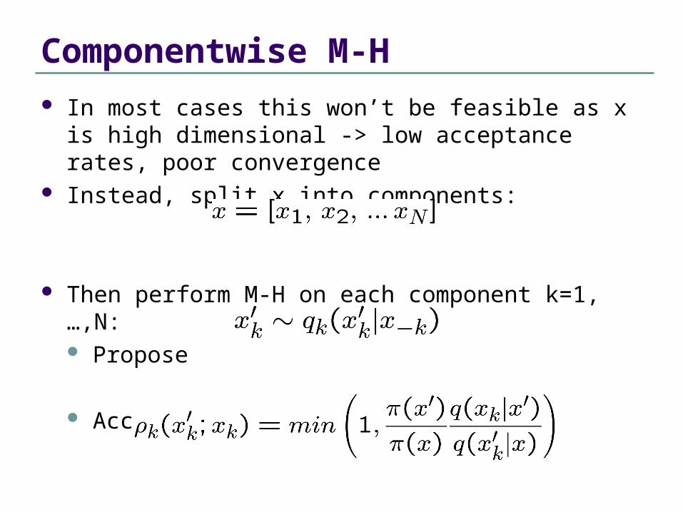
Componentwise M-H In most cases this won’t be feasible as x is high

dimensional -> low acceptance rates, poor convergence Instead, split x into components:

Then perform M-H on each component k=1,…,N: Propose

Accept with probability

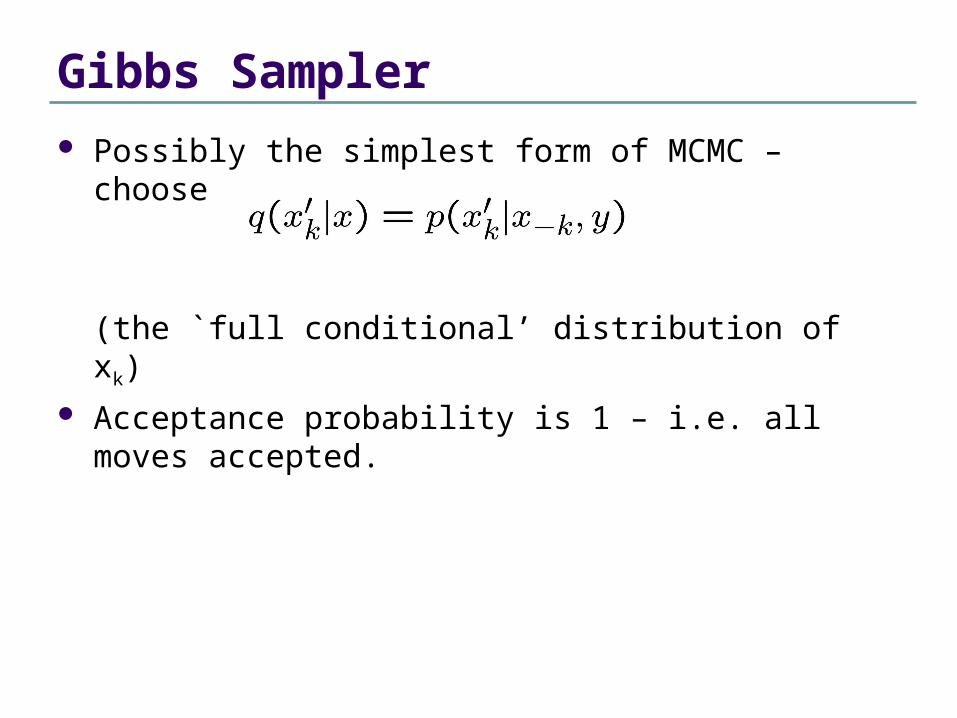
Gibbs Sampler Possibly the simplest form of MCMC – choose

(the `full conditional’ distribution of xk) Acceptance probability is 1 – i.e. all moves accepted.

Other types of MCMC Reversible Jump MCMC – extension of M-H to cases

where x can have varying dimension (e.g. in sparsity estimation) – see Green (1995) – Biometrika

Perfect simulation – special MCMC schemes that achieve exact samples from (x) – highly desirable, but slow and not yet practical for many cases

Design Issues and Recommendations

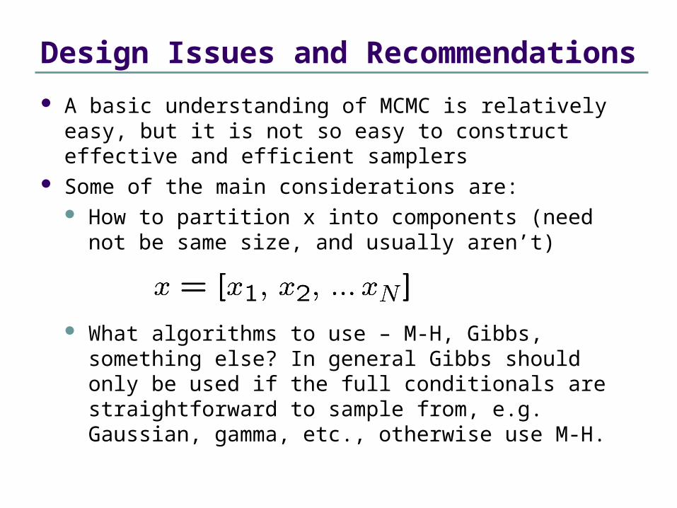
A basic understanding of MCMC is relatively easy, but it is not so easy to construct effective and efficient samplers

Some of the main considerations are: How to partition x into components (need not be same

size, and usually aren’t)

What algorithms to use – M-H, Gibbs, something else? In general Gibbs should only be used if the full conditionals are straightforward to sample from, e.g. Gaussian, gamma, etc., otherwise use M-H.

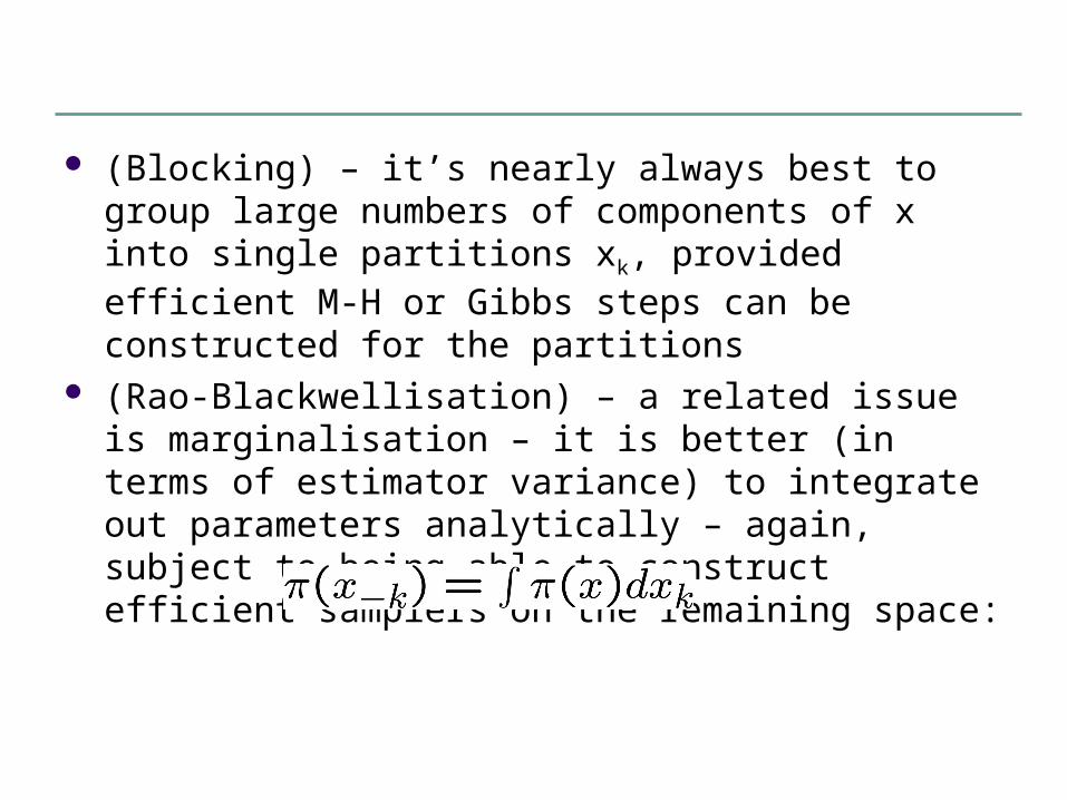
(Blocking) – it’s nearly always best to group large

numbers of components of x into single partitions xk, provided efficient M-H or Gibbs steps can be constructed for the partitions

(Rao-Blackwellisation) – a related issue is marginalisation – it is better (in terms of estimator variance) to integrate out parameters analytically – again, subject to being able to construct efficient samplers on the remaining space:

References for MCMC MCMC in Practice – Gilks et al – Chapman and Hall

(1996) Monte Carlo Statistical Methods – Robert and Casella –

Springer (1999)

MCMC Case study – Gabor Regression models

Now consider design of a sampler for harmonic models. Full details forthcoming as

Wolfe, Godsill and Ng (2004) - Bayesian variable selection and regularisation for time-frequency surface estimation – Journal of Royal Statistical Society (Series B – methodological)

(See also Wolfe and Godsill (NIPS 2002))

See http://www.eecs.harvard.edu/~patrick/research/

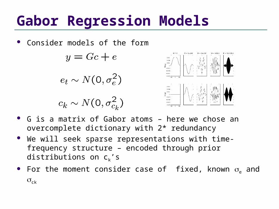
Gabor Regression Models Consider models of the form

G is a matrix of Gabor atoms – here we chose an overcomplete dictionary with 2* redundancy

We will seek sparse representations with time-frequency structure – encoded through prior distributions on ck’s

For the moment consider case of fixed, known e and ck

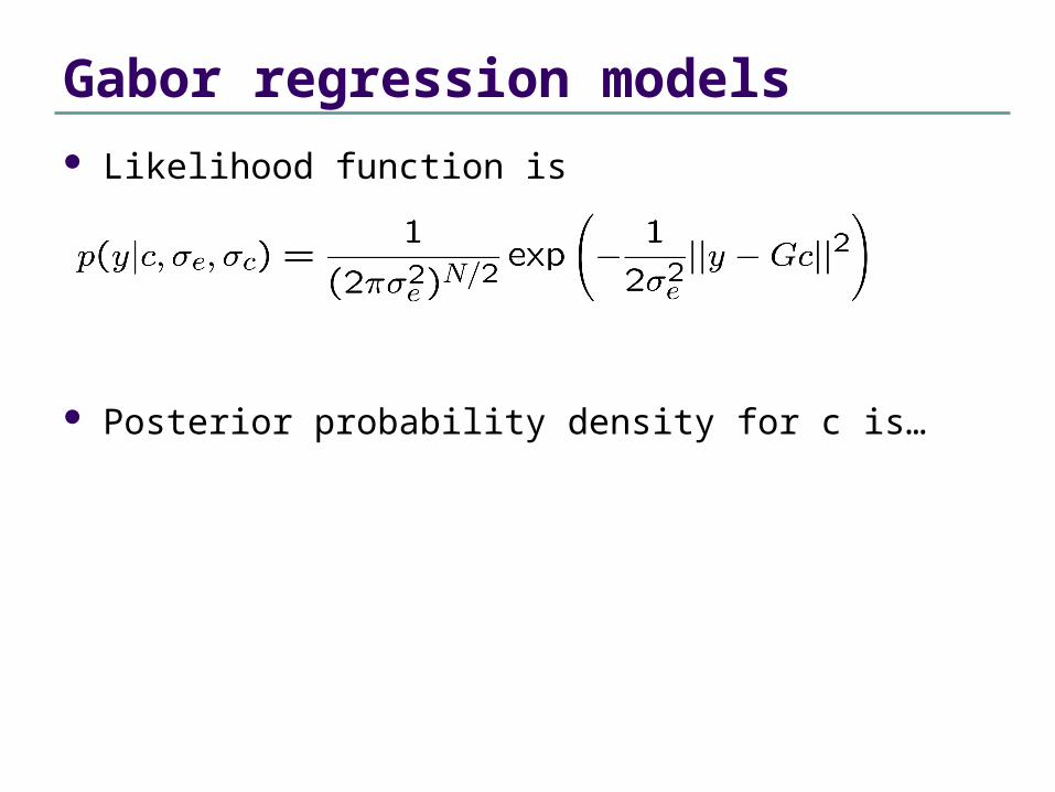
Gabor regression models Likelihood function is

Posterior probability density for c is…

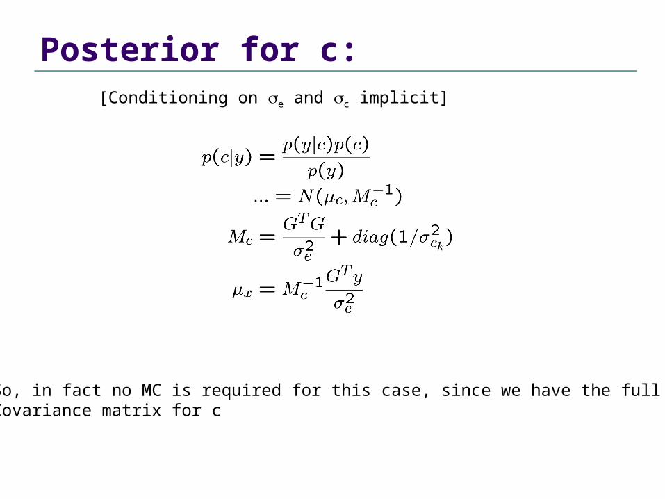
Posterior for c:

So, in fact no MC is required for this case, since we have the full mean andCovariance matrix for c

[Conditioning on e and c implicit]

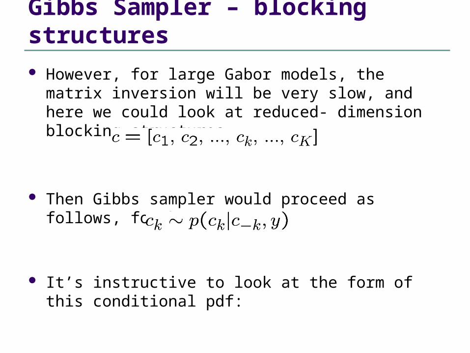
Gibbs Sampler – blocking structures However, for large Gabor models, the matrix inversion

will be very slow, and here we could look at reduced- dimension blocking structures

Then Gibbs sampler would proceed as follows, for k=1,…,K:

It’s instructive to look at the form of this conditional pdf:

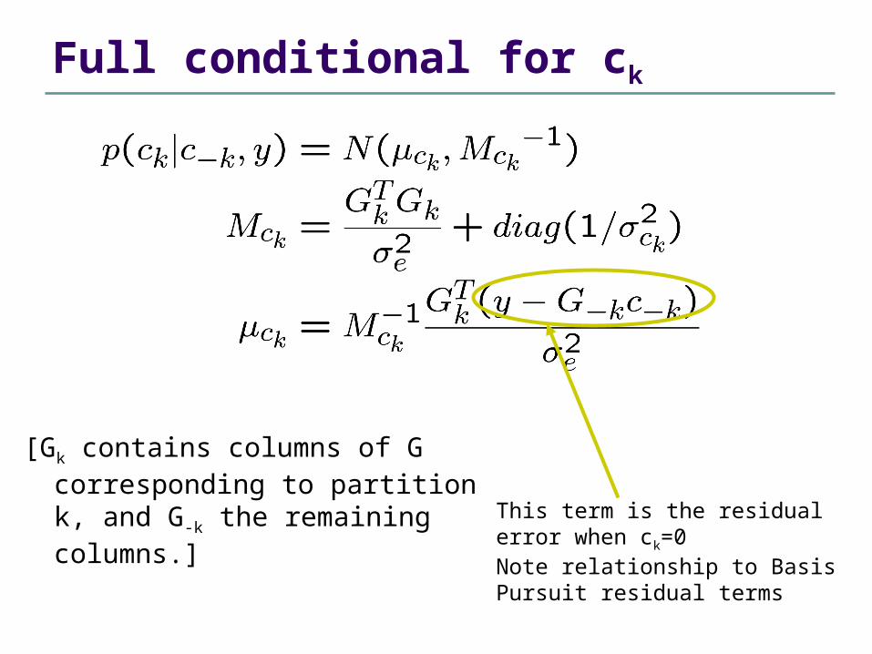
Full conditional for ck

[Gk contains columns of G corresponding to partition k, and G-k the remaining columns.] This term is the residual

error when ck=0 Note relationship to BasisPursuit residual terms

This form of Gibbs sampler can be very cheap computationally

The interest in this work is to extend the modelling capabilities provided by other algorithms – giving new forms of sparsity and structure. The extra steps are added in modular fashion, retaining the conditionally Gaussian structure of the coefficients and the efficient implementation

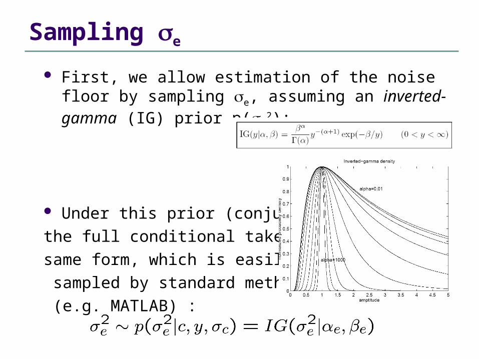
Sampling e

First, we allow estimation of the noise floor by sampling e, assuming an inverted-gamma (IG) prior p(e

2):

Under this prior (conjugate)

the full conditional takes the

same form, which is easily

sampled by standard methods

(e.g. MATLAB) :

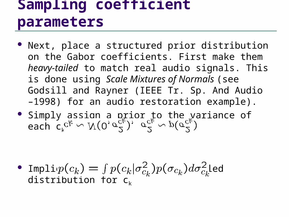
Sampling coefficient parameters Next, place a structured prior distribution on the Gabor

coefficients. First make them heavy-tailed to match real audio signals. This is done using Scale Mixtures of Normals (see Godsill and Rayner (IEEE Tr. Sp. And Audio –1998) for an audio restoration example).

Simply assign a prior to the variance of each ck:

Implies a non-Gaussian heavy-tailed distribution for ck

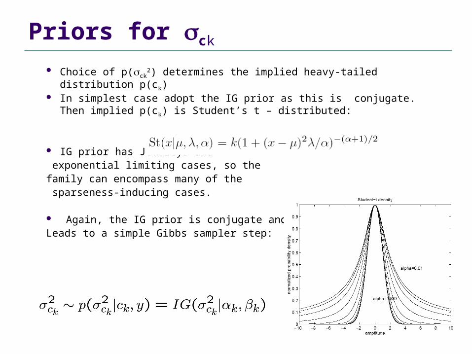
Priors for ck

Choice of p(ck2) determines the implied heavy-tailed distribution p(ck)

In simplest case adopt the IG prior as this is conjugate. Then implied p(ck) is Student’s t – distributed:

IG prior has Jeffreys and exponential limiting cases, so the family can encompass many of the sparseness-inducing cases.

Again, the IG prior is conjugate andLeads to a simple Gibbs sampler step:

Direct Sparsity Modelling

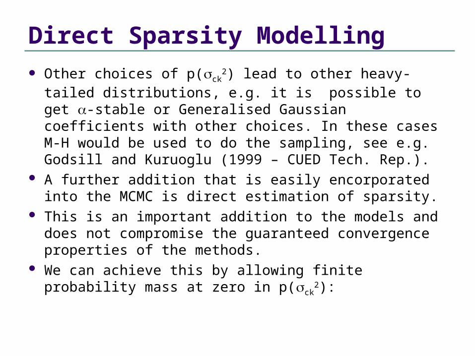
Other choices of p(ck2) lead to other heavy-tailed

distributions, e.g. it is possible to get -stable or Generalised Gaussian coefficients with other choices. In these cases M-H would be used to do the sampling, see e.g. Godsill and Kuruoglu (1999 – CUED Tech. Rep.).

A further addition that is easily encorporated into the MCMC is direct estimation of sparsity.

This is an important addition to the models and does not compromise the guaranteed convergence properties of the methods.

We can achieve this by allowing finite probability mass at zero in p(ck

2):

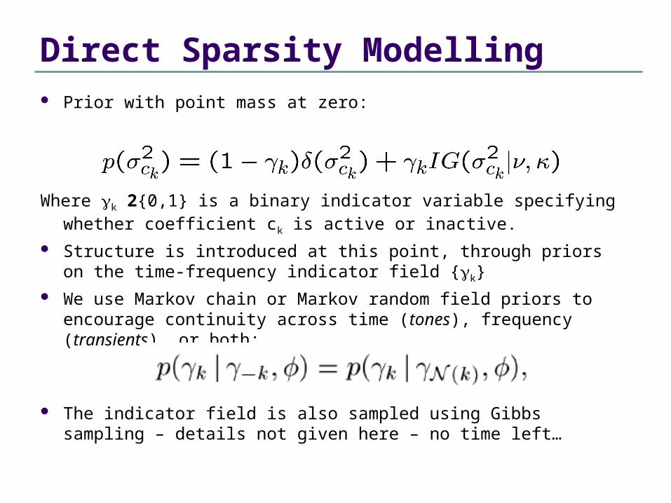
Direct Sparsity Modelling Prior with point mass at zero:

Where k 2{0,1} is a binary indicator variable specifying whether coefficient ck is active or inactive.

Structure is introduced at this point, through priors on the time-frequency indicator field {k}

We use Markov chain or Markov random field priors to encourage continuity across time (tones), frequency (transients), or both:

The indicator field is also sampled using Gibbs sampling – details not given here – no time left…

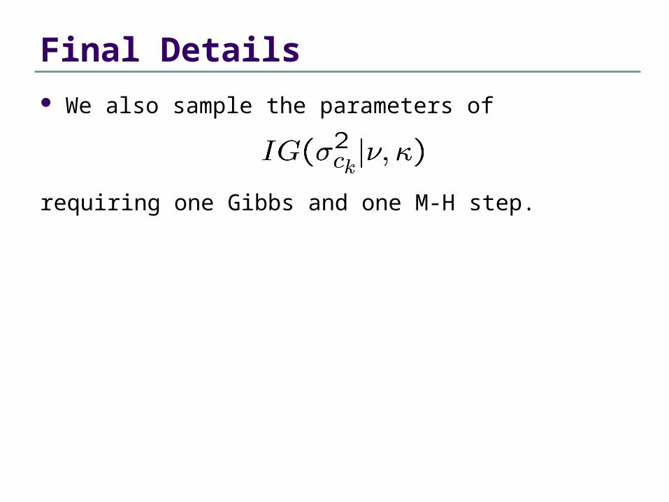
Final Details We also sample the parameters of

requiring one Gibbs and one M-H step.

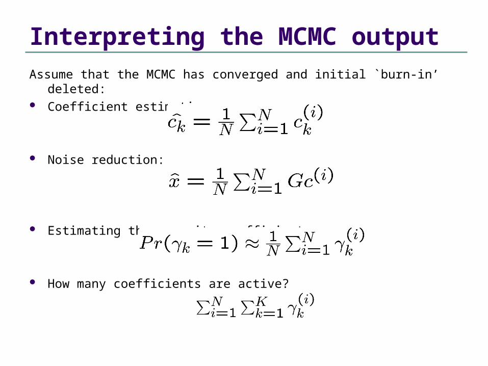
Interpreting the MCMC outputAssume that the MCMC has converged and initial `burn-in’ deleted: Coefficient estimation:

Noise reduction:

Estimating the sparsity coefficients:

How many coefficients are active?

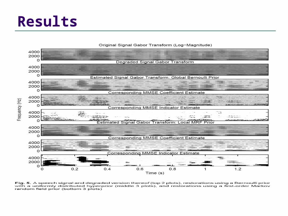
Results

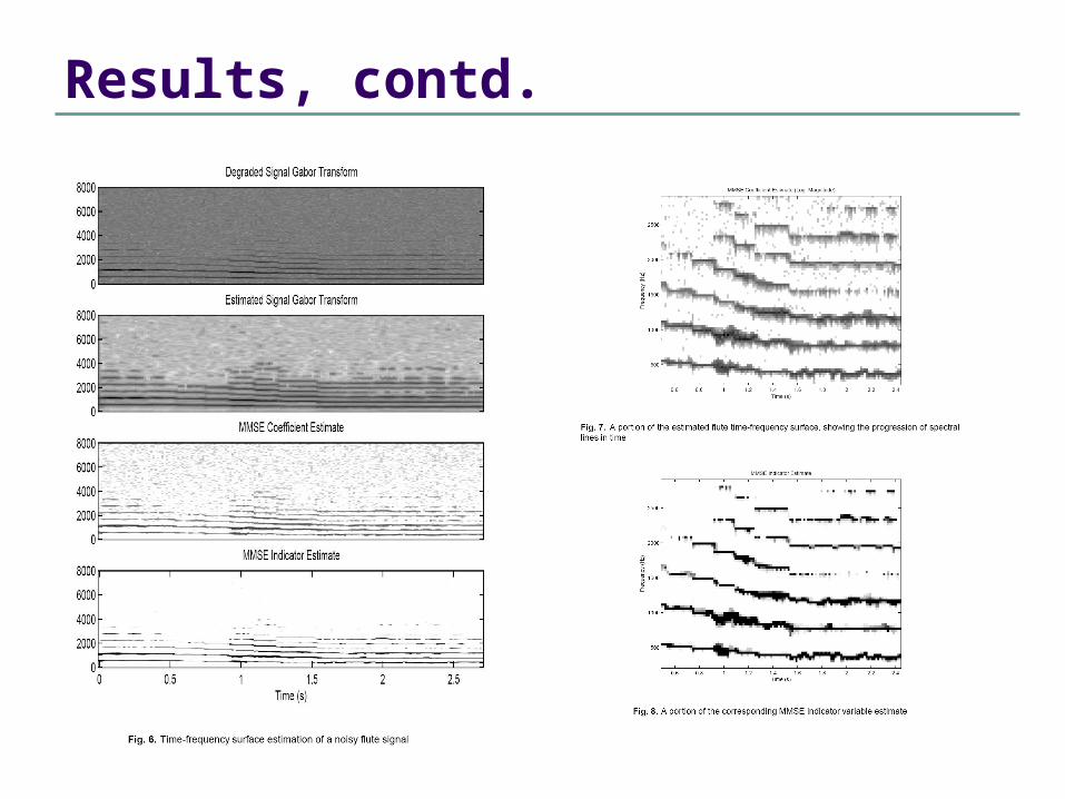
Results, contd.

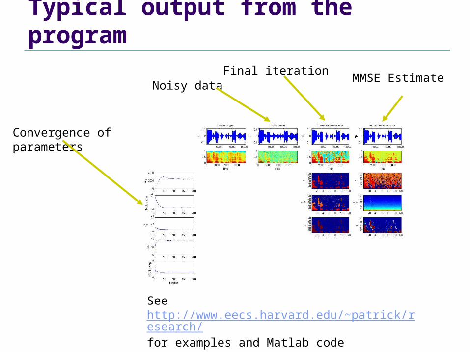
Typical output from the program

Convergence of parameters

Noisy dataFinal iteration

MMSE Estimate

See http://www.eecs.harvard.edu/~patrick/research/for examples and Matlab code

Conclusion Why use MCMC methods in harmonic models?

Extend the range of models computable Guaranteed convergence (in the limit) Computations can be quite cheap Code would contain same building blocks as EM,

IRLS or basis pursuit for similar models – easy to modify to MCMC for baseline comparison

It’s really not as complicated or slow as people think!! Why not use MCMC methods?

Can be computationally expensive Convergence diagnostics unreliable You may not want to explore new models

References C.P. Robert and G. Casella, Monte Carlo

StatisticalMethods, New York: Springer Verlag, 1999 W. R. Gilks and S. Richardson and D. J. Spiegelhalter,

Markov chain Monte Carlo in practice, London: Chapman and Hall, 1996

P. J. Green, Reversible Jump Markov-chain Monte Carlo computation and Bayesian model determination, Biometrika, 82(4), pp. 711-732, 1995

Harmonic models and MCMC – SJG references – see www-sigproc.eng.cam.ac.uk/~sjg

P. J. Wolfe, S. J. Godsill, and W.J. Ng. Bayesian variable selection and regularisation for time-frequency surface estimation Journal of the Royal Statistical Society, Series B, 2004. Read paper (with discussion). To Appear.

M.Davy and S. J. Godsill. Bayesian harmonic models for musical signal analysis (with discussion). In J.M. Bernardo, J.O. Berger, A.P. Dawid, and A.F.M. Smith, editors, Bayesian Statistics VII. Oxford University Press, 2003.

P. J. Wolfe and S. J. Godsill. Bayesian modelling of time-frequency coefficients for audio signal enhancement. In S. Becker, S. Thrun, and K. Obermayer, editors, Advances in Neural Information Processing Systems 15, Cambridge, MA. MIT Press, 2002. S. J. Godsill and P. J. W. Rayner.

Digital Audio Restoration: A Statistical Model-Based Approach. Berlin: Springer, ISBN 3 540 76222 1, September 1998.

S. J. Godsill and P. J. W. Rayner. Robust reconstruction and analysis of autoregressive signals in impulsive noise using the Gibbs sampler. IEEE Trans. on Speech and Audio Processing, 6(4):352-372, July 1998.

S. J. Godsill and E. E. Kuruoglu. Bayesian inference for time series with heavy-tailed symmetric alpha -stable noise processes. In Proc. Applications of heavy tailed distributions in economics, engineering and statistics, June 1999. Washington DC, USA. CUED Tech. Rep.