MCMC diagnostics for higher dimensions using Kullback ...vroy/Research/KLDiag.pdf · makes use of adaptive kernel ... 2017 18:12 Journal of Statistical Computation and Simulation

November 22, 2017 18:12 Journal of Statistical Computation and Simulation Dixit˙Roy˙MCMC˙diag

To appear in the Journal of Statistical Computation and SimulationVol. 00, No. 00, Month 20XX, 1–19

MCMC diagnostics for higher dimensions using Kullback Leibler

divergence

Anand Dixit and Vivekananda Roy

Department of Statistics, Iowa State University

(Received 00 Month 20XX; final version received 00 Month 20XX)

In the existing literature of MCMC diagnostics, we have identified two areas for improve-ment. Firstly, the density based diagnostic tools currently available in the literature are notequipped to assess the joint convergence of multiple variables. Secondly, in case of multi-modal target distribution if the MCMC sampler gets stuck in one of the modes, then thecurrent diagnostic tools may falsely detect convergence. The Tool 1 proposed in this articlemakes use of adaptive kernel density estimation, symmetric Kullback Leibler (KL) divergenceand a testing of hypothesis framework to assess the joint convergence of multiple variables.In cases where Tool 1 detects divergence of multiple chains, started at distinct initial values,we propose a visualization tool that can help to investigate reasons behind their divergence.The Tool 2 proposed in this article makes a novel use of the target distribution (known uptill the unknown normalizing constant), to detect divergence when an MCMC sampler getsstuck in one of the modes of a multi-modal target distribution. The usefulness of the toolsproposed in this article is illustrated using a multi-modal distribution, a mixture of bivariatenormal distribution and a Bayesian logit model example.

Keywords: Adaptive kernel density estimation; Convergence diagnostics; Kullback Leiblerdivergence; MCMC; Monte Carlo.

1. Introduction

The process of simulating observations from a fully specified distribution is generallycarried out using a traditional technique like inversion sampling. But if the distribu-tion is analytically intractable, then there may not be any efficient methods for directsimulations from it, and in such cases, one often relies on Markov Chain Monte Carlo(MCMC) sampling techniques. Specifically, in Bayesian analysis, we often come acrosssituations where the posterior distribution of parameters of interest is only known upto some unknown normalizing constant. In such situations, one often uses MCMC algo-rithms to produce approximate observations from the analytically intractable posteriordistributions to make inference about the parameters of interest.

MCMC samplers are iterative in nature and require a starting observation. If π(θ) isthe analytically intractable target distribution from which we wish to simulate observa-tions, then MCMC samplers like the Gibbs sampler and the Metropolis Hasting samplerconstruct a Markov chain {θn : n = 0, 1, 2, · · ·} started at θ0 such that the station-ary distribution of the chain is equal to π(θ). Thus, as n → ∞, the distribution of θnconverges to π(θ). In the Bayesian inference framework, the target distribution is theposterior distribution of the unknown parameters θ given the data y and is commonly

∗Corresponding author. Email: [email protected]


denoted as π(θ|y). Hence if the stationary distribution exists and is unique, then at somepoint the MCMC sampler will start producing approximate observations from the targetdistribution. Generally, deep mathematical analysis is needed to establish quantitativeconvergence bounds for determining the sample size (n) required for the Markov chain tobe sufficiently close to the target distribution (see e.g. Rosenthal [1], Jones and Hobert[2], Roy and Hobert [3]). In the absence of such theoretical analysis, often empirical di-agnostic tools are used to check the convergence of MCMC samplers.

In the early 90’s there was an interesting debate on whether one should use multiplechains or a single long chain to diagnose convergence. Gelman and Rubin [4] and Brooksand Gelman [5] advocated the usage of multiple chains, while Raftery and Lewis [6] andGeweke [7] believed a single long chain is sufficient for assessing convergence. Gelmanand Rubin [4] used the potential scale reduction factor (PSRF) to monitor convergencein the univariate case. Suppose we are working with m chains and each chain has niterations. Let {θij : i = 1, 2, · · ·,m and j = 1, 2, · · ·, n} be the observations generated

from the m chains. Then the PSRF, denoted by R̂ is defined as,

R̂ =V̂

W, (1)

whereV̂ = ((n− 1)/n)W + (1 + (1/m))(B/n) is the pooled variance estimate,

B/n =m∑i=1

(θ̄i· − θ̄··)2/(m− 1) is the between chain variance estimate,

W =m∑i=1

n∑j=1

(θij − θ̄i·)2/(m(n− 1)) is the within chain variance estimate and

θ̄i· and θ̄·· are the ith chain mean and the overall mean respectively where i = 1, 2, · · ·,m.Brooks and Gelman [5] came up with the multivariate PSRF (MPSRF) to diagnose

convergence in the multivariate case. It is denoted by R̂p and is given by,

R̂p = maxa

aT V̂ ∗a

aTW ∗a=n− 1

n+

(1 +

1

m

)λ1, (2)

where V̂ ∗ is the pooled covariance matrix, W ∗ is the within chain covariance matrix, B∗

is the between chain covariance matrix and λ1 is the largest eigenvalue of the matrix(W ∗−1B∗)/n. In this diagnostic tool, convergence is detected when R̂ ≈ 1 in the univari-

ate case and R̂p ≈ 1 in the multivariate case. Raftery and Lewis [6] proposed a univariatediagnostic tool based on the specified level of accuracy desired by the user in quantileestimation. In this tool, the chain obtained from the sampler is used to find the numberof initial iterations that should be discarded (burn-in period), how long the chain shouldbe run after the burn-in and how should the chain be thinned in order to obtain thedesired level of accuracy in quantile estimation. Geweke [7] also proposed a univariatediagnostic tool in which he used a test statistic, to compare the mean of a function ofthe samples from two non overlapping parts of the chain. Usually, the choice is the first10% of the chain and the last 50% of the chain. Thus, Gelman and Rubin [4], Brooksand Gelman [5], Raftery and Lewis [6] and Geweke [7] are all moment based diagnostictools.

More recently, researchers have come up with density based diagnostic tools. Boone etal. [8] and Hjorth and Vadeby [9] used divergence measures to come up with univariate

2


diagnostic tools. Boone et al. [8] estimated the Hellinger distance between the kernel den-sity estimates of two chains or two parts of a single chain. If the estimated distance wasclose to zero (i.e. less than 0.10), then the Markov chains were said to have convergedelse not. Hjorth and Vadeby [9] used a measure imitating KL divergence to comparethe empirical distributions of subsequences of chains to the empirical distribution of thewhole chain, and in the case of multiple chains, they compared empirical distribution ofindividual chains to the empirical distribution of the combination of all chains.

The density based diagnostic tools mentioned before are univariate tools and cannotassess the convergence of multiple variables jointly. The Tool 1 proposed in this article,computes the adaptive kernel density estimate of the joint distribution of each multivari-ate chain, and then compares the estimated symmetric KL divergence between them to acut-off value, to assess convergence. Since the adaptive kernel density estimation suffersfrom the curse of dimensionality, for higher dimensions, Tool 1 monitors convergencemarginally i.e. one variable at a time, and since we determine the cut-off values for KLdivergence measure using a testing of hypothesis framework, they can be easily adjustedfor multiple comparison. Thus, Tool 1 is a density based diagnostic tool that can assessconvergence of multiple variables jointly. Other notable differences between Tool 1 andthe density based diagnostic tools mentioned before are, Boone et al. [8] used numericalintegration to compute the estimated Hellinger distance and Hjorth and Vadeby [9] com-pute differences between empirical distribution functions over a partition of the real line,while we provide a Monte Carlo estimate of the symmetric KL divergence to comparethe adaptive kernel density estimates of multiple chains.

If the target distribution is multi-modal, then the MCMC chain might get stuck in oneof the modes. In such cases, even if the MCMC sampler is run for a reasonably long time,it continues to produce observations around that mode. Many of the current diagnostictools only make use of the iterations obtained from the MCMC samplers to diagnoseconvergence, and so, in cases where the chain gets stuck in one of the modes, they getfooled into thinking that the target distribution is unimodal, and hence, falsely detectconvergence. Most of the times, we do not know a priori how many modes the targetdistribution has, and hence, even if we use multiple chains, there is a chance that allchains might be stuck at the same mode. In order to overcome this difficulty, we proposeTool 2 that makes a novel use of the target distribution known up till the unknown nor-malizing constant in the diagnostic tool. Yu [10] proposed a tool which also incorporatesthe target distribution, in which she estimated the unknown normalizing constant usingthe MCMC samples, and then estimated the L1 distance between the kernel densityestimate of the chain and the estimated target distribution over a compact set, wherethe difference between the two was most likely. But if the MCMC sampler is stuck ina particular mode, then the normalizing constant estimator proposed by Yu [10] is nolonger reliable.

Many other diagnostic tools are available in the literature, and a very nice review ofthem can be found in Brooks and Roberts [11]. Our tools can be used when either a singlechain or multiple chain samplers are available. This article is structured as follows. InSection 2, we provide definition and certain properties of KL divergence. In Section 3, wepropose two new MCMC convergence diagnostic tools and a visualization tool. In Section4, we provide three examples to illustrate the usefulness of the proposed diagnostic andvisualization tools. Some concluding remarks are given in Section 5.

3


2. Kullback Leibler Divergence

KL divergence is a measure used to calculate the difference between two probabilitydistributions. If P (θ) and Q(θ) are any two probability density functions on Θ ⊆ Rd,then the KL divergence between P (θ) and Q(θ) is defined as,

KL(P |Q) =

∫Θ

log

(P (θ)

Q(θ)

)P (θ)dθ. (3)

Some important properties of the KL Divergence are as follows,

• KL(P |Q) ≥ 0,• KL(P |Q) = 0 iff P = Q almost everywhere wrt the Lebesgue measure, and• KL divergence is not symmetric in P and Q.

The KL divergence is not symmetric because KL(P |Q) is the expected difference betweenlog of densities P and Q with respect to P while KL(Q|P ) is the expected differencebetween log of densities Q and P with respect to Q. The symmetric KL divergencebetween P and Q, denoted by KLsy(P,Q) is given as,

KLsy(P,Q) =KL(P |Q) +KL(Q|P )

2. (4)

3. Diagnostic tools

3.1. Tool 1

Let π(θ) be the target distribution where θ ∈ Θ ⊆ Rd. In order to explore the targetdistribution, two chains are initiated at different starting points and each chain producesn observations. As prescribed in Gelman and Rubin [4], the starting points should be overdispersed with respect to the target distribution. Let {θij : i = 1, 2 and j = 1, 2, ..., n} bethe n observations obtained from each of the two chains where θij ∈ Θ ⊆ Rd ∀ i and ∀ j.The adaptive kernel density estimates of observations obtained from the two chains aredenoted by P1n(θ) and P2n(θ) and are found by substituting i = 1 and i = 2 respectivelyin the following equation,

Pin(θ) =1

n

n∑j=1

d∏k=1

1

h(k)j

K

(θ(k) − θ(k)

ij

h(k)j

), (5)

where,

θ(k)ij denotes the kth dimension in the jth observation of the ith chain, where i = 1, 2;j = 1, 2, · · ·, n and k = 1, 2, · · ·, d,θ(k) denotes the kth dimension of a d dimensional vector at which the adaptive kerneldensity estimate is evaluated,

{h(k)j : j = 1, 2, · · ·, n and k = 1, 2, · · ·, d} are smoothing parameters and

K(·) is a Gaussian kernel.In (5), the smoothing parameters are chosen using Silverman [12] (Sec 5.3.1) wherein

observations in sparse regions are assigned Gaussian kernels with high bandwidth andobservations in high probability regions are assigned Gaussian kernels with low band-

4


width. In our examples, we use the kepdf function in the R package pdfCluster (Azzaliniand Menardi [13]) to compute the adaptive kernel density estimate of the chains. The KLdivergence between P1n and P2n, denoted by KL(P1n|P2n) and KL divergence betweenP2n and P1n, denoted by KL(P2n|P1n) can be obtained after substituting appropriatevalues of i and j in the equation given below,

KL(Pin|Pjn) =

∫Θ

(log(Pin(θ)

)− log

(Pjn(θ)

))Pin(θ)dθ. (6)

The symmetric KL divergence between P1n and P2n, denoted by KLsy(P1n, P2n) is givenbelow,

KLsy(P1n, P2n) =KL(P1n|P2n) +KL(P2n|P1n)

2. (7)

We can find the Monte Carlo estimate of KL(P1n|P2n) and KL(P2n|P1n) using (8) and(9) respectively,

K̂L(P1n|P2n) =1

n

n∑i=1

{log(P1n(θ∗1i)

)− log

(P2n(θ∗1i)

)}, (8)

where {θ∗1i}ni=1 are the observations simulated from P1n(θ) using the technique proposedby Silverman [12](Sec 6.4.1). Similarly,

K̂L(P2n|P1n) =1

n

n∑i=1

{log(P2n(θ∗2i)

)− log

(P1n(θ∗2i)

)}, (9)

where {θ∗2i}ni=1 are the observations simulated from P2n(θ) using the technique proposedby Silverman [12](Sec 6.4.1). An estimate of KLsy(P1n, P2n) is then given below,

K̂Lsy(P1n, P2n) =K̂L(P1n|P2n) + K̂L(P2n|P1n)

2. (10)

Adaptive kernel density estimation suffers from the curse of dimensionality. Hence weneed to increase our sample size (n) as the dimension (d) increases in order to obtain agood estimate of the symmetric KL divergence between any two distributions.

In order to find the appropriate sample size (n) required for achieving convergencewhen univariate and bivariate chains are drawn from similar distributions, we conduct asimulation study. In the univariate case, for each n, we generate 1000 datasets each fromf1 ≡ N(0, 1) and f2 ≡ N(0, 1). Let f̂1 and f̂2 be the adaptive kernel density estimates ofobservations drawn from f1 and f2 respectively. The estimated symmetric KL divergencebetween f1 and f2 for each pair can be computed using (10) in which P1n and P2n are

replaced by f̂1 and f̂2. The true symmetric KL divergence between f1 and f2 is known tobe zero. Thus we can then find the bias, standard deviation and root mean square error

(RMSE) of K̂Lsy(f̂1, f̂2). In the bivariate case, for each n, we generate 1000 datasets eachfrom f3 ≡ N(0, I2) and f4 ≡ N(0, I2) and carry out a similar procedure as before to

find the bias, standard deviation and RMSE of K̂Lsy(f̂3, f̂4). The results are tabulatedin Table 1.

5


Table 1. Bias, Standard Deviation and RMSE of (a) K̂Lsy(f̂1, f̂2) where f̂1 and f̂2 are adaptive kernel density

estimates of observations drawn from f1 ≡ N(0, 1) and f2 ≡ N(0, 1) (b) K̂Lsy(f̂3, f̂4) where f̂3 and f̂4 are adaptive

kernel density estimates of observations drawn from f3 ≡ N(0, I2) and f4 ≡ N(0, I2).

(a) Univariate Distribution (b) Bivariate Distribution

n Bias SD RMSE n Bias SD RMSE

1000 0.0066 0.0041 0.0078 3000 0.0113 0.0029 0.01161500 0.0046 0.0026 0.0053 6000 0.0070 0.0016 0.00722000 0.0039 0.0021 0.0045 9000 0.0053 0.0011 0.00542500 0.0032 0.0018 0.0036 12000 0.0043 0.0009 0.00443000 0.0027 0.0015 0.0031 15000 0.0037 0.0007 0.0038

In Table 1 we observe that for both univariate and bivariate chains, the bias, standarddeviation and RMSE go on reducing as the sample size (n) increases. In order to assessthe convergence of Markov chains, we intend to accurately estimate the symmetric KLdivergence up till two decimal points. In Table 1, we observe that for n = 2000 in theunivariate case and for n = 12, 000 in the bivariate case, the bias, standard deviationand RMSE are significantly small, and hence, the symmetric KL divergence can beestimated efficiently up till two decimal points. Thus if we wish to use Tool 1 for assessingconvergence, we need to run the chains for at least 2000 iterations in the univariatecase and for at least 12,000 iterations in the bivariate case. We next check if the abovementioned sample sizes hold true, when instead of the Gaussian distribution the abovesimulation study is carried out using a heavy tailed distribution, skewed distribution ora distribution with dependent coordinates. For this purpose, the above simulation studywas repeated with t distribution (df=5), chi-square distribution (df=10) and bivariatenormal distribution (with correlation coefficient equal to 0.3). The sample sizes prescribedabove were found to be sufficient for efficiently estimating the symmetric KL divergenceup till two decimal points in these cases. The tabulated results are provided in thesupplementary material. Thus we can safely use the Gaussian distribution for studyingthe bias, standard deviation and RMSE associated with the symmetric KL divergenceestimator.

Tool 1 will detect convergence i.e. indicate that the chains have mixed adequately, whenthe estimated symmetric KL divergence between P1n and P2n will be close to zero. Hencewe now need to identify cut-off points, so that estimated symmetric KL divergence belowor equal to that point will indicate convergence. Boone et al. [8] carried out a simulationstudy and came up with a criteria, wherein if the estimated Hellinger distance betweenthe kernel density estimates of univariate chains is less than 0.10, then the Markov chainshave converged else not.

We will utilize a testing of hypothesis framework to come up with cut-off points. Inour framework, the null hypothesis states that the Markov chains have diverged, i.e.,the chains have not yet mixed adequately and our alternative hypothesis states that theMarkov chains have converged, i.e., the chains have mixed adequately. In this scenario,the probability of Type 1 error will be the probability of concluding that the Markovchains have converged when in fact they have not. We would like to limit this probabilityto some level α which is typically chosen to be 0.05. As mentioned earlier, we will beestimating the symmetric KL divergence up till two decimal points, hence the cut-offvalue should also be reported up till the second decimal point. In order to find our cut-off values, we will first generate 1000 datasets each from two dissimilar distributions

6


and the maximum value of C for which P (K̂Lsy(P1n, P2n) ≤ C) ≤ α = 0.05, i.e. theprobability of Type 1 error is less than 0.05, will be our cut-off value.

In the univariate case, we will generate 1000 datasets with suitable sample size (n)each from f5 ≡ N(0, 1) and f6 ≡ N(µ, 1) where µ 6= 0. The adaptive kernel density

estimate of observations drawn from f5 and f6 are denoted by f̂5 and f̂6 respectively.

The maximum value of C for which P (K̂Lsy(f̂5, f̂6) ≤ C) ≤ α = 0.05 will be our cut-offvalue in the univariate case. In the bivariate case, we will generate 1000 datasets with asuitable sample size (n) each from f7 ≡ N(0, I2) and f8 ≡ N(µ12, I2) where µ 6= 0 andthen carry out a similar procedure as before to identify our cut-off value in the bivariatecase. By limiting the probability of Type 1 error, we are exercising control over variabilityof estimated symmetric KL divergence, but we need to make sure that its bias does notaffect the cut-off value adversely, and hence for this purpose, the suitable sample size (n)should be chosen in such a way that the bias is significantly small and does not affectthe first two decimal points of the estimated value. The µ can be chosen by the users asper their requirement. If the users are dealing with a very sensitive experiment, then thechoice of µ should be small otherwise µ can be chosen to be slightly bigger. For simulationstudies corresponding to identifying cut-off values using dissimilar distributions, Booneet al. [8] utilized N(0, 1) and N(0.2835, 1) since the true Hellinger distance between themis known to be 0.10. Hence a possible choice for µ can be 0.2835. For this choice of µ, as

mentioned before, the sample size (n) should be chosen based on the bias of K̂Lsy(f̂5, f̂6)

and K̂Lsy(f̂7, f̂8) for univariate and bivariate cases respectively.The symmetric KL divergence between any two univariate Gaussian distributions with

the same variance parameter, and any two multivariate Gaussian distributions with thesame covariance matrix can be computed analytically using (11) and (12),

KLsy(g1, g2) =(µ1 − µ2)2

2σ2, (11)

where g1 ≡ N(µ1, σ2) and g2 ≡ N(µ2, σ

2), µ1 ∈ R, µ2 ∈ R, and

KLsy(g3, g4) =1

2

{(µ4 − µ3)TΣ−1(µ4 − µ3)

}, (12)

where g3 ≡ N(µ3,Σ) and g4 ≡ N(µ4,Σ), µ3 ∈ Rd, µ4 ∈ Rd.Thus using (11) and (12), for µ = 0.2835, true symmetric KL divergence between f5

and f6 was found to be 0.04 and the true symmetric KL divergence between f7 andf8 was found to be 0.08. We then compute the bias, standard deviation and RMSE of

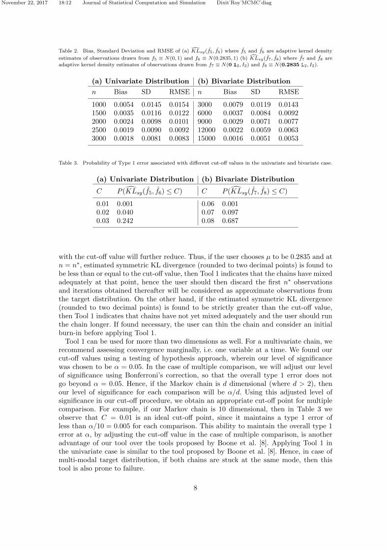
K̂Lsy(f̂5, f̂6) and K̂Lsy(f̂7, f̂8). The results are provided in Table 2.In Table 2 we observe that, for n = 2000 in the univariate case and n = 12, 000 in

the bivariate case, the bias associated with K̂Lsy(f̂5, f̂6) and K̂Lsy(f̂7, f̂8) is significantlysmall and does not affect the first two decimal points of the estimate. In Table 2 we alsoobserve that, the standard deviation and RMSE are also reasonably small for n = 2000and n = 12, 000 in the univariate and bivariate cases respectively. Hence we can carry outour cut-off procedure for µ = 0.2835 with n = 2000 in the univariate case and n = 12, 000in the bivariate case. The Type 1 error associated with different cut-off values is givenin Table 3.

In Table 3 we observe that C = 0.02 and C = 0.06 are ideal cut-off points for univariateand bivariate distributions respectively. The users should also be aware that if they choosea larger sample size than the one prescribed before, then the Type 1 error associated

7


Table 2. Bias, Standard Deviation and RMSE of (a) K̂Lsy(f̂5, f̂6) where f̂5 and f̂6 are adaptive kernel density

estimates of observations drawn from f5 ≡ N(0, 1) and f6 ≡ N(0.2835, 1) (b) K̂Lsy(f̂7, f̂8) where f̂7 and f̂8 are

adaptive kernel density estimates of observations drawn from f7 ≡ N(0 12, I2) and f8 ≡ N(0.2835 12, I2).


n Bias SD RMSE n Bias SD RMSE

1000 0.0054 0.0145 0.0154 3000 0.0079 0.0119 0.01431500 0.0035 0.0116 0.0122 6000 0.0037 0.0084 0.00922000 0.0024 0.0098 0.0101 9000 0.0029 0.0071 0.00772500 0.0019 0.0090 0.0092 12000 0.0022 0.0059 0.00633000 0.0018 0.0081 0.0083 15000 0.0016 0.0051 0.0053

Table 3. Probability of Type 1 error associated with different cut-off values in the univariate and bivariate case.


C P (K̂Lsy(f̂5, f̂6) ≤ C) C P (K̂Lsy(f̂7, f̂8) ≤ C)

0.01 0.001 0.06 0.0010.02 0.040 0.07 0.0970.03 0.242 0.08 0.687

with the cut-off value will further reduce. Thus, if the user chooses µ to be 0.2835 and atn = n∗, estimated symmetric KL divergence (rounded to two decimal points) is found tobe less than or equal to the cut-off value, then Tool 1 indicates that the chains have mixedadequately at that point, hence the user should then discard the first n∗ observationsand iterations obtained thereafter will be considered as approximate observations fromthe target distribution. On the other hand, if the estimated symmetric KL divergence(rounded to two decimal points) is found to be strictly greater than the cut-off value,then Tool 1 indicates that chains have not yet mixed adequately and the user should runthe chain longer. If found necessary, the user can thin the chain and consider an initialburn-in before applying Tool 1.

Tool 1 can be used for more than two dimensions as well. For a multivariate chain, werecommend assessing convergence marginally, i.e. one variable at a time. We found ourcut-off values using a testing of hypothesis approach, wherein our level of significancewas chosen to be α = 0.05. In the case of multiple comparison, we will adjust our levelof significance using Bonferroni’s correction, so that the overall type 1 error does notgo beyond α = 0.05. Hence, if the Markov chain is d dimensional (where d > 2), thenour level of significance for each comparison will be α/d. Using this adjusted level ofsignificance in our cut-off procedure, we obtain an appropriate cut-off point for multiplecomparison. For example, if our Markov chain is 10 dimensional, then in Table 3 weobserve that C = 0.01 is an ideal cut-off point, since it maintains a type 1 error ofless than α/10 = 0.005 for each comparison. This ability to maintain the overall type 1error at α, by adjusting the cut-off value in the case of multiple comparison, is anotheradvantage of our tool over the tools proposed by Boone et al. [8]. Applying Tool 1 inthe univariate case is similar to the tool proposed by Boone et al. [8]. Hence, in case ofmulti-modal target distribution, if both chains are stuck at the same mode, then thistool is also prone to failure.

8


In case of multiple chains, say m chains, we will find the estimated symmetric KLdivergence between each of the

(m2

)combination of chains and find the maximum among

them. If the maximum estimated symmetric KL divergence is less than or equal to thecut-off value, then Tool 1 indicates that the chains have converged else not. If the userwishes to use a single chain, then one can estimate the symmetric KL divergence betweenthe adaptive kernel density estimate of any two non overlapping parts of the chain.

In cases where the state space is bounded, adaptive kernel density estimation mightsuffer from boundary bias if high probability regions are closer to the boundary. But theobjective of Tool 1 is to check if the two chains have mixed adequately or not, hence,even if it is found that the adaptive kernel density estimate of the two chains suffers fromboundary bias, the final objective is not affected as long as the same density estimationprocedure is used for both chains. The user must also note that, if the sample simulatedfrom the adaptive kernel density estimate of the chain contain several observations fromoutside the state space, and if the target distribution is not expected to have a lot ofmass close to the boundary, then it is an indication that chains have not captured thetarget distribution adequately and thus Tool 1 indicates divergence in such a situation.

To implement Tool 1 for two univariate chains with n = 2, 000 and two bivariate chainswith n = 12, 000, it takes approximately 3.81s and 109.86s respectively on an Intel (R)Core (TM) i5-6300U 2.40GHz machine running Windows 10. For multivariate chains, weimplement Tool 1 marginally i.e. one variable at a time, which can be done in parallel.

3.2. Visualization Tool

Suppose a user is using multiple chains, say m chains (where m ≥ 3). Further supposethat application of Tool 1 revealed that the m chains have not mixed adequately and thuschains have not yet converged. This indication of divergence could be due to a variety ofreasons. A common reason for divergence is formation of clusters among multiple chains.A visualization tool can be helpful for identifying these clusters.

Peltonen et al. [14] had proposed a visualization tool based on Linear DiscriminantAnalysis and Discriminant Component Analysis which can be used to complement thediagnostic tools proposed by Gelman and Rubin [4] and Brooks and Gelman [5]. Simi-larly the visualization tool described in this section will complement Tool 1 proposed inSection 3.1.

In this tool we utilize the tile plot. As mentioned before, in case of multiple chains,say m chains, Tool 1 will find the estimated symmetric KL divergence between each ofthe

(m2

)combinations and report the maximum among them. In the visualization tool,

we will utilize the individual values provided by estimated symmetric KL divergence be-tween each of the

(m2

)distinct combinations. If the estimated symmetric KL divergence

for a particular combination is less than or equal to the cut-off value, then we will utilizea “Grey” tile to represent that the two chains belong to the same cluster else we will usea “black” tile to represent that the two chains belong to different clusters.

In the case of a multivariate chain, we monitor convergence marginally i.e. one variableat a time. Hence two multivariate chains will be considered to be in the same cluster, onlyif the estimated symmetric KL divergence for each variable is less than or equal to thecut-off value, which has been adjusted for multiple comparison. For further investigationof a multivariate Markov chain, the user can consider the following steps.

Consider a d dimensional Markov chain initialized at m different points. Suppose thesem chains (where m ≥ 3), were grouped into q clusters. The visualization tool is utilizedwhen Tool 1 indicates divergence i.e. 2 ≤ q ≤ m. In cases where Tool 1 indicates di-

9


12

34

2 3 4 5

Same Cluster

Different Cluster

Figure 1. Application of the visualization tool in which chain 1 and chain 3 are drawn from N(0, 1) while chain2, chain 4 and chain 5 are drawn from N(10, 1).

vergence, for further investigation, the user can choose a chain from each cluster andimplement the visualization tool marginally i.e. one variable at a time. This will help theuser identify, which among the d variables are responsible for inadequate mixing amongthe m multivariate chains.

In order to provide an illustration of the visualization tool, suppose we run 5 chains for5,000 iterations each wherein the 1st and the 3rd chain are drawn from N(0, 1) while the2nd, 4th and 5th chain are drawn from N(10, 1). The application of the visualization toolfor these five chains is provided in Figure 1. As expected, Figure 1 indicates presence oftwo clusters wherein chain 1 and chain 3 form a cluster while chain 2, chain 4 and chain5 form another cluster.

3.3. Tool 2

Suppose the target density is as follows,

π(θ) =g(θ)

k, θ ∈ Θ, (13)

where k is the unknown normalizing constant.Suppose a single Markov chain is run for n iterations and the observations obtained

are {θ1j}nj=1. Let P1n(θ) denote the adaptive kernel density estimate of the observationsas mentioned in (5). The KL divergence between P1n(θ) and π(θ) is given below,

KL(P1n|π) = Gn + log k, (14)

whereGn =

∫Θ

log(P1n(θ)

)P1n(θ)dθ −

∫Θ

log(g(θ)

)P1n(θ)dθ.

In the implementation of Tool 2, we will assume that KL(P1n|π)→ 0 as n→∞. Underthis assumption, Gn → −log(k) as n→∞. Hence exp(−Gn) → k as n→∞. Thus, anestimator of the normalizing constant based on KL divergence between P1n(θ) and π(θ),

denoted by k̂ is given below,

k̂ = exp

(− 1

n

n∑i=1

{log(P1n(θ∗1i)

)− log

(g(θ∗1i)

)}), (15)

10


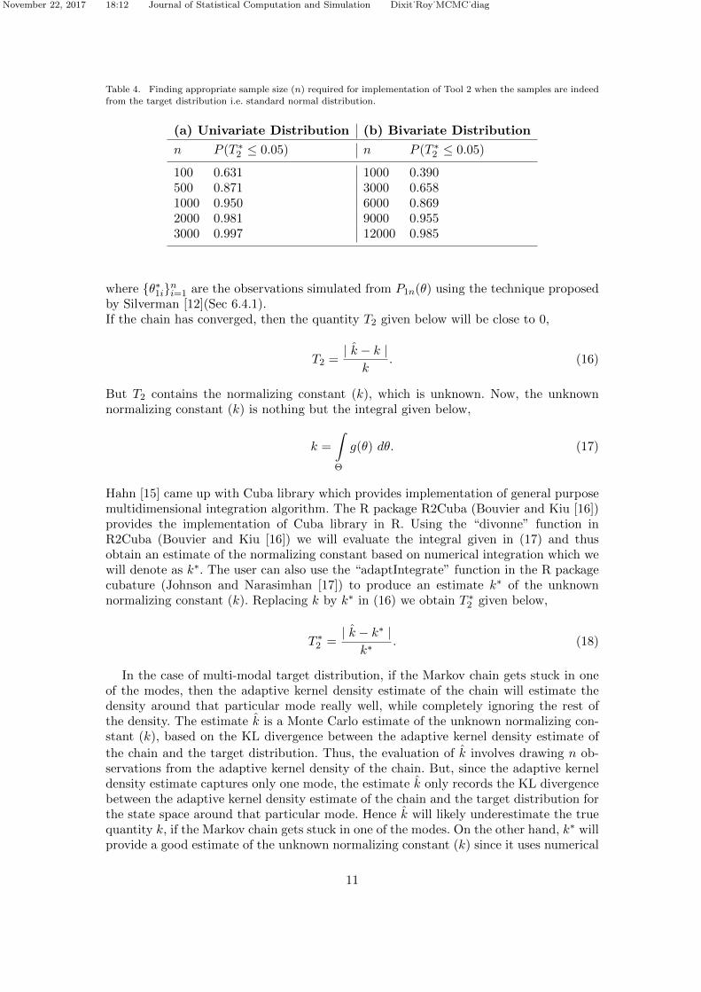
Table 4. Finding appropriate sample size (n) required for implementation of Tool 2 when the samples are indeedfrom the target distribution i.e. standard normal distribution.


n P (T ∗2 ≤ 0.05) n P (T ∗

2 ≤ 0.05)

100 0.631 1000 0.390500 0.871 3000 0.6581000 0.950 6000 0.8692000 0.981 9000 0.9553000 0.997 12000 0.985

where {θ∗1i}ni=1 are the observations simulated from P1n(θ) using the technique proposedby Silverman [12](Sec 6.4.1).If the chain has converged, then the quantity T2 given below will be close to 0,

T2 =| k̂ − k |

k. (16)

But T2 contains the normalizing constant (k), which is unknown. Now, the unknownnormalizing constant (k) is nothing but the integral given below,

k =

∫Θ

g(θ) dθ. (17)

Hahn [15] came up with Cuba library which provides implementation of general purposemultidimensional integration algorithm. The R package R2Cuba (Bouvier and Kiu [16])provides the implementation of Cuba library in R. Using the “divonne” function inR2Cuba (Bouvier and Kiu [16]) we will evaluate the integral given in (17) and thusobtain an estimate of the normalizing constant based on numerical integration which wewill denote as k∗. The user can also use the “adaptIntegrate” function in the R packagecubature (Johnson and Narasimhan [17]) to produce an estimate k∗ of the unknownnormalizing constant (k). Replacing k by k∗ in (16) we obtain T ∗

2 given below,

T ∗2 =

| k̂ − k∗ |k∗

. (18)

In the case of multi-modal target distribution, if the Markov chain gets stuck in oneof the modes, then the adaptive kernel density estimate of the chain will estimate thedensity around that particular mode really well, while completely ignoring the rest ofthe density. The estimate k̂ is a Monte Carlo estimate of the unknown normalizing con-stant (k), based on the KL divergence between the adaptive kernel density estimate of

the chain and the target distribution. Thus, the evaluation of k̂ involves drawing n ob-servations from the adaptive kernel density of the chain. But, since the adaptive kerneldensity estimate captures only one mode, the estimate k̂ only records the KL divergencebetween the adaptive kernel density estimate of the chain and the target distribution forthe state space around that particular mode. Hence k̂ will likely underestimate the truequantity k, if the Markov chain gets stuck in one of the modes. On the other hand, k∗ willprovide a good estimate of the unknown normalizing constant (k) since it uses numerical

11


integration to integrate over the entire state space. Thus T ∗2 can be interpreted as the

percentage of the target distribution not yet captured by the Markov chain. A Markovchain that captures at least 95% of the target distribution can be considered to be pro-ducing approximate observations from the target distribution. Using this interpretationof T ∗

2 , we came up with a cut-off value of 0.05 wherein if T ∗2 > 0.05, then Tool 2 indicates

that the Markov chain has not yet captured the target distribution adequately.As seen earlier, Tool 2 assumes (i) exp(−Gn) → k as n → ∞, (ii) k̂ is a consistent

Monte Carlo estimate of exp(−Gn) and (iii) k∗ is an estimate of k based on multidi-mensional numerical integration. Since (i) and (ii) depend on the sample size (n), it isimportant to know their convergence rates as a function of n. But currently in the litera-ture, a theoretical proof of the convergence of the adaptive kernel density estimate basedon a Markov chain to its stationary distribution, with respect to the KL divergence is notavailable. In the absence of such a theoretical result, it is difficult to find the convergencerates of (i) and (ii) as a function of n. Hence we conduct a simulation study to choose asuitable sample size (n). Since the cut-off value is based on the interpretation of T ∗

2 , wewill conduct a slightly different simulation study to get an intuition of the sample size (n)required to implement Tool 2. In the univariate case we will consider f1 ≡ N(0, 1) to beour target distribution, generate 1000 datasets of sample size (n) each from f1 ≡ N(0, 1)

and find k̂ using (15) while k∗ will be obtained by numerically integrating the kernel off1, thus we can then find T ∗

2 for each dataset using (18). Then we estimate P (T ∗2 ≤ 0.05)

i.e. probability of concluding convergence when the chain is indeed from the target distri-bution. The sample size (n) for which the estimate of P (T ∗

2 ≤ 0.05) is significantly high,will be our prescribed sample size (n) for Tool 2. In the bivariate case, similar procedureis carried out for f3 ≡ N(0, I2). The results are given in Table 4.

In Table 4 we observe that for n = 2000 in the univariate case and n = 12, 000 inthe bivariate case, the estimated probability of concluding that the Markov chain hasconverged, given the fact that it is indeed drawn from the target distribution is reallyhigh. This provides us an indication that n = 2000 and n = 12, 000 are sufficient forimplementing Tool 2 in univariate and bivariate distributions respectively. We also checkif the prescribed sample sizes are sufficient when the target distribution is heavy tailed,skewed or is a distribution with dependent coordinates and hence we replicated the abovestudy with t distribution (df=5), chi-square distribution (df=10) and bivariate normaldistribution (with correlation coefficient equal to 0.3). We observed that the sample sizesmentioned above are sufficient. The detailed results are provided in the supplementarymaterial.

Tool 2 is specifically designed for detecting divergence when the target distribution ismulti-modal and the chain gets stuck in one of the modes. Thus, if the user observes thateven after running the chain for a reasonably long time (sample size prescribed above),the value of T ∗

2 was found to be greater than 0.05, then it is highly likely that the chainis stuck in one of the modes and has not yet traveled through the whole state space.The value of T ∗

2 will also tell the user the percentage of the target distribution not yettraveled by the Markov chain.

Tool 2 involves the target distribution, hence if the target distribution is bounded andhas a lot of mass close to the boundary, then Tool 2 will be affected by boundary bias.Due to boundary bias, the sample generated from the adaptive kernel density estimatormight contain observations from outside the state space and log of the target distributionwithout the unknown normalizing constant (i.e. log(g(θ))) is not defined at these points.A possible solution to this situation is to consider a bootstrap sample instead of samplingfrom the adaptive kernel density estimate. Also, in the case where the bounded targetdistribution has very little mass close to the boundary and the sample generated from

12


the adaptive kernel density estimate contains none or negligible number of observationsfrom outside the state space, we can simply ignore those and implement Tool 2.

Users must be aware that Tool 2 is vulnerable to poor adaptive kernel density estima-tion. Further, estimating the unknown normalizing constant using numerical integrationis challenging, hence we do not claim that Tool 2 will solve all problems related to di-agnosing convergence of Markov chains in the case of multi-modal target distributions.But, we hope that the tool will help the users understand the challenges associated withit, and thus further boost research in this direction.

To implement Tool 2 for a univariate chain with n = 2, 000 and a bivariate chain withn = 12, 000, it takes approximately 1.31s and 35.68s respectively on an Intel (R) Core(TM) i5-6300U 2.40GHz machine running Windows 10.

4. Examples

4.1. Six Mode Example

This example was proposed by Leman et al. [18]. Suppose the target density is as follows,

π(x, y) ∝ exp

(−x2

2

)exp

(((csc y)5 − x)2

2

), (19)

where −10 ≤ x, y ≤ 10.The contour plot of the target distribution known up to the normalizing constant isgiven in Figure 2 and the marginal distribution of X and Y known up to the normalizingconstant is given in Figure 3. The visualization of joint and marginal distribution clearlyshow that the target distribution is multi-modal in nature.

X

Y

−4 −2 0 2 4

−10

010

Figure 2. Contour plot of the target distribution in the Six Mode Example.

0.00

0.05

0.10

0.15

−4 −2 0 2 4X

π(x)

Marginal Distribution of X

0.00

0.05

0.10

0.15

−10 −5 0 5 10Y

π(y)

Marginal Distribution of Y

Figure 3. Marginal Distribution of X and Y in the six mode example.

13


−5.0

−4.5

−4.0

−1 0 1 2X

Y

Chain 1

−5.0

−4.5

−4.0

−1 0 1 2X

Y

Chain 2

4.0

4.5

5.0

−2 −1 0 1X

Y

Chain 3

4.5

5.0

−2 −1 0X

Y

Chain 4

Figure 4. Visualizations of the adaptive kernel density estimates of the four chains in case 1.

We will consider two different cases to illustrate the application of the diagnostic toolsand the visualization tool proposed in section 3. In order to draw observations from thetarget distribution, we will use a Metropolis within Gibbs sampler in which X is drawnfirst and then Y.

Case 1In this case, we will run four chains wherein two chains (chain 1 and chain 2) will bestarted at a particular mode while the remaining two chains (chain 3 and chain 4)will be started at some other mode. Each of the four chains were run for n = 30, 000iterations. The adaptive kernel density estimates of the four chains are visualized inFigure 4.

In order to assess the convergence of the above Markov chains, several diagnostic toolswere implemented and the results are presented in Table 5. In Table 5 we observe thatthe PSRF proposed by Gelman and Rubin [4], MPSRF proposed by Brooks and Gelman[5], Hellinger distance approach proposed by Boone et al. [8] and Tool 1 proposed inSection 3 correctly indicate that the chains have not yet converged.

Table 5. Application of various MCMC convergence diagnostic tools for Case 1 in the Six Mode Example.

Variable R̂ H Dist R̂p Biv KL Tool 1X 1.63 0.60

21.39 104.89Y 23.80 1.00

Tool 1 has correctly identified that Markov chains have diverged, now to identify clustersamong those four chains, we will utilize our visualization tool proposed in Section 3. Theresult of the visualization tool given in Figure 5 shows that there are two clusters amongfour chains wherein chain 1 and chain 2 form a cluster, while chain 3 and chain 4 formanother.Case 2In this case as well we will run four chains but all the chains will be started at the samemode. All the four chains were run for n = 30, 000 iterations and the adaptive kerneldensity estimates of the four chains are visualized in Figure 6.

Convergence diagnostic tools used in case 1 were applied in this case as well and theresults obtained are tabulated in Table 6. In Table 6, we observe that since all chains arestuck at the same mode, the PSRF, the MPSRF and the Hellinger distance approach

14


1

2

3

2 3 4

Same Cluster

Different Cluster

Figure 5. Application of the Visualization Tool in the case 1 of the Six Mode example.

4.0

4.5

5.0

−2 −1 0 1X

Y

Chain 1

4.0

4.5

5.0

−2 −1 0 1X

Y

Chain 2

4.0

4.5

5.0

−2 −1 0 1X

Y

Chain 3

4.5

5.0

−2 −1 0X

YChain 4

Figure 6. Visualizations of the adaptive kernel density estimates of the four chains in case 2.

falsely detect convergence. Now, Tool 2 requires only one chain and since the PSRF,MPSRF and the Hellinger distance suggest that the four chains are similar, we cansimply choose any one among them. Now, T ∗

2 = 0.88 is significantly greater than zeroand thus indicates that the chains are stuck at the same mode, further it also indicatesthat 88% of the target distribution is not yet captured by the Markov chain. Thus Tool2 is both computationally cheap as well as efficient in detecting divergence in the case ofmulti-modal target distributions.

Table 6. Application of various MCMC convergence diagnostic tools for Case 2 in the Six Mode Example.

Variable R̂ H Dist R̂p T∗2

X 1.00 0.091.00 0.88

Y 1.00 0.03

4.2. Mixture of Bivariate Normal

Suppose the target density is as given below,

π

((x, y)T

)=

1

2φ2

((x, y)T , 0, Σ1

)+

1

2φ2

((x, y)T , 0, Σ2

)(20)

15


X

Y−3 −2 −1 0 1 2 3

−3

−1

13

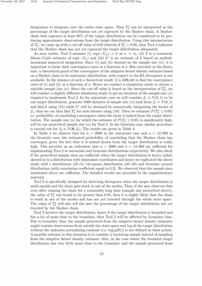
Figure 7. Joint distribution of the mixture of two bivariate normals in which the first component is highly

positively correlated while the second component is highly negatively correlated.

where (x, y)T ∈ R2, φ2

((x, y)T , 0, Σi

)is the density of bivariate normal distribution

with mean 0, covariance matrix Σi, evaluated at (x, y)T and Σi =

[1 ρiρi 1

]for i = 1, 2.

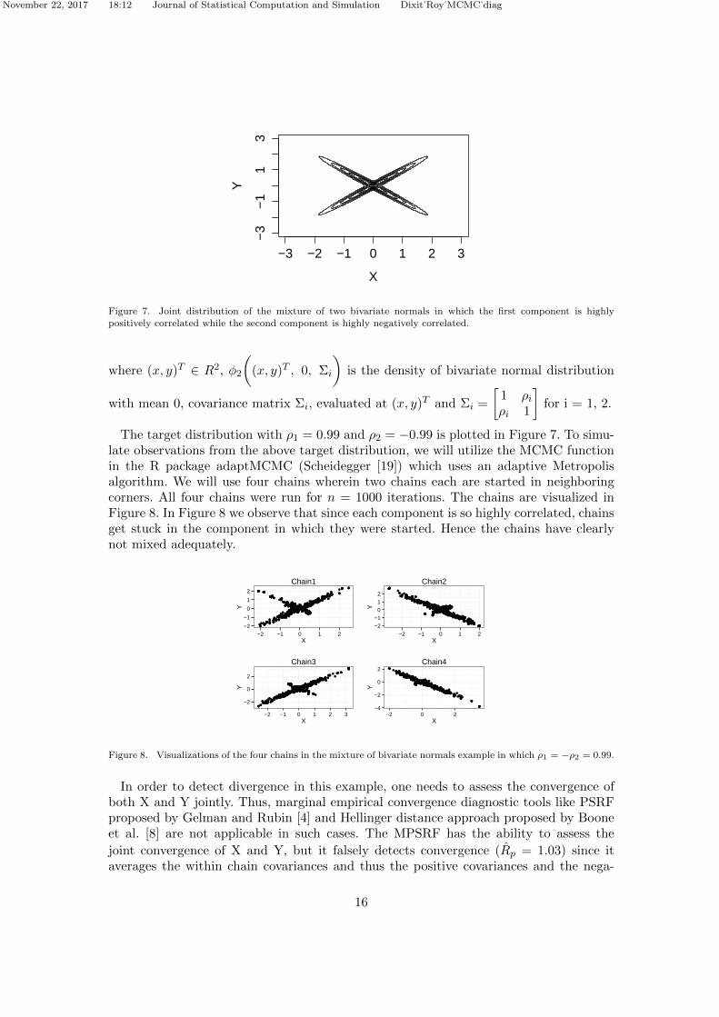
The target distribution with ρ1 = 0.99 and ρ2 = −0.99 is plotted in Figure 7. To simu-late observations from the above target distribution, we will utilize the MCMC functionin the R package adaptMCMC (Scheidegger [19]) which uses an adaptive Metropolisalgorithm. We will use four chains wherein two chains each are started in neighboringcorners. All four chains were run for n = 1000 iterations. The chains are visualized inFigure 8. In Figure 8 we observe that since each component is so highly correlated, chainsget stuck in the component in which they were started. Hence the chains have clearlynot mixed adequately.

−2

−1

0

1

2

−2 −1 0 1 2X

Y

Chain1

−2−1

012

−2 −1 0 1 2X

Y

Chain2

−2

0

2

−2 −1 0 1 2 3X

Y

Chain3

−4

−2

0

2

−2 0 2X

Y

Chain4

Figure 8. Visualizations of the four chains in the mixture of bivariate normals example in which ρ1 = −ρ2 = 0.99.

In order to detect divergence in this example, one needs to assess the convergence ofboth X and Y jointly. Thus, marginal empirical convergence diagnostic tools like PSRFproposed by Gelman and Rubin [4] and Hellinger distance approach proposed by Booneet al. [8] are not applicable in such cases. The MPSRF has the ability to assess the

joint convergence of X and Y, but it falsely detects convergence (R̂p = 1.03) since itaverages the within chain covariances and thus the positive covariances and the nega-

16


tive covariances cancel each other out. Using the bivariate KL Tool 1, the maximumestimated symmetric KL divergence between chains was found to be 1.98 which is sig-nificantly greater than the cut-off of C = 0.06. The bivariate KL Tool 1 requires at least12,000 observations to provide a good estimate hence simply comparing the estimatedsymmetric KL divergence to the cut-off value is not enough. Thus, we must also lookat the probability of observing an estimated symmetric KL divergence of 1.98 or lesswhen the chains with n = 1000 are drawn from different distributions i.e. N(012, I2) andN(µ12, I2) where µ = 0.2835. This probability which can also be looked upon as thep-value in terms of the hypothesis framework given in Section 3 was found to be verylarge (i.e. greater than 0.999). Thus we do not reject our null hypothesis and concludedthat the chains have not yet mixed adequately. Thus, in this example we observe that,even if the target distribution is unimodal, MPSRF proposed by Brooks and Gelman [5]is vulnerable to false indication of convergence. If the above chains are run for a longerperiod, then all the chains travel through both the components and mix adequately.

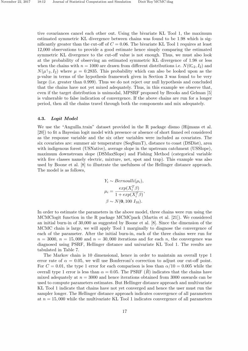
4.3. Logit Model

We use the “Anguilla train” dataset provided in the R package dismo (Hijmans et al.[20]) to fit a Bayesian logit model with presence or absence of short finned eel consideredas the response variable and the six other variables were included as covariates. Thesix covariates are: summer air temperature (SeqSumT), distance to coast (DSDist), areawith indigenous forest (USNative), average slope in the upstream catchment (USSlope),maximum downstream slope (DSMaxSlope) and Fishing Method (categorical variablewith five classes namely electric, mixture, net, spot and trap). This example was alsoused by Boone et al. [8] to illustrate the usefulness of the Hellinger distance approach.The model is as follows,

Yi ∼ Bernoulli(µi),

µi =exp(XT

i β)

1 + exp(XTi β)

,

β ∼ N(0, 100 I10).

In order to estimate the parameters in the above model, three chains were run using theMCMClogit function in the R package MCMCpack (Martin et al. [21]). We consideredan initial burn-in of 30,000 as suggested by Boone et al. [8]. Since the dimension of theMCMC chain is large, we will apply Tool 1 marginally to diagnose the convergence ofeach of the parameter. After the initial burn-in, each of the three chains were run forn = 3000, n = 15, 000 and n = 30, 000 iterations and for each n, the convergence wasdiagnosed using PSRF, Hellinger distance and univariate KL Tool 1. The results aretabulated in Table 7.

The Markov chain is 10 dimensional, hence in order to maintain an overall type 1error rate of α = 0.05, we will use Bonferroni’s correction to adjust our cut-off point.For C = 0.01, the type 1 error for each comparison is less than α/10 = 0.005 while the

overall type 1 error is less than α = 0.05. The PSRF (R̂) indicates that the chains havemixed adequately at n = 3000 and hence iterations obtained from 3000 onwards can beused to compute parameters estimates. But Hellinger distance approach and multivariateKL Tool 1 indicate that chains have not yet converged and hence the user must run thesampler longer. The Hellinger distance approach indicates convergence of all parametersat n = 15, 000 while the multivariate KL Tool 1 indicates convergence of all parameters

17


Table 7. Application of various MCMC convergence diagnostic tools to the Bayesian logit model.

n = 3, 000 n = 15, 000 n = 30, 000

Variable R̂ H Dist Tool 1 R̂ H Dist Tool 1 R̂ H Dist Tool 1(Intercept) 1.01 0.12 0.06 1.00 0.07 0.02 1.00 0.06 0.01SeqSumT 1.01 0.13 0.07 1.00 0.07 0.02 1.00 0.05 0.01DSDist 1.00 0.13 0.05 1.00 0.06 0.01 1.00 0.05 0.01USNative 1.00 0.14 0.08 1.00 0.07 0.02 1.00 0.06 0.01M - mix 1.01 0.13 0.05 1.00 0.07 0.01 1.00 0.05 0.01M - net 1.01 0.17 0.11 1.00 0.06 0.01 1.00 0.06 0.01M - spot 1.01 0.13 0.08 1.00 0.09 0.02 1.00 0.06 0.01M - trap 1.02 0.15 0.08 1.00 0.08 0.02 1.00 0.06 0.01DSMaxSlope 1.00 0.09 0.03 1.00 0.06 0.01 1.00 0.05 0.01USSlope 1.00 0.10 0.03 1.00 0.09 0.03 1.00 0.06 0.01

at n = 30, 000. Since the multivariate KL Tool 1 adjusts its cut-off point for multiplecomparison, it is advisable for the user to use iterations from 30,000 onwards for makinginference about the parameters of interest.

5. Conclusion

In this article, we have provided two new MCMC convergence diagnostic tools basedon KL divergence and smoothing methods. The advantage of the first tool over existingMCMC convergence diagnostic tools is that, it has the ability to assess the joint con-vergence of multiple variables. For multivariate chains, we assess convergence marginallyand recalibrate the cut-off point using Bonferroni’s correction to maintain the overalltype 1 error at α. Due to the use of Bonferroni’s correction, Tool 1 can be conserva-tive in the case of large number of variables. But in the case of MCMC diagnostics, aconservative tool is preferable as it provides the user greater assurance, that the chainis producing approximate observations from the target distribution, when it indicatesconvergence. In the case where the first tool indicates divergence of multiple MCMCchains, the user can use the visualization tool to further investigate reasons behind thedivergence of multiple MCMC chains. The advantage of the second tool over existingMCMC convergence diagnostic tools is that, it is equipped to detect divergence whenMCMC chains get stuck in a particular mode of a multi-modal target distribution. Tool2 is vulnerable if multidimensional numerical integration does not provide a good esti-mate of the unknown normalizing constant. Thus the proposed methods provide a usefuladdition to the set of available MCMC diagnostic tools and are equipped to detect nonconvergence of chains when other methods might fail to do so. A possible future studyinvolves deriving a theoretical proof of convergence of the adaptive kernel density esti-mate based on Markov chain samples to its stationary distribution with respect to KLdivergence measure.

Supplementary Materials

Tabulated results corresponding to Tool 1 and Tool 2 simulation studies carried out usingt distribution (df=5), chi-square distribution (df=10) and bivariate normal distribution(with correlation coefficient equal to 0.3) are provided in the supplementary material.The R code required to implement the tools in this article is also available online.

18


Acknowledgment

We would like to thank two reviewers, the AE and the Editor for their helpful commentsthat have improved the manuscript.

References

[1] Rosenthal JS. Minorization conditions and convergence rates for Markov chain Monte Carlo.Journal of the American Statistical Association. 1995;90(430):558–566.

[2] Jones G, Hobert JP. Honest exploration of intractable probability distributions via Markovchain Monte Carlo. Statist Sci. 2001 11;16(4):312–334.

[3] Roy V, Hobert JP. Convergence rates and asymptotic standard errors for Markov chainMonte Carlo algorithms for Bayesian probit regression. Journal of the Royal StatisticalSociety: Series B (Statistical Methodology). 2007;69(4):607–623.

[4] Gelman A, Rubin DB. Inference from iterative simulation using multiple sequences. Statis-tical Science. 1992;7:457–472.

[5] Brooks SP, Gelman A. General methods for monitoring convergence of iterative simulations.Journal of Computational and Graphical Statistics. 1998;7:434–455.

[6] Raftery AE, Lewis SM. How many iterations in the Gibbs sampler. Bayesian Statistics 4.1992;J.M. Bernardo, A.F.M. Smith, A.P. Dawid and J.O. Berger, eds., Oxford UniversityPress, Oxford:763–773.

[7] Geweke J. Evaluating the accuracy of sampling-based approaches to the calculations ofposterior moments. Bayesian Statistics 4. 1992;J.M. Bernardo, J.O. Berger, A.P. Dawid andA.F.M. Smith, eds., Oxford University Press, Oxford:169–193.

[8] Boone E, Merrick J, Krachey M. A Hellinger distance approach to MCMC diagnostics.Journal of Statistical Computation and Simulation. 2014;84(4):833–849.

[9] Hjorth U, Vadeby A. Subsample distribution distance and MCMC convergence. ScandinavianJournal of Statistics. 2005;32:313–326.

[10] Yu B. Estimating the L1 error of kernal estimators based on Markov samplers. TechnicalReport, UC Berkeley. 1994;.

[11] Brooks SP, Roberts GO. Convergence assessment techniques for Markov chain Monte Carlo.Statistics and Computing. 1998;8(4):319–335.

[12] Silverman BW. Density estimation for statistics and data analysis. Chapman & Hall, London.1986;.

[13] Azzalini A, Menardi G. Clustering via nonparametric density estimation: The R packagepdfCluster. Journal of Statistical Software. 2014;57(11):1–26.

[14] Peltonen J, Venna J, Kaski S. Visualizations for assessing convergence and mixing of Markovchain Monte Carlo simulations. Computational Statistics & Data Analysis. 2009;53(12):4453– 4470.

[15] Hahn T. Cuba - a library for multidimensional numerical integration. Computer PhysicsCommunications. 2005;168(2):78 – 95.

[16] Bouvier A, Kiu K. R2cuba: Multidimensional numerical integration. 2015; r package version1.1-0.

[17] Johnson SG, Narasimhan B. cubature: Adaptive multivariate integration over hypercubes.2013; r package version 1.1-2.

[18] Leman SC, Chen Y, Lavine M. The multiset sampler. Journal of the American StatisticalAssociation. 2009;104(487):1029–1041.

[19] Scheidegger A. adaptmcmc: Implementation of a generic adaptive Monte Carlo Markov chainsampler. 2012; r package version 1.1.

[20] Hijmans RJ, Phillips S, Leathwick J, Elith J. dismo: Species distribution modeling. 2016; rpackage version 1.0-15.

[21] Martin AD, Quinn KM, Park JH. MCMCpack: Markov chain Monte Carlo in R. Journal ofStatistical Software. 2011;42(9):22.

19

Documents

MCMC diagnostics for higher dimensions using Kullback ...vroy/Research/KLDiag.pdf · makes use of adaptive kernel ... 2017 18:12 Journal of Statistical Computation and Simulation