MCEETYA

2006

National Assessment Program – Science Literacy Year 6

TechnicalReport

NAP-SL 2006 Project StaffJenny Donovan from Educational Assessment Australia (EAA) was the Project Director of NAP-SL 2006. Melissa Lennon (EAA) was the Project Manager and Wendy Bodey from Curriculum Corporation (CC) was the Assessment Manager. The test development team was led by Gayl O’Connor (CC). The School Release Materials were written by Jenny Donovan, Penny Hutton, Melissa Lennon (EAA), Gayl O’Connor and Noni Morrissey from CC.

The sampling and data analysis tasks were undertaken by Nathaniel Lewis and Goran Lazendic from EAA and Margaret Wu and Mark Dulhunty from Educational Measurement Solutions (EMS). The Technical Report was written by Margaret Wu (EMS), Jenny Donovan, Penny Hutton and Melissa Lennon (EAA).

© 2008 Curriculum Corporation as the legal entity for the Ministerial Council on Education, Employment, Training and Youth Affairs (MCEETYA).

Curriculum Corporation as the legal entity for the Ministerial Council on Education, Employment, Training and Youth Affairs (MCEETYA) owns the copyright in this publication. This publication or any part of it may be used freely only for non-pro?t education purposes provided the source is clearly acknowledged. The publication may not be sold or used for any other commercial purpose.

Other than as permitted above or by the Copyright Act 1968 (Commonwealth), no part of this publication may be reproduced, stored, published, performed, communicated or adapted, regardless of the form or means (electronic, photocopying or otherwise), without the prior written permission of the copyright owner. Address inquiries regarding copyright to:

MCEETYA Secretariat, PO Box 202, Carlton South,VIC 3053, Australia.

i

Contents

Chapter 1 National Assessment Program – Science Literacy 2006: Overview 1 1.1 Introduction 1 1.2 Purposes of the Technical Report 2 1.3 Organisation of the Technical Report 2

Chapter 2 Test Development and Test Design 3 2.1 Assessment domains 3 2.2 Test blueprint 4

2.2.1 Test design 5 2.3 Test development process 6 2.4 Field trial of test items 9

2.4.1 Analysis of the trial 9 2.4.2 Reports to trial schools 13

2.5 Item selection process for the final test 13 2.6 Test characteristics of the final test 15 2.7 Reports to schools 17

Chapter 3 Sampling Procedures 18 3.1 Overview 18 3.2 Target population 19 3.3 School and student non-participation 20 3.4 Sampling size estimations 20 3.5 Stratification 23

3.5.1 Small schools 24 3.5.2 Very large schools 25

3.6 Replacement schools 25 3.7 Class selection 26 3.8 The 2006 proposed sample 27 3.9 2006 National Assessment Program – Science Literacy sample results 28

Chapter 4 Test Administration Procedures and Data Preparation 29 4.1 Online registration of class/student lists 29 4.2 Administering the tests to students 29 4.3 Marking procedures 30 4.4 Data entry procedures 31

4.4.1 Data coding rules 31

Chapter 5 Computation of Sampling Weights 32 5.1 School weight 32

5.1.1 School base weight 32 5.1.2 School non-participation adjustment 33 5.1.3 Final school weight 33

5.2 Class weight 34 5.2.1 Class weight when classes were selected with equal probability 35 5.2.2 Class weight when classes were selected with unequal probability 36

5.2.2.1 Empirical classroom weight 36 5.2.2.2 Empirical weight adjustment 36

5.2.3 Final class weight 37 5.2.4 Student weight 37 5.2.5 Final weight 38

ii

Chapter 6 Item Analysis of the Final Test 39 6.1 Item analyses 39

6.1.1 Sample size 39 6.1.2 Number of students by booklet 40 6.1.3 Initial item analysis 40

6.1.3.1 Item–person map 41 6.1.3.2 Summary item statistics 41 6.1.3.3 Test reliability 45

6.1.4 Booklet effect 45 6.1.5 Item statistics by States/Territories 46

6.1.5.1 Comparison of item difficulty parameters across States/Territories 46 6.1.5.2 Comparison of discrimination indices across States/Territories 51 6.1.5.3 Comparison of State/Territory locations in RUMM 51

6.1.6 Gender groups 51 6.1.7 Impact of item type on student performance 53

6.2 Test design 54 6.2.1 Sample test design: cluster and unit allocation 54

6.3 Item codes 56 6.4 Item analysis files 59 6.5 Comparison of State/Territory locations in RUMM 59

Chapter 7 Scaling of Test Data 60 7.1 Overview 60

7.1.1 Calibration of item parameters 60 7.1.2 Estimating student proficiency levels and producing plausible values 60

7.2 Calibration sample 61 7.2.1 Overview 61 7.2.2 Data files availability 61

7.2.2.1 CalibrationSample.sav 61 7.2.2.2 CalibrationItems.dat 62

7.2.3 Removal of one item in analyses 62 7.2.4 IRT analysis for calibrating item parameters 62

7.3 Estimating student proficiency levels and producing plausible values 63 7.3.1 Production of plausible values 64

7.4 Estimation of statistics of interest and their standard errors 64 7.5 Transform logits to a scale with mean 400 and standard deviation 100 65

Chapter 8 Equating 2003 Results to 2006 Results 66 8.1 Setting 2006 results as the baseline 66

8.1.1 ACER re-analysis in April 2007 of the 2003 results 67 8.2 Equating 2003 results to 2006 results 67

8.2.1 Link items 67 8.3 Equating procedures 69 8.4 Equating transformation 70 8.5 Link error 70

Chapter 9 Proficiency Scale and Proficiency Levels 72

References 76

Appendix A National Year 6 Primary Science Assessment Domain 77

Appendix B Sample School Reports 84

Appendix C Item Pool Feedback 89

iii

Appendix D Student Participation Form 107

Appendix E Technical Notes on Sampling 110

Appendix F Programming Notes on Sampling 113

Appendix G Characteristics of the Proposed 2006 Sample 118

Appendix H Variables in File 121

Appendix I ConQuest Control File for Producing Plausible Values 122

List of Tables

Table 2.1 BIB design used in the National Assessment Program –

Science Literacy 2006 6

Table 2.2 Proposed composition of the National Assessment Program –

Science Literacy item pool across concept areas 7

Table 2.3 Proposed composition of the National Assessment Program –

Science Literacy item pool across levels and strands 7

Table 2.4 Composition of the trial item pool (all released batches) 8

Table 2.5 Suggested logit range for acceptable difficulty for each level 13

Table 2.6 Composition of the final item pool 15

Table 2.7 Breakdown of concept areas across the final objective and practical papers 15

Table 2.8 Breakdown of strands across the final objective and practical papers 16

Table 2.9 Breakdown of levels across the final objective and practical papers 16

Table 2.10 Breakdown of item types across the final objective and practical papers 16

Table 2.11 Breakdown of major concepts across the levels within the final item pool 16

Table 2.12 Breakdown of location ranges (based on trial statistics) across the final

objective and practical papers 17

Table 3.1 The National Assessment Program – Science Literacy 2006 Exemption

and Refusal codes 20

Table 3.2 2003 and 2006 (target) jurisdiction sample size 21

Table 3.3 Proposed 2006 sample sizes for drawing samples 22

Table 3.4 Estimated 2006 Year 6 enrolment figures as provided by BEMU 23

iv

Table 3.5 Proportions of schools by school size and jurisdiction 24

Table 3.6 Number of schools to be sampled 27

Table 3.7 The National Assessment Program – Science Literacy target and achieved

sample sizes by jurisdiction 28

Table 3.8 Student non-participation by jurisdiction 28

Table 4.1 Codes used in the Student Participation Form 31

Table 5.1 Probability of selection of three classes 34

Table 5.2 Class size of three classes 34

Table 5.3 Formation of a pseudo-class from classes listed in Table 5.2 34

Table 5.4 Probability of selection of classes listed in Table 5.2 35

Table 6.1 Number of students by State/Territory 39

Table 6.2 Number of students by test booklet 40

Table 6.3 Summary item statistics 42–45

Table 6.4 Booklet difficulty parameters 46

Table 6.5 Item difficulty parameters for gender groups 52–53

Table 6.6 Percentages of students omitting responses by item type 53

Table 6.7 BIB design used in the National Assessment Program –

Science Literacy 2006 54

Table 6.8 Organisation of clusters 54–55

Table 6.9 List of item codes and details 56–58

Table 7.1 Variable names matched to the original item codes 62

Table 7.2 Codebook for CalibrationItems.dat 62

Table 7.3 Removed link item 62

Table 8.1 2003–2006 link items 68

Table 8.2 2003 anchor item parameters for scaling 2006 data 69

Table 8.3 Computation of link error 71

Table 8.4 Standard error of difference 71

Table 9.1 Cut-points for the National Assessment Program – Science Literacy 2006 72

Table 9.2 Proficiency levels of items 73–75

Table A.1 Scientific Literacy Progress Map – July 2004 version from DEST Science

Education Assessment Resource (SEAR) project 81–82

v

Table A.2 Major scientific concepts in the National Assessment Program –

Science Literacy 2006 83

Table C.1 Item pool feedback: EAA, CC and SLRC 90

Table E.1 The sort ordering procedures employed for small schools 111

Table E.2 Stratum variables for sample selection 111–112

Table F.1 Schools with estimated GeoLocation values 113–114

Table G.1 Number of schools and students to be sampled in each jurisdiction 118

Table G.2 Comparison of proposed sample and population sector proportions

across jurisdictions 119

Table G.3 Comparison of population and proposed sample proportions according

to school size 120

Table H.1 NAPSL2006_Reporting_WLE_PV_20070423.sav 121

Table I.1 File Name: ProducePV.cqc 122–123

List of Figures

Figure 2.1 Proposed composition of the National Assessment Program –

Science Literacy item pool across strands A, B and C 5

Figure 2.2 Test development flow chart 6

Figure 2.3 Colour key for judging the performance of items 10

Figure 2.4 Item map for 230 post-trial items 12

Figure 2.5 Item map for 204 post-SLRC review items 14

Figure 3.1 The National Assessment Program – Science Literacy 2006

non-participation categories 20

Figure 6.1 Item–person map 41

Figure 6.2 Comparison of item difficulty parameters across States/Territories 47–48

Figure 6.3 Discrimination index by State/Territory 49–50

Figure 6.4 Item analysis for item ID0B057 for ACT 51

Figure 8.1 Calibrated item difficulties in 2003 and 2006 for link items 68

vi

1

Chapter 1 National Assessment Program – Science Literacy 2006: Overview

1.1 Introduction In July 2001, the Ministerial Council on Education, Employment, Training and Youth Affairs

(MCEETYA) agreed to the development of assessment instruments and key performance

measures for reporting on student skills, knowledge and understandings in primary science. It

directed the newly established Performance Measurement and Reporting Taskforce (PMRT),

a nationally representative body, to undertake the national assessment program. The PMRT

commissioned the assessment in July 2001 for implementation in 2003. The Primary Science

Assessment Program (PSAP) – as it was then known – tested a sample of Year 6 students in

all States and Territories. PSAP results were reported in 2005.

The National Assessment Program – Science Literacy was the first assessment program

designed specifically to provide information about performance against MCEETYA’s National

Goals for Schooling in the Twenty-First Century. MCEETYA has since also endorsed similar

assessment programs to be conducted for Civics and Citizenship, and Information and

Communications Technology (ICT). The intention is that each assessment program will be

repeated every three years so that performance in these areas of study can be monitored over

time. The first cycle of the program was intended to provide the baseline against which future

performance could be compared.

PMRT awarded the contract for the second cycle of science testing, for 2006, to a consortium

of Educational Assessment Australia (EAA) and Curriculum Corporation (CC). Educational

Measurement Solutions (EMS) was sub-contracted to CC to provide psychometric services.

2

The Benchmarking and Educational Measurement Unit (BEMU) was nominated by PMRT to

liaise between the contractors and PMRT in the delivery of the project.

The Science Literacy Review Committee (SLRC), comprising members from all States,

Territories and sectors, was a consultative group to the project.

1.2 Purposes of the Technical Report This technical report aims to provide detailed information with regard to the conduct of the

National Assessment Program – Science Literacy 2006 so that valid interpretations of the

2006 results can be made, and future cycles can be implemented with appropriate linking

information from past cycles. Further, a fully documented set of the National Assessment

Program – Science Literacy procedures can also provide information for researchers who are

planning surveys of this kind. The methodologies used in the National Assessment Program –

Science Literacy 2006 can inform researchers of the current developments in large-scale

surveys. They can also highlight the limitations and suggest possible improvements in the

future. Consequently, it is of great importance to provide technical details on all aspects of the

survey.

1.3 Organisation of the Technical Report This report is divided into nine chapters.

Chapter 2 provides an outline of the test development and test design processes, including

trialling and item selection, and the assessment domains of scientific literacy.

The sampling procedures across jurisdictions, schools and classes are discussed in Chapter 3.

Chapter 4 includes information about how the tests were administered and marked, including

coding for student demographic data and participation or non-inclusion. It also provides an

explanation of the reporting processes.

Chapter 5 details the processes involved in computing the sampling weights.

Chapter 6 provides an extensive analysis of all items included in the final test forms, including

item difficulties based on Rasch modelling.

Scaling and item calibration procedures leading to the placement of items and student scores

within the Proficiency levels of the Scientific Literacy Progress Map are outlined in Chapter 7.

Chapter 8 discusses the processes used to equate the 2003 assessment and the 2006

assessment.

Chapter 9 provides information about the proficiency scale used for reporting the results,

including the cut-scores for each of the levels and the placement of all test items within the

levels.

3

Chapter 2 Test Development and Test Design

2.1 Assessment domains The National Assessment Program – Science Literacy measures scientific literacy. This is the

application of broad conceptual understandings of science to make sense of the world,

understand natural phenomena and interpret media reports about scientific issues. It also

includes asking investigable questions, conducting investigations, collecting and interpreting

data and making decisions. The construct evolved from the definition of scientific literacy

used by the Organisation for Economic Co-operation and Development (OECD) Programme

for International Student Assessment (PISA):

... the capacity to use scientific knowledge, to identify questions and to draw

evidence-based conclusions in order to understand and help make decisions about

the natural world and the changes made to it through human activity.

(OECD 1999, p. 60)

A scientific literacy assessment domain was developed for the assessment in consultation with

curriculum experts from each State and Territory and representatives of the Catholic and

independent school sectors. This domain includes the definition of scientific literacy and

outlines the development of scientific literacy across three main areas.

Three main areas of scientific literacy were assessed:

Strand A: formulating or identifying investigable questions and hypotheses, planning

investigations and collecting evidence

4

Strand B: interpreting evidence and drawing conclusions from their own or others’

data, critiquing the trustworthiness of evidence and claims made by others,

and communicating findings

Strand C: using science understandings for describing and explaining natural

phenomena and for interpreting reports about phenomena.

A conscious effort was made to develop assessment items that related to everyday contexts.

The scientific literacy domain is detailed in Appendix A. The items drew on four concept

areas: Earth and Beyond (EB); Energy and Change (EC); Life and Living (LL); and Natural

and Processed Materials (NP). These major scientific concepts are found most widely in

curriculum documents across all States and Territories and were used by item writers to guide

test development. The list of endorsed examples for each of these major concepts is in

Table A.2.

The intention was to ensure that all Year 6 students were familiar with the materials and

experiences to be used in the National Assessment Program – Science Literacy and so avoid

any systematic bias in the instruments being developed.

2.2 Test blueprint In 2005 MCEETYA published a Response for Tender (RFT) document. Consequently,

EAA/CC developed the following proposal for the tests:

It is anticipated that the 2006 final test forms will contain approximately 100 items in

total (excluding link items from 2003) providing sufficient assessment items for up to

two hours of testing for each student in the national sample. This number of items will

also provide items to form part of the assessment kit to be released for teacher use and

items to be held secure for 2009.

The total number of new items to be developed for trial is estimated at 275 (the item

pool), based on developing and trialling 2.5 times the number of items required for the

final test forms. This allows for maximum flexibility through the review process when

various criteria are applied to each item to assess item suitability for retention in the

item pool. It was proposed that 25 items from 2003 be embedded in the 2006 test as link

items. Ultimately, eleven items were approved for use as link items in the main test.

These are summarised in Table 8.1 on page 68. In the final test nine items from 2003

were included.

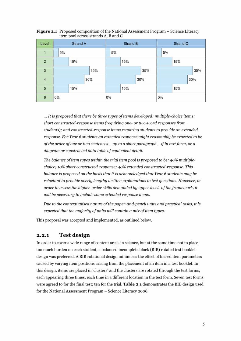
The following diagram indicates a proposed composition of the instruments that will

enable coverage of a wide range of student performance over the three strands of

science literacy, and thus also provides an outline of the test specifications.

5

Figure 2.1 Proposed composition of the National Assessment Program – Science Literacy item pool across strands A, B and C

Level Strand A Strand B Strand C

1 5% 5% 5%

2 15% 15% 15%

3 35% 35% 35%

4 30% 30% 30%

5 15% 15% 15%

6 0% 0% 0%

… It is proposed that there be three types of items developed: multiple-choice items;

short constructed-response items (requiring one- or two-word responses from

students); and constructed-response items requiring students to provide an extended

response. For Year 6 students an extended response might reasonably be expected to be

of the order of one or two sentences – up to a short paragraph – if in text form, or a

diagram or constructed data table of equivalent detail.

The balance of item types within the trial item pool is proposed to be: 50% multiple-

choice; 10% short constructed-response; 40% extended constructed-response. This

balance is proposed on the basis that it is acknowledged that Year 6 students may be

reluctant to provide overly lengthy written explanations to test questions. However, in

order to assess the higher-order skills demanded by upper levels of the framework, it

will be necessary to include some extended response items.

Due to the contextualised nature of the paper-and-pencil units and practical tasks, it is

expected that the majority of units will contain a mix of item types.

This proposal was accepted and implemented, as outlined below.

2.2.1 Test design In order to cover a wide range of content areas in science, but at the same time not to place

too much burden on each student, a balanced incomplete block (BIB) rotated test booklet

design was preferred. A BIB rotational design minimises the effect of biased item parameters

caused by varying item positions arising from the placement of an item in a test booklet. In

this design, items are placed in ‘clusters’ and the clusters are rotated through the test forms,

each appearing three times, each time in a different location in the test form. Seven test forms

were agreed to for the final test; ten for the trial. Table 2.1 demonstrates the BIB design used

for the National Assessment Program – Science Literacy 2006.

6

Table 2.1 BIB design used in the National Assessment Program – Science Literacy 2006

Booklet Block 1 Block 2 Block 3

1 Cluster 1 Cluster 2 Cluster 4

2 Cluster 2 Cluster 3 Cluster 5

3 Cluster 3 Cluster 4 Cluster 6*

4 Cluster 4 Cluster 5 Cluster 7

5 Cluster 5* Cluster 6 Cluster 1

6 Cluster 6 Cluster 7 Cluster 2

7 Cluster 7 Cluster 1 Cluster 3

* The Energy Transfer unit from Cluster 5 does not appear in Booklet 5, but instead appears at the end of Cluster 6 in Booklet 3.

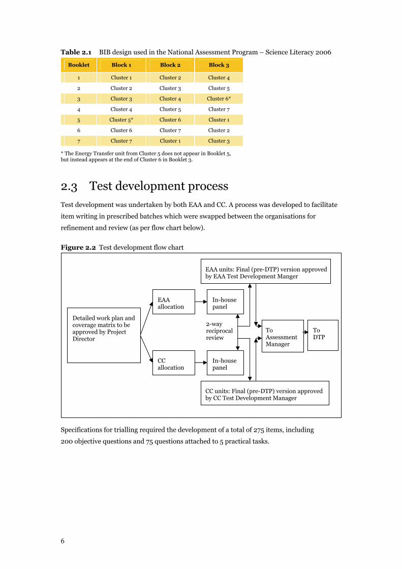
2.3 Test development process Test development was undertaken by both EAA and CC. A process was developed to facilitate

item writing in prescribed batches which were swapped between the organisations for

refinement and review (as per flow chart below).

Figure 2.2 Test development flow chart

Specifications for trialling required the development of a total of 275 items, including

200 objective questions and 75 questions attached to 5 practical tasks.

2-way reciprocalreview

EAA allocation

In-house panel

To Assessment Manager

To DTP

CC units: Final (pre-DTP) version approved by CC Test Development Manager

Detailed work plan and coverage matrix to be approved by Project Director

CC allocation

In-house panel

EAA units: Final (pre-DTP) version approvedby EAA Test Development Manger

7

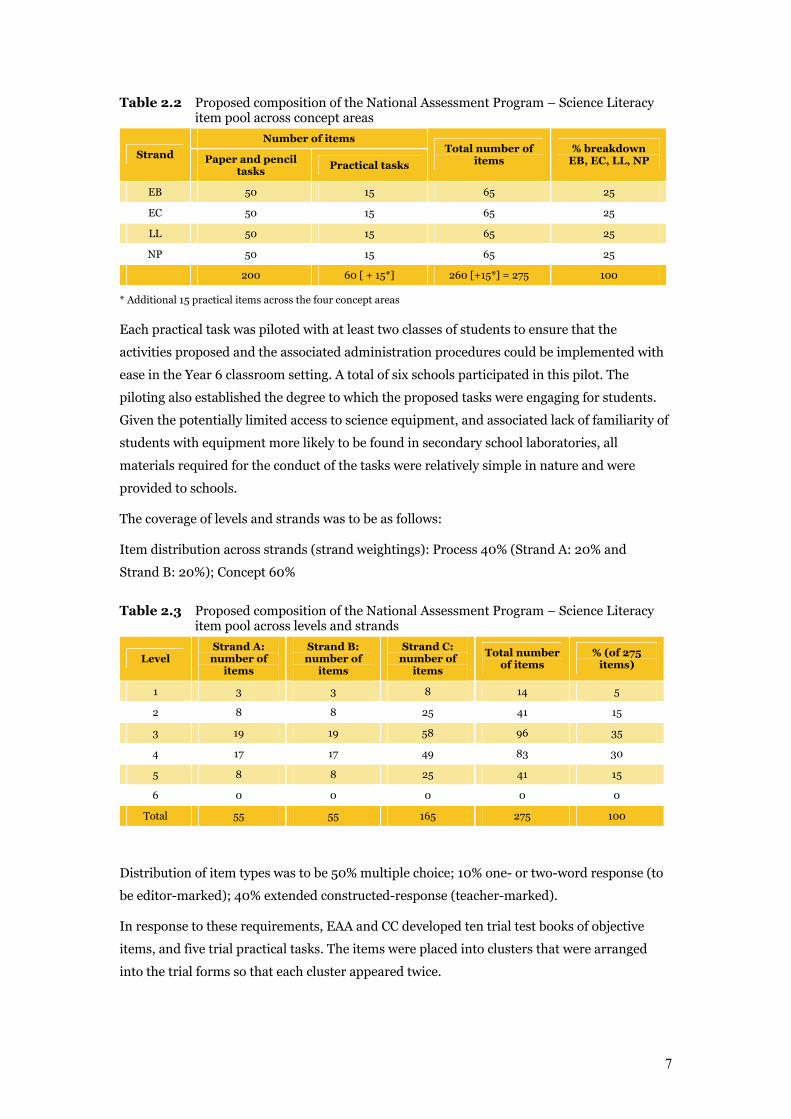
Table 2.2 Proposed composition of the National Assessment Program – Science Literacy item pool across concept areas

Number of items

Strand Paper and pencil tasks Practical tasks

Total number of items

% breakdown EB, EC, LL, NP

EB 50 15 65 25

EC 50 15 65 25

LL 50 15 65 25

NP 50 15 65 25

200 60 [ + 15*] 260 [+15*] = 275 100

* Additional 15 practical items across the four concept areas

Each practical task was piloted with at least two classes of students to ensure that the

activities proposed and the associated administration procedures could be implemented with

ease in the Year 6 classroom setting. A total of six schools participated in this pilot. The

piloting also established the degree to which the proposed tasks were engaging for students.

Given the potentially limited access to science equipment, and associated lack of familiarity of

students with equipment more likely to be found in secondary school laboratories, all

materials required for the conduct of the tasks were relatively simple in nature and were

provided to schools.

The coverage of levels and strands was to be as follows:

Item distribution across strands (strand weightings): Process 40% (Strand A: 20% and

Strand B: 20%); Concept 60%

Table 2.3 Proposed composition of the National Assessment Program – Science Literacy item pool across levels and strands

Level Strand A:

number of items

Strand B: number of

items

Strand C: number of

items

Total number of items

% (of 275 items)

1 3 3 8 14 5

2 8 8 25 41 15

3 19 19 58 96 35

4 17 17 49 83 30

5 8 8 25 41 15

6 0 0 0 0 0

Total 55 55 165 275 100

Distribution of item types was to be 50% multiple choice; 10% one- or two-word response (to

be editor-marked); 40% extended constructed-response (teacher-marked).

In response to these requirements, EAA and CC developed ten trial test books of objective

items, and five trial practical tasks. The items were placed into clusters that were arranged

into the trial forms so that each cluster appeared twice.

8

The trial forms contained a cluster (Cluster 9) of link items drawn from the secure item pool

from 2003. These items were included to inform the equating study.

Descriptors were written for each item and a draft marking key was developed. The marking

guide included possible responses to constructed response questions.

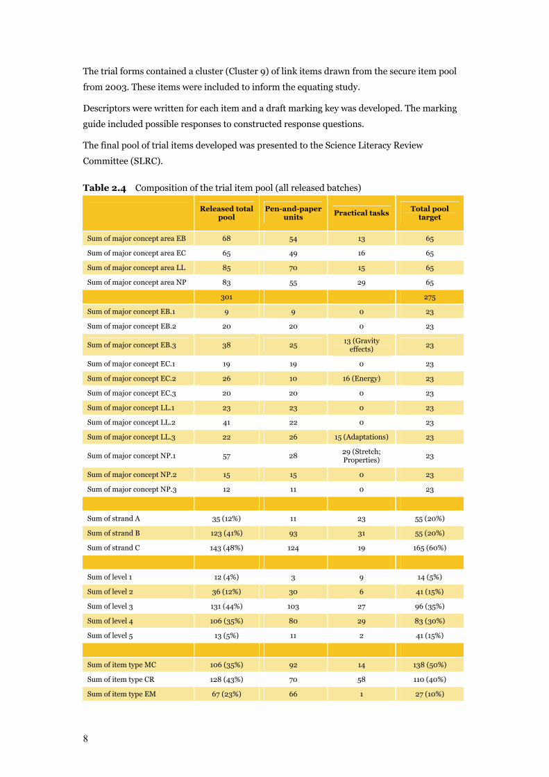
The final pool of trial items developed was presented to the Science Literacy Review

Committee (SLRC).

Table 2.4 Composition of the trial item pool (all released batches)

Released total pool

Pen-and-paper units

Practical tasks Total pool

target

Sum of major concept area EB 68 54 13 65

Sum of major concept area EC 65 49 16 65

Sum of major concept area LL 85 70 15 65

Sum of major concept area NP 83 55 29 65

301 275

Sum of major concept EB.1 9 9 0 23

Sum of major concept EB.2 20 20 0 23

Sum of major concept EB.3 38 25 13 (Gravity effects)

23

Sum of major concept EC.1 19 19 0 23

Sum of major concept EC.2 26 10 16 (Energy) 23

Sum of major concept EC.3 20 20 0 23

Sum of major concept LL.1 23 23 0 23

Sum of major concept LL.2 41 22 0 23

Sum of major concept LL.3 22 26 15 (Adaptations) 23

Sum of major concept NP.1 57 28 29 (Stretch; Properties)

23

Sum of major concept NP.2 15 15 0 23

Sum of major concept NP.3 12 11 0 23

Sum of strand A 35 (12%) 11 23 55 (20%)

Sum of strand B 123 (41%) 93 31 55 (20%)

Sum of strand C 143 (48%) 124 19 165 (60%)

Sum of level 1 12 (4%) 3 9 14 (5%)

Sum of level 2 36 (12%) 30 6 41 (15%)

Sum of level 3 131 (44%) 103 27 96 (35%)

Sum of level 4 106 (35%) 80 29 83 (30%)

Sum of level 5 13 (5%) 11 2 41 (15%)

Sum of item type MC 106 (35%) 92 14 138 (50%)

Sum of item type CR 128 (43%) 70 58 110 (40%)

Sum of item type EM 67 (23%) 66 1 27 (10%)

9

2.4 Field trial of test items Students from 31 selected schools across NSW, ACT, VIC and SA participated in the trial in

October 2005. The trial schools were selected to reflect the range of educational contexts

around the country, and included government, non-government and Catholic; low and high

socioeconomic drawing areas; metropolitan and regional; large and small; high and low

LBOTE population etc.

In total approximately 1100 students from the trial schools across the four selected States

participated in the trial. Each student completed one of the ten trial objective test papers and

one of the five practical tasks. Within each class, teachers were asked to evenly distribute the

ten objective test forms amongst students. On completion of the objective forms students

within a class were asked to separate into groups of three (or groups of two where necessary)

for completion of the practical task. Students within the one class completed the same

practical task.

Classroom teachers were provided with an administration manual in advance of the trial to

allow them to familiarise themselves with the test procedures. An invigilator was sent to each

trial school to deliver and collect the materials (to ensure the security of the materials) and to

also observe and support the classroom teacher throughout the assessment. At the completion

of each session the invigilator completed a session report form in conjunction with the

classroom teacher, to provide feedback about various aspects of the trial. This feedback, in

conjunction with a range of other sources of feedback, informed the selection and refinement

of items for the final pool.

A team of experienced markers was engaged for a one-week period. Test developers from both

EAA and CC trained the markers and remained on-site to oversee the marking process. On

completion of marking of each cluster or practical task, a debrief session with the test

developer trainer was held and updates were made to marking guides.

2.4.1 Analysis of the trial In the first instance, the trial scores were data-entered and analysed by EAA’s data analysis

team. An initial analysis using RUMM software was run, then the dataset was supplied to

EMS who ran an analysis using Quest. The results of the parallel analyses were consistent. The

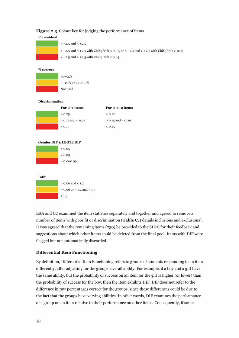
analyses were compiled onto a spreadsheet and a colour coding (‘traffic light’) system was

implemented to act as a broad indicator of each item’s performance (see Figure 2.3).

Key criteria for judging the performance of items were discrimination and measures of fit.

Percentage correct was noted but only informed a decision to eliminate an item if other

statistics were poor. Differential Item Functioning (DIF) for gender and Language

Background Other Than English (LBOTE) were also considered.

10

Figure 2.3 Colour key for judging the performance of items

Fit residual

> –2.5 and < +2.5

> –2.5 and < +2.5 with ChiSqProb < 0.05, or < –2.5 and > +2.5 with ChiSqProb > 0.05

< –2.5 and > +2.5 with ChiSqProb < 0.05

% correct

40–95%

0–40% or 95–100%

Not used

Discrimination

For 0–1 items For 0–1–2 items

> 0.25 > 0.20

> 0.15 and < 0.25 > 0.15 and < 0.20

< 0.15 < 0.15

Gender DIF & LBOTE DIF

> 0.05

< 0.05

< 0.000 09

Infit

> 0.06 and < 1.2

< 0.06 or > 1.2 and < 1.3

> 1.3

EAA and CC examined the item statistics separately and together and agreed to remove a

number of items with poor fit or discrimination (Table C.1 details inclusions and exclusions).

It was agreed that the remaining items (230) be provided to the SLRC for their feedback and

suggestions about which other items could be deleted from the final pool. Items with DIF were

flagged but not automatically discarded.

Differential Item Functioning

By definition, Differential Item Functioning refers to groups of students responding to an item

differently, after adjusting for the groups’ overall ability. For example, if a boy and a girl have

the same ability, but the probability of success on an item for the girl is higher (or lower) than

the probability of success for the boy, then the item exhibits DIF. DIF does not refer to the

difference in raw percentages correct for the groups, since these differences could be due to

the fact that the groups have varying abilities. In other words, DIF examines the performance

of a group on an item relative to their performance on other items. Consequently, if some

11

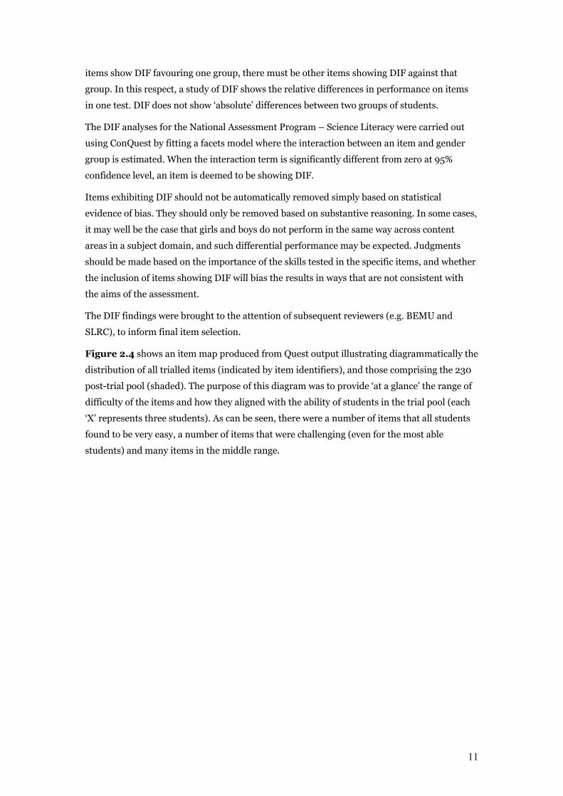
items show DIF favouring one group, there must be other items showing DIF against that

group. In this respect, a study of DIF shows the relative differences in performance on items

in one test. DIF does not show ‘absolute’ differences between two groups of students.

The DIF analyses for the National Assessment Program – Science Literacy were carried out

using ConQuest by fitting a facets model where the interaction between an item and gender

group is estimated. When the interaction term is significantly different from zero at 95%

confidence level, an item is deemed to be showing DIF.

Items exhibiting DIF should not be automatically removed simply based on statistical

evidence of bias. They should only be removed based on substantive reasoning. In some cases,

it may well be the case that girls and boys do not perform in the same way across content

areas in a subject domain, and such differential performance may be expected. Judgments

should be made based on the importance of the skills tested in the specific items, and whether

the inclusion of items showing DIF will bias the results in ways that are not consistent with

the aims of the assessment.

The DIF findings were brought to the attention of subsequent reviewers (e.g. BEMU and

SLRC), to inform final item selection.

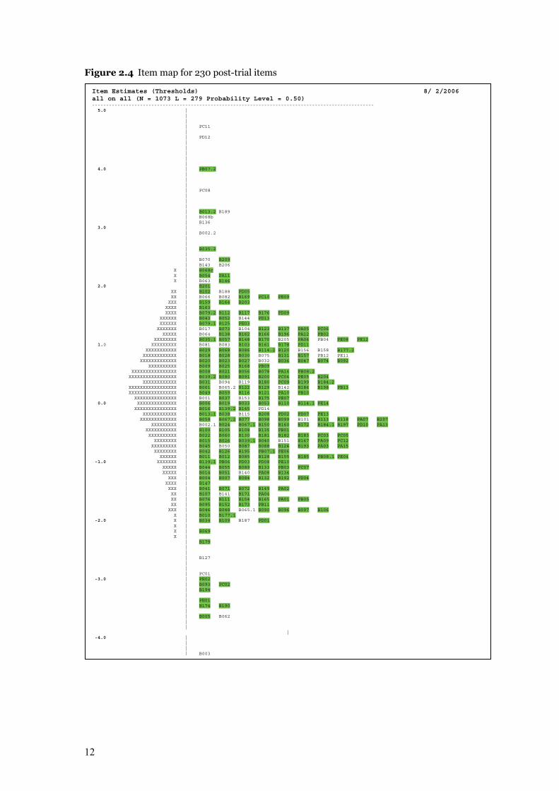
Figure 2.4 shows an item map produced from Quest output illustrating diagrammatically the

distribution of all trialled items (indicated by item identifiers), and those comprising the 230

post-trial pool (shaded). The purpose of this diagram was to provide ‘at a glance’ the range of

difficulty of the items and how they aligned with the ability of students in the trial pool (each

‘X’ represents three students). As can be seen, there were a number of items that all students

found to be very easy, a number of items that were challenging (even for the most able

students) and many items in the middle range.

12

Figure 2.4 Item map for 230 post-trial items

Item Estimates (Thresholds) 8/ 2/2006 all on all (N = 1073 L = 279 Probability Level = 0.50) ---------------------------------------------------------------------------------------------------- 5.0 | | | | PC11 | | PD12 | | | | | 4.0 | PB07.2 | | | | PC08 | | | | B013.2 B189 | B068b | B136 3.0 | | B002.2 | | | B035.2 | | B070 B209 | B143 B206 X | B068c X | B054 PA11 X | B063 B146 2.0 | B201 XX | B102 B188 PD05 XX | B066 B082 B169 PC10 PE09 XXX | B159 B164 B203 XXXX | B163 XXXX | B079.2 B112 B117 B176 PD09 XXXXXX | B043 B052 B144 PD13 XXXXXX | B079.1 B125 PE03 XXXXXXX | B017 B073 B104 B123 B137 PA05 PC06 XXXXX | B064 B138 B162 B166 B196 PA12 PB02 XXXXXXXX | B035.1 B057 B148 B170 B205 PA06 PB04 PE08 PE12 1.0 XXXXXXXXX | B081 B083 B103 B161 B178 PD11 XXXXXXXXXXX | B029 B068 B086 B114.2 B120 B156 B158 B177.2 XXXXXXXXXXXX | B018 B028 B030 B075 B131 B157 PB12 PE11 XXXXXXXXXXXXX | B020 B023 B027 B032 B036 B047 B074 B092 XXXXXXXXXX | B009 B025 B168 PB09 XXXXXXXXXXXXXXXX | B008 B021 B056 B078 PA14 PB08.2 XXXXXXXXXXXXXXXXX | B039.2 B080 B091 B200 PC04 PE05 B204 XXXXXXXXXXXX | B031 B094 B119 B180 PC09 B199 B184.2 XXXXXXXXXXXXXXXXX | B061 B065.2 B122 B129 B142 B186 B198 PB13 XXXXXXXXXXXXXXXXX | B049 B059 B116 B121 PA10 PB10 XXXXXXXXXXXXXXX | B001 B037 B153 B175 PE07 0.0 XXXXXXXXXXXXXX | B006 B019 B033 B053 B110 B114.1 PE14 XXXXXXXXXXXXXXX | B016 B139.2 B145 PD14 XXXXXXXXXXXX | B013.1 B038 B115 B208 PD02 PD07 PE13 XXXXXXXXXXXXX | B058 B067.2 B077 B098 B099 B101 B113 B118 PA07 B207 XXXXXXXXX | B002.1 B024 B067.1 B150 B160 B172 B184.1 B197 PD10 PA13 XXXXXXXXXXX | B100 B105 B108 B135 PB01 XXXXXXXXXX | B022 B060 B130 B181 B182 B183 PC03 PC05 XXXXXXXX | B015 B026 B039.1 B040 B151 B167 PA09 PC12 XXXXXXXXX | B045 B050 B087 B088 B124 B193 PA03 PA15 XXXXXXXX | B042 B126 B195 PB07.1 PE06 XXXXXX | B011 B012 B085 B128 B155 B185 PB08.1 PE04 -1.0 XXXXXXX | B139.1 PB06 PD03 PD08 PE10 XXXXX | B044 B055 B089 B133 PB03 PC07 XXXXX | B014 B051 B140 PA08 B134 XXX | B004 B007 B084 B132 B192 PD04 XXXX | B147 XXX | B041 B071 B072 B149 PA02 XX | B107 B141 B171 PA04 XX | B076 B111 B154 B165 PA01 PB05 XX | B095 B152 B173 PB11 XXX | B046 B048 B065.1 B090 B096 B097 B106 X | B010 B177.1 -2.0 X | B034 B109 B187 PD01 X | X | B069 X | | B179 | | | B127 | | | PC01 -3.0 | PE02 | B093 PC02 | B194 | | PE01 | B174 B190 | | B005 B062 | |

| -4.0 | | | | B003

13

The range of item difficulty was approximately 10 logits for the pool of 230 items.

The range of items was examined and acceptable levels for item difficulty were proposed:

Table 2.5 Suggested logit range for acceptable difficulty for each level

Level 5 Level 4 Level 3 Level 2 Level 1

Location >1.0 0 to 2.0 –1.0 to 1.0 –2.0 to 0 < –2.0

Notes:

• For Level 5, the small number of cases precludes suggesting upper limit.

• For Level 1, the small number of cases precludes suggesting lower limit.

The purpose of proposing such levels was to check that levels initially ascribed to items were

confirmed by the data analysis: were Level 1 items the easiest items and were Level 5 items the

most difficult? Items that appeared to fall outside the proposed ranges were flagged for

further scrutiny of item demand and possible reclassification.

The entire analysis of trial items, including deleted items and comments, was provided to

BEMU for their reference.

2.4.2 Reports to trial schools Reports were developed and provided to schools that had participated in the trial. The reports

were received in schools in December 2005. They contained ten A4 sheets: one for each of the

ten test booklets used in the assessment. Individual students’ results were given for the test

booklet which they completed in the assessment. In addition there was a school report for

each of the practical tasks conducted by the school. An information sheet providing advice on

interpreting the reports was also included.

2.5 Item selection process for the final test Items that were retained after the trial process for further consideration as possible items for

the final test pool were provided to the SLRC via a website. Reviewers using a login and

password could examine each item and then rank it in order of priority for its inclusion in the

final test. There was a field available for comments. Reviewers could click tabs to open up

psychometric detail about the trial analysis, the stimulus, the key or marking guide and

acceptable responses for constructed response items. SLRC members could enlist groups of

people to review the items and then group the responses as the feedback from the jurisdiction

represented.

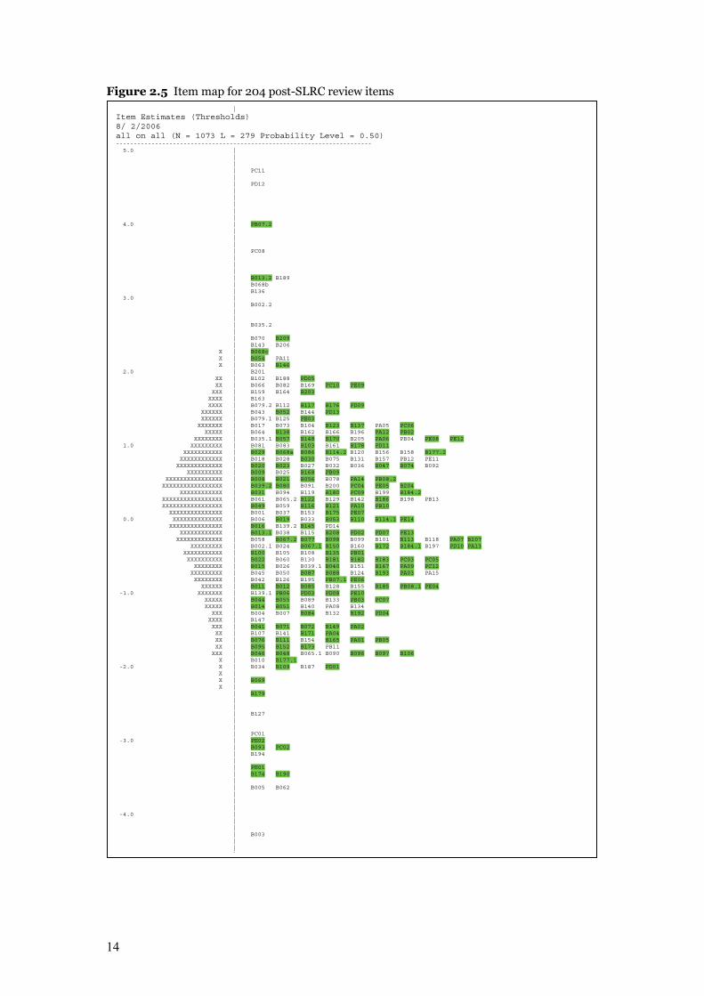
Figure 2.5 illustrates diagrammatically the distribution of all trialled items (indicated by

item identifiers) and those comprising the post-SLRC feedback pool items (shaded). As for

Figure 2.4, each ‘X’ represents three students in the trial.

14

Figure 2.5 Item map for 204 post-SLRC review items

|

Item Estimates (Thresholds) 8/ 2/2006 all on all (N = 1073 L = 279 Probability Level = 0.50) ------------------------------------------------------------------------ 5.0 | | | | PC11 | | PD12 | | | | | 4.0 | PB07.2 | | | | PC08 | | | | B013.2 B189 | B068b | B136 3.0 | | B002.2 | | | B035.2 | | B070 B209 | B143 B206 X | B068c X | B054 PA11 X | B063 B146 2.0 | B201 XX | B102 B188 PD05 XX | B066 B082 B169 PC10 PE09 XXX | B159 B164 B203 XXXX | B163 XXXX | B079.2 B112 B117 B176 PD09 XXXXXX | B043 B052 B144 PD13 XXXXXX | B079.1 B125 PE03 XXXXXXX | B017 B073 B104 B123 B137 PA05 PC06 XXXXX | B064 B138 B162 B166 B196 PA12 PB02 XXXXXXXX | B035.1 B057 B148 B170 B205 PA06 PB04 PE08 PE12 1.0 XXXXXXXXX | B081 B083 B103 B161 B178 PD11 XXXXXXXXXXX | B029 B068a B086 B114.2 B120 B156 B158 B177.2 XXXXXXXXXXXX | B018 B028 B030 B075 B131 B157 PB12 PE11 XXXXXXXXXXXXX | B020 B023 B027 B032 B036 B047 B074 B092 XXXXXXXXXX | B009 B025 B168 PB09

XXXXXXXXXXXXXXXX | B008 B021 B056 B078 PA14 PB08.2 XXXXXXXXXXXXXXXXX | B039.2 B080 B091 B200 PC04 PE05 B204

XXXXXXXXXXXX | B031 B094 B119 B180 PC09 B199 B184.2 XXXXXXXXXXXXXXXXX | B061 B065.2 B122 B129 B142 B186 B198 PB13 XXXXXXXXXXXXXXXXX | B049 B059 B116 B121 PA10 PB10 XXXXXXXXXXXXXXX | B001 B037 B153 B175 PE07 0.0 XXXXXXXXXXXXXX | B006 B019 B033 B053 B110 B114.1 PE14 XXXXXXXXXXXXXXX | B016 B139.2 B145 PD14 XXXXXXXXXXXX | B013.1 B038 B115 B208 PD02 PD07 PE13

XXXXXXXXXXXXX | B058 B067.2 B077 B098 B099 B101 B113 B118 PA07 B207 XXXXXXXXX | B002.1 B024 B067.1 B150 B160 B172 B184.1 B197 PD10 PA13 XXXXXXXXXXX | B100 B105 B108 B135 PB01 XXXXXXXXXX | B022 B060 B130 B181 B182 B183 PC03 PC05 XXXXXXXX | B015 B026 B039.1 B040 B151 B167 PA09 PC12 XXXXXXXXX | B045 B050 B087 B088 B124 B193 PA03 PA15 XXXXXXXX | B042 B126 B195 PB07.1 PE06 XXXXXX | B011 B012 B085 B128 B155 B185 PB08.1 PE04 -1.0 XXXXXXX | B139.1 PB06 PD03 PD08 PE10 XXXXX | B044 B055 B089 B133 PB03 PC07 XXXXX | B014 B051 B140 PA08 B134 XXX | B004 B007 B084 B132 B192 PD04 XXXX | B147 XXX | B041 B071 B072 B149 PA02 XX | B107 B141 B171 PA04 XX | B076 B111 B154 B165 PA01 PB05 XX | B095 B152 B173 PB11 XXX | B046 B048 B065.1 B090 B096 B097 B106 X | B010 B177.1 -2.0 X | B034 B109 B187 PD01 X | X | B069 X | | B179 | | | B127 | | | PC01 -3.0 | PE02 | B093 PC02 | B194 | | PE01 | B174 B190 | | B005 B062 | | | -4.0 | | | | B003 | |

|

15

EAA and CC met to review the SLRC feedback and further reduced the item pool. In addition,

EAA and CC independently developed draft final lists of preferred test items for 2006 which

were then exchanged and compared. The final pool containing 110 items was agreed as

reflecting the best balance of items against the original specifications.

A final pool of potential test items was presented to an SLRC meeting and approved for use in

the 2006 testing. The final pool included 11 link items from 2003 from the 18 that had been

used in the trial (see Appendix C).

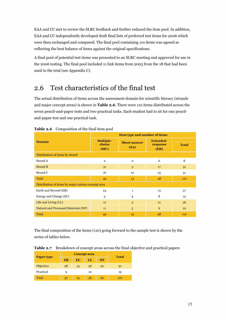
2.6 Test characteristics of the final test The actual distribution of items across the assessment domain for scientific literacy (strands

and major concept areas) is shown in Table 2.6. There were 110 items distributed across the

seven pencil-and-paper tests and two practical tasks. Each student had to sit for one pencil-

and-paper test and one practical task.

Table 2.6 Composition of the final item pool

Item type and number of items

Domain Multiple-choice

(MC)

Short-answer

(SA)

Extended-response

(ER) Total

Distribution of items by strand

Strand A 2 0 6 8

Strand B 31 3 17 51

Strand C 16 10 25 51

Total 49 13 48 110

Distribution of items by major science concept area

Earth and Beyond (EB) 23 1 13 37

Energy and Change (EC) 3 4 8 15

Life and Living (LL) 12 3 21 36

Natural and Processed Materials (NP) 11 5 6 22

Total 49 13 48 110

The final composition of the items (110) going forward to the sample test is shown by the

series of tables below.

Table 2.7 Breakdown of concept areas across the final objective and practical papers

Concept area Paper type

EB EC LL NP Total

Objective 28 15 26 22 91

Practical 9 10 19

Total 37 15 36 22 110

16

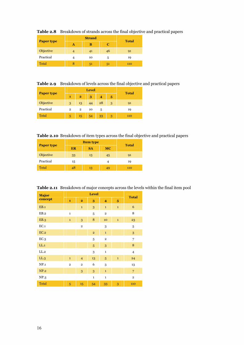
Table 2.8 Breakdown of strands across the final objective and practical papers

Strand Paper type

A B C Total

Objective 4 41 46 91

Practical 4 10 5 19

Total 8 51 51 110

Table 2.9 Breakdown of levels across the final objective and practical papers

Level Paper type

1 2 3 4 5 Total

Objective 3 13 44 28 3 91

Practical 2 2 10 5 19

Total 5 15 54 33 3 110

Table 2.10 Breakdown of item types across the final objective and practical papers

Item type Paper type

ER SA MC Total

Objective 33 13 45 91

Practical 15 4 19

Total 48 13 49 110

Table 2.11 Breakdown of major concepts across the levels within the final item pool

Level Major concept 1 2 3 4 5

Total

EB.1 1 3 1 1 6

EB.2 1 5 2 8

EB.3 1 3 8 10 1 23

EC.1 2 3 5

EC.2 2 1 3

EC.3 5 2 7

LL.1 5 3 8

LL.2 3 1 4

LL.3 1 4 13 5 1 24

NP.1 2 2 6 3 13

NP.2 3 3 1 7

NP.3 1 1 2

Total 5 15 54 33 3 110

17

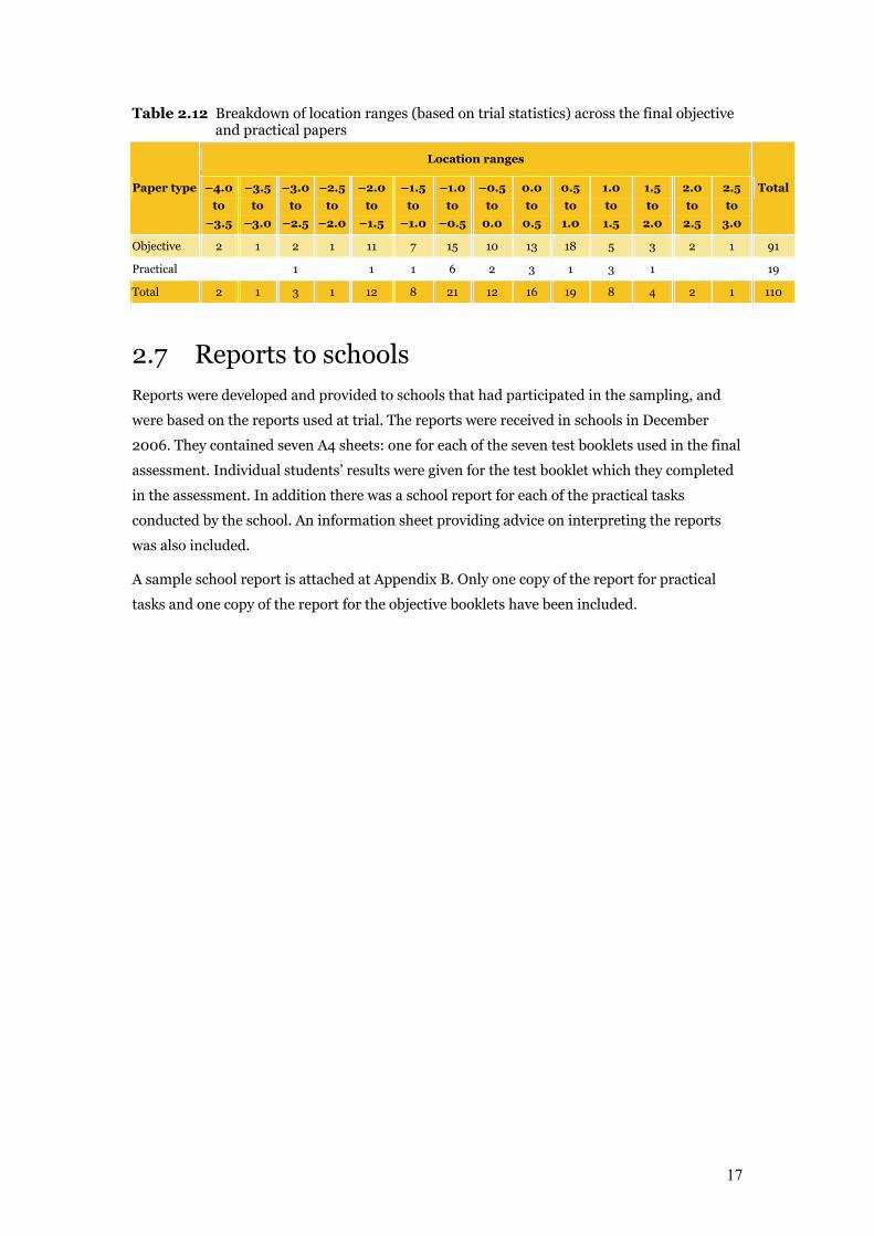
Table 2.12 Breakdown of location ranges (based on trial statistics) across the final objective and practical papers

Location ranges

Paper type –4.0

to

–3.5

–3.5

to

–3.0

–3.0

to

–2.5

–2.5

to

–2.0

–2.0

to

–1.5

–1.5

to

–1.0

–1.0

to

–0.5

–0.5

to

0.0

0.0

to

0.5

0.5

to

1.0

1.0

to

1.5

1.5

to

2.0

2.0

to

2.5

2.5

to

3.0

Total

Objective 2 1 2 1 11 7 15 10 13 18 5 3 2 1 91

Practical 1 1 1 6 2 3 1 3 1 19

Total 2 1 3 1 12 8 21 12 16 19 8 4 2 1 110

2.7 Reports to schools Reports were developed and provided to schools that had participated in the sampling, and

were based on the reports used at trial. The reports were received in schools in December

2006. They contained seven A4 sheets: one for each of the seven test booklets used in the final

assessment. Individual students’ results were given for the test booklet which they completed

in the assessment. In addition there was a school report for each of the practical tasks

conducted by the school. An information sheet providing advice on interpreting the reports

was also included.

A sample school report is attached at Appendix B. Only one copy of the report for practical

tasks and one copy of the report for the objective booklets have been included.

18

Chapter 3 Sampling Procedures

3.1 Overview The desired (target) population for the National Assessment Program – Science Literacy

consisted of all students enrolled in Year 6 in Australian schools in 2006.

As defined in the tender specifications, the number of students sampled in each jurisdiction

was to be determined with the following considerations in mind:

It was desirable that the estimated mean scores for all jurisdictions were of similar precision.

While this was an ultimate goal, it was recognised that reduced sample sizes would be needed

for the smaller jurisdictions (i.e. ACT, NT and TAS). This is because most schools in the

smaller jurisdictions will need to participate to form a large enough sample. As there are a

number of national and international assessment projects implemented in Australia, many

schools from the smaller jurisdictions will need to participate in multiple assessment projects,

and consequently there will be too much administrative burden on the schools, particularly

for the smaller schools.

Due to budgetary constraints, the nationwide achieved sample was to be approximately 12 000

students located within approximately 600 schools throughout Australia.

Accordingly, the 2006 sample differed from that drawn in 2003 in the following ways:

The sample frame, by definition, is more closely aligned to the national desired population

than the sample frame in 2003, since the 2006 sample frame contained very small and very

remote schools that were excluded in 2003.

Target sample sizes across the jurisdictions have been determined so that the precisions of

estimates are as similar across jurisdictions as possible.

19

ACT, TAS and NT all had smaller sample sizes compared to other States, but their sample

sizes were comparable or larger than their corresponding sample sizes in 2003.

The target sample sizes for the larger jurisdictions (NSW, VIC, SA, WA and QLD) were

reduced in 2006 compared to those of 2003.

The total achieved sample size for 2006 was 12 911. This was smaller than the total achieved

sample size for 2003 (14 172).

The sample design for the National Assessment Program – Science Literacy was a two-stage

stratified1 cluster sample. Stage 1 consisted of selecting schools that had Year 6 students. In

this stage, schools were selected with probabilities proportional to their measure of size2. This

selection procedure is referred to as ‘probability proportional to size’ (PPS) sampling. Stage 2

involved the random selection of an intact Year 6 class from the sampled schools selected in

Stage 1.

3.2 Target population The operational definition of the target population was a sampling frame which consisted of a

list of all Australian schools and their 2005 Year 6 enrolment sizes as supplied by BEMU.

Generally, large scale sampling surveys of this type include provisions for excluding schools

before sampling of schools takes place. This might be for reasons such as the school being

located in geographically remote locations or of extremely small size. This approach was taken

in 2003. In 2006, it was deemed desirable to include as many schools in the defined

population as possible. Essentially this meant there were to be no school-level exclusions from

the supplied sampling frame prior to sample selection. As such, the nationally defined

population for the National Assessment Program – Science Literacy 2006 was more inclusive

than the 2003 defined population3. However, the inclusion of schools that would previously

have been excluded was expected to result in an increased non-response rate for 2006

compared to 2003. Consequently, a slightly inflated sample size would be required to deal

with this expected increase in non-response rate at the school level, so that the actual achieved

number of schools and students in the sample was adequate.

Additionally, schools were excluded in 2003 if their estimated enrolment size was fewer than

five students because group work required a minimum of five students to complete the

practical task (PSAP 2003, section 2.3). In contrast, in 2006, if a small school (fewer than five

1 Stratification involves ordering and grouping schools according to different school characteristics (e.g. State, sector, urban/rural) which helps ensure adequate coverage of all desired school types in the sample.

2 The school measure of size is related to estimated enrolment size of Year 6 students at the school.

3 In 2003 very small and very remote schools were excluded from the sample frame, but this was not the case in 2006.

20

students) was selected, then this school was only required to complete the paper-and-pencil

tasks. In this way, very small schools were not excluded from the survey.

3.3 School and student non-participation In large scale surveys of this kind it is important to document reasons for non-participation so

that interpretations of the main findings from the study can be appropriately made within the

contexts of the survey. Examples of non-participation include remoteness, parental objection

etc. As for the 2003 survey, the 2006 study made provisions to document the reasons for

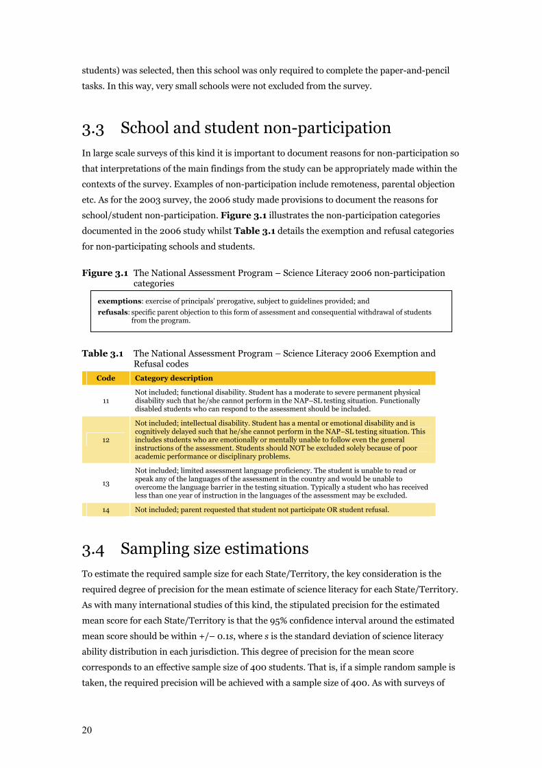
school/student non-participation. Figure 3.1 illustrates the non-participation categories

documented in the 2006 study whilst Table 3.1 details the exemption and refusal categories

for non-participating schools and students.

Figure 3.1 The National Assessment Program – Science Literacy 2006 non-participation categories

Table 3.1 The National Assessment Program – Science Literacy 2006 Exemption and Refusal codes

Code Category description

11 Not included; functional disability. Student has a moderate to severe permanent physical disability such that he/she cannot perform in the NAP–SL testing situation. Functionally disabled students who can respond to the assessment should be included.

12

Not included; intellectual disability. Student has a mental or emotional disability and is cognitively delayed such that he/she cannot perform in the NAP–SL testing situation. This includes students who are emotionally or mentally unable to follow even the general instructions of the assessment. Students should NOT be excluded solely because of poor academic performance or disciplinary problems.

13

Not included; limited assessment language proficiency. The student is unable to read or speak any of the languages of the assessment in the country and would be unable to overcome the language barrier in the testing situation. Typically a student who has received less than one year of instruction in the languages of the assessment may be excluded.

14 Not included; parent requested that student not participate OR student refusal.

3.4 Sampling size estimations To estimate the required sample size for each State/Territory, the key consideration is the

required degree of precision for the mean estimate of science literacy for each State/Territory.

As with many international studies of this kind, the stipulated precision for the estimated

mean score for each State/Territory is that the 95% confidence interval around the estimated

mean score should be within +/– 0.1s, where s is the standard deviation of science literacy

ability distribution in each jurisdiction. This degree of precision for the mean score

corresponds to an effective sample size of 400 students. That is, if a simple random sample is

taken, the required precision will be achieved with a sample size of 400. As with surveys of

exemptions: exercise of principals’ prerogative, subject to guidelines provided; and

refusals: specific parent objection to this form of assessment and consequential withdrawal of students from the program.

21

this kind, simple random samples are usually not used because of logistical difficulties in

administering tests in potentially 400 different locations. Consequently, less efficient

sampling methods will be used, and the required sample size will need to be larger than 400.

More specifically, when the design effect4 of the sample design is taken into account, the

required sample size for each State/Territory is given by:

nc = n* deff (1)

where nc is the required sample size, n * is the effective sample size, and deff is the design

effect.

In the 2006 National Assessment Program – Science Literacy proposal, the required sample

size was set at 12 000 students (down from 14 000 in 2003).

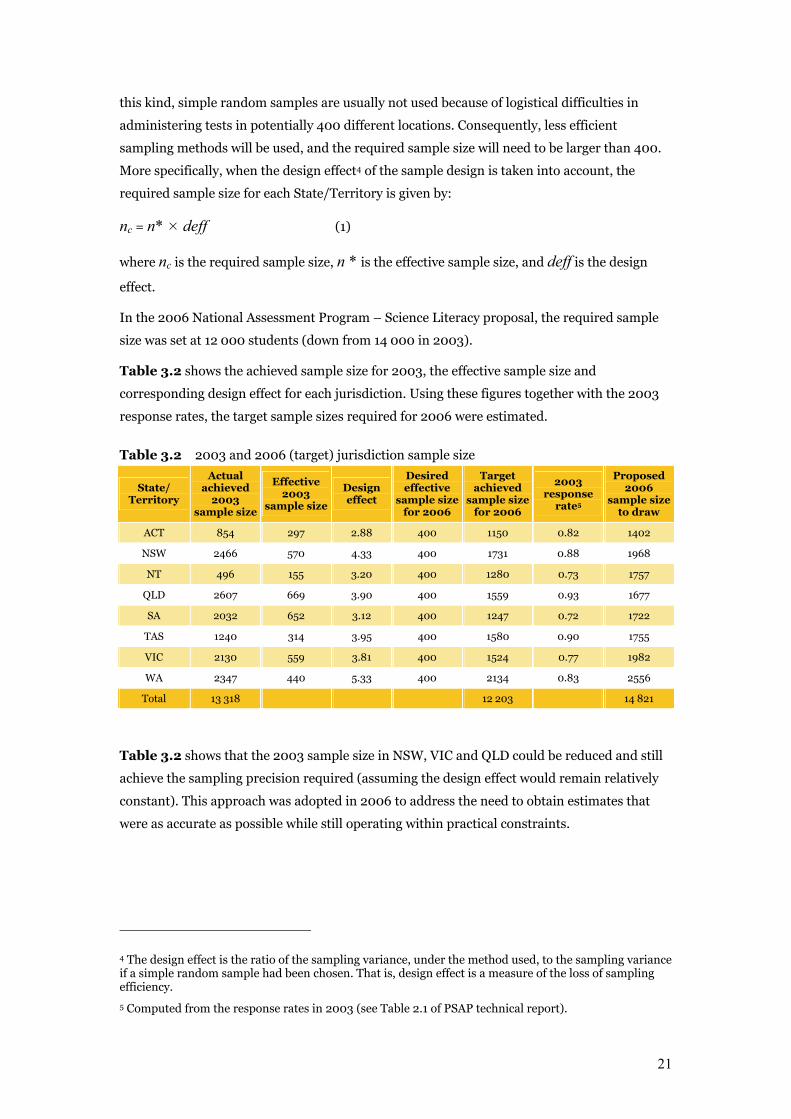
Table 3.2 shows the achieved sample size for 2003, the effective sample size and

corresponding design effect for each jurisdiction. Using these figures together with the 2003

response rates, the target sample sizes required for 2006 were estimated.

Table 3.2 2003 and 2006 (target) jurisdiction sample size

State/ Territory

Actual achieved

2003 sample size

Effective 2003

sample size

Design effect

Desired effective

sample size for 2006

Target achieved

sample size for 2006

2003 response

rate5

Proposed 2006

sample size to draw

ACT 854 297 2.88 400 1150 0.82 1402

NSW 2466 570 4.33 400 1731 0.88 1968

NT 496 155 3.20 400 1280 0.73 1757

QLD 2607 669 3.90 400 1559 0.93 1677

SA 2032 652 3.12 400 1247 0.72 1722

TAS 1240 314 3.95 400 1580 0.90 1755

VIC 2130 559 3.81 400 1524 0.77 1982

WA 2347 440 5.33 400 2134 0.83 2556

Total 13 318 12 203 14 821

Table 3.2 shows that the 2003 sample size in NSW, VIC and QLD could be reduced and still

achieve the sampling precision required (assuming the design effect would remain relatively

constant). This approach was adopted in 2006 to address the need to obtain estimates that

were as accurate as possible while still operating within practical constraints.

4 The design effect is the ratio of the sampling variance, under the method used, to the sampling variance if a simple random sample had been chosen. That is, design effect is a measure of the loss of sampling efficiency.

5 Computed from the response rates in 2003 (see Table 2.1 of PSAP technical report).

22

The calculation of the 2006 proposed target sample size was based on the observed 2003

participation rates and design effects for each of the jurisdictions. There was some suggestion

that the participation rates for 2006 would be higher than for 2003, as schools were given

directives in 2006 from the government about the importance of participation. However,

participation rates were not anticipated to increase overall from 2003 given that the defined

population included schools that would have been excluded from the sampling frame in 2003.

It was not known how stable the estimated 2003 design effects would be and, as such,

approximate averages were used to estimate target sample sizes rather than specific

jurisdiction values. In 2003 the average observed design effect was 3.815 across the

jurisdictions and the average response rate was 82%. These figures were used to guide the

computation of desired 2006 sample sizes. That is, the proposed target sample size for each

jurisdiction assumed that the overall response rate was equal to 85% and there was a design

effect equal to 4.

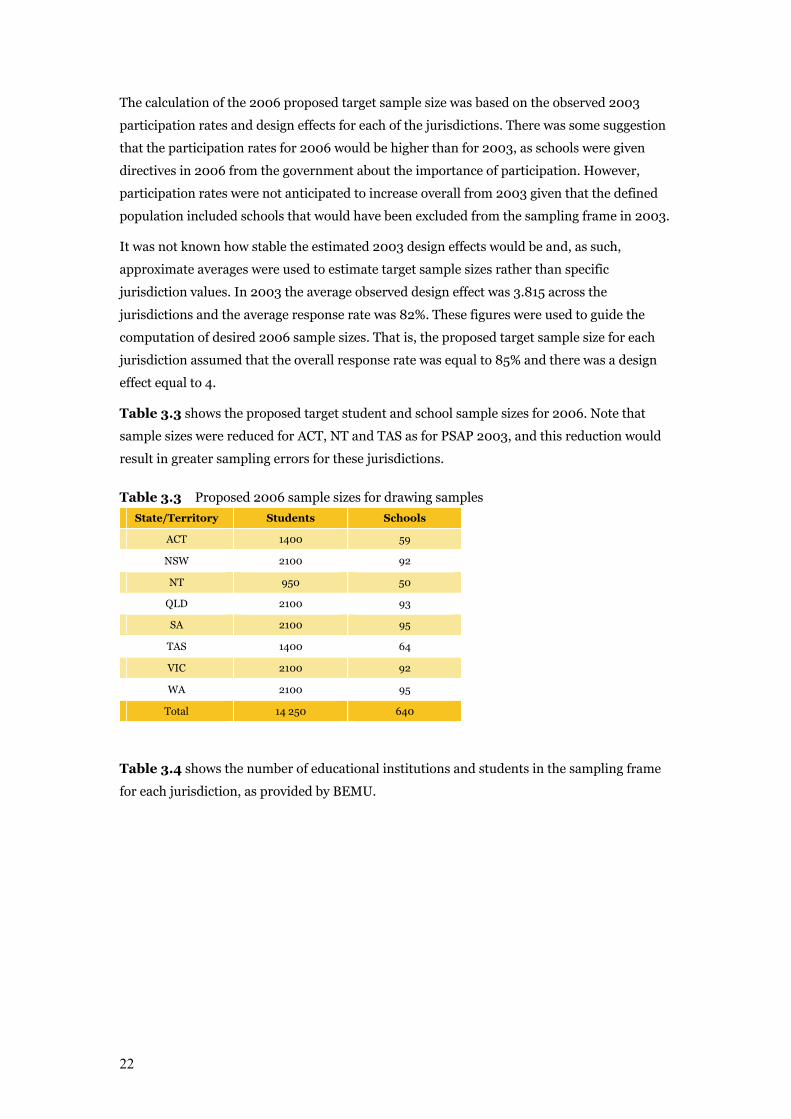
Table 3.3 shows the proposed target student and school sample sizes for 2006. Note that

sample sizes were reduced for ACT, NT and TAS as for PSAP 2003, and this reduction would

result in greater sampling errors for these jurisdictions.

Table 3.3 Proposed 2006 sample sizes for drawing samples

State/Territory Students Schools

ACT 1400 59

NSW 2100 92

NT 950 50

QLD 2100 93

SA 2100 95

TAS 1400 64

VIC 2100 92

WA 2100 95

Total 14 250 640

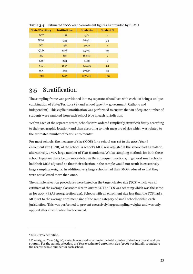
Table 3.4 shows the number of educational institutions and students in the sampling frame

for each jurisdiction, as provided by BEMU.

23

Table 3.4 Estimated 2006 Year 6 enrolment figures as provided by BEMU

State/Territory Institutions Students Student %

ACT 108 4364 2

NSW 2345 86 961 33

NT 148 3002 1

QLD 1378 55 712 21

SA 618 18 837 7

TAS 223 6462 2

VIC 1805 64 405 24

WA 872 27 673 10

Total 7497 267 416 100

3.5 Stratification The sampling frame was partitioned into 24 separate school lists with each list being a unique

combination of State/Territory (8) and school type (3 – government, Catholic and

independent). This explicit stratification was performed to ensure that an adequate number of

students were sampled from each school type in each jurisdiction.

Within each of the separate strata, schools were ordered (implicitly stratified) firstly according

to their geographic location6 and then according to their measure of size which was related to

the estimated number of Year 6 enrolments7.

For most schools, the measure of size (MOS) for a school was set to the 2005 Year 6

enrolment size (ENR) of the school. A school’s MOS was adjusted if the school had a small or,

alternatively, a very large number of Year 6 students. Whilst sampling methods for both these

school types are described in more detail in the subsequent sections, in general small schools

had their MOS adjusted so that their selection in the sample would not result in excessively

large sampling weights. In addition, very large schools had their MOS reduced so that they

were not selected more than once.

The sample selection procedures were based on the target cluster size (TCS) which was an

estimate of the average classroom size in Australia. The TCS was set at 25 which was the same

as for 2003 (PSAP 2003, section 2.2). Schools with an enrolment size less than the TCS had a

MOS set to the average enrolment size of the same category of small schools within each

jurisdiction. This was performed to prevent excessively large sampling weights and was only

applied after stratification had occurred.

6 MCEETYA definition.

7 The original Year 6 (gr06) variable was used to estimate the total number of students overall and per stratum. For the sample selection, the Year 6 estimated enrolment size (gr06) was initially rounded to the nearest whole number for each school.

24

3.5.1 Small schools If a large number of schools were sampled that had enrolment sizes (ENR) less than the TCS,

then the actual number of students sampled could be less than the overall target sample.

Schools with enrolment sizes less than the TCS are classified as small schools in both PISA

(2003) and TIMSS (2003). Both studies have different approaches for the treatment of small

schools within the sampling frame. In 2006 National Assessment Program – Science Literacy,

PISA (2003) guidelines were utilised for classifying and stratifying small schools, whilst an

adapted version of TIMSS’ (2003) treatment of small school MOS values was used.

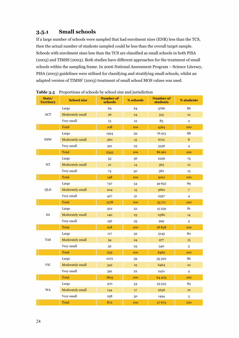
Table 3.5 Proportions of schools by school size and jurisdiction

State/ Territory

School size Number of

schools % schools

Number of students

% students

Large 69 64 3766 86

Moderately small 26 24 515 12 ACT

Very small 13 12 83 2

Total 108 100 4364 100

Large 1394 59 76 913 88

Moderately small 360 15 6712 8 NSW

Very small 591 25 3336 4

Total 2345 100 86 961 100

Large 53 36 2256 75

Moderately small 21 14 363 12 NT

Very small 74 50 382 13

Total 148 100 3001 100

Large 747 54 49 652 89

Moderately small 204 15 3662 7 QLD

Very small 427 31 2397 4

Total 1378 100 55 711 100

Large 322 52 15 259 81

Moderately small 140 23 2580 14 SA

Very small 156 25 999 5

Total 618 100 18 838 100

Large 117 52 5145 80

Moderately small 54 24 977 15 TAS

Very small 52 23 340 5

Total 223 100 6462 100

Large 1072 59 55 520 86

Moderately small 342 19 6464 10 VIC

Very small 391 22 2421 4

Total 1805 100 64 405 100

Large 470 54 23 523 85

Moderately small 144 17 2656 10 WA

Very small 258 30 1494 5

Total 872 100 27 673 100

25

As a preliminary exercise, schools were classified into different sizes according to PISA (2003,

p. 53) classification rules: Large (MOS >= 25) and Small schools which were sub-divided into

either Moderately Small (TCS/2 <= MOS < TCS) or Very Small (MOS < TCS/2) schools.

Table 3.5 shows the proportions of Large, Moderately Small and Very Small schools within

each jurisdiction. It can be seen that there are many small schools in each jurisdiction. As

such, it was important that an appropriate strategy was utilised to prevent an over-selection

of small schools, which would have resulted in a sample size lower than the desired target

sample size.

PISA (2003) guidelines were utilised for classifying and stratifying small schools, which

involved deliberately under-sampling small schools and slightly over-sampling large schools.

This ensured that small schools were represented in the sample while still achieving an

adequate overall student sample size without substantially increasing the total number of

schools sampled (see OECD 2003, pp. 53–57).

The MOS for a small school was set to the average ENR of all schools within the same explicit

stratum and school size category. This strategy was adapted from the TIMSS (2003) approach

to ensure that selection of very small schools would not result in excessively large sampling

weights (see IEA 2003, pp. 119–120, section 5.4.1).

3.5.2 Very large schools Selecting schools with a probability proportional to size (PPS) can result in a school being

sampled more than once if its ENR is sufficiently large. This can occur when the school

enrolment size is larger than the explicit stratum sampling interval. To overcome this, very

large schools had their MOS set equal to the size of the sampling interval of the explicit

stratum that the school belonged to (an option that was utilised in TIMSS 2003, p. 120,

section 5.4.2).

3.6 Replacement schools Replacement schools were included in the sample to help overcome problems in relation to

school non-participation. For example, if the non-participation rate is high, then the target

sample sizes will not be achieved. Further, if non-participating schools tend to be lower

performing schools, then a bias in the estimated achievement levels will likely occur.

If a school did not participate for some reason, then a replacement school was selected for

inclusion in the sample. Replacement schools were assigned as per PISA 2003 procedures

(p. 60). That is, for a sampled school, the school immediately following it in the sampling

frame was assigned as the first replacement school for it, and the school immediately

preceding it was assigned as the second replacement school.

26

3.7 Class selection One classroom containing Year 6 students was sampled per school. Classrooms generally had

equal probabilities of selection. The overall procedure for class selection was as follows:

1 each class in a school was assigned a random number

2 the classes in a school were ordered by the assigned random numbers

3 the first class on each school’s ordered list was chosen for the sample.

Small classes

Quite often schools had multilevel or remedial classes that contained small numbers of Year 6

students. If many of these small classes are selected, the total sample size will likely be less

than the original target sample size, as the class size for these classes is much smaller than the

average class size of 25 which was used as the basis for the estimation of the number of

schools and classes to be selected.

To overcome this problem, a strategy was employed that built on both TIMSS (2003) and the

procedures used for the National Assessment Program (literacy and numeracy trial 2006)8.

Classes with fewer than 20 students were combined with another class at the same school. The

resulting pseudo-class was considered a single classroom for sampling purposes.

Pseudo-classes were created from a maximum of two intact classrooms to minimise the

administrative burden on schools and each pseudo-class comprised no more than 30 students

in total. The formal procedure for creating pseudo-classes was:

(1) randomly order the school class list

(2) starting from the first class in the list, check to see if the class has fewer than 20

students (small-class)

(3) combine the small-class with the next class where the resulting sum is not larger than

30 students

(4) continue through the ordered school list until all classes have been

checked/combined.

8 See NAP WEBSITE MANUAL V02 22_02_06.pdf.

27

Using this method, the resulting sample size was close to, but slightly less than, the original

proposed sample size (approx 97%). Because of the structure of school classes, it was possible

a small class (fewer than 20 students) could potentially not be combined into a pseudo-class

(e.g. because there was only one remedial class at the school and all other classes were

standard size). In these cases, the second class in the list was taken, provided that:

(1) the second class was larger than the first class, and

(2) the second class had more than 20 students.

This procedure for handling small classes means that the resulting sample size will closely

match the proposed sample size. In these cases, however, classes are selected with unequal

probabilities, because the probability of selection depends on the number of classes, class

sizes and the probability of forming pseudo-classes. The estimation of appropriate sampling

weights to account for unequal probability of selection is covered in detail in Chapter 5,

Computation of Sampling Weights.

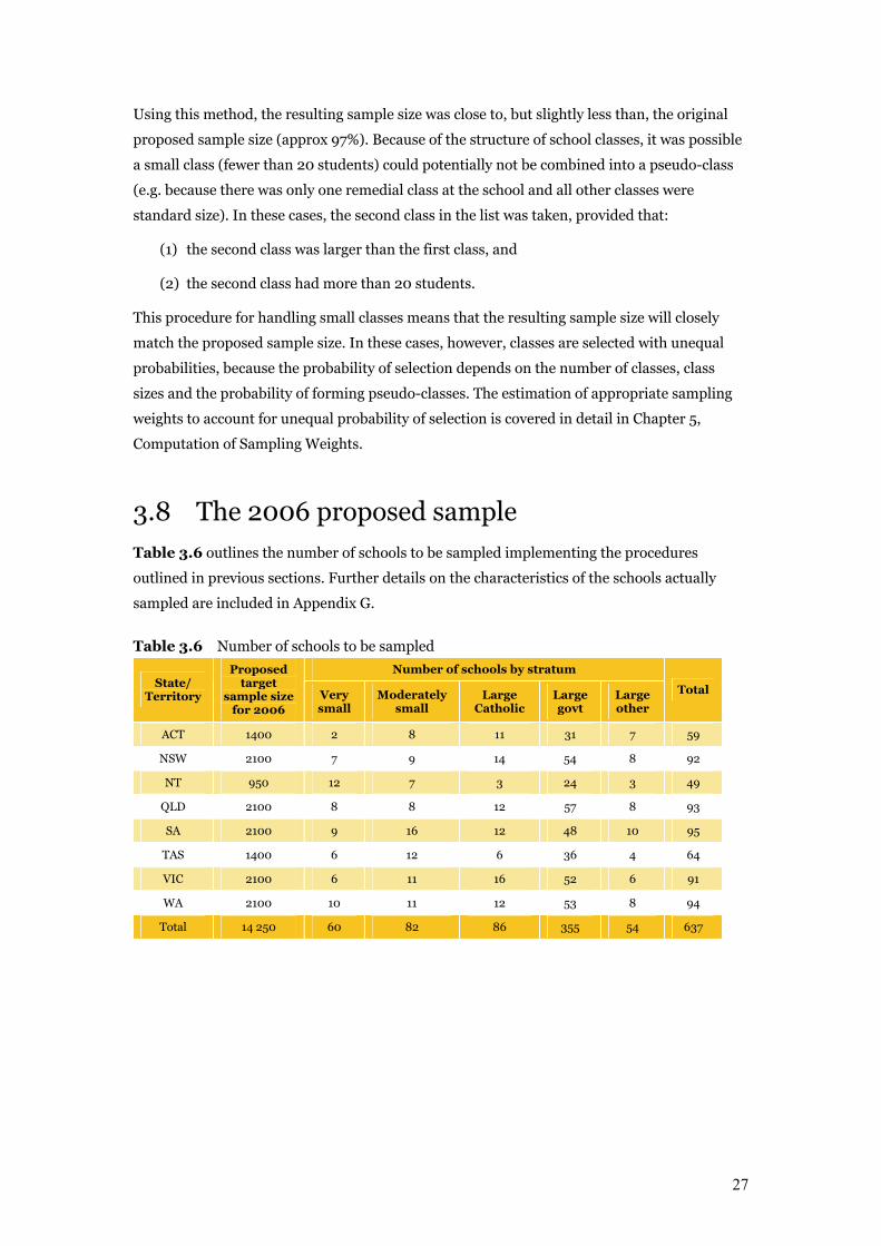
3.8 The 2006 proposed sample Table 3.6 outlines the number of schools to be sampled implementing the procedures

outlined in previous sections. Further details on the characteristics of the schools actually

sampled are included in Appendix G.

Table 3.6 Number of schools to be sampled

Number of schools by stratum State/

Territory

Proposed target

sample size for 2006

Very small

Moderately small

Large Catholic

Large govt

Large other

Total

ACT 1400 2 8 11 31 7 59

NSW 2100 7 9 14 54 8 92

NT 950 12 7 3 24 3 49

QLD 2100 8 8 12 57 8 93

SA 2100 9 16 12 48 10 95

TAS 1400 6 12 6 36 4 64

VIC 2100 6 11 16 52 6 91

WA 2100 10 11 12 53 8 94

Total 14 250 60 82 86 355 54 637

28

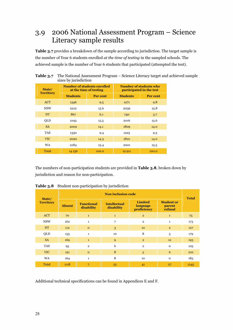
3.9 2006 National Assessment Program – Science Literacy sample results

Table 3.7 provides a breakdown of the sample according to jurisdiction. The target sample is

the number of Year 6 students enrolled at the time of testing in the sampled schools. The

achieved sample is the number of Year 6 students that participated (attempted the test).

Table 3.7 The National Assessment Program – Science Literacy target and achieved sample sizes by jurisdiction

Number of students enrolled at the time of testing

Number of students who participated in the test State/

Territory Students Per cent Students Per cent

ACT 1346 9.5 1271 9.8

NSW 2212 15.6 2039 15.8

NT 867 6.1 740 5.7

QLD 2195 15.5 2016 15.6

SA 2002 14.1 1809 14.0

TAS 1330 9.4 1225 9.5

VIC 2020 14.3 1810 14.0

WA 2184 15.4 2001 15.5

Total 14 156 100.0 12 911 100.0

The numbers of non-participation students are provided in Table 3.8, broken down by

jurisdiction and reason for non-participation.

Table 3.8 Student non-participation by jurisdiction

Non inclusion code

State/ Territory

Absent Functional disability

Intellectual disability

Limited language

proficiency

Student or parent refusal

Total

ACT 70 1 1 2 1 75

NSW 162 1 7 2 1 173

NT 112 0 3 10 2 127

QLD 155 1 10 8 5 179

SA 169 1 9 2 12 193

TAS 95 2 6 2 0 105

VIC 191 0 8 5 6 210

WA 164 1 8 10 0 183

Total 1118 7 52 41 27 1245

Additional technical specifications can be found in Appendices E and F.

29

Chapter 4 Test Administration Procedures and Data Preparation

4.1 Online registration of class/student lists In 2006 BEMU commissioned an online software application from Curriculum Corporation

called the Online Student Registration System (OSRS). School Contact Officers of schools

selected for the sample were informed that they were to register their students online or for a

few jurisdictions that this task had been done centrally. State and Territory Liaison Officers

were briefed in providing support to principals to use the site. OSRS was designed to capture

information that had previously been provided by students on the test book covers in 2003.

Pre-registration meant that test books could be overprinted with individual student details,

ensuring that every student received the correct test form and that student details were

correct. It should be noted, however, that much data that schools were requested to provide

on OSRS proved to be missing. Thus the data was incomplete when supplied for analysis

preventing the inclusion of some demographic variables in the item response model

(e.g. LBOTE).

4.2 Administering the tests to students The final assessments were administered to the sampled students in October 2006. The

participating schools were sent the following assessment materials: School Contact Officer’s

Manual; Test Administrator’s Manual; and the assessment instruments; together with the

appropriate practical materials for the particular task being undertaken.

30

The assessment instruments were administered to a sample consisting of 4.83% of the total

Australian Year 6 student population. Tests were administered on the following dates:

• 18 October 2006 – Northern Territory, Queensland, Tasmania

• 25 October 2006 – Australian Capital Territory, New South Wales, South Australia,

Victoria, Western Australia.

Students’ regular class teachers administered the tests to minimise disruption to the normal

class environment. Standardised administration procedures were developed and published in

the Test Administrator’s Manual. In all schools in which students were to complete the

assessment, teachers and school administrators were provided with the Manual. Detailed

instructions were also given in relation to the participation or exclusion of students with

disabilities and students from non-English speaking backgrounds.

The teachers were able to review the manual before the assessment date and raise questions

with the coordinators of the National Assessment Program – Science Literacy in their

jurisdiction. A toll-free telephone number was provided and also an email address if teachers

had any questions.

Teachers were required to complete a student participation form, confirming details about

any student who may have not participated or had been excluded (see Appendix D).

A quality-monitoring program was established to gauge the extent to which class teachers

followed the specified administration procedures. This involved trained monitors observing

the administration of the Assessment in a random sample of classes in 30 of the 630 schools

involved. The monitors reported conformity with the administration procedures.

4.3 Marking procedures The multiple-choice items had only one correct answer. The open-ended items required

students to construct their own responses. The open-ended items were further categorised

into those that required a single-word or short-sentence response and those that required a

more substantive response (referred to as ‘extended-response’ items). Some open-ended items

had polytomous scores. That is, students could score either one or two marks depending on

the quality or extent of their response.

Over half of the items were open-ended and required marking by trained markers. Some

involved single answers or phrases that could be marked objectively.

Marking Guides were prepared by EAA and CC. The marking team included experienced

teacher-markers employed by EAA. The markers participated in a four-hour training session

conducted by a member of the test construction team. The session involved formal

presentations by the trainers, followed by hands-on practice with sample student answer

books. In addition, the markers undertook a further two hours of marking in which a pair of

markers marked the same student answer books and moderators reconciled differences in

31

discussion with the markers. Markers were monitored constantly for reliability by having

samples of their student answer books check-marked by group leaders. In cases where there

were differences in scoring between markers and the group leaders, the scoring was

reconciled jointly in consultation with the professional leader. This procedure, coupled with

the intensive training at the beginning of the marking exercise, ensured that markers were

applying the scoring criteria consistently.

4.4 Data entry procedures The multiple-choice responses and teacher-marked scores were data processed. A validation

of the data processing was performed that ensured accuracy in data capture.

Scanning software was used to capture images of all the student responses. These have been

indexed and provided to BEMU for future reference.

Demographic information and information collected to determine student inclusion in the

testing population was collected from participating schools using the Student Participation

Form that had two parts: Part A was designed to collect information about the school

(including information about the number of students enrolled in Year 6 and the number of

classes in Year 6); and Part B collected relevant information about individual students.

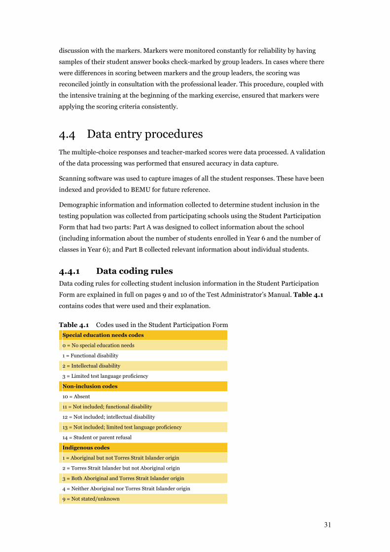
4.4.1 Data coding rules Data coding rules for collecting student inclusion information in the Student Participation

Form are explained in full on pages 9 and 10 of the Test Administrator’s Manual. Table 4.1

contains codes that were used and their explanation.

Table 4.1 Codes used in the Student Participation Form

Special education needs codes

0 = No special education needs

1 = Functional disability

2 = Intellectual disability

3 = Limited test language proficiency

Non-inclusion codes

10 = Absent

11 = Not included; functional disability

12 = Not included; intellectual disability

13 = Not included; limited test language proficiency

14 = Student or parent refusal

Indigenous codes

1 = Aboriginal but not Torres Strait Islander origin

2 = Torres Strait Islander but not Aboriginal origin

3 = Both Aboriginal and Torres Strait Islander origin

4 = Neither Aboriginal nor Torres Strait Islander origin

9 = Not stated/unknown

32

Chapter 5 Computation of Sampling Weights

The sampling weights calculated for the National Assessment Program – Science Literacy

were based on procedures detailed in TIMSS (IEA 2004), except for the computation of some

class weights. The procedures outlined in TIMSS are designed for several different sampling

scenarios. Only the procedures relevant to the National Assessment Program – Science

Literacy context are presented here.

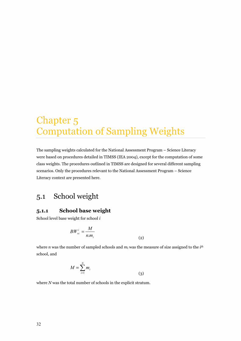
5.1 School weight

5.1.1 School base weight School level base weight for school i

i

isc mn

MBW.

= (2)

where n was the number of sampled schools and mi was the measure of size assigned to the ith

school, and

∑

=

=N

iimM

1 (3)

where N was the total number of schools in the explicit stratum.

33

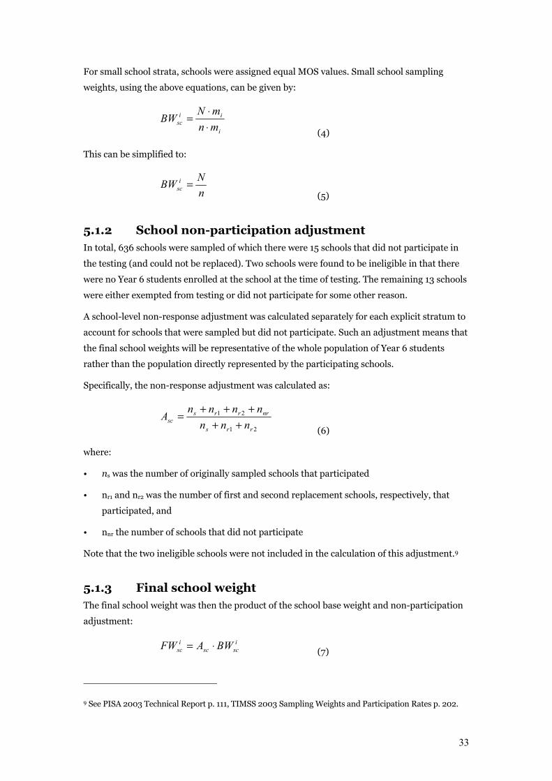
For small school strata, schools were assigned equal MOS values. Small school sampling

weights, using the above equations, can be given by:

i

iisc mn

mNBW⋅⋅

= (4)

This can be simplified to:

nNBW i

sc = (5)

5.1.2 School non-participation adjustment In total, 636 schools were sampled of which there were 15 schools that did not participate in

the testing (and could not be replaced). Two schools were found to be ineligible in that there

were no Year 6 students enrolled at the school at the time of testing. The remaining 13 schools

were either exempted from testing or did not participate for some other reason.

A school-level non-response adjustment was calculated separately for each explicit stratum to

account for schools that were sampled but did not participate. Such an adjustment means that

the final school weights will be representative of the whole population of Year 6 students

rather than the population directly represented by the participating schools.

Specifically, the non-response adjustment was calculated as:

21

21

rrs

nrrrssc nnn

nnnnA++

+++=

(6)

where:

• ns was the number of originally sampled schools that participated

• nr1 and nr2 was the number of first and second replacement schools, respectively, that

participated, and

• nnr the number of schools that did not participate

Note that the two ineligible schools were not included in the calculation of this adjustment.9

5.1.3 Final school weight The final school weight was then the product of the school base weight and non-participation

adjustment:

i

scsci

sc BWAFW ⋅= (7)

9 See PISA 2003 Technical Report p. 111, TIMSS 2003 Sampling Weights and Participation Rates p. 202.

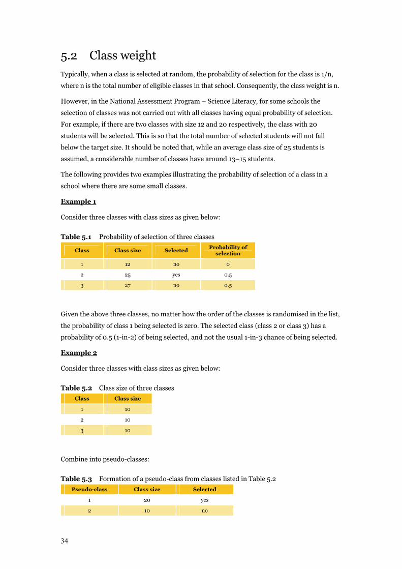
34

5.2 Class weight Typically, when a class is selected at random, the probability of selection for the class is 1/n,

where n is the total number of eligible classes in that school. Consequently, the class weight is n.

However, in the National Assessment Program – Science Literacy, for some schools the

selection of classes was not carried out with all classes having equal probability of selection.

For example, if there are two classes with size 12 and 20 respectively, the class with 20

students will be selected. This is so that the total number of selected students will not fall

below the target size. It should be noted that, while an average class size of 25 students is

assumed, a considerable number of classes have around 13–15 students.

The following provides two examples illustrating the probability of selection of a class in a

school where there are some small classes.

Example 1

Consider three classes with class sizes as given below:

Table 5.1 Probability of selection of three classes

Class Class size Selected Probability of

selection

1 12 no 0

2 25 yes 0.5

3 27 no 0.5

Given the above three classes, no matter how the order of the classes is randomised in the list,

the probability of class 1 being selected is zero. The selected class (class 2 or class 3) has a

probability of 0.5 (1-in-2) of being selected, and not the usual 1-in-3 chance of being selected.

Example 2

Consider three classes with class sizes as given below:

Table 5.2 Class size of three classes

Class Class size

1 10

2 10

3 10

Combine into pseudo-classes:

Table 5.3 Formation of a pseudo-class from classes listed in Table 5.2

Pseudo-class Class size Selected

1 20 yes

2 10 no

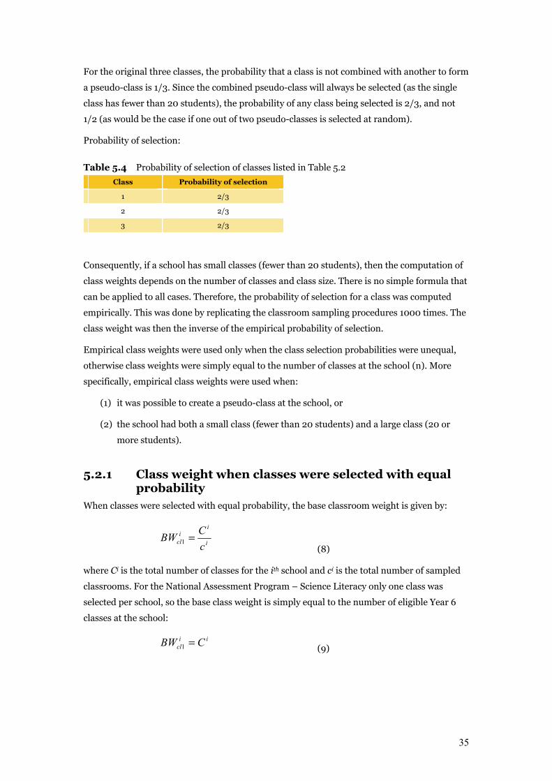
35

For the original three classes, the probability that a class is not combined with another to form

a pseudo-class is 1/3. Since the combined pseudo-class will always be selected (as the single

class has fewer than 20 students), the probability of any class being selected is 2/3, and not

1/2 (as would be the case if one out of two pseudo-classes is selected at random).

Probability of selection:

Table 5.4 Probability of selection of classes listed in Table 5.2

Class Probability of selection

1 2/3

2 2/3

3 2/3

Consequently, if a school has small classes (fewer than 20 students), then the computation of

class weights depends on the number of classes and class size. There is no simple formula that

can be applied to all cases. Therefore, the probability of selection for a class was computed

empirically. This was done by replicating the classroom sampling procedures 1000 times. The

class weight was then the inverse of the empirical probability of selection.

Empirical class weights were used only when the class selection probabilities were unequal,

otherwise class weights were simply equal to the number of classes at the school (n). More

specifically, empirical class weights were used when:

(1) it was possible to create a pseudo-class at the school, or

(2) the school had both a small class (fewer than 20 students) and a large class (20 or

more students).

5.2.1 Class weight when classes were selected with equal probability

When classes were selected with equal probability, the base classroom weight is given by:

i

ii

cl cCBW =1

(8)

where Ci is the total number of classes for the ith school and ci is the total number of sampled

classrooms. For the National Assessment Program – Science Literacy only one class was

selected per school, so the base class weight is simply equal to the number of eligible Year 6

classes at the school:

ii

cl CBW =1 (9)

36

5.2.2 Class weight when classes were selected with unequal probability

5.2.2.1 Empirical classroom weight

The base empirical classroom weight when a single natural (non-pseudo) class was selected is

given by:

∑

=

= R

jij

icl

d

RBW

1

2

(10)

where R is the number of times the class selection procedure was replicated and d is an

indicator equal to one (1) if the sampled class for school i is sampled for replication j otherwise

d is equal to zero (0).

When a pseudo-class is selected, it is possible for the (natural) classes constituting the

pseudo-class to have different probabilities of being selected. However, as we do not have

readily available information on the natural class which a student is from, a weighted average

of classroom weights is computed for all students in the selected pseudo-class, as illustrated

below.

When a pseudo-class was selected, the base empirical class weight was set equal to the

weighted mean of the base class weight for the two natural classes that were originally used to

create the pseudo-class:

21

22113 nn

bnbnBW icl +

+=

(11)

where b1 and b2 are equal to the base empirical class weight (BWicl3) for the first and second

natural classes of the selected pseudo-class at school i respectively. In addition, n1 and n2 are

the class sizes for the first and second natural classes, respectively, of the selected pseudo-

class.

5.2.2.2 Empirical weight adjustment

The procedure for selecting a class for participation, in certain situations, resulted in a class

having zero probability of selection for inclusion in the study. Consider example 1 illustrated

previously. In example 1 there are 64 eligible Year 6 students at the school in three classes of

sizes 12, 25 and 27 students. However, the class with 12 students has zero probability of

selection as this class could not be combined with another to form a pseudo-class and there

was always a larger class that would be selected instead of this class. This means that either

the class of 25 or 27 students would be sampled with a probability of 0.5, resulting in a class

weight of 2 for this school. Overall the school is estimated to have either 50 or 54 students

which is fewer than the 64 that actually are at the school. To overcome this bias an adjustment

37

was made to account for students that had zero probability of selection. The zero probability

adjustment is:

icl

isc

isci

cl nnnA

0−=

(12)

where nisc is the number of students at school i and nicl0 is the number of students at school i

who had zero probability of inclusion in the study due to the class selection procedure. nicl0 by

definition is the number of students in a single small class at a school where that small class

could not be combined with another class to form a pseudo-class and, in addition, there was

also a large class at the same school that could be selected for participation instead of the

small class.

5.2.3 Final class weight The final class weight was then a product of the base class weight and the zero probability of

selection adjustment:

i

clicl

icl BWAFW Δ⋅=

(13)

where equals: 1 when a class was selected with equal probability; 2 when a natural class

was selected without equal probability; and 3 when a pseudo-class was selected without equal

probability. Note that Aicl is always equal to 1 whenever equals 1. That is, the final class

weight is equal to the base class weight when classes were selected with equal probabilities.

5.2.4 Student weight Each student in the sampled class was certain of selection at the student level. The student

base weight was therefore equal to 1 for all students.

0.1=i

stBW (14)

A student non-participation adjustment was calculated for any school that had at least one

student that was eligible to do the test but did not participate for some reason. This was given

by:

irs

inr

irsi

st sssA +

= (15)

where sirs was the number of eligible students that participated, and sirs was the number of

eligible students that did not participate10, at the ith school.

10 These are the absent and refusal students and does not include exclusions such as functionally disabled.

38

The final student weight is then equal to the product of the student base weight and non-

participation adjustment.

i

stist

ist BWAFW ⋅=

(16)

This simplifies to

ist

ist AFW =

(17)

That is, the student final weight is equal to the student non-participation adjustment.

5.2.5 Final weight In summary, the final weight is the product of the final school, class and student weights:

i

sti

cli

sci FWFWFWW ⋅⋅=

(18)

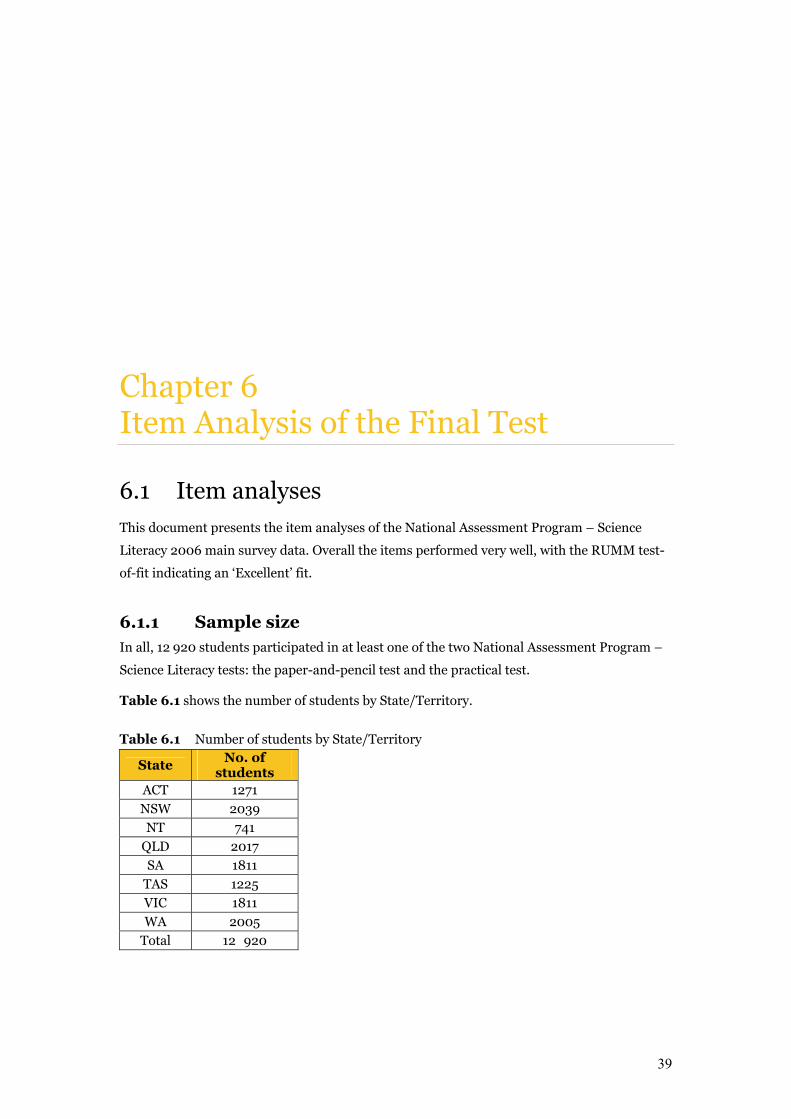
39

Chapter 6 Item Analysis of the Final Test

6.1 Item analyses This document presents the item analyses of the National Assessment Program – Science

Literacy 2006 main survey data. Overall the items performed very well, with the RUMM test-

of-fit indicating an ‘Excellent’ fit.

6.1.1 Sample size In all, 12 920 students participated in at least one of the two National Assessment Program –

Science Literacy tests: the paper-and-pencil test and the practical test.

Table 6.1 shows the number of students by State/Territory.

Table 6.1 Number of students by State/Territory

State No. of

students ACT 1271

NSW 2039

NT 741

QLD 2017

SA 1811

TAS 1225 VIC 1811

WA 2005

Total 12 920

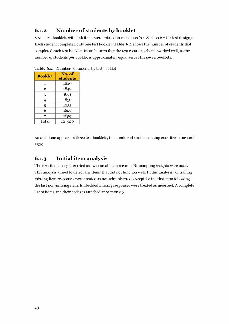
40

6.1.2 Number of students by booklet Seven test booklets with link items were rotated in each class (see Section 6.2 for test design).

Each student completed only one test booklet. Table 6.2 shows the number of students that

completed each test booklet. It can be seen that the test rotation scheme worked well, as the

number of students per booklet is approximately equal across the seven booklets.

Table 6.2 Number of students by test booklet

Booklet No. of

students 1 1849

2 1842

3 1861

4 1850

5 1832 6 1827

7 1859

Total 12 920

As each item appears in three test booklets, the number of students taking each item is around

5500.

6.1.3 Initial item analysis The first item analysis carried out was on all data records. No sampling weights were used.

This analysis aimed to detect any items that did not function well. In this analysis, all trailing

missing item responses were treated as not-administered, except for the first item following

the last non-missing item. Embedded missing responses were treated as incorrect. A complete

list of items and their codes is attached at Section 6.3.

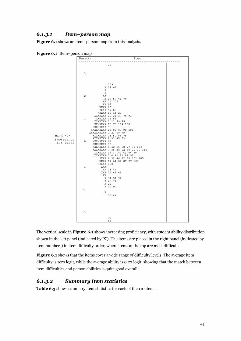
41

6.1.3.1 Item–person map

Figure 6.1 shows an item–person map from this analysis.

Figure 6.1 Item–person map

Each 'X' represents 76.5 cases

Person Item ---------------------------------------------------- |24 | | | | | 3 | | | | | | | | |109 | X|54 61 | X| | X| | 2 XX| | X|39 57 63 70 | XX|74 106 | XX|99 | XXXX|68 | XXXX|47 69 | XXXXX|13 14 29 | XXXXXXX|10 21 27 78 91 | 1 XXXXXX|16 59 | XXXXXXX|1 11 89 95 | XXXXXXX|15 73 104 108 | XXXXXXXX|9 | XXXXXXXXX|26 80 83 98 101 | XXXXXXXXXX|2 23 60 79 | XXXXXXXX|28 50 56 85 | XXXXXXXX|8 33 45 53 | 0 XXXXXXXX|67 | XXXXXXXX|36 | XXXXXXXX|5 12 55 62 77 90 103 | XXXXXXXX|7 35 38 52 58 65 96 110 | XXXXXXX|19 37 40 43 66 75 | XXXXXXX|3 4 41 81 82 93 | XXXX|6 32 46 72 88 102 105 | XXXX|17 64 84 87 97 107 | XXXXX|100 | -1 XXX| | XX|18 44 | XXX|25 48 49 | XX| | X|31 51 94 | X|20 71 | X|22 | X|34 92 | -2 | | X| | |30 42 | | | | | | | | | | | -3 | | | | |76 | |86 |

The vertical scale in Figure 6.1 shows increasing proficiency, with student ability distribution

shown in the left panel (indicated by ‘X’). The items are placed in the right panel (indicated by

item numbers) in item difficulty order, where items at the top are most difficult.

Figure 6.1 shows that the items cover a wide range of difficulty levels. The average item

difficulty is zero logit, while the average ability is 0.22 logit, showing that the match between

item difficulties and person abilities is quite good overall.

6.1.3.2 Summary item statistics

Table 6.3 shows summary item statistics for each of the 110 items.

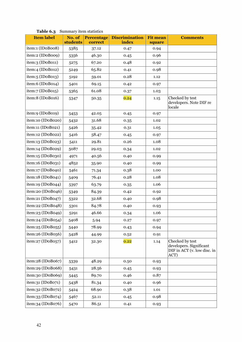
42

Table 6.3 Summary item statistics

Item label No. of students

Percentage correct

Discrimination index

Fit mean square

Comments

item:1 (ID0B008) 5385 37.12 0.47 0.94

item:2 (ID0B009) 5356 46.30 0.45 0.96

item:3 (ID0B011) 5275 67.20 0.48 0.92

item:4 (ID0B012) 5249 65.82 0.41 0.98

item:5 (ID0B013) 5192 59.01 0.28 1.12

item:6 (ID0B014) 5401 69.15 0.42 0.97

item:7 (ID0B015) 5365 61.08 0.37 1.03

item:8 (ID0B016) 5347 50.35 0.24 1.15 Checked by test developers. Note DIF re locale

item:9 (ID0B019) 5453 42.05 0.45 0.97

item:10 (ID0B020) 5432 31.68 0.35 1.02

item:11 (ID0B021) 5426 35.42 0.31 1.05

item:12 (ID0B022) 5416 58.47 0.45 0.97

item:13 (ID0B023) 5411 29.81 0.26 1.08

item:14 (ID0B029) 5087 29.03 0.34 1.02

item:15 (ID0B030) 4971 40.56 0.40 0.99

item:16 (ID0B031) 4852 35.90 0.40 0.99

item:17 (ID0B040) 5461 71.34 0.38 1.00

item:18 (ID0B041) 5409 76.41 0.28 1.08

item:19 (ID0B044) 5397 63.79 0.35 1.06

item:20 (ID0B046) 5349 84.39 0.42 0.92

item:21 (ID0B047) 5322 32.68 0.40 0.98

item:22 (ID0B048) 5301 84.78 0.40 0.93

item:23 (ID0B049) 5291 46.66 0.34 1.06

item:24 (ID0B054) 5408 5.94 0.27 0.97

item:25 (ID0B055) 5440 78.99 0.43 0.94

item:26 (ID0B056) 5428 44.99 0.52 0.91

item:27 (ID0B057) 5412 32.30 0.22 1.14 Checked by test developers. Significant DIF in ACT (v. low disc. in ACT)

item:28 (ID0B067) 5339 48.29 0.50 0.93

item:29 (ID0B068) 5431 28.56 0.45 0.93

item:30 (ID0B069) 5445 89.70 0.46 0.87

item:31 (ID0B071) 5438 81.34 0.40 0.96

item:32 (ID0B072) 5424 68.90 0.38 1.01

item:33 (ID0B074) 5467 52.11 0.45 0.98

item:34 (ID0B076) 5470 86.51 0.41 0.93

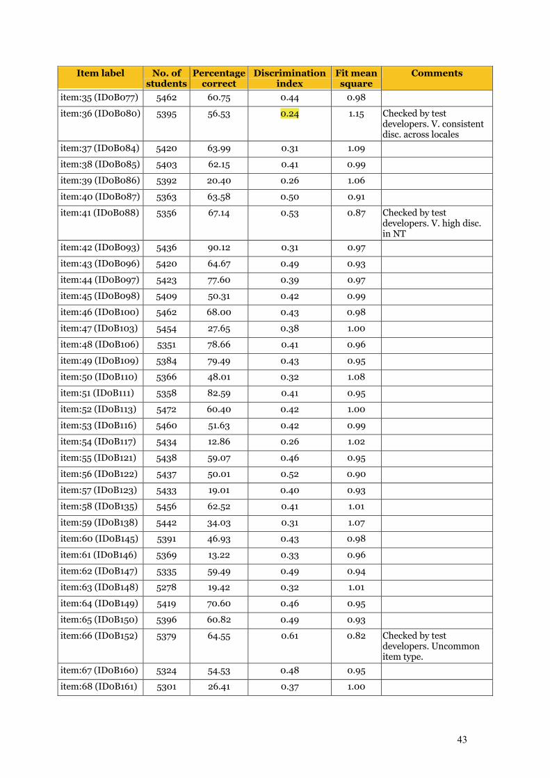
43

Item label No. of students

Percentage correct

Discrimination index

Fit mean square

Comments

item:35 (ID0B077) 5462 60.75 0.44 0.98

item:36 (ID0B080) 5395 56.53 0.24 1.15 Checked by test developers. V. consistent disc. across locales

item:37 (ID0B084) 5420 63.99 0.31 1.09

item:38 (ID0B085) 5403 62.15 0.41 0.99

item:39 (ID0B086) 5392 20.40 0.26 1.06

item:40 (ID0B087) 5363 63.58 0.50 0.91

item:41 (ID0B088) 5356 67.14 0.53 0.87 Checked by test developers. V. high disc. in NT

item:42 (ID0B093) 5436 90.12 0.31 0.97

item:43 (ID0B096) 5420 64.67 0.49 0.93

item:44 (ID0B097) 5423 77.60 0.39 0.97

item:45 (ID0B098) 5409 50.31 0.42 0.99

item:46 (ID0B100) 5462 68.00 0.43 0.98

item:47 (ID0B103) 5454 27.65 0.38 1.00

item:48 (ID0B106) 5351 78.66 0.41 0.96

item:49 (ID0B109) 5384 79.49 0.43 0.95

item:50 (ID0B110) 5366 48.01 0.32 1.08

item:51 (ID0B111) 5358 82.59 0.41 0.95

item:52 (ID0B113) 5472 60.40 0.42 1.00

item:53 (ID0B116) 5460 51.63 0.42 0.99

item:54 (ID0B117) 5434 12.86 0.26 1.02

item:55 (ID0B121) 5438 59.07 0.46 0.95

item:56 (ID0B122) 5437 50.01 0.52 0.90

item:57 (ID0B123) 5433 19.01 0.40 0.93

item:58 (ID0B135) 5456 62.52 0.41 1.01

item:59 (ID0B138) 5442 34.03 0.31 1.07

item:60 (ID0B145) 5391 46.93 0.43 0.98

item:61 (ID0B146) 5369 13.22 0.33 0.96

item:62 (ID0B147) 5335 59.49 0.49 0.94

item:63 (ID0B148) 5278 19.42 0.32 1.01

item:64 (ID0B149) 5419 70.60 0.46 0.95

item:65 (ID0B150) 5396 60.82 0.49 0.93

item:66 (ID0B152) 5379 64.55 0.61 0.82 Checked by test developers. Uncommon item type.

item:67 (ID0B160) 5324 54.53 0.48 0.95

item:68 (ID0B161) 5301 26.41 0.37 1.00

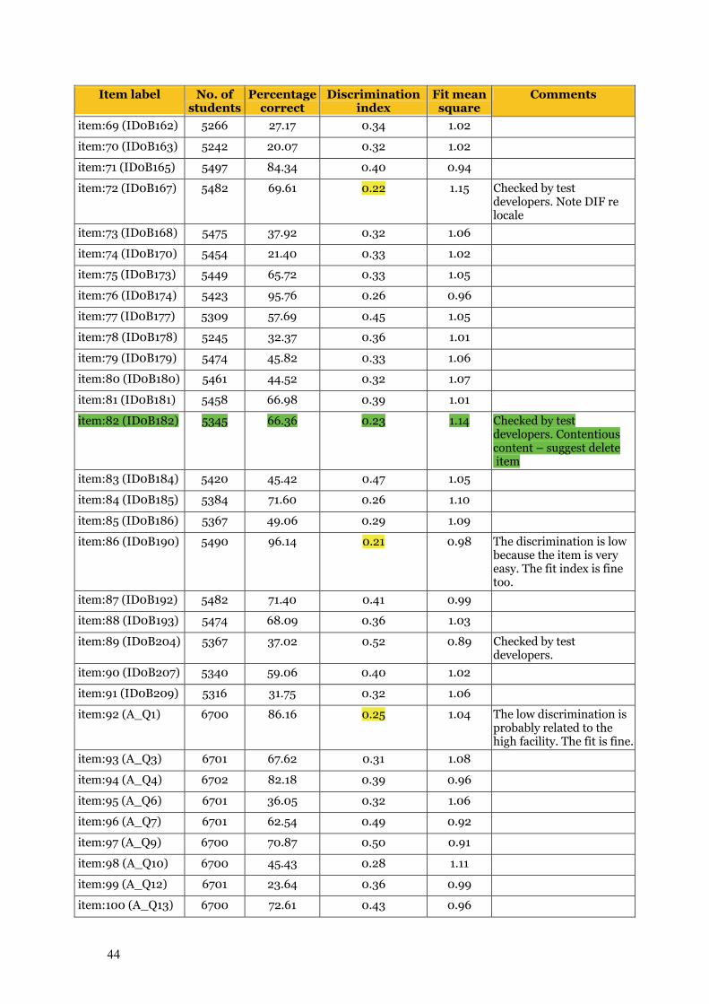
44

Item label No. of students

Percentage correct

Discrimination index

Fit mean square

Comments

item:69 (ID0B162) 5266 27.17 0.34 1.02

item:70 (ID0B163) 5242 20.07 0.32 1.02

item:71 (ID0B165) 5497 84.34 0.40 0.94

item:72 (ID0B167) 5482 69.61 0.22 1.15 Checked by test developers. Note DIF re locale

item:73 (ID0B168) 5475 37.92 0.32 1.06

item:74 (ID0B170) 5454 21.40 0.33 1.02

item:75 (ID0B173) 5449 65.72 0.33 1.05

item:76 (ID0B174) 5423 95.76 0.26 0.96

item:77 (ID0B177) 5309 57.69 0.45 1.05

item:78 (ID0B178) 5245 32.37 0.36 1.01

item:79 (ID0B179) 5474 45.82 0.33 1.06

item:80 (ID0B180) 5461 44.52 0.32 1.07

item:81 (ID0B181) 5458 66.98 0.39 1.01

item:82 (ID0B182) 5345 66.36 0.23 1.14 Checked by test developers. Contentious content – suggest delete item

item:83 (ID0B184) 5420 45.42 0.47 1.05

item:84 (ID0B185) 5384 71.60 0.26 1.10

item:85 (ID0B186) 5367 49.06 0.29 1.09

item:86 (ID0B190) 5490 96.14 0.21 0.98 The discrimination is low because the item is very easy. The fit index is fine too.

item:87 (ID0B192) 5482 71.40 0.41 0.99

item:88 (ID0B193) 5474 68.09 0.36 1.03

item:89 (ID0B204) 5367 37.02 0.52 0.89 Checked by test developers.

item:90 (ID0B207) 5340 59.06 0.40 1.02

item:91 (ID0B209) 5316 31.75 0.32 1.06

item:92 (A_Q1) 6700 86.16 0.25 1.04 The low discrimination is probably related to the high facility. The fit is fine.

item:93 (A_Q3) 6701 67.62 0.31 1.08

item:94 (A_Q4) 6702 82.18 0.39 0.96

item:95 (A_Q6) 6701 36.05 0.32 1.06

item:96 (A_Q7) 6701 62.54 0.49 0.92

item:97 (A_Q9) 6700 70.87 0.50 0.91

item:98 (A_Q10) 6700 45.43 0.28 1.11

item:99 (A_Q12) 6701 23.64 0.36 0.99

item:100 (A_Q13) 6700 72.61 0.43 0.96

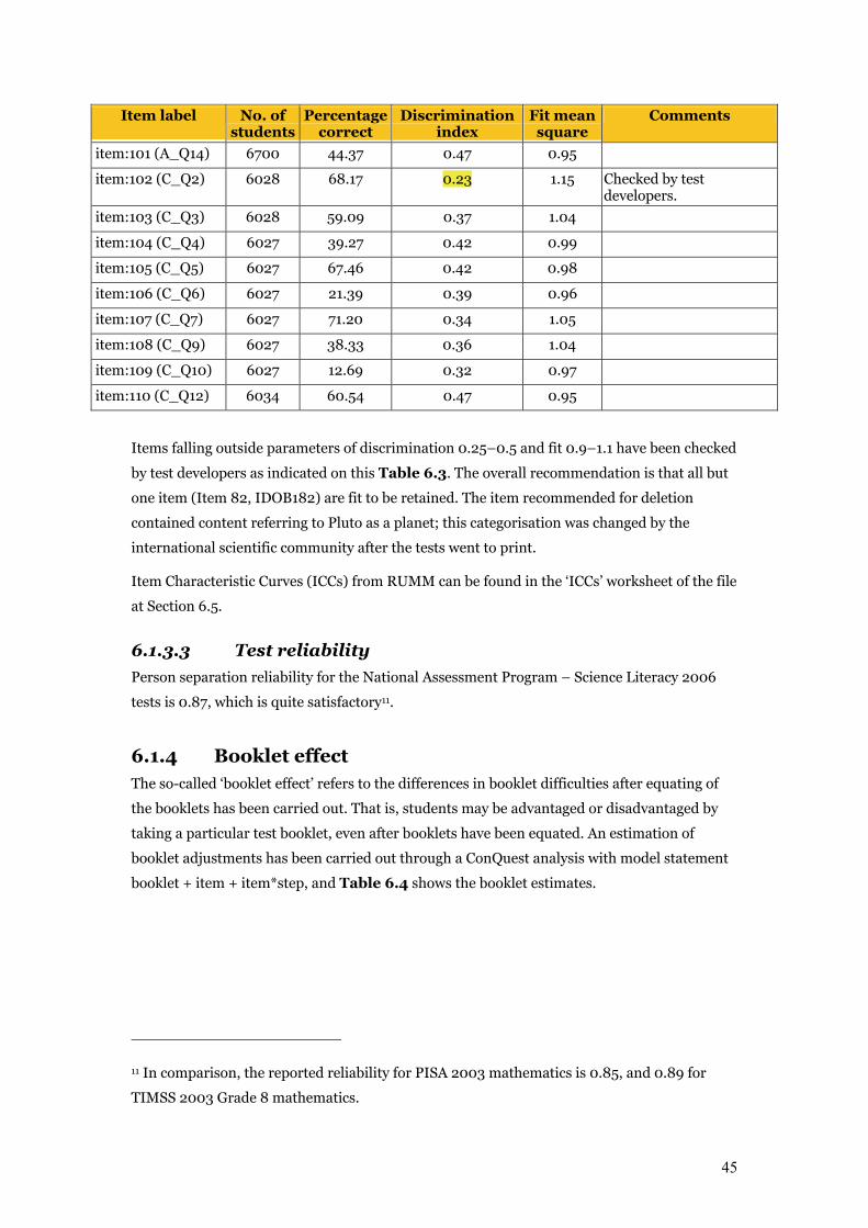
45

Item label No. of students

Percentage correct

Discrimination index

Fit mean square

Comments

item:101 (A_Q14) 6700 44.37 0.47 0.95

item:102 (C_Q2) 6028 68.17 0.23 1.15 Checked by test developers.

item:103 (C_Q3) 6028 59.09 0.37 1.04

item:104 (C_Q4) 6027 39.27 0.42 0.99

item:105 (C_Q5) 6027 67.46 0.42 0.98

item:106 (C_Q6) 6027 21.39 0.39 0.96

item:107 (C_Q7) 6027 71.20 0.34 1.05

item:108 (C_Q9) 6027 38.33 0.36 1.04

item:109 (C_Q10) 6027 12.69 0.32 0.97

item:110 (C_Q12) 6034 60.54 0.47 0.95

Items falling outside parameters of discrimination 0.25–0.5 and fit 0.9–1.1 have been checked

by test developers as indicated on this Table 6.3. The overall recommendation is that all but

one item (Item 82, IDOB182) are fit to be retained. The item recommended for deletion

contained content referring to Pluto as a planet; this categorisation was changed by the

international scientific community after the tests went to print.

Item Characteristic Curves (ICCs) from RUMM can be found in the ‘ICCs’ worksheet of the file

at Section 6.5.

6.1.3.3 Test reliability

Person separation reliability for the National Assessment Program – Science Literacy 2006

tests is 0.87, which is quite satisfactory11.

6.1.4 Booklet effect The so-called ‘booklet effect’ refers to the differences in booklet difficulties after equating of

the booklets has been carried out. That is, students may be advantaged or disadvantaged by

taking a particular test booklet, even after booklets have been equated. An estimation of

booklet adjustments has been carried out through a ConQuest analysis with model statement

booklet + item + item*step, and Table 6.4 shows the booklet estimates.

11 In comparison, the reported reliability for PISA 2003 mathematics is 0.85, and 0.89 for

TIMSS 2003 Grade 8 mathematics.

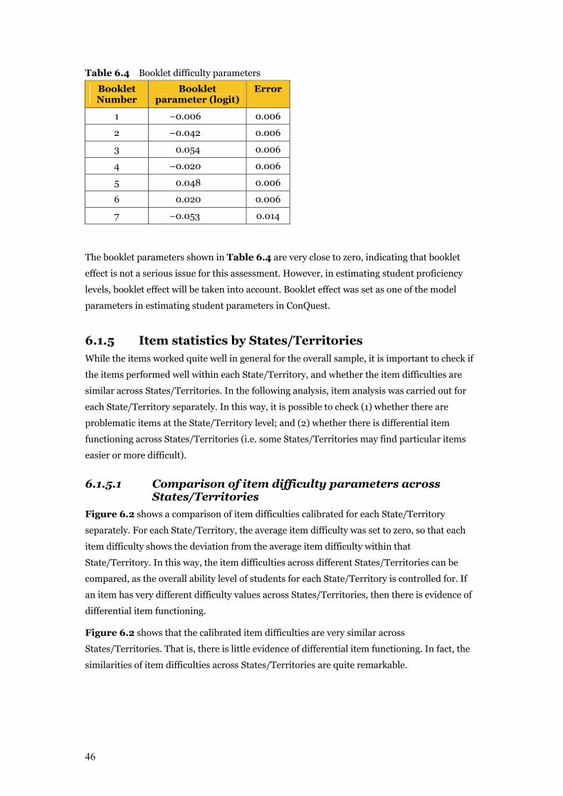
46

Table 6.4 Booklet difficulty parameters

Booklet Number

Booklet parameter (logit)

Error

1 –0.006 0.006

2 –0.042 0.006

3 0.054 0.006

4 –0.020 0.006

5 0.048 0.006

6 0.020 0.006

7 –0.053 0.014

The booklet parameters shown in Table 6.4 are very close to zero, indicating that booklet

effect is not a serious issue for this assessment. However, in estimating student proficiency

levels, booklet effect will be taken into account. Booklet effect was set as one of the model

parameters in estimating student parameters in ConQuest.

6.1.5 Item statistics by States/Territories While the items worked quite well in general for the overall sample, it is important to check if

the items performed well within each State/Territory, and whether the item difficulties are

similar across States/Territories. In the following analysis, item analysis was carried out for

each State/Territory separately. In this way, it is possible to check (1) whether there are

problematic items at the State/Territory level; and (2) whether there is differential item

functioning across States/Territories (i.e. some States/Territories may find particular items

easier or more difficult).

6.1.5.1 Comparison of item difficulty parameters across States/Territories

Figure 6.2 shows a comparison of item difficulties calibrated for each State/Territory

separately. For each State/Territory, the average item difficulty was set to zero, so that each

item difficulty shows the deviation from the average item difficulty within that

State/Territory. In this way, the item difficulties across different States/Territories can be

compared, as the overall ability level of students for each State/Territory is controlled for. If

an item has very different difficulty values across States/Territories, then there is evidence of

differential item functioning.

Figure 6.2 shows that the calibrated item difficulties are very similar across

States/Territories. That is, there is little evidence of differential item functioning. In fact, the

similarities of item difficulties across States/Territories are quite remarkable.

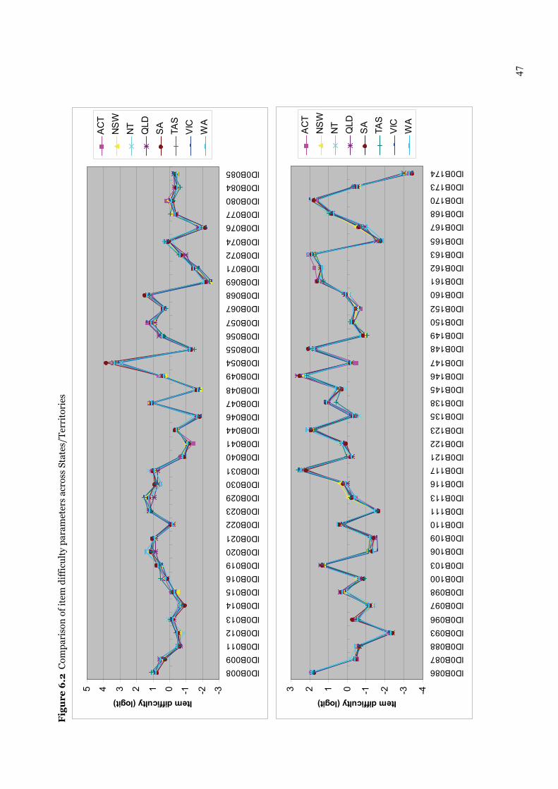
47

Fig

ure

6.2

Com

par

ison

of i

tem

dif

ficu

lty

par

amet

ers

acro

ss S

tate

s/T

erri

tori

es

-3-2-1012345

ID0B008ID0B009ID0B011ID0B012ID0B013

ID0B014ID0B015ID0B016ID0B019ID0B020ID0B021

ID0B022ID0B023ID0B029ID0B030ID0B031

ID0B040ID0B041ID0B044ID0B046ID0B047ID0B048

ID0B049ID0B054ID0B055ID0B056ID0B057

ID0B067ID0B068ID0B069ID0B071ID0B072ID0B074

ID0B076ID0B077ID0B080ID0B084ID0B085

Item difficulty (logit)

AC

TN

SW

NT

QLD

SA

TAS

VIC

WA

-4-3-2-10123

ID0B086ID0B087ID0B088ID0B093ID0B096

ID0B097ID0B098ID0B100ID0B103

ID0B106ID0B109ID0B110ID0B111ID0B113

ID0B116ID0B117ID0B121ID0B122ID0B123

ID0B135ID0B138ID0B145ID0B146ID0B147

ID0B148ID0B149ID0B150ID0B152

ID0B160ID0B161ID0B162ID0B163ID0B165

ID0B167ID0B168ID0B170ID0B173ID0B174

Item difficulty (logit)

AC

TN

SW

NT

QLD

SA

TAS

VIC

WA

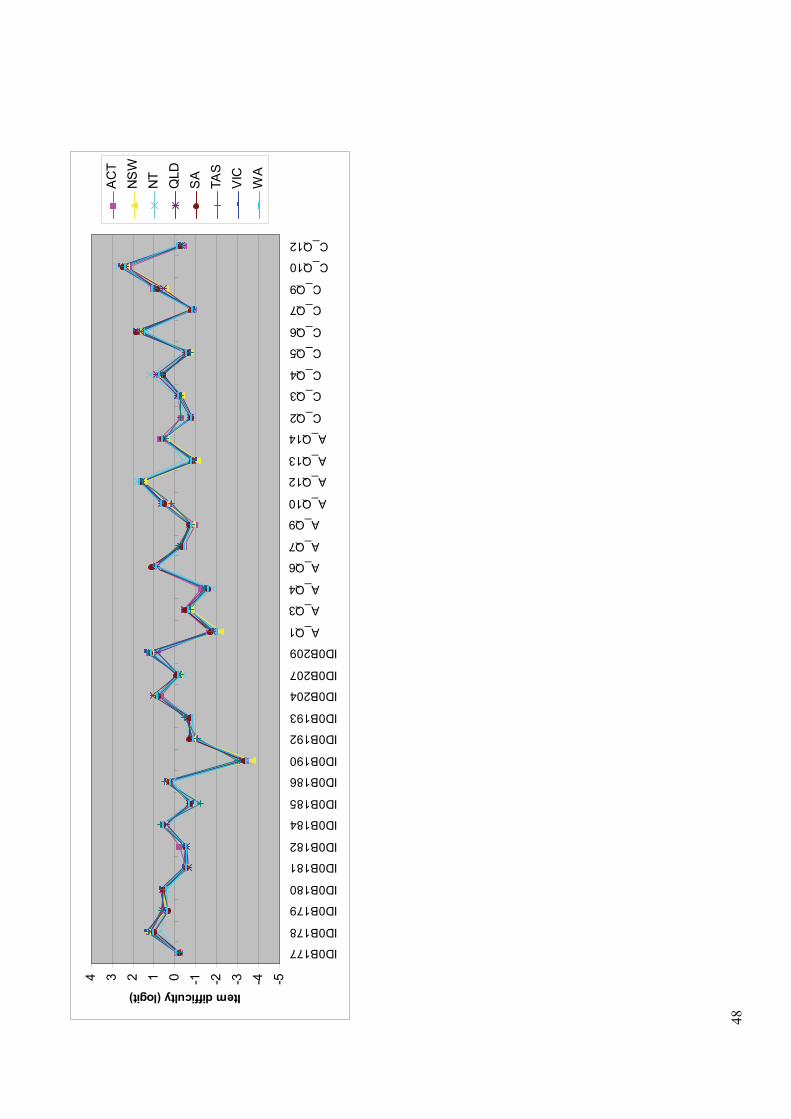
48

-5-4-3-2-101234

ID0B177

ID0B178

ID0B179

ID0B180

ID0B181

ID0B182

ID0B184

ID0B185

ID0B186

ID0B190

ID0B192

ID0B193

ID0B204

ID0B207

ID0B209

A_Q1

A_Q3

A_Q4

A_Q6

A_Q7

A_Q9

A_Q10

A_Q12

A_Q13

A_Q14

C_Q2

C_Q3

C_Q4

C_Q5

C_Q6

C_Q7

C_Q9

C_Q10

C_Q12

Item difficulty (logit)A

CT

NS

WN

TQ

LDS

ATA

SV

ICW

A

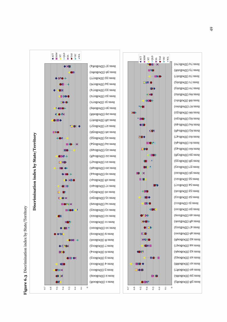
49

Fig

ure

6.3

Dis

crim

inat

ion

ind

ex b

y St

ate/

Ter

rito

ry

Dis

crim

ina

tio

n i

nd

ex

by

Sta

te/T

err

ito

ry

0

0.1

0.2

0.3

0.40.5

0.60.7

item:1 (ID0B008)

item:2 (ID0B009)

item:3 (ID0B011)

item:4 (ID0B012)

item:5 (ID0B013)

item:6 (ID0B014)

item:7 (ID0B015)

item:8 (ID0B016)

item:9 (ID0B019)

item:10 (ID0B020)

item:11 (ID0B021)

item:12 (ID0B022)

item:13 (ID0B023)

item:14 (ID0B029)

item:15 (ID0B030)

item:16 (ID0B031)

item:17 (ID0B040)

item:18 (ID0B041)

item:19 (ID0B044)

item:20 (ID0B046)

item:21 (ID0B047)

item:22 (ID0B048)

item:23 (ID0B049)

item:24 (ID0B054)

item:25 (ID0B055)

item:26 (ID0B056)

item:27 (ID0B057)

item:28 (ID0B067)

item:29 (ID0B068)

item:30 (ID0B069)

item:31 (ID0B071)

item:32 (ID0B072)

item:33 (ID0B074)

item:34 (ID0B076)

item:35 (ID0B077)

item:36 (ID0B080)

item:37 (ID0B084)

AC

T

NSW

NT

QL

D

SA TA

S

VIC

WA

0

0.1

0.2

0.3

0.4

0.5

0.60.7

item:38 (ID0B085)

item:39 (ID0B086)

item:40 (ID0B087)

item:41 (ID0B088)

item:42 (ID0B093)

item:43 (ID0B096)

item:44 (ID0B097)

item:45 (ID0B098)

item:46 (ID0B100)

item:47 (ID0B103)

item:48 (ID0B106)

item:49 (ID0B109)

item:50 (ID0B110)

item:51 (ID0B111)

item:52 (ID0B113)

item:53 (ID0B116)

item:54 (ID0B117)

item:55 (ID0B121)

item:56 (ID0B122)

item:57 (ID0B123)

item:58 (ID0B135)

item:59 (ID0B138)

item:60 (ID0B145)

item:61 (ID0B146)

item:62 (ID0B147)

item:63 (ID0B148)

item:64 (ID0B149)

item:65 (ID0B150)

item:66 (ID0B152)

item:67 (ID0B160)

item:68 (ID0B161)

item:69 (ID0B162)

item:70 (ID0B163)

item:71 (ID0B165)

item:72 (ID0B167)

item:73 (ID0B168)

item:74 (ID0B170)

AC

T

NSW

NT

QL

D

SA TA

S

VIC

WA

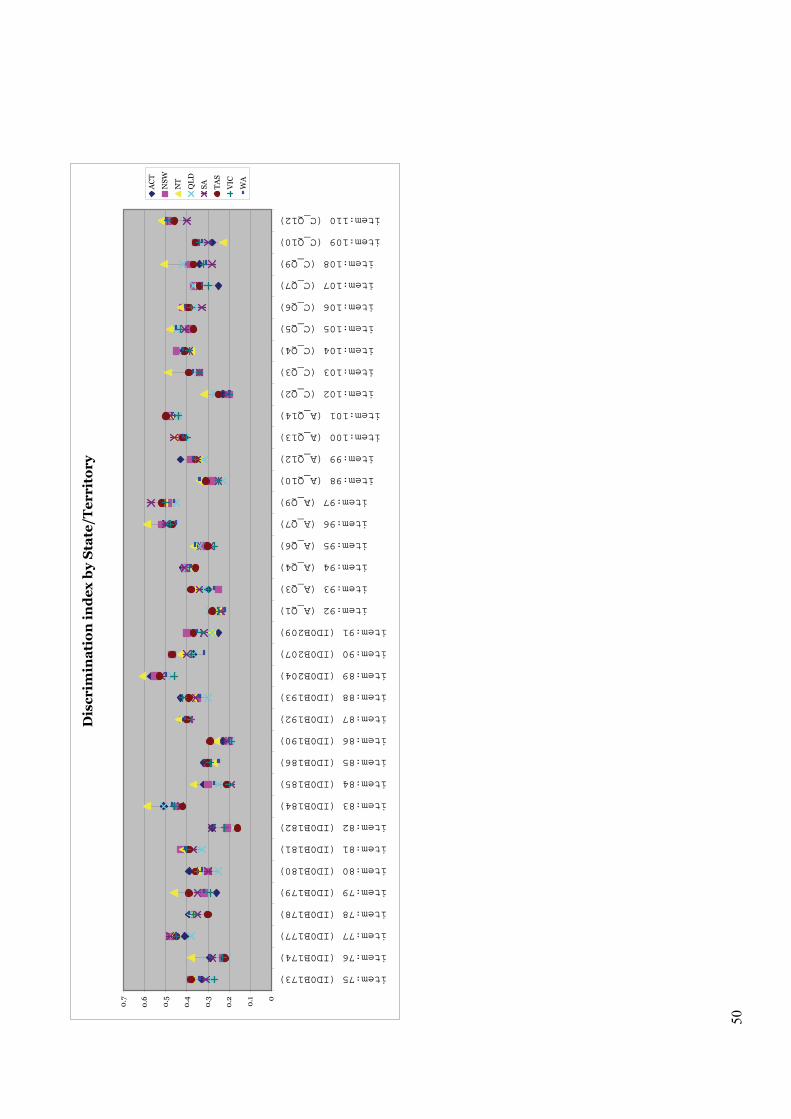
50

Dis

crim

ina

tio

n i

nd

ex b

y S

tate

/Te

rrit

ory

0

0.1

0.2

0.3

0.40.5

0.60.7

item:75 (ID0B173)

item:76 (ID0B174)

item:77 (ID0B177)

item:78 (ID0B178)

item:79 (ID0B179)

item:80 (ID0B180)

item:81 (ID0B181)

item:82 (ID0B182)

item:83 (ID0B184)

item:84 (ID0B185)

item:85 (ID0B186)

item:86 (ID0B190)

item:87 (ID0B192)

item:88 (ID0B193)

item:89 (ID0B204)

item:90 (ID0B207)

item:91 (ID0B209)

item:92 (A_Q1)

item:93 (A_Q3)

item:94 (A_Q4)

item:95 (A_Q6)

item:96 (A_Q7)

item:97 (A_Q9)

item:98 (A_Q10)

item:99 (A_Q12)

item:100 (A_Q13)

item:101 (A_Q14)

item:102 (C_Q2)

item:103 (C_Q3)

item:104 (C_Q4)

item:105 (C_Q5)

item:106 (C_Q6)

item:107 (C_Q7)

item:108 (C_Q9)

item:109 (C_Q10)

item:110 (C_Q12)

AC

T

NSW

NT

QL

D

SA TA

S

VIC

WA

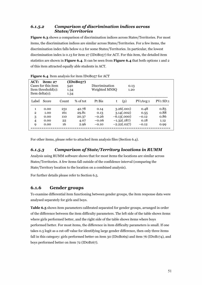
51

6.1.5.2 Comparison of discrimination indices across States/Territories

Figure 6.3 shows a comparison of discrimination indices across States/Territories. For most

items, the discrimination indices are similar across States/Territories. For a few items, the

discrimination index falls below 0.2 for some States/Territories. In particular, the lowest

discrimination index is 0.13 for item 27 (ID0B057) for ACT. For this item, the detailed item

statistics are shown in Figure 6.4. It can be seen from Figure 6.4 that both options 1 and 2

of this item attracted equally able students in ACT.

Figure 6.4 Item analysis for item ID0B057 for ACT

ACT: item: 27 (ID0B057) Cases for this item 540 Discrimination 0.13 Item threshold(s): 1.34 Weighted MNSQ 1.20 Item delta(s): 1.34 ------------------------------------------------------------------------------------------------------------ Label Score Count % of tot Pt Bis t (p) PV1Avg:1 PV1 SD:1 ------------------------------------------------------------------------------------------------------------- 1 0.00 231 42.78 0.14 3.26(.001) 0.48 0.85 2 1.00 161 29.81 0.13 3.14(.002) 0.55 0.88 3 0.00 110 20.37 –0.26 –6.13(.000) –0.12 0.86 4 0.00 22 4.07 –0.06 –1.32(.187) 0.18 1.12 9 0.00 16 2.96 –0.10 –2.22(.027) –0.12 0.99 ================================================================

For other items, please refer to attached item analysis files (Section 6.4).

6.1.5.3 Comparison of State/Territory locations in RUMM

Analysis using RUMM software shows that for most items the locations are similar across

States/Territories. A few items fall outside of the confidence interval (comparing the

State/Territory location to the location on a combined analysis).

For further details please refer to Section 6.5.

6.1.6 Gender groups To examine differential item functioning between gender groups, the item response data were

analysed separately for girls and boys.

Table 6.5 shows item parameters calibrated separated for gender groups, arranged in order

of the difference between the item difficulty parameters. The left side of the table shows items

where girls performed better, and the right side of the table shows items where boys

performed better. For most items, the difference in item difficulty parameters is small. If one

takes 0.5 logit as a cut-off value for identifying large gender difference, then only three items

fall in this category: girls performed better on item 30 (ID0B069) and item 76 (ID0B174), and

boys performed better on item 72 (ID0B167).

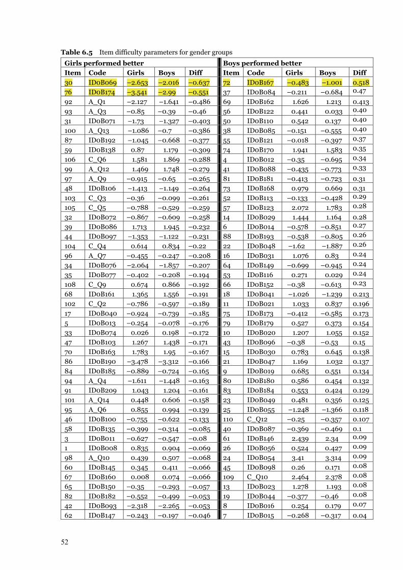
52

Table 6.5 Item difficulty parameters for gender groups

Girls performed better Boys performed better

Item Code Girls Boys Diff Item Code Girls Boys Diff

30 ID0B069 –2.653 –2.016 –0.637 72 ID0B167 –0.483 –1.001 0.518

76 ID0B174 –3.541 –2.99 –0.551 37 ID0B084 –0.211 –0.684 0.47

92 A_Q1 –2.127 –1.641 –0.486 69 ID0B162 1.626 1.213 0.413

93 A_Q3 –0.85 –0.39 –0.46 56 ID0B122 0.441 0.033 0.40831 ID0B071 –1.73 –1.327 –0.403 50 ID0B110 0.542 0.137 0.40

100 A_Q13 –1.086 –0.7 –0.386 38 ID0B085 –0.151 –0.555 0.40

87 ID0B192 –1.045 –0.668 –0.377 55 ID0B121 –0.018 –0.397 0.37

59 ID0B138 0.87 1.179 –0.309 74 ID0B170 1.941 1.583 0.358106 C_Q6 1.581 1.869 –0.288 4 ID0B012 –0.35 –0.695 0.34

99 A_Q12 1.469 1.748 –0.279 41 ID0B088 –0.435 –0.773 0.33897 A_Q9 –0.915 –0.65 –0.265 81 ID0B181 –0.413 –0.723 0.31

48 ID0B106 –1.413 –1.149 –0.264 73 ID0B168 0.979 0.669 0.31

103 C_Q3 –0.36 –0.099 –0.261 52 ID0B113 –0.133 –0.428 0.29

105 C_Q5 –0.788 –0.529 –0.259 57 ID0B123 2.072 1.783 0.28

32 ID0B072 –0.867 –0.609 –0.258 14 ID0B029 1.444 1.164 0.28

39 ID0B086 1.713 1.945 –0.232 6 ID0B014 –0.578 –0.851 0.27

44 ID0B097 –1.353 –1.122 –0.231 88 ID0B193 –0.538 –0.805 0.26

104 C_Q4 0.614 0.834 –0.22 22 ID0B048 –1.62 –1.887 0.26

96 A_Q7 –0.455 –0.247 –0.208 16 ID0B031 1.076 0.83 0.24634 ID0B076 –2.064 –1.857 –0.207 64 ID0B149 –0.699 –0.945 0.24635 ID0B077 –0.402 –0.208 –0.194 53 ID0B116 0.271 0.029 0.24

108 C_Q9 0.674 0.866 –0.192 66 ID0B152 –0.38 –0.613 0.23

68 ID0B161 1.365 1.556 –0.191 18 ID0B041 –1.026 –1.239 0.213

102 C_Q2 –0.786 –0.597 –0.189 11 ID0B021 1.033 0.837 0.196

17 ID0B040 –0.924 –0.739 –0.185 75 ID0B173 –0.412 –0.585 0.173

5 ID0B013 –0.254 –0.078 –0.176 79 ID0B179 0.527 0.373 0.154

33 ID0B074 0.026 0.198 –0.172 10 ID0B020 1.207 1.055 0.152

47 ID0B103 1.267 1.438 –0.171 43 ID0B096 –0.38 –0.53 0.15

70 ID0B163 1.783 1.95 –0.167 15 ID0B030 0.783 0.645 0.138

86 ID0B190 –3.478 –3.312 –0.166 21 ID0B047 1.169 1.032 0.137

84 ID0B185 –0.889 –0.724 –0.165 9 ID0B019 0.685 0.551 0.134

94 A_Q4 –1.611 –1.448 –0.163 80 ID0B180 0.586 0.454 0.132

91 ID0B209 1.043 1.204 –0.161 83 ID0B184 0.553 0.424 0.129

101 A_Q14 0.448 0.606 –0.158 23 ID0B049 0.481 0.356 0.125

95 A_Q6 0.855 0.994 –0.139 25 ID0B055 –1.248 –1.366 0.118

46 ID0B100 –0.755 –0.622 –0.133 110 C_Q12 –0.25 –0.357 0.107

58 ID0B135 –0.399 –0.314 –0.085 40 ID0B087 –0.369 –0.469 0.1

3 ID0B011 –0.627 –0.547 –0.08 61 ID0B146 2.439 2.34 0.09

1 ID0B008 0.835 0.904 –0.069 26 ID0B056 0.524 0.427 0.09

98 A_Q10 0.439 0.507 –0.068 24 ID0B054 3.41 3.314 0.09660 ID0B145 0.345 0.411 –0.066 45 ID0B098 0.26 0.171 0.08

67 ID0B160 0.008 0.074 –0.066 109 C_Q10 2.464 2.378 0.08665 ID0B150 –0.35 –0.293 –0.057 13 ID0B023 1.278 1.193 0.08

82 ID0B182 –0.552 –0.499 –0.053 19 ID0B044 –0.377 –0.46 0.08

42 ID0B093 –2.318 –2.265 –0.053 8 ID0B016 0.254 0.179 0.07

62 ID0B147 –0.243 –0.197 –0.046 7 ID0B015 –0.268 –0.317 0.04

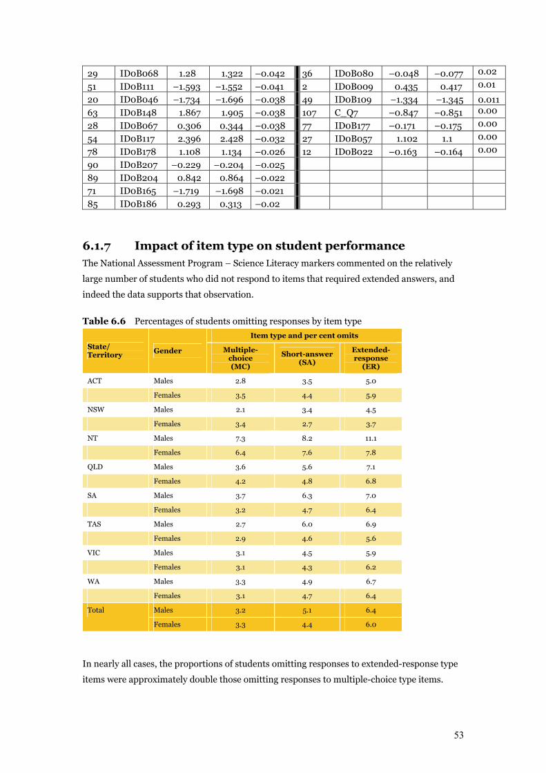
53

29 ID0B068 1.28 1.322 –0.042 36 ID0B080 –0.048 –0.077 0.02

51 ID0B111 –1.593 –1.552 –0.041 2 ID0B009 0.435 0.417 0.01820 ID0B046 –1.734 –1.696 –0.038 49 ID0B109 –1.334 –1.345 0.011

63 ID0B148 1.867 1.905 –0.038 107 C_Q7 –0.847 –0.851 0.00

28 ID0B067 0.306 0.344 –0.038 77 ID0B177 –0.171 –0.175 0.00

54 ID0B117 2.396 2.428 –0.032 27 ID0B057 1.102 1.1 0.00

78 ID0B178 1.108 1.134 –0.026 12 ID0B022 –0.163 –0.164 0.00

90 ID0B207 –0.229 –0.204 –0.025

89 ID0B204 0.842 0.864 –0.022

71 ID0B165 –1.719 –1.698 –0.021

85 ID0B186 0.293 0.313 –0.02

6.1.7 Impact of item type on student performance The National Assessment Program – Science Literacy markers commented on the relatively

large number of students who did not respond to items that required extended answers, and

indeed the data supports that observation.

Table 6.6 Percentages of students omitting responses by item type

Item type and per cent omits

State/ Territory Gender Multiple-

choice (MC)

Short-answer(SA)

Extended-response

(ER)

ACT Males 2.8 3.5 5.0

Females 3.5 4.4 5.9

NSW Males 2.1 3.4 4.5

Females 3.4 2.7 3.7

NT Males 7.3 8.2 11.1

Females 6.4 7.6 7.8

QLD Males 3.6 5.6 7.1

Females 4.2 4.8 6.8

SA Males 3.7 6.3 7.0

Females 3.2 4.7 6.4

TAS Males 2.7 6.0 6.9

Females 2.9 4.6 5.6

VIC Males 3.1 4.5 5.9

Females 3.1 4.3 6.2

WA Males 3.3 4.9 6.7

Females 3.1 4.7 6.4

Males 3.2 5.1 6.4 Total

Females 3.3 4.4 6.0

In nearly all cases, the proportions of students omitting responses to extended-response type

items were approximately double those omitting responses to multiple-choice type items.

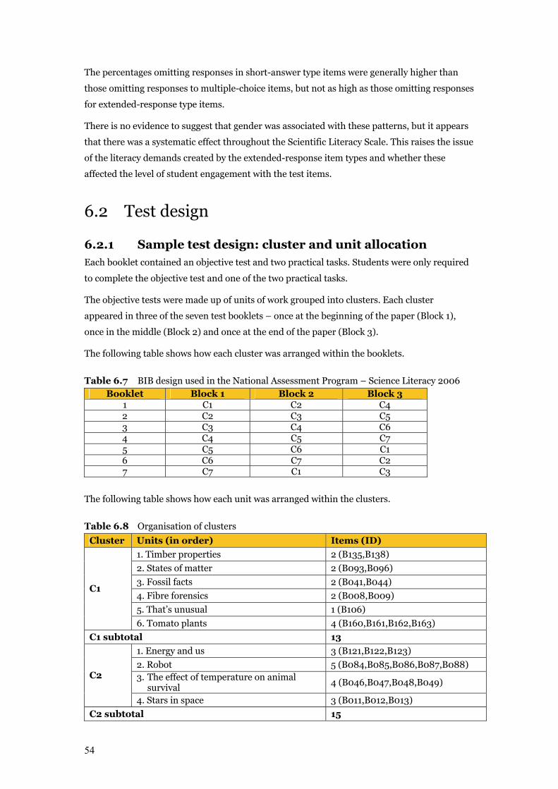
54

The percentages omitting responses in short-answer type items were generally higher than

those omitting responses to multiple-choice items, but not as high as those omitting responses

for extended-response type items.

There is no evidence to suggest that gender was associated with these patterns, but it appears

that there was a systematic effect throughout the Scientific Literacy Scale. This raises the issue

of the literacy demands created by the extended-response item types and whether these

affected the level of student engagement with the test items.

6.2 Test design

6.2.1 Sample test design: cluster and unit allocation Each booklet contained an objective test and two practical tasks. Students were only required

to complete the objective test and one of the two practical tasks.

The objective tests were made up of units of work grouped into clusters. Each cluster

appeared in three of the seven test booklets – once at the beginning of the paper (Block 1),

once in the middle (Block 2) and once at the end of the paper (Block 3).

The following table shows how each cluster was arranged within the booklets.

Table 6.7 BIB design used in the National Assessment Program – Science Literacy 2006 Booklet Block 1 Block 2 Block 3

1 C1 C2 C4 2 C2 C3 C5 3 C3 C4 C6 4 C4 C5 C7 5 C5 C6 C1 6 C6 C7 C2 7 C7 C1 C3

The following table shows how each unit was arranged within the clusters.

Table 6.8 Organisation of clusters

Cluster Units (in order) Items (ID)

1. Timber properties 2 (B135,B138)

2. States of matter 2 (B093,B096)

3. Fossil facts 2 (B041,B044)

4. Fibre forensics 2 (B008,B009)

5. That’s unusual 1 (B106)

C1

6. Tomato plants 4 (B160,B161,B162,B163)

C1 subtotal 13

1. Energy and us 3 (B121,B122,B123)

2. Robot 5 (B084,B085,B086,B087,B088) 3. The effect of temperature on animal survival 4 (B046,B047,B048,B049)

C2

4. Stars in space 3 (B011,B012,B013)

C2 subtotal 15

55

1. Mission to Mars 4 (B165,B167,B168,B170)

2. Solid, liquid, gas 4 (B055,B056,B057, B054)

3. Natural events 3 (B109,B110,B111) C3

4. Stingray adaptations 1 (B067)

C3 subtotal 12

1. Muffins for breakfast 3 (B190,B192,B193) 2. Native grasslands and the striped legless lizard 3 (B113,B116,B117)

3. The night sky 2 (B097; B098) C4

4. Rock cycle 3 (B014,B015,B016)

C4 subtotal 11 1. Breathing in, breathing out 1 (B040) 2. Weather station 5 (B019,B020,B021,B022,B023) 3. Phases of the moon 1 (B080) 4. Food web of native animals 4 (B145,B146,B147,B148)

C5

5. Energy transfer 3 (B029,B030,B031) C5 subtotal 14

1. Classification of living things 3 (B076,B074,B077) 2. Water quality monitoring 2 (B100,B103) 3. Properties of plastics 4 (B069,B071, B068,B072) 4. What gemstone is that? 3 (B149,B150,B152)

C6

5. Musical instruments 3 (B204,B207,B209) C6 subtotal 15

1. Cave diggers 3 (B179,B180,B181) 2. Bar magnets 1 (B173) 3. Camping holiday 2 (B174) 4. Curtains 3 (B184,B185,B186) 5. Planets 1 (B182)

C7

6. Bean plants 2 (B177,B178) C7 subtotal 11

Notes:

Please note that due to page limitations Energy transfer was moved from Cluster 5 in

Booklet 5 to the end of Cluster 6 in Booklet 3.

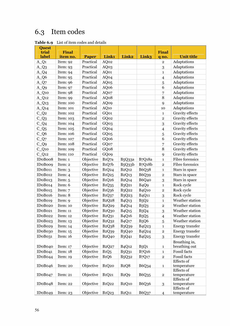
56

6.3 Item codes Table 6.9 List of item codes and details

Quest trial label

Final item no. Paper Link1 Link2 Link3

Final q no. Unit title

A_Q1 Item: 92 Practical AQ02 2 Adaptations A_Q3 Item: 93 Practical AQ03 3 Adaptations A_Q4 Item: 94 Practical AQ01 1 Adaptations A_Q6 Item: 95 Practical AQ04 4 Adaptations A_Q7 Item: 96 Practical AQ05 5 Adaptations A_Q9 Item: 97 Practical AQ06 6 Adaptations A_Q10 Item: 98 Practical AQ07 7 Adaptations A_Q12 Item: 99 Practical AQ08 8 Adaptations A_Q13 Item: 100 Practical AQ09 9 Adaptations A_Q14 Item: 101 Practical AQ10 10 Adaptations C_Q2 Item: 102 Practical GQ01 1 Gravity effects C_Q3 Item: 103 Practical GQ02 2 Gravity effects C_Q4 Item: 104 Practical GQ03 3 Gravity effects C_Q5 Item: 105 Practical GQ04 4 Gravity effects C_Q6 Item: 106 Practical GQ05 5 Gravity effects C_Q7 Item: 107 Practical GQ06 6 Gravity effects C_Q9 Item: 108 Practical GQ07 7 Gravity effects C_Q10 Item: 109 Practical GQ08 8 Gravity effects C_Q12 Item: 110 Practical GQ09 9 Gravity effects ID0B008 Item: 1 Objective B1Q7a B5Q33a B7Q18a 1 Fibre forensics ID0B009 Item: 2 Objective B1Q7b B5Q33b B7Q18b 2 Fibre forensics ID0B011 Item: 3 Objective B1Q24 B2Q12 B6Q38 1 Stars in space ID0B012 Item: 4 Objective B1Q25 B2Q13 B6Q39 2 Stars in space ID0B013 Item: 5 Objective B1Q26 B2Q14 B6Q40 3 Stars in space ID0B014 Item: 6 Objective B1Q35 B3Q21 B4Q9 1 Rock cycle ID0B015 Item: 7 Objective B1Q36 B3Q22 B4Q10 2 Rock cycle ID0B016 Item: 8 Objective B1Q37 B3Q23 B4Q11 3 Rock cycle ID0B019 Item: 9 Objective B2Q28 B4Q13 B5Q2 1 Weather station ID0B020 Item: 10 Objective B2Q29 B4Q14 B5Q3 2 Weather station ID0B021 Item: 11 Objective B2Q30 B4Q15 B5Q4 3 Weather station ID0B022 Item: 12 Objective B2Q31 B4Q16 B5Q5 4 Weather station ID0B023 Item: 13 Objective B2Q32 B4Q17 B5Q6 5 Weather station ID0B029 Item: 14 Objective B2Q38 B3Q39 B4Q23 1 Energy transfer ID0B030 Item: 15 Objective B2Q39 B3Q40 B4Q24 2 Energy transfer ID0B031 Item: 16 Objective B2Q40 B3Q41 B4Q25 3 Energy transfer

ID0B040 Item: 17 Objective B2Q27 B4Q12 B5Q1 1 Breathing in, breathing out

ID0B041 Item: 18 Objective B1Q5 B5Q31 B7Q16 1 Fossil facts ID0B044 Item: 19 Objective B1Q6 B5Q32 B7Q17 2 Fossil facts

ID0B046 Item: 20 Objective B1Q20 B2Q8 B6Q34 1 Effects of temperature

ID0B047 Item: 21 Objective B1Q21 B2Q9 B6Q35 2 Effects of temperature

ID0B048 Item: 22 Objective B1Q22 B2Q10 B6Q36 3 Effects of temperature

ID0B049 Item: 23 Objective B1Q23 B2Q11 B6Q37 4 Effects of temperature

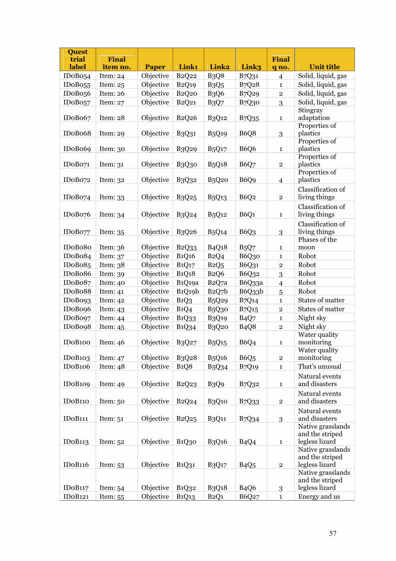
57

Quest trial label

Final item no. Paper Link1 Link2 Link3

Final q no. Unit title

ID0B054 Item: 24 Objective B2Q22 B3Q8 B7Q31 4 Solid, liquid, gas ID0B055 Item: 25 Objective B2Q19 B3Q5 B7Q28 1 Solid, liquid, gas ID0B056 Item: 26 Objective B2Q20 B3Q6 B7Q29 2 Solid, liquid, gas ID0B057 Item: 27 Objective B2Q21 B3Q7 B7Q30 3 Solid, liquid, gas

ID0B067 Item: 28 Objective B2Q26 B3Q12 B7Q35 1 Stingray adaptation

ID0B068 Item: 29 Objective B3Q31 B5Q19 B6Q8 3 Properties of plastics

ID0B069 Item: 30 Objective B3Q29 B5Q17 B6Q6 1 Properties of plastics

ID0B071 Item: 31 Objective B3Q30 B5Q18 B6Q7 2 Properties of plastics

ID0B072 Item: 32 Objective B3Q32 B5Q20 B6Q9 4 Properties of plastics

ID0B074 Item: 33 Objective B3Q25 B5Q13 B6Q2 2 Classification of living things

ID0B076 Item: 34 Objective B3Q24 B5Q12 B6Q1 1 Classification of living things

ID0B077 Item: 35 Objective B3Q26 B5Q14 B6Q3 3 Classification of living things

ID0B080 Item: 36 Objective B2Q33 B4Q18 B5Q7 1 Phases of the moon

ID0B084 Item: 37 Objective B1Q16 B2Q4 B6Q30 1 Robot ID0B085 Item: 38 Objective B1Q17 B2Q5 B6Q31 2 Robot ID0B086 Item: 39 Objective B1Q18 B2Q6 B6Q32 3 Robot ID0B087 Item: 40 Objective B1Q19a B2Q7a B6Q33a 4 Robot ID0B088 Item: 41 Objective B1Q19b B2Q7b B6Q33b 5 Robot ID0B093 Item: 42 Objective B1Q3 B5Q29 B7Q14 1 States of matter ID0B096 Item: 43 Objective B1Q4 B5Q30 B7Q15 2 States of matter ID0B097 Item: 44 Objective B1Q33 B3Q19 B4Q7 1 Night sky ID0B098 Item: 45 Objective B1Q34 B3Q20 B4Q8 2 Night sky

ID0B100 Item: 46 Objective B3Q27 B5Q15 B6Q4 1 Water quality monitoring

ID0B103 Item: 47 Objective B3Q28 B5Q16 B6Q5 2 Water quality monitoring

ID0B106 Item: 48 Objective B1Q8 B5Q34 B7Q19 1 That’s unusual

ID0B109 Item: 49 Objective B2Q23 B3Q9 B7Q32 1 Natural events and disasters

ID0B110 Item: 50 Objective B2Q24 B3Q10 B7Q33 2 Natural events and disasters

ID0B111 Item: 51 Objective B2Q25 B3Q11 B7Q34 3 Natural events and disasters

ID0B113 Item: 52 Objective B1Q30 B3Q16 B4Q4 1

Native grasslands and the striped legless lizard

ID0B116 Item: 53 Objective B1Q31 B3Q17 B4Q5 2

Native grasslands and the striped legless lizard

ID0B117 Item: 54 Objective B1Q32 B3Q18 B4Q6 3

Native grasslands and the striped legless lizard

ID0B121 Item: 55 Objective B1Q13 B2Q1 B6Q27 1 Energy and us

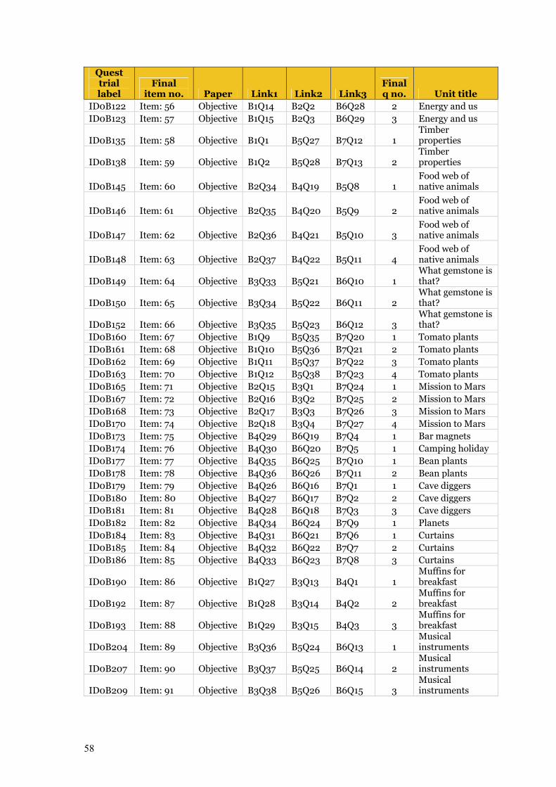
58

Quest trial label

Final item no. Paper Link1 Link2 Link3

Final q no. Unit title

ID0B122 Item: 56 Objective B1Q14 B2Q2 B6Q28 2 Energy and us ID0B123 Item: 57 Objective B1Q15 B2Q3 B6Q29 3 Energy and us

ID0B135 Item: 58 Objective B1Q1 B5Q27 B7Q12 1 Timber properties

ID0B138 Item: 59 Objective B1Q2 B5Q28 B7Q13 2 Timber properties

ID0B145 Item: 60 Objective B2Q34 B4Q19 B5Q8 1 Food web of native animals

ID0B146 Item: 61 Objective B2Q35 B4Q20 B5Q9 2 Food web of native animals

ID0B147 Item: 62 Objective B2Q36 B4Q21 B5Q10 3 Food web of native animals

ID0B148 Item: 63 Objective B2Q37 B4Q22 B5Q11 4 Food web of native animals

ID0B149 Item: 64 Objective B3Q33 B5Q21 B6Q10 1 What gemstone is that?

ID0B150 Item: 65 Objective B3Q34 B5Q22 B6Q11 2 What gemstone is that?

ID0B152 Item: 66 Objective B3Q35 B5Q23 B6Q12 3 What gemstone is that?

ID0B160 Item: 67 Objective B1Q9 B5Q35 B7Q20 1 Tomato plants ID0B161 Item: 68 Objective B1Q10 B5Q36 B7Q21 2 Tomato plants ID0B162 Item: 69 Objective B1Q11 B5Q37 B7Q22 3 Tomato plants ID0B163 Item: 70 Objective B1Q12 B5Q38 B7Q23 4 Tomato plants ID0B165 Item: 71 Objective B2Q15 B3Q1 B7Q24 1 Mission to Mars ID0B167 Item: 72 Objective B2Q16 B3Q2 B7Q25 2 Mission to Mars ID0B168 Item: 73 Objective B2Q17 B3Q3 B7Q26 3 Mission to Mars ID0B170 Item: 74 Objective B2Q18 B3Q4 B7Q27 4 Mission to Mars ID0B173 Item: 75 Objective B4Q29 B6Q19 B7Q4 1 Bar magnets ID0B174 Item: 76 Objective B4Q30 B6Q20 B7Q5 1 Camping holiday ID0B177 Item: 77 Objective B4Q35 B6Q25 B7Q10 1 Bean plants ID0B178 Item: 78 Objective B4Q36 B6Q26 B7Q11 2 Bean plants ID0B179 Item: 79 Objective B4Q26 B6Q16 B7Q1 1 Cave diggers ID0B180 Item: 80 Objective B4Q27 B6Q17 B7Q2 2 Cave diggers ID0B181 Item: 81 Objective B4Q28 B6Q18 B7Q3 3 Cave diggers ID0B182 Item: 82 Objective B4Q34 B6Q24 B7Q9 1 Planets ID0B184 Item: 83 Objective B4Q31 B6Q21 B7Q6 1 Curtains ID0B185 Item: 84 Objective B4Q32 B6Q22 B7Q7 2 Curtains ID0B186 Item: 85 Objective B4Q33 B6Q23 B7Q8 3 Curtains

ID0B190 Item: 86 Objective B1Q27 B3Q13 B4Q1 1 Muffins for breakfast

ID0B192 Item: 87 Objective B1Q28 B3Q14 B4Q2 2 Muffins for breakfast

ID0B193 Item: 88 Objective B1Q29 B3Q15 B4Q3 3 Muffins for breakfast

ID0B204 Item: 89 Objective B3Q36 B5Q24 B6Q13 1 Musical instruments

ID0B207 Item: 90 Objective B3Q37 B5Q25 B6Q14 2 Musical instruments

ID0B209 Item: 91 Objective B3Q38 B5Q26 B6Q15 3 Musical instruments

59

6.4 Item analysis files Access to the data files and output from the analyses is available to researchers or future

contractors who want to replicate procedures on application to MCEETYA Secretariat at

enquiries@mceetya.edu.au. Relevant data files are listed throughout the Technical Report.

6.5 Comparison of State/Territory locations in RUMM

Data showing the comparison of State/Territory locations in RUMM is provided in the file:

NAPSL2006_CheckStateLocations.xls.

60

Chapter 7 Scaling of Test Data

7.1 Overview The process of scaling refers to the estimation of student achievement distributions using

information from students’ responses to the test items. In the National Assessment Program –

Science Literacy, the scaling process involved two separate phases:

7.1.1 Calibration of item parameters The calibration of item parameters used a calibration sample in which equal numbers of

respondents from each jurisdiction are included. See Section 7.2 on the selection of the

calibration sample and the methodology for the calibration of item parameters.

7.1.2 Estimating student proficiency levels and producing plausible values

Once item parameters have been determined, student proficiency levels are estimated. As the

main purpose of the study is to obtain profiles of student achievement at the population level,

rather than at the individual student level, a methodology using plausible values (Wu 2005)

was adopted.

The following sections describe in detail the two phases of the scaling process.

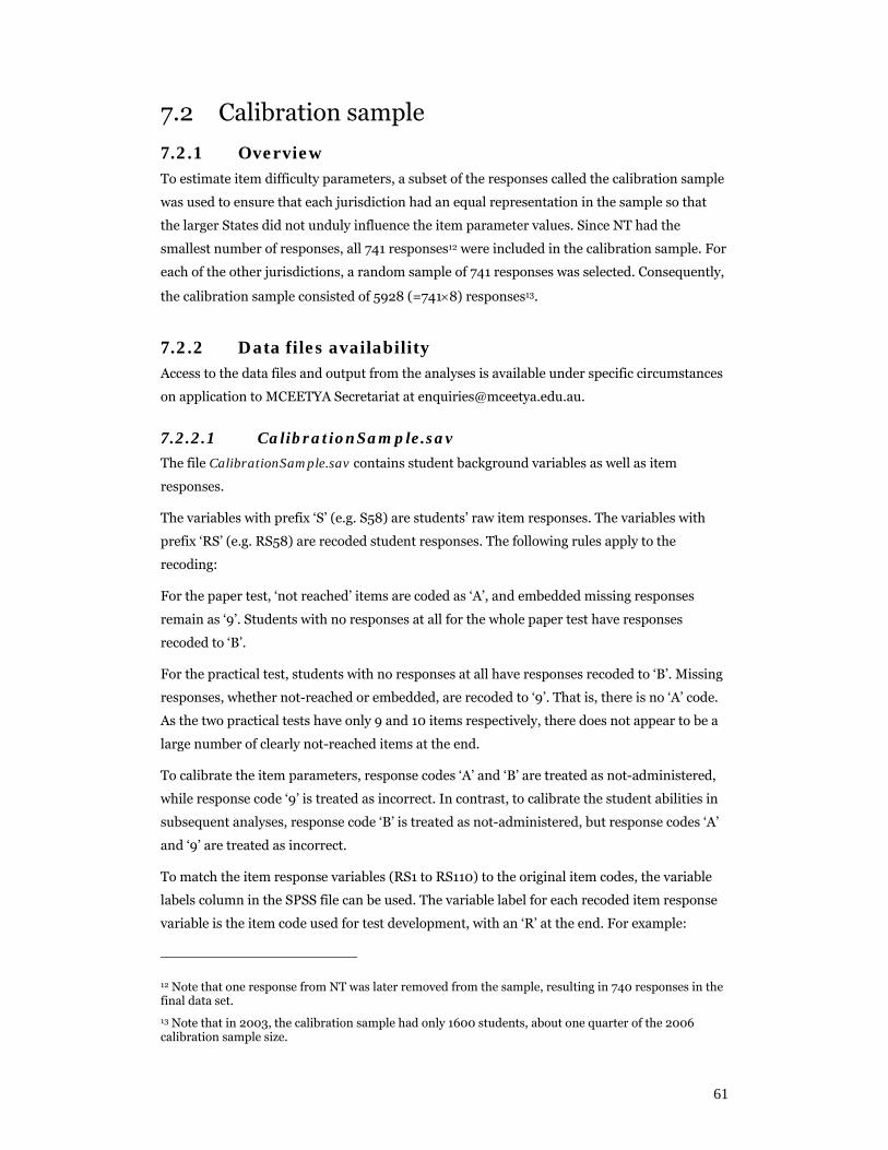
61

7.2 Calibration sample

7.2.1 Overview To estimate item difficulty parameters, a subset of the responses called the calibration sample

was used to ensure that each jurisdiction had an equal representation in the sample so that

the larger States did not unduly influence the item parameter values. Since NT had the

smallest number of responses, all 741 responses12 were included in the calibration sample. For

each of the other jurisdictions, a random sample of 741 responses was selected. Consequently,

the calibration sample consisted of 5928 (=741×8) responses13.

7.2.2 Data files availability Access to the data files and output from the analyses is available under specific circumstances

on application to MCEETYA Secretariat at enquiries@mceetya.edu.au.

7.2.2.1 CalibrationSample.sav

The file CalibrationSample.sav contains student background variables as well as item

responses.

The variables with prefix ‘S’ (e.g. S58) are students’ raw item responses. The variables with

prefix ‘RS’ (e.g. RS58) are recoded student responses. The following rules apply to the

recoding:

For the paper test, ‘not reached’ items are coded as ‘A’, and embedded missing responses

remain as ‘9’. Students with no responses at all for the whole paper test have responses

recoded to ‘B’.

For the practical test, students with no responses at all have responses recoded to ‘B’. Missing

responses, whether not-reached or embedded, are recoded to ‘9’. That is, there is no ‘A’ code.

As the two practical tests have only 9 and 10 items respectively, there does not appear to be a

large number of clearly not-reached items at the end.

To calibrate the item parameters, response codes ‘A’ and ‘B’ are treated as not-administered,

while response code ‘9’ is treated as incorrect. In contrast, to calibrate the student abilities in

subsequent analyses, response code ‘B’ is treated as not-administered, but response codes ‘A’

and ‘9’ are treated as incorrect.

To match the item response variables (RS1 to RS110) to the original item codes, the variable

labels column in the SPSS file can be used. The variable label for each recoded item response

variable is the item code used for test development, with an ‘R’ at the end. For example:

12 Note that one response from NT was later removed from the sample, resulting in 740 responses in the final data set.

13 Note that in 2003, the calibration sample had only 1600 students, about one quarter of the 2006 calibration sample size.

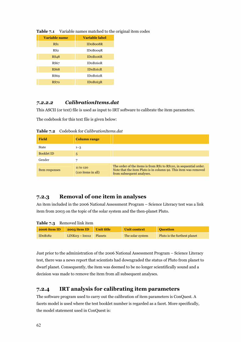
62

Table 7.1 Variable names matched to the original item codes

Variable name Variable label

RS1 ID0B008R

RS2 ID0B009R

RS48 ID0B106R

RS67 ID0B160R

RS68 ID0B161R

RS69 ID0B162R

RS70 ID0B163R

7.2.2.2 CalibrationItems.dat

This ASCII (or text) file is used as input to IRT software to calibrate the item parameters.

The codebook for this text file is given below:

Table 7.2 Codebook for CalibrationItems.dat

Field Column range

State 1–3

Booklet ID 5

Gender 7

Item responses 11 to 120

(110 items in all)

The order of the items is from RS1 to RS110, in sequential order. Note that the item Pluto is in column 92. This item was removed from subsequent analyses.

7.2.3 Removal of one item in analyses An item included in the 2006 National Assessment Program – Science Literacy test was a link

item from 2003 on the topic of the solar system and the then-planet Pluto.

Table 7.3 Removed link item

2006 item ID 2003 item ID Unit title Unit context Question

ID0B182 LINK03 – I0012 Planets The solar system Pluto is the furthest planet

Just prior to the administration of the 2006 National Assessment Program – Science Literacy

test, there was a news report that scientists had downgraded the status of Pluto from planet to

dwarf planet. Consequently, the item was deemed to be no longer scientifically sound and a

decision was made to remove the item from all subsequent analyses.

7.2.4 IRT analysis for calibrating item parameters The software program used to carry out the calibration of item parameters is ConQuest. A

facets model is used where the test booklet number is regarded as a facet. More specifically,

the model statement used in ConQuest is:

63

bookid + item + item*step

The full syntax of ConQuest commands is in the control file CalibrationSample1.cqc.

The use of the term ‘bookid’ in ConQuest model statements is to ensure that the estimation of

the item parameters takes into account of the so-called ‘booklet effect’ (OECD 2005, p. 198).

However, as there is only one domain in the National Assessment Program – Science Literacy

2006 (unlike PISA where there are three domains: mathematics, science and reading) and all

items are calibrated together, it is not expected that there will be significant booklet effect, as

is shown later in the results of the item analysis.

Three output files are produced from ConQuest:

CalibrationSample_noPluto.shw

This is a summary file, showing booklet and item parameter values, population parameter

estimated and item–person maps.

CalibrationSample_noPluto.itn

This file is known as the ‘itanal’, showing classical test statistics as well as IRT statistics for

each item.

itemparam.anc

This file is produced through an Export statement in ConQuest. It contains the values of the

parameters that can be used as anchor values later when student abilities are estimated.

7.3 Estimating student proficiency levels and producing plausible values

In this phase, student proficiency levels are estimated for the full data set

(NAPSL2006_Reporting_WLE_PV_20070423.sav. See Appendix H for descriptions of

variables).

The scaling model used is a one-parameter item response model with conditioning variables

in the population latent regression model. See PISA Technical Report for a description of the

model (OECD 2005).

The conditioning variables included are

• School mean proficiency (average of students’ weighted likelihood estimates for each school)

• State

• Sector

• Gender

• ATSI status

• Geolocation.

64

Note that the variable LBOTE is not in the above list. LBOTE was collected by OSRS; however,

that information was incomplete with many missing values. Consequently, it could not be

used in the scaling process.

To prepare the data to be used as conditioning variables, two separate steps are taken:

Step A: Produce WLE estimate (weighted likelihood estimate) for each student in the full data

set, and compute the average WLE for each school. The software program Quest is used for

the estimation of WLE estimates, with item parameters anchored at values from the Item

Calibration Phase. Both embedded-missing (code ‘9’) and not-reached items (code ‘A’) are

treated as incorrect. If a test has no valid responses from a student, the responses (code ‘B’)

are treated as not-administered.

Step B: Dummy variables are created for State, Sector, Gender, ATSI and Geolocation.

7.3.1 Production of plausible values The software program ConQuest is used for the scaling of student proficiency levels and the

generation of plausible values. Note that Case Weight is used in this analysis. Both booklet

parameters and item parameters are anchored. Both embedded-missing (code ‘9’) and not-

reached items (code ‘A’) are treated as incorrect. If a test has no valid responses from a

student, the responses (code ‘B’) are treated as not-administered. Ten plausible values are

generated (instead of the usual five).

The ConQuest control file used is ProducePV.cqc, shown in Appendix I.

7.4 Estimation of statistics of interest and their standard errors

Once the plausible values are produced for each student, statistics of interest can be computed

together with their standard errors. For example, the mean achievement level in science for

Year 6 students in Australia can be estimated, as well as jurisdiction average achievement

levels. The estimates will also have associated standard errors to indicate the confidence

which we have about the results.

The plausible-values methodology has been used for large-scale studies such as TIMSS, PISA

and NAEP. In the National Assessment Program – Science Literacy 2006, this methodology

was also used for the estimation of statistics and standard errors. For a detailed description of

the methodology, see Mislevy, Beaton, Kaplan and Sheehan (1992), and Beaton and Gonzalez

(1995).

Briefly, the methodology is summarised below. The plausible values for each student show the

indicative level of the student’s achievement. So the estimate for a population statistic is

computed using the plausible values as if they represent each student’s level of achievement.

For example, to compute the estimated mean of the population, take the first plausible value

65

for each student and compute the average across students, weighted by the sampling weight

(student final weight). Repeat the process with all ten plausible values, and then average the

ten estimated means for the ten runs. Similarly, for the estimation of percentiles and

percentages in levels, plausible values are used in the same way.

The standard errors associated with the estimated statistics are not straightforward to

compute, as the sampling method is not simple random sampling but a complex two-stage

sampling. Typically, for complex sampling such as the one used for NAP–SL 2006, replication

methods such as Balanced Repeated Replicate (BRR) or Jackknife are used to compute

standard errors (Rust & Rao 1996). In the National Assessment Program – Science Literacy

2006, the method of Jackknife was used. Jackknife replication weights are computed

(variables RW1 to RW310 in the file NAPSL2006_Reporting_WLE_PV_20070423.sav).

The statistic of interest is computed using each of the replicate weights in turn. The variations

in the estimated statistic obtained from using different replicate weights contribute to the

estimate of the sampling variance for the estimated statistic. Combining this sampling

variance with the variance from using the ten plausible values (measurement error) provides

an estimate of the standard error for the estimated statistic.

SPSS macros were written to carry the procedures of the estimation of statistics and their

standard errors.

7.5 Transform logits to a scale with mean 400 and standard deviation 100

To facilitate the interpretation of the results, it is a common practice to transform logit scores.

It was decided that, for the National Assessment Program – Science Literacy surveys, the

proficiency scale should have a national mean of 400 and a standard deviation of 100. This

scale was chosen to avoid having negative values on the scale representing student

proficiency. Further, a standard deviation of 100 provides easy interpretation of proficiency

levels in terms of how far away a score is from the mean.

The transformation used in 2006 is given below.

Score on proficiency scale = (Logit–0.200543797)/0.954513216*100+400

Note that the mean of 400 is the national mean, computed using student sampling weights to

reflect the average achievement of all Year 6 students in Australia. It is not the average of

jurisdiction means, as that average does not take into account the number of students in each

jurisdiction. In summary, house weights are used to set the average score of 400, not senate

weights.

66

Chapter 8 Equating 2003 Results to 2006 Results

8.1 Setting 2006 results as the baseline While the first cycle of the National Assessment Program – Science Literacy was conducted in

2003 (then known as PSAP), and the 2006 survey was the second round of the National

Assessment Program – Science Literacy, it was decided that the 2006 survey be used to set the

scale of a mean of 400 and a standard deviation of 100 (see Section 7.5), instead of the 2003

survey. The reasons for this decision are summarised below.

(1) The 2006 survey test design was more robust than the 2003 test design. In 2006, a balanced

incomplete block (BIB) test design consisting of seven test booklets was used. In contrast, in

2003 only two test booklets were used, resulting in item-position effect for most items.

(2) There were considerably more items in 2006 than in 2003, resulting in a better coverage

of the test contents in 2006. In 2006, 110 items were included in the final test, while only 72

items were included in the 2003 test.

(3) The 2006 survey produced a much higher population variance in achievement than 2003

did. In logits, the 2006 population standard deviation was 0.95, while the 2003 population

standard deviation was 0.78. This could be an indication that:

• the 2006 items were generally more discriminating than the 2003 items; that is, the 2006

items were higher quality items

• the 2006 sampling was more comprehensive, as remote schools were also included

in the sample, while the 2003 sampling focused only on areas where students were

well-resourced.

67

8.1.1 ACER re-analysis in April 2007 of the 2003 results Owing to errors in the weightings in the 2003 analysis, ACER carried out a re-analysis of

2003 data in April 2007. Some of the following tables contain results from the original 2003

analysis and some contain results from the 2007 re-analysis, depending on whether the 2006

analysis was carried out pre- or post-ACER re-analysis.

8.2 Equating 2003 results to 2006 results As a consequence of the decision to use 2006 results as the baseline, 2003 results were

equated to 2006 results. To carry out the equating, link items between the 2003 and 2006

tests were used.

8.2.1 Link items The equating methodology as originally conceived in a draft paper (NAPSL06_001_TestDesign.doc)

proposed that around 25 items from 2003 be embedded in the 2006 test as link items. The

methodology also recommended that 15–20 items from the secure item pool of 2003 be

included in the 2005 trial of items for the 2006 test.

It was important to find items that performed well statistically and also covered the range of

science literacy strands A, B and C and the science concept areas: Earth and Beyond; Energy

and Change; Life and Living; and Natural and Processed Materials. This reduced the number

of items available. Sixteen items were selected for trialling and formed a cluster as part of the

BIB design. Of these, five performed poorly at trial and were deemed inappropriate to include

in the 2006 test. A concern at the small number of available link items was flagged.

Ultimately, eleven items were approved for use as link items in the main test. These are

summarised in Table 8.1. In the final test nine items from 2003 were included.

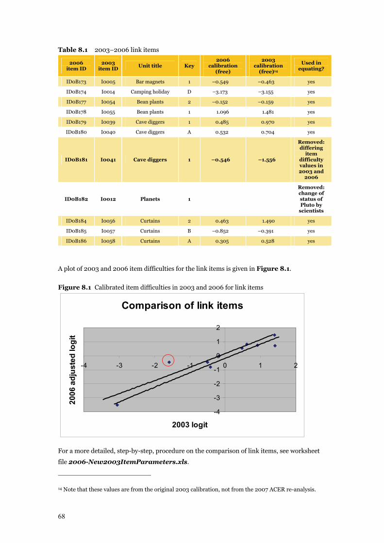
68

Table 8.1 2003–2006 link items

2006 item ID

2003 item ID Unit title Key

2006 calibration

(free)

2003 calibration

(free)14

Used in equating?

ID0B173 I0005 Bar magnets 1 –0.549 –0.463 yes

ID0B174 I0014 Camping holiday D –3.173 –3.155 yes

ID0B177 I0054 Bean plants 2 –0.152 –0.159 yes

ID0B178 I0055 Bean plants 1 1.096 1.481 yes

ID0B179 I0039 Cave diggers 1 0.485 0.970 yes

ID0B180 I0040 Cave diggers A 0.532 0.704 yes

ID0B181 I0041 Cave diggers 1 –0.546 –1.556

Removed: differing

item difficulty values in 2003 and

2006

ID0B182 I0012 Planets 1

Removed: change of status of Pluto by

scientists

ID0B184 I0056 Curtains 2 0.463 1.490 yes

ID0B185 I0057 Curtains B –0.852 –0.391 yes

ID0B186 I0058 Curtains A 0.305 0.528 yes

A plot of 2003 and 2006 item difficulties for the link items is given in Figure 8.1.

Figure 8.1 Calibrated item difficulties in 2003 and 2006 for link items

Comparison of link items

-4

-3

-2

-1

0

1

2

-4 -3 -2 -1 0 1 2

2003 logit

2006

adj

uste

d lo

git

For a more detailed, step-by-step, procedure on the comparison of link items, see worksheet

file 2006-New2003ItemParameters.xls.

14 Note that these values are from the original 2003 calibration, not from the 2007 ACER re-analysis.

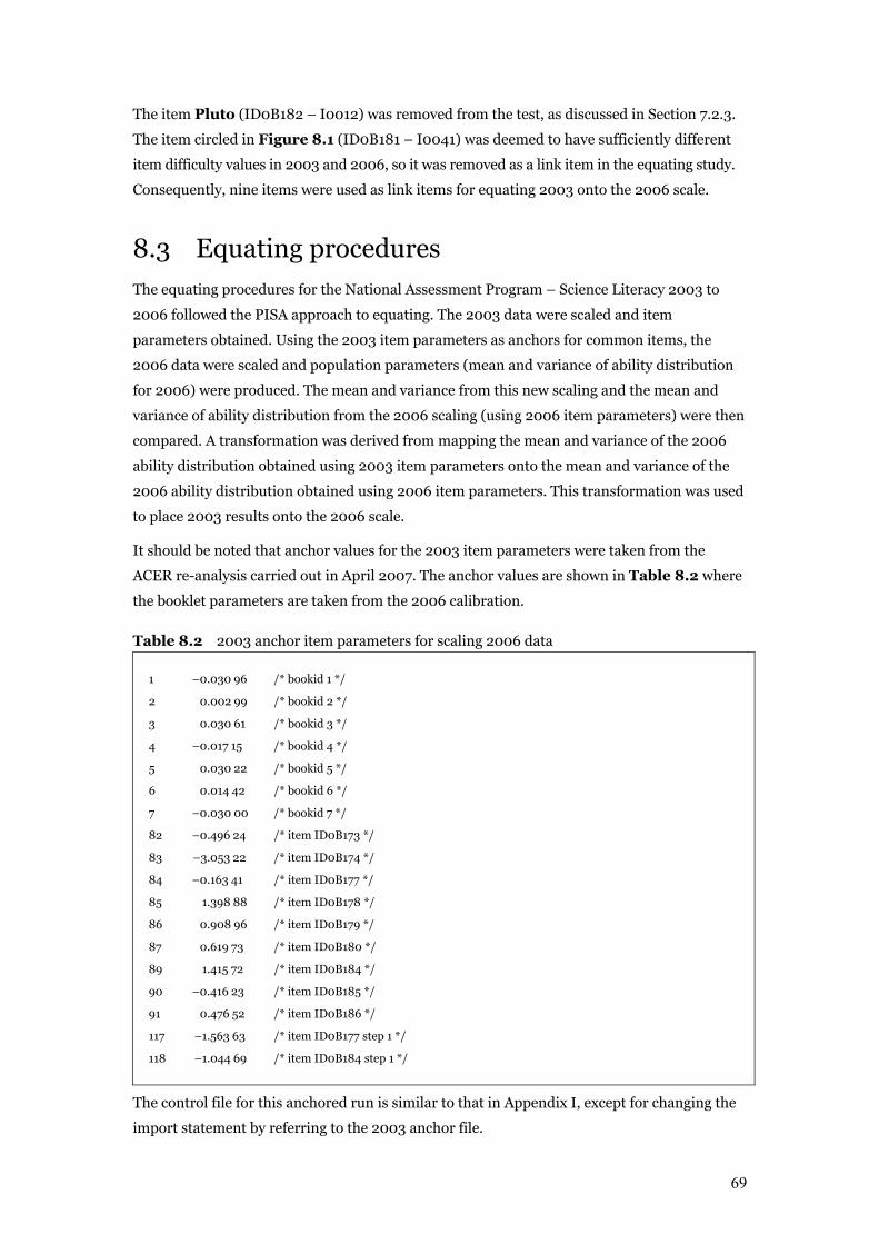
69

The item Pluto (ID0B182 – I0012) was removed from the test, as discussed in Section 7.2.3.

The item circled in Figure 8.1 (ID0B181 – I0041) was deemed to have sufficiently different

item difficulty values in 2003 and 2006, so it was removed as a link item in the equating study.

Consequently, nine items were used as link items for equating 2003 onto the 2006 scale.

8.3 Equating procedures The equating procedures for the National Assessment Program – Science Literacy 2003 to

2006 followed the PISA approach to equating. The 2003 data were scaled and item

parameters obtained. Using the 2003 item parameters as anchors for common items, the

2006 data were scaled and population parameters (mean and variance of ability distribution

for 2006) were produced. The mean and variance from this new scaling and the mean and

variance of ability distribution from the 2006 scaling (using 2006 item parameters) were then

compared. A transformation was derived from mapping the mean and variance of the 2006

ability distribution obtained using 2003 item parameters onto the mean and variance of the

2006 ability distribution obtained using 2006 item parameters. This transformation was used

to place 2003 results onto the 2006 scale.

It should be noted that anchor values for the 2003 item parameters were taken from the

ACER re-analysis carried out in April 2007. The anchor values are shown in Table 8.2 where

the booklet parameters are taken from the 2006 calibration.

Table 8.2 2003 anchor item parameters for scaling 2006 data 1 –0.030 96 /* bookid 1 */

2 0.002 99 /* bookid 2 */

3 0.030 61 /* bookid 3 */

4 –0.017 15 /* bookid 4 */

5 0.030 22 /* bookid 5 */

6 0.014 42 /* bookid 6 */

7 –0.030 00 /* bookid 7 */

82 –0.496 24 /* item ID0B173 */

83 –3.053 22 /* item ID0B174 */

84 –0.163 41 /* item ID0B177 */

85 1.398 88 /* item ID0B178 */

86 0.908 96 /* item ID0B179 */

87 0.619 73 /* item ID0B180 */

89 1.415 72 /* item ID0B184 */

90 –0.416 23 /* item ID0B185 */

91 0.476 52 /* item ID0B186 */

117 –1.563 63 /* item ID0B177 step 1 */

118 –1.044 69 /* item ID0B184 step 1 */

The control file for this anchored run is similar to that in Appendix I, except for changing the

import statement by referring to the 2003 anchor file.

70

8.4 Equating transformation The result of the equating process was the derivation of a transformation formula for 2003

results to be placed on the 2006 scale. This equation is given below.

2003 result on 2006 scale = ((2003 logit – 0.5215) / 0.9595) * 0.9545) + 0.2005

The above transformation essentially performs a constant shift of around –0.32. The scale

factor is very close to 1, indicating that an adjustment of the scale factor is not really necessary.

For standard errors, the transformation involved only the scale factor, as follows:

2003 standard error on 2006 scale in logit = (2003 S.E. in logit) / 0.9595 * 0.9545

8.5 Link error In establishing trends from 2003 to 2006, it is necessary to make judgments about the

statistical significance of the difference in science achievement between 2003 and 2006. An

appropriate estimation of the magnitude of equating errors is important when trends are

reported. An underestimate of the equating errors will often result in erroneous claims of

change in achievement levels when there is no significant difference.

Equating errors come from at least two sources: the sampling of students and the sampling of

items. Equating errors due to the sampling of students affect the accuracy with which the item

parameters are estimated, and the magnitude of these errors diminishes when the sample size

increases. However, equating errors due to the sampling of items have not often been taken

into account, and the magnitude of these errors does not diminish when the sample size

increases. For the estimates of population parameters (e.g. mean), the magnitude of equating

errors due to the sampling of items tends to be much larger than the magnitude of equating

errors due to the sampling of students. Consequently, it is important to estimate the equating

error due to the sampling of items.

Following the approach used in PISA (OECD 2005), equating error (called ‘link error’ in

PISA) is computed as follows: calibrate the items using 2003 and 2006 data separately. If the

link items behave exactly the same way in 2003 and 2006 (and they follow the Rasch model),

there should only be a constant difference between 2003 and 2006 item parameters for

matched items. However, in real life, items will vary from 2003 to 2006 and some items will

vary more than others. The degree to which the item parameters change from 2003 to 2006

can be assessed in the following way. Take the difference between 2003 and 2006 item

difficulties for each link item, where the 2003 item difficulties have been placed on the 2006

scale. Compute the standard error of the mean of the differences. This standard error is used

as equating error due to the sampling of items. Table 8.3 shows the computation.

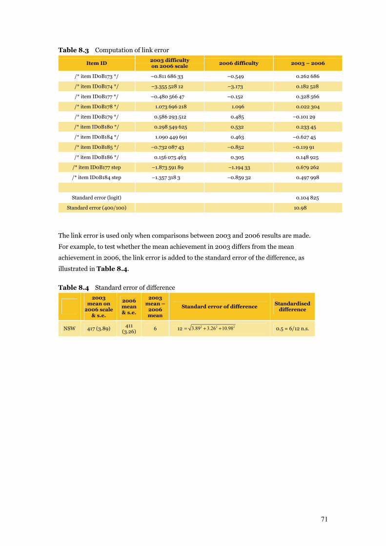
71

Table 8.3 Computation of link error

Item ID 2003 difficulty on 2006 scale 2006 difficulty 2003 – 2006

/* item ID0B173 */ –0.811 686 33 –0.549 0.262 686

/* item ID0B174 */ –3.355 528 12 –3.173 0.182 528

/* item ID0B177 */ –0.480 566 47 –0.152 0.328 566

/* item ID0B178 */ 1.073 696 218 1.096 0.022 304

/* item ID0B179 */ 0.586 293 512 0.485 –0.101 29

/* item ID0B180 */ 0.298 549 625 0.532 0.233 45

/* item ID0B184 */ 1.090 449 691 0.463 –0.627 45

/* item ID0B185 */ –0.732 087 43 –0.852 –0.119 91

/* item ID0B186 */ 0.156 075 463 0.305 0.148 925

/* item ID0B177 step –1.873 591 89 –1.194 33 0.679 262

/* item ID0B184 step –1.357 318 3 –0.859 32 0.497 998

Standard error (logit) 0.104 825

Standard error (400/100) 10.98

The link error is used only when comparisons between 2003 and 2006 results are made.

For example, to test whether the mean achievement in 2003 differs from the mean

achievement in 2006, the link error is added to the standard error of the difference, as

illustrated in Table 8.4.

Table 8.4 Standard error of difference

2003 mean on

2006 scale & s.e.

2006 mean & s.e.

2003 mean –

2006 mean

Standard error of difference Standardised

difference

NSW 417 (3.89) 411

(3.26) 6 12 2 2 23.89 3.26 10.98= + + 0.5 = 6/12 n.s.

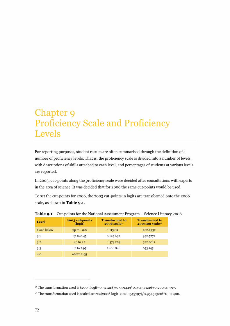
72

Chapter 9 Proficiency Scale and Proficiency Levels

For reporting purposes, student results are often summarised through the definition of a

number of proficiency levels. That is, the proficiency scale is divided into a number of levels,

with descriptions of skills attached to each level, and percentages of students at various levels

are reported.

In 2003, cut-points along the proficiency scale were decided after consultations with experts

in the area of science. It was decided that for 2006 the same cut-points would be used.

To set the cut-points for 2006, the 2003 cut-points in logits are transformed onto the 2006

scale, as shown in Table 9.1.

Table 9.1 Cut-points for the National Assessment Program – Science Literacy 2006

Level 2003 cut-points

(logit) Transformed to

2006 scale15 Transformed to 400/100 scale16

2 and below up to –0.8 –1.113 89 262.2932

3.1 up to 0.45 0.129 692 392.5772

3.2 up to 1.7 1.373 269 522.8611

3.3 up to 2.95 2.616 846 653.145

4.0 above 2.95

15 The transformation used is (2003 logit–0.521218)/0.959443*0.954513216+0.200543797.

16 The transformation used is scaled score=(2006 logit–0.200543797)/0.954513216*100+400.

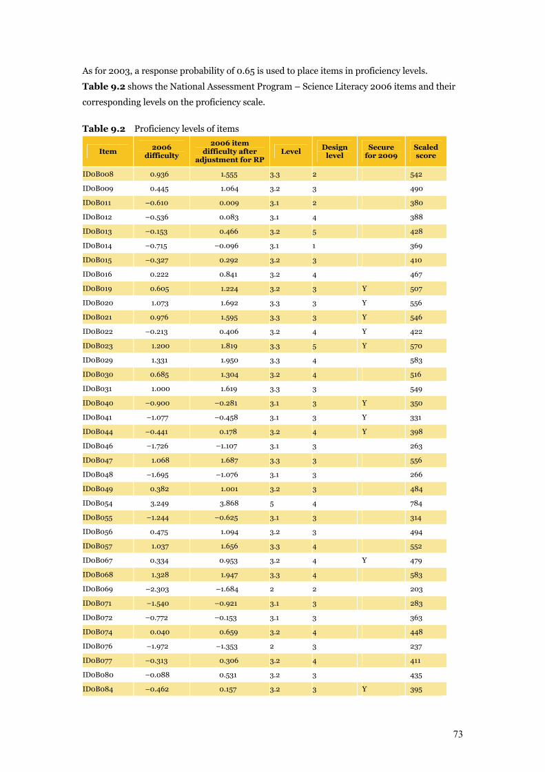
73

As for 2003, a response probability of 0.65 is used to place items in proficiency levels.

Table 9.2 shows the National Assessment Program – Science Literacy 2006 items and their

corresponding levels on the proficiency scale.

Table 9.2 Proficiency levels of items

Item 2006

difficulty

2006 item difficulty after

adjustment for RPLevel

Design level

Secure for 2009

Scaled score

ID0B008 0.936 1.555 3.3 2 542

ID0B009 0.445 1.064 3.2 3 490

ID0B011 –0.610 0.009 3.1 2 380

ID0B012 –0.536 0.083 3.1 4 388

ID0B013 –0.153 0.466 3.2 5 428

ID0B014 –0.715 –0.096 3.1 1 369

ID0B015 –0.327 0.292 3.2 3 410

ID0B016 0.222 0.841 3.2 4 467

ID0B019 0.605 1.224 3.2 3 Y 507

ID0B020 1.073 1.692 3.3 3 Y 556

ID0B021 0.976 1.595 3.3 3 Y 546

ID0B022 –0.213 0.406 3.2 4 Y 422

ID0B023 1.200 1.819 3.3 5 Y 570

ID0B029 1.331 1.950 3.3 4 583

ID0B030 0.685 1.304 3.2 4 516

ID0B031 1.000 1.619 3.3 3 549

ID0B040 –0.900 –0.281 3.1 3 Y 350

ID0B041 –1.077 –0.458 3.1 3 Y 331

ID0B044 –0.441 0.178 3.2 4 Y 398

ID0B046 –1.726 –1.107 3.1 3 263

ID0B047 1.068 1.687 3.3 3 556

ID0B048 –1.695 –1.076 3.1 3 266

ID0B049 0.382 1.001 3.2 3 484

ID0B054 3.249 3.868 5 4 784

ID0B055 –1.244 –0.625 3.1 3 314

ID0B056 0.475 1.094 3.2 3 494

ID0B057 1.037 1.656 3.3 4 552

ID0B067 0.334 0.953 3.2 4 Y 479

ID0B068 1.328 1.947 3.3 4 583

ID0B069 –2.303 –1.684 2 2 203

ID0B071 –1.540 –0.921 3.1 3 283

ID0B072 –0.772 –0.153 3.1 3 363

ID0B074 0.040 0.659 3.2 4 448

ID0B076 –1.972 –1.353 2 3 237

ID0B077 –0.313 0.306 3.2 4 411

ID0B080 –0.088 0.531 3.2 3 435

ID0B084 –0.462 0.157 3.2 3 Y 395

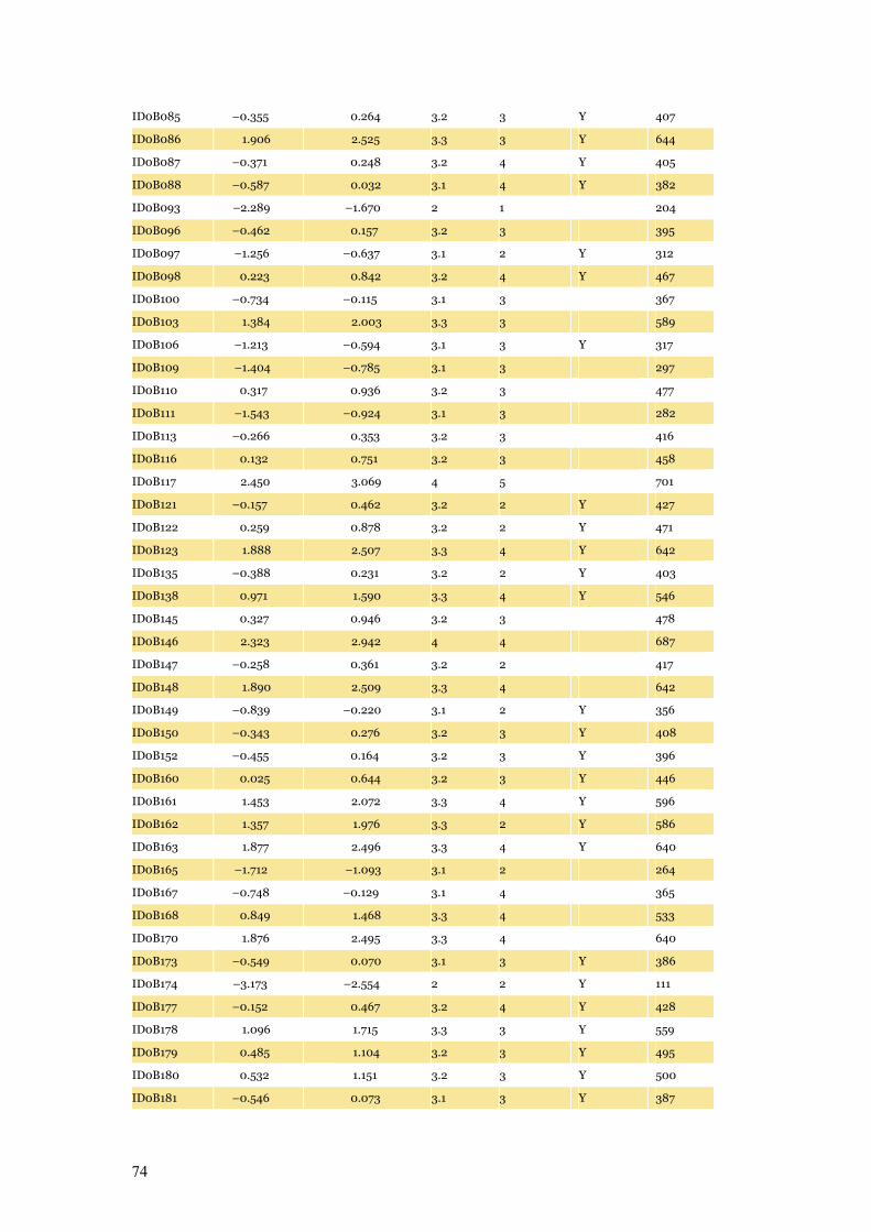
74

ID0B085 –0.355 0.264 3.2 3 Y 407

ID0B086 1.906 2.525 3.3 3 Y 644

ID0B087 –0.371 0.248 3.2 4 Y 405

ID0B088 –0.587 0.032 3.1 4 Y 382

ID0B093 –2.289 –1.670 2 1 204

ID0B096 –0.462 0.157 3.2 3 395

ID0B097 –1.256 –0.637 3.1 2 Y 312

ID0B098 0.223 0.842 3.2 4 Y 467

ID0B100 –0.734 –0.115 3.1 3 367

ID0B103 1.384 2.003 3.3 3 589

ID0B106 –1.213 –0.594 3.1 3 Y 317

ID0B109 –1.404 –0.785 3.1 3 297

ID0B110 0.317 0.936 3.2 3 477

ID0B111 –1.543 –0.924 3.1 3 282

ID0B113 –0.266 0.353 3.2 3 416

ID0B116 0.132 0.751 3.2 3 458

ID0B117 2.450 3.069 4 5 701

ID0B121 –0.157 0.462 3.2 2 Y 427

ID0B122 0.259 0.878 3.2 2 Y 471

ID0B123 1.888 2.507 3.3 4 Y 642

ID0B135 –0.388 0.231 3.2 2 Y 403

ID0B138 0.971 1.590 3.3 4 Y 546

ID0B145 0.327 0.946 3.2 3 478

ID0B146 2.323 2.942 4 4 687

ID0B147 –0.258 0.361 3.2 2 417

ID0B148 1.890 2.509 3.3 4 642

ID0B149 –0.839 –0.220 3.1 2 Y 356

ID0B150 –0.343 0.276 3.2 3 Y 408

ID0B152 –0.455 0.164 3.2 3 Y 396

ID0B160 0.025 0.644 3.2 3 Y 446

ID0B161 1.453 2.072 3.3 4 Y 596

ID0B162 1.357 1.976 3.3 2 Y 586

ID0B163 1.877 2.496 3.3 4 Y 640

ID0B165 –1.712 –1.093 3.1 2 264

ID0B167 –0.748 –0.129 3.1 4 365

ID0B168 0.849 1.468 3.3 4 533

ID0B170 1.876 2.495 3.3 4 640

ID0B173 –0.549 0.070 3.1 3 Y 386

ID0B174 –3.173 –2.554 2 2 Y 111

ID0B177 –0.152 0.467 3.2 4 Y 428

ID0B178 1.096 1.715 3.3 3 Y 559

ID0B179 0.485 1.104 3.2 3 Y 495

ID0B180 0.532 1.151 3.2 3 Y 500

ID0B181 –0.546 0.073 3.1 3 Y 387

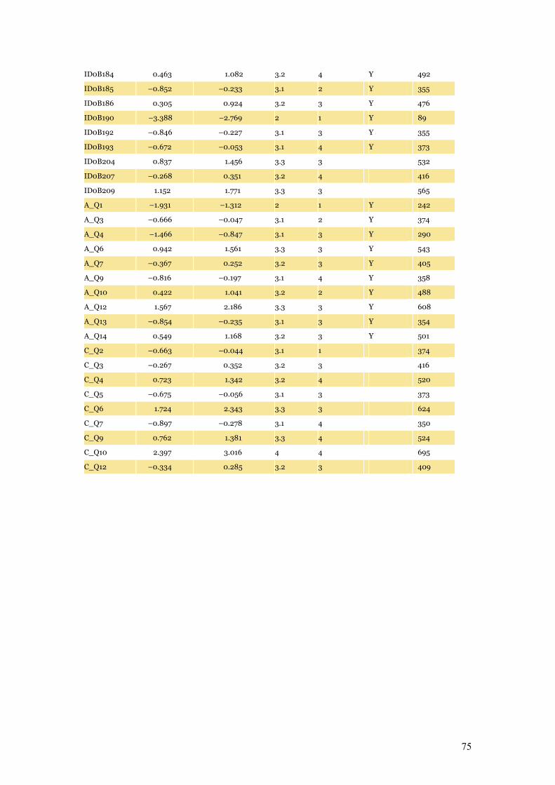
75

ID0B184 0.463 1.082 3.2 4 Y 492

ID0B185 –0.852 –0.233 3.1 2 Y 355

ID0B186 0.305 0.924 3.2 3 Y 476

ID0B190 –3.388 –2.769 2 1 Y 89

ID0B192 –0.846 –0.227 3.1 3 Y 355

ID0B193 –0.672 –0.053 3.1 4 Y 373

ID0B204 0.837 1.456 3.3 3 532

ID0B207 –0.268 0.351 3.2 4 416

ID0B209 1.152 1.771 3.3 3 565

A_Q1 –1.931 –1.312 2 1 Y 242

A_Q3 –0.666 –0.047 3.1 2 Y 374

A_Q4 –1.466 –0.847 3.1 3 Y 290

A_Q6 0.942 1.561 3.3 3 Y 543

A_Q7 –0.367 0.252 3.2 3 Y 405

A_Q9 –0.816 –0.197 3.1 4 Y 358

A_Q10 0.422 1.041 3.2 2 Y 488

A_Q12 1.567 2.186 3.3 3 Y 608

A_Q13 –0.854 –0.235 3.1 3 Y 354

A_Q14 0.549 1.168 3.2 3 Y 501

C_Q2 –0.663 –0.044 3.1 1 374

C_Q3 –0.267 0.352 3.2 3 416

C_Q4 0.723 1.342 3.2 4 520

C_Q5 –0.675 –0.056 3.1 3 373

C_Q6 1.724 2.343 3.3 3 624

C_Q7 –0.897 –0.278 3.1 4 350

C_Q9 0.762 1.381 3.3 4 524

C_Q10 2.397 3.016 4 4 695

C_Q12 –0.334 0.285 3.2 3 409

76

References

Biggs, J. and Collis, K. (1982) Evaluating the quality of learning: the SOLO taxonomy.

New York: Academic Press.

Beaton, A.E. and Gonzalez, E. (1995) NAEP primer. Chestnut Hill, MA, Boston College:

Boston.

Mislevy, R.J., Beaton, A.E., Kaplan, B. and Sheehan, K.M. (1992) Estimating population

characteristics from sparse matrix samples of item responses. Journal of Educational

Measurement, 29, pp. 133–161.

IEA (2004) TIMSS 2003 technical report.

OECD (2005) PISA 2003 technical report.

Rust, K.F. and Rao, J.N.K. (1996) Variance estimation for complex surveys using replication

techniques. Statistical Methods in Medical Research, Vol. 5, Hodder Arnold, London,

pp. 283–310.

Wu, M.L. (2005) The role of plausible values in large-scale surveys. Postlethwaite (ed.).

Special Issue of Studies in Educational Evaluation (SEE) in memory of R.M. Wolf. 31

(2005) pp. 114–128.

77

Appendix A National Year 6 Primary Science Assessment Domain

A.1. Assessment domains: scientific literacy The national review of the status and quality of teaching and learning of science in Australian

schools (Goodrum, Hackling & Rennie 2001) argued that the broad purpose of science in the

compulsory years of schooling is to develop scientific literacy for all students.

Scientific literacy is a high priority for all citizens, helping them to:

• be interested in and understand the world around them

• engage in the discourses of and about science

• be sceptical and questioning of claims made by others about scientific matters

• be able to identify questions, investigate and draw evidence-based conclusions

• make informed decisions about the environment and their own health and wellbeing.

Scientific literacy is important as it contributes to the economic and social wellbeing of the

nation and improved decision making at public and personal levels (Laugksch 2000).

PISA focuses on aspects of preparedness for adult life in terms of functional knowledge and

skills that allow citizens to participate actively in society. It is argued that scientifically-literate

people are ‘able to use scientific knowledge and processes not just to understand the natural

world but also to participate in decisions that affect it’ (OECD 1999, p. 13).

78

The OECD–PISA defined scientific literacy as:

the capacity to use scientific knowledge, to identify questions (investigate)17 and to draw

evidence-based conclusions in order to understand and help make decisions about the

natural world and the changes made to it through human activity.

(OECD 1999, p. 60)

This definition has been adopted for the national assessment of Science Literacy (NAP-SL) in

accord with the Ball, Rae and Tognolini (2000) report recommendation.

A.2. Scientific literacy: progress map A scientific literacy progress map was developed based on the construct of scientific literacy

and on an analysis of State and Territory curriculum and assessment frameworks. The

progress map describes the development of science literacy across three strands of knowledge

which are inclusive of Ball et al.’s concepts and processes and the elements of the OECD–PISA

definition.

The five elements of scientific literacy, including concepts and processes used in PISA 2000

(OECD–PISA 1999), include:

• demonstrating understanding of scientific concepts

• recognising scientifically investigable questions

• identifying evidence needed in a scientific investigation

• drawing or evaluating conclusions

• communicating valid conclusions.

These elements have been clustered into three, more holistic strands which have been

described below. The second and third elements and conducting investigations to collect data

are encompassed in strand A; the fourth and fifth elements and conducting investigations to

collect data are included in strand B; and the first element is included in strand C.

Strand A: Formulating or identifying investigable questions and hypotheses, planning

investigations and collecting evidence

This process strand includes posing questions or hypotheses for investigation or recognising

scientifically investigable questions; planning investigations by identifying variables and

devising procedures where variables are controlled; gathering evidence through measurement

17 Because of the constraints of large-scale testing, PISA was not able to include performance tasks such as conducting

investigations. Consequently, its definition of scientific literacy omitted reference to investigating. The word

‘investigate’ was inserted into the definition for the purposes of the National Science Assessment, as the sample

testing methodology to be used allowed for assessments of students’ ability to conduct investigations.

79

and observation; and making records of data in the form of descriptions, drawings, tables and

graphs using a range of information and communications technologies.

Strand B: Interpreting evidence and drawing conclusions from their own or others’ data,

critiquing the trustworthiness of evidence and claims made by others, and communicating

findings

This process strand includes identifying, describing and explaining the patterns and

relationships between variables in scientific data; drawing conclusions that are evidence-

based and related to the questions or hypotheses posed; critiquing the trustworthiness of

evidence and claims made by others; and communicating findings using a range of scientific

genres and information and communications technologies.

Strand C: Using science understandings for describing and explaining natural phenomena,

and for interpreting reports about phenomena

This conceptual strand includes demonstrating conceptual understandings by being able to:

describe, explain and make sense of natural phenomena; understand and interpret reports

(e.g. TV documentaries, newspaper or magazine articles or conversations) related to scientific

matters; and make decisions about scientific matters in students’ own lives which may involve

some consideration of social, environmental and economic costs and benefits.

Scientific literacy has been described here in three strands to facilitate the interpretation of

student responses to assessment tasks. However, authentic tasks should require students to

apply concepts and processes together to address problems set in real-world contexts. These

tasks may involve ethical decision making about scientific matters in students’ own lives and

some consideration of social, environmental and economic costs and benefits.

The scientific literacy progress map describes progression in six levels from 1 to 6 in terms of

three aspects:

• increasing complexity, from explanations that involve one aspect to several aspects, and

then through to relationships between aspects of a phenomenon

• progression from explanations that refer to and are limited to directly experienced

phenomena (concrete) to explanations that go beyond what can be observed directly and

involve abstract scientific concepts (abstract); and

• progression from descriptions of ‘what’ happened in terms of the objects and events, in

explanations of ‘how’ it happened in terms of processes, to explanations of ‘why’ it

happened in terms of science concepts.

The process strands (strands A and B) are based on the WA and VIC assessment profiles, as

these most clearly describe these learning outcomes.

The conceptual strand (strand C) has been abstracted across conceptual strands and makes

no reference to particular concepts or contexts. As the progression in the conceptual domain

80

is based on increasing complexity and abstraction, links have been made to the Structure of

Observed Learning Outcomes (SOLO) taxonomy (Biggs & Collis 1982).

The taxonomy was written to describe levels of student responses to assessment tasks. The

basic SOLO categories include:

prestructural no logical response

unistructural refers to only one aspect

multistructural refers to several independent aspects

relational can generalise (describe relationships between aspects)

within the given or experienced context; and

extended abstract can generalise to situations not experienced.

The three main categories of unistructural, multistructural and relational can also be applied,

as cycles of learning, to the four modes of representation:

sensorimotor the world is understood and represented through motor activity

iconic the world is represented as internal images

concrete writing and other symbols are used to represent and describe the experienced

world; and

formal the world is represented and explained using abstract conceptual systems.

The conceptual strand (strand C) of the progress map therefore makes links to the SOLO

categories of concrete unistructural (level 1), concrete multistructural (level 2), concrete

relational (level 3), abstract unistructural (level 4), abstract multistructural (level 5) and

abstract relational (level 6).

The SOLO levels of performance should not be confused with Piagetian stages of cognitive

development. Biggs and Collis (1982, p. 22) explain that the relationship between Piagetian

stages and SOLO levels ‘is exactly analogous to that between ability and attainment’ and that

level of performance depends on quality of instruction, motivation to perform, prior

knowledge and familiarity with the context. Consequently performance for a given individual

is highly variable and often sub-optimal.

The agreed proficiency standards serve to further elaborate the progress map. Level 3 is now

described as 3.1, 3.2, 3.3. A ‘proficient’ standard is a challenging level of performance, with

students needing to demonstrate more than minimal or elementary skills.

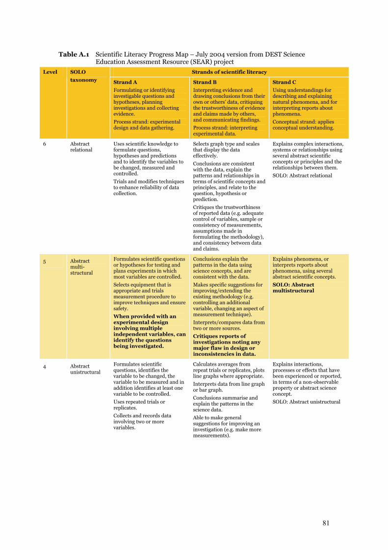
81

Table A.1 Scientific Literacy Progress Map – July 2004 version from DEST Science Education Assessment Resource (SEAR) project

Strands of scientific literacy Level SOLO

taxonomy Strand A

Formulating or identifying investigable questions and hypotheses, planning investigations and collecting evidence.

Process strand: experimental design and data gathering.

Strand B

Interpreting evidence and drawing conclusions from their own or others’ data, critiquing the trustworthiness of evidence and claims made by others, and communicating findings.

Process strand: interpreting experimental data.

Strand C

Using understandings for describing and explaining natural phenomena, and for interpreting reports about phenomena.

Conceptual strand: applies conceptual understanding.

6 Abstract relational

Uses scientific knowledge to formulate questions, hypotheses and predictions and to identify the variables to be changed, measured and controlled.

Trials and modifies techniques to enhance reliability of data collection.

Selects graph type and scales that display the data effectively.

Conclusions are consistent with the data, explain the patterns and relationships in terms of scientific concepts and principles, and relate to the question, hypothesis or prediction.

Critiques the trustworthiness of reported data (e.g. adequate control of variables, sample or consistency of measurements, assumptions made in formulating the methodology), and consistency between data and claims.

Explains complex interactions, systems or relationships using several abstract scientific concepts or principles and the relationships between them.

SOLO: Abstract relational

5 Abstract multi-structural

Formulates scientific questions or hypotheses for testing and plans experiments in which most variables are controlled.

Selects equipment that is appropriate and trials measurement procedure to improve techniques and ensure safety.

When provided with an experimental design involving multiple independent variables, can identify the questions being investigated.

Conclusions explain the patterns in the data using science concepts, and are consistent with the data.

Makes specific suggestions for improving/extending the existing methodology (e.g. controlling an additional variable, changing an aspect of measurement technique).

Interprets/compares data from two or more sources.

Critiques reports of investigations noting any major flaw in design or inconsistencies in data.

Explains phenomena, or interprets reports about phenomena, using several abstract scientific concepts.

SOLO: Abstract multistructural

4 Abstract unistructural

Formulates scientific questions, identifies the variable to be changed, the variable to be measured and in addition identifies at least one variable to be controlled.

Uses repeated trials or replicates.

Collects and records data involving two or more variables.

Calculates averages from repeat trials or replicates, plots line graphs where appropriate.

Interprets data from line graph or bar graph.

Conclusions summarise and explain the patterns in the science data.

Able to make general suggestions for improving an investigation (e.g. make more measurements).

Explains interactions, processes or effects that have been experienced or reported, in terms of a non-observable property or abstract science concept.

SOLO: Abstract unistructural

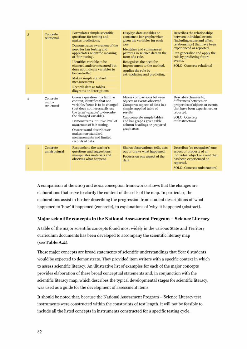
82

3 Concrete relational

Formulates simple scientific questions for testing and makes predictions.

Demonstrates awareness of the need for fair testing and appreciates scientific meaning of ‘fair testing’.

Identifies variable to be changed and/or measured but does not indicate variables to be controlled.

Makes simple standard measurements.

Records data as tables, diagrams or descriptions.

Displays data as tables or constructs bar graphs when given the variables for each axis.

Identifies and summarises patterns in science data in the form of a rule.

Recognises the need for improvement to the method.

Applies the rule by extrapolating and predicting.

Describes the relationships between individual events (including cause and effect relationships) that have been experienced or reported.

Can generalise and apply the rule by predicting future events.

SOLO: Concrete relational

2 Concrete multi-structural

Given a question in a familiar context, identifies that one variable/factor is to be changed (but does not necessarily use the term ‘variable’ to describe the changed variable).

Demonstrates intuitive level of awareness of fair testing.

Observes and describes or makes non-standard measurements and limited records of data.

Makes comparisons between objects or events observed. Compares aspects of data in a simple supplied table of results.

Can complete simple tables and bar graphs given table column headings or prepared graph axes.

Describes changes to, differences between or properties of objects or events that have been experienced or reported.

SOLO: Concrete multistructural

1 Concrete unistructural

Responds to the teacher’s questions and suggestions, manipulates materials and observes what happens.

Shares observations; tells, acts out or draws what happened.

Focuses on one aspect of the data.

Describes (or recognises) one aspect or property of an individual object or event that has been experienced or reported.

SOLO: Concrete unistructural

A comparison of the 2003 and 2004 conceptual frameworks shows that the changes are

elaborations that serve to clarify the content of the cells of the map. In particular, the

elaborations assist in further describing the progression from student descriptions of ‘what’

happened to ‘how’ it happened (concrete), to explanations of ‘why’ it happened (abstract).

Major scientific concepts in the National Assessment Program – Science Literacy

A table of the major scientific concepts found most widely in the various State and Territory

curriculum documents has been developed to accompany the scientific literacy map

(see Table A.2).

These major concepts are broad statements of scientific understandings that Year 6 students

would be expected to demonstrate. They provided item writers with a specific context in which

to assess scientific literacy. An illustrative list of examples for each of the major concepts

provides elaboration of these broad conceptual statements and, in conjunction with the

scientific literacy map, which describes the typical developmental stages for scientific literacy,

was used as a guide for the development of assessment items.

It should be noted that, because the National Assessment Program – Science Literacy test

instruments were constructed within the constraints of test length, it will not be feasible to

include all the listed concepts in instruments constructed for a specific testing cycle.

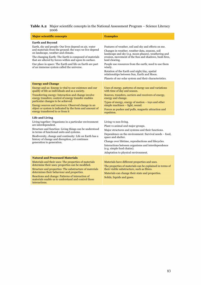
83

Table A.2 Major scientific concepts in the National Assessment Program – Science Literacy 2006

Major scientific concepts Examples

Earth and Beyond

Earth, sky and people: Our lives depend on air, water and materials from the ground; the ways we live depend on landscape, weather and climate.

The changing Earth: The Earth is composed of materials that are altered by forces within and upon its surface.

Our place in space: The Earth and life on Earth are part of an immense system called the universe.

Features of weather, soil and sky and effects on me.

Changes in weather, weather data, seasons, soil landscape and sky (e.g. moon phases), weathering and erosion, movement of the Sun and shadows, bush fires, land clearing.

People use resources from the earth; need to use them wisely.

Rotation of the Earth and night/day, spatial relationships between Sun, Earth and Moon.

Planets of our solar system and their characteristics.

Energy and Change

Energy and us: Energy is vital to our existence and our quality of life as individuals and as a society.

Transferring energy: Interaction and change involve energy transfers; control of energy transfer enables particular changes to be achieved.

Energy sources and receivers: Observed change in an object or system is indicated by the form and amount of energy transferred to or from it

Uses of energy, patterns of energy use and variations with time of day and season.

Sources, transfers, carriers and receivers of energy, energy and change.

Types of energy, energy of motion – toys and other simple machines – light, sound.

Forces as pushes and pulls, magnetic attraction and repulsion.

Life and Living

Living together: Organisms in a particular environment are interdependent.

Structure and function: Living things can be understood in terms of functional units and systems.

Biodiversity, change and continuity: Life on Earth has a history of change and disruption, yet continues generation to generation.

Living vs non-living.

Plant vs animal and major groups.

Major structures and systems and their functions.

Dependence on the environment: Survival needs – food, space and shelter.

Change over lifetime, reproductions and lifecycles.

Interactions between organisms and interdependence (e.g. simple food chains).

Adaptation to physical environment.

Natural and Processed Materials

Materials and their uses: The properties of materials determine their uses; properties can be modified.

Structure and properties: The substructure of materials determines their behaviour and properties.

Reactions and change: Patterns of interaction of materials enable us to understand and control those interactions.

Materials have different properties and uses.

The properties of materials can be explained in terms of their visible substructure, such as fibres.

Materials can change their state and properties.

Solids, liquids and gases.

84

Appendix B Sample School Reports

85

Sam Sample Sampleville Primary School Sampleville Road Sampleville VIC 3804

Dear Sam Sample

Re: National Assessment Program – Science Literacy (2006)

On behalf of Educational Assessment Australia and Curriculum Corporation I wish to thank you, your staff and Year 6 students for participating in the Ministerial Council on Education, Employment, Training and Youth Affairs (MCEETYA) National Assessment Program – Science Literacy in October this year.

We appreciate the effort your staff made to ensure that the assessment was administered consistently, completed and returned to us.

Enclosed with this letter are the reports for participating Year 6 students at your school. There are two reports for each student: one for the pencil and paper (objective) test and one for the practical task.

There are seven A4 report sheets – one for each of the seven test booklets used in the national assessment. The results for each student for the pencil and paper (objective) test are located on the A4 report sheet corresponding to the objective test booklet they completed. The student’s results for the practical task are located on the one A3 report sheet. All participating students at your school performed the same practical task.

We have included an information sheet to help interpret these reports. Please provide a copy of this information to anyone requesting these results.

Please pass on our thanks to the staff and students involved in this National Assessment Program – Science Literacy.

Yours sincerely

Dr Jenny Donovan Project Director

86

National Assessment Program – Science Literacy (2006)

Interpreting the student reports Each Year 6 student completed one of the seven different pencil and paper (objective) test forms and one of two practical tasks. The student reports provide information about each student’s achievement on the particular objective test and practical task that s/he completed. Each item tested appeared in three of the seven test booklets in a different position. So although each test booklet was different there were commonalities between the booklets. Each test booklet comprised a different number of questions and only one third of the questions were common with another booklet. Therefore, the total score achieved by any one student can only be compared to other students completing the same booklet. The objective test report and the practical task report include the following information:

1. the relevant science strand and major concept addressed by each question (please refer to the key at the end of the A3 practical task report for more information)

2. a description of the skill tested by the question – practical task report only 3. a description of the question context and major concept examples – objective test booklets only 4. the maximum possible score for each item and the percentage of students in the school (across multiple

booklets) who achieved that score 5. the percentage of students in the national sample population who achieved the maximum score on each item

(the sample population contains approximately 5% of the total Year 6 national population) 6. the name of each student who completed the test for the corresponding test booklet, his/her achievement on

each item and overall score on the test. These reports can be used to:

7. compare your students’ achievement on each item against the sample population (by comparing the two columns showing the % of students attaining the maximum score)

8. compare student achievement within the seven booklets and practical task by looking at the maximum possible score and the total for each student for each test

9. identify areas in the curriculum and strands that may need to be covered in more detail by examining the performance of students in each strand/major concept.

Below is part of a sample report form with some key information explained.

National Assessment Program – Science Literacy (Trial) <School Name> Year 6 Objective Booklet 1

Q no.

Strand. Major concept* Unit title: major concept example

Item M

ax Score

% m

aximum

score (your school)

% m

aximum

score (sam

ple population)

Student Nam

e

Student Nam

e

Student Nam

e

Student Nam

e

1 NP.1 Hot chocolate: the properties of materials can be used to explain their use 1 95 100 1 1 1 0 2 NP.3 Hot chocolate: materials can change their state and properties 2 90 95 0 2 1 1 3 LL.3 Butterflies and moths: adaptation to physical environment 1 85 90 1 1 1 0 4 LL.2 Butterflies and moths: change over lifetime 1 80 85 0 - 1 1 5 LL.3 Butterflies and moths: adaptation to physical environment 1 75 80 1 1 1 0 Maximum score possible 6 Total score 3 5 5 2

This student achieved the maximum score (2) for this item. 90% of students in the sample population

achieved the maximum score for this item.

The following students completed Booklet 1.

This student did not attempt this item.

75% of students at your school achieved the maximum score for this item. This student attempted this item

and achieved a score of 0.

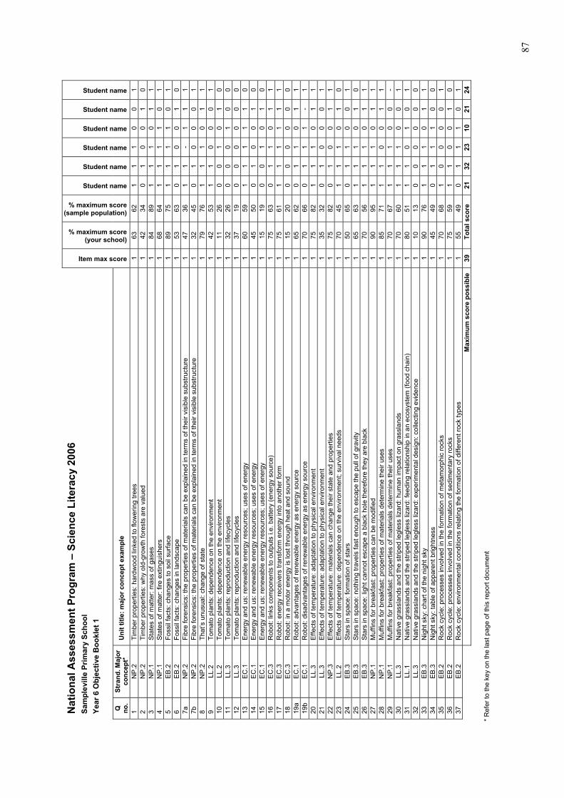
87

* R

efer

to th

e ke

y on

the

last

pag

e of

this

repo

rt do

cum

ent

Nat

iona

l Ass

essm

ent P

rogr

am –

Sci

ence

Lite

racy

200

6 Sa

mpl

evill

e Pr

imar

y Sc

hool

Ye

ar 6

Obj

ectiv

e B

ookl

et 1

Q

no.

Stra

nd. M

ajor

co

ncep

t*

Uni

t titl

e: m

ajor

con

cept

exa

mpl

e

Item max score

% maximum score (your school)

% maximum score (sample population)

Student name

Student name

Student name

Student name

Student name

Student name

1 N

P.2

Ti

mbe

r pro

perti

es: h

ardw

ood

linke

d to

flow

erin

g tre

es

1 63

62

1

1 1

0 0

1 2

NP

.2

Tim

ber p

rope

rties

: why

old

-gro

wth

fore

sts

are

valu

ed

1 42

34

0

1 0

0 1

0 3

NP

.1

Sta

tes

of m

atte

r: m

ass

of g

ases

1

84

89

1 1

1 0

1 1

4 N

P.1

S

tate

s of

mat

ter:

fire

extin

guis

hers

1

68

64

1 1

1 1

0 1

5 E

B.2

Fo

ssil

fact

s: c

hang

es to

soi

l sur

face

1

89

75

1 1

1 1

0 1

6 E

B.2

Fo

ssil

fact

s: c

hang

es in

land

scap

e 1

53

63

0 1

0 0

1 0

7a

NP

.2

Fibr

e fo

rens

ics:

the

prop

ertie

s of

mat

eria

ls c

an b

e ex

plai

ned

in te

rms

of th

eir v

isib

le s

ubst

ruct

ure

1 47

36

1

1 -

1 1

1 7b

N

P.2

Fi

bre

fore

nsic

s: th

e pr

oper

ties

of m

ater

ials

can

be

expl

aine

d in

term

s of

thei

r vis

ible

sub

stru

ctur

e 1

32

45

0 1

0 0

0 1

8 N

P.2

Th

at’s

unu

sual

: cha

nge

of s

tate

1

79

76

1 1

1 0

1 1

9 LL

.2

Tom

ato

plan

ts: d

epen

denc

e on

the

envi

ronm

ent

1 42

53

1

1 0

0 0

1 10

LL

.2

Tom

ato

plan

ts: d

epen

denc

e on

the

envi

ronm

ent

1 11

26

0

0 1

0 1

0 11

LL

.3

Tom

ato

plan

ts: r

epro

duct

ion

and

lifec

ycle

s 1

32

26

0 0

0 1

0 0

12

LL.3

To

mat

o pl

ants

: rep

rodu

ctio

n an

d lif

ecyc

les

1 37

19

0

0 0

0 0

0 13

E

C.1

E

nerg

y an

d us

: ren

ewab

le e

nerg

y re

sour

ces;

use

s of

ene

rgy

1 60

59

1

1 1

1 1

0 14

E

C.1

E

nerg

y an

d us

: ren

ewab

le e

nerg

y re

sour

ces;

use

s of

ene

rgy

1 45

50

0

1 0

0 1

0 15

E

C.1

E

nerg

y an

d us

: ren

ewab

le e

nerg

y re

sour

ces;

use

s of

ene

rgy

1 15

19

0

0 1

0 1

0 16

E

C.3

R

obot

: lin

ks c

ompo

nent

s to

out

puts

i.e.

bat

tery

(ene

rgy

sour

ce)

1 75

63

0

1 1

0 1

1 17

E

C.3

R

obot

: ene

rgy

rece

iver

s tra

nsfo

rm e

nerg

y in

to a

noth

er fo

rm

1 75

61

1

1 1

1 1

1 18

E

C.3

R

obot

: in

a m

otor

ene

rgy

is lo

st th

roug

h he

at a

nd s

ound

1

15

20

0 0

0 0

0 0

19a

EC

.1

Rob

ot: a

dvan

tage

s of

rene

wab

le e

nerg

y as

ene

rgy

sour

ce

1 65

62

0

1 1

0 1

1 19

b E

C.1

R

obot

: dis

adva

ntag

es o

f ren

ewab

le e

nerg

y as

ene

rgy

sour

ce

1 70

66

0

1 1

1 -

1 20

LL

.3

Effe

cts

of te

mpe

ratu

re: a

dapt

atio

n to

phy

sica

l env

ironm

ent

1 75

82

1

1 1

0 1

1 21

LL

.3

Effe

cts

of te

mpe

ratu

re: a

dapt

atio

n to

phy

sica

l env

ironm

ent

1 35

32

0

1 0

0 0

1 22

N

P.3

E

ffect

s of

tem

pera

ture

: mat

eria

ls c

an c

hang

e th

eir s

tate

and

pro

perti

es

1 75

82

0

1 0

0 1

1 23

LL

.2

Effe

cts

of te

mpe

ratu

re: d

epen

denc

e on

the

envi

ronm

ent;

surv

ival

nee

ds

1 70

45

1

1 1

0 1

0 24

E

B.3

S

tars

in s

pace

: for

mat

ion

of s

tars

1

50

65

0 1

1 0

0 1

25

EB

.3

Sta

rs in

spa

ce: n

othi

ng tr

avel

s fa

st e

noug

h to

esc

ape

the

pull

of g

ravi

ty

1 65

63

1

1 1

0 1

0 26

E

B.3

S

tars

in s

pace

: lig

ht c

anno

t esc

ape

a bl

ack

hole

ther

efor

e th

ey a

re b

lack

1

70

56

1 1

1 0

1 1

27

NP

.1

Muf

fins

for b

reak

fast

: pro

perti

es c

an b

e m

odifi

ed

1 90

95

1

1 1

0 1

1 28

N

P.1

M

uffin

s fo

r bre

akfa

st: p

rope

rties

of m

ater

ials

det

erm

ine

thei

r use

s 1

85

71

1 1

0 0

1 1

29

NP

.1

Muf

fins

for b

reak

fast

: pro

perti

es o

f mat

eria

ls d

eter

min

e th

eir u

ses

1 70

67

1

1 1

0 0

- 30

LL

.3

Nat

ive

gras

slan

ds a

nd th

e st

riped

legl

ess

lizar

d: h

uman

impa

ct o

n gr

assl

ands

1

70

60

1 1

1 0

0 1

31

LL.1

N

ativ

e gr

assl

ands

and

the

strip

ed le

gles

s liz

ard:

feed

ing

rela

tions

hip

in a

n ec

osys

tem

(foo

d ch

ain)

1

80

51

1 1

0 1

0 1

32

LL.3

N

ativ

e gr

assl

ands

and

the

strip

ed le

gles

s liz

ard:

exp

erim

enta

l des

ign:

col

lect

ing

evid

ence

1

10

13

0 0

0 0

0 0

33

EB

.3

Nig

ht s

ky: c

hart

of th

e ni

ght s

ky

1 90

76

1

1 1

0 1

1 34

E

B.3

N

ight

sky

: tab

le o

f app

aren

t brig

htne

ss

1 45

49

0

1 1

1 0

0 35

E

B.2

R

ock

cycl

e: p

roce

sses

invo

lved

in th

e fo

rmat

ion

of m

etam

orph

ic ro

cks

1 70

68

1

0 0

0 0

1 36

E

B.2

R

ock

cycl

e: p

roce

sses

invo

lved

in th

e fo

rmat

ion

of s

edim

enta

ry ro

cks

1 75

59

1

1 0

0 1

0 37

E

B.2

R

ock

cycl

e: e

nviro

nmen

tal c

ondi

tions

rela

ting

the

form

atio

n of

diff

eren

t roc

k ty

pes

1 55

49

0

1 1

1 0

1

M

axim

um s

core

pos

sibl

e 39

To

tal s

core

21

32

23

10

21

24

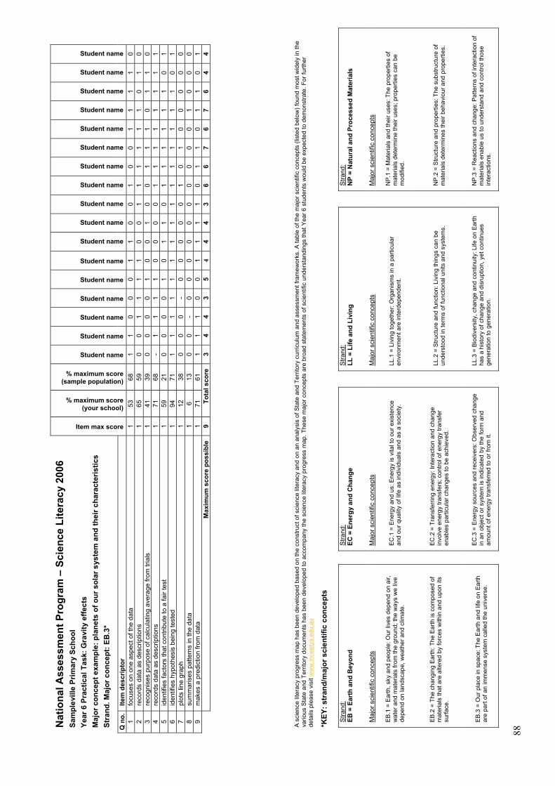
88

A

sci

ence

lite

racy

pro

gres

s m

ap h

as b

een

deve

lope

d ba

sed

on th

e co

nstru

ct o

f sci

ence

lite

racy

and

on

an a

naly

sis

of S

tate

and

Ter

ritor

y cu

rric

ulum

and

ass

essm

ent f

ram

ewor

ks. A

tabl

e of

the

maj

or s

cien

tific

con

cept

s (li

sted

bel

ow) f

ound

mos

t wid

ely

in th

e va

rious

Sta

te a

nd T

errit

ory

docu

men

ts h

as b

een

deve

lope

d to

acc

ompa

ny th

e sc

ienc

e lit

erac

y pr

ogre

ss m

ap. T

hese

maj

or c

once

pts

are

broa

d st

atem

ents

of s

cien

tific

und

erst

andi

ngs

that

Yea

r 6 s

tude

nts

wou

ld b

e ex

pect

ed to

dem

onst

rate

. For

furth

er

deta

ils p

leas

e vi

sit w

ww

.mce

etya

.edu

.au

*KEY

: str

and/

maj

or s

cien

tific

con

cept

s

Stra

nd:

EB =

Ear

th a

nd B

eyon

d

Stra

nd:

EC =

Ene

rgy

and

Cha

nge

S

trand

: LL

= L

ife a

nd L

ivin

g

Stra

nd:

NP

= N

atur

al a

nd P

roce

ssed

Mat

eria

ls

Maj

or s

cien

tific

con

cept

s

Maj

or s

cien

tific

con

cept

s

Maj

or s

cien

tific

con

cept

s

Maj

or s

cien

tific

con

cept

s

EB

.1 =

Ear

th, s

ky a

nd p

eopl

e: O

ur li

ves

depe

nd o

n ai

r, w

ater

and

mat

eria

ls fr

om th

e gr

ound

; the

way

s w

e liv

e de

pend

on

land

scap

e, w

eath

er a

nd c

limat

e.

E

C.1

= E

nerg

y an

d us

: Ene

rgy

is v

ital t

o ou

r exi

sten

ce

and

our q

ualit

y of

life

as

indi

vidu

als

and

as a

soc

iety

.

LL.1

= L

ivin

g to

geth

er: O

rgan

ism

s in

a p

artic

ular

en

viro

nmen

t are

inte

rdep

ende

nt.

N

P.1

= M

ater

ials

and

thei

r use

s: T

he p

rope

rties

of

mat

eria

ls d

eter

min

e th

eir u

ses;

pro

perti

es c

an b

e m

odifi

ed.

EB

.2 =

The

cha

ngin

g E

arth

: The

Ear

th is

com

pose

d of

m

ater

ials

that

are

alte

red

by fo

rces

with

in a

nd u

pon

its

surfa

ce.

E

C.2

= T

rans

ferri

ng e

nerg

y: In

tera

ctio

n an

d ch

ange

in

volv

e en

ergy

tran

sfer

s; c

ontro

l of e

nerg

y tra

nsfe

r en

able

s pa

rticu

lar c

hang

es to

be

achi

eved

.

LL.2

= S

truct

ure

and

func

tion:

Liv

ing

thin

gs c

an b

e un

ders

tood

in te

rms

of fu

nctio

nal u

nits

and

sys

tem

s.

N

P.2

= S

truct

ure

and

prop

ertie

s: T

he s

ubst

ruct

ure

of

mat

eria

ls d

eter

min

es th

eir b

ehav

iour

and

pro

perti

es.

EB

.3 =

Our

pla

ce in

spa

ce: T

he E

arth

and

life

on

Ear

th

are

part

of a

n im

men

se s

yste

m c

alle

d th

e un

iver

se.

E

C.3

= E

nerg

y so

urce

s an

d re

ceiv

ers:

Obs

erve

d ch

ange

in

an

obje

ct o

r sys

tem

is in

dica

ted

by th

e fo

rm a

nd

amou

nt o

f ene

rgy

trans

ferr

ed to

or f

rom

it.

LL

.3 =

Bio

dive

rsity

, cha

nge

and

cont

inui

ty: L

ife o

n E

arth

ha

s a

hist

ory

of c

hang

e an

d di

srup

tion,

yet

con

tinue

s ge

nera

tion

to g

ener

atio

n.

N

P.3

= R

eact

ions

and

cha

nge:

Pat

tern

s of

inte

ract

ion

of

mat

eria

ls e

nabl

e us

to u

nder

stan

d an

d co

ntro

l tho

se

inte

ract

ions

.

Nat

iona

l Ass

essm

ent P

rogr

am –

Sci

ence

Lite

racy

200

6 Sa

mpl

evill

e Pr

imar

y Sc

hool

Ye

ar 6

Pra

ctic

al T

ask:

Gra

vity

effe

cts

Maj

or c

once

pt e

xam

ple:

pla

nets

of o

ur s

olar

sys

tem

and

thei

r cha

ract

eris

tics

Stra

nd. M

ajor

con

cept

: EB

.3*

Q n

o.

Item

des

crip

tor

Item max score

% maximum score (your school)

% maximum score (sample population)

Student name

Student name

Student name

Student name

Student name

Student name

Student name

Student name

Student name

Student name

Student name

Student name

Student name

Student name

Student name

Student name

Student name

1 fo

cuse

s on

one

asp

ect o

f the

dat

a 1

53

68

1 1

0 0

0 1

1 0

0 1

0 0

1 1

1 1

0 2

reco

rds

data

as

desc

riptio

ns

1 65

59

0

0 1

1 1

1 0

0 1

1 1

1 1

1 0

1 0

3 re

cogn

ises

pur

pose

of c

alcu

latin

g av

erag

e fro

m tr

ials

1

41

39

0 0

0 0

1 0

0 1

0 0

1 1

1 0

1 1

0 4

reco

rds

data

as

desc

riptio

ns

1 71

68

-

1 1

1 1

0 0

0 0

1 1

1 1

1 1

1 1

5 id

entif

ies

fact

ors

that

con

tribu

te to

a fa

ir te

st

1 59

21

0

0 0

0 1

0 1

1 0

1 1

1 1

1 1

0 1

6 id

entif

ies

hypo

thes

is b

eing

test

ed

1 94

71

1

1 1

1 1

1 1

1 1

1 1

1 1

1 1

0 1

7 pl

ots

line

grap

h 1

12

38

0 0

0 -

0 0

0 0

0 1

0 1

0 0

0 0

0 8

sum

mar

ises

pat

tern

s in

the

data

1

6 13

0

0 -

0 0

0 0

0 0

0 0

0 0

1 0

0 0

9 m

akes

a p

redi

ctio

n fro

m d

ata

1 71

61

1

1 1

0 0

1 1

1 1

0 1

1 0

1 1

0 1

M

axim

um s

core

pos

sibl

e 9

Tota

l sco

re

3 4

4 3

5 4

4 4

3 6

6 7

6 7

6 4

4

89

Appendix C Item Pool Feedback

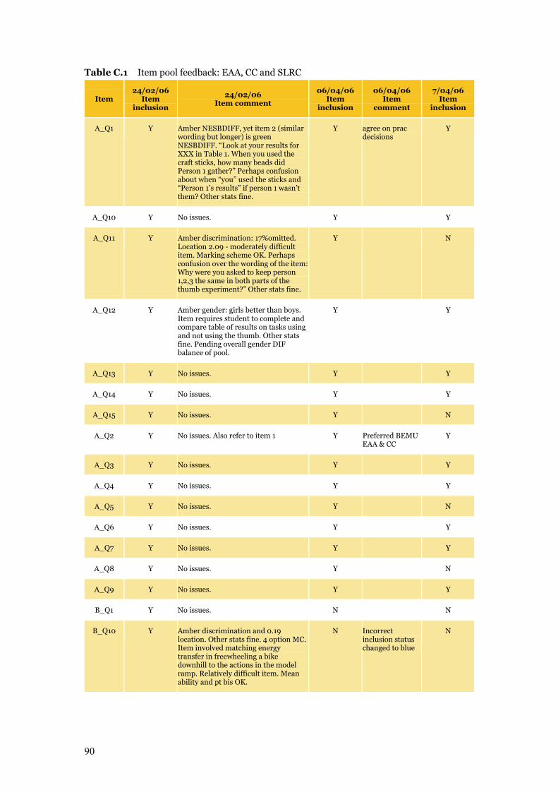
90

Table C.1 Item pool feedback: EAA, CC and SLRC

Item 24/02/06

Item inclusion

24/02/06 Item comment

06/04/06 Item

inclusion

06/04/06 Item

comment

7/04/06 Item

inclusion

A_Q1 Y Amber NESBDIFF, yet item 2 (similar wording but longer) is green NESBDIFF. “Look at your results for XXX in Table 1. When you used the craft sticks, how many beads did Person 1 gather?” Perhaps confusion about when “you” used the sticks and “Person 1’s results” if person 1 wasn’t them? Other stats fine.

Y agree on prac decisions

Y

A_Q10 Y No issues. Y Y

A_Q11 Y Amber discrimination: 17%omitted. Location 2.09 - moderately difficult item. Marking scheme OK. Perhaps confusion over the wording of the item: Why were you asked to keep person 1,2,3 the same in both parts of the thumb experiment?” Other stats fine.

Y N

A_Q12 Y Amber gender: girls better than boys. Item requires student to complete and compare table of results on tasks using and not using the thumb. Other stats fine. Pending overall gender DIF balance of pool.

Y Y

A_Q13 Y No issues. Y Y

A_Q14 Y No issues. Y Y

A_Q15 Y No issues. Y N

A_Q2 Y No issues. Also refer to item 1 Y Preferred BEMU EAA & CC

Y

A_Q3 Y No issues. Y Y

A_Q4 Y No issues. Y Y

A_Q5 Y No issues. Y N

A_Q6 Y No issues. Y Y

A_Q7 Y No issues. Y Y

A_Q8 Y No issues. Y N

A_Q9 Y No issues. Y Y

B_Q1 Y No issues. N N

B_Q10 Y Amber discrimination and 0.19 location. Other stats fine. 4 option MC. Item involved matching energy transfer in freewheeling a bike downhill to the actions in the model ramp. Relatively difficult item. Mean ability and pt bis OK.

N Incorrect inclusion status changed to blue

N

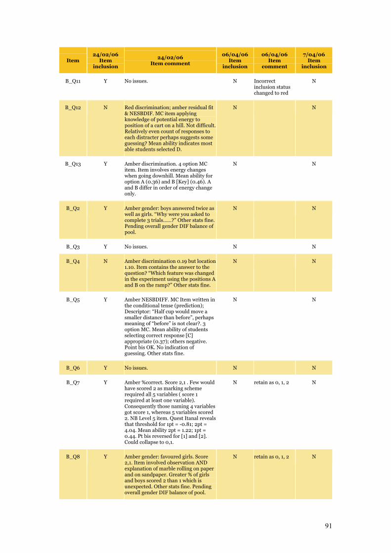
91

Item 24/02/06

Item inclusion

24/02/06 Item comment

06/04/06 Item

inclusion

06/04/06 Item

comment

7/04/06 Item

inclusion

B_Q11 Y No issues. N Incorrect inclusion status changed to red

N

B_Q12 N Red discrimination; amber residual fit & NESBDIF. MC item applying knowledge of potential energy to position of a cart on a hill. Not difficult. Relatively even count of responses to each distracter perhaps suggests some guessing? Mean ability indicates most able students selected D.

N N

B_Q13 Y Amber discrimination. 4 option MC item. Item involves energy changes when going downhill. Mean ability for option A (0.36) and B [Key] (0.46). A and B differ in order of energy change only.

N N

B_Q2 Y Amber gender: boys answered twice as well as girls. “Why were you asked to complete 3 trials……?” Other stats fine. Pending overall gender DIF balance of pool.

N N

B_Q3 Y No issues. N N

B_Q4 N Amber discrimination 0.19 but location 1.10. Item contains the answer to the question? “Which feature was changed in the experiment using the positions A and B on the ramp?” Other stats fine.

N N

B_Q5 Y Amber NESBDIFF. MC Item written in the conditional tense (prediction); Descriptor: “Half cup would move a smaller distance than before”, perhaps meaning of “before” is not clear?. 3 option MC. Mean ability of students selecting correct response [C] appropriate (0.37); others negative. Point bis OK. No indication of guessing. Other stats fine.

N N

B_Q6 Y No issues. N N

B_Q7 Y Amber %correct. Score 2,1 . Few would have scored 2 as marking scheme required all 5 variables ( score 1 required at least one variable). Consequently those naming 4 variables got score 1, whereas 5 variables scored 2. NB Level 5 item. Quest Itanal reveals that threshold for 1pt = -0.81; 2pt = 4.04. Mean ability 2pt = 1.22; 1pt = 0.44. Pt bis reversed for [1] and [2]. Could collapse to 0,1.

N retain as 0, 1, 2 N

B_Q8 Y Amber gender: favoured girls. Score 2,1. Item involved observation AND explanation of marble rolling on paper and on sandpaper. Greater % of girls and boys scored 2 than 1 which is unexpected. Other stats fine. Pending overall gender DIF balance of pool.

N retain as 0, 1, 2 N

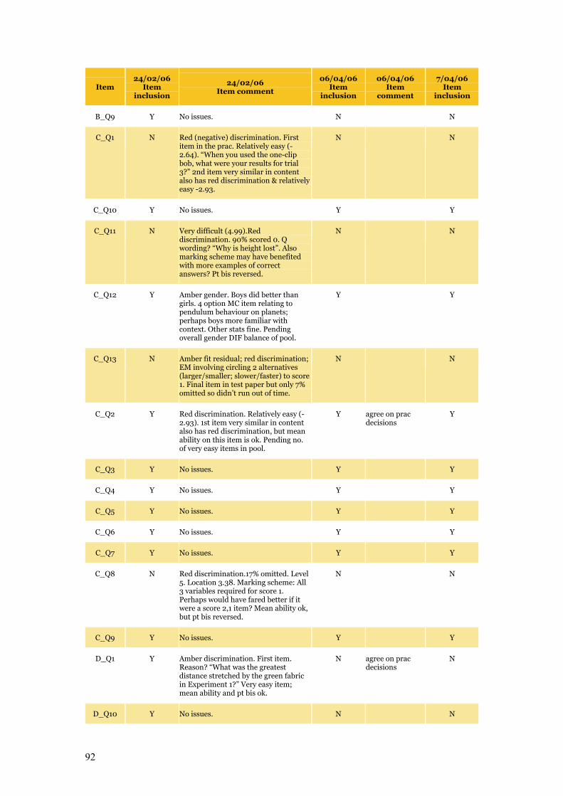
92

Item 24/02/06

Item inclusion

24/02/06 Item comment

06/04/06 Item

inclusion

06/04/06 Item

comment

7/04/06 Item

inclusion

B_Q9 Y No issues. N N

C_Q1 N Red (negative) discrimination. First item in the prac. Relatively easy (-2.64). “When you used the one-clip bob, what were your results for trial 3?” 2nd item very similar in content also has red discrimination & relatively easy -2.93.

N N

C_Q10 Y No issues. Y Y

C_Q11 N Very difficult (4.99).Red discrimination. 90% scored 0. Q wording? “Why is height lost”. Also marking scheme may have benefited with more examples of correct answers? Pt bis reversed.

N N

C_Q12 Y Amber gender. Boys did better than girls. 4 option MC item relating to pendulum behaviour on planets; perhaps boys more familiar with context. Other stats fine. Pending overall gender DIF balance of pool.

Y Y

C_Q13 N Amber fit residual; red discrimination; EM involving circling 2 alternatives (larger/smaller; slower/faster) to score 1. Final item in test paper but only 7% omitted so didn’t run out of time.

N N

C_Q2 Y Red discrimination. Relatively easy (-2.93). 1st item very similar in content also has red discrimination, but mean ability on this item is ok. Pending no. of very easy items in pool.

Y agree on prac decisions

Y

C_Q3 Y No issues. Y Y

C_Q4 Y No issues. Y Y

C_Q5 Y No issues. Y Y

C_Q6 Y No issues. Y Y

C_Q7 Y No issues. Y Y

C_Q8 N Red discrimination.17% omitted. Level 5. Location 3.38. Marking scheme: All 3 variables required for score 1. Perhaps would have fared better if it were a score 2,1 item? Mean ability ok, but pt bis reversed.

N N

C_Q9 Y No issues. Y Y

D_Q1 Y Amber discrimination. First item. Reason? “What was the greatest distance stretched by the green fabric in Experiment 1?” Very easy item; mean ability and pt bis ok.

N agree on prac decisions

N

D_Q10 Y No issues. N N

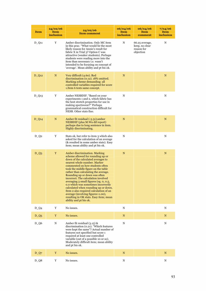
93

Item 24/02/06

Item inclusion

24/02/06 Item comment

06/04/06 Item

inclusion

06/04/06 Item

comment

7/04/06 Item

inclusion

D_Q11 Y Amber discrimination. Only MC item in this prac. “What would be the most likely reason for Annie’s result for fabric X in Trial 3? Option C was attractive (weaker students). Perhaps students were reading more into the item than necessary i.e. wasn’t intended to be focusing on concept of ‘average’. Mean ability and pt bis ok.

N 66.25 average, keep, no clear reason for objection

N

D_Q12 N Very difficult (4.60). Red discrimination (0.12). 18% omitted. Marking scheme demanding: all controlled variables required for score 1.Item 6 tests same concept.

N N

D_Q13 Y Amber NESBDIF. “Based on your experiments 1 and 2, which fabric has the best stretch properties for use in making sportswear?” Perhaps grammatical construction difficult for NESB. Other stats fine.

N N

D_Q14 N Amber fit residual (-3.31);amber NESBDIF (plus M.Wu dif report) perhaps due to long sentence in item. Highly discriminating.

N N

D_Q2 Y Stats ok, but refer to item 3 which also asked for the calculation of an average (& resulted in some amber stats). Easy item; mean ability and pt bis ok.

N N

D_Q3 Y Amber discrimination. Marking scheme allowed for rounding up or down of the calculated averages to nearest whole number. Marker commented on how students often took the middle figure on the table rather than calculating the average. Rounding up or down was often incorrect. The calculation involved averaging 3 small figures (eg. 0, 0.5, 0.0 which was sometimes incorrectly calculated when rounding up or down. Item 2 also required calculation of an average (involving figures>1.00), resulting in OK stats. Easy item; mean ability and pt bis ok.

N N

D_Q4 Y No issues. N N

D_Q5 Y No issues. N N

D_Q6 N Amber fit residual (3.15) & discrimination (0.21). “Which features were kept the same”? Actual number of features not specified but score 1 required at least one controlled variable (out of a possible 10 or so). Moderately difficult item; mean ability and pt bis ok.

N N

D_Q7 Y No issues. N N

D_Q8 Y No issues. N N

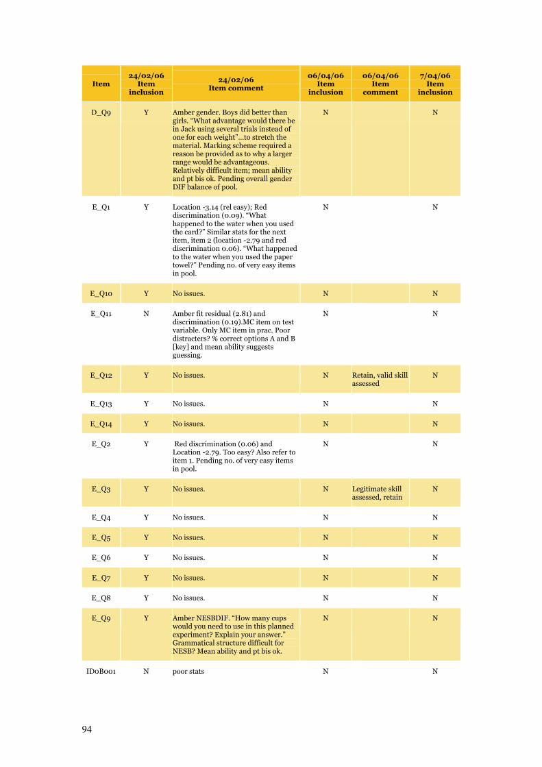
94

Item 24/02/06

Item inclusion

24/02/06 Item comment

06/04/06 Item

inclusion

06/04/06 Item

comment

7/04/06 Item

inclusion

D_Q9 Y Amber gender. Boys did better than girls. “What advantage would there be in Jack using several trials instead of one for each weight”…to stretch the material. Marking scheme required a reason be provided as to why a larger range would be advantageous. Relatively difficult item; mean ability and pt bis ok. Pending overall gender DIF balance of pool.

N N

E_Q1 Y Location -3.14 (rel easy); Red discrimination (0.09). “What happened to the water when you used the card?” Similar stats for the next item, item 2 (location -2.79 and red discrimination 0.06). “What happened to the water when you used the paper towel?” Pending no. of very easy items in pool.

N N

E_Q10 Y No issues. N N

E_Q11 N Amber fit residual (2.81) and discrimination (0.19).MC item on test variable. Only MC item in prac. Poor distracters? % correct options A and B [key] and mean ability suggests guessing.

N N

E_Q12 Y No issues. N Retain, valid skill assessed

N

E_Q13 Y No issues. N N

E_Q14 Y No issues. N N

E_Q2 Y Red discrimination (0.06) and Location -2.79. Too easy? Also refer to item 1. Pending no. of very easy items in pool.

N N

E_Q3 Y No issues. N Legitimate skill assessed, retain

N

E_Q4 Y No issues. N N

E_Q5 Y No issues. N N

E_Q6 Y No issues. N N

E_Q7 Y No issues. N N

E_Q8 Y No issues. N N

E_Q9 Y Amber NESBDIF. “How many cups would you need to use in this planned experiment? Explain your answer.” Grammatical structure difficult for NESB? Mean ability and pt bis ok.

N N

ID0B001 N poor stats N N

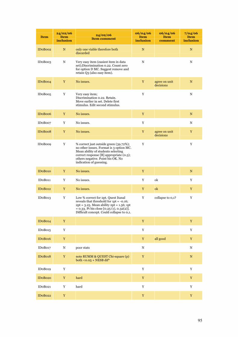
95

Item 24/02/06

Item inclusion

24/02/06 Item comment

06/04/06 Item

inclusion

06/04/06 Item

comment

7/04/06 Item

inclusion

ID0B002 N only one viable therefore both discarded

N N

ID0B003 N Very easy item (easiest item in data set);Discrimination 0.22. Count zero for option D MC. Suggest remove and retain Q3 (also easy item).

N N

ID0B004 Y No issues. Y agree on unit decisions

N

ID0B005 Y Very easy item; Discrimination 0.22. Retain. Move earlier in set. Delete first stimulus. Edit second stimulus.

Y N

ID0B006 Y No issues. Y N

ID0B007 Y No issues. Y N

ID0B008 Y No issues. Y agree on unit decisions

Y

ID0B009 Y % correct just outside green (39.72%); no other issues. Format is 3 option MC. Mean ability of students selecting correct response [B] appropriate (0.5); others negative. Point bis OK. No indication of guessing.

Y Y

ID0B010 Y No issues. Y N

ID0B011 Y No issues. Y ok Y

ID0B012 Y No issues. Y ok Y

ID0B013 Y Low % correct for 2pt. Quest Itanal reveals that threshold for 1pt = -0.16; 2pt = 3.25. Mean ability 2pt = 1.56; 1pt = 0.33. Pt bis close [0.25 (1), 0.32(2)]. Difficult concept. Could collapse to 0,1.

Y collapse to 0,1? Y

ID0B014 Y Y Y

ID0B015 Y Y Y

ID0B016 Y Y all good Y

ID0B017 N poor stats N N

ID0B018 Y note RUMM & QUEST Chi-square (p) both <0.05 + NESB dif*

Y N

ID0B019 Y Y Y

ID0B020 Y hard Y Y

ID0B021 Y hard Y Y

ID0B022 Y Y Y

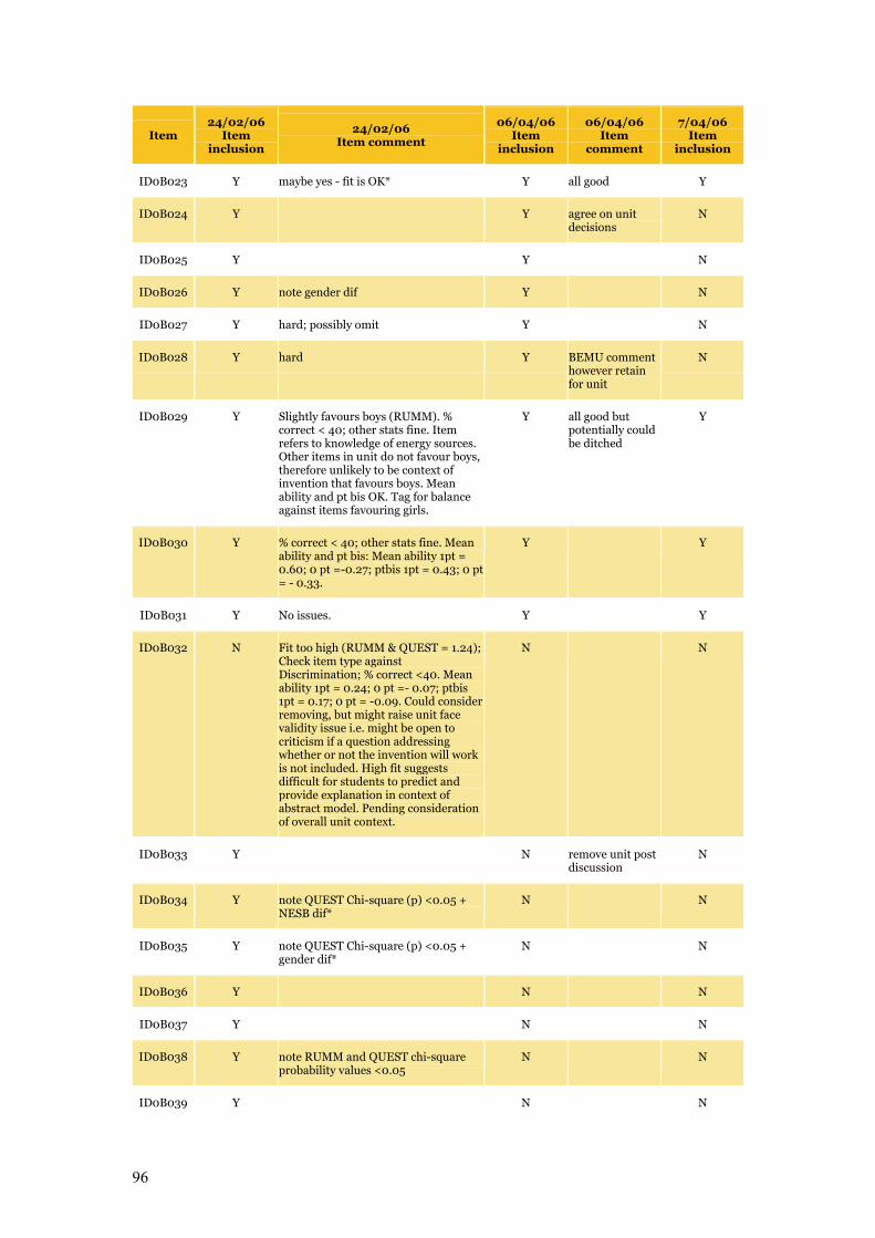
96

Item 24/02/06

Item inclusion

24/02/06 Item comment

06/04/06 Item

inclusion

06/04/06 Item

comment

7/04/06 Item

inclusion

ID0B023 Y maybe yes - fit is OK* Y all good Y

ID0B024 Y Y agree on unit decisions

N

ID0B025 Y Y N

ID0B026 Y note gender dif Y N

ID0B027 Y hard; possibly omit Y N

ID0B028 Y hard Y BEMU comment however retain for unit

N

ID0B029 Y Slightly favours boys (RUMM). % correct < 40; other stats fine. Item refers to knowledge of energy sources. Other items in unit do not favour boys, therefore unlikely to be context of invention that favours boys. Mean ability and pt bis OK. Tag for balance against items favouring girls.

Y all good but potentially could be ditched

Y

ID0B030 Y % correct < 40; other stats fine. Mean ability and pt bis: Mean ability 1pt = 0.60; 0 pt =-0.27; ptbis 1pt = 0.43; 0 pt = - 0.33.

Y Y

ID0B031 Y No issues. Y Y

ID0B032 N Fit too high (RUMM & QUEST = 1.24); Check item type against Discrimination; % correct <40. Mean ability 1pt = 0.24; 0 pt =- 0.07; ptbis 1pt = 0.17; 0 pt = -0.09. Could consider removing, but might raise unit face validity issue i.e. might be open to criticism if a question addressing whether or not the invention will work is not included. High fit suggests difficult for students to predict and provide explanation in context of abstract model. Pending consideration of overall unit context.

N N

ID0B033 Y N remove unit post discussion

N

ID0B034 Y note QUEST Chi-square (p) <0.05 + NESB dif*

N N

ID0B035 Y note QUEST Chi-square (p) <0.05 + gender dif*

N N

ID0B036 Y N N

ID0B037 Y N N

ID0B038 Y note RUMM and QUEST chi-square probability values <0.05

N N

ID0B039 Y N N

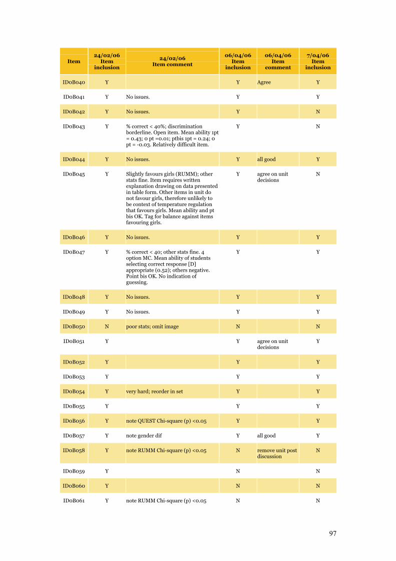
97

Item 24/02/06

Item inclusion

24/02/06 Item comment

06/04/06 Item

inclusion

06/04/06 Item

comment

7/04/06 Item

inclusion

ID0B040 Y Y Agree Y

ID0B041 Y No issues. Y Y

ID0B042 Y No issues. Y N

ID0B043 Y % correct < 40%; discrimination borderline. Open item. Mean ability 1pt = 0.43; 0 pt =0.01; ptbis 1pt = 0.24; 0 pt = -0.03. Relatively difficult item.

Y N

ID0B044 Y No issues. Y all good Y

ID0B045 Y Slightly favours girls (RUMM); other stats fine. Item requires written explanation drawing on data presented in table form. Other items in unit do not favour girls, therefore unlikely to be context of temperature regulation that favours girls. Mean ability and pt bis OK. Tag for balance against items favouring girls.

Y agree on unit decisions

N

ID0B046 Y No issues. Y Y

ID0B047 Y % correct < 40; other stats fine. 4 option MC. Mean ability of students selecting correct response [D] appropriate (0.52); others negative. Point bis OK. No indication of guessing.

Y Y

ID0B048 Y No issues. Y Y

ID0B049 Y No issues. Y Y

ID0B050 N poor stats; omit image N N

ID0B051 Y Y agree on unit decisions

Y

ID0B052 Y Y Y

ID0B053 Y Y Y

ID0B054 Y very hard; reorder in set Y Y

ID0B055 Y Y Y

ID0B056 Y note QUEST Chi-square (p) <0.05 Y Y

ID0B057 Y note gender dif Y all good Y

ID0B058 Y note RUMM Chi-square (p) <0.05 N remove unit post discussion

N

ID0B059 Y N N

ID0B060 Y N N

ID0B061 Y note RUMM Chi-square (p) <0.05 N N

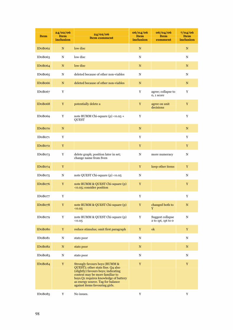
98

Item 24/02/06

Item inclusion

24/02/06 Item comment

06/04/06 Item

inclusion

06/04/06 Item

comment

7/04/06 Item

inclusion

ID0B062 N low disc N N

ID0B063 N low disc N N

ID0B064 N low disc N N

ID0B065 N deleted because of other non-viables N N

ID0B066 N deleted because of other non-viables N N

ID0B067 Y Y agree; collapse to 0, 1 score

Y

ID0B068 Y potentially delete a Y agree on unit decisions

Y

ID0B069 Y note RUMM Chi-square (p) <0.05 + QUEST

Y Y

ID0B070 N N N

ID0B071 Y Y Y

ID0B072 Y Y Y

ID0B073 Y delete graph; position later in set; change name from Sven

N more numeracy N

ID0B074 Y Y keep other items Y

ID0B075 N note QUEST Chi-square (p) <0.05 N N

ID0B076 Y note RUMM & QUEST Chi-square (p) <0.05; consider position

Y Y

ID0B077 Y Y Y

ID0B078 Y note RUMM & QUEST Chi-square (p) <0.05

Y changed both to Y

N

ID0B079 Y note RUMM & QUEST Chi-square (p) <0.05

Y Suggest collapse 2 to 1pt, 1pt to 0

N

ID0B080 Y reduce stimulus; omit first paragraph Y ok Y

ID0B081 N stats poor N N

ID0B082 N stats poor N N

ID0B083 N stats poor N N

ID0B084 Y Strongly favours boys (RUMM & QUEST); other stats fine. Q4 also (slightly) favours boys; indicating context may be more familiar to boys.Q1 requires knowledge of battery as energy source. Tag for balance against items favouring girls.

Y Y

ID0B085 Y No issues. Y Y

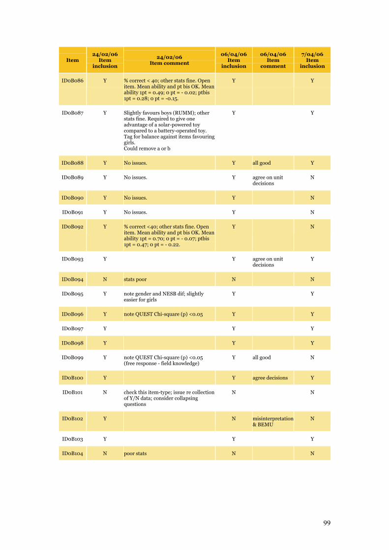
99

Item 24/02/06

Item inclusion

24/02/06 Item comment

06/04/06 Item

inclusion

06/04/06 Item

comment

7/04/06 Item

inclusion

ID0B086 Y % correct < 40; other stats fine. Open item. Mean ability and pt bis OK. Mean ability 1pt = 0.49; 0 pt = - 0.02; ptbis 1pt = 0.28; 0 pt = -0.15.

Y Y

ID0B087 Y Slightly favours boys (RUMM); other stats fine. Required to give one advantage of a solar-powered toy compared to a battery-operated toy. Tag for balance against items favouring girls. Could remove a or b

Y Y

ID0B088 Y No issues. Y all good Y

ID0B089 Y No issues. Y agree on unit decisions

N

ID0B090 Y No issues. Y N

ID0B091 Y No issues. Y N

ID0B092 Y % correct <40; other stats fine. Open item. Mean ability and pt bis OK. Mean ability 1pt = 0.70; 0 pt = - 0.07; ptbis 1pt = 0.47; 0 pt = - 0.22.

Y N

ID0B093 Y Y agree on unit decisions

Y

ID0B094 N stats poor N N

ID0B095 Y note gender and NESB dif; slightly easier for girls

Y Y

ID0B096 Y note QUEST Chi-square (p) <0.05 Y Y

ID0B097 Y Y Y

ID0B098 Y Y Y

ID0B099 Y note QUEST Chi-square (p) <0.05 (free response - field knowledge)

Y all good N

ID0B100 Y Y agree decisions Y

ID0B101 N check this item-type; issue re collection of Y/N data; consider collapsing questions

N N

ID0B102 Y N misinterpretation & BEMU

N

ID0B103 Y Y Y

ID0B104 N poor stats N N

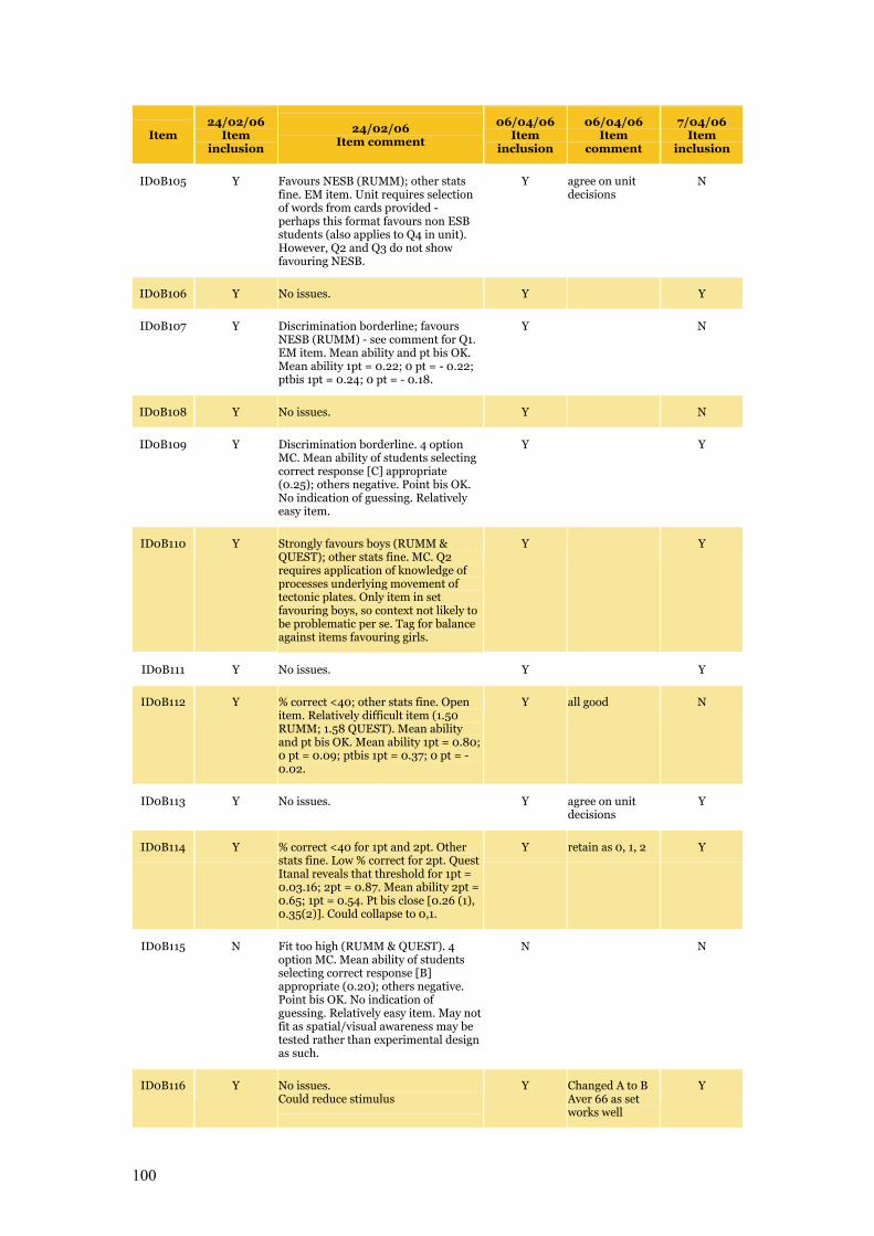
100

Item 24/02/06

Item inclusion

24/02/06 Item comment

06/04/06 Item

inclusion

06/04/06 Item

comment

7/04/06 Item

inclusion

ID0B105 Y Favours NESB (RUMM); other stats fine. EM item. Unit requires selection of words from cards provided - perhaps this format favours non ESB students (also applies to Q4 in unit). However, Q2 and Q3 do not show favouring NESB.

Y agree on unit decisions

N

ID0B106 Y No issues. Y Y

ID0B107 Y Discrimination borderline; favours NESB (RUMM) - see comment for Q1. EM item. Mean ability and pt bis OK. Mean ability 1pt = 0.22; 0 pt = - 0.22; ptbis 1pt = 0.24; 0 pt = - 0.18.

Y N

ID0B108 Y No issues. Y N

ID0B109 Y Discrimination borderline. 4 option MC. Mean ability of students selecting correct response [C] appropriate (0.25); others negative. Point bis OK. No indication of guessing. Relatively easy item.

Y Y

ID0B110 Y Strongly favours boys (RUMM & QUEST); other stats fine. MC. Q2 requires application of knowledge of processes underlying movement of tectonic plates. Only item in set favouring boys, so context not likely to be problematic per se. Tag for balance against items favouring girls.

Y Y

ID0B111 Y No issues. Y Y

ID0B112 Y % correct <40; other stats fine. Open item. Relatively difficult item (1.50 RUMM; 1.58 QUEST). Mean ability and pt bis OK. Mean ability 1pt = 0.80; 0 pt = 0.09; ptbis 1pt = 0.37; 0 pt = - 0.02.

Y all good N

ID0B113 Y No issues. Y agree on unit decisions

Y

ID0B114 Y % correct <40 for 1pt and 2pt. Other stats fine. Low % correct for 2pt. Quest Itanal reveals that threshold for 1pt = 0.03.16; 2pt = 0.87. Mean ability 2pt = 0.65; 1pt = 0.54. Pt bis close [0.26 (1), 0.35(2)]. Could collapse to 0,1.

Y retain as 0, 1, 2 Y

ID0B115 N Fit too high (RUMM & QUEST). 4 option MC. Mean ability of students selecting correct response [B] appropriate (0.20); others negative. Point bis OK. No indication of guessing. Relatively easy item. May not fit as spatial/visual awareness may be tested rather than experimental design as such.

N N

ID0B116 Y No issues. Could reduce stimulus

Y Changed A to B Aver 66 as set works well

Y

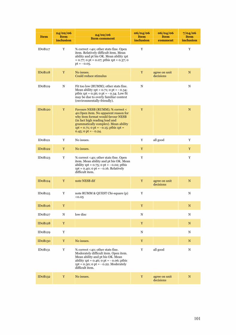
101

Item 24/02/06

Item inclusion

24/02/06 Item comment

06/04/06 Item

inclusion

06/04/06 Item

comment

7/04/06 Item

inclusion

ID0B117 Y % correct <40; other stats fine. Open item. Relatively difficult item. Mean ability and pt bis OK. Mean ability 1pt = 0.77; 0 pt = 0.07; ptbis 1pt = 0.37; 0 pt = - 0.05.

Y Y

ID0B118 Y No issues. Could reduce stimulus

Y agree on unit decisions

N

ID0B119 N Fit too low (RUMM); other stats fine. Mean ability 1pt = 0.71; 0 pt = - 0.34; ptbis 1pt = 0.56; 0 pt = - 0.34. Low fit may be due to overly familiar context (environmentally-friendly).

N N

ID0B120 Y Favours NESB (RUMM); % correct < 40.Open item. No apparent reason for why item format would favour NESB (in fact high reading load and grammatically complex). Mean ability 1pt = 0.71; 0 pt = - 0.15; ptbis 1pt = 0.45; 0 pt = - 0.24.

Y N

ID0B121 Y No issues. Y all good Y

ID0B122 Y No issues. Y Y

ID0B123 Y % correct <40; other stats fine. Open item. Mean ability and pt bis OK. Mean ability 1pt = 0.75; 0 pt = - 0.02; ptbis 1pt = 0.40; 0 pt = - 0.16. Relatively difficult item.

Y Y

ID0B124 Y note NESB dif Y agree on unit decisions

N

ID0B125 Y note RUMM & QUEST Chi-square (p) <0.05

Y N

ID0B126 Y Y N

ID0B127 N low disc N N

ID0B128 Y Y N

ID0B129 Y N N

ID0B130 Y No issues. Y N

ID0B131 Y % correct <40; other stats fine. Moderately difficult item. Open item. Mean ability and pt bis OK. Mean ability 1pt = 0.46; 0 pt = - 0.06; ptbis 1pt = 0.30; 0 pt = - 0.22. Moderately difficult item.

Y all good N

ID0B132 Y No issues. Y agree on unit decisions

N

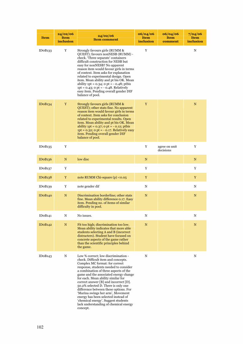
102

Item 24/02/06

Item inclusion

24/02/06 Item comment

06/04/06 Item

inclusion

06/04/06 Item

comment

7/04/06 Item

inclusion

ID0B133 Y Strongly favours girls (RUMM & QUEST); favours nonNESB (RUMM) - check. ‘Three separate’ containers difficult construction for NESB but easy for nonNESB? No apparent reason item would favour girls in terms of context. Item asks for explanation related to experimental design. Open item. Mean ability and pt bis OK. Mean ability 1pt = 0.34; 0 pt = - 0.48; ptbis 1pt = 0.43; 0 pt = - 0.48. Relatively easy item. Pending overall gender DIF balance of pool.

Y N

ID0B134 Y Strongly favours girls (RUMM & QUEST); other stats fine. No apparent reason item would favour girls in terms of context. Item asks for conclusion related to experimental results. Open item. Mean ability and pt bis OK. Mean ability 1pt = 0.37; 0 pt = - 0.12; ptbis 1pt = 0.32; 0 pt = - 0.17. Relatively easy item. Pending overall gender DIF balance of pool.

Y N

ID0B135 Y Y agree on unit decisions

Y

ID0B136 N low disc N N

ID0B137 Y Y Y

ID0B138 Y note RUMM Chi-square (p) <0.05 Y Y

ID0B139 Y note gender dif N N

ID0B140 N Discrimination borderline; other stats fine. Mean ability difference 0.17. Easy item. Pending no. of items of similar difficulty in pool.

N N

ID0B141 N No issues. N N

ID0B142 N Fit too high; discrimination too low. Mean ability indicates that more able students selecting A and B (incorrect distracters). Student have focused on concrete aspects of the game rather than the scientific principles behind the game.

N N

ID0B143 N Low % correct; low discrimination - check. Difficult item and concepts. Complex MC format: for correct response, students needed to consider a combination of three aspects of the game and the associated energy change for each. Mean ability similar for correct answer [B] and incorrect [D]. 50.2% selected D. There is only one difference between these options. For ‘Marina swings her arm’, Movement energy has been selected instead of ‘chemical energy’. Suggest students lack understanding of chemical energy concept.

N N

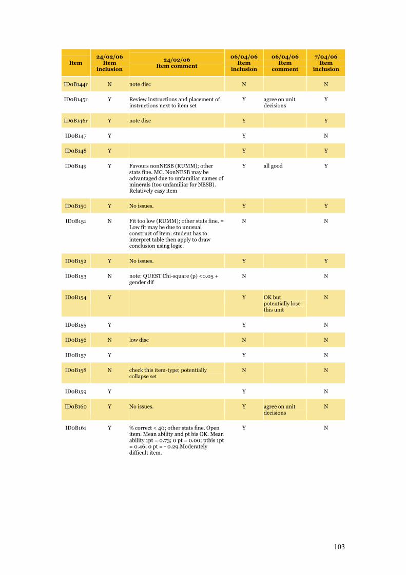
103

Item 24/02/06

Item inclusion

24/02/06 Item comment

06/04/06 Item

inclusion

06/04/06 Item

comment

7/04/06 Item

inclusion

ID0B144r N note disc N N

ID0B145r Y Review instructions and placement of instructions next to item set

Y agree on unit decisions

Y

ID0B146r Y note disc Y Y

ID0B147 Y Y N

ID0B148 Y Y Y

ID0B149 Y Favours nonNESB (RUMM); other stats fine. MC. NonNESB may be advantaged due to unfamiliar names of minerals (too unfamiliar for NESB). Relatively easy item

Y all good Y

ID0B150 Y No issues. Y Y

ID0B151 N Fit too low (RUMM); other stats fine. = Low fit may be due to unusual construct of item: student has to interpret table then apply to draw conclusion using logic.

N N

ID0B152 Y No issues. Y Y

ID0B153 N note: QUEST Chi-square (p) <0.05 + gender dif

N N

ID0B154 Y Y OK but potentially lose this unit

N

ID0B155 Y Y N

ID0B156 N low disc N N

ID0B157 Y Y N

ID0B158 N check this item-type; potentially collapse set

N N

ID0B159 Y Y N

ID0B160 Y No issues. Y agree on unit decisions

N

ID0B161 Y % correct < 40; other stats fine. Open item. Mean ability and pt bis OK. Mean ability 1pt = 0.73; 0 pt = 0.00; ptbis 1pt = 0.46; 0 pt = - 0.29.Moderately difficult item.

Y N

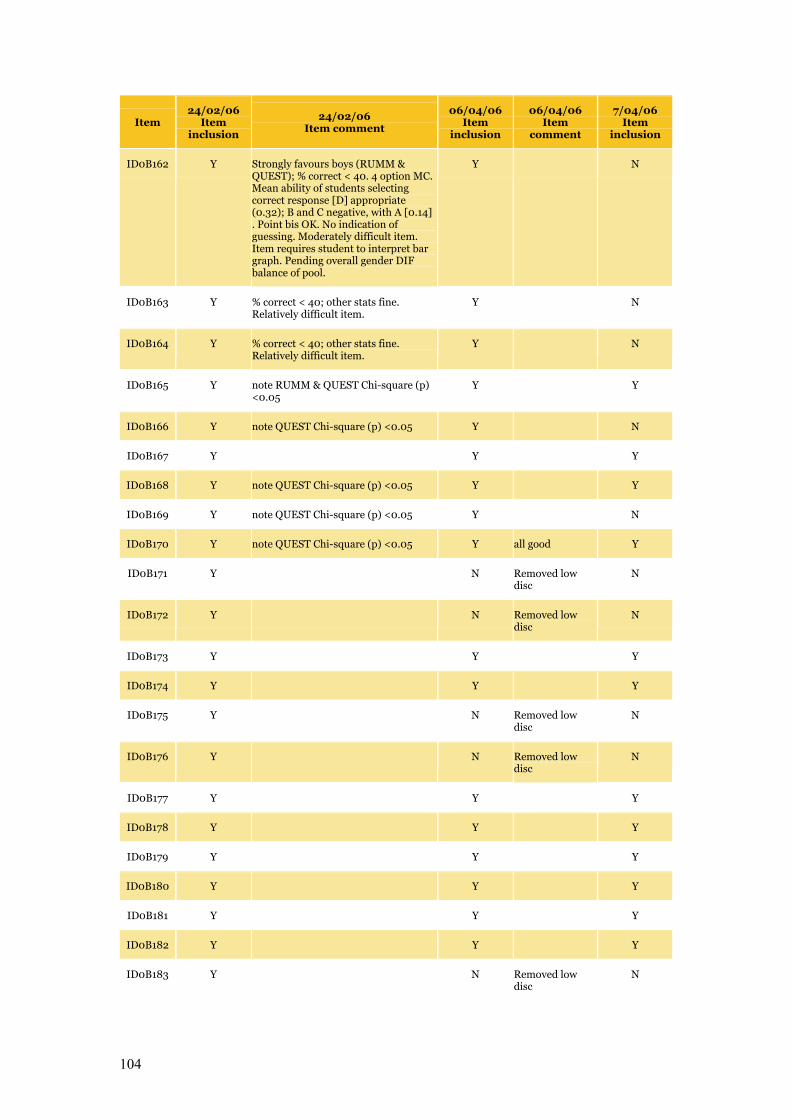
104

Item 24/02/06

Item inclusion

24/02/06 Item comment

06/04/06 Item

inclusion

06/04/06 Item

comment

7/04/06 Item

inclusion

ID0B162 Y Strongly favours boys (RUMM & QUEST); % correct < 40. 4 option MC. Mean ability of students selecting correct response [D] appropriate (0.32); B and C negative, with A [0.14] . Point bis OK. No indication of guessing. Moderately difficult item. Item requires student to interpret bar graph. Pending overall gender DIF balance of pool.

Y N

ID0B163 Y % correct < 40; other stats fine. Relatively difficult item.

Y N

ID0B164 Y % correct < 40; other stats fine. Relatively difficult item.

Y N

ID0B165 Y note RUMM & QUEST Chi-square (p) <0.05

Y Y

ID0B166 Y note QUEST Chi-square (p) <0.05 Y N

ID0B167 Y Y Y

ID0B168 Y note QUEST Chi-square (p) <0.05 Y Y

ID0B169 Y note QUEST Chi-square (p) <0.05 Y N

ID0B170 Y note QUEST Chi-square (p) <0.05 Y all good Y

ID0B171 Y N Removed low disc

N

ID0B172 Y N Removed low disc

N

ID0B173 Y Y Y

ID0B174 Y Y Y

ID0B175 Y N Removed low disc

N

ID0B176 Y N Removed low disc

N

ID0B177 Y Y Y

ID0B178 Y Y Y

ID0B179 Y Y Y

ID0B180 Y Y Y

ID0B181 Y Y Y

ID0B182 Y Y Y

ID0B183 Y N Removed low disc

N

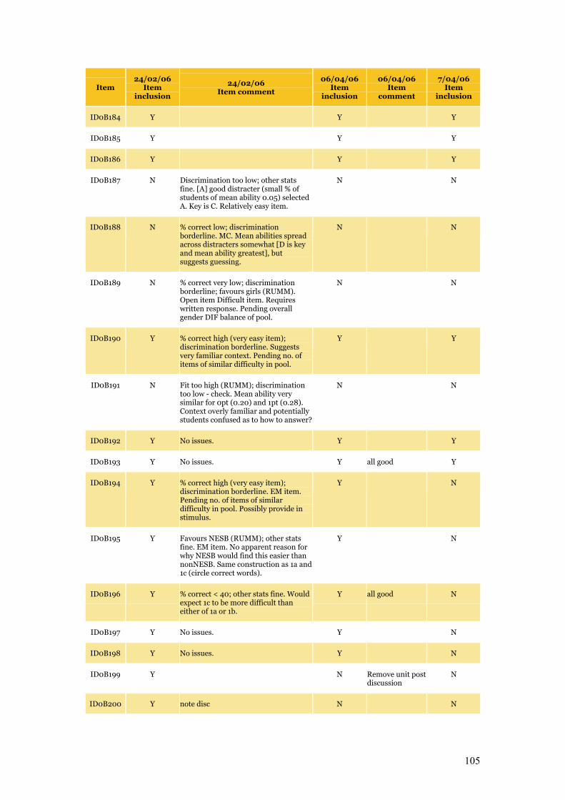
105

Item 24/02/06

Item inclusion

24/02/06 Item comment

06/04/06 Item

inclusion

06/04/06 Item

comment

7/04/06 Item

inclusion

ID0B184 Y Y Y

ID0B185 Y Y Y

ID0B186 Y Y Y

ID0B187 N Discrimination too low; other stats fine. [A] good distracter (small % of students of mean ability 0.05) selected A. Key is C. Relatively easy item.

N N

ID0B188 N % correct low; discrimination borderline. MC. Mean abilities spread across distracters somewhat [D is key and mean ability greatest], but suggests guessing.

N N

ID0B189 N % correct very low; discrimination borderline; favours girls (RUMM). Open item Difficult item. Requires written response. Pending overall gender DIF balance of pool.

N N

ID0B190 Y % correct high (very easy item); discrimination borderline. Suggests very familiar context. Pending no. of items of similar difficulty in pool.

Y Y

ID0B191 N Fit too high (RUMM); discrimination too low - check. Mean ability very similar for 0pt (0.20) and 1pt (0.28). Context overly familiar and potentially students confused as to how to answer?

N N

ID0B192 Y No issues. Y Y

ID0B193 Y No issues. Y all good Y

ID0B194 Y % correct high (very easy item); discrimination borderline. EM item. Pending no. of items of similar difficulty in pool. Possibly provide in stimulus.

Y N

ID0B195 Y Favours NESB (RUMM); other stats fine. EM item. No apparent reason for why NESB would find this easier than nonNESB. Same construction as 1a and 1c (circle correct words).

Y N

ID0B196 Y % correct < 40; other stats fine. Would expect 1c to be more difficult than either of 1a or 1b.

Y all good N

ID0B197 Y No issues. Y N

ID0B198 Y No issues. Y N

ID0B199 Y N Remove unit post discussion

N

ID0B200 Y note disc N N

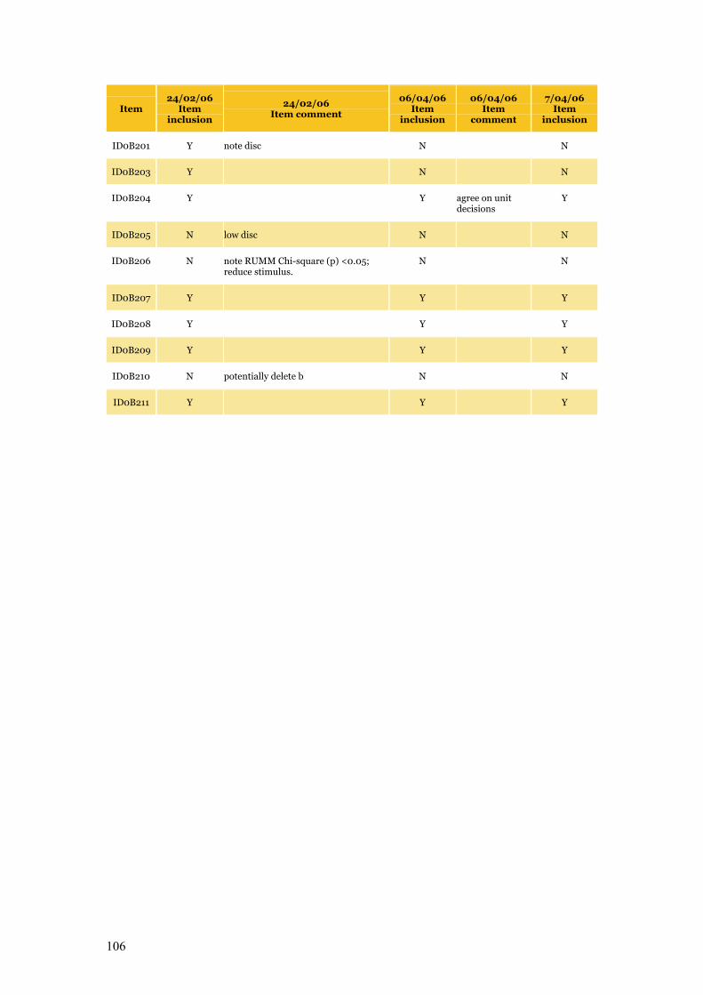
106

Item 24/02/06

Item inclusion

24/02/06 Item comment

06/04/06 Item

inclusion

06/04/06 Item

comment

7/04/06 Item

inclusion

ID0B201 Y note disc N N

ID0B203 Y N N

ID0B204 Y Y agree on unit decisions

Y

ID0B205 N low disc N N

ID0B206 N note RUMM Chi-square (p) <0.05; reduce stimulus.

N N

ID0B207 Y Y Y

ID0B208 Y Y Y

ID0B209 Y Y Y

ID0B210 N potentially delete b N N

ID0B211 Y Y Y

107

Appendix D Student Participation Form

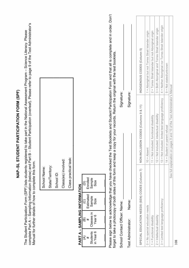
10

8

NA

P–SL

STU

DEN

T PA

RTI

CIP

ATI

ON

FO

RM

(SPF

)

The

Stu

dent

Par

ticip

atio

n Fo

rm (S

PF)

list

s st

uden

ts re

gist

ered

to ta

ke p

art i

n th

e N

atio

nal A

sses

smen

t Pro

gram

– S

cien

ce L

itera

cy. P

leas

e co

mpl

ete

Par

t A –

Sam

plin

g In

form

atio

n (b

elow

) and

Par

t B –

Stu

dent

Par

ticip

atio

n (o

verle

af).

Ple

ase

refe

r to

page

9 o

f the

Tes

t Adm

inis

trato

r’s

Man

ual f

or fu

rther

det

ails

of h

ow to

com

plet

e th

is fo

rm.

Sch

ool N

ame:

Sta

te/T

errit

ory:

Sch

ool I

D:

Cla

ss(e

s) in

volv

ed:

Cla

ss p

ract

ical

task

:

Ple

ase

sign

bel

ow to

ack

now

ledg

e th

at y

ou h

ave

chec

ked

the

Test

Boo

klet

s an

d S

tude

nt P

artic

ipat

ion

Form

and

that

all

is c

ompl

ete

and

in o

rder

. Don

’t fo

rget

to ta

ke a

pho

toco

py o

f bot

h si

des

of th

is fo

rm a

nd k

eep

a co

py fo

r you

r rec

ords

. Ret

urn

the

orig

inal

with

the

test

boo

klet

s.

Sch

ool C

onta

ct O

ffice

r: N

ame:

Sig

natu

re:

Test

Adm

inis

trato

r:

Nam

e:

S

igna

ture

:

PAR

T A

– S

AM

PLIN

G IN

FOR

MA

TIO

N

(A)

(B)

(C)

(D)

# S

tude

nts

in Y

ear 6

# C

lass

es in

Y

ear 6

Est

imat

ed

Sam

ple

Size

Enr

olle

d S

ampl

e Si

ze

__

__

__

__

__

__

__

__

SPEC

IAL

EDU

CA

TIO

N N

EED

S (S

EN) C

OD

ES (C

olum

n 7)

N

ON

-INC

LUSI

ON

CO

DES

(Col

umns

9 &

11)

IN

DIG

ENO

US

CO

DES

(Col

umn

5)

0 =

No

spec

ial e

duca

tion

need

s

10 =

Abs

ent

1 =

Abo

rigin

al b

ut n

ot T

orre

s S

trait

Isla

nder

orig

in

1 =

Func

tiona

l dis

abili

ty

11 =

Not

incl

uded

; fun

ctio

nal d

isab

ility

2

= To

rres

Stra

it Is

land

er b

ut n

ot A

borig

inal

orig

in

2 =

Inte

llect

ual d

isab

ility

12

= N

ot in

clud

ed; i

ntel

lect

ual d

isab

ility

3

= B

oth

Abo

rigin

al a

nd T

orre

s S

trait

Isla

nder

orig

in

3 =

Lim

ited

test

lang

uage

pro

ficie

ncy

13

= N

ot in

clud

ed; l

imite

d te

st la

ngua

ge p

rofic

ienc

y 4

= N

eith

er A

borig

inal

nor

Tor

res

Stra

it Is

land

er o

rigin

14

= S

tude

nt o

r par

ent r

efus

al

9 =

Not

sta

ted/

unkn

own

See

full

expl

anat

ion

on p

ages

9 a

nd 1

0 of

the

Test

Adm

inis

trato

r’s M

anua

l

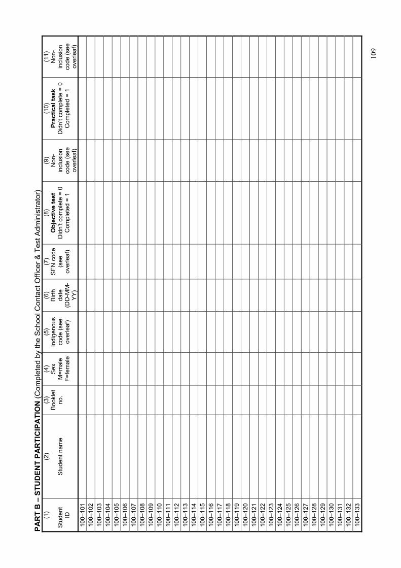
109

PAR

T B

– S

TUD

ENT

PAR

TIC

IPA

TIO

N (C

ompl

eted

by

the

Sch

ool C

onta

ct O

ffice

r & T

est A

dmin

istra

tor)

(1

) S

tude

nt

ID

(2)

S

tude

nt n

ame

(3)

Boo

klet

no

.

(4)

Sex

M=m

ale

F=fe

mal

e

(5)

Indi

geno

us

code

(see

ov

erle

af)

(6)

Birt

h da

te

(DD

-MM

-Y

Y)

(7)

SE

N c

ode

(see

ov

erle

af)

(8)

Obj

ectiv

e te

st

Did

n’t c

ompl

ete

= 0

Com

plet

ed =

1

(9)

Non

-in

clus

ion

code

(see

ov

erle

af)

(10)

Pr

actic

al ta

sk

Did

n’t c

ompl

ete

= 0

Com

plet

ed =

1

(11)

N

on-

incl

usio

n co

de (s

ee

over

leaf

) 10

0–10

1

10

0–10

2

10

0–10

3

10

0–10

4

10

0–10

5

10

0–10

6

10

0–10

7

10

0–10

8

10

0–10

9

10

0–11

0

10

0–11

1

10

0–11

2

10

0–11

3

10

0–11

4

10

0–11

5

10

0–11

6

10

0–11

7

10

0–11

8

10

0–11

9

10

0–12

0

10

0–12

1

10

0–12

2

10

0–12

3

10

0–12

4

10

0–12

5

10

0–12

6

10

0–12

7

10

0–12

8

10

0–12

9

10

0–13

0

10

0–13

1

10

0–13

2

10

0–13

3

110

Appendix E Technical Notes on Sampling

Stratification details

For each jurisdiction, schools were separated into three separate strata according to their size:

very small; moderately small; and large. The target proportion of students and number of

schools selected within each of the strata were determined using the PISA (2003) treatment of

small schools (pp. 53–56). Essentially, the aim was to balance selecting an adequate sample

without substantially increasing the number of sampled schools.

Large schools within each jurisdiction were further separated according to their school sector.

The target numbers of large schools were proportionally allocated amongst the school sectors

for each jurisdiction. Very small and moderately small strata were sorted according to school

sector, then by the remaining implicit stratification variables (Location and MOS). This

strategy meant that the sampling frame was divided into 40 explicit strata overall. That is,

there were 24 strata containing large schools (8 jurisdictions x 3 sectors); eight moderately

small school strata (1 per jurisdiction); and eight very small school strata (1 per jurisdiction).

The stratification for small schools was slightly more complex than for large schools. Small

schools were ordered by sector, GeoLocation and then gr06. The sort order was alternated so

that ‘like schools’ were always nearby.

The stratum was sorted first by sector. Within each sector, schools were further sorted by

GeoLocation. This sort order was alternated between ascending to descending between

sectors (i.e. sector1 had GeoLocation sorted ascending, sector2 had GeoLocation sorted

descending, sector3 had GeoLocation sorted ascending). The sort order for gr06 was then

alternated from low to high, then low to high, each time a new sector/GeoLocation

classification was encountered. Table E.1 illustrates the sort-order procedures that were

employed for small schools.

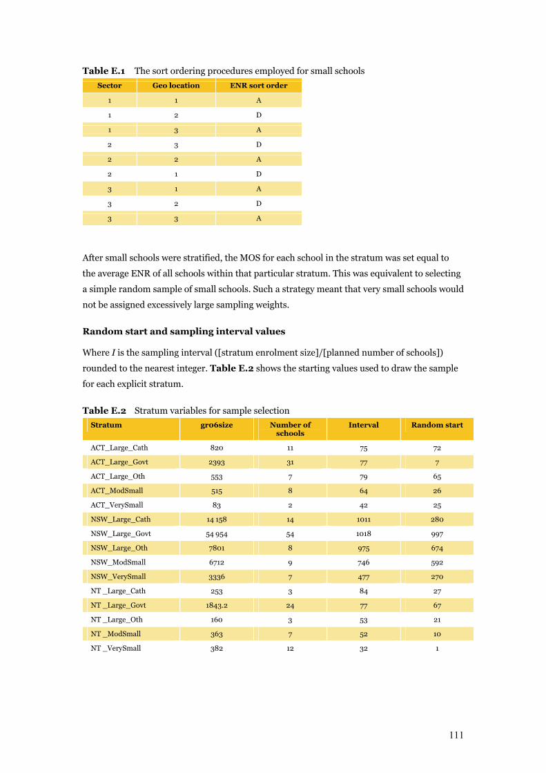
111

Table E.1 The sort ordering procedures employed for small schools

Sector Geo location ENR sort order

1 1 A

1 2 D

1 3 A

2 3 D

2 2 A

2 1 D

3 1 A

3 2 D

3 3 A

After small schools were stratified, the MOS for each school in the stratum was set equal to

the average ENR of all schools within that particular stratum. This was equivalent to selecting

a simple random sample of small schools. Such a strategy meant that very small schools would

not be assigned excessively large sampling weights.

Random start and sampling interval values

Where I is the sampling interval ([stratum enrolment size]/[planned number of schools])

rounded to the nearest integer. Table E.2 shows the starting values used to draw the sample

for each explicit stratum.

Table E.2 Stratum variables for sample selection

Stratum gr06size Number of schools

Interval Random start

ACT_Large_Cath 820 11 75 72

ACT_Large_Govt 2393 31 77 7

ACT_Large_Oth 553 7 79 65

ACT_ModSmall 515 8 64 26

ACT_VerySmall 83 2 42 25

NSW_Large_Cath 14 158 14 1011 280

NSW_Large_Govt 54 954 54 1018 997

NSW_Large_Oth 7801 8 975 674

NSW_ModSmall 6712 9 746 592

NSW_VerySmall 3336 7 477 270

NT _Large_Cath 253 3 84 27

NT _Large_Govt 1843.2 24 77 67

NT _Large_Oth 160 3 53 21

NT _ModSmall 363 7 52 10

NT _VerySmall 382 12 32 1

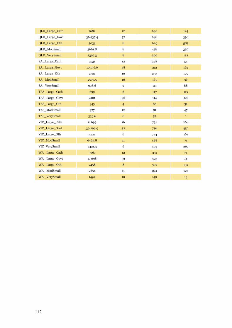
112

QLD_Large_Cath 7682 12 640 124

QLD_Large_Govt 36 937.4 57 648 396

QLD_Large_Oth 5033 8 629 585

QLD_ModSmall 3661.8 8 458 350

QLD_VerySmall 2397.3 8 300 152

SA _Large_Cath 2731 12 228 54

SA _Large_Govt 10 196.6 48 212 162

SA _Large_Oth 2331 10 233 129

SA _ModSmall 2579.5 16 161 36

SA _VerySmall 998.6 9 111 88

TAS_Large_Cath 699 6 117 115

TAS_Large_Govt 4101 36 114 60

TAS_Large_Oth 345 4 86 31

TAS_ModSmall 977 12 81 47

TAS_VerySmall 339.6 6 57 1

VIC_Large_Cath 11 699 16 731 264

VIC_Large_Govt 39 299.9 52 756 456

VIC_Large_Oth 4521 6 754 161

VIC_ModSmall 6463.8 11 588 71

VIC_VerySmall 2421.3 6 404 267

WA _Large_Cath 3967 12 331 74

WA _Large_Govt 17 098 53 323 14

WA _Large_Oth 2458 8 307 132

WA _ModSmall 2656 11 241 127

WA _VerySmall 1494 10 149 13

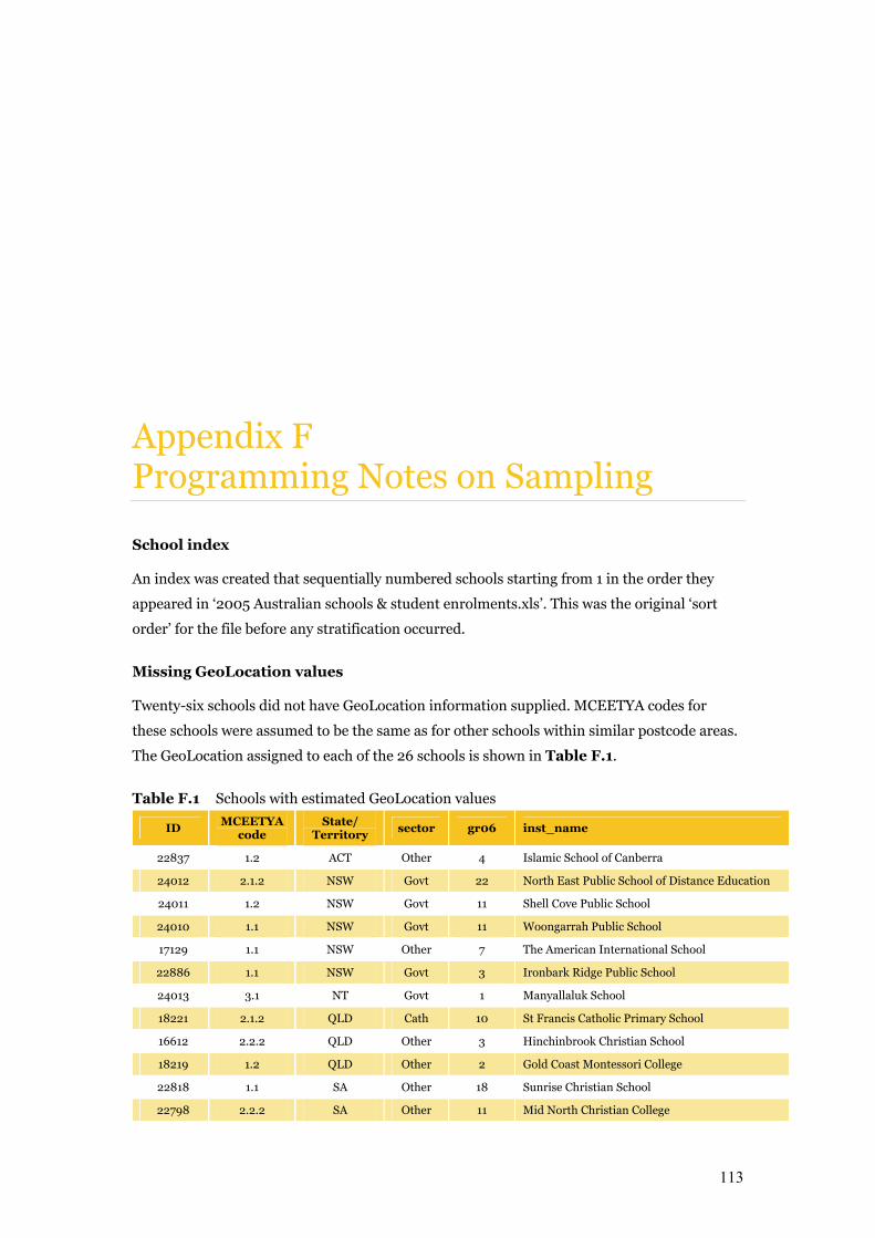
113

Appendix F Programming Notes on Sampling

School index

An index was created that sequentially numbered schools starting from 1 in the order they

appeared in ‘2005 Australian schools & student enrolments.xls’. This was the original ‘sort

order’ for the file before any stratification occurred.

Missing GeoLocation values

Twenty-six schools did not have GeoLocation information supplied. MCEETYA codes for

these schools were assumed to be the same as for other schools within similar postcode areas.

The GeoLocation assigned to each of the 26 schools is shown in Table F.1.

Table F.1 Schools with estimated GeoLocation values

ID MCEETYA

code State/

Territory sector gr06 inst_name

22837 1.2 ACT Other 4 Islamic School of Canberra

24012 2.1.2 NSW Govt 22 North East Public School of Distance Education

24011 1.2 NSW Govt 11 Shell Cove Public School

24010 1.1 NSW Govt 11 Woongarrah Public School

17129 1.1 NSW Other 7 The American International School

22886 1.1 NSW Govt 3 Ironbark Ridge Public School

24013 3.1 NT Govt 1 Manyallaluk School

18221 2.1.2 QLD Cath 10 St Francis Catholic Primary School

16612 2.2.2 QLD Other 3 Hinchinbrook Christian School

18219 1.2 QLD Other 2 Gold Coast Montessori College

22818 1.1 SA Other 18 Sunrise Christian School

22798 2.2.2 SA Other 11 Mid North Christian College

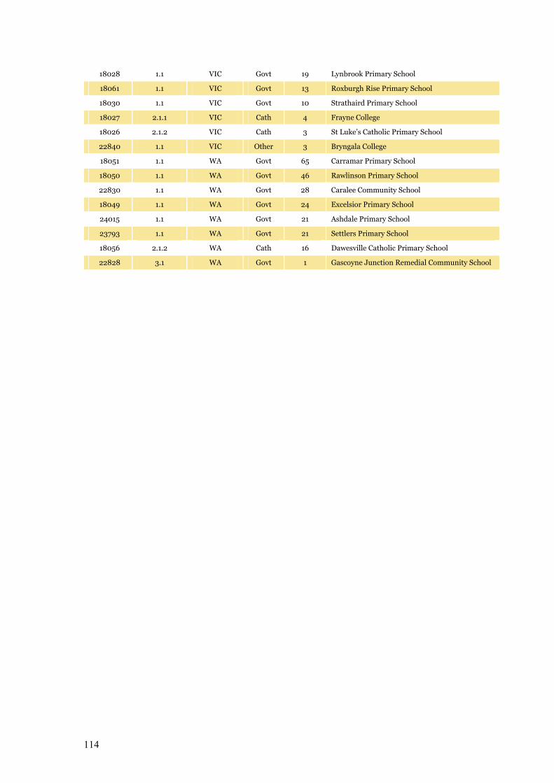
114

18028 1.1 VIC Govt 19 Lynbrook Primary School

18061 1.1 VIC Govt 13 Roxburgh Rise Primary School

18030 1.1 VIC Govt 10 Strathaird Primary School

18027 2.1.1 VIC Cath 4 Frayne College

18026 2.1.2 VIC Cath 3 St Luke’s Catholic Primary School

22840 1.1 VIC Other 3 Bryngala College

18051 1.1 WA Govt 65 Carramar Primary School

18050 1.1 WA Govt 46 Rawlinson Primary School

22830 1.1 WA Govt 28 Caralee Community School

18049 1.1 WA Govt 24 Excelsior Primary School

24015 1.1 WA Govt 21 Ashdale Primary School

23793 1.1 WA Govt 21 Settlers Primary School

18056 2.1.2 WA Cath 16 Dawesville Catholic Primary School

22828 3.1 WA Govt 1 Gascoyne Junction Remedial Community School

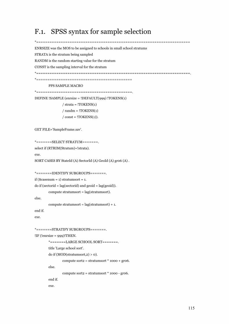
115

F.1. SPSS syntax for sample selection *=====================================================================

ENRSIZE was the MOS to be assigned to schools in small school stratums

STRATA is the stratum being sampled

RANDM is the random starting value for the stratum

CONST is the sampling interval for the stratum

*=====================================================================.

*===========================================

PPS SAMPLE MACRO

*===========================================.

DEFINE !SAMPLE (enrsize = !DEFAULT(999) !TOKENS(1)

/ strata = !TOKENS(1)

/ randm = !TOKENS(1)

/ const = !TOKENS(1)).

GET FILE='SampleFrame.sav'.

*=======SELECT STRATUM=======.

select if (RTRIM(Stratum)=!strata).

exe.

SORT CASES BY StateId (A) SectorId (A) GeoId (A) gr06 (A) .

*=======IDENTIFY SUBGROUPS=======.

if ($casenum = 1) stratumsort = 1.

do if (sectorid = lag(sectorid) and geoid = lag(geoid)).

compute stratumsort = lag(stratumsort).

else.

compute stratumsort = lag(stratumsort) + 1.

end if.

exe.

*=======STRATIFY SUBGROUPS=======.

!IF (!enrsize = 999)!THEN.

*=======LARGE SCHOOL SORT=======.

title 'Large school sort'.

do if (MOD(stratumsort,2) > 0).

compute sort2 = stratumsort * 1000 + gr06.

else.

compute sort2 = stratumsort * 1000 - gr06.

end if.

exe.

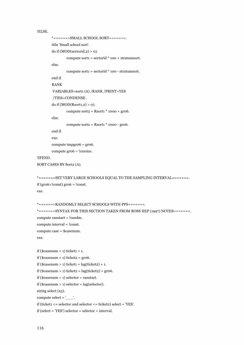
116

!ELSE.

*=======SMALL SCHOOL SORT=======.

title 'Small school sort'.

do if (MOD(sectorid,2) > 0).

compute sort1 = sectorid * 100 + stratumsort.

else.

compute sort1 = sectorid * 100 - stratumsort.

end if.

RANK

VARIABLES=sort1 (A) /RANK /PRINT=YES

/TIES=CONDENSE .

do if (MOD(Rsort1,2) > 0).

compute sort2 = Rsort1 * 1000 + gr06.

else.

compute sort2 = Rsort1 * 1000 - gr06.

end if.

exe.

compute tmpgr06 = gr06.

compute gr06 = !enrsize.

!IFEND.

SORT CASES BY Sort2 (A).

*=======SET VERY LARGE SCHOOLS EQUAL TO THE SAMPLING INTERVAL=======.

if (gr06>!const) gr06 = !const.

exe.

*=======RANDOMLY SELECT SCHOOLS WITH PPS=======.

*=======SYNTAX FOR THIS SECTION TAKEN FROM ROSS IIEP (1997) NOTES=======.

compute ranstart = !randm.

compute interval = !const.

compute case = $casenum.

exe.

if ($casenum = 1) ticket1 = 1.

if ($casenum = 1) ticket2 = gr06.

if ($casenum > 1) ticket1 = lag(ticket2) + 1.

if ($casenum > 1) ticket2 = lag(ticket2) + gr06.

if ($casenum = 1) selector = ranstart.

if ($casenum > 1) selector = lag(selector).

string select (a3).

compute select = '___'.

if (ticket1 <= selector and selector <= ticket2) select = 'YES'.

if (select = 'YES') selector = selector + interval.

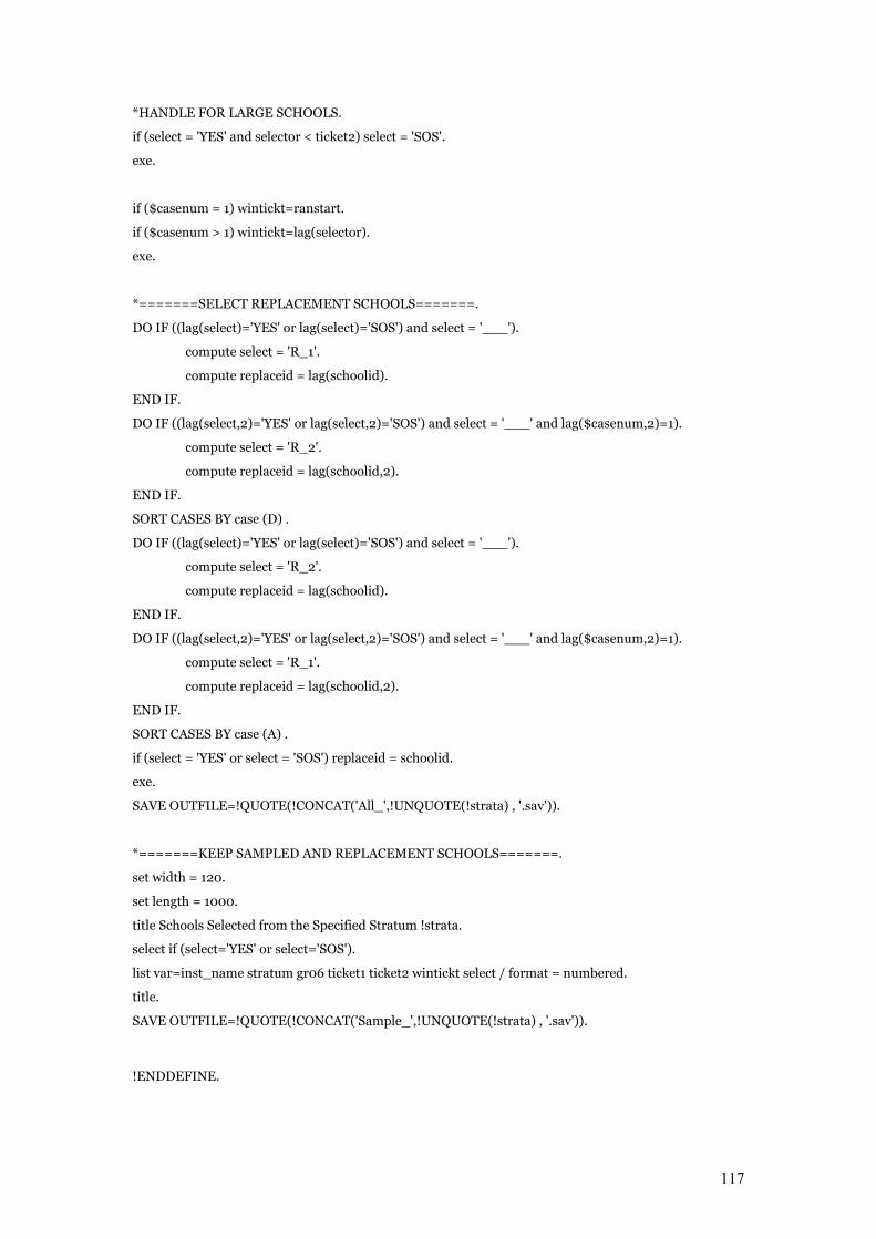
117

*HANDLE FOR LARGE SCHOOLS.

if (select = 'YES' and selector < ticket2) select = 'SOS'.

exe.

if ($casenum = 1) wintickt=ranstart.

if ($casenum > 1) wintickt=lag(selector).

exe.

*=======SELECT REPLACEMENT SCHOOLS=======.

DO IF ((lag(select)='YES' or lag(select)='SOS') and select = '___').

compute select = 'R_1'.

compute replaceid = lag(schoolid).

END IF.

DO IF ((lag(select,2)='YES' or lag(select,2)='SOS') and select = '___' and lag($casenum,2)=1).

compute select = 'R_2'.

compute replaceid = lag(schoolid,2).

END IF.

SORT CASES BY case (D) .

DO IF ((lag(select)='YES' or lag(select)='SOS') and select = '___').

compute select = 'R_2'.

compute replaceid = lag(schoolid).

END IF.

DO IF ((lag(select,2)='YES' or lag(select,2)='SOS') and select = '___' and lag($casenum,2)=1).

compute select = 'R_1'.

compute replaceid = lag(schoolid,2).

END IF.

SORT CASES BY case (A) .

if (select = 'YES' or select = 'SOS') replaceid = schoolid.

exe.

SAVE OUTFILE=!QUOTE(!CONCAT('All_',!UNQUOTE(!strata) , '.sav')).

*=======KEEP SAMPLED AND REPLACEMENT SCHOOLS=======.

set width = 120.

set length = 1000.

title Schools Selected from the Specified Stratum !strata.

select if (select='YES' or select='SOS').

list var=inst_name stratum gr06 ticket1 ticket2 wintickt select / format = numbered.

title.

SAVE OUTFILE=!QUOTE(!CONCAT('Sample_',!UNQUOTE(!strata) , '.sav')).

!ENDDEFINE.

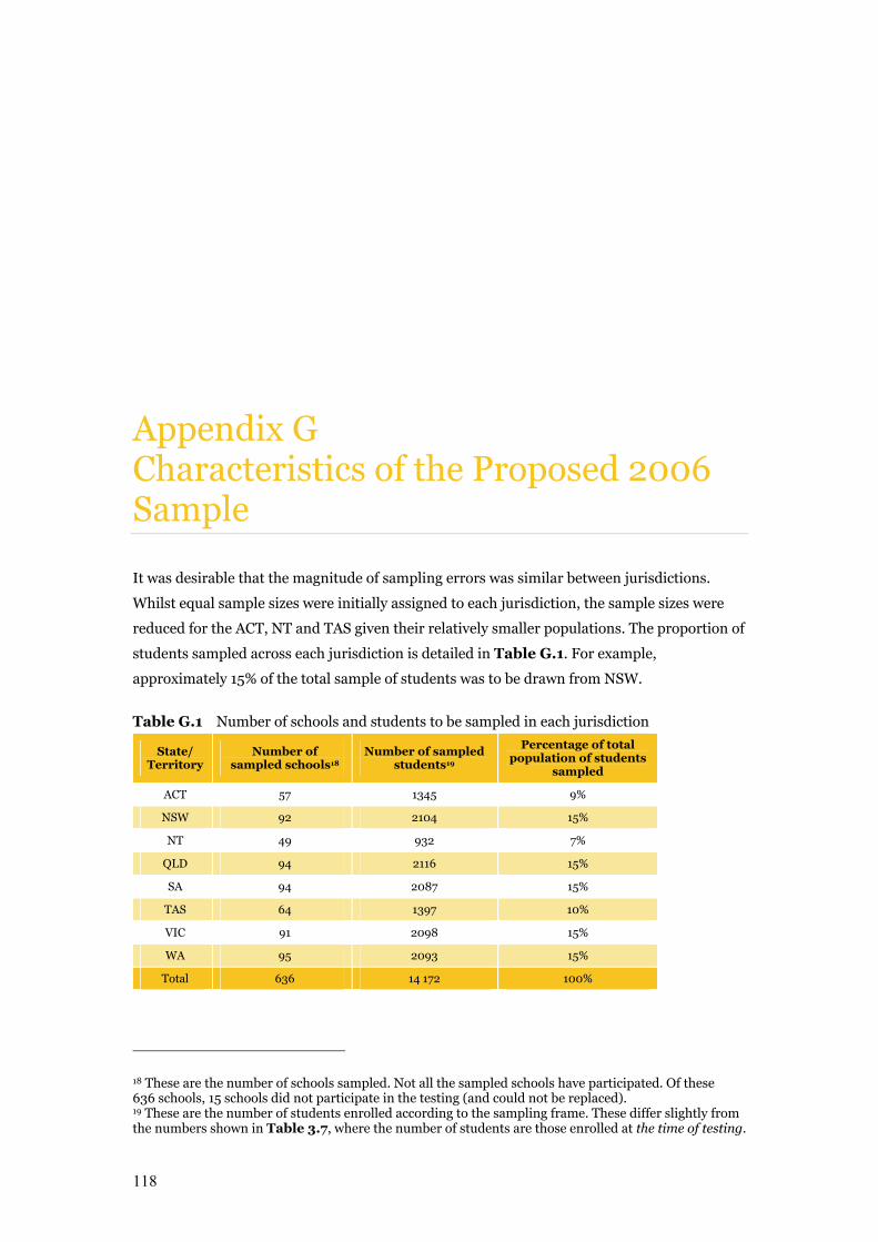
118

Appendix G Characteristics of the Proposed 2006 Sample

It was desirable that the magnitude of sampling errors was similar between jurisdictions.

Whilst equal sample sizes were initially assigned to each jurisdiction, the sample sizes were

reduced for the ACT, NT and TAS given their relatively smaller populations. The proportion of

students sampled across each jurisdiction is detailed in Table G.1. For example,

approximately 15% of the total sample of students was to be drawn from NSW.

Table G.1 Number of schools and students to be sampled in each jurisdiction

State/ Territory

Number of sampled schools18

Number of sampled students19

Percentage of total population of students

sampled

ACT 57 1345 9%

NSW 92 2104 15%

NT 49 932 7%

QLD 94 2116 15%

SA 94 2087 15%

TAS 64 1397 10%

VIC 91 2098 15%

WA 95 2093 15%

Total 636 14 172 100%

18 These are the number of schools sampled. Not all the sampled schools have participated. Of these 636 schools, 15 schools did not participate in the testing (and could not be replaced). 19 These are the number of students enrolled according to the sampling frame. These differ slightly from the numbers shown in Table 3.7, where the number of students are those enrolled at the time of testing.

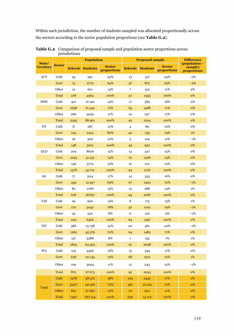
119

Within each jurisdiction, the number of students sampled was allocated proportionally across

the sectors according to the sector population proportions (see Table G.2).

Table G.2 Comparison of proposed sample and population sector proportions across jurisdictions

Population Proposed sample State/

Territory Sector

Schools Students Sector

proportionsSchools Students

Sector proportions

Difference (population –

sample) proportions

ACT Cath 23 991 23% 13 317 24% –1%

Govt 73 2772 64% 37 875 65% –2%

Other 12 601 14% 7 153 11% 2%

Total 108 4364 100% 57 1345 100% 0%

NSW Cath 421 16 190 19% 17 389 18% 0%

Govt 1658 61 542 71% 65 1488 71% 0%

Other 266 9229 11% 10 227 11% 0%

Total 2345 86 961 100% 92 2104 100% 0%

NT Cath 8 287 10% 4 89 10% 0%

Govt 124 2414 80% 40 739 79% 1%

Other 16 300 10% 5 104 11% –1%

Total 148 3001 100% 49 932 100% 0%

QLD Cath 209 8626 15% 14 327 15% 0%

Govt 1023 41 312 74% 70 1568 74% 0%

Other 146 5774 10% 10 221 10% 0%

Total 1378 55 712 100% 94 2116 100% 0%

SA Cath 77 3114 17% 14 335 16% 0%

Govt 459 12 957 69% 67 1464 70% –1%

Other 82 2766 15% 13 288 14% 1%

Total 618 18 837 100% 94 2087 100% 0%

TAS Cath 29 900 14% 8 175 13% 1%

Govt 170 5042 78% 50 1102 79% –1%

Other 24 520 8% 6 120 9% –1%

Total 223 6462 100% 64 1397 100% 0%

VIC Cath 386 13 738 21% 20 461 22% –1%

Govt 1262 45 379 70% 64 1482 71% 0%

Other 157 5288 8% 7 155 7% 1%

Total 1805 64 405 100% 91 2098 100% 0%

WA Cath 125 4526 16% 15 349 17% 0%

Govt 638 20 143 73% 68 1501 72% 1%

Other 109 3004 11% 12 243 12% –1%

Total 872 27 673 100% 95 2093 100% 0%

Cath 1278 48 372 18% 105 2442 17% 1%

Govt 5407 191 561 72% 461 10 219 72% 0%

Other 812 27 482 10% 70 1511 11% 0% Total

Total 7497 267 414 100% 636 14 172 100% 0%

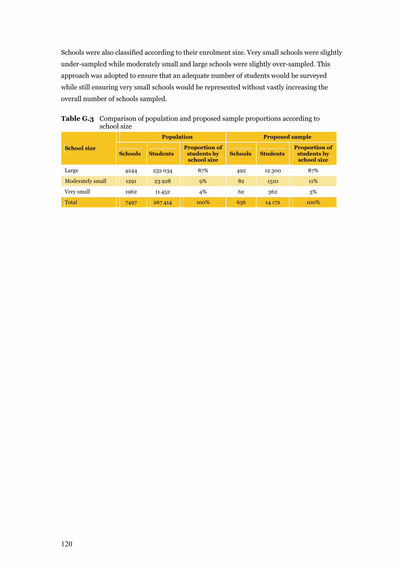
120

Schools were also classified according to their enrolment size. Very small schools were slightly

under-sampled while moderately small and large schools were slightly over-sampled. This

approach was adopted to ensure that an adequate number of students would be surveyed

while still ensuring very small schools would be represented without vastly increasing the

overall number of schools sampled.

Table G.3 Comparison of population and proposed sample proportions according to school size

Population Proposed sample

School size Schools Students

Proportion of students by school size

Schools Students Proportion of

students by school size

Large 4244 232 034 87% 492 12 300 87%

Moderately small 1291 23 928 9% 82 1510 11%

Very small 1962 11 452 4% 62 362 3%

Total 7497 267 414 100% 636 14 172 100%

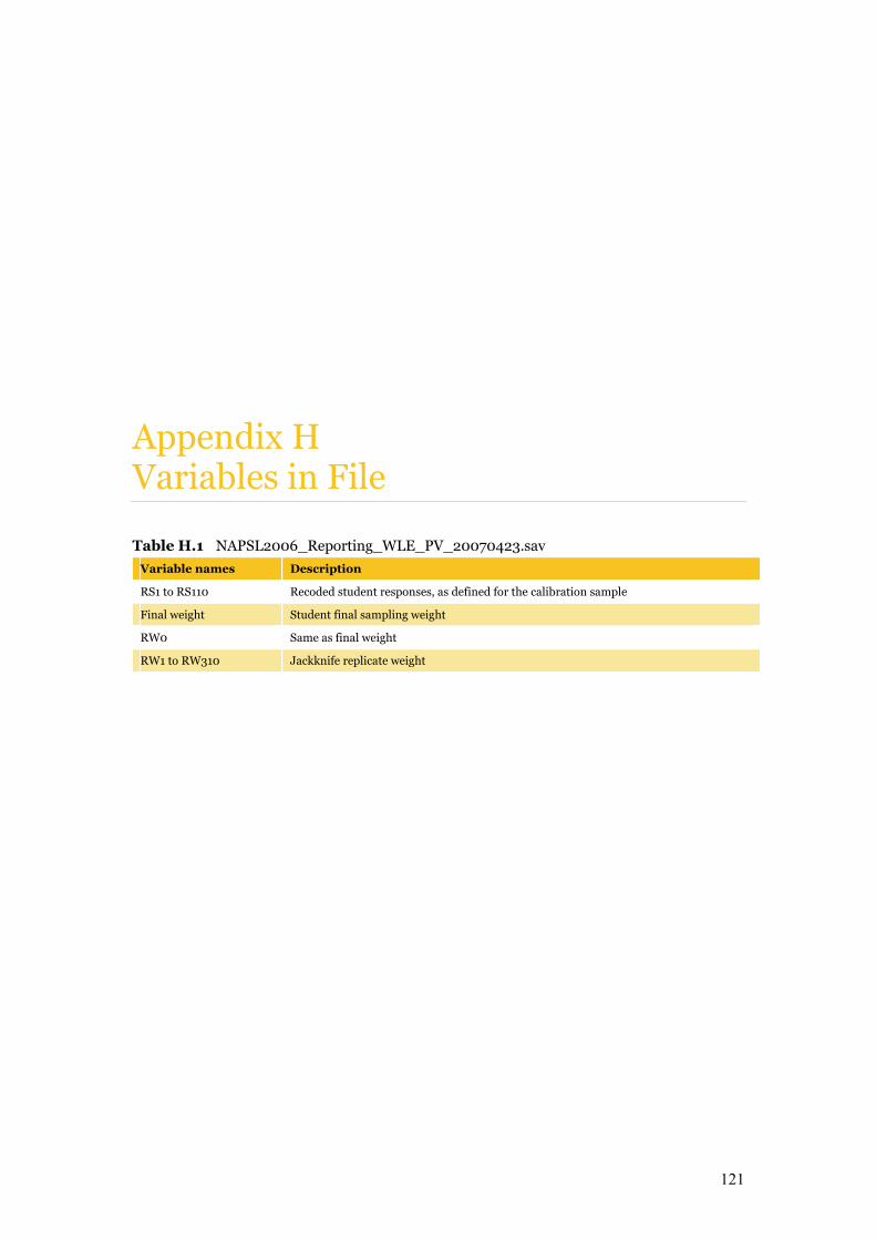
121

Appendix H Variables in File

Table H.1 NAPSL2006_Reporting_WLE_PV_20070423.sav

Variable names Description

RS1 to RS110 Recoded student responses, as defined for the calibration sample

Final weight Student final sampling weight

RW0 Same as final weight

RW1 to RW310 Jackknife replicate weight

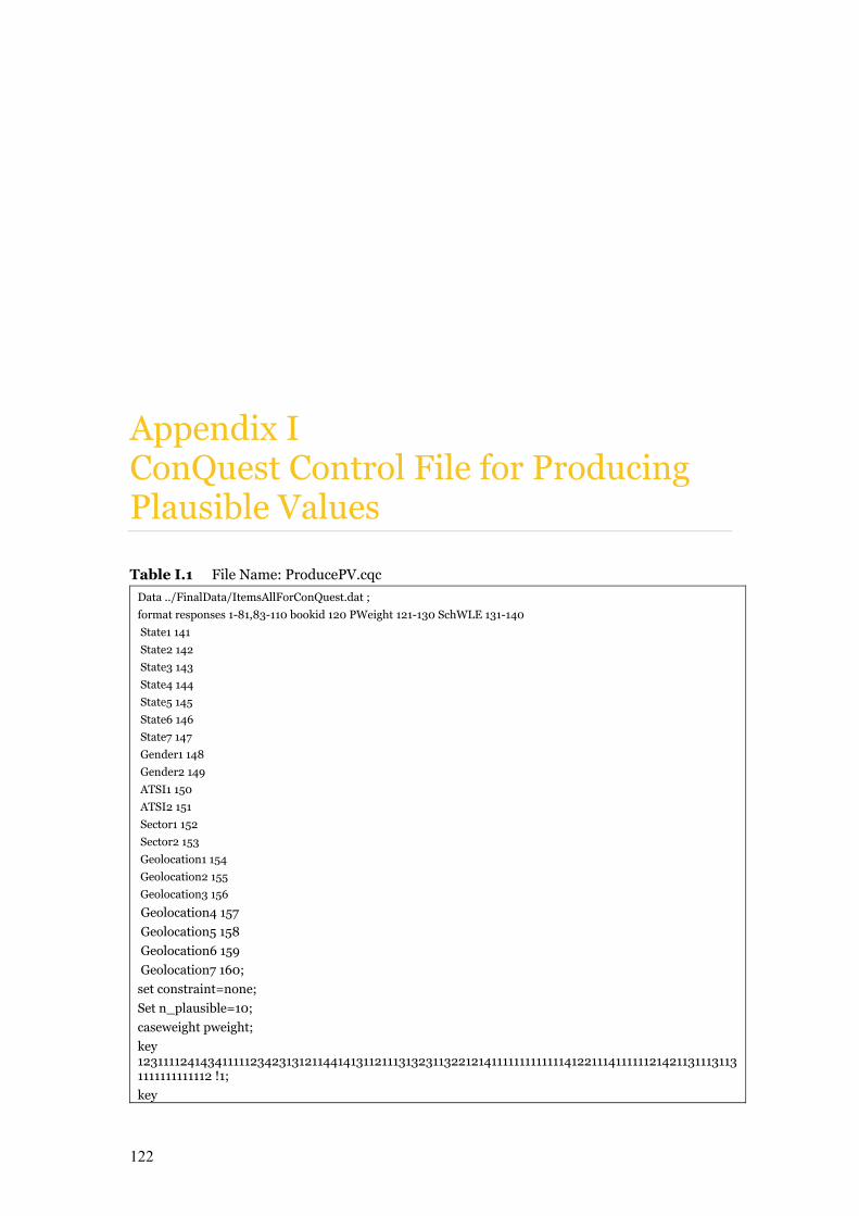
122

Appendix I ConQuest Control File for Producing Plausible Values

Table I.1 File Name: ProducePV.cqc

Data ../FinalData/ItemsAllForConQuest.dat ;

format responses 1-81,83-110 bookid 120 PWeight 121-130 SchWLE 131-140

State1 141

State2 142

State3 143

State4 144

State5 145

State6 146

State7 147

Gender1 148

Gender2 149

ATSI1 150

ATSI2 151

Sector1 152

Sector2 153

Geolocation1 154

Geolocation2 155

Geolocation3 156

Geolocation4 157

Geolocation5 158

Geolocation6 159

Geolocation7 160;

set constraint=none;

Set n_plausible=10;

caseweight pweight;

key 1231111241434111112342313121144141311211131323113221214111111111111141221114111111214211311131131111111111112 !1;

key

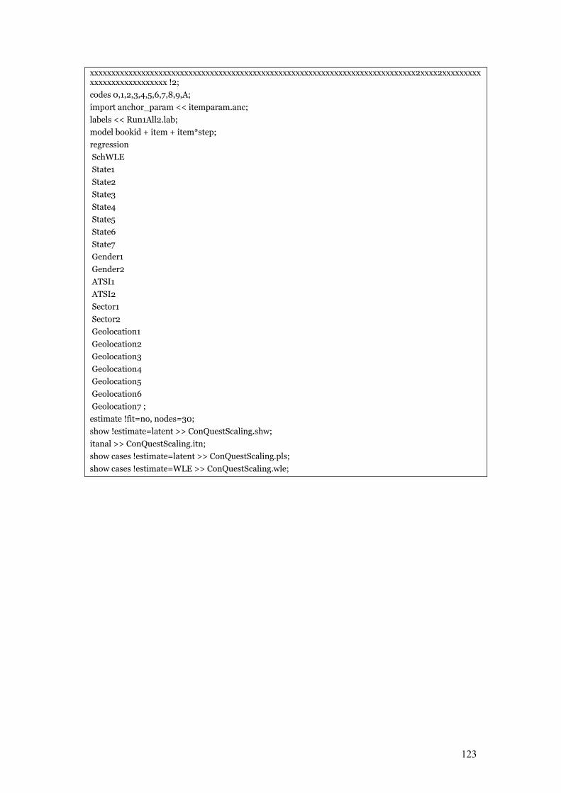
123

xxxxxxxxxxxxxxxxxxxxxxxxxxxxxxxxxxxxxxxxxxxxxxxxxxxxxxxxxxxxxxxxxxxxxxxxxxxx2xxxx2xxxxxxxxxxxxxxxxxxxxxxxxxxx !2;

codes 0,1,2,3,4,5,6,7,8,9,A;

import anchor_param << itemparam.anc;

labels << Run1All2.lab;

model bookid + item + item*step;

regression

SchWLE

State1

State2

State3

State4

State5

State6

State7

Gender1

Gender2

ATSI1

ATSI2

Sector1

Sector2

Geolocation1

Geolocation2

Geolocation3

Geolocation4

Geolocation5

Geolocation6

Geolocation7 ;

estimate !fit=no, nodes=30;

show !estimate=latent >> ConQuestScaling.shw;

itanal >> ConQuestScaling.itn;

show cases !estimate=latent >> ConQuestScaling.pls;

show cases !estimate=WLE >> ConQuestScaling.wle;

124