Embed Size (px)
Citation preview
8/14/2019 MCA Costs of Production
http://slidepdf.com/reader/full/mca-costs-of-production 1/45
The Theory of the Firm
8/14/2019 MCA Costs of Production
http://slidepdf.com/reader/full/mca-costs-of-production 2/45
The Costs of Production
8/14/2019 MCA Costs of Production
http://slidepdf.com/reader/full/mca-costs-of-production 3/45
Outline
• What are costs?
• Link between firm’s production process and its
total cost• Measures of Cost
• Costs in the short-run and costs in the long-run
8/14/2019 MCA Costs of Production
http://slidepdf.com/reader/full/mca-costs-of-production 4/45
Basic Concepts
• Total Revenue- Amount a firm receives for
the sale of its output• Total Cost- Market value of the inputs a firm
uses in production
• Profit = Total Revenue – Total Cost
8/14/2019 MCA Costs of Production
http://slidepdf.com/reader/full/mca-costs-of-production 5/45
Actual Cost & Opportunity Cost
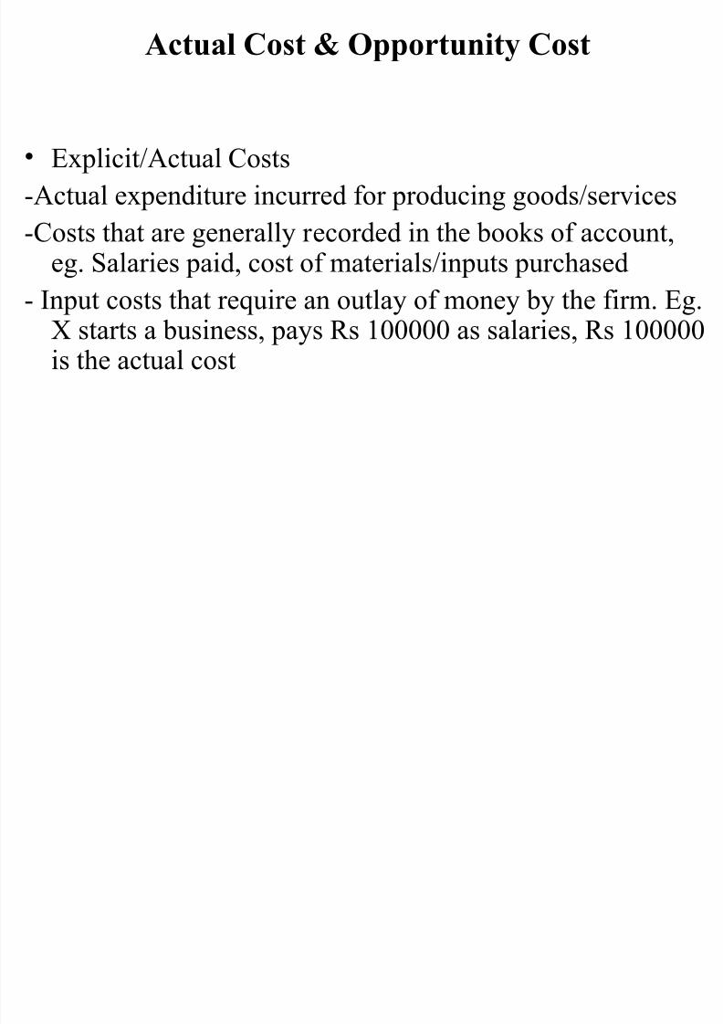
• Explicit/Actual Costs
-Actual expenditure incurred for producing goods/services
-Costs that are generally recorded in the books of account,eg. Salaries paid, cost of materials/inputs purchased
- Input costs that require an outlay of money by the firm. Eg.X starts a business, pays Rs 100000 as salaries, Rs 100000is the actual cost
8/14/2019 MCA Costs of Production
http://slidepdf.com/reader/full/mca-costs-of-production 6/45
Actual Cost & Opportunity Cost
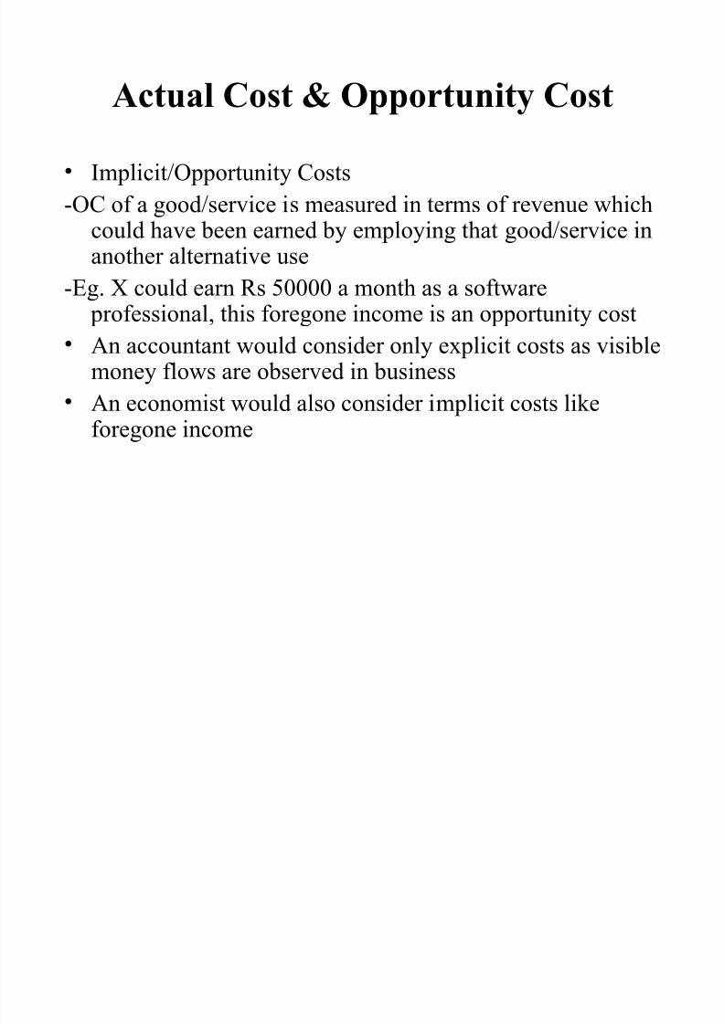
• Implicit/Opportunity Costs
-OC of a good/service is measured in terms of revenue whichcould have been earned by employing that good/service in
another alternative use-Eg. X could earn Rs 50000 a month as a software
professional, this foregone income is an opportunity cost
• An accountant would consider only explicit costs as visible
money flows are observed in business• An economist would also consider implicit costs like
foregone income
8/14/2019 MCA Costs of Production
http://slidepdf.com/reader/full/mca-costs-of-production 7/45
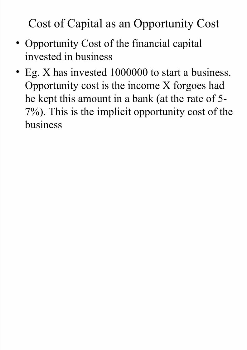
Cost of Capital as an Opportunity Cost
• Opportunity Cost of the financial capitalinvested in business
• Eg. X has invested 1000000 to start a business.
Opportunity cost is the income X forgoes hadhe kept this amount in a bank (at the rate of 5-
7%). This is the implicit opportunity cost of the
business
8/14/2019 MCA Costs of Production
http://slidepdf.com/reader/full/mca-costs-of-production 8/45
Economic Cost
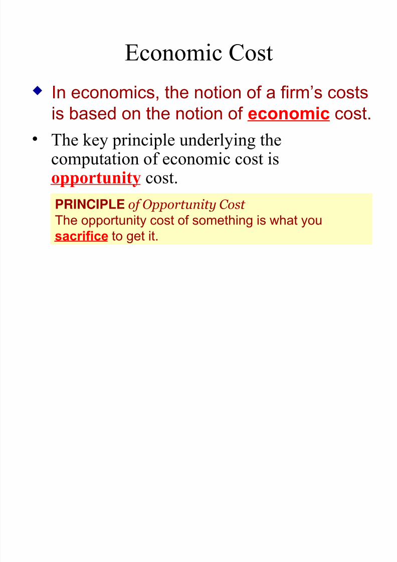
• The key principle underlying thecomputation of economic cost isopportunity cost.
PRINCIPLE of Opportunity Cost The opportunity cost of something is what you
sacrifice to get it.
In economics, the notion of a firm’s costs
is based on the notion of economic cost.
8/14/2019 MCA Costs of Production
http://slidepdf.com/reader/full/mca-costs-of-production 9/45
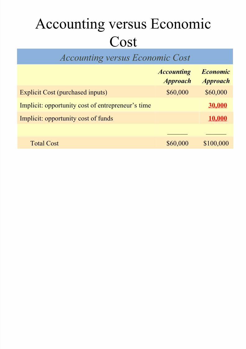
Accounting versus Economic
Cost
$100,000$60,000Total Cost
______ ______
10,000Implicit: opportunity cost of funds
30,000Implicit: opportunity cost of entrepreneur’s time
$60,000$60,000Explicit Cost (purchased inputs)
Economic
Approach
Accounting
Approach
Accounting versus Economic Cost
8/14/2019 MCA Costs of Production
http://slidepdf.com/reader/full/mca-costs-of-production 10/45
Economic Profit Vs Accounting Profit
• Economic Profit = Total Revenue minus
Total Cost, including both explicit and
implicit costs
• Accounting Profit = Total Revenue minusTotal explicit costs
• Economic Value-Added = NOPAT – Cost of
Capital (Cost of Debt + Cost of Equity)
8/14/2019 MCA Costs of Production
http://slidepdf.com/reader/full/mca-costs-of-production 11/45
Fixed Costs & Variable Costs
• In buying factor inputs, the firm will incur costs
• Costs are Classified as:
– Fixed costs – costs that are not related directly to
production – rent, insurance costs, admin costs. Theycan change but not in relation to output/production.
– Fixed Costs are incurred even when output is nil
– Variable Costs – costs directly related to variations in
output. Raw materials, labour, primarily.
– Increase in volume means a proportionate increase in
total variable cost and vice versa
8/14/2019 MCA Costs of Production
http://slidepdf.com/reader/full/mca-costs-of-production 12/45
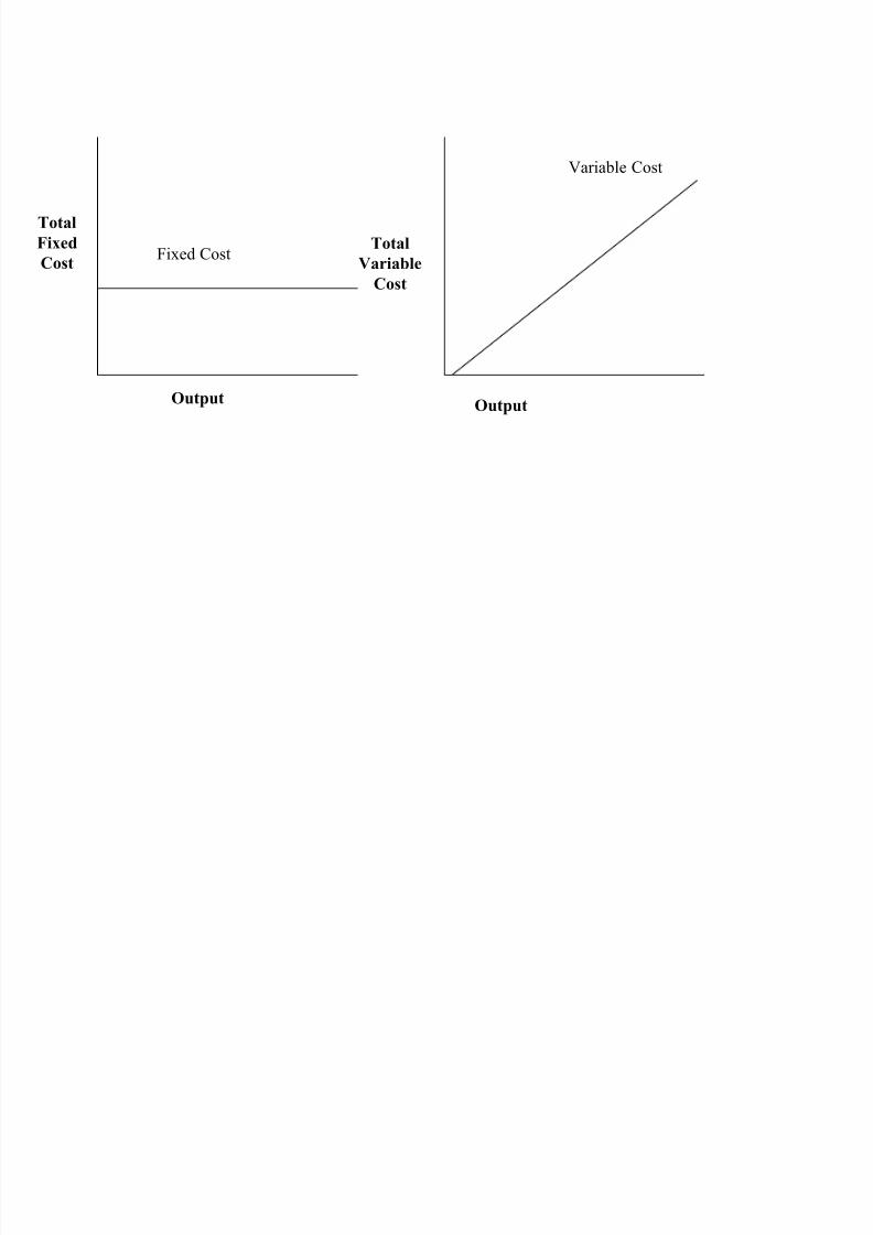
Total
Fixed
CostFixed Cost
Output
Total
Variable
Cost
Variable Cost
Output
8/14/2019 MCA Costs of Production
http://slidepdf.com/reader/full/mca-costs-of-production 13/45
Short-run & Long-run Costs
• Time Horizon key factor in dividing costs into short-run and
long-run costs• Short run – In the short-run increase in production results from
adding successive quantities of variable factors to a fixed factor
- Short-run costs are costs that vary with output when fixed plant
and capital equipment remain the same- Relevant when a firm decides whether or not to produce more in
the immediate future
• Long run – Increases in capacity results in increasing production.All costs become variable in the long-run
- Long-run costs are those which vary with output when all inputfactors including plant and equipment vary
- Relevant when a firm decides whether to set up a new plant.
8/14/2019 MCA Costs of Production
http://slidepdf.com/reader/full/mca-costs-of-production 14/45
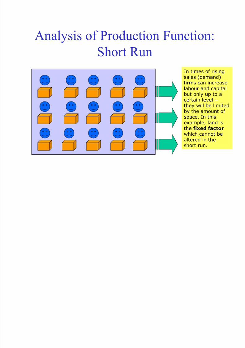
Analysis of Production Function:
Short Run
In times of risingsales (demand)firms can increaselabour and capitalbut only up to acertain level –they will be limitedby the amount of space. In thisexample, land is
the fixed factor which cannot bealtered in theshort run.
8/14/2019 MCA Costs of Production
http://slidepdf.com/reader/full/mca-costs-of-production 15/45
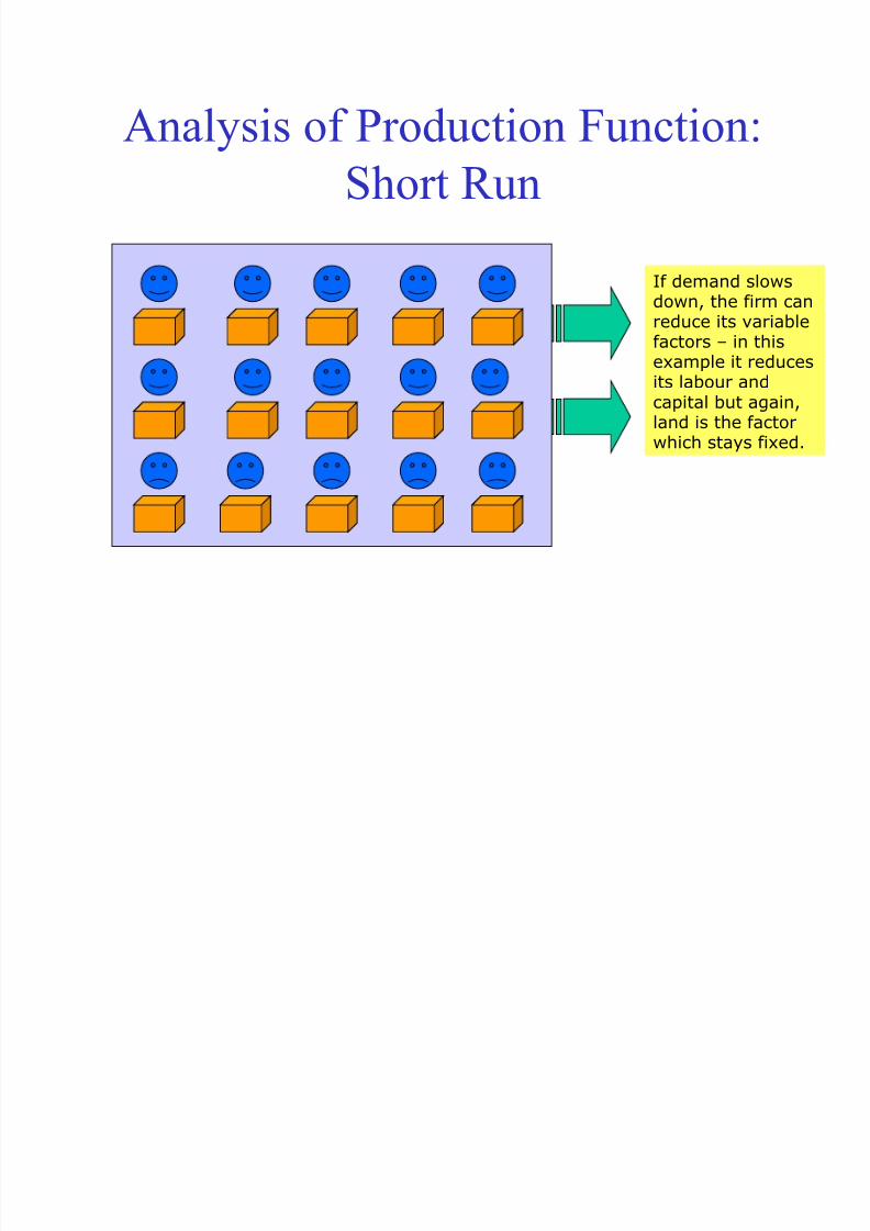
Analysis of Production Function:
Short Run
If demand slows
down, the firm canreduce its variablefactors – in thisexample it reducesits labour andcapital but again,land is the factorwhich stays fixed.
8/14/2019 MCA Costs of Production
http://slidepdf.com/reader/full/mca-costs-of-production 16/45
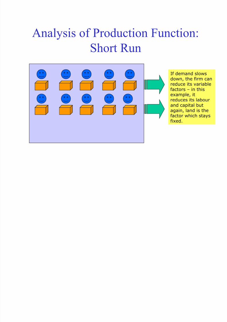
Analysis of Production Function:
Short Run
If demand slows
down, the firm canreduce its variablefactors – in thisexample, itreduces its labourand capital butagain, land is thefactor which stays
fixed.
8/14/2019 MCA Costs of Production
http://slidepdf.com/reader/full/mca-costs-of-production 17/45
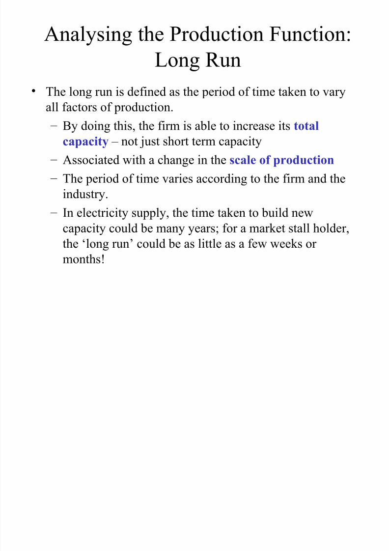
Analysing the Production Function:
Long Run• The long run is defined as the period of time taken to vary
all factors of production.
– By doing this, the firm is able to increase its total
capacity – not just short term capacity
– Associated with a change in the scale of production
– The period of time varies according to the firm and the
industry.
– In electricity supply, the time taken to build new
capacity could be many years; for a market stall holder,
the ‘long run’ could be as little as a few weeks or
months!
8/14/2019 MCA Costs of Production
http://slidepdf.com/reader/full/mca-costs-of-production 18/45
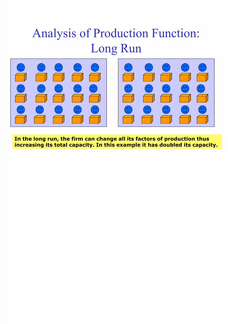
Analysis of Production Function:
Long Run
In the long run, the firm can change all its factors of production thusincreasing its total capacity. In this example it has doubled its capacity.
8/14/2019 MCA Costs of Production
http://slidepdf.com/reader/full/mca-costs-of-production 19/45
8/14/2019 MCA Costs of Production
http://slidepdf.com/reader/full/mca-costs-of-production 20/45
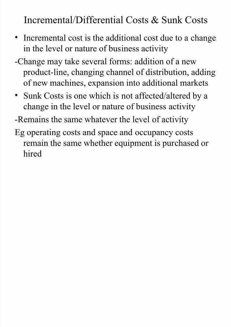
Incremental/Differential Costs & Sunk Costs
• Incremental cost is the additional cost due to a changein the level or nature of business activity
-Change may take several forms: addition of a new
product-line, changing channel of distribution, adding
of new machines, expansion into additional markets• Sunk Costs is one which is not affected/altered by a
change in the level or nature of business activity
-Remains the same whatever the level of activityEg operating costs and space and occupancy costs
remain the same whether equipment is purchased or
hired
8/14/2019 MCA Costs of Production
http://slidepdf.com/reader/full/mca-costs-of-production 21/45
Other Cost Categories
• Out-of-pocket and Book Costs-Out-of-pocket costs involve current cash payments to
outsiders
-Book costs do not require current cash payments, eg
depreciation• Direct and Indirect Costs
-Direct/traceable costs can be identified very easilywith a unit of operation eg salary of a divisionalmanager
-Indirect costs are those that are not easily traceable toa unit of operation eg salary of a general manager
8/14/2019 MCA Costs of Production
http://slidepdf.com/reader/full/mca-costs-of-production 22/45
…Other Cost Categories
• Replacement and historical costs
-Historical cost is the original price paid for
equipment, replacement cost means price
that would have to be paid currently for acquiring the same equipment
• Controllable and Uncontrollable costs
8/14/2019 MCA Costs of Production
http://slidepdf.com/reader/full/mca-costs-of-production 23/45
Production & Costs
8/14/2019 MCA Costs of Production
http://slidepdf.com/reader/full/mca-costs-of-production 24/45
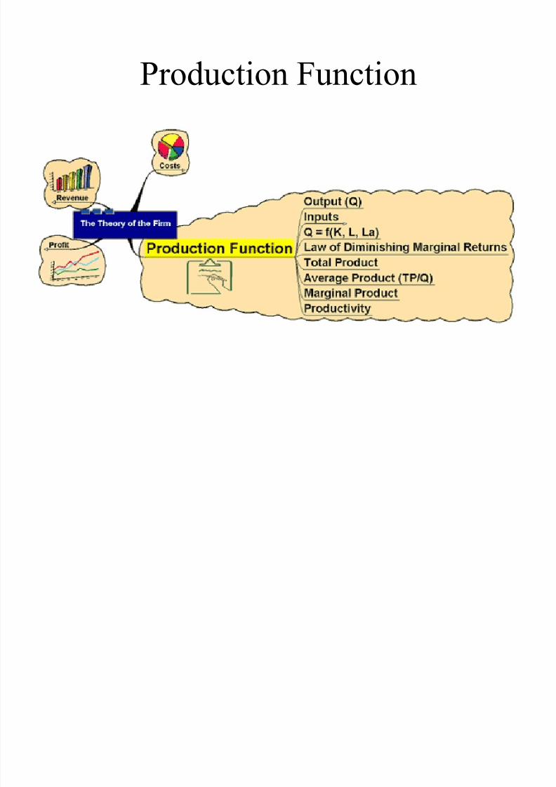
Production Function
8/14/2019 MCA Costs of Production
http://slidepdf.com/reader/full/mca-costs-of-production 25/45
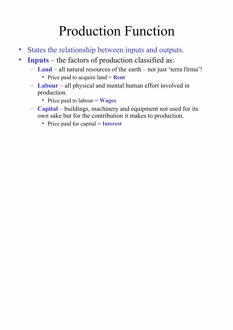
Production Function• States the relationship between inputs and outputs.
• Inputs – the factors of production classified as: – Land – all natural resources of the earth – not just ‘terra firma’!
• Price paid to acquire land = Rent
– Labour – all physical and mental human effort involved in production.
• Price paid to labour = Wages
– Capital – buildings, machinery and equipment not used for itsown sake but for the contribution it makes to production.
• Price paid for capital = Interest
8/14/2019 MCA Costs of Production
http://slidepdf.com/reader/full/mca-costs-of-production 26/45
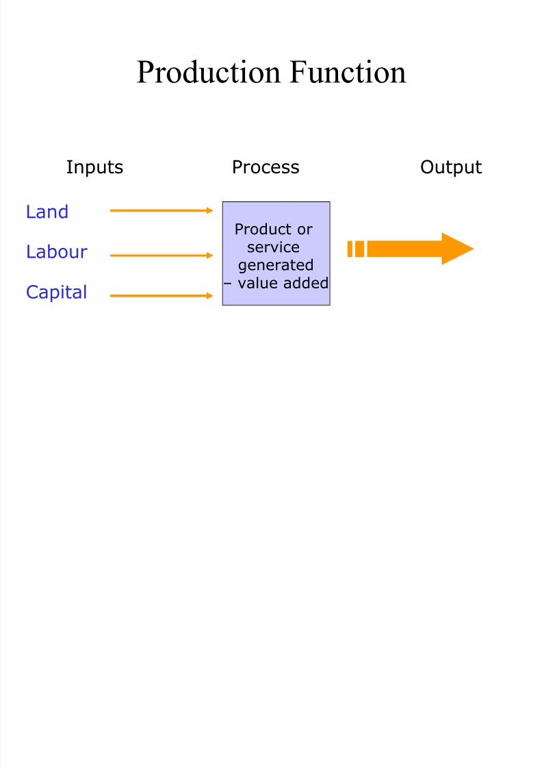
Production Function
Inputs Process Output
Land
Labour
Capital
Product orservice
generated
– value added
8/14/2019 MCA Costs of Production
http://slidepdf.com/reader/full/mca-costs-of-production 27/45
… Production Function
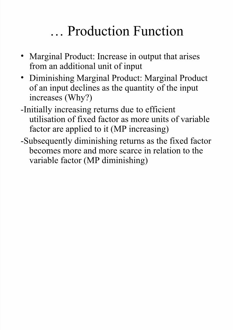
• Marginal Product: Increase in output that arisesfrom an additional unit of input
•Diminishing Marginal Product: Marginal Productof an input declines as the quantity of the inputincreases (Why?)
-Initially increasing returns due to efficient
utilisation of fixed factor as more units of variablefactor are applied to it (MP increasing)
-Subsequently diminishing returns as the fixed factor becomes more and more scarce in relation to the
variable factor (MP diminishing)
8/14/2019 MCA Costs of Production
http://slidepdf.com/reader/full/mca-costs-of-production 28/45
Analysis of Production Function:
Short Run
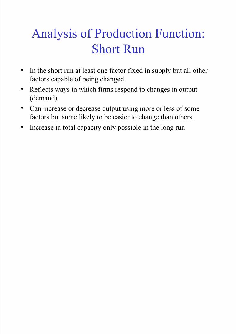
• In the short run at least one factor fixed in supply but all other
factors capable of being changed.
• Reflects ways in which firms respond to changes in output
(demand).
• Can increase or decrease output using more or less of some
factors but some likely to be easier to change than others.
• Increase in total capacity only possible in the long run
8/14/2019 MCA Costs of Production
http://slidepdf.com/reader/full/mca-costs-of-production 29/45
Production Function
• Mathematical representation of the
relationship:
• Q = f (K, L, La)
• Output (Q) is dependent upon the amount
of capital (K), Land (L) and Labour (La)
used.
8/14/2019 MCA Costs of Production
http://slidepdf.com/reader/full/mca-costs-of-production 30/45
Diminishing Returns and
Marginal Cost• The key principle behind the firm’s short-
run cost curves is the principle of
diminishing returns.PRINCIPLE of Diminishing ReturnsSuppose that output is produced with two or more
inputs and we increase one input while holding the
other inputs fixed. Beyond some point—called the
point of diminishing returns—output will increase at a
decreasing rate.

8/14/2019 MCA Costs of Production
http://slidepdf.com/reader/full/mca-costs-of-production 31/45
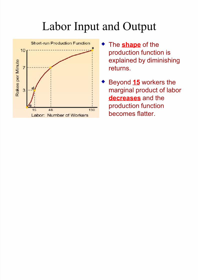
Labor Input and Output
The shape of the
production function is
explained by diminishing
returns.
Beyond 15 workers the
marginal product of labor
decreases and the
production functionbecomes flatter.
8/14/2019 MCA Costs of Production
http://slidepdf.com/reader/full/mca-costs-of-production 32/45
Costs
• Total Cost - the sum of all costs incurred in
production
• TC = FC + VC• Average Cost – the cost per unit of output
• AC = TC/Output
• Marginal Cost – the increase in total cost thatarises from producing an additional unit of output
• MC = TCn – TCn-1 units
8/14/2019 MCA Costs of Production
http://slidepdf.com/reader/full/mca-costs-of-production 33/45
8/14/2019 MCA Costs of Production
http://slidepdf.com/reader/full/mca-costs-of-production 34/45
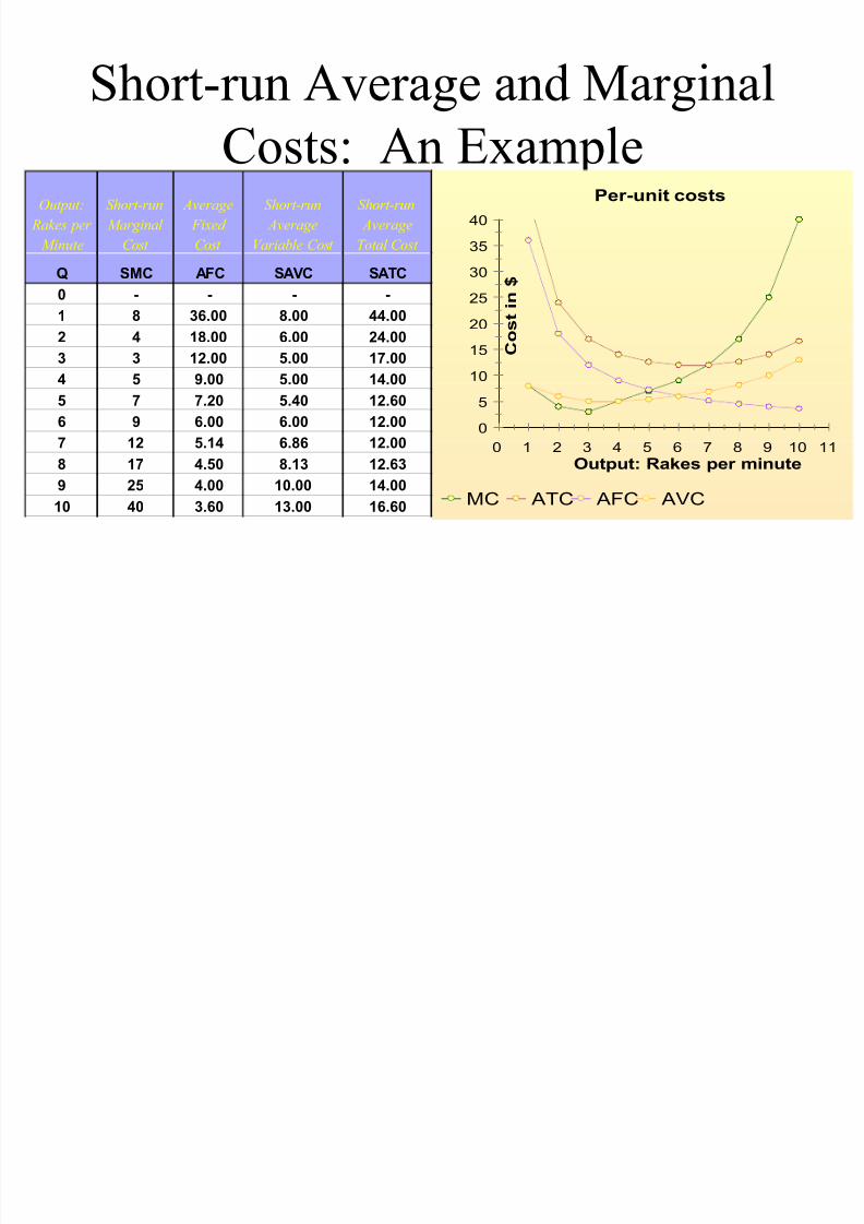
Short-run Average and Marginal
Costs: An Example
0
5
10
15
20
25
30
35
40
C o s t i
n $
0 1 2 3 4 5 6 7 8 9 10 11
Output: Rakes per minute
MC ATC AFC AVC
Per-unit costs
Total Cost
Average
Short-run
Variable Cost
Average
Short-run
Cost
Fixed
Average
Cost
Marginal
Short-run
Minute
Rakes per
Output:
SATCSAVCAFCSMCQ
----0
44.008.0036.0081
24.006.0018.0042
17.005.0012.0033
14.005.009.0054
12.605.407.2075
12.006.006.0096
12.006.865.14127
12.638.134.50178
14.0010.004.00259
16.6013.003.604010
8/14/2019 MCA Costs of Production
http://slidepdf.com/reader/full/mca-costs-of-production 35/45
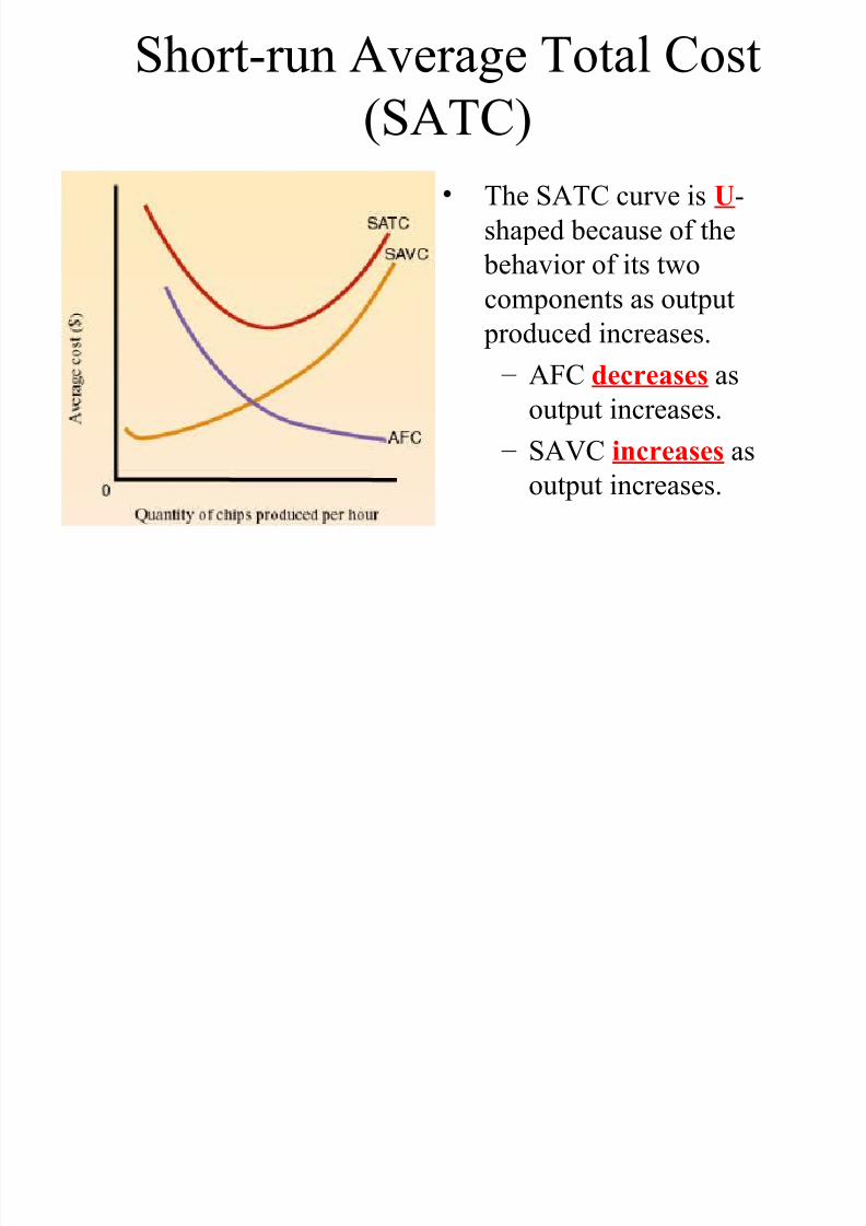
Short-run Average Total Cost
(SATC)
• The SATC curve is U-
shaped because of the
behavior of its two
components as output produced increases.
– AFC decreases as
output increases.
– SAVC increases asoutput increases.
8/14/2019 MCA Costs of Production
http://slidepdf.com/reader/full/mca-costs-of-production 36/45
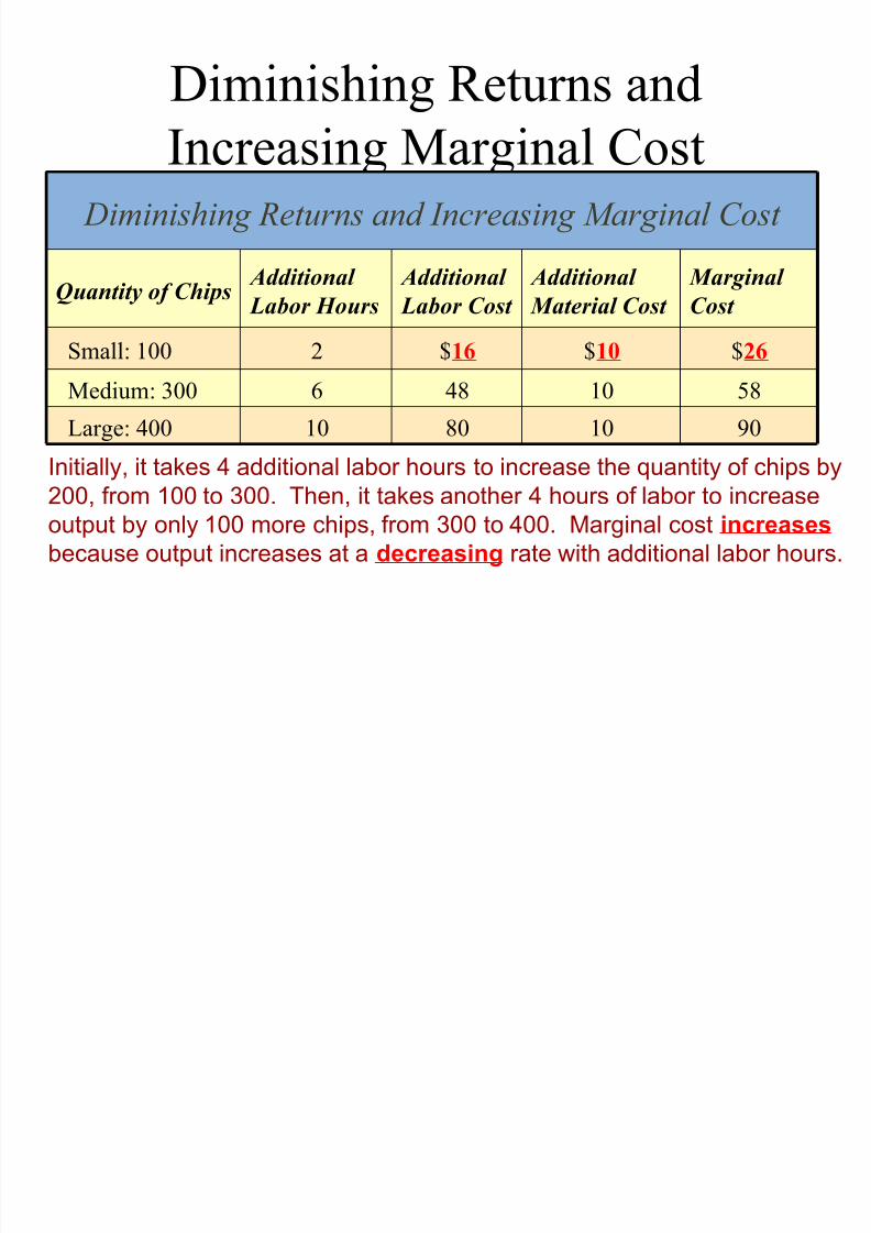
Diminishing Returns and
Increasing Marginal Cost
90108010Large: 400
5810486Medium: 300
$26$10$162Small: 100
Marginal
Cost
Additional
Material Cost
Additional
Labor Cost
Additional
Labor Hours
Quantity of Chips
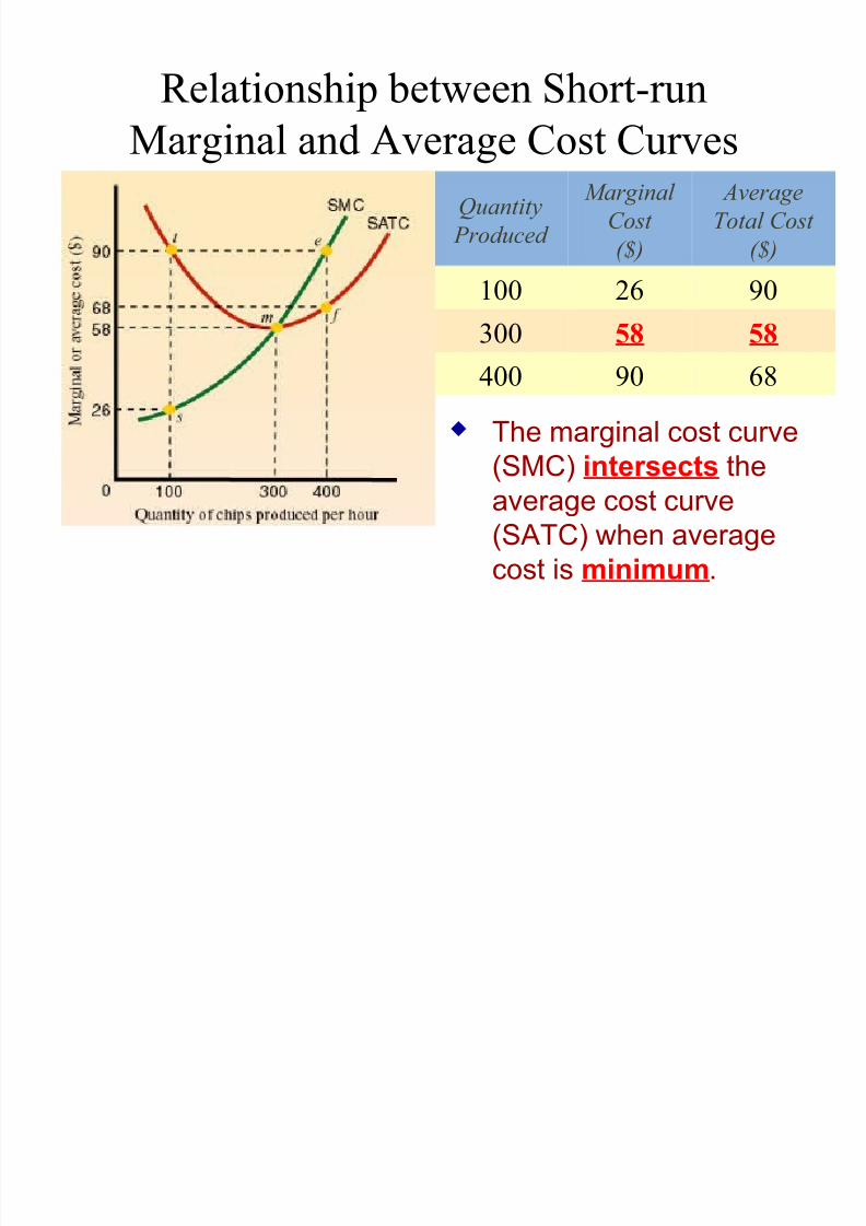
Diminishing Returns and Increasing Marginal Cost
Initially, it takes 4 additional labor hours to increase the quantity of chips by200, from 100 to 300. Then, it takes another 4 hours of labor to increase
output by only 100 more chips, from 300 to 400. Marginal cost increases
because output increases at a decreasing rate with additional labor hours.
8/14/2019 MCA Costs of Production
http://slidepdf.com/reader/full/mca-costs-of-production 37/45
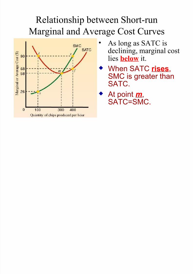
Relationship between Short-run
Marginal and Average Cost Curves• As long as SATC isdeclining, marginal costlies below it.
When SATC rises,SMC is greater thanSATC.
At point m,
SATC=SMC.
8/14/2019 MCA Costs of Production
http://slidepdf.com/reader/full/mca-costs-of-production 38/45
8/14/2019 MCA Costs of Production
http://slidepdf.com/reader/full/mca-costs-of-production 39/45
Production and Cost in the Long
Run• The key difference between the short run and thelong run is that there are no diminishing returns inthe long run.
Diminishing returns occur because workersshare a fixed facility. In the long run the firmcan expand its production facility as itsworkforce grows.
8/14/2019 MCA Costs of Production
http://slidepdf.com/reader/full/mca-costs-of-production 40/45
Long-run Average Cost
• Long-run average cost (LAC) is total cost
divided by the quantity of output when the firm
can choose a production facility of any size.
• The LAC curve describes the behavior of average
cost as the plant size expands. Initially, the curve
is negatively sloped, then beyond some point, it
becomes horizontal.
8/14/2019 MCA Costs of Production
http://slidepdf.com/reader/full/mca-costs-of-production 41/45
Long-run Average Cost
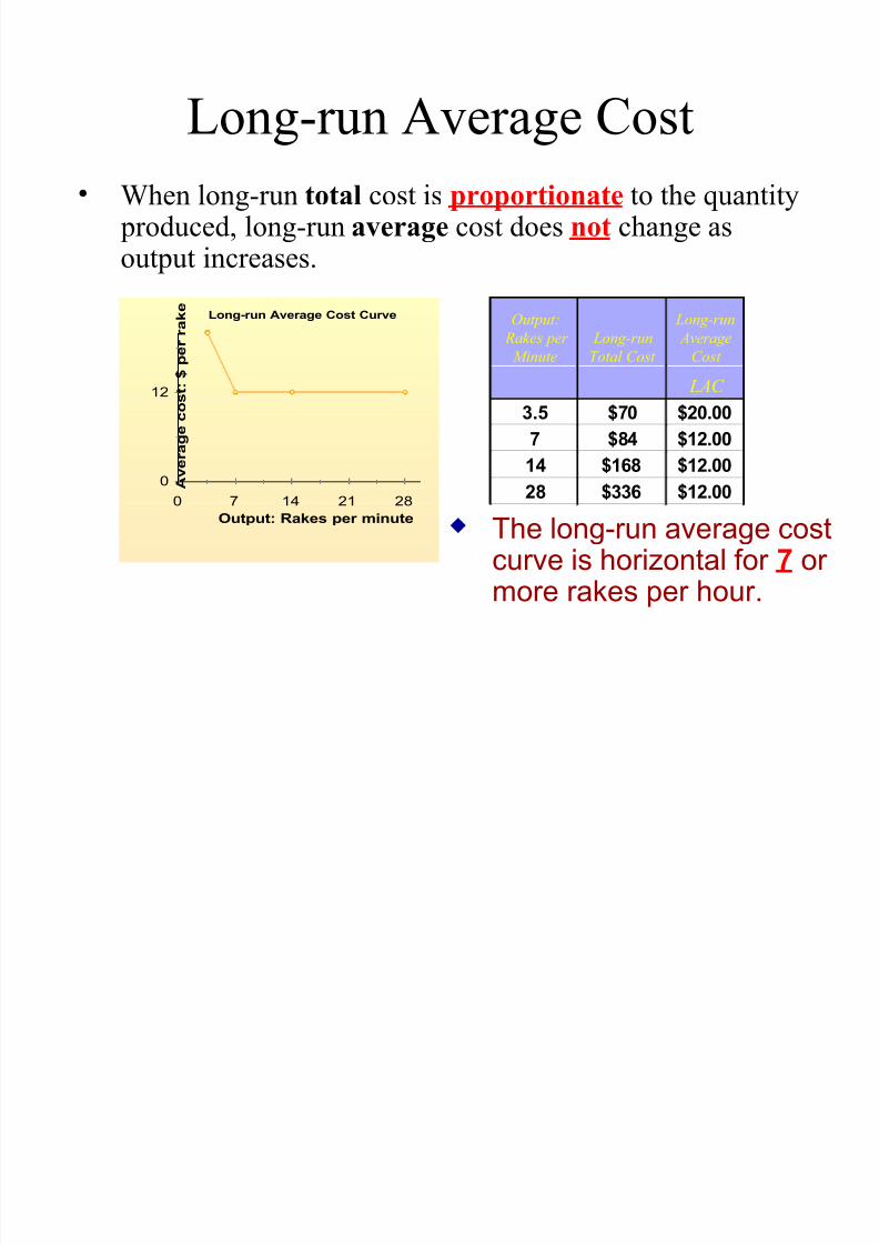
• When long-run total cost is proportionate to the quantity produced, long-run average cost does not change asoutput increases.
The long-run average costcurve is horizontal for 7 or more rakes per hour.
0
12
A v e
r a g e c o s t : $ p e r r a k e
0 7 14 21 28
Output: Rakes per minute
Long-run Average Cost Curve
Cost
Average
Long-run
Total Cost
Long-run
Minute
Rakes per
Output:
LAC
$20.00$703.5
$12.00$847
$12.00$16814$12.00$33628
8/14/2019 MCA Costs of Production
http://slidepdf.com/reader/full/mca-costs-of-production 42/45
Labor Specialization
• In a large operation, each worker specializes infewer tasks thus is more productive than his or her counterpart in a small operation.
• Higher productivity (more output per worker)means lower labor costs per unit of output, thuslower production costs (ever-decreasing averagecost).
8/14/2019 MCA Costs of Production
http://slidepdf.com/reader/full/mca-costs-of-production 43/45
Economies of Scale
• Economies of scale: a situation in which an increase in
the quantity produced decreases the long-run average
cost of production.
• Economies of scale refer to cost savings associated withspreading the cost of indivisible inputs and input
specialization.
• When economies of scale are present, the LAC curve will
be negatively sloped.
8/14/2019 MCA Costs of Production
http://slidepdf.com/reader/full/mca-costs-of-production 44/45
Minimum Efficient Scale
• The minimum efficient scale describes the
output at which economies of scale are exhausted
and the long-run average cost curve becomes
horizontal.
• Once the minimum efficient scale has been
reached, an increase in output no longer decreases
the long-run average cost.
8/14/2019 MCA Costs of Production
http://slidepdf.com/reader/full/mca-costs-of-production 45/45
Diseconomies of Scale
• A firm experiences diseconomies of scale when
an increase in output leads to an increase in long-
run average cost—the LAC curve becomes
positively sloped.
• Diseconomies of scale may arise for two reasons:
– Coordination problems
– Increasing input costs


![[3] Production and Costs](https://img.pdfslide.us/doc/110x75/55cf949c550346f57ba329fa/3-production-and-costs.jpg)