Embed Size (px)
Citation preview

1
MCA: A Multichannel Approachto SAR Autofocus
Robert L. Morrison, Jr.*, Student Member, IEEE, Minh N. Do. Member, IEEE andDavid C. Munson, Jr. Fellow, IEEE
Abstract—We present a new non-iterative approach to syn-thetic aperture radar (SAR) autofocus, termed the MultiChannelAutofocus (MCA) algorithm. The key in the approach is toexploit the multichannel redundancy of the defocusing operationto create a linear subspace, where the unknown perfectly-focusedimage resides, expressed in terms of a known basis formed fromthe given defocused image. A unique solution for the perfectly-focused image is then directly determined through a linearalgebraic formulation by invoking an additional image supportcondition. The MCA approach is found to be computationallyefficient and robust, and does not require prior assumptionsabout the SAR scene used in existing methods. In addition,the vector-space formulation of MCA allows sharpness metricoptimization to be easily incorporated within the restorationframework as a regularization term. We present experimentalresults characterizing the performance of MCA in comparisonwith conventional autofocus methods, and discuss the practicalimplementation of the technique.
Index Terms—SAR autofocus, blind deconvolution, circulardeconvolution, multichannel, image restoration, sharpness opti-mization, signal subspace methods.
I. INTRODUCTION
IN synthetic aperture radar (SAR) imaging, demodulationtiming errors at the radar receiver, due to signal delays
resulting from error in the estimated trajectory of the radarplatform (i.e., line-of-sight motion perturbations within theslant plane) or from error inserted by signal propagationthrough the ionosphere, produce unknown phase errors in theFourier imaging data. As a consequence of the phase errors,the resulting SAR images can be improperly focused. TheSAR Autofocus problem is concerned with the restoration ofthe perfectly-focused image given the phase-corrupted Fourierdata and assumptions about the underlying SAR scene.In typical SAR data acquisitions, the phase error can be
modeled as varying only along one dimension in the Fourierdomain. The following mathematical model relates the phase-corrupted Fourier imaging data G to the perfect dataG through
This work was supported by the National Science Foundation under GrantCCR 0430877.R. L. Morrison was with the Department of Electrical and Computer
Engineering and the Coordinated Science Laboratory, University of Illinoisat Urbana-Champaign, IL 61801 USA. He is now with the MassachusettsInstitute of Technology Lincoln Laboratory, Lexington, MA 02420 USA (e-mail: [email protected]).M. N. Do is with the Department of Electrical and Computer Engineering,
the Coordinated Science Laboratory, and the Beckman Institute, University ofIllinois at Urbana-Champaign, IL 61801 USA (e-mail: [email protected]).D. C. Munson, Jr. is with the Department of Electrical Engineering and
Computer Science, University of Michigan, Ann Arbor, MI 48109-2122 USA(e-mail: [email protected]).
the one-dimensional phase error function !e as [1]
G[k, n] = G[k, n]ej!e[k], (1)
where the row index k = 0, 1, . . . , M ! 1 corresponds tothe cross-range frequency index and the column index n =0, 1, . . . , N ! 1 corresponds to the range (spatial-domain)coordinate. The SAR image g is formed by applying an inverse1-D DFT to each column of G: g[m, n] = DFT−1
k G[k, n].Because the phase error !e is a 1-D function of k, eachcolumn of g has been defocused by the same blurring kernelb[m] = DFT−1
k ej!e[k] as
g[m, n] = g[m, n] !M b[m], (2)
where !M denotes M -point circular convolution, and g is theperfectly-focused image.The SAR autofocus problem has received much attention
(note references [2]–[11]). Most of the existing approachesto autofocus create an estimate of the phase error function!e, and apply this estimate to the corrupt data to producea focused restoration. To accurately estimate the phase error,appropriate prior assumptions about the underlying SAR sceneare invoked. For example, the widely-used Phase GradientAutofocus (PGA) technique is based on the model of a singletarget at each range coordinate embedded in white complexGaussian clutter [1, p.257], [3] (although, in practice PGA isused for a broader class of imagery). Other autofocus tech-niques utilize image sharpness metrics, where an optimizationroutine is employed to determine the phase error estimatethat minimizes (or maximizes) a particular metric evaluatedon the image intensity [4]–[6]. Commonly utilized metricsinclude entropy and various powers of the image intensity,which tend to favor sparse images such as collections of pointscatterers. While the restoration results obtained using theseapproaches often are outstanding, the techniques sometimesfail to produce correct restorations [5], [12]. The restorationstend to be inaccurate when the underlying scene is poorlydescribed by the assumed image model.From the defocusing relationship in (2), we see that there is
a multichannel nature to the SAR autofocus problem. Figure1 presents this analogy: the columns g [n] of the perfectly-focused image g can be viewed as a bank of parallel fil-ters that are excited by a common input signal, which isthe blurring kernel b. Thus, there is a similarity to blindmultichannel deconvolution (BMD) problems in that both thechannel responses (i.e., perfectly-focused image columns) andinput (i.e., blurring kernel) are unknown, and it is desiredto reconstruct the channel responses given only the output

2
b
g[1]
g[2]
g[N ]
g[1]
g[2]
g[N ]
Fig. 1. Diagram illustrating the multichannel nature of the autofocus problem.Here, b is the blurring kernel, g[n] are the perfectly-focused image columns,and g[n] are the defocused columns.
signals (i.e., defocused image columns) [13]. However, thereare two main differences between the SAR autofocus problemconsidered here and the setup assumed in the BMD literature.First, the filtering operation in the SAR autofocus problemis described by circular convolution, as opposed to standarddiscrete-time convolution. Second, the channel responses g [n],n = 0, 1, . . . , N ! 1, in the autofocus problem are not short-support FIR filters, but instead have support over the entiresignal length. Subspace-based techniques for directly solvingfor the channel responses have been proposed for the generalBMD problem; here, under mild conditions on the channelresponses and input, the unknown channel responses aredetermined exactly (up to a scaling constant) as the solution ofa system of linear equations [14], [15]. It is of interest to applya similar linear algebraic formulation to the SAR autofocusproblem, so that the implicit multichannel relationship can becaptured explicitly.In [16], we presented initial results in applying existing
subspace-based BMD techniques to the SAR autofocus prob-lem. However, a more efficient and robust approach is toconsider the dual problem of directly solving for a commonfocusing operator f (i.e., the inverse of the blurring kernel b),as opposed to solving for all of the channel responses g [n],n = 0, 1, . . . , N ! 1 [17]. To accomplish this, we explicitlycharacterize the multichannel condition of the SAR autofocusproblem by constructing a low-dimensional subspace wherethe perfectly-focused image resides. The subspace characteri-zation provides a linear framework through which the focusingoperator can be directly determined. To determine a uniquesolution, we assume that a small portion of the perfectly-focused image is zero-valued, or corresponds to a region oflow return. This constrains the problem sufficiently so that thefocusing operator can be obtained as the solution of a knownlinear system of equations; thus, the solution is determinedin a non-iterative fashion. We refer to this linear algebraicapproach as the MultiChannel Autofocus (MCA) algorithm.In practice, the constraint on the underlying image may beenforced approximately by acquiring Fourier-domain data thatare sufficiently oversampled in the cross-range dimension, sothat the coverage of the image extends beyond the brightlyilluminated portion of the scene determined by the antenna
pattern [1].Existing SAR autofocus methods implicitly have relied upon
the multichannel condition to properly restore images [18].In the MCA approach, we have systematically exploited themultichannel condition using an elegant subspace framework.While the success of existing autofocus approaches requiresaccurate prior assumptions about the underlying scene, suchas the suitability of sharpness metrics or knowledge of pointscatterers, MCA does not require prior assumptions aboutthe scene characteristics. The MCA approach is found to becomputationally efficient, and robust in the presence of noiseand deviations from the image support assumption. In addition,the performance of the proposed technique does not dependon the nature of the phase error; in previous SAR autofocustechniques that do not explicitly exploit the linear structure ofthe problem, the performance sometimes suffers considerablywhen the phase errors are large and rapidly-varying. MCAis simply expressed in a vector-space framework, allowingsharpness metric optimization to be easily incorporated as aregularization term, and enabling SAR autofocus to be castinto a more unified paradigm with other image restorationproblems.The organization of the paper is as follows. Section 2
presents the SAR autofocus problem statement, and establishesthe notation used in this paper. In Section 3, a linear algebraicframework is derived for the problem, and the MCA imagerestoration procedure is formulated. An analysis of the MCAtechnique, and its computationally efficient implementation,are presented in Section 4. Section 5 addresses incorporationof sharpness metric optimization within the MCA restorationframework as a regularization procedure. In Section 6, theapplication of MCA in practical scenarios is discussed. Section7 presents simulation results using synthetic and actual SARimages. The performance of the proposed technique is com-pared with that of conventional autofocus algorithms; MCA isfound to offer restoration quality on par with, or often superiorto, the best existing autofocus approaches.
II. PROBLEM SETUP
A. Notation
We introduce vector notation for discrete signals. Thecolumn vector b " CM is composed of the values of b[m],m = 0, 1, . . . , M ! 1. Column n of g[m, n], representinga particular range coordinate of a SAR image, is denotedby the vector g [n] " CM . We define vecg " CMN tobe the vector composed of the concatenated columns g [n],n = 0, 1, . . . , N ! 1. The notation AΩ refers to the matrixformed from a subset of the rows of A, where ! is a setof row indices. Lastly, Cb " CM×M is a circulant matrixformed with the vector b:
Cb =
!
"""#
b[0] b[M ! 1] . . . b[1]b[1] b[0] . . . b[2]...
.... . .
...b[M ! 1] b[M ! 2] . . . b[0]
$
%%%&. (3)

3
B. Problem Description and Characterization of the SolutionSpaceThe aim of SAR autofocus is to restore the perfectly-focused
image g given the defocused image g and assumptions aboutthe characteristics of the underlying scene. Using (1) and (2),the defocusing relationship in the spatial-domain is expressedas
g = F HD(ej!e)F' () * g (4)
Cb
where F " CM×M is the 1-D DFT unitary matrix withentries Fk,m = 1√
Me−j2"km/M , F H is the Hermitian of
F and represents the inverse DFT, D(ej!e ) " CM×M isa diagonal matrix with the entries ej!e[k] on the diagonal,and Cb " CM×M is a circulant matrix formed with theblurring kernel b, where b[m] = DFT −1
k ej!e[k]. Thus, thedefocusing effect can be described as the multiplication of theperfectly-focused image by a circulant matrix with eigenvaluesequal to the unknown phase errors. Likewise, we define thesolution space to be the set of all images formed from g withdifferent φ
g(φ) =F HD(e−j!)F' () * g (5)
CfA
where fA is an all-pass correction filter. Note that g(φe) = g.Autofocus algorithms typically solve for the phase error
estimate φ directly, and apply this to the corrupt imaging dataG to restore the image:
g[m, n] = DFT−1k G[k, n]e−j![k]. (6)
Most SAR autofocus methods are iterative, evaluating somemeasure of quality in the spatial domain and then perturbingthe estimate of the Fourier phase error function in a mannerthat increases the image focus. In this paper, we present anon-iterative approach where a focusing operator f is directlydetermined to restore the image; given f , it is straightforwardto obtain φ = φe. Underlying the approach is a linearsubspace characterization for the problem, which allows thefocusing operator to be computed using a linear algebraicformulation. This is addressed in the next section.
III. MCA RESTORATION FRAMEWORKA. Explicit Multichannel ConditionOur goal is to create a subspace for the perfectly-focused
image g, spanned by a basis constructed from the givendefocused image g. To accomplish this, we generalize therelationship in (5) to include all correction filters f " CM ,that is, not just the subset of allpass correction filters f A.As a result, for a given defocused image g, we obtain anM -dimensional subspace where the perfectly-focused imageg lives
g(f ) = Cfg, (7)
where g(f ) denotes the restoration formed by applying f . Thissubspace characterization explicitly captures the multichannel
condition of SAR autofocus: the assumption that each columnof the image is defocused by the same blurring kernel.To produce a basis expansion for the subspace in terms of g,
we select the standard basis ekM−1k=0 for CM , i.e., ek[m] = 1
if m = k and 0 otherwise, and express the correction filter as
f =M−1+
k=0
fkek. (8)
Note that at this point we do not enforce the allpass condition;the advantage of generalizing to all f " CM is to createa linear framework. Using the linearity property of circularconvolution, we have
Cf =M−1+
k=0
fkCek.
From this, any image g in the subspace can be expressed interms of a basis expansion as
g(f ) =M−1+
k=0
fkϕ[k](g), (9)
whereϕ[k](g) = Cekg (10)
are known basis functions (since g is given) for the M -dimensional subspace containing the unknown perfectly-focused image g. In matrix form, we can write (9) as
vecg(f ) = !(g)f (11)
where
!(g) def= [vecϕ[0](g), vecϕ[1](g), . . . , vecϕ[M−1](g)](12)
is referred to as the basis matrix. Note that for there to be aunique solution for f , !(g) must have rank M . We exploreconditions on the rank of the defocused image g in more detailin Section 4.
B. MCA Direct Solution ApproachTo formulate the MCA approach, we express the unknown
perfectly-focused image in terms of the basis expansion in (9):
vecg = !(g)f #, (13)
where f# is the true correction filter satisfying g(f #) = g.Here, the matrix !(g) is known, but g and f # are unknown.By imposing an image support constraint on the perfectly-focused image g, the linear system in (13) can be constrainedsufficiently so that the unknown correction filter f # can bedirectly solved for. Specifically, we assume that g is approx-imately zero-valued over a particular set of low-return pixels!:
g[m, n] =
,"[m, n] for m, n " !g′[m, n] for m, n #" !,
(14)
where "[m, n] are low-return pixels (|"[m, n]| $ 0) andg′[m, n] are unknown non-zero pixels. We define ! to bethe set of non-zero pixels (i.e., the complement of !), andwe say that these pixels correspond to the region of support

4
(ROS). In practice, the desired image support condition canbe achieved by exploiting the spatially-limited illuminationof the antenna beam, or by using prior knowledge of low-return regions in the SAR image. We will elaborate more onthe practical application of the image support assumption inSection 6.Enforcing spatially-limited constraint (14) directly into mul-
tichannel framework, (13) becomes:-
ξvecg!
.=
-!(g)Ω
!(g)Ω
.f# (15)
where ξ = vecgΩ is a vector of the low-return con-straints, !(g)Ω are the rows of !(g) that correspond tothe low-return constraints, and !(g)Ω are the rows of !(g)that correspond to the unknown pixel values of g within theROS. Given that ξ has dimension M !1 or greater (i.e., thereare at least M!1 zero constraints), when ξ = 0 the correctionfilter f# can be uniquely determined up to a scaling constantby solving for f in
!(g)Ωf = 0. (16)
We denote this direct linear solution method for determiningthe correction filter as the MultiChannel Autofocus (MCA)approach, and define
!Ω(g) def= !(g)Ω
to be the MCA matrix formed using the constraint set !.Given the assumption ξ = 0, the MCA approach requires
that !Ω(g) is a rank M ! 1 matrix (note that !Ω(g) is amatrix formed from a subset of the rows of the basis matrix!(g), and thus will have rank less than or equal to M ). InSection 4, we state the necessary conditions for which this rankcondition is satisfied. The solution f to (16) can be obtainedby determining the unique vector spanning the nullspace of!Ω(g) as
f = Null(!Ω(g)) = #f#, (17)
where # is an arbitrary complex constant. To eliminate themagnitude scaling #, we use the Fourier phase of f to correctthe defocused image according to (6):
![k] = !"/
DFTmf [m]0
. (18)
In other words, we enforce the allpass condition of f todetermine a unique solution from (17).
C. Restoration Using the SVDWhen |"[m, n]| #= 0 in (14), or when the defocused
image is contaminated by additive noise, the MCA matrix hasfull column rank. In this case, we cannot obtain f as thenull vector of !Ω(g). However, by performing the singularvalue decomposition (SVD) of !Ω(g), a unique vector thatproduces the minimum gain solution (in the $2-sense) can bedetermined. We express the SVD as
!Ω(g) = U"VH
, (19)
where " = diag(%1,%2, . . . ,%M ) is a diagonal matrix of thesingular values satisfying %1 % %2 % . . . % %M % 0. Since
f is an allpass filter we have &f&2 = 1. Although we can nolonger assume the pixels in the low-return region to be exactlyzero, it is reasonable to require the low-return region to haveminimum energy subject to &f&2 = 1. A solution f satisfying
f = arg min‖f‖2=1
&!Ω(g)f&2 (20)
is given by f = V[M ], which is the right singular vector
corresponding to the smallest singular value of !Ω(g) [19].
IV. PERFORMANCE ANALYSIS
A. General Properties of !Ω(g)
A key observation underlying the success of the MCAapproach is that the circulant blurring matrix Cb is unitary.This result is arrived at using (4), where all the eigenvalues ofCb are observed to have unit magnitude, and the fact thatthe DFT matrix F is unitary, as follows
CbCHb = F HD(ej!e)FF HD(e−j!e)F = I. (21)
We observe that the basis matrix !(g) has a special structureby rewriting (7) for a single column as
g[n](f ) = f !M g[n] = Cg[n]f . (22)
Comparing with (11), where the left side of the equation isformed by stacking the column vectors g [n](f), and using(22), we have
!(g) =
!
"""#
Cg[0]Cg[1]
...Cg[N−1]
$
%%%&. (23)
Analogous to (12), we define !(g) to be the basis matrixformed by the perfectly-focused image g, i.e., !(g) is formedby using g instead of g in (12). Likewise, !Ω(g) = !(g)Ω
is the MCA matrix formed from the perfectly-focused image.From the unitary property of Cb, we establish the followingresult.Proposition 1 (Equivalence of singular values): Suppose
that g = Cbg. Then, !Ω(g) = !Ω(g)Cb and thesingular values of !Ω(g) and !Ω(g) are identical.Proof: From the assumption, g [n] = b !M g[n]. Therefore,Cg[n] = Cg[n]Cb, and from (23)
!(g) =
!
"""#
Cg[0]CbCg[1]Cb
...Cg[N−1]Cb
$
%%%&= !(g)Cb. (24)
Note that (24) implies that !(g)Ω = !(g)ΩCb. As aresult,
!Ω(g)!HΩ (g) = !Ω(g)CbCHb!H
Ω (g) = !Ω(g)!HΩ (g),
and thus !Ω(g) and !Ω(g) have the same singular values. #Thus, from Proposition 1, we can write the SVD of the
MCA matrices for g and g as !Ω(g) = U"V H and

5
!Ω(g) = U"VH, respectively. The following result demon-
strates that the MCA restoration obtained through !Ω(g) andg is the same as the restoration obtained using !Ω(g) and g.Proposition 2 (Equivalance of restorations): Suppose that
!Ω(g) (or equivalently!Ω(g)) has a distinct smallest singularvalue. Then applying the MCA correction filters V [M ] andV
[M ]to g and g, respectively, produce the same restoration
in absolute values; i.e.,1111CV [M ]g
1111 =1111CV [M ]g
1111. (25)
Proof: Expressing!Ω(g) = !Ω(g)Cb in terms of the SVDof !Ω(g) and !Ω(g), we have
!Ω(g) = U"VH
= U"V HCb. (26)
Because of the assumption in the proposition, the right singularvector corresponding to the smallest singular value of !Ω(g)is uniquely determined to within a constant scalar factor & ofabsolute value one [19]
V[M ]H
= &V [M ]HCb, (27)
where |&| = 1. Taking the transpose of both sides of (27)produces V
[M ]= &∗CHbV [M ]. Using the unitary property
of Cb
V [M ] = &∗−1CbV [M ]. (28)
We then have
CV [M ]g = &∗−1CbCV[M ]
g
= &∗−1CV [M ]Cbg
= &∗−1CV[M ]
g,
and thus CV [M ]g and CV [M ]g have the same absolutevalue since |&∗−1| = 1. #Proposition 2 is useful for two reasons. First, it demonstrates
that applying MCA to the perfectly-focused image or anydefocused image described by (4) produces the same restoredimage magnitude, and also produces the same restored phaseto within the phase offset "&∗−1 (which is constant over theentire image). In other words, the restoration formed using theMCA approach does not depend on the phase error function;the MCA restoration depends only on g and the selection oflow-return constraints ! (i.e., the pixels in g we are assumingto be low-return). This finding is significant because existingautofocus techniques tend to perform less well when the phaseerrors are large and rapidly-varying [1], [12]. We note thatwhile the MCA restoration is the same under any phase errorfunction, this result does not imply anything about the qualityof the restoration. Second, Proposition 2 shows that it issufficient to examine the perfectly-focused image to determinethe conditions under which unique restorations are possibleusing MCA.
M L
N
g!
Low-Return Rows
Low-Return Rows
Fig. 2. Illustration of the spatially-limited image support assumption in thespecial case where there are low-return rows in the perfectly-focused image.
B. Special Case: Low-Return Rows
A case of particular interest is where ! corresponds to aset of low-return rows. The consideration of row constraintsmatches a practical case of interest where the attenuationdue to the antenna pattern is used to satisfy the low-returnpixel assumption (this is addressed in Section 6). In this case,!Ω(g) has special structure that can be exploited for efficientcomputation. This form also allows the necessary conditionsfor a unique correction filter to be precisely determined.Figure 2 shows an illustration of the special case, where
there are L rows within the ROS, and the top and bottomrows are low-return. We define the set L = l1, l2, . . . , lR tobe the set of low-return row indices, where R = M !L is thenumber of low-return rows and 0 ' lj ' M ! 1, such that
g[m, n] =
,"[m, n] for m " Lg′[m, n] for m #" L.
(29)
To explicitly construct the MCA matrix in this case, we firstuse (7) to express
gT = gT CT f#, (30)
where T denotes transpose. We consider the transposed imagesbecause this allows us to represent the low-return rows in gas column vectors, which leads to an expression of the form(16) where !Ω(g) is explicitly defined. Note that
CT f = [fF , Ce1fF , . . . , CeM−1fF ], (31)
where Cel is the l-component circulant shift matrix, and
fF [m] = f [(!m)M ], (32)
m = 0, 1, . . . , M!1, is a flipped version of the true correctionfilter ((n)M denotes n modulo M ). Using (30) and (31), weexpress the l-th row of g as
(gT )[l] = gT Celf#F . (33)

6
Note that multiplication with the matrix Cel in the expres-sion above results in an l-component left circulant shift alongeach row of gT .The relationship in (33) is informative because it shows how
the MCA matrix !Ω(g) can be constructed given the imagesupport constraint in (29). For the low-return rows satisfying(gT )[lj ] $ 0, we have the relation
(gT )[lj ] = gT Celjf#F $ 0 (34)
for j = 1, 2, . . . , R. Enforcing (34) for all of the low-returnrows simultaneously produces
0 $
!
"""#
gT Cel1gT Cel2
...gT CelR
$
%%%&
' () *
f#F , (35)
!L(g)
where (with abuse of notation) !L(g) " CNR×M is the MCAmatrix for the row constraint set L. In this special case, !Lplays the same role as !Ω for the general case. Thus, wesee that in this case the MCA matrix is formed by stackingshifted versions of the transposed defocused image, wherethe shifts correspond to the locations of the low-return rowsin the perfectly-focused image. Determining the null vector(or minimum right singular vector) of !L(g) as defined in(35) produces a flipped version of the correction filter; thecorrection filter f can be obtained by appropriately shifting theelements of fF according to (32). The reason for consideringthe flipped form in (35) is that it provides a special structurefor efficiently computing f , as we will demonstrate in the nextsubsection.To determine necessary conditions for a unique and correct
solution of the MCA equation (16), we restrict our analysisto the model in (29) where the low-return rows are identicallyzero: "[m, n] = 0. From Propositions 1 and 2, the conditionsfor a unique solution to (16) can be determined using!L(g) inplace of !L(g). This in turn is equivalent to requiring !L(g)to be a rank M ! 1 matrix.Proposition 3 (Necessary condition for unique and
correct solution)Consider the image model g[m, n] = 0 for m " L andg[m, n] = g′[m, n] for m #" L. Then a necessary condition forMCA to produce a unique and correct solution to the autofocusproblem is
rank(g!) % M ! 1R
. (36)
Proof: First notice that
rank(gT Celj) = rank(g) = rank(Cbg)= rank(g) = rank(g!),
because Celj and Cb are unitary matrices, and the zero-row assumption of the image g. Then from (35) we have
rank(!L(g)) ' R rank(g!).
Therefore, a necessary condition for rank(!L(g)) = M ! 1is rank(g!) % (M ! 1)/R. Furthermore, notice that the filter
f Iddef= [1, 0, . . . , 0]T is always a solution to (16) for g as
defined in the proposition statement: !L(g)f Id = 0. This isbecause applying f Id to g returns the same image g, whereall the pixels in the low-return region are zero by assumption.Thus, the unique solution for (16) is also the correct solutionto the autofocus problem. #Noting that M = R + L, and using condition (36), we
derive the minimum number of zero-return rows R requiredto achieve a unique solution as a function of the rank of g !:
R % L ! 1rank(g!) ! 1
. (37)
The condition rank(g !) = min(L, N) usually holds, with theexception of degenerate cases where the rows or columns ofg! are linearly dependent. Since rank(g !) ' min(L, N), (37)implies
R % L ! 1min(L, N) ! 1
. (38)
The condition in (38) provides a rule for determining the min-imum R (the minimum number of low-return rows required)as a function of the dimensions of the ROS in the general casewhere "[n, m] #= 0.
C. Efficient Restoration ProcedureForming the MCA matrix according to (35) and performing
its full SVD can be computationally expensive in terms of bothmemory and CPU time when there are many low-return rows,since the dimensions of !L(g) are NR rows by M columns.As an example, for a 1000 by 1000 pixel image with 100 low-return rows, !L(g) is a 100000 * 1000 matrix; in this case,it is not practical to construct and invert such a large matrix.Due to the structure of !L(g), it is possible to efficiently
compute the minimum right singular vector solution in (20).Note that the right singular vectors of !L(g) can be deter-mined by solving for the eigenvectors of
BL(g) = !HL (g)!L(g). (39)
Without exploiting the structure of the MCA matrix, formingBL(g) " CM×M and computing its eigenvectors requiresO(NRM2) operations. Using (35), the matrix product (39)can be expressed as
BL(g) =R+
j=1
CT eljg∗gT Celj, (40)
where g∗ = (gT )H (i.e., all of the entries of g are conjugated).Let H(g) def= g∗gT . The effect of CT elj in (40) is tocircularly shift H(g) up by lj pixels along each column,while Celj circularly shifts H(g) to the left by lj pixelsalong each row. Thus, H(g) can be computed once initially,and then BL(g) can be formed by adding shifted versionsof H(g), which requires only O(NM 2) operations. Thus,the computation has been reduced by a factor of R. Inaddition, the memory requirements have also been reducedby R times (assuming M $ N ), since only H(g) " CM×M
needs to be stored, as opposed to !HL (g) " CNR×M . As a
result, the total cost of constructingBL(g) and performing itseigendecomposition is O(NM 2) (when M ' N ).

7
V. APPLICATION OF SHARPNESS METRIC OPTIMIZATIONTO MCA
A. Bringing Metrics to the MCA Framework
The vector space framework of the MCA approach al-lows sharpness metric optimization to be incorporated as aregularization procedure. The use of sharpness metrics canimprove the solution when multiple singular values of !Ω(g)are close to zero. In addition, metric optimization is beneficialin cases where the low-return assumption |"[m, n]| $ 0holds weakly, or where additive noise with large varianceis present. In these nonideal scenarios, we show how theMCA framework provides an approximate reduced-dimensionsolution subspace, where the optimization may be performedover a small set of parameters.Suppose that instead of knowing that the image pixels in
the low-return region are exactly zero, we can assume onlythat
&vecgΩ&22 ' c (41)
for some specific constant c. Then, the MCA condition be-comes
&!Ω(g)f&22 ' c&f&2
2. (42)
Note that the true correction filter f # must satisfy (42).The goal of using sharpness optimization is to determine
the best f (in the sense of producing an image with max-imum sharpness) satisfying (42). We now derive a reduced-dimension subspace for performing the optimization where(42) holds for all f in the subspace. To accomplish this,we first determine %M−K+1, which we define as the largestsingular value of !Ω(g) satisfying %2
k ' c. Then we expressf in terms of the basis formed from the right singular vectorsof !Ω(g) corresponding to the K smallest singular values,i.e.,
f =M+
k=M−K+1
vkV[k]
, (43)
where vk is a basis coefficient corresponding to the basisvector V
[k]. To demonstrate that every element of the K-
dimensional subspace in (43) satisfies (42), we define S #K =
spanV [M−K+1], V
[M−K+2], . . . , V
[M ], and note that [20]
max‖f‖2=1f∈S!
K
&!Ω(g)f&22 = max
‖f‖2=1f∈S!
K
&U"VH
f&22
= max‖v‖2=1
v1=v2=...=vM!K=0
&"v&22
= max‖v‖2=1
M+
k=M−K+1
%2k|vk|2 = %2
M−K+1
' c, (44)
where vdef= V
Hf . In the second equality, the unitary property
of V is used to obtain &f&2 = &v&2, and also f = V v, fromwhich it is observed that f " S#
K implies v1 = v2 = . . . =vM−K = 0. We note that the subspace S#
K does not contain
all f satisfying (42). However, it provides an optimal K-dimensional subspace in the following sense: for any subspaceSK where dim(SK) = K , we have [19]
max‖f‖2=1f∈SK
&!Ω(g)f&22 % max
‖f‖2=1f∈S!
K
&!Ω(g)f&22 = %2
M−K+1. (45)
Thus, S#K is the best K-dimensional subspace in the sense that
every element is feasible (i.e., satisfies (42)), and among allK-dimensional subspaces S#
K minimizes the maximum energyin the low-return region.Substituting the basis expansion (43) for f into (7) allows g
to be expressed in terms of an approximate reduced-dimensionbasis:
gd =K+
k=1
dkψ[k], (46)
whereψ[k] = CV
[M−K+k]g, (47)
dk = vM−K+k , and gd is the image parameterized by thebasis coefficients d = [d1, d2, . . . , dK ]T . To obtain the bestg that satisfies the data consistency condition, we optimize aparticular sharpness metric over the coefficients d, where thenumber of coefficients K + M .
B. Performing the Metric Optimization
We define the metric objective function C : CK , R as themapping from the basis coefficients d = [d1, d2, . . . , dK ]T toa sharpness cost
C(d) =M−1+
m=0
N−1+
n=0
S(Id[m, n]), (48)
where Id[m, n] = |gd[m, n]|2 is the intensity of each pixel,Id[m, n] = Id[m, n]/'gd
is the normalized intensity with'gd
= &gd&22, and S : R+ , R is an image sharpness
metric operating on the normalized intensity of each pixel.An example of a commonly used sharpness metric in SARis the image entropy: SH(Id[m, n]) def= !Id[m, n] ln Id[m, n][5], [6]. A gradient-based search can be used to determine alocal minimizer of C(d) [21]. The k-th element of the gradient!dC(d) is determined using
(C(d)(dk
=+
m,n
(S(Id[m, n])(Id[m, n])
/2
'gd
gd[m, n])∗[k][m, n]
! 2'2
gd
Id[m, n]+
m",n"
gd[m′, n′])∗[k][m′, n′]0
, (49)
where - denotes the complex conjugate. Note that (49) canbe applied to a variety of sharpness metrics. Considering theentropy example, the derivative of the sharpness metric is(SH(Id[m, n])/(Id[m, n] = !(1 + ln Id[m, n]).

8
xX ′
X
Antenna Footprint
Reflectivity Function
Fig. 3. The antenna pattern shown superimposed on the scene reflectivityfunction for a single range (y) coordinate. The finite beamwidth of the antennacauses the terrain to be illuminated only within a spatially-limited window;the return outside the window is near zero.
VI. SAR DATA ACQUISITION AND PROCESSING
In this section, we discuss the application of the MCAtechnique in practical scenarios. One way of satisfying theimage support assumption used in MCA is to exploit theSAR antenna pattern. In spotlight-mode SAR, the area ofterrain that can be imaged depends on the antenna footprint,i.e., the illuminated portion of the scene corresponding to theprojection of the antenna main-beam onto the ground plane[1]. There is low return from features outside of the antennafootprint. The fact the SAR image is essentially spatially-limited, due to the profile of the antenna beam pattern, suggeststhat the proposed autofocus technique can be applied inspotlight-mode SAR imaging given that the SAR data aresampled at a sufficiently high rate [1], [22], [23].The amount of area represented in a SAR image, the
image field of view (FOV), is determined by how densely theanalog Fourier transform is sampled. As the density of thesampling is increased, the FOV of the image increases. Fora spatially-limited scene, there is a critical sampling densityat which the image coverage is equal to the support of thescene (determined by the width of the antenna footprint). Ifthe Fourier transform is sampled above the critical rate, theFOV of the image extends beyond the finite support of thescene, and the result resembles a zero-padded or zero-extendedimage. Our goal is to select the Fourier domain samplingdensity such that the FOV of the SAR image extends beyondthe brightly illuminated portion of the scene. In doing so, wecause the perfectly-focused digital image to be (effectively)spatially-limited, allowing the use of the proposed autofocusapproach.Figure 3 shows an illustration of the antenna pattern along
the x-axis. A length X ′ region of the scene is brightlyilluminated in the x dimension. To use the MCA approachto autofocus, we need the image coverage X to be greaterthan the illuminated region X ′. To model the antenna pattern,we consider the case of an unweighted uniformly-radiatingantenna aperture. Under this scenario, both the transmit andreceive patterns are described by a sinc function [24]–[26].Thus, the antenna footprint determined by the combined
transmit-receive pattern is modeled as [1], [24]
w(x) = sinc2(W−1x x), (50)
whereWx =
*0R0
D, (51)
sinc(x) def= (sin+x)/(+x), x is the cross-range coordinate, *0
is the wavelength of the radar, R0 is the range from the radarplatform to the center of the scene, and D is the length ofthe antenna aperture. Near the nulls of the antenna patternat x = ±Wx, the attenuation will be very large, producinglow-return rows in the perfectly-focused SAR image consistentwith (29).Using the model in (50), the Fourier-domain sampling
density should be large enough so that the FOV of the SARimage is equal to or greater than the width of the mainlobeof the sinc window: X % 2Wx. In spotlight-mode SAR, theFourier-domain sampling density in the cross-range dimensionis determined by the pulse repetition frequency (PRF) of theradar. For a radar platform moving with constant velocity,increasing the PRF decreases the angular interval betweenpulses (i.e., the angular increment between successive lookangles), thus increasing the cross-range Fourier-domain sam-pling density and FOV [1], [23], [24]. Alternatively, keepingthe PRF constant and decreasing the platform velocity alsoincreases the cross-range Fourier-domain sampling density;such is the case in airborne SAR when the aircraft is flyinginto a headwind. In many cases, the platform velocity andPRF are such that the image FOV is approximately equal tothe mainlobe width of (50); in these cases, the final images areusually cropped to half the mainlobe width of the sinc window[1], because it is realized that the edge of the processed imagewill suffer from some amount of aliasing. Our frameworksuggests that the additional information from the disgardedportions of the image can be used for SAR image autofocus.Another instance where the image support assumption can
be exploited is when prior knowledge of low-return featuresin the SAR image is available. Examples of such featuresinclude smooth bodies of water, roads, and shadowy regions[5]. If the image defocusing is not very severe, then low-returnregions can be estimated using the defocused image. InverseSAR (ISAR) provides a further application for MCA. In ISARimages, pixels outside of the support of the imaged object (e.g.,aircraft) correspond to a region of zero return [5]. Thus, givenan estimate of the object support, MCA can be applied.
VII. EXPERIMENTAL RESULTSFigure 4 presents an experiment using an actual SAR image.
To form a ground truth perfectly-focused image, an entropy-minimization autofocus routine [6] was applied to the givenSAR image. Figure 4(a) shows the resulting image, wherethe sinc-squared window in Figure 4(b) has been appliedto each column to simulate the antenna footprint resultingfrom an unweighted antenna aperture. The cross-range FOVequals 95 percent of the mainlobe width of the squared-sinc function, i.e., the image is cropped within the nulls ofthe antenna footprint, so that there is very large (but not

9
(a)
!1000 !500 0 500 10000
0.2
0.4
0.6
0.8
1
Cross!Range Coordinate
Mag
nitu
de
(b)
(c) (d)
Fig. 4. Actual 2335 by 2027 pixel SAR image: (a) perfectly-focused image, where the simulated sinc-squared antenna footprint in (b) has been applied toeach column, (c) defocused image produced by applying a white phase error function, and (d) MCA restoration (SNRout = 10.52 dB).
infinite) attenuation at the edges of the image. Figure 4(c)shows a defocused image produced by applying a white phaseerror function (i.e., independent phase components uniformlydistributed between !+ and +) !e to the perfectly-focusedimage in Figure 4(a) according to (1); the application ofwhite phase error functions has been considered previouslyin the autofocus literature as a particularly stressing caseto test the robustness of autofocus algorithms [4], [5], [27].We applied MCA to the defocused image assuming the topand bottom rows of the perfectly-focused image to be low-return. The MCA restoration is displayed in Figure 4(d). Therestored image is observed to be in good agreement with theground truth image. To quantitatively assess the performanceof autofocus techniques, we use the restoration quality metricSNRout (i.e., output signal-to-noise ratio), which is defined as[28]:
SNRout = 20 log10&vecg&2
&(|vecg|! |vecg|)&2;
here, the “noise” in SNRout refers to the error in the magnitudeof the reconstructed image g relative to the perfectly-focused
image g, and should not be confused with additive noise(which is considered later). For the restoration in Figure 4(d),SNRout = 10.52 dB.
To evaluate the robustness of MCA with respect to thelow-return assumption, we performed a series of experimentsusing the idealized window function in Figure 5(a). Thewindow has a flat response over most of the image; thetapering at the edges of the window is described by a quarter-period of a sine function. In each experiment, the gain at theedges of the window (i.e., the inverse of the attenuation) isincreased such that the pixel magnitudes in the low-returnregion (corresponding to the top and bottom rows) becomelarger. In Figure 5(a), a window gain of 0.1 is shown. Foreach value of the window gain, a defocused image is formedand the MCA restoration is produced.
Figure 5(b) shows a plot of the restoration quality metricSNRout versus the gain at the edges of the window, wherethe top two rows and bottom two rows are assumed to below-return. The simulated SAR image in Figure 5(c) wasused as the ground truth perfectly-focused image in this set

10
0 50 100 150 200 250 3000
0.1
0.2
0.3
0.4
0.5
0.6
0.7
0.8
0.9
1
Cross!range coordinate
Gai
n
(a)
10!4 10!3 10!2 10!1!5
0
5
10
15
20
25
30
Gain in the low!return region
Out
put S
NR
(b)
(c) (d) (e)
Fig. 5. Experiments evaluating the robustness of MCA as a function of the attenuation in the low-return region: (a) window function applied to each columnof the SAR image, where the gain at the edges of the window (corresponding to the low-return region) is varied with each experiment (a gain of 0.1 isshown); (b) plot of the quality metric SNRout for the MCA restoration (measured with respect to the perfectly-focused image) versus the window gain inthe low-return region; (c) simulated perfectly-focused 309 by 226 pixel image, where the window in (a) has been applied; (d) defocused image produced byapplying a white phase error function; and (e) MCA restoration (SNRout = 9.583 dB).
of experiments; here, a processed SAR image1 is used asa model for the image magnitude, while the phase of eachpixel is selected at random (uniformly distributed between !+and + and uncorrelated) to simulate the complex reflectivityassociated with high frequency SAR images of terrain [29].The plot in Figure 5(b) demonstrates that the restorationquality decreases monotonically as a function of increasingwindow gain. We observe that for values of SNRout lessthan 3 dB, the restored images do not resemble the perfectly-focused image; this transition occurs when gain in the low-return region increases above 0.14. For gain values less thanor equal to 0.14, the restorations are faithful representations ofthe perfectly-focused image. Thus, we see that MCA is robustover a large range of attenuation values, even when thereis significant deviation from the ideal zero-magnitude pixelassumption. As an example, the MCA restoration in Figure5(e) corresponds to an experiment where the window gain is
1The processed SAR images in this paper were provided by Sandia NationalLaboratories.
0.1. Figures 5(c) and (d) show the perfectly-focused and de-focused images, respectively, associated with this restoration.The image in Figure 5(e) is almost perfectly restored, withSNRout = 9.583 dB.In Figure 6, the performance of MCA is compared with
existing autofocus approaches. Figure 6(a) shows a perfectly-focused simulated SAR image, constructed in the same manneras Figure 5, where the window function in Figure 5(b) hasbeen applied (the window gain is 1 * 10−4 in this experi-ment). A defocused image formed by applying a quadraticphase error function (i.e., the phase error function variesas a quadratic function of the cross-range frequencies) isdisplayed in Figure 6(b); such a function is used to modelphase errors due to platform motion [1]. The defocused imagehas been contaminated with additive white complex-Gaussiannoise in the range-compressed domain such that the inputsignal-to-noise ratio (input SNR) is 40 dB; here, the inputSNR is defined to be the average per-pulse SNR: SNR =20 log101/M
+
k
maxn
|G[k, n]|/%p, where %p is the noise

11
(a) (b) (c)
(d) (e) (f)
Fig. 6. Comparison of MCA with existing autofocus approaches: (a) simulated 341 by 341 pixel perfectly-focused image, where the window function inFigure 5(b) has been applied; (b) noisy defocused image produced by applying a quadratic phase error, where the input SNR is 40 dB (measured in the range-compressed domain); (c) MCA restoration (SNRout = 25.25 dB); (d) PGA restoration (SNRout = 9.64 dB); (e) entropy-based restoration (SNRout = 3.60dB); and (f) restoration using the intensity-squared sharpness metric (SNRout = 3.41 dB).
standard deviation. Figure 6(c) shows the MCA restorationformed assuming the top two and bottom two rows to below-return; the image is observed to be well-restored, withSNRout = 25.25 dB. To facilitate a meaningful comparisonwith the perfectly-focused image, the restorations are producedby applying the phase error estimate to the noiseless defocusedimage; in other words, the phase estimate is determined in thepresence of noise, but SNRout is computed with the noiseremoved. A restoration produced using PGA is displayed inFigure 6(d) (SNRout = 9.64 dB) [1]. Figures 6(e) and (f) showthe result of applying a metric-based autofocus technique [6]using the entropy sharpness metric (SNRout = 3.60 dB) andthe intensity-squared sharpness metric (SNRout = 3.41 dB),respectively. Of the four autofocus approaches, MCA is foundto produce the highest quality restoration in terms of bothqualitative comparison and the quality metric SNRout. In par-ticular, the metric-based restorations, while macroscopicallysimilar to the MCA and PGA restorations, have much lowerSNR; this is due to the metric-based techniques incorrectlyaccentuating some of the point scatterers.Figure 7 presents the results of a Monte Carlo simulation
comparing the performance of MCA with existing autofocusapproaches under varying levels of additive noise. Ten trialswere conducted at each input SNR level, where in each trial anoisy defocused image (using a deterministic quadratic phaseerror function) was formed using different randomly-generatednoise realizations with the same statistics. Four autofocusapproaches (MCA, PGA, entropy-minimization, and intensity-
squared minimization) were applied to each defocused image,and the quality metric SNRout was evaluated on the resultingrestorations. Plots of the average SNRout (over the ten trials)versus the input SNR are displayed in Figure 7 for thefour autofocus methods. The plot shows that at high inputSNR (SNR % 20 dB), MCA provides the best restorationperformance. At very low SNR, metric-based methods producethe highest SNRout; however, this performance is observed tolevel out around 3.5 dB due to the limitation of the sharpnesscriterion (several point scatterers are artificially accentuated).PGA provides the best performance in the intermediate rangeof low SNR starting around 13 dB. Likewise, we observe thatthe MCA restorations start to resemble the perfectly-focusedimage at 13 dB. PGA also approaches a constant SNRout valueat high input SNR; the limitation in PGA is the inability toextract completely isolated point scatterers free of surroundingclutter.On average, the MCA restorations in the experiment of
Figure 7 required 3.85 s of computation time, where the algo-rithm was implemented using MATLAB on an Intel Pentium 4CPU (2.66 GHz). In comparison, PGA, the intensity-squaredapproach, and the entropy approach had average run-times of5.34 s, 18.1 s, and 87.6 s, respectively. Thus, MCA is observedto be computationally efficient in comparison with existingSAR autofocus methods.Figure 8 presents an experiment using a sinc-squared an-
tenna pattern, where a significant amount of additive noise hasbeen applied to the defocused image. The perfectly-focused
12
(a) (b)
(c) (d)
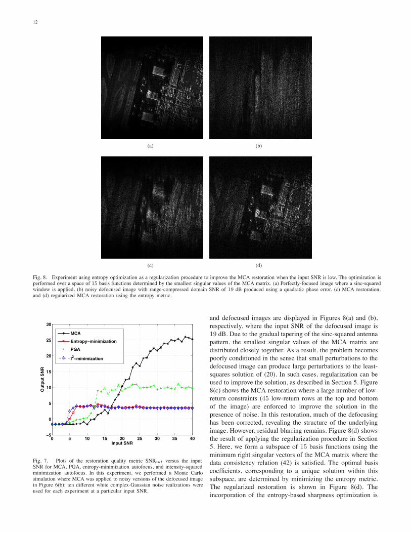
Fig. 8. Experiment using entropy optimization as a regularization procedure to improve the MCA restoration when the input SNR is low. The optimization isperformed over a space of 15 basis functions determined by the smallest singular values of the MCA matrix. (a) Perfectly-focused image where a sinc-squaredwindow is applied, (b) noisy defocused image with range-compressed domain SNR of 19 dB produced using a quadratic phase error, (c) MCA restoration,and (d) regularized MCA restoration using the entropy metric.
0 5 10 15 20 25 30 35 40!5
0
5
10
15
20
25
30
Input SNR
Out
put S
NR
MCAEntropy!minimizationPGA
I2!minimization
Fig. 7. Plots of the restoration quality metric SNRout versus the inputSNR for MCA, PGA, entropy-minimization autofocus, and intensity-squaredminimization autofocus. In this experiment, we performed a Monte Carlosimulation where MCA was applied to noisy versions of the defocused imagein Figure 6(b); ten different white complex-Gaussian noise realizations wereused for each experiment at a particular input SNR.
and defocused images are displayed in Figures 8(a) and (b),respectively, where the input SNR of the defocused image is19 dB. Due to the gradual tapering of the sinc-squared antennapattern, the smallest singular values of the MCA matrix aredistributed closely together. As a result, the problem becomespoorly conditioned in the sense that small perturbations to thedefocused image can produce large perturbations to the least-squares solution of (20). In such cases, regularization can beused to improve the solution, as described in Section 5. Figure8(c) shows the MCA restoration where a large number of low-return constraints (45 low-return rows at the top and bottomof the image) are enforced to improve the solution in thepresence of noise. In this restoration, much of the defocusinghas been corrected, revealing the structure of the underlyingimage. However, residual blurring remains. Figure 8(d) showsthe result of applying the regularization procedure in Section5. Here, we form a subspace of 15 basis functions using theminimum right singular vectors of the MCA matrix where thedata consistency relation (42) is satisfied. The optimal basiscoefficients, corresponding to a unique solution within thissubspace, are determined by minimizing the entropy metric.The regularized restoration is shown in Figure 8(d). Theincorporation of the entropy-based sharpness optimization is

13
found to significantly improve the quality of the restoration,producing a result that agrees well with the perfectly-focusedimage. Thus, by exploiting the linear algebraic structure ofthe SAR autofocus problem and the low-return constraints inthe perfectly-focused image, the dimension of the optimizationspace in metric-based methods can be greatly reduced (from341 to 15 parameters in this example).The simulations in this paper assume that the Fourier
imaging data lie on a Cartesian grid. Further work is neededto determine how well MCA works for large data angleswhere the polar grid deviates substantially from Cartesian.Recent work suggests that the proposed MCA scheme shouldbe modified for larger data angles [30].
VIII. CONCLUSION
In this paper, we have proposed a new subspace-basedapproach to the synthetic aperture radar (SAR) autofocus prob-lem, termed the MultiChannel Autofocus (MCA) algorithm.In this approach, an image focusing operator is determineddirectly using a linear algebraic formulation. Assuming that asmall portion of the perfectly-focused image is zero-valued, orcorresponds to a region of low return, near-perfect restorationsof the focused image are possible without requiring prior as-sumptions about the underlying scene; the success of existingautofocus approaches tends to rely on the accuracy of suchprior assumptions, such as the suitability of image sharpnessmetrics or the presence of isolated point scatterers. In practice,the desired image support condition can be achieved by ex-ploiting the spatially-limited nature of the illuminating antennabeam.The MCA approach is computationally efficient, and robust
in the presence of noise and deviations from the ideal imagesupport assumption. The restoration quality of the proposedmethod is independent of the severity of the phase errorfunction; existing autofocus approaches sometimes performpoorly when the phase errors are large and rapidly-varying. Inaddition, the vector-space formulation of MCA allows sharp-ness metric optimization to be incorporated into the restorationframework as a regularization term, enabling SAR autofocusto be cast into a more unified paradigm with other imagerestoration problems. Here, the parameter set over which theoptimization is performed is greatly reduced in comparison tothe number of unknown phase error components. We havepresented experimental results, using actual and simulatedSAR images, demonstrating that the proposed technique canproduce superior restorations in comparison with existingautofocus approaches.
ACKNOWLEDGMENT
The authors would like to thank Professor Yoram Breslerof the University of Illinois for discussions on how the resultsin [15] might be adapted to the SAR autofocus problem. Inaddition, the authors thank Dr. Charles Jakowatz and SandiaNational Laboratories for the actual SAR data used in thispaper.
REFERENCES[1] C. V. Jakowatz, Jr., D. E. Wahl, P. H. Eichel, D. C. Ghiglia, and
P. A. Thompson, Spotlight-Mode Synthetic Aperture Radar: A SignalProcessing Approach., Kluwer Academic Publishers, Boston, 1996.
[2] P. H. Eichel, D. C. Ghiglia, and C. V. Jakowatz, Jr., “Speckle processingmethod for synthetic-aperture-radar phase correction,” Optics Letters,vol. 14, no. 1, pp. 1101–1103, January 1989.
[3] C. V. Jakowatz, Jr. and D. E. Wahl, “Eigenvector method for maximum-likelihood estimation of phase errors in synthetic-aperture-radar im-agery,” J. Opt. Soc. Am. A, vol. 10, no. 12, pp. 2539–2546, December1993.
[4] L. Xi, L. Guosui, and J. Ni, “Autofocusing of ISAR images based onentropy minimization,” IEEE Transactions on Aerospace and ElectronicSystems, vol. 35, no. 4, pp. 1240–1252, October 1999.
[5] J.R. Fienup and J. J. Miller, “Aberration correction by maximizinggeneralized sharpness metrics,” Journal of the Optical Society ofAmerica A, vol. 20, no. 4, pp. 609–620, April 2003.
[6] T. J. Kragh, “Monotonic iterative algorithm for minimum-entropy aut-ofocus,” in Proc. Adaptive Sensor Array Processing (ASAP) Workshop,Lexington, MA, June 2006.
[7] F. Berizzi and G. Corsini, “Autofocusing of inverse synthetic aprtureradar images using contrast optimization,” IEEE Transactions onAerospace and Electronic Systems, vol. 32, no. 3, pp. 1185–1191, July1996.
[8] W. D. Brown and D. C. Ghiglia, “Some methods for reducingpropagation-induced phase errors in coherent imaging systems – I:Formalism,” J. Opt. Soc. Amer. A, vol. 5, pp. 924–942, 1988.
[9] D. C. Ghiglia and W. D. Brown, “Some methods for reducingpropagation-induced phase errors in coherent imaging systems – II:Numerical results,” J. Opt. Soc. Amer. A, vol. 5, pp. 943–957, 1988.
[10] C. E. Mancill and J. M. Swiger, “A map drift autofocus technique forcorrecting higher-order SAR phase errors,” in Twenty-Seventh AnnualTri-Service Radar Symposium, Monterey, CA, June 1981, pp. 391–400.
[11] R. G. Paxman and J. C. Marron, “Aberration correction of speckledimagery with an image sharpness criterion,” in Statistical Optics,Proceedings of the SPIE, San Diego, CA, 1988, vol. 976.
[12] R. L. Morrison, Jr. and D. C. Munson, Jr., “An experimental study ofa new entropy-based SAR autofocus technique,” in Proc. of the IEEEInternational Conference on Image Processing, Rochester, NY, 2008,vol. II, pp. 441–444.
[13] L. Tong and S. Perreau, “Multichannel blind identification: Fromsubspace to maximum likelihood methods,” Proceedings of the IEEE,vol. 86, no. 10, pp. 1951–1968, October 1998.
[14] M. Gurelli and C. Nikias, “EVAM: An eigenvector-based algorithm formultichannel blind deconvolution of input colored signals,” IEEE Trans.on Signal Processing, vol. 43, no. 1, pp. 134–149, January 1995.
[15] G. Harikumar and Y. Bresler, “Blind restoration of images blurred bymultiple filters: Theory and efficient algorithms,” IEEE Trans. on ImageProcessing, vol. 8, no. 2, pp. 202–219, 1999.
[16] R. L. Morrison, Jr. and M. N. Do, “A multichannel approach to metric-based SAR autofocus,” in Proc. of the IEEE International Conferenceon Image Processing, Genoa, Italy, 2005, vol. 2, pp. 1070–1073.
[17] R. L. Morrison, Jr. and M. N. Do, “Multichannel autofocus algorithm forsynthetic aperture radar,” in Proc. of the IEEE International Conferenceon Image Processing, Atlanta, GA, 2006.
[18] R. L. Morrison, Jr., M. N. Do, and D. C. Munson, Jr., “SAR imageautofocus by sharpness optimization: A theoretical study,” IEEE Trans-actions on Image Processing, vol. 16, no. 9, pp. 2309–2321, September2007.
[19] G. H. Golub and C. F. Van Loan, Matrix Computations, Johns HopkinsUniversity Press, Baltimore, 1996.
[20] R. A. Horn and C. R. Johnson, Matrix Analysis., Cambridge UniversityPress, New York, 2005.
[21] D. G. Luenberger, Linear and Nonlinear Programming., KluwerAcademic Publishers, Boston, 2003.
[22] J. Walker, “Range-doppler imaging of rotating objects,” IEEE Trans.Aerosp. Elctron. Syst., vol. AES-16, pp. 23–52, January 1980.
[23] D. C. Munson, Jr., J. D. O’Brien, and W. K. Jenkins, “A tomographicformulation of spotlight-mode synthetic aperture radar,” Proceedings ofthe IEEE, vol. 71, no. 8, pp. 917–925, August 1983.
[24] M. Soumekh, Synthetic Aperture Radar Signal Processing with MATLABAlgorithms, John Wiley, New York, 1999.
[25] R. E. Blahut, Theory of Remote Image Formation, Cambridge UniversityPress, Cambridge, 2004.
[26] M. I. Skolnik, Introduction to Radar Systems, McGraw-Hill, New York,2002.

14
[27] D. E. Wahl, P. H. Eichel, D. C. Ghiglia, and C. V. Jakowatz, Jr.,“Phase gradient autofocus—a robust tool for high resolution SAR phasecorrection,” IEEE Transactions on Aerospace and Electronic Systems,vol. 30, no. 3, pp. 827–835, July 1994.
[28] M. Vetterli and J. Kovacevic, Wavelets and Subband Coding, PrenticeHall, New Jersey, 1995.
[29] D. C. Munson, Jr. and J. L. C. Sanz, “Image reconstruction fromfrequency-offset Fourier data,” Proceedings of the IEEE, vol. 72, no. 6,June 1984.
[30] H. J. Cho and D. C. Munson, Jr., “Overcoming polar format issues inMultiChannel SAR Autofocus,” in Forty-Second Asilomar Conferenceon Signals, Systems, and Computers, Monterey, CA, 2008.
Robert L. Morrison, Jr. was born in Voorhees, NewJersey in 1977. He received the B.S.E. degree inelectrical engineering from the University of Iowain 2000, and the M.S. and Ph.D. degrees in elec-trical engineering from the University of Illinois atUrbana-Champaign in 2002 and 2007, respectively.Robert is currently a member of the technical staffat the Massachusetts Institute of Technology Lin-coln Laboratory. His research interests include radarimaging, medical imaging, and signal processing.
Minh N. Do was born in Thanh Hoa, Vietnam, in1974. He received the B.Eng. degree in computerengineering from the University of Canberra, Aus-tralia, in 1997, and the Dr.Sci. degree in commu-nication systems from the Swiss Federal Instituteof Technology Lausanne (EPFL), Switzerland, in2001.Since 2002, he has been an Assistant Professor
with the Department of Electrical and ComputerEngineering and a Research Assistant Professor withthe Coordinated Science Laboratory and the Beck-
man Institute, University of Illinois at Urbana-Champaign. His research in-terests include image and multi-dimensional signal processing, computationalimaging, wavelets and multiscale geometric analysis, and visual informationrepresentation.He received a Silver Medal from the 32nd International Mathematical
Olympiad in 1991, a University Medal from the University of Canberra in1997, the best doctoral thesis award from the Swiss Federal Institute ofTechnology Lausanne in 2001, and a CAREER award from the NationalScience Foundation in 2003. He was named a Beckman Fellow at the Centerfor Advanced Study, UIUC in 2006, and received of a Xerox Award forFaculty Research, College of Engineering, UIUC, in 2007. He is a memberof the IEEE Signal Processing Society Signal Processing Theory and Methodsand Image and MultiDimensional Signal Processing Technical Committees,and an Associate Editor of the IEEE Transactions on Image Processing.
David C. Munson, Jr. David C. Munson, Jr.received the B.S. degree in electrical engineering(with distinction) from the University of Delawarein 1975, and the M.S., M.A., and Ph.D. degreesin electrical engineering from Princeton Universityin 1977, 1977, and 1979, respectively. From 1979to 2003 he was with the University of Illinois atUrbana-Champaign, where he was the Robert C.MacClinchie Distinguished Professor of Electricaland Computer Engineering, Research Professor inthe Coordinated Science Laboratory, and a faculty
member in the Beckman Institute for Advanced Science and Technology.In 2003 he became Chair of the Department of Electrical Engineering andComputer Science at the University of Michigan, Ann Arbor. He currently isthe Robert J. Vlasic Dean of Engineering at the University of Michigan.Professor Munson’s teaching and research interests are in the general area
of signal and image processing. His research is focused on radar imaging,passive millimeter-wave imaging, and computer tomography. He has heldsummer industrial positions in digital communications and speech processing,and he has served as a consultant in synthetic aperture radar. He is co-founderof InstaRecon, Inc., a start-up to commercialize fast algorithms for imageformation in computer tomography. He is affiliated with the Infinity Project,where he is coauthor of a textbook on the digital world, which is used in highschools nationwide to introduce students to engineering.Professor Munson is a Fellow of the Institute of Electrical and Electronics
Engineers (IEEE), a past president of the IEEE Signal Processing Society,founding editor-in-chief of the IEEE Transactions on Image Processing, andco-founder of the IEEE International Conference on Image Processing. Inaddition to multiple teaching awards and other honors, he was presented theSociety Award of the IEEE Signal Processing Society, he served as a Distin-guished Lecturer of the IEEE Signal Processing Society, he received an IEEEThird Millennium Medal, and he was the Texas Instruments DistinguishedVisiting Professor at Rice University.