MC3: Econometric Theory and Methods - UCLuctpjea/lnotes1.pdf · University College London Department of Economics M.Sc. in Economics MC3: Econometric Theory and Methods Course notes:

University College London

Department of Economics

M.Sc. in Economics

MC3: Econometric Theory and Methods

Course notes: 1

Econometric models, random variables,probability distributions and regression

Andrew Chesher

5/10/2006Do not distribute without permission.

Course Notes 1, Andrew Chesher, 5/10/2006 1

1. Introduction

These notes contain:

1. a discussion of the nature of economic data and the concept of an econometric model,

2. a review of some important concepts in probability distribution theory that arise frequentlyin developing econometric theory and in the application of econometric methods,

3. an introduction to the concept of a regression function in the context of distributiontheory, as a preparation for the study of estimation of and inference concerning regressionfunctions.

Since 2005 the Probability and Statistics Refresher Course has been wider in scope than inearlier years and has taken place during the �rst week of term so that all M.Sc. students couldattend. That covered most of the material in item 2 above (Sections 4 - 7 of these notes), so Iwill not lecture on that this term. You should read all the sections of these notes carefully andstudy any elements that are new to you. Raise questions in class if you need to.

2. Data

Econometric work employs data recording economic phenomena and usually the environment inwhich they were obtained.Sometimes we are interested in measuring simple economic magnitudes, for example the

proportion of households in poverty in a region of a country, the degree of concentration ofeconomic power in an industry, the amount by which a company�s costs exceed the e¢ cient levelof costs for companies in its industry.Often we are interested in the way in which the environment (broadly de�ned) a¤ects in-

teresting economic magnitudes, for example the impact of indirect taxes on amounts of goodspurchased, the impact of direct taxes on labour supply, the sensitivity of travel choices to alter-native transport mode prices and characteristics.Challenging and important problems arise when we want to understand how people, house-

holds and institutions will react in the face of a policy intervention.The data used in econometric work exhibit variation, often considerable amounts. This

variation arises for a variety of reasons.Data recording responses of individual agents exhibit variation because of di¤erences in

agents�preferences, di¤erences in their environments, because chance occurrences a¤ect di¤erentagents in di¤erent ways and because of measurement error.Data recording time series of aggregate �ows and stocks exhibit variation because they are

aggregations of responses of individual agents whose responses vary for the reasons just described,because macroeconomic aggregates we observe may be developed from survey data (e.g. ofhouseholds, companies) whose results are subject to sampling variation, because of changes inthe underlying environment, because of chance events and shocks, and, because of measurementerror.


3. Econometric models

Economics tells us about some of the properties of data generating processes. The knowledgethat economics gives us about data generating processes is embodied in econometric models.Econometric models are constructions which set out the admissible properties of data generatingprocesses. As an example consider an econometric model which might be used in the study ofthe returns to schooling.Suppose we are interested in the determination of a labour market outcome, say the log wage

W , and a measure (say years) of schooling (S) given a value of another speci�ed characteristic(X) of an individual. Here is an example of the equations of a model for the process generatingwage and schooling data given a value of X.

W = �0 + �1S + �2X + "1 + �"2

S = �0 + �1X + "2

The term "2 is unobserved and allows individuals with identical values of X to have di¤erentvalues of S, something likely to be seen in practice. We could think of "2 as a measure of�ability�. This term also appears in the log wage equation, expressing the idea that higherability people tend to receive higher1 wages, other things being equal. The term "1 is alsounobserved and allows people with identical values of S, X and "2 to receive di¤erent wages,again, something likely to occur in practice.In econometric models unobservable terms like "1 and "2 are speci�ed as random variables,

varying across individuals (in this example) with probability distributions. Typically an econo-metric model will place restrictions on these probability distributions. In this example a modelcould require "1 and "2 to have expected value zero and to be uncorrelated with X. We willshortly review the theory of random variables. For now we just note that if "1 and "2 are randomvariables then so are W and S.The terms �0, �1, �2, �, �0 and �1 are unknown parameters of this model. A particular

data generating process that conforms to this model will have equations as set out above withparticular numerical values of the parameters and particular distributions for the unobservable"1 and "2. We will call such a fully speci�ed data generating process a structure.Each structure implies a particular probability distribution for W , S and X and statistical

analysis can inform us about this distribution. Part of this course will be concerned with theway in which this sort of statistical analysis can be done.In general distinct structures can imply the same probability distribution for the observable

random variables. If, across such observationally equivalent structures an interesting parametertakes di¤erent values then no amount of data can be informative about the value of that pa-rameter. We talk then of the parameter�s value being not identi�ed. If an econometric modelis su¢ ciently restrictive then parameter values are identi�ed. We will focus on identi�cationissues, which lie at the core of econometrics, later in the course.To see how observationally equivalent structures can arise, return to the wage-schooling

model, and consider what happens when we substitute for "2 in the log wage equation using"2 = S��0��1X which is implied by the schooling equation. After collecting terms we obtain

1 If � > 0.


the following.

W = (�0 � ��0) + (�1 + �)S + (�2 � ��1)X + "1

S = �0 + �1X + "2

Write this as follows.

W = 0 + 1S + 2X + "1

S = �0 + �1X + "2

0 = �0 � ��0 1 = �1 + �

2 = �2 � ��1Suppose we had data generated by a structure of this form. Given the values of W , S, X andalso the values of "1 and "2 we could deduce the values of 0, 1, 2, �0 and �1. We wouldneed only three observations to do this if we were indeed give the values of "1 and "2.2 But,given any values of �0 and �1, many values of the four unknowns �0, �1, �2 and � would beconsistent with any particular values of 0, 1, and 2. These various values are associatedwith observationally equivalent structures. We could not tell which particular set of values of�0, �1, �2 and � generated the data. This is true even if we are given the values of "1 and "2.This situation get no better once we do not have this information as will always be the case inpractice.Note that only one value of �0 and �1 could generate a particular set of values of S given

a particular set of values of X and "2.3 It appears that �0 and �1 are identi�ed. However if,say, large values of "2 tend to be associated with large values of X, then data cannot distinguishthe impact of X and "2 on S, so models need to contain some restriction on the co-variation ofunobservables and other variables if they are to have identifying power.Note also that if economic theory required that �2 = 0 and �1 6= 0 then there would be

only one set of values of �0, �1 and � which could produce a given set of values of W and Sgiven a particular set of values of X, "1 and "2.4 Again data cannot be informative about thosevalues unless data generating structures conform to a model in which there is some restrictionon the co-variation of unobservables and other variables. These issues will arise again later inthe course.The model considered above is highly restrictive and embodies functional form restrictions

which may not �ow from economic theory. A less restrictive model has equations of the followingform

W = h1(S;X; "1; "2)

S = h2(X; "2)

where the functions h1 and h2 are left unspeci�ed. This is an example of a nonparametricmodel. Note that structures which conform to this model have returns to schooling (@h1=@S)

2Ruling out cases in which there was a linear dependence between the values of S and X.3Unless the X data take special sets of values, for example each of the 100 values of X is identical.4Again unless special sets of values of X arise.


which may depend upon S, X and the values of the unobservables. In structures conforming tothe linear model the returns to schooling is the constant �1.The linear model we considered above is in fact, as we speci�ed it, semiparametric, in the

sense that, although the equations were written in terms of a �nite number of unknown para-meters, the distributions of "1 and "2 were not parametrically speci�ed. If we further restrictedthe linear model, requiring "1 and "2 to have, say, normal distributions then we would have afully parametric model.In practice the �true�data generating process (structure) may not satisfy the restrictions of

an econometric model. In this case we talk of the model as being misspeci�ed. Part of our e¤ortwill be devoted to studying ways of detecting misspeci�cation.Since in econometric analysis we regard data as realisations of random variables it is essential

to have a good understanding of the theory of random variables, and so some important elementsof this are reviewed now. We �rst consider a single (scalar) random variable and then someextensions needed when many random variables are considered simultaneously, as is often thecase.

4. Scalar random variables

A scalar random variable, X, takes values on the real line, <1, such that for all x 2 <1, theprobability P [X � x] is de�ned. A proper random variable (we shall always deal with these)has

P [�1 < X <1] = 1: (4.1)

The function FX(x) = P [X � x] is called the distribution function5 . This function is non-decreasing. The set of values at which the distribution function is increasing is called thesupport (of the distribution) of X. The probability that X falls in an interval (a; b] is6

P [X 2 (a; b]] = FX(b)� FX(a):

If the support of X contains a �nite or countably in�nite number of elements then X has adiscrete distribution. In econometric work we frequently encounter discrete binary random vari-ables whose two points of support (zero and one) indicate the possession or not of an attribute,or occurrence or not of an event (e.g. having a job, owning an asset, buying a commodity).We also encounter discrete random variables with many points of support, e.g. in studying thereturns to R&D investment when we might look at data on the number of patents a companyregisters in a year.X is continuously distributed over intervals for which the derivative

fX(x) =@

@xFX(x)

exists7 . X is a continuous random variable if it is continuously distributed over its support.5Sometimes the cumulative distribution function.6The square bracket, �]�indicates that the value �b�is contained in the interval whose probability of occurrence

is being considered, �(� indicates that the value �a� is not.7We require the left and right derivatives to be �nite and equal, i.e.

lim�x!0�

FX(x+�x)� FX(x)�x

= lim�x!0+

FX(x+�x)� FX(x)�x

= fX(x)


We often use continuous random variables as models for econometric data such as income,and the times between events (e.g. unemployment durations), even though in reality our data arerecorded to �nite accuracy. When data are coarsely grouped, as income responses in householdsurveys sometimes are, we employ discrete data models but often these are derived from anunderlying model for a continuous, but unobserved, response. We do encounter random variableswhich are continuously distributed over only a part of their support. For example expendituresrecorded over a period of time are often modelled as continuously distributed over positive valueswith a point mass of probability at zero.For continuous random variables the function fX(x), de�ned over all the support of X, is

called the probability density function. The probability that continuously distributed X falls inintervals [a; b], (a; b], [a; b) and (a; b) is

FX(b)� FX(a) =Z b

a

dFX(x) =

Z b

a

d

dxFX(x)dx =

Z b

a

fX(x)dx:

Because of (4.1) Z 1

�1fX(x)dx = 1;

that is, the probability density function integrates to one over the support of the random variable.Purely discrete random variables have support on a set of points X = fxigMX

i=1 where thenumber of points of support, MX , may be in�nite and x1 < x2 < � � � < xm < : : : . Often thesepoints are equally spaced on the real line in which case we say that X has a lattice distribution.The probability mass on the ith point of support is pi = p(xi) = FX(xi) � FX(xi�1) wherewe de�ne x0 = �1, and

PMX

i=1 pi = 1. If A � X is a subset of the points of support thenP [X 2 A] =

Pxi2A p(xi).

Example 1. The exponential distribution.

Let X be a continuously distributed random variable with support on [0;1) withdistribution function FX(x) = 1� exp(��x), x � 0, FX(x) = 0, x < 0, where � > 0.Note that FX(�1) = FX(0) = 0, FX(1) = 1, and FX(�) is strictly increasing overits support. The probability density function of X is fX(x) = � exp(��x). Sketchthis density function and the distribution function. This distribution is often used asa starting point for building econometric models of durations, e.g. of unemployment.

4.1. Functions of a random variable

Let g(�) be an increasing function and de�ne the random variable Z = g(X). Then, with g�1(x)denoting the inverse function satisfying

a = g(g�1(a))

we haveFZ(z) = P [Z � z] = P [g(X) � z] = P [X � g�1(z)] = FX(g�1(z)): (4.2)

with fX(x) �nite.


The point here is that fZ � zg is an event that occurs if and only if the event fg(X) � zg occurs,and this event occurs if and only if the event

�X � g�1(z)

occurs - and identical events must

have the same probability of occurrence.In summary

FZ(z) = FX(g�1(z)):

Put another way8 ,FX(x) = FZ(g(x)):

For continuous random variables and di¤erentiable functions g(�), we have, on di¤erentiatingwith respect to x, and using the �chain rule�

fX(x) = fZ(g(x))� g0(x)

and using z = g(x), x = g�1(z),

fZ(z) = fX(g�1(z))=g0(g�1(z)):

Here 0 denotes the �rst derivative.If g(�) is a decreasing function and X is a continuous random variable then (4.2) is replaced

byFZ(z) = P [Z � z] = P [g(X) � z] = P [X � g�1(z)] = 1� FX(g�1(z)):

Notice that, because g(�) is a decreasing function, the inequality is reversed when the inversefunction, g�1(�) is applied. Drawing a picture helps make this clear.In summary,

FX(x) = 1� FZ(g(x)):

For continuous random variables and di¤erentiable g(�)

fX(x) = �fZ(g(x))� g0(x)fZ(z) = �fX(g�1(z))=g0(g�1(z)):

The results for probability density functions for increasing and decreasing functions g(�) arecombined in

fX(x) = fZ(g(x))� jg0(x)jfZ(z) = fX(g

�1(z))=��g0(g�1(z))�� :

If the function g(�) is not monotonic the increasing and decreasing segments must be treatedseparately and the results added together.

Example 2. The normal (Gaussian) and log normal distributions.

8Substitute z = g(x) and use g�1(g(x)) = x.


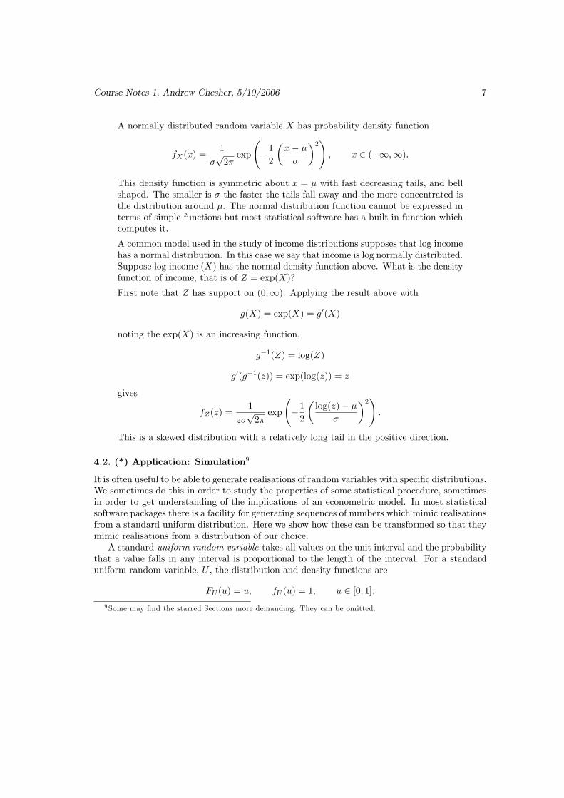
A normally distributed random variable X has probability density function

fX(x) =1

�p2�exp

�12

�x� ��

�2!; x 2 (�1;1):

This density function is symmetric about x = � with fast decreasing tails, and bellshaped. The smaller is � the faster the tails fall away and the more concentrated isthe distribution around �. The normal distribution function cannot be expressed interms of simple functions but most statistical software has a built in function whichcomputes it.

A common model used in the study of income distributions supposes that log incomehas a normal distribution. In this case we say that income is log normally distributed.Suppose log income (X) has the normal density function above. What is the densityfunction of income, that is of Z = exp(X)?

First note that Z has support on (0;1). Applying the result above with

g(X) = exp(X) = g0(X)

noting the exp(X) is an increasing function,

g�1(Z) = log(Z)

g0(g�1(z)) = exp(log(z)) = z

gives

fZ(z) =1

z�p2�exp

�12

�log(z)� �

�

�2!:

This is a skewed distribution with a relatively long tail in the positive direction.

4.2. (*) Application: Simulation9

It is often useful to be able to generate realisations of random variables with speci�c distributions.We sometimes do this in order to study the properties of some statistical procedure, sometimesin order to get understanding of the implications of an econometric model. In most statisticalsoftware packages there is a facility for generating sequences of numbers which mimic realisationsfrom a standard uniform distribution. Here we show how these can be transformed so that theymimic realisations from a distribution of our choice.A standard uniform random variable takes all values on the unit interval and the probability

that a value falls in any interval is proportional to the length of the interval. For a standarduniform random variable, U , the distribution and density functions are

FU (u) = u; fU (u) = 1; u 2 [0; 1]:9Some may �nd the starred Sections more demanding. They can be omitted.


Suppose we want pseudo-random numbers mimicing realisations of a random variable Wwhich has distribution function FW (w) and let the inverse distribution function (we will some-times call this the quantile function) be QW (p) for p 2 [0; 1], i.e.

QW (p) = F�1W (p); p 2 [0; 1]

equivalentlyFW (QW (p)) = p:

Let U have a standard uniform distribution and let V = QW (U). Then, using the results above(work through these steps) the distribution function of V is

FV (v) = P [V � v] = P [QW (U) � v] = P [U � Q�1W (v)] = FU (Q�1W (v)) = Q�1W (v) = FW (v)

So, the distribution function of V is identical to the distribution function of W . To generatepseudo-random numbers mimicing a random variable with distribution function FW we generatestandard uniform pseudo-random numbers, u, and use QW (u) as our pseudo-random numbersmimicing values drawn from the distribution of W .

4.3. Quantiles

The values taken by the quantile function are known as the quantiles of the distribution of X.Some quantiles have special names. For example QX(0:5) is called the median of X, QX(p)for p 2 f0:25; 0:5; 0:75g are called the quartiles and QX(p), p 2 f0:1; ; 0; 2; : : : ; 0:9g are calledthe deciles. The median is often used as a measure of the location of a distribution and theinterquartile range, QX(0:75)�QX(0:25) is sometimes used as a measure of dispersion.

4.4. Expected values and moments

Let Z = g(X) be a function of X. The expected value of Z is de�ned for continuous and discreterandom variables respectively as

EZ [Z] = EX [g(X)] =

Z 1

�1g(x)fX(x)dx (4.3)

EZ [Z] = EX [g(X)] =

MXXi=1

g(xi)p(xi) (4.4)

which certainly exists when g(�) is bounded, but may not exist for unbounded functions.Expected values correspond to the familiar notion of an average. They are one measure of

the location of the probability distribution of a random variable (g(X) = Z above). They alsoturn up in decision theory as, under some circumstances10 , an optimal prediction of the valuethat a random variable will take.10When the loss associated with predicting yp when y is realised is quadratic: L(yp; y) = a+ b(y� yp)2, b > 0,

and we choose a prediction that minimises expected loss.


The expected value of a constant is the value of the constant because, e.g. for continuousrandom variables (work through these steps for a discrete random variable) and the constant a:

EX [a] =

Z 1

�1afX(x)dx = a

Z 1

�1fX(x)dx = a� 1 = a:

The expected value of a constant times a random variable is the value of the constant times theexpected value of the random variable, because, again for continuous random variables and aconstant b,

EX [bX] =

Z 1

�1bxfX(x)dx = b

Z 1

�1xfX(x)dx = bEX [X]:

ThereforeEX [a+ bX] = a+ bEX [X]:

For additively separable g(X) = g1(X) + g2(X) we have

EX [g(X)] = EX [g1(X)] + EX [g2(X)]:

Show that this is true using the de�nitions (4.3) and (4.4).The expected values EX [Xj ] for positive integer j are the moments of order j about zero

of X and EX [(X � E[X])j ] are the central moments and in particular V arX(X) = E[(X �E[X])2] is the variance. Note that if X does not have bounded support then these moments areexpectations of unbounded functions and so in some cases may not exist.It is sometimes helpful to think of the probability that X lies in some region A � <1 as being

itself an expectation. To do this de�ne the indicator function

1[x2A] = 1; x 2 A= 0; x =2 A:

ThenP [X 2 A] = EX [1[X2A]]:

4.5. Moment generating functions

Expected values, and moments generally, attract a lot of interest in econometric work and itis useful to have a variety of methods for calculating them. Moment generating functions aresometimes helpful in this respect. The moment generating function of a random variable X isde�ned, when it exists, as the expectation of the function exp(tX) where t is a constant.

MX(t) = EX [exp(tX)]: (4.5)

This function clearly exists for all random variables with bounded support, discrete or continu-ous. It exists for some, but not all, random variables with support on the whole real line.Considering the de�nition of the expectation of a function of a random variable we see that,

if M (i)X (0) denotes the ith derivative of MX(t) evaluated at t = 0 then M

(i)X (0) = EX [X

i], thatis, is equal to the ith moment about zero. For continuous random variables for example

M(1)X (t) =

@

@t

Z 1

�1exp(tx)fX(x)dx =

Z 1

�1x exp(tx)fX(x)dx


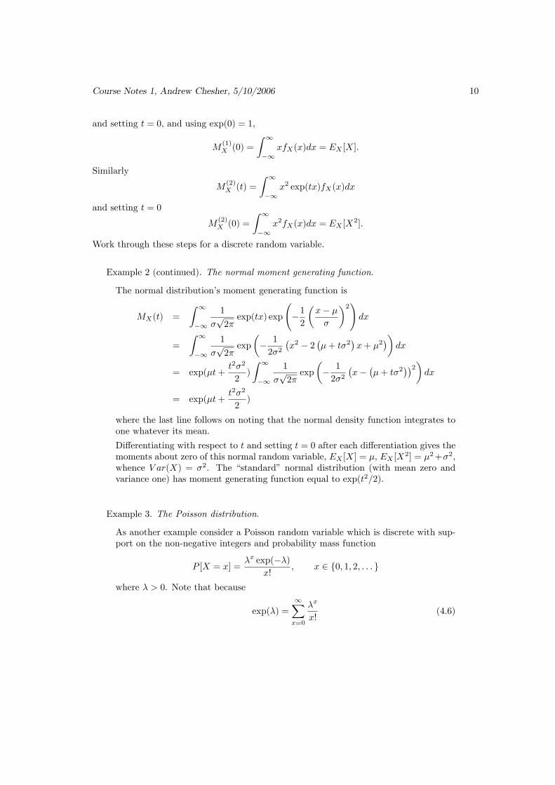
and setting t = 0, and using exp(0) = 1,

M(1)X (0) =

Z 1

�1xfX(x)dx = EX [X]:

Similarly

M(2)X (t) =

Z 1

�1x2 exp(tx)fX(x)dx

and setting t = 0

M(2)X (0) =

Z 1

�1x2fX(x)dx = EX [X

2]:

Work through these steps for a discrete random variable.

Example 2 (continued). The normal moment generating function.

The normal distribution�s moment generating function is

MX(t) =

Z 1

�1

1

�p2�exp(tx) exp

�12

�x� ��

�2!dx

=

Z 1

�1

1

�p2�exp

�� 1

2�2�x2 � 2

��+ t�2

�x+ �2

��dx

= exp(�t+t2�2

2)

Z 1

�1

1

�p2�exp

�� 1

2�2�x�

��+ t�2

��2�dx

= exp(�t+t2�2

2)

where the last line follows on noting that the normal density function integrates toone whatever its mean.

Di¤erentiating with respect to t and setting t = 0 after each di¤erentiation gives themoments about zero of this normal random variable, EX [X] = �, EX [X2] = �2+�2,whence V ar(X) = �2. The �standard� normal distribution (with mean zero andvariance one) has moment generating function equal to exp(t2=2).

Example 3. The Poisson distribution.

As another example consider a Poisson random variable which is discrete with sup-port on the non-negative integers and probability mass function

P [X = x] =�x exp(��)

x!; x 2 f0; 1; 2; : : : g

where � > 0. Note that because

exp(�) =1Xx=0

�x

x!(4.6)


this is a proper probability mass function. This distribution is often used as a startingpoint for modelling data which record counts of events.

The moment generating function of this Poisson random variable is

MX(t) =1Xx=0

exp(tx)�x exp(��)

x!

=1Xx=0

(�et)xexp(��)x!

= exp(�et � �) (4.7)

where to get to the last line we have used (4.6) with � replaced by �et.

The �rst two moments of this Poisson random variable are then easily got by dif-ferentiating the moment generating function with respect to t and setting t = 0,EX [X] = �, EX [X2] = �2+�, from which we see that V ar[X] = E[X2]�E[X]2 = �.So a Poisson random variable has variance equal to its mean. One way to tell if aPoisson distribution is a suitable model for data which are counts of events is to seeif the di¤erence between the sample mean and sample variance is too large to be theresult of chance sampling variation.

4.6. (*) Using moment generating functions to determine limiting behaviour of dis-tributions

Consider a �standardised�Poisson random variable constructed to have mean zero and varianceone, namely:

Z =X � �p�:

We will investigate the behaviour of the moment generating function of this random variable as� becomes large.What is the moment generating function of Z? Applying the de�nition (4.5)

MZ(t) = EZ [exp(tZ)]

= EX [exp(t

�X � �p�

�)]

= EX [exp(tp�X)] exp(�t

p�)

= exp(�et=p� � �� t

p�)

where the last line follows on substituting t=p� for t in (4.7).

When � is large enough, t=p� is small for any positive t, and et=

p� ' 1 + t=

p� + t2=(2�).

Substituting in the last line above gives, for large �, MZ(t) ' exp(t2=2) which is the moment


generating function of a standard (zero mean, unit variance) normally distributed random vari-able. This informal argument suggests that a Poisson random variable with a large mean isapproximately distributed as a normal random variable.In fact this is the case. However a formal demonstration would (a) have to be more careful

about the limiting operation and (b) be conducted in terms of the characteristic function whichis de�ned as CX(t) = EX [exp(itX)] where i2 = �1. This generally complex valued function of talways exists because exp(itX) is a bounded function11 of X. Further, under very general condi-tions there is a one to one correspondence between characteristic functions and the distributionsof random variables. That means that if we can show (as here we can) that the characteristicfunctions of a sequence of random variables converge to the characteristic function of a randomvariable, Y , say, then the distributions of the sequence of random variables converge to thedistribution of Y .

5. Many random variables

In econometric work we usually deal with data recording many aspects of the economic phe-nomenon of interest. For example in a study of consumers�expenditures we will have records foreach household of expenditures on many goods and services, perhaps for more than one periodof time, and also data recording aspects of the households�environments (income, householdcomposition etc.). And in macroeconometric work we will often observe many simultaneouslyevolving time series. We model each recorded item as a realisation of a random variable and sowe have to be able to manipulate many random variables simultaneously. This requires us toextend some of the ideas above and to introduce some new ones.For the moment consider two random variables, X and Y . The extension of most of what we

do now to more than two random variables is, for the most part obvious, and will be summarisedlater.The joint distribution function of X and Y is12

P [X � x \ Y � y] = FXY (x; y); (x; y) 2 <2

which is a non decreasing function of both its arguments, with FXY (�1;�1) = 0, FXY (1;1) =1. The support of a pair of random variables is a set of points in the real two dimensional plane,<2. The distribution function of, say, X alone is extracted from this by noting that

P [X � x] = P [X � x \ Y � 1] = FXY (x;1) = FX(x):

We call this a marginal distribution function.

11

exp(itX) = cos(tX) + i sin(tX)

andj cos(tX) + i sin(tX)j = cos2(tX) + sin2(tX) = 1:

12A \B is the event which occurs if and only if the events A and B both occur.


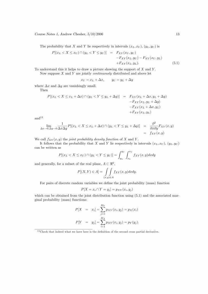
The probability that X and Y lie respectively in intervals (xL; xU ), (yL; yU ) is

P [(xL < X � xU ) \ (yL < Y � yU )] = FXY (xU ; yU )

�FXY (xL; yU )� FXY (xU ; yL)+FXY (xL; yL): (5.1)

To understand this it helps to draw a picture showing the support of X and Y .Now suppose X and Y are jointly continuously distributed and above let

xU = xL +�x; yU = yL +�y

where �x and �y are vanishingly small.Then

P [(xL < X � xL +�x) \ (yL < Y � yL +�y)] = FXY (xL +�x; yL +�y)

�FXY (xL; yL +�y)�FXY (xL +�x; yL)+FXY (xL; yL)

and13

lim�x!0;�y!0

1

�x�yP [(xL < X � xL +�x) \ (yL < Y � yL +�y)] =

@2

@x@yFXY (x; y)

= fXY (x; y)

We call fXY (x; y) the joint probability density function of X and Y .It follows that the probability that X and Y lie respectively in intervals (xL; xU ), (yL; yU )

can be written as

P [(xL < X � xU ) \ (yL < Y � yU )] =Z yU

yL

Z xU

xL

fXY (x; y)dxdy

and generally, for a subset of the real plane, A � <2,

P [(X;Y ) 2 A] =Z Z(x;y)2A

fXY (x; y)dxdy:

For pairs of discrete random variables we de�ne the joint probability (mass) function

P [X = xi \ Y = yj ] = pXY (xi; yj)

which can be obtained from the joint distribution function using (5.1) and the associated mar-ginal probability (mass) functions:

P [X = xi] =

MYXj=1

pXY (xi; yj) = pX(xi)

P [Y = yj ] =

MXXi=1

pXY (xi; yj) = pY (yj):

13Check that indeed what we have here is the de�nition of the second cross partial derivative.


Thinking of the joint probabilities being arrayed in a table these last two operations involveadding up entries across rows or columns of the table to produce totals to appear in the marginsof the table, hence the expression, �marginal distribution�.

5.1. Expected values, variance and covariance

Let g(�; �) be a scalar function of two arguments. The expected value of Z = g(X;Y ) is de�nedfor continuous and discrete random variables respectively as

EZ [Z] = EXY [g(X;Y )] =

Z 1

�1

Z 1

�1g(x; y)fXY (x; y)dxdy

EZ [Z] = EXY [g(X;Y )] =

MXXi=1

MYXj=1

g(xi; yj)pXY (xi; yj)

where for discrete random variables with X 2 fxigMXi=1 , Y 2 fyig

MYi=1

P [X = xi \ Y = yj ] = pXY (xi; yj):

For additively separable functions,

EXY [g1(X;Y ) + g2(X;Y )] = EXY [g1(X;Y )] + EXY [g2(X;Y )]:

Check this using the de�nitions above. Also note14 that for functions of one random variablealone, say Y ,

EXY [g(Y )] = EY [g(Y )]

which is determined entirely by the marginal distribution of Y .Once we deal with multiple random variables there are some functions of interest which re-

quire consideration of the joint distribution. Of particular interest are the cross central moments,E[(X � E[X])i(Y � E[Y ])j ] which may of course not exist for all i and j.The variances of X and Y , when they exist, are obtained when we set i = 2, j = 0 and i = 0,

j = 2, respectively. Setting i = 1, j = 1 gives the covariance of X and Y

Cov(X;Y ) = EXY [(X � E[X])(Y � E[Y ])]:

The correlation between X and Y is de�ned as

Cor(X;Y ) =Cov(X;Y )

(V ar(X)V ar(Y ))1=2:

This quantity, when it exists, always lies in [�1; 1].14For continuous random variables,

EXY [g(Y )] =

Z 1

�1

Z 1

�1g(y)fXY (x; y)dxdy

=

Z 1

�1g(y)

�Z 1

�1fXY (x; y)dx

�dy

=

Z 1

�1g(y)fY (y)dy = EY [g(Y )]


5.2. Conditional probabilities

Conditional distributions are of crucial importance in econometric work. They tell us how theprobabilities of events concerning one set of random variables depend (or not) on values takenby other random variables.For events A and B the conditional probability that event A occurs given that event B occurs

is

P [AjB] = P [A \B]P [B]

(5.2)

We require that B occurs with non-zero probability. Then we can write

P [A \B] = P [AjB]� P [B]= P [BjA]� P [A]

the second line following on interchanging the roles of A and B, from which

P [AjB] =P [BjA]P [A]

P [B]=

P [BjA]P [A]P [B \A] + P [B \ �A]

=P [BjA]P [A]

P [BjA]P [A] + P [Bj �A]P [ �A]

where �A is the event occurring when the event A does not occur. This is known as BayesTheorem.For three events,

P [A \B \ C] = P [AjB \ C]� P [BjC]� P [C]

and so on. This sort of iteration is particularly important when we deal with time series, or theresults of sequential decisions, in which A, B, C, and so on, are a sequence of events ordered intime with C preceding B preceding A and so forth.

5.3. Conditional distributions

Let X and Y be discrete random variables. Then the conditional probability mass function ofY given X is, applying (5.2)

pY jX(yj jxi) = P [Y = yj jX = xi] = pXY (xi; yj)=pX(xi):

For continuous random variables a direct application of (5.2) is problematic because P [X 2(x; x +�x)] approaches zero as �x approaches zero. However it is certainly possible to de�nethe conditional distribution function of Y given X 2 (x; x +�x) for any non-zero value of �xdirectly from (5.2) as

P [Y � yjX 2 (x; x+�x)] =FXY (x+�x; y)� FXY (x; y)

FX(x+�x)� FX(x)

=(FXY (x+�x; y)� FXY (x; y)) =�x

(FX(x+�x)� FX(x)) =�x


and letting�x pass to zero, gives what we will use as the de�nition of the conditional distributionfunction of Y given X = x:

P [Y � yjX = x] =@

@xFXY (x; y)=

@

@xFX(x) =

1

fX(x)

@

@xFXY (x; y)

from which, on di¤erentiating with respect to y, we obtain the conditional probability densityfunction of Y given X as

fY jX(yjx) =fXY (x; y)

fX(x): (5.3)

Note that this is a proper probability density function wherever fX(x) 6= 0 in the sense thatfY jX(yjx) � 0 andZ 1

�1fY jX(yjx)dy =

Z 1

�1fXY (x; y)dy=fX(x) = fX(x)=fX(x) = 1:

Turning (5.3) around,

fXY (x; y) = fY jX(yjx)fX(x)= fXjY (xjy)fY (y)

where the second line follows on interchanging the roles of x and y. It follows that

fY jX(yjx) =fXjY (xjy)fY (y)RfXjY (xjy)fY (y)dy

=fXjY (xjy)fY (y)

fX(x)

which is the equivalent for density functions of Bayes Theorem given above. This simple expres-sion lies at the heart of a complete school of inference - Bayesian inference.

5.4. Independence

Two random variables are said to be independently distributed if for all sets A and B,

P [X 2 A \ Y 2 B] = P [X 2 A]P [Y 2 B]:

Consider two random variables X and Y such that the support of the conditional distribution ofX given Y is independent of Y and vice versa. Then the random variables are independent if thejoint distribution function of X and Y is the product of the marginal distribution functions of Xand Y for all values of their arguments. For jointly continuously distributed random variablesthis implies that the joint density is the product of the two marginal densities and that theconditional distributions are equal to their marginal distributions.We use the idea of independence extensively in econometric work. For example when

analysing data from household surveys it is common to proceed on the basis that data fromdi¤erent households at a common point in time are realisations of independent random vari-ables, at least conditional on a set of household characteristics. That would be a reasonablebasis for analysis under some survey sampling schemes.


5.5. Regression

Consider a function of Y , g(Y ). The conditional expectation of g(Y ) given X = x is de�ned forcontinuous random variables as

EY jX [g(Y )jX = x] =

Z 1

�1g(y)fY jX(yjx)dy

and for discrete random variables as

EY jX [g(Y )jX = xi] =

MYXj=1

g(yj)pY jX(yj jxi):

These functions are given the generic name regression functions.When g(Y ) = Y we have the mean regression function which describes how the conditional

expectation of Y given X = x varies with x. This is often referred to as the regression function.V ar[Y jX = x] is less commonly referred to as the scedastic function.In econometric work we are often interested in the forms of these functions. We will shortly

consider how regression functions can be estimated using realisations of random variables andstudy the properties of alternative estimators. Much of the interest in current econometric workis in the mean regression function but scedastic functions are also of interest.For example in studying the returns to schooling we might think of the wage rate a person

obtains after completing education as a random variable with a conditional distribution givenX, years of schooling. The mean regression tells us how the average wage rate varies with yearsof schooling - we might be interested in the linearity or otherwise of this regression function andin the magnitude of the derivative of the regression function with respect to years of schooling.The scedastic function tells us how the dispersion of wage rates varies with years of schooling.

If we are interested in wage inequality then this is an interesting function in its own right. Aswe will see the form of the scedastic function is also important when we come to consider theproperties of estimators of the (mean) regression function.We can think of the conditional distribution function as a regression function. De�ne

Z(Y; c) = 1[Y <c]. Then

EY jX [Z(Y; c)jX = x] =

Z 1

�11[Y <c]fY jX(yjx)dy =

Z c

�1fY jX(yjx)dy = FY jX(cjx):

Sometimes we are interested in the way in which the conditional distribution of some randomvariable (e.g. wages) varies with conditioning variables and then we might consider the condi-tional quantile functions. Let QY jX(p; x) be such that FY jX(QY jX(p; x)jx) = p. For p = 0:5this is called the median regression function and generally a quantile regression function.The p-quantile regression function satis�es

p =

Z QY jX(p;x)

�1fY jX(yjx)dy:

It is possible to estimate quantile regression functions. If we do this and �nd that for di¤erentvalues of p they are not parallel then we have evidence that the dispersion and/or shape of theconditional distribution of Y given X depends upon the value of X.


6. Iterated expectations

We will frequently make use of the following important result, known as the law of iteratedexpectations.

EY [Y ] = EX [EY jX [Y jX]]

Loosely speaking this says that to obtain the expectation of Y we can average the expectedvalue of Y obtained at each possible value of X, weighting these conditional expectations (of Ygiven X = x) by the probability that X = x occurs. Formally, for continuous random variableswe have

EX [EY jX [Y jX]] =

Z 1

�1

�Z 1

�1yfY jX(yjx)dy

�fX(x)dx

=

Z 1

�1

Z 1

�1yfY jX(yjx)fX(x)dydx

=

Z 1

�1

Z 1

�1yfXY (x; y)dydx

=

Z 1

�1

Z 1

�1yfXjY (xjy)fY (y)dydxZ 1

�1y

�Z 1

�1fXjY (xjy)dx

�fY (y)dy

=

Z 1

�1yfY (y)dy

= EY [Y ]:

Work carefully through the steps in this argument. Repeat the steps for a pair of discreterandom variables15 .

7. Many random variables

Here the extension of the previous results to many random variables is sketched for the case inwhich the random variables are jointly continuously distributed.Let the N�element vector

X =

264 X1...XN

375denote N random variables with joint distribution function

P [X � x] = P [N\i=1

(Xi � xi)] = FX(x)

15More di¢ cult - how would you prove the result if the support of Y depended upon X, so that given X = x,Y 2 (�1; h(x)) where h(x) is an increasing function of x, and h(1) =1?


where x = (x1; : : : ; xN )0. Here and later in this section 0 denotes transposition not di¤erentiation.The joint density function of X is

fX(x) =@N

@x1 : : : @xNFX(x):

The expected value of X is

EX [X] =

264 EX1 [X1]...EXN

[XN ]

375and we de�ne the N �N variance covariance matrix of X as EX [(X �EX [X])(X �EX [X])0] =EX [XX

0]� EX [X]EX [X]0 whose (i; j) element is Cov(Xi; Xj) which is V ar(Xi) when i = j.Here for example

EX1 [X1] =

Z 1

�1: : :

Z 1

�1x1fX(x)dx1 : : : dxN

=

Now consider a vector random variable X partitioned thus: X 0 = (X 01; X

02) with joint distri-

bution and density functions respectively FX(x1; x2) and fX(x1; x2) where Xi has Mi elements.The marginal distribution function of, say, X2 is

FX2(x2) = FX(1; x2);

the marginal density function of X2 is

fX2(x2) =

@

@x2FX(1; x2):

Alternatively

fX2(x2) =

Zx12<M1

fX(x1; x2)dx1

and the conditional density function of X1 given X2 is

fX1jX2(x1jx2) =

fX(x1; x2)

fX2(x2)

:

The regression (function) of scalar g(X1) on X2 is

EX1jX2[g(X1)jX2 = x2] =

Zx12<M1

g(x1)fX1jX2(x1jx2)dx1.


7.1. The multivariate normal distribution

If M�element X has a multivariate normal distribution then its probability density functiontakes the form

fX(x) = (2�)�M=2 j�j�1=2 exp(�1

2(x� �)0 ��1(x� �))

where � is symmetric positive de�nite, M �M . We write X � NM (�;�).To develop the moments of X and some other properties of this distribution it is particularly

helpful to employ the multivariate moment generating function, MX(t) = EX [exp(t0X)] where

t is a M�element vector. This is just an extension of the idea of the simple moment generatingfunction introduced earlier. We can get moments of X by di¤erentiating MX(t). For example,

@

@tiMX(t) = EX [Xi exp(t

0X)]

and so@

@tiMX(t)jt=0 = EX [Xi]:

Check that the derivative of MX(t) with respect to ti and tj evaluated at zero gives EX [XiXj ]:The multivariate normal moment generating function is obtained as follows.

MX(t) =

Z� � �Z(2�)

�M=2 j�j�1=2 exp(t0x) exp(�12(x� �)0 ��1(x� �))dx

=

Z� � �Z(2�)

�M=2 j�j�1=2 exp(�12

�x0��1x� 2x0��1(�+�t) + �0��1�

�)dx

= exp(t0�+1

2t0�t)

�Z� � �Z(2�)

�M=2 j�j�1=2 exp(�12(x� (�+�t))0 ��1(x� (�+�t)))dx

= exp(t0�+1

2t0�t):

Note that this reproduces the result for the univariate normal distribution if we set M = 1.Di¤erentiating with respect to t once and then twice, on each occasion setting t = 0 givesEX [X] = �, V ar[X] = �.Here is another use of the moment generating function. Consider a linear function of Z = BX

where B is R�M . The moment generating function of R�element Z is

MZ(t) = EZ [exp(t0Z)]

= EX [exp(t0BX)]

= exp(t0B�+1

2t0B�B0t) (7.1)

from which we can conclude that Z � NR[B�;B�B0]. So, all linear functions of normal randomvariables are normally distributed. In particular every element of X, Xi is univariate normalwith mean �i and variance equal to �ii which is the (i; i) element of �.


Partition X so that X 0 = (X 01

...X 02) where Xi has Mi elements and partition � and � con-

formably,

� =

��1�2

�; � =

��11 �12�21 �22

�:

Note thatX1 = Q1X

where Q1 =�IM1

...0�. Employing this matrix Q1 in (7.1) leads to X1 � NM1 [�1;�11] and

similarly for X2.With the marginal density functions in hand we can now develop the conditional distributions

for multivariate normal random variables. Dividing the joint density of X1 and X2 by themarginal density of X2 gives, after some algebra, the conditional distribution of X1 given X2,

X1jX2 = x2 � NM1 [�1 +�12��122 (x2 � �2) ;�11 � �12��122 �21]:

So, we haveE[X1jX2 = x2] = �1 +�12��122 (x2 � �2) :

andV ar[X1jX2 = x2] = �11 � �12��122 �21

In the multivariate normal case then, mean regression functions are all linear, and conditionalvariances are not functions of the conditioning variable. We say that the variation about themean regression function is homoscedastic. Of course conditional variances change as we condi-tion on di¤erent variables.Notice that if the covariance of X1 and X2 is small, the regression of X1 on X2 is insensitive

to the value of X2 and the conditional variance of X1 given X2 is only a little smaller than themarginal variance of X1.Suppose we consider only a subset, XI

2 say, of the variables in X2 (�I� for included). Theconditional distribution of X1 given XI

2 is derived as above, but from the joint distribution ofX1 and XI

2 alone. We have �X1XI2

�� N

��1�I2

�;

��11 �I12�I21 �I22

��where �I2, �

I21 contain only the rows in �2 and �21 respectively relevant to X

I2 . Similarly �

I22

contains only rows and columns relevant to XI2 .

It follows directly that the conditional distribution of X1 given XI2 is

X1jXI2 = x

I2 � NM1 [�1 +�

I12

��I22��1 �

xI2 � �I2�;�11 � �I12

��I22��1

�I21]:

Notice that the coe¢ cients in the regression function and the conditional variance both alter aswe condition on di¤erent variables but that in this normal case the regression function remainslinear with homoscedastic variation around it.


7.2. Iterated expectations

Now consider the extension of the law of iterated expectations. Consider three random variables,X1, X2 and X3. First, using the law for the two variable case, and conditioning throughout onX1 we have

EX3jX1[X3jX1] = EX2jX1

[EX3jX2X1[X3jX2; X1]jX1]:

The result is some function of X1. Now apply the law for the two variable case again. We getthe following.

EX3[X3] = EX1

[EX2jX1[EX3jX2X1

[X3jX2; X1]jX1]]:Now develop the law for the case of four random variables. You should see the structure of thegeneral law for N random variables.

7.3. Omitted variables?

In some econometrics textbooks you will read a lot of discussion of �omitted variables�and the�bias� in estimators that results when we �omit regressors� from models. We too will look atthis �bias�. The development in the previous section suggests that we can think of this in thefollowing way.When we estimate regression functions using di¤erent regressors we are estimating di¤erent

parameters, that is di¤erent regression coe¢ cients. In the multivariate normal setting, when X2is used as the set of conditioning variables, we estimate �12�

�122 as the coe¢ cients on x2, and

when the set of conditioning variables XI2 is used, we estimate �

I12

��I22��1

as the coe¢ cientson xI2.Of course XI

2 consists of variables that appear in X2. These common variables may havedi¤erent coe¢ cients in the two regression functions, but they may not have. In particular if thecovariance between XI

2 and the remaining elements in X2 is zero then the coe¢ cients on XI2

will be the same in the two regression equations.In this multivariate normal setting the �bias�that is talked of arises when we take estimates

of one set of regression coe¢ cients and regard them (usually incorrectly) as estimates of a dif-ferent set of regression coe¢ cients. Outside the multivariate normal setting there are additionalconsiderations.These arise because the multivariate normal model is very special in that its regression

functions are all linear. In most other joint distributions this uniform linearity of regressionfunctions, regardless of the conditioning variables, is not generally present.We can write the regression of X1 on XI

2 as equal to the conditional expectation of theregression of X1 on the complete X2 with respect to the conditional distribution of X2 givenXI2 . Let X

E2 denote the excluded elements of X2 and write the regression of X1 on X2 as

E[X1jX2 = x2] = �0IxI2 + �0ExE2 :

Then the regression of X1 on XI2 is

E[X1jXI2 = x

I2] = �

0IxI2 + �

0EE[X

E2 jXI

2 ] = xI2]:

The additional consideration alluded to above is that except in very special circumstances,outside a multivariate normal setting, E[XE

2 jXI2 = x

I2] is not a linear function of x

I2.


One implication of this is that when we see non-linearity in a scatter plot for data on twovariables, it may be the case that there is a linear e¤ect for one variable on the other but in thecontext of a wider model in which we condition on a larger set of variables.

7.4. Regression functions and linearity

As noted earlier, much econometric work focuses on the estimation of regression functions andit is common to �nd restrictions imposed on the functional form of a regression function, some-times �owing from economic theory, but often not. In microeconometric work the conditioningvariables in an econometric regression model usually capture features of the agents� environ-ments.From now on we will use the symbol Y to denote the random variable whose conditional

distribution is of interest and we will use the symbol X to denote regressors, k in number unlessnoted.The elementary textbooks all start, as we shall shortly do, by considering linear regression

functions and a single response, that is the case in which Y is a scalar random variable, andthere exists a column vector of constants � such that, for all x,

E[Y jX = x] = �0x:

In analysing multiple responses (vector Y ) too, it is common to �nd a linear regression functionassumed, that is that there exists a matrix of constants, B, such that for all x,

E[Y jX = x] = Bx:

Surprisingly, given the ubiquity of linearity assumptions like these, it is hard to �nd any elementof economic theory which predicts linearity of regression functions. Linearity is usually anempirical issue - if we employ a linear model then we should try to see if the linearity restrictionis appropriate.Suppose that in fact the regression of Y on X is a nonlinear function of x, say

E[Y jX = x] = g(x; �): (7.2)

Taking a Taylor series expansion of g(x; �) around some central point x0, in the distribution ofX will lead to a linear approximation

E[Y jX = x] + g(x0; �) + �0(x� x0)

where the ith element of this vector � is

�i =@

@xig(x; �)jx=x0 :

So, if the second derivatives of the function g(x; �) are not very large over the main part of therange of X then a linear model may be a good approximation. Taking the Taylor series one morestep produces a quadratic approximation. We might �nd (but not necessarily) that a quadraticapproximation

E[Y jX = x] = �0 + �0x+ x0Ax


where �0 = g(x0; �), is close to the true nonlinear regression. In some applied work you will seelinear models extended by the addition of polynomial functions of regressors.A simpler, and it turns out easier to estimate version of the general nonlinear regression

function (7.2) is the followingE[Y jX = x] = g(x0�):

in which the conditioning variables combine linearly but their combined e¤ect on the expectationof Y is nonlinear. This sort of restriction is known as a �single index�restriction.An important, implication of a single index restriction of this sort is that

@

@xiE[Y jX = x] = g0(x0�)�i

where

g0(z) =@

@zg(z):

This implies@@xiE[Y jX = x]

@@xjE[Y jX = x]

=�i�j:

The ratio of two partial derivatives of the regression function at every value of x is independentof g(�) and of x. This provides us with a route to investigating whether a single index assumptionis appropriate and to a way of estimating ratios of the �i�s that does not require speci�cation ofg(�). Estimators of this sort are known as semi-parametric estimators.We have started talking about estimation of regression functions. It is time to consider how

this can be done.

Documents

MC3: Econometric Theory and Methods - UCLuctpjea/lnotes1.pdf · University College London Department of Economics M.Sc. in Economics MC3: Econometric Theory and Methods Course notes: