MBiC PROCESSING: EXPERIMENTAL DESIGN AND OPTBMIZATION

Martin W. Weiser David N. Lauben

Philip Madrid

Mecfianical Engineering Department University of New Mexico

P. 0. Box 999 Albuquerque, New Mexico 87131

Telephone 505-277-253 1

Ceramic Processing: Experirnen~l Design and Optimization

Martin W. Weiser, David N. Lauben, and Philip Madrid Mechanical Engineering Department

University of New Mexico Albuquerque, NM 87131

Keywords

Ceramics, experimental design, Taguchi, optimization, slip casting, clay, four-point bend testing

Objectives

1. To gain some insight into the processing of ceramics and how green processing can affect the properties of ceramics.

2. To investigate the technique of slip casting as one of the methods used to fabricate cermics. 3. To learn how heat treatment time and temperature contribute to the properties of cermics:

o Density, @ Strength, @ Effect of under and over firing.

4. To experience some of the problems inherent in mechanically testing brittle materials and to lean about the statistical nature of the strength of ceramics and other brittle materials.

5. To investigate orthogonal arrays as tools to examine the effect of many experimental pxmeters using a minimum number of experiments.

6. To recognize appropriate uses for clay based ceramics developed by the slip casting process. 7. To measure several different properties important to ceramic use and optimize them for a given

application.

Equipment and Supplies

1. Three acrylic molds for slip casting bars as shown in Figure 1. 2. Six plaster bats for slip casting the bars as described in appendix B. 3. A programmable furnace capable of 1200°C with a minimum hearth size of one square foot and

height of three inches. It is possible to use a furnace with a smaller hearth size or that is not programmable but this will require more firing(s) andlor more supervision.

4. Approximately two kilograms each of an earthenware clay such as redart* and a moderate stonewae clay such as goldart*. Other materials may be substituted for the earthenware and stonewxe clays to change the experimental results for variety andlor a different firing temperature. Suggested replacements are ball clay or kaolin for the stoneware clay and fluxes such as feldspar or talc for the

This work was supported in part by a grant from the University of New Mexico Teaching Allocation Subcommittee.

* Cedar Heights Clay but available from most local ceramic suppliers.

e w e n w x e clay. Replacing one or more of the clays will require the relative amounts of the conqponemts to be adjusted.

5. A minimum of three 500 ml wide mouth bottles for mixing the slips. 6, A 50 to 200 ml buret for adding the dispersant solution. 7. 50 rnl of a polymeric dispersant such as the Daxad series of sodium salts of polyacrylic acid ( P M )

or polymethylacrylic acid (PMAA)+ or onium salts of PAA or PMAA.* 8. Approxinnately one kilogram of coarse grog if this parameter is to be varied.

General Bxkground

This laboratosy experiment is designed to familiarize students with some of the processing techniques and propeaies of ceramics. This is necessary since advanced ceramics have been proposed for a wide variety of applications, many of which were unheard of just twenty years ago. This results from factors that include: realization of how diverse ceramic properties are, the desire to operate equipment in more extreme conditiions, and improved reliability stemming from better processing and materials design. This experiment will describe some of the properties of ceramics and investigate the processing and properties of a relatively simple ceramic, structural clay.

Cermics are a broad class of materials that exhibit diverse properties. They are most conmonly divided into several chemical groups that include the oxides (A1203, SiO,, MgO, etc.), nitrides (AIN, Si3N,, BN, etc.), cxbides (Sic, B,C, Tic , etc.), halides (NaCl, KCl, LiF, etc.) and many other inorganic com- pounds. Some common applications are window and container glass which are amorphous solid solutions of SiO,, CaO, Na,O and other oxides, sharpening stones composed of alumina (A1203) or silicon carbide (Sic) m d transducers that are used in nearly all forms of electro-acoustic (speakers) equipment based upon BaTiO, and related materials. Of great economic importance are ceramics used as refractories to contain molten metals or glasses (silica-SiO,, mullite-3A1203@2Si02, and zirconia-ZrO,), and as sensors (c-ZrO,). More recent ag~plications are in thermal engines (A1203, S ic , Si,N,, and MoSi,), fiber optics (SiO, and phosphide glasses), and superconductors (YBa2Cu30,). The previous discussion shows that ceramics a e very impodant products in both everyday life and for the production of other materials.

There are four primary properties that come to mind when ceramics are discussed; resistance to high temperature, corrosion resistance, high hardness, and brittleness. The first three of these properties are normally assets, while the last is generally considered detrimental for most applications (grinding and polishing media are an exception). It is the first three properties that are currently driving the investigation of the use of ceramics for applications such as thermal engines while the fourth presents mmy of the m,ajor obstacles to more widespread use.

Mmy of the problems with brittleness in ceramics can be overcome by the use of ceramic matrix composites anclior use of improved processing techniques. Ceramic composites attack the brittleness problem directly by making the material more difficult to fracture (toughening) while irnproved processing techniques aMernpt to eliminate the pre-existing flaws that are normally the initiation site for fracture. Toughening methods currently in use include: fiber or whisker reinforcement to bridge cracks, particle reinforcement .to deflect cracks, and transformation toughening to push cracks closed. Each of these

D a a d 37LN and 30, W.R. Grace & Co. Dxvan C and 821-A, R.T. Vanderbilt Company, Inc.

techniques has both advantages and disadvantages, but the use of any of them makes the cermic more difficult to fabricate.

A significant amount of research has been done recently that has focussed on improved cermic processing techniques after it was recognized that removing the strength limiting flaws during the latea- stages of fabrication was a difficult process. Several approaches have been investigated including both colloidal routes to improve consolidation of powders such as pressure filtration and chemical routes to form the ceramic in situ such as chemical vapor infiltration. There have been notable successes in both xeas with selected materials but no single technique has emerged as the ultimate method for ceramic fabrication.

Experimental Background

This experiment uses an inexpensive, easily processed ceramic to illustrate some of the principles of' ceramic fabrication and mechanical properties. Unfortunately, this material has a complex chemical and phase structure. Detailed analysis of the processing kinetics and resultant microstructure would be difficult for the ceramic examined in this laboratory, especially for a course of this depth. However, certain trends or correlations can still be observed and explained based on general principles of cermic science. Several simpler systems could have been used for this experiment, but they were 1eie87er too expensive, toxic, difficult to process, required too high a heat treatment temperature, or a ctombination of these factors.

The processing of ceramics can be broken down into two major steps: the formation of the green body and the heat treatment to form the final product. The term green body comes from the early ponerqr indushq and denotes the ceramic in a consolidated, friable state prior to heat treatment. The green body is normally formed by one of four methods. These are packing individual ceramic powder parhicles toge&er by dry pressing, extrusion of a plastic body, injection molding, and slip casting. Heat treat,ment of ceramics is also known as firing which is also a vestige from pottery. It is carried out at high temperatures (800 to 2500°C) in a furnace that is often designed to allow a controlled atmosphere surrounding the sample.

The specimens for this experiment are to be processed by slip casting. Slip casting involves the production of a liquid slurry or slip from the dry components and pouring the slip into molds where it solidifies. The slip is made by adding the ceramic powder to a liquid solvent which lubricaltes and disperses the powder particles. The most common solvent is water, but a number of alcohols and organic solvents have been used in specialized cases. The dispersion of the powder particles in the solvent depends strongly on the nature of the particlelsolvent interface and the electrostatic forces bemeen the particles. The interface and electrostatic forces can be modified by changing the pH (acidiQ/alkaliinityp of the solvent andlor the addition of dispersants and binders that bond to the particles. These dispersms are normally organic molecules that are related to the surfactants found in detergents. One of tibe principle reasons for controlling the interfacial behavior of the particles is to allow the slip to be highly concentrated while having a reasonable viscosity. This is often referred to as a high solids loading of the slip. The high solids loading makes it easier to form a homogeneous green body with fewer voids.

A typical slip casting mold is designed to draw the water out of the slip through one or more mold surfaces. Porous plaster bats are often used to draw the water out of the slip by capillary action. Since plaster is easily fabricated and quite effective at holding water, it is one of the rnost commonily used

materials for this process. However, technologies based upon a permeable membrane are also used that permit the water to be either pressed or sucked out of the slip.

This experiment uses an acrylic mold to contain the slip in the vertical plane. The mold is placed on top sf a plaster bat to support the slip and remove water as shown in Figure 1. This geometry results in unidirectional water flow in the forming green body through the bottom of the sample. This yields more uniform samples than slip casting in a mold cavity in which the water is drawn off in more than one direction. After the green body is solid enough to hold its shape, the acrylic mold is removed and the sample is dried further in air. Nearly all the remaining water which is not chemically bonded to the cermic powder can be removed by oven drying the sample at about 80°C. At this point the green body is quite porous and still contains a considerable amount of chemical water and the dispersants. The samples are weak and must be handled with care prior to firing.

Figure 1 The mold and plaster bat used to slip cast the ceramic samples.

During the firing operation several different phenomena occur. The first of these is that the chemically bonded water is driven off in the 100-400°C range. This water is part of the crystal structure of the cermic powders such as kaolinite (A12(Si205)(OH),). Kaolinite typically decomposes into alumina (A120,) and silica (SiO,) when the water is driven off. This reaction is irreversible except under extreme conditions. The next step in the process is for the particles to begin sintering together, allowing the system to reduce its internal surface energy. Sintering is a diffusion controlled process where the rate exponentially increases with temperature. In some ceramics, materials are included that form low melting

liquids that can greatly enhance the diffusion and sintering rates. These materials are normially referred to as fluxes. These liquids may be absorbed by the bulk of the material which is known as trmsient liquid phase sintering or they may remain in the ceramic component as glasses or second phases upon cooling.

The firing temperatures of the clays are frequently cited in terms of a pyrometric cone rather thm a specific temperature. Pyrometric cones are used because they integrate the effect of temperature over time on a standard ceramic composition. The pyrometric cone gives a better representation of the cowaplex reactions occurring during ceramic firing than would a simple measure of the temperature. Pyrometric cones are narrow triangular pyramids of a tightly controlled ceramic composition. They are normally 1.5 to 3 inches tall and are fired in the same fkrnace as the product being processed. The cones are placed with their long axis at an 8" angle from vertical and allowed to deform under the influence of gravity during the firing as the material softens under the combined effects of temperature and time: at temperature.

The pyrometric cone gives a visual measure of the firing process since the tip of the cone will faill over as it deforms. A firing is said to have achieved a certain pyrometric cone if the cone with hail number bends so the that tip of the cone is at one-half of the original cone height. Normally a series of three or more cones are used to allow the progress of the firing to be followed. The cones are numbered from 040 at the lowest firing temperatures to 50 with the highest firing temperatures. A leading zero, i.e. 06 or 810, is the equivalent of a negative sign before the other digits. Typical terra cotta is fired at cone 010 to 04, stoneware at cone 6 to 10, artistic porcelain at cone 10 to 15, and industrial porcelain such as spxfl-kglugs at approximately cone 20. Pyrometric cones have been fired using various carefully contrcllled tirne- temperature profiles (heating rates of 1 or 5"CImin followed by a moderate quench) to determine the temperature equivalent.

Experimental Materials

Two different types of pottery clay are used in this experiment because they are readily available, inexpensive, non-toxic, and can be fired at temperatures of less than 1200°C. This is a significantly Bower temperature than required for most of the advanced ceramics and is within the capabilities of mmy furnaces that are available in materials processing laboratories. The redart clay contains a relatively large fraction of fluxes and can be fired at temperatures below 1200°C. The goldart clay contains less flux md as a result is more refractory. The compositions and properties of the clays that are to be used in this experiment are summarized in Table I.

The compositions are supplied in terms of their oxide equivalents even though the elements are not necessarily distributed in this fashion. Most of the material will be present as various types of silicates such as kaolinite, illite, silica, and ferrous oxides. Kaolinite is a sheet silicate with a chemical composition of Al,(Si2O5)(OH), which can be contaminated with most of the other elements. It forms Lhe basis of most clays and is present in the form of small platelike particles that contribute significmtly to the plasticity of the clay. Illite is one of the principal fluxes in this system and is normally morphous with a composition of A12~xMgxK,~x,(Si,~55,,A10,5+Y05)(OH,). The variables x and y in this formula indicate that the composition is variable and depends upon the relative abundance of the three cations, K+l? l ~ I g + ~ , and AP3. The chemical formula of silica is SiO, which is normally present as a-quartz. The ferrous oxides are FeO, Fe203, and Fe304 which either form small particles or are included as part of the strucbre of one of the other components.

Table I Nominal Composition a d Properties of the Clays Used in this Experiment

Colnposition (wt%) Silica (SiO,) Alumina (Al,03) Iron Oxide (Fe203) Titania (TiO,) Magnesia (MgO) Calcia (CaO) Soda (Na,O) Potassia (K,O) Sulfur (S)

Redart

64.27 16.41 7.04 1.06 1.55 0.23 0.40 4.07

Goldart

56.72 27.30

1.42 1.75 0.42 0.22 0.16 1.87 0.12

Loss on Ignition 4.92 10.03 Standard Firing Cone 04 6 Std. Cone Temp @ 1 "Clmin 1060°C 1230°C

Fired Shrinkage (-Alllo) Cone 05 Cone 1 Cone 3 Cone 10

Absorption (wt% W,O) Cone 05 Cone 1 Cone 3 Cone 10

From Data Sheets supplied by Cedar Heights Clay

Exmination of the composition data shows that redart contains significantly more of the fluxes (FqO,, MgO, Na,O, and K20) and less Al,03 than the goldart. This difference in composition reduces the firing temperature redart clay. The ferrous oxides result in the reddish color of both the green and fired clay body. The clays exhibit similar firing shrinkages and amounts of porosity (percent water absorption) at the lowest firing temperatures listed (A05). However, the goldart remains significantly more porous at intermediate tenlperatures (A1) and only achieves nearly completely closed porosity at much higher remperamres (810). It should also be noted that the goldart clay contains more organic matter as indicated by the higher loss on ignition.

Processing Parameters

There are a multitude of different parameters that affect the properties of a ceramic. Some of these are of an intrinsic nature and depend upon the type of ceramic material used. However, the vast majority of the pzameters are process related and may be controlled by the experimentalist. The properties of ceramics

are probably more dependent on the processing than most other classes of materials. The following list sumar izes many of the different parameters and how they affect the processing and properties.

Composition - Clay based ceramics are composed of three primary types of oxides: refractories, glass formers, and fluxes along with reinforcements. s Refractory components such as Al,O, and Cr203 have high melting temperatures and increase the

firing temperature of the clay body. r Glass Forrners such as SiO, and B,O, form a vitreous (glassy) matrix which holds the more

refractory particles together. Fluxes such as Li,O, Na,O, K,O, MgO, CaO, and FeO, enter the glass network and assist in dissolving the refractory elements into the glassy matrix. As a result the fluxes lower the melting temperature of the glass and the firing temperature of the body.

o Reinforcements can be added to the material in order to modify the properties. In clay based ceramics the most common are granules of previously fired clay ranging from 20 psn to 2 m in diameter known as grog. Grog is added to control drying shrinkage and improve the drying rate Different types of particles, fibers, and flakes are added to other ceramics in order to modify the properties by forming a composite. The most common purpose is to improve the mechmical properties, particularly the fracture toughness.

In this experiment the composition of the body is controlled by altering the proportions of the different clays. The use of a higher fraction of the refractory clay should increase the necessary firing temperahre but the effect is rarely linear. In addition, this should increase the strength of the product if the sarnples are fired to the same fraction of theoretical density since the crystalline phases that incorporate the refractory oxides are stronger than the vitreous phases based upon silica.

Green Processing - The green processing technique employed will have a dramatic effect on the properties since many of the strength limiting flaws are introduced during this step.

Dry Pressing is very fast and efficient but there is a tendency for the particles to bridge voids m d leave large pores behind. In addition the shapes that can be dry pressed are limited (due to the need to uniformly distribute the pressing stresses. Extrusion of a plastic (moist and easily deformed) ceramic material is a good method to produce pieces of uniform cross section. However, the process is limited to producing parts with a uniform cross section and only certain ceramic materials can be formed into a plastic suspension.

@ Injection Molding incorporates the ceramic powder into a polymeric base that is molded under pressure to the desired shape. This is an expensive process and there is normally a large mount of polymer that must be removed during the later stages of processing by either burning it out or converting it into a desirable ceramic phase.

@ Slip Casting is very useful for producing high quality parts with complex shapes. Proper dispersion of the ceramic powder virtually insures that no large voids will be formed and complex shapes can be made with properly designed molds.

Slip Casting - The properties of the slip cast part are strongly dependent upon the nature of the slip that is used to cast the parts. A well dispersed slip with a high solids loading normally results in a high densiv, homogeneous green body.

Solvent choice influences the viscosity of the slip, the ability to disperse the ceramic particles, land the ability to dry the green body. Water is the most frequently used solvent because it disperses oxides fairly well, has a low viscosity, and is easy to remove from the green body.

Slip pH has a strong effect on the dispersion of the powder particles. The p r i m q force that prevents I;he particles from flocculating (clumping together) is electrostatic repulsion between particle surfaces. The pH of the slip influences the surface charge of the particles with flocculation occurring when the surface charge approaches zero (the isoelectric point). However, extreme pH's @igk or low) can increase flocculation due to the high ionic strength of the slip. Dispersants are frequently added to the slip to modify the electrostatic repulsion between particles and allow either the solids loading of the slip to be increased or the viscosity to be decreased. They work by binding to the particle surfaces and preventing the particles from approaching each other too closely. Too much dispersant will increase the viscosity of the slip since most dispersants are mode rat el:^ high molecular weight linear polymers. This experiment utilizes one of the salts of either polyacrylic or polymethylacrylic acid as a dispersant. Binders and plasticizers are sometimes added to the slip to increase the strength of the green body. These are normally low molecular weight polymers that can be induced to cross-link after the green body is dried.

Firing - The firing process removes the organics and chemically bonded water from the ceramic compact md fuses the particles together into a solid mass. In addition, it may result in densification and the elimination of p'ores.

Temperature of firing normally refers to the maximum temperature during the firing process. The firing temperature must be high enough to cause the particles to fuse together and densify if desired. But it must be low enough to prevent sagging due to high temperature creep and grain growth, paflicularly abnormal grain growth where a few grains become much larger than the rest. Optimal firing of rnany ceramics is accomplished by a complex combination of ramps and holds at various ternperah~res in order to promote different reactions or diffusion mechanisms at different points in the firing process. Time normally refers to the hold time at the maximum firing temperature. It must be long enough for the particles to fuse together and densify but short enough to prevent creep and grain growth.

(P R m p Rate is the rate at which the furnace is heated and cooled from one temperature to another. Too high a ramp rate can cause a variety of problems such as uneven heating causing thermal stresses, trapping of gases that evolve as the organics break down, and thermal shock as phase trmsitions occur. Too slow a ramp rate wastes energy and may favor diffusion processes during sintering that lead to undesirable results. A number of different ramp rates are frequently employed over different temperature ranges to optimize the process in these temperature ranges. Clay based cermics are susceptible to cracking due to the a to B quartz transition at 573°C and the evolution of chemical water at 100 to 250°C. Consequently, low ramp rates are typical in these temperature ranges, particularly for large sections.

Errpesimenahl Design and Response

This laboratory experiment is intended to simulate the development process for ceramic materials that might be employed in commercial or industrial use. Specimen testing is intended to demonstrate that by altering the parameters associated with ceramic processing, the properties are directly affected. Four dissimilar parameters, each having a significant effect on the property characteristics, are studied in the laboratorgr. These parameters should be preselected from those listed in Table 11. Also in this table is listed the range for each parameter. These ranges are judged suitable for this experiment based on their feasibility and whether they would prove to have a significant bearing toward the results.

Table 11 Possible Settings of the Experimental Parameters

Parameters Composition (wt % refractory clay) Inclusions (wt % of total clay) Dispersant type Dispersant concentration by volume Peak firing temperature (AT from mean) Peak firing time Ramp rate

Range or Tvpe of Se:aing 0 to 100% 0 to 20%

Na-PAA, Na-PMAA, NH,-PPa4?. 0 to 2%

-100 to iooOe 0 to 8 hrs

1 to 10°C/min

Each parameter selected for study will be allowed to take on three specific values from within these ranges. These settings are referred to as levels for the designed experiment. The precise levels for each parmeter will be selected so that they will have the potential for influencing the system response. The specific parameter as well as the values for the parameter levels should be selected by the course .

instructor(s) prior to the beginning of the experiment. The nomenclature used to describe each of the parameters and levels will be selected by the class during the first laboratory lecture. The effect of each of the chosen parameters on the quality of the product will be examined through the use of the additivity theory and Taguchi's signal-to-noise method. These techniques allow the relative effects of each of the parameters to be evaluated and the combination of the parameters that will result in an optimal product to be predicted.

The measured result of the experiment is referred to as the response. The objective of this experimental process is to determine how the optimal response may be obtained. If multiple responses are exmined, as is the case with this experiment, the overall optimal response of the system may not be the ol?kimal situation for any of the individual responses. This is where engineering judgement is needed. This experiment is designed to allow evaluation of the individual responses listed in Table 111.

Table III Plausible Individual Measured Responses

Strength as measured by maximum bending stress Final mass density Fractional porosity Deformation during firing (sagging) Firing shrinkage

Optimizing the overall performance of the product may involve maximizing one response such as strenga while minimizing another. The student will be called upon to decide what the optimal performance of the product is based upon those responses that are measured and to determine how the overall performance can be optimized.

In this experiment we intend to investigate the effect of four of the eight different parameters listed in Table I1 at three levels each. If all of the possible combinations of four parameters at three levels each were investigated employing the traditional scientific method, a total of 81 different experimej~ts (3" or test conditions would have to be conducted. In addition, testing only a single specimen from1 each experiment would not yield information on the repeatability of the experiment or the effect of noises associated with the different parameters. Conducting several replications (several tests of the same

experiment) !lvould soon make the total number of tests to be conducted prohibitive. This problem is circumvenkd by using the method of orthogonal arrays to allow the effects of each of the parameters to be asceaained with a minimum number of experiments. In this laboratony experiment an L9 orthogonal array will be used ,which allows four parameters to be tested at three levels each, using only 9 test conditions. A number of specimens can then be fabricated under each test condition to gain statistical information about the product without requiring an inordinate amount of work.

'Table BV shows the L9 orLhogonal array that will be used in this laboramry experiment. Once the four !pxmeterrs a.nd each of their three levels to be investigated are selected they will be randomly assigned as pame te r s A, B, 6 , and D. The random assigment of the actual parameters to the c o l u m of the o&ogcsnal a rays helps insure that the investigator does not unduly influence the outcome of the experiment. It also dramatically lowers the probabilitg: that exactly the same set of experiments will be conducted in the lab in the near future. A number of samples will be tested for some of the responses and as such the indicated response in the table will be the average of all of the individual responses. The s t r e n g ~ and density responses are such responses while the sagging response will only be measured once since measurement of it is mutually exclusive of measurement of most of the other responses.

Table IV The L9 Orthogonal Array and Sample Responses

Levels for each Parameter Responses Em - - A B C D Strength Density Deformation

Through the (data reduction process associated with the Taguchi method the effect of each parameter on each of the nrleasured responses is found along with an optimal combination of parameter levels for each response. Two examples of this method of data reduction are provided in Appendix A. If the condition for a pmiculx response is not one of the original nine experimental conditions, a confirming experiment must be conducted. The confirming experiment will be based upon the combination of parameters that predict the optimal response.

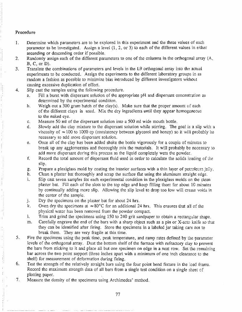
Procedure

1. Determine which parameters are to be explored in this experiment and the three values of each parameter to be investigated. Assign a level (1, 2, or 3) to each of the different values in either ascending or descending order if possible.

2. Randomly assign each of the different parameters to one of the columns in the orthogonal array (A, B, C, or D).

3. Translate the combinations of parameters and levels in the L9 orthogonal array into the actual experiments to be conducted. Assign the experiments to the different laboratory groups in as random a fashion as possible to minimize bias introduced by different investigators wir;hout causing excessive duplication of effort.

4. Slip cast the samples using the following procedure. a. Fill a buret with dispersant solution of the appropriate pH and dispersant concentration as

determined by the experimental condition. b. Weigh out a 300 gram batch of the clay(s). Make sure that the proper amount of each

of the different clays is used. Mix the dry ingredients until they appear homogeneous to the naked eye.

c. Measure 50 ml of the dispersant solution into a 500 ml wide mouth bottle. d. Slowly add the clay mixture to the dispersant solution while stirring. The goal is a slip with a

viscosity of = 100 to 1000 cp (consistency between glycerol and honey) so it will probably be necessary to add more dispersant solution.

e. Once all of the clay has been added shake the bottle vigorously for a couple of minutes to break up any agglomerates and thoroughly mix the materials. It will probably be necessary to add more dispersant during this process as the liquid completely wets the powder.

f. Record the total amount of dispersant fluid used in order to calculate the solids loading of the slip.

g. Prepare a plexiglass mold by coating the interior surfaces with a thin layer of petroleum jelly, h. Clean a plaster bat thoroughly and scrap the surface flat using the aluminum straight edge. i. Slip cast seven samples for each experimental condition in the plexiglass molds on the clean

plaster bat. Fill each of the slots to the top edge and keep filling them for about BO minutes by continually adding more slip. Allowing the slip level to drop too low will create voids in the center of the sample.

j. Dry the specimens on the plaster bat for about 24 hrs. k. Oven dry the specimens at = 80°C for an additional 24 hrs. This ensures that all of the

physical water has been removed from the powder compact. 1. Trim and grind the specimens using 150 to 240 grit sandpaper to obtain a rectangular shape. m. Carefully engrave the end of the bars with a sharp object such as a pin or X-acto knife so that

they can be identified after firing. Store the specimens in a labeled jar taking care not to break them. They are very fragile at this time.

5. Fire the specimens using the peak time, peak temperature, and ramp rates defined by t!he parameter levels of the orthogonal array. Dust the bottom shelf of the furnace with refractory clay to prevent the bars from sticking to it and place all but one specimen on edge in a neat row. Set the remaining bar across the two point support (three inches apart with a minimum of one inch clearance to the shelf) for measurement of deformation during firing.

6. Test the strength of the relatively straight bars using the four point bend fixture in the lload frame. Record the maximum strength data of all bars from a single test condition on a single sheet of plotting paper.

7. Measure the density of the specimens using Archimedes' method.

8. Conduct the confirming experiment(s) if required.

We have conducted this experiment during the Spring and Fall 1991 semesters in a class of approximately 30 Mechanica.1 Engineering seniors. The experiment requires approximately three three-hour laboratory periods to conduct. The laboratory periods are spread over three weeks to allow time for processing steps such as drying and firing of the samples. During the Spring semester the clay body composition, pH of the slip, the firing temperature, and the firing duration were varied. During the Fall semester the firing duration was replaced by the inclusion of different fractions of grog (prefired clay granules) and the ranges of the other variables were modified based upon our experience during the Spring semester. We will present the results from the Fall 1991 semester here.

The parameters and their levels for the experiment that was conducted are presented in Table V. The slips were dispersed with Daxad 305 and ammonium hydroxide to achieve the desired pH. The furnace was heated and cooled at S°C/min and held at temperature for 1 hr. The top and bottom surfaces of the sample bars vvere ground flat and approximately parallel on a 180 grit belt grinder lubricated with flowing water prior to mechanical testing and the broken bars were then used to measure the density of the sample via ~rchimedes'method. However, the results of the density measurements are not presented here due to space limitations.

Table V Parameters and Levels for the Fall 1991 Ceramics Experiment

Parameter Variable Levels

1 - - 2 - 3

A Fraction Redart Clay 0.60 0.80 1 .00 B Fraction Grog 0.00 0.10 0.20 C pH of Dispersant 7 10 12 D Firing Temperature ("C) 1050 1100 1150

The flexural strength as measured in four point bending is presented in Table VI for each of the different experiments. The Taguchi signal-to-noise ratio, q , was calculated using the more is better criterion as presented in appendix A. The particular combination of parameter levels used for each experiment can be found by inserting the values given in Table V into the definition of the L9 orthogonal array given in Table IV.

Based upon these results the effect of each of the different parameters at each of the different levels was calculated foir both the flexural strength and q . The results of these calculations are shown in Table VII and plotted later in Figure 2.

The optimum condition was assumed to be the maximum strength and it is always desired to achieve the maximum value of the Taguchi signal-to-noise ratio, q. The maximum flexural strength was predicted to

Table VI Flexural Strength (MPa) of the Ceramic Bars

Experiment Replication 1 2 3 4 5 6 7

1 2.83 1.98 2.41 3.02 3.35 2.59 2 3.56 3.11 2.98 3.24 3.34 3.87 2.97 3 3.43 3.01 3.53 3.37 3.93 4 8.74 8.11 8.18 8.23 8.67 7.13 6.92 5 2.55 2.37 2.06 2.19 2.06 2.53 2.19 6 3.54 3.61 3.40 3.80 4.54 7 6.71 3.77 5.39 7.03 7.55 5.27 5.44 8 6.59 5.47 6.94 6.50 6.48 6.69 6.42 9 3.52 3.21 3.12 3.25 3.24 3.24 2.82

Mean

2.70 3.30 3.45 8.00 2.80 3.78 5.88 6.44 3.20

Overall Mean 4.34 11.84

Table VII Parameter Effects for the Flexural Strength and 7

Parameter Flexural Strength (MPa) Taguchi 7 (dB) 1 2 3 1 2 3

A -139 0:3 5 0,8 4 -2: 1 0.3 1 120 B 1.19 -0.33 -0.86 1.81 -0.69 -1. IL2 C -0.30 0.50 -0.47 0.09 0.92 -1.01 D -1.61 -0.20 1.63 -3.38 0.30 3.08

be 8.50 MPa for experimental condition A3BlC,D3 and the maximum 7 was predicted to be 119.45 dB for the same experimental condition. This confirming experiment was performed along with A,B,GI,D, which was predicted to have both the second best flexural strength and 7 . The results of these confirming experiments are presented in Table VIII.

Table VIII Flexural Strength (MPa) for the Confirming Experimenb

Condition Replication Mean SIN 1 2 3 4 5 6 7

C,D3 9.78 8.68 8.48 6.87 8.5811.14 4.51 8.30 17.32 A ~ B I C I D ~ 8.31 8.83 9.18 9.27 9.71 7.94 9.90 9.02 19.03

Discussion

The experiment was performed rather smoothly and there were a couple of mild surprises that helped make this a real experiment rather than a cut anddried exercise.Examination of the data in Table VI shows that there was some variability in the flexural strength of the samples as is expected in brittle materials where the strength is often controlled by flaws. However, the variability was not so great as to render the data useless for explaining how changing the parameters can affect the strength.

The effects of the parameters are shown in Table VII and Figure 2 where it is seen that the firing temperamre had the greatest effect upon the strength followed by the two different material composition factors. This is more or less as expected since sintering is a diffusional process and the rate of diffusion increases exponentially with increasing temperature. The first surprise to the students is that the strength is nearly a linear function of the firing temperature which does not agree with the diffusional nature of the sintering process. This can be explained based upon the competition between densification and grain growlh that occurs during sintering. Brittle materials with larger grains typically exhibit lower strengths than similar materials with smaller grains since the size of the largest flaw in the material normally scales w i h the grain size. However, no microscopy was performed to check this theory.

Fraction Redart Fraction Grog Dispersant pH Firing Temperature

4 1

-4 e-L I I I t I t I I I I I

0.60 0.80 1 .00 0.00 0.10 0.20 7 10 1 2 1050 1100 1150 IFsaction Redart Fraction Grog Dispersant pH Firing Temperature

Figure 2 The parameter effects for the flexural strength and the Taguchi signal-to-noise ratio, q.

The oher surprise was that the confirming experiment that was predicted to have the largest flexural strength and optimum Taguchi signal-to-noise ratio did not have the best values. However, it did have a higher strength and a good value of q compared to the nine original experiments. The second confirming experiment, which was predicted to have the second best strength and q, resulted in the best values obtained during the course of this investigation. This indicates that there were interactions between the parameters ha.t are not accounted for in the Taguchi Experimental Method. It might also be possible to explain this result based upon the inconsistent processing since the flexural strength for the first

confirming experiment had the greatest variabiliv of all of the experiments performed even ljhough the Taguchi signal-to-noise ratio predicted that it would have relatively small variabiliv. It would probably be a wise idea to remn the experiment to check this hypothesis.

The values obtained for both the flexural strength and y for the second confirming experimenlt agreed reasonably well with the predicted values for the first confirming experimena&. In addition, the conditions for the hivo experiments only vxied in the least significant experimental parmeter. This finding is in good agreement with the fact &at the effects from the least significant parmeters should not really be used to make predictions since they often fall below the level of the noise in the system. Thiis can be tested by performing analysis of variance (ANOVA), however, this was not done in this case. It also points out the fact that it is normally a good idea to perform the experiment that is predicted to have the second and possibly the third best response in order to find the true optimum response of the system.

'This experiment is a very good hands on introduction to ceramic processing and properties along with h e Taguchi Method of Experimental Design. The results agree fairly well with theory so they can be explained to all but the most introducto~ Materials Science classes. However, the system is not so well behaved that there are no surprises. This property is very useful as a tool to acquaint the student with the fact that real experiments rarely go exactly as planned. In addition, there are a wide variety of pxmeters that can be easily varied so that exactly the same experiment is never performed twice. This prevents the students from using a file to write up the results and keeps the instructor interested since there will always be something that is a little bit different from the last time the experiment was performed.

References

1 M.S. Phadke, , Prentice Hall, NJ 1989,.

2 W.D. Kingery, H.K. Bowen, and D.R. Uhlmmn, Introduction to Ceramics, 3"d Edition, John Wiley & Sons, New York 1976-

3 P. Boch, "Ceramic Processes: Powders in Suspensions - Slip Casting", J. Mater. Educ.,, 6 131 365- 97 (1984).

4 6 . Taguchi, Jikken Keikakuho, Vol. 1 and 2, 3"d Edition (in Japanese), M m z e n , Tokyo Japan, 1977 and 1978 English Translation: 6. Taguchi, System of Experimental Design, VoE. 1 amT 2, ed.by D. Clausing, UNIPUBIKraus International Publications, New York, 1987.

5 P.J. Ross, , McGraw Hill, 1988.

6 L. Panchula and J.W. Patterson, "Demonstration of a Simple Screening Strategy for Multifactor Experiments in Engineering", in National Educators Workshop: Standard Experiments in Materials, Science. & Technoloyy , ed. by J. A. Jacobs and J. Harris, National Institute for Science and Technology, Gaithersberg , MD 1990 .

Appendix A Taguchi Method Design of Experiments

Introduction

The traditional method of investigating the effect of multi-factor or multi-parameter system response is to systematically vary each parameter while simultaneously holding all others constant. This method is very useful for exlploring how a single parameter influences the response. However, it becomes time intensive and costly when many parameters and/or many different parameter settings are investigated. For example, malysis of a four parameter system with three levels for each parameter requires 81 different experiments (39. Conduicting every possible combination for a given set of parameters and levels is referred to as a full facmorial experiment. If one considers that each experiment should be performed a number of times to verify that ale results are reproducible it is seen that hundreds of experiments may be needed to fully investigate this relatively simple system.

marakhlly there are alternative strategies available that dramatically decrease the required n u d e r of experiments. The most familiar of these, and the method associated with certain laboratory experiments (of this course, is the orthogonal array. With orthogonal arrays, as well as other alternative test strategies, it is c o m o n for the volume of information concerning a particular physical relationship to be reduced somewhat. However, provided certain stipulations are met, the data can still be highly informative. The odogonal array is an ordered test sequence that permits statistical comparisons of test results on a partial factorial basis. Its chief advantage is that it allows the experimenter to rapidly determine what factors are critical and to what degree.

(Orthogonal '4rrays

Ohogonal asrays were first conceived by Jacques Wadamard, a French mathematician, in 1897. His purpose was to develop an optimal mathematical system that would allow accurate evaluation of that system" results without a full factorial arrangement. However, it was Genichi Taguchi, a Japanese expert in quality control and assurance, who incorporated these arrays into the manufacturing and design engineering realm. Taguchi also developed a method (to be discussed later in this appendix) that accurately accounts for the statistical variability of the experimental results.

The use of o r~ogona l arrays decreases the number of required experiments to the minimum dictated by the degrees of freedom present in the system. To demonstrate how degrees of freedom are evaluated, it is helghii to make a comparative analogy with an important concept of materials science: the Gibbs Phase Rule for phase equilibria. The Gibbs Phase Rule is expressed as P + F = C + 2, where P is the number of phases, F is the number of degrees of freedom, C is the number of components, and "2" is the number of default degrees of freedom corresponding to pressure and temperature. The number of degrees of freedom in designed experiments is generated in a similar manner. In orthogonal arrays it is a function of the number of different parameters and the number of different levels that each parameter is allowed. The n u d e r of degrees of freedom for a system that obeys this criteria is given by

where DF is the number of degrees of freedom, F is the number of different factors, V is the number of different values that each factor can have, and the "1 " accounts for the mean of all of the responses.

Application of equation A.1 to our system of four different parameters with three levels for each yields nine degrees of freedom, nearly an order of magnitude fewer experiments than the tradition~al approach. In fact, the number of degrees of freedom of a Taguchi experimental system is closely related to the number of equations required to solve a set of linear equations containing N unknowns.

Taguchi differentiates experimental factors into two categories: those that the experimenter can comrol md those that are beyond control. The first of these are known as parameters while the latter are known as noises. As discussed below, the parameters can be assigned several levels. The noises normally assume a random value governed by an appropriate distribution function. However, for experimental pueposes they are sometimes intentionally introduced to the system in a controlled manner as parameters. Using Taguchi's nomenclature, equation A. 1 can be rewritten as

where P and L are the number of parameters and levels, respectively

The similarity of the orthogonal array to a set of linear equations brings forth the first criteria for applicability which is: the effect on the response from each system parameter must be additive. Strictly speaking, this means that orthogonal arrays cannot be expected to produce perfect results when the parameters interact with one another. The problem with parameter interaction is that it produces a response that is not equivalent to the sum of the individual parameter influences. Typically, parmeters have small interactions which allow a nearly linear relationship between the responses of an individual parameter and the overall system.

The non-additive interactions between parameters are classified as synergistic when the paralneters compliment each other to improve the response, and anti-synergistic when the parameters conflict with each other and diminish the response. It turns out that synergistic interactions present fewer problems than anti-synergistic interactions in the analysis. Unfortunately, the parameters in most systems interact to some extent and designed experiments will not yield perfectly conclusive results. However, for a vast majority of systems the interactions are not overwhelming. In these situations these arrays can be used to optimize the system, especially when measures are taken to minimize interactions between parameters.

Orthogonal arrays are based upon the assignment of each of the parameters to one axis in an orthogonal n- dimensional coordinate system. Everyone is familiar with orthogonal coordinate systems of 2 or 3 dimensions, normally referred to as cartesian coordinate systems. Features of these lower dimensional systems can be generalized into higher order, n-dimensional versions. In these multidimensional coordinate systems, the system response to a given set of values of the parameters can be ploltted as a point in the n-dimensional space. It follows that each point in space corresponds to a given set of conditions of the n parameters and is in fact given by a unique combination of the parameters.

A slight complication of designed experiments is that orthogonal arrays only exist for a select number of test conditions. This does tend to limit the usefulness of this method to particular parameter and level combinations. It is possible to use dummy arguments to supplement the parameters and/or levels present, thereby allowing arbitrary quantities of either to be examined. However, there are two disadvantages involved with the use of dummy arguments. The first is that more experiments must be performed ~ l h a n

dictated by the degrees of freedom of the system. The extra experiments allow the array to remain orthogonal with balanced interactions among the parameters. The second is that the set of experiments may be more sensitive to the effects of some parameters than to others due to the arrangement of the

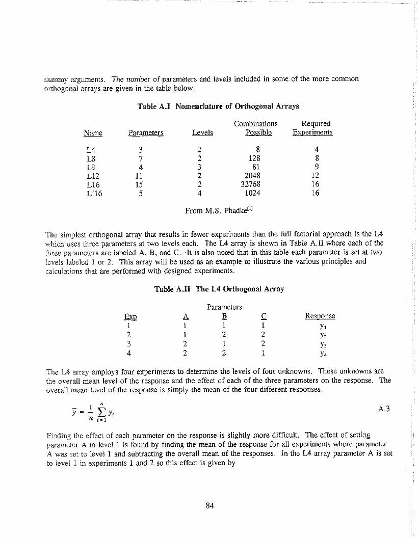
dummy uguments. The number of parameters and levels included in some of the more c o m o n oaogonal arrays are given in the table below.

Table A.I Nomenclature of Orthogonal Arrays

Combinations Required Parameters Levels Possible Ex~eriments

From M.S. Phadke[ll

The simplest odogonal array that results in fewer experiments than the full factorial approach is the L4 which uses three parameters at two levels each. The LA array is shown in Table A.11 where each s f the three pxmete r s are labeled A, B, and C. .It is also noted that in this table each parameter is set at two levels Babeled 1 or 2. This array will be used as an example to illustrate the various principles and calculations that are performed with designed experiments.

Table A.II The L4 Orthogonal Array

Parameters E3.P - A - B - C Response 1 1 1 1 Y 1

2 1 2 2 Y2

3 2 1 2 Y3

4 2 2 1 Y4

The U asray employs four experiments to determine the levels of four unknowns. These unknowns are the overall mean level of the response and the effect of each of the three parameters on the response. The overall mean level of the response is simply the mean of the four different responses.

Finding the effect of each parameter on the response is slightly more difficult. The effect of setting p x m e t e r A to level 1 is found by finding the mean of the response for all experiments where parameter ,A was set to level 1 and subtracting the overall mean of the responses. In the L4 array parameter A is set to level 1 in experiments 1 and 2 so this effect is given by

where a, is used to denote the effect of parameter A at level 1 on the response. The effect of parameter A at level 2 is found in a similar manner such that

Using the same reasoning, the effects of the other parameters are found in a similar fashion. For example, the effect for b, would require the responses generated by the first and third experiments. This process can be extended to larger arrays. Equation A.6 shows this relationship in its general form. The effect of any particular parameter level is found by subtracting the overall mean from the mean of the responses where the parameter of interest has that desired level. In this equation the effect of parameter Q at level m is desired, and there are n experiments where parameter Q was set to level m.

Examination of equations A.4 and A.5 reveals that a, = - a,. In fact one of the results of the orthogonality of the arrays is that the sum of the effects of different levels for each parameter must equal zero regardless of the number of levels involved such that

As part of this type of experimentation it is frequently necessary or desirable to conduct more than one test per condition. Conducting multiple tests, known as experimental replications, insures that the statistical variability of the testing process is reduced. It also insures that the result of the experiment is repeatable. If the response for a given condition has a high degree of variability this usually means that the response is susceptible to outside factors. These factors are referred to as noises in the system. Reducing the level of noise is almost always beneficial for the process. In manufacturing situations, it may be more desirable to reduce the noise in the system than to achieve the absolute optimal response.

An additional concern is that systematic errors may occur that can distort the results. The most common type of systematic error is for one of the measuring systems, such as a thermocouple, to drift resulting in recording different values for the same phenomena. The normal solution to this problem is randomization of the experimental process so that the drift does not affect one parameter more than another. Another common solution is to periodically run a calibration experiment to check for drift. Phadke['] states that systematic errors are normally not as large a problem as simple set up errors, particularly with the small number of experiments required in a Taguchi style experiment. As such he recommends that the experiments be run in order and that the most difficult parameters to change be placed on the left hand side of the array (parameter A & B). This is because the left hand parameters in most orthogonal arrays will have to be changed less frequently during the course of experimentation than the others. If this technique is employed, it is a good idea to run calibration experiments to check for systematic errors,

pafliculxly if the experimental process is long and drawn out. A commor. technique is to rerun the first experiment after the end of the main experimental process.

Signal-to Noise Ratios

The signal-to-noise ratio, SIN, is frequently used to combine optimization of the response with reduction of the vxiabiliity due to noise. The term SIN originated in the area of electronic circuit design where it was desirable to maximize the output of an amplifier for a given power input while minimizing the mount of noise introdiuced into the signal. It is obvious that the optimal result is an infinite SIN due to a combination of' the output going towards infinity and the noises going to zero. A further result of the electronic origin of the SIN is that the values are normally converted to decibels, dB

SIN = 181og (signal-to-noise $nction) A. 8

where the exact form of the signal-to-noise@nction depends upon both the nature of the response to be optimized and the nature of the noises. An additional advantage of this formulation is that values for the extreme cases are converted to more manageable numbers. Signal-to-noise ratios approaching infinity (a good system) yield much smaller, more tightly grouped numbers using this transformation while in very noisy systems (SIN * O), the transformation results in more widely spread numbers.

The signal-to-noisefinction for any given set of replicated measurements can be evaluated in the general sense as a coartbination of two factors: mean value of a desired response and variability about that mean. These factors are accounted for in the relationship

where p is the mean value of the response and a is the standard deviation of the response for the populafon. lit is readily seen that larger values of the mean or smaller values of the standard deviation will result in 21 larger SIN. This is a typical case of more-is-better where the desire is to maximize the response of the system while minimizing the noise.

The signal-to-noise evaluation is designed so that it is always desirable to get the most positive value. 'This makes practical sense if the response is viewed from the standpoint of a ratio of desired output to undesirable signal randomness. For this reason it is sometimes necessary to modify the formulation of the signal-to-noise function or the logarithmic transformation from the most obvious form.

Taguchi introduced the concept of a parabolic loss function which is closely related to the signal-to-noise ratio in that it states that a part or process that is not right on target leads to an additional, avoidable cost. This Taguchi loss function, L(y), for a given part or process step is

where y is the measured response, T is the target value, k is the cost of deviation from the target.

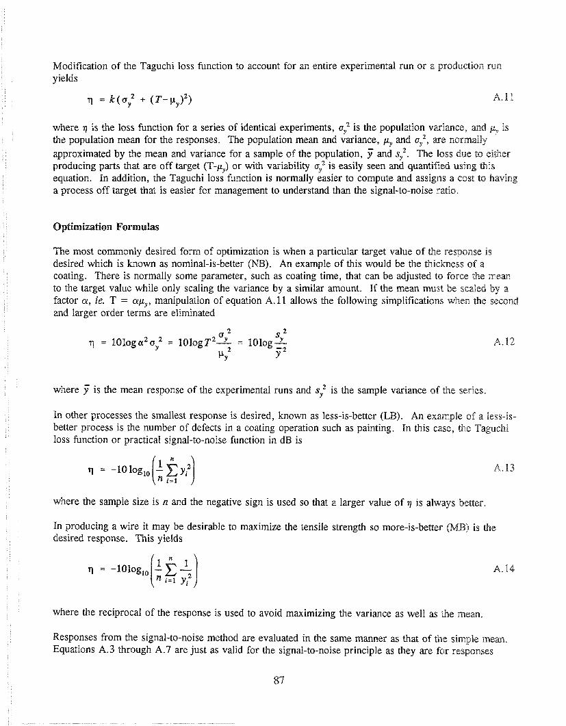
Modification of the Taguchi loss function to account for an entire experimental run or a production run yields

where 17 is the loss function for a series of identical experiments, a: is the population vxiance, and gn, is the population mean for the responses. The population mean and variance, p, and a;, are normally approximated by the mean and variance for a sample of the population, y and s;. The lioss due to either producing parts that are off target (T-y) or with variability a; is easily seen and quantified using this equation. In addition, the Taguchi loss function is normally easier to compute and assig~ls a cost to having a process off target that is easier for management to understand than the signal-to-noise ratio.

Optimization Formulas

The most commonly desired form of optimization is when a particular target value of the response is desired which is known as nominal-is-better (NB). An example of this would be the ~ i c k n e s s of a coating. There is normally some parameter, such as coating time, that can be adjusted to force the mean to the target value while only scaling the variance by a similar amount. If the mean must be scaled by a factor a, ie. T = ah, manipulation of equation A. 11 allows the following simplifications when the second and larger order terms are eliminated

where is the mean response of the experimental runs and s: is the sample variance of the series.

In other processes the smallest response is desired, known as less-is-better (LB). An example of a less-is- better process is the number of defects in a coating operation such as painting. In this case, the Taguchi loss function or practical signal-to-noise function in dB is

where the sample size is n and the negative sign is used so that a larger value of 7 is always better

In producing a wire it may be desirable to maximize the tensile strength so more-is-better (MB) is the desired response. This yields

where the reciprocal of the response is used to avoid maximizing the variance as well as the mean.

Responses from the signal-to-noise method are evaluated in the same manner as that of the simple mem. Equations A.3 through A.7 are just as valid for the signal-to-noise principle as they are for responses

developed using a statistical average. The y values are now assumed to be generated by the appropriate equations for 7 listed above and are assumed to be in decibels rather than having the same dimensions or units of the physical properties they evaluate. Taguchi's signal-to-noise ratio has the added feature of evaluating consistency among a series of replications as well as how close the system output is to the desired output. Simply put, the signal-to-noise method requires both optimum magnitude (high, low, or nominal) md consistent results to yield the best response. As a result it is strongly recommended that one of the varimts of Taguchi's signal-to-noise ratio be used to optimize the system rather than only the response. The disadvantage of having to perform each experiment more than once is more than compensated for by the knowledge gained about the quality of the response.

Compuhtional Procedure

Once the overall mean for all the responses and the effects of each parameter have been calculated the system can be optimized to predict which level of each parameter will give the best result. The general equation for the: model used to evaluate a predicted response has the form

yPed = + C para. efi + C interahon e 8 + error

The terms on the right side of this equation,are, from left to right, the overall mean, the summation of all of the parmeter effects, the summation of any interaction effects between the parameters, and any statistical error anributed to differences in the measured response between the statistical sample and its population.

Parameter interactions are present when two or more parameters interact to cause a different net effect ahm if both p a m e t e r effects were evaluated as separate entities and then summed together. Much of the time interactions are regarded as an undesirable part of experimental testing, especially in partial factorial experirnentation.This is because it is difficult for them to be properly identified without conducting an additional series of designed experiments or several different confirming experiments. A common example of a p,arameter interaction is when two reactive chemicals are introduced as parameters in a production process. If the chemicals were to be evaluated onan individual basis, one chemical without the other, the response could be radically different than if both were evaluated together.

Error invades experimentation from numerous sources that are either in or out of the experimenter's control. One source of error stems from inaccuracies in the measurement of some physical quantity. Error like this might be based on inconsistency of testing done by the experimenter(s) or using poorly calibrated measuring equipment. With careful control of the process and the related measurement melihods, this type of error may be significantly reduced, if not eliminated. A source of error less easily ecanhro~led may result from the random behavior of a tested material based on its flaws or microstructural difkrences.

Because the method used in this experiment is not designed to account for such things as interactive parmeters or statistical error, those respective terms in equation A.15 are not taken into account. This results in a equation for the predicted response being

Ypred = Y + C para. efi

For a three parameter system the predicted response can be expressed as

where the last three terms in this equation represent the desired effects of these parameterz;. For instmce, if the largest possible mean response is desired, the predicted response is found by taking the most positive level for each parameter and adding this to the mean. If the smallest possible mean response is desired, the predicted response is found by taking the most negative level of each parameter and adding it to the mean. For the Taguchi signal-to-noise response the most positive parameter effects are always desired to optimize conditions. If the experiment defined by the predicted parameter levels has not already been conducted, it is then necessary to conduct this experiment to confirm that this is indeed the largest response. If the prediction and the confirming experiment do not agree, there is a strong indication that the parameters interact and that Taguchi's method may not give accurate results. h o & e r complication that can arise is that several conditions may generate similar predictions, which is more common in higher order arrays. In both cases it will be necessary to conduct more than one confirming experiment utilizing the best few sets of levels to determine which results in the one optimal response.

Often times it is convenient to show the relative effect for each parameter by means of a line chart. These charts graphically represent the relationship each parameter level has on the response. Typically two things are inferred by these types of graphs: the relative magnitude of effects between parameters ;and the trend of effects for the various levels within any given parameter. Both pieces of informat:ion can be extremely useful for optimization purposes.

Another way of demonstrating the relative effect each parameter setting has on the response is the use of a Pareto diagram. This diagram is a simple bar graph that arranges categories of influence in descending order. The specific categories considered in this chart depend on the situation analyzed. The intent of these charts is to graphically demonstrate how some parameters have significant influences on the results, while others are relatively insignificant. In a majority of designed experiments the numbel- of pame te r s having a major role in the outcome is considerably smaller than the others. This is referred to in quality engineering circles as separating the vital few from the trivial many. For experiments conducted in the laboratory the objective of using Pareto diagrams is to compare and contrast the optimum of parmeter levels affecting the response(s).

Two examples follow showing how this data reduction process is carried out. The first example is a system that includes three parameters at two levels each to demonstrate the fundamental principles of this experimental process. A designed experiment of this size is listed in Table A.1 as the L4 ofiogonal array. The second example involves an L9 orthogonal array with four parameters at three levels each, to show how the technique can be extended to a more complicated system.

Example 1

The orthogonal array and the fictitious experimental results for this example are shown in Table A.III. Each experiment has been carried out repeatedly to improve the quality of the responses. These results are shown as the five test replications to the right of the test matrix. The mean response, q, and the variance (square of the standard deviation) for each experimental condition are then tabulated to the right of the raw data. This example assumes that the test objective is to minimize the response (LB). For example, the measured response might be the density of a manufactured part or experimental specimen.

Table A.III Results from an L4 Designed Experiment

Or~ogona l 'Matrix Experimental Replications

ExoLI El C 1 2 3 4 5 Mean 22 1 1 1 1 13.9 12,8 1<5 15.1 13.4 13.94 0.81 -22.90 2 1 2 2 14.4 11.8 13.2 13.4 12.9 13.14 0.88 -22.39 3 2 1 2 19.4 18.5 14.9 15.3 17.6 17.14 3.89 -24.73 4 2 2 1 9.3 10.4 12.6 12.4 11.4 11.22 1.92 -21.05

Overall Means 13.86 1.88 -22.77

The Taguchi signal-to-noise ratio was calculated via equation A. 13. In this case all of the signal-to-noise values are negative so the largest and most desirable 7 is that which is least negative. The variance is provided as an indication of the combined noises within the system. A couple points of interest should be observed. First, based on the mean and the signal-to-noise responses, the fourth experimental condition is the best of the four test conditions. This suggests that the random noises of this experimental condition are low enough to give the lowest overall response even though they are not the lowest observed. Also, the sequence of experimental conditions, from best to worse, is the same for both methods. This is one indication that the experiment is probably "on track". If the two methods produced sequences that were drastically different there would be some reason for concern.

The next step in this process is to find the effect each parameter has on the response. To do this the mean for all the individual responses corresponding to each particular parameter level must be calculated. The overall mean is then subtracted from each of these values as shown in equation A.6. For instance the first two experimental conditions both have parameter A set to level 1. By first finding the mean of these two responses and subtracting the overall response mean, the effect a, is found to be

The value of a, is found by a corresponding computation where the levels of the A parameter are set to level 2.

It should be noted that for a two level system the effect on the parameter of the first level is always the negative of the second. The effects of each level on each of the parameters for all three responses (mean, q , md variance) are calculated in a similar manner and are tabulated in Table A.IV.

The system is optimized by selecting the parameter combination yielding a response that is closest to the desired. In this example the mean is to be minimized so the level of each parameter with the most negative effect is used to determine the optimal predicted mean. The best combination is when level 1 is used for parameters A and C and level 2 is used for parameter B. This combination is denoted as A,B,C, and yields a predicted response of 10.58 which is calculated as shown in equation A.17. Since this combination was not used as one of the original four experiments it is necessary to conduct a confirming

Table A.IV Example L4 Array Parameter Effects on System Responses

Parameter A Parameter B Parameter C

Mean a, = -0.32 bl = 1.68 c, = -1.28 a, = 0.32 b, = -1.68 c, = 1.2!8

7 a, = 0.123 bl = -1.047 c, = 0.7'93 a, = -0.123 b2 = 1.047 c2 = -0.793

Variance a, = -1.04 b, = 0.47 cl = 0.85 a, = 1.04 bz = -0.47 c, = -0.85

experiment. An additional point is that parameter B had the greatest effect on the mean followed by C and A.

A similar analysis can be conducted for the other two responses. The variance of the system will be minimized (less noisy) under condition AlB2& with an expected value of -0.48. This experiment Was conducted with a result of 0.88 indicating that there are either strong interactions between the pame te r s that affect the level of noise or large random noises entered the experiments. In addition, it is impossible for the variance to be less than zero. The signal to noise ratio is maximized for condition A,B2G, with a predicted value of -20.81. This is the same combination that was predicted to minimize the: mean, which is comforting.

The relative effect of the different parameters on the responses can be shown by generating a Pareto diagram based on the reduced data. The relative effects are found by taking the difference between the maximum and minimum effect of each individual parameter. Table A.V gives the difference betvveen the maximum and minimum level for each parameter and the percentage that each parameter contributes toward the total effect.

Table A.V Relative Parameter Effects for Example 1

Mean Response Signal-to-Noise Noise a, - a, = 0.64 (9.8%) a, - a, = 0.246 (6.3%) a, - a, = 2.04 (43.6%) bl - b, = 3.36 (51.2%) bl - b2 = 2.094 (53.3%) bl - C, = 0.94 (20.1 %) C, - C, = 2.56 (39.0%) C, - C , = 1.586 (40.4%) c1 - C, = 1.70 (36.3%)

The percents are plotted as a bar chart to create the Pareto diagram for the system. The Pareto diagram for this system is shown in Figure A.1. It is seen that significance of each parameter depends upon response considered. As stated above parameter B is the most important in determining the mean and signal-to-noise ratio while A is the most important in determining the noise.

Example 2

This example uses an L9 orthogonal array to explore the effect of four parameters at three levels on the measured response. Multiple test runs were conducted in this example but only the final response for each experimental condition is shown in Table A.VI. This example assumes that the response is some&ing which is to be maximized, such as strength.

Mean Noise Measured Response

Figure A.1 Pareto diagram of the responses of example 1.

Table A.VI Results from an L9 Designed Experiment

Parameter level combinations Mean Em - A - B - C - D Res~onse

Overall Mean 575

As in the previous example, the first step in this process is to find the effect that each parameter level has on the response. The first three experimental conditions were all conducted with parameter A set to level 1. The effect of level 1 on parameter A is found in the same way as in the previous example

Corresponding computations are made for parameter A at levels 2 and 3 which are shown below.

The effect of each of the different levels on each of the parameters i s calculated in a similar manner and is tabulated in Table A.VII.

Table A.VII Example L9 Array Parameter Effects on System Response

Parameter A Parameter B Parameter C Parameter D

The maximum predicted strength is found by using the maximum value of the effect for each of the four parameters. The combination of parameter levels that maximizes the response is A,B,C,D, ~vith a predicted value of 831.67. This condition is not one of the original nine combinations that were tested so a confirming experiment is required. The parameter that had the greatest bearing on the response was parameter D, followed by C, A, and B in descending order of importance. The effect that each pamete r had upon the strength is shown in Figure A.2 as a line plot.

Parameter A Parameter B Parameter C Parameter D

Figure A.2 The parameter effects from example 2.

Am additional observation is that some parameters have levels that are much more beneficial to the desired system response than others. The effects of parameters C and D show this behavior such that one of the levels is Barge and positive while the other two are moderate and negative. This type of behavior indicates &at the proper range of levels for these parameters was not chosen for the experiment to truly optimize alae performance of the system since all of the beneficial effects occurred for one of the levels. It is then necessary to conduct either the entire experiment or an experiment based upon another orthogonal array using new levels for these parameters. The next experiment should use a range of levels for the pxmeters 'hat had very skewed effects that explores the values of the levels around the optimum from the first experiment in more detail.

The use of orthogonal arrays of designed experiments is a powerful tool for efficiently investigating the effect of a number of parameters on the response of a system. The method dramatically decreases the number of experiments that must be performed in comparison with the classical scientific experimental approach. However, there are a number of difficulties that can arise which limit the usefulness of the method. The biggest of these is that systems of orthogonal arrays rely on the response of the system being determined by addition of the individual effects of each parameter. Interaction of the parameters invalidates this assumption and means that the predicted response will not be accurate. If the interactions are weak (a common occurrence) this simply lowers the precision of the prediction. However, if the interactions are strong the entire system will be invalidated. As with all powerful analysis tools the engineer or scientist must apply a good deal of knowledge and common sense to design a set of experiments that attempts to minimize parameter interactions and use good judgement in interpreting the results.

Appendix B Plaster Bats

Plaster bats are frequently used to cast ceramic slurries because they are inexpensive, easily shaped, and reasonably efficient. Plaster is composed of fine needles of hydrated calcium sulfate (gypsurn) containing a continuous network of submicrometer pores. It is these pores that wick the water or other solvent out sf the ceramic slurry during slip casting. Unfortunately, these pores become clogged with fine cermic particles, salts, and organics from the slurry which necessitates periodic replacement of the bat.

Plaster bats can be cast into nearly any shape in order to make a mold for slip casting a cermic slurry. We use flat bats with an impervious mold placed on its top surface to contain the slurry. The geometry is simpler to work with, and results in unidirectional casting and fewer voids and less residual stress in the green body.

Procedure

1. Coat the inside surfaces of the bat mold with a thin layer of petroleum jelly to prevent the plaster from sticking to the mold. We use a sheet of glass for the bottom of the mold and a 15 by 20 cnn wood rectangle 4 cm tall held together by nails for the sides of the mold.

2. Separately measure 1 g of dry plaster-of-parishnd 0.61 ml of water (use a graduated cylinder and not a beaker) for each one cm3 of plaster to be cast. This allows for some waste and the water may need to be adjusted based upon the relative humidity (less in more humid climates than Albuquerque).

3. Add the plaster to the water in a flexible bucket while stirring and breaking up the lumps. The best tool for stirring is your hand. The only drawback to this method is that the plaster can tend to dry the skin so application of hand lotion after washing is suggested.

4. Pour the plaster slurry into the mold and vibrate to fill the corners of the mold and to bring the air bubbles to the surface. Wipe the excess plaster out of the bucket and allow the rest to harden. Bt can be broken away from the bucket followed by washing. Putting unhardened plaster down the drain is not recommended since it tends to set in the pipes.

5. Level the top surface of plaster bat with a straightedge. We use a piece of aluminum sheet 5 by 25 by 0.2 cm.

6. When the bat has hardened enough to keep its shape (approximately 30 to 90 minutes) remove it from the mold. Then scrape the top and bottom surfaces smooth and flat using the straightedge a d gently bevel all of the corners to keep them from breaking off.

7. Allow the bat to air dry for two to four days to remove most of the excess water. The rest of the water can be removed by drying in a low temperature oven (< 90°C). Do not heat the plaster bat above 100°C since this may result in partial dehydration of the plaster accompanied by cracking md sometimes explosive fracture. Plaster particles should be kept out of the ceramic body to avoid fracture of the ceramic body during firing.

After use the plaster bat can be renewed by scrubbing the surface and redrying. If the surface becomes pitted, it is most easily flattened by soaking in water for a few minutes to soften it and scrapping with the straightedge. The bats will probably have to be retired after five to ten uses depending upon the hardness of the water and the dispersants used.

"1 Pottery Plaster available from most ceramics supply companies.

95