Embed Size (px)
Citation preview
Maybe It Really Is Different This Time
Presentation to: Nomura Quantitative Investment Strategies ConferenceJune 16, 2009
Robert C. [email protected]

1
Agenda
A Review of August, 2007
B The “Stickers” versus the “Adapters”
C The Stickers’ case:
Long-term perspective: HML and WML
Normal ebb and flow
D The Adapters’ case:
Quant crowding
Adjusting for trading and liquidity
E The future of quantitative equity management
2
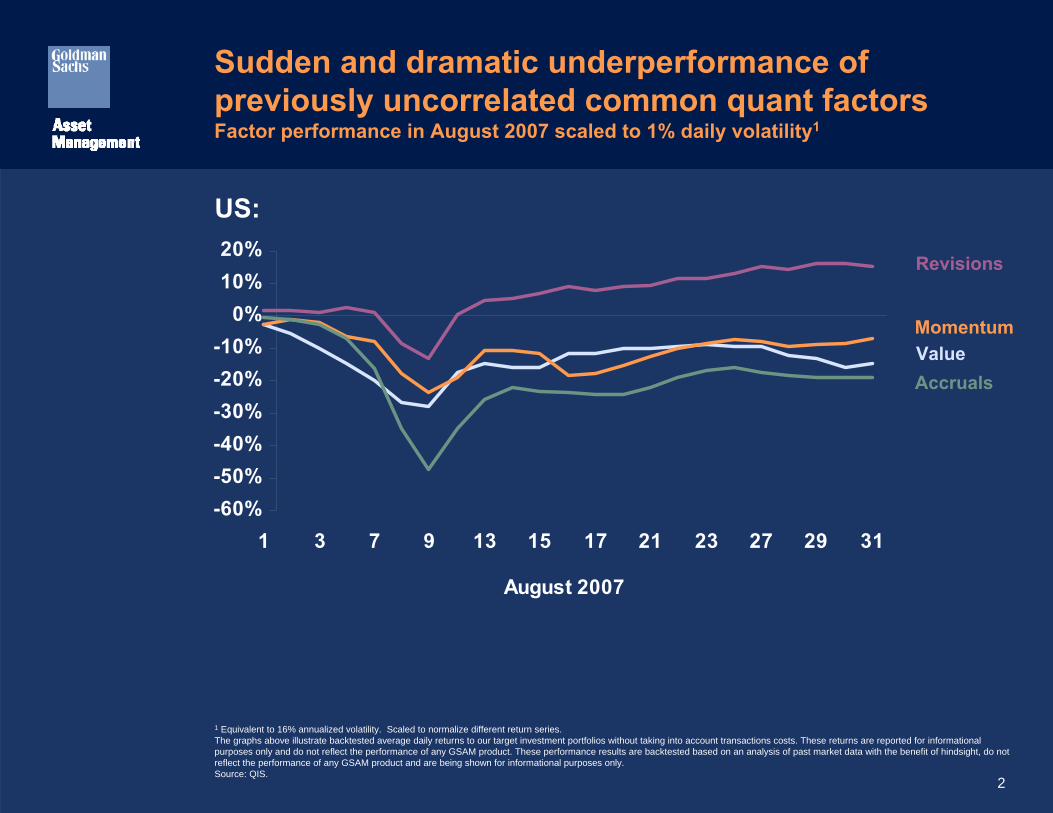
Sudden and dramatic underperformance of previously uncorrelated common quant factorsFactor performance in August 2007 scaled to 1% daily volatility1
US:
Revisions
MomentumValueAccruals
-60%-50%-40%-30%-20%-10%
0%10%20%
1 3 7 9 13 15 17 21 23 27 29 31
August 2007
1 Equivalent to 16% annualized volatility. Scaled to normalize different return series.The graphs above illustrate backtested average daily returns to our target investment portfolios without taking into account transactions costs. These returns are reported for informational purposes only and do not reflect the performance of any GSAM product. These performance results are backtested based on an analysis of past market data with the benefit of hindsight, do not reflect the performance of any GSAM product and are being shown for informational purposes only. Source: QIS.
3
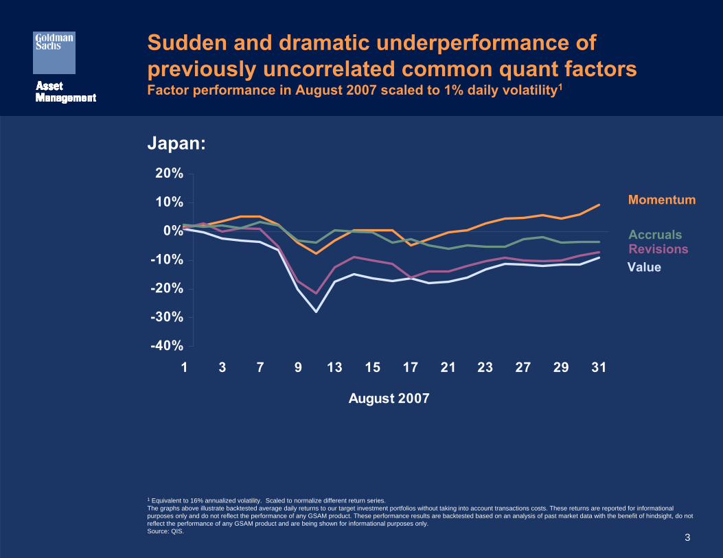
Sudden and dramatic underperformance of previously uncorrelated common quant factorsFactor performance in August 2007 scaled to 1% daily volatility1
Japan:
Revisions
Momentum
Value
Accruals
-40%
-30%
-20%
-10%
0%
10%
20%
1 3 7 9 13 15 17 21 23 27 29 31
August 2007
1 Equivalent to 16% annualized volatility. Scaled to normalize different return series.The graphs above illustrate backtested average daily returns to our target investment portfolios without taking into account transactions costs. These returns are reported for informational purposes only and do not reflect the performance of any GSAM product. These performance results are backtested based on an analysis of past market data with the benefit of hindsight, do not reflect the performance of any GSAM product and are being shown for informational purposes only. Source: QIS.
4
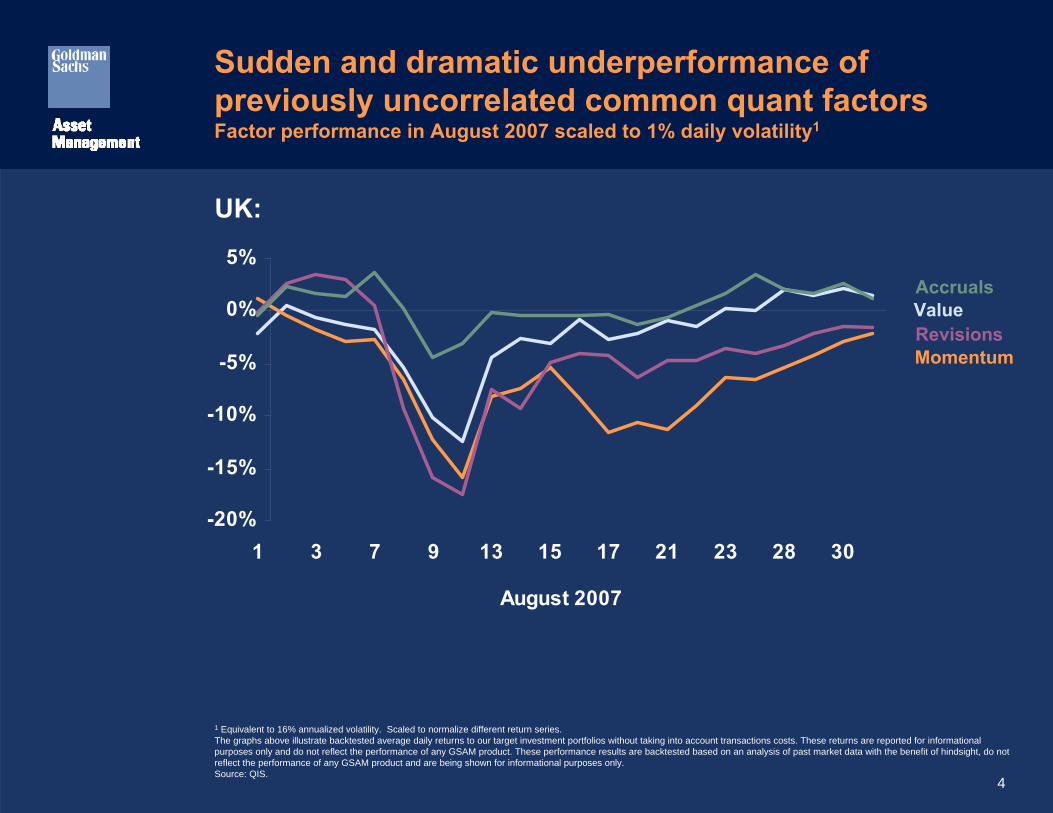
Sudden and dramatic underperformance of previously uncorrelated common quant factorsFactor performance in August 2007 scaled to 1% daily volatility1
UK:
RevisionsMomentum
ValueAccruals
-20%
-15%
-10%
-5%
0%
5%
1 3 7 9 13 15 17 21 23 28 30
August 2007
1 Equivalent to 16% annualized volatility. Scaled to normalize different return series.The graphs above illustrate backtested average daily returns to our target investment portfolios without taking into account transactions costs. These returns are reported for informational purposes only and do not reflect the performance of any GSAM product. These performance results are backtested based on an analysis of past market data with the benefit of hindsight, do not reflect the performance of any GSAM product and are being shown for informational purposes only. Source: QIS.

5
Sudden and dramatic underperformance of previously uncorrelated common quant factorsFactor performance in August 2007 scaled to 1% daily volatility1
Continental Europe:
RevisionsMomentum
ValueAccruals
-25%
-20%
-15%
-10%
-5%
0%
5%
1 3 7 9 13 15 17 21 23 27 29 31
August 2007
1 Equivalent to 16% annualized volatility. Scaled to normalize different return series.The graphs above illustrate backtested average daily returns to our target investment portfolios without taking into account transactions costs. These returns are reported for informational purposes only and do not reflect the performance of any GSAM product. These performance results are backtested based on an analysis of past market data with the benefit of hindsight, do not reflect the performance of any GSAM product and are being shown for informational purposes only. Source: QIS.
6
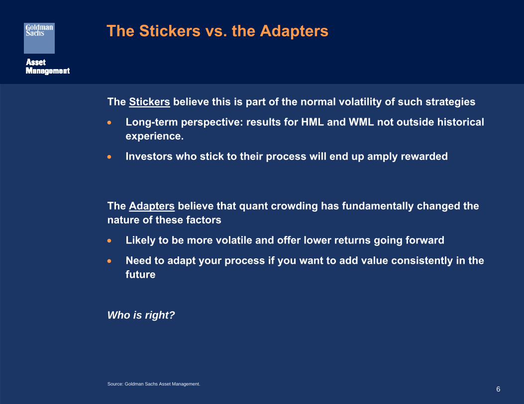
The Stickers vs. the Adapters
The Stickers believe this is part of the normal volatility of such strategies
• Long-term perspective: results for HML and WML not outside historicalexperience.
• Investors who stick to their process will end up amply rewarded
The Adapters believe that quant crowding has fundamentally changed the nature of these factors
• Likely to be more volatile and offer lower returns going forward
• Need to adapt your process if you want to add value consistently in the future
Who is right?
Source: Goldman Sachs Asset Management.
7
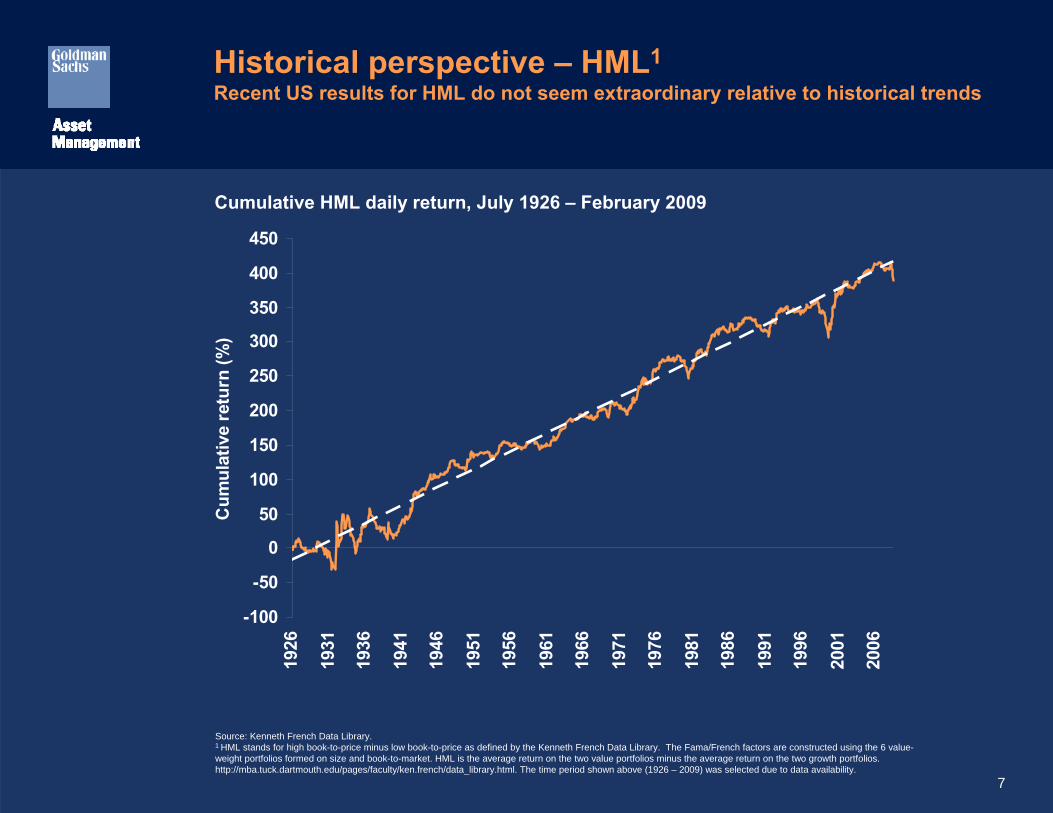
Historical perspective – HML1Recent US results for HML do not seem extraordinary relative to historical trends
Cumulative HML daily return, July 1926 – February 2009
Source: Kenneth French Data Library. 1 HML stands for high book-to-price minus low book-to-price as defined by the Kenneth French Data Library. The Fama/French factors are constructed using the 6 value-weight portfolios formed on size and book-to-market. HML is the average return on the two value portfolios minus the average return on the two growth portfolios. http://mba.tuck.dartmouth.edu/pages/faculty/ken.french/data_library.html. The time period shown above (1926 – 2009) was selected due to data availability.
-100
-50
0
50
100
150
200
250
300
350
400
450
1926
1931
1936
1941
1946
1951
1956
1961
1966
1971
1976
1981
1986
1991
1996
2001
2006
Cum
ulat
ive
retu
rn (%
)
8
-100
0
100
200
300
400
500
600
700
800
900
1927
1932
1937
1942
1947
1952
1957
1962
1967
1972
1977
1982
1987
1992
1997
2002
2007
Cum
ulat
ive
retu
rn (%
)
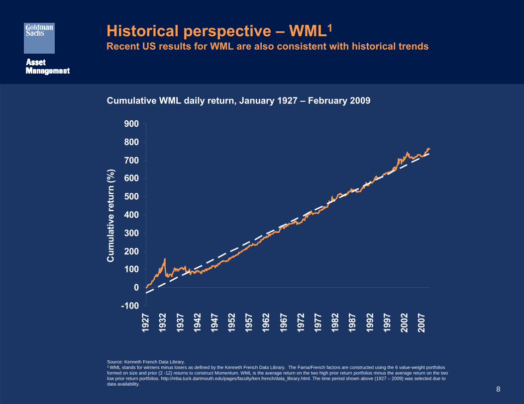
Historical perspective – WML1Recent US results for WML are also consistent with historical trends
Cumulative WML daily return, January 1927 – February 2009
Source: Kenneth French Data Library. 1 WML stands for winners minus losers as defined by the Kenneth French Data Library. The Fama/French factors are constructed using the 6 value-weight portfolios formed on size and prior (2 -12) returns to construct Momentum. WML is the average return on the two high prior return portfolios minus the average return on the two low prior return portfolios. http://mba.tuck.dartmouth.edu/pages/faculty/ken.french/data_library.html. The time period shown above (1927 – 2009) was selected due to data availability.
9
0.0%
0.2%
0.4%
0.6%
0.8%
1.0%
1.2%
1.4%
Mar
-99
Dec-
99
Sep
-00
Jun-
01
Mar
-02
Dec-
02
Sep
-03
Jun-
04
Mar
-05
Dec-
05
Sep
-06
Jun-
07
Mar
-08
Dec-
08
Sele
ct Q
uant
AU
M /
Rus
sell
3000
AU
M
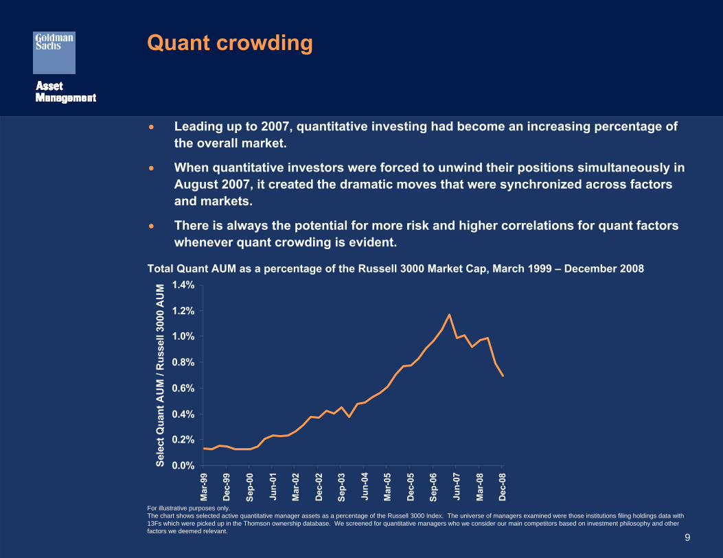
Quant crowding
• Leading up to 2007, quantitative investing had become an increasing percentage of the overall market.
• When quantitative investors were forced to unwind their positions simultaneously in August 2007, it created the dramatic moves that were synchronized across factors and markets.
• There is always the potential for more risk and higher correlations for quant factors whenever quant crowding is evident.
Total Quant AUM as a percentage of the Russell 3000 Market Cap, March 1999 – December 2008
For illustrative purposes only. The chart shows selected active quantitative manager assets as a percentage of the Russell 3000 Index. The universe of managers examined were those institutions filing holdings data with 13Fs which were picked up in the Thomson ownership database. We screened for quantitative managers who we consider our main competitors based on investment philosophy and other factors we deemed relevant.
10
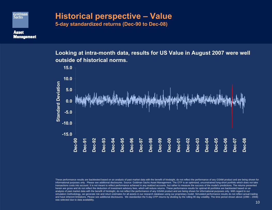
Historical perspective – Value5-day standardized returns (Dec-90 to Dec-08)
Looking at intra-month data, results for US Value in August 2007 were well outside of historical norms.
These performance results are backtested based on an analysis of past market data with the benefit of hindsight, do not reflect the performance of any GSAM product and are being shown for informational purposes only. Please see additional disclosures. Source: Goldman Sachs Asset Management. The OTP is an optimized, unconstrained long-short portfolio which does not take transactions costs into account. It is not meant to reflect performance achieved in any realized accounts, but rather to measure the success of the model's predictions. The returns presented herein are gross and do not reflect the deduction of investment advisory fees, which will reduce returns. These performance results for optimal tilt portfolios are backtested based on an analysis of past market data with the benefit of hindsight, do not reflect the performance of any GSAM product and are being shown for informational purposes only. With regard to our simulation methodology, we generate risk and return estimates for all assets in our research database using our proprietary model. Simulated performance results do not reflect actual trading and have inherent limitations. Please see additional disclosures. We standardize the 5-day OTP returns by dividing by the rolling 90 day volatility. The time period shown above (1990 – 2008) was selected due to data availability.
-15.0
-10.0
-5.0
0.0
5.0
10.0
15.0D
ec-9
0
Dec
-91
Dec
-92
Dec
-93
Dec
-94
Dec
-95
Dec
-96
Dec
-97
Dec
-98
Dec
-99
Dec
-00
Dec
-01
Dec
-02
Dec
-03
Dec
-04
Dec
-05
Dec
-06
Dec
-07
Dec
-08
Sta
ndar
d De
viat
ion
11
-15.0
-10.0
-5.0
0.0
5.0
10.0
15.0De
c-90
Dec-
91
Dec-
92
Dec-
93
Dec-
94
Dec-
95
Dec-
96
Dec-
97
Dec-
98
Dec-
99
Dec-
00
Dec-
01
Dec-
02
Dec-
03
Dec-
04
Dec-
05
Dec-
06
Dec-
07
Dec-
08
Sta
ndar
d D
evia
tion
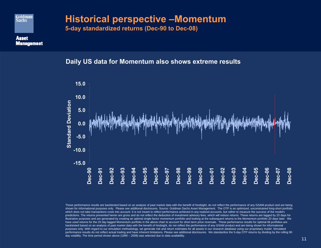
Historical perspective –Momentum5-day standardized returns (Dec-90 to Dec-08)
Daily US data for Momentum also shows extreme results
These performance results are backtested based on an analysis of past market data with the benefit of hindsight, do not reflect the performance of any GSAM product and are being shown for informational purposes only. Please see additional disclosures. Source: Goldman Sachs Asset Management. The OTP is an optimized, unconstrained long-short portfolio which does not take transactions costs into account. It is not meant to reflect performance achieved in any realized accounts, but rather to measure the success of the model's predictions. The returns presented herein are gross and do not reflect the deduction of investment advisory fees, which will reduce returns. These returns are lagged by 20 days for illustrative purposes and are generated by creating an optimal single-factor momentum portfolio and looking at the subsequent returns to the Momentum portfolio 20 days later. We have used returns for the 20 day lagged Momentum portfolio in the above chart to account for short term price reversals. These performance results for optimal tilt portfolios are backtested based on an analysis of past market data with the benefit of hindsight, do not reflect the performance of any GSAM product and are being shown for informational purposes only. With regard to our simulation methodology, we generate risk and return estimates for all assets in our research database using our proprietary model. Simulated performance results do not reflect actual trading and have inherent limitations. Please see additional disclosures. We standardize the 5-day OTP returns by dividing by the rolling 90 day volatility. The time period shown above (1990 – 2008) was selected due to data availability.
12
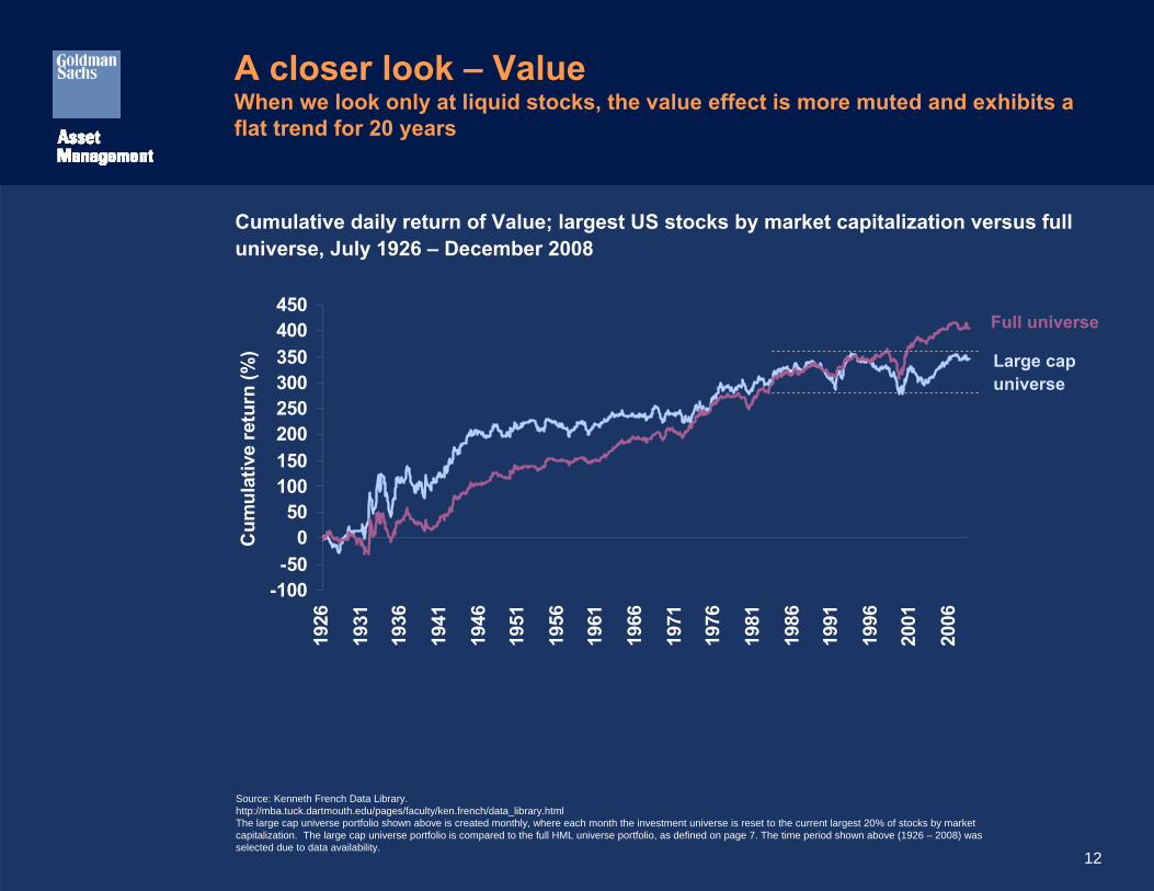
A closer look – ValueWhen we look only at liquid stocks, the value effect is more muted and exhibits a flat trend for 20 years
Cumulative daily return of Value; largest US stocks by market capitalization versus full universe, July 1926 – December 2008
-100-50
050
100150200250300350400450
1926
1931
1936
1941
1946
1951
1956
1961
1966
1971
1976
1981
1986
1991
1996
2001
2006
Cum
ulat
ive
retu
rn (%
)
Full universe
Large cap universe
Source: Kenneth French Data Library. http://mba.tuck.dartmouth.edu/pages/faculty/ken.french/data_library.htmlThe large cap universe portfolio shown above is created monthly, where each month the investment universe is reset to the current largest 20% of stocks by market capitalization. The large cap universe portfolio is compared to the full HML universe portfolio, as defined on page 7. The time period shown above (1926 – 2008) was selected due to data availability.
13
-1000
100200300400500600700800900
1926
1931
1936
1941
1946
1951
1956
1961
1966
1971
1976
1981
1986
1991
1996
2001
2006
Cum
ulat
ive
retu
rn (%
)
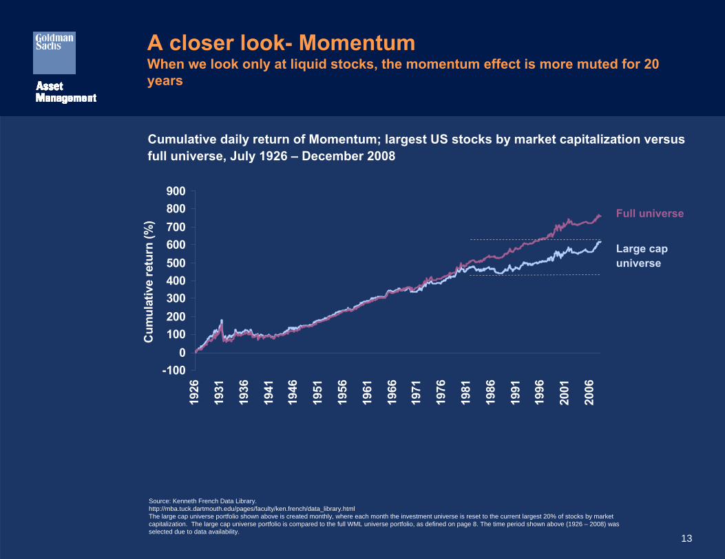
A closer look- MomentumWhen we look only at liquid stocks, the momentum effect is more muted for 20 years
Cumulative daily return of Momentum; largest US stocks by market capitalization versus full universe, July 1926 – December 2008
Full universe
Large cap universe
Source: Kenneth French Data Library. http://mba.tuck.dartmouth.edu/pages/faculty/ken.french/data_library.htmlThe large cap universe portfolio shown above is created monthly, where each month the investment universe is reset to the current largest 20% of stocks by market capitalization. The large cap universe portfolio is compared to the full WML universe portfolio, as defined on page 8. The time period shown above (1926 – 2008) was selected due to data availability.
14
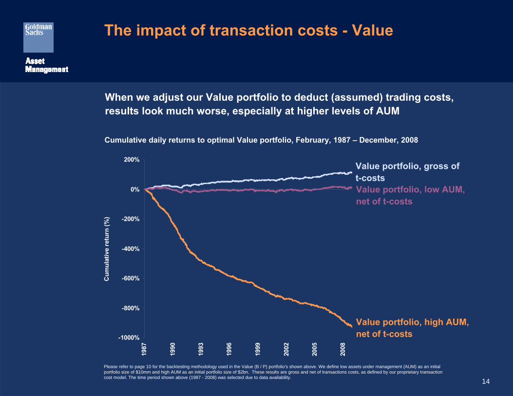
The impact of transaction costs - Value
When we adjust our Value portfolio to deduct (assumed) trading costs, results look much worse, especially at higher levels of AUM
Cumulative daily returns to optimal Value portfolio, February, 1987 – December, 2008
-1000%
-800%
-600%
-400%
-200%
0%
200%
1987
1990
1993
1996
1999
2002
2005
2008
Cum
ulat
ive
retu
rn (%
)
Value portfolio, gross of t-costsValue portfolio, low AUM, net of t-costs
Value portfolio, high AUM, net of t-costs
Please refer to page 10 for the backtesting methodology used in the Value (B / P) portfolio’s shown above. We define low assets under management (AUM) as an initial portfolio size of $10mm and high AUM as an initial portfolio size of $2bn. These results are gross and net of transactions costs, as defined by our proprietary transaction cost model. The time period shown above (1987 - 2008) was selected due to data availability.
15
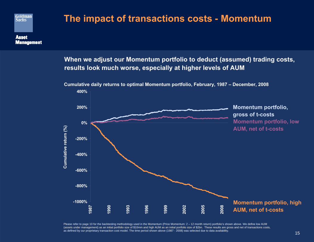
The impact of transactions costs - Momentum
When we adjust our Momentum portfolio to deduct (assumed) trading costs, results look much worse, especially at higher levels of AUM
Cumulative daily returns to optimal Momentum portfolio, February, 1987 – December, 2008
-1000%
-800%
-600%
-400%
-200%
0%
200%
400%19
87
1990
1993
1996
1999
2002
2005
2008
Cum
ulat
ive
retu
rn (%
)
Momentum portfolio, gross of t-costsMomentum portfolio, low AUM, net of t-costs
Momentum portfolio, high AUM, net of t-costs
Please refer to page 10 for the backtesting methodology used in the Momentum (Price Momentum: 2 – 12 month return) portfolio’s shown above. We define low AUM (assets under management) as an initial portfolio size of $10mm and high AUM as an initial portfolio size of $2bn. These results are gross and net of transactions costs, as defined by our proprietary transaction cost model. The time period shown above (1987 - 2008) was selected due to data availability.
16
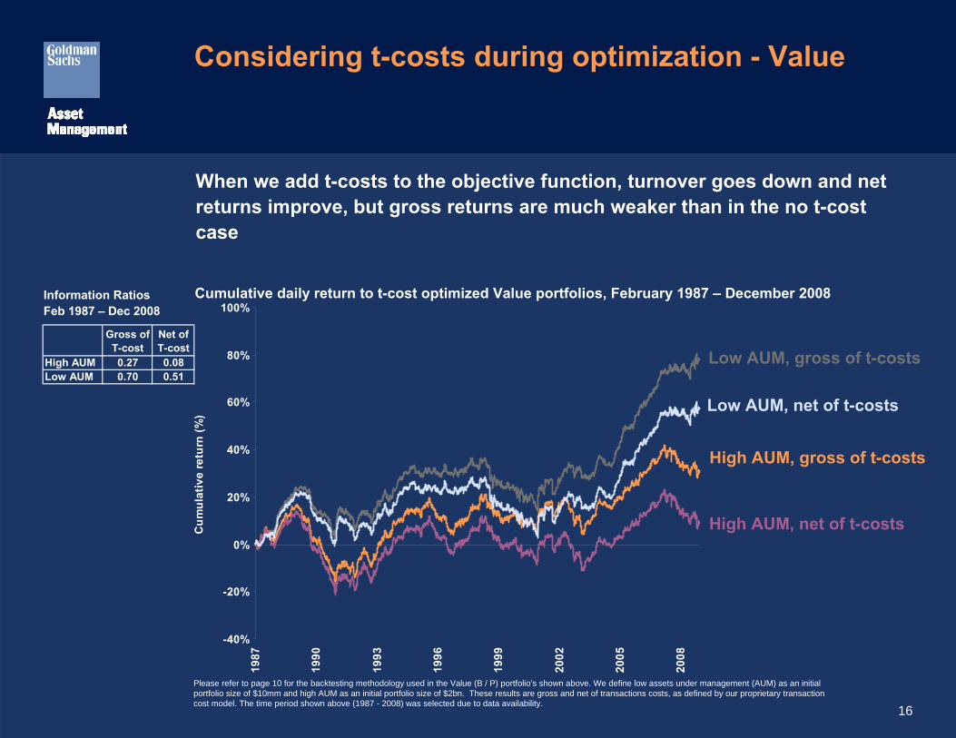
Considering t-costs during optimization - Value
When we add t-costs to the objective function, turnover goes down and net returns improve, but gross returns are much weaker than in the no t-cost case
Cumulative daily return to t-cost optimized Value portfolios, February 1987 – December 2008
-40%
-20%
0%
20%
40%
60%
80%
100%
1987
1990
1993
1996
1999
2002
2005
2008
Cum
ulat
ive
retu
rn (%
)
Low AUM, net of t-costs
Low AUM, gross of t-costs
High AUM, gross of t-costs
High AUM, net of t-costs
Information RatiosFeb 1987 – Dec 2008
Please refer to page 10 for the backtesting methodology used in the Value (B / P) portfolio’s shown above. We define low assets under management (AUM) as an initial portfolio size of $10mm and high AUM as an initial portfolio size of $2bn. These results are gross and net of transactions costs, as defined by our proprietary transaction cost model. The time period shown above (1987 - 2008) was selected due to data availability.
Gross of T-cost
Net of T-cost
High AUM 0.27 0.08Low AUM 0.70 0.51
17
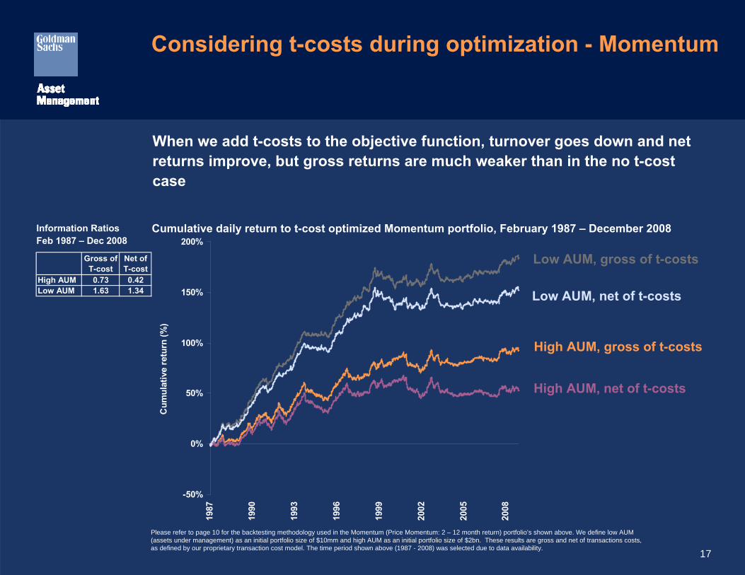
Considering t-costs during optimization - Momentum
When we add t-costs to the objective function, turnover goes down and net returns improve, but gross returns are much weaker than in the no t-cost case
Cumulative daily return to t-cost optimized Momentum portfolio, February 1987 – December 2008
-50%
0%
50%
100%
150%
200%
1987
1990
1993
1996
1999
2002
2005
2008
Cum
ulat
ive
retu
rn (%
)
Low AUM, net of t-costs
Low AUM, gross of t-costs
High AUM, gross of t-costs
High AUM, net of t-costs
Information RatiosFeb 1987 – Dec 2008
Please refer to page 10 for the backtesting methodology used in the Momentum (Price Momentum: 2 – 12 month return) portfolio’s shown above. We define low AUM (assets under management) as an initial portfolio size of $10mm and high AUM as an initial portfolio size of $2bn. These results are gross and net of transactions costs, as defined by our proprietary transaction cost model. The time period shown above (1987 - 2008) was selected due to data availability.
Gross of T-cost
Net of T-cost
High AUM 0.73 0.42Low AUM 1.63 1.34
18
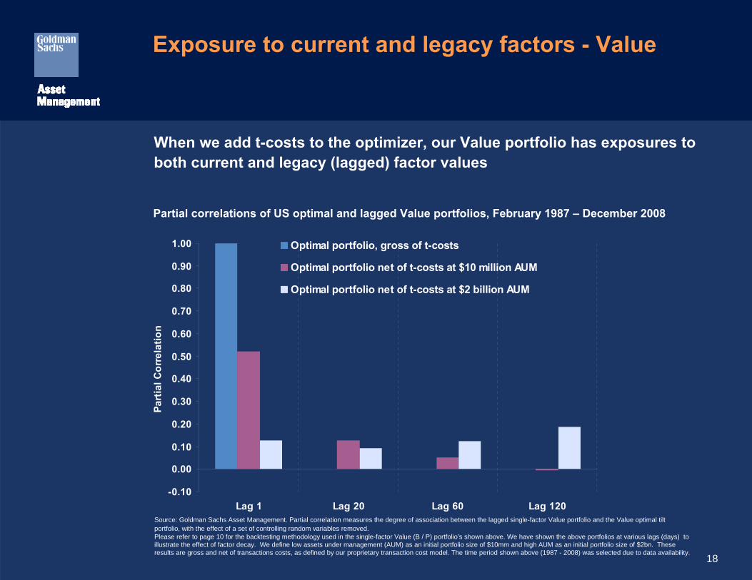
Exposure to current and legacy factors - Value
When we add t-costs to the optimizer, our Value portfolio has exposures to both current and legacy (lagged) factor values
Source: Goldman Sachs Asset Management. Partial correlation measures the degree of association between the lagged single-factor Value portfolio and the Value optimal tilt portfolio, with the effect of a set of controlling random variables removed.Please refer to page 10 for the backtesting methodology used in the single-factor Value (B / P) portfolio’s shown above. We have shown the above portfolios at various lags (days) to illustrate the effect of factor decay. We define low assets under management (AUM) as an initial portfolio size of $10mm and high AUM as an initial portfolio size of $2bn. These results are gross and net of transactions costs, as defined by our proprietary transaction cost model. The time period shown above (1987 - 2008) was selected due to data availability.
Partial correlations of US optimal and lagged Value portfolios, February 1987 – December 2008
-0.10
0.00
0.10
0.20
0.30
0.40
0.50
0.60
0.70
0.80
0.90
1.00
Lag 1 Lag 20 Lag 60 Lag 120
Part
ial C
orre
latio
n
Optimal portfolio, gross of t-costs
Optimal portfolio net of t-costs at $10 million AUM
Optimal portfolio net of t-costs at $2 billion AUM
19
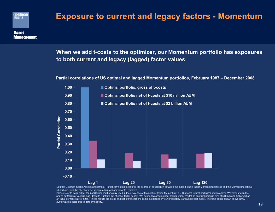
Exposure to current and legacy factors - Momentum
When we add t-costs to the optimizer, our Momentum portfolio has exposures to both current and legacy (lagged) factor values
Source: Goldman Sachs Asset Management. Partial correlation measures the degree of association between the lagged single-factor Momentum portfolio and the Momentum optimal tilt portfolio, with the effect of a set of controlling random variables removed.Please refer to page 10 for the backtesting methodology used in the single-factor Momentum (Price Momentum: 2 – 12 month return) portfolio’s shown above. We have shown the above portfolios at various lags (days) to illustrate the effect of factor decay. We define low assets under management (AUM) as an initial portfolio size of $10mm and high AUM as an initial portfolio size of $2bn. These results are gross and net of transactions costs, as defined by our proprietary transaction cost model. The time period shown above (1987 -2008) was selected due to data availability.
Partial correlations of US optimal and lagged Momentum portfolios, February 1987 – December 2008
-0.10
0.00
0.10
0.20
0.30
0.40
0.50
0.60
0.70
0.80
0.90
1.00
Lag 1 Lag 20 Lag 60 Lag 120
Part
ial C
orre
latio
n
Optimal portfolio, gross of t-costs
Optimal portfolio net of t-costs at $10 million AUM
Optimal portfolio net of t-costs at $2 billion AUM
20
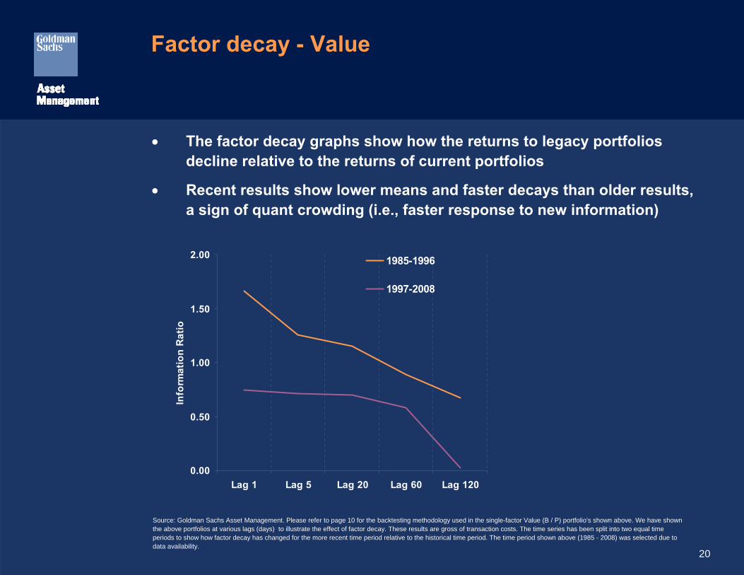
Factor decay - Value
• The factor decay graphs show how the returns to legacy portfolios decline relative to the returns of current portfolios
• Recent results show lower means and faster decays than older results, a sign of quant crowding (i.e., faster response to new information)
0.00
0.50
1.00
1.50
2.00
Lag 1 Lag 5 Lag 20 Lag 60 Lag 120
Info
rmat
ion
Rat
io
1985-1996
1997-2008
Source: Goldman Sachs Asset Management. Please refer to page 10 for the backtesting methodology used in the single-factor Value (B / P) portfolio’s shown above. We have shown the above portfolios at various lags (days) to illustrate the effect of factor decay. These results are gross of transaction costs. The time series has been split into two equal time periods to show how factor decay has changed for the more recent time period relative to the historical time period. The time period shown above (1985 - 2008) was selected due to data availability.
21
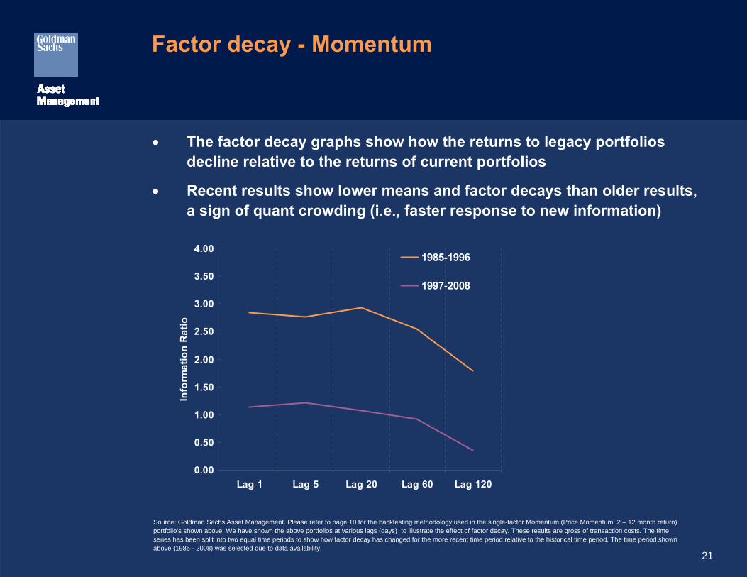
Factor decay - Momentum
• The factor decay graphs show how the returns to legacy portfolios decline relative to the returns of current portfolios
• Recent results show lower means and factor decays than older results, a sign of quant crowding (i.e., faster response to new information)
0.00
0.50
1.00
1.50
2.00
2.50
3.00
3.50
4.00
Lag 1 Lag 5 Lag 20 Lag 60 Lag 120
Info
rmat
ion
Rat
io
1985-1996
1997-2008
Source: Goldman Sachs Asset Management. Please refer to page 10 for the backtesting methodology used in the single-factor Momentum (Price Momentum: 2 – 12 month return) portfolio’s shown above. We have shown the above portfolios at various lags (days) to illustrate the effect of factor decay. These results are gross of transaction costs. The time series has been split into two equal time periods to show how factor decay has changed for the more recent time period relative to the historical time period. The time period shown above (1985 - 2008) was selected due to data availability.
22
-2.00
-1.00
0.00
1.00
2.00
3.00
4.00
5.00
Lag 1 Lag 5 Lag 20 Lag 60 Lag 120
Info
rmat
ion
Rat
io
1985-19961997-2008
-2.00
-1.00
0.00
1.00
2.00
3.00
4.00
5.00
Lag 1 Lag 5 Lag 20 Lag 60 Lag 120
Info
rmat
ion
Rat
io
-3.00
-2.00
-1.00
0.00
1.00
2.00
3.00
4.00
5.00
6.00
7.00
Lag 1 Lag 5 Lag 20 Lag 60 Lag 120
Info
rmat
ion
Rat
io
0.00
1.00
2.00
3.00
4.00
5.00
Lag 1 Lag 5 Lag 20 Lag 60 Lag 120
Info
rmat
ion
Rat
io
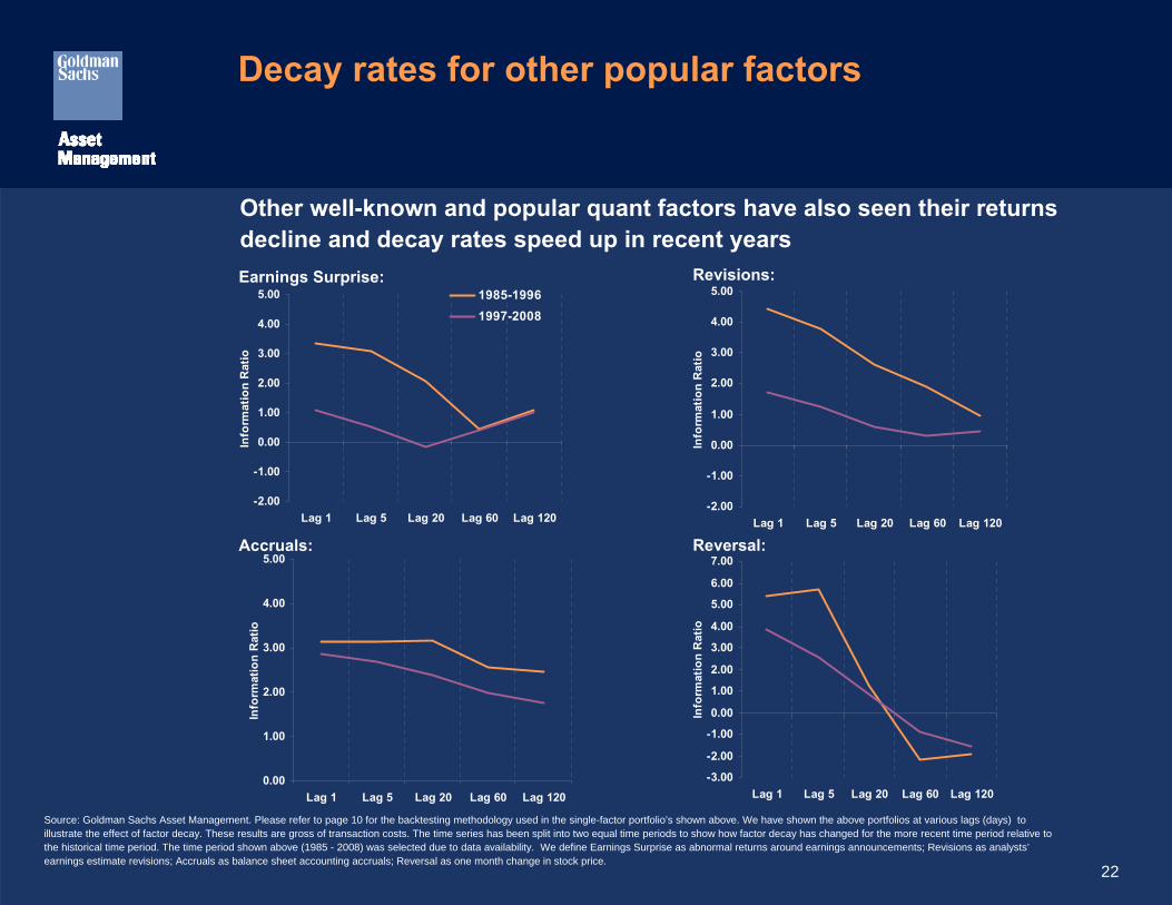
Decay rates for other popular factors
Other well-known and popular quant factors have also seen their returns decline and decay rates speed up in recent yearsEarnings Surprise: Revisions:
Accruals: Reversal:
Source: Goldman Sachs Asset Management. Please refer to page 10 for the backtesting methodology used in the single-factor portfolio’s shown above. We have shown the above portfolios at various lags (days) to illustrate the effect of factor decay. These results are gross of transaction costs. The time series has been split into two equal time periods to show how factor decay has changed for the more recent time period relative to the historical time period. The time period shown above (1985 - 2008) was selected due to data availability. We define Earnings Surprise as abnormal returns around earnings announcements; Revisions as analysts’earnings estimate revisions; Accruals as balance sheet accounting accruals; Reversal as one month change in stock price.
23
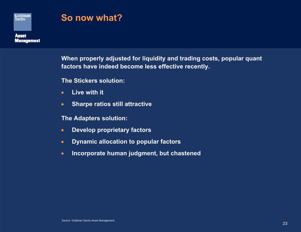
So now what?
When properly adjusted for liquidity and trading costs, popular quant factors have indeed become less effective recently.
The Stickers solution:
• Live with it
• Sharpe ratios still attractive
The Adapters solution:
• Develop proprietary factors
• Dynamic allocation to popular factors
• Incorporate human judgment, but chastened
Source: Goldman Sachs Asset Management.
24
Sources of alpha
• Alpha can only be derived when prices don’t accurately reflect all public information (i.e., price ≠ fair value).
• This can only happen when investors over- or under-react to information.
• Thus, the Value effect is really an over-reaction effect; Momentum is an under-reaction effect.
• Investors tend over-react to information that confirms their prior beliefs and under-react to information that contradicts those beliefs.
• We can develop proprietary factors by looking for other situations where investors systematically over- or under-react to information.
Source: Goldman Sachs Asset Management.
25
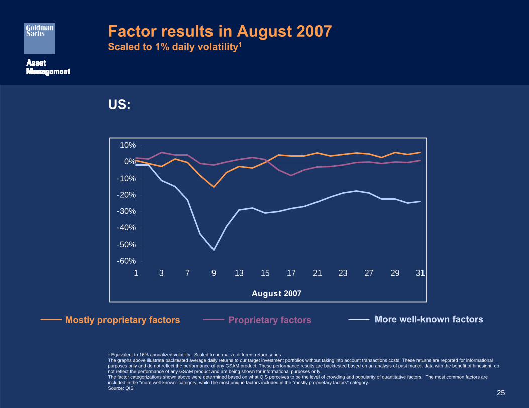
Factor results in August 2007Scaled to 1% daily volatility1
More well-known factorsMostly proprietary factors
-60%
-50%
-40%
-30%
-20%
-10%
0%
10%
1 3 7 9 13 15 17 21 23 27 29 31
August 2007
Proprietary factors
US:
1 Equivalent to 16% annualized volatility. Scaled to normalize different return series.The graphs above illustrate backtested average daily returns to our target investment portfolios without taking into account transactions costs. These returns are reported for informational purposes only and do not reflect the performance of any GSAM product. These performance results are backtested based on an analysis of past market data with the benefit of hindsight, do not reflect the performance of any GSAM product and are being shown for informational purposes only. The factor categorizations shown above were determined based on what QIS perceives to be the level of crowding and popularity of quantitative factors. The most common factors are included in the “more well-known” category, while the most unique factors included in the “mostly proprietary factors” category. Source: QIS
26
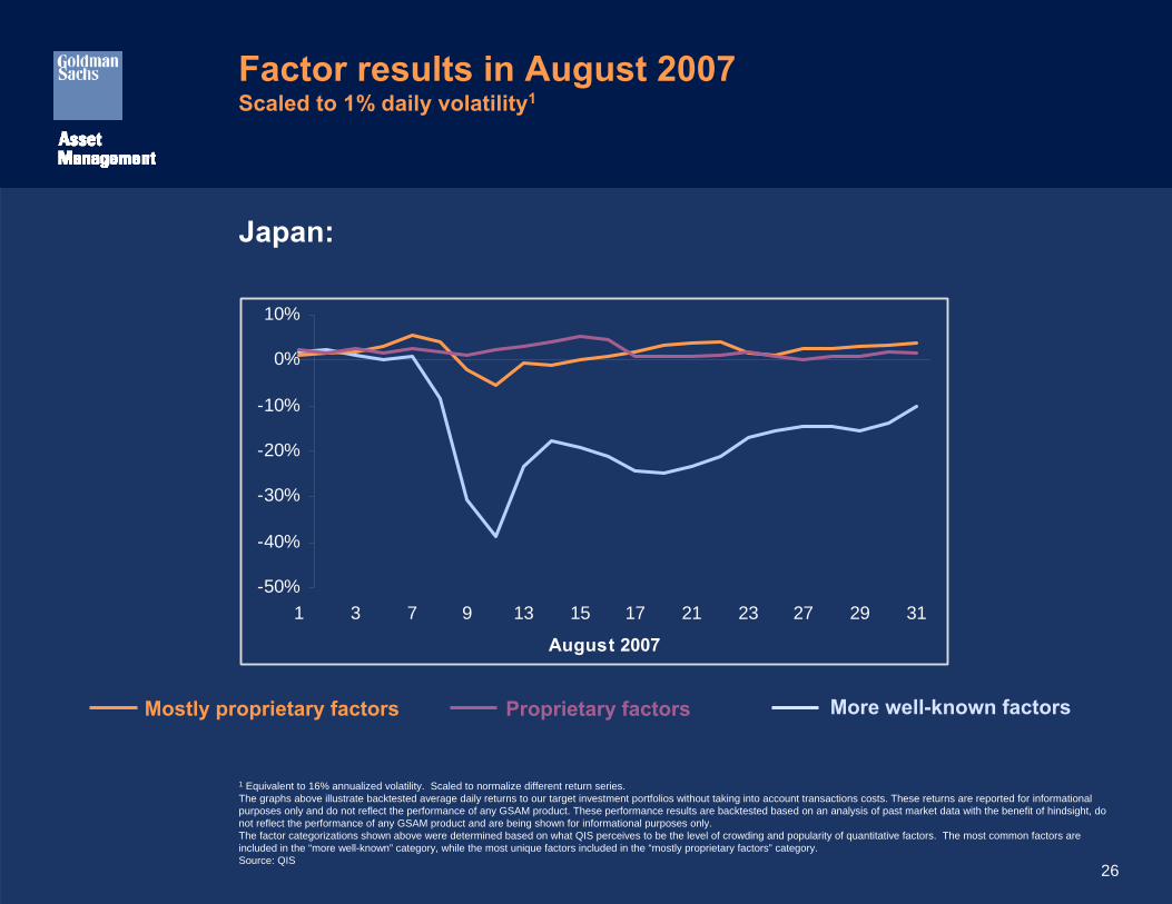
Factor results in August 2007Scaled to 1% daily volatility1
-50%
-40%
-30%
-20%
-10%
0%
10%
1 3 7 9 13 15 17 21 23 27 29 31
August 2007
Japan:
More well-known factorsMostly proprietary factors Proprietary factors
1 Equivalent to 16% annualized volatility. Scaled to normalize different return series.The graphs above illustrate backtested average daily returns to our target investment portfolios without taking into account transactions costs. These returns are reported for informational purposes only and do not reflect the performance of any GSAM product. These performance results are backtested based on an analysis of past market data with the benefit of hindsight, do not reflect the performance of any GSAM product and are being shown for informational purposes only. The factor categorizations shown above were determined based on what QIS perceives to be the level of crowding and popularity of quantitative factors. The most common factors are included in the “more well-known” category, while the most unique factors included in the “mostly proprietary factors” category. Source: QIS
27
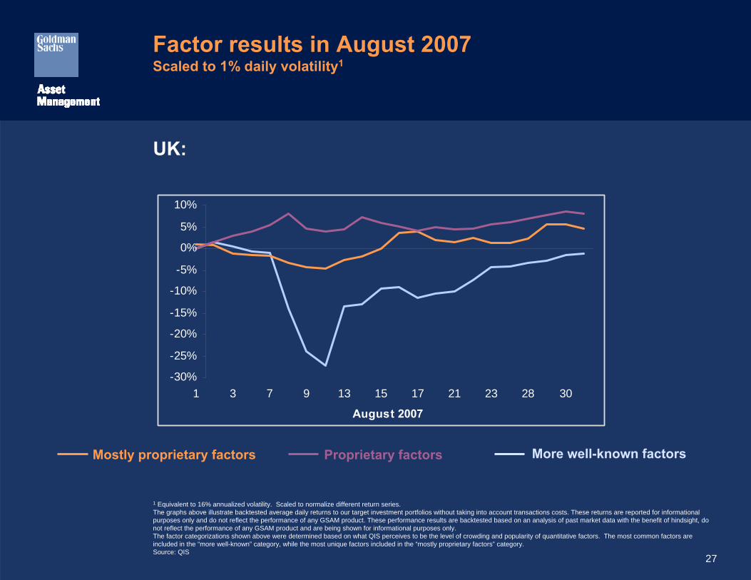
Factor results in August 2007Scaled to 1% daily volatility1
-30%
-25%
-20%
-15%
-10%
-5%
0%
5%
10%
1 3 7 9 13 15 17 21 23 28 30
August 2007
UK:
More well-known factorsMostly proprietary factors Proprietary factors
1 Equivalent to 16% annualized volatility. Scaled to normalize different return series.The graphs above illustrate backtested average daily returns to our target investment portfolios without taking into account transactions costs. These returns are reported for informational purposes only and do not reflect the performance of any GSAM product. These performance results are backtested based on an analysis of past market data with the benefit of hindsight, do not reflect the performance of any GSAM product and are being shown for informational purposes only. The factor categorizations shown above were determined based on what QIS perceives to be the level of crowding and popularity of quantitative factors. The most common factors are included in the “more well-known” category, while the most unique factors included in the “mostly proprietary factors” category. Source: QIS
28
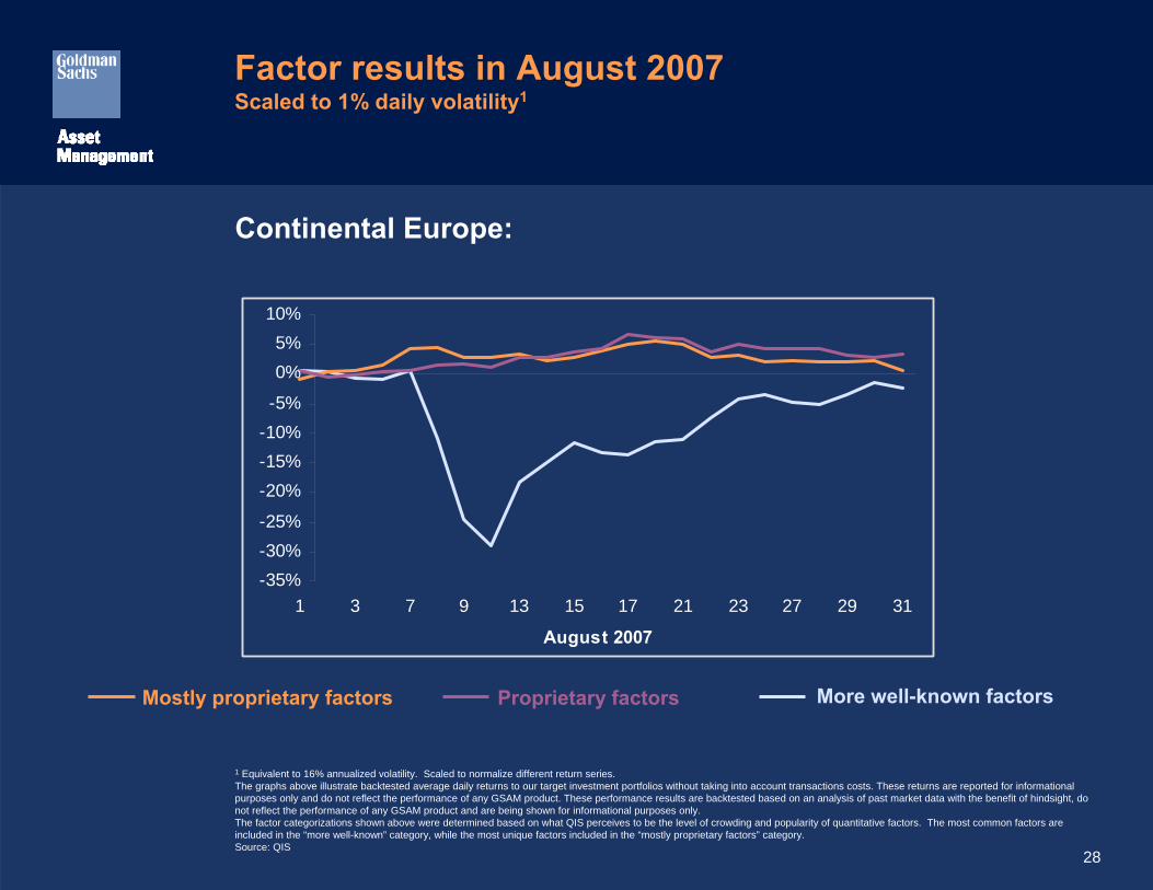
Factor results in August 2007Scaled to 1% daily volatility1
-35%-30%-25%
-20%-15%-10%-5%
0%5%
10%
1 3 7 9 13 15 17 21 23 27 29 31
August 2007
Continental Europe:
More well-known factorsMostly proprietary factors Proprietary factors
1 Equivalent to 16% annualized volatility. Scaled to normalize different return series.The graphs above illustrate backtested average daily returns to our target investment portfolios without taking into account transactions costs. These returns are reported for informational purposes only and do not reflect the performance of any GSAM product. These performance results are backtested based on an analysis of past market data with the benefit of hindsight, do not reflect the performance of any GSAM product and are being shown for informational purposes only. The factor categorizations shown above were determined based on what QIS perceives to be the level of crowding and popularity of quantitative factors. The most common factors are included in the “more well-known” category, while the most unique factors included in the “mostly proprietary factors” category. Source: QIS
29
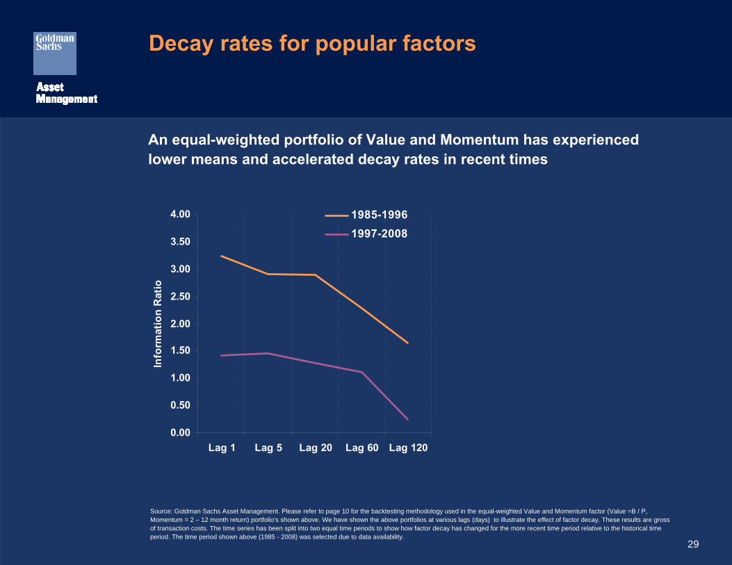
Decay rates for popular factors
An equal-weighted portfolio of Value and Momentum has experienced lower means and accelerated decay rates in recent times
0.00
0.50
1.00
1.50
2.00
2.50
3.00
3.50
4.00
Lag 1 Lag 5 Lag 20 Lag 60 Lag 120
Info
rmat
ion
Rat
io
1985-19961997-2008
Source: Goldman Sachs Asset Management. Please refer to page 10 for the backtesting methodology used in the equal-weighted Value and Momentum factor (Value =B / P, Momentum = 2 – 12 month return) portfolio’s shown above. We have shown the above portfolios at various lags (days) to illustrate the effect of factor decay. These results are gross of transaction costs. The time series has been split into two equal time periods to show how factor decay has changed for the more recent time period relative to the historical time period. The time period shown above (1985 - 2008) was selected due to data availability.
30
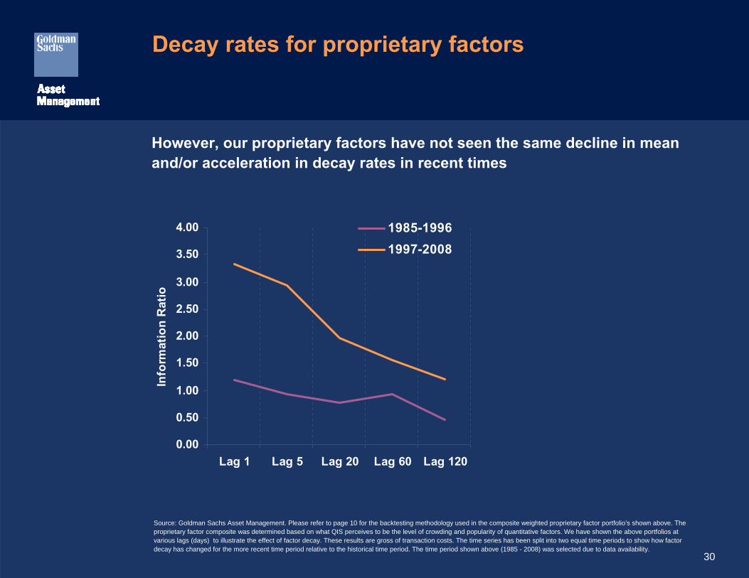
Decay rates for proprietary factors
However, our proprietary factors have not seen the same decline in mean and/or acceleration in decay rates in recent times
0.00
0.50
1.00
1.50
2.00
2.50
3.00
3.50
4.00
Lag 1 Lag 5 Lag 20 Lag 60 Lag 120
Info
rmat
ion
Rat
io
1985-19961997-2008
Source: Goldman Sachs Asset Management. Please refer to page 10 for the backtesting methodology used in the composite weighted proprietary factor portfolio’s shown above. The proprietary factor composite was determined based on what QIS perceives to be the level of crowding and popularity of quantitative factors. We have shown the above portfolios at various lags (days) to illustrate the effect of factor decay. These results are gross of transaction costs. The time series has been split into two equal time periods to show how factor decay has changed for the more recent time period relative to the historical time period. The time period shown above (1985 - 2008) was selected due to data availability.
31
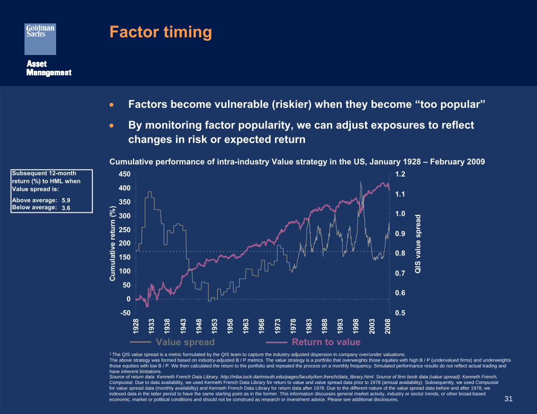
Factor timing
• Factors become vulnerable (riskier) when they become “too popular”
• By monitoring factor popularity, we can adjust exposures to reflect changes in risk or expected return
1 The QIS value spread is a metric formulated by the QIS team to capture the industry-adjusted dispersion in company over/under valuations.The above strategy was formed based on industry-adjusted B / P metrics. The value strategy is a portfolio that overweights those equities with high B / P (undervalued firms) and underweightsthose equities with low B / P. We then calculated the return to the portfolio and repeated the process on a monthly frequency. Simulated performance results do not reflect actual trading and have inherent limitations. Source of return data: Kenneth French Data Library. http://mba.tuck.dartmouth.edu/pages/faculty/ken.french/data_library.html. Source of firm book data (value spread): Kenneth French, Compustat. Due to data availability, we used Kenneth French Data Library for return to value and value spread data prior to 1978 (annual availability). Subsequently, we used Compustatfor value spread data (monthly availability) and Kenneth French Data Library for return data after 1978. Due to the different nature of the value spread data before and after 1978, we indexed data in the latter period to have the same starting point as in the former. This information discusses general market activity, industry or sector trends, or other broad-based economic, market or political conditions and should not be construed as research or investment advice. Please see additional disclosures.
Cumulative performance of intra-industry Value strategy in the US, January 1928 – February 2009
Return to valueValue spread
Above average: 5.9Below average: 3.6
Subsequent 12-month return (%) to HML when Value spread is:
-50
0
50
100
150
200
250
300
350
400
450
1928
1933
1938
1943
1948
1953
1958
1963
1968
1973
1978
1983
1988
1993
1998
2003
2008
Cum
ulat
ive
retu
rn (%
)
0.5
0.6
0.7
0.8
0.9
1.0
1.1
1.2
QIS
val
ue s
prea
d
32
Fix the underlying problem
• Quants have embraced objective models to forecast returns because theydo not trust biased human judgment
• An alternative solution is to train analysts and traders to recognize and control their biases
• Not strictly a quant approach, but uses insights gleamed from quantitative analysis
• Can also use quant/statistical models to improve analysts forecasts of the underlying fundamentals (EPS, ROE, growth, payout, etc.)
Source: Goldman Sachs Asset Management.
33
Conclusions
• Historical results for many popular quant factors look much weaker when we adjust for liquidity and trading costs
• Crowding has fundamentally changed the outlook for many of thesefactors:⎯ Likely to prove more volatile and provide lower Sharpe ratios in the
future⎯ Stronger results still possible for smaller managers who focus in less
liquid stocks or markets
• Some opportunities for quant managers⎯ Develop proprietary factors that capitalize on over- and under-
reaction⎯ Dynamic allocation to popular factors based on perceived crowding⎯ Work with traditional analysts and traders to minimize over- and
under-reaction
Source: Goldman Sachs Asset Management.

34
Tracking Error (TE) is one possible measurement of the dispersion of a portfolio’s returns from its stated benchmark. More specifically, it is the standard deviation of such excess returns. TE figures are representations of statistical expectations falling within “normal” distributions of return patterns. Normal statistical distributions of returns suggests that approximately two thirds of the time the annual gross returns of the accounts will lie in a range equal to the benchmark return plus or minus the TE if the market behaves in a manner suggested by historical returns. Targeted TE therefore applies statistical probabilities (and the language of uncertainty) and so cannot be predictive of actual results. In addition, past tracking error is not indicative of future TE and there can be no assurance that the TE actually reflected in your accounts will be at levels either specified in the investment objectives or suggested by our forecasts.
References to indices, benchmarks or other measures of relative market performance over a specified period of time are provided for your information only and do not imply that the portfolio will achieve similar results. The index composition may not reflect the manner in which a portfolio is constructed. While an adviser seeks to design a portfolio which reflects appropriate risk and return features, portfolio characteristics may deviate from those of the benchmark.
The strategy may include the use of derivatives. Derivatives often involve a high degree of financial risk because a relatively small movement in the price of the underlying security or benchmark may result in a disproportionately large movement in the price of the derivative and are not suitable for all investors. No representation regarding the suitability of these instruments and strategies for a particular investor is made.
Past performance is not indicative of future results, which may vary. The value of investments and the income derived from investments can go down as well as up. Future returns are not guaranteed, and a loss of principal may occur.
Backtested PerformanceBacktested performance results do not represent the results of actual trading using client assets. They do not reflect the reinvestment of dividends, the deduction of any fees, commissions or any other expenses a client would have to pay. If GSAM had managed your account during the period, it is highly improbable that your account would have been managed in a similar fashion due to differences in economic and market conditions.
Simulated PerformanceSimulated performance is hypothetical and may not take into account material economic and market factors that would impact the adviser’s decision-making. Simulated results are achieved by retroactively applying a model with the benefit of hindsight. The results reflect the reinvestment of dividends and other earnings, but do not reflect fees, transaction costs, and other expenses, which would reduce returns. Actual results will vary.
Expected ReturnsExpected return models apply statistical methods and a series of fixed assumptions to derive estimates of hypothetical average asset class performance. Reasonable people may disagree about the appropriate statistical model and assumptions. These models have limitations, as the assumptions may not be consensus views, or the model may not be updated to reflect current economic or market conditions. These models should not be relied upon to make predictions of actual future account performance. GSAM has no obligation to provide updates or changes to such data.
Opinions expressed are current opinions as of the date appearing in this material only. No part of this material may, without GSAM’s prior written consent, be (i) copied, photocopied or duplicated in any form, by any means, or (ii) distributed to any person that is not an employee, officer, director, or authorised agent of the recipient.
Copyright © 2009, Goldman, Sachs & Co. All rights reserved. Rev#21110.OTHER.OTU
General notes