THE SOLUTION OF LARGE MULTI-DIMENSIONAL POISSON PROBLEMS

bY

Harold S. Stone

. -

May 1974

Technical Report No, 85

DIGITAL SYSTEMS LABORATORY

Departments of Electrical Engineering and Computer Science

Stanford University

Stanford, California

This work was supported by NASA-Ames Research Center underGrant NCAR-74>-407.

6

Manuscript documentation unit for:

"The solution Of large Poisson problems" by Harold S. Stone

Key words: block tridiagonal equations, Buneman's algorithm, cyclic

odd-even reduction, drum memories, minimum latency.

CR categories: 5.14, 5.17, 6.34

Preferred address for future correspondence:

Professor Harold S. StoneDepartment of Electrical and

Computer EngineeringUniversity of MassachusettsAmherst, Massachusetts 01002

t

.

Figure Captions

Fig. 1 Data Structure for Poisson solver. The interval Tis equal to the drum rotating during the solutionone Poisson system of lower-dimension.

Fig. 2 Timing for drum reads and writes when simultaneousreading and writing is allowed. Indices shown infigure give the value of j for each record.

Fig. 3 Timing for drumreading and wri t

read s and writes whing is not allowed.

.en simultaneous

Fig. 4 Record positions for first reduction iteration andnext to last back substitution. Asterisks indicaterecords containing known solutions.

THE SOLUTION OF IARGE MULTI-DIMENSIONAL POISSON PROBLEMS

by Harold S. Stone

Abstract

The Buneman algorithm for solving Poisson problems can be adapted

to solve large Poisson problems on computers with a rotating drum memory

so that the computation is done with very little time lost due to rota-

tional latency of the drum.

I. Introduction

Large computations that do not fit into central memory often

are arranged so that the majority of the data resides on an auxiliary

memory, and the computation itself is structured as a sequence of

core-contained subproblems. Each subproblem is read from the auxiliary

memory into central memory, hopefully while another computation proceeds,

so that no time is lost waiting for the read operation. The major

challenge in solving large problems is to structure the sequence of

subproblems and the data storage format in auxiliary memory so as to

minimize the time lost while waiting for data transfers.

In this paper we examine a method for solving large Poisson problems

. a OI+ a computer with a rotating drum memory, and we show that drum latency

can be made very small with proper selection of parameters. Among the

obvious candidate algorithms for solving Poisson problems with minimum

latency are iterative schemes [Young, 19711 because these schemes access

data records sequentially at uniformly spaced time intervals. In this

paper we choose to ignore the iterative schemes in favor of direct methods

that generally have a lower computational complexity. In particular, we

examine Buneman's algorithm [Buneman, 19691 and the related algorithm

known as cyclic odd-even reduction [Buzbee et al., 19701. Both of thesem-

algorithms have interesting properties that lead to minimum latency

implementations. For these algorithms the intervals between record

accesses vary considerably from iteration to iteration, but the distance

between records varies by an equivalent amount so that latency is held low.

2-

Latency is not the only problem, however, in the design of such

algorithms because latency can be held to very low values just be

increasing buffer space. If buffer space is sufficiently large to

hold the entire problem, then drum latency reduces to zero. Fortunately,<->

the algorithms obtain very low latency with a small fixed amount of

buffer storage.

In Section II of this paper we review the Buneman algorithm

which is the basis of the algorithm for the solution of large problems.

In Section III we discuss the storage structures for a minimum latency

implementation of the Buneman algorithm for systems with drum memories.

Section IV treats several peripheral matters such as practical aspects

of implementation and a minimum latency implementation of the cyclic

odd-even reduction algorithm. The final section contains a brief. -

summary and some suggestions for further research.

-3-

11. The solution of core-contained problems

In this section, we present a brief review of the Buneman

algorithm for solving Poisson's equation as described in Buzbee

et al. [1970]. In later sections we show how this algorithm canm-

be adapted to solve problems too large to be contained in main memory.

The problem at hand is the solution of Poisson's equation in two

or three dimensions. To simplify the analysis we shall assume that the

two-dimensional surface is a square of size N X N, and the three-

dimensional volume is a cube of size N on each side. The algorithm

works best for N of the form N = 2m-l, which we assume to be the case

for the remainder of the analysis. We also assume that the Poisson

. - problem has Dirichlet boundary conditions along all boundaries. These

assumptions are not necessary and can be relaxed as described by Buzbee

et al. Cl9701 without changing our conclusions about methods for solvingm-

large problems.

Under the state boundary conditions the problem reduces to the

solution of the system of equations M xN =x where M is block tridiagonal

of the form:

M

A

I I

A I

I

( )1

For two-dimensional problems, when the square grid is of size

2N X N, h1 has dimension N2 X N , I is an identity matrix of size N,

and A is an N X N tridiagonal matrix. For three-dimensional problems,

the cubic grid has N points in each dimension, and M has dimensiont-1

N X N .3 3 In this case the identity matrix I has size N2 X N2, the

A matrix is block tridiagonal of size N2 X N and is the matrix for2

a two-dimensional system of the form just described. Thus a three-

dimensional Poisson problem contains N coupled two-dimensional problems,

and similarly, a two-dimensional problem contains N coupled one-

dimensional problems. This obviously generalizes to higher dimensions,

but dimensionality greater than three is rarely encountered in practice.

The method of solution involves computations that decouple the

. - problems of lower dimension. Buneman's algorithm is a variation of an

algorithm known as cyclic odd-even reduction. In this type of algorithm,

half of the lower dimensional problems are eliminated during the first

iteration, and during each successive iteration half of the remaining

problems are eliminated until a single system of lower dimension remains.

This is olved, and its solution is used to solve the two lower dimensional

problems last eliminated. The available solutions are then substituted

into four lower dimensional problems, then these into eight lower dimen-

sional problems, etc., until all of the eliminated lower dimensional

problems have been solved. The order in which the substitutions are made

is the reverse of the order in which problems are eliminated. Under the

stated conditions, namely that the M matrix is symmetric with all block

factors constant on each diagonal, each matrix of lower dimension eliminated

-5-

by the algorithm is not a Poisson system itself, but is the product of

Poisson matrices. At the kth iteration, the matrices are each products

of 2k Poisson matrices, so that during back substitution, each system

eliminated during the kth iteration can be solved by solving a sequencekof 2 Poisson problems of the same dimension as the eliminated matrices.

To make these ideas explicit the computation in brief is given below.

To solve M x =xN when M has the form of (1), partition 5 and x to

conform to M, so that

XN

. -

3

22

0

0

.

X- N

d

Llx =

z2

.

LN

t hwhere each x-i and Xi is a vector with l/N"-* as many components as xN

and x. For two-dimensional problems each zi and xi is a vector with N

components, and for three-dimensional problems, each has N2 components.

Next we compute a sequence of vectors p 04, p, p and matricesN

A Ck

and

. The vectors are of dimension equal to the dimension of x and x,-

are partitioned to conform to the partitioning of 2 and y.N To begin

the iteration, initialize the quantities as indicated below for j =

2, 4, 6,. . .,2m-2

-6-

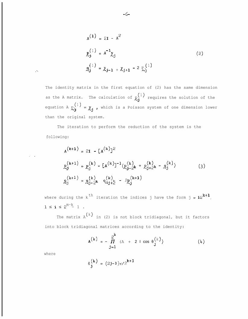
A1( 1 = 21 - A2

( 11Ej = A-'y

-j

( )1 12.j = Lj-1 + Lj+l

( )- 2 P.-J

(2)

The identity matrix in the first equation of (2) has the same dimension

as the A matrix. The calculation of p ( >1-j

requires the solution of the

( 1equation A p. 1-3 =Lj 9 which is a Poisson system of one dimension lower

than the original system.

The iteration to perform the reduction of the system is the

following:

Ack+‘) = 21 - [Ack)12

. a

(k+l)

itj = ~j(k) - [n(k']-l(~&;?l, + $hk - fJ,i"') (3)

@t-l >

2jP) + qP)k _ 2p@+l)= s-j-$ -j+2 -j

where during the k th iteration the indices j have the form j = i2 k-t1 ,m-klSiS2 - 1 .

The matrix A ( >k in (2) is not block tridiagonal, but it factors

into block tridiagonal matrices according to the identity:

Ak( 12k

=- n (A + 2 I cos 8 ( >k3

) (4)j=l

where

8 (k) = (2j-l)fi/2k+1j

-7-

and A and I are the block matrices of M given in (1). Thus we can

obtain p (k+l > in the k th-j iteration of (3) by solving a sequence of

2k Poisson problems of lower dimension.

Since we assume N has the form 2m-1, after m-2 iterations of

the reduction allows us to write the single equation

,&m-l);lm-l = ,(m-l)p(m-l) + q(E-,‘,-p-l 4 - (5)

which can be solved for x-2m-l by using the factorization given in (4).

At this point we can proceed with the back substitution using the

iteration:

Ak( > ( ( )k2-j - Ej > ( 1k

=Sj - zj-2k + Ej+2( k)

. -

for j = i*2k, and i odd in the interval 1 < i I m-k2

for (x - p k ),( >-j -j then use

,

(6)

1. we solve (6)

k k2j

( >= ~j +(x - P ( >-j -j ) (7)

to solve for x-j ' Boundary conditions force % and xN2m to be zero in (6).

This concludes the general description of the algorithm. The data

flow of the algorithm is the aspect that concerns us most in this paper

since the challenging problem is to support the data flow when using a

rotating auxiliary memory. In the next section we investigate various

ways to carry out the computation described in (3) and (6) when the

problem must reside on an auxiliary memory.

-8-

III. The solution of large Poisson problems

In this section we investigate a method for organizing a computa-

tion to solve Poisson's problem when the problem is too large for central

memory. We assume that the data resides on an auxiliary memory such as

a drum or fixed-head disk, so that the rotational position of the memory

is the unique state variable that describes the state of the memory.

Although the entire computation is too large for central memory, the

central memory is at least large enough to contain several problems of

lower dimension. For example, to solve a three-dimensional problem with

a mesh size of 64 points in each dimension requires sufficient storage for

218 mesh points. This 'is far too large to be contained in central memory

f&-all but a very few computers. However, one two-dimensional subproblem. -

contains only 212 = 4096 points, and can easily fit in central memory of

typical scientific computers. In fact, eight to 16 subproblems might be

able to reside simultaneously in a typical scientific computer memory.

Large two-dimensional problems that require the techniques discussed in

this section have 256 to 512 or more points in each dimension, or approxi-

mately 216 to 218 or more mesh points in total.

The reason that the direct method for solving Poisson's equation is

somewhat challenging to implement on a computer with a rotating memory is

that each point in the solution vector of the problem is influenced by every

point of the right-hand side of (1). Thus, any implementation of any

algorithm whatsoever requires data flow to go from every point to every other

point, and this is contrary to the natural unidirectional flow of a drum

memory. The strategy we choose is to use the unidirectional flow of infor-

-9-

mation of the drum for iterations (2) and (3) to collapse the data

into a single problem of lower dimension. The back substitution calls

for a reverse flow of information, which is impossible for a rotating

disk, Here we make use of the natural periodicity of the drum to spread

information as required for the back substitution. Latency cannot be

made zero for the back substitution process as we describe it, but it

can be kept to a small amount.

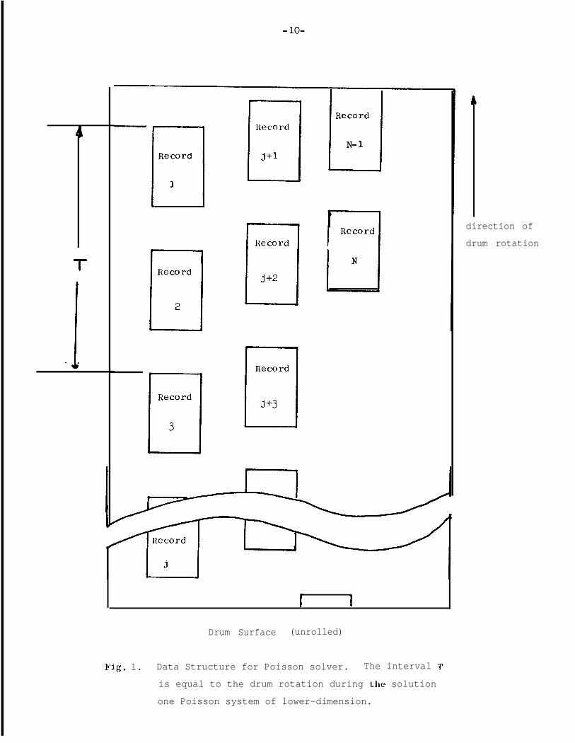
The method we use to organize data is shown in Fig. 1. Each record

contains p-j

and sj for fixed j. The records are initialized with the

.thvalue of x. in the J3

record, and subsequent copies of the j th record

contain p. and q-J

-j as they are produced during the evaluation of (2) and

(3) . When x-j

is calculated during the back substitution phase, it over-

. - writes p-j

in one or more copies of the j th record according to a scheme

described later in this section.

Since the matrix A ( >k is independent of j in (2) and (3), it is not

necessary to store a copy of A ( 1k with each record, nor is it necessary

to update A ( >k for each j as indicated in (2) and (3). However, if

boundary conditions are Neumann or periodic, and different faces of the

boundary have different types of conditions, then the A ( >k matrices may

be dependent on j, and we must allow for the possibility of storing and

recomputing A ( >k for each j. The algorithm is valid for these boundary

conditions with slight alterations in the factorization given in (4) and

with slight changes to other minor details in the calculation.

The important aspect of the data organization given in Fig. 1

T

I. -

Drum Surface (unrolled)

direction of

drum rotation

Fig. 1. Data Structure for Poisson solver. The interval T

is equal to the drum rotation during the solution

one Poisson system of lower-dimension.

-ll-

is that the records are spaced around the drum so that the physical

distance between records j and j+2 is just long enough to permit the

computation in (2) to take place while the drum is rotating. As men-

tioned previously, the computation excludes the computation of A ( >1 if

this matrix is the same for all j, as is the case for the stated boundary

conditions. Fig. 2 shows the timing for the reading and writing of

records during the computation of (2). Note that the first three

records are read into memory and reside there while p ( 11 ( >1-2 and q-2 are

computed. During this period, the next two records are read into

At the Close of the computation of g21( > ( >1memory. and q-2 , the data

required to compute p ( >2 and q ( >

2are available in memory. These

quantities are computed while the next two records are read into memory,

( > ( >1. - and the record containing p21 and q-2 is written back onto the drum.

If simultaneous reading and writing of the drum is not permitted, then

a scheme such as that shown in Fig. 3 is required. In this figure the

initial configuration of records is such that two records are grouped

together, followed by a space to allow the writing of a third record,

and the pattern repeats around the drum. The distance between successive

records in an adjacent pair is equal to the drum travel during one third

of the calculation of (2) for one value of j, so that one pattern of

two records and a blank record position passes under the read head

during one iteration of (2). The timing in Fig. 3 shows that when the

calculation of (2) has ended for one value of j, new data are available

-for the repetition of (2) for the next value of j. The output record

is written during the blank position time between pairs of input.

recordsL . Fig. 3 is essentially the same as Fig. 2 in all other respects,

DrumPosition

1

2

34

56

78

910

11

12

1314

1516

17. -18

1920

21

22

2324

2526

2728

2930313? -

..Fig. 2

Iteration 1

Read Compute Write

1

2

34

56

78

910

11

12

1314

1516

1718

1920

21

22

2324

2526

2728

29303132...

2

2

446688

10

10

12

12

141416

16

18

18

20

20

22

22

2424262628

28

30...

2

4

6

8

10

12

14

16

18

20

22

24

26

28...

Iteration 2

Read Compute Write

Iteration 3

Read Compute Write

2

4

6

8

10

12

14

16

18

20

22

24

26

28l

.

.

4

44

48888

12

12

12

12

16

1616

16

20

20

20

20

24.

L4f)

.

.

.

4

8

12

16

20

...

4

8

12

16

20

.

.

.

88888

888

16...

Timing for drum reads and writes when simultaneous reading and writingis allowed. Indiccls shown in figure give the value of j for each record.

-13-

Drum Position Read Compute Write Read Write Comwte

1

2

34

t-1 56789

10

1112

131415

-7 16. -1718

1920

21

22

23b

1

2

3

45

67

89

1011

12

13

1415

.e.

2

2

2

444666888

10101012

12

12

14..*

2 .-- 2

4 4

6 6

8 8

10

12...

10

12...

444444888...

Fig. 3. Timing for drum reads and writes when

simultaneous reading and writing is not allowed.

-14-

Idle computer time at the beginning of iterations in both figures is not

lost. It can be used to complete computations of the prior iteration.

The interesting aspect of this data organization concerns what

happens when (3) is evaluated. Note that the input data to (3) is the.

output data from (2) or from the previous iteration of (3). After

reading the first three records to initiate the evaluation of (3) for

the first value of j, the output data for each successive value of j

requires two input records to be read. During each successive scan of

the input data for an iteration of (3), the amount of data read reduces

by a factor of 2, and the spacing between records read increases by a

factor of 2. Thus it takes approximately twice as long to read two input

records for (3) for k=2 as it takes to read two input records to evaluate(2) (2). - (2). However, the time required to compute p.

-3and q.

-Jis roughly double

( > 1the time reauired to compute p, 1 ( 1and q, because it is dominated by the

time required to solve two problems of lower dimension, while the first

iteration is dominated by the time required to solve a single system of

lower dimension. This follows because A is block tridiagonal, while A ( >1

factors into two block tridiagonal systems, as given in (4).

The timing for two iterations of (3) is shown in Fig. 2. Note that

for each successive iteration the space between input records doubles, but

the computation time doubles as well. Thus if drum latency is negligible

for (2), it is also negligible for every iteration of (3).

This completes the description of the reduction phase of the algorithm.

-During each iteration of this phase, drum latency can be made essentially

zero. Between iterations latency depends on how closely the data comes to

occupying an integral number of drum bands. If the data spans an integral

-15-

number of bands, then drum latency between iterations is also essentially

zero. Note that a new iteration can begin at the first available value

of j, and not necessarily at the least value of j since (3) can be done

for j in any order. If data spans an integral number of bands except

for a fraction a of a single band, then the latency during the reduction

phase is approximately a[(log2 N) -11 since there are (log2 N) -1 tran-

sitions between iterations.

The reduction phase is relatively straightforward because there are

~ no constraints on the placement of output data. We simply choose to write

out each record as it is produced. The back substitution phase is more

difficult to implement because the position of both the input and output

data of each computation are fixed by the placement of data during the

. - reduction phase. In particular, to solve for the odd unknowns we must

substitute the computed values of the even unknowns into their. respective

positions between the odd records, Moreover, the data from which the even

unknowns are computed are displaced in the direction of rotation from the

final position for the even unknowns, During the back substitution phase

the data flow must be in the reverse direction. Consequently, we have to

move information against the natural direction of information flow of the

drum.

Since mechanical drums cannot be rotated in one direction and then in

the opposite direction, we must move the information backwards by moving it

forward around the drum for almost a full revolution, A data file can be

moved forward around the surface of a rotating drum provided there is

sufficient buffer capacity in memory to hold portions of the file while the

drum rotates. For the reduction phase we need only two buffers for data

I ..

-6

being read, three buffers for the computation, and one buffer for data

being written, giving a total of six buffers. We surely do not wish to

increase the number of buffers to much more than this for back substitu-

a-> tion. Instead we determine how records should be spaced around a band

to take advantage of the periodicity of the drum and avoid extra buffers

in core. We now show that record spacing should be chosen to be k/l1 of

a drum revolution where k is an integer in the range 1 5 k 5 11.

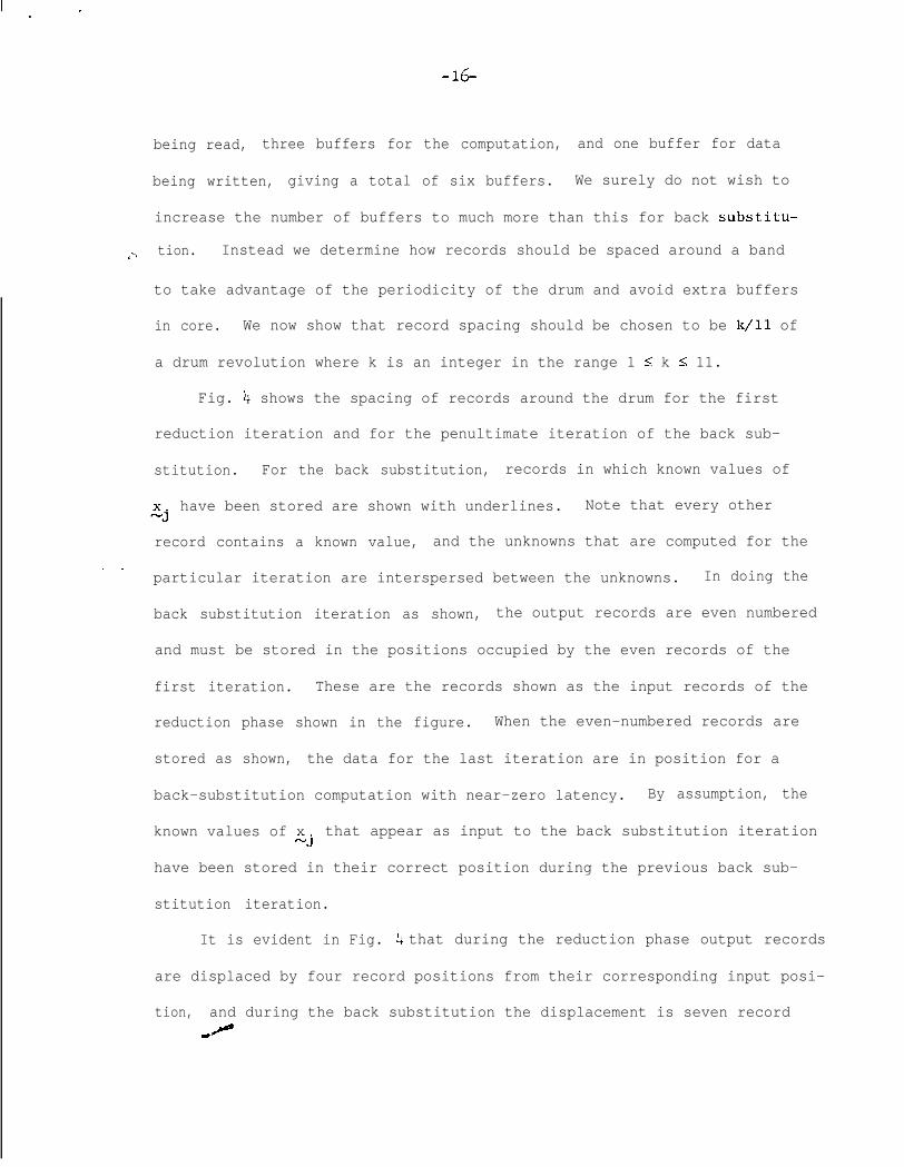
Fig. 4 shows the spacing of records around the drum for the first

reduction iteration and for the penultimate iteration of the back sub-

stitution. For the back substitution, records in which known values of

2-j have been stored are shown with underlines. Note that every other

record contains a known value, and the unknowns that are computed for the. -

particular iteration are interspersed between the unknowns. In doing the

back substitution iteration as shown, the output records are even numbered

and must be stored in the positions occupied by the even records of the

first iteration. These are the records shown as the input records of the

reduction phase shown in the figure. When the even-numbered records are

stored as shown, the data for the last iteration are in position for a

back-substitution computation with near-zero latency. By assumption, the

known values of x4

that appear as input to the back substitution iteration

have been stored in their correct position during the previous back sub-

stitution iteration.

It is evident in Fig. it that during the reduction phase output records

are displaced by four record positions from their corresponding input posi-

tion, and during the back substitution the displacement is seven recorda/@

- 17-

Read

1

2

3456789

10

11

12

13141516

1718

1920

Compute

2

2

446688

10

10

12

12

141416

16

18e

Write

10

12

14

16

.

.

Read Compute Write

2

4*

6

8*

10

12*

14'

16*.

2

2

2

2

6666

10

10

10

10...

4-x

6*

Fig. 4. Record positions for first reduction iteration and next to

last back substitution. Asterisks indicate records containingknown solutions.

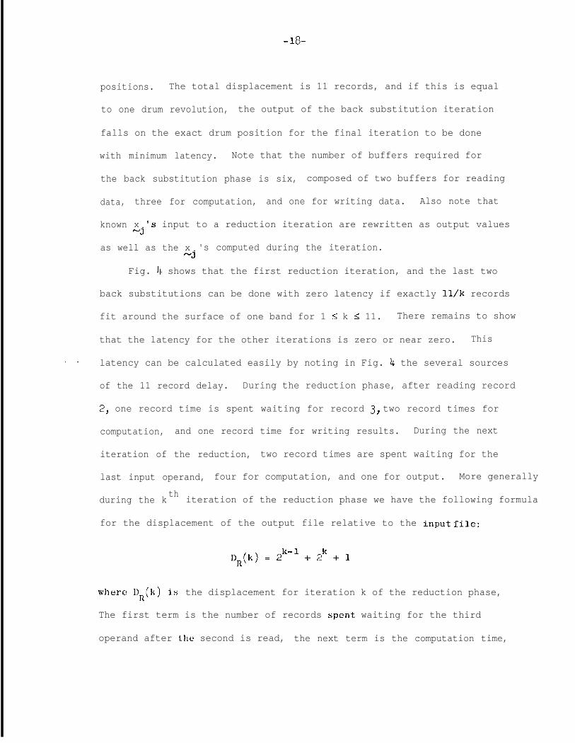
-18-

positions. The total displacement is 11 records, and if this is equal

to one drum revolution, the output of the back substitution iteration

falls on the exact drum position for the final iteration to be done

with minimum latency. Note that the number of buffers required for

the back substitution phase is six, composed of two buffers for reading

data, three for computation, and one for writing data. Also note that

known x-j

's input to a reduction iteration are rewritten as output values

as well as the x-j

's computed during the iteration.

Fig. 4 shows that the first reduction iteration, and the last two

back substitutions can be done with zero latency if exactly 11/k records

fit around the surface of one band for 1 I k I 11. There remains to show

that the latency for the other iterations is zero or near zero. This

. - latency can be calculated easily by noting in Fig. 4 the several sources

of the 11 record delay. During the reduction phase, after reading record

2, one record time is spent waiting for record 3, two record times for

computation, and one record time for writing results. During the next

iteration of the reduction, two record times are spent waiting for the

last input operand, four for computation, and one for output. More generally

during the k th iteration of the reduction phase we have the following formula

for the displacement of the output file relative to the input file:

DR(k) = 2k-1 +2k+1

where DR(k) i.s the displacement for iteration k of the reduction phase,

The first term is the number of records spent waiting for the third

operand after the second is read, the next term is the computation time,

-1g-

and the third term is the time spent writing results. During the back

substitution phase the displacement for reading the kth iteration output

to produce input for iteration k-l is given by:

DB(k) = 2k + 2k+1 + 1.

The terms correspond to the terms in DR(k), and the first terms in DB(k)

are double the values of the terms in D$k). The total displacement is

DR(k) + DB(k) = g.;lk-' + 2. When k = 1, the total displacement is 11,

as indicated in Fig. 4. For k = 2, the displacement is 20, which is equal

to -2 modulo 11. Thus when one band holds eleven records, the data for

the second iteration is displaced only nine records around the drum during

the reduction phase and back substitution processing, and this is not an-,

. - entire drum revolution. A delay of two record times must be introduced

into the computation somewhere, probably during the back substitution

phase of the computation. Thus instead of writing the computed values of

Zj as soon as they are computed in the back substitution, they should be

buffered and delayed two additional record times. Since output records are

produced and written every four record times during this iteration, only

one additional write buffer is necessary to achieve the necessary displacement.

For k = 3, the total displacement is 36 = -6 mod 11. Here we must

displace records by six record times, but output is written every eight

record times during the back substitution for this iteration, so that only

one buffer more than the original complement of six is required to achieve

the required displacement of the output records. But this is the same

requirement as for k = 2, so no extra buffers are required. For all back

substitution iterations the output records are written at intervals greater

than 11 and displacements need never exceed 11 so that a single extra write

-2o-

buffer suffices for all iterations.

We now have two constraints on the arrangement of records on the

drum. These are:

1. One record time should equal a half of the time required

to solve a core-contained problem of lower dimension.

th2. One record time should equal k/l1 of a revolution

time, for k an integer in the interval 1 i; k I 11.

To satisfy both constraints simultaneously, we suggest that the

record displacement be selected according to the second constraint, which

is problem independent, and that the problem size be designed to satisfy

the first constraint. It is the usual case that the number of mesh points. -

in each dimension may be selected with some flexibility provided that a

sufficient number of points exist to give the desired accuracy. We suggest

that if for a particular situation the solution of a core-contained problem

does not take sufficient time to satisfy the first constraint, then the

number of mesh points can be increased to lengthen this computation, and

the total time to solve the entire problem does not increase.

Increasing the number of mesh points merely decreases drum latency.

In the next section we look at specific examples to estimate the

efficiency of this implementation for various problem sizes.

‘1‘Ll-

IV. Analysis of effectiveness of the algorithm

In this section we give figures for the drum latency anticipated

as a function of problem size, and estimate the efficiency of the

algorithm for various realistic sets of parameters. We also discuss

the implication of electronic "drums", such as circulating memories

using magnetic bubbles or charge-coupled diodes that may be available

in several years.

First, to calculate the total drum latency for a computation, we

note there are two sources of latency:

1. Latency from iteration to iteration because the data does

not occupy an integral number of bands.

. - 2. Latency during back substitution arising from the need

to rewrite data in specific locations.

Each of these sources of latency can be identified with each iteration,

and the total latency for any iteration cannot exceed ten records, or

one record less than a full drum revolution. As a rough approximate we

can estimate latency to be 3.3 record times, or one half a revolution

per iteration. The number of iterations required is 2[log2 N) -11 so a

rough estimate of the latency in one calculation is ll[(log2 N) -11 record

times. The total time spent in a calculation with no latency is approxi-

mately N record times per iteration for 2(log2 N - 1) iterations, giving

-roughly 2Nc ( log2 11) -11 record times, Then the fraction of additional

time contributed by latency is:

-22-

latent time 11?-- .

active time 2N

This time becomes quite small as N increases.

Table I shows an exact calculation of the latency for several values

of N. For this calculation the computation is assumed to begin as the

first record passes the read head and terminates when the last record

is written as output. During each record the computer is assumed either

to be idle or computing, so that each record time contributes to latency

or to active computing. In analyzing Table I, consider how large the

problems are when the problem is three-dimensional. The problem of size

31 can be done comfortably by most large scientific computers, and is a

dseful size to attack. The problem of size 63 strains the capacity of

all but the largest of presently available scientific computers. Note

that the per cent latency is extremely low for this size of problem so

that it appears to be quite feasible to use the scheme described here

when such problems are attempted. Problems of size 12'7 are within reach

of just a few super computers such as ILLIAC IV, and the very low loss of

time due to latency makes this scheme quite attractive for such problems.

The major constraint of rotating memories in this drum allocation

scheme concerns the need to have 11/k records per revolution in order to

reduce latency during back substitution. Recall that data must be trans-

mitted in the reverse direction of drum rotation, and WC use the natural

-pcriodicity of the drum to accomplish this. If the number of records per

revolution exceeds 11, then computation is degraded in two different ways.

Both the latency and the buffer space incrcasc as the number of records

a-> N

15

31

63

1v

Latent ActiveRecords Records

19

40

40

55 1538 3.58

- 23-

Table I

F Latent

98 19.4

258 15.5

642 6.23

Drum latency for various problem sizes,

Ic

-24-

per revolution increases. There may be factors that dictate that

record spacing be smaller than l/11th of a drum revolution, and this

appears to be reasonable if the degradation due to latency and extra

,-> buffering is acceptable. It is unlikely that there is sufficient

justification to exceed 11 records per revolution by a substantial

amount.

Since typical drums rotate once every 10 to 40 msec., the record

spacing for the solution of a core-contained two dimensional problem is

2/llths of this time, which is from 1.82 to 7.27 msec. Hackney [lgr(O]

reports times of 56 msec. and 196 msec. for solving a two-dimensional

problem of size 32 x 32 and 64 X 64 respectively, on a CDC 6600. Modern

computers such as ILLIAC IV have achieved speed increases from 10 to 30-.times over the speed of a CDC 6600 so that Hackney's problem may be done

in roughly 2 to 10 msec. on such computers. From these crude estimates

we see that a problem of size 31 is likely to require at least 2/11 ths of

a drum revolution and a problem of size 63 to require more than this.

Consequently, the periodicity of 11 records per revolution is compatible

with expected parameters for computer speed and drum revolution time when

the core-contained problem is two-dimensional. In fact, it may be necessary

to place 11/2 or 11/3 records around a drum band.

Present projections indicate that electronic memories may replace

drum memories in future computers. Such electronic memories are likely

to be circulating memories based upon a magnetic bubble or charge-coupled

diode technology. Like drums, accesses for these electronic memories

experience a latency while information is rot :~t cc1 into position. However,

I .

-25-

latency is much less than for present drums, possibly of the order of

10 to 100 times less than the latency of mechanical drums. The limiting

latency factor occurs when one record occupies a single band, at which

points true zero latency is achieved because all iterations take an

integral number of revolutions of the drum.

Electronic drums have an advantage not shared with mechanical drums.

They can be reversed instantaneously and read in the opposite direction,

if so designed. This feature can be used to great advantage with the

algorithm cited here because the ideal way to perform the back substitution

is to reverse the direction of rotation of the memory. For the back

substitution all information flow should be in the direction opposite

to the flow of information during the forward reduction. Moreover the-:spacing between records is correct to achieve minimum latency during the

back substitution provided that output records produced during the forward

iteration are delayed through buffering by D,(k) - DR(k) = 3a;lk-' record

positions during the kth iteration. The delay is achievable with the

addition of single write buffer.

Before closing this section we should mention other algorithms that

are susceptible to this type of data structuring for minimum latency

operation. Cyclic odd-even reduction [Buzbee et al., 1970] is similar tom-

Buneman's algorithm except that the forward reduction involves matrix

multiplication rather than the solution of matrix equations. Like Buncman's

algorithm, the computation time per iteration doubles with each iteration

of the reduction process, and the number of input records decreases by

roughly half, with the spacing between them doubling. The b a s i c c y c l e t i m e

- 26-

for this iteration depends on the time required to multiply a block

tridiagonal matrix by another matrix. However the basic cycle time for

the back substitution is the time required to solve a block tridiagonal

system in memory, which is the same basic cycle time as Buneman's

algorithm. Because of the constraints of the drum memory, the reduction

phase and back substitution phase must use the same basic cycle time,

and the cycle time must therefore be the maximum of the matrix multi-'

plication and matrix solution times, Therefore, we cannot take advantage

of the faster time of matrix multiplication if we use cyclic odd-even

reduction.

One advantage that does accrue to cyclic-odd even reduction is the

fact that some computations can be avoided if a single equation is solved-7

. - repeatedly for different right-hand sides, The drum algorithm can take

advantage of this savings only in so far as the savings are realized in

both the reduction and back substitution phases. Any savings realized

in one phase and not the other is lost because of the constraint that

records spacing produced during the reduction phase must be identical to

the record spacing for back substitution.

v. Summary and comments

We have taken a highly regular Poisson problem and have shown

storage on the disk, and the result is the ability to solve the

problem with very little time lost to drum latency, The regularity

of the data structure is somewhat unexpected because computations change

from iteration to iteration. The major issue that is settled here is

that large Poisson problems can be solved effectively with a small high-

speed memory and a large rotating drum memory. The algorithms used are

efficient in that if all of memory were high-speed memory then the

computation speed for this algorithm would be reasonably close to the

speed of the best known algorithm for solving Poisson's equation, say

to within a small constant factor independent of the size of the problem.

When we change from rectangular boundaries to something less

structured, the present algorithm is not sufficient in itself to provide

a solution. For such problems we have some doubt that a high-speed drum

can be used effectively so as to make latency negligible. Periodic or

other regular data structures are absolutely essential when large drum

memories are used as a tightly coupled auxiliary memory, and such

structures are present only when Poisson's equations are solved over

highly regular regions.

In closing we should mention that we can predict the effectiveness

of a minimum latency storage organization by comparing the computation

time for the problem as we have described it to the computation time for

- 28-

a problem in which random access is made to records on the drum, with

a corresponding latency experienced for each record read. In the

minimum-latency case each record requires one record time to read, and

essentially zero latency time to access. In the random-access mode,

<-\ each record on the average requires one record time to read and one half

a drum revolution, or 5.5 records of latency for accessing the record,

Thus the computation time for the random access problem is likely to be

5.5 + 1 = 6.5 times as long as for the minimum latency code. For large

problems the factor of 6.5 represents a very tangible savings in compu-

tation time.

References

Buneman, O., 1969. "A compact non-iterative Poisson solver,"Report 294, Inst. for Plasam Res., Stanford University,Stanford, Calif., 1969.

Buzbee, B. L., Golub, G. H., and Nielson, C. W., 1970. "Ondirect methods for solving Poisson's equations," SIAMJ. Numer. Anal., vol. 7, No. 4, pp. 627-636, Dec. 1970*

Hackney, R. W., 1970. "The potential calculation and someapplications," Methods Computational Phys., Vol. 9, pp.135-211, 1970.

Young, D. M., 1971. Iterative Solution of Large Linear Systems,Academic Press, New York, 1971.