Embed Size (px)
Citation preview

I4
I
•
(.1
I

This is an advanced text for first-year graduate students in physics and engineeringtaking a standard classical mechanics course. It is the first book to describe the subjectin the context of the language and methods of modern nonlinear dynamics.
The organizing principle of the text is integrability vs nonintegrability. Flows inphase space and transformations are introduced early and systematically and areapplied throughout the text. The standard integrable problems of elementary physicsare analyzed from the standpoint of flows, transformations, and integrability. Thisapproach then allows the author to introduce most of the interesting ideas of modernnonlinear dynamics via the most elementary nonintegrable problems of Newtonianmechanics. The book begins with a history of mechanics from the time of Plato andAristotle, and ends with comments on the attempt to extend the Newtonian method tofields beyond physics, including economics and social engineering.
This text will be of value to physicists and engineers taking graduate courses inclassical mechanics. It will also interest specialists in nonlinear dynamics, mathema-ticians, engineers, and system theorists.


CLASSICAL MECHANICStransformations, flows, integrabic and chaotic dynamics


CLASSICAL MECHANICStransformations, flows, integrable and chaotic dynamics
JOSEPH L. McCAULEYPhysics Department
University of Houston, Houston, Texas 77204-5506
CAMBRIDGEUNIVERSITY PRESS

CAMBRIDGE UNIVERSITY PRESSCambridge, New York, Melbourne, Madrid, Cape Town, Singapore,São Paulo, Delhi, Dubai, Tokyo
Cambridge University PressThe Edinburgh Building, Cambridge CB2 8RU, UK
Published in the United States of America by Cambridge University Press, New York
www.cambridge.orgInformation on this title: www.cambridge.org/9780521578820
© Cambridge University Press 1997
This publication is in copyright. Subject to statutory exceptionand to the provisions of relevant collective licensing agreements,no reproduction of any part may take place without the writtenpermission of Cambridge University Press.
First published 1997Reprinted (with corrections) 1998
A catalogue record for this publication is available from the British Library
Library of Congress Cataloguing in Publication data
McCauley, Joseph L.Classical mechanics: transformations, flows, integrable, and
chaotic dynamics / Joseph L. McCauley.p. cm.
Includes bibliographical references and index.ISBN 0 521 48132 5 (hc). ISBN 0 521 57882 5 (pbk.)1. Mechanics. I. Title.QC125.2.M39 1997531'.01'515352—dc20 96-31574 CIP
ISBN 978-0-521-48132-8 HardbackISBN 978-0-521-57882-0 Paperback
Transferred to digital printing 2010
Cambridge University Press has no responsibility for the persistence oraccuracy of URLs for external or third-party internet websites referred to inthis publication, and does not guarantee that any content on such websites is,or will remain, accurate or appropriate. Information regarding prices, traveltimetables and other factual information given in this work are correct atthe time of first printing but Cambridge University Press does not guaranteethe accuracy of such information thereafter.

For my mother,Jeanette Gilliam McCauley,
and my father,Joseph Lee McCauley (1913—1985).
Ebensomeiner Lebensgefahrtin und Wanderkameradin,
Cornelia Maria Erika Küffner.

Middels kiokbør mannikke aitfor kiok;
fagreste livetlever den mennen
som vet mAtelig mye.
Middels klokbør en mann
ikke altfor klok;sorgløst er hjertetsjelden i brystet
hos ham som er helt kiok.
Hâvamil

Contents
Foreword page xiiiAcknowledgements xviii
1. Universal laws of nature 1
1.1 Mechanics in the context of history 1
1.2 The foundations of mechanics 10
1.3 Conservation laws for N bodies 25
1.4 The geometric invariance principles of physics 291.5 Covariance of vector equations vs invariance of solutions 37
Exercises 41
2. Lagrange's and Hamilton's equations 45
2.1 Overview 45
2.2 Extrema of functionals 462.3 Newton's equations from the action principle 502.4 Arbitrary coordinate transformations and Lagrange's equations 53
2.5 Constrained Lagrangian systems 602.6 Symmetry, invariance, and conservation laws 63
2.7 Gauge invariance 70
2.8 Hamilton's canonical equations 72Exercises 76
3. Flows in phase space 803.1 Solvable vs integrable 803.2 Streamline motions and Liouville's theorem 81
3.3 Equilibria and linear stability theory 943.4 One degree of freedom Hamiltonian systems 101
3.5 Introduction to 'clockwork': stable periodic and stablequasiperiodic orbits 103
3.6 Introduction to integrable flows 104
3.7 Bifurcations in Hamiltonian systems 118
Exercises 121
4. Motion in a central potential 126
4.1 Overview 126
4,2 Integration via two constants of the motion 127
4.3 Maps, winding numbers, and orbital stability 129
4.4 Clockwork is rare in mechanical systems 134
4.5 Hidden symmetry in the Kepler problem 138

x Contents
4.6 Periodicity and nonperiodicity that are not like clockwork 141
Exercises 144
5. Small oscillations about equilibria 148
5.1 Introduction 148
5.2 The normal mode transformation 148
5.3 Coupled pendulums 152
Exercises 154
6. Integrable and chaotic oscillations 1566.1 Qualitative theory of integrable canonical systems 156
6.2 Return maps 162
6.3 A chaotic nonintegrable system 163
6.4 Area-preserving maps 1706.5 Computation of exact chaotic orbits 175
6.6 On the nature of deterministic chaos 177
Exercises 184
7. Parameter-dependent transformations 187
7.1 Introduction 187
7.2 Phase flows as transformation groups 187
7.3 One-parameter groups of transformations 189
7.4 Two definitions of integrability 192
7.5 Invariance under transformations of coordinates 194
7.6 Power series solutions of systems of differential equations 195
7.7 Lie algebras of vector fields 197
Exercises 202
8. Linear transformations, rotations, and rotating frames 2048.1 Overview 2048.2 Similarity transformations 2048.3 Linear transformations and eigenvalue problems 2058.4 Rotations form a Lie group 2088.5 Dynamics in rotating reference frames 213Exercises 220
9. Rigid body motions 2239.1 Euler's equations of rigid body motion 223
9.2 Euler's rigid body 228
9.3 The Euler angles 2329.4 Lagrange's top 2349.5 Integrable problems in rigid body dynamics 2379.6 Noncanonical flows as iterated maps 2409.7 Nonintegrable rigid body motions 241
Exercises 242
10. Lagrangian dynamics and transformations in configuration space 24710.1 Invariance and covariance 247

Contents xi
10.2 Geometry of the motion in configuration space 251
10.3 Basis vectors in configuration space 25610.4 Canonical momenta and covariance of Lagrange's equations in
configuration space 258Exercises 261
11. Relativity, geometry, and gravity 26211.1 Electrodynamics 26211.2 The principle of relativity 26511.3 Coordinate systems and integrability on manifolds 27511.4 Force-free motion on curved manifolds 28011.5 Newtonian gravity as geometry in curved space-time 28411.6 Einstein's gravitational field equations 28711.7 Invariance principles and laws of nature 291
Exercises 294
12. Generalized vs nonholonomic coordinates 29512.1 Group parameters as nonholonomic coordinates 29512.2 Euler—Lagrange equations for nonintegrable velocities 30212.3 Group parameters as generalized coordinates 304Exercises 306
13. Noncanonical flows 30713.1 Flows on spheres 30713.2 Local vs complete integrability 311
13.3 Globally integrable noncanonical flows 31613.4 Attractors 321
13.5 Damped-driven Euler—Lagrange dynamics 32513.6 Liapunov exponents, geometry, and integrability 331
Exercises 332
14. Damped-driven Newtonian systems 33414.1 Period doubling in physics 33414.2 Fractal and multifractal orbits in phase space 34714.3 Strange attractors 35914.4 The two-frequency problem 361
Exercises 371
15. Hamiltonian dynamics and transformations in phase space 373
15.1 Generating functions for canonical transformations 373
15.2 Poisson brackets and infinitesimal transformations: symmetry,invariance, and conservation laws 377
15.3 Lie algebras of Hamiltonian flows 386
15.4 The Dirac quantization rules 39015.5 Hidden symmetry: superintegrability of the Kepler and isotropic
harmonic oscillator problems 393
15.6 Noncanonical Hamiltonian flows 397
Exercises 406
xii Contents
16. Integrable canonical flows 40916.1 Solution by canonical transformations 40916.2 The Hamilton—Jacobi equation 41216.3 Integrability and symmetry 41516.4 Action-angle variables 421
16.5 Central potentials 42616.6 The action integral in quantum theory 427Exercises 429
17. Nonintegrable canonical flows 43017.1 The Henôn—Heiles model 43017.2 Perturbation theory and averaging 43217.3 The standard map 43517.4 The Kolmogorov—Arnol'd—Moser (KAM) theorem 43717.5 Is clockwork possible in the solar system? 439Exercises 440
18. Simulations, complexity, and laws of nature 441
18.1 Integrability, chaos, and complexity 441
18.2 Simulations and modelling without invariance 44218.3 History in the context of mechanics 448Exercises 452
Bibliography 453Index 467
Foreword
Invariance principles and integrability (or lack of it) are the organizing principles of thistext. Chaos, fractals, and strange attractors occur in different nonintegrable Newtoniandynamical systems. We lead the reader systematically into modern nonlinear dynamicsvia standard examples from mechanics. Goldstein1 and Landau and Lifshitz2presumeintegrability implicitly without defining it. Arnol'd's3 inspiring and informative bookon classical mechanics discusses some ideas of deterministic chaos at a level aimed atadvanced readers rather than at beginners, is short on driven dissipative systems, andhis treatment of Hamiltonian systems relies on Cartan's formalism of exteriordifferential forms, requiring a degree of mathematical preparation that is neithertypical nor necessary for physics and engineering graduate students.
The old Lie—Jacobi idea of complete integrability ('integrability') is the reduction ofthe solution of a dynamical system to a complete set of independent integrations via acoordinate transformation ('reduction to quadratures'). The related organizing prin-ciple, invariance and symmetry, is also expressed by using coordinate transformations.Coordinate transformations and geometry therefore determine the method of this text.For the mathematically inclined reader, the language of this text is not 'coordinate-free', but the method is effectively coordinate-free and can be classified as qualitativemethods in classical mechanics combined with a Lie—Jacobi approach to integrability.We use coordinates explicitly in the physics tradition rather than straining to achievethe most abstract (and thereby also most unreadable and least useful) presentationpossible. The discussion of integrability takes us along a smooth path from the Keplerproblem, Galilean trajectories, the isotropic harmonic oscillator, and rigid bodies toattractors, chaos, strange attractors, and period doubling, and also to Einstein'sgeometric theory of gravity in space-time.
Because we emphasize qualitative methods and their application to the interpreta-tion of numerical integrations, we introduce and use Poincaré's qualitative method ofanalysis of flows in phase space, and also the most elementary ideas from Lie's theory ofcontinuous transformations. For the explicit evaluation of known integrals, the readercan consult Whittaker4, who has catalogued nearly all of the exactly solvableintegrable problems of both particle mechanics and rigid body theory. Other problemsthat are integrable in terms of known, tabulated functions are discussed in Arnol'd'sDynamical Systems JJJ•5
The standard method ofcomplete solution via conservation laws is taught in standardmechanics texts and implicitly presumes integrability without ever stating that. Thismethod is no longer taught in mathematics courses that emphasize linear differentialequations. The traditional teaching of mechanics still reflects (weakly, because very, veryincompletely) the understanding of nonlinear differential equations before the advent ofquantum theory and the consequent concentration on second order linear equations.Because the older method solves integrable nonlinear equations, it provides a superior

xiv Foreword
starting point for modern nonlinear dynamics than does the typical course in lineardifferential equations or 'mathematical methods in physics'. Most mechanics texts don'tmake the reader aware of this because they don't offer an adequate (or any) discussion ofintegrability vs nonintegrability. We include dissipative as well as conservative systems,and we also discuss conservative systems that are not Hamiltonian.
As Lie and Jacobi knew, planar dynamical systems, including dissipative ones, have aconservation law. We deviate from Arnol'd by relaxing the arbitrary requirement ofanalyticity in defining conservation laws. Conservation laws for dissipative systems aretypically multivalued functions. We also explain why phase space is a Cartesian spacewith a scalar product rule (inner product space), but without any idea of the distancebetween two points (no metric is assumed unless the phase space actually is Euclidean).By 'Cartesian space', therefore, we mean simply a Euclidean space with or without ametric. Finally, the development of the geometric ideas of affine connections andcurvature in chapter 11 allows us to use global integrability of the simplest possible flowto define phase space as a flat manifold in chapter 13. The language of general relativityand the language of dynamical systems theory have much geometric overlap: in bothcases, one eventually studies the motion of a point particle on a manifold that isgenerally curved.
After the quantum revolution in 1925, the physics community put classicalmechanics on the back burner and turned off the gas. Following Heisenberg's initialrevolutionary discovery, Born and Jordan, and also Dirac discovered the quantumcommutation rules and seemingly saved physicists from having to worry further aboutthe insurmountable difficulties presented by the unsolved Newtonian three-bodyproblem and other nonintegrable nonlinear dynamics problems (like the doublependulum). Einstein6 had pointed out in 1917 that the Bohr—Sommerfeld quantizationrules are restricted to systems that have periodic trajectories that lie on tori in phasespace, so that quantization rules other than Bohr—Sommerfeld are required for systemslike the three-body problem and mixing systems that yield Gibbs' microcanonicalensemble. The interesting difficulties posed by nonintegrability (or incomplete integra-bility) in both classical and quantum mechanics were conveniently forgotten orcompletely ignored by all but a few physicists from 1925 until the mid-1970s, in spite ofa 1933 paper by Koopman and von Neumann where the 'mixing' class of two degree offreedom Hamiltonian systems is shown not to admit action-angle variables because ofan 'everywhere dense chaos'.
This is the machine age. One can use the computer to evaluate integrals and also tostudy dynamical systems. However, while it is easy to program a computer andgenerate wrong answers for dynamics problems (see section 6.3 for an integrableexample), only a researcher with a strong qualitative understanding of mechanics anddifferential equations is likely to be prepared to compute numbers that are both correctand meaningful. An example of a correct calculation is a computation, with controlleddecimal precision, of unstable periodic orbits of a chaotic system. Unstable periodicorbits are useful for understanding both classical and quantum dynamics. An exampleof a wrong computation is a long orbit calculation that is carried out in floating-pointarithmetic. Incorrect results of this kind are so common and so widely advertised inboth advanced and popular books and articles on chaos theory that the presentation ofbad arithmetic as if it were science has even been criticized in the media.7 It is a diseaseof the early stage of the information age that many people labor under the comfortableillusion that bad computer arithmetic is suddenly and magically justified whenever a

Foreword xv
system is chaotic.8 That would be remarkable, if true, but of course it isn't.The mathematics level of the text assumes that a well-prepared reader will have had a
course in linear algebra, and one in differential equations that has covered power seriesand Picard's iterative method. The necessary linear algebra is developed in chapters 1and 8. It is assumed that the reader knows nothing more about nonlinear systems ofdifferential equations: the plotting of phase portraits and even the analysis of linearsystems are developed systematically in chapter 3. If the reader has no familiarity withcomplex analysis then one idea must be accepted rather than understood: radii ofconvergence of series solutions of phase flows are generally due to singularities on theimaginary time axis.
Chapter 1 begins with Gibbs' notation for vectors and then introduces the notation oflinear algebra near the end of the chapter. In chapter 2 and beyond we systematicallyformulate and study classical mechanics by using the same language and notation thatare normally used in relativity theory and quantum mechanics, the language of linearalgebra and tensors. This is more convenient for performing coordinate transform-ations. An added benefit is that the reader can more clearly distinguish superficial fromnonsuperficial differences with these two generalizations of classical mechanics. In somelater chapters Gibbs' notation is also used, in part, because of convenience.
Several chapter sequences are possible, as not every chapter is prerequisite for theone that follows. At the University of Houston, mechanics is taught as a one-yearcourse but the following one-semester-course chapter sequences are also possible(where some sections of several chapters are not covered): 1, 2, 3,4, 5,7, 8, 9, 15 (a moretraditional sequence): 1, 2, 3,4, 6, 8,9, 12, 13 (integrability and chaos), 1, 2, 3, 4, 6, 7, 12,15, 16, 17 (integrable and nonintegrable canonical systems): 1, 2, 3, 4, 8, 9, 12, 13, 14(integrability and chaos in noncanonical systems), or 1, 2, 3, 4, 5, or 6, 8, 9, 10, 11(integrability and relativity).
The historic approach to mechanics in the first chapter was motivated by differentcomments and observations. The first was Herbert Wagner's informal remark thatbeginning German students are well prepared in linear algebra and differentialequations, but often have difficulty with the idea of force and also are not familiar withthe definition of a vector as it is presented in elementary physics. Margaret and HughMiller made me aware that there are philosophers, mathematicians, and others whocontinue to take Aristotle seriously. Postmodernists and deconstructionists teach thatthere are no universal laws, and the interpretation of a text is rather arbitrary. Themarriage of cosmology and particle physics has led to the return to Platonism withinthat science, because of predictions that likely can never be decided empirically.Systems theorists and economists implicitly assume that commodity prices9 and themovement of money define dynamical variables that obey mathematically precisetime-evolution laws in the same sense that a collection of inanimate gravitating bodiesor colliding billiard balls define dynamical variables that obey Newton's universal lawsof motion. Other system theorists assert that 'laws of nature' should somehow 'emerge'from the behavior of 'complex systems'. Awareness of Plato's anti-empiricism andAristotle's wrong ideas about motion leads to greater consciousness of the fact that thelaw of inertia, and consequently physics, is firmly grounded in empirically discovereduniversal laws of kinematics that reflect geometric invariance principles.'0 Beliefsabout 'invisible hands', 'efficient markets', and 'rational expectations with infiniteforesight"1 are sometimes taught mathematically as if they might also represent laws ofnature, in spite of the lack of any empirical evidence that the economy and other

xvi Foreword
behavioral phenomena obey any known set of mathematical formulae beyond thestage of the crudest level of curve-fitting. Understanding the distinction between theweather, a complex Newtonian system subject to universal law, and mere modellingbased upon the statistics of irregularities that arise from effectively (mathematically)lawless behavior like stock trading might help to free economists, and perhaps otherbehaviorists, from the illusion that it is possible either to predict or even to understandthe future of humanity in advance from a purely mathematical standpoint, and wouldalso teach postmodernists the difference between physics, guesswork-modelling andsimulations, and pseudo-science.
I am very grateful to Harry Thomas for many stimulating, critical and therefore veryhelpful discussions on geometry and integrability, and for sharing with me his lecturenotes on a part of the proof of Bertrand's theorem. I'm also grateful to his colleague andformer student Gerhard Muller for making me aware that the double pendulumprovides a relatively elementary example of a nonintegrable and chaotic Newtoniansystem. I am extremely grateful to Eigil Anderson for introducing me to the descriptionof Lie's work in E. T. Bell's history of mathematics in 1992: without having read thesimple sentence by Bell stating that Lie showed that every one-parameter transform-ation on two variables has an invariant, the main organizing principle of this book(integrability) would have remained too primitive to be effective. Jam grateful to my oldfriend and colleague, Julian Palmore, for pointing me to his paper with Scott Burnswhere the conservation law for the damped linear harmonic oscillator is derived. Julianalso read and criticized my heuristic definitions of solvability and global integrabilityand helped me to make them sharper than they were before, but they are certainly notas precise as he would have liked them to be. I have also followed his advice, givenseveral years ago, to emphasize flows in phase space. Dyt Schiller at Siegen, FinnRavndal in Oslo, and Herbert Wagner in München have provided me with usefulgeneral criticism of earlier versions of the manuscript. George Reiter read sections 1.1,1.2, and 18.1 critically. I am very grateful to copy editor Jo Clegg for a careful reading ofthe original manuscript, to Sigmund Stintzing for proofreading chapters 9 and 15 of thetypescript, and especially to Herbert Wagner and Ludwig Maxmillians Universität(München) for guestfriendship during the fall 1996 semester of my sabbatical, when thetypescript was proofed and corrected. I have enjoyed a lecture by Per Bak onlong-range predictability vs qualitative understanding in physics, have also benefitedfrom conversations with Mike Fields and Marty Golubitsky on flows and conservationlaws, and from a discussion of differential forms with Bob Kiehn. I am grateful toGemunu Gunaratne for many discussions and critical questions, to J. M. Wilkes for a1977 letter on rotating frames, to Robert Helleman for pointing me to Arnol'd'sdiscussion of normal forms. I am especially grateful to many of the physics andengineering students at the University of Houston who have taken my classicalmechanics and nonlinear dynamics courses over the last several years. Chapter 8 wasread and corrected, in part, by graduate students Rebecca Ward Forrest and QiangGao. The computer graphics were produced as homework exercises by Ola Markussen,Rebecca Forrest, Youren Chen, and Dwight Ritums. I would also like to thank LindaJoki for very friendly help with some of the typing. Special thanks go to Simon Capelin,Publishing Director for the Physical Sciences at Cambridge University Press, for hissupport and encouragement.
Finally, I am extremely grateful to my stimulating and adventurous wife, CorneliaKüffner, who also longs for the Alps, the Norwegian fjords and mountains, and other

Foreword xvii
more isolated places like the Sierra Madre, Iceland, and the Fcerøyene while we live,work, and write for 9 months of each year in Houston.
Joseph L. McCauley
Bibliography
1 Goldstein, H., Classical Mechanics, second edition, Addison-Wesley, Reading, Mass.(1980).
2 Landau, L. D., and Lifshitz, E. M., Mechanics, third edition, Pergarnon, Oxford (1976).3 Arnol'd, V. I., Mathematical Methods of Classical Mechanics, second edition,
Springer-Verlag, New York (1989).4 Whittaker, E. T., Analytical Dynamics, Cambridge University Press (1965).5 Arnol'd, V. I., Dynamical Systems III, Springer-Verlag, Heidelberg (1993).6 Einstein, A., Verh. Deutsche Phys. Ges. 19, 82 (1917).7 Brugge, P., Mythos aus dern Computer: über Ausbretung und Missbrauch der
'Chaostheorie', Der Spiegel 39, 156—64 (1993); Der Kult urn das Chaos: über Ausbretungund Missbrauch der 'Chaostheorie', Der Spiegel 40, 232—52 (1993).
8 McCauley, J. L., Chaos, Dynamics and Fractals, an algorithmic approach to deterministicchaos, Cambridge University Press (1993).
9 Casti, J. L., and Karlqvist, A., Beyond Belief, Randomness, Prediction, and Explanation inScience, CRC Press, Boca Raton (1991).
10 Wigner, E. P., Symmetries and Reflections, Univ. Indiana Pr., Bloomington (1967).11 Anderson, P. W., Arrow, K. J., and Pines, D., The Economy as an Evolving Complex
System, Addison-Wesley, Redwood City, California (1988).

Acknowledgments
The writer acknowledges permission to quote passages from the following texts: Johns HopkinsPr.: The Cheese and the Worms (1992) by Carlo Ginzburg; Vintage Pr.: About Looking (1991),Keeping a Rendezvous (1992), Pig Earth (1992), and About our Faces (1984) by John Berger; Wm.Morrow and Co., Inc. and the John Ware Literary Agency: Searching for Certainty (1990) byJohn Casti; Dover: Johannes Kepler (1993) by Max Caspar; Symmetries and Reflections, E. P.Wigner; Indiana Univ. Pr. (1967), permission granted by Mrs. Wigner one week after ProfessorWigner's death, Addison-Wesley Pubi. Co.: Complexity: Metaphors, Models, and Reality (1994);Santa Fe Institute, Cowan, Pines, & Meltzler, Springer-Verlag: Mathematical Methods ofClassical Mechanics (2nd ed., 1980) by V. I. Arnol'd, and Dover Publications, Inc.: Ordinary
Equations (1956) by E. L. Ince.Several drawings in the text are reprinted with the permission of: Addison-Wesley PubI. Co.:
figures 1.5, 3.7, and 5.9a—c from Classical Mechanics (2nd edition, Copyright 1980, 1950),Goldstein, Springer-Verlag: figures 35, 73, & 79 from Mathematical Methods of ClassicalMechanics (2nd edition, Copyright 1989, 1978), Arnol'd, Professors E. J. Saletan and A. H.Cromer: figures 5 & 25 from Theoretical Mechanics (Wiley, 1971), and McGraw-Hill: figure 4.31from Advanced Mathematical Methods for Scientists and Engineers (1st edition, Copyright 1978),Bender and Orszag.
1
Universal laws of nature
In the presentation of the motions of the heavens, the ancients began with the principle that anatural retrograde motion must of necessity be a uniform circular motion. Supported in thisparticular by the authority of Aristotle, an axiomatic character was given to this proposition,whose content, in fact, is very easily grasped by one with a naive point of view; men deemed itnecessary and ceased to consider another possibility. Without reflecting, Copernicus and TychoBrahe still embraced this conception, and naturally the astronomers of their time did likewise.
Johannes Kepler, by Max Caspar
1.1 Mechanics in the context of history
It is very tempting to follow the mathematicians and present classical mechanics in anaxiomatic or postulational way, especially in a book about theory and methods.Newton wrote in that way for reasons that are described in Westfall's biography (1980).Following the abstract Euclidean mode of presentation would divorce our subjectsuperficially from the history of western European thought and therefore from its realfoundations, which are abstractions based upon reproducible empiricism. A postula-tional approach, which is really a Platonic approach, would mask the way thatuniversal laws of regularities of nature were discovered in the late middle ages in anatmosphere where authoritarian religious academics purported pseudo-scientificallyto justify the burning of witches and other nonconformers to official dogma, and alsotried to define science by the appeal to authority. The axiomatic approach would fail tobring to light the way in which universal laws of motion were abstracted from firmlyestablished empirical laws and discredited the anti- and pseudo-scientific ways ofmedieval argumentation that were bequeathed to the west by the religious interpretersof Plato and Aristotle.
The ages of Euclid (ca. 300 BC), Diophantus (ca. 250 BC), and Archimedes (287 to212 BC) effectively mark the beginnings of geometry, algebra, recursive reasoning, andstatics. The subsequent era in western Europe from later Greek and Roman throughfeudal times until the thirteenth century produced little of mathematical or scientificvalue. The reason for this was the absorption by western Christianity of the ideas ofPlato and his successor Aristotle. Plato (429 to 348 BC) developed an abstract modelcosmology of the heavens that was fundamentally anti-empirical. We can label it'Euclidean' because the cosmology was based upon Euclidean symmetry and waspostulational-axiomatic, purely abstract, rather than empirical. We shall explain whyPlato's cosmology and astronomy were both unscientific and anti-scientific. Aristotle(387 to 322 BC) observed nature purely qualitatively and developed a nonquantitativepseudo-physics that lumped together as 'motion' such unrelated phenomena as arolling ball, the growth of an acorn, and the education of boys. Authoritarianimpediments to science and mathematics rather than free and creative thought basedupon the writings of Diophantus and Archimedes dominated academé in western

2 Universal laws of nature
Europe until the seventeenth century. The reasons can be identified as philosophical,political, and technical.
On the political side, the Romans defeated Macedonia and sacked Hellenisticcivilization (148 BC), but only fragments of the works that had been collected in thelibraries of Alexandria were transmitted by the Romans into early medieval westernEurope. Roman education emphasized local practicalities like rhetoric, law, andobedience to authority rather than abstractions like mathematics and naturalphilosophy. According to Plutarch (see Bell, 1945, or Dunham, 1991), whose story issymbolic of what was to come, Archimedes was killed by a Roman soldier whose ordershe refused to obey during the invasion of Syracuse (Sicily). At the time of his death,Archimedes was drawing geometric diagrams in the dust. Arthur North Whiteheadlater wrote that 'No Roman lost his life because he was absorbed in the contemplationof a mathematical diagram.'
Feudal western Europe slept scientifically and mathematically while Hindi andMuslim mathematicians made all of the necessary fundamental advances in arithmeticand algebra that would eventually allow a few western European scientific thinkers torevolutionize natural philosophy in the seventeenth century. Imperial Rome be-queathed to the west no academies that encouraged the study of abstract mathematicsor natural philosophy. The centers of advanced abstract thought were Hellenisticcreations like Alexandria and Syracuse, cut off from Europe by Islamic conquest in theseventh century. The eventual establishment of Latin libraries north of the Alps, dueprimarily to Irish (St Gallen in Switzerland) and Anglo-Saxon monks, was greatlyaided by the reign of Karl der Grosse in the eighth century. Karl der Grosse, orCharlemagne, was the first king to unite western Europe from Italy to north Germanyunder a single emperor crowned in Rome by the Pope. After thirty years of war Karl derGrosse decisively defeated the still-tribal Saxons and Frisians, destroyed theirlife-symbol Irminsul(Scandinavian Yggdrasil), and offered them either Christianity anddispersal, or death. Turning relatively free farmer-warriors into serfs with a thin veneerof Christianity made the libraries and monasteries of western Europe safer fromsacking and burning by pagans, and also insured their future support on the backs of alarger peasant class. The forced conversion from tribal to more or less feudal ways didnot reach the Scandinavians at that time, who continued international trading alongwith the occasional sacking and burning of monasteries and castles for several centuriesmore (Sweden fell to Christianity in the twelfth century).
Another point about the early Latin libraries is that they contained little of scientificor mathematical value. Karl der Grosse was so enthusiastic about education that hetried to compile a grammar of his own Frankish-German dialect, and collectednarrative poems of earlier tribal times (see Einhard, 1984), but the main point is that thephilosophy that was promoted by his victories was anti-scientific: St Augustine, whoseCity of God Charlemagne admired and liked to have read to him in Latin, wrote theneoPlatonic philosophy that dominated the monasteries in western Europe until thetwelfth century and beyond. Stated in crude modern language, the academic forerun-ners of research support before the thirteenth century went overwhelmingly forreligious work: assembly and translation of the Bible, organization and reproduction ofliturgy, church records, and the like.
Thought was stimulated in the twelfth and thirteenth centuries by the entry ofmathematics and philosophy from the south (see Danzig, 1956, and Dunham, 1991).Recursive reasoning, essential for the development and application of mathematics,
1.1 Mechanics in the context of history 3
had been used by Euclid to perform the division of two integers but was not introducedinto feudal western Europe until the thirteenth century by Fibonacci, Leonardo of Pisa.Neither arithmetic nor recursive reasoning could have progressed very far under theunmathematical style of Roman numeration (MDCLX VI — XXIX = MDCXXXVII).Brun asserts in Everything is Number that one can summarize Roman mathematics asfollows: Euclid was translated (in part) into Latin around 500, roughly the time of theunification and Christianization of the Frankish tribes after they conquered theRomanized Celtic province of Gaul.
The Frankish domination of Europe north of the Alps eliminated or suppressed theancient tribal tradition of free farmers who practiced direct democracy locally. Thepersistence of old traditions of the Alemannische Thing, forerunner of the Lands-gemeinde, among some isolated farmers (common grazing rights and local justice asopposed to Roman ideas of private property and abstract justice administeredexternally) eventually led through rebellion to greater freedom in three Swiss Cantonsin the thirteenth century, the century of Thomas Aquinas, Fibonacci, and SnorreSturlasson. The Scandinavian Aithing was still the method of rule in weaklyChristianized Iceland' in the thirteenth century, which also never had a king.Freedom/freodom/frihet/frelsi/Freiheit is a very old tribal word.
Fifteen centuries passed from the time of ancient Greek mathematics to Fibonacci,and then another four from Fibonacci through Stevin and Viéte to Galileo(1554—1642), Kepler (1571—1630), and Descartes (1596—1650). The seventeenth cen-tury mathematics/scientific revolution was carried out, after Galileo's arrest andhouse-imprisonment in northern Italy, primarily in the northwestern Europeannations and principalities where ecclesiastic authority was sufficiently fragmentedbecause of the Protestant Reformation. History records that Protestant leaders wereoften less tolerant of and less interested in scientific ideas than were the Catholics (thethree most politically powerful Protestant reformers were Augustinian in outlook).Newton (1642—1727), as a seventeenth century nonChristian Deist, would have beensusceptible to an accusation of heresy by either the Anglican Church or the Puritans.A third of a century later, when Thomas Jefferson's Anglican education was stronglyinfluenced by the English mathematician and natural philosopher William Small,and Jefferson (also a Deist) studied mathematics and Newtonian mechanics, theAnglican Church in the Colony of Virginia still had the legal right to burn heretics atthe stake. The last-accused American witch was burned at the stake in Massachusettsin 1698 by the same Calvinistic society that introduced direct democracy at townmeetings (as practiced long before in Switzerland) into New England. In the wake ofGalileo's trial, the recanting of his views on Copernican astronomy, and his im-prisonment, Descartes became frightened enough not to publish in France in spite ofdirect 'invitation' by the politically powerful Cardinal Richelieu (Descartes' workswere finally listed on the Vatican Index after his death). Descartes eventuallypublished in Holland, where Calvinists condemned his revolutionary ideas while thePrince of Orange supported him. Descartes eventually was persuaded to go toSweden to tutor Queen Christina, where he died. The spread of scientific ideas and
The tribal hierarchy of a small warring aristocracy (jar!), the large class of free farmers (karl), and staves(thrall) is described in the Rigst hula and in many Icelandic sagas. In the ancient Thing, all free farmerscarried weapons and assembled to vote on the important matters that affected their future, including thechoice of leadership in war. In Appenzell, Switzerland, men still wear swords to the outdoor town meetingwhere they vote. The Norwegian parliament is called Storting, meaning the big (or main) Thing.

4 Universal laws of nature
philosophy might have been effectively blocked by book-banning, heretic-burnings,and other religio-political suppression and torture, but there was an importantcompetition between Puritanism, Scholasticism, and Cartesian—Newtonian ideas,and the reverse actually happened (see Trevor-Roper, 1968). As Sven Stolpe wrote inChristina of Sweden,
Then there was the new science, giving educated people an entirely new conception of theuniverse, overthrowing the old view of the cosmos and causing an apparently considerableportion of the Church's structure to totter. Sixteenth-century culture was mainly humanistic. Inher early years, Christina had enthusiastically identified herself with it. The seventeenth centuryproduced another kind of scholar: they were no longer literary men and moralists, but scientists.Copernicus, Tycho Brahe, Kepler, and Galileo were the great men of their time. The initiallydiscouraging attitude of the Church could not prevent the new knowledge from spreading allover Europe north of the Alps, largely by means of the printing presses of Holland.
The chapter that quote is taken from is entitled 'French Invasion', and refers to theinvasion of the ideas of free thought from France that entered Stockholm whereProtestant platitudes officially held sway. It was Queen Christina who finally ended thewitch trials in Sweden. To understand feudal and medieval dogma, and what men likeGalileo, Descartes, and Kepler had to fear and try to overcome, one must return to StAugustine and Thomas Aquinas, the religious interpreters of Plato and Aristotlerespectively.
The Carthaginian-educated Augustine (340—420), bishop of Hippo in North Africa,was a neoPlatonist whose contribution to the west was to define and advance thephilosophy of puritanism based upon predestination. Following Plotinus (see Dij-ksterhuis, 1986), Augustine promoted the glorification of God while subjugating thestudy of nature to the absolute authority of the Church's official interpreters of theBible. We inherit, through Augustine, Plotinus's ideas that nature and the world aredevilish, filled with evil, and worth little or no attention compared with theneoPlatonic idea of a perfect heavenly Christian kingdom. It was not until the twelfthcentury that Aristotle's more attractive pseudo-science, along with mechanisticinterpretations of it (due, for example, to the Berber—Spanish philosopher 'Averröes',or Ibn-Rushd (1126—1198)), entered western Europe. It's difficult to imagine howexciting Aristotle's ideas (which led to Scholasticism) must have been to cloisteredacademics whose studies had been confined for centuries to Augustinian platitudesand calculating the date of Easter. Karl der Grosse's grandfather had stopped thenorthward advance of Islam and confined it to Spain south of the Pyrenees, butmathematics and natural philosophy eventually found paths other than over thePyrenees by which to enter western Europe.
There was also a technical reason for stagnation in ancient Greek mathematics:they used alphabetic symbols for integers, which hindered the abstract developmentof algebra. The Babylonian contribution in the direction of the decimal arithmeticwas not passed on by Euclid, who completely disregarded practical empirics in favorof purely philosophic abstraction. The abstract and also practical idea of writingsomething like 10 + 3 + 5/10 + 9/100 = 13.59 or 2/10 + 4/100 + 7/1000 = 0.247
was not yet brought into consciousness. Hindu—Arabian mathematics along witholder Greek scientific ideas came into northern Italy (through Venice, for example)via trade with Sicily, Spain, and North Africa. Roman numerals were abandoned infavor of the base-ten system of numeration for the purpose of calendar-making(relatively modern calendars appeared as far north as Iceland in the twelfth century
1.1 Mechanics in the context of history 5
as a result of the Vikings' international trading2). The north Italian Fibonacci wassent by his father on a trading mission to North Africa, where he learned newmathematics. He introduced both algebra and relatively modern arithmetic intoItaly, although the algebra of that time was still stated entirely in words rather thansymbolically: no one had yet thought of using 'x' to denote an unknown number inan equation. The introduction of Aristotle's writings into twelfth-century monaste-ries led part of the academic wing of feudalism to the consideration of Scholasticism,the Aristotelian alternative to Augustinian Puritanism, but it took another fourcenturies before axiom-saturated natural philosophers and astronomers were able tobreak with the rediscovered Aristotle strongly enough to discover adequate organiz-ing principles in the form of universal mathematical, and therefore truly mechanistic,laws of nature. Universal mechanistic laws of nature were firmly established in theage of Kepler, Galileo, and Descartes following the Reformation and CounterReformation (revivals of Puritanism, both) the era when Augustine's ideas of relig-ious predestination fired the Protestant Reformation through Luther, Zwingli, andCalvin.
Plato apparently loved order and was philosophically repelled by disorder. Headvanced a theoretical political model of extreme authoritarianism, and also acosmologic model of perfect order that he regarded as a much deeper truth than theobserved retrograde motions of heavenly bodies. His advice to his followers was toignore all sense-impressions of reality, especially empirical measurements, because'appearances' like noncircular planetary orbits are merely the degenerated, irregularshadow of a hidden reality of perfect forms that can only be discovered through purethought (see Dijksterhuis, 1986, Collingwood, 1945, or Plato's Timaeus). The Platonicideal of perfection resided abstractly beyond the physical world and coincided withnaive Euclidean geometric symmetry, so that spheres, circles, triangles, etc. wereregarded as the most perfect and therefore 'most real' forms (Plato's idea of a hidden,changeless 'reality' has been replaced by the abstract modern idea of invariance). Theearth (then expected to be approximately spherical, not flat) and all earthly phenomenawere regarded as imperfect due to their lack of strict Euclidean symmetry, while theuniverse beyond the earth's local neighborhood ('sphere') was treated philosophicallyas if it were finite and geometrically perfect. Augustine's idea of earthly imperfection vsa desired heavenly perfection stems from the Platonic division of the universe into twofundamentally different parts, the one inferior to the other.
Plato's main influence on astronomy is that the perfectly symmetric state of circularmotion at constant speed must hold true for the 'real', hidden motions of heavenlyforms. The consequence of this idea is that if empirical observations should disagreewith theoretical expectations, then the results of observation must be wrong. We canlabel this attitude as Platonism, the mental rejection of reality in favor of a desiredfantasy.
In Plato's cosmology, heavenly bodies should revolve in circles about the earth.Since this picture cannot account for the apparent retrograde motions of nearbyplanets, Ptolemy (100—170) added epicycles, circular 'corrections' to uniform circularmotion. According to neoPlatonism this is a legitimate way of 'saving the appearance'which is 'wrong' anyway. Aristarchus (310 to 230 BC) had believed that the sun rather
2 According to Ekeland, a thirteenth-century Franciscan monk in Norway studied pseudo-random numbergeneration by arithmetic in the search for a theoretically fairer way to 'roll dice'. In tribal times, tossing dicewas sometimes used to settle disputes (see the Saga of Olaf Haraldsson) and foretell the future.

6 Universal laws of nature
than the earth ought to be regarded as the center of the universe, but this idea laydormant until the Polish monk Copernicus took it up again and advanced it stronglyenough in the early sixteenth century to make the Vatican's 'best seller list' (the Index).
According to Aristotle's earthly physics, every velocity continually requires a 'cause'(today, we would say a 'force') in order to maintain itself. In the case of the stars (andother planets), something had first to produce the motion and then to keep that motioncircular. In neoPlatonic Christianity, the circularity of orbits was imagined to bemaintained by a sequence of perfect, solid spheres: each orbit was confined by sphericalshells, and motion outside the space between the spheres was regarded as impossible(this picture naturally became more complicated and unbelievable as more epicycleswere added). Within the spheres, spirits or angels eternally pushed the stars in theircircular tracks at constant speed, in accordance with the Aristotelian requirement thatwhatever moves must be moved (there must always be a mover). In other words, therewas no idea of universal purely mechanistic laws of motion, universal laws of motionand a universal law of force that should, in principle, apply everywhere and at all timesto the description of motion of all material bodies.
Augustine had taught that in any conflict between science and Christianity,Christian dogma must prevail. As Aristotle's writings began to gain in influence, itbecame necessary that the subversive teachings be reinterpreted and brought intoagreement with official Christian dogma. The religious idea of God as the creator of theuniverse is based upon the model of an artist who sculpts a static form from a piece ofbronze or a block of wood, with the possibility of sculptural modifications as timepasses. The picture of God as interventionist is not consistent with the Aristoteliannotion of the universe as a nonmathematical 'mechanism'. The forced Christianizationof Aristotle was accomplished by the brilliant Italian Dominican monk Tommasod'Aquino (1225—1274), or Thomas Aquinas (see Eco, 1986, for a brief and entertainingaccount of Tomasso). Aristotle offered academics what Augustine and Plato did not: acomprehensive world view that tried to explain rather than ignore nature (in neo-Platonism, stellar motions were regarded as 'explained' by arithmetic and geometry).Aristotle's abstract prime mover was replaced in Aquinian theology by God as theinitial cause of all motion.
In Aristotelian physics, absolute weight is an inherent property of a material body:absolutely heavy bodies are supposed to fall toward the earth, like stones, whileabsolutely light ones supposedly rise upward, like fire. Each object has a nature(quality) that seeks its natural place in the hierarchy of things (teleology, or the seekingof a final form). The Aristotelian inference is that the earth must be the heaviest of allbodies in the universe because all projectiles eventually fall to rest on the earth. Anyobject that moves along the earth must be pushed so that absolute rest appears to be thenatural or preferred state of motion of every body.
The Aristotelian method is to try to observe phenomena 'holistically' and then alsotry to reason logically backward to infer the cause that produced an observed effect.The lack of empiricism and mathematics led to long, argumentative treatises thatproduce wrong answers because both the starting point and the method were wrong.Thought that leads to entirely new and interesting results does not flow smoothly,pedantically, and perfectly logically, but requires seemingly discontinuous mentaljumps called 'insight' (see Poincaré and Einstein in Hadamard, 1954).
An example of Aristotelian reasoning is the idea that velocity cannot exist without aforce: when no force is applied then a moving cart quickly comes to a halt. The idea of

1.1 Mechanics in the context of history 7
force as the cause of motion is clear in this case. That projectiles move with constantvelocity due to a force was also held to be true. This is approximately true for thelong-time limit of vertically falling bodies where friction balances gravity, but theAristotelians never succeeded in explaining where the driving force should come fromonce a projectile leaves the thrower's hand. Some of them argued that a 'motive power'must be generated within the body itself in order to maintain the motion: either a spiritor the air was somehow supposed to act to keep the object moving.
The single most important consequence of the combined Platonic—Aristoteliantheory is: because the moon, sun, and other plants and stars do not fall toward the earththey must therefore be lighter than the earth. But since they do not rise forever upwardit also follows that the heavenly bodies must obey different laws of motion than do theearthly ones. There was no idea at all of universal mechanical laws of motion and forcethat all of matter should obey independently of place and time in the universe.
The key physical idea of inertia, of resistance to change of velocity, did not occur toGalileo's and Descartes' predecessors. As Arthur Koestler has suggested, the image of afarmer pushing a cart along a road so bad that friction annihilated momentum was themodel for the Platonic—Aristotelian idea of motion. Observation did play a role in theformation of philosophic ideas, but it was observation at a child-like level because noprecise measurements were made to check the speculations that were advancedargumentatively to represent the truth. There was a too-naive acceptance of thequalitative appearances that were condemned as misleading by Plato. The idea that ahorizontal component of force must be imparted to a projectile in order to make itmove parallel to the earth as it falls downward seems like common sense to manypeople. The law of inertia and Newton's second law of motion are neither intuitive norobvious. Were they intuitive, then systematic and persistent thinkers like Plato andAristotle might have discovered correct mathematical laws of nature a long time ago.
Descartes asserted that Aristotle had asked the wrong question: instead of askingwhich force causes a body to move he should have asked what is the force necessary tostop the motion. After the twelfth century, but before Kepler and Galileo, medievalphilosophers were unable to break adequately with the Platonic—Aristotelian methodof searching for absolute truth by the method of pure logic and endless argumentation.The replacement of the search for absolute truth by the search for precise, empiricallyverifiable universal mathematical truth based upon universal laws of nature, was finallydiscovered in the seventeenth century and has had enormous consequences for dailylife. In contrast with the idea of spirit-driven motion, it then became possible todiscover and express mathematically the empirically discovered universal regularitiesof motion as if those aspects of nature represented the deterministic workings of anabstract machine. Before the age of belief in nature as mathematically behavingmechanism, many academics believed in the intervention of God, angels, and demonsin daily life.3 Simultaneously, weakly assimilated farmers and villagers lived under athin veneer of Christianity and continued to believe in the pagan magic from oldertribal times. The Latin words for farmer (peasant derives from pagensis) andcountry-side dweller (paganus) indicate that Christianity was primarily a religion of thecities and of the leaders of the Platonic feudal hierarchy.
The following quotes are from Carlo Ginzburg's book The Cheese and the Worms,
Kepler's mother's witchcraft trial was decided by the law faculty at the University of Tubingen. His oldthesis advisor at Tubingen criticized him severely for going beyond arithmetic and geometry for theexplanation of heavenly motions.

8 Universal laws of nature
and describe the inquisition4 of a late-sixteenth century miller who could read andthink just well enough to get himself into trouble. The miller lived in Friuli, a frontierregion between the Dolomites and the Adriatic in northern Italy. In what follows, theInquisitor leads the self-educated miller with questions derived from the miller'sanswers to earlier questions, which had led the miller to state his belief in a primordialchaos:
Inquisitor: Was God eternal and always with the chaos?Menocchio: I believe that they were always together, that they were never separated, that is, neitherchaos without God, nor God without chaos.
In the face of this muddle, the Inquisitor tried to achieve a little clarity before concluding the trial.
The aim of the questioner was to lead the accused miller into making a clearcontradiction with official doctrine that could be considered proof of a pact with thedevil:
Inquisitor: The divine intellect in the beginning had knowledge of all things: where did he acquire thisinformation, was it from his essence or by another way?
Menocchio: The intellect acquired knowledge from the chaos, in which all things were confusedtogether: and then it (the chaos) gave order and comprehension to the intellect,just as we know earth,water, air, and fire and then distinguish among them.
Finally, the question of all questions:
Inquisitor: Is what you call God made and produced by someone else?Menocchio: He is not produced by others but receives his movement within the sh(fting of the chaos,and proceeds from imperfect to perfect.
Having had no luck in leading Menocchio implicitly to assign his 'god' to having beenmade by a higher power, namely by the devil, the Inquisitor tries again:
Inquisitor: Who moves the chaos?Menocchio: It moves by itself
The origin of Menocchio's ideas is unknown. Superficially, they may sound verymodern but the modern mechanistic worldview began effectively with the overthrow ofthe physics—astronomy sector of Scholasticism in the late middle ages. Aristotle's ideasof motion provided valuable inspiration to Galileo because he set out systematically todisprove them, although he did not free himself of Platonic ideas about astronomy. ForKepler, the Aristotelian idea that motion requires a mover remained a hindrance thathe never overcame as he freed himself, and us, from dependence on Platonic ideas aboutcircular orbits, and Ptolemy's epicycles.
The Frenchman Viéte(1540—1603) took an essential mathematical step by abandon-ing in part the use of words for the statement of algebraic problems, but he did not writeequations completely symbolically in the now-common form ax2 + bxy + cy2 = 0.
That was left for his countryman Descartes (and his colleague Fermat, who did notpublish), who was inspired by three dreams on consecutive winter nights in Ulm toconstruct analytic geometry, the reduction of geometry to algebra, and consequently hisphilosophic program calling for the mathematization of all of science based upon theideas of extension and motion. Fortunately for Newton and posterity, before dreaming,Descartes had just spent nearly two years with the Hollander physicist Beeckman who
Plato discusses both censorship and the official protection of society from dangerous ideas in The Republic.

1.1 Mechanics in the context of history 9
understood some aspects of momentum conservation in collisions. The ancient Greekshad been blocked by the fact that line-segments of arbitrary length generally cannot belabeled by rational numbers (by integers and fractions), but arithmetic progress in therepresentation of irrational numbers was finally made by the Hollander Stevin(1548—1620), who really established the modern decimal system for us, and also byViéte. Enough groundwork had been performed that Newton was able to generalizethe binomial theorem and write (1 — x)112 = 1 — x/2 — x2/23 — x3/16 — andtherefore to deduce that = 3(1 — 2/9)1/2 = 3(1 — 1/9 — 1/162 — 1/1458 — ...) =
which represents a revolutionary analytic advance compared with the stateof mathematics just one century earlier. The mathematics that Newton needed for thedevelopment of differential calculus and dynamics were developed within the half-centurybefore his birth. Approximate integral calculus had been already used by Archimedesand Kepler to compute the volumes of various geometric shapes. Pascal, Fermat, andDescartes were able to differentiate certain kinds of curves. Newton did not learn hisgeometry from Euclid. Instead, he learned analytic geometry from Descartes.
The fundamental empirical building blocks for Newton's unified theory of mechan-ics were the two local laws of theoretical dynamics discovered empirically by Galileo,and the global laws of two-body motion discovered empirically by Kepler. Thesediscoveries paved the way for Newton's discovery of universally applicable laws ofmotion and force that realized Descartes' dream of a mathematical/mechanisticworldview, and thereby helped to destroy the credibility of Scholasticism among manyeducated advisors (normally including astrologers) to the princes and kings ofnorthwestern Europe. Even Newton had initially to be dislodged from the notion that amoving body carries with it a 'force': he did not immediately accept the law of inertiawhile studying the works of Galileo and Descartes, and was especially hostile toCartesian ideas of 'mechanism' and relativity of motion (see Westfall, 1980). The newmechanistic worldview was spread mainly through Descartes' philosophy and analyticgeometry, and contributed to ending the persecution, legal prosecution, and torture of'witches' and other nonconformers to official dogma, not because there was no longeran adequate supply of witches and nonconformers (the number grew rapidly as theaccusations increased), but because the mysticism-based pseudo-science and non-science that had been used to justify their inquisition, imprisonment, torture, and evendeath as collaborators with the devil was effectively discredited by the spread ofmechanistic ideas. Heretic- and witch-burnings peaked around the time of the deaths ofGalileo, Kepler, and Descartes and the birth of Newton, and had nearly disappeared bythe end of the seventeenth century.
The fundamental idea of universal mechanistic laws of nature was advocatedphilosophically by Descartes but was realized by Newton. The medieval belief in thesupernatural was consistent with the neoPlatonic worldview of appearances vs hiddenreality, including the intervention in daily life by angels and demons. Tomassod'Aquino wrote an essay arguing that the 'unnatural' magicians must get their powerdirectly from the devil rather than from the stars or from ancient pagan gods. His logicprovided the theoretical basis for two fifteenth-century Dominican Monks who wroteThe Witches' Hammer and also instigated the witch-hunting craze in the Alps and thePyrenees, remote regions where assimilation by enforced Romanization was especiallyweak. In Augustinian and Aquinian theology, angels and demons could act asintermediaries for God and the devil. Spirits moved stars and planets from within, theangels provided personal protection. According to the sixteenth-century Augustinian
10 Universal laws of nature
Monk Luther, the devil could most easily be met in the outhouse (see Oberman, 1992).The dominant medieval Christian ideas in the sixteenth century were the reality of thedevil, the battle between the Christian God and the devil, and the approach of theChristian version of Ragnarok, pre-medieval ideas that are still dominant in present-day sixteenth-century religious fundamentalism that remains largely unchanged byseventeenth-century science and mathematics, even as it uses the twentieth-centurytechnology of television, computers, and fax-machines to propagate itself.
1.2 The foundations of mechanics
The Polish monk Copernicus (1473—1 531) challenged the idea of absolute religiousauthority by proposing a sun-centered solar system. Like all other astronomer-astrologers of his time, Brahe and Kepler included, Copernicus used epicycles tocorrect for the Platonic idea that the natural motion of a planet or star should becircular motion at constant speed. The arrogant, life-loving Tyge Brahe, devoted toobservational astronomy while rejecting Copernicus' heliocentrism, collected extensivenumerical data on planetary orbits. Brahe invented his own wrong cosmology, usingepicycles with the earth at the center. In order to amass the new data, he had toconstruct crude instruments, some of which have survived. His observation of theappearance of a new star in 1572 showed that the heavens are not invariant, but thisdiscovery did not rock the firmly anchored theological boat. Suppression of new ideasthat seriously challenged the officially accepted explanations was strongly enforcedwithin the religious system, but mere models like the Copernican system were toleratedas a way of representing or saving appearances so long as the interpretations were notpresented as 'the absolute truth' in conflict with official Church dogma. In 1577, Braherecorded the motions of a comet that moved in the space between the 'crystallinespheres', but this result was also absorbed by the great sponge of Scholasticism.
After his student days Kepler tried first to model the universe Platonically, on thebasis of geometry and numerology alone. That was well before his thoughts becamedominated and molded by Brahe's numbers on Mars' orbit. Without Brahe's data onthe motion of Mars, whose orbit among the outer planets has the greatest eccentricity(the greatest deviation from circularity), Kepler could not have discovered his threefundamental laws of planetary motion. The story of how Kepler came to work on Marsstarts with a wager on eight days of work that ran into nearly eight years of numericalhard labor, with the self-doubting Swabian Johannes Kepler in continual psychologi-cal battle with the confident and dominating personality of Tyge Brahe who rightlyfeared that Kepler's ideas and reputation would eventually triumph over his own.Brahe came from a long line of Danish aristocrats who regarded books and learning asbeneath their dignity. He left Denmark for Prague while complaining that the king whohad heaped lavish support upon him for his astronomical researches did not supporthim to Brahe's liking (he gave him the island Hveen where, in typical feudal fashion,Brahe imprisoned and otherwise tyrannized the farmers). Kepler, Scholasticallyeducated at the Protestant University of Tubingen, was a pauper from a degeneratingfamily of Burgerlische misfits. He fell into a terrible first marriage and had to strugglefinancially to survive. Kepler's Protestantism, influenced by Calvinism, caused himeventually to flee from Austria, where he was both school teacher and official astrologerin the province of Styria, to Prague in order to avoid persecution during the CounterReformation. While in Catholic Austria he was protected by Jesuits who respected his

1.2 The foundations of mechanics 11
'mathematics': it was one of Kepler's official duties in Styria to produce astrologicalcalendars. Içepler predicted an exceedingly cold winter and also a Turkish invasion ofAustria in 1598, both of which occurred. His other predictions that year presumablywere wrong, but his track record can be compared favorably with those of the professedseers of our modern age who advise heads of state on the basis of computer simulationsthat produce 'forecasts'5.
In his laborious, repeated attempts at curve-fitting Kepler discovered many timesthat the motion of Mars lies on a closed but noncircular orbit, an ellipse with one focuslocated approximately at the sun. However, he rejected his formula many times becausehe did not realize that it represented an ellipse. Finally, he abandoned his formulaaltogether and tried instead the formula for an ellipse! By finally identifying his formulafor an ellipse as a formula for an ellipse, Kepler discovered an approximate mathe-matical law of nature that divorced solar system astronomy from the realm of purelywishful thinking and meaningless mathematical modelling.
In spite of the lack of circular motion about the sun at constant speed, Keplerdiscovered that Mars traces out equal areas in equal times, which is a generalization ofthe simple idea of uniform circular motion. Kepler's first two laws (we state them below)were widely disregarded and widely disbelieved. Neither Brahe nor Galileo acceptedKepler's interpretation of Brahe's data. Both were too interested in promoting theirown wrong ideas about astronomy to pay serious attention to Kepler, who hadunwittingly paved the wayfor Newton to reduce astronomy to the same laws of motion andforce that are obeyed by earthly projectiles.
Kepler did not deviate from the Aristotelian idea that a velocity must be supportedby a cause. Anything that moved had to have a mover. He was inspired by Gilbert'swritings on magnetism and speculated that the sun 'magnetically' sweeps the planetsaround in their elliptic orbits, not understanding that the planets must continuallyfalltoward the sun in order to follow their elliptic paths in empty Euclidean space. Hisexplanation of the angular speed of the planet was the rotation of the sun, which byaction-at-a-distance 'magnetism' dragged the planets around it at a slower rate.According to Kepler, it was a differential rotation effect due to the sweeping action ofthe magnetic 'spokes' that radiated out from the sun and swept the planets along inbroom-like fashion.
Kepler's success in discovering his three laws stemmed from the fact that heeffectively transformed Brahe's data from an earth-centered to a sun-centered coordi-nate system, but without using the relatively modern idea of a coordinate system as aset of rectangular axes. Kepler, Galileo, and Descartes were contemporaries of eachother and it was the Jesuit6-educated Descartes who first introduced (nonrectilinear)coordinate systems in his reduction of geometry to algebra.
The previous age was that of Luther, Calvin, Zwingli, and the Religious Reforma-tion, and of the artist who so beautifully expressed the medieval belief in and fear of thedevil as well as other aspects of the age, Albrecht DUrer(1471—1528). For perspective,
Prediction and explanation do not depend merely upon 'taking enough factors into account'. A largenumber of variables cannot be used to predict or explain anything unless those variables obey anempirically discovered and mathematically precise universal law. That physics describes motionuniversally, and that everything is made of atoms that obey the laws of quantum mechanics, does not implythat, commodity prices or other behavioral phenomena also obey mathematical laws of motion (seechapter 18).
6 The Jesuits, known outside Spain as the intellectual wing of the Counter Reformation, protected Kepler inAustria because of their respect for his 'mathematics' and Jesuit astronomers recorded evidence of sunspotsat their observatory in lngolstadt in 1609. They also did their full share in the persecutions.
12 Universal laws of nature
the great English mathematician and natural philosopher Newton was born in 1646while Kepler, Descartes, and Galileo died in 1630, 1666, and 1642 respectively. The fearof hell and damnation induced by the Augustinian idea of predestination is the key tounderstanding the mentality of the men who led the Religious Reformation. Theleading Reformers were authoritarian and anti-scientific: Jean Cauvin, or John Calvin,burned a political adversary at the stake in his Geneva Theocracy. Martin Luthercomplained that Copernicus wanted to destroy the entire field of astronomy. Luther'srelatively mild and more philosophic companion Melancthon reckoned that the stateshould intervene to prevent the spread of such subversive ideas. Zwingli's followerswhitewashed the interiors of Swiss churches to get rid of the art (as did Luther's,eventually). Like every true puritan, Luther was driven to find evidence that he wasamong God's chosen few who would enter heaven rather than hell. As he lay on hisdeathbed, his Catholic adversaries awaited word of a sign that the devil had taken himinstead! Luther did contribute indirectly to freedom of thought: by teaching that theofficial semioticians in Rome and in the local parish were not needed for theinterpretation of the Bible, he encouraged the fragmentation of clerical and politicalauthority, including his own.
The Italian Catholic Galileo Galilei discovered the empirical basis for the law ofinertia through systematic, repeated experiments: Galileo and his followers deviatedsharply from the Scholastic method by performing simple controlled experiments andrecording the numbers. Abstraction from precise observations of easily reproducibleexperiments on very simple motions led Galileo to assert that all bodies shouldaccelerate at the same constant rate near the earth's surface,
= — g, (1.Ob)
where g 9.8 m/s2. Galileo's universal 'local law of nature' violates Aristotle's notionof heaviness versus lightness as the reason why some bodies rise and others fall, butGalileo himself did not explain the reason for the difference between vertical andhorizontal motions on earth. For horizontal motions, also contradicting Aristotle,Galileo discovered the fundamental idea of inertia (but without so naming it):extrapolating from experiments where the friction of an inclined plane is systematicallyreduced, he asserted that a body, once set into motion, should tend to continue movingat constant velocity on an ideal frictionless horizontal plane without any need to bepushed along continually:
= constant. (1.Oa)
These ideas had occurred in more primitive forms elsewhere and earlier. It is only oneshort step further to assert, as did Descartes, that the natural state of motion of anundisturbed body in the universe is neither absolute rest nor uniform circular motion,but is rectilinear motion at constant speed. This law is the foundation of physics. Withoutthe law of inertia, Newton's second law would not follow and there would be no physicsas we know it in the sense of universal laws ofmotion and force that apply to all bodies atall times and places in the universe, independent ofthe choice of initial location and time.
Galileo believed rectilinear motion at constant speed to be only an initial transient.He expected that the orbit of a hypothetical projectile tossed far from the earth musteventually merge into a circle in order to be consistent with his belief in a finite andperfectly spherical universe. He was therefore able to believe that planets and starscould move in circles about the sun as a result of inertia alone, that no (tangential or

1.2 The foundations of mechanics 13
centripetal) force is required in order to keep a planet on a circular track. According toGalileo, a planet experiences no net force at all along its orbit about the sun.
The idea that the natural state of undisturbed motion of a body is constant velocitymotion was an abomination to organized religion because it forced the philosophicconsideration of an infinite universe, and the highest religious authority in westernEurope had already asserted that the universe is finite. Infinitely long straight lines areimpossible in a finite universe. Following his famous dreams, Descartes, a devoutCatholic libertine, made a pilgrimage and prayed to the holy Maria for guidance whileabandoning Church dogma in favor of freedom of thought, especially thoughts aboutnature as nonspirit-driven mechanism where everything except thought is determinedaccording to universal mathematical law by extension and motion. This is, in part, theorigin of the modern belief that money, price levels, and other purely social phenomenashould also obey objective laws of motion.
Galileo and Descartes planted the seeds that led directly to the discrediting ofAristotelian physics, but Galileo systematically ignored Kepler's discoveries inastronomy (Kepler sent his papers to Galileo and also supported him morally andopenly during the Inquisition). Descartes' speculations on astronomy are hardly worthmentioning. According to Koestler (1959), Galileo was not subjected to the Inquisitionbecause of his discoveries in physics, which were admired rather than disputed by manyreligious authorities including the Pope, but rather because he persisted in insinuatingthat the politically powerful church leaders were blockheads for rejecting Copernicus'heliocentric theory. When forced under the Inquisition to prove the truth ofCopernicus' system or shut up, Galileo failed: Kepler had already shown the details ofthe Copernican theory to be wrong, but had no notion at all of the physical idea of'inertia'. Kepler did not understand that a body, once set into motion, tends to remain inrectilinear motion at constant speed and that a force must act on that body in order toalter that state of motion. Galileo studied gravity from the local aspect, Kepler from aglobal one, and neither realized that they were both studying different aspects of thevery same universal phenomenon. This lack of awareness of what they were doing is thereason for the title of Koestler's book The Sleepwalkers. There was, before Newton, nounification of their separate results and ideas. Even for Newton, the reasoning that ledto unification was not smooth and error-free (see Westfall, 1980).
Some few of Descartes' ideas about mechanics pointed in the right direction but mostof them were wrong. Descartes retained the Platonic tradition of believing strongly inthe power of pure reason. He believed that the law of inertia and planetary motioncould be deduced on the basis of thought alone without adequately consulting nature,hence his vortex theory of planetary motions. That is the reason for the failure ofCartesian mechanics: experiment and observation were not systematically consulted.Descartes' mathematics and philosophy were revolutionary but his approach tomechanics suggests an updated version of Scholasticism, a neoScholasticism wheremathematics is now used, and where the assumption of spiritualism in matter isreplaced by the completely impersonal law of inertia and collisions between bodies:
(1) without giving motion to other bodies there is no loss of motion: (2) every motion is eitheroriginal or is transferred from somewhere; (3) the original quantity of motion is indestructible.
The quote is from the English translation (1942) of Ernst Mach's description ofDescartes' ideas, and one can see a very crude qualitative connection with the idea ofmomentum conservation.

14 Universal laws of nature
Some writers have suggested that Descartes introduced the idea of linear momen-tum, p = my, where m is a body's inertial mass and v its speed, while others argue thathe, like Galileo, had no clear idea of inertial mass. The clear introduction of the idea ofinertial mass, the coefficient of resistance to change in velocity, is usually attributed toNewton. Descartes understood the action—reaction principle (Newton's third law), andalso conservation of momentum in elastic collisions (Beeckman also apparently had anidea of the law of inertia). In the end, it fell to Newton to clear up the muddle ofconflicting ideas and finally give us a clear, unified mathematical statement of threeuniversal laws of motion along with the universal law of gravity.
Having formulated the basis of modern geometry, Descartes asserted wordily thatthe natural state of undisturbed motion of any body is rectilinear motion at constantspeed. Newton took the next step and formulated mathematically the idea that a causeis required to explain why a body should deviate from motion with constant velocity.Following Newton, who had to make many discoveries in calculus in order to gofurther than Descartes, the law of inertia can be written as
(1.la)
where i3 is a body's velocity in the undisturbed state. Such a body moves at constantspeed along a straight line without being pushed. If force-free motion occurs at constantvelocity, then how does one describe motion that differs from this natural state? Thesimplest generalization of Galileo's two local laws (1.Oa) and (1.Ob) is
= cause of deviation from uniform rectilinear (1.2a)
where m is a coefficient of resistance to any change in velocity (Newton could haveintroduced a tensor coefficient rather than a scalar one, but he implicitly assumedthat Euclidean space is isotropic, an idea first emphasized explicitly by his contempor-ary Leibnitz (Germany, 1646—1716)). In other words, Newton finally understood that itis the acceleration, not the velocity, that is directly connected with the idea of force(Huygens (Holland, 1629—1695) derived the formula for centripetal acceleration andused Newton's second law to describe circular motion 13 years before Newtonpublished anything). If a body's mass can vary, then the law of inertia must be rewrittento read
=° (1.lb)
where = mv is the momentum and m is the resistance to acceleration. The law ofinertia according to Newton then states that the motion of a body with mass m subjectto no net force obeys the law
= mv = constant, (1.lc)
which is Newton's first law of motion and also the law of conservation of momentum.The consequence is that if the body should fragment into two or more parts withseparate masses m1, where Em1 = m, then momentum is conserved in the fragmentation:
(lid)

1.2 The foundations of mechanics 15
Newton's second law of motion, his generalization of Galileo's local law of gravity, thenreads
(1.2b)
where f is a vector called the net force and stands for the cause of any deviation fromuniform rectilinearity of the motion. This generalization reduces to the law of inertiaunder the right circumstances: is constant whenever F vanishes if the coefficient ofinertia m is constant. Whenever the net force F does not vanish then the body's motionis altered, but not without resistance to change. If m is constant then F = md whereii = dF/dt is the acceleration. The more massive the body, the greater the force requiredto alter the velocity of the body.
If we follow Newton then the net force that alters the motion of a body can only bedue to the presence of other bodies whose motions are temporarily ignored in thewriting of (1.2b), bodies whose own accelerations must also obey (1.2b). This idea isrepresented by the action—reaction principle, or Newton's third law: a body that feels aforce should simultaneously exert a force on the body that causes the original forceaccording to the rule
= — (1.3)
where is the force exerted on body i by body k. In other words, forces are not causedby properties of empty space (empty Euclidean space anyway has no features todistinguish one part of it from any other part) or by invisible animation like spirits: aforce, the cause of any deviation whatsoever from constant momentum motion, shouldbe caused by the action of another material body.
Can one discover universal, mathematically precise descriptions of forces that can beused in Newton's laws to describe any of the variety of motions that are observed innature? The first step in this direction was also taken by Newton, who solved examplesof what we would now call inverse problems: given that a body's orbit is elliptic,circular, parabolic, or hyperbolic with a motionless force-center, the sun, at one focus,what is the force law that produces the orbit? We present a modern version of Newton'sapproach to this problem as described in the Principia see exercise 2 for Newton's firstderivation of the law of gravity. Note that if we write L = F x and N = F x todefine the angular momentum and torque, where F defines the position of the body then
(1.4)
follows directly from Newton's second law (1.2b), which means that the angularmomentum vector is conserved in the absence of a net torque on the body. A centralforce law yields angular momentum conservation immediately: if F =f(r)?, where is
the unit vector in the r-direction, then the force on the mass m is always directed alongthe position vector of that body relative to the force-center, which (by the action—reaction principle) implies the presence of a second body at the force-center whose ownmotion, for the time being, we choose to ignore. In this case L = mF x i3 is constant atall times and therefore defines a fixed direction L in space. Because both the velocityand linear momentum must remain forever perpendicular to the angular momentum,this conservation law confines the motion of the mass m to a fixed plane perpendicular

16 Universal laws of nature
to the angular momentum vector E. Planar orbits agree with observations of planetarymotions, so Newton was able to restrict his considerations to central forces.
Next, if we write Newton's law in cylindrical coordinates (r,O) in the plane of themotion, which we take perpendicular to the z-axis, then equation (1.2b) has the form
mf — mrO2 = f(r)
(1.5a)
where = mr2dO/dt is the magnitude of the angular momentum and is constant.These equations can therefore be rewritten in the form
f(r)r =mr m
2 (1.5b)= mr 0 = constant.
It is easy to show directly by differentiation and insertion into the first equation of(1.5b) that the assumption that the orbit is a conic section, that
I = C(1 + (1.6)
where C and are constants is called the eccentricity of the conic section), requiresthatf(r) must vary as the inverse square of the distance r of the body from the force-center,which lies at one of the two focal points of the conic section (the origin of coordinateslies at one focus): f(r) = — If < 1 then the conic section is an ellipse frmeasures the noncircularity of the ellipse in this case), which agrees with Kepler's firstlaw (figure 1.1), whereas e > 1 yields a hyperbola. The special limiting cases = 0 and
= 1 describe circular and parabolic orbits respectively. The four different types oforbits that arise as is varied in (1.6) are called conic sections because equation (1.6) canalso be derived purely geometrically by asking for the shapes of the curves that definethe intersections of a plane with a cone, a geometric interpretation that Newtonunderstood. Newton's inverse square law of gravity follows from the assumption thatplanetary orbits are perfect ellipses.
Is Newton's inverse solution unique? Surprisingly enough, we shall prove in chapter4 that there are only two possible central force laws that can yield closed (thereforeperiodic) orbitsfor arbitrary initial conditions, and that both of those closed orbits areelliptic. Namely, if
f= (1.7)
with k > 0 then the orbit is elliptic with the force-center at the center of the ellipse (theproof was first worked out by Newton). This is the case of an isotropic simple harmonicoscillator: the force constant k is independent of direction and is the same in all possibledirections. Any central force is a spherically symmetric force. An anisotropic harmonicoscillator would be represented by a force law F = (— k1x, — k2y, — k3z) where at leastone of the three force constants k. differs from the other two, representing an absence ofspherical symmetry.

1.2 The foundations of mechanics 17
Fig. 1.1 Kepler's ellipse (fig. 35 from Arnol'd, 1989), with p = 1/C.
If, on the other hand,
(1.8)
with k> 0 then the orbit is an ellipse with the force-center at one focus (or, as Whittakershows, with two force-centers at both foci), which corresponds to the idealizeddescription of a single planet moving about a motionless sun. The determination of theforce laws that yield elliptic orbits for all possible initial conditions, or closed orbits ofany kind for arbitrary initial conditions, is summarized by the Bertrand—Königstheorem that is proven in chapter 4 (according to Westfall, 1980, Newton knew this).Newton's solution of the Kepler problem is therefore unique. The only element missingin the analysis above is the motion of the sun itself, which we also take into account inchapter 4.
This does not really answer our original question: we have assumed withoutdiscussion that Newton's differential equations describing the Kepler problem, whichare nonlinear, have unique solutions. Linear equations always have unique solutionsbut nonlinear equations do not. An example is given by dx/dt = x'12 with x(0) = 0.
Three possibilities follow: x = 0 for all t, x = t2/4 for t � 0 (with x = 0 for t <0), orx = 0 for 0 � t < t0 with x = (t — t0)2/4 for t � t0. The condition for uniqueness ofsolutions of nonlinear equations is stated in chapter 3.
Notice that spherically symmetric force laws do not imply spherically symmetricorbits: although the surfaces of constant force for f(r) = — k/r2 and f(r) = — kr areboth spheres, the corresponding orbits are ellipses rather than circles. In general,differential equations with a given symmetry (here spherical) can give rise to solutionsthat exhibit less symmetry. Plato's idea of hidden forms representing ideal perfection isakin to the spherical symmetry of the gravitational force law. Two synonyms forspherically symmetric are: (i) rotationally invariant and (ii) isotropic, meaning the samein all possible directions.
According to the law of motion (1.2b) and the action—reaction principle(1.3), we maybejustified in neglecting the sun's motion to within a good first approximation: for anytwo masses m1 and m2 obeying
m1d1 = = — (1.9a)
where F,k denotes the force exerted on body i by body k, then it follows that themagnitudes of the accelerations are given by the ratio
(1.9b)a2 m1
of the two masses. If m2/m1 1, as is true if m1 represents the sun's mass and m2represents a planet's mass (or if m1 represents the earth and m2 represents the moon),

18 Universal laws of nature
then we can ignore the acceleration of the first body, to a first approximation, andtherefore solve for the motion of the second body as if the first one forever remainsunaccelerated from an initial state of rest.
We show next that Kepler's second and third laws also follow easily from Newtonianmechanics. For the proof, nothing is needed but angular momentum conservation andsome analytic geometry. From conservation of angular momentum, which followsautomatically for any central force regardless of the functionf(r), we obtain the 'arealvelocity' as (figure 1.2)
dS 1 . L= —r20 = = constant, (1.10)
dt 2 rn
where S is the area traced out by the body's radius vector: equal areas are thereforetraced out by a planet in equal times, which is Kepler's second law. Note that the orbitunder consideration need not be elliptic (f(r) is arbitrary), nor need it be closed (forexample, hyperbolic orbits in the Kepler problem and other open orbits in any othercentral force problem necessarily yield Kepler's second law).
To obtain Kepler's third law, we must integrate (1.10) over the area of a planet'selliptic orbit. Geometrically, the area of the orbit is given by S = irab, where a and b arethe semi-major and -minor axes of the ellipse and are related to each other via theorbit's eccentricity by the rule b = a(1 — Combination of these results yieldsthat irab = where is the orbit's period (the orbit is closed and therefore isperiodic). Kepler's third law, z = follows easily. Note thatneither conservation of energy nor the numerical value of the force parameterk = is needed for the proof.
According to Newton, the parameter in the inverse square law is given byk = and by using Kepler's third law we can also write k = (a3/t2)m. Planetarydata show that the ratio a3/t2 is approximately constant: for the earth—sun system thenumerical value is 3375 m3/yr2 whereas for Mars—sun and Venus—sun one finds 3357and 3328 respectively. To within a pretty good approximation, it appears that the forceparameter k is proportional to the mass rn. That k/rn is not precisely constant within thesolar system might be due to the acceleration of the sun, which depends weakly uponthe planet's mass.
Newton went much further than this. He reasoned that the trajectory of a projectilenear the earth and the orbit of a planet about the sun should have exactly the samecause, and that the cause also explains the apparent lack of symmetry between the'up—down' and horizontal directions from the standpoint of an earthbound observer.To illustrate Newton's idea, imagine standing on the Forcellina with a backpack full ofapples. Imagine tossing successive apples with greater and greater initial velocity, butwith negligible atmospheric friction (and imagine that there are no higher mountainsalong the trajectory). The first apple is tossed toward Bellinzona. The second is tossedfurther in the same direction toward Domodossola, and the third even further towardHerbriggen. For low enough initial speeds the trajectory is parabolic and the earth'scurvature is not important, but for higher initial speeds one must take into account thecurvature of the earth. Newton reasoned that if you could toss hard enough, an applecould travel around the earth, pass over Meran and come back to its starting point:given a large enough initial speed, the apple must go into an elliptic orbit with the earth

1.2 The foundations of mechanics 19
Fig. 1.2 The area! (or sectorial) velocity (fig. 3.7 from Goldstein).
at one focus7. Newton arrived, by similar thinking, at the speculation that the cause ofGalileo's observations, the cause of the difference in acceleration along the vertical andhorizontal directions near earth, may be the same as the cause of Kepler's elliptic orbits(he then checked the speculation over a long time with a lot of numerics). Therefore, inthe Newtonian description a planet continually falls radially inward toward the sunjust as a projectile continually falls vertically toward the earth, but the planet orbitingthe sun has large enough azimuthal velocity that it translates just far enoughtransversally during each small time interval At to stay on the elliptic orbit as it falls.
In order that all projectiles should fall locally toward the earth with exactly the samelocal acceleration g = 9.8 m/s2, it is necessary that the ratio f(r)/m in (1.5b) isindependent of the mass m of any projectile. This can only be true if the magnitude ofthe force of attraction between the projectile with mass m1 and force-center with massm2 has the form
G2m1(1.lla)
where G2 depends upon the details of the second but not the first body. From theaction—reaction principle we obtain that G2m1 = G1m2 where G1m2/r2 is the magni-tude of the force exerted by body 1 on body 2. This requires that Gk = wheremay vary from one pair of bodies to the next. We know from experiment (sun—Mars,earth—projectile, earth—moon, etc.) that, to at least four decimal accuracy,G = x 1O10Nm2/kg2 should be a universal constant, the very sameconstant for every pair of bodies no matter where in space the pair is located or at whattime the question is asked. This reasoning yields Newton's universal law of gravitywhere the magnitude of the attraction between any two bodies is given by
Gm1 m2
— r2 '(1.llb)
and G is a universal constant of nature. That one never has to vary G or introduce anyfudge factors in order to fit empirical orbital data illustrates the essential differencebetween the mere mathematical modelling of irregular phenomena and laws of nature:research fields that are totally disconnected from physics have no universal constants.Whether G is precisely the same number at all times and places in the universe can neverbe known (how can we possibly know G to 1000 or one million decimal accuracy?), but
A parabolic orbit is therefore an approximation, over short distances, to a section of an elliptic orbit.
y
0 x

20 Universal laws of nature
so far as earthbound experiments and observations over the last few centuries areconcerned G is known to be constant to within reasonably high precision.
Newton proved that the neoPlatonic—Aristotelian presumption that 'heavenlyphysics' differs from 'earthly physics' is not only unnecessary, it is also wrong8: bothprojectile and planetary motions are accounted for via the same universal law ofmotion, equation (1.2b), and by the same abstract deterministic cause, the universal lawof gravitational attraction
= (1.llc)
where is a unit vector running from the location of the body with mass m1 to that ofbody with mass and denotes the force exerted on body i by body k.
It follows easily from (1.1 ic) that (with negligible atmospheric friction) the only forceon a projectile with mass m is vertical, pointing toward the earth's center, and has themagnitude F = mg with g = GM/R2 where R is the earth's radius. The constantg 9.8 rn/s2 then determines the ratio M/R2 for the earth, given G.
Why isn't the law of gravity called Newton's fourth law9? In spite of his enormoussuccess in accounting universally for trajectory and planetary motions, Newton wasrepelled by the idea of gravity as 'action at a distance'. Action at a distance means thattwo bodies like the sun and earth are supposed to attract each other instantaneouslyover completely empty space, but with no mechanism for transmitting the force fromone body to the other. Both Descartes and Newton regarded the notion of action at adistance as a retreat into mysticism. Newton did not want the idea attributed to him:how could two bodies influence each other over a distance consisting only of emptyspace? Newton gave us a very useful mathematical description of how gravity effectsmotion but he could not explain why there is a law of gravity in the first place or how itworks (how the force is actually transmitted). In order to help the reader to appreciateNewton's conceptual difficulty (and the writer's as well), and keeping in mind that,naively seen, gravity is supposed not to differ qualitatively from a tug or a push on anox-cart, we refer the reader to exercise 1.
The British experimenter Faraday (1791—1867) also could not accept the mysteriousidea of action at a distance. His reaction was to construct the mathematical idea of afield of force. If we define the vector field
= (1.lld)
then the field lines radiate outward from the body of mass M so that we can think of themass M as the source of this field (the field lines must end on a spherical sink at infinity).In this way of thinking, the force field of the body with mass M is present in Euclideanspace (so that matter-free space is no longer a void) whether or not there is anotherbody with mass m that is available to experience the force, which would be given by
= — = — (1.lle)
8 No mathematical result analogous to Newton's laws has yet been discovered or established in fields likeeconomics that are disconnected from physics.Arnol'd, in Ordinary D(fferential Equations attributes the law of gravity not to Newton, but to Hooke. Werefer the reader to Westfall (1980) for an account of the controversy.

1.2 The foundations of mechanics 21
The gravitational field lines break the perfect three dimensional symmetry of emptyEuclidean space and account for the difference between the vertical and the horizontalexperienced by an earthbound observer. The language of fields of force provides anappealing and useful way of describing action at a distance, but it still falls short ofexplaining how the gravitational force is transmitted from one body to another throughempty space.
From a purely mathematical standpoint, we can regard Newton's law of gravity asan abstract example of mechanism. One cannot see, feel, or otherwise identify anymechanical connections between two attracting masses but the bodies somehow causeeach other to accelerate as if mechanical linkages were there nonetheless. Thetime-evolution of a Newtonian system is correspondingly deterministic: a system ofmasses evolving in time under Newtonian gravity evolves in a strict machine-likefashion. Newtonian gravity is an example of an abstract, universal mechanism. Themachine-like nature of deterministic laws of time-evolution is explained in chapter 6:every system of differential equations digitized correctly for computation defines itsown automaton that processes computable digit strings arithmetically. Arithmeticitself has a universal machine-like nature, as Turing (English, 19 12—1954) showed in the1930s. By digitizing the laws of motion for numerical computation the differentialequations for gravitationally interacting bodies define automata that compute theorbit for initial conditions written as decimal expansions (digital programs), inmachine-like fashion.
By showing that the forces that determine a body's motion are caused by otherbodies that obey the very same laws of motion, and that the paths and speeds of bothprojectiles and stars must obey the same universally applicable and precise determinis-tic mathematical laws, Newton eliminated the opportunity for angels and demons to doany real work. As far as the motion of matter is concerned, they are at best allowed tofiddle around with initial conditions in the very distant past (Newton himself did notbelieve this — see chapter 17).
Newtonian mechanics stabilized and guaranteed the deterministic revolutionsadvocated philosophically by Descartes: for mechanical systems where the solutions ofNewton's equations are finite and unique for all times t, the future and past would becompletely determined by the infinitely precise specification of the positions andvelocities of all bodies in the system at a single time However, precise mechanicallaws of motion can tell us nothing at all about how or why one particular set of initialconditions occurred rather than other possibilities during the early stages of formationof the universe. Statistical arguments amount only to wishful thinking: there is only oneuniverse. The attempt to explain too much about cosmology would lead us, as it ledPlato and others, into errors.
A conservation law is a scalar, vector, or tensor function of the coordinates andvelocities that remains constant along a trajectory. Whether or not there are anyconserved quantities depends upon the mathematical form of the force law thatdetermines the mechanical system's time-development. For one body of mass m underthe influence of an external force we have shown above that there are two possiblevectorial conservation laws in Newtonian mechanics: linear momentum is conservedonly if F = 0, and angular momentum is conserved whenever the force produces no nettorque, as is always the case for central forces.
We now show that there is (at the very least) a third possible conservation law inNewtonian mechanics, but this particular conserved quantity is a scalar, not a vector.

22 Universal laws of nature
We restrict our considerations in what follows to bodies with constant mass m,although this restriction can easily be relaxed. The work—energy theorem follows easilyfrom (1.2b): with
di5 dmi32(1.12)
and
(1.13)
we see by integration that AT = W follows where T = mv2/2 is the kinetic energy if
w=j (1.14)
is the work done by the net force P as the body moves along its trajectory from locationF1 to location F2. In general, the integral in (1.14) is not independent of the pathconnecting the two end points, so that the work computed for any trajectory other thanthe one actually followed by the body will yield a different number for Wthan will thenatural trajectory (in the language of chapter 2, the work is a functional, not a function).The right way to say this mathematically, without further assumptions, is that thedifferential form F . dF = + + is not an exact differential, and there-fore the integral of this differential form does not yield a function that can be identifiedas 'the work function' U(x): i.e., there is generally no function U(x) satisfying thecondition that W = U(x2) — U(x1) depends only on the 'point function' U evaluated atthe end points, independently of the path chosen for the integration.
Mathematically, the condition for the work W to be path-independent is that theintegral representing the work done around any arbitrary closed path C vanishes,
w= (1.15a)Jc
By Stoke's theorem,
PdF= (1.16)Jc JJ
where the integral on the right hand side is over the area enclosed by the loop C. For anarbitrary infinitesimal loop, it follows that the pointwise condition for the integrabilityof the differential form F . dF is simply that
V x F = 0, (1.17a)
which requires that
F = — VU(F) (1.17b)
where U is a scalar function of position called the potential energy. Such forces arecalled conservative forces because the work done by such a force is always path-independent,
W = U(F1) — U(F2). (1.15b)

1.2 The foundations of mechanics 23
This path-independence (integrability) leads immediately to a scalar conservation law:combining W = AT with W = — AU yields AT + AU = 0, which means that thequantity
E=T+U (1.18a)
is constant along any trajectory of a body whose law of motion is described by
= — (1.19)
The quantity E is called the total mechanical energy, the total energy, orjust the energy.For different trajectories, representing different initial conditions, there are different
constants E. In other words, E is constant along a particular trajectory but variesnumerically from trajectory to trajectory. In any case, the scalar quantity E = T + U isthe body's 'total mechanical energy' so long as U is the potential energy of the net force,which is permitted to contain contributions from one or more different conservativeforces. Whenever nonconservative forces also act on the body, the total energy is stillgiven by E = T + U where U is the potential energy of the net conservative force, but inthis case it does not follow that E is a constant of the motion.
As an example, for a body with mass m the force of gravity acting locally F = — mg,
can be rewritten as the gradient of a scalar potential: F = — dU/dy where U = mgy.
Gravity 'breaks' the symmetry of Euclidean space between the vertical and thehorizontal by assigning larger potential energies to greater heights (translationalinvariance is broken along the field lines).
Newtonian gravity in the general case also provides us with an example of aconservative force: U = — GMm/r yields the inverse square law force of universalgravitational attraction (1.llc) between two bodies with masses m and M. TheCoulomb force is an inverse square law force and therefore also follows from a 1/rpotential. Another example of the potential energy of a conservative force is given byHooke's law of perfect elasticity F = — k(x — xe), where U = k(x — x0)2/2.
Note that the addition of a constant C to a potential energy U produces noobservable effect, as it merely shifts the total energy E by the same constant C withoutchanging the kinetic energy T.
We now prove another easy theorem: every one dimensional bounded motion due toa conservative force is periodic, meaning that (whatever the initial conditions) themotion repeats itself systematically after a definite time t, and after any integralmultiple of the time r. In other words, one dimensional bounded motions always yieldclosed orbits. This theorem follows from energy conservation,
E = + U(x) = constant, (1.18b)
combined with the assumption that the motion is bounded. According to figure 1.3, themotion is bounded if there are two turning points x1 and x2 defined by setting T = 0 inequation (1.18a), points where U(x1) = E = U(x2) if U(x) <E for x1 <x <x2. Themotion is then confined to the interval x1 x � x2 because motion outside that
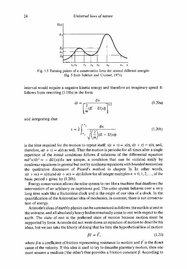
24 Universal laws of nature
U(x)
/X1X2 X3 X4 X5 X6 X
Fig. 1.3 Turning points of a conservative force for several different energies(fig. 5 from Saletan and Cromer, 1971).
interval would require a negative kinetic energy and therefore an imaginary speed. Itfollows from rewriting (1.18b) in the form
dt= 2
dx1/2 (1.20a)
[_(E — U(x))]
and integrating that
= 2J (E— U(x))
(1.20b)
is the time required for the motion to repeat itself: x(t + t) = x(t), v(t + t) = v(t), and,therefore, a(t + t) = a(t) as well. That the motion is periodic for all times after a singlerepetition of the initial conditions follows if solutions of the differential equationmd2x/dt2 = — dU(x)/dx are unique, a condition that can be violated easily bynonlinear equations in general but not by nonlinear equations with bounded motion (seethe qualitative discussion of Picard's method in chapter 3). In other words,x(t + nr) = x(t) and v(t + nz) = v(t) follow for all integer multiples n = 0, 1, 2,..., of thebasic period t given by (1.20b).
Energy conservation allows the solar system to run like a machine that disallows theintervention of an arbitrary or capricious god. The solar system behaves over a verylong time scale like a frictionless clock and is the origin of our idea of a clock. In thequantification of the Aristotelian idea of mechanics, in contrast, there is not conserva-tion of energy.
Aristotle's ideas of earthly physics can be summarized as follows: the earth is at rest inthe universe, and all absolutely heavy bodies eventually come to rest with respect to theearth. The state of rest is the preferred state of motion because motion must besupported by force. Aristotle did not write down an equation of motion to describe hisideas, but we can take the liberty of doing that for him: the hypothetical law of motion
= (1.21)
where fi is a coefficient of friction representing resistance to motion and P is the directcause of the velocity. If this idea is used to try to describe planetary motion, then onemust assume a medium ('the ether') that provides a friction constant /3. According to
1.3 Conservation laws for N bodies 25
(1.21), (i) a body remains at rest if no net force acts on it, and (ii) a net force is required inorder to generate and maintain a velocity. This equation can be derived from Newton'slaw by assuming that the net force consists of linear friction plus a nonfrictional drivingforce F, by considering time intervals that are long enough that acceleration iseffectively damped by friction. The Aristotelian equation of motion can be used todescribe some commonplace phenomena: after a brief initial transient, a ball releasedfrom rest stops accelerating and falls downward with constant velocity through theatmosphere (Stoke's law).
According to Aristotelian critics of science, it is a negative attribute of 'Cartesianthinking' to idealize and abstract by the method of separating and isolating differentcauses from each other to understand how different hypothetical effects follow fromdifferent isolated causes ('reductionism'). Aristotle (whose spirit many system theoristsof today implicitly follow) lumped the sprouting of acorns, the rolling of a ball, and theeducation of a schoolboy under the same heading of 'motion'. As Westfall (1980), writes,'Galileo set mechanics on a new course by redefining motion to eliminate most of itsAristotelian connotations. From the discussion of motion, he cut away sproutingacorns and youths alearning.'
1.3 Conservation laws for N bodies
We now attempt to take explicitly into account N — 1 additional bodies thatcontribute, in part, to the force and torque experienced by our test body above. Writing
= = fext + (1.22)t
for the net force on the ith body, then denotes the force exerted on the body i by body
j within the system while denotes the net force exerted on body i by bodies that arenot counted as part of the system. Here, one must assume that the latter are so massivethat their reaction to the motion of the N bodies within our system can be neglected.Otherwise, we would have to take their accelerations into account and our systemwould consist of more than N bodies.
Beginning with Newton's second law for the dynamical system,
(1.23)j*
and the third law, the action—reaction principle
Ffl = —(1.24)
we can sum over all bodies in the system to obtain
= eXt + (1.25)i=1 i=1 i=lj*i
Since
= + =0, (1.26)i=lj*i i*j

26 Universal laws of nature
this reduces to
N N
= text = Fext. (1.27)1=1 i=1
By defining the location of the center of mass of the system,
N
(1.28)
we obtain the total momentum of the system
= (1.29)
which also obeys Newton's second law in the form
dP = (1,30)
where fext is the net external force acting on all N bodies in the system. That there is nocontribution from the internal forces guarantees that a piece of chalk at rest on a tablecannot suddenly gain a net momentum due to the action of the (electrostatic) forces thathold the chalk together. Conservation of total momentum of the system thencorresponds to the vanishing of the net external force.
Consider next the N-body system's total angular momentum:
(1.31)
The angular momentum changes in time according to
(1.32)
Noting that
x = x + x + F, x = x = (1.33)i i i
where is the net external torque, we see that the internal forces cannot contributeto any change in the N-body system's total angular momentum
= (1.34)
and that conservation of total angular momentum corresponds to the vanishing of thenet external torque. Conservation of angular momentum explains why, for example, ifyou spin on a piano stool (one with relatively good bearings) with your armsoutstretched and then suddenly fold them in close to your chest, the rotation ratesuddenly speeds up.
So far, we have derived two of the three geometric conservation laws for an N-bodysystem from Newton's laws of motion. The third, conservation of energy, also follows

1.3 Conservation laws for N bodies 27
easily. If we compute the work done by the net force along the system's trajectoryduring a time interval from t1 to t2, then
\
=+ (1.35)
i 1 •j*i
which can be rewritten as2
== = T2 — T1. (1.36)
In other words, the work done by the net forces on all of the bodies shows up as thechange in total kinetic energy of the N bodies.
To go further, we find it convenient to transform to center of mass and relativecoordinates. The center of mass coordinate R was defined above; the relativecoordinates are defined as follows:
= R + (1.37)
and the relative velocities are given then by
= V + (1.38)
This decomposition is very useful for it allows us to separate the kinetic energy intocenter of mass and relative contributions:
T= + = MV2/2 + (1.39)
which follows from the fact that
N
= 0, (1.40)
a consequence of the definition of the center of mass.Next, we restrict to conservative external forces
= — (1.41)
so that
2
= — (1.42)i 1 i 1
In other words, the net work of the external forces equals a potential difference.We also restrict to conservative internal forces
= — (1.43)
where is the potential energy of the ith body in the force field due to thejth body. Weapply the action—reaction principle in the form where the forces are presumed to actonly upon the line of centers passing through the two bodies. In this case, candepend only upon the distance between the two bodies, so that with = —
(1.44)

28 Universal laws of nature
and the action—reaction principle reads
= — V = — Ffl (1.45)
since = Ufl• Finally, we compute the net work done by the internal forces:(.2 (.2
—
(1.46)i*j 1 1 1
but
= V, = — (1.47)
and
= dF, = — (1.48)
so that(.2 2 2
= — (1.49)1 i*j 1 i*j I i<j 1
Therefore, if we define the system's total potential energy by
U = U1 + U11, (1.50)i i<j
then the total mechanical energy
E=T+U (1.51)
is conserved along every trajectory of the dynamical system. This conservation law wasfirst derived and then used by Rudolf Clausius around 1855 as the basis for hisstatement of the first law of thermodynamics: the total energy of a closed, isolatedsystem does not change with time.
Finally, we return to center of mass and relative coordinates. Beginning with thelinear transformations
(1.52)
and consequently
= + (1.53)
we have earlier shown how to separate the kinetic energy into center of mass andrelative contributions:
T= + = MV2/2 + (1.54)
This decomposition is useful for application to rigid body problems and we shall use itlater. For the case of two bodies, it is more convenient to rewrite the relative kineticenergy
Trei = (1.55)
in the following way. Since, by definition of total momentum, it follows that
+ = 0, (1.56)

1.4 Geometric invariance principles of physics 29
we can add a null term to Trei to get
Tiei = — + (1.57)
This result can be rearranged to yield
Trei = pv2/2, (1.58)
where p = m1m2/M is the 'reduced mass' and = — is the relative velocity of thetwo bodies. This is the form of the relative kinetic energy that we shall use to analyzecentral potential problems in chapter 4. We shall also use equation (1.56) to deriveanother approximation in chapter 14 that allows the analytic formulation of aconceptually simple example of a deterministic mechanical system that becomeschaotic via an infinite sequence of repeated events called period doubling.
Consider the collision of two bodies moving under no net external force. Since thecenter of mass kinetic energy is conserved, we can concentrate on the relative motionalone. We can then write
T;ei = (1.59)
where Trei and denote the relative kinetic energy before and after the collisionrespectively, and is Newton's 'coefficient of restitution', 0 � � 1. With = 1 thecollision is totally elastic (no kinetic energy is lost) while = 0 denotes a totallyinelastic collision (the bodies stick together and move as a unit). By using equations(1.58) and (1.59), we conclude that the magnitude of the relative velocity obeys therelationship
v' = czv, (1.60)
which says that the relative velocity is reduced in magnitude in an inelastic collision.We turn next to a qualitative discussion of the equations of motion that emphasizes
the grounding of Newton's first two laws and also the three basic conservation laws infour basic symmetries, three of which describe Euclidean geometry.
1.4 The geometric invariance principles of physics
A body always accelerates toward the earth at the same rate g 9.8 m/s2, independent-ly of where (near sea level) the experiment is performed and independently of when theexperiment is performed (independently of the initial time), and independently of thebody's mass, so long as air resistance is negligible. This regularity of motion madepossible the discovery of universal, machine-like laws of nature. A body in free-fall(including a block sliding on a frictionless inclined plane) is also abstractly machine-like(deterministic), meaning that it behaves according to a precise and unchangingmathematical law. Determinism (combined with uniqueness of solutions) means thatprecisely the same initial conditions yield precisely the same trajectories. The basis forthe universal law of gravity is the regularity of the planetary orbits (expressed byKepler's first law) combined with Galileo's local laws of inertia and free-fall. TheGalilean and Keplerian regularities could not hold if the geometry of space, at leastlocally, were not approximately Euclidean.

30 Universal laws of nature
Galileo's law of nature = — g can be rephrased in terms of a conservation law: theenergy of a projectile is conserved if air resistance is ignored. The law of inertia, the mostfundamental regularity of motion, can also be rewritten via integration as a conserva-tion law: momentum is conserved if no net force acts. Conservation laws and invarianceprinciples are inseparable. A conservation law reflects the constancy in time of somedynamical quantity along a system's trajectory whereas the idea of invariance isrepresented by a quantity that does not change when a transformation of coordinates isperformed on the dynamical system at a fixed time.
A transformation ofcoordinates provides an abstract way of describing an operationthat may be performed on a physical system. Invariance under coordinate changesfollows from symmetry. Symmetry means that an object or a system looks the samebefore and after some operation or sequence of operations has been performed. A cubelooks the same after a ninety-degree rotation about a symmetry axis, for example,whereas a sphere looks the same after any rotation through any axis through its center.Three common examples of operations that can be performed (in reality and/ormentally and mathematically) on physical systems are: rigid rotation of a body orsystem of bodies about a fixed axis (change of orientation), a rigid translation along anaxis (change of coordinate origin), and translation of the system at constant ornonconstant velocity (change to a moving frame of reference). The use of coordinatetransformations is a way to represent mathematically the physical idea of performingan operation on a dynamical system, which may be as simple as moving a piece oflaboratory equipment. The connection between invariance principles, which followfrom the symmetries of a system, and the corresponding conservation laws can beunderstood by using coordinate transformations.
The assumption that a body can move at any speed in a straight line is equivalent tothe assumption of a Cartesian axis, which requires either an infinite Euclidean space (ora Euclidean torus). Empty Euclidean space is homogeneous and isotropic because it is afeatureless void. Next in symmetry would follow a curvilinear coordinate system likethe polar angles (04) on a perfectly smooth sphere.
The use of Cartesian coordinate systems in Newtonian dynamics presumes that it ispossible to extrapolate from the local perspective of our limited experience on earthand within the solar system to the abstraction of an infinitely long straight line thatrepresents the direction along which the force-free motion of a hypothetical bodywould be allowed to take place in an unbounded universe. That space is at leastapproximately Euclidean locally, within our solar system, is indicated by the successesof Newtonian theory in explaining both projectile motions and planetary orbits fromthe same laws of motion and force. That this approximation should be validthroughout the entire universe beyond the neighborhood of our solar system isguaranteed by no known experiments or observations, and is still debated incosmology circles. From a scientific standpoint, we must discover the clues to MotherNature's geometry, like her mechanics, empirically. For the time being, we followGalileo, Descartes, and Newton and ignore all other possibilities than Euclideangeometry.
In matter- and force-field-free space any point along a single Cartesian direction isequivalent to any other point because empty Euclidean space is uniform, homogene-ous, the same everywhere along the chosen direction. A Cartesian axis in a Euclideanspace defines the idea of translational invariance: nothing exists to allow one point to bedistinguished from any other along that axis. Translational invariance provides the

1.4 Geometric invariance principles of physics 31
simplest illustration of a symmetry principle. The idea of symmetry is that of lack ofperceptible difference once an operation has been performed. The concept of symmetryarises from Euclidean abstractions like perfect cubes, perfect spheres, and perfectlystraight lines. Granted that we start our theorizing from the unrealistic abstraction of acompletely empty universe, hardly any other assumption than the Euclidean onepresents itself to us initially. Mentally introducing one body into empty Euclideanspace, and assuming that this does not change the geometry of space and time, then thatobject's position along the direction of observation is labeled by a Cartesian coordinatex, starting from some arbitrarily chosen origin. In the absence of other matter and theircorresponding force fields, the choice of coordinate origin cannot play any role at allbecause empty Euclidean space (no other bodies means no other gravitational fields) isitself completely uniform. Translational invariance of Euclidean space means that thelaws of motion are independent of the choice of coordinate origin: the choice of locationin empty, field-free space, where an experiment is to be performed makes no differencein the outcome of the experiment. It is assumed that the presence of a second body, theobserver, does not break the symmetry of translational invariance (the hypotheticalobserver's gravitational field is ignored). For experiments performed on earth,translational invariance is broken vertically by the earth's gravitational field. For localexperiments where the flat earth approximation g constant is valid we haveapproximate translational invariance horizontally over distances short enough thatthe earth's curvature is irrelevant. Translational invariance guarantees that identicallyprepared and identically performed mechanical experiments will always yield identicalnumerical results whether performed in Ventimiglia on 23 September 1889, or in Bozenon 5 November 1994, for example.
Mathematical abstractions like infinitely long and perfectly straight lines are goodapproximations to reality only if the universe is infinite and is assumed to be Euclideanat all distances. If, at large distances from earth, the universe should be finite andspherical, then we would be led, as was Galileo, to the notion that uniform rectilinearmotion must eventually somehow give way to uniform circular motion. One can seehow Galileo arrived at his idea that uniform circular motion should follow from inertiaalone, without the need for a centripetal force. In a Euclidean space this is impossible.On the surface of a sphere, for example, a curved two dimensional Riemannian space,one can construct two Cartesian axes locally and approximately only in the tangentplane to any point on the sphere. By 'local', we mean a small enough but still finiteregion where curvature and gradients can be ignored. By 'global' we mean any finite (orpossibly infinite) region over which curvature and gradients matter. Cartesiancoordinates cannot be constructed globally on a sphere although they can always beconstructed globally on a cylinder, which can be thought of geometrically as theEuclidean plane rolled onto itself and then pasted together. One cannot, in contrast,make a sphere out of a flat sheet of paper or rubber without cutting, tearing, andstretching the sheet before pasting it together (a piece of an exploded balloon cannot bespread flat on a table because of the intrinsic curvature of the surface).
Galileo observed that we can also perform a mechanical experiment on a ship thatsails at constant velocity without changing the results. This observation is the basis forNewton's realization that the first and second laws implicitly imply and require theexistence of a certain class of preferred Cartesian frames of reference. That Newton'ssecond law and the law of inertia single out preferred frames of reference, called inertialframes, can easily be understood by making a coordinate transformation. Denoting p1
32 Universal laws of nature
and F1 as the Cartesian components of the momentum and force vectors, Newton's lawof motion has the vectorial component form
= F1, (1.61)
where x1 is the coordinate labeling the ith Cartesian axis, p1 = my1, and we take m to beconstant for convenience, although this assumption is not essential. The transform-ation to another frame that accelerates linearly at the rate A = d V/dt along axis x,relative to the initially chosen frame is then given by
= x1 J Vdt
= v1 — fAdt (1.62)
= a1 — dV/dt.
In the new frame, denoted by the primed coordinates, Newton's laws are unchangedalong the two Cartesian axes where k i, but along the axis x1 of the acceleration Awe find that
(1.63)
which differs from Newton's law in an inertial frame by the extra 'inertial term' md V/dtthat expresses the acceleration of the primed frame relative to the original one.Whenever A = d V/dt = 0, then we retrieve
(1.64)
in the primed frame, which tells us that we have assumed implicitly that Newton's law(1.61) was written down originally in an unaccelerated Cartesian frame. But 'unac-celerated' relative to what? The answer, as Newton and Leibnitz (and later Mach andEinstein) could only conclude, is relative to empty Euclidean space, also called'absolute space'. In other words, acceleration relative to completely empty Euclideanspace produces measurable physical effects in Newtonian theory. What are thoseeffects?
First, the statement offorce-free motion relative to an accelerated frame is that everybody is observed to accelerate in that frame at the same rate a' = — A, independently ofits mass m, where A is the acceleration of the reference frame relative to absolute space.This means that every force-free body accelerates past the 'primed' observer (anobserver whose position is fixed in the primed frame) as it would be if attracted by aninvisible massive body whose local gravitational acceleration is given by g = A =d V/dt. Second, since the primed observer is at rest, both v' = 0 and a' = 0 hold thatobserver in the primed system of coordinates. Therefore, also according to (1.63), aforce F' = MA (where M is the observer's mass) must exist in order to hold the observerin place in the accelerated frame: the observer would experience the very same effect if atrest in an unaccelerated frame on a planet whose local gravitational acceleration isgiven by the magnitude g = A. The observer's weight on that hypothetical planet

1.4 Geometric invariance principles of physics 33
would be given by w = mA. Since g = GmpianeJR2, then A = d V/dt determines the ratioof mass to radius-squared for the hypothetical planet.
Summarizing, linear acceleration relative to absolute space is detectable and isphysically indistinguishable from the effect of a local gravitational field. This is thefamous 'principle of equivalence'. The important point for us at this stage is: mechanicalmeasurements and predictions that are made in constantly linearly acceleratedCartesian frames are not equivalent to measurements and observations made innonaccelerated Cartesian frames, but instead are equivalent to measurements made inapproximate inertial frames where there is a uniform gravitational field along thedirection of motion.
To emphasize that the Newtonian idea of force is not responsible for the noninertialeffect described above, we show how the force F' in the accelerated frame is derived by acoordinate transformation from the force F in the original frame. If, for example,F(x,t) = — dU(x,t)/dt, where U is a potential energy, then it follows that U'(x',t)= U(x,t) is the potential energy in the accelerated frame, where x and x' are con-nected by the transformation (1.62). Using the definition F'(x',t) = — dU'(x',t)/dt, itfollows by application of the chain rule for differentiation that F'(x',t)= — dU(x — $Vdt,t)/dt, because dx/dx' = 1, so that no extra force is introduced on theright hand side of equation (1.63) as a consequence of the coordinate transformation (1.62).In particular, if F is a constant force then F' = F is the same constant force. In otherwords, the difference between equations (1.61) and (1.63) is due entirely to accelerationrelative to absolute space and has nothing to do with any additional force acting on thebody. The noninertial effect is required by the law of inertia.
To try to be internally consistent (which is possible in Cartan's reformulation ofNewtonian theory — see chapter 11) we would have to follow Einstein's observationthat gravity, locally, cannot be regarded as a force in the usual sense of the word:free-fall in a constant gravitational field yields all of the necessary properties of aninertial frame in spite of the acceleration toward the gravitating body! This line ofthought is deferred until chapter 11.
According to equations (1.61) and (1.63), constant velocity motions (motionswhere dvddt = 0) are transformed into other constant velocity motions (motionswhere also = 0) only if A = 0, only if the two frames in question are both'unaccelerated relative to absolute space'. Then, and only then, is it correct to saythat the trajectory of a force-free body is always rectilinear at constant speed. Inother words, it is implicit in the law of inertia (Newton's first law) that this lawholds, as we have stated it in section 1.1, with respect to, and only with respect to,frames that are 'unaccelerated'. Stated mathematically, dp1/dt = 0 describes force-free motion in any nonaccelerated frame. In contrast, = — md V/dt is requiredto describe force-free motion in a linearly accelerated frame but the term on theright hand side is not a force (this can be proven experimentally by the use of scales:a force-free body in the unprimed frame accelerates in the primed frame, but isweightless there).
The abstract class of frames that are unaccelerated relative to any approximateinertial frame are preferred for the formulation of the basic principles of mechanicssimply because the law of inertia singles out rectilinear motion at constant speed as aspecial st ate of motion that is physically indistinguishablefrom the state of the rest. In theend as it was in the beginning, it is the statement of the law of inertia in empty Euclideanspace that leads to the prediction that acceleration relative to absolute space has
34 Universal laws of nature
precise, measurable consequences, but that constant velocity relative to absolute spacehas no measurable consequence at all.
Where do we find approximate inertial frames in nature? A frame that falls freely inthe gravitationalfield of a more massive body is approximately inertial over times that areshort enough that the gradient of the gravitationalfield can be ignored. Were this not true,then the law of inertia could not have been discovered by Galileo's technique. The earthspins on its axis but can be used as an approximate inertial frame for the discussion of agreat many practical problems where that rotation can be ignored. However, if onewants to describe the motion of a spherical pendulum over a time interval on the orderof a day or longer, then the earth can no longer be treated approximately as an inertialframe and the spinning about its own axis must be taken into account (see exercise 6 inchapter 8). The earth approximates a local inertial frame for the purpose of carrying outa great many experiments precisely because the earth is in free-fall about the sun, andbecause the effects of the moon and other planets can be treated as weak perturbationsto this motion.
That equations (1.61) and (1.64) have the same vectorial form expresses the formalidea of of Newton's law of motion under Galilean transformations.Galilean transformations are those that transform inertia/frames into inertialframes, andso the transformation (1.62) is an example of a Galilean transformation wheneverA = 0, which requires that V is both time-independent and position-independent. Inother words, Galilean transformations include transformations that connect inertialframes with other inertial frames via constant velocity transformations. These trans-formations leave the Cartesian vectorial form = of Newton's law of motionunchanged, yielding = F in the primed frame, although the force componentas a function of the transformed position x' is not necessarily the same as the forcecomponent as a function of position x. That is, it does not necessarily follow thatF(x') = in two or more dimensions, although this equality can easily hold in therestricted case of one dimensional motion. The correct transformation law for the forcecomponents in Cartesian coordinates is discussed below in this section.
We must pay attention to initial conditions when performing coordinate trans-formations. The vector equations (1.61) describe the motion of a body as observedfrom the standpoint of an inertial observer, and equations (1.63) describe the motionof a body from the standpoint of an observer in an arbitrarily linearly acceleratedframe defined by the transformations (1.62). If A = 0 then that frame is inertial,otherwise it is noninertial (unless A = g!). Here is the main point: if we should alsoconnect the initial conditions in the two different frames by using the transformation(1.62), then the corresponding solutions of equations (1.61) and (1.64) describe themotion of one and the same body from the standpoint of two separate observers intwo different inertial reference frames. However, if we should want to describe thepreparation and performance of identical experiments in two different inertial frames,meaning that the primed observer and the unprimed one should use two separate butidentical bodies or machines prepared under identical conditions, then we cannottransform initial conditions according to (1.62) with A = 0. Instead, we must set theinitial conditions and equal to the same numerical values. In the lattercase, one then imagines two different laboratories with identical apparati andidentical preparation, but in two separate frames in relative motion with each other(for example, one laboratory is at rest on the side of the road while the second is on atrain in locomotion).

1.4 Geometric invariance principles of physics 35
What follows is a discussion of Newtonian relativity based upon Galilean transform-ations. We proceed via Gedankeneksperimenten, or 'thought experiments'. Theexamples discussed above are also examples of gedanken experiments.
Following Einstein, who taught us the importance of gedanken experiments forunderstanding relativity principles, let us assume that you are enclosed in a box so thatyou cannot look at the external surroundings to decide whether or not you're inmotion. Suppose, in addition, that you have available all the necessary equipment toperform certain purely mechanical experiments. For example, you may have availablea balI, meter sticks, and a stopwatch in order to perform measurements on the motionof the ball. The point to be understood is this: there is no experiment that you canperform to detect motion at constant velocity through 'absolute space'. In other words,the results of all possible mechanical experiments are completely independent of thechoice of reference frame so long as that frame is unaccelerated relative to absolutespace; is inertial.
Suppose that your box is in a uniform gravitational field and that it slidesfrictionlessly along a perfectly flat surface at constant velocity relative to anotherinertial frame, and that the surface is perpendicular to the gravitational field lines. Yourbox also constitutes an inertial frame of reference and the frames are connected by thetransformation (1.62) with A = 0. The gedanken experiment consists of tossing a ballvertically, along the local gravitational field lines which are antiparallel to thewhich is perpendicular to the xL-axis. No matter whether the box is at rest relative to thefield lines or moves horizontally at constant speed in a straight line, the ball first risesvertically and then falls vertically back into your hand: the results of the experiment arecompletely independent of the horizontal motion of the box. This is another example ofthe fact that one cannot devise an experiment, using the ball (or anything else that ismechanical), that will tell us whether or not the box is in rectilinear motion at constantspeed relative to empty Euclidean space. Again, the results of identically preparedpurely mechanical experiments are invariant (meaning completely unchanged) underGalilean transformations, are identical no matter which inertial frame we choose as ourobservation point. Stated mathematically, for the same numerical choices of initialconditions, the solutions of Newton's law of motion in two different inertial frames areidentical whenever the force is invariant under the transformation (1.62) with A = 0,
meaning that the functional form of the force is unchanged by the transformation.Here's another gedanken experiment: suppose that the box moves vertically upward
along the field lines with constant velocity relative to an approximate inertial framethat we can take to be the earth (and where we neglect air resistance). If a ball is tossedupward with velocity relative the moving origin, and from a height above thatorigin, then the equations of motion of the ball are d2x'k/dt2 = g, exactly the same asif the moving frame were at rest relative to the parallel gravitational field lines thatthread throughout space. This means that the velocity = — and displacement
= v4t — are precisely the same as they would be for an experiment carriedout at the same initial velocity in the frame that is fixed on the moon (we assumeimplicitly the vertical displacements are so small that the variation in g with heightcannot be detected in the experiment).
We now introduce two more Cartesian axes labeled by the coordinates y and z (or x2,and x3). These axes are equivalent to the x- (or x1-)axis because empty Euclidean spaceis isotropic, meaning that it is the same in all directions. In other words, emptyEuclidean space is also rotationally symmetric: if you probe geometrically in one

36 Universal laws of nature
direction, then rotate through any angle and 'look' in another direction, Euclideanspace appears exactly the same in every geometric sense. This way of thinking is neitherautomatic nor intuitive: it violates common sense because our local vertical direction,due to gravity, is not equivalent to the local horizontal directions. This way of thinkingis, in fact, the product of an abstract extrapolation. Before Leibnitz, no one stated thisabstraction explicitly and clearly, that the three separate directions in empty Euclideanspace should, in principle, be equivalent to each other.
Isotropy of empty Euclidean space in the absence of bodies other than our 'test'body, means that if you choose any other direction for the motion of the body (x2 or x3rather than x1, for example) then the linear momentum along the new direction is stillconserved. That is because empty Euclidean space is the same in all directions, and thissymmetry has a mechanical consequence: the law of conservation of angular momen-tum. Angular momentum could not be conserved in the absence of external torque ifempty space were curved or rotationally bumpy. In other words, rotational invarianceis the symmetry principle upon which the conservation of angular momentum relies forits validity: conservation of angular momentum requires the isotropy of empty Euclideanspace.
We shall prove that assertion formally in chapter 2 using a method based uponcoordinate transformations. An elementary example of the connection of rotationalsymmetry to angular momentum is provided by the problem of the motion of twobodies of masses m1 and m2 in a central force. The spherical symmetry of the universalgravitational potential requires that empty Euclidean space is isotropic, is the same inall directions.
We have observed that two fundamental conservation laws of physics requireunderlying symmetry principles that reflect the absence of any geometric properties inempty Euclidean space. There is also a third basic conservation law, conservation oftotal mechanical energy. The symmetry in this case is that of 'translations in time', anidea that we can only discuss abstractly. You can translate or rotate a box in space inthe laboratory, but cannot translate yourself forward or backward in time. An idealclock or frictionless simple pendulum is, nevertheless, time-translational invariance: itticks at exactly the same rate forever. The energy and therefore the amplitude of itsoscillations is a constant of the motion, is invariant. A real pendulum is subject tofriction. Its amplitude is not invariant but decreases exponentially with time.
The Aristotelian equation of motion = f represents the idea that the naturalunhindered state of a body is a state of rest. The derivation of two possible analogs ofmomentum conservation for this equation are assigned in the chapter 18 exercises.Depending upon the law of force, the model can be consistent with both translationaland rotational invariance, but there is no energy conservation law (planets cannot fallfreely about the sun and have to be pushed instead, in which case /3 is the frictioncoefficient of 'the ether').
All five of the basic geometric symmetry principles, translational invariance,rotational invariance, invariance with respect to translations among inertial frames,time translational invariance, and the principle of equivalence are all reflected inGalileo's original description of the trajectory of a body falling freely near the earth'ssurface: = — gAt2/2, = = — and = As Wigner(1967) has pointed out, Galilean kinetics implicitly exhibit the grounding of Newtonianphysics in invariance principles.

1.5 Covariance vs invariance 37
1.5 Covariance of vector equations vs invariance of solutions
We continue our discussion of Newtonian relativity by deducing the complete class ofcoordinate transformations called Galilean, where dp1/dt = in Cartesian coordi-nates x. transforms into = in Cartesian coordinates As we already haveshown above, the transformation (1.62) among relatively moving frames belongs to thisclass if and only if the velocity V is a constant, and if and only if one of the frames isinertial, in which case both are inertial.
For single-particle motion, consider any differentiable, single-valued and invertiblebut otherwise arbitrary transformation of coordinates from one Cartesian frame inEuclidean space to another, x = The inverse transformation is denotedby x• = and these transformations may be linear or nonlinear. What is themost general transformation that always reproduces the vectorial form = F, ofNewton's second law for the case where the force is conservative, where F =—
Because the potential energy is a scalar function U of the coordinates and the time, itstransformation rule is simple: U'(f,t) = = Therefore, by the chainrule for partial derivatives, the Cartesian components of the force have thetransformation rule
(l.65a)ôXk
where we have introduced the summation convention: sum over all repeated indices inany expression. We can summarize this by writing
F' = RF (1.65b)
where R is a 3 x 3 matrix and
F1
F= F2 (1.66)
F3
is a column vector, using the notation of linear algebra (equation (1.65a) uses thenotation of tensor analysis).
Previously, we have used Gibbs' notation whereby vectors are denoted by arrows. Inthe rest of this text (except chapter 4 and several other places where Gibbs' notation isunavoidable), we will use the notation (1.65a) of tensor analysis, and (1.66) of linearalgebra, to denote components of vectors, and vectors F.
This allows the development of classical mechanics in the same language andnotation as are commonly used in both relativity and quantum theory.
The main point in what follows is that
= + (1.67a)
or
= + (1.67b)

38 Universal laws of nature
does not obey the same transformation rule as F' = RF unless the coordinatetransformation is time-independent.
In order that Newton's second law has the same form dp'/dt = F' with p' = my' in thenew frame, it is necessary to restrict to the class of transformations where theacceleration, written in Cartesian coordinates, transforms in exactly the same way asthe force, where
= (1.68)
This condition determines the most general form of the transformation class thatproduces an equation of the form dp'/dt = F' from the equation dp/dt = F, with p = my
and p' = my', because the vector equation (where p is a column vector)
(1.69)
is then guaranteed to hold independently of the coordinate system that we choose, solong as we start with one that belongs to the class oftransformations that we shall discoverbelow.
An example where equation (1.69) is violated is given by the transformation from aninertial to a linearly accelerated frame. In that case
(1.70)
and the extra term on the left hand side represents the acceleration of the noninertialframe relative to the unprimed frame, which is taken to be inertial.
Since x = it follows directly by differentiation that
(1.71)
Calculating the acceleration relative to the primed frame then yields
_____
= + + (1.72)
To achieve our goal, the three second derivatives on the right hand side of(1.72) mustvanish in order that both the acceleration and the force transform according to thesame matrix-multiplication rule. This restricts the class of transformations to trans-formations of the form g,(x1,x2,x3,t) = + a,t where a, is constant and whereb. is linear in the three position variables x1. Therefore, R,k = is a constantmatrix. We then obtain the requirement that
= R,IT,&F'k, (1.73)
where
= (1.74)
should be the same equation as
= F. (1.75)
Pausing, we note that only in the special case where the components as a function

1.5 Covariance vs invariance 39
of the transformed position variables are identical with the components as afunction of x1 will the resulting second order differential equations for and beidentical. In general, = R.kFk(x) does not reduce to the simple condition that
= This means that the force law generally changes its mathematical formwhenever we change coordinates, so the two sets of second order differential equationsfor x1(t) and describing the motion in the two separate frames will generally differfrom each other, and so therefore will their solutions.
Continuing, from the chain rule we obtain
= = = (1.76)
where ökj (not is the Kronecker delta, which means that the transpose of R is theinverse of T; = T Therefore, (1.75) follows automatically from (1.72). Taking intoaccount that = T' then yields = R 1, which says that the matrix R is anorthogonal matrix.
Using the rule det (Rfl) = (det R)2 = det I = 1, where det R denotes the determinantof the matrix R, and I is the 3 x 3 identity matrix, we obtain that det R = 1 or —1. Themost general form of an orthogonal matrix is a rotation (where det R = 1) or a rotationcombined with an inversion (where det R = — 1 due, for example, to x1 being replacedby —x1). Restricting for now to motion in the Euclidean plane and to detR = 1, weobtain from the orthogonality condition RR = I that
(a (a2+b2 (1 0(177)
'\c d) d) — 1- bd c2 + d2) — 1
which is solved by writing a = cos 0 = d, b = — sin 0 = — c, where U is a rotation anglewith the x3-axis and generally can depend upon the position (x1,x2) in the plane.However, by considering the transformation of Newton's laws for two or more particles(see section 2.6) one finds that U must be constant, in which case R represents a rigidrotation. In a rigid rotation, straight lines are transformed into straight lines, and circlesare transformed into circles. A perceptive mathematician once wrote that 'geometry isthe art of reasoning from badly drawn figures.' Every mechanics problem should beginwith a badly drawn figure.
In two dimensions, the most general transformation that leaves Newton's law ofmotion unchanged in form is therefore the 'Galilean transformation'
(178a)x'2 = x2sinO + x2cosO + + u2t,j
which is a rigid rotation of coordinate axes through an angle U counterclockwise aboutthe x3-axis, combined with a rigid translation of the coordinate origin by an amount
and also a transformation to an inertial frame that moves with constantvelocity (u1,u2) relative to the original inertial frame (note that (1.62) with A = 0
provides a special case of this transformation). In contrast, the most general lineartransformation of the form
= ax1 + bx2 +(1 78b)
with nonvanishing determinant, ad — bc 0, is called an affine transformation.

40 Universal laws of nature
Having assumed that the force is conservative, let us now show that this is un-necessary. Assume that x' = Rx + b + Ut is the vector equation of a Galileantransformation, meaning that the matrix R and the column vectors b and u areconstants. Then with dp/dt — F(x,v) = 0 and dp'/dt = Rdp/dt it follows that 0 =R(dp/dt — F) = dp'dt — RF so that we can always define F' = RF as the force in thenew Galilean frame. We must then substitute = RkLx'k — bk — Ukt and
= — Ukt into F(x,v,t) in order to get F' as a function of the primed variables.Formally stated, Newton's second law is covariant with respect to Galilean
transformations: equations (1.78) define the only transformations where, starting froma Cartesian inertial frame, the simple Cartesian vector form = of Newton'slaw is left intact by the transformation. In any other frame Newton's law does not havethe form = F: extra terms appear on the left hand side unless dp'/dt — F'= R(dp/dt — F).
In curvilinear coordinates, even in an inertial frame, Newton's laws no longer havethe simple component form = where = because of extra accelerationterms on the left hand side of the second law. We know that we can write down
= in Cartesian coordinates in an inertial frame and then transform tononinertial and/or curvilinear coordinate systems, but is there a way directly to writedown formal equations of motion that are correct in an arbitrary frame of reference,and that reduce to the simple form = F. with = in a Cartesian inertialframe, but without performing the coordinate transformation explicitly for each separateproblem? In other words, is it possible to rewrite the physical content of Newton's lawsin a more abstract way so that the new equations describing classical dynamics arecovariant vector equations with respect to all differentiable coordinate transform-ations, including transformations to curvilinear coordinate systems and/or noninertialframes? The affirmative answer to this question is provided by the work of the Frenchmathematician Lagrange (1736—1813).
When vector equations of motion transform in covariant fashion, then the vectorialform will look formally the same in different frames. However, the second orderdifferential equations that are obtained by writing out the components of the vectorsexplicitly in terms of derivatives of the position variables will generally be different indifferent coordinate systems. As an example, consider the covariance of Newton's lawof motion under Galilean transformations: the equation = F. holds in all inertialframes (this is the formal vector equation) but, because the force components andF(x',t) are not the same functions of the xi's and x's in the two inertial coordinateframes, FL(x'), the second order differential equations of dynamics will bedifferent in different inertial frames. This leads us to the difference between invarianceand covariance. To make the distinction clear we must first define what we mean byinvariance of functions and equations or motion under coordinate transformations.
Whenever the coordinate transformation is Galilean then the column vectorequation dp/dt = F with column vector p = my transforms into the column vectorequation dp'/dt = F' with column vector p' = my', with the forces related by the vectortransformation rule F' = RF. All that is required for the force to transform this way isthat it transforms like the gradient of a scalar potential energy. If the potential U ismerely a scalar function then the transformation rule for the potential energy isU(x1,x2,t) = A simple example is provided by the case where the potentialU is not rotationally symmetric, where, for example, U(x1,x2) = Clearly,
differs from the function U (the variables and are connected by

Exercises 41
the transformation (1 .78a) with both and set equal to zero). Because U and U' aredifferent functions of x and x' it follows that the second order differential equations for
and in the two different frames are different in spite of the formal similarity of theabstract vector equations dp/dt = F(x,t) and dp'/dt = F'(x',t). Here we have covariancewithout invariance. The lack of invariance follows from the fact that =R,kFk(x) = R,kFk(h(x')) F,(x'), because U'(x') U(x').
The idea of invariance of functions, of equations of motion and their solutions, is amuch stricter requirement than covariance, which is only a formal vectorial idea ofsimilarity. In restricted cases, for example whenever the potential U is rotationallysymmetric, we shall obtain not merely the formal similarity of the vector equationsdp,/dt = and = F(x',t) but also the identity of the resulting differentialequations for and x, and therefore the identity of their solutions as well. An exampleof invariance of the potential energy and correspondingly of the equations of motion(and therefore of their solutions, for the same numerical values of the initial conditions)is given by the case where U(x1,x2) = + so that U(x1,x2) =
+ = + = In other words, the transformed and original poten-tial energies U' and U are exactly the same function because the function U isrotationally symmetric, which simply means that the potential energy does not changeits functionalform whenever the coordinate system is rotated. Every invariant is a scalarfunction, but not every scalar function is invariant under some restricted class oftransformations (we forewarn the reader that many writers on relativity theory havewritten the word 'invariant' when they should have written 'scalar'). The kinetic energyis also rotationally invariant because the scalar product of the velocity with itself isinvariant under rigid rotations, so that the resulting differential equations and theirsolutions are identical for identical initial conditions in both Cartesian inertial frames.
The force-free equation of motion dp1/dt = 0 is not merely covariant but is invariantunder Galilean transformations. The invariance of the law of inertia = 0 underGalilean transformations defines the Newtonian principle of relativity.
The rigid rotations and rigid translations included in (1.78a) are exactly thetransformations that leave the basic defining figures of Euclidean geometry invariant:straight lines and circles are transformed into straight lines and circles under rigidtranslations and rotations, and so the shape of every solid body is also left invariant bythese transformations (all scalar products of vectors, and therefore all angles andlengths, are preserved by rigid rotations and rigid translations). Rigid translations andrigid rotations are the transformations, according to F. Klein, that describe the basicsymmetries of (force- and matter-free) Euclidean space because they preserve theshapes and sizes of all solid geometric figures.
The deep connection between symmetries and conservation laws was first pointedout in mechanics by G. Hamel and F. Engel based upon the methods of S. Lie, and wasalso emphasized by F. Klein and his school. It was Einstein who made physicistsextensively aware of relativity and invariance principles.
Exercises
1. Show that if the earth were attached to the sun by a steel cable rather than attractedby gravity, then the diameter of the cable would be greater than the diameter of theearth (approximate the earth's orbit by a circle). (Koestler, 1959)
2. Inscribe N chords of equal length within a circle of radius r. A body of mass m
42 Universal laws of nature
travels at constant speed v along the chords and is perfectly reflected in eachcollision with the circle (there is no momentum change tangent to the circle).(a) Show that the radial momentum change per collision is = my sin 0, where 0
is the angle between tangent and chord.(b) Show that the net centripetal force obeys F = 2irmv/t = mv2/r as N -+ cc.
(c) Show that if t r312 (Kepler's third law) then F = — k/r2 with k > 0.
(Newton)
3. (a) A cylindrical station in interstellar space spins on its symmetry axis withconstant angular speed w. Explain why an astronaut of mass m standing insidethe cylinder has weight w = mra2, where r is the cylinder's radius ('weight' iswhatever a scale reads when you stand on it). If the force of static frictionsuddenly disappears, does the astronaut slide or continue rotating with thecylinder?
(b) Correspondingly, calculate the percentage by which your weight mg is reducedby the earth's rotation while standing at the equator.
4. The escape velocity of a particle is the minimum initial radial velocity required atthe surface of the earth in order that a body can escape from the earth'sgravitational field. Neglecting the resistance of the atmosphere and the earth'srotation, use energy conservation to find the escape velocity.
5. Consider the vertical motion of a particle moving under the influence of gravityand subject to air resistance. At low enough velocities, the force of fluid friction islinear in the velocity v of the particle. Write down Newton's law of motion for theparticle and show that the maximum possible velocity for a fall from rest isumax = mg//i, wheref= — /iv is the force due to air resistance. (Do not solve thedifferential equation; use basic principles of physics directly.)
6. Show, in cylindrical coordinates (r,0), that
— = Fr,
where Pr = but that
dp0
dt— F0
where Po = mr2O. Note in particular that dpr/dt Fr.
7. Prove that an orbit that is a conic section (the force-center lies at one focus),
= C(1 + tcosO),
requires the inverse square law force
f(r) = — = —4, k >0.
8. Explain why several of the trajectories shown in the figure on page 513 of Koestler,The Sleepwalkers, are dynamically impossible. Sketch the correct trajectories,ignoring atmospheric drag.
Exercises 43
9. Show that, for a single particle with constant mass, Newton's equation of motionimplies the following differential equation for the mechanical energy E = T + U:
dE -.'\= v - Fc) = - v
where = — VU andj is the net nonconservative force. Give an example of anonconservative force that does not change the total energy E. (Hint: refer to one ofthe exercises of this chapter.)
10. A particle of mass m moving in one dimension is subject to the force
F = — kx + -
with k > 0 and a > 0. Find the potential U(x) and sketch its form.Determine the turning points as a function of the energy E and the force
constants k > 0 and a> 0.
11. Show that for an elliptic orbit with the force-center at one focus:(a) the eccentricity is given by
/ 2EL2\112
where b = and(b) the orbit's period is given by Kepler's third law,
= 2ir(m/k)"2a312.
12. Show that for orbits that are conic sections (the force-center lies at one focus) theorbit is elliptic if E <0, parabolic if E = 0, and hyperbolic if E > 0. What is thecondition for a circular orbit?
13. Show that if the orbit is an ellipse with the force-center at the ellipse's center, thenf(r) = — kr with k > 0. (Newton)
14. Show that the orbit equations (1.5b) can be written as a single nonlinear differentialequation
id/i '\(0))—
= mFr
for the orbit equation r =f(0). Show that the substitution u = 1/r yields
u"(O) + u(0) = —
Note, therefore, that the proof of uniqueness of Newton's solution of the Keplerproblem (Fr = — ku) is equivalent to the trivial problem of proving uniquesolutions for linear equations.
15. A shell of mass M is fired with an initial velocity whose horizontal and verticalcomponents are and At the highest point on the trajectory, the shell explodes
44 Universal laws of nature
into two fragments with masses m1 and m2. Denoting by AT the kinetic energy thatis gained in this 'reverse inelastic collision', show that the two fragments areseparated by a horizontal distance
= +g [ m2,JJ
when they hit the ground. (Saletan and Cromer, 1971)
16. A spaceship decelerates vertically at rate a = — a on its approach to the moon.Calculate the weight of an astronaut during the deceleration.
17, Show explicitly that, under the transformation (1.78a) with = 0, straight lines aretransformed into straight lines, and circles are transformed into circles.

2
Lagrange's and Hamilton's equations
2.1 Overview
Lagrange's equations can be derived from Newton's laws. We shall show that bothsystems of equations follow from an extremum principle. The use of extremumprinciples is not confined to classical mechanics or to physics, but in physics bothquantum and general relativistic field equations also follow from extremum principles.In mechanics the extremum principle of interest is called the action principle, and itsintegrand is a function that is called the Lagrangian.
The equations of Lagrange (French, 1736—1813) are more general than Newton's lawof motion in two ways. First, the formal Euler—Lagrange equations can be derivedmathematically from variational principles independently of mechanics, but in this casethe integrand of the action is not the Lagrangian function of classical mechanics (theSwiss mathematician Euler lived from 1707 to 1783). Second, and within the confines ofmechanics, both the Lagrangian and the action survived the quantum revolution. Thiswas shown by Dirac, whose observation formed the basis for Feynman's path integralformulation of quantum mechanics. In the Feynman—Dirac formulation of quantumtheory the action plays the central role, but a single classical mechanical trajectorydominates only in the semi-classical limit of an integrable canonical system. Wheneverquantum effects are important then a complete set of nonclassical, generally nondif-ferentiable, trajectories must be used to describe the physics.
There is a more important sense in which the Lagrangian and Hamiltonianformulations of mechanics are not more general than Newton's laws: within theconfines of classical mechanics the Lagrangian and Hamiltonian formulations aremerely a rewriting of Newton's laws that in no way change the physical content ofNewtonian theory. They allow us to free ourselves from the necessity to start theformulation of a problem by using Cartesian coordinates and an inertial referenceframe where one can only afterward transform to other, more convenient startingpoints.
Newton's laws, as stated in section 1.2, are restricted to inertial frames where onetypically begins with a statement of Newton's laws in Cartesian coordinates. The vectorequation of motion
=F (2.la)
presumes only an inertial frame of reference, but the component form
(2.lb)

46 Lagrange's and Hamilton's equations
with = my1 is only true in a Cartesian coordinate system in an inertial frame: in othercoordinate systems (elliptic, hyperbolic, etc.), there are extra terms on the left hand side.For example, for planar problems in cylindrical coordinates (2. ib) must be replaced by
— rgY) = Fr,
=(2.lc)
where Pr = mdr/dt is the radial component of linear momentum.Because inertial frames and Cartesian coordinates are neither the most general nor
the most convenient starting points for the analysis and solution of most problems inphysics, we would like a more general formulation of the physical content of Newton'slaws than that represented by (2.la) and (2.lb). Some problems are best studied inspherical coordinates (or elliptic or some other system of curvilinear coordinates), andsome problems are most conveniently formulated and analyzed in rotating or linearlyaccelerated reference frames. Lagrange's formulation of mechanics provides us with theneeded generality through a rewriting of Newton's law of motion that is directlyapplicable in arbitrary coordinate systems and arbitrarily accelerated reference frames.The Lagrangian formulation is covariant with respect to arbitrary differentiablecoordinate transformations in configuration space, the 3N dimensional Euclideanspace of the positions of the N particles (see chapter 10 for the explicit proof ofcovariance). This is a distinct advantage over the formulation represented by (2.la) and(2.lb). Also, Lagrange's equations are useful for expressing the deep and importantconnection between symmetry, invariance, and conservation laws. Noether's theoremconnects conservation laws to symmetry through the invariance of the Lagrangianunder a very restricted class of coordinate transformations.
At the end of this chapter, we also introduce Hamilton's canonical formulation ofdynamics in phase space, the best approach to the study of conservative Newtoniansystems because it is the formulation that immediately permits a direct qualitativeanalysis of the motion (chapter 3) without knowing any quantitative details of possiblesolutions.
Because of the deep connection between Hamilton's canonical form of the equationsof motion and the representation of continuous symmetries of physical systems, anabstract generalization of canonically conjugate variables and Hamilton's equationsalso survived the quantum revolution, providing us directly with Heisenberg'sformulation of quantum mechanics, the formulation whose roots grew directly out ofthe empirical attempt to analyze and understand transitions between atomic energylevels in terms of an ad hoc generalization of the old Bohr—Sommerfeld quantizationrules.
2.2 Extrema of functionals
Every reader is familiar with the idea of a 'point function', or just 'function' of one ormore coordinates, The usual notation is to write y = f(x) in one dimension or z = g(x,y)in two dimensions, e.g. for y =f(x), a functionf is just a rule (a 'mapping') that assigns anumber y, given a number x. Of immediate interest is that there is an extension of thisidea of 'mapping' to the case where one considers not merely a function evaluated at a

2.2 Extrema of functionals 47
point but a 'functional' that depends on a path. The useful aspect of ordinary functionsy =f(x) is, in fact, that they are completely independent of the path used to arrive at agiven point x: if x is a holonomic variable andfis an ordinary function (meaning that dfis an exact differential) then y is also a holonomic variable. A nonholonomic variable isone that depends on the path.
To illustrate the idea of a functional, consider a collection of curves with the same endpoints. An example of a functional is a rule that assigns a number to each curve, that is,to each function between the prescribed limits. An example of a functional that belongsto this category is therefore given by the integral
(.X2
I[f]= J
f(x)dx, (2.2a)xl
which is linear in the functionf and has a numerical value that is independent of thedetails of the shape of the curve y = f(x), whenever dF(x) = J(x)dx is an exact differential,and depends only on the function F at the two end points. Nontrivially differentfunctionsf1 andf2 yield different numbers I[f1] and I[f2] only if Fk(x2) — Fk(xl) varieswith k. For a formal and more general definition of functionals based upon the idea ofan abstract vector space of functions, we refer the reader to the excellent texts byLiusternik and Sobolev (1961) and by Dubrovin, Fomenko, and Novikov (1984).
In order to pave the way for Lagrangian mechanics, we must consider functionalsthat are nonlinear in both the integration path and its slope between two specific limits:
I= J
(2.2b)x1
where the curve is given by a function y = f(x), and y' = df/dx is the slope at the samepoint x. In general, the integrand 1(y,y',x)dx is not an exact differential, and so thefunctional I is path-dependent. We shall generally write I in what follows to stand forthe functional I['1]. The generalization to include derivatives of higher order than thefirst, y",y", and so on, is easy once one understands the basic method of treatment.
The relation of functionals to mechanics arises through the following question: givena functional of the form (2.2a), for which paths defined by y =f(x) in some general classof functions is the functional an extremum? That is, which paths yield maxima, minima,or saddle-points for the evaluation of the integral I? This question leads to an oldsubject called the calculus of variations, and we start on that path by reviewing brieflythe related subject of locating extrema of functions of several variables.
In order to find the extrema of a functionf(x1,. . . , Xm) of m variables (x1, . . . , Xm), one
must impose the conditions for a stationary point:
(2.3)
for i = ito m. If one rewrites the integral I above as Riemann sum, then the problem offinding the extrema of that sum is like the problem of locating extrema of a function of adefinite number m of variables except that the number of variables m must bepermitted to approach infinity. It is the limit of infinitely many variables that leads us tothe idea of a 'functional derivative', the derivative of a functional with respect to thefunctions that constitute its domain of definition. With this motivation in mind, we can

48 Lagrange's and Hamilton's equations
arrive at the same idea formally and more directly without using the Riemann sumexplicitly.
Consider the space of all admissible curves y =f(x), all with the same end points x1and x2. This requires an abstract space of functionsf that can be differentiated at leastonce, and for which the integral I is finite. If we formally write
= I (— öy + öy'Jdx (2.4a)
aY Ithen the meaning of 5y is that it is the difference, at fixed x, between two different nearby
functions y =f1(x) andy =f2(x). That is,f2(x) —f1(x) = 5f(x) = öy for each fixed valueof x. The quantity 5y is called the 'virtual variation' and represents the change from onefunction,f1, to another nearby onef2 at fixed x. The idea is shown graphically in figure(2.1). By we mean simply the difference in the slopes of the two nearby and nearlyequal functionsf1 andf2 at the same point x. Since the virtual variation is taken atfixed x, we can exchange the orders of functional variation ö and derivative d/dx:
= = (2.5)
In other words, the derivative with respect to x and the operation of making a virtualchange in the function space commute with each other. One integration by parts thenyields
M = +J —
öydx. (2.4b)ôy
Because of the restriction to variations with fixed end points, we must require that= 0 at both x1 and x2 so that
d51
= J (j— —5ydx. (2.4c)
dxôy
Next, we identify the 'functional derivative' of the functional I in analogy with theexpression
öf= (2.6a)
(thinking again of the integral as a Riemann sum) as the expression
M = I (2.6b)5y(x)
which yields the functional derivative1 as
M ô1"27
öy(x) —
Pushing the analogy based upon the Riemann sum to its logical consequence, thecondition that a function y = f(x) yields an extremum for the functional I for completely
It is formally possible to construct the entire functional analog of a Taylor expansion by the introduction ofhigher order functional derivatives.

2.2 Extrema of functionals 49
y
(x2,y2)
X X2 X
Fig. 2.1 Virtual variations at fixed x.
arbitrary and unconstrained variations 5y(x) is simply the condition that the firstfunctional derivative of I vanishes at every point x. The consequence is that thefollowing differential equation, called the Euler—Lagrange equation,
&t'—o 28
dxay'
must be satisfied by any functionf that makes the path-dependent functional I[fl an
extremum. The harder question whether a particular extremum is a maximum,minimum, or saddle-point is not discussed explicitly here.
To illustrate the usefulness of variational principles in mechanics we show how toformulate the well-known Brachistochrone problem, where a bead slides frictionlesslydown a wire in the presence of gravity. Consider all possible shapes of wires with theend points fixed, and find the shape that yields the least time of descent. The descenttime is given by the integral
=(2.9a)
where ds2 = dx2 + dy2 = dx2(1 +f(x)2) is the square of the arc length along the pathy =f(x), and v = follows from energy conservation if we choose the zero ofpotential energy so that E = mgy0. Therefore, 1(y,y',x) = [(1 + y'2)/2gy]112, and thedifferential equation for y =f(x) follows from the Euler—Lagrange equation
dô1— (29b)
Next, we show how to use a variational principle to formulate and find the shortestdistance between two points on the surface of a sphere. The arc-length ds on a sphere ofradius r is given by ds2 = (rdO)2 + (rsin = (rdO)2[1 + (f'(O) sin 0)2], where wehave written =f(0). With no loss of generality, we can take r = 1. The arc-length foran arbitrary path between points 1 and 2 on the sphere therefore has the form
S = JdO[1 +(f'(0)sinO)2]"2 (2.lOa)
xl

50 Lagrange's and Hamilton's equations
and depends upon the path. The Euler—Lagrange equation yields the differentialequations that describe a geodesic, or great circle, on the spherical surface. Since is
independent of f(0), we obtain easily that
f'(6)sin20210b
[1 + (f'(O)sin O)2]h/2— c, (
where c is a constant. It follows easily that
f'(O)= 1
1/sin 01/2' (2.lOc)
i]
whose integration yields the equation of a geodesic on the unit sphere.
2.3 Newton's equations from the action principle
We begin by showing how Newton's equations of motion can be obtained from avariational principle. For discussions of the history of variational principles inmechanics and geometry we can recommend the texts by Bliss (1962), Lanczos (1949),Hamel (1967), and Sommerfeld (1947—52). We begin with a particular functional that isknown in mechanics as the action,
A= J
(T— U)dt, (2.11)(I
where Tand U are the kinetic and potential energies of N particles with masses Forvirtual variations of the particles' positions, and with both end points fixed, in aninertial frame (the spatial variations in particle positions are performed at fixed time t)we obtain
N
ÔÁ = —
j+ (2.12)
i=1
The extremum condition öA = 0 is satisfied for arbitrary variations only if
+ = 0, (2.13a)
which is a special case of a result known in the literature as D'Alembert's Principle2,and where the second term in the equation represents the 'virtual work' done by theconservative forces. The word virtual is used because the variations in particle positionsare only hypothetical displacements at fixed time rather than real motions of themechanical system. The latter can only occur when the time t changes. In particular, thevariations are fixed-time displacements that must respect any and all geometricconstraints imposed upon the system but are otherwise arbitrary.
An example is given by the case where a marble rolls along the surface of a
2 If we set the momentum derivatives equal to zero and replace gradients of potentials by arbitrarynonconstraint forces, then we have a general condition for the equilibrium of a constrained system.According to the brief sketch of history provided by Lanczos (1949), this principle, the principle of virtualwork, was popular in medieval times and goes back (in disguised form) to Aristotle (see also Hamel, 1967).

2.3 Newton's equations from the action principle 51
y
hemispherical bowl: the motion is constrained to lie on the surface of a sphere, and theequation of the constraint isjust that the distance of the marble from the sphere's centeris constant. The particle's trajectory is therefore not free to explore all three dimensionsbut is confined to a two dimensional surface.
If there are no constraints, which means that the Nd virtual displacements are allcompletely arbitrary, then Newton's law = — for a conservative system followsfrom equation (2.1 3a). The reason for this conclusion is that, with completely arbitraryvariations in particle position, the variational equation cannot be satisfied in any wayother than term by term. Conversely, whenever there are constraints then equation(2.1 3a) cannot be satisfied term by term, and we shall present two methods for treatingthe constrained cases below.
Another elementary example of a constraint is provided by placing a block on aninclined plane: the block is prevented by the constraint force, the normal force Nexerted by the plane on the block, from falling vertically downward in the presence ofgravity (figure 2,2). Here we use N as the symbol for the normal force, although Nis alsoused to denote the number of bodies in the system. In this case the constraint equationy = x tan 0 can be used systematically to eliminate one of the two Cartesian coor-dinates (x,y), so that we have only one independent position coordinate. Note that theforce of constraint N is perpendicular to the one dimensional surface defined by theconstraint equation 4(x,y) = y — x tan 0 = 0 (for a large class of constraints the force ofconstraint points in the direction of the normal to the constraining surface). As we havestated above, if a body is confined to move on the surface of a sphere then we haveanother example of a constrained system where the equation of constraint is given inspherical coordinates (with origin at the sphere's center) by the formula r = a, where r isthe radial coordinate of the particle and a is the radius of the sphere. If we write thisconstraint equation in the form 4(r) = r — a = 0, then again we see that the force ofconstraint f is perpendicular to the surface of the sphere, fcc V4.
Next we generalize by introducing the class of constraints called holonomic, whichmeans that the constraints are defined globally independently of any path taken by thebody. This means that the constraints can be written in the form of point functions
= 0, where I = 1,2,..., k, and k is the number of different constraints. Inthis case the corresponding constraint forcesj are always perpendicular to constrain-ing surfaces çb,(F1, .. . , = 0, and therefore can be written in the form
=(2.14)
x
Fig. 2.2 A constrained system.

52 Lagrange's and Hamilton's equations
where the coefficients )., may depend upon the time t. We prove this as follows: since itfollows from . . , rJ\T,t) = 0 that
dq5k = = 0, (2.15)
it follows from combining equations (2.14) and (2.15) that the work
= = = (2.16)
done by the constraints for real displacements due to motion of the bodies isnonvanishing whenever the constraints are explicitly time-dependent. In that case, theconstraint forces are not perpendicular to the real displacements. However, because thevirtual displacements are performed at fixed time t, the virtual work vanishes,
= = = — = 0, (2.17)
simply because of the condition öt = 0. It follows that the constraint forces areperpendicular to the virtual displacements so long as the surfaces of constraint do notchange with time.
Taking into account that the constraint forces have vanishing virtual work, we canthen rewrite the variational equation (2.13a) in the form
+ = 0, (2.13b)
and although the virtual variations are not all independent (because they are coupledby k constraints), the inclusion of the constraint forces allows us to satisfy Newton's lawterm by term in (2.13b), yielding Newton's second law in the form
(2.18a)
A different way to say this is that one agrees to choose the k unknown coefficients inthe definition (2.1 8a) of the constraint forces precisely so that equation (2.1 3b) issatisfied for each separate index i. Without the explicit inclusion of the constraintforces, the variational equations (2.13b) cannot be satisfied term by term unless thesystem is completely unconstrained.
So far only conservative nonconstraint forces have been included in our discussion ofthe variational principle, so we must also generalize the method of derivation to permitdissipation. For systems with dissipative forces the variational principle (the actionprinciple, also called Hamilton's principle) must be changed to read:
(t2 rt2c5
fTdt
= J5Wdt (2.19)
J(l
where
(2.20)
which is a fixed-time variation, is the virtual work done by all nonconstraint forces andmay include dissipative as well as conservative contributions. This yields the varia-tional equation in the form

2.4 Lagrange's equations 53
N
— = 0. (2.13c)
If the virtual displacements are unconstrained, then Newton's law of motion =follows where is the net force on the ith body. If there are k time-independentconstraints, then the virtual work done to the constraint forces vanishes (because theconstraint forces are perpendicular to the virtual displacements) and the variationalequation can be rewritten as
N
— 3). =0 (2.13d)i= 1
to yield
(2.18b)
where the right hand side represents the net external force plus the net force ofconstraint on the ith particle. This concludes our proof that Newton's law, in its mostgeneral form, follows from the action principle.
2.4 Arbitrary coordinate transformations and Lagrange's equations
Newton's law in the form
(2.la)
requires that we use an inertial frame of reference, while the component form
(2.lb)
is correct only in a Cartesian inertial frame. Cartesian coordinates can be defined'locally' (in an infinitesimal region near any point) on a nonEuclidean surface like asaddle or a sphere, but can be defined 'globally' (with the same coordinate axesextending without limit to infinity) only in a Euclidean space (meaning a 'flat' ornoncurved space). The law of inertia demands a Euclidean space, but nonEuclideanspaces can only arise due to constraints that confine the motion of the system to acurved subspace that is embedded in the dN dimensional Euclidean configurationspace of the positions of the N particles, where d = 1, 2, or 3.
Consider next a completely general transformation of coordinates from Cartesian toany other holonomic coordinate system, meaning any global coordinate system thatcan be constructed completely independently of any need to integrate the velocities ofthe bodies under consideration. Spherical, cylindrical, elliptic, or any other curvilinearset of coordinates will do, because one can define them globally and geometricallyindependently of the dynamical system under discussion. Denoting the new andarbitrary coordinates by the symbols we can write the transformation formally as
= = . . , qf,t) = . . , . , q1,t),h1(q1, . . ., q1,t)), (2.21a)
when n = dN is the number of Cartesian coordinates andf= dN — k is the number ofnew coordinates k constraints having been eliminated explicitly before carrying outthe transformation. Equation (2.21a), written in terms of the new set of variables(q1,. . .,q1), is called a 'point transformation' because points in the two different

54 Lagrange's and Hamilton's equations
reference frames correspond to each other in one-to-one fashion (there is nopath-dependence, no anholonomy, meaning that J, and are ordinary functionsrather than functionals). Configuration space may be nonEuclidean only if k � 1 but isotherwise Euclidean and is simply the space of thef variables
q. in (2.21a) are traditionally called 'generalized coordinates' forpurely historic reasons: they are very general in the sense that any holonomic system ofcoordinates will do. All Cartesian and curvilinear coordinates in Euclidean space areholonomic. More generally, a holonomic coordinate is any coordinate that followsfrom integrating an exact differential. If, instead of starting with a 'point transform-ation' of the form Xk . ., qf,t), we had tried to start with a transformationdefined by the generalized velocities, where Wa = and had then tried to definea set of generalized coordinates (holonomic coordinates) as time integrals of thetransformed velocities Wa, then the transformation matrix would first have to satisfythe integrability condition = This integrability condition is non-trivial and is usually not satisfied by arbitrary velocity transformations, as we show inchapter 12 in the context of rigid body dynamics for the nonintegrable velocities thatarise naturally in rigid body theory (chapter 9). Parameterizations of the motion thatare constructed by integrating nonexact differential forms, meaning nonintegrablevelocities are called nonholonomic coordinates, or quasicoordinates and also arediscussed in chapter 12.
The main point for what follows is: because the differentiable transformation (2.21a)is completely arbitrary and may even be explicitly time-dependent, we shall arrive at aformulation of Newtonian dynamics that is valid in arbitrary coordinate systems, evenin noninertial frames.
Because the constraints are here assumed to have been eliminated explicitly, there isno need to include the forces of constraint in our formulation and so we can start withthe variational principle in the form
N
(2.13c)
where includes both conservative and dissipative effects and is the net nonconstraintforce on body i. The first aim is to express both terms in the variational equation byequivalent expressions in terms of generalized coordinates. It is easy to transform theforce term. Writing
f= (2.22)
k=1 i=1
we can then identify
Qk = (2.23)i=1
as the generalized force acting on the kth generalized coordinate qk, yielding
— = 0, (2.24)
where from now on (unless otherwise stated) we use summation convention (sum overany and all repeated indices), meaning, for example, the sum over the repeated index k is

2.4 Lagrange's equations 55
implicit in equation (2.24). To go further, we must also transform the acceleration termin (2.24).
Noting that
= qk + (2.25a)
we see also that
d dvi.= —I I — (2.26a)
dt2 dt\\
and since
(227)
and
= + (2.25b)
if follows that
(2.28)
which is a very useful result. It allows us to see, for example, that
d2F, d 1 4 d 1
= — = (2.26b)
so that we can now combine all of our results to rewrite our variational equation, whichwas derived in the last section from Hamilton's principle, in the form
3T '\(2.29a)
Since all constraints have already been eliminated, thef variations are completelyarbitrary so that each coefficient of in the variational equation must vanish term byterm for k = 1,. . . ,f otherwise there is no way to satisfy (2.29a) for completely arbitraryvariations. The equations of dynamics then have the form
doT OT(2.29)
and are called Lagrange's equations of the first kind.In Cartesian coordinates in an inertial frame, = x1, the kinetic energy of a single
particle is T = and Lagrange's equations (2.29') simply reproduce Newton'ssecond law in the usual form md2x1/dt2 = where Q, = In general, the differentialequations (2.29') are second order in time for the generalized coordinates and hold fordissipative as well as for conservative systems. These equations of motion describeneither more nor less physics than do Newton's laws, because they are merely atransformation of Newton's laws to arbitrary holonomic coordinate systems. But, in

56 Lagrange's and Hamilton's equations
contrast with our original formulation, where = F., Lagrange's equations aredirectly applicable in the form (2.29') in accelerated as well as in inertial frames ofreference.
We now give two examples of the transformation (2.21a) to other inertial coordinatesystems for a single particle. In cylindrical coordinates, where q1 = p, q2 = çb, andq3 = z, and where the hats denote unit vectors,
F = + (2.21b)
yields
dF = dp5 + + (2.25c)
so that dq1/dt = dp/dt, dq2/dt = and dq3/dt = dz/dt. The kinetic energy isthen given by
T = m(.2+ p2qY + (2.25c')
and Lagrange's equations for a single particle then read
= (2.29b)
d2z=
In spherical coordinates, where q1 = r, q2 = 0, and q3 =
F = (2.21c)
defines the vectorial transformation function in equation (2.21a), and
dF = + rdOC + r sin (2.25d)
In this case, dq1/dt = dr/dt, dq2/dt = rd0/dt, and dq3/dt = rsin 0d4'/dt and the kineticenergy is given as
T = + r2 sin2 (2.25d')
Lagrange's equations then read
— rO2 — rsino2qY) = Qr,
— = Q0, (2.29c)
=
Any system of curvilinear coordinates can serve as 'generalized coordinates', or just'coordinates'. For other curvilinear coordinate systems, see the very readable text byMargenau and Murphy (1956).

2.4 Lagrange's equations 57
Returning to the physics, to the law of inertia and Newton's second law, weemphasize strongly that Lagrange's equations are merely a rewriting of Newton'ssecond law and the law of inertia for application within a completely general coordinatesystem, even a noninertial one. No new physics is introduced by the rewriting, by theachievement of general covariance in configuration space.
For example, for a particle moving in one dimension, the transformation to a linearlyaccelerated frame is given by
= x — Jv(t)dt (2.30)
and a(t) = dv(t)/dt is the acceleration of the primed frame relative to the unprimed one.Since the unprimed frame is taken as inertial, then
= = + = (2.31)
so that
p = = + v(t)) (2.32)
is the linear momentum relative to the inertial frame, but expressed in the noninertialcoordinates, and therefore
+ a(t)) = F' (2.33)
where F' is the net force on the body in the noninertial frame. The extra 'inertial term'(or, better said, noninertial term) ma(t) represents the acceleration of the primed framerelative to absolute space (relative to the collection of all inertial frames of reference). Ina linearly accelerated frame a force-free particle accelerates past any observer who is atrest in that frame, while simultaneously the observer himself experiences a forceF' = Mdv/dt in the direction of the acceleration that holds him in place and isqualitatively and quantitatively similar to the effect of 'weight' to a uniform gravi-tational field with local strength g = dv/dt. The physics of this phenomenon hasnothing whatsoever to do with any difference in form between Newton's andLagrange's equations, but has instead everything to do with the fact that noninertialeffects occur whenever motions are observed relative to noninertial frames.
So far, we have kept the discussion general enough that dissipative forces areincluded. If we now restrict our considerations to conservative forces defined by ascalar potential . . , that depends upon positions but not velocities, then with
. . , 1N) = U(q1 qj) we have3
= — (2.34)qk
Defining the integrand of the action A by the Lagrangian L = T — U, where L is afunction of both the generalized coordinates and generalized velocities and also thetime, then we can rewrite (2.29') to obtain Lagrange's equations of the second kind
We include the tilde on U here to remind the reader that the potential energy is a scalar but is neverinvariant under completely arbitrary coordinate transformations. For consistency, we should also writeT(x 1,...,x1,x 1,...,x1,t) = T(q 1,...,q1,q q1,t). In section 2.6 we shall find it absolutely necessary to takethis sort of care with our notation.

58 Lagrange's and Hamilton's equations
ÔL0. (2.35a)
If, rather than starting with the variational equation (2.29'), we had started at the verybeginning with the action
A= J
Ldt. (2.36)Li
with the Lagrangian L expressed directly in terms of thefgeneralized coordinates thef generalized velocities dqjdt and the time t, then because the variations oq, arecompletely independent of each other, and because there are no dissipative forces, theaction principle 5A = 0 for variations vanishing at the end points yields directlyLagrange's equations of the second kind
———=0. (2.35a)
As an example, in Cartesian coordinates in an inertial frame, the Lagrangian for aparticle with mass m is
L = T — V = + — U(x1,x2) (2.35b)
and Lagrange's equations yield Newton's laws in their most familiar form,
_rL (2.35c)
In cylindrical coordinates in an inertial frame, in contrast, with
L = + r2O2) — U(r,O) (2.35d)
and U(x1,x2) = U(r,O), Lagrange's equations yield directly Newton's law in theirtransformed form
00 . . oCmr2EI = — + r02) = — -i-—. (2.35e)
Next, with a brevity that fails completely to foreshadow its importance for physics, weintroduce a vector in configuration space,
p, = (2.37a)
which is called the canonical momentum, the momentum conjugate to the coordinateq.. Sometimes, this quantity is equal to the mass multiplied by the generalized velocity
but is generally not the same as As an example, in sphericalcoordinates where
T = + r2 sin2 042), (2.25d')
we find that
Pr = = (2.37a)

2.4 Lagrange's equations 59
is the linear momentum along the radial direction, that
Po = = (2.37c)
and that
p4, = = mr2 sin2 0j (2.37d)
is the angular momentum about the z-axis.With the introduction of Hamilton's equations (section 2.8 and chapter 3) and the
discussion of the geometric interpretation of Lagrange's equations (chapter 10), thereader will be in a better position to appreciate the significance of the idea of the'canonical momentum' conjugate to a generalized coordinate. Later, in section 2.6, weshall show that it is the canonical momentum rather than the generalized velocity
that comes into play when we derive the connection between symmetry,invariance, and conservation laws by using the Lagrangian formalism.
We can also rewrite Lagrange's equations of the first kind in the form
=+ (2.38a)
which illustrates that the rate of change of canonical momentum usually differs fromthe generalized force in arbitrarily chosen coordinate systems because of position-dependent kinetic energy terms. For example, in cylindrical coordinates we obtain
dPr= rO2 — (2.38b)
Whenever there are no dissipative forces, whenever the net force on each particle isconservative, then we can introduce the Lagrangian L = T — U and can rewriteLagrange's equations of the second kind in the form
= (2.37e)
Again, we expect to find kinetic energy contributions to the right hand side of thisequation.
Finally, if we apply Lagrange's equations in a linearly accelerated frame, where
= = + v(t))2 = (2.31)
then
p = + my (2,38c)
is the canonical momentum, and Lagrange's equations read simply
= + dv/dt) = F'. (2.38d)
In other words, the canonical momentum is the momentum in the inertial frame, butrewritten in terms of the noninertial coordinates! If we interpret p as the canonical

60 Lagrange's and Hamilton's equations
momentum rather than as the linear momentum, then Newton's law in the simple formdp/dt = F is no longer restricted to inertial frames but is covariant with respect totransformations to and among linearly accelerated Cartesian frames as well.Covariance is not a physical principle but is something that can be achieved by thereformulation of vector equations, with a careful definition of what constitutes a vectorand what does not (see chapters 8 and 10).
We conclude this section with the reminder that Lagrange's equations have the sameform (2.38a) in every coordinate system in configuration space. We discuss thegeometry and transformation theory beneath this aspect of Lagrangian mechanicsexplicitly in chapters 8 and 10. In chapter 10 we show how general covariance inconfiguration space works for Lagrange's equations.
2.5 Constrained Lagrangian systems
Next we derive a method for including constraints explicitly, as an alternative to theircomplete elimination. The reason is that nonholonomic constraints cannot beeliminated, but holonomic ones can be treated within the same formalism. Consider aconstrained Lagrangian system where L = T — U in an n dimensional configurationspace (n = Nd when d is the dimension of physical space (d = 1, 2, or 3)), and wherethere are k constraints of the form
+ = 0, (2.39a)
for variations performed at fixed time t. If
=, (2.40)
then the constraints are holonomic because the differential form (2.39a) is integrable (anintegrating factor is allowed here). In this case (2.39a) can be integrated at fixed time toyield a point function . ., = 0 of the generalized coordinates. Otherwise, thedifferential form (2.39a) is nonintegrable (no integrating factor exists), which means thatthe constraint is nonholonomic. In that case, any integral of the constraint equation(2.39a) is path-dependent and so the integrations cannot be performed until thecoordinates are known as functions of t, that is, until after the dynamics problem hasbeen solved. We emphasize that we include the case where the differential form (2.39a) isnonintegrable, but has an integrating factor, within the classification of holonomicconstraints. Another distinct possibility for a nonholonomic constraint is one given byan inequality.
An example of a holonomic constraint is one where the radial position r = L of amass m attached to the end of a rod of length L is fixed, if we take the other end of therod as the origin of coordinates.
An example of a nonholonomic constraint that is given by an inequality is providedby the case where a particle slides under the influence of gravity on the surface of acylinder of radius R. In this case, the particle's radial position r, measured from thecylinder's center, obeys the constraint r � R.
An example of a nonintegrable constraint given by a differential form is provided bythe motion of a disk that rolls without slipping on a plane (see figure 2.3). Here, there aretwo constraints,

2.5 Constrained Lagrangian systems 61
Fig. 2.3 A disc rolls without slipping (fig. 1.5 from Goldstein, 1980).
dx =(241)
dy = sin O,j
and we leave it as an exercise for the reader to show that this pair of differential forms isnonintegrable and has no integrating factor.
We return now to the original action principle, but for the case where the ngeneralized coordinates cannot all be varied freely because they are subject to k � 1constraints. As earlier in this chapter, we use the summation convention in this section(sum over all repeated indices in an expression). In the action principle, with end pointsfixed, one then obtains
=— = 0 (2.42)
which yields the by-now familiar variational equation
—
öq1 = 0. (2.43)
However, no further simplification is possible because the k constraints couple the nvirtual variations 5q1. In order to go further we must include the effects of the forces ofconstraint explicitly in the equations of motion. To do this in the most elegant way, wefollow Lagrange and introduce his method of undetermined multipliers (the onlyalternative to Lagrange's method is to eliminate the constraints beforehand, and thento work withf= Nd — k independent variables as we did earlier).
Introducing k unknown parameters 2k and then writing
= 0 (2.44)
for a fixed time variation, we can rewrite our variational equation (2.43) to read
—
+ 2kaik) = 0.
Then variations are not independent, but the object of introducing the extra term in(2.45a) is to agree to choose the k undetermined multipliers (Lagrange's undeterminedmultipliers) 2k so that the equation
— = (2.45b)

62 Lagrange's and Hamilton's equations
is satisfied for each index i = 1,2,..., n. The terms on the right hand side can representnothing other than the constraint forces If the constraints are holonomic,then, as we proved earlier, the constraint forces are perpendicular to the surfacesdefined by the constraint equations 41(q1, . . . , = 0. Note, however, that we now mustsolve n + k differential equations: the n Lagrangian differential equations given by(2.45b) along with the k (integrable or nonintegrable) first order differential equations
a grand total of n + k variables (q1,. . . , and (2k,. . 2k). Solving for the unknownmultipliers is therefore an integral part of solving the dynamics problem in theLagrange multiplier formulation of dynamics.
As an example, consider the motion of a block on a frictionless inclined plane (figure2.2). The kinetic energy is
T= m(.2 + (2.46)
and the potential energy is U = mgy. Here, the holonomic constraint is dy = dx tan 0so that we have n = 2 and k = 1. Lagrange's equations with one undeterminedmultiplier yield
(247)m9 —2 + mg 0.
We can eliminate 2 to obtain
(2.48)
which can be integrated immediately. Using the constraint equation, we can then solveto find
2 = mg cos2 0. (2.49a)
We identify = — 2 tan 0 as the force of constraint in the x-direction and = 2 asthe force of constraint in the y-direction.
Finally, let us return to the discussion of equations (2.14) to (2.17) in our earlierdiscussion of constraints. There we observed that the real displacements generally arenot perpendicular to the constraint forces. We can now illustrate this effect by anexample: consider a massless rod fixed at one point in space, tilted at an angle relativeto and rotating steadily about the z-axis (figure 2.4). A bead of mass m slidesfrictionlessly on the rod and we denote its distance from the rod's fixed point by q. TheLagrangian is
L = T = +mv2 = + (2.49b)
where r = q sin and Lagrange's equation reads
= qoi2 sin2 o. (2.49c)
The virtual variations are, by definition, along the direction of the rod and therefore areperpendicular to the constraint force which, because the bead slides frictionlessly, isnormal to the rod. Clearly, however, the actual displacement of the bead is generally

2.6 Symmetry, invariance, and conservation laws 63
Fig. 2.4 Rotating rod (fig. 73 from Arnol'd, 1989).
not perpendicular to the constraint force and that is the main point to be made by thisexample.
2.6 Symmetry, invariance, and conservation laws
We return to our action principle where the action is given by
A = J'Ldt (2.36)
with L = T — U. Instead of virtual variations and the search for an extremum, weconsider only paths that are solutions of the dynamics (extremum paths), but where thevariations will now represent infinitesimal transformations of coordinates4. Thefinite transformation is given by qj(a) = ..,q1,a). Each value of a defines adifferent coordinate system, and all transformations in the class are generated bycontinuously varying the parameter a (this method is generalized to include more thanone parameter in chapters 7, 8, 12 and 15). The qualitative idea is that we shouldimagine two different 'snapshots' of the same configuration of the particles of thesystem in two different coordinate systems taken at the same time t. We can take theviewpoint that the laboratory frame is transformed, while the system remains fixed inspace, or one can transform the dynamical system while leaving the laboratory framefixed in space. We denote byf the inverse transformation, . .,
a = 0 to yield the identity transformation = F1(q1,.. . , q1; 0) =Up to this point, we have not been careful enough with our notation, as we have
sometimes used the very same symbols L, T, and U to denote the Lagrangian, kinetic,and potential energies in any and all coordinate systems. In what follows, we must use amore refined notation, one that takes into account that whenever we transformcoordinates we get a Lagrangian than the one we started with: the Lagrangianis a scalar function of the generalized coordinates and velocities and therefore trans-forms according to the rule L'(q',dq'/dt,t) = L(q,dq/dt,t) whenever we change coordi-nate systems. The kinetic and potential energies are themselves scalar functions:T'(q',dq'/dt,t) = T(q,dq/dt,t) and U'(q',t) = U(q,t). In particular, we shall denote theLagrangian in the coordinate system (q1(a),. . . , q1(a)) by = Sincethe variations near the identity (a = 0 defines the identity transformation) are definedto first order by
=öa, (2.50)
The study of symmetry by infinitesimal coordinate transformations goes back to S. Lie.

64 Lagrange's and Hamilton's equations
it follows that the first variation in the action,
= — A(O)J
dt=
Jt2+ dt, (2.51 a)
has the form
=
=(2.51a')
The time-integral is missing in (2.51a') because both the original and infinitesimallytransformed paths satisfy Lagrange's equations in the two different coordinate systems:both paths are simply different coordinate descriptions of the same dynamics inconfiguration space. Note that the shift in the action due to a change in at fixed time isequal to the difference in the quantity
G = , (2.52a)
but evaluated at two different times t1 and t2. We are now in the right position toformulate the connection of symmetry, invariance, and conservation laws mathemat-ically.
In general, the Lagrangian is a scalar function of the generalized coordinates andvelocities under arbitrary differentiable point transformations in configuration space.This sounds impressive, but the size of this collection of transformations is much toogreat to be of any practical use in physics. We therefore consider a much smaller andvery restricted, but much more useful, class of coordinate transformations, those thatdepend continuously upon one parameter and leave the Lagrangian and therefore alsothe action invariant under variations in the parameter The idea of a scalar function isjust the idea of getting the same number: the Lagrangian at two 'image points',
q = F.(q1,.. . , qf,c1), is equal to the same number whenever wereplace the generalized coordinates and velocities by specific numbers, becauseL(q,dq/dt,t) = L'(q',dq'/dt,t). Invariance is a much more restricted area that reflects, inaddition, the identity of functions under transformation: one gets not only the samenumber, for a given set of values of the generalized coordinates and velocities, but theoriginal and transformed Lagrangians are exactly the same function,L(q,dq/dt,t) = L(q',dq'/dt,t), or just L = L' (the reader can now see why sloppy notationmust be eliminated). For example, in the plane, the two different ways of writing thekinetic energy, = m(t2 + = + = yield the samenumerical value whenever the Cartesian coordinates are connected to the cylindricalones by the transformation x = r cos y = r sin but the functions T and T' are notthe same function of the respective variables. If we think of a third function T" of thevariables (iYcb), then the functions T and T" are identical but both differ from thefunction T' (or, stated differently, x2 + y2 is not the same function of x and y asx2 + (xy)2).
At this stage we do not yet require that the Lagrangian is invariant, only that theaction is. The invariance principle for the action under infinitesimal transformations issimply 5A = 0 for arbitrary variations and yields
G = = constant (2.52')
2.6 Symmetry, invariance, and conservation laws 65
at all times, which is a conservation law! This is the content of Noether's theorem inparticle mechanics, that the quantity G is conserved along the system's trajectories inconfiguration space whenever the infinitesimal transformation (2.50) leaves the actioninvariant. In other words, there is a connection between quantities that remain constantin time along dynamical trajectories and time-independent transformations of coor-dinates that leave the action invariant. There is also a missing third part to thisrelationship that we discover and illustrate below via two examples, namely, the idea ofan underlying geometric symmetry as the reason for the invariance, and therefore alsofor the conservation law. Before going on to the examples that illustrate the underlyingsymmetries we will rewrite Noether's theorem directly as an invariance principle for theLagrangian, rather than merely for the action.
We first approach our rewriting from a more general standpoint, one that beginswithout assuming that is an invariant function under our coordinate transform-ations as a is varied. Suppose only that the kinetic energy has the quadratic form
= where = generally depends upon the which istrue if the original transformation from Cartesian to generalized coordinates is
time-independent. This result follows from substituting (2.25a) into the original kineticenergy expression in Cartesian coordinates, which then yields
= (2.25a')äq,
If, in a new choice of generalized coordinates . ., different from (q1(a), .. .
we should choose the parameter a as one of those coordinates, say q'k = a, then usingthe scalar property T'(q',dq'/dt) = we obtain
Pk = = = = = = G(a), (2.52b)
where we have used the generalization of equation (2.28).
— — — aqja)(2 28')aa'
and where G = G(0). Finally, Lagrange's equation in the primed system for the kthgeneralized coordinate reads
(251bdt dt
So far, we have not assumed that the Lagrangian is invariant, so that L arestill permitted to be three different functions of their respective generalized coordinatesand velocities. Now, we come to the main point: from (2.51b) we see that, by the rightchoice of coordinate system, a conserved canonical momentum = G(a = 0) canalways be constructed whenever the action is invariant under a set of differentiabletransformations. Also, invariance of the action as originally expressed in terms of theLagrangian in the system can be replaced by the statement that theLagrangian is independent of the particular generalized coordinate = a in theprimed system. In this case is exactly the same function of the coordinates andvelocities dq(a)/dt as is L, the Lagrangian with a = 0, of the original coordinates
= and velocities = In other words, the function does not

66 Lagrange's and Hamilton's equations
change as is varied and is exactly the same function as the original Lagrangian L. Thisis the idea of invariance under a coordinate transformation that depends continuouslyupon a parameter In outdated language q'k was called an 'ignorable coordinate'.
We show next that invariance principles and conservation laws follow fromunderlying symmetries of the Lagrangian. In order to discover and illustrate thisconnection we turn to two of the most important cases: conservation of linear andangular momentum.
As we have seen above, whenever the Lagrangian is invariant under translations—* + & along some axis in configuration space, which is the same as saying that
L is independent of the coordinate then
(2.53a)
and the corresponding conservation law states simply that Pk is constant. That is,whenever the Lagrangian has translational invariance along some particular direction
in configuration space then the corresponding canonical momentum Pk is conserved.Conservation of linear momentum in Euclidean space (Newton's first law) is the mostimportant special case of this result: a free particle has the Lagrangian
L = (2.53b)
in an inertial frame in one dimension, using Cartesian coordinates. The transformationof interest isjust a translation of the coordinate origin, x' = x — a, and the correspond-ing conservation law is simply that the linear momentum p = mdx/dt is constant. Theunderlying reason for this result is geometric, namely, the homogeneity of Euclideanspace: the x-axis looks the same everywhere (this is no longer true if you place anobstacle like a rock at some point on the axis), which is the same as saying that thex-axis is everywhere homogeneous, or uniform. This particular symmetry of Euclideanspace, that one point on an axis in empty space is the same as every other point so far asthe motion of a free particle is concerned, is the underlying geometric reason for thetranslational invariance of the free-particle Lagrangian. Translational invariance of theLagrangian is, in turn, the reason for conservation of linear momentum and thereforefor Newton's first law. Whereas symmetry is a geometric idea, invariance is algebraic,or analytic. An object has symmetry when it looks the same from two or more differentperspectives, and invariance is the analytic expression of this notion: a function isinvariant when it does not change under a coordinate transformation. In our examplehomogeneity of empty Euclidean space provides the symmetry (other particles thatinteract with the particle under consideration will eliminate or 'break' that symmetry),translations along a particular Cartesian axis x. provide the invariance principle, andthe corresponding conserved quantity is just the component of linear momentumalong that axis. This is the first illustration of the deep connection, expressed byNoether's theorem, between symmetry, invariance, and conservation laws. One can saythat symmetry implies invariance implies a conservation law. Given a conservedquantity, one can also turn the relation around and ask for the underlying symmetryprinciple.
Next, consider a rigid rotation of an N-body system in Euclidean space. Without lossof generality, we may use Cartesian coordinates and can take the rotation of the

2.6 Symmetry, invariance, and conservation laws 67
coordinate system (while vectors are left fixed) to be counterclockwise about the z-axis,
x,(O) = + y,sinO )= — sinO + y1 cos 0 (2.54a)
J
so that the infinitesimal transformations evaluated near the identity obey
= )= — (2.54b)
c5zj=OJ
for a counterclockwise rotation through an infinitesimal angle In Cartesiancoordinates,
N
T=
+ + (2.55)
and the canonical momenta conjugate to the Cartesian coordinates are just the linearmomenta: = = and = Substitution intoNoether's result (2.52') yields directly that
= constant. (2.56)
The left hand side is just the component of total angular momentum of the N-bodysystem about the z-axis. In other words, if we imagine a rigid rotation of a particularconfiguration (a 'snapshot' at time t) of N bodies, and if the Lagrangian is invariantunder rotations, then the total angular momentum about the axis of rotation is aconserved quantity in the dynamics problem. The underlying symmetry principle in thiscase is the isotropy of empty Euclidean space: in the absence of other particles outsideour system (particles that exert a net torque), Euclidean space is perfectly isotropicbecause it looks the same in all directions (in particular, all three Cartesian axes arehomogeneous). In other words, the isotropy of empty Euclidean space is the geometricquality that is responsible for the conservation of angular momentum: if space is notisotropic, then angular momentum cannot be conserved.
In order to understand the above result better, we can arrive at it from a differentperspective, namely, by asking, formulating, and answering the following question:what does it mean to say that the Lagrangian is rotationally invariant? If, as we havethe freedom to do, we should choose the rotation angle U as one of our generalizedcoordinates in configuration space, then
p0 = (2.57)
and
dp0 f3L(258)
dt —
Rotational invariance means that
= 0, (2.59)
68 Lagrange's and Hamilton's equations
so that (by Lagrange's equation for Po) the corresponding canonical momentum isconserved: p0 is constant. Now, let us evaluate p0 in Cartesian coordinates:
N /p0 =
=+ +
N / ay.(o)
=+ + (2.60)
and for the infinitesimal rotation given by (2.54b), we obtain
Po = — = (2.61)
which is an example of equation (2.52').Invariance under a configuration space transformation q, —+ means that L = L',
that L(q',dq'/dt,t) = L(q,dq/dt,t) is exactly the same function in two different coordinatesystems. A consequence is that the Lagrangian equations of motion for q(t) and q '(t) areidentical (which is not true if L is merely a scalar and not an invariant). The simplestexample of this is provided by the description of a free particle in two differentCartesian inertial frames: in either frame, the differential equation is the same and statesmerely that d(mv1)/dt = 0. This invariance principle is the Newtonian relativity prin-ciple and also reflects a symmetry of absolute Euclidean space, namely, its insensitivityto velocities (but not to accelerations). Taken all together, invariance under rigidtranslations, rigid rotations, time translations, and transformations among inertialframes is called Galilean invariance.
Lagrange's equations are vector equations in configuration space (chapter 10). Aclass of transformations that leaves vector equations unchanged in form definescovariance under that class of transformations. In contrast, a class of transformationsthat leaves certain scalar functions unchanged in form defines the idea of invariance forthat class of functions. We discussed earlier that, given Newton's laws, the symmetry ofEuclidean space is the underlying reason for the three geometric conservation laws, thelaws of conservation of momentum, angular momentum, and total energy. We haveshown that transformations that leave a certain scalar function, the LagrangianL = T — U, invariant provide the ground upon which these and other conservationlaws in physics may be discussed. This invariance has nothing to do with the generalcovariance of Lagrange's equations. Instead, the special class of transformations thatleaves the Lagrangian invariant represents symmetry operations on the physical systemdefined by the Lagrangian. The Klein—Lie definition of geometry by transformationgroups that leave the geometric objects of a given space invariant is very close in spiritto Noether's theorem, which connects symmetries of the Lagrangian with conservationlaws. Emmy Noether, a German mathematician, lived from 1882 to 1935.
We turn now to the discussion of a nice example from Saletan and Cromer (1971), themotion of a single particle described via Cartesian coordinates in an inertial frame,where
L = + + — U(x1,x2,x3). (2.62)
Under transformations in configuration space, L cannot be invariant unless T and Useparately are invariant, for the former depends upon the generalized velocities while

2.6 Symmetry, invariance, and conservation laws 69
the latter does not and configuration space transformations do not mix generalizedcoordinates and generalized velocities. Therefore, we begin by concentrating on thekinetic energy term. The treatment of the potential energy is illustrated by the solutionof exercise 13. Consider the system in two different coordinate systems
and (x1,x2,x3) where = F1(x1,x2,x3,a). For an infinitesimal transform-ation
= (2.63)
the kinetic energy changes by the amount
öT= (2.64)
and since our transformations are time-independent, we can use the idea of(2.25a) toobtain
= (2.65)
Using the notation
= (2.66)
we then have
5T= (2.67a)
We search now for the infinitesimal transformations that leave this expressioninvariant, those for which ÔT = 0. In particular, we restrict to the neighborhood of theidentity transformation where
= (2.67b)
so that the partial derivative of with respect to x3 is evaluated at = 0. For arbitraryvalues of the velocities invariance requires
= (2.68)
and the existence of as a point function of the x's then requires
= f32Zk(2.69)
aXkoXJ
combining (2.68) and (2.69) yields
= 0, (2.70)
which means that the are linear functions of the coordinates
= + (2.71)

70 Lagrange's and Hamilton's equations
with and constants, but where = — This antisymmetry condition on thematrix b is satisfied if we write = where is the totally antisymmetricthree-index symbol: Cijk = 1 for all symmetric permutations of(i,j,k) = 1,2,3, = — 1
for antisymmetric permutations, and Cijk = 0 if any two indices coincide. Clearly, theconstants in the infinitesimal transformation ox1 represent pure translations, and aswe shall show in chapter 8, the term represents a rotation. Hence, a translationcombined with a rotation is the most general time-independent transformation thatleaves the kinetic energy T invariant. We will learn later that invariance principlesdescribed by transformations in configuration space are not the whole story.
We end with the observation that invariance of the action through invariance of theLagrangian is not the most general invariance that leaves the differential equations of adynamics problem in configuration space invariant. To see this, consider anytransformation that shifts the Lagrangian by a total time derivative L' = L + dA/dt. Itis clear from the action principle that Lagrange's equations for L' and L are identical (ifwe restrict to variations with fixed end points), and that the solutions of both sets ofequations are also identical. What kinds of transformations in physics correspond tothis kind of invariance principle? In order to answer this question, we turn now toanother extremely important example.
2.7 Gauge invariance
Here we temporarily revert to Gibbs' notation for vectors. Consider a body with netcharge Q in an external electromagnetic field. By 'external' we mean that we are goingto ignore the reaction of our charge on the charges that create the fields underconsideration. Clearly, this is only an approximation.
A charge in an electromagnetic field moves according to the Lorentz force
(2.72)
where and denote the electric and magnetic fields created by distant charges. If weassume that our charge moves in a nonpolarizable, nonmagnetic medium, thenMaxwell's equations are
V E =
V x =C
where p is the charge density andj is the current density. We can derive the fields frompotentials as follows: since
VB = = V x A, (2.74)

2.7 Gauge invariance 71
it follows that the magnetic field can be described as the curl of a vector potential, andsince
v x+
=0 E = — — Vq5, (2.75)
the electric field has contributions from both the scalar and vector potentials.Gauge transformations are defined by
A' = A + VA
iaA (2.76)
c3tBecause the equations of motion depend only upon fields, and not upon the potentials,the equations of motion and therefore the trajectories as well are left invariant by agauge transformation because fields themselves are left invariant:
= and fi' = (2.77)
under any guage transformation.By using equations (2.72), (2.74), and (2.75), the Lorentz force can be written as
F= xVxA. (2.78)C C
In Cartesian coordinates (x1, x2, x3), we obtain
x V x A = A — . vA (2.79)
so that
dA -(2.80)
dt 3t
and also
(2.81)dt &
It follows that
(2.82)c cdt
and with
-. dA1(2.83)
dtav, dt
we obtain
(2.84)
Since
= 0, (2.85)

72 Lagrange's and Hamilton's equations
we obtain finally that
(2.86)
where the velocity-dependent potential U is defined by
(2.87)
so that if we use the Lagrangian L = T — U in Cartesian coordinates, Lagrange'sequations
(2.88)dt3v1 3x,
yield the Newton/Lorentz equations of motion for the charge.Consider next a gauge transformation of the electromagnetic fields. The new
Lagrangian is given by
L'= T— U'= T— U L (2.89)c\ôt ) cdt
Recall now the action principle. If we introduce any function A(Q,t) of the generalizedcoordinates and the time, then a new Lagrangian defined by
(2.90)
yields an action A' that is related to the old action L by
A' = A + A(q,t)I. (2.91)
therefore, for variations with fixed end points we obtain öA' = 5A, so that 5A' = 0
yields exactly the same equations of motion as does 5A = 0. So, we see that the actionitself need not be invariant in order to describe symmetries of the system, althoughinvariance of the action is a sufficient condition for a symmetry.
An extension of Noether's theorem to include momentum and energy represented byfield equations shows that gauge invariance corresponds to charge conservation (seeMercier, 1963).
2.8 Hamilton's canonical equations
Lagrange's equations are second order in the time forf generalized coordinates. Everysecond order system for f variables can be rewritten as a first order system for 2fvariables. Whenever one starts with a Lagrangian system with Lagrangian L = T — U,
then the first order system takes on the very special form of a Hamiltonian canonicalsystem (the Irish theorist Hamilton lived from 1805 to 1865).
Beginning with the Lagrangian L written in terms off generalized coordinates q1, thefgeneralized velocities and the time t (noninertial reference frames are permittedas are certain time-dependent potentials U, e.g. one can consider a charged particle inan oscillating electric field) and the canonical momenta

2.8 Hamilton's canonical equations 73
p, = (2.37e)
we construct the Hamiltonian H by the Legendre transform
IH = — L. (2.92)
i= 1
The point of constructing the Legendre transform is to construct H directly as afunction of the 2f variables (q1,...,q1,p1,...,p1) and the time t. Therefore,
dH=
+ + (2.93)
while
d — dL = + — — d41 — dt)
= — — -i-- dt). (2.94)
Equating coefficients in equations yields Hamilton's canonical form of the equations ofmotion:
3H au———,and-—= ——. (2.95)
In this case, we study the motion in phase space, the 2f dimensional space of thecanonically conjugate variables and momenta (q1,. . . , q1,p1,. . .
It follows that
dHÔH 3L(296dtat at' . )
so that the Hamiltonian is a conserved quantity whenever the Lagrangian has noexplicit time-dependence. That is, whenever the mechanical system has time-transla-tional invariance. In this case, solutions depend only upon time differences t — t, andnot upon the absolute value of the time t. This is the third geometric invarianceprinciple, the one that was missing in our discussion of the connection betweensymmetry, invariance, and conservation laws in the last section. The reason for this ispurely technical: in order to describe this symmetry from the standpoint of a variationalprinciple, one must introduce time-dependent virtual variations (see Mercier, 1963).
For the special case where the kinetic energy is quadratic in the generalized velocities(which means that the coordinate transformations are time-independent),
IT = (2.97)
then the coefficients are time-independent and so depend upon the generalizedcoordinates alone. With = it follows that
(2.98)j=1

fH=
i= 1
IT =
1=1
= = mx
= m5'
= m2.
• px . py . pzx = y = — , z =m m m
3Upx = — py =
—= —
where
74 Lagrange's and Hamilton's equations
so that L = T — U yields directly that
(2.99)
(2.100)
Therefore, in this special case
H=T+U=E (2.101)
is the total mechanical energy. Because is time-independent under our assumptions,whenever U is also time-independent, then L and H have no explicit time-dependenceand the total mechanical energy £ is conserved.
For a first example, we use Hamilton's equations to reproduce Newton's laws for asingle particle in Cartesian coordinates. With
L = + + 22) — U(x,y,z)
the canonical momenta are given by
The Hamiltonian is
H = + + — L = + + + U(x,y,z) (2.104a)
and Hamilton's equations are then
(2. 102a)
(2.103a)
(2.105a)
As the second example, we describe the motion of the particle using sphericalcoordinates:
L = + r2O2 + — U(r,O,çb) (2.102b)
and
so that
Pr = = mror
po = mr2O (2. 103b)

2.8 Hamilton's canonical equations 75
H = + Po0 + — L=
+ +r2 sin2
+ U(r,04). (2.104b)
Hamilton's equations of motion for the trajectory in the six dimensionalphase space are then
m mr mrsinO
— — 3U . — (2.105b)
Hamilton's canonical equations also follow directly from Hamilton's principle If wewrite the action as
A= J
(p14, — H)dt (2.106)tl
and agree to make variations with fixed end points in configuration space, the fdimensional subspace of phase space, then after one integration by parts we obtain
= J—
+ (_ — (2.107)
so that independent variations (no constraints) of the coordinates and momenta yieldHamilton's equations of motion.
In order to motivate the method of the next chapter, and to show that Hamiltoniansystems can arise independently of a Lagrangian, we consider briefly the flow of an idealincompressible fluid in the Cartesian plane, a fluid with no viscosity and where adefinite volume of fluid can change its shape but not its size. An incompressible fluid isone where the fluid density p is constant in both space and time. According to thecontinuity equation
+ =0,
incompressibility means that the velocity field V = V V = 0,so that the velocity is given by a vector potential V = V x A. Since the flow is twodimensional, we can write A = th/i(x,y) where the unit vector is perpendicular to the(x,y)-plane and is called the stream function of the flow. Stream functions areonly possible in two dimensions. In Cartesian coordinates the flow is then described bythe equations
= = — (2.108a)ax
which bear a nonaccidental resemblance to Hamilton's canonical equations5, exceptthat in Hamiltonian theory the corresponding variables q and p are not restricted to beCartesian. In fact, if we should consider the motion of any small particle that moves
The motion of N point vortices in the plane is a Hamiltonian system, but there is no kinetic energy term inH. The fluid's kinetic energy is the potential energy of interaction of the vortices and is the Hamiltonian.Correspondingly, the canonically conjugate coordinates and momenta are just the Cartesian positioncoordinates of the vortices (see Lin, 1943).

76 Lagrange's and Hamilton's equations
along with the local flow field, then the motion of that particle is described in Cartesiancoordinates by Hamilton's equations
(2.108b)
Streamlines, particle trajectories of (2.108b), are lines of constant i,Ii and the velocityfield defined by (2.108a) is everywhere tangent to a streamline. The stream function is
time-independent and obeys
(2109)dt 3x X ox
and is therefore a conserved quantity for the flow.We shall show in the next chapter that the theory of Hamiltonian systems is part of
the more general theory of flows in phase space, where a flow can be either compressibleor incompressible. There, the important idea is not that of density but of the velocityfield that is tangent to the streamlines (the idea of a density can be introduced only for avery restricted class of initial conditions and is of little use in dynamical systems theory).A subclass of all flows in phase space is the class of incompressible flows generated bythe 2fdimensional analog of a stream function, the Hamiltonian. There, the generalizedcoordinates and canonical momenta are treated formally as if they were Cartesian, eventhough they generally are not Cartesian in Lagrangian configuration space. Theoryand applications of Hamiltonian systems are presented in parts of chapters 3,4,6,7,8,9, 15, 16, and 17.
Exercises
1. A cord of indefinite length passes freely over pulleys at heights y1 and Y2 above theplane surface of the earth, with a horizontal distance x2 — x1 between them. If thecord has a uniform linear mass density, then find the differential equation thatdescribes the cord's shape, and solve it. Show also that the problem is identical withthat of finding the minimum surface of revolution.
(Goldstein, 1980)
2. Suppose that a particle falls a known distance y0 in a time t0 = ..J(2yjg), but that thetimes of fall for distances other than y0 are not known. Suppose further that theLagrangian for the problem is known, but instead of solving Lagrange's equationsfor y as a function of t, we guess that the solution has the form
y = at + bt2.
If the constants a and b are always adjusted so that the time to fall y0 is correctlygiven by t0, show directly that the integral
1' '0
J 0
is an extremum for real values of the coefficients only when a = 0 and b = g/2.(Note: there are two separate ways to solve this problem.) (Goldstein, 1980)
3. The equations of constraint for a rolling disk, are special cases of general lineardifferential equations of constraint of the form

Exercises 77
. . . , = 0.
A constraint condition of this type is holonomic only ii an integrating factorM(x1,. . can be found that turns it into an exact differential. Clearly thefunction must be such that
=
for all I ski. Show that no such integrating factor can be found for either of (2.41).(Goldstein, 1980)
4. Two wheels of radius a are mounted on the ends of a common axle of length b suchthat the wheels rotate independently. The whole combination rolls withoutslipping on a plane. Show that there are two nonholonomic equations of constraint
cos 0 dx + sin 0 dy = 0,
sin Odx — cosOdy = +
(where 0, 4, and 4/ have meanings similar to those in the problem of a singlevertical disc, and (x,y) are the coordinates of a point on the axle midway betweenthe two wheels). Show also that there is one holonomic equation of constraint,
0 = C — — 4/)
where C is a constant. (Goldstein, 1980)
5. A particle moves in the (x,y)-plane under the constraint that its velocity vector isalways directed towards a point on the x-axis whose abscissa is some givenfunction of timef(t). Show that forf(t) differentiable but otherwise arbitrary, theconstraint is nonholonomic. (Goldstein, 1980)
6. Two equal masses m arejoined by a rigid weightless rod with length 1. The center ofmass of the system is constrained to move on a circle of radius a. Set up the kineticenergy in generalized coordinates. (The rod's rotations are not confined to a plane.)
7. Two mass points of mass m1 and m2 are connected by a string passing through ahole in a smooth table so that m1 rests on the table surface and m2 hangs suspended.Assuming that m2 moves only in a vertical line but m1 is free to move in the plane ofthe table, what are convenient generalized coordinates for the system? Write downthe Lagrange equations for the system and then reduce the problem to a singlesecond order differential equation. Obtain a first integral of the equation. Are thereinitial conditions such that m1 does not fall through the hole? If so, how can this bepossible? Next, repeat the problem for the case where m2 is not confined to thevertical line.
8. Obtain the Lagrangian and equations of motion for the double pendulum, wherethe lengths of the rods are and 12 with corresponding masses m1 and m2.
(Goldstein, 1980)

78 Lagrange's and Hamilton's equations
9. A particle is placed at the top of a vertical hoop. Calculate the reaction of the hoopon the particle by means of Lagrange's undetermined multipliers and Lagrange'sequations, and find the height at which the particle falls off. (Goldstein, 1980)
10. A uniform hoop of mass m and radius r rolls without slipping on a fixed cylinder ofradius R > r. The only external force is due to gravity. If the hoop starts rollingfrom rest on top of the cylinder, use the method of Lagrange multipliers to find thepoint at which the hoop falls off the cylinder.
11. A charged particle moves in a constant electric field E which is parallel to aconstant magnetic field B. Find the equation of motion and also the general formof a trajectory. Repeat the problem for the case where E and B are perpendicular toeach other.
12. A problem of constrained motion can be thought of as the limit of an uncon-strained problem in which the potential energy grows very rapidly over a shortdistance Consider a particle moving in the potential
U of For given energy and angularmomentum obtain an expression for the maximum and minimum values of x. Findthe force on the particle. Now go to the limit as —*0, and show that the motion inthe limit is the same as the motion for a problem with the appropriate constraint.Show also in the limit that the force on the particle has the properties we haveassumed for the force of constraint. (Saletan and Cromer, 1971)
13. From symmetry considerations alone, find a conserved quantity for the Lagran-gian (in three dimensions),
L = — V,x1 sin (2irx3/R) — U,x2cos(2irx3/R),
where U, and R are constants. Does this agree with Noether's theorem? What is thesymmetry of L? Find a generalized coordinate whose corresponding canonicalmomentum is conserved. (Saletan and Cromer, 1971)
14. Assume that a one-particle Lagrangian has the symmetry of a uniform helixrepresented by the transformation x1 = A cos çb, x2 = A sin 4, x3 = UseNoether's theorem to show that G = cp3 + L3 is conserved. (Arnol'd, 1989)
15. (a) In Cartesian coordinates, the divergence of a velocity is given by
V•12=i=1
where = Let x1 where q. = definesany set of curvilinear coordinates. The generalized velocity, a tangent vector inconfiguration space, is defined to be J7 = . ., 4,). If 2T = then showthat
=
where g = det

Exercises 79
(b) Consider spherical coordinates (q 1,q2,q3) = (r,19,çb). In elementary vector analy-sis, the velocity vector is defined by
- di . . .
V' = = rP + r sin = (r,rO,r sin 04)
where and are orthonormal vectors. Note that = is defined to bethe tangent vector in configuration space. Show that the usual divergenceformula
-. 1 1 0= —(r2 + —(Vs sin 9) + . —
r Or r sin 0 00 r sin 0
agrees with the result of part (a), that V' J2' = V J7 in spherical coordinates,where g = r4 sin2 0 follows from the kinetic energy (see Margenau andMurphy, 1956, p. 196). As we show in chapter 10, the vectors in theconfiguration space formula V = are generally not orthonormal.

3
Flows in phase space
the historical value of a science depends not upon the number of particular phenomena it canpresent but rather upon the power it has of coordinating diverse facts and subjecting them to onesimple code.
E. L. Ince, in Ordinary Equations
3.1 Solvable vs integrable
In this chapter we will consider n coupled and generally nonlinear differentialequations written in the form dxddt = V4(x1, . . . Since Newton's formulation ofmechanics via differential equations, the idea of what is meant by a solution has a shortbut very interesting history (see Ince's appendix (1956), and also Wintner (1941)). In thelast century, the idea of solving a system of differential equations was generally the'reduction to quadratures', meaning the solution of n differential equations by means ofa complete set of n independent integrations (generally in the form of n — 1
conservation laws combined with a single final integration after n — 1 eliminatingvariables). Systems of differential equations that are discussed analytically in mechan-ics textbooks are almost exclusively restricted to those that can be solved by thismethod. Jacobi (German, 1804—1851) systematized the method, and it has becomeirreversibly mislabeled as 'integrability'. Following Jacobi and also contemporaryideas of geometry, Lie (Norwegian, 1842—1899) studied first order systems of differen-tial equations from the standpoint of invariance and showed that there is a universalgeometric interpretation of all solutions that fall into Jacobi's 'integrable' category.Lie's approach to the study of differential equations is based upon the idea ofgenerating finite coordinate transformations from differential equations viewed asdefining infinitesimal coordinate transformations. Lie's methodology was developed toits present advanced state by the Frenchman Cartan (1869—195 1), and is used in veryadvanced texts like those by Fomenko (1988) and Olver (1993). Poincaré (French,1854—1912) developed the geometric, or qualitative, method of analysis of systems offirst order ordinary differential equations as flows in phase space, and also introducediterated maps as a method for the analysis of solutions. We will refer to solution byreduction to quadratures as complete integrability (or integrability), which we definefor flows in phase space along with Lie's geometric interpretation in section 3.6.
Poincaré's qualitative analysis is the best starting point and should always precedeany quantitative analysis, whether the quantitative analysis is to be analytic, numeric,or mixed. The reason for this is that the only available general method for solvingsystems of nonlinear differential equations is the method of successive approximations,Picard's recursive method, which does not require Lie—Jacobi integrability and isdescribed in many elementary advanced texts on ordinary differential equations (seeInce (1956) or Moore (1962)). Whenever solutions exist, and whenever the differential

3.2 Streamline motions and Liouville's theorem 81
equations satisfy a Lipshitz condition, then systematic approximations to thosesolutions can be generated iteratively (recursively) whether a system is Hamiltonian ornonHamiltonian, whether the motion is regular or chaotic. The iterative method'sstrength is that it does not discriminate at all. That is simultaneously its weakness. Therecursive method of solution is universal and therefore provides no geometric insightinto the nature of the motion that we also want to understand qualitatively. Qualitativeunderstanding is useful as a guide to careful numerical computation, meaningcomputation with error control. Most dynamics problems, whether integrable,nonintegrable, or chaotic, cannot be solved analytically and must be studied numeri-cally, at least in part.
The main point for now is that there is geometric information about the motionthat one can obtain directly from the differential equations without any knowledgewhatsoever of the quantitative form of the trajectories. From a mathematics stand-point, there is no reason to restrict ourselves to Hamiltonian, to Newtonian, or tointegrable systems, and so we begin from a much more general starting point, onethat is restricted neither to conservative forces nor to problems in Newtonian particlemechanics.
3.2 Streamline motions and Liouville's theorem
We can motivate the study of flows in phase space by rewriting Newton's law of motionfor a single particle of mass m in two dimensions, using Cartesian coordinates, asfollows: with (x1,x2,x3,x4) = (x,dx/dt,y,dy/dt) and (F2,F4) = we have the firstorder system of
= x2
=(3.la)
x3 = x4= F4/m
in a four dimensional space, where the forces depend on (x1,x2,x3,x4). The space ofthe four Cartesian coordinates (x1,x2,x3,x4) is called phase space. In a generalization toN particles in d dimensions, the phase space of a Newtonian particle system will have2Nd dimensions and therefore is always even (more generally, given an nth orderordinary differential equation, one can always study that equation as a dynamicsproblem in phase space by rewriting the equation as a first order system of n coupleddifferential equations). Note that equilibrium points are given by setting the right handside of(3. 1 a) equal to zero. In general, there may be zero, one, or two or more equilibriain phase space depending on the force law in (3.la) or the functions in (3.2a) below.
In the Newtonian example above, the configuration subspace of phase space, the(x1,x3)-subspace, is Euclidean. The coordinates defining phase space in this model areall Cartesian (x2 and x4 also are Cartesian), but no meaning can be attached to the ideaof a distance between two arbitrary points in the full four dimensional phase spacebecause x2 and x4 are velocities while x1 and x3 are positions. In all that follows, unlessa particular model (3.2a) should dictate that phase space is Euclidean with the metricdefined by the Pythagorian theorem, then phase space is a vector space without ametric: there is generally no definition of the distance between two points in phasespace, but we assume that Cartesian axes and global parallelism are possible. Phasespace is an example of an inner product space. The inner product is defined below.

82 Flows in phase space
Nonmetric spaces are also used elsewhere in physics: the spaces of thermodynamicvariables, the (p, V)-plane and the (E,S)-plane, for example, are Cartesian but notEuclidean because there is no metric: it makes no sense physically or geometrically todefine a distance between two points in the (p, 1')- or (E,S)-planes.
More generally, and without needing to refer to Newton or classical mechanics, andwhere the axes labeled by coordinates x1 are treated formally as Cartesian (althoughthey are not necessarily Cartesian in 'physical' three dimensional Euclidean space)consider any autonomous system of n coupled ordinary differential equations
= (3,2a)
where the index runs from ito n and n can be even or odd. Zeros of all n of the defineequilibria of the system. Autonomous (or self-regulating) means that there is no explicittime-dependence in the functions that each V1 depends only on the pointx = (x1, . . . and not explicitly upon t. This defines what is known in the modernliterature as an 'abstract dynamical system', including Newtonian and Hamiltoniandynamics, we impose the restriction that the solutions exist as point functions of theinitial conditions and the time (the usual idea of a solution), are unique, differentiable,and remain finite for allfinite times t. We shall discuss the condition that guarantees allof this below. First, we introduce the phase flow (streamline) picture of dynamics.
A 'dynamical system' is defined to be completely deterministic. With the conditionsof uniqueness and finiteness of solutions for all times t, both past and future arecompletely determined by the specification of a single infinite-precision initial condi-tion (x10, . . . There is no possibility of randomness in a deterministic system, whichoperates like an abstract machine. We shall see in chapters 4 and 6 that randomnessmay be mimicked deterministically in the form of pseudo-randomness in the simplestcases. Normally, we assume that initial conditions and parameters are 'chosen' from themathematical continuum, which consists of points (think of numbers as binarystrings). Clearly, this is impossible on a computer, in experiment, and in observations ofnature. Whenever initial conditions and parameters are chosen to be computable,meaning that they can be generated decimal by decimal via algorithms, then themachine-like quality of the time-evolution of a dynamical system is most clearly seen inits reduction to the processing of decimal strings of numbers representing positions,
by an automaton that is defined by the differential equations. We illustrateautomata for discrete iterated maps derived from differential equations in chapter 6.For example, x(t) = x0et is not computable unless both the initial condition x, and thetime t are chosen to be computable numbers. In all of the discussion of numericalcomputations of solutions that follows, we assume implicitly that this is the case (infloating-point arithmetic on a computer, the roundoff-truncation algorithm is un-known to the programer and was constructed by the engineer who designed the chip).
Then dimensional space is called the phase space or the state space of the dynamicalsystem. Each point (x1,.. . represents a possible state (and therefore also a possibleinitial condition) of the dynamical system at one time t. A trajectory of the dynamicalsystem is a curve (a one dimensional path) in the n dimensional phase space. Accordingto (3.2a) the velocity vector V = (V1, . . . , V,,) at any point x = (x1,. . . in phase spaceis tangent to the particular trajectory that passes through that point (the condition foruniqueness of trajectories is stated below).
In fluid flow in three dimensions the velocity field v(r,t) of the flow is tangent to thestreamline of a 'fluid particle' (a 'very small' mass of the fluid), and a plot of the vector
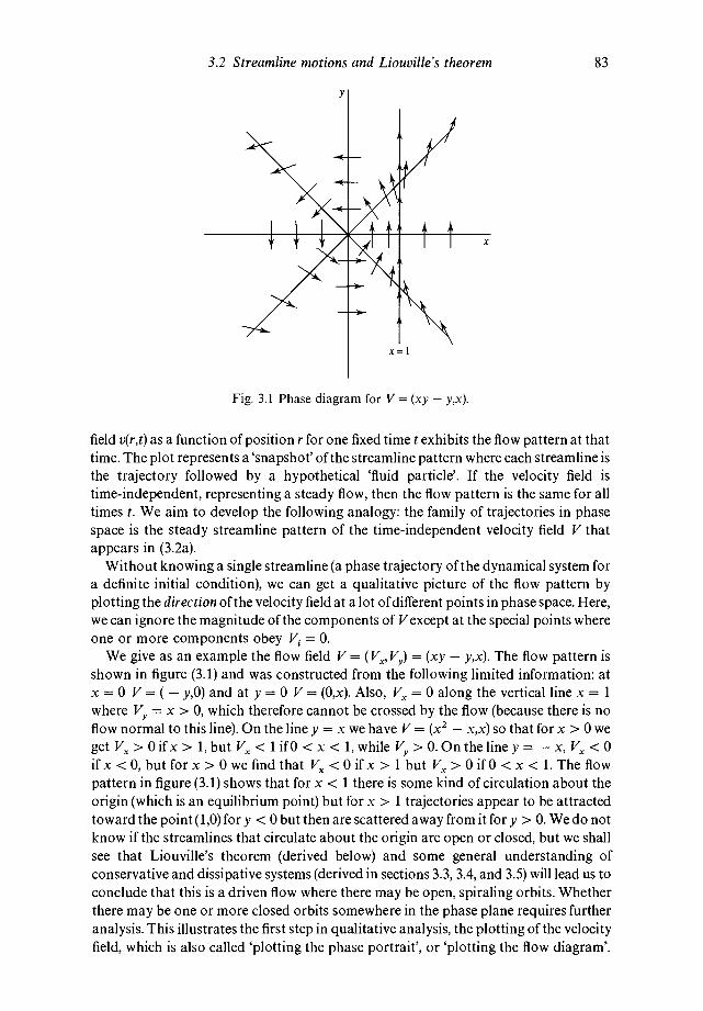
3.2 Streamline motions and Liouville's theorem 83
x = 1
Fig. 3.1 Phase diagram for V = (xy — y,x).
field v(r,t) as a function of position r for one fixed time t exhibits the flow pattern at thattime. The plot represents a 'snapshot' of the streamline pattern where each streamline isthe trajectory followed by a hypothetical 'fluid particle'. If the velocity field istime-independent, representing a steady flow, then the flow pattern is the same for alltimes t. We aim to develop the following analogy: the family of trajectories in phasespace is the steady streamline pattern of the time-independent velocity field V thatappears in (3.2a).
Without knowing a single streamline (a phase trajectory of the dynamical system fora definite initial condition), we can get a qualitative picture of the flow pattern byplotting the direction of the velocity field at a lot of different points in phase space. Here,we can ignore the magnitude of the components of V except at the special points whereone or more components obey = 0.
We give as an example the flow field V = (Vs, = (xy — y,x). The flow pattern isshown in figure (3.1) and was constructed from the following limited information: atx = 0 V = ( — y,O) and at y = 0 V = (0,x). Also, = 0 along the vertical line x = 1
where = x> 0, which therefore cannot be crossed by the flow (because there is noflow normal to this line). On the line y = x we have V = (x2 — x,x) so that for x > Owe
get 1,but lifO<x<ifx <0, but for x >0 we find that <0 ifx>1 but >0 ifO <x <1. The flowpattern in figure (3.1) shows that for x < 1 there is some kind of circulation about theorigin (which is an equilibrium point) but for x > 1 trajectories appear to be attractedtoward the point (1,0) for y <0 but then are scattered away from it for y> 0. We do notknow if the streamlines that circulate about the origin are open or closed, but we shallsee that Liouville's theorem (derived below) and some general understanding ofconservative and dissipative systems (derived in sections 3.3, 3.4, and 3.5) will lead us toconclude that this is a driven flow where there may be open, spiraling orbits. Whetherthere may be one or more closed orbits somewhere in the phase plane requires furtheranalysis. This illustrates the first step in qualitative analysis, the plotting of the velocityfield, which is also called 'plotting the phase portrait', or 'plotting the flow diagram'.

84 Flows in phase space
Here are three easy examples from Newtonian mechanics. Free-particle motiond2x/dt2 = 0 is described by the velocity field V = (x2,O). The streamlines are parallel tothe x1-axis and represent a constant velocity translation along that axis. The con-struction of the following two flow diagrams is assigned in exercise 1. The simpleharmonic oscillator d2x/dt2 + x = 0 with m = 1 and a) = 1 has the flow fieldV = (x2, —x1) and describes circulation about the origin, which is an equilibrium point(figure 3.2). Because the velocity field has equal magnitude at equal distances from theorigin and is always perpendicular to the radius vector from the origin, the streamlinesmust be concentric circles about the origin (figure 3.2 shows the more general case ofconcentric ellipses). The scattering problem d2x/dt2 — x = 0 defines the flow fieldV = (x2,x,), which also has an equilibrium point at the origin and yields the flow field offigure 3.3, which reminds us of hyperbolae.
It is easy to derive the equations describing the streamlines for the last two examples.For the simple harmonic oscillator, from x1dx,/dt + x2dx2/dt = x1x2 — x2x1 = Owe
obtain the streamline equation as G(x,dx/dt) = + = constant, which describes afamily of circles concentric about the origin. For the scattering problem, x1dx,/dtx2dx2/dt = x1x2 — x2x1 = 0 follows and so we get the streamline equation in the formG(x,dx/dt) = — = constant, describing a family of hyperbolae centered on theorigin. For an arbitrary planar flow it is nontrivial to derive the streamline equation, sothat plotting of the directions of the vector field V in one or more two dimensionalsubspaces can be an extremely valuable tool for understanding the flow pattern. For anarbitrary flow in three or more dimensions there is no guarantee that a streamlineequation exists because every streamline equation is a time-independent conservationlaw, The existence of global' conservation laws is not guaranteed in three or moredimensions, as we explain below.
Summarizing, for any trajectory (any solution of the dynamical system fort = tot = the velocity V = (V1, V2,. . . , is everywhere tangent to that trajectory. If wethink of the collection of all trajectories as the flow of a phase fluid, then V(x,, . . . is
just the velocityfield of the flow, is known, and therefore can be plotted in phase space orin a two (with computer graphics, three) dimensional subspace of phase spaceindependently of any quantitative information about solutions. One can use thistechnique to get limited information about what solutions do as tincreases (or decreases)without knowing how a single trajectory develops quantitatively from a single preciseinitial condition. We now develop the language and tools of the flow picture.
Whenever the velocity field is at least once differentiable with respect to all of the nvariables when all of those first partial derivatives are bounded in some finite regionof phase space, then the solution of the system (3.2a) exists as a point function of theinitial conditions and the time, and is also unique for a specific initial condition withinthe bounded region. Existence of solutions is nontrivial: an alternative to the existenceof solutions as functions might be the idea of solutions as pat h-dependent functionals.More general than first-differentiability, if the velocity field satisfies a Lipshitzcondition then both existence and uniqueness of solutions are guaranteed along withan approximate method of construction of solutions: the dynamical system is theniteratively solvable over a finite region in phase space, over a finite time interval, byPicard's method of successive approximations, regardless of what may be true of the
A 'global' conservation law holds for all finite times. In chapter 13 we discuss 'local' conservation laws thatdo not.

3.2 Streamline motions and Liouville's theorem 85
Fig. 3.2 Streamlines of a simple harmonic oscillator.
x2
Fig. 3.3 Phase flow of a scattering problem.
motion qualitatively: whether the system is Hamiltonian, whether the motion is regularor chaotic, and whether or not the velocity field represents a flow in phase space are inprinciple irrelevant. We assume, in all that follows, that solutions, velocities, andaccelerations are all bounded (but not necessarily uniformly) at all finite times (thesolution does not blow up at any finite time, but may blow up as the time goes toinfinity). Solvable means (i) that solutions exist as point functions of initial conditionsand time (that integration of the differential equations does not lead to path-dependentanswers), are unique and differentiable, and (ii) that solutions can be constructedapproximately by recursion. If computable numbers are chosen as parameters andinitial conditions, then solutions may be constructed to any desired degree of decimalaccuracy by Picard's recursive method (in chapter 6, we point out the fundamentallimitations imposed on predictability by computation time whenever a flow is chaotic).
Determinism is reflected abstractly by the fact that the solutions of(3.2a) depend onlyupon the initial conditions and the time difference t —
= . . — t0), (3.3a)
where t, is the time at which the initial conditions are specified and where is the samefunction for all times and for all initial conditions. We can think of the differentialequations (3.3a) as generating a one-parameter collection of coordinate transform-ations from holonomic coordinates . . . = (x10,. . . to holonomic coor-dinates (x1(t), . . . where the parameter in the transformation is just the timedifference t — Each different value of the time difference t — t0 defines a differentcoordinate transformation and path-independence of the integration of the differentialequations ('existence' of solutions) guarantees that the variables (x 1(t),. . . areholonomic for all times t.

86 Flows in phase space
The idea of a flow is a fixed pattern of streamlines that threads throughout phasespace and is the same at all times: the phase portrait represents the idea that the familyof solutions (3.3a) of the system (3.2a) exists as the same continuous pattern for all times— cc <t < cc. From an analytic standpoint, this is the same as saying that thetransformations (3.3a) 'exist' abstractly and can, in principle, be carried out for any andall finite times t. This is a nontrivial requirement: it requires that a flow, the coordinatetransformation picture, is defined by differential equations whose solutions do not goto infinity at any finite time In other words, flows are defined by equations whosesolutions (3.3a) are unique and remain bounded for all finite times. An example of aplanar flow is given by the one dimensional Newtonian scattering problem
p=_U'(x)}(3.lb)
where U(x) = — (ax)2 with a real. Trajectories are given by
x(t) = c1eat + c2e_aI(3 3b)
p(t) = ma(c1e"t — c2e_0t)J
and are (nonuniformly) bounded at all finite times. The two constants are determinedby initial conditions. That trajectories are scattered to infinity at infinite time does notcontradict the idea of a definite flow pattern at any and all finite times: the caordinatetransformation (3.3a) is given by (3.3b) with x0 = c1 + c2 and p0 = ma(c1 — c2). On theother hand, the one dimensional system
= (3.2b)
has the solution
x(t) = x0(3.3c)
1 — x0(t — t0)
and therefore does not define a phase flow: the solution has singularities at finite times= + 1/x0 so that there is no flow pattern that continues from t = — cc to t = cc.
Correspondingly, there exist no transformations of the form (3.3a) that can be carriedout over time intervals that include Therefore, there is no flow diagram, no steadyflow pattern that is correct independently for all times t. Finite-time singularities (alsocalled spontaneous singularities) are a feature of nonlinear problems: the coefficients inthe differential equation, which are completely analytic and even are constant in (3.2b)give no hint beforehand that singularities will appear (in retrospect, we must always askwhether quadratic terms on the right hand side produce spontaneous singularities).That linear equations cannot have spontaneous singularities is guaranteed by Fuch'stheorem (see Bender and Orszag, 1978 or Ince, 1956). We prove in chapter 13 that aclass of damped, driven Euler—Lagrange models that include tops (chapter 9) and theLorenz model (introduced below) have no spontaneous singularities and thereforedefine flows in phase space.
If the right hand side V(x1,. . . is analytic and time-independent (meaning that theright hand side is a polynomial or a convergent power series in the excepting isolatedsingular points), then it is easy to demonstrate that Picard's recursive method merelyreproduces the solution as a power series in the time interval t — t0: when the right handside of the differential equation is analytic in the coordinates (and whether or not wehave a flow), then the solution is also analytic in the time. However, the radius of

3.2 Streamline motions and Liouville's theorem 87
convergence of the resulting power series solution is generally smaller than that of theradius of convergence of the as functions of the For example V(x) = x2 has infiniteradius of convergence in x whereas x(t) = x0(1 + x3t)' = x0(1 — x4t + —
has the finite radius of convergence =Continuing with the Lie-inspired picture of a phase flow as an infinite collection of
one-parameter coordinate transformations in phase space, the inverse transformationis defined formally by
= . . — t) (3.3d)
and represents the idea that the differential equations can be integrated backward intime (this is possible whenever the Jacobi determinant defined below is finite).Differentiation of (3.3a) once with respect to t yields
= . . . — t0)/dt. (3.2c)
According to (3.3a) and (3.2c), we can think of both the solution and the derivativesas functions of then initial conditions. This possibility is used implicitly in the
construction of the Jacobi determinant below. If we set t = t, in (3.2c) then we obtainthe original differential equations for any time t =
= . . — = (3.2d)
because the zero of time is irrelevant in an autonomous system: the differentialequations (3.2a) are left unchanged by (are invariant under) a shift in the time origin.The finite coordinate transformation (3.3a) is said to be 'generated infinitesimally' bythe differential equations (3.2a), which can be written in the form of an infinitesimalcoordinate transformation near the identity:
= V4(x10,. . . (3.2e)
The finite coordinate transformation (3.3a) is called 'global' because it holds at all times— cc <t < cc and transforms all of phase space, whereas the infinitesimal transform-ation (3.2e) is confined to infinitesimal displacements.
An easy example of the transformation/phase flow picture is provided by the simpleharmonic oscillator where, for t0 = 0,
x1(t) = = x10cost + x20sint(3 3e)
x2(t) = tJ12(x10,x20,t) = — x10 sin t + x20 cost.
It is left as an exercise for the reader to construct the inverse transformation that isequivalent to an integration of the harmonic oscillator differential equations backwardin time. The infinitesimal transformation near the identity (near t = 0) is given bydifferentiating (3.3e),
5x1(t) = X20öt(3 ic)
öx2(t) = — x10&,j
and reflects the original differential equations of the flow for times sufficiently near to= to.
We can also write the global transformation (3.3a) symbolically as
x.(t) = U(t — (3.3f)

88 Flows in phase space
where is the initial condition, U(t — t0) is called the time-evolution operator andsymbolically represents the solution, the result of the simultaneous solution (generallyvia recursion) of the n differential equations that generate the transformation, leadingto the functions in (3.3a). The purpose of introducing the time-evolution operatorinto the theory of differential equations is to be able to represent and discuss some of theproperties of the transformations (3.3a) more conveniently via purely algebraicmanipulations (see chapter 7).
If the velocity field of a flow is analytic, then so is the solution and the time-evolutionoperator takes on a particularly simple form: we make a Taylor expansion (where theradius of convergence is necessarily determined by the nearest singularity of (3.3a) inthe complex t-plane (see Ince, 1956, or Bender and Orszag, 1978)),
+ At) = xL(t) + + + ..., (3.3g)
and also notice that we can write (using summation convention)
V.V, (3.2f)
for the derivative with respect to t,dF(x1, . .. = LF of any time-independentfunction F(x1,. . where L = For example, = = V1. Repeateddifferentiation of the differential equations (3.2a) with respect to t therefore yields theTaylor series (3.3g) in the form
x1(t + At) = + + + ... = (3.3h)
Therefore, U(t — t0) = is the time-evolution operator and simply summarizes forus, in algebraic form, the infinite order differential operator that represents the idea of'integrating', meaning solving, a system of differential equations with analytic velocityfield (excepting isolated singularities). An infinite order differential operator com-presses into a single formula the idea of the infinitely many coupled integrations, theabstract limit of Picard's iterative method when the number of recursive steps isallowed mentally to go to infinity2. We stress that the radii of convergence of formulaelike (3.3g) and (3.3h) are unknown because the location of singularities of solutions inthe complex time plane are a priori unknown (it is not accidental that Newtondiscovered the universal laws of dynamics and gravity from systems whose solutionsare parabolae and ellipses).
The time-evolution operator representing the solution (3.3e) of the simple harmonicoscillator was easy to construct because the flow is linear and gives rise to solutions thatare analytic for all finite real times t, so that the Taylor expansion of the solution aboutany point in phase space has infinite radius of convergence (Galileo's first empiricaldiscovery of the regularities of mechanical systems came from observations of simplependulums, whose solutions are correspondingly analytic). Except for a degeneratecase, the solutions of linear equations with constant coefficients have no singularities inthe complex t-plane except at infinite real or imaginary time (this is shown explicitly bythe general result (3.17c) below). For the simple harmonic oscillator we can insert
(3.2g)
2 One must define a metric in phase space in order to discuss convergence; the metric is Euclidean. Given ametric, the convergence in Picard's method corresponds to iteration toward a fixed point in a contractionmapping, whose solution is therefore path-independent.

3.2 Streamline motions and Liouville's theorem 89
Fig. 3.4 A ball of initial conditions traces out a hypercylinder of streamlinesin phase space.
in x.(t) = U(t) = to construct the Taylor expansions whose summations yieldthe solution of the simple harmonic oscillator problem. This is left as an easy exercisefor the reader.
Although we have restricted our considerations to autonomous systems, our ideascan be extended formally to externally driven systems where the velocity fieldV(x1, . .. is time-dependent by writing x, +1 = t with = 1 and then working inan n + 1 dimensional phase space. An example is given below and in exercise 10.
The flow of a small but finite portion of the phase fluid is described by the (hyper)tubeof streamlines traced out by the time-development starting from a finite phase spacevolume element 5c�(t0) = öx1(t0). . . Every point in this volume element serves asa possible initial condition for the dynamical system, so that each point in the volumeelement has a trajectory passing through it. Uniqueness of trajectories is guaranteed bysatisfying a Lipshitz condition, which is also the condition required for the applicabilityof Picard's method (a Lipshitz condition is automatically satisfied if the first derivativesof the velocity field are all bounded at all finite times, which automatically requiresboundedness of solutions at all finite times for polynomial velocity fields). Thecollection of trajectories passing through forms a (hyper)cylinder, a tube in phasespace (figure 3.4).
In nature, we can never specify the location of a point, a state, or anything withinfinite precision, so that a finite value of can represent the finite ignorance that ispresent at the start of every experiment or sequence of observations. In numericalcomputation where errors are avoided (in contrast with floating-point computations),initial conditions can be specified algorithmically with arbitrarily high precision:decimal expansions of numbers can be generated to within as high a precision ascomputer time will permit. Even in a floating-point computation the initial conditionsare determined precisely by the machine's design: the choice of a single floating-pointinitial condition on a computer does not simulate the limitation in experiment orobservations of nature to finite and relatively low resolution.
For the time being, we set aside the very difficult question of how the volume elementmight differ significantly in shape from and concentrate instead upon the
much easier question: how does the size of the volume element change with time? If öc�
X3
SQ(t)
xl

90 Flows in phase space
is small enough, in principle infinitesimal, then thinking of equation (3.3a) as atransformation of coordinates, we can write
= J(t)ö�)(t0) (3.4)
where we could take t, = 0, and where
J(t) = . .
(3 5a. . .
is the Jacobi determinant of the transformation. It would appear that we cannot usethis result without first solving the differential equations, but this is not true: the Jacobideterminant also satisfies a differential equation. To see this, we need only study theform of the derivative3
dJ — . .
+ +. .
(3 6)dt — . . . .
By the chain rule for Jacobi determinants, we can write
. . — . .
J(t) (3 7a)ö(x1(t0),. . . a(x1(t),. . .
and this reduces to
. . . —Jo (3 7b)
.. . —
because the variables (x1(t), . . . are independent. The quantity
(3.8a)i=1
defines the divergence of the flow field V in phase space, so we obtain the first orderdifferential equation
(3.9)
for the time-development of the Jacobian.Now we come to a very important point in our formulation of the properties of phase
space. By defining the divergence of the velocity field by the formula
(3.8b)i=1
we have implicitly adopted the Cartesian definition of a scalar product, but withoutassuming that we can define the distance between any two points in phase space (theCartesian result (3.8b) was derived from the Cartesian definition = dx1 . . .
Unless the phase space is Euclidean (which is rare), this means that phase space is aninner product space that is not a metric space. Clearly, the phase space of a canonicalHamiltonian system is not a metric space (canonically conjugate variables q and pgenerally do not even have the same units). The Cartesian definition = dx1 . . .
requires a space where infinite parallelism is possible, but no idea of a distance between
This proof of Liouville's theorem was sometimes used by Lars Onsager in his statistical mechanics courseat Yale.

3.2 Streamline motions and Liouville's theorem 91
two points is required in this definition other than that between two points that lie onthe same axis Note that the Cartesian properties of phase space are preserved underaffine transformations but not under general nonlinear transformations of coordinates(see exercise 5).
Conservative dynamical systems can now be defined by the divergence-free conditionV = 0, which means that a conservative system is now defined to be one where the
phase flow is incompressible; if we can think of the flow as that of a fluid with massdensity p(x1,x2,. . . then local mass conservation (or conservation of probability)corresponds to the continuity equation
(3.lOa)
where V is the n dimensional gradient in phase space. If the divergence of the velocityfield vanishes, then we can rewrite (3.lOa) in the form
(3.lOb)
which is the condition that dp/dt = 0, that p is constant in time along a streamline= dp/dt is the time derivative along a streamline in the flow). A conservative flow is
one where there are no sources or sinks of the flow in phase space. This does not mean thatevery Hamiltonian system has one or more conservation laws, but it does include bothenergy-conserving and all other Hamiltonian systems as special cases. For example, itis easy to show that a Newtonian system where the net force is conservative (andtherefore where energy is conserved) is included in our more general definition: the onedimensional Newtonian problem
_U'(x)}(3.lb)
yields
(3.8c)op
Conservative flows are also called volume-preserving flows because the size of thevolume element is left invariant by the one-parameter coordinate transformations(3.3a) that define the time-development of the flow.
The canonical form of a conservative system of n = 2f first order differentialequations is Hamiltonian and defines a phase-volume-preserving flow where thecondition of a source- and sink-free velocity field Vis satisfied by the construction of the2f dimensional analog of a stream function called the Hamiltonian,H(x1,...,xf,y1,...,yf,t). The flow is then described by the canonical differentialequations
OH . OHand —--——forz= 1,...f (3.11)
Oyi
where each pair of variables is called canonically conjugate. It followsimmediately that

92 Flows in phase space
——o (312)
— — —
so that every canonical Hamiltonian flow is automatically incompressible (in chapter15 we shall also introduce and discuss noncanonical Hamiltonian flows). In accordancewith the viewpoint that the canonical equations (3.11) generate the flow infinitesimallyand yield the finite transformation that takes one from the coordinate system(x1(t0),.. . ,x1(tj,y1(t0), . . . ,y1(t0)) to the system (x1(t), . . . ,x1(t),y1(t),. . . the Hamil—tonian H is called the infinitesimal generator of the transformation. As an example, theHamiltonian H = xy has the equations of motion = 3H/
= — y. We show in section 3.6 that every conservative planar flow is Hamiltonian.However, most Hamiltonian systems that can be constructed mathematically (likeH = xy) cannot be Legendre-transformed into Lagrangian descriptions of Newtonianflows.
If a Hamiltonian system can be derived from a Newtonian one, then we will write(x1, . . . ,x1,y1, . . . ,y1) = (q1,.. . . ,P4 in accordance with the notation of chapter2, but note that we have arrived here at the idea of a Hamiltonian descriptioncompletely independently of Newton's laws and Lagrangian mechanics simply bythinking of an even number of differential equations with a divergence-free velocityfield as describing an incompressible, inviscid flow in a phase space of even dimension.Notice that if H depends explicitly upon the time then the dynamical system may haveno conserved quantity, but the n + 1 dimensional flow defined by setting = t isstill volume-preserving.
Lagrangians L = T — U and the corresponding Hamiltonians in Newtonian par-ticle mechanics represent conservative forces because these systems follow from therequirement that the generalized force is the configuration space gradient of a scalarpotential (in Cartesian coordinates, the forces are curl-free). The potentials U may betime-dependent, in which case neither the Hamiltonian nor the total energy isconserved. Our general definition of a conservative system as an incompressible flow inphase space includes the case where H varies with time and is not conserved, but ourdefinition is very general and can also be applied to flows that are not defined byLagrangians and even to abstract dynamical systems that are represented by discretemaps with a discrete time variable and that have no velocity field at all. An example isprovided by the discrete abstract dynamical system defined by the iterated map
(3 3i)—
where phase space is the two dimensional space of the variables (x,y). This discretedynamical system is conservative if the map is area-preserving, i.e., if the Jacobideterminant
oxn(3.5b)
oxn oyn
of the transformation (3.3i) is equal to unity. A dissipative flow is one where J < 1.
In order to check our definition further against the usual definition, let us askwhether the damped, driven harmonic oscillator

3.2 Streamline motions and Liouville's theorem 93
9 + /39 + = F(t) (3.ld)
is conservative or dissipative. With x1 = y, x2 = dy/dt, and x3 = t, we obtain
—/3, (3.8d)
so that the system is nonconservative, as expected, under our broader definition.Furthermore, it follows by a direct integration of(3.9) that J(t) = so that any finitevolume element obeys oc�(t) = and vanishes as the time goes to infinity. IfF = 0 then this is easily understood: all solutions approach the equilibrium point inphase space because friction (with /3 > 0) drains energy out of the system at the ratedE/dt = — /3v2 where v = dy/dt. This equilibrium point illustrates the idea of a zerodimensional attractor. 1fF 0, if for example F(t) is oscillatory, then y(t) consists of twoparts: a transient contribution that depends upon the initial conditions and vanishes ast goes to infinity, and a particular integral which is a solution that is dependent of theinitial data. In this case, all solutions that have initial conditions in 5Q(t0) approach thatcurve asymptotically, illustrating the idea of a one dimensional attractor in the threedimensional (y,dy/dt,t)-phase space, and therefore vanishes as t approachesinfinity because the attracting point set is one dimensional and therefore has zerovolume.
The damped, driven harmonic oscillator illustrates something that is quite general:whenever the flow field V has a negative divergence, then every finite volume elementcontracts asymptotically onto an attracting point set that has a dimension less than thedimension of the phase space: the resulting condition that oc�(t) —* 0 as t goes to infinityis satisfied by flow into a point-sink (zero dimensional attractor), contraction ontostable limit cycle (one dimensional attractor), and by higher dimensional possibilitiesthat are discussed in chapter 13. In a general nonconservative flow, phase space isdivided into regions where driving dominates (J> 1) and regions where dissipationdominates (J < 1). Curves or closed surfaces in phase space where J = 1 but J > 1 (orJ < 1) inside the region while J < 1 (or J> 1) outside have special significance becausethey lead to the idea of higher dimensional attractors (repellers). An example of anautonomous nonconservative planar flow with a one dimensional attractor, a limitcycle, is given in section 3.3.
If we set F = 0 and replace /3 by — /3 with /3 > 0 in the damped harmonic oscillator(3.ld), then we get a driven oscillator where increases exponentially with the timet. Instead of spiraling into the origin like the trajectories of the damped oscillator,trajectories spiral out to infinity (we prove this explicitly in the next section). In general,regions of phase space where the divergence of the velocity is negative are regions wheredamping dominates driving decreases toward zero), while regions with positivedivergence are regions where external driving dominates dissipation increases withtime). We shall see in sections 3.3 and 3.4 that closed orbits (periodic orbits) in phasespace are generally characteristic of conservative flows, but that dissipative flows canalso have closed orbits (periodic solutions called limit cycles are one example) wheneverdamping balances dissipation locally over some region of phase space to produce asteady state (see sections 3.3 and 3.4).
In a Newtonian or Hamiltonian description of particle mechanics in configurationspace, the coordinates that are treated implicitly as Cartesian in phase space mayactually be cylindrical, spherical, elliptic, or some other curvilinear possibility. The

94 Flows in phase space
configuration space of a Lagrangian system is therefore geometrically distinct from theq-subspace of a Hamiltonian system in phase space. Note that integration over thep-subspace of phase space does not leave us with the correct volume element ofLagrangian configuration space. The q-subspace of phase space is always Cartesianwithout a metric whereas Lagrangian configuration space has the metric tensordefined by ds2 = = 2Tdt2, where ds is the arc length, whenever the transform-ation to generalized coordinates is time-independent. The point is that the phase spaceformulation of a dynamical system formally treats the canonically conjugate variables(q1,. . . ,p1) of a canonical Hamiltonian flow as if they were Cartesian, even define acurvilinear coordinate system in the configuration space of a Lagrangian system4. This isillustrated in section 3.5 below where for a pendulum we plot U vs dO/dt as if bothcoordinates were Cartesian when in fact they are angular position and angularfrequency.
The theoretical reason why the treatment of the and as Cartesian in a 2fdimensional phase space that is defined to be flat does not conflict with the fact thatfdimensional Lagrangian configuration space may be curved is explained by thegeometric (meaning Lie-algebraic) interpretation of the fundamental Poisson bracketrelations in section 15.3. This point is not explained explicitly elsewhere in theliterature, although it is implicit in every discussion of Hamiltonian flows via Poissonbrackets (see chapter 15). Curvature of Lagrangian configuration spaces is discussed inchapters 10 and 11. Whereas the Cartesian properties of the phase space of non-canonical flows are preserved only under affine transformations, which are linear, theCartesian divergence formula (3.12) and volume element dQ = dq1 . dpf for Hamil-tonian flows are preserved under a much larger class of nonlinear transformations thatare called canonical or symplectic (see chapters 6 and 15). For this reason, the phasespace of a canonical Hamiltonian system is called a symplectic space in the modernliterature (see Arnol'd, 1989).
We go on next to classification of equilibria and the stability of motions nearequilibria. By stability, we mean at this stage only the idea of local stability near anequilibrium point: a trajectory that starts near enough to, but not at, equilibrium,remains near that particular equilibrium point for all times unless the equilibrium pointis unstable. Below and in chapter 4 we also introduce orbital stability based upon theidea that a collection of trajectories that start near one another within an infinitesimaldefinite ball of initial conditions in phase space remain near to one another as the timeincreases without bound. Orbital stability arises from the insensitivity of solutions withrespect to small changes in initial conditions.
3.3 Equilibria and linear stability theory
Consider the autonomous system
= (3.2a)
At an equilibrium point, the velocity vector V= (V1,. . vanishes. Denote such apoint by X = . . . This point is stable if nearby trajectories remain near it as thetime increases without bound. Otherwise it is unstable.
Questions requiring us to define the distance between two points in phase space do not arise in thequalitative analysis of a dynamical system. One must define a metric in order to construct approximationsto solutions via Picard's method, but not in order to discuss the geometric nature of the flow pattern.

3.3 Equilibria and linear stability theory 95
In order to analyze the stability locally, we expand the right hand side of(3.2a) aboutthe equilibrium point X,
a v.. = . . + + ..., (3.13)
XJ x=X
where = x3 — and summation convention is used (sum over repeated indices). Ifwe keep only the linear term in the displacement 5X4 from equilibrium, we obtain thevariational equation
= AöX (3.14)
where A is the (constant) Jacobi matrix with entries
. (3.15)Xj x=X
Since A is a constant matrix
ox 1(t)
OX(t) = (3.16)
is the displacement from equilibrium, and so
OX(t) = e"OX(O) (3.17a)
where OX(O) is the initial displacement from equilibrium. We see by inspection thatU(t) = etA is the time-evolution operator for this example.
If we can diagonalize the matrix A, then
Aê1 = (3.18a)
where is the eigenvalue corresponding to the eigenvector 4 When the n eigenvectorse1 are linearly independent, then from
OX(O)=
(3.17b)
and from (3.21a) and (3.21b) we obtain
OX(t)=
(3.17c)
by using also the fact that = in the power series expansion for etA.In the two dimensional phase plane (n = 2), the possible equilibria are determined by
the different possible eigenvalue problems (3.18a), and there are only six that aredistinct. In particular, there are only two topologically distinct equilibria for conserva-tive systems: from Liouville's theorem we obtain
(3.8c)
so that traceless matrices A describe conservative systems.Consider first the simplest case where n = 2. The most general traceless two by two
matrix has the form
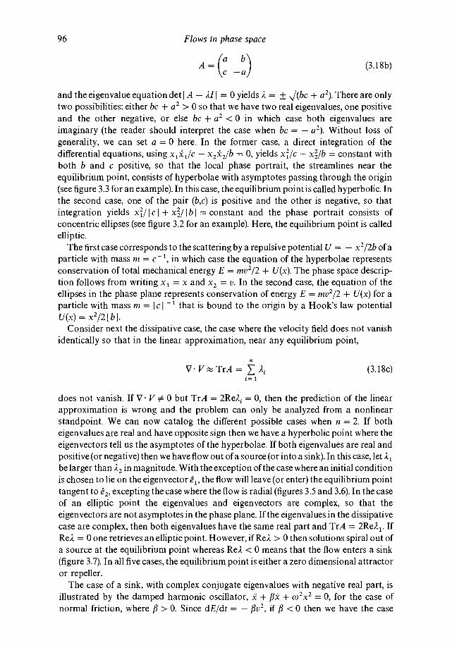
96 Flows in phase space
A = (a(3.18b)
and the eigenvalue equation det I A — 211 = 0 yields 2 = ± ,J(bc + a2). There are onlytwo possibilities: either bc + a2 > 0 so that we have two real eigenvalues, one positiveand the other negative, or else bc + a2 <0 in which case both eigenvalues areimaginary (the reader should interpret the case when bc = — a2). Without loss ofgenerality, we can set a = 0 here. In the former case, a direct integration of thedifferential equations, using — = 0, yields — = constant withboth b and c positive, so that the local phase portrait, the streamlines near theequilibrium point, consists of hyperbolae with asymptotes passing through the origin(see figure 3.3 for an example). In this case, the equilibrium point is called hyperbolic. Inthe second case, one of the pair (b,c) is positive and the other is negative, so thatintegration yields
Ic +
Ib
I= constant and the phase portrait consists of
concentric ellipses (see figure 3.2 for an example). Here, the equilibrium point is calledelliptic.
The first case corresponds to the scattering by a repulsive potential U = — x2/2b of aparticle with mass m = in which case the equation of the hyperbolae representsconservation of total mechanical energy E = mv2/2 + U(x). The phase space descrip-tion follows from writing x1 = x and x2 = v. In the second case, the equation of theellipses in the phase plane represents conservation of energy E = mv2/2 + U(x) for aparticle with mass m = c 1 that is bound to the origin by a Hook's law potentialU(x) = x2/2IbI.
Consider next the dissipative case, the case where the velocity field does not vanishidentically so that in the linear approximation, near any equilibrium point,
V TrA=
(3.18c)
does not vanish. If V V 0 but TrA = 2Re%1 = 0, then the prediction of the linearapproximation is wrong and the problem can only be analyzed from a nonlinearstandpoint. We can now catalog the different possible cases when n = 2. If botheigenvalues are real and have opposite sign then we have a hyperbolic point where theeigenvectors tell us the asymptotes of the hyperbolae. If both eigenvalues are real andpositive (or negative) then we have flow out of a source (or into a sink). In this case, letbe larger than in magnitude. With the exception of the case where an initial conditionis chosen to lie on the eigenvector the flow will leave (or enter) the equilibrium pointtangent to ê2, excepting the case where the flow is radial (figures 3.5 and 3.6). In the caseof an elliptic point the eigenvalues and eigenvectors are complex, so that theeigenvectors are not asymptotes in the phase plane. If the eigenvalues in the dissipativecase are complex, then both eigenvalues have the same real part and TrA = 2Re21. IfRe). = 0 one retrieves an elliptic point. However, if Re). > 0 then solutions spiral out ofa source at the equilibrium point whereas Re). < 0 means that the flow enters a sink(figure 3.7). In all five cases, the equilibrium point is either a zero dimensional attractoror repeller.
The case of a sink, with complex conjugate eigenvalues with negative real part, isillustrated by the damped harmonic oscillator, + + w2x2 = 0, for the case ofnormal friction, where /3 > 0. Since dE/dt = /3v2, if /3 <0 then we have the case

3.3 Equilibria and linear stability theory 97
Fig. 3.5 Nonradial flow into a sink.
Fig. 3.6 Radial flow into a sink.
x
Fig. 3.7 Spiralling flow into a zero dimension attractor.
where, instead of friction, energy is dumped into the oscillator through the forcef = I /31 v. In this case both eigenvalues have the same positive real part and the phaseflow represents the effect of a source at the origin in the (x,v)-space.
In the general case in n dimensions, if there is an equilibrium point at X and thelowest order approximation to the motion near X yields linear equations, then thesolution of the linear equations is just

98 Flows in phase space
öX(t)=
(3.17c)
Since bounded motions of conservative systems near equilibrium points require thatthose equilibria are elliptic points (if the equilibrium point is hyperbolic, then theparticle is 'scattered' and eventually is repelled from equilibrium), and since ellipticpoints require pairs of imaginary eigenvalues, the dimension n of phase space must beeven to obtain bounded motion in a conservative linearized system. In this case, we canthen write n = 2f In a conservative system in a phase space of old dimension boundedmotion may permit the generalization of a hyperbolic point. An example of this is thelinearized Lorenz model (n = 3) for a special choice of two of the three controlparameters in that problem.
The Lorenz model is defined by the nonlinear equations
)(3.19)
± = — /3z + xy)
in an (x,y,z)-phase space and has the three control parameters a, /3, and p. The Lorenzmodel can be derived from the Euler equations for a symmetric top by including lineardissipation and driving, as we show in chapter 13 where we also prove that the modeldefines a flow where the solutions are uniformly bounded.
The condition for a conservative system is satisfied by the Lorenz model whenever
—a—f3—1=0, (3.20)ax ay az
so that /3 + a = — 1.
There are three distinct equilibria: = 53 = 2 = 0 and = ( ± [/3(p — 1)]h/2,
± [/3(p — 1)] "2,p — 1). When p < 1 there is only one equilibrium point, the one at theorigin.
Linear stability is determined by the Jacobi matrix
—a a 0
A= p—2 —1 (3.21a)
53 —/3
evaluated at an equilibrium point. With = (0,0,0), we obtain
—a a 0
A= p —1 0 (3.21b)
0 0 —/3
and the eigenvalue equation
(/3 + )L)[(a + 2)(1 + A) — pa] = 0 (3.22)
has (with p � 0) the three real roots A1 = — /3 and 22,3 = { — (a + 1) ±[(a + 1)2 + 4a(p — 1)]h/2}/2. Note that when a + /3 + 1 = 0, theeigenvalues add up tozero, as required (the trace of a matrix equals the sum of its eigenvalues), but that either
or the pair 22,3 has a positive real part. Therefore, the equilibrium point (0,0,0) isalways unstable and represents a generalization to three dimensions of a hyperbolicpoint or a spiral. The spiral occurs whenever the argument of the square root in 223 is

3.3 Equilibria and linear stability theory 99
negative. If we set /3 equal to zero, then we retrieve the familiar case of a hyperbolic or anelliptic point.
Sources and sinks of streamlines can occur in a dissipative system (an example is theLorenz model whenever ci + /3 + 1 0), but not in a conservative system. A sinkattracts all nearby streamlines (all of them flow into it) whereas a source repels allnearby streamlines (they flow out of it), When V is divergence-free, there can be nosources or sinks of the flow. A sink can be zero dimensional (stable equilibrium point),one dimensional (stable limit cycle), or higher dimensional (attracting torus), or evenchaotic ('strange' attractor). For the corresponding repellers, all of the streamlines flowout of the respective sources. This is not possible in a conservative system because itwould violate Liouville's theorem: an f dimensional block of initial conditions withvolume element 5Q = .. . would become equal to zero after infinite time shouldall of those points flow into a source (SQ = 0 would then follow due to the reduction indimension). In contrast with dissipative systems conservative systems have neitherattractors nor repellers. Because limit cycles are important later in the text, we now givean example of one.
Consider the damped-driven Newtonian system
(3.23a)
which represents a particle with unit mass attached to a spring with unit force constant,and subject to nonlinear driving and dissipative forces. The energy E = + x2)/2obeys the time-evolution law
dE/dt = — + — 1), (3.24)
and from Newton's law it follows that E =fx, where the nonconservative force isidentified as — 5c(x2 + — 1). This force represents contributions from bothexternal driving and dissipation. With r2 = x2 + y2, x = r cos 0, and y = r sin 0, there isa net dissipation whenever r2 = x2 + > 1, where V• V < 0, but the system gainsenergy per unit time in the region where r2 < 1 where V' V> 0. Therefore, the phaseplane is divided into two distinct regions of energy gain and energy loss by the unitcircle, because E = 0 and also V = 0 whenever r = 1. On the unit circle, we have asteady state where driving is balanced by dissipation so that the energy E is maintainedconstant. By inspection, the unit circle x2 + = 1 is also a solution of (3.24). Next, weshow that this solution is a 'stable limit cycle', a one dimensional attractor, by showingthat nearby initial conditions have this solution as their asymptotic (and periodic) limit.Because the curve is closed with everywhere continuous slope, the motion on the limitcycle is periodic. Now for the 'limiting' part, the attractor aspect.
In polar coordinates it follows that
= r(1 — r2)sin2O325
= (1 — r2)sinOcos0 — 1,( .
so that the cycle at r = 1 attracts nearby trajectories: , > 0 if r < 1, <0 if r > 1,
— 1 when r 1, and so the direction of motion on the limit cycle is clockwise. Notethat there is (by necessity) an unstable spiral at the origin. Note also that the amplitudeand period of oscillation on the limit cycle are completely independent of the initialconditions, in contrast with the case of linear oscillations. Because the periodic orbit atr = 1 attracts nearby trajectories (figure 3.8a), the limit cycle is called stable (an
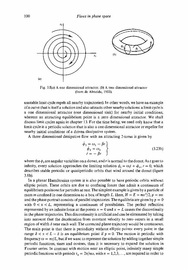
unstable limit cycle repels all nearby trajectories). In other words, we have an exampleof a curve that is itself a solution and also attracts other nearby solutions: a limit cycle isa one dimensional attractor (one dimensional sink) for nearby initial conditions,whereas an attracting equilibrium point is a zero dimensional attractor. We shalldiscuss limit cycles again in chapter 13. For the time being, we need only know that alimit cycle is a periodic solution that is also a one dimensional attractor or repeller fornearby initial conditions of a driven dissipative system.
A three dimensional dissipative flow with an attracting 2-torus is given by
= — fir
=t = — fir
where the are angular variables on a donut, and r is normal to the donut. As tgoes toinfinity, every solution approaches the limiting solution = w1t + r = 0, whichdescribes stable periodic or quasiperiodic orbits that wind around the donut (figure3.8b).
In a planar Hamiltonian system it is also possible to have periodic orbits withoutelliptic points. These orbits are due to confining forces that admit a continuum ofequilibrium positions for particles at rest. The simplest example is given by a particle ofmass m confined in one dimension to a box of length L. Here, H = E = mv2/2, p = my
and the phase portrait consists of parallel trajectories. The equilibria are given by p = 0
with 0 < x <L, representing a continuum of possibilities. The perfect reflectionrepresented by an infinite force at the points x = 0 and x = L causes the discontinuityin the phase trajectories. This discontinuity is artificial and can be eliminated by takinginto account that the deceleration from constant velocity to zero occurs in a smallregion of width near each wall. The corrected phase trajectory would be continuous.The main point is that there is periodicity without elliptic points: every point in therange ö <x <L — 5 is an equilibrium point if p = 0. The motion is periodic withfrequency w = irv/L, but if we want to represent the solution by adding together simpleperiodic functions, sines and cosines, then it is necessary to expand the solution inFourier series. In contrast with motion near an elliptic point, infinitely many simpleperiodic functions with periods r,7 = 2ir/nco, with n = 1,2,3,..., are required in order to
100 Flows in phase space
xI
(a)
Fig. 3.8(a) A one dimensional attractor. (b) A two dimensional attractor(from de Almeida, 1988).
}(3.23b)

3.4 One degree of freedom Hamiltonian systems 101
describe this sort of periodic motion mathematically. Notice also that this kind ofperiodic motion is stable in the same sense as the harmonic oscillator: if you change theenergy slightly (by changing v slightly), or change the length L only slightly, then theresult is a new orbit with nearly the same period as the old one. In other words, there isorbital stability because the geometric shapes of the trajectories and their periods areinsensitive to small changes in the orbital parameters.
A particle in a one dimensional box or an oscillator with one degree of freedom bothrepresent ideal clocks. An ideal clock is frictionless and ticks periodically forever. TheKepler problem describes the historic idea of a clock. Perfect clockwork is not the onlypossibility for motion in a Hamiltonian system that is completely integrable viaconservation laws: stable quasiperiodic orbits, an approximate form of clockwork,occur whenever there are two or more frequencies in a mechanics problem. However,whether one considers a pair of oscillators or any larger number of oscillators the resultis qualitatively the same, as we show in section 3.5.
Examples of quasiperiodic motion are easy to construct. Consider a particle withmass m moving in a rectangular box with sides of lengths a and b that are perfectlyreflecting walls which is a two-frequency problem. With H = E = + the twoperiods of the motion are r1 = 2a/v1 and t2 = 2b/v2. The trajectory of the particle is notperiodic unless one period is an integral multiple of the other. If the ratio of the periodsis irrational then the trajectory can never close on itself and is both quasiperiodic andorbitally stable.
3.4 One degree of freedom Hamiltonian systems
Consider the case in Lagrangian particle mechanics where f= 1 and whereL = mg(q)(dq/dt)2/2 + U(q,t), so that p = mg1(q)dq/dt and H = p2/mg(q) + U(q,t) isthe total mechanical energy. So far, we have only assumed that the transformation togeneralized coordinates is time-independent. If U depends explicitly upon t, then wehave a problem with a three dimensional phase space. In that case deterministic chaosis possible. If, on the other hand, U is independent of t, then E = constant and theproblem reduces to a single integration: the differential form on the right hand side of
dt — 3 26a- [2(E — U(q))]"2 L
is exact, and so the solution for q(t) is given by inverting the result of the followingintegration:
— — 3 26b- Jqo [2(E —(.
In other words, one conservation law determines the solution of a one degree offreedom problem completely.
Bounded motion occurs whenever there are two turning points: E == U(qmax) holds whenever p = 0 50 that <q < (figure 3.9). In other
words, U must decrease as q increases away from (because p2 > 0) but mustdecrease as p approaches zero as q approaches In other words, U(q) must have at

102 Flows in phase space
U (q)
(a)
(b)
Fig. 3.9(a) A potential U(q) that confines for q <q1. (b) The steamlines dueto U(q) (from Percival and Richards, 1982).
least one minimum in the bounded region of configuration space, and the period of thetrajectory is simply
I dq,Jg(q)3
— Jqmin [2(E —. c)
That is, bounded motion for a one degree of freedom, time-independent, one-particleHamiltonian is always periodic.
That the minimum of the potential at q, corresponds to an elliptic point (and that amaximum defines a hyperbolic point) follows from the quadratic approximationU(q) = U(q,) + 5q2 U"(q0)/2 + ..., valid near equilibrium where U'(q0) = 0, followsimmediately from the resulting linear dynamical equations (ignore all terms of orderhigher than quadratic in the Taylor expansion for U(q)). In this approximation we canwrite w2 = U"(q,) > 0, so that near the elliptic point, E = p2/2mg(q,) + mw2(q — q,)2/2and the motion is that of a simple harmonic oscillator with period z = 2icg(q,)/w.
Except for separatrix motion where the period is infinite (see exercise 13), nothing butclockwork can occur for bounded one degree of freedom motion. In order to introducethe idea of a separatrix consider the motion of a simple pendulum that is fixed at onepoint in space but is free to rotate through 2ir radians: U = mgy =mgl(1 — cos 0) = 2mgl sin2 (0/2) where 1 is the length and U is the deviation from stable

3.5 Stable periodic and quasiperiodic orbits 103
equilibrium. There is an elliptic point at 0 = 0 so that for low enough energies there aretwo turning points and the period of the motion is
= 2[2(E — U(0))/m] 1/2' (3.26d)
but when the energy is high enough then the pendulum makes 2ir rotations. The energythat divides these qualitatively different motions defines the separatrix, a trajectorywhere at least one turning point is a hyperbolic point. Since it takes infinite time toarrive at a hyperbolic point, we know that t = on the separatrix (a separatrix isshown as the dashed curve in figure 3.9(b)). One can also see this directly from theintegral for the period t by using the fact that the potential is quadratic in öO near ahyperbolic point.
3.5 Introduction to 'clockwork': stable periodic and stable quasiperiodic orbits
We begin by proving a general theorem, Poincaré's recurrence theorem, which statesthat for a conservative system with bounded motion in phase space a trajectory mustreturn arbitrarily closely to any initial condition after a finite time, and thereforereturns to visit points in a small neighborhood of its starting point arbitrarily often astime goes on.
The proof of the recurrence theorem is an easy application of Liouville's theorem:consider a finite phase volume element at time t0. Every point in the volumeelement is an initial condition for the phase trajectory that passes through that point.At a later time t, the size (but not the shape) of the phase volume is the same,
= If we imagine our bounded region in phase space to be partitionedmentally into N blocks, all approximately of size öQ(t0), then after a finite time tr thephase tube that originates with the block 5Q(t0) and ends with the volume elementsoc�(t) must intersect itself, otherwise the region of phase space under considerationwould be infinite (N would be infinite). It follows that there are arbitrarily manyintersection times tr,tr,t. , but there is no guarantee that these times are integralmultiples of each other or even bear any simple relation to each other. Stated in otherterms, every initial condition (and every other point on a bounded trajectory) must beapproximately repeated infinitely often as t goes to infinity, but not necessarilyperiodically or even in stable fashion. Another way to say it is that the bounded orbitsin phase space of a conservative system must be either periodic or quasiperiodic, butnot necessarily orbitally stable. This behavior stands in contrast to that of dissipativesystems where, even if n = 3, one may find sources and sinks that are zero, one, two, andeven fractal dimensional. An example of a Newtonian system with both periodic andquasiperiodic orbits is given by a particle in a two dimensional box, which we discussedin section 3.3 above. In order to illustrate the periodicity and quasiperiodicity ofbounded motions in conservative systems further we turn now to the next simplest case,the linearized description of a conservative system near an elliptic point.
Consider a conservative system in a phase space of n = 2fdimensions. If we considermotion sufficiently near to an elliptic point, then the eigenvalues of the matrix A in thelinear approximation are pairs of imaginary numbers, so each component of the localsolution has the form
=cos (wit + Os). (3.27a)
104 Flows in phase space
If we ask for the condition that the trajectory in phase space is periodic with period r,for the condition that
+ t)=
(wit + 0) cos — sin (wit + sin wit] (3.27b)
is the same as then = i where each number nL isan integer. Therefore, we obtain the commensurability condition that for every pair ofthe 2f frequencies, = is a rational number, a ratio of two integers. Weconclude that if even one of the 2f frequency ratios is irrational (e, iv, and arecommon examples of irrational numbers), then the trajectory in the 2f dimensionalphase space cannot close on itself and is therefore nonperiodic. In this case it is calledquasiperiodic because for short enough times it can appear, within finite accuracy, to beperiodic. The way that quasiperiodic orbits can mimic clockwork for finite times and infinite precision is analyzed in detail in the next chapter.
As a specific example, consider the case of a harmonic oscillator in the plane: the totalmechanical energy E = (dx/dt)2/2 + + (dy/dt)2/2 + is constant. Thephase space is the space of(x,y,dx/dt,dy/dt) and the solution in configuration space, the(x,y)-subspace, is given by
x(t) = c1cos(w1t + 0k), y(t)= c2cos(co2t + 02). (3.27c)
Periodic orbits are given by w1/co2 = n1/n2 with n1 and n2 integers while quasiperiodicorbits, orbits that never close on themselves but have a two dimensional closure as tgoes to infinity, are given by irrational frequency ratios. The orbits in configurationspace are called Lissajou's figures.
The important idea of orbital stability can now be illustrated: if you shift the initialconditions only slightly, then the result is a geometrically similar orbit or exactly thesame period (see figure 3.2, for example). In other words, the motion is insensitive tosmall changes in initial conditions. Furthermore, if you change the frequencies onlyslightly, then you will again get an elliptic orbit that differs but little from the originalone.
We have introduced orbitally stable periodicity and orbitally stable quasiperiodicityin a restricted context: conservative dynamical systems in a 2fdimensional phase spacein the linear approximation.
With limited experience in the theory of differential equations, one might expect thatthis clockwork is a special feature that disappears as soon as one introducesnonlinearity. That expectation can be true or false, depending upon the class of systemone considers.
3.6 Introduction to integrable flows
• . Lie showed that every infinitesimal transformation (on two variables) defines a oneparameter group. He also proved that any such group has an invariant.
E. T. Bell in The Development of Mathematics
Jacobi systematized the notion of complete integrability before Poincaré developed thegeometric theory of dynamical systems theory, and there is confusion due to variousdifferent uses of the word 'integrable' in the mechanics and differential equations

3.6 Introduction to integrable flows 105
literature. The Lie—Jacobi idea of complete integrability in dynamical systems theory issolution via a complete set of conservation laws, also known as 'reduction toquadratures' (meaning reduction, at least in principle, of the solution to n independentintegrations). A more subtle and far less restrictive idea of integrability is that of theexistence of solutions as point functions (path-independent solutions, which are justordinary functions), and is closer to what we mean by the word solvable in this text: weassume that in (3.2c) is an exact differential so that the variables are holonomic,because we assume conditions under which we can construct the solution as a functionof the initial data and the time recursively, via Picard's method.
By a nonintegrable flow, we therefore mean any flow whose solution is not, inprinciple, reducible by a single coordinate transformation, determined by conservationlaws that hold for all — <t < to n independent integrations. Every flow issolvable recursively, but a completely integrable flow is defined to be one where thestreamlines are completely determined by n — 1 conservation laws that hold for allfinite times t5. Both completely integrable and 'nonintegrable' (meaning anything otherthan completely integrable) flows can always be solved recursively via infinitely manycoupled integrations (by Picard's method) under the assumptions of this text: one-timedifferentiability of the velocity field (or, more generally, a Lipshitz condition) alongwith boundedness of solutions at all finite times. Convergence of any resulting seriesapproximation is then limited by singularities in the complex time plane, because flowspermit no singularities on the real-time axis.
In a 'nonintegrable' flow, the first evidence of chaotic dynamics was discoveredgeometrically by Poincaré around the turn of the century. The first analytic evidence of'everywhere dense chaos' in a special class of two degree of freedom Hamiltoniansystems with only one global conservation law (the Hamiltonian) was reported byKoopman and von Neumann in 1932,
An elementary and incomplete discussion of Jacobi's approach to integrability canbe found in Kilmister (1964). More advanced discussions can be found in the texts byWhittaker (1965) and Duff (1962). An introduction that is similar in spirit to the onepresented below can be found in the first few pages of Fomenko (1988).
In the last quarter of the last century the method of solving systems of nonlineardifferential equations via conservation laws was greatly advanced by the geometerMarius Sophus Lie's systematic development of the theory of coordinate transform-ations that depend continuously upon one or more parameters. Lie's pioneering workwas motivated by the search for general methods of solving nonlinear ordinary andpartial differential equations of the first order. In that era, the main idea of a solution inmechanics was Jacobi's reduction of n coupled nonlinear differential equations to nindependent integrations by the method of finding n — 1 constants of the motion. Wepresent next what mathematicians would call an heuristic (as opposed to rigorous)approach to integrable flows, one that is motivated by Jacobi's method supplementedby Lie's most elementary discovery. This combination leads both to analytic andgeometric definitions of integrability via conservation laws.
The simplest example of a dynamical system that is completely integrable viaconservation laws is provided by any one degree of freedom Newtonian system. Themost elementary example is provided by free-particle motion, where the equations ofmotion in phase space are
We shall see that for a canonical Hamiltonian system, where n = one needs only f independent butcompatible conservation laws for complete integrability, which is then called Liouville integrability.

106 Flows in phase space
dp0
dt
dx — p (3.28a)
dt —
The solution is a constant velocity translation,
p = constant
x = + c, (3.28b)
so that the streamlines are parallel to each other and to the x-axis. We shall eventuallyexplain that the differential equations (3.28a) and the solution (3.28b) contain thecomplete geometric essence of the idea of integrability via a complete set of conserva-tion laws.
A more general example of a completely integrable flow is provided by the motion ofa particle of unit mass in a potential U(x),
= — U'(x). (3.29a)
It follows that the energy
E = + U(x) (3.29b)
is left invariant by the Newtonian flow
=_U'(x),}(3.29c)
so that the solution for x(t) is reduced to the definite integralx
—
= [2(E —(3.29d)
We can think of the complete solution as contained in the two equations
G(x,dx/dt) = + U(x) = E
dx (3.29e)t + D
= j [2(E — U(x))/m]112= F(x,E).
The first equation in (3.29e) describes the form of the family of streamlines in phasespace, while the second describes the details of the motion along any particularstreamline. The same interpretation applies to equations (3.28b) above. These flows areboth completely solvable for all times t by a single conservation law. After we define theidea of complete integrability to include much more general dynamical systems, weshall see that the qualitative form
G(x,dx/dt) = C3 30 )t+D=F(x,C) . a
of solutions (3.28b) and (3.29e) characterizes complete integrability via conservation

3.6 Introduction to integrable flows 107
laws for n = 2 and is not restricted to force-free bodies or even to Hamiltonian flows. Inparticular, we will discover that planar flows are completely integrable in the analyticsense of (3.29e) and in the geometric sense of(3.28b), except at isolated singular points.
Notice in particular that we can 'straighten out' the streamlines of the interactingproblem (3.29c) by the coordinate transformation
= G(x,dx/dt) = E(3 30b)
Y2 = t + D = F(x,E) = F(x,G(x,dx/dt)) = H(x,dx/dt).
In the (y1,y2)-coordinate system the streamlines are all parallel to the y2-axis, reducingthe flow abstractly and formally to free-particle motion at constant speed in acoordinate system that is not necessarily Cartesian, and whose construction isequivalent to knowing the solution. We will show that this 'rectification' or 'straighten-ing out' of the streamlines is a universal geometric feature of all completely integrableflows in regions that exclude equilibrium points and limit cycles.
By 'global' in what follows, we mean a finite but generally not small region in phasespace where the velocity field varies nontrivially. By 'local', we mean a very small butstill finite region of size as the mathematicians would say. The neglected velocitygradients determine the size of in local approximations.
A one dimensional autonomous flow dx/dt = V(x) is trivially integrable becausedt = dx/V(x) is an exact differential that can be immediately integrated (unless theintegral is infinite) to yield t + C = f(x), where C is a constant6. Following in the spiritof Jacobi and Lie, we now offer the following heuristic definition of integrable flows forn � 2: we shall call the flow defined by
= (3.2a)
completely integrable if the complete solution can be obtained by performing nindependent integrations of n different exact differentials in at least one coordinatesystem (in the two examples above, this was exactly the procedure in the originalvariables). Before confidently analyzing the easy case where n = 2, and then advancingperilously to n = 3 and 4 and beyond, we begin with the basic definition of integrabilityfrom elementary calculus,
An exact differential X1dx1 + ... + inn holonomic variables (x1,. . . is onewhere = for all indices i and k where i k. In this case, there is a 'pointfunction', meaning a path-independent function, orjust function G(x1,. . . such thataG/oxk = Xk. Therefore, X1dx1 + ... + = dG is an exact differential, and theoriginal differential form is then called either integrable or exact. If the secondcross-partials are not all equal but the differential form admits an integrating factor (or'multiplier') M(x1, . . . whereby = then the differential formM(X1dx1 + ... + is integrable and is equal to the exact differential dG of afunction G(x1,.. . which means that line integrals of are path-independent.If at least one pair of cross-partials is unequal and no integrating factor M exists, thenwe shall call the differential form nonintegrable, including the case where there exists an
6 'Integrable' does not mean that the resulting integrals are easy to evaluate analytically. For the analyticevaluation of the classical integrals of dynamics, we refer the reader to Whittaker (1965) and Whittaker andWatson (1963). Here, we do not evaluate those integrals explicitly and we do not care in principle whetherthe resulting integrals are evaluated analytically or numerically, as we concentrate upon understanding thequalitative properties of flows that are common to all integrable systems. It is not necessary that theintegrals can be evaluated in terms of elementary functions, as physics is certainly not confined to systemsdescribed by tabulated or known functions.

108 Flows in phase space
integrating factor within the classification of integrable differential forms. This isunconventional terminology in the context of elementary calculus, but our adoptedword-usage agrees with the meaning of the words integrable vs nonintegrable indynamical systems theory, as we shall emphasize in section 13.2.
In the modern literature on differential forms, there is a distinction made between anexact differential form and a 'closed' one. An exact differential form gives rise to asingle-valued function G, which means that all closed loop integrals of vanishidentically. In the case of closure, = holds almost everywhere but thefunction G is permitted to be multivalued so that certain closed loop integrals of thedifferential form are nonzero (see Arnol'd, 1989, Dubrovin et al., 1984 or Buck,1956). 'Exact' is therefore reserved for differential forms where = aXk/dXL at allpoints so that there are no singularities that can make closed loop integrals ofnonzero. In general, we need only the condition of closure, not exactness of thedifferential forms, in all that follows. Closed differential forms play a central role in thetheory of Liouville integrability (chapter 16), and in the integrability of dissipative flows(see below).
We now arrive at the main building block in our analysis, namely, Jacobi's basictheorem: every two dimensional flow, dx1/dt = V1(x1,x2), dx2/dt = V2(x1,x2), whetherdissipative or conservative, has a conservation law. This result was also discovered byLie in the context of continuous transformation groups: every one-parameter coordi-nate transformation on two variables has an invariant. By rewriting the flow equationsin the form
dt = dx1/V1 = dx2/V2 (3.31a)
we can study the time-independent differential form
V2(x1,x2)dx1 — V1(x1,x2)dx2 = 0. (3.31b)
In calculus and in thermodynamics, we learn that every differential form in twovariables either is closed or else has an integrating factor M(x1,x2) that makes itintegrable (Jacobi proved this), so that we can integrate the differential form
M(V2dx1 — V1dx2) = dG (3.31c)
to obtain G(x1,x2) = C, which is a conservation law: C is the same constant along onestreamline, but varies from streamline to streamline. Even one dimensional Newtoniansystems (planar Newtonian flows) where the mechanical energy E is not constant areincluded in this category. Synonyms for conservation law are: 'invariant (along atrajectory)', 'first integral', and 'integral of the motion'.
We now state the mathematical condition under which the required conservationlaw exists, which is just the condition under which Jacobi's multiplier M exists. We canrewrite the differential form V2dx1 — V1dx2 = 0 as the one dimensional differentialequation
dx2 = V2(x1,x2)= F(x1,x2) (3.32a)
dx1 V1(x1,x2)
whose solution satisfies the integral equation
x2 = x20 + J F(s,x2(s))ds. (3.32b)

3.6 Introduction to integrable flows 109
According to Picard's method, this equation can be solved by the method of successiveapproximations so long as F satisfies a Lipshitz condition, which for our purposesmeans that the ratio of the components of the velocity in phase V2/ V1 must be at leastonce continuously differentiable with respect to the variable x1. This requires that weavoid integrating over equilibria or other zeros of V1. The resulting solution of theintegral equation yields x2 as a function of x1. The same result follows from solving theconservation law G(x1,x2) = C to find the solution x2 =f(x1,C) of(3.32b), which is justthe statement that the conservation law determines x2 as a function of x1 and C: theform x2 =f(x1,C) of the conservation law represents our definition of an 'isolatingintegral' (the phrase 'isolating integral' is used to mean any conservation law at all incertain other texts). In other words, the required conservation law is only a rewriting ofthe solution of the integral equation (3.32b). In particular, differentiating the conserva-tion law once yields
dG = + = 0, (3.33a)ax, ax2
and comparison with the differential form V2dx1 — V1dx2 = 0 then shows that
V2/V1. (3.33b)
This last equation is satisfied only if
V1 = — and V2 = (3.33c)ax2 ax,
which guarantees the existence of the integrating factor M, The existence of theconservation law follows from satisfying Picard's conditions for a unique solution ofthe differential equation (3.32a). This in turn guarantees, by differentiation, that therequired integrating factor M exists. Excepting a few special cases there is no systematicway to construct the integrating factor M(x1,x2) even though it is guaranteed to exist.Whether or not the integrating factor can be guessed or constructed is in principleirrelevant: we shall see that its existence has universal geometric consequences.
Notice that the condition that a two dimensional flow is phase-volume preserving,
= — (3.34a)ax2 ax,
is precisely the condition that the differential form V2(x1,x2)dx1 — V1(x1,x2)dx2 = 0 is
closed without any need for an integrating factor. This means that the velocity field of aconservative two dimensional flow can always be obtained from a stream function G:
(3.35)
By inspection, the system is Hamiltonian with Hamiltonian G and canonicallyconjugate variables (q,p) = (x2,x1), but the collapse of an integrable conservative flowinto Hamiltonian form is peculiar to two dimensions and generally is not true forintegrable conservative flows in higher dimensions. In particular, every odd dimen-sional conservative integrable flow is necessarily noncanonical.
It is easy to give examples of conservation laws for planar conservative flows because
110 Flows in phase space
no integrating factor is necessary in order to construct the conserved quantity G. First,with V = (x2, — x1) there is an elliptic point at the origin and x1dx1 + x2dx2 = 0 yieldsG(x1,x2) = + = C. The conservation law describes the family of circles thatrepresents the simple harmonic oscillations of a particle of unit mass with energyE = C/2 in a Hooke's law potential U(x) = x2/2. With V= (x2,x1), representingscattering from a repulsive quadratic potential at the origin, we obtainG(x1,x2) = — = C where E = C/2 is the energy of a particle with position x = x1
and velocity v = x2. This conservation law describes the family of hyperboiae that arethe trajectories of the scattering problem in the phase plane.
If the flow is dissipative then equation (3.34a) does not hold but is replaced by themore general integrability condition
3MV2 aMV,'334b
— ax1'
which means that dissipative two dimensional flows are not Hamiltonian althoughthey define a conservation law G(x1,x2) = C where dG = M(V2dx1 — V1dx2). Thiscase is harder because we generally would have to guess the integrating factor in orderto construct the conservation law. However, an easy example is given by V =(x1 — x2,x1 + x2), representing a sink at the origin. It is then easy to check that thesolution in radial coordinates is given by dr/r = dO = dt, which shows that r = Ce°. Wecan rewrite this solution as a conservation law in r — 0 = C. Transforming back toCartesian coordinates yields the conservation law for this dissipative system in the form
G(x1,x2) = + — = C. (3.36)
Direct differentiation then yields the integrating factor as M = + We havehad to put the cart before the horse, finding the integrating factor only after havingfound the solution. This is a possible reason why traditional texts on mechanics anddifferential equations that emphasize quantitative methods have ignored the existenceof conservation laws for dissipative systems.
As another dissipative example, consider the damped simple harmonic oscillator
+ + w2x = 0. (3.37)
With x1 = x and x2 = dx/dt the corresponding differential form
(fix2 + w2x1)dx1 + x2dx2 = 0 (3.38a)
is not closed but is guaranteed to have an integrating factor M that yields atime-independent conservation law G(x,dx/dt) = constant via the condition
= M[(/3x2 + + = 0. (3.38b)
Whether or not one is clever enough to find the integrating factor M(x1,x2) is not themain point (both the integrating factor and the conservation law are exhibited inexercise 18): the conserved quantity G exists mathematically and determines the flowpattern in the phase plane. For the damped harmonic oscillator, we can plot the phaseportrait to see that the streamline pattern is a family of spirals that flow into a sink atthe origin. The conservation law G(x,dx/dt) = C is the equation that describes thatfamily of spirals: different constants C correspond to different spirals within the same

3.6 Introduction to integrable flows 111
family. By writing the solution of the damped oscillator equation only in the explicitlytime-dependent form of a sum of damped sines and cosines, one never discovers thequalitative geometric information that shows how those quantitative details are theconsequence of a conservation law.
That dissipative systems can have conservation laws is a fact that we are conditionedby education in both physics and mathematics not to expect, in spite of Ince's chapterIV (1956), which was first published in 1926. Typical modern courses on differentialequations teach little or nothing about conservation laws ('first integrals'), whilemechanics courses traditionally associate conservation laws primarily with systemsthat conserve mechanical energy, momentum, or angular momentum, as if otherpossible conservation laws were unimportant. In the differential equations literature,where conservation laws are mentioned at all the assumption is usually made that afunction must be continuous in order to qualify as a conservation law7. Continuity isonly an abstract mathematical idea, not a physical principle. Even in mathematics thereis no reason other than convention to impose that restriction on conservation laws. Weshow next that conservation laws for dissipative systems can be constructed and aresingular at the locations of attractors and repellers.
The flow defined by
= x1
=
has a source at the origin and can be rewritten in polar coordinates x1 = rcos 0,
x2 = r sin 0, as
r=r=0.
The flow is therefore radial out of the source and the conservation law (excepting theorigin) is simply
0 = tan'(x2/x1) = constant,
which is singular at the origin (0 is undefined at the origin). Except at one point, theorigin, 0 is constant along a given streamline, varies from streamline to streamline, andis a perfectly good conservation law. Note that this conservation law (and the one forthe dissipative flow discussed above) is multivalued for 2ir-rotations about theequilibrium point.
Very early in our discussion of phase flows we generalized the traditional definitionof conservative, which in mechanics texts is restricted to the description of mechanicalsystems with constant mechanical energy. We generalized the definition to include alldynamical systems that generate phase-volume-preserving flows. Hamiltonian systemsand systems with constant mechanical energy belong to this larger category, but thecategory also includes abstract dynamical systems that are not Newtonian. Forexample, a Hamiltonian system may have no analytic conservation law if theHamiltonian is time-dependent and has no symmetry, yet every time-dependentHamiltonian system leaves the phase volume element invariant. The same is true if theflow is noncanonical with no global conservation law but has vanishing divergence ofthe phase space velocity field. On the other hand, a flow that includes dissipative forces
See, for example, p. 76 of Ordinary Equations by Arnol'd.
112 Flows in phase space
will not leave the phase volume element invariant, but every integrable dissipative flowhas conservation laws. In particular, every planar dissipative flow has one conservationlaw. In spite of those conservation laws, the latter flows are called nonconservativebecause they do not leave the phase volume element = dx1 . .. invariant.
The three examples discussed above explain geometrically why two dimensionaldissipative flows have conservation laws: the condition C = G(x10,x20) fixes theconstant C in terms of the two initial conditions x10 at time t = t0 and is simply theequation of the family of streamlines of the flow, G(x1,x2) = C, in the phase plane. Onevalue of the constant C defines one streamline and other streamlines follow from othervalues of C. If we can solve G(x1,x2) = C to find the streamline equations in the formx2 =f2(x1,C) and/or x1 =f1(x2,C), then we can rewrite the differential equations in aform that is explicitly separable: dt = dx1/v1(x1,C) and/or dt = dx2/v2(x2,C). Theseequations are integrable (not meaning at all that the resulting integrations8 are trivialto carry out analytically) and integration yields the solution in the formt + C, = where C, is a constant that is fixed by t0 and x,0. If we can invert thesolution to solve for the two variables then since the three constants C, C1, and C2are fixed by the initial conditions (x10,x2,) we can also write the solution of the pair ofdifferential equations (3.2a) for n = 2 in the form of a one-parameter coordinatetransformation on two variables, precisely the form that leads us to Lie's basic theoremon invariance under one parameter coordinate transformations: the transformation
x1(t) = —(3 3')
x2(t) = —
that solves (3.3a) with n = 2 has a global invariant G(x1x2) = C. Lie's theorem does notcarry over to transformations on three or more variables, the case of dynamical systemswith n � 3. This leaves the door open for nonintegrable flows only in three or moredimensions.
We must note that having a conservation law in the form G(x1,x2) = C is notautomatically sufficient to guarantee integrability. Complete integrability of the flowmeans that the conservation law, in principle, reduces the solution of a two dimensionalflow to a single integration: the condition that a conservation law leads to theintegrability condition dt = dx,/v(x1,C) is that G(x1 ,x2) = C must be of such a form as todetermine either x1 =f1(x2,C) or x2 =f2(x1,C), in which case we call the conservationlaw an 'isolating integral'. Notice that isolating integrals are generally multivalued: forthe harmonic oscillator, for example x2 = ± (C — The isolating property is anontrivial condition that is not necessarily satisfied by every conservation law,especially if n � 3. Even in elementary cases respect must be paid to the requirements ofthe implicit and inverse function theorems in order that the determination of onevariable in terms of the other and the constant C holds at least locally (for the implicitand inverse function theorems, see Buck, 1956, or Dubrovin et al., 1984).
Next, we show that if a flow is completely integrable then the motion in phase space isuniversally determined geometrically, independently of any quantitative details thatmay make it hard or even impossible to find the solution in terms of the originalcoordinates (x1,x2) and to express it analytically in terms of known, elementaryfunctions of those coordinates. The point is that there is a special coordinate system inwhich all integrable flows look like free-particle motion at constant speed.
Consult Gradstein and Ryzhik (1965) for a vast compilation of known integrals in terms of knownelementary functions.

3.6 Introduction to integrable flows 113
The geometric interpretation that follows next was first pointed out by Lie and isbased upon the construction of a special coordinate transformation in phase space (seealso Olver, 1993). The result is of central importance because it provides the universalgeometric basis for understanding the qualitative distinction between integrable andnonintegrable flows. Using the conservation law in the form C = G(x1,x2), we can writet + C1 = = F(x1,x2) (or t + C2 = H(x1,x2)). Lie's next step was to define anew pair of coordinates (y1,y2) by the transformations = G(x1,x2) and Y2 = F(x1,x2).In this new system of coordinates the original pair of differential equations is bothseparable and trivial to integrate: dy1/dt = 0 and dy2/dt = 1. The qualitative interpre-tation of those equations is clear. Every pair of first order differential equations (3.2a) intwo variables is equivalent, by the special coordinate transformation y1 = G(x1,x2) andY2 = F(x1,x2) to a translation at constant speed: y1 = C and Y2 = t + C1: completelyintegrable flows are those where the effects of interactions, binding and scattering, can bemathematically eliminated by a special choice of coordinates that can be constructed forall times — co <t < co from the conservation laws. In other words, the solution of acompletely integrable flow can be written in such a form to make it appear qualitativelyas if there were no interactions at all. We provided an example earlier: the phase flow fora particle of unit mass in a potential U(x) can be transformed into a family of parallelstreamlines by using the variables y1 = G(x,y) andy2 = F(x,G(x,y)) = H(x,y), where theconservation law G and the function F are defined by the solution of the dynamicsproblem. We now discuss the qualitatively different possibilities.
Geometrically, there are only two distinct possibilities for a translation at constantspeed in phase space: the solutions y1 = C and y2 = t + C1 must represent a linearvelocity along an infinitely long axis if the streamlines in the original coordinates (x1,x2)do not close on themselves as t goes to infinity. For a conservative system, thiscorresponds to a vector field V(x1 ,x2) = (V1, V2) that has either a hyperbolic point or noequilibrium point at all. For dissipative systems, this also includes the case of astreamline-source (an unstable equilibrium point with Re 2 > 0) where the flow isunbounded as t goes to infinity, but also includes the case of a sink of streamlines (astable equilibrium point, where Re 21,2 <0) where the flow lines are all bounded and allconverge to the equilibrium point as t goes to infinity. Stable and unstable equilibria arethe zero dimensional sinks and sources of a nonconserved flow. There are also thetrajectories that approach (or are repelled by) one dimensional sinks (or sources) calledlimit cycles, and these trajectories also fall into this category because they are not closed(only the trajectory that lies directly on the limit cycle is periodic, therefore closed).
If the (x1,x2)-streamlines close on themselves in finite time, then the velocity field Vcannot vanish along a streamline and must represent a conservative system with aperiodic orbit, or else a dissipative system with a motion on a limit cycle (a trajectory ona separatrix can close on itself only in infinite time). Because of Liouville's theorem, alimit cycle can occur only in a dissipative system, and is a generalization to nonlinearoscillations of the geometry of a streamline about an elliptic point (the connectionbetween periodic orbits in conservative systems and limit cycles in dissipative ones isexplored further in section 13.4). In these two cases, the (y1,y2) translation is atranslation about a circle with constant angular velocity, with radius fixed by y1 = C.
This is because the motion in phase space in the coordinates (x1,x2) lies on a simpleclosed curve that encloses an elliptic point in the conservative case (figure or is
We can also have closed orbits without elliptic points where there is a continuum of equilibria; the particlein a box provides us with such an example.

114 Flows in phase space
the limit cycle that encloses a source that is called a focus in the dissipative case (a focusis an equilibrium point where Re 0 and 0 for i = 1,2, and the trajectoriesare spirals). The transformation from (x1,x2) to (Yl'Y2) changes all of those simple closedcurves into circles. Nonclosed streamlines are not transformed into closed ones, andvice versa, by the transformations F and G, so that, geometrically seen, this is really atopologic and not a metric result: any simple closed curve is equivalent, by a continuouscoordinate transformation, to a circle. In our case, a differentiable simple closed curve isequivalent to a circle by a differentiable coordinate transformation.
It is easy to understand qualitatively how a planar differentiable closed curve ofarbitrary shape can be deformed smoothly into a circle by a differentiable coordinatetransformation. Let t denote the arc-length along the curve, which is described by a pairof differential equations
dx=f(x,y)
dy (3.39a)= g(x,y).
The solution can be written in the form
G(x,y) = C3 39b
F(x,C) = t + D.
The coordinate transformation (y1,y2) = (G(x,y),F(x,y)) yields a curve y, = C,
Y2 = t + D. We can identify Y2 according to Y2 = where (R4) are polar coordi-nates, and where R is determined in practice by the condition Yi = C. With thisidentification, we obtain a circle of radius R. For a closed curve, no other identificationis possible.
To illustrate Lie's transformation to parallel flow we start with two well-knownexamples for a conservative system. First, with V = (x2, — x1) there is an elliptic pointat the origin, and G(x1,x2) = + = C follows directly from x1dx1 + x2dx2 = 0.
With V1 = x2 = ± (C — we obtain from dt = ± dx1/(C — (and from atable of integrals) that t + C1 = ± sin (x,/C) = ± sin 1 + =F(x 1,x2), and so y2 is in this case an angular variable. Here, is the radius of the circleand the angular frequency w on the circle is unity. In the second example, V =has a hyperbolic point at the origin and this yields G(x1,x2) = — =C. The result of integrating dt = dx1/V1 = ± — C)"2 is thatt + C1 = ± ln(x1 + x2) = F(x,,x2), which does not yield y1 as an angular variable.Note that in both cases the transformations from (x1,x2) to (Yj,Y2) are singular at theequilibrium points (the effects of binding and scattering make the two transformationssingular at one point). Computation of the Jacobi determinant in each case shows alsothat these transformations are not phase-volume-preserving (dy,dy2 dx1dx2), butthe geometric idea of a Lie translation is qualitatively similar to the case studied inchapter 2 where a Lagrangian is independent of and therefore is conserved: inneither the Lagrangian nor the general case is it necessary that the constant speedtranslation represents the motion of a material body in Euclidean space. In particular,Galileian translations preserve the Euclidean metric and scalar products and thereforepreserve Euclidean geometry (section 1.4), but Lie's transformation to translationvariables does not preserve any scalar product or any aspect of physics other than theproperty of integrability: we interpret the special variables (Yl'Y2) as describing a

3.6 Introduction to integrable flows 115
translation in the qualitative geometric sense of topology, where no metric need be leftinvariant by the coordinate transformation used to define (Y1'Y2).
If the flow is dissipative, then we may or may not be able to discover the integratingfactor M(x1,x2) for the velocity field Vby guesswork. In the dissipative case, there canbe stable equilibria that are sinks of streamlines and unstable ones that are sources ofthe flow. An easy example of a source at (0,0) is provided by the flow where V =(x1 — x2,x2 + x1), which yields = 1 + i = (the source is called an unstable focusand the streamlines spiral away from it). Here, we find that G(x1,x2) = ln +— tan1(x2/x1) = C, and also that F(x1,x2) = tan'(x2/x1); the proof is left to the
reader as an easy exercise. The transformation functions F and G are, as expected,singular at the location of the source precisely because infinite time is needed to leaveany source (or to reach any sink). The Lie transformation therefore sends sources andsinks off to infinity in (y1,y2)-space.
For a nonlinear flow in a three dimensional Cartesian phase space the analysis is nolonger so simple. With three first order nonlinear differential equations
dt = = = (3.40a)
and where each component V depends upon all three variables(x1,x2,x3), we are no longer guaranteed complete integrability. The search for anintegrating factor follows a method due to Jacobi, but an integrating factor generallydoes not exist except in very special cases. Consider the case where there is atime-independent function G1(x1,x2,x3) = C1 that is left invariant by the flow (3.40a),and therefore satisfies the first order linear partial differential equation
(3.41a)
The analysis that follows excludes the Lorenz model, where the only global conserva-tion laws that are known analytically are known only for a few special parameter valuesand are time-dependent. The differential equations
(3.40b)V1 V2 V3
generate the characteristic curves (or just the characteristics) of the partial differentialequation (3.41a) and are simply the streamlines along which G1 is constant. That
VG1 = 0 means that VG1 is perpendicular to V. The flow is therefore confined to atwo dimensional surface that may be curved and is not necessarily orientable. Thesimplest examples of integrable three dimensional flows arise in rigid body theory andare confined to spheres or ellipsoids (chapters 9 and 13) or tori (chapter 13) in phasespace. Spheres and tori are orientable surfaces, but nonorientable surfaces like Möbiusstrips and Klein bottles (or Klein tori) also may occur in nonlinear dynamics (seeFomenko, 1988).
If the conservation law is an isolating integral, e.g. if x3 = h1(x1,x2,C then becausethe resulting flow is two dimensional, a second conservation law g2(x1,x2,C1) =G2(x1,x2,x3) = C2 also exists (because an integrating factor exists) and satisfies (3.41a),so that V is perpendicular to both VG1 and VG2:
MV= VG1 x VG2 (3.42)
where M(x) is a scalar function called Jacobi's multiplier. Note that the Jacobi

116 Flows in phase space
multiplier must satisfy the condition V MV = 0. The most general way to satisfy thisdivergence-free condition would be to write MV = V x A where A is a vector potential,but this case is generally nonintegrable (MV = V x A does not automatically satisfy(3.42)). However, any flow field of the form V = kVG1 x VG2, where G1, G2 and k aretime-independent scalar functions, automatically satisfies (3.41a) and therefore leavesboth G1 and G2 invariant. The components of the flow have the form = kc1fkôGj/
where Cijk is the completely antisymmetric three-index symbol.The flow on a two dimensional surface that is imbedded in three dimensional
Cartesian space, defined by an isolating integral G1 = C1, is generally integrable: ifG(x1,x2,x3) = C1 implies that x3 = h3(x1,x2,C2), where it does not matter which of thethree Cartesian coordinates we label as x3, then the flow can be reduced to a planar flowof the form dt = dx1/v1(x1,x2,C1) = dx2/v2(x1,x2,C1), which is integrable because anintegrating factor N(x1,x2) always exists away from singular points. In other words,there are generally either two isolating integrals or none. Denote the second isolatingintegral by G2(x1,x2,x3) = C2. One of the three differential equations, say dt = dx1/V1,can then be replaced by dt = dx1/v1(x1,C1,C2). We can integrate this to obtaint + D =f1(x1,C1,C2) = F(x1,x2,x3). Transforming to new variables (Y1,Y2'Y3) whereYi = G1(x1,x2,x3), Y2 = G2(x1,x2,x3), and y3 = F(x1,x2,x3), we obtain the solution of(3.40a) in the form of a constant speed translation along the y3-axis: Yi = C1, Y2 = C2,
and y3 = t + D. We defer the different possible geometric interpretations of theseconstant speed translations until chapters 9 and 13, where coordinates are chosen sothat the flow is studied directly on the surface G1 = constant rather than as a projectiononto one of the Cartesian planes.
For dissipative systems, in addition to zero dimensional attractors and repellers(equilibria) and one dimensional closed curves that attract or repel (limit cycles), thereare also closed two dimensional attracting or repelling surfaces that have the geometryof spheres or tori, depending upon whether or not the velocity field has zeros(equilibria) that lie on that surface. Spheres and tori also appear as invariant sets in theconservative case, but not as attracting or repelling point sets for nearby orbits.
In the noncanonical case, we shall call an n dimensional flow generated by a vectorfield V completely integrable if, in at least one coordinate system, the solution of the ndifferential equations = is determined by the integration of n independentclosed differential forms. The underlying idea is that n — 1 of those differentials arerepresented by n — 1 time-independent conservation laws dG1 = 0 = 0 thatare isolating integrals, so that n — 1 equations of the form xj
. .. 1)exist
for all — cc <t < cc. That is, n — 1 of the coordinates are determined by the nthcoordinate x,, (it does not matter which coordinate we call along with the n — 1
constants of the motion C1,. . . By the substitution of the n — 1 equations forinto the equation of motion for the nth variable = . the singleremaining differential equation is reduced to the one dimensional form
= . . and is an exact differential. The complete solution of thesystem of equations then follows (i) from inverting the result of this last integration tofind = . . and (ii) by substituting this result back into the n — 1
equations x3 . . 1) to find = . for j = 1,.. . ,n — 1.
Because we have solved the system by the reduction to n independent integrations (thefirst n — 1 integrations are represented by the n — 1 first integrals = Ci), the flow iscalled completely integrable. Two results then follow: the motion is confined to atwo-dimensional subspace of the original n dimensional phase space. By Lie's

3.6 Introduction to integrable flows 117
coordinate transformation the family of streamlines on that two dimensional surfacecan be rewritten (in any open region that excludes equilibria, attractors, and repellers)as a single translation at constant speed. Geodesic flow on a closed, bounded twodimensional surface of constant negative curvature does not admit such a coordinatetransformation globally.
Nonintegrability for n � 3 is possible only for nonlinear flow fields V: we have shownabove how to construct the solution of a linear equation for arbitrary n in terms of realand complex exponentials, and the same method can be used to exhibit the integrabilityof linear equations in n dimensions explicitly: let . denote the coordinatesystem in phase space where the matrix A in equation (3.14) is diagonal. It follows thatdt = so that t + = representing n independent translations withconstant (unit) velocity.
We can study a nonautonomous system of the form dx/dt = V(x,t) with boundedsolutions as a two dimensional flow generated by dx/dt = V(x4), = 1, Thedifferential form dx — V(x,t)dt = 0 has an integrating factor away from singularities ofthe velocity field, although it is impossible in most cases of interest to construct itexactly. In other words, there is always a time-dependent conservation law of the formG(x,t) = C. From the perspective of Picard's method, this two dimensional flow isuniquely solvable and the solution can also be constructed to within as high a degree ofaccuracy as one wishes by the method of successive approximations, so long as theflow is generated by a velocity field V(x,t) whose first derivatives (along with thesolution) are bounded over the desired region in the (x,t)-phase space. An example of adriven one dimensional system that is not a flow is provided by the Riccati equationdx/dt = x2 + t, which has an infinite number of spontaneous singularities on thepositive time axis (see Bender and Orszag, 1978, for both local and global analyses ofthis problem). For a two dimensional flow described by dx/dt = V(x,t), however, thereis a direct systematic approach to the approximate construction of the conservationlaw G(x,t) = C. It goes as follows. The conservation law is time-dependent and obeys
(3.41b)
Next, assume that G(x,0) = x so that x0 = C, and that both G(x,t) and V(x,t) can beexpanded as power series in t,
G(x,t) = G,(x) + tG1(x) +(3 41c)
V(x,t) = V0(x) + tV1(x) +
where G0(x) = x. Substituting (3.41c) into (3.41b) and setting the coefficient of forn = 0,1,..., equal to zero yields
G1(x) = —
2G2(x) = — V1(x) — V0(x)G'1(x) (3.41d)
which can be solved recursively. This method of construction is due to Newton. Theresult was sent (indirectly) as a anagram in Latin to the German philo-sopher—mathematician Leibnitz, the father of our present-day calculus notation, andalso the discoverer of binary arithmetic. Because C = x0, the conservation law is trivial:

118 Flows in phase space
initial conditions x1, = U( — satisfy the condition dG/dt = 0, but they do notrestrict the flow to a lower dimensional manifold.
It is hard to understand how Newton accomplished as much as he did in mechanicsand mathematics. He bequeathed to us the first system of universal deterministic lawsof nature (the three laws of motion and the law of gravity), calculus (independently ofLeibnitz), differential equations, series solutions, and applied recursive methods to thesolution of both differential and algebraic equations. As Alfred North Whiteheadwrote, we are still living off the intellectual capital of the seventeenth century.
We illustrate in the next chapter that any two degree of freedom canonicalHamiltonian system with only two (rather than three) global isolating integrals may becompletely integrable. In the central force problem, both conservation of energy andangular momentum hold and the solution in that case is reduced, through the choice ofcoordinate system that exploits symmetry, to only two independent integrations via thetwo independent constants of the motion. In general, for the integrability of anf degreeof freedom Hamiltonian flow, onlyf, not 2f— 1 independent, global isolating integralsneed exist. The catch to this apparent simplicity is that thosef conservation laws mustsatisfy a nontrivial compatibility condition that is explained in detail only much later inchapter 16.
As an example, geodesic flow on a surface of constant positive curvature, thetwo-sphere, can be formulated as a Hamiltonian flow in a four dimensional Cartesian
space. The Lagrangian is L = (dO/dt)2 + (sin for a particle ofunit mass on a sphere of unit radius. It is easy to show that the correspondingHamiltonian problem is integrable via two conservation laws: both H and yieldisolating integrals. The Lagrangian configuration space (not the q-subspace of phasespace) is the unit sphere, where the coordinates (04) are orthogonal but not Cartesian,and the trajectories (discussed in chapter 2 from the standpoint of a variationalproblem) are great circles on that sphere. We point out in chapter 13 that the analogousproblem of geodesic flow on a 'compact' surface of constant negative curvature is bothnonintegrable and chaotic.
Iff= 1, the existence of a conserved Hamiltonian guarantees integrability in the twodimensional phase space, as the integrability condition coincides with the phase-volume-preserving condition V V = a2H/oqap — = 0. A two degree offreedom canonical Hamiltonian system is generally nonintegrable. For f> 2, thephase-volume-preserving condition (Liouville's theorem) does not guarantee integra-bility for conservative systems in general or for Hamiltonian systems in particular.There is a second theorem by Liouville, called Liouville's theorem on involutionsystems (chapter 16), that defines the integrable class of canonical Hamiltoniansystems, those withf global, functionally independent, 'commuting', isolating integrals(commutation, a compatibility condition, is explained in chapters 7 and 15). There arealso other integrability theorems by Lie for nonHamiltonian systems where n> 2, andthere are examples of dissipative systems where n � 3 that are integrable for specialchoices of control parameters (see labor, 1989). We turn now to the use of conservationlaws in the reduction of degrees of freedom for the study of canonical flows.
3.7 Bifurcations in Hamiltonian systems
We consider here only the special case where the Lagrangian L = T — U has a kineticenergy T = g13dq1dq1/2dt2 that is quadratic in the generalized velocities, and where the

3.7 in Hamiltonian systems 119
matrix g and potential U depend upon the generalized coordinates but not the time.The canonical momentum is then linear in the generalized velocities,
= (3.43)
so that inversion yields
=
g the inverse of the positive semi-definite matrix g that depends upon thegeneralized coordinates alone. The Hamiltonian then has the form
H = T+ U = + U. (3.45)
In addition, assume that we have found a generalized coordinate system where thereare exactly c conserved canonical momenta,
= = = constant, (3.46)
which means that both and U are independent of the c coordinates that areconjugate to the conserved momenta = In particular, g can depend only uponthe remaining f— c free coordinates, and so we label the remaining f— c freecoordinates by the indices 1 throughf— c. Restricting further to the case where g is adiagonal in our chosen coordinate system (this is consistent with the examples ofchapter 4), we can then rewrite the Hamiltonian as
H = + + U, (3.47)
where the primed-sum is over c nonconserved momenta and the double-primed-sum is over the c conserved ones. Since g' and U depend only upon the remaining(qj,.. . ,qf -a), we have a reduced Hamiltonian for those coordinates, H =2 + Veff, where
—'effzdefines an effective potential for the reduced problem withf— c degrees of freedom anddepends only uponf— c coordinates and perhaps also the time t.
Equilibria are given by
(3.49)
which requires = 0 for all i because g1 is also a positive definite matrix, and by'°
(350)— — — —
Stable equilibria of this system are potential minima. Unstable equilibria are potentialmaxima and saddle-points.
'° Setting the time derivative of the canonical momentum equal to zero guarantees equilibrium in anyinertial frame, but does not guarantee that the body is at rest in the coordinate system of interest if thatframe is accelerated (see chapter 8).

120 Flows in phase space
Consider next an effective potential Veff that is time-independent but depends uponsome control parameter 2. Assume also that the motion is bounded for some finiteregion in phase space that contains the potential minimum. It is enough here toillustrate the main idea for one degree of freedom,f= 1, so that there are two turningpoints qmjn and umax in configuration space. To go further, assume that there is a criticalvalue 2 where the following properties hold: for 2 there is a potentialminimum at but = 0 and < 0 for 2 > so that the equilibriumpoint is unstable for 2 > Therefore, for 2 > U decreases as q decreases orincreases away from q0. However, because there are two turning points, the functionVeff(q,A) must eventually increase again as a function of q. Therefore, two new stableequilibria must come into existence on either side of q, as 2 is increased beyond
The qualitative shape of the potential along with corresponding local phase portraitsis shown as figures 3.10 and 3.11.
The phenomenon whereby equilibria become unstable as a control parameter 2 isvaried is called 'bifurcation' and our potential-based model yields a 'pitchfork'bifurcation: the once-stable equilibrium at q0 persists as an unstable one as 2 isincreased beyond and two new equilibria at q1(A) and q2(1) grow out of thebifurcation point at This is shown as the bifurcation diagram in figure (3.12), whereequilibrium solutions of Hamilton's equations are plotted against the parameter 2. Thismechanism for loss of stability of equilibria is quite general for Hamiltonian systems,and we shall meet it again in chapter 17 along the route from integrability to chaos inHamiltonian systems.
Suppose that the effective potential VCff is symmetric about reflection through anaxis that passes vertically through the equilibrium point In this case, q1 and q2 mustbe equidistant from q, and represent a 'broken symmetry'. The symmetry is 'broken'whenever one of these new equilibrium solutions is occupied and the other is not, forany energy E < as is shown schematically in the bifurcation diagram of figure3.12. In this case, our example illustrates a 'symmetry-breaking pitchfork bifurcation'.As an example, consider the model effective potential where
Veff(q,l) = — 2)q2/2 + bq4/4, (3.51)
and where a and b are constants. Equilibria satisfy the equation
4[a(2C — 2) + = 0 (3.52)
so that there is one equilibrium point at the origin. There are also two equilibriasymmetrically placed about the origin which are given by
= ± [a(2 — 2C)/b]112. (3.53)
Note that these two equilibria do not exist when 2 Therefore, we have a pitchforkbifurcation at Because the effective potential Veff is symmetric about the origin, thebifurcation breaks that symmetry. The origin is a stable equilibrium point when 2but is unstable for 2 > 2C' as is shown in figure 3.10. However, the two equilibria givenby equation (3.53) correspond to two minima of the effective potential Veff and aretherefore stable. Another way to say it is that an elliptic point at the origin becomeshyperbolic as 2 is increased through and two new elliptic points come into existenceon either side of it as is illustrated in figure 3.llb. An example from physics that showsthe same qualitative behavior as this model is given as exercise 19.

(a)
\ /q
Exercises
Fig. 3.10(a) Effective potential for ), (b) Steamlines for )
Fig. 3.11(a) Effective potential for (b) Steamlines for 2.>
(A)
121
Fig. 3.12 Bifurcation diagram for a pitchfork.
Exercises
1. Draw the streamlines for a body moving at constant velocity, and a body fallingfreely in a uniform gravitation field.
2. Plotthevectorfields V= — x1),and(x2,x1),and V= ( — x — x2, — 13y + y2x)in the phase plane.
U (q)
4
q
(b)
U (q)
(a)
q
(b)

122 Flows in phase space
3. Use the time-evolution operator to derive the simple harmonic oscillator solutionfrom the initial conditions.
4. Determine whether each of the following dynamical systems is conservative ordissipative:
(a)
(b)(c) Pr = 2r2sinr, =
For the conservative systems, locate the equilibria, determine the stability, and plotthe global phase portrait.
5. = and Yk show that
where = .. . ,y,j,. . . . . and = . With(x1,.. . Cartesian so that
show that
V.
where j = . .
is the Jacobian of the transformation. Show in cylindrical
coordinates that J = r, and that
,V. V=—+—+— =— +- +— +—.3y az 3r r
(See Whittaker (1965), page 277; see also exercise 15 in chapter 2.)
6. Consider the model
= r(y — x)= px — y.
(a) When is the flow conservative? Find the equilibria, determine their stability,and plot the local and global phase portraits for that case.
(b) For which parameter values is the system Hamiltonian? Derive the Hamil-tonian H.
7, Construct the inverse of the transformation that describes the time-evolution of thesimple harmonic oscillator.
8. A particle of mass m moves along the x-axis. Its potential energy at any point x is
U(x) = U0x2e_x2,
where U0 is a constant.

Exercises 123
(a) Find the force on the particle.(b) Find all the points on the x-axis where the particle can be in equilibrium, that
is, where the force is zero. Determine whether each equilibrium point is stableor unstable, that is, whether in its immediate neighborhood the force is towardor away from the equilibrium point. Sketch the potential and label theequilibrium points.
(c) Determine the maximum total energy that the particle can have and stillexecute bounded motion. If E < E, is the motion necessarily bounded?Explain.
(d) Sketch the qualitatively different possible phase portraits (vary E).
9. A particle of mass m moving in one dimension is subject to the force
F= —kx+-.
(a) Find the potential and sketch it (assume that the constants k and a are bothpositive).
(b) Locate equilibria, determine their stability, and plot the phase diagram.
10. Consider the driven dissipative system + + x = cos cot in the phasespace, where q5 = cot.
(a) Show that there are no equilibria (no zero dimensional attractors or repellers).By concentrating upon the 'particular integral' (the t -+ solution) of the solutionx = Aetcoswt + 1/1 + w4 sin (cot + /3) where tanfl = [(1 — co2)/2co], show that(b) the projection of the motion into the lies on an ellipse,(c) there is a one dimensional attractor that is a spiral on an elliptic cylinder that is
concentric with the 4-axis.
11. The potential energy U(x) of a conservative system is continuous, is strictlyincreasing for x < — 1, zero for I x
j � 1, and is strictly decreasing for x > 1. Locatethe equilibrium points and sketch the phase diagram for the system.
(Jordan and Smith, 1977)
12. A simple pendulum strikes a wall that is inclined at an angle cc to the vertical.Sketch the phase diagram, for cc positive and cc negative, when (i) there is no loss ofenergy at impact, and when (ii) the magnitude of the velocity is halved on impact.
(Jordan and Smith, 1977)
13. Sketch the potential energy and phase portrait of the dynamical system withHamiltonian H(q,p) = + —
Find the equation of the separatrix and give a qualitative description of themotion on the separatrix. Obtain the period of small oscillations in the neighbor-hood of any of the equilibria.
(Percival and Richards, Introduction to Dynamics, Cambridge, 1982)
14. For two independent oscillators, where
E = + + +
observe that x1 � A and I x2 � B and

124 Flows in phase space
(a) find values for A and B in terms of the energies E1 and E2, where E = E1 + E2.(b) Show also that the above described rectangle is inscribed within the ellipse
U � E where U = +(Arnol'd, 1989)
15. For the system defined in exercise 14, and within the inscribing rectangle, plotLissajou's figures for w = 2, taking into account several phase differences
— = 2ir, it/2, it, and 3ir/2.
16. For the system defined in exercise 14 plot the Lissajou figures for w = 1 andw = 29/3 1, for both ç61 — = 0 and it/2.
17. Consider the flow defined by V = (x — y,y + x).
(a) Show that the streamlines spiral away from a source at the origin, and that= 1 + i =
(b) Show that G(x,y) = + y2) — tan 1y/x = C2 is conserved along stream-lines, but with a different constant C2 along each streamline.
(c) In Lie's transformation to the translation variables (Y1,Y2) = (G(x,y),F(x,y))show that F(x,y) = tan - y/x = t + D.
(Hint: use cylindrical coordinates (r4).)
18. Consider the damped harmonic oscillator + + w2x = 0 in the form x1 = x,
x2 = so that
= x2
= — fiX2 — W2X1.
Show that the equation
dx1 — dx2—
— fix2 — w2x1
becomes
dx udu+2 2°x u +fiu+wunder a change of variable x = x1, u = x2/x1. Setting = fi2 — 4w2 and integra-ting, show that the conserved quantity g(x,u) = G(x1,x2) = C is given by
1 2 2
g(x,u)= lnlxl + + +2u +
= 0
corresponding to underdamped, critically damped, and overdamped oscillationsrespectively. (Burns and Palmore, 1989)
19. A point mass is constrained to move on a massless hoop of radius a fixed in avertical plane that is rotating about the vertical with constant angular speed w.
Exercises 125
Obtain the Lagrangian, the Hamiltonian, and construct the effective potential,taking gravity to be the only external force (other than constraint forces). Locate allequilibria and determine their stability, permitting w to vary. Observe that theHamiltonian has a certain reflection symmetry. Show that for co <we, where is acritical rotation speed, there is only one equilibrium point that exhibits thereflection symmetry of the Hamiltonian, but that when w > there are twosolutions that 'break' that symmetry. Plot the phase portraits for both co <w a function of Co. Sketch stable solutions assolid curves, unstable ones as dashed curves, and observe that the diagram has theform of a pitchfork. (This is an example of a symmetry-breaking pitchforkbifurcation.)

4
Motion in a central potential'
4.1 Overview
The great success of Newtonian mechanics was the mathematical explanation of theclockwork motion of the planets about the sun by the same universal laws of motionand force that account for projectile motions. With this success determinism and stableperiodicity defined the mechanical model to be imitated. However, among arbitrarycentral potential problems, the periodic orbits that characterize the bounded motionsof the Kepler and isotropic simple harmonic oscillator problems are a rarity. Theabsence of stable quasiperiodicity in both of these two degree of freedom systems is'accidental': it is due to the analytic form of a third global conservation law, one thatreflects a 'hidden' symmetry.
By a central potential we mean a sum of two or more terms that depend upon theparticle separation r alone, like
U(r) = — + ar2. (4.Oa)
The rarity of perfect clockwork among the bounded, stable orbits that arise fromproblems with an arbitrarily chosen central potential U(r) is the content of theBertrand—Königs theorem which states that, for bounded motion, the only centralpotentials that yield periodic orbits for all values of the force constants and initialconditions are the isotropic oscillator and Kepler problems. For all other centralpotentials, e.g. (4.Oa) above which is a linear combination of the Kepler and isotropicoscillator potentials, quasiperiodic orbits will be the outcome of an arbitrary choice ofinitial conditions. In the Kepler and isotropic oscillator problems, which are 'superin-tegrable', a third global conservation law can be used to solve for the orbit equationpurely algebraically without evaluating a single integral. The analyticity of thatconservation law forces the orbit equation r =f(O,E,M) to be a single-valued function ofthe angular variable 0. One needs multivaluedness of the orbit functionfin order to getquasiperiodicity: for a quasiperiodic orbit, r = f(O,E,M) must be infinitely many-valuedin 0.
Among the integrable systems quasiperiodic orbits are more typical than theperiodic orbits that define perfect clockwork. Stable quasiperiodicity can imitateclockwork to within finite accuracy over short enough time intervals, so thatperiodicity is not the worst criticism of taking the Kepler problem as illustrative ofclassical mechanical behavior. Most systems are nonintegrable, but to go further wemust first define 'orbital instability' analytically. The latter represents the geometricidea of sensitivity of long-time behavior with respect to even the smallest possiblechanges in initial conditions.
In this chapter we will use Gibbs notation (arrows) for the vectors.

4.2 Integration via two constants of the motion 127
In harder dynamics problems than Newtonian central potential problems it is oftenuseful to follow Poincaré and replace a system of first order differential equations by aniterated map. The properties of differential equations and their corresponding maps arein one-to-one correspondence with each other, but the maps are much easier to analyzethan the entire flow. We illustrate this in part by deriving the map that universallydescribes motion in a central potential. An iterated map can be used to formulateanalytically, and rather simply, the important idea of sensitivity with respect to smallchanges in initial conditions.
Deterministic chaos can be understood from the nongeometric standpoint ofsymbolic dynamics as deterministic disorder on a lattice, and is required for describingmechanical motions that exhibit the apparent randomness (pseudo-randomness) thatgives rise to statistical behavior. In the last section of this chapter we explain how theunstable periodic and nonperiodic orbits of deterministic chaotic systems differsymbolically and qualitatively from the stable periodic and quasiperiodic orbits thatcharacterize integrable systems.
4.2 Integration via two constants of the motion
We restrict our discussion to the motion of a body in a central force field
F=—VU(r) (4.1)
where the potential U(r) is rotationally symmetric and depends only upon r, thedistance from the center of force to the particle whose motion we discuss. The reducedmotion of two bodies of masses m1 and m2 gives rise to this problem, where the mass ofthe hypothetical particle is then = m1m2/(m1 + m2).
Since
(4.2)
the angular momentum is conserved, which means not only that its magnitude is fixedbut that its direction is fixed in space (fixed in an inertial frame). Since both the positionand velocity are perpendicular to the angular momentum, this conservation law (basedupon rotational symmetry) confines the particle's orbit to a plane perpendicular to theangular momentum. Therefore, we need begin only with the four dimensional phasespace (r,6,pr,po) where the configuration space (r,6) is given by the polar coordinates ofthe particle in the plane. Polar coordinates are chosen with the intention of furtherexploiting the rotational symmetry (we have not yet used the fact that the magnitude ofthe angular momentum is constant in time).
The Lagrangian L = T — U is
L = + — U(r) (4.3)
and the canonical momenta conjugate to (r,O) are
Pr = (4.4)
and
= (4.5a)

128 Motion in a central potential
Because
= 0, (4.6)
Pe is conserved (is the magnitude of the angular momentum) so that we can use
O = (4.5b)
to eliminate dO/dt from the equations of motion, but this elimination cannot be carriedout in the Lagrangian. First, we must construct the Hamiltonian:
H = prr + p00 — L = + yr2O2/2 + U(r) = E (4.7a)
where E is the total mechanical energy and is conserved. Now, we can eliminate dO/dt toobtain
E = pt2/2 + V(r) (4.7b)
where V(r) = + U(r) is the effective potential for the radial motion, which canbe studied in the completely independently of the angular motion.
We have used two conservation laws in a problem withf= 2, and the result is areduction of the solution of the dynamics to two integrations:
dt= [2(E — V(r))/y]112
(4.8a)
must be integrated and then must be inverted to find r(t), and also
dO — 4 9- [2(E — V(r))/y]"2
must be integrated to find 0(r), and then inverted to obtain r =f(0). Whether theintegrations are to be performed analytically or numerically, and whether theinversions are actually carried out is irrelevant: we started with the need for fourcoupled integrations, but the problem has been reduced to two integrations by theexploitation of two independent constants of the motion, and those two integrationscompletely determine the motion for all times t.
In what follows, we restrict to problems with bounded motion so that the effectivepotential V(r) must have at least two turning points that confine the motion to a regionof configuration space rmjn <r < rmax (figure (4.1)). This means that the effectivepotential energy V(r) has at least one minimum between the two turning points. If U blowsup as r goes to infinity, this works for all energies E � U(r0) where is the location of thepotential minimum. If U vanishes as r blows up then U(r0) � E <0 is required (figure4.lb). The existence of at least one minimum of V(r) requires that U(r) goes to minusinfinity more slowly that 1/r2, and also that U(r) vanishes negatively as r goes to infinitymore slowly than 1/r2. The goal is now to extract as much qualitative information aspossible about the nature of the motion in a central potential without evaluating eitherof the above integrals explicitly. Without loss of generality we now take a = 1 and alsoset = M in what follows. The restriction to bounded motion requires two turningpoints for the effective potential and so requires that E < 0 if U(r) vanishes at infinity (orE < if U(r) approaches any constant as r goes to infinity).
First, note that there is a at least one elliptic point in the (r,pr)-subspace of phase space

4.3 Maps, winding numbers, and orbital stability 129
V(r)
(a)
Fig. 4.1(a) A potential that binds for all energies (two turning points). (b) Apotential that allows binding (E <0) or scattering (E > 0).
at the minimum of the effective potential, at r = r0 where J/'(r0) = 0 with V'(r0) > 0. Thestreamlines in the phase planes are therefore closed curves with period
drtr
= 2Jr [,J2(E — V(r)),i]112(4.8b)
where E = V(r1) = V(r2).
The motion in the (0,p0)-subspace is even simpler. Since Po = M is constant along astreamline, the streamlines here are all parallel to the 0-axis. However, this is not aconstant velocity translation: d0/dt = M/jir2 > 0 is not constant except in the specialcase of circular motion, which can only occur at an extremum r0 of V(r), whereV(r0) = 0. Instead, the 0 motion is periodic with nonuniform velocity: any initialcondition 0(t0) must be repeated, modulo 2ir at a time t0 + t8, where the period t0 is
determined by the relationship 0(t. + t0) = 0(t0) + 2it (or by 0(t0 + nt0) = 0(t0) + 2nirwhere n is any integer). We therefore have a two-frequency problem. It follows that themotion in the four dimensional phase space, or in the two dimensional (r,0)-configuration-space, may be either periodic or quasiperiodic depending upon whetheror not the period ratio tO/tr is a rational number, a ratio of integers. We nowreformulate this commensurability condition via a single integral.
4.3 Maps, winding numbers, and orbital stability
Since the radial motion is confined to rmjn <r < rmax, the motion in configurationspace is confined to an annulus (figure 4.2(a)), and dO/dt > 0 means that the motionwithin that annulus is always in the counterclockwise direction as r and 0 vary withtime. The integral
r,,,00drM/r2
= irmin [2(E — V(r))]"2(4.lOa)
defines the angular displacement A0 between two successive turning points of the radial
V (r)
/r
(b)

130 Motion in a central potential
Fig. 4.2(a) Motion in configuration space with a winding number W = 1/3.
(b) A possible quasiperiodic orbit (fig. 3.7 from Goldstein, 1980). (c) Motionwith W = 1/4 (isotropic oscillator). (d) Motion with W = 1/2 (gravitational
free-fall).
motion (we have set p = 1 for convenience, but the same effect can be accomplished byrescaling the variable r). By symmetry, this is the same as the angle between any twosuccessive turning points in figure (4.2). Now, it is possible to establish a geometric/analytic criterion for a closed orbit in configuration space, which is to say for a periodicorbit in the configuration plane. If, after n angular displacements of = 1, the orbitmakes exactly m2ir-revolutions inside the annulus and then closes on itself then theorbit is periodic. If we write 1 = 2it W where, W is called the winding number of theorbit, then the criterion for a closed orbit is just that W must be rational, W = rn/n
where n and rn are integers. It takes just a little thought to see that this is the same asrequiring the frequency ratio co0/w,. to be rational, but Wand the frequency ratio aregenerally not the same rational number. In contrast, if the winding number W isirrational then the orbit can never close on itself and is quasiperiodic (perhaps as infigure 4.2(b)).
Since the isotropic simple harmonic oscillator (U(r) = kr2/2) has only elliptic orbits
(a)

4.3 Maps, winding numbers, and orbital stability 131
centered on r = 0, it follows that W = 1/4 (figure 4.2(c)). ForE <0 the Kepler problem(U(r) = — k/r) has only elliptic orbits with a focus at r = 0, so it follows from figure4.2(d) that W = 1/2.
Let us review what we mean by 'almost periodic', or quasiperiodic. There are twoparts to it: if Wis irrational, then (i) the orbit seems to have a rational winding numberW0 (hence a definite period if we only know 0 to finite accuracy (which is always thecase in observation), but if we wait long enough, it will become clear that W0 is not theright winding number. (ii) There is an idea of stability: if we make a betterapproximation W1 to the irrational winding number, it will seem that the orbit isperiodic with period > to, but if we wait still longer in our observation, we will seethat t1 is not the period, but that another number t2 seems to be the period, and thissequence of approximations by larger and larger finite periods (that differ from eachother only by last digits, and so are approximately equal to each other when decimalexpansions are truncated) over longer and longer finite times can be carried out adinfinitum.
To see how quasiperiodicity can simulate periodicity with finite accuracy over shortenough time intervals, consider any irrational number and construct its continuedfraction expansion. With W = ,J2 — 1, for example, this is easy: write (1 + W)2, so that1 + W= but 1 + 2W+ W2 = 2 yields W(2 + 14') = 1, which can be iterated toyield the desired continued fraction expansion:
W=1=1=111
(4.11)
2+2
From (4.11), we get the following sequence of rational successive approximationsW = — 1 = which is by the very nature
of the irrational numbers a nonperiodic decimal expansion (only rational numbershave periodic, including truncating decimal expansions): W, = 1/2 =W1 = 1/(2 + 1/2) = 2/5 = W2 = [1/(2 + 1/(2 + 1/2)] = 5/12 = O.41666",and so on. Since we have used base 10 arithmetic, the error in our approximation to Whas the form W — Wm lOso that after an exponentially large number n 2irlON
of 2ir revolutions of the orbit, the use of the rational winding number will yield anerror in the leading digit of 0(t). On the other hand, for discrete 'times' n 2irlON, theorbit will appear to be periodic with rational winding number Wm, so long as theaccuracy of our knowledge of 0(t) is much less than N decimal places. There is an idea oforbital stability that is implicit in this description: after several 2ir revolutions, the orbithas not changed very much from its earlier shape. Next, we state the idea of orbitalstability explicitly.
To quantify the idea of orbital stability, we introduce the linear circle map by writing= + where 0,, = 0(t,,) are the angular positions at the discrete times t,, where
the orbit hits one of the turning points r = rmjn or r = rmax. Then
0,, = 2ir W + = 2irn W + 00. (4.12)
We can plot the values of 0,, on a circle of unit radius, or on any other simple closedcurve for that matter. Whenever W is rational, there is only a finite number of points,which is to say that the solution 0,, of (4.12) is periodic modulo 2ir, and the planar orbit
132 Motion in a central potential
of the dynamical system also closes on itself, as in figures 4.2(a), (c), and (d). If W isirrational, on the other hand, then the discrete orbit of equation (4.12) never repeatsitself but instead comes arbitrarily near to every point on the circle (or closed curve)infinitely many times as n approaches infinity (this result is known as Jacobi's theorem).This is easy to understand: as one takes ever better rational approximations Wm to anirrational winding number W, then the number of points visited by the map becomesboth larger and closer together on the circle, and as m goes to infinity the rationalapproximations to the irrational orbit become dense on the unit circle. Whether theexact solution visits points on the circle uniformly or nonuniformly depends upon thechoice of winding number, but the motion on the circle is both nearly periodic (isquasiperiodic) and is ergodic: time averages on the circle may be replaced by angularaverages with some (at this stage unknown) density p(O), but the density p(O) is notnecessarily uniform. This ergodicity has nothing to do with either chaos or statisticalmechanics because it is the result of stable quasiperiodicity. That the motion is stable isshown below. This kind of stability rules out deterministic chaos and along with it thekind of mixing in phase space that, according to Gibbs, yields statistical mechanics.
In order to formulate the idea of orbital stability explicitly, we must consider a moregeneral circle map
= (4.13a)
where F(O) = 0 + f(0) andf(0 + 2ir) = f(0). The analysis that follows is not restricted tocircle maps but applies equally well to arbitrary one dimensional maps (4.13a) where 0is generally not an angular variable.
Consider next the orbit 8. —+ ... of the map that starts from the initialcondition Consider also another orbit starting from a nearby initial condition0, + öÜ,, whereby
0,, + o0,, = F(0,,_1 + (4.13b)
after n iterations. If we assume that 50, is small enough, then we can track the differencebetween the two orbits linearly, yielding
(4.14a)
which means that we expand (4.13b) about the entire original orbit, point by point. Inorder that the linear approximation (4.14a) is valid for large n, we must take the initialdifference in initial data 50, to be sufficiently small. Equation (4.14a) can then beiterated easily to yield the solution
fl—i
= fl (4.14b)i=O
where the equality only denotes that we have found the exact solution of the linearequation. From (4.14b) it is clear that the slope F' of the map determines stability orlack of it. If the slope has a magnitude less than unity on the average, then the two orbitstend to approach each other as n increases (ö0,, decreases in magnitude as n increases).If, on the other hand, the average slope is greater than unity than the two orbits tend toseparate as if they were repelled by each other. This is interesting, for since the slope isdetermined by the original orbit alone, this means that it looks as if a single orbit eitherattracts or repels all nearby orbits that have initial conditions in a 'ball' of width öÜ,. To

4.3 Maps, winding numbers, and orbital stability 133
go further with this description, by taking the absolute value and exponentiating, wecan rewrite (4.14b) as
=I I
(4.14c)
where is called the Liapunov exponent for the trajectory with initial condition 00and is given by the time average of the slope of the map along the corresponding orbit:
(4.15)
Whenever 2 <0, we have a very strong kind of orbital stability in the sense that all ofthe nearby orbits approach a common limiting orbit as n goes to infinity. This can onlyhappen in a dissipative system with 'sinks' like attracting equilibria, stable limit cycles,and attracting tori: the orbits appear to attract each other because they are all flowingtoward the same attractor in phase space. An example is provided by the tent map
F(x)= {
ax, x < 1/2
}(4.13c)
a(1 — x), x> 1/2
with slope magnitude a < 1:2= Ina is negative for all initial conditions whenevera < 1. Qualitatively speaking, such behavior represents that of an overdampednonconservative system of differential equations, where all trajectories flow into a sink.To see the analogy, note that fixed points of the map, which are analogous to theequilibria of a set of differential equations, satisfy the condition x = F(x) so that (4.13c)has two equilibria, at x = 0 and x = a/(1 + a). Next, we need to determine the stabilityof these fixed points. Linearizing about an equilibrium point yields
-1 (4.1 3d)
with = — x, which has the solution
(4.1 3e)
Therefore, a fixed point is stable if I F'(x) < 1, unstable if I F'(x)I> 1, and a bifurcation
occurs whenever I F'(x)I= 1. For the tent map (4.13c), there is a bifurcation at a = 1 so
that both equilibria are stable for a < 1, unstable if a > 1.
When 2 > 0 then all nearby orbits appear to repel each other exponentially fast as nincreases, so that small differences ö00 are magnified into large differences at laterdiscrete times n. This is a form of orbital instability where orbits that are very near toeach other initially are quantitatively and therefore qualitatively different from eachother at large times. An example is provided by the tent map with slope magnitudea> 1, where 1 = lna > 0. We discuss this case further in section 6.5.
When A = 0, we have marginal stability, and this turns out to be all that can happenin a map representing an integrable canonical system. As an example, the linear circlemap has slope magnitude equal to unity, so that A = 0 for all initial conditions Ourorbits are all stable, whether periodic or quasiperiodic, as they are insensitive to smallchanges in initial conditions.
The goal of the next section is to illustrate that stable periodicity is rare both innature and in dynamical systems theory.

134 Motion in a central potential
4.4 Clockwork is rare in mechanical systems
The earth's orbit about the sun is the basis for our idea of a clock. Is it possible thatother naturally occurring macroscopic systems defined by other central forces alsohave periodic orbits, and could just as well have served the same historic purpose? Toformulate this question mathematically, we ask for the form of the potentials U(r) thatnever yield bounded motion in the form of quasiperiodic orbits, so that every boundedmotion of the Newtonian dynamical system is periodic. In other words, we look forcentral forces that, like the Kepler and isotropic linear oscillator problems, yieldperiodicity independently of initial conditions (independently of E and M) andindependently of the value of the force constant k.
An arbitrary central potential of the form
U(r) = — + k0lnr + (4.Ob)
yields bounded motion so long as > 0 and > 2 — where > 0. The are calledforce constants, or coupling constants since they couple different degrees of freedom toeach other. An example would be a potential energy of the form
U(r) = — + (4.Oc)
Does this potential yield periodic orbits for all values of(E,M,k — 1,k The question canbe formulated as follows: is the integral
drM/r2
= Jrmin [2(E — V(r))]'12(4.lOa)
equal to a rational number independent of the values of those four parameters? Theanswer, in general, is no: the integral defines a function 't =f(E,M,k_1,k1) thatgenerally varies as the parameters are varied. Most integrals of the form (4.lOa) witharbitrary central potentials cannot possibly be independent of the initial conditionsand the force constants k.. That 1 is completely independent of (E,M,k) in the Keplerand linear oscillator problems must therefore be rare. Are there other central potentialsfor which this rarity occurs?
Circular orbits are trivially periodic with a single constant frequency w9 = dO/
dt = where V(r0) = 0 and V'(r0)> 0. We can look at perturbed, circular motionnear a given circular orbit by writing 5r = r — r0 nd making the approximationV(r) V(r,) + or2 V"(r0)/2, which yields a simple harmonic oscillator equation for theradial motion along with dO/dt (1 — In other words, as soon as welook at anything but circular motion we have a twb-frequency problem again.
Since perturbed circular orbits of potentials U(r) that always yield closed orbits mustalso be periodic, we can begin our search for the desired class by asking an easierquestion: for which central potentials is the winding number Wof all perturbed circularorbits a constant, independent of E, M, and the coupling constants in U(r)? Then,when is that constant a rational number?
In order to determine Wfor a perturbed circular orbit of a potential U(r), we need notevaluate the integral (4.10) where W= b/2ir is the winding number because, as thereader knows, one can read off the required frequencies that define the winding number
4.4 Clockwork is rare in mechanical systems 135
directly from the linear oscillator equations of motion. Rather than do this directly, wetransform coordinates, x = M/r in the integral (4.lOa), yielding V(r) = x2/2 + U(M/x)for the effective potential. The angular displacement is then given by
=
dx(4.lOb)
and is precisely the half-period of oscillation, 1 = t/2, of a hypothetical particle in onedimension with the Hamiltonian
h = + w(x) = E, (4.16)
where w(x) = x2/2 + U(M/x) is a harmonic oscillator potential plus a generallynonharmonic contribution U(M/x).
Circular orbits that correspond to rmjn = r0 = rmax are given by the stable equilib-rium conditions w'(x0) = O,w"(x0) > 0 and are located at = MV'(r0). In this case,rmjn = r0 = rmax and the annulus collapses onto a circle. If E is slightly greater than V(r0)then the orbits are confined to a very thin annulus and are nearly circular: for smalloscillations in the potential w(x), equivalent to a perturbed circular orbit (as in figures4.2(a), (c), and (d) but with the two annuli very near to each other) in the originalproblem, we make the approximation w(x) w(x0) + w"(x0)(x — x0)2/2, and the fre-quency of oscillations is given by co = so that t = = t/2.
Given that 1 = it/co = for perturbed circular orbits, we need only ask:when is this result independent of E,M, and the force constants? In other words, forwhich potentials U(r) are the winding numbers Wfixed independently of all parametersin the problems that are to be subject to external manipulation? Prior to the formationof the solar system, Mother Nature did not have to worry about choosing initialconditions carefully in order to produce clockwork orbits of planets, because (withE <0) the gravitational potential energy U(r) = — k/r takes care of that automaticallyfor all possible initial conditions E <0!
We must compute w"(x0) in order to find that condition. With
w"(x0) = 3Mx0U'(r0) + M2U"(r0)(4.17)
and using = 1/ V(r0) we obtain
=(4.18)
so that
It [ U'(r) 11/2= = + r0U"(r0)]
(4.19)
In general, 11' depends upon M and the force constants, although not upon E, throughthe equilibrium position r0. This result is independent of r0, hence of all variables likeM,k,.. ., only if the expression U'(r)/(3 U'(r) + rU"(r)) is equal to a constant independentof r for all values of r. We can easily integrate this differential equation to obtainU(r) = where k and a are constants. For bounded motion where k < 0,a> — 2 is
required, we split the further analysis into two parts: either U = kr2 with k > 0,a > 0, orelse U = — kr's with k > 0,0 < fi < 2. The case where a = 0 is also included butcorresponds to U = k mr with k > 0.

136 Motion in a central potential
Notice immediately that qualifying potentials can never be a sum of two or moreterms: the potential (4.Oc) will, for arbitrary initial conditions, produce a quasiperiodicorbit in spite of the fact that each contribution, taken alone, has no quasiperiodic orbits.
In all cases, for perturbed circular orbits it follows that the winding number is givenby
W= [2(c + 2)h/2]1 (4.20)
and depends only upon the exponent, not at all upon the force constant k. Weget periodic perturbed orbits only if W is the ratio of two integers. This is the caseonly for the positive exponents = 2,7,14,..., and for the negative exponents
= — 1, — 13/4 In particular, for the Kepler problem = — 1) we obtainW = 1/2, while for the isotropic simple harmonic oscillator (x = 2) we get W = 1/4.
The next question is: of these rational winding numbers, which ones survive when thenonlinear terms are included, when we allow energies E>> w(x0)?
Here, we follow the 'hammer and tongs' method presented by Arnol'd (1978) (thisentire section follows Arnol'd): we compute the winding number W for an energydifferent from the case where E is only slightly greater than and equate the newresults to the perturbation theory result W = + — 1• Thejustification for thismatching is that in the cases of interest, the cases where orbits are periodic for allenergies E, the potential must be such that the winding number is rational and isindependent of the energy E, which means that W must be the same number at veryhigh and very low energies. This lack of dependence of Won E cannot hold for arbitrarycentral potentials, as we have already shown by studying the nearly circular orbits ofarbitrary central potentials.
Consider first the case U = kr2 with k > 0 and > 0. Since Wis to be independent ofE, we can take and use the limit where E goes to infinity, in which case E =w( 2 '2Ifw t — /Xmaxi e se y — en
= y2 + (4.21)
and for large E (large Xmax),W(X)/E y2. In this case, the limit where E goes to infinity,we obtain
dy(4.22)
This is a harmonic oscillator integral, so W = 1/4 follows, which means (by matching tothe result (4.20)) that = 2 is necessary. For positive exponents > 0, only theisotropic simple harmonic oscillator has periodic orbits for all possible values of theorbit parameters. Note that W = 1/4 means that the orbit must close after exactly one2ir-revolution about the inner circle, with exactly 4 angular displacements of =The resulting form of the orbit therefore cannot be qualitatively different from the oneshown as figure 4.2(c). Poincaré's method of qualitative analysis is very powerful: we areonly lacking the detail that the closed orbit is precisely an ellipse, a fact that requires anexact quantitative analysis that is carried out in section 15.5 based upon the method ofsection 4.5.
We will get the same amount of information about the orbit for the Kepler problemby following the same method of qualitative analysis.
For the case U(r) = — kr - with k > 0 and 0 < /3 < 2, we can take the limit where E

4.4 Clockwork is rare in mechanical systems 137
goes to zero. In this case w(xmin) = W(Xmax), SO Xmin = 0 and Xmax = whereJ = k/Ma. In this case,
x2/2)]"2(4.23a)
which can be rescaled (using %ax/2 = and transformed (using y = X/Xmax) toyield
=(yfi (4.23b)
This is a known integral and has the value W = 1/(2 — f'). The only value of/i for whichthis equals the result (4.20) for the perturbed circular orbits is fi = 1, the Keplerproblem. As W = 1/2, in two angular displacements through = ir, the orbit makesexactly one 2ir-loop about the inner circle and closes. The orbit therefore cannot have aform qualitatively different than that shown as figure 4.2(d). We show in section 4.5,using an algebraic method, that this closed orbit is an ellipse, a result that wasdiscovered purely empirically by Kepler and was used by Newton to determine the 1/r2dependence of the force in the law of universal gravitational attraction. What is nowsurprising to us is not that the inverse square law produces an ellipse, but that theinverse square law and the Hooke's law potential are the only central force laws that areincapable of producing quasiperiodic orbits!
Hence, of all possible central potentials and combinations of central potentials, onlythe Kepler problem and the isotropic simple harmonic oscillator yield strict clockworkfor all possible values of the initial conditions independently of the values taken on bythe energy, angular momentum, and the force constants. Had the form of thegravitational potential been any form other than 1/r, then Mars' orbit about the suncould not be strictly elliptic and would be unlikely even to be periodic2. This gives uspause to think about the role played by what look like mathematical accidents innature, in the discovery of universal laws of nature.
Although we can work out all of the consequences of the inverse square force law, wecannot explain why gravity obeys that particular law in the first place, at least notwithin the confines of classical mechanics. In the general case (see chapter 1), there is norequirement that a conservative force must be divergence-free in empty space. Thereason for bringing up this point is that the two conservative forces that are responsiblefor all of the macroscopic phenomena of classical physics, Newtonian gravity and theCoulomb force, are divergence-free in empty space. Since the reasoning is the same forboth cases, we discuss only gravity for the sake of definiteness. With U = mt, theNewtonian gravitational potential obeys the Poisson equation
= 4irp (4.24)
where p is the mass density of the concentration of matter that causes the potential 1.This means that = 0 in empty space, outside the distribution of matter that causesthe gravitational field, so that
VF=0 (4.25)2 Newtonian gravity falls Out of the Schwarzschild solution of general relativity as an approximation: the
Schwarzschild solution to the field equations of general relativity yields a small hr3 correction toNewtonian gravity, and this term causes a precession of the otherwise elliptic orbit of a planet about thesun in the general relativistic equivalent of the two-body problem.
138 Motion in a central potential
holds in empty space, in a vacuum. The divergence-free condition leads to the fact thatand therefore U, are proportional to 1/rn with /3 = 1 for a spherically symmetric mass
distribution in three dimensions (one finds /3 = 0 with ln r in two dimensions, but/3 = D — 2 in a D dimensional Euclidean space where D � 3). Interestingly enough,considering the Bertrand—Konigs theorem, we also find that U varies as r2 inside auniform mass distribution, p = constant. Geometrically, the force-lines of a diver-gence-free field can only end on the sources of the field, which in this case are called'gravitational mass'. If gravitational force lines could end in empty space, thenpotentials with an exponent /3 unequal to unity could also occur. As we have seenabove, the importance of this fact for dynamics is that, of all possible positiveexponents, /3 = 1 is the only one that yields stable periodic orbits for the central forceproblem for all values of the energy, angular momentum, and masses for whichbounded motion occurs. If it were true, e.g. that /3 = 1/2, then the unperturbed motionof the earth about the sun would be likely to be quasiperiodic rather than periodic forarbitrary initial conditions.
We have left some dirt under the rug that needs to be swept up: what does it mean toget a winding number of 1/2 for an open orbit (the planar orbits are closed for E <0,open for E � 0)? The interpretation must be that the orbit closes 'at infinity': this isconsistent with the fact that for arbitrarily large but finite energies the orbit is closed.This interpretation is suggested by the fact that the turning point at Xmjn = 0 representsthe point at infinity. Even here, a question arises that must be answered before theinterpretation is entirely clear: we can see that for 0 < /3 < 1 and for /3 = 1, there is noproblem: Xmin is not an extremum of w(x). However, when 1 </3 < 2, then W'(Xmjn) = 0
and the turning point sits on a point of unstable equilibrium, although it is not the usualsort of equilibrium because W"(Xmin) = — cc. That Xmjn is a point of unstable equi-librium turns out not to present a conceptual problem, because it is easy to show thatthe time required to approach or leave this equilibrium point is finite. For motion nearthe turning point at Xmin = 0,
E = 0 — (4.26a)
so that
± (4.26b)
which yields (with x = 0 at t = 0)
x cc (4.26c)
which is finite for /3 <2 (we know from previous analysis of the linear problem thatinfinite time is required to reach or leave a hyperbolic point when /3 = 2).
This completes our discussion of the Bertrand—Königs theorem, which is just thestatement that, of all possible central potentials, only the harmonic oscillator and theKepler problem yield periodic orbits for all possible values of the parameters and initialconditions that define the system.
4.5 Hidden symmetry in the Kepler problem
My goal is to show that the heavenly machine is not a kind of divine living being but similar to aclockwork in so far as all the manifold motions are taken care of by one single absolutely simple

4.5 Hidden symmetry in the Kepler problem 139
magnetic bodily force, as in a clockwork all motion is taken care of by a simple weight. Andindeed I also show how this physical representation can be presented by calculation andgeometrically.
Johannes Kepler
The Bertrand—Konigs theorem proves a unique kind of periodicity for the harmonicoscillator and Kepler problems, but it does not explain why the harmonic oscillator andthe Kepler problem are singular. Why, of all possible problems with central potentials,do only these two problems yield clockwork no matter how you choose the energy,angular momentum, and the force constant? In other words, what is the mechanism thatcauses the orbits of those problems always to close on themselves, eliminating thepossibility of the quasiperiodicity that otherwise should generally occur?
The reason, in both cases, is that there is an extra global conserved quantity,functionally independent of the Hamiltonian and the angular momentum.
Since a general four dimensional flow needs three conserved quantities to beintegrable, there is no surprise in finding that there is a third conserved quantity.Normally, one does not ask questions about it because it is not needed to exhibitintegrability, but the ignorance only reflects a choice motivated by convenience: in acanonical two degree of freedom system, one needs only two, not all three, compatibleconservation laws in order to obtain the complete solution.
The integral of (4.9) gives us 0 = h(r,E,M) which can be inverted to find the orbitequation r =f(O,E,M) that describes the motion in the annulus. For quasiperiodicmotions, the functionf must be an infinitely many-valued function of 0, a function thatreturns arbitrarily often to the neighborhood of any point on the orbit but never exactlyrepeats itself: with W = irrational, a rational approximation W mm means thatr is almost repeated after m revolutions of U through 2ir, and there are infinitely manyrational approximations to Wfor which this is true: the orbit passes arbitrarily closelyto every possible value of r inside the annulus as the time goes to infinity.
If the orbit is closed, W = m/n and r returns exactly to its initial value after mThe orbit equation must therefore be described by an rn-valued
functionf of 0. In the case of both the Kepler and harmonic oscillator problems, m = 1
and the orbit equation is therefore single-valued in 0, is an analytic function of 0. Thereason for the analyticity must lie in the nature of the third conserved quantity. We nowshow how this works for the Kepler problem (see section 15.5 for how it works in theoscillator problem). We start by guessing that the conserved quantity is a vector,although it could be a scalar or a tensor or higher rank.
We begin with Newton's second law for the linear momentum j3 == — U'(r)P (4.27)
for a central potential, and note that
x I'J = — (4.28)
Since F . = we obtain
x A'? = — yU'(Fi — = pU'—
(4.29a)
which has the form
x A? = (4.29b)

140 Motion in a central potential
Now x lvi = x lvi since angular momentum is conserved, so that for the Kepler
problem, where U = — k/r we obtain a new conserved quantity:
x — = 0, (4.29c)
which yields
x A1—pkP (4.30)
as a constant of the motion along with the energy and angular momentum. The vectorA is called the Laplace—Runge—Lenz vector, or just the Runge—Lenz vector.
The orbit equation now follows from algebra: since
= M2 — (4,31)
then
r = (4.32a)
+ 14uk
which is a single-valued function of 0, meaning that r is periodic rather than infinitelymultivalued in 0, in accordance with the Bertrand—Königs theorem. And sinceA2 = 2pEM2 + k2p2, if we write e = (1 + along with p' = A/pk, then theorbit equation has the form
r =. (4.32b)
ecos0 + 1
This shows that 0 <e < 1 (E <0) yields an ellipse (Kepler's first law), e = 1 (E = 0) aparabola, e> 1 (E > 0) a hyperbola, while e = 0 yields a circle (E = V(r0) is aminimum).
If, in accordance with figure 1.1, we write
2a = p'/(l + e) + p'/(l — e) = 2p'/(l — e2) = k/I El (4.33)
and e = (a2 — b2)"2/a so that b = a(1 — e2)112, then we can also derive Kepler's thirdlaw.
Approximating the section of area in figure 1.1 by the triangle shown, we obtainAA = r2t50/2, so that dA/dt = M/2 where M = p9 is constant. Since the area of anellipse is A = itab, this yields
= 2irab4u/M (4.34a)
for the period. With a = k/2I
EI
and b =I
E 1)112, we obtain
= 2itk/(2IE I )3/2 (4.34b)
We can then eliminate E in favor of a to get Kepler's third law:
= 2ira312k112. (4.34c)

4.6 Periodicity and nonperiodicity unlike clockwork 141
By knowing that the energy and the angular momentum are conserved, one can solvethe Kepler problem by two independent integrations. By knowing that the Runge—Lenz vector and the angular momentum are conserved, one can solve the Keplerproblem algebraically without the need to consider the energy or to calculate anintegral.
This concludes our discussion of central potentials, potentials that yield dynamicsproblems whose symmetry group is the group of rotations in three dimensionalEuclidean space. Rotational symmetry is the obvious symmetry of these problems, butaccording to Noether's theorem a nontrivial third conservation law suggests that theKepler and isotropic oscillator problems may have hidden symmetries correspondingto a symmetry group that is larger than, but contains, the rotation group. In order todiscover the larger group of the Kepler problem that includes the rotation group as asubgroup and is based upon the conserved vector A (and also the larger symmetrygroup that yields an extra conserved tensor for the isotropic harmonic oscillator), wemust first develop the elementary formalism of Lie algebras and Poisson brackets. Weattack the theme of the hidden symmetries in chapter 15 using the mathematical toolsdeveloped in chapter 7.
Having used three rather than two nontrivial conserved quantities to solve theproblem completely, the reader might now ask why we have not instead used oralong with M2 and E to solve the problem, especially as all three components of theangular momentum are conserved. It is not possible to tackle the problem in this way,but to understand this it helps first to learn a little group theory (chapter 7). Then, inchapters 12 and 15 we explain why two or more Cartesian components of the angularmomentum vector cannot be chosen simultaneously as canonical momenta. Thereason is that this would require using two or more corresponding rotation—transform-ation angles as generalized coordinates, but we show in chapter 12 that the requiredrotation angles are a nonholonomic pair and therefore cannot serve simultaneously asgeneralized coordinates (this problem does not arise unless one tries to use more thanone rotation angle as a coordinate). In other words, while all three of the Cartesianangular momentum components are compatible with the Hamiltonian, no twoCartesian components of angular momentum are compatible with each other, butcompatibility is a geometric idea that is best approached from the standpoint of Liealgebras of multiparameter transformation groups.
4.6 Periodicity and nonperiodicity that are not like clockwork
Stable periodic and stable quasiperiodic orbits follow from canonical systems that areintegrable, are qualitatively akin to a system of harmonic oscillators: all of the orbits inthese systems are insensitive to small changes in initial conditions. Systems with fdegrees of freedom are called integrable whenever the solution can be reduced to findependent integrations by findingf independent (global) conservation laws. We haveexamples of such systems both in mathematics and as idealizations of systems thatoccur in nature: the simple pendulum, the motion of the earth about the sun, and themotion of a mass attached to an elastic spring. But there is, in mathematics, a kind ofunstable periodicity as well. Correspondingly, there are important systems that cannotbe solved by symmetry and are therefore nonintegrable, systems where chaos ispossible in portions of the phase space. The problem of three bodies interacting viaNewtonian gravity provides one such example.

142 Motion in a central potential
Consider another example, the decimal expansion of any rational number. Thatexpansion is periodic no matter which base of arithmetic we use. Irrational numbers, onthe other hand, have nonperiodic decimal expansions in every base of arithmetic. As anexample, look at the decimal expansions (in base 10) for 1/7 = 10/70 and 1/6.9 = 10/69,
which differ in magnitude by only 1/463:
1/7 = 0.142859 (4.35)
and has a basic block 142859 of length 6 that repeats infinitely often whereas
10/69 = 0.1449275362318840579710 (4.36)
has a basic block of 22 digits that repeats infinitely often. In other words, by shifting theinitial condition from 1/7 only slightly to 10/69, the period changes from 6 to 22! This issensitivity with respect to small changes in initial conditions, unstable periodicity, and itis interesting to ask what kinds of mechanical systems have this kind of periodicity3.Whereas the harmonic oscillator's periodicity is like clockwork, this kind of periodicityis more like the tosses of a hypothetical 10-sided die (see the histograms in figure 4,3),
We can go further: there are also unstable nonperiodic orbits. Look at the decimalexpansion for
= 1.73205" (4.37)
and also that for
= = 1.72916"'. (4.38)
These expansions are nonperiodic. They start out with the same two first digits (thenearby initial conditions are and ,.J2.99) but diverge thereafter. By starting with,j2.999999 instead of ,J2.99, we can mimic the decimal expansion of much longerbefore seeing the inevitable divergence of the two results. We have here clear examplesof unstable nonperiodicity.
By dividing the unit interval into 10 bins of equal width 1/10, each decimal expansiongenerates a deterministic walk on the interval that is apparently random — onlyapparently, because there is no breakdown of cause and effect: the sequences areperfectly deterministic because they follow from an algorithm. This nonperiodicity islike the tosses of a 10-sided die. Whether or not that 'die' is fair is an unsolved problemin number theory, but the reader is invited to compute the respective histograms for thefirst several hundred or thousand digits in each expansion (you can do this on acomputer by devising an algorithm that avoids the use of floating-point arithmetic).There is, in the absence of proof, no reason at all to believe that the histograms will bethe same, even if one could take the not even computable limit of infinitely many digits4.
Algorithms for digit strings enter mechanics via the study of a dynamical system by the method of symbolicdynamics. Viewed from that perspective, algorithms that generate decimal expansions are the mostfundamental forms of determinism, are the most basic abstract idea of mechanism. There is nothing that ismore mechanical, more mechanically simple, than the generation of one digit after the other, for example,by taking the square root of an integer.One could in principle discover the limiting distributions analytically, if one were cleverer and luckier thanevery mathematician who's previously tried it, but the limiting distribution of digits would not predictcorrectly the histograms that one gets for finitely many decimals.

4.6 Periodicity and nonperiodicity unlike clockwork 143
3
2
0123456789(a)
Fig. 4.3(a) Histogram for a deterministic walk on lattices of ten points,P/Q = 1/7. (b) Histogram due to a slightly different initial condition
P/Q = 10/69.
The digit string analog of a numerically fair die is one where, in the limit of aninfinitely long digit string, one digit occurs as often as any other digit (0,1,2, . . . ,8,9 eachoccur 1/10th of the time), and any block of any N digits occurs as often as any otherblock of N digits (for example, 00,01,02,. . . ,10,1 1,12,.. . ,98,99 each occur 1/100th of thetime, 000,001,.. . ,999 each occur 1/1000th of the time, and so on). Such digit stringswere called 'normal' by Lebesgue, their theory was developed by Borel (the father ofmodern probability theory), and we so far have only two explicit examples of normalnumbers. Both were constructed by an English graduate student in mathematics,Champernowne.
It is extremely interesting to ask which conservative mechanical systems have thiskind of unstable periodicity and unstable nonperiodicity, motions that are like thetosses of a 10-sided die. This is a perfectly fair question, because the tosses of dice are notrandom: there is no breakdown of cause and effect. The rolls of dice are subject toNewton's laws of motion just as are the motions of the planets about the sun. Chaoticmotions arise in nonintegrable systems with bounded motion that have at least onepositive Liapunov exponent (the Russian mathematician Liapunov lived from1857—19 18; his work on stability was continued by Poincaré). These are the dynamicalsystems that may mimic the instability of certain aspects of arithmetic5, and to discoverand study them one must abandon the method of solution by symmetry, the methodwhere solutions are sought by findingf different constants of the motion. In chapters 6,9 and 14 we show how systems of differential equations give rise to the study of iteratedmaps. In chapter 6, we also show by the numerical computation of a certain 'returnmap' how different initial conditions for the double pendulum give rise to motions thatare stable periodic or quasiperiodic in some parts of the phase space, but are chaotic inother parts of the phase space. Next, we give an example of a completely chaotic map,one that generates motions that are in stark contrast with the stable periodic and stablequasiperiodic motions of the linear twist map. For this map, all of the trajectories areunstable: there are no regions in phase space where stable motions occur.
Consider the iterated map defined by = lOx,,_1 mod 1. 'Mod 1' means simply:
The grading of arithmetic in elementary school is based upon sensitivity with respect to small changes ininitial conditions: if a student makes a mistake in a single digit in the division of two numbers or in theextraction of a square root, the rest of the (computed) decimal expansion is completely wrong and theteacher typically awards the student with a zero for that problem. This was true until the granting ofpermission to use floating-point arithmetic (hand calculators and desktop computers) in the classroom.
(b)

144 Motion in a central potential
whenever > 1, then subtract off the integer part, so that 0 < < 1 always holds.The phase space is then the unit interval [0,1], but with mod 1 this is the same asidentifying the points 0 and 1 as the same point, so that a circle of unit circumference isreally the phase space. The map is called the decimal (or base 10) Bernoulli shift. We canwrite down the map's exact solution: it is simply = mod 1, where x0 is the initialcondition. Next, consider any initial condition that is rational, = P/Q where P and Qare integers. The solution is then x,, = mod 1. If we divide the unit interval intoQ different bins of length 1/Q, then each iterate falls into one of those Q bins, for eachiterate has the form P'/Q, and there are only Q possible values of P', which are 1 or 2 or
or Q — 1. Therefore, the orbit is periodic with an integer period that is less than orequal to Q. For example, for x0 = 1/7, the orbit is the 6-cycle 1/7, 3/7, 2/7, 6/7, 4/7, 5/7,where x7 = x1 = 1/7. It follows that irrational initial conditions yield nonperiodicorbits. All of these orbits are unstable because the Liapunov exponent for each is2 = ln 10 > 0: a small change in an initial condition is magnified exponentially aftera discrete time n 10, yielding a qualitatively different orbit. For example, forx0 = (\/3) — 1, the orbit after only three iterations is different than the orbit of
= — 1. The dynamics are very simple: one iteration means in the decimalexpansion of the initial condition, shift the decimal point one digit to the right. In otherwords, if x0 = where c, = 0,1,2,.. .,9, then x1 = andx,, = 0.e In other words, 2 = ln 10 means here that the nth digit of the initialcondition becomes the first digit of the trajectory after n iterations! This instabilityshows up for periodic orbits in the following way: if we shift the initial condition for P/Qto P'/Q', where Q' > Q but the difference ox, = P/Q — P'/Q' is small compared withx, = P/Q, then the result is typically an orbit of much longer period. An example isgiven by the two initial conditions x, = 1/7 and = x, + Ox, = 10/69, whose decimalexpansions (see equations (4.35) and (4.36) above) are periodic, and we get a 6-cycle anda 22-cycle respectively. The unit interval is densely filled with rational numbers, so thatthe unstable periodic orbits densely permeate the phase space. And, there is acontinuum of unstable nonperiodic orbits because the irrational numbers yield thecontinuum.
Clearly, we are not used to chaotic behavior from our study of integrable systems.Nor has the freshman chemistry instructor's advice about 'least significant digits'prepared us for the computation of chaotic motions: truncating a decimal expansionfor an initial condition means throwing away the chance to predict even the first digit ofthe system's trajectory at some later time. We see why the name 'Bernoulli' applies: J.Bernoulli was one of the great contributors to probability theory, and the Bernoullishift with 2 = ln 10 mimics the tosses of a 10-sided die. Whether or not the die is fair isthe question whether or not the initial condition is effectively normal to base 10. Anumber that is effectively normal to a given base yields a roughly even distribution ofblocks of digits, for finitely many digits in the number string, but need not be normalwhen infinitely many digits are taken into account.
Exercises
1. Consider the Newtonian two-body problem with = 0. Is gravitational collapsebetween two point masses possible in finite time? Analyze the integral f int + D = f(r,E) to estimate the time variation of r for small initial separations r, nearzero. Is this a phase flow?

Exercises 145
2. A particle of mass m is constrained to move under gravity without friction on theinside of a paraboloid of revolution whose axis is vertical. Derive the onedimensional problem that describes the motion. What condition must be imposedon the particle's initial velocity to produce circular motion? Find the periods tr and
for small oscillations about this circular motion. When is the perturbed circularorbit periodic?
3. A particle with mass m moves in a constant gravitational field = (0, — g) alongthe curve y = ax4. Find the equation that describes small oscillations aboutequilibrium and find also the period. Is the equilibrium an elliptic point? If not, plotthe phase portrait near equilibrium for the linearized problem.
4. A particle moves in a central force field given by the potential
e —U = —
r
where k and a are positive constants. Using the method of the effective onedimensional potential, discuss the nature of the motion, stating the ranges of Mand E appropriate to each type of motion. (a) When are circular orbits possible? (b)Find the periods of radial and angular oscillations for motions near circularmotion. (c) Find at least one periodic orbit. (d) For a = 0, show that part (c) yieldsW = 1/2. Sketch the orbit.
5. (a) Show that if a particle describes a circular orbit under the influence of anattractive central force directed toward a point on the circle, then the forcevaries as the inverse fifth power of the distance.
(b) Show that for the orbit described the total energy of the particle is zero.(c) Find the period of that motion.(d) Find and v as a function of angle around the circle and show that all three
quantities are infinite as the particle goes through the center of force.(Goldstein, 1980)
6. For the central potential problem, sketch qualitatively the configuration spaceorbits (r,O), for winding numbers
(a) W=*,(b) and(c)
7. For a central potential, the configuration space orbit for W = 1/,J2, does not closeon itself. Sketch several of the orbits corresponding to rational winding numbersgiven by truncating the continued fraction
1w-1=12+
2+ 2+...

146 Motion in a central potential
(Note: Writing = 1 + x and squaring yields x= 2
Iteration then yields
1
12+ 2+...8. A uniform distribution of dust in the solar system adds to the gravitational
attraction of the sun on a planet an additional force
= — mCF.
where m is the mass of the planet, C is a constant proportional to the gravitationalconstant and the density of the dust, and F is the radius vector from the sun to theplanet, both considered as points. (The additional force is very small whencompared with the direction sun—planet gravitational force.)
(a) Calculate the period of a circular orbit of radius of the planet in thiscombined field.
(b) Calculate the period of radial oscillations for slight disturbances from thiscircular orbit.
(c) Show that nearly circular orbits can be approximated by a precessing ellipseand find the precession frequency. Is the precession in the same or oppositedirection to the orbital angular velocity?
(d) Is the winding number for this problem rational or irrational?(Goldstein, 1980)
9. Show that the motion of a particle in the potential field
k hV(r)=
where h and k are positive constants, is the same as that of the motion under theKepler potential alone when expressed in terms of a coordinate system rotating orprecessing around the center of force.
For negative total energy show that if the additional potential term is very smallcompared to the Kepler potential, then the angular speed of precession of theelliptical orbit is
2citmh
The perihelion of Mercury is observed to precess (after correction for knownplanetary perturbations) at the rate of about 40" of arc per century. Show that thisprecession could be accounted for classically if the dimensionless quantity
h
ka
(which is a measure of the perturbing inverse square potential relative to thegravitational potential) were as small as 7 x 10—8. (The recent eccentricity ofMercury's orbit is 0.206, and its period is 0.24 year.) (Goldstein, 1980)

Exercises 147
10. The additional term in the potential behaving as r2 in the previous problem looksvery much like the centrifugal barrier term in the equivalent one dimensionalpotential. Why is it that the additional force term causes a precession of the orbitwhile an addition to the barrier through a change in angular momentum does not?
(Goldstein, 1980)

5
Small oscillations about equilibria
5.1 Introduction
Every linear system of ordinary differential equations can be solved by the method ofseries expansion (see Fuch's theorem in Ince, 1956, or Bender and Orszag, 1978).Moreover, every linear system with constant coefficients can be solved in closed form interms of real and complex exponentials (see chapter 3), whether conservative ordissipative. If a conservative Hamiltonian system with f degrees of freedom is linear,then it is trivially integrable (only nonlinear systems can be nonintegrable) andtherefore can be solved by constructingf independent constants of the motion. For alinear system, the Hamiltonian is quadratic and thef conserved quantities are obtainedeasily by a certain transformation of coordinates: in the transformed system, theHamiltonian decouples into f independent quadratic Hamiltonians. If the motion isbounded, then one has the normal mode decomposition into f independent simpleharmonic oscillators. Although a finite number of simple harmonic oscillators cannotequilibrate in energy and therefore is not a statistical mechanical system, this resultprovides the purely formal basis for the famous equipartition theorem in classicalstatistical mechanics1. The main point in what follows is to construct the transform-ation to the normal mode system, which we approach from the standpoint ofLagrangian mechanics.
5.2 The normal mode transformation
Beginning with Hamilton's equations
äH. 3H——, (5.la)
and the Hamiltonian
IH = — L (5.lb)
as constructed from a Lagrangian
L=T—U, (5.2)
we temporarily restrict our discussion to a kinetic energy that is quadratic in thegeneralized velocities:
In that case, it is necessary to assume that the oscillators share energy with each other by the mechanism ofa weak interaction that makes the system completely nonintegrable. The cat map in chapter 6 provides adiscrete model of a completely nonintegrable system: phase space is permeated densely by a set of unstableperiodic orbits, orbits with positive Liapunov exponents.

5.2 The normal mode transformation 149
i—
We also restrict our considerations in this chapter to interaction energies U(q1,. . .
that depend upon the generalized coordinates alone. The kinetic energy is given by aq-dependent symmetric matrix g, = that is positive definite because T � 0. Thecanonical momenta follow from
p,=
= + (5.4a)
so that we obtain
f= = 2T (5.5)
i=1 i,j
and therefore
H=T+U=E. (5.6)
In addition, the matrix g is symmetric and positive definite and so is its inverse g1,where
= (5.4b)
In other words, under these circumstances, the Hamiltonian is the total mechanicalenergy of the dynamical system.
Equilibria of the system follow from
q1 = = = 0
3U (5.7a)p1 = — = 0,
and as we know from chapter 3, hyperbolic and elliptic points are the only possibleequilibria. With a positive definite matrix g 1dq1/dt = 0 requires that Pk = 0 for allindices k, so that the equilibrium conditions can be stated as
= 0
= 0(5.7b)
Hyperbolic points in phase space correspond to either saddles or maxima of thepotential U, whereas elliptic points correspond to potential minima.
We note that if one or more canonical momenta are conserved, then these must bereplaced in the Hamiltonian by constants and those kinetic energy terms must then beincluded along with U to define an effective potential V. In this case, it is V rather thanU that appears in equations (5.7a) and (5.7b). We can writef= dN — n as the effectivenumber of degrees of freedom if n is the number of conserved canonical momenta.
Small oscillations are possible motions near an elliptic point, that is, near a point ofstable equilibrium (q10,. . . but we also permit unstable equilibria in what follows.To analyze the stability of an equilibrium point q. we write = — q10 and expand

150 Small oscillations about equilibria
the potential to second order in the small displacements
U(q1,...,q1) U(q10,...,q1,) + +.... (5.8)i,j=1
This approximation yields linear equations that describe the motion sufficiently near tothe equilibrium point.
Replacing H — . . by H, we obtain the energy as
IH T(p1,. . . ,p,-) + (5.9)
i,j= 1
where Tip) is obtained from (5.3) by replacing q by the constant q0 in g. In thisapproximation, both T and U are quadratic in the small displacements p and 5q fromequilibrium.
The matrix B is symmetric, = and is also positive semi-definite whenever weexpand about an elliptic point. Since dq1/dt = we can introduce the columnvector
(5.10)
and write L = T — U, where
and U (5.11)
The Lagrangian equations of motion are therefore
g7= —By. (5.12)
To search for solutions of the form
I= Re (5.13)
k= 1
we write
(5.14)
to obtain the eigenvalue equation
Co2 = Bij, (5.15)
which we can rewrite, with 2 = co2, as
= ).gij. (5.16)
Because B and g are real and symmetric, each can be diagonalized separately bydifferent transformations, but here we need to know whether they can be simultaneouslydiagonalized (matrices that do not commute with each other generally are notdiagonalized by the same transformation). With the unitary scalar product betweenany two complex vectors and zj defined by
I= (5.17)
1=1

5.2 The normal mode transformation 151
we obtain
= and = (5.18)
where is the eigenvector corresponding to the eigenvalue It follows that
— = 0, (5.19)
from which two conclusions also follow: (i) if we set i = j, then g ispositive semi-definite, so that = (the eigenvalues are all real). (ii) If thenis perpendicular to the vector If there is degeneracy, if = then and are stilllinearly independent and so we can use them to construct two new orthogonaleigenvectors. Henceforth, we shall assume that any necessary orthogonalizationprocedures have been performed, and that and are perpendicular if i j. We arefree to choose the normalization, so we agree here to set = 1. Only if g = I is theidentity (which is always true in a Cartesian coordinate system) does this reduce to theusual choice of normalization whereby = 1 (eigenvectors of unit length).
To find thefeigenvalues = we must solve for thef roots of the polynomialgiven by det[B — w2g] = 0.
Next, we construct the normal mode transformation (the 'principal axis transform-ation'). After solving for the f eigenvectors, we use them to construct the matrix
1lii p121
N= , (5.20)?)jf
where the entries of the kth eigenvector 17k form the kth column of the matrix. Byconstruction, N satisfies the matrix equation
BN = gNA (5.21)
where A is the diagonal matrix whose entries are the eigenvalues: =The reason for constructing N is to investigate the linear transformation =
First, note that U = = where = is the Hermiteanadjoint of N). Since = and Bilk = = 21ö1k, we obtain theresult that = JA = A is a diagonal matrix. Therefore,
IU = = (5.22)
k= 1
In other words, the transformation 4 = N diagonalizes not only the kinetic energymatrix g, which is the metric tensor in configuration space (see chapter 10), but also,simultaneously, the potential energy matrix B. With
T= (5.23)
we obtain the energy as a sum overf independent linear oscillators:
IE = T + U
= k=1+ (5.24)
The transformation = N 1il is called the normal mode transformation and the findependent coordinates = (we need only the real parts) are called thenormal modes, and the frequencies Wk are called the natural frequencies of oscillation ofthe system.

152 Small oscillations about equilibria
Each normal mode defines a two dimensional subspace of the 2fdimensional phase space, and each two dimensional subspace so-defined has only thetrajectories of an elliptic point. If we study the motion in the f dimensionalconfiguration space . then we will also obtain results that are recognizablefrom the analyses of chapters 3 and 4. As an example, consider the projection of theconfiguration space trajectory onto any two dimensional subspace
= [c1 cos (co,t + O,),ck cos (wkt + Ok)]. (5.25)
If we ask whether the projected trajectory is periodic or not, the condition+ + r)) = yields, after an easy calculation, the familiar condition
= n1/n2 where n1 and n2 are both integers. Otherwise, the projected trajectory isquasiperiodic and never closes. The reader should determine the relationship of thefrequency ratio to the winding number W.
5.3 Coupled pendulums
Next, we study an example in detail in order to illustrate the application of the methoddescribed above: consider two simple pendulums of equal mass m and length I coupledby a massless spring whose elastic constant is k (figure 5.1). The kinetic energy of the twodegree of freedom system is
T = + (5.26)
and the potential energy, which provides the coupling, is given as
U = mgl(1 — cos01 + 1 — cosO2) + — 02)2. (5.27)
The small angle approximation then yields the Lagrangian L = T — U as
L = + — + — — 02)2. (5.28)
Before proceeding to analyze this or any problem, the first step is to transform todimensionless variables, that way, one can identify the strong couplings and also theweaker ones that may be treated as perturbations under the right circumstances. WithL' = L/mgl, t'2 = t2g/l, and a = kl/gm, L',t', and are dimensionless and we obtain
L'= +
— (5.29)
where
U' = + + — 02)2. (5.30)
With
=(5.31)

5.3 Coupled pendulums 153
Fig. 5.1 Coupled pendulums (fig. 79 from Arnol'd, 1989).
we have T' = g
with
B= (1 + —
(5.32)\\—a
The eigenvalue problem to be solved then yields the determinant
1 + — 2 —= 0 (533)1+a—2
from which we obtain the eigenvalues = 1 + 22 = 1. The natural frequencies aregiven by w1 = 1 and w2 = (1 +
By solving for the two eigenvectors given by = we can construct theprincipal axes:
11' 1'\ i(i\1)and (5.34)
The normal mode transformation is therefore given by
01+02535' (.
and the inverse transformation is given by
0 5361 ' 2 (.
Finally, we obtain the Lagrangian in the form of two decoupled simple harmonicoscillators
L' = + — + (5.37)
whose solution we discussed qualitatively in chapter 3, albeit in the much more generalcontext of linear oscillations of general conservative dynamical systems.
In order to exhibit the phenomenon of beats, which is interference of two signals intime at a fixed position in space, we write the solution in the form
= a1 sint + b1cost,(5.38)
= a2 sin wt + b2coswtj
where w = (1 + and a, and b, are constants.The inverse transformation then yields

154 Small oscillations about equilibria
— a1 sint + b1cost + a2 sin wt + b2coscot1
(5.39)0 — a1slnt + b1cost — a2sinwt — b2coswt
2
With the initial conditions 01(0) = 02(0) = d02(0)/dt = 0 and d01(0)/dt = c, we obtain
ci. 1.01=—Isint+—sinwt2\ w
ci. 1. (5.40)02 = —I Slflt — —slflWt2\ w
Beats can occur whenever there is a small frequency difference, which means that amust be small. In this limit, we have
—
2
2
and obtain
01
at (5.42)02 —
We can also write 01(t) A1(t) sin t, 02(t) A2(t) cost, where the amplitudes A. areoscillatory with a period r 4ir/a that is very large compared with the period 2ir ofsin t and cost, whose oscillations are said to be amplitude-modulated by thelow-frequency factors A1.
The generalization of the normal mode transformation to dissipative flows isdescribed in chapter 5 of Arnol'd (1983).
Exercises
1. A mass particle moves in a constant vertical gravitational field along the curvedefined by y = ax4, where y is the vertical direction. Find the equation of motionfor small oscillations about the position of equilibrium. Write down the integralthat describes the period of both small and large oscillations.
2. A pendulum is attached to the ceiling of a boxcar which accelerates at a constantrate a. Find the equilibrium angle of the pendulum and also the frequency of smalloscillations.
3. Obtain the normal modes of vibration for the double pendulum shown in figure5.1, assuming equal lengths, but not equal masses. Show that when the lower massis small compared to the upper one the two resonant frequencies are almost equal.If the pendulum is set into motion by pulling the upper mass slightly away from thevertical and then releasing it, show that subsequent motion is such that at regular

Exercises 155
intervals one pendulum is at rest while the other has its maximum amplitude. Thisis the familiar phenomenon of 'beats'.
4. Consider a double pendulum with rods of equal length but with unequal masses m1and m2 attached at the end points. The pendulum is attached at one point in spacebut both rods are free to make 2ir-rotations.(a) Locate all equilibria.(b) Use the normal mode equations to compute the normal mode frequencies and
thereby determine the stability of the four different equilibria.(c) Sketch, in every case, the pendulum configurations that correspond to stable
oscillations (include all stable modes even when there is a second unstablemode).
5. Two particles, each of mass m, move in one dimension at the junction of threeelastic springs confined to a straight line. The springs all have unstretched lengthsequal to a, and the force constants are k, 3k, and k,
Find both the eigenfrequencies and eigenvectors for the normal modes ofoscillation of the system. (Goldstein, 1980)
6. Consider two pendulums (rod lengths and 12 , masses m1 and m2) coupled by anelastic spring with potential energy — 42)2. Find the normal mode equationsand solve them approximately for the cases of weak —* 0) and strong (cz —* cc)
coupling. (Arnol'd, 1989)

6
Integrable and chaotic oscillations1
Hamiltonian dynamics is geometry in phase space.V.1. Arnol'd
6.1 Qualitative theory of integrable canonical systems
An integrable flow2 has a special coordinate system where the motion is a translation atconstant speed. For any integrable four dimensional noncanonical flow
= x4) (6.1)
with three time-independent conservation laws G.(x1,. . . ,x4) = two of the conserva-tion laws confine the motion to a two dimensional surface and the third describes thestreamlines of the flow on that surface. Eliminating three of the four coordinates x1 byusing the three conservation laws, the solution for the fourth coordinate has the form ofa constant speed translation,
h(x4,C1,C2,C3) = = + D. (6.2)
By again using the three conservation laws to eliminate the three constantsin favor of the three variables (x1,x2,x3), we can also writeh(x4,C1,C2,C3) = F(x1,x2,x3,x4) = t + D, so that Lie's transformation to the explicittranslation variables (u1,. . . has the form = G(x1,. . . = for i = 1, 2, and 3,and = F(x1,.. . = t+ D.
When the four dimensional system is canonical with a time-independent Hamil-tonian H, then only one global constant besides H is needed in order to exhibitintegrability. This was illustrated by the central potential problems in chapter 4 where,with two degrees of freedom, we used the energy E and angular momentum M toexpress the complete solution in terms of two independent integrations.
For a canonical system, two independent translation coordinates are consistent withintegrability based upon the use of only two independent constants of the motion:denote the special coordinate system by the variables (Q1,Q2,P1,P2) and the Hamil-tonian in these variables by K. Then with
= = constant (6.3a)
This chapter provides some numerical and some analytic realization of the ideas discussed qualitatively insections 3.5 and 4.6.
2 Until chapter 13 we will write 'integrable' when we mean 'completely integrable'. 'Nonintegrable' meansnot completely integrable, and is clarified in section 13.2.

6.1 Integrable canonical systems 157
for i = 1,2, it follows directly that K cannot depend upon Q1 or Q2 and can only dependupon P1 and P2. Therefore,
P= (6.3b)
so that there are two conserved canonical momenta, P1 and P2. Clearly, if one canconstruct the transformation to such a coordinate system then one needs only two3conserved quantities in order to exhibit integrability and determine the completesolution.
We now give two simple examples where not only QL but also and K can beidentified explicitly without the need for the advanced transformation group theory ofchapters 7, 15, and 16: the simple harmonic oscillator, and a particle in a box. In the firstcase H = E = + w2q2)/2, and E and w are independent of each other. Therefore,
(6.4)
means that K = Pw = E, or P = E/w. Here, the new generalized coordinateQ = wt + Q, is an angle in the (q,p)-plane and is not defined by the coordinate q alone:one needs the entire phase space in order to picture the translation coordinate Qgeometrically. Presumably, this is the origin of the term 'phase space' because Q is herethe phase of a trigonometric function.
In the second example, consider a particle of mass m in a box of length L, so that theparticle's position is given by 0 � x � L. By inspection, the motion is periodic withfrequency co = iw/L where H =E = mv2/2. In this case, there is no elliptic point andthe generalized coordinate Q = cot + Q0 is the argument of the trigonometric functionsin a Fourier series representation of the sawtooth curve that represents the motion,
x(t)=
(6.5)
The time derivative of this Fourier series,
= (6.6)m
must then represent the momentum. In central potential problems, the identification ofthe two coordinates is easy but the construction of the two canonical momenta isnontrivial (chapter 16).
In contrast with the noncanonical case, every integrable four dimensional canonicalflow has the same universal geometric features independent of all other details of theHamiltonian. This universality is made explicit in the special (Q1,Q2,P1,P2)-coordi-nate system where the are translations (there is no corresponding geometricuniversality for noncanonical flows). So long as one restricts to easy exactly solvableexamples like the Kepler problem, the isotropic harmonic oscillator, or Lagrange'stop (chapter 9), one has little or no motivation to understand the geometry ofintegrable flows in phase space. Most mechanical systems are nonintegrable and must
By writing G4(x 1,...,x4,t) = F t = D, we can always construct a trivial fourth time-dependentconservation law. In a canonical system, both of the 'missing' constants of the motion may be trivialintegration constants, although the third constant in the Kepler problem is nontrivial.

158 Integrable and chaotic oscillations
be approached numerically with little or no help from an exact quantative analysis.Lacking qualitative understanding, one has no idea what to expect from numericalintegrations performed on a computer.
We first explain the connection of conservation laws to orbital stability. Anintegrable canonical flow with two degrees of freedom has a coordinate system in phasespace where the coordinates are two constant velocity translations. Translationcoordinates are possible only because there are two frequencies in the problem thatdescribe stable periodic or stable quasiperiodic motion. One way to describe the orbitalstability is as follows: both frequencies depend smoothly upon two conservedquantities, for example on E and M in the central potential problems, and thereforecannot change rapidly from one orbit to a nearby one. There is no way to get a doublingor halving of a period merely by changing a least significant digit in one of theconserved quantities. If we recall the idea of orbital instability discussed in the lastsection of chapter 4 illustrated by decimal expansions for numbers, then we see that thatkind of wildly variable behavior4 is ruled out whenever we can characterize two degreeof freedom motion by two frequencies that depend smoothly upon two conservedquantities. Still another way to say this is that our examples above are all described bylinear circle maps with vanishing Liapunov exponents. That there are no positiveLiapunov exponents is intimately connected with the fact that there are two frequenciesthat vary smoothly with two constants of the motion: a linear circle map directlyreflects the effect of two frequencies that vary smoothly (or remain constant) with smallchanges in two conserved quantities.
What is the qualitative nature of the subspace defined by the translation variables Q1and Q2? Compatibility of the two conservation laws is also necessary in order that wecan construct a coordinate system where there are two conserved canonical momenta
(we explain in chapter 15 why two orthogonal components of the angularmomentum cannot serve simultaneously as canonical momenta). In this coordinatesystem, the Hamiltonian K can depend only upon the momenta and not upon thegeneralized coordinates Qk,
(6.7a)
so that
Qk = = = constant. (6.7b)
Thef constant generalized velocities can therefore depend only upon thef conservedquantities As in the noncanonical case, an integrable canonical Hamiltonian flow isone where the interactions can be transformed away: there is a special system ofgeneralized coordinates and canonical momenta where the motion consists of findependent global translations Qk = Wkt + alongf axes, with both the andconstant.
Irrespective of the details of the interactions, all integrable canonical flows aregeometrically equivalent by a change of coordinates to f hypothetical free particlesmoving one dimensionally at constant velocity in the (Q1, . . . ,P4 coordinate system.This coordinate system does not exist unless the Hamiltonian flow is integrable,
Behavior whereby a change in a 'least significant digit' in an initial condition produces another discreteperiodic orbit, but one with a wildly different period than the first orbit.

6.1 Integrable canonical systems 159
because the construction of the transformation to this coordinate system for anf degreeof freedom canonical system relies explicitly upon havingf independent, compatible(meaning 'commuting') constants of the motion (chapter 16). Deferring the explanationof compatibility, we ask what is the geometric nature of thef dimensional subspace inphase space where these f independent translations occur? In the same way as theoriginal canonical variables (q1,. . . ,p1), the canonically conjugate variables (Q1,.. . ,Pf)define 2f Cartesian axes in phase space, and the motion is restricted to thef-axes labeledby It is the fact that the axes are Cartesian that determines the geometry of thesurface that these constant velocity translations are confined to.
There are only two distinct geometric possibilities for any one of thef independenttranslations: the constant may represent a Cartesian velocity corresponding tounbounded motion in a scattering problem, in which case there is a linear velocity Wk. Ifthe motion is bounded, then there must be a period whereby + = modulo2ir where = 2ir/w1. If the motion in the original (q1, . . . ,Pf) coordinate system isbounded in all 2fdirections, then so must be the motion in the (Q1,.. . ,Pf) coordinatesystem, so that there aref angular frequencies follows that the geometry of thef-surface to which thosef 'translations' are confined can only have the geometry of anfdimensional torus in phase space: the Qk are the translation variables on the fdimensional torus, and the Pk-axes are all orthogonal to the torus. We prove this quitegenerally in chapter 16 but will now explain it directly for the casesf= 2 andf= 1.
We consider first the case where f= 2. The two orthogonal translations= w1t + define two Cartesian axes because these translations are defined for all
times t from minus to plus infinity, with no exceptions. If the motion is unbounded in alldirections in the original configuration space of the variables (q1,q2), then we need go nofurther: we have two translations at constant velocities v1 and v2 that are determined bythe conserved canonical momenta P1 and P2. The motion is described as twoindependent free-particle motions in our (Q1,P1,Q2,P2)-system, but in the original(q1,p1,q2,p2)-system we will generally have a scattering problem (one example isprovided by the Kepler problem with energy E � 0): all integrable scattering problemscan be transformed to a coordinate system where there is no scattering at all.
Next, suppose that the motion is unbounded in one direction in the (q1,q2)-configuration space but is bounded in the other direction. This corresponds to thecombination of a periodic motion in the variable Q1 on a circle, and an unboundedmotion in the Cartesian coordinate Q2 (or the reverse). To understand the geometry ofthe two dimensional surface in phase space where this motion occurs, join the twoopposite sides of a piece of graph paper with perpendicular axes Q1 and Q2 together sothat the points Q1 = 0 and Q1 = 2ir of the Q1-axis coincide and are exactly the samepoint. The resulting two dimensional surface is a cylinder. The motion on that cylinderis simply the combination of a translation at constant velocity along the Q2-axiscombined with a circular motion at constant frequency w1 along the Cartesian Q 1-axis.The possible motions are just spirals on the cylinder. Of course, we have a perfectlycircular cylinder in terms of the coordinates (Q 1,P but when we transform backto the original (q1,p1,q2,p2)-system the cylinder is continuously deformed, may evenbecome stretched, compressed, twisted, and smoothly bent in different sections, and sois not circular in the original four coordinates although the motion remains topologi-cally cylindrical.
Next, suppose that the motion in the original (q1,p1,q2,p2)-phase space is bounded inall four directions. In this case, both Q1 and Q2 can only be Cartesian coordinates on a

160 Integrable and chaotic oscillations
completely closed two dimensional surface. What is the geometry of that surface? Wemust think of the transformation of any two dimensional surface described by thevariables (Q1,P1,Q2,P2) back to one described by the coordinates (q1,p1,q2,p2) qualitat-ively in the following way: in these coordinate transformations in phase space, the twodimensional surfaces are continuously and even differentiably deformed into eachother without cutting or tearing (cutting and tearing would violate Liouville's theorem,but stretching, twisting, and smoothly bending are permitted). Therefore, we are free toimagine that our sketch of the perpendicular Q1- and Q2-axes is not made on paper, asabove in the case of the cylinder, but instead is made on a sheet of rubber. Since thepoints Q1 = 0 and 2ic are identical, then we must join and glue two opposite sides of therubber sheet just as we imagined doing above, where paper was sufficient. In addition,we must now join and glue the remaining two opposite sides of the rubber sheettogether so that the two points Q2 = 0 and 2ir also coincide with each other. The resultis a closed two dimensional surface like a donut, a two dimensional torus, and this is theonly closed two dimensional surface that can be constructed from a piece of rubberwithout cutting or tearing (keep strongly in mind that our transformations in phasespace do not tolerate cutting or tearing). In the very special (Q1,P1,Q2,P2)-system, thedonut is perfectly circular. We can draw a 2-torus in a three dimensional phase space(figure 3.8b), but in the case wheref= 2 we cannot draw a picture of the whole donut allat once because it is a two dimensional donut in afour dimensional space (note that thesame is true of the cylinder described above), Pictorally, the best that one can do is tolook for evidence of the donut in the form of projections of orbits onto configurationspace (chapters 4 and 9), or the way that a cross-section of the donut shows up wheneverthe torus intersects the (q 1,p1 )-plane or the (q2,p2)-plane (see figure 6.1). Quite generally,whenever one finds two frequencies that depend only upon two constants of the motionin a two degree of freedom problem, then that is analytic evidence for integrability andfor tori in phase space.
In the original (q1,p1,q2,p2)-coordinate system, the 2-torus is no longer perfectlycircular but is deformed (different cross-sections of it can be stretched, bent, andcompressed in different ways). What is important is that the donut feature, a closedsurface with a hole, cannot be changed by a transformation of coordinates: holes areexamples of 'topologic invariants'. Any surface that has a hole in it in one coordinatesystem will have a hole in it in any other coordinate system that is reached from theoriginal system by a continuous transformation. A sphere cannot be continuouslytransformed into a donut and vice versa, but a perfect donut can be continuouslytransformed into a highly deformed one. Our transformations in phase space are notmerely continuous: they are always differentiable as well.
There are two frequencies w1 and w2 for the two translations on the 2-torus. Ifis rational, then the motion is periodic on the torus (the orbit on the torus closes onitself) and is periodic in the original variables as well: the solution (q1(t),p1(t),q2(t),p2(t))has the general form
= w1t + +(6 8a)
= + Q10,P1,w2t + Q20,P2)
written as the transformation from one coordinate system to the other and dependsupon two independent frequencies w1 and co2, but is also a periodic function of the timewith a period i:

6.1 Integrable canonical systems 161
P1
1374 -
Fig. 6.1 Poincaré section of a stable orbit on a torus, initial conditions:= — 1.7, 02 = 1.4, p1 = 1.374, and P2 = 0.
+ r) =(6 8b)
+ r) = p1(t).J
If, on the other hand, the frequency ratio w1/co2 is irrational, then the orbit on the torusnever closes and is quasiperiodic. As we saw in chapter 4, central potential problemswith bounded motion fall into the general category described here. Every integrabletwo degree of freedom flow, no matter how nonlinear Hamilton's equations may be inthe original coordinate system, can be transformed (can be understood qualitatively)into a problem of two independent oscillators.
Forf = 1, the geometry in phase space is easy: if the motion is bounded in the original(q,p)-system, then the single translation Q = cot + Q, with P = constant can be arotation about a circle with radius fixed by P (the circle is a 1-torus). This behaviorreflects the presence of an elliptic point in the original (q,p)-coordinate system or, ifthere is no elliptic point, then there are confining forces, like those represented byperfectly reflecting walls. In the latter case, as in the former, t = 2ir/w is the time for onecomplete cycle of the motion.
Generalizing tofdegrees of freedom, we assert without proof that the only possibleclosedfdimensional surface in phase space wherefindependent, Cartesian translationscan occur has the topology of anf-torus. This is discussed in chapter 16 based upon ageometric result from chapter 11. On the f-torus, the motion is either periodic (allfrequency ratios (O,/Wk are rational) or quasiperiodic (at least one frequency ratio isirrational). This result is universal in the qualitative sense that it holds for all integrableHamiltonian flows independently of the details of the Hamiltonian, and shows directlythe connection of bounded motion in integrable flows with a collection offindependentharmonic oscillators: there arefindependentfrequencies COk whose ratios determine thenature of the motion. This is at once very general and very limiting: it means that if youchoose the right coordinate system, then the Kepler problem, certain rigid bodyproblems, and a lot of other problems look qualitatively the same as each other. Thereis another way to say this: so long as we restrict our studies to integrable flows, then weare not looking at motions that are dynamically more complex than a collection ofindependent translations in phase space (free particles) or a collection of simpleharmonic oscillators.
162 Integrable and chaotic oscillations
6.2 Return maps
The bounded integrable motion of a two degree of freedom autonomous Hamiltonianflow is confined to a two dimensional torus in the four dimensional phase space.Consequently, there are two frequencies and w2 in the problem (these are generallynot known beforehand), and the motion on the torus is periodic if the frequency ratiow1/co2 is rational, quasiperiodic if it is irrational. If the motion is nonintegrable thenthere may be parts of phase space where this description still holds, but the motion canbe considerably more complicated in other parts of phase space. In this section, weintroduce return maps as tools for analyzing and characterizing mechanical systemswhere nonintegrability occurs.
In order to study two degree of freedom problems in a way that allows us to see theevidence for tori in a two dimensional subspace numerically, and also to provide a moreconvenient starting point for studying nonintegrable flows, we follow Poincaré andintroduce the idea of a return map for our two degree of freedom system. Our particulardiscrete map is to be constructed by the following rule, which is not unique: every timethat q5 passes through 0 with p1 > Owe plot a point in the (q2,p2)-plane. Based upon theidea that a trajectory intersects the (q2,p2)-plane at discrete intervals, we shall obtain adiscrete set of points by using this method. How those points organize themselves,whether onto a simple closed curve or in a more complicated (including pseudo-random) manner, is the main subject of this chapter.
We denote the intersection times of the trajectory with the (q2,p2) plane byand we denote the corresponding intersections by
Unless there is periodicity, the time is not a simple multiple of the time t,,_1.Especially for chaotic orbits, there is no simple, known analytic relationship betweenthe different intersection times In fact, we generally cannot know these times withoutfirst solving the dynamics problem. In spite of that ignorance, the determinism ofHamilton's equations can be used to show that there should be a functionalrelationship of the form
=(69)
=
which is a two dimensional iterated map.We can argue as follows that there should be such a map. Denote by tn_i a time at
which q = 0 and by t,, the succeeding time when q1 vanishes again, with p > 0 at bothtimes (if does not vanish on the trajectory in question, then any other suitablenumeric value c of q1 may be chosen in place of zero). Next, write the formal solution attime in terms of its previous value (initial condition) at time
= — tn_(6 10)
= i),tn — )j
where a = 1,...f and we have used = 0. Setting = 0 in the transform-ation (6.10) then yields a functional relation of the form5
— =f(pi(tn_i),q2(tn_i),p2(tn_i)). (6.11)
One must respect the requirements of the implicit function theorem in order to be able to do this.

6.3 A chaotic nonintegrable system 163
In order to go further, the conservation law — — 1)) = E = con-stant implies a relation of the form
— 1) = — — 1),E), (6.12)
called an 'isolating integral', and where the condition -1) > 0 must be employed atsome stage to get a sign right in (6.12). Substitution of (6.11) and (6.12) into thetransformations (6.10) for and then yields the two dimensional (energy-dependent) iterated map
=(613)
p,, =
where = and = This formal argument suggests that a two degree offreedom Hamiltonian system can be studied in part via a two dimensional iterated map.The two dimensional map does not contain complete information about the dynamicalsystem, but it contains enough information about the dynamics for us to be able to useit in what follows to characterize both integrability and nonintegrability in mechanicalsystems. The formal argument can also be extended to suggest that there should behigher dimensional maps for higher degree of freedom systems.
If there is an additional conserved quantity G(q1,q2,p1,p2) = C1, then we can rewriteit in the form = C1, and therefore as = C1. If theconservation law is an isolating integral that holds for all finite times, then we can solveit for either = or = In this case, the points in thedescribed by the map (6.13) must fall on a single curve for fixed values of E and C1. Bythe reasoning of the last section, we expect this curve to be a simple closed curve. Wehave called conservation laws that permit the determination or
= of one variable in terms of the other 'isolating integrals' because they arefirst integrals of the motion that isolate one degree of freedom in a way that permits theelimination of that variable, hence a reduction in dimensionality of the dynamicsproblem (we assume that the Hamiltonian is an isolating integral). If the implicitfunction theorem is not satisfied so that the second conservation law cannot be used toisolate one degree of freedom for all finite times, then the trajectory of the map (6.13) fora fixed value of E will generally not be confined to a simple closed curve and may appearto wander over a finite region of the at least for some initial conditions.One purpose of this chapter is to describe in part the nature of the wandering that mayoccur whenever a discrete trajectory of the map is not constrained to a one dimensionalcurve by a second isolating integral.
6.3 A chaotic nonintegrable system
The idea of randomness may be a historic but misleading concept in physics.M. J. Feigenbaum
Every linear system of equations, regardless of the number of degrees of freedom, istrivially integrable and is trivially solvable in terms of real and complex exponentials(see chapters 3 and 5). But there are not only linear, but also nonlinear systems with alarge number of degrees of freedom that can never approach statistical equilibrium(equipartition of energy is impossible in an integrable system with finitely many degreesof freedom). This was discovered numerically for a certain set of coupled nonlinear

164 Integrable and chaotic oscillations
oscillators by Fermi, Pasta, and Ulam. As Poincaré discovered geometrically around1900, and Koopman and von Neumann discovered analytically in 1932, deterministicchaos does not require a large number of degrees of freedom: in a canonicalHamiltonian systemf= 2 is adequate. We give numerical evidence of this below. Themain point is that there are low dimensional deterministic dynamical systems that arenonintegrable and can generate statistical behavior while there are high degree offreedom systems that are integrable and therefore cannot: the consequence of inte-grability is qualitative equivalence to a translation at constant speed, which is the veryopposite of chaotic dynamical behavior.
We now illustrate that nonintegrability and chaos are common in mechanics bystudying a very simple conservative system that is very incompletely discussed in manystandard texts: the double pendulum. The reason that this problem is often neglected isthat other texts do not use the qualitative approach to the theory of differentialequations along with numeric computation.
Consider first the Lagrangian of two massless rods of length 1 with two equal massesm attached at each end, and with the two rods attached to each other and to a pivot toform a double pendulum. Each rod makes an angle with the vertical, so that
L = + + O2 cos(01 — 02)] — mgl(3 — 2cos 01 — cos 02). (6.14)
We have chosen as generalized coordinates the angles q1 = 01 and q2 = and thecorresponding canonical momenta are given by
p1 —02)11 (615)P2 = m12[O2 + — 02)]. j
The Hamiltonian then follows as
1 + — 2p1p2cos(01 — 02)H =1
+ mgl(3 — 2cosO1 — cosO2) (6.16)m 2)
and is conserved. If the system has one additional global isolating integral that iscompatible with H (describes a symmetry that commutes with the Hamiltonian, in thelanguage of chapters 7, 15, and 16), then the motion is integrable. That is, thetrajectories are confined to a 2-torus in the four dimensional phase space and are either
stable periodic or stable quasiperiodic on that torus. On the other hand, if there is no
second isolating integral then the trajectories are merely confined to the three
dimensional energy surface H(01,02,p1,p2) = E = constant.Next, we ask: what is the nature of the double pendulum's motion in phase space?
Because we combine qualitative analysis with a numerical integration to investigate the
return map, we can in part answer this question. First, some qualitative analysis.
For any initial condition for which there is a 2-torus (tori occur at low energies in the
small oscillations about stable equilibria, for example), imagine the intersection of the
torus with the (q2,p2)-plane. In this case, we would expect the following behavior for our
return map (6.13): a periodic orbit would show up as a discrete set of points on a simple
closed curve in that plane whereas a quasiperiodic orbit would more and more fill in the
curve and would yield a dense set of points on that curve as n goes to infinity. In both
cases, the points lie on a simple closed curve that is the intersection of the donut with the
(ci2,p2)-plane. Only finite numbers of points can be obtained in computation, and only
periodic sets of points can be generated by performing machine calculations while

6.3 A chaotic nonintegrable system 165
using floating-point arithmetic in fixed precision. Before getting into a more seriousdiscussion of what can happen in computation, we first ask and answer the mainqualitative question: why should we expect the points in a Poincaré section to organizethemselves onto a simple closed curve?
In the special coordinate system where thefcanonical momenta are constants andthef generalized coordinates are independent translations, Qk = Wkt + the radii ofthe torus are constant, and so the cross-section of the torus is circular. In thiscoordinate system, the return map (6.13) has a very simple form: since the points Q1 = 0and 2ic coincide modulo 2ir, we simply plot = and = whenevert',, = where r1 = 2ir/co1 is the period of Q1. The return map therefore has the form ofa linear twist map
=+
with winding number W = c02/col, and can also be written in terms of its solution
=
Forf= 2, this circular torus is imbedded in thefour dimensional (Q1,Q2,p1,p2)-phasespace, but cross-sections of it do not look perfectly circular when transformed back intothe original (q1,q2,p1,p2)-coordinate system: the coordinate transformation
q1(t) = + Q10,P1,w2t +(6 18
p1(t) = + Q10,P1,w2t +
which is just the solution, is a continuous, differentiable deformation that neither cuts,tears, nor repastes sections of the torus (the transformation itself must respectLiouville's theorem, as we show implicitly in chapter 15). The intersection of the toruswith the (q2,p2)-plane is therefore a continuous deformation of the circle and can inprinciple be any simple, differentiable closed curve.
An example of a Poincaré section is shown as figure 6.1. The figure agrees with theexpected intersections of deformed circular 2-tori with the (q2,p 2)-plane, as if there werean additional isolating integral that confines the motion to that torus. The Poincarésection in figure 6.1 is in qualitative agreement with what we would obtain for anintegrable two degree of freedom problem. However, this is not the whole story as therest of the available phase space has not been probed.
That the truth is considerably more complicated is shown by the Poincaré sections(which in reality are due to pseudo-orbits for a reason that is explained below) in figure6.2(a). There, we see a scatter of points that reminds us superficially of something likecoin-tossing or dart-throwing and suggests that if there is a second conserved quantity
= C1 then it does not act as an isolating integral for the initial conditionsconsidered here.
Given the discussions of Liapunov exponents and unstable periodic and nonperiodicorbits in chapter 4, we should now look for evidence of exponential instability of orbitswith nearby initial conditions. Evidence in that direction is provided by the two timeseries for 01(t) shown as figure 6.3 for two slightly different initial conditions (one couldas well compare two analogous time series for p2(t), 02(t), or p1(t)). The two time seriestrack each other very well for any finite time t r, but are very sensitive to their

166 Integrable and chaotic oscillations
3
'10-.
/ I /
—
1
1 -P1
o.'
—2
—3.0 —2.5 —2.0 —1.5 —1.0 —0.5 0 0.5 1.0 1.5 2.0 2.5 3.0
(a) Qi
4
3.
2-
Pt
0
—2
I
—3.0 —2.5 —2.0 —1.5 —1.0 —0.5 0 0.5 1.0 1.5 2.0 2.5 3.0
(b) Qi
Fig. 6.2(a) Poincaré section of a chaotic orbit, initial conditions: °1 = 300,= 500, p1 = 1, and Pz = 1.5. (b) As (a) but restricted to a forward
integration time short enough that backward integration recovers the firstdigit of the initial conditions.
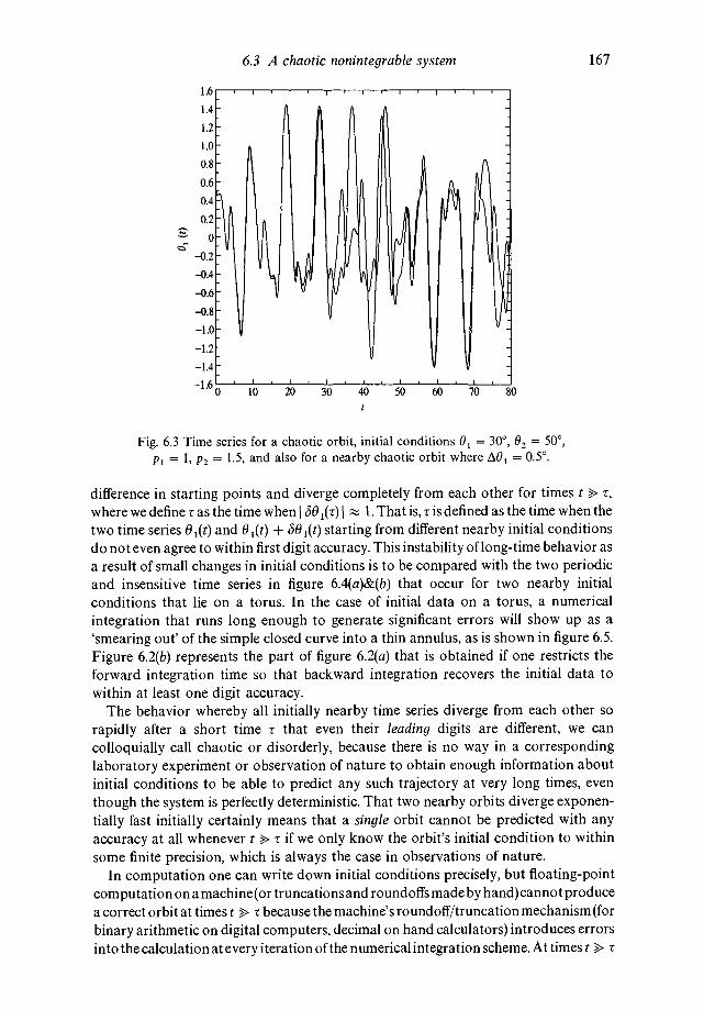
6.3 A chaotic nonintegrable system 167
Fig. 6.3 Time series for a chaotic orbit, initial conditions 01 = 300, 02 = 50°,= L = 1.5, and also for a nearby chaotic orbit where = 0.50.
difference in starting points and diverge completely from each other for times t r,
where we define t as the time when 581(r) 1. That is, t is defined as the time when thetwo time series 01(t) and 01(t) + starting from different nearby initial conditionsdo not even agree to within first digit accuracy. This instability of long-time behavior asa result of small changes in initial conditions is to be compared with the two periodicand insensitive time series in figure 6.4(a)&(b) that occur for two nearby initialconditions that lie on a torus. In the case of initial data on a torus, a numericalintegration that runs long enough to generate significant errors will show up as a'smearing out' of the simple closed curve into a thin annulus, as is shown in figure 6.5.Figure 6.2(b) represents the part of figure 6.2(a) that is obtained if one restricts theforward integration time so that backward integration recovers the initial data towithin at least one digit accuracy.
The behavior whereby all initially nearby time series diverge from each other sorapidly after a short time x that even their leading digits are different, we cancolloquially call chaotic or disorderly, because there is no way in a correspondinglaboratory experiment or observation of nature to obtain enough information aboutinitial conditions to be able to predict any such trajectory at very long times, eventhough the system is perfectly deterministic. That two nearby orbits diverge exponen-tially fast initially certainly means that a single orbit cannot be predicted with anyaccuracy at all whenever t >> t if we only know the orbit's initial condition to withinsome finite precision, which is always the case in observations of nature.
In computation one can write down initial conditions precisely, but floating-pointcomputation on a machine (or truncations and roundoffs made by hand) cannot producea correct orbit at times t t because the machine's roundoff/truncation mechanism (forbinary arithmetic on digital computers, decimal on hand calculators) introduces errorsinto the calculation at every iteration of the numerical integration scheme. At times t

168 Integrable and chaotic oscillations
(a)
82(r)
() t
(b)
Fig. 6.4(a) Time series for a stable orbit, initial conditions: 01 = — 0.65,
62 = 1.4, p1 = 1.419, P2 = 0, and = 0.2. (b) Time series for a nearby stableorbit.
Fig. 6.5 Smearing of the torus due to accumulated innaccuracies offloating-point arithmetic, initial conditions: = 0.072 = 02, Pi = 1.5, and
the machine-produced orbit is dominated by roundoff/truncation error and is called apseudo-orbit: at times t x, even the first digit in the pseudo-orbit is wrong (see exercises6 and 7). On the other hand, the roundoff/truncation algorithm of a computer isdeterministic (integer-based algorithms are the simplest form of determinism) and
02(t)
1.0
0
—1.0
1.0
—1.0
P1
P2 = 1

6.3 A chaotic nonintegrable system 169
cannot introduce 'randomness' into the dynamics. That the roundoff/truncationalgorithm of a computer is in no way the source of the sensitivity of the trajectories ofdeterministic chaotic dynamical systems is shown by the exact solutions, calculatedprecisely in digital arithmetic, of simple models like the Bernoulli shift (chapter 4), thetent map (see below), and Arnol'd's cat map (see also below).
The analysis of section 6.4 leads us to understand why we should expect that thetrajectory represented by the time series in figure 6.3 has a positive Liapunov exponent2 In a two degree of freedom integrable Hamiltonian system with boundedmotion, there are two frequencies w, and w2 that suffer only small changes wheneverinitial conditions are shifted slightly. In a two degree of freedom Hamiltonian systemwith chaotic oscillations, there must be (for each chaotic trajectory) two finite Liapunovexponents, one positive and one negative, as we show in our discussion of iterated mapsin the next section. There, the periods of the unstable periodic orbits can changedrastically whenever initial conditions are shifted only slightly, as we illustratedsymbolically in section 4.6 and show explicitly for iterated maps in sections 6.4 and 6.5(see also exercises 11 and 12).
Since the Jacobi determinant is unity, our conservative differential equations can beintegrated backward in time. This provides the computer programer with a method forchecking whether or not the numbers make sense: beginning with any point on acomputed trajectory, you can use that point as the initial condition and then integratenumerically backward in time to try to retrieve the original initial condition. If theoriginal initial condition at time t0 is recovered to within several digit accuracy, thenthat tells you the accuracy of your machine calculation forward in time. When there is apositive Liapunov exponent 2, then for times t 2-' you will not even be able torecover the first digits of the initial conditions in a backward integration in a machinecalculation that simulates mathematics by introducing errors, as does 'floating-pointarithmetic' or fixed precision 'real arithmetic'.
Energy and other constants of the motion will be conserved to within good numericaccuracy in any calculation where one computes accurately enough to be able toretrieve the initial data to within several digits by integrating backward in time on themachine. Merely using energy conservation as a check on accuracy in a numericalcalculation is inadequate and can be highly misleading: energy is often conserved togood accuracy in pseudo-orbit calculations that extend to times t 2' where thecomputed pseudo-orbit does not approximate the correct orbit at all. Even in anonchaotic system, energy may be approximately conserved for times that are muchlonger than the time over which initial conditions can be recovered to one digitaccuracy by a backward integration. The point is: the mathematical dynamical systemretraces its path perfectly when one performs a computation that integrates theequations backward in time without introducing errors. The method for iterating achaotic map forward in time without the introduction of errors is illustrated in the lastsection of this chapter by using a simple chaotic map.
The chaotic behavior indicated in figure 6.2(b) is nonintegrable: it is not theprojection onto the phase plane of motion on a 2-torus. Hence, we expect that thedouble pendulum does not have a second global isolating integral that is compatiblewith the Hamiltonian, although there may be a local compatible isolating integral oreven a globally incompatible one. The double pendulum is an example of somethingthat is rather common and basic, namely, that low dimensional deterministic chaos isgenerated by relatively simple mechanical systems.

170 Integrable and chaotic oscillations
It is also necessary to understand that merely having one or even several nearbyorbits that repel each other is not sufficient for deterministic chaos: an unstable limitcycle repels all nearby orbits but those orbits are generally not chaotic. Fordeterministic chaos, the orbits must all be uniformly bounded in some region of phasespace and there must be no stable orbits available to attract the orbits that are repelledby the unstable ones. We can define (orbital) stability by Liapunov exponents. A stableorbit attracts nearby orbits with a negative Liapunov exponent, an unstable one repelsnearby orbits with a positive Liapunov exponent, and a vanishing Liapunov exponentrepresents borderline or marginal stability. A sure recipe for chaos is uniformlybounded motion with all orbits inside the bounded region unstable. The simplest caseof this, algebraically, is provided by the Bernoulli shift introduced in chapter 4. Thedouble pendulum is considerably more complicated, as there are regions in phase spacewhere the orbits are chaotic along with others where there is no chaos at all.
6.4 Area-preserving maps
In the beginning of chapter 3, we asserted that any area-preserving map in twodimensions is a discrete model of a conservative dynamical system. If we should try tomodel the double pendulum's Poincaré section analytically, then we would be leddirectly to the study of area-preserving maps of the form (6.13). That the map (6.13) isarea-preserving follows as a special case of Poincaré's theorem on integral invariants:integrals of the form
I'2
=(6.19a)
are time-invariant and are, more generally, invariant under general canonical trans-formations. The proof, requiring calculus and also the recognition that certainquantities are invariant under canonical transformations, is formulated below.
First, let us see why the time-invariance of the integral (6.19a),
f rr I rrJJ
=JJ
(6.19b)i=1 1=1
for any two times—
and implies that the map (6.13) is area-preserving. Since pointsin the surface of integration - 1
at time - transform in one-to-one fashion by thetransformation
= i),Pi(tn._ 1),p — t) 1.(6 20)
= j),pi(tn_ — )j
(the solution of Hamilton's equations) into points of the integration surface at time tn,we need only prove that the differential form is time-invariant, that
I I
=(6.19c)
If we then restrict our discussion to the surface of section defined by equation (6.13),where and tn are chosen so that all of the points of the return map lie in the(q2,p2)-subspace, then it follows from (6.19c) that idpn_ = which is thearea-preserving condition for the map (6.13) for a two degree of freedom system.
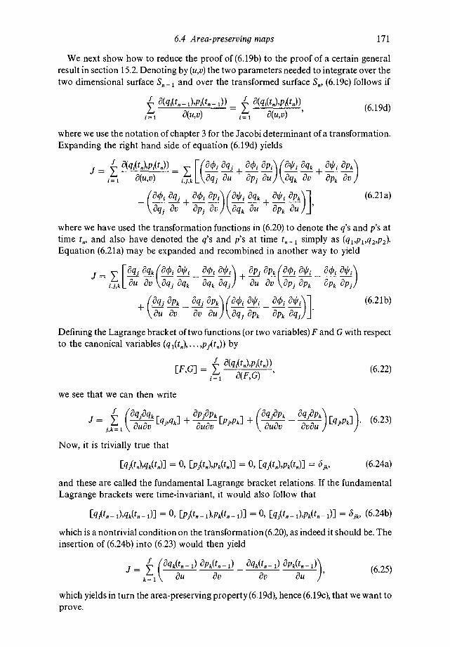
6.4 Area-preserving maps 171
We next show how to reduce the proof of (6.19b) to the proof of a certain generalresult in section 15.2. Denoting by (u,v) the two parameters needed to integrate over thetwo dimensional surface S,_1 and over the transformed surface Sn, (6. 19c) follows if
1)) — 6 19d—
' . )
where we use the notation of chapter 3 for the Jacobi determinant of a transformation.Expanding the right hand side of equation (6.19d) yields
v3(u,v) — au) aPk
(6.21a)
EU)]
where we have used the transformation functions in (6.20) to denote the q's and p's attime and also have denoted the q's and p's at time simply as (q1,p1,q2,p2).Equation (6.21a) may be expanded and recombined in another way to yield
i,j,k 3u ôPk
+ôcbi (6.21b)
aPk
Defining the Lagrange bracket of two functions (or two variables) F and G with respectto the canonical variables by
(t) (t))[F,G] = , (6.22)
we see that we can then write
=[qJ,qk]
+PJ'Pk +
—
(6.23)
Now, it is trivially true that
= 0, [pJ.(tfl),pk(tfl)] = 0, = öjk, (6.24a)
and these are called the fundamental Lagrange bracket relations. If the fundamentalLagrange brackets were time-invariant, it would also follow that
1)] = 0, i),pk(tfl_ 1)] = 0, 1),pk(tfl_ = (6.24b)
which is a nontrivial condition on the transformation (6.20), as indeed it should be. Theinsertion of (6.24b) into (6.23) would then yield
—— 1) 1)
(6 25)'
which yields in turn the area-preserving property (6. 19d), hence (6.19c), that we want toprove.

172 Integrable and chaotic oscillations
We show in section 15.2 that the fundamental Lagrange bracket relations are notmerely time-invariant, they are also invariant under the entire class of transformationsin phase space that is called canonical. As we show in that chapter, the time-evolutiontransformation (6.20), the solution of Hamilton's equations, provides one example of acanonical transformation.
Therefore, in accordance with what is required for understanding Hamiltoniansystems with bounded motion in phases space, let us restrict our further considerationsin this section to area-preserving maps with bounded discrete trajectories.
Poincaré's recurrence theorem (see chapter 3) applies to every conservative system,to area-preserving maps as well as to continuous flows. Therefore, any block of initialconditions of an area-preserving map must intersect itself after some finite time, andthereafter infinitely often as the discrete time n goes to infinity: aside from any possibleseparatrix motions, all of the map's orbits are either periodic or quasiperiodic. How-ever, any map that models the double pendulum must generate a fair degree of variety:in parts of phase space, the map must produce only stable periodic and quasiperiodicorbits (orbits with two frequencies, where both Liapunov exponents vanish) corre-sponding to the behavior shown as figure 6.1. But that is not all: in other parts of thephase space, corresponding for example to figure 6.2, the map must generate unstableorbits with one positive and one negative Liapunov exponent. As preparation forstudying maps where the Liapunov exponents vary strongly over phase space, let usformulate the way to extract the two Liapunov exponents for an orbit of a twodimensional map.
For an arbitrary two dimensional discrete map of the plane,
+1 =
}(626)
+ 1 =
we begin by linearizing about any exact orbit (x0,y0) —* (x1,y1) —*... —* —+ .... Thelinear equation
= (6.27)
describes the time-evolution of the difference for small enough times, where the vectoris given by
=(6.28)
and the Jacobi matrix
E3f äf
A =(6.29)
which follows from linearizing the equation of motion for the perturbed initialcondition along the original trajectory, is evaluated for each iteration at the pointon the exact trajectory, which itself starts from the initial condition

6.4 Area-preserving maps 173
Consider next the solution by iteration of the linearized equations,
= . . . = J,,öX0 (6.30)
in terms of the matrix =The eigenvalues of vary with n, as do the eigenvectors and both are
obtained by solving the eigenvalue problem given by
(631)=
Note that the directions of the eigenvectors are generally not constant along thetrajectory original —+ ... —* —p.... If the eigenvectors e1(n) and e2(n) (whichwe assume to be normalized, so that II = 1) are linearly independent, then we canexpand the difference in the two initial conditions in the form
= (6.32)
and then obtain an equation for the difference between the nth iterates,
= = (6.33)
The Liapunov exponents and 22 are then defined by
(6.34)
for large n, so that
n 1. (6.35)
The exponents characterize the trajectory passing through (x0,y0) and (except formaps with constant derivatives) will vary when the initial conditions are changed.Geometrically, a positive exponent > 0 corresponds to a local expansion of smallareas along the direction of while 2k <0 yields a local contraction of small areasalong the direction ek(n). That is because areas = transform according to therule
= I J,, I(6.36a)
where = Ax4y0 an initial element of area in phase space, and II
= det J,, is theJacobian determinant of the transformation from (x0,y0) to It follows thatdet so that for large enough n we can rewrite (6.36a) as
(6.36b)
Hence, + 22 = 0 corresponds to an area-preserving map whereas + 22 <0describes a dissipative map. The condition for deterministic chaos is sensitivity oftrajectories with respect to small changes in initial conditions and requires the action ofat least one positive Liapunov exponent. The condition
I = I P2 I is therefore bothnecessary and sufficient for orbitally stable motion in an area-preserving map,

174 Integrable and chaotic oscillations
requiring = 22 = 0. For dissipative systems, nonchaotic motion requires <0 for= 1,2, which corresponds to a zero dimensional attractor in the two dimensional
phase space. For a chaotic area-preserving map we need > 0, and then22 = — <0 follows.
In general, it is difficult to study area-preserving maps that model systems like thedouble pendulum where phase space is divided in a complicated way into regions oforbital stability and regions where orbits have nonvanishing Liapunov exponents,
> 0 and 22 = — <0, and so we defer that subject until chapter 17. It is mucheasier to model systems that are 'completely chaotic' in the sense that they exhibitpseudo-random behavior over all of their available phase space. In a completelychaotic system, there are no regions in phase space with stable orbits: all of the system'sorbits are unstable. In one dimension, the Bernoulli shift is an example of a completelychaotic system. A two dimensional analog of the Bernoulli shift that is area-preservingis Arnol'd's cat map.
The cat map is defined by the transformation
= +(6.37a)
j
and is area-preserving (the Jacobi determinant of the transformation from to1) is unity). 'Mod 1' in equation (6.37a) simply means that one must always
subtract off the integer parts, so that x,, and always lie between 0 and 1, in which casethe phase space is the unit square. The part of(6.37a) that is responsible for the chaos issimply the one dimensional map
(6.37b)
the binary Bernoulli shift. Now, let us look at some details of the cat map.By an application of the method of proof of section 4.6, where we proved that
rational numbers used as initial conditions for the decimal Bernoulli shift yield periodicorbits (or the proof of the next section where we show that rational initial conditionsyield periodic orbits for the binary tent map), if follows that rational initial conditions(x0,y0) = (P/Q,P'/Q') for the cat map yield periodic orbits. It then follows that anyirrational initial condition, e.g. (x0,y0) = — 1,\/3 — 2), yields a nonperiodic orbit, adiscrete orbit that is confined to the unit square but that never closes on itself. All ofthese orbits, both periodic and quasiperiodic, are unstable because all of them have onepositive (and therefore one negative) Liapunov exponent. It is easy to compute the twoLiapunov exponents:
11,2 = in(3)
= ± ln(3)
(6.38)
Since every trajectory has the same exponents, and since one exponent is positive, wehave a model of an area-preserving Poincaré map where the phase space, the unitsquare, is 'filled up' by unstable periodic and unstable nonperiodic orbits. Because thesystem has no stable orbits, arbitrary shifts in the last digits of any initial condition willgenerally produce a completely different orbit with a completely different period orquasiperiod than the one we started with (see examples in the next two sections).

6.5 Computation of exact chaotic orbits 175
6.5 Computation of exact chaotic orbits
Arnol'd's cat map is the area-preserving transformation
(637a)5
of the unit square.Because of the modulo 1 condition on both x and y, the motion is confined to the
surface of a two dimensional torus: the points x = 0 and 1 are identical modulo aninteger, as are the points y = 0 and 1. We shall use this map to illustrate two points: first,closed form algebraic solutions are not ruled outjust because a system is chaotic (closedform algebraic solutions are not necessarily possible just because a system isintegrable). More important is that exact chaotic orbits can be computed as precisely asone wishes, within the limits set by computer time. Information need not 'get lost' in achaotic system as one computes (as it did in the floating-point computation of thedouble pendulum problem above) so long as one takes precautions and carries out thecomputation correctly. As we showed above, however, the length of time that one cansee into the future when a trajectory has a positive Liapunov exponent is very severelylimited by computer time.
Recall that the map has two nonzero Liapunov exponents, = In [(3 += — 22. This follows from writing
i) = (21 (6.39)
1 1
where (3 ± are the eigenvalues of the matrix A. Hence, the map is uniformlychaotic, and the unit square is densely filled with unstable periodic orbits. Both periodicand nonperiodic orbits of the map can be computed exactly, as we shall show.
Note that
=(xc)
mod 1 (6.40)
for any initial condition where
An_(F2n F2n_i)(641)
2n—1 2n—2
and is a Fibonacci number: F1 = 1. Equation (6.41)yields the exact solution, in closed algebraic form, of the cat map.
Consider first the periodic orbits. All rational initial conditions can be written in theform
(x,,y,) = (P/N,Q/N) (6.42)
where the unit square is partitioned into N2 equal squares, each of side 1/N, and P and
Q are integers: 0 � P,Q � N. Because there are N2 cells, and A'1 is an integer matrix (allentries are integers), the cell labeled by P and Q must be revisited after not more than N2iterations of the map, and by uniqueness, the motion must then repeat. Hence, allrational initial conditions yield periodic orbits, and all these orbits are unstable, arechaotic, because > 0: if you shift an initial condition slightly from one rational pair

176 Integrable and chaotic oscillations
of numbers to another pair with larger denominators, then the resulting orbit usuallyhas a much longer period than that of the original orbit. As a typical example, the initialcondition (1/7,1/7) lies on an 8-cycle (eight iterations of the map are necessary before theinitial condition is repeated) whereas (1/9,1/9) lies on an 1 1-cycle, and a much longercycle will be found if you have the patience to compute the orbit for the initial condition(10/91,1/9), for example. Such drastic changes in period cannot occur for small changesin initial conditions of a completely stable, hence nonchaotic, mechanical system.
All cycles start from rational initial conditions and are unstable, while irrationalstarting points yield unstable nonperiodic chaotic orbits: there are no regions on theunit torus where stable orbits occur. Like the Bernoulli shifts and tent maps, thisdynamical system is 'uniformly hyperbolic' (has a dense set of unstable periodic orbitswith a constant positive Liapunov exponent). Arnol'd (1983) has shown that the map'sinvariant density is uniform, meaning that a 'measure one' set of irrational initialconditions yields orbits whose distribution of iterates covers the torus uniformly asn -+ cc. However, other irrational initial conditions produce nonuniform (evenmultifractal) distributions of the map's iterates over the torus. An arbitrary choice ofinitial conditions in computation or experiment differs from the idealized andunattainable notion of a random draw of initial conditions from the mathematicalcontinuum.
The main idea in what follows is that the digit strings for the initial conditions mustbe computed along with those for the iterates of the map. Because the map is piecewiselinear and A1 > 0, the information in the Nth bit of(x0,y0) is transformed at a finite rateuntil in relatively short time it becomes information in the first bits of x,, andTherefore, to know to N-bit accuracy, the initial condition (x0,y0) must becomputed to within roughly n + N ln 2/ln bit accuracy, and this is easy to do for thecat map. We need only use an algorithm for an irrational number (or a pair ofalgorithms), such as the algorithm for 1 to write x0 and y0 in (6.37a) as N-bitbinary strings. The exact solution is then given by
= + 143
= +
where the coefficients Fm are Fibonacci numbers.All of the required arithmetic can be done as binary-point shifts on x0 and y.
combined with addition of finite-length binary strings. However, we must keep exactlyas many bits in x, and y0 as we need in order to compute both and accurately toN-bits, where N is our desired accuracy. That FmXo consists only of binary-point shiftsplus addition on x0(mod 1) is easy to see: with
Fm=
= .. . (6.44)
where = 0 or 1, we have F3 = 11 = 10 + 1, F4 = 101 = 100 + 1, F5 =1000, F6 = 1101 = 1000 + 100 + 1, and so on. For example, givenx, = — 1 0.01 10, then F4x0 = 0.10 + 0.01 = 0.11 will be exact to 2-bits if thereare no 'carries' in the neglected terms. If we want to know F3x, to 3-bits we have to use
— 1 = 0.01101, so that F3x0 = 0.101 + 0.011 = 0.000. For example, givenx0 = — 1 = to 16 bits, we can compute F4x0 =lOx, + x,mod 1 = to 14-bit accuracy. The reader should note
6.6 On the nature of deterministic chaos 177
that it is necessary to have a method for handling 'carries'. For example, if we use= to 4-bits to compute F4x, = 0.10 + 0.01 = to 2-bits, this is
wrong, but x, = to 5-bits yields the correct 3-bit result F3x, = 0.000. So,can be computed from (6.43) to any prescribed precision N by using an algorithm
that generates the digits of the initial condition (x0,y0) in binary arithmetic. Theresulting computed orbit is a uniform approximation to an exact nonperiodic chaoticorbit so long as one uses an algorithm to generate the number of bits of an irrationalinitial condition that the action of the positive Liapunov exponent demands.
Clearly, to start with a point and iterate the cat map backward to recover thefirst N bits of an initial condition we must first have computed the nth iterate toabout n + N ln 2/ln A bits. Information cannot get lost if one computes a chaotic orbitcorrectly. On the contrary, information about the dynamics is gained: the informationencoded as the high order bits in the initial condition defines a binary program thatdetermines the long-time behavior of the dynamical system seen as a simple automa-tion. Throwing away those bits by using floating-point arithmetic is akin to truncatinga computer program and throwing it into a loop that prevents you from obtaining theinformation that you aimed to get by writing the program in the first place. Deter-ministic chaos means deterministic unpredictable motion in nature, but this does notimply motion that is unpredictable on a computer in a correctly formulated andcorrectly carried out calculation. The idea that deterministic chaotic motion is notcomputable is a misconception that has been widely and carelessly propagatedthroughout much of the literature. Deterministic chaotic orbits can be computed towithin as many decimals as one wants within the limits imposed by the time neededfor thecomputation. The inability to compute chaotic orbits at long times is not that thedecimals cannot be generated and computed in principle (all of the digits aremathematically determined), rather, it is the amount of computation time that is neededto generate and compute them correctly that limits our ability to see where a chaoticorbit is going. A numerical computation is not the same thing as a real experiment,especially when a system is chaotic. In the former case initial conditions are specifiedprecisely and the system is closed whereas in the latter case initial conditions areimprecisely known and the system is open. Simulations of nature are never the same asnature and the systematic errors introduced into computation by the use of floating-point arithmetic do not account for the difference.
6.6 On the nature of deterministic chaos
Because the properties that we identify as chaotic in the cat map can be understood byfirst understanding the Bernoulli shift, and because those properties are characteristicof an entire class of one dimensional maps, we now turn to noninvertible maps of theinterval in order to clarify what we mean by deterministic chaos. The differentialequations defining a flow have unique solutions and are time-reversible. The maps thatthey give rise to are uniquely invertible. Chaotic behavior also occurs in noninvertibleone dimensional maps, but noninvertible maps cannot be derived from flows exceptperhaps by making drastic approximations to higher dimensional maps in dissipativesystems.
In order to understand how the exponentially rapid separation of trajectories worksnumerically, we study a one dimensional map
+ 1 = (6.45)

178 Integrable and chaotic oscillations
where the iterations x, are uniformly bounded and therefore lie in some definite intervalfor all values of the discrete time n. By rescaling the iterates we can always replace thisinterval by the unit interval [0,1]. The condition that the motion on the unit interval(which is our phase space) is bounded is satisfied by mapsf(x) that peak once or more inthe interval [0,1] but satisfy 0 �f(x) � 1, that 1S,fmax � 1. It then follows directly that0 � x,, � 1. Therefore, we have self-confined motion with atleast a two-valued inverse
The Liapunov exponent was defined in chapter 4 by starting with two exact orbitsx0—*x1 —*x2 —*... —*... and x0 + + + —* ... +ox,, —* . . . and then choosing I
I1 in order to linearize the map along the first orbit.
If we satisfy the conditions I Ox,, II
1, then we can study the linearized equation
(6.46)
whose solution
IOx,, I I Ox,,
I(6.47)
defines the Liapunov exponent
n—i i2(x,,,n) = —ln for n > 1, (6.48)
n
= x,, is the nth iterate off starting with x. Except for certain very simplemaps, the Liapunov exponent 2 varies with the choice of initial condition x,, (see chapter14 for simple examples).
It is typical that one does not obtain pointwise convergence to a definite number A(x,)that is completely independent of n for large but finite n in computation whenever themap's slopef' varies along a trajectory (deterministic noise). The main point is that themap's average slope determines everything: the Liapunov exponent is just the timeaverage of the logarithm of the slope along a trajectory, and whenever that average ispositive (whenever the magnitude off' is larger than one, on the average), then we getexponential magnification of small differences in initial conditions.
A positive Liapunov exponent describes the exponentially rapid separation of twoinitially nearby trajectories and is the mechanism for the instability of long-timebehavior of two different orbits that begin very near to each other: if one plots thediscrete time series x,, vs n for the two nearby initial conditions, then the iterates willtrack each other for times n — In Ox,, I/A but will diverge from each other whenn 1 (where equations (6.46 and 6.47) no longer hold).
If one knows the initial state of a dynamical system to within finite resolutions, whichis at best the case in any observation of nature, then one can only predict thetime-evolution of the system with accuracy over a time interval n that is given by
1, where the uncertainty Ox0 represents the resolution of the experiment.In computation, in contrast with observations and experiments on physical systems,
Ox,, = 0 because one starts with a single precisely defined initial condition given in theform of a finite length digit string x0 = in some integer base p ofarithmetic. By using an algorithm (say, the rule for computing the digits one by one of
rather than floating-point arithmetic on a computer, one can then generate asmany digits c.(O) as one pleases. In any case, the digits take on any one of p possible

6.6 On the nature of deterministic chaos 179
values 1,2,3,... ,ji — 1, and we can choose freely to work in any base = 2,3,4 Thisfreedom of choice of base of arithmetic is somewhat analogous to the freedom to chooseto study a partial differential equation in rectangular, spherical, elliptic, or any other setof curvilinear coordinates. Just as there may be a coordinate system where the solutionof a particular partial differential equation is the simplest, there may be a base ofarithmetic where the behavior of a particular map is most transparent.
In digital arithmetic, which von Neumann called 'an application of informationtheory', to what extent can we (or can't we) compute the first N digits of the nth iterate
= (6.49)
of a chaotic map without making a single error? This is an interesting question becausethe system is deterministic, yet it is supposed to be in some sense unpredictable. If thereis a limit to our ability to see into the future, what determines that limit whenever thesystem has bounded trajectories with positive Liapunov exponents? It is quite easy tosee that, for arbitrary maps that yield bounded motion, the only limitation is that ofcomputation time.
In order to understand that limitation, we must also discretize the informationpropagation equation (6.47), where 2(x0,n) is the Liapunov exponent for the particulartrajectory under consideration after n iterations. By we mean /1 — N the last computeddigit CN(O) in our initial condition x,, = . Since the maximum erroroccurs when the first digit of is on the order of unity, when i/p in magnitude,then we obtain from (6.47) the condition
1 (6.50a)
which means that (for N large)
n Nln p/A (6.50b)
is roughly the number of iterations that one can perform without committing an errorin the first digit of given only the first N digits of This is an information flowproperty, one that follows whenever the Liapunov exponent is positive. When theexponent is negative, then one gains accuracy in computation as n is increased. In thelatter sort of system, CN(O) is the least significant digit. In the chaotic system, one canwith justification say that e1(O) is the least significant digit!
The information propagation condition (6.50b) tells us that the most fundamentallimitation on the ability to compute and therefore to predict the future from the past inany deterministic system is the limitation of computation time. This limitation isnontrivial because it means that it is necessary to increase the precision of thecomputation (as we demonstrated with the cat map), by systematically computingmore and more digits in the initial condition x0 as one iterates the map, and also byholding more and more digits of every other computed iterate as well (because the'present condition' is the initial condition for future states and so on). Iftruncation and roundoff are used (e.g. floating-point arithmetic), then uncontrollableerrors will be introduced into the calculation. As we stated in section 4.6, chaoticdynamical systems are precisely those systems that have orbits that reflect thecomplexity of the digit strings of both rational and irrational numbers. Contrary topopular expectations, this conclusion is not at all changed by considering nonlinearmaps where the slope is not piecewise constant (see chapter 9 in McCauley, 1993).
The time series in figure 6.2 for the map of the double pendulum at long times do not
180 Integrable and chaotic oscillations
represent true orbits but rather pseudo-orbits. Pseudo-orbits arise any time thatroundoff/truncation errors are introduced into a computation, because those errors arethen magnified exponentially by the map's positive Liapunov exponents. A machineprogram that uses floating-point or fixed precision arithmetic only produces an inexact'simulation' of the desired mathematics and will easily produce a pseudo-orbitwhenever the system is chaotic. Floating-point arithmetic is only a weak side-steppingof the difficult problem of how to handle digit strings of numbers. This erroneousmethod may well be abandoned in favor of accuracy as computer technology evolvesfurther.
Another way to look at this is that every pseudo-orbit is an exact orbit of some othermap that the machine's roundoff/truncation algorithm has invented to try to simulateyour computation. Is chaos an artifact of bad machine arithmetic? Does the 'chaos' goaway if the computation is performed correctly? That the answer to this question is nocan be understood most easily by computing the solutions of simple maps like theBernoulli shift, the tent map, and the cat map correctly by hand, or by restricting tointeger operations when programming a computer. These piecewise linear maps can besolved exactly and easily by using decimal expansions in a definite base of arithmetic.
To see how this works, consider the binary tent map
x,,÷1 = if < 1/2, = 2(1 — if > 1/2 (6.51)
where the Liapunov exponent is = ln 2 for every trajectory. If we choose a rationalinitial condition, x0 = P/Q where P and Q are integers, then either x1 = 2P/Q or2(Q — P)/Q, each of which is one of the Q fractions 0, 1/Q, 2/Q (Q — 1)/Q, as is everyhigher iterate. Therefore, after at most Q iterations repeats one of the earlier iteratesand the orbit is periodic. Conversely, irrational initial conditions yield nonperiodicorbits. All orbits of the binary tent map are unstable because A = In 2 > 0, and we wantto understand better how this instability works.
Consider as an example the orbit starting from the point x0 = 1/5: it is easy to showthat this is a 3-cycle with points 1/5, 2/5, and 4/5. Next, try to track this orbit by startingfrom a nearby initial condition, say x, + ox, = 10/51. The result is another periodicorbit, but one with a cycle length much greater than 3! Matters get even worse if youtake the initial condition of be 100/501, which is even nearer to 1/5. This is in starkcontrast to stable periodic orbits of integrable systems where a small change in initialconditions produces (through a small shift in the constant canonical momenta Pk) onlya small change in frequencies and periods. It means that you can never have enoughinformation about initial conditions in experiment or observation to know where achaotic system is going in the long run. This is very bad news for people who want tobelieve that the future is predictable. One can understand both the short- and long-timebehavior of systems with chaotic behavior, and one can even compute chaotictrajectories precisely, but one cannot in any practical way predict which trajectory willoccur whenever we encounter one of these systems in nature.
In observations and experiments, statistics also come into play because one cannotcontrol initial conditions with absolute precision: in a gedanken experiment, therepetition of N identically prepared experiments means that there are N differenttrajectories that start near to each other and emanate from a tiny 'ball' of initialconditions in phase space (from a small interval, in the case of one dimensional maps). Ifwe divide the phase space into N different bins of finite width (not all of which need havethe same size and shape), then we normally would plot a histogram to reflect how often

6.6 On the nature of deterministic chaos 181
a given bin in phase space is visited by the different time series that originate from eachinitial condition in the interval. Each time series represents the repetition of anidentically prepared experiment, but the experiments are identical only to within thefinite precision variation in the initial conditions (the size of the ball of initial conditionsis determined by the precision within which the 'identical repeated experiments' areprepared). This is stated in the spirit of the collection of experimental or observationaldata. However, there is a much deeper reason why there are statistics in the first place:each exact orbit of a chaotic dynamical system generates its own histogram! This wasdiscussed briefly in section 4.6, but we can add some details here. The different classes ofstatistics that can be generated for different classes of initial conditions is one way tocharacterize these systems.
For any map (6.26) we can write the initial condition and all subsequent iterates insome definite base p of arithmetic (p = 2,3,4,. . = . where eachdigit takes on one of the p values 0,1,2,... ,p — 1. In this case, when a single orbit
{ has a positive Liapunov exponent, then
(6.50b)
is the number of iterations that one can perform before the information stored as theNth digit (more generally, stored as several of the first N digits) of the initial conditionx0 will determine the first digit of the nth iterate x,. Since the decimal Bernoulli shiftabove (where 2 = ln 10) consists only of a digit shift per iteration when the iterates arewritten in base 10, = 1(n + 1), it is precisely the nth digit in the initialcondition x0 that, after n iterations, becomes the first digit of the nth iterate
= (6.52)
The statistics of the orbit follow easily, but we describe the general method of histogramconstruction below in the context of the binary tent map.
The binary tent map (6.51) is completely transparent in binary arithmetic (basep = 2) where = 0 or 1. In this case, the map can be replaced by a simple auto-mation, e1(n) = 1(n — 1) if 1 — 1) 1) = 1,
which is only slightly more complicated than reading the digits of an initial conditionone by one, as we have done for the decimal Bernoulli shift above. The tent map'sautomation follows easily by noting that, in binary arithmetic,
1.00000"0" (6.53a)
which is just the statement that
1 = 1/2 + 1/4 + 1/8 + ... (6.53b)
and therefore that
1 — = 0.(1 — e1(n))(1 — . (l — (6.53c)
For the binary tent map, therefore, the first bit of the nth iterate is determined bythe pair of bits — in the initial condition: e 1(n) = 0 — = 00 or 11 but
= 1 if = 01 or 10. Here, the information flows at the rate of a bit periteration, corresponding to the fact that the Liapunov exponent is 2 = ln 2. Informa-tion flow at the average rate of a digit per iteration in an integral base p of arithmeticthat is roughly is the very essence of deterministic chaos.
We can now systematically derive the statistics generated by a single orbit that starts

182 Integrable and chaotic oscillations
from a definite initial condition x0. Divide the unit interval into 2" bins of equal width2" and label the bins from left to right by the 2"" N-bit binary words 00" 00" 01,
Whenever the first N bits e1(n) of coincide with one of thesewords, then the bin labeled by that word is visited by the map. If we denote byP(c1 . the frequency with which the bin labeled by the N bit word is visited,then the required 2" probabilities {P(E1 . are given by the histogram that followsfrom iterating the map from a definite initial condition. For N = 1, we get 2 bins and thecoarsest level of description of the statistics generated by the dynamics, but finercoarse-grained descriptions are provided by increasing the precision N. In experimentand in computation, both the precision N and the time n are always finite: the limitswhere n and N are infinite are misleading abstractions that have little or nothing to dowith nature, and certainly have nothing to do with computation. The bin probabilitiesthat we encounter in any case are always empirical frequencies (they follow fromhistograms) and cannot arbitrarily be replaced by infinite time, infinite precision limits,even if those limits are known mathematically. Finally, the bin probabilities{P(s1E2 are not independent of the choice of initial data, but are different fordifferent classes of initial data.
Normal numbers were defined in section 4.6. The property of a normal number is asfollows: the number is expanded in some base of arithmetic, base j1 = 2,3,4, or anyhigher integer, and the number then has the form x = where the digits ö1take on the discrete set of values 0,1,2,. . . ,y — 1. Consider next a string of digits oflength M, e1s2 As the can take on different values, there are differentpossible strings of length M. Let P(E1E2 . . denote the frequency with which aparticular block E1E2 occurs as the string is read left to right by sliding an M-digitwindow one digit at a time (see McCauley, 1993, chapter 9). For a normal number,P(E1E2" . = for all M for the infinite length string. It is not known whether thenumber it is normal to any base, but it is known that it is effectively normal to base 10for M � 5. By effectively normal, we mean that P(c1E2 . . .
10M for a reading offinitely many digits (clearly, it is effective normality and not the abstract limiting casethat is of interest for science). 'Effective normality' for it occurs for a string of lengthN> 500 digits. Therefore, the histograms obtained from iterating the decimal tentmap, starting from the initial condition x0 = it, are approximately even for a division ofthe unit interval into 10M bins, with M = 1, 2, 3, 4, or 5, the same distribution that onewould 'expect' to obtain for a large number of tosses of a fair 10-sided die.
One does not know whether either or is normal to any base of arithmetic, butit is easy to verify by a correctly written computer program that both numbers areeffectively normal to base 2 for up to at least 5000 bits. For an arbitrary map, the bitdistribution of the initial condition is not the same as the histograms that one obtainsfrom iterating a map although one can prove (see chapter 9 in McCauley, 1993) that, forthe binary tent map, a normal initial condition also yields even bin statistics when themap is iterated. Therefore, iteration of the binary tent map, starting from either x0 =,j(2) — 1 or — 1 will yield histograms that reflect the statistics that one would'expect', on the basis of the law of large numbers (see Gnedenko and Khinchin, 1962), tofind for a large number of tosses of a fair coin. However, we also point out that it isextremely easy to construct initial conditions that yield very uneven histogramsand sometimes histograms where certain bins are never visited:
= is one example;x0 = 0.10110011100011110000" is
another.

6.6 On the nature of deterministic chaos 183
Finally, you cannot eliminate deterministic chaos by a coordinate transformation:periodic orbits transform into periodic orbits, and nonperiodic orbits transform intononperiodic ones as well (the periods only involve counting and so are topologicinvariants). A generalization to other maps of the digital arithmetic performed abovefor the tent map leads to the study of the 'symbolic dynamics' of a whole class oftopologically related maps (maps that are related by continuous but generally highlynondifferentiable coordinate transformations). Symbolic dynamics is a method thatconcentrates upon the topologically invariant properties of chaotic systems. This isimportant, for one reason, because it allows us to use the simplest map in a class tounderstand the periodic orbits, the possible statistics and other properties of everysystem in the same class.
Liapunov exponents (and fractal dimensions) are not topologic invariants: they arenot invariant under arbitrary continuous but nondifferentiable coordinate transform-ations. However, you cannot transform a dynamical system with finite Liapunovexponents into a one with vanishing exponents by a nonsingular transformation, Theproof is as follows: consider a noninvertible map
(6.54a)
and also a map
1 = (6.54b)
which is obtained from the original map (6.54a) by a coordinate transformation,
= h(Xn), (6.55)
where h' 0. That is, the transformation h is invertible. We denote by A and theLiapunov exponents of the maps (6.54a) and (6.54b) respectively, i.e.,
(6.56)i=O
The question is: how is ci related to 2, where 2 is the exponent for the correspondingtrajectory of mapf (trajectories map one to one)? From (6.54a) we obtain
(6.57a)
and likewise,
dZn+t = (6.57b)
follows from (6.54b), so that from = we obtain
1—
1
(6 58)—
h'(x) f (xv) (6.59)
184 Integrable and chaotic oscillations
when the above results are combined. Inserting the above results yields
a(
f'(x1) I + ln i)) (6.60)(x1)
which can be rewritten in the form
a = 2 + (6.61)h(x1)
It follows that a — 2 for large n. For times n 1, the Liapunov exponent, fortrajectories that map onto each other, is invariant under differentiable coordinatetransformations which means that you cannot transform chaos away. In chapter 13 weshow that integrability is also invariant under differentiable coordinate transform-ations.
Is chaos computable; e.g. is = mod 1 computable? Is the solution x(t) = x0et ofdx/dt = x computable? Both are either computable or noncomputable together: if x0 isgenerated decimal by decimal (or faster) by an algorithm (like the various rules forcomputing x0 = of which Newton's method is optimal), then both and x(t) arecomputable (granted, in the second case t must also be chosen to be a computablenumber). If x, is assumed to be noncomputable (most numbers defined to belong to thecontinuum belong to this category), then neither x,, = -' mod 1 nor dx/dt = x havecomputable solutions. Computable numbers form a countable subset of the continu-um, and they are all that we have available for the numerical study of either periodic ornonperiodic orbits (see Minsky, 1967, chapter 9 or McCauley, 1993, chapter 11). In fact,both problems are equivalent: if we study the solutions of dx/dt = x on the unit circle,so that x(t) = etx. mod 1, and in addition strobe the solution at times t,, = n In 2, then
= mod 1 = mod 1 = x,.
Exercises
1. For a particle of mass m in a box with perfectly reflecting walls, 0 � x1 � a1,0 � x2 � a2, show that the canonical momenta P. conjugate to the generalizedcoordinates Q- = + are given by = and therefore that K = (ir2/
+ (Hint: use = along with H = +
2. For the Kepler problem, compute a Poincaré section numerically and usingCartesian coordinates. Choose initial conditions corresponding to the order ofmagnitude of the earth—sun system, but use dimensionless variables in order tointegrate numerically.
3. For the double pendulum, with = 12 = 1, g = 1, and m1 = m2 = 1, computenumerically and also plot the Poincaré sections for the following initial conditions:(a) 01(t0) = — 0.65, — 0.7, and — 0.85 with 02(t0) = 1.4,p2(t0) = 0,andE = 2.24483
(b) same as (a) except that 01(t0) = — 0.822, 02(t0) = 1.4335
(c) 01(t0) = — 0.5, 02(t0) = 1.4, otherwise same as (a)(d) 01(t0) = 0.5p2(t0) = p1(t0) = 0, 02(t0) = it.
For cases (a), (b), and (c), plot the Poincaré sections only for times that are smallenough that you can recover most of the digits of your initial condition by in-

Exercises 185
tegrating backward in time. For case (d), ignore that constraint on accuracy untilexercise 6.
4. Plot and compare the time series 02(t) vs t for the following cases:(a) The initial data in exercise 3(b) above and also for the case where 02(t,) =
1.4400.
(b) The initial data in exercise 3(d) above and also for the case where 02(t,) =3.1416.
5. (a) For exercise 3(a), integrate far enough forward in time that energy E is notconserved even to one digit accuracy. Is the torus in the Poincaré section'smeared out'?
(b) Compare the integration time scale for one-digit energy conservation with thetime scale for one-digit initial condition recovery in backward integration.What does this mean?
6. Denote by 02(t) the time series in exercise 3(d) starting from 02(t,) = it and by02(t) + the time series that starts from 02(t,) + 502(t) = 3.1416. Let t denotethe time t for which I t502(t)
I1. Treating the point 02(t) for any time t � r as the
initial condition, integrate the differential equations backward in time and attemptto recover the original initial condition 02(t,) = it to within several digits (checkyour result for three different times t < t1 < t2 < ta).(a) Show that when t � t even the leading digit of the 'recovered initial condition'
is wrong.(b) Show that if t then as many digits as you like of 02(tc,) can be recovered.Note: Be aware that, in single precision on a binary computer, it is represented byabout 25 binary digits and the rest of the (infinitely long) binary string is truncatedand is approximated by a 'floating exponent' M in 2M• Note also that 25 binarydigits are equivalent to about 7 base 10 digits: 225 = 10N means that N = 25 In 2/In 10 = 7.52.
7. If
=xnexdx
where!, = e — 1 and 11 = 1, then show that 1,, = e — nln_1 if n � 2 is an integer.(a) Starting with e computed from a PC or hand calculator, compute by
recursion from 10. Compare with the exact result known to several decimals in atable of tabulated functions.
(b) Show that this map effectively has a Liapunov exponent 1 '—j In (n) for forwarditerations. How, then, can one compute recursively?
(c) As a first approximation, set 15000 0 and compute 14995 by backwarditeration of the map. To how many decimals is your result accurate?
(Julian Palmore)
8. Compute the Liapunov exponents for the bakers' transformation
xn+1 2xnm01h1
—
Is the system conservative or dissipative?
186 Integrable and chaotic oscillations
9. For the bakers' transformation with a = draw a sequence of diagrams in phasespace that shows how the block of initial conditions 0 � x � 1, 0 � y � is
transformed by the map (for n = 1,2,3,.. .). Identify graphically the effects of thetwo Liapunov exponents in the resulting figures.
10. Using the idea of a return map and the example of section 7.5, explain how forwardand backward integrations in time can be carried out so that one does not 'lose' theinitial condition 02(t0) in the double pendulum problem. Show in detail how thiscan be done for the cat map for three forward iterations to 6-bit accuracy (wherethe first 6 bits of (x3,y3) are to be computed exactly for all iterates).
11. Find and compare the periods of the cat map's orbits when (x0,y0) = and (u).12. We can construct a three dimensional histogram for the cat map in the following
way. Writing binary expansions
=y,, = 0.51(n)"
for the map's iterates, subdivide the unit square into four bins and label each bin bythe symbols c1(n)ö1(n) = 00,10,01,11. Then, compute and plot the histograms forthe initial conditions (x0,y0) =/ j5 5
k12'12j12 12
j \ (29 29
Use an algorithm to generate in binary, and compute the histograms for 500iterates of the initial condition — — 1).
7
Parameter-dependent transformations
Kunsten alene kan skape verker, som aidrigF. Engel (1922)
7.1 Introduction
Marius Sophus Lie was born the son of a Lutheran priest in Nordfjordeid, a smallvillage near the Sunmøre Alps. He grew up near Oslo and spent his vacations in thestill-typical Norwegian way: ski tours in the winter and foot tours in the summer. Afterhis student days at the University of Oslo he was influenced by the writings of theGerman geometer Plucker, whose student Felix Klein (1849—1925) he came to knowwell in Berlin. In Paris, where Lie and Klein roomed together, Lie met the outstandingFrench mathematicians Darboux and Jordan, and began his work on contacttransformations while there. He set out on foot alone to make a Wanderung to Italy butwas arrested outside Paris and jailed for a month due to the onset of the Franco—Prussian war: he carried with him several letters on mathematics from Klein thatcaused French police to suspect him of being a German agent with encodedinformation. Back in Oslo, Lie finished his doctor's degree and then taught and wrotefor several years at the University. After sending Engel to work with him, Klein leftLeipzig for Göttingen and arranged that Lie replace him in Leipzig. It was at Leipzigthat Lie and his German collaborators Engel and Scheffers wrote several voluminousworks on transformation theory and differential equations. Lie's program was taken upand greatly advanced by the Frenchman E. Cartan. Quantum physicists use Cartan'scontributions to Lie algebras but most physicists remain unaware that Lie groups andLie algebras originated in the search for solutions of nonlinear first order differentialequations. Poisson (French mathematician, 1781—1840) and Jacobi contributed fore-runners of the Lie algebra of operators defined by vector fields.
Galois (1811—1832) had developed group theory in order to put the search forsolutions of algebraic equations on a systematic footing. Lie set for himself the sametask for differential equations. The result of that effort is the theory of Lie groups. Thestudy of a Lie group in the tangent space near the identity transformation is called a Liealgebra and leads to a system of differential equations. Lie classified systems ofdifferential equations according to their invariants. An invariant is a conservation law.
7.2 Phase flows as transformation groups
A vector field V defines a system of differential equations as a flow in phase space. Thesolutions
= . . . — t0) (7.la)

188 Parameter-dependent transformations
of the first order system
x= (7.2)
also describe a transformation from a coordinate system (x1(t0),x2(t,),. . . definedby the parameter value to another coordinate system (x1(t),x2(t),. . . defined bythe parameter t. Since all of these coordinate transformations are defined by specifyingdifferent values of the time difference t — to,, we have a one-parameter collection ofcoordinate transformations. The condition for the existence of the streamline picture isthat these transformations can be performed for all finite values of the parameter, whichis in this case the time t. In the language of differential equations, for any specified initialcondition, the solutions (7.la) of (7.2) must yield a transformation from the initialcondition to any point on the trajectory that passes through it, either forward orbackward in time, for all finite times. Whenever this is true, as we show next, then thetransformations form a group.
This collection of transformations has certain properties: first, there is an identitytransformation
= . . (7.1 b)
Second, we can go backward in time (the differential equations (7.2) can be integratedbackward in time whenever the Jacobi determinant does not vanish), yielding
= . . — t) (7.3)
as the inverse of the transformation (7.la). Third, we can reach the final destination inmore than one way: we can get there directly, as in equation (7.la), but we can alsotransform indirectly by using an intermediate step,
x.(t1) = . . — t0), (7.4)
= . . . — ti), (7.5)
so that the transformation functions must also satisfy the closure condition
— t0)
= — t1), . . . . . . — t1),t1 — t0). (7.6)
Fourth, and finally, the order of combination of three or more transformations made insequence does not matter in the following sense:
qJ(qJ(qJ(x(t0),t, — t0),t2 — t1),t — t2) = tP(kY(x(t0),t1 — t0),t — t1), (7.7)
which is an associativity rule (we have introduced an obvious shorthand notation inequation (7.7)).
The four rules stated above are equivalent to saying that our collection oftransformations forms a group. The condition for the validity of the streamline picture isexactly the condition that the solutions, a collection of coordinate transformations,form aone-parameter group where the time difference t — t0 is the group parameter.
In order to state the group properties algebraically, we can represent the solutions ofequations (7.2) by using the time-evolution operator U(t —
= U(t — t0)x(t0), (7.8)
where the operator U stands for the transformation 'P. Denoting time differences t —by x, for a one-parameter collection of transformations U(t) where t varies continuous-

7.3 One-parameter groups of transformations 189
ly the following rules must be obeyed by the time-evolution operator in order that thetransformations form a one-parameter group.
(1) There is an identity element U(0) = I: IU(t) = U(z)I = U(t).(2) Each element U(t) of the group has a unique inverse U(r) 1 = U( — t), so that
U(r)U( t) = U( t)U(r) = I.(3) There is a group combination law so that every combination ('product') of two
transformations in the group is again a member of the group (this is called theclosure rule for the group): U(r1)U(r2) = U(r1 + t2).
(4) The group combination law is associative: U(r1)(U(t2)U(i3)) = (U(i1)U(t2))U(t3).
As we saw in chapter 3, for the case of linear differential equations
dX(t)= AX(t) (7.9)
with constant matrix A, then X(t) = so that the time-evolution operator isgiven explicitly by
U(t) = = I + tA + t2A2/2! + ... + + ..., (7.10)
where I is the identity matrix.Whenever the time-evolution operator of (7.10) represents bounded solutions for all
finite times (when the solutions of the system of differential equations do not blow up atany finite time), then the motion is geometrically equivalent to a flow in phase space,and the phase flow picture takes us quite naturally to the study of parameter-dependenttransformation groups.
The condition for the existence of the time-evolution operator and the phase flowpicture is that the solution is not interrupted by a singularity at any finite time.Singularities at infinite time are consistent with the phase flow picture. All of this wasexplained in chapter 3 and is discussed further in section 7.6. We assume that thevelocity field satisfies a Lipshitz condition so that solutions exist, are unique, and U(t)can be constructed approximately to any desired degree of accuracy over a finite regionin phase space (whose size is unknown, a priori) by Picard's method.
The study of a flow leads to a one-parameter group, but every one-parameter groupof differentiable transformations also defines a flow in phase space. From the finitetransformations, a set of differential equations can be derived by differentiation,treating the group parameter formally or abstractly as if it were the time. A group isAbelian' if all of the group elements commute with each other. Every continuousone-parameter group is Abelian and is also a Lie group.
7.3 One-parameter groups of transformations
Consider the continuous transformations
x(a) = (7.11)
where a is a parameter, x and stand for the coordinates (x1 and the
A soaring Statue of Niels Henrik Abel, who died at age 27 in 1829, stands just inside Slottsparken (thepalace grounds) along Bygdoy Alle in Oslo. A modest statue of Sophus Lie, who died at 57 in 1899, standsoutside the Matematisk lnstitutt at the University of Oslo, and another in Nordijordeid near the SunmøreAlps.

190 Parameter-dependent transformations
transformation functions . . We show below how a set of differential equationsgenerates the flow infinitesimally.
The identity transformation is given by setting a = 0, so that x(0) = 'P(x(0),0) (thechoice a = 0 is convenient but is not necessary), the inverse is given by
x(0) = (7.12)
and every combination of transformations is again a transformation:
x(c) = (7.13)
x(c) = (7.14)
so that the group closure rule is
= ,/i(x(0),c). (7.15)
Therefore, there must be a definite combination law for the group parameter:
C = (7.16)
where b = 0 yields the identity: a = 4(a,0). An infinitesimal transformation x + dx =follows from setting b = whereby c = a + da and x(c) = x(a) + dx, so that
dx1 = (7.17)
and = is to be evaluated at b = 0. From a + da = 4(a,5a) we find
da = (7.18)
where v(a) = is to be evaluated at b = 0. A canonical parameter is additive,like the time. In general, however, jj is not linear in a but a canonical parameter U can beconstructed by integrating dO = da/v(a).
An infinitesimal transformation from x to x + dx induces in any scalar phase spacefunction the transformation F —* F + dF where
dF/dO = LF (7.19)
and the linear operator L, the 'infinitesimal generator' or 'infinitesimal operator' of thegroup, is determined by the velocity field V(x):
n
VV. (7.20)
The differential equations that describe the flow locally are given by applying (7.16) and(7.17), with a canonical parameter 0, to the n coordinates x1,
dxjdO = (7.21)
so that we do not deviate qualitatively from the study of dynamical systems in phasespace: every flow in phase space describes a hypothetical dynamical system, and everyflow can be described as a one-parameter group of transformations.
Time-independent conserved quantities G(x1,. . . functions of the phase spacecoordinates that are left invariant by the transformations and therefore obey the firstorder partial differential equation
LG = =0. (7.22a)

7.3 One-parameter groups of transformations 191
Geometrically, this requires that the velocity vector V is tangent to the surfaceG = constant, because this equation can be understood as
V VG = 0, (7.22b)
and because the gradient of G is normal to the surface G = constant.A simple example of a two dimensional phase flow is given by rotations in the
Euclidean plane. With Cartesian coordinates x and y, an infinitesimal rotation isdescribed by dx(0) = y(0)dO, dy(0) = — x(0)dO. In this case, the rotation angle 0 is thecanonical parameter and the vector field that defines the flow locally is given byV = (y, — x). The infinitesimal operator is L = — Integration of (7.22a)yields F(x(O),y(0)) = and direct application of the exponential of the operatorto x(0) = e0Lx and y(O) = yields, by way of the power series definition of the ex-ponential of an operator that,
x(O) = = = xcosO + ysinO (7.23a)
and
y(O) = iJi2(x,y,O)= = — xsin0 + ycos0, (7.23b)
which hold for all values of 0(the radii of convergence of the power series expansions ofsin 0 and cos 0 are infinite).
All functions that are rotationally invariant satisfy the first order partial differentialequation
LG = — =0, (7.24)
and the method of characteristics (see Duff, 1962, or Sneddon, 1957) yields
dO = dy/x = — dx/y, (7.25)
which can be integrated to yield x2 + y2 = constant. This is no surprise: all rotationallyinvariant functions of x and y alone must have the form G(x,y) =f(x2 + y2).
Consider the simplest case where G = (x2(0) + y2(0))/2. The quantity G is invariantunder the infinitesimal rotation, dx/dO = y and dy/dO = — x, and we can use thedifferential equations to rewrite G = (xdy/dO — ydx/dO)/2, which is proportional to theangular momentum about the z-axis, if 0 is proportional to the time t. Here, wehave used the fact that since both 0 and t are canonical parameters (are both additive),then 0 = cot + must hold, where co and are constants. This is easy to prove: if0 =f(t), andf(t1) +f(t2) =f(t1 + t2) holds, it follows by differentiation thatf'(t) mustbe a constant. Hencef(t) = cot + with co and constants.
Notice also that we can use these very same equations to describe the onedimensional simple harmonic oscillator in the phase plane: with variables (Q,P)rescaled so that the ellipse in the phase plane becomes a circle, H = P2/2 + Q2/2 andV = (P, — Q), so that the time-evolution operator of the simple harmonic oscillator issimply the rotation operator in the (Q,P)-plane. The infinitesimal generator of rotationsis the angular momentum operator in phase space,
M = = — (7.26)

192 Parameter-dependent transformations
Because P and Q are always treated in phase space as if they were Cartesiancoordinates, P in the oscillator problem is analogous to x in the angular momentum,and Q is analogous to y. We could go further with the analogy and write H = (PdQ/dt — QdP/dt)/2, the form of the generator of rotations in the (Q,P)-plane. Since it is alsotrue that G = (x2 + y2)/2, we can use Hamilton's equations to describe infinitesimalrotations,
(727)dO
Here, we have an example of a Hamiltonian system that has no Lagrangian. It isindicated by this example, and is demonstrated further in chapters 15 and 16, thatHamiltonian systems have a validity as stream functions (or infinitesimal generatingfunctions) that extends well beyond their derivation in chapter 2 from a Lagrangianformulation of Newtonian dynamics. The description of rotations as a Hamiltonianflow in phase space is not accidental: rotations are area-preserving flows (dxdy is the'volume-element' in the phase plane), and any area-preserving flow has a divergence-free velocity field V which automatically yields the differential equations of the flow incanonical form, as we saw in section 3.6.
In what follows, we always assume that the canonical parameter has been found,because the differential equations of the flow take on their simplest form in that case.
7.4 Two definitions of integrability
There are at least three separate meanings of the idea of global integrability in thetheory of differential equations. The most general idea defines global coordinatesystems from the standpoint of a set of differential forms and is guaranteed by existencetheorems. The second is the idea of complete integrability discussed in section 3.6,meaning the reduction of the solution of n differential equations to n independentintegrations, for all finite times — <t < co, via a single set of n — 1 isolatingintegrals. Complete integrability of a flow implicitly presumes integrability of theexistence sort, but the reverse is not true. By 'isolating integrals', we mean specificallyn — 1 conservation laws . . = that determine n — 1 variables in the form
= 1,...,n — 1.
A flow in phase space is generated locally by a vector field. The streamlines areeverywhere tangent to the vector field of the flow. The solution of the differentialequations defines a one-parameter coordinate transformation from one set of holo-nomic coordinates (the initial conditions) to another (the positions at time t). Flowswith n > 3 are generally not completely integrable but all flows considered here aresolvable, meaning that U(t) exists and can be approximated iteratively by polynomialsin t. To make matters even more complicated, there is a third idea of integrability thatwe shall discuss in chapter 13.
The global coordinate transformations (7.la) generated infinitesimally by a flowrepresent the most general idea of integrability: the transformations exist as functions ofthe initial conditions and the time, meaning that the are holonomic coordinates forall t. Existence theorems guarantee that the variables x1(t) that arise from integration ofthe differential equations are path-independent. By a solvable flow we mean in this textthat:

7.4 Two definitions of integrability 193
(1) Solutions exist as differentiable functions of initial data and the time t over a finitedomain.
(2) Solutions are unique (this could be relaxed, but not for a flow).(3) There is a systematic method for constructing the transformations approximately
(Picard's iterative method).(4) There are no singularities at real finite times t.
The first three points are guaranteed over finite regions in phase space whenever thevelocity field satisfies a Lipshitz condition over a generally larger finite region.Consider an alternative to point (1), where solutions of differential equations do notexist as global coordinate transformations: given a set of holonomic coordinates(x1, . . . if the differential form w1dt = B(x)Lkdxk is nonintegrable (is not an exactdifferential form and no integrating factor exists) then there is no global coordinatesystem where da1 = because the line integrals of the right hand side ofthe differential form are path-dependent. Since integration does not yield the functionsrequired to define a coordinate transformation, the are called nonholonomicvariables. Nonintegrable velocities of the form w1 = are used as coordinates tostudy rigid body motions as integrable and nonintegrable flows in chapter 9, and arediscussed theoretically in chapters 11, 12, and 13.
The Lie—Jacobi idea of complete integrability presumes the existence of holonomiccoordinate systems (x10,.. . and (x1(t),. . . for all values of t and and thereforetakes the more general kind of integrability for granted. For n � 3 the transformations(7.la) describe a completely integrable flow in the sense of Lie and Jacobi if thetime-evolution operator can be transformed into a translation operator describing asingle constant speed translation: a completely integrable flow is one where there aren — 1 time-independent invariants . . = C4 that isolate n — 1 of the variablesin the form x4 for all finite times, I = 1,.. .,n — 1, so that thedifferential equation for the variable is an exact differential and can be integrated toyield the solution in the form
= = 1,...,n —(7 28a)
F(x1,. . . = t + D.
In this case, a single transformation
= = 1,...,n — 11)(7.28b)
= F(x1,. . )
transforms the flow to a coordinate system where the operator of the group U(t) =describes a constant speed translation, for all finite times t, over a global region in phasespace2, meaning a finite region that is much greater in size than (or a region largeenough that the gradients of the velocity field matter. A completely integrable flowgenerates a global coordinate transformation to a special coordinate system where themotion is a constant speed translation along one axis of a set of orthogonal coordinates
(Yi, . . . For a specific set of values of the constants (C1, . . . the flow is confinedto one two dimensional surface imbedded in the n dimensional phase space. A non-integrable flow defines a one-parameter group that is not globally equivalent to a single2 Eisenhart (1961, p. 34) states that every one-parameter group is a translation group, but this claim is
demonstrably false.

194 Parameter-dependent transformations
translation group: the translation variables do not exist as holonomic coordinates forall — <t < in that case.
Our choice of language leaves open the possibility that 'nonintegrable' may includesingular conservation laws that permit separate transformations of the form (7.28b)piecewise for finite times ... — t < < < < <
7.5 Invariance under transformations of coordinates
We distinguish between scalar functions and a function that is, in addition, invariantunder some restricted class of transformations. Scalar products of vectors are examplesof scalars that are invariant only under certain restricted transformations.
Consider a transformation of coordinates x' = Tx where T is an operator. In thelanguage of chapter 2, x' = Tx can be shorthand notation for a linear or nonlineartransformation q = . . or, in the language of this chapter, it can stand for
= . . = Next, consider any scalar function g(x) of the coordi-nates (a scalar function evaluated at a point x is just a number). Since g(Tx) is ingeneral a different function of x, is not the same function as g, we formally introduce theoperator °T that transforms the old function g into the new function g':
g'(x') = = g(x). (7.29)
We can rewrite this as
g(x') = 'g(x). (7.20b)
An example of this relationship is given by the equation of section 7.3
F(x(O),y(O)) = e°'F(x,y) where L = Therefore, °T = in this case.The idea of a function that is invariant under a coordinate transformation is ex-
pressed by = g(x), so that g(T tx) = g(x), or
g(x) = g(Tx) = g(x'), (7.30)
which expresses the invariance of the function g explicitly in the language of chapter 2.Every scalar product of two vectors is invariant under the group of transformationsthat defines the geometry of a space and therefore is used to define those objects asvectors3. As an example, g(x,y) = x2 + y2, the Euclidean scalar product of a positionvector with itself, is invariant under rotations about the z-axis, as is h(x,y,dx/dt,dy/dt) = xdy/dt ydx/dt, but g(x,y) = x3y is not rotationally invariant although x3y is aperfectly good scalar function. The function x3y is, however, invariant under theone-parameter rescaling transformation x' = 2x and y' =
Consider next the action of a coordinate-dependent operator L(x) on a scalarfunction, L(x)g(x) = h(x). Then
OTL(x)g(x) = OTh(x) = h(T tx) = L(T 'x). (7.31)
Therefore,
OTL(X)OT = L(T 5x)QTg(x) = (7.32)
In chapters 8 and 10, objects are defined as vectors, tensors, scalars, etc. according to their behavior under aspecific group of coordinate transformations. In this refined picture, merely having n components is notenough to qualify an object to be counted as a vector. The generalized velocity does not transform as avector under time-dependent coordinate transformations in configuration space, but the canonicalmomentum does.

7.6 Power series and equations 195
where 'is the inverse of °T' so that the transformation rule for operators is given by
L'(x) = L(T 'x) = (7.33)
Therefore, an operator is invariant under a collection of coordinate transformationswhenever
= L(x), (7.34)
that is, when it has exactly the same form in both coordinate systems. An example isprovided by the Laplace operator
(7.35)
under rotations of Cartesian coordinates about the z-axis, as is easy to verify. We willuse the idea of invariance of operators under a group of transformations in the nextsection.
7.6 Power series solutions of systems of differential equations
We have started formally with the idea of the global flow, the collection of solutions ofthe differential equations, and have differentiated to obtain the differential equationsthat generate the flow locally. The differential equations of the flow are just theinfinitesimal transformations of the group expressed in terms of a canonical groupparameter. If one could know all possible flows in advance, then there would not be anyreason to begin an analysis of a dynamics problem with differential equations. Exceptin the simplest of cases, we cannot do that because we need only the vector field in orderto describe a flow locally, whereas the entire future of a global flow is encoded digitallyin the initial conditions whenever a nonintegrable flow is chaotic: there, knowing aninfinite time orbit would require knowledge of infinitely many digits in all n of the initialconditions an amount of knowledge that is unnecessary for solving the Keplerproblem.
Globally, the flow is characterized by all possible different solutions and these followfrom the application of the group operator to different initial conditions:
= = (7.36)
The group operator U, in turn, is generated by the differential operator L, that is, by thevector field V. If F(x) can be expanded in a Taylor series
F(x(O)) = F(x) + OdF(x)/dO + O2d2F(x)/d02/2 + ... (7.37)
where x = x(O) means set U = 0 after differentiating F(x(O)) with respect to 0, then bysuccessive differentiations of dF/dO = LF with respect to 0, we can substitute L ford/dO, re-sum the power series, and obtain F(x(0)) = F(U(0)x) = U(0)F(x), whereU(0) = This also requires that the velocity field is analytic in the since we need todifferentiate V1(x) infinitely many times in order to expand the exponential in a powerseries. We have also used the fact that the infinitesimal generator L is invariant underthe group that it generates:
n n
L = = (7.38)

196 Parameter-dependent transformations
and have also assumed that the power series (7.37) converges for all values of 0 and for allinitial conditions.
Most of the time, the power series has a finite radius of convergence or diverges, butwhen the group is compact then the exponentiation of L to obtain U is possible for allvalues of 0 (the infinite series converges).
In general, there were no convergence problem, then every nonlinear system ofself-regulating differential equations defining a flow via an analytic velocity field couldbe solved from the initial data (x1,. . . in the form x1(t) = U(t)x1, which is defined bythe power series,
= = + + + .... (7.39)
This is precisely the approach that solved the problem of integrating the equations ofinfinitesimal rotations to construct the transformation equations that describe finiterotations in section 7.2. Why cannot the same method be used to solve every problem ofdifferential equations with an analytic right hand side? The problem with this approachis that power series typically do not converge for all times for arbitrary solutions ofsystems of equations: in fact, radii of convergence are generally limited bysingularities in the complex time plane because (for a flow) there are no singularities onthe real-time axis. If the velocity field components are all analytic at some point inphase space (can be expanded in Taylor series about that point in phase spacecoordinates), then the system of differential equations also has an analytic solution inthe neighborhood of that point but there is no way except by explicit construction ofthe power series to find out how large is its radius of convergence. In other words, theradius of convergence of the velocity field as a function of the does not tell us theradius of convergence of the solution as a power series in t — t0.
Even if the series-solution's radius of convergence is finite, the motion at large timesusually cannot be discovered from a power series expansion about a point at t = 0.
Whenever a power series solution has a finite radius of convergence then one canproceed by analytic continuation to later times, but even if the power series shouldconverge for all times, more and more terms in the series would be required in order todiscover the long-time behavior of the solution. All of this is true with a vengencewhenever the motion is chaotic (whenever the system has at least one positive Liapunovexponent). To summarize the main point, unless the Taylor expansion of the solution inthe time has an infinite radius of convergence, then the time-evolution operator writtenin the simple form U(t) = for all values of the time and for all values of the initialconditions requires analytic continuation.
Finally, whenever the velocity field satisfies a Lipshitz condition (as do the Lorenzmodel and the double pendulum, two dynamical systems that are chaotic in parts oftheir phase space), then the solution can be constructed in the form of a sequence ofsuccessive approximations, a form that is particularly suitable for computation so longas one uses a method that controls the errors. This result can be used to prove formallythat the solution is analytic in some neighborhood of a point whenever the velocity fieldis analytic at that point, but it provides us with no way of actually computing the radiusof convergence. When the system is autonomous and the velocity field is analytic thenthe power series of the solution in t — t0 is generated by Picard's method. When, inaddition, the system defines a flow, then there are no spontaneous singularities, but we

7.7 Lie algebras of vector fields 197
still cannot say what the radius of convergence is because it is determined bysingularities in the complex t-plane.
The reason that deterministic chaotic solutions are extremely hard to computecorrectly even at moderate times is that they present a problem that is related to thecomputation of digit strings of irrational numbers: if you make a mistake in thecomputation of even one digit of for example, then the rest of the computedexpansion will be completely wrong. The same is true of deterministic chaotic orbits.
Coordinate transformations can be generalized to include multiparameter groups.That generalization was constructed by Lie, leads to his principal theorems, andincludes dissipative as well as conservative dynamical systems.
7.7 Lie algebras of vector fields
We now generalize to the case of two or more flows. The reason for this generalization iseasy to motivate. Consider three rotations, three different transformations in threedifferent Cartesian planes. Each rotation is itself a flow, and the group parameter, theanalog of the time, is just the rotation angle. Now, instead of three separate rotationstaken alone, consider (as indeed we shall in chapters 8 and 9) a transformation that isitself some combination of the three distinct rotations. What are the properties of thatcollection of transformations, given that they depend upon all three parameterssimultaneously? To answer this question, we may as well consider the problem of anarbitrary multiparameter collection of transformations that go beyond rotations inchapters 15 and 16. Now, we shall find out what is meant by 'noncommuting flows', or'incompatible flows'.
Consider r different flows Uk(Ok), each with its own canonical parameter 0k and withvector field Vk(x) = (Vt,.. k = 1,.. .,r:
= at 0k = 0. (7.40)
The corresponding infinitesimal operator for the kth flow is given by
Lk=
(7.41)
and the differential equations that describe the flow locally are =Generally, two distinct flows are not compatible in the sense that they do not commute:U1(01)U2(02) usually differs from U2(02)U1(01). This is the global picture. In the local(meaning infinitesimal) picture the degree of incompatibility is measured by the non-commutivity of the infinitesimal operators L1 and L2: for a function F(x) =F(x1,.. . we find
{F(U1U2x) — F(U2U1x)} = (L1,L2)F(x) when 01 = 02 = 0, (7.42)
where (L2,L1) = L2L1 — L1L2 is called the commutator4 of L2 and L1. The commuta-tor is not, as it might appear, a second order differential operator. Rather,
(L2,L1) =—
(7.43)i,k =1
The use of the Kiammersymbol = L.L1 — LkLI for two differential operators and L5 in mechanicsand differential equations goes back to Jacobi.

198 Parameter-dependent transformations
is also a first order differential operator. So, L3 = (L2,L1) is the infinitesimal operator ofa third flow whose vector field V3 is given by the Poisson bracket V3 = [V1, V2] of thevector fields V1 and V2 of the first two flows:
[V1,V2]1 = = — (7.44a)k=1 Xk
That is, the infinitesimal generator of the new flow is given by
n n
L3= = k=1
(7.45a)
Notice that with the Cartesian inner product of phase space we can write these twoequations as vector equations in the form
[V1,V2] = — = V3 (7.44b)
and
= V. (7.45b)
Because the Jacobi identity
[V1,[V2,V3]] + [V2,[V3,V1]] + [V3,[V1,V2]] = 0 (7.46a)
is satisfied by the Poisson brackets of the vector fields, as the reader can easily check, itfollows that the commutators of the infinitesimal generators also satisfy the Jacobiidentity:
(L1,(L2,L3)) + (L2,(L3,L1)) + (L3,(L1,L2)) = 0. (7.46b)
Our antisymmetric vector algebra under the Poisson bracket operation (or, equivalent-ly, operator algebra under the commutator operation) generates a linear algebra that iscalled a Lie algebra. In other words, the vector fields of the flows generate the same Liealgebra under the Poisson bracket operation as do the operators LL under commuta-tion. Whether one discusses Lie algebras in terms of Poisson brackets of vector fields orin terms of commutators of operators is only a matter of choice. As we shall see, the ideaof a Lie algebra is one of the most powerful unifying ideas in the theory of dynamicalsystems.
In general, the very general Lie algebra defined above does not close with any finitenumber of infinitesimal generators: for two arbitrarily chosen flows V1 and 172 thegenerator L3 of the third flow is usually not a linear combination of L1 and L2. As anexample of a Lie algebra that closes with a finite number of commutation rules,consider real rotations in three mutually perpendicular Cartesian planes. The vectorfields that define the three flows locally are V1 = (z, — y), V2 = ( — x,z), and V3 =(y, — x). It follows from direct calculation that the corresponding infinitesimalgenerators obey the 'angular momentum' commutation rules
= clJkLk, (7.47)
where we have used summation convention (sum over the repeated index k) and is
the completely antisymmetric three-index symbol (or third rank tensor): = 0 if anytwo indices coincide, = 1 for symmetric permutations of (ij,k) = (1,2,3), and

7.7 Lie algebras of vector fields 199
Fig. 7.1 Wheel—axle system (from Burke, 1985).
= — 1 for antisymmetric permutations of (1,2,3). An arbitrary flow generated by(7.47) has the form
/3 \= U1(01)U2(02)U3(03) = expç (7.48)
i= 1
and this means that any combination of three generally noncommuting rotationsU1(01)U2(02)U3(03) is equivalent to a single rotation through a single angle about asingle axis Euler's theorem on rigid body motion follows from this result (sections 8.4and 9.1).
We started with the assumption that each global flow Uk defines a one dimensionalrotation group (rotations in a single Cartesian plane). According to equation (7.48) anarbitrary product of two or more noncommuting rotation operators for differentCartesian planes is still a rotation operator. In other words, the three separate onedimensional flows combine to form a larger group, the group of rotations in threedimensions which is itself a very small subset of the set of all possible global flows inphase space. The fact that we have a three dimensional subgroup is reflected locally bythe fact that the three infinitesimal operators form a complete set under commuta-tion: the commutator of any two of the L. and is given by the third operator Lk.
To go further, consider two translations U1 and U2 in the Euclidean plane withinfinitesimal generators d/dx and d/dy: U1(Ax) = and = Thesetranslations commute, so that the sequence traces out a rectangle, aclosed curve in the (x,y)-plane. We think of a sequence of rotations as a path traced outon a sphere: imagine rotating a single vector that intersects the sphere's surface; thepath is just the curve traced by the point of intersection. However, the sequence
U j 1U2 with = does not yield a closed path because L1 and L2 do notcommute. In fact, 1 + for a se-quence of four infinitesimal transformations, which explains why the path cannot closeon itself. We can also look at noncommuting transformations in the Euclidean plane.They can be very useful: you cannot parallel park a car without them (the followingexample is taken from Burke, 1985), although with a car where the rear wheels and frontwheels both rotate together through 90°, parallel parking would be a trivial problemequivalent to only two (commuting) perpendicular translations and
Imagine instead a typical car with a rigid rear axle and with front-wheel steer-ing (see figure 7.1). A straight line translation of the car is generated by
y

200 Parameter-dependent transformations
LT = cos + sin where the relevant group parameter is r, the position vectorof any point P in the car. The steering is represented by the operator = A
general motion of the car requires both steering and forward-driving and is given by acombination of a translation and a rotation, LD = LT + (tan This corre-sponds to figure 7.1, where L is the distance from rear to front axle. Note that(Lst,LD) = (L cos2 = LR is a rotation operator. The car cannot rotate througha large angle 0 in a small space in a single motion (in a single finite transformation) butcan accomplish the same result by means of the sequence of finite transformations
even though (one might also say because) and LD do notcommute with each other. Note next that (LD,LR) = (L cos2 O) 1(sin 0ô/ôx —cos = L51 and corresponds to the operation of a slide perpendicular to the caritself because the unit vector (cos 0,sin 0) that defines LT is perpendicular to the one(sin 0, — cos 0) that defines Although a slide is not directly possible withoutbreaking traction, a result that is geometrically equivalent to a slide can be effected bythe repeated performance of the sequence of transformations URUD, forexample ... URUD, which corresponds to apossible parallel parking sequence. Parallel parking is possible but requires intricatemanipulations because of the noncommuting nature of steer and drive. To complete thestory, (LR,LsI) = (L2 cos3 q5) 'L-r, where LT is a linear combination of LD and and(Lst,LR) = 2 sin so that our six operators close under commutation to generate aLie algebra (an algebra of driving).
We ask next: what does the Lie algebra look like in the general case of an r parametertransformation group? Here, every product Uk(Ok)U,(O,) of two or more (generallynoncommuting) flows is again a flow that belongs to the group. In particular, we wantto state the condition under which the infinitesimal transformations that define the Liealgebra can be integrated independently of path to generate a global Lie group (this isnot integrability in the sense of a flow, but is only integrability in the sense that thetransformation functions should exist independently of path). Each group element is anelement of a one-parameter subgroup, but these r subgroups can combine to form alarger group that is a multiparameter Lie group. The conditions for a set oftransformations
xL(0) = . . . . (7.49)
depending continuously and differentiably upon r parameters 0 = (0k,. .. to form a
Lie group are: (i) that the group combination law = is possiblebecause there is a combination law for the parameters
= . . ,0"), (7.50)
(ii) there is an identity, x = where, without loss of generality, we can take 0;
and (iii) each transformation has a unique inverse x(0) =Lie's idea was to study the flows locally in the tangent space near the identity, which
is determined by the n vector fields with components
dx' = (7.51a)
Although in phase space it makes no difference, if we wish to consider transformationsin Lagrangian configuration space (as we do in chapters 10 and 12) then we must payattention to whether a given vector is covariant (lower indices) or contravariant (upperindices). For this purpose a certain tensor must be introduced. The method of

7.7 Lie algebras of vector fields 201
construction of the matrix g along with the method of construction of covariant andcontravariant components of vectors is displayed in section 10.3. In configurationspace, if the frame is obtained from an inertial frame by a time-independent trans-formation, then g is the metric tensor that appears in the kinetic energy: ds2 =2T (dt)2 = is the infinitesimal distance squared between two points inconfiguration space. If configuration space is Euclidean and Cartesian coordinates areused then = and (as is always the case in phase space) there is no distinctionbetween covariant and contravariant components of vectors.
The group parameter combination law yields
= (7.52)
Consider the matrix v with entries and let A denote its inverse; both v and A dependupon U = (0',... 0'). Then
= (7.53)
and so it follows that
dx' = (7.54)
The transformation that is induced in any scalar function F(x) = F(x1,.. is
therefore given by writing
dF = (7.55)
where
= (7.56)
is the infinitesimal generator that is determined by the velocity field whose componentsare given by We are now prepared to turn to Lie's integrability condition for theexistence of the global transformations (7.49).
The condition that the transformations exist is a path-independence condition that isexpressed by the integrability conditions
a2 a2
— aotaos'
which must be satisfied for all i and for all s,t. These conditions guarantee that thetransformations (7.49) exist as point functions and yield, after a little manipulation, that
= —
(7.58)
which is the closure relation for the Lie algebra expressed in terms of Poisson bracketsof the vector fields. If we write
= —
(7.59)
then the quantities are independent of 0, because there is no explicit 9-dependenceon the left hand side of the Poisson bracket relation above (note that thecoefficients in the driving-algebra above do not satisfy the global integrabilitycondition). The constants are called the structure constants of the Lie algebra. Theclosure relation

202 Parameter-dependent transformations
= (7.60)
for the Lie algebra means simply that the Poisson bracket of any two vectors in thetangent space is itself a linear combination of the r linearly independent vector fieldsthat define the Lie algebra. The corresponding infinitesimal generators satisfy thecommutation rules = The vector fields of the Lie algebra provide rlinearly independent (but not necessarily orthogonal) basis vectors in the tangent spacenear the group identity, in terms of which any other vector in the tangent space can beexpanded.
If the are constants, then the partial differential equations
(7.51b)
are integrable in the sense that they define global coordinate transformations(integrability of the first kind). Otherwise, one has a Lie algebra that does not generate aglobal coordinate transformation.
Poisson brackets will be used in chapter 15 to formulate the connection betweensymmetry, invariance, and conservation laws in Hamiltonian mechanics. We knowthat the Hamiltonian is the stream function of a vector field that generates the flow thatcorresponds to some mechanical system. We shall discover that the conservedquantities in a Hamiltonian system are stream functions that define other flows(representing other possible mechanical systems), and that these flows have vanishingPoisson brackets with each other and with the Hamiltonian (section 15.2). Rotationson a sphere do not commute and will be used in chapter 9 to study rigid body motions.We show in chapter 16 that operators representing a complete set of commutingtranslations in phase space can be used to construct the solution of any integrablecanonical Hamiltonian system. There, the compatibility condition is put to work.
Exercises
1. Show by direct calculation that the simple harmonic oscillator solution= t0) satisfies the closure and associativity conditions (7.6) and
(7.7).
2. Observe that the velocity u in the Galilean transformation x' = x — Ut is acanonical parameter (why?). Show that x' = U(u)x where
U(U) = with L = — ti3/3x.
3. For a Newtonian two-body problem, construct the infinitesimal generator ofGalilean transformations and use it to construct the functional form of invariants.Identify the basic physically significant invariant.
4. Show directly by substitution thatf(x,y) = x2y + y3 is not a rotationally invariantscalar function.
5. For the Lorentz transformations
x' = y(x — Ut)
= y(t ux/c2),
2withy=(1—u/c)
Exercises 203
(a) Derive the group parameter combination law (with /3 = u/c)
— /312+1323/313 — 1 + $121323
(b) Note that /3 is not a canonical parameter. Show that 0 = + /3)/(1 — /3)] is
canonical, and show that this is a 'rotation angle' in the pseudo-Cartesian(x,ct)-plane. (Hint: write cos 4) = y/(1 — /32)+ and show that 0 = i4).)
(c) Show that L = — (cta/ax) — (xa/3ct) follows from the transformations. Showthat the transformations therefore can be rewritten as
x' = U(4))x, ct' = U(4))ct,
with U(4)) =(d) Show that invariant scalars, LF(x,ct) = 0, are of the form F(x2 — c2t2).
(e) Show that the wave operator
1 ô2
is Lorentz invariant.
6. Derive equations (7.42), (7.43), and (7.44a).
7. Prove mathematically that parallel parking is possible for a car that tows aboat-trailer. (This is easier mathematically than in reality!)
8. Show that the operators L1, L2, and L3, where Lk = Vk V is defined by the velocityfield Vk = . . . . . . , . satisfy the Jacobi identity (7.46b). Showalso that the velocity fields satisfy (7.46a).
9. Show that the integrability condition (7,57) yields the closure relation (7.60) for aLie algebra. Show also that = with the same structure constants
10. Derive equation (7.58).

8
Linear transformations, rotations, and rotatingframes
8.1 Overview
In this chapter we return to transformations among Cartesian frames of reference. Inthe first chapter we studied physics in inertial and linearly accelerated frames. Here, weformulate physics in rotating frames from both the Newtonian and Lagrangianstandpoints.
Once one separates the translational motion of the center of mass then rigid bodytheory for a single solid body is the theory of rigid rotations in three dimensions. Thedifferent coordinate systems needed for describing rigid body motions are the differentpossible parameterizations of the rotation group. The same tools are used to describetransformations among rotating and nonrotating frames in particle mechanics, and sowe begin with the necessary mathematics. We introduce rotating frames and themotions of bodies relative to those frames in this chapter and go on to rigid bodymotions in the next. Along the way, we will need to diagonalize matrices and so weinclude that topic here as well.
In discussing physics in rotating frames, we are prepared to proceed in one of twoways: by a direct term by term transformation of Newton's laws to rotating frames, orby a direct application of Lagrange's equations, which are covariant. We follow bothpaths in this chapter because it is best to understand physics from as many differentangles as possible. Before using Lagrange's equations, we also derive a formulation ofNewton's equations that is covariant with respect to transformations to and amongrotating Cartesian frames. The resulting equation is written down in Gibbs' notation inevery standard text, but usually without informing the reader that the result can beunderstood as a covariant equation by identifying the vectors that transform incovariant fashion. By using the same matrix/column vector notation in Cartesiancoordinates to discuss Newton's law that we use to introduce and discuss the rotationgroup, we are aided in our identification of covariant objects.
8.2 Similarity transformations
We begin with a real Euclidean vector space of n dimensions and a tranformation fromone Cartesian frame to another: x' = Ux where U is an n by n matrix and x and x' arecolumn vectors'. Consider any relation of the form y = Bx between any two vectors inthe frame. This relationship is a covariant statement so long as we restrict ourdiscussion to coordinate systems that can be reached by linear transformation. Sincey' = Uy, it follows that y' = UBx = UBU1x', so that y' = B'x' with B' = UBU'.The matrix U is called a similarity transformation because y = Bx and y' = B'x' have
The use of bold letters to signify abstract vectors and operators, as opposed to coordinate representationsof vectors and matrices is defined in section 8.3.

8.3 Linear transformations and eigenvalue problems 205
the same vectorial form (covariance). Note that B simply transforms like a mixed tensorof the second rank. We restrict now to those transformations that leave the entire
Euclidean space similar to itself, which means that we look only at transformations thatpreserve both lengths of vectors and angles between vectors. In particular, sizes andshapes of rigid bodies are left invariant under these similarity transformations. This canbe summarized by saying that we use the transformation group that leaves theEuclidean scalar product invariant.
The Euclidean scalar product of two vectors is given by
(8.1)
where lxi = is the length of x, and 0 is the angle between x and y. Thesetransformations are called similarity transformations because the shape of a rigid bodyis not distorted in any way by a transformation that leaves all angles and distanceswithin the body unchanged (invariant). In other words, the rigid body remains similarto itself under such a transformation. Since
(8.2)
where is a row vector and 0a = it follows that
= = (8.3)
is not merely a scalar but is invariant (is the same function of the and as it is of the x1and whenever U = that is, whenever the matrix U is orthogonal. In otherwords, orthogonal matrices leave rigid bodies similar to themselves because theyrespect the lengths and angles that are the building blocks of Euclidean geometry.
Notice also that orthogonal transformations form a group: if U1 and U2 areorthogonal, then U1 U2 is also orthogonal. In technical language, the restriction to realvectors and orthogonal transformations means that we restrict ourselves to single-valued representations of rotations2. Since the theory of rigid body motion ismathematically equivalent to the theory of time-dependent rotation matrices (as wediscuss in chapters 9 and 11), it is useful to derive some facts about the rotation groupbefore proceeding to the formulation and study of rigid body motions.
Note also that when U is a linear transformation that depends upon the time, thendx'/dt = Udx/dt + (dU/dt)x is not a covariant statement, even though x' = Ux is
covariant. Before discussing this in the context of Newton's second law, we first developsome useful results from the theory of linear transformations.
8.3 Linear transformations and eigenvalue problems
The relation y = Bx between two vectors x andy can be inverted to yield x = B 1ysolong as detB 0, because B1 cx: 1/detB. If B can be diagonalized, then this requiresthat all of its eigenvalues are nonvanishing because det B is proportional to the productof its eigenvalues: if A = U1BU is diagonal, then detA = detB becausedet A det B =det AB. In particular, orthogonal matrices obey det U = + 1 or — 1
because det U'U = det I = 1, where I is the identity matrix, but also det U1U =det U' det U = (det U)2, so the result follows. We restrict our discussion to proper
2 Two-valued complex rotations were introduced to describe rigid body motions by Cayley and Klein andarise naturally in the quantum mechanical theory of half-integral spin (see Klein and Sommerfeld, 1897,and also Goldstein, 1980).

206 Linear transformations, rotations, and rotating frames
rotations and det U = 1, since det U = — 1 means that there is a reflection of acoordinate axis as well as a rotation.
The rules of matrix multiplication allow us to treat a vector equation y = Bx as acoordinate-free statement y = Bx under similarity transformations. In other words,one can do vector and operator algebra abstractly without ever writing down arepresentation for the vectors and matrices in a specific coordinate system (oneeventually needs a specific coordinate system in order to discuss analytic properties ofsolutions of the differential equations). This leads to the idea of the same vector x in twodifferent coordinate systems. Therefore, we must use a notation that distinguishes theabstract vectors and operators from their representations in a particular coordinatesystem as column (or row) vectors and matrices. In this chapter we will use bold type tospecify abstract vectors x,y,... and abstract operators U,B,..., and normal type x,y,...and U,B,... to specify their matrix representations in a particular coordinate system.This notation distinction is in the interest of clarity because one can transform thevectors and leave the frame fixed, or one can transform the frame (transform thecoordinates) and leave the vectors fixed. The results are applied to the derivation of a setof generalized coordinates called Euler angles in chapter 9.
Once we chose a Cartesian frame, we need a set of basis vectors, and it is useful to pickan orthonormal basis set e1,. . . where ëZek = öjk. In all that follows, we will use x andy to denote the components of vectors, and e andf to denote the basis vectors. Since
x1
x= , (8.4)
xn
an obvious (but not the only) choice of orthonormal basis is given by writing x =where
1 0 0
0 1 0
e1 = 0 , = 0 ,..., = 0 . (8.5)
0 0 1
With a given orthonormal basis (not necessarily the one just written above), thecomponents of x are given in that system by x1 = where we shall also use (x,y) todenote the scalar product of any two vectors x andy. The operator B with respect tothe same basis has a matrix representation B with matrix elements that obeyBLk = by inspection3. We note here only that matrices can be used to representlinear operators, operators that satisfy B(x + y) = Bx + By.
Next, we consider the eigenvalue problem because we need certain of its results inmuch that follows. The eigenvalue problem for the matrix B is defined by Bx = Ax
where A is a number. In other words, an eigenvector x defines a direction that is leftinvariant by B. Matrices that can always be diagonalized by a transformation ofcoordinates, A = U where = are symmetric matices = orthog-
This is the same as writing B in Gibbs' (or 'elementary physics') notation, where is a dyadic (ranktwo Cartesian tensor), and also the same as I B 1k> in Dirac's 'quantum mechanics' notation, where B is
any linear operator.

8.3 Linear transformations and eigenvalue problems 207
onal matrices (OJ' = unitary matrices = and normal matrices. Weconcern ourselves here with symmetric (real self-adjoint, or real Hermitean4) andorthogonal matrices. Note that eiA is orthogonal if A is self-adjoint(A = At), whereasiA is self-adjoint if A is real and antisymmetric (A* = A and = — A).
We begin by establishing two useful results. First, the eigenvalues of a symmetricmatrix are real, and here we need a unitary scalar product = (x*y) = Exry1, where
is the complex conjugate of the transpose of x (the complex conjugate of a rowvector) because the eigenvectors are generally complex: with = and Axk =
= A (A is real andsymmetric, and is the complex conjugate of the transpose of A). Therefore, we canwrite = so that if we set i = k, it follows by comparison that =Second, eigenvectors belonging to distinct eigenvalues are orthogonal: since
= Ak(xk,xj), it follows that (xk,xl) = 0 unless = If there is degeneracy= but x1 and Xk are linearly independent) then it is possible to use the linearly
independent pair to construct two new eigenvectors and which are perpendicular.Henceforth, we shall assume that if degeneracy occurs then this orthogonalization hasbeen performed, for then we have the most important result: the eigenvectors of asymmetric matrix are a complete orthogonal set (there are n perpendicular eigenvectorsif A is n by n), so that we can use the eigenvectors as a basis. We assume also that alleigenvectors have been normalized to unity, so that = öik where Aek = Akek.
Notice next that the direct product is an n by n matrix, where the direct productis defined by the rule
= (x1)(yr =(8.6)
x2 x2y1 x2y1
but also notice that we have a projection operator: with x = then = xkek.
Therefore, = I, the identity matrix. This is called the resolution of the identity,and is also called the spectral decomposition of the identity (all n eigen values of I areequal to unity). It follows that we have an expansion for the matrix A as well:A = Al = = which is called the spectral resolution of the operator Ain terms of its eigenvalues and eigenvectors. For any analytic function of the matrix A, itfollows thatf(A) has the spectral resolutionf(A) =
If we transform coordinates and leave the vectors fixed in the linear space, then wemust transform both basis vectors and components simultaneously. With x =
= the transformation matrix U in x' = Ux is easy to construct: with theresolution of the identity given by = I, by the basis in the primed frame, weobtain
x = Exkek = = (8.7)
where x = with = In other words, the transformation matrix hasmatrix elements given by scalar products of basis vectors in the two different frames.
Likewise, it is easy to discover the transformation rule for the basis vectors:
= = (8.8)
The resolution of the identity will be used in the next chapter to show how to expand
In an infinite dimensional space, as occurs in functional analysis and quantum mechanics, because ofconvergence of infinite series, the terms symmetric, self-adjoint, and Hermitean do not have identicalmeaning. In this case, what one usually wants is self-adjointness, which is a rather stringent condition.

208 Linear transformations, rotations, and rotating frames
mutually perpendicular angular velocities in terms of Euler's angles. The diagonaliz-ation of the moment of inertia tensor, which is real symmetric, will be used to introducethe 'principal moments of inertia' in a frame fixed in a rotating body.
8.4 Rotations form a Lie group
We know how the Cartesian coordinates x1 and x2 transform under a rotationclockwise through an angle 03 about the x3-axis:
= + x2sin03 )x'2 = —x1 sin 03 + x2cosO3? (8.9)
x'3=x3. )
Here, vectors are left fixed in space and the coordinate system is rotated. If we usematrices and column vectors, we can write x' = R3x where
cos03 sin 03 0
R3(03) = — sin 03 cosO3 0 . (8.10)
0 01It is equally easy to write down matrices that represent clockwise rotations of frames(with vectors fixed) or counterclockwise rotations of vectors (with frames fixed) in the(x1,x3)- and the (x2,x3)-planes:
cos02 0 —sin02
R2(62) = 0 1 0 (8.11)
sin 02 0 cosO2
1 0 0
R1(01) = 0 cos01 sin
0 —sinO1 cos01
Following Lie, we look at the transformations near the identity and by consideringinfinitesimal rotations through angles ö01:
cosö03 sin503 0 1 ö03 0
R3 = — sin t503 cos503 0 — 0
0
I is the identity matrix and
010M3= —1 0 0 (8.14)
000is the matrix representation of the infinitesimal generator of rotations about thex3-axis. See also chapter 7 for infinitesimal generators as differential operators, where
a aM3 = x1— — x2— (8.15)
ox2 Ox1
is the corresponding infinitesimal generator for corresponding transformations of
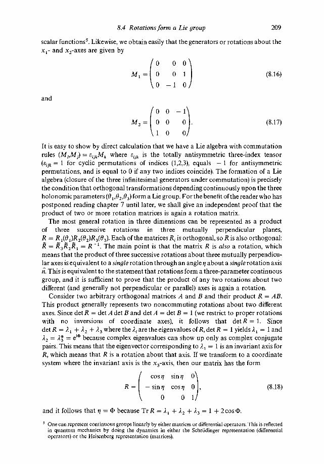
8.4 Rotations form a Lie group 209
scalar functions5. Likewise, we obtain easily that the generators or rotations about thex1- and x2-axes are given by
0 00M1= 0 0 1 (8.16)
0 —1 0
and
0 0 —1
M2= 0 0 0 . (8.17)
10 0
It is easy to show by direct calculation that we have a Lie algebra with commutationrules (M1,M3) = where Cilk is the totally antisymmetric three-index tensor(&ijk = 1 for cyclic permutations of indices (1,2,3), equals — 1 for antisymmetricpermutations, and is equal to 0 if any two indices coincide). The formation of a Liealgebra (closure of the three infinitesimal generators under commutation) is preciselythe condition that orthogonal transformations depending continuously upon the threeholonomic parameters (01,02,03) form a Lie group. For the benefit of the reader who haspostponed reading chapter 7 until later, we shall give an independent proof that theproduct of two or more rotation matrices is again a rotation matrix.
The most general rotation in three dimensions can be represented as a productof three successive rotations in three mutually perpendicular planes,R = R1(01)R2(02)R3(03). Each of the matrices is orthogonal, soR is also orthogonal:
= R3R2R1 = R'. The main point is that the matrix R is also a rotation, whichmeans that the product of three successive rotations about three mutually perpendicu-lar axes is equivalent to a single rotation through an angle 'i about a single rotation axisii This is equivalent to the statement that rotations form a three-parameter continuousgroup, and it is sufficient to prove that the product of any two rotations about twodifferent (and generally not perpendicular or parallel) axes is again a rotation.
Consider two arbitrary orthogonal matrices A and B and their product R = AB.This product generally represents two noncommuting rotations about two differentaxes. Since det R = det A det B and det A = det B = 1 (we restrict to proper rotationswith no inversions of coordinate axes), it follows that detR = 1. Sincedet R = + 12 + 23 where the are the eigenvalues of R, det R = 1 yields = 1 and22 = = because complex eigenvalues can show up only as complex conjugatepairs. This means that the eigenvector corresponding to = 1 is an invariant axis forR, which means that R is a rotation about that axis. If we transform to a coordinatesystem where the invariant axis is the x3-axis, then our matrix has the form
cosll sinll 0
R = — 0 , (8.18)
0 01and it follows that = because TrR = + 22 + 23 = 1 +
One can represent continuous groups linearly by either matrices or differential operators. This is reflectedin quantum mechanics by doing the dynamics in either the Schrodinger representation (differentialoperators) or the Heisenberg representation (matrices).

210 Linear transformations, rotations, and rotating frames
It now follows that the product of two or more orthogonal matrices is also a rotationmatrix: for example, if R = R 1R2R3, then R' = R2R3 is a rotation, and R = R1R' is alsoa rotation. The most general rotation in three dimensions can be written asR = R 1R2R3, where the R1 represent rotations through angles 01,02, and 03 in the threemutually perpendicular Euclidean planes, but we can obtain another form for R asfollows: consider an infinitesimal rotation
R (I + (501M1)(I + (502M2)(I + ö03M3) I + . Al. (8.19)
Using the idea of rotations as a group we are able to construct an arbitrary rotationmatrix R, which can be thought of as the result of any number of products of rotationsabout different axes and through different angles, as a single rotation through a definiteangle 'i about a single axis Following Lie, we can buildup any finite transformation Rby iterating the infinitesimal transformation (I + M/N) N times,
R (I + M/N)N, (8.20)
where (50 . = so that
R = (8.21)
follows as N goes to infinity. In other words, R = R1(01)R2(02)R3(03) = but it isimportant to realize that the finite angles are not the same as the components =of the single rotation angle in the exponent of R: rotations do not commute (theinfinitesimal generators do not commute), and when two matrices and do notcommute then is not equal to In other words, although is a canonicalparameter (and holonomic coordinate) for rotations within the plane perpendicular tothe axis x1, we get entirely different parameters for rotations through the sameangles (0 1,02,03) that are performed in different sequences. If we express the relationshipby a differential form = then this differential form is nonintegrable becausethe three generators do not commute with each other. To say that different paths in04- space give different results for the integrals of the three differential forms for the is
the same as saying that the parameters are not holonomic variables (see chapter 12).Therefore, there is no function ('point function') of the form =f(01,02,03). Anotherway to say it is that any differential expression of the form = will be nonexact.A rotation is a path on a Riemannian surface (a sphere), and translations onRiemannian surfaces do not commute with each other because of the intrinsiccurvature of the surface.
Having proven that the matrix describing the most general result of any number ofsuccessive rotations can be written in the form R = is antisymmetric, so R isorthogonal), we want to use this result to describe dynamics from the standpoint of anobserver in a rotating frame. First it is useful to do a little tensor analysis as preparationfor what follows.
Recall that if we think of a vector geometrically as anything with a magnitude and adirection, then we do not get coordinate-free statements about vectors and relation-ships among vectors (chapter 1 and chapter 10). Coordinate-free vectors v are definedas n-component objects whose components transform according to matrix multiplica-tion rules, either as
= (8.22a)
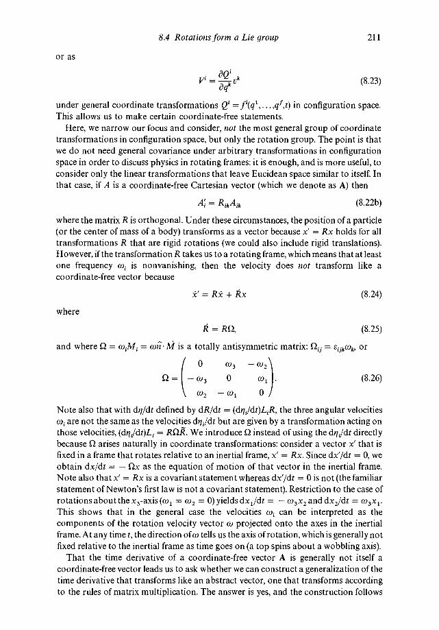
8.4 Rotations form a Lie group 211
or as
V = (8.23)
under general coordinate transformations Qi =ft(q',. . . ,q1,t) in configuration space.This allows us to make certain coordinate-free statements.
Here, we narrow our focus and consider, not the most general group of coordinatetransformations in configuration space, but only the rotation group. The point is thatwe do not need general covariance under arbitrary transformations in configurationspace in order to discuss physics in rotating frames: it is enough, and is more useful, toconsider only the linear transformations that leave Eucidean space similar to itself. Inthat case, if A is a coordinate-free Cartesian vector (which we denote as A) then
= (8.22b)
where the matrix R is orthogonal. Under these circumstances, the position of a particle(or the center of mass of a body) transforms as a vector because x' = Rx holds for alltransformations R that are rigid rotations (we could also include rigid translations).However, if the transformation R takes us to a rotating frame, which means that at leastone frequency is nonvanishing, then the velocity does not transform like acoordinate-free vector because
= Rx + Rx (8.24)
where
= RQ, (8.25)
and where = = M is a totally antisymmetric matrix: = or
0 (03
0 . (8.26)
0
Note also that with defined by dR/dt = the three angular velocitiesare not the same as the velocities but are given by a transformation acting on
those velocities, = We introduce instead of using the directlybecause Q arises naturally in coordinate transformations: consider a vector x' that isfixed in a frame that rotates relative to an inertial frame, x' = Rx. Since dx'/dt = 0, weobtain dx/dt = — Qx as the equation of motion of that vector in the inertial frame.Note also that x' = Rx is a covariant statement whereas dx'/dt = 0 is not (the familiarstatement of Newton's first law is not a covariant statement). Restriction to the case ofrotations about the x3-axis(w1 = (02 = 0) yields dx1/dt = — w3x2 and dx2/dt = w3X1.
This shows that in the general case the velocities can be interpreted as thecomponents of the rotation velocity vector w projected onto the axes in the inertialframe. At any time t, the direction of w tells us the axis of rotation, which is generally notfixed relative to the inertial frame as time goes on (a top spins about a wobbling axis).
That the time derivative of a coordinate-free vector A is generally not itself acoordinate-free vector leads us to ask whether we can construct a generalization of thetime derivative that transforms like an abstract vector, one that transforms accordingto the rules of matrix multiplication. The answer is yes, and the construction follows

212 Linear transformations, rotations, and rotating frames
from a general method that was introduced by Eddington (1963) to construct thecovariant derivative. Consider the scalar product (A,B) of any two coordinate-freevectors. When we write components in a definite Cartesian frame, then we can ignoreupper indices since = for Cartesian coordinates in Euclidean space. TheEuclidean scalar product, under transformations to rotating frames, obeys the ruled(A,B)/dt = d(A',B')/dt, or
= A1B, + AE = (8.27)
(and is also invariant under the rotation group), although the two terms in the middle,taken separately, do not obey = or = Consider next the specialcase where A has constant components in an inertial frame: dA/dt = 0, and thereforedefines a parallel field of constant vectors. In matrix notation, A' = RA with R =where = — Q. Then with = we get
= AE = + A'E' = A'(E' — (8.28)
which shows that the vector defined by
= — (8.29a)
transforms by the rule of matrix multiplication and therefore is a coordinate-free vectorunder transformations to rotating frames (notice that where thevelocities are nonintegrable unless the rotation axis remains fixed in direction ininertial frames). This means: if DB/Dt = 0 in one frame then DB/Dt = 0 in all frameswhereas the same is not true of either dB/dt or taken separately because each termtaken separately is coordinate-dependent. The operator D/Dt = Id/dt — is calledthe absolute derivative (or the Lie derivative, or the 'fishing derivative', and is thetime-translation version of a covariant derivative). The interpretation of the two termsin D/Dt is straightforward: d/dt yields the time rate of change of a vector relative to therotating frame (the 'apparent' change of the vector, like the velocity of a fish relative tothe local current), while represents the time rate of change of the rotating framerelative to inertial frames (relative to 'absolute space', or like the flow of the localcurrent relative to the bank where the fishing rod is held). The absolute derivative willbe used to rewrite Newton's law in a covariant form (in a coordinate-free form) in thenext section.
In order to see explicilty how the Lie derivative works as a covariant derivative wemust understand how the rotation generators combine in a sequence of two or moretransformations. Consider the transformation B" = R2B' = R1B, where the vector B isresolved relative to an inertial frame. Then = and so B' — R1B where
= R1cz1R11. In the next transformation, where B" = R2B', we obtain
R2(E' — R2 — = A" — (8.30a)
which we can write as
R2(E' — = B" — (8.30b)

8.5 Dynamics in rotating reference frames 213
if we make the identification = + 1, which shows how the rotation ratematrices combine in two successive transformations. Let us check to see if this is correctby looking at the direct transformation B" = RB where R = so that E" —= RB. With = R1� = R2R1 + R2R1 = + we obtain
= = + R2c1R2 = + R2R11�1R1k2, (8.31)
which agrees with our conclusion drawn from two successive transformations. Notethat c�" is a linear combination of the rotation generators L' in the doubled-primedframe, and is therefore an element of the Lie algebra of the rotation group. A method forcalculating transformations of generators is developed in the exercises and is used nearthe end of chapter 12 (if we rotate Cartesian frames rather than Cartesian vectors, then
= which is the form needed in chapter 12).Before going further, it is useful to show how to write the absolute derivative in
Gibbs' vector notation. Since = clJkcok, it follows that the absolute derivative inGibbs' notation is just
(8.29b)
because
(A x B)1 = EIJkAJBk. (8.32)
85 Dynamics in rotating reference frames
If we begin with Newton's law dp/dt = F for the motion of a body relative to an inertialframe with Cartesian coordinates x1, then we can obtain the law of motion relative to arotating Cartesian frame with coordinates directly by transformation:
Rdp/dt = RF = F' (8.33)
where F' is the net force on the body in the rotating system. The point is that any force Fthat is the gradient of a scalar potential (like gravity) transforms like a coordinate-freevector but the velocity v and acceleration dv/dt do not: the force on the right hand sideof Newton's law obeys the rule of matrix multiplication, F' = RF, but the left hand sidetransforms like a coordinate-dependent vector: Rdv/dt d(Rv)/dt. Therefore, New-ton's law dp/dt = F with p = my is not a covariant statement. So far as physics goes,that does not matter: we can use Rdp/dt to derive the correct equation for a rotatingframe as follows. With x' = Rx, v' = dx'/dt, and dR/dt = we have
v' = Rv + (8.34)
(x and F transform like vectors under time-dependent rotations, but dx/dt does not) sothat, with a' = dv'/dt,
a' = Ra + 2Rc�v + RQ2x + (8.35a)
which means that
a' = F'/m + 2RQv + + (8.35b)
If the mass m is constant then dp/dt = ma, so that
Rdp/dt = Rma = dp'/dt — (8.36)

214 Linear transformations, rotations, and rotating frames
Using v = R 1v' — then yields
Rdp/dt = dp'/dt — + mQ'2x' — mCIx' (8,37)
where = = RQR -1 transforms like a second rank tensor because of the can-cellation of two terms of opposite sign (one sees by differentiation that the timederivative of a coordinate-free rank two tensor is also a coordinate-free rank two tensorif and only if that tensor commutes with i)). Note that (W'mM'm) = = is alinear combination of the three generators M mustalso obey the closure relation (M,M) = We can (and later will) also transformthe rotation rates more simply according to co' = Rco. Since Q,, = and notonly transforms like a third rank tensor but is invariant, = where the arethe components of the rotation vector co projected onto the rotating axesFinally, we obtain Newton's description of the motion of a body relative to a rotatingcoordinate system in the form
— 2mQ'v' + mc�'2x' — = F'. (8.38)
The extra terms on the left hand side represent the effects of rotation relative to absoluteEuclidean space: 2�)'v' is the Coriolis acceleration, is the centrifugal acceleration,and (dci/dt)x' is sometimes called the fluctuation acceleration. Some people writedp'/dt = with = F' + where is supposed to be (but is not) the net forceon the body. In this case = 2mQ'v' — + m(dc�'/dt)x' is called a fictitiousforce, because it is not a force: it is merely the result of acceleration relative to inertialframes that can be completely eliminated merely by transforming back to an inertialframe of reference. Forces represent the actions of energy-carrying fields, transform likecoordinate-free vectors, and cannot be eliminated by a mere coordinate transformation(cannot be transformed to a frame where all of their components vanish). It is correct towrite and to think of ma' + maframe = F', where a' is the acceleration of the bodyrelative to the rotating frame and aframe is the acceleration of the frame relative toabsolute space.
Although it is common to do so it makes no sense qualitatively to interpret theCoriolis and centrifugal accelerations as forces divided by mass. Formally, the forcetransforms as F' = RF so that no new forces are introduced by the coordinatetransformation. Physically, imagine that a ball (a force-free object) remains at rest ortravels at constant velocity on ice, which we can treat as approximately frictionless. Ifthe reader chooses to spin on ice skates and to describe the motion of the ball from hisrotating frame, the spinning introduces no force, no new effect whatsoever on themotion of the ball, which continues to move at constant velocity in the inertial frame.The ball does not react at all to the spinning and therefore no new force is exerted on theball. Seen from a deeper perspective, one should not delude oneself into believing thatthe second law dp/dt = F is the fundamental law from which the law of inertiadp/dt = 0 can be 'derived'. Rather, the reverse is the case: the second law in the formdp/dt = F is only valid in a frame whereforce-free motion is described by dp/dt = 0. Notonly are the Coriolis and centrifugal effects not forces, Einstein also has observed thatgravity, locally, is not a force either: like the Coriolis and centrifugal accelerations,gravity can be eliminated locally by a coordinate transformation, which is impossiblefor real forces like electromagnetic ones. The best that we can say here is that gravitybehaves like an ordinary force in the Newtonian approximation to physics, providingthe inertial frame is not chosen locally to be in free-fall.

8.5 Dynamics in rotating reference frames 215
There is a another way to arrive at Newton's laws of motion in rotating frames: byuse of the covariant derivative. We can introduce a 'covariant momentum', a co-ordinate-free vector, by writing
p'0 = mDx'/Dt = m(dx'/dt — (8.39)
where x' = Rx, R = and = As we showed in the last section, p'0 transformsaccording to matrix multiplication and so qualifies as an abstract vector: if the vector p'0vanishes in one frame then it vanishes in all frames, which is not true of the velocityv = dx/dt. It is an easy exercise to show that
= F' (8.40)
yields equation (8.38) in rotating frames and also reduces to dp/dt = F, with p = my, ininertial frames. In (8.40), we have a covariant formulation of Newton's laws, one that isvalid in both rotating and nonrotating frames. That is because both sides of equation(8.40) transform in the same way, by matrix multiplication. In the absence of a net forceF, we have
Dp'0/Dt = 0, (8.41)
which is just the covariant statement of the fact that dp/dt = 0 in any inertial frame, amere covariant rewriting of Newton's first law. Equation (8.41) means that there is acoordinate system (actually there are infinitely many) where the vector field p0 hasconstant components. Because = in force-free motion in a rotating frame, aforce-free body does not move in a straight line at constant speed relative to that frame:if R is a transformation to a rotating frame from an inertial frame where v = 0, then theobserved motion of a free body in the noninertial frame, from the viewpoint of anobserver standing at the origin, is circular.
We must take care to distinguish between general covariance and a principle ofrelativistic invariance. The principle of relativistic invariance is in this case Galileaninvariance, representing the complete equivalence of all inertial frames for performingexperiments and observations. According to S. Lie and F. Klein, whose work paved theway for the generalization of geometry to topology6 in mathematics, the laws ofmechanics are dependent upon and reflect our idea of the geometry of space (here takento be Euclidean, with the Newtonian idea of absolute time), while 'geometry' is definedby invariance under some particular group of transformations. In Klein's words:
Es ist eine Manniqfaltigkeit und in derselben eine Transformationsgruppe gegeben; man soil die derMannigfaltigkeit angehörigen Gebilde hinsichtlich soicher Eigenschaften untersuchen, die durch dieTransformationen der Gruppe nicht geandert werden... [oder] Man entwickle die auf die Gruppebezugliche Invarianten theorie.
[Klein 1872, pp. 462—411
The objects that are left invariant under the transformations of the group define thegeometry of the space. Similar objects are transformed unchanged into each otherunder the transformations of the invariance group. For example, rigid bodies aretransformed into themselves, with different orientations and center of mass positions,
6 In topology, two geometrical objects with the same dimension (two curves, two surfaces, etc.) are regardedas similar if the one can be deformed continuously into the other by a (generally nondifferentiable)coordinate transformation. It is from this perspective, familar to us in phase space, that every simple closedcurve is equivalent to a circle, and every curved trajectory is equivalent to a straight line. Clearly, Galileaninvariance is not respected in topologic arguments.

216 Linear transformations, rotations, and rotating frames
under rigid rotations and translations in Euclidean space because their shapes are leftinvariant by those transformations (the same holds for transformations to uniformlymoving frames). Rigid body shapes are left invariant because orthogonal transform-ations leave invariant the basic building blocks of Euclidean geometry: lengths ofstraight lines and angles between those lines. For classical mechanics excludingelectromagnetic theory (which excludes quite a lot), the invariance group is theGalilean group, which includes translations and rigid rotations along with transform-ations among inertial frames. One can always enlarge the transformation groupformally to permit more (like time-dependent rotations) and even arbitrary transform-ations (like nonlinear transformations to generalized coordinates), and such anenlargement allows us to rewrite true statements about geometry and physics in other,more general, coordinate systems. The enlargement of the group beyond the basicinvariance group of Euclidean space leads to the idea of general covariance ofequations of motion in configuration space (Lagrange's equations). However, if thetransformation group is too large, as is the case in the general theory of relativity wherethe idea of covariance includes all possible differentiable (single-valued and invertible)coordinate transformations in a nonEuclidean space-time (see chapter 11), then theidentity is the only function that is left invariant, and Klein's idea of how to definegeometry in terms of the metric invariants of a group of transformations fails (see Bell,1945, for a stimulating description of Klein's Erlanger Program). From the standpointof Klein's idea, the lack of invariance is the same as lack of metric geometry, so that it isnecessary to define what one means by 'geometry' in some other way than Klein's ingeneral relativity theory. The only alternative is to concentrate on qualitative features,the topologic invariants. Noether's theorem for physicists is akin in spirit to Klein'sidea in geometry: the physically important quantities are the conserved ones, which arenot metric invariants (Klein's case refers only to force-free motion because the kineticenergy defines the metric for time-independent transformations (chapter 10)), butrather are quantities that leave the action invariant.
In contrast with Galilean invariance and other ideas of invariance based upon metricgeometry (based upon the invariance of scalar products under a special transformationgroup), topology is a generalization of geometry whereby one forgets the metric andother quantitative details altogether, and where two or more different figures areregarded as equivalent (are topologically similar to each other) if one figure can betransformed into the other by any continuous deformation whatsoever, including verynonphysical and nondifferentiable deformations that get rid of sharp edges withoutsanding or filing (a cube and a sphere are topologically the same object, for example). Inthis case, one of the invariants is the number of holes in an object (a donut cannot bedeformed continuously into a sphere or a cube, nor can a figure eight in two dimensionsbe deformed continuously into a circle). We think topologically whenever, as in thephase space formulations of chapters 3, 6, 13, 14, and 16, we argue that mechanicalmotions that are quantitatively different from each other are qualitatively similar toeach other. There, we follow Lie and permit a very large class of differentiablecoordinate transformations in a vector space that is not a metric space, the class of allpossible differentiable, invertible, and single-valued coordinate transformations inphase space, and the resulting transformation group is so large that we end up with onlytopologic invariants, like the number of holes in a surface. In chaos theory, numbertheory (a subject previously ignored by physicists) is often very useful for understandingthe statistics generated by whole classes of chaotic trajectories (see chapters 4 and 6 for

8.5 Dynamics in rotating reference frames 217
simple examples), and more generally for understanding the topologically invariantproperties of dynamical systems like the way that the periodic and nonperiodicunstable orbits arrange themselves, via the method of symbolic dynamics (computabil-ity theory and the related theory of formal grammars also come into play in symbolicdynamics). Nature is complex, and the little that we can formulate correctly in terms ofnonlinear differential equations in three or more variables is often too complicated forany hope of a direct quantitative solution (fluid turbulence is a very good example ofthis), and so entirely different branches of mathematics are often useful in helping us togain some qualitative understanding of those aspects of nature that can be quantified inthe first place7. We use the language of the theory of continuous groups because thatway of looking at things is not merely very beautiful mathematically, it also allows us tounify a lot of aspects of dynamics that would otherwise look like a conglomeration ofdisconnected facts. In particular, the ideas of metric and topologic invariance undertransformation groups are far more useful for gaining both qualitative and quantitativeunderstanding of nonlinear dynamics than is the idea of general covariance ofequations of motion. Invariance is geometric and places constraints on solutions, whichis an important feature for observations of nature, whereas covariance is not geometricand only places a constraint on the formal appearance of a set of differential equations(which is not important for observations of nature).
Before going on to applications, we should introduce the Lagrangian description ofthe equations of motion in rotating frames. We prove explicitly in chapter 10 that theLagrangian approach automatically provides us with a covariant description of themotion, so that we can apply Lagrange's equations directly in any noninertial frame. Ifwe start with the Lagrangian L = T — U in an inertial frame, then because theLagrangian is a scalar, L'(x',dx'/dt,t) = L(x,dx/dt,t). The potential energy is also ascalar U(x,t) = U'(x',t), and since
vv = — 2üT�'x' — (8.42)
we get
L' = m(iYv' — — — U'(x',t) (8.43)
in Cartesian coordinates (we stick to Cartesian coordinates in all that follows). Thecanonical momentum is then
== — (8.44)
and is identical to the covariant momentum defined above. We show in chapter 10 thatthe canonical momentum transforms like a covariant vector. Therefore, Newton's lawof motion takes on the form
= (8.45)dt
in any frame, rotating or inertial is also a covariant vector). Writing out thedetails of the right hand side simply yields the law of motion in the form
There is no justification for believing that everything in the universe can be quantified. As Wigner hasstated (1967), physics is not the study of nature; physics is the study of the regularities of nature (thatNewton's law generates irregular, chaotic solutions does not contradict this: Newton's law follows fromGalilean invariance, which is a regularity of nature).

218 Linear transformations, rotations, and rotating frames
dmV =— V'U' + — mQ'2x' + (8.46)
Finally, we get the Hamiltonian description by the Legendre transformation
H' = — L'. (8.47)
Replacing v' by p' and x' everywhere on the right hand side yields H' in several forms:
H' = m15'v'/2 + + U', (8.48a)
H' = — + mc�'x')/2m + + U', (8.48b)
and finally,
H' = p'p'/2m — + U'. (8.48c)
This yields Hamilton's equations:
= = — V1,.H' = p'/m —(8 49)= — VXH' = c�'p' —
and Newton's law for rotating frames is obtained by substitution.Note that Hamilton's equations (8.49) can be rewritten in the form
p' = and = F' (8.49')
if we make use of the Lie derivative D/Dt = d/dt — However, Hamilton's equationsare not covariant under general time-dependent coordinate transformations in con-figuration space (or under linear transformations to rotating frames) because in thatcase the Hamiltonian does not transform like a scalar: H(q,p,t) H'(q',p',t). The reasonfor this is that extra terms are picked up by H' in the Legendre transformation (8.47)whenever the velocity v is not coordinate-free. In the language of chapter 15, H' =H + which is a sum of two different scalar functions (S is called the generatingfunction for the transformation).
Relative to the rotating frame the Coriolis deflection, the contribution of the Coriolisacceleration to the observed trajectory, is obtained as follows. Let the x3-axes of therotating and inertial frames coincide and assume that there is a counterclockwiserotation of the noninertial frame relative to the inertial frame. If the rotation rate issmall, then the force-free motion of a body obeys the equation
— 2Q'v' 0, (8.50)
according to an observer fixed in the rotating frame. For a constant rotation frequency(03 = w, this equation is linear in v', with constant coefficients, and therefore has thesolution
v'(t) = (8.51a)
and at short times we obtain
v'(t) (I + (8.51b)
This is the Coriolis deflection, an apparent deflection of the force-free body relative tothe rotating frame. Since

8.5 Dynamics in rotating reference frames 219
5v'(t) = v'(t) — v'(O) = 2wt — v'1(O) , (8.52)
0
the apparent deflection is clockwise and perpendicular to v(0) because v(0) and 5v(t) areperpendicular to each other. Again, a free particle does not follow a straight line atconstant speed relative to a rotating frame, but regardless of the apparent complexity ofthe observed path, the particle is only traveling at constant velocity relative to anyinertial frame.
We now consider some applications of the above theory. For the first application, webegin with
H' = + + U', (8.48a)
which shows that, from the point of view of a rotating observer, a body moves in aneffective potential
V = + U'. (8.53)
If we choose the axis of rotation parallel to the x'3-axis, then c�2 = —w (8.53) reduces to
V = U' — + (8.54)
Now, suppose that a body at rest in the rotating frame is dragged by the rotation as theearth's mass is dragged by its rotation. Then the body is at rest in the rotating frame,
= 0, and so equipotentials of the effective potential,
V = U' — m 2r2 sin2 0/2 = constant (8.55)
should describe the shape of any rotating body that is free to relax into a state of rest, asteady state, in the rotating frame. This predicts a tendency toward equatorial bulging,or flattening of the body, which is in the right direction for explaining the bulge of theearth about the equator as well as the flattened shapes of galaxies.
A second application of the same result is to Newton's famous pail experiment. If,standing on the earth (and ignoring the earth's rotation temporarily), we spin a bucketof water with the rotation axis parallel to the local direction of gravity then theequipotential surfaces are given locally by
V = mgz — m w 2(x2 + y2)/2 = constant. (8.56)
At the first instant when the bucket is set spinning, the water does not follow but(because of no-slip boundary conditions at the walls of the bucket) is eventuallydragged into rotation. When, finally the steady state is reached and the water is at restwith respect to the bucket, we expect the surface of the water to be an equipotential of V,which yields (with the constant set equal to zero) the famous parabolic shape predictedby Newton, in illustration of the physical effects of rotation relative to absolute space:
z = w2(x2 + y2)/2g. (8.57)
Note that we cannot derive these effects by setting the canonical momentum p = 0,
because that guarantees equilibrium in inertial frames, whereas we require a steadystate in a particular rotating frame.

220 Linear transformations, rotations, and rotating frames
As our last application, we derive the Larmor effect, which illustrates how atransformation to a rotating frame can be used to simplify the solution of a certain classof problems. Since — c�x represents the cross product of two vectors, co x x, it is clearthat the cross product v x B is represented in matrix notation by — where B is acolumn vector and = In a rotating frame, a charged particle in a magneticfield therefore obeys
= — + — V'U' — (8.58)
Since the idea of the introduction of the rotating frame is to simplify the solution of theproblem, we choose w so that
2mc�'v' — = 0, (8.59)
which means that
— = 0. (8.60)
Rearrangement yields easily that
= — qB/2m. (8.61)
Now, the equation of motion is simply
= — — VU'. (8.62)
Choosing the axis of rotation parallel to the x'3-axis yields
= mlw'12x' — V'U'. (8.63)
If the magnetic field is small enough, then we neglect the first term and obtain anapproximate equation of motion in the rotating frame,
— V'U', (8.64)
that is identical to the unperturbed motion in the inertial frame, where now we want toknow the solution. The approximate solution follows easily: if the unperturbed orbit isa bounded motion of some shape with winding number W, then the perturbed motionin the inertial frame is simply a precession of the unperturbed orbit with frequency
= qB/2m, which means that we get an orbit with a different winding number than theunperturbed one. In particular, if we start with the Coulomb potential where U cc 1/r,then the approximate solution is a precessing elliptic orbit. We leave it to the reader todetermine the condition under which this precessing ellipse forms a closed orbit.
Exercises
Note: the results of exercises 7 and 8 are necessary to solve exercises 1 and 2 in chapter12.
1. Two observers, one accelerated and one inertial, have an argument. Each claimsthe right to use dp/dt = F to describe physics in his own frame. Suggest anexperiment that can be performed to determine who is right and who is wrong.
Exercises 221
2. If B is a square matrix and A is the exponential of B, defined by the infinite seriesexpansion of the exponential,
B"
then prove the following properties:(a) eBeC = providing B and C commute.(b) A1 =(c) = CAC(d) A is orthogonal if B is antisymmetric.(e) eiB is unitary if B is self-adjoint.
(Goldstein, 1980)
3. A particle is thrown upward vertically with initial speed reaches a maximumheight and falls back to the ground. Show that the 'Coriolis deflection', when itagain reaches the ground, is opposite in direction, and four times greater inmagnitude, than the Coriolis deflection when it is dropped at rest from the samemaximum height.
(Goldstein, 1980)
4. Work exercise 4 of chapter 1 while taking into account the earth's rotation.
5. A projectile is fired horizontally along the earth's surface. Show that to a firstapproximation, the angular deviation from the direction of fire resulting from theCoriolis deflection varies linearly with time at a rate
wcosO,
where w is the angular frequency of the earth's rotation and 0 is the colatitude, thedirection of deviation being to the right in the Northern Hemisphere.
(Goldstein, 1980)
6. The Foucault pendulum experiment consists in setting a long pendulum in motionat a point on the surface of the rotating earth with its momentum originally in thevertical plane containing the pendulum bob and the point of suspension. Show thatits subsequent motion may be described by saying that the plane of oscillationrotates uniformly 2ircos 0 radians per day, where 0 is the colatitude. What is thedirection of rotation? The approximation of small oscillations may be used.
(Goldstein, 1980)
7. Let A and B denote two abstract operators acting on a linear vector space. Letf(2) =
22(a) Show thatf(2) = B + 2(A,B) + +
(Hint:provethatf'(2) = (A,f(2)),thatf"(2) = (A,f'(A)) = (A,(A,f(2)),andsoon.)(b) Show that if A commutes with the commutator (A,B), then = + B+
8. (a) Use the power series in 7(a) above to prove the following transformation rulesfor rotation generators if R3(03) = then
= £M3 — £x(MJ— M21)cosO3 + (MJ— M21)sinO3
222 Linear transformations, rotations, and rotating frames
where are three orthonormal Cartesian unit vectors.
(b) If = 02M2, show that
= 02M2 cos 03 + O2M1 sin 03.
(c) If = 02M1, show that
= O1M1cosO2 + 01M3 sin 02,
and
R3R2cZ1R2R3 = Ô1cosO2(M1cosO3 — M2sinO3) + O1M3 sin 02.
9. The problem of two opposite charges interacting by a Coulomb potential is just theKepler problem. Consider the case where E <0 so that the orbit is an ellipse. Now,perturb the problem by introducing a magnetic field B perpendicular to the planeof the orbit. In the limit of weak fields B, under what condition is the perturbedorbit closed?

9
Rigid body dynamics
9.1 Euler's equations of rigid body motion
We begin with Euler's theorem: the most general motion of a rigid body about a fixedpoint is a rotation about some axis. This does not mean that the motion of the body isrestricted to a fixed axis, only that the net result of any motion with one point fixed, nomatter how complicated, is mathematically equivalent to a single rotation about asingle, fixed axis. The purely rotational motion of the body can be parameterized bythree independent angles representing three noncommuting rotations about threeseparate axes. A real motion of the body can then be described as an infinite sequence ofinfinitesimal transformations whose net finite result can be represented by matricesrepresenting three independent finite rotations. Since rotations form a group, theresulting transformation is again a rotation matrix, a single matrix that describes arotation about a single axis, the invariant axis of the matrix, through a single angle.Euler's theorem merely states that the initial and final states can always be connectedby a single rotation matrix, no matter how complicated is the actual motion. If we allowthe instantaneous rotation axis and angle to vary with time, then the rotation matricestaken at different times do not commute with each other unless they represent rotationsabout the same instantaneous axis. The representation that shows this most explicitly isgiven by
= (9.1)
where and 'i are the instantaneous rotation axis and angle at a time t, and the matricesare infinitesimal generators for rotations in three mutually perpendicular planes.
For different values of the angles the different matrices generally do not commutebecause the generators of infinitesimal rotations are noncommuting.
We showed in chapter 1 that the kinetic energy divides additively into the kineticenergy of the center of mass plus the kinetic energy about the center of mass. For a rigidbody, the latter is the kinetic energy of rotation about the center of mass. Thisdecomposition corresponds to Chasles's theorem, which states that the most generalmotion of a rigid body is a translation of the center of mass combined with a rotationabout the center of mass. This does not mean that the instantaneous rotation axis mustpass through the center of mass: it means that one can treat an arbitrary motionmathematically as if it were a rotation about the center of mass, but only if one includesat the same time the required translational kinetic energy of the center of mass. This isillustrated better by a picture than by words: the three drawings in figure 9.1 show adouble pendulum where a bob is attached to a rod and is free to rotate about the pointof attachment. The first drawing shows the initial state. The second shows the center ofmass in its final state, but as if the bob had not rotated about its point of attachment atthe pivot. In the third drawing, the bob is brought into the final state by a single

224 Rigid body dynamics
(a)
-":Q
(c)
Fig. 9.1(a) Double pendulum: disk attached to rod at pivot point P.Diagrams (a) and (c) represent configurations of the double pendulum at two
different times. Chasles's theorem is applied to the disk in (b) and (c). (b)Imagine rod and disk to be disconnected: center of mass of disk 0 is
translated to new position, while rod rotates into new position about pivotpoint Q. (c) Disk is rotated through angle 4 about its center of mass 0 and
then reconnected to the rod at the pivot point P.
rotation about its center of mass. The point is: the real rotation is about the point ofattachment of the bob to the rod, but we can formulate the problem mathematic-ally by dividing it artificially into a translation of the center of mass plus a rotationabout the center of mass. The main point for the reader is that one must take the rotationangle in the bob's kinetic energy to be 4, not Oin figure 9.1(c), otherwise an error will bemade.
Summarizing, there are two possible approaches to the formulation of rigid bodyproblems. Whenever one point in the body is fixed, it is useful to formulate the kineticenergy as purely rotational energy, using the fixed point as the origin of coordinates.When no point in a body is fixed in an inertial frame, as when a top spins while slidingon a frictionless plane, then the decomposition of the kinetic energy into translationaland rotational parts is very useful because it allows us to avoid the introduction of atime-dependent moment of inertia tensor. The next step is to derive the moment ofinertia through the formulation of the angular momentum.
Consider the motion of any point x that is fixed in the rigid body that rotates about afixed point. In the inertial frame the motion of the point traces out a curve on the surfaceof a sphere, but the point is at rest in any frame that is fixed in the rotating body. Thetransformation from the inertial to the body-fixed frame is given by x' = Rx, so that
dx'/dt = Rdx/dt + = 0 (9.2)
Q1g
(b)
Q

9.1 Euler's equations of rigid body motion 225
holds for the position vector x' of any and every particle in the body. Therefore,dx/dt = — is the equation of motion of a particle in the inertial frame. That is, thevelocity of the pth particle in any rigid body about either the center of mass or somerotation axis is just
VP = — (9.3)
where c� = and is the position of the particle relative to the chosen origin ofcoordinates. If we can find out how the frequencies in vary with time, which is thesame as solving the dynamics problem in a certain coordinate system to be introducedin section 9.2, then we can solve (9.3) and determine the curve traced out on the spherein the inertial frame, which tells us how the rigid body moves in that frame. Toward thatend, note that x i5 is represented by — c�rV where
0 x3 —x2
—x3 0 x1 ' (9.4)
x2 —x1 0
so that the total angular momentum of the rigid body is given by
M ==
(9.5a)
To go further, we use the well-known result = — (5imöjl, from which itfollows that
= — (9.6)
This permits us to write M = 1w, where I is the 3 x 3 matrix
=— (9.7)
that is determined by the instantaneous distribution of mass about the chosen originand therefore is generally time-dependent. The rotation frequencies transform accord-ing to the coordinate-free tensor rule = 1, and we leave it as an exercise for thereader to prove that this reduces tow' = (detR)Rw, and so tow' = Rw if det R = + 1.
The column vector w is called an axial vector. Under these conditions, M = 1w
transforms like a coordinate-free axial vector under rotations, which is to say that Mtransforms like a coordinate-free vector under proper rotations, if the matrix Itransforms like a coordinate-free second rank tensor.
A coordinate-free matrix T transforms as
= RIIRJkTIk, (9.8a)
or
T' = RTR, (9.8b)
which is the same as saying that T is a coordinate-free rank two tensor. Since
I=
— (9.9)
where E is the identity matrix, I transforms like a second rank tensor, I' = whichmeans that M transforms like a coordinate-free axial vector.

226 Rigid body dynamics
To the extent that it is of calculational use, we can rewrite the sum (9.7) as a Stieltjesintegral over the mass distribution. In any case, the moment of inertia reflects thesecond moments of the mass distribution of the body.
The kinetic energy of rotation about the origin of coordinates isN NV I — V
— L. — —
p=1
and since
= — (9.11)
we obtain
T= 4&Iw = (9.12)
which is rotationally invariant because it is the scalar product of two vectors that arecoordinate-free under rotations, and because rotations leave the Euclidean scalarproduct invariant.
From this point of view, the moment of inertia tensor looks like a metric for therotational motion', For an arbitrary rotating frame, the moment of inertia tensor isboth coordinate- and time-dependent. Because the moment of inertia tensoris symmetric, it can always be diagonalized. Furthermore, if we work in any body-fixedframe then the moment of inertia is time-independent. Any frame fixed in the rotationbody will do, but if we choose the frame whose axes line up with the directions of theinertia tensor's three perpendicular eigenvectors, which is called the principal axisframe, then the matrix I is both diagonal and constant (in other words the preferredcoordinate system is constructed by diagonalizing the inertia tensor). This preferredframe reflects the geometric distribution of mass within the rigid body. If there issymmetry in the distribution, then it will show up as eigenvalue-degeneracy of theinertia tensor.
The rotational equations of motion are easy to write down from the standpoint ofNewton's laws. Since dM/dt = N in an inertial frame, where N is the net torque, theequation of motion in a frame that is fixed in the rotating body follows fromRdM/dt = RN = N', where R is the transformation matrix that describes the motionof any particle in the body relative to an inertial frame. Therefore, we obtain
(9.13a)
or
— = (9.13b)
as the equations of motion in the body-fixed frame (the primes denote the computationof the vectors M and N and the operator Q with respect to the body-fixed axes).
Consider next the transformation U from any body-fixed frame whatsoever to theprincipal axis frame: A = U1U1 is a diagonal matrix with elements '2, andwhich are called the principal moments, and its three mutually perpendicular2
However, the w1dt are not exact differentials of generalized coordinates — see section 12.1.2 If a body has symmetry then there is a degeneracy: one or more of the principle moments will coincide

9.1 Euler's equations of rigid body motion 227
eigenvectors define the directions of the body's principal axes. In the principal axisframe, the equations of motion are called Euler's equations and take on their simplestform:
11th'1 — 13) = N'1)12w2 — w'1co'3(13 — = N'2 (9.13c)
13w3 — w'2co'1(11 — '2) = N'3.)
From the standpoint of Euler's equations we can study rigid body motion as a flow inphase space, which is very convenient. However, equations (9.13b) or (9.13c) are not acomplete formulation of the problem, which generally requires a six dimensional phasespace. In the most general case of no translation, the rigid body rotates about a pointthat is fixed in the body but is subject to an external torque due to gravity denoted bythe constant force F, which is concentrated at the center of mass. The force is constantin the inertial frame but the center of mass position is not. In the inertial frame onecannot solve the problem
= —
dx (9.13'a)=
in the six dimensional (M,x)-phase space because the frequencies are not known.Instead, one must supplement these equations by six equations of motion for themoment of inertia tensor, which requires altogether a twelve dimensional phase space.
In any body-fixed frame, one can study the problem
— Q'M' = —
= c�'F',(9.13'b)
where x' is the constant vector that points from the fixed point to the center of mass, inthe six dimensional space because the moment of inertiatensor is constant (determining M'(t) determines w'(t), which is not true in the inertialframe). In other words, with F' = RF the force components F(t) in the body-fixed frameare unknown until the time-dependence of co'(t) is known, which requires solving forboth w' and F' simultaneously. There are only four known integrable cases, and wediscuss them all in section 9.5.
In the body-fixed frame we have a flow in a six dimensional phase space even if werestrict to constant forces. Clearly, the M'-, x'-, and F'-subspaces are all Euclidean. Thesubspace of the variables or the qualitatively equivalent phase space(w'1,w'2,w'3) is also Euclidean because, in the body-fixed frame, the 'metric tensor' I isconstant. Whenever the metric is constant then Cartesian coordinates can be definedby rescaling the variables M. Therefore, the six dimensional phase space is a Cartesianspace. With one or more conservation laws, the motion will generally be confined to acurved space of lower dimension.
and the corresponding eigenvectors are only linearly independent, not orthogonal. However, it iselementary to use this pair to form an orthogonal pair. Due to the symmetry of the body, it does not matterwhich orthogonal pair you choose.

228 Rigid body dynamics
Rigid body problems are difficult because they are very rich. All of the interestingphenomena of modern dynamical systems theory can be illustrated in the context ofrigid body theory by adding dissipation to compete with the driving provided by thetorque in chapter 13. We now reproduce some standard results of classical rigid bodytheory by using phase space analysis.
9.2 Euler's rigid body
We consider the torque-free motion of a rigid body in the principal axis frame, theframe fixed in the body where the inertia tensor is both constant and diagonal. Free-fallof any object in the earth's gravitational field is an example that satisfies the conditionof absence of torque. All problems of this type are not only solvable but also areintegrable, as we now show. The dynamical system where all moments of inertia areequal (a sphere or a cube with a uniform mass distribution, or a geometricallyunsymmetric body with an uneven mass distribution) is trivial, so we start with the nextdegree of symmetry.
For a solid of revolution, where = 13, the frequency w'3 is constant and weneed only solve the linear equations
11th'1 — w'2w'3(11 — 13) = 0111th'2 — w'1w'3(13 — = 0 (9.14)
J
Writing = w'3(11 — and denoting the column vector with components by co',
we have
th' = QM3co' (9.15)
where
010M3= —1 0 0 (9.16)
000is the generator of rotations about the co'3-axis. The solution is given by
w'(t) = (9.17)
Since = — M3 and = P12 where
100P12 = 0 1 0 (9.18)
000is the projection operator for projections into the plane perpendicular to x3, it followsfrom resummation of the series
= I + + + ..., (9.19)

9.2 Euler's rigid body 229
with c' = c�t, that
w'(t) = (P3 + P12 cos + M3 sin Qt)w'(O) (9.20)
where P3 = E — P12 is the projection operator onto the x3-axis and where E is theidentity matrix.
The interpretation of the solution is simple: the vector w rotates at constant angularfrequency about the x3-axis. This is guaranteed by the form of the kinetic energy,
T = + + (9.21)
because both T and w3 are constant: any motion that leaves + invariant is arotation in the (x1,x2)-plane. From the viewpoint of an observer in an inertial frame, theangular momentum M is fixed in space in both magnitude and direction while the bodyrotates. Though M = 1w, one cannot conclude that w is a constant vector in the inertialframe because I varies with time there. Denoting quantities with the subscripts as thosecalculated relative to the space-fixed axes, with I is the tensor of theprincipal moments (we are denoting objects in the body-fixed frame by unprimedsymbols in this section), it follows by differentiation that
= (9.22)
so that is constant only when the space-fixed inertia matrix commutes with theangular velocity matrix. An example is the case of a symmetric top that spins about itssymmetry axis if that axis does not wobble in an inertial frame.
The result derived above has an important practical application: since the earth isapproximately an oblate spheroid in free-fall about the sun, the result describes theprecession of the earth's axis of rotation about the symmetry axis x3. If we call the axisof rotation the celestial north pole and the axis x3 the geometric north pole, then it isclear that the two are distinct.
The study of the more general problem of a completely asymmetric body ismotivated by a simple experiment: wrap a rubber band around a book so that the bookcannot open, and then toss the book into the air, spinning it initially and successivelyabout each of its three principal axes. You will observe stable motion about two of theprincipal axes, but the motion about the third axis is unstable: the book always wobblesabout one of the axes, and nothing that you do can eliminate the wobbling. Note alsothat the wobbling occurs about the principal axis x2 if we order the moments in theform > > 13.
In order to analyze and understand the results of the experiment described above,consider the torque-free motion of any completely asymmetric rigid body in theprincipal axis frame. Euler's equations in the noninertial frame are
11th', — w'2w'3(12 —13) = 0)12w2 — w'1w'3(13 — = 0 (9.23a)130)3 — — '2) = 0.j
As we noted at the end of the last section, we have three first order differentialequations for the three angular frequencies so the phase space of this problem iseither the space of the three frequencies w or the space of the three components of

230 Rigid body dynamics
angular momentum
M'1 = M'2M'3(1/13 — 1/12) )M'2 = M'1M'3(1/11 — 1/13) (9.23b)13 = M'2M'1(1/12 — 1/1k) J
which we can rewrite as
)= — bxz (9.23c)
J
where x = M'1, y = M'2, z = M'3, and a, b, and c are positive constants if > > 13.
Note that this system is conservative in the general sense of chapter 3: the divergence ofthe phase flow velocity V = (ayz, — bxz,cxy) vanishes. Note also that
+ y9 + z± = 0 (9.24)
so that x2 + y2 + z2 = constant, which is just the statement that the magnitude of theangular momentum M is conserved. This constrains the motion to the surface of asphere of radius M in the three dimensional space, and kinetic energyconservation yields the streamline equation on the sphere3. With two global constantsof the motion, a three dimensional flow is integrable. Now, we apply the qualitativemethods of analysis of chapter 3.
There are six distinct equilibria located at (0,0, ± 1), (0, ± 1,0), and ( ± 1,0,0). Linearstability analysis about the first two equilibria at the points (0,0, ± 1), i.e., for rotationsabout the principal axis yields the characteristic exponents 2 = ± so thatthis pair of equilibria is elliptic. A similar result follows for rotations about the principalaxis M'1. However, rotations about M'2 are unstable: there, 2 = ± so that(0, ± 1,0) is a hyperbolic point. This explains the observed results when the book istossed into the air in rotation about the three different principal axes. The global phaseportrait is shown as figure 9.2. Clearly, one need not obtain a quantitative solution ofthe differential equations in order to understand the qualitative nature of the motion.
We have just described the motion from the viewpoint of a hypothetical observerwho is fixed in the principal axis frame. What does the motion look like from thestandpoint of an inertial observer? In this case, the vector M is fixed in space and itscomponents, the projections onto the space-fixed axes are also constants. The matrixequation of motion of the components,
DM/Dt = 0, (9.25a)
is just the statement that
dM/dt = 0 (9.25b)
in inertial frames. However, as the rigid body rotates, its instantaneous axis of rotationw changes with time, and its projection onto the space-fixed axes can be studied byapplying the inverse transformation R1 to the principal axis solution for the angularfrequency w.
With two conservation laws that determine two of the three variables, the Euler topprovides an example of an integrable flow in a three dimensional phase space. From
Moreover, because both T and M are conserved, the orbits lie at the intersection of the sphere with thekinetic energy ellipsoid.

9.2 Euler's rigid body 231
section 3.6, we know that a flow described by the nonlinear system dM/dt = V with= is integrable if and only if V1 = where G and H are the
two conserved quantities (since the phase flow generated by = is conserva-tive, the use of Jacobi's first multiplier is unnecessary). Equating the two expressions for
allows us to identify Gas the square of the magnitude of the angular momentum, andH as the kinetic energy.
If we take the first conservation law G as the square of the angular momentum, thenthe motion is confined to a sphere in the Me-phase space and conservation of kineticenergy determines the streamlines on that sphere. If, instead, we should identify the firstintegral G as the kinetic energy, then the motion in the angular momentum phase spaceis confined to an ellipsoid, and constancy of angular momentum determines thestreamlines on the ellipsoid. Topologically, a sphere and an ellipsoid are identical, andso the qualitative description of the motion is the same in both cases. In either case, thetrajectories are given geometrically by the intersections of spheres with ellipsoids(different spheres and different ellipsoids follow from varying the magnitudes of theangular momentum and the kinetic energy). Whittaker (1965) demonstrates theintegrability of Euler's top by using Euler angles as variables, which is morecumbersome and less enlightening than the phase space approach used here4.
Integrability can be demonstrated directly by obtaining integrals for the threeangular frequencies with two constants of the motion, T and M2, we can eliminateany two of the frequencies from one of Euler's equations, say the equation for w, toobtain an equation of the form dt = which is integrable by inspection, andyields the time-development of one angular frequency w = w(t). Therefore, thetime-dependence of each angular frequency can be found directly by integration.
Suppose that you want to design machinery. You may then want to find out how the
See Whittaker (1965) for solutions of most of the known integrable problems of particle and rigid bodymechanics. Other problems, integrable and nonintegrable, are discussed in Arnol'd's Dynamical SystemsIII.
Fig. 9.2 Phase portrait for Euler's rigid body (fig. 4.31 from Bender andOrszag, 1978).

232 Rigid body dynamics
body moves in the inertial frame. Given the frequencies in the inertial frame, thebody's motion would be determined as follows: let x, a vector with one end located atthe fixed point, denote the position of any point in the rigid body. As the body rotatesthe vector x rotates with it. If we draw a sphere that is centered on the fixed point, has aradius less than the length of the vector x, and is itself fixed in the inertial frame, then theintersection of x with the sphere traces out a curve that describes the body's motion.Now, x' = Rx describes the same vector in the body-fixed frame and both x and x' havethe same constant length but dx'/dt = 0. If the primed and unprimed axes are made tocoincide at t = 0, then x' is the same as the initial condition x(0) in the inertial frame andthe equation x(t) = R — '(t)x' then contains the information that describes the curve thatis traced out on the sphere. Since dR/dt = the frequencies co determine Q and withit the transformation matrix R(t). The solution of Euler's equations in the inertial framewould determine the rigid body's motion completely, and the calculation of x(t) wouldtherefore yield a complete solution of the problem in a form that would allow one todesign machinery by checking for (and perhaps then eliminating) wobbling andvibrations.
Unfortunately, as we showed in section 9.1, it is not so simple to solve for thefrequencies in the inertial frame. Moreover, given the solution in the form of M'(t)and co'(t) in the principal axis frame, there is not enough information to determine eitherR(t) or w(t). How can we solve for the motion in the inertial frame? If we couldcoordinatize the sphere on which the motion occurs by the parameters in our problem,which would be equivalent to a direct determination of R(t), then we would reach ourgoal. How can we coordinatize the rotation matrix R(t) in terms of parameters whosetime-dependence we can calculate without so much trouble?
Since
= (9.26)
then can the time-dependent parameters be found from the 'velocities' coXt)? Canthese three parameters be used to specify R(t)? In principle, yes, but not withoutpractical difficulty as we show in chapter 12: there is no way to use the parametersto define a global coordinate system, although one can use them to define localCartesian coordinate systems during an infinitesimal time interval öt at each time t.This is explained in chapter 12. Instead of digging deeper in this direction, we nowintroduce another way to coordinatize R(t) in terms of parameters whose time-dependence we can calculate more easily from the equations of rigid body dynamics.
9.3 The Euler angles
The Euler angles (çlyji,O) are rotation angles in three separate coordinate systems thatare themselves defined by the Euler angles (see figure 9.3). Because they can be definedpurely geometrically, independently of integrating the frequencies they provide away of defining coordinates that describe motions on the sphere. In order to be able touse the Euler angles in rigid body theory, we must find a way to express the threerotation frequencies in the body-fixed frame in terms of them and their timederivatives. What follows is an exercise in the application of results derived earlier insection 8.3 and yields a parameterization of the rotation group that is very useful for

9.3 The Euler angles 233
Fig. 9.3 The Euler angles defined geometrically (fig. 25 from Saletan andCromer, 1971).
answering the question left open in the last section, and also for analyzing a certain classof dynamics problems that we study in section 9.4.
Denoting the three coordinate transformations by = D(4')x, = andx' = the transformation from the inertial to the body-fixed frame is given byx' = Ax where A thematrix the Euler angles
= R(01,02,03). By inspection of figure 9.3, the three separate transformationsare given in the three separate coordinate systems by
sin4 0
D(4) = — sin cos 4 0 , (9.27a)
0 01and
1 0 0
C(O) = 0 cos 0 sin U , (9.27b)
0 —sinU cosO
and
sins/i 0
= — sin cos 0 . (9.27c)
0 01It is now clear why this representation is called degenerate: both D and B have the sameinfinitesimal generator, namely, M3.
Denoting the rotation rate projected onto the body-fixed frame by
= + w'2ê'2 + (9.28a)
where is the unit vector along the axis we can also resolve w' onto threenonorthogonal axes in three of the four different coordinate systems:
U) = + OJ + (9.28b)
8
z
x

234 Rigid body dynamics
Here, the are three orthonormal unit vectors in the and are the threeorthonormal unit vectors in the and the three orthonormal unit vectors ê1 arein the inertial frame. It follows from taking a scalar product that
co'1 = = + (9.29)
where x + is a row vector where elements are complex conjugates of the elements of thevector x.
Since the basis vectors transform according to the rule (see section 8.3)
= A11ê1 + A12ê2 + A13ê3, (9.30)
it follows that
= A13 = sin sin 0. (9.31)
And since x' = we obtain
e'1 = (BC)1j1 + (BC)12J2 + (9.32)
so that
= (BC)11 = (9.33)
Therefore, we have shown that
co'1 = + (9.34)
It is left to the reader to show by similar exercises that
co'2 = — (9.35)
and
co'3 = + (9.36)
Taken together, we find that
co'1 = += — (9.37)
co'3=q5cos0+çlí. jCalculating the cross-partial derivatives of the right hand side of these equations showswhy we cannot use the parameters defined by = codt as generalized coordinates:the velocities co are nonintegrable and so are not generalized velocities.
The Euler top provides an example of an integrable dynamical system solved interms of variables that are themselves nonintegrable: this only means that the solutions
of the Euler top cannot be integrated to define three coordinate axes in
configuration space, although the nonintegrable velocities define perfectly goodCartesian axes in phase space, in agreement with Lie's idea of a flow as the infinitesimalgenerator of global coordinate transformations.
9.4 Lagrange's top
Consider a solid of revolution with one point on its symmetry axis fixed in space. In theliterature, this system is known both as the 'heavy symmetric top' and also as thesymmetric top spinning on a rough plane. The latter phrase seems somewhat more

9.4 Lagrange's top 235
appropriate for, without friction or something else to hold the apex of the top fixed,whether the top is heavy or light is irrelevant. We shall emphasize this below byformulating the problem where the same top spins while its apex slips on a frictionlessplane.
We now consider the Lagrangian for a rigid body with one point fixed in space. It isnot particularly useful to divide the kinetic energy into translational and rotationalcontributions, although one can always do that. It is more direct simply to compute thekinetic energy about the fixed point, which can be treated as rotational. The apex of thetop, the point fixed in space, lies on the symmetry axis of the body. Therefore, if we takethe apex as the origin of coordinates with the x3-axis along the symmetry axis, then themoments of inertia are just the principal moments, the same as if we had taken theorigin of coordinates to lie at the center of mass. This point is important, because itexplains the difference in the way that we must formulate the kinetic energy when thetop's apex is not fixed in an inertial frame but is allowed to slide frictionlessly on a planethat is perpendicular to gravity.
In terms of the Euler angles the rotation rates in the body-fixed frame are
= += — (9.37)
j
The symmetric top = '2 13) with one point on the symmetry axis fixed in spacethen can be described by a Lagrangian L = T — U, and + = sin2 0 +reflects the rotational symmetry. We therefore obtain the top's kinetic energy in theform
T = LL(O2 + qYsin2o) + + (9.38)
and U = — MgI cos 0 is the potential energy. From the Lagrangian L we immediatelyobtain two conserved canonical momenta:
= = 13(jicoso + i/i) = (9.39a)
is the component of angular momentum along the body-fixed x'3-axis. The identifica-tion = M'3 follows because, as we showed in chapter 2, whenever we choose arotation angle as a generalized coordinate then the conjugate canonical momentum isjust the projection of the angular momentum vector onto the rotation axis. Therefore,
= = + + = M3 (9.39b)
is also constant and is the angular momentum along the inertial x3-axis. Also, since theLagrangian L has no explicit time-dependence H is also conserved. With three degreesof freedom and three globally analytic conserved quantities, we therefore have anintegrable canonical flow in phase space. The object now, however, is to use theseconserved quantities to understand the motion qualitatively in configuration space.
Since CO'3 = M'3/13 is constant, and M3 is also constant, we can write the top'sprecession rate

236 Rigid body dynamics
.M3—M'3cos0940
as a function of 0 alone.Also, we can redefine E' = H/I1 — as the Hamiltonian,
E' + sin2 0) + Mglcos 0/It, (9.41)
so that we have a one dimensional problem in the (0,dO/dt)-phase space withHamiltonian
E' = + V(0), (9.42)
with the effective potential
(M3 — M'3cos0)2V(0)
=+ mglcos0/11. (9.43)
Therefore, the motion is completely determined by solving the one dimensionalproblem for 0(t), along with specifying the six initial conditions, three of which we canthink of as fixing the values of the constants E',M'3, and M3.
For stable oscillations where 0 changes by less than ic, there must be two turningpoints 0 < 01 <02 <it where d0/dt vanishes (V(01) = V(02) = E') and the 0-motion isperiodic with period
ç02dO
= J0 [2(E' —(9.44)
This means that there must also be an elliptic point somewhere in the (0,d0/dt)-phasespace due to a minimum of the effective potential V(0).
For the purpose of understanding the motion, it is useful to follow the trajectorytraced by the intersection of the top's symmetry axis with the unit sphere, and to studythe motion of that point as a function of (41,0) within the cylindrical band (01,02) on thesphere's surface (figure 9.4). The different ranges of values of the constant angularmomenta M'3 and M3 in the precession rate
.M3—M'3cosO945
sin2O(. )
yield three qualitatively different kinds of trajectories. Since d0/dt changes sign at theturning points and 02, it is only a question whether and where d41/dt changes sign. IfM3 > M'3 then d41/dt never vanishes and we have precession with nutation, as is shownin figure 9.4(a). Although d41/dt cannot vanish at both turning points it can vanish at 01if M3 = M'3 cos 01, in which case M3 — M'3 cos 02 > 0. This yields the trajectory offigure 9.4(b). Finally, we can also have d41/dt <0 at some angle 0
d41/dt 0 at some angle 0' intermediate between 01 and 02, which yields figure9.4(c). There are no other geometrically distinct possibilities for oscillations between thetwo turning points. For a discussion of the functional forms of 0(t) and 41(t) we refer thereader to Whittaker (1965) and to Whittaker and Watson (1963), as each integrableproblem of mechanics defines (or falls into the class of) one of the many 'specialfunctions of mathematical physics'.

Oi
(9.46)
9.5 Integrable problems in rigid body dynamics 237
(a) (b) (c)
Fig. 9.4(a) Configuration space for M3 > M'3 (fig. 5.9a from Goldstein, 1980).(b) Configuration space for M3 = M'3 cos 01 (fig. 5.9c from Goldstein, 1980).
(c) Configuration space for M3 = M'3 cos 0', 01 <0' <02 (fig. 5.9b fromGoldstein, 1980).
Do the trajectories close within the cylindrical band or not? To answer this, weintegrate dçb/d0 one time to obtain the change = between any two successiveturning points:
ç02 [(M3 — M'3 cos sin2 0]2d0
= J0 [2(E' — V(0))]"2
By now the reader has seen that we are studying the same kind of problem,qualitatively, that we analyzed in chapter 4 under the heading of central potentials: theconfiguration space trajectories close if t = 2irP/Q where P and Q are integers, butthose trajectories are quasiperiodic (never close but instead made infinitely many closeapproaches to closure, and even fill up the 0-band ergodically (but not statisticallymechanically or chaotically) as t goes to infinity) if the winding number W = t/2ir isirrational. The linear twist map follows directly from this analysis, just as in chapter 4.The winding number W = t/2ir is a function of the three parameters E', M'3, and M3.For arbitrary choices of these parameters, W(E',M'3,M3) is irrational and the orbits aregenerally quasiperiodic. Closed orbits can occur only for very special choices of initialconditions. Note also that the elliptic point generally does not fall within the band[01,62].
Furthermore, as is always the case with integrable motion, the orbits are marginallystable. The circle map for this problem is given by & = - wheref(4) = + 2ir W,so that f'(çb) = 1 and therefore the Liapunov exponent of all orbits is A = 0.
The analysis of the motion of a top that slips on a frictionless horizontal plane isintegrable and is assigned as a set of exercises, because that problem can be formulatedand solved by the same sequence of steps that we have exhibited above. There is onlyone difference to pay attention to: since there is no fixed point of the motion, the kineticenergy must be resolved into rotational and translational contributions about thecenter of mass which itself oscillates vertically.
9.5 Integrable problems in rigid body dynamics
Consider the description by Euler's equations (the Euler—Poisson equations) of a solidbody that is free to rotate about a point that is fixed in the body. Let x denote the vector

238 Rigid body dynamics
from the fixed point to the center of mass. In the inertial frame x varies with t while theforce of gravity F is a constant. In the body-fixed frame x' = Rx is a constant vector butthe force F' = RF in the body-fixed frame is time-dependent and is unknown until R(t)is known. Therefore, we must add to the three Euler equations
— c�'M' = — (9.47a)
the three additional differential equations
= Q'F' (9.48a)
where
o
c�= 0 w'1 (9.49)
0
and
o X'3 —X2
= — x'3 0 x'1 . (9.50)
X'2 0
The phase space is therefore the space of the six unknowns (Mi, . . . ,F'3) or . .
It is now easy to show by direct differentiation that the following three quantities areleft invariant by the flow: first, the magnitude of the force P'F' = F2 = C1 is constant.Second, the total energy
E = + (9.51)
is conserved, and third, c1'F' = C2 is also constant. With three globally conservedquantities in a six dimensional phase space, we need one more conserved quantity inorder to have an integrable problem.
Following Arnol'd (1978) and Fomenko (1988), we now list the known integrablecases:
(1) Euler's case (1750): x' = 0, and M is conserved.(2) Lagrange's case (1788): = '2 x'1 = x'2 = 0, and co3 is conserved (the
projection of M onto the top's symmetry axis is conserved).(3) Kowalevskaya's case (1889): '1 = = 213, x'3 = 0, and the extra constant of the
motion is
— — vF'1)2 + — vF'2)2 (9.52)
where v = +(4) Goryachev—Chaplygin's case (1900): = '2 = 413, x'3 = 0, and in this case the
scalar product of L with F vanishes.
The flow defined by the motion of a symmetric rigid body in a gravitational field withone arbitrarily chosen point in the body fixed in space is nonintegrable (there is no
9.5 Integrable problems in rigid body dynamics 239
fourth globally conserved quantity). Kowalevskaya's case is named after the brilliantRussian mathematician of the last century, Sonya Kowalevskaya (1850—1891). Hercomplete solution can be found in Whittaker (1965) and is based upon the use of herdiscovery, local singularity analysis: she noticed that the solutions in the other twointegrable cases, when extended to the complex time-plane, had singularities that werepoles of finite order (there are no algebraic or logarithmic branch points of essentialsingularities). By requiring the solution in the general case to be of the same nature, shefound the integrable case that bears her name. To understand why the absence of thespontaneous singularities other than poles in the complex time plane leads toinvariants that are understood from the standpoint of symmetry, we refer the reader tothe text by Fomenko (1988).
With three conservation laws we can always solve for and eliminate the threecomponents of the force to obtain Euler's equations in the form
— f�'M' = (9.53)
Therefore, the problem can always be studied in the three dimensional Euclidean phasespace of the variables (M'1,M'2,M'3).
If we look at Lagrange's top or any of the other three integrable rigid body cases interms of the reduced Euler equations (9.53), then there is one conservation law and themotion is confined to a two dimensional Riemannian surface in the three dimensionalEuclidean phase space If we look at the same problem in Euler angles,then there are three conserved quantities and the motion is confined to a threedimensional Euclidean torus in the six dimensional space. Thesetwo descriptions of the dynamics are geometrically inequivalent to each other: thecanonical description cannot be transformed into the noncanonical one because therelation between the velocities (w'1,w'2,w'3) and the generalized velocities
given by equations (9.34)—(9.36) is nonintegrable: there is no coordinatetransformation defined by point functions from the generalized coordinates tothe nonholonomic coordinates
In the nonintegrable case, which is the general case, one should expect to find chaoticmotions in at least parts of the phase space. Any initial conditions that are far fromthose that yield small oscillations should provide a good starting point in the search forchaos. We continue the discussion of integrable and nonintegrable flows motivated byrigid body problems in chapter 13.
Consider next the equilibria for the general case where the body may or may not besymmetric and where the external torque is nonzero. In this case the equilibria in phasespace are solutions of the six algebraic equations
= — = 0 (9.47b)
and
= = 0. (9.48b)
Equation (9.48b) tells us that w' and F' are colinear, w' = CF' where C is a scalar. Sincewe can write

240 Rigid body dynamics
= —
(9.47b) can be written as
— = + = — =0 (9.54)
which tells us that M' and x' are colinear, that CM' = x'. Note that M' is constantbecause x' is constant, in agreement with dM'/dt = 0. Furthermore, with the x'3-axischosen to lie along the vector x' we have M'1 = M'2 = 0, which (via = MVIi) yieldsalso that co' is colinear with x'. Therefore, in equilibrium (which is a steady state ofconstant angular velocity w'3) the vectors M', w', x', and F' are all colinear and there aretwo equilibrium points: one with x' parallel to w' and one with x' antiparallel to w'. Wehave the investigation of conditions for the stability of these two equilibria as exercisesfor the interested reader.
9.6 Noncanonical flows as iterated maps
It is easy to argue heuristically that a three dimensional noncanonical flow should bediscussed via a two dimensional iterated map, as we did in chapter 6 for a two degree offreedom canonical flow. Here, we discuss two ways to arrive at maps from flowsalthough there are infinitely many ways to get a map from a flow (a third method fornonautonomous systems is presented in section 14.4). This lack of uniqueness does notmatter: the details of the map are irrelevant from the standpoint of topologicallyuniversal properties like the number of orbits of a given period and their periods. Inother words, we expect that every map that can be derived from a particular flowbelongs to a certain universality class that includes other flows as well, and that thereare well-defined properties (like periods, numbers of orbits of a given period, and otherabstract topologic invariants) that can be extracted from any map in the class. Theseproperties are universal in the sense that the same properties follow from every map inthe class. To develop and illustrate this 'principle of weak universality' would, however,go far beyond the scope of this text, and so we refer the interested reader to the literatureon the subject, which is by now extensive (see chapter 9 in McCauley, 1993, andreferences therein).
We start with any noncanonical three dimensional bounded flow,
dx= V1(x,y,z)
= (9.55)
dz= V3(x,y,z),
and first construct a return map as follows (this is the method of E. Lorenz): pick one ofthe three variables, say z, and consider its time series z(t). There will be one or moremaxima where dz/dt = 0 with d2z/dt2 > 0. Denote the (unknown) times of occurrenceof these maxima by and denote the corresponding maxima by Since V3 = 0 atthese points we expect to find a functional relationship of the form Zn =f(Xn,Yn) where(xn,yn) denotes the value of the coordinates (x,y) at time At the same time, we canthink of the solution of (9.55) at any later time as a coordinate transformation on the

9.7 Nonintegrable rigid body motions 241
solution at any earlier time, and for a transformation from time t, to time t,,÷1 thattransformation has the form
=1
—)
1 = 1 — (9.56)
= 1—
If we substitute into the condition for an extremum and write; = — t,,, then weobtain
V3(4i = 0 (9.57)
which we can formally solve (granted the cooperation of the implicit function theorem)to find; = which allows us to eliminate the unknown time differences;. If wesubstitute z = f(x,y) and r = h(x,y) formally into the first two of the three equations(9.56), then we end up with two equations that have the form of a two dimensionaliterated map:
1=
(9 58a)1
=
By instead making the elimination x = g(y,z), we would obtain a different iterated map
=(9 58b)
=
which describes the distribution of successive maxima of z(t). In both cases, the iteratedmap contains partial information about some aspects of the dynamical system.
This is not the only way to define a Poincaré map, however. Another way is toconsider the (unknown) times t,, when the trajectory passes through the (y,z)-plane inphase space with positive velocity dx/dt > 0. In this case, x = vanishes at the timest,, and a similar formal argument leads us to expect a two dimensional map of the form(9.58a), but with different functions on the right hand side:
=(9 58c)
1=
There is a one-to-one correspondence between flows and maps derived from flows.Conservative flows can have as equilibria only elliptic and hyperbolic points and thesame is true of the return maps. More generally, Poincaré's recurrence theorem appliesso that bounded motion can only be periodic or quasiperiodic. Regular motion followsif there is an extra conservation law that holds for all finite times. Regular motion isstable against small changes in initial conditions, whether periodic or quasiperiodic.Here, the map must have two vanishing Liapunov exponents. Nonintegrability isnecessary but not sufficient for deterministic chaos, as we illustrate in chapter 17. In achaotic region, both the periodic and quasiperiodic orbits will be sensitive to smallchanges in initial conditions and the map must have two Liapunov exponents
= — <0 (chapter 6).
9.7 Nonintegrable rigid body motions
We have shown above that every rigid body problem in the six dimensional phase spacedefined by the principal axis frame has three conservation laws, so that the motion is

242 Rigid body dynamics
confined to a three dimensional bounded subspace of phase space. However, we do notknow, a priori, to which subspace the motion is confined. Therefore, we performnumerical experiments to search for evidence of nonintegrability in the form of chaosby constructing two dimensional return maps in the spirit of the last section. Inparticular, we study the distribution of intersections of trajectories with a singleCartesian plane in the six dimensional phase space.
Figures 9.5 through 9.7 show time series, intersections of trajectories with a phaseplane, and also a Poincaré section for Lagrange's top, which is an integrable flow. Alltrajectories are either stable periodic or stable quasiperiodic, and therefore are in-sensitive to small changes in initial conditions. The parameter values chosen for thenumerical integrations are: '1 = = 106.5 gem2, 13 = 17.2g cm2, m = 16.Og,
(X,Y,Z) = (0,0,2.25 cm). The initial conditions are = 4s', w2(0) = 5s',(03(0) = 2s1, F1(0) = F2(0) = 0, and F3(0) = 15680 dyne.
Figures 9.8 through 9.10 show plots for a nonintegrable flow, Euler's asymmetric topwith one point fixed in space, and subject to a torque due to a constant gravitationalfield (constant driving force). Figures 9.8 and 9.9 show the time series and a Poincarésection. Figure 9.10 shows the difference between two time series due to slightlydifferent initial conditions. All of the figures are typical of a system that exhibitssensitivity to small changes in initial conditions. In certain other parts of the phasespace, this flow is nonchaotic. The parameter values and initial conditions are (sameunits as above): = 100, '2 = 30, 13 = 17.2, (X,Y,Z) = (1,2,2.25). The initial condi-tions are = 4, (02(0) = 5, (03(0) = 2, F1(0) = 5000, F2(0) = 6000, andF3(0) = 15680.
There are several lessons to be learned from this work. First, one needs only aconstant driving force in a physical system (in this case gravity) along with asymmetry(at least two unequal moments of inertia) in order to produce deterministic chaos (thesymmetric top is also nonintegrable except for the Lagrange and Kowalevskaya cases).The second lesson is that rigid body motions cannot be predicted in any practical wayover long time intervals when they are observed in nature: there, in comparison withcomputation, we know initial conditions to within only few decimal precision, andperturbations due to the environment are completely uncontrolled. This combinationof circumstances limits our ability to see into the future to relatively short time intervals(see also chapter 6).
Exercises
1. Find the principal moments of inertia about the center of mass of a book with auniform mass density.
2. A uniform right circular cone of height h, half-angle and density p rolls on its sidewithout slipping on a uniform horizontal plane in such a way that it returns to itsoriginal position in a time r. Find expressions for the kinetic energy and thecomponents of the angular momentum of the cone.
(Whittaker, 1965)
3. Use = to show that the axial-vector equation w' = (det R)Rw also holds.Show also that M' = (detR)RM.

Exercises 243
Lagrange's top
(Oi
Fig. 9.5 Time series for Lagrange's top.
Lagrange's top10
5
0
—5
—10—10 —5 0 5 10
Fig. 9.6 Projection of the motion onto a phase plane for Lagrange's top.
Lagrange's top2
0
S I—2
S I
-4 5 I.
—6 •—
—8
—tO —5 0 5 10
Fig. 9.7 Poincaré section for Lagrange's top.

244 Rigid body dynamics
Fig. 9.8 Time series for an asymmetric top.
Asymmetric top
0 100 200 300 400
Fig. 9.9 Poincaré section for an asymmetric top.
500
4.3
2.
1•
. •.• .
0
5 10
Fig. 9.10 Difference in time series for two slightly different initial conditionsof an asymmetric top.

Exercises 245
4. A plane pendulum consists of a uniform rod of length 1 and negligible thicknesswith mass m1, suspended in a vertical plane by one end. At the other end a uniformdisk of radius a and mass m2 is attached to the rod with a pivot so that it can rotatefreely in its own plane, which is the vertical plane. Set up the equations of motion inthe Lagrangian formulation. (Note: use Chasle's Theorem and take care to choosethe right angle for the motion of the disk!).
(Goldstein, 1980)
5. For exercise 4, locate the equilibria and determine the periods of small oscillationsabout any and all elliptic points. When is the motion of the pendulum periodic?Quasiperiodic?
6. An automobile is started from rest with one of its doors initially at right angles. Ifthe hinges of the door are toward the front of the car, the door will slam shut as theautomobile picks up speed. Obtain a formula for the time needed for the door toclose if the accelerationf is constant, the radius of gyration of the door about theaxis of rotation is r0, and the center of mass is at a distance a from the hinges. Showthat iffis 0.33 rn/s2 and the door is a uniform rectangle 1.33 m wide, the time will beapproximately 3 seconds.
(Goldstein, 1980).
7. Using Euler's equations with two conservation laws for the torque-free case of anasymmetric rigid body, derive an integral representation of the period ofoscillations about an elliptic point. (Hint: concentrate first on defining the twoturning points for any one of the three variables x, y, or z.)
8. (a) Show that the components of the angular velocity along the space set of axesare given in terms of the Euler angles by
= U cos çb + sin O sin
= 0 sin çb — sin 0 cos= + q.
(b) Show that the velocities w. are nonintegrable.
9. Show that the angular velocities in equations (9.34), (9.35) and (9.36) arenonintegrable.
10. Express the rolling constraint of a sphere on a plane surface in terms of the Eulerangles. Show that the conditions are nonintegrable and that the constraint istherefore nonholonornic.
(Goldstein, 1980).
11. For Lagrange's top, locate all equilibria of the effective potential V(O) anddetermine the stability condition, the condition for an elliptic (rather thanhyperbolic) point. In particular, show that near 0 = 0
V(O) = c + AU2
where A = — mgl/2 so that oscillations are confined to the region 0 = 0
only if > What are the turning points and 02 in this case?
12. For Lagrange's top, assume that there are two turning points 0 <02 <01 <iv. Asthe energy E' is increased 01 —* iv. Denote the energy by when 01 = iv. What is the

246 Rigid body dynamics
nature of the motion when E'> (Hint: write u = cos 0 and rewrite energyconservation in the form =f(u) = (1 — — flu) — (b — au)2. Analyze theproblem in the context of discussing the zeros off(u), plottingf(u) vs u qualitativelyfor both 'physical' and 'nonphysical' values of u.)
13. A symmetric top has no point fixed, as its contact point slips without friction on ahorizontal plane. Formulate the Lagrangian and show that the problem isintegrable by carrying out a procedure analogous to that used for Lagrange's top.
14. Consider a generally unsymmetric rigid body with one point fixed frictionlessly inspace, and in a uniform gravitational field. Verify that E, PF, and are alwaysconserved quantities.
15. Consider Kowalevskaya's top. Integrate the Euler equations numerically forseveral different initial conditions and compute.
(a) The time series w1(t).(b) The Poincaré section defined by the intersection of the trajectory with the
(w1,co2)-plane. Compute a point (co1,w2) every time that w3 = 0 with th3 > 0.
In this exercise check your integrations for accuracy by integrating backward intime.
16. Consider the case of a completely asymmetric rigid body in the presence of gravity:13. Integrate the Euler equations numerically for several different initial
conditions and compute.
(a) The time series w1(t).(b) The Poincaré section defined by the intersection of the trajectory with the
(w1,co2)-plane. Compute a point (w1,w2) every time that w3 = 0 with (03 > 0.
In this exercise check your integrations for accuracy by integrating backward intime.

10
Lagrangian dynamics and transformations inconfiguration space'
10.1 Invariance and covariance
We will prove explicitly that Lagrange's equations maintain their vectorial form underarbitrary differentiable coordinate transformations in configuration space, the ndimensional space of the variables qt. Those equations have the same formalappearance
doT OT(2.29)
or
dOL OL(2.35a)
regardless of the choice of generalized coordinates. This is equivalent to saying that wehave a covariant formulation of the laws of mechanics. The Lagrangian is a scalarfunction under point transformations of coordinates in configuration space: expressedin terms of the new variables, L(q,dq/dt,t) = L'(q',dq'/dt,t). By a covariant formulationof mechanics, we mean that for any other choice of generalized coordinates, q" =
.,q1,t), the Lagrangian L' also obeys Lagrange's equations in the newconfiguration space variables:
dOL' OL'
—= 0. (10.1)
Covariance means only this formal preservation of form. It does mean that theLagrangian is invariant under the transformations, and it does not follow that thesecond order differential equations for that ones gets by substituting for T anexplicit expression in terms of the generalized coordinates and generalized velocities,and for a definite function of the generalized coordinates, are the same in differentcoordinate systems. Invariance of the second order differential equations for thecoordinates would require invariance of the Lagrangian (requiring invariance ofthe matrix g and the force Q) under coordinate transformations, which is a much morestringent requirement than mere covariance. Lagrange's equations are, by construc-tion, implicitly covariant, whereas invariance follows only if we restrict to transform-ations that are symmetries of the Lagrangian (and therefore yield conservation laws, byNoether's theorem). Co variance is implicit in the construction of chapter 2. We want toexhibit it explicitly here, term by term in Lagrange's equations.
1 In this chapter (and in chapter 11) we will distinguish contravariant from covariant components of vectorsby using upper and lower indices.

248 Transformations in configuration space
Newton's equations
(2.la)
are covariant only with respect to transformations among inertial frames of reference,and the component form
(2.lb)
holds only for transformations among inertial frames where Cartesian coordinates areused.
Covariance does not require that T, U, and L are the same functions in two or moredifferent coordinate systems. The Lagrangian itself is not generally invariant but is onlya scalar function of the generalized coordinates and velocities under arbitrary con-figuration space transformations. An invariant Lagrangian would, in addition, satisfythe condition L(q,dq/dt,t) = L(q',dq'/dt,t), which would mean that L' = L is the samefunction in two different coordinate systems. In this case, the second order differentialequations for the coordinates qt(t) in the two different frames are identical with eachother, term by term. As we have shown in chapter 2, invariance under continuoustransformations is intimately connected with symmetries and their correspondingconservation laws. Invariance and covariance are two entirely different ideas becausethe first is geometric while the second is only a formal mathematical rewriting ofequations of motion. An example of invariance is the homogeneity and isotropy ofempty Euclidean space (translation and rotation invariance), or the lack of resistance ofabsolute space to velocities but not to accelerations (Galilean relativity). The group oftime-independent transformations leaving the kinetic energy invariant automaticallyleaves the matrix g invariant. The transformation group that leaves the entireLagrangian invariant describes the symmetries of the physical system and (viaNoether's theorem) yields the conservation laws of physics. The second idea, the idea ofgeneral covariance (covariance with respect to a large class of arbitrary differentiablecoordinate transformations that leaves no point function invariant), is purely formal, isa mere rewriting of statements that are true from a restricted perspective (true only ininertial frames, for example) to make corresponding statements that are true from alarger perspective (true in arbitrary reference frames as well), and is devoid of anygeometric or physical content. Given a set of differential equations and a group oftransformations, covariance under that group is something that one generally canachieve by the definition of covariant derivatives (see chapter 8, velocity vs canonicalmomentum, equation (8.34) vs (8.39), and chapter 11 for specific examples).
Because our transformations in configuration space are allowed to depend explicitlyupon the time t, the direct application of Lagrange's equations is permitted innoninertial frames while the same is not true of equation (2.la). We have already usedthis fact in chapters 8 and 9 to discuss rotating frames and rigid body motions. Oneobtains exactly the same description of physics by starting with Newton's law in aninertial frame and then transforming to an accelerated frame.
Before exhibiting the general covariance of Lagrange's equations in configurationspace, we first show how to express those equations in the standard form that is used inclassical differential geometry and tensor analysis. In order to achieve both aims, we

10.1 Invariance and covariance 249
again divide vectors into two classes, as in chapter 8: those that transform in a certainrestricted way under arbitrary configuration space coordinate transformations, andthose that do not (those that are in some sense 'proper', and those whose behaviormight be regarded as socially lacking in polite company2). We concentrate first upondefining the first-class vectors and discuss the second-class vectors afterwards, butevery student of elementary physics is familiar with the second (and larger) class ofvectors: they are anything with magnitude and direction. Every student of elementarylinear algebra is familiar with the more sophisticated (therefore smaller) first class ofvectors: they obey the rules of matrix multiplication under coordinate transformations(the first-class vectors always belong to the second class, but the reverse is not true). Themain point is that the first-class vectors are coordinate-free and therefore do not changetheir formal appearance just because of a change of coordinates. In contrast, thecoordinate-dependent vectors do not travel so well and so can look entirely different indifferent frames of reference. In fact, they can even disappear in certain coordinatesystems, an act that is impossible for their more strictly regulated cousins.
In this section we restrict our discussion to coordinate transformations that areindependent of the time t, because this permits the identification and use of aRiemannian metric in configuration space. The most general case is presented insection 10.4, based upon the results of section 10.3. In our restricted case, the kineticenergy is a scalar function of the generalized coordinates and velocities of the formT = which is a matrix multiplication rule.
We can conveniently introduce an example of the contravariant components of avector via the differential expression
= (10.2)
so that the generalized velocity dq/dt transforms contravariantly,
= (10.3)
whenever the coordinate transformations do not depend upon the time t. Moregenerally, the components of any vector A that transform according to the rule
= (10.4a)
are called the contravariant components of that vector (as we shall see below, everycoordinate-free vector must have both covariant and contravariant components). Inagreement with our definition of first-class vectors, note that (10.4a) is merely the rulefor matrix multiplication. Upper indices are used here to denote contravariantcomponents.
The gradient of a potential energy provides the most common example of thecovariant components of a vector: under an arbitrary coordinate transformation, withU(q,t) = U'(q',t), we obtain
0U'105— ( . )
2 Many mathematicians are addicted to coordinate.free formulations.
250 Transformations in configuration space
and the covariant components of any vector A transform in exactly the same way,according to
= IA,. (10.6a)
Again, this is just the rule for multiplication by anf x fmatrix whose entries areLower indices are used to denote covariant components of vectors. Although we useupper indices on the generalized coordinates, the position q has only second-classstatus, as it transforms nonlinearly according to the rule q" = . . . ,q1,t). Theposition vector gains admission to first-class society only if we restrict ourselves tolinear transformations.
Notice that covariant and contravariant components of first-class vectors transformunder matrices that are the inverses of each other. That these matrices are inversesfollows from the chain rule for differentiation:
,j= öik, (10.7)
which also allows us to define scalar products of any two vectors by combiningcontravariant and covariant components with each other in the following way:
= qkALB = AkBk. (10.8)
In the theory of exterior differential forms, Ak is called a vector (meaning tangentvector) while Bk is called a covector; the contraction of a vector with a covector definesthe scalar product without assuming a metric: in general, we may take as our definitionof scalar product the contraction rule (A,B) = Our idea of a first-class vector istherefore coordinate-free: given the components of the vector in one coordinate system,we use the rule of matrix multiplication to tell us the components of that same vector inany other coordinate system. The idea of a first-class vector is abstract because it is acoordinate-free idea. For example, a coordinate-free vector that vanishes in one framemust vanish in all frames because of the matrix multiplication rule. The same cannot besaid of a second-class vector, like the velocity of a particle.
Anf x fmatrix is the representation in a given generalized coordinate system of anabstract linear operator. A linear operator 0 transforms any abstract vector in anabstract linear space into another vector in the same space and is represented bydifferent f x f matrices in different coordinate systems but is, like the idea of acoordinate-free vector (or 'abstract' vector), a coordinate-free idea. A coordinate-freeoperator transforms like a tensor under our group of coordinate transformations inconfiguration space, and is represented in any coordinate system by a matrix whosecomponents transform to any coordinate system like the direct product of two vectors.In other words, the covariant components of a second rank tensor form a matrix whosecomponents 7',, transform in exactly the same way as the product of the covariantcomponents of two vectors: since
= (10.6'a)
then the transformation rule for the covariant-component representation of T is

10.2 Geometry of the motion in configuration space 251
= (1O.6b)
Note that the direct product of two vectors is simply a matrix with entries A
contravariant representation of the same operator T is also possible: the contravariantcomponents T" of the same tensor operator T transform like the product of thecontravariant components of two vectors
= T1". (10.4b)
and mixed representations ('mixed tenors') are also possible. In a mixed representation,the components transform like the direct product A1Bk.
First-class vectors and tensors are coordinate-free ideas: they have an abstractexistence independent of any particular coordinate system, and independent of whetherwe define coordinate systems at all. In particular, a vector equation of the form A = 0
holds in all coordinate systems (no new terms can pop up and destroy the equality bytransforming coordinates). The advantage of this point of view is: if you can rewrite thelaws of physics in terms of coordinate-free vectors, in terms of abstract vectors, then theabstract vector equations of mOtion may be applied directly in any coordinate system,with no need whatsoever to pay any particular respect to Galilean frames of reference.This does not mean that Galilean frames and absolute space have disappeared or havelost their standing as the foundation of physics, only that they are 'second-class' ideasthat are hidden in the closet in a first-class society, which shows the real danger offormalism: the most important ideas can be hidden from view in order to satisfysomeone's notion of what is or is not proper. Finally, Lagrange's equations haveprecisely the form A = 0, where A is a coordinate-free vector, as we show explicitly insection 10.4.
10.2 Geometry of the motion in configuration space
We can use the kinetic energy T = for the case of time-independent coordinatetransformations to define an f x f matrix g, called the metric, by
(10.9)
and where the original coordinates have been rescaled by the masses in the problem.The identification of the matrix g as a Riemannian metric is straightforward:ds2 = is the line element in configuration space, the square of the infinitesimaldistance between two points, and T = (ds/dt)2/2 = is the kinetic energy,where 0 because T � 0. The system is imbedded in an Nd dimensional Euclideanspace, where N is the number of particles and d is the dimension of space (d = 1, 2, or 3)so that the f dimensional configuration space is generally Riemannian if there areconstraints (correspondingly, if the metric is nonEuclidean, then there is no globaltransformation to a Cartesian coordinate system3, one where = ö. If there are noconstraints, then the metric is Euclidean because the original Nd dimensional space isEuclidean.
The ability to define a Cartesian coordinate system globally is equivalent to stating that the space isEuclidean.

252 Transformations in configuration space
Here's another way to say it. Since the matrix g is positive definite and symmetric, itcan be diagonalized locally and has only positive eigenvalues, so that ds2 = in aspecial local frame (different points (q',. .
. ,qf) yield different local frames where g isdiagonal). If the = 1 then the are Cartesian coordinates and the space is locally (butnot necessarily globally) Euclidean (one can always draw Cartesian coordinates in thetangent plane to a sphere, for example).
Motion that is constrained to the surface of the unit sphere is an example of motionon a Riemannian surface: with
T = + sin2 (10.10)
we obtain from Lagrange's equations that
sin2 0)= 0 (10.11)
so that
(10.12)
is constant. Also,
2sin0cos0qY, (10.13)
so that after one integration we obtain
2t2sin2O (10.14)
where e is constant. We can leave it as an easy exercise for the reader to see that thesecombine to yield a differential equation for 4, =f(O) that is identical to the one derivedearlier in section 2.2 for geodesic motion on the surface of a sphere. The quickest way tosee that we have a geodesic is to choose a coordinate system where both 4, and its timederivative vanish initially, so that they remain zero at all future times. It then followsfrom d26/dt2 = 0 that U = cot + 00, which is the equation of a great circle on the sphere.
Since the kinetic energy is a scalar under transformations to and among generalizedcoordinate systems, and since dq1/dt are contravariant components of the generalizedvelocity vector, then the operator g must transform like a second rank tensor:
= (10.15)
Otherwise, the line element ds2 would not be a scalar.Given a coordinate system, there are two different ways to define the components of
an abstract vector: in terms of either the contravariant components, or the covariantones. The contravariant components V of a vector V give rise to covariant componentsof the same vector by the operation = where is the metric tensor. InCartesian coordinates, the two possible definitions coincide because in that case
= öLJ• The metric not only allows us to define the idea of the distance between twopoints in configuration space, it also permits us to define the length of a vector: thelength squared of any vector V is given by (V,V) = = V Furthermore, thescalar product of two abstract vectors A and B has the form (A,B) = =
and behaves as a scalar function of the generalized coordinates (and the

10.2 Geometry of the motion in configuration space 253
generalized velocities and the time) under coordinate transformations dependsupon thef generalized coordinates q. alone).
We have restricted to time-independent transformations, those where T =defines the metric for a particular choice of generalized coordinates. Sincetime-independent transformations guarantee that the metric depends upon thegeneralized coordinates alone, any explicit time-independence can enter into theequations of motion only through the potential U. Now we exhibit the explicit form ofthe equations of dynamics in configuration space.
It follows from Lagrange's equations that
(10.16)
so that
= + = + + (10.17)
and with
(10.18)
we then obtain
—= + (10.19)
where
— agfk,1020U — +
a Christoffel symbol of the first kind. Lagrange's equations of the first kind thentake the form
+ = (10.21)
It is an elementary exercise in tensor analysis to show that both sides of this equationtransform like covariant components of vectors in configuration space, which exercisewould prove that the law of motion is itself covariant. A covariant equation is onewhere both sides of the equation transform in exactly the same way. The idea, therefore,is to prove that
(d0T ÔT"\ — (d3T 3T1022
— aq' ( . )
If, in addition, the generalized force transforms like a covariant vector, as indeed itdoes if it is the gradient of a scalar potential, then both sides of Lagrange's equationstransform the same way. That is, they transform covariantly. However, we do not provethis here but instead prove the covariance of Lagrange's equations by the method ofsection 10.3 where time-dependent transformations are allowed. We shall see that wedo not need a metric in order to prove the general covariance of Lagrange's equations.
254 Transformations in configuration space
Indeed, if the idea of manifest covariance were restricted to time-independenttransformations, then it would be of very little interest.
Equation (10.21) has an identifiable geometric meaning: with Q, = 0, it is theequation of a geodesic, the shortest distance between two points in ourf dimensionalconfiguration space. This interpretation follows easily from asking for the equation ofthe curve for which the arc length
2 2 2
Jds
= J J(10.23)
is an extremum (this is an easy exercise for the reader to prove).Defining the inverse metric tensor g' by = we can use the index raising
operation V' = gik Vk to obtain Lagrange's equations of the first kind in the form
4' +
{jk,l} is called a Christoffel symbol of the second kind:
{jk,l} = g"[/k,p]. (10.25)
That Lagrange's equations are covariant with respect to arbitrary differentiable(single-valued and invertible) transformations in configuration space does not meanthat all frames in configuration space are physically equivalent for doing experimentalphysics4, because the solutions obtained in different frames generally are not identical inform but are related by the (generally nonlinear) coordinate transformation q =
. . and its inverse . . . In transformations among Cartesianinertial frames, in contrast, Newton's equation of free-particle motion is not merelycovariant but is invariant: solutions of Newton's equation for free-particle motion indifferent inertialframes are identical for identical initial conditions. This is the basis forthe fact that one cannot perform an experiment (nor can one find a solution) thatdistinguishes one inertial frame from another. This, and not covariance, is what onemeans by 'physics', and it is Galilean invariance, not general covariance, that enforcesthis particular symmetry. Invariance principles form the basis for reproducibility ofexperiments regardless of absolute position and absolute time, and this invariance isonly masked by the general covariance of Lagrange's equations under arbitrarydifferentiable coordinate transformations in configuration space. General covarianceof equations of motion seems always to be possible because it merely reflects amathematical rewriting of the equations of motion that neither reflects nor changes theunderlying geometry of space or the physics (see Weyl, 1963, and also Wigner, 1967).
We are indebted to B. Riemann (1 826—1866) for the idea of configuration space as adifferentiable manifold in f dimensions that is not necessarily Euclidean. BeforeRiemann, there was the idea of a curved surface embedded in a three dimensionalEuclidean space (Gauss (1777—1855), Bolyai (1802—1860), Lobachevskii (1793—1856)),but it was Riemann who intuitively extended this idea to higher dimensions byintroducing the idea of a manifold, the generalization tof dimensions of a surface thatmay be neither homogeneous nor isotropic, so that there may be no translational orrotational invariance globally (in which case Cartesian coordinate systems are onlypossible in infinitesimal neighborhoods that are analogous to a tangent plane to a pointon a sphere). The English word manifold (many-fold) comes from the German word
General covariance does not even guarantee that all coordinate systems are available! See section 11.7 fordetails.

10.2 Geometry of the motion in configuration space 255
Mannigfaltikeit used by Riemann, which means simply diversity or variety. Euclideanspace has no diversity and no variety because it is perfectly homogeneous and isotropic.Riemann's idea of a differentiable manifold (or of a surface imbedded in a Euclideanspace) with geometric diversity can be described qualitatively as a patchwork orquiltwork of 'local' (meaning infinitesimally small) Euclidean hyperplanes. Oneimagines that the Riemannian surface is enveloped by a lot of very small tangent planes,each of which is Euclidean. In each of these planes, infinitesimally near to any point onthe surface, we can describe the dynamics locally in Cartesian fashion. To make thisuseful, there must be a coordinate transformation that connects the local coordinates inany two neighboring patches with each other. The qualitative aspects of Riemanniangeometry on closed, orientable surfaces of constant curvature can be understood bystudying geometry and vector analysis on a two-sphere that is imbedded in threedimensional Euclidean space (one can always think of a Riemannian space of fdimensions as imbedded in a Euclidean space off + 1 dimensions whenever it isconvenient to do so).
On a 'fiat' manifold, one where = all Christoffel symbols vanish so that thegeodesic equations reduce to the equations of a straight line in Euclidean space:d2q'/dt2 = 0. In general, configuration space (the Lagrangian manifold) can be 'curved'(Riemannian) due to constraints. A curved manifold is one where there is no coordinatesystem where the Christoffel symbols all vanish identically. In this case, there is no wayto construct a Cartesian coordinate system globally, meaning over a finite portion ofthe manifold. Conversely, if there exists a global coordinate system where theChristoffel symbols all vanish identically, then the space is fiat (Cartesian coordinatescan always be constructed locally, meaning infinitesimally, in any tangent hyperplaneto the manifold). In that coordinate system the are all constants. By a diagonaliz-ation of g and rescaling of variables, we can always construct a Cartesian coordinatesystem. A flat space is, by definition, one where it is possible to construct a Cartesiancoordinate system.
A Cartesian manifold is any flat space with or without a metric. With a metric, aCartesian manifold becomes a Euclidean space. In chapter 6 the torus of integrable twodegree of freedom Hamiltonian systems is a Cartesian manifold (without a metric)because we were able to define that torus by the Cartesian axes (phase space variablesare always Cartesian) = constant and Qk = Wkt + On the other hand, a spherewith a handle attached to it is not flat even though it is topologically equivalent to thetorus. Topology ignores metric and curvature properties and classifies geometricobjects in the most crude (most abstract) geometric way possible, which is to say purelyqualitatively. The only topological invariants are the number of holes in the surface (thenumber of holes is called the genus of the object). Spheres with handles and tori withone hole (figure eight tori are also possible) are topologically, but not metrically, thesame because they are both of genus one.
Vector algebra on a sphere (or on any curved manifold) is very different from what weare used to in the Euclidean plane. In the latter case we can freely translate vectors toform scalar and vector products, and we can rotate them without changing theirlengths, but it makes no sense to compare (to add or subtract) vectors at two differentpoints on a sphere. The reason is that the length of a vector depends on the metric g, andthe metric varies from one point to another over the sphere. Geometrically, you cannottranslate a vector from one place to another without changing its direction or length orboth. Another way to say this is that it is impossible to construct a vector that has
256 Transformations in configuration space
components that are constant over the entire sphere, or even over any finite section of it.The very idea of translating any vector parallel to itself is partly lost because thisprocedure would trace out a curve that is a straight line in Euclidean space, and straightlines do not exist on a sphere except infinitesimally in a tangent plane. Thegeneralization, a geodesic or a great circle on the sphere, has some properties of astraight line in Euclidean space.
Finally, there are no metric-based geometric conservation laws in an arbitrarycurved space: nothing is left invariant during the motion from one point to anotherbecause there is no underlying symmetry (differential equations that may be triviallyintegrable in a Euclidean space are generally nonintegrable in a curved space). Of allpossible curved spaces, Helmholtz (who tried to geometrize Newtonian mechanics inconfiguration space) argued in favor of spaces of constant curvature because there oneretains some degree of symmetry and therefore some conservation laws. Riemannpointed out that constant-curvature spaces are exactly the spaces where rigid bodymotions are possible (a sphere in n dimensions is an example of a space of constantcurvature).
10.3 Basis vectors in configuration space5
It is now time to take stock of what we've been doing. We have introduced a refined orpreferred idea of what constitutes a vector: in our considerations of general coordinatetransformations in configuration space, a first-class vector is not merely any object with
f components. Rather, in configuration space, a vector A is represented by any objectwhose components transform according to the rules of matrix multiplication either as
(10.26)
or as
A'1 = (10.27)
Any f-component object that does not transform in one of these two ways does notrepresent a coordinate-free vector under the group of general coordinate transform-ations in configuration space. We repeat: an abstract vector is not merely anything withNd configuration-space components, but is an object that transforms in one of twospecific ways under a very large group of transformations, and the generalizedcoordinates are not the components of such a vector under general nonlinearcoordinate transformations (see chapter 8 for an exception, that of linear transform-ations). Furthermore, the components dqt/dt of the generalized velocity transform likethe contravariant components of an abstract vector only when the transformations aretime-independent (conversely, when the dqt/dt transform like the components of avector, then transformations to time-dependent reference frames are forbidden): with
= . .. and = Fk(q then
= + (10.28)
The results of this section are used in section 12.1. See also Hauser (1965), Margenau and Murphy (1956), orAdler, Bazin, and Schiffer (1965) for discussions of basis vectors in configuration space.

10.3 Basis vectors in configuration space 257
so that the contravariant character of the generalized velocity is lost unless thetransformation functions ft are all independent of the time. In addition, because
T = +
b d 1030— — 3qi an a—
( .
we cannot define a Riemannian metric because the condition that ds2 =v2dt2 = does not hold any more. However, we can still define a tensor g thatcan be used to raise and lower indices, one that includes the Riemannian metric as aspecial case. We gain some insight by this approach because it forces us to constructbasis vectors in configuration space, something that we have managed to ignore so far.
We begin once more with the transformation from Cartesian to generalizedcoordinates,
F = = . = . . . .
and define our Nd basis vectors by
(10.32)j=1 q
Thesef basis vectors are linearly independent but are generally not orthogonal, nor arethey necessarily normalized to unit length. If we expand the right hand side in terms ofthef mutually orthogonal Cartesian basis vectors (there are d for the subspace of eachparticle, and the particle's subspaces are mutually orthogonal), then the expansioncoefficients are the partial derivatives with respect to the qt of the Nd Cartesiancoordinates Independently of the last section, it is now possible to define thecontravariant components of a vector V by the expansion
V = (10.33)
Contravariance of the components V follows easily: first, if we transform to a newframe, then we get n new basis vectors defined by
(10.34)
so that the basis vectors transform like covariant ones. This invariance of form of thevector V
(10.35)
under transformations of coordinates holds only if
(10.36)
which means that the components jA transform contravariantly. It follows that theobject g, defined now as
(10.37)

258 Transformations in configuration space
transforms like the covariant components of a second rank tensor g:
= = (10.38)
Furthermore, the matrix g does the same job as a metric in the following limited sense:although we cannot define the distance between two points in configuration space inthe Riemannian way, the scalar product of two vectors is given by
(V,U) = = VU1 = (10.39)
and is a scalar function of the generalized coordinates, the generalized velocities, andthe time, under arbitrary coordinate transformations. In particular, the length of avector U is given by
In addition, we can define the covariant components of the vector
V = (10.40)
by
= (10.41)
so that the contravariant basis vectors in
v = VJ1 (10.42)
are given by
= (10.43)
which can be inverted to yieldjk = (10.44)
where gg 1 = g 'g = 1, and where the inverse matrix g 1 has elementsThe tensor
— — v' 1045—
— —
(the last equality follows because the N subspaces of the N different particles areorthogonal) is not a metric whenever the transformations are time-dependent, becausein that case one cannot make the identification
ds2 = (10.46)
where T = (ds/dt)2 is the kinetic energy of the N bodies, due to the two extra terms inthe kinetic energy. Nevertheless, we have a tensor that we can use to define both lengthsand scalar products of vectors, and we can also use it to formulate the generalcovariance of Lagrange's equations under arbitrary point transformations in configur-ation space, including time-dependent ones.
10.4 Canonical momenta and covariance of Lagrange's equations in configurationspace
Now, we are prepared to display the general covariance of Lagrange's equations undergeneral linear and nonlinear time-dependent coordinate transformations.

10.4 Canonical momenta and covariance 259
First, note that,
1047— +
so that the configuration-space gradient term in Lagrange's equations does nottransform like a covariant vector. However, the canonical momentum
= (10.48)
always transforms like the covariant components of an abstract vector p, whether ornot the generalized velocities transform like the contravariant components of acoordinate-free vector. Since the transformation = F"(q1,. and its inverse areindependent of the generalized velocities, then
3T.j .j ( )
Since
= + (10.50a)
where = F.(q',. . .,q-',t), and since the transformation functions in =
. . ,q1,t) and their derivatives are independent of the generalized velocities, itfollows directly from (10.50a) that
(1O.50b)
which states the identity of two separatef x fmatrices. Insertion of(10.50b) into (10.49)yields
—
i •'k' ( . )aqaq
which proves that the canonical momenta
(10.52)
are the covariant components of an abstract vector p. The Lagrangian L is a scalarfunction of generalized coordinates and velocities by construction, although theLagrangian is not generally invariant under coordinate transformations except for thecase where the transformations are time-independent and the transformations arerestricted to those that simultaneously are symmetries of the kinetic and potentialenergies. In the modern language of differential forms, the canonical momentumalways transforms like a covector whether or not the components dq'/dt transform likea vector.
When L = T — U, where the potential U depends upon the generalized coordinatesand the time alone, then we also can write
(10.53)

260 Transformations in configuration space
The canonical momenta play a central role in the Hamiltonian formalism, and theHamiltonian formalism is central for understanding integrability and nonintegrabilityin classic and quantum mechanics.
Even if the components of a vector A transform by matrix multiplication rules underour large group of transformations, it does not follow that the time derivative dA/dt isalso a coordinate-free vector. Therefore, to see how Lagrange's equations transform inconfiguration space we must calculate as follows: since
— ÔT' aq" ÔT'1047
—+
äq1'
and since
— — ô4"10 54— + —
it follows that
d 3T d1055
dt — dt+ (
This result can be rewritten as
d dp , d eq" aq"(10.56)
Combining the above results yields
(dp1 ÔT"\ —(10 57)
dt aqi) — dt
which is the desired matrix multiplication rule. Therefore, every term in Lagrange'sequations, whether Lagrange's equations are written in the first form
— = QI (10.58)
or in the second form
(10.59)
obeys exactly the same transformation rule, that of matrix multiplication. Lagrange'sequations are covariant under general time-dependent transformations in configur-ation space.
The converse is that when different quantities in the same equation transform indifferent ways (some by the matrix multiplication rule, others not), then that equation isnot covariant, is not an abstract vector equation that is coordinate-free. That does notmean that the equation is wrong or useless (witness Newton's laws), only that todetermine the right equation in another coordinate system you must transform eachterm separately (we did this for Newton's law in chapter 8 in order to show how toderive covariant equations). The worst blunder in respectable society would be to
Exercises 261
proclaim that one can write F = dp/dt in rotating and/or linearly accelerated frames,because force is a coordinate-free idea whereas velocity and acceleration are not6.
That each term in Lagrange's equations transforms as a covariant vector under thegeneral point transformations q' =f'(q'1,.. . proves the assertion made earlierabove: Lagrange's equations are covariant under general time-dependent linear andnonlinear coordinate transformations in configuration space (are abstract vectorequations). A shorter way to say it is that the vector equations A = 0 and B = 0 holdand are coordinate-free, where in any coordinate system thefcomponents of the vectorA have the form = — and B always has thef components = —
Coordinate-free statements are sometimes convenient. If all of the componentsof an abstract vector vanish in one frame, then they vanish in all frames (this is not trueof a second-class vector like the linear momentum or the generalized velocity). Thecanonical momentum is such a vector, and so the vanishing of all of the components p1of the canonical momentum in any frame guarantees the same result in all possibleframes, inertial or noninertial. In contrast, if the velocity vector vanishes in an inertialframe (or in a noninertial frame) then it does not vanish in noninertial frames (or doesnot vanish in inertial frames). If one wants to state coordinate-free conditions forequilibrium, or to make statements of Newton's first and second laws that are free of therestriction to inertial frames, then this can only be done by rewriting Newton's laws in aform that is acceptable in arbitrary frames by using, not the linear momentum my, butthe canonical momentum p (see chapter 8 on rotating frames for applications of thisaspect of the covariance principle).
We dedicate this chapter to the memory of Lagrange. As one reviewer noted, it waspresented without the benefit of a single (badly drawn) figure.
Exercises
1. Prove that the integration of equation (10.14) yields the geodesic discussed insection 2.2.
2. By comparison of (10.11) and (10.13) with (10.24), write down the Christoffelsymbols {jk,l} for the motion of a point particle confined to a sphere of unit radius.
3. Identify and use the metric for spherical coordinates in three dimensionalEuclidean space to write down the covariant and basis vectors forspherical coordinates. (Hint: start with the kinetic energy for a single particle inspherical coordinates.)
4. Construct the gradient operator
V =
in spherical coordinates (q1,q2,q3) = (r,04), and compute the formula for V
V = (41,. . . ,41) is the tangent vector in configuration space (see also exercise15 in chapter 2 and exercise 5 in chapter 3).
6 One generally cannot get rid of forces by coordinate transformations. Gravity is the only known exception:one can get rid of gravity locally by jumping off a cliff into a vacuum, or by failing around the earth in asatellite outside the atmosphere. In both cases there is the phenomenon of weightlessness.

11
Relativity, geometry, and gravity
11.1 Electrodynamics
We begin with Maxwell's equations of the electromagnetic field,
V. = 4itp
VxE=c
VB=O (11.la)
-.V x B = - + —j,cot c
where static positive (or negative) electric charges are sources (or sinks) of conservativeelectric field lines.
A time-varying magnetic flux through a closed circuit creates a nonconservativeelectric field within the conductor, one where electric field lines ioop around the wireand close on themselves. This causes free charges to move as if there were a potentialdifference in the circuit, even though there is none, and follows from integrating
(11.2a)
over the area enclosed by a closed circuit and then applying Stoke's theorem to obtainthe 'induced emf',
(11.2b)
where is the flux of the magnetic field B through the circuit. This result shows thatthe electric field that follows from a vector potential alone,
(11.3)c
is nonconservative, because the closed loop integral representing the in the circuitdoes not vanish. In contrast, a conservative electric field is given as the gradient of ascalar potential and therefore can only produce a field that does not close on itself butinstead has electric charges as sources and sinks. Let us now look at the electricalanalog of Faraday's law of induction.
Every moving charge causes source-free magnetic field lines that loop around andend on themselves (Ampere's law), but a time-varying electric flux in the absence ofcharge produces the same effect. If we think of a parallel-plate capacitor in an electricalcircuit (it helps conceptually in what follows to let the plates be far apart from eachother, with only a vacuum between them), then by integrating

11.1 Electrodynamics 263
(11.4a)
over an area equal in size to a capacitor plate, and perpendicular to the electric fieldlines between the two plates, it follows from Stoke's theorem that
(11.4b)j at
where 1?E is the flux of the electric field between the capacitor plates. If we think ofcircular plates (or, equivalently, study the field far from a pair of arbitrarily shapedplates) then it follows by symmetry that the magnetic field surrounding the approxi-mately parallel electric field lines between capacitor plates should be given by
(11.4c)2ircr
during the charging process. In other words, a magnetic field loops symmetricallyabout the space between the two capacitor plates that contains no free charges andtherefore no electric current, but only time-varying electric field lines. Magnetic fieldenergy is located in otherwise empty space in the absence of matter or motion of matter.The magnetic field can be detected by observing the deflection of a sensitive enoughcompass needle that is placed within its range.
Maxwell returned to Newton's objection to the absurd idea of action at a distancebetween material bodies in a (Euclidean) vacuum. By including the time-varyingelectric field term on the right hand side of Ampere's law
V x fi (11.5a)cat c
action at a distance was predicted and, moreover, the propagation of electromagneticwaves at a speed equal to c = 1/2 also followed: it is easy to see that the waveequations
(11.6)
follow from the source-free equations
V•E =0
c at
Vñ=0 (11.lb)
c atonly because of Maxwell's 'displacement current' term aE/at in
(11.4a)c at
264 Relativity, geometry, and gravity
which follows from Maxwell's generalization of Ampere's law. Without this term thereis action at a distance, but the wave equations (11.6) still do not explain the rigidCoulomb force law as a result of wave propagation within classical Maxwell theory,although they do predict retarded and nonspherically symmetric fields for movingcharges.
We know that symmetries imply conservation laws. What is the conservation lawthat follows from gauge invariance? By formulating a Lagrangian description andcorresponding action principle for fields one can derive Noether's theorem for the fieldtheory and then show that gauge invariance corresponds to charge conservation (seeMercier, 1963). We can indicate the importance of charge conservation for the theory asfollows. Historically, Maxwell completed the equation
(11.5b)
to obtain equation (1 1.5a) because otherwise charge conservation is violated. To seethis, we start only with a Coulomb field plus local charge conservation
VE = 4itp
(11.7a)
It follows that
+ = 0, (11.7b)
which means that the argument of the divergence must be the curl of another (as yetunknown) vector, call it
+ 4itpv = V x (11.8)
To determine we must specify its divergence. If we do not want to introduce new fieldsources, for which there is no evidence, then we must choose
Vh=0, (11.9)
which forces the lines of the field 1 to close on themselves, as they have no sources orsinks at any finite point in space. All that remains for a complete theory is to specify thecurl of E, because a vector is determined whenever its divergence and curl are specified.If we could do that without empirical evidence then we would arrive completely atMaxwell's equations from the standpoint of charge conservation.
Action at a distance in Newtonian gravity is consistent with Galilean relativity: amoving mass in Newtonian theory has the same gravitational field as when at rest: thefield is like a rigid set of Keplerian spokes radiating outward from the body. However,rigid translation of a spherically symmetric Coulomb field is not consistent withMaxwell's theory, which takes the constancy of the velocity of light into account andleads to the special theory of relativity, where Lorentz transformations replace Galileanones connecting inertial frames of reference. In different Lorentz frames one getsdifferent gravitational fields, which violates the Galilean relativity principle: the static

11.2 The principle of relativity 265
potential equation = — kp is not invariant under Lorentz transformations (seechapters 7 and 10 for the invariance of operators under coordinate transformations). Acondition that the source-free Maxwell equations are invariant under Lorentz frames isthat electromagnetic phenomena are transmitted at the speed of light rather thaninstantaneously. It was theoretical electrodynamics rather than the Michelson—Morleyexperiment that led Einstein (1879—1955) to suggest that the constancy of the speed oflight in inertial frames is a law of nature. Gravity cannot exist merely as action at adistance, but should also travel between two macroscopic bodies at the speed of light.This leads to the expectation that gravity and electromagnetism may not be entirelyindependent, and may represent approximate parts of a larger field theory valid atmuch higher energies: if the speed of a gravitational wave is given by c = 1/2, onecan ask, then how do the basic undefined constants of electromagnetism, and c,, enterinto gravitational theory? In spite of this expectation, attempts earlier in the century byEinstein and Weyl (see Eddington, 1963, and Einstein, 1923), and more recently byothers, have not revealed any unification that has led to unique, measurableconsequences that have been empirically verified. Leaving hard questions likeunification aside, we now turn to Einstein's revolutionary treatment of inertial framesof reference.
11.2 The principle of relativity
Riemann's idea of a manifold in more than three dimensions was extended to fourdimensional space-time by Einstein in his special theory of relativity, which replacedGalilean relativity as the basic invariance principle of all of physics. We start bydiscussing Einstein's modification of the law of inertia, which follows from taking intoaccount the invariance of the speed of light in inertial frames.
There are two invariance principles that define the special theory of relativity, or just'relativity': (i) the results of measurement cannot depend upon the particular inertialframe in which an experiment is carried out, and (ii) the speed of light is the sameuniversal constant c for all inertial observers. The second condition eliminates Galileantransformations as the transformations connecting different inertial frames with eachother, because the Galilean law of addition of velocities c' = c — u is violated by light. Ifwe apply the second condition directly to the propagation of a light signal in an inertialframe then we can derive the correct constant velocity transformation of coordinatesthat connects different inertial frames with each other. If we try to connect inertialframes by transformations that are linear in position and time, then we can start byassuming that
x' = y(x —(11.10)
t =y(t—/3x)j
where y and /3 are unknown constants and (x,t) and (x',t') represent two framesconnected by a constant velocity transformation (both frames are inertial). At theinstant that the origins of the relatively moving frames coincide (at x = x' = 0), twoobservers (each fixed at the origin of his own frame) synchronize their watches to readt = t' = 0. At that instant, a light signal is emitted along the x- and x'-axes. It makes nodifference whether the source is fixed in either frame or in some third inertial frame: in

266 Relativity, geometry, and gravity
all frames, the speed of the signal is the same, c 3 x 10⁸ rn/s. This means that
— (ct)2 = x'2 — (ct')2, (11.11)
which contradicts common sense. Insertion of (11.10) and comparison of coefficientsyields = u/c and y = (1 — u2/c2)
The transformations that connect different inertial frames with each other aretherefore given by
x' = y(x — Ut)2
(11.12a)t = y(t — ux/c ),J
where y = (1 — u2/c2) 112 and are called the Lorentz transformations after the theoristwho discovered them (the transformations were also studied by Poincaré). The inversetransformation is given by
x = y(x' + Ut')2
(11.12b)t = y(t + ux'/c ).J
It was left for Einstein to interpret the Lorentz transformations for us. The result is thetwo postulates of special relativity stated above. According to the Lorentz transform-ations, time is not absolute after all: clocks that are once synchronized at the same pointin space in two uniformly separating frames will not be synchronized at later or earliertimes. At small velocities u c, we retrieve the Galilean transformations and theillusion of absolute time to a good first approximation:
(11.13)
In addition, we can enlarge the transformations (11.12a) to include rigid spatialrotations and rigid translations, as Euclidean three dimensional space is both isotropicand homogeneous.
Consider a car of length L0 in its own rest frame (primed frame). An observer 0 in amoving frame can measure the car's length by marking two points x1 and x2 on his ownmoving Cartesian x-axis simultaneously, at the same time t = t1 = t2, representing thefront and rear positions of the car at time t. According to (11.12b),L = x2 — x1 = L0/y <L0. However, the car's driver 0' will disagree that 0 marked twopoints on the x-axis simultaneously: according to 0', the two points x1 and x2 recordedby 0 in the determination of the car's length L were marked at times t'1 and t'2respectively (on the driver 0"s watch), where (because At = 0 in (11.12b))At' = t'2 — t'1 = — uLjc2 <0. In other words, the driver accuses 0 of marking theposition of the front of the car too late. Furthermore, 0' can explain the lengthdiscrepancy: note that L, + uAt' = L0(1 — u2/c2) = L]y2, or y(L, + uAt') = L0/y = L,which is the same as L = Ax = y(Ax' + uAt') = Ljy. Both observers are correct andcloser agreement than this cannot be achieved: the measured length of an objectdepends upon the relative velocity of the measurer and the object. Disagreementbetween 0' and 0 over whether both the front and rear of the car were marked by theobserver 0 at exactly the same time is inevitable because of the invariance of the speedof light, which eliminates absolute time and, along with it, the idea of simultaneity inrelatively moving inertial frames.
The idea of simultaneity, dear to our intuition (like absolute time), does not exist

11.2 The principle of relativity 267
except in a highly restricted circumstance. To emphasize the point, suppose that twocampfires are lit in the primed frame at the same time t' but at two spatially separatedpoints x'1 and x'2. According to a moving observer 0 in the unprimed frame, the fireswere started with a time difference At = t2 — t1 = yuAx'/c2 between them, whereAx' = x'2 — x'1. Relatively moving observers can agree on simultaneity and only twoevents occur at exactly the same point in space-time. The geometry of space is stillEuclidean, but the geometry of space-time is not the geometry of three dimensionalEuclidean space. What does this mean?
We can understand length contraction by realizing that spatial distances and dis-placements are not invariant under Lorentz transformations. The idea of a rigid body,an ancient Euclidean idealization, is not invariant under Lorentz transformations. InNewtonian relativity, the geometry of space is Euclidean. According to Lie and Klein,Euclidean space is defined by the objects that are left invariant by rigid translations andrigid rotations, and the shapes of rigid bodies are left invariant by Galilean transform-ations. Following this idea further, in Einstein's special theory of relativity the ge-ometry must be defined by those objects that are left invariant by the Lorentz group oftransformations (11.12a) in four dimensional space-time. A car (an approximate rigidbody) that moves at an appreciable fraction of the speed of light relative to an inertialobserver, and appears to that observer to be 'squashed' in the direction of motion, is stillgeometrically similar via a Lorentz transformation in fiat space-time to the car at rest:as we show below, the Lorentz transformations are unitary and are hyperbolic 'rota-tions' in space-time (the rotation angle is imaginary). The two descriptions of the car,one in the moving frame and one in the rest frame, are not invariant even though theyare connected by a similarity transformation. What, is invariant if a solid object's shapeis not? Maxwell's source-free equations (but not Newton's second law with an action-at-a-distance force on the right hand side) are left invariant by the Lorentz group. Inother words, the analog of rigid bodies (invariant geometric structures) of space-timecannot be the rigid bodies of Euclid and Newtonian mechanics.
Lorentz transformations are similarity transformations between inertial frames inspace-time: inertial frames are similar to each other. This means that the lengthcontraction of an object in the direction of its motion is apparent in the sense that, in therest frame of the object, there is no decrease in atomic spacings (no increase in density)due to the motion relative to other inertial frames or relative to absolute space-time. Inother words, Lorentz transformations do not leave distances between objects invariant(do not leave the Euclidean metric invariant), but instead leave the metric and distancesin four dimensional space-time invariant. The length contraction is also real in the sensethat it is the result of every correctly performed measurement. There is no illusion asidefrom the idea of a rigid three dimensional body, which is a Euclidean but not a relativisticgeometric idea any more than is 'rigidly ticking' or 'uniformly flowing' absolute time,
Time is not absolute, and the (x,y,z,t) space-time is a pseudo-Cartesian space withindefinite metric: the distance squared ds2 = (cdt)2 — dx2 — dy2 — dz2 is left invariantby (11.12), 50 that is not positive definite. In what follows, the effect of the metric
(11.14)
on real vectors
x=(") (11.15a)

268 Relativity, geometry, and gravity
is taken into account by using the Minkowski notation
x=(x), (11.15b)
whereby the unitary scalar product = x2 — (ct)2 is Lorentz-invariant. With thisdefinition, the Lorentz transformation
A=( .(11.16)
—'vs y
in X' = AX is unitary because = A1.Since the transformation is unitary all scalar products of vectors in Minkowski space
are invariant. This invariance allows us to determine the form of covariant vectors Aand tensors T, objects that transform like A' = AA and T' = A + TA. For example, thevelocity of an object
(11.17a)
is not invariant (because v is not invariant) but the Minkowski velocity U = dX/dt,with dt = dt/y is invariant:
u+u = — c2. (11.17b)
In other words,
=
=
= (Ydx/dt)(11.18)
\U2 yic y,C
transforms like U' = AU, and dt = dt/y is called the proper time. By the inversetransformation (11.12b) we get 5t = yöt' for fixed x', so that = ót/y is the timerecorded on a clock that travels with a body that is at rest at any point x' in the primedframe. In other words, is the time interval according to a clock that travels with thebody under observation. We can assume, in addition, that the two separate clocks(observer's with time t, and observed's with time r) were synchronized to zero at thesame point in space-time. The observer's time is the component of the position vector ofthe body under observation, whereas t is an invariant for the observed body's motion.
The covariant momentum is therefore
(11.19)\y,mc
and we expect that the law of inertia in space-time, the foundation of physics, has theform
(11.20)dr
Einstein's principle (i) stated above reflects the law of inertia, which we have nowexpressed in the form of Newton's first law.
Generalizing to three space dimensions, with X = (x1,x2,x3,ict) we have

11.2 The principle of relativity 269
10 0001 00
A= (11.21)0 0 y iyfl
0 0 y
so that Newton's second law in the three dimensional Euclidean subspace of space-timeis
(11.22a)
with fi = ymv, and where P is a force law in classical mechanics.Newton's second law should be covariant under the linear transformations that
define the relativity principle of mechanics, as we showed in chapter 1. Covariance iseasy to exhibit if we can sensibly define a fourth component F4 of the force, so that inmatrix notation (11.22a) becomes a four-component column vector equation
dP dU—=m-—---=F/y=K, (11.22b)di dr
which defines the vector K, except for K4. Covariance follows easily: with P = A + P' wehave
(11.22c)di dr
so that
—=AK=K' (11.23)di
defines the force K' in the second inertial frame, given the force K in any other inertialframe (one proceeds in practice by choosing a convenient inertial frame in which todefine a Newtonian force P).
Next, we determine K4. Again, we use the fact that all scalar products are not merelyscalars but are in addition Lorentz invariants. Note that
(11.24a)di 2dx
which yields directly that
(11.24b)
If we define kinetic energy T by
(11.25a)
and use mdu4/dt = K4 with u4 = yic, then (11.25a) yields the kinetic energy as
T= ymc2. (11.25b)
At low velocities 1 we get T mc2 + mv2/2, which is the Newtonian kinetic energy

270 Relativity, geometry, and gravity
plus the 'rest energy' mc2 of the body of mass m. Given (1 1.25b), the covariantmomentum can be written as
ymv1
ymv2P=mU= . (11.26)
ymv3
iT/c
As an example of a relativistic mechanics problem, we formulate the Kepler problem inspace-time. If we take the sun to be unaccelerated by an orbiting planet of mass m, thenin the sun's inertial frame the gravitational potential energy is spherically symmetricand is given by U(r) = — k/r. Working with the space part of Newton's second law inspace-time,
= = — VU(r), (11.27a)
angular momentum conservation follows immediately because we have a central force(in any other inertial frame, the gravitational force is not central, as we shall showbelow): mr2dO/dt = M = constant so that the orbit lies in a plane in the threedimensional Euclidean subspace of space-time. The Lagrangian
L = — mc2(1 — v2/c2) + k/r (11.28a)
yields Newton's law (11 .27a) in the sun's rest frame, and Lagrange's equations follow asusual from the action principle
= of Ldt = 0. (11.28b)
As Bergmann (1942) points out, the form (11.28a) of the Lagrangian follows fromassuming that the covariant momentum P1 = is the canonical momentum inCartesian coordinates, and then integrating
= = (11.27b)
once to yield L = — mc2y1 + constant. We have set the integration constant equal tozero.
With cylindrical coordinates (r,O), and canonical moment calculated from L,one easily finds the Hamiltonian to be
H = T + U(r) = ymc2 — k/r, (11.29)
which is constant because L has no explicit time-dependence. Noting that
1(1130)—
mc2 ) — 1 — fr2 + M2/y2mr2)
we can solve for y as a function of dr/dt:
y2(1 — = 1 + M2/m2c2r2. (11.31)

11.2 The principle of relativity 271
This allows us to find a differential equation for the orbit equation 0 =f(x) wherex = hr. Using dO/dt = —f'(x)(dr/dt)/r2 and angular momentum conservation to getdr/dt = — M/ymf'(x), we can combine our results and write
(H+kx'\ M2x2 / M \21 2 1
= 1 + 2 2 (11.32)mc J m c \mcf(x)J
which is the nonlinear orbit equation for the relativistic Kepler problem. Next, we try toanalyze the problem qualitatively.
To study the radial problem as a flow in the (r,pr)-subspace of phase space, one mustfirst prove that there are no singularities at any finite time. We look only at the problemfrom the standpoint of bounded orbits, ignoring the scattering problem. For boundedorbits, there must be two turning points rmjn <r <rmax where dr/dt = 0 defines theturning points. Therefore, the equation of the turning points is
7H+k'r"22 ) = 1 +(—) . (11.33)
mc /With x = hr we get a quadratic equation for x whose solution is
— Hk/M2c2 ± {(Hk/M2c2) — 4[1 — (k/Mc)2](m2c4 — H2)/M2c2)}11211 34X
— 2[1 — (k/Mc)2] . )
For k/Mc = 1 there are no turning points. For k/Mc> 1 and large enough there are noturning points. For k/Mc < 1 there are always two turning points if 0 < H <mc2; inthis case there is a phase flow with bounded orbits.
For the case k/Mc < 1 and 0 <H <mc2 we can study the problem as a flow in the(r,pr)-phase space: Lagrange's equations for Pr and dpr/dt yield
(11.35)
and
3L M2 k(11.36)
ymr r
Since
H + k/r2
(11.37)mc
we can write the phase flow equations in the form
c2prr
— H + k/r
M2c2 k (11.38)Pr = (H + k/r)r3 —
By setting the right hand sides equal to zero, we find that there is an equilibrium point(meaning a circular orbit in configuration space) at
M2c2 1
(11.39)

272 Relativity, geometry, and gravity
In addition, the orbit equation (11.32) can be integrated exactly in closed form by atransformation. As we have foreseen, the solutions differ qualitatively depending uponthe parameter k/Mc. If k/Mc < 1 and H > 0 there is a precessing ellipse that yields aclosed orbit in the limit c = co. When k/Mc = 1 there is escape to infinity at a finitevalue of 0, indicating a spontaneous singularity. If k/Mc> 1 then gravitational collapseis possible, but r goes to zero as U goes to infinity. With M h/2ir as the smallestpossible angular momentum (h is Planck's constant), and k = Ze2 for the analogousCoulomb problem (e is the electronic charge and Z is the net charge on the nucleus), thefine structure constant is 1/137 so that Z > 137 for collapse. Corresponding-ly, the Dirac equation in relativistic quantum mechanics has no solution for Z> 137.
This formulation of the Kepler problem illustrates that you do not have to useequations that are explicitly covariant in order to study physics (finding solutionsrequires the use of symmetry, which means abandoning manifest covariance). When-ever the equations of motion are not covariant (our Lagrangian formulation is notcovariant, but it could be replaced by a covariant one), then you have to carry out thetransformations explicitly to see what physics looks like in other coordinate systems. Inany other inertial frame than the 'heavy sun's', the relativistic Kepler problem ismathematically more difficult because the sun's gravitational field is neither sphericallysymmetric nor time-independent in a frame where the sun moves. In fact, the relativisticKepler problem for two bodies requires a time-dependent potential energy and maynot conserve energy locally because of gravitational radiation. We now show why weexpect this order of difficulty from the relativistic two-body problem of gravity.
Consider the gravitational field due to a body moving with constant velocity. Thegravitational potential 1 satisfies U = m11 where m1 is the mass of any body thatexperiences the gravitational field of the moving body. In the rest frame of the bodymass m2 that creates the field, both the potential and field = VI are sphericallysymmetric: I = Gm2/r, meaning that the field lines radiate out like spokes from thebody and the equipotential surfaces are concentric spheres. As the body moves, theradial field lines that are dragged along with it cannot appear radial in the eyes of anobserver who is not in the body's rest frame. Newtonian gravity makes the approxi-mation of assuming action at a distance, which is like setting c = co in a relativisticallycovariant wave equation like the scalar equation
(11.40)
where p is the density of matter creating the field and vanishes outside the source body.This equation predicts that gravity travels at the speed of light, in accordance with therequirement that no signal can exceed the speed of light in an inertial frame, so that anymotion of the source will create a change in the field lines that will start locally andpropagate outward from the source at the speed c. The condition, in relativity theory,that the field lines are dragged rigidly along and are spherically symmetric in the body'srest frame is that
(11.41)
where v is the body's speed. With a constant velocity v along the x-axis, we get
(11.42)

11.2 The principle of relativity 273
which, by a change of variables, yields the gravitational potential as seen by an observerlocated at the field point (x,y,z), and who sees the source of the field moving at constantspeed v along the x-axis:
GM
= [(x — v2t2)2 + (1 — $2Xy2 +(11.43)
Clearly, this field does not have spherical symmetry. Unfortunately, this is not anextension to space-time of the theory of gravity either: the equation determining thegravitational field
(11.44)
is not compatible with the wave equation = 4irp and (11.44) do not yieldthe wave equation (11.40)). The attempt to repair the internal contradiction via a vectorfield leads to a Maxwell-type theory where like masses repel. The only alternative is atheory based upon a higher rank tensor, which one could attempt to construct byrequiring that the gravitational field should satisfy the equation for local mass—energyconservation analogous to the way that the existence of the magnetic field can bededuced from the existence of an electric field by the requirement of chargeconservation.
Maxwell's equations are not covariant under Galilean transformations (and New-ton's static gravitational field is not a vector under Lorentz transformations). Lorentzdiscovered that Maxwell's equations are covariant under the one parameter transform-ations (11.12), and that the source-free equations are invariant. However, he did notinterpret their meaning for physics correctly because he and a lot of other physicistswere still ensmogged by the pre-medieval idea of an ether. Even a genius like Maxwellbelieved in the ether. Einstein, like Newton before him, eliminated the reign ofconfusion by discarding the ether and assuming that the velocity of light is a Lorentzinvariant, is the same universal constant c for all inertial observers. Like electromag-netism, the force of gravity should be a wave propagating at the speed of light.According to T = ymc2, no body with finite rest mass m can travel at a speed as large asc whereas massless energy, like light and gravity, must travel with the speed of light.
Before going further, we exhibit Maxwell's equations in manifestly covariant form.Starting with the Maxwell equations (11.la), which are valid in any Lorentz frame, weconstruct the electromagnetic field tensor F,
0 B3 —B2 —iE1
—B3 0 B1 —iE2(11.45)
B2 —B1 0 —iE3
iE1 iE2 iE3 0
where the 3 x 3 magnetic submatrix has the form of the infinitesimal generator of arotation. The two Maxwell equations with sources then become
(11.46)c
wherej = (j,icp) is the electric current density and satisfies charge conservation locallyin the form

274 Relativity, geometry, and gravity
(11.47)
The two sourceless Maxwell equations are given by
+ + =0. (11.48)
This equation requires that
(11.49)
where A = and represents the fields in terms of the potentials:
E
}
(11.50)
In addition, gauge invariance (demanded by charge conservation) can be formulatedcovariantly in the Lorentz gauge where
(11.51)
The differential equation expressing magnetic induction locally,
V x (11.52)C
makes an interesting prediction: for an observer who travels along with a steadilymoving charge, there is only a steady and radially symmetric electric field, the Coulombfield. However, an observer who watches the charge from any other inertial frame canprove that the moving charge generates a magnetic field given by ii = x E/c, whereE is the field measured by that observer (and is not spherically symmetric about themoving source even though it is radial). In other words, you can eliminate the magneticfield (but not the electric field) by a Lorentz transformation. This tells us that electricand magnetic phenomena are not two separate ideas: linear combinations of both fieldsdefine the new fields under a Lorentz transformation. To be completely coordinate-free, we can discuss the properties of 'the electromagnetic field' as defined by theabstract tensor F.
A four dimensional space-time manifold also is used in the general theory ofrelativity, a geometric theory of gravity based upon the principle of equivalence. Thelatter is a local invariance principle. Special relativity also ends up as a local (asopposed to global) invariance principle in Einsteinean gravity. A global invarianceprinciple is one that is valid over finite regions of space-time where gradients of fieldsvary nontrivially. A local one is rigorously valid only over finite but small enoughregions of space-time that fields can be linearized because gradients are ignored (on thescale of the universe, one can sometimes treat the solar system over observationallylong time spans as a local region). The sections that follow approach gravity asgeometry from the standpoint of integrability, We also continue to develop the tensoranalysis that we could easily have continued in chapter 10.

11.3 Coordinate systems and integrability 275
11.3 Coordinate systems and integrability on manifolds
Gravity, as we have noted in section 1.4, is peculiar in a way that other forces(electrostatic, magnetic, farmer pushing a cart, etc.) are not. No other force obeys theprinciple of equivalence, the equivalence, resulting from the strict equality of the inertialand gravitational definitions of mass, between the effects of linear acceleration and alocal gravitational field. Furthermore, free-fall along the gravitational field lines locallyeliminates the effect of the gravitational force completely and constitutes a local inertialframe. So long as the gradient of the gravitational field is negligible, a freely fallingframe is inertial: you would become weightless if you could jump off a cliff into avacuum, and a ball placed at rest beside you would remain there during the free-fall.The equivalence is complete: because of the equality of inertial and gravitational mass,an observer in an accelerated frame feels a noninertial effect that is indistinguishablefrom the effect of 'weight' in the inertial frame of a nonaccelerated planet. The latterfollows because a force F' = MA is required to hold an observer at rest in a noninertialframe, so that the acceleration A of the frame relative to absolute space produces aneffect equivalent to that of a local gravitational field where g = A.
First Mach, and later Einstein, wanted to explain the Newtonian noninertial effectsof acceleration relative to absolute space as having their true origin in accelerationrelative to very distant matter in the universe. Newton himself was aware that theprediction of observable physical effects due to acceleration relative to absolute space isopen to philosophic objection. The physical effects attributed to acceleration relative toinertial frames may be philosophically undesirable in some quarters', but they arepresent in Newtonian theory because of the law of inertia, and are present in generalrelativistic theories as well2. No one has yet managed to construct a working theorythat explains noninertial effects systematically, free of objection, as global effects thatare due to the presence of very distant matter in the universe.
Mach's principle is philosophically attractive but is also unpractical (which does notmean that it's wrong). Physics has historically been the attempt to describe theregularities and some irregularities of nature universally as if they were the conse-quences of a simple impersonal machine whose behavior is describable using a fewessential local variables and local interactions that obey universally valid equations ofmotion. Physics has, from the time of Galileo, been based upon simplification andidealization, upon ignoring details of interactions not only with far-away bodies buteven of nearby ones in order to understand how relatively simple, ideal dynamicalsystems behave in principle. Any theory that attempts to take all of the matter in theuniverse into account will be likely to be too complicated to be of any use in answeringvery many questions. Another way to say it is that a theory that tries to take too manydetails into account, 'a theory of everything', would be a theory that could account inpractice for relatively few observations, if any, and would therefore effectively be atheory of nearly nothing. The reason for this is there would be no possibility of solvingthe equations of such a theory by any method other than by ignoring all 'unnecessarydetails'. Even though we expect the Newtonian three-body problem to be considerably
In quantum field theory there is no such thing as empty space due to vacuum fluctuations (zero-pointenergy). Perhaps distant matter is conceptually unnecessary: that acceleration relative to the localdistribution of zero-point energy should produce physical effects might make sense.
2 Einstein first abolished absolute time and later geometrized gravity, but he did not manage to abolish theinertial effects of acceleration locally. That is, Mach's principle has not yet successfully been derived fromor built into general relativity.

276 Relativity, geometry, and gravity
less complex than fluid turbulence, with its nonlinear partial differential equations andinfinitely many variables and boundary conditions, we cannot even solve the three-bodyproblem in the Newtonian theory of gravity except by making approximations that are sodrastic that we still do not understand the full three-body problem mathematically.Therefore, physicists usually accept the idea of absolute space implicitly in practice, ifnot philosophically in principle, just as they accept that classical mechanics must beused to formulate theories of fluid turbulence in spite of the (effectively irrelevant) factthat every atom and molecule of a fluid obeys the laws of quantum mechanics(turbulence in superfluids may be different). Newton's relativity principle represents thelaw of inertia, the idealization of an essentially empty universe as an infinite Euclideanspace, and is useful for describing local motions where all relative velocities are smallcompared with the speed of light, and where gravitational effects are not too strong.
Newton's first law depends upon Galilean invariance between inertial frames ofreference and presumes that empty absolute space is Euclidean: perfectly long straightlines are presumed to exist, so that Cartesian coordinates can be used globally.Cartesian axes are homogeneous. Another way to state the first law is: in inertialframes, the momentum of a body is conserved so long as no net force acts on that body.Homogeneity of space means simply that, along a particular direction, empty space iscompletely uniform, is 'flat' as relativity theorists and geometers would say. If, instead,empty space were curved or bumpy, then the linear momentum of a force-free bodycould not be conserved (the effect of curvature of configuration space in the destructionof linear momentum conservation is implicit in the geometric formulation of Lag-range's equations in chapter 10). Conservation of momentum reflects the translationalsymmetry of empty Euclidean space. Newton's first law and the correspondingNewtonian relativity principle could not be true in the absence of the uniformity ofempty space. Euclidean geometry alone does not force us to the conclusion that the lawof inertia is right (translational invariance is consistent with the Aristotelian equationof motion (1.21)), but the law of inertia and the corresponding conservation law formomentum cannot hold globally unless empty space is globally uniform.
The special relativity principle did not solve the problem of gravity and indicates thatNewton's law of gravity is only a static approximation. A better theory would yieldgravity as a signal that propagates at the speed of light rather than instantaneously asaction at a distance, but gravity is not an ordinary force because it can be eliminated byfree-fall in a uniform field. The purpose here is not to discuss all possible technicaldetails but instead to show how gravity was understood as geometry by Einstein byusing only the principle of equivalence and the special relativistic law of inertia
= 0 locally for a force-free body) on a curved space-time manifold that islocally flat. In general relativity, the Lorentz transformations, the law of inertia, and theprinciple of equivalence hold only locally, which means over small enough regions ofthe space-time manifold (in a tangent plane) that gradients of the gravitational field canbe neglected.
Globally, space-time in general relativity is intrinsically curved by the presence ofmass and energy. Euclidean and pseudo-Euclidean space-times are called flat. We willconsider smooth curved manifolds that are locally flat (locally Lorentzian) because weassume them to be differentiable, so that Cartesian (x',x2,x3,ct) and all othercurvilinear coordinate systems can be defined over a small enough finite region in thetangent plane to any point on the manifold; then, we can always describe free-bodymotion locally by = 0 in a tangent hyper-plane. The attempt to define

11.3 Coordinate systems and integrability 277
coordinate systems globally in a curved space poses a nontrivial and very interestingintegrability problem that we will discuss because it is central to understanding generalrelativity theory and also has application to the geometry of invariant manifolds inphase space. In what follows, ds represents the arc-length along an arbitrary curve onan arbitrary space-time manifold. In a local Lorentz frame we can use ds = cdt where ris the proper time of the observed body. More than this, we cannot yet say.
Einstein took the principle of equivalence, a local invariance principle, as his startingpoint. It suggested to him that gravity might be accounted for geometrically in anonEuclidean space-time. Locally, the Lorentz transformations connect nearby framesthat are inertial because they are in free-fall. The principle of inertia, which states that aforce-free body moves at constant speed with respect to an inertial frame of reference,holds locally in any inertial frame in space-time and is simply
d(11.53)
where (x1,x2,x3,x4) = (x,y,z,ct). On a curved manifold, the law of inertia is not a globallaw of force-free motion. It represents the approximation whereby a force-free bodytravels in a straight line at constant speed in a tangent plane near a point on anonEuclidean manifold, and is valid locally over small enough space-time intervals (thesize of the interval is determined by the field gradients that are neglected).
The formal generalization to the global equation of free-particle motion is simple: theshortest distance between two points in flat space-time is a straight line, the extremumof a variational principle of the integral of the arc-length ds along a path evaluatedbetween two fixed points in space-time. The condition that a body travels along theshortest path between two globally separated points along the space-time path is thatwe get a minimum for the integral
2 2 2
J ds = J = J(1
which requires that
dvd2+ —a— = 0. (11.55)
This free-body equation of motion is the obvious generalization to nonflat spaces of theidea of force-free motion at constant speed along a straight line in a flat space. Next, let(q1,q2,q3) denote any admissible set of generalized coordinates in space (holonomiccoordinates) and let q4 = ct. Usually, the q' are curvilinear coordinates that reflect thesymmetry of some finite portion of the manifold where we want to study the motion,and in a tangent plane we will normally take the generalized coordinates qt to beCartesian. If gravity can be understood as geometry on a curved four dimensionalmanifold, then theforce-free equations(11.55) should describe how a body of relativelyvery small mass moves in the presence of a second and relatively massive body thatcreates the gravitational field described geometrically by the metric g, which mustreduce approximately to the diagonal Lorentz metric ( — 1,1,1,1) in any local Cartesiancoordinate system. In this approximation the body that is the source of thegravitational field is treated here to zeroth order as unaccelerated (static gravitationalfield).
278 Relativity, geometry, and gravity
What determines the Christoffel symbols that are supposed to reproduce themotions that we identify as caused by gravity? In a purely mechanical theory, only thedistribution of matter and energy are allowed to do that. Einstein had to use trial anderror to arrive at gravitational field equations that allow matter to determine thegeometry in the simplest possible way. We now follow the path that leads to Einstein'sfield equations, which determine the geometry and thereby allow the geodesic equationfor a given distribution of mass—energy in space-time to determine the motion of a 'testmass'.
We begin with the idea of parallelism in flat and curved spaces by starting with anexample of a manifold that indicates that global parallelism generally does not exist oncurved manifolds. Then, we go on to a local approach on an arbitrary manifold andexplain why global parallelism is impossible on curved manifolds.
If you should transport the tail of a vector around any closed curve in Euclideanspace so that the vector is always moved parallel to itself locally, then the vector will stillbe parallel to its original direction when the tail is returned to its starting point. Thecorollary is that parallelism is path-independent, so that constant vector fields arepossible in Euclidean space over finite and even infinite distances. To visualize thecreation of a constant vector field via 'parallel transport', imagine translating the vectorparallel to itself, along a path that is locally parallel to the vector, all the way to infinity.Then, returning to the vector's initial position, translate it transversely over a finitedistance to some other starting point in the space (which changes neither its length nordirection), and repeat the process of parallel transport to infinity. Do this for a largeenough number of points in space and you will have a globally parallel and constantvector field, a lot of arrows of the same length flying in the same direction over asemi-infinite region of space.
Global parallelism exists trivially in a flat space; the existence of global parallelismcan even be taken as the definition of a flat space. Correspondingly, the system ofdifferential equations = = constant is defined and integrable everywhere in aflat space and defines Cartesian axes x'1 = + globally. In contrast, the analogousequations on a sphere require polar coordinates (q1,q2) = (04) but the required flowequations dO/dt = 0 and d4/dt = 1 are not defined at C = 0 and it, and the constantcomponents = (0,1) also do not define a constant vector field on the spherebecause the unit vector in the direction is not constant along an orbit. Globalparallelism and the construction of Cartesian coordinates on a manifold are equivalentto the integrability of the equations = = constant at every point on themanifold. The construction of an orthogonal (O,çb) coordinate system on a sphere isequivalent to the integrability of the equations dO/ds = 0 and = 1 on the sphere,except at the elliptic points C = 0 and iv. In general, the global construction of a set oforthogonal coordinates {qi} (curvilinear coordinates) on a manifold requires theintegrability of the generating set of differential equations dq1/ds = with constantright hand sides on that manifold. Spherical coordinates cannot be defined globally ona saddle-surface: ellipsoidal coordinates cannot be defined globally on a sphere with ahandle attached to it, and Cartesian coordinates do not exist globally on a sphere. Aflow field = with constant velocity components that is trivially integrable onone surface is nonintegrable (perhaps because not everywhere defined) on metricallyinequivalent surfaces. If geometry determines gravity, and if geometry is that of acurved space-time manifold that is itself determined by the distribution and motion ofmatter, then we can expect that we may have a lot of trouble finding admissible global

11.3 Coordinate systems and integrability 279
coordinate systems in general relativity. The reason is simply that the number ofcoordinate systems that can be defined globally on arbitrary curved manifolds is verysmall compared with the number that can be defined in Euclidean space, where everyconceivable coordinate system is compatible with the (flat) manifold.
The impossibility of global parallelism on a curved manifold corresponds to ageneral kind of nonintegrability that corresponds geometrically to a certain lack ofpath-independence. Consider the case of a Riemannian surface of constant positivecurvature, the sphere: if a ship follows a great circle on the oceans, a geodesic, then it canarrive back at its starting point parallel to itself after a trip around the world. Considernext any other hypothetical closed path on the globe where, at the starting point, theship's fore—aft direction does not line up with the tangent vector to the path. If the shipis transported (by its motor or sail, or abstractly in a geometry calculation) around theloop while, in each very small but finite displacement, maintaining the ship'sorientation parallel to itself ('parallel transport'), then the ship will not line up with it'sinitial orientation after a complete 2ir-circuit around the ioop. The amount of theangular discrepancy depends on the choice of path. This is a kind of nonintegrabilityand it arises because the ship's fore—aft direction is not initially parallel to the tangentvector to the curve along which the ship moves on the curved manifold. In general,parallel transport is globally integrable on a curved manifold only if the vector istransported parallel not only to itself but also parallel to the tangent to the curve alongwhich it moves, Whenever the vector is itself the velocity vector along the path, then thiskind of parallel transport defines a geodesic (see below).
In what follows, we shall not rely upon the global definition of geodesics by thevariational principle, because we will not assume a metric. We start instead with the lessrestrictive idea of local parallelism as expressed by a set of 'affine connections' in aninner product space (see section 10.3 for the construction of the tensor g that allows thetransformation of covectors into vectors and vice versa). Whenever we can use a metricalong with holonomic coordinates, then the affine connections can be calculated fromthe metric. If we were to use, instead, a local description in terms of nonintegrablevelocities (see section 12.2), then the connections are the structure coefficients of a Liealgebra.
Finally, note also (see chapter 10, for example) that the geodesic equations (11.55)generated by (11.54a) above also follow from Hamilton's principle
oJTds=0 (11.54b)
if we take T = which is the square of the integrand in (11.54a). Note that thesame geodesic equations fall out if we replace the integrand T of (1 1.54b) by anydifferentiable function F(T).
Einstein's idea is to understand the two laws of nature represented by the Galileanlaw of inertia and the principle of equivalence as purely local consequences of a singleglobal law of nature represented by the geodesic equation (11.55) along with ageometric condition that determines the gravitational field. Einstein wants us tounderstand the Keplerian orbits of planets as the consequence of a globally valid law ofinertia, an idea that reminds us superficially of Galileo's notion that inertia alone isenough to cause a circular orbit.

280 Relativity, geometry, and gravity
11.4 Force-free motion on curved manifolds
We need not, and do not, assume that the tensor g defined by the method of section 10.3defines a metric: we do not assume that the space-time manifold is a metric space.Instead, we assume that space-time is an affine manifold locally, which means thatcomparisons of vectors at slightly separated points is possible by means of a formulathat is linear in the vector and the displacement, with local coefficients that are calledthe affine connections, orjust 'connections'. Whenever space-time is a metric space andholonomic coordinates are used, then the connections coincide with the Christoffelsymbols defined by the metric in chapter 10.
Our starting point is the definition of parallelism locally, the idea of the translation ofa vector parallel to itself, and parallel to the tangent vector to a curve, over a small butfinite distance along any curve on the manifold. Parallel transplantation along a curveis always possible locally in the tangent plane of a curved differentiable manifold(spheres and saddles are examples of such manifolds). Consider a vector A that istransported parallel to itself locally so that it has the same components at q and atq + dq (locally, the vector A has constant components in the q-frame). Seen fromanother coordinate system = fP(q), the components A theq'-frame are
= (11.56)
The condition for a constant vector locally, meaning local parallelism in the q-frame, isthat
aqv= =
= (11.57)
where is called the affine connection in the q'-frame (affine because it transforms likea tensor under affine transformations, which are linear transformations (see chapter 1),but does not transform like a tensor under nonlinear coordinate transformations).
Although we have not yet explained how the connections are to be calculated, thecondition for parallel transport of any vector A in the q-frame is just
= (11.58)
or
= (11.59)
The condition for parallel transport over a finite distance along a curve = FM(s),
where s is the arc-length, is that the partial differential equations (11.59) are integrable.The condition for global parallelism, as we shall see, is that there is a global coordinatesystem where all of the connections vanish identically. In what follows, we assume thatthe connections are symmetric in the lower indices, which rules out the use ofnonintegrable velocities as local coordinates (see Dubrovin et al., 1984).
Notice that if we consider a tangent vector AM = dqM/ds, then we can define a specialclass of curves on the manifold by the equations
— = 0, (11.60)

11.4 Force-free motion on curved 281
so that
— = 0, (11.61)dsaq ds dsdswhich states that
dq7 dq7— —s-- =0. (1 1.62a)
In other words, the condition for parallel transport of the tangent to a curve along itsown direction yields the differential equation of a curve that describes 'the straightest'path between two points on the manifold. This defines geodesics on an affine manifold.The manifold, through the connections, determines the 'straightest' possible curves onitself. Whenever the connections are not identically zero in some coordinate system onthe manifold, then the equations = 0 are not integrable at some points on thatmanifold. Cartesian coordinates and global parallelism cannot exist on the manifold inthis case (the sphere provides the simplest case).
Note that if is an arbitrary tangent vector to a curve, then the equation
(11.62b)
expresses the idea that the tangent vector is displaced parallel to itself along the curve.Although dq7ds is an obvious tangent vector, any vector of the form V° = A(s)dq7ds is
also a tangent vector so that the most general geodesic equation on an affine manifoldhas the form
U \ q 1( q A Il— 7pV — v.ds\ dsj ds
However, by a new choice of parameter given by dp = ds/1(s) we can always bring thisequation into the form (1 1.62b).
We can now offer a more analytic definition of global flatness. Flat manifolds aremanifolds where the equations d2qu/ds2 = 0 are defined and integrable everywhere onthe manifold,for all points — < co, without excluding even one or two pointsfrom the manifold. In this case, the coordinates are Cartesian coordinates xu: flatmanifolds are those where Cartesian coordinates can be constructed globally all theway to infinity and are called Cartesian manifolds. Euclidean space is a Cartesianmanifold with a metric. Curved manifolds are those where the dynamical systemd2q"/ds2 = 0 is not everywhere integrable because the connections do not vanishidentically in any global coordinate system on the manifold. On a sphere, for example,in polar coordinates (q1,q2) = (O,çb) the equation d2çb/ds2 = 0 is undefined at 0 = 0 andit because is undefined at those two points.
We now introduce the idea of the covariant derivative, which allows us to organizeour ideas more systematically. Consider the scalar product of any covector with thevector dq7/dr that defines the tangent to some curve on the manifold. The derivativewith respect to s of the scalar product is also a scalar along the curve
(1163ds ds — aq7 ds ds ds ds — IL.V ds ds
282 Relativity, geometry, and gravity
where
+ = (11.64)
is called the covariant derivative because it transforms like a rank two tensor underarbitrary coordinate transformations, so long as A,4 transforms like a covector. Notethat
— = —(11.65)
follows from = This means that
(11.66)
guarantees that the differential form is exact. In other words, = AV,,4 is thecondition that each component A of the
of the manifold. The parallel transport condition
(11.67)
is therefore the infinitesimal statement that the covariant derivative of the vector Avanishes.
As a check on our definition, note that the covariant derivative of the velocity vectorA'1 = dq'1/ds is
= + (11.68)
and so the contraction of this derivative with the velocity vector dqM/dr yields
(1169)ds — ds2 ds ds —
which is the equation that defines the curve.The vanishing of the covariant derivative of a vector A guarantees that the vector is
translated along a curve on the manifold with its direction maintained locally parallelto itself. The allowed curves on the manifold are determined by the geometry of themanifold through the connections. A flat space accepts everything, but not all curvesare allowed on every curved manifold because the defining differential equations maybe nonintegrable on a given manifold. Now for the main question.
When is global parallelism generated by the integration of the equations of localparallelism? In other words, when does parallel transport of a vector A about anarbitrary path lead to global parallelism, to the possibility of an everywhere constantvector field? This reduces to the question of integrability of the arbitrary differentialform
dAV = (11.70)
of a vector field A whose covariant derivative vanishes. Such a differential form woulddefine a constant vector in a flat space, because with F = 0 in Cartesian coordinates it
11.4 Force-free motion on curved manifolds 283
would follow that
(11.71)
so that the A,2 are globally constant in a Cartesian frame (in contrast, the components ofa constant vector A vary whenever F 0 in a nonCartesian frame), defining a constantvector field. The differential form (11.70) is integrable if
dA,1 = = — (11.72)
is closed, which requires that
= (11.73)
Direct differentiation, along with substitution of (11.72), yields the integrabilitycondition as
= 0 (11.74)
where
= — + — (11.75)
is called the Riemann curvature tensor. Whenever this tensor vanishes identically overall of space-time, with no points excepted (delta-function singularities might representpoint particles), then the differential form
dA, = (11.76)
is exact, is globally integrable. When (11.76) is exact, then
= A,1(2) — A,1(1) (11.77)
is path-independent, so that we can define the components A,1 at a second arbitrarypoint in space by starting at point 1 and translating A,1 parallel to itself along any curvethat connects the two points. In particular, since the integral (11.77) vanishes forarbitrary closed paths, if we transport the vector about a closed loop then it must lineup with its former direction after a 2it-revolution.
In other words, if the Riemann curvature tensor vanishes identically then thedifferential equations
(11.78)
can be integrated independently of path to produce a globally constant and parallelvector field A, which means that the manifold is fiat. In this case, the differentialequations = 0 (meaning = = constant) can be integrated globallyto construct mutually perpendicular Cartesian axes defined by = + In thisCartesian coordinate system all of the connections vanish, and so vanishes as

284 Relativity, geometry, and gravity
well. The vanishing off in a Cartesian coordinate system is equivalent to the vanishingof in all coordinate systems because transforms like a fourth rank tensor,which means that we should write R in order to remind ourselves that the Riemanncurvature tensor is defined completely coordinate-free.
What does the integrability following from R = 0 mean geometrically? We have seenfrom the discussion above that it means that we can define parallelism globally by freelytranslating vector fields around on the manifold independently of path, an idea that wetook for granted in the study of elementary physics. The Riemann tensor R is called thecurvature tensor because a space with nonvanishing curvature tensor is not fiat, anddistant parallelism (with corresponding global Cartesian axes) does not exist on such amanifold. A space with a nonvanishing Riemann tensor is called a curved space. There,integrability fails and differential forms that would be trivially integrable in a flat spaceare generally nonintegrable,
For example, differentials dxM of Cartesian coordinates that are defined locally in atangent plane cannot be integrated to define a global Cartesian coordinate systemunless the space-time is flat (and therefore has no mass at all): the simplest differentialequation of special relativity, = 0, in Cartesian coordinates is nonintegrablein a curved space-time, and so the parameters that we would like to identify asCartesian coordinates are nonholonomic rather than generalized coordinates (see alsosection 12.1 for nonintegrability and nonholonomic coordinates). In other words, thevery point that we normally take for granted in physics, the construction at will of aglobal coordinate system, rests on the question of whether a locally defined velocityvector where the q'2 are any set of curvilinear coordinates defined locally in atangent plane, can be integrated independently of path, but this is only possible if themetric has enough symmetry to admit global conservation laws. Arbitrary curvilinearcoordinate systems are not guaranteed to exist globally in an arbitrary curvedspace-time. In other words, the search for solutions of the equations of general relativityis tied much more strongly to the search for a coordinate system that reflects thesymmetry of the system than it is in classical mechanics, where one can write down anycoordinate system and integrate numerically or make approximations. Even worse,unless we know the symmetry of the manifold we cannot know in advance if a globalcoordinate system exists. This is the main geometric point that is missed in discussionsthat concentrate upon the purely formal idea of general covariance.
11.5 Newtonian gravity as geometry in curved space-time
We now present Cartan's beautiful explanation of Newtonian gravity as the lack ofparallelism in a curved space-time where space is Euclidean and time is absolute.Consider a body of mass m1 in the gravitational field of a much heavier body of massm2. The idea is to rewrite Newton's law of motion
d2x1(11.79)
as a geodesic equation in space-time, where U = m1t is the gravitational potentialenergy. This is possible only because of the principle of equivalence: is independent ofthe moving body's mass. Cartan's geometric reformulation of Newtonian physics issimple: fixed-time snapshots of three dimensional space are Euclidean (the three

11.5 Newtonian gravity as geometry 285
planes with i = 1,2,3 have no curvature), time is absolute, but the three (x",t) manifoldsare all curved. In particular, the time is affine, s = at + b, so that each body's clock ticksuniformly from the standpoint of any other body's clock, where s is now the time as readby a clock that travels along with our body of mass m. In what follows we set x4 = t andwe can rescale the time variable for the motion of any planet about the sun so that,effectively, a = 1, b = 0.
Working in the Cartesian system of coordinates3 centered on the source-body ofmass M ('the sun'), the geodesic equations are
+ = 0, i = 1,2,3
d2t0 (11.80)
ds2
That last equation tells us that a global Cartesian time axis exists, and it is trivial to readoff the affine connections:
= = 0 otherwise, (11.81)
where i,k,1 = 1,2,3. Therefore, the Riemann tensor in the 'sun's' Cartesian coordinatesystem is given by
Rfk, = = 0 otherwise. (11.82)
Defining the Ricci curvature tensor as the contraction ('trace') of the Riemanncurvature tensor
Rk, = (11.83)
we find that
R00 = Rkl = 0 otherwise, (11.84)
so that the gravitational field equations
= = 4irp (11.85)
become
R00=4itp. (11.86)
What Hertz (who tried to geometrize forces) found to be impossible in configurationspace, Cartan (with the hindsight of Einstein's correct formulation of gravity) hasmanaged for gravity: the complete geometrization of Newtonian gravity in absolutespace and absolute time.
To abandon the Cartesian coordinates of the field-source, one can get a (coordinate-free) description of gravity and motion in a gravitational field only by first making asuitable replacement for the mass density on the right hand side of equation (11.86). Astatic point mass is represented by a delta function density, and the singularity of the
Misner et at. (1973) and Fock (1959) systematically call Cartesian coordinates in an inertial frame 'Galileancoordinates'. Galileo introduced and emphasized the idea of inertial frames, but he certainly did not inventCartesian coordinates.
286 Relativity, geometry, and gravity
Ricci curvature tensor determines the connections and therefore the static gravitationalfield in that case. The underlying invariance principle, 'the physics', is simply theNewtonian principle of equivalence, first discovered by Galileo: replacement of gravityby a geodesic equation is possible because all bodies fall freely at the same rate,independent of mass, in a local (or uniform) gravitational field.
Because space is Euclidean global parallelism exists there, but not in space-time cuts:the amount by which a four-vector (A 1,A2,A3,A4) fails to line up with itself after paralleltransport about any small-enough closed curve (an s-sized rectangle) in an (x1,t)manifold is described by the covariant derivative and determined by the Riemanncurvature (local nonintegrability):
öA4 =0= —
(11.87)
Kepler's elliptic orbits about the sun are due to free-fall of a planet in the sun'sgravitational field, are geodesics in absolute space-time, and are curved because of thecurvature of the three space-time manifolds (x",t). In general, two geodesics that startvery near to each other will separate spatially from each other (will not remain parallelto each other), and the deviation 5x" is given to first order by
+ x1(5X = 0, k = 1,2,3
d2(11.88)
—sdt2X
an idea that leads to the formulation of Liapunov exponents for neighboringtrajectories (but no necessarily to nonintegrability and chaos in phase space — see
chapter 13). Of course, trajectories that separate from each other more slowly thanexponentially have vanishing Liapunov exponents. Stated covariantly, equation(11.88) reads
D dx"
—h--—= -a-- ox (11.89)
where D/Ds denotes the covariant derivative. This suggests that exponentially fastseparation of nearby trajectories may arise from the negative curvature of a manifold, apoint that brings the geometry of a two dimensional manifold to bear on our discussionof the integrability of phase space flows where n � 4 (chapter 13).
We can now treat gravity, Coriolis and centrifugal accelerations, and also thenoninertial effect of a linearly accelerated frame from a unified geometric point of view.Abandoning the inertial frame of the sun, let us transform to a frame that is bothrotating and linearly accelerated relative to the sun's inertial frame: x' = Rx + a whereboth the orthogonal matrix R and the translation vector a are time-dependent (theprimed frame could be a frame that rotates with the sun, for example). Combining theresults of chapters 1 and 8, the equation of motion is
d2x' dx'— + (Q'2 — Q')x' + a + = 0. (11.90)

11.6 Einstein's gravitationalfield equations 287
Understood as a geodesic (11.90) representingforce-free motion in absolute space-time,this equation yields the connections
= 0, i = 1,2,3
r01, = = —(11.9 1)
= + — + a.
The connections defined by c� are called gauge potentials and are not symmetric in thelower indices (the space is not a metric space). Gauge potentials are the generalizationto noncommuting potentials defined by matrices (or operators) of the idea of the'Abelian' gauge potential A of classical electromagnetic theory: as is implicit in section8.6, the gauge potential connections above can be rewritten in terms of the structureconstants of the Lie algebra of the rotation group. Note that if we define 1' = 1 +then the transformation to a frame that is accelerated linearly, with constantacceleration a, can be treated as an abelian gauge transformation on the gravitationalpotential Here, the gravitational potential '1 does not transform like a scalarfunction, and correspondingly the gravitational force does not transform like acovariant vector. So is the principle of equivalence built into Cartan's reformulation ofNewtonian gravity!
It is now easy to write down Einstein's field equations for curved space-time. Thoseequations motivated Cartan's ingenious geometric description of Newtonian gravity.
11.6 Einstein's gravitational field equations
What are Einstein's field equations, the equations that determine the connections?Clearly, we can not determine them by setting the Riemann tensor equal to zerobecause then space would be flat, and Einstein's idea is that space-time, including thethree dimensional 'spatial' subspace, is curved by mass and energy. If we take the traceover the two indices and fi and set the result equal to zero,
(11.92)
then space is flat. This tensor also characterizes a curved space (does not vanishidentically in a curved space because there is then no global frame where the F's vanish).Einstein identified (11.92) as the equations of the gravitational field, the equations thatdetermine the connections, by assuming that = 0 except where matter is located.In particular, this tensor must be singular at the location of a point mass, just as is theNewtonian gravitational potential. More generally, the Einstein field equations aregiven by
R = = T, is the mass—energy tensor (the generalization to movingmass—energy of the mass density p) and ic is a constant to be determined. This turns outto be the simplest mathematics ansatz that completely determines the connections rand simultaneously yields the right answer in the Newtonian limit. For a pointsingularity at the origin, it yields connections that, in the geodesic equations,reproduces Newton's second law with the Newtonian inverse square law force as azeroth order approximation (we expect this from the standpoint of Cartan's geometric

288 Relativity, geometry, and gravity
reformulation of Newtonian gravity). More generally, and in contrast with Cartan'sformulation but in agreement with special relativity, the Einstein field equationsdescribe the propagation of nonlinear waves at the speed of light ('gravitational waves').
The Newtonian limit is realized in weak fields as follows. To keep the analysis easy,we assume that the connections are given as the Christoffel symbols determined by ametric g where ds2 =
r" — 1 ad aged11 94. ( . )
In the case of connections defined by a metric, the connections are symmetric:= a restriction that does not apply to affine connections defined by rotating
frames in Euclidean space. A slowly varying weak field g, to lowest order and in localCartesian coordinates, must reduce to — for the spatial indices and + 1for the time index. In this case ds/c dr dt and the spatial variation coordinatesalong the geodesic obey
,12aq ra2 qbc dtdt
If we neglect c we also get
+ 0. (11.96)
With index a 0 this reduces to qg(11.97)
Therefore, we identify g00 1 + 21/c2 as the approximate matrix element where 1 isthe Newtonian gravitational potential due to a source fixed at the origin of coordinates.With dr denoting the time interval measured by a clock that is fixed in the x-frame atthe spatial point (x',x2,x3), we have
cdt = c(g00)"2dt (11.98)
so that
dt dt(1 + 21/c2)"2. (11.99)
In (11.99) dr is the proper time of a clock at rest in the gravitational field 1. Therefore, aclock at rest in the gravitational field ticks at a slower rate the lower the potential. Aclock fixed in the gravitational field is effectively accelerated: to be at rest in agravitational field is locally equivalent to being fixed in an accelerated frame ofreference.
From a broader point of view, Newtonian physics represents the zeroth ordersolution to the Einstein field equations, and can be derived from a systematicperturbation expansion in powers of 1/c2 (see Fock, 1959, or Dubrovin et al., 1984).
Schwarzschild, who also introduced the action-angle variables (see chapter 16)

11.6 Einstein's gravitationalfield equations 289
around 1916, solved Einstein's free-space gravitational field equations (11.91) todetermine the space-time manifold surrounding a mass distribution represented by afixed singularity of mass m at the origin of a set of local coordinates. Global coordinatesthat extend over all of space-time do not necessarily exist for an arbitrary manifold, butthe Schwarzschild problem has spherical symmetry so that spherical coordinates canbe used to find that solution. The result, plugged into (11.97), reproduces Kepler'selliptic orbits and Newton's second law with the Newtonian gravitational force, tolowest order in perturbation theory, indicating that gravity can be geometrized.Experimental tests of some low order corrections to Newtonian predictions can befound in the literature (see Bergmann, 1942, Adler et al., 1965, Misner et al., 1973, orEddington, 1963). Next, we display the Schwarzschild solution (see Adler et al., pp.164—74 for details).
With spherical symmetry we can take
ds2 = g00(r)c2dt2 — grr(r)dr2 — r2d02 — r2 sin2 (11.100)
A straightforward three- to four-page solution of Einstein's field equations = 0
using the Christoffel symbols yields
/ 2" d2ds = (1 — )c2dt2
— r— r2d02 — r2 sin2 0d42. (11.101)
\ rjThe coefficient of dt2, with no modification of the spatial part of the metric, wouldreproduce Newtonian mechanics with the choice c = Gm/c2. However, the coefficientof dr2 suggests that we have something more than a Newtonian result. In particular, wehave the famous Schwarzschild singularity: is infinite when = 2a = 2Gm/c2. Forthe sun, the Schwarzschild radius is on the order of a kilometer. Solutions obtainedfrom (11.101) are valid only if r > Note that the radius R of a planet whose mass is mand whose escape speed is the speed of light is given in Newtonian theory by R = r5.
Denoting the derivative d/ds by a dot, the geodesic equations are given by theEuler—Lagrange equations of Hamilton's principle (1 1.54b)
— — (i — — r2(O2 + = 0 (11.102)
and read
= r2sinocosoqY
= 0 (11.103)ds
rJ
It is easy to see, as expected from spherical symmetry, that the orbit is planar. Thismeans that we can choose 0 = With this choice, r2d4/ds = h is an integrationconstant as is also expected, so that d4/dt can be eliminated as in the Newtonian

290 Relativity, geometry, and gravity
problem. Also, we have (1 — 2a/r)dt/ds = I = constant so that dt/ds can also beeliminated for r > The radial equation is given by
1= (i — (i (11.104)
which is also a conservation law. With r = 1/x the turning points are determined by thesolutions of the cubic equation x3 — x2/2a + x/h2 + (c212 — 1)/2ah2 = 0. As in theclassical problem, there must be exactly two positive turning points r1 and r2 wheredr/ds = 0, representing the case of bounded motion. Note that if r <r, there are noturning points.
The equation for the orbit dO/dr can be found and integrated to yield a resultanalogous to the angular displacement (4.lOb).
= dx(1 1.105)
where E = (c212 — l)/2h2 and w(x) = x2/2 — ax/h2 — ax3. We know from chapter 4that this integral can represent a rational number multiplied by 2ir only for a verysparse and special set of values of the constants cc, 1, and h. Therefore, the bounded orbitsare generally quasiperiodic, which differs from Newtonian gravity. Perturbationtheory, for the case where the bounded orbit is approximately Newtonian (approxi-mately elliptic) yields a precessing ellipse. The computed precession rate can be found inthe literature and compares well with the known precession rate of the orbit of theplanet Mercury, although this is not the only possible source of orbital precession. Thereader who has understood the method of this chapter and that of chapter 10 will haveno difficulty working out the details missing in the above analysis by following the veryreadable chapter 6 of Adler et al. (1965).
In the Schwarzschild solution, the connections representing a static point mass arestatic, and the curved space-time near the mass is spherically symmetric. A particle ofsmall enough mass that the source of the field does not accelerate appreciably (andthereby generate a time-dependent metric) obeys the force-free equation (1 1.62a) and sofollows a geodesic on the curved space-time manifold that is caused by the massive,static point source. The two-body problem in general relativity is still unsolved. Themetric may be time-dependent because of gravitational radiation (energy could not bestrictly conserved within the solar system in that case).
In the Schwarzschild solution action at a distance (which Newton could not explainby a mechanism) has been replaced by the steady warping of empty Euclidean spacedue to the presence of a mass. Far from concentrations of mass, the Einsteineanspace-time manifold is flat, but the static Schwarzschild solution does not clarify for usthe wave-propagation mechanism whereby flat space-time is caused to become curvedby the sudden introduction of matter.
Of all papers and books written as introductions to special and general relativity,none are easier or more enjoyable to study than Einstein's original work, including theEnglish translation. Integrability is discussed in Bergmann, (1942), Adler et al., (1965)and Eddington (1963). The book by Misner et al. (1973) is hard to read but is ency-clopedic and constitutes a comprehensive and invaluable source of information.

11.7 Invariance principles and laws of nature 291
11.7 Invariance principles and laws of nature
It is not necessary to look deeper into the situation to realize that laws of nature could not existwithout principles of invariance. This is explained in many texts of elementary physics eventhough only few of the readers of these texts have the maturity necessary to appreciate theseexplanations. If the correlations between events changed from day to day, and would be differentfor different points of space, it would be impossible to discover them. Thus the invariances of thelaws of nature with respect to displacements in space and time are almost necessary prerequisitesthat it be possible to discover, or even catalogue, the correlations between events which are thelaws of nature.
E. P. Wigner (1967)
An arbitrary nonEuclidean manifold has no global symmetry. Accelerating bodiesradiate gravitational waves and therefore lose energy. Local conservation laws (partialdifferential equations that are continuity equations) therefore generally do not give riseto global conservation laws over arbitrary finite submanifolds of space-time, althoughone expects mass—energy to be conserved if all of the mass—energy in the universe weretaken into account. Given local conservation laws, some degree of integrability isrequired for global conservation laws, but the required differential forms in a curvedspace-time are generally nonintegrable (see section 13.2 for the analogous problem inphase space). If the metric has spherical symmetry, then global spherical coordinatesmay fall out, as they do in the Schwarzschild solution described incompletely above,but if a metric has no symmetry at all then there is no guarantee that a globalcoordinate system can be constructed (nonintegrability). In general relativity Klein'sattempt to define geometry by transformations that leave the metric invariant (theErlanger Program) fails. It's hard to understand what one can possibly mean by a'geometric object' in a space-time where there are no four dimensional analogs of rigidbodies because there is no invariance. In a space-time without adequate symmetry thesearch for metric invariants can be replaced by the search for purely qualitativeinvariants, namely, topologic invariants. In the spirit of Klein's program, topologicinvariants can be used to distinguish qualitatively different curved spaces from eachother. The geometric objects that are called 'wormholes' in geometrodynamics arecalled spheres with one or more handles in dynamical systems theory. Very little isknown about the behavior of dynamical systems on such manifolds.
While the general two-body problem remains unsolved, Fock (1959) has shown howto solve it as a systematic perturbation expansion to second order in v2/c2. There, withassumptions that yield symmetry, all of the conservation laws of classical mechanicshold. The dynamics problem is integrable and yields a precessing ellipse for thebound-state motions.
The equations of general relativity can be proven to be covariant for arbitrarydifferentiable transformations in space-time. As his starting point for the geometrictheory of gravity, Einstein argued (unconvincingly, for this author) that the principle ofequivalence means that inertial frames should play no special role in the formulation ofphysics, that any reference frame, accelerated or not, should be as good as an inertialframe for the formulation of the laws of physics. By stating that one frame should be asgood as any other for the formulation of the laws of physics, Einstein seemed to elevatecovariance of equations (coordinate-free descriptions of geometry and motion) to thestatus of a physical principle. But what can it possibly mean to say that an arbitraryframe is as good as an inertial frame for the formation of the laws of physics?

292 Relativity, geometry, and gravity
In local regions of the universe where matter is irregularly distributed and rapidlyevolving, the space-time manifold may have no global symmetry and may changerapidly. In such a locale, inertial frames, Lorentz transformations, and uniformgravitational fields might be good approximations only over space-time regions thatare too small to be of any macroscopic physical significance. In that case, what we haveidentified in chapter 1 as universal laws of nature do not hold macroscopically,although we expect Lorentz invariance to hold microscopically. As Wigner has pointedout (1967), it is only an untested article of faith, a local dogma of present-day science, tobelieve that physics (meaning the universal laws that follow from the regularities ofnature) is the same everywhere and at all times in the universe,
In an arbitrary curved space-time, there is no guarantee that a global coordinatesystem can be constructed, except far enough away from matter that space-time isapproximately flat. In that case, we know what we mean by 'physics', and approximateinertial frames are certainly preferred there for experiments and observations of nature.It seems impossible to apply Einstein's statement in any meaningful way to aspace-time region with an arbitrarily rapidly varying metric with no symmetry. Weconclude that Einstein's statement about covariance makes sense only in a restrictedsense in the context of local frames, and even then only to space-time regions wherelocal frames are a good approximation for describing phenomena over macroscopicspace-time regions, like the solar system over thousands of years. There, inertial framesare again preferred because identical experiments performed in different inertial framesgive identical numbers, and the laws of the regularities of nature take on their simplestform in those frames. But another class of frames is not far behind in theoretical value,and is even better from a practical standpoint: a uniformly accelerated frame is just asgood as a nonaccelerated frame in a uniform gravitational field, because in either ofthese two cases an identically prepared and performed experiment will yield the samenumbers. It seems that the latter either is or at least should have been what Einsteinmeant by 'general relativity'.
Global nonintegrability rules out any possibility that general covariance couldprovide us with a strong principle, even if it could be granted that general covariancecould be regarded as a physical principle (Kretschmann pointed out in 1917 that itcannot be). Transformations to arbitrarily curvilinear (more generally, holonomic)coordinates are possible globally in the 3Nd Euclidean space of an unconstrainedclassical Newtonian system, but most of those curvilinear coordinate systems arepossible only locally in general relativity or in a constrained classical Lagrangiansystem because of the general nonintegrability (or lack of definition at singular pointson a manifold) of the velocity fields needed to generate them, In other words, if amanifold is curved, then stating that a dynamics theory is 'generally covariant' does notguarantee that there are a lot of different global reference frames available for thediscussion of large-scale, long-time motions. The number and type of global coordinatesystems that are available for use is a question of symmetry and integrability(invariance). Cartesian and Euclidean spaces have maximal symmetry, so that allpossible curvilinear coordinate systems can be constructed in those spaces.
As Wigner has pointed out (in the context of general relativity and the idea of theexpanding universe), it is impossible to give examples that prove that the laws ofregularities of nature are the same in every corner of the universe and at all times,because time translational invariance and also spatial translational and rotationalsymmetries do not hold globally in such a universe. In other words, we cannot have

11.7 Invariance principles and laws of nature 293
confidence that at early or late times, and in far corners of the expanding universe, thelaws of nature are guaranteed to be always the same. In order to identify laws of natureempirically, there must be some sort of motion whose description is free of the initialconditions of time and location. Otherwise, every set of observations would look like alaw unto itself (as seems to be the case in observations of social and individualbehavioral phenomena). Covariance of equations does not guarantee an experimenterthe existence of coordinate-free regularities, phenomena and correlations that arereproducible independently of time and place because they reflect an underlyinginvariance principle. Only invariance principles can produce true (as opposed to formalvectorial) reference frame independence.
Geometric gravity theory has no relativity principle other than the principles ofequivalence and Lorentz invariance, both of which are strictly local. In principle, thereneed be no global invariants on a finite portion of any arbitrary manifold where bodiesare continually and even chaotically in motion.
Finally, if one uses holonomic coordinates qt and introduces a metric according tods2 = then the connections rare the Christoffel symbols of section 10.2 andare symmetric in the two lower indices. The derivations of this chapter after section 11.2hold for an affine space with or without a metric. For example, the connectionsdefined by using rotating frames in Newtonian mechanics are metric-free and need notbe symmetric in the two lower indices. In the absence of a metric the tensor g that isneeded for raising and lowering of indices can be constructed from local basis vectorsby the method of section 10.3. In general, commuting translations of locally orthogonalcoordinates indicate a flat manifold: the coordinates can be chosen both locally andglobally to be Cartesian. The statement that the transport of an arbitrary vectorparallel to itself along a very small path (x,y) to (x + to (x + öx,y + öy) in theCartesian plane yields the same result as parallel transport along the alternative path(x,y) to (x,y + öy) to (x + öx,y + 5y) is equivalent to the statement that the infinitesimalgenerators of translations d/dx and d/dy commute with each other. Commutation ofoperators can be used to express the idea of parallelism locally, just as the Cartesianaxes that are generated by the iteration of the infinitesimal transformations express theidea of parallelism globally. In other words, flatness of a manifold and commutation oftranslations on the manifold are not independent ideas.
In contrast, noncommuting translations in locally orthogonal coordinates indicate acurved manifold: that parallel transport of a vector along a path defined by (04) to(0 + 504) to (0 + ö04 + ö4) yields a different result than the transport of a vectorparallel to itself along the path (04) to (0,çb + öj) to (0 + 504 + &/) is not differentthan saying that the generators of rotations do not commute with each other. It wouldbe both natural and interesting to go on and discuss Berry's geometric phase,noncommuting gauge potentials, and metric-free connections defined by the structureconstants of a Lie algebra, as well as geodesic equations expressed in terms of non-integrable velocities, but as every reasonable discussion must eventually end we shallrefer the reader instead to the literature (see Shapere and Wilczek, 1989, or Dubrovin etal., 1984).
Utiyama (1956), has derived a nonvanishing Riemann tensor from a locally Lorentzinvariant microscopic theory. There, one starts with quantum mechanics and noncom-muting gauge fields in a locally flat space-time, and the passage from the local picture tothe global one is nonintegrable, which gives rise to a Riemann curvature tensor in termsof the gauge fields (see also Kaempffer, 1965).

294 Relativity, geometry, and gravity
For an entertaining account of cosmology as the marriage of particle physics withgeneral relativity, and the Platonism of both cosmology and ultra-high energy particlephysics for lack of adequate empirical data, see the popular book The End of Physics byLindley.
Exercises
1. Show that Lorentz transformations leave the metric g defined by ds2 =c2dt2 — dx2 — dy2 — dz2 invariant.
2. Show that Newton's law in space-time dPM/dt = KM is Co variant under the Lorentz
transformations if p = and K =\ymlcJ \y1F v/c
3. Work exercise 7.5.
4. Show for a charge traveling with constant velocity that ii = x i/c. (Hint: useMaxwell's equations directly.)
Show that + [av,p] =
6. Prove that the covariant derivative of AM = gMVA is given by
AM,, = = +
7. Show that = 0.
8. Following Adler eta!., (1965), work out the details of the Schwarzschild solution toEinstein's field equations.

12
Generalized vs nonholonomic coordinates
Die Untersuchung nichtholonomer, d. h. nicht integrabler Bedingungsgleichungen in derMechanik hat die Mathematiker in den letzten 20 Jahren vielfach beschaftigt das Studiumder Lagrange—Eulerischen Gleichungen führte mich immer tiefer in die Gruppentheorie.
G. Hamel (1904)
12.1 Group parameters as nonholonomic coordinates
We return to rigid body theory in order to illustrate the difference between holonomic(generalized) and nonholonomic (quasi) coordinates. If we begin with the description ofthe rotational motion of a rigid body from the standpoint of an observer in an inertialframe then transformation to a rotating frame is given by
x'p = (12.1)
where the entries in the column vector are the Cartesian coordinates of the pthparticle of the body in the inertial frame, x'p denotes the position vector of the sameparticle in the rotating frame, which is any frame fixed in the rigid body, and R is anorthogonal matrix of the form
R = R1(01)R2(62)R3(03) (12.2a)
where = eOiMi. The angles are clockwise rotation angles in three different planes(are the canonical group parameters corresponding to the infinitesimal generators Me),and the generators M1 are 3 x 3 matrices obeying the commutation rules =
where is the completely antisymmetric three-index symbol and summationover the index k is implicit. More compactly, we can write
R = = (12.3a)
where ,j and are a single rotation angle and axis. That equations (1 2.2a) and (1 2.3a) areequivalent is the content of Euler's theorem, the statement that rotations in threedimensions form a group: the product of any number of rotations about different axescan be accomplished by a single rotation through a single axis. The angle is thecanonical parameter for the one dimensional subgroup of rotations confined toone particular Cartesian plane, while the three angles provide the 'canonical para-meterization' (see Eisenhart, 1961, or Campbell, 1966) of the full rotation group SO + (3).
Since the operators do not commute, it is clear that the parameters cannot beglobally additive: in the product of two successive transformations = eYIMI, thethree parameters are connected with the six parameters and by theBaker—Campbell—Hausdorf formula, an advanced result from linear operator theory.
Next, we define the completely antisymmetric matrix by writing dR/dt = RIT�
where, = aIfkwk. The Cartesian entries w represent the
296 Generalized vs nonholonomic coordinates
components of the instantaneous rotation frequencies projected upon the inertial axes;= Rw is then the rotation vector in the body-fixed frame. It follows that the three
angles defined by
= Jwidt (12.4)
also provide a possible parameterization of rotations in three dimensions. Hence, wehave at least four different possible parameterizations of rotations: via (i) the canonicalparameters (01,02,03) of the three noncommuting one dimensional subgroups, (ii) theEuler angles, (iii) the canonical parameters (111,112,113) of the full three dimensionalrotation group, and (iv) the time integrals of the three rotation frequencies(wl,w2,w3). The parameters (01,02,03) and the Euler angles are holonomic and can beused as generalized coordinates, but the parameters are nonholonomic. According tothe above analysis, we suspect that the parameters also are nonholonomic. If theare not holonomic, then there is no way to rewrite the six differentials =combined with the three velocities given by Euler's equations (9.13c) in Hamiltonianform, but an Euler—Lagrange formulation of the equations of motion is still possible.
Observe that the transformation R that takes one from space-fixed to body-fixedaxes at the same instant t has an inverse R1 that describes the time-evolution of therigid body. Each particle in the rigid body is fixed relative to the body, so thatdx,/dt = 0 holds for all N particles, including the pth one. Transforming back to thespace-fixed frame by using = + = 0 then yields
= — (12.3b)
which is the same as equation (9.3) of rigid body theory. Once one solves the dynamicsequations to find the time-dependence then (12.3b) can be integrated to yield thetime-development of (each particle in) the rigid body, that is, the solution, in the form
= R (12.5a)
where = x', is the pth particle's initial position at time t = 0 and
R' = (12.5b)
The reason for the result (12.5b) is that the inverse R 1 of the matrix R satisfies thematrix differential equation
dR'/dt= (12.5c)
Combination of these results and direct differentiation shows that the matrix R1 is thetime-evolution operator for the dynamical system. By this approach, we have implicitlyparameterized the motion of (every one of the N particles in) the rigid body by any oneof the four possible sets of group parameters (i)—(iv) that we should choose to work with.This is the same as treating the three group parameters as the coordinates of the rigidbody. If one chooses the parameters the time integrals (12.4) of the Cartesian rotationrates then the continuation of this procedure leads to the derivation of Euler'sequations of rigid body motion in terms of the 'velocities' directly from Newton'sequations of motion.
We derived Euler's equations from Newton's second law rather than from Lag-range's equations of the first kind because the parameters ci, do not qualify as generalized

12.1 Group parameters as nonholonomic coordinates 297
coordinates. The reason for this is that the rotation frequencies w, are not generalizedvelocities. In particular, is not an exact differential unless the motion is restricted toa single plane, in which case and are a canonically conjugate coordinate- andmomentum-pair, where is the angular momentum about the Cartesian axis
Furthermore, the parameters and 'h are not identical. This follows from a result ofchapter 8 where we showed that the matrices c� and M are not identical but arerelated by the time-dependent transformation matrix R. A qualitative argumentindicates that the parameters are generally nonholonomic: concentrating upon thematrix R as expressed by both (12.2a) and (12.3a), it is clear that we cannot assign asingle triplet of parameters ('1 to a single triplet of coordinates (01,02,03), because
if we replace (12.2a) by
K = R 1)R3(03)R2(02), (1 2.2b)
then the result, for the same values of(01,02,03) as before, is
R' = (12.3c)
with a different set of parameters In other words, the parameters cannot bedefined independently of the specific path traced out by the angles We show by directcalculation in the next section that the are holonomic coordinates for precisely thesame reason that the Euler angles are: they uniquely define different geometricorientations of a rigid body independently of the motion of the body. Another way tosay it is that one does not have to integrate a set of differential equations in order todefine the variables Oa because those variables are defined globally geometrically ratherthan merely locally.
In order to simplify the notation, we can define the purely rotational kinetic energy ofa rigid body by
T ==
(12.6a)
where
Nd-. N
(12.7)
which means that the masses of the particles have been absorbed into the definition ofthe velocities by rescaling each velocity. It follows that
N N
2T=v2= (12.8)i,k=1 i=1
because velocities of different particles belong to orthogonal subspaces in the Nddimensional configuration space, where d is the dimension of space.
Using a matrix notation that is close to Hamel's notation, and beginning with any setoff= Nd generalized coordinates for the position of a particle in a rigid body, wewrite
= (12.9)

298 Generalized vs nonholonomic coordinates
where
(12.10)
is the velocity of the ith particle in the rigid body, and inversely that
w = irdq/dt (12.lla)
where it V = Vit = I is the identity matrix. We can therefore introduce basis vectorsin configuration space via
N
= = (12.12a)qk
in agreement with the definition in chapter 10, and so
= (12.13)
Next, we define the virtual change
= (12.14)
where is any variation whatsoever.The idea of virtual changes is familiar from our study of variational principles in
chapter 2, but here is taken to represent any change whatsoever. In particular and incontrast with the variational derivation of Lagrange's equations via variations at fixedtime and with fixed end points (as in chapter 2), we consider variations 5 that can beparameterized by the time t. The central question is: when can one treat the parameters; defined by (12.4) above as the generalized coordinates of a rigid body, for thevelocities Wk of equation (12.11 a)? The condition for this is simply that the expressions
are exact differentials, which is also the condition that the velocities can serve asgeneralized velocities.
To analyze the question, we write
= (12.15)
where 'd;' = wkdt will eventually have to be understood as a nonexact differential, andto lowest order it follows that
—=
— = (12.16a)
where we define
p — v V 12 17—
In order that the can be used as generalized coordinates ('holonomic' coordinates), itis necessary and sufficient that = 0 holds as an identity, because this is equivalentto the integrability condition
= (12 18a)

12.1 Group parameters as nonholonomic coordinates 299
for the existence of the angles ; as path-independent functions ('point functions') of theoriginal generalized coordinates where
(12.19)
Therefore, when 0, then the parameters the time integrals of the velocities w,in (12.lla), are 'nonholonomic coordinates', which means that the functionals (12.4)depend upon the path followed by the rigid body during its motion.
But what is and what is the relation between the which are exactderivatives of holonomic coordinates and the nonintegrable velocities w1? To answerthese questions, we follow Hamel (1904).
We ask now for the meaning of the three-index symbol We know from chapter 7that there is another place in mathematics where a three-index symbol arises in aquestion of integrability: in the theory of groups of coordinate transformations de-pending continuously upon several parameters.
Mathematically, we shall interpret the differential form
dq= VöO, (12.llb)
written using matrix notation, as an infinitesimal transformation with n groupparameters (n = 3 for the motion of simple rigid bodies, but we can generalize toinclude groups other than that describe more complicated motions, like twowheels coupled by an axle, a problem discussed by Hamel). Equation (12.1 ib) followsfrom (12.lla) and the reason why we must write öO in (12.llb) rather than dO isexplained by equations (12.22)—(12.26) below. In addition, we write 50 rather thanbecause we parameterize our transformations via the holonomic variables 0 that areanalogous to the variables 0 in equation (12.2a) above rather than directly followingHamel, who considered only the parameterization analogous to that given by equation(12.4).
We begin by summarizing the necessary results from the transformation theory ofchapter 7. The conditions for a set of transformations
(12.20)
depending continuously and differentiably upon n parameters (Or,... ,0,j to form agroup are: (i) that the group combination law, written symbolically as f(f(q,O),fJ) =f(q,y), is possible because there is a combination law for the parameters
= . . . . . . ,fln), (12.21)
(ii) that there is an identity, q (iii) that each transformation has a uniqueinverse q =f(q(O),O'), and (iv) the group combination law must be associative.
Lie studied the transformations locally in the tangent space near the identity, whichreduces to a study of the n vector fields with components in the infinitesimalcoordinate transformation
= (12.22)
which is the same as equation (12.llb). Correspondingly, the closure condition for theinfinitesimal transformation becomes
+ = . (12.23)

300 Generalized vs nonholonomic coordinates
and guarantees that two successive transformations with parameters 0 and öÜ areequivalent to a single transformation with parameter 0 + do. The reader will note thatwe have introduced an exact differential and also a different variation Toobtain the connection between the two, we expand (12.23) to lowest order in toobtain
(12.24a)
which by definition is an exact differential.Consider next the matrix v with entries and let ). denotes its inverse. Both v and).
depend upon 0 = (0k,.. . Then
= (12.25a)
and so it follows that
dq1 = (12.26)
The transformation that is induced in any scalar function F(q1,. . . ,qf) is therefore givenby
dF = (123.27)
where
= (12.28)
is the infinitesimal generator determined by the velocity field whose components aregiven by
As is emphasized above, we have begun with the transformations in the form=j(q1,. . which correspond in rigid body theory to the
formula x' = R1(01)R2(02)R3(03)x, although the canonical parameterization in terms ofthe 'h, where x' = is always possible. Instead of the we could try to think of thetransformation functionsJ as functions of the Euler angles, the or the Hamelregarded J as a function of the parameters cc without considering the other threepossibilities explicitly, but the parameters that Hamel denotes in his 1904 paper asare denoted here by
We have now arrived at our main point: is exact, but there is absolutely noguarantee, and no reason to believe, that the right hand side of equation (12.25a) foris an exact differential. We can therefore introduce a new, generally nonholonomicvariable cc whose inexact derivative is denoted as 'dcc' and is defined by setting 'dcc'equal to the right hand side of (12.25a): 'dan' = That 'th' = is thecorrect identification follows from comparing (12.lla) and (12.llb) (see also equation(12.22)).
It takes only a few more manipulations to derive the condition that infinitesimaltransformations generate a group. The result, Lie's integrability condition for theglobal existence of the coordinate transformationsJ over all of configuration space, isjust the closure condition
= (12.29)

12.1 Group parameters as nonholonomic coordinates 301
for the infinitesimal generators, which is simply the closure condition guaranteeing thatthe n operators form a Lie algebra. If the Lie algebra can be integrated to define agroup then the coefficients are constants, the structure constants of the group, andare independent of both the group parameters and the generalized coordinates. If the
are not constants then the integrability condition is not satisfied and the Lie algebradoes not give rise to a Lie group.
Our next step is to show that = The proof is as follows: note that
q1 + dq, + 5(q1 + dq1) = q, + + + + (12.30a)
whereas
q1 + öq1 + d(q, + öq,) = q1 + + + + (12.30b)
Next, we can write = 5dq, because we arrive at the same point q1 + dq1 startingfrom the point q1 in configuration space no matter whether we get there by a singletransformation via one parameter + dOe, starting from = 0, or by way of twosuccessive transformations with two parameters and Setting the left hand sidesof (12.30a) and (12.30b) equal to each other then yields
0 = + — (12.31a)
Substituting the commutation rule = yields
0 = c + — (12.31b)
Since = we finally obtain
— = (12.32)
which shows by comparison with equation (12.16a) that = Note that, appliedto the parameters the operations d and ö commute, (d,o) = 0, if and only if all of theninfinitesimal operators commute, = 0.
The structure constants fail to vanish whenever the operators do notcommute, and in this case there is, by (12.32), a set of nonholonomic variables. Butwhich differential expression is nonintegrable when The differentialcoefficients in
=— (12.18b)
from section 12.1 follow from the equation
= (12.16b)
so that the noncommutation condition 0 guarantees that the differentialsare nonintegrable, hence that the variables are nonholonomic. Finally, if one askswhy it is that is the left hand side of (12.16a) and not then the answer isprovided by the expressions (12.22)—(12.26) above, The differential form for dcc in(12.16a)is integrable and then becomes an exact differential dcc = if and only if allof the rotations are confined to a single plane perpendicular to the Cartesian axis x1.
By starting with holonomic variables variables with exact derivatives dOa, wehave arrived quite naturally at a set of nonintegrable variations that are preciselywhat we mean by the inexact differentials 'dcc'. In this way, for a noncommuting group,

302 Generalized vs nonholonomic coordinates
does the holonomic give rise to the nonholonomic. One can do the same with any set ofgeneralized coordinates: an arbitrary differential form . . . is generallynonintegrable.
Granted that the right hand side of equation (1 2.25a) is generally nonintegrable, if wenext parameterize those equations by the time t, then we obtain
dO,/dt = (12.24b)
and
= (12.25b)
which show explicitly how the nonintegrable velocities are related to the exact timederivatives In section 12.3 we provide two explicit examples of equation (12.25b)in the context of rigid body motion. In fact, the usual expressions for the rotation rates
for rigid body motions in inertial and rotating frames in terms of the time derivativesof the Euler angles would provide examples of (12.25b) were it not for the fact that twoof the generators corresponding to the Euler angles are equal, so that those threegenerators do not close under commutation (do not generate a Lie algebra).
In the next section, we show how the structure constants of the Lie algebra enterEuler's equations of rigid body motion by deriving Euler's equations by a coordinatetransformation within a variational equation rather than directly from Newton's law ofmotion,
12.2 Euler—Lagrange equations for nonintegrable velocities
We begin as earlier with the kinetic energy of a rigid body in the formNT_12_IV 2_I
— 2v — 2 —i= 1
with arbitrary variations given byN
öT= (12.33)
and with the Euler—Lagrange equations given by
aT\—
= (12.34)
with no further immediate simplification because the generalized coordinates of theparticles of the body are fixed at any time t by the three parameters;. With
= (12.12b)
we get
T= = (12.35)
where is the metric tensor for the group-parameter description of the motion. Itfollows that
= = (12.36)
Nonintegrable velocities 303
and that
= (12.37)
To go further, we note that with
N
5T= (12.38)
and
= = — (12.39)
we obtain
= öT+ (12.40)
But
= = (12.41)
so that the Euler—Lagrange equations now read
= öT + (12.42)
But
— = (12.43)
so that
— = (12.44)
and so
+ = + + (12.45)t t qk
finally yields
+ = 0. (12.46)
Since the variations in the three parameters are unconstrained, we obtain the Euler—Lagrange equations for rigid body motion in the form
+ flA11vW!LJV—
Jt).k = (12.47)
where the constants = are the structure constants of the Lie algebra. Thecondition that the are generalized coordinates and that the are conjugatecanonical momenta is that the structure constants all vanish, which is the requirementthat all of the infinitesimal operators of the Lie algebra commute with each other:

304 Generalized vs nonholonomic coordinates
= 0. In this case, and only in this case, do we retrieve Lagrange's equations inthe standard holonomic form of chapter 2. If the structure coefficients are not allconstants, then we still have a Lie algebra in terms of the nonintegrable velocitiesbut the infinitesimal transformations wdt = Hdq then cannot be integrated indepen-dently of path in configuration space to yield a Lie group.
We started in chapter 2 with a coordinate transformation to an arbitrary set ofcoordinates, called generalized coordinates or holonomic coordinates, and now wehave found that there are definite conditions that must be satisfied before a set ofparameters can serve as generalized coordinates, or just 'coordinates'. On the otherhand, a Lagrangian description of the equations of motion is still possible even in thenonholonomic case. Euler's equations of rigid body motion provide an example: with
= we have the group, and since the kinetic energy of a body has noexplicit dependence upon the generalized coordinates but depends only upon thenonintegrable velocities WA, we have
+ = NA (12.48)
where = is the angular momentum, is the moment of inertia, and NA is thetorque. Other applications of the Euler—Lagrange equations (12.47), especially tomotions of rigid bodies with more than three nonintegrable velocities WA, can be foundin Hamel (1904), in Whittaker (1965), and in Kilmister (1964) (see also Marsden, 1992,and Arnol'd, 1993).
12.3 Group parameters as generalized coordinates
We begin with the connection of the parameter to the canonical parameters 0, forrotations in the three mutually independent planes. With = or = where
= — and = we can also write R = Therefore, we can also write
R 1(01)R2(02)R3(03) (12.49)
where the are clockwise rotation angles about three different axes in three differentcoordinate systems (see figure 12.1) and = eOiMi (no summation convention here). Inorder to get a relationship between the nonintegrable frequencies and the exactderivatives dojdt, we start with
R = + R1E2R3 + R1R213, (12.50)
or
= R11�1R2R3 + R1R2Q2R3 + R1R2R3Q3, (12.51)
from which it follows that
= + + (12.52)
It follows from the sequence of problems given as exercises 1 and 2, based upon thetransformation rule for generators that
e0 = E — x x cos 0 + x L sin 0, (12.53)

12.3 Group parameters as generalized coordinates 305
y
Fig. 12.1 The holonomic coordinates defined geometrically by threesuccessive rotations of Cartesian axes.
where = that
= O1cosO2cosO3 + O2sinO3= — O1cosO2sinO3 + O2cosO3 (12.54a)
=— sin02 + 03.
These are the projections of the rotation frequency vector onto the space-fixed axes.An alternative to the method used is to derive (1 2.54a) by the method of section 9.3.
Checking the second cross-partials shows immediately that the are not exactdifferentials. From this standpoint it is also interesting to note that the attempt to treatthe as coordinates is essentially like trying to use the components of theinstantaneous rotation axis as coordinates, because = ant.
We cannot take the as generalized coordinates, but if we interpret the angles asrotations about three axes in three different coordinate systems (see figure 12.1),according to = R3x, = and x' = then we can take the as generalizedcoordinates even though the three corresponding rotations still do not commute. Infact, we can interpret the x'-frame as any body-fixed frame, in particular, we can take itto be the principal axis frame of the rigid body. The frequencies in the principal axisframe follow from w' = Rw, where
cos 02 cos 03 cos 02 sin 03 — sin 02
R = R1 — sin 03 cos03 0 , (12.55)
sin 02 cos 03 sin 02 sin 03 cos 02
and are given by
= — sin 02= O3sinO1cosO2 + O2cosO1 (12.54b)
w'3 = O3cosO1cosO2 — O2sinO1,
which is an example of the group theoretic equation (12.25b). As an application of thegeneralized coordinates (01,02,03), we can study the symmetric top (with principalmoments = 12 13) with one point on the symmetry axis fixed in space. TheLagrangian is L = T — U, where U = — Mglcos cos 02, and the kinetic energy inthe principal axis frame is given by
63
'63
11,11
x

306 Generalized vs nonholonomic coordinates
+ (12.56)
+ cos cos — ê2 sin
Of the three canonical momenta
p1 = (12.57)
only p3 is conserved, where
p3 = = — 03 sin 02)sin 02 + 11(02 cos 01 + 03 sin 01 cos 02)sin 01 cos 02(JU3
+ 13(03 cos cos 02 — 02 sin 01) cos 01 cos 02, (12.58)
If M is the angular momentum in the space-fixed frame then M' = RM is the angularmomentum in the body-fixed frame. We can compute M = to obtain
M3 = — O3sinO2)sin02 + 11(O2cosO1 + (12.59)
+ 13(03 cos 01 cos 02 — 02 sin 01)cos cos 02.
showing that p3 = M3, as expected, where p3 is the canonical momentum conjugate to03. Because neither of the other two canonical momenta p1 is conserved (the LagrangianL depends explicitly upon the angles 01 and 02), this choice of generalized coordinatesdoes not provide the shortest path to the solution of the top problem. Since thecorresponding component of angular momentum is the canonical momentum conju-gate to the rotation angle about a given axis taken as a generalized coordinate, weexpect that p2 and Pi are angular momenta about the two axes and
Exercises
1. If = Rç� and R = R1(01)R2(02)R3(03), use the results of exercises 7 and 8 inchapter 8 to show that Q = + + (compare this resultwith equation (12.53)).
2. (a) Derive equations (12.55) and (12.54b).(b) Prove directly by differentiation that the angular velocities w, and are non-
integrable.
3. Derive the Lagrangian of section 12.3 where the kinetic energy is given by equation(12.56).(a) Prove by a coordinate transformation that p3 = M3 where M3 is the projection
of the angular momentum onto the x3-axis in the inertial frame.(b) Prove by a coordinate transformation that p2 and p1 are the components of
angular momentum about the two axes and respectively.

13
Noncanonical flows
Die Mechanik ist das Rückgrat der mathematischen Physik.A. Sommerfeld (1964)
13.1 Flows on spheres
We begin with the symmetric top in the absence of a torque (section 9.2). The motion isconfined to a sphere (or an ellipsoid) in the three dimensional phase space. On thesphere there are four elliptic points bounded by the separatrices that connect twohyperbolic points with each other (figure 9.2). We can generalize this to other integrableflows that are confined to a spherical surface, or to a flow confined by a conservationlaw to any closed surface that is topologically equivalent to a sphere (any closed surfacethat has no holes in it, is not toroidal, is topologically and differentiably equivalent to asphere).
Consider first any flow that is confined by conservation laws to a closed twodimensional surface. Since all streamlines are bounded and cannot intersect eachother (the solutions are unique), every streamline must either close on itself or elsemust start and end on hyperbolic points or, for a dissipative flow, on sources andsinks. If all streamlines close on themselves (the first family-defining case), then theflow is topologically equivalent to one where the streamlines are geodesics on asphere. In that case there are two elliptic points where the velocity field vanishes. If notall of the streamlines close on themselves and the flow is conservative (the secondgeneral case), then there must be hyperbolic points, but it is geometrically clear fromimagining all possible smooth distortions of the streamlines of the Euler top thathyperbolic points can only come in pairs combined with four elliptic points: everysuch flow is therefore qualitatively equivalent to the flow described by Euler's top.Flows on two dimensional surfaces that can be transformed differentiably into asphere are integrable1.
Euler's equations for a solid of revolution
11th1 —w2w3(I1 _13)_O)11w2 — (01(03(13 — = 0 (9.14a)
0)3=0 J
can be used to illustrate the first family-case mentioned above, that of closedstreamlines with two elliptic points on the sphere. We can rewrite these equations in theform
1 The concept of a differentiable manifold was introduced intuitively and nonrigorously by Riemann in hisdevelopment of his original ideas about the geometry intrinsic to nonEuclidean spaces. See section 10.2 fora description of Riemann's idea. According to Arnol'd (1979—81), all orientable closed two dimensionalsurfaces are topologically equivalent to a sphere or to a sphere with one or more handles.
308 Noncanonical flows
)y= (9.14b)
±=0,
along with conservation of angular momentum x2 + y2 + z2 = 1. There are twoequilibria at (0,0, ± 1) and both are elliptic points. Note that if we transform to angularvariables then the differential equations on the sphere are simply = 0 and = 1,
which describe a constant speed translation due to the conservation law 0 = constant(figure 13.1). The transformation from (x,y) to (04) is the Lie transformation. The Lietransformation defines an orthogonal coordinate system on the sphere except at thetwo elliptic points where is undefined. Each component of the velocity vector on thesphere is constant but the direction of that vector is not constant. This case is 'generic',which means that it defines a topologically distinct family for all flows on closedsurfaces where there are two elliptic points: other nonlinear flows with two ellipticpoints on a different closed surface must be a differentiable transformation of thestreamlines and locations of the equilibria of the simplest case.
Topological arguments based upon differentiable coordinate transformations arevery powerful because one can use the simplest dynamical system in the class tounderstand and characterize the entire class, so long as one can identify thetopologically invariant quantities. The number and different types of equilibria arethe simplest examples of topological invariants if we exclude degeneracy (the casewhere two elliptic points coalesce is degenerate and produces a dipolar flow patternon the sphere). We have achieved more than we expected by using the Euleriandescription of rigid body motion: we have discovered that spheres in phase space aretypical for integrable noncanonical motion where there are two or more ellipticpoints.
To show that the above geometric arguments also apply in the dissipative case, wegive an example of a source—sink flow on the sphere that is an easy generalization of theconservative flow with two elliptic points. Equations (9.14b) translate into theequations of geodesics on the sphere with elliptic points at both poles, 0 = 0 and = 1
(we have rescaled the time by i)), and so if we write instead that
O=sin0}(13.1)
then we obtain a source at 0 = 0 and a sink at 0 = it. The streamlines are spirals aboutthe sphere (figure 13.2). Integration of the exact differential d4 = dO/sin 0 yields thenontrivial conservation law h(04) = ln[tan(O/2)] — = The lack of continuity ofthis conservation law at the source and sink prevents its triviality: different streamlinesdefine different constants C2. The same is not true of the system = = sin 0: in thatcase, 0 = / and C2 = 0 for all streamlines, by continuity of the flow into the source orsink. Our conclusion is again very general: any velocity field on the sphere v =where v0 vanishes linearly at a source/sink (or as with a > 1) will yield a non-trivial conservation law because of a logarithmic singularity (or because of a 01divergence) at the point-source/sink. Note also that Lie's reduction of the problem to asingle constant speed translation still makes sense: with v = h(04) = C2 andw =f(04) = t + D = g(O,C2), the time t goes to minus infinity as any streamlineapproaches the source (due to the singularity in h), and to plus infinity as the samestreamline approaches the sink. Infinite time is required to leave an unstable

= xz — y= yz + x
± = — —
= xz — y= yz + x= —
13.1 Flows on spheres 309
Fig. 13.1 Translations on a sphere.
Fig. 13.2 Spiraling flow from a source into a sink.
equilibrium point or to reach a stable one because goes to minus infinity as 0approaches the source, and to plus infinity as 0 approaches the sink.
Finally, we rewrite this flow as a three dimensional one in Cartesian coordinates:with x = sin 0 cos 4, y = sin 0 sin 4, and z = cos 0, which amount to assuming thatG(x,y,z) = x2 + y2 + z2 = C1 with C1 = 1, we obtain from (13.1) the nonconservativeflow
}
which has a source at (0,0,1) and a sink at (0,0, — 1). This flow is confined to the unitsphere because dr/dt = 0. The corresponding conservative velocity field =MV= VG x VH is easily constructed and has singularities at z = 1 and z = — 1. Wediscuss singular conservative flows on the sphere from a hydrodynamics viewpointbelow.
If we make the substitution — — y2 = — 1 in the equation for dz/dt in (13.2a)then we obtain
(13.2b)
In contrast with (13.1), the motion is no longer confined to the unit sphere: becauserdr/dt = (r — 1)z, the upper hemisphere repels any streamline that starts at a pointwhere r > 1 and 0 < z < 1 (streamlines that start at z > 1 or z < — 1 cannot cross the

310 Noncanonical flows
planes z = 1 and z = — 1). Such a streamline must spiral about the sphere withdz/dt <0 and therefore eventually crosses the equator at z = 0 in finite time,whereafter it continues to spiral downward as it is attracted by the lower hemisphere. Inmodern language, the sphere is an invariant set for the flow: any streamline that startson the sphere stays on the sphere and obeys the integrable equations (13.2a). Forstreamlines that begin outside the sphere in the region — 1 <z < 1 (with r < 1 orr> 1), the upper hemisphere repels and the lower hemisphere attracts.
Singular flows where the velocity field diverges at two or more points are possible onthe surface of a sphere and are important in ideal fluid hydrodynamics. In fact, there isalso a singular type of conservative flow. We need only consider two qualitativelydistinct possibilities: flow from a source to a sink, with source and sink located atopposite poles, and 'parallel-transport' on a sphere. Both flows can be studied as planarproblems that are mapped onto the sphere by stereographic projection (see Klein,1963), and the two flows are related to each other by a conformal mapping but we takethe direct approach instead.
With
(13.3)
where is the stream function for motion on a sphere, and (04) are sphericalcoordinates on the unit sphere, an incompressible, steady flow satisfies
(13.4)
From V x V x = — (proven in Cartesian coordinates), we obtain Laplace'sequation on the unit sphere for the stream function
1 . 1= +
----s= 0 (13.5)
except at the singular points (the right hand side is really a delta-function, in otherwords).
Consider first the source—sink flow, where = The solution is
(13.6)2it 2
where J is the flow rate out of the source and into the sink, and this yields
J/21tv0=— (13.7)sin U
which diverges at both poles, at 0 = 0 and it. Hence, steady nonsingular flow is notpossible in this case. In general, the divergence-free condition satisfied by V = V x Adoes not yield integrable motions for an arbitrary three dimensional flow where there isno conservation law, but the regularity of the streamlines in this case tells us that thisflow is integrable. The flow depends upon only two variables 0 and 4 and is integrable.
In the second case, that of the generalization of 'parallel flow' to a sphere (the flowlines are nonintersecting circles), = and here we obtain
13.2 Local vs complete integrability 311
K(13.8)
a multivalued potential representing a vortex of strength 'C at 0 = 0 and one of oppositestrength at 0 = iv. In this case,
,c/2itvA. = (13.9)
sinO
which also blows up at 0 = 0 and iv. The flow is qualitatively like that of figure 13.1.Our hydrodynamics is linear: we can superpose stream functions to construct other
flows. If we write — J = 'C = — 2iv and then add (13.6) and (13.8) together, we get= ln[tan(O/2)] — which is the conserved quantity h(04) for the dissipative flow
(13.1) on a sphere. The stream function for a singular conservative flow on a sphere issimultaneously the conservation law for a corresponding nonsingular dissipative flowon the same sphere! In the hydrodynamic case where i,li = ln[tan(O/2)] — thestreamlines swirl out of a vortical source at 0 = 0 and into a vortical sink at 0 = iv. This
is a symmetry-breaking solution, as the streamlines do not have the symmetry ofLaplace's equation which is just the symmetry of the sphere.
13.2 Local vs complete integrability
We pointed out in chapter 7 that there are at least three different meanings of the wordintegrability in the context of differential equations. A very general kind of integrabilitythat guarantees that holonomic coordinates are generated by integrating differentialforms globally was defined in chapter 12 and is satisfied by every flow: the solutions ofthe differential equations exist globally as functions of the initial conditions and the timeand define the n variables = as holonomic coordinates by a globalcoordinate transformation U(t) on the initial conditions (x10,. which areCartesian holonomic coordinates. Complete integrability, as defined by Jacobi and Lie,requires in addition that the streamlines can be 'straightened out' globally (excludingsources and sinks) by a coordinate transformation that is determined by n — 1
conservation laws, which means that the time-evolution operator U(t) is equivalent forall finite times t (by a coordinate transformation that is itself determined by theconservation laws) to a pure time-translation U(t) = a constant speed motion ona two dimensional manifold. This corresponds to 'integrability by quadratures' in theolder literature. In addition to complete integrability of a flow, there is also the idea of'local integrability', that is restricted to small but finite regions in phase space and issatisfied by arbitrarily chosen flows, including chaotic ones.
We remind the reader that 'global' means a finite (or infinite) region of phase spacewhere the velocity field varies nontrivially (where nonlinearity may be important indetermining the flow). By local, we mean a finite but small enough region of phase spacethat gradients of the velocity field can be neglected. The size of any local region can beestimated from the neglected gradients of the velocity field.
Before discussing local integrability, we use certain of the results of chapters 7, 11,and 12 to give a more precise definition of phase space by starting with an ndimensional manifold rather than with the idea of a coordinate system in an a prioriundefined space. We can then use integrability on the manifold to derive any desiredcoordinate system the differential equations that generate the coordinate system

312 Noncanonicalfiows
infinitesimally are globally integrable. In particular, we found in chapter 11 that onedoes not need a metric in order to describe the geometry of an affine manifold. Here weneed only the connections so we assume only an affine manifold. A flat manifold isone where the Riemann tensor vanishes. In that case the n differential equations
= = constant are globally integrable = 0 is globally integrable for= 1,... ,n) with no points of the manifold excluded and can be used to define a global
Cartesian coordinate system via = + for all points — cc < cc on themanifold, starting from an arbitrary point . . on the manifold.
On a manifold of positive curvature, the n local differential equationsdx1/dt = = constant defining local parallel flow are nonintegrable unless singularpoints like equilibria are excluded from the manifold. In that case, constant compo-nents of velocity do not represent a constant vector field because the vectors that definethe different directions locally vary on the manifold, but a remnant of the idea of globalparallelism survives in the form of integrability of a vector that is translated along acurve with its direction always maintained parallel to the curve's tangent vector. Forexample, the constant components of velocity on a sphere defined in sphericalcoordinates by dO/dt = 0, dçb/dt = 1 exclude the elliptic points at 0 = 0 and it but theglobal velocity field, while locally parallel to itself, is not globally parallel on the sphere.Phase space, as defined in chapter 3, was implicitly assumed to be a flat differentiablemanifold, one with a Cartesian volume element but with no corresponding requirementof a metric, so long as we stick to purely qualitative analysis and ignore Picard'sapproximation method. Global parallelism and Cartesian coordinates follow from theassumption that the flow = = constant is defined, and therefore is integrable,for — cc <x, < cc with no points on the manifold excluded. With this definition, phasespace can always be called a Cartesian space. If there is a metric then Cartesian spacecoincides with Euclidean space.
We have used the Lie—Jacobi method (see section 3.6) to show that a completelyintegrable flow
= . (13.lOa)
requires that there are n — 1 global isolating integrals = and that theglobal coordinate transformation (excluding all equilibrium points)
= = = 1,...,n —(13 11)
to a parallel flow is possible via the determination of n — 1 variables through then — 1
isolating integrals and holds for all times — cc < t < cc. Clearly, whenever theconservation laws are multivalued functions of the x's, then some care is necessary inthe application of (13.11)— see the discussion of radial flow in section 3.6 for a simpleexample where G = 4 is a phase angle. The solution for the nth coordinate then hasthe form t + D . = F(x1,. . Again, 'global' need not mean thewhole phase space but can mean a finite part of it between any two equilibrium points,or within or outside a separatrix or limit cycle: the Lie transformation (13.11) sendssources and sinks off to infinity, and so when more than one equilibrium point (or otherdifferentiable attractor or repeller) is present then the transformation (13.11) trans-

13.2 Local vs complete integrability 313
forms the streamlines within the basin of attraction of one equilibrium point, or insidethe separatrix of a conservative problem. For example, for the problem of the simplependulum the functional form of the conservation law (energy conservation) is the sameeverywhere in phase space, but the solutions inside and outside the separatrix(representing the limit of a 2it-rotation) are qualitatively different from each other, andso there are two different Lie transformations for the two qualitatively different regionsin phase space. The Lie transformation is 'global' in the sense that it is not restrictedmerely to a local region in phase space and holds for all finite times. By using thetransformation (13.11) based upon n — 1 global isolating integrals, an integrable flow istransformed into a flow that is locally parallel to itself over some finite (or possiblyinfinite) portion of phase space.
Through n — 2 isolating integrals an integrable flow in then dimensional flat space isconfined to a two dimensional surface that may be curved (unless n = 2). The (n — 1)th
isolating integral, if it exists, is the streamline equation on that surface. If the surface hascurvature then any two global coordinates defined on the surface and describing theintegrable flow are not Cartesian but are curvilinear and orthogonal. An example isgiven by the torque-free symmetric top, where the Lie transformation is simply thetransformation from Cartesian to spherical coordinates: dO/dt = 0 and d4/dt = 1
except at the two elliptic points 0 = 0 and it.Now for the third idea of integrability: all flows are trivially integrable in a local
sense. Local integrability is represented by what Arnol'd calls 'The basic theorem of thetheory of ordinary differential equations': in a small enough neighborhood of anynonequilibrium point, every smooth flow can be transformed into a flow that is locallyparallel to itself. The smoothness requirement eliminates from consideration velocityfields like V(x) = x2 sin(1/x) near x = 0. We now discuss Arnol'd's basic theorem.
In a small enough neighborhood of any nonequilibrium point x, where 0, forat least one index i, and with = + öt) — where x(t) = x, we can write
(13.lOb)
so that the solution locally (neglecting field gradients) is just
+ 5t) + . . . (13.lOc)
Here, the local velocity field V(x) is a constant for 5t small enough. Local integrabilityrequires the knowledge of only n trivial constants of the motion, then initial conditions
Next, we show how to replace this local flow by a locally parallel flow via a smoothlocal coordinate transformation.
Assume that a rotation (a transformation that is linear in the phase spacecoordinates) has already been performed so that at the point x0 the velocity field V(x0) isparallel to the In other words, the flow passes through the point x0perpendicular to the (x1,.. . hyperplane. In this case = 0 with i n at x0but 0 with i n at nearby points + 5x0 in the hyperplane. We nexttransform from the coordinates x at time t to another coordinate system (yi'..
.at
the same time t, and where the vector V(x0) is also parallel to the axis andperpendicular to the n — 1 hyperplane axes with i n. Concentrating for themoment on the state x + ox of the flow at time t + Ot, we choose for our localtransformation the pure translation
+ = (13.12)

314 Noncanonicalfiows
where (x1,. . and (yi'. ,y,j both lie in the hyperplane and represent states at time t.Notice that only parallel lines transverse to the hyperplane connect the point(Yi'. + with the point(y1,. . . With = öt, this transformationtherefore defines a flow where = 0 if i n but = 1. Note that both flowsarrive at the samepoint (x1 + + = +at the same time t + öt, but from different initial conditions at time t: the first flow startsat a point x0 + 5x0 where V(x, + ox,) has a component that lies in the hyperplane, whilethe second flow starts at the transformed pointy0 that is the projection of the tail of thevelocity vector V(x + Ox) at the point x + Ox onto the hyperplane. Equation (13.12)therefore transforms the flow dx/dt = V(x) locally into a purely parallel local flowtransverse to the hyperplane.
Every n dimensional flow has n 'local constants of the motion'. In the transformedsystem there are n trivially conserved quantities: then — 1 locally defined coordinatesfor i = 1,. . . ,n — 1, and the constant D in = t + D. However, local integrabilitybased upon initial conditions as constants of the motion generally does not implyglobal integrability of the flow for all times t where n — 1 nontrivial isolating integralsare required: local integrability holds for all flows at nonequilibrium points whether theflow is integrable or nonintegrable, including chaotic flows. When is a flow completelyintegrable (when can locally defined constants of the motion be extended analytically tohold for all finite times t)? This question can be reformulated in the following way: whenare the locally defined coordinates (y1,. .
. ,y,,) holonomic? This is the same as askingwhen the locally defined velocity field v(x) = (v1,. . . is globally integrable.
We can summarize the two transformations described above in the form
= = 0, i(13 13a)
= UflkVk(x) = 1
where the n local coordinates are defined in an infinitesimal region near x0 by thelocally defined velocities by = v.dt. The transformation matrix U includes a lineartransformation (a rotation of coordinates) and an infinitesimal translation, and wasconstructed above for points x in the neighborhood of an arbitrary nonequilibriumpoint x0 where V(x0) is parallel to
The axes (y1,. . . where local integrability holds have been constructed only in asmall neighborhood of a point x,, and generally do not define a global coordinatesystem in phase space. We ask next for the condition that the locally definedcoordinates can be globally extended. Since the matrix U is constant only in theneighborhood of a single point x0, we must replace (13.12) by the more generalstatement
= = 0,(13 13b)
= Uflk(x)Vk(x) = 1 J
where the velocity field v(x) is generally nonintegrable. Any n local coordinatesdefined by n arbitrarily chosen differential forms
dy1 = = (13.13c)

13.2 Local vs complete integrability 315
are typically nonholonomic, which is why there is no global extension of Arnol'd's'basic theorem' for an arbitrarily chosen flow in phase space.
Consider next an arbitrary transformation U(x) of the velocity field V(x) given by(13.13b) that is not restricted to the local transformation (13.12). The condition for nholonomic coordinates (n globally defined, path-independent coordinates) is that thevelocities v1(x) are integrable, that
(1314)ax,
for all indices I k and for all indices i, which allows us to rewrite (13.13c) to read
= = (13.13d)
so that = .. . for i = 1,. . . ,n isjust the statement that a global transformationof coordinates exists. The differential equations in the new globally defined coordinatesare given by
==
Vk(F 1(y)) (13.lOd)
where = '(yi,. . . ,y,j is the inverse transformation.If, now, we ask when local integrability near an arbitrary nonequilibrium point x
reflects complete integrability of the flow, then we must restrict transformations U(x) ofthe velocity field to those that are generated locally by (13.12),
= = =(13 13e)
= = Uflk(x)dxk = dt. J
Complete integrability then requires that the integrability condition (13.14) holds for(13.13e) for all finite times t, which yields
dy1 = = dGk(xl,...,xfl) = 0, i n(13 15)
= = dF(x1,.. . = dt.
This is just the infinitesimal statement of Lie's global transformation
(1316)
which holds for any completely integrable flow.The question whether a flow is completely integrable is therefore equivalent to the
question whether the locally defined velocity field v(x) is integrable and yields a set ofholonomic coordinates. If a flow is completely integrable, then integrability of the first,second, and third kinds coalesce into a single idea of integrability (which was assumedimplicitly in some of the older literature). Conversely, a nonintegrable flow is onewhere the coordinates are holonomic, but the variables defined locally by (13.12)are not holonomic over arbitrarily long time intervals. The unification of the separateideas of integrability, the reduction of the idea of an integrable flow to the constructionof a special set of holonomic coordinates, is implicit in Lie's construction of histransformation to constant speed translations. Confusion of trivial with nontrivialconserv ation laws led some earlier writers to ignore the possibility of nonintegrabilityof flows, meaning the neglect of flows that are not integrable by quadratures (see

316 Noncanonical flows
Eisenhart, 1961, pp. 33—4, Duff, 1962, p. 26, and also Whittaker, 1965, pp. 53 and 275;see also the discussion of Goldstein and Landau—Lifshitz in section 16.1 below).
In the theory of partial differential equations it is possible to prove that n — 1
functionally independent solutions of a linear partial differential equation VG = 0
exist. Locally, these are just the constants (yi,.. .
Palmore (1996) has arguedthat these local constants can always be extended analytically until one meets asingularity. In other words, by analytic continuation, every 'nonintegrable' flow inphase space has n — 1 time-independent global conservation lawsy1 = = .. . but they are singular: during a finite time 0 � t <t1 the flowcan be parallelized via a Lie transformation (13.11), but at time t1 one of theconservation laws has a singularity and so there is no parallelization by thatparticular transformation for t � t1.
According to Arnold's basic theorem, however, there is nothing special about thetime t1: the flow can again be parallelized locally for t � t1, and the same argumentapplies again. This means that the singularities of the conservation laws of anonintegrable flow must be like branch cuts or phase singularities: moveable andarbitrary, like the international date line in the attempt to impose linear time oncircular time.
This leads to the following picture of a nonintegrable flow: integrability holdspiecewise within infinitely many time intervals 0 � t < t1, t1 t < t2,..., but at thetimes a singularity of a conservation law is met and 'the clock must be reset'.
13.3 Globally integrable noncanonical flows
Questions of integrability inevitably reduce to the question whether a given differentialform or set of differential forms is exact. We call a differential form X1dx1 +
+ integrable if it is a closed differential or else has an integrating factor thatmakes it closed, and we call it nonintegrable otherwise. The condition for a closeddifferential form is that all of the cross-partials are equal, that
(13.17)ax,,
in which case there is a point function u(x1,. . . such that
du = X1dx1 + ... + (13.18)
because X,, = When this is true, then all line integrals of the differential form areindependent of path so long as isolated singular points where (13.17) is violated are notcrossed. For nonclosed differential forms, line integrals of the form are generallypath-dependent. For a Hamiltonian system, the differential form in question isLdt = — Hdt, where L is the Lagrangian, the integrand of the action. We showin chapter 16 that the condition for a Hamiltonian flow to be integrable is that Ldt is theclosed differential form of a multivalued q-space potential, a state of affairs that was notforeseen in the action principle of chapter 2.
If the X,, are the covariant components of a coordinate-free vector, one thattransforms according to the matrix multiplication rule
(13.19)

13.3 Globally integrable noncanonical flows 317
where = . . and therefore dy1 = then Xkdxk = holds but
(aXk aöXkdxk =
—
=—
(13.20)
holds as well, showing that integrability (or lack of it) is an invariant property: if(13.17)holds then the variational equation (13.20) vanishes in every coordinate system and
is also integrable. Integrability is not coordinate-dependent: like the effect of apositive Liapunov exponent, integrability cannot be eliminated by differentiablecoordinate transformations (the Lie transformation is generally singular and canchange the Liapunov exponent, however). The 'two form' (13.20) is called the exteriorderivative of the 'one form' X.dx1 in the modern literature (see Buck, 1956, Dubrovin etal,, 1984, 1985, or Arnol'd 1983, 1989).
By Lie's theorem (section 3.6), every one-parameter transformation group on twovariables has an invariant, so that flows in the Cartesian plane are generally completelyintegrable by way of an isolating integral. Correspondingly, flows in the Cartesianplane cannot be chaotic: they are equivalent by a differentiable change of coordinates toa translation at constant speed, representing a global idea of perfect order that is theopposite of deterministic chaos. The Lie transformation to time translations is singularat a sink or source of a dissipative flow: in the original coordinates the nearbystreamlines are repelled by the source and also by each other, but in Lie's translationvariables the sink is sent off to infinity so that the (singularly-) transformed flow linesare all parallel to each other and are nonattracting and nonrepelling. We discuss thismore carefully in section 13.6, where we observe that there are open flows wherepositive Liapunov exponents and integrability coexist harmoniously (there can be local'streamline-repulsion' without chaos).
We now discuss further some general aspects of integrability where n � 3, where
dtdXidXn(13.21)
The condition that a function G(x,t) is conserved is that G satisfies the first order partialdifferential equation
(13.22)dt at
which is just the condition that G is constant along streamlines in phase space (G isequal to different constants along different streamlines). The streamlines are deter-mined by (13.21), which are called the characteristic curves (or just characteristics) of(13.22). Here, G(x1,. . . is generally a time-dependent constant of the motion. Thelinear, homogeneous partial differential equation (13.22) may have more than onesolution, which isjust the statement that a given dynamical system may have more thanone conserved quantity.
Examples of time-dependent conservation laws for five dimensional flows are givenin Sneddon's treatment of the solution of nonlinear partial differential equations in twovariables by Cauchy's method of characteristic strips (1957).
A completely integrable noncanonical system with a time-dependent right hand side(representing a flow in an n + 1 dimensional phase space) is one where n functionallyindependent isolating integrals that hold for all finite times can be found, and it is easyto see in principle how this works (here, we follow in part the discussion in Kilmister,

318 Noncanonicalfiows
1964). Suppose that there are n + 1 conserved quantities . . n + 1 solutionsof the equation
+ = 0, (13.23)
where we sum over the repeated index i. Considered all together, we have a system ofn + 1 linear equations in n + 1 variables. By Cramer's rule, the determinant of thecoefficients must vanish,
(13.24)
which means that at least one of the constants is not functionally independent of theother n (it is easy to prove by differentiation that any function of one or more constantsof the motion is also a constant of the motion, a functionally dependent one). It followsby the same reasoning that if we look for time-independent conservation laws of anautonomous system, then there can be at most n — 1 of them.
Mathematically, a bounded invariant set is the closure of any region of phase spacewhere a bounded orbit is confined as the time goes to infinity. Every point in aninvariant set is a possible initial condition, and if an initial condition is chosen fromwithin that set then the resulting trajectory is confined to the invariant set forever. In adissipative system, invariant sets may be either attracting or repelling in the sense thatthey attract or repel nearby orbits. Attraction/repulsion of orbits outside an invariantset is impossible in a conservative system on account of Liouville's theorem. Equilibriaand periodic orbits are examples of zero and one dimensional invariant sets. Anyintegrable three dimensional flow has exactly two functionally independent isolatingintegrals, and so bounded orbits can also be confined to two dimensional invariant sets,as we have discussed in section 13.1 above and also in chapter 3 for the case of flow onan attracting torus.
Consider the case of an integrable flow in three dimensions where there are twotime-independent isolating integrals. In this case, as we showed in section 3.6, the vectorfield has the form MV = VG x VH where G(x,y,z) = C1 and H(x,y,z) = C2 are the twoinvariants of the flow, and the motion is confined to the two dimensional surfaceG = C1. If we can construct new variables where u = G and are localcoordinates defined on the surface G = C1, then H(x,y,z) = C2 depends onlyupon those two coordinates (is the streamline equation). We have also shown that if thevector field has equilibria on the surface G = C1, then those equilibria can appear onlyin certain compatible combinations (excluding degeneracy, at least two elliptic pointsare necessary for a bounded velocity field on the closed surface) and the surface has thetopology of a sphere, a closed Riemannian surface with no holes. We now ask: what isthe geometry of a surface G(x,y,z) = C1 for the case where the flow velocity V nevervanishes on that surface? We consider only the case where the motion in the variables(x,y,z) is uniformly bounded for all times t, so that the surface G is closed.
In this case, the differential equations on the surface G must have the form
=(13 25)
=

13.3 Globally integrable noncanonicalfiows 319
where the vector field v = (v1,v2) has no zeros. In order to understand the differentpossible flows qualitatively, it is enough to understand the simplest possible case, thecase where the velocity vector v is a constant, where both components are constants.This means that the manifold is Cartesian and that we can transform to a constantvelocity translation. Denoting the coordinates by (01,02) for this special case, andthe constant velocities by cot, the solution is simply
01(t) = C01t + 01010(13 26)
02(t) = W2t + 020.J
Before going further, we should make contact with Lie's form of the solution as a singletranslation in the coordinates w + t + D, with both u and v constant (to show that thetwo translations combine to form a single translation on the confining surface). Theaxis of the coordinate u = G(x,y,z) is locally normal to the surface G and is constant,u = C1. If we write
02 = w201/w1 + C2, (13.27)
then this is just the streamline equation
h(01,02) = 02 — (w2/co1)01 = C2 (13.28)
and defines the coordinate v = H(x,y,z) = h(01,02), which is perpendicular to thecoordinatew = t + 010/w1 = 01/w1 = t + D = F(x,y,z).Now,whatisthetopologyofaconfining surface G where the velocity field cannot vanish and that admits translationsat constant velocity?
Since the motion is bounded in the original variables (x,y,z), G is a closed surface.Therefore, the variables (01,02) must be periodic with period This means that thepoints 0 and on the axis 01 must be identified as the same point, and likewise 0 and 2irare the same point on the 02-axis. The surface G is therefore a circular torus with tworadii r1 and r2 fixed by u and v (see figure 3.8b).
For the general case of bounded motion where and are notconstants but do not vanish, then the coordinates on G must be periodic modulotwo different lengths, if we think as a position variable. Here, we can transform tothe variables (v,w) = (C2, t + D), and then to the constant velocity variables (0 1,02) by arotation and a rescaling. The point is that the more general flow where v is not constantis equivalent, by a differentiable transformation of coordinates, to the constant velocitycase so that the surface G(x,y,z) = C1 cannot be other than a smooth deformation of thecircular torus. Note that a sphere with a handle is topologically the Riemannian analogof a torus. This corresponds to the case where there are no equilibria, but where aconstant velocity field on the confining surface is impossible because of curvature.
From the standpoint of the theory of oscillations, the problem of flow on a sphere isfundamentally a one-frequency problem because the periodic orbits enclose ellipticpoints (for separatrix motion, that period is infinite). In contrast, the flow on aEuclidean torus is irreducibly a two-frequency problem: w2/w1 determines the windingnumber Wof a constant speed translation w = t + D on the torus, and the orbits on thetorus close on themselves only if the frequency ratio is rational. Otherwise, the orbits donot close in finite time and are quasiperiodic on the torus (as we discussed in sections 4.3and 6.2). In other words, the form of the solution on a Cartesian torus is irreducibly ofthe form = — t0),w2(t — t0)) whenever the frequency ratio w2/co1is irrational.

320 Noncanonical flows
If we consider an integrable flow in n dimensions, then there are n — 1 isolatingintegrals G1 = Cg and a single translation t + D = F. The flow is restricted to a twodimensional surface by n 2 of the conservation laws which determine n — 2 of thecoordinates; as functions of the other two and then — 2 constants Ck. The remaining(n — 1)th isolating integral then describes the streamlines on the confining twodimensional surface. Consider only the case where the motion in the variables (x1,. . .
is uniformly bounded, so that the confining two dimensional surface is closed and has noboundaries (the surface closes on itself). Ifthe flow has equilibria on that surface, then thesurface has the topology of a two-sphere imbedded in n dimensions. If the velocity fielddoes not vanish anywhere on the surface, then the surface has the topology of a 2-torus inthe n dimensional phase space, and the trajectories are either stable periodic or stablequasiperiodic on the torus. In the case of dissipative flow on a sphere there must be atleast two equilibria,j ust as in the conservative case (in the conservative case, there is alsothe degenerate possibility that two elliptic points that are not separated by a separatrixmay coincide, giving rise to a dipolar flow pattern). Two geometrically consistentpossibilities are: (i) source—sink flow, and (ii) two stable foci separated by an unstablelimit cycle, or two unstable foci separated by a stable limit cycle. One can also replace thetwo stable foci in (ii) by two unstable foci surrounded by two stable limit cycles that arethemselves separated by a third unstable limit cycle, and so on.
There are conditions that must be met for the above-stated conclusions to be correct(the same restrictions hold in the case of time-dependent conservation laws). In orderthat the n — 2 conservation laws .. — C1 = 0 determine n — 2 variables
= 3,4,...,n, in terms of two variables x1 and x2 then — 2 constants C1,.. .,C,,_2, then — 2 conservation laws must yield a nonsingular two dimensional surface. In this case,the (n — 2) x n matrix äGdÔXk has rank n — 2, and by the implicit function theorem wecan then define local coordinates in the neighborhood of any point on the surface wherethe normal to that surface does not vanish. If one or more of the invariants G. is suchthat this procedure fails, then the motion is not necessarily isolated on a twodimensional surface in the n dimensional phase space but may only be confined to asurface of higher dimension and is therefore nonintegrable. Motion on Möbius strips,Klein bottles, and other nonorientable surfaces is possible. Even in the case where thereduction procedure works, the two-sphere and the 2-torus may not be the onlypossible closed, boundary-less two-surfaces to which integrable motion need beconfined. Another topologically distinct possibility is a toroidal two-surface with twoor more holes in the shape of a figure eight (see Armstrong, 1983, or Fomenko, 1988), orthe Riemannian case of a sphere with two or more handles attached (Arnol'd (1993) andFomenko point out that analytic conservation laws cannot exist on the latter type ofsurface). Now for the main point.
We have not yet asked the extremely interesting and pregnant question whathappens if one perturbs a conservative integrable flow defined by a velocity field V byadding a 'small' vector field V that makes the resulting flow driven-dissipative. TheHamiltonian case is discussed in chapter 17. Here, we discuss the noncanonical case.For the cases n = 2 and 3 do all of the two-spheres or 2-tori disappear immediately, ordo some of them survive the perturbation in distorted form? The analysis of thisquestion leads to the study of attractors in phase space.
Complete integrability is essential for understanding nonchaotic Hamiltoniansystems but is difficult to prove for most nonchaotic dissipative systems whenevern � 3. For example, we can prove (so far) that the Lorenz model
13.4 Attractors 321
'1
(13.29)= — 13z + xy )
has enough time-dependent conservation laws to be completely integrable only forthree sets of parameter values where (a,/3,p) = (1/2,1,0), (1,2,1/9), or where (l/3,l,p isarbitrary). In spite of the lack of proof of complete integrability, this model is known tohave nonchaotic motions for p <cr(a + /3 + 3)/(a — /3 — 1), with a — /3 + 1 > 0. Thisis a much larger parameter range for the occurrence of orbitally stable boundedmotions than can be explained on the basis of our ability to prove completeintegrability. In a driven-dissipative system we can often short-circuit the question ofcomplete integrability in order to rule out chaos everywhere in phase space. It turns outthat local integrability due to a zero, or differentiable one or two dimensional attractoris enough to keep the motion regular, and so we turn to the discussion of howself-confinement and attractors appear through nonconservative perturbations ofintegrable systems with bounded integrable motion. Examples of attracting closedcurves and tori were given in chapter 3.
13.4 Attractors
In order that a nonconservative system has a periodic orbit, Bendixson's 'negativecriterion' must be satisfied: the divergence of the flow cannot be of a single sign over allof phase space. The proof is easy and follows from an application of the divergencetheorem in phase space. Let C be any periodic solution of a flow with velocity field V; Cis therefore a closed curve. Let p1 denote the outer normal to that curve. Since V iseverywhere perpendicular to il it follows that
Jv. = = 0, (13.30)
where the first integral is over the area bounded by C and the second is the closed lineintegral around C. Therefore, if Vhas a divergence that does not change sign in someregion of phase space, there are no periodic solutions within that region.
The idea of foliation of the phase space of completely integrable systems by'confining surfaces' is useful. If we use Euler's top as an example of completeintegrability, then we can understand how global conservation laws can 'foliate' aphase space: for each different value of the angular momentum, the top's motion isconfined to a sphere in the three dimensional angular momentum phase space (kineticenergy conservation then yields the streamlines on each sphere). In the phase space,these spheres are all concentric with each other and there is no motion, for any set ofinitial conditions, that is not confined to one of these spheres. Consequently, the spheresare said to 'foliate' the phase space, which can be thought of geometrically as consistingof the concentric system of infinitely thin spherical 'foils'. For the one dimensionalsimple harmonic oscillator, the phase space is foliated by concentric ellipses, which areone dimensional tori. When dissipation and driving are added to such a system (as inthe generalization of Euler's top in section 13.1), is all of the foliation immediatelydestroyed or does some part of it survive?
To answer that question in part, we now give an example of a periodic solution of adriven-dissipative equation. Consider as an example the Newtonian system

322 Noncanonical flows
(13.31)
which we can think of as a particle with unit mass attached to a spring with unit forceconstant, but subject also to a nonlinear dissipative force. In what follows, we take
> 0. The energy E = (±2 + x2)/2 changes according to
dE/dt = — c±2(x2 + ±2 — 1). (13.32)
From Newton's law it follows that E = —f±, where the nonconservative force is givenbyf= + ±2 — 1). This force represents contributions from both external drivingand dissipation, and the effect that dominates depends upon where you look in thephase plane. To see this, note that there is an energy flow through the systemcorresponding to positive damping (represented by a net dissipation) wheneverr2 = x2 + ±2> 1, but the system gains energy in the region r2 < 1. Therefore, the phaseplane is divided into two distinct regions of energy gain and energy loss by a circle atr = 1, because E = 0 on that circle. On the unit circle, we have a steady state whereenergy gain is balanced by dissipation so that the energy E is maintained constant. Byinspection, the unit circle x2 + ±2 = 1 is a solution of (13.31), and this solutionillustrates what we mean by a 'limit cycle' when we show below that nearby initialconditions have this solution as their (periodic) limit (see figure 3.8(a)), which is thesame as saying that the limit cycle is a one dimensional attractor for nearby initialconditions (in this special case, the limit cycle is a global attractor for all possible initialconditions).
When g = 0 then the solutions of the conservative system (the harmonic oscillator)are concentric circles and the phase plane is 'foliated' by one dimensional tori. When
> 0, all of those tori except one are destroyed: the only surviving torus is the one atr = 1, where periodicity through energy balance is maintained because the dissipationrate matches the energy input rate at r = 1.
If, in our model, we transform to polar coordinates r2 = x2 + ±2, tan 0 = ±/x, itfollows that
—r2)sin2O1333
O = (1 — r2)sinOcosO — 1,
so that the cycle is stable: >0 ifr < 1, t <0 ifr> 1,O — 1 when r 1, and so thedirection of motion on the limit cycle is clockwise. Note that there is (by necessity) anunstable spiral at the origin. Note also that the amplitude and period of oscillation onthe limit cycle are completely independent of the initial conditions, in contrast with thecase of linear oscillations. More to the point, the amplitude and period of the limit cycleare actually determined by one particular solution of the corresponding conservativesystem. In other words, we have a one dimensional periodic attractor that is defined bya conservation law. Because the motion on the limit cycle is stable periodic, it istherefore integrable.
In general, a limit cycle of a set of driven-dissipative nonlinear equations is a periodicsolution that divides the phase plane into regions of net average energy gain and energyloss. For Newtonian flows the generalization of the above example is easy, and we statethe analysis for the case of a single particle with energy E = (dx/dt)2 + U(x), althoughone can make a more general statement by starting with a Hamiltonian flow andperturbing it dissipatively. With x = x and y = dx/dt, a planar Newtonian flow isdefined by

13.4 Attractors 323
(1334)= — U'(x) +f(x,y)
so that dE/dt = —fy. Suppose thatf changes sign in an open region of phase spaceconsistent with the requirement of a periodic solution. If we integrate around anyclosed curve C we get
t+ T
E(T) — E(O) =— J
y(s)f(x(s),y(s))ds, (13.35a)
and if C is a limit cycle, a periodic solution of the Newtonian flow(13.35) with period T,then this requires that E(T) = E(O), which means that
t+T
Jy(s)f(x(s),y(s))ds = 0
on C. Stability would require E(T) — E(O) > 0 for any curve C' enclosed by C, and alsothat E(T) — E(O) < 0 for any curve C" that encloses C. For weakly dissipativeNewtonian flows, this leads to a practical method for locating limit cycles.
Letf(x,y) = — rh(x,y) where c is small. In this case, we require a potential U(x) suchthat, for some range of energies Emin <E <Emax, the motion of the conservative system(the = 0 system) is bounded and is therefore periodic with period
= 2j'[2(E
(13.36)
where x1 and x2 are the turning points of U(x). To lowest order in we expect that thelimit cycle is approximately, very roughly, given by one of these periodic solutions (weassume that we can construct the limit cycle from the conservative solution by aperturbation approach). The first question is: which unperturbed periodic orbit shouldwe start with? The second question is: how can we use that unperturbed orbit tocompute the limit cycle approximately to first order in c? Both questions are analyzedin the easily readable text by Jordan and Smith (1977), but we address only the firstquestion here.
Let A be the amplitude parameter in the solution (x0(t),y,(t)) of the conservativesolution with period z that is nearest to the limit cycle. If in(13.35a) we replace the exactsolution by this nearby unperturbed solution (whose period and amplitude we have notyet determined), then A is fixed by the condition that E(T) E(0) = 0, or by thecondition
t+T
g(A)=
0, (13.37)
which determines the amplitude of the conservative cycle that best approximates thelimit cycle for small The stability condition can then be formulated as <0,which means energy gain inside the cycle and energy loss outside it, causing solutionsoff the cycle to spiral toward it. The method introduced here is the method of energybalance, or 'the method of averaging'.
When an integrable conservative system with stable periodic orbits is perturbedweakly by nonlinear dissipative and driving that are able to satisfy energy balance('averaging'), then a limit cycle is born through the destruction of global periodicity,

324 Noncanonical flows
leaving behind one particular distorted periodic orbit as an attractor or repeller. In anonlinear driven-dissipative system that is far from (unperturbed) integrable conserva-tive ones, a limit cycle can be born from a certain kind of bifurcation as a controlparameter is varied: a stable limit cycle can follow from the loss of stability of a spiralsink through a Hopf bifurcation. A Hopf bifurcation occurs when the real parts of twocomplex conjugate eigenvalues 1 and 1* pass through zero as a control parameter p is
varied, so that Re 1 <0 if p (spiral flow into a sink) and Re I > 0 if p > (spiralflow out of a source) with dRe 1/dp > 0 at As an example of a Hopf bifurcation,consider again our model (13.31) but with a control parameter p,
2 2 }(13.38a)
y=(p—x —y)y—x.The origin is an equilibrium point, so consider the linear flow
(13.38b)
near the origin. The eigenvalues, for — 2 <p < 2, are complex:
= ± P2)1'2 (13.39)
When p = 0 the origin is elliptic and the phase plane of the linear flow is foliated by1-tori. If p <0, all tori are destroyed and the origin is a sink due to over damping: theonly remnant of the tori is the spiraling motion into the sink. When p > 0, the motionspirals out of a source at the origin, but in the full nonlinear system (13.38a)a 1-torus atr = survives as a stable limit cycle that attracts all other trajectories. As p passesthrough 0 we have a Hopf bifurcation that describes the change of stability fromspiraling flow into a sink to spiraling flow out of a source and onto the limit cycle.
Regardless of the details of how a limit cycle is born, it is always a closed streamlinewhere the flow is both integrable and periodic: a closed curve is topologicallyequivalent to a circle, and so there is a continuous transformation that takes us from thedynamics on the limit cycle to dynamics on a circle where the differential equationshave the explicitly integrable form
(13.40)
We have seen how periodicity follows as a consequence of an average energy balance inNewtonian systems: the net energy is conserved for each cycle of the motion althoughenergy is not conserved pointwise along the limit cycle.
After one dimensional attractors, the next smooth case is that of a two dimensionalattractor, a sphere or a torus (or a topologically equivalent surface). We consider nextthe case of an attracting Cartesian torus. Three dimensional tori in four dimensionsoccur for two simple harmonic oscillators, but two dimensional tori can also occur inthree and higher dimensional nonNewtonian flows.
On a circular torus the differential equations have the explicitly integrable form
r=0= (13.41)
= W2.

13.5 Damped-driven Euler—Lagrange dynamics 325
In a Newtonian system, local periodicity should follow as a consequence of localenergy-flow balance. A three dimensional model of an attracting 2-torus is given by theflow
= — 13r
= (13.42)= — fir.
With 0,, = and r,, = r(t,,) where t,, = = 2irn/w2, we obtain the linear twist map
0,, = + — brn_i}(13.43a)
= br,,_1
with b = and = w1/w2. Since 0 <b < 1 we obtain the linear circle map
+ (13.43b)
for large n, which represents motion on a circular 2-torus. Attraction onto the torus isrepresented by the contraction to zero of r,,, which can be regarded geometrically as avariable perpendicular to the surface of the torus.
With one and two dimensional attractors, one does not need to prove completeintegrability in order to rule out the possibility of chaos in dimensions n � 3. Themotion is integrable on a smooth attractor which is either a differentiable curve orsurface. Attractors can only occur in dissipative systems. In either the Newtonian ornonNewtonian case the first step in the search for an attractor is to neglect driving anddissipation and search for a conservation law G(x1,. . . ,x,,) = C that is analogous to theenergy of a Newtonian flow on the angular momentum of an Euler top. If aconservation law is found that globally foliates the phase space by an infinite hierarchyof smooth Euclidean surfaces, then the next step is to see whether the inclusion ofdamping and driving leads to circumstances whereby dC/dt < 0 at large distances butdC/dt > 0 at small scales, which suggests a region of phase space where the motion istrapped due to the competition between driving and dissipation. Inside any trappingregion we expect to find at least one attractor. We turn now to an interesting class ofNewtonian flows where the idea of an attractor can occur in much more general formthan that of a limit cycle, a sphere, or a torus.
13.5 Damped-driven Euler—Lagrange dynamics
Writers of purely mathematical texts do not feel compelled to restrict themselves to thestudy of mathematical models that reflect laws of nature, but Newton's laws of motion(and their relativistic and quantal generalizations) are the only universal laws of motionthat are known to man: the empirically based law of inertia is the fundamental basis forthe laws ofmotion. We want to show how the interesting recent discoveries of nonlineardynamics are reflected in mathematical models that are inspired by physics, but inorder to study self-confinement and attractors of autonomous flow in three dimensions(or in any odd dimensional phase space) we cannot start with Newtonian particlemechanics. There, except for time-dependent external driving (which we considerexplicitly via two models in the next chapter), the phase space dimension is always even.There is also a reason of convenience to choose flows that follow from Newtonian

326 Noncanonical flows
mechanics as our take-off point for the study of attractors in phase space: we have justseen in the discussion of limit cycles that it is useful to start with a conserved quantitythat confines the motion of an unperturbed conservative flow in order to arrive at theidea of an attractor with dimension one. In that case, we had no need to distinguishbetween a trapping region (a region where, after long times, the flow is self-confined)and an attractor. In what follows we use conservation laws that are broken bydissipation and driving to introduce trapping regions in phase space. Because thetrapping region has the dimension n of the phase space, attractors of any dimension lessthan n may in principle occur in a trapping region of a dissipative flow.
A Newtonian starting point for the self-confinement of a damped-driven nonlinearflow to a definite finite region in a flat n dimensional phase space is provided by theEuler—Lagrange equations
+ = NA, (13.44a)
which are conservative. Here, the inertia matrix I is taken to be diagonal and constantand the c's are the structure constants of some Lie algebra (of rigid body systems morecomplicated than a top, for example) and so must obey the antisymmetry condition
= — The symbols J, I, and N can, but need not, denote the angular momentum,moment of inertia, and torque of a rigid body problem: for the time being, all that werequire is the mathematical structure of the Euler—Lagrange equations (13.44a), so itdoes not matter whether those equations are taken to represent rigid body motions orsome other model. We consider only the case where the vector N is a constant vector inwhat follows. That is, we study an autonomous system with constant forcing N in the ndimensional phase space with Cartesian coordinates (J1, .. . (because the metricis diagonal and constant, the are Cartesian). In the geometric language of chapter 11,(1 3.44a) with vanishing torque is the equation of a geodesic, described in nonholonomiccoordinates, in the tangent plane to a point on the manifold. The affine connections aresimply F'A = A similar relationship can be derived for use in the pseudo-Cartesian tangent planes of general relativity theory (see 'tetrads' in Dubrovin et al.,1984).
There are always at least two quantities that are conserved whenever NA = 0, and thestudy of the nonconservation of either of those quantities in the presence of dampingcan lead to the deduction of a trapping region in the (J1,. . . space. A trappingregion is more general than the idea of an attractor: it is a region within which any andall trajectories become self-confined after a long enough finite time (the trapping time istrajectory-dependent). If there is an attractor, then it lies within the trapping region butthe trapping region (as we shall see) generally has a larger dimension than the attractor.For example, the trapping region always has dimension n, but fixed points and limitcycles have dimension 0 and 1 respectively.
If n = 3 with NA = 0, and there is no damping, then the motion is integrable (weprove this below), but this feature is not essential in what follows, and whenever weassume that n> 3. To obtain a model that can have an attractor of dimension greaterthan zero, we must generalize the Euler—Lagrange dynamics (13.45a) by addingdamping, which we take to be linear:
+ + = N2. (13.45)

13.5 Damped-driven Euler—Lagrange dynamics 327
Since
(13.46)
if we require that Tr b > 0 then we expect to find that very large scale motions will bedamped, which is a necessary condition for an attractor to exist somewhere in the phasespace. To have an attractor that is not a zero dimensional sink then the energy inputmust dominate dissipation locally at small scales to make the smallest scale motionsunstable. That is, to have an attractor the large scale motions must be unstable againstfurther growth but the motions at small enough scales must also be unstable againstfurther decay: these circumstances lead to attractors of dimension higher than zero inphase space, and it is helpful to use a quantity that is conserved whenever b = 0 in orderto formulate this notion quantitatively. We show next that the conservative flow withN = 0 always has two algebraic invariants, so that the n = 3 flow without forcing isalways integrable.
The conservative flow (13,45a) with NA = 0 always leaves the kinetic energyT= + + ... +C is really only a disguised form of the proof that a Lie algebra has at least one Casimiroperator (see Hammermesh, 1962, or Racah, 1951), an operator that commutes with allof the infinitesimal generators of the algebra, and this conserved quantity is ageneralization of the square of the angular momentum.
We can show directly by differentiation that the quantity
(13.47)
is left invariant by the unforced conservative flow
+ = 0, (13.44b)
where by we mean the inverse of the matrix
= (13.48)
Hammermesh states that the matrix g provides a metric for defining inner products inlinear representations of Lie algebras, but that g is such a metric is not used at all inwhat follows. Instead, from the differential equations (13.44b) we obtain
= — (13.49)
so that dC/dt = 0 follows if the rank three tensor is antisymmetric underexchange of the two indices c and v. In fact, this tensor is antisymmetric under exchangeof any two of the three indices (o,p,v). Therefore, dC/dt = 0 and C is left invariant by theconservative flow (13.44b).
We have two conservation laws that describe two ellipsoids in phase space, or twohyperellipsoids if n> 3. Denote the kinetic energy ellipsoid by E1 and the 'angularmomentum' ellipsoid described by the conserved quantity C by E2. In the conservative

328 Noncanonical flows
flow (where b = 0), the invariant curves (the solutions of (13.44b)) lie in intersections ofE1 and E2 and both these ellipsoids foliate the phase space. In this case, each streamlineof the flow is self-confined to an n — 2 dimensional hypersurface in the n dimensionalphase space.
When b 0, then (even if N = 0) the foliations of phase space are destroyed(invariant curves of(13.44a) quite generally do not lie on intersections of E1 with E2).Next, we state what we expect to happen when dissipation and steady driving areadded, and then we prove that the expectations are indeed borne out by the modelunder consideration.
Consider the surface E2 for large values of J, and assume that Tr b > 0. Think of anypoint on E2 as an initial condition for the flow so that the ellipsoid changes rigidly insize as the single point on E2 follows the streamline: then for large enough J we expectthat dC/dt < 0, while E2 contracts rigidly according to the law
(13.50a)
Since this expression is generally not positive definite, we cannot conclude that Cdecreases eventually to zero as t goes to infinity. In fact, in order to get a trapping regionthat contains an attractor with dimension greater than zero, the action of the matrixg 1b combined with that of the constant vector N in (13.50a) must be such as to dividethe phase space into regions of net dissipation at large enough J and regions of netenergy input at small enough J. Let us assume that the matrix b has been constructed sothat this is the case. Then as E2 contracts rigidly while one point on E2 follows astreamline, E2 will eventually intersect a third surface E3 that is defined by thecondition that dC/dt = 0 at all points along the intersection. Inside the surface E3,dC/dt > 0 and so any trajectory that enters E3 tends to be repelled outward again. Ifthese expectations are borne out, then we can define the trapping region optimally asthe smallest ellipsoid that contains the (still unknown) surface E3. Every streamlinemust enter the n dimensional region in finite time, and having entered cannotescape again (this is self-trapping, or self-confinement). For each set of parameter valueswe also expect to find at least one attracting point set somewhere within the ellipsoidaltrapping region
To find E3 and explicitly, to show that the expectations just described are borneout, we follow Lorenz and define next a vector e with components that solve thelinear equations
(b' + F')e = N, (13.51)
where b' = g 1b. In this case, direct comparison with (13.50a) yields
= èb'e — (J — e)b'(J — e). (13.50b)
This means that dC/dt = 0 on the surface E3 defined by
êb'e = (J — e)b'(J — e). (13.52)
To get a trapping region (a closed surface E3) it is sufficient to have a positive definitematrix b', which explicitly guarantees that Tr b' > 0 and also makes E3 an ellipsoid or

13.5 Damped-driven Euler—Lagrange dynamics 329
hyperellipsoid. It follows from (13.50b) that dC/dt < 0 outside the ellipsoid E3(attraction toward E3) but dC/dt > 0 inside the ellipsoid E3 (expulsion from E3), but theellipsoid E3 usually does not contain an invariant curve (invariant set, orjust 'solution')of the flow (13.45). We can define the trapping region E2
the ellipsoidthat in equations (13.45), then a set of equations with finite,
constant values of NA can always be obtained by a translation = + inphase space. This translation is carried out explicitly for the Lorenz model in theexercise 7.
That definition of trapping regions is not unique (not necessarily optimal) becausethey need only enclose all of the attractors: had we started with the kinetic energy ratherthan the 'angular momentum' C, then we would have arrived at a quantitativelydifferent (but qualitatively similar) trapping region.
It is possible that there are integrable attractors inside the trapping region but itis also possible that a trajectory that is confined within continually enters, leaves,and re-enters the ellipsoid E3 in a very complex way that does not correspond to anysort of global integrability at all. With Tr b <0, all finite-sized volume elements inphase space are always contracted so that —+ 0 as t goes to infinity. An attractorrepresents the closure of an infinite time orbit and therefore always defines a point setwith size = 0. An attractor is therefore a point set with dimension less than n,whereas the trapping region always has precisely the dimension n. If the attractor is astable equilibrium point, then it has dimension 0. A stable limit cycle has dimension 1,and a quasiperiodic orbit on a stable torus has, asymptotically, dimension 2. We shallsee in the next chapter that chaotic orbits can define attractors and repellers wherenonintegrable motions occur and that can have nonintegral dimensions (we introduceHausdorif's generalization of the intuitive idea of dimension in chapter 14 and showthere that it is easy to find invariant sets of chaotic dynamical systems that havenonintegral Hausdorif dimensions). Numerical studies of the Lorenz model indicatethat chaotic motions can occur within a trapping region. This leads to the idea of'strange attractors', which may or may not have a nonintegral dimension. Let us nowreturn to the details of our class of models.
As a point on an initial ellipsoid E2(0) taken as initial condition at t = 0 for (13.45a)follows a trajectory, then E2 contracts rigidly in size according to (13.50b). Thattrajectory is therefore uniformly bounded at all times t � 0 by the initial ellipsoid E2(0).Since this is true for any and all trajectories, this proves that (13.45a) defines a flow inphase space (under these circumstances the solutions can have no finite-time singular-ities). The converse, however, is not true: an arbitrary flow is not necessarily uniformlybounded for all negative times.
To give an example, we return to a specific class of damped-driven Euler—Lagrangeflows. If n = 3 and = which represents the motion of a rigid body with threemoments of inertia in three dimensions, then C = + + is just the square of theangular momentum. More generally, we can assume that n � 3 but still require that
= 0 (this condition defines the class of models considered in section 2 ofLorenz's paper, 1963). In this case, it still follows that C = + ... + and so thetrapping region is the smallest hypersphere, the sphere with radius thatcontains the entire ellipsoid E3.
With different labeling of terms, we can see by inspection that our class of modelsincludes the model discussed by Lorenz in his original paper, namely, the model

330 Noncanonical flows
1
= px — y — (13.53)= — /3z + xy. J
Normally, textbook writers will advise the reader to ignore all nonlinear terms in orderto identify a specific linear system. To the contrary, a conservative Euler top flow isobtained by deleting all linear terms in (13.53), yielding
)y= (13.54)
± = xy. J
This flow represents a torque-free symmetric top with 11 = '2 13. For example, if wewrite the equations of Euler's top in the form
= ayz1
5' = — (9.23c)± = cxy,
then x2 + y2 + z2 = constant and with a = 0, b = c = 1 (symmetric top with= 13), and with linear damping-driving added on corresponding to the matrix
a —a 0
b= 0 1 —p , (13.55)00/3then we get exactly the Lorenz model. The Lorenz model is therefore formallyequivalent to a certain damped, driven symmetric top, and to get a trapping region inphase space we need only Tr b = — a — /3 — 1 <0 along with the condition that a, /3,and p are all positive. The latter condition is specifically needed in order to get theellipsoid E3, and the trapping region is therefore the smallest sphere that contains thatellipsoid. In general, truncations to finitely many modes of the Navier—Stokesequations can give rise to equations of motion of the form (13.55) of the damped, drivenEuler—Lagrange equations of rigid body motion.
We now have a generalization of the circumstances that led, in the simpler case of thelast section, to the deduction of a stable limit cycle. We cannot determine, withoutfurther analysis, the nature of any attractor that we may find within the trapping region
but we do expect to find at least one attractor there for a given set of parametervalues (an expectation is, however, never a proof).
The different attractors of the Lorenz model (the damped symmetric Euler top)include sinks and limit cycles, for different parameter values, but are not restrictedeither to those geometric objects or to tori or to any other smooth Euclidean surfacesthat would limit the flow to complete integrability.
We have explained heuristically (chapter 9) how three dimensional flows can lead touniquely invertible two dimensional iterated maps. Numerical computations on theLorenz model for p > (see Schuster, 1988, or McCauley, 1993, chapter 2) lead to anapparently one dimensional hat-shaped map that is superficially reminis-cent of the tent map, which is continuous and has a two-valued inverse. In order topreserve uniqueness of the inverse z,,_1 '(zn), the numerically indicated Lorenzmap must therefore be nondifferentiable: discontinuous and highly fragmented2.
2 The speculation that the Lorenz map may be fractal was made by Jan Frøyland in 1985 (unpublished).

13.6 Liapunov exponents, geometry, and integrability 331
It is commonplace to emphasize that the addition of nonlinear terms to linearequations can lead to deterministic chaos, but a viewpoint that implicitly takes lineardifferential equations as the starting point for discussions of nonlinear dynamics is notuseful: most of the textbook problems of classical mechanics are conservative andintegrable but are nonlinear. A better starting point is to begin with nonlinearintegrable systems, especially with nonlinear conservative ones, and then add dissi-pation and driving. The addition of linear damping and driving to nonlinearconservative systems can lead to attractors and even to chaos, as is illustrated by theLorenz model.
13.6 Liapunov exponents, geometry, and integrability
The one dimensional flow dx/dt = — x has a negative Liapunov exponent). = — 1 inforward integration and a positive Liapunov 2 = 1 in backward integration. Dissi-pative flows toward zero and one dimensional sinks have analogous Liapunovexponents, which explains why regular flows like the Lorenz model with p <Pc cannotbe integrated backward to recover initial conditions except over excessively short timeintervals, whenever floating-point arithmetic is used. The abstract Lorenz model isprecisely time reversible: = — as is true of every flow, whether conservativeor driven-dissipative.
Positive Liapunov exponents alone are not sufficient for chaos and can even becompatible with integrability, as the example above illustrates. Sensitivity with respectto small changes in initial conditions leads to chaos if (i) the motion is uniformlybounded for all times and (ii) there are no regular attractors in the bounded region ofphase space.
The usual recipe given in chaos cookbooks for computing Liapunov exponents bylong-time floating-point integrations is misleading. A typical flow cannot even becharacterized by a single Liapunov exponent (see chapter 14 for easy examples). For anarbitrary flow, Jacobi's equation describing the initial separation of any two nearbytrajectories (see Whittaker, 1965, or Jordan and Smith, 1977) is
(13.57)
At large times one might expect to find that 5x1(t) where fk(t) is
uniformly bounded and the 2k are Liapunov exponents, but times large enough thatt violate the linearization approximation (13.56) severely. The Jacobi equation isonly valid at times t and initial separations < 1 where the ignorednonlinear terms are negligible. Liapunov exponents, defined in this way, are at best alocal, not a global idea. We show in the next chapter that Liapunov exponents generallyvary strongly with changes in initial conditions, and that for an arbitrary flow or map,whether chaotic or not, a Liapunov exponent can be constant, at best, for a restrictedclass of initial conditions.
The question of integrability of a flow with n � 4 that is confined to a twodimensional manifold imbedded in n � 4 dimensions cannot be decided independent-ly of the geometry and topology of the manifold to which it is confined. Geodesics ontwo dimensional surfaces that have enough symmetry to admit global, orthogonal,holonomic coordinates q1 and q2 are globally describable by a Lagrangian

332 Noncanonical flows
L = The Lagrangian configuration space is generally curved with metric g.The corresponding Hamiltonian is H = and is conserved, and phasespace has four dimensions. For integrability, we need a second conservation law. Formotion on a two-sphere, a surface of constant positive curvature, the variables are(O4'po'Pç,,) and is conserved. In the case of a surface of constant negative curvature,the negative curvature yields a positive Liapunov exponent. If the surface is compactthen the trajectories are bounded and there is no analogous second conservation lawthat is analytic. The motion is both nonintegrable and chaotic, and was first studiedby the French mathematician Hadamard, The initial separation of two neighboringtrajectories on a surface of Riemannian curvature K is described locally, but notglobally, by the simple differential equation j + Ky = 0, which follows from equation(11.89). If K <0 then there is one positive and one negative Liapunov exponent (seeappendix 1 in Arnol'd, 1989, and also Fomenko, 1988).
Consider the motion on a billiard table with one ball fixed and another free to move.Removal of the convex region corresponding to the fixed ball introduces the effect ofnegative curvature in configuration space. The idealized problem can be studiedmathematically as a limiting case of geodesic motion on a surface of constant negativecurvature (see Sinai, 1970).
Exercises
1. For Euler's top show that V = kVT x VM2 gives the right flow, where Tand Mare the kinetic energy and angular momentum. What is k?
2. Verify the argument of the text that, for
= xz — y= yz + x
the unit sphere is an attractor if ir/2 < 0 < ir, a repeller if 0 < 6 < ir/2.
(a) Show that any solution that starts in the region r> 1, — 1 < z < 1 (or r < 1) is
confined to that region forever.(b) By rewriting the differential equations in cylindrical coordinates, show that the
streamlines in the region — 1 < z < 1 are spirals. Show that the upperhemisphere with r = 1 is a repeller and the lower hemisphere with r = 1 is anattractor for all initial conditions in — 1 <z < 1.
3. Show that the transformation
x = (R — cos42)cosq51, — it � it
z = sin çb2, R> 1
from Cartesian coordinates (x,y,z) to angular coordinates defines a circulartorus (with radius R corresponding to the angle Derive the differentialequations that describe motion on the torus in Cartesian coordinates and also intorus coordinates.
Exercises 333
4. For the Van der Pol oscillator
find approximately the amplitude A of the limit cycle (assume that T = 2it if we
set = 0). Compute also g'(A) and show that the limit cycle is an attractor.
5. Show that the Lorenz model has three equilibria at (0,0,0) and at ( ± \/[/3(p — 1)],
±..J[/3(p—1)],p—1).
6. Show that the last equilibrium point to become unstable does so via a Hopfbifurcation at = [a(a + /3) + — /3 — 1) (see Schuster, 1988, or McCauley,1993 for the method).
7. Show that, with R2 =x2 +y2 +z'2 where z'=z—p—a1 then R =0 on theintersection of the sphere with an ellipse given by
t7x2 + y2 + f3[z' + (o + p)/2]2 = /3[(cr + p)/2]2,
and that R > 0 inside the ellipse but that <0 outside it. (See McCauley, 1993,chapter 2.)
8. Show that the flow defined by 9 y = 0 is (a) integrable and (b) has Liapunovexponents A1 = — 22 = 1.
9. Even in the regular regime where P <Pc, the Lorenz model and other regulardissipative systems cannot be integrated backward in time over intermediate tolong time intervals to recover initial conditions if floating-point arithmetic is used.To understand this, observe that the simplest flow with a positive Liapunovexponent in forward integration is — x = 0 (the flow = — x has a positiveLiapunov exponent in backward integration). Integrating forward and backwardin time numerically, and using floating-point arithmetic, how far forward in timecan you integrate (a) = x and (b) = — x and still recover the first digit of theinitial condition? Compare the results of both floating-point integrations withtables of et and e_t that are known to several decimal places.
10. Show that the initial conditions = — t) = U(t0 — t)x,(t) trivially solveequation (13.22).

14
Damped-driven Newtonian systems
14.1 Period doubling in physics
We now give an example of a simple mechanical system where, by making approxi-mations along with a single simplifying assumption, we can derive the algebraic form ofthe return map. Although the resulting iterated map looks deceptively simplealgebraically it yields chaotic motions at long times for large enough values of thecontrol parameter. Depending upon the strength of a certain control parameter, thereis only one frequency in the driven system but we shall find that the response to theperiodic driving force may be either periodic (frequency locking without a secondfrequency) or nonperiodic.
Consider the problem of a partially inelastic ball that bounces vertically in a uniformgravitational field, colliding successively with a vibrating table top. Using the y-axis tomeasure positions of both ball and table top, let y denote the ball's position at time t andlet Y = A sin wt describe the location of the table top, whose equilibrium position is atthe origin Y = 0. In other words, we assume that the table is massive and is rigidlydriven: its reaction to the ball is completely ignored. We also assume that h A, where
= (Yn)max is the maximum height achieved by the ball after the nth collision with thetable. In this case, we can make the approximation that the time between two successivecollisions is given by
— (14.1)
where is the velocity of the ball at y Ojust after the nth collision and v, is the ball'svelocity just before the nth collision. With this approximation, we have
1—
and we shall model the inelasticity by following Newton: assume that
— = — — (14.2)
where V,, = Aw cos is the table's position at the time t,, of the nth collision and a isNewton's coefficient of restitution (section 1.3). The parameter a, with 0 < a < 1,
measures the degree of inelasticity of each collision: a = 0 yields = whichrepresents a totally inelastic collision where the ball sticks to the table, and a = 1 yieldsthe limit of a totally elastic collision where = — + 2 There are two competingeffects. With a < 1, the ball tends to lose kinetic energy in a collision but if it hits thetable as the table rises then there is the tendency of the ball's kinetic energy to increase,especially as the table moves upward and is near to Y = 0, where the table's velocity is amaximum. The interaction between these two competing tendencies causes chaoticorbits of the ball in a definite range of control parameter values. In order to determinethe control parameter we next write the map in dimensionless form.
Our two dimensional map has the form
14.1 Period doubling in physics 335
g
= + (1 + (14.3a)
Using dimensionless variables u = 2wv'/g and = wt, the map takes on the deceptive-ly simple looking form
1 (143b)
so that y and a are dimensionless control parameters. In what follows, we fix a and varyy. Taking the (u,çb)-space as phase space, we see that, with J the Jacobi matrix, then
1 1detf= = . =a (14.4)— ysin& a —
so that elastic collisions are area-preserving while inelastic collisions lead to contrac-tions of blobs of initial conditions in phase space as the discrete time n increases,characteristic of a dissipative system. Next, we deduce the existence of an attractor forthe inelastic case. The method of deduction is very similar to that carried out for theLorenz model (see McCauley, 1993).
Taking 0 <a < 1 to be fixed in all that follows, note that if
(14.5a)
then
(14.5b)1—a
as well, so that orbits that start inside the strip [ — y(l — a),y(1 — a)] remain thereforever (self-confinement, or self-trapping through nonlinearity). Note also that if
(14.5c)
then
(14.5d)
which means that iterations that start outside the strip [— y(l — a),y(1 — a)] mustapproach the strip as the time n is increased. The iterations must enter the rectangularstrip in finite time and then remain there forever. This suggests the presence of one ormore attractors within the strip [ — y(l — a),y(1 — a)]. The main problem in whatfollows is to discover the number and nature of those attractors, and so we begin withattractors of the simplest sort, those with dimension equal to zero. In this case, theattractor must be a point, a finite number of points, or else a countable set of points.
To start our discovery of attractors, we begin by defining cycles of the map. A 1-cycleis just a fixed point of the map,
where u=2irn, n=0,± 1,±2,...l '146u=au+ycos4, 5
336 Damped-driven Newtonian systems
so that the fixed points are confined to a cylinder in phase space. We shall define cyclesof higher order below as the need arises. In a dissipative system a fixed point representsa steady state of the driven system (energy must be continually pumped through thesystem and dissipated to maintain the steady state) while a cycle of order n > 1 is thediscrete analog of a limit cycle, which also requires energy flow through the system. Astable n-cycle is an attractor. An unstable one is a repeller. Stable fixed points are the
attractors and so we start by looking for them. The physics follows from thebalance of the energy input rate with the dissipation rate. To deduce the consequencesof this condition requires mathematics, and the mathematical consequences of a steadystate can be nontrivial, both algebraically and number theoretically, as we shall soondiscover.
The fixed point condition is
= + u where u = 2irn
2itn(1 — (14.7)cos4 =
y
and where u = 2itn guarantees that 4' = modulo 2irn, where n is allowed to be anypositive or negative integer or zero, so far. However, because — 1 <cos 4 < 1 we alsoobtain the condition that
Y > Ymin = 2irn(1 — ce), (14.8)
otherwise there is no fixed point. In other words, when Y <Ymin then it is impossible tofind a periodic orbit (y � 0 here and in all that follows), because a 1-cycle is an orbit withperiod zero. We shall see that orbits with higher period follow for higher values of y. Anexample of the motion for 0 <y <)'max is shown as figure 14.1.
Note also that the integer n cannot be arbitrarily large: the condition — 1 <cos1 determines N = umax whenever and y are fixed. In what follows, we always willassume that is fixed while y is varied by varying the table's frequency w or amplitudeA. Having located all fixed points, we must now determine when they are stable andwhen they are unstable.
A stable fixed point is an attractor for the motion of the ball whereas an unstablefixed point is a repeller, and fixed points (u = 2irn) exist only if y > 2irn(1 — for eachvalue of n. Next, we perform linear stability analysis for fixed points of two dimensionalmaps. The method applies to any two dimensional map although we stick to thenotation of our particular map for the time being.
Consider the motion near, but not on, any fixed point with u = 2itn andcos = 2irn(1 — Writing
& = + (14.9)Un = U + J
and expanding the map to first order in the small changes about the fixed point(corresponding to one value of n) yields the linear equations
= Joxn__ i,l.'14 10
5

14.1 Period doubling in physics 337
Ball bouncing on a table
0.05 ,. -, ,.
004
003
0.02
o.oi
.-0.0l2100 2150 2200 2250 2300 2350 2400
t (s)
Fig. 14.1 1-cycle for 0 <y <Ymax = 3.81.
where 5X0 is the initial condition,
(14.11)
and where
1• 1 .
(14.12)
is the Jacobi matrix evaluated at the equilibrium point under consideration.If we diagonalize J by solving the eigenvalue problem Je = Ae, then stability can be
discussed in terms of the two eigenvalues and P2 where detJ = P1P2 = a < 1. Inparticular, stability of a fixed point requires that both eigenvalues have magnitudes lessthan unity. If either eigenvalue has magnitude greater than unity then the fixed point isunstable. Writing p1 = r1e10, there are three possibilities: either both exponents are real,in which case = a/p2 with > 1 and P2 < 1 (or vice versa) and we have a hyperbolicpoint, or else with P2 < 1 we also have = a/p2 < 1, and we have a sink. Or, botheigenvalues are complex, in which case r1 = r2 = a112 < 1, and we have spiraling flowinto a sink. Whenever y increases enough that one eigenvalue lands on the unit circle,then we have a bifurcation because a further increase in y will yield an unstable fixedpoint.
In our model the area contraction condition P1P2 = a < 1 rules out all possibilitiesfor 1-cycles except hyperbolic points and sinks. With /3 = sin / =[y2 — (2irn)2(1 — a)2]112/y the eigenvalues are given by
1 +a—y/3±[(l +a—y)2—4a]"2x±(x2—4a)"21413P1,2—
2 — 2
where x = 1 + a — fly and we take to have the plus sign. Note that P2 = a/p1 <pi,and note also that both eigenvalues are increasing functions of x. Recalling that, foreach value of n, the condition that — 1 <cos < 1 requires that y � 2irn(1 — a) =Ymin, there are no fixed points for < Ymin50 that y = Ymin corresponds to / = 0 which is

338 Damped-driven Newtonian systems
the configuration of maximum momentum transfer from the table to the ball. Thiscorresponds toO <P2 = = 1. For a slightly greater value of x we therefore have0 <P2 < 1, and the ball has stable periodic oscillations. In other words, for afixed range of the variable x there are two real eigenvalues in the range — 1 <P2(there is also an intermediate range of y-values where both eigenvalues are complex) sothat the fixed point attracts all iterations. For y > Ymin we have çb > 0 and < 1, butthere is (for each fixed n) a limit: when x is decreased enough (by increasing y) so that
P2 = — 1, then we find that y = — + (1 + = Therefore, forY > Ymax there is a hyperbolic point rather than a sink.
In other words, the stability region for each fixed point is defined by Ymin <Y <Ymax,which corresponds to 0< sin / < [1 — (2xn(1 — We can summarize thisstability range of the fixed point by the diagram of figure 14.2: stability requires thatboth eigenvalues lie within the unit circle in the complex 2-plane. Whenever one of thetwo eigenvalues reaches the circle, as a result of changing the dimensionless controlparameter y, then a further increase causes the sink to disappear. Physically, ii you drivethe system too weakly there is no fixed point at all, but if you drive it too strongly thenevery fixed point that arises from a bifurcation as the driving strength y is increasedeventually becomes unstable because the table contacts the ball too much out of phasewith the table's point of maximum velocity on the upswing.
The ball has no natural frequency, but in the range Ymin <Y <Ymax the ball's motionis periodic with a period that is an integral multiple of the table's frequency. In otherwords, we have a kind of frequency locking with only one frequency on hand initially,the frequency co of the table. For example, the return time of the ball (betweensuccessive collisions with the table) is r, = t,, — = 1/g, so that the fixed-pointcondition (14.7) can be rewritten as r = 2irn/w, which says that the ball's motion islocked into periodicity with a period t that is n times the table's period. However, thislocked motion is stable only if the ball's motion is controlled by momentum transfersthat occur sufficiently near to the maximum possible momentum transfer, otherwisethe locked motion is unstable. Next, we look for the stable cycles of higher order thatarise through bifurcations whenever y � Ymax
For any two dimensional map
(14 14)—
the condition for a 2-cycle is
x2 =f(x1,y1)
}(14.15a)
=
and the same with the indices 1 and 2 interchanged, which isjust a cycling of the systembetween two separate points (x1,y1) and (x2,y2). Another way to say it is that the 2-cycleis a fixed point of the second iterate of the map:
=(14 1 5b)
—
holds for both of the two points. A stable 2-cycle is a zero dimensional attractor, anunstable one is a zero dimensional repeller. To determine stability or lack of same, wemust look at orbits sufficiently near to the 2-cycle.

and the matrix J is given by
=oX,, = J"0X0
=(14.17)
1 1
a—1
a —ysinçb2
+U1 —&+Ui +U2u1 = au2 + ycos(40 + u2)= au1 + + u1)
14.1 Period doubling in physics 339
Eigenvalues
7mm
1.0
0.5
E
—0.5
—1.0
0.5 1.0
Fig. 14.2 Eigenvalues in the complex y-plane as a function of y.
Setting x,, = x + Ox, and y,, = y + Oy,,, where (x,y) is either of the two points on the2-cycle yields
(14.16)
where
—1.0 —0.5 0
Real
J J1J2( 1
——
(14.18)
and is just the product of two Jacobi matrices evaluated at the two points on the 2-cycle.Denoting the eigenvalues of the matrix J by p1 and p2 where P1P2 = a2, we have astable 2-cycle if neither eigenvalue has a magnitude greater than unity, instability ifeither eigenvalue has magnitude greater than unity, and bifurcations occur whenevereither eigenvalue reaches the unit circle as a result of changing y. We now look for theconditions that a 2-cycle exists and is stable.
We can write the 2-cycle equations in the form
(14.19)

340 Damped-driven Newtonian systems
where & and 42 are the same modulo 2it. This requires that u1 + u2 = 2ick, where, atthis stage, k can be either zero or any positive or negative integer. We can simplify theseequations a bit more: substituting the u1 equation into the u2 equation yields
ycos40 = u2(1 + — (14.20)
Next, we note that the 2-cycle equations must hold trivially for the 1-cycle. If we insertthe fixed point solutions u = 2irn and cos çb. = 2irn(1 — into (14.20), then we obtaink = 2n, which says that k can only be a positive or negative integer with magnitude2,4,6 In particular, if we should find that a nontrivial 2-cycle grows out of thebifurcation at y = Ymax' then k = 2n must hold for that 2-cycle.
Finally, if we substitute into the equation for u1 above, then we obtain
y cos +y cos =
— (y cos & + + (14.21)
which can be solved numerically for At this stage, we must begin to quote resultsrather than derive them. Taking cos as the variable to be solved for, there is only onesolution, the stable fixed point if Ymjn <Y <Ymax. If y > Ymax' then there are threesolutions: one corresponding to the unstable cycle or order one, and two morecorresponding to a nontrivial 2-cycle (i.e., to cos & and also to cos 4 1). Further algebrashows that the 2-cycle is stable <y <y'. A stable 2-cycle is shown in figure 14.3.
In the literature (see Holmes, 1982), it is shown that the bouncing ball map has aninfinite sequence of pitchfork bifurcations, also called period-doubling bifurcations: foreach fixed value of n, at corresponding parameter values Ym— i <Y <Ym, a stable cycleof order exists and cycles of orders 1,2,... ,2m 1 persist but are all unstable. Aty = Ym'the 2m cycle also becomes unstable and a stable cycle of order 2m+ 1 appears (in this
notation, Ymin = Yi' Ymax = Y2' andy' = y3). This bifurcation sequence continues until, ata critical point all cycles of order 2m are unstable, form = 1,2,3,... ,co. Each branchin the bifurcation diagram (figure 14.4) gives rise to a complete binary tree qualitativelylike the one shown as figure 14.5 for the period-doubling sequence of the logistic map.For y > chaotic orbits with positive Liapunov exponents can occur. Results of somenumerical computations for the bouncing ball map are shown as figure (14.6).
Universal scaling near the period-doubling critical point was discovered for a class ofone dimensional maps by Feigenbaum (1980), who argued (i) that period doubling isubiquitous in mechanical systems and (ii) that, with enough dissipation, universalbehavior shown by a class of one dimensional maps may also appear in higherdimensional systems, like the bouncing ball model.
In order to explain period doubling and how it can lead to chaos, we fall back on onedimensional maps that peak once in the unit interval (unimodal maps).Note that self-confined motion occurs whenever 0 <fmax < 1, because this conditionguarantees that 0 < 1 so long as 0 < x,_1 < 1. In particular, if weconsider the logistic mapf(x) = Dx(1 — x), wherefmax = D/4, then self-confined motionon the unit interval (the phase space) occurs so long as 0 � D � 4. Like the tent map(chapter 6), the logistic map has a two-valued inverse; the reason why multivaluednessof the map's inverse is necessary for chaos in one dimension is shown implicitly in thenext section by the method of backward iteration.
The logistic map can be understood as a simple-minded population growth modelbased upon two competing effects: if denotes the fraction of some species living at

14.1 Period doubling in physics
Fig. 14.3 Stable 2-cycle for k = 3, = 0.8, and y> 5.21 (A = 0.013).
0
Fig. 14.5 Period-doubling bifurcation diagram.
341
time n, then births are represented by the term and deaths by — As we shallsee, even this simple-minded model leads to chaotic dynamics, dynamics where allorbits are unstable and unstable nonperiodic orbits with points appear. The point tobe understood is that the orbits of the logistic map have the complexity of the orbits ofthe bouncing ball model, but some aspects of the logistic map are a little easier tohandle both algebraically and numerically.
y
0.4
0.3
0.2
0.1
0
Ball bouncing on a table
0
3750 4100 4250 4500
Bifurcation tree'
V
Fig. 14.4 First branches of the bifurcation trees.
D3 D
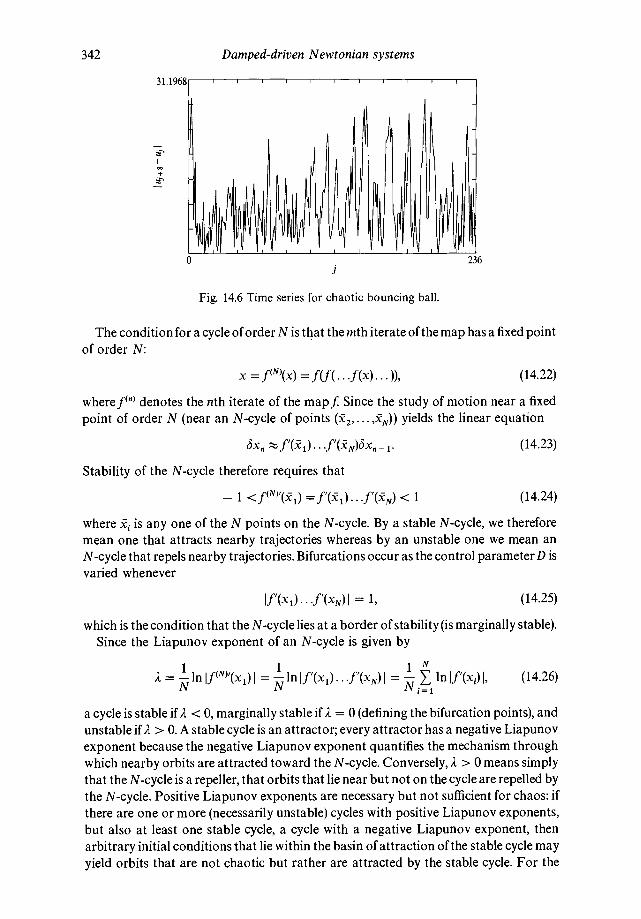
342 Damped-driven Newtonian systems
The condition for a cycle of order N is that the mth iterate of the map has a fixed pointof order N:
x =f(f(.. .f(x). . . )), (14.22)
where f(tO denotes the nth iterate of the mapf Since the study of motion near a fixedpoint of order N (near an N-cycle of points ,xN)) yields the linear equation
(14.23)
Stability of the N-cycle therefore requires that
— 1 < 1 (14.24)
where is any one of the N points on the N-cycle. By a stable N-cycle, we thereforemean one that attracts nearby trajectories whereas by an unstable one we mean anN-cycle that repels nearby trajectories. Bifurcations occur as the control parameter D isvaried whenever
If'(xi). . .f'(xN)I = 1, (14.25)
which is the condition that the N-cycle lies at a border of stability (is marginally stable).Since the Liapunov exponent of an N-cycle is given by
1 11N
(14.26).L i=1
a cycle is stable if A <0, marginally stable if). = 0(defining the bifurcation points), andunstable if). > 0. A stable cycle is an attractor; every attractor has a negative Liapunovexponent because the negative Liapunov exponent quantifies the mechanism throughwhich nearby orbits are attracted toward the N-cycle. Conversely, A > 0 means simplythat the N-cycle is a repeller, that orbits that lie near but not on the cycle are repelled bythe N-cycle. Positive Liapunov exponents are necessary but not sufficient for chaos: ifthere are one or more (necessarily unstable) cycles with positive Liapunov exponents,but also at least one stable cycle, a cycle with a negative Liapunov exponent, thenarbitrary initial conditions that lie within the basin of attraction of the stable cycle mayyield orbits that are not chaotic but rather are attracted by the stable cycle. For the
J
Fig. 14.6 Time series for chaotic bouncing ball.

14.1 Period doubling in physics 343
logistic map, the basin of attraction of a stable cycle is almost the entire unit interval.We turn now to the analysis of the logistic map.
It is easy to calculate the first few bifurcations analytically: there are two fixed points fthe logistic map, x = 0 and x = 1 — 1/D, and stability is determined by the condition— 1 <D(1 — 2x) < 1: x = 0 is stable for 0 <D < 1, unstable otherwise, with Liapunovexponent 2 = ln D I. The second fixed point at x = 1 — comes into existence atD = 1, is stable for 1 <D < 3 but persists unstable if D> 3. Note that this 1-cycle has adifferent Liapunov exponent given by
(14.27)
The Liapunov exponent is negative whenever the 1-cycle is stable, when 1 <D <3, andis positive for D > 3. In other words, both 1-cycles persist in unstable form beyondD = 3 as repellers, a repeller being any orbit with a positive Liapunov exponent. Here,again, these positive Liapunov exponents do not produce any chaos because as soon asD is increased slightly beyond 3 there is another attractor available.
According to Feigenbaum (1980), initial conditions near but not on the second1-cycle will not quite repeat after one cycle of the motion but will slightly overshoot orundershoot. However, after two cycles of the motion the orbit may close exactly,yielding an attracting 2-cycle.
Therefore, to determine the attractor when D > 3, let us search systematically for a2-cycle, whose equations are given by
x1 = Dx2(1 — x2)(14 28)
x2 = Dx1(1 — x1).j
The 2-cycle is stable whenever f'(x1)f'(x2) I < 1, which is the same as saying that theLiapunov exponent
2 = (14.29)
for the 2-cycle is negative. An easy calculation of a few pages yields
= [1 + 1/D + (1 — 2/D — 3/D2)"2]/21430
x2=[1+1/D—(1—2/D—3/D2)112]/2, ( . )
and therefore that
2=+lnI2D+4—D21. (14.31)
Note that both the 1-cycles and the 2-cycle all have entirely different Liapunovexponents, which illustrates the very general fact that Liapunov exponents dependstrongly upon initial conditions (except in the very special cases of symmetric tent mapsand Bernoulli shifts). Note also from (14.30) that the 2-cycle does not exist forD < 3 butis born of a pitchfork bifurcation at D = 3, just where the fixed point becomesmarginally stable (the Liapunov exponents of both the 1-cycle and the 2-cycle vanish atD = 3). However, for 3 <D < 1 + the 2-cycle is stable because it has a negativeLiapunov exponent. ForD> 1 + \/6, 1 > 0 for the 2-cycle, and both the 1-cycles andthe 2-cycle are repellers rather than attractors.
Further analysis shows that, at D = 1 + an attracting 4-cycle is born, and thisperiod doubling continues systematically until a critical parameter value is reached:denoting D1 = 3 and D2 = 1 + ,J6, there are period-doubling bifurcations at further

344 Damped-driven Newtonian systems
parameter values D3,D4,... where, at a stable is born but it becomesunstable at In other words, in the 'window of stability' <D all cyclesof order are repellers with (different) positive Liapunov exponents, but there is alsoan attractor: a with a negative Liapunov exponent. That is born of apitchfork bifurcation at D a criticalparameter value all cycles of order with n finite have become repellers withpositive Liapunov exponents, and the 'infinite cycle' with points, the firstnonperiodic orbit, has a vanishing Liapunov exponent (this nonperiodic orbit isactually a multifractal, but we are not yet prepared to explain what this means).
It is via period doubling that chaos, in the form of unstable periodicity and unstablenonperiodicity is created systematically in a one-frequency problem: for D slightlygreater than not only do all of the periodic orbits with periods have positiveLiapunov exponents, but the nonperiodic orbit that was marginally stable (with 2 = 0)at now also has a small positive Liapunov exponent. The condition for deterministicchaos is satisfied at D slightly greater than there is bounded motion with noattractors. All periodic and nonperiodic orbits are now repellers, so that sensitivity withrespect to small changes in initial conditions follows for every choice of initialconditions.
The reason why a 4-cycle occurs before a 3-cycle is explained by Sarkovskii'stheorem: if a continuous map of the unit interval has a 3-cycle, then cycles of all otherinteger orders also occur in the following sequence, corresponding to starting aroundD = 4 with the logistic map and then decreasing D systematically to 0 (see Devaney,1986, for the proof):
3>5 >7> ... > 2.3 > 2.5 > 2,7 > ...> 2m.3 > 2m.5
(14.32)
This means: as D is increased in the logistic map (or in any other unimodal map), then1-cycles must occur first, cycles of all orders follow, and therefore a nonperiodic with
points must occur before a cycle of odd order can occur, the 3-cycle occurring last asD is increased. For an arbitrary continuous map of the interval, there need not be even asingle cycle (nothing is said here about stability, either), but if a cycle of any order at alloccurs, then all cycles listed to the right of that cycle in the Sarkovskii sequence (14.32)must occur as well (the proof of the theorem assumes only that the map is continuousbut is not necessarily differentiable). We leave it as a homework exercise for the readerto show that the logistic map has a 3-cycle. Devaney also gives a nice example of a mapwith piecewise constant slope that has a 5-cycle but has no 3-cycle.
Near the period-doubling critical point (the transition to chaos), where the logisticmap's orbit is nonperiodic with 'period' there are universal exponents that describethe transition to the region where unstable nonperiodicity is possible. Those exponentsare analogous to universal critical exponents in the theory of phase transitions inequilibrium statistical mechanics and quantum field theory. As Feigenbaum has shown(1980), all one dimensional maps with self-confined motion and a quadratic maximum(for the logistic map, — c(x — 1/2)2 near x = 1/2) have the same criticalexponents. Maps with maxima of other orders define other universality classes, andeach class has its own critical exponents, in qualitative agreement with the idea ofuniversality classes in the theory of phase transitions. However, this idea of universalityrelies upon fixed points of maps at the transition to chaos but does not describe any of

14.1 Period doubling in physics 345
the topologically universal properties of chaotic orbits of the map that occur forD > The treatment of universality properties at the transition to chaos is basedupon the renormalization group idea and is beyond the scope of this text. For the studyof universality at the transition to chaos, we refer the reader to the extensive literatureon the subject, in particular, see the informative Los Alamos Science paper byFeigenbaum, and also the very readable review article by Hu (1987) (see also Schuster,1988, or McCauley, 1993).
For the logistic map,just beyond the period-doubling critical point nonperiodicorbits with positive Liapunov exponents appear. However, as D is increased 'windowsof stability' must also occur: the periodic orbits in the Sarkovskii sequence (14.32) thatare not present for D appear via bifurcations, and are stable in a small range ofparameter values of D. All of these 'windows of stability' first appear and then disappearvia bifurcations as D is increased from D to appearand then go unstable is the 3-cycle. The case where D = 4 is very special because thedynamics there again become simple: at D = 4, orbits of all possible integer periodsexist and are unstable. The dynamics at D = 4 are simple because the logistic map withD = 4 turns out to be a simple pseudo-random number generator that is conjugate, bya coordinate transformation, to the binary tent map.
Consider the binary tent map,
— <1/21433
— 12(1( . )
If we transform variables according to
(14.34)
then the equation = becomes
= (14.35)
or
= (14.36)
UsingO = sin1 \/z,sinO = = — z)/1,yieldssin2z = 2sinzcosz,or
= — zn), (14.37)
which is a logistic map. Periodic orbits of the tent map occur with all possible periodsfor rational initial conditions, and these orbits transform into period orbits of thelogistic map with irrational initial conditions (the period of an orbit is an example of atopologic invariant). Nonperiodic orbits of the tent map occur with every irrationalinitial condition, and these orbits transform into nonperiodic orbits of the logistic mapwith both rational and irrational conditions (every periodic orbit of the logistic mapstarts at an irrational number, and every rational initial condition yields a nonperiodicrbit). Since the Liapunov exponent is invariant under differentiable coordinatetransformations, almost every orbit of the logistic map has the same Liapunovexponent). = ln 2 even though the slope of the logistic map varies, and even though thelogistic map has different Liapunov exponents for different initial conditions for every
346 Damped-driven Newtonian systems
other value of D (one sees by substitution of D = 4 into the formulae above for theLiapunov exponents for one of the 1-cycles and the 2-cycle that A = in 2 in all threecases). That the 1-cycle x = 0 has an exponent A = ln 4, rather than ln 2 at D = 4, is
allowed by the fact that the transformation from the tent map to the logistic map is notdifferentiable at x = 0.
It was first noted by von Neumann that the logistic map would make a goodpseudo-random number generator on a computer were it not for the fact thatroundoff/truncation error in floating-point arithmetic destroys that possibility inpractice. In general, the forward iteration of a chaotic one dimensional map on acomputer in the floating-point mode does not generate correct orbits of the mapbecause a chaotic map magnifies the roundoff/truncation error exponentially with eachiteration. The answer to the question of how to compute chaotic orbits correctly, withcontrolled precision, was described in chapter 6 and is described briefly again in thischapter. In contrast to the numerically unstable procedure of forward iteration ofchaotic maps on a computer, there are universal properties and universality classeswithin the chaotic regime that follow from topological invariance. The topologicproperties can be discovered by a combination of analytic and numerical methods,especially by discovering the hierarchy of unstable periodic orbits.
Again, we stress that while the 1-cycles and 2-cycle have different Liapunovexponents for arbitrary values of D, at D = 4 all orbits have A = in 2, as is required byconjugacy with the binary tent map except for the singular orbit at x = 0. This equalityof exponents for (nearly) all values of initial conditions is a singular phenomenon that isnot reflected by typical chaotic dynamical systems, where Liapunov exponentsgenerally vary from orbit to orbit with changes in initial conditions. In other words, adynamical system does not have merely 'a' Liapunov exponent, but has instead anentire spectrum of exponents. We will emphasize this aspect of chaotic dynamics againin the next section.
Summarizing, period doubling represents one possible route to chaos via a definitebifurcation sequence: for <D all orbits with periods 1 are unstable withpositive Liapunov exponents, but there is no chaos at long times there because stableattractors with periods from to still exist. At D = the Liapunov exponent forthe first orbit with points vanishes, and for D > all orbits with periods
= 1,2,3,. . . ,co have positive Liapunov exponents, as do the nonperiodic orbits thatare created for D � so that the motion is necessarily chaotic because it is bounded,but with no attractor available to capture the iterates (except when D falls into awindow of stability of an orbit with period other than We expect that perioddoubling is the typical path to chaos in an oscillatory system with only one frequency.In a flow defined by differential equations period doubling can take the form ofsuccessive doublings of the period of the limit cycles of a dissipative equation (seeFeigenbaum's discussion of the Duffing equation (1980) as an example).
We did not discuss the critical orbit of the logistic map, the nonperiodic orbit withvanishing Liapunov exponent that occurs at D = That orbit is multifractal but themultifractal property requires a study of dynamics near the transition point. We turnnext to simpler dynamical systems that generate fractal and muitifractal orbits in phasespace in order to show how different classes of initial conditions generate both spectraof Liapunov exponents and corresponding spectra of fractal dimensions. At the end ofthat discussion, we shall return briefly to the fractal orbit generated by the logistic mapat criticality.

14.2 Fractal and orbits 347
14.2 Fractal and multifractal orbits in phase space
If we were to continue with either the bouncing ball model or the logistic map then inthe limit of infinitely many period doublings we would arrive at an orbit consisting of
points, as would be indicated by the continuation of the bifurcation diagram shownas figure 14.5. This orbit, we call the critical orbit, because it occurs for the limitingvalue D and is the first nonperiodic orbit to occur as D (or y) is increased. Atthe complete invariant set (the closure of all possible orbits at infinite time) includes thecritical orbit of infinitely many period doublings along with all periodic orbits withperiods and organizes itself naturally onto a complete binary tree (orbits withperiods 2,22,23,. . . are all present). By writing the natural numbers between zero andone as binary strings, the continuum of the unit interval can also be organized onto acomplete binary tree. Therefore, the critical orbit has 'as many' points as does thecontinuum in the sense of 'cardinality' defined by the mathematician Cantor(1845—1918). In fact, the critical orbit defines a Cantor set, a set of points that can beapproximated, to within any desired finite precision, by an unstable cycle at As
we shall later see, this possibility to describe the critical orbit, to within finite precision,by the hierarchy of unstable orbits with periods gives us a way to estimate the fractaldimension of the critical orbit. First, we must define 'fractal dimension'.
We can think of a Cantor set as any set that has 'as many' points as the continuum(meaning the same cardinality), but such a set does not necessarily take up any space onthe real line. To explain this, and to introduce the idea of fractal dimension in itssimplest terms, we now turn to uniform Cantor sets that are generated by much simplerdynamical systems than the bouncing ball model or the logistic map (as we shall seebelow, nonuniform Cantor sets are also generated by the logistic map whenever D > 4).
Examples of Cantor sets can be constructed algorithmically by starting with thecontinuum and systematically deleting finite parts of it. The simplest example is themiddle thirds Cantor set: start with the unit interval and remove the open middle thirdinterval. The Cantor set is covered by the two closed intervals [0,1/3] and [2/3,1] andthe interval end points 0, 1/3, 2/3, 1 belong to the Cantor set. Next, remove the openmiddle thirds of the two remaining closed intervals: the Cantor set is still covered by thefour closed intervals [0,1/9], [2/9,1/3], [2/3,7/9], and [8/9,1], and consists of the endpoints 0,1/9,2/9,1/3,2/3,7/9,8/9,1 as well as infinitely more points that are still coveredby the four closed intervals. At the nth stage of recursive construction, the Cantor set iscovered by 2" closed intervals, each of length 1,, = 3
", and consists of all end points ofthose intervals plus infinitely many points that still lie beneath the intervals.
Notice at this stage that we can write down an exact scaling law: if we denote as N,,the number of intervals of size i,, in generation n needed to cover the Cantor set, thenN,, = where D = In 2/ln 3, for n = 1,2,3 The number D is called the fractaldimension (Hausdorif dimension) of the Cantor set, which is the set of all end pointsand limits of infinite sequences of end points that follow from taking the limit ofinfinitely many open interval removals as prescribed above.
The middle thirds Cantor set has no length: N,,l,, = -D goes to zero as n goes toinfinity because D < 1. However, there is a sense in which this set has 'as many' pointsas the continuum: consider the numbers from 0 to 1 written as binary strings. Thesenumbers can be thought of as occupying all of the branches of a complete binary tree.Next, note that the intervals that cover the middle thirds Cantor set also lie on acomplete binary tree; there are 2" intervals in each generation n, and these intervals give

348 Damped-driven Newtonian systems
rise to points in the Cantor set as n goes to infinity (Cantor set points are representedby the end points of the closed intervals shown as solid bars in figure 14.7). Both theCantor set and the continuum consist points (this is Cantor's idea of cardinality:both sets have the same cardinality, but a set with cardinality is not qualitativelydifferent from one with cardinality because numbers in the continuum can beexpanded in either base ten or base 2, or in any other base). In contrast, the rationalnumbers can be put into one-to-one correspondence with the integers and so have onlya cardinality of co. The dimension of each rational is zero (the dimension of a point iszero because a point has no size), and the dimension of the rationals is also zero becausethe dimension of any countable point set is zero. It is easy to prove that any countablepoint set (like the rationals) has no size: simply cover each rational by an interval of size
where n = 0,1,2,... represents the ordering of the countable set according to theintegers (the set can be put into one-to-one correspondence with the nonnegativeintegers n = 0,1,2,3,.. .). The size of the set is therefore less than
= 2s, (14.38)n0
which can be made as small as we like since is arbitrary. A countable point set like therationals takes up no space at all in the continuum although between any two numberson the real line, no matter how closely spaced, there are always infinitely many rationalnumbers. The middle thirds Cantor set is nonintuitive: unlike the rationals, it has asmany points as the continuum but, like the rationals, it has no size at all. Themathematical idea of the continuum is itself nonintuitive, except perhaps to a mind likeCantor's, and is not the same as the physicist's intuitive idea of continuity based upongeometry.
In physics we are not concerned with the mathematical continuum because infiniteprecision in nature (in observation and in experiment) is both impossible andmeaningless (which is why we cannot trust the predictions of 'measure theory'), so whatdoes a physicist mean by a fractal? By fractal, we mean that there is a scaling lawwhereby, when you measure (for example) the size of an object in nature (or try to covera point set representing a Poincaré section of an orbit in phase space) with precision I,,,then the number of rulers (bins, boxes) of size I,, needed to measure the size of the objectoptimally (or to cover the point set optimally) obeys the scaling law where Dis not an integer. Roughly speaking, the object looks, at resolution I,,, as if it consists of
fragments, but the number of fragments that it appears to consist of increasesexponentially whenever you increase the resolution I,, of the measurement. Further-more, this kind of scaling cannot go on forever in nature: both in observations andexperiments, fractal scaling can hold at best between two extreme limits 1mm 1n 1max
where, in the crudest case, the limits are 1mifl an interatomic spacing and lmax thephysical extent of the object. An example is provided by the coastline of Norway, whoseperimeter size L = Ni = 11 — D obeys fractal scaling with D 1.28 for a range of 'rulersizes' 4km < 1 < 370 km (imagine estimating the perimeter of the coastline by placingrulers end to end on a large map).
The middle thirds Cantor set can be generated systematically by backward iterationof the ternary tent map (similar to figure 14.7, but with equal slopes of magnitudea = b = 3). Any unimodal map that peaks above unity, like the logistic mapf(x) = 4D(1 — x)with D > 4 or like any asymmetric version of the tent map or logistic

14.2 Fractal and orbits 349
1(z)
Fig. 14.7 Backward iteration of the unit interval by a tent map with slopemagnitudes a <b, and ab > a + b, generates a Cantor set that organizes
itself naturally onto a complete binary tree.
map, will also generate a fractal (a Cantor set) in backward iteration. For any of thesemaps, we can divide the unit interval into two nonoverlapping sets, the escape set andthe invariant set. The escape set consists of all initial conditions such that, for somefinite n, 1 so that = goes off to minus infinity as n goes to infinity (eachmap is extended continuously to minus infinity). For example, for the ternary tent map,if 1/3 <x0 < 2/3 then x1 > 1 and the remaining iterations escape to infinity. Incontrast, the invariant set consists of all possible initial conditions x0 such thatx, remains in the unit interval as n goes to infinity.
The ternary tent map's invariant set can be constructed recursively by backwarditeration of the entire unit interval by the tent map. In one backward iteration, weobtain the two closed intervals [0,1/3] and [2/3,1]. Any initial condition x0 that iscovered by these two intervals will therefore yield a first iterate that obeys 0 � x1 � 1,but the resulting x2 is not necessarily still in the unit interval. If we perform twobackward iterations of the unit interval then we obtain four closed intervals [0,1/9],[2/9,1/3], [2/3,7/9], and [8/9,1]. Any initial condition x0 that lies beneath any of thesefour intervals will yield 0 � x2 � 1, but the third iterate is not necessarily still confinedto the unit interval. Generalizing, if we want to choose an so that is still inside theunit interval after n or fewer iterations, then we can and must choose that initialcondition to be any number that lies beneath any one of the = intervals of size
= that are given by n backward iterations of the whole unit interval by theternary tent map. The limit where there would be infinitely many backward iterationsleads us to infer that the invariant set of the ternary tent map, the set of initial conditionsthat do not escape to infinity, is the middle thirds Cantor set. In other words, boundedmotion of the ternary tent map (or of any unimodal map peaking above unity) takesplace on a repelling fractal. The fractal is a repeller because any initial condition that ischosen near to, but not on, the fractal will escape from the unit interval in finite time.The escape time depends upon how near to the fractal one starts the iterations. Anotherway to see that the fractal is a repeller (a 'strange repeller') is to say that each orbit on
• • • •• • • •
350 Damped-driven Newtonian systems
(and oil) the fractal invariant set has a positive Liapunov exponent 2 = In 3, so thatparticular bounded orbit is a repeller.
Note that we can write the interval sizes as = where 2 = ln 3 is the Liapunovexponent of every orbit of the ternary tent map. This formula can be deduced from amore general standpoint. Consider the error propagation condition
ex, (14.39)
where 2(x,) is the Liapunov exponent for the trajectory starting at xc,. The maximumpossible error (where the phase space is the unit interval or a subset thereof) is 1
(more precisely, the maximum error is i/p if we compute in base p arithmetic). Ifthe initial condition lies under the interval I,,, and is known or specified to precisionthen this is the same as saying that 5x, in. The result is
1,, (14.40)
which is exact for all symmetric tent maps that peak at or above unity (in =a with slope magnitude a � 2).
It is impossible to compute bounded trajectories near a repelling fractal usingforward iterations with floating-point arithmetic on a computer. Determining theintervals by backward iteration is a convergent process, however, because backwarditerations contract intervals. Another way to say it is that one dimensional maps thatexpand intervals in forward iteration have a negative Liapunov exponent in backwarditeration. Therefore, one can always determine the interval sizes and positions asaccurately as one wishes by using floating-point arithmetic and backward iteration. Weillustrate next that it is also possible to compute exact orbits, to within any desiredprecision, on a repelling fractal.
If we study the ternary tent map in ternary arithmetic, expanding all iterations in theform
Xn = = (14.41)
where = 0, 1, or 2, then the ternary tent map can be rewritten as an automaton forthe ternary digits:
if c1(n—1)=0 1= .
?.(14.42)
— —1) if e1(n —1) = 1.j
This follows easily from using 1 — Xn = 0.(2 —
1 = . in ternary arithmetic, just as 1 = 0.999" in decimal arithmetic.The advantage of using this procedure is that one sees precisely how the 'far away' digitsin the initial condition are propagated in finite time into the leading digits of higheriterations, which property is the vary hallmark of deterministic chaos (sensitivity withrespect to small changes in initial conditions).
The next point is: by using the replacement rules 0.1000 .. = . =and so on, the points on the middle thirds Cantor set can be seen to consist
of all possible ternary numbers that can be constructed using only 0's and 2's (l's are notallowed, except by the replacement rules). It is easy to see by examples that all of the endpoints can be written as strings using only 0's and 2's: 1/9 = 0.001 =7/9 = 2/3 + 1/9 = 0.021 = and so on. Hence, end points of the Cantor set
14.2 Fractal and orbits 351
consist of finite binary strings with only 0's and 2's. Note that with only 0 and 2, we havea binary rather than a ternary alphabet, corresponding geometrically to the fact that allpoints in the Cantor set are covered either by the left interval [0,1/3] or by the rightinterval [2/3,1].
However, all of the orbits of the map starting from end points taken as initialconditions hop onto the unstable fixed point at x = 0 in finite time. Unstable periodicorbits with all possible integer periods follow from rational numbers that are infiniteperiodic binary strings using 0's and 2's. For example, x, = yields x1 =
and = for n � 2, so that the string must be the ternaryexpansion for the unstable fixed point x = 3/4. However, the choice x0 =yields x1 = 0.02002002" x2 = . x3 = . x4 = = x2,
which is an unstable 3-cycle. Cycles of all possible orders can be constructedsystematically by inventing different algorithms for period binary strings (the binaryexpansion of every rational number provides just such an algorithm).
The periodic orbits with cycle numbers greater than one are the points of the Cantorset that are rational limits of infinite sequences of end points. For example, 2/9 = 0 and an an endpoint sequence starting with 0.02, 0.0220200., 0.0220202000.,
gives rise to the periodic limit which is a rationalnumber and is also a periodic point (belongs to a 3-cycle) for the ternary tent map on theCantor set.
Limits of sequences of end points also give rise to irrational numbers on the Cantorset (like every set with elements, most of the points on the Cantor set are irrational),and these numbers lie on (and define) the unstable periodic orbits of the ternary tentmap. For example, the initial condition (constructed by an obvious algorithm: if n 0'sprecede a 2, then n + 1 0's follow that 2 before the next 2 occurs) x, =
belongs to the Cantor set and gives rise to an unstableperiodic orbit of the tent map. By computing this initial condition to high enoughprecision, we can compute the tent map's corresponding orbit to any desired precisionon the repelling fractal via the automaton (14.42). In order to know the tent map's orbitto one decimal precision for n iterations, for example, we must compute the first nternary digits of x0. This is the same as saying that we have one digit per iterationinformation transfer in base three because the Liapunov exponent is 2 = ln 3. Thegeneralization of this idea to one dimensional maps with variable slope that peak at orabove unity is easy: one computes slopes and symbol sequences by backward iteration(see McCauley, 1993). This method leads to the study of universal properties of classesof chaotic maps. For higher dimensional maps, or for maps of the unit interval thatpeak beneath unity, instead of iterating a map forward in time on a computer, whichonly leads to error buildup after very short times, the right approach is to extract theunstable periodic orbits of the dynamical system systematically. This method also leadsto the study of universal properties of classes of dynamical systems, because the periodsof orbits and their symbol sequences are topologic invariants (see the references byCvitanovic et al., 1985).
The fractal dimension D = In 2/ln 3 of the middle thirds Cantor set is the dimensionof the set of all possible initial conditions in [0,1] that yield bounded motion of theternary tent map. In other words, D = ln 2/In 3 is the dimension of a set that consists ofall possible bounded orbits, both periodic and nonperiodic, of the tent map. We have asingle dimension because there is only one Liapunov exponent 1 = ln 2/ln 3 for every
352 Damped-driven Newtonian systems
orbit. The logistic mapf(x) = 4x(1 — x) at D = 4 has only a single Liapunov exponentbecause of conjugacy to the binary tent map. In general, as we saw above for the logisticmap with D unequal to 4, a map with variable slope does not have merely one Liapunovexponent but has instead different Liapunov exponents for different classes of initialconditions. We show next that, whenever there is a spectrum of Liapunov orbits, thenthere is also a corresponding spectrum of fractal dimensions.
First, as a prelude to what follows, notice that the middle thirds Cantor set exhibitsan exact geometric self-similarity. If you pick out of figure 14.5 any nth generationsub-tree for the case where both slopes are equal to the same number a > 2, the one thatgrows from a single interval of size = a - ", and then rescale all intervals on thatsub-tree by multiplying them by the same factor you obtain an exact replica of theentire original binary tree of intervals. This is the same as saying that the relation
= 1 is exact for all n = 1,2 It is also the same as saying that the entire fractal isgenerated recursively by the iteration of a single largest length scale 11 = 1/3. Or, it is thesame as saying that the ternary tent map has only one Liapunov exponent,independently of the choice of initial conditions.
Whenever (as is typical of both dynamical systems and nature) we encounter a fractalthat does not possess exact geometric self-similarity, but a more complicated sort ofself-similarity, then the relation = 1 must be generalized to allow for nonuniform-ity of the hierarchy of intervals that, in each generation, cover the fractal optimally,
1, (14.43)
where is the optimal partitioning, the partitioning generated by the dynamicalsystem (backward iteration for one dimensional maps) in generation n, and DH is calledthe Hausdorif dimension (D = ln 2/ln 3 is therefore the Hausdorif dimension for themiddle thirds Cantor set). If you choose a partitioning other than the optimal one, thenyou will always overestimate DH.
However, the Hausdorif dimension that follows from an optimal partitioninghierarchy that is made up of fundamentally nonuniform intervals is only one point in anentire spectrum of fractal dimensions. Returning to equation (14.40) where e
— we
see that nonuniform partitionings are generated by variable Liapunov exponents. Anyfractal that is generated recursively by the iteration of two or more largest length scalesis called a multiscalefractal, orjust 'multifractal' (there are also multifractal probabilitydistributions, but we do not consider them here). The Cantor set at the period-doublingcritical point is not so simple as a two-scale multifractal. It is a (more complicated)multifractal, but there is a way, in a fairly good approximation (see McCauley, 1993), toestimate the fractal dimension by using a two-scale approximation to that Cantor set.
To see how one gets a spectrum of fractal dimensions from of a simple example, weneed look no further than any asymmetric tent map that peaks above unity (figure 14.7):
f(x)= lb(1 — x), x > a/(a +
(14.44)
This map has slopes a and — b, and there is an escape set and a complementaryinvariant set that is a repelling fractal whenever ab/(a + b)> 1, which isjust a disguisedform of the condition 1/a + 1/b < 1 on the two first generation intervals = 1/a and12 = 1/b. In the case where 1/a + 1/b = 1, then the map peaks at unity and the

14.2 Fractal and orbits 353
Unit interval
Fig. 14.8 Complete binary tree of symbol sequences generated by backwarditeration of unimodal maps peaking above unity.
condition 1/a + 1/b = 1 is just the condition that backward iteration of the mappartitions the unit interval without generating an escape set: every point in the unitinterval belongs to the invariant set. If, with = 1/a and 12 = 1/b, 1/a + 1/b < 1, thenthere is an escape set and also a corresponding repelling fractal invariant set. However,in contrast with the middle thirds Cantor set, this fractal is not geometricallyself-similar (the fractal is not uniform): if you pick out any infinite sub-tree of thecomplete binary tree of intervals (see figure 14.7), say, the sub-tree that grows from thesecond generation interval 1/b2, then merely by rescaling every interval on the infinitetree by the same number b2 it is not possible to obtain an exact replica of the entireoriginal tree. The reason for this is the nonuniformity of the fractal. The fractal isnonuniform because it is constructed recursively (by backward iteration of the tentmap) by the iteration of two different largest scales: 11 = 1/a and 12 = 1/b.
Because the tent map has only two slopes a and — band generates a complete binarytree of intervals in backward iteration, we still have binary combinatorial simplicity: inthe nth generation of description of the fractal there are = 2" intervals andNm = n!/m!(n — m)! have the same size im = = where
Am = + n — mlb (14.45)
is the Liapunov exponent for a trajectory that starts under any interval with size By
necessity, such a trajectory visits the left first generation interval 11 = 1/a (to which weassign the letter L) m times, and the right first generation interval 12 = 1/b (denoted byR) n — m times in n forward iterations of the map (different intervals 'm with different LRorderings generate the same exponent, because the exponent is independent of theorderings), where the meaning of the 'symbol sequences' (binary LR-sequences) infigure 14.8 is: if you start with a specific interval im and then iterate n times forward, themap will visit the two first generation intervals = 1/a (L) and 12 = 1/b (R) in exactlythe sequence shown in figure 14.8. In other words, in generation n = 3, LRL means that
lies under x1 lies under 12, and x2 lies under 11, where = 1/a and 12 = 1/b denotethe two first generation intervals (symbolic dynamics, which we are introducing here, isthe generalization to maps with arbitrary slope of the method of studying the ternarytent map in ternary arithmetic).
LLL LLR LRR LRL RRL RRR RLR RLL

354 Damped-driven Newtonian systems
The symbol sequence orderings shown in figure 14.8 are universal for all unimodalmaps that peak at or above unity and contract intervals to generate a complete binarytree in backward iteration (the same maps, peaking beneath unity, generate incompletetrees, define other universality classes, and are a lot harder to analyze). More generally,the allowed symbol sequences of any given map are universal: they are not properties ofa specific map but rather are universal topologic properties characteristic of an entireclass of maps. This is an extremely important point whose further discussion wouldtake us well beyond the scope of this introductory book (see McCauley, 1993, for theeasy case, Cvitanovic et al., 1985, for the harder cases).
We have seen already that two scales means a spectrum of Liapunov exponents: forthe asymmetric tent map, 2(x) = x ln a + (1 — x)lnb with x( = rn/n) varying from 0 to 1has the range 2min � 2 � 2max where (with a <b) 2mm = ln a corresponds to x = 0 andto the symbol sequence LLL... L..., and 2max = in b corresponds to x = 1 and thesymbol sequence RRR.... We show next how this multiplicity of scales gives rise to aspectrum of fractal dimensions.
First, because the two first generation scales determine everything, the condition(14.43) for the Hausdorif dimension deduces to a°" + = 1 for the tent map:
2"
1 = = = + (14.46)i1
If 1/a + 1/b = 1, then DH = 1, but 0 < DH < 1 follows if 1/a + 1/b < 1. Now, veryimportant to note is that, although there is no geometric self-similarity of the entirenonuniform fractal, there are special subsets of our multiscalefractal that do scaleexactly because of perfect geometric self-similarity: consider the infinite hierarchy ofintervals defined by 1m = a - tmb
-+ the ratio x = rn/n is fixed, but where n varies
from ito infinity (therefore, m also varies to maintain fixed x). For each fixed n, there areNm such intervals, and these intervals define a fractal dimension D(Am) according to
Nm = (14.47)
where 2m is the Liapunov exponent given by Im = Remember, the idea is to fixx = rn/n, while varying rn and n. Also, borrowing an idea from Boltzmann, we candefine an entropy S by writing
S(2m) = ln Nm. (14.48)
If we combine the Mandelbrot equation (14.47) with the Boltzmann equation (14.48) bywriting Im = and also define s(2) = S(2)/n, then we arrive at the very generalrelationship
D(2) = s(2)/1 (14.49)
as the fractal dimension of the set of initial conditions with the same Liapunovexponent 2. What is the meaning of the entropy in this expression? It is simply thelogarithm of the number of different symbol sequences that have the same ratiox = rn/n regardless of the orderings of the L's and R's within the sequence (to eachinfinite precision initial condition there corresponds a unique LR-sequence but manydifferent LR-sequences may have the same ratio rn/n). So, whenever we writeD = ln 2/ln 3 for the ternary tent map, we can now understand that in 3 in thedenominator represents the Liapunov exponent, while ln 2 in the numerator represents
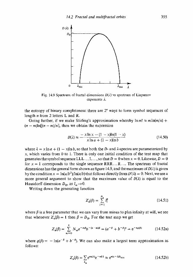
14.2 Fractal and orbits 355
D
Fig. 14.9 Spectrum of fractal dimensions Do.) vs spectrum of Liapunovexponents 2.
the entropy of binary completeness: there are ways to form symbol sequences oflength n from 2 letters L and R.
Going further, if we make Stirling's approximation whereby in m! m ln(m/n) +(n — m)ln[(n — m)/njj, then we obtain the expression
D(2)— xlnx —(1 — x)ln(1 — x)
(14.50)xlna +(1 — x)lnb
where 2 = x in a + (1 — x)ln b, so that both the D- and A-spectra are parameterized byx, which varies from 0 to 1. There is only one initial condition of the tent map thatgenerates the symbol sequence LLL... L. . ., so that D = 0 when x = 0. Likewise, D = 0
for x = 1 corresponds to the single sequence RRR. . . R.... The spectrum of fractaldimensions has the general form shown as figure 14.9, and the maximum of D(2) is givenby the condition x = ln(a/b2)/ln(a/b) that follows directly from D'(A) = 0. Next, we use amore general argument to show that the maximum value of D(2) is equal to theHausdorif dimension DH, as 0,
Writing down the generating function
N
=(14.51)
where fi is a free parameter that we can vary from minus to plus infinity at will, we seethat whenever = 1 then /3 = DH. For the tent map we get
= = + = (14.52a)
where g(/3) = — ln(a° + We can also make a largest term approximation asfollows:
= (14.52b)A,,,

356 Damped-driven Newtonian systems
where the extremum condition required to minimize the exponent in (14.52b) is givenby
/3 = (14.53)
For a given value of /3, this condition determines a value 2(fl) such that we canapproximate the entire generating function by a single term. Hence,
g(/3) = 2/3 — s(2) (14.54)
holds approximately with 2 determined by (14.53), and where g(/3) = — +Note that 2 = dg/d/3 follows from (14.53) and (14.54). Note also that, since g = 0 at/3 = DH, it must be true that DH = /3 = s(2)/1 = D(2) for the particular value of 2 thatdetermines Which part of the D(2) spectrum is this? To answer this question, wemaximize D(2) = s(2)/2. The extremum condition D'(1) = 0 yields the condition thats'(2) = s(1)/1 = D(2), but since /3 = s'(2) we can then conclude that /3 = DH = D(2)max. Inother words, we expect that the peak of the D(2) spectrum is the same as the Hausdorifdimension of the fractal repeller. This argument can be extended to maps other than thetent map, but we do not provide the proof here.
The idea propagated in some texts that a chaotic dynamical system can becharacterized by a single Liapunov exponent is very misleading: only the simplestsystems, systems with constant slope and systems that are differentiably conjugate tosystems with constant slope, can be characterized by a single Liapunov exponent. Ingeneral, Liapunov exponents of trajectories of chaotic systems depend strongly onclasses of initial conditions, as we have shown for the logistic map in the last section andin this section for the asymmetric tent map. Correspondingly, there is a spectrum ofexponents, and this spectrum of exponents generates a spectrum of fractal dimensionsof which the Hausdorif dimension is the largest dimension.
As a prelude to devil's staircases in the two-frequency problems of section 14.4, weend this section with the construction of the devil's staircase for the middle thirdsCantor set. In the first stage of iterative construction of the middle thirds Cantor set, wediscovered that the end points 3 and 1 — 3 1 belong to the Cantor set. For n = 2, wediscovered in addition the end points 32, 31 3—2, 1 — 3_i + 32, and 1 — 3—2
These end points and all other end points of the Cantor set can be written as finitelength ternary strings using only two symbols, = 0 or 2. For example, 3 1 =
0.1 = 0.022"' while 1 — 3_2 = and so on. All of the elements of the Cantorset can be written using the binary symbols; = 0 or 2, and all possible combinations of0's and 2's describe all the elements in the set. Hence, the Cantor set is in one-to-onecorrespondence with all possible binary strings, so that the cardinality of the set iswhich is the same as the cardinality of the continuum. This tells us that 'almost all' of thepoints in the Cantor set are irrational numbers.
We construct a function called the Cantor function as follows: with; = 0 or 2 weinterpret the function defined by
(14.55)
as a binary number (e,/2 = 0 or 1), where x = is an element of theCantor set (;= 0 or 2). It is easy to see that if x1 and x2 are the end points of aremoved open interval (part of the escape set of the tent map), then P(x1) = P(x2). For

14.2 Fractal and orbits 357
P (x)
11111 111111
Fig. 14.10 A few steps in the devil's staircase of the ternary tent map.
example, with x1 = = we get P(x1) = 0.01111 = 0.1 = 1/2. Ifx2 = 1 — then P(xi) = 0.1 = 1/2. If x1 = 1/32 = 0.01 = then P(x1) =
= = 1/4, whereas x2 = 31 — 3-2 also yields P(x2) = 0.01W = 1/4.
Having x1 = 1 — 3' + 32 yields P(x1) = = = 3/4, whereasx2 = 1
— 3—2 also yields P(x1) = 0.11W = 3/4. If we extend the definition of P(x) toinclude P(x) = constant on the closure [x1,x2] of every removed open interval, thenP(x) has the following properties: P is continuous but nondecreasing and has a slopethat vanishes almost everywhere. The plot of P(x) vs xis called the devil's staircase, andthe first few staircase steps are plotted in figure 14.10.
The Cantor function P(x) can be understood as a certain probability distribution forthe iterates of the ternary tent map on the middle thirds Cantor set. Consider anynonperiodic orbit of the symmetric tent map that generates, as its distribution ofiterates, a uniform probability distribution on the Cantor set: = 2" on any nthgeneration interval = of the tent map (think of the distribution {P1} as ahistogram). That the Cantor function represents the uniform distribution can be seen asfollows: P(x) = 1/2 for x = 3' means that half of the iterates of the map fall into theinterval [0,3'] and half in [1 — That P(x) = 1/4 for x = 1/3_2 means 1/4 ofthe iterates fall into the interval [0,1/3—2], while P(x) = 3/4 if x = 3_i + 3_2 meansthat 3/4 of the iterates fall into the three intervals [o32] [3 — 3_2 3 i], and[1 — 1 — + 32]. The remaining 1/4 land in the interval [1 — 3_21] Themethod of construction of the very special (and hard to find) class of initial conditions ofthe ternary tent map that generates even histograms on the fractal is discussed inMcCauley (1993).
Next, note that if you should choose a covering that is too large, then by virtue of1, you will overestimate the fractal dimension D, because 1,, = 1/Nfl yields
D = 1. Similarly, an underestimate of the covering size will underestimate D: in theextreme case we have D = 0 for a countable point set, a set that can be covered by acountable infinity of arbitrarily small intervals. The same argument holds fornonuniform coverings where we must use the generalization of 1, whereby
N,,
1. (14.56)
We now return to the nonperiodic orbit of the logistic map at the transition to chaos.That orbit has points and is multifractal. Although the nonperiodic orbit at

358 Damped-driven Newtonian systems
criticality (at D = 3.57) has a vanishing Liapunov exponent, it is born as aresult of the orbits with periods 2,22,. . . all of which have positive Liapunovexponents at D = We can try to use the periodic orbits systematically to estimatethe fractal dimension of the critical nonperiodic orbit. Consider the 4-cycle at
3.57. We can locate that cycle approximately as follows: if we start the iterationsnear the unstable fixed point x = 1 — 1/Do 0.72, they will stay there for a while andwill then diverge, but the next path that they follow is one near the 2-cycle. Afterlanding near the 2-cycle for a while, the iterates will diverge and will land near theunstable 4-cycle. In this way, we can locate approximately the points on the 4-cycle,and also the points on the 8-cycle and all cycles of higher order. We find the 4-cycle isgiven approximately at by x1 = 0.89, x2 = 0.35, x3 = 0.81, and x4 = 0.55. Weknow, by completeness of the binary tree of period doubling, that we needintervals in generation n to cover the Cantor set of the nonperiodic orbit at criticality.Another way to say it is: if you measure the points on the critical orbit with crudeenough resolution, then the observed motion will look like a nonperiodic bouncingaround in bins (you can see the nonperiodicity corresponding to points only byresolving the orbit with infinite precision over infinite times, both of which arecompletely impossible). In particular, we can take the two first generation intervals tobe defined by the 4-cycle: = x4 — x2 0.2 and 12 = — 0.08. Insertion ofthese two scales into
+ 1 (14.57)
yields DH 0.34, which is much less than the known estimate of DH 0.54 that followsfrom a higher order analysis. This tells us that the two intervals yielded by the 4-cycleare too small to cover the Cantor set, that the points on the are much moredispersed than our crude estimate of DH would indicate.
It is instructive to see how well we can estimate the fractal dimension D = in 2/ln 3 ofthe middle thirds Cantor set by looking at low order periodic orbits. The 4-cycle ofthe ternary tent map is easily found by digital experimentation to be given by therational numbers x0 = x1 = x2 =x3 = x4 = = x0. The two intervals that cover this 4-cycleare = x2 — x1 4/27 and 12 = x0 — x3 8/27, so that equation (14.43) yieldsDH 0.4, which is much smaller than D = in 2/in 3 0.63. Here it is geometricallyclear why the 4-cycle underestimates the fractal dimension: the 4-cycle, along with allother cycles, is covered by the optimal choice of two intervals of length 11 = 1/3 whoseend points are transients on the path to an unstable 1-cycle at x = 0: because a point ona cycle cannot be an end point in the optimal covering, cycle coverings will by necessityalways underestimate DH.
Finally, while the critical nonperiodic orbit is a multifractal it is not merely a 2-scalemultifractal. However, there is a particular 2-scale approximation to the fractal thatyields a very good approximation to the fractal dimension. Feigenbaum (1980) andCvitanovic have shown that the period-doubling limit near is described by thefunctional equation (universal for maps with quadratic maxima) g(x) =— ag(g( — where = and 12 = can be understood as two first generationlength scales, With the universal result and
+ 1, (14.58)

14.3 Strange attractors 359
we can solve this quadratic equation for to find
— 1)](14.59)
in
which is fairly close to the standard numerical estimate of DHLet us not give up so easily in our quest to deduce this dimension from the hierarchy
of unstable periodic orbits. We return to the 4-cycle of the logistic map at butinstead of thinking like a naive theorist let us approach the problem from thestandpoint of an empiricist who only knows that, at resolution one needs boxes ofthat size to cover the orbit. That is the key: we cover the 4-cycle with 2 boxes of size
= 0.2, the smaller interval 12 = 0.08 being too small for resolution. This procedureyields 2 with D 0.43, which is slightly better but still too small, the sameprocedure applied to the 4-cycle of the ternary tent map yields 2 with 8/27,so that D 0.57, which is not too bad for the crudest level of empiricism.
Theorists will not be satisfied with this last method of estimation, widely known as'box-counting', but many researchers use the 'box-counting method' in order to lookfor evidence of the scaling law Nn D over a finite, usually small, range of differentbox sizes (a range of experimental resolutions) 11,12,. Evidence for fractal scaling ofraw data is usually not accepted by the community unless (among other things) one canproduce strong evidence that the scaling holds over a range il/IN �
A theoretically more respectable way to approach the problem of determining DH(and also one that can be applied to experimental data) is via the transfer matrixmethod (adapted from statistical mechanics), which compares the sizes of the intervalsin generation n with those of generation n + 1. The use of the resulting intervalcontraction rates (the transfer matrix elements) leads to a more accurate way toestimate DH from the unstable cycles at the period-doubling critical point.
At the period-doubling critical point the orbit is fractal and marginally stable, notchaotic. Unimodal maps that peak above unity and generate a complete binary tree ofever-contracting intervals in backward iteration have trajectories that are fractal,chaotic, and repelling. The bouncing ball model,just beyond the period-doubling limit,for some initial conditions, has a region of phase space that can be called a nonfractalstrange attractor. We turn next to invariant sets that may be fractal, chaotic, or both,and especially to the partial explanation of the popular phrase 'strange attractor'.
14.3 Strange attractors
A path from regular to chaotic motion different from period doubling was proposed byRuelle, Takens, and Newhouse (RTN). Historically, before period doubling universal-ity was discovered, the RTN path to chaos was proposed as an alternative to Landau'sidea of the development of turbulence in the Navier—Stokes equations of hydro-dynamics. According to Landau, who only argued qualitatively and intuitively and didnot use the Navier—Stokes equations explicitly to back up his argument, turbulenceshould appear as the consequence of the successive instability of conditionally periodicmotions (quasiperiodicity) with infinitely many different frequency ratios. In otherwords, Landau argued in favor of the need for infinitely many unstable frequencies as aprelude to turbulence. Another way to think of it is that turbulence would require thesuccessive instabilities of tori of dimension n, for n = 1,2,3,. . . ,co.

360 Damped-driven Newtonian systems
Ruelle, Takens, and Newhouse replaced the direct study of the Navier—Stokesnonlinear partial differential equations by the study of an infinite system of coupledordinary differential equations that would follow from the Navier—Stokes equationssystematically by a mode-expansion (by an expansion in orthogonal functions of thespatial coordinates, but with time-dependent expansion coefficients). One effect offinite viscosity is to truncate this into a finite but very large number. The Lorenz modelfollows from the arbitrary truncation to three modes of such an expansion. RTNargued (as Lorenz had shown) that one does not need infinitely many modes, but onlythree (which includes the possibility of three-frequency problems), for deterministicchaos. It has long been known from observation that fluid turbulence in open flows is aproblem of successive instabilities of many vortices of many different sizes, likely withchaotic vorticity in both space and time. A precise and widely accepted definition offluid turbulence has not yet been found, but turbulence is certainly not described by low(n 3) degree of freedom chaos.
We return to the perturbation of an integrable conservative flow by combineddamping and driving that can make the flow nonintegrable for large enough controlparameter values. In the case of weak enough driving and dissipation foliations aredestroyed and replaced by a trapping region, but one foliation may survive in distortedform for a limited range of the perturbation parameter. Inside the trapping region weexpect to find one or more attractors of the flow. Motion far from any attracting region isoverdamped: dissipation dominates to reduce the amplitudes of large deviations fromthe attractor. For the RTN scenario to work, we also must have at least two separatefrequencies in the dynamics problem. If the system with n � 3 is autonomous, then atlow enough driving the motion is overdamped everywhere in phase space, correspond-ing to a zero dimensional sink. The motion spirals into the sink due to the presence of atleast one frequency in the unperturbed problem. At higher rates of driving the sinkbecomes a source and one frequency is excited yielding a one dimensional attractor,where motions with amplitudes much greater than the size of the stable limit cycle areoverdamped but amplitudes that are small compared with the size of the limit cycle areunstable and grow as a result of negative damping. At even higher driving rates the limitcycle becomes unstable via a Hopf bifurcation and two frequencies are excited, meaningthat an attracting 2-torus appears. On the 2-torus the motion is either stable periodic orstable quasiperiodic depending upon the winding number. Both the one and twodimensional tori are the consequence of average energy balance in some region of phasespace. RTN showed that the next bifurcation for quasiperiodic orbits actually leads to athree dimensional torus that is, under small perturbations, unstable with respect todecay onto a 'strange attractor'. Motion on a strange attractor is chaotic but notnecessarily fractal, and not all fractal invariant sets are chaotic. The bouncing ball modelat criticality has a nonchaotic fractal invariant set, the orbit, inside the trappingregion (inside the rectangular slice). Some chaotic sets are attracting, others arerepelling, and some are neither attracting nor repelling. The logistic map just beyondcriticality has a strange nonattracting set that includes a class of orbits that arenonfractal, but fractal trajectories also occur for other choices of initial conditions forthe very same control parameter values (we remind the reader of the D(1) spectrum).Unimodal maps that peak above unity and generate a complete binary tree ofever-contracting intervals in backward iteration generate 'strange' trajectories that arefractal, repelling, and chaotic ('strange repeller'). Unimodal maps that peak above unitygenerate a complete binary tree of intervals that define the geometric or 'physical'

14.4 The two-frequency problem 361
pictures of a strange attractor. For that work we refer the reader to the literature (e.g.McCauley, 1993, or Cvitanovic et a!., 1988).
We turn next to a model that is motivated by physics, and where the RTN predictionof the transition of quasiperiodic orbits from torus-confinement to chaos can bestudied. Given the stable periodic and quasiperiodic orbits on a torus in a two-frequency system, the RTN scenario leaves open the possibility that persisting periodicattractors (periodic orbits on the torus with negative Liapunov exponents) mightshort-circuit the onset of chaos via unstable quasiperiodicity through the persistence ofattracting periodic orbits (stable periodic orbits might persist alongside the unstablequasiperiodic ones). We have to pay serious attention to this possibility because 'modelocking' has been observed in nature. Mode locking is the phenomenon whereby twovery weakly coupled nonlinear oscillators (like two pendulum clocks on opposite sidesof a wall) tend to synchronize, indicating a rational rather than an irrational frequencyratio. In the section that follows we shall discuss both the quasiperiodic and periodicmotions and their respective transitions to chaotic behavior in a model where the RTNprediction of the transition to chaos via quasiperiodicity occurs. We shall also showthat, in the same model, attracting periodic orbits persist long after the quasiperiodicones have become unstable, so that one would have to ask Mother Nature how shechooses her initial conditions to be able to tell whether or not it is possible to see theRTN transition to chaos (instead of stable and unstable periodicity) in observations oftwo-frequency systems in nature. Measure theorists argue that mathematics is capableof determining which class of initial conditions is likely to be chosen, but we reject thatclaim as there is no evidence for it from observation (and a computer calculation is atbest a simulation that does not qualify either as a real experiment or as an observationof nature).
14.4 The two-frequency problem
The damped, periodically driven pendulum is defined by the Newtonian equation
mU+ + w0sinO = A + Kcoscot (14.60)
in which there are two 'bare' frequencies: and w. This is also the equation of theJosephson junction in the theory of superconductivity. Instead of studying the systemas a flow in a three dimensional phase space, we can derive a two dimensional iteratedmap called the stroboscopic map
=(14.61)
=
where n = 0,1,2,... correspond to times 0,2T,3T,... and T = 2ir/co is the period of theexternal driving force. To see this, simply begin with the solution written in thestandard form
0(t) = — t,)l (14 62)r(t) = — t0) J
where r = dO/dt. Next, let T= t — t, be the period and denote 0(nT) = andr(nT) = Then
On =(1463)
= 1,T).j

362 Damped-driven Newtonian systems
Because the functions and are independent of the index n, we have an iterated mapof the form (14.61).
It is the choice of strobing time equal to the driving period Tthat guarantees that thefunctions G1 and G2 do not change with time (with n). The Jacobian J of thestroboscopic map (14.61) is simply
J(t + T,t) =+T)4(t+ T)) = (14.64)
This result follows from
(14.65)
so that areas in the two dimensional space contract at the constant rate
b = (14.66)
where fi> 0 in the case of ordinary friction.In order to model the damped-driven pendulum by a two dimensional map that has
some qualitatively similar properties, note that G1(O + 2ir,r) = 2ir + G1(O,r) whileG2(O + 2ir,r) = G2(O,r). A model satisfying these conditions is provided by the much-studied dissipative standard map,
= + + +(1467)
= + 5
wheref(O + 2ir) =f(O) and J = b, so that 0 < b < 1 represents dissipation and b = Iyields the limit of an undamped system. Very small b therefore represents the limit of avery strong dissipation.
If, in the dynamical system, should relax rapidly relative to 0,, so that
r,, (14.68)
for large enough n, so that we could solve to obtain r,, g(0,,), then we could insteadstudy the dynamics approximately as a one dimensional circle map
= G1(0,,,g(0,,)) = F(0,,) (14.69)
where F(0,, + 2ir) = F(0,,) + 2ir. So far, no one has managed to prove rigorously thatthis approximation is valid for the damped-driven pendulum. However, we can stillinvent a simple model where the approximation holds: if f(0) = 0 then we have thelinear twist map
(1470)r,,+1=br,, J
which has the solution
(1471)=
At long times, for 0 <b < 1, we obtain the linear circle map
0,, + (14.72)

14.4 The two-frequency problem 363
+
+
+
+
—2 I I I I I I
—2
Fig. 14.11 Numerically computed return map for stable motions of thedamped-driven pendulum (K = 0.3).
which represents motion on a two dimensional torus if we think of the map asrepresenting a flow in a higher dimensional phase space. The system (14.67) with finite
therefore describes motion toward an attracting two dimensional torus = 0
means that the motion is on the torus). The computed return map for the damped-driven pendulum equations in the nonchaotic regime is shown in figure 14.11 and islinear, as expected.
More generally, the system (14.71) represents attraction by a torus for the case where0 < b < 1. In what follows, we shall therefore analyze a one dimensional circle map
= = + + (14.73)
in order to get an analytic idea of the dynamics of the two-frequency problem on thetorus. Qualitatively, this replacement of a distorted torus by a perfectly circular onemay be a reasonable approximation only so long as we avoid the regime where the onedimensional map has a multivalued inverse, which means that the parameter K shouldobey K � where for K > the map F is not uniquely invertible. A nonuniquelyinvertible one dimensional map may exhibit deterministic chaos, but a one dimensionalmap with a multivalued inverse cannot follow exactly from a set of differentialequations because (with finite Jacobi determinant) we can always integrate thedifferential equations backward in time uniquely. In other words, one cannot expect toinvestigate the chaotic regime of the damped-driven pendulum by using a onedimensional map, even if we could get away with it when the motion is nonchaotic.
As a definite model, consider the sine circle map
= 0,, + 2itQ — Ksin0,, (14.74)
which reduces at zero driving strength (at K = 0) to the linear circle map
= 0,, + (14.75)

364 Damped-driven Newtonian systems
If is rational, then the motion is periodic; irrational corresponds to quasiperiodicmotion that is ergodic but nonmixing. In what follows, we take K � 0. Here, as insection 4.3, f� represents the ratio of two unrenormalized frequencies.
In experiments, 'frequency locking' is typically observed in two-frequency systems,meaning that there is a tendency for the 'effective' or 'renormalized' frequency ratio,which we shall discover below to be the winding number W, to 'lock in' at a rationalvalue, reflecting the tendency of two coupled nonlinear oscillators to synchronize witheach other through a weak coupling. This warns us that the RTN prediction, althoughmathematically very general, may not necessarily be the route to chaos that two-frequency systems in nature will follow: near the end of the section, we shall explainmathematically why stable quasiperiodic orbits may be hard to observe in nature andwhy, instead, the periodic orbits (orbits with rational winding numbers W) maydominate the dynamics in observations of nature. First, we shall show that, forirrational winding numbers, the sine circle map has a transition to chaos that agreesqualitatively with expectations based upon the RTN prediction (the circle map issupposed to represent the dynamics of stable or marginally stable orbits of thedamped-driven swing on the torus). In any case, whether the transition to chaos is byquasiperiodic or by periodic orbits, the study of the dynamics near the transitionrequires the use of the renormalization group method, and so we shall eventually referthe reader to the literature for the study of critical point properties, because the study ofthe renormalization group method would take us well beyond the scope of this text.
A generally nonlinear circle map = 1) is defined by
+ 2x) = 2ir + (14.76)
so that
= + + (14.77)
where
+ 2ir) =f(O,) mod 2ir. (14.78)
In order to analyze an arbitrary circle map, it is useful to introduce the renormalizedwinding number, or just the winding number W. In general, Wand Q do not coincidebecause c� is the exact winding number only when K = 0, which describes the linearcase. It follows easily that it is not f�, but rather the winding number
W= lim —O0(14.79)
27tn
that reflects periodicity or lack of same. As a simple check, if +1 = + then= 00 + and we retrieve W = Q, as expected. More generally, for any linear or
nonlinear circle map, W tells us the average number of rotations through 2ir periteration simply because — is the total distance travelled around the circleduring n iterations of the map.
Arnol'd (1965) shown that, if W is irrational and if F is invertible, then anarbitrary nonlinear circle map
1= is conjugate, by a continuous transform-
ation, to a rotation through some angle that is, to the linear circle map! In order toformulate this conjugacy, we write
1 = = + 2irW, (14.80)

14.4 The two-frequency problem 365
which is a pure rotation with the same winding number Was given by (14.79) for theoriginal mapf(O). Next, we ask, when is it possible to find a transformation from 0 to 4)such that the conjugacy (14.80) holds for an arbitrary circle map F? That is, we want toconstruct analytically a transformation
4) = H(O) (14.81)
so that the mapping R defined by
R=HFH1, (14.82)
where
On+1 = (14.83)
obeys
R(4)) = 4) + 2irW. (14.84)
According to Arnol'd (1965, 1983), the condition for this transformation to exist is thatF is sufficiently smooth and invertible, and W is irrational. Take care to note thatArnol'd's result is universal: F can be a sine circle map or anything else that obeys(14.76) so long as it is smooth and invertible, and Wis irrational. If the transformation isin addition differentiable (which we assume to be true in what follows), then every stablequasiperiodic orbit of the sine circle map has a vanishing Liapunov exponent:Liapunov exponents are invariant under differentiable coordinate transformations,and the linear circle map has a vanishing exponent.
As we already know, noninvertibility of a one dimensional map is necessary fordeterministic chaos, so it is only possible for the map
+Kf(O),(1485)
f(O+2ir)=f(0),
with f(O) = — sin 0 to be chaotic if K> 1. This follows from
f'(O) = 1 — KcosO, (14.86)
which shows thatf(O) is monotonically increasing for K < 1: here, sincef(1) =f(0)mod 1, f(O) is single-valued, hence invertible. At K = 1, f'(O) = 0 at 0=0(= mod 1). When K> lf(O) has a maximum and minimum (mod 2ir) at
0 = 1 (14.87)
and
U = (14.88)
respectively. Therefore, chaos requires K> 1 where there is no chance of conjugacy toa map that is manifestly nonchaotic, namely, the linear circle map.
As we shall see below, periodic orbits have no transition to chaos at K = 1, only thequasiperiodic ones do. Before discussing the critical point where the transition forquasiperiodicity occurs, we first deduce some essential properties of the periodic andquasiperiodic orbits in the regular regime where K < 1.

366 Damped-driven Newtonian systems
For one thing, we eventually want to understand why, in nature, oscillations alwaystend to 'lock in' at some rational frequency W = P/Q for a finite range
of K > 0. Frequency locking means: we shall find that there is a continuum of thepair of numbers that, within definite limits, yield exactly the same windingrational number Wfor the same fixed value of K! The winding number turnsout to be continuous and is monotonically increasing with but is itself determined bythe pair of numbers (K,00). Geometrically, this frequency locking corresponds towedges of parametric resonance in the that are called Arnol'd tongues. Inwhat follows, we show how to derive a few Arnol'd tongues in the small K limit. Withthe system of resonant wedges in mind, we then discuss semi-quantitatively whathappens as K approaches unity from below (as the sine circle map approachesnoninvertibility). Finally, after all is said and done, we shall return to the question whyfrequency locking tends to be observed in nature, and will state the reason why periodicrather than quasiperiodic behavior can dominate mathematically in the dynamics.
First, we want to illustrate by an example how periodic motion occurs for a fixedrational winding number Wand a fixed value of K along a finite width AQ of the Q-axis,and thereby forms the resonant wedges called Arnol'd tongues in the (Q,K)-plane. Forthe sine circle map
= + — (14.89)
if we set the winding number
W=0n0° (14.90)
equal to a definite rational number P/Q, then we can in principle solve algebraically forthe range of values of c� over which this latter condition holds for a fixed value of K inthe unit interval. Since W = yields the correct average rotation through 2ir whenK = 0, the idea is to solve for as an expansion in powers of K whenever K is small.
We fix both W and K and then ask for the range of c� (corresponding to differentchoices of over which the corresponding periodic orbits exist. If W = 0, we have afixed point
= + 2irc� — K sin (14.91)
or
2itc� — KsinO0 = 0, (14.92)
which yields
= (14.93)2ir
For all such values of the orbit is periodic with winding number W = 0. Note that,for fixed K, this periodicity occurs for all values of that lie within a wedge of widthK/ir that is centered on = 0 in the (figure 14.12). All points within thiswedge (corresponding, at fixed K, to varying the initial condition 00 from — ir to it) havethe very same winding number: W = 0.
To construct periodic orbits with W = 1/1, we must solve
= 00 + 2irQ — KsinO0 (14.94)
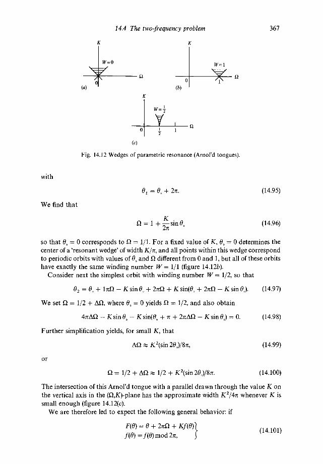
= 1 + (14.96)2ir
so that 0 corresponds to = 1/1. For a fixed value of K, 0 determines thecenter of a 'resonant wedge' of width K/it, and all points within this wedge correspondto periodic orbits with values of 0 and 1, but all of these orbitshave exactly the same winding number W = 1/1 (figure 14.12b).
Consider next the simplest orbit with winding number W = 1/2, so that
02 = 00 + — KsinO0 + + Ksin(0, + 2irc� — KsinO0). (14.97)
We set Q = 1/2 + where 00 = 0 yields = 1/2, and also obtain
— Ksin 00 — K sin(00 + it + — K sin = 0. (14.98)
Further simplification yields, for small K, that
K2(sin 200)/8ir, (14.99)
or
= 1/2 + 1/2 + K2(sin2O0)/8it. (14.100)
The intersection of this Arnol'd tongue with a parallel drawn through the value K onthe vertical axis in the has the approximate width K2/4ir whenever K issmall enough (figure 14.12(c).
We are therefore led to expect the following general behavior: if
14101f(0)=f(0)mod2it, . )
(a)
0
K
(b)
14.4 The two-frequency problem 367
K K
w4
011(c)
Fig. 14.12 Wedges of parametric resonance (Arnol'd tongues).
01 = + 2ir. (14.95)
with
We find that

368 Damped-driven Newtonian systems
then under suitable differentiability conditions and for rational winding numbers,
W=P/Q, (14.102)
we should solve for cycles by using
= + 2irQW= 0, + 2irP (14.103)
to obtain
0, + 2irQQ = 0, + 2irP (14.104)
where f(Q) is obtained from functional composition. We can write c� = P/Q + inorder to obtain the shape of the resonant wedge for a cycle with rational windingnumber W = P/Q, where = umax — is the width of the wedge. By thismethod, it is possible to understand that wedges of parametric resonance grow fromevery rational winding number on the a-axis.
When K = 0, the quasiperiodic orbits occupy all of the space on the and theperiodic orbits are confined to the countable point set where is rational. In order tounderstand qualitatively how, for finite K, the winding numbers of quasiperiodic orbitscan define a Cantor set of finite size, and where the complementary set is a devil'sstaircase of resonant wedges, we make the following observations. Every rationalnumber gives rise to a resonant wedge of finite width for finite K, and we can choose toorganize the rational winding numbers W = P/Q according to numerators Q ofincreasing size: 1, 1/2, 1/3, 2/3, 1/4, 3/4, 1/5, 2/5, 3/5, 4/5, . . . ,0. This is a nonintuitiveproperty of the continuum that is hard to imagine geometrically, and the closest that wecan come to a visualization is to plot the corresponding devil's staircase: if, for fixedK < 1, we remove the width of each resonant wedge from the a-axis, then what is leftover is a Cantor set of bare winding numbers that give rise to quasiperiodic orbits: theremoval of infinitely many closed intervals (the resonant wedges) from the unit intervalon the c�-axis leaves behind a Cantor set of open sets. The nonintuitive part is that it ishard to see how wedges of finite width growing from every rational value of c� do notimmediately overlap for any finite value of K > 0. The plot vs K would represent adevil's staircase of resonant wedges, that is geometrically similar to figure 14.10. Toshow that the wedges do not overlap for 0 <K < 1 we must compute the sum of thewidths of all wedges in 0 <Q < 1 and show that the sum is less than unity. We nextestimate the sum of all tongue widths for the case where K is very small.
Notice that for each value of Q there are at most Q — 2 different winding numbers(this is an overestimate for Q), excepting the case W = 1/2. Assume for simplicity thatall cycles with the same denominator Q have tongue widths no greater than on theorder of We can now show that the devil's staircase takes up an amount of space onthe order of K whenever K is small. A simple series summation shows that (to within aconstant factor)
(14.105)Q=3
where is the amount of space in [0,1] on the a-axis that is occupied by the devil'sstaircase. The result is consistent with the facts that (i) the K = 0 set occupies no space,and (ii) the resonant wedges grow continuously and smoothly from the K = 0 set. The

14.4 The two-frequency problem 369
proof that the wedges take up very little space for very small K is only a variation on theusual proof that the rational numbers take up no space at all (as we showed in the lastsection). For small K, therefore, the c� values that give rise to irrational values of thewinding number Woccupy a Cantor set with finite length 1 — 1 — 3K, whichis nearly the entire unit interval for K small (as indeed it must be). Both the staircase andthe complementary Cantor set have fractal dimension equal to unity for small Kbecause both sets have finite length. But what happens to these dimensions as Kapproaches unity?
Bohr, Bak, and Jensen (1984, 1985) have used a numerical analysis to show that, asK -+ 1 -, 'St —* 1 - as well', and have obtained numerical evidence for the scaling law
1— as 1 (14.106)
for the size of the Cantor set near the point where the circle map becomesnoninvertibie. In other words, the quasiperiodic orbits at K = 1 have winding numbersthat originate in bare winding numbers that occupy a fractal set with zero size. Bohret al. have numerically estimated a fractal dimension of D 0.87 for that zero-lengthCantor set. For details, we refer the reader to the literature (Cvitanovic et al., 1985,Schuster, 1988, or McCauley, 1993). We return now to the reason why periodicityseems to win over quasiperiodicity in two-frequency systems in nature, at least withinthe nonchaotic regime.
Frequency locking was first observed and reported in the seventeenth century by theHoliander physicist Christian Huyghens, who observed that two separate clocks on awall tended to synchronize with each other after a while. This suggests the qualitativeidea of an attractor, and indeed the tendency to frequency locking in nature can beunderstood by using the idea of attracting periodic orbits: because the invertible circlemap with an irrational winding number is conjugate to the linear circle map by acoordinate transformation, every stable quasiperiodic orbit necessarily has a vanishingLiapunov exponent (this means that the Liapunov exponent at a wedge boundary iszero, which can be easily checked for the W = 0 and 1 orbits discussed above). In otherwords, stable quasiperiodic orbits of the nonlinear circle map do not attract nearbyorbits. However, the stable periodic orbits of the nonlinear circle map have negativeLiapunov exponents, which means that they do attract nearby orbits, and this providesa practical mechanism for frequency locking. For example, the Liapunov exponent ofall orbits of the sine circle map with W = 1/1 is given by
1 = in 1 — [K2 + — 1)2]h/2 (14.107)
so that the stability range of the orbit with W = 1/1 and 0,, = 0, for example, is0 <K <2 because that is the range where simultaneously (i) the 1-cycle is stablebecause f'(O) has magnitude less than unity, consequently (ii) 2 <0. Note that thestability range for this particular periodic orbit extends to K = 2, whereas allquasiperiodic orbits have become unstable (and so 1> 0 may occur) whenever K> 1.Note also that 2 = 0 at the wedge boundaries where
= 1 ± K/2ir, (14.108)
as expected.
k —* 1 means 'as k approaches unity from below (k < 1 and k —+ 1).

370 Damped-driven Newtonian systems
We want to show next that the orbits with rational winding numbers becomeunstable through period-doubling bifurcations. Each unstable orbit has a positiveLiapunov exponent, but we expect that chaos does not set in until all periodic orbitshave become unstable: so long as there is at least one attracting periodic orbit, orbitsthat are repelled by any of the unstable periodic and unstable quasiperiodic orbits willstill have a relatively calm 'resting place' unless one chooses initial conditions that lieprecisely on an unstable quasiperiodic or unstable periodic orbit. Choosing initialconditions that lie on an unstable quasiperiodic orbit is not so easy, however: thewinding number Wis not a parameter that is easily accessible to control, in practice, inthe laboratory.
The circumstances with the logistic map are entirely similar: for the fixed pointx = 1 — lID, the Liapunov exponent is). = ln I (D — 2)1 and is negative for 1 <D <3,which is the stability range of that fixed point. When D > 3, the fixed point has apositive Liapunov exponent but this does not cause any chaos so long as there are otherstable cycles for the trajectories to settle onto. The idea of chaos requires boundedmotion (self-confined motion, for example) with mutually repelling orbits: for anychoice of initial conditions in the relevant region in phase space, all nearby orbits mustrepel each other because each orbit has its own positive Liapunov exponent. Accordingto Feigenbaum (1980) period doubling may be ubiquitous in nature, as the mechanismin nonlinear dynamics whereby unstable periodicity can develop out of stableperiodicity via pitchfork bifurcations. Therefore, let us look next for evidence of perioddoubling in the sine circle map.
In order to illustrate period doubling for an analytically calculable example, we lookat the 1-cycle with W = = 1/1 so that 00 = 0. This 1-cycle is stable so long as0 <K <2, as we have shown above, and is unstable for K> 2. If period doublingoccurs, this 1-cycle cannot give birth to a 2-cycle with W = 1/2. This would begeometrically impossible, as the two points on the 2-cycle have to coalesce into thesingle point 00 = 0 as K approaches 2 from above. The only possibility that is allowedby the geometry of the circle map is that W = = 2/2. This 2-cycle is geometricallypossible: the equations of the 2-cycle are (with 02 = + 4ir)
= 00 + 2x — KsinO0(14 109)
00 = — 2ir — KsinO1.J
In this case, with W = 2/2, undershoots by the amount K sin 00 in a single2ir-revolution, and in the next 2ir-revolution 01 + it falls short of by the amountK sin which tells us that we must have sin = — sin for periodicity. With 00 > 0,
this means that 01 = 2iv — This combination permits the coalescence of both andinto a single value at the bifurcation point K = 2. Here, we quote Feigenbaum
(1980), who said it very well:
• . . for some range of parameter values, the system exhibits an orderly periodic behavior; that is,the system's behavior reproduces itself every period to time T. Beyond this range, the behaviorfails to reproduce itself after Tseconds; it almost does so, but in fact it requires two intervals ofTto repeat itself. That is, the period has doubled to 2T. This new periodicity remains over somerange of parameter values until another critical parameter value is reached after which thebehavior almost reproduces itself after but in fact, it now requires 4Tfor reproduction. .
Going on with the mathematics, equations (14.109) simplify to read
Ksin6, = (14.110)

Exercises 371
which has solutions if K > 2 but not if K <2. Next, we look at stability of this 2-cyclethat is born of a pitchfork bifurcation at K = 2.
For stability, we need — 1 <f'(0,)f'(01) < 1, which reduces to the single equation(1 — K cos < 1. Instability occurs whenever (1 — K cos = 1. There are threepossibilities, but one is eliminated by the second of the pair of conditions that followfrom the numeric solution of
1 — KcosO0 = —1. (14.111)
Using this condition along with equation(14.11O), it follows that = (K2 — 1)1/2, andinstability occurs whenever the equation
02sin
= (2 +(14.112)
has a solution. The first solution is at K1 = = 0), the second falls at a parametervalue K2 corresponding to an angle 00 that falls short of x/2 by a finite distance. ForK1 <K <K2 the 2-cycle is stable, as can be seen from returning to the stabilitycondition (1 — K cos < 1, which is simultaneously the condition that the 2-cyclewith W = 2/2 has a negative Liapunov exponent. At K > K2 the 2-cycle persists inunstable form and a stable 4-cycle occurs. We refer the reader to the paper by Perez andGlass (1982) for further details of the rich 'phase diagram' that emerges from perioddoublings within mode lockings as well as the application of circle map dynamics toheartbeat rhythms.
Exercises
Period doubling (bouncing ball)
1. Why, physically, should the 1-cycle become unstable merely because q50 deviatestoo far from 0 as y approaches Ymax? What is beneath the mathematics of thisinstability?
2. Plot qualitatively the motions of the ball and table vs time for the case where n = 3,
k =6.
3. Determine the upper stability limit y' for the ball's 2-cycles. If the algebra is toodifficult, then determine y' numerically to within two decimals.
4. Perform numerical integrations (using n = 1) and show that the ball's orbitchanges systematically from a 1-cycle to a 2-cycle to a 4-cycle as the parameter y isincreased steadily from Ymin = 2ir(1 — ci). (For example take = 1/2.)
5. Show numerically that, for Y > Ymax, the map has two separate solutions that areboth different from cos = 2irn(1 —
6. Obtain numerical evidence for chaotic motion when y is large enough. Are thereany windows of stability (e.g. cycles of odd order) imbedded within the chaoticregime y >
Period doubling (logistic map)
7. For the 1-cycle at x = 1 — 1/D, show that A = lnI2 — D . Show, therefore, that the
orbit is stable for 1 <D < 3. Observe that A = In 2 at D = 4.

372 Damped-driven Newtonian systems
8. Solve for the location of the 2-cycle and show that the stability range isD1 <D <D2 with D1 = 3 and D2 = 1 + In particular, compute the Liapunovexponent for the 2-cycle. Show that 2 = 1/2 ln I 2D + 4 —
Iand that (i) 2 <0 for
9. Locate the 'window of stability' of the 3-cycle of the logistic mapf(x) = Dx(1 — x).
Circle map
10. For the damped-driven pendulum, choose a set of parameter values (/3,w0,w),integrate the differential equation numerically, and plot
1vs 0,, for different
values of K. For K not too large, can you represent your results in the form of acircle map 0,, + = 0,, + — K'f(O,,)? If so, what are and K'? (Hint: transformto dimensionless variables before integrating the differential equation.)
11. For K small and for both W = 1/3 and W = 2/3, determine f�(K,00) and also thetwo tongue widths.
12. Show numerically that for K > K2 the 2-cycle with = 2/2 and W = 2/2bifurcates into a 4-cycle. What is the winding number of the 4-cycle?
13. For the orbits with W = 2/2 and K1 <K <K2, prove that the Liapunov exponentvanishes along the wedge boundaries.

15
Hamiltonian dynamics and transformations inphase space
15.1 Generating functions for canonical transformations
If we start with a Lagrangian L, then the formulation of dynamics is covariant withrespect to general coordinate transformations in configuration space. The Lagrangiantransforms like a scalar under those transformations. Given any Lagrangian ingeneralized coordinates, one can construct the corresponding Hamiltonian as afunction of the coordinates q1 and the canonically conjugate momenta and the phaseflow description of dynamics follows. Because the generalized velocities generally donot transform like the components of a vector in configuration space, Hamilton'sequations are themselves not covariant with respect to general coordinate transform-ations in configuration space. Also, if we start with a Hamiltonian system then anarbitrary point transformation of the 2fcoordinates (q1, .. .
in phase space generallywill not yield another Hamiltonian system. Whether the transformed equations are orare not Hamiltonian does not take away from their correctness or usefulness: everytransformed set of equations is correct if the starting point is correct and if thetransformation is carried out without making an error. If we restrict the class by askingfor the collection of transformations in phase space whereby any Hamiltonian system istransformed into another Hamiltonian system, then we arrive at the subject of thischapter: the transformations that are called canonical.
It is possible to define canonical transformations in the following way. Phase space isa flat differentiable manifold with Cartesian coordinate axes labeled by the canonicallyconjugate variables (q1, . . .
whether or not the generalized coordinates areCartesian or curvilinear in a corresponding Lagrangian configuration space. Canonicaltransformations can be defined as transformations that leave invariant the Cartesianphase volume element dQ1 = dq1 . . . dq1dp1 . . . dpf, and consequently the correspond-ing incompressibility condition for the velocity in phase space,
(15.1)
Canonical transformations are thereforej ust transformations among Cartesian coordi-nate systems in the phase space of canonicalf degree of freedom systems, Lagrangianconfiguration space is a metric space and is Riemannian in the presence of constraints.The q-submanifold of phase space is Cartesian without a metric and coincides withLagrangian configuration space only if the latter is Euclidean and only if Cartesiancoordinates are used there. Otherwise, the q-subspace of phase space and configurationspace are entirely different manifolds. In other words, the reader must recognize that,even though the same variables q- are used to label axes in both cases, the two spaces aregeometrically different from each other: one manifold is always flat with Cartesian axes

374 Transformations in phase space
while the other manifold may be curved and the generally label curvilinear, notCartesian, axes.
We will not follow the path outlined above but will follow an equivalent path. Theinvariance of the Cartesian phase volume element can then be derived as a consequenceof our starting point. Consider a Hamiltonian system
(15.2)
withf degrees of freedom and consider also a transformation of the 2f coordinates inphase space'
Q. = = (15.3)
where (q,p) denotes a point in phase space and therefore is shorthand notation for the 2fgeneralized coordinates and canonical momenta (q1, . . . ,q1,p,, . . . ,p4. Whether thisHamiltonian description follows from a Lagrangian or simply from the incompressibil-ity condition for some other kind of flow is irrelevant in all that follows. The main ideais the condition that the transformation yields another set of canonically conjugatephase space variables (Q,, .. . ,P1), with Hamiltonian K(Q,P,t) so that
(15.4)
Whenever this is true, then we call the transformation (15.3) canonical.Our starting point for deriving the condition that the transformation (15.3) is
canonical is the action principle. We can derive the first set of canonical equations fromthe action principle with all end points q,(t,) and fixed,
f t2 1
— (15.5)
and the second set follows from
= — K)dt= (_ —
+ — (15.6)
also with all end points and fixed. If both sets of dynamical equations are tofollow from varying only the first action A,, then it follows that the two separatedifferential forms in the integrands for A1 and A2 must differ by a closed differential:
1 1dS
=— Hdt)
—
P.dQ1 — Kdt). (15.7)
This yields A1 = A2 + S(t2) S(t1), so that öA1 = 5A2. Formally, this is an extension
Our transformations are related to those known in the older literature on geometry as contacttransformations. The terminology was introduced by Lie and is explained in the texts by Sommerfeld(1964) and Whittaker (1965).
15.1 Canonical transformations 375
of our earlier treatment of gauge transformations, but whereas the form of S in that casewas such as to yield exactly the same equations of motion from both A1 and A2, thiscase is different: K and H are generally not the same function, so that the two differentHamiltonian systems, related by a coordinate transformation, generally providedifferent mathematical descriptions of the same mechanical system (the exception tothe rule occurs in the case of a symmetry transformation, in which case H is invariant).
The function S is called the generating function of the canonical transformation(15.3). It follows that S(q,Q,t) satisfies the conditions
(15.8)
The condition that dS = L1dt — L2dt is a closed differential is nontrivial: each separatecontribution to dS is generally not closed2 and generally yields a path-dependentintegral A1. Path-dependence formed the basis for deriving Lagrange's equations ofmotion from the action principle in chapter 2.
Therefore, the condition that the transformation is canonical is satisfied if thegenerating function S can be constructed. The generating function provides a des-cription of the transformation in the form
p, = = g1(q,Q,t), P1 =—
= h1(q,Q,t). (15.9)
These equations must, in principle, be solvable for the original form of the transform-ation: Q1 = 4.(q,p,t) and P1 = as well as for the inverse transformation, where(q,p) are expressed as functions of (Q,P,t). Therefore, the generating function S(q,Q,t)provides a potentially complete description of the canonical transformation, anddetermination of the generating function determines the new Hamiltonian as well:
(15.10)
Note that the Hamiltonian transforms like a scalar function, K(Q,P,t) == H(q,p,t), only if the canonical transformation is time-indepen-
dent. If the reader has followed the discussion of Noether's theorem in chapter 2, then itwill come as no surprise that canonical transformations (15.3) that leave theHamiltonian invariant, those yielding H(q,p,t) = H(Q,P,t), which means that K and Hare the same function, will play a very special role in the search for solutions ofHamilton's equations (chapter 16).
Notice also that, on the right hand side of the expression for dS, there are 4f phasespace variables (q,p,Q,P), but only 2f of these are independent. Above, we have chosenthose 2f to be (q,Q) in our discussion of the generating function, but this is not the onlychoice: there are three other possibilities, (q,P), (Q,p), and (p,P), all of which can bereached by Legendre transformations. For example, with the notation F1 = S, then
IF2 = F1 + Q.P1 (15.11)
i= 1
also satisfies the condition that the two original differential forms differ by closeddifferential form, and we have a description of the same canonical transformation in
2 We show in chapter 16 that Ldt is closed for integrable canonical systems.

376 Transformations in phase space
terms of the generating function F2(q,P,t):
(15.12)
Notice that this means that when both F1 and F2 are expressed in terms of the variables(Q,P,t), then
—(15 13)
because we have the same transformation and the same Hamiltonian K in either case.With
F3 = F1 — (15.14)
we obtain
(15.15)
while
F4 = F3 + (15.16)
yields
(15.17)
It is possible to write down the generating functions for several relatively simplecanonical transformations. The first and most important of these is the identitytransformation which is given, for example, by
fF2
=(15.18)
Direct calculation yields Q1 = and P. =Second, general coordinate transformations in configuration space, the subject of
much of chapter 2, are canonical:
IF2
= k=1. (15.19)
yields
..,q1,t) and p1 = (15.20)
where we have used summation convention in order to illustrate the result in thelanguage of chapter 2 (the canonical momentum transforms like the covariant

15.2 Poisson brackets, symmetry, and conservation laws 377
components of a configuration space vector). This is interesting: Hamilton's equationsare not covariant under these transformations, but that does not matter because thegeneral coordinate transformations of Lagrangian theory are only a subset of the muchlarger collection of canonical transformations. 'Manifest covariance' of dynamicalequations is sometimes an important tool, but it is not necessary in order to formulatephysics correctly. For the latter, one needs empirically correct invariance principles andequations of motion that reflect them, covariant or not.
Third, orthogonal transformations (including time-dependent transformation torotating frames) are a subset of general configuration space transformations andtherefore also are canonical.
Fourth, we can write a generating function that interchanges the labeling of thephase space variables: F1 = yields = and = — In the originalformulation of Lagrangian dynamics starting with L = T — U, the coordinates labelparticle positions whereas the canonical momenta are derivatives of the kineticenergy with respect to the generalized velocities Therefore, in the Lagrangiandescription, there is no equivalence of q and p. However, there are Hamiltonian systemswhere this interchange transformation leaves the Hamiltonian invariant: the simpleharmonic oscillator written in the rescaled form H = (p2 + q2)/2 is only one example.Here, in the phase flow picture, there is no difference whatsoever between thecoordinates q and p, and there are other systems with this kind of invariance (pointvortices in the plane are another example).
Finally, we can see that the collection of all canonical transformations forms a group.First, starting with
f IdS = — P.dQ1 + (K — H)dt, (15.21)
i=1 i=1
we see that the transformations dS12(q,Q) and dS23(Q,q') can be carried out sequen-tially, but also can be combined to yield the direct transformation described bydS13(q,q') = dS12(q,Q) + dS23(Q,q'), so that we have a group combination law forsuccessive transformations. The reader can check to verify that this combination law isassociative. Above, we have shown that the identity can always be constructed, and it isclear that the inverse of dS12(q,Q) is dS21(Q,q) = — dS12(q,Q). Therefore, all of theconditions for a group are satisfied.
15.2 Poisson brackets and infinitesimal transformations: symmetry, invariance, andconservation laws
We can introduce the relevant Poisson brackets in a simple way. Consider any pointfunction F(q,p,t) of the 2f phase space variables and the time t. Then
dF 1 '\ 3F 3F=
++
=
____
—+ (15.22)
which we can write as
= {F,H}qp + (15.23)
where

378 Transformations in phase space
I{F,G}qp
= —
(15.24)
is called the Poisson bracket of F with G, evaluated in the (q,p)-coordinate system3. Inparticular, Hamilton's equations can be written as
= {q1,H} and = (15.25)
In fact, all derivatives in phase space can be expressed in terms of Poisson brackets. Thefundamental Poisson bracket relations are
= = 0, and = 0, (15.26)
where = = — and are called canonically conjugate variables, andwe could identify as the Kronecker delta öjk were it not for the antisymmetrycondition {pk,qk} = — {qk,pk} = — 1.
The important point to be proven now is that all Poisson bracket relations for scalarpoint functions F and G are invariant under canonical transformations. To show this,we can begin with the generating functions and use them to derive a direct way todetermine whether a given set of variables is canonically conjugate. This will lead usautomatically to the invariance of Poisson bracket relations.
The idea is to find conditions that guarantee that the transformation from the system
3H.(15.2)
actually yields
(15.4)
with
K = H + (15.27a)
We illustrate the proof using notation for f= 1 for simplicity, but the proof goesthrough in the same way forf> 1. Starting with Q = 4(q,p,t) and P = have
(15.28)op Ot Oq Op Oq Oq Ot
Using
(15.27b)
then yields
— OQ OK OQ 02S OQ OK + (15 29 )— Op Oq OtOp Op Oq Op OqOt
+ . a
This differs from the definition of Poisson brackets introduced in chapter 7. We show the connectionbetween the two definitions below.
15.2 Poisson brackets, symmetry, and conservation laws 379
which we can rewrite as
3Q a2s aQ(aKaQaKaP— aq ap 3p) 3q ôtôp op Oq OPOq
OQ+ + —. (15.29b)
Op OqOt Ot
We can rearrange this to read
OQOQ'\OK(OQOP OQOP
Op Op Oq) OPk\Oq Op OpOq
(1529c)Oq OtOp Op OqOt Ot'
and also
(15,29d)
From the condition that
= (15.29e)
we obtain two results. First, it is necessary that
{Q,P}qp = 1. (15.30)
Second, using
OF2 OF2(15.31)
we see that we need
5 — O2S1532
Ot Sq,p — OPOt(
in order that
I Os) o2s o2s— + = — +
OtOP=0. (15.33)
However, it follows from a short calculation that for arbitrary scalar phase spacefunctions F'(Q,P) = F(q,p) and G'(Q,P) = G(q,p),
{F',G'}Qp = {F,G}qp{q,p}Qp, (15.34)
so that all Poisson bracket relations are preserved under canonical transformations ifthe fundamental bracket relations (15.26) are preserved. Under these circumstances, itfollows that
{Q,F}q,p = (15.35)
of which the condition (15.32) is only one special case. In other words, the invariance of

380 Transformations in phase space
the fundamental bracket relations under canonical transformations guarantees that allother Poisson bracket relations are preserved as well:
{F',G'}Qp = {F,G}qp{q,p}Qp = {F,G}q,p. (15.36)
Likewise, with p = we obtain
—Th,li . . — ôpôK 3paK ?4i
1 7(5.3)
Using
(15.27a)
yields
— ap(aH aq ap"\ op 02S Op(OH Oq OHOp
oP Op OP) OQ OtOP OQ+
a
This can be rearranged to read
OH ( OS)= — + + (15.38b)
Using
OF2 OF2p = and Q = (15.39)
it is necessary that
C On 02s(15.40)
OtJQP Ot OqOt OtOq
and
{q,p}Qp = 1 (15.41)
in order that
j3= (15.42)Oq
is satisfied.Continuing similarly, one can prove quite generally that all of the fundamental
bracket relations = = 0, and = 0, are preserved under generaltime-dependent canonical transformations. It follows that all Poisson bracket relationsof scalar functions are preserved as well, so that it makes no difference which set ofcanonically conjugate coordinates and momenta one uses to evaluate them. In otherwords, we can drop the subscripts {'}q,p or on Poisson brackets and use anycomplete canonical set of variables to evaluate a set of Poisson bracket relations.
The invariance of the Euclidean scalar product under the symmetry operations ofEuclidean space defines the objects that are left invariant (are left similar to themselves)

15.2 Poisson brackets, symmetry, and conservation laws 381
under those transformations. According to F. Klein, and more generally, the geometricproperties of any space are defined by the objects that are left invariant under a group oftransformations, so that it is always a transformation group that defines the metricgeometry of a space. Straight lines transform into straight lines, circles into circles, andrigid bodies into other rigid configurations of themselves under rigid translations andrigid rotations, the basic symmetry operations of Euclidean space. As we have notedabove, the phase space of Hamiltonian systems has many properties similar toCartesian coordinates in Euclidean space but there is no idea of a distance between twopoints (no metric) in phase space. However, Klein's idea still applies: the invarianceproperty that defines the geometry of phase space, which was called symplecticgeometry by H. Weyl, is simply a certain tensor (section 15.6) that guarantees thepreservation of scalar Poisson brackets relations under canonical transformations. Inthe modern mathematics literature canonical transformations are called symplectic,and canonically conjugate variables are called symplectic coordinates. Since there is nometric, the invariances of symplectic geometry are qualitative, like the idea of theinvariance of the nature of a Cartesian torus under differentiable coordinate transform-ations. Tori turn out to be important for bounded motion in Hamiltonian dynamics(chapter 16) because, with symplectic coordinates (q1,. . . ,p1) we are always working ona flat manifold, and the torus is the only closed, orientable Cartesian manifold. In phasespace in general, we are not interested in the idea of metric invariance but concernourselves with the more useful idea of topologic invariance, the idea (for example) thatsimple closed curves are equivalent to a circle, and that integrable systems areequivalent to a set of translations at constant speed. Constant speed translations canoccur on any surface, curved or flat, and the closed manifolds of bounded motion ofintegrable noncanonical flows are typically curved rather than flat.
Consider next a one-parameter continuous group of canonical transformations
= = = = (15.43)
where each transformation in the group is generated by varying the group parameterand where = 0 yields the identity: = = and = P•(O) = Assume alsothat is a canonical parameter for the transformation group (see chapters 7 and 12 forthe definition of a canonical parameter). For an infinitesimal transformation, we write
Q. = q, + and P. = p, + (15.44)
where
= and = (15.45)
Since the fundamental Poison bracket relations must be satisfied,
{Qi'Pk}q,p = {qi,pk}q,p = tik, (15.46)
it follows that
{öqj,öpk}qp = 0 (15.47a)
to first order in Written out explicitly, this states, for i = k, that
(15.47b)

382 Transformations in phase space
for each i = 1,. . . But this is just the requirement for a divergence-free velocity field= in phase space, one where the canonical group parameter a
plays the role of the 'time'. That is, the velocity field must be given by a stream functionG:
—and
—1548
dx — da — ( . )
The Hamiltonian form of these equations is not accidental: every one-parametercontinuous group defines a flow in phase space (see chapter 7), and whenever that flowis phase-volume-preserving (is divergence free4), then the flow can be put into canonicalform by finding a stream function, or Hamiltonian, G. The Hamiltonian G is called theinfinitesimal generator of the group of transformations, and a, the canonical groupparameter, is analogous to the time (a obeys an additive group parameter combinationlaw). It follows without fanfare that the Hamiltonian H is the infinitesimal generator ofa dynamical system where the canonical group parameter is the time t (this is half of themeaning of 'canonical' in the context of Hamiltonian mechanics — the other half of themeaning is stated below). We now see what the Hamiltonian formulation accomplishes:it places all volume-preserving flow in phase space on an equal footing, because everydivergence-free flow defines a set of stream functions Gk that generate the group. For aone dimensional group, whether the group parameter is the time t or some othercanonical parameter is unimportant for the development of the mathematical theory.
An example of an infinitesimal generator is the angular momentum about some axis,say, the x3-axis where (x1,x2,x3) are Cartesian coordinates: with G =M3 = = (x1p2 — x2p1), where p3 = we obtain
dx1 — — dx2 — — dp1 — dp2 — 3G— 15 49—h——— ( )
which are the differential equations of an infinitesimal rotation about the x3-axis inphase space. We leave it as an easy exercise for the reader to integrate these equationsand obtain the form of the finite rotations.
An even easier example is that of translations along the Cartesian (q1,.. .
coordinate axes in phase space. If we take G = — then we get a pure translationalong the pk-axis, whereas G = Pk yields a pure translation along the
Now, we can connect the infinitesimal generator to the generating function. It is easyto verify by direct calculation that the generating function F2 is given, to first order in
by
fF2(q,P) + öaG. (15.50)
1=1
That is, this expression defines the generating function near the identity (S. Lieintroduced and developed the method of studying groups of transformations near theidentity). To first order in 5a, we obtain from this the equations of the infinitesimaltransformation
Liouville's theorem is satisfied by every flow that is generated by a stream function G; that is, the 2fdimensional phase space volume element is preserved under the canonical transformations of the group. Itis possible to prove even more generally that the phase space volume element is preserved under allcanonical transformations.

15.2 Poisson brackets, symmetry, and conservation laws 383
= and op1 = — (15.51)pi
Under the infinitesimal transformation generated by G, a scalar phase space functionF(q,p) changes by the amount
dF = OaXF = Oa{F,G} (15.52)
where the first order differential operator X is defined by
3GÔX = { ,G}
=. (15.53)
We can construct the finite transformation by iterating the infinitesimal transform-ation. Since
F + dF = (1 + OxX)F, (15.54)
iteration with = a'/N yields the finite transformation in the form
= (15.55)
where
(i + (15.56)
Equally directly, we can write
= F(q,p) + + +
= F(q,p)+ OCLXF + + ... = (15.57)
where = is the group operator, and is analogous to the time-evolutionoperator. Clearly, we assume here that the symmetry generated by G is globallyanalytic except for isolated singularities (see section 7.6 for a brief discussion of theconvergence of series representations of group operators).
In particular, the finite transformations of the group are given by
= = and = = (15.58)
At this stage, it is a good idea to have an example. With G = M3 = (x1p2 — x2p1) andp1 = we have the generator of rotations in the (x1,x2)-plane, and = 0 is therotation angle. Let's calculate x1(0) = U(0)x1 = fr1(x1,x2,p1,p2,0) as an exercise. Byusing the fact (easy to prove) that
{A,BC} = {A,B}C + B{A,C}, (15.59)
we obtain from the fundamental bracket relations that Xx1 ={x1,x1p2 — x2p1} = — x2, X2x1 = — Xx2 = — {x2,x1p2 — x2p1} = — x1, X3x1 =— Xx1 = x2, and X4x1 = Xx2 = x1, so that the circle closes. This yields, by resumma-tion of the power series in 0, that
x1(0) = = x1 cos0 — x2 sin 0, (15.60)
so that we have calculated the transformation function (it is independent of the p.because rigid rotations do not mix coordinates and momenta). It is equally easy tocalculate the other three transformation functions.

384 Transformations in phase space
There is a deep connection between invariance principles, symmetries, and conserva-tion laws that we can now express in a very beautiful and useful form, a form thatfollows from treating all group generators on an equal footing with the Hamiltonian,which is the generator of translations in time.
As we have pointed out above, under an infinitesimal transformation generated by G,a scalar phase space function F(q,p) changes by the amount
dF = = (15.52)
where the operator X is defined by
X = { ,G}=
(15.53)
Therefore, functions that are invariant under the transformations generated by Gsatisfy the first order partial differential equation
XF = {F,G} = 0. (15.61)
It follows from this, combined with the time-evolution law
dF/dt = {F,H}, (15.62)
that a conserved quantity leaves the Hamiltonian invariant and therefore generates acontinuous symmetry operation on the dynamical system. The point is simple and followsfrom a two-pronged interpretation: regarded as
= {G,H}, (15.63)
{ G,H} = 0 means that G is conserved. Regarded as
= {H,G}, (15.64)
{G,H} = 0 means that the Hamiltonian is left invariant by the one-parameter group oftransformations generated by G. For example, a rotationally symmetric Hamiltonian isone where = 0 for all three components of the angular momentum (becausethe M. are the generators of infinitesimal transformations in the three mutuallyperpendicular Euclidean planes), and this means that all three components of angularmomentum are conserved by the motion of the dynamical system. In general,conservation laws generate symmetries of the dynamical system and vice versa. Thisillustrates the deep connection between symmetry, invariance, and conservation lawsthat holds both in classical and in quantum mechanics (recall our discussion ofNoether's theorem in chapter 2).
More explicitly, let us consider the case where the Hamiltonian H is invariant underrotations in the (x,y)-plane. Here, the angular momentum = — is theinfinitesimal generator of rotations about the z-axis, and rotational invariance yieldsthe first order partial differential equation
3H oH OH OH= — + — = 0. (15.65)

15.2 Poisson brackets, symmetry, and conservation laws 385
This yields (if we integrate (15.65) using the method of characteristics, as in Duff, 1962,for example) that if we use four Cartesian variables then H can only have theform H can depend only upon thecoordinates and momenta in combinations that are left invariant under a rotationabout the z-axis.
Finally, we have observed that the Hamiltonian flow is a Lie group flow where theinfinitesimal generator is the Hamiltonian H and the group parameter is the time t.That is, the motion of the dynamical system is a canonical transformation in phasespace:
= and = (15.66)
where (q,p) denote the 2f initial conditions (q1(O),. . . ,p,.(O)), and
{qj(t),pj(t)}qp = = 0, and {pj(t),pj(t)}qp = 0. (15.67)
In section 6.4, in order to prove that the return map
=1? (69)
=
for a two degree of freedom Hamiltonian system is area-preserving, that= we showed that this property follows if the fundamental
Lagrange brackets
[q/t),qk(t)] = 0, = 0, = öjk (6.24a)
are time-translational invariant, which would mean that
= 0, = 0, = (6.24b)
but where the Lagrange brackets in (6.24a) and (6.24b) are defined with respect to thevariables (q1(t), . . . ,pf(t)):
[F G] — (6 22)— 3(F,G)
We now prove that the fundamental Lagrange bracket relations are invariant underarbitrary canonical transformations. Let u, =J(q1,. . . ,p1) denote any 2f variablesconstructed from the (q1, . . . ,p1) by By 2f independent variables wemean that
(15.68)
Consider next the sum
= (15.69a)1 1 l,k,m (qm,pm)
where we temporarily define Lagrange brackets with respect to canonical variablesdenoted as (q1, .. . ,p1):
f
i=1 '

386 Transformations in phase space
By direct expansion of (15.69a), requiring only two lines of calculus, we obtain
= k,,n= 1
+ = = (15.69b)
Next, let (Q1,. .. be any other set of canonically conjugate variables obtained from(q1, . . . by a canonical transformation. Since the variables (Q1,
. .. ,P1) satisfy the
fundamental Poisson bracket relations
{Q1,Pk} = = 0, and = 0 (15,69c)
with respect to the original variables (q1,. . . ,pf), it follows from inserting (15.69b) into(15.69c) that the Lagrange bracket relations
= 0, [P3,Pk] = 0, = (15.71)
also hold with respect to the variables (q1,. . . 'p4. In other words, like the fundamentalPoisson bracket relations, the fundamental Lagrange bracket relations are canonicalinvariants. Consequently, the iterated map (6.24a) is area-preserving because theintegral
I'2
=JJ'dq1dPi (6.19a)
is invariant under canonical transformations.Consider next the closed line integral
(15.72)
in an n dimensional phase space where M is a vector. By Stokes' theorem
= — (15.73)1 &k 1 Xk
then (6.19a) becomes
I I
=(15.74)
which shows that the closed loop integral on the left hand side of(6.19a) is also invariantunder canonical transformations. This result is essential for the discussion of integrabil-ity in the next chapter.
15.3 Lie algebras of Hamiltonian flows
The generalization to a multiparameter group of transformations is immediate: with mgroup parameters = . then QL = and P1 = yield
fF2(q,P) q.P1 + &çGq (15.75)
15.3 Lie algebras of Hamiltonian flows 387
and the infinitesimal transformations are given by
(15.76)
opi = — p1 —Pi
which is a generalization of the equations of Hamilton to the case of several differentinfinitesimal generators Gk in a multiparameter flow. In this case, a scalar phase spacefunction F(q,p) transforms according to F —* F + dF where
dF = +=
(15.77)
and the operators are defined by
x —G 1578
——
in terms of the m different velocity fields of the rn-parameter group flow
(15.79)ap,
and the phase space gradient V.Recall that in chapter 7, where we did not restrict to Hamiltonian or even to
conservative systems, we arrived quite naturally at the following definition of a Poissonbracket of the velocity fields for two different flows:
(15.80)
for phase space variables (x1,. . . which we can now take to be (q1,. . . ,p4 withn = 2f We also showed that Lie's integrability condition, the condition that the pointtransformations
= and P, = (15.81)
exist globally, is satisfied whenever the m different vector fields close under the Poissonbracket operation,
= (15.82)
and thereby form a complete basis set of vectors in the tangent space near the groupidentity. The coefficients are constants, the 'structure constants' of the group oftransformations.
This definition of the Poisson bracket is more general than the one that we haveadopted earlier in this chapter. To demonstrate this, we now derive the bracketfor two infinitesimal generators from the brackets of their corresponding velocity fields:
[Vl,V2]k = —{G1,G2} (15.83)qk

388 Transformations in phase space
forn=1,...,f,and
= (15.84)Pk
for n =f+ 1,... ,2f, which completes the proof. Furthermore, because the vector fieldsgenerated by the Ga satisfy the Jacobi identity (see chapter 7), so do the infinitesimalgenerators themselves:
+ + = 0. (15.85)
The integrability condition for the rn-parameter group of transformations can also bewritten (see chapter 7) as the closure condition for infinitesimal operators of the Liealgebra under commutation,
= (15.86)
where the constants are the same structure constants as appear in the Poissonbracket closure condition for the velocity fields above. By using Jacobi's identity, weobtain from the commutator closure conditions the closure conditions
= (15.87)
in terms of the 'new' Poisson brackets, which we shall refer to from now on simply as thePoisson brackets. Integration then yields the closure condition in terms of theinfinitesimal generators Ga in the form
= + (15.88)
where the = — are antisymmetric integration constants.The constants are extremely important: they allow us to interpret the fundamen-
tal Poisson bracket relations
= 0, = 0, = (15.89)
group theoretically: the fundamental bracket relations, which can be taken as thedefinition of canonically conjugate variables, mean that any set of 2f canonicallyconjugate variables (q,p) are infinitesimal generators for a complete set of commutingtranslations in the 2f dimensional phase space, and that is the canonical parameterfor the infinitesimal generator and vice versa. So, we finally can see why the phasespace coordinates (q,p) are called canonically conjugate: the meaning is grouptheoretical. In other words, the quantity = — is the infinitesimal generator oftranslations along the p-axis, and is the generator of translations along the
An equivalent way to say this is that the fundamental bracket relations merelyrepresent the fact that the coordinates (q1, . . .
define Cartesian axes on the phasespace manifold. This is the same as saying that phase space is a 'fiat' manifold: thecommutation of translations is equivalent to the statement that the parallel displace-ment of an arbitrary vector along the infinitesimal path from (q,p) to (q + öq,p) to(q + öq,p + öp) yields precisely the same result as does parallel displacement of thesame vector along the path (q,p) to (q,p + 5p) to (q + öq,p + 5p). In contrast,translations along orthogonal axes on a curved manifold do not commute with eachother: on the surface of a sphere (or on any curved manifold) two infinitesimaltranslations along two locally perpendicular axes like the spherical coordinate axes

15.3 Lie algebras of Hamiltonian flows 389
do not commute with each other (this is the famous 'deficit' obtained in paralleltransport of tangent vectors along alternative infinitesimal paths that form a closedloop). Hence, the commutation rules (M1,M,) = for rotations in a threedimensional flat manifold can be interpreted as the lack of commutation of translationson a curved two dimensional manifold, the sphere.
Carrying this further, we can identify the generator of rotations in phase space by= It is easy to show that
== (15.90)
=These bracket relations, combined with the fundamental Poisson bracket relations(15.89) show that we have a Lie algebra where the q's, p's, and M's are the generators of acomplete set of translations and rotations for the Cartesian axes of phase space.Hamiltonian mechanics allows one to perform translations and rotations on asymplectic manifold because the manifold is flat and the coordinates (q1,.. . ,p1) areCartesian. The fact that the q's and p's in phase space are always of Cartesian characterhas implications for quantization rules: one cannot directly apply the rules of'canonical quantization' described in the next section except when the quantum systemis described in Cartesian coordinates. Transformations to some, but not all, othercanonical coordinate systems can be carried after quantization has been performed.
If, as in our study of central potentials in chapter 4, we consider rigid rotations withCartesian coordinates (x1,x2,x3) in Euclidean space, then the components of angularmomentum have the form Mg = where Pk = mdxk/dt and {XJ,Pk} =follows by direct calculation that
= CjJfgMk, (15.91)
so that the structure constants of the group of proper rotations in three dimensionalEuclidean space (this group is denoted by SO + (3)) has structure constants equal toa fact that we already know from chapter 8. Whenever the Hamiltonian is sphericallysymmetric, then = 0 for i = 1,2,3, but we can only use one of these conservedquantities, not all three, to reduce the problem by eliminating a degree of freedom.
The point here is that only compatible conserved quantities, quantities that satisfyboth = 0 and = 0 can be used to eliminate (isolate) degrees of freedom.Compatible conserved quantities are said to be 'in involution' in the older literature onmechanics and Lie algebras, but physicists also call them 'commuting constants of themotion' because the operators defined by any two of them commute whenever therespective Poisson bracket vanishes. Why is compatibility necessary? In other words,why can't we use two or more noncommuting conserved quantities simultaneously toreduce the number of degrees of freedom and thereby simplify the problem to be solved?This was explained in chapter 12 and can also be stated as follows. Let be thegeneralized coordinate conjugate to the generator That is conserved means that
does not appear in H. Hence, = is a conserved canonical momentum. Canonicalmomenta must commute, = 0, so that two or more noncommuting generators,whether or not they are conserved, cannot simultaneously serve as canonical momenta.Noncommuting conserved quantities are said to be incompatible, since only one of themcan be chosen to be a conserved canonical momentum in the attempt to reduce thedimension of the problem. In the language of chapter 12, either of the taken alonequalifies as a generalized coordinate, but taken together the pair is nonholonomic.

390 Transformations in phase space
15.4 The Dirac quantization rules
The final empirical discovery that allowed the construction of quantum mechanics wasmade by Heisenberg, who (as did many others) tried to understand the known facts ofatomic spectra in terms of the old Bohr—Sommerfeld theory, a collection of ad hoc rulesthat no one could derive or understand. Heisenberg tried to apply the theory totransitions between energy levels and deduced a formula that Max Born, his thesisadvisor, recognized as the rule for matrix multiplication. Born and Jordan, andindependently Dirac, succeeded in interpreting and generalizing Heisenberg's matrixmultiplication rule. In his fundamental 1926 paper, Dirac inferred that the correctgeneralization of Heisenberg's observation is the rule AB — BA = (ih/27r)C{A B)' whereA and B are 'q-numbers' ('quantum variables'), as Dirac called them, or self-adjointoperators as we now call them, h is Planck's constant, {A,B} is the Poisson bracket ofany pair of classical variables A and B and C is the quantum operator representing thatPoisson bracket. This rule, when applied to the fundamental Poisson bracket relations(15.26), yields the fundamental canonical quantization rules,
(qk,p,) = ihckjI/21r, (qk,ql) = 0, (Pk'Pl) = 0, (15.92)
where the q's and p's are taken to be self-adjoint operators and I is the identityoperator5. These commutation rules, as stated, are only valid in Cartesian coordinates.In quantum mechanics, the equivalence of Cartesian with other systems of coordinatesin phase space is lost (there is either configuration space or momentum space but nophase space in quantum mechanics) and is replaced by the idea of unitary transform-ations among different coordinate systems.
Dirac (1926) stated that 'The correspondence between the quantum and classicaltheories lies not so much in the limiting operation h —* 0 as in the fact that themathematical operations on the two theories obey in many cases the same laws.' Here,Dirac refers to the similarity in the algebraic structure of the Poisson bracket rules andthe commutation rules for quantum operators. The classical fundamental Poissonbracket rules define the Lie algebra of translations in phase space. Which Lie algebra dothe canonical commutation rules represent? For the generators of rigid rotations, thereis no essential difference between the Lie algebra of the classical theory and that of thequantum theory, aside from factors of h and the state space that each operates on: if X1 isour usual anti-self-adjoint generator of rotations, then = is self-adjoint, sothat (Xk,XI) = 8klmXm becomes (Mk,MI) = which is well known inquantum theory. For the generators of translations, the Lie algebra that includes thequantum conditions — Plqk = is not identical with the one described bythe classical conditions = but the former can be understood as a certaingeneralization of the latter. We now deduce the Lie algebra that the quantumcommutation rules reflect.
Every Hamiltonian system uses group parameters as phase space coordinates: thecanonically conjugate variables (q1,. . . ,qf,pl, . . . are themselves the canonical groupparameters for a complete set of commuting translations in phase space, the space ofthe and of which q space is anf dimensional subspace. That the and p1 aresimultaneously infinitesimal generators and canonical group parameters of commut-ing translations is expressed by the fundamental Poisson bracket relations
In this chapter we use I rather than E for the identity matrix.

15.4 The Dirac quantization rules 391
{qk,pl} = {qk,qi} = 0, = 0. (15.93)
From these Poisson bracket rules it follows by direct calculation that the 2finfinitesimal operators defined by = { and = { ,Pk} all commute with eachother: = 0, (Y1,Y) = 0, and (X1,Y3) = 0. Consider next the action of theoperators = — and = — on any analyticphase space function F(q1 . . . . . ,p10), where (q10,.. . ,q10,p10,.. . ,p10) is any otherpoint in phase space. The action of either operator on F is simply a Taylor expansion in
— or (p, — which is equivalent to 'translating' that function from the pointto the point (q,p), and we have used an obvious shorthand notation: we can
therefore write F(q,p) = U(q,p)F(q0,p,), where
U(q,p) = U1 ... U1 V1 ... V1 = exp[E(q1 — + — (15.94)
because all 2fof the operators U1 and commute with each other. Now, let us comparethis set of circumstances with the analogous one in quantum mechanics.
In quantum mechanics, and p1 are self-adjoint operators obeying the fundamentalcommutation rules
(qk,pI) = (qk,ql) = 0, = 0. (15.92)
Here, we must abandon the 2f dimensional phase space of classical Hamiltonianmechanics: quantum mechanics requires an infinite dimensional abstract space ofcomplex vectors 'F. Otherwise, the fundamental commutation rule (qk,pk) = ihl/2ircannot be satisfied. The group theoretic interpretation of the fundamental commuta-tion rules (15.92) follows from the commutation rules of the unitary operatorsU(q) = and U(p) = because the quantum analog of a canonical transformationin phase space is a unitary transformation in the infinite dimensional space of statevectors 'F, as was first emphasized by Dirac, If(q,p) = ic is a 'c-number', which meansthat it is the identity operator, then the operators of finite translations U(q) = andU(p) = obey U(q)U(p) = + ipp - icqp/2 and therefore fail to commute only to within aphasefactor. This commutation to within a phase factor corresponds to the fact that wecannot define a single physical state in quantum mechanics by a single vector 'F =with real phase 0. Instead, we must think of a physical state in quantum mechanics asthe collection of all 'rays' e'°'F with 'Ffixed, but permitting all possible different realphases 0. The reason for this is that 'F' = U(q)U(p)'F belongs to the same physical stateas does 'F" = U(p)U(q)'F, because 'F' and 'F" differ only be a phase factor, and theabsolute phase of a state in quantum mechanics is undeterminate. In other words,commutation of the operators U(q) and U(p) to within a phase factor corresponds to theindeterminacy of the absolute phase 0 of any vector 'F = that is, to a certain kindof gauge invariance. This was first pointed out by Weyl (1960).
According to Weyl, the gauge invariance described above falls into the general caseof 'ray representations' of Lie groups, where a single state {elO'F} is defined by thecollection of 'rays' e'°'F with all different possible phases (see Hammermesh, 1962). Lie'sintegrability condition is, in this case, replaced by the more general closure condition
= + where the are antisymmetric constants6. The group
6 Note that even this commutation rule has its analog in the classical Poisson bracket formalism (seeequation (15.88)), and that in both cases the constants represent commuting translations.

392 Transformations in phase space
theoretic interpretation of the fundamental commutation rules (15.92) of quantummechanics is therefore as follows: with = 0, we have a 'complete set of commutingtranslations in ray space', where the constant cc h on the right hand side of thecommutation rule (15.92) for q,, and Pk corresponds to the arbitrariness in the phase ofany quantum state vector tY. In other words, the operators q and p are the infinitesimalgenerators of the finite 'commuting' translations U(q) and U(p) in the infinitedimensional ray-space. It follows by inference from the analysis of chapter 12 that thecorresponding canonical group parameters q and p constitute a sort of generalizationto Hilbert space of the idea of a pair of nonholonomic coordinates in phase space orconfiguration space. Either member of the pair can be used alone as an holonomiccoordinate to form either representations '1'(q) = <q,'P> in q-space, or representations
= <p,'P> in p-space. The consequence of trying to use both 'quantally non-holonomic coordinates' simultaneously is the uncertainty principle AqiXp � h/2ir. Thatone cannot use two or more of the rotation angles simultaneously as generalizedcoordinates in the classical theory of rigid rotations, and that one cannot constructrepresentations of state vectors as a simultaneous function of q and p in quantummechanics, have the same source: both pairs of 'coordinates' are nonholonomic in thesense that they are group parameters corresponding to pairs of noncommutingoperators. In one case, the operators act in configuration space or phase space (theclassical case) whereas in the other case they act in an infinite dimensional abstractlinear vector space.
The gauge invariance represented by arbitrariness in phase 0 of the state vector, or'wave function' = <q,'1'>, is of fundamental importance. For example, thesuperfluidity of 4He at temperatures less than TA 2.1 K corresponds to 'broken gaugeinvariance', and the velocity of the superfiow, to a first approximation, is given by theBohr—Sommerfeld result
= hVO/2ir, (15.95)
where 0 is the phase of a certain one-body probability amplitude (in the next chapter,we will see that this represents a classical integrability condition). Superfluidity requiresa certain 'stiffness' against dissipation. The dissipation occurs through a mechanismcalled 'phase slip', which is the quantum analog of the mechanism of vorticity creationin the boundary layers of a normal viscous fluid. The points where the magnitude ofklJ(q) vanishes are, as Dirac showed, points where the phase 0 is undefined. These are'topologic singularities' that normally can be identified as singular vortex lines withcirculation quantized according to the old Bohr—Sommerfeld rule (the quantizationrules makes single-valued). Topologic singularities will always appear at largeenough times, which means that every superfiow is only metastable and that all'persistent currents' will eventually decay if you wait long enough (the currents can,under the right conditions, persist for years with no apparent decay). The point is thatthe decay time for the superfiow is long whenever the system is very 'stiff' against thecreation of topologic singularities that can move transverse to the flow.
One may ask: why do electrons and other particles obey different laws of motionthan macroscopic billiard balls? This viewpoint is qualitatively Aristotelian. Theviewpoint of physics is that these 'particles' are submicroscopic singularities of fields,not microscopic billiard balls, and to know their laws of motion one must ask MotherNature via experiment.

15.5 Hidden symmetry 393
15.5 Hidden symmetry: superintegrability of the Kepler and isotropic harmonicoscillator problems
When there are not onlyf butf+ 1 global, independent, and commuting isolatingintegrals, then the system is 'overintegrable' of those isolating integrals eliminatesthe quasiperiodic orbits. We have shown how this works for the Kepler problem inchapter 4. We now discuss in more detail the two central force systems with thisproperty, the Kepler problem and the isotropic harmonic oscillator. The aim here is toexhibit the origin of the nontrivial (f+ 1)th conservation law in a 'hidden symmetry'.Both Hamiltonians are rotationally invariant, but each Hamiltonian is, in addition,invariant under a larger group of transformations that is not obvious upon superficialinspection.
Beginning with the Kepler Hamiltonian
H = pp/2m + k/IxI, (15.96)
rotational invariance in three dimensional Euclidean space (configuration space) isexpressed by
{Mk,H} = 0. (15.97)
If we introduce the Laplace—Runge—Lenz vector
A = — — kmx/IxI (15.98)
where
0 p3 —p2
= — p3 0 Pi , (15.99)
P2 Pi 0
then we showed by direct calculation in chapter 4 that
(15.100)
that the vector A is conserved, which means also that
{A1,H} = 0, (15.101)
expressing invariance of the Hamiltonian under infinitesimal transformations gener-ated by the components of A.
Furthermore,
{Ak,Mj} = (15.102)
and if we introduce the vector D
D = A/(2mIH 1)1/2 (15.103)
in place of A, then we obtain also
{DD,M1} = 0 (15.104)
and
= 0. (15.105)

394 Transformations in phase space
In other words, H and the lengths squared, D2 and M2, of D and M all have vanishingPoisson brackets with each other and therefore can be used to reduce the problem to aone dimensional curve, as was done in chapter 4. Of course, we need that D2 is analytic(in particular, single-valued) in order to get single-valuedness of the orbit equation.
Now, we are in a position to ask: what is the symmetry group of the Kepler problem?With only the angular momentum M1, H is invariant under the group ofsingle-valued real rotations in three dimensions. However, we can show by a lengthycalculation that
{ == tjJkDk (15.106)
=
that the six generators D, and Mk leave the Kepler Hamiltonian invariant close undercommutation and therefore define a Lie algebra! What is the Lie group generator byexponentiating these six generators? It is the group of proper rotations in a fourdimensional Euclidean space, because each commutation rule describes rotations, eachgenerator generates a rotation in a plane, and with six generators there are sixindependent planes. But that is just what's needed for rotations in four dimensions.However, this 'hidden symmetry' is nonintuitive because the abstract fourth dimensionis not a direction in configuration space or phase space. By writing
Mk+iDkk 2
(15. 107)
KMk—iDk
k2
we can see that splits into two commuting sub-algebras:
{JI,Kk} = 0 )= (15.108)
{ = )
which exhibits explicitly that there are two independent analytic conserved quantitiesthat are compatible with each other and with the Hamiltonian. This explains why theKepler problem has only periodic orbits, a fact that is predicted by Bertrand—Königstheorem (see chapter 4).
Next, we treat the other problem that is very special from the standpoint ofBertrand's theorem: the isotropic harmonic oscillator.
We begin with the two dimensional anisotropic oscillator where H = H1 + H2 with
= + (15.109)
With the generator
= E3JkXJPk (15.110)
of rotations about the x3-axis perpendicular to the (x1,x2)-plane,
{I'v13,H} = — (15.111)
for the isotropic oscillator, w1 = and we have rotational invariance:
{M3,H} = 0. (15.112)

15.5 Hidden symmetry 395
Hence, M3 is conserved as we already know from chapter 4. Introducing the secondrank tensor
A43 = (pip3 + (15.113)
we see also that the components A of transformations that leave Hinvariant because
= 0. (15.114)
Now, it is easy to get the orbit equation algebraically without ever performing anintegral: it follows by an easy calculation that
1M12/2 (15.115)
and also that
= 0. (15.116)
The latter result means that A is confined to the plane of the orbit, the (x1,x2)-plane.To go further, we diagonalize HI — A where I is the identity tensor. Denoting by
the two eigenvectors, we have
5(HI — A)y = — + — A2) = M2/2. (15.117)
Note that this is the equation of an ellipse if H — > 0. In order for this to be true,
H — = {H ± [H2 + — H1H2)]"2}/2 (15.118)
should be positive, which means that
— H1H2 <0 (15.119)
is required. This reduces to the condition
— > 0, (15.120)
which is true. Therefore, we have for the orbit the equation of an ellipse,
+ = 1. (15.121)
What is the symmetry group of the two dimensional isotropic oscillator? Noting thatA15 = A21, there are only three independent components of A, A11, A22, and A15.Writing
K1=A12/w )K2 = (A22 — A11)2w (15.122)
K3 = M3/2, J
we find that
H2 = 4co2(K1 + K2 + K3). (15.123)
Furthermore, the generators K4 close under commutation,
{K4,K3} = (15.124)
yielding the Lie algebra of either or SU(2). SU(2) is the group of unitarytransformations in a complex two dimensional space. Without further analysis, onecannot decide between these two groups.
396 Transformations in phase space
Proceeding to the three dimensional isotropic oscillator, where H = H1 + H2 + H3,we note that the tensor A is still symmetric, = A has at most sixindependent components. Furthermore, an easy calculation yields
{AIJ,Mk} = + (15.125)
and
= + ö + + + (15.126)
where = C1JkXJPk, so that combined with the bracket relations
(15.127)
the three angular momenta M1 and the six independent components of the tensor Aclose under the Poisson bracket operation and therefore form a Lie algebra. Whichalgebra is it?
In fact, there are only eight independent quantities because, for example, A33 can berewritten as A33 = H — A11 — A22. Defining eight new phase space functions as
A, = (2A33 — A11 — A22)/co
= ± ( — 1)(A13 ± iA23)/w= (A11 — A22 ± 2iA12)/co (15.128)
M, = M3M1 ±iM2,
it is possible to show by a longer but still easy calculation that these six generators alsoclose under the Poisson bracket operation, yielding
{M,,M+1} = —(±i)M±1{AO,M±1} =
{M,,A,} =0= — ( ± 2i)M,
{A+l,A_(+l)} = (i/2)M, (15.129){A,,A±2} = 0
{A+1,A±2} == — (1/2)M÷1
{ = 0
and that the resulting commutation rules represent the Lie algebra of the SU(3) group,the group of unitary transformations (without reflection) in a three dimensionalcomplex vector space. Rewritten in Cartan's canonical form, the generators are given as
H1 = +H2 = —
— 1 (A,f (15.130)
=

15.6 Noncanonical Hamiltonian flows 397
where may be chosen so that one of the and either the E's or (for one valueof A) may be chosen to yield a triplet of operators that look like SU(2) generators,while the other H1 commutes with the triplet. In quantum mechanics, this formula-tion of the isotropic oscillator has found application in the classification of nuclearspectra.
In general, the Hamiltonian of the n dimensional isotropic oscillator (with n � 2)is left invariant by the transformations of the group SU(n).
Summarizing, Bertrand's theorem holds because the Kepler problem and theisotropic three dimensional simple harmonic oscillator each have a nontrivial(f+ 1)th conserved quantity that is analytic in the orbit parameters, which forcesthe orbit equation to be single-valued (finite multivaluedness would also yieldperiodicity).
Hidden symmetries were of much interest in the 1960s because of the prediction ofthe existence of an unstable particle ('resonance'), the particle, by the use of the Liealgebra of SU(3) in quantum field theory. An experiment performed at a later dateverified the existence of the in agreement with the prediction. The particle waspreviously 'missing' in the sense that the SU(3) theory predicted a certain decimet ofparticles, but only nine of the particles were known from experiment at the time of thetheoretical prediction.
15.6 Noncanonical Hamiltonian flows
We have shown how the theory of canonically conjugate Hamiltonian systems can beformulated naturally from the standpoint of Lie algebras of Poisson brackets. Moregenerally, we showed in chapter 7 that Poisson brackets and Lie algebras provide anatural algebraic framework for discussing vector fields that describe both conserva-tive and dissipative flows, without any need for a Hamiltonian system with canonicallyconjugate variables. We show next, surprisingly enough, that there are noncanonicalPoisson bracket formulations with a corresponding Hamiltonian for an interestingclass of noncanonical flows. This formulation applies to certain flows whetherdissipative or conservative. These are the so-called noncanonical Hamiltonian flows onPoisson manifolds.
We can choose words to introduce noncanonical Hamiltonian flows in either of twoways: we can speak of generalizing the symplectic case, or we can speak of restrictingthe more general nonsymplectic case in order to reach the symplectic one. We regardthe latter as the better choice because the Poisson manifolds include the symplecticmanifolds as a special case. The restriction of arbitrary phase flows to the class ofnoncanonical7 Hamiltonian flows is based upon the construction of a particular Liealgebra of vector fields that is an invariant sub-algebra of all the Lie algebra of allpossible phase flows.
It is conceptually beneficial to begin by exhibiting the analogy between a Euclideanspace and a Lie algebra. The transformations that define Euclidean (or Cartesian)space, global rigid translations and global rigid rotations of global Cartesiancoordinate systems, leave the Euclidean scalar product invariant. The rules are givensimply in terms of a vector inner product rule (a,b) that is symmetric for any two vectorsa and b and that maps two vectors into a number:
It would be more accurate to say 'not-necessarily canonical' rather than noncanonical, but thisphraseology would be too cumbersome.

398 Transformations in phase space
(1) commutivity: (a,b) = (b,a)(2) associativity: (Aa,b) = 2(a,b)
(3) distributivity: (a1 + a2,b) = (a1,b) + (a2,b).
No inner product rule is needed for the abstract definition of a Lie algebra of vectors.The idea of an inner product is replaced by an outer product rule [a,b] that isantisymmetric for any two vectors a and b, and where that rule maps the two vectorsinto a third vector c = [a,b]. The rules for Lie algebra of vectors are simply:
(1) anticommutivity: [a,b] = — [b,a](2) associativity: [1a,b] = A[a,b](3) distributivity: [a1 + a2,b] = [a1,b] + [a2,b](4) Jacobi identity: 0.
Note that the cross product rule of elementary vector algebra is a totally antisymmetricouter product rule, so that for orthonormal Euclidean unit vectors in threedimensions = x = satisfies the rules for a Lie algebra, the algebra ofinfinitesimal rotations, since = C.jk. The 'angular momentum commutation rules' inquantum mechanics, the commutation rules for the generators of infinitesimalrotations, are sometimes written in this form (see Landau and Lifshitz, 1977).
A Poisson manifold can be thought of as a phase space along with a certain Poissonbracket algebra of functions on that manifold and is defined as follows: given the flatmanifold (phase space) of a dynamical system, a Poisson manifold is described bydefining an antisymmetric bracket operation {g,h} on differentiable functions g and hdefined on the manifold, so that {g,h} =fis also a function on the same manifold. Thebracket operation must satisfy the following rules
(1) bilinearity: {g,h} is bilinear in g and h(2) antisymmetry (anticommutivity): {g,h} = — {h,g}(3) Jacobi's identity: {{f,g},h} + {{h,f},g} + {{g,h},f} = 0
(4) Leibnitz's rule: {fg,h} =f{g,h} + g{f,h}.
Rules 1—3 define a Lie algebra. Leibnitz's rule is also satisfied if we define the Poissonbracket by a gradient operation,
{g,h} = (15.131a)
where the gradient is defined with respect to whatever phase space coordinates are inuse. Note that rule (2) requires that B must be a completely antisymmetric tensor,
= — B. Transformations that leave Poisson bracket operations invariant are calledPoisson transformations. One may call the bracket operation (15.131a) a Poissonbracket, a Lie bracket, or a Lie—Poisson bracket. Jacobi's identity is not automaticallysatisfied by an arbitrary antisymmetric tensor B, but we shall come to that point ingood time.
Beginning with the differential equations of any flow written in the vector form
(15.132)
where V is an n-component vector in phase space, which is a flat vector space with aCartesian inner product rule, we can arrive systematically at the definition (15.131a) of

15.6 Noncanonical Hamiltonian flows 399
Poisson brackets of functions in phase space by considering the Lie algebra of the classof flows with the restricted form = BVH1, where B is a totally antisymmetric matrixthat is the same for every flow in the class, and where is a scalar function that definesthe particular flow under consideration in that class. We can motivate the study of thisclass of flows algebraically by the following observation: the condition that a particularflow V = BVH leaves a function G invariant is
dG -—=VVG+—=VHBVG+—=O. (15.133)dt
If H is time-independent, then it follows that H is a conserved quantity becauseVTFIBVH = 0 due to the antisymmetry of B. From a restricted point of view, thiscorresponds to the class of dynamical systems that have at least one global time-dependent conservation law. From a larger perspective, H may depend upon the time tand is then not a conserved quantity. We shall adhere in what follows mainly to therestricted case because we can always generalize to a phase space of n + 1 dimensions ifneed be.
Next, we show how to arrive at the Lie bracket definition (15.131a) by generalizingthe reasoning of section 15.3 that led from the general Poisson brackets of vector fieldsin an arbitrary phase space (chapter 7) to the canonical Poisson brackets of functions ofcanonically conjugate variables (q1,. . . 'p4 on a symplectic manifold. The Poissonbracket rule (7.44a) of chapter 7 that describes the Lie algebra of all possible differentflows V1, V2, V3,... in phase space can be written as
V3 = [V1,V2] = — V1VV2, (7.44b)
where, as is usual in phase space, we assume a Cartesian inner product (but with nometric) V2 = Vik V2k for two vectors V1 and V2. Now, we restrict ourselves to theclass of phase flows in our n dimensional space that is defined by vector fields of theform = where B is a totally antisymmetric tensor that is common to everyflow in the collection and where the are scalar functions in phase space thatdistinguish the different flows from each other within the class. The Poisson bracketrule for two such flows now reads
[V1,V2] = — (15.134)
and defines a third flow [V1,V2] = V3, but V3 generally does not have the form of thetensor B operating on the gradient of a third scalar function H3. If we restrict the classby requiring closure under the Poisson bracket operation, if we enforce that
[BVH1,BY2] = — = BVH3 (15.135)
so that flows of the form = form a Lie algebra that is an invariant sub-algebraof the algebra of all possible phase space flows, then a short calculation shows that(15.135) follows from (15.134) with H3 = — VH1BVH2, but only if the antisymmetrictensor B satisfies the nontrivial condition
+ + = 0, (15.136)
which reminds us of a Jacobi identity. Indeed, if we require that the Lie—Poissonbracket rule (15.131a) satisfies the Jacobi identity (3) above, then we arrive precisely at

400 Transformations in phase space
the condition (15.136), which is algebraically very interesting. Furthermore, with(15.136) in force,
[BVH1,BVH2] = — = BV( —
= BV{H1,H2}, (15.137)
so that the Poisson brackets (15.131a) of functions g and h defined on the Poissonmanifold represent the same Lie algebra as do vector fields of the form =Actually, we should be a little more careful: Poisson bracket relations of the form
{g,h} = + C9h (15.131b)
follow from our reasoning, where C9,, = — C,,9 is an antisymmetric constant. We knowthat these antisymmetric constants are of the utmost importance in the canonical case.
We satisfy the Jacobi identity (1 5.136) for the case where n = 3 in order to gain someinsight into the nontriviality of the condition on the tensor B. Writing the antisym-metry condition on the 3 x 3 matrix B in terms of an axial vector b, = allowsus to rewrite (15.136) as
= 0 (15.138)
where
0 b3 —b2
= — b3 0 b1 , (15.139a)
x2 —b1 0
which is recognizable in Gibbs' notation as the condition
(15.139b)
for the differential form to be integrable via an integrating factor M, the conditionthat b = VG/M so that M is Jacobi's first multiplier because itfollows immediately that V = BVH = — or, in Gibbs' notation, V = VG xVH/M. If both H and G are time-independent then the flow defined by the vector field Vis integrable because both H and G are conserved. This is not surprising: in threedimensions, the existence of one conservation law implies the existence of a second oneand integrability follows if each conservation law isolates one coordinate in terms of theremaining variables. For example, torque-free tops with different moments of inertiaand therefore different kinetic energies can all have the same angular momentum, sothat we can take H = M2 and G = T, although we can take H = Tand G = M2just aswell, showing that the choice of conservation law that one calls the Hamiltonian isgenerally not unique for a noncanonical flow.
Although for n > 3 (15.136) is a nontrivial condition on the tensor B and generallydoes not lead to an integrability condition on an axial vector field, it is a condition thatis satisfied by a large enough class of flows to be of interest. All such flows, whethercanonical or noncanonical, whether dissipative or conservative, are Hamiltonianwhere H, is the Hamiltonian: for any functionf of the phase space variables (x1,. . .
we can write

15.6 Noncanonical Hamiltonian flows 401
{f,HJ + + PVf+ (15.140)
In particular, the equations of motion of the flow have the Hamiltonian form
= = = (BVHi)k = Vk (15.141)
and the Poisson bracket relations for the n position variables are simply
= B,3. (15.142)
Lie's approach to this problem was the inverse of ours: his idea was to specify thecommutation rules and then to study the consequences, whereas we have treatedthe commutation rules (15.142) as the consequence of the particular dynamics problemof interest. From Lie's perspective, one would start by studying commutation rules ofthe form = so that B,3 = is linear in the phase space variables x,. Weleave it as an exercise for the reader to determine whether closure under commutationof the x, with constant structure coefficients is consistent with dissipative flows or if italways requires a conservative flow. Lie was the first to study Poisson manifolds underthe heading of 'function groups' (see Eisenhart, 1961).
From the perspective of a single dynamical system, the Hamiltonian may not beunique: any conserved quantity H, that depends on all n of the variables x, will do thejob. However, if one starts by defining the form of B, which means that one defines theentire class of flows under consideration, then of course there may be only oneHamiltonian for a given system. Note also that every symplectic manifold is a Poissonmanifold but that the reverse does not hold: we can easily construct noncanonicalHamiltonian systems with odd or even dimension n that have no possible representa-tion in terms of canonically conjugate variables (x1, .. . ,y1) = (x1,.. . and Hamil-ton's canonical equations
(15143)dt dt
In order to arrive at the canonical formulation (15.143), the phase space must be of evendimension and the tensor B must be a constant matrix with a very special form to beexhibited below. For a noncanonical system, the tensor B is usually not constant.
For an example of a noncanonical Hamiltonian flow, consider Euler's equations forthe motion of a rigid body in a constant gravitational field (see section 9.5):
— = — (9.47a)
along with
= c�'F' (9.48a)
where
0
I�= 0 (9.49)
0
402 Transformations in phase space
and where
0 x3 —X2
= — x'3 0 x'1 , (9.50)
X'2 —Xi 0
so that the phase space is the manifold of the six unknowns (M'1,. . . ,F'3) or (wi, .. . ,F'3)
because x' is a constant vector in the principal axis frame. The total energy is given by
E = + (9.51)
and is always conserved if gravity is the only force acting on the body. We can thereforechoose H = E as the noncanonical Hamiltonian, but only for a definite choice of thetensor B in (15.136). In order to determine the form of B we require that df/dt = {f,H}yields the right equation of motion for any phase space functionf In particular, we canconstruct the tensor B by forcing the Poisson bracket formulation to yield the rightequations of motion for (or and With a bit of foresight as to what we're upagainst, we start by assuming that
{g,h} = V + + (15.144)
where B0, B1, and B2 are three completely antisymmetric 3 x 3 matrices: this expressionsatisfies rules (1)—(4) above for the six dimensional (M'1,. . . ,F'3)-phase space. Byrestriction to the case where x' = 0, the torque-free case, we reproduce the correct result(9.47a) from dMddt = {ML,H} only if B0 = — Next, with x' 0 we can reproduceequation (9.48) from = only ifB1 = — (meaning that = —
along with B2 = 0. The desired noncanonical Poisson bracket operation is thereforegiven by
{g,h} = — — — (15.145)
The fundamental Lie—Poisson brackets are given by
= —
= — (15.146)
= 0 )
and represent the Lie algebra of a complete set of infinitesimal translations androtations in the six dimensional Cartesian phase space of the rigid body (compare withequations (15.89) and (15.90)). This is just the Lie algebra of the Euclidean group, asubset of the Galilean group. The noncanonical Hamiltonian formulation holdswhether or not the rigid body equations correspond to an integrable case. Even thoughthere are at least three conservation laws even in the nonintegrable case we have usedonly one conservation law in order to formulate a Hamiltonian description: we choosethe energy because it depends upon all six of the variables, whereas the conservedquantity F'F' depends upon only three of the variables. For the reader who worries thatwe have treated a six dimensional problem by using 3 x 3 matrices, note that we canwrite the Poisson brackets correctly by using the 6 x 6 matrix

15.6 Noncanonical Hamiltonian flows 403
B=
(15.147)
An integrable noncanonical flow, whether conservative or dissipative, can be describedquite generally as a noncanonical Hamiltonian flow on a Poisson manifold if there is atleast one conserved quantity H that depends upon all of the n coordinates. Anyintegrable flow described infinitesimally by the differential equations
(15.148)
has n — 1 isolating integrals, and we can use n — 3 of them to reduce the problem to thestudy of a flow in three dimensions, where the velocity field of the reduced problem thenhas the form = and where g and h are the remaining twoinvariants of the n dimensional flow. Let us take g(x1,x2,x3) = C1 as the confiningsurface so that h is the streamline equation of the surface g = C1; h generally dependsonly upon two variables, say x1 and x2 (one can as well interchange the roles of h and g).The point is that g serves as a noncanonical Hamiltonian (as with a canonical system,the flow takes place on a constant Hamiltonian surface): defining the noncanonicalPoisson bracket operation by
{a,f3} = (15.149)
where
1
0 —
= — — ah/ax3 0 ahlox, (15.150)
— 0
(because b = Vh/m), we see quite generally that
= {a,g} = Va, (15.151)
which is the right time-evolution equation if the function a has no explicit time-dependence. In particular, the flow itself is described by the Poisson bracket equations
-= = = (15.152)
Note that {h,g} = 0 follows and is the compatibility relation between the confiningsurface and the streamline equation on that surface, in perfect analogy with commutingconserved quantities in canonical Hamiltonian dynamics. Note also that the basicLie—Poisson bracket relations are given by
{ = —
I.. J— n
oX1 UXm
= —

404 Transformations in phase space
where b = Ah/M, so that the generators of translations on a Poisson manifold generallydo not commute with each other and generally do not close under commutation.Therefore, the six generators (x1,.. . generally do not give rise to an integrablesix-parameter Lie group.
We emphasize that there is no restriction to conservative systems: the system underconsideration may be dissipative but must be integrable with time-independentconservation laws. We can easily exhibit the Poisson manifold/noncanonical Hamil-tonian description for an integrable dissipative system by considering a linear flow thatspirals out of a source at the origin due to the velocity field V = (x1 — x2,x1 + x2). Aswe stated in chapter 3, H(x1,x2) = ln r — U = C is conserved, where x1 = rcos U andx2 = r sin U. The idea is to use H as a noncanonical Hamiltonian by defining thePoisson bracket relation {cçfl} to reproduce the correct equations of motion:
= {cçH} = (15.154)
In particular, dxddt = = must hold. With
= — b x (15.155)
we get the right answer if the vector F is perpendicular to the phase plane and has themagnitude b = 1/M where M is the integrating factor for the differential formdx1 V2 — dx2 V1 ( = dG/M). The fundamental bracket relations in this case are given by
{ = 1/M = — r2, or by {r,U} = — r3. It is clear that the Hamiltonian for asource/sink problem will generally be a multivalued function that is undefined at thelocation of a source or a sink. Closed sets of Poisson brackets generally do not followfrom flows defined by dissipative systems. For the Dirac-quantization of a noncanoni-cal dynamical system, one needs a closed set of Lie brackets.
Dirac's quantization rule uses the Lie algebra structure of a closed set of Poissonbracket relations in phase space to define a new Lie algebra by an algebraiccorrespondence rule and can be applied to noncanonical as well as to canonicalclassical systems: according to Dirac, one must construct seif-adjoint operators A andB that satisfy the commutation relation [A,B] = (ih/2n)C, where the operator C isconstructed by replacing the quantities in the classical Poisson bracket C = {A,B} byself-adjoint operators. As is well known, this replacement is not unique except in trivialcases because there is no unique prescription for deciding the ordering of the operators
in a given scalar function C(x1,. . . in order to construct an operator C(X1,. . .
that is symmetric in the For example, C(A,B) = AB is unambiguously replaced byC = (AB + BA)/2, but there is no unique replacement by operators of the expressionC(A,B) = cos(AB). Even in the case where the problem of nonuniqueness does not arise(nonuniqueness occurs in both canonical and noncanonical cases) one cannot expect tobe able to apply Dirac's quantization rule without doing some hard work in thenoncanonical case. To illustrate this, consider the integrable conservative flow definedby the torque-free rigid body with energy E = M1/11 + + The threePoisson variables do not commute with each other = — 0 ifi j) and therefore the three corresponding quantum operators cannot be diagonal-ized simultaneously. In the symmetric case where = '2' we can rewrite the energy asE = M2/211 + — Here, since M2 commutes with M3, the applicationof Dirac's quantization rule leads directly and easily to a simple formula for the energy

15.6 Noncanonical Hamiltonian flows 405
levels in terms of the eigenvalues of the seif-adjoint operators M2 and M3 by quantizingthe system according to the noncanonical Poisson bracket relations
{ = — The noncanonical approach is used by Landau and Lifshitz(1977), who go on to discuss the quantization of the completely asymmetric torque-freetop via the same noncanonical Poisson bracket relations (the minus sign in{ MØMJ} = — occurs because we work in a rotating frame). Landau's treatment(actually 0. Klein's treatment, as Landau points out) of the completely asymmetrictorque-free rigid body does not lead to a simple formula for the energy levels of theasymmetric top: because the three M4 do not commute with each other, the best thatone can do is to compute the energy levels numerically one at a time. Landau'streatment shows, however, that one does not need canonically conjugate coordinatesand momenta in order to quantize a system via Dirac's rules: all that one needs is a Liealgebra, Cartesian variables, and closure under commutation of the vector fields thatappear in any set of Lie—Poisson bracket relations (closure under commutation,preferably with constant structure coefficients so that the state vectors andprobability amplitudes (the 'wave functions') are determined by an integrable Liegroup). What = — k and the canonical Poisson bracket rules = 0,
{ = 0, and = 0 have in common is that both sets of commutation rulesdescribe Lie algebras: the former describe the complete set of three noncommutingtranslations on the surface of a two-sphere, a Poisson manifold that is Riemannian,whereas the canonical bracket rules describe a complete set of 2f commutingtranslations on a 2f dimensional symplectic manifold that is a flat differentiablemanifold.
The problem of quantizing the completely asymmetric top in the presence of gravityis a very interesting unsolved problem that can be formulated by applying Dirac's ruleto the Lie algebra (15.146), the algebra of the Euclidean group in three dimensions, toconstruct the corresponding quantum Lie algebra. Because this system is noninte-grable, it cannot be solved by using any method that relies upon constructing statevectors and energy eigenvalues by the simultaneous diagonalization of a complete setof commuting self-adjoint operators that commute with the Hamiltonian E.
We end this section with a discussion of the symplectic case, where we have aHamiltonian system with f generalized coordinates and f canonical momenta('symplectic coordinates') and where the Poisson brackets have the structure
1
Writing (x1,. . . = (x1,. . . ,y1), these brackets have the Poisson manifold structure
{g,h} = — (15.156b)
with the totally antisymmetric tensor B given by = 0 if both indices fall into therange [i,f] or if both fall into the range [1+ i,2f], = — 1 if i = 1 tofwithj =f+ 1
to 2f, and = 1 if I =f+ ito 2fwithj = 1 tof Forf= 1
B=(? (15.157)

406 Transformations in phase space
and forf= 2 we get
B=(0 ° 0(15.158)
For f> 2 the structure of the symplectic tensor B should be fairly clear from thisexample. The main point is: for rotations and translations in a Euclidean space, theEuclidean inner product of two vectors is invariant (the Euclidean metric is invariant).In a symplectic space (the phase space of a canonical Hamiltonian system), the totallyantisymmetric tensor B that defines the Lie—Poisson bracket {g,h} = — VgBVh is leftinvariant by canonical transformations: B is the same f x f matrix for every set ofcanonically conjugate coordinates and momenta (for every set of 'local symplecticcoordinates'). This summarizes briefly the old and interesting subject of canonicaltransformations in up to date terminology.
As Weinstein (1983) has pointed out, many of the modern ideas about Poissonmanifolds and Poisson algebras were implicit in the work of Sophus Lie. Perhaps thereader has by now begun to appreciate the depth of Lie's (according to Hamel, 1904,then seemingly unsubstantiated) claim: 'Die Prinzipien der Mechanik haben einengruppentheoretischen Ursprung.' Quantum mechanics is also included, but today wewould take the liberty to replace Lie's choice of adjective 'gruppentheoretischen' by themore accurate one 'liealgebraischen'.
Exercises
1. (a) Show that the transformation
Q = p + iaq, = p —. iaq
2ia
is canonical and find the generating function F2.(b) Use the transformation to formulate the linear harmonic oscillator problem in
the variables (Q,P).
2. For which constants and /3 is the transformation
Q = p =
canonical? Find the generating function F1.
3. Let A = — denote the vector potential for the constant magnetic field B.
(a) If are the Cartesian components of the velocity of a particle in the magneticfield, then evaluate the Poisson brackets
I = 1,2,3.

Exercises 407
(b) If is the canonical momentum conjugate to evaluate the Poisson brackets
(Goldstein, 1980)
4. (a) Prove that the Poisson bracket of two constants of the motion is itself aconstant of the motion even when the constants depend on time explicitly.
(b) Show that if the Hamiltonian and a quantity F are constants of the motion,then the nth partial derivative of F with respect to t must also be a constant ofthe motion.
(c) As an illustration of this result, consider the uniform motion of a free particle ofmass m. The Hamiltonian is certainly conserved, and there exists a constant ofthe motion
ptF=x——.m
Show by direct computation that the partial derivative of F with t, which is aconstant of the motion, agrees with [H,F].
(Goldstein, 1980)
5. (a) For a single particle show directly, i.e., by direct evaluation of the Poissonbrackets, that if u is a scalar function only of r2, p2, and r p, then
[u,M] = 0.
(b) Similarly show directly that if F is a vector function,
F = ur + vp —
w are scalar functions of the same type as in part (a), then
=
(Goldstein, 1980)
6. Continuing from equation (15.42), complete the proof that the fundamentalPoisson bracket relations = = 0, and = 0 are preserved inform under canonical transformations.
7. Verify equations (15.82) and (15.83), and therefore also equation (15,87).
8. Verify the Poisson bracket relations for the components of the Laplace—Runge—Lenz vector
A = — —
9. Verify that the components of the two dimensional matrix A defined by (15.113) forthe two dimensional isotropic harmonic oscillator are constants of the motion.
10. Verify all of the Poisson bracket relations stated for the {f,g} = VfBVg in section15.6. In particular, show that (15.136) must be true in order that the Jacobi identify{{f,g},h} + {{hf'},g} + {{g,h}f} = 0 is satisfied.

408 Transformations in phase space
11. For a Lie algebra defined by = show that = 0 if C =
where is the inverse of the matrix = Show also that for a 'rigid body'defined by the energy
T= f11J/2
where I is diagonal and constant, that {C,T} = 0 so that C is conserved bytorque-free motion.
12. Consider flows where the tensor B = — is defined by = = Aredissipative flows allowed?

16
Integrable canonical flows
If you can't define it precisely, then you don't know what you're talking about.Julian Palmore'
16.1 Solution by canonical transformations
The solution of Hamilton's equations via a canonical transformation, for example bythe Hamilton—Jacobi method, requires the construction of some formally prescribedcoordinate system (Q1,.. . whose existence always requires that a (generallyunstated) integrability requirement must be satisfied by the flow in question. This, weexpect on quite general grounds from section 13.2.
In the traditional discussion of the Hamilton—Jacobi method and action-anglevariables found in most mechanics texts, integrability requirements are always ignoredin favor of purely formal manipulations that may be misleading and inapplicable. Here,we follow Jacobi, Liouville (1809—1882), Lie, and Einstein and discuss the integrabilityrequirements for solution via canonical transformations explicitly. Whittaker (1965)makes the integrability requirement clear in his presentation of Liouville's theorem oninvolution systems, but also makes incorrect statements about integrability require-ments earlier in his text. Goldstein (1980) does not define integrability vs nonintegrabil-ity at all and makes several statements that are completely wrong. Landau and Lifshitz(1976) recognize a demand for integrability when they seeit, but then make the mistakeof assuming implicitly that all canonical systems are integrable. A completelyintegrable canonical flow is one where some of the desired methods of generatingfunction construction work because the required generating functions exist globally.
In Goldstein's popular text (1980), generating functions that produce canonicaltransformations to three different canonical coordinate systems are discussed in aneffort to formulate alternative ways to express the complete solution of a canonicalHamiltonian system. In two cases, the solution in the new coordinate system is triviallyintegrable, and this presumably should be the motivation for trying to construct thecorresponding generating functions. In particular, Goldstein prefaces his formulationof the motivation for the Hamilton—Jacobi method by stating that we can search for thecanonical transformation from the canonical variables (q(t),p(t)) at time t back to theinitial conditions (q0,p0) at time t0 < t, and states that this is the most general procedure.That for a canonical phase flow the transformation defined by = U( — and
= U( — exists (if a Lipshitz condition is satisfied) and is canonical is beyondthe realm of disputation. The generating function = + hasthe infinitesimal generator H, is given locally by
F2 + ötH + ..., (16.1)
George & Harry's in New Haven, Ca. 1966.

410 Integrable canonical flows
and generates
q10=
— (16.2)
If the generating function F2 could be constructed globally, then the idea would then beto obtain thef equations q10 = U( — t)qj(t) directly from (16.2) and then invert them tofind the solution in the form q1(t) = and = That some of this is,as Goldstein writes, both true and most general is beyond dispute. However,Goldstein's advice amounts merely to advocating solution by integrating Hamilton'sequations backward in time, a procedure that is completely equivalent in complexity tointegrating forward in time! Therefore, what Goldstein presumably wants us to assumeis that the 2f initial conditions can play the role of 2f nontrivial conserved quantities.This, we know from section 13.2, would constitute a false even if historic hope. Thereason for the confusion in Goldstein can be traced to the complete lack of anydistinction between integrable and nonintegrable flows. We can characterize hisapproach as one where (i) all Hamiltonian systems are assumed implicitly to be globallyintegrable, and (ii) no distinction is made between local and global constants of themotion. Even worse, the generating function F2 defined locally by (16.1) does notalways exist globally.
The idea behind one particular Hamilton—Jacobi method of solution is theconstruction of a function F2(q,P) that treats a complete set of 2f canonical variables(Q,P) as 2f constants: for any Hamiltonian H(q,p,t), the proposal is made to transformfrom an arbitrary set of 2fcanonical variables (q,p) to a new set of 2fcanonical variablesdefined by = = constant and = = constant, defining Hamilton's 'equilib-rium problem'. Here, if Goldstein were right, the 2f/3's and would be allowed to bethe 2f initial conditions (q0,p0). The solution would then be expressible in the form
— (16.3)
where
= = 0&sj
(16.4)= — = 0,
and where the choice K = 0 can be imposed for consistency. Although the equilibriumproblem turns out to be well defined for globally integrable Hamiltonian systems, wecannot identify the constant variables as the initial conditions (q0,p,). We will showbelow that, in any global solution via canonical transformation, at most f of the 2fconserved quantities may be trivial local constants of the motion like the initial

16.1 Solution by canonical transformations 411
conditions (q,,p0). In particular, at Ieastf (but not 2f— 1) of the first integrals must becompatible globally conserved quantities.
Now for the integrability requirement: if we set K = 0 in
K = H(q,p,t) + = + (16.5)
then we obtain the time-dependent Hamilton—Jacobi partial differential equation
+=0 (16.6)
for the global generating function F2 that solves the equilibrium problem (16.4).Because we have chosen K = 0 and dQL/dt = = 0, it is necessary for the existenceof F2(q,P) that
fdF2
=— Hdt = Ldt (16.7)
be a closed differential, but the integrand Ldt of the action of an arbitrary Hamiltoniansystem is not a closed differential!
That Ldt must be closed is an integrability condition that must be satisfied if theHamilton—Jacobi method equation is to be solvable globally, meaning solvable for allfinite times. Whenever the action is path-dependent, then the generating function F1defined by (16.7) does not exist globally as a function of the q's, ct's and t and a solutionof the Hamilton—Jacobi equation, if it exists at all, will be limited to times that are muchsmaller than a period of the motion. In the nonintegrable case, the action may be apath-dependentfunctional analogous to the 'quasi coordinates' of chapter 12. We showin the next section how the integrability condition demanded by (16.7), the equality of acomplete set of second cross-partial derivatives, is satisfied whenever the Hamiltoniandynamical system has at leastf global, commuting isolating integrals that hold for allfinite times.
Most mechanics textbook writers follow the outdated literature by not making itclear that thef commuting conservation laws needed for complete integrability cannotbe replaced arbitrarily by f trivial local constants provided by any f of the 2f initialconditions2. Einstein, who was not a traditional theorist, explained the missingintegrability condition in 1917 in his criticism of Bohr—Sommerfeld quantization, butLiouville had already provided a more complete explanation in the nineteenth century.In the era before Poincaré discovered a geometric example of nonintegrability that ischaotic, there seems to have been no clear idea that solutions of differential equationscould be anything but completely integrable, meaning solution by 'reduction toquadratures' (in section 13.2, we pointed out this assumption in the texts by Whittakerand Eisenhart). On this basis of historic confusion, wrong statements about the use ofinitial conditions as constants of the motion were made by many physicists andmathematicians who wrote about classical mechanics (the list excludes Arnol'd,Einstein, Kolmogorov, Koopman, Moser, von Neumann, Poincaré, and Wintner). The
2 Along with assuming implicitly that all Hamiltonian systems are integrable, the popular and stimulatingtext by Landau and Lifshitz leads the reader to confuse the two entirely different generating functionsdefined by (16.1) and (16.7): the first does not exist globally while the second one exists globally only for anintegrable system: see equations (43.6 and 43.7) on p. 139 of Mechanics, third edition, by Landau andLifshitz (1976).

412 Integrable canonical flows
modern approach to integrability can be found in the monograph by Fomenko (1988),which unfortunately presumes a very advanced knowledge of differential geometry,topology, and Lie algebras.
16.2 The Hamilton—Jacobi equation
We consider next the global solution of Hamilton's equilibrium problem. The analysisholds for time-dependent Hamiltonians, time-dependent conservation laws, andbounded or unbounded motion in phase space.
We begin with a Hamiltonian system where, for reasons to become clear as weproceed, there are at leastf first integrals of the motion . . . ,p,-,t) = satisfyingthe canonical commutation rules = 0. The system {Ga} is called an 'involutionsystem' in the older literature. We need not assume that the first integrals and theHamiltonian are time-independent. Thef quantities Ga must commute with each otherbut are permitted to be time-dependent first integrals of the motion,
= + = 0, (16.8)
so that {Ga,H} is not assumed to vanish. The Ga generatef canonical transformations,but these transformations generally do not leave the Hamiltonian invariant.
We assume also that thef first integrals Ga = are isolating integrals so that theycan be rewritten in the form p1 . . ,q,.,C1,.. . ,C,.,t), where the C1 are constantsindependent of the time, and the functionsJ are generally two-valued. Thef isolatingintegrals
P1 —fXql,...,qf,Cl,...,Cf,t) = 0 (16.9)
must all commute with each other, —fk} = 0, and from this it follows that
{Pkf} + {/j,p1} = 0, (16.10)
from which follows
(1611)
The latter result is part of the integrability condition required to make dF1 = Ldtexact: it guarantees that the canonical momentum is the q-subspace gradient of amultivalued potential so that = is a closed differential in the q's.However, the entire differential form Ldt = p1dq1 — Hdt must be closed in thefq's andthe time t if the time-dependent Hamilton—Jacobi differential equation is to becompletely integrable. In addition, therefore, observe that
—
1612(.)so that
1613ôPk —
( .

16.2 The Hamilton—Jacobi equation 413
Notice that the left hand side of equation (16.13) is just the total derivative of h withrespect to where H(q,p,t) =
— = (16.14)dq,
This means that when we replace byf, everywhere in the integrand of the classicalaction, Ldt, we obtain
f ILdt = — Hdt = — hdt, (16.15)
1 1
and by (16.11) and (16.14) this particular differential form, considered as a function ofthef+ 1 variables (q1,. . . is closed,
Ldt = — hdt = (16.16)
which is the content of Liouville's involution theorem. Under these conditions, theclassical Hamiltonian system is completely integrable in the sense that the Hamil-ton—Jacobi equation has a global solution (the action is path-independent), and themotion in phase space is confined to an f+ 1 dimensional surface that is theintersection of thefcompatible surfaces . . = along with the time axis, inthe 2f+ 1 dimensional (q1,.. . ,p1,t)-phase space.
As Whittaker (1965) shows by an example from rigid body theory (see p. 325 of histext), one can use Liouville's result to solve a certain class of integrable problems asfollows. Considered as a function of all 2f + 1 of its variables we have
= + + (16.17)
Comparison with the expression Ldt = above suggests that we ask whether thefquantities
= &D(q,C,t)(16.18)
also are constants of the motion. Note that
( dC1"\ I16 19
cit = cit+ dt) +
= + )
along streamlines because each is conserved. Since is a point function of its 2f+ 1variables, we can freely interchange orders of integration to obtain
=+
=— (16.20)
which we would expect to vanish. Can we prove this?That the motion follows from an invariance property of
Pfaffian differential forms (Whittaker, 1965, pp. 307, 308, and 325) but we can obtainthat result by a more familiar method as follows. By writing Ldt = — theaction principle takes on the form

414 Integrable canonical flows
('12/f f= — H)dt = — (16.21)
.311 i=1 El c=1
Choosing as coordinates the noncanonical variables (q1, . . . ,qf,C1,. . . and choosingvariations with fixed end points, we obtain from öÁ = 0 the 2f differential equations
(16.22)
which provides us with a noncanonical description of Hamilton's equilibrium problemin terms off nontrivial constants and f constants b,, most or all of which may betrivial integration constants (compare (16.22) with the canonical description (16.4)).
An alternative way to see that the b's are constants is to use = F2(q,P,t)where, in the original statement of the equilibrium problem, thefQ's andfP's denotedby (fl,a) are all constants corresponding to K = 0. Here, we have
— — 1 ôPk— — — . (16.23)
k=1 k k=1
The ba are allowed to be trivial local constants that, together with thef global constantsgive us the 2f constants necessary to pin down a single solution of Hamilton's
equations, and have the form = . ,q,-,C1, . . . ,C1,t). The idea is to invert thesefequations and solve for the f generalized coordinates in the form =g1.(t,C1,. . .,C1,b1,. . .,b4. Then, one substitutes these f equations intop1 =j(q1,.. .,qf,C1,. . .,C1,t) in order to obtain f equations of the formp1(t) = h1(t,C i,.. .,C1,b1,. . that, together with the f give us the completesolution, in the desired form, of the Hamiltonian dynamics problem for a definite choiceof 2f initial conditions (q0,p0) expressed via the constants (C,b).
We illustrate the method for two trivially integrable examples: first, for a particlewith mass m in a potential U(q), where H(q,p) = p2/2m + U(q) = E is constant. Withone constant of the motion H = E, we obtain from integrating Ldt = pdq — Hdt,which is here exact, that
= — U(q))]112 — Et. (16.24a)
The second constant is trivial, is given by
I \/mdq1624b
— i3E — J [2(E — U(q))]112 — '
and the result should be compared with the elementary result from section 3.6 where
—
= [2(E(16.24c)
Next, we illustrate the method of separation of variables. Consider a one dimensionalparticle of unit mass in a potential U(q) = — p/q, so that H = p2/2 — JL/q. TheHamilton—Jacobi equation is
(16.25)

16.3 Integrability and symmetry 415
Because the Hamilton H is time-independent we can separate variables in the form= S(q) +f(t) wheref(t) = — Et = pt/q,. A simple integration then yields
S(q) = (2pq0)112 l(q/q0)li'2 + [2pq(q, — q)/q0]"2. (16.26)
There are two trivial integration constants q, and b = and we can also compute=In general, for a time-independent Hamiltonian, complete separation of variables in
the time-independent Hamilton—Jacobi equation
= E, (16.27)
where F2 = 1 — Et would amount to assuming that
I,q1,C1, . . . ,C4
=,C1), (16.28)
but this is not at all required by the integrability conditions (16.11) that make thereduced action integrand = a closed differential form. In other words, theremay be integrable systems that are not separable in any canonical coordinate system(see Landau and Lifshitz, 1976, and Gutzwiller, 1990, for examples of separableproblems).
16.3 Integrability and symmetry
Die Prinzipien der Mechanik haben einen gruppentheoretischen Ursprung.Marius Sophus Lie
We show next howf commuting isolating integrals put completely integrable motionon a flat f-dimensional manifold in phase space. The idea is to consider a time-independent Hamiltonian H(q,p) and also a time-independent generating functionF2(q,P) = '1(q,C), which solves the time-independent Hamiltonian—Jacobi equation
H(q,p) = = K(P) (16.29)
where
.= = 0 and Qk = = = constant. (16.30a)
The solution of (16.29) is then given by the reduced action
I
=(16.31a)
if the integrability condition (16.11) holds, so that the integral in (16.31a) is path-independent, if it does not encircle a singularity of an isolating integral.
Historically, the canonical coordinates (Q,P) in (16.30a) have been labeled 'action-angle variables' although the so-called angle variables are really translation variableson a flat manifold. Our method of proof that the Lie transformation to thef translationvariables Qk = + Qk. exists for an integrable canonical system is based upon the useof the operators that generate f commuting symmetries and is a marriage of themethods of sections 12.1 and 15.2: we shall parameterize integrable motion by usingf
416 Integrable canonical flows
group parameters, simultaneously using the Poisson brackets of thef correspondingconserved quantities to construct the operators that define the required coordinatetransformations and yield the 'angle variables'. In the next section we show how toconstruct the canonically conjugate action variables.
In order to exhibit the generality of the result, which does not need an underlyingLagrangian mechanics at all (see also Duff, 1962, and Sneddon, 1957), we begin fromthe very general standpoint of a canonical Hamiltonian system, a conservativedynamical system with f degrees of freedom that is given by the generalization to 2fdimensions of the idea of a stream function in two dimensional ideal fluid hy-drodynamics:
H = H(x1,. . . ,Xf,Yl,.. . so that the Cartesian forms of the divergence-freecondition
——o (1633)
— —
and phase volume element = dx1 . . . dxfdy1 .. . dy,- are preserved both by the flowand by all canonical transformations. The Hamiltonian equations (16.32a) are calledcanonical, and the variables representing one degree of freedom are calledcanonically conjugate. The time is the canonical group parameter for the HamiltonianH that generates the flow infinitesimally, and the phase space coordinates(x1,. . . ,x1,y1,. . . ,y4 are simultaneously infinitesimal generators and canonical groupparameters for a complete set of commuting translations along the 2f Cartesian(x,y)-axes in phase space, as we showed in chapter 15 by interpreting the fundamentalPoisson bracket relations. Here, we use the notation (x1,. . . ,x1,y1,. . . ,y1) to emphasizethat the canonically conjugate variables, whatever their curvilinear origin in Lagran-gian dynamics, are always defined to be Cartesian coordinates in phase space, which is aflat differentiable manifold of 2fdimensions. It is unnecessary to assume that there is acorresponding Lagrangian, or that H = T + U or even that our Hamiltonianrepresents a Newtonian mechanical system. We shall see in what follows that there willbe no mathematical distinction at all between the Hamiltonian H and the f firstintegrals Ga that commute with it and lead to complete integrability.
Suppose that there are f time-independent, functionally independent and globalconstants of the motion = Ca holding for all times t, that commute with eachother and with a time-independent Hamiltonian H(q,p), so that = 0, where {,}denotes the Poisson bracket operation of chapter 15. Then
Xa = {,Ga}= —
(16.34)
is the infinitesimal operator of the one-parameter symmetry group generated by theconserved quantity Ga. Consider next an f-parameter transformation where the kthpair is denoted by (xk(O1, . . . ,01)'y&(Oi,. . . and the °a are the canonical parameters ofthef different one-parameter transformation groups generated by thef constants of themotion Ga. The transformed pair (xk(Oj,..
. '0f)'Yk(01' . . . is canonically conjugateby construction: the infinitesimal transformation that generates the finite transform-

16.3 Integrability and symmetry 417
ation is simply
3G 1
öXk — (16.35a)c1
and the generating function F2(x1,. . . ,x1,y1(01,. . . . . ,0,)), to lowest orderin is given by
I IF2 . + (16.35b)
and differs from the generating function F2 that is implicit in equations (16.29) and(16.31). If thef independent conservation laws G0, = = constant generatef differentflows, then each separate infinitesimal transformation can be integrated to yield thefinite one-parameter transformation in the form = (no summation conven-tion here), so that xk(O1,. . . = U1(01)... Uf(Of)xk. Since = 0 where= — denotes the commutator of the two operators, we have = 0,
so that U1(01)... U1(01) = U(01,...,01) = also follows. Therefore, wehave f commuting finite translations Whenever the crth flow has one or moresingularities on the imaginary as is typical in the theory of differentialequations, then the radii of convergence of the exponential formulae =applied to thef canonically conjugate pairs will be determined by the nearestsingularity on the imaginary but analytic continuation may be used to extendthe formulae to larger (real) values of °a•
Seen purely mathematically, each conserved quantity GG, is also a Hamiltonian with a(real) canonical 'time-like' parameter 0,, where the flow is generated by the Hamil-tonian system
= = — (16 32b)ay1' dO,,
Furthermore, each G,, must be an integrable Hamiltonian because it is in involutionwithf other Hamiltonians, thef — 1 other and also H. It is clear that a nonintegrableHamiltonian cannot generate a symmetry of an integrable Hamiltonian system, norcan we assume any special properties of the flow generated by G,, without attributingthe very same properties automatically and implicitly to the flow generated by theHamiltonian H whose flow we want to analyze. From the phase space standpoint, thereis no distinction at all between H and thef constants of the motion G,, that commutewith it. Now for the marriage preparations.
In the theory of rigid body rotations (chapters 9 and 12), the transformation x' = Rxfrom inertial to body-fixed Cartesian axes is given by an orthogonal three by threematrix R(01,02,03) where the 0, are the canonical group parameters corresponding tothree noncommuting subgroups generated by matrices M, that obey the commutationrule [M1,M3] = (one can also use other parameterizations of the group,but this is unimportant). The equation dR/dt = defines the rotation generator
= and in the inertial frame the Cartesian position vector x of the pth particle inthe rigid body then obeys dx/dt = — c�x. It also follows that dR - 1/dt = —
-1, 50
that x(t) = R 1(01,02,03)x(O). Therefore, R '(01,02,03) is the time-evolution operatorfor the dynamical system, and the motion has been parameterized quite naturallythrough the time dependence of the three group parameters 0,.

418 Integrable canonicalfiows
The useful analogy of Hamiltonian dynamics with rigid body dynamics is as follows:in rigid body theory, the transformations R(01,02,03) connect all possible states of arotating body in configuration space. Therefore, R - 1 qualifies to serve as thetime-evolution operator. In the present case, the transformations U(01,. . . leaveinvariant the f dimensional surface on which the motion occurs (integrable Hamil-tonian motion is confined geometrically to the intersection of thefcompatible surfacesGa = constant) and also connect all states of the Hamiltonian system on that surface.Therefore, we can use U(01, . . . ,04 as the time-evolution operator for our Hamiltoniansystem just by letting the group parameters Ua depend upon the time t, exactly as we didin the theory of rigid body motions.
Our method of treatment of integrable systems is completely analogous to theparameterization of rigid body motion by a set of parameters of SO + (3). In the lattercase, the rotation operators do not commute but the starting point is in both cases thesame: in anf degree of freedom system,f independent group parameters can be usedto parameterize the dynamics. In our case, thefoperators commute so that we can write
Xk(Uj + AU1,.. + AU1) = U1(A01),.. .,Uf(AOf)xk(Ol,. .= U(A01), . . . ,AUf)xk(Ol, . . . ,0,.), (16.36)
where U(A01,.. . 40,.) = exp(A01X1 + ... + AUJ.XJ). Because the operators commute,the variables Ua and on the right hand side of (16.36) combine additively,U(A01, . . . ,A01)U(01,.. . = U(01 + AU1,... + AU1), just as does the time tin thetime-evolution operator. Therefore, if we use the group operator U(A01, .. . ,A01) as thetime-evolution operator by letting the increments depend directly upon the time t,then the only possibility is that AUa = WaAt where At = t — t0 and the frequencies Waare constants3, independent of the time and can depend upon the initial data onlythrough the constants of the motion Ga.
So far, we have not had to assume that thef conserved quantities Ga are isolatingintegrals (we have had no need to express the canonical momenta in terms of thefgeneralized coordinates and thefconstants Ce).
Because the f operators Xa commute with each other, the parameters °a areholonomic (this follows from the analysis of section 12.1). Therefore, we can choose thefvariables Ua(t) = COat + Ua as generalized coordinates for our f degree of freedomHamiltonian system. The 2f variables Ga(X,Y) = Ca and Oa(t) = COat + Oa provide acomplete solution of the dynamics problem, albeit not a canonically conjugate one.
To get a canonical description of integrable motion asf commuting translations, wemust also construct thef canonical momenta conjugate to thef constant velocitytranslations Qa = 0a. We denote the corresponding canonical momenta by Sincethe transformation from the (0,1) coordinates to the (x,y) coordinates has no explicittime-dependence,the scalar relation K(0,I) = H(x,y) defines the new Hamiltonian K. Itfollows immediately that K can depend only upon the momenta 'a because the generalizedvelocities COa = dOa/dt are constants. By Hamilton's equations for the canonicalvariables 0a and 'a'
0K .0K'a = — = 0 and Oa = = Wa = constant, (16.30b)
a a
If 0 =f(t) and both 0 and tare additive, then it follows easily thatf'(t) = constant, so thatf(t) = at + b,where a and b are constants.

16.3 Integrability and symmetry 419
it follows that the momenta are also constants. The immediate result is that everyintegrable canonicalfiow is differentially equivalent to a set off independent translationsalong the f Cartesian axes labeled by the new coordinates
Consider next the geometry of the flat f dimensional manifold in phase space towhich integrable motion is confined. Because the f commuting translations{ = 0, require aflatfdimensional manifold for their existence, the surface definedby the intersection of thef surfaces = is therefore flat: the coordinates aresimply Cartesian coordinates on that manifold (see chapter 11).
Stated in other words, there is only one possibility for bounded motion that isconsistent with a constant velocity field V = (w1, . . . ,Wf,O,.. . ,O). Because no points ofthef dimensional manifold are deleted, thef axes (Or, .. . are necessarily Cartesianand the underlying manifold is therefore flat: integrable motion defines a globallyparallel flow on a flat manifold where the motion is a constant speed translation.Flatness rules out surfaces of finite curvature like spheres or spheres with handles. Forbounded motion, thef dimensional manifold must be closed because a body's positionin phase space cannot go to infinity even though the Cartesian coordinates Oa(t) golinearly to infinity as t goes to infinity. The only remaining possibilities for boundedintegrable motion are therefore flat manifolds that close on themselves,f dimensionalCartesian tori.
The representation of bounded integrable motion requires that there be a timesuch that = + = modulo the distance for n = 1,2 Geomet-rically, this is the same as saying that the Cartesian axes must wrap around incylindrical fashion and close on themselves. That Cartesian axes that close onthemselves describe a torus forf= 1 andf= 2 was explained qualitatively, which is tosay topologically, in chapter 6. That this is true forf� 3 is a matter of definition ofhigher dimensional tori with zero curvature, which we cannot picture except viaintersections with two or three dimensional subspaces.
Because bounded motion occurs along thef Cartesian axes Oa on a closed manifold,we are free to express the motion on the confiningf-surface in terms of an appropriateset of eigenfunctions generated by ourf commuting translation operators4. If we write
= — = — id/dOe, (the last term follows because is the canonical groupparameter for the translations generated by Xc,) and choose periodic boundaryconditions for the angular variable then the operator LG. is self-adj oint (see Stakgold,1979, for self-adjoint first order linear differential operators). The same boundaryconditions make the transformations orthogonal. The unnormalized eigenfunc-tions of are therefore where runs from negative to plus infinity through theintegers, including zero. The unnormalized simultaneous eigenfunctions 'P of the fcommuting operators L are given by
'P = exp(im1O1 + ... + imf Of). (16.37)
Koopman (1931) proved the correspondence of the generally nonlinear phase-volume-preserving flows ofHamiltonian systems with one-parameter groups of linear unitary transformations in the Hubert space offunctions of the phase space coordinates (x1,...,y1). He went on to prove that 'angle variables' cannot beconstructed in the completely nonintegrable case where there are no conserved quantities other than H,and that in the case where the unitary operator representing the system's time-evolution in Hilbert spacehas a pure point spectrum (the integrable case), the spectral decomposition of provides a means ofrepresenting the canonically conjugate pairs by trigonometric series. In a later paper by Koopman and vonNeumann (1932), it is noted that the case of a 'mixing' system, corresponds to nonintegrability (no angularvariables) where there is 'everywhere dense chaos', and that for this case one does not need a large value off,thatf= 2 suffices.

420 Integrable canonicalfiows
Since the eigenfunctions (16.37) form a complete set, we can use them to expand theinitial conditions in (16.36) in the form
Xk(O1,...,Of)— (16.38)
where denotes the eigenvalues (m1,. . .
The reader should note that we have not assumed that the flow generated by is
periodic in the translation coordinate Oa: to study that particular flow via equations(16.32b), one cannot arbitrarily impose periodic boundary conditions on the trajectorydefined by thef canonically conjugate pairs as a function of the 'time'Instead, the expansion (16.38) means that we have parameterized thef-torus to whichthe Hamiltonian flow of equation (16.32a) is confined byf Cartesian coordinatesThis agrees qualitatively with the fact that there are no sources or sinks in aHamiltonian flow. The absence of sources and sinks (the absence of repelling andattracting fixed points of (16.32a)) is required by virtue of the fact that everyHamiltonian flow preserves the phase volume element = dx1 . . . (Liouville'stheorem), which directly implies Poincaré's recurrence theorem for bounded flows:every phase trajectory returns arbitrarily often to the neighborhood of any point thatthe system has visited in the past whenever the phase space motion is bounded. Thefinal result, obtained from group theory and geometry, is the generalized Fourier seriesexpansion
Xk(t) = (16.39)
The expansion provides the universal quantitative realization of the qualitative contentof Poincaré's recurrence theorem for integrable systems. The failure to prove con-vergence of series of the form (16.39) for nonintegrable perturbations of an integrablesystem was a famous problem that led eventually to the Kolmogorov—Arnol'd—Mosertheorem (see chapter 17).
The operators are orthogonal (strictly speaking, the corresponding linearoperators in Hilbert space are orthogonal), are commuting translation operators on thetorus, so they also can be diagonalized simultaneously. In order to obtain explicitexpression for the frequencies one must first derive the Hamiltonian K in terms ofthe action variables. It is not surprising that the expansion (16.39) can be obtained bygroup theory since the special functions of mathematical physics follow quite generallyfrom group theory (see Talman, 1968, for other examples).
From equations (16.37) and (16.38) it follows that torus motion is separable in thesame sense that we understand separability in the theory of boundary-value problems:the simultaneous eigenfunctions of several operators are products of eigenfunctions ofthe separate operators. There is, so far as we know, no corresponding requirement thatthe Hamilton—Jacobi equation should separate in a special coordinate system.
If we can construct the Hamiltonian K in terms of the action variables It,, then we canfind the frequencies by differentiation. As we have noted above, the action variables, thecanonical momenta conjugate to the generalized coordinates are not given directlyby the f conserved quantities G1, but are provided instead by the f infinitesimalgenerators that yield the operators directly in diagonal form. Each canonicallyconjugate pair and must satisfy the Poisson bracket relations

16.4 Action-angle variables 421
} = and { ,I,,} = (16.40)
in order that =Finally, note that we cannot choose H to be one of thef conserved quantities in
the generating function F2 defined by (16.35b): with öO1, = the infinitesimaltransformations (16.35a) become Hamilton's equations
1 Ixk = h = — (16.35c)
so that H = where the frequencies are dependent upon the f Ge's (inaction-angle variables with f� 2, one cannot assume that the transformed Hamil-tonian K(11, . . . is itself an action variable). Therefore, H is itself functionallydependent upon the f independent generators of its symmetries. Since the anti-self-adjoint operators generatef orthogonal translations on the torus, the Hamiltonianoperator H = {,H} = EWaXc, the generator of time-translations of the Hamiltoniansystem (16.32a), is also anti-self-adjoint and generates constant velocity translations onthe torus (or, for unbounded motion, on a flat manifold that is infinite in extent).
In what follows, we revert to the usual physics notation (q,p) for the canonicalvariables (x,y).
16.4 Action-angle variables
We begin with an involution system, withf commuting isolating integrals in the form.,qf,C1,. . = 0. The commutation rules —fk} = 0 yield
{Pki} + = 0, (16.10)
from which it follows that
(1611)
This last condition means that the Poincaré—Cartan integral invariant
= (16.31b).) i=1
of section 15.2 is path-independent for different closed paths that ioop around the samesingularity without cutting across any new ones, because (16.11) guarantees that theintegrand = d1 is a closed differential. Clearly, for a nonvanishing integral(16.31b) the potential t' cannot be analytic and must be multivalued. Furthermore, thecanonical momentum must be the q-space gradient of the multivalued potential:
p=VD. (16,41a)
We shall see below that we can use either (16.11) or (1 6.41a) as the condition that definesan integrable canonical system: for nonintegrable systems neither of these conditionsholds, as Einstein reminded the Bohr—Sommerfeld school of quantization (whoapparently ignored Liouville's involution theorem) in 1917.
A completely integrable canonical system is one where the canonical momentum inthe q-subspace of phase space defines the streamlines of a flow defined by a vortex

422 Integrable canonical flows
potential 1 (the multivaluedness of 1 may reflect vortices in the flow pattern). Theintegrability condition (16.11) is essential for the global reduction of the Schrodingerequation of quantum mechanics to the Hamilton—Jacobi equation in any semi-classicallimit (see ter Haar, 1971, for the usual argument that connects Schrödinger withHamilton—Jacobi equations). In other words, one can define a completely integrablecanonical Hamiltonian quantum system as one that has a Hamilton—Jacobi semi-classical limit that holds for all finite times. The helium atom, a three-body problem, isnonintegrable (as was proven by Poincaré) and therefore has no such Hamilton—Jacobilimit, even though local Hamilton—Jacobi descriptions may be possible over timesshort compared with a period of the motion. Therefore, the classical helium atomcannot be described using action-angle variables and cannot be quantized semi-classically by the Bohr—Sommerfeld method.
We now concentrate on the generating function F2 that yields the transformation toaction-angle variables defined by
= — — = 0 and °k = = = constant. (16.42)
If we consider the path-independent invariant defined by the closed loop integral
= = (16.43)i=1 Ck i=1 C&
and then integrate around any simply connected closed path Ck where AOk = 2ir and= 0 for j k, then
r= (16.44)
SC,,
The condition that this result defines f canonical momenta 'k is that (16.44) isindependent of the choice of integration path Ck, which requires that the integrand
must be a closed differential d'D of a multivalued function D. The requiredintegrability condition (16.41a) is guaranteed by (16.11). The necessary and sufficientcondition for (16.41a) to hold is that there exist f global, functionally independent,commuting isolating integrals Ge,. Each canonical momentum I,, is equal to the changeA1 in the multi-valued potential D for any path where VOk = 0 if k a but where
= 2ir. The transformation to action-angle variables is just the Lie transformationfor the special case of an integrable canonical system. The price of getting the Lietransformation for only f conservation laws is that the f conservation laws must becompatible, must all commute with each other.
The integral on the right hand side of(16.44) is nonvanishing because thef canonicalmomenta are two-valued. For integrable motion and for finite times, the phase spacetrajectory intersects the (q1,p1)-plane finitely many times and the points fall on a simplyclosed curve, as we explained for the case of f= 2 in section 6.1 (see figure 6.1). Forexample, for a free particle enclosed within a one dimensional box of width L withperfectly reflecting walls, p = my or p = — my, depending upon the direction of travel.In this case, I = mvL/it, K(I) = H(p) = p2/2m = ir212/2mL2 and sow = ir2I/m2 = 4itv/L.
In principle, one should be able to use the generating function F2(q,P) to transformback to the original variables: from equation (16.41a) we have

16.4 Action-angle variables 423
Pk (16.41b)
so that we can identify the two functions F2(q,l) = J(q,C). Again, it follows from(16.41b) that the solution of the time-independent Hamilton—Jacobi equation (16.29) isgiven by the 'reduced action'
= p.dq,, (16.45).) i=1
where the p, are expressed by (16.41b) as functions of(q,C) rather than in terms of(q,1).The idea of carrying out the global coordinate transformation would be to use
= (1)kt + °ko=
= gk(q,1) (16.46)
to solve for all f of the generalized coordinates as functions of t and the factionvariables and also to substitute that result into
Pk = = (16.47a)
which would then yield the canonical momenta Pk as functions oft and thef conservedmomenta 'k• Clearly, we have to assume that (16.46) determines as a function oft andthe 2fconstants 0k. and 'k• If this determination holds, then all of the p's as well (through(16.47a)) are determined completely as functions of the time and the initial datathrough the 2f constants . .
. . . ,If),fof which are generally trivial while theremainingf are nontrivial and global.
Forging fearlessly ahead with the example of a particle in a box, F2(x,I) =L(wt + O,)/iv so that U = wt + = irx/L. This yields x = Vt + x0 as it must. With
= mv,O < t <t/2(16.48)
(— mv,t/2 < t <
where r = 2L/v and I = mvL/it = ± pL/iv, we find F2(x,I) = ± irlx/L. This yields inturn that U = wt + U, = ± 7rx/L, so that
vt,O < t < t/2(1649—vt+2L,r/2<t<t
and also that
o =cot,0 < t < t/2
(16.50)cot — 2ir,t/2 < t
where co = = 2irv/L. Equation (16.39) takes the form
x(t)=
x is real = and because x(t) is symmetric about t = r/2 it follows that= 0 for all n. From the orthogonality in function space of cos(ncot) and sin(ncot) it
follows, if we compute the Fourier coefficients for the dimensionless quantity x(t)/Lrather than x(t), that

424 Integrable canonical flows
4= — I —cos(nwt)dt = (16.52)tj0 L (0, nevenj
(see Stakgold, 1979, Margenau and Murphy, 1956, or Sommerfeld, 1964, for orthog-onal functions). The periodicity of the motion of the particle in the box is thereforeexpressed analytically by the final result
x(t)/L = 1 — (16.53)n0
(ii odd)
which obeys the periodicity condition x(t + Nt) = x(t) for N = 0,1,2 The velocity isthen given by
v(t)/L = ! sin(nwt) (16.54)
(n odd)
and represents a periodic function.Success with the free-particle model gives us the necessary confidence to go further,
but is there a catch?For anf degree of freedom system and an arbitrary choice of symplectic coordinates
(q1,. . . ,p,-), the f conservation laws in the form . . 'p4 = C0 = constant mustdetermine alif of thef canonical momenta as functions of thef generalized coordinates
yieldingf two-valued isolating integrals of the form p1 =f,(q1,. . . ,q,-,C1, . . . ,C4. Thisalone, however, does not permit us to use
— r r —
__________________
Pk 1'...' fJ —
to identify the generating function F2(q1, . . . . . ,14 merely by integration, becauseC0 = G7 The only way to go further by this method is to be able to use the resultsof the conservation laws in the form p1 =J(q1,. . . ,q1,C1, .. . ,C1) directly to perform theintegrations (16.43) and (16.45) in order to identify thef action variables and thegenerating function F2. We emphasize that the condition (16.11) guarantees that thedifferential form = . . . is closed for any arbitrary choice ofgeneralized coordinates (q1, . . . ,q4 taken as the starting point.
Returning now to the question whether there might be a 'catch' in practice, even ifyou have the luck to discover them, one or more of thefconservation laws G0(q,p) =may be such complicated and interwoven functions of the 2fq's and p's that the solutionfor the p's as functions of the q's and C's may be extremely difficult or even impossible,except numerically. The closed form solution of algebraic equations of degree higherthan three is nontrivial, not to mention transcendental equations. What existsmathematically is not necessarily conveniently solvable, but it is mathematicalexistence, not solvability, that casts integrable motion into the form off independentconstant velocity translations. In spite of any practical difficulty in determining thefrequencies as functions of thef action variables, equation (16.39) guarantees that themotion on the torus is stable periodic or stable quasiperiodic. The value of qualitativeanalysis is that it helps us to understand the geometric nature of the motion even in theabsence of analytic success.
Solvable, integrable, and separable are three different ideas. All of the systemsconsidered in this text are solvable, whether or not integrable. We have seen above that

16.4 Action-angle variables 425
integrable Hamiltonian systems are always separable in the sense that the simultaneouseigenfunctions off commuting operators factor into a product of eigenfunctions, butthere is also a different idea of separability that is prevalent in the literature onintegrability. There, one tries to use the symmetry implied by thef conservation laws tofind a coordinate system (q1,. . . ,p1) in phase space where the f degrees of freedombecome decoupled in the sense that
— — 1 ..,If) — 1
Pk — — — (16.55)i=1 i=1
which means that the function F2k depends only upon qt and not at all upon the otherin at least one special coordinate system. In this case, in the integrals (16.43) and (16.45),each term in the integrand's sum, . . is exact. This restrictionwould require that the generating function F2 that satisfies the generally nonlinear buttime-independent Hamilton—Jacobi partial differential equation
= K(I) (16.56)
must then satisfy separability in the form
IF2(q1, . . . . . ,I,.)
=..
.,14. (16.57)
Our experience with second order linear partial differential equations conditions us toexpect that symmetry implies separability in at least one special coordinate system.Here, however, we face a nonlinear first order partial differential equation. A separableHamilton—Jacobi system is always integrable but there is no known implication fromthe integrability condition (16.11) above that the Hamilton—Jacobi equation must beseparable in some special coordinate system. We refer the reader to Gutzwiller's book(1990) for a discussion of the difficulties met in trying to separate variables for the Todalattice, a known integrable problem in Hamiltonian dynamics (see also Toda, 1981).
Having developed the necessary transformation theory for autonomous Hamil-tonian systems, we next study the details of some well-known integrable systems inaction-angle variables. We also discuss perturbations of integrable systems that yieldglobally nonintegrable flows that are still integrable in fragmented parts of phase spacein chapter 17. The integrable systems that we study in the next section are atypical, asthey have separable Hamilton—Jacobi equations in at least one coordinate system. Itwas in part because both the Kepler and isotropic harmonic oscillator problems areseparable in two different coordinate systems that Einstein was led to his now-famousdiscovery of equation (16.41a)5.
Euler's solid body is integrable in two entirely different formulations. Whittaker(1965) exhibits the integrability of the canonical description of the flow in Euler anglesby finding three commuting conservation laws. With three compatible conservation
The older statement of the Bohr—Sommerfeld quantization rule is that each closed line integral
should be quantized. To eliminate the ambiguity in quantizing the Kepler and oscillator problems,Einstein pointed out that this is wrong and that it is instead the integral invariant (16.31b) that should bequantized, and that (16.41a) rules out the consideration of both helium atoms and statistical mechanics!

426 Integrable canonicalfiows
laws, one can construct the canonical variables (1,0) that describe the motion as aconstant velocity flow on a three dimensional torus in the six dimensional
space. In section 9.2, in contrast, we used the three Cartesianangular velocities as dynamical variables and showed that the motion is confined toa two dimensional sphere in a three dimensional (w1,w2,w3)-phase space. There is nocontinuous deformation of a two-sphere into a 3-torus. This is consistent with the factthat the three velocities are nonintegrable. Their time integrals are three non-holonomic variables ;, whereas the Euler angles are generalized coordinates (areholonomic coordinates). The transformation w1dt = + + is nonin-tegrable and therefore does not give rise to three functions that wouldpermit the construction of a topology-violating global coordinate transformation. Thetwo different topologic descriptions of this integrable system are not equivalent, whichshows that purely topologic descriptions of canonical flows are not necessarily unique.
16.5 Central potentials
For the simple harmonic oscillator in one dimension
H = (p2 + w2q2)/2 = K(1) (16.58)
with
(16.59)
we find that
I = = [2(E — w2q2)]1"2dq = E/w (16.60)Jqmi.,
so that K = E = 1w. Hamilton's equations of motion have the form
(16.61)
with
(16.62)
Consider next a central potential problem. Since the motion is confined to a plane inEuclidean space we have
= K(11,12). (16.63)
Here, we have a two dimensional torus with translation variables and 02 in the fourdimensional (r,0,pr,po)-phase space. In this case
1 r1i = = — [2(E — V(r)]"2dr (16.64)
with V(r) = + U(r). It follows that
12 = = (16.65)

16.6 The action integral in quantum theory 427
and to go further one must specify the central potential U(r). For the Kepler problem
U(r) = — Gm1m2/r (16.66)
one can show (see ter Haar, 1971) that
K(11,12) = — + 12)2. (16.67)
This problem exhibits 'accidental degeneracy': note that w where
= + '2)(16.68)
This means there are no quasiperiodic orbits because w1/co2 = 1 for all energies andangular momenta. Accidental degeneracy corresponds to a hidden symmetry thatyields an (f+ 1)th global conservation law that is analytic in the orbit parameters (seechapter 4). Also, there are two different coordinate systems where the Hamiltonian isseparable (see Whittaker, 1965).
The isotropic harmonic oscillator also separates in two different coordinate systems,Cartesian and spherical, and exhibits accidental degeneracy due to an analyticconservation law that reflects a hidden symmetry.
16.6 The action integral in quantum theory
Semi-classical approximations to Schrödinger's equation via the Hamilton—Jacobiequation are well known, but Dirac also showed how the action functional arises inquantum mechanics without making any approximations (p. 127 of Quantum Mechan-ics). Feynman developed Dirac's idea in q-space and arrived at the path-integralformulation of quantum theory. There, the action functional is not restricted to thepath in the q-subspace of phase space that makes the action an extremum: trajectoriesother than the classical one that satisfies Hamilton's equations are allowed in quantummechanics.
In Feynman's path integral approach to quantum mechanics, one writes
K(q,q0,t — t0) (16.69)paths
where q stands for thef coordinates (q1, . . . ,q4 in the q-subspace of phase space (the full(q,p)-phase space does not exist in quantum mechanics), K is the 'propagator', or Greenfunction, and A denotes the classical action functional. In general, each path in the sumin (16.69) generates a different number for the action A between the fixed end points qand q0. The absolute square of the propagator K yields the probability that a particlethat is known to be at the point q, in q-space at time t0 may be found at the point q at alater time t (see Feynman and Hibbs, 1965).
With the end points in q-space fixed, the 'sum' in (16.69) must be understoodmathematically as a functional integral over all possible continuous paths that connectthe two end points (functional integrals were first introduced by N. Wiener in therelated context of Brownian motion and diffusion equations (see Kac, 1959)). Thesmooth Newtonian path that solves Hamilton's equations is only one possible path outof a continuum of generally nondifferentiable paths in the sum. The tangent vectordq/dt, hence also the canonical momentum p = does not exist at a definite

428 Integrable canonical flows
position q along most trajectories in the functional integral, in agreement with theuncertainty principle.
In order to get the prefactor right in (16.69), one must evaluate the function spaceintegral. We concentrate here only on the complex exponential in the integrand.If the classical system is integrable, then Liouville's integrability theorem tells us, forpaths that are consistent with the classical conservation laws (and hence aredifferentiable), that the action A = 1(q,C,t) —. = is path-independentwhere C denotes the requiredf conserved quantities (C1,... ,C1). If one approximatesthe path integral of an integrable system by summing only over these paths, then asidefrom a prefactor one obtains
— '—' (16.70)paths
with a path-independent exponent M. For an integrable system, in this approximation,the propagator is the complex exponential of a classically determined quantum phasedifference that itself depends only upon the end points. For a nonintegrable system,no such simplicity is possible, except perhaps locally over times that are shortcompared with a period of the classical motion. There, the details of the paths enter intothe evaluation of the path integral because the action integrand Ldt is globallynonintegrable.
There is at least one case where the approximation to the phase indicated in (16.70) isvalid: if the Lagrangian is Gaussian (free particle or harmonic oscillator) then the resultis exact. Also, if the system is integrable and the Lagrangian is not quadratic, but oneevaluates the path integral by using a stationary phase approximation, then again theclassical phase difference is independent of path.
For example, integrability is clearly seen in the free-particle Feynman propagator inone dimension,
m 1/2
— t0)= — t0)]
(16.71)
where A = mv2(t — t0)/2 = m(x — x for one dimensional motion.The same is true for the simple harmonic oscillator and other quadratic examplesstudied in Feynman and Hibbs (1965). With a quadratic Lagrangian (Gaussian pathintegral), whether you evaluate the Lagrangian first and then do the path integral orvice versa is irrelevant, because the same classical phase difference M' falls out in eithercase.
Recent studies have used the path integral in order to study nonintegrable quantumdynamics (any quantum system that has no global Hamilton—Jacobi description) fromthe standpoint of the classification and computation of the unstable periodic orbits ofthe corresponding nonintegrable classical system. There, the periods and certain othersymbolic dynamics properties are topologic invariants and provide a coordinate-freedescription of the chaotic classical dynamics (see Friedrich, 1992, and referencestherein). A fascinating approximate result has been obtained from this method: thesemi-classical reproduction of the energy spectrum of the quantum helium atom. Theclassical problem is a nonintegrable three-body system of two electrons and a doublycharged positive nucleus. Action-angle variables and Bohr—Sommerfeld quantizationdo not exist in this case. In the calculation, the classical problem is approximated by a

Exercises 429
one dimensional problem where the two electrons move only on opposite sides of thenucleus. This problem is chaotic, and the quantum energy spectrum has beenreproduced by computing the low order unstable periodic orbits in order to evaluateFeynman's path integral approximately. This problem and other nonintegrable ones inatomic physics represent an extremely interesting frontier of research in nonlineardynamics and quantum mechanics.
Exercises
1. Solve the simple harmonic oscillator
H(q1p) = p2/2m + mw2q2/2
by the Hamilton—Jacobi method. Show that
= — t0)]{(a2 + q2)cos[w(t — tj] — 2aq}.
Verify that p = -i---, H =
and also compute
b=
(Whittaker, 1965)
2. Use separation of variables S(q1,q2,P1,P2) = S1(q1) + S2(q2) — Et to solve theHamilton—Jacobi equation for the two dimensional isotropic harmonic oscillator.
(ter Haar, 1971)
3. Use the Hamilton—Jacobi equation to obtain the orbit equation for a particlemoving in a two dimensional potential U = k/r. (Hint: use coordinates (u,v) =(r + x,r — x).)
(ter Haar, 1971).
4. Compute the action variables and the Hamiltonian K(11,12,13) for the threedimensional harmonic oscillator. Show that all three frequencies are equal to eachother.
5. L = + sin2 0) defines geodesic motion on the unit sphere. In Lagrangianconfiguration space, and 0 are coordinates on a surface of constant positivecurvature, the two-sphere. Show that this does not conflict with the fact that
can be treated as Cartesian coordinates in a four dimensional phasespace:
(a) Show that L dt is exact and find(b) Find the orbit equation 4 This defines a third conserved quantity
that eliminates quasiperiodic orbits on the 2-torus in phase space.(c) Identify the translation variables (01,02) where = = constant, and
then construct the action variables 'k (and also K(11,12)).

17
Nonintegrable canonical flows
The Irregularity of the Moon's Motion hath been all along the just Complaint of Astronomers;and indeed I have always look'd upon it as a great Misfortune that a Planet so near to us as theMoon is, and which be so wonderfully useful to us by her Motion, as well as by her Light andAttraction (by which our Tides are chiefly occasioned) should have her Orbit so unaccountablyvarious, that it is in any manner vain to depend on any Calculation of an Ellipse, a Transit, or anAppulse of her, tho never so accurately made.
Isaac Newton (1702)
17.1 The Henón—Heiles model
Every cookbook can be encoded as a finite-length computer program. Even if one canprove that a system is a flow in phase space as we did for a class of driven-dissipativedynamical systems in chapter 13, we have at our disposal no cookbook recipe fordeciding whether the system is completely integrable. In practice, one has recourse totwo imperfect tests and neither can play the role of an infallible final authority.
One test is numeric and negative. There, one searches phase space for evidence ofdeterministic chaos by computing Poincaré sections numerically for a lot of differentinitial conditions (or looks for divergent time series with nearby initial conditions). Nonumerical search can be complete, and the absence of chaos does not necessarily implycomplete integrability.
The second method is analytic but local. Here, one studies the poles of solutions inthe complex time plane. This method was introduced and used with success by S.Kowalevskaya in rigid body theory. In the papers by Tabor (1989), integrable cases ofboth the Lorenz and Henón—Heiles models are discovered by the use of that method.For a comprehensive discussion of integrability and methods of locating analytic firstintegrals, we refer the reader to the very advanced book by Fomenko (1988).
We follow the numerical path by reviewing the results that were obtained for amodel introduced by Henôn and Heiles in astronomy (published in the same era asLorenz's original work):
H = + + U = E = constant (17.1)
with
U = (Ax2 + By2 + 2Dx2y — 2Cy3/3)/2. (17.2)
The known completely integrable cases occur for (i) D/C = 0, and all values of A, B, (ii)D/C = — 1, A/B = 1, (iii) D/C = — 1/6, and all values of A,B, and (iv) D/C = — 1/16,
A/B = 1/16 (see Tabor, 1989). We therefore consider next a case that is not known to becompletely integrable.
For the parameter values A = B = C = D = 1,

17.1 The Henón—Heiles model 431
Fig. 17.1 Equipotentials of the Henón—Heiles problem.
U = (x2 + y2 + 2x2y — 2y3/3)/2 (17.3)
and there are four equilibria at (0,0), (0,1), ( — — 1/2), and (\/3/4, — 1/2). Theorigin (0,0) is an elliptic point in the linear approximation whereas (0,1) is a saddle-pointof U so that the motion is unbounded for y> 1. We consider the region of boundedmotion 0 <y < 1, corresponding to low enough energies E. The equipotentials infigure 17.1 show that uniformly bounded motion occurs if E < 1/6 (the secondderivatives of the potential U show that escape to infinity is possible only if E> 1/6).We know that the model is integrable in the small oscillation approximation where thepotential U is approximated as quadratic, and so we expect regular motions for lowenough energies. At higher energies still obeying E < 1/6 the door is left open for moreinteresting behavior.
We study a Poincaré map numerically as the energy E is increased. The numericallygenerated map indicates a sequence of bifurcations that lead eventually to theappearance of sensitivity with respect to small changes in initial conditions. Figure 17.2shows the results of numerical computations for E = 1/12, 1/8, and 1/6 for severaldifferent initial conditions. The results represent a return map where a point is
plotted whenever x passes through 0 with > 0. For E = 1/24 (see Berry, 1978) thecomputed motion falls on smooth curves that can be identified as intersections of toriwith the The computation shows four elliptic and three hyperbolic points.Only elliptic and hyperbolic points occur as equilibria in an area-preserving iteratedmap (see chapter 6). ForE = 1/12, nothing qualitatively new occurs but forE = 1/8 wesee evidence of bifurcations: there are at least four new elliptic points, but in additionsome of the iterations appear to be distributed irregularly, suggesting chaotic orbits.The maximum Liapunov exponent of an orbit can be estimated numerically andcrudely from the time required for two nearby time series, e.g. for x(t) vst, for twonearby initial conditions to diverge from each other A where is the time neededfor the difference between the two series to become on the order of unity. ForE = 1/6,
the disorder in the phase plane generated by pseudo-orbits has increased due toperiod-doubling bifurcations where elliptic points have become hyperbolic. The scatterwill not disappear if we limit the calculations to integration times short enough that onecan recover one or more digits of the initial data in a backward integration ofHamilton's equations: uniformly bounded pseudo-orbits with positive Liapunovexponents mean that the trajectories are chaotic. Correspondingly, the exponentialinstability of nearby orbits cannot be eliminated by a correct computation that avoids
y
x
(0.85, —1)

432 Nonintegrable canonicalfiows
/—-..
)
,—. 3. - —-
I
0
(a) y
Fig. 17.2 Poincaré sections of the Henón—Heiles model for energiesE = 1/12. 1/8, and 1/6.
the uncontrollable errors committed by using floating-point arithmetic. The map isarea-preserving and chaotic, so there must be a positive and a negative Liapunovexponent of equal magnitudes. These exponents are not constants but instead vary withinitial conditions from one class of exact trajectories to another.
How much of the computed regular behavior indicated in figure 17.2 can beaccounted for by a perturbation treatment that assumes integrability? This question ismotivated by the expectation that not all tori are destroyed immediately as theperturbation strength C is increased from zero. In an integrable canonical system, fdimensional invariant tori foliate the 2f dimensional phase space, making chaoticmotion impossible, but under the weakest possible perturbation that makes the systemnonintegrable some tori disappear suddenly while others persist for stronger perturba-tions. The proof of existence and method of computing the persisting tori fromperturbation theory were worked out theoretically by Kolmogorov, Arnol'd, andMoser before the Henón—Heiles model was introduced. Next, we discuss canonicalperturbation theory and then survey the KAM theorem, which is a theorem aboutperturbation expansions.
17.2 Perturbation theory and averaging
In chapter 16 we introduced two generating functions that are useful if the model isintegrable. We now consider a generating function, one that locally solves a time-independent Hamilton—Jacobi partial differential equation, in the search for 'nearlyintegrable' systems. A nearly integrable canonical system is one where there are a lot ofpersisting tori that can be described by perturbation theory, and where the chaotic

17.2 Perturbation theory and averaging 433
—
/,vo 4
—
:
—1 0
(b) y
.. 'C.
0 :
—1 0
(c)

434 Nonintegrable canonicalfiows
motions occupy relatively little of the available phase space. Those tori that persistunder perturbation can be described by perturbing the integrable system (the lowenergy quadratic approximation to the Henôn—Heiles model is an example). Theresulting generating function is 'localalized' in phase space in the sense that it isconfined to undestroyed tori and therefore does not hold for arbitrary initialconditions, especially those that yield chaotic motions in small portions of phase space.
Beginning with an integrable canonical system with Hamiltonian HO(J1,.. . ,J4 inaction-angle variables, we consider a perturbation that makes the system nonintegr-able,
H = + cH1(J,O) + ... (17.4)
so that the variables (Or,. . . ,J1) are not action-angle variables for the perturbedHamiltonian H. The parameter c is to be treated as small in what follows.
We now construct canonical perturbation theory, the Poincaré—von Zeipel methodof studying perturbations via canonical transformations. We try to transform to a newset of canonical variables (OJ) where we want the new Hamiltonian K, to 0(c), todepend on I alone, for an obvious reason. Also, we denote the generating function byF2 = S(O,J). The idea of canonical perturbation theory is to try to construct thegenerating function to the required order in the small parameter c, S = S, + cS1 +where
IS0
=(17,5)
generates the identity transformation and
—
== + c + ...,
== üj + + ... (17.6a)
By direct substitution, these equations can be rewritten approximately as
— 3S1(U,J) +...,
(17.6b)+...
where the unperturbed Hamiltonian can be rewritten formally as
H0(J) + c-i-f + ... (17.7a)
and where we begin now to use the summation convention. The result is that
H(U,J) + + H1(UJ)) + ... = K0(J) + K1(O,J) + ... (17.7b)

17.3 The standard map 435
and the aim is to find a way to identify K(J). To do this, the method ofaveraging, an uncontrolled approximation, must be used.
We define
<H1> = f H1d0 (17.8)
where H1 = <H1> + {H1} so that {H1} is the oscillatory part of the perturbation H1.Note also that
K1 = + H1 (17.9)
and that2it
(17.10)Jo
The idea is to try to choose S so that K1 is independent of Therefore, with
K1 = + <H1> + {H1} (17.11)
we choose
+ <H1> = 0. (17.12)
If this approximation holds, then K is approximately dependent only on thef variablesExpanding in Fourier series
H1 =
(17.13)
S1 =mk —
we find that
= (17.14)m w (J)
which leads to the famous problem of small denominators in perturbation theory.Clearly, for rational frequency ratios perturbation theory fails completely but diver-gence of the perturbation series may also occur for irrational frequency ratios.
17.3 The standard map
The Henôn—Heiles system shows evidence of a sequence of bifurcations. As the energyE is increased, the computed motion for some initial conditions is not confined to toribut appears to be disorderly: slightly different initial conditions yield entirely differentcompletely deterministic trajectories after only a short time. For low enough energiesthe motion is regular (integrable), but as E is increased the size of the regular regions inphase space decreases while regions consisting of a scatter of points (the disorder) grow.

436 Nonintegrable canonical flows
In order to attempt to describe the change from integrable to nonintegrable and evenchaotic motion, we start with a model that has an integrable limit, the perturbed circlemap. Circle maps were introduced in chapter 4.
If we begin with a two degree of freedom integrable system in action-angle variables,then = E, = + and the motion is either periodic or quasiperiodic ona two dimensional torus in the four dimensional phase space. The circle map followsfrom the following Poincaré section: consider the intersection of the orbit with theplane transverse to the torus of radius J1, whenever advances through If wedenote J2 by J,, and 02 by in the nth intersection of the orbit with the plane, then thePoincaré map of any integrable canonical system is given by the linear circle map
'1715
where = w1/w2. If the bare winding number c� is rational then the is
periodic and the orbit consists of a finite set of points. If is irrational then themotion is quasiperiodic, the orbit generates a dense (but not necessarily uniformlydense) set of points whose closure is the entire circle as n cij. This is the universalnature of the return map for any integrable two degree of freedom canonical systemwith bounded motion.
We know that the return map of a canonical system is area-preserving (chapters 6and 15). In the case of a two dimensional return map Liouville's theorem can be useddirectly to exhibit the area-preserving property:
1, (17.16)
which is just the Poisson bracket relation for the variablesNext, we perturb the integrable system by generalizing to a circle map of the form
1 (1717)= + +
The extra terms represent a perturbation that makes the Hamiltonian flow non-integrable, like the nonquadratic potential energy term in the Henón—Heiles model.The perturbed twist map must be area-preserving, and so (17.16) must be satisfied atleast to Using the Poisson bracket notation for (17.16) we find that
J= + + cg}= + '1718= + + 1,g}
= 1 + + 1,g}.
Therefore, we impose the condition
{0j} + = 0 (17.19)
to = 0Since
+ 0(c) (17.20)
and since

17.4 The Kolmogorov—Arnol'd—Moser theorem 437
= + = +=
+ 0(e), (17.21)
the area-preserving condition requires that
+ = 0. (17.22a)
At this point we are still free to model perturbed twist maps by different choices off andg, so long as we satisfy the area-preserving constraint (17.22a).
A map that is discussed in the literature (see Lichtenberg and Lieberman, 1983, andreferences therein) follows from assuming that
= 0 and g = 0, (17.22b)+ 1
yielding
= +(1723)
= 0,, +
We can now develop the perturbation theory as follows. We linearize about a periodone fixed point of the map = J,, = J0, so that c�(J0) = mis an integer (see chapter14 for fixed points of maps). Then, we set J,, = J0 + tXJ,, to obtain
+(17 24)
= 0,, + 2irm +
If then we set I,, = then we find that
+ = I,, + )= 0, + 2irm + 'n+i ? (17.25)
With k = 2lECfmax andf* f/fmax we obtain the map
'1 (1726)mod2ir.j
The Chirikov—Taylor model, also known as the standard map, follows from the choicef*(0) = sin 0. This model is discussed in the texts by Lichtenberg and Lieberman (1983)and Zaslavskii et al. (1991). For different choices of the force constant K and initialconditions, motions qualitatively reminiscent of those shown in figure 17.2 can bereproduced by the standard map, as is illustrated in figure 17.3.
17.4 The Kolmogorov—Arnol'd—Moser (KAM) theorem
Whenever e = 0 the system is integrable. The base winding number defines aninvariant torus. Which tori persist under weak perturbation, and which of themsuddenly disappear? In other words, when does stable periodic or stable quasiperiodicmotion with winding number persist under a perturbation that introduces somedegree of nonintegrability into phase space? The KAM theorem states a sufficientcondition for the persistence of an invariant torus with winding number c� undersufficiently weak perturbation. The KAM condition is not intuitive because it is one of

438 Nonintegrable canonical flows
(a)
Fig. 17.3(a) Plot of the standard map for k = 0.95, J, = 0.3, and = 0.5.
(b) Plot of the standard map for k = 1.2, J, = 0.1 and 0, = 0.1.
'sufficient incommensurability' of the winding number with respect to approximationsby rational winding numbers. Winding numbers and their continued fraction expan-sions are explained in chapter 4.
For the nonintegrable perturbed system, consider the systematic approximation ofan irrational winding number by a sequence of rational approximationsp1/q1,p2/q2,.. . If, as n -+ cc, we can show that
I —I> (17.27)
as —* 0, then the orbit with irrational winding number c� survives, according to KAM,as a stable quasiperiodic orbit under the perturbation and so, therefore, does thecorresponding torus. The quantity K(t) is a positive constant dependent on theperturbation strength c. Rapidly convergent sequences of rational approximations aregenerated by continued fractions (Newton's method produces faster convergence byskipping some of the rational approximates). The closely related problem of thedissipative circle map was discussed in chapter 14. Dissipative circle maps can bederived from standard maps by making the latter dissipative. The theory of bothsystems has been discussed extensively by Arnol'd (1963, 1978). According to thecondition (17.27), almost all irrational tori should survive under weak perturbation: fora weak enough perturbation, almost all of phase space should remain foliated by toriwith quasiperiodic orbits. This can be understood by calculating the relative size of theintervals where the KAM condition fails.
We can ask: what is the fraction of the unit interval where the condition
— � (17.28)
(b)

17.5 Is clockwork possible in the solar system? 439
holds as n —* co when c 1? If we denote the length of that point set by L(c), then wefind that
L(c) q512 K(c) (17.29)
since the q — 5/2 series converges. Hence, the size of the gaps where the KAM condition(17.27) is violated vanishes as -+ 0.
What happens to the periodic and quasiperiodic orbits that do not survive? Of theperiodic orbits, some remain stable while others become unstable periodic. Discussionscan be found in the literature under the heading of the Poincaré—Birkhoff theorem. Weknow from the numerical work on the Henón—Heiles problem that new pairs of stableperiodic orbits emerge as older stable orbits are destroyed via pitchfork bifurcations(period-doubling bifurcations). Pitchfork bifurcations were discussed in chapter 3.Period doubling for area-preserving maps has been discussed by MacKay inCvitanovic (1984).
An example of an irrational winding number that is destroyed under perturbation isgiven by it, which has a rapidly convergent continued fraction expansion. On the otherhand, the famous Golden Mean, or any other winding number whose continuedfraction expansion is populated asymptotically by unity,
+1 +
11+111+1...,
(17.30)
will survive for small enough e because rational approximations to these windingnumbers are the most slowly convergent of all (computable) winding numbers. Thisclass of winding numbers is sometimes mislabeled as 'the most irrational'. This ismisleading because most irrational numbers that can be defined to exist cannot becomputed by any algorithm, including continued fractions (see McCauley, 1993,chapter 11).
175 Is clockwork possible in the solar system?
We now return to the theme of chapters 1 and 4. The basis for the Platonic belief in astable, clockwork universe was advanced superficially by Newton's explanation ofKepler's two-body problem: Keplerian elliptic orbits are the epitome of clockwork. TheNewtonian law of gravity was derived from the assumption that the planetary orbits areperfect ellipses. The underpinning for imagining the Newtonian solar system as eitherperfect clockwork or even quasiperiodic clockwork was destroyed two centuries later byPoincaré's treatment of the three-body problem: mathematicians have not, so far, beenable to prove that even a highly idealized model of our solar system (using point masses)isabsolutely stable. Because of chaotic motions in the phase space of the mathematicalproblem of three point masses interacting gravitationally, we cannot even prove that thecorresponding idealized (and oversimplified) model of the earth—moon—sun system isstable. Results of numerical integrations of solar system models are of doubtful valueunless the computer program can recover initial conditions via backward integration.The same applies to all cosmological models of the universe.
440 Nonintegrable canonical flows
Newton was aware of the irregularities that arose in the comparison of knownplanetary orbits with the expectation of Keplerian ellipses and circles. He formulatedthe three-body problem and used (the equivalent of the first term in) a perturbationexpansion to try to explain the known anomalies of the moon's orbit, but failed toexplain all of them. Newton believed God must intervene from time to time to reset'initial conditions' in order to maintain the stability of the solar system.
The Newtonian model of the solar system is nonintegrable. Some initial conditionsyield stable orbits, others yield chaotic ones. To date, we still do not understand howthe observed orbits of planets in our solar system, most of which are approximatelycircular and (perhaps only) apparently stable as expected on the basis of the Kepleriantwo-body problem, should fall out of an idealized mathematical description of the solarsystem based upon point masses. Modern workers have tried to understand theobserved planetary orbits from the standpoint of the KAM theorem (see Sussman andWisdom, 1992).
Exercises
1. Reproduce the Poincaré sections (Fig. 17.2) and compute the time series x(t) vs t forthe Henón—Heiles model. From the time series, estimate the length of the timeinterval over which backward integration reproduces your initial conditions towithin at least one-digit accuracy.
2. For the simple pendulum in a uniform gravitational field,
2m 2m 2 4. 6.
solve the problem to lowest order in canonical perturbation theory, taking
H1=
Start by showing in the action-angle variables of the simple harmonic oscillatorthat
112H = w01 — ——sin4O +
6m
where = ,.Jgl, and therefore that we can write
12
H1 = — —(3 — 4cos2O + cos4O).48m
Show finally that the new frequency is given approximately by
Ta) = —= = a)0 — —
8m
and that the correction to the generating function is given by
12
S1 = — (8 sin 20— sin4O).192w0m
(Lichtenberg and Lieberman, 1983)
3. Reproduce the Poincaré sections shown in the text for the standard map.

18
Simulations, complexity, and laws of nature
18.1 Integrability, chaos, and complexity
Phase space flows divide into two basic classes: completely integrable and 'nonintegr-able' (incompletely integrable). In the first case the motion is equivalent to a singletime-translation for all finite times (chapter 3). In the second case singularities of theconservation laws prevent this degree of simplicity (section 13.2).
Nonintegrable systems can be divided further into two classes: those that are inprinciple predictable for all times, and those that are not. The first class includesdeterministic dynamics where there is a generating partition1. An example, theasymmetric tent map, was given in chapter 14. A chaotic dynamical system generatesinfinitely many different statistical distributions through the variation of classes ofinitial conditions. Only the differentiable distribution (corresponding to the invariantdensity) is generated by initial data that occur with measure one. The fragmentedstatistical distributions, including multifractal ones, occur for the measure zero set ofinitial conditions.
Whenever a dynamical system is computable (McCauley, 1993), which is the onlycase that can be used computationally and empirically, then the measure zero initialconditions are of dominant importance. There is, as yet, no known case in nature wherethe differentiable probability distribution describes the experiments or observationsperformed on a driven-dissipative chaotic dynamical system. The generating partitionforms the support of every probability distribution that occurs mathematically, andcan be discovered (when it exists) through backward iteration of the Poincaré map.
When there is a generating partition then dynamical systems divide further intotopologic universality classes where the long-time behavior and statistical distributioncan be discovered via symbolic dynamics. For example, the logistic map f(x) =Dx(1 — x) with <D <4 belongs to the same universality class as the Henón map(Cvitanovic et al., 1988) whereas the logistic map with D � 4 belongs to the universalityclass of the binary tent map (McCauley, 1993). A single symbol sequence correspondsto a single initial condition, and all of these maps are in principle perfectly predictablefor all times merely by reading a symbol sequence letter by letter (McCauley, 1993,Moore, 1990).
According to von Neumann (1966), a dynamical system is complex whenever it iseasier to build than to describe mathematically. Under this definition chaoticdynamical systems with a generating partition (the logistic map and the Henôn map)are not complex, whereas an embryo or a living cell should be.
As in parts of chapters 6 and 14, we must think of the dynamical system as acomputer (automaton) and the initial condition as the program. The system's long-timebehavior is encoded in the far-away digits of the initial condition in some base of
1 In McCauley (1993) a generating partition is called the 'natural partition'. See also chapter 14 in this book.

442 Simulations, complexity, and laws of nature
arithmetic. For example, the automaton defined by the binary tent map performs atrivial computation: in binary arithmetic it either reads a bit or else flips all bits andthen reads one (chapter 6). The bakers' transformation, an area-preserving map of theunit square, is computationally equally trivial: it merely reads each bit in the initialcondition written as a two-sided binary sequence (McCauley, 1993).
Complex dynamical systems are not necessarily chaotic and may have a high degreeof computational capability. Moore (1990) has shown that a simple generalization ofthe bakers' transformation is equivalent to a Turing machine and therefore hasuniversal computational capability: through its dynamics, it can compute any digitalprogram that can be written algorithmically. The program is encoded digitally as theinitial condition. For example, the map can compute an exact replica of its ownbehavior: there, both the map and initial condition are encoded as the initial conditionfor the map. Such systems are not merely chaotic and are not necessarily chaotic. Theyhave no generating partition (no solvable symbolic dynamics) and the long-timedynamical behavior is undecidable in Turing's sense: given an algorithm for an initialcondition as an infinite digit string, there is in principle no way to predict or evenunderstand the long-time behavior of the map, statistically or otherwise, in the absenceof a digit by digit calculation. It is impossible to classify and understand the differentpossible statistics that may arise from different programs and there are certainly nouniversal scaling laws for arbitrary sets of initial conditions. Given perfect knowledge ofthe initial condition (in the form of an algorithm), it is impossible to say anything at allabout the long-time behavior of the map in advance of a detailed calculation for a specificinitial condition. Moore states that such a system can be realized physically by billiardballs reflected from mirrors. So far, there exists no explicit construction of a modeldefined by a particle in a potential well with three or more degrees of freedom exhibitingsuch behavior.
We have just described the case of maximum computational complexity. There mustbe lesser degrees of complexity as well. Aside from the Turing machine, and relatedideas like NP-completeness (see Garcy and Johnson, 1979), there is as yet no precisedefinition of complexity or degrees of complexity. In particular, no one has yetconstructed a dynamics model that simulates time-evolution of complexity that mightmimic organic evolution from simple cells and bacteria to plants, fish, and animals.More fundamentally, the complexity exhibited by a living cell is still far beyond thelimit of all known dynamical models. The degree of computational complexity neededto describe a living cell is unknown.
18.2 Simulations and modelling without invariance
Consider an economic system. . . we do grant that the probability distribution governing thesedoings definitely exists — i.e., there is a true objective law that governs the way the economicsystem behaves.
J. L. Casti (1990)
Irregularities are common in nature. Stable periodicity and quasiperiodicity areextremely rare. Mathematically, very simple-looking nonlinear differential equationswith only three variables, and also noninvertible one dimensional maps, can generatechaotic motions deterministically. Certain simple two dimensional maps and Newto-nian dynamical systems are capable of maximum computational complexity. Fluidturbulence provides numerous examples of irregularities in both space and time in a
18.2 Simulations and modelling without invariance 443
precisely defined Newtonian dynamical system: we know how to formulate fluidmechanical time-evolution according to Newton's laws of motion, but infinitely manydegrees of freedom represented by nonlinear partial differential equations are thestumbling block in our attempt to understand turbulence mathematically. We do not yetunderstand nonlinear partial differential equations of the second order, or even thebehavior of nonlinear dynamical systems with finitely many degrees of freedom (like thedouble pendulum or the three-body problem) well enough to be able to derive most of theimportant features of fluid turbulence from Newtonian physics in a systematic way thatstarts from energy and momentum conservation and makes controlled approximations.
We do understand how the simplest abstract one dimensional chaotic dynamicalsystem (the binary tent map) can generate all possible histograms that can beconstructed simply by varying the initial conditions. All possible statistical distribu-tions are included in the distributions of blocks of digits in decimal expansions of initialconditions. The corollary is that statistics, taken alone, that are generated by anunknown dynamical system are inadequate to infer the dynamical law that regulatesthe behavior (McCauley, 1993, chapters 7 and 9).
In principle, it is possible to extract the universality class, and even an iterated map,from a chaotic time series generated by some Newtonian systems. In practice, the datamust be extremely precise in order to eliminate all possibilities other than the correctone, or even to narrow down the choices to a single topologic universality class. Giventhe most accurate existing data on a fluid dynamical system, the unique extraction ofthe universality class from a chaotic time series has yet to be accomplished, showinghow hard the problem is in reality (see Chhabra et al., 1989, and references therein, andalso Gunaratne, 1990).
Beyond the realm of physics, irregularities also abound in the behavior of individualsand groups of individuals. Given what we know about laws of inanimate nature, is itreasonable to expect that we can extract universal laws of human behavior from timeseries or statistics representing socio-economic behavior? Is it possible to reduce someaspects of human behavior, collective or individual, to a set of universal formulae, oreven to a finite set of invariable rules?
System theorists and economists often speak of the economy, which depends onhuman behavior and man-made rules, as if it were a mechanical system like theweather, the abstract mathematical equivalent of N interacting inanimate bodies thatcannot choose to obey or not to obey laws of motion. The weather is regulateddeterministically by the thermo-hydrodynamic equations with boundary and initialconditions for the earth's atmosphere, but there are as yet no known, empiricallyestablished universal economic or other behavioral laws of nature. By disregardingGalileo's historic and fruitful severing of the abstract study of inanimate motion fromimprecise notions like youths alearning, acorns asprouting, and markets emerging,some mathematical economists try to describe the irregularities of individual andcollective human nature as if the price movements of a commodity, determined byhuman decisions and man-made political and economic rules, would define mathemat-ical variables and abstract universal equations of motion analogous to ballistics andastronomy, or analogous to a cooking recipe (which also can be written as a finitenumber of rules, and therefore as a finite-length computer program). In contrast withmathematically lawful physical phenomena, where there are conservation laws andinvariance principles, everything of socio-economic interest changes uncontrollably.An exception might be Pavlovian—Skinnerian stimulus-response like advertising

444 Simulations, complexity, and laws of nature
stimulated consumerism that implicitly rules out creatively intelligent behavior likeunbounded language/idea production, and the discovery of new mathematical ideas(see Hadamard, 1954, for the latter).
The mere existence of statistics, and even the existence of an underlying mechanism,does not necessarily imply that there is an underlying mathematical law that can bediscovered. It has not been proven that human thought and behavior are completelymechanical, but even if that were the case there are still mechanical systems withbehavior too complex to be described by differential equations, maps, or finite sets ofrules (including finite-length computer programs) with simple or arbitrary (usuallymisnamed 'random') initial conditions. Social behavior, even if it were mechanical, iscertainly not predictable and may not even be effectively computable in the followingsense: the observed statistics vary with time, and any mechanism that governs theirbehavior need not be so simple that it can be compressed into a 'formula' that is shorterthan merely writing down the statistics as the individual or collective behavior isobserved daily. This kind of behavior is generated by both simple and complicateddeterministic automata that are capable of universal computation, and their long-timebehavior cannot be understood in advance of the occurrence of that behavior. Given anarbitrary program (initial condition), the future behavior is not predictable in advance,nor is it qualitatively understandable in advance of the calculation that generates thestatistics iteration by iteration (which also cannot be known before they occur, becausethey vary from initial condition to initial condition). In contrast, the differentialequations and coupled iterated maps studied in dynamical systems theory usually canbe reduced to automata that are too simple to be programmed to compute anythingother than their own orbits, automata that are too limited in 'behavior' to simulate eventhe simplest creative decision-making by the human brain.
Our discussion centers on what Wigner (1967) has called 'the unreasonableeffectiveness of mathematics' in describing the motion of inanimate objects in nature,and that fields far beyond physics have tried unsuccessfully to imitate by postulatinglaws that are not derivable from the universal laws of physics and are not empiricallycorrect over long time intervals. Examples of the latter are 'invisible hands', 'efficientmarkets', 'rational markets with infinite foresight', 'behavior modification', 'Marxistdeterminism' and so on. Rather than merely assuming that the socio-economic sciencesare susceptible to abstract and precise mathematization in the style of physics,chemistry, and genetics, it is interesting to ask why any aspect of nature, animate orinanimate, should obey precise and relatively simple mathematical rules like Newton'slaws of motion or Schrödinger's equation. In other words, what is required of someaspects of nature in order that we can discover that there is systematic 'behavior'('motion' in Aristotle's sense) that can be identified via controlled, repetitive experi-ments or repeated observations, and may be described as if it evolved in time in anabstract and relatively simple machine-like fashion (according to Descartes' dream),analogous to Keplerian orbits or Galilean trajectories of apples? After all, many systemtheorists and economists commonly assume that the economy operates like awell-defined dynamical system (deterministic or stochastic), the equivalent of anautomaton that is too simple to simulate any kind of creative behavior, including theviolation of politically legislated laws.
This is a strange assumption. Without human brains and human agreementseconomic behavior could not exist, whereas Newton's laws of motion would still hold
18.2 Simulations and modelling without invariance 445
universally. Like the rules of arithmetic, we cannot change laws of nature merely bymaking decisions or by thinking wishfully. There is an unbridgeable gap betweennatural irregular behavior like chaos in the gravitational three-body problem or thedouble pendulum, whose motions are dictated by universal local laws that can bewritten as a finite number of simple mathematical formulae, and statistics that arecollected from the observation of unpredictability that is caused by human convention,invention, and intervention like the buying and selling of commodities and real estate,the education of a student, or discovering a new mathematical theorem. Universal lawsthat are generalizations of simple regularities of nature like parabolic trajectories andKeplerian orbits differ markedly from human-created systems of merely conventionalbehavior, meaning learned or agreed-on behavior, which can always be violated. AsWigner has pointed out, there is a deep and unavoidable connection between the strictreproducibility of experiments (as in kinematics), or reproducibility of observations (asin astronomy), invariance principles like translational and rational invariance, andmathematical laws of motion.
Wigner has pointed out that without translational and rotational invariance in spaceand translational invariance in time, the fundamental results from which the universallaws of nature follow (like Keplerian orbits and Galilean trajectories) could not havebeen discovered. In particular, no new or old laws of nature have been discovered byanalyzing chaotic or complex time series.
Experiments involving gravity are reproducible precisely because absolute positionand absolute time are irrelevant as initial conditions, which is the same as saying thatEuclidean space is homogeneous and isotropic and that the flow of time is homogene-ous. The translational invariance of the law of inertia dp/dt = 0 is just a way of sayingthat the law of inertia can be verified regardless of where, in absolute space and absolutetime, you perform the experiment. The law of inertia is the foundation of physics: from itfollows Newton's second law of motion, and not the reverse. If absolute time andabsolute position were relevant initial conditions, then the law of inertia would nothold and there would have been no Galilean or Keplerian regularities, and consequent-ly no universal laws of mechanics could have been discovered by Newton.
Mathematical models that are merely postulated without the support of empiricallydiscovered invariance principles have led neither to qualitative understanding nor tolong-term predictability. Without empirically valid invariance principles, there are nofundamental constants in an empirical model. We do not yet know how to derive thefundamental constants of physics from a more fundamental theory, but the argument ofsections 1.2 and 1.4 indicates that both rotational and translational invariance arenecessary in order that the gravitational constant G should be the same for allgravitating bodies in the solar system. In models of the economy, nothing that isnontrivial is left invariant by the time-evolution of the system (there are no knownnontrivial conservation laws of human behavior). Without the relativity principlediscovered by Galileo, which is just a restatement of the law of inertia, Newton wouldnot have known how to write down a correct, universal differential equation of motiondescribing forced motion.
In fields far beyond physics where there is no analog of the first law of motion butmathematical models are postulated anyway, there is still always the assumption thatthere are underlying machine-like regularities, 'laws', that are accurately reflected by themodel even though no lawful regularities have ever been discovered. Imagine a

446 Simulations, complexity, and laws of nature
mathematical model of the economy (or of any other sort of social behavior) that is basedupon differential equations or some other dynamical systems approach (iterated maps,cellular automata2, and stochastic models provide three other popular methods). Themodel will depend upon unknown parameters and also upon initial conditions. Overshort enough time intervals, any limited set of empirical data can be reproduced by amodel with enough unknown parameters. When the parameters are determined byfitting the model to a specific set of initial conditions, then over long enough timeintervals the parameters that should then be treated as constants in the model must beallowed to vary in a completely unforeseeable way in both time and space in order to tryto account for the newer statistics that arise daily. For example, the parameter values in amodel that were chosen to describe last year's stock market behavior or last year'seconomy will not allow the model to be used to predict stock market behavior or theeconomy correctly during the present year even if the initial conditions can be correctlychosen. Even if, by accident, next week's stock market prediction should turn out to becorrect (as is occasionally and accidentally the case), the chosen model will eventuallyand systematically predict the market incorrectly, and also will provide no real insightinto how the stock market or the economy really work. The consequence of the lack ofinvariance is that the 'constants' in these models must be changed in unforeseeable waysin order to use the 'two-weeks-ago model' to try to account for the consequences of lastweek's observed behavior. That there are fundamental constants like the universalgravitational constant Gin physics is not accidental and could not be true if there were nounderlying invariance principles like the isotropy and homogeneity of space.
To illustrate the danger inherent in modelling and simulations that are not guided byempirically established laws of nature, let us imagine that Newton knew Kepler's lawsof planetary motion but that Galileo and Descartes had never lived. Consequently, weshall calculate as if the law of inertia, the action—reaction principle, and the principle ofequivalence were unknown. In order to represent the only physical idea available, thatabsolute velocity is a natural state and that motion must be maintained by a cause,Newton could have written
/3 is the resistance to planetary motion provided by the fictitious ether. He wouldhave had neither the empirical nor philosophic motivation to write down anything else(we can presume that Newton learned his analytic geometry from Fermat). We nowstate a simple fact: all three of Kepler's laws and the observed planetary positions can beaccounted for in detail by this Aristolian law of motion, although it obeys no relativityprinciple and therefore provides a completely false 'explanation' of planetary motionsand gravity. The proof follows easily from the method of analysis of the Kepler problemused in chapter 1. Merely assume the formula for a conic section,
I = C(1 + (1.6)
which describes Kepler's first law if c < I, and then derive the force law that producesthis orbit in accordance with Aristotle's law of motion (1.21). The calculation iselementary and is assigned as exercise 3. The result, in cylindrical coordinates, is thenoncentral force law2 The universal computational capability of certain cellular or other automata must not be confused with the
entirely different uses of the word universality in deterministic chaos and critical phenomena.

18.2 Simulations and modelling without invariance 447
f = (1.21)
where = flrdO/dt is constant in the simplest case, and would be the angularmomentum ifthe linearfriction constant /3 ofthe ether could be replaced by the mass m ofthe planet orbiting the fixed sun (there is enough free choice in the angular component F0of that we can satisfy Kepler's second law by choosing to be constant). Plato's idealcircular orbits appear if = 0, and we also obtain the correct hyperbolic orbits ofscattering problems whenever c> 0. The proof that third law also follows isidentical to the proof in the Newtonian case, as neither conservation of energy (whichdoes not follow from (1.21)) nor the correct force law for gravity is needed to derive eitherof those two laws from the Newtonian description of Keplerian motion.
The Aristotelian model of the solar system gets the positions right while getting thevelocities wrong, and cannot describe vertical free-fall on earth (or the accompanyinghorizontal motion at constant velocity) without changing the force law, but it still doesa betterjob of prediction than does the best known model of the economy: no arbitrarytime-variation of the three parameters in the model is necessary, even at long times. Bystarting with an orbit equation that includes precession of the perihelion of Mercury,we could derive another force law that would agree perfectly with the known data.Clearly, Newton would have rejected the result out of hand although such curve-fittingis welcome in less demanding quarters.
Perhaps Newton, who also performed experiments, would eventually have dis-covered the law of inertia. Without Descartes and the spread of his mechanisticphilosophy, however, the witch- and heretic-hunters might eventually have adequatelyhindered or even burned a Deist like Newton, completely eliminating the possibility ofknowledge of universal laws of nature in our time. The oft-heard assertion that'someone else eventually would have discovered all of the important ideas anyway'assumes either that history does not matter or else that history plays an organic role increating ideas. It automatically presumes a society that is open enough to the freeexchange and discussion of new ideas to provide the intellectual resources likewell-stocked libraries that are necessary for informing and stimulating creativethought. It also ignores the fact that Newton's genius has not yet been matched,including in our own time. As Whitehead said, we are still living off the intellectualcapital of the seventeenth century. It seems that this capital of physics cannot be soeasily borrowed by the soft sciences, which really should be renamed the 'hard' sciencesbecause no mathematical laws are available there that would permit any universalunderstanding of socio-economic phenomena.
The Aristotelian force law demonstrates that mere agreement with limited empiricaldata provides no evidence at all that a forced 'fit' by an arbitrarily chosen mathematicalmodel explains the underlying phenomena that have produced the data. Given alimited set of data, it is often possible to invent an arbitrary model with enoughparameters to reproduce the data. It may even be possible to achieve limited short-termpredictability with an arbitrary model, but nothing but misunderstanding of theunderlying phenomena can result from a model that is not grounded in empiricallyverifiable invariance principles.

448 Simulations, complexity, and laws of nature
18.3 History in the context of mechanics
In the index to the six hundred odd pages of Arnold Toynbee's A Study of History, abridgedversion, the names of Copernicus, Galileo, Descartes, and Newton do not occur.
Arthur Koestler
We return briefly to the theme of chapter 1, where we discussed the beginning oftheoretical and experimental physics ('reductionism') in the context of western history.
Newton, along with Faraday and Maxwell, lie buried in Westminster Abbey inLondon. Tycho Brahe's bones were not transported back to Denmark. He mercifullydied before he could know of Kepler's greater success as an astronomer, and was buriedin the Tyn Church in Prague. Descartes, who loved to lie in bed each morning andthink, died shortly after tutoring the demanding, nail-hard, and unphilosophicChristina regularly at five a.m. in the freezing palace library. He was buried briefly inStockholm but eventually landed (after a visit to Sant-Geneviéve) in the Church ofSainte-Germain des Prés. Late in life, perhaps with a feeling of nothing more ofsignificance to do, Kepler fell prey to the wandering ways of the degenerated men in hisfamily, died in the beautiful old Bavarian city of Regensburg and was buried in theLutheran churchyard there. The church and graveyard were destroyed during theThirty Years War, the attempt by the Swedish army under Christina's father, GustavAdolph, to make Germany and Switzerland safe for Protestantism.
Christina eventually had enough of Puritanism, abdicated the throne and convertedto Catholicism in Innsbruck on the way to live in Rome. Under the influence ofDescartes, and other French Catholic libertines in Stockholm, she had come to believethat Catholicism offered more freedom than Lutheranism. In Rome Christina dis-covered the competing neoPuritanism of the Counter Reformation.
Earlier in Friuli, the Inquisitor attempted to lead Domenico Scandella, or Menoc-chio, into revealing the real source of his ideas as the devil, the presumed ruler of allthings earthly:
Inquisitor: Do you believe in an earthly paradise?Menocchio: I believe that the earthly paradise is where there are gentlemen who have manypossessions and live without working.
Carlo Ginzburg (1992).
Menocchio, the miller whose half-baked ideas about the origin of the universe seemmore interesting than the purely rhetorical pedantic pablum that was propagated byhis learned Inquisitors, was subjected to two trials that lasted over parts of severalyears. He spent three years in prison as the consequence of explaining his personalviews on cosmology to an ecclesiasticjudge from the lovely old city of Vittorio Veneto,and ended life as a broken old man abandoned by his family, demonstrating that worseluck sometimes follows bad luck.
In the unabridged ten volumes of Toynbee's grand scheme of history (1947), there are three brief referencesto Copernicus, two to Galileo, three to Newton, and none at all to Kepler! Spengler's Decline of the West,whose second chapter is entitled 'The meaning of numbers', pays much more attention to the role of sciencein history: in the abridged version there are five references to Euclid, two to Archimedes, three references toCopernicus, nine to Desargues and Descartes, twenty-one to Newton and Leibnitz, seven to Gauss, five toHertz, Kirchhoff, and Kelvin, four to Cauchy, six to Lagrange, Riemann, and Klein, one to Planck, andtwenty-seven all together to God, Jesus, Mohammed, Charlemagne, Luther, and Calvin. That mightrepresent a somewhat reasonable balance were it not for the fact that Einstein, who revolutionizedscientific thought in Spengler's lifetime, is not mentioned at all, in spite of the fact that Minkowski andLorentz are.
18.3 History in the context of mechanics 449
Galileo, who also spoke his mind confidently but had a high position and was wellrespected, was also arrested and incarcerated: first in the Villa Medici, then in anapartment overlooking St Peter's Square, then formally in the Grand Duke's villa atTrinita del Monte, later in an apartment in a palace in Siena. Finally, he was returned tohis farm at Arcetri and his house in Firenze where he took up dynamics again havingabandoned it for fifteen years during his campaign in favor of the Copernican system.He rests in the Church of Santa Croce in Firenze in the good intellectual company ofMachiavelli and Michaelangelo.
Paradise. . . was. . . the invention of the relatively leisured class.. . . Work is the condition forequality.. . . bourgeois and Marxist ideals of equality presume a world of plenty, they demandequal rights before a cornucopia . . . to be constructed by science and the advancement ofknowledge.. . . The peasant ideal of equality recognizes a world of scarcity. . . mutual fraternalaid in struggling against this scarcity and a just sharing of what the world produces. Closelyconnected with the peasant's recognition, as a survivor, of scarcity is his recognition of man'srelative ignorance. He may admire knowledge and the fruits of knowledge but he never supposesthat the advance of knowledge reduces the extent of the unknown.. . . Nothing in his experienceencourages him to believe in final causes.. . . The unknown can only be eliminated within thelimits of a laboratory experiment. Those limits seem to him to be naive.
John Berger, Pig Earth
Thomas Jefferson, a colonial product of The Enlightenment, was a self-taught scholarof the Old English language and English history in the time of cyning, Alfred theGreat. Jefferson saw the settlement of America in the historic context of theVolkerwanderung4. Unlike the flamboyant Descartes, who was adept with both swordand pen, Jefferson was not a soldier. He was an ineffective war governor during theAmerican War of Independence who enjoyed playing music and discussing philosophywith captured 'Hessian' officers and their visiting families held under house arrest inVirginia. He later served as envoy to France and adapted so well to European life thathe did not want to return home. He did return, and became the first (and perhaps last)American President to be shaped more by Newtonian ideas that by the Reformationand Counter Reformation5.
Sophus Lie, a solitary researcher who established no school but whose ideas stillattract many followers, became physically weakened following a mental breakdownthat fell on him due to his belief that his dominating colleague and strong supporter,Felix Klein, had taken the credit for his own implicit idea of defining geometry byinvariance under coordinate transformations. He had always missed the Norwegianheimat and he finally abandoned cosmopolitan Leipzig for Oslo and died there soonafterward.
The bones of Karl der Grosse supposedly lie in a golden casket high above the floorof the octagonal cathedral that he ordered to be built in Aachen. His Frankish linguisticresearches did not survive: the son who best succeeded him politically spoke only Latinand despised the tribal folklore assembled by his father.
The German farmers from the three Forest Cantons who presumably met at theRuth around the end of the thirteenth century and swore, among other things, to give
The Vô°lkerwanderung did not end within the British Isles until the thirteenth-century defeat of theNorwegians by the Scots, and was superficially brought to a conclusion within Switzerland by the Walsermigrations of the thirteenth century (later Walser settlements can be found in many other parts of theworld).He said of Bacon, Locke, and Newton: 'I consider them as the three greatest men that ever lived, withoutany exception.'

450 Simulations, complexity, and laws of nature
up the ancient tribal tradition of feuding among themselves, also inspired the revivaland transmission into the future of another old tribal tradition: in 1314 the herders ofSchwyz ransacked the monastery at Einsiedeln and kidnapped the monks, who heldlegal title to the nearby Alpine pastures. In 1315 a small band of cow and sheep herdersdefeated a much larger Austrian Army at Morgarten, an act that was repeatedsystematically and often enough over the next two hundred years to give birth to theSwiss Confederation. Communal grazing rights and direct democracy persist in someAlpine villages.
John Berger, in About Looking, tries to make us aware of the extent to whichabstraction has replaced many deep-rooted practices in daily life since the beginning ofthe industrial revolution:
The nineteenth century, in western Europe and North America, saw the beginning of a process,today being completed by corporate capitalism, by which every tradition which has previouslymediated between man and nature was broken.
A similar viewpoint was expressed over seventy years ago by the poetic historianSpengler6, who in Decline of the West characterized western European/North Ameri-can civilization as one where the entire countryside is dominated by a few enormouscities called megalopolises. The abstract driving force of a megalopolis is the spirit ofmoney-making, an abstraction that has become so common that it is regarded as'practical'. In a single uncontrolled approximation, traditions and other ideas of thecountryside that interfere with progress defined as economic development are rejectedas unrealistic or irrelevant in the face of a single, quantitative position whose units aredollars, yen, and marks. Spengler managed to characterize our era of westerncivilization reasonably well without any quantitative mathematics, although theLie—Klein idea of invariance of geometry under coordinate transformations may haveinspired his speculative comparison of entirely different cultures and their latercivilizations (he apparently studied mathematics and physics in universities, as well asart, literature and music).
The following (end of a) dialogue can be found in the book by Cowan et al. (1994)Complexity; Metaphors, Models, and Reality (p. 16) about complex adaptable systemsin biology, economics, and other fields:
Lloyd: Why do we have measures of complexity? Certainly, you have a measure of complexitythat's just a number that says, 'This object is so much complex,' that doesn't tell you anything aboutthe system. On the other hand, assume that you have a particular state that you want to attain —say,
a slightly better state of the economy than we have now — and you want to know how complicated thatproblem is to solve, and you're able to measure complexity. One of the Murray Gell-Mann'sproposals for how complicated a problem is, is 'what's the minimum amount of money you'd need tosolve it?'Anderson: Well, that's proportional to computer time.Lloyd: Perhaps the unit of complexity should be 'money'. And if you are able, in some sense, toformalize the difficulty of solving this problem, of getting the economy better, and you find you can
6 Following Goethe, an anti-Newtonian who followed Plato and Aristotle, Spengler regarded humansocieties as organisms moving toward a 'destiny', a vague idea of organic determinism that Goethe believedto be in conflict with mechanistic time-evolution that proceeds via local cause and effect. In trying todistinguish between global 'destiny' and local 'cause and effect', Spengler was not aware of the idea ofattractors in mathematics, which depend precisely upon local cause and effect. In 'system theory', whichpermeates modern sociological thinking, there is also confusion generated by the mythology that treating'the whole' is possible without knowing the local interactions that determine the behavior of the wholemachine.

18.3 History in the context of mechanics 451
measure its complexity in terms of dollars, or maybe yen, then that kind of measure could beextremely useful.Anderson: Yes, I agree. I was actually being purposely provocative. I hoped to be, anyway.
The prediction of a computable chaotic trajectory is limited, decimal by decimal, bycomputation time, but there are also integrable many-body problems that are notcomplex and also require large amounts of dollars, yen or marks. It is also stated in thesame book (p. 11) that (low dimensional chaos) 'is basically not complex in a true sense:it has not settled down to a simple fixed point, indeed, but the number of bits necessaryfor specification of where you are is highly limited.' This claim is partly false: the binaryspecification of a single state in the logistic mapf(x) = 4x(1 — x) requires preciselyN(n) = 2 bits, where N0 is the number of bits in any simple initialcondition x, =
.If the string representing is arbitrarily truncated to
m � N(n) bits, then after on the order of m iterations the first bit (and all other bits) inx,,, where n' n + m, is completely wrong. Multiplication of two finite binary stringsof arbitrary length cannot be carried out on any fixed-state machine, and ifmultiplication is done incorrectly at any stage then the bits in cannot be known evento one-bit accuracy. The complexity of a dynamical system, like fractal dimensions andLiapunov exponents, probably cannot be satisfactorily described by a single number.As we said above, von Neumann (1966), who stimulated the discussion of complexmachines over forty years ago7, stated that machines of low complexity are easier totalk about (mathematically) than to build (the logistic and Henôn maps), whereas theopposite is true of systems with a high degree of complexity (living cells, the growth ofembryos).
In the transition from village to modern and now postmodern life, direct contact withraw nature has largely been replaced by artificial simulations of life: television, zoos,Hollywood movies, contrived novels, Disneyland, and virtual reality now provide thecommon basis for daily experience. Even in the hard sciences, computer simulations areoften confused with experiments and observations of nature.
Today, in the west, as the culture of capitalism abandons its claim to be a culture and becomesnothing more than an Instant-Practice, the force of time is pictured as the supreme andunopposed annihilator.
John Berger, About our Faces
Postmodernism has cut off the present from all futures. The daily media adds to this by cutting offthe past.
John Berger, Keeping a Rendezvous
The recent postmodern advertisement of 'the end of history' was anticipated bySpengler, who argued that all traditional cultures evolve irreversibly toward rootlessdestinies that are developed civilizations dominated by the megalopolis.
History is not arbitrary, random, or irrelevant but it also is not mathematicallydescribable. The universality of mathematical laws of motion, so far as anyone hasdemonstrated, does not extend beyond the bounds of physics and physics-basedsciences like chemistry and genetics. Even Darwin's 'laws' (in contrast with Mendel's)
According to Freeman Dyson (1992), the now-common assumption that biological replication can bestudied independently of metabolism (e.g. Eigen's school), goes back to (an interpretation of Gödel'stheorem by) von Neumann. The idea that it makes sense to try to describe life at the molecular level in termsof information alone, without any consideration of energy, was characterized extremely well in a lecture(1995 Geilo NATO-ASI) on protein-folding: We shall now approximate a mountain landscape by a golfcourse.

452 Simulations, complexity, and laws of nature
have a socio-economic rather than physico-chemical origin. The best that we can say isthat previous conditions ('initial conditions') matter. In the biologic-historic realm'initial conditions' are of the utmost importance:
The genetic information which assures reproduction works against dissipation. The sexualanimal is like a grain of corn — is a conduit of the past into the future. The scale of that span overmillennia and the distance covered by that temporal short circuit which is fertilization are suchthat sexuality opposes the impersonal passing of time and is antithetical to it.
John Berger, About our Faces
Exercises
Consider the 'Aristotelian' law of motion
1. (a) If = — VU where U is the gradient of a scalar, show that whenever U istranslationally invariant the analog of momentum conservation is that theposition R of the center of mass is a constant, representing the idea of the stateof rest as the natural state of a force-free body.
(b) Show that there is no relativity principle, that there are no transformations tomoving frames that leave the force-free equation of motion
dt
invariant.
2. (a) Show that momentum conservation follows from = 0 (translationalinvariance) in the form
= 0.
(b) Show also that the momentum conservation law
=0
follows from the equation of motion combined with the action—reactionprinciple, whether or not is translationally invariant.
3. Use the formula for a conic section to show that Kepler's first law follows from theforce law F = sin in cylindrical coordinates, and that Kepler'ssecond and third laws follow as well.
Observe that circular orbits = 0) with constant velocity imply a constanttangential force and vanishing radial component of force. In physics, the oppositeis required: a constant radial force that points toward the center of the orbit, alongwith vanishing tangential component of force are required for uniform circularmotion.
4. Observe that the force law of exercise 3 cannot be used to account for projectiletrajectories on earth. Show instead that Galileo's parabolic trajectories arereproduced by the force law f = {constant, ± — y2)]} whereE = + gy = constant is maintained by a balance of driving against friction.
Bibliography
Chapter 1
Classical mechanics
Arnol'd, V. I., Mathematical Methods of Classical Mechanics, transl. from Russian,Springer-Verlag, Berlin (1989).
Goldstein, H., Classical Mechanics, Addison-Wesley, Reading, Mass. (1980).Hamel, G., Mechanik, Teubner, Stuttgart (1912).Knudsen, J. M. and Hjorth, P. G., Elements of Newtonian Mechanics, Springer-Verlag,
Heidelberg (1995).Landau, L. D. and Lifshitz, E. M., Mechanics, Pergamon, Oxford (1976).Symon, K., Mechanics, Addison-Wesley, Reading, Mass. (1960).Whittaker, E.T., Analytical Dynamics, Cambridge University Press (1965).
Symmetry and invariance principles
Saletan, E. and Cromer, A., Theoretical Mechanics, Wiley, New York (1971).Wigner, E. P., Symmetries and Reflections, University of Indiana Press, Bloomington (1967).
Coordinate transformations and geometry
Arnol'd, V. I., Geometrical Methods in the Theory of Ordinary Differential Equations,Springer-Verlag, New York (1983).
Buck, C., Advanced Calculus, McGraw-Hill, New York (1956).Dubrovin, B. A., Fomenko, A. T., and Novikov, S. P., Modern Geometry — Methods and
Applications. Part I. The Geometry of Surfaces, Transformation Groups, and Fields,transi. by R. G. Burns, chapter 1, Springer-Verlag, New York (1984).
Margenau, H. and Murphy, G.M., The Mathematics of Chemistry and Physics, vanNostrand, Princeton (1964).
From ancient to medieval mathematics
Brun, V., Alt er Tall, Matematikkens historiefra oldtid til renessanse, Universitetsforlaget,Lommedalen (1981).
Danzig, T., Number, The language of science, Doubleday Anchor Books, Garden City, NJ(1956).
Ekeland, I., Zufall, Glück, und Chaos, trans!. from French, chapter 1, Carl Hanser Verlag,München (1991).
The mechanics—mathematics revolution in western Europe
Arnol'd, V. I., Huygens and Barrow, Newton, and Hooke, transi. from Russian,Birkhäuser-Verlag, Base! (1990).
454 Bibliography
Arnol'd, V. I,, Ordinary Equations, Springer-Verlag, Berlin (1992).Barbour, J,, Absolute or Relative Motion, vol. I, Cambridge University Press (1989).Bell, E. T., The Development of Mathematics, McGraw-Hill, New York (1945).Bell, E. T., Men of Mathematics, Simon and Schuster, New York (1965).Cajori, F., editor, Sir Issac Newton's Mathematical Principles of Natural Philosophy and His
System of the World, transl. from Latin, Dover, New York (1969).Caspar, M., Johannes Kepler, transl. from German by C. D. Hellman, Dover, New York
(1993).Dunham, W., Journey through Genius, Penguin, New York (1991).Galileo, G., Dialogue Concerning the Two Chief World Systems, transl. from Italian by
S. Drake, 2nd revised edn, University of California Press, Berkeley (1967).Gindikin, S. G., Tales of Physicists and Mathematicians, transl. from Russian by A. Shuchat,
Birkhäuser, Boston (1988).Holton, G., Science and Anti-Science, chapter 4 'The Jefferson Research Program', Harvard
University Press, Cambridge, Mass. (1993).Hoyle, F., Nicolaus Copernicus, Heinemann, London (1973).Koestler, A., The Sleepwalkers, Macmillan, New York (1959).Kuhn, T. S., The Copernican Revolution, Harvard University Press, Cambridge, Mass. (1957).Mach, E., The Science of Mechanics, transi. from German, Open Court, LaSalle, Ill. (1942).Weinstock, R., American Journal of Physics 50, 610 (1982).Westfall, R. S., Never at Rest, A Biography of Isaac Newton, Cambridge University Press
(1980).
The Cartesian revolution
Davis, P. J. and Hersh, R., Descartes' Dream: The World According to Mathematics,Harcourt Brace Janovich, San Diego (1986).
Descartes, R., 'Principles of Philosophy', in Descartes by J. Cottingham, R. Stoothoff, andD. Murdoch, Cambridge University Press (1988).
Stolpe, S., Christina of Sweden, transl. from Swedish, Macmillan, New York (1966).
Creativity in problem-solving
Hadamard, J., The Psychology of Invention in the Mathematical Field, Dover, New York(1954).
Plato, Puritanism, and the devil
Calvin, J., in Witchcraft in Europe, ed. by Kors, A. C. and Peters, E., University ofPhiladelphia Press (1972).
Collingwood, R. G., The Idea of Nature, chapter 2, Oxford University Press, London (1945).Dijksterhuis, E.J., The Mechanization of the World Picture, Pythagoras to Newton, transi.
from Hollandisch, chapters 1—4, Princeton University Press (1986).Einhard, The of Charlemagne, transl. from Latin, Penguin, New York (1984).Luther, M., in Witchcraft in Europe, ed. by Kors, A. C. and Peters, E., University of
Philadelphia Press (1972).Oberman, H. A., Luther: Man Between God and the Devil, transi. from German, Doubleday,
New York (1992).Plato, Timaeus, transl. by F. M. Cornfeld, The Liberal Arts Press, New York (1959).
Aristotle, Scholasticism, magic, and witches
Aquinas, T. in Magic and the World of Nature in Witchcraft in Europe, ed. by Kors, A. C.and Peters, E., University of Philadelphia Press (1972).
Bibliography 455
Collingwood, R. G., The Idea of Nature, chapter 3, Oxford University Press, London (1945).Dijksterhuis, E. J., The Mechanization of the World Picture, Pythagoras to Newton, transi.
from Hollandisch, chapters 2—4, Princeton University Press (1986).Eco, U., Travels in Hyperreality, chapter 6, Harcourt Brace, Orlando (1986).Ginzburg, C., The Cheese and the Worms, The Cosmos of a Sixteenth Century Miller, transi.
from Italian, Johns Hopkins University Press, Baltimore (1992).Kramer, H. and Sprenger, J., Malleus transl. from Latin, Pushkin Press,
London (1948).Trevor-Roper, H., The Crisis of the Seventeenth Century, Harper and Row, New York
(1968).Weizsäcker, C. F. von, Foreword to Information and the Origin of by Kuppers, B.-O.,
transi. from German, MIT Press, Cambridge, Mass. (1990).
Tribal freedom and direct democracy
Jones, G., A History of the Vikings, Oxford University Press (1991).Thürer, G., Free and Swiss, trans!. from German, University of Miami, Coral Gables (1971).
Chapter 2
Variational calculus
Bliss, G. A., Calculus of Variations, Math. Assoc. of America, La Salle, Ill. (1962).Dubrovin, B. A., Fomenko, A. T., and Novikov, S. P., Modern Geometry — Methods and
Applications. Part I. The Geometry of Surfaces, Transformation Groups, and Fields,transl. by R. G. Burns, Springer-Verlag, New York (1984).
Hamel, G., Theoretische Mechanik, 2d Augabe, Springer-Verlag, Berlin (1967).Lanczos, C., The Variational Principles of Mechanics, University of Toronto Press (1949).Margenau, H. and Murphy, G. M., The Mathematics of Chemistry and Physics, vol. I, van
Nostrand, Princeton (1956).
Function space and functionals
Liusternik, L. and Sobolev, V., Elements of Functional Analysis, Ungar, New York (1961).
Lagrange's and Hamilton's equations
Arnol'd, V. I., Mathematical Methods of Classical Mechanics, transl. from Russian,Springer-Verlag, Berlin (1989).
Corben, H. C. and Stehle, P., Classical Mechanics, Wiley, New York (1960).Goldstein, H., Classical Mechanics, Addison-Wesley, Reading, Mass. (1980).Sommerfeld, A., Vorlesungen über Theoretische Physik, Bd. 1 Mechanikk, Dieterich,
Wisbaden (1947—52).Whittaker, E. T., Analytical Dynamics, chapters 3, 4 and 9, Cambridge University Press
(1965).
Noet her's theorem, transformations, and symmetries
Engel, F., Uber die zehn allgemeinen Integrale der klassischen Mechanik, pp. 270—5, Nachr.Kgl. Ges. Wiss., Göttingen (1916).
Mercier, A., Analytical and Canonical Formalism in Physics, Dover, New York (1963).Saletan, E. J. and Cromer, H. A., Theoretical Mechanics, Wiley, New York (1971).

456 Bibliography
Fluid mechanics and Hamiltonian systems
Lin, C. C., On the Motion of Vortices in Two Dimensions, University of Toronto Press (1943).Mime-Thompson, L. M., Theoretical Aerodynamics, Dover, New York (1958).
Chapter 3
Arnol'd, V. I., Mathematical Methods of Classical Mechanics, transl. from Russian,Springer-Verlag, Berlin (1989).
Arnol'd, V.1., Ordinary Differential Equations, MIT Press, Cambridge, Mass. (1981).Bell, E. T., The Development of Mathematics, McGraw-Hill, New York (1945).Bell, E.T., Men of Mathematics, Simon and Schuster, New York (1965).Bender, C. M. and Orszag, S. A., Advanced Mathematical Methods for Scientists and
Engineers, chapter 4, McGraw-Hill, New York (1978).Buck, C., Advanced Calculus, McGraw-Hill, New York (1956).Burns, S. A. and Palmore, J. I., Physica D37, 83 (1989).Davis, H.T., Nonlinear Integral and Differential Equations, chapters 4, 10, and 11, Dover,
New York (1960).de Almeida, 0., Hamiltonian Systems: Chaos and Quantization, Cambridge University Press
(1988).Dubrovin, B. A., Fomenko, A. T., and Novikov, S. P., Modern Geometry — Methods and
Applications. Part I. The Geometry of Surfaces, Transformation Groups, and Fields,transl. by R. G. Burns, Springer-Verlag, New York (1984).
Duff, G. F. D., Partial Differential Equations, University of Toronto Press (1962).Fomenko, A. T., Integrability and Nonintegrability in Geometry and Mechanics, transl. from
Russian by M. V. Tsaplina, section 1 of chapter 1, Kiuwer, Dordrecht (1988).Gradstein, I. M. and Ryzhik, IS., Tables of Integrals, Series, and Products, transl. from
Russian, Academic, New York (1965).Ince, E. L., Ordinary Differential Equations, chapters I—IV and appendix, Dover, New York
(1956).Jordan, D. W. and Smith, P., Introduction to Nonlinear Ordinary Differential Equations,
chapters 1 and 2, Clarendon Press, Oxford (1977).Kilmister, C. W., Hamiltonian Dynamics, Wiley, New York (1964).Klein, F. and Lie, S., Mathematische Annalen 4, 80 (1871).Lie, S., Forhand. Vid.-Sels. Christiania 198 (1874); 1 (1875).McCauley J. L., Chaos, Dynamics, and Fractals: an algorithmic approach to deterministic
chaos, sections 1.1—1.3, and 2.1, Cambridge University Press (1993).Moore, R. A., Introduction to Differential Equations, Allyn & Bacon, Boston (1962).Olver, P.J., Applications of Lie Groups to Differential Equations, Springer, New York (1993).Percival, I. and Richards, D., Introduction to Dynamics, Cambridge University Press (1982).Tabor, M., Chaos and Integrability in Nonlinear Dynamics, Wiley, New York (1989).Whittaker, E. T., Analytical Dynamics, chapters 3, 4, and 9, Cambridge University Press
(1965).Whittaker, E. T. and Watson, G. N., Modern Analysis, Cambridge University Press (1963).Wintner, A., The Analytical Foundations of Celestial Mechanics, section 194—202, Princeton
University Press (1941).
Chapter 4
Arnol'd, V. I., Mathematical Methods of Classical Mechanics, transi. from Russian,Springer-Verlag, Berlin (1989).
Ekeland, I., Zufall, Glück und Chaos, Carl Hanser Verlag, Munchen (1991).Goldstein, H., Classical Mechanics, Addison-Wesley, Reading, Mass. (1980).
Bibliography 457
Kac, M., Statistical Independence in Probability, Analysis, and Number Theory, The CarusMath. Monogr. No. 12, pub. by The Mathematical Society of America, distr. by JohnWiley & Sons (1959).
Martinez-Y-Romero, R. P., Nüñez-Yépez, H. N., and Salas-Brito, A. L., Eur. J. Phys. 15, 26(1992).
McCauley, J. L., Chaos, Dynamics, and Fractals: an algorithmic approach to deterministicchaos, Cambridge University Press (1993).
McIntosh, H. V., American Journal of Physics, 27, 620 (1959).Whittaker, E. T., Analytical Dynamics, Cambridge University Press (1965).
Chapter 5
Arnol'd, V. I., Geometrical Methods in the Theory of Ordinary Differential Equations,Springer-Verlag, Berlin (1983).
Arnol'd, V. I., Mathematical Methods of Classical Mechanics, transl. from Russian,Springer-Verlag, Berlin (1989).
Bender, C. M. and Orszag, S. A., Advanced Mathematical Methods for Scientists andEngineers, McGraw-Hill, New York (1978).
Goldstein, H., Classical Mechanics, Addison-Wesley, Reading, Mass. (1980).Ince, E. L., Ordinary D(fferential Equations, Dover, New York (1956).Margenau, H. and Murphy, G. M., The Mathematics of Chemistry and Physics, vol. I, van
Nostrand, Princeton (1956).ter Haar, D., Elements of Hamiltonian Mechanics, Pergamon, Oxford (1964).Whittaker, E. T., Analytical Dynamics, chapter 7, Cambridge University Press (1965).
Chapter 6
Armstrong, G., Basic Topology, Springer-Verlag, New York (1983).Arnol'd, V. I., Mathematical Methods of Classical Mechanics, transl. from Russian,
Springer-Verlag, Berlin (1989).Arnol'd, V.1., Geometrical Methods in the Theory of Ordinary Djfferential Equations,
Springer-Verlag, Berlin (1983).Borel, E., Les Nombres Inaccessibles, Gauthier-Villars, Paris (1952).Cvitanovic, P., Gunaratne, G., and Procaccia, I., Phys. Rev. A38, 1503 (1988).Delachet, A., Contemporary Geometry, Dover, New York (1962).Gnedenko, B. V. and Khinchin, A. Ya., An Elementary Introduction to the Theory of
Probability, transl. from Russian, Dover, New York (1962).Jordan, D. W. and Smith, P., Introduction to Nonlinear Ordinary Equations,
chapter 9, Clarendon Press, Oxford (1977).Kac, M., Statistical Independence in Probability, Analysis, and Number Theory, The Carus
Math. Monogr. No. 12, pub. by The Mathematical Society of America, distr. by JohnWiley & Sons (1959).
Knuth, D. E., The Art of Computer Programming II: Semi-Numerical Algorithms,Addison-Wesley, Reading, Mass. (1981).
MacKay, R. M. and Meiss, J. D., Hamiltonian Dynamical Systems, Adam Hilger Ltd, Bristol(1987).
McCauley, J. L., Chaos, Dynamics, and Fractals: an algorithmic approach to deterministicchaos, chapters 2, 3, 9, and 11, Cambridge University Press (1993).
Minsky, M. L., Computation, Finite and Infinite Machines, Prentice-Hall, Englewood Cliffs,NJ (1967).
Niven, I., Irrational Numbers, The Carus Math. Monogr. No. 11, pub. by The MathematicalSociety of America, distr. by John Wiley & Sons (1956).
Schuster, H. G., Deterministic Chaos, Physik-Verlag, Weinheim (1984).Whittaker, E. T., Analytical Dynamics, chapter 10, Cambridge University Press (1965).

458 Bibliography
Chapter 7
(* indicates biographical writings on Lie and his works.)Arnol'd, V. I., Mathematical Methods of Classical Mechanics, transi. from Russian,
Springer-Verlag, Berlin (1989).Bender, C. M. and Orszag, S. A., Advanced Mathematical Methods for Scientists and
Engineers, McGraw-Hill, New York (1978).Burke, W. L., Applied Differential Geometry, Cambridge University Press (1985).Duff, G. F. D., Partial D(fferential Equations, University of Toronto Press (1962).Eisenhart, L. P., Continuous Groups of Transformations, Dover, New York (1961).*Engel, F., Sophus Lie Norsk matematisk tidsskr(Ji 4, 97 (1922).Hammermesh, M., Group Theory, pp. 469—77 Addison-Wesley, Reading, Mass. (1962).*Holst, E., av Sophus Lies ungdomsliv Ringeren 9 (1899).Ince, E. L., Ordinary D(fferential Equations, Dover, New York (1956).*Jahren B., Sophus Lie 150 hr Normat 4, 145 (1992).Lie, S. and Engel, F., Theorie der Transformationsgruppen, vols. 1 and 2. Teubner, Leipzig
(reprinted in 1930).Lie, S. and Scheffers, G., Vorlesungen über Dzfferentialgleichungen mit bekannten
infinitesimalen Transformationen, Teubner, Berlin (1891).McCauley, J. L., Chaos, Dynamics, and Fractals: an algorithmic approach to deterministic
chaos, Cambridge University Press (1993).Olver, P. J., Applications of Lie Groups to Equations, Springer, New York (1993).Racah, G., Group Theory and Spectroscopy, Princeton lecture notes (1951).Sneddon, I. N., Elements of Partial D(fferential Equations, McGraw-Hill, New York (1957).Tabor, M., Chaos and Integrability in Nonlinear Dynamics, Wiley, New York (1989).Wybourne, B. G., Classical Groups,for Physicists, Wiley, New York (1974).
Chapter 8
Bell, E.T., The Development of Mathematics, McGraw-Hill, New York (1945).Delachet, A., Contemporary Geometry, Dover, New York (1962).Eddington, A. S., The Mathematical Theory of Relativity, Cambridge University Press,
London (1963).Goldstein, H., Classical Mechanics, Addison-Wesley, Reading, Mass. (1980).Kibble, T. W. B., Classical Mechanics, Longman, London (1985).Klein, F., Vergleichende Betrachtungen fiber neuere geometrische Forschungen, Deichert,
Erlangen (1872).Klein, F. and Sommerfeld, A., Theorie des Kreisels, Teubner, Leipzig (1897).Margenau, H. and Murphy, G.M., The Mathematics of Chemistry and Physics, vol. I, van
Nostrand, Princeton (1956).McCauley, J. L., American Journal of Physics 45, 94 6, (1977).Saletan, E. and Cromer, A., Theoretical Mechanics, Wiley, New York (1971).Weyl, H., Philosophy of Mathematics and Natural Science, pp. 67—91, Athenaeum, New York
(1963).Wigner, E. P., Symmetries and Reflections, University of Indiana Press, Bloomington (1967).Yaglom, I. M., Felix Klein and Sophus Lie, transl. from Russian, Birkhäuser, Boston (1988).
Chapter 9
Arnol'd, V. I., Mathematical Methods of Classical Mechanics, transl. from Russian,Springer-Verlag, Berlin (1989).
Arnol'd, V.1. (ed.) Dynamical Systems III, Springer-Verlag, Heidelberg (1993).Bender, C. M. and Orszag, S. A., Advanced Mathematical Methods for Scientists and
Engineers, McGraw-Hill, New York (1978).

Bibliography 459
Fomenko, A. T., Integrability and Nonintegrability in Geometry and Mechanics, transl. fromRussian by M.V. Tsaplina, chapter 1, section 1, Kiuwer, Dordrecht (1988).
Goldstein, H., Classical Mechanics, Addison-Wesley, Reading, Mass. (1980).McCauley, J. L., Chaos, Dynamics, and Fractals: an algorithmic approach to deterministic
chaos, chapter 2, Cambridge University Press (1993).Saletan, E. J. and Cromer, H. A., Theoretical Mechanics, Wiley, New York (1971).Steeb, W.-H. and Louw, J. A., Chaos and Quantum Chaos, chapter 9, World Scientific,
Singapore (1986).Tabor, M., Nature 310, 277 (1984).Whittaker, E.T., Analytical Dynamics, Cambridge University Press (1965).Whittaker, E. T. and Watson, G. N., Modern Analysis, Cambridge University Press (1963).
Chapter 10
Adler, R., Bazin, M., and Schiffer, M., Introduction to General Relativity, chapter 1,McGraw-Hill, New York (1965).
Buck, C., Advanced Calculus, McGraw-Hill, New York (1956).Dubrovin, B. A., Fomenko, A. T., and Novikov, S. P., Modern Geometry — Methods and
Applications. Part I. The Geometry of Surfaces, Transformation Groups, and Fields,transl. by R. G. Burns, chapters 3 and 4, Springer-Verlag, New York (1984).
Eddington, A. S., The Mathematical Theory of Relativity, Cambridge University Press,London (1963).
Hauser, W., Introduction to the Principles of Mechanics, Addison-Wesley, Reading, Mass.(1965).
Kilmister, C. W., Hamiltonian Dynamics, Wiley, New York (1964).Klein, F., Vergleichende Betrachtungen über neuere geometrische Forschungen, Deichert,
Erlangen (1872).Margenau, H. and Murphy, G.M., The Mathematics of Chemistry and Physics, vol. I, van
Nostrand, Princeton (1956).McCauley, J. L., American Journal of Physics 45, 94 (1977).Weyl, H., Philosophy of Mathematics and Natural Science, pp. 67—91, Athenaeum, New York
(1963).Wigner, E. P., Symmetries and Reflections, University of Indians Press, Bloomington (1967).
Chapter 11
Adler, R., Bazin, M., and Schiffer, M., Introduction to General Relativity, McGraw-Hill, NewYork (1965).
Anderson, J. L., Principles of Relativity Physics, Academic, New York (1967).Becker, R. and Sauter, F., Electromagnetic Fields and Interactions, transl. from German,
Blaisdell, New York (1964).Bergmann, P.G., Introduction to the Theory of Relativity, Prentice-Hall, New York (1942).Buck, C., Advanced Calculus, McGraw-Hill, New York (1956).Cartan, E., On manifolds with an affine connection and the general theory of relativity, transl.
from French, Biblios, Naples/Atlantic Highlands, NJ (1986).Dubrovin, B. A., Fomenko, A. T., and Novikov, S. P., Modern Geometry — Methods and
Applications. Part I. The Geometry of Surfaces, Transformation Groups, and Fields,transl. by R. G. Burns, chapters 3 and 4, Springer-Verlag, New York (1984).
Eddington, A. S., The Mathematical Theory of Relativity, Cambridge University Press,London (1963).
Einstein, A., Zur elektrodynamik bewegter Körper, Annalen der Physik 17, 891—921 (1905).Einstein, A., Die Grundlage der ailgemeinen Relativitätstheorie, Annalen der Physik 49, 111
(1916).

460 Bibliography
Einstein, A. and others, The Principle of Relativity, transi. from German, Dover, New York(1923).
Einstein, A., The Meaning of Relativity, Princeton University Press (1953).Eisenhart, L. P., Continuous Groups of Transformations, Dover, New York (1961).Fock, V. A., The Theory of Space, Time and Gravitation, transi. from Russian, Pergamon,
New York (1959).Kaempffer, W., Concepts in Quantum Mechanics, sections 20 and 21, Academic, New York
(1965).Kretschmann, E., Ann. Phys. 53, 575 (1917).Lindley, D., The End of Physics, Basic Books, New York (1993).Mercier, A., Analytical and Canonical Formalism in Physics, Dover, New York (1963).Misner, C. W., Thorn, K. S., and Wheeler, J. A., Gravitation, W. H. Freeman & Co., San
Francisco (1973).Schutz, B. F., Geometrical Methods of Mathematical Physics, Cambridge University Press
(1980).Shapere, A. and Wilczek, F., Geometric Phases in Physics, World Scientific, Singapore
(1989).Utiyama, R., Phys. Rev. 101, 1597 (1956).Weyl, H., Philosophy of Mathematics and Natural Science, pp. 67—9 1, Athenaeum, New York
(1963).Wigner, E. P., Symmetries and Reflections, University of Indiana Press, Bloomington (1967).
Chapter 12
Arnol'd, V. I. (ed.), Dynamical Systems III, Springer-Verlag, Heidelberg (1993).Arnol'd, V. I., Kozlov, V. V., and Neishtadt, A. I., Mathematical Aspects of Classical and
Celestial Mechanics, in Dynamical Systems III, ed. by V. I. Arnol'd, Springer-Verlag,Heidelberg (1993).
Boltzmann, L., Uber die Form der Lagrangeschen Gleichungen für nichtholonome,generalisierte Koordinaten, Sitzungsberichte der Wiener Akademie Bd. CXI. Abt. ha.'Dez. 1902'.
Campbell, J. E., Continuous Groups, Chelsea, New York (1966).Desloge, E. A., Classical Mechanics, vol. 2, pp. 79—732, Wiley, New York (1982).Eisenhart, L. P., Continuous Groups of Transformations, Dover, New York (1961).Goldstein, H., Classical Mechanics, 2nd edn, Addison-Wesley, Reading, Mass. (1980).Hamel, G., Die Lagrange-Eulerschen Gleichungen der Mechanik, Zeitschr. für Math. und
Physik 50, 1—57, (1904).Hamel, G., Theoretische Mechanik, 2nd edn, pp. 473—506, Springer-Verlag, Berlin (1967).Kilmister, C. W., Hamiltonian Dynamics, pp. 40—6, Wiley, New York (1964).Magnus, W., On the Exponential Solution of Differential Equations of a Linear Operator,
Communications on Pure and Applied Math., vol. VII, 660 and 663—73 (1954).Marsden, J. E., Lectures on Mechanics, Cambridge University Press (1992).McCauley, J. L., Chaos, Solitons, & Fractals 4, 1845 (1994).Merzbacher, E., Quantum Mechanics, pp. 162 and 358, Wiley, New York (1965).Saletan, E. and Cromer, A., Theoretical Mechanics, Wiley, New York (1971).Whittaker, E. T., Analytical Dynamics, Cambridge University Press (1965).
Chapter 13
Armstrong, G., Basic Topology, Springer-Verlag, New York (1983).Arnol'd, V. I., Ordinary Differential Equations, transl. from Russian by R. A. Silverman, pp.
48, 49, 76 and 77, MIT, Cambridge (1979—81).Arnol'd, V.1., Geometric Methods in the Theory of Ordinary Differential Equations, transl.
from Russian by Joseph Szücs, Springer-Verlag, New York (1983).

Bibliography 461
Arnol'd, V. 1., Mathematical Methods of Classical Mechanics, transi. from Russian,Springer-Verlag, Berlin (1989).
Arnol'd, V. I., (ed.) Dynamical Systems III, Springer-Verlag, Heidelberg (1993).Arnol'd, V.1., Kozlov, V. V., and Neishtadt, A. I., Mathematical Aspects of Classical and
Celestial Mechanics, in Dynamical Systems III, ed. by V.1. Arnol'd, Springer-Verlag,Heidelberg (1993).
Buck, C., Advanced Calculus, McGraw-Hill, New York (1956).Burns, S. A. and Palmore, J. 1., Physica D37, 83 (1989).Dubrovin, B. A., Fomenko, A. T., and Novikov, S. P., Modern Geometry — Methods and
Applications. Part I. The Geometry of Surfaces, Transformation Groups, and Fields,transl. by R. G. Burns, chapters 2 and 5, Springer-Verlag, New York (1984).
Dubrovin, B. A., Fomenko, A. T., and Novikov, S. P., Modern Geometry — Methods andApplications. Part II. The Geometry and Topology of Manifolds, transl. by R. G. Burns,chapters 1—4, Springer-Verlag, New York (1985).
Duff, G. F. D., Partial D(fferential Equations, p. 26, University of Toronto Press (1962).Eisenhart, L. P., Continuous Groups of Transformations, pp. 33—4, Dover, New York (1961).Fomenko, A. T., Integrability and Nonintegrability in Geometry and Mechanics, transl. from
Russian by M. V. Tsaplina, Kluwer, Dordrecht (1988).Hadamard, J., J. Math. Pure and Applied 4, 27 (1898); Soc. Sci. Bordeaux Proc. Verb. 147
(1898).Hammermesh, M., Group Theory, Addison-Wesley, Reading, Mass. (1962).Ince, E. L., Ordinary Differential Equations, Dover, New York (1956).Jordan, D. W. and Smith, P., Introduction to Nonlinear Ordinary D(fferential Equations,
chapter 9, Clarendon Press, Oxford (1977).Kilmister, C. W., Hamiltonian Dynamics, Wiley, New York (1964).Klein, F., On Riemann's Theory of Algebraic Functions and their Integrals, transi. from
German, Dover, New York (1963).Lie, S. and Scheffers, G., Vorlesungen über D(fferentialgleichungen mit bekannten
infinitesimalen Transformationen, Teubner, Berlin (1891).Lorenz, E., J. Atm. Sci., 20, 130 (1963).McCauley, J. L., Chaos, Dynamics, and Fractals: an algorithmic approaches to deterministic
chaos, Cambridge University Press (1993).McCauley, J. L., Chaos, Solitons & Fractals 4, 1969 (1994); 5, 1493 (1995).McCauley, J. L., Physica A, to be published (1997).Olver, P. J., Applications of Lie Groups to D(fferential Equations, p. 30, Springer-Verlag, New
York (1993).Palmore, J., private communication (1996).Racah, G., Group Theory and Spectroscopy, Princeton lecture notes (1951).Schuster, H. G., Deterministic Chaos, 2nd revised edn, VCH Verlagsgesellschaft, Weinheim
(1988).Sinai, Ya. G., Russian Math. Surveys, 25, 137 (1970).Sneddon, I., Elements of Partial D(fferential Equations, p. 66, McGraw-Hill, New York (1957).Sommerfeld, A., Mechanics, Academic, New York (1964).Stefanni, H. and MacCullum, M., Equations, their solution using symmetries,
Cambridge University Press (1989).Tabor, M., Nature, 310, 277 (1984).Tabor, M., Chaos and Integrability in Nonlinear Dynamics, Wiley, New York (1989).Tabor, M. and Weiss, J., Phys. Rev., A24, 2157 (1981).Whittaker, E.T., Analytical Dynamics, pp. 53 and 397, Cambridge University Press (1965).Zakharov, V. E., What is Integrability?, chapters 2 and 3, Springer-Verlag, Berlin (1991).
Chapter 14
Asterisks indicate references on Cantor sets and on Cantor's idea of the continuum.Arnol'd V.1., Trans. Am. Math. Soc. 46, 213 (1965).

462 Bibliography
Arnol'd, V.1., Geometric Methods in the Theory of Ordinary Djfferential Equations,Springer-Verlag, Berlin (1983).
*Boas, R. P., A Primer of Real Functions, The Carus Math. Monographs No. 13, Wiley,New York (1960).
Bohr, T., Bak, P., and Jensen, M. H., Physica Scripta T9, 50 (1985); Phys. Rev. A30, 1960(1984); Phys. Rev. A30, 1970 (1984).
Cvitanovic, P. and Søderberg, B., Physica Scripta 32, 263 (1985).Cvitanovic, P., Jensen, M. H., Kadanoff, L. P., and Procaccia, I., Phys. Rev. Lett. 55, 343
(1985).Cvitanovic, P., Gunaratre, G., and Procaccia, I., Phys. Rev. A38, 1503 (1988).Devaney, R. L., An Introduction to Chaotic Dynamical Systems, Benjamin, Menlo Park, USA
(1986).*Dunham, W., Journey through Genius, chapter on G. Cantor, Penguin, New York (1991).Feigenbaum, M.J., Los Alamos Science (1980).*Gelbaum, B. R. and Olmsted, J. H., Counterexamples in Analysis, Holden-Day, San
Francisco (1964).Glass, L. and Perez, R., Phys. Rev. Lett. 48, 1772 (1982).Green, J. M., J. Math, Phys. 20, 1183 (1980).Grossmann, S. and Thomae, S., Z. Naturforschung 32A, 1353 (1977).Guckenheimer, J. and Holmes, P., Nonlinear Oscillations, Dynamical Systems and
of Vector Fields, Springer-Verlag (1983).Holmes, P.J., J. Sound Vibr. 84, 173—89 (1982).Hu, B., Phys. Reports 31, 233 (1982).Hu, B., in Proc. of the 1986 Summer School on Statistical Mechanics, ed. by C. K. Hu,
Academia Sinica (1987).*McCauley, J. L., Chaos, Dynamics and Fractals, chapters 4—9, Cambridge University Press
(1993).*Minsky, M. L., Computation, Finite and Infinite Machines, chapter 9, Prentice-Hall,
Englewood Cliffs, NJ (1967).Perez, R. and Glass, L., Phys. Lett. 90A, 441 (1982).Pierañ ski, P. and Malecki, J., Phys. Rev. A34, 582 (1986).Schuster, H. G., Deterministic Chaos, VCH Verlagsgesellschaft, Weinheim (1988).
Chapter 15
Anderson, P.W., Rev. Mod. Phys. 38, 298 (1966).Arnol'd, V. I., Mathematical Methods of Classical Mechanics, transl. from Russian,
Springer-Verlag, Berlin (1989).Arnol'd, V.!., Kozlov, V. V., and Neishtadt, A. I., Mathematical Aspects of Classical and
Celestial Mechanics, in Dynamical Systems III, ed. by V.1. Arnol'd, Springer-Verlag,Heidelberg (1993).
Dirac, P. A. M., Proc. Roy. Soc. AllO, 561—9, (1926); A109, 642—53 (1926).Dubrovin, B. A., Fomenko, A. T., and Novikov, S. P., Modern Geometry — Methods and
Applications. Part I. The Geometry of Surfaces, Transformation Groups, and Fields,transl. by R. B. Burns, chapters 2 and 5, Springer-Verlag, New York (1984).
Duff, G. F. D., Partial Equations, University of Toronto Press (1962).Eisenhart, L. P., Continuous Groups of Transformations, Dover, New York (1961).Engel, F., Uber die zehn ailgemeinen Integrale der klassischen mechanik, pp. 270—5, Nachr.
Kgl. Ges. Wiss., Gottingen (1916).Fisher, D. S., Huse, D. A., Fisher, M. P. A., and Fisher, D., Are Superconductors Really
Superconducting? Nature 358, 553 (1992).Fomenko, A. T., Integrability and Nonintegrability in Geometry and Mechanics, transl. from
Russian by M. V. Tsaplina, chapter 1, Kluwer, Dordrecht (1988).Goldstein, H., Classical Mechanics, Addison-Wesley, Reading, Mass. (1980).Gutzwiller, M. C., Chaos in Classical and Quantum Mechanics, Springer-Verlag, New York
(1990).

Bibliography 463
Hamel, G., Zeitschr.für Math. und Physik 50, 1(1904).Hamel, G., Theoretische Mechanik, Springer-Verlag, Berlin (1949, 1967).Hammermesh, M. Group Theory, Addison-Wesley, Reading, Mass. (1962).Kaempffer, W., Concepts in Quantum Mechanics, Academic, New York (1965).Kilmister, C. W., Hamiltonian Dynamics, Wiley, New York (1964).Landau, L. D. and Lifshitz, E. M., Quantum Mechanics, nonrelativistic theory, 3rd edn, transi.
from Russian by J. B. Sykes and J. S. Bell, Pergamon Press, Oxford (1977).Marsden, J. E., Lectures on Mechanics, Cambridge University Press (1992).Martinez-Y-Romero, R. P., Nüflez-Yépez, H. N., and Salas-Brito, A. L., Eur. J. Phys. 15, 26
(1992).McIntosh, H.V., American Journal of Physics, 27, 620 (1959).Pollard, H., Mathematical Introduction to Celestial Mechanics, chapter 3, sections 1—3,
Prentice-Hall, Engelwood Cliffs, NJ (1966).Sommerfeld, A., Mechanics, Academic, New York (1964).Tabor, M. and Treve, Y. M., eds., Mathematical Methods in Hydrodynamics and Integrability
in Dynamical Systems, American Institute of Physics, New York (1982).Weinstein, A., J. Geom, 18, 523—57 (1983) and Exp. Math. 1, 95—6 (1983).Weyl, H., The Theory of Groups and Quantum Mechanics, transl. from German, Dover, New
York (1960).Whittaker, E. T., Analytical Dynamics, Cambridge University Press (1965).Wybourne, B. G., Classical Groups for Physicists, Wiley, New York (1974).
Chapter 16
Arnol'd, V. I., Mathematical Methods of Classical Mechanics, transi. from Russian,Springer-Verlag, Berlin (1989).
Arnol'd, V. I., Kozlov, V. V., and Neishtadt, A. I., Mathematical Aspects of Classical andCelestial Mechanics, in Dynamical Systems III, ed. by V.1. Arnol'd, Springer-Verlag,Heidelberg (1993).
Berry, M. V. and Ford, J., in Topics in Nonlinear Dynamics, ed. by S. Jorna, AmericanInstitute of Physics, New York (1987).
Dirac, P. A. M., Quantum Mechanics, 4th edn, Oxford University Press, London (1958).Duff, G. F. D., Partial Differential Equations, pp. 58—62, University of Toronto Press (1962).Einstein, A., Verh. Deutsche Phys. Ges. 19, 82 (1917).Feynman, R. P. and Hibbs, A. R., Quantum Mechanics and Path Integrals, McGraw-Hill,
New York (1965).Fomenko, A. T., Integrability and Nonintegrability in Geometry and Mechanics, transl. from
Russian by M. V. Tsaplina, Kluwer, Dordrecht (1988).Friedrich, H., Physics World 32—6 (Apr. 1992).Goldstein, H., Classical Mechanics, Addison-Wesley, Reading, Mass. (1980).Gutzwiller, M. C., Chaos in Classical and Quantum Mechanics, Springer-Verlag, New York
(1990).Hamel, G., Zeitschr. für Math. und Physik 50, 1 (1904).Hamel, G., Theoretische Mechanik, Springer-Verlag, Berlin (1949, 1967).Kac, M. (ed.), Probability and Related Topics in Physical Sciences, chapter IV and appendix
II, Interscience, New York (1959).Kaempffer, W., Concepts in Quantum Mechanics, Academic, New York (1965).Kilmister, C. W., Hamiltonian Dynamics, Wiley, New York (1964).Koopman, B.O., Proc. Nat. Acad. of Sci. 17, 316—18 (1931).Koopman, B. 0. and von Neumann, J., Proc. Nat. Acad. of Sci. 18, 255—63 (1932).Landau, L.D. and Lifshitz, E.M., Mechanics, Pergamon, Oxford (1976).Lichtenberg, A. J. and Lieberman, M. A., Regular and Stochastic Motion, chapter 5,
Springer-Verlag, New York (1983).Lie, M. A. and Scheffers, G., Vorlesungen über mit bekannten
infinitesimalen Transformationen, Teubner, Berlin (1891).
464 Bibliography
Margenau, H. and Murphy, G. M., The Mathematics of Chemistry and Physics, vol. I, vanNostrand, Princeton (1956).
McCauley, J. L., Chaos, Solitons, & Fractals 4, 2133 (1994); 5, 1493 (1995).Moser, J. K., Memoirs Am. Math. Soc. 81, 1 (1968).Moser, J. K., Math. Intelligencer 1, 65 (1978).Pollard, H., Mathematical Introduction to Celestial Mechanics, chapter 3, sections 4 and 5,
Prentice-Hall, Engeiwood Cliffs, NJ (1966).Sneddon, I., Elements of Partial D(fferential Equations, pp. 7 8—80, McGraw-Hill, New York
(1957).Sommerfeld, A., Mechanics, Academic, New York (1964).Stakgold, I., Green Functions and Boundary Value Problems, Wiley-Interscience, New York
(1979).Steeb, W.-H. and Louw, J. A., Chaos and Quantum Chaos, chapter 9, World Scientific,
Singapore (1986).Tabor, M., Chaos and Integrability in Nonlinear Dynamics, Wiley, New York (1989).Talman, J. D., Special Functions, A Group Theoretic Approach, Benjamin, New York (1968).ter Haar, D., Elements of Hamiltonian Mechanics, Pergamon, Oxford (1971).Toda, M., Theory of Nonlinear Lattices, chapter 5, Springer-Verlag, Berlin (1981).Whittaker, E. T., Analytical Dynamics, Cambridge University Press (1965).Wintner, A., The Analytical Foundations of Celestial Mechanics, sections 194—202 and
227—40, Princeton University Press (1941).
Chapter 17
Arnol'd, V.1., Russ. Math. Surv. 18, 85 (1963).Arnol'd, V. I., Mathematical Methods of Classical Mechanics, Springer-Verlag, transl. from
Russian, Berlin (1989).Arnol'd, V. I. and Avez, A., Ergodic Problems in Classical Mechanics, chapters 1 and 2,
Benjamin, New York (1968).Berry, M. V., in Topics in Nonlinear Dynamics, ed. by S. Jorna, American Institute of
Physics, New York (1987).Cvitanovic, P., (ed.) Universality in Chaos, Adam Hilger, London (1984).Fomenko, A. T., Integrability and Nonintegrability in Geometry and Mechanics, transl. from
Russian by M. V. Tsaplina, Kluwer, Dordrecht (1988).Gutzwiller, M. C., Chaos in Classical and Quantum Mechanics, Springer-Verlag, New York
(1990).Henôn, M., in Chaotic Behavior of Deterministic Systems, ed. by G. loos, R. G. Helleman,
and R. Stora, North Holland, Amsterdam (1983).Kolmogorov, A. N., DokI. Akad. Nauk. SSSR 98, 525 (1954); English version in: Proc. of the
1954 International Congress of Mathematics, North-Holland, Amsterdam (1957).Lichtenberg, A. J. and Lieberman, M. A., Regular and Stochastic Motion, chapter 5,
Springer-Verlag, New York (1983).MacKay, R. M. and Meiss, J. D., Hamiltonian Dynamical Systems, Adam Huger Ltd, Bristol
(1987).McCauley, J. L., Chaos, Dynamics, and Fractals: an algorithmic approach to deterministic
chaos, chapters 2, 3, 9, and 11, Cambridge University Press (1993).Moser, J., Göttingen math. Phys. K!, 1 (1962).Niven, I., Irrational Numbers, The Carus Mathematical Monographs No. 11, Math. Assoc.
Of America, Rahway (1956).Peterson, I., Newton's Clock: Chaos in the Solar System, W. H. Freeman & Co., New York
(1993).Steeb, W.-H. and Louw, J. A., Chaos and Quantum Chaos, chapter 12, World Scientific,
Singapore (1986).Sussman, G. J. and Wisdom, J., Science 257, 56 (1992).

Bibliography 465
Tabor, M., Chaos and Integrability in Nonlinear Dynamics, Wiley, New York (1989).Whittaker, E. T., Analytical Dynamics, chapter 14, Cambridge University Press (1965).Zaslavskii, G. M., Sagdeev, R. Z., Usikov, D. A., and Chernikov, A. A., Weak Chaos and
Quasi-Regular Patterns, Cambridge University Press (1991).
Chapter 18
Chaotic dynamics with generating partitions, topologic universality
Cvitanovic, P., Gunaratne, G., and Procaccia, I., Phys. Rev. A38, 1503 (1988).McCauley, J. L., Chaos, Dynamics, and Fractals: an algorithmic approach to deterministic
chaos, Cambridge University Press (1993).
Complex dynamical systems
Bennett, C. H., Nature 346, 606 (1990).Garcy, M. R. and Johnson, D. S., Computers and Intractability: A Guide to the Theory of
NP-completeness, Freeman, San Francisco (1979).Lipton, R. J. Science 268, 542 (1995).McCauley, J. L., Physica A, 237, 387 (1997).McCauley, J. L., in Discrete Dynamics in Nature and Society, 1, 17 (1997).Moore, C., Phys. Rev. Lett. 64, 2354 (1990).Moore, C., Nonlinearity 4, 199 and 727 (1991).
Invariance principles and laws of nature
Wigner, E. P., Progress of Theoretical Physics 11, 437 (1954).Wigner, E. P., Symmetries and Reflections, University of Indiana Press, Bloomington (1967).
Equations of motion from chaotic time series
Chhabra, A., Jensen, R.V., and Sreenivasan, K. R., Phys. Rev. A40, 4593 (1989).Gunaratne, G. H., Universality beyond the onset of chaos, in Soviet and American
Perspectives on Chaos, ed. by D. Campbell, American Institute of Physics, New York(1990).
Beyond behaviorism
Hadamard, J., The Psychology of Invention in the Mathematical Field, Dover, New York(1954).
System theory and socio-economic theory
Ackoff, R. L., Redesigning the Future, Wiley-Interscience, New York (1974).Anderson, P. W., Arrow, K. J., and Pines, D., The Economy as an Evolving Complex System,
Addison-Wesley, Redwood City (1988).Arthur, W. B., Increasing Returns and Path Dependence in the Economy, University of
Michigan Press, Ann Arbor (1994).Bak, P. and Paczuski, M., Complexity, Contingency, and Criticality, Proc. Nat. Acad. Sci. 92,
6689 (1995).Bertalanify, L. von, General Systems Theory, G. Braziller, New York (1968).Casti, J. L., Searching for Certainty, What Scientists can know about the Future, Wm.
Morrow & Co., New York (1990).

466 Bibliography
Casti, J. L. and Karlqvist, A., Beyond Belief Randomness, Prediction and Explanation inScience, CRC Press, Boca Raton (1991).
Collins, R., Theoretical Sociology, Harcourt Brace Janovich, San Diego (1988).Cootner, P. (ed.), The Random Character of Stock Market Prices, MIT, Cambridge, Mass.
(1964).Cowan, G. A., Pines, D., and Meltzer, D., Complexity; Metaphors, Models, and Reality,
Addison-Wesley, Reading, Mass. (1994).Eigen, M. and Winkler, R., Das Spiel: Naturgesetzte steuern den Zufall, R. Piper Verlag,
München (1965).Kelly, K., Out of Control, The New Biology of Machines, Social systems, and the Economic
World, Addison-Wesley, Reading, Mass. (1994).Peters, E. E., Chaos and Order in the Capital Markets, Wiley, New York (1991).
Mechanism too complex for simple formulae with arbitrary initial data
Chomsky, N., Language and Mind, Harcourt Brace Janovich, New York (1968).Eigen, M. and Winkler, R., Das Spiel: Naturgesetzte steuern den Zufall, R. Piper Verlag,
München (1965).Hopkin, D. and Moss, B., Automata, Elsevier North-Holland (1976).Turing, A., Proc. Lon. Math. Soc. (2) 42, 230 (1937).von Neumann, J., Theory of Self-Reproducing Automata, University of Illinois Press, Urbana
(1966).
A bit of history
Bonjour, E., Oilier, H. S., and Potter, G. R., A Short History of Switzerland, OxfordUniversity Press, London (1952).
Caspar, M., Johannes Kepler, transl. from German by C. D. Hellman, Dover, New York(1993).
Dyson, F., From Eros to Gaia, Pantheon, New York (1992).Ginzburg, C., The Cheese and the Worms, The Cosmos of a Sixteenth Century Miller, transl.
from Italian, Johns Hopkins University Press, Baltimore (1992).Holton, G., Science and Anti-Science, chapters 5 and 6 on 'the end of science' and
'anti-science', Harvard University Press, Cambridge, Mass. (1993).Koestler, A., The Sleepwalkers, Macmillan, New York (1959).McCauley, J. L., Science, freedom, simulations and the unbearable triviality of
postmodernism, Gulf Coast VIII, I. Winter (1995—1996).Muller, H.J., The Uses of the Past, Oxford University Press, New York (1952).Olby, R., Origins of Mendelism, 2nd edn, University of Chicago Press (1985).Spengler, 0., Decline of the West, transi. from German, Oxford University Press (1965).Stolpe, S., Christina of Sweden, transi. from Swedish, Macmillan, New York (1966).Toynbee, A., A Study of History, abridgement of vols. I—IV by 0. C. Somerwell, Oxford
University Press (1947).Westfall, R. S., Never at Rest, A Biography of Isaac Newton, chapter 1, Cambridge
University Press (1980).Young, R. M., Darwin's Metaphor, Cambridge University Press (1985).
Books by John Berger
About our Faces, Vintage Press, New York (1984).About Looking, Vintage Press, New York (1991).Keeping a Rendezvous, Vintage Press, New York (1992).Pig Earth, Vintage Press, New York (1992).

accidental degeneracy 427action-angle variables 421action functional 50, 75, 427action at a distance 20, 290action—reaction principle 15affine transformations 226angular momentum 15, 26, 225'angle variables' (translation
coordinates) 156, 418Archimedes 9area-preserving maps 170—4areal velocity 19Aristarchus 5Aristotelian law of motion 24,
446Aristotle 1, 6Arnol'd, V.1. 136, 313Arnol'd tongues 366attractors 93, 321, 329, 359Augustine 4automata 181, 350, 441autonomous system 82axial vector 225
backward iteration 349, 353basic theorem of the theory of
ordinary differentialequations 313
beats 154Bernoulli shift 143Bertrand—Konigs theorem
134-8bifurcations 118, 133, 338, 370Bohr—Sommerfeld quantization
421bouncing ball model 334Brachistochrone 49Brahe 10
canonical group parameter 190canonical transformations 373canonically conjugate variables
73, 109Cantor function 356Cantor sets 347Cartesian spaces (Cartesian
manifolds) 81, 90, 159, 389,405, 416
center of mass 28central forces 16, 127, 426chaos
deterministic 105, 177, 419
Index
semi-classical limit ofquantum theory 429
chaotic orbits, exactcomputations 175, 350,451
charge conservation 264Chasles's theorem 223Chirikov—Taylor model 437Christoffel symbols 253circle maps
linear 131, 237nonlinear 363
clockwork 134, 439coarse-graining of phase space
182commutators 198, 301, 389compatibility of conservation
laws of canonical systems158, 389, 412
complexity 441computable numbers 82configuration space, Lagrangian
54conic sections 16connections
affine 280conservation laws 21, 65, 110,
111, 190, 309, 317conservative force 22constraint forces 51constraints
holonomic 60continued fractions 131, 439contravariant components of
vectors 249coordinate systems
global 53, 202local 277
coordinate tranformations 30,37, 53, 85, 162, 171, 183,250, 417
Copernicus 10covariance 40, 57, 217, 248, 268covariance vs invariance 41, 68,
247, 293covariant components of vectors
249covector 250, 281cycles 340
damped and driven-dissipativesystems 93, 326, 334, 361
degrees of freedom f (fcanonically conjugate pairsof variables) 73
derivativecovariant 212, 282exterior 317Lie 212
Descartes 3, 13, 25determinism 21, 29, 82, 85devil's staircase 357differentials
closed 108, 374, 411, 413exact 22, 107
dimensions ofattractors/repellors 93, 96,100, 348
Dirac quantization 390, 404dynamical system (abstract) 82
economics, mathematicalmodelling 443
effective potential 120, 128, 236eigenvalues, eigenvectors 150electrodynamics 262electromagnetic field tensor 273elliptic orbits 16, 43 (ex. 13) 136,
140, 394—5elliptic point 96, 121energy 23, 28, 74entropy, Boltzmann 354equatorial flattening 219equilibria 94, 149Euclidean space 21, 30Euler angles 232Euler—Lagrange equations 49,
304, 326Euler's equations 227, 401Euler's theorem 199, 223Euler's top 228
Feynman's path integral(Dirac—Feynmanquantization) 427
Fibonacci 5field, vector 20fixed points 336flat spaces (flat manifolds) 94floating-point errors xiv, 82,
165—9, 179flows in phase space 86, 331flows
conservative 91

468
flows (cont.)dissipative 92
flows on curved manifolds 231,307
flows on tori 100, 159, 161, 168fractal orbits 247fractal scaling 347functional derivative 47functionals 47, 411functions not transforming like
scalars 72, 375
Galilean transformations 29, 34,402
Galileo 12, 279gauge transformations 70, 287,
391generalized coordinates 54, 304,
418generalized force 54generating functions, 373generating partition 354, 441geodesics 50, 254geometric theory of ordinary
differential equations 81geometry, Lie—Klein definition
68, 215, 267, 381Gibbs' notation for vectors 70gravitational collapse 272gravitational field equations,
Einstein's 287gravity as a gauge field 284group, definition of a 188group parameters as
coordinates 295, 418groups, one-parameter 189—92,
381, 417
Hamilton's canonical equations73, 109, 158
Hamilton's equations,noncanonical 397
Hamilton's principle 75, 279Hamilton—Jacobi equations
410harmonic oscillator, isotropic
394Hausdorif dimension 352Henôn—Heiles model 430—2hidden symmetry 138, 393holism 6, 43holonomic coordinates 53, 193Hopf bifurcation 322hyperbolic point 96, 121
incompressibility 75inertia 14inertia tensor, moment of 226inertial reference frames 31, 34,
224infinitesimal generators of
coordinate transformations88, 190, 300, 387
infinitesimal transformations 64,87, 210, 299, 381
information theory 179
Index
initial conditions 21, 34, 343,351—2, 440
initial conditions as trivialconservation laws 118, 409
integral invariants 179integrable canonical flows 409integrable flows in three
dimensions 15, 230, 318integrable flows in four
dimensions 128, 156, 160,332
integrable rigid body motions237—411
integrabilitydifferent ideas of 22, 54, 104,
107, 158, 193, 201, 282, 312,316, 411
local vs global 311integrability based on symmetry
(canonical flows) 415integration backward in time
167, 188, 331invariance principles 30, 274,
291, 445invariant operators 194invariant scalar functions 41, 64,
68, 194invariant solutions and laws of
nature 34invariants 190, 267, 351involution systems 412iterated maps 92, 132, 162, 172,
240, 335, 361, 436
Jacobi determinant 90Jacobi identity 198Jacobi matrix 95, 172Jacobi multiplier 114Jacobi's equation 286, 331
Kepler 10Kepler's laws 16, 140Kepler problem
general relativistic 289relativistic, 70
kinetic energy 23, 27kinetic energy, rotational 226Kolmogorov—Arnol'd--Moser
theorem 437—9Kowalevskaya's top 238
Lagrange brackets 171, 385Lagrange multipliers 61Lagrange's equations 55, 57, 270Lagrange's equations,
covariance, 253Lagrange's top 234Lagrangian configuration space
(sometimes curved) vs theq-subspace of phase space(always flat) 118
Landau's scenario 359Laplace—Runge—Lenz vector
140, 393Larmor effect 220law of gravity 12, 16
law of inertia 12, 14, 275, 445Legendre transform 72, 375length contraction 26Liapunov exponents 133, 165,
173, 183, 286, 331, 342, 350Lie, M. S. 187, 406Lie algebras 197, 394—6, 398,
405Lie algebras of vector fields 197,
386, 399Lie groups 200, 299, 396Lie's transformation eliminating
interactions 113, 156, 312,315
limit cycles 99, 322linear algebra/tensor analysis
notation for vectors andtensors 37
Liouville's theorem 90Liouville's involution theorem
412Lissajous figures 123—4 (cx. 13,
14)local laws of nature 12, 14, 29local vs global (laws of motion,
invariance principles) 31,274
logistic map 340Lorentz force 70Lorentz transformations 266Lorenz model 98, 328
Mach's principle 275manifold ('space') 215, 254
curved 284flat 255, 281, 312, 419Poisson 398
mass 14matrices 37, 205metric, Riemannian 251Minkowski space 268momentum
canonical 58, 215, 59covariant 215linear 14
momentum conservation 14, 26multifractal 352
Newton I. 9, 440, 447Newton's coefficient of
restitution 29Newton's laws of rotating
frames 213—15Newton's pail 219Newton's second law 15Newton's universal law of
gravity 19Noether's theorem 65nonholonomic 'coordinates' 301,
426noninertial reference frames 32,
57, 213, 224nonintegrability 107, 164, 283,
301, 332nonintegrability in quantum
mechanics 405, 429

Index 469
nonintegrable rigid bodymotions 241, 405
nonintegrable velocities 302nonlinear oscillations (see
oscillations)normal modes 151normal numbers 143, 182
one dimensional motion in apotential 23, 101
operators (see also infinitesimalgenerators, and timeevolution)
coordinate-free (see tensors,coordinate-free)
orthogonal 205self-adjoint 207unitary 207
oscillationslinear 149chaotic 165, 342, 431
oscillations with a singlefrequency 101, 231, 319,335
oscillations with two frequencies100, 129, 158—60, 165, 319,361
parallel displacement of vectors199, 256, 280
parametric resonance, wedges of366
particle in a box 100, 422partition function 355path-independence 22, 428pendulum, damped-driven 361pendulum, double 164pendulums, coupled 152period doubling bifurcations
340, 370periodic motion
stable 104, 152unstable 142
perturbation theorymethod of averaging 323,
432Poincaré—von Zeipel method
343phase flows as transformation
groups 187phase portraits 85, 231phase space 73, 82pitchfork bifurcation 120, 340Plato 5Poincaré section 161, 432, 438Poincaré's recurrence theorem
103Poisson brackets 198, 377Poisson bracket relations,
fundamental 380, 388Poisson brackets of
noncanonical Hamiltonianflows 398, 402—4
potential energy 22power series solutions of
differential equations 196principal axis tranformation
151, 226principle of equivalence 33, 275,
277pseudo-orbits 165, 180Ptolemy 5
quasiperiodic motion(nonperiodic motion)
stable 104, 152unstable 142
randomness, apparent 142, 163,346
reductionism 25, 445relative coordinates 28relativity
Galilean 34, 41, 251, 402general 287special 265
repellers 336, 349, 53return maps 162Riemann, B. 254Riemann curvature tensor 283rotating frames 211rotation group 208rotational invariance 30roundoff/truncation algorithms
168Ruelle—Takens—Newhouse
scenario 360
scalar functions 41, 57, 63scalar product
Euclidean 205unitary 150
Scholasticism 4separation of variables 419, 425separatrix 102simulations vs laws of nature
441simultaneity 266small denominators probelm in
perturbation theory 435solvable differential equations
80, 192sources and sinks of flows 90,
97spectra of fractal dimensions
356spectra of Liapunov exponents
356spontaneous singularities 86,
272stability near equilibria 95, 133,
336stability, orbital 132, 158, 173,
342standard map 435
dissipative 362
state space 82statistical independence 143 182statistics from chaotic orbits
143, 182Stokes' theorem 22, 386stream function 75, 109, 310, 382streamlines in phase space 82structure constants 201, 301superfluidity 392symbolic dynamics 354symmetry 31symmetry, invariance, and
conservation laws 66, 384symplectic spaces 94, 381systems theory 443
tensors, coordinate-free 206,225, 250
tent mapsasymmetric 352symmetric 133, 180, 345, 350
three-body problem 439time dilation 266time-evolution operator 88, 188,
296, 417time reversibility 188, 331time series 167, 244Tomasso d' Aquino 6topology 159, 215, 320, 351, 392,
426tori in phase space 100, 159,
161, 168, 319, 325, 419transformations, similarity 204translational invariance 30trapping regions 328trees 347, 353turning points 22, 128, 271, 290twist map, linear 165, 325
universal constants of nature 19universal laws of motion 12universality near critical points
340universality, topologic 351
variational principle 48, 61, 303vectors and vector equations,
coordinate-free 38, 206,210, 249, 261
vectors, basis 206, 256vectors in configuration space
58, 249vector fields in phase space 83Vieté 8virtual variations 49, 298virtual work 52volume elements in phase space
89, 373vortices 75, 311, 421
Wigner, E. p. 291, 444winding numbers 130, 363work—energy theorem 22, 27