Embed Size (px)
Citation preview
Available online at www.sciencedirect.com
Computers & Industrial Engineering 54 (2008) 185–201
www.elsevier.com/locate/dsw
Maximum utilization of vehicle capacity: A case of MRO items
Ashutosh Sarkar a,*, Pratap K.J. Mohapatra b,1
a Department of Mechanical Engineering, Institute of Technology, Banaras Hindu University, Varanasi 221005, Indiab Department of Industrial Engineering & Management, Indian Institute of Technology, Kharagpur, West Bengal 721302, India
Received 23 November 2006; received in revised form 18 June 2007; accepted 12 July 2007Available online 19 July 2007
Abstract
With the pressure to remain competitive, organizations are increasingly depending on third parties for support for logis-tical services like transportation, particularly for MRO items that involve a large number of items, each with small indi-vidual weights and a large number of suppliers. In order to cut costs, it is important to maximize vehicle utilization. In thispaper we have addressed a case of an integrated steel plant that engages a third-party transporter for transportation of itsMRO supplies. The problem here is to find a subset of suppliers so as to maximize the utilization of vehicle capacity whichis used for carrying items with known weight. The mathematical formulation of the problem is similar to the traditionalsubset sum problem. We propose an exchange algorithm for finding a solution of the problem. The proposed exchange
algorithm has a lower time complexity. Further, its quality of solutions is found to be superior to many currently availablealgorithms, when tested on a number of test problems given in the literature. The algorithm is also applied to maximize theutilization of the truck capacity for the aforementioned case of an integrated steel plant. When used for the data availablefrom the case, the algorithm resulted in a very high level of utilization of the vehicle and thus huge savings in terms of costs.� 2007 Elsevier Ltd. All rights reserved.
Keywords: Capacity utilization; Subset sum problem; Third party logistics; Transportation
1. Introduction
This paper addresses a case of an integrated steel plant where the plant engages a third-party transporter tobring a large number of MRO (maintenance, repairs and operations) items from its suppliers. The variety ofitems procured annually by the plant exceeded 80,000. The items were sourced from a supplier base of nearly10,000 and a third-party transporter was engaged for bringing the items from these suppliers to the plant. Thisarrangement, presumably, enhanced the operational efficiency, reduced transaction costs, relieved the plantfrom the relatively less value adding function like transportation, and allowed it to focus on its core compe-tencies. It is an economically viable method for achieving productivity and service enhancements through effi-cient running of the whole supply chain (Andersson & Norman, 2002; Lim, 2000; Stank & Daugherty, 1997).
0360-8352/$ - see front matter � 2007 Elsevier Ltd. All rights reserved.doi:10.1016/j.cie.2007.07.003
* Corresponding author. Tel.: +91 542 2368157.E-mail addresses: [email protected] (A. Sarkar), [email protected] (P.K.J. Mohapatra).
1 Tel.: +91 3222 283738; fax: +91 3222 255303.
186 A. Sarkar, P.K.J. Mohapatra / Computers & Industrial Engineering 54 (2008) 185–201
Substantial cost saving and improvement in operational efficiency is possible by maximizing vehicle capacityutilization and minimization of vehicle travel time.
In this paper, we take up the problem of identifying the subset of a given set of suppliers so that loading ofitems from these suppliers maximizes the utilization of the vehicle capacity. The paper is organized as follows:the problem has been formulated as a subset sum problem and is presented in Section 2. Section 3 reviews theexisting algorithms for the subset sum problem. A superior algorithm both in terms of solution quality andtime complexity is proposed in Section 4. Section 5 presents the computational experiments and the compar-isons made with the existing algorithms. Section 6 presents the application of the proposed algorithm for acase. Section 7 concludes the various findings of the study.
2. Mathematical formulation
The problem discussed above can be formulated as under:
Given a set of n suppliers, each having a specified weight of items, the objective is to find a subset ofsuppliers from whom the available items are to be collected and loaded onto a truck with load-carryingcapacity, c, so as to maximize the capacity utilization of the truck, i.e. to maximize the weight of theitems loaded.
Mathematically, the problem can be expressed as follows:Given c > 0 and 0 < wi < c " i = 1, . . . ,n
Maximize
z ¼Xn
i¼1
wixi
Subject to the constraints:
Xn
i¼1
wixi 6 c
xi 2 0; 1
where wi (wi > 0) is the weight of the material to be loaded at supplier i. If the vehicle visits supplier i, thenxi = 1, else xi = 0.
The above is the traditional subset sum problem (SSP), which is about filling a knapsack of fixedload carrying capacity with items of various weights and maximizing the utilization. The subset sumproblem is a variant of the well-known knapsack problem which maximizes the returns instead of thetotal weight. Both are NP-hard combinatorial optimization problems (Garey & Johnson, 1989). In whatfollows, we review the well-known algorithms for the subset sum problem, develop a new heuristic-basedexchange algorithm, showed the algorithm’s superiority in terms of quality of solution and timecomplexity, and use it to solve the vehicle capacity-utilization problem of the third-partytransporter.
3. Literature review
Also known as Value-Independent Knapsack Problem (Balas & Zemel, 1980; Faaland, 1973) and Stickstack-
ing Problem (Ahrens & Finke, 1975), the subset sum problem has been used in many applications: in workloadallocation of parallel unrelated machines with setup times (Dietrich, Escudero, & Chance, 1993), cryptography(Konheim, 1981), cooperative voting games (Prasad & Kelly, 1990), and in the cutting stock problem (Gilmore& Gomory, 1961).
The problem can be solved by using both exact methods giving an optimal solution as well as heuristicalgorithms that give near-optimal solutions. Among the exact methods, dynamic programming (Ahrens &Finke, 1975; Faaland, 1973) and branch and bound algorithms (Horowitz & Sahni, 1974) are the mostcommon. The dynamic programming approach requires a very large core memory (Martello & Toth,
A. Sarkar, P.K.J. Mohapatra / Computers & Industrial Engineering 54 (2008) 185–201 187
1984) and is inefficient for large problems. Experiments on knapsack problem, when strong correlationsexist between profits and weights, show that enumerative techniques, like branch and bound, give verypoor bounds, and, for SSP, they require complete enumeration. Martello and Toth (1984) used a combi-nation of dynamic programming with tree search methods and solved SSP problems of large dimensions.However, the subset sum problem, being NP-hard (Kellerer, Mansini, & Speranza, 2000), demands highcomputational time or storage, or both; and it is better to look for efficient heuristic algorithms for solv-ing the problem.
Heuristic algorithms, also known as approximation schemes, are based on some simple rules that are iter-atively used to arrive at near-optimal solutions. These solutions are good enough for practical purposes andrequire less computational time and storage. The performance of an algorithm, r, referred to as the worst-caseperformance ratio, is the largest possible value of e where
e 6zz�
where z is the solution produced by the heuristic for a given problem and z* is its optimalsolution.
These algorithms produce a worst-case performance ratio, e, with a time complexity O(nf(e)), where f(e)grows linearly with 1/(1 � e) (Martello & Toth, 1985). Thus, a disadvantage of these algorithms is that thecomputational time grows exponentially with improvements in the quality of solution. However, thesealgorithms show a better average-case performance than their worst-case performance, making them suit-able for practical purposes.
Many approximation schemes are available in the literature to solve the subset sum problem (Ghosh &Chakravarti, 1999; Johnson, 1974; Kellerer et al., 2000; Lawler, 1979; Martello & Toth, 1984; Sahni, 1975).Below we discuss the details of three of these schemes:
1. Johnson’s algorithm (Johnson, 1974).2. Greedy algorithm (Martello & Toth, 1984).3. Switch algorithm (Ghosh & Chakravarti, 1999).
The first was selected because this method was the basis for all subsequent refinements. The second wasselected because it significantly enhanced the time complexity of the algorithm. The third was selected becauseour proposed algorithm has made use of the principle of switching of elements – a technique that was also usedin the switch algorithm.
3.1. Johnson’s Algorithm (Jk)
One of the earliest works proposing a heuristic algorithm for solving the subset sum problem was due toJohnson (1974). The algorithm is given below.
Let I = {1, 2, . . . ,n} be the set of elements from which a subset X is to be selected and the sum of theweights of this subset be close to c. Let us also define a set B such that B = {i 2 Ijwi > c/(k + 1)} for agiven positive integer k.
Step 1. Let X be a subset of B such that z =P
i2X wi, z 6 c and is close to c.Set H = InX, R = c–z.Step 2. For each i 2 H do
wj ¼ maxi2Hfwi : wi 6 Rg;
set H ¼ H � fjg; X ¼ X [ fjg; R ¼ R� wj
Stop
Johnson showed that since jXj 6 k, the time complexity of the first step of this algorithm is O(nk). The timecomplexity of the second step is O(n2).
188 A. Sarkar, P.K.J. Mohapatra / Computers & Industrial Engineering 54 (2008) 185–201
3.2. The Greedy Algorithm (G)
Martello and Toth (1984) modified the second step of Jk to suggest a more efficient greedy algorithm (G)with a time complexity of O(n). Given the maximum capacity of the vehicle as c, the algorithm starts withsorting H in non-increasing order of wi. The complete algorithm is given below.
Set V = mini2H{wi}, Z = c
For each i 2 H do
If wi 6 Z then set X ¼ X [ fig; Z ¼ Z � wi
If Z < V then stop
Stop
Martello and Toth (1985, 1984) did many improvements to this greedy algorithm and produced betterresults in terms of the worst-case performance ratio. Reviewing the then existing approximation schemesfor the subset sum problems, Martello and Toth (1985) have experimentally compared four approximationschemes, namely, Gens and Levner (1978), Johnson (1974), Lawler (1979), and Martello and Toth (1984),and have shown that their algorithm gives the least worst-case performance ratio.
3.3. The Switch Algorithm
Ghosh and Chakravarti (1999) proposed a neighborhood search algorithm for the subset sum problem andobtained better solutions than those obtained with the Martello and Toth (1984) algorithm, when experi-mented on a set of test problems. They used the greedy algorithm, G, to propose a new scheme which we referto as the switch algorithm.
3.4. Algorithm switch
The algorithm starts with an arbitrary permutation of elements of I and uses the greedy algorithm, G, tosearch for better solutions in the neighborhood. Let E and F be the greedy solutions for two permutations P
and Q, such that P, Q � I. Then E and F are neighbors if Q can be obtained by exchanging the position ofexactly two elements of P. The switch algorithm is given in the following steps:
Step 0: For any arbitrary permutation P, find the greedy solution X* using the greedy algorithm G, suchthat X* = G (P,c and set Z� ¼
Pj2X �wjxj. Go to step 1.
Step 1: Select Q, a neighbor of P, such that the greedy solution G(Q,c) produces a solution better than Z*.If such a solution doesn’t exist, terminate; else go to step 2.
Step 2: Set X* = G (Q,c) and Z� ¼P
j2X �wjxj. Go to step 1.
The switch algorithm searches for better solutions in the neighborhood of an arbitrary permutation ofelements belonging to I. Since the neighborhood is formed by switching the position of two elements in thearbitrarily selected permutation, the search neighborhood is very small and leads to solutions that arelocally optimal. Local search does not guarantee a high-quality solution in the final iteration. Further, withthe position of two elements in the permutation switched, the time complexity of the switch algorithm isO(n3), as stated by Ghosh & Chakravarti (1999). Thus, the switch algorithm is basically a local search algo-rithm based on the switch neighborhood structure that gives superior-quality solutions compared to thealgorithm proposed by Martello & Toth (1984), but achieves it at the cost of higher computational time.Improving the quality of the solution further with a concurrent reduction in computational time was achallenge. The exchange algorithm, proposed and discussed below, is an outcome of accepting thatchallenge.
A. Sarkar, P.K.J. Mohapatra / Computers & Industrial Engineering 54 (2008) 185–201 189
4. The exchange algorithm
The majority of the algorithms forwarded in the literature to solve the subset sum problem use and improvethe greedy algorithm, G. The proposed exchange algorithm also uses the greedy scheme to solve the problem.
The exchange algorithm has two phases. In the first phase, it uses the greedy algorithm, G, to obtain aninitial solution, and, in the second phase, a new algorithm improves upon the initial solution.
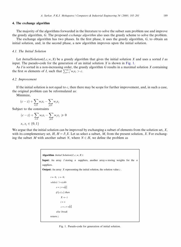
4.1. The Initial Solution
Let InitialSolution(I,c,w,X) be a greedy algorithm that gives the initial solution X and uses a sorted I asinput. The pseudo-code for the generation of an initial solution X is shown in Fig. 1.
As I is sorted in a non-increasing order, the greedy algorithm G results in a maximal solution X containingthe first m elements of I, such that
Pmþ1i¼1 wixi > c.
4.2. Improvement
If the initial solution is not equal to c, then there may be scope for further improvement, and, in such a case,the original problem can be reformulated as:
Minimize,
ðc� zÞ þX
i2X
wixi �X
j 62X
wjxj
Subject to the constraints
ðc� zÞ þX
i2X
wixi �X
j 62X
wjxj P 0
xi; xj 2 f0; 1g
We argue that the initial solution can be improved by exchanging a subset of elements from the solution set, X,with its complementary set, H, H = InX. Let us select a subset, M, from the present solution, X. For exchang-ing the subset M with another subset N, where N 2 H, we define the problem as
Algorithm :),,,( XwcIutionInitial Sol
Input: An array I storing n suppliers, another array w storing weights for the n
suppliers.
Output: An array X representing the initial solution, the solution value z .
,0←i ;0←z
)!( niwhile = do
[ ]iwzs +=
( )csif ≤ then
iX ←
++i
[ ]iwzz +=
else break
return z
Fig. 1. Pseudo-code for generation of initial solution.
190 A. Sarkar, P.K.J. Mohapatra / Computers & Industrial Engineering 54 (2008) 185–201
Maximize;X
i2N
wixi
Subject toX
i2N
wixi �X
j2M
wjxj > 0
X
i2N
wixi �X
j2M
wjxj 6 c� z
xi; xj 2 f0; 1g
ðAÞ
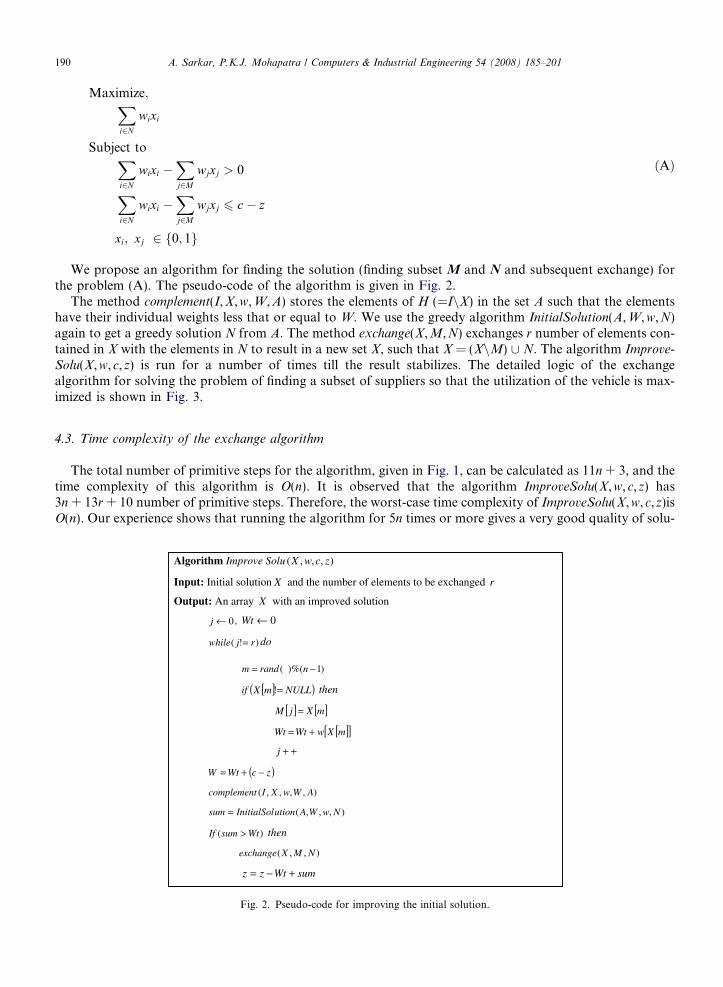
We propose an algorithm for finding the solution (finding subset M and N and subsequent exchange) forthe problem (A). The pseudo-code of the algorithm is given in Fig. 2.
The method complement(I,X,w,W,A) stores the elements of H (=InX) in the set A such that the elementshave their individual weights less that or equal to W. We use the greedy algorithm InitialSolution(A,W,w,N)again to get a greedy solution N from A. The method exchange(X,M,N) exchanges r number of elements con-tained in X with the elements in N to result in a new set X, such that X = (XnM) [ N. The algorithm Improve-
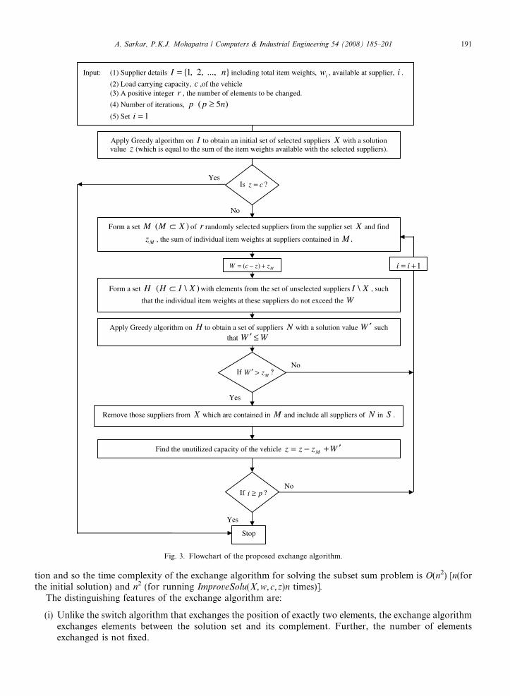
Solu(X,w,c,z) is run for a number of times till the result stabilizes. The detailed logic of the exchangealgorithm for solving the problem of finding a subset of suppliers so that the utilization of the vehicle is max-imized is shown in Fig. 3.
4.3. Time complexity of the exchange algorithm
The total number of primitive steps for the algorithm, given in Fig. 1, can be calculated as 11n + 3, and thetime complexity of this algorithm is O(n). It is observed that the algorithm ImproveSolu(X,w,c,z) has3n + 13r + 10 number of primitive steps. Therefore, the worst-case time complexity of ImproveSolu(X,w,c,z)isO(n). Our experience shows that running the algorithm for 5n times or more gives a very good quality of solu-
Algorithm Improve Solu ),,,( zcwX
Input: Initial solution X and the number of elements to be exchanged r
Output: An array X with an improved solution
0←j , 0←Wt
)!( rjwhile = do
)1)%(( −= nrandm
[ ]( )NULLmXif =! then
[ ] [ ]mXjM =
[ ][ ]mXwWtWt +=
++j
( )zcWtW −+=
),,,,( AWwXIcomplement
),,,( NwWAutionInitialSolsum =
)( WtsumIf > then
),,( NMXexchange
sumWtzz +−=
Fig. 2. Pseudo-code for improving the initial solution.
Input: (1) Supplier details }...,,2,1{ nI = including total item weights, iw , available at supplier, i .
(2) Load carrying capacity, c ,of the vehicle (3) A positive integer r , the number of elements to be changed.
(4) Number of iterations, )5( npp ≥(5) Set 1=i
Apply Greedy algorithm on I to obtain an initial set of selected suppliers X with a solution value z (which is equal to the sum of the item weights available with the selected suppliers).
Form a set M )( XM ⊂ of r randomly selected suppliers from the supplier set X and find
Mz , the sum of individual item weights at suppliers contained in .M
MzzcW +−= )(
Form a set )\( XIHH ⊂ with elements from the set of unselected suppliers XI \ , such
that the individual item weights at these suppliers do not exceed the W
Apply Greedy algorithm on H to obtain a set of suppliers N with a solution value W ′ such that WW ≤′
IfMzW >′ ?
Remove those suppliers from X which are contained in M and include all suppliers of N in S .
Find the unutilized capacity of the vehicle Wzzz M ′+−=
Is cz = ?
If pi ≥ ?
Stop
No
Yes
Yes
Yes
No
No
1+= ii
Fig. 3. Flowchart of the proposed exchange algorithm.
A. Sarkar, P.K.J. Mohapatra / Computers & Industrial Engineering 54 (2008) 185–201 191
tion and so the time complexity of the exchange algorithm for solving the subset sum problem is O(n2) [n(forthe initial solution) and n2 (for running ImproveSolu(X,w,c,z)n times)].
The distinguishing features of the exchange algorithm are:
(i) Unlike the switch algorithm that exchanges the position of exactly two elements, the exchange algorithmexchanges elements between the solution set and its complement. Further, the number of elementsexchanged is not fixed.
192 A. Sarkar, P.K.J. Mohapatra / Computers & Industrial Engineering 54 (2008) 185–201
(ii) Unlike all the algorithms discussed earlier that have a constant search space for all iterations, the searchspace in the exchange algorithm varies at each iteration.
(iii) As the exchange algorithm has a variable search space for all iterations, it is more likely to give superiorresults compared to other algorithms.
(iv) The exchange algorithm has a better time complexity compared to the switch algorithm and thus can beefficiently implemented for practical problems.
5. Computational results
The exchange algorithm is applied to some of the test problems given in the literature. The results are com-pared with those obtained with the existing approximation schemes. The algorithm is thereafter applied to thereal-life data available for the third-party transporter case presented earlier. The experiments were conductedon a Pentium 4 machine with 2.4 GHz processor and 256 MB RAM.
5.1. Fixing a value of r
As discussed earlier, r, the number of elements removed from the solution set S is to be selected for improv-ing the initial solution. It may be recalled that the original subset sum problem contains two types of param-eters: {wi} and c. Johnson’s algorithm (Jk), which is the basis of a number of developments, defines aparameter k to solve the problem. Usually, k is assigned a value 2 to minimize the time complexity of the algo-rithm. However, the effect of kon the quality of solutions has not been reported.
The exchange algorithm requires a value to be given for the parameter r. As shown earlier, the contributionof r to the time complexity of the algorithm is linear. It is desirable to explore the effect of r on the quality ofsolution and fix its most acceptable value. To achieve this end, r was raised from 2 to 5 in increments of 1, andthe algorithm was applied on a number of test problems. The problems were generated by taking the weights,wi’s, to be randomly distributed in [1,10E] and c to be equal to bn10E/4c (Soma & Toth, 2002), where E is apositive integer. We measure the quality of solution equal to the performance ratio e and defined as under:
TableEffect
The pr
Size n
50
1000
e ¼Pn
i¼1wixi
c:
We have considered five values of number of suppliers, n(=50,100,200,500 and 1000). For each n and for aparticular value of E (equal to either 3 or 6), we have randomly generated 100 set of values of item weights,thus getting a total of 1000 (=5 · 2 · 100) test instances. The exchange algorithm requires randomly selecting rnumber of suppliers from the solution set, X. We have tested each instance ten times, each time with a differentset of random numbers generated automatically by the srand function available in the C programming lan-guage. The average of ten solutions is assumed to represent the solution to a test instance. For each n andfor a particular value of E the average solutions to 100 instances are again averaged to obtain the averagequality of solution produced by the exchange algorithm for the test problem with the selected values of n
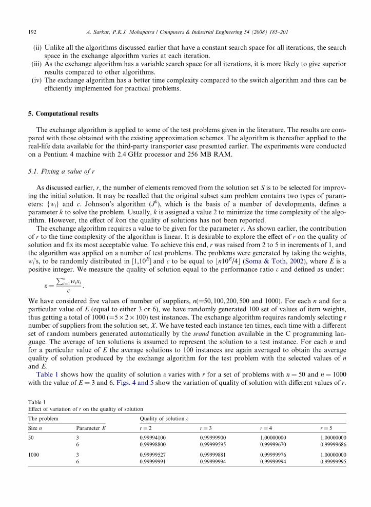
and E.Table 1 shows how the quality of solution e varies with r for a set of problems with n = 50 and n = 1000
with the value of E = 3 and 6. Figs. 4 and 5 show the variation of quality of solution with different values of r.
1of variation of r on the quality of solution
oblem Quality of solution e
Parameter E r = 2 r = 3 r = 4 r = 5
3 0.99994100 0.99999900 1.00000000 1.000000006 0.99998800 0.99999595 0.99999670 0.99999686
3 0.99999527 0.99999881 0.99999976 1.000000006 0.99999991 0.99999994 0.99999994 0.99999995
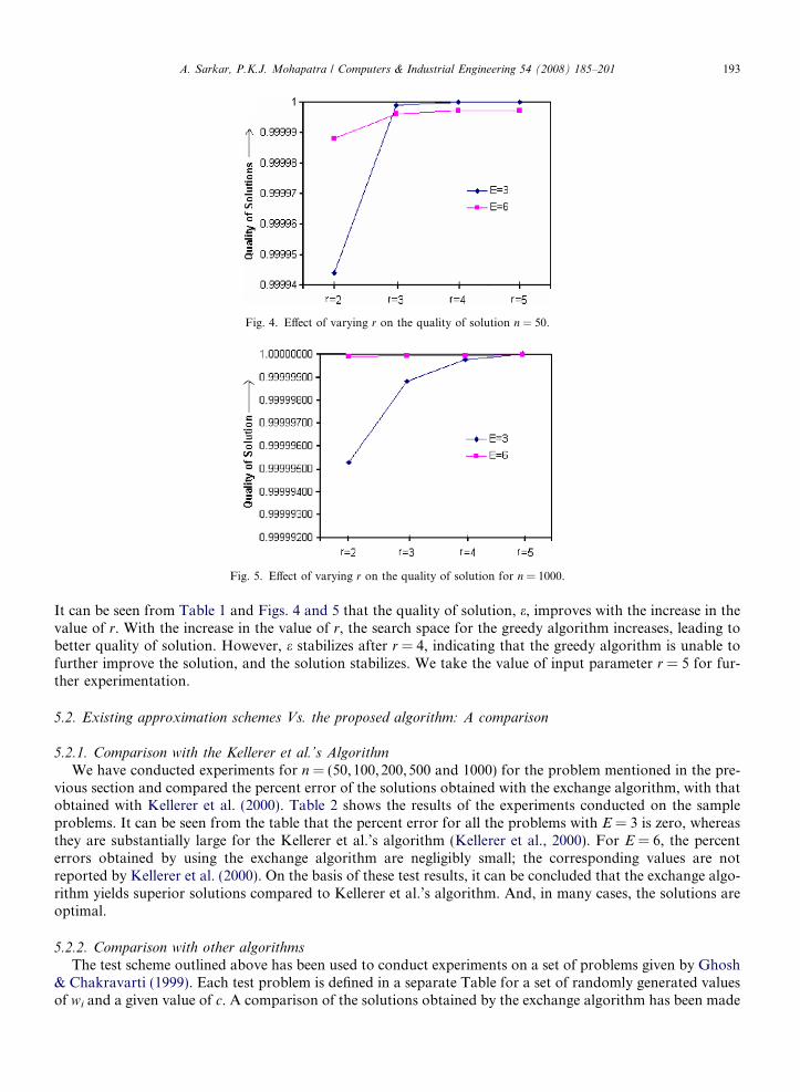
Fig. 4. Effect of varying r on the quality of solution n = 50.
Fig. 5. Effect of varying r on the quality of solution for n = 1000.
A. Sarkar, P.K.J. Mohapatra / Computers & Industrial Engineering 54 (2008) 185–201 193
It can be seen from Table 1 and Figs. 4 and 5 that the quality of solution, e, improves with the increase in thevalue of r. With the increase in the value of r, the search space for the greedy algorithm increases, leading tobetter quality of solution. However, e stabilizes after r = 4, indicating that the greedy algorithm is unable tofurther improve the solution, and the solution stabilizes. We take the value of input parameter r = 5 for fur-ther experimentation.
5.2. Existing approximation schemes Vs. the proposed algorithm: A comparison
5.2.1. Comparison with the Kellerer et al.’s Algorithm
We have conducted experiments for n = (50, 100,200,500 and 1000) for the problem mentioned in the pre-vious section and compared the percent error of the solutions obtained with the exchange algorithm, with thatobtained with Kellerer et al. (2000). Table 2 shows the results of the experiments conducted on the sampleproblems. It can be seen from the table that the percent error for all the problems with E = 3 is zero, whereasthey are substantially large for the Kellerer et al.’s algorithm (Kellerer et al., 2000). For E = 6, the percenterrors obtained by using the exchange algorithm are negligibly small; the corresponding values are notreported by Kellerer et al. (2000). On the basis of these test results, it can be concluded that the exchange algo-rithm yields superior solutions compared to Kellerer et al.’s algorithm. And, in many cases, the solutions areoptimal.
5.2.2. Comparison with other algorithms
The test scheme outlined above has been used to conduct experiments on a set of problems given by Ghosh& Chakravarti (1999). Each test problem is defined in a separate Table for a set of randomly generated valuesof wi and a given value of c. A comparison of the solutions obtained by the exchange algorithm has been made
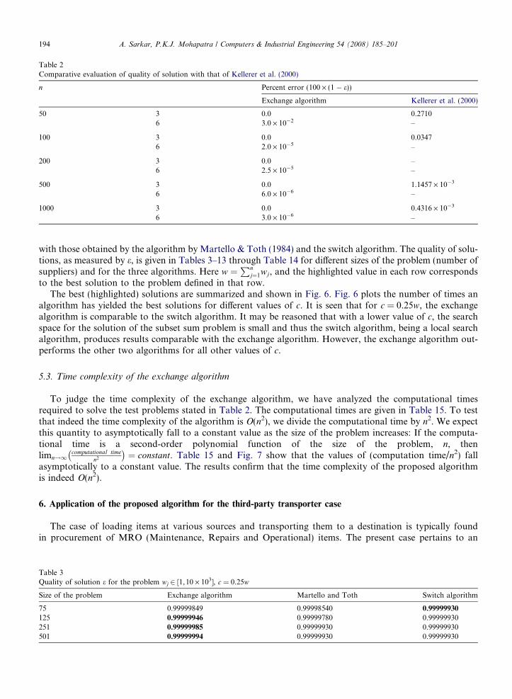
Table 2Comparative evaluation of quality of solution with that of Kellerer et al. (2000)
n Percent error (100 · (1 � e))
Exchange algorithm Kellerer et al. (2000)
50 3 0.0 0.27106 3.0 · 10�2 –
100 3 0.0 0.03476 2.0 · 10�5 –
200 3 0.0 –6 2.5 · 10�5 –
500 3 0.0 1.1457 · 10�3
6 6.0 · 10�6 –
1000 3 0.0 0.4316 · 10�3
6 3.0 · 10�6 –
194 A. Sarkar, P.K.J. Mohapatra / Computers & Industrial Engineering 54 (2008) 185–201
with those obtained by the algorithm by Martello & Toth (1984) and the switch algorithm. The quality of solu-tions, as measured by e, is given in Tables 3–13 through Table 14 for different sizes of the problem (number ofsuppliers) and for the three algorithms. Here w ¼
Pnj¼1wj, and the highlighted value in each row corresponds
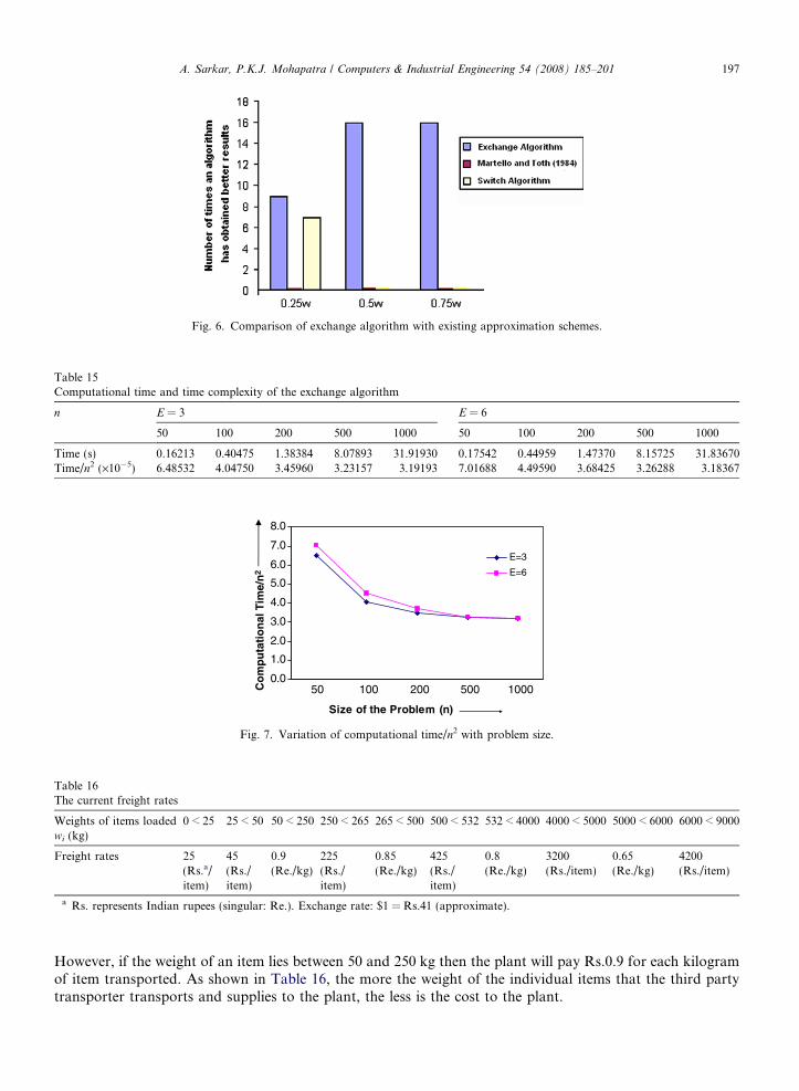
to the best solution to the problem defined in that row.The best (highlighted) solutions are summarized and shown in Fig. 6. Fig. 6 plots the number of times an
algorithm has yielded the best solutions for different values of c. It is seen that for c = 0.25w, the exchangealgorithm is comparable to the switch algorithm. It may be reasoned that with a lower value of c, the searchspace for the solution of the subset sum problem is small and thus the switch algorithm, being a local searchalgorithm, produces results comparable with the exchange algorithm. However, the exchange algorithm out-performs the other two algorithms for all other values of c.
5.3. Time complexity of the exchange algorithm
To judge the time complexity of the exchange algorithm, we have analyzed the computational timesrequired to solve the test problems stated in Table 2. The computational times are given in Table 15. To testthat indeed the time complexity of the algorithm is O(n2), we divide the computational time by n2. We expectthis quantity to asymptotically fall to a constant value as the size of the problem increases: If the computa-tional time is a second-order polynomial function of the size of the problem, n, thenlimn!1
computational timen2
� �¼ constant. Table 15 and Fig. 7 show that the values of (computation time/n2) fall
asymptotically to a constant value. The results confirm that the time complexity of the proposed algorithmis indeed O(n2).
6. Application of the proposed algorithm for the third-party transporter case
The case of loading items at various sources and transporting them to a destination is typically foundin procurement of MRO (Maintenance, Repairs and Operational) items. The present case pertains to an
Table 3Quality of solution e for the problem wj 2 [1,10 · 103], c = 0.25w
Size of the problem Exchange algorithm Martello and Toth Switch algorithm
75 0.99999849 0.99998540 0.99999930
125 0.99999946 0.99999780 0.99999930251 0.99999985 0.99999930 0.99999930501 0.99999994 0.99999930 0.99999930
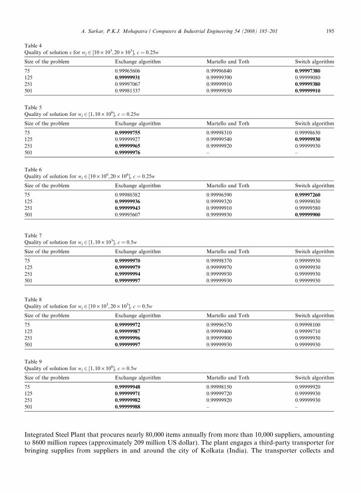
Table 4Quality of solution e for wj 2 [10 · 103,20 · 103], c = 0.25w
Size of the problem Exchange algorithm Martello and Toth Switch algorithm
75 0.99965606 0.99996840 0.99997380
125 0.99999931 0.99999390 0.99999080251 0.99997067 0.99999910 0.99999380
501 0.99981337 0.99999930 0.99999910
Table 5Quality of solution for wj 2 [1,10 · 106], c = 0.25w
Size of the problem Exchange algorithm Martello and Toth Switch algorithm
75 0.99999755 0.99998310 0.99998630125 0.99999927 0.99999540 0.99999930
251 0.99999965 0.99999920 0.99999930501 0.99999976 – –
Table 6Quality of solution for wj 2 [10 · 106,20 · 106], c = 0.25w
Size of the problem Exchange algorithm Martello and Toth Switch algorithm
75 0.99980382 0.99996590 0.99997260
125 0.99999936 0.99999320 0.99999030251 0.99999943 0.99999910 0.99999580501 0.99995607 0.99999930 0.99999900
Table 7Quality of solution for wj 2 [1,10 · 103], c = 0.5w
Size of the problem Exchange algorithm Martello and Toth Switch algorithm
75 0.99999970 0.99998370 0.99999930125 0.99999979 0.99999970 0.99999930251 0.99999994 0.99999930 0.99999930501 0.99999997 0.99999930 0.99999930
Table 8Quality of solution for wj 2 [10 · 103,20 · 103], c = 0.5w
Size of the problem Exchange algorithm Martello and Toth Switch algorithm
75 0.99999972 0.99996570 0.99998100125 0.99999987 0.99999400 0.99999710251 0.99999996 0.99999900 0.99999930501 0.99999997 0.99999930 0.99999930
Table 9Quality of solution for wj 2 [1,10 · 106], c = 0.5w
Size of the problem Exchange algorithm Martello and Toth Switch algorithm
75 0.99999948 0.99998150 0.99999920125 0.99999971 0.99999720 0.99999930251 0.99999982 0.99999920 0.99999930501 0.99999988 – –
A. Sarkar, P.K.J. Mohapatra / Computers & Industrial Engineering 54 (2008) 185–201 195
Integrated Steel Plant that procures nearly 80,000 items annually from more than 10,000 suppliers, amountingto 8600 million rupees (approximately 209 million US dollar). The plant engages a third-party transporter forbringing supplies from suppliers in and around the city of Kolkata (India). The transporter collects and
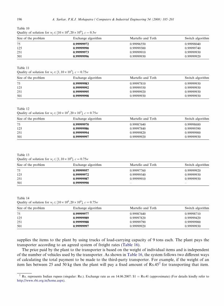
Table 11Quality of solution for wj 2 [1,10 · 103], c = 0.75w
Size of the problem Exchange algorithm Martello and Toth Switch algorithm
75 0.99999983 0.99997810 0.99999930125 0.99999992 0.99999550 0.99999930251 0.99999995 0.99999920 0.99999930501 0.99999998 0.99999930 0.99999930
Table 12Quality of solution for wj 2 [10 · 103,20 · 103], c = 0.75w
Size of the problem Exchange algorithm Martello and Toth Switch algorithm
75 0.99999970 0.99987640 0.99998680125 0.99999986 0.99997840 0.99999390251 0.99999994 0.99999820 0.99999900501 0.99999997 0.99999920 0.99999930
Table 13Quality of solution for wj 2 [1,10 · 106], c = 0.75w
Size of the problem Exchange algorithm Martello and Toth Switch algorithm
75 0.99999957 0.99997760 0.99999920125 0.99999972 0.99999540 0.99999930251 0.99999987 0.99999910 0.99999930501 0.99999990 – –
Table 14Quality of solution for wj 2 [10 · 106,20 · 106], c = 0.75w
Size of the problem Exchange algorithm Martello and Toth Switch algorithm
75 0.99999977 0.99987640 0.99998710125 0.99999989 0.99997820 0.99999420251 0.99999988 0.99999790 0.99999900501 0.99999997 0.99999920 0.99999930
Table 10Quality of solution for wj 2 [10 · 106,20 · 106], c = 0.5w
Size of the problem Exchange algorithm Martello and Toth Switch algorithm
75 0.99999972 0.99996550 0.99998040125 0.99999990 0.99999300 0.99999740251 0.99999973 0.99999910 0.99999930501 0.99999996 0.99999930 0.99999920
196 A. Sarkar, P.K.J. Mohapatra / Computers & Industrial Engineering 54 (2008) 185–201
supplies the items to the plant by using trucks of load-carrying capacity of 9 tons each. The plant pays thetransporter according to an agreed system of freight rates (Table 16).
The price paid by the plant to the transporter is based on the weight of individual items and is independentof the number of vehicles used by the transporter. As shown in Table 16, the system follows two different waysof calculating the total payment to be made to the third-party transporter. For example, if the weight of anitem lies between 25 and 50 kg then the plant will pay a fixed amount of Rs.452 for transporting that item.
2 Rs. represents Indian rupees (singular: Re.). Exchange rate as on 14.06.2007: $1 = Rs.41 (approximate) (For details kindly refer tohttp://www.rbi.org.in/home.aspx).
0.0
1.0
2.0
3.0
4.0
5.0
6.0
7.0
8.0
50 100 200 500 1000
Size of the Problem (n)
E=3
E=6
Co
mp
uta
tio
nal
Tim
e/n
2
Fig. 7. Variation of computational time/n2 with problem size.
Fig. 6. Comparison of exchange algorithm with existing approximation schemes.
Table 15Computational time and time complexity of the exchange algorithm
n E = 3 E = 6
50 100 200 500 1000 50 100 200 500 1000
Time (s) 0.16213 0.40475 1.38384 8.07893 31.91930 0.17542 0.44959 1.47370 8.15725 31.83670Time/n2 (·10�5) 6.48532 4.04750 3.45960 3.23157 3.19193 7.01688 4.49590 3.68425 3.26288 3.18367
Table 16The current freight rates
Weights of items loadedwi (kg)
0 < 25 25 < 50 50 < 250 250 < 265 265 < 500 500 < 532 532 < 4000 4000 < 5000 5000 < 6000 6000 < 9000
Freight rates 25(Rs.a/item)
45(Rs./item)
0.9(Re./kg)
225(Rs./item)
0.85(Re./kg)
425(Rs./item)
0.8(Re./kg)
3200(Rs./item)
0.65(Re./kg)
4200(Rs./item)
a Rs. represents Indian rupees (singular: Re.). Exchange rate: $1 = Rs.41 (approximate).
A. Sarkar, P.K.J. Mohapatra / Computers & Industrial Engineering 54 (2008) 185–201 197
However, if the weight of an item lies between 50 and 250 kg then the plant will pay Rs.0.9 for each kilogramof item transported. As shown in Table 16, the more the weight of the individual items that the third partytransporter transports and supplies to the plant, the less is the cost to the plant.
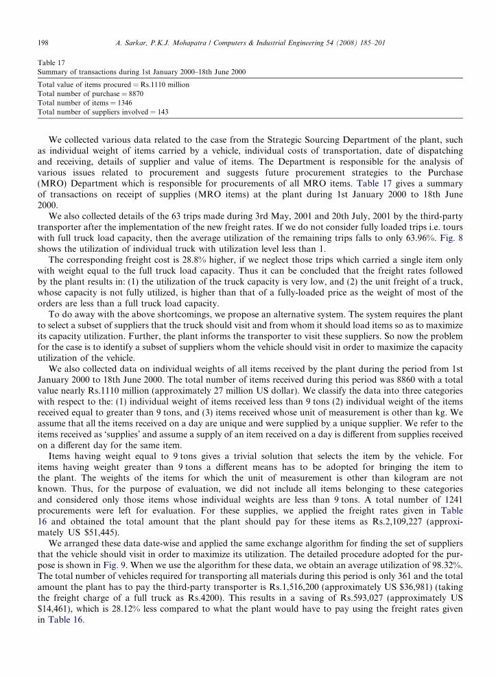
Table 17Summary of transactions during 1st January 2000–18th June 2000
Total value of items procured = Rs.1110 millionTotal number of purchase = 8870Total number of items = 1346Total number of suppliers involved = 143
198 A. Sarkar, P.K.J. Mohapatra / Computers & Industrial Engineering 54 (2008) 185–201
We collected various data related to the case from the Strategic Sourcing Department of the plant, suchas individual weight of items carried by a vehicle, individual costs of transportation, date of dispatchingand receiving, details of supplier and value of items. The Department is responsible for the analysis ofvarious issues related to procurement and suggests future procurement strategies to the Purchase(MRO) Department which is responsible for procurements of all MRO items. Table 17 gives a summaryof transactions on receipt of supplies (MRO items) at the plant during 1st January 2000 to 18th June2000.
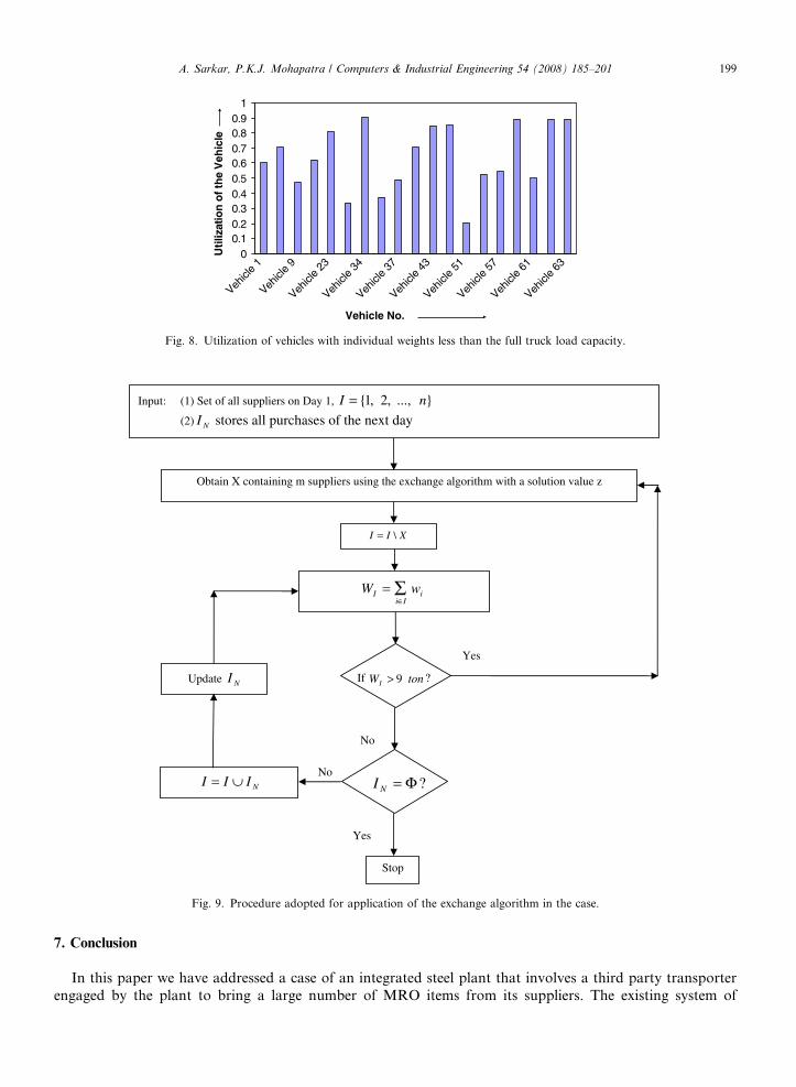
We also collected details of the 63 trips made during 3rd May, 2001 and 20th July, 2001 by the third-partytransporter after the implementation of the new freight rates. If we do not consider fully loaded trips i.e. tourswith full truck load capacity, then the average utilization of the remaining trips falls to only 63.96%. Fig. 8shows the utilization of individual truck with utilization level less than 1.
The corresponding freight cost is 28.8% higher, if we neglect those trips which carried a single item onlywith weight equal to the full truck load capacity. Thus it can be concluded that the freight rates followedby the plant results in: (1) the utilization of the truck capacity is very low, and (2) the unit freight of a truck,whose capacity is not fully utilized, is higher than that of a fully-loaded price as the weight of most of theorders are less than a full truck load capacity.
To do away with the above shortcomings, we propose an alternative system. The system requires the plantto select a subset of suppliers that the truck should visit and from whom it should load items so as to maximizeits capacity utilization. Further, the plant informs the transporter to visit these suppliers. So now the problemfor the case is to identify a subset of suppliers whom the vehicle should visit in order to maximize the capacityutilization of the vehicle.
We also collected data on individual weights of all items received by the plant during the period from 1stJanuary 2000 to 18th June 2000. The total number of items received during this period was 8860 with a totalvalue nearly Rs.1110 million (approximately 27 million US dollar). We classify the data into three categorieswith respect to the: (1) individual weight of items received less than 9 tons (2) individual weight of the itemsreceived equal to greater than 9 tons, and (3) items received whose unit of measurement is other than kg. Weassume that all the items received on a day are unique and were supplied by a unique supplier. We refer to theitems received as ‘supplies’ and assume a supply of an item received on a day is different from supplies receivedon a different day for the same item.
Items having weight equal to 9 tons gives a trivial solution that selects the item by the vehicle. Foritems having weight greater than 9 tons a different means has to be adopted for bringing the item tothe plant. The weights of the items for which the unit of measurement is other than kilogram are notknown. Thus, for the purpose of evaluation, we did not include all items belonging to these categoriesand considered only those items whose individual weights are less than 9 tons. A total number of 1241procurements were left for evaluation. For these supplies, we applied the freight rates given in Table16 and obtained the total amount that the plant should pay for these items as Rs.2,109,227 (approxi-mately US $51,445).
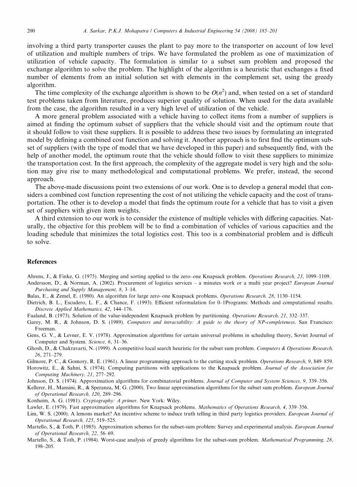
We arranged these data date-wise and applied the same exchange algorithm for finding the set of suppliersthat the vehicle should visit in order to maximize its utilization. The detailed procedure adopted for the pur-pose is shown in Fig. 9. When we use the algorithm for these data, we obtain an average utilization of 98.32%.The total number of vehicles required for transporting all materials during this period is only 361 and the totalamount the plant has to pay the third-party transporter is Rs.1,516,200 (approximately US $36,981) (takingthe freight charge of a full truck as Rs.4200). This results in a saving of Rs.593,027 (approximately US$14,461), which is 28.12% less compared to what the plant would have to pay using the freight rates givenin Table 16.
00.10.20.30.40.50.60.70.80.9
1
Vehicl
e 1
Vehicl
e 9
Vehicl
e 23
Vehicl
e 34
Vehicl
e 37
Vehicl
e 43
Vehicl
e 51
Vehicl
e 57
Vehicl
e 61
Vehicl
e 63
Vehicle No.
Uti
lizat
ion
of t
he
Veh
icle
Fig. 8. Utilization of vehicles with individual weights less than the full truck load capacity.
Input: (1) Set of all suppliers on Day 1, }...,,2,1{ nI =(2) NI stores all purchases of the next day
Obtain X containing m suppliers using the exchange algorithm with a solution value z
XII \=
∈=
IiiI wW Σ
If tonWI 9> ?
NIII ∪=
Stop
Yes
No
Yes
?Φ=NINo
Update NI
Fig. 9. Procedure adopted for application of the exchange algorithm in the case.
A. Sarkar, P.K.J. Mohapatra / Computers & Industrial Engineering 54 (2008) 185–201 199
7. Conclusion
In this paper we have addressed a case of an integrated steel plant that involves a third party transporterengaged by the plant to bring a large number of MRO items from its suppliers. The existing system of
200 A. Sarkar, P.K.J. Mohapatra / Computers & Industrial Engineering 54 (2008) 185–201
involving a third party transporter causes the plant to pay more to the transporter on account of low levelof utilization and multiple numbers of trips. We have formulated the problem as one of maximization ofutilization of vehicle capacity. The formulation is similar to a subset sum problem and proposed theexchange algorithm to solve the problem. The highlight of the algorithm is a heuristic that exchanges a fixednumber of elements from an initial solution set with elements in the complement set, using the greedyalgorithm.
The time complexity of the exchange algorithm is shown to be O(n2) and, when tested on a set of standardtest problems taken from literature, produces superior quality of solution. When used for the data availablefrom the case, the algorithm resulted in a very high level of utilization of the vehicle.
A more general problem associated with a vehicle having to collect items from a number of suppliers isaimed at finding the optimum subset of suppliers that the vehicle should visit and the optimum route thatit should follow to visit these suppliers. It is possible to address these two issues by formulating an integratedmodel by defining a combined cost function and solving it. Another approach is to first find the optimum sub-set of suppliers (with the type of model that we have developed in this paper) and subsequently find, with thehelp of another model, the optimum route that the vehicle should follow to visit these suppliers to minimizethe transportation cost. In the first approach, the complexity of the aggregate model is very high and the solu-tion may give rise to many methodological and computational problems. We prefer, instead, the secondapproach.
The above-made discussions point two extensions of our work. One is to develop a general model that con-siders a combined cost function representing the cost of not utilizing the vehicle capacity and the cost of trans-portation. The other is to develop a model that finds the optimum route for a vehicle that has to visit a givenset of suppliers with given item weights.
A third extension to our work is to consider the existence of multiple vehicles with differing capacities. Nat-urally, the objective for this problem will be to find a combination of vehicles of various capacities and theloading schedule that minimizes the total logistics cost. This too is a combinatorial problem and is difficultto solve.
References
Ahrens, J., & Finke, G. (1975). Merging and sorting applied to the zero–one Knapsack problem. Operations Research, 23, 1099–1109.Andersson, D., & Norman, A. (2002). Procurement of logistics services – a minutes work or a multi year project? European Journal
Purchasing and Supply Management, 8, 3–14.Balas, E., & Zemel, E. (1980). An algorithm for large zero–one Knapsack problems. Operations Research, 28, 1130–1154.Dietrich, B. L., Escudero, L. F., & Chance, F. (1993). Efficient reformulation for 0–1Programs: Methods and computational results.
Discrete Applied Mathematics, 42, 144–176.Faaland, B. (1973). Solution of the value-independent Knapsack problem by partitioning. Operations Research, 21, 332–337.Garey, M. R., & Johnson, D. S. (1989). Computers and intractability: A guide to the theory of NP-completeness. San Francisco:
Freeman.Gens, G. V., & Levner, E. V. (1978). Approximation algorithms for certain universal problems in scheduling theory, Soviet Journal of
Computer and System. Science, 6, 31–36.Ghosh, D., & Chakravarti, N. (1999). A competitive local search heuristic for the subset sum problem. Computers & Operations Research,
26, 271–279.Gilmore, P. C., & Gomory, R. E. (1961). A linear programming approach to the cutting stock problem. Operations Research, 9, 849–859.Horowitz, E., & Sahni, S. (1974). Computing partitions with applications to the Knapsack problem. Journal of the Association for
Computing Machinery, 21, 277–292.Johnson, D. S. (1974). Approximation algorithms for combinatorial problems. Journal of Computer and System Sciences, 9, 339–356.Kellerer, H., Mansini, R., & Speranza, M. G. (2000). Two linear approximation algorithms for the subset sum problem. European Journal
of Operational Research, 120, 289–296.Konheim, A. G. (1981). Cryptography: A primer. New York: Wiley.Lawler, E. (1979). Fast approximation algorithms for Knapsack problems. Mathematics of Operations Research, 4, 339–356.Lim, W. S. (2000). A lemons market? An incentive scheme to induce truth telling in third party logistics providers. European Journal of
Operational Research, 125, 519–525.Martello, S., & Toth, P. (1985). Approximation schemes for the subset-sum problem: Survey and experimental analysis. European Journal
of Operational Research, 22, 56–69.Martello, S., & Toth, P. (1984). Worst-case analysis of greedy algorithms for the subset-sum problem. Mathematical Programming, 28,
198–205.
A. Sarkar, P.K.J. Mohapatra / Computers & Industrial Engineering 54 (2008) 185–201 201
Prasad, K., & Kelly, J. S. (1990). NP-completeness of some problems concerning voting games. International Journal of Game Theory, 19,1–9.
Sahni, S. (1975). Approximate algorithms for the 0–1 Knapsack problem. Journal of Association of Computing Machinery, 22,115–124.
Soma, N. Y., & Toth, P. (2002). An exact algorithm for the subset sum problem. European Journal of Operational Research, 136,57–66.
Stank, T. P., & Daugherty, P. J. (1997). The impact of operating environment on the formation of cooperative logistics relationships.Transportation Research-E (Logistics and Transportation Review), 33(1), 53–65.