Maximum Margin Planning

Nathan D. Ratliff ndr@ri.cmu.eduJ. Andrew Bagnell dbagnell@ri.cmu.edu

Robotics Institute, Carnegie Mellon University, Pittsburgh, PA. 15213 USA

Martin A. Zinkevich maz@cs.ualberta.ca

Department of Computing Science, University of Alberta, Edmonton, AB T6G 2E1, Canada

Abstract

Imitation learning of sequential, goal-directed behavior by standard supervisedtechniques is often difficult. We frame learn-ing such behaviors as a maximum marginstructured prediction problem over a spaceof policies. In this approach, we learn map-pings from features to cost so an optimal pol-icy in an MDP with these cost mimics the ex-pert’s behavior. Further, we demonstrate asimple, provably efficient approach to struc-tured maximum margin learning, based onthe subgradient method, that leverages ex-isting fast algorithms for inference. Althoughthe technique is general, it is particularly rel-evant in problems where A* and dynamicprogramming approaches make learning poli-cies tractable in problems beyond the limita-tions of a QP formulation. We demonstrateour approach applied to route planning foroutdoor mobile robots, where the behavior adesigner wishes a planner to execute is oftenclear, while specifying cost functions that en-gender this behavior is a much more difficulttask.

1. Introduction

In “imitation learning” a learner attempts to mimican expert’s behavior or control strategy. In numerousinstances, notably within robotics (Pomerleau, 1989;LeCun et al., 2006), supervised learning approacheshave been used to great effect to learn mappings fromfeatures to decisions. Long-range and goal-directed be-havior, by contrast, has proven more difficult to cap-ture using these techniques.

Appearing in Proceedings of the 23 rd International Con-ference on Machine Learning, Pittsburgh, PA, 2006. Copy-right 2006 by the author(s)/owner(s).

In mobile robotics, the motivating application of ourimitation learning approaches, researchers often en-courage long-horizon goal directed behavior by parti-tioning an autonomy software into a “perception” sub-system and a “planning” subsystem. The perceptionsystem computes various models and features of an en-vironment. For instance, perception might determinethe supporting surface, obstacles lying above this sur-face, average color at various locations, density of ladarreturns, et cetera. Planning takes as input a cost-mapover the vehicle configuration or state space (Hebertet al., 1998) and computes a minimal risk (cost) paththrough it that serves as a coherent sequence of deci-sions for the robot over a long horizon. This approachhas proven powerful and lies at the heart of many au-tonomous mobile robotic systems in both indoor andoutdoor environments.Unfortunately, the leap from perception’s model tocosts for a planner is often a difficult one. In prac-tice, it is often done by hand-designed heuristics thatare painstakingly validated by observing the result-ing robot behavior. In this work, we propose a novelmethod whereby we attempt to automate the mappingfrom perception features to costs. We do so by fram-ing the problem as one of supervised learning to takeadvantage of examples given by an expert describingdesired behavior. In essence, we leverage the fact thatthe desired behavior is often quite clear to a humandesigner while specifying costs that engender this be-havior is a much more difficult task, particularly whenit involves simultaneously tweaking a large set of knobsthat map features to costs.Learning to plan so as to mimic a teacher’s behav-ior may be cast as a structured prediction problemover the space of policies. The learner’s goal is totake example input features and example policies ortrajectories through the state space (e.g. paths) andlearn to predict the same sequence of decisions. De-cisions at each state must be coordinated and their

Maximum Margin Planning

costs balanced to achieve a satisfactory global plan-ning strategy that implements the desired behavior.In this approach, our goal is to learn mappings fromfeatures to cost functions so an optimal policy in aMarkov Decision Problem with this cost function im-itates the expert’s behavior. We demonstrate that wecan learn such mappings in the structured large mar-gin framework. (Taskar et al., 2005)The key contributions of this work are three-fold.First, we demonstrate a novel method for learning toplan. Second, we demonstrate an efficient, simple ap-proach to structured maximum-margin classification(in both online and batch settings) that is applica-ble whenever a fast specialized algorithm is availableto compute the minimum of the loss-augmented costfunction. This approach demonstrates linear conver-gence when used in batch settings and is applicable tolarge problems where other Quadratic Programmingtechniques are not. We develop an online theory forStructured Maximum Margin and show that our al-gorithm achieves sublinear regret that scales inverselywith the margin and without a dependence on the sizeof the policy we must learn. Finally, we demonstrateempirically that our method is particularly applicableto problems of relevance in mobile robotics. We out-line our current research directions and other naturalapplications of Max Margin Planning in the conclu-sions (Section 5). We also discuss related approachesto imitation learning and structured classification inSection 5.

2. Preliminaries

We model the planning problem with discrete MarkovDecision Processes. Let x and a index the state and ac-tion spaces X andA, respectively; and let p(y|x, a) ands denote, respectively, the transition probablities andinitial state distribution. A discount factor on rewards(if any) is absorbed into the transition probabilities.Our reward functions1 are learned from supervised ex-amples to produce policies that mimic demonstratedbehavior. We repeatedly make use of the linear pro-gramming formulation of the MDP problem (Puter-man, 1994), denoting by v ∈ V the primal variables ofthe value function, and by µ ∈ G the dual state-actionfrequency counts. We consider here only stationarypolicies; the generalization is straightforward.The input to our algorithm is a set of training instancesD = {(Xi,Ai, pi, Fi, yi,Li)}ni=1. A training instanceconsists of an MDP with transition probabilities pi,

1In some deciplines is it more common and suitable todescribe problems in terms of costs rather than rewards.In what follows, the term “cost” is used interchangeably tomean “negative reward”.

state-action pairs (xi, ai) ∈ Xi × Ai over which d-dimensional feature vectors are place in the form ofa d× |X ||A| feature matrix Fi. yi denotes the desiredtrajectory (or full policy) that exemplifies behavior wehope to match. We often consider the alternate repre-sentation for such a trajectory in terms of µi, a vectorof state-action frequency counts. Note that since weare encoding the policies in terms of the dual state-action frequency counts, this formulation can attemptto learn to match either trajectories or entire policies.This will be described in detail below. We also discussthe role of the loss vector li below.We use subscripts to denote indexing by training in-stance, and reserve superscripts for indexing into vec-tors. (E.g. µx,a

i is the expected state-action frequencyfor state x and action a of example i.) Note that wewill sometimes write D = {(Xi,Ai, pi, fi, yi,Li)}ni=1 ≡{(Xi,Ai,Gi, Fi, µi, li)}ni=1, using fi(y) to denote vectorof expected feature counts Fiµ of the ith example. It isuseful for some problems, such as robot path planning,to imagine representing the features as a set of mapsand example paths through those maps. For instance,one feature map might indicate the elevation at eachstate, another the slope, and a third the presence ofvegetation.The learner attempts to find a linear mapping2 ofthese features to rewards so that for each problem in-stance the best policy over the resulting reward func-tion µ∗ = arg maxµ∈Gi

wT Fiµ is “close” to the demon-strated policy µi. The notion of closeness is definedby a loss-function L : Y × Y → R+ between so-lutions. In our work this function is of the formL(y, yi) = Li(y) = lTi µ. Intuitively, a loss vectorli ∈ R|X ||A|+ is placed over state-action pairs that de-fines for each state-action pair how much the learnerpays for failing to match the behavior of an examplepolicy yi as the cumulative loss of the learned policythrough this MDP. (See Figure 4)The maximum margin principle builds in a degree ofrobustness where we attempt to make the suppliedsolution yi look significantly better than alternativepolicies. In particular, we adopt the structured max-margin framework and attempt to make yi better thanany other solution y by a margin that scales with thesize of the loss of y; we wish to ensure that the cor-rect policy looks much more attractive than very badpolicies.

2Although space doesn’t permit full details, both formu-lations we use for learning later straightfowardly generalizeto handle nonlinearity through the use of kernelization.

Maximum Margin Planning

2.1. Loss-functions

The framework thus described admits any loss func-tion that factors over state-action pairs. A naturalloss function in the case of deterministic acyclic pathplanning is the count of the number of states that theplanner visits that the teacher did not. We have foundsomewhat better performance by smoothing this lossfunction so that nearby paths are also admissible. In ageneral MDP, we might penalize choosing different ac-tions from the teacher at any states the teacher reachesor penalize reaching states the teacher chooses not toenter. We also assume that L(y, yi) ≥ 0.

2.2. Quadratic Programming Formulation

Given a training set D = {(Xi,Ai, pi, fi, yi,Li)}ni=1,the structured large margin criteria (Taskar et al.,2005) implies we are solving the following quadraticprogram:3

minw,ζi

12‖w‖2 +

γ

n

∑i

βiζqi (1)

s.t. ∀i wT fi(yi) + ζi ≥ maxy∈Yi

wT fi(y) + Li(y) (2)

The intuition behind these constraints is that we al-low only weight vectors for which the example policieshave higher expected reward than all other policies bya margin that scales with the loss. The slack variablesζi permit violations of these constraints for a penaltythat scales with the hyperparameter γ ≥ 0. βi > 0are data dependent scalars that can be used for nor-malization when the examples are of different lengths.q ∈ {1, 2} distinguishes between L1 and L2 slack penal-ties commonly found in the literature (Tsochantaridiset al., 2005).If we consider the case for which both fi(·) and Li(·)are linear in the state-action frequencies µ as describedabove (i.e. they factor over state-action pairs), themaximum margin problem becomes

minw,ζi

12‖w‖2 +

γ

n

∑i

βiζqi (3)

s.t. ∀i wT Fiµi + ζi ≥ maxµ∈Gi

wT Fiµ + lTi µ (4)

where µ ∈ Gi expresses the Bellman-flow constraintsfor each MDP, namely that µ ≥ 0 satisfies:∑

x,a

µx,api(x′|x, a) + sx′

i =∑

a

µx′,a

The nonlinear, convex constraints in Equation 4 canbe transformed into a compact set of linear constraints

3Unless stated otherwise, ‖.‖ denotes the L2 norm.

(Taskar et al., 2005; Taskar et al., 2003) by computingthe dual of the right hand side of each yielding:

∀i wT Fiµi + ζi ≥ minv∈Vi

sTi v (5)

where v ∈ Vi are the value-functions that satisfy theBellman primal constraints:

∀x, a vx ≥ (wT Fi + li)x,a +∑x′

pi(x′|x, a)vx′(6)

By combining the constraints together we can writeone compact quadratic program:

minw,ζi,vi

12‖w‖2 +

γ

n

∑i

βiζqi (7)

s.t. ∀i wT Fiµi + ζi ≥ sTi vi (8)

∀i, x, a vxi ≥ (wT Fi + li)x,a +

∑x′

pi(x′|x, a)vx′

i (9)

This results provides a represenation of what we callthe Maximum Margin Planning (MMP) problem as acompact quadratic program. Note that the numberof constraints scales linearly with state-action pairsand training examples. While off-the-shelf quadraticprogramming software can be applied at this point todirectly optimize this program, we provide an alter-native formulation in Section 3 that allows us improvesignificantly over this via the utilization of subgradientmethods.We consider additional useful loss functions in Section4, where we detail examples relevant to path planningproblems.

3. Efficient Optimization

In practice, solving the quadratic program in Equa-tion 9 is at least as hard as solving the linear program-ming formulation of a single MDP. While this can bean appropriate strategy for a class of MDPs, it is gen-erally appreciated that for many problems there existspecially designed algorithms such as policy iterationand A* that can solve particular classes of MDPs boththeoretically and empirically more rapidly. Developingefficient specialized algorithms, and especially lever-aging existing inference algorithms, is an open prob-lem for general structured maximum margin problems.(Taskar et al., 2005). We present a simple approachbased on the subgradient method (Shor, 1985) that al-lows the use of fast maximization algorithms (e.g. fastplanners) for a provably efficient learning strategy.The first step is to transform the optimization pro-gram into a “hinge-loss” form. The hinge-loss viewis a common way to understand the maximum mar-gin problem and relate it to other methods like logis-tic regression and AdaBoost. This view comes from

Maximum Margin Planning

noting that the slack variables ζi are tight and thusequal maxµ∈Gi

(wT Fi + lTi )µ−wT Fiµi. We can there-fore move these constraints into the objective function,simplifying the problem into a single cost function:

cq(w) =1n

n∑i=1

βi

(maxµ∈Gi

(wT Fi + lTi )µ− wT Fiµi

)q

+

λ

2‖w‖2 (10)

where we have multiplied through by λγ to make a

regularized risk functional interpretation more clear(Rifkin & Poggio, 2003). Again, q ∈ {1, 2} defines theslack penalization.This objective function is convex, but nondifferen-tiable. We can optimize it by utilizing a generaliza-tion of gradient descent called the subgradient method(Shor, 1985). A subgradient of a convex functionc :W → R at w is defined as a vector g such that

∀w′ ∈ W, gT (w′ − w) ≤ c(w′)− c(w) (11)

Note that subgradients need not be unique, though atpoints of differentiability, they necessarily agree withthe gradient. We denote the set of all subgradients ofc(·) at point w by ∂c(w).To compute the subgradient of c(w), we make useof the following four well known properties: (1) sub-gradient operators are linear; (2) the gradient is theunique subgradient of a differentiable function; (3) de-noting y∗ = argmaxy[f(x, y)] for differentiable f(., y),∇xf(x, y∗) is a subgradient of the piecewise differen-tiable convex function maxy[f(x, y)]; (4) an analogouschain rule holds as expected. We are now equippedto compute a subgradient gq

w ∈ ∂c(w) of our objectivefunction (10):

gqw =

1n

n∑i=1

qβi

((wT Fi + lTi )µ∗ − wT Fiµi

)q−1 ·

Fi∆wµi + λw (12)

where µ∗ = arg maxµ∈Gi(wT Fi + lTi )µ and ∆wµi =

µ∗ − µi. This latter expression points out that, intu-itively, the subgradient compares the state-action vis-itation frequency counts between the example policyand the optimal policy with respect to current rewardfunction wT Fi.Note that computing the subgradient requires solvingthe problem µ∗ = arg maxµ∈Gi(w

T Fi + lTi )µ for eachMDP. This is precisely the problem of solving the par-ticular MDP with the reward function wT Fi + lTi , andcan be efficient implemented via a myriad of special-ized algorithms. Algorithm 1 details the applicationof the subgradient method to the Maximum MarginPlanning problem.

Algorithm 1 Max Margin Planning

1: procedure MMP(Training set {Fi, µi, li}Ni=1,Regularization parameter λ > 0, Stepsize se-quence {αt} (learning rate), Iterations T )

2: t← 13: w ← 04: while t ≤ T do5: Compute optimal policy and state action

visitation frequencies µ∗,i for each in-put map for loss augmented cost map(wT Fi + lTi ).

6: Compute g ∈ ∂c(w) as in Equation 12.7: w ← w − αtg8: (Optional): Project w on to any additional

constraints.9: t← t + 1

10: end while11: return w12: end procedure

The basic iterative update given gt ∈ ∂c(wt) and αt is

wt+1 = PW [wt − αtgt] (13)

where P projects w onto any problem specific (convex)constraints we may impose on w.4

3.1. Guarantees in the Batch Setting

In the batch setting, this algorithm is one of a wellstudied class of algorithms forming the subgradientmethod (Shor, 1985).5 Crucial to this method isthe choice of stepsize sequence {αt}; and convergenceguarantees vary accordingly. Our results are devel-oped from (Nedic & Bertsekas, 2000) which analyzesincremental subgradient algorithms, of which the sub-gradient method is a special case.Our results require a strong convexity assumption tohold for the objective function. Given W ⊆ R

d, afunction f :W → R is η-strongly convex if there existsg :W → R

d such that for all w,w′ ∈ W:

f(w′) ≥ f(w) + (g(w))T (w′ − w) + η‖w′ − w‖2 (14)

Theorem 1. Linear convergence of constantstepsize sequence. Let the stepsize sequence {αt}

4It is actually sufficient that P be an approximateprojection operator that need only satisfy the inequality∀w′ ∈ W, ‖PW [w]− w′‖ ≤ ‖w − w′‖.

5The term “subgradent method” is used in lieu of “sub-gradient descent” because the method is not technicallya descent method. Since the stepsize sequence is chosenin advance, the objective value per iterate can, and oftendoes, increase.

Maximum Margin Planning

of Algorithm (1) be chosen as αt = α ≤ 1λ . Fur-

thermore, assume for a particular region of radiusR around the minimum, ∀w, g ∈ ∂c(w), ‖g‖ ≤ C.Then the algorithm converges at a linear rate to aregion of some minimum point x∗ of c bounded by

‖xmin − x∗‖ ≤√

αC2

λ ≤ Cλ .

Proof. (Sketch) By the strong convexity of cq(w) andProposition 2.4 of (Nedic & Bertsekas, 2000) we have

‖wt+1 − w∗‖2 ≤ (1− αλ)t+1‖w0 − w∗‖2 +αC2

λ

−→t→∞

αC2

λ≤ C2

λ2

2

This theorem shows that we attain a linear conver-gence rate under a sufficiently small constant stepsize,but that convergence is only to a region around theminimum. Alternatively, we can choose a diminishingstepsize rule of the form αt = r

t for t ≥ 1, where r issome positive constant that can be thought of as thelearning rate. Under this rule, Algorithm 1 is guaran-teed to converge to the minimum, but only at a sublin-ear rate under the above strong convexity assumption(see (Nedic & Bertsekas, 2000), Proposition 2.8).

3.2. Optimization in an Online Setting

In contrast with many optimization techniques, thesubgradient method naturally extends from the batchsetting (as presented) to an online one. In the onlinesetting one imagines seeing several planning problemson closely related domains: in particular, one may ob-serve a domain, be required to plan a path for it, andthen observe the “correct” path (or observe the cor-rections of the suggested path). At each time step i:(1) We observe Gi and Fi, (2) Select a weight vectorwi and using this compute a resulting path (3) Finallywe observe the true policy yi. Thus, we can defineci(w) = λ

2 ‖w‖2 + maxµ∈Gi

(wT Fi + li)µ − wT Fiµi tobe the strongly convex cost function (see Equation 10)at time i, which we can compute given yi, Gi, andFi. This is now an online convex programmingproblem (Zinkevich, 2003), to which we will applythe extension of Greedy Projection by (Hazan et al.,2006) where the learning rate is 1/(iλ).The loss we truly care about on round i is the plan-ning loss, L(µi, σi), where σi is the policy we choose.Space doesn’t permit a proof,6 but the following maybe derived using tools from (Hazan et al., 2006):Theorem 2. Sublinear regret for subgradi-ent MMP. Assume that the features in each stateare bounded in norm by 1. Further, assume that

6See appendix of extended version of paper at http://(removed for review).

there is a w∗ that with hindsight achieves for all i,maxµ∈Gi

wT Fi(µ− µi) + lTi µ = 0, then:∑i

L(µi, σi) ≤1λ

(1 + lnn) + nλ‖w∗‖2 (15)

Choosing λ =√

1+ln n‖w∗‖

√n, then:∑

i

L(µi, σi) ≤ ‖w∗‖√

n(1 + lnn) (16)

Thus, if we know n and the achievable margin, our lossgrows only sublinearly in the number of time steps.2

Further, in the case when there is no perfect w∗, wecan instead achieve a competitive ratio that scales in-versely with the margin. Observe that Theorem 2 isa result about the additive loss function L specifically.If we attempted instead to consider, for instance, asetting where we did not require more margin fromhigher loss paths (e.g. 0/1 loss on paths) our boundwould be much weaker and scale with the size of thedomain.

3.3. Modifications for Acyclic Positive Costs

For infinite horizon problems in acyclic domains A*and its variants are generally the most efficient routeto finding a good plan. Such domains require rewardsto be strictly negative (equivalently, costs must bestrictly positive), otherwise infinite reward paths mayresult. The strictness of this negativity is to ensurethe existence of an admissable heuristic.Assuming Fi ≥ 0 (element-wise), this can be imple-mented via component-wise negativity constraints onw or a set of constraints enforcing the negativity of thereward for each state-action pair individually. Exactprojection onto the former can be implemented sim-ply by setting the violated components of w to 0, andan approximate projection onto the latter can be im-plemented efficiently by iteratively projecting onto themost violated constraint.

3.4. Incorporating Prior Knowledge

It is often important to be able to build in prior knowl-edge about cost-functions that may improve learningperformance. One useful technique is to regularize thesolution about a prior belief on w instead of the 0 vec-tor. Another is to have our loss function mark certainstate-action pairs as being poor choices: this forces ouralgorithm to have large margin with respect to them.Finally, we may incorporate domain knowledge in theform of constaints on w: e.g., we may require thata certain area state have at least double the cost ofanother state. All of these are powerful methods to

Maximum Margin Planning

transfer expert knowledge to the learner in additionto the use of training examples.

4. Experimental Results

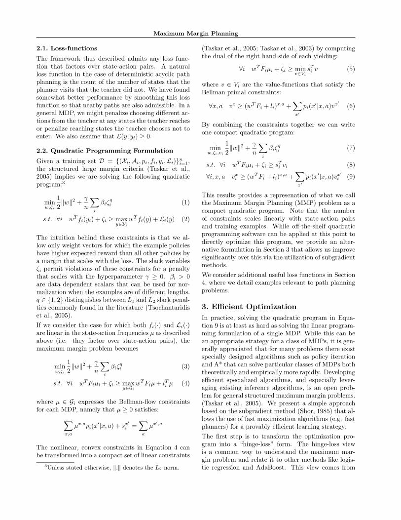
To validating these concepts we focused on the practi-cal problem of path planning using the batch learningalgorithm presented in section 3. In this setting, theMDP can be viewed as a two-dimensional map dis-cretized uniformely into an array of cells. Each cellrepresents a particular location in the world and typ-ical actions include moving from a given cell to oneof the eight neighboring cells. In all experiments, weused A∗ as our specialized planning algorithm, setβi = 1/‖µi‖q1, chose q = 2, and used reasonable valuesfor regularization.We first exhibit the versatility of our algorthm in learn-ing distinct concepts within a single domain. Differingexample trajectories, demonstrated in one region ofa map, lead to a significantly different behavior in aseparate holdout region after learning. Figure 1 showsqualitatively the results of this experiment. The be-havior presented in the top row suggests a desire tostay on the road, while that portrayed in the bottomrow embodies more clandestine needs. By column,from left to right, the images depict the training exam-ple presented to the algorithm, the learned cost mapon a holdout region after training, and the resultingbehavior produced by A∗ over this region.7

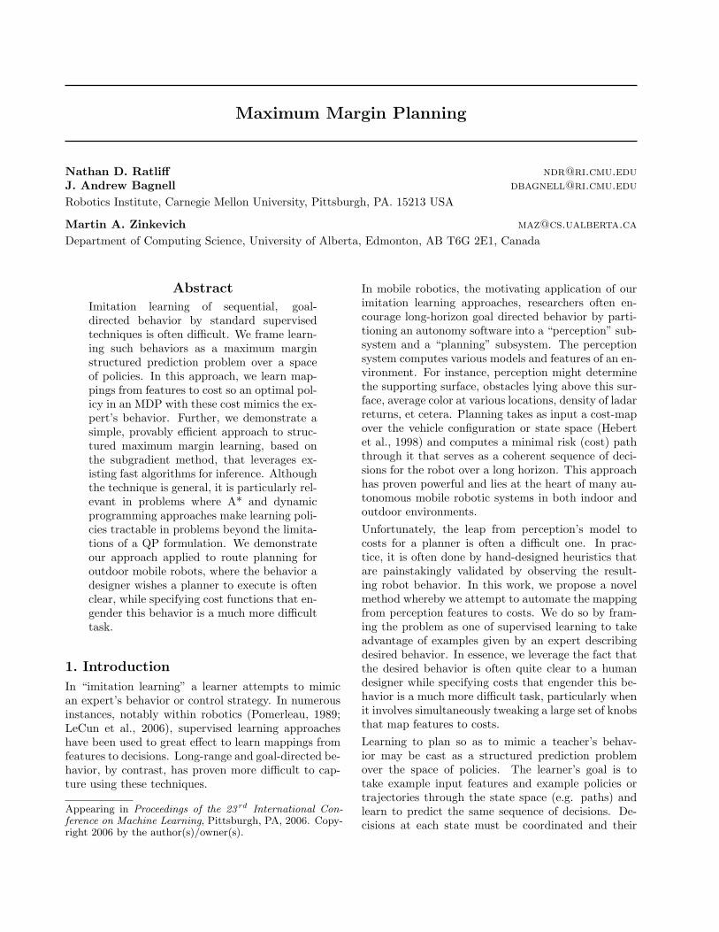
For our second experiment, the data derived entirelyfrom laser range readings (ladar) over the region of in-terest collected during an overhead helicopter sweep.8

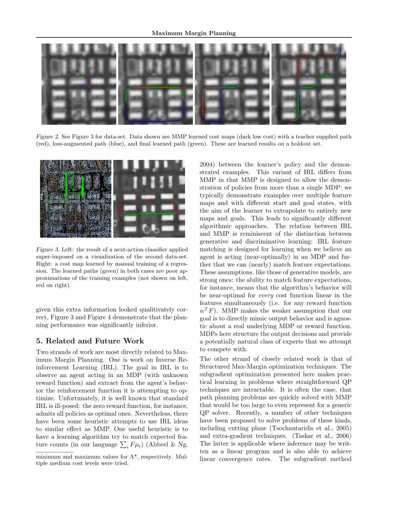
A visualization of the raw data is depicted in Figure 3.Figure 2 shows typical results from a holdout region.The learned behavior (green) often matches well thedesired behavior (red). Even when the learner failedto match the desired trajectory exactly, the learnedbehavior adheres to the primary rules set forth im-plicitly by the examples. Namely, the learner finds anefficient path that avoids buildings (white) and grassyareas (gray) in lieu of roads.Notice that the loss-augmented path (blue) in this fig-ure performs generally worse than the final learned tra-jectory. This is because loss-augmentation makes areasof high loss more desirable than they would be in the

7The features used in this experiment were derived en-tirely from a single overhead satellite image. We dis-cretized the image into five distinct color classes and addedsmoothed versions of the resulting features to propegateproximity information.

8Raw features were computed from mean and standarddeviations from each of elevation, signal reflectance, hue,saturation, and local ladar shape information (Vandapelet al., 2004). Again, we added smoothed versions of theraw features to utilize proximity information.

Figure 1. Demonstration of learning to plan based on satel-lite color imagery. For a particular training/holdout regionpair, the top row trains the learner to follow the road whilethe bottom row trains the learner to “hide” in the trees.From left to right, the columns depict the single trainingexample presented, the learned cost map over the holdoutregion, and the corresponding learned behavior over thatregion. Cost scales with intensity.

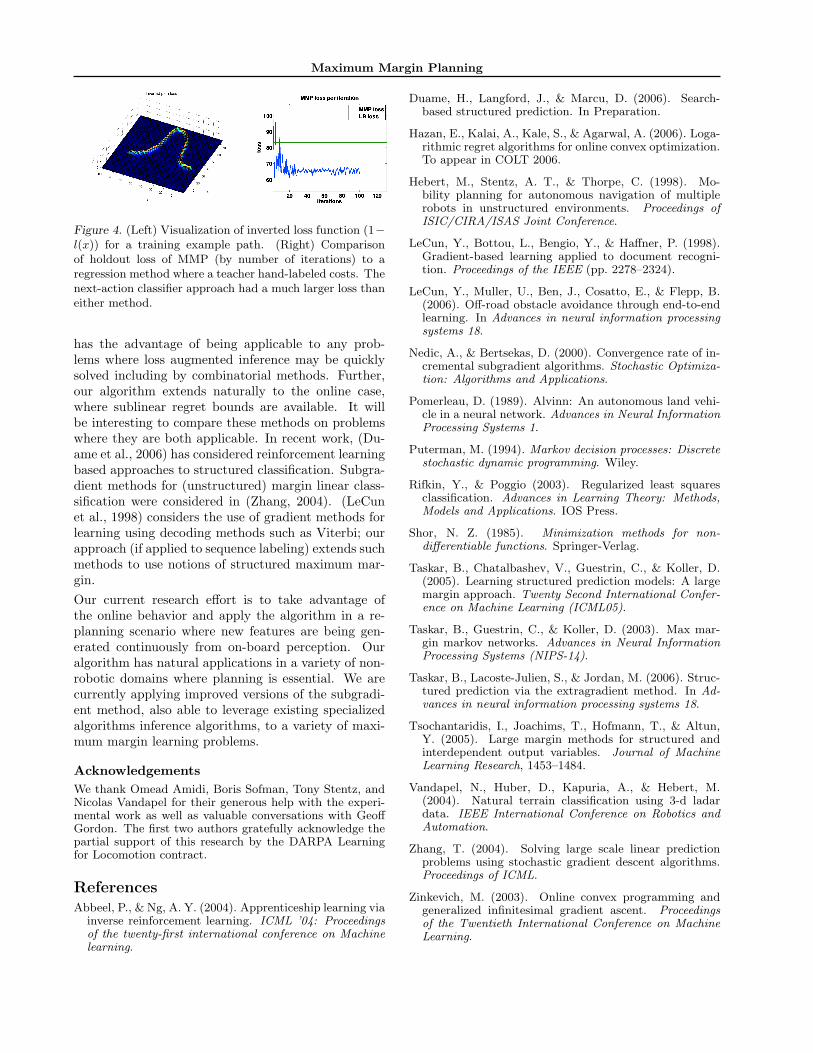
final learned map. Intuitively, if the learner is able toperform well with respect to the loss-augmented costmap, then it should perform even better without theloss-augmentation; that is, the concept is learned withmargin.For comparison, we attempted to learn similar behav-ior using two alternative approaches to MMP. First,we tried the reactive approach of directly learning fromexamples a mapping that takes state features to nextactions as in (LeCun et al., 2006).9 Unfortunately, theresulting paths were rather poor matches to the train-ing data. See Figure 3 for a typical example of a pathlearned by the classifier.A somewhat more successful attempt was to try tolearn costs directly by a hand labeling of regions. Thisprovides dramatically more explicit information to thelearner than MMP requires: a trainer provided exam-ples regions of low, medium, and high costs, basedupon (1) expert knowledge of the planner, (2) iter-ated training and observation, and (3) the trainer hadprior knowledge of the cost maps found under MMPbatch learning on this data set.10 Although cost maps

9We used the same training data, training RegularizedLeast Squares classifiers (Rifkin & Poggio, 2003) to predictwhich nearby state to transition to. It proved difficult toengineer good features here; our best results come from us-ing the same local state features as MMP augmented withdistance and orientation to the goal. The learner typicallyachieved between 0.7-0.85 prediction accuracy.

10The low cost examples came from the example pathsand the medium/high cost examples were supplied sepa-rately. Low cost and high cost examples were chosen as

Maximum Margin Planning

Figure 2. See Figure 3 for data-set. Data shown are MMP learned cost maps (dark low cost) with a teacher supplied path(red), loss-augmented path (blue), and final learned path (green). These are learned results on a holdout set.

Figure 3. Left: the result of a next-action classifier appliedsuper-imposed on a visualization of the second data-set.Right: a cost map learned by manual training of a regres-sion. The learned paths (green) in both cases are poor ap-proximations of the training examples (not shown on left,red on right).

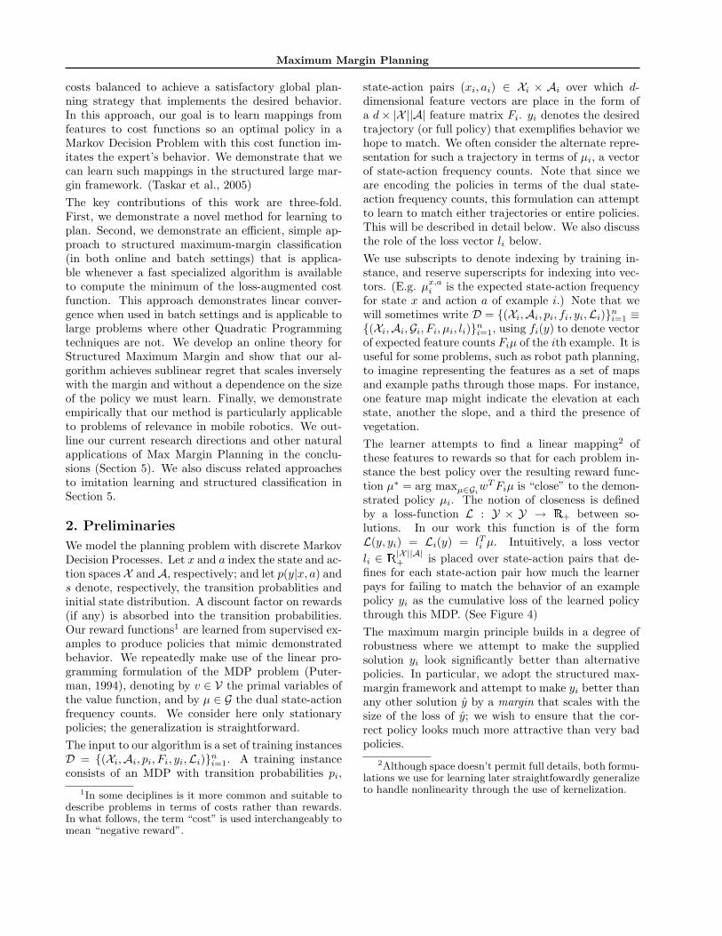
given this extra information looked qualitivately cor-rect, Figure 3 and Figure 4 demonstrate that the plan-ning performance was significantly inferior.

5. Related and Future Work

Two strands of work are most directly related to Max-imum Margin Planning. One is work on Inverse Re-inforcement Learning (IRL). The goal in IRL is toobserve an agent acting in an MDP (with unknownreward function) and extract from the agent’s behav-ior the reinforcement function it is attempting to op-timize. Unfortunately, it is well known that standardIRL is ill-posed: the zero reward function, for instance,admits all policies as optimal ones. Nevertheless, therehave been some heuristic attempts to use IRL ideasto similar effect as MMP. One useful heuristic is tohave a learning algorithm try to match expected fea-ture counts (in our language

∑i Fµi) (Abbeel & Ng,

minimum and maximum values for A*, respectively. Mul-tiple medium cost levels were tried.

2004) between the learner’s policy and the demon-strated examples. This variant of IRL differs fromMMP in that MMP is designed to allow the demon-stration of policies from more than a single MDP: wetypically demonstrate examples over multiple featuremaps and with different start and goal states, withthe aim of the learner to extrapolate to entirely newmaps and goals. This leads to significantly differentalgorithmic approaches. The relation between IRLand MMP is reminiscent of the distinction betweengenerative and discriminative learning: IRL featurematching is designed for learning when we believe anagent is acting (near-optimally) in an MDP and fur-ther that we can (nearly) match feature expectations.These assumptions, like those of generative models, arestrong ones: the ability to match feature expectations,for instance, means that the algorithm’s behavior willbe near-optimal for every cost function linear in thefeatures simultaneously (i.e. for any reward functionwT F ). MMP makes the weaker assumption that ourgoal is to directly mimic output behavior and is agnos-tic about a real underlying MDP or reward function.MDPs here structure the output decisions and providea potentially natural class of experts that we attemptto compete with.The other strand of closely related work is that ofStructured Max-Margin optimization techniques. Thesubgradient optimization presented here makes prac-tical learning in problems where straightforward QPtechniques are intractable. It is often the case, thatpath planning problems are quickly solved with MMPthat would be too large to even represent for a genericQP solver. Recently, a number of other techniqueshave been proposed to solve problems of these kinds,including cutting plane (Tsochantaridis et al., 2005)and extra-gradient techniques. (Taskar et al., 2006)The latter is applicable where inference may be writ-ten as a linear program and is also able to achievelinear convergence rates. The subgradient method

Maximum Margin Planning

Figure 4. (Left) Visualization of inverted loss function (1−l(x)) for a training example path. (Right) Comparisonof holdout loss of MMP (by number of iterations) to aregression method where a teacher hand-labeled costs. Thenext-action classifier approach had a much larger loss thaneither method.

has the advantage of being applicable to any prob-lems where loss augmented inference may be quicklysolved including by combinatorial methods. Further,our algorithm extends naturally to the online case,where sublinear regret bounds are available. It willbe interesting to compare these methods on problemswhere they are both applicable. In recent work, (Du-ame et al., 2006) has considered reinforcement learningbased approaches to structured classification. Subgra-dient methods for (unstructured) margin linear class-sification were considered in (Zhang, 2004). (LeCunet al., 1998) considers the use of gradient methods forlearning using decoding methods such as Viterbi; ourapproach (if applied to sequence labeling) extends suchmethods to use notions of structured maximum mar-gin.Our current research effort is to take advantage ofthe online behavior and apply the algorithm in a re-planning scenario where new features are being gen-erated continuously from on-board perception. Ouralgorithm has natural applications in a variety of non-robotic domains where planning is essential. We arecurrently applying improved versions of the subgradi-ent method, also able to leverage existing specializedalgorithms inference algorithms, to a variety of maxi-mum margin learning problems.

AcknowledgementsWe thank Omead Amidi, Boris Sofman, Tony Stentz, andNicolas Vandapel for their generous help with the experi-mental work as well as valuable conversations with GeoffGordon. The first two authors gratefully acknowledge thepartial support of this research by the DARPA Learningfor Locomotion contract.

ReferencesAbbeel, P., & Ng, A. Y. (2004). Apprenticeship learning via

inverse reinforcement learning. ICML ’04: Proceedingsof the twenty-first international conference on Machinelearning.

Duame, H., Langford, J., & Marcu, D. (2006). Search-based structured prediction. In Preparation.

Hazan, E., Kalai, A., Kale, S., & Agarwal, A. (2006). Loga-rithmic regret algorithms for online convex optimization.To appear in COLT 2006.

Hebert, M., Stentz, A. T., & Thorpe, C. (1998). Mo-bility planning for autonomous navigation of multiplerobots in unstructured environments. Proceedings ofISIC/CIRA/ISAS Joint Conference.

LeCun, Y., Bottou, L., Bengio, Y., & Haffner, P. (1998).Gradient-based learning applied to document recogni-tion. Proceedings of the IEEE (pp. 2278–2324).

LeCun, Y., Muller, U., Ben, J., Cosatto, E., & Flepp, B.(2006). Off-road obstacle avoidance through end-to-endlearning. In Advances in neural information processingsystems 18.

Nedic, A., & Bertsekas, D. (2000). Convergence rate of in-cremental subgradient algorithms. Stochastic Optimiza-tion: Algorithms and Applications.

Pomerleau, D. (1989). Alvinn: An autonomous land vehi-cle in a neural network. Advances in Neural InformationProcessing Systems 1.

Puterman, M. (1994). Markov decision processes: Discretestochastic dynamic programming. Wiley.

Rifkin, Y., & Poggio (2003). Regularized least squaresclassification. Advances in Learning Theory: Methods,Models and Applications. IOS Press.

Shor, N. Z. (1985). Minimization methods for non-differentiable functions. Springer-Verlag.

Taskar, B., Chatalbashev, V., Guestrin, C., & Koller, D.(2005). Learning structured prediction models: A largemargin approach. Twenty Second International Confer-ence on Machine Learning (ICML05).

Taskar, B., Guestrin, C., & Koller, D. (2003). Max mar-gin markov networks. Advances in Neural InformationProcessing Systems (NIPS-14).

Taskar, B., Lacoste-Julien, S., & Jordan, M. (2006). Struc-tured prediction via the extragradient method. In Ad-vances in neural information processing systems 18.

Tsochantaridis, I., Joachims, T., Hofmann, T., & Altun,Y. (2005). Large margin methods for structured andinterdependent output variables. Journal of MachineLearning Research, 1453–1484.

Vandapel, N., Huber, D., Kapuria, A., & Hebert, M.(2004). Natural terrain classification using 3-d ladardata. IEEE International Conference on Robotics andAutomation.

Zhang, T. (2004). Solving large scale linear predictionproblems using stochastic gradient descent algorithms.Proceedings of ICML.

Zinkevich, M. (2003). Online convex programming andgeneralized infinitesimal gradient ascent. Proceedingsof the Twentieth International Conference on MachineLearning.