Embed Size (px)
Citation preview

Maximization Problems ParameterizedUsing Their Minimization Versions:
The Case of Vertex Cover
Meirav Zehavi
Department of Computer Science, Technion - Israel Institute of Technology, Haifa32000, Israel
Abstract. The parameterized complexity of problems is often studiedwith respect to the size of their optimal solutions. However, for a max-imization problem, the size of the optimal solution can be very large,rendering algorithms parameterized by it inefficient. Therefore, we sug-gest to study the parameterized complexity of maximization problemswith respect to the size of the optimal solutions to their minimizationversions. We examine this suggestion by considering the Maximal Min-imal Vertex Cover (MMVC) problem, whose minimization version,Vertex Cover, is one of the most studied problems in the field ofParameterized Complexity. Our main contribution is a parameterizedapproximation algorithm for MMVC, including its weighted variant. Wealso give conditional lower bounds for the running times of algorithmsfor MMVC and its weighted variant.
1 Introduction
The parameterized complexity of problems is often studied with respect to thesize of their optimal solutions. However, for a maximization problem, the sizeof the optimal solution can be very large, rendering algorithms parameterizedby it inefficient. Therefore, we suggest to study the parameterized complexity ofmaximization problems with respect to the size of the optimal solutions to theirminimization versions. Given a maximization problem, the optimal solution toits minimization version might not only be significantly smaller, but it mightalso be possible to efficiently compute it by using some well-known parameter-ized algorithm—in such cases, one can know in advance if for a given instance ofthe maximization problem, the size of the optimal solution to the minimizationversion is a good choice as a parameter. Furthermore, assuming that an opti-mal solution to the minimization version can be efficiently computed, one mayuse it to solve the maximization problem; indeed, the optimal solution to themaximization problem and the optimal solution to its minimization version mayshare useful, important properties.
We examine this suggestion by studying the Maximal Minimal VertexCover (MMVC) problem. This is a natural choice—the minimization version
arX
iv:1
503.
0643
8v1
[cs
.DS]
22
Mar
201
5

of MMVC is the classic Vertex Cover (VC) problem, one of the most stud-ied problems in the field of Parameterized Complexity. In Weighted MMVC(WMMVC), we are given a graph G = (V,E) and a weight function w : V →R≥1. We need to find the maximum weight of a set of vertices that forms a min-imal vertex cover of G. The MMVC problem is the special case of WMMVCin which w(v) = 1 for all v ∈ V .
Notation: Let vc (vcw) denote the size (weight) of a minimum vertex cover(minimum weight vertex cover) of G, and let opt (optw) denote the size (weight)of a maximal minimal vertex cover (maximal-weight minimal vertex cover) ofG. Clearly, vc ≤ min{vcw, opt} ≤ max{vcw, opt} ≤ optw. Observe that the gapbetween vcw = max{vc, vcw} and opt = min{opt, optw} can be very large. Forexample, in the case of MMVC, if G is a star, then vcw = 1 while opt = |V |− 1.
The standard notation O∗ hides factors polynomial in the input size. A prob-lem is fixed-parameter tractable (FPT) with respect to a parameter k if it canbe solved in time O∗(f(k)), for some function f . The maximum degree of a ver-tex in G is denoted by ∆. Given v ∈ V , N(v) denotes the set of neighbors ofv. Also, let γ denote the smallest constant such that it is known how to solveVC in time O∗(γvc), using polynomial space. Currently, γ < 1.274 [12]. GivenU ⊆ V , let G[U ] denote the subgraph of G induced by U . Finally, let M denotethe maximum weight of a vertex in G.
1.1 Related Work
MMVC: Boria et al. [4] show that MMVC is solvable in time O∗(3m) and poly-nomial space, and that WMMVC is solvable in time and space O∗(2tw), wherem is the size of a maximum matching of G, and tw is the treewidth of G. Sincemax{m, tw} ≤ vc (see, e.g., [19]), this shows that WMMVC is FPT with respectto vc. Moreover, they prove that MMVC is solvable in time O∗(1.5874opt) andpolynomial space, where the running time can be improved if one is interested inapproximation.1 Boria et al. [4] also prove that for any constant ε > 0, MMVC
is inapproximable within ratios O(|V |ε− 12 ) and O(∆ε−1), unless P=NP. They
complement this result by proving that MMVC is approximable within ratios|V |− 1
2 and 32∆ in polynomial time.
Recently, Bonnet and Paschos [3] and Bonnet et al. [2] obtained results relat-ing to the inapproximability of MMVC in subexponential time. Furthermore,Bonnet et al. [2] prove that for any 1 < r ≤ |V | 12 , MMVC is approximable
within ratio 1r in time O∗(2
|V |r2 ).
Vertex Cover: First, note that VC is one of the first problems shown to beFPT. In the past two decades, it enjoyed a race towards obtaining the fastest pa-rameterized algorithm (see [7,17,1,27,18,10,28,8,29,12]). The best parameterizedalgorithm, due to Chen et al. [12], has running time O∗(1.274vc), using poly-nomial space. In a similar race [10,13,11,30,32,24], focusing on the case where
1 For example, they show that one can guarantee the approximation ratios 0.1 and0.4 in times O∗(1.162opt) and O∗(1.552opt), respectively.
2
∆ = 3, the current winner is an algorithm by Issac et al. [24], whose runningtime is O∗(1.153vc). For Weighted VC (WVC), parameterized algorithmswere given in [28,21,22,31]. The fastest ones (in [31]) use time O∗(1.381vcw)and polynomial space, time and space O∗(1.347vcw), and time O∗(1.443vc) andpolynomial space.
Kernels for VC and WVC were given in [10,14,25], and results relating to theparameterized approximability of VC were also examined in the literature (see,e.g., [5,6,20]). Finally, in the context of Parameterized Complexity, we wouldalso like to note that vc is a parameter of interest; indeed, apart from VC, thereare other problems whose parameterized complexity was studied with respect tothis parameter (see, e.g., [9,23,26]).
1.2 Our Contribution
While it can be easily seen that WMMVC is solvable in time O∗(2vc) andpolynomial space (see Section 2), we observe that this result might be essen-tially tight. More precisely, we show that even if G is a bipartite graph andw(v) ∈ {1, 1 + 1
|V |} for all v ∈ V , an algorithm that solves WMMVC in time
O∗((2−ε)vcw), which upper bounds O∗((2−ε)vc), contradicts the SETH (StrongExponential Time Hypothesis). We also show that even if G is a bipartite graph,an algorithm that solves MMVC in time O∗((2− ε) vc
2 ) contradicts the SETH.Then, we turn to present our main contribution, ALG, which is a parame-
terized approximation algorithm for WMMVC with respect to the parametervc. More precisely, we prove the following theorem, where α is a user-controlledparameter that corresponds to a tradeoff between time and approximation ratio.
Theorem 1. For any α <1
2− 1M+1
such that1
xx(1− x)1−x≥ 3
13 where x =
1− 1−αM(2α−1)+1−α ,2 ALG runs in time O∗((
1
xx(1− x)1−x)vc), returning a minimal
vertex cover of weight at least α · optw. ALG has a polynomial space complexity.
For example, for the smallest possible α, the running time is bounded byO∗(3
vc3 ) < O∗(1.44225vc), and for any constant α < 1
2− 1M+1
, there is a constant
ε > 0 such that the running time is bounded by O∗((2− ε)vc).ALG is based is on a mix of two bounded search tree-based procedures.3 In
particular, the branching vectors of one of these procedures are analyzed withrespect to the size of a minimum vertex cover of a minimum vertex cover ofG. Another interesting feature of this procedure is that once it reaches a leaf(of the search tree), it does not immediately return a result, but to obtain thedesired approximation ratio, it first performs a computation that is, in a sense,
2 In particular, the result holds for any1
2<
1
2− 17.35841·M+1
≤ α < 1
2− 1M+1
.
3 Information on the bounded search technique, which is perhaps the most well-knowntechnique used to design parameterized algorithms [16], is given in Section 3.
3

an exhaustive search. We would like to note that in the design of our secondprocedure, we integrate rules that are part of the iterative compression-basedalgorithm for VC by Peiselt [29]. Since ALG can be used to solve MMVC, inwhich case M = 1, we immediately obtain the following corollary.
Corollary 1. For any α < 23 such that 1
xx(1−x)1−x ≥ 313 where x = 2 − 1
α ,4
ALG runs in time O∗(( 1xx(1−x)1−x )vc), returning a minimal vertex cover of size
at least α · opt. ALG has a polynomial space complexity.
2 Upper and Lower Bounds
In this section, we give upper and conditional lower bounds related to the pa-rameterized complexity of WMMVC and MMVC with respect to vc and vcw.Recall, in this context of the next results, that vc ≤ vcw and MMVC is a specialcase of WMMVC.
Observation 1. WMMVC is solvable is time O∗(2vc) and polynomial space.
Proof. The algorithm is as follows. First, compute a minimum vertex cover S ofG in time O∗(γvc) using polynomial space, and initialize A to S. Then, for everysubset S′ ⊆ S, if B = S′ ∪ (
⋃v∈S\S′ N(v)) is a minimal vertex cover of weight
larger than the weight of A, update A to store B. Finally, return A.Clearly, we return a minimal vertex cover. Now, let A∗ be an optimal solution.
Consider the iteration where we examine S′ = A∩S. Then, since A∗ is a vertexcover, B ⊆ A∗. Suppose, by way of contradiction, that there exists v ∈ A∗ \ B.The vertex v does not belong to S (since A∩S ⊆ B). Moreover, it should have aneighbor outside A∗ (since A∗ is a minimal vertex cover). Thus, since S is a vertexcover, v has a neighbor in S \ A∗. This implies that v ∈
⋃u∈S\S′ N(u), which
contradicts the assumption that v /∈ B. We conclude that B = A∗. Therefore, thealgorithm is correct, and it clearly has the desired time and space complexities.
ut
Now, we observe that even in a restricted setting, the algorithm above isessentially optimal under the SETH.
Lemma 1. For any constant ε > 0, WMMVC in bipartite graphs, where w(v) ∈{1, 1 + 1
|V |} for all v ∈ V , cannot be solved in time O∗((2 − ε)vcw) unless the
SETH fails.
Proof. Fix ε > 0. Suppose, by way of contradiction, that there exists an algo-rithm, A, that solves WMMVC in the restricted setting in time O∗((2− ε)vcw).We aim to show that this implies that there exists an algorithm that solves theHitting Set (HS) problem in time O∗((2− ε)n), which contradicts the SETH[15]. In HS, we are given an n-element set U , along with family of subsets ofU , F = {F1, F2, . . . , Fm}, and the goal is to find the minimum size of a subset
4 In particular, the result holds for any 0.53183 ≤ α < 23.
4
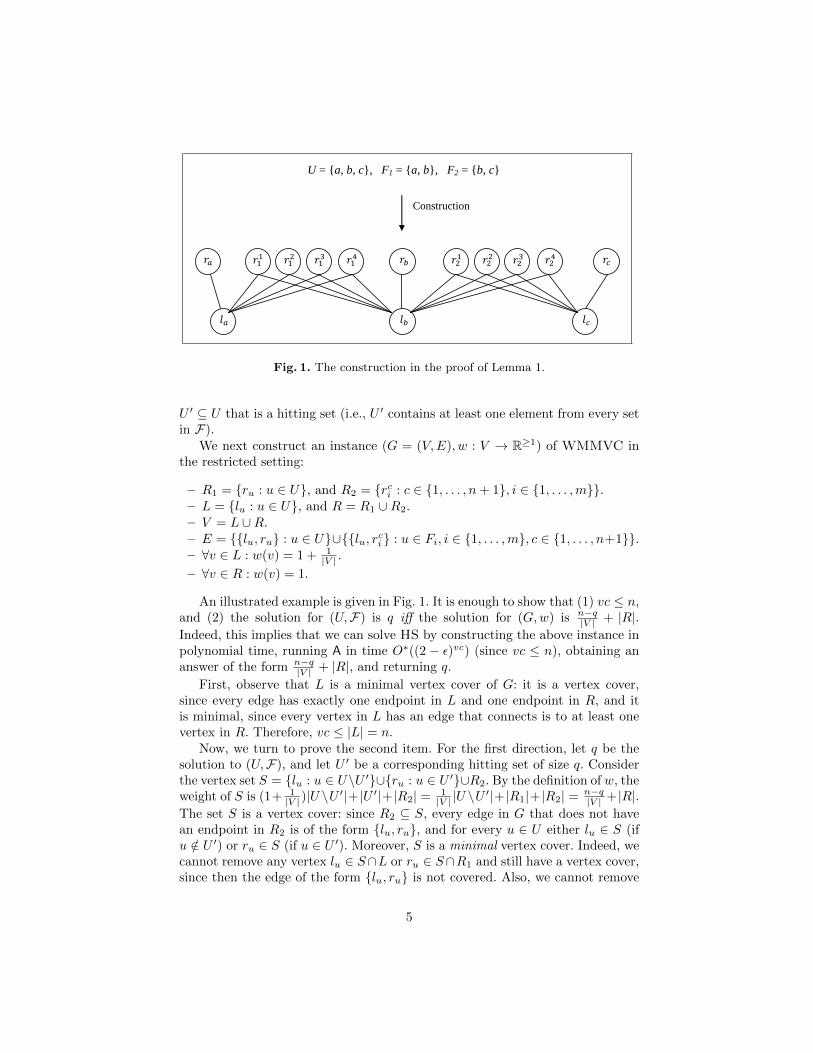
U = {a, b, c}, F1 = {a, b}, F2 = {b, c}
Construction
Fig. 1. The construction in the proof of Lemma 1.
U ′ ⊆ U that is a hitting set (i.e., U ′ contains at least one element from every setin F).
We next construct an instance (G = (V,E), w : V → R≥1) of WMMVC inthe restricted setting:
– R1 = {ru : u ∈ U}, and R2 = {rci : c ∈ {1, . . . , n+ 1}, i ∈ {1, . . . ,m}}.– L = {lu : u ∈ U}, and R = R1 ∪R2.– V = L ∪R.– E = {{lu, ru} : u ∈ U}∪{{lu, rci } : u ∈ Fi, i ∈ {1, . . . ,m}, c ∈ {1, . . . , n+1}}.– ∀v ∈ L : w(v) = 1 + 1
|V | .
– ∀v ∈ R : w(v) = 1.
An illustrated example is given in Fig. 1. It is enough to show that (1) vc ≤ n,and (2) the solution for (U,F) is q iff the solution for (G,w) is n−q
|V | + |R|.Indeed, this implies that we can solve HS by constructing the above instance inpolynomial time, running A in time O∗((2 − ε)vc) (since vc ≤ n), obtaining ananswer of the form n−q
|V | + |R|, and returning q.
First, observe that L is a minimal vertex cover of G: it is a vertex cover,since every edge has exactly one endpoint in L and one endpoint in R, and itis minimal, since every vertex in L has an edge that connects is to at least onevertex in R. Therefore, vc ≤ |L| = n.
Now, we turn to prove the second item. For the first direction, let q be thesolution to (U,F), and let U ′ be a corresponding hitting set of size q. Considerthe vertex set S = {lu : u ∈ U\U ′}∪{ru : u ∈ U ′}∪R2. By the definition of w, theweight of S is (1+ 1
|V | )|U \U′|+|U ′|+|R2| = 1
|V | |U \U′|+|R1|+|R2| = n−q
|V | +|R|.The set S is a vertex cover: since R2 ⊆ S, every edge in G that does not havean endpoint in R2 is of the form {lu, ru}, and for every u ∈ U either lu ∈ S (ifu /∈ U ′) or ru ∈ S (if u ∈ U ′). Moreover, S is a minimal vertex cover. Indeed, wecannot remove any vertex lu ∈ S∩L or ru ∈ S∩R1 and still have a vertex cover,since then the edge of the form {lu, ru} is not covered. Also, we cannot remove
5

any vertex rci ∈ R2, since there is a vertex lu /∈ S such that {lu, rci } ∈ E (to seethis, observe that because U ′ is a hitting set, there is a vertex u ∈ U ′∩Fi, whichcorresponds to the required vertex lu).
For the second direction, let p be the solution to (G,w), and let S be acorresponding minimal vertex cover of weight p. Clearly, p ≥ w(R) = n+m(n+1), since R is a minimal vertex cover of G. Observe that for all u ∈ U , bythe definition of G and since S is a minimal vertex cover, exactly one amongthe vertices lu and ru is in S. Suppose that there exists rci ∈ R2 \ S. Then,for all u ∈ Fi, we have that lu ∈ S (by the definition of G and since S is avertex cover), which implies that for all c ∈ {1, . . . , n+ 1}, we have that rci /∈ S(since S is a minimal vertex cover). Thus, p = w(S ∩ (L ∪ R1)) + |S ∩ R2| ≤n(1 + 1
|V | ) + (m− 1)(n+ 1) < n+m(n+ 1), which is a contradiction. Therefore,
R2 ⊆ S.Denote U ′ = {u : ru ∈ S ∩ R1}. By the above discussion and the definition
of w, |S| = |V \R2|2 + |R2| = |R1| + |R2| = |R|, and p − |S| = 1
|V | |S ∩ L| =1|V | (n − |S ∩ R1|). Denoting |U ′| = q, we have that p = n−q
|V | + |R|. Thus, it
remains to show that U ′ is a hitting set. Suppose, by way of contradiction, thatU ′ is not a hitting set. Thus, there exists Fi ∈ F such that for all u ∈ Fi, we havethat u /∈ U ′. By the definition of U ′, this implies that for all u ∈ Fi, we havethat lu ∈ S. Thus, N(r1i ) ⊆ S, while r1i ∈ S (since we have shown that R2 ⊆ S),which is a contradiction to the fact that S is a minimal vertex cover. ut
Next, we also give a conditional lower bound for MMVC. The proof is quitesimilar to the one above, and is thus relegated to Appendix A. Informally, theidea is to modify the above proof by adding a copy l′u of every vertex lu ∈ L,which is only attached to its “mirror vertex”, ru, in R1. While previously theweights 1 + 1
|V | encouraged us to choose many vertices from L, now the copies
encourage us to choose these vertices.
Lemma 2. For any constant ε > 0, MMVC in bipartite graphs cannot be solvedin time O∗((2− ε) vc
2 ) unless the SETH fails.
3 A Parameterized Approximation Algorithm
In this section we develop ALG (see Theorem 1). When referring to α, supposethat it is chosen as required in Theorem 1, and define x accordingly. The al-gorithm is a mix of two bounded search tree-based procedures, ProcedureA andProcedureB, which are developed in the following subsections.5 For these proce-dures, we will prove the following lemmas.
Lemma 3. Let U be a minimum(-size) vertex cover of G, and let U ′ be aminimum(-size) vertex cover of G[U ]. Moreover, suppose that |U ′| ≤ vc
2 .
5 ProcedureA could also be developed without using recursion; however, relying on thebounded search tree technique simplifies the presentation, emphasizing the partssimilar between ProcedureA and ProcedureB.
6

Then, ProcedureA(G,w, α, U, U ′, ∅, ∅) runs in time O∗(( 1xx(1−x)1−x )vc), using
polynomial space and returning a minimal vertex cover of weight at least α ·optw.
Lemma 4. Let U be a minimum(-size) vertex cover of G such that the size ofa minimum(-size) vertex cover of G[U ] is larger than vc
2 .Then, ProcedureB(G,w,U, ∅, ∅) runs in time O∗(3
vc3 ), using polynomial space
and returning a minimal vertex cover of weight at least1
2− 1M+1
· optw.
Having these procedures, we give the pseudocode of ALG below. The algo-rithm computes a minimum vertex cover U ′ of a minimum vertex cover U , solvingthe given instance by calling either ProcedureA (if |U ′| ≤ vc
2 ) or ProcedureB (if|U ′| > vc
2 ).
Algorithm 1 ALG(G = (V,E), w : V → R≥1, α)
1: Compute a minimum vertex cover U of G in time O∗(γvc) and polynomial space.2: Compute a minimum vertex cover U ′ ofG[U ] in timeO∗(γvc) and polynomial space.
3: if |U ′| ≤ vc2
then4: Return ProcedureA(G,w, α, U, U ′, ∅, ∅).5: else6: Return ProcedureB(G,w,U, ∅, ∅).7: end if
Now, we turn to prove Theorem 1.
Proof. The correctness of the approximation ratio immediately follows fromLemmas 3 and 4. Observe that the computation of U ′ can indeed be per-formed in time O∗(γvc) since U ′ ⊆ U , and therefore |U ′| ≤ |U | ≤ vc. More-over, since γ < 1.274, by Lemmas 3 and 4, the running time is bounded byO∗(max{( 1
xx(1−x)1−x )vc, 3vc3 }). Since α is chosen such that ( 1
xx(1−x)1−x )vc ≥ 3vc3 ,
the above running time is bounded by O∗(( 1xx(1−x)1−x )vc). ut
In the rest of this section, we give necessary information on the boundedsearch tree technque (Section 3.1), after which we develop ProcedureA (Section3.2) and ProcedureB (Section 3.3).
3.1 The Bounded Search Tree Technique
Bounded search trees form a fundamental technique in the design of recursiveparameterized algorithms (see [16]). Roughly speaking, in applying this tech-nique, one defines a list of rules of the form Rule X. [condition] action, where Xis the number of the rule in the list. At each recursive call (i.e., a node in thesearch tree), the algorithm performs the action of the first rule whose conditionis satisfied. If by performing an action, the algorithm recursively calls itself at
7

least twice, the rule is a branching rule, and otherwise it is a reduction rule.We only consider actions that increase neither the parameter nor the size of theinstance, and decrease at least one of them. Observe that, at any given time, weonly store the path from the current node to the root of the search tree (ratherthan the entire tree).
The running time of the algorithm can be bounded as follows. Suppose thatthe algorithm executes a branching rule where it recursively calls itself ` times,such that in the ith call, the current value of the parameter decreases by bi.Then, (b1, b2, . . . , b`) is called the branching vector of this rule. We say thatβ is the root of (b1, b2, . . . , b`) if it is the (unique) positive real root of xb
∗=
xb∗−b1 + xb
∗−b2 + . . . + xb∗−b` , where b∗ = max{b1, b2, . . . , b`}. If b > 0 is the
initial value of the parameter, and the algorithm (a) returns a result when (orbefore) the parameter is negative, (b) only executes branching rules whose rootsare bounded by a constant c, and (c) only executes rules associated with actionsperformed in polynomial time, then its running time is bounded by O∗(cb).
In some of the leaves of a search tree corresponding to our first procedure,we execute rules associated with actions that are not performed in polynomialtime (as required in the condition (c) above). We show that for every such leaf `in the search tree, we execute an action that can be performed in time O∗(g(`))for some function g. Then, letting L denote the set of leaves in the search treewhose actions are not performed in polynomial time, we have that the runningtime of the algorithm is bounded by O∗(cb +
∑`∈L g(`)).
3.2 ProcedureA: The Proof of Lemma 3
The procedure ProcedureA is based on the bounded search tree technique. Eachcall is of the form ProcedureA(G,w, α, U, U ′, I, O), where G,w, α, U and U ′ al-ways remain the parameters with whom the procedure was called by ALG, whileI and O are disjoint subsets of U to which ProcedureA adds elements as theexecution progresses (initially, I = O = ∅). Roughly speaking, the sets I and Oindicate that currently we are only interested in examining minimal vertex cov-ers that contain all of the vertices in I and none of the vertices in O. Formally,we prove the following result.
Lemma 5. ProcedureA returns a minimal vertex cover S that satisfies the fol-lowing condition:
– If there is a minimal vertex cover S∗ of weight optw such that I ⊆ S∗ andO ∩ S∗ = ∅, then the weight of S is at least α · optw.
Moreover, each leaf, associated with an instance (G,w, α, U, U ′, I ′, O′), corre-sponds to a unique pair (I ′, O′), and its action can be performed in polynomial
time if I ′ ∪ O′ 6= U ′, and in time O∗(|{U ⊆ U : I ′ ⊆ U , O′ ∩ U = ∅, |U | ≥(1− x)vc}|) otherwise.
Let vc′ = |U ′|. To ensure that ProcedureA runs in time O∗(( 1xx(1−x)1−x )vc),
we propose the following measure:
8

Measure: vc′ − |U ′ ∩ (I ∪O)|.Next, we present each rule within a call ProcedureA(G,w, α, U, U ′, I, O). After
presenting a rule, we argue its correctness (see Lemma 5). Since initially I =O = ∅, we thus have that ProcedureA guarantees the desired approximation ratio.For each branching rule, we also give the root of the corresponding branchingvector (with respect to the measure above). We ensure that (1) the largest rootwe shall get is 2, (2) the procedure stops calling itself recursively, at the latest,once the measure drops to 0, and (3) actions not associated with leaves canbe performed in polynomial time. Observe that initially the measure is vc′.Thus, as explained in Section 3.1, the running time of ProcedureA is bounded by
O∗(2vc′+
∑(I′,O′)∈P
|{U ⊆ U : I ′ ⊆ U , O′ ∩ U = ∅, |U | ≥ (1− x)vc}|), where P is
the set of all partitions of U ′ into two sets. This running time is bounded by
O∗(2vc′+ |{U ⊆ U : |U | ≥ (1− x)vc}|) = O∗(2vc
′+
vcmax
i=(1−x)vc
(vc
i
)). Since x <
12 (by the definition of x and since α <
1
2− 1M+1
), vc′ ≤ vc2 and 1
xx(1−x)1−x ≥
313 > 2
12 , this running time is further bounded by O∗((
1
xx(1− x)1−x)vc). Thus,
we also have the desired bound for the running time, concluding the correctnessof Lemma 5.
Reduction Rule 1. [There is v ∈ O such that N(v) ∩O 6= ∅] Return U .
In this case there is no vertex cover that does not contain any vertex from O, andtherefore it is possible to return an arbitrary minimal vertex cover. The actioncan clearly be performed in polynomial time.
Reduction Rule 2. [There is v ∈ X such that N(v) ⊆ X, where X = I ∪(⋃u∈ON(u))] Return U .
Observe that any vertex cover that does not contain any vertex from O, mustcontain all the neighbors of the vertices in O. Thus, any vertex cover that con-tains all the vertices in I and none of the vertices in O, also contains the vertexv and all of its neighbors; therefore, it is not a minimal vertex cover. Thus, it ispossible to return an arbitrary minimal vertex cover. The action can clearly beperformed in polynomial time.
Reduction Rule 3. [U ′ = I ∪O] Perform the following computation.
1. Let A = I ∪ (⋃v∈ON(v) ∩ U). As long as there is a vertex v ∈ A such that
N(v)∩U ⊆ A, choose such a vertex (arbitrarily) and remove it from A. LetA′ be the set obtained at the end of this process.
2. Let A = A′ ∪ (⋃v∈U\A′ N(v) \ U).
3. Denote F = {U ⊆ U : I ⊆ U , O ∩ U = ∅, |U | ≥ (1− x)vc}.6
6 It is not necessary to explicitly store F—we only need to iterate over it; therefore,by the pseudocode, it is clear that the space complexity of the action is polynomial.
9

4. Initialize B = U .
5. For all F ∈ F :(a) Let BF = F ∪ (
⋃v∈U\F N(v))
(b) If BF is a minimal vertex cover:– If the weight of BF is larger than the weight of B: Replace B by BF .
6. Return the set of maximum weight among A and B.
First, observe that this rule ensure that, at the latest, the procedure stops callingitself recursively once the measure drops to 0. Furthemore, by the pseudocode,the action can be performed in time O∗(|F|), which by the definition of F , isthe desired time. It remains to prove that Lemma 3 is correct.
We begin by considering the set A. Since U ′ = I∪O is a vertex cover of G[U ]and the previous rules were not applied, we have that A is vertex cover of G[U ]such that I ⊆ A and O ∩ A = ∅. Thus, by its definition, A′ is a minimal vertexcover of G[U ] such that A′ ⊆ A. Thus, since U is a vertex cover, every edgeeither has both endpoints in U , in which case it has an endpoint in A′, or it hasexactly one endpoint in U and exactly one endpoint in V \ U , in which case ithas an endpoint that is a vertex in A′ or a neighbor in V \U of a vertex in U \A′.Therefore, A is a vertex cover. Moreover, every vertex in A′ has a neighbor inU \ A′ (by the minimality of A′) and every vertex in (
⋃v∈U\A′ N(v) \ U), by
definition, has a neighbor in U \ A′. Thus, we overall have that A is a minimal
vertex cover such that A ∩ U ⊆ A.Since A is a minimal vertex cover, by the pseudocode, we return a weight,
W , of a minimal vertex cover. Assume that there is a minimal vertex cover S∗ ofweight optw such that I ⊆ S∗ and O∩S∗ = ∅. This implies that A ⊆ S∗∩U . Now,to prove Lemma 3, it is sufficient to show that W ≥ α·optw. Denote F ∗ = S∗∩U .Since S∗ is a minimal vertex cover, we have that S∗ = F ∗ ∪ (
⋃v∈U\F∗ N(v)).
If S∗ contains at least (1 − x)vc elements from U , there is an iteration wherewe examine F = F ∗, in which case BF∗ = S∗, and therefore we return optw.Thus, we next suppose that |S∗∩U | < (1−x)vc. Since B is initially U , to prove
Lemma 3, it is now sufficient to show that max{w(A), w(U)} ≥ α · w(S∗).Since S∗ is a vertex cover such that I ⊆ S∗ and O ∩ S∗ = ∅, we have that
A∩U ⊆ A ⊆ F ∗. By the definition of A and since S∗ is a minimal vertex cover,this implies that S∗ \ U ⊆ A \ U . Thus, overall we have that
max{w(U), w(A)}w(S∗)
=max{w(U), w(A)}
w(S∗ \ U) + w(S∗ ∩ U)≥ max{w(U), w(A)}w(A \ U) + w(S∗ ∩ U)
=max{w(U), w(A)}
w(A) + w(S∗ ∩ U)− w(A ∩ U)
≥ w(U)
w(U) + w(S∗ ∩ U)=
1
2− w(U\S∗)w(U)
≥ 1
2− |U\S∗|w(S∗∩U)+|U\S∗|
≥ 1
2− x·vcM ·(1−x)·vc+x·vc
=1
2− xM−(M−1)x
10

Since x = 1− 1−αM(2α−1)+1−α , we have that the expression above is equal to α.
Branching Rule 4. Let v be a vertex in U ′\(I∪O). Return the set of maximumweight among A and B, computed in the following branches.
1. A⇐ProcedureA(G,w, α, U, U ′, I ∪ {v}, O).2. B ⇐ProcedureA(G,w, α, U, U ′, I, O ∪ {v}).
The correctness of Lemma 5 is preserved, since every vertex cover either containsv (an option examined in the first branch) or does not contain v (an optionexamined in the second branch). Moreover, it is clear that the action can beperformed in polynomial time and that the branching vector is (1,1), whose rootis 2.
3.3 ProcedureB: The Proof of Lemma 4
This procedure is based on combining an appropriate application of the ideasused by the previous procedure (considering the fact that now the size of anyvertex cover of G[U ] is larger than vc
2 ) with rules from the algorithm for VC byPeiselt [29]. Due to lack of space, the details are given in Appendix B.
References
1. Balasubramanian, R., Fellows, M., Raman, V.: An improved fixed-parameter algo-rithm for vertex cover. Inf. Process. Lett. 65(3), 163–168 (1998)
2. Bonnet, E., Lampis, M., Paschos, V.T.: Time-approximation trade-offs for inap-proximable problems. CoRR abs/1502.05828 (2015)
3. Bonnet, E., Paschos, V.T.: Sparsification and subexponential approximation.CoRR abs/1402.2843 (2014)
4. Boria, N., Croce, F.D., Paschos, V.T.: On the max min vertex cover problem. In:WAOA. pp. 37–48 (2013)
5. Bourgeois, N., Escoffier, B., Paschos, V.T.: Approximation of max independentset, min vertex cover and related problems by moderately exponential algorithms.Discrete Applied Mathematics 159(17), 1954–1970 (2011)
6. Brankovic, L., Fernau, H.: A novel parameterised approximation algorithm forminimum vertex cover. Theor. Comput. Sci. 511, 85–108 (2013)
7. Buss, J., Goldsmith, J.: Nondeterminism within P. SIAM J. on Computing 22(3),560–572 (1993)
8. Chandran, L.S., Grandoni, F.: Refined memorization for vertex cover. Inf. Process.Lett. 93(3), 123–131 (2005)
9. Chapelle, M., Liedloff, M., Todinca, I., Villanger, Y.: Treewidth and pathwidthparameterized by the vertex cover number. In: WADS. p. 232243 (2013)
10. Chen, J., Kanj, I.A., Jia, W.: Vertex cover: Further observations and further im-provements. J. Algorithms 41(2), 280–301 (2001)
11. Chen, J., Kanj, I.A., Xia, G.: Labeled search trees and amortized analysis: improvedupper bounds for NP-hard problems. Algorithmica 43(4), 245–273 (2005)
12. Chen, J., Kanj, I.A., Xia, G.: Improved upper bounds for vertex cover. Theor.Comput. Sci. 411(40-42), 3736–3756 (2010)
11

13. Chen, J., Liu, L., Jia, W.: Improvement on vertex cover for low degree graphs.Networks 35(4), 253–259 (2000)
14. Chlebik, M., Chlebiova, J.: Crown reductions for the minimum weighted vertexcover problem. Discrete Appl. Math. 156(3), 292–312 (2008)
15. Cygan, M., Dell, H., Lokshtanov, D., Marx, D., Nederlof, J., Okamoto, Y., Paturi,R., Saurabh, S., Wahlstrom, M.: On problems as hard as CNF-SAT. In: CCC. pp.74–84 (2012)
16. Downey, R., Fellows, M.: Fundamentals of parameterized complexity. Springer(2013)
17. Downey, R.G., Fellows, M.R.: Fixed-parameter tractability and completeness II:on completeness for W[1]. Theor. Comput. Sci. 141(1-2), 109–131 (1995)
18. Downey, R.G., Fellows, M.R., Stege, U.: Parameterized complexity: a frameworkfor systematically confronting computational intractability. DIMACS 49, 49–99(1999)
19. Fellows, M.R., Jansen, B.M.P., Rosamond, F.A.: Towards fully multivariate algo-rithmics: Parameter ecology and the deconstruction of computational complexity.Eur. J. Comb. 34(3), 541–566 (2013)
20. Fellows, M.R., Kulik, A., Rosamond, F.A., Shachnai, H.: Parameterized approxi-mation via fidelity preserving transformations. In: ICALP. pp. 351–362 (2012)
21. Fomin, F.V., Gaspers, S., Saurabh, S.: Branching and treewidth based exact algo-rithms. In: ISAAC. pp. 16–25 (2006)
22. Fomin, F.V., Gaspers, S., Saurabh, S., Stepanov, A.A.: On two techniques of com-bining branching and treewidth. Algorithmica 54(2), 181–207 (2009)
23. Fomin, F.V., Liedloff, M., Montealegre-Barba, P., Todinca, I.: Algorithms param-eterized by vertex cover and modular width, through potential maximal cliques.In: SWAT. pp. 182–193 (2014)
24. Issac, D., Jaiswal, R.: An O∗(1.0821n)-time algorithm for computing maximumindependent set in graphs with bounded degree 3. CoRR abs/1308.1351 (2013)
25. Jansen, B.M.P., Bodlaender, H.L.: Vertex cover kernelization revisited - upper andlower bounds for a refined parameter. Theory Comput. Syst. 53(2), 263–299 (2013)
26. Kobayashi, Y.: Treewidth and pathwidth parameterized by the vertex cover num-ber. In: WADS. pp. 232–243 (2013)
27. Niedermeier, R., Rossmanith, P.: Upper bounds for vertex cover further improved.In: STACS. pp. 561–570 (1999)
28. Niedermeier, R., Rossmanith, P.: On efficient fixed-parameter algorithms forweighted vertex cover. J. Algorithms 47(2), 63–77 (2003)
29. Peiselt, T.: An iterative compression algorithm for vertex cover. Ph.D. thesisFriedrich-Schiller-Universitat Jena, Germany (2007)
30. Razgon, I.: Faster computation of maximum independent set and parameterizedvertex cover for graphs with maximum degree 3. JDA 7(2), 191–212 (2009)
31. Shachnai, H., Zehavi, M.: A multivariate framework for weighted FPT algorithms.CoRR abs/1407.2033 (2014)
32. Xiao, M.: A note on vertex cover in graphs with maximum degree 3. In: COCOON.pp. 150–159 (2010)
12

A Proof of Lemma 2
Fix ε > 0. Suppose, by way of contradiction, that there exists an algorithm, A,that solves MMVC in the restricted setting in time O∗((2 − ε) vc
2 ). We aim toshow that this implies that there exists an algorithm that solves HS in timeO∗((2 − ε)n), which contradicts the SETH [15]. To this end, we construct angraph G = (V,E) that defines an instance of MMVC in the restricted setting:
– R1 = {ru : u ∈ U}, and R2 = {rci : c ∈ {1, . . . , n+ 1}, i ∈ {1, . . . ,m}}.– L = {lcu : u ∈ U, c ∈ {1, 2}}, and R = R1 ∪R2.– V = L ∪R.– E = {{lcu, ru} : u ∈ U, c ∈ {1, 2}} ∪ {{l1u, rci } : u ∈ Fi, i ∈ {1, . . . ,m}, c ∈{1, . . . , n+ 1}}.
It is enough to show that (1) vc ≤ 2n, and (2) the solution for (U,F) is qiff the solution for (G,w) is (n− q) + |R|. Indeed, this implies that we can solveHS by constructing the above instance in polynomial time, running A in timeO∗((2− ε)n) (since vc ≤ 2n), obtaining an answer of the form (n− q) + |R|, andreturning q.
First, observe that L is a minimal vertex cover of G: it is a vertex cover,since every edge has exactly one endpoint in L and one endpoint in R, and itis minimal, since every vertex in L has an edge that connects is to at least onevertex in R. Therefore, vc ≤ |L| = 2n.
Now, we turn to prove the second item. For the first direction, let q be thesolution to (U,F), and let U ′ be a corresponding hitting set of size q. Considerthe vertex set S = {lcu : u ∈ U \U ′, c ∈ {1, 2}}∪{ru : u ∈ U ′}∪R2. Observe that|S| = 2|U \U ′|+ |U ′|+ |R2| = |U \U ′|+ |R1|+ |R2| = (n− q) + |R|. The set S isa vertex cover: since R2 ⊆ S, every edge in G that does not have an endpoint inR2 is of the form {lcu, ru}, and for every u ∈ U either [l1u, l
2u ∈ S (if u /∈ U ′)] or
[ru ∈ S (if u ∈ U ′)]. Moreover, S is a minimal vertex cover. Indeed, we cannotremove any vertex lu ∈ S ∩L or ru ∈ S ∩R1) and still have a vertex cover, sincethen the edge of the form {lcu, ru} is not covered. Also, we cannot remove anyvertex rci ∈ R2, since there is a vertex l1u /∈ S such that {l1u, rci } ∈ E (to see this,observe that because U ′ is a hitting set, there is a vertex u ∈ U ′ ∩ Fi, whichcorresponds to the required vertex l1u).
For the second direction, let p be the solution to the instance defined by G,and let S be a corresponding minimal vertex cover of size p. Clearly, p ≥ |R| =n+m(n+1), since R is a minimal vertex cover of G. Observe that for all u ∈ U ,by the definition of G and since S is a minimal vertex cover, we can assumeWLOG that either [l1u, l
2u ∈ S and ru /∈ S] or [l1u, l
2u /∈ S and ru ∈ S]. Indeed, to
see this, note that if l1u, ru ∈ S, then l2u /∈ S, and thus we can replace (in S) ru byl2u and still have a solution. Suppose that there exists rci ∈ R2 \ S. Then, for allu ∈ Fi, we have that l1u ∈ S (by the definition of G and since S is a vertex cover),which implies that for all c ∈ {1, . . . , n + 1}, we have that rci /∈ S (since S is aminimal vertex cover). Thus, p = |S∩(L∪R1)|+ |S∩R2| ≤ 2n+(m−1)(n+1) <n+m(n+ 1), which is a contradiction. Therefore, R2 ⊆ S.
13

Denote U ′ = {u : ru ∈ S ∩R1}. By the above discussion, p = |S ∩ L|+ |S ∩R1| + |R2| = 1
2 |S ∩ L| + |R1| + |R2| = (n − |S ∩ R1|) + |R|. Denoting |U ′| = q,we have that p = (n − q) + |R|. Thus, it remains to show that U ′ is a hittingset. Suppose, by way of contradiction, that U ′ is not a hitting set. Thus, thereexists Fi ∈ F such that for all u ∈ Fi, we have that u /∈ U ′. By the definition ofU ′, this implies that for all u ∈ Fi, we have that l1u ∈ S. Thus, N(r1i ) ⊆ S, whiler1i ∈ S (since we have shown that R2 ⊆ S), which is a contradiction to the factthat S is a minimal vertex cover. ut
B ProcedureB: The Proof of Lemma 4 (Cont.)
The procedure ProcedureB is based on the bounded search tree technique. Eachcall is of the form ProcedureB(G,w,U, I,O), where G,w and U always remainthe parameters with whom the procedure was called by ALG, while I and Oare disjoint subsets of U to which ProcedureB adds elements as the executionprogresses (initially, I = O = ∅). As in the case of ProcedureA, the sets I and Oindicate that currently we are only interested in examining minimal vertex coverthat contains all of the vertices in I and none of the vertices in O. Formally, weprove the following result.
Lemma 6. ProcedureB returns a minimal vertex cover S that satisfies the fol-lowing condition:
– If there is a minimal vertex cover S∗ of weight optw such that I ⊆ S∗ and
O ∩ S∗ = ∅, then the weight of S is at least1
2− 1M+1
· optw.
To ensure that ProcedureB runs in time O∗(3vc3 ), we use the measure below:
Measure: vc− |U ∩ (I ∪O)| − |S(I ∪O)|, where S(I ∪O) contains the verticesin U \ (I ∪O) that do not have a neighbor in U \ (I ∪O).
Next, we present each rule within a call ProcedureB(G,w,U, I,O). After pre-senting a rule, we argue its correctness (see Lemma 6). Since initially I = O = ∅,we thus have that ProcedureB guarantees the desired approximation ratio. Foreach branching rule, we also give the root of the corresponding branching vector(with respect to the measure above). We ensure that (1) the largest root we
shall get is at most 313 , (2) the procedure stops calling itself recursively, at the
latest, once the measure drops to 0, and (3) the procedure only executes ruleswhose actions can be performed in polynomial time. Observe that initially themeasure is vc. Thus, as explained in Section 3.1, the running time of ProcedureBis bounded by O∗(3
vc3 ).
Reduction Rule 1. [There is v ∈ O such that N(v) ∩O 6= ∅] Return U .
Follow the explanation given for Rule 1 of ProcedureA.
Reduction Rule 2. [There is v ∈ X such that N(v) ⊆ X, where X = I ∪(⋃u∈ON(u))] Return U .
14

Follow the explanation given for Rule 2 of ProcedureA.
Reduction Rule 3. [U = I∪O∪S(I∪O)] Perform the following computation.
1. Let A = I ∪ (⋃v∈ON(v) ∩ U). As long as there is a vertex v ∈ A such that
N(v)∩U ⊆ A, choose such a vertex (arbitrarily) and remove it from A. LetA′ be the set obtained at the end of this process.
2. Let A = A′ ∪ (⋃v∈U\A′ N(v) \ U).
3. Return the set of maximum weight among A and U .
Observe that this rule ensure that, at the latest, the procedure stops calling itselfrecursively once the measure drops to 0. We next prove that Lemma 4 is correct.In a manner similar to the explanation following Rule 3, we have that A is aminimal vertex cover such that A ∩ U ⊆ A. In particular, A ∩ U is a minimalvertex cover of G[U ], and therefore its size is larger than vc
2 (otherwise ALGwould have called ProcedureA). Thus, by the pseudocode, we return a weight ofa minimal vertex cover. Assume that there is a minimal vertex cover S∗ of weightoptw such that I ⊆ S∗ and O ∩ S∗ = ∅. This implies that A ⊆ S∗ ∩ U . Now, itis sufficient to show that max{w(A), w(U)} ≥ α · w(S∗). As in the explanation
following Rule 3, S∗ \ U ⊆ A \ U . Thus, we have that
max{w(U), w(A)}w(S∗)
=max{w(U), w(A)}
w(S∗ \ U) + w(S∗ ∩ U)≥ max{w(U), w(A)}w(A \ U) + w(S∗ ∩ U)
=max{w(U), w(A)}
w(A) + w(S∗ ∩ U)− w(A ∩ U)
≥ w(U)
w(U) + w((S∗ \ A) ∩ U)=
w(U)
2w(U)− w(U \ (S∗ \ A))
=1
2− w(U\(S∗\A))w(U)
≥ 1
2− w(U∩A)w(U)
≥ 1
2−vc2
M · vc2 + vc
2
=1
2− 1M+1
Next, we denote U = U \ (I ∪O). In the remaining (branching) rules, we first
branch on neighbors of leaves in G[U ] whose degree in this subgraph is at least
two, then on leaves in G[U ], then of vertices of degree at least three in G[U ],
and finally (in the last two rules) on the remaining vertices in G[U ] that arenot isolated in this subgraph. Although we can merge some of them, we presentthem separately for the sake of clarity.
Branching Rule 4. [There are v, u ∈ U such that N(u)∩ U = {v} and |N(v)∩U | ≥ 2] Return the set of maximum weight among A and B, computed in thefollowing branches.
15

1. A⇐ProcedureB(G,w,U, I ∪ {v}, O).
2. B ⇐ProcedureB(G,w,U, I ∪ (N(v) ∩ U), O ∪ {v}).
The correctness of Lemma 6 is preserved since every vertex cover contains eitherv (an option examined in the first branch) or does not contain v, in which case itmust contain all the neighbors of v (an option examined in the second branch).
We get a branching vector that is at least as good as (|{v, u}|, |(N(v)∩ U)∪{v}|). Indeed, in the first branch, v is inserted to U and u is inserted to S(I∪O),
and in the second branch, (N(v) ∩ U) is inserted to I and v is inserted to O.
Since this branching vector is at least as good as (2, 3) (because |N(v)∩ U | ≥ 2),
we get a root that is at most 313 .
Branching Rule 5. [There are v, u ∈ U such that N(u)∩ U = {v}] Return theset of maximum weight among A and B, computed in the following branches.
1. A⇐ProcedureB(G,w,U, I ∪ {v}, O).
2. B ⇐ProcedureB(G,w,U, I ∪ (N(v) ∩ U), O ∪ {v}).
For correctness, follow the explanation given in the previous rule. Also, since theprevious rule did not apply, N(v) ∩ U = {u}. Thus, at each branch, one vertexin {v, u} is inserted to I, and the other is inserted to S(I ∪O) ∪O. We get the
branching vector (|{v, u}|, |{v, u}|) = (2, 2), whose root is at most 313 . We note
that we did not merge this rule with the previous one, since in the last rule weuse the fact that Rule 4 has a branching vector better than (2, 2).
Branching Rule 6. [There is v ∈ U such that |N(v) ∩ U | ≥ 3] Return the setof maximum weight among A and B, computed in the following branches.
1. A⇐ProcedureB(G,w,U, I ∪ {v}, O).
2. B ⇐ProcedureB(G,w,U, I ∪ (N(v) ∩ U), O ∪ {v}).
For correctness, follow the explanation given in Rule 4. Clearly, we get thebranching vector (|{v}|, |(N(v) ∩ U) ∪ {v}|). This branching vector is at least
as good as (1, 4) (since |N(v) ∩ U | ≥ 3), and thus we get a root that is at most
313 .
Branching Rule 7. [There are v, u, r ∈ U such that N(v)∩ U = {u, r}, N(u)∩U = {v, r} and N(r) ∩ U = {v, u}] Return the set of maximum weight amongA, B and C, computed in the following branches.
1. A⇐ProcedureB(G,w,U, I ∪ {v, u}, O).2. B ⇐ProcedureB(G,w,U, I ∪ {v, r}, O).3. C ⇐ProcedureB(G,w,U, I ∪ {u, r}, O).
The correctness of Lemma 6 is preserved since every vertex cover contains atleast two vertices from {v, u, r}, thus it contains v, u (an option examined in thefirst branch),7 or it contains v, r (an option examined in the second branch),
7 It might also contain r: once we insert v, u to I, we do not insert r to O.
16

or it contains u, r (an option examined in the third branch). At each branch,two vertices of the triangle are inserted to I, and the other one is inserted toS(I ∪O). Thus, we get the branching vector (3, 3, 3), whose root is 3
13 .
Branching Rule 8. Let v be a vertex in U such that |N(v) ∩ U | = 2. Returnthe set of maximum weight among A and B, computed in the following branches.
1. A⇐ProcedureB(G,w,U, I ∪ {v}, O).
2. B ⇐ProcedureB(G,w,U, I ∪ (N(v) ∩ U), O ∪ {v}).
For correctness, follow the explanation given in Rule 4. In this rule, G[U ] doesnot contain vertices of degree at least three (due to Rule 6), triangles (due to theprevious rule) or leaves (due to Rules 4 and 5). Thus, the connected components
in G[U ] are only cycles, each on at least four vertices. Thus, after inserting v to I(in the first branch), we can next apply Rule 4. This results in a branching vector
that is at least as good as (1 + (2, 3), 3) = (3, 4, 3), whose root is at most 313 .
17