Maxime Rio et al- Partial amplitude synchronization detection in brain signals using Bayesian Gaussian mixture models

8/3/2019 Maxime Rio et al- Partial amplitude synchronization detection in brain signals using Bayesian Gaussian mixture mo…

http://slidepdf.com/reader/full/maxime-rio-et-al-partial-amplitude-synchronization-detection-in-brain-signals 1/5

Partial amplitude synchronization detection in brain signals using

Bayesian Gaussian mixture models

Maxime Rio, Axel Hutt, Bernard GirauLoria

Campus Scientifique - BP 239 - 54506 Vandoeuvre-lès-Nancy Cedex

{maxime.rio, axel.hutt, bernard.girau}@loria.fr

ABSTRACT

In the last decade, the analysis of the synchronization

between different brain signals has attracted much

attention. In this context, detection methods of amplitude

synchrony computed on time-frequency maps consider

the baseline activity before stimulus onset. The presentwork introduces a new method to detect subsets of

synchronized channels that do not consider any baseline

information. It is based on a Bayesian Gaussian mixture

model applied at each location of a time-frequency map.

The work assesses the relevance of detected subsets by a

stability measure.

KEY WORDS

Amplitude synchronization, Partial synchronization,

Morlet wavelet, Gaussian mixture model, Mean-field

approximation

1 Introduction

In neuroscience, synchronization mechanisms play an

important role to explain underlying brain processes.

The concept of synchronization itself has been defined

in many different ways, leading to different methods

to quantify it between different channels of an

electrophysiological record (see [1, 2] for reviews).

In this article, we will focus on event-

related synchronization (ERS) and event-relateddesynchronization (ERD) [3]. This kind of

synchronization is defined as an increase or decrease,

respectively for ERS and ERD, of the signal power in

particular frequency bands, related to a stimulus or a

response. It is typically quantified using averages over

several trials of time-frequency power distributions,

compared to some basis activity recorded before a

stimulus onset. This data analysis approach has fruitfully

shown ERS/ERD phenomena in alpha, beta and gamma

bands for sensory and motor tasks.

As stated in [3], ERS/ERD quantities are computed

as a percentage of power increase/decrease compared to

some baseline activity. This approach is due to the overall

decrease of power in high frequencies: phenomenons

of interest at high frequencies have a much smaller

amplitude than those at low frequencies. However,

in a special case called partial synchronization such

a normalization process is unnecessary to investigate

relative ERS/ERD phenomenons.

We describe partial synchronization as synchronization

of recorded channels within different subsets.

Consequently, when a temporal epoch shows partial

synchronization it is possible to segregate channels intoseveral synchronized clusters. The proposed method

performs such a clustering of channels at each time for

a specific frequency band while selecting the number of

relevant clusters through a Bayesian approach.

The following section describes the steps of the

method:

1. the time-frequency representation applying wavelet

analysis,

2. the clustering algorithm using a Bayesian Gaussian

mixture model,

3. the stability analysis, used to quantify the spread in

time and frequency of a cluster.

Section 3 presents the application of the method on an

artificial test case and a real dataset.

2 Method

2.1 Morlet wavelet

In a first step, the signal X (c)(t ) of each channel c is

decomposed into a time-frequency representation by a

continuous wavelet transform (CWT), using a normalizedMorlet wavelet.

Let ψ (t ) be a mother wavelet, daughter wavelets are

defined as translations and dilatations of this mother

wavelet:

ψ a,τ(t ) =1√

aψ

t − τ

a

(1)

where a is the scale, and τ the shift. The CWT

coefficients are computed by a convolution of the signal

X (c)(t ) with the daughter wavelets:

W (c)

a,τ =

X (c)(t )1

√a

ψ ∗t − τ

a dt (2)

where ∗ denotes the complex conjugate.

A wavelet ψ (t ) localizes the signal within a

time-frequency window [t 0 ± σt ; f 0 ± σ f ], also called

hal00534076,

version

1

8

Nov2010

Author manuscript, published in "Cinquième conférence plénière française de Neurosciences Computationnelles, "Neurocomp'10", Lyon : France (2010)"

http://hal.archives-ouvertes.fr/

http://hal.archives-ouvertes.fr/hal-00534076/fr/



“Heisenberg box” [4]. With regards to the power of the

wavelet, t 0 and f 0 are respectively the central time and

frequency, σt and σ f are the standard deviations in time

and frequency:

t 0 =

t |ψ (t )|2 dt

f 0 =

f |ψ ( f )|2

d f

σt =

(t − t 0)2|ψ (t )|2 dt

σ f =

( f − f 0)2|ψ ( f )|2 d f

(3)

where ψ ( f ) is the Fourier transform of the wavelet.

For a daughter wavelet ψ a,τ(t ), time-resolution

increases as frequency-resolution decreases with the

scale, and the other way around. The Heisenberg box

becomes [(t 0 − τ)±aσt ;f 0a± σ f

a].

It is important to note that the maximum time-

frequency resolution is bounded from below: σt σ f 1

4π .

The Morlet wavelet is extensively used to analyseelectrophysiological signals. Its normalized version, a

special case of the Gabor wavelet [5], is defined as

follows:

ψ (t ) = π−14 e−

t 2

2 eiη t (4)

where η is the number of cycles of the Morlet wavelet.

This wavelet is well defined for η > 5, and usually η is

chosen between 5 and 7.

For the Morlet wavelet, σt =1√

2and σ f = 1

2√

2π, which

reach the theoretical time-frequency resolution bound [4].

More details about how to implement CWT with a

Morlet wavelet are given in [6].

2.2 Bayesian Gaussian mixture models

Let w = (|W (1)

a,τ |2, . . . , |W (c)

a,τ |2,. .. ) be the vector

containing the squared modulus of wavelet coefficients

for all channels at some scale a and shift τ. Channels will

be grouped using w as an input to a clustering algorithm.

More specifically, we use a Bayesian version of the

Gaussian mixture model to do this clustering. Bayesian

approaches exhibit several advantages compared to

standard methods like, e.g., model comparison and

automatic pruning of irrelevant clusters [7].

Let W = (W 1, . . . ,W c, . . . ) be a set of randomvariables whose observations are w. A latent vectorial

random variable Z c is associated to each W c, indicating

from which Gaussian component it has been drawn. For

K Gaussian components, the conditional probability of

W c on Z c is written:

p(wc| zc) = ΠK k =1N (wc| µk ,λ

−1k ) zc,k (5)

where zc = ( zc,1, . . . , zc,K ) so that only one zc,k is equal

to 1, all the others are zero, and N denotes the Gaussian

density function. In Eq. (5), µk and λk are the mean and

standard deviation of the corresponding density function.

The density of the latent variables Z c is defined asfollows:

p( zc) = ΠK k =1π

zc,k

k withK

∑k =1

πk = 1 (6)

where πk is the proportion of the k -th Gaussian

component in the mixture.

The parameters of the model are µk , λk and πk for each

Gaussian component k . In a Bayesian formulation, these

parameters are treated as random variables, with a density

function defined by hyperparameters.

A common choice for parameter distributions are

conjugated distributions in order to keep furthercomputations simple [7, 8]. In the present context

assuming with an exponential model, it means that

• each µk follows a Gaussian distribution, p( µk ) =N ( µk |m µ,β−1),

• each λk follows a Gamma distribution, p(λk ) =G (λk |aλ, bλ)

• and π= (π1, . . . ,πK ) follows a Dirichlet distribution,

p(π) = D ir (π|α).

Then Bayesian inference consists in computing the

posterior probability of the model, which is the jointprobability of the latent variables and parameters given

the observed variables:

p( z, µ,λ,π|w) =ΠC

c=1 p(wc| µ,λ, zc) p( µ) p(λ) p( zc|π) p(π)

p(w)(7)

where µ = ( µ1, . . . , µK ), λ= (λ1, . . . ,λK ), z = ( z1, . . . , zC ),

and p(w) the marginal probability of the model.

For mixture models, the posterior probability can

not be computed exactly. To estimate p( z, µ,λ,π|w),

we apply a deterministic approximation, called naive

mean-field approximation or variational Bayes [7] [8].

The major idea is to approximate the joint posteriorprobability by a factorized distribution:

p( z, µ,λ,π|w) ≈ q(π)ΠC c=1q( zc)ΠK

k =1q( µk )q(λk ) (8)

This approximated posterior q is made as close as

possible to the real posterior probability p by minimizing

the Kullback-Leibler divergence KL(q|| p). It is

equivalent to maximizing the quantity L m:

KL(q|| p) = −

q( ν) lnp( ν, w)

q( ν)d ν

L m =

q( ν) ln

p( ν

|w)

q( ν) d ν

(9)

where ν = (π, z, µ,λ) represent all parameters and hidden

variables of the model.

This leads to the approximated posterior functional

form, which is a set of exponential distributions:

q( zc) = ΠK k =1 π

zc,k

k withK

∑k =1

πk = 1

q( µk ) = N ( µk |m µk , βk

−1)

q(λk ) = G (λk |aλk , bλk

)

q(π) = D ir (π|(α0, . . . , αK ))

(10)

and an iterative procedure, like the E-M algorithm,

with re-estimation equations used to optimize the

hyperparameters of these distributions.

hal00534076,

version

1

8

Nov2010



Since, this algorithm provides convergence to a local

maximum only several trials with random initializations

are carried out. The quantity L m is also a lower bound

of the marginal probability p(w). Consequently, it is

computed to compare inferred posterior probabilities and

select the best trial.

The whole inference procedure as been computed

using the variational message passing algorithm (VMP),detailed in [9]. This algorithm is used to derive the re-

estimation equations as messages exchanged through a

graphical representation of the probabilistic model.

The number of Gaussian components needed to model

the data is automatically determined, with an automatic

relevance determination mechanism [7]. Due to the

Dirichlet distribution associated with the parameters π,

irrelevant components are systematically pruned from the

model. Moreover, models are initialized with a large

number of components. A component k to be discarded

is not assigned to any point w.r.t the posterior probability:

C

∑c=1

Eq( z)[ zc,k ] < ε (11)

where ε > 0 is chosen arbitrary small. In practice, one

chooses ε = 1, which means that, on average, pruned

components are not even associated to one channel.

2.3 Stability measure

Since CWT is a redundant transform due to the strong

correlation in the Heisenberg box, a promising way

to investigate the quality of detected components at

each computed time-frequency point is to comparemodels inferred at adjacent time-frequency points in

the Heisenberg box and examine whether a stable

synchronization pattern arises. We call “pattern” the

way channels are grouped together, meaning which

channel is grouped with which other channels in the same

component.

Let M 1 be the mixture model whose posterior

probability has been inferred at a time-frequency

location [t 1, f 1], and M 2 a mixture model inferred

at a neighbouring time-frequency location [t 2, f 2].

Neighbourhood V M 1 of M 1 is defined by the Heisenberg

box associated with the daughter wavelet ψ a1

,τ1

(t ) used

to compute coefficients at [t 1, f 1]. This is justified by the

fact that a large part of the surrounding daughter wavelets

power overlaps in this region with the power of ψ a1,τ1(t ).

The same kind of approach using redundancy of the CWT

is used in [10], for single trial phase analysis in this case.

First, we compute a similarity measure S k 1,k 2 between

each component k 1 from M 1 and each component k 2 from

M 2 as follows:

S k 1,k 2 =∑C

c=1 q( zc,k 1 | M 1) q( zc,k 2 | M 2) ∑C

c=1 q( zc,k 1 | M 1)2

∑C

c=1 q( zc,k 2 | M 2)2

(12)

which is the cosine similarity [11] between vectors

of posterior probability q( z1,k 1 , . . . , zC ,k 1 | M 1) and

q( z1,k 2 , . . . , zC ,k 2 | M 2) that have been estimated previously.

It compares the allocation of channels to the component

k 1 in M 1 with the allocation of channels to the component

k 2 in M 2. The measure S k 1,k 2 takes values between 0

and 1, reaching 1 if both components regroup the same

channels and reject the same other channels, and 0 if

their allocation is totally different.

Then we look for the best coupling between

components of both model. A list of couples L1,2 is

formed iteratively, in a greedy approach : at each stepthe couple (k 1, k 2) that maximizes S k 1,k 2 is added to L1,2,

where k 1 and k 2 are not part of any previously selected

couple.

The similarity S M 1, M 2 between M 1 and M 2 is computed

as the average over the similarity measures between each

couple in L1,2:

S M 1, M 2 =1

card ( L1,2) ∑(k 1,k 2)∈ L1,2

S k 1,k 2 (13)

where card denotes the number of element of L1,2

Components are considered effective only if they fulfil

criterion (11). Consequently, when two models do not

have the same number of effective components, non-

coupled components k are still added to L1,2 as coupled

with nothing (k , .) and their similarity Sk ,. value is null.

Finally, the stability of a model M 1 is computed as the

average of the similarity of M 1 with all the other models

contained in the time-frequency neighbourhood V M 1 :

S M 1 =1

card (V M 1 ) ∑ M 2∈V M 1

S M 1, M 2 (14)

3 Results

3.1 Artificial dataset

The method has first been evaluated with an artificial

dataset made of transient waves buried in white Gaussian

noise.

4 2 0 2

4

T i m e ( s )

( a )

( b )

( c )

( d )

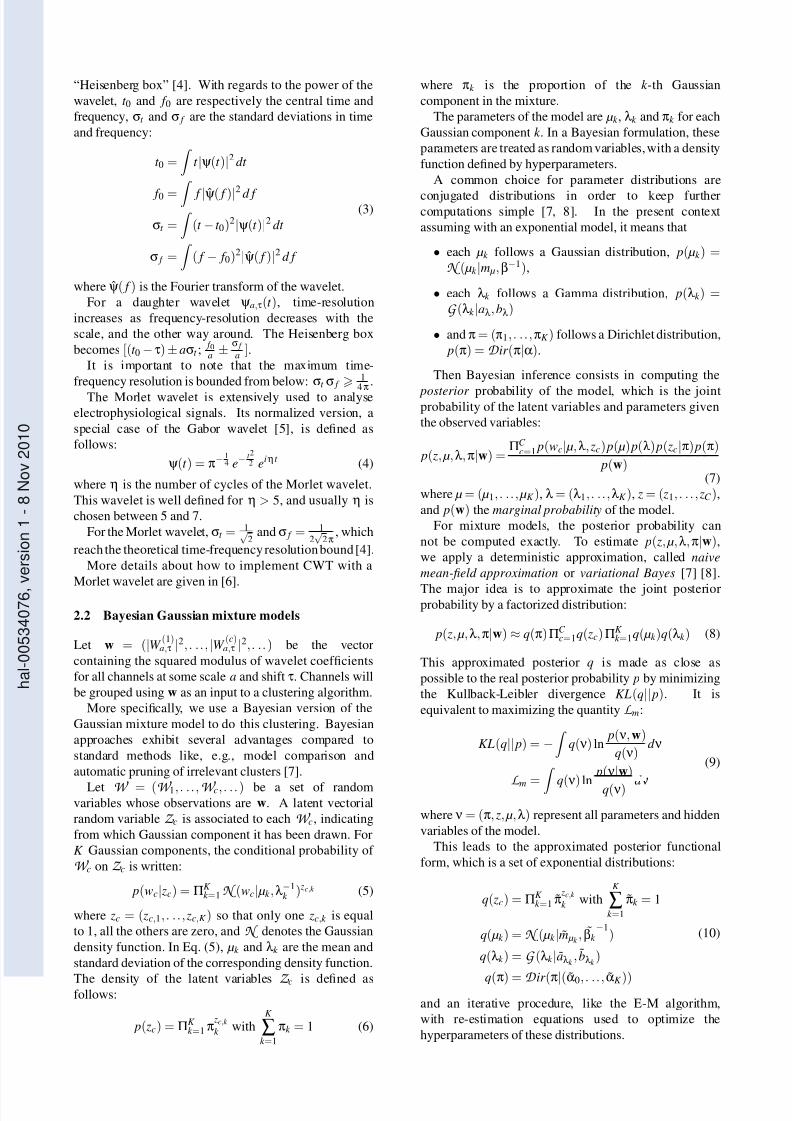
Figure 1: Time courses of the 4 types of channels

contained in the artificial dataset. Types (a), (b) and (c)

contain 2 of 3 Gabor atoms. Type (d) contains all 3 Gabor

atoms.

This dataset consists in 40 channels. Each channel was

composed by a set of Gabor atoms, defined using the

hal00534076,

version

1

8

Nov2010



- 3 . 9 9 - 1 . 9 8 0 . 0 3 2 . 0 4 4 . 0 5

0 . 0 2

0 . 0 3

0 . 0 4

0 . 0 6

0 . 0 9

0 . 1 2

0 . 1 7

0 . 2 4

( a )

- 3 . 9 9 - 1 . 9 8 0 . 0 3 2 . 0 4 4 . 0 5

0 . 0 2

0 . 0 3

0 . 0 4

0 . 0 6

0 . 0 9

0 . 1 2

0 . 1 7

0 . 2 4

( b )

- 3 . 9 9 - 1 . 9 8 0 . 0 3 2 . 0 4 4 . 0 5

T i m e ( s )

0 . 0 2

0 . 0 3

0 . 0 4

0 . 0 6

0 . 0 9

0 . 1 2

0 . 1 7

0 . 2 4

F

r

e

q

u

e

n

c

y

(

H

z

)

( c )

- 3 . 9 9 - 1 . 9 8 0 . 0 3 2 . 0 4 4 . 0 5

0 . 0 2

0 . 0 3

0 . 0 4

0 . 0 6

0 . 0 9

0 . 1 2

0 . 1 7

0 . 2 4

( d )

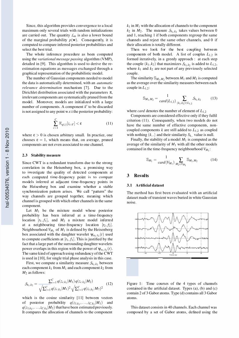
Figure 2: Squared modulus of the CWT computed with

a normalized Morlet wavelet for the 4 types of channels

contained in the artificial dataset. See figure 1 for the

representation in the time domain.

normalized Morlet wavelet waveform (4). 3 Gabor atoms

were used, with parameters (τ, a) = (0, 0.5), (−2, 0.8)and (1.5, 1.0). 10 channels were generated for each

possible pair of atoms, plus 10 channels with all three

atoms. A Gaussian white noise with mean µ = 0 and

standard deviation σ = 0.1 is added to each channel.

Sampling frequency is set at 1 Hz.

For the first step of the method, the Morlet CWT, a

geometrically sampled scale was used for the frequency

axis [6]. Figures 1 and 2 illustrate the 4 possible types of

channels with their associated representations in time and

in the time-frequency plane.

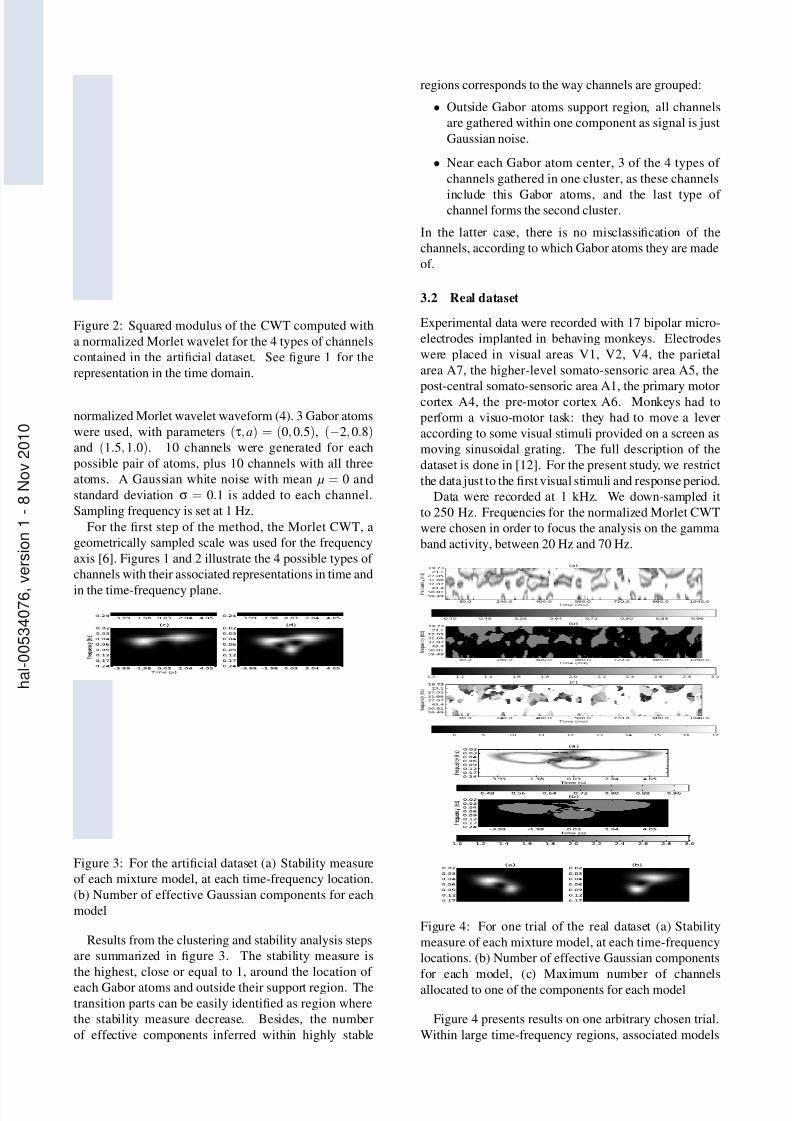
- 3 . 9 9 - 1 . 9 8 0 . 0 3 2 . 0 4 4 . 0 5

T i m e ( s )

0 . 0 2

0 . 0 3

0 . 0 4

0 . 0 6

0 . 0 9

0 . 1 2

0 . 1 7

0 . 2 4

F

r

e

q

u

e

n

c

y

(

H

z

)

( a )

0 . 4 8 0 . 5 6 0 . 6 4 0 . 7 2 0 . 8 0 0 . 8 8 0 . 9 6

- 3 . 9 9 - 1 . 9 8 0 . 0 3 2 . 0 4 4 . 0 5

T i m e ( s )

0 . 0 2

0 . 0 3

0 . 0 4

0 . 0 6

0 . 0 9

0 . 1 2

0 . 1 7

0 . 2 4

F

r

e

q

u

e

n

c

y

(

H

z

)

( b )

1 . 0 1 . 2 1 . 4 1 . 6 1 . 8 2 . 0 2 . 2 2 . 4 2 . 6 2 . 8 3 . 0

Figure 3: For the artificial dataset (a) Stability measure

of each mixture model, at each time-frequency location.

(b) Number of effective Gaussian components for each

model

Results from the clustering and stability analysis steps

are summarized in figure 3. The stability measure is

the highest, close or equal to 1, around the location of

each Gabor atoms and outside their support region. The

transition parts can be easily identified as region where

the stability measure decrease. Besides, the number

of effective components inferred within highly stable

regions corresponds to the way channels are grouped:

• Outside Gabor atoms support region, all channels

are gathered within one component as signal is just

Gaussian noise.

• Near each Gabor atom center, 3 of the 4 types of

channels gathered in one cluster, as these channels

include this Gabor atoms, and the last type of channel forms the second cluster.

In the latter case, there is no misclassification of the

channels, according to which Gabor atoms they are made

of.

3.2 Real dataset

Experimental data were recorded with 17 bipolar micro-

electrodes implanted in behaving monkeys. Electrodes

were placed in visual areas V1, V2, V4, the parietal

area A7, the higher-level somato-sensoric area A5, the

post-central somato-sensoric area A1, the primary motorcortex A4, the pre-motor cortex A6. Monkeys had to

perform a visuo-motor task: they had to move a lever

according to some visual stimuli provided on a screen as

moving sinusoidal grating. The full description of the

dataset is done in [12]. For the present study, we restrict

the data just to the first visual stimuli and response period.

Data were recorded at 1 kHz. We down-sampled it

to 250 Hz. Frequencies for the normalized Morlet CWT

were chosen in order to focus the analysis on the gamma

band activity, between 20 Hz and 70 Hz.

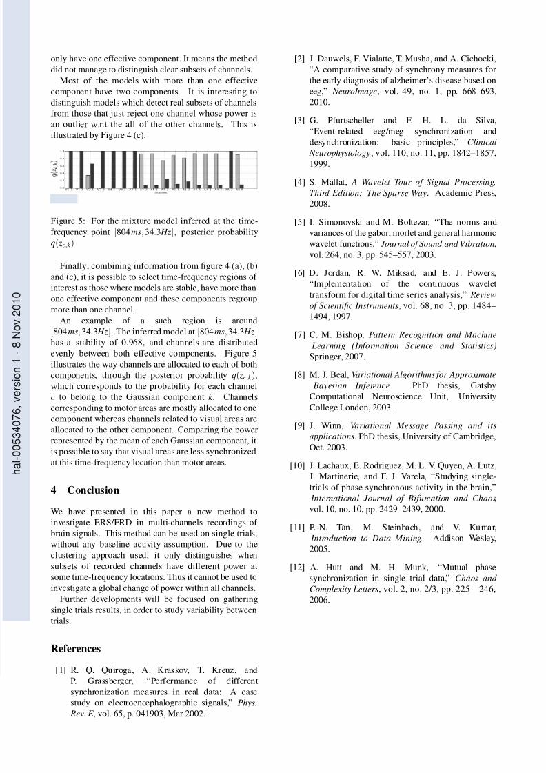
Figure 4: For one trial of the real dataset (a) Stability

measure of each mixture model, at each time-frequency

locations. (b) Number of effective Gaussian components

for each model, (c) Maximum number of channels

allocated to one of the components for each model

Figure 4 presents results on one arbitrary chosen trial.

Within large time-frequency regions, associated models

hal00534076,

version

1

8

Nov2010



only have one effective component. It means the method

did not manage to distinguish clear subsets of channels.

Most of the models with more than one effective

component have two components. It is interesting to

distinguish models which detect real subsets of channels

from those that just reject one channel whose power is

an outlier w.r.t the all of the other channels. This is

illustrated by Figure 4 (c).

Figure 5: For the mixture model inferred at the time-

frequency point [804 ms, 34.3 Hz], posterior probability

q( zc,k )

Finally, combining information from figure 4 (a), (b)

and (c), it is possible to select time-frequency regions of

interest as those where models are stable, have more than

one effective component and these components regroup

more than one channel.

An example of a such region is around

[804 ms, 34.3 Hz]. The inferred model at [804 ms, 34.3 Hz]has a stability of 0.968, and channels are distributed

evenly between both effective components. Figure 5

illustrates the way channels are allocated to each of both

components, through the posterior probability q( zc,k ),

which corresponds to the probability for each channel

c to belong to the Gaussian component k . Channels

corresponding to motor areas are mostly allocated to onecomponent whereas channels related to visual areas are

allocated to the other component. Comparing the power

represented by the mean of each Gaussian component, it

is possible to say that visual areas are less synchronized

at this time-frequency location than motor areas.

4 Conclusion

We have presented in this paper a new method to

investigate ERS/ERD in multi-channels recordings of

brain signals. This method can be used on single trials,

without any baseline activity assumption. Due to theclustering approach used, it only distinguishes when

subsets of recorded channels have different power at

some time-frequency locations. Thus it cannot be used to

investigate a global change of power within all channels.

Further developments will be focused on gathering

single trials results, in order to study variability between

trials.

References

[1] R. Q. Quiroga, A. Kraskov, T. Kreuz, and

P. Grassberger, “Performance of different

synchronization measures in real data: A case

study on electroencephalographic signals,” Phys.

Rev. E , vol. 65, p. 041903, Mar 2002.

[2] J. Dauwels, F. Vialatte, T. Musha, and A. Cichocki,

“A comparative study of synchrony measures for

the early diagnosis of alzheimer’s disease based on

eeg,” NeuroImage, vol. 49, no. 1, pp. 668–693,

2010.

[3] G. Pfurtscheller and F. H. L. da Silva,

“Event-related eeg/meg synchronization anddesynchronization: basic principles,” Clinical

Neurophysiology , vol. 110, no. 11, pp. 1842–1857,

1999.

[4] S. Mallat, A Wavelet Tour of Signal Processing,

Third Edition: The Sparse Way. Academic Press,

2008.

[5] I. Simonovski and M. Boltezar, “The norms and

variances of the gabor, morlet and general harmonic

wavelet functions,” Journal of Sound and Vibration,

vol. 264, no. 3, pp. 545–557, 2003.

[6] D. Jordan, R. W. Miksad, and E. J. Powers,“Implementation of the continuous wavelet

transform for digital time series analysis,” Review

of Scientific Instruments, vol. 68, no. 3, pp. 1484–

1494, 1997.

[7] C. M. Bishop, Pattern Recognition and Machine

Learning (Information Science and Statistics).

Springer, 2007.

[8] M. J. Beal, Variational Algorithms for Approximate

Bayesian Inference. PhD thesis, Gatsby

Computational Neuroscience Unit, University

College London, 2003.

[9] J. Winn, Variational Message Passing and its

applications. PhD thesis, University of Cambridge,

Oct. 2003.

[10] J. Lachaux, E. Rodriguez, M. L. V. Quyen, A. Lutz,

J. Martinerie, and F. J. Varela, “Studying single-

trials of phase synchronous activity in the brain,”

International Journal of Bifurcation and Chaos,

vol. 10, no. 10, pp. 2429–2439, 2000.

[11] P.-N. Tan, M. Steinbach, and V. Kumar,

Introduction to Data Mining. Addison Wesley,2005.

[12] A. Hutt and M. H. Munk, “Mutual phase

synchronization in single trial data,” Chaos and

Complexity Letters, vol. 2, no. 2/3, pp. 225 – 246,

2006.

hal00534076,

version

1

8

Nov2010

Documents

Maxime Rio et al- Partial amplitude synchronization detection in brain signals using Bayesian Gaussian mixture models