Embed Size (px)
Citation preview

TRANSACTIONS OF THEAMERICAN MATHEMATICAL SOCIETYVolume 160, October, 1971
MAXIMA AND HIGH LEVEL EXCURSIONS
OF STATIONARY GAUSSIAN PROCESSESO
BY
SIMEON M. BERMAN
Abstract. Let X(t), f^O, be a stationary Gaussian process with mean 0, variance
1 and covariance function r(t). The sample functions are assumed to be continuous on
every interval. Let r(t) be continuous and nonperiodic. Suppose that there exists a,
0<aS2, and a continuous, increasing function g(t), räO, satisfying
(0.1) lim^^ - L for every c> 0,i-o g(t)
such that
(0.2) l-r(t) ~ g(\t\)\t\°, f->0.
For u > 0, let v be defined (in terms of «) as the unique solution of
(0.3) u2g(\lv)v-a = 1.
Let I a be the indicator of the event A ; then
hxwxfidsJo
represents the time spent above u by X(s), O^s^T. It is shown that the conditional
distribution of
(0.4) v I /„c» „,<&,.'o
given that it is positive, converges for fixed T and u -> oo to a limiting distribution
Ta, which depends only on a but not on T or g.
Let jF(A) be the spectral distribution function corresponding to r(t). Let Flp\X) be
the iterated /»-fold convolution of F(X). If, in addition to (0.2), it is assumed that
(0.5) Fm is absolutely continuous for some p > 0,
then max (X(s) : Oásár), properly normalized, has, for t ~* oo, the limiting extreme
value distribution exp (~e~x).
Received by the editors September 22, 1970.
AMS 1970 subject classifications. Primary 60G10, 60G15, 60G17; Secondary 60F99.
Key words and phrases. Conditional distribution, limiting distribution, extreme value
distribution, asymptotic independence, excursion over high level, sample function maximum,
occupation time, correlation function, local behavior, spectral distribution, absolute con-
tinuity, method of moments, Laplace-Stieltjes transform.
0) This paper represents results obtained at the Courant Institute of Mathematical
Sciences, New York University, under the sponsorship of the National Science Foundation,
Grant NSF-GP-11460. .
Copyright © 1971, American Mathematical Society
65
License or copyright restrictions may apply to redistribution; see http://www.ams.org/journal-terms-of-use

66 SIMEON M. BERMAN [October
If, in addition to (0.2), it is assumed that
(0.6) F(A) is absolutely continuous with the derivative /(A),
and
(0.7) lim log h I °° |/(A+/z)-/(A)| dX = 0,ft-»0 J - «
then (0.4) has, for u -> oo and T-> oo, a limiting distribution whose Laplace-Stieltjes
transform is
(0.8) exp [constant f" (e-**-l)tñr¿x)\, A > 0.
1. Discussion of the results. The conditional limiting distribution of (0.4) for
fixed T was obtained for a=2 and g=constant in [3], and for a = 1 and g=constant
in [5]. We remark that when a=2 then the only nontrivial case is g=constant;
indeed, 2t~2(\— r(t)) converges for t—>0 to J"œA2i/F(A) which is either 0,
positive or infinite. If g(0) = 0, then the first case arises and X(t)=X(0), so that
r(t)==\; therefore, the only interesting case is g(0)>0. If a<2, then g(0) = 0 is
possible; for example, if the spectral density/(A) exists and
/(A)= lAI^-^dAI"1) for large \X\,
then (0.2) is satisfied for some constant multiple of gi\t\).
The extreme value limit distribution has been obtained for a = 2 in several works
under increasingly general conditions (Volkonskiï and Rozanov [14], Cramer and
Leadbetter [6], Beljaev [1], Quails [11], and Berman [4]). For a= 1 and g constant,
it was studied by Pickands [10]. A sufficient condition for (0.5) is
/•OO
(1.1) \ris)\p ds < oo for some p > 0;J-oo
indeed, if p is an integer, rp(s) is the Fourier-Stieltjes transform of Fm. (1.1) is
implied by several of the conditions used in earlier works, namely, rit) = 0(t~e),
t ->- oo for some e>0 (see [6, p. 257]) and the integrability of r2 (see [4] and [10]).
The only previous investigation of the limiting distribution of (0.4) for u —> co
and T-*- oo is that of Volkonskiï and Rozanov [14] in the case a = 2. In addition to
(0.2) they also assumed that 1— rit)— g(0)r2~A4í4/4!; and, in place of the mild
conditions (0.6) and (0.7), assumed that the process satisfies the "strong mixing
condition." Their proof is based on the fact that the "horizontal-window" con-
ditional limiting distribution of the excursion above a high level is *F2, the Rayleigh
distribution; and that the upcrossings tend to a limiting Poisson process.
Our condition (0.6) implies that r(/) -> 0 for / -> oo (Riemann-Lebesgue
Theorem). It also implies that jZx |/(A+A)-/(A)| dX tends to 0 with A. The con-
dition (0.7) prescribes a rate for such convergence. It is well known that this rate
is related to the rate of convergence of r(t) to 0 for t -> oo (see [13]).
License or copyright restrictions may apply to redistribution; see http://www.ams.org/journal-terms-of-use
1971] MAXIMA AND HIGH LEVEL EXCURSIONS 67
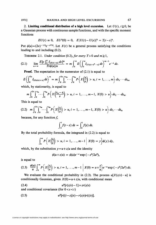
2. Limiting conditional distribution of a high level excursion. Let U(t), í2¡0, be
a Gaussian process with continuous sample functions, and with the specific moment
functions
£■¿7(0 = 0, EU2(0) = 0, E\U(t)-U(s)\2 = 2\tsf.
Put <£(w) = (2,T)~1,2e~*2,2. Let X(t) be a general process satisfying the conditions
leading to and including (0.2).
Theorem 2.1. Under condition (0.2), for every T>0 andm^l,
limE[vjTi^ ,dsr = mrE{rIvJW>i._Adx~\-*dz.u-co Tv<f>(u)¡u Jo Uo J
Proof. The expectation in the numerator of (2.1) is equal to
-EJ IixisM>^ds\ =m\ •••) Pixß\>u,i=l,...,m\(&i;-asm,
which, by stationarity, is equal to
m rrTm ..rmpIx&—^\ > u,i= l,...,m-\,X(0) > u\dsv--dsm.
This is equal to
(2.2) mi Sm- • • pP Ja-Í^) > u, i = 1,..., m-1, X(0) > u\ dSl-■ -dsm
because, for any function /
ff(t~s)ds= f/W*.Jo Jo
By the total probability formula, the integrand in (2.2) is equal to
[P{X$>U>i=l---'m-1 X(0) = yU(y) dy,
which, by the substitution y = u + z/u and the identity
<p(u+z¡u) = <p(u)e-sexp(-z2¡2u2),
is equal to
<"> *H"'W?H<-'.•• ••'»-'X(0) = tz + -U-aexp (-z2j2u2) dz.
We evaluate the conditional probability in (2.3). The process u[X(s\v) — u] is
conditionally Gaussian, given X(0) = u + z/u, with conditional mean
(2.4) u2[r(s¡v)-l] + zr(slv)
and conditional covariance (for 0 <s <t)
(2.5) u2[r((t-s)lv)-r(slv)r(tlv)].
License or copyright restrictions may apply to redistribution; see http://www.ams.org/journal-terms-of-use
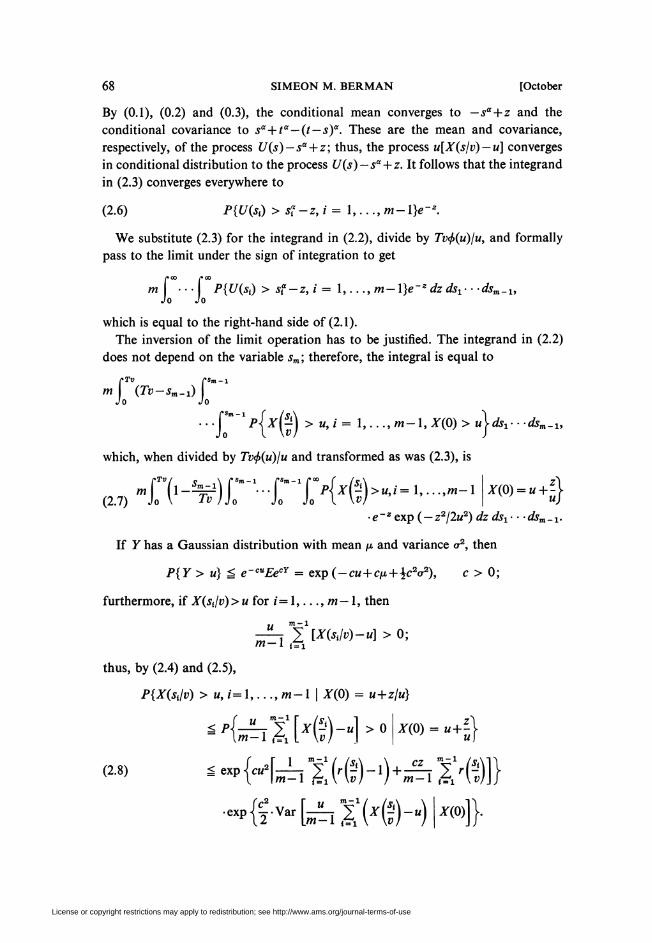
68 SIMEON M. BERMAN [October
By (0.1), (0.2) and (0.3), the conditional mean converges to —sa + z and the
conditional covariance to s" + ta — it—s)a. These are the mean and covariance,
respectively, of the process Uis)—sa + z; thus, the process u[Xis/v) — u] converges
in conditional distribution to the process Uis) — s"+z. It follows that the integrand
in (2.3) converges everywhere to
(2.6) P{UiSi) > sf-z, i= I,..., m-\}e~z.
We substitute (2.3) for the integrand in (2.2), divide by Tv<f>iu)ju, and formally
pass to the limit under the sign of integration to get
(»CO i* oo
m\ ••■ P{Uisf) > s"-z, i = 1,..., m—\)e~z dzdsx- ■ -dsm-XtJo Jo
which is equal to the right-hand side of (2.1).
The inversion of the limit operation has to be justified. The integrand in (2.2)
does not depend on the variable sm ; therefore, the integral is equal to
m (Tv-Sn-ÙJo Jo
■ ■ ■ p"*p{ir(j) > u, i = 1,..., m-l, A-(O) > «}■&!■• •&„,_,,
which, when divided by Tv<f>(u)lu and transformed as was (2.3), is
■e~z exp ( — z2/2«2) dz dsi- ■ -i/ym_i.
If Y has a Gaussian distribution with mean zt and variance a2, then
P{Y > u} ^ e~cuEecY = expi-cu + cn + $c2o2), c > 0;
furthermore, if Xisijv)>u for /= 1,..., m— 1, then
u m_1
-?- 2 [Xisjv)-u] > 0;m— i i=1
thus, by (2.4) and (2.5),
P{XisJv) > u, í=1, ..., w-1 | AT(0) = u + z/u)
License or copyright restrictions may apply to redistribution; see http://www.ams.org/journal-terms-of-use
1971] MAXIMA AND HIGH LEVEL EXCURSIONS 69
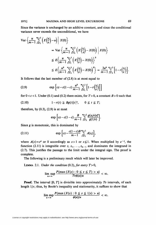
Since the variance is unchanged by an additive constant, and since the conditional
variance never exceeds the unconditional, we have
MsVJKH Xl/S)
X(0)\
It follows that the last member of (2.8) is at most equal to
(2.9) e,P[cz-c(l-c)^mf[l-r^))}
for 0 < c < 1. Under (0.1) and (0.2) there exists, for T> 0, a constant B > 0 such that
(2.10) l-r(t)ZBg(t)\t\«, OïtïT;
therefore, by (0.3), (2.9) is at most
r ,, . B y g(stiv)snexp cz-c(l-c)-T > , , V •
y L 'm-\ fa g(\\v) J
Since g is monotonie, this is dominated by
(2.11) expjcz-^^^1^)],
where A(s)—sa or 0 accordingly as s>l or s^l. When multiplied by e~z, the
function (2.11) is integrable over z, i,,..., sm-i and dominates the integrand in
(2.7). This justifies the passage to the limit under the integral sign. The proof is
complete.
The following is a preliminary result which will later be improved.
Lemma 2.1. Under the condition (0.2), for every T> 0,
P{max (X(s) :Q -¿s -¿T)> u}hm sup -S- t j./ \i- < °°-
„-.«o Tv<p(u)lu
Proof. The interval [0, T] is divisible into approximately Tv intervals, of each
length l¡v; thus, by Boole's inequality and stationarity, it suffices to show that
P{max (X(s) :0<s< llv) > u}hm sup —i-v w ,. ~—=——- < oo.
U-oo <?(«)/"
License or copyright restrictions may apply to redistribution; see http://www.ams.org/journal-terms-of-use

70 SIMEON M. BERMAN [October
Since
F{max AYs) > u} Ú jP{A"(0) > i/}+P{max AT(j) > u, A(0) ^ «},
it suffices, by the well-known estimate
(2.12) ^(¿-¿) = [*W * * ^p
to show that the lim sup of
P{max (A(í/tz) :0iîal)>B, AÏO) S u}l(4>(u)¡u)
is finite. By the total probability formula this is equal to
ë)l>{maxWâ:0^^)>M X(0)=yU(y)dy,
X(0) = u--\ exp [z-z2\2u2\ dz.
which, as in the argument leading to (2.3), is equal to
<2-i3) f4s"WH^By formula (2.4), with — z in place of z, the conditional mean of u[Xisjv) — u] is
(2.14) u2[r(s¡v)-\]-r(s¡v)z.
Put
XJs) = u2[Xis¡v)-u\-u2[ris¡v)-\] + ris¡v)z.
Now risjv) -»■ 1 as u -»• oo uniformly for 0 gí í =£ 1 ; furthermore, we are concerned
only with large values of « in proving the lemma ; thus we may suppose that the
conditional mean (2.14) satisfies
u2[ris\v)-\\-ris\v)z < -\z, for0 ¿ * 3a 1, and z > 0.
It follows that the conditional probability in (2.13) is at most
(2.15) P\ max Zu(j) > \zOSsSl
A(0) -»4By (2.14) and the definition of Xu,
E[Xu(s) | AYO) = u-zlu] m 0;
E{\Xu(t)-Xu(s)\2 | A(0) = w-z/h} = Var{[Afu(r)-Afu(i)] [ XQ) = u-z¡u}
íNar(Xu(t)-Xu(s))
= u2E\X(t¡v)-X(s¡v)\2
= 2u2[l-riit-s)lv)], 0 < s < t.
License or copyright restrictions may apply to redistribution; see http://www.ams.org/journal-terms-of-use
1971] MAXIMA AND HIGH LEVEL EXCURSIONS 71
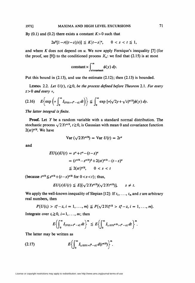
By (0.1) and (0.2) there exists a constant K>0 such that
2u2[\-riit-s)lv)\ ú K\t-s\a, 0<í<(ál,
and where K does not depend on u. We now apply Fernique's inequality [7] (for
the proof, see [9]) to the conditioned process Xu: we find that (2.15) is at most
f> oo
constant x <f>iy) dy../^/constant,/a/constant
Put this bound in (2.13), and use the estimate (2.12); then (2.13) is bounded.
Lemma 2.2. Let Uit), r^O, be the process defined before Theorem 2.1. For every
z > 0 and every r,
(2.16) ¿jexp (r j^/rr,«»*"-*] *)} ^ £°«p [t(V2>> + VO"'2]^) *■
TAe /arier integral is finite.
Proof. Let y be a random variable with a standard normal distribution. The
stochastic process \/2Ytalz, r^O, is Gaussian with mean 0 and covariance function
2(íí)a/2- We have
Var (V2Tia/2) = Var U(t) = 2t"
and
EUis)Uit) = sa + ta-it-sy
= ital2-sal2)2 + 2ist)al2-it-s)a
^ 2ist)al2, 0 < s < t
(because ta<2-¿sal2 + it-s)al2 for 0<s<t); thus,
EU(s)U(t) ^ E[(V2Ysal2)(V2Yt<"2)], s # t.
We apply the well-known inequality of Slepian [12]:lft1,...,tm and z are arbitrary
real numbers, then
P{U(tf) > t?-z, i=\,...,m}ú P{V2Yt?12 > tf-z, i - 1.m).
Integrate over í¡^0, /=1,..., m; then
f ("» \m r rca s m
EU Iimn>e-ïidty ^ EU /^yt1"2>t«-¿\dt \ .
The latter may be written as
Jo Iw2Yt>t*-zldit"l2)j .
License or copyright restrictions may apply to redistribution; see http://www.ams.org/journal-terms-of-use
72 SIMEON M. BERMAN [October
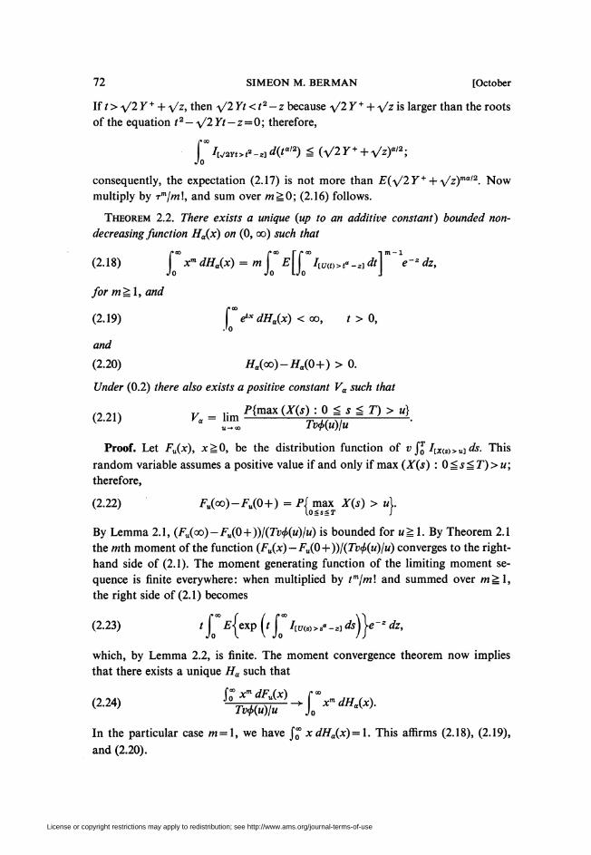
If t > i/2 Y + + \lz, then ^2 Yt < t2 - z because y/2 Y + + \/z is larger than the roots
of the equation t2 — \/2Yt — z = 0; therefore,
f W>t»-,]</(ra'2) Ú(V2Y+ + ^zf'2;
consequently, the expectation (2.17) is not more than E(^\/2Y+ + \/z)mal2. Now
multiply by Tm¡m\, and sum over m^O; (2.16) follows.
Theorem 2.2. There exists a unique (up to an additive constant) bounded non-
decreasing function Ha(x) on (0, 00) such that
m-l
e'zdz.í»oo /»oo r ñ 00
(2.18) xmdHa(x) = m\ E\\ Imt)>e^,dtJo Jo Uo
for m^l, and
(2.19) i" éx dHa(x) < 00, r > 0,.'0
a/ici
(2.20) Ha(oo)-Ha(0 + ) > 0.
Under (0.2) //zere ¿z/so e-xziij a positive constant Va such that
(2.21) Va = hm ^W:0^ * ^ -T) > «>U-* 00 Tí;<£(m)/w
Proof. Let Fu(x), x^0, be the distribution function of v jf¡ IlXis)>u) tft. This
random variable assumes a positive value if and only if max (X(s) : 0¿s^T)>u;
therefore,
(2.22) Fu(co)-FJ0 + ) = Pi max X(s) > «I.lOSsST J
By Lemma 2.1, (Fu(oo)-Fu(0+))l(Tv<p(u)lu) is bounded for u^ 1. By Theorem 2.1
the mth moment of the function (Fu(x) — Fu(0+))l(Tv<f>(u)lu) converges to the right-
hand side of (2.1). The moment generating function of the limiting moment se-
quence is finite everywhere: when multiplied by tm\m\ and summed over w^l,
the right side of (2.1) becomes
(2.23) '/„"M6*15 (' j7/[U(s>>s"-2] *)}*"" dz'
which, by Lemma 2.2, is finite. The moment convergence theorem now implies
that there exists a unique Ha such that
(2 24) ti*mdFu(x) r-dH(.(124) Tv<f>(u)lu-*J0 X dHÁX)-
In the particular case m = l, we have J^ xdHa(x) = l. This affirms (2.18), (2.19),
and (2.20).
License or copyright restrictions may apply to redistribution; see http://www.ams.org/journal-terms-of-use
1971] MAXIMA AND HIGH LEVEL EXCURSIONS 73
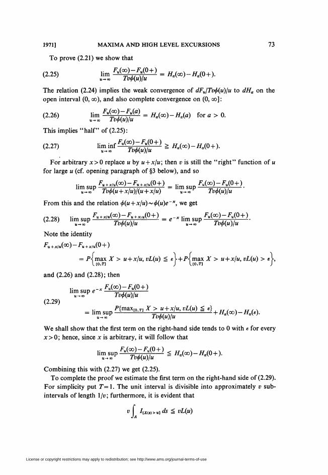
To prove (2.21) we show that
(2.25) lim F"(^)~J;;(0 + ) = Ha(m) - tf8(0 + ).u-oo Tv<f>(u)fu
The relation (2.24) implies the weak convergence of dFJTv(f>(u)/u to dHa on the
open interval (0, oo), and also complete convergence on (0, oo] :
<2-26) ^F%u)lf-H^-H^ f0ra>°-
This implies "half" of (2.25):
<2"27) ^Fu%(ufu+) * ^>7#'+).
For arbitrary x>0 replace u by u + x/u; then i; is still the "right" function of u
for large u (cf. opening paragraph of §3 below), and so
lim Fu + xlu(co)-Fu + xlu(0 + ) = F„(oo)-Fu(0 + )
„^« Tvcf>(u + x/u)/iu + x/u) u~« Tv<piu)/u
From this and the relation <f>iu + x[u)~<j>iu)e~x, we get
(2.28) lim sup ̂ + ̂)-/;V-(Q + ) = ,-. lim sup F^ZFf + )-«-.oo Tv<f>iu)/u u-oo Tvf(u)/u
Note the identity
^u + */u(co)-Fu + x/11(0-|-)
= P-j max A > u + x/u, vL(u) ^ e f+Pi max X > u + x/u, vL(u) > e V,Lco.T] J Uo.rj J
and (2.26) and (2.28); then
,,Fu(oo)-Fu(0 + )11111 OLÍ}./ C
U-t-co
(2.29)
lim sup <?"u^oo Tv<f>(u)/u
.. F{max[0,r] X > u + x/u, vL(u) ^ e}" h™lup ?W-~—i+/«oo)-^(.).
We shall show that the first term on the right-hand side tends to 0 with e for every
x>0; hence, since x is arbitrary, it will follow that
Combining this with (2.27) we get (2.25).
To complete the proof we estimate the first term on the right-hand side of (2.29).
For simplicity put 7*=1. The unit interval is divisible into approximately v sub-
intervals of length l/v; furthermore, it is evident that
f» hxm>u]ds ^ vL(u)
JA
License or copyright restrictions may apply to redistribution; see http://www.ams.org/journal-terms-of-use
74 SIMEON M. BERMAN [October
for every subinterval A of [0, 1]; thus, by the argument in the proof of Lemma 2.1
(Boole's inequality and stationarity) we find that
P\ max X > u + x/u, vL(u) ^ e( [0,1]
is at most equal to
(2.30) vP\ max u(X(s/v)-u) > x Iíuix(sm-u»oi ds ^I OSsgl Jo
Now write the probability as the integral of the conditional probability given
X(0) = u — z/u. By the standard weak convergence methods ([15], those based on
the estimates of the conditional moments of the increments of the process, as in the
proof of Lemma 2.1) it can be shown that the conditioned process u(X(s/v) — u),
O^íál, converges not only in distribution to the process U(s) — sa — z, as in
Theorem 2.1, but also weakly over the function space C[0, 1]; therefore, the joint
distribution of the functionals in (2.30) (the maximum and the occupation time)
converges to the joint distribution under the limiting process. Divide (2.30) by
4>(u)/u and pass to the limit under the conditional expectation integral, as in Lemma
2.1 ; the ratio converges to
f Wmax U(s)-sa > x + z, f ILJo 1(0.11 Jo
u(s)-s">^ds ^ eVe'dz
The integrand converges pointwise to 0 as e -> 0; indeed if the process U(s) — sa
spends little time above z, then it is very unlikely to exceed z + x. Passage to the
limit under the sign of integration is again permitted by Fernique's inequality. The
proof is complete.
An immediate consequence of Theorems 2.1 and 2.2 is:
Theorem 2.3. Let Ta be the distribution function with the moment sequence
Vz1 J" xm dHa(x), m=\,
that is, the distribution defined as
0 for x S 0,
(Ha(x)-Ha(0 + ))/Va forx>0.
Under (0.2), the conditional distribution of v jj IiXi.s)>u^ds, given that it is positive,
converges to Ta.
Proof. For any nonnegative random variable Y, E(Ym | Y>0) = EYm/P{Y>0};
thus, by (2.22),
fJ7 f\ Am\ Ci a n\ E{v ft Ims)>u,ds}m
By Theorems 2.1 and 2.2 this converges, for m ̂ 1, to the right-hand side of (2.1),
divided by Va. This is the mih moment of the distribution function Ya. Since Ha
License or copyright restrictions may apply to redistribution; see http://www.ams.org/journal-terms-of-use

1971] MAXIMA AND HIGH LEVEL EXCURSIONS 75
has a moment generating function which is everywhere finite, so does Wa; thus,
¥„ is uniquely determined by its moments. The assertion of the theorem now
follows by application of the moment convergence theorem.
3. Limiting distribution of the maximum. We begin with some remarks about
the construction of the function v = v(u) in (0.3). This condition was used in the
proofs in §2 only to show that «2[1 — r(s/v)] converges to sa for u -> oo. If w(u) is
an increasing function of u such that w(u)ju —>■ 1 for u —> oo, and if v' = v\w) is
defined as
w2gi\¡v')iv')-« = 1,
then u2[l— r(s/v')]~w2[l — r(s/v')] -+sa. So v' may be interchanged with v; in
other words, v may be defined by (0.3) not only in terms of u but also in terms of
any function asymptotic to u.
In this section we consider the limiting distribution of max (X(s) : 0^ s^ t) for
t -* oo. For t >0, let v be defined in terms of t as the unique solution of
(3.1) 21ogr«(l/»)r-«=l.
Our result is
Theorem 3.1. 7/(0.2) andiO.5) hold, then the random variable
log (vVJ2VÍTr logt))!V(2 log r)f max X(s) - V(2 log /) - -
V(2 log t) J
has, for t -> oo, the limiting distribution exp ( — e~x).
(The constant Va is defined in Theorem 2.2.)
Proof. The main idea of the proof is, as in previous studies, that the distribution
of the maximum of the process over a large time interval is close to the distribution
of the maximum of certain independent random variables. Suppose t is a positive
integer; then
max A"(i) = max ( max ATs)).
Ifmax(A(j) : j-l ^sSj)J=l, ---, t, were independent, thenmax (Af(.s) : Ofks^t)
would be the maximum of t independent random variables with the common
distribution function
Gix) = p\ max AT(i) g x\;losssi J
thus, max (Af(j) : O^s^t) would have the distribution function G\x).
For fixed x, put
(3.2) u = V(2 log 0+-V(21og/)-
License or copyright restrictions may apply to redistribution; see http://www.ams.org/journal-terms-of-use

76 SIMEON M. BERMAN [October
By the definition (3.1) of v, and the increasing character of g, we have
va:/2 log t -s* g(0) (positive or zero) ; therefore,
(log (WJ2V(tt log t)))IV(2 log 0 -¿ 0,
and so, by (3.2),
(3.3) m ~ V(2 log i)> ' -* °°-
The opening remarks of this section imply: If v is defined by (3.1) and u by (3.2),
then the relations between u and v employed in §2 may also be used under these new
definitions.
It follows from (2.21) (with T=l), (3.2) and (3.3) that 1 -G(u)~e-xt-\ t -+ 00;
therefore,
(3.4) G'(t0->exp(-e-*);
thus, the limiting distribution of the maximum of t independent random variables
with the common distribution function G is exp ( — e~x).
The rest of the proof consists of showing that the submaxima over the various
intervals may actually be assumed to be asymptotically independent. The proof
follows a familiar pattern ; we shall, wherever possible, refer to previous work for
details.
We break the interval [0, t] into approximately [t] intervals of unit length. (There
is a small piece left over when t is not an integer ; however, the proof for such t is
reducible to that for integral t.) For arbitrary e, 0 < e < I, we clip an open segment
of length e from the right endpoint of each interval. The remaining intervals are
h = U- l,j-*lj=U ■■■, [*■]• We have
(3.5) lim sup P< max X(s) > u\—P< max X(s) > u ee
in fact, by Boole's inequality and stationarity, the difference of probabilities in
(3.5) is not more than íPíjmax (X(s) : 0^s^e)>u}, which, by (2.21) and (3.2),
converges to ee~x.
Let Mt be the set of integer multiples of (log t)~3la; then, by the argument in [10],
(3.6) lim V(2 log 0 max X(s)— max X(s) = 0
in probability; thus, the limiting distributions of the two maxima are the same.
Put
(3.7) n = integral part of t (log t)3la,
and let <£(wi, u2; p) be the standard bivariate normal density with correlation
coefficient p.
License or copyright restrictions may apply to redistribution; see http://www.ams.org/journal-terms-of-use

1971] MAXIMA AND HIGH LEVEL EXCURSIONS 77
We shall show that in calculating the limiting distribution of the maximum over
(Ii u • • ■ u Im) r\ Mt, we may assume that the pieces of the process corresponding
to different intervals I¡ are mutually independent. As in [4], it suffices to show that
„ CrUtln)
(3.8) n 2 <t>(u,u;y)dync/íSíán Jo
converges to 0 as t -> oo.
By (0.5), the remark following (1.1), and the Riemann-Lebesgue lemma, it
follows that r"(t) -> 0 for t -> oo ; therefore, r(t) -> 0. By the same argument as in
[4], it suffices to show: there exists q, 0 <q < 1, such that
(3.9) nf-2 g \r(jt¡ri)\ -► 0 for t -> oo.í = i
By the Holder inequality,
(3.10) 2 |rO/»)| ^ n1 -«■»( t r2^/"))1,2P-í=i \j=i /
Let/<P)(A) be the Radon-Nikodym derivative of Fm(X); then, as is well known,
the convolution/<2p,(A) is a continuous function, and
»(jtln) = 2 £ cos (A/Y//i)/(2p)(A) ¿A.
Substitute this in (3.10); then, by the well-known cosine summation formula, the
right-hand side of (3.10) is at most
\ Jo sin(Ai/2«) 1
By a standard argument and the relation t/n -*■ 0, the last expression is asymptotic
to
»w,qSïAV»<a) *)"*'.
For arbitrary ß, 0 < /? < 1, this is at most (by | sin Ar | ^ | Ar |s)
\l/2p
nUt"-1 (" x'-ywwdx)1
The integral is finite because /<2p) is continuous ; thus, the expression above is of
the order nt(ß~1)lp; therefore, the quantity on the left side of (3.9) is of the order
n2tq-2+(ß-i)iP_ By tne definition (3.7) of«, this converges to 0 if q is chosen so that
0<q<(l -B)lp; therefore, (3.9) holds.
By the remarks preceding (3.8) and (3.9), the distribution of the maximum on
Mt n (Ii u • • • u Im) is asymptotically the same as that of [t] independent random
variables with the common distribution function
G(x) = p\ max X(s) g A
License or copyright restrictions may apply to redistribution; see http://www.ams.org/journal-terms-of-use

78 SIMEON M. BERMAN [October
By the same argument as for (3.6), we may replace Mt n 7, by the full set I},
7=1,..., [/]; thus, the maximum is asymptotically the same as the maximum of
[t] independent random variables with the common distribution function
Geix) = p{ max X{s) ¿ xX.
By the reasoning leading to (3.4), with T= 1 — e, we find that the limiting distribu-
tion of max Xis) over 7X u- • -u 7[(] is exp ( — (1— e)e~x). Since e>0 is arbitrary,
we put e = 0 here and in (3.5). This completes the proof of the theorem.
As in [4], we have
Corollary 3.1. For arbitrary b>0, and with u given by (3.2),
lim p\ max Xis) á «r = exp( — be~x).(-.to (ogsäto Jt
Another result is
Corollary 3.2. Iflx, I2,... are the intervals defined above, then
it: r \S P< max X(s) > u, max Xis) > u >
i,l-T,i+J i /¡ ¡¡ J
-PÍmax Xis) > wj-F-jmax Xis) > uX
converges to 0 as t -> oo.
Proof. By stationarity, the inequalities on u may be reversed, and the summation
simplified :
(3.11) 2 (t'W)f = 2
pjmax Xis) ^ u\-P2\max Xis) ^
Let M* be the set of integral multiples of (log t)'61". By the same reasoning as for
(3.6), the sets 7; may be replaced by I¡ n Mf. Put
n = integral part oftilogt)61",
then, as in [4], the sum (3.11), with I, r\ Mf* in place of I¡,j= 1,..., [r], is at most
It] ->„ i-nktln + i-l)
2(['W)'f 2 <Ku,u;y)dy,i = 2 • neltSkg2nlt Jo
which is at most
rr(jtln)rrutln-)
In 2 <f>iu, u; y) dy.neltél£2n JO
Like (3.8), it converges to 0.
4. Preliminary estimates of the limiting distribution of the high level excursion.
Throughout this section we assume that conditions (0.2) and (0.5) are satisfied.
License or copyright restrictions may apply to redistribution; see http://www.ams.org/journal-terms-of-use
1971] MAXIMA AND HIGH LEVEL EXCURSIONS 79
v and u are defined by (3.1) and (3.2), respectively. For fixed e, 0<e<l, I, is the
interval [/— l,j—e], as defined in the previous section.
For fixed b > 0, let A be the number of intervals I¡ for which max ( Af(j) : self)
>u, /=1,..., [tb]. As the sum of [tb] indicator random variables, A has the
expected value
[tb]P{max iX(s) : 0 = s Ú l-e)> u),
which, by Theorem 2.2, is asymptotic to Vatbil — e)v<f>iú)¡u, which by (3.1) and (3.2),
converges to /3(1 — e)e~x; hence
(4.1) EN^bil-e)e~x, r->oo.
By definition, P{A = 1}=F{max (ATí) : s e 7j u • • • u 7[()) > u}. By the proof of
Theorem 3.1 and by Corollary 3.1, this implies
(4.2) F{TV ̂ 1}-> 1 -exp [-bil-e)e~x].
For any nonnegative integer valued random variable A, P{N> 1} S EN—P{N^ 1} ;
thus, by (4.1) and (4.2),
limsupF{A> 1} = 6(l-e)e-*-H-exp[-e(l-e)e-*];(-.00
therefore, from the inequality e~w — 1 + w^^w2, w>0, it follows that
(4.3) limsupPÍA > 1} ^ $[bil-e)e-x]2 = \b2e~2x.¡-.00
Lemma 4.1. Let Wt be defined as in Theorem 2.3; then, for any y>0,
(4.4) lim suppjo < v f f 7[X(S)>U] <k S y) & bYa(y)e-x+ib2e-2x
Proof. By the decomposition of the event into disjoint subsets, the probability
in (4.4) is not more than
(4.5) P|0 < v 2 J; /«(.»«i dsúy,N= 1 j+P{A > 1}.
The events {v§¡jI[Xis)>uids>0, N=l},j=l,..., [tb], are disjoint; therefore, (4.5)
is not more than
bm f r >
2 P\0 < v\ 7K(S)>U]dsúy,N=l \+P{N > 1},1 = 1 \ Jij J
which, by stationarity, is at most
tbP^O < »£ SIlx<s)>u]ds í yj+P{N > 1}.
License or copyright restrictions may apply to redistribution; see http://www.ams.org/journal-terms-of-use
max X(s) > uOgsgl-s
80 SIMEON M. BERMAN [October
Now pass to the limit and apply Theorems 2.2 and 2.3, Corollary 3.1, and (4.3):
íAf|o<zjÍ Iau)>uids Ú yX
= tbP\ max X(s)> u\-P\v\ 7[X(s)>u]<fc ^ ykogsSl-e J I Jo
~ be-xil-e)Yaiy).
Lemma 4.2. For b>0 andy>0,
lim inf P\ 0 < v 2 \ W»«j ds £ y\ * b(l -e)e~xYaiy)-b2e¡-•00 I. j = l Jlj J
Proof. The probability above is at least
p{° < » 2 I W>«] ds^y,N=lj,
which, as in the previous proof, is equal to
an ( c \2P\0 < t>| /„«»jds ^y,N=lj.
This is equal to
2 PÍO <v\ Ilxw>tí ds á y, max (x(s) ;i,e|J4)íí=l I Jli \ k*i J
Bo]
which is also equal to
(4.6)
Bo] f rVF^0<iz Ims)>u)ds^y
i = l V. Jlt
- 2 P\° < v I /«<S)>U]* ̂ J, max ÍaYj) : se\J Ik\ > u\.
By stationarity, Theorems 2.2 and 2.3, and (3.1) and (3.2), the first sum in (4.6) is
asymptotic to
tbP^O < v£ £7[X(S)>U]ds £ y\-> A(l-«y-*Y„(y).
The second sum in (4.6) is at most
Bi>] Bo] ( 1
2 2 2 p\ max *(*) > ">max *(■*) > u r»
which, by Corollary 3.2, is asymptotic to [iAF{max (A(j) : 0 = s = 1 - e) > m}]2,
which, by Theorem 2.2, converges to [be~x(l— e)]2<b2e~2x.
Lemma 4.3. For A > 0, the Laplace-Stieltjes transform
' [exp ( - A» 2 j W>>«J*)j
License or copyright restrictions may apply to redistribution; see http://www.ams.org/journal-terms-of-use
1971] MAXIMA AND HIGH LEVEL EXCURSIONS 81
has a lim sup (t -> oo) not exceeding
exp[-b(l-e)e-x] + be~x f%-*dT^y+2l£L_Jo 2A
and a lim inf at least equal to
exp [-b(l -e)e~x] + be-x(l -e) f"*-*» í¿"Fa(j;)
Proof. Let G(j) be the distribution function of
KM f
¿V 2x
um r
i = l Jl¡
then, by the reasoning leading to (4.2),
G(0+) = pjmax (x(s) : se \J l\ ^ «j-^exp [-b(l-e)e~x].
This and Lemmas 4.1 and 4.2 furnish bounds for the lim sup and lim inf of G(y)
= [G(y)-G(^ + )] + G(0 + ). The assertion of the lemma now follows by use of the
identity
¡X'e'^dG(y) = 1-A frJ»[l -G(y)] dy.Jo .'o
5. Limiting distribution of the time spent above u. If X(t) satisfies (0.6) then, as
is well known, it has the stochastic integral representation
(5.1) X(s)= r e'V/W^A),J — CO
where i is the standard Brownian motion process.
The function r-As) = (\ — |s|)+ is a correlation function. Its spectral density is
(1-cosA)/ttA2. Put
P(S) =r-^rl(r)dr
This is also a correlation function. Its spectral density is, by the convolution rela-
tion, equal to
A-*(l-cos A)29(\)
]™x A-4(l-cosA)2<A
Since rx(s) vanishes outside [—1, 1], p(s) vanishes outside [ — 2, 2].
For T> 0 we define a process XT(s) on the same probability space as the process
X(s): Let i be the Brownian motion in the representation (5.1), and put
(W)(A)= | /(A+ylT)<p(y)dy;J - 00
License or copyright restrictions may apply to redistribution; see http://www.ams.org/journal-terms-of-use

82 SIMEON M. BERMAN [October
then define XT as
(5.2) XT(s) = f" eiAV((9T/)(A))^A).J — 00
This is also Gaussian and stationary with mean 0, variance 1 and correlation
function
(5.3) EXT(0)XT(s) = f °° e"°(<pTf)(X) d\ = r(s)p(s¡T),J— CO
where r(s) is the covariance function of X(t) (cf. [2]).
Lemma 5.1. 7/(0.7) holds, then
lim logr[l-£Ar(0)Afr(0)] = 0.T-* oo
Proof. It follows from (5.1) and (5.2) that
£Af(0)AfT(0) = P [/(A)W)(A)]1/2<A;J— CO
therefore
i -£Ar(0)ArT(0) = P VfWf- V(<pTf)] dxJ — 00
= £^^7)(/-fe/))rfA
- J00«,|/_(,pr/)| ^a=jr. 9(y)(f„ |/(A+f)-/(A)iA)^-
The last integral is evaluated by splitting the domain of integration with respect to y:
f 9>Cv)(r /(a+|)-/(A) dX) Ï sup r \f(X+y)-f(X)\dX.J\yl<logT \J-co \ ■* / / y s (log T)IT J - °o
This is of smaller order than (log T)'1 for r-> oo; indeed, if h = (\¡T) log 5", then
log r-log A, and so (0.7) implies
-log/zsup i" |/(A+j)-/(A)| ¿A ̂ sup (-log y) f |/(A+>-)-/(A)| ¿A^O.y^hj — oo ï/^ft J — oo
The integral over the complementary domain is also o((log T")-1):
f <p(y)(r \f(x+Û-f(X)\dx)dyJ|y|>iogr \J-cc \ 11 I
S f ?(y)\2 f /(A) JA] zfv = 2 f 9<y) ¿y.Jlvl>logT I J-oo J Jlvl>iogr
Since <p(y) = 0(X~i), the last integral, multiplied by log T, converges to 0. This
completes the proof.
License or copyright restrictions may apply to redistribution; see http://www.ams.org/journal-terms-of-use
1971] MAXIMA AND HIGH LEVEL EXCURSIONS 83
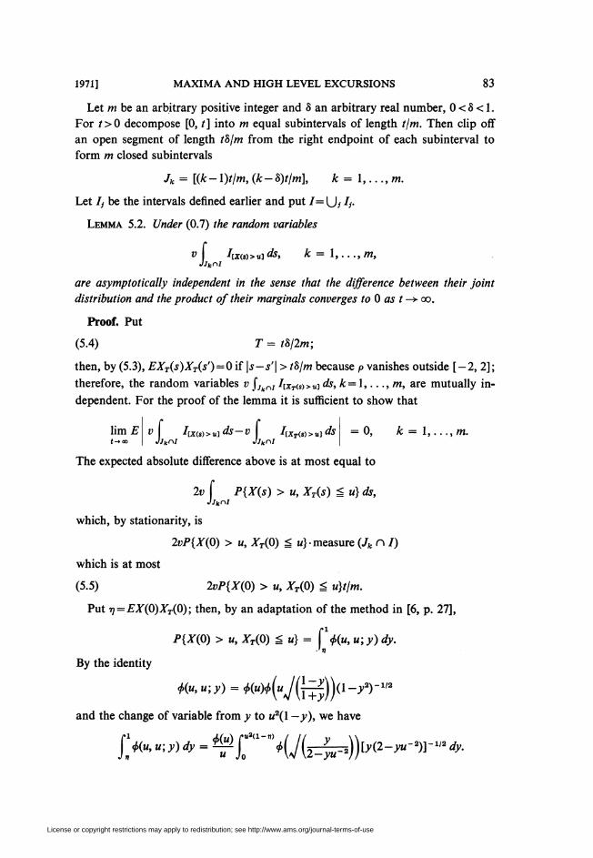
Let m be an arbitrary positive integer and S an arbitrary real number, 0 < 8 < 1.
For />0 decompose [0, t] into m equal subintervals of length t/m. Then clip off
an open segment of length tS/m from the right endpoint of each subinterval to
form m closed subintervals
Jk = P -1)//«, (* - 8)f/i»], k = 1,..., m.
Let Ij be the intervals defined earlier and put 7= \J¡ I¡.
Lemma 5.2. Under (0.7) the random variables
A I[x(s)>u]ds, k — I,..., m,
are asymptotically independent in the sense that the difference between their joint
distribution and the product of their marginals converges to 0 as r —>- oo.
Proof. Put
(5.4) T = thflm;
then, by (5.3), EXTis)XTis') = 0 if \s — s'\ > to/m because p vanishes outside [ — 2, 2];
therefore, the random variables v j¿ ¡7[Jf3,<s)>u]ds,k=l,...,m, are mutually in-
dependent. For the proof of the lemma it is sufficient to show that
lim E(-.00
v Iix(S)>uids-v 7(JJiçnl JJknI
rxT(s>>u] ds = 0, k = 1,..., m.Jjkr\I Jjknt
The expected absolute difference above is at most equal to
2» f P{Xis) > u, XT(s) £ u} ds,JJkr\l
which, by stationarity, is
2t>P{AY0) > u, Afr(0) ̂ u}- measure (7fc n 7)
which is at most
(5.5) 2vP{XiO) > u, AVÍO) ̂ u}t/m.
Put T7=FA(0)A'T(0); then, by an adaptation of the method in [6, p. 27],
7>{AY0) > u, AV(0) ̂ «} = !%("> u;y) dy.
By the identity
<f>iu,u;y) = t(u)t(uj(\=^yi-y2)-u2
and the change of variable from y to «2(1 —y), we have
¡yu,u;y)dy = M ^^{^^^(l-yu-2)]-^ dy.
License or copyright restrictions may apply to redistribution; see http://www.ams.org/journal-terms-of-use
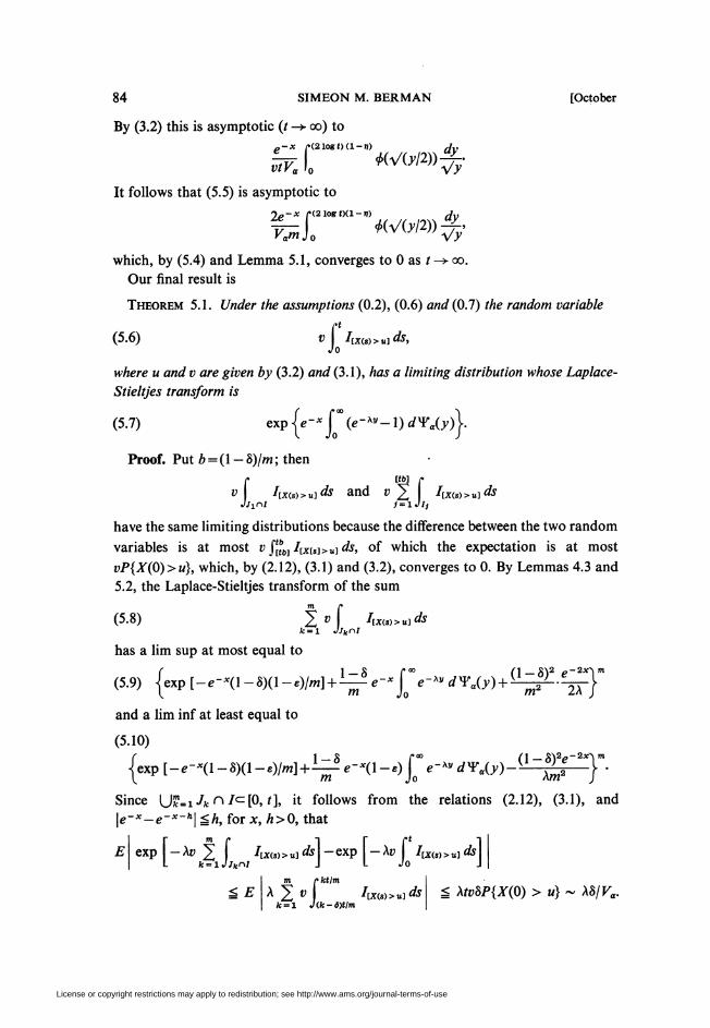
84 SIMEON M. BERMAN [October
By (3.2) this is asymptotic (/ -» oo) to
ST. f. «Vwa»^-It follows that (5.5) is asymptotic to
2e-x «aioBtxi-« ^
which, by (5.4) and Lemma 5.1, converges to 0 as t -> oo.
Our final result is
Theorem 5.1. Under the assumptions (0.2), (0.6) and (0.7) iAe random variable
(5.6) » 7[X(S) >„]<&,Jo
where u and v are given by (3.2) and (3.1), has a limiting distribution whose Laplace-
Stieltjes transform is
(5.7) «p{«-J*(«-**-l)¿Y*00}.
Proof. Put A = ( 1 - 8)/m ; then
Iíx(s)>u-¡ds and v 2 \ 7[X(s)>u]öfe/in/ j = lJI)
have the same limiting distributions because the difference between the two random
variables is at most v J"^ 7[X[s]>u]í/í, of which the expectation is at most
i;F{A(0)>m}, which, by (2.12), (3.1) and (3.2), converges to 0. By Lemmas 4.3 and
5.2, the Laplace-Stieltjes transform of the sum
(5.8) 2 v Iixis)>uidsfc = l JJknr
has a lim sup at most equal to
f 1-8 f" d-8)2 e-2x~)m(5.9) lexpt-e-'O-aKl-eVifil + ̂ -e-*^ e"*» rfY^) + ü-^i-.f^ j
and a lim inf at least equal to
(5.10)
|exp[-e-*(l-8)il_e)/w]+i_e-(l-£)Jo e-^rfY8(y)-U j^f j •
Since Ufc=i7fcn7c:[0, r], it follows from the relations (2.12), (3.1), and
\e-*-e-*-h\ úh, for x, A>0, that
E exp - A» > Az(ö*«j fife -exp - At) 7[X(s)>ul ds1 k=lJjknt J L Jo J |
m /» ktlm
^ E A 2 v\ ¿ire»«] * ^ Ai,;SF{A(0) > h} ~ A8/K«.
License or copyright restrictions may apply to redistribution; see http://www.ams.org/journal-terms-of-use
1971] MAXIMA AND HIGH LEVEL EXCURSIONS 85
It follows that the transform of (5.6) has a lim sup at most equal to expression
(5.9) + AS/ Va and a lim inf at least expression (5.10) — AS/ Va.
Since 8 and e are arbitrary we put S = e=0. Since m is an arbitrary positive integer,
we let m —> oo: The expressions (5.9) and (5.10), with 8 = e = 0, have the common
limit (5.7).
Remark. The transform (5.7) represents the distribution of the sum of a random
number of independent random variables, where the summands have the common
distribution *Fa, and where the random number has a Poisson distribution with
mean e~x.
Added in proof. The validity of (2.21) under a weaker condition on g was
recently announced by C. R. Quails and H. Watanabe in Notices Amer. Math.
Soc. 18 (1971), 532. Abstract #684-F4.
References1. Ju. K. Beljaev, On the number of level crossings by a Gaussian stochastic process. II, Teor.
Verojatnost. i Primenen. 12 (1967), 444-457. (Russian) MR 36 #948.
2. S. M. Berman, Occupation times of stationary Gaussian process, J. Appl. Probability 7
(1970), 721-733.3. -, Excursions above high levels for stationary Gaussian processes, Pacific J. Math.
36 (1971), 63-80.
4. -, Asymptotic independence of the numbers of high and low level crossings of stationary
Gaussian processes, Ann. Math. Statist, (to appear).
5. -, A class of limiting distributions of high level excursions of Gaussian processes,
Z. Wahrscheinlichkeitstheorie und Verw. Gebiete (to appear).
6. H. Cramer and M. R. Leadbetter, Stationary and related stochastic processes. Sample
function properties and their applications, Wiley, New York, 1967. MR 36 #949.
7. X. Fernique, Continuité des processes Gaussiens, C. R. Acad. Sei. Paris 258 (1964), 6058-
6060. MR 29 #1662.8. M. Loève, Probability theory, 3rd ed., Van Nostrand, Princeton, N. J., 1963. MR 34
#3596.9. M. B. Marcus, A bound for the distribution of the maximum of continuous Gaussian pro-
cesses, Ann. Math. Statist. 41 (1970), 305-309.
10. J. Pickands III, Maxima of stationary Gaussian processes, Z. Wahrscheinlichkeitstheorie
und Verw. Gebiete 7 (1967), 190-223. MR 36 #955.
U.C. Quails, On a limit distribution of high level crossings of a stationary Gaussian process,
Ann. Math. Statist. 39 (1968), 2108-2113. MR 38 #6661.
12. D. Slepian, The one-sided barrier problem for Gaussian noise, Bell System Tech. J. 41
(1962), 463-501. MR 24 #A3017.13. E. C. Titchmarsh, Introduction to the theory of Fourier integrals, 2nd ed., Clarendon
Press, Oxford, 1948.
14. V. A. Volkonskii and Ju. A. Rozanov, Some limit theorems for random functions. I, II.
Teor. Verojatnost. i. Primenen. 4 (1959), 186-207 = Theor. Probability Appl. 4 (1959), 178-197.
MR 22 #12586; Teor. Verojatnost. i Primenen. 6 (1961), 202-215. (Russian) MR 25 #597.
15. P. Billingsley, Convergence of probability measures, Wiley, New York, 1968.
Courant Institute of Mathematical Sciences, New York University,
New York, New York 10012
License or copyright restrictions may apply to redistribution; see http://www.ams.org/journal-terms-of-use