Max-Planck-Institut

fur Mathematik

in den Naturwissenschaften

Leipzig

Multivariate construction of effective

computational networks from observational data

by

Joseph Lizier and Mikail Rubinov

Preprint no.: 25 2012

Multivariate construction of effective computational networks

from observational data

Joseph T. Lizier1, ∗ and Mika Rubinov2, †

1Max Planck Institute for Mathematics in the Sciences,

Inselstraße 22, 04103 Leipzig, Germany

2Brain Mapping Unit, Department of Psychiatry,

University of Cambridge, United Kingdom

(Dated: May 3, 2012)

Abstract

We introduce a new method for inferring effective network structure given a multivariate time-

series of activation levels of the nodes in the network. For each destination node in the network,

the method identifies the set of source nodes which can be used to provide the most statistically

significant information regarding outcomes of the destination, and are thus inferred as those source

information nodes from which the destination is computed. This is done using incrementally condi-

tioned transfer entropy measurements, gradually building the set of source nodes for a destination

conditioned on the previously identified sources. Our method is model-free and non-linear, but

more importantly it handles multivariate interactions between sources in creating outcomes at des-

tinations, rejects spurious connections for correlated sources, and incorporates measures to avoid

combinatorial explosions in the number of source combinations evaluated. We apply the method to

probabilistic Boolean networks (serving as models of Gene Regulatory Networks), demonstrating

the utility of the method in revealing significant proportions of the underlying structural network

given only short time-series of the network dynamics, particularly in comparison to other methods.

Keywords: computational neuroscience, effective networks, information transfer, information theory

∗lizier@mis.mpg.de†mr572@cam.ac.uk

1

I. INTRODUCTION

A key objective of computational neuroscience is to infer a network which underpins the

observed activity levels between individual sources in brain imaging data. Typically this

process begins by pre-processing the raw recorded data in some way to form a multivariate

time series for the source node variables; e.g. the source node time-series could be the result

of beamforming applied to MEG recording variables, with artifact removal, etc. The idea

then is to take the multivariate time series representing the activity level of each source node,

and translate this into a network structure revealing the (directed) connections between the

nodes and ideally an explanation for how the dynamics of each node results from their inputs

elsewhere in the network. There are three fundamentally different notions of the type of

network one may try to infer: functional, structural and effective networks.

Functional network inference constructs such networks using a measure of correlation

between nodes to infer connectivity [1]. This can certainly highlight relationships between

nodes, but only reveals undirected relationships, and provides no explanation for how the

relationship manifests.

Structural network inference seeks to find which nodes in the system have physical, di-

rected connections. While one can infer direct causal links between source variables under

certain limited circumstances [2], in general one needs to be able to intervene in the network

to produce such insights [3, 4]. Indeed, to properly do this one needs to be intervene on

a large scale (beyond what can be done in the brain using localised interventions of TMS)

and under general circumstances the task is simply impossible from multivariate time-series

observations alone [5, 6]. Furthermore, knowing the structural network alone does not tell

us about time or experimentally modulated changes in how the network is interacting [1],

nor how information processing takes place.

Effective network analysis seeks to bridge between these two approaches. This approach

examines directed relationships between nodes (across time) and seeks to infer the minimal

neuronal circuit model which can replicate and indeed explain the recorded activity patterns

[1, 7]. Friston states that effective connectivity is closer than the functional connectivity

approach “to the intuitive notion of a connection and can be defined as the influence on

neural system exerts over another” [1]. Certainly the effective network should reflect the

underlying structural network, however it is not intended to give a unique solution to the

2

“inverse problem” of inferring the structural network from time series, and indeed it should

be experimentally and time dependent (to capture the result of external modulations) [1].

In this paper, we focus on effective network inference as the most meaningful and useful

way of capturing and explaining the observed interactions between nodes given the multi-

variate time-series of their activity levels. While we should not interpret an effective network

as directly inferring the underlying neural structure, it should be interpreted as attempting

to provide the best explanation of how the source nodes appear to interact to produce their

next states, which reflects the underlying structural network. Directed measures such as

the transfer entropy [8] and Granger causality [9] are popularly used for effective network

inference. This is because they capture the directed, dynamic predictive effect of a source

on a destination variable, provide some explanation regarding how the dynamics are created

from these interactions, and are readily testable against null models of no source-destination

interaction to allow robust statistical testing of whether a directed link should be inferred

[10–15]. The transfer entropy is model-free and captures non-linear interactions (due to

its underlying information-thereotic formulation), while the Granger causality is faster and

simpler to measure. While the intuition behind these measures suits the task of effective net-

work inference very well, the generally used pairwise form of these measures (which examine

the univariate effect of a source on a destination) are susceptible to missing outcomes created

by collective interactions between multiple nodes, and to inferring superfluous connections

due to correlations of one strong source to other apparent sources (e.g. common cause or

pathway effects). Certainly multivariate forms of these measures exist and are known to

address these problems (e.g. the conditional transfer entropy [16, 17]), however an obvious

brute force approach in applying them for effective network inference suffers combinatorial

explosion in evaluating all potential groupings of candidate sources.

In this paper, we present a systematic algorithm employing the use of multivariate di-

rected dependence measures to infer effective networks. The method properly captures

collective interactions and eliminates false positives, while remaining computationally ef-

ficient. Our approach seeks to find the simplest network which can statistically capture

dependencies in the data set in terms of how the next state of each variable is computed

from the other variables (see Fig. 1). We view each node as a computing unit: computing

its next state at each time step using the its own previous states and those of other nodes in

the network. Our method infers where the information in the next state of the node comes

3

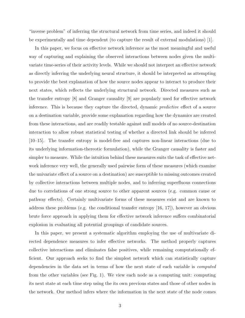
FIG. 1. Central question: how to infer the set of nodes VX = {Y1, Y2} which can be used to infer

the computation of the next state of X, for each node X in the network?

from, and assigns incoming links to the node accordingly. In describing the computation at

each node, our method also provides a simple explanation of how the dynamics are created,

in terms of probability distributions of the destination node in terms of its sources.

Our method is rooted in information theory, and as such is model-free and captures

non-linear relationships. It is specifically designed to capture both uni- and multivariate

relationships between sources in creating the outcomes in the destinations. Crucially, it does

not suffer combinatorial explosion in the number of possible source sets considered, while it

automatically tailors the power of inference (in terms of how much of the network can be

inferred) to the support supplied by the amount of available data. The less observational

data we have, the more conservative the method is in terms of inferring effective connections.

We begin by describing the information-theoretic quantities used here (in particular the

transfer entropy). We show how the information content in a destination can be funda-

mentally decomposed in terms of (conditional) information contributions from its causal

information sources; this decomposition forms the inspiration for our approach. We then

describe existing effective network inference techniques using the transfer entropy, and out-

line the manner in which they cannot detect collective interactions and may infer spurious

links due to source correlations. To address these issue, we present a new criteria for inferring

an effective computational network by inferring the set of sources for each destination node

which makes the destination conditionally independent of all other sources in the network.

Constructing this network becomes an optimisation problem, which we propose to address

using a greedy algorithm with post-processing (e.g. using the Kernigan-Lin approach). Im-

portantly, our greedy algorithm builds the network using strong information sources first,

and then iteratively conditioning on previously selected sources - this allows our technique

to capture collective interactions and reject spuriously correlated sources, unlike other ap-

4

proaches. Finally, we demonstrate an application of the method to infer effective networks

from short time-series observations of probabilistic random Boolean network dynamics. This

test bed is selected since it provides a large state space for the dynamics, highly non-linear

interactions, incorporates large noise effects, and is a useful mode for Gene Regulatory Net-

works [18]. Our application demonstrates the significant improvement that our technique

provides over the default univariate application of transfer entropy, and also provides some

commentary on parameter settings for the method.

II. INFORMATION-THEORETIC PRELIMINARIES

In this section, we present the fundamental information-theoretic quantities used in this

work, then describe how the information in a destination variable may be decomposed into a

sum of incrementally conditioned contributions from each of the sources to that destination.

A. Fundamental quantities

In this section we present the fundamental information-theoretic variables used here, as

formed for measurements on time-series data (i.e. for a variable X with realisations xn at

each time step n in the time series).

The fundamental quantity in information theory [19, 20] is the amount of information

required to predict the next state xn+1 of an information destination X, i.e. the entropy HX

of xn+1:

HX = 〈− log2 p(xn+1)〉n . (1)

Note that the expectation value taken over all realisations/observations n is equivalent to

averaging by the observational probability in the full joint space (i.e. p(xn+1) here).

The joint entropy of two random variables X and Y is a generalization to quantify the

uncertainty of their joint distribution: HX,Y = 〈log2 p(xn, yn)〉n. The conditional entropy of

X given Y is the average uncertainty that remains about xn when yn is known: HX|Y =

〈log2 p(xn|yn)〉n.

The mutual information between X and Y measures the average reduction in uncertainty

about xn that results from learning the value of yn, or vice versa: IX;Y = HX − HX|Y =

5

〈log2 p(xn | yn)/p(xn)〉n. Of course, we can measure the (time-lagged) mutual information

across e.g. one time step: I(yn;xn+1) = 〈log2 (p(xn+1|yn)/p(xn+1))〉n.

The conditional mutual information between X and Y given Z is the mutual information

between X and Y when Z is known: IX;Y |Z = HX|Z − HX|Y,Z . For example, I(yn;xn+1 |

zn) = 〈log2 (p(xn+1 | yn, zn)/p(xn+1 | zn))〉nFinally, the entropy rate is the limiting value of the entropy of the next state xn+1

of X conditioned on the previous k states x(k)n of X: HµX = limk→∞H

[xn+1|x(k)n

]=

limk→∞HµX(k).

The apparent transfer entropy [8, 16] is the mutual information from realisations yn of a

source variable Y to realisations xn+1 of X, conditioned on the history x(k)n of X (see Fig. 2):

TY→X = I(yn;xn+1 | x(k)n ) =⟨

log2

(p(xn+1 | x(k)n , yn)/p(xn+1 | x(k)n )

)⟩n. Clearly the value of

TY→X depends on the history length k: it has been recommended that k → ∞ should be

used to properly represent the concept of information transfer, while limiting k to capture

the direct causal sources in the past of X (e.g. k = 1 in many applications) brings the

measure closer to an inference of causal effect [16, 17].

The transfer entropy itself may be conditioned on another potential source variable Z,

to provide the conditional transfer entropy [16, 17] (see Fig. 2):

TY→X|Z = I(yn;xn+1 | x(k)n , zn)

=⟨log2

(p(xn+1 | x(k)n , zn, yn)/p(xn+1 | x(k)n , zn)

)⟩n. (2)

The conditional transfer entropy eliminates the detection of information from Y about X

that was redundantly provided by Z, and also captures multivariate interactions between

Y and Z which create outcomes in X (e.g. XOR interactions X = Y ⊕ Z ) [16, 17]. It

is well known that neither of these properties is provided by the apparent transfer entropy

[16]. Finally, we note that if (the in general multivariate) Z captures all of the other causal

information contributors to X apart from Y , then we call TY→X|Z the complete transfer

entropy T cY→X [16, 17].

B. Information (de)composition

For the purposes of this work, we are particularly interested in how prediction of the

next state of an information destination X can be made from a set of causal information

6

contributors VX to X. We consider VX to be a subset of some large set of variables or

nodes D which make up the entire network, i.e. VX ∈ D. For simplicity in presenting

the mathematics, we assume that VX causes X over a lag of one time step, though the

extension to variable delays is trivial (one simply expands VX to consider not only the

potential contribution from nodes at the previous time step, but from several time steps

back also - see Section IV B 4).

As such, we can express the entropy of X in terms of the information I(vx,n;xn+1) from

the set of causal information contributors VX at the previous time step n, plus any intrinsic

uncertainty or stochasticity UX remaining in the destination after considering these sources:

HX = I(vx,n;xn+1) + UX , (3)

UX = H(xn+1 | vx,n). (4)

We can make an alternative decomposition of the entropy HX by taking a computational

perspective: we consider HX in terms of how much information is contributed by the past

of X and the remaining uncertainty after considering that past. The information from the

past of X is captured by the active information storage [17, 21], AX = I(x(k)n ;xn+1) where

x(k)n = xn−k+1, . . . , xn−1, xn is the joint vector of the past k values of X, up to and including

xn. The remaining uncertainty after considering the past of X is the entropy rate HµX . The

decomposition is then given by:[22]

HX = I(x(k)n ;xn+1) +H(xn+1 | x(k)n ), (5)

HX = AX +HµX . (6)

We then further partition the information from the causal contributors in order to align

Eq. (3) and Eq. (5) [17]:

HµX = I(vx,n;xn+1 | x(k)n ) + UX , (7)

HX = AX + I(vx,n;xn+1 | x(k)n ) + UX , (8)

HX = AX + TVX→X + UX . (9)

Here, TVX→X = I(vx,n;xn+1 | x(k)n ) is the collective transfer entropy [17], and repre-

sents the (multivariate) information transfer from the set of joint sources VX to X. As

such, Eq. (9) shows how the information in the next state is a sum of information storage,

information transfer, and intrinsic uncertainty.

7

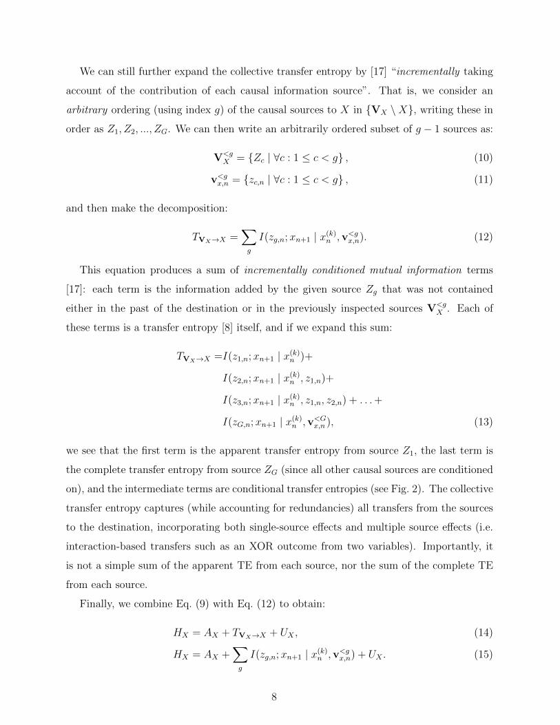
We can still further expand the collective transfer entropy by [17] “incrementally taking

account of the contribution of each causal information source”. That is, we consider an

arbitrary ordering (using index g) of the causal sources to X in {VX \X}, writing these in

order as Z1, Z2, ..., ZG. We can then write an arbitrarily ordered subset of g − 1 sources as:

V<gX = {Zc | ∀c : 1 ≤ c < g} , (10)

v<gx,n = {zc,n | ∀c : 1 ≤ c < g} , (11)

and then make the decomposition:

TVX→X =∑g

I(zg,n;xn+1 | x(k)n ,v<gx,n). (12)

This equation produces a sum of incrementally conditioned mutual information terms

[17]: each term is the information added by the given source Zg that was not contained

either in the past of the destination or in the previously inspected sources V<gX . Each of

these terms is a transfer entropy [8] itself, and if we expand this sum:

TVX→X =I(z1,n;xn+1 | x(k)n )+

I(z2,n;xn+1 | x(k)n , z1,n)+

I(z3,n;xn+1 | x(k)n , z1,n, z2,n) + . . .+

I(zG,n;xn+1 | x(k)n ,v<Gx,n ), (13)

we see that the first term is the apparent transfer entropy from source Z1, the last term is

the complete transfer entropy from source ZG (since all other causal sources are conditioned

on), and the intermediate terms are conditional transfer entropies (see Fig. 2). The collective

transfer entropy captures (while accounting for redundancies) all transfers from the sources

to the destination, incorporating both single-source effects and multiple source effects (i.e.

interaction-based transfers such as an XOR outcome from two variables). Importantly, it

is not a simple sum of the apparent TE from each source, nor the sum of the complete TE

from each source.

Finally, we combine Eq. (9) with Eq. (12) to obtain:

HX = AX + TVX→X + UX , (14)

HX = AX +∑g

I(zg,n;xn+1 | x(k)n ,v<gx,n) + UX . (15)

8

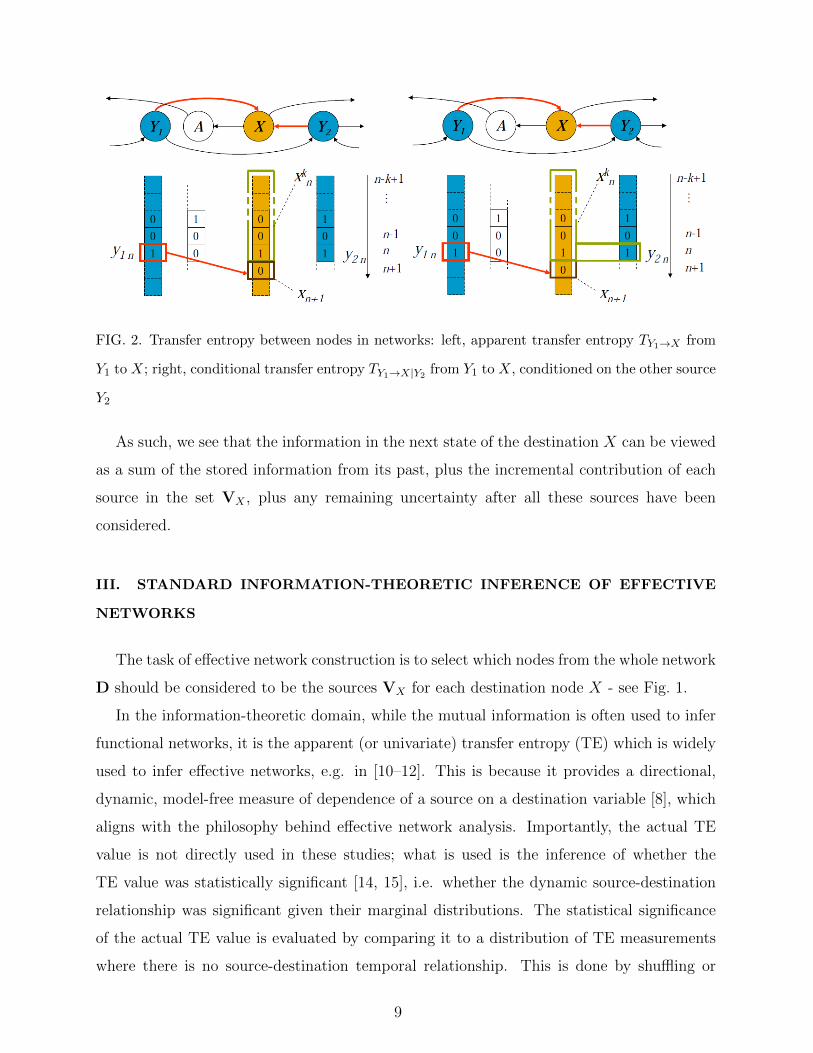
FIG. 2. Transfer entropy between nodes in networks: left, apparent transfer entropy TY1→X from

Y1 to X; right, conditional transfer entropy TY1→X|Y2 from Y1 to X, conditioned on the other source

Y2

As such, we see that the information in the next state of the destination X can be viewed

as a sum of the stored information from its past, plus the incremental contribution of each

source in the set VX , plus any remaining uncertainty after all these sources have been

considered.

III. STANDARD INFORMATION-THEORETIC INFERENCE OF EFFECTIVE

NETWORKS

The task of effective network construction is to select which nodes from the whole network

D should be considered to be the sources VX for each destination node X - see Fig. 1.

In the information-theoretic domain, while the mutual information is often used to infer

functional networks, it is the apparent (or univariate) transfer entropy (TE) which is widely

used to infer effective networks, e.g. in [10–12]. This is because it provides a directional,

dynamic, model-free measure of dependence of a source on a destination variable [8], which

aligns with the philosophy behind effective network analysis. Importantly, the actual TE

value is not directly used in these studies; what is used is the inference of whether the

TE value was statistically significant [14, 15], i.e. whether the dynamic source-destination

relationship was significant given their marginal distributions. The statistical significance

of the actual TE value is evaluated by comparing it to a distribution of TE measurements

where there is no source-destination temporal relationship. This is done by shuffling or

9

rotating[23] the source values to generate many surrogate source time series, and generating

a surrogate TE value from each one. One then tests whether the null hypothesis that there

was no directed source-destination temporal relationship is supported by the actual TE value

(rejecting this null hypothesis and concluding the actual TE value statistically significant if

there is a probability less than α of the actual TE value being observed by chance under

the null hypothesis). Such statistical significance has been evaluated for performing effective

connectivity analysis with the transfer entropy in several applications to neural data; e.g.

[10–13].

This use of the transfer entropy provides model-free and non-linear capabilities, and

the statistical significance approach adds objectivity in determining whether a connection

should be inferred, and robustness to low amounts of data [12]. As alluded to in Section

II A however, a particular problem however is that it ignores multivariate effects in only

considering univariate sources. In the context of effective network inference, this means

that:

• it can miss inferring links whose effect is only manifested via interactions (e.g. XOR

functions);

• it can infer redundant links, e.g. adding potential sources whose information contri-

bution is only due to their being correlated with a true information source, or adding

links which are only manifested due to indirect causes through other variables in the

data. For example, the method is susceptible to inferring redundant links Y → X due

to either pathway relationships Y → Z → X, or common cause relationships Z → Y

and Z → X

One can directly take a multivariate approach, e.g. by examining Granger causality

from each variable, conditioning out the whole remainder of the system [24]. And indeed,

this could be mirrored in theory via the complete transfer entropy [16], which provides

advantages of non-linearity and model-freedom over the Granger causality approach, but

is in fact impossible in practise due to the limitations of available observations. Although

Granger causality can be computed with less data, going directly to condition out all other

variables is still undesirable. This is because where information is held redundantly by two

potential sources, both will reduce the conditioned contribution of the other to zero when

the measure is made conditioning out all variables in the system. Such a situation becomes

10

increasingly likely in large neural data sets, where the brain’s massive redundancy comes

into play, and also in short data sets where undersampling in large multivariate spaces begins

to mask real information contributions.

We need an approach between these two extremes, which can infer links whether they

are involved in uni- or multivariate interactions creating information in the destination, and

appropriately handles redundancy in the data set. We will consider how to do this in the

next section, building on our information-theoretic view of the information (de)composition

of destination variables provided in Section II.

IV. MULTIVARIATE EFFECTIVE SOURCE SELECTION

Our goal, as previously stated, is to find the simplest network which can statistically

capture dependencies in the data set in terms of how the next state of each variable is

computed from the other variables. This means that we wish to find the simplest set

of sources VX in the network D which can make X conditionally independent from the

remaining sources D \VX , given its own past x(k)n also. To restate this in the notation of

Section II, we seek to infer the simplest set of sources VX in the network D from which

the greatest amount of information about a destination X can be statistically-significantly

predicted (minimizing remaining uncertainty, see Eq. (3)).

Since I(vx,n;xn+1) monotonically increases with the size of the set VX , then the prediction

of the next state (from the observed data set) can be trivially maximized by including all of

the potential sources D in VX . However, a large proportion of this increase is because the

measurement becomes more and more biased with the size of the set VX , and the increase

does not mean that all of those sources actually provide statistically-significant information

about xn+1. So we clarify our goal as:

To identify the set of source variables VX ∈ D for X which maximises the

collective transfer entropy TVX→X to X, subject to the condition that each

source Z in VX incrementally adds information to X in a statistically significant

fashion (i.e. that TZ→X|VX\Z is statistically significant ∀Z ∈ VX).

We point out that the goal cannot be satisfied by the following approaches:

• Maximising the number of sources in VX is not sound, since (in all likelihood) many of

11

the sources in the complete data set will not provide a statistically significant amount

of information to the destination in addition to that provided by other sources.

• Selecting sources which have individually large univariate transfer entropies or lagged

mutual information values to X will not address the goal either, since this ignores

the contributions from sources involved in multivariate interactions, and does not

discriminate out redundant contributions.

• Selecting sources which contribute large amounts of information conditioned on all

other potential sources in D will not address the goal, since this is impractical with

short data sets and wilfully eliminates all redundant contributions (even though the

observer requires one copy of that redundant information to help with predicting the

destination).

Selecting the set of sources VX to meet the above goal is a non-trivial optimisation

problem, since we have∑|D|

m=1

(|D|m

)= 2|D| potential solutions; clearly this is an NP-hard

problem as the size of the solution space expands exponentially with the problem size,

and we cannot directly evaluate whether a given candidate solution is optimal. We have a

quality function for potential solutions VX to the optimisation problem, being the amount of

information they are able to predict about the next state of X, subject to the condition that

every source in VX contributes a statistically significant amount of information conditioned

on all other sources in VX .

In the following sections, we present an efficient algorithm to address this optimisation

problem, then discuss its properties and parameter settings.

A. Iterative greedy method

We propose the use of a greedy method to avoid evaluating all possible source combina-

tions, by instead incrementally building the source set VX making a greedy choice at each

selection step about which new source to add to VX . The method seeks to incrementally

add sources Z to VX , taking inspiration from the information decomposition in Eq. (12)

and Eq. (15), by adding the source at each selection step which adds the most information

about the destination X conditioned on the previously selected sources.

The steps of the basic iterative greedy method are as follows:

12

1. Initialise VX = ∅.

2. Evaluate TZ→X|VXfor every source Z ∈ D \VX .

3. Select the source Z ∈ D \ VX which provided the largest incremental information

contribution TZ→X|VXabout the next state of X, while that the information was

statistically significant against null models.

4. Repeat steps 2 and 3 until no source Z can be found to be added to VX . Termination

of the algorithm occurs because either there is no more information in X left to

account for, or no source Z provides a statistically significant information contribution

TZ→X|VXwhich could account for part of the remaining uncertainty in X.

We make several comments on these steps as follows.

To evaluate the statistical significance of a conditional transfer entropy TZ→X|VX, one

follows the known algorithm [11, 12, 14, 15] for the apparent transfer entropy with a slight

modification: shuffling or rotating the source only, but not the destination or conditioned

time series (this preserves the temporal ordering within the destination and with respect

to the conditioned time series). The null hypothesis is altered to suggest that there is no

temporal relationship from the source to the destination state change, conditioned on the

other sources.

We note that the statistical significance need not be evaluated for the conditional TE

from every potential source Z at step 3; one simply should evaluate statistical significance

for the sources in descending order of the conditional TE they provide until identifying a

source which provides a statistically significant incremental information contribution. We

must explore beyond the source with the largest conditional TE value if it did not prove

to be statistically significant, because a source with a lower conditional TE may provide

this in a statistically significant fashion and consequently be selected. This could happen

where the lower TE source had a lower entropy but was more strongly correlated with the

activity in the destination variable. While this is possible, it is likely that the algorithm

would only evaluate the statistical significance for a large proportion of sources when none

of them become selected at step 3. Thus, the average runtime of the algorithm is likely to

be better than the asympototic worst case performance.

13

Next, note that we called step 3 a greedy selection, and hence we have a greedy method,

because the selection may not be optimal. It could make a non-optimal choice if:

• the selected source Z1 contributes a large amount of information redundantly with

another non-selected source Z2, and another separate amount of information redun-

dantly with another non-selected source Z3. Z2 and Z3 won’t be selected at a later

step because the information they each appear to provide is redundant with Z1; and

• Z2 and Z3 actually provide a large amount of joint or interaction-based transfer to X,

which cannot be detected for either in isolation by step 2 unless the other source has

already been included in VX .

In this case, the extra information from Z2 and Z3 will not be detected.

This situation, and indeed the simpler situation where two sources provide an interaction

based outcome in the destination but neither provide a detectable information contribution

on their own, can be addressed by the following enhancement:

5. When no source Z can be found providing a statistically significant information con-

tribution TZ→X|VX, repeat steps 2 and 3 considering joint pairs of sources Z =

{Za, Zb|Za, Zb ∈ D \VX} instead of single sources Z.

We note that this enhancement costs computational time, i.e. O (|D \VX |2) transfer en-

tropy evaluations (not including statistical significance calculations). As such, the user

must weigh up the computational cost of including this step against the potential benefit

gained from capturing multivariate interactions where neither source makes a detectable

information contribution on its own. Of course, step 5 can be extended to triplets Z =

{Za, Zb, Zc|Za, Zb, Zc ∈ D \VX} (and so on) when no variables are identified as adding con-

tributions at the pair level (or so on), if one has enough computational time (or conversely

if the available data set |D| is small enough), though it is unlikely that the computational

time cost would justify any additional benefit here.

Additionally, we suggest a pruning/partition optimisation step as an enhancement:

6. Once we have finalised the determination of VX after the above (i.e. no further sources

add statistically significant information to the destination X), then check whether each

Z ∈ VX adds a statistically significant amount of information TZ→X|VX\Z given all of

14

the other sources selected for VX . Where a source fails this test it is removed from VX .

Importantly, if multiple sources fail the test, then we remove only the source Z which

provided the least amount of information TZ→X|VX\Z , then repeat this step with the

remaining VX . The partitioning of D into VX and D \VX could be further explored

here using the Kernighan-Lin optimisation algorithm [25], which uses several steps to

test not only the aforementioned pruning, but also a local-maxima avoidance strategy

to explore whether other additional sources in VX may provide a better solution.

We refer to the algorithm including steps 5 and 6 as the enhanced iterative greedy method.

Certainly, the most recently selected source in VX has already passed the pruning test

of step 6. Each other source passed the test at the time they were selected, however they

were selected when VX contained less other sources. As such, there is a possibility that

sources selected later by the algorithm (say Z2 and Z3 in the previous example) are able

to provide all of the information provided by an earlier selected source (i.e. source Z1 in

the previous example). This step serves to make sure that we have identified the simplest

set VX that can be used to maximally, statistically significantly predict X. As such, it

ensures that our selection VX meets the goal we articulated at the start of Section IV. The

removal of only one source at a time is important, since this avoids a situation where all

sources providing redundant information are removed, leaving no sources in VX containing

this information about X (which is a key problem with the exclusive use of the analogue

of complete transfer entropy in [24]). Crucial also is that this pruning step will not remove

sources which provide significant joint interaction-based outcomes with other sources in VX ,

since the interaction-based contribution is captured in TZ→X|VX\Z . Furthermore, this step

helps to add some robustness against spurious source selection: were a spurious source to be

selected at an early step simply due to statistical fluctuations, there is the opportunity to

remove it here if the real sources providing the same plus more information were discovered

at a later step.

Finally, we note that our basic iterative greedy algorithm could viewed as analogous to

forward feature selection in the domain of machine learning, where the “features” here are

the source nodes and one is trying to learn/predict the destination node. An important

distinction though is that our algorithm seeks to limit its inference as a function of the

amount of available data (as detected by the statistical significance tests), whereas feature

selection typically includes as many features as one is able to process. Furthermore, we note

15

that the idea of iteratively constructing source nodes for a given destination is considered

by Faes et al. [26]. The perspective of the algorithm is different, seeking to judge whether

a single link should be inferred rather than considering how to infer a network, yet the

end result is somewhat equivalent. The algorithm presented in that study also seeks to

limit inference as a function of statistical power, and uses bias correction to check that

newly added sources are reducing the remaining entropy beyond the bias level. This is

weaker than a test of statistical significance used here, since a source could appear to reduce

entropy beyond the bias level, but still not do so in a statistically significant fashion. This

could also lead to spurious sources with high entropy but low statistical significance being

included instead of lower entropy actual sources.

B. Comments on the technique and parameter setting

Before testing the algorithms, we explore parameter setting options and provide comments

on the properties of the technique.

1. History length to condition on

We have three available choices regarding how to handle the history length k of the desti-

nation variable X in the transfer entropy measurements, and consequently our interpretation

of self-links in the network:

• Set k to a large value, implicitly including x(k)n in VX . This takes a computational

perspective of the information in the next state, properly decomposing it into stored

and transferred information. This is advantageous if one wishes to understand the

emergent computation taking place on the network (i.e. akin to describing computa-

tion in cellular automata in terms of blinkers, gliders and glider collisions [16, 17, 21]).

It specifically ensures that effective connections are inferred where new information

is transferred from the source to the destination. This approach may be closer to

the spirit of effective network inference in seeking a minimal network to replicate the

dynamics.

• Minimise k to include only the x(k)n which are (or at least are thought to be) direct

causal sources to xn+1 (implicitly including x(k)n in VX). In many systems this would

16

result in setting k = 1. Such a setting brings the measures closer to approximating

the causal influence of sources on the destination [5].

• Set k = 0 in relevant transfer entropy equations, making them simply mutual infor-

mation or conditional mutual information measurements. This makes no assumption

about self-links in the data set, and is the most model-free approach. In following this

approach, one should then allow the previous step of the destination xn to itself be

selectable for VX from the set of sources, such that self-links can be inferred if they

are statistically significant.

Each of these options could be justified from certain perspectives, and so the choice between

them depends on precisely how the user wishes to interpret the effective network.

2. False detection rate

In theory, one should correct for multiple comparisons, e.g. the common Bonferonni

correction by correcting the threshold for the statistical significance tests from the original

α to αc = α/L where L is the number of possible connections evaluated. This allows one

to interpret the selected α as the (upper limit on the) probability that we infer at least

one connection in the network due to statistical fluctuations (if the source and destination

actually had no relationship under the null hypothesis).

In performing statistical tests with the apparent transfer entropy only, it is clear that

one makes |D|(|D| − 1) comparisons, and computing a correction is straightforward. With

multiple rounds of comparisons in our approach, it is possible that one may compare the

same source-destination pair multiple times (i.e. if a source Z1 were rejected initially, with

another source Z2 selected, then the source Z1 is tested again using a transfer entropy

conditioned on Z1). It is unclear how many times the pair may be tested, since we do not

know a priori how many sources will be selected for each destination (and therefore how

many times a source might be tested). As such, it is difficult to judge what correction

should be made here. However, we observe that:

1. the algorithm will not make a statistical test for each source Z ∈ VX until the final

selection round when no source is found to be significant, and it is likely that when

17

a significant source is found that only very few sources were previously evaluated for

statistical significance in that round;

2. the comparisons for the same source in different rounds (with more other sources

conditioned on in later rounds) are not independent, and indeed we conjecture that a

spurious source with high statistical significance (due to correlations to actual sources)

in an early round is likely to have reduced statistical significance in later rounds once

the actual sources are discovered.

As such, we conjecture that the multiple rounds of comparisons in our approach are not likely

to lead to a higher false discovery rate for spurious sources than in the baseline apparent

transfer entropy approach.

Of course, we note that one could simply view the α in use as adjusting the sensitivity and

hence the true-positive/false-alarm trade-off (e.g. driving the locus of the receiver/relative

operating characteristic or ROC curve), and not rely so much on directly interpreting its

numerical meaning.

3. A pluggable general algorithm

In the preceeding description, we have not made any description of how the transfer

entropies are measured here. This is because the iterative greedy algorithm(s) are applicable

to any type of entropy estimation techniques, i.e. using discrete-valued variables or otherwise

discretising continuous valued data, or using kernel estimation with static [8, 27] or variable

[28] kernel widths for continuous-valued data, etc.

We also note that the iterative greedy algorithm(s) presented here for the conditional

transfer entropy could be applied identically to with partial correlations / Granger causality

as the directional measure. Clearly one loses the advantages of nonlinearity and model

freedom of the transfer entropy technique, though if the underlying time-series are Gaussian

with linear relationships the two measures are equivalent anyway [29], and the linear methods

require much less data and can be evaluated much more quickly (indeed there are analytic

alternatives to the use of bootstrapping for the statistical significance testing).

18

4. Consider variable time-lag for all sources

As previously stated, to simplify the mathematics above we have assumed that direct

influences on xn+1 come from potential source variables zn for Z ∈ D at time step n only. Of

course, we could consider all source variables zn+1−λ for some other known source-destination

time lag λ instead of simply using λ = 1. More generally though, the source-destination

time lag could be unknown and different for each interaction. This is known to be the case in

real neuro data sets, and indeed other authors have examined how to select the appropriate

delay from one source to a destination [10, 11].

As such, our algorithm can be generalised by considered potential sources zn+1−λ for Z ∈

D for various delays say λ = 1 . . . l. There is certainly no problem in selecting contributions

from two or more lags from the one source Z to X; obviously this does not alter the inferred

effective network structure, but does provide additional information to explain the dynamics.

Furthermore, we note that widening our consideration for l possible delays simply linearly

increases the time complexity of the algorithm by a factor l. The consideration of various

source-destination lags is included in the approach of Faes et al. [26].

V. APPLICATION TO PROBABILISTIC RANDOM BOOLEAN NETWORKS

To explore the performance of our technique, we test it using time series observations

of probabilistic random Boolean networks (pRBNs). These models are chosen for testing

for several reasons. RBNs provide a very large sample space of dynamics, including highly

non-linear behaviour and the inclusion of collective interactions, making the task of effective

network inference here particularly challenging. Adding to this challenge is the inclusion

of stochasticity on the Boolean functions (i.e. the “p” in pRBNs). Importantly, RBNs

(and pRBNs) are an important model for Gene Regulatory Networks [18], a domain where

researchers face similar challenges to computational neuroscientists in inferring underlying

network structure, and pRBNs have been used to test such inference methods in this domain

(see e.g. [30]).

Here, we use software from Zhao et al. [30] to generate pRBN networks and dynamics to

test our method against. We simulate pRBNs with 20 nodes, and 40 directed edges randomly

assigned subject to a maximum of 3 incoming edges per node (self-links are allowed). Each

19

node has a random Boolean function assigned from its inputs (subject to each node being an

information contributor to that function[31]) and then fixed for the experiment. Dynamics

are generated by starting the network in a random state, and then each node executes its

update function synchronously for each time n+1 using the values of the input nodes at time

step n. The rule executions at each time step for each node are subject to a 0.20 probability

of bit-flipping (i.e. noise). The inclusion of only rules where each node contributes (making

collective interactions more prominent than in ordinary RBNs) and the addition of noise

makes the inference task more challenging here.

We evaluate the performance of our technique and standard apparent TE inference by

comparing the inferred effective network to the known underlying structural network. We

have discussed previously that effective network inference should not necessarily be to re-

produce the underlying structural network, but must certainly reflect it. Indeed, in this

example where the network performs a random exploration of the state space of possible

dynamics (due to the random initial state, and noise at each step) as opposed to being

driven by task-related inputs, and we ensure that the causal inputs occur in step with the

time-series observations we have, then we should expect good effective network inference

to closely reflect the underlying structure, given enough observations. Evaluation against

the underlying structural network also provides insight into how well our method improves

on the apparent transfer entropy technique in terms of detecting true collective interactions

and avoiding inferring spurious connections due to correlations only.

We investigate these methods using several different numbers of time-series observations

(N = 20 to 400), and set the threshold for the tests of statistical significance at α = 0.01 (no

adjustment for multiple comparisons; we are viewing α as a sensitivity parameter for ROC

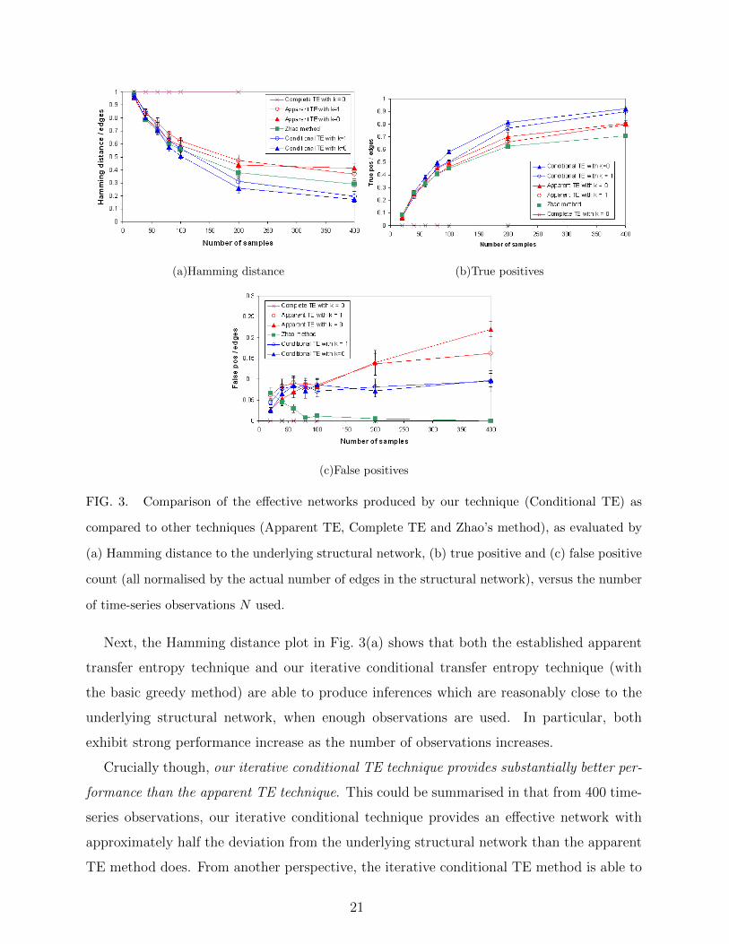
performance). We present the results in terms of Hamming distance of the inferred effective

network from the underlying structural network, true positive count and false positive count

in Fig. 3 (note all counts are normalised by the total number of actual causal edges here,

40). The Hamming distance measure is simply the sum of the other two measures.

First, the plots show that inferring effective networks using the complete TE (i.e. condi-

tioning on all other nodes in the network) has no utility from the finite number of samples

here - it is not able to statistically significantly infer any connections, so has no false posi-

tives but no true positives either. This was as expected when we discussed the proposal of

this method by Quinn et al.[24] in Section III.

20

(a)Hamming distance (b)True positives

(c)False positives

FIG. 3. Comparison of the effective networks produced by our technique (Conditional TE) as

compared to other techniques (Apparent TE, Complete TE and Zhao’s method), as evaluated by

(a) Hamming distance to the underlying structural network, (b) true positive and (c) false positive

count (all normalised by the actual number of edges in the structural network), versus the number

of time-series observations N used.

Next, the Hamming distance plot in Fig. 3(a) shows that both the established apparent

transfer entropy technique and our iterative conditional transfer entropy technique (with

the basic greedy method) are able to produce inferences which are reasonably close to the

underlying structural network, when enough observations are used. In particular, both

exhibit strong performance increase as the number of observations increases.

Crucially though, our iterative conditional TE technique provides substantially better per-

formance than the apparent TE technique. This could be summarised in that from 400 time-

series observations, our iterative conditional technique provides an effective network with

approximately half the deviation from the underlying structural network than the apparent

TE method does. From another perspective, the iterative conditional TE method is able to

21

produce an effective network closer than the structural network as the apparent TE method

does with 400 time-series observations, but with half the number of observations.

This is as expected from the advantages of the conditional TE discussed in Section II A,

which are properly utilised by our technique as discussed in Section IV. In particular, we

know that the conditional TE detects collective interactions that the apparent TE cannot,

and this is demonstrated in the significantly larger true positive rate for our technique in

Fig. 3(b) (approaching an impressive 90% of the network with 400 time series observations).

Furthermore, the conditional TE dismisses spurious connections due to correlations where

the apparent TE cannot, and this is demonstrated in the significantly smaller false positive

rate for our technique in Fig. 3(c).

Interestingly, the false positive rate for the apparent TE technique appears to be increas-

ing with the number of time-series observations in Fig. 3(c). This may be due to spurious

correlations (e.g. between Z and X due to a pathway relationship Z → Y → X) appearing

to have more statistical significance with regards to apparent TE when they are measured

over a larger number of time-series observations. In contrast, the false positive rate for our

technique remains stable with the number of time-series observations used. In part this is

because our conditional TE based technique is better able to properly ignore such spurious

correlated sources by conditioning out the actual primary sources (since by the data pro-

cessing theorem these sources should be selected first, at least in the absence of noise, and

should be more likely to be selected in the presence of noise). Indeed, the false positive rate

remains stable around the level at which one would expect from the given α = 0.01 (i.e.

at 0.1 ∗ 40 = 4 false inferences out of 360 non-existent edges, giving a false positive rate

of 0.011). This may seem surprising, since as discussed in Section IV B 2 more statistical

tests are made with our technique, and an increase in false positives could be expected. As

suggested there however, it seems that no increase in false positives is observed since there

are generally not many more statistical tests actually made with the technique in practice,

and indeed when they do occur they are not independent of the tests at the preceding step.

Note that we have plotted results for both setting k = 0 and 1. For k = 0, the network

can infer self-links where it seems they exist, whereas with k > 0 these cannot be inferred:

in both cases we normalise by the number of links that could be inferred by that technique.

As discussed regarding the choice of this parameter in Section IV B 1, we could expect the

performance with k = 0 to be closer to the underlying structural network - since the nodes

22

do not in general have a causal influence on their next state, so this approach is a better

model to the causal process. Certainly, this expectation bears out to an extent. We see

that for an intermediate number of observations, the inference with k = 0 out-performs

that with k = 1 for both the apparent TE technique and our conditional TE technique.

The performance gap seems to close at larger numbers of observations though, and for the

apparent TE it is reversed due to a significantly larger false positive rate with k = 0. It

seems then that conditioning on the history of the destination, even if it is not a causal

source, may provide some stability against false positive inference. As previously discussed

Section IV B 1, the choice between these parameter settings largely comes down to what

the user wants the effective network to represent. The performance gap for matching the

structural network is not as large as one may expect, and indeed it seems k > 0 adds some

stability, as well as the ability to interpret the results as representing computation on the

network.

Finally, note that we have included the inference results from the technique presented by

Zhao et al. [30], as calculated using the software distributed for that paper. The method

of [30] uses pairwise, cross-time mutual information measurements across the network, then

explores all of the different thresholdings of these to see which minimises a cost function

combining the description length of the network (i.e. the number of links) and unexplained

uncertainty in the state of the nodes. We note that our conditional TE technique significantly

outperforms that of [30] in terms of the Hamming distance and true positive rate, though

does have a larger false positive rate. It is important to note that the sensitivity parameter

for the technique from [30] used here Γ = 0.4 cannot be tuned to provide a better true

positive or Hamming distance here.

VI. DISCUSSION AND CONCLUSION

We have presented an iterative greedy method to infer effective networks from multivari-

ate time-series observations using incremental conditional transfer entropy measurements.

Our technique is consistent with the original intention of effective network analysis, in that

it seeks to infer the simplest network to explain the observed dynamics. In particular, it

does so by considering how the dynamics of each node are computed as a function of the

source nodes, and hence our approach infers effective computational networks.

23

In being information-theoretic, and based on the transfer entropy, our technique provides

inference of directional, non-linear relationships, using model-free analysis. We provide a

crucial improvement to effective connectivity analysis over standard apparent transfer en-

tropy analysis by using (iteratively) conditional TE, which is known to capture collective

multivariate interactions (e.g. XOR relationships) and ignore spurious correlations (e.g.

from pathway or common cause effects). Importantly, we structure an iterative greedy al-

gorithm (with enhancements) in such as way as to avoid combinatorial explosions in the

number of source combinations considered, while avoiding conditioning out all redundant

contributions (only removing them when the redundant information has already been in-

cluded in the network). Furthermore, in employing rigorous tests of statistical significance,

we avoid overfitting and limit the inference to the statistical power in our data set. Impor-

tantly also, our technique infers an effective network which is usefully able to explain the

dynamics of the nodes using (conditional) probability distributions; such explanation is a

key goal of effective network inference.

While our effective connectivity approach does not explicitly seek to infer the causal or

structural network underpinning the data, it should reflect this network, and given a large

ensemble of input distributions to the network or sampling across many types of biases, it

may indeed also provide useful inference of the structural network from the observational

data. Indeed, we have demonstrated the validity of the technique using the particularly

challenging example of probabilistic random Boolean networks, showing in particular that

our conditional TE based approach significantly outperforms standard apparent TE effective

network inference (when evaluated against the underlying structural network).

In future work, we seek to apply the technique to various types of brain recordings. In

doing so, we will certainly need to incorporate several practical considerations, including

variable source-destination lags as discussed in Section IV B 4. We shall also seek to refine

the steps of our algorithm, in particular the post-processing optimisation steps.

ACKNOWLEDGMENTS

MR acknowledges travel support from the Max Planck Institute for Mathematics in the

Sciences, and JL acknowledges travel support from the Brain Mapping Unit at the University

24

of Cambridge, both of which contributed to this work.

[1] K. J. Friston, Human Brain Mapping 2, 56 (1994).

[2] For example, using the “back-door” approach (as discussed in [3, 5]), though this requires a

priori knowledge of where all other causal links are to the given node, defeating the purpose

of general inference.

[3] N. Ay and D. Polani, Advances in Complex Systems 11, 17 (2008).

[4] J. Pearl, Causality: Models, Reasoning, and Inference (Cambridge University Press, Cam-

bridge, 2000).

[5] J. T. Lizier and M. Prokopenko, European Physical Journal B 73, 605 (2010).

[6] D. Chicharro and A. Ledberg, PLoS ONE 7, e32466+ (Mar. 2012), http://dx.doi.org/10.

1371/journal.pone.0032466.

[7] O. Sporns, Networks of the brain (MIT Press, Cambridge, Massachusetts, USA, 2011).

[8] T. Schreiber, Physical Review Letters 85, 461 (2000).

[9] C. W. J. Granger, Econometrica 37, 424 (1969).

[10] M. Wibral, B. Rahm, M. Rieder, M. Lindner, R. Vicente, and J. Kaiser, Progress in Biophysics

and Molecular Biology 105, 80 (2011), ISSN 00796107.

[11] R. Vicente, M. Wibral, M. Lindner, and G. Pipa, Journal of Computational Neuroscience 30,

45 (2011), ISSN 0929-5313.

[12] J. T. Lizier, J. Heinzle, A. Horstmann, J.-D. Haynes, and M. Prokopenko, Journal of Compu-

tational Neuroscience 30, 85 (2011).

[13] M. Lindner, R. Vicente, V. Priesemann, and M. Wibral, BMC Neuroscience 12, 119+ (2011),

ISSN 1471-2202.

[14] M. Chavez, J. Martinerie, and M. Le Van Quyen, Journal of Neuroscience Methods 124, 113

(2003).

[15] P. F. Verdes, Physical Review E 72, 026222 (2005).

[16] J. T. Lizier, M. Prokopenko, and A. Y. Zomaya, Physical Review E 77, 026110+ (2008).

[17] J. T. Lizier, M. Prokopenko, and A. Y. Zomaya, Chaos 20, 037109+ (2010).

[18] S. A. Kauffman, The Origins of Order: Self-Organization and Selection in Evolution (Oxford

University Press, New York, 1993).

25

[19] T. M. Cover and J. A. Thomas, Elements of Information Theory, 99th ed. (Wiley-Interscience,

New York, 1991) ISBN 0471062596.

[20] D. J. C. MacKay, Information Theory, Inference, and Learning Algorithms (Cambridge Uni-

versity Press, Cambridge, 2003).

[21] J. T. Lizier, M. Prokopenko, and A. Y. Zomaya, “Local measures of information storage in

complex distributed computation,” (2011).

[22] Note that the correctness of these equations is independent of k; altering k merely changes the

proportions of information that is attributed to either the information storage or the entropy

rate.

[23] Rotation is required where one is considering multiple past values of the source, e.g. performing

an embedding of l past values to obtain a state vector of the source y(l)n , or otherwise requires

the entropy rate of the source to be preserved. Otherwise, if considering a single past source

value yn only, investigation of the null hypothesis to destroy the relationship p(xn+1 | x(k)n , yn)

is facilitated by shuffling alone.

[24] C. Quinn, T. Coleman, N. Kiyavash, and N. Hatsopoulos, Journal of Computational Neuro-

science 30, 17 (2011), ISSN 0929-5313.

[25] B. W. Kernighan and S. Lin, The Bell Systems Technical Journal 49, 291 (1970).

[26] L. Faes, G. Nollo, and A. Porta, Physical Review E 83, 051112+ (2011).

[27] H. Kantz and T. Schreiber, Nonlinear Time Series Analysis (Cambridge University Press,

Cambridge, MA, 1997).

[28] A. Kraskov, H. Stogbauer, and P. Grassberger, Physical Review E 69, 066138+ (2004).

[29] L. Barnett, A. B. Barrett, and A. K. Seth, Physical Review Letters 103, 238701+ (2009).

[30] W. Zhao, E. Serpedin, and E. R. Dougherty, Bioinformatics 22, 2129 (2006).

[31] This means that every input must have some discernable effect on the rule - otherwise the rule

could be made without that input. E.g. A two-input rule where the destination node copies

the value of one of the inputs but ignores the other could be captured as a one-input rule;

such two-input rules would not be selected.

26