NUWC-NPT Technical Report 12,154 10 February 2014

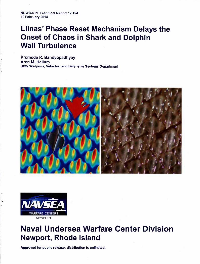
Llinas' Phase Reset Mechanism Delays the Onset of Chaos in Shark and Dolphin Wall Turbulence Promode R. Bandyopadhyay Aren M. Helium USW Weapons, Vehicles, and Defensive Systems Department

MAVSEA WARFARE CENTERS

NEWPORT

Naval Undersea Warfare Center Division Newport, Rhode Island Approved for public release; distribution is unlimited.

PREFACE

This report was prepared under NWA 100000802958, principal investigator Promode R. Bandyopadhyay (Code 851). The sponsoring activity is the Office of Naval Research (ONR- 341, Thomas McKenna).

The technical reviewer for this report was James L. Dick (Code 8514).

The primary author gratefully acknowledges productive discussions with T. McKenna, R. Llinas, V. Makarenko, J. Simmons, and S. Roy. Also, the authors thank J. C. S. Meng, W. R. C. Phillips, and A M. Savill for their comments on the manuscript. AMH was sponsored by the ONR-33 Post-Doctoral Program.

Reviewed and Approved: 10 February 2014

J^UM 7^>i^ Brian T. McKeon

Head, USW Weapons, Vehicles, and Defensive Systems Department

On the cover: Left: Model of the periodic distribution of the lateral diffusion ofvorticity—compare this with the shark skin photograph on the right; upper red overlay is a model of the sub-harmonic map of the primary vorticity; lover overlay is a photograph of one dermal denticle of the Atlantic sharpnose shark (reference 36). Color codes: The fluctuating percentage of the real pari of the lateral diffusion coefficient varies from 0.014 (red) to -0.01 (blue); subharmonic red is the maximum magnitude of the main component of the vorticity (0.6). Right: Photograph of skin of tiger shark (reference 37); compare this with the model on the left.

REPORT DOCUMENTATION PAGE Form Approved

OMB No. 0704-0188 The public reporting burden for this collection of information is estimated to average 1 hour per response, including the time for reviewing instructions, searching existing data sources, gathering and maintaining the data needed, and completing and reviewing the collection of information. Send comments regarding this burden estimate or any other aspect of this collection of information, including suggestions for reducing this burden, to Department of Defense, Washington Headquarters Services, Directorate for Information Operations and Reports (0704-0188), 1215 Jefferson Davis Highway, Suite 1204, Arlington, VA 22202-4302. Respondents should be aware that notwithstanding any other provision of law, no person shall be subject to any penalty for falling to comply with a collection of information if it does not display a currently valid OPM control number. PLEASE DO NOT RETURN YOUR FORM TO THE ABOVE ADDRESS.

1. REPORT DATE (DD-MM-YYYY) 10-02-2014

2. REPORT TYPE 3. DATES COVERED (From - To)

4. TITLE AND SUBTITLE

Llinas' Phase Reset Mechanism Delays the Onset of Chaos in Shark and Dolphin Wall Turbulence

5a. CONTRACT NUMBER

5b. GRANT NUMBER

5c. PROGRAM ELEMENT NUMBER

6. AUTHOR(S)

Promode R. Bandyopadhyay and Aren M. Helium

5d. PROJECT NUMBER

5e. TASK NUMBER

5f. WORK UNIT NUMBER

7. PERFORMING ORGANIZATION NAME(S) AND ADDRESS(ES)

Naval Undersea Warfare Center Division 1176 Howell Street Newport, Rl 02841-1708

8. PERFORMING ORGANIZATION REPORT NUMBER

TR 12,154

9. SPONSORING/MONITORING AGENCY NAME(S) AND ADDRESS(ES)

Office of Naval Research One Liberty Center 875 North Randolph Street, Suite 1425 Arlington, VA 22203-2966

10. SPONSORING/MONITOR'S ACRONYM

ONR 11. SPONSORING/MONITORING

REPORT NUMBER

12. DISTRIBUTION/AVAILABILITY STATEMENT

Approved for public release; distribution is unlimited.

13. SUPPLEMENTARY NOTES

14. ABSTRACT Turbulent boundary layers (TBLs) develop in the flow over planetary surfaces, over the bodies of swimming animals (like sharks and dolphins), and over the hulls of ships and submarines. Evidence points to organization in turbulence production, despite the apparent randomness and lack of a unified theory. Here, the dynamical systems of neuroscience are used to develop a self- regulation theory to show for the first time how the skins of sharks and dolphins control the chaos of turbulence. To remove the apparent randomness, the turbulence production cycles are split into pre- and post-breakdown regions, both during the organized laminar-to-turbulent transition and in the TBL, which is chaotic. S:uart-Landau oscillators describe the instabilities of the surface- normal diffusion of vorticity, which is coupled to the instabilities' spanwise diffusion. Similar to Llinas' olivo-cerebellar temporal phase reset mechanism, the shark and dolphin skins impose combinations of vorticity diffusion templates internal to the oscillators and external microvibration or flow oscillations, synchronizing the oscillators laterally and thereby eliminating chaos. The theory—proving biological adaptation to environment—has potential application to tornado path management. Shark and dolphin skins are major targets of reverse engineering mechanisms of drag and noise reduction.

15. SUBJECT TERMS

Hydrodynamics Turbulent Boundary Layers Drag Reduction Transition Delay Swimming Animals Biological Adaptation Sharks Dolphins Olivo-cerebellar Dynamics Chaos Control Dynamical Systems

16. SECURITY CLASSIFICATION OF:

a. REPORT

(U)

b. ABSTRACT

(U)

c. THIS PAGE

(U)

17. LIMITATION OF ABSTRACT

SAR

18. NUMBER OF PAGES

54

19a. NAME OF RESPONSIBLE PERSON

Promode R. Bandyopadhyay

19b. TELEPHONE NUMBER (Include area code)

401-832-2712 email: promode.bandyopadhya@navy.mil

ao(5(^US3 Standard Form 298 (Rev. 8-981

Prescribed by ANSI Std. Z39-18

TABLE OF CONTENTS

Section Page

LIST OF ILLUSTRATIONS ii

1 INTRODUCTION 1

2 PRE- AND POST-BREAKDOWN REGIONS IN NEAR-WALL TURBULENCE ARE AUTONOMOUS 3

3 SHARK DERMAL DENTICLES ARE TEMPLATES OF S-WAVE TRIADS 7

4 TBL IS PERENNIALLY AND CHAOTICALLY TRANSITIONAL 9

5 LATERALLY CRASHING DIFFUSION WAVES PRODUCE WALL STREAKS 13

6 SHARK SKIN IS A SPATIO-TEMPORAL DIFFUSION TEMPLATE FOR RESETTING THE PHASE OF CHAOTIC WAVE TRIADS 15

7 DOLPHIN LATERAL MICROGROOVES VIBRATE TO RESET PHASE OF CHAOTIC WAVE TRIADS 17

8 DISCUSSION AND SUMMARY 19

APPENDIX A—METHODS A-l

APPENDIX B—EXTENDED DATA B-l

APPENDIX C—SUPPLEMENTARY INFORMATION C-l

REFERENCES R-l

LIST OF ILLUSTRATIONS

Figure Page

la Separation of Near-Wall TBL into Pre- and Post-Breakdown Regions (Regions of Molecular and Eddy Viscosity—Regions without and with Hairpin Vortices, Respectively) 3

Ib-g Comparison of Present Theories for Transitional Flows 5 2 Shark Skin Is a Negative of the TBL Instability Map 8 3 Spatio-Temporal Instability Phase Maps of a TBL II 4 Nucleation Site of Hairpin Vortex and the Origin of Streaks and

Small-Wavelength Oscillations 14 5 Shark Skin Is a Template of Organized Lateral Diffusion for Control

of Chaos Onset 16 6 Dolphin Chaos Control with Surface-Grooved Diffusion Perturbations

Coupled to the SL Oscillator, and External STS-Wave Microvibration of Surface 18

B-l Viscous Unsteady Sublayer Growth Decay Is a Limit Cycle B-2 B-2a Combined Image of Streak and Phase Iso-Contours B-3 B-2b Spatio-Temporal Lateral Streak Spacing /lr

+ in Units of z+ in Baseline TBL (/+ > 0.2 x 104); Axes (z+, t+) B-3

B-3a-h Effects of Amplitude of//,- on Lateral Diffusion of Vorticity Waves in TBL B-4 B-3i-l Laterally Crashing Diffusion Waves in TBL Lead to the Formation of

Streaks and Coupling of High and Low Frequencies B-5 B-4 Shark "Strong" Riblet Model (Excluding Dermal Denticles): Acting on

coz+ in the Region Marked by Vertical Dotted Lines B-6

B-5 Riblet Chaos Control B-7 B-6 Chaos Control in Sharks Using Dermal Denticles, Riblets, and Their Vibration....B-8 B-7a-e Alternative Riblet Modeling Using Coupled Oscillators B-9 B-7f-h TBL Streaks Identified by Iso-Contours of\coz\ < 0.2 in (z+, t+) B-9 B-8a, b Chaos Control with Perturbations External to SL Oscillator: LEBU B-IO B-8c External Perturbation Iexl Breaks Streaks B-IO B-9 Chaos Control with Perturbations External to SL Oscillator: Stokes'

Drag Reduction B-II B-IO Schematic Explaining Spatio-Temporal Phase Reset B-12

n

LLINAS' PHASE RESET MECHANISM DELAYS THE ONSET OF CHAOS IN SHARK AND DOLPHIN WALL TURBULENCE

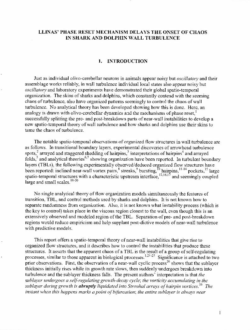
1. INTRODUCTION

Just as individual olivo-cerebellar neurons in animals appear noisy but oscillatory and their assemblage works reliably, in wall turbulence individual local states also appear noisy but oscillatory and laboratory experiments have demonstrated their global spatio-temporal organization. The skins of sharks and dolphins, which constantly contend with the seeming chaos of turbulence, also have organized patterns seemingly to control the chaos of wall turbulence. No analytical theory has been developed showing how this is done. Here, an analogy is drawn with olivo-cerebellar dynamics and the mechanisms of phase reset,1

successfully splitting the pre- and post-breakdown parts of near-wall instabilities to develop a new spatio-temporal theory of wall turbulence and how sharks and dolphins use their skins to tame the chaos of turbulence.

The notable spatio-temporal observations of organized flow structures in wall turbulence are as follows. In transitional boundary layers, experimental discoveries of arrowhead turbulence spots, arrayed and staggered shedding of hairpins,3 interpretations of hairpins4 and arrayed folds, and analytical theories ' showing organization have been reported. In turbulent boundary layers (TBLs), the following experimentally observed/deduced organized flow structures have been reported: inclined near-wall vortex pairs,8 streaks,9 bursting,10 hairpins,11'14 pockets,15 large spatio-temporal structures with a characteristic upstream interface,1 '16'17 and seemingly coupled large and small scales.18'20

No single analytical theory of flow organization models simultaneously the features of transition, TBL, and control methods used by sharks and dolphins. It is not known how to separate randomness from organization. Also, it is not known what instability process (which is the key to control) takes place in the viscous region closest to the wall, even though this is an extensively observed and modeled region of the TBL. Separation of pre- and post-breakdown regions would reduce empiricism and help supplant post-dictive models of near-wall turbulence with predictive models.

This report offers a spatio-temporal theory of near-wall instabilities that give rise to organized flow structures, and it describes how to control the instabilities that produce these structures. It asserts that the apparent chaos of a TBL is the result of a group of self-regulating processes, similar to those apparent in biological processes.1'21"23 Significance is attached to two prior observations. First, the observation of a near-wall cyclic process26 shows that the sublayer thickness initially rises while its growth rate slows, then suddenly undergoes breakdown into turbulence and the sublayer thickness falls. The present authors' interpretation is that the sublayer undergoes a self-regulating growth-decay cycle; the vorticity accumulating in the sublayer during growth is abruptly liquidated into Strouhal arrays of hairpin vortices.16 The instant when this happens marks a point of bifurcation; the entire sublayer is always near

bifurcation. The second prior observation is that high- and low-speed streaks converge and diverge. The present authors' interpretation is that the locations where the streaks converge and diverge are where the diffused sublayer vorticity is dislocating due to lateral diffusive coupling a la phase change in crystals; hence, forms of the Ginzburg-Landau (GL) theory of superconducting dislocation should phenomenologically apply.

The near-wall pre- and post-breakdown flows are split heuristically, choosing the complex SL oscillator description to describe the pre-breakdown instability process (see Methods in appendix A). Olivo-cerebellar control mechanisms1 place the methods of chaos control on a common foundation. Assuming that a cellular flow has developed from a homogeneity due to end-effects, the theory shows how vorticity develops from a periodic to a chaotic state, and then—by dint of new principles of chaos control—how the periodic state is conserved, delaying the onset of chaos. Several disparate experimental and theoretical patterns are strikingly reproduced.

2. PRE- AND POST-BREAKDOWN REGIONS IN NEAR-WALL TURBULENCE ARE AUTONOMOUS

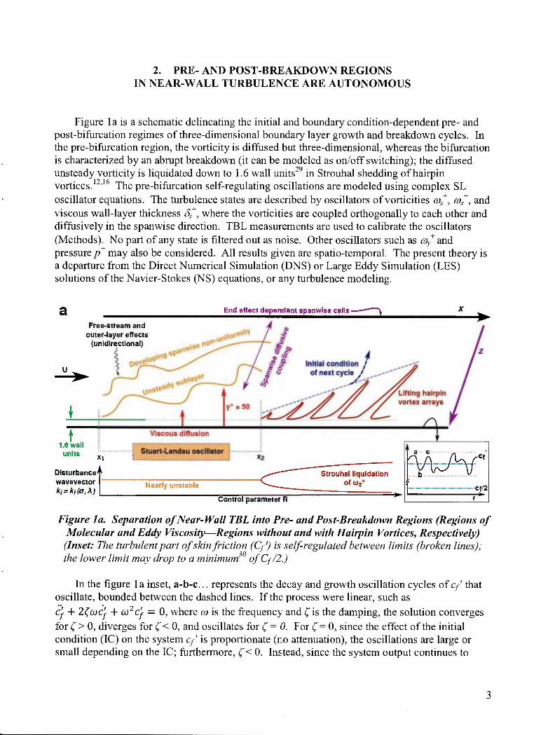
Figure la is a schematic delineating the initial and boundary condition-dependent pre- and post-bifurcation regimes of three-dimensional boundary layer growth and breakdown cycles. In the pre-biflircation region, the vorticity is diffused but three-dimensional, whereas the bifurcation is characterized by an abrupt breakdown (it can be modeled as on/off switching); the diffused unsteady vorticity is liquidated down to 1.6 wall units29 in Strouhal shedding of hairpin vortices. ' The pre-bifurcation self-regulating oscillations are modeled using complex SL oscillator equations. The turbulence states are described by oscillators of vorticities &>z

+, cox+, and

viscous wall-layer thickness Ss+, where the vorticities are coupled orthogonally to each other and

diffusively in the spanwise direction. TBL measurements are used to calibrate the oscillators (Methods). No part of any state is filtered out as noise. Other oscillators such as ci)y+ and pressure p+ may also be considered. All results given are spatio-temporal. The present theory is a departure from the Direct Numerical Simulation (DNS) or Large Eddy Simulation (LES) solutions of the Navier-Stokes (NS) equations, or any turbulence modeling.

a End effect dependent spanwise cells ■

Free-stream and outer-layer effects

(unidirectional)

t 1.0 wall

unite Xl

Disturbance" wavevector k,= ki(a,\)

Nearly unstable

Strouhal liquidation Of <i)z

+

Control parameter R

rvw Cf/2

——••

Figure la. Separation of Near-Wall TBL into Pre- and Post-Breakdown Regions (Regions of Molecular and Eddy Viscosity—Regions without and with Hairpin Vortices, Respectively) (Inset: The turbulent part of skin friction (Cf') is self-regulated between limits (broken lines); the lower limit may drop to a minimum of Cf/2.)

In the figure la inset, a-b-c... represents the decay and growth oscillation cycles of cf that oscillate, bounded between the dashed lines. If the process were linear, such as c'f + l^odc'r + (x)2c'f — 0, where co is the frequency and ^is the damping, the solution converges for C^* 0, diverges for C< 0, and oscillates for C = 0. For {"= 0, since the effect of the initial condition (IC) on the system cf is proportionate (no attenuation), the oscillations are large or small depending on the IC; furthermore, C< 0. Instead, since the system output continues to

oscillate within bounds, the effect of the IC is being attenuated; that is, the process is nonlinear and self-correcting: c^ + 2/(c^)c^ + a)2Cf = 0, where the damping /(cf) = a0c^2 - 2^0o) is negative when c/ is small and positive when it is large. Here, ao is a constant, (ao, Co) > 0, and ao, Co, and co determine the shape of the limit cycle. Orr-Sommerfeld and GL or SL equations are examples of linear and nonlinear systems, respectively.

The post-bifurcation region is responsible for turbulence mixing characterized by eddy viscosity. The split of the TBL into pre- and post-bifurcation regimes reduces information overflow, allowing focus on the instability process. The present work focuses on the spatio- temporal instabilities of the pre-bifurcation regime (figures 1 and B-l—the latter in the Extended Data presented in appendix B), where the matters most important to chaos control and viscous drag reduction occur.

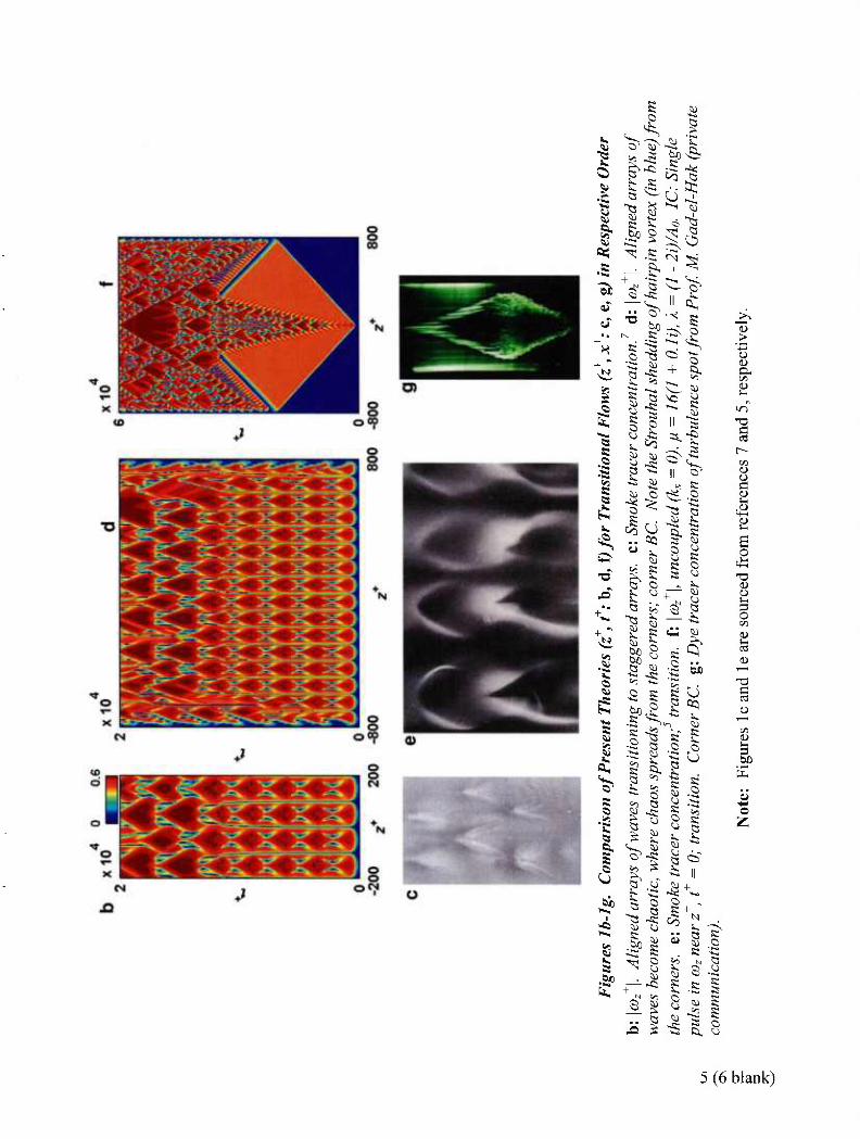
The arrayed and staggered distributions of vorticity during transition,3 known as K- and H- types, respectively, have been accurately reproduced. Time t+ in theory and distance x+ in smoke or dye flow visualization (which is a time history and is like a strip-chart record) are positive in opposite directions.31 Emmons' turbulence spot2 is reproduced (figures lb - Ig).

Ik

|

I a

R

^ ^

^ "^ -S ^N R

-oh

as C a

R .g

R

U R O y

0

^^

-R +

"R ~^ 2 II

CO

*- II

.0 ^

I

k, a;

0

o R

k, 5

2 Q

R

I R

I a ft

I

Ik a

5

k

I 0

•S R 0

U k,

5 U

b" o

1 0 u R S

k, >^

R

s R ^j U R 0 u k

&

ISD '-1

g

R

I >

I a

^3

.1

^3 R

a. 2 t>3 o

«R U

k

k

sf 0

o o a S

^ a> g . 8 2

5

k o u

R 0

Q

5 a

> u u CL 1/3 (U

-a

aj o c u kl

-+- u

o •+- -a o o

o si

u s- K3

03 u

E

e

5, u

5 (6 blank)

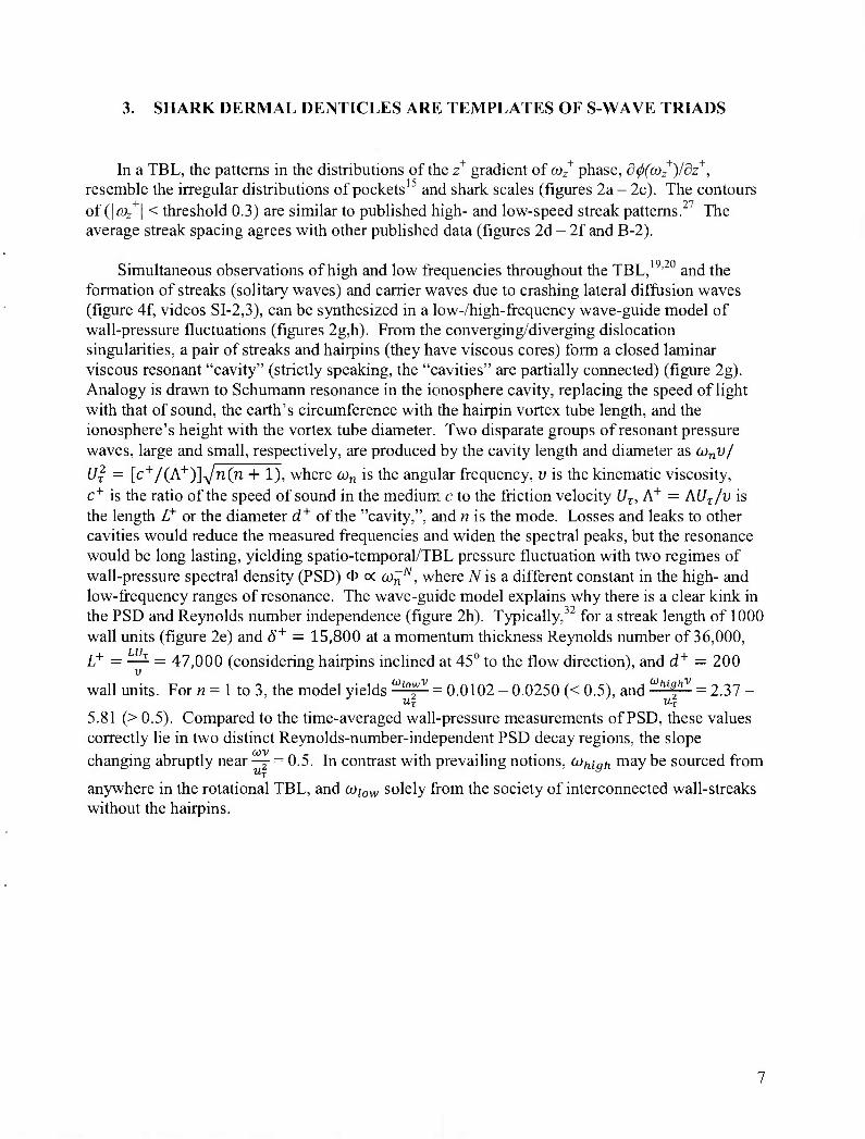
3. SHARK DERMAL DENTICLES ARE TEMPLATES OF S-WAVE TRIADS

In a TBL, the patterns in the distributions of the z gradient of ft>r+ phase, 5^fft>z

+)/9z+, resemble the irregular distributions of pockets15 and shark scales (figures 2a - 2c). The contours of (l&Jt I < threshold 0.3) are similar to published high- and low-speed streak patterns. The average streak spacing agrees with other published data (figures 2d - 2f and B-2).

Simultaneous observations of high and low frequencies throughout the TBL,19'20 and the formation of streaks (solitary waves) and carrier waves due to crashing lateral diffusion waves (figure 4f, videos S 1-2,3), can be synthesized in a low-/high-frequency wave-guide model of wall-pressure fluctuations (figures 2g,h). From the converging/diverging dislocation singularities, a pair of streaks and hairpins (they have viscous cores) form a closed laminar viscous resonant "cavity" (strictly speaking, the "cavities" are partially connected) (figure 2g). Analogy is drawn to Schumann resonance in the ionosphere cavity, replacing the speed of light with that of sound, the earth's circumference with the hairpin vortex tube length, and the ionosphere's height with the vortex tube diameter. Two disparate groups of resonant pressure waves, large and small, respectively, are produced by the cavity length and diameter as (x)nu/ Ux = [c+/(A+)]-v/n(n + 1), where <jdn is the angular frequency, v is the kinematic viscosity, c+ is the ratio of the speed of sound in the medium c to the friction velocity L/T, A

+ = A(/T/u is the length Z,+ or the diameter d+ of the "cavity,", and n is the mode. Losses and leaks to other cavities would reduce the measured frequencies and widen the spectral peaks, but the resonance would be long lasting, yielding spatio-temporal/TBL pressure fluctuation with two regimes of wall-pressure spectral density (PSD) <t> oc <X)^N, where A^is a different constant in the high- and low-frequency ranges of resonance. The wave-guide model explains why there is a clear kink in the PSD and Reynolds number independence (figure 2h). Typically,32 for a streak length of 1000 wall units (figure 2e) and 5+ = 15,800 at a momentum thickness Reynolds number of 36,000,

L+ = —- — 47,000 (considering hairpins inclined at 45° to the flow direction), and d+ = 200

wall units. For « = 1 to 3, the model yields ^L = 0.0102 - 0.0250 (< 0.5), and ^f^ = 2.37 - u| u| 5.81 (> 0.5). Compared to the time-averaged wall-pressure measurements of PSD, these values correctly lie in two distinct Reynolds-number-independent PSD decay regions, the slope changing abruptly near — = 0.5. In contrast with prevailing notions, (jOhigh may be sourced from

anywhere in the rotational TBL, and (JL)IOW solely from the society of interconnected wall-streaks without the hairpins.

• Present mc SK

♦ NN1 .$ •:> NN2

SM f V 11 & ' ▼ □

12

LAH

0*0 l

V ^> T T 0 v

8 • 0

100

— Ree=27400 — Ree=39700 — Re=76700

V "hi*

*>

^

\

10

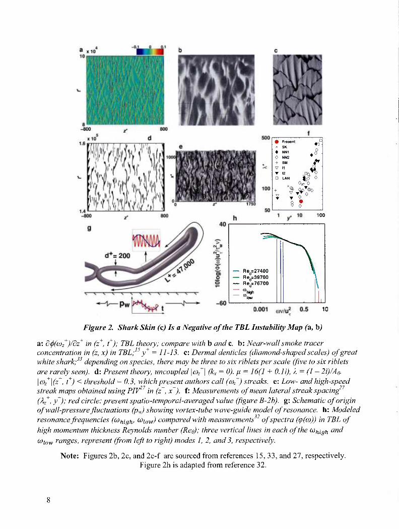
Figure 2. Shark Skin (c) Is a Negative of the TBL Instability Map (a, h)

a: d^(cozr)/dz+ in (z+, t+); TBL theory; compare with b and c. b: Near-wall smoke tracer

concentration in (z, x) in TBL;15 y+ = 11-13. c: Dermal denticles (diamond-shaped scales) of great white shark; depending on species, there may be three to six riblets per scale (five to six riblets are rarely seen), d: Present theory, uncoupled \cOz+\ (kx = 0). ^ = 16(1 + O.li), X = (1 - 2i)/Ao. \coz

+\(z+, t+) < threshold = 0.3, which present authors call (ah ) streaks, e: Low- and high-speed streak maps obtained using PIV27 in (z+, x+). f: Measurements of mean lateral streak spacing (b > y )', red circle: present spatio-temporal-averaged value (figure B-2b). g: Schematic of origin of wall-pressure fluctuations (pw) showing vortex-tube wave-guide model of resonance, h: Modeled resonance frequencies (u)high> ^low) compared with measurements of spectra ((p(co)) in TBL of

high momentum thickness Reynolds number (Ree); three vertical lines in each of the (Ohigh and

(Oiow ranges, represent (from left to right) modes 1, 2, and 3, respectively.

Note: Figures 2b, 2c, and 2e-f are sourced from references 15, 33, and 27, respectively. Figure 2h is adapted from reference 32.

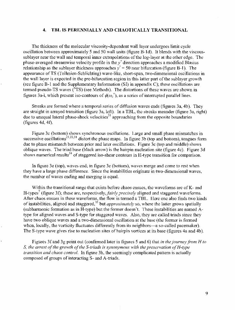
4. TBL IS PERENNIALLY AND CHAOTICALLY TRANSITIONAL

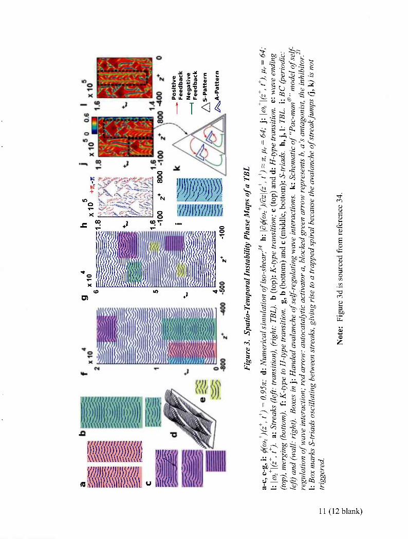
The thickness of the molecular viscosity-dependent wall layer undergoes limit cycle oscillation between approximately 5 and 50 wall units (figure B-ld). It blends with the viscous- sublayer near the wall and temporal inner extrapolations of the log-layer at the other edge. The phase-averaged streamwise velocity profile in the v+ direction approaches a modified Blasius relationship as the sublayer thickness approaches >'+= 50 near bifurcation (figure B-l). The appearance of TS (Tollmien-Schlichting) wave-like, short-span, two-dimensional oscillations in the wall layer is expected in the pre-bifurcation region in this latter part of the sublayer growth (see figure B-l and the Supplementary Information (SI) in appendix C); these oscillations are termed pseudo-TS waves (STS) (see Methods). The distortions of these waves are shown in figures 3a-l, which present iso-contours of 0((Oz+), as a series of interrupted parallel lines.

Streaks are formed where a temporal series of diffusion waves ends (figures 3a, 4b). They are straight in arrayed transition (figure 3a, left). In a TBL, the streaks meander (figure 3a, right) due to unequal lateral phase-shock velocities ' approaching from the opposite boundaries (figures 4d, 4f).

Figure 3c (bottom) shows synchronous oscillations. Large and small phase mismatches in successive oscillations ' ' distort the phase maps. In figure 3b (top and bottom), tongues form due to phase mismatch between prior and later oscillations. Figure 3c (top and middle) shows oblique waves. The triad base (black arrow) is the hairpin nucleation site (figure 4c). Figure 3d shows numerical results 4 of staggered iso-shear contours in H-type transition for comparison.

In figure 3e (top), waves end; in figure 3e (bottom), waves merge and come to rest when they have a large phase difference. Since the instabilities originate in two-dimensional waves, the number of waves ending and merging is equal.

Within the transitional range that exists before chaos ensues, the waveforms are of K- and H-types (figure 3f); these are, respectively, fairly precisely aligned and staggered waveforms. After chaos ensues in these waveforms, the flow is termed a TBL. Here one also finds two kinds of instabilities, aligned and staggered,35 but approximately so, where the latter grows spatially (subharmonic formation as in H-type) but the former doesn't. These instabilities are named A- type for aligned waves and S-type for staggered waves. Also, they are called triads since they have two oblique waves and a two-dimensional oscillation at the base (the former is formed when, locally, the vorticity fluctuates differently from its neighbors—a so-called pacemaker). The S-type wave gives rise to nucleation sites of hairpin vortices at its base (figures 4a and 4b).

Figures 3f and 3g point out (confirmed later in figures 5 and 6) that in the journey from H to S, the arrest of the growth of the S-triads is synonymous with the preservation of H-type transition and chaos control. In figure 3h, the seemingly complicated pattern is actually composed of groups of interacting S- and A-triads.

The comer and periodic boundary conditions produce variations of instabilities. The former produces a Strouhal shedding of hairpin vortices (blue at right in figure 3j and blue outlines at left in figure 4b), with oscillating interaction with oblique waves (figures 3i, right; 4b; B-2a), while periodic boundary conditions produce pure oblique waves (figure 3i, left). In figure 3i (right), in comers, waves end and merge.

In a TBL, there is sometimes an avalanche of interactions between the S- and A-triads in which the S-type jumps streaks, laterally swallowing an array of A-triads (figures 3j and 3k). The process can continue downstream, and repeated subharmonic growth fills the spectrum; note that in contrast to H-type, S-waves can grow. Apart from these global pattems, locally the vorticity waves can end or merge (figure 3e) or oscillate (arrow in figure 3c) between them. Interactions of both wave triads yield spatio-temporal self-regulation (figure 3k).

In figure 3k, the group pattems are unstable because the antagonistic diffusion is slow. In biology, stable patterns are produced in embryos when the head-to-tail and left-to-right axes are being determined (with some handedness), the signal for this vanishing soon after. Similarly, K- and H-types of transition are produced when the IC and BC are felt, and then K- and H-types become unstable (the effect of handedness growing to further bifurcation), which is called a TBL. Therefore, the activator (a) and inhibitor (b) equations21 in a TBL have many variations of the same embryonic theme, depending on how many bifurcations have taken place (i.e., how high the Re number is). To control chaos, sharks and dolphins manage these variations using competing instabilities.

In figure 31, atz+ = -200 the vorticity diffusion rates in the activator (:: a) and inhibitor (:: b) parts of the self-regulation process in S-waves are equal, yielding the boxed "trapped spiral."

When weakening (less red), the arrayed K-type transitional waves become A-type in a TBL, whose start is given by the onset of chaos (see figure 5k). However, when strengthening, both K- and H-type transitional waves become S-type in a TBL (figure 5f). This becomes clear during chaos control where the instability process is slowed down.

10

il J B * «! S « C O oi W oi IL a. u. z u.

t T <i

+ m

o

X

St ill

U)'

o o 00

N

o o

Vh

ism

9M ■wm'/m

V&WM I il - ifla u

to IO m

iiiijiiinimiini

i7/i)it'/'/;ii»/7// L

as

S

I i e Q

Si

bo o ^ .•

> ^^ o -S

•2 ^

> VD

=1

n

I- ?-1

■o

3

CO ^

.2 ir^

1

a & 1 2 o ^^

u

*-» • ^^ 3 S e o

u a

=

g a

II

^ I I < a D,

* &

I

WD £? Q

s P

to

-s;

-■<

u

"5

9 -*^

&5

— <» Q

|a^ S <») ..

5^ 5«i c^

6><l 5

be

Si a

0 C

2i c

2

a

Ml

O .bo ^ 5

-s SPSs

- ^^ + ^ ^^ ^ ^ ^3

5 :r s m

CO

r ^ H S o bo

oq .bo .. c

o

-I— u

c ,1- -4—

o u 3 o

-T3

o 3 53

e

11 (12 blank)

5. LATERALLY CRASHING DIFFUSION WAVES PRODUCE WALL STREAKS

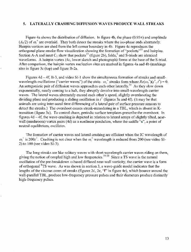
Figure 4a shows the distribution of diffusion. In figure 4b, the phase (0.95::) and amplitude (AQ/I) of coz

+ are overlaid. They both detect the streaks where the iso-phase ends alternately. Hairpin vortices are shed from the left comer boundary in 4b. Figure 4c reproduces the orthogonal plane smoke flow visualization showing the formation of "pockets"15 and hairpins. Section A-A and inset Ci show that pockets15 (figure 2b), folds,5 and S-triads are identical waveforms. A hairpin vortex (4c, lower sketch and photograph) forms at the base of the S-triad. After comparison, the hairpin vortex nucleation sites are marked in figures 4a and 4b (markings also in figure 3c (top) and figure B-2a.

Figures 4d - 4f, B-3, and video SI-1 show the simultaneous formation of streaks and small- wavelength oscillations ("carrier waves") of the state. coz

+ streaks form where Re(a)z+){z+, t+) = 0.

An antagonistic pair of diffusion waves approaches each other laterally.31 As they slow down exponentially, nearly coming to a halt, they abruptly devolve into small-wavelength carrier waves. The lateral waves alternately exceed each other's speed, slightly overshooting the dividing plane and producing a sliding oscillation in t+ (figures 3a and 4f). (It may be that animals are using inter-aural time differencing of a lateral pair of surface pressure sensors to detect the streaks.) The overshoot causes streak-meandering in a TBL, which is absent in K- transition (figure 3a). To control chaos, periodic surface templates prescribe the overshoot. In figures 4d - 4f, the wave-crashing is depicted in relation to lateral arrays of slightly tilted, near- wall (mushroom) vortex pairs (4d) as a nonlinear pendulum, where the saddle "s", a point of neutral equilibrium, oscillates.

The formation of carrier waves and lateral crashing are efficient when the IC wavelength of coz

+ is 200z+. Crashing is not clear when the a)z+ wavelength is reduced from 200 (see video SI-

2) to 100 (see video SI-3).

The long streaks are like solitary waves with short-wavelength carrier waves riding on them, giving the notion of coupled high and low frequencies. " Since a TS wave is the natural oscillation of the pre-breakdown u-based diffused near-wall vorticity, the carrier wave is a form of orthogonal TS wave. As was shown in section 3, a wave-guide model indicates that the lengths of the viscous cores of streaks (figures 2c, 2e, "f' in figure 4e), which bounce around the wall-parallel TBL, produce low-frequency pressure pulses and their diameters produce distinctly high-frequency pulses.

13

(t>=7t Ja^V2

J9^N. -J*

"^^ ,^§P^ z*=o

Figure 4. Nucleation Site of Hairpin Vortex and the Origin of Streaks end Small-Wavelength Oscillations

a: \d a>z Idz |. b: Overlay of iso-phase (0.95TT) and amplitude (Ao/2) of (0:+. a: transition; b-f:

TBL. c: Figure 5 ofFalco showing simultaneous smoke visualization of surface parallel (top) (y =9-14) and longitudinal plane (bottom) TBL. Inset Q: S-triadfrom a. Circles in a and b are nucleation sites of hairpins, (d-f): Simultaneous formation of streaks and small-wavelength oscillations of the state, d: Cross-stream (z, y) near-wall smoke tracer concentration; the mushroom-like longitudinal vortex oairs are slanted, e: Schematic of nonlinear pendulum behavior ofvorticity diffusion; phase: (s: saddle, unstable 180°) and foci (f: stable, 0°).

f (Upper Traces): Re(coz+)(z+, t+), /u- = 0.5. coz

+ scale bar at z+=50: 2VT j1] = 1.2. Note crashing

of lateral diffusion waves and formation of carrier waves. Color indicates ^(coz+) at z+=50.

f (Lower Trace): Re(coz+)(z+, i* = 0); scale bar at z+ = 50: 0.2.

Note: Figures 4c and 4d are sourced from references 15 and 5, respectively.

14

SHARK SKIN IS A SPATIO-TEMPORAL DIFFUSION TEMPLATE FOR RESETTING THE PHASE OF CHAOTIC WAVE TRIADS

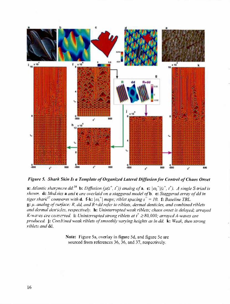
Figure 5 shows the results of the modeling of chaos control by sharks. Skins of great white,33 Atlantic sharpnose,36 and tiger shark37 dermal denticles (dd), with embedded riblets, are shown in figures 2c, 5a, and 5e, respectively. The model using a bi-modal periodic distribution (inz, t, or z, x) of the coefficient of lateral diffusion ^ (see Methods) is shown in figures 5b and 5d. The agreement of figures 5b and 5d with the \G>Z

+\ of TBL S-waves (figures 5c and 5f) and

shark skins (figures 5a and 5e) is remarkable.

Figure 5f shows the baseline TBL \o)zt\. Figure 5g is a diffusion contour map of the riblets

(R), the dermal denticles (dd), and of their combination (R+dd). At the uninterrupted riblet spacing of 10z+, lateral diffusion (£„) perturbations of 2.5% (weak riblets) delay the onset of chaos, and K-type waves are conserved for t+ < 80,000 (figure 5h); a 20% perturbation (strong riblets) then applied at /+ > 80,000, the chaotic region in 5h, produces orderly arrays of A-waves, suppressing S-waves (figure 5i). However, the riblets need to be interrupted along the dd outlines (5d,e,g) because the animal is flexible and non-uniform in JC.

Figure 5j shows the combined effects of weak riblets that are interrupted by the dd (see Methods). Figure 5k shows the effects of combining weak interrupted riblets, dd, and strong diffusion perturbations after chaos has ensued (f* > 80,000). This is the predicted chaos control due to sharks.

See figures B-4 through B-7 and the SI for additional results.

15

« <k4.i*U« »*« » -,

« * «;«■•(» » * * « ^^^ {» < . «. * »■*!♦*.».*.♦**■»■■«!k * «

* * »t»!*;» « > «.« *i» +,'»> »

800

Figure 5. Shark Skin Is a Template of Organized Lateral Diffusion for Control of Chaos Onset

a: Atlantic sharpnose dd. b: Diffusion (ILI(Z+

, t )) analog of a. c: \coz+\(z+, t+). A single S-triad is

shown, d: Modules a and c are overlaid on a staggered model ofb. e: Staggered array ofdd in tiger shark*' compares with d. f-k: \coz

+\ maps; riblet spacing s+ = 10. f: Baseline TBL. gi ji. analog of surface: R, dd, and R+dd refer to riblets, dermal denticles, and combined riblets and dermal denudes, respectively, h: Uninterrupted weak riblets; chaos onset is delayed; arrayed K-waves ere con?er\>ed. i: Uninterrupted strong riblets at t+ > 80,000; arrayed A-waves are produced, y. Coir.blned weak riblets of smoothly varying heights as in dd. k: Weak, then strong riblets and dd.

Note: Figure 5a, overlay in figure 5d, and figure 5e are sourced from references 36, 36, and 37, respectively.

16

DOLPHIN LATERAL MICROGROOVES VIBRATE TO RESET PHASE OF CHAOTIC WAVE TRIADS

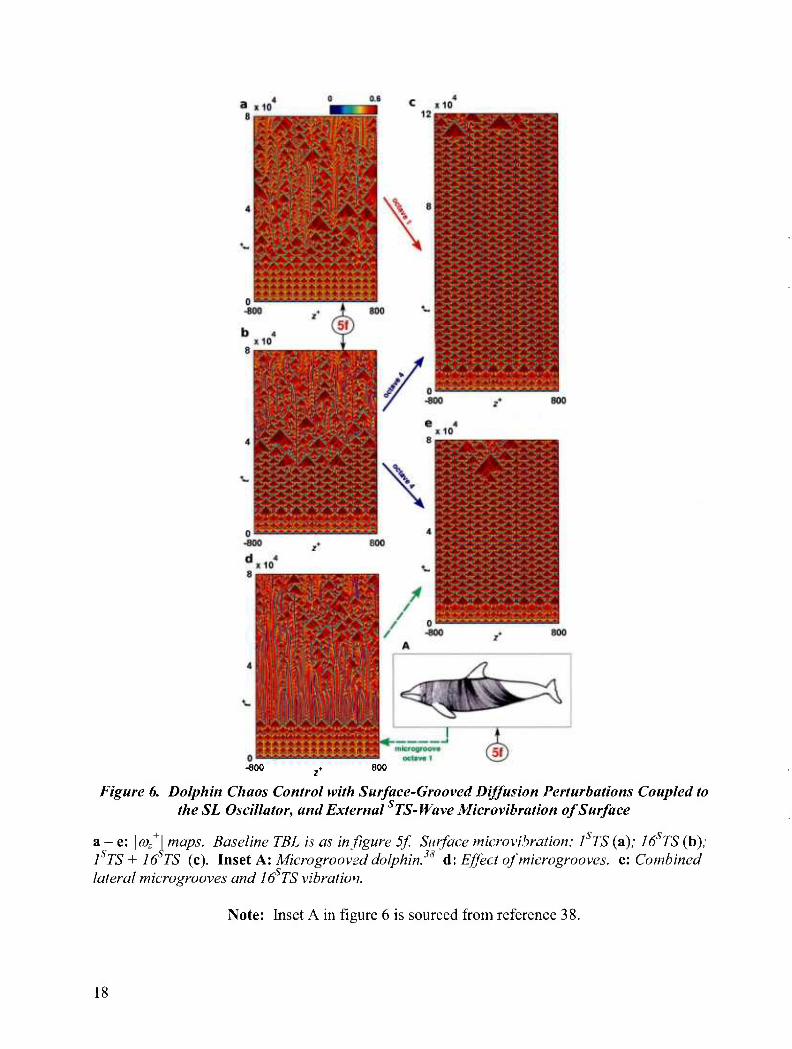
Figure 6 shows how dolphins control chaos with surface perturbations coupled to the SL oscillator. The baseline TBL in figure 5f applies. In dolphins, the lateral surface microgrooves (inset A in figure 6)38 organize the lateral coupling and a two-dimensional SL oscillator is approached (see Methods); the TS waves are prominent in figures 3c (bottom) and 4b.

The dolphin's microgrooves impart variation in the coefficient of lateral diffusion whose periodicity matches that of TS waves. Active vibration of the microgrooves, modeled as/«/ (see Methods), is assumed to be in integer multiples (1, 16) of STS waves (figures 6a and 6b). With bimodal vibration (1STS + 16STS), chaos onset is delayed the most (figure 6c). With grooves alone, fewer S- but more A-triads are produced (figure 6d). When microgrooves and vibrations (16STS) are combined, there is a clear delay in the onset of chaos (figure 6e).

The diffusion template lock-in mechanism of chaos control by sharks and dolphins is a spatio-temporal version of Llinas' olivo-cerebellar temporal SPR mechanism1 (figure B-10). In the latter, the relative physical locations of the inferior-olive neurons are not important for phase synchronization, while the spatial locations of the oscillators are important in TBL chaos control.

Riblets in sharks are longitudinally proud and periodic in z . Dolphins can have longitudinal arrays of transverse microgrooves inx+ (inset A in figure 6). Both surface patterns control diffusion. Compared with the baseline in figure 5f, the S-triads in figure 6e are fewer and there is a corresponding increase in A-triads; the \<J)Z\ map is similar in riblets (figure 5i).

When chaos is controlled, turbulence production-induced drag is reduced, the limit being 50%.30 The present authors therefore see nothing in their theory that contradicts the prior claims ' regarding dolphins' high drag reduction.

Engineering drag reduction methods, such as outer layer devices42 (figure B-8) and Stokes' 0'43 spanwise shaking of walls (figure B-9), potentially can be modeled as periodic perturbations that are external (Iex,) to the SL oscillator (lacking in coupling).

17

-800 800

Figure 6. Dolphin Chaos Control with Surface-Grooved Diffusion Perturbations Coupled to the SL Oscillator, and External TS-Wave Microvibration of Surface

a — e: \o)z'\ maps. Baseline TBL is as in figure 5f. Surface microvibration: 1 TS (a); 16 TS (b); 1 TS + 16 TS (c). Inset A: Microgrooveddolphin.' d: Effect of microgrooves. e: Combined lateral microgrooves and 16 TS vibration.

Note: Inset A in figure 6 is sourced from reference 38.

18

8. DISCUSSION AND SUMMARY

Wall turbulence models, on which some climate models may be based, tend to be statistical, although there is no instant when any of the states have profdes matching these models. Economics theories have similar artificial reality. Newton's laws of motion, on the other hand, apply at all instants, and the present theory does as well. If IC and BC are sufficiently known, the present theory makes a short-term theoretical prediction. It describes TBLs using orthogonal SL oscillators diffusively coupled laterally. Sharks and dolphins control the growth of chaos in turbulence and maintain the existing transitional organization by (1) imposing a weak lateral and longitudinal periodic perturbation to the oscillator's diffusion matching their skin topology, and (2) imposing periodic perturbations external to the oscillator much as in Llinas'1 olivo-cerebellar synchronization, again using their skin.

Turbulence production over a wall is highest near^ = 10 - 15. The theory considered instabilities in a layer parallel to the wall at this height. Due to wall proximity, the coupling with the third orthogonal oscillator {a>v

+) was ignored. In the unstable wall-parallel layer at ^+ ~ II, unsteadiness of the pre-breakdown laminar flow is modeled by a parabolic equation44 (equation A-2 in Methods), where reversal of the direction of vorticity diffusion makes the equations singular parabolic, whose attribute is irregularities within the flow field. In the present case, this gives rise to rows of stagnation points (breaks in a)z

+ contours—figure 3a) appearing as streaks, and dislocation sites where streaks merge or diverge. The boundaries where diffusion changes sign are regions of large variation in tracer concentration and density (figures 3b and 3e), and where chaos ensues (e.g., at the K to H transition, as slightly-handed streak jumps). The surface templates in sharks/dolphins control the motion of the stagnation points by ensuring similar handedness in bifurcations24 of the diffusion wavefronts, restricting the diversification of scales.

The Reynolds numbers (Re) of whales (up to blue whales) (0.4-3 x 109) and dolphins (0.2- O Q

1.75 x 10 ) are similar to those of ships/submarines (> 2 x 10 ) and unmanned underwater vehicles (> 2 x 10 ), respectively. The feasibility of cost-effective chaos control in practical flows is not in doubt. The removal of/ex/ establishes a new TBL having higher lateral mixing (figure B-8b), and dolphins may also delay the onset of chaos up to almost halfway between the dorsal fin and the tail (inset A in figure 6), beyond which chaos' enhanced mixing keeps the TBL attached. It would be useful to document the dynamic skin properties of whales whose high Re number may involve chaos management mechanisms similar to high-frequency neural control.45

Currently in weather simulation, the mean paths of hurricanes are computed but no predictions are offered for tornadoes due to spatial resolution issues. Alternatively, since a self- regulating model of weather should be valid,46'47 a low spatial resolution model would produce accurate results if weak orthogonal oscillators are included as control oscillators. Four-equation riblet modeling carried out with low spatial resolution (see figures B-7a, c, e) reproduces the measurements qualitatively. Tuning such oscillators with high spatial resolution is difficult; high-resolution simulations with fewer orthogonal coupled oscillators have been emphasized here instead. Even a one-oscillator model {coz, figures If, 2d, B-4, B-7f-h, and B-8b,c) captures some of the TBL spatio-temporal organization. Persistent chaos control, as animals must be doing, requires inclusion of all three orthogonal coupled vorticity oscillators of amplitude 1,

19

0.01, and 0.0001 (in the z, x, and ^ directions, respectively), and of the viscous layer thickness, which has a mass conservation property.

For the delay of chaos onset, the perturbations required are weak. But the diverse interactions of S- and A-wave triads produce a Reynolds number-like effect (see figure 7D2 in Kazantsev et al.1), which requires larger perturbations for control.

Laterally growing non-uniformities and end-effects are present even in laminar boundary layers (LBLs). LBLs approaching Recri, become unsteady and can be described by highly diffusive SL equations with periods matching those of TS waves (see Methods). Such two- dimensional waves are seen in TBLs, and during control they become clear (figure B-8b). During swimming, dolphins also develop arrays of parallel azimuthal microgrooves not only near their nose, but over most of their length (see inset A in figure 6).

The lateral crashing of diffusion waves in a TBL is similar to oblique shedding in cylinders spreading from the ends to the center at the speed of phase "shock."31 While the crashing of diffusion waves and the formation of carrier waves and streaks remain qualitatively unchanged with lateral diffusion, the carrier waves are clearer at low values (//,■ = 0.5) (figures 4f and B-3). When //,. drops from 64 to 0.5 in t+ = 1700, the number of crashes increases from four to five, which is a Reynolds number-like effect. Although results are given here primarily for^,. = 16, //,- should change in steps as the near-wall turbulence instability goes through bifurcations to produce STS waves; arrayed, staggered, and chaotic triads; and their more intricate interactions.

The present approach is compatible with common engineering drag reduction methods, which are modeled as perturbations external {Iexf) to the TBL oscillators (figures B-8 and B-9).

Lateral diffusion of vorticity forms streaks and small-wavelength carrier waves, but evidence of their coupling is lacking. A society of laterally balancing streaks form ad inflnitum on a whale from head to tail—but the size of the largest scales is limited by the competition of the activator and inhibitor parts of the self-regulation process of instabilities.

Only the phases of non-uniformities that are lower or higher even-harmonics of STS wavelength are reset to null the instigation of chaos because other wavelengths do not couple with the TBL oscillators. This accrues from the disturbance rejection property of SL equations. This property limits the work cost of control, which would be less than previously thought.

Dolphins use wavelengths of (STS, 16STS) for longitudinal surface vibration acting on the coz oscillator for control. Dolphins' fatty skin is conducive for this, whereas sharks' dermal denticles and riblets are made of rigid teeth-like material that acts like armor. In sharks (figures 5f-5k), external perturbation did not yield large benefits. In the evolutionary reaction-diffusion bifurcations, ' sharks and dolphins have taken more aggressive and docile turns, respectively, and their chaos control strategies are consistent with that selection. The hydrodynamics, control, and sensing of sharks/dolphins' flapping fin propulsion are self-regulating,24 just as their wall- turbulence is. Both flapping fin hydrodynamics and wall-turbulence are transitional,35 and have

20

bi-stable attractors. The mechanism of how these animals use their actuators, sensors, and controllers to interact with their surroundings has a common theoretical foundation.

The self-regulating, transitional, and deterministic nature of a TBL at all Re numbers makes chaos control an exercise in finding the locally effective spatio-temporal phase reset mechanism. The perturbations of tornadoes in planetary boundary layers are likely to have predictable control solutions, just as sharks and dolphins likely deal with the oscillating fin-necklace vortices submerged in their TBLs. Theoretical insights into cerebral electrical storms during seizures could be gleaned by modeling neuronal networks as dislocating three-dimensional streaks.

This report has shown chaos control by surface "emplating" (evolutionary interactive templating between the turbulence environment and the animal skin) and external stimulation. In a broadened definition, nascent chaos control may be deemed to be present in other systems in nature, such as economics regulation, parental guidance, social bonding, rhyming naming of siblings, and large-scale societal regimentation.

21 (22 blank)

APPENDIX A METHODS

METHODS SUMMARY

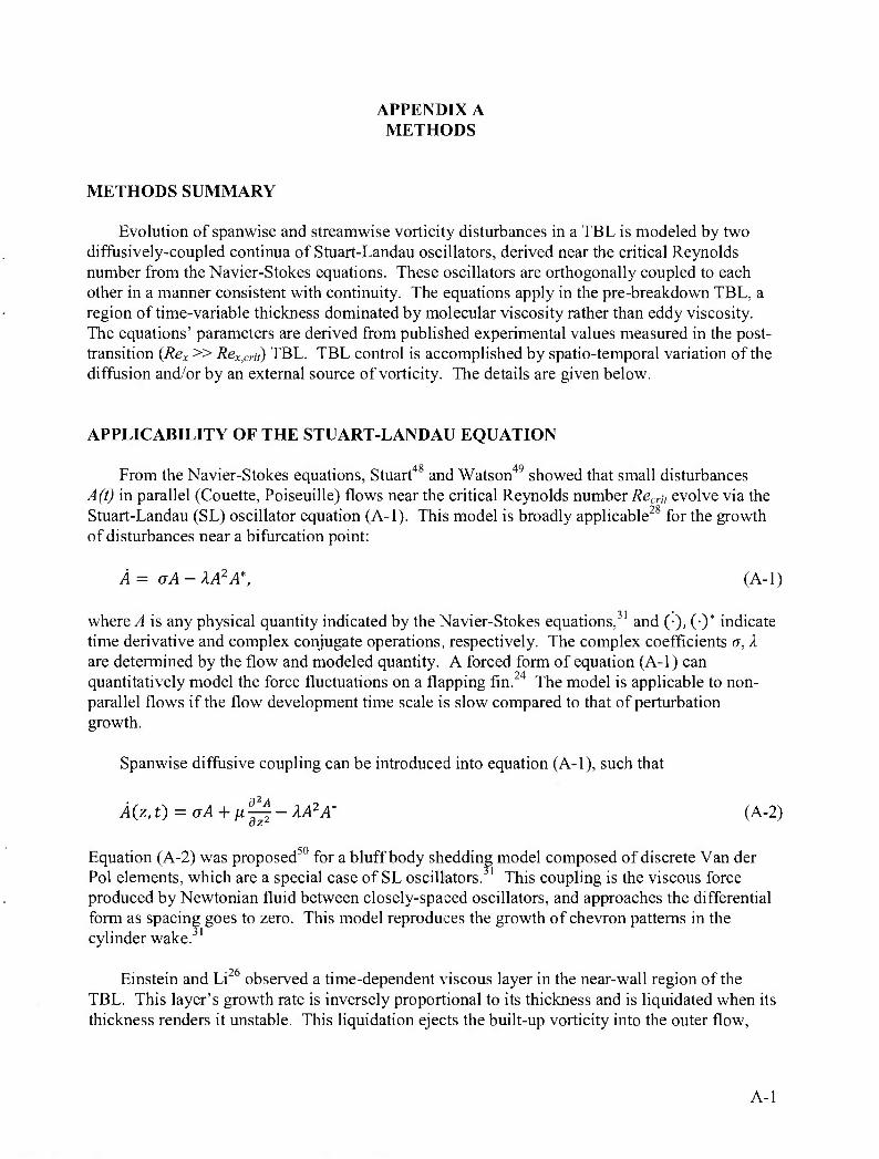
Evolution of spanwise and streamwise vorticity disturbances in a TBL is modeled by two diffusively-coupled continua of Stuart-Landau oscillators, derived near the critical Reynolds number from the Navier-Stokes equations. These oscillators are orthogonally coupled to each other in a manner consistent with continuity. The equations apply in the pre-breakdown TBL, a region of time-variable thickness dominated by molecular viscosity rather than eddy viscosity. The equations' parameters are derived from published experimental values measured in the post- transition {Rex » Rex,cl-ii) TBL. TBL control is accomplished by spatio-temporal variation of the diffusion and/or by an external source of vorticity. The details are given below.

APPLICABILITY OF THE STUART-LANDAU EQUATION

From the Navier-Stokes equations, Stuart and Watson49 showed that small disturbances A(t) in parallel (Couette, Poiseuille) flows near the critical Reynolds number Recrii evolve via the Stuart-Landau (SL) oscillator equation (A-l). This model is broadly applicable for the growth of disturbances near a bifurcation point:

A = aA-XA2A\ (A-l)

where A is any physical quantity indicated by the Navier-Stokes equations,31 and (•), CO* indicate time derivative and complex conjugate operations, respectively. The complex coefficients o-, X are determined by the flow and modeled quantity. A forced form of equation (A-l) can quantitatively model the force fluctuations on a flapping fin.24 The model is applicable to non- parallel flows if the flow development time scale is slow compared to that of perturbation growth.

Spanwise diffusive coupling can be introduced into equation (A-l), such that

y4(z, t) = ff.4 + ^0 - Ai42i4* (A-2)

Equation (A-2) was proposed50 for a bluff body shedding model composed of discrete Van der Pol elements, which are a special case of SL oscillators. This coupling is the viscous force produced by Newtonian fluid between closely-spaced oscillators, and approaches the differential form as spacing goes to zero. This model reproduces the growth of chevron patterns in the cylinder wake.

Einstein and Li observed a time-dependent viscous layer in the near-wall region of the TBL. This layer's growth rate is inversely proportional to its thickness and is liquidated when its thickness renders it unstable. This liquidation ejects the built-up vorticity into the outer flow.

A-l

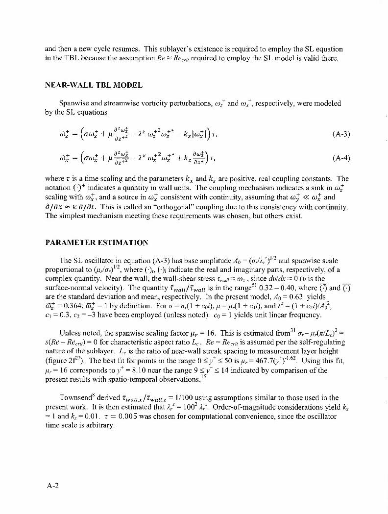
and then a new cycle resumes. This sublayer's existence is required to employ the SL equation in the TBL because the assumption Re ~ Recri, required to employ the SL model is valid there.

NEAR-WALL TBL MODEL

Spanwise and streamwise vorticity perturbations, a)z+ and to/, respectively, were modeled

by the SL equations

d)+ = ((raj+ + M^r-Az wz+2aj+* -/cja^ljr, (A-3)

aj+ = (ffa)+ + \i j^- - Xx aj+ &)+ + fcz-^f-J T, (A-4)

where T is a time scaling and the parameters kx and /cz are positive, real coupling constants. The notation O* indicates a quantity in wall units. The coupling mechanism indicates a sink in o)^" scaling with 60^", and a source in OKJ" consistent with continuity, assuming that (xiy « (o^ and d/dx « K: d/(3t. This is called an "orthogonal" coupling due to this consistency with continuity. The simplest mechanism meeting these requirements was chosen, but others exist.

PARAMETER ESTIMATION

The SL oscillator in equation (A-3) has base amplitude AQ = (ff/v) and spanwise scale proportional to Cu,/ov) , where (Or, (Oi indicate the real and imaginary parts, respectively, of a complex quantity. Near the wall, the wall-shear stress zwau ~ cor, since dvldx ~ 0 (D is the surface-normal velocity). The quantity fwaii/fWaii is in the range51 0.32 - 0.40, where (•) and (•) are the standard deviation and mean, respectively. In the present model, AQ = 0.63 yields (Oz = 0.364; oJz = 1 by definition. For a = ov(l + CQ/), JU = jur(l + C\i), and X: = (I + C2i)/Ao2, C] = 0.3, C2 = -3 have been employed (unless noted), CQ = 1 yields unit linear frequency.

Unless noted, the spanwise scaling factor ^r = 16. This is estimated from31 <jr- fxr(7r/Lc)2 - s{Re - Recrit) = 0 for characteristic aspect ratio Lc. Re = Recri, is assumed per the self-regulating nature of the sublayer. Lc is the ratio of near-wall streak spacing to measurement layer height (figure 2f27). The best fit for points in the range 0 </ < 50 is /^ = 467J(y+)'L62. Using this fit, fir= 16 corresponds to;/ = 8.10 near the range 9 <y+ < 14 indicated by comparison of the present results with spatio-temporal observations.15

o

Townsend derived fWaii,x/^waii,z = 1/100 using assumptions similar to those used in the present work. It is then estimated that Xr

x = 1002 A/. Order-of-magnitude considerations yield kx

= 1 and ^ = 0.01. T = 0.005 was chosen for computational convenience, since the oscillator time scale is arbitrary.

A-2

PERIOD OF A TWO-DIMENSIONAL UNCOUPLED SL OSCILLATOR

Let coz+(z+, t+) = M(z+, t+)exp{i0(z+, t+)), where magnitude M e R, M > 0, and phase jJ € R.

In regions where M(z+, t+) ~ M(/+), 0{z+, t+) ~ $ (/+), equation (A-3) simplifies to

M = (arM - A$M3) T, (p = (at - Af M2) r,

such that for M> 0, lim M = Ao= (cr,//!,.2)172. An analogous limiting value 000= (o;- (<Tr/Arz)A.iZ)T

t + ->oo

yields the period of the two-dimensional (Tollmien-Schlichting) wave T= In/cpoo, where T = IOOTT for the constants used here. This period is used in the modeling of microgrooves and microvibrations in dolphin chaos control.

SIMULATIONS

The equations are solved with a finite-difference fourth-order Runge-Kutta solver with time step dt+ = 0.2 and spatial grid dz^ = 1. Harmonic boundary conditions are applied at z = ±L/2 unless noted. When used, comer boundary conditions coz

+{±L/2, t+) are applied in combination with ar= (7r(z ) near the boundary; to obtain cr,(|z+| - L/2) ~ (JriCenter and smooth descent to zero at the boundary, (Tr(z

+) = cr,-ce„,erx [er/((z+ + L/2)/25) - erj{{z+ -LI2)I25) - 1]. The value 0"r>eenter (= 1) is the a, value used for all z when using harmonic boundary conditions. This equation yields a "comer" width of z+~ 50, matching Recrj,. Unless noted, the initial conditions, which embody lateral cellularization due to end-effects, are 0)^{z+, 0) = 0.1sin(27i/+/200), (o^{z+, 0) = 10"57V(z+), where N{z+) are uniformly distributed random numbers with range (-0.5,0.5) {N simulates free- stream turbulence).

CONTROL

"Controlled" forms of equations (A-3) and (A-4) are:

6>t = (W + /iz(z+,t+)gf - Az cofaif - /c,K+l + /ez.t(z+,t+))T,

d)+ = {aa>+x + ^(z+,t+)01 - A- ayfcot* + kz

d-£ + /e^(z+,t+))

The physical mechanism of "/^-control" is alteration of the local aspect ratio Lc. The mechanism of "/exrcontrol" is the addition of vorticity from a source outside the model.

A-3

SHARK CHAOS CONTROL

Uninterrupted riblets are modeled using //(2+) = //(z+) =/Z(l + KMsin{2nz+/s+)), where p. = 16(1 - 0.3/) is the flat plate value. The spacing between riblet peaks s+= 10 is used unless noted. KM gives the "strength" of the riblets, where the terms "weak" and "strong" riblets denote KM =

0.025 and 0.2, respectively.

Riblets interrupted by the dermal denticles are modeled using //(z+, /+) = //(z+, t+) = fl {\ + KMsm.(2nz+/s+) + Sc{z+, t+) - 5c), where Sc(z+, t+) = (V4)|sin(/+/200) - sin(7iz+/25)|, and the overbar denotes an average over a period. The Y* multiple in the latter equation gives the height of the denticles relative to the riblets.

DOLPHIN CHAOS CONTROL

The dolphin's microgrooves38 are modeled using //r(?+) = //(t+) = fi{\ + Kgroovesm(t+/50)), where Kgroove= 0.075. Microvibrations39 are modeled using Z'"^, (t*) = 0.005(/i:/a5,sin(/'+/800) + Ki/ovvsin(/+/50)). Where both microvibration frequencies are applied, Kfast- lj KSIOW= 1/16, such that their amplitudes are proportional to the ratio of the periods.

A-4

APPENDIX B EXTENDED DATA

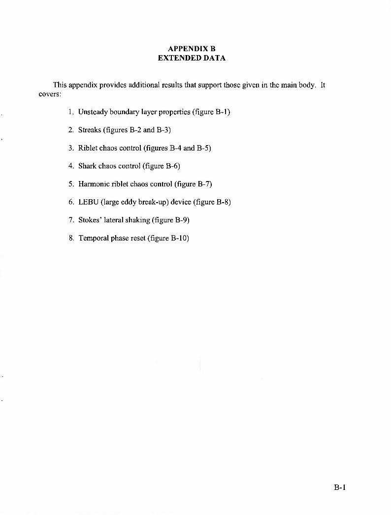
This appendix provides additional results that support those given in the main body. It covers:

1. Unsteady boundary layer properties (figure B-l)

2. Streaks (figures B-2 and B-3)

3. Riblet chaos control (figures B-4 and B-5)

4. Shark chaos control (figure B-6)

5. Harmonic riblet chaos control (figure B-7)

6. LEBU (large eddy break-up) device (figure B-8)

7. Stokes' lateral shaking (figure B-9)

8. Temporal phase reset (figure B-l0)

B-l

UNSTEADY BOUNDARY LAYER PROPERTIES

40 SO

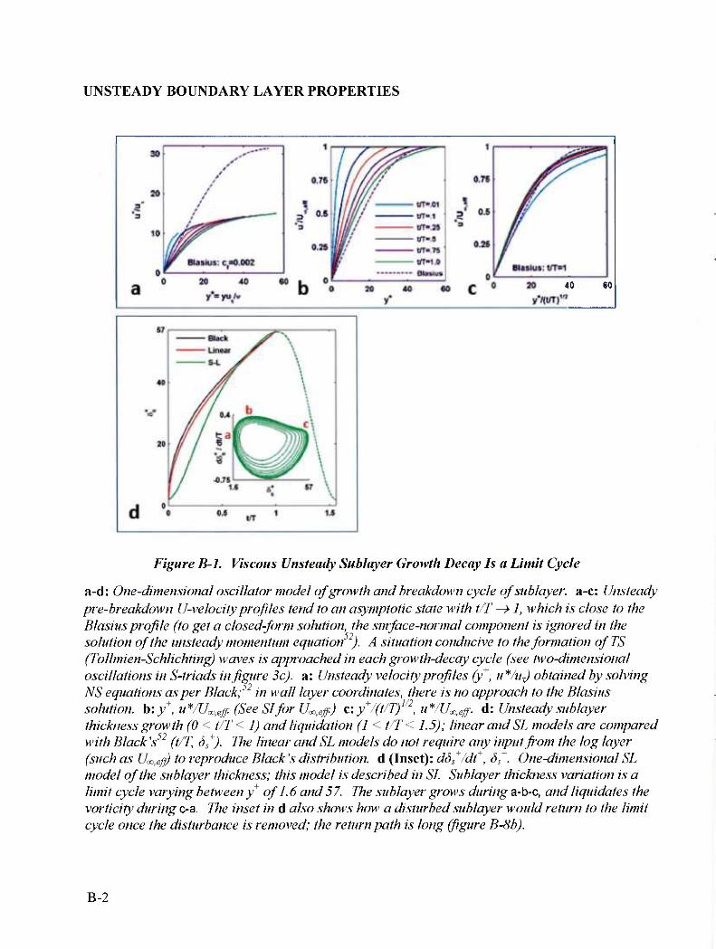
Figure B-l. Viscous Unsteady Sublayer Growth Decay Is a Limit Cycle

a-d: One-dimensional oscillator model of growth and breakdown cycle of sublayer, a-c: Unsteady pre-breakdown U-velocity profiles tend to an asymptotic state with t/T —> 1, which is close to the Blasius profile (to get a closed-form solution, the surface-normal component is ignored in the solution of the unsteady momentum equation' ). A situation conducive to the formation ofTS (Tollmien-Schlichting) waves is approached in each growth-decay cycle (see two-dimensional oscillations in S-triads in figure 3c). a: Unsteady velocity profiles (y+, U^/UT) obtained by solving NS equations as per Black;'2 in wall layer coordinates, there is no approach to the Blasius solution. h:y+, u^/U^eff. (See SI for U^eff) c:y+/(t/T)1/2, u*/U^,eff. d: Unsteady sublayer thickness growth (0 < t/T < 1) and liquidation (1 < t/T < 1.5); linear and SL models are compared with Black's52 (t/T, Ss

+). The linear and SL models do not require any input from the log layer (such as U^eff) to reproduce Black's distribution, d (Inset): d3,+/dt+, Ss

+. One-dimensional SL model of the sublayer thickness; this model is described in SI. Sublayer thickness variation is a limit cycle varying betweeny+ of 1.6 and57. The sublayer grows during a-b-c, and liquidates the vorticity during c-a. The inset in d also shows how a disturbed sublayer would return to the limit cycle once the disturbance is removed; the return path is long (figure B-8b).

B-2

STREAKS

180000 178000

176000 174000 172000

+ ^ 170000 168000

166000 164000 162000

160000 -8(

:?= %£^3k^S^ -—t^^-^t-*^ tayi^ifi^^fe1--^^

tefe iiii n==3p%= =zltE==^ (. ^ :E5F3z5S!—^ ^^

^ i'

"tT-Ip^—.^ ■. «=^: g: iiiS ̂^$=^\

^E^S3£&

! ')

j ^^^rflSS H ^^^^

^ R » TNL^ *E>5=±=J^r5ter^-

?=== ^^^ ^^^g

i ^s ^^S y^~z^iF5^3 Si

j . ^J ^L-'-lt ^^^ ̂ ^i^fe^S^BS^^IBg

)0 -600 -400 -200 0 200 + z

400 600 800

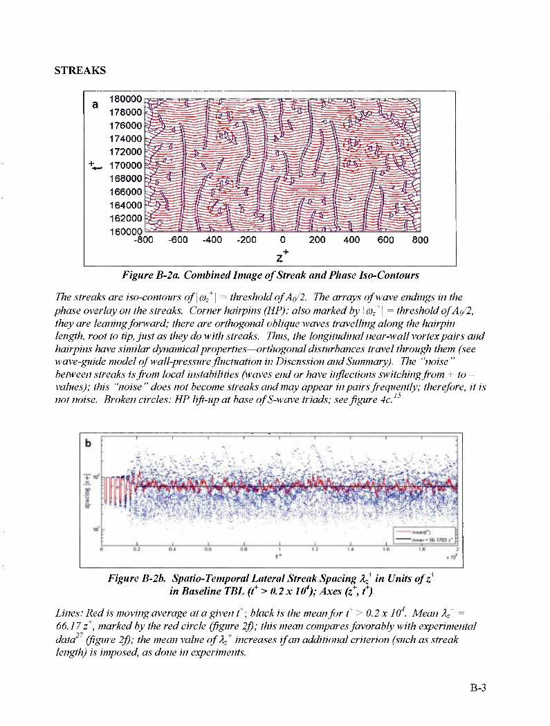
Figure B-2a. Combined Image of Streak and Phase Iso-Contours

The streaks are i so-contour s of az+ = threshold ofAo 2. The arrays of wave endings in the

phase overlay on the streaks. Corner hairpins (HP): also markedby\(02+\ = thresholdofA(/2,

they are leaning foi-ward; there are orthogonal oblique wax'es travelling along the hairpin length, root to tip, just as they do with streaks. Thus, the longitudinal near-wall vortex pairs and hairpins have similar dynamical properties—orthogonal disturbances travel through them (see wcn'e-guide model of wall-pressure fluctuation in Discussion and Summary). The "noise " between streaks is from local instabilities (waves end or have inflections switching from + to- values); this "noise " does not become streaks and may appear in pairs frequently; therefore, it is not noise. Broken circles: HP lift-up at base ofS-wave triads; see figure 4c.

Figure B-2b. Spatio-Temporal Lateral Streak Spacing An+ in Units ofz

in Baseline TBL (t+ > 0.2 x 10*); Axes (z+, t+)

Lines: Red is moving a\>erage at a given C\ black is the mean for t+ > 0.2 x JO4. Mean ^ = 66.17 z+, marked by the red circle (figure 2f); this mean compares favorably with experimental data27 (figure 2f); the mean value of ^ increases if an additional criterion (such as streak length) is imposed, as done in experiments.

B-3

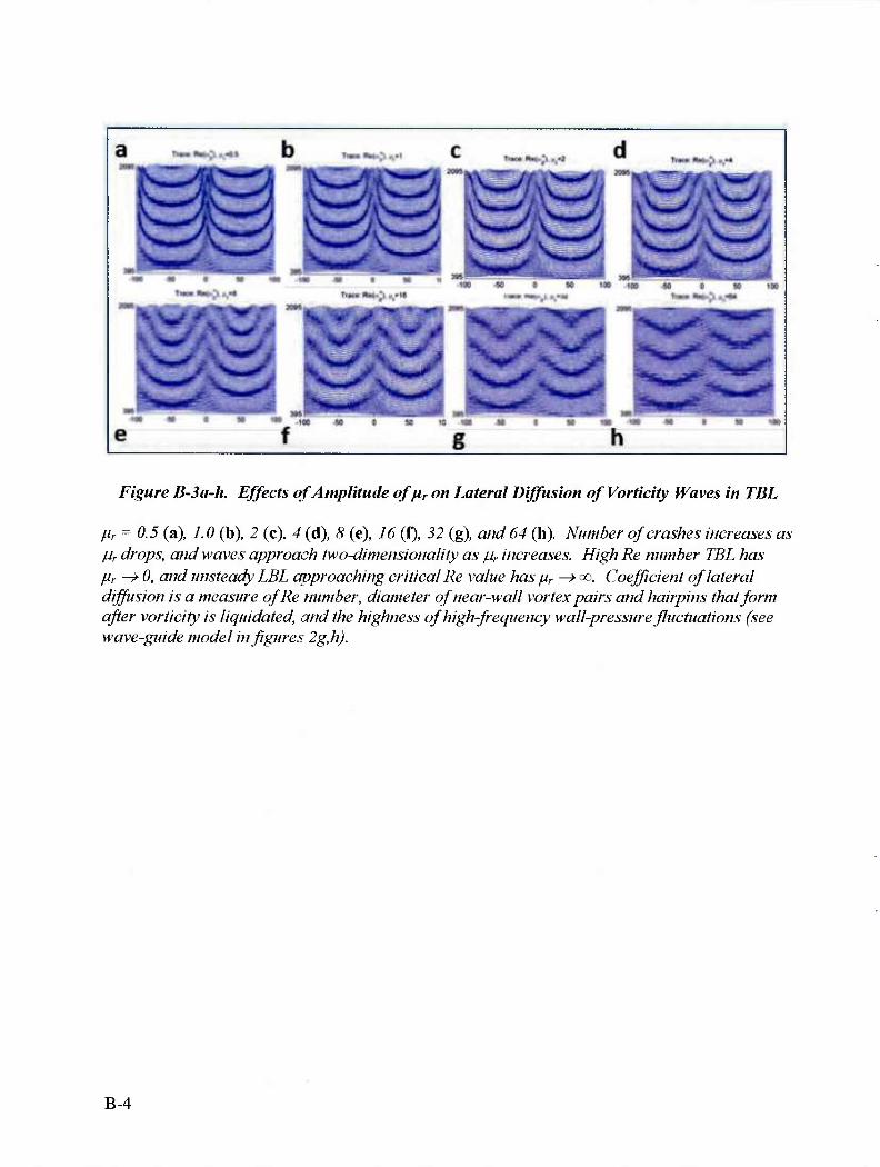
Figure B-3a-h. Effects of Amplitude offir on lateral Diffusion of Vorticity Waves in TBL

iur = 0.5 (a), 1.0 (b), 2 (c), 4 (d), 8 (e), 16 (f), 32 (g), and 64 (h). Number of crashes increases as fur drops, and waves approach two-dimensionality as p.? increases. High Re number TBL has Hr -> 0, and unsteady LBL approaching critical Re value has jUr —> «. Coefficient of lateral diffusion is a measure of Re number, diameter of near-wall vortex pairs and hairpins that form after vorticity is liquidated, and the highness of high-frequency wall-pressure fluctuations (see wave-guide model in figures 2g,h).

B-4

-100 -50 0 50 100 100 50 0 50 100

lri»ce,Re(Mp trace. Re(ri*)

M -100

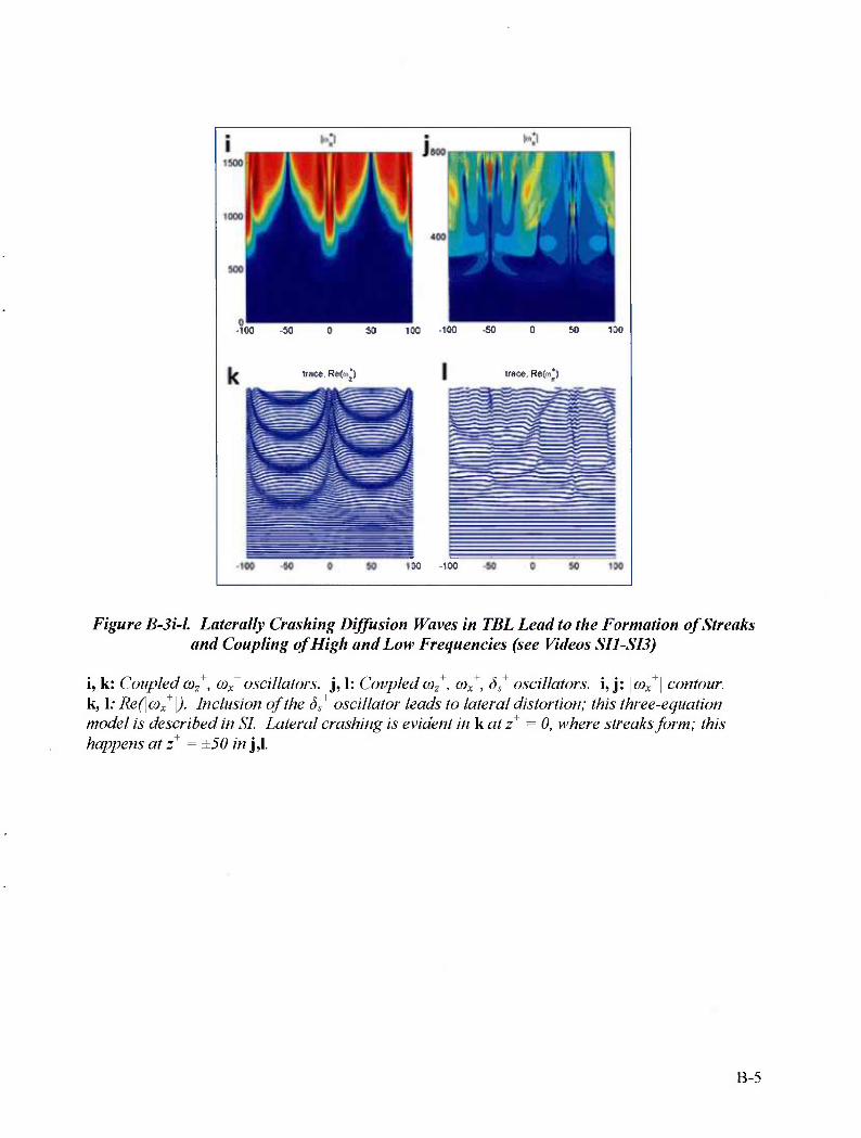
Figure B-3i-l. Laterally Crashing Diffusion Waves in TBL Lead to the Formation of Streaks and Coupling of High and Low Frequencies (see Videos SI1-SI3)

i, k: Coupledcoz+, cox

+ oscillators, j, 1: Coupledcoz+, a)x

+, Ss+ oscillators, i, j: \cox

+\ contour. k, 1; Re(\o)x

+\). Inclusion of the 5S* oscillator leads to lateral distortion; this three-equation model is described in SI. Lateral crashing is evident in kat z+ = 0, where streaks form; this happens at z+ = ±50 in j,l.

B-5

RIBLET CHAOS CONTROL

I i I l i I j

A.

At Si Aist

Streak sfwctngnl* CoM nbtsft-muz-wnpCO-spflcalO wan

KO 4M m

Figure B-4. Shark "Strong" Riblet Model (Excluding Dermal Denticles): Acting on co:+ in the

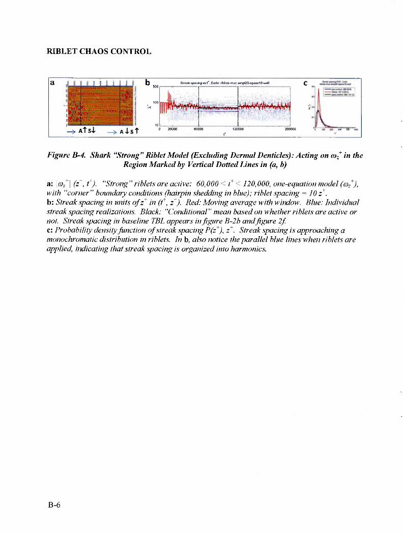
Region Marked by Vertical Dotted Lines in (a, b)

a: |fijz+| (z+, t+). "Strong" riblets are active: 60,000 < t+ < 120,000, one-equation model (coz

+), with "corner" boundary conditions (hairpin shedding in blue); riblet spacing = 10 z+. b: Streak spacing in units ofz+ in (t+, z+). Red: Moving average with window. Blue: Individual streak spacing realizations. Black: "Conditional" mean based on whether riblets are active or not. Streak spacing in baseline TBL appears in figure B-2b and figure 2f. c: Probability density function of streak spacing P(z+), z+. Streak spacing is approaching a monochromatic distribution in riblets. In b, also notice the parallel blue lines when riblets are applied, indicating that streak spacing is organized into harmonics.

B-6

RIBLET CHAOS CONTROL (Cont'd)

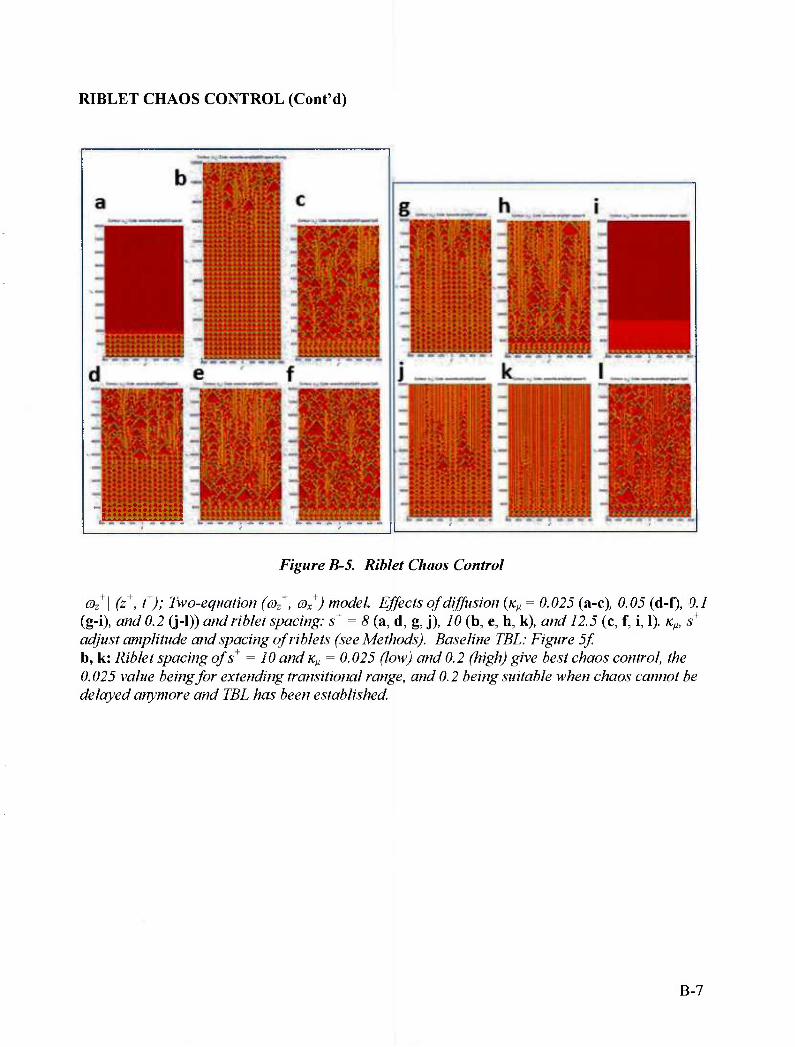
Figure B-5. Riblet Chaos Control

I®/ (z+, t+); Two-equation (a-t, (0X+) model. Effects of diffusion {K^ = 0.025 (a-c), 0.05 (d-f), 0.1

(g-i), awi/ 0.2 (j-l)) a«t/ 77^/e? spacing: 5+ = 5 (a, d, g, j), 70 (b, e, h, k), and 12.5 (c, f, i, 1). ty, 5+

adjust amplitude and spacing ofriblets (see Methods). Baseline TBL: Figure 5f. b, k: Riblet spacing ofs+ = 10 and K^ = 0.025 (lowj and 0.2 (high) give best chaos control, the 0.025 value being for extending transitional range, and 0.2 being suitable when chaos cannot be delayed anymore and TBL has been established.

B-7

SHARK CHAOS CONTROL

c«" m, "■—». "* M, —^^^

+ dermal denticles

4»»***««4«*<*<>

I^^Si^Sti t an m was me

+ 1 ext

ate «a wc nr

combined

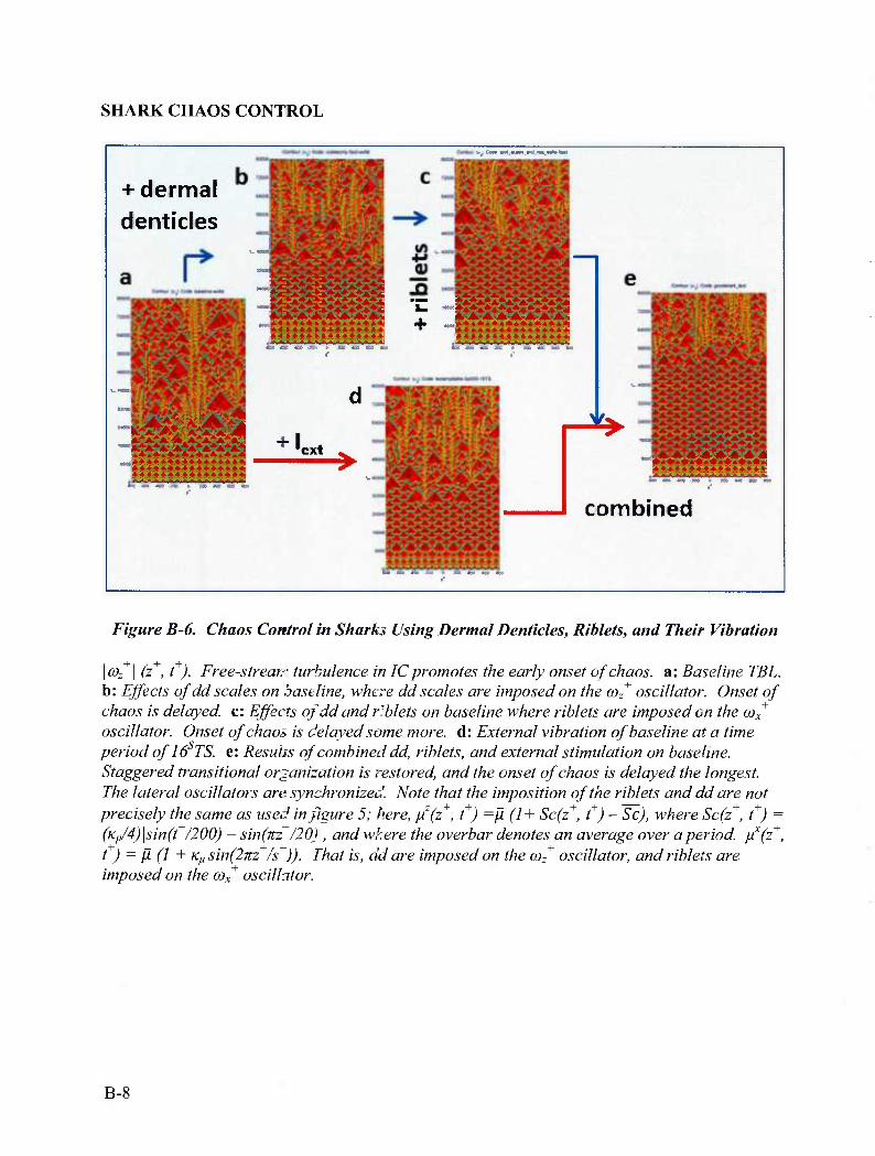
Figure B-6. Chaos Control in Sharks Using Dermal Denticles, Riblets, and Their Vibration

\coz \ (z , t ). Frees trear- turbulence in IC promotes the early onset of chaos, a: Baseline TEL. b: Etffects of dd scales on baseline, where dd scales are imposed on the coz

+ oscillator. Onset of chaos is delayed, c: Effects of dd and riblets on baseline where riblets are imposed on the cox

+

oscillator. Onset of chaos is delayed some more, d: External vibration of baseline at a time period of 16 TS. e: Resuhs of combined dd, riblets, and external stimulation on baseline. Staggered transitional organization is restored, and the onset of chaos is delayed the longest. The lateral oscillators are synchronized. Note that the imposition of the riblets and dd are not precisely the same as used in figure 5; here, nz(z+, t+) =ji (1+ Sc(z+, f) - Sc), where Sc(z+, t+) = (K//4)\sin(t /200) - sin(nz /20) , and where the overbar denotes an average over a period, ^(z*, t ) - ft (1 + KM sin(2KZ /s )). That is, dd are imposed on the coz

+ oscillator, and riblets are imposed on the a)x

+ oscillator.

B-8

HARMONIC RIBLET CHAOS CONTROL

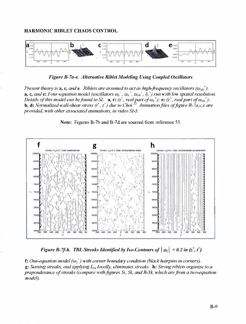
Figure B-7a-e. Alternative Riblet Modeling Using Coupled Oscillators

Present theory is a, c, and e. Riblets are assumed to act as high-frequency oscillators (<X)xh). a, c, and e: Four-equation model (oscillators cor

+) cyx

+, (oxh , Ss+) run with low spatial resolution.

Details of this model can be found in SI. a, c: (z+, real part ofcox+); e: (z+, real part of G)xh);

b, d: Normalized wall-shear stress (t+, z+) due to Choi. Animation files of figure B-7a,c,e are provided, with other associated animations, in video SI-5.

Note: Figures B-7b and B-7d are sourced from reference 53.

i-^cej c«i g

Cflrtqv -rl-0 J C«» (

'

'

UCOOL * \i» '• ''I ^ r' ►

1 >M.. i

""^Sos

/-•■-'■ ii';;-

-MO -wo ft m «» aw

, ,, • , \l i, «

"^fe -m-MB-MO o ioa 40a aw ■»

MOM .'

i 7X00

hf*l 0M<«9-cMn

1 H ll

Ik

r-'-l''J

no 400 000 ttKi

FigureB-7f-h. TBL Streaks Identified by Iso-Contours of\a)z\ < 0.2 in (z+, t+)

f: One-equation model (coz+) with corner boundary condition (black hairpins in corners).

g: Sensing streaks, and applying Iext locally, eliminates streaks, h: Strong riblets organize to a preponderance of streaks (compare with figures 5i, 5k, and B-5k, which are from a two-equation model).

B-9

LEBU (LARGE EDDY BREAK-UP) DEVICE

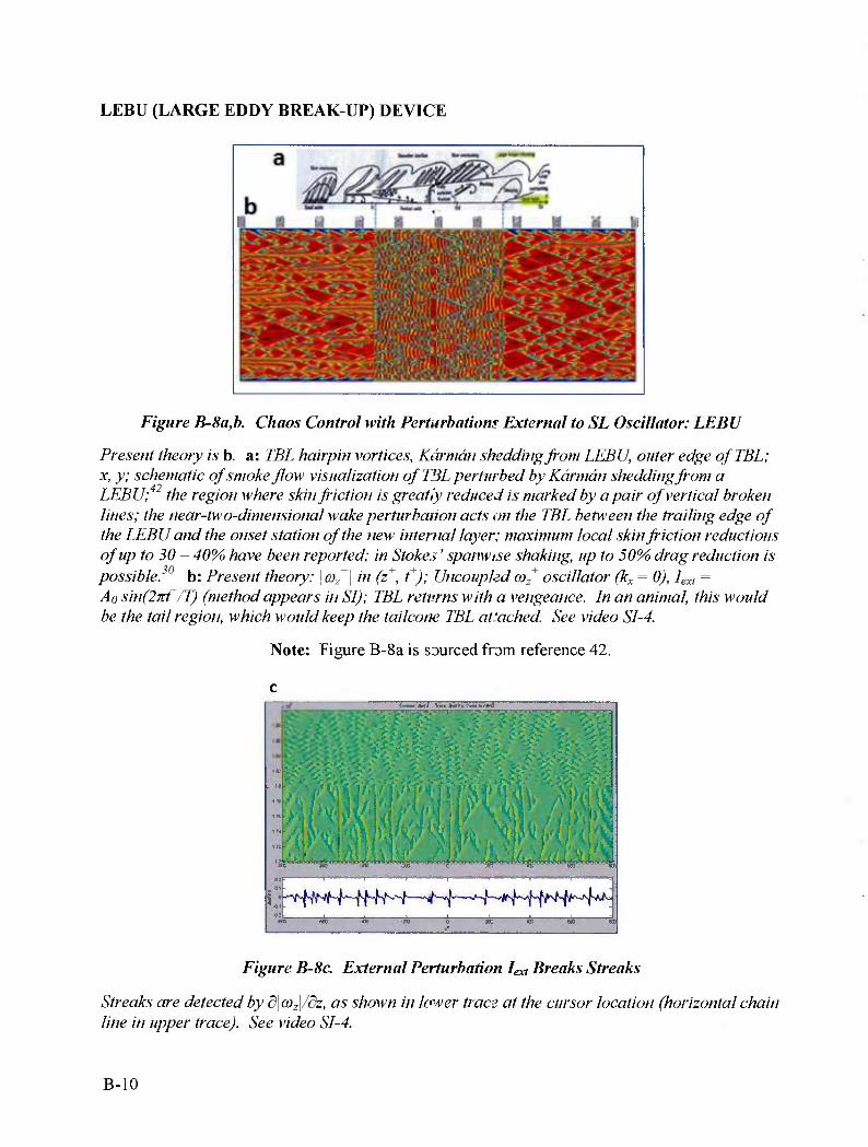
Figure B-8a,b. Chaos Control with Perturbatiom External to SL Oscillator: LEBU

Present theory is b. a: TBL hairpin vortices, Karmdn shedding from LEBU, outer edge ofTBL; x, y; schematic of smoke flow visualization of FBL perturbed by Kdrmdn shedding fi-om a LEBU;4 the region where skin fiction is great iy reduced is marked by a pair of vertical broken lines; the near-two-dimensional wake perturbation acts on the TBL between the trailing edge of the LEBU and the onset station of the new internal layer; maximum local skin friction reductions of up to 30 - 40% have been reported; in Stoke* ' spanwise shaking, up to 50% drag reduction is possible.30 b: Present theory: \co:

+\ in (z+, t+); Uncoupledm-^ oscillator (kx = 0), Iext = Ao sin(2nt+/T) (method appears in SI); TBL returns with a vengeance. In an animal, this would be the tail region, which would keep the tailcom TBL at'ached. See video SI-4.

Note: Figure B-8a is sourced from reference 42.

iiiiii -^-•^^^^^s^^.y^^h^^—*>£

,--*}--~--*j-~x^sft**y~*s{^

ao on

Figure B-8c. External Perturbation Iext Breaks Streaks

Streaks are detected by d\a)z\/dz, as shown in lower trace at the cursor location (horizontal chain line in upper trace). See video SI-4.

B-10

STOKES' LATERAL SHAKING

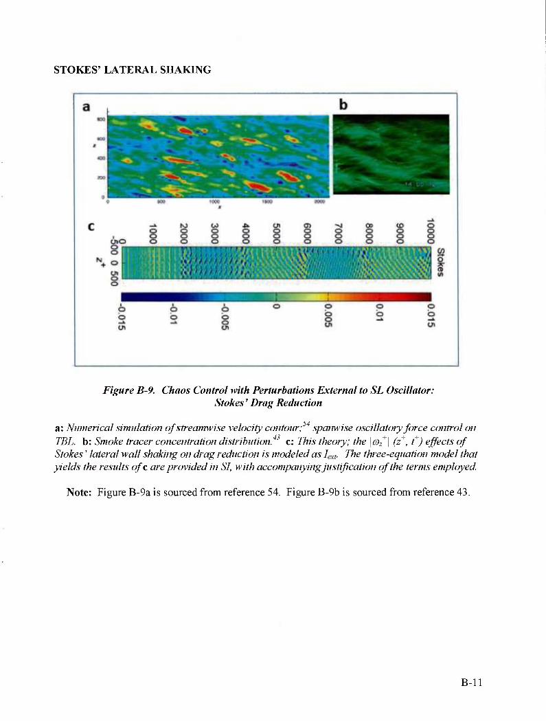
Figure B-9. Chaos Control with Perturbations External to SL Oscillator: Stokes' Drag Reduction

.54 a: Numerical simulation ofstreamwise velocity contour; spanwise oscillatory force control on TBL. b: Smoke tracer concentration distribution.4' c: This theory; the \(0z

+\ (z+, t+) effects of Stokes' lateral wall shaking on drag reduction is modeled as Iexl. The three-equation model that yields the results ofc are provided in SI, with accompanying justification of the terms employed.

Note: Figure B-9a is sourced from reference 54. Figure B-9b is sourced from reference 43.

B-ll

TEMPORAL PHASE RESET

Temporal Phase Reset

0 5^ 2« 3C 4.0 SO

(e)

(d)

t

4

Spatial Template

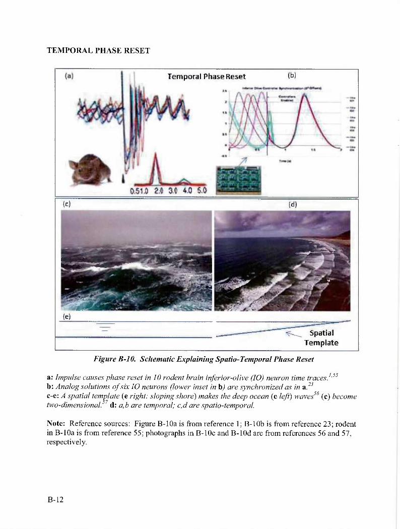
Figure B-10. Schematic Explaining Spatio-Temporal Phase Reset

a: Impulse causes phase reset in 10 rodent brain inferior-olive (IO) neuron time traces.155

b: Analog solutions of six 10 neurons (lower inset in h) are synchronized as in a.23

c-e: A spatial template (e right: sloping shore) makes the deep ocean (e left) waves56 (c) become two-dimensional, d: a,b are temporal; c,d are spatio-temporal.

Note: Reference sources: Figure B-lOa is from reference 1; B-lOb is from reference 23; rodent in B-lOa is from reference 55; photographs in B-lOc and B-lOd are from references 56 and 57, respectively.

B-12

APPENDIX C SUPPLEMENTARY INFORMATION (SI)

SI METHODS AND DISCUSSION

This appendix describes the methods used to generate the figures provided in the extended data of appendix B. It also discusses these methods and provides further discussion of the results in the main body. It covers:

1. Unsteady boundary layer properties:

• Linear sublayer thickness model

• Log-layer bounded sublayer thickness model

• Stuart-Landau sublayer thickness model

• Inclusion of sublayer thickness in model: Coupling between vorticity and

sublayer equations.

2. Shark chaos control

3. LEBU (Large Eddy Break-Up) device

4. Stokes' lateral shaking for drag reduction

VIDEOS

Note: Videos are available from the principal author.

Other supplementary information available for download includes the videos listed below. These videos are animations that make certain results more clear:

Video SI-1. Animation of the (Oz laterally crashing waves using the model shown in still form in figure 4f. It shows how streaks are formed. Oscillators: £or

+ as per baseline (wavelength of 200 wall units; Methods), aix

+{z+fi) = 0, rather than noise.

Video SI-2. Animation of i?e(a)z ) crashing waves using OJ^ initial condition wavelength/l/c = 200z+. Clear formation of streaks and carrier waves when Xic= 200z+, compared to 100z+. Streaks form where Re(a)z) crosses sign with spacing ^/c/2. Oscillators: coz , 0)x , Ss ; IC: a)x

+(z+,0) = 0, 4+(z+,0) = 10; model details given later in this appendix.

Video SI-3. Animation ofRe(a)z) crashing waves using initial condition wavelength A/c = 100z+. Compare crashing behavior to Video SI-2; crashing is not as clear when initial wave

C-l

length is 100 wall units. Oscillators: (o?, co^, 8S+; IC: fi^+(z+,0) = 0, d^{z+fi) = 10; model details

given later in this appendix.

Video SI-4. Animation of 5|aj^|/5z+, where contours and traces of that variable are plotted simultaneously with a moving cursor. A strong oscillator (LEBU) is applied at t+ =180,000. This video shows how streaks are annihilated. Also see the stationary view in figure B-8b.

Video SI-5. This is a presentation-like movie containing animations of wj, ooj, and w^, for cases with and without harmonic riblets. Increasing lock-in with increasing number of control oscillators is apparent. See figures B-7a,c,e for stationary view and see this appendix for accompanying methods and discussion.

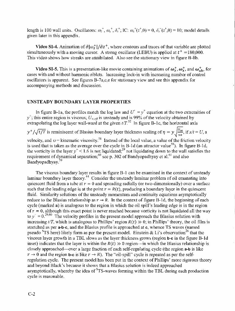
UNSTEADY BOUNDARY LAYER PROPERTIES

In figure B-la, the profiles match the log law and IT =yr equation at the two extremities of y+\ this entire region is viscous; L/^^-is unsteady and is 99% of the velocity obtained by extrapolating the log layer wall-ward at the given t/T^ In figure B-lc, the horizontal axis

y+I^Jt/T is reminiscent of Blasius boundary layer thickness scaling of 77 = y I—, if x/if = C/, a

velocity, and v = kinematic viscosity.5 Instead of the local value, a value of the friction velocity is used that is taken as the average over the cycle in B-ld (an attractor value59). In figure B-Id, the vorticity in the layer j/ < 1.6 is not liquidated; not liquidating down to the wall satisfies the requirement of dynamical separation;60 see p. 302 of Bandyopadhyay et al.61 and also Bandyopadhyay.59

The viscous boundary layer results in figure B-I can be examined in the context of unsteady laminar boundary layer theory.44 Consider the unsteady laminar problem of oil emanating into quiescent fluid from a tube at r = 0 and spreading radially (or two-dimensionally) over a surface such that the leading edge is at the point r = R{t), producing a boundary layer in the quiescent fluid. Similarity solutions of the unsteady momentum and continuity equations asymptotically reduce to the Blasius relationship as r -»/?. In the context of figure B-ld, the beginning of each cycle (marked a) is analogous to the region in which the oil spill's leading edge is in the region of r = 0, although this exact point is never reached because vorticity is not liquidated all the way to y+ = 0.29'60 The velocity profiles in the present model approach the Blasius solution with increasing t/T, which is analogous to Phillips' region R{t) » 0; in Phillips' theory, the oil film is stretched as per a-b-c, and the Blasius profile is approached at c, whence TS waves (named pseudo TS here) likely form as per the present model. Einstein & Li's observation that the viscous layer growth in a TBL slows as the layer thickness grows (region b-c in the figure B-ld inset) indicates that the layer is within the R{t) » 0 region—in which the Blasius relationship is closely approached—over a large fraction of each self-regulating cycle (the region a-b is like r -> 0 and the region b-c is like r -> R). The "oil-spill" cycle is repeated as per the self- regulation cycle. The present model has been put in the context of Phillips' more rigorous theory and beyond Black's because it shows that a Blasius solution is indeed approached asymptotically, whereby the idea of TS-waves forming within the TBL during each production cycle is reasonable.

C-2

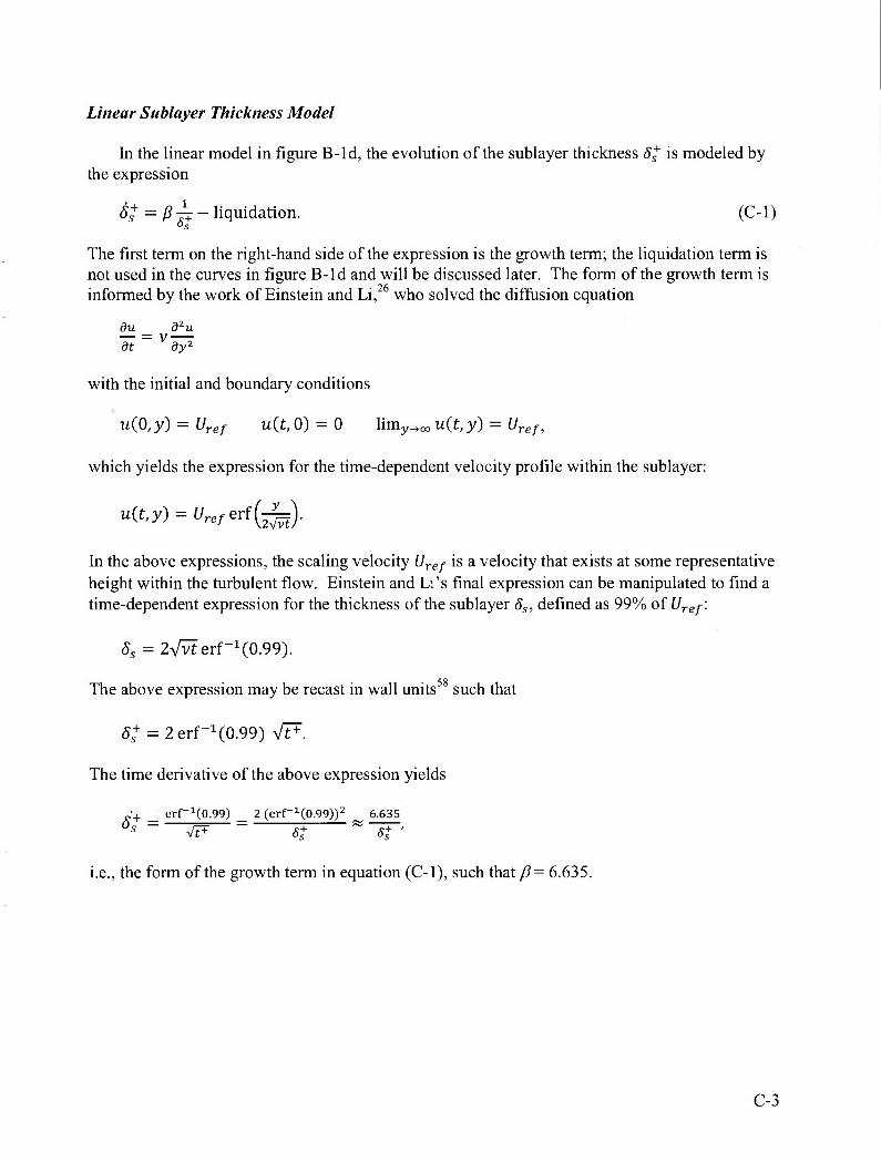
Linear Sublayer Thickness Model

In the linear model in figure B-ld, the evolution of the sublayer thickness 5S+ is modeled by

the expression

5+ = £ -^ - liquidation. (C-1) Or Js

The first term on the right-hand side of the expression is the growth term; the liquidation term is not used in the curves in figure B-ld and will be discussed later. The form of the growth term is informed by the work of Einstein and Li, 6 who solved the diffusion equation

du _ d2u at - Vd^

with the initial and boundary conditions

uiO,y) = Uref u(t, 0) = 0 limy^oo u(t# y) = t/re/,

which yields the expression for the time-dependent velocity profile within the sublayer:

u(t,y) = Ureferf{^=).

In the above expressions, the scaling velocity (/re^ is a velocity that exists at some representative height within the turbulent flow. Einstein and L:'s final expression can be manipulated to find a time-dependent expression for the thickness of the sublayer Ss, defined as 99% of (/re^:

5S = 2Vvt erf-1 (0.99).

The above expression may be recast in wall units such that

5+ = 2 erf"1 (0.99) VF.

The time derivative of the above expression yields

„•+ _ errHo.gg) _ 2 (err1(0.99))2 6.635 s ~ 7F _ st * st '

i.e., the form of the growth term in equation (C-l), such that /?= 6.635.

C-3

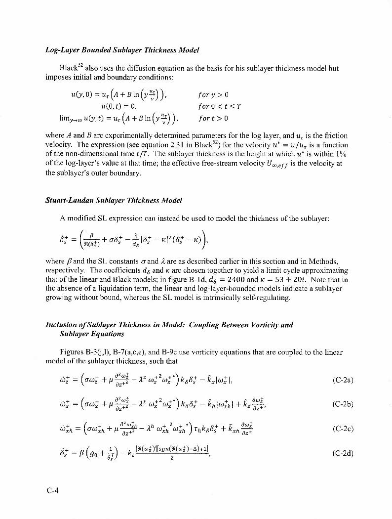
Log-Layer Bounded Sublayer Thickness Model

,52 Black also uses the diffusion equation as the basis for his sublayer thickness model but imposes initial and boundary conditions:

u(y,0) = uT(i4 + flln(y^)), fory>0

u(0, t) = 0, forO <t<T

lim^oo u(y, t)=uT^A + B in (y^) ), /or t > 0

where A and B are experimentally determined parameters for the log layer, and uT is the friction velocity. The expression (see equation 2.31 in Black52) for the velocity u* = u/uT is a function of the non-dimensional time t/T. The sublayer thickness is the height at which it* is within 1% of the log-layer's value at that time; the effective free-stream velocity t/oo,e// is the velocity at the sublayer's outer boundary.

Stuart-Landau Sublayer Thickness Model

A modified SL expression can instead be used to model the thickness of the sublayer:

where /?and the SL constants crand A are as described earlier in this section and in Methods, respectively. The coefficients ds and K are chosen together to yield a limit cycle approximating that of the linear and Black models; in figure B-ld, ds = 2400 and K = 53 + 20i. Note that in the absence of a liquidation term, the linear and log-layer-bounded models indicate a sublayer growing without bound, whereas the SL model is intrinsically self-regulating.

Inclusion of Sublayer Thickness in Model: Coupling Between Vorticity and Sublayer Equations

Figures B-3(j,l), B-7(a,c,e), and B-9c use vorticity equations that are coupled to the linear model of the sublayer thickness, such that

d)z+ = (W + /-^--Az wfaj;*) ksS+ - nx\(0*\, (C-2a)

a>; = (W + /-^.-Ax cofa>t*) ks5+ - kh\a>+xh\ + k^, (C-2b)

d)+h = ((Ta)+h + n-jffi- Ah coih2a)^Thks8^ + kxh^r (C-2c)

4+ = /? M £) " ^ l^)^*^)-^, (C-2d)

C-4

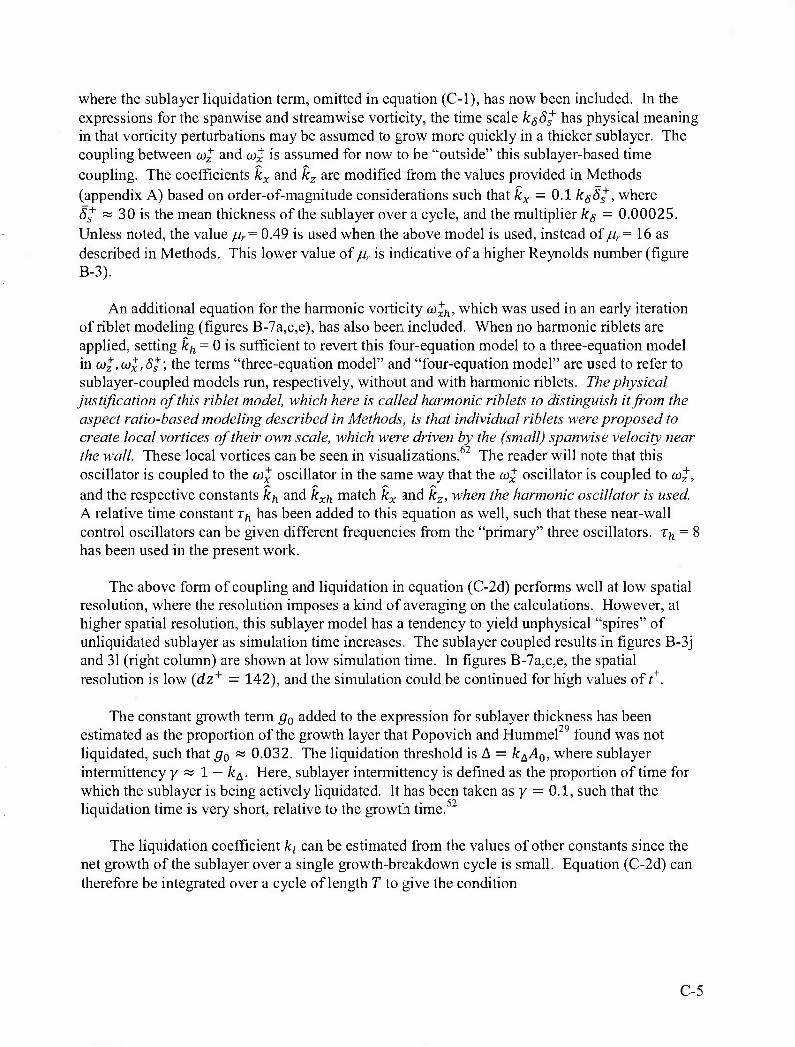
where the sublayer liquidation term, omitted in equation (C-l), has now been included. In the expressions for the spanwise and streamwise vorticity, the time scale kgS^ has physical meaning in that vorticity perturbations may be assumed to grow more quickly in a thicker sublayer. The coupling between OJ^ and a)^ is assumed for now to be "outside" this sublayer-based time coupling. The coefficients kx and kz are modified from the values provided in Methods (appendix A) based on order-of-magnitude considerations such that kx — 0.1 ks5*, where 5/ « 30 is the mean thickness of the sublayer over a cycle, and the multiplier kg = 0.00025. Unless noted, the value jur= 0.49 is used when the above model is used, instead of//,.= 16 as described in Methods. This lower value of//,- is indicative of a higher Reynolds number (figure B-3).

An additional equation for the harmonic vorticity a)Jh, which was used in an early iteration of riblet modeling (figures B-7a,c,e), has also been included. When no harmonic riblets are applied, setting fch = 0 is sufficient to revert this four-equation model to a three-equation model in ojz .(Ox.Sg; the terms "three-equation model" and "four-equation model" are used to refer to sublayer-coupled models run, respectively, without and with harmonic riblets. The physical justification of this riblet model, which here is called harmonic riblets to distinguish it from the aspect ratio-based modeling described in Methods, is that individual riblets were proposed to create local vortices of their own scale, which were driven by the (small) spanwise velocity near the wall. These local vortices can be seen in visualizations.62 The reader will note that this oscillator is coupled to the cd^ oscillator in the same way that the oi^ oscillator is coupled to OJ^ , and the respective constants kh and kxh match kx and kz, when the harmonic oscillator is used. A relative time constant Th has been added to this squation as well, such that these near-wall control oscillators can be given different frequencies from the "primary" three oscillators. T/j = 8 has been used in the present work.

The above form of coupling and liquidation in equation (C-2d) performs well at low spatial resolution, where the resolution imposes a kind of averaging on the calculations. However, at higher spatial resolution, this sublayer model has a tendency to yield unphysical "spires" of unliquidated sublayer as simulation time increases. The sublayer coupled results in figures B-3j and 31 (right column) are shown at low simulation time. In figures B-7a,c,e, the spatial resolution is low (dz+ = 142), and the simulation could be continued for high values of/+.

The constant growth term g^ added to the expression for sublayer thickness has been estimated as the proportion of the growth layer that Popovich and Hummel found was not liquidated, such that g^ ~ 0.032. The liquidation threshold is A = kAA0, where sublayer intermittency y ~ 1 — kA. Here, sublayer intermittency is defined as the proportion of time for which the sublayer is being actively liquidated. It has been taken as y = 0.1, such that the liquidation time is very short, relative to the growtn time.52

The liquidation coefficient /c; can be estimated from the values of other constants since the net growth of the sublayer over a single growth-breakdown cycle is small. Equation (C-2d) can therefore be integrated over a cycle of length T to give the condition

C-5

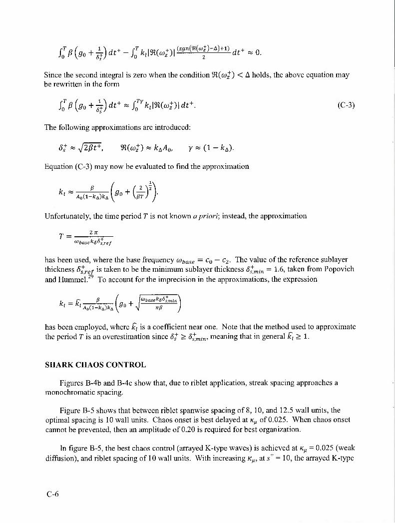
j> (so+jV) at- - % km^)\ ^f-^ dt*»o.

Since the second integral is zero when the condition 51 (60^) < A holds, the above equation may be rewritten in the form

!oP{9o+j;)dt+*SZrklmo)+)\dt+. (C-3)

The following approximations are introduced:

Equation (C-3) may now be evaluated to find the approximation

kl*A0il-kJkA[9o + {w)\

Unfortunately, the time period T is not known a priori; instead, the approximation

2 71 T =

<^basekSSs,ref

has been used, where the base frequency ajbase = c0 — C2. The value of the reference sublayer thickness (5/ref is taken to be the minimum sublayer thickness Sgmin = 1.6, taken from Popovich and Hummel.29 To account for the imprecision in the approximations, the expression

. _ C /? f . l<*baSeksSt.r,

has been employed, where ki is a coefficient near one. Note that the method used to approximate the period T is an overestimation since 5S

+ > S^min, meaning that in general ki>l.

SHARK CHAOS CONTROL

Figures B-4b and B-4c show that, due to riblet application, streak spacing approaches a monochromatic spacing.

Figure B-5 shows that between riblet spanwise spacing of 8, 10, and 12.5 wall units, the optimal spacing is 10 wall units. Chaos onset is best delayed at /cM of 0.025. When chaos onset cannot be prevented, then an amplitude of 0.20 is required for best organization.

In figure B-5, the best chaos control (arrayed K-type waves) is achieved at K^ = 0.025 (weak diffusion), and riblet spacing of 10 wall units. With increasing KM, at s+ = 10, the arrayed K-type

C-6

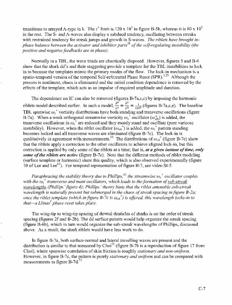
1 T ■}

transitions to arrayed A-type in k. The / limit is 120 x 10" in figure B-5b, whereas it is 80 x 10 in the rest. The S- and A-waves also display a subdued tendency, oscillating between streaks with restrained tendency for streak jumps and growth in S-waves. The riblets have brought in- phase balance between the activator and inhibitor parts of the self-regulating instability (the positive and negative feedbacks are in phase).

Normally in a TBL, the wave triads are chaotically disposed. However, figures 5 and B-6 show that the shark dd's and their staggering provide a template for the TBL instabilities to lock in to because the templates mimic the primary modes of the flow. The lock-in mechanism is a spatio-temporal version of the temporal Self-referential Phase Reset (SPR).1-23 Although the process is nonlinear, chaos is eliminated and the initial condition dependence is removed by the effects of the template, which acts as an impulse of required amplitude and duration.

The dependence on IC can also be removed (figures B-7a,c,e) by imposing the harmonic

riblets model described earlier. In such a model, — = -r = —^r (figures B-7a,c,e). The baseline A* Xh ioo2 v ^ > > J

TBL spanwise co* vorticity distributions have both standing and transverse oscillations (figure B-7a). When a weak orthogonal streamwise vorticity co^ oscillator (o)^) is added, the transverse oscillations in <»z

+ are reduced and they mostly stand and oscillate (pure varicose instability). However, when the riblet oscillator (ft)^+) is added, the (Qz pattern standing becomes locked and all transverse waves are eliminated (figure B-7c). The lock-in is qualitatively in agreement with measurements.5 The distributions of cox/,+ (figure B-7e) show that the riblets apply a correction to the other oscillators to achieve aligned lock-in, but this correction is applied by only some of the riblets at a time; that is, at a given instant of time, only some of the riblets are active (figure B-7e). Note that the different methods of riblet modeling (surface template or harmonic) share this quality, which is also observed experimentally (figure 10 of Lee and Lee 2). For temporal representation of figure B-7, see video SI-5.

Paraphrasing the stability theory due to Phillips, the streamwise cox+ oscillator couples

with the coz transverse and main oscillators, which leads to the formation of sub-streak wavelengths (Phillips 'figure 4); Phillips' theory hints that the riblet amenable sub-streak wavelength is naturally present but submerged in the chaos of streak spacing in figure B-2a; once the riblet template (which in figure B-7c is (JOxh ) is offered, this wavelength locks-in to that—a Llinas phase reset takes place.

The wing-tip to wing-tip spacing of dermal denticles of sharks is on the order of streak spacing (figures 2f and B-2b). The dd surface pattern would help organize the streak spacing (figure B-6b), which in turn would organize the sub-streak wavelengths of Phillips, discussed above. As a result, the shark riblets would have less work to do.

In figure B-7a, both surface-normal and lateral travelling waves are present and the distribution is similar to that measured by Choi5 (figure B-7b is a reproduction of figure 17 from Choi), where spanwise correlation of skin friction is roughly stationary and non-uniform. However, in figure B-7c, the pattern is purely stationary and uniform and can be compared with measurements in figure B-7d.

C-7

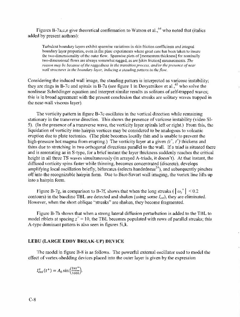
Figures B-7a,c,e give theoretical confirmation to Watson et al.,64 who noted that (italics added by present authors):

Turbulent boundary layers exhibit spanwise variations in skin friction coefficients and integral boundary layer properties, even in flat plate experiments where great care has been taken to insure the two-dimensionality of the outer flow. Spanwise plots of [momentum thickness] for nominally two-dimensional flows are always somewhat ragged, as are [skin friction] measurements. The reason may be because of the raggedness in the transition process, and/or the presence of near wall structures in the boundary layer, inducing a standing pattern in the flow.

Considering the induced wall image, the standing pattern is interpreted as varicose instability; they are rings in B-7c and spirals in B-7a (see figure 1 in Desyatnikov et al.,65 who solve the nonlinear Schrodinger equation and interpret similar results as solitons of self-trapped waves; this is in broad agreement with the present conclusion that streaks are solitary waves trapped in the near-wall viscous layer).

The vorticity pattern in figure B-7c oscillates in the vertical direction while remaining stationary in the transverse direction. This shows the presence of varicose instability (video Sl- 5). (In the presence of a transverse wave, the vorticity layer spirals left or right.) From this, the liquidation of vorticity into hairpin vortices may be considered to be analogous to volcanic eruption due to plate tectonics. (The plate becomes locally thin and is unable to prevent the high-pressure hot magma from erupting.) The vorticity layer at a given fz+, t+) thickens and thins due to stretching in two orthogonal directions parallel to the wall. If a triad is situated there and is resonating as in S-type, for a brief instant the layer thickness suddenly reaches the critical height in all three TS waves simultaneously (in arrayed A-triads, it doesn't). At that instant, the diffused vorticity spins faster while thinning, becomes concentrated (discrete), develops amplifying local oscillation briefly, bifurcates (selects handedness24), and subsequently pinches off into the recognizable hairpin form. Due to Biot-Savart wall imaging, the vortex line lifts up into a hairpin form.

Figure B-7g, in comparison to B-7f, shows that when the long streaks (| ft)z+ | < 0.2

contours) in the baseline TBL are detected and shaken (using some 7^,), they are eliminated. However, when the short oblique "streaks" are shaken, they become fragmented.

Figure B-7h shows that when a strong lateral diffusion perturbation is added to the TBL to model riblets at spacing z+ = 10, the TBL becomes populated with rows of parallel streaks; this A-type dominant pattern is also seen in figures 5i,k.

LEBU (LARGE EDDY BREAK-UP) DEVICE

The model in figure B-8 is as follows. The powerful external oscillator used to model the effect of vortex-shedding devices placed into the outer layer is given by the expression

2ntJr\ ^(t+)=4,sin(HL)

C-8

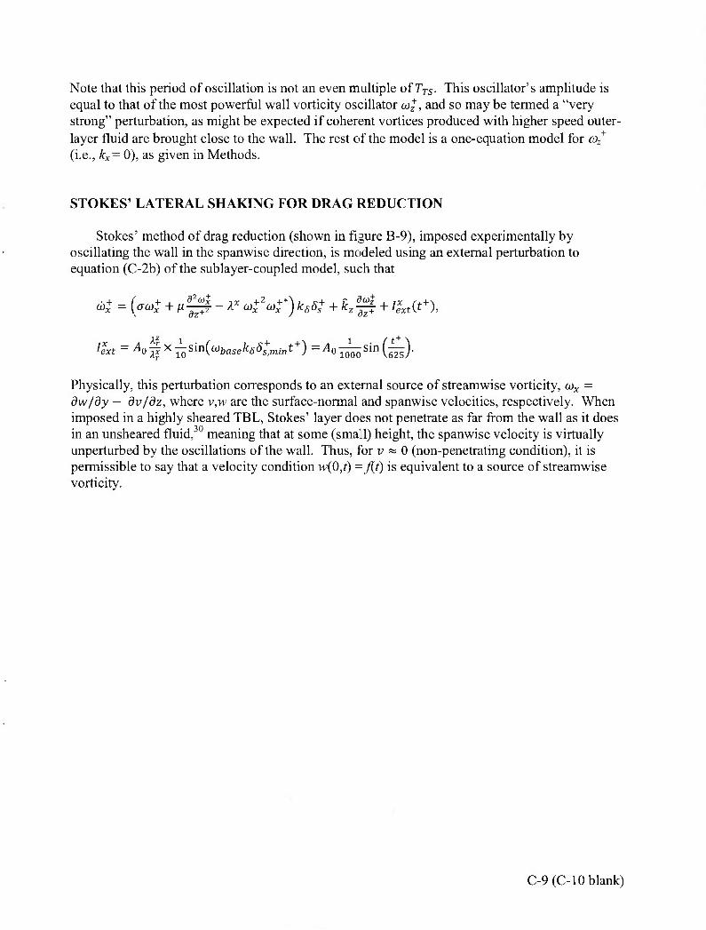
Note that this period of oscillation is not an even multiple ofTTS. This oscillator's amplitude is equal to that of the most powerful wall vorticity oscillator OJ^ , and so may be termed a "very strong" perturbation, as might be expected if coherent vortices produced with higher speed outer- layer fluid are brought close to the wall. The rest of the model is a one-equation model for a)z

+

(i.e., kx= 0), as given in Methods.

STOKES' LATERAL SHAKING FOR DRAG REDUCTION

Stokes' method of drag reduction (shown in figure B-9), imposed experimentally by oscillating the wall in the spanwise direction, is modeled using an external perturbation to equation (C-2b) of the sublayer-coupled model, such that

,,+ _ /'_,.+ , ..s2^ a)x

l^xt = Ao^t * ^sm{a)baseksS+mint+) =^o^sin(^).

Physically, this perturbation corresponds to an external source of streamwise vorticity, cox = dw/dy - dv/dz, where v,w are the surface-normal and spanwise velocities, respectively. When imposed in a highly sheared TBL, Stokes' layer does not penetrate as far from the wall as it does in an unsheared fluid, 0 meaning that at some (small) height, the spanwise velocity is virtually unperturbed by the oscillations of the wall. Thus, for v » 0 (non-penetrating condition), it is permissible to say that a velocity condition w(0,t) =j{t) is equivalent to a source of streamwise vorticity.

C-9(C-10 blank)

REFERENCES

1. V. B. Kazantsev, V. I. Nekorkin, V. I. Makarenko, and R. Llinas, "Self-Referential Phase Reset Based on Inferior Olive Oscillator Dynamics," Proceedings of the National Academy of Sciences, vol. 101,2004, pp. 18183-18188.

2. H. W. Emmons, "The Laminar-Turbulent Transition in a Boundary Layer, Part I," Journal of Aeronautical Sciences, vol. 18, no. 7, 1951, pp 490-498.

3. C. F. Knapp and P. J. Roache, "A Combined Visual and Hot-Wire Anemometer Investigation of Boundary-Layer Transition," AIAA Journal, vol. 6, no. 1, 1968, pp. 29-36.

4. P. S. Klebanoff, K. D. Tidstrom, and L. M. Sargent, "The Three-Dimensional Nature of Boundary-Layer Instability," Jowrao/q/F/wz't/Mec/zaw/c^, vol. 12, no. 1, 1962, pp. 1-34.

5. A. E. Perry, T. T. Lim, and E. W. Teh, "A Visual Study of Turbulent Spots," Journal of Fluid Mechanics, vol. 104, 1981, pp. 387-405.

6. G. S. Raetz, "A New Theory of the Cause of Transition in Fluid Flows," Norair Report NOR-59-383, Hawthorne, California, 1959.

7. T. Herbert, "Secondary Instability of Boundary Layers," Annual Review of Fluid Mechanics, vol. 20, 1988, pp. 487-526.

8. A. A. Townsend, The Structure of Turbulent Shear Flow, Cambridge University Press, New York, 1976.

9. F. R. Hama, J. D. Long, and J. C. Hegarty, "On Transition from Laminar to Turbulent ¥\ow" Journal of Applied Physics, vol. 28, no. 4, 1957, pp. 388-394.

10. S. J. Kline, W. C. Reynolds, F. A. Schraub, and P. W. Runstadler, "The Structure of Turbulent Boundary hdiysrs," Journal of Fluid Mechanics, vol. 30, no. 4, 1967, pp. 741-773.

11. T. Theodorsen, "Mechanism of Turbulence," Proceedings of the 2" Midwestern Conference on Fluid Mechanics, Ohio State University, 1952, pp. 1-18.

12. M. R. Head and P. R. Bandyopadhyay, "New Aspects of Turbulent Boundary Layer Structure," Journal of Fluid Mechanics, vol. 107, 1981, pp. 297-338.

13. C. R. Smith, "Visualisation of Turbulent Boundary Layer Structure Using a Moving Hydrogen Bubble Wire Probe," Workshop on Coherent Structure of Turbulent Boundary Layers, Lehigh University, 1978, p. 48.

14. A. E. Perry and M. S. Chong, "On the Mechanism of Wall Turbulence," Journal of Fluid Mechanics, vol. 119, 1982, pp. 173-217.

R-

15. R. E. Falco, "The Production of Turbulence Near a Wall," AIAA-80-1356, AIAA 13th Fluid and Plasma Dynamics Conference, Snowmass, Colorado, 1980.

16. P. R. Bandyopadhyay, "Large Structure with a Characteristic Upstream Interface in Turbulent Boundary Layers," Physics of Fluids, vol. 23, 1980, pp. 2326-2327.

17. R. J. Adrian, C. D. Meinhart, and C. D. Tomkins, "Vortex Organization in the Outer Region of the Turbulent Boundary Layer," Journal of Fluid Mechanics, vol. 422, 2000, pp. 1-54.

18. G. L. Brown and A. S. W. Thomas, "Large Structure on a Turbulent Boundary Layer," Physics of Fluids, vol. 20, pt. 10, 1977, pp. S243-S252.

19. P. R. Bandyopadhyay and A. K. M. F. Hussain, "The Coupling Between Scales In Shear Flows," Physics of Fluids, vol. 27, no. 9, 1984, pp. 2221-2228.

20. I. Marusic, R. Mathis, and N. Hutchins, "Predictive Model for Wall-Bounded Turbulent Flow," Science, vol. 329 (5988), 2010, pp. 193-196.

21. H. Meinhardt, Models of Biological Pattern Formation, Academic Press, London, 1982.

22. A. M. Turing, "The Chemical Basis Of Morphogenesis," Philosophical Transactions of the Royal Society, vol. B237, 1952, pp. 37-72.

23. P. R. Bandyopadhyay et al. "Synchronization of Animal-Inspired Multiple High-Lift Fins in an Underwater Vehicle Using Olivo-Cerebellar Dynamics," IEEE Journal of Oceanic Engineering, vol. 33, no. 4, 2008, pp. 563-578.

24. P. R. Bandyopadhyay, H. A. Leinhos, and A. M. Helium, "Handedness Helps Homing in Swimming and Flying Animals," Scientific Reports, vol. 3, 2013, article no. 1128, DOI: 10.1038/srep01128.

25. P. R. Bandyopadhyay and J. C. Hansen, "Breakup and Then Makeup: A Predictive Model of How Cilia Self-Regulate Their Hardness for Posture Control," Scientific Reports, vol. 3, 2013, article no. 1956, DOI: 10.1038/srep01956.

26. H. A. Einstein and H. Li, "The Viscous Sublayer Along a Smooth Boundary," Transactions of the American Society of Civil Engineering, vol. 123, no. 1, 1958, pp. 293-313.

27. Z.-C. Liu, R. J. Adrian, and T. J. Hanratty, "A Study of Streaky Structures in a Turbulent Channel Flow with Particle Image Velocimetry," 8th International Symposium on Applications of Laser Techniques to Fluid Mechanics, Lisbon, Portugal, 1996.

R-2

28. V. L. Ginzburg and L. D. Landau, "On the Theory of Superconductivity," Jowrna/o/ Experimental and Theoretical Physics (USSR), vol. 20, 1950, p. 1064.

29. A. T. Popovich and R. L. Hummel, "Experimental Study of the Viscous Sublayer in Turbulent Pipe ¥\ovi" AIChE Journal, vol. 13, no. 5, 1967, pp. 854-860.

30. P. R. Bandyopadhyay, "Stokes' Mechanism of Drag Reduction," Transactions of the ASME Journal of Applied Mechanics, vol. 73, 2006, pp. 483-489.

31. P. Albarede and P. A. Monkewitz, "A Model for the Formation of Oblique Shedding and 'Chevron' Patterns in Cylinder Wakes," Physics of Fluids A, vol. 4, no. 4, 1992, pp. 744- 756.

32. J. B. Forest, "The Wall Pressure Spectrum of High Reynolds Number Rough-Wall Turbulent Boundary Layers," MS Thesis, VP1&SU, Blacksburg, VA, 2012.

33. T. Sewell, "Dermal Denticles of Great White Shark," Electron Microscope Unit, University of Cape Town, Smithsonian Museum of Natural History, http://ocean.si.edu/ocean- photos/biomimicry-shark-denticles, 16 April 1997.

34. E. Laurien and L. Kleiser, "Numerical Simulation of Boundary-Layer Control Transition and Transition Control," Journal of Fluid Mechanics, vol. 199, 1989, pp. 403-440.

35. P. R. Bandyopadhyay, "Turbulence Spot-Like Feature of a Boundary Layer," Annals of the New York Academy of Sciences, vol. 404, no. 1, 1983, pp. 393-395.

36. M. Anderson, "Dermal Denticles of Atlantic Sharpnose Shark Skin," NOAA Teacher at Sea, http://teacheratsea.wordpress.com/tag/dermal-denticles/, 7 August 2011.

37. "Dermal Denticles of Tiger Shark {Galeocerdo cuvier)," http://dermaldenticles.blogspot.com/, 26 February 2009.

38. S. H. Ridgway and D. A. Carder, "Features of Dolphin Skin with Potential Hydrodynamic Importance," IEEE Engineering in Medicine and Biology, vol. 12, no. 3, 1993, pp. 83-88.

39. M. Haider and D. B. Lindsley, "Microvibrations in Man and Dolphin," Science , vol. 146, 1964, pp. 1181-1183.

40. J. Gray, "Studies in Animal Locomotion. VI The Propulsive Power of Dolphins," Journal of Experimental Biology, vol. 13, no. 2, 1936, pp. 192-199.

41. M. O. Kramer, "Boundary Layer Stabilization by Distributed Damping," Journal of the American Society for Naval Engineers, vol. 72, 1960, pp. 25-33.

R-3

42. A. M. Savill and J. C. Mumford, "Manipulation of Turbulent Boundary Layers by Outer- Layer Devices: Skin-Friction and Flow-Visualization Results," Journal of Fluid Mechanics, vol. 191, 1988, pp. 389-418.

43. K.-S. Choi, J.-R. DeBisschop, and B. R. Clayton, "Turbulent Boundary-Layer Control by Means of Spanwise-Wall Oscillation," AIAA Journal, vol. 36, no. 7, 1998, pp. 1157-1163.

44. W. R. C. Phillips, "On a Class of Unsteady Boundary Layers of Finite Extent," Journal of Fluid Mechanics, vol. 319, 1996, pp. 151-170.

45. E. M. Izhikevich, "Neural Excitability, Spiking and Bursting," International Journal of Bifurcation and Chaos, vol. 10, no. 6, 2000, pp. 1171-1266.

46. A. A. Tsonis and J. B. Eisner, "The Weather Attractor Over Very Short-Time Scales. Nature, vol. 333, 1988, pp. 545-547.

47.1. Procaccia, "Complex or Just Complicated?," Nature, vol. 333, 1988, pp. 498-499.

48. J. T. Stuart, "On the Non-Linear Mechanics of Disturbances in Parallel Flows, Part 1. The Basic Behavior in Plane Poiseuille Flow," Journal of Fluid Mechanics, vol. 9, no. 3, 1960, pp. 353-370.

49. J. Watson, "On the Non-Linear Mechanics of Disturbances in Parallel Flows, Part 2. The Development of a Solution for Plane Poiseuille Flow and for Plane Couette Flow," Journal of Fluid Mechanics, vol. 9, no. 3, 1960, pp. 371-389.

50. B. R. Noack, F. Ohle, and H. Eckelmann, "On Cell Formation in Vortex Streets," Journal of Fluid Mechanics, vol. 227, 1991, pp. 293-308.

51. P. H. Alfredsson, A. V. Johansson, J. H. Haritonidis, and H. Eckelmann, "The Fluctuating Wall-Shear Stress and the Velocity Field in the Viscous Sublayer," Physics of Fluids, vol. 31, no. 5, 1988, pp. 1026-1033.

52. T. J. Black, "An Analytical Study of the Measured Wall Pressure Field Under Supersonic Turbulent Boundary Layers," NASA-CR 888, National Aeronautics and Space Administration, 1968.

53. K.-S. Choi, "Near-Wall Structure of a Turbulent Boundary Layer with Riblets," Journal of Fluid Mechanics, vol. 208, 1989, pp. 417-458.

54. Y. Du and G. E. Kamiadakis, "Suppressing Wall Turbulence by Means of a Transverse Traveling Wave," Science, vol. 288, 2000, pp. 1230-1234.

R-4

55. http://demeliou.wordpress.com/2013/03/26/rodents-friend-foe-and-laboratory-subject/.

56. http://3.bp.blogspot.com/_oxTtTxAI5IA/SlyhTZeL2FI/AAAAAAAAACY/F42ZfQwEvgY/sl6 O0-h/rough-seas.jpg .

57. http://wallippo.com/wallpaper/swirling-waves-on-shore-5d2fcl344d3fc89848994bbl80780b57 .

58. H. Schlichting, Boundary-Layer Theory, McGraw-Hill, New York, 1979.

59. P. R. Bandyopadhyay, "A Low Dimensional Structural Model of a Turbulent Boundary Layer Separating Intermittently in Space," NUWC-NPT Technical Report 10,400. Naval Undersea Warfare Center Division, Newport, RI; also in Separated and Complex Flows - 1995, Proceedings of the ASME/JSME Fluids Engineering Conference and Exhibition, Hilton Head, SC, 13-18 August 2006, pp. 75-82.

60. G. Haller, "Exact Theory of Unsteady Separation for Two-Dimensional Flows," Journal of Fluid Mechanics, vol. 512, 2004, pp. 257-311.

61. P. R. Bandyopadhyay, D. N. Beal, J. D. Hrubes, and A. Mangalam, "Relationship of Roll and Pitch Oscillations in a Fin Flapping at Transitional to High Reynolds Numbers," Journal of Fluid Mechanics, vol. 702, 2012, pp. 298-331.

62. S.-J. Lee and S.-H. Lee, "Flow Field Analysis of Turbulent Boundary Layer over a Riblet Surface," Experiments in Fluids, vol. 30, 2001, pp. 153-166.

63. W. R. C. Phillips, "The Instability of Finite Amplitude Waves in Strong Viscid and Inviscid Shear," in Mathematical Modeling and Simulation in Hydrodynamic Stability, D. N. Riahi, ed.. World Scientific, Singapore, 1996.

64. R. D. Watson, J. B. Anders, and R. M. Hall, "Skin Friction at Very High Reynolds Numbers in the National Transonic Facility," NASA/TP-2006-214497, 2006.

65. A. S. Desyatnikov, D. Buccoliero, M. R. Dennis, and Y. S. Kivshar, "Spontaneous Knotting of Self-Trapped Waves," Scientific Reports, vol. 2, 2012, article no. 771, DOI: I0.1038srep00771.

R-5 (R-6 blank)

NUWC-NPT Technical Report 12,154

INITIAL DISTRIBUTION LIST

Addressee

OASN(FM&C) (Attn: J.C.S. Meng)

Office of Naval Research (ONR-32—T. Swean; ONR-33—T. McMullen, K.-H. Kim, R. Joslin; ONR-34—T. Allard; ONR-341—T. McKenna, J. Tangney)

NSWC Carderock (Attn: T. Farabee (1), Library (1))

NSWC Panama City (Attn: Library)

Space and Naval Warfare Systems Command (Attn: Library)

Space and Naval Warfare Systems Center, San Diego (Attn: J. Rohr)

Naval Research Laboratory (Attn: Library)

Defense Advanced Research Projects Agency (Attn: Library)

NASA Langley Research Center (Attn: Library)

Electric Boat Corporation, Groton (Attn: Library)

The Charles Stark Draper Laboratory, Cambridge, MA (Attn: Library)

Pennsylvania State University, Applied Research Laboratory (Attn: Library)

Massachusetts Institute of Technology (Attn: Library)

University of Rhode Island (Attn: Library)

Brown University Library (Attn: Library)

Defense Technical Information Center

Center for Naval Analyses

No. of Copies

1

7

2

1