1

Data Preparation and Preliminary Trails with TURINA

--TURkey’s INterindustry Analysis Model

Ozhan Gazi (European University of Lefke) Wang Yinchu (China Economic Information Network of the State Information Center)

Ozhan Meral (European University of Lefke)

To be presented at 18th INFORUM World Conference

September 5th – 12th, 2010 Hikone, Japan

2

INFORUM has had her Turkish researcher on Inter-industry model since 1994 when Gazi Özhan visited University of Maryland of College Park as a visiting scholar. The 16th INFORUM international conference was held in 2008 in the European University of Lefke, North Cyprus. Prior to that conference, in the summer of 2008, Paul Salmon, University of Rennes in France and Gazi Özhan, European University of Lefke, cooperated together and worked out an INFORUM Turkey Model Version 1.0, called TinyTurk. In that version of the model, the 2002 Input-output table of Turkey and the time series of GDP by expenditure are used and there are 59 sectors in the model. The model has one vector equation which is that the intermediate output plus final demand is equal to the gross output. This first version of the model was presented in the 16th INFORUM International Conference (Salmon and Özhan, 2008).

From the middle of May to the middle of June of 2010, Wang was invited to go to North Cyprus for cooperation research to do further work on the INFORUM Turkey model. This paper is an overview of that one month work.

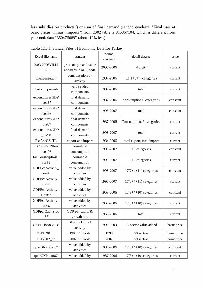
The study is organized in six sections. Section 1 describes the general data situation required for the model. The framework of this section is basically inspired by the work of Shantong and Wang (1999). In this section some consistency checks are carried out for main macroeconomic data series. In Section 2 an extensive adjustment analysis is performed on the Input-output tables, namely 1998 and 2010 IO tables. Section 3 describes the treatment of the inconsistencies between IO tables and National Income Accounts. Section 4 introduces the preparation of time series vector data to be used in the model. The framework of the model is presented in Section 5. Finally, Section 6 concludes the study. 1. Data Situation The availability of the data for building a model is always the first priority issue. There are 22 excel files which contain different or duplicate data. Their content, period covered and detail degree and so on are listed in Table1.1. In addition to these excel files, there is a PDF file which is an electronic copy of the book “Statistical Indicators, 1923 - 2008” published by Turkish Statistical Institute in December of 2009.

After looking at all of these files carefully and doing some comparison on data, three points are noticed. They are: (A) There is Input-output table for 1998 (TurkStat, 2010a); (B) Some relatively detail sector classification time series started from 1998 (TurkStat, 2010c); (C) Most economic statistics end at 2008; From them, 1998-2008 is considered as the sample period of the INFORUM Turkey model version 2.0. In the meantime, some problems in data aspect are noticed, too. These problems are: (A). The sector 30 (recycling materials) is blank in 1998 IO table. Sector 6 (Uranium and thorium ores) is blank in 1998 and 2002 tables (TurkStat, 2010b). (B). The sum of value added (third quadrant, “Value added at basic price” plus “Taxes

3

less subsidies on products”) or sum of final demand (second quadrant, “Final uses at basic prices” minus “imports”) from 2002 table is 315867104, which is different from yearbook data “350476089” (about 10% less). Table 1.1. The Excel Files of Economic Data for Turkey

Excel file name content period

covered detail degree price

2003-2006YILLIK

gross output and value added by NACE code

2003-2006 4 digits current

Compensation compensation by

activity 1987-2006 11(1+3+7) categories current

Cost components value added components

1987-2006 total current

expendituresGDP_con87

final demand components

1987-2006 consumption 6 categories constant

expendituresGDP_con98

final demand components

1998-2007 total constant

expendituresGDP_cur87

final demand components

1987-2006 Consumption, 6 categories current

expendituresGDP_cur98

final demand components

1998-2007 total current

ExtAccGS_TL export and import 1984-2006 total export, total import current FinConsExpNResi

_con98 household

consumption 1998-2007 10 categories constant

FinConsExpResi_cur98

household consumption

1998-2007 10 categories current

GDPEcoActivity_con98

value added by activities

1998-2007 17(2+4+11) categories constant

GDPEcoActivity_cur98

value added by activities

1998-2007 17(2+4+11) categories current

GDPEcoActivity_Con87

value added by activities

1968-2006 17(3+4+10) categories constant

GDPEcoActivity_Cur87

value added by activities

1968-2006 17(3+4+10) categories current

GDPperCapita_cur87

GDP per capita & growth rate

1968-2006 total current

GSYH 1998-2008 GDP by kind of

activity 1998-2009 17 sector value added basic price

IOT1998_bp 1998 IO Table 1998 59 sectors basic price IOT2002_bp 2002 IO Table 2002 59 sectors basic price

quarGNP_con87 value added by

activities 1987-2006 17(3+4+10) categories constant

quarGNP_cur87 value added by 1987-2006 17(3+4+10) categories current

4

activities

TEFE 1994-2009 Wholesale price index 1994-2009 37 categories

UFE2003-2009 Monthly producer

price index 2003-2009 37 categories

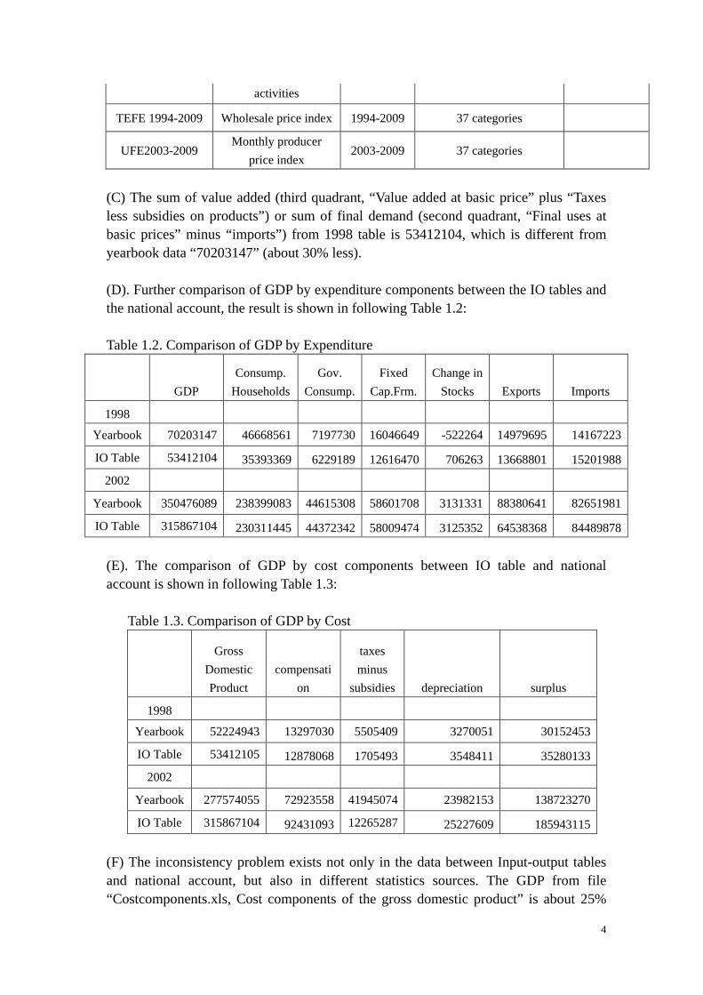
(C) The sum of value added (third quadrant, “Value added at basic price” plus “Taxes less subsidies on products”) or sum of final demand (second quadrant, “Final uses at basic prices” minus “imports”) from 1998 table is 53412104, which is different from yearbook data “70203147” (about 30% less). (D). Further comparison of GDP by expenditure components between the IO tables and the national account, the result is shown in following Table 1.2: Table 1.2. Comparison of GDP by Expenditure

GDP

Consump. Households

Gov. Consump.

Fixed Cap.Frm.

Change in Stocks Exports Imports

1998

Yearbook 70203147 46668561 7197730 16046649 -522264 14979695 14167223

IO Table 53412104 35393369 6229189 12616470 706263 13668801 15201988

2002

Yearbook 350476089 238399083 44615308 58601708 3131331 88380641 82651981

IO Table 315867104 230311445 44372342 58009474 3125352 64538368 84489878 (E). The comparison of GDP by cost components between IO table and national account is shown in following Table 1.3:

Table 1.3. Comparison of GDP by Cost

Gross

Domestic Product

compensation

taxes minus

subsidies depreciation surplus

1998

Yearbook 52224943 13297030 5505409 3270051 30152453

IO Table 53412105 12878068 1705493 3548411 35280133

2002

Yearbook 277574055 72923558 41945074 23982153 138723270

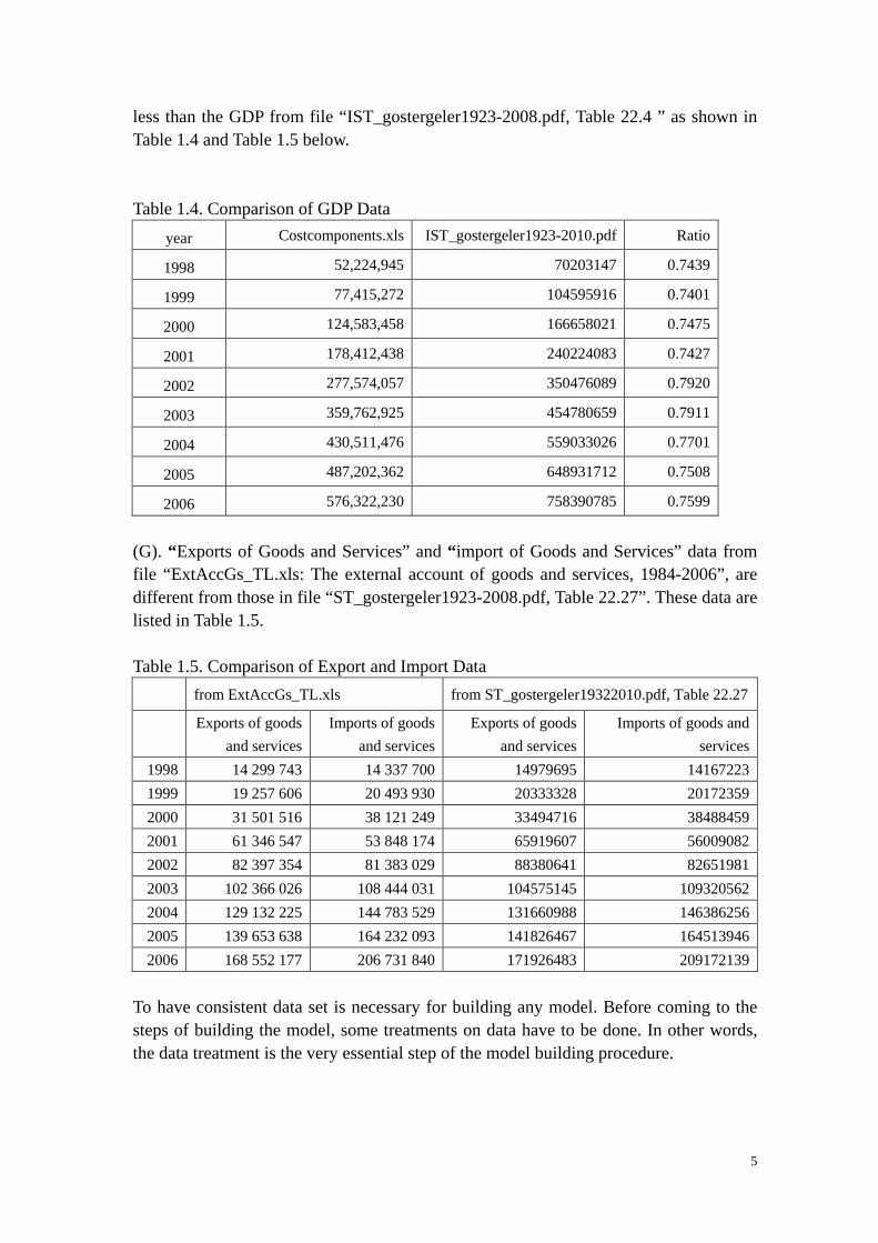
IO Table 315867104 92431093 12265287 25227609 185943115 (F) The inconsistency problem exists not only in the data between Input-output tables and national account, but also in different statistics sources. The GDP from file “Costcomponents.xls, Cost components of the gross domestic product” is about 25%

5

less than the GDP from file “IST_gostergeler1923-2008.pdf, Table 22.4 ” as shown in Table 1.4 and Table 1.5 below. Table 1.4. Comparison of GDP Data

year Costcomponents.xls IST_gostergeler1923-2010.pdf Ratio

1998 52,224,945 70203147 0.7439

1999 77,415,272 104595916 0.7401

2000 124,583,458 166658021 0.7475

2001 178,412,438 240224083 0.7427

2002 277,574,057 350476089 0.7920

2003 359,762,925 454780659 0.7911

2004 430,511,476 559033026 0.7701

2005 487,202,362 648931712 0.7508

2006 576,322,230 758390785 0.7599

(G). “Exports of Goods and Services” and “import of Goods and Services” data from file “ExtAccGs_TL.xls: The external account of goods and services, 1984-2006”, are different from those in file “ST_gostergeler1923-2008.pdf, Table 22.27”. These data are listed in Table 1.5. Table 1.5. Comparison of Export and Import Data from ExtAccGs_TL.xls from ST_gostergeler19322010.pdf, Table 22.27

Exports of goods

and services Imports of goods

and services Exports of goods

and services Imports of goods and

services 1998 14 299 743 14 337 700 14979695 14167223 1999 19 257 606 20 493 930 20333328 20172359 2000 31 501 516 38 121 249 33494716 38488459 2001 61 346 547 53 848 174 65919607 56009082 2002 82 397 354 81 383 029 88380641 82651981 2003 102 366 026 108 444 031 104575145 109320562 2004 129 132 225 144 783 529 131660988 146386256 2005 139 653 638 164 232 093 141826467 164513946 2006 168 552 177 206 731 840 171926483 209172139

To have consistent data set is necessary for building any model. Before coming to the steps of building the model, some treatments on data have to be done. In other words, the data treatment is the very essential step of the model building procedure.

6

2. The Initial Adjustments on the Input-output Tables Although lots of data adjustment work will be done later in related data preparation step, some initial treatment has to be done first, especially for the Input-output tables (Wang, 1998).

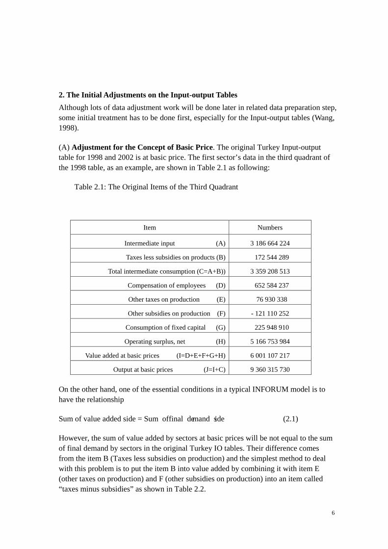
(A) Adjustment for the Concept of Basic Price. The original Turkey Input-output table for 1998 and 2002 is at basic price. The first sector’s data in the third quadrant of the 1998 table, as an example, are shown in Table 2.1 as following:

Table 2.1: The Original Items of the Third Quadrant

Item Numbers

Intermediate input (A) 3 186 664 224

Taxes less subsidies on products (B) 172 544 289

Total intermediate consumption (C=A+B)) 3 359 208 513

Compensation of employees (D) 652 584 237

Other taxes on production (E) 76 930 338

Other subsidies on production (F) - 121 110 252

Consumption of fixed capital (G) 225 948 910

Operating surplus, net (H) 5 166 753 984

Value added at basic prices (I=D+E+F+G+H) 6 001 107 217

Output at basic prices (J=I+C) 9 360 315 730

On the other hand, one of the essential conditions in a typical INFORUM model is to have the relationship

Sum of value added side = Sum of final demand side (2.1)

However, the sum of value added by sectors at basic prices will be not equal to the sum of final demand by sectors in the original Turkey IO tables. Their difference comes from the item B (Taxes less subsidies on production) and the simplest method to deal with this problem is to put the item B into value added by combining it with item E (other taxes on production) and F (other subsidies on production) into an item called “taxes minus subsidies” as shown in Table 2.2.

7

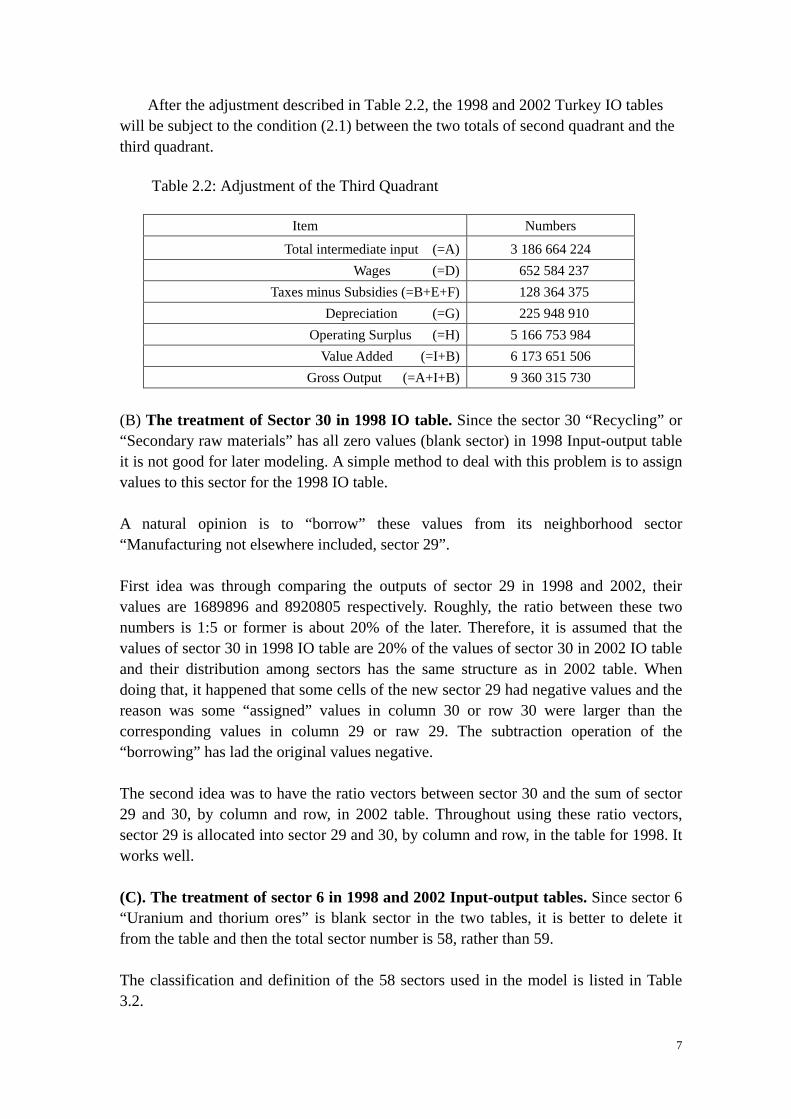
After the adjustment described in Table 2.2, the 1998 and 2002 Turkey IO tables will be subject to the condition (2.1) between the two totals of second quadrant and the third quadrant.

Table 2.2: Adjustment of the Third Quadrant

Item Numbers

Total intermediate input (=A) 3 186 664 224 Wages (=D) 652 584 237

Taxes minus Subsidies (=B+E+F) 128 364 375 Depreciation (=G) 225 948 910

Operating Surplus (=H) 5 166 753 984 Value Added (=I+B) 6 173 651 506

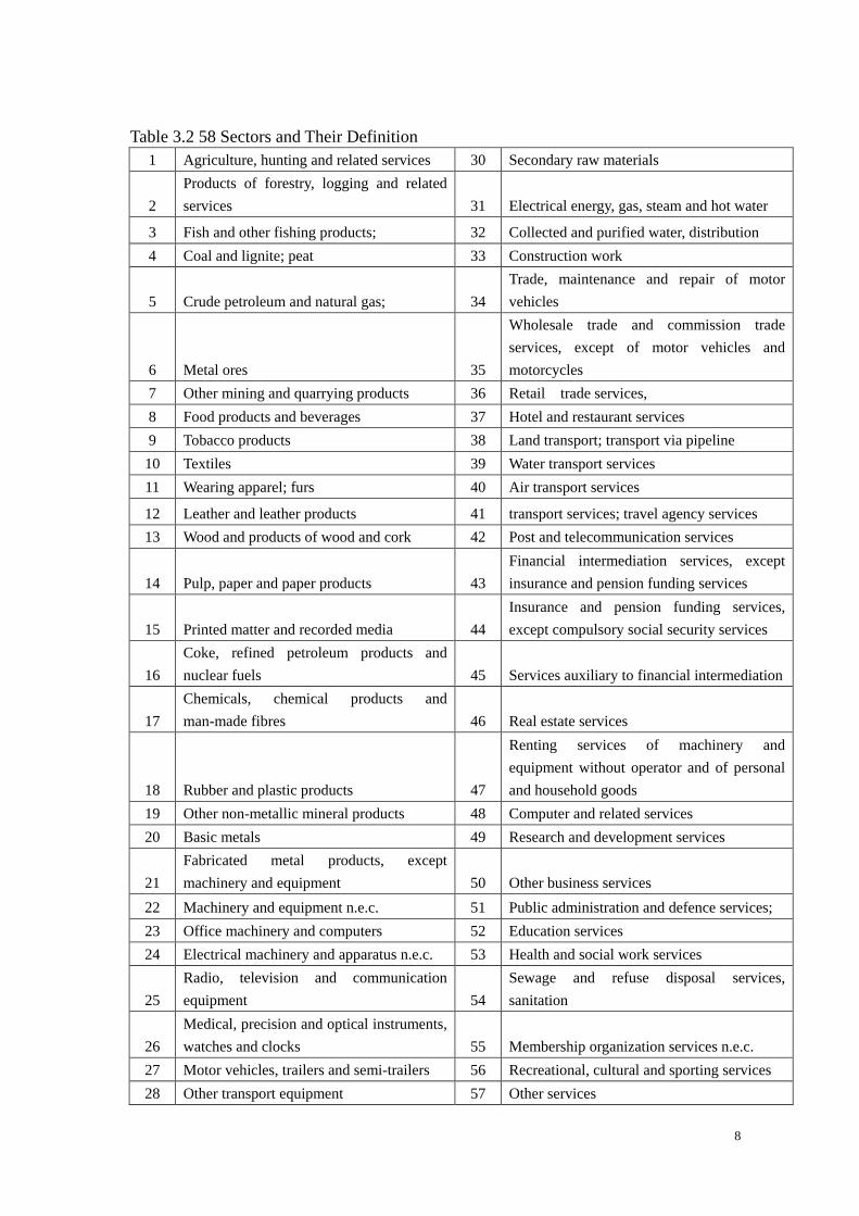
Gross Output (=A+I+B) 9 360 315 730 (B) The treatment of Sector 30 in 1998 IO table. Since the sector 30 “Recycling” or “Secondary raw materials” has all zero values (blank sector) in 1998 Input-output table it is not good for later modeling. A simple method to deal with this problem is to assign values to this sector for the 1998 IO table. A natural opinion is to “borrow” these values from its neighborhood sector “Manufacturing not elsewhere included, sector 29”. First idea was through comparing the outputs of sector 29 in 1998 and 2002, their values are 1689896 and 8920805 respectively. Roughly, the ratio between these two numbers is 1:5 or former is about 20% of the later. Therefore, it is assumed that the values of sector 30 in 1998 IO table are 20% of the values of sector 30 in 2002 IO table and their distribution among sectors has the same structure as in 2002 table. When doing that, it happened that some cells of the new sector 29 had negative values and the reason was some “assigned” values in column 30 or row 30 were larger than the corresponding values in column 29 or raw 29. The subtraction operation of the “borrowing” has lad the original values negative. The second idea was to have the ratio vectors between sector 30 and the sum of sector 29 and 30, by column and row, in 2002 table. Throughout using these ratio vectors, sector 29 is allocated into sector 29 and 30, by column and row, in the table for 1998. It works well. (C). The treatment of sector 6 in 1998 and 2002 Input-output tables. Since sector 6 “Uranium and thorium ores” is blank sector in the two tables, it is better to delete it from the table and then the total sector number is 58, rather than 59. The classification and definition of the 58 sectors used in the model is listed in Table 3.2.

8

Table 3.2 58 Sectors and Their Definition

1 Agriculture, hunting and related services 30 Secondary raw materials

2 Products of forestry, logging and related services 31 Electrical energy, gas, steam and hot water

3 Fish and other fishing products; 32 Collected and purified water, distribution 4 Coal and lignite; peat 33 Construction work

5 Crude petroleum and natural gas; 34 Trade, maintenance and repair of motor vehicles

6 Metal ores 35

Wholesale trade and commission trade services, except of motor vehicles and motorcycles

7 Other mining and quarrying products 36 Retail trade services, 8 Food products and beverages 37 Hotel and restaurant services 9 Tobacco products 38 Land transport; transport via pipeline

10 Textiles 39 Water transport services 11 Wearing apparel; furs 40 Air transport services

12 Leather and leather products 41 transport services; travel agency services 13 Wood and products of wood and cork 42 Post and telecommunication services

14 Pulp, paper and paper products 43 Financial intermediation services, except insurance and pension funding services

15 Printed matter and recorded media 44 Insurance and pension funding services, except compulsory social security services

16 Coke, refined petroleum products and nuclear fuels 45 Services auxiliary to financial intermediation

17 Chemicals, chemical products and man-made fibres 46 Real estate services

18 Rubber and plastic products 47

Renting services of machinery and equipment without operator and of personal and household goods

19 Other non-metallic mineral products 48 Computer and related services 20 Basic metals 49 Research and development services

21 Fabricated metal products, except machinery and equipment 50 Other business services

22 Machinery and equipment n.e.c. 51 Public administration and defence services; 23 Office machinery and computers 52 Education services 24 Electrical machinery and apparatus n.e.c. 53 Health and social work services

25 Radio, television and communication equipment 54

Sewage and refuse disposal services, sanitation

26 Medical, precision and optical instruments, watches and clocks 55 Membership organization services n.e.c.

27 Motor vehicles, trailers and semi-trailers 56 Recreational, cultural and sporting services 28 Other transport equipment 57 Other services

9

29 Furniture; other manufactured goods n.e.c. 58 Private households with employed persons

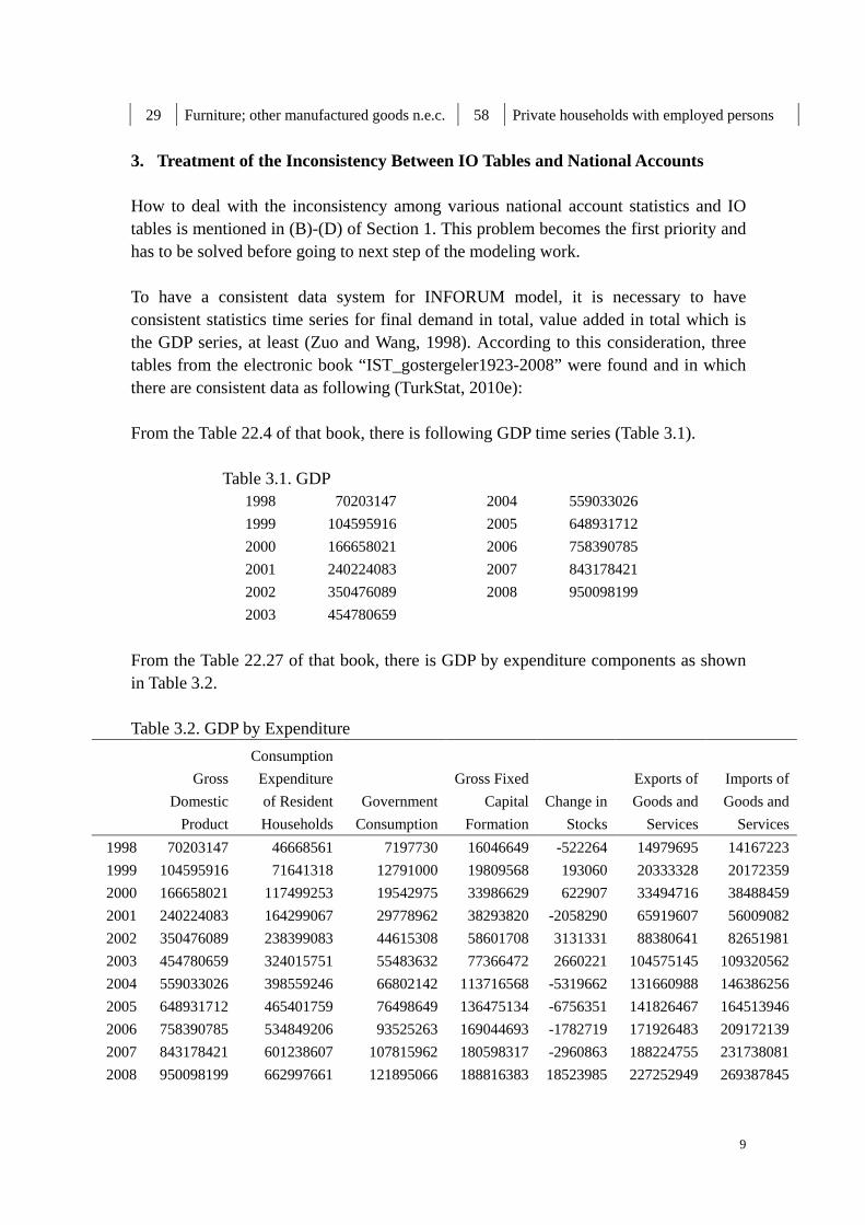
3. Treatment of the Inconsistency Between IO Tables and National Accounts How to deal with the inconsistency among various national account statistics and IO tables is mentioned in (B)-(D) of Section 1. This problem becomes the first priority and has to be solved before going to next step of the modeling work. To have a consistent data system for INFORUM model, it is necessary to have consistent statistics time series for final demand in total, value added in total which is the GDP series, at least (Zuo and Wang, 1998). According to this consideration, three tables from the electronic book “IST_gostergeler1923-2008” were found and in which there are consistent data as following (TurkStat, 2010e): From the Table 22.4 of that book, there is following GDP time series (Table 3.1). Table 3.1. GDP

1998 70203147 2004 559033026 1999 104595916 2005 648931712 2000 166658021 2006 758390785 2001 240224083 2007 843178421 2002 350476089 2008 950098199 2003 454780659

From the Table 22.27 of that book, there is GDP by expenditure components as shown in Table 3.2. Table 3.2. GDP by Expenditure

Gross

Domestic Product

Consumption Expenditure of Resident Households

Government Consumption

Gross Fixed Capital

Formation

Change in

Stocks

Exports of Goods and

Services

Imports of Goods and

Services 1998 70203147 46668561 7197730 16046649 -522264 14979695 14167223 1999 104595916 71641318 12791000 19809568 193060 20333328 20172359 2000 166658021 117499253 19542975 33986629 622907 33494716 38488459 2001 240224083 164299067 29778962 38293820 -2058290 65919607 56009082 2002 350476089 238399083 44615308 58601708 3131331 88380641 82651981 2003 454780659 324015751 55483632 77366472 2660221 104575145 109320562 2004 559033026 398559246 66802142 113716568 -5319662 131660988 146386256 2005 648931712 465401759 76498649 136475134 -6756351 141826467 164513946 2006 758390785 534849206 93525263 169044693 -1782719 171926483 209172139 2007 843178421 601238607 107815962 180598317 -2960863 188224755 231738081 2008 950098199 662997661 121895066 188816383 18523985 227252949 269387845

10

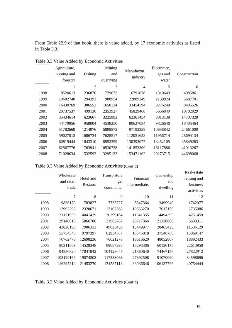
From Table 22.9 of that book, there is value added, by 17 economic activities as listed in Table 3.3. Table 3.3 Value Added by Economic Activities

Agriculture, hunting and

forestry Fishing

Mining and

quarrying

Manufactur. industry

Electricity, gas and

water Construction

1 2 3 4 5 6 1998 8520613 236870 729072 16791078 1310649 4085861 1999 10682740 294393 988954 22889249 2139824 5687701 2000 16430769 386553 1658124 33454594 3276249 8405526 2001 20737537 499136 2353927 45829468 5656849 10702029 2002 35434614 623667 3225992 62361454 8013139 14707329 2003 44179956 958004 4538250 80627034 9826640 18405464 2004 51782669 1214976 5898572 97193358 10658842 24661000 2005 59027013 1686734 7628517 112051658 11956714 28694134 2006 60819444 1843310 8952359 130393077 13452105 35849263 2007 62567776 1763941 10530738 141853309 16117886 41013267 2008 71028634 1532592 13295133 153471162 20273715 44698068

Table 3.3 Value Added by Economic Activities (Cont’d)

Wholesale and retail

trade

Hotel and Restaur.

Transp.storage,

communic.

Financial intermediate.

Ownership and

dwelling

Real-estate renting and

business activities

7 8 9 10 11 12 1998 9836179 1783827 7735727 5347364 3499949 1742077 1999 12992298 2320671 12102368 10663270 7617159 2735086 2000 21121955 4041429 20299164 11641355 14494393 4251459 2001 29140019 5866786 31963787 20717364 21130606 6693311 2002 42820198 7986333 49025450 15449977 28465425 11536129 2003 55754340 9797397 62934587 15545818 37546758 15069147 2004 70762478 12698236 76021278 18616620 48052807 18892433 2005 80211869 14528348 89087295 18293386 60120175 22613950 2006 94856320 17041942 104123045 21860640 74467156 27822912 2007 103129169 19074202 117583068 27392508 91070060 34598696 2008 116295314 21453270 134587118 33036646 106137796 40754444

Table 3.3 Value Added by Economic Activities (Cont’d)

11

Public administration

Education Health and

social work

Other community,

social and person service

Private household

with employed

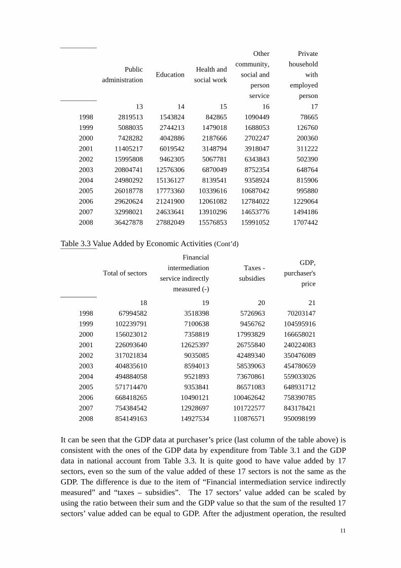
person 13 14 15 16 17 1998 2819513 1543824 842865 1090449 78665 1999 5088035 2744213 1479018 1688053 126760 2000 7428282 4042886 2187666 2702247 200360 2001 11405217 6019542 3148794 3918047 311222 2002 15995808 9462305 5067781 6343843 502390 2003 20804741 12576306 6870049 8752354 648764 2004 24980292 15136127 8139541 9358924 815906 2005 26018778 17773360 10339616 10687042 995880 2006 29620624 21241900 12061082 12784022 1229064 2007 32998021 24633641 13910296 14653776 1494186 2008 36427878 27882049 15576853 15991052 1707442

Table 3.3 Value Added by Economic Activities (Cont’d)

Total of sectors

Financial intermediation

service indirectly measured (-)

Taxes - subsidies

GDP, purchaser's

price

18 19 20 21 1998 67994582 3518398 5726963 70203147 1999 102239791 7100638 9456762 104595916 2000 156023012 7358819 17993829 166658021 2001 226093640 12625397 26755840 240224083 2002 317021834 9035085 42489340 350476089 2003 404835610 8594013 58539063 454780659 2004 494884058 9521893 73670861 559033026 2005 571714470 9353841 86571083 648931712 2006 668418265 10490121 100462642 758390785 2007 754384542 12928697 101722577 843178421 2008 854149163 14927534 110876571 950098199

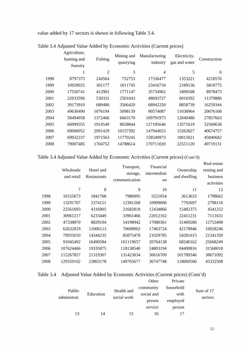
It can be seen that the GDP data at purchaser’s price (last column of the table above) is consistent with the ones of the GDP data by expenditure from Table 3.1 and the GDP data in national account from Table 3.3. It is quite good to have value added by 17 sectors, even so the sum of the value added of these 17 sectors is not the same as the GDP. The difference is due to the item of “Financial intermediation service indirectly measured” and “taxes – subsidies”. The 17 sectors’ value added can be scaled by using the ratio between their sum and the GDP value so that the sum of the resulted 17 sectors’ value added can be equal to GDP. After the adjustment operation, the resulted

12

value added by 17 sectors is shown in following Table 3.4. Table 3.4 Adjusted Value Added by Economic Activities (Current prices)

Agriculture, hunting and

forestry Fishing

Mining and quarrying

Manufacturing industry

Electricity, gas and water

Construction

1 2 3 4 5 6 1998 8797375 244564 752753 17336477 1353221 4218576 1999 10928925 301177 1011745 23416734 2189136 5818775 2000 17550741 412902 1771147 35734962 3499568 8978473 2001 22033596 530331 2501043 48693727 6010392 11370886 2002 39173910 689480 3566420 68942250 8858739 16259344 2003 49630490 1076194 5098139 90574087 11038964 20676168 2004 58494958 1372466 6663170 109791973 12040486 27857663 2005 66999355 1914549 8658844 127185646 13571619 32569638 2006 69006052 2091429 10157392 147944653 15262827 40674757 2007 69932237 1971563 11770245 158549973 18015021 45840682 2008 79007485 1704752 14788614 170711020 22551120 49719131

Table 3.4 Adjusted Value Added by Economic Activities (Current prices) (Cont’d)

Wholesale and retail

Hotel and Restaurants

Transport, storage,

communication

Financial intermediati

on

Ownership and dwelling

Real-estate renting and

business activities

7 8 9 10 11 12 1998 10155673 1841768 7986995 5521054 3613633 1798662 1999 13291707 2374151 12381268 10909006 7792697 2798116 2000 22561693 4316905 21682818 12434866 15482375 4541252 2001 30961217 6233449 33961466 22012162 22451231 7111631 2002 47338870 8829104 54198942 17080361 31469286 12753498 2003 62632819 11006113 70698902 17463724 42178946 16928246 2004 79935010 14344235 85875478 21029785 54281615 21341350 2005 91045492 16490584 101119657 20764138 68240162 25668249 2006 107624466 19335875 118138540 24803194 84490816 31568018 2007 115267857 21319307 131423034 30616709 101789346 38671092 2008 129359102 23863178 149705677 36747748 118060560 45332508

Table 3.4 Adjusted Value Added by Economic Activities (Current prices) (Cont’d)

Public

administrat. Education

Health and social work

Other community

social and person service

Private household

with employed

person

Sum of 17 sectors

13 14 15 16 17

13

1998 2911095 1593970 870243 1125868 81220 70203147 1999 5205289 2807454 1513102 1726954 129681 104595917 2000 7934617 4318462 2336784 2886440 214017 166658020 2001 12118022 6395752 3345588 4162918 330673 240224084 2002 17683792 10460830 5602567 7013288 555406 350476089 2003 23371447 14127860 7717615 9832142 728803 454780658 2004 28218343 17098136 9194623 10572067 921667 559033027 2005 29532942 20173876 11736111 12130462 1130386 648931711 2006 33607712 24101168 13684565 14504817 1394502 758390785 2007 36882011 27533113 15547590 16378580 1670057 843178419 2008 40519926 31014120 17326646 17787373 1899244 950098202

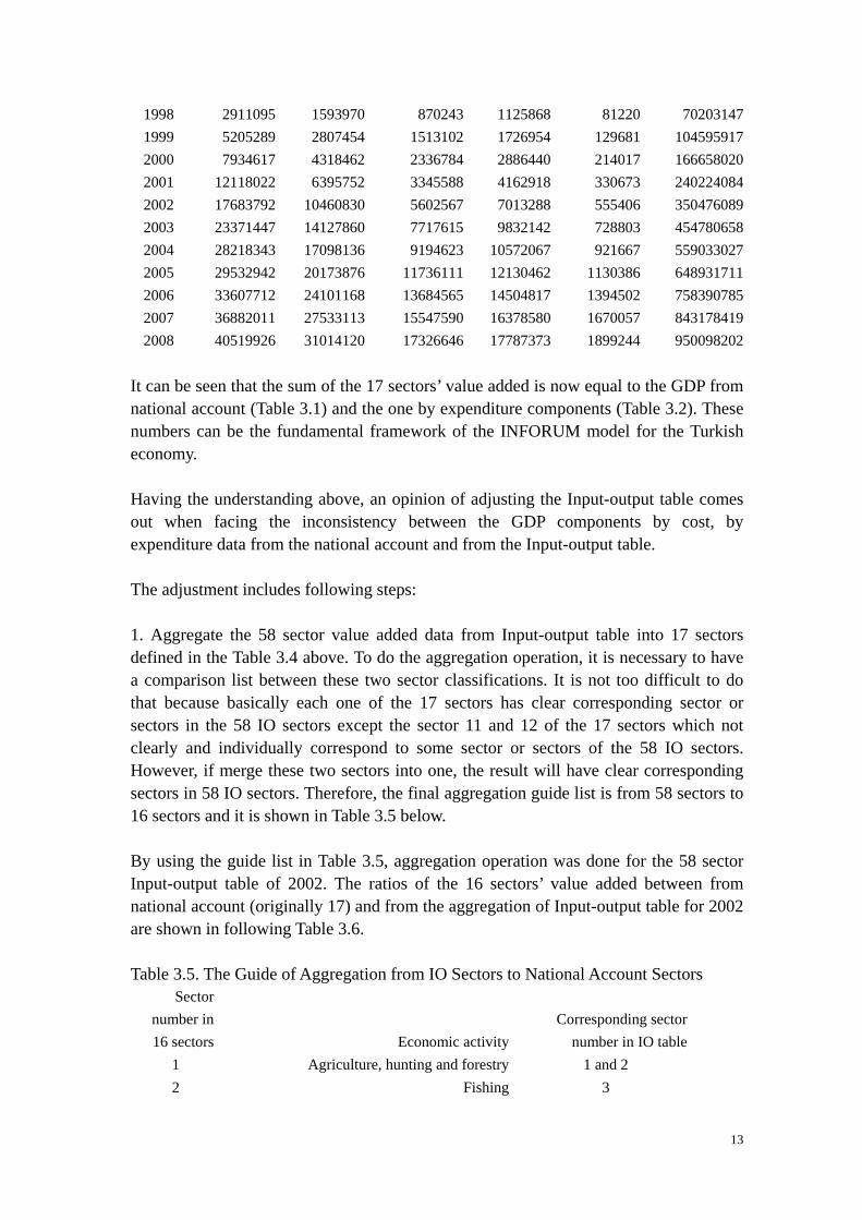
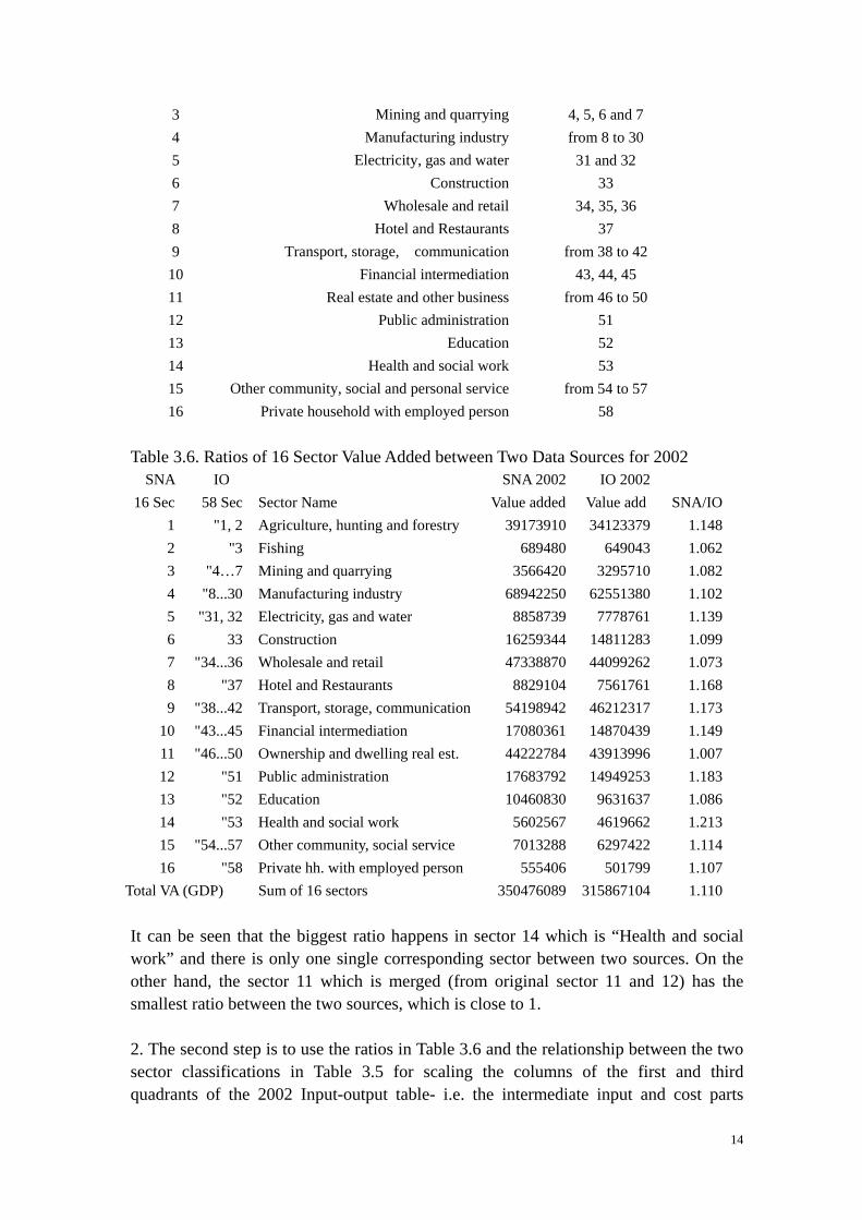
It can be seen that the sum of the 17 sectors’ value added is now equal to the GDP from national account (Table 3.1) and the one by expenditure components (Table 3.2). These numbers can be the fundamental framework of the INFORUM model for the Turkish economy. Having the understanding above, an opinion of adjusting the Input-output table comes out when facing the inconsistency between the GDP components by cost, by expenditure data from the national account and from the Input-output table. The adjustment includes following steps: 1. Aggregate the 58 sector value added data from Input-output table into 17 sectors defined in the Table 3.4 above. To do the aggregation operation, it is necessary to have a comparison list between these two sector classifications. It is not too difficult to do that because basically each one of the 17 sectors has clear corresponding sector or sectors in the 58 IO sectors except the sector 11 and 12 of the 17 sectors which not clearly and individually correspond to some sector or sectors of the 58 IO sectors. However, if merge these two sectors into one, the result will have clear corresponding sectors in 58 IO sectors. Therefore, the final aggregation guide list is from 58 sectors to 16 sectors and it is shown in Table 3.5 below. By using the guide list in Table 3.5, aggregation operation was done for the 58 sector Input-output table of 2002. The ratios of the 16 sectors’ value added between from national account (originally 17) and from the aggregation of Input-output table for 2002 are shown in following Table 3.6. Table 3.5. The Guide of Aggregation from IO Sectors to National Account Sectors

Sector number in 16 sectors Economic activity

Corresponding sector number in IO table

1 Agriculture, hunting and forestry 1 and 2 2 Fishing 3

14

3 Mining and quarrying 4, 5, 6 and 7 4 Manufacturing industry from 8 to 30 5 Electricity, gas and water 31 and 32 6 Construction 33 7 Wholesale and retail 34, 35, 36 8 Hotel and Restaurants 37 9 Transport, storage, communication from 38 to 42

10 Financial intermediation 43, 44, 45 11 Real estate and other business from 46 to 50 12 Public administration 51 13 Education 52 14 Health and social work 53 15 Other community, social and personal service from 54 to 57 16 Private household with employed person 58

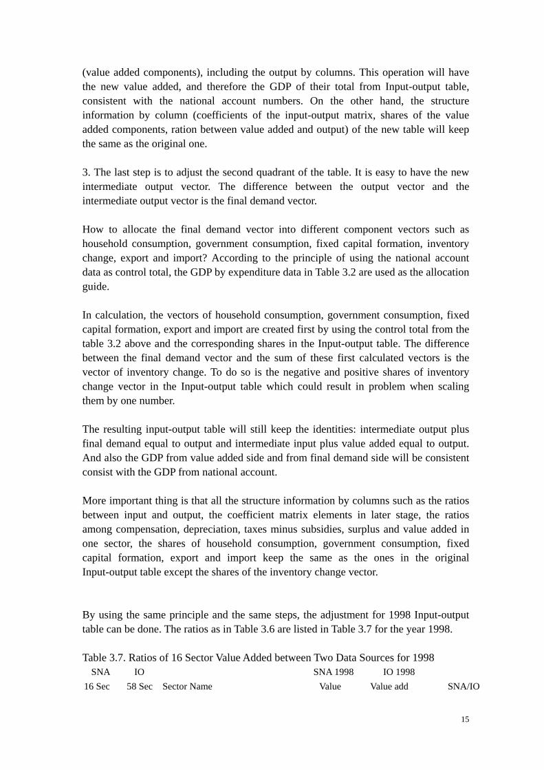
Table 3.6. Ratios of 16 Sector Value Added between Two Data Sources for 2002

SNA IO SNA 2002 IO 2002 16 Sec 58 Sec Sector Name Value added Value add SNA/IO

1 "1, 2 Agriculture, hunting and forestry 39173910 34123379 1.148 2 "3 Fishing 689480 649043 1.062 3 "4…7 Mining and quarrying 3566420 3295710 1.082 4 "8...30 Manufacturing industry 68942250 62551380 1.102 5 "31, 32 Electricity, gas and water 8858739 7778761 1.139 6 33 Construction 16259344 14811283 1.099 7 "34...36 Wholesale and retail 47338870 44099262 1.073 8 "37 Hotel and Restaurants 8829104 7561761 1.168 9 "38...42 Transport, storage, communication 54198942 46212317 1.173

10 "43...45 Financial intermediation 17080361 14870439 1.149 11 "46...50 Ownership and dwelling real est. 44222784 43913996 1.007 12 "51 Public administration 17683792 14949253 1.183 13 "52 Education 10460830 9631637 1.086 14 "53 Health and social work 5602567 4619662 1.213 15 "54...57 Other community, social service 7013288 6297422 1.114 16 "58 Private hh. with employed person 555406 501799 1.107

Total VA (GDP) Sum of 16 sectors 350476089 315867104 1.110 It can be seen that the biggest ratio happens in sector 14 which is “Health and social work” and there is only one single corresponding sector between two sources. On the other hand, the sector 11 which is merged (from original sector 11 and 12) has the smallest ratio between the two sources, which is close to 1. 2. The second step is to use the ratios in Table 3.6 and the relationship between the two sector classifications in Table 3.5 for scaling the columns of the first and third quadrants of the 2002 Input-output table- i.e. the intermediate input and cost parts

15

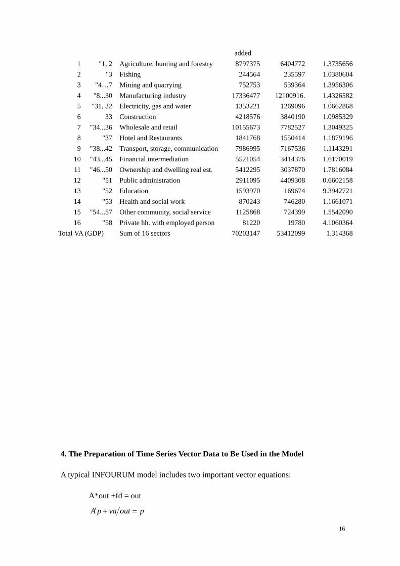
(value added components), including the output by columns. This operation will have the new value added, and therefore the GDP of their total from Input-output table, consistent with the national account numbers. On the other hand, the structure information by column (coefficients of the input-output matrix, shares of the value added components, ration between value added and output) of the new table will keep the same as the original one. 3. The last step is to adjust the second quadrant of the table. It is easy to have the new intermediate output vector. The difference between the output vector and the intermediate output vector is the final demand vector. How to allocate the final demand vector into different component vectors such as household consumption, government consumption, fixed capital formation, inventory change, export and import? According to the principle of using the national account data as control total, the GDP by expenditure data in Table 3.2 are used as the allocation guide. In calculation, the vectors of household consumption, government consumption, fixed capital formation, export and import are created first by using the control total from the table 3.2 above and the corresponding shares in the Input-output table. The difference between the final demand vector and the sum of these first calculated vectors is the vector of inventory change. To do so is the negative and positive shares of inventory change vector in the Input-output table which could result in problem when scaling them by one number. The resulting input-output table will still keep the identities: intermediate output plus final demand equal to output and intermediate input plus value added equal to output. And also the GDP from value added side and from final demand side will be consistent consist with the GDP from national account. More important thing is that all the structure information by columns such as the ratios between input and output, the coefficient matrix elements in later stage, the ratios among compensation, depreciation, taxes minus subsidies, surplus and value added in one sector, the shares of household consumption, government consumption, fixed capital formation, export and import keep the same as the ones in the original Input-output table except the shares of the inventory change vector. By using the same principle and the same steps, the adjustment for 1998 Input-output table can be done. The ratios as in Table 3.6 are listed in Table 3.7 for the year 1998. Table 3.7. Ratios of 16 Sector Value Added between Two Data Sources for 1998

SNA IO SNA 1998 IO 1998 16 Sec 58 Sec Sector Name Value Value add SNA/IO

16

added 1 "1, 2 Agriculture, hunting and forestry 8797375 6404772 1.3735656 2 "3 Fishing 244564 235597 1.0380604 3 "4…7 Mining and quarrying 752753 539364 1.3956306 4 "8...30 Manufacturing industry 17336477 12100916. 1.4326582 5 "31, 32 Electricity, gas and water 1353221 1269096 1.0662868 6 33 Construction 4218576 3840190 1.0985329 7 "34...36 Wholesale and retail 10155673 7782527 1.3049325 8 "37 Hotel and Restaurants 1841768 1550414 1.1879196 9 "38...42 Transport, storage, communication 7986995 7167536 1.1143291

10 "43...45 Financial intermediation 5521054 3414376 1.6170019 11 "46...50 Ownership and dwelling real est. 5412295 3037870 1.7816084 12 "51 Public administration 2911095 4409308 0.6602158 13 "52 Education 1593970 169674 9.3942721 14 "53 Health and social work 870243 746280 1.1661071 15 "54...57 Other community, social service 1125868 724399 1.5542090 16 "58 Private hh. with employed person 81220 19780 4.1060364

Total VA (GDP) Sum of 16 sectors 70203147 53412099 1.314368 4. The Preparation of Time Series Vector Data to Be Used in the Model A typical INFOURUM model includes two important vector equations: A*out +fd = out

poutvapA =+′

17

where A is input-output coefficient matrix in constant price, A′ is the transpose of matrix A, out is gross output vector in constant price, fd is final demand vector in constant price, va is value added vector in current price and p is price index vector. Since INFORUM model is also a dynamic model, it is necessary to have all of these matrices and vectors, mentioned above, as time series for the analysis period. However, it is difficult to have statistics and input-output tables which can naturally satisfy this condition. One of the most important tasks of the model builder is to use available statistics and limited input-output tables at hand and to create or close such condition. The adjusted Input-output tables for 1998 and 2002 mentioned in section 2 and 3 will be the IO data base for TURINA. In this section, the preparation of the time series vectors of value added (va), output (out), final demand (fd) and price index (p) will be described, respectively. (A) Final Demand Vector. There are 6 component vectors of the final demand in fact.

These 6 vectors are household consumption, government consumption, fixed capital formation, inventory changes, export and import.

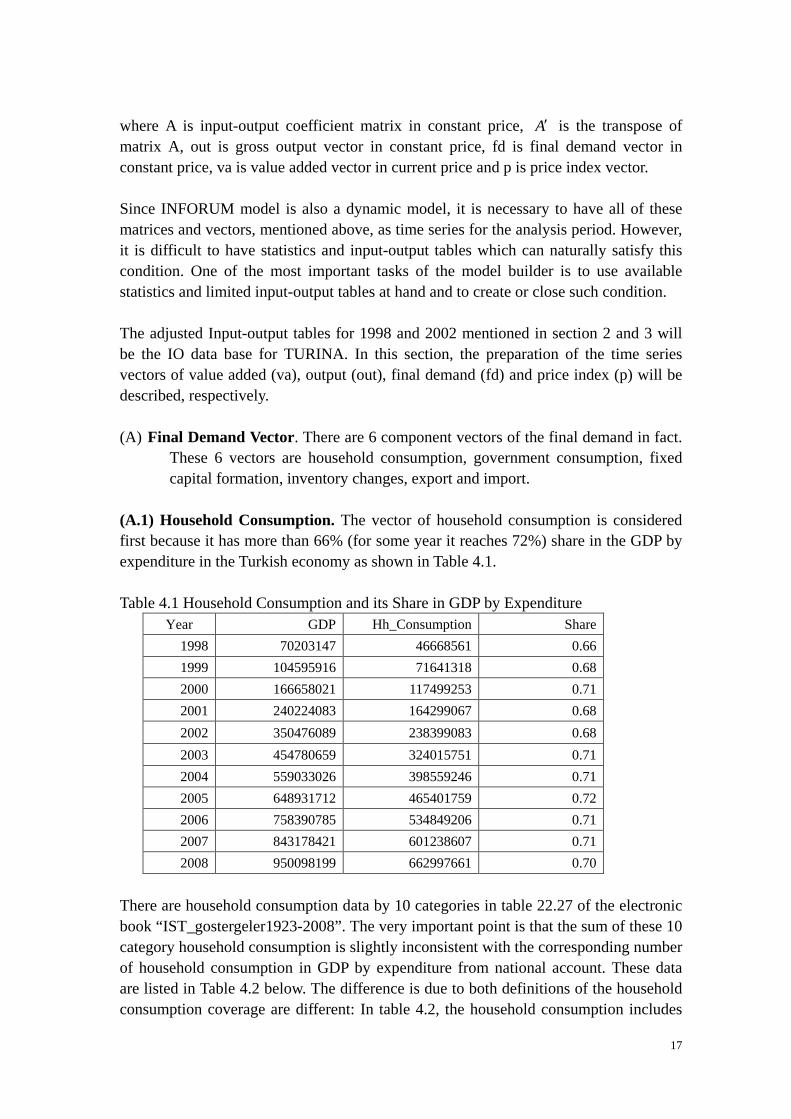
(A.1) Household Consumption. The vector of household consumption is considered first because it has more than 66% (for some year it reaches 72%) share in the GDP by expenditure in the Turkish economy as shown in Table 4.1. Table 4.1 Household Consumption and its Share in GDP by Expenditure

Year GDP Hh_Consumption Share 1998 70203147 46668561 0.66 1999 104595916 71641318 0.68 2000 166658021 117499253 0.71 2001 240224083 164299067 0.68 2002 350476089 238399083 0.68 2003 454780659 324015751 0.71 2004 559033026 398559246 0.71 2005 648931712 465401759 0.72 2006 758390785 534849206 0.71 2007 843178421 601238607 0.71 2008 950098199 662997661 0.70

There are household consumption data by 10 categories in table 22.27 of the electronic book “IST_gostergeler1923-2008”. The very important point is that the sum of these 10 category household consumption is slightly inconsistent with the corresponding number of household consumption in GDP by expenditure from national account. These data are listed in Table 4.2 below. The difference is due to both definitions of the household consumption coverage are different: In table 4.2, the household consumption includes

18

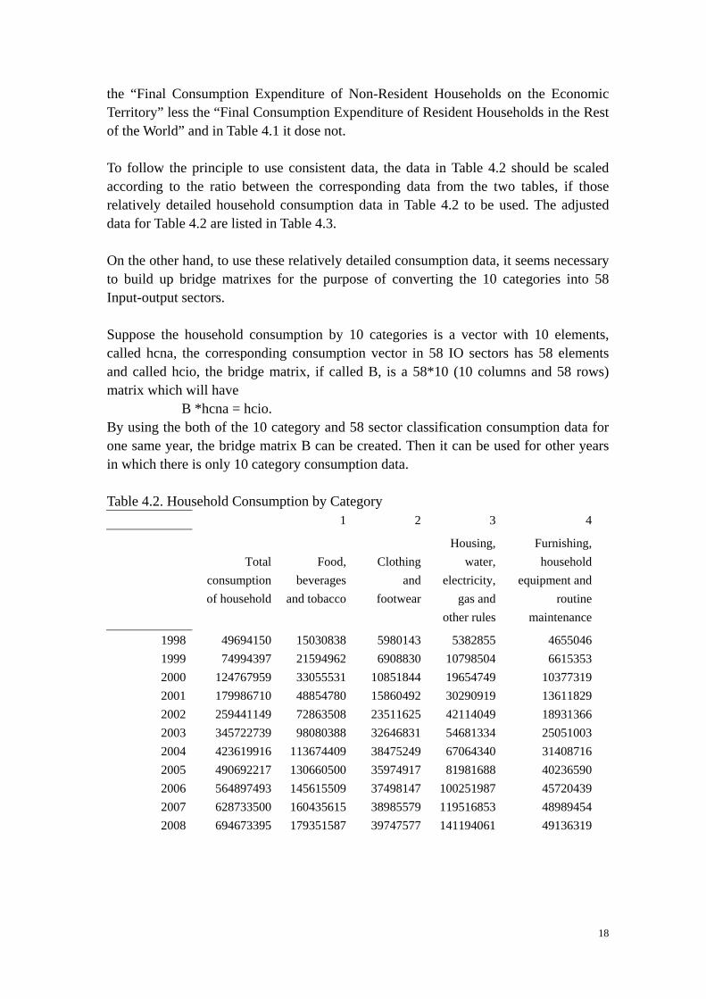
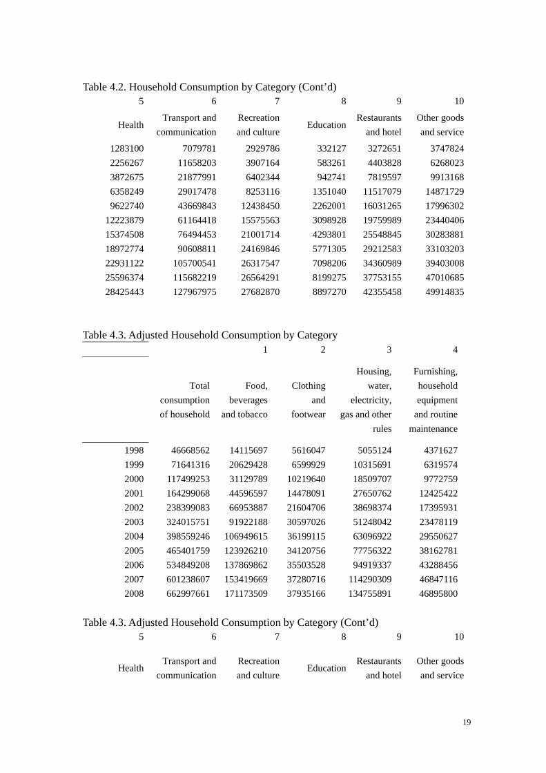
the “Final Consumption Expenditure of Non-Resident Households on the Economic Territory” less the “Final Consumption Expenditure of Resident Households in the Rest of the World” and in Table 4.1 it dose not. To follow the principle to use consistent data, the data in Table 4.2 should be scaled according to the ratio between the corresponding data from the two tables, if those relatively detailed household consumption data in Table 4.2 to be used. The adjusted data for Table 4.2 are listed in Table 4.3. On the other hand, to use these relatively detailed consumption data, it seems necessary to build up bridge matrixes for the purpose of converting the 10 categories into 58 Input-output sectors. Suppose the household consumption by 10 categories is a vector with 10 elements, called hcna, the corresponding consumption vector in 58 IO sectors has 58 elements and called hcio, the bridge matrix, if called B, is a 58*10 (10 columns and 58 rows) matrix which will have B *hcna = hcio. By using the both of the 10 category and 58 sector classification consumption data for one same year, the bridge matrix B can be created. Then it can be used for other years in which there is only 10 category consumption data. Table 4.2. Household Consumption by Category

1 2 3 4

Total consumption of household

Food, beverages

and tobacco

Clothing and

footwear

Housing, water,

electricity, gas and

other rules

Furnishing, household

equipment and routine

maintenance

1998 49694150 15030838 5980143 5382855 4655046 1999 74994397 21594962 6908830 10798504 6615353 2000 124767959 33055531 10851844 19654749 10377319 2001 179986710 48854780 15860492 30290919 13611829 2002 259441149 72863508 23511625 42114049 18931366 2003 345722739 98080388 32646831 54681334 25051003 2004 423619916 113674409 38475249 67064340 31408716 2005 490692217 130660500 35974917 81981688 40236590 2006 564897493 145615509 37498147 100251987 45720439 2007 628733500 160435615 38985579 119516853 48989454 2008 694673395 179351587 39747577 141194061 49136319

19

Table 4.2. Household Consumption by Category (Cont’d)

5 6 7 8 9 10

Health Transport and

communication Recreation and culture

Education Restaurants

and hotel Other goods and service

1283100 7079781 2929786 332127 3272651 3747824 2256267 11658203 3907164 583261 4403828 6268023 3872675 21877991 6402344 942741 7819597 9913168 6358249 29017478 8253116 1351040 11517079 14871729 9622740 43669843 12438450 2262001 16031265 17996302

12223879 61164418 15575563 3098928 19759989 23440406 15374508 76494453 21001714 4293801 25548845 30283881 18972774 90608811 24169846 5771305 29212583 33103203 22931122 105700541 26317547 7098206 34360989 39403008 25596374 115682219 26564291 8199275 37753155 47010685 28425443 127967975 27682870 8897270 42355458 49914835

Table 4.3. Adjusted Household Consumption by Category

1 2 3 4

Total consumption of household

Food, beverages

and tobacco

Clothing and

footwear

Housing, water,

electricity, gas and other

rules

Furnishing, household equipment

and routine maintenance

1998 46668562 14115697 5616047 5055124 4371627 1999 71641316 20629428 6599929 10315691 6319574 2000 117499253 31129789 10219640 18509707 9772759 2001 164299068 44596597 14478091 27650762 12425422 2002 238399083 66953887 21604706 38698374 17395931 2003 324015751 91922188 30597026 51248042 23478119 2004 398559246 106949615 36199115 63096922 29550627 2005 465401759 123926210 34120756 77756322 38162781 2006 534849208 137869862 35503528 94919337 43288456 2007 601238607 153419669 37280716 114290309 46847116 2008 662997661 171173509 37935166 134755891 46895800

Table 4.3. Adjusted Household Consumption by Category (Cont’d)

5 6 7 8 9 10

Health Transport and

communication Recreation and culture

Education Restaurants

and hotel Other goods and service

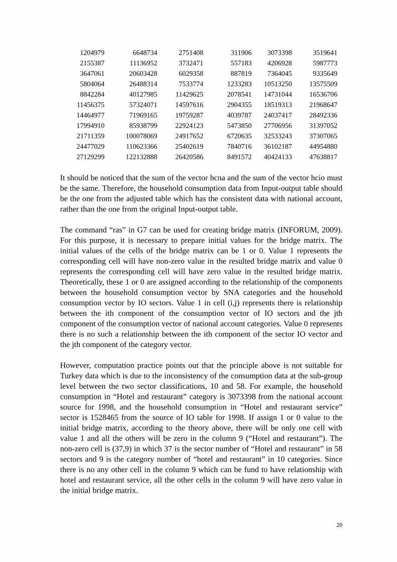
20

1204979 6648734 2751408 311906 3073398 3519641 2155387 11136952 3732471 557183 4206928 5987773 3647061 20603428 6029358 887819 7364045 9335649 5804064 26488314 7533774 1233283 10513250 13575509 8842284 40127985 11429625 2078541 14731044 16536706

11456375 57324071 14597616 2904355 18519313 21968647 14464977 71969165 19759287 4039787 24037417 28492336 17994910 85938799 22924123 5473850 27706956 31397052 21711359 100078069 24917652 6720635 32533243 37307065 24477029 110623366 25402619 7840716 36102187 44954880 27129299 122132888 26420586 8491572 40424133 47638817

It should be noticed that the sum of the vector hcna and the sum of the vector hcio must be the same. Therefore, the household consumption data from Input-output table should be the one from the adjusted table which has the consistent data with national account, rather than the one from the original Input-output table. The command “ras” in G7 can be used for creating bridge matrix (INFORUM, 2009). For this purpose, it is necessary to prepare initial values for the bridge matrix. The initial values of the cells of the bridge matrix can be 1 or 0. Value 1 represents the corresponding cell will have non-zero value in the resulted bridge matrix and value 0 represents the corresponding cell will have zero value in the resulted bridge matrix. Theoretically, these 1 or 0 are assigned according to the relationship of the components between the household consumption vector by SNA categories and the household consumption vector by IO sectors. Value 1 in cell (i,j) represents there is relationship between the ith component of the consumption vector of IO sectors and the jth component of the consumption vector of national account categories. Value 0 represents there is no such a relationship between the ith component of the sector IO vector and the jth component of the category vector. However, computation practice points out that the principle above is not suitable for Turkey data which is due to the inconsistency of the consumption data at the sub-group level between the two sector classifications, 10 and 58. For example, the household consumption in “Hotel and restaurant” category is 3073398 from the national account source for 1998, and the household consumption in “Hotel and restaurant service” sector is 1528465 from the source of IO table for 1998. If assign 1 or 0 value to the initial bridge matrix, according to the theory above, there will be only one cell with value 1 and all the others will be zero in the column 9 (“Hotel and restaurant”). The non-zero cell is (37,9) in which 37 is the sector number of “Hotel and restaurant” in 58 sectors and 9 is the category number of “hotel and restaurant” in 10 categories. Since there is no any other cell in the column 9 which can be fund to have relationship with hotel and restaurant service, all the other cells in the column 9 will have zero value in the initial bridge matrix.

21

Obviously, there will be no such a matrix B which can have the left side vector (hcna) with value 3073398 for element 9 and the right side vector (hcio) with value 1528465 for element 37 for the equation

B *hcna = hcio. To solve this problem, it is necessary to “eas” the assignment operation of cell’s relationship with each other. For example, for the elements in column 9 (“hotel and restaurant” consumption in 10 categories) of the initial bridge matrix, not only the element 37 (“Hotel and restaurant” consumption in 58 sectors) is assigned value 1.0, but other elements such as element 55 (“Membership organization services n.e.c.”) is also assigned value 1.0 which supposes some expenditure in membership service probably can be put in account of the consumption categories of “Hotel and restaurant”. After preparing the initial bridge matrix, the command to create the bridge matrix in G7 is just ras consBM fcehh hhc 1998 (or 2002) in which the parameter consBM is the name of the initial and the resulted bridge matrix, fcehh (58 sector of consumption in IO ) is the row control sum and hhc (10 category consumption in SNA) is the column control sum. 1998 or 2002 is the year when there is both consumption vector data of 10 categories and 58 sectors. The resulting matrix consBM is the flow bridge matrix for the year 1998 or 2002. To have the coefficient bridge matrix, just use the “coef” command under G7 coef consBM hhc For the bridge matrices from year 1999 to year 2001, interpolation can be done between the matrix for 1998 and the matrix for 2002. After the interpolation, each column in resulted bridge matrix should be scaled according to the principle that the sum of each column in bridge matrix is equal to 1.0. The reason is obvious. For the bridge matrices after the year 2002, they can be just the copy of the bridge matrix for 2002. (A.2) Government consumption. It is one component of the final demand. In the data source “IST_gostergeler1923-2008.pdf, T22.27”, there are two columns for government consumption: “Compensation of Employee” and “Purchases of Goods and Services”. Since no more further detailed information for government consumption can be found in various statistics, it is decided that to allocate the government consumption in total into 58 Input-output sectors by using the sector shares of the government consumption from the Input-output tables for year 1998 and 2002. For the years between 1998 and 2002, interpolation and scaling operation will be done to create the consumption vector. For the years after 2002, sector shares of the 2002 vector of the government consumption will be used for creating the vector of consumption by allocating the total government consumption.

22

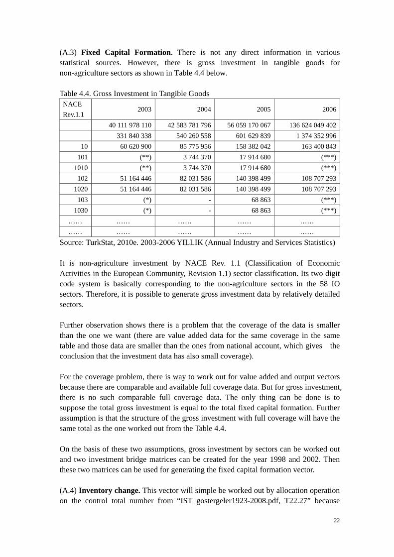
(A.3) Fixed Capital Formation. There is not any direct information in various statistical sources. However, there is gross investment in tangible goods for non-agriculture sectors as shown in Table 4.4 below. Table 4.4. Gross Investment in Tangible Goods NACE Rev.1.1

2003 2004 2005 2006

40 111 978 110 42 583 781 796 56 059 170 067 136 624 049 402 331 840 338 540 260 558 601 629 839 1 374 352 996

10 60 620 900 85 775 956 158 382 042 163 400 843 101 (**) 3 744 370 17 914 680 (***)

1010 (**) 3 744 370 17 914 680 (***) 102 51 164 446 82 031 586 140 398 499 108 707 293

1020 51 164 446 82 031 586 140 398 499 108 707 293 103 (*) - 68 863 (***)

1030 (*) - 68 863 (***) …… …… …… …… …… …… …… …… …… ……

Source: TurkStat, 2010e. 2003-2006 YILLIK (Annual Industry and Services Statistics) It is non-agriculture investment by NACE Rev. 1.1 (Classification of Economic Activities in the European Community, Revision 1.1) sector classification. Its two digit code system is basically corresponding to the non-agriculture sectors in the 58 IO sectors. Therefore, it is possible to generate gross investment data by relatively detailed sectors. Further observation shows there is a problem that the coverage of the data is smaller than the one we want (there are value added data for the same coverage in the same table and those data are smaller than the ones from national account, which gives the conclusion that the investment data has also small coverage). For the coverage problem, there is way to work out for value added and output vectors because there are comparable and available full coverage data. But for gross investment, there is no such comparable full coverage data. The only thing can be done is to suppose the total gross investment is equal to the total fixed capital formation. Further assumption is that the structure of the gross investment with full coverage will have the same total as the one worked out from the Table 4.4. On the basis of these two assumptions, gross investment by sectors can be worked out and two investment bridge matrices can be created for the year 1998 and 2002. Then these two matrices can be used for generating the fixed capital formation vector. (A.4) Inventory change. This vector will simple be worked out by allocation operation on the control total number from “IST_gostergeler1923-2008.pdf, T22.27” because

23

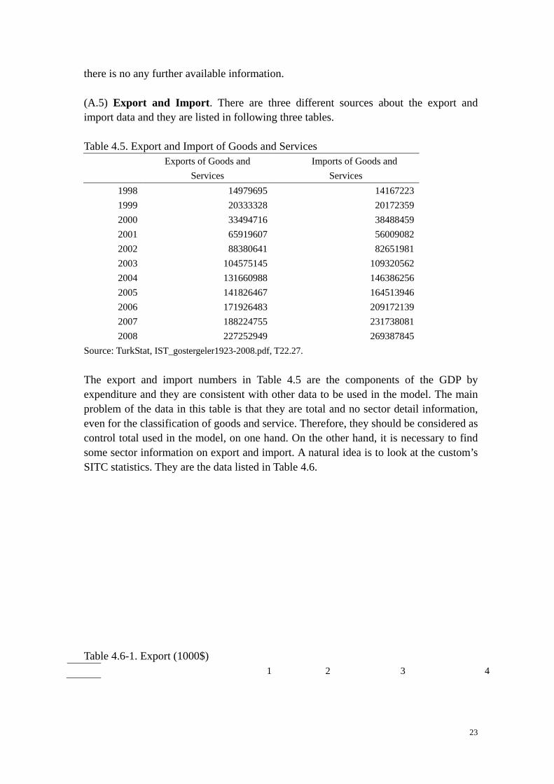
there is no any further available information. (A.5) Export and Import. There are three different sources about the export and import data and they are listed in following three tables. Table 4.5. Export and Import of Goods and Services

Exports of Goods and Services

Imports of Goods and Services

1998 14979695 14167223 1999 20333328 20172359 2000 33494716 38488459 2001 65919607 56009082 2002 88380641 82651981 2003 104575145 109320562 2004 131660988 146386256 2005 141826467 164513946 2006 171926483 209172139 2007 188224755 231738081 2008 227252949 269387845

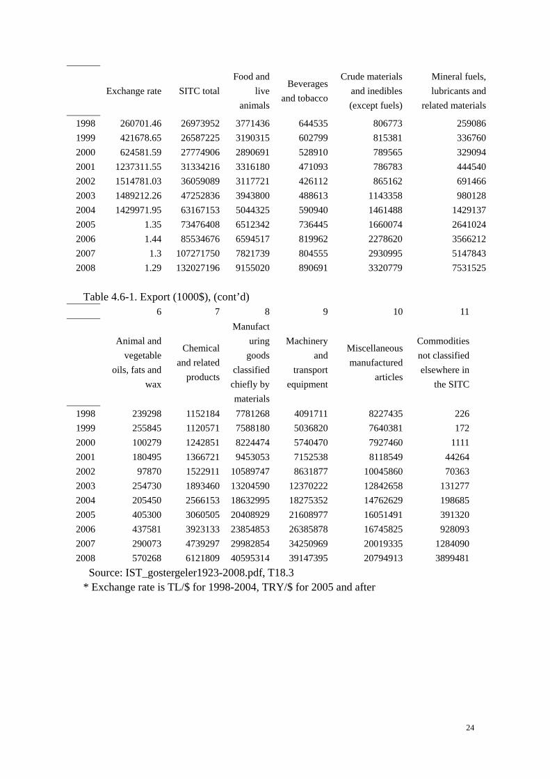
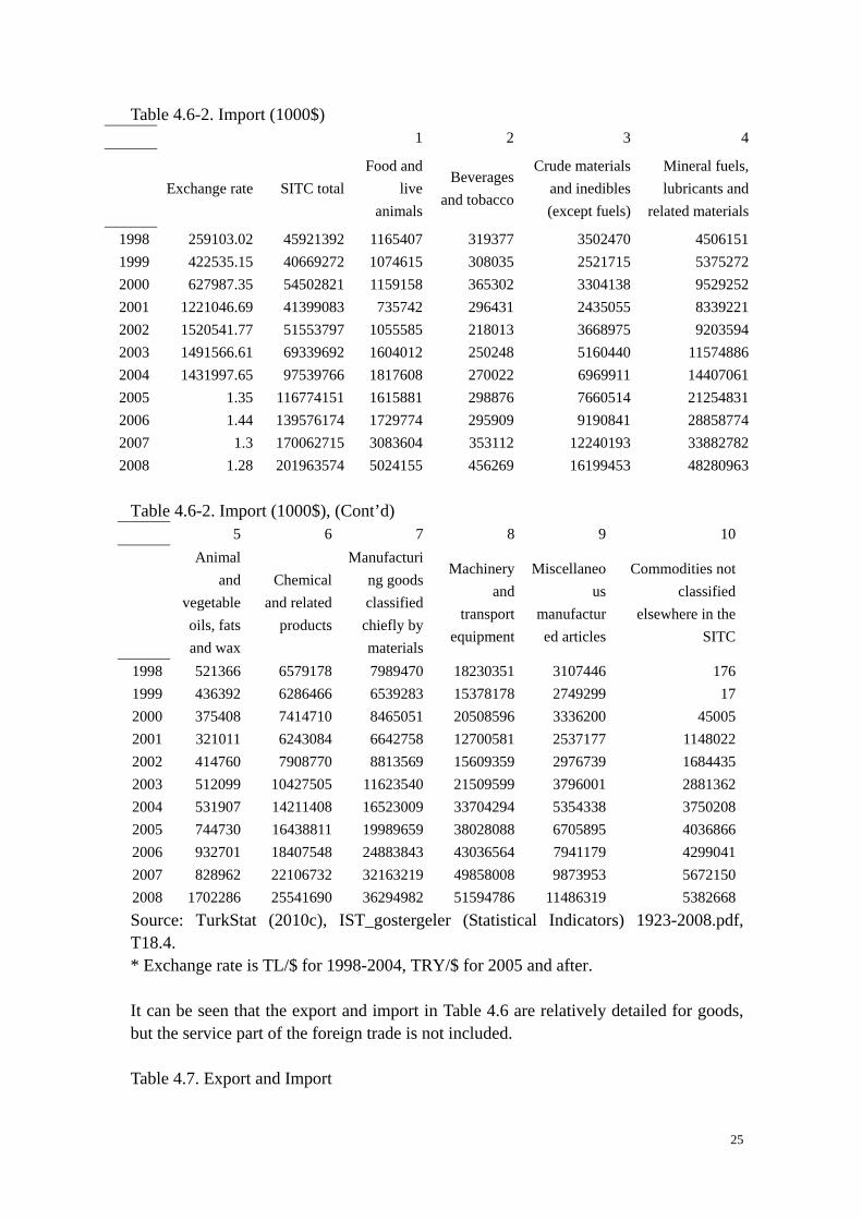
Source: TurkStat, IST_gostergeler1923-2008.pdf, T22.27. The export and import numbers in Table 4.5 are the components of the GDP by expenditure and they are consistent with other data to be used in the model. The main problem of the data in this table is that they are total and no sector detail information, even for the classification of goods and service. Therefore, they should be considered as control total used in the model, on one hand. On the other hand, it is necessary to find some sector information on export and import. A natural idea is to look at the custom’s SITC statistics. They are the data listed in Table 4.6. Table 4.6-1. Export (1000$) 1 2 3 4

24

Exchange rate SITC total Food and

live animals

Beverages and tobacco

Crude materials and inedibles (except fuels)

Mineral fuels, lubricants and

related materials

1998 260701.46 26973952 3771436 644535 806773 259086 1999 421678.65 26587225 3190315 602799 815381 336760 2000 624581.59 27774906 2890691 528910 789565 329094 2001 1237311.55 31334216 3316180 471093 786783 444540 2002 1514781.03 36059089 3117721 426112 865162 691466 2003 1489212.26 47252836 3943800 488613 1143358 980128 2004 1429971.95 63167153 5044325 590940 1461488 1429137 2005 1.35 73476408 6512342 736445 1660074 2641024 2006 1.44 85534676 6594517 819962 2278620 3566212 2007 1.3 107271750 7821739 804555 2930995 5147843 2008 1.29 132027196 9155020 890691 3320779 7531525

Table 4.6-1. Export (1000$), (cont’d) 6 7 8 9 10 11

Animal and vegetable

oils, fats and wax

Chemical and related

products

Manufacturing

goods classified chiefly by materials

Machinery and

transport equipment

Miscellaneous manufactured

articles

Commodities not classified elsewhere in

the SITC

1998 239298 1152184 7781268 4091711 8227435 226 1999 255845 1120571 7588180 5036820 7640381 172 2000 100279 1242851 8224474 5740470 7927460 1111 2001 180495 1366721 9453053 7152538 8118549 44264 2002 97870 1522911 10589747 8631877 10045860 70363 2003 254730 1893460 13204590 12370222 12842658 131277 2004 205450 2566153 18632995 18275352 14762629 198685 2005 405300 3060505 20408929 21608977 16051491 391320 2006 437581 3923133 23854853 26385878 16745825 928093 2007 290073 4739297 29982854 34250969 20019335 1284090 2008 570268 6121809 40595314 39147395 20794913 3899481

Source: IST_gostergeler1923-2008.pdf, T18.3 * Exchange rate is TL/$ for 1998-2004, TRY/$ for 2005 and after

25

Table 4.6-2. Import (1000$) 1 2 3 4

Exchange rate SITC total Food and

live animals

Beverages and tobacco

Crude materials and inedibles (except fuels)

Mineral fuels, lubricants and

related materials

1998 259103.02 45921392 1165407 319377 3502470 4506151 1999 422535.15 40669272 1074615 308035 2521715 5375272 2000 627987.35 54502821 1159158 365302 3304138 9529252 2001 1221046.69 41399083 735742 296431 2435055 8339221 2002 1520541.77 51553797 1055585 218013 3668975 9203594 2003 1491566.61 69339692 1604012 250248 5160440 11574886 2004 1431997.65 97539766 1817608 270022 6969911 14407061 2005 1.35 116774151 1615881 298876 7660514 21254831 2006 1.44 139576174 1729774 295909 9190841 28858774 2007 1.3 170062715 3083604 353112 12240193 33882782 2008 1.28 201963574 5024155 456269 16199453 48280963

Table 4.6-2. Import (1000$), (Cont’d)

5 6 7 8 9 10

Animal and

vegetable oils, fats and wax

Chemical and related

products

Manufacturing goods classified chiefly by materials

Machinery and

transport equipment

Miscellaneous

manufactured articles

Commodities not classified

elsewhere in the SITC

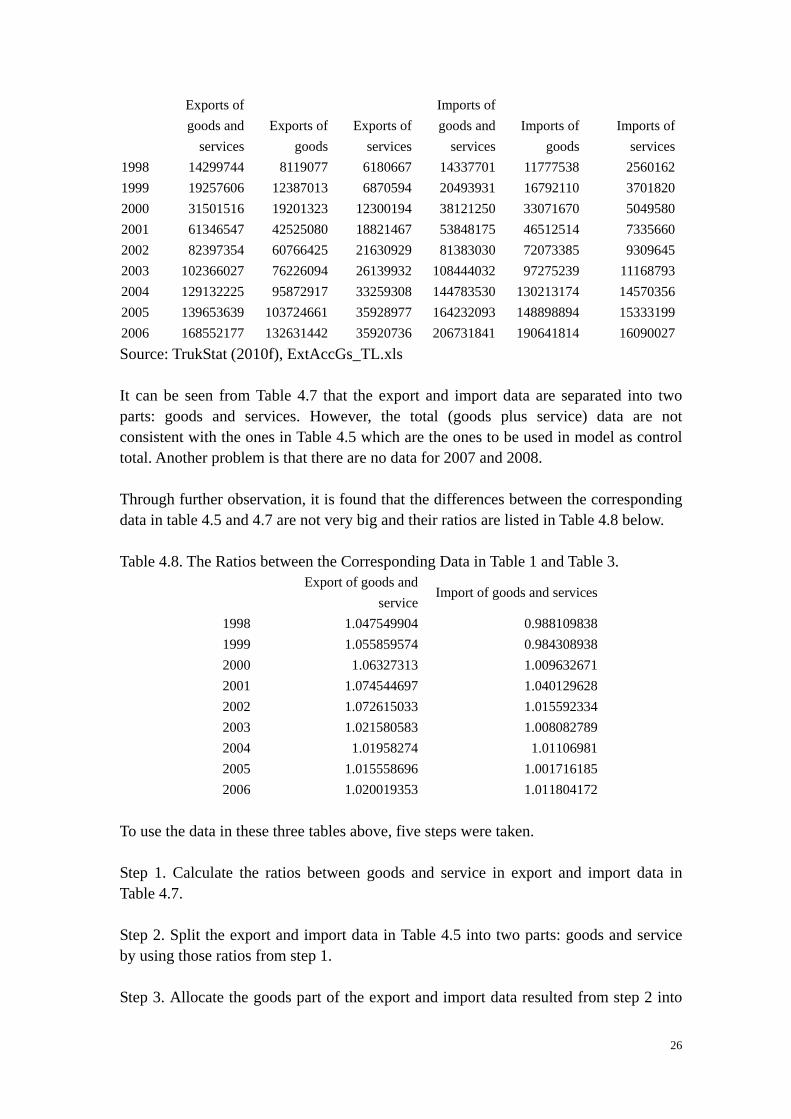
1998 521366 6579178 7989470 18230351 3107446 176 1999 436392 6286466 6539283 15378178 2749299 17 2000 375408 7414710 8465051 20508596 3336200 45005 2001 321011 6243084 6642758 12700581 2537177 1148022 2002 414760 7908770 8813569 15609359 2976739 1684435 2003 512099 10427505 11623540 21509599 3796001 2881362 2004 531907 14211408 16523009 33704294 5354338 3750208 2005 744730 16438811 19989659 38028088 6705895 4036866 2006 932701 18407548 24883843 43036564 7941179 4299041 2007 828962 22106732 32163219 49858008 9873953 5672150 2008 1702286 25541690 36294982 51594786 11486319 5382668 Source: TurkStat (2010c), IST_gostergeler (Statistical Indicators) 1923-2008.pdf, T18.4. * Exchange rate is TL/$ for 1998-2004, TRY/$ for 2005 and after. It can be seen that the export and import in Table 4.6 are relatively detailed for goods, but the service part of the foreign trade is not included. Table 4.7. Export and Import

26

Exports of goods and

services Exports of

goods Exports of

services

Imports of goods and

services Imports of

goods Imports of

services 1998 14299744 8119077 6180667 14337701 11777538 2560162 1999 19257606 12387013 6870594 20493931 16792110 3701820 2000 31501516 19201323 12300194 38121250 33071670 5049580 2001 61346547 42525080 18821467 53848175 46512514 7335660 2002 82397354 60766425 21630929 81383030 72073385 9309645 2003 102366027 76226094 26139932 108444032 97275239 11168793 2004 129132225 95872917 33259308 144783530 130213174 14570356 2005 139653639 103724661 35928977 164232093 148898894 15333199 2006 168552177 132631442 35920736 206731841 190641814 16090027 Source: TrukStat (2010f), ExtAccGs_TL.xls It can be seen from Table 4.7 that the export and import data are separated into two parts: goods and services. However, the total (goods plus service) data are not consistent with the ones in Table 4.5 which are the ones to be used in model as control total. Another problem is that there are no data for 2007 and 2008. Through further observation, it is found that the differences between the corresponding data in table 4.5 and 4.7 are not very big and their ratios are listed in Table 4.8 below. Table 4.8. The Ratios between the Corresponding Data in Table 1 and Table 3.

Export of goods and

service Import of goods and services

1998 1.047549904 0.988109838 1999 1.055859574 0.984308938 2000 1.06327313 1.009632671 2001 1.074544697 1.040129628 2002 1.072615033 1.015592334 2003 1.021580583 1.008082789 2004 1.01958274 1.01106981 2005 1.015558696 1.001716185 2006 1.020019353 1.011804172

To use the data in these three tables above, five steps were taken. Step 1. Calculate the ratios between goods and service in export and import data in Table 4.7. Step 2. Split the export and import data in Table 4.5 into two parts: goods and service by using those ratios from step 1. Step 3. Allocate the goods part of the export and import data resulted from step 2 into

27

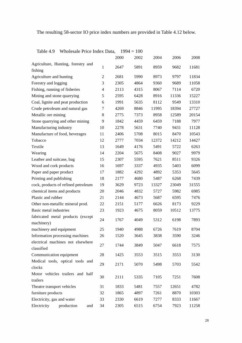
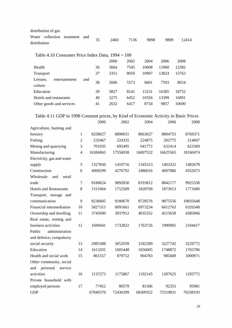
10 SITC categories, according to the SITC classification category shares of export and import data of goods in the Table 4.6. Step 4. Create export and import bridge matrices for the year 1998 and 2002 for the purpose of projecting the import and export by 11 categories (10 SITC goods categories plus service) resulted from the step 3 and step 2 into 58 Input-output sectors Step 5. Extend the export and import bridge matrices for other years so that there will be export and import by 58 Input-output sectors. To finish these five steps described above, there is no technical problem except the shortage of 2007 and 2008 data in Table 4.7. It was solved just by using the ratios from the year 2006 because the 2007 and 2008 data could not be found. (B) Price Index Vector. There is not a ready made price index vector with 58 sectors. The price index vector has been constructed at three steps using four different sources: (a). Wholesale Price Index Data for 35 sectors, 1994 = 100, T19.7 from

IST_gostergeler1923-2008; Table 4.9 in this report. (b). Consumer Price Index Data Table for 6 sectors, 1994 = 100, T19.14 from

IST_gostergeler1923-2008; Table 4.10 in this report. (c). GDP at current prices, for 17 sectors, Table 3.4 in this report. (d). GDP at constant prices at 1998 prices, for 17 sectors, Table 4.11 in this report. The first two tables are available in the electronic book Statistical Indicators 1923-2008. The last two tables are available in TurkStat website. The four tables, except for Table 3.4, are given below just for 2000 to 2008 in their original form with only two-year intervals. Price index numbers for the following 44 sectors are directly obtained from the first two tables, i.e. from Table 4.9 and Table 4.10: IO Sectors: 1-32, 37, 38, 48 – 50, 52 – 58. In national accounts statistics GDP data are available for only 17 broad economic sectors but not for all IO sectors. Table 4.11 gives the constant price GDP values by 17 sectors and their corresponding values in current price are the ones as the same as in the Table 3.3 of last section. Both of them can produce implicit GDP price deflator by 17 sectors. For our purpose price indices for the following 14 sectors are obtained form Table 3.3 and 4.11 implicitly: IO sectors 33 – 36, 39 – 47, 51. Therefore, 44 IO sectors price index vector is obtained from either Wholesale price index number or CPI index number. The remaining 14 price indices are implicitly derived from SNA data for the Turkish economy.

28

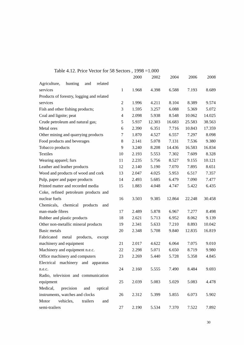
The resulting 58-sector IO price index numbers are provided in Table 4.12 below. Table 4.9 Wholesale Price Index Data, 1994 = 100

2000 2002 2004 2006 2008 Agriculture, Hunting, forestry and fishing

1 2647 5891 8959 9682 11681

Agriculture and hunting 2 2681 5990 8973 9797 11834 Forestry and logging 3 2305 4864 9360 9689 11058 Fishing, running of fisheries 4 2113 4315 8067 7114 6720 Mining and stone quarrying 5 2595 6428 8916 11336 15227 Coal, lignite and peat production 6 1991 5635 8112 9549 13310 Crude petroleum and natural gas 7 4269 8846 11995 18394 27727 Metallic ore mining 8 2775 7373 8958 12589 20154 Stone quarrying and other mining 9 1842 4459 6459 7188 7977 Manufacturing industry 10 2278 5631 7740 9431 11128 Manufacture of food, beverages 11 2406 5708 8015 8470 10543 Tobacco 12 2777 7034 12372 14212 14427 Textile 13 1649 4176 5491 5722 6263 Wearing 14 2204 5675 8408 9027 9979 Leather and suitcase, bag 15 2307 5595 7621 8511 9326 Wood and cork products 16 1697 3337 4935 5403 6099 Paper and paper product 17 1882 4292 4892 5353 5645 Printing and publishing 18 2177 4680 5487 6268 7439 cock, products of refined petroleum 19 3629 9723 13327 23049 31555 chemical items and products 20 2046 4832 5727 5982 6985 Plastic and rubber 21 2144 4673 5687 6595 7476 Other non-metallic mineral prod. 22 2151 5177 6626 8173 9229 Basic metal industries 23 1923 4675 8059 10512 13775 fabricated metal products (except machinery)

24 1767 4049 5312 6198 7893

machinery and equipment 25 1940 4988 6726 7619 8704 Information processing machines 26 1520 3645 3838 3590 3246 electrical machines not elsewhere classified

27 1744 3849 5047 6618 7575

Communication equipment 28 1425 3553 3515 3553 3130 Medical tools, optical tools and clocks

29 2171 5070 5498 5703 5542

Motor vehicles trailers and half trailers

30 2111 5335 7105 7251 7608

Theatre transport vehicles 31 1833 5481 7557 12651 4782 furniture products 32 1865 4897 7261 8870 10303 Electricity, gas and water 33 2330 6619 7277 8333 11667 Electricity production and 34 2305 6515 6754 7923 11258

29

distribution of gas Water collection treatment and distribution

35 2460 7136 9898 9809 12414

Table 4.10 Consumer Price Index Data, 1994 = 100

2000 2002 2004 2006 2008 Health 36 3664 7545 10608 11960 12582 Transport 37 3351 8050 10907 13824 15763 Leisure, entertainment and culture

38 2606 5573 6601 7593 8024

Education 39 3827 8141 13231 16385 18752 Hotels and restaurants 40 3275 6452 10356 13399 16891 Other goods and services 41 2632 6417 8734 9857 10690 Table 4.11 GDP in 1998 Constant prices, by Kind of Economic Activity in Basic Prices

2000 2002 2004 2006 2008 Agriculture, hunting and forestry 1 8258027 8890031 8063027 8894755 8769371 Fishing 2 235467 224335 224875 202775 214847 Mining and quarrying 3 701035 695495 641772 632414 623369 Manufacturing 4 16384063 17556938 16007532 16625565 18160474 Electricity, gas and water supply 5 1327830 1410716 1345313 1403322 1482678 Construction 6 4069299 4276792 3486016 4007886 4352673 Wholesale and retail trade 7 9180624 9892830 8193812 8842177 9925338 Hotels and Restaurants 8 1511064 1752509 1828709 1873613 1771680 Transport, storage and communication 9 8236845 9180670 8728576 9875556 10835648 Financial intermediation 10 5827315 6091661 6973234 6612763 6326348 Ownership and dwelling 11 3745690 3937912 4035352 4215658 4385066 Real estate, renting and business activities 12 1690441 1732822 1763726 1990905 2104417 Public administration and defence; compulsory social security 13 2983388 3052039 3182289 3227742 3229772 Education 14 1613201 1605448 1656605 1748872 1765786 Health and social work 15 861557 879752 904783 985849 1000971 Other community, social and personal service activities 16 1137273 1175867 1192145 1287625 1293772 Private household with employed persons 17 77452 80579 81586 92355 95981 GDP 67840570 72436399 68309352 72519831 76338193

30

Table 4.12. Price Vector for 58 Sectors , 1998 =1.000 2000 2002 2004 2006 2008

Agriculture, hunting and related services 1 1.968 4.398 6.588 7.193 8.689 Products of forestry, logging and related services 2 1.996 4.211 8.104 8.389 9.574 Fish and other fishing products; 3 1.595 3.257 6.088 5.369 5.072 Coal and lignite; peat 4 2.098 5.938 8.548 10.062 14.025 Crude petroleum and natural gas; 5 5.937 12.303 16.683 25.583 38.563 Metal ores 6 2.390 6.351 7.716 10.843 17.359 Other mining and quarrying products 7 1.870 4.527 6.557 7.297 8.098 Food products and beverages 8 2.141 5.078 7.131 7.536 9.380 Tobacco products 9 3.240 8.208 14.436 16.583 16.834 Textiles 10 2.193 5.553 7.302 7.609 8.328 Wearing apparel; furs 11 2.235 5.756 8.527 9.155 10.121 Leather and leather products 12 2.140 5.190 7.070 7.895 8.651 Wood and products of wood and cork 13 2.047 4.025 5.953 6.517 7.357 Pulp, paper and paper products 14 2.493 5.685 6.479 7.090 7.477 Printed matter and recorded media 15 1.883 4.048 4.747 5.422 6.435 Coke, refined petroleum products and nuclear fuels 16 3.503 9.385 12.864 22.248 30.458 Chemicals, chemical products and man-made fibres 17 2.489 5.878 6.967 7.277 8.498 Rubber and plastic products 18 2.621 5.713 6.952 8.062 9.139 Other non-metallic mineral products 19 2.341 5.633 7.210 8.893 10.042 Basic metals 20 2.348 5.708 9.840 12.835 16.819 Fabricated metal products, except machinery and equipment 21 2.017 4.622 6.064 7.075 9.010 Machinery and equipment n.e.c. 22 2.298 5.071 6.650 8.719 9.980 Office machinery and computers 23 2.269 5.440 5.728 5.358 4.845 Electrical machinery and apparatus n.e.c. 24 2.160 5.555 7.490 8.484 9.693 Radio, television and communication equipment 25 2.039 5.083 5.029 5.083 4.478 Medical, precision and optical instruments, watches and clocks 26 2.312 5.399 5.855 6.073 5.902 Motor vehicles, trailers and semi-trailers 27 2.190 5.534 7.370 7.522 7.892

31

Other transport equipment 28 2.146 6.418 8.849 14.814 5.600 Furniture; other manufactured goods n.e.c. 29 2.151 5.648 8.375 10.231 11.884

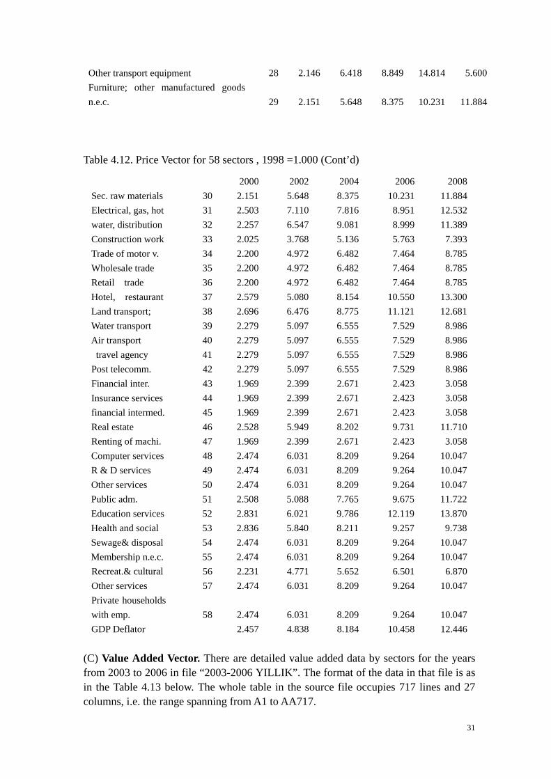
Table 4.12. Price Vector for 58 sectors , 1998 =1.000 (Cont’d)

(C) Value Added Vector. There are detailed value added data by sectors for the years from 2003 to 2006 in file “2003-2006 YILLIK”. The format of the data in that file is as in the Table 4.13 below. The whole table in the source file occupies 717 lines and 27 columns, i.e. the range spanning from A1 to AA717.

2000 2002 2004 2006 2008 Sec. raw materials 30 2.151 5.648 8.375 10.231 11.884 Electrical, gas, hot 31 2.503 7.110 7.816 8.951 12.532 water, distribution 32 2.257 6.547 9.081 8.999 11.389 Construction work 33 2.025 3.768 5.136 5.763 7.393 Trade of motor v. 34 2.200 4.972 6.482 7.464 8.785 Wholesale trade 35 2.200 4.972 6.482 7.464 8.785 Retail trade 36 2.200 4.972 6.482 7.464 8.785 Hotel, restaurant 37 2.579 5.080 8.154 10.550 13.300 Land transport; 38 2.696 6.476 8.775 11.121 12.681 Water transport 39 2.279 5.097 6.555 7.529 8.986 Air transport 40 2.279 5.097 6.555 7.529 8.986 travel agency 41 2.279 5.097 6.555 7.529 8.986 Post telecomm. 42 2.279 5.097 6.555 7.529 8.986 Financial inter. 43 1.969 2.399 2.671 2.423 3.058 Insurance services 44 1.969 2.399 2.671 2.423 3.058 financial intermed. 45 1.969 2.399 2.671 2.423 3.058 Real estate 46 2.528 5.949 8.202 9.731 11.710 Renting of machi. 47 1.969 2.399 2.671 2.423 3.058 Computer services 48 2.474 6.031 8.209 9.264 10.047 R & D services 49 2.474 6.031 8.209 9.264 10.047 Other services 50 2.474 6.031 8.209 9.264 10.047 Public adm. 51 2.508 5.088 7.765 9.675 11.722 Education services 52 2.831 6.021 9.786 12.119 13.870 Health and social 53 2.836 5.840 8.211 9.257 9.738 Sewage& disposal 54 2.474 6.031 8.209 9.264 10.047 Membership n.e.c. 55 2.474 6.031 8.209 9.264 10.047 Recreat.& cultural 56 2.231 4.771 5.652 6.501 6.870 Other services 57 2.474 6.031 8.209 9.264 10.047 Private households with emp. 58 2.474 6.031 8.209 9.264 10.047 GDP Deflator 2.457 4.838 8.184 10.458 12.446

32

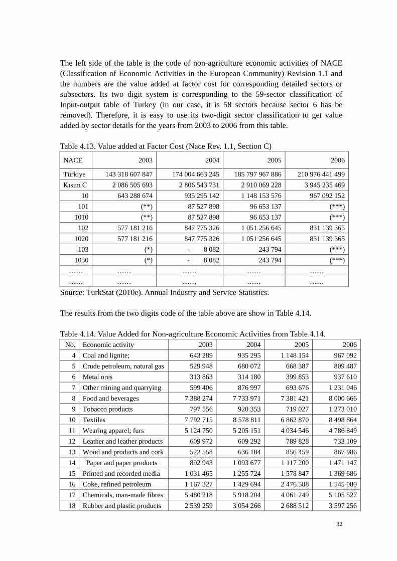
The left side of the table is the code of non-agriculture economic activities of NACE (Classification of Economic Activities in the European Community) Revision 1.1 and the numbers are the value added at factor cost for corresponding detailed sectors or subsectors. Its two digit system is corresponding to the 59-sector classification of Input-output table of Turkey (in our case, it is 58 sectors because sector 6 has be removed). Therefore, it is easy to use its two-digit sector classification to get value added by sector details for the years from 2003 to 2006 from this table. Table 4.13. Value added at Factor Cost (Nace Rev. 1.1, Section C)

NACE 2003 2004 2005 2006

Türkiye 143 318 607 847 174 004 663 245 185 797 967 886 210 976 441 499 Kısım C 2 086 505 693 2 806 543 731 2 910 069 228 3 945 235 469

10 643 288 674 935 295 142 1 148 153 576 967 092 152 101 (**) 87 527 898 96 653 137 (***)

1010 (**) 87 527 898 96 653 137 (***) 102 577 181 216 847 775 326 1 051 256 645 831 139 365

1020 577 181 216 847 775 326 1 051 256 645 831 139 365 103 (*) - 8 082 243 794 (***)

1030 (*) - 8 082 243 794 (***) …… …… …… …… …… …… …… …… …… ……

Source: TurkStat (2010e). Annual Industry and Service Statistics. The results from the two digits code of the table above are show in Table 4.14. Table 4.14. Value Added for Non-agriculture Economic Activities from Table 4.14.

No. Economic activity 2003 2004 2005 2006 4 Coal and lignite; 643 289 935 295 1 148 154 967 092 5 Crude petroleum, natural gas 529 948 680 072 668 387 809 487 6 Metal ores 313 863 314 180 399 853 937 610 7 Other mining and quarrying 599 406 876 997 693 676 1 231 046 8 Food and beverages 7 388 274 7 733 971 7 381 421 8 000 666 9 Tobacco products 797 556 920 353 719 027 1 273 010

10 Textiles 7 792 715 8 578 811 6 862 870 8 498 864 11 Wearing apparel; furs 5 124 750 5 205 151 4 034 546 4 786 849 12 Leather and leather products 609 972 609 292 789 828 733 109 13 Wood and products and cork 522 558 636 184 856 459 867 986 14 Paper and paper products 892 943 1 093 677 1 117 200 1 471 147 15 Printed and recorded media 1 031 465 1 255 724 1 578 847 1 369 686 16 Coke, refined petroleum 1 167 327 1 429 694 2 476 588 1 545 080 17 Chemicals, man-made fibres 5 480 218 5 918 204 4 061 249 5 105 527 18 Rubber and plastic products 2 539 259 3 054 266 2 688 512 3 597 256

33

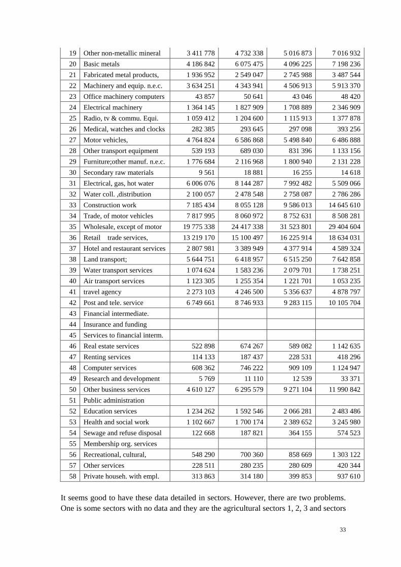
19 Other non-metallic mineral 3 411 778 4 732 338 5 016 873 7 016 932 20 Basic metals 4 186 842 6 075 475 4 096 225 7 198 236 21 Fabricated metal products, 1 936 952 2 549 047 2 745 988 3 487 544 22 Machinery and equip. n.e.c. 3 634 251 4 343 941 4 506 913 5 913 370 23 Office machinery computers 43 857 50 641 43 046 48 420 24 Electrical machinery 1 364 145 1 827 909 1 708 889 2 346 909 25 Radio, tv & commu. Equi. 1 059 412 1 204 600 1 115 913 1 377 878 26 Medical, watches and clocks 282 385 293 645 297 098 393 256 27 Motor vehicles, 4 764 824 6 586 868 5 498 840 6 486 888 28 Other transport equipment 539 193 689 030 831 396 1 133 156 29 Furniture;other manuf. n.e.c. 1 776 684 2 116 968 1 800 940 2 131 228 30 Secondary raw materials 9 561 18 881 16 255 14 618 31 Electrical, gas, hot water 6 006 076 8 144 287 7 992 482 5 509 066 32 Water coll. ,distribution 2 100 057 2 478 548 2 758 087 2 786 286 33 Construction work 7 185 434 8 055 128 9 586 013 14 645 610 34 Trade, of motor vehicles 7 817 995 8 060 972 8 752 631 8 508 281 35 Wholesale, except of motor 19 775 338 24 417 338 31 523 801 29 404 604 36 Retail trade services, 13 219 170 15 100 497 16 225 914 18 634 031 37 Hotel and restaurant services 2 807 981 3 389 949 4 377 914 4 589 324 38 Land transport; 5 644 751 6 418 957 6 515 250 7 642 858 39 Water transport services 1 074 624 1 583 236 2 079 701 1 738 251 40 Air transport services 1 123 305 1 255 354 1 221 701 1 053 235 41 travel agency 2 273 103 4 246 500 5 356 637 4 878 797 42 Post and tele. service 6 749 661 8 746 933 9 283 115 10 105 704 43 Financial intermediate. 44 Insurance and funding 45 Services to financial interm. 46 Real estate services 522 898 674 267 589 082 1 142 635 47 Renting services 114 133 187 437 228 531 418 296 48 Computer services 608 362 746 222 909 109 1 124 947 49 Research and development 5 769 11 110 12 539 33 371 50 Other business services 4 610 127 6 295 579 9 271 104 11 990 842 51 Public administration 52 Education services 1 234 262 1 592 546 2 066 281 2 483 486 53 Health and social work 1 102 667 1 700 174 2 389 652 3 245 980 54 Sewage and refuse disposal 122 668 187 821 364 155 574 523 55 Membership org. services 56 Recreational, cultural, 548 290 700 360 858 669 1 303 122 57 Other services 228 511 280 235 280 609 420 344 58 Private househ. with empl. 313 863 314 180 399 853 937 610

It seems good to have these data detailed in sectors. However, there are two problems. One is some sectors with no data and they are the agricultural sectors 1, 2, 3 and sectors

34

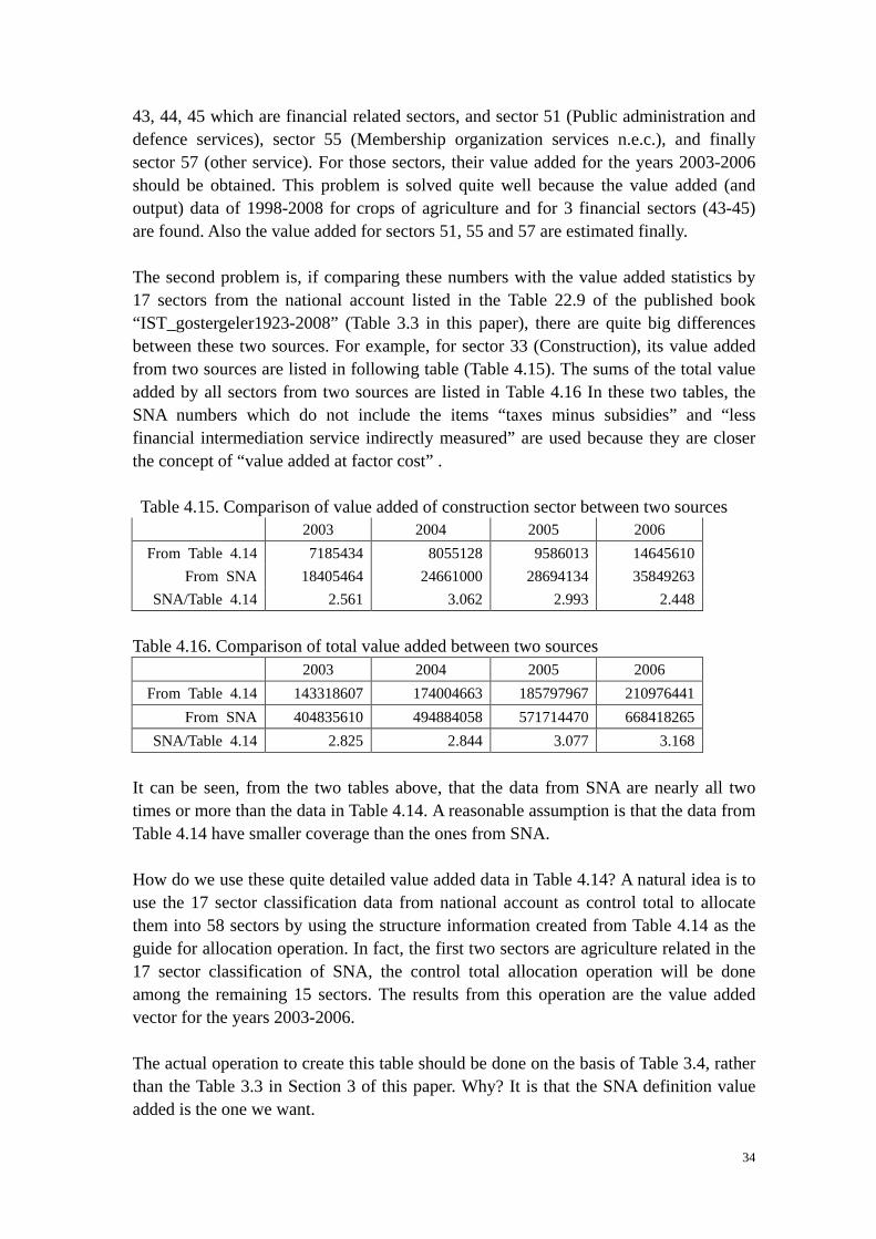
43, 44, 45 which are financial related sectors, and sector 51 (Public administration and defence services), sector 55 (Membership organization services n.e.c.), and finally sector 57 (other service). For those sectors, their value added for the years 2003-2006 should be obtained. This problem is solved quite well because the value added (and output) data of 1998-2008 for crops of agriculture and for 3 financial sectors (43-45) are found. Also the value added for sectors 51, 55 and 57 are estimated finally. The second problem is, if comparing these numbers with the value added statistics by 17 sectors from the national account listed in the Table 22.9 of the published book “IST_gostergeler1923-2008” (Table 3.3 in this paper), there are quite big differences between these two sources. For example, for sector 33 (Construction), its value added from two sources are listed in following table (Table 4.15). The sums of the total value added by all sectors from two sources are listed in Table 4.16 In these two tables, the SNA numbers which do not include the items “taxes minus subsidies” and “less financial intermediation service indirectly measured” are used because they are closer the concept of “value added at factor cost” . Table 4.15. Comparison of value added of construction sector between two sources

2003 2004 2005 2006 From Table 4.14 7185434 8055128 9586013 14645610

From SNA 18405464 24661000 28694134 35849263 SNA/Table 4.14 2.561 3.062 2.993 2.448

Table 4.16. Comparison of total value added between two sources

2003 2004 2005 2006 From Table 4.14 143318607 174004663 185797967 210976441

From SNA 404835610 494884058 571714470 668418265 SNA/Table 4.14 2.825 2.844 3.077 3.168

It can be seen, from the two tables above, that the data from SNA are nearly all two times or more than the data in Table 4.14. A reasonable assumption is that the data from Table 4.14 have smaller coverage than the ones from SNA. How do we use these quite detailed value added data in Table 4.14? A natural idea is to use the 17 sector classification data from national account as control total to allocate them into 58 sectors by using the structure information created from Table 4.14 as the guide for allocation operation. In fact, the first two sectors are agriculture related in the 17 sector classification of SNA, the control total allocation operation will be done among the remaining 15 sectors. The results from this operation are the value added vector for the years 2003-2006. The actual operation to create this table should be done on the basis of Table 3.4, rather than the Table 3.3 in Section 3 of this paper. Why? It is that the SNA definition value added is the one we want.

35

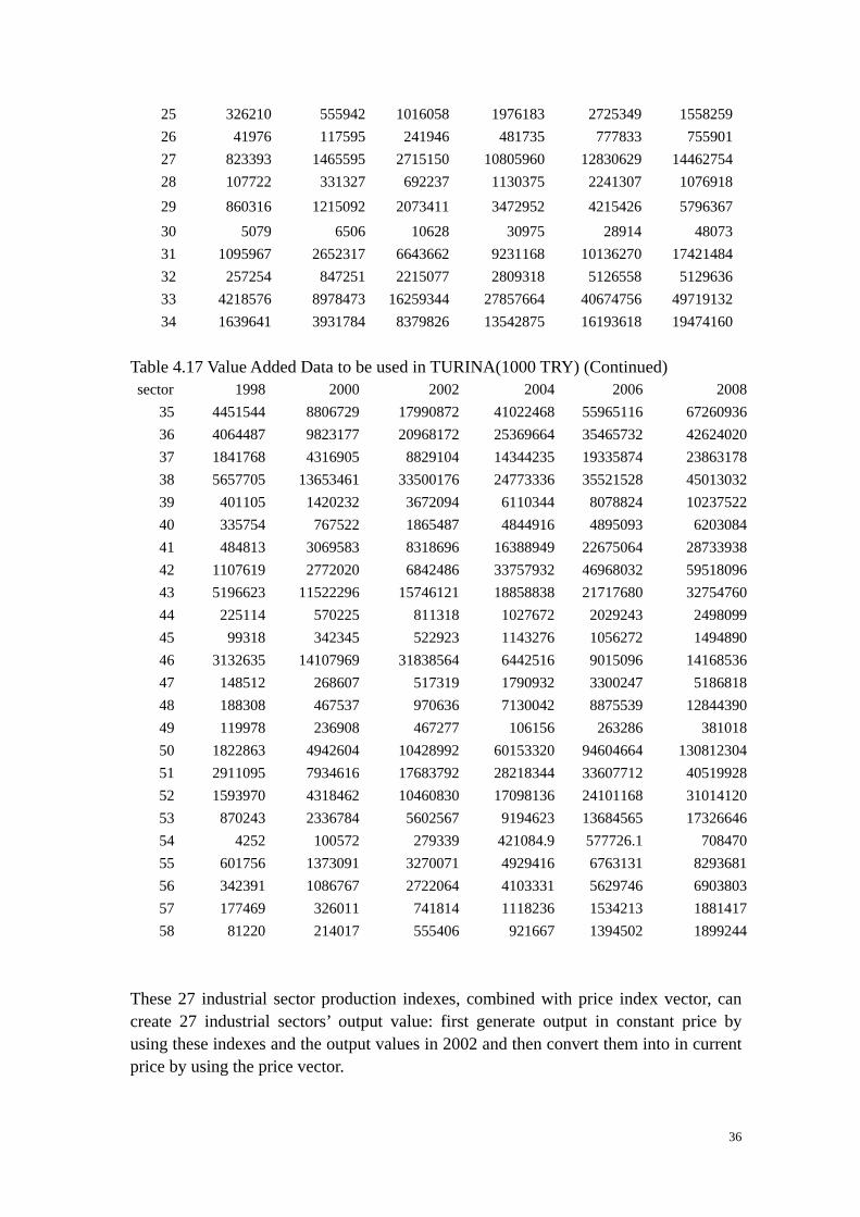
For the value added vector of year 2007 and 2008, there are output index data for 27 industry sectors (described in next part of “output vector”). The growth rate in constant price and the price vector are used for creating the first initial estimation for these industry sectors’ value added. For service sectors, since there are 11 service sectors’ value added data from 1998-2008 in Table 3.4 and other 3 finance related sectors found in yearbook, their data for 2007-2008 are more or less ready. For the value added vector between 1998 and 2002, since we have consistent Input-output tables with 17 sector SNA data for these two years, the value added vectors between the two years can be worked out firstly by interpolation among these two years’ value added by sectors. Then by using the control total of 17 sector value added from SNA to adjust them into proper values for the year 1999, 2000 and 2001. After doing all the work mentioned above, the value added vector time series for the model TURINA are ready and they are listed in Table 4.17 for every two years (the sector names are omitted in that table). Table 4.17 Value Added Data to be used in TURINA (1000 TRY) Sector 1998 2000 2002 2004 2006 2008

1 8479915 17033626 38077944 56858452 67075480 76797104 2 317460 517115 1095966 1636510 1930578 2210388 3 244564 412902 689481 1372466 2091429 1704752 4 231583 632237 1310208 2220536 2489872 5770324 5 110613 305142 633516 1614597 2084104 3633483 6 76833 144067 274494 745911 2413968 2896438 7 333725 689701 1348202 2082126 3169446 2488368 8 3307829 6817416 13152184 12687819 15824779 20912062 9 257625 480311 902041 1509868 2517929 2088778

10 1467737 4912049 10391947 14073804 16810182 16367053 11 940972 2931417 6136660 8539210 9468066 9323752 12 180445 466987 947050 999562 1450039 2031876 13 276488 428306 757617 1043679 1716817 2726848 14 300534 806298 1646198 1794212 2909830 3014279 15 385506 693724 1289425 2060054 2709146 4493774 16 2277166 1664683 1742054 2345457 3056065 9181426 17 1048409 2708825 5491796 9708996 10098390 11496930 18 516455 1240628 2478926 5010618 7115130 7437882 19 1087692 2185948 4190076 7763546 13879021 13773013 20 824245 1955794 3897837 9967004 14237627 16274090 21 781869 1306716 2373074 4181790 6898128 8704845 22 1089368 2450578 4827322 7126368 11696249 13823009 23 50234 57984 89763 83077 95771 101172 24 379210 935242 1878845 2998741 4642028 5261962

36

25 326210 555942 1016058 1976183 2725349 1558259 26 41976 117595 241946 481735 777833 755901 27 823393 1465595 2715150 10805960 12830629 14462754 28 107722 331327 692237 1130375 2241307 1076918 29 860316 1215092 2073411 3472952 4215426 5796367 30 5079 6506 10628 30975 28914 48073 31 1095967 2652317 6643662 9231168 10136270 17421484 32 257254 847251 2215077 2809318 5126558 5129636 33 4218576 8978473 16259344 27857664 40674756 49719132 34 1639641 3931784 8379826 13542875 16193618 19474160

Table 4.17 Value Added Data to be used in TURINA(1000 TRY) (Continued) sector 1998 2000 2002 2004 2006 2008

35 4451544 8806729 17990872 41022468 55965116 67260936 36 4064487 9823177 20968172 25369664 35465732 42624020 37 1841768 4316905 8829104 14344235 19335874 23863178 38 5657705 13653461 33500176 24773336 35521528 45013032 39 401105 1420232 3672094 6110344 8078824 10237522 40 335754 767522 1865487 4844916 4895093 6203084 41 484813 3069583 8318696 16388949 22675064 28733938 42 1107619 2772020 6842486 33757932 46968032 59518096 43 5196623 11522296 15746121 18858838 21717680 32754760 44 225114 570225 811318 1027672 2029243 2498099 45 99318 342345 522923 1143276 1056272 1494890 46 3132635 14107969 31838564 6442516 9015096 14168536 47 148512 268607 517319 1790932 3300247 5186818 48 188308 467537 970636 7130042 8875539 12844390 49 119978 236908 467277 106156 263286 381018 50 1822863 4942604 10428992 60153320 94604664 130812304 51 2911095 7934616 17683792 28218344 33607712 40519928 52 1593970 4318462 10460830 17098136 24101168 31014120 53 870243 2336784 5602567 9194623 13684565 17326646 54 4252 100572 279339 421084.9 577726.1 708470 55 601756 1373091 3270071 4929416 6763131 8293681 56 342391 1086767 2722064 4103331 5629746 6903803 57 177469 326011 741814 1118236 1534213 1881417 58 81220 214017 555406 921667 1394502 1899244

These 27 industrial sector production indexes, combined with price index vector, can create 27 industrial sectors’ output value: first generate output in constant price by using these indexes and the output values in 2002 and then convert them into in current price by using the price vector.

37

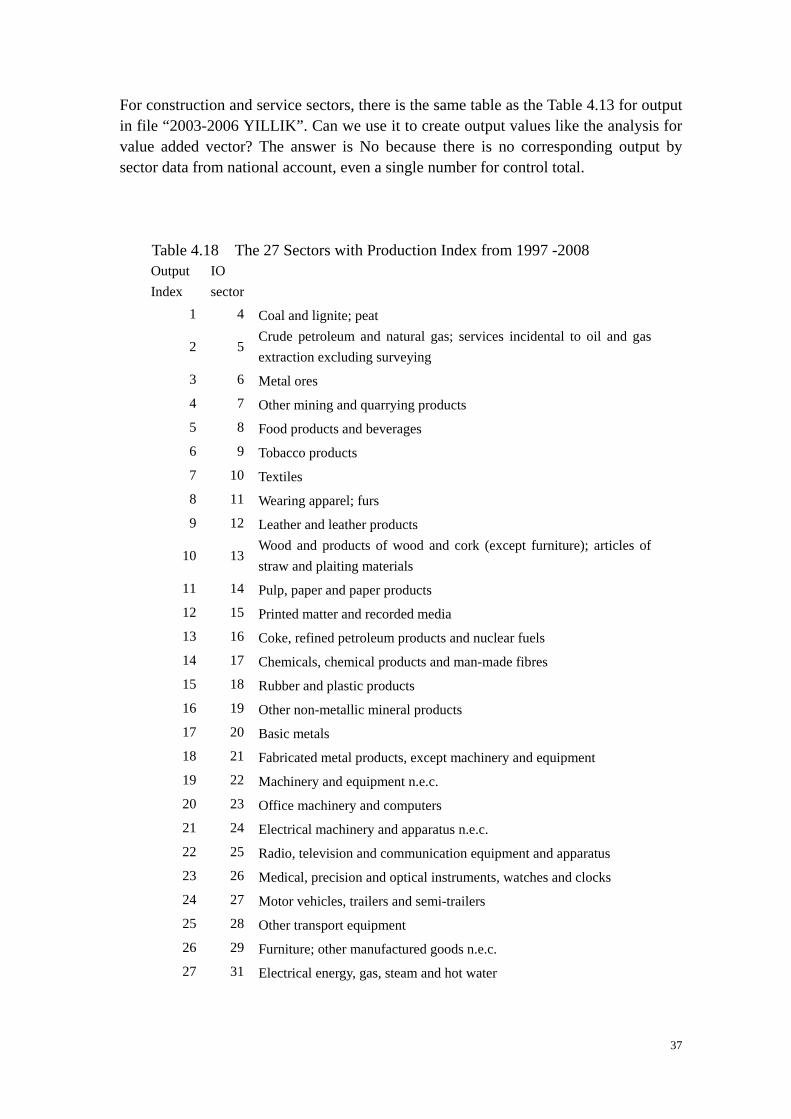
For construction and service sectors, there is the same table as the Table 4.13 for output in file “2003-2006 YILLIK”. Can we use it to create output values like the analysis for value added vector? The answer is No because there is no corresponding output by sector data from national account, even a single number for control total.

Table 4.18 The 27 Sectors with Production Index from 1997 -2008 Output Index

IO sector

1 4 Coal and lignite; peat

2 5 Crude petroleum and natural gas; services incidental to oil and gas extraction excluding surveying

3 6 Metal ores 4 7 Other mining and quarrying products 5 8 Food products and beverages 6 9 Tobacco products 7 10 Textiles 8 11 Wearing apparel; furs 9 12 Leather and leather products

10 13 Wood and products of wood and cork (except furniture); articles of straw and plaiting materials

11 14 Pulp, paper and paper products 12 15 Printed matter and recorded media 13 16 Coke, refined petroleum products and nuclear fuels 14 17 Chemicals, chemical products and man-made fibres 15 18 Rubber and plastic products 16 19 Other non-metallic mineral products 17 20 Basic metals 18 21 Fabricated metal products, except machinery and equipment 19 22 Machinery and equipment n.e.c. 20 23 Office machinery and computers 21 24 Electrical machinery and apparatus n.e.c. 22 25 Radio, television and communication equipment and apparatus 23 26 Medical, precision and optical instruments, watches and clocks 24 27 Motor vehicles, trailers and semi-trailers 25 28 Other transport equipment 26 29 Furniture; other manufactured goods n.e.c. 27 31 Electrical energy, gas, steam and hot water

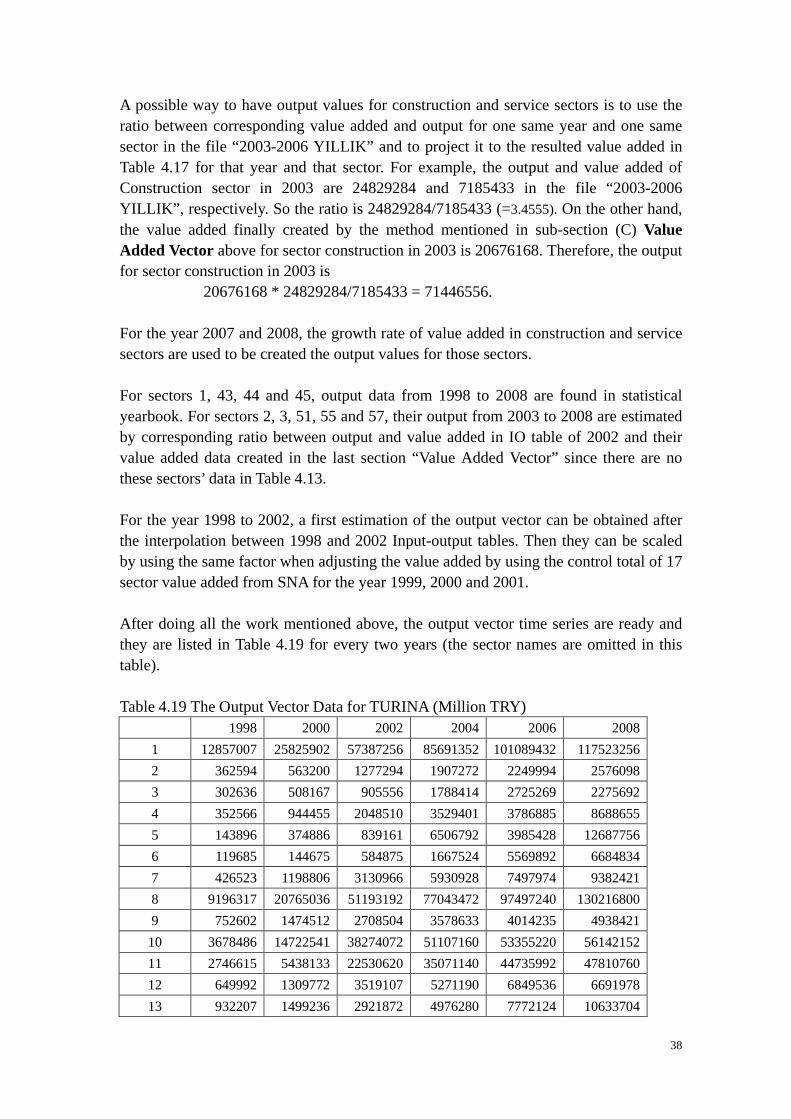
38

A possible way to have output values for construction and service sectors is to use the ratio between corresponding value added and output for one same year and one same sector in the file “2003-2006 YILLIK” and to project it to the resulted value added in Table 4.17 for that year and that sector. For example, the output and value added of Construction sector in 2003 are 24829284 and 7185433 in the file “2003-2006 YILLIK”, respectively. So the ratio is 24829284/7185433 (=3.4555). On the other hand, the value added finally created by the method mentioned in sub-section (C) Value Added Vector above for sector construction in 2003 is 20676168. Therefore, the output for sector construction in 2003 is

20676168 * 24829284/7185433 = 71446556.

For the year 2007 and 2008, the growth rate of value added in construction and service sectors are used to be created the output values for those sectors. For sectors 1, 43, 44 and 45, output data from 1998 to 2008 are found in statistical yearbook. For sectors 2, 3, 51, 55 and 57, their output from 2003 to 2008 are estimated by corresponding ratio between output and value added in IO table of 2002 and their value added data created in the last section “Value Added Vector” since there are no these sectors’ data in Table 4.13. For the year 1998 to 2002, a first estimation of the output vector can be obtained after the interpolation between 1998 and 2002 Input-output tables. Then they can be scaled by using the same factor when adjusting the value added by using the control total of 17 sector value added from SNA for the year 1999, 2000 and 2001. After doing all the work mentioned above, the output vector time series are ready and they are listed in Table 4.19 for every two years (the sector names are omitted in this table). Table 4.19 The Output Vector Data for TURINA (Million TRY) 1998 2000 2002 2004 2006 2008

1 12857007 25825902 57387256 85691352 101089432 117523256 2 362594 563200 1277294 1907272 2249994 2576098 3 302636 508167 905556 1788414 2725269 2275692 4 352566 944455 2048510 3529401 3786885 8688655 5 143896 374886 839161 6506792 3985428 12687756 6 119685 144675 584875 1667524 5569892 6684834 7 426523 1198806 3130966 5930928 7497974 9382421 8 9196317 20765036 51193192 77043472 97497240 130216800 9 752602 1474512 2708504 3578633 4014235 4938421

10 3678486 14722541 38274072 51107160 53355220 56142152 11 2746615 5438133 22530620 35071140 44735992 47810760 12 649992 1309772 3519107 5271190 6849536 6691978 13 932207 1499236 2921872 4976280 7772124 10633704

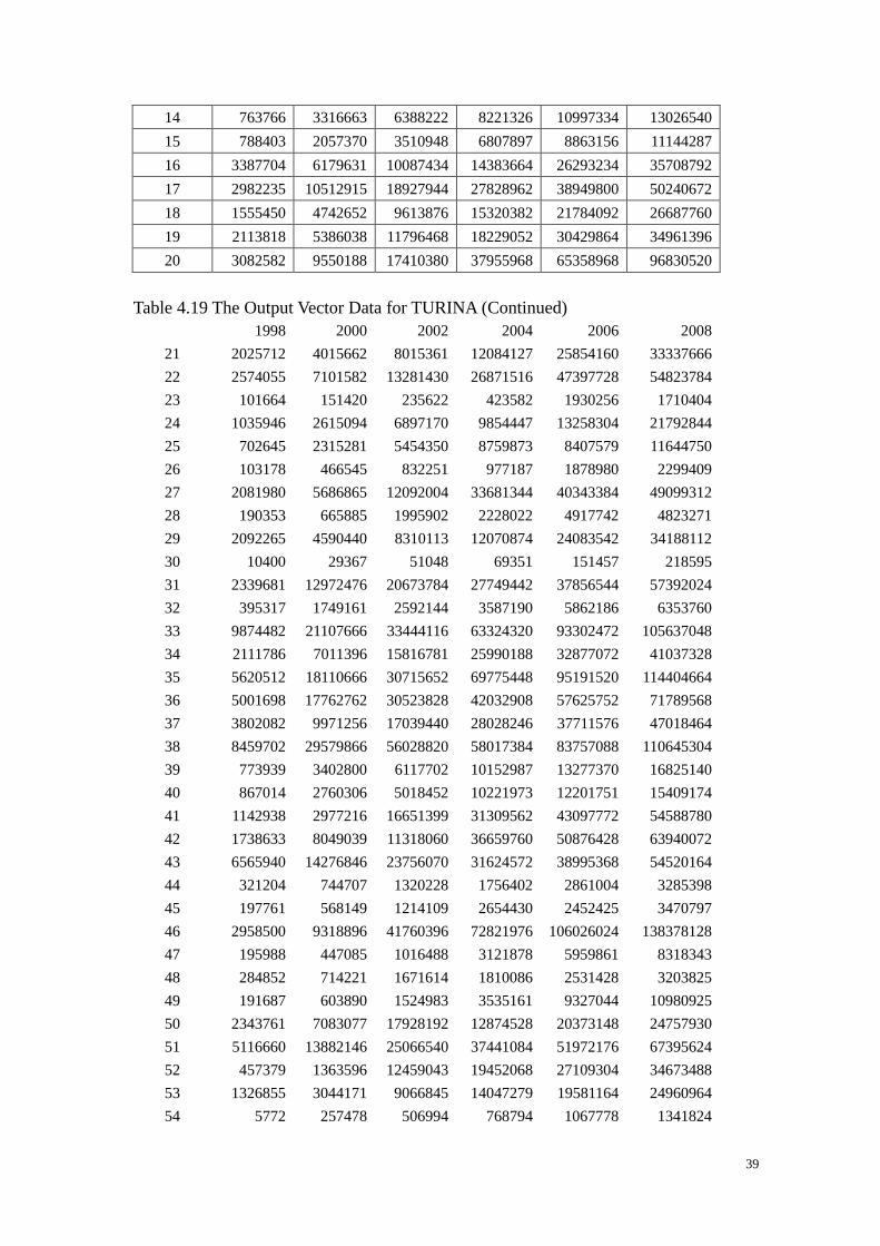
39

14 763766 3316663 6388222 8221326 10997334 13026540 15 788403 2057370 3510948 6807897 8863156 11144287 16 3387704 6179631 10087434 14383664 26293234 35708792 17 2982235 10512915 18927944 27828962 38949800 50240672 18 1555450 4742652 9613876 15320382 21784092 26687760 19 2113818 5386038 11796468 18229052 30429864 34961396 20 3082582 9550188 17410380 37955968 65358968 96830520

Table 4.19 The Output Vector Data for TURINA (Continued)

1998 2000 2002 2004 2006 2008 21 2025712 4015662 8015361 12084127 25854160 33337666 22 2574055 7101582 13281430 26871516 47397728 54823784 23 101664 151420 235622 423582 1930256 1710404 24 1035946 2615094 6897170 9854447 13258304 21792844 25 702645 2315281 5454350 8759873 8407579 11644750 26 103178 466545 832251 977187 1878980 2299409 27 2081980 5686865 12092004 33681344 40343384 49099312 28 190353 665885 1995902 2228022 4917742 4823271 29 2092265 4590440 8310113 12070874 24083542 34188112 30 10400 29367 51048 69351 151457 218595 31 2339681 12972476 20673784 27749442 37856544 57392024 32 395317 1749161 2592144 3587190 5862186 6353760 33 9874482 21107666 33444116 63324320 93302472 105637048 34 2111786 7011396 15816781 25990188 32877072 41037328 35 5620512 18110666 30715652 69775448 95191520 114404664 36 5001698 17762762 30523828 42032908 57625752 71789568 37 3802082 9971256 17039440 28028246 37711576 47018464 38 8459702 29579866 56028820 58017384 83757088 110645304 39 773939 3402800 6117702 10152987 13277370 16825140 40 867014 2760306 5018452 10221973 12201751 15409174 41 1142938 2977216 16651399 31309562 43097772 54588780 42 1738633 8049039 11318060 36659760 50876428 63940072 43 6565940 14276846 23756070 31624572 38995368 54520164 44 321204 744707 1320228 1756402 2861004 3285398 45 197761 568149 1214109 2654430 2452425 3470797 46 2958500 9318896 41760396 72821976 106026024 138378128 47 195988 447085 1016488 3121878 5959861 8318343 48 284852 714221 1671614 1810086 2531428 3203825 49 191687 603890 1524983 3535161 9327044 10980925 50 2343761 7083077 17928192 12874528 20373148 24757930 51 5116660 13882146 25066540 37441084 51972176 67395624 52 457379 1363596 12459043 19452068 27109304 34673488 53 1326855 3044171 9066845 14047279 19581164 24960964 54 5772 257478 506994 768794 1067778 1341824

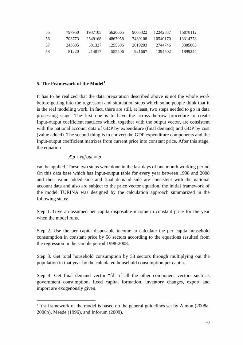
40

55 797950 1937105 5620665 9005322 12242837 15078112 56 703773 2549168 4867058 7439108 10540170 13314778 57 243695 581327 1255606 2019203 2744746 3385805 58 81220 214017 555406 921667 1394502 1899244

5. The Framework of the Model1

It has to be realized that the data preparation described above is not the whole work before getting into the regression and simulation steps which some people think that it is the real modeling work. In fact, there are still, at least, two steps needed to go in data processing stage. The first one is to have the across-the-row procedure to create Input-output coefficient matrices which, together with the output vector, are consistent with the national account data of GDP by expenditure (final demand) and GDP by cost (value added). The second thing is to convert the GDP expenditure components and the Input-output coefficient matrixes from current price into constant price. After this stage, the equation

poutvapA =+′

can be applied. These two steps were done in the last days of one month working period. On this data base which has Input-output table for every year between 1998 and 2008 and their value added side and final demand side are consistent with the national account data and also are subject to the price vector equation, the initial framework of the model TURINA was designed by the calculation approach summarized in the following steps: Step 1. Give an assumed per capita disposable income in constant price for the year when the model runs. Step 2. Use the per capita disposable income to calculate the per capita household consumption in constant price by 58 sectors according to the equations resulted from the regression in the sample period 1998-2008. Step 3. Get total household consumption by 58 sectors through multiplying out the population in that year by the calculated household consumption per capita. Step 4. Get final demand vector “fd” if all the other component vectors such as government consumption, fixed capital formation, inventory changes, export and import are exogenously given. 1 The framework of the model is based on the general guidelines set by Almon (2008a, 2008b), Meade (1996), and Inforum (2009).

41

Step 5. Calculate the gross output vector, in constant price, according to the equation out = (I-A)-1*fd Step 6. Calculate the value added vector “va”, in current price, according to the relationship analysis between output and value added from the sample period 1998-2008. Step 7. Calculate the price index vector, p, according to the equation

poutvapA =+′

Step 8. Have GDP in current price and in constant price, which is the sum of value added vector and final demand vector, respectively. Step 9. Have GDP per capita in constant price and in current price, and the GDP deflator. Step 10. Estimate the disposable income per capita in current price and in constant price according to the regression analysis from the sample period 1998 and 2008. Step 11. If the resulted disposable income per capita is very close to the one used in step 2, the model finishes the run for that year and goes to the next year. Otherwise, use this new disposable income per capita and go to step 2 for the next iteration of the model. Obviously, the logical structure of the model is quite simple in this stage and its key point is the relationship analysis between value added vector in current price and gross output vector in constant price as in other countries INFORUM models. Further development of TURINA can be done to make other final demand component vectors endogenous. Or it can be extended to have value added by cost component vectors, plus employment and productivity. Also it is possible to develop the accounting block to include total taxes, government revenue, and so on. However, the modeling practice got trouble from the very beginning which caused by the most simple time series data “personal disposable income”. There is no official report directly about the variable “personal disposable income” in Turkish statistics. From the annual report of Turkish national planning agency, there is data about personal disposable income of previous year or years. According to these data, a time series of personal disposable income of Turkey was obtained. However, the name of this income series is “Private disposable income” but not “Personal disposable income” for some unexplained reason. A comparison between this series and the household consumption series from the GDP by expenditure in National Accounts is listed in the following table (Table 5.1).

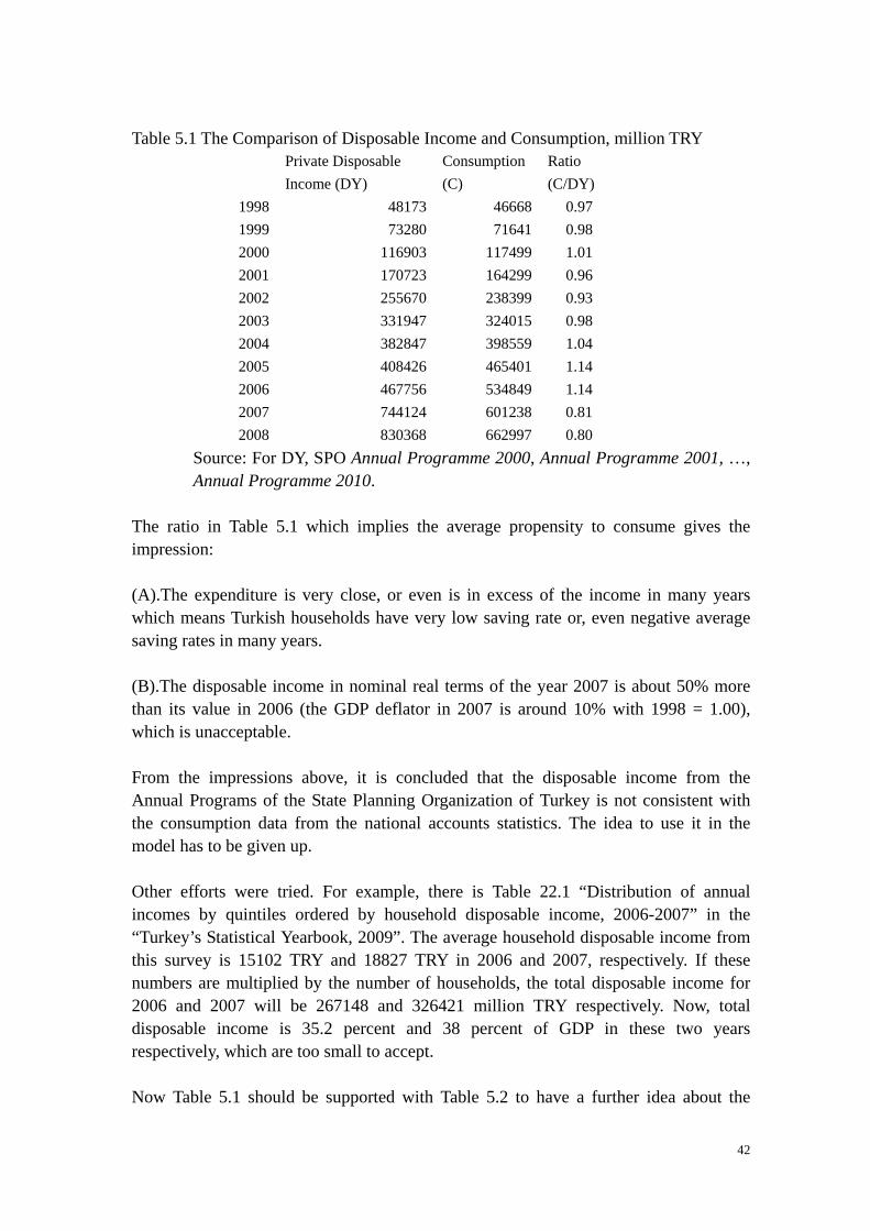
42

Table 5.1 The Comparison of Disposable Income and Consumption, million TRY

Private Disposable Income (DY)

Consumption (C)

Ratio (C/DY)

1998 48173 46668 0.97 1999 73280 71641 0.98 2000 116903 117499 1.01 2001 170723 164299 0.96 2002 255670 238399 0.93 2003 331947 324015 0.98 2004 382847 398559 1.04 2005 408426 465401 1.14 2006 467756 534849 1.14 2007 744124 601238 0.81 2008 830368 662997 0.80

Source: For DY, SPO Annual Programme 2000, Annual Programme 2001, …, Annual Programme 2010.

The ratio in Table 5.1 which implies the average propensity to consume gives the impression: (A).The expenditure is very close, or even is in excess of the income in many years which means Turkish households have very low saving rate or, even negative average saving rates in many years. (B).The disposable income in nominal real terms of the year 2007 is about 50% more than its value in 2006 (the GDP deflator in 2007 is around 10% with 1998 = 1.00), which is unacceptable. From the impressions above, it is concluded that the disposable income from the Annual Programs of the State Planning Organization of Turkey is not consistent with the consumption data from the national accounts statistics. The idea to use it in the model has to be given up. Other efforts were tried. For example, there is Table 22.1 “Distribution of annual incomes by quintiles ordered by household disposable income, 2006-2007” in the “Turkey’s Statistical Yearbook, 2009”. The average household disposable income from this survey is 15102 TRY and 18827 TRY in 2006 and 2007, respectively. If these numbers are multiplied by the number of households, the total disposable income for 2006 and 2007 will be 267148 and 326421 million TRY respectively. Now, total disposable income is 35.2 percent and 38 percent of GDP in these two years respectively, which are too small to accept. Now Table 5.1 should be supported with Table 5.2 to have a further idea about the

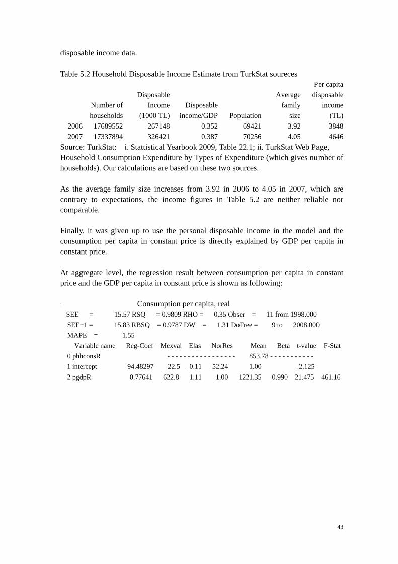
43

disposable income data. Table 5.2 Household Disposable Income Estimate from TurkStat soureces

Number of households

Disposable Income

(1000 TL) Disposable

income/GDP

Population

Average family

size

Per capita disposable

income (TL)

2006 17689552 267148 0.352 69421 3.92 3848 2007 17337894 326421 0.387 70256 4.05 4646

Source: TurkStat: i. Stattistical Yearbook 2009, Table 22.1; ii. TurkStat Web Page, Household Consumption Expenditure by Types of Expenditure (which gives number of households). Our calculations are based on these two sources. As the average family size increases from 3.92 in 2006 to 4.05 in 2007, which are contrary to expectations, the income figures in Table 5.2 are neither reliable nor comparable. Finally, it was given up to use the personal disposable income in the model and the consumption per capita in constant price is directly explained by GDP per capita in constant price. At aggregate level, the regression result between consumption per capita in constant price and the GDP per capita in constant price is shown as following: : Consumption per capita, real SEE = 15.57 RSQ = 0.9809 RHO = 0.35 Obser = 11 from 1998.000 SEE+1 = 15.83 RBSQ = 0.9787 DW = 1.31 DoFree = 9 to 2008.000 MAPE = 1.55 Variable name Reg-Coef Mexval Elas NorRes Mean Beta t-value F-Stat 0 phhconsR - - - - - - - - - - - - - - - - - 853.78 - - - - - - - - - - - 1 intercept -94.48297 22.5 -0.11 52.24 1.00 -2.125 2 pgdpR 0.77641 622.8 1.11 1.00 1221.35 0.990 21.475 461.16

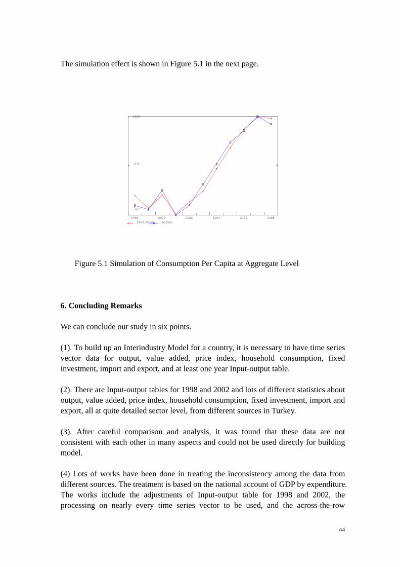
44

The simulation effect is shown in Figure 5.1 in the next page. Figure 5.1 Simulation of Consumption Per Capita at Aggregate Level 6. Concluding Remarks We can conclude our study in six points. (1). To build up an Interindustry Model for a country, it is necessary to have time series vector data for output, value added, price index, household consumption, fixed investment, import and export, and at least one year Input-output table. (2). There are Input-output tables for 1998 and 2002 and lots of different statistics about output, value added, price index, household consumption, fixed investment, import and export, all at quite detailed sector level, from different sources in Turkey. (3). After careful comparison and analysis, it was found that these data are not consistent with each other in many aspects and could not be used directly for building model. (4) Lots of works have been done in treating the inconsistency among the data from different sources. The treatment is based on the national account of GDP by expenditure. The works include the adjustments of Input-output table for 1998 and 2002, the processing on nearly every time series vector to be used, and the across-the-row

1028

872

717

1998 2000 2002 2004 2006 2008 Predicted Actual

45

procedure plus the conversion from current price to constant price. (5) After the data comparison, analysis and treatment, one data bank, which has consistent data from 1998 to 2008, is ready to be used for building an interindustry model for Turkey. In that data bank, there are Input-output tables for each year from 1998 to 2008 and the aggregation values from these Input-output tables are consistent with the national account data of GDP by expenditure (final demand) and GDP by cost (value added) for every year. (6) The disposable income data, which normally is a key variable in the model iteration mechanism, was found not acceptable. It was decided to use the relationship between per capita GDP and per capita consumption to replace the relationships between per capita GDP and per capita disposable income and between per capita disposable income and per capita consumption when starting the next step of the model build for Turkey. List of References Almon C (2008), The Craft of Economic Modeling, Vols 1, 2, 3. University of Maryland. http://www.inforum.umd.edu. (e-books). INFORUM (2009). INTERDYME, the Software Package for Interindustry Model: version 1996, version 1997, version 1998, …, version 2009. Li Z, Yinchu W (1998). “The Treatment of the Discrepancy between the Systems of Input Output and National Accounting”. The 12th International Conference on Input-Output Techniques. New York. Meade, D. (1996) An Overview of INTERDYME, INFORUM Working Paper. Salmon P., Ozhan G.. (2008). TINYTURK A Tiny Model Based on Turkish Data, First Steps to Building an INFORUM Model. In Grassini M., Bardazzi R. (eds): Energy Policy and International Competitiveness, Firenze University Press, pp. 141-159. Shantong L, Yinchu W (1999), “The Multisectoral Development Analysis Model (MUDAN) for China”. The Practical Macroeconomic Models in China. China Financial and Economic Press, Beijing. State Planning Organization (SPO) (2010). http://www.dpt.gov.tr: a. Annual Programme 2000, (e-book). b. Annual Programme 2001, (e-book). c. Annual Programme 2002 , (e-book). d. Annual Programme 2003, (e-book).

46

e. Annual Programme 2004, (e-book). f. Annual Programme 2005, (e-book). g. Annual Programme 2006, (e-book). h. Annual Programme 2007, (e-book). m. Annual Programme 2008, (e-book). n. Annual Programme 2009, (e-book). o. Annual Programme 2010, (e-book). TurkStat (2010). http://www.tuik.gov.tr: a. National Accounts/Input-Output Tables/I-O Table 1998. b. National Accounts/Input-Output Tables/I-O Table 2002. c. Statistical Indicators 1923-2008, (e-book). d. Turkey’s Statistical Yearbook 2009, (e-book). e. “2003-2006 Yıllık” Annual Industry and Services Statistics. f. Other current statistics on the web: http://www.tuik.gov.tr . Yinchu W (1998). “From Data Preparation to Construction of Simulation Models: the QUICKDYME Approach in COMPASS”, The 12th International Conference on Input-Output Techniques. New York