Embed Size (px)
Citation preview

MATURE HARDWOOD FORESTS OF THE CENTRAL PIEDMONT OF NORTH CAROLINA: LANDSCAPE DISTRIBUTION AND UNDERSTORY CHANGE
By
Kristin Taverna
A thesis submitted to the faculty of the University of North Carolina at Chapel Hill In partial fulfillment of the requirements for the degree of
Masters of Science in the Curriculum of Ecology
Chapel Hill
2004
Approved by
Advisor: Peter S. White
Advisor: Robert K. Peet
Reader: Dean L. Urban

ii
© 2004 Kristin Taverna
ALL RIGHTS RESERVED
iii
ABSTRACT KRISTIN TAVERNA: Mature Hardwood Forests of the Central Piedmont
of North Carolina: Landscape distribution and Understory Change. (Under the direction of P.S. White and R.K. Peet)
The natural landscape of the Piedmont region of North Carolina has a complex
history of human impact. Past agricultural disturbance, combined with recent development,
has greatly reduced the extent of the once dominant oak-hickory (Quercus-Carya) hardwood
forests. More localized disturbances continue to impact stands long considered the stable
endpoint of succession. In order to further understand the distribution and dynamics of
remnant hardwood forests, I used a multi-scale approach to examine (1) whether the current
landscape distribution of hardwood stands is a biased subset of their original extent that can
be predicted using hypothesized drivers of past agricultural use and (2) whether understory
composition in mature, unfragmented hardwood stands exhibit stability over time. Results
show that the current distribution of hardwood is non-random and stands are strongly
predicted by the interaction of soil quality, soil moisture, distance to streams, and slope
angle. Hardwood is largely confined to river valleys and upland areas with steep topography
or relatively poor soil quality. At the stand-level, hardwood forests are undergoing
significant decline of herbaceous species, combined with dramatic increases in understory
woody species abundance. Compositional change is occurring largely independent of
environmental conditions, showing that the steady state notion for hardwood forests is
fundamentally incompatible with human-accelerated environmental change in the Piedmont
region.

iv
ACKNOWLEDGEMENTS
Current thanks and funding (need to add) Association of Southeastern Biologists Center for the Study of the American South Curriculum of Ecology University of North Carolina – Graduate School Previous Duke Forest contributors and funding Original survey: Thank Robert Peet, Norman Christensen, Dorothy Allard, Gary Thorburn, and the Duke Forest staff for their collaboration and assistances, NSF grant DEB-7708743 for financial support, all of which made collection of the original plot data possible. Thank Laura Phillips, Dean Urban and the Duke forest staff for their collection and assistance, and NSF grant DEB-9707551 for financial support, all of which made resampling of the plots possible.

v
TABLE OF CONTENTS

vi
LIST OF TABLES
Table 2.1: Land cover classes for the study area and the percentage of total area occupied by each class………………………………………………………...1
Table 2.2: Names and descriptions of environmental variables sampled for analysis……2 Table 2.3: Generalized linear model coefficients for hardwood and pine models………..3 Table 2.4: Comparison of predictive accuracy of the generalized linear model (GLM),
classification tree model (CART), and classification tree model built using information from the corresponding GLM model (CART2) for each land cover…………………………………………………………………………...4
Table 3.1: Environmental variables recorded for each hardwood plot in 1977.
Data were not recollected in 2000 and are assumed to be constant over time...5 Table 3.2: Summary statistics for change in species richness at the subplot (25m2) and
plot (1000m2) scale from 1977-2000………………………………………….6 Table 3.3: Indicator values (percent of perfect indication) and frequency statistics of
species associated with 1977 plots or 2000 plots, listed in order of statistical significance (p-value) by year…………………………………………………7
Table 3.4: Environmental variables correlated with change in species richness at 25m2
from 1977 to 2000. Data listed are for species separated by growth form (Herb, Shrub, Tree)…………………………………………………………....8
Table 3.5: Coefficients of determination for the correlations between NMS ordination
axes and measured environmental variables. Environmental variables were measured in 1977 and are assumed to be constant over time…………………9
vii
LIST OF FIGURES
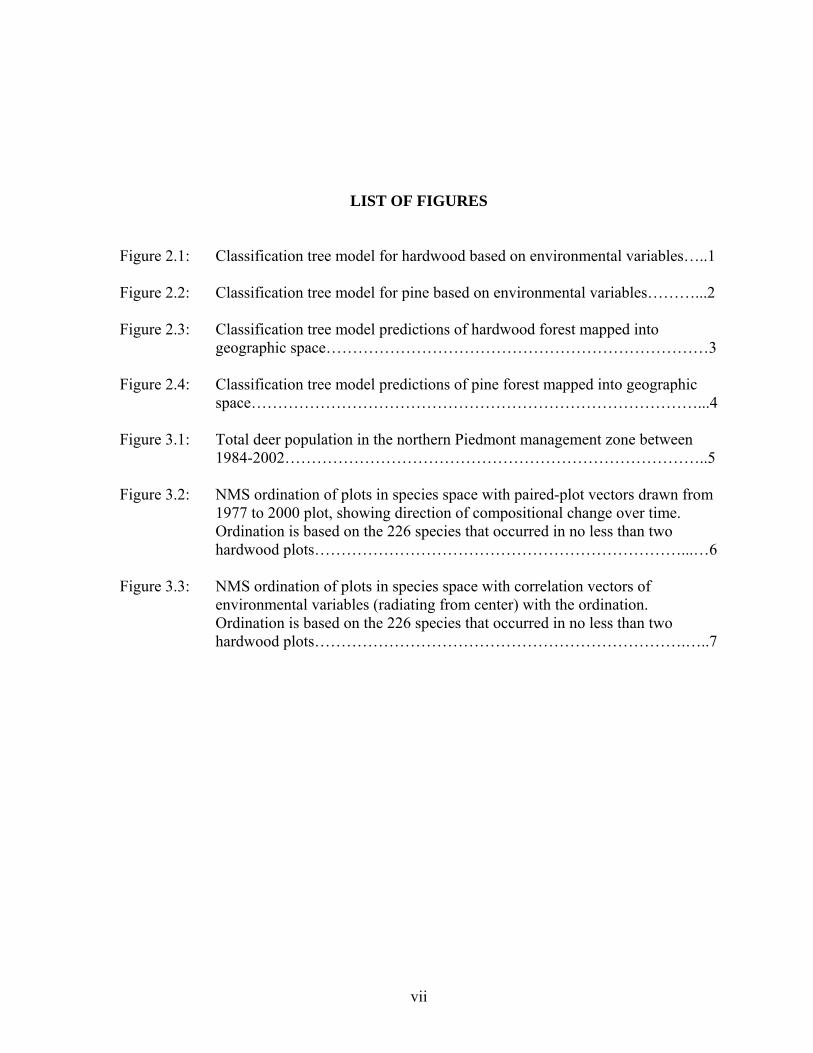
Figure 2.1: Classification tree model for hardwood based on environmental variables…..1 Figure 2.2: Classification tree model for pine based on environmental variables………...2 Figure 2.3: Classification tree model predictions of hardwood forest mapped into
geographic space………………………………………………………………3 Figure 2.4: Classification tree model predictions of pine forest mapped into geographic
space…………………………………………………………………………...4 Figure 3.1: Total deer population in the northern Piedmont management zone between
1984-2002……………………………………………………………………..5 Figure 3.2: NMS ordination of plots in species space with paired-plot vectors drawn from
1977 to 2000 plot, showing direction of compositional change over time. Ordination is based on the 226 species that occurred in no less than two hardwood plots……………………………………………………………...…6
Figure 3.3: NMS ordination of plots in species space with correlation vectors of
environmental variables (radiating from center) with the ordination. Ordination is based on the 226 species that occurred in no less than two hardwood plots…………………………………………………………….…..7

CHAPTER 1
INTRODUCTION:
MATURE HARDWOOD FORESTS OF THE CENTRAL PIEDMONT OF NORTH
CAROLINA: LANDSCAPE DISTRIBUTION AND UNDERSTORY CHANGE

2
The natural landscape of the Piedmont region of the Southeastern US has a complex
history of human impact, spanning over 10,000 years beginning with Native American use of
the land (Delcourt et al. 1993). Intertwined with the historic land-use of the region is the
development of the native flora, described in the earliest accounts as principally oak-hickory
(Quercus-Carya) dominated forests (Ashe 1897, Oosting 1942; 1956, Braun 1950). As the
land-use patterns of the region have shifted over time, so has the extent and composition of
Piedmont oak-hickory forests.
In the Piedmont of North Carolina, the most extensive alteration of native forestlands
occurred with the arrival of Europeans in the 18th century. By 1830, European settlement of
the Piedmont was complete and extensive land conversion to agriculture began on a large
scale (Trimble 1974). Exploitative land-use often led to severe soil erosion and made it
necessary to clear more land for production. This pattern of land-use continued until the
1920’s, at which time poor management practices and economic factors forced many
agriculturalists to abandon the land and allow it to grow back into forest (Trimble 1974, Peet
& Christensen 1980). The sites that were converted to farmland in the 19th century lost their
hardwood canopy and are now largely dominated by successional pine species, such as
loblolly pine (Pinus taeda) and shortleaf pine (Pinus echinata), with shade-tolerant hardwood
species in the understory.
The large-scale loss of native hardwood stands and re-growth of pine significantly
changed the vegetation pattern in the region (Christensen 1989). The once dominant
hardwood forests are now remnant patches scattered among a mosaic of different land-uses.

3
Although they cover a fraction of their original area, these remnant patches are unique in that
the forest canopy has remained in hardwood over time, giving them the important attribute of
continuity (White 2001). This habitat-type has persisted in the midst of other forms of
disturbance, such as selective extraction of timber, understory grazing by domestic livestock,
low-intensity ground fires, and hurricane related wind-throw. Previous research has shown
that given the long-lasting impacts of historical land-use and the slow migration of certain
plant species in the Piedmont (Hans et al. 2001, Matlack 1994, Peterken & Game 1984, Jolls
2003), it behooves us to identify and protect hardwood forest remnants throughout the
region.
This thesis is an examination of hardwood forests of the Piedmont of North Carolina
at both the landscape scale and the scale of forest communities. This multi-scale approach
allows for a broader discussion of how historic land-use and modern management practices
continue to shape native hardwood forests today. In the remainder of this Chapter I expand
on the discussion of Piedmont hardwood forests and present the general approaches and
questions addressed in subsequent chapters.
The study of Piedmont hardwood forests in North Carolina has a long history in
ecology, beginning in the 1930s with the establishment of Duke University Forest and the
pioneering work on secondary forest succession by Oosting (1942) and his student Catherine
Keever (1950). Using a chronosequence approach, Oosting (1942) documented the variation
in forest communities following agricultural disturbance to predict that pine forests would
eventually yield to hardwood dominated communities in the Piedmont. Oak-hickory forests
were considered the predictable end-point of succession to which post-agricultural forests

4
would, if given enough time (~ 80-100 years), eventually succeed. These hardwood forest
communities varied across the landscape as species composition and structure shifted with
local moisture and edaphic gradients from mesic, bottomland sites to xeric, exposed ridge-
tops (Bordeau 1954, Skeen et al. 1993). Additional work by Peet & Christensen (1980, 1981,
1984) provided further support for this model of successional change, as well as a more
detailed examination and description of the variation of hardwood forest composition with
environmental conditions.
Common throughout the discussions of Piedmont hardwood forests was the
recognition that there are relatively few extant mature hardwood stands in the region owing
to the early land-use history. In his analysis of Piedmont plant communities, Oosting (1942)
noted:
‘Occasional hardwood stands are found which include trees 200-300 years of age and which show little evidence of recent disturbance…but, almost invariably, they occupy sites which for some reason could not be cultivated to the best advantage’.
Oosting, and other authors since then (Coile 1948, Trimble 1974, Healy 1985, Peet &
Christensen 1980, Skeen et al. 1993), invoked a number of environmental variables as
predictors of whether a site was cleared for agriculture. Examples include; soil quality
(nutrient level and texture), soil moisture, topographic position, and local slope angle. The
emphasis on certain environmental variables suggests that the hardwood stands remaining on
the landscape largely represent a biased subset of the original distribution of oak-hickory
forests. The above environmental predictors of land-use change have also been used in the
context of agricultural abandonment (Trimble 1974, Healy 1985) with the idea that the least
productive areas would have been abandoned first and left to grow into pine, and only the
highest-quality agricultural fields would have remained in production over time.

5
Although studies have highlighted certain environmental variables as important in
influencing land-use change and vegetation pattern, the efficacy of these variables for
prediction of the resultant modern, spatially discrete, landscape-scale vegetation patterns of
the Piedmont has largely remained untested. Knowledge of the current pattern of hardwood
forests and associated environmental variables has important implications for regional
conservation and future restoration, particularly since species composition is tightly linked to
environmental conditions (Peet & Christensen 1980). In Chapter 2, I address this issue using
a modeling approach within a Geographic Information System (GIS) for Orange, Durham,
and Wake Counties, North Carolina. I begin with the aforementioned theoretical model of
landscape change and from that establish specific hypotheses for the landscape
environmental variables that should best predict hardwood presence and pine presence.
Specifically, I first hypothesize that hardwood stands will largely be located in sites difficult
to plow. This includes sites located in wet or seasonally flooded areas near streams, areas
with high soil plasticity, areas with a steep slope angle, and areas with a high relative slope
position (on hill and ridge tops). Second, with the onset of agricultural abandonment, only
the highest-quality agricultural fields would have remained in production over time. The less
productive or less easily cultivated areas would have been abandoned first and left to grow
back into successional pine stands. I expect to find pine stands in areas further from streams,
with an above average slope angle and/or higher soil plasticity.
Classification trees were used to model and test my hypotheses with the following
environmental predictor variables: soil plasticity (surrogate for percent 2:1 lattice clay in soil
B horizon), distance of stand to stream, relative slope position, slope angle and topographic
convergence index (surrogate for soil moisture). In addition, model performance was

6
compared to a common linear modeling approach to examine possible advantages of using a
non-parametric technique, such as classification trees, for ecological data as they can
accommodate non-linear relationships and allow for multiple environmental settings for each
vegetation type.
Following the landscape-level analysis, I proceed in Chapter 3 to examine long-term
change in remnant hardwood stands on the scale of forest communities (a description of the
questions addressed in Chapter 3 will follow the discussion below). Previous research has
highlighted the importance of understanding the local composition and dynamics of remnant
forest stands as they often contain unique species assemblages and different soil composition
than forests that were once agricultural fields or pasture (Honnay et al. 1999, Bossuyt et al.
1999). These sites are of significant conservation value for the protection of native flora and
fauna and for regional restoration activities, and thus it is important to understand their long-
term dynamics and possible shifts in species composition over time.
Ecological theory and observation suggest that following disturbance species
composition changes over time toward a dynamic equilibrium wherein compositional
fluctuations are largely based on internal dynamics (Peet 1992, Pickett & White 1985). At
scales larger than a single tree, local fluctuations in a mature forest should average out,
producing a relatively stable composition, with compositional variation reflecting primarily
variation in local environment (e.g. Christensen & Peet 1984). In the Piedmont of North
Carolina, oak-hickory forests have long been described as the expected late- successional
community, owing to observations of extant hardwood forests (Ashe 1897, Oosting 1942)
and historical records (Davis 1996). Results from recent observational studies of mature oak-
hickory forests, however, do not provide support for this expectation of stability due to

7
widespread absence of oak regeneration and increases in mesic shade-tolerant species, such
as red maple (Acer rubrum) and sugar maple (Acer barbatum) (Christensen 1977, Peet &
Loucks 1977, Lorimer 1984, Abrams 1998, McDonald 2002). Indeed, regional authors have
suggested that oak should not be considered a typical dominant in late successional forests,
and its stability is probably limited to sites of extreme edaphic or climatic conditions
(Abrams 1992).
The dominant hypothesis for the persistence of oak-hickory forest canopies is the
historic occurrence of periodic low-intensity surface fires throughout the region (Lorimer
1985, Abrams 1992, White & White 1996). Hardwood forests were periodically burned by
aboriginal populations and subsequently by early settlers to suppress woody growth and
encourage an herbaceous understory for browse species (Healy 1985, Frost 1998). Fire
would have favored oak regeneration over more mesic species because of physiological
adaptations such as thick bark, ability to sprout back after fire, and drought tolerance
(Lorimer 1985, Abrams 1992). The frequent use of fire in Piedmont forests declined by the
early 1900s, and the practice had nearly ceased by 1940 with the modern era of fire
suppression (Hatley 1977, White & White 1996, Frost 1998). Understory grazing by
domestic livestock could have also served to mimic some effects of low-intensity ground
fires by suppressing growth of woody species, but this practice also largely ceased over much
of the Piedmont by the mid-1900s (White & White 1996, McDonald et al. 2002).
The elimination of processes that once supported oak regeneration and the increase in
additional factors linked to oak decline, such as disease (e.g. Bruhn et al. 2000) and seed
predation (Marquis et al. 1976, Strole & Anderson 1992), is thought to have led to the
widespread declines of oak populations throughout Eastern forests. Given the changing

8
composition of hardwood canopy species, we might similarly expect shifts in forest
understory species, such as herbs, shrubs, and tree seedlings. The near simultaneous loss of
low-intensity fires and domestic grazing might well have led to gradual increases in the
density of shrub and tree species in the understory of hardwood forests. Additional causes of
understory change could include dramatic increases in white-tailed deer (Odocoileus
virginianus) populations, exotic species invasions, and progressive fragmentation. Many
authors have highlighted the importance of studying the spatial and temporal dynamics of
understory flora, stressing the importance of the understory in maintaining the functional
integrity of forest ecosystems (see Gilliam & Roberts 2003). From a conservation
perspective, understory herbs tend to have a higher risk of extinction than woody plants in
forests with human induced disturbance and decreasing patch size (see Jolls 2003).
Remarkably, there has been very little documentation of long-term compositional
change in the understory of temperate deciduous forests in Eastern North America. In the
few cases where historic data do exist, authors have shown a general pattern of local native
herbaceous species decline with accompanying increases in exotic species (Brewer 1980,
Davison & Forman 1982, Drayton & Primack 1996, Rooney & Dress 1997, Rooney et al. in
press). Such local losses in species richness imply possible regional threats to plant
diversity, but these studies are often based on species lists from survey data for only one site
(see Brewer 1980, Drayton & Primack 1996). Rooney et al. (in press) conducted a broader
analysis of understory change using data for sixty-two upland forest stands in northern
Wisconsin, originally compiled by Curtis (1959). They found significant losses over a 50
year period with native species richness declining an average of 18.5% at the 20m2 scale and
suggest overabundant deer as a key driver of community change. They also concluded that

9
most of the changes cannot be related to succession, habitat loss or invasion by exotic
species. The analysis improved upon earlier studies of understory change by providing
multiple site comparisons, but the resurvey relied on approximations of original plot
locations rather than permanently marked and resampled plots (see also Davison & Forman
1982). Studies done without accurate plot replication are limited in their ability to detect
regional directional change in understory species composition.
Many authors have stressed the need for long-term permanent plot studies to further
our understanding of forest understory communities (Gilliam & Roberts 2003). In Chapter 3,
I assess the understory compositional trends in central Piedmont hardwood forests over a 23
year period using data from a recent resurvey of permanent vegetation plots established by
Peet & Christensen in 1977-78 in the North Carolina Piedmont. The sites are part of Duke
University Forest in Orange and Durham Counties and were originally established to study
Piedmont forest succession. The hardwood plots were selected for their mature hardwood
canopy and minimal evidence of human disturbance due to logging, fire, or grazing since
about 1900 (Peet & Christensen 1980, Christensen & Peet 1984). My main objective is to
assess the stability of understory composition in hardwood stands spanning a range of soil
types and site conditions for all species ≤ 1m tall at 25m2 and 1000m2. I address this
objective by asking three general questions. (1) Is the understory of mature hardwood forest
stands in the study area exhibiting compositional change, and if so, is there evidence for
consistency in the direction of change across plots? (2) Which species show the greatest
rates of gain, loss, and overall variability, and what if any species attributes are typically
associated with such trends? (3) Is change in composition or species richness partly
correlated with site environmental conditions or with richness of the original vegetation?

10
Based on the recent evidence presented above, I predicted significant shifts in understory
composition over time and expected them to follow two of the aforementioned trajectories:
increases in the abundance of shade-tolerant woody seedlings, and declines in abundance and
diversity of herbaceous native species. Further, I predicted that rates of change would be
highest in more productive stands (higher in soil resources and moisture) because such places
(a) have greater resources to support the establishment of new species and (b) higher initial
diversity and hence greater potential for loss because of light limitation, deer browsing, and
exotic species invasion.
In Chapter 4, I integrate the information from the landscape analysis of hardwood
distribution with the results from the community-level analysis of understory change to
expand upon broader conservation implications and to assess possible future trajectories of
Piedmont hardwood forests in the context of human-accelerated environmental change.

CHAPTER 2
MODELING LANDSCAPE VEGETATION PATTERN IN RESPONSE TO
HISTORIC LAND-USE: A HYPOTHESIS-DRIVE APPROACH FOR THE NORTH
CAROLINA PIEDMONT
12
Introduction
Numerous studies of spatial pattern in vegetation (e.g., Franklin 1995, Guisan &
Zimmerman 2000) have shown that for each spatial scale or level of analysis there are many
possible explanatory variables. In order to identify the dominant predictors, researchers often
use repeated hypothesis testing to eliminate the least significant variables and construct an
explanation around the significant predictors. This approach can lead to inappropriate
explanatory variables, particularly when linear models are used on ecological data that is
strongly non-linear and often contain high-order interactions (Draper 1995).
In this study I approach the modeling of spatial vegetation pattern with specific
hypotheses and predictor variables for the Piedmont region of North Carolina. My
hypotheses are based on previous work in the region that describes how current vegetation
pattern must be considered in the context of environmental conditions and the long history of
anthropogenic disturbance (Oosting 1942, Trimble 1974, Christensen & Peet 1981, Healy
1985). The dominant vegetation pattern today is mainly the result of large-scale clearing of
hardwood forests for agriculture in the 18th and 19th centuries and subsequent land
abandonment and forest regeneration in the late 19th – early 20th century. Most forest stands
not cleared for agriculture have retained their hardwood canopy, and most post-agriculture
sites are dominated by successional pine forests (Christensen & Peet 1981). Specific
predictor variables of land clearing included: soil quality, soil moisture, topographic position,
and slope angle (Oosting 1942, Coile 1948, Trimble 1974, Healy 1985). Although studies
have highlighted these environmental variables as important in influencing land-use change

and vegetation pattern, the efficacy of these variables for prediction of the resultant modern,
spatially discrete, landscape-scale vegetation patterns of the Piedmont has largely remained
untested.
I developed two scenarios of the impact of land-use on the resultant contemporary
vegetation pattern and formulated testable predictions derived from each. First, during the
period of extensive clearance for agriculture, hardwood stands persisted in areas difficult to
plow. I expect that hardwood stands will predominantly be located in wet or seasonally
flooded areas near streams, areas with high soil plasticity, areas with a steep slope angle, and
areas with a high relative slope position (on hill and ridge tops). Second, with the onset of
agricultural abandonment, only the highest-quality agricultural fields would have remained in
production over time. The less productive or less easily cultivated areas would have been
abandoned first and left to grow back into successional pine stands. I expect to find pine
stands in areas further from streams, with an above average slope angle and/or higher soil
plasticity.
A thorough test of my predictions can not be done using traditional linear
classification models since they do not account for the multiple environmental conditions
under which both relict hardwood stands (sites not cleared for agriculture) and pine stands
could occur given the predictor variables. Instead, I use statistical methods that model
multiple topographic and edaphic pathways for a particular vegetation type (Moore et al.
1991, De’Ath & Fabricius 2000, Vayssières et al. 2000). First, I use classification trees
(CART) to assess my two hypothesized transitions of landscape change for the North
Carolina Piedmont (Oosting 1942, Trimble 1974). Second, a generalized linear model
(GLM), a common parametric model employed by ecologists (e.g., Brown 1994), is built for

14
comparison with the CART model to assess the accuracy of each method in predicting
vegetation.
Study Area
The study was conducted using remotely sensed and GIS-derived data for Orange,
Durham, and Wake Counties, North Carolina, located in the eastern portion of the North
Carolina Piedmont. The region is characterized by a warm temperate climate, with a mean
monthly temperature in July of 26.7oC and a mean of 5.3oC in January. The mean annual
precipitation is 1168mm with July and August being the wettest months (North Carolina
Climate Office 2003). Topography ranges from flatlands of the Durham Triassic Basin to the
rolling hills and occasional steep slopes and bluffs in the adjacent uplands of the Carolina
Slate Belt and the eastern felsic crystalline system. The elevation within the study area
ranges from 75m to 255m.
Soil parent material varies widely across the study area, forming a complex of
metamorphic and igneous rocks along with areas of Triassic basin sedimentary mudstones
and sandstones. The soils of the region are all highly weathered, yet differences in lithology
and topography have created areas with striking soil differences over relatively short
horizontal distances (Daniels et al. 1999). Of importance to this study is the observation that
slight differences in soil nutrients and slope can change soil permeability and plasticity,
creating areas of high shrink-swell clays and poor drainage that are often less suitable for
agriculture (Peet & Christensen 1980, Daniels et al. 1999). The large-scale pattern of soil
plasticity is associated with soil parent material and the soils of the Triassic basin system
tend to be higher in plasticity compared to rest of the study area. Outside of the Triassic

15
basin, the Carolina slate belt soils typically have a less permeable B horizon than soils of the
felsic crystalline system (Daniels et al. 1999). Also present are scattered intrusions of
igneous rock resistant to weathering (high quartz content), creating sites with a rocky soil
profile. Additional information on the soil systems in the area can be found in Daniels et al.
(1999) and Peet & Christensen (1980).
The vegetation of the study area has a long history of anthropogenic disturbance, with
extensive vegetation alteration occurring during the period of European colonization (Peet &
Christensen 1980, Healy 1985). The oak-hickory (Quercus-Carya) hardwood forests that
dominated the landscape prior to European arrival (Ashe 1897, Braun 1950) are now largely
scattered fragments among different land-uses. The hardwood stands that persisted during the
growth of agriculture were not without disturbance and often used for selective extraction of
timber products and domestic livestock grazing (Oosting 1942, Peet & Christensen 1980,
White & White 1996). By the late 19th -early 20th century, economic factors and poor land
management forced abandonment of much farmland in the region (Peet & Christensen 1980).
Mature Pinus taeda (loblolly pine) forest now dominates in areas that were initially cleared
for agriculture and later abandoned. Some of the oldest (>80 year old) pine stands in the
region are now transitioning into the later stages of succession as the pine trees die back and
understory hardwood species grow into the canopy (Peet 1992, McDonald et al. 2002).
Methods
Data
Land cover data was based on a July 1999 Enhanced Thematic Mapper (ETM) image
at 30m spatial resolution. Maunz (2002) previously classified the image in ERDAS
IMAGINE using a supervised classification. Pixels with known land-cover types were

16
selected based on 1997 digital orthophoto quarter quads (DOQQs) and used as training areas
for the image classification (Maunz 2002). The image was initially classified into twelve
classes for improved accuracy: Deciduous forest, Pine forest, Field (4 classes), Wet field,
Suburban, Urban, Asphalt, Water (2 classes). Areas of mixed forest, comprising hardwood
and pine, were split between the two forest classes depending on the percentage of each
forest class present. Areas with >50% hardwood were grouped in the hardwood class and
areas with >50% pine were grouped with pine. The initial twelve classes were collapsed into
6 classes for the purposes of this study: Hardwood, Pine, Field (includes agriculture land and
sparse vegetation), Suburban, Urban and Water. The percentage of total land area covered
by each land cover class is listed in Table 2.1.
Predictor variables were selected a priori based on the land-use history of the region
and the hypothesized model of landscape change. The predictors of hardwood and pine
forest include the environmental variables; soil plasticity (surrogate for % 2:1 lattice clay in
soil), distance of stand to stream, relative slope position, slope angle and topographic
convergence index (surrogate for soil moisture) (Table 2.2).
Topographic variables (slope, relative slope position and topographic convergence
index) were derived based on a Shuttle Radar Topography Mission (SRTM) digital elevation
model at 28 m spatial resolution (Table 2.2). Slope was calculated in degrees using
ArcINFO. Relative slope position (RSP) was calculated for each grid cell of the DEM using
ArcINFO and classified into one of seven possible classes (Parker 1982). The classes
represent percent distance from slope bottom (0%) to nearest ridge (100%). Each class was
ranked according to position, ranging from valley bottom (25) to ridge (0). Relative position
along a slope affects the general thermal and hydrologic regime of a site (Parker 1982).

17
Topographic convergence index (TCI) measures the topographic effects on drainage,
taking into account upslope contributing area and local slope angle. It is calculated with the
formula: ln[A/tan(beta)], where A is upslope contributing area and beta is local slope angle
(Wolock and McCabe 1995). The index is used as a surrogate for soil moisture potential,
with maximum TCI occurring at the wettest sites. TCI was calculated in grid format using
ArcINFO with a spatial resolution of 28m to match the DEM layer.
Simple Pearson correlation analysis led me to discard the RSP variable since it was
highly correlated with TCI (r =0.71). I chose TCI over RSP since it is a continuous, rather
than categorical variable, and therefore provides a more detailed representation of change
across the landscape.
The distance-to-stream variable was calculated for perennial streams and lakes based
on the USGS National Hydrology Database (NHD) available at the 1:100,000 scale. The
distance measure was calculated in meters in grid format (30m resolution) using the Spatial
Analyst extension available in ArcGIS version 8.1.
The plasticity index (PI) was calculated for the B-horizon of each soil series in the
study region. The plasticity index is the difference between the plastic limit and liquid limit
for a soil and indicates the average water-content range over which the soil has plastic
properties (Brady & Weil 2002). Soils with a high PI (>25) are generally expansive clays
with a high percentage of 2:1 lattice clay, giving it high shrink-swell capacity.
PI was derived using the County digitized soil survey maps (SSURGO data) and
associated attribute databases available via the USDA Natural Resources Conservation
Service (NASIS 2003). Mapping scales generally range from 1:12,000 to 1:63,360. The PI
for each soil series was calculated by the NRCS using the formula: PI = plastic limit – liquid

18
limit. The average value of the range for the liquid limit and plastic limit was used for each
soil series. Each County soil data layer was converted to raster format with 30m spatial
resolution to match the land-cover layer. The PI value was assigned to each raster cell for the
soil series.
Spatial sampling
All environmental variables and hardwood or pine presence/absence were sampled
within a geographic information system (GIS) to create four data sets from which the
vegetation models were generated. The four data sets were based on the following land
cover categories:
(1) All hardwood stands ≥15 ha
(2) All sites, excluding hardwood or water
(3) All pine stands ≥ 1 ha
(4) All sites, excluding pine, hardwood and water
Since hardwood is the dominant land cover in the study region (31.4% of total land area), I
restricted my sampling to sites ≥15 ha to exclude individually scattered hardwood pixels and
smaller hardwood patches that have a higher probability of being mixed forest or planted
vegetation in urban/suburban areas.
I generated 1000 random sample points throughout each of the four land cover layers.
Five hundred random samples were selected from each data set for use as training data sets.
The training data sets were merged to create two final datasets for model development. The
first dataset was comprised of land cover categories (1) and (2), listed above. This dataset
was used to test my first hypothesis of hardwood presence on the landscape via a comparison

19
with all other land sites, given that the region was dominated by hardwood prior to extensive
agriculture (Ashe 1897, Oosting 1942, Christensen and Peet 1981).
The second dataset consisted of land cover categories (3) and (4) and was used to test
my second hypothesis of where pine exists relative to all other non-forested sites. It is
important to note that ‘non-forested sites’ includes agricultural fields, sparse vegetation and
urban sites. A more precise test of my second hypothesis would have been a comparison of
pine stands to strictly agricultural sites, but mixed classifications in the 1999 land-cover map
prevented me from making such a comparison. For example, agricultural fields and sparse
vegetation are highly reflective and some pixels were incorrectly classified as fields along
roadways and in urban areas due to their similarity in spectral characteristics with urban sites.
The test of the second hypothesis remains valid with the grouping of ‘non-forested sites’
since many urban sites were potentially in agriculture during the period of extensive
cultivation. Two validation data sets were constructed to assess the accuracy of the models
developed using the training data, with sample size n=407 for the hardwood data and n=300
for the pine data.
Classification tree model
Classification tree models (CART) are a non-parametric approach to vegetation
modeling that does not try to model a general relationship between response and predictor
variables (Moore et al. 1991, De’Ath & Fabricius 2000, Vayssières et al. 2000). Rather the
trees are developed by recursively partioning a dataset into subsets that are increasing
homogenous in terms of the response variable (Chambers & Hastie 1992, Urban 2002). Each
split in the tree is made at a particular value of the explanatory variable and it allows for the

20
use of continuous and categorical variables. The path to each terminal node (final
classification) in a tree defines a set of environmental conditions under which the splitting
rules that lead to that node will apply (Chambers & Hastie 1992, Moore et al. 1991).
Because of the recursive algorithm, CART models are especially useful for discovering
alternative environmental settings that lead to the same response for data structures that make
sense ecologically but are difficult to capture with linear models (Urban et al. 2002,
Vayssières et al. 2000). In addition, each path can be implemented into a GIS to graphically
display the various habitat positions (Urban et al. 2002).
I developed two separate CART models for both the hardwood and pine data sets
using the Tree model option of Splus version 6.0. The first CART model incorporated the
five environmental variables listed in Table 2.2, and the second included only those variables
determined to be significant by the logistic regression model. The second set of CART
models were built solely to compare predictive accuracy with the full CART models. All
trees were pruned to eliminate superfluous branches and to avoid over-fitting the data
(Breiman et al. 1984). Cross-validation and a cost complexity measure were used to
determine the optimum tree, deleting those branches that reduced deviation the least
(Franklin 1998, Vayssières et al. 2000).
The first set of CART model predictions were mapped in a GIS to provide a spatial
representation of the different habitat conditions predicted for hardwood and pine by the
CART analysis. The geographic display of the CART models also allowed me to examine
the results in relation to my initial hypotheses of landscape change.

21
Generalized linear model
Generalized linear models (GLM) are frequently used by plant ecologists to model
species response to environmental data (Yee & Mitchell 1991, Franklin 1995). Logits are
among the models commonly used to model land use change (e.g., Wear and Bolstad 1998,
Morisette et al. 1999, Schneider and Pontius 2001). Logistic regression is a particular form of
GLM used for binary response variables. The binary response variable is assumed to be
independent and to follow a binomial distribution (Bio et al. 1998, Franklin 1995). I created
logistic regression models to examine the probability of hardwood or pine occurring under a
given set of environmental conditions. A logistic link function (logit) was employed to
convert the linear predictor variables to vegetation type probability values (Brown 1994).
Separate logistic models were developed for the hardwood and pine data sets using
the GLM option of Splus version 6.0. A GLM was created for all combinations of the five
predictor variables summarized in Table 2.2. A χ2-test was performed to test if the
coefficients of the fitted model were significantly different from zero, thereby showing the
importance of each predictor variable in determining hardwood or pine presence. Only
significant variables (p<.05) were retained for the final model.
The logit response is a continuous probability value (0-1) specifying the likelihood
that a given sample point is hardwood or pine vegetation. In order to collapse this
probability into a binary prediction a threshold of 0.50 was set for the training data. All
locations with probability ≥ 0.50 were classified as hardwood or pine and assigned a value of
1 (for p<0.50, value=0). This threshold value was assumed reasonable for the training data
since the prior probabilities of being classified as hardwood/pine or not was the same (0.5)
for both classes in each data set, with sample size n=500 for each class (Kutner 1996). The

22
thresholds for the hardwood and pine validation data were determined separately since the
prior probability of hardwood/pine occurrence or non-occurrence was 0.53 and 0.46 for
hardwood and 0.25 and 0.75 for pine. I used a receiver operating characteristic (ROC) curve
to determine the optimal threshold value for the each validation dataset (Fielding & Bell
1997, Vayssières et al. 2000). ROC curves present the predictive accuracy of a logistic
model over the full range of possible threshold values (0-1). A threshold value of 0.50 was
chosen for hardwood and 0.47 was chosen for pine to maximize the prediction of
hardwood/pine occurrence and non-occurrence (Hosmer & Lemeshow 2000).
Model assessment and comparison of methods
A comparison of CART to GLM models is often difficult because the error rates and
goodness-of-fit statistics computed by each method do not provide a common independent
criterion. Vayssières et al. (2000) stated that the solution is to compare models based on their
ability to correctly classify new cases, or predictive accuracy. I compared the predictive
accuracy of each model using both the training data set and the validation data set. The
confusion matrix for each model provided information on predictive accuracy for the ‘event’
(hardwood or pine) and ‘non-event’ (non-hardwood or non-pine/hardwood) cases. The
confusion matrix is the cross-tabulation of data cases in predicted classes by observed
classes, set up as a 2x2 matrix for a binary response variable (Hand 1997).
I further utilized the predictive accuracy information to test whether the observed
difference in performance for the two models (CART and GLM) was significant. This was
done for the validation data sets using the correlated proportions comparison test developed
by Linnet & Brandt (1986). It tests the null hypothesis of no difference in performance

23
between the two models. The predictive accuracy values of the two models are combined
into two additional matrices for calculation of the test statistic (e.g., Vayssières et al. 2000).
The Linnet & Brandt test was also used to test the observed difference in performance
between the two CART models developed for both hardwood and pine data sets.
Results
Classification tree model
The full CART models generated using the training data had the following form
(abbreviations are defined in Table 2.2):
Hardwood presence = f(Dist.stream, PI, Slope, TCI) (1)
Pine presence = f(Dist.stream, PI, Slope, TCI) (2)
The hardwood CART correctly classified hardwood occurrence for 69% of the
validation data (accuracy value =0.694; Table 2.4). The pine CART correctly classified pine
occurrence for 78% of the validation data (accuracy value=0.776; Table 2.4). The CART
model diagrams are presented in Figs. 2.1 and 2.2 for hardwood and pine, respectively. The
final pruned classification tree for hardwood had 15 terminal nodes, with 9 terminal nodes
classified as hardwood. The final pruned tree for pine had 12 terminal nodes, with 6
classified as pine. Recall that each terminal node represents a separate possible path for
classification of a pixel. New locations can be classified by following the appropriate path to
a node. The tree is read from top-down and the variables are listed in order of how much
deviance they explain. For example, distance-to-stream forms the first split in the hardwood
classification tree and therefore is the primary determinant in whether a site is hardwood or
not (Figure 2.1). The hierarchical relationships formed in a tree may represent specific

24
interactions that cannot be captured in a GLM, but the repetition of variables can be difficult
to evaluate for their ecological rationality.
Figure 2.1 shows that in areas less than 231.4m but greater than 76m from streams,
hardwood occurs predominantly on sites with steeper slopes (slope>1.57). It also occurs on
sites with low slope (<0.003) and high soil moisture (TCI>3.94) or at a few sites with low
slope and average to low soil moisture. Soil plasticity is not a strong predictor for sites less
than 231.4m from streams and the opposite is true for sites far from streams (see Figure 2.1).
For sites greater than 231.4m from streams, hardwood occurs on sites with low soil plasticity
and high slope (slope>1.97), sites with soil plasticity ranging from 12.25-15.75, and sites
with soil plasticity ranging from 22.75-35.0. The sites with moderate soil plasticity (12.25-
15.75) largely represent floodplain soils that experience periodic flooding or upland soils
found on slopes and ridge tops outside of the Triassic Basin.
In contrast to the hardwood model, soil moisture (TCI) is the dominant predictor of
whether pine occurs at a site or not (Figure 2.2). Distance-to-stream is not used as a
predictor variable until further down in the tree, and thus it has lower explanatory power. In
drier areas with low TCI (<5.97), pine predominantly occurs on sites with high soil plasticity
(PI>24.25). It also occurs in dry sites with low soil plasticity and moderately steep slopes
(slope>1.86), and dry sites closer to streams (<214.2m) with low soil plasticity and low
slope. In sites further from streams (>214.2m), pine occurs in sites with average soil
moisture. For the slightly wetter sites displayed on the right-hand side of the tree (TCI >
5.97), pine occurs where there is high soil plasticity (PI>24.25) and low to moderate increase
in slope (>0.14).

25
The CART model predictions for hardwood and pine were mapped into a GIS and are
displayed in Figures 2.3 & 2.4. The translation of each model into geographic space provides
a useful visual interpretation of the model predictions. All grid cells that satisfy the model
conditions for each branch of the CART are coded a different color to represent the different
locations (and potentially different species and/or community types) for which hardwood and
pine are predicted to be located. The numbers in the terminal nodes of each classification tree
(Figs.2.1 & 2.2) correspond with the vegetation classes mapped in Figs.2.3 & 2.4.
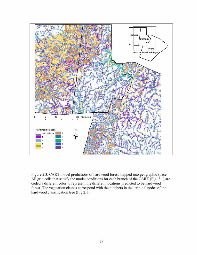
The map of hardwood predictions (Fig.2.3) clearly shows the strong presence of
hardwood along river valleys in areas less than 230m from streams. The majority of these
stands are located in areas with higher slope (class 1) or low slope less than 75m from
streams (class 2). The other dominant hardwood regions (classes 3-5; Fig.2.3) corresponds
with areas further from streams with higher plasticity or slope than the surrounding
landscape. The CART model successfully predicted the location of 66% of the actual
hardwood in the study area.
The CART pine predictions (Fig.2.4) are more dispersed throughout the study area as
compared to the discrete zones of predicted hardwood (Fig.2.3). The presence of pine is not
as strongly effected by distance to stream, but rather it is associated with areas of higher soil
plasticity and varying soil moisture. For example, pine classes 2-4 in Figure 2.4 represent a
strong belt of predicted pine starting in central Durham County and heading south. This
region largely corresponds with the location of Triassic basin sediment. The Triassic basin
has a history of agricultural use (partially due to a local relief less than surrounding area), but
it also contains some of highest soil plasticity in the study area. Figure 2.4 also emphasizes
the pine predicted to be in drier sites closer to streams (class 5; Fig.2.4), as well as pine sites

26
located in upland areas (>214m from streams) with slightly below average soil moisture
(class 7). The CART model successfully predicted the location of 72% of the actual pine in
the study area.
Generalized linear model
The logistic regression (GLM) models developed for hardwood and pine forest for
comparison with the CART models are presented below (Equation 3 and 4). Abbreviations
for the independent variables are defined in Table 2.2.
P(Hardwood) = α + β1Dist.stream + β2TCI + β3Slope, (3)
P(Pine) = α + β1TCI + β2PI+ β3Dist.stream (4)
The values of the model coefficients are listed in Table 2.3. Although it was
hypothesized that all four original variables (Table 2.2) are important predictors for
determining hardwood or pine presence, soil plasticity index (PI) was not significant in the
hardwood GLM according to the χ2-test and slope was not significant in the pine GLM
(Table 2.3).
The hardwood GLM correctly classified hardwood occurrence for less than 50% of
the validation data (accuracy value = 0.420, Table 2.4) with a threshold value of 0.50. The
pine model correctly classified less than 20% of the pine occurrences in the validation data
(accuracy value =0.180, Table 2.4) with an optimum threshold value of 0.47. The pine GLM
had considerably higher classification success with the non-pine/hardwood locations
(accuracy value = 0.654, Table 2.4).

27
Model comparison
Model comparisons based on predictive accuracy of ‘event’ cases indicate that the
CART models produced the most accurate classification for both the hardwood and pine data
(Table 2.4). The predictive ability of a GLM was higher only for the ‘non-event’ cases of the
pine data (accuracy value = 0.654 vs. 0.460 for CART). Predictive ability was consistently
lower for validation data since it was not used to build the models.
The results of Linnet & Brandt’s test were also included in Table 2.4. Recall that this
tests the null hypothesis of no difference in performance between the two models. I tested
for differences in predictive ability between GLM and CART on the validation data sets.
CART models were significantly better predictors for both hardwood and pine (p <.001).
The results of the second set of CART models built for hardwood and pine are also
included in Table 2.4 (CART2). These models were built using the significant variables
identified in the GLM’s (Table 2.3) to examine whether they improve predictive accuracy.
The models were pruned to 20 terminal nodes for hardwood and 14 terminal nodes for pine
following the same procedure as the original CART models. Predictive accuracy only
slightly increased for the ‘non-event’ cases in each model. The results of Linnet & Brandt’s
test were not significant for either hardwood or pine, meaning there was no significant
difference in predictive ability between the two CART models.
Discussion
Model predictions
The CART models developed for the hardwood and pine datasets show the relative
importance and hierarchical relationships of the environmental predictor variables on

28
vegetation pattern in the North Carolina Piedmont. Yet the significance of each predictor
variable cannot be understood solely based on environmental controls. They are only
relevant in the context of historic land-use patterns, showing that the dominant pattern of
vegetation across the landscape remains strongly tied to past agricultural use.
Piedmont agriculturalists tended to avoid areas too difficult to farm, thereby allowing
some forest stands to remain in hardwood over time (Oosting 1942, Trimble 1974, Peet &
Christensen 1980). The current distribution of hardwood is strongly predicted (69%
accuracy) by the variables initially hypothesized as being important in determining whether a
site is easily cultivated. The primary determinant of hardwood presence/absence in the study
area is distance to stream, but additional (interacting) factors are needed to explain hardwood
presence near vs. far from streams. Not surprisingly, hardwood stands near streams are
predominantly found in areas with higher soil moisture, as these sites would have often
flooded and been inhospitable for most agricultural crops. Hardwood stands near streams are
also present in areas with steeper slope (Fig.2.1), as these areas would have been more
difficult to cultivate than surrounding level topography.
For hardwood sites further from streams, the model did not provide strong support for
my initial hypothesis that hardwood would be found on dry ridge-tops. Lack of support
could be due to the moderate topography of the study area combined with the resolution of
the analysis. The dry ridge-tops known to support remnant hardwood stands (Peet &
Christensen 1980) are likely not extensive enough to have been included and sampled in this
analysis. Rather the model associated hardwood further from streams with areas of steep
slopes or mid to above-average soil plasticity. Soils with a high soil plasticity index
generally have poor water drainage and increased shrink-swell capacity, making them

29
difficult to cultivate under higher moisture regimes and potentially leading to extended
anaerobic soil conditions (Brady & Weil 2002). The Carolina Slate Belt system in the
northwest portion of the study area contains a higher proportion of plastic soils than the
surrounding region (excluding the Triassic basin), as well as areas of sharp topographic
variation (Daniels et al. 1999). The moderately high soil plasticity, combined with the
irregular topography, likely helped maintain hardwood dominance along the Carolina Slate
Belt and the majority of the predicted hardwood sites located >231m from streams are
associated with this soil system (Fig.2.3; Class 4-5). Some additional hardwood is predicted
to run along the Triassic basin in western Wake County due to higher soil plasticity (Fig.2.3;
Class 5), but as I will discuss below, the low slopes and high plasticity of the Triassic basin
proved to be more predictive of pine forests.
Pine forest did not become a dominant vegetation type of the North Carolina
Piedmont until the decline in agriculture, beginning around the late 19th century (Peet &
Christensen 1980, Healy 1985). Early successional pine grew into forest canopy as fields
were abandoned throughout the study area. The pine CART model provides some support
for my second hypothesis in that the chief determinants of pine presence were soil moisture
(low and high) and high soil plasticity, as well as drier sites with above-average slope. It is
likely that agriculturalists initially exploited these areas for cultivation, but high soil
plasticity or above-average slopes could have rendered them less productive or less easily
cultivated, thus leading to early abandonment. Poor management practices in the Piedmont
often led to severe soil erosion (Trimble 1974), and in regions such as the Triassic Basin,
topsoil erosion would have exposed a plastic B horizon and provided less favorable growing
conditions (Daniels et al. 1999). While the data presented in the study do not provide
30
specific evidence for a causal relationship, the strong belt of predicted pine in the Triassic
Basin region, through central Durham and western Wake Counties, provides support for this
assertion (Fig.2.4; Class 2-4).
The additional predictions of pine presence in drier sites closer to streams, as well as
upland sites with slightly above average soil moisture highlights an important transition in
land-use patterns for the study area. The region no longer has a broad agricultural economy,
primarily due to increased urban development, and the results reflect that more than just the
least productive agricultural sites have been abandoned and grown into successional pine
forest. An additional factor that could have led to greater dispersion of pine predictions is the
lack of a mixed-forest class in the 1999 land cover map. A mixed-forest class would have
further discriminated among hardwood and pine for each model and provided more accurate
predictions for each type. Instead sites that could be mixed-forest were grouped as either
hardwood or pine in the land-use map (Maunz 2002). The pine models were more likely
effected by this grouping since I sampled all stands ≥1 ha (vs. hardwood stands ≥15 ha), and
this would have included more scattered pixels that should be classified as mixed-forest.
Model performance
The CART and GLM model comparisons indicate that on the basis of proportion of
accurately classified pixels and the Linnet and Brandt test statistic the CART model
produced the most accurate classification (Table 2.4). It is well understood that ecological
data often does not conform to a specific functional form, and thus methods such as CART
that allow for non-linearity and interactions often improve predictive ability over linear
models (Vayssières et al. 2000). This is particularly true in my study where alternative

31
environmental settings lead to the same response (hardwood or pine presence/absence). In
contrast, the logistic GLM models imposed a structure on the response data that could not
capture the multiple relationships between predictor variables.
The reduced set of predictor variables (identified by the GLM models) analyzed in
the second set of CART models were as effective at predicting hardwood or pine presence in
the study area. This result shows that ecologists can benefit from using both methods of
analysis when modeling species response to the environment (Vayssières 2000). A GLM
model often provides a useful summary of relationships and a measure of variable
significance, while CART allows for an easier and more meaningful interpretation of
ecological contingencies. Breiman et al. (1984) also suggests that researchers initially use
CART with ecological data to identify interaction terms which may then be used in the
development of a parametric model, such as a GLM.
Conclusion
This study provides an example of how a hypothesis-driven approach to vegetation
modeling can allow researchers to move beyond simple pattern recognition to develop a
greater understanding of how historic disturbance and environmental factors affect
landscape-level vegetation pattern. This approach is particularly relevant in regions that have
a history of anthropogenic disturbance, as vegetation distribution is not solely controlled by
relationships along primary environmental gradients. Rather, these patterns are governed by
compensatory relationships that yield similar outcomes for various environmental settings or
contingencies. Future work will build on the vegetation CART models developed in this
study, to describe how recent development has interacted with environmental and
anthropogenic variables to create the broader land-use pattern in the region. The

32
incorporation of social drivers of land-use change will support additional hypotheses and
further refine model predictions of vegetation-environment relationships.

33
Table 2.1. Land cover classes for the study area and the percentage of total area occupied by each class. Land Cover % of Total Hardwood 31.4 Pine 9.3 Field 24.1 Suburban 17.6 Urban 11.2 Water 6.3

34
Table 2.2. Names and descriptions of environmental variables sampled for analysis. Variables marked with an asterisk were used in the final analysis (the discarded variable was highly correlated with TCI). Variable Description Mean Std.dev Min Max Variable Dist.stream* Distance to nearest stream (m) 328.57 269.17 0 3222.45 Continuous PI* Plasticity Index 22.25 13.77 1.17 57.5 Continuous Slope* Maximum slope(o) 0.91 0.70 0 41.77 Continuous RSP Relative slope position NA NA 0 25 Categorical±
TCI* Topographic Convergence Index 5.76 2.29 0.242 22.44 Continuous
± Seven slope position categories were calculated for RSP

35
Table 2.3. GLM coefficients for hardwood and pine models. Coefficients correspond to the variables listed in Equations 3& 4. * variables significant from χ2-test at p<(.05). **variables significant from χ2-test at p<(.001). Variables
Hardwood
Pine
Dist.stream
0.0015**
0.0010**
TCI
-0.0169*
0.2550**
Slope
-0.4711**
-0.1415
PI
-0.0001
-0.0202**

36
Table 2.4. Comparison of predictive accuracy of the generalized linear model (GLM), classification tree model (CART), and classification tree model built using information from the corresponding GLM model (CART2) for each land cover. Accuracy values are reported for the training and validation datasets. Predictive accuracy is the proportion of correctly classified pixels for the entire scene. *L&B test statistic is the statistic for the Linnet and Brandt test (1986) comparing the performance of CART and GLM models. Land cover Hardwood Non-hardwood Model CART GLM CART2 CART GLM CART2 Training data 0.748 0.440 0.658 0.672 0.444 0.728 Validation data 0.693 0.420 0.569 0.593 0.365 0.561 L&B test statistic* 7.292 p-value <0.001
Land cover Pine Non-pine/hardwood
Model CART GLM CART2 CART GLM CART2 Training data 0.778 0.360 0.718 0.576 0.397 0.642 Validation data 0.776 0.180 0.632 0.460 0.654 0.513 L&B test statistic* 5.385 p-value <0.001

37
dist.stream<231.39dist.stream>231.39
500/10001
Slope<1.57Slope>1.57
165/444
1
Dist.stream<75.97Dist. stream>75.97
146/3481
38/1262
Slope<1.47Slope>1.47
108/2221
Tci<3.94Tci>3.94
98/211
1
5/246
Slope<0.003Slope>0.003
93/1871
3/157
Slope<0.83Slope>0.83
82/1720
pi<50pi>50
45/1090
pi<31.75pi>31.75
44/980
36/900
0/89
1/110
26/638
1/11
0
19/961
pi<12.25pi>12.25
221/556
0
Slope<1.97Slope>1.97
28/1260
20/1160
2/103
pi<15.75pi>15.75
193/4300
26/804
pi<22.75pi>22.75
139/3500
47/169
0
pi<35pi>35
89/181
1
45/1165
21/650
Figure 2.1. CART model for hardwood based on environmental variables (see Equation 3). Abbreviations used for variables are defined in Table 2.2. The circles represent internal nodes and rectangles terminal nodes of the final pruned tree. The terminal nodes with numbers 1-9 are predicted to be hardwood (numbered to represent different hardwood types). Terminal nodes with ‘0’ represent absence of hardwood. Ratio below each node is the proportion of observations misclassified at that node.

38
Tci<5.97Tci>5.97
500/10002
PI<24.25PI>24.25
335/7692
Slope<1.86Slope>1.86
256/5222
Dist.stream<214.23Dist.stream>214.23
225/4650
Tci<5.14Tci>5.14
55/1392
41/1175
8/220
Tci<5.48Tci>5.48
141/3260
Tci<4.63Tci>4.63
126/3040
PI<22.25PI>22.25
93/1970
Tci<3.71Tci>3.71
64/1352
7/250
46/1107
22/620
33/1070
7/226
16/573
79/2472
PI<24.25PI>24.25
66/2310
38/1660
Slope<0.144Slope>0.144
28/650
3/170
23/484
Figure 2.2. CART model for pine based on environmental variables (see Equation 3). Abbreviations used for variables are defined in Table 2.2. The circles represent internal nodes and rectangles terminal nodes of the final pruned tree. The terminal nodes with numbers 1-7 are predicted to be pine (numbered to represent different pine site conditions). Terminal nodes with ‘0’ represent absence of pine. Ratio below each node is the proportion of observations misclassified at that node.
39
Figure 2.3. CART model predictions of hardwood forest mapped into geographic space. All grid cells that satisfy the model conditions for each branch of the CART (Fig. 2.1) are coded a different color to represent the different locations predicted to be hardwood forest. The vegetation classes correspond with the numbers in the terminal nodes of the hardwood classification tree (Fig.2.1).

40
Figure 2.4. CART model predictions of pine forest mapped into geographic space. All grid cells that satisfy the model conditions for each branch of the CART (Fig. 2.2) are coded a different color to represent the different locations predicted to be pine forest. The vegetation classes correspond with the numbers in the terminal nodes of the hardwood classification tree (Fig.2.2).

CHAPTER 3
MATURE HARDWOOD FORESTS IN THE CENTRAL PIEDMONT OF NORTH
CAROLINA: LONG-TERM UNDERSTORY CHANGE

42
Introduction
Ecological theory and observation suggest that following disturbance species
composition changes over time toward a dynamic equilibrium wherein compositional
fluctuations are largely based on internal dynamics (Peet 1992, Pickett & White 1985). At
scales larger than a single tree, local fluctuations in a mature forest should average out,
producing a relatively stable composition. The mature hardwood forests of the Piedmont
region of the Southeastern United States have long been assumed to represent the stable
endpoint of succession in this region (e.g. Ashe 1897, Oosting 1942, Braun 1950, Peet &
Christensen 1980, Delcourt & Delcourt 2000), with compositional variation reflecting
primarily variation in local environment (e.g. Christensen & Peet 1984). However, in the
contemporary mature hardwood forests of the Piedmont the expectation of stability is open to
question due to several potential causes of ongoing change. Among these are long-term fire
suppression, increases in deer populations, exotic species invasions, and ongoing recovery
from past anthropogenic disturbance (logging, grazing by livestock). Some species,
particularly understory herbs, may be slow in equilibrating following disturbance events and
environmental change (Christensen 1977, Brewer 1980, Peet & Christensen 1988).
Each of the above processes could effect different subsets of the understory flora and
lead to directional change in species composition. For example, fire suppression might
increase the abundance of shade-tolerant woody saplings (Lorimer 1985, Abrams 1992,
2003) and eliminate light-demanding herbaceous species originally associated with open
woodlands, increases in local deer populations could decrease density and diversity of

43
understory herbs (Bratton 1979, Rooney & Dress 1997, Waller & Alverson 1997), and
increases in aggressive exotic species could restrict overall native species diversity
(Richardson et al. 1989, Alvarez & Cushman 2002, Gorchov & Trisel 2003, Jolls 2003). In
addition, large infrequent disturbances, such as hurricanes, affect these forests. Hurricane
disturbance could lead to transient increases in local (stand-level) richness due to enhanced
establishment in newly formed forest patches (Marks 1974, White 1999). Hurricane
disturbance may also accelerate the regeneration and growth of shade-intolerant species in
forest stands due to increased light availability (Parker et al. 1985, Peet & Christensen 1980).
In studies of long-term species change, researchers in Eastern forests have nearly
always focused on canopy species. Interestingly, this work has revealed trends even in older
stands, such as a decrease in oak dominance and increase in shade-tolerant species, such as
Acer rubrum or Acer barbatum (Christensen 1977, Peet & Loucks 1977, Lorimer 1984,
Abrams 1998, McDonald 2002). Previous work on understory composition in temperate
forests have shown patterns of local native species decline with accompanying increases in
exotic species (Brewer 1980, Davison & Forman 1982, Drayton and Primack 1996, Rooney
and Dress 1997, Rooney et al. in press), but these studies have been based on approximations
of original plot locations rather than permanently marked and resampled plots or, more often,
species lists from survey data for only one site. Studies done without accurate plot
replication and multiple site comparisons have limited ability to detect regional directional
change in understory species composition.
In 1977 Peet & Christensen established a series of permanently marked vegetation
plots in the North Carolina Piedmont. The Piedmont region has served as a model system for
work on succession (e.g., Oosting 1942, Keever 1950), and their vegetation data have been

44
used to define the trajectory of forest composition and structural convergence toward the
mature hardwood forests of the region (Christensen & Peet 1984). Additional work showed
how understory herb composition of hardwood forests is tightly correlated with soil pH,
nutrient status and soil moisture conditions (Peet & Christensen 1980, 1988), and thus any
analysis of hardwood stability requires consideration of variation with site characteristics.
A subset of the Peet & Christensen plots were resampled to evaluate the 23-year shift
in species abundance and composition in temperate hardwood forests spanning a range of
soil types and site conditions. My general objective was to assess the stability of understory
composition for all species (≤1m tall). Specifically, I predicted that shifts in understory
composition occurred over time and predominantly followed two of the aforementioned
trajectories: increases in the abundance of shade-tolerant woody species, and declines in
abundance and diversity of herbaceous native species. Further, I predicted that rates of
change would be highest in more productive stands (higher in soil resources and moisture)
because such places (a) have greater resource availability to support the establishment of new
species and (b) higher initial diversity and hence greater potential for loss because of light
limitation, deer browsing, and exotic species invasion. I addressed my objective through
examination of several specific questions, each examined at 25m2 and 1000m2, to highlight
possible differences based on scale (Palmer 1990). First, is the understory of mature
hardwood forest stands in the study area exhibiting compositional change, and if so, is there
evidence for consistency in the direction of change across plots? Second, which species
show the greatest rates of gain, loss, and overall variability, and what if any species attributes
are typically associated with such trends? And, third, is change in composition or species

45
richness partly correlated with site environmental conditions or with richness of the original
vegetation?
Methods
Study Area
This study uses data collected from Piedmont hardwood forest stands in or near Duke
University Forest located in Orange and Durham Counties, North Carolina. The region is
characterized by a warm temperate climate, with a mean monthly temperature in July of
26.7oC and in January of 5.3oC. The mean annual precipitation is 1168mm with July and
August being the wettest months (North Carolina Climate Office 2003). Topography is
predominantly rolling hills with gentle slopes (<5%), and occasional steep slopes and bluffs
along river valleys and hillsides. The elevation within the study area ranges from 75m to
255m.
The landscape is ancient and the soils reflect the long history of leaching in their low
nutrient status and high clay content. Soil parent material varies widely across the study area
and includes areas of Triassic basin sedimentary mudstones and sandstones, metamorphic
Carolina slate, and igneous mafic and felsic intrusions (Daniels et al. 1999). Soils derived
from diorite or diabase tend to be more fertile, or on the highly weathered uplands have
weathered to shrink-swell clays. The more typical Carolina slate (a highly metamorphosed
volcanic ash) weathers to infertile soil dominated by red kaolinitic clays. Differences in
parent material often are responsible for strong soil differences over horizontal distances of
less than a meter, and hardwood forest composition varies in response to these conditions
(Peet & Christensen 1980, Palmer 1990). Further details on hardwood vegetation variation

46
in relation to soil conditions can be found in Peet & Christensen (1980). The hardwood
plots used in this study cover a range of soil types and are representative of conditions
typically found throughout the North Carolina Piedmont.
The North Carolina Piedmont has a long history of anthropogenic disturbance and
much of the current landscape is dominated by successional pine forest growing on sites
abandoned from agriculture. Those areas less suitable for cultivation are predominantly the
ones that have remained in hardwood forest, but these sites have not been without
disturbance and have a history of selective cutting and domestic livestock grazing (Healy
1985). In addition, hardwood forests were periodically burned by the original aboriginal
populations and subsequently by the early settlers to suppress woody growth and encourage
an herbaceous understory favorable for livestock, but the use of fire has largely been
suppressed since the early 20th century (Hatley 1977, Frost 1998). Grazing could have
served to mimic some effects of low-intensity ground fires by suppressing woody growth,
and it persisted in the hardwood forest stands of Duke Forest up until its establishment in the
1930s (McDonald 2002). The plots used in this study were originally selected in 1977 for
their mature hardwood canopy and minimal evidence of human disturbance due to logging,
fire, or grazing since about 1900 (Peet & Christensen 1980, Christensen & Peet 1984).
Although the hardwood plots have remained free of overt anthropogenic disturbance
for over 100 years, other forms of disturbance have occurred over time. Of particular
importance is the increase in white-tailed deer (Odocoileus virginianus) populations
throughout the region. Studies in North American temperate forests have shown that deer are
responsible for a significant decline in richness and cover of understory vegetation (Waller &
Alverson 1997, Rooney et al. in press). The state of North Carolina began using deer harvest

47
statistics to estimate deer populations in the mid 1980’s (Downing 1980) and the data
indicate that deer populations in the northern Piedmont of North Carolina have increased
considerably over the past 25 years, Figure 3.1.
An additional notable disturbance is the occurrence of hurricanes. In particular,
Hurricane Fran passed through the region in September, 1996. The eye of Fran passed 15
miles east of Duke Forest and the strong winds (up to 35meters/second) caused severe
damage, labeling it as the most destructive natural disaster ever to strike North Carolina
(Carpino 1998). Research done following the hurricane found that most damage in Duke
Forest occurred in mature hardwood forests located along river bottoms due to flooded soil
conditions, as well as hardwood stands located on exposed ridge slopes and tops (Carpino
1998). The 2000 resurvey of the Peet & Christensen hardwood plots identified nine plots
(out of 36) as experiencing some level of hurricane damage, as evidenced by down trees. In
addition, 10 stands were so badly damaged by Hurricane Fran that they were impossible to
resample.
Field Methods
Peet and Christensen established a series of 105 permanent hardwood forest plots in
1977 as part of their research on Piedmont secondary succession (1981, 1984, 1988) and
hardwood forest vegetation (1980). Thirty-six of these plots were precisely relocated and
resampled during the interval of 1999-2001 (referenced as 2000) using the same
methodology as 1977, except for leaf cover scale (see description below). The basic
sampling unit was a 0.1ha (20 x 50m) plot with a 50m transect running the length of the plot
down the centerline. The frequency and cover of all understory species (vascular plants <1m
tall) were recorded in twenty-five 0.5 x 2m contiguous subplots arranged along the center

48
transect. All understory species present in the 0.1 ha plot, but absent in the subplots, were
recorded. Multiple environmental, soil nutrient and soil texture variables were measured for
each plot in 1977 (Table 3.1; see also Peet & Christensen 1980). These data were not
recollected in the 2000 resurvey and are assumed to have been constant over time.
In the original 1977 survey, leaf cover was estimated to the nearest percent for each
species per subplot. In the 2000 resurvey, leaf cover was estimated using the protocol of the
North Carolina Vegetation Survey, which assigns cover based on a ten-point scale (see Peet
et al. 1998). To allow comparison across years, the ten-point cover scale was converted to
percentages using the geometric mean of each cover class (Oksanen 1976). The average
percent cover for each species per plot was calculated as the average cover across subplots.
Species present in the 0.1 ha plot, but absent in the subplots were assigned a cover of 0.02
percent.
To ensure accurate comparisons of species richness and composition between the
1977 and 2000 data sets, I updated all species nomenclature to conform to Kartesz (1999). In
addition, I created two separate datasets for each year for calculations of richness and
composition to control for possible taxonomic problems across years due to misidentification
or species identified only to genus. For comparison of species richness, I maintained full
species identifications for most taxa and grouped to genera only those species considered
difficult to split from related taxa based on vegetative characteristics. For comparison of
species composition, all potentially problematic species were grouped to genus and all
family-level and unknown designations were removed. The final species list for richness
contained 331 taxa, 314 identified to species, 11 to genus and 6 to family or above. The final
species list for composition contained 302 taxa, 285 identified to species and 17 to genus.

49
All woody (shrub and tree) species were assigned a shade tolerance value of low, mid, or
high, following USDA (2002).
Data Analysis
Change in understory composition and variation based on taxa
I first compare changes between 1977 and 2000 in total species richness at each site
at both the subplot (25m2) and plot (1000m2) scales. I also compare changes in richness at
25m2 and 1000m2 for species grouped by growthform (tree, shrub, and herb). I tested the
significance of changes in richness between survey periods (1977-2000) using paired exact
randomization tests with 1000 randomizations and plots serving as replicates (null
hypothesis: difference in richness across years is equal to zero; see Manly, 1997, for a
description of methods for paired randomization tests). In addition, I qualitatively compared
change in richness for plots that were noted to have experienced hurricane damage in 1996 (9
out of 36) with all remaining plots.
To assess changes in understory composition between 1977 and 2000, I first ran a
block multi-response permutation procedure (MRPP) to test the null hypothesis of no change
in understory composition within plots at 25m2 and 1000m2 between survey periods. Block
MRPP is a multivariate permutation procedure for use with paired-plot compositional data.
Two groups were defined to represent the two sample periods and each pair of plots, one for
each time period, was considered a block (36 total). Tests of significance are based on
random permutations across groups of within block differences of species composition,
calculated using a Euclidean dissimilarity measure and species presence/absence (Mielke &
Berry 2001). Tests were performed in PC-ORD version 4.24 (McCune & Mefford 1999).
Further details of the method can be found in Mielke (1984) and Mielke & Berry (1982).

50
Consistency in the direction of compositional change across plots at 1000m2 was
assessed using nonmetric multidimensional scaling with varimax rotation (NMS; Mather
1976, Kruskal 1964) as implemented in PC-ORD version 4.24 (McCune & Mefford 1999).
This analysis was limited to 1000m2 since species cover data is only available at the plot
level. NMS ranks plots based on dissimilarity, calculated using a Bray-Curtis dissimilarity
measure and average species cover. NMS was run with a random starting configuration and
25 runs of the real data. To reduce noise from rare species, those occurring in fewer than two
plots were deleted from the dataset prior to the NMS ordination. Appropriate dimensionality
was assessed using a Monte Carlo test and a configuration with the minimum stress level was
used. The direction of compositional change over time between each pair of plots was
examined by drawing vectors between each pair of plots on the two-dimensional ordination
(McCune & Grace 2002). The lengths of each vector represent the amount of compositional
change based on dissimilarity between plots. The relative position of 1977 plots and 2000
plots on an ordination axis were compared with a two-sample t-test (Peterson & McCune
2001). Plots that experienced hurricane damage were identified separately in the ordination
diagram to examine the direction and extent of compositional change in relation to other
hardwood plots.
An indicator species analysis (Dufrene & Legendre 1997) was performed in PC-ORD
to examine individual species relationships to the two sample periods (1977 and 2000). The
test provides a method for assessing which species have the strongest affinity to one time
period, thereby emphasizing species with the strongest influence on compositional change
over time in the NMS ordination. The indicator value for each species is calculated by
combining the relative abundance and relative frequency of each species in each group

51
(year), and the highest indicator value (IVmax) across groups is used as the overall indicator
value for each species. The statistical significance of IVmax for each species is evaluated
using a Monte Carlo test with 1000 randomizations (null hypothesis: IVmax no larger than
would be expected by chance).
Change in association with environmental variables
I conducted a simple correlation analysis to examine the environmental factors
correlated with change in richness at 25m2 and 1000m2 for species grouped by growthform
(herb, shrub, tree). I did not test for correlations with the full dataset as growthform data is
nested within this dataset and would provide redundant results. A correlation analysis was
also used to examine the change in diversity for each growthform in relation to the original
1977 richness at each scale. Spearman’s ranked correlations were used to avoid assumptions
about normality of the data. Environmental variables are listed in Table 3.1.
To assess change in species composition in relation to environment, I compared the
length of the paired plot vectors to environmental variables in the NMS ordination. The
relationships between individual environmental variables and plot scores were initially
overlaid on the ordination with a vector biplot. The angles of each environmental vector
indicate the direction of highest correlation and the lengths represent the strength of the
correlation. A varimax rotation was used to improve the alignment of environmental
variables with one primary ordination axis (Mather 1976). Correlations between the
ordination axes and environmental variables were calculated with Pearson’s r2. I correlated
the length of the paired-plot vectors with 1977 plot positions on the primary environmental

52
ordination axis using Spearman’s rank correlation to test if the extent of compositional
change between plots varied with environment.
Results
Change in understory species richness
Across all sites, I observed decreases in regional species richness with much of the
loss driven by decreases in herb species. Peet & Christensen (1980) recorded a total of 272
species throughout the hardwood plots in 1977 and the 2000 resurvey recorded 252 species
for a net loss of 21 species, 18 of which were herb species (see Appendix A for full list of
species lost and gained). Native species richness exhibited greater declines with a net loss of
28 species (23 herb) due to the 7 new exotic species recorded in 2000 (Appendix A). Total
loss of native species was 70 species (58 herbs).
In addition to overall herb loss, another important trend is the decline in the number
and abundance of regionally rare native herb species over time. Sixty-one percent (89 out of
145) of herb species occurring in 10 or fewer plots in 1977 declined in plot frequency, and
more than half of those that declined (52 species) were not recorded at all in 2000. There
were 123 infrequent native herb species (10 or fewer plots) in 2000, and 25 of these species
(20.3%) maintained the same plot frequency over time.
The loss in overall regional diversity contrasts with the change observed at the
subplot (25m2) and plot (1000m2) scales for paired plots. At 25m2 there was no significant
change in total or native species richness (Table 3.2). Total richness and native richness
predominantly increased at 1000m2 (22 out of 36 plots), but only total species richness
showed significant increases (p ≤.05) due to a slightly higher mean difference in richness

53
from the new exotic species recorded in 2000 (Table 3.2). Plots damaged by the hurricane
had some of the greatest increases in total species richness; 8 out of 9 hurricane plots
increased in total richness (increases range from 10-25 species per plot) at 1000m2. Seven of
the hurricane plots increased in total species richness at 25m2.
The analysis of change in richness by growthform provides insight on which species
are influencing the shift in richness patterns from regional to local scales. Change in herb
richness per plot conforms to the regional pattern in that richness showed significant declines
at both 25m2 and 1000m2 for all herbs and native herbs (Table 3.2). This contrasts with the
change in tree richness, which showed strong increases at the subplot and plot scales (Table
3.2), but no regional increases in richness (net loss of 2 species, Appendix A). Shrub
richness did not significantly change at 25m2 (p= 0.227), but there were significant increases
in richness at 1000m2 (p= .011). Eight hurricane plots increased in total richness at 1000m2
across all growthforms (results vary for 25m2), and the greatest increases were largely for
tree species (increases range from 4-11 species per plot).
Change in understory composition
Understory composition exhibited significant change between 1977 and 2000 at both
25m2 and 1000m2 (blocked MRPP 25m2: p= 0.001, R= 0.003; 1000m2: p= 0.013, R= 0.002;
R measures within-group agreement). There is also strong evidence of directional change in
composition across all plots at 1000m2 based on the NMS paired-plot vectors (Fig.3.2). Plots
show significant separation by year (group) along the vertical ordination axis (n= 72, t= 5.00,
p= 0; Fig. 3.3). These results imply there was a dominant trend in shifts of species
composition across the majority of plots between 1977 and 2000. Hurricane damaged plots
did not exhibit strong differences in extent or direction of compositional change in
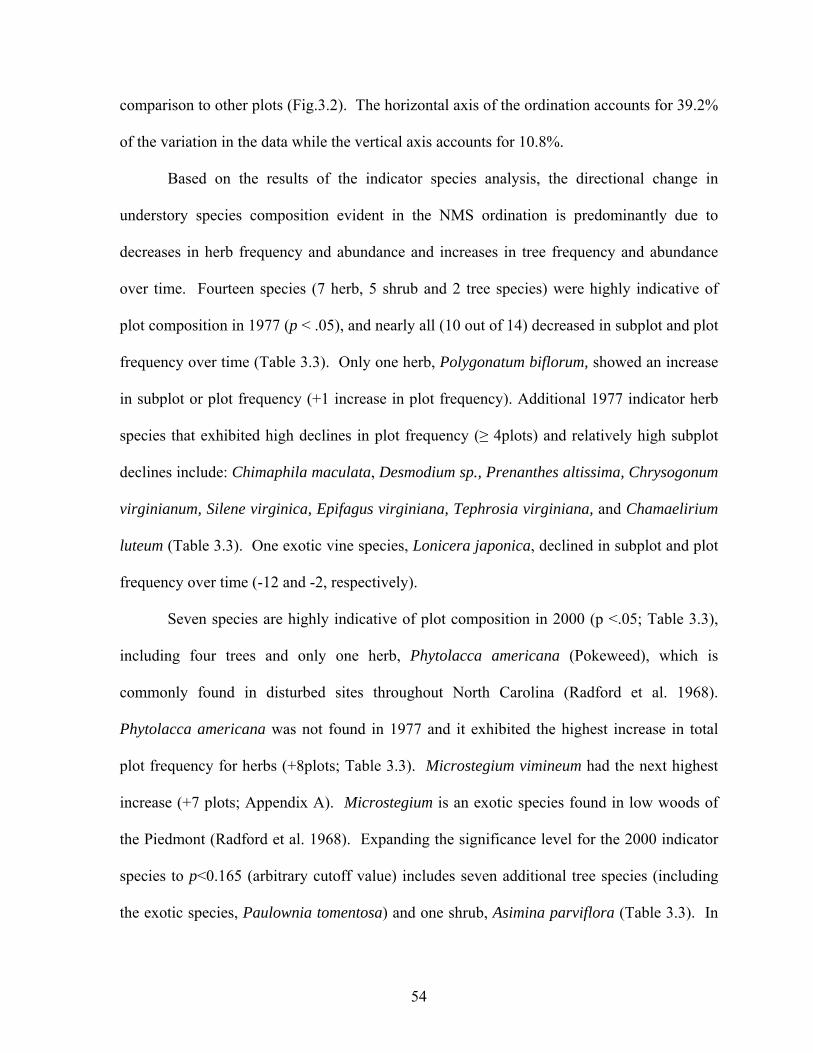
54
comparison to other plots (Fig.3.2). The horizontal axis of the ordination accounts for 39.2%
of the variation in the data while the vertical axis accounts for 10.8%.
Based on the results of the indicator species analysis, the directional change in
understory species composition evident in the NMS ordination is predominantly due to
decreases in herb frequency and abundance and increases in tree frequency and abundance
over time. Fourteen species (7 herb, 5 shrub and 2 tree species) were highly indicative of
plot composition in 1977 (p < .05), and nearly all (10 out of 14) decreased in subplot and plot
frequency over time (Table 3.3). Only one herb, Polygonatum biflorum, showed an increase
in subplot or plot frequency (+1 increase in plot frequency). Additional 1977 indicator herb
species that exhibited high declines in plot frequency (≥ 4plots) and relatively high subplot
declines include: Chimaphila maculata, Desmodium sp., Prenanthes altissima, Chrysogonum
virginianum, Silene virginica, Epifagus virginiana, Tephrosia virginiana, and Chamaelirium
luteum (Table 3.3). One exotic vine species, Lonicera japonica, declined in subplot and plot
frequency over time (-12 and -2, respectively).
Seven species are highly indicative of plot composition in 2000 (p <.05; Table 3.3),
including four trees and only one herb, Phytolacca americana (Pokeweed), which is
commonly found in disturbed sites throughout North Carolina (Radford et al. 1968).
Phytolacca americana was not found in 1977 and it exhibited the highest increase in total
plot frequency for herbs (+8plots; Table 3.3). Microstegium vimineum had the next highest
increase (+7 plots; Appendix A). Microstegium is an exotic species found in low woods of
the Piedmont (Radford et al. 1968). Expanding the significance level for the 2000 indicator
species to p<0.165 (arbitrary cutoff value) includes seven additional tree species (including
the exotic species, Paulownia tomentosa) and one shrub, Asimina parviflora (Table 3.3). In

55
contrast, the additional indicator species for 1977 includes ten herb species and three tree
species (Table 3.3).
Of the tree species that increased in plot frequency (≥2 plots) over time, 10 are
classified as highly shade tolerant, 18 are mid-shade tolerant, and 3 have low shade tolerance
(Appendix A). The highly shade-tolerant tree species showing the greatest increases in
subplot and plot frequency that are also indicative of plot composition in 2000 (p<0.165)
include; Carpinus caroliniana, Acer barbatum, and Ostrya virginiana (Table 3.3). Some
historically dominant (and less shade tolerant) oak and hickory species also exhibited
increases in frequency over time. Quercus falcata, Quercus alba, and Carya ovata showed
the greatest increases at both the subplot and plot scale (Table 3.3). The only oak or hickory
species that declined in plot frequency or had strong declines in subplot frequency are
Quercus coccinea, Quercus marilandica, Quercus michauxii, Carya glabra, and Carya
pallida (Appendix A).
The shade intolerant tree species that increased in subplot and plot frequency are
Liriodendron tulipifera, Liquidamber styraciflua and Quercus phellos. Liriodendron is
highly indicative of plot composition in 2000 (IVmax p<0.05) and showed the highest increase
in subplot occurrences (+105; +6 in plot frequency) across all tree species. Liquidamber
increased in subplot frequency by 26 and plot frequency by 2, Quercus phellos increased by
1 and 8 for subplot and plot frequency, respectively (Appendix A).
Change in species richness and composition with environment
Relationships between change in species richness and environmental variables varied
with growthform at 25m2 and no significant relationships were found at 1000m2 (Table 3.4).

56
Herb species had the strongest correlations with environment, with positive correlations
associated with pH and soil cation variables (Ca, Mg, K) (Table 3.4). A positive correlation
implies that species richness tended to increase along the environmental gradient over time.
This suggests that herb richness was more likely to increase at 25m2 in nutrient rich sites
(sites with higher pH and soil cations). It is important to note that soil cation variables and
pH are positively correlated with each other (0< p<.01), which explains some portion of the
correlation. This is also true of the soil texture variables (p =0 for all soil texture
correlations), with %sand negatively correlated with %silt and %clay, and all three together
adding to 100. Change in herb species richness is positively correlated with %sand (p< .01)
and negatively correlated with %silt and %clay (p< .01 and p<.05, respectively).
Change in tree species richness showed no relationship with pH or soil cations and
was only moderately correlated with %silt (r = -0.35; p=0.04). Tree and herb richness are
both negatively correlated with elevation (p< .01). Elevation is often considered a surrogate
for soil moisture (Peet & Christensen 1980), and thus a negative correlation means low, wet
sites tended to increase in species richness over time, while higher, dry sites generally
decreased. Change in shrub richness was not correlated with any examined environmental
variables. Only change in herb richness showed a relationship with the original (1977) plot
richness (r = 0.43; p< .01), which is also partly explained by the relationship with soil pH
and nutrients as overall richness tends to increase with soil fertility (see Peet & Christensen
1980).
Change in overall species composition at 1000m2 is moderately correlated with
environment (Spearman’s rank correlation: r = 0.38, p= 0.023), based on the analysis of
paired-plot vector length with 1977-plot position along axis 1 of the NMS ordination

57
(Fig.3.2). A positive correlation means that vector length increased from left to right along
axis 1, and thus plots with higher soil cations, pH, and %sand exhibited greater
compositional change over time (Fig.3.2-3.3). Yet it is important to note that the overall
coefficient of determination (r2) of plot vector length with axis 1 is 0.103 (Table 3.5). This
relatively low r2 value (only 10% of variation explained) implies that although there is some
relationship with environment, species change at 1000m2 is predominantly occurring across
all plots, largely independent of the measured environmental factors. This is also represented
by the nearly orthogonal position of the ‘group’ (year) vector to the primary environmental
vectors in the NMS vector biplot (Fig.3.3).
Discussion
The understory composition of mature hardwood forests in Duke Forest does not
provide support for the ‘steady-state’ paradigm of successional theory; these plots are not
stable. Although species fluctuations are to be expected in late-successional stands due to
natural dynamics (Pickett & White 1985), current successional theory does not explain the
larger directional change that appears to be occurring across all hardwood plots, apart from
any apparent hurricane effect. The apparent shift in species composition could be the result
of different factors that have persisted or increased over time. I discuss the results in the
context of the mechanisms initially described as common for eastern hardwood forests:
recovery from an earlier regime of chronic fire or grazing, increases in white-tailed deer
populations, exotic species invasion, and small-scale variation due to hurricane disturbance.
On a regional scale, I found an overall decline in understory native species richness
with herbaceous species showing the strongest decreases. These results support the findings

58
of other studies that show widespread regional losses of species diversity (e.g. Tilman et al.
1994, Pimm et al. 1995), and highlight a potential trend towards increased species loss in
mature hardwood forests over time (see Gilliam & Roberts 2003). My results differ from
other studies of temperate forests in that a similar pattern of overall understory species loss is
not observed at smaller scales (Davison & Forman 1982, Kwiatkowska 1994, Drayton &
Primack 1996, Rooney et al. in press). The Duke Forest hardwood plots have not yet
exhibited significant change in understory native species richness at the subplot (25m2) or
plot (1000m2) scale. The apparent stability of understory species richness is due to the
combined effect of decreasing herb richness and increasing tree seedling richness at both
scales.
I predicted overall declines in herb diversity and abundance, largely due to the
growing evidence of the detrimental impacts of white-tailed deer populations on forest
understory flora (Anderson 1994; 1997, Kelley 1994, Waller et al. 1997, Rooney et al. in
press). Although I did not specifically test for deer effects, the significant decline in herbs
and the estimated 100% increase in white-tailed deer populations in the northern Piedmont of
North Carolina since 1985 provides support for herbivory as a possible causal factor of
decline. Research by Kelley (1994) found that deer browsing on forest herbs is generally
concentrated in the spring (April and May) when many understory plants are available and
before agricultural crops begin to provide food (see also Roberts & Gilliam 2003). Nearly all
of the herb species that exhibited relatively high decreases in plot frequency (≥ 4 plots) are
primarily woodland herbs present in the spring, either vegetatively or in flower (Radford et
al. 1968). Deer herbivory could also be a reason for the decline in the exotic species,
Lonicera japonica (Japanese honeysuckle), as it is considered an important regional food

59
item for Piedmont populations of white-tailed deer (Osborne 1993). Lonicera japonica is the
only exotic species that decreased in frequency at the subplot and plot level.
Increases in white-tailed deer populations have been suggested to contribute to the
decline of oak and hickory species in hardwood forests due to their high preference and
browsing intensity on Quercus alba (white oak) and Carya ovata (shagbark hickory)
seedlings and saplings (Strole & Anderson 1992; see also Marquis et al. 1976, Tilghman
1989). Such a factor would further exacerbate the oak and hickory decline often attributed to
fire suppression (Lorimer 1985, Abrams 1992) and competition with shade-tolerant species
(Lorimer et al. 1994, McDonald et al. 2003). My results run contrary to this expectation as
over half of the oak and hickory species present in 1977, including Quercus alba and Carya
ovata, increased in subplot and plot frequency over time. Oak and hickory species are indeed
reproducing in the understory, but other factors appear to be preventing them from surviving
into older age-classes in Duke Forest (see McDonald et al. 2002) and the Piedmont region
(Abrams 2003). The overall increase in tree seedling richness combined with the significant
declines in herbaceous species richness highlights the need for further research on deer
effects in the Piedmont region.
Although not supporting a deer effect, the strong increase in tree seedling richness
across nearly all plots provides support for my initial hypothesis of increases in woody
species abundance due to recovery from past fire and grazing disturbance. The cessation of
ground-level disturbance from low-intensity fires and understory grazing in hardwood forests
since the early 1900s has facilitated the recruitment of woody species throughout Eastern
forests (Abrams 2003). This recruitment has largely supported shade tolerant species, such
as Acer rubrum and Acer barbatum, since they tend to be faster growing and more
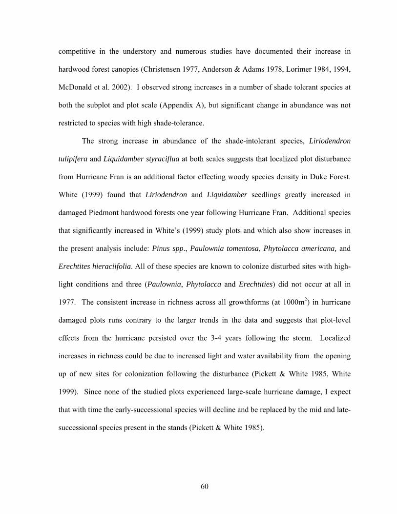
60
competitive in the understory and numerous studies have documented their increase in
hardwood forest canopies (Christensen 1977, Anderson & Adams 1978, Lorimer 1984, 1994,
McDonald et al. 2002). I observed strong increases in a number of shade tolerant species at
both the subplot and plot scale (Appendix A), but significant change in abundance was not
restricted to species with high shade-tolerance.
The strong increase in abundance of the shade-intolerant species, Liriodendron
tulipifera and Liquidamber styraciflua at both scales suggests that localized plot disturbance
from Hurricane Fran is an additional factor effecting woody species density in Duke Forest.
White (1999) found that Liriodendron and Liquidamber seedlings greatly increased in
damaged Piedmont hardwood forests one year following Hurricane Fran. Additional species
that significantly increased in White’s (1999) study plots and which also show increases in
the present analysis include: Pinus spp., Paulownia tomentosa, Phytolacca americana, and
Erechtites hieraciifolia. All of these species are known to colonize disturbed sites with high-
light conditions and three (Paulownia, Phytolacca and Erechtities) did not occur at all in
1977. The consistent increase in richness across all growthforms (at 1000m2) in hurricane
damaged plots runs contrary to the larger trends in the data and suggests that plot-level
effects from the hurricane persisted over the 3-4 years following the storm. Localized
increases in richness could be due to increased light and water availability from the opening
up of new sites for colonization following the disturbance (Pickett & White 1985, White
1999). Since none of the studied plots experienced large-scale hurricane damage, I expect
that with time the early-successional species will decline and be replaced by the mid and late-
successional species present in the stands (Pickett & White 1985).

61
The disturbance and creation of forest patches due to Hurricane Fran could also have
contributed to the moderate increase in exotic species abundance and diversity over time.
Each of the five exotic species that occurred in greater than one plot in 2000 (Ligustrum
sinense, Microstegium vimineum, Verbascum thapsus, Paulownia tomentosa, and Glechoma
hederacea) was found to have invaded at least one hurricane damaged plot. These species
are easily dispersed and are commonly found in roadsides and disturbed sites throughout
much of North Carolina (Radford et al. 1968). I initially did not expect the hardwood forests
of Duke Forest to experience strong increases in exotic species as they have remained
relatively intact and isolated from regional anthropogenic disturbances, such as habitat
fragmentation, over at least the last 70 years. However, given the predominant trend towards
increased exotic species presence throughout Eastern forests (Rooney et al. in press) and the
habitat disturbance that continues surrounding Duke Forest, I anticipate that their abundance
and diversity will increase in the future.
Change in species richness and composition with environment
The significant correlations between change in herb richness and environmental
variables at 25m2 suggests there are local patterns of species change along primary
environmental gradients, with the drier, less fertile sites showing little change (or loss) in
herb composition and the mesic fertile sites the greatest increase. These results add a
temporal perspective to the earlier work by Peet & Christensen (1980) where they found that
herbs show stronger variation in richness in response to multiple environmental variables
than shrubs and trees. Some authors have also suggested that rate of succession is a function
of site (Peet & Loucks 1977, Fralish et al. 1991), and my results (for herbs and trees) support

62
the expectation that mesic sites show the greatest change over time. Soil cation (Ca, Mg, K)
concentrations appear to be an important factor in the amount of change in herb richness over
time, but it is unclear whether this is because of limitations in soil nutrients or if herb species
experience less competition with other understory species (such as trees and shrubs) in sites
with higher soil cations. There could also be a hurricane effect as plots with higher soil
cations includes some of the sites most damaged by the hurricane (plots 505-509, Fig. 3.3).
The hurricane effect could additionally explain some of the significant increase in herb and
tree seedling richness at lower elevations as hardwood stands in lower areas sustained more
hurricane damage in Duke Forest (Carpino 1998).
The moderate positive correlation between change in overall species composition (as
represented by plot vector length) and environmental variables provides some support of my
initial prediction of greater overall species change in areas of higher soil fertility and lower
elevation due to increased availability of resources. This result differs from the above
discussion of richness in that it pertains to change based on the entire species assemblage
within a plot, rather than just measures of richness. Viewed together, the results suggests that
increases in species richness in low elevation, fertile plots contributed to greater species
turnover over time, whereas the decreases in richness in drier, less fertile plots did not cause
as much overall compositional change. I interpret this result with some reservation given the
weak coefficient of determination (r2 = .103) for the correlation of plot vector length with the
primary environmental axis of the NMS ordination. It instead seems that directional
compositional change is occurring over time across all plots, largely independent of
environmental conditions.

63
The systematic declines in herbaceous species richness, coupled with the dramatic
increases in woody seedling abundance signal important shifts in mature hardwood forests of
the Piedmont. The past legacy of human disturbance in the forest stands and current
disturbance regimes continue to upset the dynamic equilibrium thought to have existed in
mature oak-hickory hardwood forests. Some authors have suggested that the current shift
toward a more mesic hardwood forest is more typical of late-successional stands and the
historic dominance of oak-hickory forests was primarily a consequence of higher fire
frequency (Abrams 2003, White & White 1996). Whether fires should be reintroduced to the
ecosystem is a matter of debate, but indeed, important to consider in order protect the
hardwood stands from future species loss. Loss of fire could explain some of our species
losses, but many are species typically associated with mesic closed forest, and these are much
more likely the victims of increased deer pressure. Loss of herbaceous species highlights yet
another alarming trend, particularly since their reduction cannot be attributed to the
mechanisms commonly associated with species extinction, such as habitat fragmentation and
invasive species (Wilcove 1998, Jolls 2003). This implies that more research is needed to
understand the mechanisms responsible for the decline as well as more active management
and long-term monitoring to help prevent further loss of native understory flora.
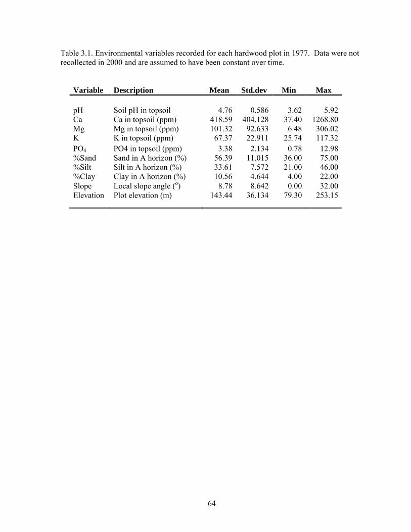
64
Table 3.1. Environmental variables recorded for each hardwood plot in 1977. Data were not recollected in 2000 and are assumed to have been constant over time.
Variable Description Mean Std.dev Min Max pH Soil pH in topsoil 4.76 0.586 3.62 5.92Ca Ca in topsoil (ppm) 418.59 404.128 37.40 1268.80Mg Mg in topsoil (ppm) 101.32 92.633 6.48 306.02K K in topsoil (ppm) 67.37 22.911 25.74 117.32PO4 PO4 in topsoil (ppm) 3.38 2.134 0.78 12.98%Sand Sand in A horizon (%) 56.39 11.015 36.00 75.00%Silt Silt in A horizon (%) 33.61 7.572 21.00 46.00%Clay Clay in A horizon (%) 10.56 4.644 4.00 22.00Slope Local slope angle (o) 8.78 8.642 0.00 32.00Elevation Plot elevation (m) 143.44 36.134 79.30 253.15

65
Table 3.2. Summary statistics for change in species richness at the subplot (25m2) and plot (1000m2) scale from 1977-2000 (n= 36 paired plots). Data listed are for all species (Total), species separated by growthform (Herb, Shrub, Tree), and native species of each species group (labeled with N.). *Plots w/ + change = Total number of plots (out of 36) that increased in species richness. **Plots w/ – change = Total number of plots (out of 36) that decreased in species richness. Growthform Total N.Total Herb N.Herb Shrub N.Shrub Tree N.Tree Plots w/ + change* 19 15 11 10 12 13 26 26 Plots w/ - change ** 15 15 21 22 16 17 6 6
25m2 Mean richness difference 0.14 -0.06 -1.50 -1.80 -0.30 -0.25 1.97 1.97
(n=36) Permutation test statistic 93 86 40 33 26 28 86 86
p-value 0.460 0.530 0.036 0.014 0.227 0.290 0.0001 0.0001 Plots w/ + change 22 22 12 9 22 21 30 30 Plots w/ - change 13 13 22 24 10 10 5 5
1000m2 Mean richness difference 3.17 2.11 -2.06 -2.86 1.11 0.97 4.11 4.00
(n=36) Permutation test statistic 204 173 61 44 62 57 161 157
p-value 0.030 0.093 0.041 0.006 0.011 0.019 0 0

66
Table 3.3. Indicator values (percent of perfect indication) and frequency statistics of species associated with 1977 plots or 2000 plots, listed in order of statistical significance (p-value) by year. The p-value is based on the proportion of 1000 randomized trials (Monte Carlo test) with indicator value equal to or exceeding the observed indicator value. All species with p-value ≤ 0.165 were included to show trends between years. Year: 1= 1977, 2= 2000. Growthform: 1=Tree, 2=Shrub, 3=Herb. Nativity: N=Native, I= Introduced (exotic). Indicator value Change in frequency
Species name Nativity Growthform 1977 2000 Year p-value 25 subplots Plot Chimaphila maculata N 3 72 18 1 0.001 -52 -4 Desmodium spp. N 3 82 11 1 0.002 -66 -4 Viburnum rafinesquianum N 2 72 24 1 0.002 -3 -2 Vitis aestivalis N 2 52 4 1 0.013 -28 -8 Goodyera pubescens N 3 35 4 1 0.014 -9 -7 Euphorbia corollata N 3 39 5 1 0.015 -7 -9 Euonymus americana N 2 56 16 1 0.027 10 -1 Aureolaria virginica N 3 35 1 1 0.029 -8 -8 Lonicera japonica I 2 53 7 1 0.038 -12 -2 Polygonatum biflorum N 3 57 24 1 0.038 -13 1 Carya glabra N 1 59 27 1 0.039 -37 0 Nyssa sylvatica N 1 66 10 1 0.044 -14 4 Sambucus nigra N 2 14 0 1 0.044 -16 -5 Houstonia caerulea N 3 14 0 1 0.046 -3 -5 Prenanthes altissima N 3 41 9 1 0.086 -16 -5 Celtis laevigata N 1 14 0 1 0.102 -8 -4 Pinus taeda N 1 40 8 1 0.104 -19 -3 Chrysogonum virginianum N 3 14 1 1 0.112 -4 -4 Lespedeza spp. 3 23 3 1 0.124 -16 -3 Silene virginica N 3 11 0 1 0.128 -1 -4 Epifagus virginiana N 3 11 0 1 0.13 -6 -4 Dioscorea villosa N 3 32 4 1 0.133 -7 0 Tephrosia virginiana N 3 11 0 1 0.133 -2 -4 Viburnum prunifolium N 2 49 13 1 0.134 -18 2 Solidago spp. N 3 36 3 1 0.14 -25 -1 Juniperus virginiana N 1 72 13 1 0.153 -3 4 Maianthemum racemosum N 3 34 5 1 0.157 -17 0 Chamaelirium luteum N 3 13 1 1 0.164 -1 -4 Rubus spp. N 2 2 47 2 0.003 29 13 Phytolacca americana N 3 0 22 2 0.004 7 8

67
Vitis rotundifolia N 2 22 74 2 0.015 150 2 Quercus falcata N 1 3 30 2 0.026 18 11 Carpinus caroliniana N 1 5 40 2 0.028 102 8 Liriodendron tulipifera N 1 16 55 2 0.037 105 6 Fraxinus americana +pennsylvanica N 1 18 54 2 0.041 88 9 Ulmus alata N 1 8 35 2 0.071 49 6 Asimina parviflora N 2 0 15 2 0.096 2 5 Pinus virginiana N 1 3 17 2 0.096 0 6 Ostrya virginiana N 1 7 32 2 0.097 60 4 Paulownia tomentosa I 1 0 11 2 0.111 0 4 Quercus alba N 1 32 58 2 0.125 37 4 Acer barbatum N 1 6 35 2 0.142 56 5

68
Table 3.4. Environmental variables correlated with change in species richness at 25m2 from 1977 to 2000. Data listed are for species separated by growth form (Herb, Shrub, Tree). Only correlations with p<0.05 are shown below. No factors were significantly correlated with change in richness at 1000m2. Symbol is: * p < 0.01.
25m2 Variables Tree Shrub Herb pH 0.44* Ca 0.52* Mg 0.54* K 0.41 PO4 Sand 0.47*Silt -0.35 -0.42*Clay -0.39 Slope Elevation -0.46* -0.49*Full 1000m2 richness 0.43*

69
Table 3.5. Coefficients of determination for the correlations between NMS ordination axes and measured environmental variables. Environmental variables were measured in 1977 and are assumed to have been constant over time. r2 NMS Axis 1 2 3 Group 0.001 0.263 0.039 Vector length 0.103 0.006 0.089 pH 0.624 0.001 0.027 Ca 0.497 0.016 0.085 Mg 0.554 0.000 0.039 K 0.149 0.009 0.002 PO4 0.018 0.012 0.018 %sand 0.470 0.052 0.000 %silt 0.602 0.053 0.000 %clay 0.355 0.038 0.003 Slope 0.023 0.011 0.078 Elevation 0.312 0.022 0.025

70
0
20
40
60
80
100
120
140
160
180
200
1975 1980 1985 1990 1995 2000
Dee
r pop
ulat
ion
(in th
ousa
nds)
Figure 3.1. Total deer population in the northern Piedmont management zone between 1984-2002. Population density is based on the population reconstruction model of Downing (1980) complied by the North Carolina Wildlife Resources Commission (unpublished data). Understory surveys were conducted in 1977 and 2000.

71
Figure 3.2. NMS ordination of plots in species space with paired-plot vectors drawn from 1977 to 2000 plot, showing direction of compositional change over time. Ordination is based on the 226 species that occurred in no fewer than two hardwood plots. Symbols are plots coded for year (triangle= 1977, square = 2000), filled symbols represent the plots with hurricane damage.

72
Figure 3.3. NMS ordination of plots in species space with correlation vectors of environmental variables (radiating from center) with the ordination. Ordination is based on the 226 species that occurred in no fewer than two hardwood plots. Environmental variables were measured in 1977 and are assumed to have been constant over time. All correlation vectors have r2≥ .250. Length of correlation vectors represents the strength of the correlation and angle indicates direction of highest correlation. Symbols are plots coded for year (triangle= 1977, square = 2000). (Group) is a categorical variable for year (1977 or 2000). All other environmental variables are defined in Table 3.1.

CHAPTER 4
CONCLUSIONS

74
This study has demonstrated how both the landscape distribution and local dynamics
of hardwood stands in the North Carolina Piedmont are shaped by the interaction of
environmental factors with historic and present disturbance regimes. Oak-hickory hardwood
forests are no longer present at their original extent and their biased distribution suggests that
we may never know the full range of species assemblages that once existed in association
with the forests of this region. Given the lack of early records on hardwood forests, it is
difficult to assess the species loss that has already occurred as a result of previous
agricultural disturbance and habitat fragmentation.
The understory analysis in mature hardwood forests (Chapter 3) highlights an
additional trend of recent herbaceous species decline occurring separate from the above
threats. The Duke Forest hardwood stands have remained relatively intact during the study
period and the significant species decline cannot be strongly attributed to the mechanisms
commonly associated with species extinction, such as habitat loss and fragmentation, direct
exploitation, and exotic species invasion (Wilcove 1998, Jolls 2003). These results echo the
findings of the long-term analysis conducted by Rooney et al. (in press) in which they
conclude that similar patterns of species loss suggest a major and largely unacknowledged
trend of biotic impoverishment occurring in temperate forests throughout North America.
Indeed, it is not unreasonable to assume that the recent pattern of herbaceous species decline
in unfragmented hardwood forests of the Piedmont would have remained undetected for
some time without the baseline data collected by Peet & Christensen.

75
The observation that historically ‘steady-state’ hardwood stands of the Piedmont
exhibit understory and overstory (Christensen 1977, McDonald 2002, 2003) directional
change and remain only as patches on the landscape by no means reduces their conservation
value. These forests will likely never fit the traditional definition of old-growth (sensu
Martin 1992, see also White & White 1996), but as a regional resource they have important
attributes that have yet to be fully recognized. Hardwood stands that have remained
continuously forested and free of severe soil disturbance since European settlement, even in
the presence of other disturbances, likely support regional rare flora and are important for the
protection of biological diversity.
Given the projected increases in population for the Piedmont region, which will place
an even greater demand on forested areas, it is crucial that greater effort is put towards
studying the mechanisms important in effecting change, along with increased support for the
protection of remaining remnant hardwood stands. Future research on mechanisms of
hardwood compositional change could entail combining field experiments (such as deer
exclosures) with structural equation modeling. Structural equation modeling is a useful
technique for hardwood forest research in this region since it is a method for evaluating
complex hypotheses involving multiple causal pathways among variables (McCune & Grace
2002). This modeling framework would allow us to compare the relative strengths of
different variables, such as deer herbivory and fire suppression, in effecting species change
and examine how they interact to cause shifts in understory composition. It would also be
useful for future analyses to be expanded to include the understory as well as higher strata
(e.g., shrub and overstory layers) since success in the understory is clearly linked to overstory
development.

76
Knowledge of the distribution of mature hardwood stands and their shifting
composition has important implications for conservation planning. We need to know what
species are being lost and why in order to take proper management actions to preserve the
ecological integrity of the stands. Programs such as the Nature Conservancy and the North
Carolina Natural Heritage program have identified a number of unique stands of Piedmont
hardwood, but these areas are not all currently protected and nor is there any ongoing
systematic monitoring program. Inadequate monitoring can lead to a lack of detection of
regional threats on native species and result in the continued loss of flora.
More proactive measures for the protection and monitoring of remnant hardwood
stands will not only support the stands themselves, but also contribute to regional restoration
efforts in post-agriculture or other disturbed forest sites. Previous research has shown that it
may take tens to hundreds of years for some forest plant species to recolonize secondary
forests due to factors such as seed limitation and slow dispersal capabilities (e.g., Peterken &
Game 1984, Whitney & Foster 1988, Bossuyt et al. 1999). If remnant stands do indeed
support a distinct flora in comparison to more heavily disturbed sites, introductions into
potentially suitable but unoccupied sites should be considered. Regional restoration efforts
should also aim to support the reintroduction of natural disturbance regimes, such as low-
intensity ground fires.
Without active monitoring, protection and restored natural disturbance regimes, I
forecast a continued decline in the extent of oak-hickory hardwood forests in the North
Carolina Piedmont, along with a shift towards a more overall mesic species composition.
Indeed, it has been suggested that, even for sites that remain protected, upland oak-hickory
will become a rare ecosystem type in the future (Fralish et al. 1991, Abrams 2003). In

77
addition, understory trends will likely include an increased loss of sensitive herb species
along with the further spread of exotic species. Proactive measures to monitor changes in
diversity and to identify and respond to particular threats would greatly help reduce the
impact of anthropogenic disturbance on native forests in the future.

78
APPENDIX A. FULL SPECIES LIST FOR DUKE FOREST HARDWOOD PLOTS FROM 1977 TO 2000
Number of species =319. Change in frequency reflects absolute change. L/G: New species gained (+) or species lost (-) between 1977 and 2000 GF: Growthform, 1=Tree; 2=Shrub; 3=Herb Nativity: N=Native; I=Introduced (exotic) ShadeT: Shade tolerance, High; Medium (Mid); Low 1977 Subplot Occurrence: Total number of subplots species occurred in across all plots in 1977 1977 Subplot Change in frequency Scientific name L/G GF Nativity ShadeT Occurrence Subplot Plot Acer barbatum 1 N High 42 56 5 Acer rubrum 1 N Mid 516 37 1 Amelanchier arborea 1 N High 7 5 4 Betula nigra - 1 N Low 0 0 -1 Carpinus caroliniana 1 N High 39 102 8 Carya alba 1 N Mid 106 6 2 Carya cordiformis 1 N Mid 3 13 5 Carya glabra 1 N Mid 168 -37 0 Carya ovata 1 N Mid 88 30 12 Carya pallida 1 N Mid 6 -5 0 Castanea dentata - 1 N Low 1 -1 -1 Celtis laevigata 1 N High 9 -8 -4 Celtis occidentalis 1 N Mid 1 10 5 Cercis canadensis 1 N High 93 29 0 Chionanthus virginicus 1 N High 24 -7 -1 Cornus florida 1 N High 223 3 3 Crataegus flabellata - 1 N Mid 2 -2 -1 Crataegus flava 1 N Low 0 0 -4 Crataegus marshallii 1 N High 0 1 1 Crataegus sp. 1 N Mid 0 0 0 Diospyros virginiana 1 N Mid 17 -2 2 Fagus grandifolia 1 N High 53 39 12 Fraxinus americana +pensylvancia 1 N Mid 33 88 9 Gleditsia triacanthos - 1 N Low 0 0 -1 Ilex ambigua 1 N High 4 -1 1 Ilex decidua 1 N High 6 -5 1 Ilex opaca 1 N High 5 0 5 Juglans nigra 1 N Mid 2 -1 0 Juniperus virginiana 1 N Mid 40 -3 4 Liquidambar styraciflua 1 N Low 18 26 2 Liriodendron tulipifera 1 N Low 27 105 6

79
Morus rubra 1 N Mid 9 -2 1 Nyssa sylvatica 1 N High 69 -14 4 Ostrya virginiana 1 N High 76 60 4 Oxydendrum arboreum 1 N Mid 26 18 2 Paulownia tomentosa + 1 I Mid 0 0 4 Pinus echinata 1 N Mid 8 -8 3 Pinus taeda 1 N High 31 -19 -3 Pinus virginiana 1 N Mid 1 0 6 Platanus occidentalis - 1 N Mid 0 0 -1 Prunus americana + 1 N Low 0 0 1 Prunus serotina 1 N High 146 -3 -2 Quercus alba 1 N Mid 308 37 4 Quercus coccinea 1 N Low 2 -2 -4 Quercus falcata 1 N Mid 7 18 11 Quercus marilandica 1 N Low 3 -3 -1 Quercus michauxii 1 N Mid 0 0 -4 Quercus montana 1 N Low 7 16 4 Quercus phellos 1 N Low 15 1 8 Quercus rubra 1 N Mid 85 -9 5 Quercus stellata 1 N Mid 25 4 2 Quercus velutina 1 N Mid 71 -8 4 Robinia pseudoacacia 1 N Low 9 -4 -1 Sassafras albidum 1 N Mid 29 4 0 Styrax grandifolius + 1 N High 0 1 2 Ulmus alata 1 N Mid 7 49 6 Ulmus rubra 1 N High 25 7 4 Aesculus sylvatica 2 N Mid 30 -14 2 Alnus serrulata - 2 N High 0 0 -1 Asimina parviflora 2 N High 0 2 5 Campsis radicans 2 N Low 9 -5 -2 Castanea pumila 2 N High 1 -1 0 Ceanothus americanus - 2 N High 0 0 -3 Cornus foemina + 2 N Mid 0 1 3 Corylus americana 2 N Mid 3 -3 -3 Elaeagnus umbellata 2 I Low 3 4 1 Euonymus americana 2 N Mid 205 10 -1 Gaylussacia baccata + 2 N High 0 3 1 Hamamelis virginiana 2 N Mid 19 -10 -2 Hydrangea arborescens - 2 N High 6 -6 -1 Itea virginica - 2 N High 0 0 -1 Ligustrum sinense 2 I High 4 7 2 Lindera benzoin 2 N Mid 7 1 -1 Lonicera japonica 2 I High 181 -12 -2 Lonicera sempervirens 2 N High 43 7 3 Mahonia bealei + 2 I High 0 0 1 Parthenocissus quinquefolia 2 N Mid 121 2 8 Passiflora incarnata + 2 N High 0 2 3

80
Rhododendron periclymenoides 2 N High 17 -11 -3 Rhus aromatica - 2 N High 0 0 -1 Rhus copallinum 2 N Low 0 0 0 Rosa carolina 2 N Mid 14 -4 0 Rubus spp. 2 N Mid 4 29 13 Sambucus nigra - 2 N Low 16 -16 -5 Smilax bona-nox 2 N High 28 -9 1 Smilax glauca 2 N High 10 0 4 Smilax rotundifolia 2 N Low 11 17 9 Staphylea trifolia 2 N High 1 -1 1 Toxicodendron radicans 2 N High 52 -13 2 Trachelospermum difforme + 2 N High 0 9 1 Vaccinium fuscatum + 2 N High 0 1 1 Vaccinium pallidum 2 N High 75 -4 1 Vaccinium stamineum 2 N High 81 10 0 Vaccinium tenellum 2 N High 32 -19 -1 Viburnum acerifolium 2 N High 122 79 5 Viburnum dentatum - 2 N High 2 -2 -1 Viburnum prunifolium 2 N High 39 -18 2 Viburnum rafinesquianum 2 N High 443 -3 -2 Viburnum rufidulum 2 N High 20 15 4 Vitis aestivalis 2 N High 55 -28 -8 Vitis rotundifolia 2 N Mid 127 150 2 Actaea racemosa 3 N 4 2 0 Adiantum pedatum - 3 N 0 0 -1 Agrimonia pubescens 3 N 18 4 -5 Amphicarpaea bracteata 3 N 24 5 1 Andropogon spp. 3 N 15 -10 2 Anemone virginiana - 3 N 0 0 -2 Antennaria plantaginifolia 3 N 6 -6 -3 Aplectrum hyemale - 3 N 1 -1 -1 Arabis canadensis - 3 N 1 -1 -1 Arisaema dracontium + 3 N 0 3 1 Arisaema triphyllum 3 N 2 8 1 Aristolochia serpentaria 3 N 22 -8 1 Arnoglossum atriplicifolium - 3 N 0 0 -1 Asclepias variegata - 3 N 0 0 -1 Asclepias verticillata - 3 N 0 0 -1 Asplenium platyneuron 3 N 15 -1 1 Aureolaria virginica 3 N 9 -8 -8 Baptisia sp. + 3 N 0 0 2 Bignonia capreolata - 3 N 4 -4 -1 Boehmeria cylindrica 3 N 2 -1 1 Botrychium biternatum 3 N 0 12 2

81
Botrychium virginianum 3 N 37 -3 -1 Brachyelytrum erectum 3 N 3 1 1 Bromus pubescens 3 N 0 2 -1 Carex spp. 3 N 123 5 -3 Chamaecrista fasciculata + 3 N 0 0 1 Chamaelirium luteum 3 N 2 -1 -4 Chasmanthium latifolium 3 N 2 -2 1 Chasmanthium laxum - 3 N 0 0 -1 Cheilanthes lanosa 3 N 18 -6 0 Chimaphila maculata 3 N 129 -52 -4 Chrysogonum virginianum 3 N 4 -4 -4 Circaea lutetiana 3 N 3 16 1 Cirsium vulgare + 3 I 0 0 1 Clematis viorna 3 N 0 0 -1 Clematis virginiana 3 N 10 -4 0 Clitoria mariana 3 N 8 -5 -1 Commelina communis 3 I 0 0 -1 Conopholis americana - 3 N 1 -1 -2 Conyza canadensis + 3 N 0 0 1 Coreopsis major 3 N 4 -4 -1 Coreopsis verticillata 3 N 3 -3 -3 Cryptotaenia canadensis 3 N 3 -3 -1 Cunila origanoides 3 N 1 0 1 Cynoglossum virginianum + 3 N 0 0 1 Danthonia sericea 3 N 0 1 -1 Danthonia spicata 3 N 34 -15 4 Dennstaedtia punctilobula 3 N 0 0 2 Desmodium laevigatum 3 N 31 -31 -6 Desmodium nudiflorum 3 N 126 -27 -1 Desmodium obtusum - 3 N 2 -2 -3 Desmodium paniculatum 3 N 2 -2 -3 Desmodium perplexum 3 N 0 1 -4 Desmodium rotundifolium 3 N 7 -6 -6 Desmodium sp. - 3 N 2 -2 -2 Desmodium viridiflorum + 3 N 0 0 1 Dichanthelium sp. 3 N 48 5 0 Dioscorea villosa 3 N 26 -7 0 Eleocharis sp. + 3 N 0 1 1 Elephantopus carolinianus 3 N 3 -1 -1 Elephantopus tomentosus - 3 N 0 0 -3 Elymus hystrix 3 N 15 17 1 Elymus villosus - 3 N 0 0 -2 Elymus virginicus + 3 N 0 0 1 Epifagus virginiana - 3 N 6 -6 -4

82
Epigaea repens 3 N 2 -2 -1 Erechtites hieraciifolia + 3 N 0 2 2 Erigeron annuus - 3 N 0 0 -1 Erythronium americanum - 3 N 1 -1 -1 Eupatorium capillifolium + 3 N 0 0 1 Eupatorium fistulosum + 3 N 0 0 1 Eupatorium hyssopifolium - 3 N 0 0 -1 Euphorbia corollata 3 N 12 -7 -9 Eurybia divaricata 3 N 2 -2 0 Festuca subverticillata 3 N 2 15 1 Fragaria virginiana 3 N 5 -3 -1 Galactia volubilis - 3 N 5 -5 -1 Galium aparine - 3 N 0 0 -1 Galium circaezans 3 N 101 19 -1 Galium obtusum - 3 N 0 0 -2 Galium pilosum - 3 N 3 -3 -2 Galium triflorum 3 N 15 -3 -2 Gelsemium sempervirens - 3 N 0 0 -1 Geum canadense 3 N 17 -7 1 Geum sp. + 3 N 0 0 1 Geum virginianum - 3 N 0 0 -1 Glechoma hederacea + 3 I 0 4 2 Goodyera pubescens 3 N 12 -9 -7 Heliopsis helianthoides + 3 N 0 0 1 Hepatica nobilis 3 N 23 6 1 Heuchera americana 3 N 0 0 -2 Hexastylis arifolia 3 N 96 60 1 Hexastylis minor 3 N 18 -5 0 Hieracium gronovii - 3 N 3 -3 -2 Hieracium venosum 3 N 25 -13 0 Houstonia caerulea - 3 N 3 -3 -5 Houstonia purpurea - 3 N 0 0 -2 Huperzia lucidula 3 N 1 2 0 Hypericum hypericoides 3 N 0 0 -2 Hypericum nudiflorum + 3 N 0 0 1 Hypericum prolificum - 3 N 0 0 -1 Hypoxis hirsuta 3 N 2 0 1 Impatiens capensis 3 N 0 6 0 Ipomoea pandurata 3 N 4 -2 0 Iris cristata 3 N 5 -2 -2 Iris verna 3 N 0 0 0 Juncus coriaceus 3 N 3 -3 0 Juncus tenuis + 3 N 0 2 1 Lactuca canadensis 3 N 0 0 -1 Lathyrus venosus - 3 N 1 -1 -1 Leersia virginica 3 N 0 1 1 Lespedeza hirta - 3 N 7 -7 -4

83
Lespedeza procumbens + 3 N 0 1 2 Lespedeza repens 3 N 8 -8 -4 Lespedeza sp. + 3 0 2 3 Lespedeza violacea 3 N 3 -3 3 Lespedeza virginica 3 N 1 -1 0 Liatris pilosa - 3 N 1 -1 -1 Ligusticum canadense 3 N 3 -1 -3 Lilium michauxii - 3 N 1 -1 -3 Liparis liliifolia 3 N 1 -1 -1 Lobelia inflata + 3 N 0 4 1 Lobelia nuttallii + 3 N 0 0 1 Lobelia sp. + 3 N 0 0 1 Luzula acuminata 3 N 1 2 -1 Lycopodium digitatum 3 N 0 0 0 Lycopus virginicus - 3 N 1 -1 -1 Lysimachia ciliata 3 N 3 -2 -1 Maianthemum racemosum 3 N 59 -17 0 Marshallia obovata - 3 N 0 0 -1 Matelea carolinensis 3 N 13 -6 0 Medeola virginiana + 3 N 0 0 1 Melanthium virginicum + 3 N 0 0 2 Melica mutica 3 N 7 -2 -3 Menispermum canadense 3 N 5 5 1 Microstegium vimineum 3 I 25 16 7 Mitchella repens + 3 N 0 0 2 Monarda fistulosa + 3 N 0 0 1 Monotropa hypopithys - 3 N 0 0 -1 Muhlenbergia schreberi - 3 N 0 0 -1 Onoclea sensibilis 3 N 3 2 1 Oxalis spp. 3 N 5 25 2 Parthenium integrifolium - 3 N 15 -15 -2 Passiflora lutea 3 N 0 2 0 Penstemon australis - 3 N 0 0 -1 Penstemon laevigatus - 3 N 0 0 -3 Phlox sp. + 3 N 0 1 1 Phryma leptostachya 3 N 9 13 5 Physalis virginiana - 3 N 1 -1 -2 Phytolacca americana + 3 N 0 7 8 Piptochaetium avenaceum 3 N 20 -10 -4 Pityopsis graminifolia - 3 N 1 -1 -2 Plantago rugelii + 3 N 0 0 1 Pleopeltis polypodioides 3 N 0 0 -1 Poaceae spp. 3 N 29 35 17 Podophyllum peltatum 3 N 3 -1 0 Polygonatum biflorum 3 N 117 -13 1

84
Polygonum sp. + 3 0 1 1 Polygonum virginianum - 3 N 8 -8 -1 Polypodium virginianum 3 N 2 0 0 Polystichum acrostichoides 3 N 44 -14 4 Porteranthus trifoliatus - 3 N 0 0 -1 Potentilla canadensis 3 N 10 -3 0 Prenanthes altissima 3 N 38 -16 -5 Prenanthes serpentaria + 3 N 0 6 2 Prunella vulgaris 3 N 0 0 0 Pteridium aquilinum + 3 N 0 0 1 Pycnanthemum incanum - 3 N 2 -2 -1 Pycnanthemum tenuifolium - 3 N 1 -1 -1 Pyrola americana - 3 N 2 -2 -1 Ranunculus spp. 3 N 1 0 0 Rhus glabra 3 N 0 0 2 Rudbeckia laciniata 3 N 11 -11 -1 Ruellia caroliniensis 3 N 2 6 -5 Salvia lyrata 3 N 1 -1 2 Sanguinaria canadensis 3 N 0 9 2 Sanicula spp. 3 N 30 11 0 Scleria oligantha 3 N 14 19 2 Scrophularia spp. + 3 N 0 0 1 Scutellaria elliptica 3 N 0 8 2 Scutellaria integrifolia 3 N 2 1 1 Scutellaria serrata 3 N 13 -13 0 Sedum ternatum 3 N 0 0 0 Sericocarpus asteroides 3 N 1 0 -3 Sericocarpus linifolius - 3 N 0 0 -1 Silene virginica - 3 N 1 -1 -4 Silphium asteriscus - 3 N 2 -2 -2 Silphium compositum - 3 N 0 0 -1 Sisyrinchium angustifolium - 3 N 16 -16 -1 Smallanthus uvedalius 3 N 5 2 0 Smilax herbacea - 3 N 0 0 -1 Solidago spp. 3 N 36 -25 -1 Stellaria media + 3 I 0 0 1 Stellaria pubera 3 N 10 5 2 Stylosanthes biflora - 3 N 3 -3 -2 Symphyotrichum dumosum + 3 N 0 0 1 Symphyotrichum undulatum 3 N 16 -14 0 Tephrosia virginiana - 3 N 2 -2 -4 Thalictrum revolutum 3 N 1 0 -1 Thalictrum thalictroides 3 N 19 2 -2 Thaspium barbinode 3 N 6 0 -1

85
Thaspium trifoliatum 3 N 1 -1 0 Tiarella cordifolia 3 N 22 -6 -2 Tipularia discolor 3 N 0 0 -2 Tradescantia virginiana + 3 N 0 0 1 Tragia urticifolia - 3 N 4 -4 -1 Trifolium pratense + 3 I 0 0 1 Trillium catesbaei 3 N 16 -16 -2 Uvularia perfoliata 3 N 70 1 4 Uvularia puberula 3 N 0 4 0 Uvularia sessilifolia - 3 N 1 -1 -2 Verbascum thapsus + 3 I 0 0 3 Verbesina alternifolia + 3 N 0 0 1 Verbesina occidentalis 3 N 24 -1 0 Vernonia glauca - 3 N 0 0 -2 Vernonia sp. + 3 N 0 0 1 Viola spp. 3 N 39 -1 -5 Zizia aurea - 3 N 0 0 -1

86
REFERENCES Abrams, M.D. 1992. Fire and the development of oak forests. BioScience 42:346-353. Abrams, M.D. 1998. The red maple paradox. BioScience 48: 355-364. Abrams, M.D. 2003. Where has all the white oak gone? BioScience 53: 927-939. Alvarez, M.E. and Cushman, J.H. 2002. Community-level consequences of a plant invasion:
Effects on three habitats in coastal California. Ecological Applications 12:1434-1444. Anderson, R.C. 1994. Height of white-flowered trillium (Trillium grandiflorum) as an index
of deer browsing intensity. Ecological Applications 4:104-109. Anderson, R.C. 1997. Native pests: the impact of deer in highly fragmented habitats. In:
Schwartz, M.W. (ed.) Conservation in highly fragmented landscapes. Chapman & Hall, New York, NY. Pp.117-134.
Anderson, R.C. and Adams, D.E. 1978. Species replacement patterns in central Illinois white
oak forests. In: Pope, P.E. (ed.) Proceedings of the Central Hardwoods Conference. II. Purdue University, West Lafayette, Indiana. Pp. 285-301.
Ashe, W.W. 1897. Forest of North Carolina. In: Pinchot, G. and Ashe, W.W. (eds.) Timber
trees and forests of North Carolina. North Carolina Geological Survey, Bulletin No.6, Winston, North Carolina.
Bio, A.M.F., Alkemade, R.& Barendregt, A.1998. Determining alternative models for
vegetation response analysis: a non-parametric approach. Journal of Vegetation Science 9:5-16.
Bordeau, P. 1954. Oak seedlings ecology determining segregation of species in Piedmont
oak-hickory forests. Ecological Monographs 24: 297-320. Bossuyt, B., Hermy, M. and Deckers, J. 1999. Migration of herbaceous plant species across
ancient-recent forest ecotones in central Belgium. Journal of Ecology 87:628-638. Brady, N.C. and Weil, R.R. 2002. The nature and properties of soils. 13th ed. Prentice Hall,
New Jersey.

87
Bratton, S.P. 1979. Impacts of white-tailed deer on the vegetation of Cades Cove, Great Smoky Mountains National Park. Proceedings of the Annual Conference of the Southeastern Association of Game Fish Commissions 33:305-312.
Braun, E.L. 1950. Deciduous forests of eastern North America. Hafner Publishing Company,
New York. Breiman, L., Friedman, J.H., Olshen, R.A.& Stone,C.J.1984. Classification and regression
trees. The Wadsworth statistics/probability series, Chapman & Hall, Inc., New York, NY.
Brown, D.G. 1994. Predicting vegetation types at treeline using topography and biophysical
disturbance variables. Journal of Vegetation Science 5:641-656. Bruhn, J.N., Wetteroff, J.J., Mihail, J.D., Kabrick, J.M. and Pickens, J.B. 2000. Distribution
of Armillaria species in upland Ozark Mountain forests with respect to site, overstory species composition and oak decline. Forest Pathology 30: 43-60.
Carpino, E.A. 1998. Ecological determinants of hurricane damage in a Southeastern
Piedmont forest. M.E.M. thesis, Duke University, Durham, North Carolina. Chambers, J.M. and Hastie, T.J. 1992. Statistical models in S. Wadsworth & Brooks/Cole,
Pacific Grove, CA. Christensen, N.L.1977. Changes in structure, pattern, and diversity associated with climax
forest maturation in Piedmont, North Carolina. American Midland Naturalist 97:176-188.
Christensen, N.L.1989. Landscape history and ecological change. Journal of Forest History
33:116-124. Christensen, N.L. and Peet, R.K. 1981. Secondary forest succession on the North Carolina
piedmont. Pp 230-245 In: West, D., Shugart, H. and Botkin, D. (eds). Forest Succession: Concept and applications. Springer-Verlag, NY.
Christensen, N.L. and Peet, R.K. 1984. Convergence during secondary forest succession.
Journal of Ecology 72:25-36. Coile, T.S. 1948. Relation of soil characteristics to site index of loblolly and shortleaf pines
in the lower Piedmont Region of North Carolina. Duke University School of Forestry Bulletin. No.13. Durham, North Carolina.

88
Curtis, J.T. 1959. The Vegetation of Wisconsin. University of Wisconsin Press, Madison,
Wisconsin. Daniels, R.B., Buol, S.W., Kleiss, H.J., Ditzler, C.A. 1999. Soil systems in North Carolina.
Technical Bulletin 314. North Carolina State University, Raleigh, North Carolina. Davis, M.B. 1996. Eastern old-growth forests: prospects for rediscovery and recovery.
Island Press, Seattle, Washington. Davison, S.E. and Forman, R.T.T. 1982. Herb and shrub dynamics in a mature oak forest: a
thirty-year study. Bulletin of the Torrey Botanical Club 109:64-73. De’Ath, G. and Fabricius, K.E. 2000. Classification and regression trees: a powerful yet
simple technique for ecological data analysis. Ecology 81:3178-3192. Delcourt, P.A., Delcourt, H.R., Morse, D.F., and Morse, P.A. 1993. “History, evolution, and
organization of vegetation and human culture,” In: Martin, W.H., Boyce, S.G., and Echternacht, A.C. (eds.) Biodiversity of the Southeastern United States: lowland terrestrial communities. Wiley and Sons, New York, NY.
Delcourt, H.R., and Delcourt, P.A. 2000. Deciduous forests, Chapter 10. In: Barbour, M.G.
and Billings, W.D. (eds.). North American Terrestrial Vegetation, 2nd Ed. Pp. 357-395. Cambridge, UK, Cambridge University Press.
Downing, R.L. 1980. Vital statistics of animal populations. In: Schemnitz S. (ed.) Wildlife
management techniques manual. 4th edition. Pp 247-267. The Wildlife Society, Bethesda, Maryland, USA.
Draper, D. 1995. Assessment and propagation of model uncertainty (with discussion).
Journal of the Royal Society Series B 57:45-97. Drayton, B. and Primack, R.B. 1996. Plant species lost in an isolated conservation area in
Metropolitan Boston from 1894-1993. Conservation Biology 10:30-39. Dufrêne, M. and Legendre, P. 1997. Species assemblages and indicator species: the need for
a flexible asymmetrical approach. Ecological Monographs 67:345-366. Fielding, A.H. & J.F. Bell.1997. A review of methods for the assessment of prediction errors
in conservation presence/absence models. Environmental Conservation 24:38-49. Fralish, J.S., Crooks, F.B., Chambers, J.L. and Harty, F.M. 1991. Comparison of
presettlement, second-growth and old-growth forest on six types in the Illinois Shawnee Hills. American Midland Naturalist 125: 294-309.
89
Franklin, J. 1995. Predictive vegetation mapping: geographic modeling of biospatial patterns in relation to environmental gradients. Progress in Physical Geography 19:474-499.
Franklin, J.1998. Predicting the distribution of shrub species in southern California from
climate and terrain-derived variables. Journal of Vegetation Science 9:733-748. Frost, C.C. 1998. Presettlement fire frequency regimes of the United States: a first
approximation. In: Tall Timbers Fire Ecology Conference Proceedings 20:70-81, Tall Timbers Research Station, Tallahassee, Florida.
Gilliam, F.S. and Roberts, M.R. 2003. The herbaceous layer in forests of Eastern North
America. Oxford University Press, New York. Gorchov, D.L. and Trisel, D.E. 2003. Competitive effects of the invasive shrub, Lonicera
maackii (Rupr.) Herder (Caprifoliaceae), on the growth and survival of native tree seedlings. Plant Ecology 166: 13-24.
Guisan, A., and Zimmerman, N.E. 2000. Predictive habitat distribution models in ecology.
Ecological Modeling 135:147-186. Hand, D.J. 1997. Construction and assessment of classification rules. John Wiley & Sons
Ltd., Chichester. Hans, J., J.Butaye, M.Dumortier, M.Hermy, N.Lust. 2001. Effects of age and distance on the
composition of mixed deciduous forest fragments in an agricultural landscape. Journal of Vegetation Science 12:635-642.
Hatley, M.T. 1977. The dividing path: the direction of Cherokee life in the eighteenth
century. MS thesis, University of North Carolina, Chapel Hill, North Carolina. Healy, R.G. 1985. Competition for land in the American South: agriculture, human
settlement, and the environment. Conservation Foundation, Washington, D.C. Honnay O., Hermy, M. and Coppin, P. 1999. Impact of habitat quality on forest plant species
colonization. Forest Ecology and Management 115:157-170. Hosmer, D.W., Lemeshow, S. 2000. Applied Logistic Regression. Wiley, New York. Jolls, C.L. 2003. Populations of and threats to rare plants of the herb layer. In: Gilliam, F.S.
and Roberts, M.R. (eds.) The herbaceous layer in forests of Eastern North America. Pp.105-159. Oxford University Press, New York.
Kartesz, J.T. 1999. A synonymized checklist and atlas with biological attributes for the
vascular flora of the United States, Canada and Greenland. First edition. In: Kartesz, J.T. and Meacham, C.A. Synthesis of the North American Flora, Version 1.0. North Carolina Botanical Garden, Chapel Hill, NC.

90
Keever, C. 1950. Causes of succession on old fields of the Piedmont, North Carolina.
Ecological Monographs 20: 229-250. Kelley, T.M. 1994. Effect of white-tailed deer on the understory vegetation of an oak-hickory
forest and growth of trees in a white pine plantation. MS thesis. Department of Biological Sciences, Illinois State University, Normal.
Kruskal, J.B. 1964. Nonmetric multidimensional scaling: a numerical method. Psychometrika
29:115-129. Kutner, M.H.1996. Logistic regression, Poisson regression and generalized linear models. In:
Neter, J. Kutner, M.H., Nachtseim, C.J. & Wasserman, W. (eds.) Applied Linear Statistical Models. 4th ed., Irwin, Times Mirror Higher Education Group,Inc. Chicago, IL.
Kwiatkowska, A.J. 1994. Changes in species richness, spatial pattern and species frequency
associated with the decline of oak forest. Vegetatio 112:171-180. Linnet, K. and Brandt, E.1986. Assessing diagnostic tests once an optimal cutoff point has
been selected. Clin.Chem. 32:1341-1346. Lorimer, C.G. 1984. Development of the red maple understory in northeastern oak forests.
Forest Science 30:3-22. Lorimer, C.G. 1985. The role of fire in the perpetuation of oak forests. In: Johnson, J.E. (ed.)
Proceedings of challenges in oak management and utilization. Cooperative Extension Service, University of Wisconsin, Madison.
Lorimer, C.G., Chapman, J.W. and Lambert, W.D. 1994. Tall understory vegetation as a
factor in the poor development of oak seedlings beneath mature stands. Journal of Ecology 82: 227-237.
Manly, B.F.J. 1997. Randomization and Monte Carlo methods in biology, 2nd edition.
Chapman & Hall, London. Marquis, D.A., Eckert, P.L. and Roach, B.A. 1976. Acorn weevils, rodents, and deer all
contribute to oak regeneration difficulties in Pennsylvania. USDA Forest Service Northeastern Forest Experiment Station Research Paper NE-356.
Mather, P.M. 1976. Computational methods of multivariate analysis in physical geography.
J.Wiley & Sons, London. 532pp. Matlack, G.R. 1994. Plant species migration in a mixed-history forest landscape in eastern
North America. Ecology 75 (5): 1491-1502.

91
Marks, P.L. 1974. The role of pin cherry (Prunus pensylvanica) in the maintenance of stability in northern hardwood ecosystems. Ecological Monographs 44: 73-88.
Martin, W.H. 1992. Characteristics of old-growth mixed mesophytic forests. Natural Areas
Journal 13: 127-135. Maunz, S.J. 2002. Interactions of stream channel geometry, riparian species distribution and
land cover in an urban watershed. M.A. thesis, University of North Carolina, Chapel Hill, North Carolina.
McCune, B. and Grace, J.B. 2002. Analysis of ecological communities. MjM Software
Design, Gleneden Beach, Oregon. 300pp. McCune, B. and Mefford, M.J. 1999. PC-ORD. Multivariate analysis of ecological data.
Version 4.24. MjM Software, Gleneden Beach, Oregon, USA. McDonald, R.I., Peet, R.K. & Urban, D.L. 2002. Environmental correlates of oak decline and
red maple increase in the North Carolina Piedmont. Castanea 67:84-95. McDonald, R.I., Peet, R.K. and Urban, D.L. 2003. Spatial pattern of Quercus regeneration
limitation and Acer rubrum invasion in a Piedmont forest. Journal of Vegetation Science 14: 441-450.
Mielke, P.W., Jr. 1984. Meteorological applications of permutation techniques based on
distance functions. Pp.813-830. In P.R.Krishnaiah & P.K.Sen, eds., Handbook of Statistics, Vol.4. Elsevier Science Publishers.
Mielke, P.W., Jr. and Berry, K.J. 1982. An extended class of permutation techniques for
matched pairs. Communications in Statistics. Part A – Theory and Methods 11:1197-1207.
Mielke, P.W., Jr. and Berry, K.J. 2001. Permutation methods: a distance function approach.
Springer Series in Statistics. 344pp. Moore, I.D., Lee, B.G. & Davey, S.M. 1991. A new method for predicting vegetation
distributions using decision tree analysis in a geographic information system. Environmental Management 15:59-71.
Morisette, J.T., Khorram,S. & Mace, T. 1999. Land-cover change detection enhanced with
generalized linear models. International Journal of Remote Sensing 20:2703-2721. National Soil Information System (NASIS). June 2003. Soil Survey Staff. Digital soil survey
area attribute tables, Electronic media. Orange, Durham and Wake Counties, North Carolina. U.S. Department of Agriculture, Natural Resources Conservation Service.
North Carolina Climate Office. 2003. North Carolina State University, Raleigh.

92
Oksanen, L. 1976. On the use of Scandinavian type class system in cover estimation. Annales
Botanici Fennici 13:149-153. Oosting, H.J. 1942. An ecological analysis of the plant communities of Piedmont, North
Carolina. American Midland Naturalist 28:1-126. Oosting, H.J. 1956. The study of plant communities. W.H. Freeman, San Francisco, CA. Osborne, J.S. 1993. The white-tailed deer in North Carolina. North Carolina Wildlife
Resources Commission, Raleigh, North Carolina. Palmer, M.W. 1990. Spatial scale and patterns of vegetation, flora and species richness in
hardwood forests of the North Carolina piedmont. Ceonoses 5:89-96. Parker, A.J. 1982. The topographic relative moisture index: an approach to soil-moisture
assessment in mountain terrain. Physical Geogography 3:160-168. Parker, G.R., Leopold, D.J. and Eichenberger, J.K. 1985. Tree dynamics in an old-growth,
deciduous forest. Forest Ecology and Management 11: 31-57. Peet , R.K. 1992. Community structure and ecosystem function. In: Glenn-Lewin, D.C., Peet,
R.K. & Veblen, T.T. (eds.) Plant succession: theory and prediction. Chapman & Hall, London.
Peet, R.K, and Christensen, N.L.1980. Hardwood forest vegetation of the North Carolina
Piedmont. Veröffentlichungen Geobotanik Institut ETH. Stiftung Rübel 69:14-39.
Peet, R.K. and Christensen, N.L. 1988. Changes in species diversity during secondary forest succession on the North Carolina piedmont. In: During, H.J., Werger, M.J.A. and Willems, J.H. (eds.). Diversity and pattern in plant communities. Pp.233-245. SPB Academic Publishing, The Hague.
Peet, R.K. and Loucks, O.L. 1977. A gradient analysis of southern Wisconsin upland forests. Ecology 58: 485-499.
Peet, R.K., Wentworth, T.R., White, P.S. 1998. A flexible, multipurpose method for
recording vegetation composition and structure. Castanea 63:262-274. Peterken, G.F. and Game, M. 1984. Historical factors affecting the number and distribution
of vascular plant species in central Lincolnshire. Journal of Ecology 72: 155-182. Peterson, E.B. and McCune, B. 2001. Diversity and succession of epiphytic macrolichen
communities in low-elevation managed conifer forests in Western Oregon. Journal of Vegetation Science 12:511-524.

93
Pickett, S.T.A. and White, P.S. 1985. The ecology of natural disturbance and patch dynamics. Academic Press, Orlando, Florida.
Pimm, S.L., Russell, G.J., Gittleman, J.L., and Brooks, T.M. 1995. The future of
biodiversity. Science 269:347-350. Radford, A.E., Ahles, H.E. and Bell, C.R. 1968. Manual of the vascular flora of the
Carolinas. University of North Carolina Press, Chapel Hill, North Carolina. Richardson, D.M., Macdonald, I.A.W., and Forsyth, G.G. 1989. Reductions in plant species
richness under stands of alien trees and shrubs in the fynbos biome. South African Forestry Journal 149:1-8.
Rooney, T.P. and Dress, W.J. 1997. Species loss over sixty-six years in the ground layer
vegetation of Heart’s Content, an old-growth forest in Pennsylvania USA. Natural Areas Journal 17:297-305.
Rooney, T.P., Weigmann S.M., Rogers, D.A., Waller, D.M. in press. Biotic impoverishment
and homogenization in unfragmented forest understory communities. Conservation Biology.
Schneider, L.C., and Pontius, R.G. 2001. Modeling land-use change in the Ipswich
watershed, Massachusetts, USA. Agriculture Ecosystems & Environment 85:83-94. Skeen, J.N., Doerr, P.D., and Van Lear, D.H. 1993. Oak-hickory-pine forests. In: Martin,
W.H., Boyce, S.G., and Echternacht, A.C. (eds.) Biodiversity of the Southeastern United States: lowland terrestrial communities. Wiley and Sons, New York, NY.
Strole, T.A. and Anderson, R.C. 1992. White-tailed deer browsing species preferences and
implications for central Illinois forests. Natural Areas Journal12: 139-144. Tilghman, N.G. 1989. Impacts of white-tailed deer on forest regeneration in northwestern
Pennsylvania. Journal of Wildlife Management. 53: 424-453. Tilman, D., May, R. M., Lehman, C. L., and Nowak, M. A. 1994. Habitat destruction and the
extinction debt. Nature 371:65-66. Trimble, S.W. 1974. Man-induced soil erosion on the southern Piedmont, 1700-1970. Soil
Conservation Society of America. Urban, D.L. 2002. Classification and regression trees. In: McCune, B. and Grace, J.B.
Analysis of ecological communities. MjM Software Design, Gleneden Beach, Oregon.
Urban, D., Goslee, S., Pierce, K., & Lookingbill, T. 2002. Extending community ecology to landscapes. Ecoscience 9:200-212.

94
USDA, NRCS. 2002. The PLANTS Database, Version 3.5 (http://plants.usda.gov). National Plant Data Center, Baton Rouge, LA 70874-4490 USA.
Vayssières, M.P., Plant, R.E., & Allen-Diaz, B.H. 2000. Classification trees: an alternative non-parametric approach for predicting species distributions. Journal of Vegetation Science 11:679-694.
Waller, D. M., and Alverson, W. S. 1997. The white-tailed deer: a keystone herbivore.
Wildlife Society Bulletin 25: 217-226. Wear, D.N., and Bolstad, P. 1998. Land-use changes in southern Appalachian landscapes:
spatial analysis and forecast evaluation. Ecosystems 1:575-594.
Whitney, G.G. and Foster, D.R. 1988. Overstorey composition and age as determinants of the understorey flora of woods of central New England. Journal of Ecology 76:867-876.
White, P.S. 2001. Director’s Message: Our forests of continuity. North Carolina Botanical
Garden Newsletter (May-June), Chapel Hill, NC. White, P.S. and White, R.D. 1996. Old growth oak and oak-hickory forests. In: M.B. Davis,
(ed). Eastern Old-Growth Forests. Pp 178-198. Island Press, Washington D.C. White, R.D. 1999. The impacts of Hurricane Fran on a North Carolina Piedmont woodland.
M.A. thesis, University of North Carolina, Chapel Hill, North Carolina. Wilcove, D.S., Rothstein, D., Dubow, J., Phillips, A., Losos, E. 1998. Quantifying threats to
imperiled species in the United States. BioScience 48:607-615. Wolock, D.M., and McCabe, J. 1995. Comparison of single and multiple flow direction
algorithms for computing topographic parameters in TOPMODEL. Water Resources Research 31:1315-1324.
Yee, T.W. and Mitchell, N.D.1991. Generalized additive models in plant ecology. Journal of
Vegetation Science 2:587-602.