Tampereen teknillinen yliopisto. Julkaisu 1209 Tampere University of Technology. Publication 1209

Matti Pellikka Finite Element Method for Electromagnetics on Riemannian Manifolds Topology and Differential Geometry Toolkit Thesis for the degree of Doctor of Science in Technology to be presented with due permission for public examination and criticism in Rakennustalo Building, Auditorium RG202, at Tampere University of Technology, on the 2nd of May 2014, at 12 noon. Tampereen teknillinen yliopisto - Tampere University of Technology Tampere 2014

ISBN 978-952-15-3279-5 (printed) ISBN 978-952-15-3285-6 (PDF) ISSN 1459-2045

Abstract

This thesis applies new branches of mathematics in computational electromagnetics soft-ware. Namely, we consider the application of algebraic topology and differential geometryin finite element modeling. We conclude that from this approach, one can draw benefits topractical electromagnetic modeling. For example, more efficient numerical formulations,field-circuit coupling, and metric and coordinate free modeling techniques.

We present efficient methods for homology and cohomology computation of finiteelement meshes together with their software implementation. The presented homologyand cohomology solver is a part of finite element mesh generator Gmsh. Therefore, itsuse can be easily incorporated into finite element modeling workflow.

We demonstrate the use of homology and cohomology computation results in staticand quasistatic electromagnetic field problems. We describe finite element formulationswhich can be used in lumped parameter extraction from field problems and which canbe naturally coupled to electronic circuit problems. Importantly, cohomology computa-tion enables the use of magnetic scalar potential in eddy current problems without anytopological restrictions, leading to more efficient and robust field computations.

Lastly, we present a finite element programming environment, where the language ofdifferential geometry has the main role. We interpret the finite element model as a Rie-mannian manifold, and the fields of interest as differential forms. Using the environment,one can give the computational instructions in metric and coordinate free manner, as theused metric and coordinate system are provided separately. Then, the environment trans-lates the instructions to the actual floating-point operations, which ultimately depend onthe used metric and coordinate system. The programming environment implementationbuilds on top of the Gmsh API. That is, we implement tools from differential geometrywhich utilize an existing finite element framework.

The main contribution of this thesis is the development of these tools to the pointwhere they can be readily expoited in computationally demanding engineering problems.Also, this thesis offers a unified exposition of the needed mathematical concepts and theirrelation to the electromagnetic field problem formulations.

Preface

I have made this thesis in the inspirational environment of the electromagnetics researchgroup in the Tampere University of Technology. The thesis topic builds on top of thelong-term basic research conducted in our research group, to bring some of its resultscloser to engineering practice.

I have done this work under the supervision of Professor Lauri Kettunen, whose en-thusiasm, sincerity, and farsightedness reflects in the atmosphere of the whole researchgroup, creating a close-knit research community. In addition to Lauri Kettunen, I havebeen privileged to be guided by two other members of our research group, whose ad-vice and perspective complement each other: University Lecturer Saku Suuriniemi andSenior Research Fellow Timo Tarhasaari. Much of my progress is also due to ProfessorChristophe Geuzaine from the University of Liège, the main developer of the finite el-ement library Gmsh. In addition to his encouragement, he enabled and supported theimplementation of the methods of this thesis to Gmsh.

I would also like to than Lasse Söderlund and Maija-Liisa Paasonen for taking careof administrative tasks, as well as Juha Tampio, Antti Stenvall, Valtteri Lahtinen, ErkkiHärö, Arto Poutala, and Olli Pekkola for giving feedback to some of the software imple-mentations I have done for this thesis.

Other people I’d like to thank for more or less casual interaction during my thesis workinclude Jukka-Pekka Uusitalo, Teemu Rovio, Pasi Raumonen, Janne Keränen, TuukkaNieminen, Arttu Rasku, Aki Korpela, Risto Mikkonen, Stefan Kurz, and other presentand past personnel of our research group who are responsible for its friendly atmosphere.

Lastly, I thank my dear wife Kiti for taking care of the fundamentals on the homefront, as well as my son Eevertti for demanding my undivided attention on regular basis;and my daughter Muusa for inspiring me while finalizing this thesis.

1

Contents

List of symbols 5

1 Introduction 10

1.1 Background, motivation, and usefulness of the research . . . . . . . . . . 121.1.1 Homology and cohomology computation . . . . . . . . . . . . . . 121.1.2 Differential geometry and Riemannian manifolds . . . . . . . . . . 13

1.2 Survey of recent research . . . . . . . . . . . . . . . . . . . . . . . . . . . 141.3 Original contributions . . . . . . . . . . . . . . . . . . . . . . . . . . . . 14

1.3.1 Development of reduction techniques for homology and cohomologycomputation . . . . . . . . . . . . . . . . . . . . . . . . . . . . . . 15

1.3.2 Implementation of homology and cohomology solver . . . . . . . . 151.3.3 Cohomology based formulations of the electromagnetic boundary

value problems . . . . . . . . . . . . . . . . . . . . . . . . . . . . 151.3.4 Implementation of Riemannian manifold programming interface . 16

1.4 Organization . . . . . . . . . . . . . . . . . . . . . . . . . . . . . . . . . 16

2 Mathematical concepts 17

2.1 Algebraic structures . . . . . . . . . . . . . . . . . . . . . . . . . . . . . 182.1.1 Abelian group . . . . . . . . . . . . . . . . . . . . . . . . . . . . . 182.1.2 Homological algebra . . . . . . . . . . . . . . . . . . . . . . . . . 212.1.3 Vector space . . . . . . . . . . . . . . . . . . . . . . . . . . . . . . 252.1.4 Exterior algebra . . . . . . . . . . . . . . . . . . . . . . . . . . . . 27

2.2 Manifold and its cell decomposition . . . . . . . . . . . . . . . . . . . . . 292.2.1 Real coordinate space . . . . . . . . . . . . . . . . . . . . . . . . . 302.2.2 Euclidean space . . . . . . . . . . . . . . . . . . . . . . . . . . . . 302.2.3 Manifolds . . . . . . . . . . . . . . . . . . . . . . . . . . . . . . . 312.2.4 Cell complex of a manifold . . . . . . . . . . . . . . . . . . . . . . 342.2.5 Finite elements . . . . . . . . . . . . . . . . . . . . . . . . . . . . 37

2.3 Homology and cohomology of a manifold . . . . . . . . . . . . . . . . . . 382.3.1 Chain complexes of a manifold . . . . . . . . . . . . . . . . . . . . 382.3.2 Cochain complexes of a manifold . . . . . . . . . . . . . . . . . . 402.3.3 Homology and cohomology of a manifold . . . . . . . . . . . . . . 40

2.4 Differential forms . . . . . . . . . . . . . . . . . . . . . . . . . . . . . . . 432.4.1 The basic construction . . . . . . . . . . . . . . . . . . . . . . . . 432.4.2 Integration . . . . . . . . . . . . . . . . . . . . . . . . . . . . . . 452.4.3 de Rham cohomology . . . . . . . . . . . . . . . . . . . . . . . . . 46

2

2.4.4 Harmonic differential forms . . . . . . . . . . . . . . . . . . . . . 472.4.5 Whitney forms . . . . . . . . . . . . . . . . . . . . . . . . . . . . 48

3 Homology and cohomology computation of finite element meshes 51

3.1 Construction of chain complexes from a finite element mesh . . . . . . . 523.1.1 Data structures and construction of the cell complex . . . . . . . 523.1.2 Construction of chain complexes . . . . . . . . . . . . . . . . . . . 53

3.2 Reduction of chain complexes . . . . . . . . . . . . . . . . . . . . . . . . 543.2.1 Reduction algorithms . . . . . . . . . . . . . . . . . . . . . . . . . 543.2.2 Reduction pair . . . . . . . . . . . . . . . . . . . . . . . . . . . . 553.2.3 Homology reduction algorithms . . . . . . . . . . . . . . . . . . . 573.2.4 Cohomology reduction algorithms . . . . . . . . . . . . . . . . . . 61

3.3 Computation of homology and cohomology . . . . . . . . . . . . . . . . . 623.3.1 Smith normal form . . . . . . . . . . . . . . . . . . . . . . . . . . 643.3.2 Kernel-image problem . . . . . . . . . . . . . . . . . . . . . . . . 643.3.3 Quotient problem . . . . . . . . . . . . . . . . . . . . . . . . . . . 653.3.4 The homology and cohomology computation algorithm . . . . . . 67

3.4 The homology and cohomology solver in Gmsh . . . . . . . . . . . . . . . 673.4.1 Homology computation routine . . . . . . . . . . . . . . . . . . . 683.4.2 Cohomology computation routine . . . . . . . . . . . . . . . . . . 68

3.5 Post-processing of homology and cohomology . . . . . . . . . . . . . . . . 693.5.1 Basis element representative selection . . . . . . . . . . . . . . . . 703.5.2 Basis selection . . . . . . . . . . . . . . . . . . . . . . . . . . . . . 703.5.3 Computation of harmonic representatives . . . . . . . . . . . . . . 73

3.6 Examples . . . . . . . . . . . . . . . . . . . . . . . . . . . . . . . . . . . 743.6.1 Example: Solid cube . . . . . . . . . . . . . . . . . . . . . . . . . 743.6.2 Example: Closed surfaces . . . . . . . . . . . . . . . . . . . . . . 753.6.3 Example: Torus knots . . . . . . . . . . . . . . . . . . . . . . . . 76

4 Application of cohomology in the finite element method for electromag-

netics 79

4.1 Electromagnetic modeling . . . . . . . . . . . . . . . . . . . . . . . . . . 804.2 Static problems . . . . . . . . . . . . . . . . . . . . . . . . . . . . . . . . 81

4.2.1 Electrokinetic problem . . . . . . . . . . . . . . . . . . . . . . . . 814.2.2 Cohomology basis functions . . . . . . . . . . . . . . . . . . . . . 834.2.3 Electric field -conforming formulation . . . . . . . . . . . . . . . . 854.2.4 Current density -conforming formulation . . . . . . . . . . . . . . 864.2.5 Electrostatic problem . . . . . . . . . . . . . . . . . . . . . . . . . 884.2.6 Magnetostatic problem . . . . . . . . . . . . . . . . . . . . . . . . 89

4.3 Circuit coupled eddy current problem . . . . . . . . . . . . . . . . . . . . 904.3.1 Eddy current problem . . . . . . . . . . . . . . . . . . . . . . . . 904.3.2 Faraday’s law conforming formulation . . . . . . . . . . . . . . . . 914.3.3 Ampere’s law conforming formulation . . . . . . . . . . . . . . . . 92

4.4 Examples . . . . . . . . . . . . . . . . . . . . . . . . . . . . . . . . . . . 934.4.1 Induced EMF in squirrel cage rotor . . . . . . . . . . . . . . . . . 934.4.2 Mutual inductance magnetostatic problem . . . . . . . . . . . . . 94

3

4.4.3 Induction heating eddy current problem . . . . . . . . . . . . . . 97

5 Finite element imitation of the Riemannian manifold 103

5.1 Motivation . . . . . . . . . . . . . . . . . . . . . . . . . . . . . . . . . . . 1035.2 Imitation of the manifold . . . . . . . . . . . . . . . . . . . . . . . . . . . 104

5.2.1 Differentials of the charts . . . . . . . . . . . . . . . . . . . . . . . 1055.2.2 Finite element charts for the manifold . . . . . . . . . . . . . . . 1065.2.3 Chains . . . . . . . . . . . . . . . . . . . . . . . . . . . . . . . . . 1065.2.4 Implementation details . . . . . . . . . . . . . . . . . . . . . . . . 106

5.3 Imitation of tensorial objects . . . . . . . . . . . . . . . . . . . . . . . . . 1085.3.1 Representation and transformations of tensors on the manifold . . 1095.3.2 Metric tensor on the manifold . . . . . . . . . . . . . . . . . . . . 1095.3.3 Implementation details . . . . . . . . . . . . . . . . . . . . . . . . 110

5.4 Application examples . . . . . . . . . . . . . . . . . . . . . . . . . . . . . 1125.4.1 Example program: Poisson equation and harmonic field solver on

Riemannian 3-, and 2-manifolds . . . . . . . . . . . . . . . . . . . 1125.4.2 Parametrization for a surface patch . . . . . . . . . . . . . . . . . 1145.4.3 Laplace problem with a pullback metric . . . . . . . . . . . . . . 1145.4.4 Invisibility cloaking in electrostatics . . . . . . . . . . . . . . . . . 1155.4.5 Finding an atlas of charts for a surface . . . . . . . . . . . . . . . 1175.4.6 Eddy currents on a conductor surface . . . . . . . . . . . . . . . . 118

6 Conclusion 122

6.1 Homology and cohomology solver . . . . . . . . . . . . . . . . . . . . . . 1226.2 Riemannian manifold interface . . . . . . . . . . . . . . . . . . . . . . . . 1226.3 Future developments . . . . . . . . . . . . . . . . . . . . . . . . . . . . . 123

Bibliography 124

Index 129

4

List of symbols

Chapter 2

(Ek, φ) Euclidean reference k-cell, page 37

(M,K), (S,L) A regular CW-complex of a manifold M or a submanifoldS, page 36

(U, x) A chart, page 31

(V, o) Oriented vector space, page 30

[g] The equivalence class of g, page 20

Λk(T ∗M) The k-cotangent bundle of a manifold M , page 44

Λk(V ∗) The vector space of alternating k-linear maps on a vectorspace V , page 28

D A differentiable atlas, page 31

∂M The boundary of a manifold, page 32

∂, ∂k (k:th) boundary homomorphism, page 21

βk The k:th Betti number, page 27

wk A Whitney k-form, page 49

Σk A basis of a k-cochain group, page 40

Σk A basis of a k-chain group, page 39

δ, δk (k:th) coboundary homomorphism, page 23

C, C′, C, C Chain complex, page 21

·H The conjugate/Hermitian transpose of a column vector or amatrix, page 26

·T The transpose of a column vector or a matrix, page 19

σk A k-cell, page 35

ǫk A basis k-cochain, page 40

C The field of complex numbers, page 32

dxi i:th coordinate basis covector, page 33

d The exterior derivative of a differential form, page 44

δIJ Kronecker delta for multi-indices, page 28

5

∆k Standard k-simplex, page 37

det A The determinant of a matrix A, page 28

dimG Rank of the free subgroup of the finitely generated freeabelian group G, page 20

dim V The dimension of a vector space V , page 25

En The n-dimensional Euclidean space, page 29

γ, γk a k-cochain, page 23

Hk(M,S) The space of harmonic differential k-forms, page 47

im f Image of a map f, page 18

ι·· The incidence relation of cells, page 36

〈·, ·〉 An inner product, page 26

Z The ring of integers, page 19

Zn The group of n-tuples of integers, page 19

Zn The group of integers modulo n, page 20

ker f Kernel of a map f, page 18

λi A finite element shape function at i:th node, page 37

Dk The matrix representation of the k:th boundary homomor-phism, page 39

G The coordinate chart representation of a metric tensor g,page 34

‖ · ‖ A norm, page 30

ω An element of a dual space of a vector space, page 26

ω♯ The sharp operator, page 26

Ωk(M),Ωk(M,S) The vector space of differential k-forms on a manifold M(whose trace vanish on a submanifold S), page 44

∂∂xi i:th coordinate basis vector, page 32

R The field of real numbers, page 29

Rn+ The half-space of the real coordinate space R

n, page 30

F Field of real or complex numbers, page 25

Fn Vector space of n-tuples of real or complex numbers, page 25

∼ Equivalence relation, page 20

⋆ The Hodge operator, page 29

t, tS The trace operator of a differential form (to a submanifoldS, page 44

τ A topology, page 30⊗(

k,l(T )M) The (k, l)-tensor bundle of a manifold M , page 109

6

ω The coefficient representation of ω, page 26

v The coefficient representation of v, page 25

∧ The exterior product, page 28

ζ, ζk a k-cocycle, page 24

Bk(C;G) k:th coboundary group, page 24

Bk k:th boundary group, page 21

Bnr (y) Open y-centered r-radius Euclidean n-ball, page 30

c, ck a k-chain, page 21

Ck(C;G) k:th cochain group of a chain complex C, page 23

Ck(M), Ck(M,S) The k:th cochain group of a manifold M (relative to a sub-manifold S), page 40

Ck k:th chain group, page 21

Ck(M), Ck(M,S) The k:th chain group of a manifold M (relative to a sub-manifold S), page 38

F A Free subgroup, page 20

g The metric tensor, page 34

G/H The quotient group of groups G and H, page 20

HΩk(M,S) The Sobolev space of differential k-forms, page 47

Hk(C;G) k:th cohomology group of the chain complex C, page 24

Hk(M ;G), Hk(M,S;G) The k:th cohomology group of a manifold M (relative to asubmanifold S), page 41

HkdR(M,S) Relative k:th de Rham cohomology space of a manifold M

and a submanifold S, page 46

Hk(C) k:th homology group of the chain complex C, page 21

Hk(M), Hk(M,S) The k:th homology group of a manifold M (relative to asubmanifold S), page 41

I, J Multi-index, page 28

K,L A cell complex, page 36

M A differentiable manifold, page 31

T The torsion subgroup, page 20

TpM A tangent space of a manifold M at p, page 33

T ∗pM A cotangent space of a manifold M at p, page 33

TM The tangent bundle of a manifold M , page 43

v An element of a vector space, page 25

V ∗ The dual space of a vector space V , page 26

v The flat operator, page 26

7

W k(M,S) The vector space of Whitney k-forms, page 49

z, zk a k-cycle, page 21

Zk(C;G) k:th cocycle group, page 24

Zk k:th cycle group, page 21(

nk

)

The binomial coefficient, page 28

Chapter 3

(b, a) A reduction pair, page 55

Hk The basis representation matrix of a k:th cohomology group,page 63

Hk The basis representation matrix of a k:th homology group,page 63

O(·) The computational complexity class, page 57

Q Queue data structure, page 59

R(·, ·) The computational complexity of the removeReductionPair

routine, page 57

Chapter 4

∂t The partial derivative with respect to time, page 80

E A 1-cohomology basis function, page 83

e A Whitney 1-form, page 83

F A 2-cohomology basis function, page 83

f A Whitney 2-form, page 83

N A 0-cohomology basis function, page 83

n A Whitney 0-form, page 83

Wk A k-cohomology basis function, page 83

ǫ The permittivity (1,1)-tensor, page 80

µ The permeability (1,1)-tensor, page 80

Ω A 3-submanifold of R3, page 80

ρ The charge density 3-form, page 80

Σ A 2-submanifold of R3, page 80

σ The conductivity (1,1)-tensor, page 80

b The magnetic flux density 2-form, page 80

d The electric flux density 2-form, page 80

e The electric field 1-form, page 80

h The magnetic field 1-form, page 80

j The current density 2-form, page 80

8

JM(p) A Jacobian matrix of the map φM at a point p, page 105

µ A map from preprocessor model to a manifold M , page 104

φσ A map from euclidean reference cell of a finite element tothe preprocessor model, page 106

φM A map from preprocessor model to a coordinate chart of amanifold M , page 104

ϕ A map from m-manifold M to n-manifold N , page 104

p Model coordinates of a point p on a manifold M , page 107

u Finite element coordinates of a point p on a manifold M ,page 106

x Manifold coordinates of a point p on a manifold M , page 105

M An m-manifold, page 104

N An n-manifold, page 104

9

Chapter 1

Introduction

The finite element method is a widely applied method in sciences and engineering to solveboundary value problems. A boundary value problem has three ingredients

1. A regular domain1 and its parametrization.

2. Equations of unknown functions and their partial derivatives, i.e. partial differentialequations, that are required to hold in the domain.

3. Equations of unknown functions and their partial derivatives that are required tohold on the boundary of the domain, i.e. boundary conditions.

In the finite element method, the numerical solution of the boundary value problemstands on two concepts. The decomposition of a domain to finite elements to approximatethe unknown field, and the evaluation of bilinear functionals associated with the finiteelements in the domain and on its boundary. Traditionally, the domain is interpreted asa subset of the Euclidean space, while the bilinear functionals arise from the integrationof a dot product of vector fields or a product of scalar fields.

In this thesis, we take an axiomatic approach to the mathematical structures utilized inthe boundary value problems and reinterpret the finite element method accordingly. Thecleanest means to achieve this would be to utilize the category theory [25], instead of theset theory. However, since the main audience of this thesis is engineering practitioners,rather than mathematicians, we try to limit concepts not included in the usual finiteelement modeling curriculum.

The reinterpretation of the finite element method involves new computational stepsand software design aspects to accommodate to the changes. The reinterpretation hastwo main themes, the global topology and the metric of the domain.

The domain of a boundary value problem can have topological features that are con-sidered to be global in contrast to local. Such features are the existence of holes ofdifferent dimension in the domain, such as tunnels or voids. It turns out, that thesefeatures together with the boundary conditions of the unknown field need to be takeninto account to ensure the existence and the uniqueness of the solution of a boundaryvalue problem. In other words, such analysis is an indispensable part of the boundaryvalue problems.

1A weakly Lipschitz domain [27]

10

To this end, we have studied computational methods to detect such holes their relationto the boundary conditions, and means to take them into account in the finite elementmethod. Such study is called computational homology and cohomology. In the finiteelement setting, the starting point of the homology and the cohomology computationis the finite element mesh together with the information where the unknown field isconstrained by the boundary conditions.

Homology and cohomology has the most visible appearance the in the electromagneticmodeling. Already the Maxwell’s equations hint to this direction, if one studies in theirintegral form the interplay between the integration domain and its boundary. Histori-cally, the conscious interest in the homology computation in electromagnetic modelingarose from the need to compute “cuts” for the magnetic scalar potential in domains withtunnels. However, as we argue in this thesis, cohomology permeates all electromagneticboundary value problems and cohomology computation is a powerful tool in vector po-tential formulations and in the field-circuit coupling in electromagnetic modeling. To thisend, we present finite element formulations of electromagnetic field problems that exploitthe results of cohomology computation.

The first aim of this thesis is to make cohomology computation a commonplace prac-tice in the finite element modeling. Therefore, in the course of this thesis we have imple-mented a homology and cohomology solver as an integrated part of a finite element meshgenerator.

By metric we refer to local measure of distances and angles within the domain. In theframework of the Euclidean space, it is assumed that the metric is constant with respectto Cartesian coordinates across the domain. Such metric is called Euclidean metric.In the generalization called Riemannian manifold, metric can vary from point to point,stripping the metric meaning from the coordinate numbers. The object that carries theinformation of the local metric is called the metric tensor.

With the Euclidean space interpretation of the domain the classical vector analysisformalism is often used, which has three shortcomings. First, the formalism is hard-wiredto the Euclidean metric, and special care is needed to use a general metric tensor. Sec-ond, the expressions often depend on the employed coordinate system of the domain.This needlessly obscures the notation with excessive details. Third, classical vector anal-ysis is devised for 3-dimensional domains, which makes the notation cumbersome in2-dimensional domains and the formalism insufficient for higher dimensional domains.Therefore, we have adapted the formalism of differential geometry in this thesis.

The Riemannian manifold interpretation of the domain together with the differentialgeometry formalism are the ingredients of the second major topic of the thesis. We haveimplemented a finite element programming environment, which performs the Riemannianmanifold interpretation and allows the user to program finite element solvers using thelanguage of the differential geometry.

The framework of the differential geometry overcomes the mentioned limitations of theclassical vector analysis. It is indifferent about the used metric, the coordinate system,and the dimension of the domain. That is, expressions are invariant under such changes.In a computational setting, such feature can easily be exploited with an interface wherethe metric and coordinate system are provided separately from the expressions encodingcomputational procedures. The software then translates the expressions to the actual nu-merical computations that ultimately depend on the used metric and coordinate system.

11

That is, one is able to write programs in a way that resembles the workflow of an appliedmathematician. This constitutes the second aim of this thesis.

1.1 Background, motivation, and usefulness of the

research

The interest in homology and differential geometry in computational electromagneticsresearch community rose in the 1980s. The impetus for this was the increased performanceof computers that made the numerical solution of 3-dimensional field problems possiblein acceptable time. It was soon noticed however, that the application of the scalar andvector potential formulations to three dimensions was not straightforward.

1.1.1 Homology and cohomology computation

The magnetic scalar potential formulation of magnetostatics requires that there’s a “cut”in the domain where the magnetic scalar potential is multi-valued. The jump of the scalarpotential across the cut equals the magnetomotive force that generates the magneticfield. In two-dimensional problems, the cut was easy to designate manually. However ina three-dimensional field problem, the room for complexity of the modeling domain ismuch larger. This initiated a research for algorithms to produce the cuts automatically,even without having an exact definition of the “cut” in mind. Even today, these ad hocalgorithms are widely used in commercial simulation software.

It was discovered that the exact definition of the cut involves algebraic topologyconcept called homology2. An algorithm for the cut computation in finite element mesheswas introduced in [45]. However, the inexact algorithms that worked in many practicalsituations persisted commercially.

At the time, the general homology computation was believed to be computationallyexpensive as it involves the computation of Smith normal form integer matrix decompo-sition. For this reason, general homology computation was not pursued in computationalelectromagnetics. However, the research on general homology computation continued ona path where the size of the homological problem was first made smaller with so-called“reduction techniques” [39], which have acceptable efficiency.

Also an another approach was considered. Instead of producing a cut for the scalarpotential, one can produce a “source field” or “loop field” to accompany the scalar poten-tial. Such vector field belongs to the 1-cohomology class, and specialized algorithms basedon spanning trees and 1-homology computation were developed for 1-cohomology com-putation. Such approach is more convenient than cut computation in magnetoquasistaticproblems where both scalar and vector potentials are needed.

In the three dimensional vector potential formulations, it was noticed that the netquantities such as the net current or the magnetic flux are troublesome to impose usingthe boundary conditions of the vector potential. A completely non-intuitive 1-cohomology

2The cut in a domain M ⊂ R3 is a representative of an element of the relative 2-homology group

H2(M, ∂M). The representative is called a cut if it is an orientable submanifold of M and can beembedded in R

3 [43].

12

vector field needs to be constructed on the boundary. The robust technique to constructsuch vector fields involves cohomology computation on the boundary of the domain.

In the both above examples, the homology or cohomology relates to the net quanti-ties. Net quantities are the state-variables in the circuit models of the electromagnetism.Therefore, it should be just a matter of formulation to exploit cohomology computationin the field-circuit coupling in electrical engineering.

The evident topological problems in both scalar and vector potential approaches andthe relation to the circuit coupling motivated the research done for this thesis. To pre-pare for unforeseen applications, we solve for general, possibly relative, homology andcohomology groups, not just for 1-homology and 1-cohomology that are known to beimportant in the applications of the computational electromagnetics.

As an outcome, we now have an efficient homology and cohomology solver within afinite element mesh generator. Therefore, it can be easily integrated to the usual finiteelement modeling workflow. Furthermore, we have demonstrated its usage in industrialscale electromagnetic field problems which shows that it is a viable tool in electricalengineering.

1.1.2 Differential geometry and Riemannian manifolds

Soon after the introduction of the vector potentials to the finite element method it wasdiscovered that the mere “three-component scalar potential” is not the right approach forvectorial finite elements in electromagnetism[7]. Such approximation enforces the conti-nuity of all three components across the finite element interfaces, while only tangentialor normal continuity conforms to the boundary conditions derived from the Maxwell’sequations.

As a solution, so-called edge and facet elements, Whitney forms in general, soon pen-etrated the research community and commercial simulation software. While the Whitneyforms are differential forms living on a differentiable manifold, the viewpoint that theyare vector fields in the Euclidean space still persists. However, the interest what else canbe gained from the framework of differential geometry in practical electrical engineeringwas sparked.

The differential form interpretation fits naturally to the geometric finite element set-ting and makes it possible to develop software the separates metric and coordinates fromexpressions that are used to compute the elements of the final system matrix.

Using other than the Euclidean metric in the computations has been found beneficialin many modeling techniques. Some of them are called “transformation techniques”[34], where the modeling domain is still the Euclidean space, but one can perform thecomputations on user-defined non-Cartesian coordinate chart instead of the Cartesianone. In a more general setting of the Riemannian manifold one can consider domains forwhich no Cartesian coordinate chart exist. For example, one can perform computationson a curved surface using a flat finite element mesh. Both of these techniques are coveredby the Riemannian manifold interpretation of the domain of a boundary value problem.

However, the Riemannian manifold interpretation increases the complexity of a finiteelement solver, since the free choices of the coordinate chart and the metric need to betaken into account in the numerical computations. The complexity can be alleviatedby the inclusion of an additional layer to the software on which computational instruc-

13

tions can be written in terms of the differential geometry. Underneath this layer, thesoftware translates the expressions into coordinate chart and metric dependent floating-point operations. Such programming interface has been developed on the course of thisthesis.

1.2 Survey of recent research

The role of homology computation in computational electromagnetics was first recog-nized in [42] and later considered in [43, 44, 6, 45]. However, efficient general homologycomputation methods we’re not available to fully exploit the findings at the time.

First steps towards efficient general homology computation were the introduction ofreduction of chain complexes [39, 38] in computational homology. Similar algorithms, butbased on homotopy invariance of homology rather than properties of chain complexes werediscussed in context of finite element meshes and electromagnetics in [61].

Since in the computational electromagnetism 1-cohomology computation has the mostimportance, specialized algorithms for 1-cohomology computation based on 1-homologycomputation are considered in [21, 22]. The results of such computation are often calledthick-cuts, recognized in [41]. Direct 1-cohomology computation methods for computa-tional electromagnetics were considered in [18, 19].

The road to general cohomology computation by the reduction of chain complexes waspaved by the Coreduction homology algorithm [47], which was then applied to cohomologycomputation of finite element meshes in [49] by the author.

Other software that perform homology and cohomology computation include CHomP [12,38], javaPlex [62, 11], and GAP homology [37, 36] packages. The design objectives of thesepopular packages are slightly different from ours, with less emphasis on problem positionin finite element modeling.

Earlier, a Riemannian manifold approach to the finite element modeling has beentaken in Manifold Code [35], as it separates the metric from the coordinate representationof the domain. However, the metric tensor is defined indirectly by providing the weakforms in contrast to our approach. It aims to solve “second-order nonlinear ellipticsystems of partial differential equations on domains with the structure of Riemanniantwo- and three-manifolds”.

A similar project called PyDEC [4, 5] is a Python library for finite element and discreteexterior calculus. In PyDEC, the metric tensor is the pullback metric of an embeddingof the simplicial complex into an n-dimensional Euclidean space.

1.3 Original contributions

In this section we specify the original contributions by the author that to our knowledgefirst appear in this thesis or in an earlier article by the author.

14

1.3.1 Development of reduction techniques for homology and

cohomology computation

The reduction techniques for the homology computation considered in [61] had someshortcomings. They are inefficient in the computation of absolute homology of closedmanifolds and in the computation of relative homology where the boundary of the man-ifold is the relative subdomain.

In chapter 3 of this thesis and in the article [49], the author applies chain equivalencesinspired by the Coreduction Homology Algorithm [47] in homology computation. Themain difference in our approach with respect to the Coreduction Homology Algorithmis that the author is able to also produce the representatives of the homology groupgenerators.

The algorithms considered in [61] and the above homology algorithm are also appliedby the author in the cohomology computation to produce the representatives of thecohomology group generators.

1.3.2 Implementation of homology and cohomology solver

On the course of this thesis, the author has implemented a homology and cohomologysolver as an integrated part of the finite element mesh generator Gmsh. It is describedin the chapter 3 and appears in the articles [49], [49],[50], and [51].

The specification of the input and output, the user interface, the reduction techniques,and the homology and cohomology computation steps are implemented by the author. Forthe Smith normal form computation, a subroutine within the homology and cohomologycomputation steps, a library developed by the author of [61] was used.

1.3.3 Cohomology based formulations of the electromagnetic

boundary value problems

The cohomology has appeared in a form or another in the electromagnetic boundary valueproblem formulations for a long time. What has been lacking however, is a general finiteelement formulation framework where the cohomology has an equipotent role it shouldhave.

In chapter 4 the author represents such framework and coins the term Cohomologybasis function to bring cohomology in front matter from behind the scenes. In the arti-cle [51] the author applies the framework to a magnetic field oriented formulation of amagnetoquasistatic problem.

The formulation framework makes it easier to recognize which parts of the problemstem from cohomology. For instance, it makes clear that to assign electric potentialvalues on equipotential boundary surfaces, a common task in everyday electromagneticmodeling, is the same thing as choosing the cohomology class of the solution.

The formulation framework unifies the aspects of many formulations. For example“floating potentials” [17], “thick-cuts” or “source fields” [41, 55, 33], and “thick-links” or“thinned conductors” [60, 20], and it clarifies the duality [16] of complementary formula-tions. In the framework of the author, all these terms are just different instances of thecohomology basis functions at work.

15

1.3.4 Implementation of Riemannian manifold programming in-

terface

The author has designed and implemented a C++ programming interface that imitatesthe structure and objects defined on the Riemannian manifold. The interface utilizesthe application programming interface of Gmsh to provide the usual finite element datastructures. The interface is described in chapter 5 and in the article [52].

The main benefit of the interface is that it allows one to write programs using thelanguage of the differential geometry, which is inherently coordinate and metric free.However, the description of a finite element mesh and the actual computations in thefinite element method depend on the coordinates and the metric. This gap has beenfilled by the author in the represented library.

1.4 Organization

The organization of this thesis is as follows. In chapter 2 we define the mathematicalconcepts employed in this thesis. We begin with purely algebraic concepts and the conceptof manifold which is used to model the domain of a boundary value problem. Then,these two tracks are merged to define homology and cohomology of a manifold, and todefine differential forms that model the fields on a manifold. Although this is chapter isstandard material in many textbooks, we find it necessary to be able to read this thesisas an independent piece of work.

In chapter 3 we describe how the homology and the cohomology of a manifold iscomputed. The computation has three stages: the construction of the chain complex, theexploitation of the reduction techniques on the chain complex, and finally the solution ofthe algebraic problems using integer arithmetic. In the chapter, we also consider post-processing techniques of the homology and the cohomology computation results makethem more appealing for visualization in exploitation in the solution of boundary valueproblems. In this chapter we combine the previous research to our original contributionson the subject.

In chapter 4 we formulate static and magnetoquasistatic boundary value problemsthat exploit the results of the homology and the cohomology computation. The chapteralso clarifies the engineering significance of homology and cohomology in electromag-netics. While the ingredients of this chapter can be found from earlier computationalelectromagnetics research, it provides a novel, unified framework of cohomology basisfunctions in the formulation of boundary value problems.

In chapter 5 we present a Riemannian manifold programming interface in a finite ele-ment environment. We describe how the finite element preprocessor model is interpretedas a Riemannian manifold, and how tensorial objects on the manifold are imitated withina computational environment. We also provide the motivation for such interface andexamples of its application.

16

Chapter 2

Mathematical concepts

In this chapter, we introduce the mathematical structures and theorems that are discussedand utilized in this thesis. While most of the contents of this chapter can be found fromtextbooks [29, 25, 8, 63, 23, 24, 48, 31, 57], we find it necessary to condense the topics thatare relevant to this thesis in a notionally uniform exposition. We also want to emphasizethe structured and minimalist viewpoint of mathematics and mathematical modeling.

We also pay close attention to the representations of the elements of mathematical ob-jects. In computations, one is ultimately dependent on integer and floating-point numberarithmetic. Thus in order to imitate elements of mathematical structures in computa-tions and in software, one needs to represent them as n-tuples of floating-point numbersor integers. Such representations are not unique, and turning this non-uniqueness intoan advantage is a recurring topic in this thesis.

In engineering, one utilizes a myriad of mathematical structures and theorems to solvea problem. Often, the structures are not identified, but treated as a single, inseparable mixof mathematics. In this thesis, we do the opposite. While we cannot escape the fact thatfor example the solution of a boundary value problem utilizes a variety of mathematicalideas, we can sort out some of the ingredients of the mix. The benefit of doing so isthat once we have identified the structures at play, we can utilize the mathematicaltheorems regarding that single structure in engineering. That is, recognizing whether amathematical theorem is useful in an engineering problem becomes a manageable task.

This “divide and conquer” of mathematical structures is used to establish the useful-ness of the following theorems of modern mathematics in the electromagnetic modeling:Lefschetz duality theorem, de Rham’s theorem, and Hodge’s theorem. The way the theo-rems are stated in the provided original and secondary sources is intangible to a workingengineer. In this thesis, we hope to narrow the gap.

In physics, the term general covariance is used to mean that one can use any coordinatesystem one chooses to model physical phenomena. Such property is the foundation, ratherthan a theorem, in the theory of Riemannian manifolds. Therefore, such mathematicalformalism should also empower engineering practice, which is why this thesis is writtenwithin that framework.

17

2.1 Algebraic structures

Algebraic structures lay foundations for the applied mathematics. Most of the engineeringpractice revolves around linear algebra which is the study of an algebraic structure calledthe vector space. Very often engineering problems are turned into problems of linearalgebra, for which efficient computational algorithms do exist. However, in this thesis weencounter problems that are more naturally expressed in terms of less familiar algebraicstructures.

Algebraic structures apply the idea of a closure system repeatedly. Consider a set witha binary operation for the elements of the set. If the result of the binary operation for allarguments belongs to the set, the set is called closed under that binary operation. Anotherimportant concept is a structure-preserving map between sets, called homomorphism. Itis a generalization of the linear map between vector spaces. That is, it makes no differencewhether one applies a binary operation before or after the mapping.

In this thesis, we encounter algebraic structures that are closely related to the vectorspaces and apply them to engineering problems. As the mere linear algebra formalismdoes not suit all of our needs, we need to expand our view to the close relatives of thevector space: abelian groups and graded vector spaces called exterior algebra.

2.1.1 Abelian group

Abelian group is an algebraic structure that underlies in many mathematical structureslike vector space and field. It also has significance of its own right. For example in thisthesis, homology and cohomology are first defined in terms of the abelian groups alone.

Let G be a set and let + : G × G → G be a commutative and associative map [25].Then, the pair (G,+) is an abelian group if there exists an element 0 ∈ G such thata+0 = a holds and if there exists an element −a ∈ G for all a ∈ G for which a+(−a) = 0holds. A pair (A,+) is a subgroup of (G,+), if A ⊂ G holds and the pair (A,+) is agroup of its own right.

A map f : G→ H from a group (G,+) to a group (H,⊕) is a group homomorphism

if f(a+ b) = f(a)⊕ f(b) holds for all a, b ∈ G. If a group homomorphism is injective andsurjective, it is a group isomorphism. When the context permits, an abelian group(G,+) is denoted with plain G. The kernel and image of a homomorphism f are sets

ker f := g ∈ G | f(g) = 0 and (2.1)

im f := h ∈ H |h = f(g), g ∈ G, (2.2)

which turn out to be subgroups of G and H, respectively [25].The operations a + (−b), ∑

k a = a + a + . . . + a, and∑

k−a = −a + (−a) + . . . +(−a) are abbreviated as a − b, ka, and −ka, respectively. With these conventions, thealgebraic structures of the abelian group and the module over the ring of integers areindistinguishable. Such structure is closely related to the vector space, with the differencethat the coefficients are integers rather than real numbers.

A subset S ⊂ G, 0 /∈ S, is a generating set of the group G if any element g of theset G can be expressed as a finite composition of the elements of S and their inverses

18

with the map +:

g = k1s1 + k2s2 + . . .+ knsk =n

∑

i=1

kisi, ∀ i : ki ∈ Z, si ∈ S. (2.3)

If there exists such generating set that such composition is unique, G is a free abelian

group. If the set S is finite, G is finitely generated abelian group. Such generatingset of a finitely generated free abelian group is called a basis. The number of basiselements is called the rank of the free abelian group.

Formal sum

From any finite set S one can construct a finitely generated abelian group G. Onedeclares that the elements g of the group are formal sums of the elements of the set S:

g :=n

∑

i=1

kisi, ∀ i : ki ∈ Z, si ∈ S, (2.4)

where n = |S| is the cardinality of S and si 6= sj when i 6= j. The map + and the inverseelement are defined by

g1 + g2 =n

∑

i=1

kisi +n

∑

i=1

qisi :=n

∑

i=1

(ki + qi)si. (2.5)

−g = −( n

∑

i=1

kisi

)

:=n

∑

i=1

(−ki)si. (2.6)

The set S is a basis for such group, and an element of such group can be represented

in that basis as a integer vector k =[

k1 k2 . . . kn]T ∈ Z

n of the coefficients ki in theformal sum. Then, a group element g ∈ G is denoted by g = (s1, s2, . . . , sn)k = Sk.

The integer vectors k themselves constitute a finitely generated free abelian group Zn

under the vector addition. This group is isomorphic to the abelian group G constructedvia the formal sum. More generally, any finitely generated free abelian group is isomorphicto the group Z

n [48].Let H be a finitely generated free abelian group with a basis R = (r1, r2, . . . , rm).

Then, a group homomorphism φ : G → H satisfies φ(si) = (r1, r2, . . . , rm)φi for someφi ∈ Z

m. That is, one can construct a m × n matrix F =[

φ1 φ2 . . .φn

]

that repre-sents the homomorphism φ. These observations enable one to solve algebraic problemsassociated with the “abstract” groups G and H by computations that involve the “con-crete” integer vector groups Zn and Z

m. In other words, the following diagram of finitelygenerated free abelian groups commutes:

G H

Zn

Zm

φ

F

(2.7)

19

Torsion subgroups

If an abelian group is not free, it has a non-trivial torsion subgroup. An element g ∈ Gis a torsion element if

∑

t g = 0 holds for some non-zero integer t, called the torsion

coefficient of g. Each torsion element generates a torsion torsion subgroup T of G.That is, the elements u of a torsion subgroup generated by g are of the form

u = qg =∑

q

g, q ∈ Zt, (2.8)

where Zt is the group of integers modulo t. Therefore, a torsion subgroup with the torsioncoefficient t is isomorphic to the group Zt. That is, an integer q ∈ Zt is a representationfor u.

Characterization of finitely generated abelian groups

LetG be a finitely generated abelian group with a minimal generating set S = g1, g2, . . . , gn.Then, an element g ∈ G can be written as a unique sum [48]

g =r

∑

i=1

kigi +n

∑

j=r+1

qj−rgj, ki ∈ Z, qj ∈ Ztj(2.9)

The element g ∈ G is then represented by a tuple ((k1, k2, . . . , kr), q1, . . . qn−r) ∈ Zr ×

Zt1× . . . × Ztn−r

with respect to the generating set S. It follows that G is isomorphicto the group formed by the internal direct sum Z

r ⊕ Zt1⊕ . . . ⊕ Ztn−r

. The group Ghas thus the decomposition G = F ⊕ T , where F is a rank r free subgroup and T is theinternal direct sum of torsion subgroups of G with torsion coefficients tj. The rank r andthe torsion coefficients tj are uniquely determined by G, even though the generating setS is not unique [48]. By dimG we denote the rank of the free subgroup of the finitelygenerated free abelian group G.

Quotient group and the short exact sequence

Let G be an abelian group and H its subgroup. Define an equivalence relation ∼ in G tobe such that

g1 ∼ g2 ⇐⇒ g1 − g2 ∈ H (2.10)

A coset [g] of g ∈ G is the set

[g] := g + h |h ∈ H := g +H (2.11)

of equivalent elements in G. The quotient group G/H := g+H | g ∈ G is an abeliangroup whose elements are such cosets. The map + and the inverse element are definedby

[g1] + [g2] := [g1 + g2], (2.12)

−[g] := [−g], (2.13)

20

and since for h ∈ H, [g] + [h] = [g + h] = [g] holds, the coset [h] is the zero element ofG/H.

The inclusion map i : H → G, i(h) = h, is an injective homomorphism. Definea surjective homomorphism j : G → G/H by j(g) = [g]. Then j i = 0 holds sincej(i(h)) = j(h) = [h] = 0 holds for all h ∈ H. That is, im i ⊂ ker j holds. Moreover, sinceg ∈ H = im i holds for all g ∈ ker j we obtain that ker j = im i holds. It is said that thenthe sequence of abelian groups

. . .→ Hi−→ G

j−→ G/H → . . . (2.14)

is exact at G. Since ker i = 0 and im j = G/H hold due to injectivity of i andsurjectivity of j, the sequence can be completed to form a short exact sequence

0→ Hi−→ G

j−→ G/H → 0 (2.15)

which is exact at H, G, and G/H. By the first isomorphism theorem [48], the group G/His isomorphic to the group G/ ker j = G/ im i, where the equality holds by the exactnessof the sequence. This indicates that the map i : H → G alone characterizes thestructure of the quotient group G/H.

2.1.2 Homological algebra

In homological algebra, one studies the properties of the chain complexes and relationsbetween them. A chain complex C = (C•, ∂•) is a sequence of abelian groups C• andhomomorphisms ∂• between them, usually presented as a diagram

. . .∂k+2−−→ Ck+1

∂k+1−−→ Ck∂k−→ Ck−1

∂k−1−−→ . . . (2.16)

The sequence is required to have the complex property that ∂k ∂k+1 = 0 holds for everyk. Therefore, im ∂k+1 ⊂ ker ∂k holds. However, the sequence is not necessarily exact, foran exact sequence im ∂k+1 = ker ∂k would always hold.

The homomorphisms ∂k that satisfy ∂k ∂k+1 = 0 are called boundary homomor-

phisms. If the degree k of ∂k is clear from the context, we denote it by plain ∂. Laterin this thesis, the abelian groups C• are often vector spaces and the homomorphisms ∂•

are then linear maps.The elements of the subgroups Zk = ker ∂k and Bk = im ∂k+1 of Ck are called k-cycles

and k-boundaries, respectively. The quotient group

Hk(C) := Zk/Bk = z +Bk | z ∈ Zk (2.17)

is called the k:th homology group of the chain complex C. That is, the elements [z] ofHk(C) are equivalence classes of Zk with the equivalence relation

z ≃ z′ ⇐⇒ z = z′ + ∂c, (2.18)

where z, z′ ∈ Zk and c ∈ Ck+1. The k-cycles z and z′ are then called homologous. SinceBk is a subgroup of Zk, the sequence

0 i−→ Bkj−→ Zk → Hk(C)→ 0 (2.19)

21

is exact.Let C′ = (C ′

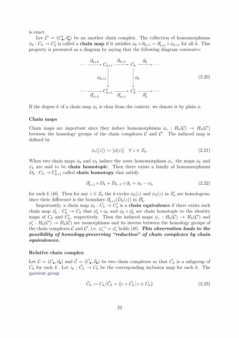
•, ∂′•) be an another chain complex. The collection of homomorphisms

φk : Ck → C ′k is called a chain map if it satisfies φk ∂k+1 = ∂′

k+1 φk+1 for all k. Thisproperty is presented as a diagram by saying that the following diagram commutes:

· · · Ck+1 Ck · · ·

· · · C ′k+1 C ′

k · · ·

∂k+2 ∂k+1 ∂k

∂′k+2 ∂′

k+1 ∂′k

φk+1 φk (2.20)

If the degree k of a chain map φk is clear from the context, we denote it by plain φ.

Chain maps

Chain maps are important since they induce homomorphisms φ∗ : Hk(C) → Hk(C′)between the homology groups of the chain complexes C and C′. The induced map isdefined by

φ∗([z]) := [φ(z)] ∀ z ∈ Zk. (2.21)

When two chain maps φk and ψk induce the same homomorphism φ∗, the maps φk andψk are said to be chain homotopic. Then there exists a family of homomorphismsDk : Ck → C ′

k+1 called chain homotopy that satisfy

∂′k+1 Dk +Dk−1 ∂k = φk − ψk (2.22)

for each k [48]. Then for any z ∈ Zk the k-cycles φk(z) and ψk(z) in Z ′k are homologous,

since their difference is the boundary ∂′k+1(Dk(z)) in B′

k.Importantly, a chain map φk : Ck → C ′

k is a chain equivalence if there exists suchchain map φ′

k : C ′k → Ck that φ′

k φk and φk φ′k are chain homotopic to the identity

maps of Ck and C ′k, respectively. Then the induced maps φ∗ : Hk(C) → Hk(C′) and

φ′∗ : Hk(C′) → Hk(C) are isomorphisms and its inverse between the homology groups of

the chain complexes C and C′, i.e. φ−1∗ = φ′

∗ holds [48]. This observation leads to thepossibility of homology-preserving “reduction” of chain complexes by chainequivalences.

Relative chain complex

Let C = (C•, ∂•) and C = (C•, ∂•) be two chain complexes so that Ck is a subgroup ofCk for each k. Let ik : Ck → Ck be the corresponding inclusion map for each k. Thequotient group

Ck := Ck/Ck = c+ Ck | c ∈ Ck (2.23)

22

is called the relative k-chain group of Ck modulo Ck. That is, the elements [c] of Ck

are equivalence classes of Ck with the equivalence relation

c1 ≃ c2 ⇐⇒ c1 = c2 + i(c) (2.24)

where c1, c2 ∈ Ck and c ∈ Ck. With the surjection j : Ck → Ck, j(c) = [c], the sequence

0→ Cki−→ Ck

j−→ Ck → 0 (2.25)

is exact. The relative chain groups Ck constitute a relative chain complex C = (C•, ∂•),where the boundary operators ∂k are defined to be such that ∂k[c] := [∂kc] holds forall [c] ∈ Ck and for each k. The resulting homology groups Hk(C) of the relative chaincomplex are called relative homology groups.

Remark 2.1.1. It is possible to choose a j : Ck → Ck that the group Ck would have atorsion subgroup. In the applications of this thesis, we will choose such j that the groupCk will be torsion-free.

Functoriality

The following pattern will emerge throughout this thesis. Let X and Y be topologicalspaces and let f be a continuous map between them. One can associate chain complexesC(X) = (C•(X), ∂•) and C(Y ) = (C•(Y ), ∂•) with them as described in a later section.Then, f induces a family of chain maps φk(f) between the chain complexes (C•(X), ∂•)and (C•(Y ), ∂•) and thus also homomorphisms (φk(f))∗ between the homology groupsHk(X) := Hk(C(X)) and Hk(Y ) := Hk(C(Y )).

In category theory, such construct that maps both sets and functions between themto other sets and functions in a structure-preserving manner is called a functor. In thisinstance, to each topological space X homology groups Hk(X) are being associated, andeach continuous mapping f between topological spacesX and Y induces a homomorphism(φk(f))∗ between their homology groups Hk(X) and Hk(Y ).

Especially, if f is an injection from a subset X ⊂ Y to Y , it induces a relative chaincomplex C(Y,X) = (C•(Y,X), ∂•). Also, if f : X → Y is a homotopy equivalence [31], theinduced homomorphism (φk(f))∗ is an isomorphism between the homology groups Hk(X)and Hk(Y ). Therefore as we shall see, the purely algebraic concept of homologygroup will reflect topological similarities of the spaces X and Y .

Cochain complex and cohomology

Let C be a chain complex and G be an abelian group. The set Ck(C;G) := Hom(Ck, G)of all homomorphisms γ : Ck → G called k-cochains is itself an abelian group when onedefines:

(γ1 + γ2)(c) = γ1(c) + γ2(c) ∀ c ∈ Ck (2.26)

−γ(c) = γ(−c) ∈ G ∀ c ∈ Ck (2.27)

The boundary homomorphisms ∂k : Ck → Ck−1 induce the coboundary homomor-

phisms δk : Ck(C;G)→ Ck+1(C;G) defined to operate on k-cochains by:

δkγ := γ ∂k+1. (2.28)

23

That is, (δkγ)(c) = γ(∂k+1c) holds for all k + 1-chains c. The cochain complex is thesequence

. . .δk+1←−− Ck+1(C, G) δk←− Ck(C, G)

δk−1←−− Ck−1(C, G)δk−2←−− . . . (2.29)

of abelian groups linked by the coboundary homomorphisms. The degree k is droppedfrom the notation δk when appropriate.

The elements of the subgroups Zk(C;G) = ker δk and Bk(C;G) = im δk−1 of Ck(C;G)are called k-cocycles and k-coboundaries, respectively. The quotient group

Hk(C;G) := Zk(C;G)/Bk(C;G) = ζ +Bk(C;G) | ζ ∈ Zk(C;G) (2.30)

is called the k:th cohomology group of the cochain complex. The relative cochain

complex and the relative cohomology groups are constructed similarly to a relativechain complex.

The elements [ζ] of the group Hk(C;G) can be regarded as homomorphisms from thehomology group Hk(C) to G. This is seen from the pairing

(ζ + δk−1γ)(z + ∂k+1c) = ζ(z) + ζ(∂k+1c) + δk−1γ(z) + δk−1γ(∂k+1c)

= ζ(z) + δkζ(c) + γ(∂kz) + γ(∂k∂k+1c)

= ζ(z) ∀ γ ∈ Ck(C;G), c ∈ Ck(C). (2.31)

That is, the result is independent of the representatives chosen for [ζ] and [z]. Therefore,we may defined a pairing Hk(C;G)×Hk(C)→ G:

[ζ]([z]) := ζ(z). (2.32)

This suggests that the group Hom(Hk(C), G) of homomorphisms Hk(C) → G and thegroupHk(C;G) are related. Indeed, there exists a surjective homomorphism hk : Hk(C;G)→Hom(Hk(C), G), which is also injective if the groups Hk−1(C) and Hk(C) are torsion-free[48, 31].

Any homomorphism φk : Ck → C ′k induces a homomorphism φk : Ck(C′;G) →

Ck(C;G) between the cochain groups in the reverse direction. It is defined by

φk(γ) = γ φk. (2.33)

Again, we drop k from the notation it is not needed. If φ is a chain map, φ commuteswith the coboundary homomorphism and is thus a chain map. A chain map φ inducesa homomorphism of the cohomology groups in the reverse direction: φ∗ : Hk(C′;G) →Hk(C;G) defined by

φ∗([ζ]) := [φ(γ)], ζ ∈ Zk(C′;G). (2.34)

The following result makes it possible to use chain equivalences not only for homology-preserving reduction of of chain complexes, but also for cohomology-preserving reduction.Let C and C′ be chain complexes of free abelian groups. If Hk(C) is isomorphic to Hk(C′),then Hk(C;G) is isomorphic to Hk(C′;G) [48]. Consequently, if φ : Ck → C ′

k is a chainequivalence, then the induced maps φ∗ : Hk(C)→ Hk(C′) and φ∗ : Hk(C′;G)→ Hk(C;G)are isomorphisms.

24

Summary

The important results from the homological algebra presented in this section are summa-rized in the following diagram:

H•(C) C C•(C;G) H•(C;G)

H•(C′) C′ C•(C′;G) H•(C′;G)

φ φφ∗ φ∗ (2.35)

That is, a chain complex C of free abelian groups Ck induces homology groups H•(C)and cohomology groups H•(C;G). If the chain map φ is a chain equivalence, then thehomomorphisms φ∗ and φ∗ are isomorphisms.

2.1.3 Vector space

Linear algebra is perhaps the most applied field of mathematics in computational sciencesas “linearization” seems to be an efficient yet accurate enough approximation to modelmany observed real world phenomena. Linear algebra studies properties of linear mapsbetween vector spaces. Like finitely generated abelian groups, finite dimensional vectorspaces can be endowed with a basis. A basis representation of the elements of a vectorspace and linear maps turn the problems of abstract algebra into problems of arithmetic,for which a wealth of computational algorithms has been devised.

Let (V,+) be an abelian group and let F be a field of real or complex numbers.They form a vector space when one defines a map · : F × V → V with the familiarrequirements, see for example [25]. As customary, the map · is dropped from the notationand the vector space is denoted with plain V .

Let S = s1, s2, . . . , sn be a finite subset of V . If any element v of V can be writtenas a linear combination v =

∑ni=1 v

isi, S is said to span V . If∑n

i=1 visi = 0 implies

v1 = v2 = . . . = vn = 0, the set S is said to be linearly independent. A linearlyindependent subset S ⊂ V that spans V is called a basis of V , and n = |S| is thedimension of V . Every finite dimensional vector space has a basis [25]. To define abasis for an infinite dimensional vector space some additional structure is required, sincean infinite sum bears no meaning without any additional structure, for example topologyor norm on V .

An element v of n-dimensional vector space V has a basis representation v ∈ Fn , and

we denote v =∑n

i=1 visi = (s1, s2, . . . , sn)v = Sv.

If a map φ : V → W is a vector space homomorphism, it is called a linear map.That is, for all c1, c2 ∈ F and v1, v2 ∈ V , φ(c1v1 + c2v2) = c1φ(v1) + c2φ(v2) holds. LetS = (s1, s2, . . . , sn) and R = (r1, r2, . . . , rm) be bases for V and W , respectively. Then,φ(si) = Rφi for some φi ∈ F

m. Consequently, an m × n matrix F =[

φ1,φ2, . . . ,φn

]

represents a linear map φ. If dim V = dimW holds and φ is an isomorphism, the matrixF is invertible.

25

The dual space V ∗ of the vector space V is a vector space of linear maps from V toF. The vector space structure for V ∗ is obtained with the definitions

(ω + η)(v) :=ω(v) + η(v), ω, η ∈ V ∗, v ∈ V (2.36)

(cω)(v) :=cω(v). (2.37)

Since a basis for the vector space F is just a single non-zero element r ∈ F, the elementsω ∈ V ∗ can be represented by vectors ω ∈ F

n . Then, the evaluation is given byω(v) = ωT v ∈ F.

A linear map φ : V → W induces a map φ∗ : W ∗ → V ∗ defined by

φ∗ω(v) := (ω φ)(v) = ω(φ(v)) ∀ ω ∈ W ∗, v ∈ V. (2.38)

The map φ∗ is called the pullback of the map φ. If φ is represented by the matrix Fin some bases of V and W , one can read from the definition of the pullback φ∗ that itis represented by the transpose matrix FT . From the above discussion one can infer astructure represented by the commutative diagrams:

V W

Fn

Fm

φ

F

and

V ∗ W ∗

Fn

Fm

φ∗

FT

(2.39)

Let 〈·, ·〉 : V ×V → F denote an inner product on n-dimensional vector space V . Givena basis for V , the inner product is represented by a symmetric or hermitian n×n matrixG. The inner product is then evaluated by 〈v1, v2〉 = vH

1 Gv2, where v1, v2 represent v1,v2 ∈ V in the basis and vH

1 denotes conjugate transpose of v1. A basis (s1, s2, . . . , sn) ofV is orthonormal, if 〈si, sj〉 = δij holds for all i, j.

Let V be a complete inner product space, i.e. a Hilbert space [25]. Then, if ω :V → F is a linear map, i.e. ω ∈ V ∗, then there exists an unique vector w ∈ V suchthat ω(v) = 〈v, w〉 holds for all v ∈ V [25, 23]. That is, the inner product on aHilbert space V induces an isomorphism1 from V to V ∗ by Riesz representationtheorem. Given a basis for V and V ∗, and the corresponding inner product matrix G, theisomorphism is given by ω = Gv, where ω and v represent ω and v, respectively. Theisomorphism V → V ∗ defined by an inner product on V and its inverse are sometimescalled flat v ∈ V ∗ and sharp ω♯ ∈ V , respectively. The isomorphism also induces aninner product on the dual space V ∗ given by the sharp:

〈ω, η〉 := 〈ω♯, η♯〉 = (G−1ω)HGG−1η = ωT G−1η. (2.40)

Let φ : V → W be a linear map. Given a basis for W the map φ has a correspondingmatrix representation F. If one requires that 〈v1, v2〉 = 〈φ(v1), φ(v2)〉 must hold for allv1, v2 ∈ V , one infers that vH

1 Gv2 = (Fv1)HHFv2 = vH1 FT HFv2 hold. That is, if the

inner product 〈·, ·〉W on W is represented by the matrix H, its corresponding “pulledback” inner product on V is represented by the matrix FT HF. In the special case whendim V = dimW holds and φ is an isomorphism, this is the change of basis formula forthe inner product matrices.

1There are also other ways to induce an isomorphism between a vector space and its dual.

26

Homology and cohomology vector space

Homology and cohomology groups can be interpreted as vector spaces, but some infor-mation about them may be lost in the process.

Let Hk(C) and Hk(C;G) be finitely generated and let the abelian groups Ck in C befree. Denote by Hk(C;F) a homology vector space which is obtained from the homologygroup by allowing the group generators have infinite field of characteristic zero coefficientsinstead of integer coefficients2. That is,

Hk(C;F) := span [zi], [zi] ∈ S, (2.41)

where S is a generating set of the group Hk(C). The dimension of the homology spaceis equal to the rank of the free subgroup F of the homology group. That is, if [zi] isa torsion element of Hk(C), it can be removed from the spanning set of Hk(C;F) sinceit is linearly dependent on the others. Therefore, when one interprets a homologygroup as a vector space, the information about its torsion subgroup is lost.The dimension of the k:th homology space is called the k:th betti number βk(C):

dimHk(C;F) := βk(C) = rankF ≤ |S|. (2.42)

In particular, if Hk(C) is torsion-free, βk(C) = |S| holds.The cohomology group Hk(C;F) is readily a vector space. However, it is a nontrivial

fact that the vector space Hom(Hk(C;F),F) of all linear maps Hk(C;F) → F is iso-morphic to the vector space Hk(C;F) [48]. In contrast, the group of homomorphismsHk(C) → G is not isomorphic to the group Hk(C;G) in general. With the isomorphismHom(Hk(C;F),F) ≃ Hk(C;G), the cohomology space Hk(C;F) turns out to be the dualspace of the homology space Hk(C;F).

2.1.4 Exterior algebra

Exterior algebra has its roots in the geometric interpretation of vectors. For example, twovectors that are linearly independent span a plane. If the vectors are linearly dependent,the spanned plane reduces to a line and thus has zero surface area. If one interchangesthe order of the spanning vectors, the plane may be thought to have the opposite orien-tation. A volume generated by three vectors behaves similarly. This concept to generategeometric entities from vectors is captured by the properties of the exterior product.

There’s also a concept that is dual to this. One can think that one assigns quantitiesto the geometric entities spanned by vectors. So-called alternating multilinear maps froman ordered set of vectors to scalar values have the desired properties. If the same vectoris more than once as an input argument, the result is zero. If the order of two inputvectors is interchanged, the result changes its sign as if the orientation was changed.

Let V be a real or complex vector space over F of dimension n. A k-linear mapω : V × . . .× V → F is alternating if

ω(. . . , vi, . . . vj, . . .) = −ω(. . . , vj, . . . vi, . . .) (2.43)

2The most natural framework for this result is modules. Abelian groups are modules over the ringof integers, and vector spaces are modules over a field. The Universal Coefficient Theorem [31] is thegeneralization of the following result in the framework of modules.

27

holds for each pair of entries vi, vj ∈ V . The space of alternating k-linear maps is denotedby Λk(V ∗). The space Λ1(V ∗) coincides with the dual space V ∗ of V and Λ0(V ∗) coincideswith F. Similarly, the space of alternating k-linear maps V ∗ × . . . × V ∗ → F is denotedby Λk(V ) and the space Λ1(V ) coincides with V . The elements of the spaces Λk(V ) andΛk(V ∗) are called k-vectors and k-covectors, respectively.

Because of the alternating property, a covector ω ∈ Λk(V ∗) is completely determinedby its values with a basis (s1, s2, . . . , sn) of V so that in ω(si1

, si2. . . , sik

) the indices i arealways in strictly increasing order. Therefore, dim Λk(V ∗) =

(

nk

)

holds [24].We adopt the multi-index notation to simplify the expressions. Multi-index I is an

ordered m-tuple I = (i1, i2, . . . , im). Denote by ~I such multi-index I for which i1 < i2 <. . . < im holds. Also define a Kronecker delta for multi-indices I and J to be suchthat

δJI =

1 if I = (i1, i2, . . . , im) is an even permutation of J = (j1, j2, . . . , jk).

−1 if I is an odd permutation of J.

0 if I is not a permutation of J.

(2.44)

The exterior product ∧ of covectors is a map ∧ : Λk(V ∗) × Λl(V ∗) → Λk+l(V ∗) isdefined by

(ω ∧ η)(v~I) :=∑

~K

∑

~J

δJKI ω(v ~J)η(v ~K), (2.45)

where JK denotes a multi-index that is the concatenation of the indices of J and K andv~I denotes a tuple of elements of V indexed by the multi-index ~I. The exterior productof vectors ∧ : Λk(V )× Λl(V )→ Λk+l(V ) is defined similarly.

Given a basis (s1, s2, . . . , sn) for V , denote a representation of its element v =∑n

i=1 visi

by v = [v1, v2, . . . , vn]T ∈ Fn. The space Λk(V ) has a basis (s~I)~I = (si1

∧ si2∧ . . . ∧ sik

)~I .

An element ω of Λk(V ∗) can be represented by ω ∈ F(n

k) so that ω =∑

~I ω~Iσ~I holds,

where σ~I = σi1 ∧ σi2 ∧ . . .∧ σik is such that σ~I(sj1, sj2

, . . . , sjk) = σ

~I(s ~J) = δIJ holds. The

exterior product induces a bilinear pairing Λk(V ∗) × Λl(V ) → F such that ω(v) = ωT v

holds.Let φ : V → W be a linear map between vector spaces with dimV = n and dimW =

m. The exterior product induces a linear map Λkφ∗ : Λk(W ∗) → Λk(V ∗) of k-covectorsdefined by

(Λkφ∗)(τ i1 ∧ τ i2 ∧ . . . ∧ τ ik) := φ∗τ i1 ∧ φ∗τ i2 ∧ . . . ∧ φ∗τ ik (2.46)

for the basis elements τ ~I of Λk(W ∗). The definition extends to all ω ∈ Λk(W ∗) by therepresentation ω =

∑

~I ω~Iτ~I . The map Λkφ∗ is also called the pullback and abbreviated

to φ∗ as the value of k is often clear from the context. Let σ ~J form a basis for Λk(V ∗).If the map φ is represented by an m× n matrix F, the pullback Λkφ∗ is represented by amatrix whose elements are determinants of the k × k matrices (FT )~I

~Jwhich contain the

rows ~I and the columns ~J of the matrix FT [24, 23]. That is,

φ∗ω =∑

~I

ω~Iφ∗τ

~I =∑

~J

∑

~I

ω~I det((FT )~I~J)σ

~J =∑

~J

ω ~Jσ~J ∈ Λk(V ∗), (2.47)

28

where ω ~J =∑

~I ω~I det((FT )~I~J) represent ω in the basis of Λk(V ∗). Similarly, the map φ

induces a linear map Λkφ : Λk(V )→ Λk(W ) of k-vectors given by

φ(v) =∑

~I

v~Iφ(s~I) =

∑

~J

∑

~I

v~I det(F

~J~I)r ~J =

∑

~J

v~Jr ~J ∈ Λk(W ), (2.48)

where s~I and r ~J form bases for Λk(V ) and Λk(V ), respectively [24, 23].The inner product on V induces inner products for the spaces Λk(V ∗). Let σ~I form a

basis for Λk(V ∗) and define

〈σ~I , σ~J〉 :=

∣

∣

∣

∣

∣

∣

∣

∣

∣

∣

〈σi1 , σj1〉 〈σi1 , σj2〉 . . . 〈σi1 , σjk〉〈σi2 , σj1〉 〈σi2 , σj2〉 . . . 〈σi2 , σjk〉

......

. . ....

〈σik , σj1〉 〈σik , σj2〉 . . . 〈σik , σjk〉

∣

∣

∣

∣

∣

∣

∣

∣

∣

∣

= det((G−1)~I ~J), (2.49)

where the matrix (G−1)~I ~J contains the rows ~I and columns ~J of the inverse of the innerproduct matrix G of V . Then, the inner product of ω =

∑

~I ω~Iσ~I and η =

∑

~J η ~Jσ~J is

given by

〈ω, η〉 =∑

~I

∑

~J

ω~Iη ~J〈σ~I , σ

~J〉. (2.50)

Again, an inner product for the space Λk(V ) is induced similarly. One defines

〈v, w〉 =∑

~I

∑

~J

v~Iw

~J〈s~I , s ~J〉 =∑

~I

∑

~J

v~Iw

~J det(G~I ~J). (2.51)

Let (σ1, σ2, . . . , σn) be an orthonormal basis for V . A linear map called Hodge

operator ⋆ : Λk(V ∗)→ Λn−k(V ∗) is defined to be the one that satisfies

η ∧ ⋆ω = 〈η, ω〉σ1 ∧ σ2 ∧ . . . ∧ σn (2.52)

for all η, ω ∈ Λk(V ∗). If (τ 1, τ 2, . . . , τn) is a non-orthonormal basis and φ is a change-of-basis map, one has σ1 ∧ σ2 ∧ . . .∧ σn = φ∗(τ 1 ∧ τ 2 ∧ . . .∧ τn) = det(FT )τ 1 ∧ τ 2 ∧ . . .∧ τn.

A similar map ⋆ : Λk(V )→ Λn−k(V ) for k-vectors is defined analogously. The Hodgeoperator satisfies ⋆⋆ω = (−1)k(n−k)ω, i.e. expect for the sign, it is its own inverse.

2.2 Manifold and its cell decomposition

In a modern treatise, a boundary value problem is established on a manifold. It is atopological space that can be addressed with real number coordinates. However, theactual choice of coordinates is left open. That is, most of the analysis is done withoutany reference to some specific choice of coordinates. It is enough to know that at a will,a coordinate system is available.

We first define the real coordinate space Rn and the Euclidean space E

n, and discusshow they are related. The precise concept of manifold can be build upon these ingredients.

29

2.2.1 Real coordinate space

The real coordinate space Rn is an n-dimensional vector space of n-tuples of real

numbers over R. The half-space Rn+ is the set

Rn+ := x = (x1, x2, . . . , xn) ∈ R

n |xn ≥ 0. (2.53)

Its boundary is the set ∂Rn+ = x = (x1, x2, . . . , xn) ∈ R

n |xn = 0.Let the ordered sets (e1, e2, . . . , en) and (v1,v2, . . . ,vn) be the standard basis and a

basis of Rn, respectively. Then there exists a linear map A : Rn → Rn that satisfies

Aei = vi ∀ i ∈ 1, 2, . . . , n (2.54)

If the determinant of the matrix A is positive, the basis (v1,v2, . . . ,vn) has the positive

orientation, otherwise it has a negative orientation. The orientation is denoted byo = ±1. The oriented real coordinate space is a pair (Rn, o).

2.2.2 Euclidean space

The Euclidean space is a model for affine and metric properties of our environment, suchas translation of rigid objects, and measurement of distances and angles. Structurally, it isan affine space together with metric properties that are induced by Cartesian coordinatesystem.

The affine space is a pair (A, V ) of a set A and a vector space V together witha map t : V × A → A denoted by t(v, a) = v + a. It is required that 0 + a = 0 and(v + w) + a = v + (w + a) hold for all a ∈ A and v, w ∈ V . Also, with a ∈ A fixed, themap V → A : ta(v) = v + a is required to be a bijection.

The Euclidean space En is an affine space (A, V ) where the n-dimensional vector

space V has an inner product 〈·, ·〉 and A has a metric defined by d(a, a+ v) :=√

〈v, v〉.The usual way to construct the Euclidean space E

n is to set A = V = Rn and define

t(v, a) := v + a and 〈v,v〉 := vT v. (2.55)

That is, the real coordinate space Rn is assumed to be a Cartesian coordinate system for

the Euclidean space En.

The inner product can be used to induce both norm ‖v‖ :=√

〈v,v〉 and topology τfor the spaces E

n and Rn. A basis for the topology is formed by the Euclidean n-balls:

An open y-centered r-radius Euclidean n-ball Bnr (y) is a set

Bnr (y) := x ∈ R

n | ‖x− y‖ < r. (2.56)

The set Rn+ ⊂ R

n can be equipped with the subspace topology of the topology definedby τ+ := U ∩ R

n+ |U ⊂ τ. A basis for such topology is formed by “sliced” Euclidean

n-balls Bnr (y) ∩ R

n+.

Remark 2.2.1. The topological spaces (Rn, τ) and (Rn+, τ+) are Hausdorff spaces.

Remark 2.2.2. The topological vector space (Rn, τ) is an object on its own right, withoutan inner product, norm, or affine structure of the Euclidean space E

n.

30

2.2.3 Manifolds

A differentiable n-dimensional manifold M is a topological space that is everywhere lo-cally homeomorphic to the topological space (Rn, τ) together with differentiable atlas ofcoordinate charts.

Charts and atlases

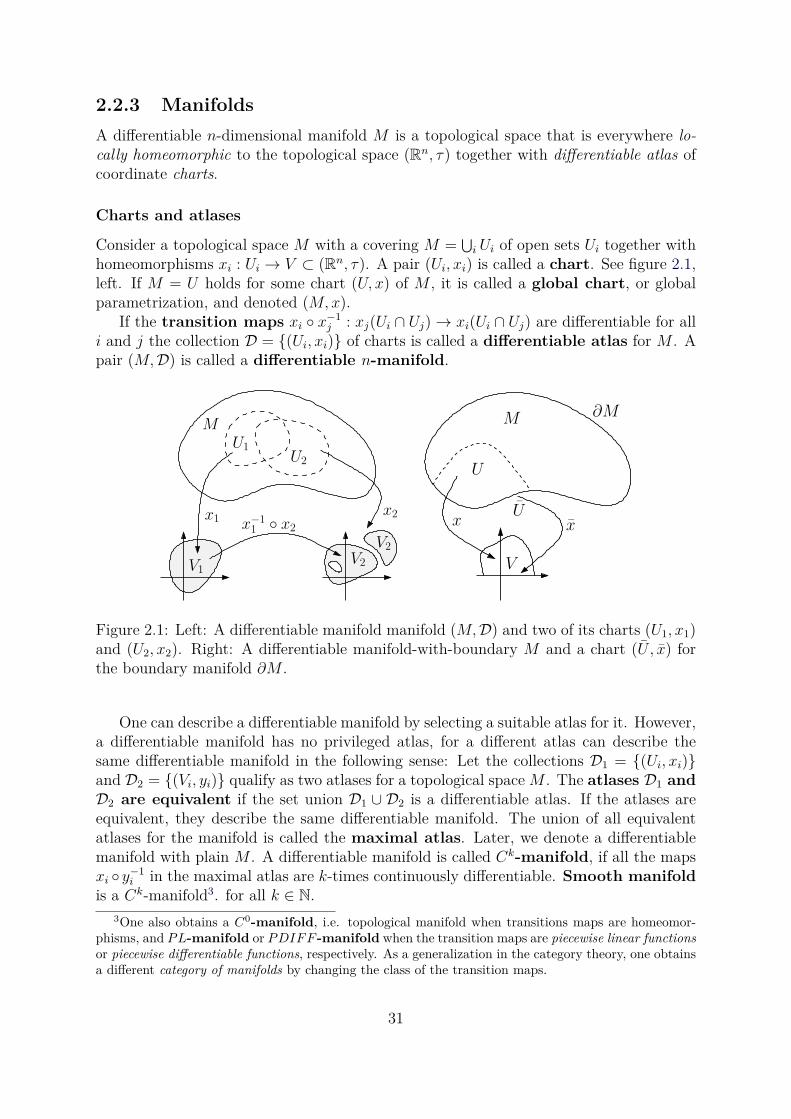
Consider a topological space M with a covering M =⋃

i Ui of open sets Ui together withhomeomorphisms xi : Ui → V ⊂ (Rn, τ). A pair (Ui, xi) is called a chart. See figure 2.1,left. If M = U holds for some chart (U, x) of M , it is called a global chart, or globalparametrization, and denoted (M,x).

If the transition maps xi x−1j : xj(Ui ∩ Uj)→ xi(Ui ∩ Uj) are differentiable for all

i and j the collection D = (Ui, xi) of charts is called a differentiable atlas for M . Apair (M,D) is called a differentiable n-manifold.

M

V2

U1

U2

x1 x−1

1 x2

V1

V2

x2

V

U

M

x xU

∂M

Figure 2.1: Left: A differentiable manifold manifold (M,D) and two of its charts (U1, x1)and (U2, x2). Right: A differentiable manifold-with-boundary M and a chart (U , x) forthe boundary manifold ∂M .

One can describe a differentiable manifold by selecting a suitable atlas for it. However,a differentiable manifold has no privileged atlas, for a different atlas can describe thesame differentiable manifold in the following sense: Let the collections D1 = (Ui, xi)and D2 = (Vi, yi) qualify as two atlases for a topological space M . The atlases D1 and

D2 are equivalent if the set union D1 ∪ D2 is a differentiable atlas. If the atlases areequivalent, they describe the same differentiable manifold. The union of all equivalentatlases for the manifold is called the maximal atlas. Later, we denote a differentiablemanifold with plain M . A differentiable manifold is called Ck-manifold, if all the mapsxi y−1

i in the maximal atlas are k-times continuously differentiable. Smooth manifold

is a Ck-manifold3. for all k ∈ N.3One also obtains a C0

-manifold, i.e. topological manifold when transitions maps are homeomor-phisms, and PL-manifold or PDIFF -manifold when the transition maps are piecewise linear functions

or piecewise differentiable functions, respectively. As a generalization in the category theory, one obtainsa different category of manifolds by changing the class of the transition maps.

31

Manifold with boundary

A differentiable n-manifold-with-boundary agrees with the definition of a differen-tiable n-manifold, except that the chart maps are required to map to the open sets of Rn

+

in its subspace topology. That is, for p ∈ Ui ⊂M , xi(p) ∈ V ⊂ Rn+ holds, where V ∈ τ+.

Since one can always choose an equivalent atlas for a manifold such that the chart mapsxi map to the half-space R

n+ instead of Rn, we make no distinction between a manifold

and a manifold-with-boundary later in this thesis. Manifolds-without-boundary are justmanifolds-with-boundary which have no boundary points.

A point p ∈ U ⊂ M is a boundary point of the manifold M , if it is mapped to∂Rn

+ by a chart (U, x) ∈ D. The boundary ∂M of a manifold M is the set of all theboundary points:

∂M := p ∈M |x(p) ∈ ∂Rn+ when p ∈ U. (2.57)

The boundary ∂M is a differentiable n− 1-manifold that has no boundary points [29]. Ifp ∈ U is a boundary point of M and (U, x) is a chart of M , the manifold ∂M inherits achart (U , x) such that x : U → V ⊂ R

n−1 where U = U ∩ ∂M holds and V is open. It isdefined by

x(p) := (x1(p), x2(p), . . . , xn−1(p)) ∈ Rn−1 when x(p) = (x1(p), x2(p), . . . , xn(p)) ∈ R

n+.

(2.58)

See figure 2.1, right. We need such inherited chart in the following sections in the defini-tion of boundary relations of cells on the manifold.

Tangent space and cotangent space

A map f : M → F is differentiable at a point p ∈ M if the function f x−1 : Rn → F

is differentiable for every chart (U, x) where p ∈ U . That is, all the partial derivatives∂(fx−1)

∂xj exist at x(p) = (x1, x2, . . . , xn). If F = C holds, one has f = Re(f)+iIm(f), whereRe(f), Im(f) : M → R. Then, f is differentiable if Re(f) and Im(f) are differentiable.Denote the space of q-times differentiable functions on the manifold M by Cq(M ;F).Maps that are q-times differentiable for all q ∈ N are called smooth. The chart mapx : M → R

n can be considered as an n-tuple of differentiable coordinate maps xi :M → R such that x(p) = (x1(p), x2(p), . . . , xn(p)) ∈ R

n holds.A tangent vector vp of a differentiable manifold (M,D) is a directional derivative

operator of maps f : M → F that are differentiable with respect to the atlas D at a pointp ∈M . Using a chart x it is defined by

vp(f) :=n

∑

i=1

vix

∂(f x−1)∂xi

∣

∣

∣

∣

∣

x(p)

, ∀ f ∈ Cq(M), (2.59)

where the coefficient vector vx = (v1x, v

2x, . . . , v

nx) ∈ F

n associated to the chart x givesthe direction and the magnitude of the directional derivative in terms of the chart (U, x).Thus one may denote

vp :=n

∑

i=1

vix

∂

∂xi. (2.60)

32

Let (V, y) be another chart for the manifold M at p. On that chart, a tangent vector v′p

is given by

v′p :=

n∑

i=1

viy

∂

∂yi. (2.61)

These two tangent vectors are equivalent if vp(f) = v′p(f) holds for all f ∈ C1(M ;F) at

p. That is, if the directional derivative of a function at the point p ∈M does not dependon the chart it is evaluated on:

vp(f) =n

∑

i=1

vix

∂(f x−1)∂xi

∣

∣

∣

∣

∣

x(p)

=n

∑

i=1

viy

∂(f y−1)∂yi

∣

∣

∣

∣

∣

y(p)

= v′p(f). (2.62)

Let f = yj hold for all j ∈ 1, 2, , . . . , n to obtain

vjy =

n∑

i=1

vix

∂(yj x−1)∂xi

∣

∣

∣

∣

∣

x(p)

. (2.63)

That is, vy = Jvx holds, where J is the real Jacobian n× n matrix of the transition mapy x−1 at p.

The set of all tangent vectors vp of the manifold M at a point p is a vector spacedenoted by TpM , called the tangent space of M at p. It is isomorphic to F

n, as eachchart (U, x) at p picks an isomorphism. The set ∂/∂x1, ∂/∂x2, . . . , ∂/∂xn is a basis forTpM called the coordinate basis.

If one considers the function f to be fixed in the directional derivative, one obtainsa map df : TpM → F. It is an element of the the dual space T ∗

pM of TpM , called thecotangent space. Let us test what happens when f = xj:

dxj(vp) := vp(xj) =n

∑

i=1

vix

∂(xj x−1)∂xi

∣

∣

∣

∣

∣

x(p)

= vjx. (2.64)

That is, dxj( ∂∂xi ) = δj

i holds for all i, j. This observation qualifies the set dx1, dx2, . . . , dxnas a basis for T ∗

pM called the coordinate cobasis. Then, df has the following repre-sentation in the coordinate cobasis:

df =n

∑

i=1

∂(f x−1)∂xi

∣

∣

∣

∣

∣

x(p)

dxi :=n

∑

i=1

ωxi dxi. (2.65)

That is, the cotangent vector df is represented by the coefficient vector ωx ∈ Fn. The

evaluation df(vp) should yield the same real or complex number regardless of the basisrepresentations of df and vp. From

df(vp) =n

∑

i=1

ωxi dxi(vp) =

n∑

i=1

ωxi v

ix = ωT

x vx = ωTx Jvy = (JTωx)T vy (2.66)

one deduces that such property is enforced by requiring that ωy = JTωx holds for therepresentation ωy of df on the chart (V, y).

Remark 2.2.3. If Fn = Cn holds, the evaluation df(vp) is not the complex inner product

of complex vectors, as in the expression ωTx vx one has the ordinary transpose and not

the conjugate transpose.

33

Orientable manifold

As the tangent spaces TpM are vector spaces that are isomorphic to Rn via a chart (U, x),

one may choose a chart at p ∈ U for which one assigns a positive orientation, and let(V, y) be an another chart with p ∈ V . The two bases ∂/∂x1, ∂/∂x2, . . . , ∂/∂xn and∂/∂y1, ∂/∂y2, . . . , ∂/∂yn of TpM have the same orientation, if the determinant of theJacobian matrix of the transition map y x−1 is positive, i.e. if det J > 0 holds.

A differentiable n-manifold is orientable, if it has an atlas D = (Ui, xi) of chartssuch that for all p ∈ Ui∩Uj with all chart domains Ui, Uj in D, the bases ∂/∂xk

i nk=1 and

∂/∂ykj n

k=1 of TpM have the same orientation. If such atlas does not exist, the manifoldis nonorientable. An oriented differentiable n-manifold is a pair (M,D), where allthe charts (Ui, xi) in the atlas D of M have the same orientation on their overlaps. Thereare exactly two possible orientations for an orientable manifold M . If M is an orientedmanifold, the same manifold with the other possible orientation is denoted −M .

The boundary ∂M of an oriented manifold M inherits the orientation of M [29].Let p ∈ U be a boundary point of M . Then, the tangent space TpM has a basis∂/∂x1, ∂/∂x2, . . . , ∂/∂xn given by a chart (U, x). One can declare that the basis∂/∂x1, ∂/∂x2, . . . , ∂/∂xn−1 of Tp∂M given by the chart (U , x) of ∂M has the sameorientation as the basis −∂/∂xn, ∂/∂x1, . . . , ∂/∂xn−1 of TpM . The tangent vectornp := −∂/∂xn is in some sense an outward normal vector of the manifold-with-boundaryM at a boundary point p ∈ ∂M .

Riemannian manifold

Let each tangent space TpM have an inner product denoted by gp(·, ·). On a coordinatechart (U, x) of M , the inner product gp can be represented by a symmetric positive definiten×n matrix Gx. If each component function gij : Rn → F is smooth, the point-wise innerproducts gp define a metric tensor g on M . A differentiable n-manifold M togetherwith a metric tensor g on M is called a Riemannian n-manifold (M, g). One oftenabbreviates this to just M if the metric tensor is clear from the context.

The metric tensor induces an isomorphism between the tangent space TpM and thecotangent space T ∗

pM of a manifold, the flat and sharp operators. Such pairing betweenthe tangent and cotangent spaces is symmetric positive definite. In category theory,one generalizes such pairing so that a different class of the pairing introduces a differentgeometry for the manifold. For example, for a symplectic manifold the pairing isnondegenerate and skew-symmetric. That is, a point-wise 2-covector whose componentfunctions are smooth.

2.2.4 Cell complex of a manifold

A cell complex is a decomposition of a topological space into a collection of simple topo-logical spaces, cells, that are nicely glued together along their boundaries. We can assignan orientation for each cell, from which we can construct an incidence map for pairs ofcells. In this thesis, we only consider finite cell decompositions of manifolds.

In practice, the finite element mesh of a domain Ω ⊂ Rn qualifies as the cell decom-

position of the manifold M whose coordinate chart maps it to Ω. The incidence mapswill be the incidence matrices of the mesh.

34

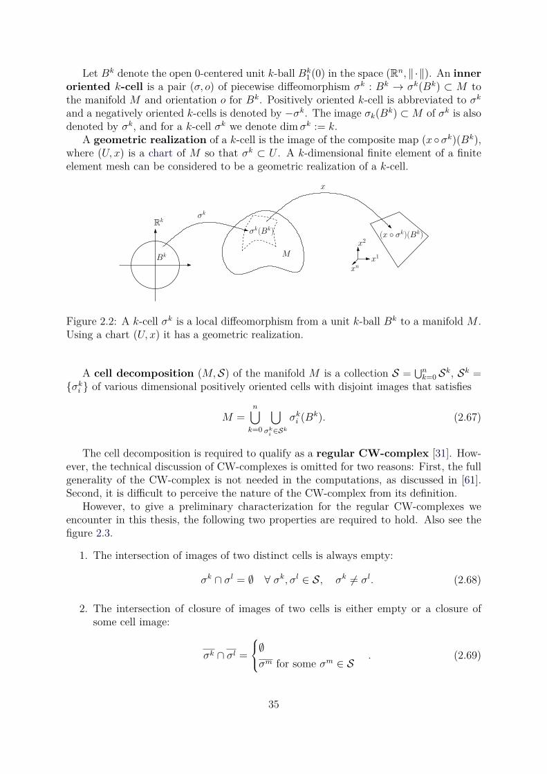
Let Bk denote the open 0-centered unit k-ball Bk1 (0) in the space (Rn, ‖·‖). An inner

oriented k-cell is a pair (σ, o) of piecewise diffeomorphism σk : Bk → σk(Bk) ⊂ M tothe manifold M and orientation o for Bk. Positively oriented k-cell is abbreviated to σk

and a negatively oriented k-cells is denoted by −σk. The image σk(Bk) ⊂M of σk is alsodenoted by σk, and for a k-cell σk we denote dim σk := k.

A geometric realization of a k-cell is the image of the composite map (x σk)(Bk),where (U, x) is a chart of M so that σk ⊂ U . A k-dimensional finite element of a finiteelement mesh can be considered to be a geometric realization of a k-cell.

MBk

Rk

x

x1

x2

xn

σk

σk(Bk) (x σk)(Bk)

Figure 2.2: A k-cell σk is a local diffeomorphism from a unit k-ball Bk to a manifold M .Using a chart (U, x) it has a geometric realization.

A cell decomposition (M,S) of the manifold M is a collection S =⋃n

k=0 Sk, Sk =σk

i of various dimensional positively oriented cells with disjoint images that satisfies

M =n

⋃

k=0

⋃

σki

∈Sk

σki (Bk). (2.67)

The cell decomposition is required to qualify as a regular CW-complex [31]. How-ever, the technical discussion of CW-complexes is omitted for two reasons: First, the fullgenerality of the CW-complex is not needed in the computations, as discussed in [61].Second, it is difficult to perceive the nature of the CW-complex from its definition.

However, to give a preliminary characterization for the regular CW-complexes weencounter in this thesis, the following two properties are required to hold. Also see thefigure 2.3.

1. The intersection of images of two distinct cells is always empty:

σk ∩ σl = ∅ ∀ σk, σl ∈ S, σk 6= σl. (2.68)

2. The intersection of closure of images of two cells is either empty or a closure ofsome cell image:

σk ∩ σl =

∅σm for some σm ∈ S . (2.69)

35

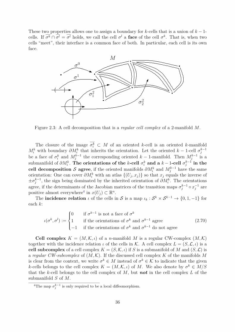
These two properties allows one to assign a boundary for k-cells that is a union of k− 1-cells. If σk ∩ σl = σl holds, we call the cell σl a face of the cell σk. That is, when twocells “meet”, their interface is a common face of both. In particular, each cell is its ownface.

M

σ2

2

σ2

1

σ1

σ0

Figure 2.3: A cell decomposition that is a regular cell complex of a 2-manifold M .

The closure of the image σki ⊂ M of an oriented k-cell is an oriented k-manifold

Mki with boundary ∂Mk

i that inherits the orientation. Let the oriented k − 1-cell σk−1j

be a face of σki and Mk−1

j the corresponding oriented k − 1-manifold. Then Mk−1j is a

submanifold of ∂Mki . The orientations of the k-cell σk

i and a k− 1-cell σk−1j in the

cell decomposition S agree, if the oriented manifolds ∂Mki and Mk−1

j have the sameorientation: One can cover ∂Mk

i with an atlas (Uj, xj) so that xj equals the inverse of±σk−1

j , the sign being dominated by the inherited orientation of ∂Mki . The orientations

agree, if the determinants of the Jacobian matrices of the transition maps σk−1j x−1

j arepositive almost everywhere4 in x(Uj) ⊂ R

n.The incidence relation ι of the cells in S is a map ιk : Sk × Sk−1 → 0, 1,−1 for

each k:

ι(σk, σl) :=

0 if σk−1 is not a face of σk

1 if the orientations of σk and σk−1 agree

−1 if the orientations of σk and σk−1 do not agree

(2.70)

Cell complex K = (M,K, ι) of a n-manifold M is a regular CW-complex (M,K)together with the incidence relation ι of the cells in K. A cell complex L = (S,L, ι) is acell subcomplex of a cell complex K = (S,K, ι) if S is a submanifold of M and (S,L) isa regular CW-subcomplex of (M,K). If the discussed cell complex K of the manifolds Mis clear from the context, we write σk ∈ M instead of σk ∈ K to indicate that the givenk-cells belongs to the cell complex K = (M,K, ι) of M . We also denote by σk ∈ M/Sthat the k-cell belongs to the cell complex of M , but not in the cell complex L of thesubmanifold S of M .

4The map σk−1

j is only required to be a local diffeomorphism.

36

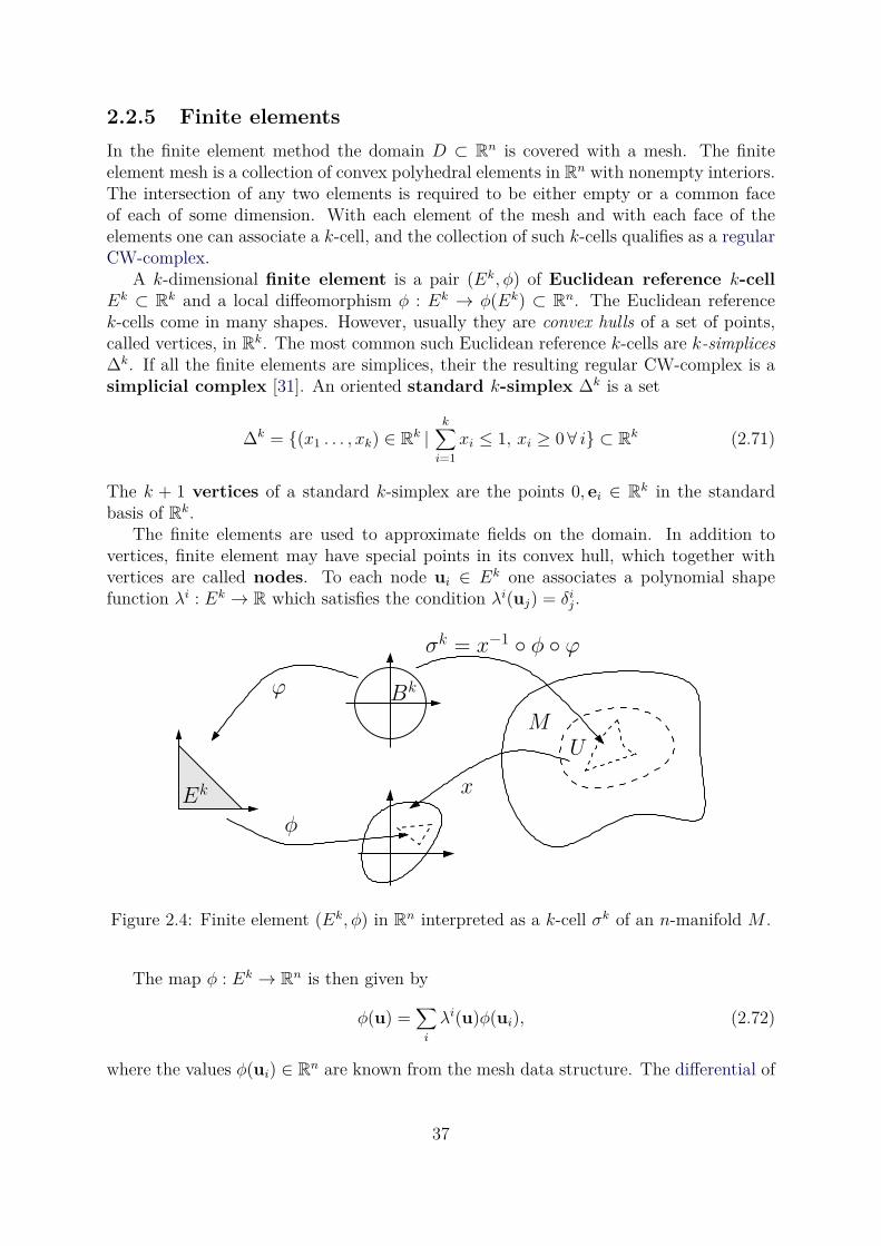
2.2.5 Finite elements

In the finite element method the domain D ⊂ Rn is covered with a mesh. The finite

element mesh is a collection of convex polyhedral elements in Rn with nonempty interiors.

The intersection of any two elements is required to be either empty or a common faceof each of some dimension. With each element of the mesh and with each face of theelements one can associate a k-cell, and the collection of such k-cells qualifies as a regularCW-complex.

A k-dimensional finite element is a pair (Ek, φ) of Euclidean reference k-cell

Ek ⊂ Rk and a local diffeomorphism φ : Ek → φ(Ek) ⊂ R

n. The Euclidean referencek-cells come in many shapes. However, usually they are convex hulls of a set of points,called vertices, in R

k. The most common such Euclidean reference k-cells are k-simplices∆k. If all the finite elements are simplices, their the resulting regular CW-complex is asimplicial complex [31]. An oriented standard k-simplex ∆k is a set

∆k = (x1 . . . , xk) ∈ Rk |

k∑

i=1

xi ≤ 1, xi ≥ 0∀ i ⊂ Rk (2.71)

The k + 1 vertices of a standard k-simplex are the points 0, ei ∈ Rk in the standard

basis of Rk.The finite elements are used to approximate fields on the domain. In addition to

vertices, finite element may have special points in its convex hull, which together withvertices are called nodes. To each node ui ∈ Ek one associates a polynomial shapefunction λi : Ek → R which satisfies the condition λi(uj) = δi

j.

MU

x

ϕ

φ

σk = x−1 φ ϕ

Bk

Ek

Figure 2.4: Finite element (Ek, φ) in Rn interpreted as a k-cell σk of an n-manifold M .

The map φ : Ek → Rn is then given by

φ(u) =∑

i

λi(u)φ(ui), (2.72)

where the values φ(ui) ∈ Rn are known from the mesh data structure. The differential of

37

the map φ = (φ1, φ2, . . . , φn) is given by Jacobian matrix J at point u = (u1, u2, . . . uk):

J :=

∂φ1

∂u1 . . . ∂φ1

∂uk

.... . .

...∂φn

∂u1 . . . ∂φn

∂uk

=∑

i

∂λi

∂u1x1i . . . ∂λi

∂ukx1i

.... . .

...∂λi

∂u1xni . . . ∂λi

∂ukxni

where φ(ui) = (x1i , x

2i , . . . x

ni ) ∈ R

n

(2.73)

A k-dimensional finite element (Ek, φ) can be interpreted as a k-cell σk ∈ M whenone insists that φ maps Ek to a chart (U, x) of an n-manifold M , see figure 2.4. That is,if one considers a piecewise diffeomorphism ϕ : Bk → Ek, the corresponding k-cell mapis σk = x−1 φ ϕ : Bk → M as required. Later in this thesis, finite elements are alsodenoted by σk = (Ek, φ), since they can be interpreted as k-cells.

2.3 Homology and cohomology of a manifold

While homology and cohomology can be considered to be purely algebraic concepts, acell decomposition of a manifold (or more generally of a topological space) can be usedto construct algebraic chain complexes.

Such chain complexes have well defined homology and cohomology groups, and theirhomological properties reflect some topological properties of the manifold. Those prop-erties we call the homology and the cohomology of the manifold, as they are independentof the cell decomposition we chose.

If the cells in a cell complex of a manifold are given a geometric realization, so are thechains as the formal sums of cells. Since homology and cohomology groups consists ofcosets of chains and cochains, they can also be given a geometric realization by realizinga representative element. That is, we are able to visually express the homology and thecohomology of the manifold.

Later in this thesis our goal is to formulate electromagnetic field problems on a man-ifold. In the following sections we show that such fields can be regarded as cochains.Therefore, the homology and the cohomology of the manifold and the cohomology of thefields are intimately linked, and need to be taken into account in the formulation of thefield problems.

2.3.1 Chain complexes of a manifold

Given cell complexes K = (M,K, ι) and L = (S,L, ι) of a manifold M and its submanifoldS, we construct finitely generated abelian groups Ck(M), Ck(S), and Ck(M,S) as formalsums of k-cells σk

i in M , S, and M \ S, respectively.Using the incidence relation ι of cells, we construct the boundary homomorphisms ∂

between the abelian groups. As a result, we obtain chain complexes C(M) = (C•(M), ∂•)and C(S) = (C•(S), ∂•), and a relative chain complex C(M,S) = (C•(M,S), ∂•).

38

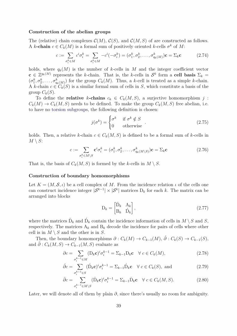
Construction of the abelian groups

The (relative) chain complexes C(M), C(S), and C(M,S) of are constructed as follows.A k-chain c ∈ Ck(M) is a formal sum of positively oriented k-cells σk of M :

c :=∑

σki

∈M

ciσki =

∑

σki

∈M

−ci(−σki ) = (σk

1 , σk2 , . . . , σ

kqk(M))c = Σkc (2.74)

holds, where qk(M) is the number of k-cells in M and the integer coefficient vectorc ∈ Z

qk(M) represents the k-chain. That is, the k-cells in Sk form a cell basis Σk =(σk

1 , σk2 , . . . , σ

kqk(M)) for the group Ck(M). Thus, a k-cell is treated as a simple k-chain.

A k-chain c ∈ Ck(S) is a similar formal sum of cells in S, which constitute a basis of thegroup Ck(S).

To define the relative k-chains ck ∈ Ck(M,S), a surjective homomorphism j :Ck(M) → Ck(M,S) needs to be defined. To make the group Ck(M,S) free abelian, i.e.to have no torsion subgroups, the following definition is chosen:

j(σk) =

σk if σk /∈ S0 otherwise

. (2.75)

holds. Then, a relative k-chain c ∈ Ck(M,S) is defined to be a formal sum of k-cells inM \ S:

c :=∑

σki

∈M\S

ciσki = (σk

1 , σk2 , . . . , σ

kqk(M\S))c = Σkc (2.76)

That is, the basis of Ck(M,S) is formed by the k-cells in M \ S.

Construction of boundary homomorphisms

Let K = (M,S, ι) be a cell complex of M . From the incidence relation ι of the cells onecan construct incidence integer |Sk−1| × |Sk| matrices Dk for each k. The matrix can bearranged into blocks

Dk =

[

Dk Ak

Bk Dk

]

, (2.77)

where the matrices Dk and Dk contain the incidence information of cells in M \S and S,respectively. The matrices Ak and Bk decode the incidence for pairs of cells where othercell is in M \ S and the other is in S.

Then, the boundary homomorphisms ∂ : Ck(M) → Ck−1(M), ∂ : Ck(S) → Ck−1(S),and ∂ : Ck(M,S)→ Ck−1(M,S) evaluate as

∂c =∑

σk−1

i∈M

(Dkc)iσk−1i = Σk−1Dkc ∀ c ∈ Ck(M), (2.78)

∂c =∑

σk−1

i∈S

(Dkc)iσk−1i = Σk−1Dkc ∀ c ∈ Ck(S), and (2.79)

∂c =∑

σk−1

i∈M\S

(Dkc)iσk−1i = Σk−1Dkc ∀ c ∈ Ck(M,S). (2.80)

Later, we will denote all of them by plain ∂, since there’s usually no room for ambiguity.

39

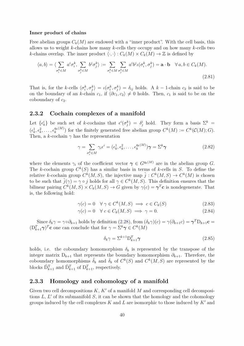
Inner product of chains

Free abelian groups Ck(M) are endowed with a “inner product”. With the cell basis, thisallows us to weight k-chains how many k-cells they occupy and on how many k-cells twok-chains overlap. The inner product 〈·, ·〉 : Ck(M)× Ck(M)→ Z is defined by

〈a, b〉 = 〈∑

σki

∈M

aiσki ,

∑

σkj

∈M

bjσkj 〉 :=

∑

σki

∈M

∑

σkj

∈M

aibjι(σki , σ

kj ) = a · b ∀ a, b ∈ Ck(M).

(2.81)

That is, for the k-cells 〈σki , σ

kj 〉 = ι(σk

i , σkj ) = δij holds. A k − 1-chain c2 is said to be

on the boundary of an k-chain c1, if 〈∂c1, c2〉 6= 0 holds. Then, c1 is said to be on thecoboundary of c2.

2.3.2 Cochain complexes of a manifold

Let ǫik be such set of k-cochains that ǫi(σk

j ) = δij hold. They form a basis Σk =

(ǫ1k, ǫ

2k, . . . , ǫ

qk(M)k ) for the finitely generated free abelian group Ck(M) := Ck(C(M);G).

Then, a k-cochain γ has the representation

γ =∑

σki

∈M

γiǫi = (ǫ1

k, ǫ2k, . . . , ǫ

qk(M)k )γ = Σkγ (2.82)

where the elements γi of the coefficient vector γ ∈ Gqk(M) are in the abelian group G.The k-cochain group Ck(S) has a similar basis in terms of k-cells in S. To define therelative k-cochain group Ck(M,S), the injective map j : Ck(M,S) → Ck(M) is chosento be such that j(γ) = γ j holds for all γ ∈ Ck(M,S). This definition ensures that thebilinear pairing Ck(M,S)× Ck(M,S)→ G given by γ(c) = γT c is nondegenerate. Thatis, the following hold:

γ(c) = 0 ∀ γ ∈ Ck(M,S) =⇒ c ∈ Ck(S) (2.83)

γ(c) = 0 ∀ c ∈ Ck(M,S) =⇒ γ = 0. (2.84)

Since δkγ = γ∂k+1 holds by definition (2.28), from (δkγ)(c) = γ(∂k+1c) = γT Dk+1c =(DT

k+1γ)T c one can conclude that for γ = Σkγ ∈ Ck(M)

δkγ = Σk+1DTk+1γ (2.85)

holds, i.e. the coboundary homomorphism δk is represented by the transpose of theinteger matrix Dk+1 that represents the boundary homomorphism ∂k+1. Therefore, thecoboundary homomorphisms δk and δk of Ck(S) and Ck(M,S) are represented by theblocks DT

k+1 and DTk+1 of DT

k+1, respectively.

2.3.3 Homology and cohomology of a manifold

Given two cell decompositions K, K ′ of a manifold M and corresponding cell decomposi-tions L, L′ of its submanifold S, it can be shown that the homology and the cohomologygroups induced by the cell complexes K and L are isomorphic to those induced by K ′ and

40

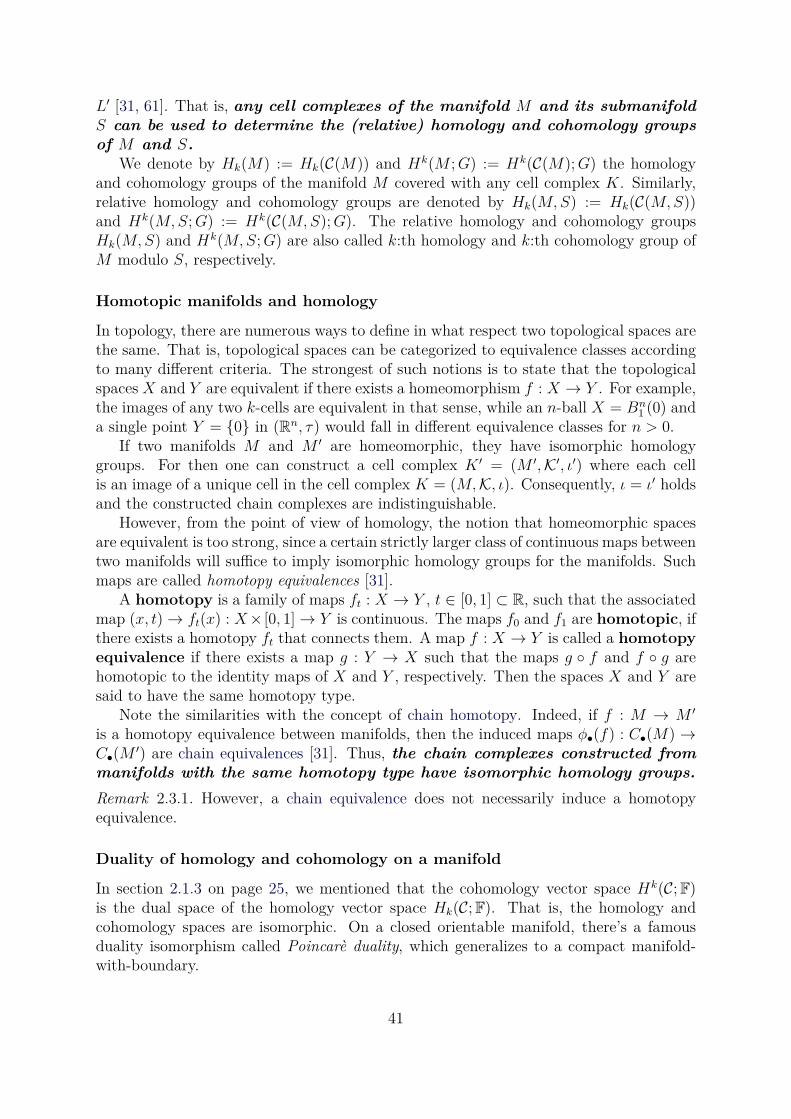
L′ [31, 61]. That is, any cell complexes of the manifold M and its submanifoldS can be used to determine the (relative) homology and cohomology groupsof M and S.

We denote by Hk(M) := Hk(C(M)) and Hk(M ;G) := Hk(C(M);G) the homologyand cohomology groups of the manifold M covered with any cell complex K. Similarly,relative homology and cohomology groups are denoted by Hk(M,S) := Hk(C(M,S))and Hk(M,S;G) := Hk(C(M,S);G). The relative homology and cohomology groupsHk(M,S) and Hk(M,S;G) are also called k:th homology and k:th cohomology group ofM modulo S, respectively.

Homotopic manifolds and homology

In topology, there are numerous ways to define in what respect two topological spaces arethe same. That is, topological spaces can be categorized to equivalence classes accordingto many different criteria. The strongest of such notions is to state that the topologicalspaces X and Y are equivalent if there exists a homeomorphism f : X → Y . For example,the images of any two k-cells are equivalent in that sense, while an n-ball X = Bn

1 (0) anda single point Y = 0 in (Rn, τ) would fall in different equivalence classes for n > 0.

If two manifolds M and M ′ are homeomorphic, they have isomorphic homologygroups. For then one can construct a cell complex K ′ = (M ′,K′, ι′) where each cellis an image of a unique cell in the cell complex K = (M,K, ι). Consequently, ι = ι′ holdsand the constructed chain complexes are indistinguishable.

However, from the point of view of homology, the notion that homeomorphic spacesare equivalent is too strong, since a certain strictly larger class of continuous maps betweentwo manifolds will suffice to imply isomorphic homology groups for the manifolds. Suchmaps are called homotopy equivalences [31].

A homotopy is a family of maps ft : X → Y , t ∈ [0, 1] ⊂ R, such that the associatedmap (x, t)→ ft(x) : X× [0, 1]→ Y is continuous. The maps f0 and f1 are homotopic, ifthere exists a homotopy ft that connects them. A map f : X → Y is called a homotopy

equivalence if there exists a map g : Y → X such that the maps g f and f g arehomotopic to the identity maps of X and Y , respectively. Then the spaces X and Y aresaid to have the same homotopy type.

Note the similarities with the concept of chain homotopy. Indeed, if f : M → M ′

is a homotopy equivalence between manifolds, then the induced maps φ•(f) : C•(M) →C•(M ′) are chain equivalences [31]. Thus, the chain complexes constructed frommanifolds with the same homotopy type have isomorphic homology groups.

Remark 2.3.1. However, a chain equivalence does not necessarily induce a homotopyequivalence.

Duality of homology and cohomology on a manifold

In section 2.1.3 on page 25, we mentioned that the cohomology vector space Hk(C;F)is the dual space of the homology vector space Hk(C;F). That is, the homology andcohomology spaces are isomorphic. On a closed orientable manifold, there’s a famousduality isomorphism called Poincarè duality, which generalizes to a compact manifold-with-boundary.

41

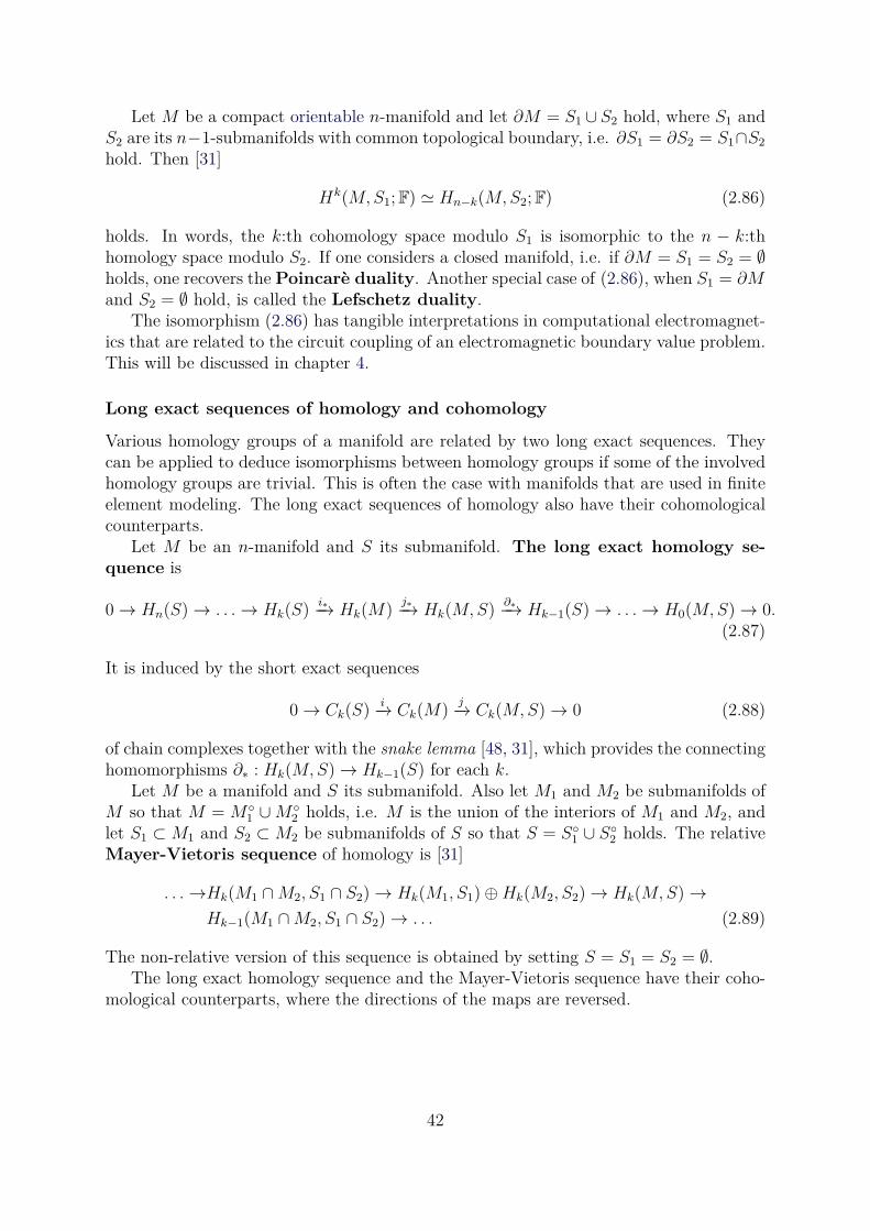
Let M be a compact orientable n-manifold and let ∂M = S1 ∪ S2 hold, where S1 andS2 are its n−1-submanifolds with common topological boundary, i.e. ∂S1 = ∂S2 = S1∩S2

hold. Then [31]

Hk(M,S1;F) ≃ Hn−k(M,S2;F) (2.86)

holds. In words, the k:th cohomology space modulo S1 is isomorphic to the n − k:thhomology space modulo S2. If one considers a closed manifold, i.e. if ∂M = S1 = S2 = ∅holds, one recovers the Poincarè duality. Another special case of (2.86), when S1 = ∂Mand S2 = ∅ hold, is called the Lefschetz duality.

The isomorphism (2.86) has tangible interpretations in computational electromagnet-ics that are related to the circuit coupling of an electromagnetic boundary value problem.This will be discussed in chapter 4.

Long exact sequences of homology and cohomology

Various homology groups of a manifold are related by two long exact sequences. Theycan be applied to deduce isomorphisms between homology groups if some of the involvedhomology groups are trivial. This is often the case with manifolds that are used in finiteelement modeling. The long exact sequences of homology also have their cohomologicalcounterparts.

Let M be an n-manifold and S its submanifold. The long exact homology se-

quence is

0→ Hn(S)→ . . .→ Hk(S) i∗−→ Hk(M)j∗−→ Hk(M,S) ∂∗−→ Hk−1(S)→ . . .→ H0(M,S)→ 0.

(2.87)

It is induced by the short exact sequences

0→ Ck(S) i−→ Ck(M)j−→ Ck(M,S)→ 0 (2.88)

of chain complexes together with the snake lemma [48, 31], which provides the connectinghomomorphisms ∂∗ : Hk(M,S)→ Hk−1(S) for each k.

Let M be a manifold and S its submanifold. Also let M1 and M2 be submanifolds ofM so that M = M

1 ∪M2 holds, i.e. M is the union of the interiors of M1 and M2, and

let S1 ⊂ M1 and S2 ⊂ M2 be submanifolds of S so that S = S1 ∪ S

2 holds. The relativeMayer-Vietoris sequence of homology is [31]

. . .→Hk(M1 ∩M2, S1 ∩ S2)→ Hk(M1, S1)⊕Hk(M2, S2)→ Hk(M,S)→Hk−1(M1 ∩M2, S1 ∩ S2)→ . . . (2.89)

The non-relative version of this sequence is obtained by setting S = S1 = S2 = ∅.The long exact homology sequence and the Mayer-Vietoris sequence have their coho-

mological counterparts, where the directions of the maps are reversed.

42

2.4 Differential forms

Differential forms describe integrands on manifolds in a coordinate-free manner. That is,they are apt to model various densities in physics. As a consequence to the coordinate-free construction, the change of variables formula of integration is a built-in property inthe integration of differential forms.

Since the integration domain is a geometric entity of certain dimension, the degree of adifferential form reflects this dimension. Also, the exterior algebra structure of differentialforms supports their geometric nature. It also reflects the Fubini’s theorem of integrationwhich states that one can construct multiple integrals by iterated integration.

The exterior derivative of differential forms is also constructed with powerful classicalresults in mind. Namely, the Stokes’, Green’s, and Divergence theorems, which are withdifferential forms combined into a single theorem: the generalized Stokes theorem.

It turns out that differential forms can be regarded as cochains. This observation givescohomology a role in analysis on manifolds. A cohomology theory whose k-cochains aredifferential k-forms is called de Rham cohomology. Integration domains on a manifold canbe given the structure of a chain complex. Since integration maps the integration domainto a scalar value, and by the generalized Stokes’ theorem, differential forms together withtheir exterior derivative form a cochain complex.

Lastly, the study of harmonic differential forms is the modern theory of irrotationaland solenoidal vector fields, which is a prominent concept in physics. Harmonic differen-tial forms are in close relationship with the de Rham cohomology. Therefore, homologyand cohomology computation can be utilized in the computation of harmonic differentialforms.

2.4.1 The basic construction

On a differentiable manifold M , a differential k-form ω smoothly assigns to a point p ∈Ma k-covector ωp. Therefore in a sense, differential forms are a generalization of vector fieldsin the classical vector analysis.

The k-covector ωp is an element of Λk(T ∗p ). Since the cotangent space T ∗

p is differentfor each p ∈ M , the tangent bundle needs to be introduced in the formal definition ofdifferential forms to make them an apt generalization of vector fields. In contrast, classicalvector fields have their values in the same vector space, R3.

The tangent bundle TM of a differentiable manifold is defined as a set

TM :=⋃

p∈M

(p, vp) | p ∈M, vp ∈ TpM (2.90)

together with a surjective projection π : TM → M defined as π(p, vp) := p. That is, theelements of the tangent bundle are pairs of points and tangent vectors on the manifold,and the projection map picks the point from the pair5. The cotangent bundle T ∗M isdefined similarly. Analogously, the k-cotangent bundle defined as the set

Λk(T ∗M) :=⋃

p∈M

(p, ωp) | p ∈M,ωp ∈ Λk(T ∗pM). (2.91)

5Interestingly, tangent bundle TM is always a differentiable manifold of its own right [24], and hasits own tangent bundle TTM .

43

A differential k-form ω is a smooth map M → Λk(T ∗M) that satisfies π ω = id.This property ensures that to each point p ∈M a k-covector of its own k-cotangent spaceΛk(T ∗

pM) is assigned. A differential 0-form is simply a smooth map M → F.Given a coordinate chart (U, x) for M , a k-form ω can be represented in the coordinate

cobasis dx1, dx2, . . . , dxn of each T ∗pM as

ω =∑

~I

ω~Idx~I , (2.92)

where the maps ω~I : M → F are smooth, i.e. 0-forms.The set of all k-forms on M constitutes a vector space, denoted Ωk(M), with the

vector space operations defined such that in each p ∈M(ω + η)p(v) = ωp(v) + ηp(v) (2.93)

(fω)p(v) = f(p)ωp(v) (2.94)

hold for all smooth maps f : M → F and for all v ∈ Λk(TpM). The exterior algebrastructure and the Hodge operator of differential forms is defined in a similar point-wisemanner. The exterior product of a k-form ω and an l-form η is defined as (ω ∧ η)p :=ωp ∧ ηp. On an orientable Riemannian n-manifold (M, g), the Hodge operator is definedas (⋆ω)p = ⋆pωp, where ⋆p is defined via the inner product gp of the tangent space TpMas in the equation (2.52).

Let φ : M → N be a differentiable map from an n-manifold M to m-manifold N . Letp ∈M and (U, x) be a chart for M and (V, y) be a chart for N . For p ∈ U and φ(p) ∈ V ,the matrix J of partial derivatives

Jji =

∂(yj φ x−1)∂xi

∣

∣

∣

∣

∣

x(p)

(2.95)

is an m× n matrix. That is, J is a representation for the linear map dφ : TpM → Tφ(p)Ncalled the differential of φ. Thus, dφ induces a pullback φ∗ : Ωk(N) → Ωk(M) ofdifferential k-forms with the point-wise definition

(φ∗ω)p := φ∗pωp. (2.96)

If S is a submanifold of M , the pullback by the inclusion map i : S →M is called trace

and denoted by tSω := i∗ω. If S is clear from the context, we omit it.The exterior derivative of differential k-forms is a linear map d : Ωk(M)→ Ωk+1(M).

Using the chart representations, for ω =∑

~I

(

ω~Idx~I)

it is defined by

dω :=∑

~I

n∑

i=1

∂ω~I

∂xidxi ∧ dx

~I . (2.97)

A k-form ω is called closed, if dω = 0 holds, and exact, if there exists a k − 1-form ηsuch that ω = dη holds. Importantly, the exterior derivative obeys the Leibniz product

rule:

d(ω ∧ η) = dω ∧ η + (−1)kω ∧ dη, (2.98)

where ω is a k-form and η is an l-form. The exterior derivative also commutes with thepullback, and therefore with the trace operator. This property is put into good use inthe analysis of boundary value problems.

44

2.4.2 Integration

Differential k-forms are tailored to be integrated over k-chains. That is, over linear com-binations of k-cells on an n-manifold M . Let C(M) be a chain complex of M with bases(σk

1 , σk2 , . . . , σ

kqk(M)) for each Ck(M). Since a k-chain c ∈ Ck(M) is a linear combination

of the basis k-cells, we define∫

cω =

∫

∑

iciσk

i

ω :=∑

i

ci∫

σki

ω (2.99)

The integration of the k-form ω over a k-cell σki is defined by using the pullback (σk

i )∗.Once ω is pulled back to Bk, one can use Lebesgue integration6 of R

k to integrate thecomponent functions ω~I of ω:

∫

σki

ω :=∫

Bk(σk

i )∗ω =∫

Bkω12...kdu1 ∧ du2 ∧ . . . ∧ duk (2.100)

where du1, du2, . . . , duk is the coordinate cobasis of the unit ball Bk and du1 ∧ du2 ∧. . . ∧ duk is interpreted as the Lebesgue measure [25] of Rk.

If φ : M → N is a differentiable map between manifolds, the change of variables

formula for differential k-forms reads:∫

cφ∗ω =

∫

φ∗(c)ω :=

∑

i

ci∫

φσki

ω, (2.101)

where φ∗ is a chain map induced by φ and defined via the k-cells by φ∗(σki ) = φ σk

i ,which is is a k-cell of the manifold N . The generalized Stokes’ theorem is

∫

cdω =

∫

∂cω. (2.102)

As differential forms are a special case of cochains, the generalized Stokes’ theorem couldalso be taken as the definition of the exterior derivative instead of the coordinate chartdefinition (2.97). That is, in the sense of the definition of the coboundary homomorphism(2.28) on the page 23.

Together with the product rule of the exterior derivative, generalized Stokes’ theoremimplies the following integration by parts formula for differential forms:

∫

cdω ∧ η = −(−1)k

∫

cω ∧ dη +

∫

∂cω ∧ η. (2.103)

Integration of differential k-forms is also defined over an orientable k-manifold S.One is to construct a k-chain that consist of all k-cells of S with matching orientationsand simply define

∫

S ω :=∫

c ω. For such k-chain c, its coset [c] belongs to the relativehomology space Hk(S, ∂S).

6For the defined smooth differential forms, Riemann integration would suffice, but later on, we willdemand only piecewise smoothness.

45

2.4.3 de Rham cohomology

The integration of differential k-form ω on an n-manifold M is a linear map∫

(·) ω :Ωk(M) → F. Since their exterior derivative satisfies the generalized Stokes’ theorem,differential forms constitute the cochain complex

0→ Ω0(M) d−→ . . .d−→ Ωk(M) d−→ Ωk+1(M) d−→ . . .

d−→ Ωn(M)→ 0. (2.104)

By construction of the section 2.1.2 on page 21, one obtains de Rham k-cohomologyspaces

HkdR(M) := ker d/ im d = ω + dη ∈ Ωk(M) | dω = 0, η ∈ Ωk−1(M). (2.105)

Let

Ωk(M,S) := ω ∈ Ωk(M) | tSω = 0 (2.106)

denote the space of k-forms on M whose trace vanishes on a part of the domain S ⊂M7.One has a short exact sequence

0→ Ωk(M,S) i−→ Ωk(M) t−→ Ωk(S)→ 0, (2.107)

where i is an inclusion map. Since tdω = dtω holds, one can define an operator d :Ωk(M,S) → Ωk+1(M,S) by dω := diω. Then, one has tdω = tdiω = dtiω = 0 asrequired. Relative de Rham k-cohomology spaces are defined by

HkdR(M,S) := ker d/ im d = ω + dη ∈ Ωk(M,S) | dω = 0, η ∈ Ωk−1(M,S). (2.108)

Later in this thesis, the operator d is denoted by plain d, since there’s usually no roomfor ambiguity.

What makes de Rham cohomology interesting is that the de Rham cohomology spacesHk

dR(M,S) are isomorphic to the homology spaces Hk(M,S). That is,

HkdR(M,S) ≃ Hk(M,S) (2.109)

is called relative de Rham’s theorem [14, 28, 27, 23, 24]. In words, de Rham’s theoremstates that if one assigns a number Ci ∈ F for each element [zi] in a basis of Hk(M,S),there exists a closed differential k-form ω ∈ Ωk(M,S) such that

∫

zi

ω = Ci ∀ i : 1 ≤ i ≤ βk(M,S) (2.110)

holds. That is, for such non-zero k-form [ω] ∈ HkdR(M,S) holds.

7Usually in our boundary value problem applications S ⊂ ∂M holds.

46

2.4.4 Harmonic differential forms

In classical vector analysis by Helmholtz decomposition [32], any smooth vector field on E3

that vanishes at infinity is uniquely determined by its divergence and curl. In boundaryvalue problems however, the domain manifold is often quite unlike E

3. The manifoldis compact, and may be closed, or the unknown field doesn’t necessarily vanish at theboundary.

In such setting, the Hodge decomposition generalizes the Helmholtz decomposition.In addition to the “rotational” and “solenoidal” components, a differential k-form on ann-manifold may have so-called harmonic component. Strikingly, the harmonic componentis related to the k:th de Rham cohomology space of the manifold, and therefore relatedto the k:th homology space of the manifold.

Let M be an n-manifold whose boundary is decomposed in two parts: S ∈ ∂M andS∗ := ∂M/S. It may hold that S = ∅ or S = ∂M . Also, the manifold M may be closed,i.e. ∂M = S = S∗ = ∅ may hold.

To be able to define such decomposition for differential that are only piecewise smooth,i.e. smooth almost everywhere on M , we begin by defining so-called L2 and Sobolev spacesof differential k-forms.

The space Ωk(M) of smooth differential k-forms can be turned into an inner productspace by defining the following inner product on Ωk(M):

〈ω, η〉 :=∫

Mω ∧ ⋆η. (2.111)

Now, the set of piecewise smooth differential k-forms ω that satisfy 〈ω, ω〉 <∞ constitutethe inner product space L2Ωk(M). In L2Ωk(M), the exterior derivative is no longerdefined everywhere, so we replace it by the weak exterior derivative. The weak exteriorderivative dω of ω ∈ L2Ωk(M) is such that it satisfies

∫

Mdω ∧ ϕ = (−1)k

∫

Mω ∧ dϕ ∀ ϕ ∈ Ωn−k−1(M,∂M). (2.112)

That is, the (n− k − 1)-forms ϕ are smooth everywhere in M , and are required to havecompact support and the traces tϕ vanish on the boundary ∂M . If ω is everywheresmooth on M , d and d coincide. Later in this thesis, we will denote the weak exteriorderivative also by d.

Next, a couple of Sobolev spaces of differential k-forms are defined:

HΩk(M,S) := ω ∈ L2Ωk(M) | dω ∈ L2Ωk+1(M), tSω = 0, (2.113)

HΩk(M,S∗) := ω ∈ L2Ωk(M) | d⋆ω ∈ L2Ωn−k−1(M), tS∗⋆ω = 0. (2.114)

The space of harmonic differential k-forms is defined as:

Hk(M,S) := ω ∈ L2Ωk(M) | dω = 0, d⋆ω = 0, tSω = 0, tS∗⋆ω = 0. (2.115)

One observes that the Hodge operator acts as an isomorphism ⋆ : Hk(M,S)→ Hn−k(M,S∗),since ⋆⋆ω = (−1)k(n−k)ω holds for any ω ∈ Ωk(M). Note the similarities with the equation(2.86) on page 42.

47

An important theorem states that the space Hk(M,S) is finite-dimensional and thatany k-form ω ∈ L2Ωk(M) has the following orthogonal Hodge decomposition [57, 28,27]

ω = dα+ (−1)n(k+1)+1⋆d⋆β + γ, (2.116)

where α ∈ HΩk−1(M,S), β ∈ HΩk+1(M,S∗) , and γ ∈ Hk(M,S). The operator(−1)n(k+1)+1⋆d⋆ : Ωk(M)→ Ωk−1(M) is often called codifferential.

Another important theorem states that in each de Rham cohomology class [ω] ofHk

dR(M,S), there exists an unique harmonic representative k-form ω ∈ Hk(M,S). Thatis,

HkdR(M,S) ≃ Hk(M,S) (2.117)

is called relative Hodge’s theorem [57, 28, 27, 24]. An isomorphism can be constructedas follows. Given ω ∈ Hk(M,S), [ω] is simply represented by ω + dα for any α ∈HΩk−1(M,S). Given [ζ] ∈ Hk

dR(M,S), one needs to solve the following boundary valueproblem for α. For any representative ζ, one seeks for such α that ω = ζ+dα ∈ Hk(M,S)holds. Then,

0 = d⋆ω = d⋆ζ + d⋆dα (2.118)

holds for an α ∈ HΩk−1(M,S) with boundary conditions

tSdα = −tSζ = 0, (2.119)

tS∗⋆dα = −tS∗⋆ζ. (2.120)

In section 3.5.3 we show how this boundary value problem can be solved using the finiteelement method.

We now summarize the isomorphisms in a diagram [28]:

Hk(M,S) HkdR(M,S) Hk(M,S;F) Hk(M,S;F)

Hn−k(M,S∗) Hn−kdR (M,S∗) Hn−k(M,S∗;F) Hn−k(M,S∗;F)

⋆

(2.121)The leftmost isomorphism is realized by the Hodge operator, and the cross on the rightis the generalization of the Lefschetz duality theorem.

2.4.5 Whitney forms

As seen in the previous sections, differential forms can be regarded as cochains. In thissection, we describe a map from k-cochains to k-forms that is isomorphic to its image,i.e. an injection. Such map is called the Whitney map and the k-forms in its image arecalled Whitney forms.

48

Whitney forms play a fundamental role in the finite element method where the un-known field is a differential k-form. The study of such finite element methods is nowadayscalled Finite element exterior calculus, in which the use of so-called polynomial finite el-ement differential forms is studied [2, 3]. Within that framework, Whitney forms are anexample of polynomial differential forms of lowest degree. Later in this thesis, Whitneyforms are employed extensively. However, the general polynomial differential forms arenot addressed later in this thesis, as their construction and the generalization of the Whit-ney map is not straightforward. Also, we only consider Whitney forms on a simplicialfinite element mesh.

Let M be an n-manifold with a submanifold S ⊂ ∂M and let them be covered with cellcomplexes. Whitney forms are defined via the finite element (En, φσn) shape functions λof first polynomial order. Whitney 0-form w

i0 ∈ L2Ω0(M) associated with a 0-cell σ0

i ∈Mis

wi0 :=

∑

σnj

(x−1 φσnj)∗λi

j, (2.122)

where the sum is taken over n-cells σnj of M that have σ0

i as a face. Here, we defineWhitney k-forms on a regular CW-complex that is a simplicial complex.

If an m-simplex σmi in M has vertices (v0, v1, . . . vm), its associated Whitney k-form,

k ≤ m, is

wik := m!

m∑

j=0

(−1)mw

j0dw

v0

0 ∧ . . . ∧ dwvj−1

0 ∧ dwvj+1

0 ∧ . . . ∧ dwvm

0 , (2.123)

i.e. dwvj

0 is omitted in each summand [63]. For example, the most frequently used in theapplications is the Whitney 1-form

wi1 = w

v0

0 dwv1

0 − wv1

0 dwv0

0 (2.124)

associated with a 1-cell σ1i of M .

The vector space of Whitney k-forms is defined as

W k(M,S) := spanσi

k∈M\S

wki ⊂ HΩk(M,S), (2.125)

i.e. the span of Whitney forms associated with k-cells in M that are not in S. Note thatfor ω ∈W k(M,S), tSω = 0 holds.

Whitney map w : Ck(M,S) → W k(M,S) ⊂ HΩk(M,S) maps a k-cochain γ =∑

i γiǫi to a Whitney k-form. It is defined as

w(γ) :=∑

i

γiwik, (2.126)

where wik is a Whitney k-form associated with a k-cell σk

i of M . Its left-inverse w−1 :L2Ωk(M,S)→ Ck(M,S) is simply given by

w−1(ω) :=∑

i

(

∫

σki

ω)

ǫi. (2.127)

49

This is indeed a left-inverse since Whitney k-forms have the property that∫

σki

wjk = δj

i

holds with a Whitney k-form wjk associated with a k-cell σk

j . If one restricts the domainof w−1 to the Whitney space W k(M,S), the Whitney map becomes an isomorphism.

Another important property of Whitney spaces is that they constitute a chain com-plex, called Whitney complex, since dω ∈ W k+1(M,S) holds for all ω ∈ W k(M,S)[8]. If this property didn’t hold, it would have severe consequences on the stability andthe convergence of the finite element method [3]. The property can be expressed as acommutative diagram:

· · · Ck(M,S) Ck+1(M,S) · · ·

· · · W k(M,S) W k+1(M,S) · · ·

δδ δ

dd d

w w (2.128)

As an important consequence, each de Rham class [ω] ∈ HkdR(M,S) can be represented

as a an element of the Whitney space ω ∈W k(M,S). It is as important to note that theHodge operator of differential k-forms does not map an element of the Whitney spaceto an element of a Whitney space. Consequently, a harmonic k-form ω ∈ Hk(M,S)cannot accurately be represented as a Whitney k-form. However, using the finite elementmethod, one can approximate a harmonic k-form by an element of the Whitney spaceW k(M,S).

50

Chapter 3

Homology and cohomology

computation of finite element

meshes

In the finite element method, the modeling domain is covered with a mesh. With eachelement of the mesh and with face of the elements one can associate a cell. Chains areintroduced as formal sums of such cells. Chains constitute abelian groups, and they forma chain complex.

From the integer matrices that represent the boundary homomorphism of the chaincomplex, the homology and the cohomology of the chain complex can be computed.However, the bases of the k-chain groups have as many elements as the finite element meshhas k-faces. The computational complexity of homology and cohomology computation iscubic with respect the size of the bases. Therefore, the size of resulting chain complexshould be reduced before the actual homology and cohomology computation takes place.

There are two conceptual approaches to achieve smaller problem size for the homol-ogy computation. The first is to reduce the number of cells in the cell complex beforeconstructing the chain complex. The cell complex reduction are designed to keep thehomotopy type of the underlying space invariant, and thus preserve the homology andcohomology of the chain complexes.

The second approach is to perform the reduction at the chain complex level. At eachstep, the chain complex is mapped to a smaller one with a chain equivalence that keepsthe homology and cohomology groups of the chain complex invariant. As any homotopyequivalence induces a chain equivalence, but the converse it not true, the reduction atchain complex level is more general and used in this thesis. The problem is to findchain equivalences that are efficient to apply and reduce the chain complex as much aspossible while keeping the homology and cohomology group generators of the reducedchain complex also as the generators in the original chain complex.

Once the chain complex is reduced, the actual group theoretic problems are solved.The problems are to find kernel and image groups of the boundary homomorphisms,solve for the inclusion map from the kernel to the image group, and finally find thequotient group induced by the inclusion map from the kernel to the image group. Asthe boundary homomorphisms are represented by integer matrices, an integer matrixdecomposition called Smith normal form [59] is employed for the computation.

51

The results of the homology and cohomology computation are sets of chains thatrepresent a generating set of the homology and cohomology groups. As the k-chains areformal sums of k-cells, i.e. k-faces of mesh elements, the results can be expressed visuallyin terms of the original finite element mesh.

As a second theme of this chapter, we discuss methods to control what kind of ho-mology and cohomology generators one will obtain. Such methods are of interest inengineering, since the generators are often related to some of the key quantities of theengineering problem at hand.

3.1 Construction of chain complexes from a finite el-

ement mesh

The finite element mesh is a collection of convex polyhedral elements in Rn with nonempty

interiors. The intersection of any two elements is required to be either empty or a commonface of each of some dimension. Therefore, a finite element mesh can be interpreted as aregular CW-complex, from which a chain complex can be constructed.

3.1.1 Data structures and construction of the cell complex

Before the actual homology and cohomology computation can commence, chain complexesmust be constructed from the provided finite element mesh. The data structures thatrepresent cells and chain complexes are described next. The data structures should besuch that they can be efficiently constructed and reduced.

Let M be an n-manifold that is represented by a mesh of finite elements (En, φ),i.e.

⋃

i φi(En) = x(M) ⊂ Rn cover a global chart (M,x) of M . The data structure

that represents a finite element mesh is able to produce an indexed list of its verticesas coordinate n-tuples of Rn, and an indexed list of its elements as integer tuples whichdenote the indices of the vertices of the element. There can be additional informationassociated to the elements that for example denote regions of the mesh where the elementsbelong.

Therefore, we take that a positively oriented k-cell, or a finite element, σk = (Ek, φ)is represented by an ordered list of vertex indices, where the order determines the ori-entation of the corresponding Euclidean reference k-cell Ek. That is, an oriented k-cellis represented by a multi-index I(σk) = (v1, v2, . . . , vm), vi ∈ N. If a k − 1-cell σk−1 ison the boundary of σk it is represented by a permutation of a proper subset I(σk−1) ofvertex indices I(σk) of σk. The incidence relation ι : Sk × Sk−1 → 0, 1,−1 of cells isthen given by the Kronecker delta of multi-indices:

ι(σki , σ

k−1i ) = δ

I(σki

)

I(σk−1

j)

(3.1)

When ι(σki , σ

k−1j ) = ±1, a k − 1-cell σk−1

j is on the boundary of σki which is on the

coboundary of σk−1j . The incidence relation ι can be represented by a sparse incidence

matrix Dk, whose elements are either 0, 1, or −1.A cell complex K = (M,K, ι) is represented by a list of its oriented cells in each

dimension. The cells σ ∈ K are flagged whether they also belong to the complex L =(S,L, ι) of the submanifold S.

52

Since the reduction algorithms in the next section require a rapid access to both theboundary and coboundary cells of a cell, two lists are associated to each cell: The listof oriented cells on its boundary and on the coboundary with the sign assigned by theincidence relation ι. That is, the the non-zero elements of both Dk and DT

k are effectivelybeing stored.

The algorithm 3.1.1 constructs a cell complex given a finite element mesh represen-tation of a manifold. In the construction of the cell complex only the combinatorialinformation of the mesh is used. That is, the provided elements-to-vertex map, while thevertex coordinates are not needed.

Algorithm 3.1.1: Construct a cell complex from a finite element meshInput: Finite element mesh of a global chart image x(M) ⊂ R

n of the n-manifoldM

Output: Cell complex K = (M,K, ι)K := ∅;forall the mesh elements of M do

create an oriented k-cell σk from a k-dimensional mesh element;if σk /∈ K then

K := K ∪ σk;if σk ∈ S then

set flag indicating that σk ∈ L holds;

for k = n to 1 do

foreach oriented k-cell σk in K do

create all k − 1-cells σk−1 on the boundary of σk;foreach k − 1-cell σk−1 on the boundary of σk do

if σk−1 /∈ K and −σk−1 /∈ K then

K := K ∪ σk−1;if σk ∈ S then

set flag indicating that σk−1 ∈ L;

ι(σk, σk−1) := ±1;

3.1.2 Construction of chain complexes

Once a cell complex K of the mesh covering the global chart image x(M) ⊂ Rn has

been constructed, it is interpreted as three chain complexes C(M) = (C•(M), ∂•), C(S) =(C•(S), ∂•), and C(M,S) = (C•(M,S), ∂•) with the cell bases as described in the section2.3.1 on page 38. A chain complex C = (C•, ∂•) is represented by the bases Σk of its k-chain groups Ck and by the matrix representations Dk of the boundary homomorphisms∂k.

The bases Σk of the chain groups Ck(M) have the decomposition

Σk = (σk1 , σ

k2 , . . . , σ

kqk(M/S), σ

kqk(M/S)+1, . . . σ

kqk(M)) = (Σk, Σk), (3.2)

53

where qk(M/S) indicates the number of k-cells that are in M but not in S. In the decom-position, Σk and Σk form cell bases for chain groups Ck(M,S) and Ck(S), respectively.

The matrix representation Dk of the incidence relation ι of the k-cells has the blockform

Dk =

[

Dk Ak

Bk Dk

]

, (3.3)

which also serves as the representation of the boundary homomorphism ∂k : Ck(M) →Ck−1(M). The boundary homomorphisms of chain complexes (C•(M,S), ∂•) and (C•(S), ∂•)are then represented by the matrices Dk and Dk, respectively, see section 2.3.1 (page 38).

In summary, a representation of a cell complex K where the cells that belong to thecell subcomplex L are flagged can be interpreted as any of the three chain complexes withno additional computational cost. Since the representation of the coboundary homomor-phism δk is DT

k+1, also the cochain complexes can be generated from the cell complexrepresentation.

Remark 3.1.1. All the chain groups in the chain complexes are finitely generated freeabelian by the construction of the section 2.3.1.

3.2 Reduction of chain complexes

The reduction of a chain complex relies on chain equivalences. A chain equivalencetransforms the chain groups of a chain complex to ones with smaller bases in such mannerthat the homology and the cohomology groups of the chain complex are preserved, asdescribed in section 2.1.2 on page 22.

There are multiple chain equivalences with different characteristics, but here we con-centrate on a class of them that removes a reduction pair from the chain complex. Suchchain equivalences are attractive since reduction pairs can be quickly detected by look-ing at the local boundary information of the basis cells of the chain groups. Reductionpairs first appeared in [39], whose definitions and propositions are cited in the followingsubsection.

The idea of the chain complex reduction is the successive removal of reduction pairsfrom the chain complex. At each recursion step, the total number of basis chains in thereduced chain complex is two less than its predecessor’s.

Although in this thesis the bases of the chain groups are cell bases of the cells belongingto a manifold, the reduction methods described in this section apply to any abstract chaincomplex consisting of finitely generated free abelian groups.

3.2.1 Reduction algorithms

There are three requirements for the algorithms and data structures that rely on thereduction pairs:

1. The algorithm should be able to quickly detect and remove a reduction pair fromthe chain complex.

2. The smaller the number of the basis chains in the final chain complex the better.

54

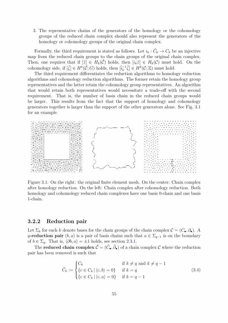
3. The representative chains of the generators of the homology or the cohomologygroups of the reduced chain complex should also represent the generators of thehomology or cohomology groups of the original chain complex.

Formally, the third requirement is stated as follows. Let ik : Ck → Ck be an injectivemap from the reduced chain groups to the chain groups of the original chain complex.Then, one requires that if [z] ∈ Hk(C) holds, then [ikz] ∈ Hk(C) must hold. On thecohomology side, if [ζ] ∈ Hk(C;G) holds, then [i−1

k ζ] ∈ Hk(C;Z) must hold.The third requirement differentiates the reduction algorithms to homology reduction

algorithms and cohomology reduction algorithms. The former retain the homology grouprepresentatives and the latter retain the cohomology group representatives. An algorithmthat would retain both representatives would necessitate a trade-off with the secondrequirement. That is, the number of basis chain in the reduced chain groups wouldbe larger. This results from the fact that the support of homology and cohomologygenerators together is larger than the support of the other generators alone. See Fig. 3.1for an example.

Figure 3.1: On the right: the original finite element mesh. On the center: Chain complexafter homology reduction. On the left: Chain complex after cohomology reduction. Bothhomology and cohomology reduced chain complexes have one basis 0-chain and one basis1-chain.

3.2.2 Reduction pair

Let Σk for each k denote bases for the chain groups of the chain complex C = (C•, ∂•). Aq-reduction pair (b, a) is a pair of basis chains such that a ∈ Σq−1 is on the boundaryof b ∈ Σq. That is, 〈∂b, a〉 = ±1 holds, see section 2.3.1.

The reduced chain complex C = (C•, ∂•) of a chain complex C where the reductionpair has been removed is such that

Ck :=

Ck if k 6= q and k 6= q − 1

c ∈ Ck | 〈c, b〉 = 0 if k = q

c ∈ Ck | 〈c, a〉 = 0 if k = q − 1

(3.4)

55

and

∂kc :=

∂c if k 6= q and k 6= q + 1

∂c− 〈∂c,a〉〈∂b,a〉

∂b if k = q

∂c− 〈∂c, b〉b if k = q + 1

∀ c ∈ Ck (3.5)

hold. The bases Σk of Ck are

Σk :=

Σk if k 6= q and k 6= q − 1

Σk \ b if k = q

Σk \ a if k = q − 1

. (3.6)

That is, the basis elements a and b removed from the bases Σq and Σq−1, and the boundaryoperators are adjusted accordingly. It is proved in [39] that C qualifies as a chain complex.

Remark 3.2.1. The boundary of a basis k-chain in the reduced chain complex doesn’tnecessarily correspond to the topological boundary of its underlying k-cell. That is, onecannot equate a basis k-chain with a basis k-cell after reduction. However, they remainrelated.

Define a chain map pk : Ck → Ck by

pkc :=

c if k 6= q

c− 〈c,a〉〈∂b,a〉

∂b if k = q − 1

c− 〈c, b〉b if k = q

, c ∈ Ck. (3.7)

It turns out that pk is a chain equivalence if one defines a chain map jk : Ck → Ck by

jkc :=

c if k 6= q

c− 〈∂c,a〉〈∂b,a〉

b if k = q, c ∈ Ck. (3.8)

Then, the map pk jk : Ck → Ck is the identity map of Ck for each k, and the mapjk pk : Ck → Ck is chain homotopic to the identity map of Ck, i.e. the map pk is a chainequivalence. That is, there exist chain maps Dk : Ck → Ck+1 for which

∂k+1 Dk +Dk−1 ∂k = jk pk − id (3.9)

holds. The maps Dk are defined by

Dkc :=

c− 〈c,a〉〈∂b,a〉

b if k = q − 1

0 otherwise, c ∈ Ck. (3.10)

The proofs for the above statements are direct substitutions and can be found in [39].Since the map pk is a chain equivalence, the induced map p∗ : Hk(C) → Hk(C) is an

isomorphism from the k:th homology group Hk(C) of C to the k:th homology group Hk(C)of C. The inverse of p∗ is the induced map j∗ : Hk(C) → Hk(C) of jk. Furthermore, theinduced map p∗ : Hk(C;Z)→ Hk(C;Z) is also an isomorphism. That is, the homologyand the cohomology groups of the chain complexes C and C are isomorphic.

56

Remark 3.2.2. The homology and the cohomology groups of the original chain complexand the reduced chain complex are merely isomorphic. That is, it is not guaranteedthat the representative chain of the element in the homology group Hk(C) of the reducedchain complex represents an element of the homology group Hk(C) of the original chaincomplex.

Elementary reduction procedure

All the reduction algorithms use the removeReductionPair routine which removes areduction pair (b, a) from a chain complex C. Its computational complexityR(|Σk|, |Σk−1|)depends on the data structure that is used to store the basis Σk of k-chains of the chaingroup Ck. For example, if the data structure is a list, a binary search tree, or a hashmap, the complexity R(|Σk|, |Σk−1|) to remove a reduction pair is O

(

max(|Σk|, |Σk−1|))

,

O(

log(max(|Σk|, |Σk−1|)))

or O(

1)

, respectively.

Procedure removeReductionPairInput: A chain complex C and a k-reduction pair (b, a)Output: A reduced chain complex CC := C;Σk := Σk \ b;Σk−1 := Σk−1 \ a;forall the k-chains ck ∈ Σk do

∂kc := ∂c− 〈∂c,a〉〈∂b,a〉

∂b;

forall the k + 1-chains ck+1 ∈ Σk+1 do

∂k+1c := ∂c− 〈∂c, b〉b;

Table 3.1: Reduction algorithms.

Name ComplexityHomology/ HomotopyCohomology invariant

k-collapse O(

qk−1 ·R(qk, qk−1))

Homology Yesk-combine O(qkqk−1) Homology YesOmit-collapse O

(

qk−1 ·R(qk, qk−1))

Homology No

k-dual-collapse O(

qk−1 ·R(qk, qk−1))

Cohomology Dualk-dual-combine O(qkqk−1) Cohomology DualCoreduction O

(

qk−1 ·R(qk, qk−1))

Cohomology No

3.2.3 Homology reduction algorithms

For the homology reduction algorithms it holds true that if [z] is a generator of Hk(C),then [ikz] is a generator Hk(C), where ik : Ck → Ck is an inclusion map.

57

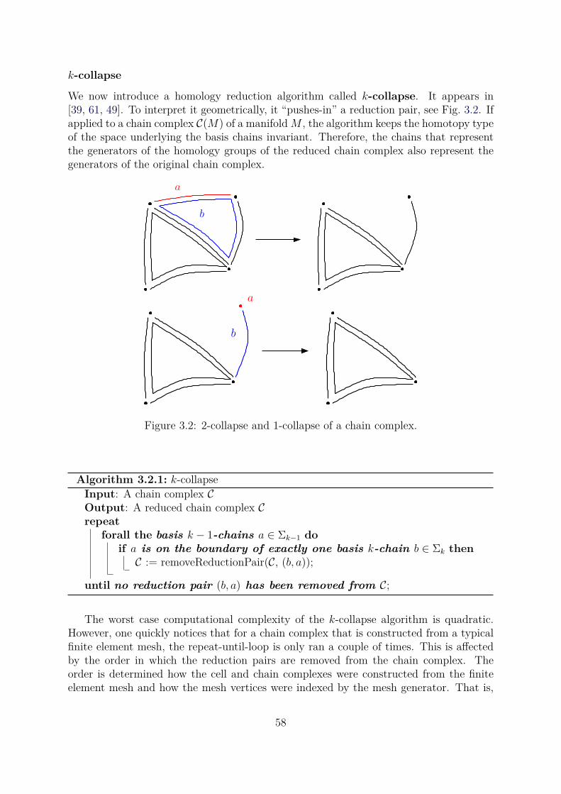
k-collapse

We now introduce a homology reduction algorithm called k-collapse. It appears in[39, 61, 49]. To interpret it geometrically, it “pushes-in” a reduction pair, see Fig. 3.2. Ifapplied to a chain complex C(M) of a manifold M , the algorithm keeps the homotopy typeof the space underlying the basis chains invariant. Therefore, the chains that representthe generators of the homology groups of the reduced chain complex also represent thegenerators of the original chain complex.

a

b

b

a

Figure 3.2: 2-collapse and 1-collapse of a chain complex.

Algorithm 3.2.1: k-collapseInput: A chain complex COutput: A reduced chain complex Crepeat

forall the basis k − 1-chains a ∈ Σk−1 do

if a is on the boundary of exactly one basis k-chain b ∈ Σk then

C := removeReductionPair(C, (b, a));

until no reduction pair (b, a) has been removed from C;

The worst case computational complexity of the k-collapse algorithm is quadratic.However, one quickly notices that for a chain complex that is constructed from a typicalfinite element mesh, the repeat-until-loop is only ran a couple of times. This is affectedby the order in which the reduction pairs are removed from the chain complex. Theorder is determined how the cell and chain complexes were constructed from the finiteelement mesh and how the mesh vertices were indexed by the mesh generator. That is,

58

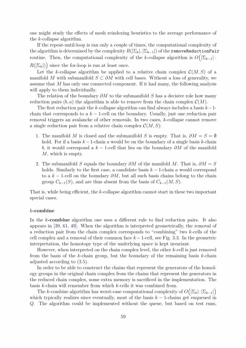
one might study the effects of mesh reindexing heuristics to the average performance ofthe k-collapse algorithm.

If the repeat-until-loop is ran only a couple of times, the computational complexity ofthe algorithm is determined by the complexityR(|Σk|, |Σk−1|) of the removeReductionPair

routine. Then, the computational complexity of the k-collapse algorithm is O(

|Σk−1| ·R(|Σk|)

)

since the for-loop is ran at least once.Let the k-collapse algorithm be applied to a relative chain complex C(M,S) of a

manifold M with submanifold S ⊂ ∂M with cell bases. Without a loss of generality, weassume that M has only one connected component. If it had many, the following analysiswill apply to them individually.

The relation of the boundary ∂M to the submanifold S has a decisive role how manyreduction pairs (b, a) the algorithm is able to remove from the chain complex C(M).

The first reduction pair the k-collapse algorithm can find always includes a basis k−1-chain that corresponds to a k − 1-cell on the boundary. Usually, just one reduction pairremoval triggers an avalanche of other removals. In two cases, k-collapse cannot removea single reduction pair from a relative chain complex C(M,S):

1. The manifold M is closed and the submanifold S is empty. That is, ∂M = S = ∅hold. For if a basis k−1-chain a would be on the boundary of a single basis k-chainb, it would correspond a k − 1-cell that lies on the boundary ∂M of the manifoldM , which is empty.

2. The submanifold S equals the boundary ∂M of the manifold M . That is, ∂M = Sholds. Similarly to the first case, a candidate basis k− 1-chain a would correspondto a k − 1-cell on the boundary ∂M , but all such basis chains belong to the chaingroup Ck−1(S), and are thus absent from the basis of Ck−1(M,S).

That is, while being efficient, the k-collapse algorithm cannot start in these two importantspecial cases.

k-combine

In the k-combine algorithm one uses a different rule to find reduction pairs. It alsoappears in [39, 61, 49]. When the algorithm is interpreted geometrically, the removal ofa reduction pair from the chain complex corresponds to “combining” two k-cells of thecell complex and a removal of their common face k−1-cell, see Fig. 3.3. In the geometricinterpretation, the homotopy type of the underlying space is kept invariant.

However, when interpreted on the chain complex level, the other k-cell is just removedfrom the basis of the k-chain group, but the boundary of the remaining basis k-chainadjusted according to (3.5).

In order to be able to construct the chains that represent the generators of the homol-ogy groups in the original chain complex from the chains that represent the generators inthe reduced chain complex, some extra memory is sacrificed in the implementation. Thebasis k-chain will remember from which k-cells it was combined from.

The k-combine algorithm has worst-case computational complexity of O(

|Σk| · |Σk−1|)

which typically realizes since eventually, most of the basis k − 1-chains get enqueued inQ. The algorithm could be implemented without the queue, but based on test runs,

59

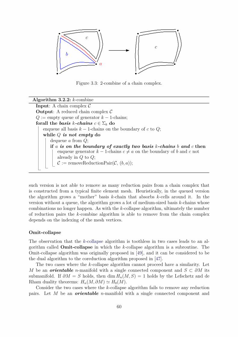
b

c

c

a

Figure 3.3: 2-combine of a chain complex.

Algorithm 3.2.2: k-combineInput: A chain complex COutput: A reduced chain complex CQ := empty queue of generator k − 1-chains;forall the basis k-chains c ∈ Σk do

enqueue all basis k − 1-chains on the boundary of c to Q;while Q is not empty do

dequeue a from Q;if a is on the boundary of exactly two basis k-chains b and c then

enqueue generator k − 1-chains c 6= a on the boundary of b and c notalready in Q to Q;C := removeReductionPair(C, (b, a));

such version is not able to remove as many reduction pairs from a chain complex thatis constructed from a typical finite element mesh. Heuristically, in the queued versionthe algorithm grows a “mother” basis k-chain that absorbs k-cells around it. In theversion without a queue, the algorithm grows a lot of medium-sized basis k-chains whosecombinations no longer happen. As with the k-collapse algorithm, ultimately the numberof reduction pairs the k-combine algorithm is able to remove from the chain complexdepends on the indexing of the mesh vertices.

Omit-collapse

The observation that the k-collapse algorithm is toothless in two cases leads to an al-gorithm called Omit-collapse in which the k-collapse algorithm is a subroutine. TheOmit-collapse algorithm was originally proposed in [49], and it can be considered to bethe dual algorithm to the coreduction algorithm proposed in [47].

The two cases where the k-collapse algorithm cannot proceed have a similarity. LetM be an orientable n-manifold with a single connected component and S ⊂ ∂M itssubmanifold. If ∂M = S holds, then dimHn(M,S) = 1 holds by the Lefschetz and deRham duality theorems: Hn(M,∂M) ≃ H0(M).

Consider the two cases where the k-collapse algorithm fails to remove any reductionpairs. Let M be an orientable n-manifold with a single connected component and

60

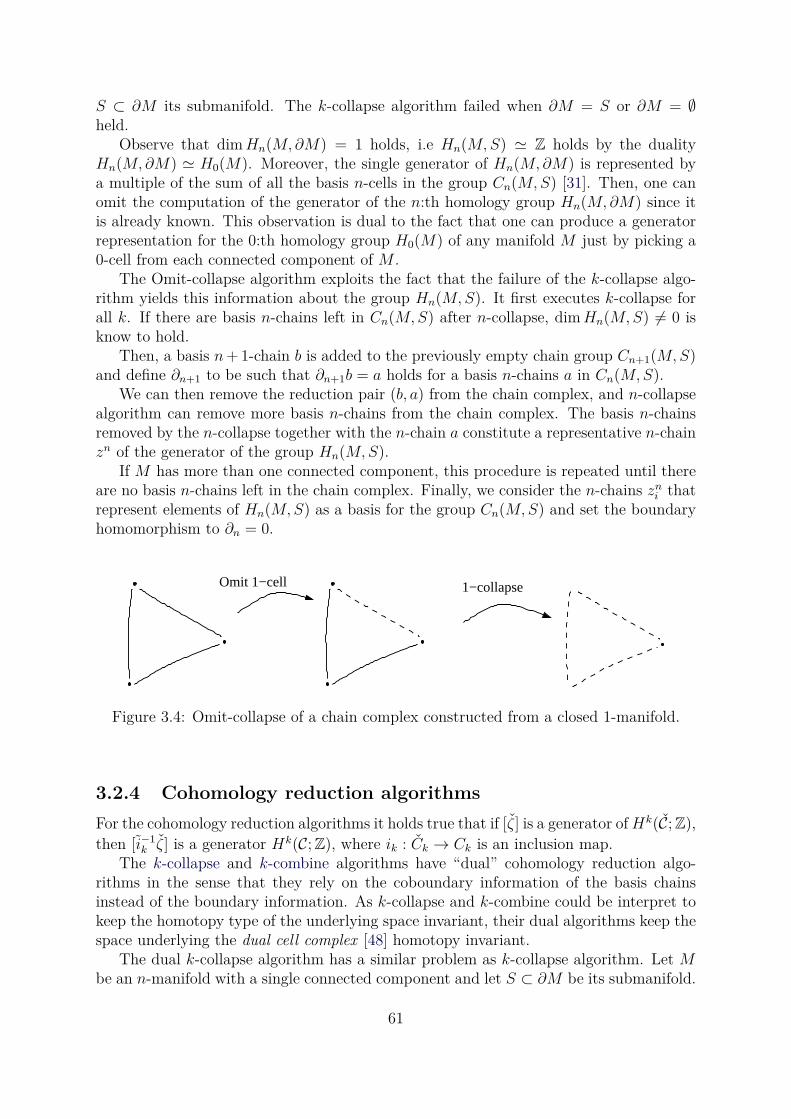
S ⊂ ∂M its submanifold. The k-collapse algorithm failed when ∂M = S or ∂M = ∅held.

Observe that dimHn(M,∂M) = 1 holds, i.e Hn(M,S) ≃ Z holds by the dualityHn(M,∂M) ≃ H0(M). Moreover, the single generator of Hn(M,∂M) is represented bya multiple of the sum of all the basis n-cells in the group Cn(M,S) [31]. Then, one canomit the computation of the generator of the n:th homology group Hn(M,∂M) since itis already known. This observation is dual to the fact that one can produce a generatorrepresentation for the 0:th homology group H0(M) of any manifold M just by picking a0-cell from each connected component of M .

The Omit-collapse algorithm exploits the fact that the failure of the k-collapse algo-rithm yields this information about the group Hn(M,S). It first executes k-collapse forall k. If there are basis n-chains left in Cn(M,S) after n-collapse, dimHn(M,S) 6= 0 isknow to hold.

Then, a basis n+ 1-chain b is added to the previously empty chain group Cn+1(M,S)and define ∂n+1 to be such that ∂n+1b = a holds for a basis n-chains a in Cn(M,S).

We can then remove the reduction pair (b, a) from the chain complex, and n-collapsealgorithm can remove more basis n-chains from the chain complex. The basis n-chainsremoved by the n-collapse together with the n-chain a constitute a representative n-chainzn of the generator of the group Hn(M,S).

If M has more than one connected component, this procedure is repeated until thereare no basis n-chains left in the chain complex. Finally, we consider the n-chains zn

i thatrepresent elements of Hn(M,S) as a basis for the group Cn(M,S) and set the boundaryhomomorphism to ∂n = 0.

Omit 1−cell 1−collapse

Figure 3.4: Omit-collapse of a chain complex constructed from a closed 1-manifold.

3.2.4 Cohomology reduction algorithms

For the cohomology reduction algorithms it holds true that if [ζ] is a generator ofHk(C;Z),then [i−1

k ζ] is a generator Hk(C;Z), where ik : Ck → Ck is an inclusion map.The k-collapse and k-combine algorithms have “dual” cohomology reduction algo-

rithms in the sense that they rely on the coboundary information of the basis chainsinstead of the boundary information. As k-collapse and k-combine could be interpret tokeep the homotopy type of the underlying space invariant, their dual algorithms keep thespace underlying the dual cell complex [48] homotopy invariant.

The dual k-collapse algorithm has a similar problem as k-collapse algorithm. Let Mbe an n-manifold with a single connected component and let S ⊂ ∂M be its submanifold.

61

Algorithm 3.2.3: Omit-collapseInput: A chain complex COutput: A reduced chain complex Cforeach k = n to 1 do

run k-collapse;

i := 1;while |Σn| 6= 0 do

pick a basis n-chain a ∈ Σn;Σn+1 := b;∂n+1b := a;C := removeReductionPair(C, (b, a));foreach k = n to 1 do

run k-collapse;create an n-chain zi that is the sum of all basis n-chains removed in theprevious n-collapse;zi := a+ zi;i := i+ 1;

Σn :=⋃

izi;∂n := 0;

Then, if S = ∅ holds, the dual k-combine algorithm cannot remove any basis cells from thechain complex C(M,S). Therefore, the cohomological counterpart of the Omit-collapsecalled Coreduction is represented.

Coreduction

The Coreduction algorithm appeared in [47] as a method for Betti number computation.In this thesis, it used as a cohomology reduction algorithm before the actual computationof the cohomology generators of a given chain complex.

If M is an n-manifold with a single connected component with a submanifold S. Then,the Coreduction algorithm cannot find any reduction pairs from a chain complex C(M,S)unless S is non-empty. Thus similarly to the Omit-collapse algorithm, a −1-chain a isadded to the chain complex with a single basis 0-chain b on its coboundary. Then, thereduction pair (b, a) is removed from the chain complex. This triggers a number of otherreduction pair removals from the chain complex, and all the cobasis 0-cochains of theremoved basis 0-chains together with the cobasis element of b constitute an representativeof the single generator of the cohomology group H0(M).

3.3 Computation of homology and cohomology

Let C be a chain complex with bases Σk of Ck for each k. The boundary homomorphisms∂k are represented by the integer matrices Dk with respect to those bases.

The goal of the homology computation is to represent the generators of the homologygroups Hk(C) in terms of the bases Σk. The numerical result is an integer matrix Hk,

62

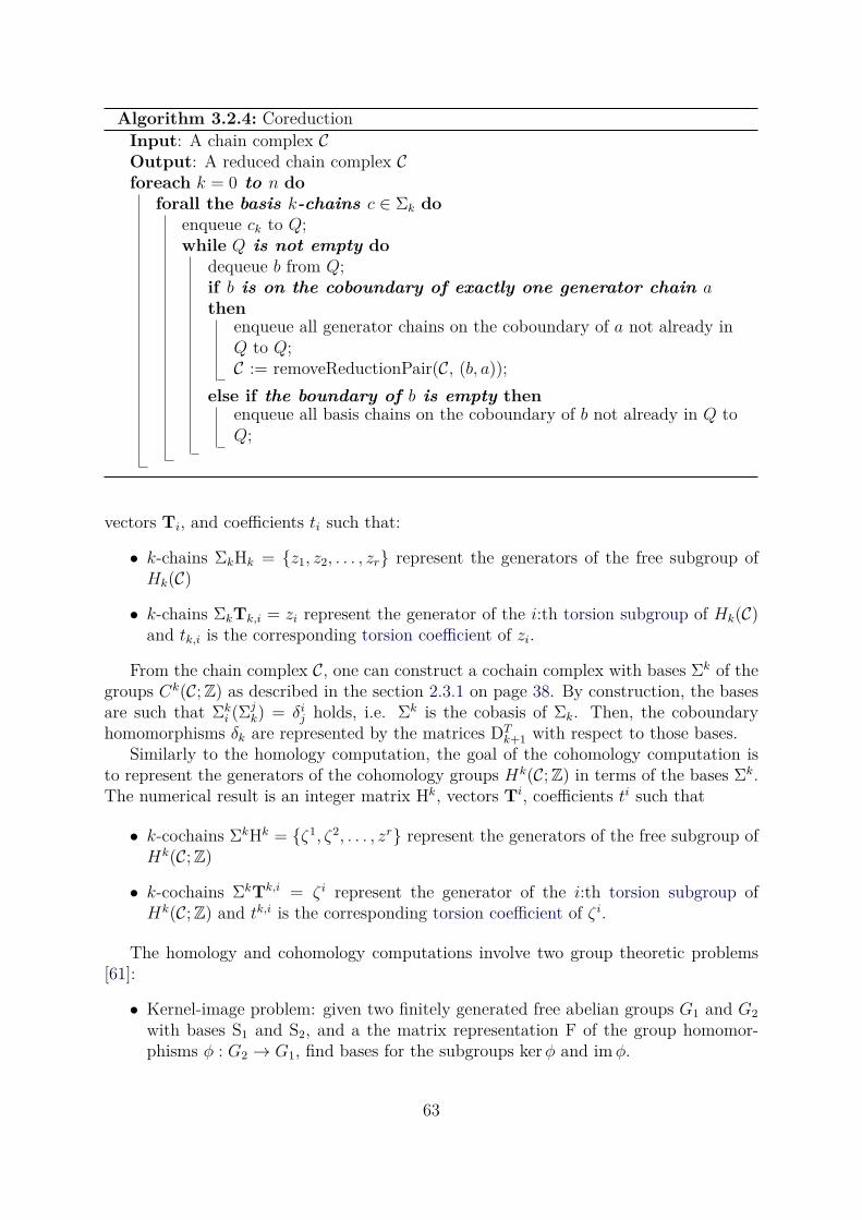
Algorithm 3.2.4: CoreductionInput: A chain complex COutput: A reduced chain complex Cforeach k = 0 to n do

forall the basis k-chains c ∈ Σk do

enqueue ck to Q;while Q is not empty do

dequeue b from Q;if b is on the coboundary of exactly one generator chain athen

enqueue all generator chains on the coboundary of a not already inQ to Q;C := removeReductionPair(C, (b, a));

else if the boundary of b is empty thenenqueue all basis chains on the coboundary of b not already in Q toQ;

vectors Ti, and coefficients ti such that:

• k-chains ΣkHk = z1, z2, . . . , zr represent the generators of the free subgroup ofHk(C)

• k-chains ΣkTk,i = zi represent the generator of the i:th torsion subgroup of Hk(C)and tk,i is the corresponding torsion coefficient of zi.

From the chain complex C, one can construct a cochain complex with bases Σk of thegroups Ck(C;Z) as described in the section 2.3.1 on page 38. By construction, the basesare such that Σk

i (Σjk) = δi

j holds, i.e. Σk is the cobasis of Σk. Then, the coboundaryhomomorphisms δk are represented by the matrices DT

k+1 with respect to those bases.Similarly to the homology computation, the goal of the cohomology computation is

to represent the generators of the cohomology groups Hk(C;Z) in terms of the bases Σk.The numerical result is an integer matrix Hk, vectors Ti, coefficients ti such that

• k-cochains ΣkHk = ζ1, ζ2, . . . , zr represent the generators of the free subgroup ofHk(C;Z)

• k-cochains ΣkTk,i = ζ i represent the generator of the i:th torsion subgroup ofHk(C;Z) and tk,i is the corresponding torsion coefficient of ζ i.

The homology and cohomology computations involve two group theoretic problems[61]:

• Kernel-image problem: given two finitely generated free abelian groups G1 and G2

with bases S1 and S2, and a the matrix representation F of the group homomor-phisms φ : G2 → G1, find bases for the subgroups kerφ and imφ.

63

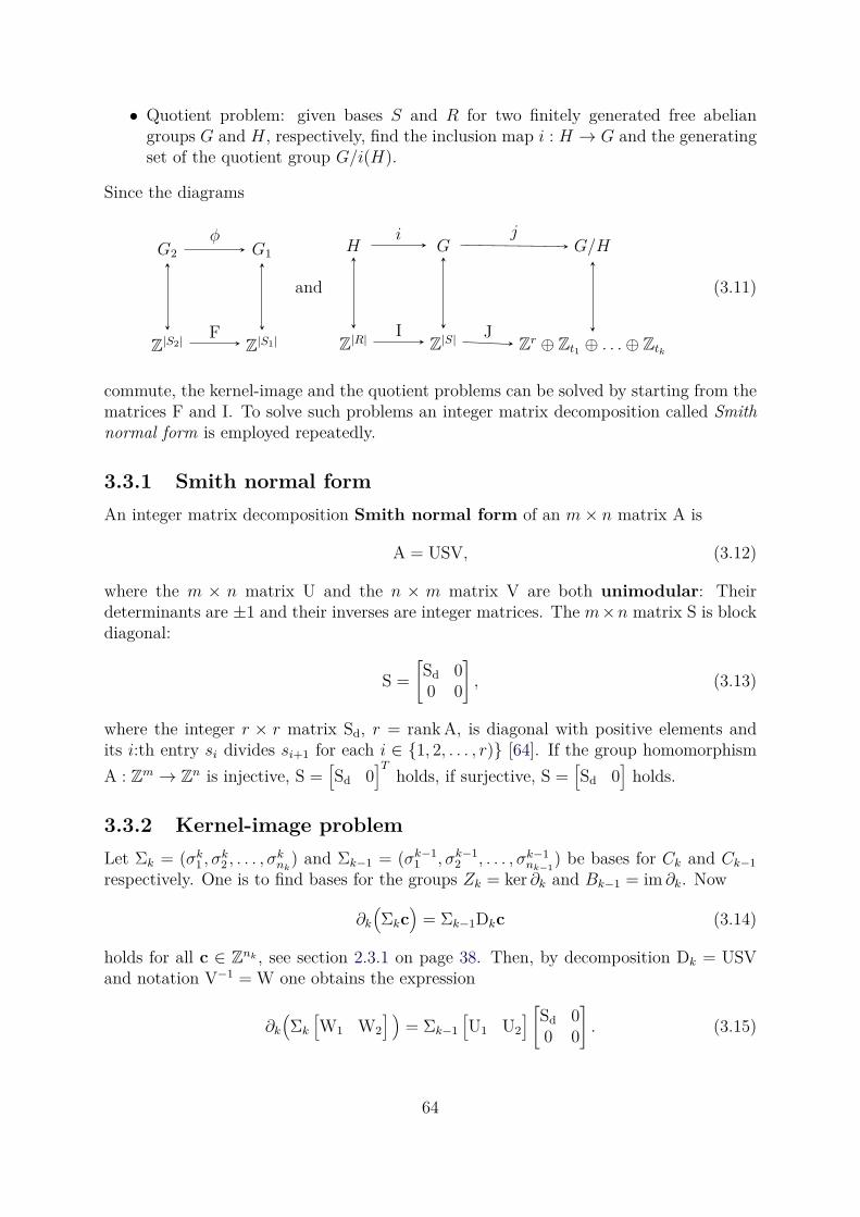
• Quotient problem: given bases S and R for two finitely generated free abeliangroups G and H, respectively, find the inclusion map i : H → G and the generatingset of the quotient group G/i(H).

Since the diagrams

G2 G1

Z|S2|

Z|S1|

φ

F

and

H G G/H

Z|R|

Z|S|

Zr ⊕ Zt1

⊕ . . .⊕ Ztk

i

I

j

J

(3.11)

commute, the kernel-image and the quotient problems can be solved by starting from thematrices F and I. To solve such problems an integer matrix decomposition called Smithnormal form is employed repeatedly.

3.3.1 Smith normal form

An integer matrix decomposition Smith normal form of an m× n matrix A is

A = USV, (3.12)

where the m × n matrix U and the n × m matrix V are both unimodular: Theirdeterminants are ±1 and their inverses are integer matrices. The m×n matrix S is blockdiagonal:

S =

[

Sd 00 0

]

, (3.13)

where the integer r × r matrix Sd, r = rank A, is diagonal with positive elements andits i:th entry si divides si+1 for each i ∈ 1, 2, . . . , r) [64]. If the group homomorphism

A : Zm → Zn is injective, S =

[

Sd 0]T

holds, if surjective, S =[

Sd 0]

holds.

3.3.2 Kernel-image problem

Let Σk = (σk1 , σ

k2 , . . . , σ

knk

) and Σk−1 = (σk−11 , σk−1

2 , . . . , σk−1nk−1

) be bases for Ck and Ck−1

respectively. One is to find bases for the groups Zk = ker ∂k and Bk−1 = im ∂k. Now

∂k

(

Σkc)

= Σk−1Dkc (3.14)

holds for all c ∈ Znk , see section 2.3.1 on page 38. Then, by decomposition Dk = USV

and notation V−1 = W one obtains the expression

∂k

(

Σk

[

W1 W2

] )

= Σk−1

[

U1 U2

]

[

Sd 00 0

]

. (3.15)

64

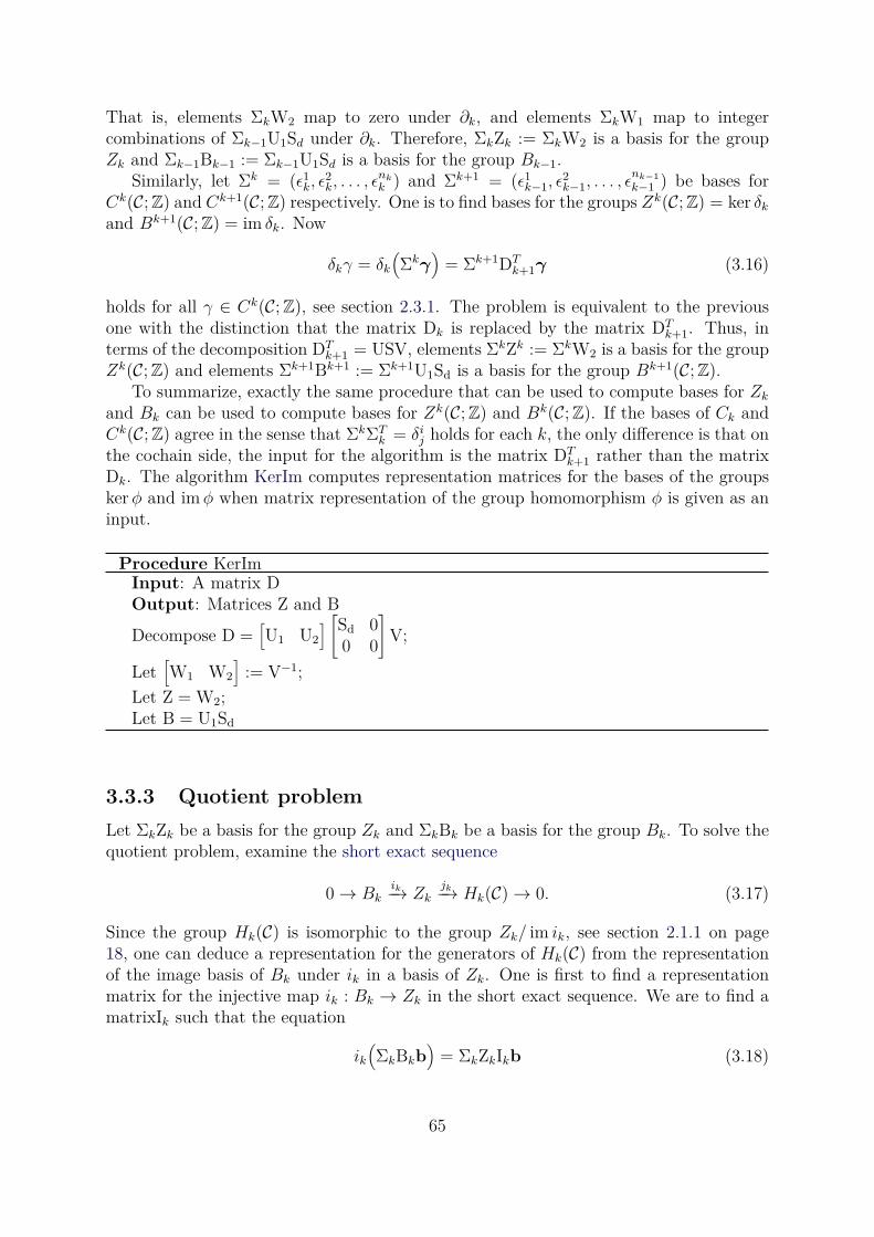
That is, elements ΣkW2 map to zero under ∂k, and elements ΣkW1 map to integercombinations of Σk−1U1Sd under ∂k. Therefore, ΣkZk := ΣkW2 is a basis for the groupZk and Σk−1Bk−1 := Σk−1U1Sd is a basis for the group Bk−1.

Similarly, let Σk = (ǫ1k, ǫ

2k, . . . , ǫ

nk

k ) and Σk+1 = (ǫ1k−1, ǫ

2k−1, . . . , ǫ

nk−1

k−1 ) be bases forCk(C;Z) and Ck+1(C;Z) respectively. One is to find bases for the groups Zk(C;Z) = ker δk

and Bk+1(C;Z) = im δk. Now

δkγ = δk

(

Σkγ)

= Σk+1DTk+1γ (3.16)

holds for all γ ∈ Ck(C;Z), see section 2.3.1. The problem is equivalent to the previousone with the distinction that the matrix Dk is replaced by the matrix DT

k+1. Thus, interms of the decomposition DT

k+1 = USV, elements ΣkZk := ΣkW2 is a basis for the groupZk(C;Z) and elements Σk+1Bk+1 := Σk+1U1Sd is a basis for the group Bk+1(C;Z).

To summarize, exactly the same procedure that can be used to compute bases for Zk

and Bk can be used to compute bases for Zk(C;Z) and Bk(C;Z). If the bases of Ck andCk(C;Z) agree in the sense that ΣkΣT

k = δij holds for each k, the only difference is that on

the cochain side, the input for the algorithm is the matrix DTk+1 rather than the matrix

Dk. The algorithm KerIm computes representation matrices for the bases of the groupskerφ and imφ when matrix representation of the group homomorphism φ is given as aninput.

Procedure KerImInput: A matrix DOutput: Matrices Z and B

Decompose D =[

U1 U2

]

[

Sd 00 0

]

V;

Let[

W1 W2

]

:= V−1;Let Z = W2;Let B = U1Sd

3.3.3 Quotient problem

Let ΣkZk be a basis for the group Zk and ΣkBk be a basis for the group Bk. To solve thequotient problem, examine the short exact sequence

0→ Bkik−→ Zk

jk−→ Hk(C)→ 0. (3.17)

Since the group Hk(C) is isomorphic to the group Zk/ im ik, see section 2.1.1 on page18, one can deduce a representation for the generators of Hk(C) from the representationof the image basis of Bk under ik in a basis of Zk. One is first to find a representationmatrix for the injective map ik : Bk → Zk in the short exact sequence. We are to find amatrixIk such that the equation

ik(

ΣkBkb)

= ΣkZkIkb (3.18)

65

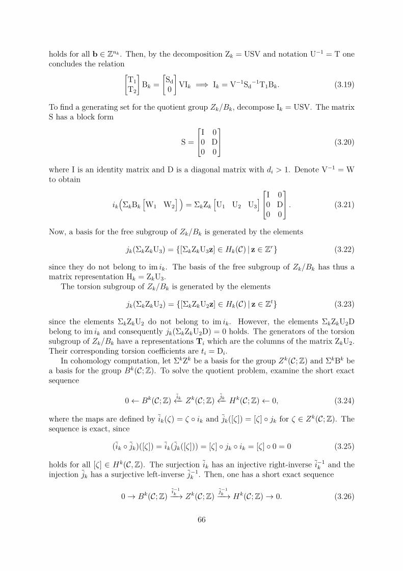
holds for all b ∈ Znk . Then, by the decomposition Zk = USV and notation U−1 = T one

concludes the relation[

T1

T2

]

Bk =

[

Sd

0

]

VIk =⇒ Ik = V−1Sd−1T1Bk. (3.19)

To find a generating set for the quotient group Zk/Bk, decompose Ik = USV. The matrixS has a block form

S =

I 00 D0 0

(3.20)

where I is an identity matrix and D is a diagonal matrix with di > 1. Denote V−1 = Wto obtain

ik(

ΣkBk

[

W1 W2

] )

= ΣkZk

[

U1 U2 U3

]

I 00 D0 0

. (3.21)

Now, a basis for the free subgroup of Zk/Bk is generated by the elements

jk(ΣkZkU3) = [ΣkZkU3z] ∈ Hk(C) | z ∈ Zr (3.22)

since they do not belong to im ik. The basis of the free subgroup of Zk/Bk has thus amatrix representation Hk = ZkU3.

The torsion subgroup of Zk/Bk is generated by the elements

jk(ΣkZkU2) = [ΣkZkU2z] ∈ Hk(C) | z ∈ Zt (3.23)

since the elements ΣkZkU2 do not belong to im ik. However, the elements ΣkZkU2Dbelong to im ik and consequently jk(ΣkZkU2D) = 0 holds. The generators of the torsionsubgroup of Zk/Bk have a representations Ti which are the columns of the matrix ZkU2.Their corresponding torsion coefficients are ti = Di.

In cohomology computation, let ΣkZk be a basis for the group Zk(C;Z) and ΣkBk bea basis for the group Bk(C;Z). To solve the quotient problem, examine the short exactsequence

0← Bk(C;Z) ik←− Zk(C;Z)jk←− Hk(C;Z)← 0, (3.24)

where the maps are defined by ik(ζ) = ζ ik and jk([ζ]) = [ζ] jk for ζ ∈ Zk(C;Z). Thesequence is exact, since

(ik jk)([ζ]) = ik(jk([ζ])) = [ζ] jk ik = [ζ] 0 = 0 (3.25)

holds for all [ζ] ∈ Hk(C,Z). The surjection ik has an injective right-inverse i−1k and the

injection jk has a surjective left-inverse j−1k . Then, one has a short exact sequence

0→ Bk(C;Z)i−1

k−−→ Zk(C;Z)j−1

k−−→ Hk(C;Z)→ 0. (3.26)

66

From that sequence one can deduce representations for the generators of Hk(C;Z) simi-larly as it was done in the homology computation.

To summarize, exactly the same computations were carried out in both the homologyquotient problem and in the cohomology quotient problem. Let

0→ Bi−→ Z

j−→ Z/B → 0 (3.27)

be a short exact sequence, where the group Z is finitely generated free abelian and B isits subgroup. The algorithm Quotient finds a basis representation H for the free subgroupF of the quotient group Z/B, representations Ti of generators of its torsion subgroupsTi and their corresponding torsion coefficients ti, when matrices B and Z that representbases for B and Z are given as an input.

Procedure QuotientInput: Matrices Z and BOutput: A Matrix H, vectors Ti and integers tj

Decompose Z = U

[

Sd

0

]

V;

Let

[

T1

T2

]

:= U−1;

Let I = V−1Sd−1T1B;

Decompose I =[

U1 U2 U3

]

I 00 D0 0

V;

Let H = ZU3;Let Ti = (ZU2)i ∀ i;Let ti = Di;

3.3.4 The homology and cohomology computation algorithm

The final algorithm 3.3.1 to compute homology and cohomology of a chain complex Cproduces the representatives of the generators of the homology and cohomology groups. Itjoins together the algorithms for the kernel-image problem and for the quotient problem.

3.4 The homology and cohomology solver in Gmsh

We have implemented a homology and cohomology solver in the finite element meshgenerator Gmsh. It knits together homology or cohomology reduction techniques pre-sented in this thesis and consequently applies the homology or cohomology computationalgorithm to the reduced chain complex.

The input for the solver is up to 3-dimensional finite element mesh that is generatedby Gmsh or imported to Gmsh. The user designates a part of the mesh that is interpretedas the manifold M and a part that is interpreted as its subdomain S.

67

Algorithm 3.3.1: An algorithm for the homology and cohomology computation.Input: Integer matrices Dk

Output: Integer matrices Hk and Tk and integer vectors tk

foreach k do

if Compute homology then

D := Dk;q := k − 1;

else if Compute cohomology then

D := DTk+1;

q := k + 1;(Zk,Bq) := KerIm(D);

foreach k do

(Hk,Tk, t) := Quotient(Zk, Bq);

The resulting representatives of the generators of the k-homology and k-cohomologygroups are stored as sets of k-dimensional mesh elements that correspond to the non-zero k-cells of the representative k-chain. As k-chains are integer combinations of themesh elements, the set contains a mesh element multiply times according to its integercoefficient and it is oriented according to the sign of the integer.

3.4.1 Homology computation routine

The routine for the homology computation is the following

1. Designate which part of the finite element mesh covers the manifold M and itssubmanifold S

2. Create a cell complex K = (M,K, ι) with algorithm 3.1.1 from the finite elementmesh

3. Remove cells that have been flagged to belong to the submanifold S

4. Run Omit-collapse algorithm 3.2.3

5. Run k-combine algorithm 3.2.2 followed by k − 1-collapse algorithm 3.2.1 for eachk = n, . . . , 1.

6. Run the homology computation algorithm 3.3.1 to compute the homology groupsof the chain complex C(M,S)

7. Express the results in terms of the original finite element mesh

3.4.2 Cohomology computation routine

The routine for the cohomology computation is the following

1. Designate a manifold M and its submanifold S from a finite element mesh

68

2. Create a cell complex K = (M,K, ι) with algorithm 3.1.1 from the finite elementmesh

3. Remove cells that have been flagged to belong to the submanifold S

4. Run Coreduction algorithm 3.2.4

5. Run the dual version of the k-combine algorithm 3.2.2 followed by the dual versionof the k + 1-collapse algorithm 3.2.1 for each k = 0, . . . , n− 1r

6. Run the cohomology computation algorithm 3.3.1 to compute the cohomologygroups of the chain complex C(M,S)

7. Express the results in terms of the original finite element mesh

3.5 Post-processing of homology and cohomology

The computational methods in the previous chapter produce representatives of generatorsof the homology and cohomology groups, once given a finite element mesh as an input.

These representations of the generating sets can further be processed since they arenon-unique on two levels:

1. The generators of homology and cohomology groups are cosets of chains and cochains.Thus, there’s an equivalence class of possible representatives for each generator ina generating set.

2. The generating set can be changed into an another by an unimodular transforma-tion. This corresponds to a change of basis of a vector space.

The motive to perform such post-processing of the representations of the homologyand cohomology groups is the topic of the next chapter, where homology and cohomologycomputations are applied in engineering problems in electromagnetics. In short, thegenerators are given a context-dependent meaning in engineering. In order to enablethat, the engineer or an automated algorithm needs to be able to choose a representationthat fits the purpose.

Starting from this section, we concentrate on the homology and cohomology vectorspaces rather than groups. In the previous section, a computational method to find basesfor the free subgroups of the homology and cohomology was described. Such bases arealso bases for the homology and cohomology vector spaces.

The reason why this thesis first considered groups rather than vector spaces was two-fold:

1. To ensure that the computationally produced basis element representatives corre-spond to integer combinations of cells, rather than linear combinations which mayhave non-integer coefficients.

2. To recognize if the homology and cohomology groups had torsion subgroups. Theexistence of torsion in a finite element model is often an indicator some technicaldifficulty or human error, which might prevent its use in the finite element method[28, 61].

69

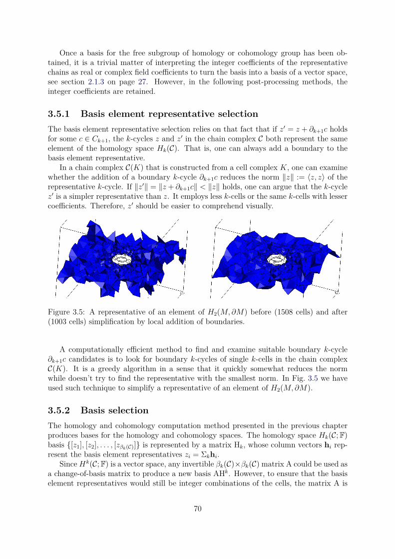
Once a basis for the free subgroup of homology or cohomology group has been ob-tained, it is a trivial matter of interpreting the integer coefficients of the representativechains as real or complex field coefficients to turn the basis into a basis of a vector space,see section 2.1.3 on page 27. However, in the following post-processing methods, theinteger coefficients are retained.

3.5.1 Basis element representative selection

The basis element representative selection relies on that fact that if z′ = z + ∂k+1c holdsfor some c ∈ Ck+1, the k-cycles z and z′ in the chain complex C both represent the sameelement of the homology space Hk(C). That is, one can always add a boundary to thebasis element representative.

In a chain complex C(K) that is constructed from a cell complex K, one can examinewhether the addition of a boundary k-cycle ∂k+1c reduces the norm ‖z‖ := 〈z, z〉 of therepresentative k-cycle. If ‖z′‖ = ‖z + ∂k+1c‖ < ‖z‖ holds, one can argue that the k-cyclez′ is a simpler representative than z. It employs less k-cells or the same k-cells with lessercoefficients. Therefore, z′ should be easier to comprehend visually.

Figure 3.5: A representative of an element of H2(M,∂M) before (1508 cells) and after(1003 cells) simplification by local addition of boundaries.

A computationally efficient method to find and examine suitable boundary k-cycle∂k+1c candidates is to look for boundary k-cycles of single k-cells in the chain complexC(K). It is a greedy algorithm in a sense that it quickly somewhat reduces the normwhile doesn’t try to find the representative with the smallest norm. In Fig. 3.5 we haveused such technique to simplify a representative of an element of H2(M,∂M).

3.5.2 Basis selection

The homology and cohomology computation method presented in the previous chapterproduces bases for the homology and cohomology spaces. The homology space Hk(C;F)basis [z1], [z2], . . . , [zβk(C)] is represented by a matrix Hk, whose column vectors hi rep-resent the basis element representatives zi = Σkhi.

Since Hk(C;F) is a vector space, any invertible βk(C)×βk(C) matrix A could be used asa change-of-basis matrix to produce a new basis AHk. However, to ensure that the basiselement representatives would still be integer combinations of the cells, the matrix A is

70

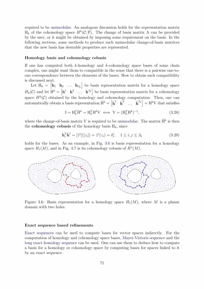
required to be unimodular. An analogous discussion holds for the representation matrixHk of the cohomology space Hk(C;F). The change of basis matrix A can be providedby the user, or it might be obtained by imposing some requirement on the basis. In thefollowing sections, some methods to produce such unimodular change-of-basis matricesthat the new basis has desirable properties are represented.

Homology basis and cohomology cobasis

If one has computed both k-homology and k-cohomology space bases of some chaincomplex, one might want them to compatible in the sense that there is a pairwise one-to-one correspondence between the elements of the bases. How to obtain such compatibilityis discussed next.

Let Hk =[

h1 h2 . . . hβk

]

be basis representation matrix for a homology space

Hk(C) and let Hk =[

h1 h2 . . . hβk

]

be basis representation matrix for a cohomologyspace Hk(C) obtained by the homology and cohomology computation. Then, one canautomatically obtain a basis representation Hk =

[

h1

h2. . . h

βk

]

= HkV that satisfies

I = HTk Hk = HT

k HkV ⇐⇒ V = (HTk Hk)−1, (3.28)

where the change-of-basis matrix V is required to be unimodular. The matrix Hk is thenthe cohomology cobasis of the homology basis Hk, since

hTi h

j= [zj]([zi]) = zj(zi) = δj

i , 1 ≤ i, j ≤ βk (3.29)

holds for the bases. As an example, in Fig. 3.6 is basis representation for a homologyspace H1(M), and in Fig. 3.7 is its cohomology cobasis of H1(M).

Figure 3.6: Basis representation for a homology space H1(M), where M is a planardomain with two holes.

Exact sequence based refinements

Exact sequences can be used to compute bases for vector spaces indirectly. For thecomputation of homology and cohomology space bases, Mayer-Vietoris sequence and thelong exact homology sequence can be used. One can use them to deduce how to computea basis for a homology or cohomology space by computing bases for spaces linked to itby an exact sequence.

71

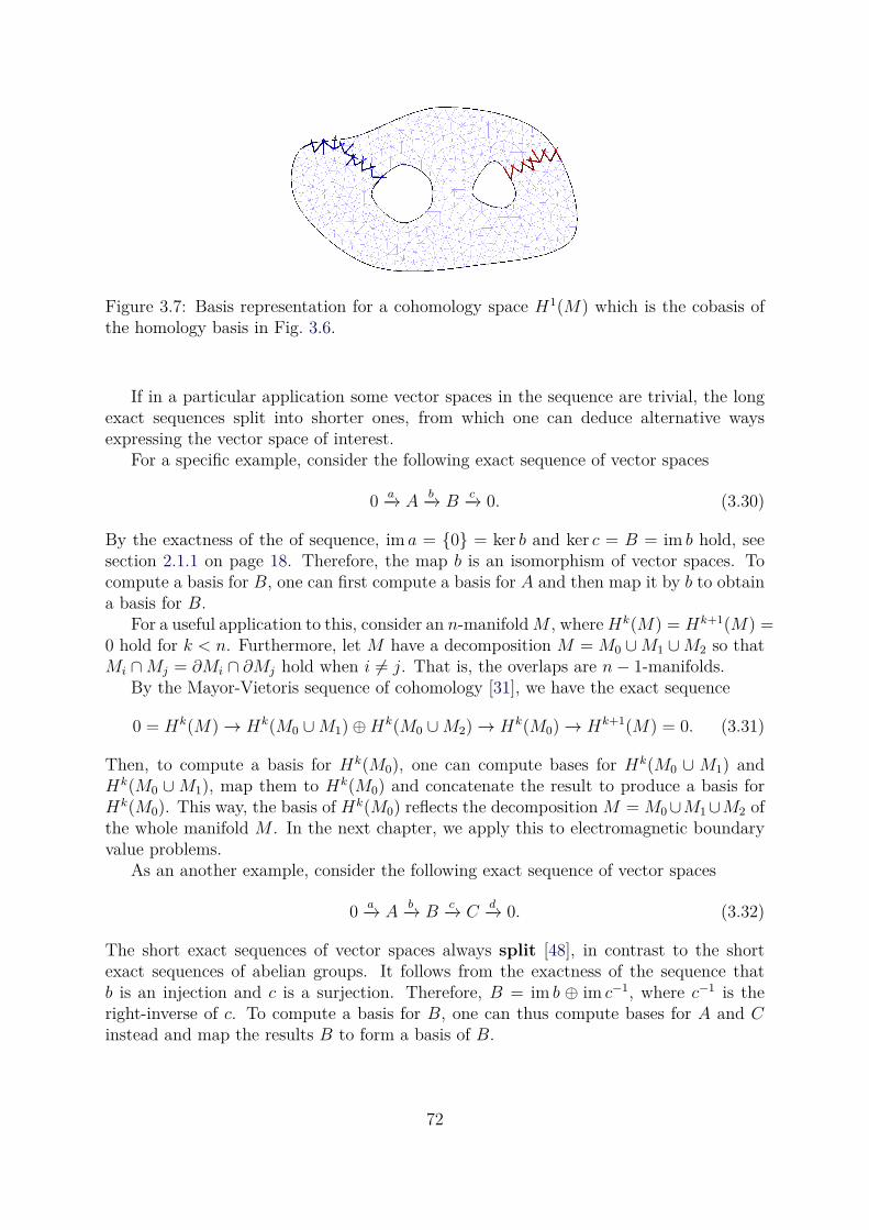
Figure 3.7: Basis representation for a cohomology space H1(M) which is the cobasis ofthe homology basis in Fig. 3.6.

If in a particular application some vector spaces in the sequence are trivial, the longexact sequences split into shorter ones, from which one can deduce alternative waysexpressing the vector space of interest.

For a specific example, consider the following exact sequence of vector spaces

0 a−→ Ab−→ B

c−→ 0. (3.30)

By the exactness of the of sequence, im a = 0 = ker b and ker c = B = im b hold, seesection 2.1.1 on page 18. Therefore, the map b is an isomorphism of vector spaces. Tocompute a basis for B, one can first compute a basis for A and then map it by b to obtaina basis for B.

For a useful application to this, consider an n-manifoldM , whereHk(M) = Hk+1(M) =0 hold for k < n. Furthermore, let M have a decomposition M = M0 ∪M1 ∪M2 so thatMi ∩Mj = ∂Mi ∩ ∂Mj hold when i 6= j. That is, the overlaps are n− 1-manifolds.

By the Mayor-Vietoris sequence of cohomology [31], we have the exact sequence

0 = Hk(M)→ Hk(M0 ∪M1)⊕Hk(M0 ∪M2)→ Hk(M0)→ Hk+1(M) = 0. (3.31)

Then, to compute a basis for Hk(M0), one can compute bases for Hk(M0 ∪ M1) andHk(M0 ∪M1), map them to Hk(M0) and concatenate the result to produce a basis forHk(M0). This way, the basis of Hk(M0) reflects the decomposition M = M0∪M1∪M2 ofthe whole manifold M . In the next chapter, we apply this to electromagnetic boundaryvalue problems.

As an another example, consider the following exact sequence of vector spaces

0 a−→ Ab−→ B

c−→ Cd−→ 0. (3.32)

The short exact sequences of vector spaces always split [48], in contrast to the shortexact sequences of abelian groups. It follows from the exactness of the sequence thatb is an injection and c is a surjection. Therefore, B = im b ⊕ im c−1, where c−1 is theright-inverse of c. To compute a basis for B, one can thus compute bases for A and Cinstead and map the results B to form a basis of B.

72

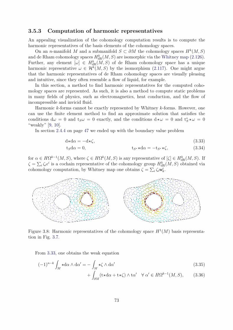
3.5.3 Computation of harmonic representatives

An appealing visualization of the cohomology computation results is to compute theharmonic representatives of the basis elements of the cohomology spaces.

On an n-manifold M and a submanifold S ⊂ ∂M the cohomology spaces Hk(M,S)and de Rham cohomology spaces Hk

dR(M,S) are isomorphic via the Whitney map (2.126).Further, any element [ω] ∈ Hk

dR(M,S) of de Rham cohomology space has a uniqueharmonic representative ω ∈ Hk(M,S) by the isomorphism (2.117). One might arguethat the harmonic representatives of de Rham cohomology spaces are visually pleasingand intuitive, since they often resemble a flow of liquid, for example.

In this section, a method to find harmonic representatives for the computed coho-mology spaces are represented. As such, it is also a method to compute static problemsin many fields of physics, such as electromagnetics, heat conduction, and the flow ofincompressible and invicid fluid.

Harmonic k-forms cannot be exactly represented by Whitney k-forms. However, onecan use the finite element method to find an approximate solution that satisfies theconditions dω = 0 and tSω = 0 exactly, and the conditions d⋆ω = 0 and t∗

S ⋆ω = 0“weakly” [9, 10].

In section 2.4.4 on page 47 we ended up with the boundary value problem

d⋆dα = −d⋆ζ, (3.33)

tSdα = 0, tS∗⋆dα = −tS∗⋆ζ, (3.34)

for α ∈ HΩk−1(M,S), where ζ ∈ HΩk(M,S) is any representative of [ζ] ∈ HkdR(M,S). If

ζ =∑

i ζiǫi is a cochain representative of the cohomology group Hk

dR(M,S) obtained viacohomology computation, by Whitney map one obtains ζ =

∑

i ζiwik.

Figure 3.8: Harmonic representatives of the cohomology space H1(M) basis representa-tion in Fig. 3.7.

From 3.33, one obtains the weak equation

(−1)n−k∫

M⋆dα ∧ dα′ =−

∫

M⋆ζ ∧ dα′ (3.35)

+∫

∂M(t⋆dα+ t⋆ζ) ∧ tα′ ∀ α′ ∈ HΩk−1(M,S), (3.36)

73

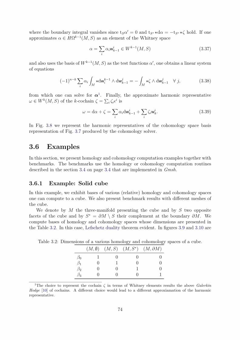
where the boundary integral vanishes since tSα′ = 0 and tS∗ ⋆dα = −tS∗ ⋆ζ hold. If one

approximates α ∈ HΩk−1(M,S) as an element of the Whitney space

α =∑

i

αiwik−1 ∈ W k−1(M,S) (3.37)

and also uses the basis of W k−1(M,S) as the test functions α′, one obtains a linear systemof equations

(−1)n−k∑

i

αi

∫

M⋆dw

k−1i ∧ dw

jk−1 = −

∫

M⋆ζ ∧ dw

jk−1 ∀ j, (3.38)

from which one can solve for α1. Finally, the approximate harmonic representativeω ∈W k(M,S) of the k-cochain ζ =

∑

i ζiǫi is

ω = dα+ ζ =∑

i

αidwik−1 +

∑

i

ζiwik. (3.39)

In Fig. 3.8 we represent the harmonic representatives of the cohomology space basisrepresentation of Fig. 3.7 produced by the cohomology solver.

3.6 Examples

In this section, we present homology and cohomology computation examples together withbenchmarks. The benchmarks use the homology or cohomology computation routinesdescribed in the section 3.4 on page 3.4 that are implemented in Gmsh.

3.6.1 Example: Solid cube

In this example, we exhibit bases of various (relative) homology and cohomology spacesone can compute to a cube. We also present benchmark results with different meshes ofthe cube.

We denote by M the three-manifold presenting the cube and by S two oppositefacets of the cube and by S∗ = ∂M \ S their complement at the boundary ∂M . Wecompute bases of homology and cohomology spaces whose dimensions are presented inthe Table 3.2. In this case, Lefschetz duality theorem evident. In figures 3.9 and 3.10 are

Table 3.2: Dimensions of a various homology and cohomology spaces of a cube.

(M, ∅) (M,S) (M,S∗) (M,∂M)

β0 1 0 0 0β1 0 1 0 0β2 0 0 1 0β3 0 0 0 1

1The choice to represent the cochain ζ in terms of Whitney elements results the above Galerkin

Hodge [10] of cochains. A different choice would lead to a different approxiamation of the harmonicrepresentative.

74

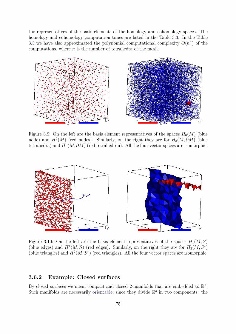
the representatives of the basis elements of the homology and cohomology spaces. Thehomology and cohomology computation times are listed in the Table 3.3. In the Table3.3 we have also approximated the polynomial computational complexity O(nα) of thecomputations, where n is the number of tetrahedra of the mesh.

Figure 3.9: On the left are the basis element representatives of the spaces H0(M) (bluenode) and H0(M) (red nodes). Similarly, on the right they are for H3(M,∂M) (bluetetrahedra) and H3(M,∂M) (red tetrahedron). All the four vector spaces are isomorphic.

Figure 3.10: On the left are the basis element representatives of the spaces H1(M,S)(blue edges) and H1(M,S) (red edges). Similarly, on the right they are for H2(M,S∗)(blue triangles) and H2(M,S∗) (red triangles). All the four vector spaces are isomorphic.

3.6.2 Example: Closed surfaces

By closed surfaces we mean compact and closed 2-manifolds that are embedded to R3.

Such manifolds are necessarily orientable, since they divide R3 in two components: the

75

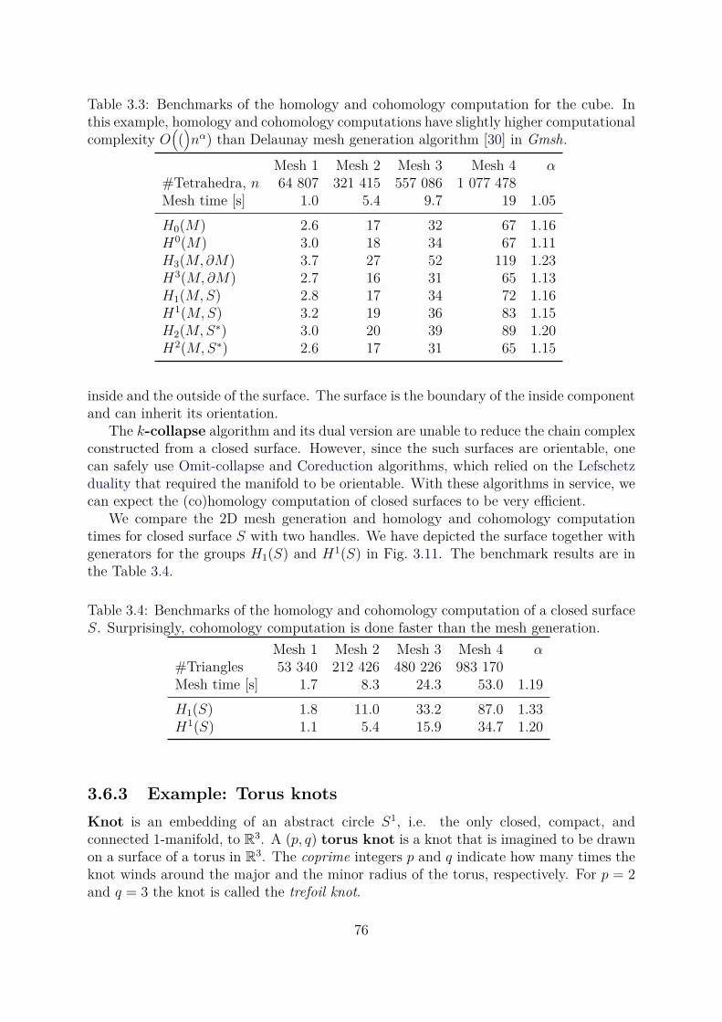
Table 3.3: Benchmarks of the homology and cohomology computation for the cube. Inthis example, homology and cohomology computations have slightly higher computationalcomplexity O

(

()

nα) than Delaunay mesh generation algorithm [30] in Gmsh.

Mesh 1 Mesh 2 Mesh 3 Mesh 4 α#Tetrahedra, n 64 807 321 415 557 086 1 077 478Mesh time [s] 1.0 5.4 9.7 19 1.05

H0(M) 2.6 17 32 67 1.16H0(M) 3.0 18 34 67 1.11H3(M,∂M) 3.7 27 52 119 1.23H3(M,∂M) 2.7 16 31 65 1.13H1(M,S) 2.8 17 34 72 1.16H1(M,S) 3.2 19 36 83 1.15H2(M,S∗) 3.0 20 39 89 1.20H2(M,S∗) 2.6 17 31 65 1.15

inside and the outside of the surface. The surface is the boundary of the inside componentand can inherit its orientation.

The k-collapse algorithm and its dual version are unable to reduce the chain complexconstructed from a closed surface. However, since the such surfaces are orientable, onecan safely use Omit-collapse and Coreduction algorithms, which relied on the Lefschetzduality that required the manifold to be orientable. With these algorithms in service, wecan expect the (co)homology computation of closed surfaces to be very efficient.

We compare the 2D mesh generation and homology and cohomology computationtimes for closed surface S with two handles. We have depicted the surface together withgenerators for the groups H1(S) and H1(S) in Fig. 3.11. The benchmark results are inthe Table 3.4.

Table 3.4: Benchmarks of the homology and cohomology computation of a closed surfaceS. Surprisingly, cohomology computation is done faster than the mesh generation.

Mesh 1 Mesh 2 Mesh 3 Mesh 4 α#Triangles 53 340 212 426 480 226 983 170Mesh time [s] 1.7 8.3 24.3 53.0 1.19

H1(S) 1.8 11.0 33.2 87.0 1.33H1(S) 1.1 5.4 15.9 34.7 1.20

3.6.3 Example: Torus knots

Knot is an embedding of an abstract circle S1, i.e. the only closed, compact, andconnected 1-manifold, to R

3. A (p, q) torus knot is a knot that is imagined to be drawnon a surface of a torus in R

3. The coprime integers p and q indicate how many times theknot winds around the major and the minor radius of the torus, respectively. For p = 2and q = 3 the knot is called the trefoil knot.

76

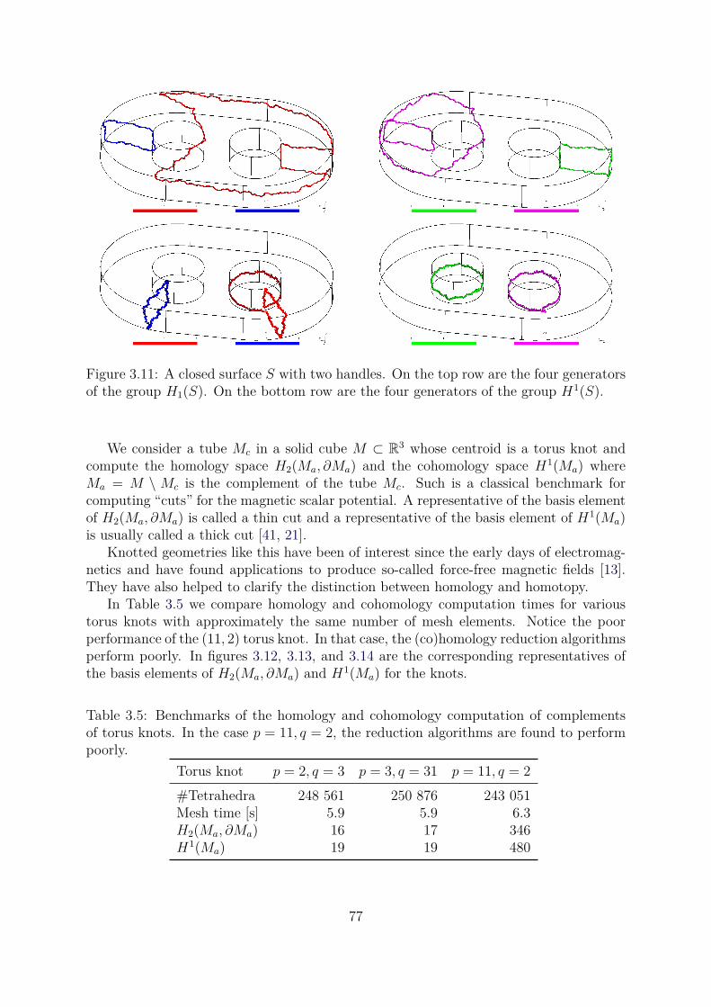
Figure 3.11: A closed surface S with two handles. On the top row are the four generatorsof the group H1(S). On the bottom row are the four generators of the group H1(S).

We consider a tube Mc in a solid cube M ⊂ R3 whose centroid is a torus knot and

compute the homology space H2(Ma, ∂Ma) and the cohomology space H1(Ma) whereMa = M \ Mc is the complement of the tube Mc. Such is a classical benchmark forcomputing “cuts” for the magnetic scalar potential. A representative of the basis elementof H2(Ma, ∂Ma) is called a thin cut and a representative of the basis element of H1(Ma)is usually called a thick cut [41, 21].

Knotted geometries like this have been of interest since the early days of electromag-netics and have found applications to produce so-called force-free magnetic fields [13].They have also helped to clarify the distinction between homology and homotopy.

In Table 3.5 we compare homology and cohomology computation times for varioustorus knots with approximately the same number of mesh elements. Notice the poorperformance of the (11, 2) torus knot. In that case, the (co)homology reduction algorithmsperform poorly. In figures 3.12, 3.13, and 3.14 are the corresponding representatives ofthe basis elements of H2(Ma, ∂Ma) and H1(Ma) for the knots.

Table 3.5: Benchmarks of the homology and cohomology computation of complementsof torus knots. In the case p = 11, q = 2, the reduction algorithms are found to performpoorly.

Torus knot p = 2, q = 3 p = 3, q = 31 p = 11, q = 2

#Tetrahedra 248 561 250 876 243 051Mesh time [s] 5.9 5.9 6.3H2(Ma, ∂Ma) 16 17 346H1(Ma) 19 19 480

77

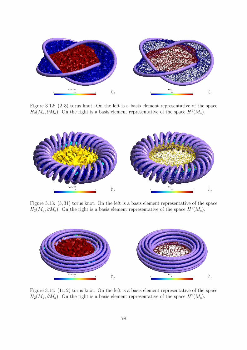
Figure 3.12: (2, 3) torus knot. On the left is a basis element representative of the spaceH2(Ma, ∂Ma). On the right is a basis element representative of the space H1(Ma).

Figure 3.13: (3, 31) torus knot. On the left is a basis element representative of the spaceH2(Ma, ∂Ma). On the right is a basis element representative of the space H1(Ma).

Figure 3.14: (11, 2) torus knot. On the left is a basis element representative of the spaceH2(Ma, ∂Ma). On the right is a basis element representative of the space H2(Ma).

78

Chapter 4

Application of cohomology in the

finite element method for

electromagnetics

In electrical engineering, field problems are often coupled to circuit problems. Then, itis convenient to drive a static or quasistatic field problem with net quantities, that serveas the state variables of the circuit. For example, such net quantities can be a voltagedifference between terminals or a net current through a terminal. Or, there may be aspecific relation between the current and the voltage which is specified by the circuitproblem.

In such situation to drive the problem with specific electric field or current densitydistribution is not justified, as the information of how they are distributed is not pro-vided by the circuit model. Instead, one assumes that the terminals are perfect electricconductors and that elsewhere there is a perfect insulation of electric current.

The perceived difficulty to drive an electromagnetic field problem with net quanti-ties depends on the chosen potential formulation. For example, in static electrokineticproblem with electric scalar potential formulation it is almost imminent how to drivethe problem with a voltage difference. The method to drive it with current is bit moretedious to implement, and the electric vector potential formulation takes the issue to awhole new level.

At first sight, it seems that each formulation and each driving quantity has its own setof tricks that one can use. However, differential forms and their relation to the homologyand the cohomology are able to provide a general framework where the symmetry betweendifferent potential formulations and drive quantities is clearly exposed.

In this chapter, it is described how electromagnetic boundary value problems can beformulated and solved by exploiting the homology and cohomology computation, andtheir link to the theory of harmonic forms. Similar formulations, with an emphasis onthe eddy current problems, have been considered in a wealth of publications [15, 41, 17,16, 40, 55, 33].

79

4.1 Electromagnetic modeling

The classical electromagnetic theory is summarized by Maxwell’s equations in the Eu-clidean 3-space E

3:∫

∂Σe = −∂t

∫

Σb ∀ Σ,

∫

∂Ωb = 0 ∀ Ω, (4.1)

∫

∂Σh =

∫

Σj + ∂t

∫

Σd ∀ Σ,

∫

∂Ωd =

∫

Ωρ ∀ Ω, (4.2)

(4.3)

and pointwise constitutive equations

d = ⋆ǫe, b = ⋆µh, j = ⋆σe. (4.4)

The differential 1-forms e and h are called electric field and magnetic field intensity,respectively. The differential 2-forms b, d, and j are called magnetic flux density, electricflux density and current density, respectively. The differential 3-form ρ is called electriccharge density. The material operators ǫ, µ, and σ that map 1-forms to 1-forms are calledpermittivity, permeability, and conductivity, respectively. The surface Σ and the volumeΩ are any 2-dimensional and 3-dimensional submanifolds of E3.

In electromagnetic modeling, one is often not concerned about the electromagneticfields in all E3. Instead, one often chooses an submanifold M ⊂ E

3, with boundary ∂Mon which to set up a boundary value problem. By the generalized Stokes’ theorem, theMaxwell’s integral equations can be converted into partial differential equations in M .For modeling purposes, the manifold M does not need to be explicitly a subset of theEuclidean 3-space, but an oriented compact Riemannian manifold (M, g) with any metrictensor g.

Also, the dimension ofM may be less than 3 based on arguments about the symmetriesof the problem. However in this chapter, for the sake of clarity and to exploit the intuitionof an electrical engineer, we set the dimension of M equal to 3.

The price to pay for the truncation of the modeling domain is to define the boundaryconditions and the emergence of cohomology in the problem domain. In a large class ofelectromagnetic boundary value problems, the unknown field, or a component of it, isa harmonic field. Harmonic 1-, and 2-forms on a 3-manifold correspond to vector fieldsthat are both irrotational and solenoidal. In addition, on complementary parts of theboundary of the domain, the tangential and the normal components of a irrotational andsolenoidal vector field vanish.

Since the space of harmonic forms is isomorphic to de Rham cohomology space, theunknown field is not uniquely determined until one has fixed a number of coefficientsthat is equal to the dimension of de Rham cohomology space. That is, one has to choosea solution from a finite dimensional vector space. We call the choice an elementfrom de Rham cohomology space the cohomology condition of the boundaryvalue problem.

This chapter describes how cohomology conditions can be imposed in a large classof electromagnetic boundary value problems. Specifically, we exploit the homology andcohomology computation results to construct cohomology basis functions for the finiteelement method.

80

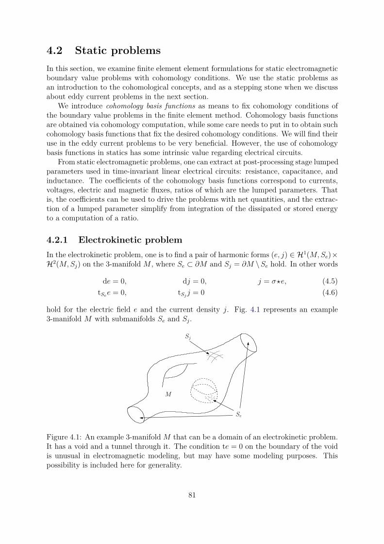
4.2 Static problems

In this section, we examine finite element element formulations for static electromagneticboundary value problems with cohomology conditions. We use the static problems asan introduction to the cohomological concepts, and as a stepping stone when we discussabout eddy current problems in the next section.

We introduce cohomology basis functions as means to fix cohomology conditions ofthe boundary value problems in the finite element method. Cohomology basis functionsare obtained via cohomology computation, while some care needs to put in to obtain suchcohomology basis functions that fix the desired cohomology conditions. We will find theiruse in the eddy current problems to be very beneficial. However, the use of cohomologybasis functions in statics has some intrinsic value regarding electrical circuits.

From static electromagnetic problems, one can extract at post-processing stage lumpedparameters used in time-invariant linear electrical circuits: resistance, capacitance, andinductance. The coefficients of the cohomology basis functions correspond to currents,voltages, electric and magnetic fluxes, ratios of which are the lumped parameters. Thatis, the coefficients can be used to drive the problems with net quantities, and the extrac-tion of a lumped parameter simplify from integration of the dissipated or stored energyto a computation of a ratio.

4.2.1 Electrokinetic problem

In the electrokinetic problem, one is to find a pair of harmonic forms (e, j) ∈ H1(M,Se)×H2(M,Sj) on the 3-manifold M , where Se ⊂ ∂M and Sj = ∂M \Se hold. In other words

de = 0, dj = 0, j = σ⋆e, (4.5)

tSee = 0, tSj

j = 0 (4.6)

hold for the electric field e and the current density j. Fig. 4.1 represents an example3-manifold M with submanifolds Se and Sj.

Sj

Se

M

Figure 4.1: An example 3-manifold M that can be a domain of an electrokinetic problem.It has a void and a tunnel through it. The condition te = 0 on the boundary of the voidis unusual in electromagnetic modeling, but may have some modeling purposes. Thispossibility is included here for generality.

81

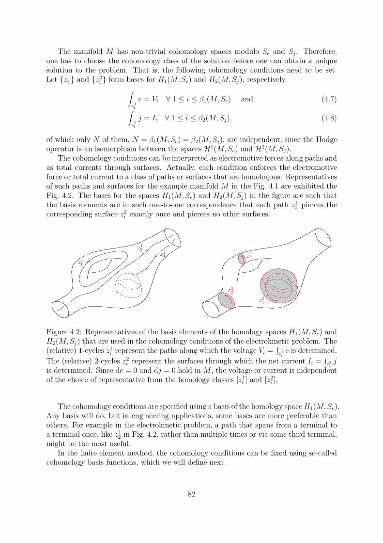
The manifold M has non-trivial cohomology spaces modulo Se and Sj. Therefore,one has to choose the cohomology class of the solution before one can obtain a uniquesolution to the problem. That is, the following cohomology conditions need to be set.Let z1

i and z2i form bases for H1(M,Se) and H2(M,Sj), respectively.

∫

z1i

e = Vi ∀ 1 ≤ i ≤ β1(M,Se) and (4.7)∫

z2i

j = Ii ∀ 1 ≤ i ≤ β2(M,Sj), (4.8)

of which only N of them, N = β1(M,Se) = β2(M,Sj), are independent, since the Hodgeoperator is an isomorphism between the spaces H1(M,Se) and H2(M,Sj).

The cohomology conditions can be interpreted as electromotive forces along paths andas total currents through surfaces. Actually, each condition enforces the electromotiveforce or total current to a class of paths or surfaces that are homologous. Representativesof such paths and surfaces for the example manifold M in the Fig. 4.1 are exhibited theFig. 4.2. The bases for the spaces H1(M,Se) and H2(M,Sj) in the figure are such thatthe basis elements are in such one-to-one correspondence that each path z1

i pierces thecorresponding surface z2

i exactly once and pierces no other surfaces.

z1

1

z1

2

z1

3

z2

3

z2

1

z2

2

Figure 4.2: Representatives of the basis elements of the homology spaces H1(M,Se) andH2(M,Sj) that are used in the cohomology conditions of the electrokinetic problem. The(relative) 1-cycles z1

i represent the paths along which the voltage Vi =∫

z1ie is determined.

The (relative) 2-cycles z2i represent the surfaces through which the net current Ii =

∫

z2ij

is determined. Since de = 0 and dj = 0 hold in M , the voltage or current is independentof the choice of representative from the homology classes [z1

i ] and [z2i ].

The cohomology conditions are specified using a basis of the homology spaceH1(M,Se).Any basis will do, but in engineering applications, some bases are more preferable thanothers. For example in the electrokinetic problem, a path that spans from a terminal toa terminal once, like z1

2 in Fig. 4.2, rather than multiple times or via some third terminal,might be the most useful.

In the finite element method, the cohomology conditions can be fixed using so-calledcohomology basis functions, which we will define next.

82

4.2.2 Cohomology basis functions

Given a finite element mesh of a manifold M , the elements of de Rham cohomologyspace Hk

dR(M,S) can be represented using the Whitney forms. To be able to fix thecohomology conditions of boundary value problem in a unified manner, we will definecohomology basis functions as integer combinations of Whitney forms for the task.

In the finite element method, the ordinary basis functions have associated coefficients,some of which are fixed in advance as Dirichlet conditions and some of which are degreesof freedom of the problem.

Similarly to the cohomology basis functions we associate coefficients that can be in-terpreted as net quantities such as current or voltage, i.e. as the cohomology conditions.Ratios of the coefficients can be used to determine lumped parameters, for example theresistance.

The coefficients can either be fixed in advance, or be a part of the finite elementsolution of the problem. Thus in the formulations, as we shall see, they behave much likeDirichlet and Neumann boundary conditions in the conventional finite element methodfor scalar fields.

Definition and properties

Let M be a 3-manifold and S ⊂ ∂M its 2-submanifold. Let ζ i =∑

j ζijǫ

j ∈ Ck(M,S)(see section 2.3.2 on page 40) be a k-cocycle so that [ζ i] ∈ Hk(M,S) holds. We defineCohomology basis function W

ik associated with ζ i as

Wik := w(ζ i) =

∑

j

ζ ijw

jk ∈ W k(M,S). (4.9)

That is, to construct cohomology basis functions one has to compute a basis of Hk(M,S)and interpolate the basis elements by the Whitney map w of section 2.4.5 on page 48.

Usually, the integer coefficient vector ζi produced by the cohomology solver is sparse,i.e. the cohomology generators have a limited support within the manifold. Therefore,the use of cohomology basis functions in the finite element method does not fill the systemmatrix dramatically. Rather, each of them produces a dense block with a couple of denserows and columns.

The cohomology basis functions span a subspace of W k(M,S) that we denote by

HW k(M,S) := Wk ∈ W k(M,S) | [Wk] ∈ HkdR(M,S). (4.10)

Now, if [ζ1], [ζ2], . . . , [ζβ1(M,S)] forms a basis for the cohomology space Hk(M,S), thecosets of cohomology basis functions [W1

k], [W2k], . . . , [Wβk(M,S)

k ] form a basis for deRham cohomology space Hk

dR(M,S). If [ζ1], [ζ2], . . . , [ζβk(M,S)] was a cobasis of a basis[z1], [z2], . . . , [zβj(M,S)] of Hk(M,S), the associated de Rham cohomology basis functionssatisfy

∫

zi

Wjk = δj

i ∀ 1 ≤ i, j ≤ βk(M,S), (4.11)

i.e. they form de Rham cohomology cobasis for the basis of Hk(M,S).For clarity, later in this chapter we shall denote Whitney 0-, 1-, and 2-forms with n,

e, and f, respectively, and cohomology basis functions with N, E, and F, respectively.

83

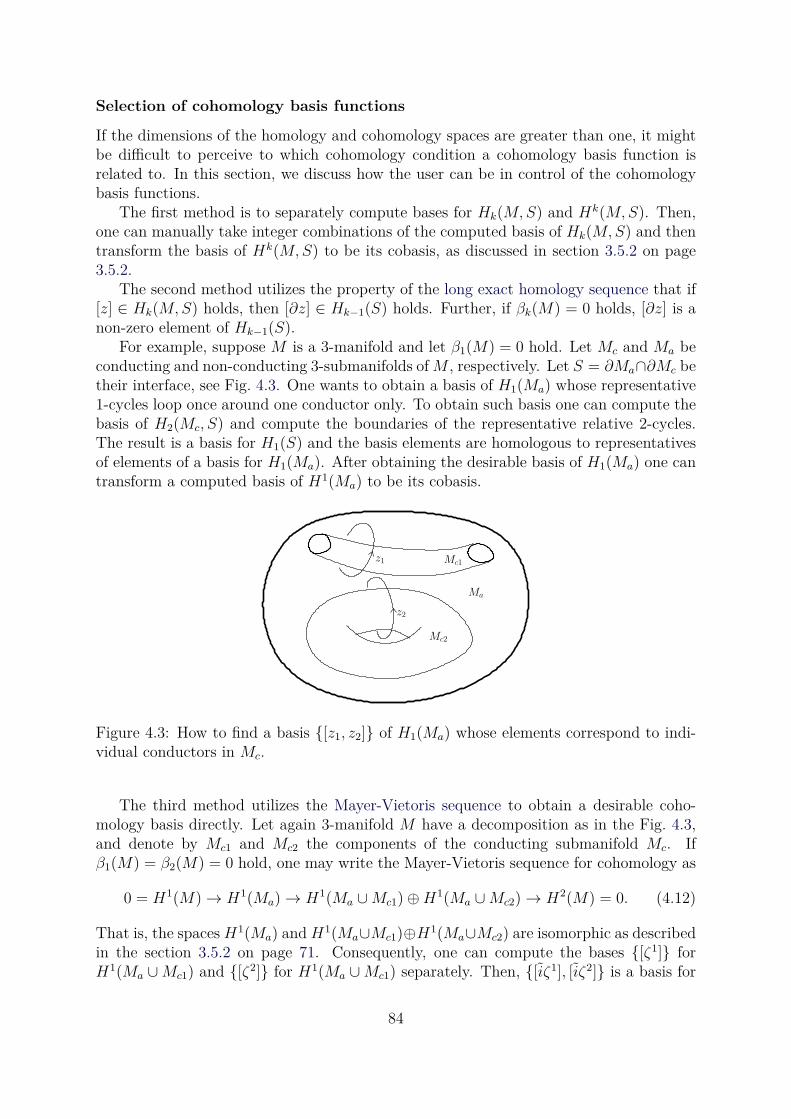
Selection of cohomology basis functions

If the dimensions of the homology and cohomology spaces are greater than one, it mightbe difficult to perceive to which cohomology condition a cohomology basis function isrelated to. In this section, we discuss how the user can be in control of the cohomologybasis functions.

The first method is to separately compute bases for Hk(M,S) and Hk(M,S). Then,one can manually take integer combinations of the computed basis of Hk(M,S) and thentransform the basis of Hk(M,S) to be its cobasis, as discussed in section 3.5.2 on page3.5.2.

The second method utilizes the property of the long exact homology sequence that if[z] ∈ Hk(M,S) holds, then [∂z] ∈ Hk−1(S) holds. Further, if βk(M) = 0 holds, [∂z] is anon-zero element of Hk−1(S).

For example, suppose M is a 3-manifold and let β1(M) = 0 hold. Let Mc and Ma beconducting and non-conducting 3-submanifolds ofM , respectively. Let S = ∂Ma∩∂Mc betheir interface, see Fig. 4.3. One wants to obtain a basis of H1(Ma) whose representative1-cycles loop once around one conductor only. To obtain such basis one can compute thebasis of H2(Mc, S) and compute the boundaries of the representative relative 2-cycles.The result is a basis for H1(S) and the basis elements are homologous to representativesof elements of a basis for H1(Ma). After obtaining the desirable basis of H1(Ma) one cantransform a computed basis of H1(Ma) to be its cobasis.

z1

z2

Mc1

Mc2

Ma

Figure 4.3: How to find a basis [z1, z2] of H1(Ma) whose elements correspond to indi-vidual conductors in Mc.

The third method utilizes the Mayer-Vietoris sequence to obtain a desirable coho-mology basis directly. Let again 3-manifold M have a decomposition as in the Fig. 4.3,and denote by Mc1 and Mc2 the components of the conducting submanifold Mc. Ifβ1(M) = β2(M) = 0 hold, one may write the Mayer-Vietoris sequence for cohomology as

0 = H1(M)→ H1(Ma)→ H1(Ma ∪Mc1)⊕H1(Ma ∪Mc2)→ H2(M) = 0. (4.12)

That is, the spaces H1(Ma) and H1(Ma∪Mc1)⊕H1(Ma∪Mc2) are isomorphic as describedin the section 3.5.2 on page 71. Consequently, one can compute the bases [ζ1] forH1(Ma ∪Mc1) and [ζ2] for H1(Ma ∪Mc1) separately. Then, [iζ1], [iζ2] is a basis for

84

the space H1(Ma), where i is the corresponding inclusion map from Ma to Ma ∪ Mc1

or Ma ∪Mc1. In such basis, each basis element corresponds to just one conductor. Byinduction, this generalizes to any finite number of conductors in M .

4.2.3 Electric field -conforming formulation

In the electric field conforming formulation, we seek to satisfy de = 0 and tSee = 0

exactly, and dj = 0 and tSjj = 0 in the weak sense. That is, the sought solution is such

that [e] ∈ H1dR(M,Se) holds. The conditions de = 0 and tSe

e = 0 are satisfied by

e =∑

σ0i∈M\Se

ϕidni +

β1(M,Se)∑

i=1

ViEi ∈ W 1(M,Se), (4.13)

where the cohomology basis functions are of the form Ei ∈ HW 1(M,Se), i.e. [Ei] span

H1dR(M,Se).The support of the nodal basis functions n does not cover Se to not fix the

cohomology condition with them, but to leave the task completely for the cohomologybasis functions.

This approximation for e deviates from the conventional finite element method, wheree fully given in terms of Whitney 0-forms. However, our choice allows one to assign moregeneral cohomology conditions on e when M contains tunnels. Such cohomology condi-tions correspond to induced electromotive forces around the tunnel, or circuit terminalsthat are not otherwise apparent in the finite element model.

Now, if one requires that

∫

M⋆σe ∧ e′ =

0 when e′ = dni

Ii when e′ = Ei∀ e′ ∈ dn

i,Ei (4.14)

holds, the j-side conditions in (4.5) and (4.6), dj = d⋆σe = 0 and tSjj = tSj

⋆σe = 0, aresatisfied weakly, since

0 =∫

M⋆σe ∧ dn

i =∫

Md⋆ σe ∧ n

i −∫

Sj

t⋆σe ∧ tni ∀ ni (4.15)

holds. By plugging (4.13) into (4.14), one obtains a linear system with blocks[

∫

M ⋆σdn ∧ dn∫

M ⋆σE ∧ dn∫

M ⋆σdn ∧ E∫

M ⋆σE ∧ E

] [

ϕ

V

]

=

[

0

I

]

. (4.16)

From this it is evident that the system matrix is symmetric and positive-definite. If onefixes all the coefficients Vi, the system reduces to

[

∫

M ⋆σdn ∧ dn

] [

ϕ]

= −[

∫

M ⋆σE ∧ dn

] [

V]

. (4.17)

From the solution to this linear system, one obtains an approximation of e ∈ H1(M,Se)that satisfies the voltage cohomology conditions in (4.7) for the chosen cohomology basisfunctions E

i. The currents I can then be computed from the equation (4.16).On the other hand, if one fixes all the coefficients Ii, the equation (4.14) reads

Ii =∫

M⋆σe ∧ E

i =∫

Mj ∧ E

i =∫

z2i

j ∀ 1 ≤ i ≤ β2(M,Sj), [z2i ] ∈ H2(M,Sj) (4.18)

85

where the last equality holds by the properties of cup product of cohomology [48]. Thatis, the current cohomology conditions in (4.7) are satisfied.

In the general case, but assuming M is connected, one must fix a total of N voltagesand currents to obtain a unique solution to the electrokinetic problem (4.5) - (4.7), whereN = β1(M,Se) = β2(M,Sj) hold. Otherwise one ends up with under- or over-determinedsystem of equations. If M is not connected, the above statement hold for each connectedcomponent of M separately.

If β1(M) = 0 holds, this formulation reduces to the “traditional” scalar finite elementmethod. To see this, let [z1] ∈ H1(M,Se) hold. By the long exact homology sequence,0 6= ∂∗[z1] = [z0] ∈ H0(Se) holds. Then, the approximate solution of e ∈ H1(M,Se) canbe expressed as an exterior derivative of a scalar potential

ϕ =∑

σ0i∈M\Se

ϕini +

β1(Se)−β0(M)∑

i=1

ViNi ∈ W 0(M), (4.19)

where the cohomology basis functions Ni ∈ W 0(M) and satisfy [tNi] ∈ H0

dR(Se). In thiscase, not the full basis of H0

dR(Se) is used, but just such basis functions that have non-zeroimage in H1

dR(M,Se). Since tdNi = 0 holds, te = tdϕ = 0 holds. That is, e ∈W 1(M,Se).

Now, by requiring

∫

M⋆σdϕ ∧ dϕ′ =

0 when ϕ′ = ni

Ii when ϕ′ = Ni∀ ϕ′ ∈ ni,Ni (4.20)

to hold, the j-side conditions in (4.5) and (4.6) are satisfied weakly, as well as the coho-mology conditions (4.7) are satisfied similarly to the previous, more general case.

Actually, this strictly nodal method is also applicable when β1(M) 6= 0 holds, butthen the cohomology conditions that regard the elements of H1(M) are implicitly set tozero. That is, there can be no non-zero electromotive force around any tunnel of M . Thisis the shortcoming of the traditional choice of nodal basis functions only.

4.2.4 Current density -conforming formulation

In the current density conforming formulation, we seek to satisfy dj = 0 and tSjj = 0

exactly, and de = 0 and tSee in the weak sense. That is, the sought solution is such that

[j] ∈ H2dR(M,Sj) holds. The conditions dj = 0 and tSj

j = 0 are satisfied by

j =∑

σ1i∈M\Sj

tidei +

β2(M,Sj)∑

i=1

IiFi ∈W 2(M,Sj), (4.21)

where the cohomology basis functions are of the form Fi ∈ HW 2(M,Sj), i.e. [Fi] span

∈ H2dR(M,Sj). Again, the support of the edge basis functions e do not cover Sj in order

to leave the cohomology condition to be fixed by the cohomology basis functions.We require that

∫

Mσ−1⋆ j ∧ j′ =

0 when j′ = dei

Vi when j′ = Fi∀ j′ ∈ de

i,Fi (4.22)

86

hold. Then, the e-side conditions de = dσ−1⋆j = 0 and tSee = tσ−1⋆j = 0 in (4.5) and

(4.6) are satisfied weakly, since

0 =∫

Mσ−1⋆ j ∧ de

i = −∫

Mdσ−1⋆ j ∧ e

i +∫

Se

tσ−1⋆ j ∧ tei ∀ ei (4.23)

holds. By plugging (4.21) in (4.22) one obtains a linear system with blocks[

∫

M σ−1⋆de ∧ de∫

M σ−1⋆F ∧ de∫

M σ−1⋆de ∧ F∫

M σ−1⋆F ∧ F

] [

t

I

]

=

[

0

V

]

(4.24)

If all the coefficients Ii are fixed, this reduces to[

∫

M σ−1⋆de ∧ de

] [

t]

= −[

∫

M σ−1⋆F ∧ de

] [

I]

(4.25)

As a solution, one obtains such j ∈ H2(M,Sj) that satisfies the current cohomologyconditions in (4.7) for the chosen cohomology basis functions F

i. By fixing all the coeffi-cients Vi instead, one obtains a solution that satisfies the voltage cohomology conditionsin (4.7), since

Vi =∫

Mσ−1⋆j ∧ F

i =∫

Me ∧ F

i =∫

z1i

e ∀ 1 ≤ i ≤ β1(M,Se), [z1i ] ∈ H1(M,Se), (4.26)

holds by the equation (4.22) and by the properties of the cup product of cohomology.Again in the general case, one can fix either Vi or Ii from each pair (Vi, Ii), but not

both, to obtain an unique solution to the electrokinetic problem (4.5) - (4.7).In the special case that β2(M) = 0 holds, one can impose the cohomology conditions

(4.7) from the boundary Sj ⊂ ∂M . This is analogous to the traditional electric field ori-ented formulation, where the cohomology conditions were imposed from to the boundarySe ⊂ ∂M using the cohomology basis functions of H0

dR(Se). Such basis functions can beobtained simply by summing up all the Whitney 0-forms associated with the 0-cells ofeach connected component of Se

However, in the current density conforming formulation the situation is a bit morecomplicated, since the cohomology basis functions of H1

dR(Sj) are not so simple to pro-duce, but full scale cohomology computation on a 2-manifold is needed.

So, let β2(M) = 0 and [z2] ∈ H2(M,Sj) hold. By the long exact homology sequence,0 6= ∂∗[z2] = [z1] ∈ H1(Sj) holds. An approximate solution of j ∈ Hk(M,Sj) can beexpressed as an exterior derivative of a 1-form

t =∑

σ1i∈M\Sj

tiei +

β1(Sj)−β1(M)∑

i=1

IiEi ∈W 1(M), (4.27)

where the cohomology basis functions Ei ∈ W 1(M) and satisfy [tEi] ∈ H1

dR(Sj). Again,not the full basis of H1

dR(Sj) is used, bust just the ones that have non-zero image inH2

dR(M,Sj). Since tSjdE

i = 0 holds, tSjj = tdt = 0 holds, i.e. j ∈W 2(M,Sj).

We require that

∫

Mσ−1⋆ dt ∧ dt′ =

0 when t′ = ei

Vi when t′ = Ei∀ t′ ∈ ei,Ei (4.28)

87

hold. Then, the e-side conditions and in (4.5) and (4.6) are satisfied weakly, as well asthe cohomology conditions (4.7) are satisfied similarly to the previous, more general case.

Again, this method is applicable when β2(M) 6= 0 holds, but then the cohomologyconditions regarding the elements of H2(M) are implicitly set to zero. That is, therecannot be a current source inside any void of M .

4.2.5 Electrostatic problem

The electrostatic problem generalizes the electrokinetic problem on two respects. First,there can be a source term, and second, a non-homogeneous boundary condition.

In the electrostatic problem, one is to find a pair of non-harmonic forms (e, d) ∈Ω1(M)× Ω2(M) on the 3-manifold M that satisfy

de = 0, dd = ρ, d = ǫ⋆e, (4.29)

tSee = 0, tSd

d = σ (4.30)

for the electric field e and the electric flux density d. The 3-form ρ stands for the chargedensity in M and the 2-form σ stands for the surface charge density on Sd. As usual,Se ⊂ ∂M and Sd = ∂M \ Se hold. If the problem is source-free and has homogeneousboundary conditions, i.e. dd = ρ = 0 and tSd

d = σ hold, one is back to the harmonic caseand can exploit the cohomology basis functions exactly as in the electrokinetic problem.

In the case where dd = ρ 6= 0 or tSdd = σ 6= 0 holds, one can use an electric

field conforming formulation with cohomology conditions. We impose the cohomologycondition only on the closed and trace-free part of d. That is, we decompose d = dz + ds,where ddz = 0, tSd

dz = 0, dds = ρ, and tSdds = σ hold. The cohomology conditions are

∫

z1i

e = Vi ∀ [z1i ] ∈ H1(M,Se), and

∫

z2i

dz = Qi ∀ [z2i ] ∈ H2(M,Sd), (4.31)

of which only β1(M,Se) = β2(M,Sd) are independent. The rest are determined as apart of the solution to the problem. These cohomology conditions can be interpreted asvoltages on the terminals and net electric fluxes through the terminals.

We solve for an electric field e = dϕ ∈ HΩ1(M,Se) using a scalar potential ϕ ∈HΩ1(M):

ϕ =∑

σ0i∈M\Se

ϕini +

β0(Se)−β1(M)∑

i=1

ViNi ∈ W 0(M), (4.32)

where the cohomology basis functions Ni ∈W 0(Se) satisfy [Ni] ∈ H0

dR(Se).By requiring that

∫

M⋆ǫdϕ ∧ dϕ′ =

− ∫

M ρ ∧ ni +

∫

Sdσ ∧ tni when ϕ′ = n

i

− ∫

M ρ ∧ Ni +

∫

Sdσ ∧ N

i +Qi when ϕ′ = Ni∀ ϕ′ ∈ ni,Ni

(4.33)

hold, we get an approximate solution for the electrostatic problem (4.29) - (4.31).

88

4.2.6 Magnetostatic problem

The magnetostatic problem is analogous to the electrostatic problem. The only differenceis that now the 1-form h may have source terms instead of the 2-form b. In comparison,in the electrostatic problem the situation was other way around, as the 2-form d mighthave had source terms, and the 1-form e was assumed source-free.

In the magnetostatic problem, one is to find a pair of non-harmonic forms (h, b) ∈Ω1(M)× Ω2(M) on the 3-manifold M that satisfy

dh = j, db = 0, b = µ⋆h, (4.34)

tShh = k, tSb

b = 0 (4.35)

for the magnetic field h and the magnetic flux density b. Here 2-form j is the currentdensity in M and 1-form k is the surface current density on Sh. Again, Sh ⊂ ∂Mand Sb = ∂M \ Sh hold. If the problem is source-free and has homogeneous boundaryconditions, i.e. dh = j = 0 and tSh

h = 0 hold, one is back to the harmonic case and onecan exploit the cohomology basis functions exactly as in the electrokinetic problem.

Historically, an important special case of the source-free magnetostatic problem occurswhen Sb = ∂M hold and β1(M) = β1(M,Sh) ≥ 1 hold. That is, the problem domain ismagnetically isolated, and there are no sources of magnetic field inside the domain, yeta non-zero magnetic field can exist inside the domain. The study of such problem led tothe awareness of homology and cohomology in the electromagnetic modeling, as it wasimportant in applications. For example, in reluctance and inductance computations.

In the case where dh = j 6= 0 or tShh = k 6= 0 hold, one can use a magnetic flux

density conforming formulation with cohomology conditions. We impose the cohomologycondition only on the closed part of h. That is, we decompose h = hz +hs, where dhz = 0,dhs = j, tSh

hz = 0, and tShhs = k hold. The cohomology conditions are

∫

z2i

b = Mi ∀ [z2i ] ∈ H2(M,Sb), and

∫

z1i

hz = Ii ∀ [z1i ] ∈ H1(M,Sh), (4.36)

of which only β2(M,Sb) = β1(M,Sh) are independent. The rest are determined as a partof the solution to the problem. These cohomology conditions can be interpreted as netmagnetic fluxes through surfaces and net currents through surfaces.

We solve for an magnetic field b = da ∈ HΩ2(M,Sb) using a vector potential a ∈HΩ1(M):

a =∑

σ1i∈M\Sb

aiei +

β1(Sb)−β1(M)∑

i=1

MiEi ∈ W 1(M), (4.37)

where the cohomology basis functions Ei ∈ W 1(Sb) satisfy [Ei] ∈ H1

dR(Sb).By requiring that

∫

Mµ−1⋆da ∧ da′ =

∫

M j ∧ ei − ∫

Shk ∧ tei when a′ = e

i

∫

M j ∧ Ei − ∫

Shk ∧ E

i +Mi when a′ = Ei∀ a′ ∈ ei,Ei

(4.38)

hold, we get an approximate solution for the magnetostatic problem (4.34) - (4.36).

89

4.3 Circuit coupled eddy current problem

We consider a special case of the eddy current problem, called coupled field-circuit

problem, which can be naturally coupled to electric circuits. In addition to the magne-toquasistatic assumption, we assume that

1. On the domain boundary ∂M , electric field is closed. I.e. t∂Mde = 0 holds.

2. No magnetomotive nor electromotive forces are induced in the domain via magneticfluxes through the holes of the domain boundary, i.e. i.e.

∫

z1 e =∫

z1 h = 0 ∀ [z1] ∈H1(∂M) holds.

3. No magnetic flux or electric current emanates from the voids of M , i.e.∫

z2 j =∫

z2 b = 0 ∀ [z2] ∈ H2(∂M) holds.

That is, we have forbidden the magnetic circuit coupling and the electromagnetic wavecoupling of the problem. What is left is the electric circuit coupling.

What makes the formulations for the eddy current problem complex but also efficientto solve is that a part of the domain is assumed non-conducting. The different behaviorof the fields in the conducting and in the non-conducting subdomains makes the problemtwo coupled problems on these two subdomains. We will show that the coupling betweenthese two subdomains, as well as the coupling to the external circuit, is tightly related tothe cohomology basis functions.

4.3.1 Eddy current problem

In the circuit coupled eddy current problem on a 3-manifold M we assume that M isdivided in two parts: the conducting submanifold Mc and insulating submanifold Ma sothat M = Mc ∪Ma and Mc ∩Ma = ∂Mc ∩ ∂Ma hold. We look for a pairs of differentialforms (e, j) ∈ Ω1(Mc) × Ω2(Mc) and (h, b) ∈ Ω1(M) × Ω2(M) on a 3-manifold M thatsatisfy

de = −∂tb dj = 0 j = ⋆σe (4.39)

tSee = 0 tSj

j = 0 (4.40)

dh = j db = 0 b = ⋆µh (4.41)

t∂Mb = 0, (4.42)

where ∂Mc = Se ∪ Sj so that ∂Se = ∂Sj = Se ∩ Sj hold. In addition, require that thefollowing hold:

dh = 0 on Ma and tj = 0 on ∂Mc ∩ ∂Ma ⊂ Sj. (4.43)

That is, the insulating submanifold has no currents and the current cannot pass throughthe interface ∂Mc ∩ ∂Ma between the insulating submanifold Ma and the conductingsubmanifold Mc.

The field th is closed on Sj ∩ ∂M , since dth = tdh = 0 holds on Sj. Thus, we mayassign meaningful cohomology conditions

Vi =∫

z1i

te [z1i ] ∈ H1(∂M \ Se, ∂Se), and Ii =

∫

z1i

th [z1i ] ∈ H1(∂M \ Se).

(4.44)

90

They correspond to voltage differences Vi between the circuit terminals on Se and netcurrents Ii from terminal to terminal on Se. If Se has N connected components, we haveN − 1 independent cohomology conditions.

In the so-called Faraday’s law and Ampere’s law conforming formulations these co-homology conditions can be related to the harmonic part of the electric field in Mc andto the harmonic magnetic field in Ma. That is, they related to the basis elements of thecohomology spaces H1(Mc, Se) and H1(Ma).

The method to exploit cohomology basis functions in the formulations builds on theideas developed in the electrokinetic problem. However, since the magnetic fluxes andthe electric currents emanating from the voids of the domain were assumed not to exist,only cohomology edge basis functions are needed.

4.3.2 Faraday’s law conforming formulation

In the Faraday’s law conforming formulation we solve for the harmonic part ε ∈ H1(Mc, Se)of the electric field e and for the magnetic vector potential a ∈ HΩ1(M,∂M). Then, theeddy currents j in Mc are j = ⋆σe = ⋆σ(ε− ∂ta).

The magnetic vector potential a is approximated as

a =∑

σ1i∈M\∂M

aiei ∈W 1(M,∂M) (4.45)

and the harmonic part of the electric field is approximated as

ε = −∑

σ0i∈Mc\Se

ϕidni +

β1(Mc,Se)∑

i=1

ViEi ∈W 1(Mc, Se), (4.46)

where the coefficients Vi determine the cohomology class of [ε] ∈ H1dR(M,Se). These

approximations satisfy the boundary conditions tSee = t∂Mb = 0 and the Faraday’s and

Gauss law for e = ε − ∂ta and b = da. The rest of the boundary conditions and partialdifferential equations are to be satisfied weakly.

We require∫

Mµ−1⋆da ∧ da′ +

∫

Mc

σ⋆ε ∧ a′ −∫

Mc

⋆σ∂ta ∧ a′ = 0 ∀ a′ ∈ ei (4.47)

∫

Mc

σ⋆ε ∧ ε′ −∫

Mc

σ⋆∂ta ∧ ε′ =

0 when ε′ = dni

Ii when ε′ = Ei

∀ ε′ ∈ dni,Ei

(4.48)

The equation (4.47) enforces Ampere’s law dh = j weakly. The equation (4.48) enforcesdj = 0 and tSj

j = 0 weakly, similarly as in the electric field conforming formulation ofthe electrokinetic problem.

The cohomology class of [ε] is related to the cohomology conditions of the eddy currentproblem. The coefficients Vi of the cohomology basis functions E

i correspond to a voltagedifference when circulating around a tunnel in Mc and between terminals Se connectedby Mc. By the equation (4.48), they also relate to the net currents Ii around tunnels inMc and from terminal to terminal on Se.

91

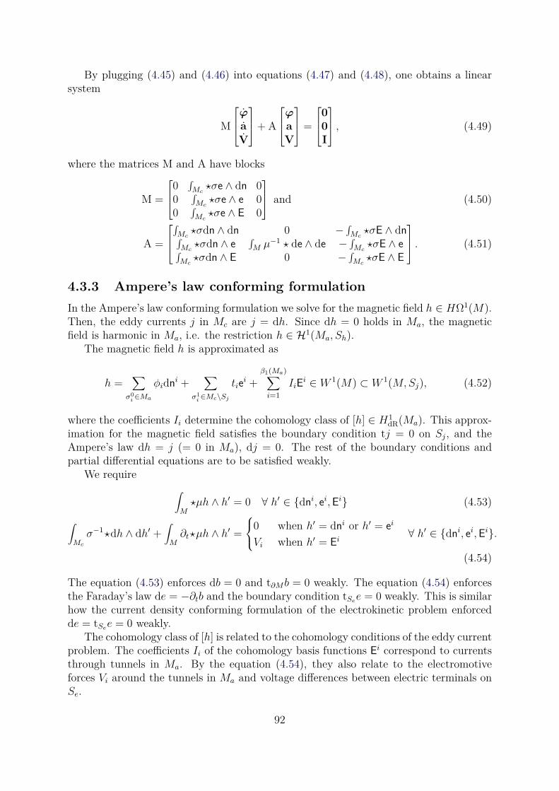
By plugging (4.45) and (4.46) into equations (4.47) and (4.48), one obtains a linearsystem

M

ϕ

a

V

+ A

ϕ

a

V

=

0

0

I

, (4.49)

where the matrices M and A have blocks

M =

0∫

Mc⋆σe ∧ dn 0

0∫

Mc⋆σe ∧ e 0

0∫

Mc⋆σe ∧ E 0

and (4.50)

A =

∫

Mc⋆σdn ∧ dn 0 − ∫

Mc⋆σE ∧ dn

∫

Mc⋆σdn ∧ e

∫

M µ−1 ⋆ de ∧ de − ∫

Mc⋆σE ∧ e

∫

Mc⋆σdn ∧ E 0 − ∫

Mc⋆σE ∧ E

. (4.51)

4.3.3 Ampere’s law conforming formulation

In the Ampere’s law conforming formulation we solve for the magnetic field h ∈ HΩ1(M).Then, the eddy currents j in Mc are j = dh. Since dh = 0 holds in Ma, the magneticfield is harmonic in Ma, i.e. the restriction h ∈ H1(Ma, Sh).

The magnetic field h is approximated as

h =∑

σ0i∈Ma

φidni +

∑

σ1i∈Mc\Sj

tiei +

β1(Ma)∑

i=1

IiEi ∈W 1(M) ⊂ W 1(M,Sj), (4.52)

where the coefficients Ii determine the cohomology class of [h] ∈ H1dR(Ma). This approx-

imation for the magnetic field satisfies the boundary condition tj = 0 on Sj, and theAmpere’s law dh = j (= 0 in Ma), dj = 0. The rest of the boundary conditions andpartial differential equations are to be satisfied weakly.

We require∫

M⋆µh ∧ h′ = 0 ∀ h′ ∈ dn

i, ei,Ei (4.53)

∫

Mc

σ−1⋆dh ∧ dh′ +∫

M∂t⋆µh ∧ h′ =

0 when h′ = dni or h′ = e

i

Vi when h′ = Ei

∀ h′ ∈ dni, ei,Ei.

(4.54)

The equation (4.53) enforces db = 0 and t∂Mb = 0 weakly. The equation (4.54) enforcesthe Faraday’s law de = −∂tb and the boundary condition tSe

e = 0 weakly. This is similarhow the current density conforming formulation of the electrokinetic problem enforcedde = tSe

e = 0 weakly.The cohomology class of [h] is related to the cohomology conditions of the eddy current

problem. The coefficients Ii of the cohomology basis functions Ei correspond to currents

through tunnels in Ma. By the equation (4.54), they also relate to the electromotiveforces Vi around the tunnels in Ma and voltage differences between electric terminals onSe.

92

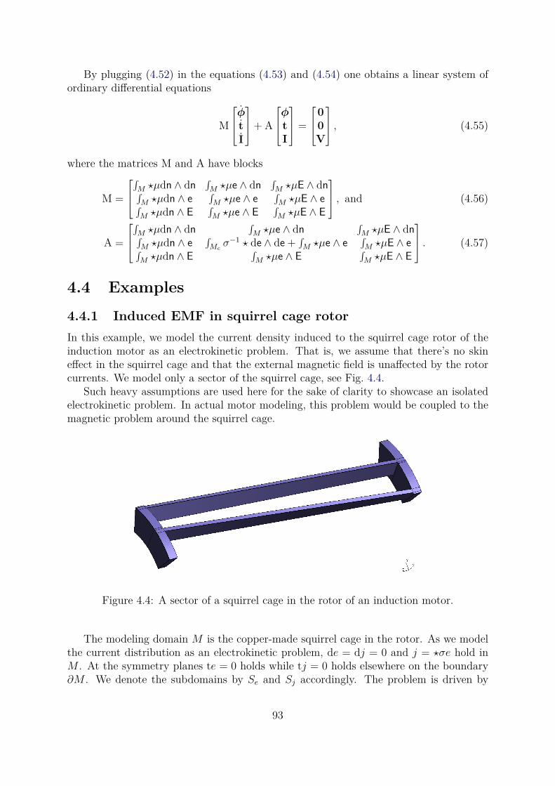
By plugging (4.52) in the equations (4.53) and (4.54) one obtains a linear system ofordinary differential equations

M

φ

t

I

+ A

φ

t

I

=

0

0

V

, (4.55)

where the matrices M and A have blocks

M =

∫

M ⋆µdn ∧ dn∫

M ⋆µe ∧ dn∫

M ⋆µE ∧ dn∫

M ⋆µdn ∧ e∫

M ⋆µe ∧ e∫

M ⋆µE ∧ e∫

M ⋆µdn ∧ E∫

M ⋆µe ∧ E∫

M ⋆µE ∧ E

, and (4.56)

A =

∫

M ⋆µdn ∧ dn∫

M ⋆µe ∧ dn∫

M ⋆µE ∧ dn∫

M ⋆µdn ∧ e∫

Mcσ−1 ⋆ de ∧ de +

∫

M ⋆µe ∧ e∫

M ⋆µE ∧ e∫

M ⋆µdn ∧ E∫

M ⋆µe ∧ E∫

M ⋆µE ∧ E

. (4.57)

4.4 Examples

4.4.1 Induced EMF in squirrel cage rotor

In this example, we model the current density induced to the squirrel cage rotor of theinduction motor as an electrokinetic problem. That is, we assume that there’s no skineffect in the squirrel cage and that the external magnetic field is unaffected by the rotorcurrents. We model only a sector of the squirrel cage, see Fig. 4.4.

Such heavy assumptions are used here for the sake of clarity to showcase an isolatedelectrokinetic problem. In actual motor modeling, this problem would be coupled to themagnetic problem around the squirrel cage.

Figure 4.4: A sector of a squirrel cage in the rotor of an induction motor.

The modeling domain M is the copper-made squirrel cage in the rotor. As we modelthe current distribution as an electrokinetic problem, de = dj = 0 and j = ⋆σe hold inM . At the symmetry planes te = 0 holds while tj = 0 holds elsewhere on the boundary∂M . We denote the subdomains by Se and Sj accordingly. The problem is driven by

93

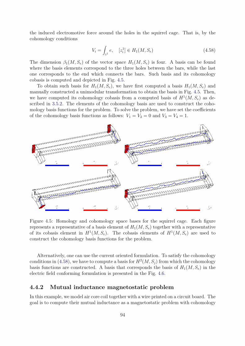
the induced electromotive force around the holes in the squirrel cage. That is, by thecohomology conditions

Vi =∫

z1

e, [z1i ] ∈ H1(M,Se) (4.58)

The dimension β1(M,Se) of the vector space H1(M,Se) is four. A basis can be foundwhere the basis elements correspond to the three holes between the bars, while the lastone corresponds to the end which connects the bars. Such basis and its cohomologycobasis is computed and depicted in Fig. 4.5.

To obtain such basis for H1(M,Se), we have first computed a basis H1(M,Se) andmanually constructed a unimodular transformation to obtain the basis in Fig. 4.5. Then,we have computed its cohomology cobasis from a computed basis of H1(M,Se) as de-scribed in 3.5.2. The elements of the cohomology basis are used to construct the coho-mology basis functions for the problem. To solve the problem, we have set the coefficientsof the cohomology basis functions as follows: V1 = V2 = 0 and V3 = V4 = 1.

Figure 4.5: Homology and cohomology space bases for the squirrel cage. Each figurerepresents a representative of a basis element of H1(M,Se) together with a representativeof its cobasis element in H1(M,Se). The cobasis elements of H1(M,Se) are used toconstruct the cohomology basis functions for the problem.

Alternatively, one can use the current oriented formulation. To satisfy the cohomologyconditions in (4.58), we have to compute a basis forH2(M,Sj) from which the cohomologybasis functions are constructed. A basis that corresponds the basis of H1(M,Se) in theelectric field conforming formulation is presented in the Fig. 4.6.

4.4.2 Mutual inductance magnetostatic problem

In this example, we model air core coil together with a wire printed on a circuit board. Thegoal is to compute their mutual inductance as a magnetostatic problem with cohomology

94

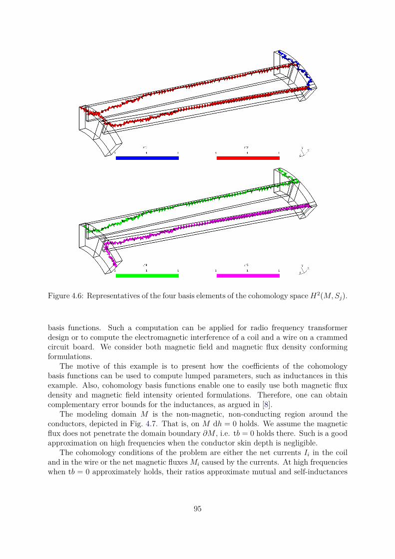
Figure 4.6: Representatives of the four basis elements of the cohomology space H2(M,Sj).

basis functions. Such a computation can be applied for radio frequency transformerdesign or to compute the electromagnetic interference of a coil and a wire on a crammedcircuit board. We consider both magnetic field and magnetic flux density conformingformulations.

The motive of this example is to present how the coefficients of the cohomologybasis functions can be used to compute lumped parameters, such as inductances in thisexample. Also, cohomology basis functions enable one to easily use both magnetic fluxdensity and magnetic field intensity oriented formulations. Therefore, one can obtaincomplementary error bounds for the inductances, as argued in [8].

The modeling domain M is the non-magnetic, non-conducting region around theconductors, depicted in Fig. 4.7. That is, on M dh = 0 holds. We assume the magneticflux does not penetrate the domain boundary ∂M , i.e. tb = 0 holds there. Such is a goodapproximation on high frequencies when the conductor skin depth is negligible.

The cohomology conditions of the problem are either the net currents Ii in the coiland in the wire or the net magnetic fluxes Mi caused by the currents. At high frequencieswhen tb = 0 approximately holds, their ratios approximate mutual and self-inductances

95

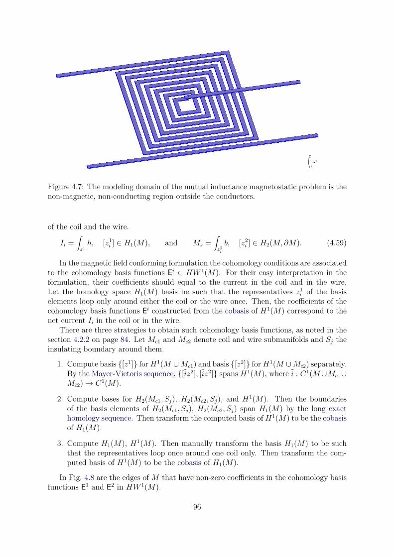
Figure 4.7: The modeling domain of the mutual inductance magnetostatic problem is thenon-magnetic, non-conducting region outside the conductors.

of the coil and the wire.

Ii =∫

z1

h, [z1i ] ∈ H1(M), and Ms =

∫

z2i

b, [z2i ] ∈ H2(M,∂M). (4.59)

In the magnetic field conforming formulation the cohomology conditions are associatedto the cohomology basis functions E

i ∈ HW 1(M). For their easy interpretation in theformulation, their coefficients should equal to the current in the coil and in the wire.Let the homology space H1(M) basis be such that the representatives z1

i of the basiselements loop only around either the coil or the wire once. Then, the coefficients of thecohomology basis functions E

i constructed from the cobasis of H1(M) correspond to thenet current Ii in the coil or in the wire.

There are three strategies to obtain such cohomology basis functions, as noted in thesection 4.2.2 on page 84. Let Mc1 and Mc2 denote coil and wire submanifolds and Sj theinsulating boundary around them.

1. Compute basis [z1] forH1(M ∪Mc1) and basis [z2] forH1(M ∪Mc2) separately.By the Mayer-Vietoris sequence, [iz2], [iz2] spans H1(M), where i : C1(M∪Mc1∪Mc2)→ C1(M).

2. Compute bases for H2(Mc1, Sj), H2(Mc2, Sj), and H1(M). Then the boundariesof the basis elements of H2(Mc1, Sj), H2(Mc2, Sj) span H1(M) by the long exacthomology sequence. Then transform the computed basis of H1(M) to be the cobasisof H1(M).

3. Compute H1(M), H1(M). Then manually transform the basis H1(M) to be suchthat the representatives loop once around one coil only. Then transform the com-puted basis of H1(M) to be the cobasis of H1(M).

In Fig. 4.8 are the edges of M that have non-zero coefficients in the cohomology basisfunctions E

1 and E2 in HW 1(M).

96

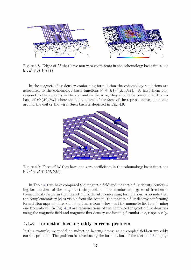
Figure 4.8: Edges of M that have non-zero coefficients in the cohomology basis functionsE

1,E2 ∈ HW 1(M)

In the magnetic flux density conforming formulation the cohomology conditions areassociated to the cohomology basis functions F

i ∈ HW 2(M,∂M). To have them cor-respond to the currents in the coil and in the wire, they should be constructed from abasis of H2(M,∂M) where the “dual edges” of the faces of the representatives loop oncearound the coil or the wire. Such basis is depicted in Fig. 4.9.

Figure 4.9: Faces of M that have non-zero coefficients in the cohomology basis functionsF

1,F2 ∈ HW 2(M,∂M)

In Table 4.1 we have compared the magnetic field and magnetic flux density conform-ing formulations of the magnetostatic problem. The number of degrees of freedom istremendously larger in the magnetic flux density conforming formulation. Also note thatthe complementarity [8] is visible from the results: the magnetic flux density conformingformulation approximates the inductances from below, and the magnetic field conformingone from above. In Fig. 4.10 are cross-sections of the computed magnetic flux densitiesusing the magnetic field and magnetic flux density conforming formulations, respectively.

4.4.3 Induction heating eddy current problem

In this example, we model an induction heating devise as an coupled field-circuit eddycurrent problem. The problem is solved using the formulations of the section 4.3 on page

97

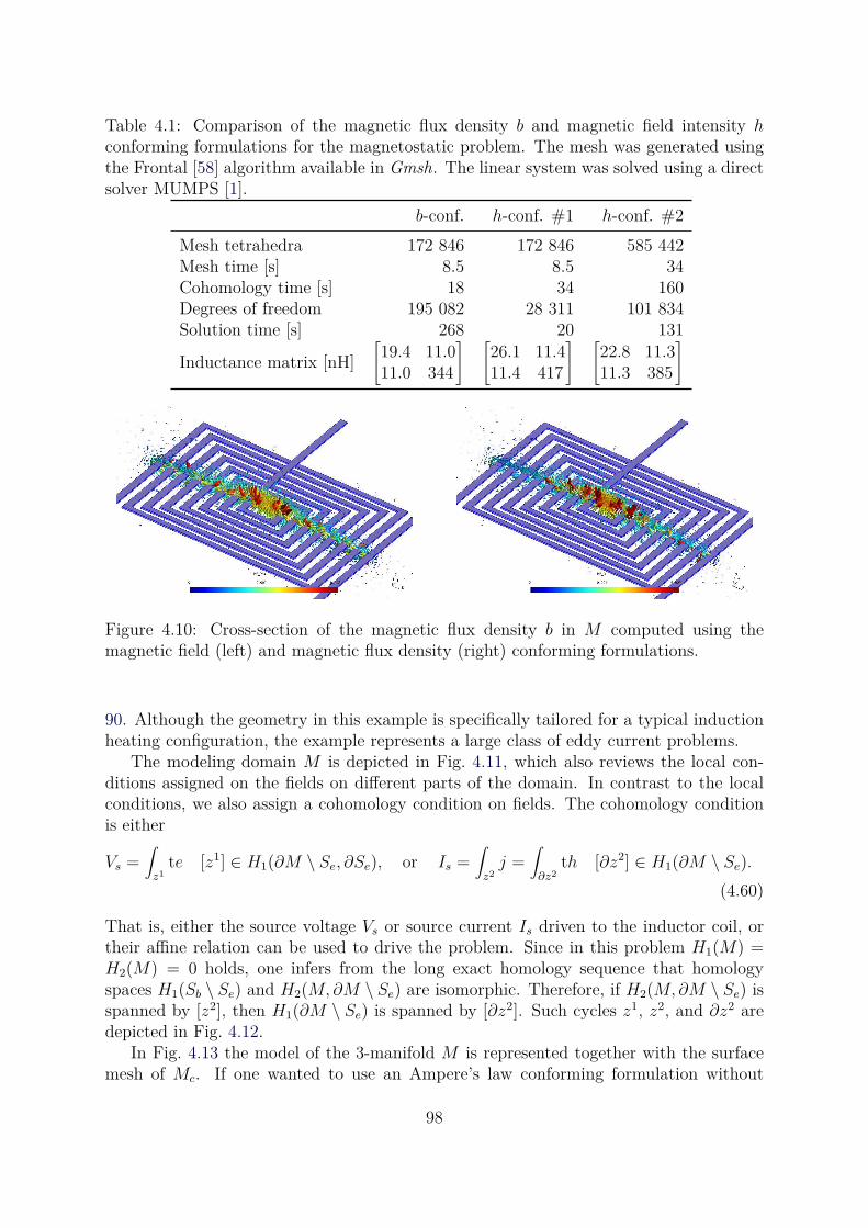
Table 4.1: Comparison of the magnetic flux density b and magnetic field intensity hconforming formulations for the magnetostatic problem. The mesh was generated usingthe Frontal [58] algorithm available in Gmsh. The linear system was solved using a directsolver MUMPS [1].

b-conf. h-conf. #1 h-conf. #2

Mesh tetrahedra 172 846 172 846 585 442Mesh time [s] 8.5 8.5 34Cohomology time [s] 18 34 160Degrees of freedom 195 082 28 311 101 834Solution time [s] 268 20 131

Inductance matrix [nH]

[

19.4 11.011.0 344

] [

26.1 11.411.4 417

] [

22.8 11.311.3 385

]

Figure 4.10: Cross-section of the magnetic flux density b in M computed using themagnetic field (left) and magnetic flux density (right) conforming formulations.

90. Although the geometry in this example is specifically tailored for a typical inductionheating configuration, the example represents a large class of eddy current problems.

The modeling domain M is depicted in Fig. 4.11, which also reviews the local con-ditions assigned on the fields on different parts of the domain. In contrast to the localconditions, we also assign a cohomology condition on fields. The cohomology conditionis either

Vs =∫

z1

te [z1] ∈ H1(∂M \ Se, ∂Se), or Is =∫

z2

j =∫

∂z2

th [∂z2] ∈ H1(∂M \ Se).

(4.60)

That is, either the source voltage Vs or source current Is driven to the inductor coil, ortheir affine relation can be used to drive the problem. Since in this problem H1(M) =H2(M) = 0 holds, one infers from the long exact homology sequence that homologyspaces H1(Sb \ Se) and H2(M,∂M \ Se) are isomorphic. Therefore, if H2(M,∂M \ Se) isspanned by [z2], then H1(∂M \ Se) is spanned by [∂z2]. Such cycles z1, z2, and ∂z2 aredepicted in Fig. 4.12.

In Fig. 4.13 the model of the 3-manifold M is represented together with the surfacemesh of Mc. If one wanted to use an Ampere’s law conforming formulation without

98

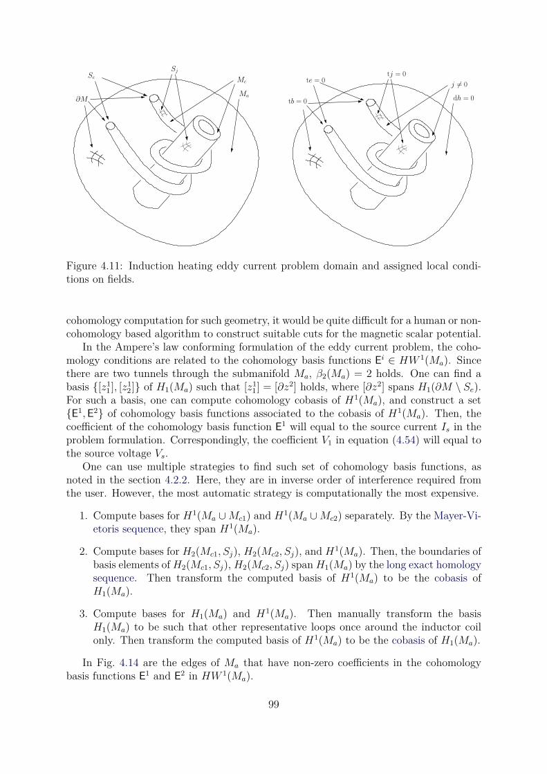
Sj

Mc

Ma

Se

∂M

tj = 0

dh = 0

te = 0j 6= 0

tb = 0

Figure 4.11: Induction heating eddy current problem domain and assigned local condi-tions on fields.

cohomology computation for such geometry, it would be quite difficult for a human or non-cohomology based algorithm to construct suitable cuts for the magnetic scalar potential.

In the Ampere’s law conforming formulation of the eddy current problem, the coho-mology conditions are related to the cohomology basis functions E

i ∈ HW 1(Ma). Sincethere are two tunnels through the submanifold Ma, β2(Ma) = 2 holds. One can find abasis [z1

1 ], [z12 ] of H1(Ma) such that [z1

1 ] = [∂z2] holds, where [∂z2] spans H1(∂M \ Se).For such a basis, one can compute cohomology cobasis of H1(Ma), and construct a setE1,E2 of cohomology basis functions associated to the cobasis of H1(Ma). Then, thecoefficient of the cohomology basis function E

1 will equal to the source current Is in theproblem formulation. Correspondingly, the coefficient V1 in equation (4.54) will equal tothe source voltage Vs.

One can use multiple strategies to find such set of cohomology basis functions, asnoted in the section 4.2.2. Here, they are in inverse order of interference required fromthe user. However, the most automatic strategy is computationally the most expensive.

1. Compute bases for H1(Ma ∪Mc1) and H1(Ma ∪Mc2) separately. By the Mayer-Vi-etoris sequence, they span H1(Ma).

2. Compute bases for H2(Mc1, Sj), H2(Mc2, Sj), and H1(Ma). Then, the boundaries ofbasis elements of H2(Mc1, Sj), H2(Mc2, Sj) span H1(Ma) by the long exact homologysequence. Then transform the computed basis of H1(Ma) to be the cobasis ofH1(Ma).

3. Compute bases for H1(Ma) and H1(Ma). Then manually transform the basisH1(Ma) to be such that other representative loops once around the inductor coilonly. Then transform the computed basis of H1(Ma) to be the cobasis of H1(Ma).

In Fig. 4.14 are the edges of Ma that have non-zero coefficients in the cohomologybasis functions E

1 and E2 in HW 1(Ma).

99

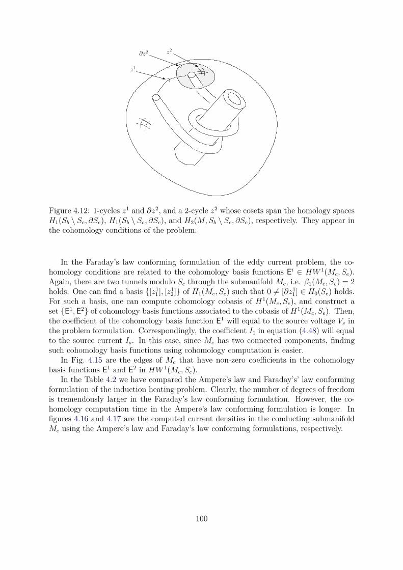
z1

z2

∂z2

Figure 4.12: 1-cycles z1 and ∂z2, and a 2-cycle z2 whose cosets span the homology spacesH1(Sb \ Se, ∂Se), H1(Sb \ Se, ∂Se), and H2(M,Sb \ Se, ∂Se), respectively. They appear inthe cohomology conditions of the problem.

In the Faraday’s law conforming formulation of the eddy current problem, the co-homology conditions are related to the cohomology basis functions E

i ∈ HW 1(Mc, Se).Again, there are two tunnels modulo Se through the submanifold Mc, i.e. β1(Mc, Se) = 2holds. One can find a basis [z1

1 ], [z12 ] of H1(Mc, Se) such that 0 6= [∂z1

1 ] ∈ H0(Se) holds.For such a basis, one can compute cohomology cobasis of H1(Mc, Se), and construct aset E1,E2 of cohomology basis functions associated to the cobasis of H1(Mc, Se). Then,the coefficient of the cohomology basis function E

1 will equal to the source voltage Vs inthe problem formulation. Correspondingly, the coefficient I1 in equation (4.48) will equalto the source current Is. In this case, since Mc has two connected components, findingsuch cohomology basis functions using cohomology computation is easier.

In Fig. 4.15 are the edges of Mc that have non-zero coefficients in the cohomologybasis functions E

1 and E2 in HW 1(Mc, Se).

In the Table 4.2 we have compared the Ampere’s law and Faraday’s’ law conformingformulation of the induction heating problem. Clearly, the number of degrees of freedomis tremendously larger in the Faraday’s law conforming formulation. However, the co-homology computation time in the Ampere’s law conforming formulation is longer. Infigures 4.16 and 4.17 are the computed current densities in the conducting submanifoldMc using the Ampere’s law and Faraday’s law conforming formulations, respectively.

100

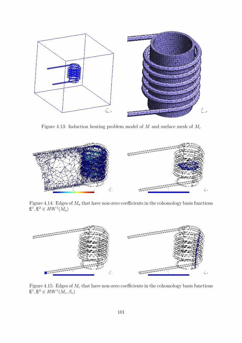
Figure 4.13: Induction heating problem model of M and surface mesh of Mc

Figure 4.14: Edges ofMa that have non-zero coefficients in the cohomology basis functionsE

1,E2 ∈ HW 1(Ma)

Figure 4.15: Edges of Mc that have non-zero coefficients in the cohomology basis functionsE

1,E2 ∈ HW 1(Mc, Se)

101

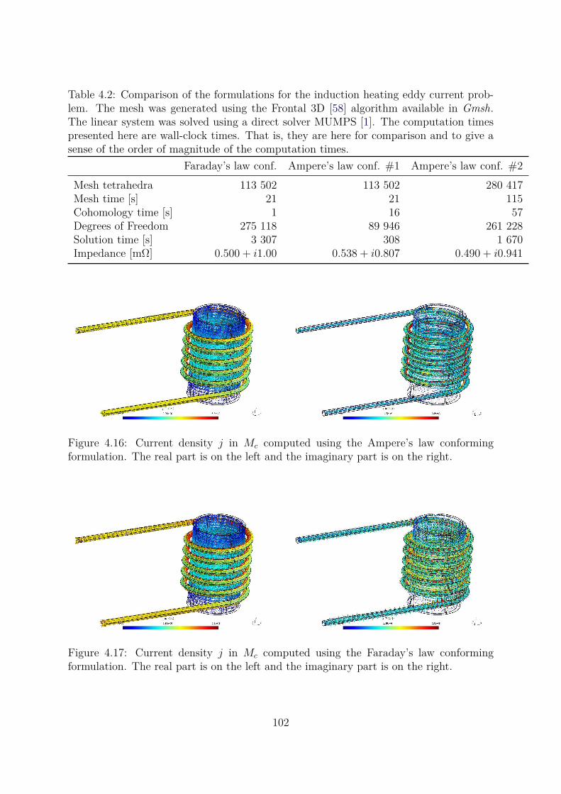
Table 4.2: Comparison of the formulations for the induction heating eddy current prob-lem. The mesh was generated using the Frontal 3D [58] algorithm available in Gmsh.The linear system was solved using a direct solver MUMPS [1]. The computation timespresented here are wall-clock times. That is, they are here for comparison and to give asense of the order of magnitude of the computation times.

Faraday’s law conf. Ampere’s law conf. #1 Ampere’s law conf. #2

Mesh tetrahedra 113 502 113 502 280 417Mesh time [s] 21 21 115Cohomology time [s] 1 16 57Degrees of Freedom 275 118 89 946 261 228Solution time [s] 3 307 308 1 670Impedance [mΩ] 0.500 + i1.00 0.538 + i0.807 0.490 + i0.941

Figure 4.16: Current density j in Mc computed using the Ampere’s law conformingformulation. The real part is on the left and the imaginary part is on the right.

Figure 4.17: Current density j in Mc computed using the Faraday’s law conformingformulation. The real part is on the left and the imaginary part is on the right.

102

Chapter 5

Finite element imitation of the

Riemannian manifold

In this chapter, we describe a C++ library that is used to imitate the structure andobjects defined on the Riemannian manifold. The library is build on the finite elementenvironment Gmsh [26], whose coordinate description of a finite element model providesa stepping stone for the Riemannian manifold abstraction.

The imitation emphasizes the separation of the manifold metric and coordinate num-bers. That is, used the coordinate chart necessarily doesn’t have a direct relation to thedistances between the points on the manifold, and so-called covariant and contravarianttensors are strictly different kind objects.

The described finite element imitation of the Riemannian manifold is designed to helpits user to program finite element pre- and post-processors for boundary value problemswhose domain is a Riemannian manifold, rather than the Euclidean space, which isassumed in the traditional software systems.

This chapter is heavily based on the author’s recent publication [52].

5.1 Motivation

The finite element method is traditionally considered to solve boundary value problemson subsets of the Euclidean space. Usually, the dimension and the coordinate system isfixed in advance or a few alternatives are provided, since the form of the partial differentialequations in the classical vector analysis depend on them.

However, differential forms on manifolds offer an alternative approach, where the formof the partial differential equations no longer depend on the used coordinate system andthe dimension. Further, one is not restricted to the Euclidean metric, but any metrictensor can be used without affecting the formulation of the boundary value problem.

The actual numerical computations still need to take the dimension, coordinate sys-tem, and the metric tensor into account. However, this can be done in a systematicmanner, where they are defined in one place, and then automatically taken into accountwhen needed. This is in contrast to the traditional approach, where one should take careat each turn when formulating a problem.

This Riemannian manifold imitation provides an interface where the slots for thedimension, coordinate system, and the metric tensor are offered. Further, it provides

103

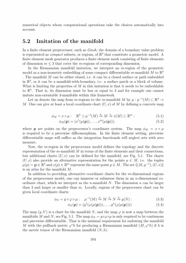
numerical objects whose computational operations take the choices automatically intoaccount.

5.2 Imitation of the manifold

In a finite element preprocessor, such as Gmsh, the domain of a boundary value problemis represented as compact subsets, or regions, of R3 that constitute a geometric model. Afinite element mesh generator produces a finite element mesh consisting of finite elementsof dimension m ≤ 3 that cover the m-regions of corresponding dimension.

In the Riemannian manifold imitation, we interpret an m-region of the geometricmodel as a non-isometric embedding of some compact differentiable m-manifold M to R

3

. The manifold M can be either closed, i.e. it can be a closed surface or path embeddedin R

3, or it can be a manifold-with-boundary, i.e. a surface patch or a block of volume.What is limiting the properties of M in this imitation is that it needs to be embeddableto R

3. That is, its dimension must be less or equal to 3 and for example one cannotimitate non-orientable 3-manifolds within this framework.

Let us denote the map from m-regions to the m-manifold M by µ : µ−1(M) ⊂ R3 →

M . One can give at least a local coordinate chart (U, x) of M by defining a concrete map

φM = x µ : R3 ⊃ µ−1(M)

µ−→Mx−→ x(M) ⊂ R

m : (5.1)

φM(p) = (x1(µ(p)), . . . , xm(µ(p))), (5.2)

where p are points on the preprocessor’s coordinate system. The map φM = x µis required to be a piecewise diffeomorphism. In the finite element setting, piecewisedifferentiable maps will suffice as the integration functionals will neglect sets with zeromeasure.

Now, the m-region in the preprocessor model defines the topology and the discreterepresentation of the m-manifold M in terms of the finite elements and their connections,but additional charts (U, x) can be defined for the manifold, see Fig. 5.1. The charts(U, x) also provide an alternative representation for the points p ∈ M , i.e. the tuplesµ(p) = p ∈ R

3 and x(p) ∈ Rm represent the same point p ∈M . The set (M,µ−1), (U, x)

is an atlas for the manifold M .In addition to providing alternative coordinate charts for the m-dimensional regions

of the preprocessor model, one can immerse or submerse them in an n-dimensional co-ordinate chart, which we interpret as the n-manifold N . The dimension n can be largerthan 3 and larger or smaller than m. Locally, regions of the preprocessor chart can begiven local coordinate charts

φN = y ϕ µ : µ−1(M)µ−→M

ϕ−→ Ny−→ y(N) : (5.3)

φN(p) = (y1(ϕ(µ(p))), . . . , yn(ϕ(µ(p)))) (5.4)

The map (y, V ) is a chart for the manifold N , and the map ϕ is now a map between themanifolds M and N , see Fig. 5.1. The map φN = yϕµ is only required to be continuousand piecewise differentiable. That is the minimal requirement for endowing the manifoldM with the pullback metric ϕ∗h for producing a Riemannian manifold (M,ϕ∗h) if h isthe metric tensor of the Riemannian manifold (N, h).

104

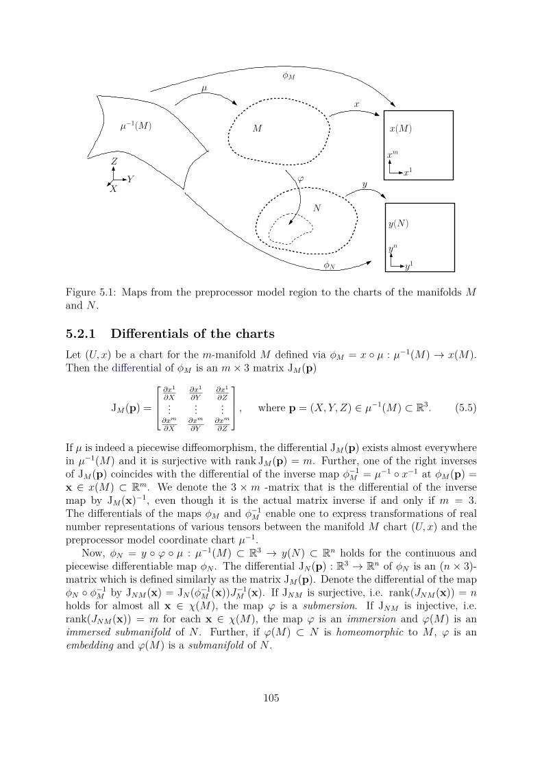
xm

x1

yn

y1

M

ϕ

N

φM

φN

µ

x

x(M)

y

y(N)

µ−1(M)

Z

YX

Figure 5.1: Maps from the preprocessor model region to the charts of the manifolds Mand N .

5.2.1 Differentials of the charts

Let (U, x) be a chart for the m-manifold M defined via φM = x µ : µ−1(M) → x(M).Then the differential of φM is an m× 3 matrix JM(p)

JM(p) =

∂x1

∂X∂x1

∂Y∂x1

∂Z...

......

∂xm

∂X∂xm

∂Y∂xm

∂Z

, where p = (X,Y, Z) ∈ µ−1(M) ⊂ R3. (5.5)

If µ is indeed a piecewise diffeomorphism, the differential JM(p) exists almost everywherein µ−1(M) and it is surjective with rank JM(p) = m. Further, one of the right inversesof JM(p) coincides with the differential of the inverse map φ−1

M = µ−1 x−1 at φM(p) =x ∈ x(M) ⊂ R

m. We denote the 3 × m -matrix that is the differential of the inversemap by JM(x)−1, even though it is the actual matrix inverse if and only if m = 3.The differentials of the maps φM and φ−1

M enable one to express transformations of realnumber representations of various tensors between the manifold M chart (U, x) and thepreprocessor model coordinate chart µ−1.

Now, φN = y ϕ µ : µ−1(M) ⊂ R3 → y(N) ⊂ R

n holds for the continuous andpiecewise differentiable map φN . The differential JN(p) : R3 → R

n of φN is an (n × 3)-matrix which is defined similarly as the matrix JM(p). Denote the differential of the mapφN φ−1

M by JNM(x) = JN(φ−1M (x))J−1

M (x). If JNM is surjective, i.e. rank(JNM(x)) = nholds for almost all x ∈ χ(M), the map ϕ is a submersion. If JNM is injective, i.e.rank(JNM(x)) = m for each x ∈ χ(M), the map ϕ is an immersion and ϕ(M) is animmersed submanifold of N . Further, if ϕ(M) ⊂ N is homeomorphic to M , ϕ is anembedding and ϕ(M) is a submanifold of N .

105

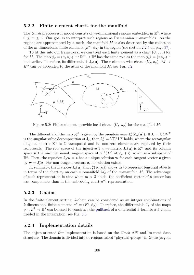
5.2.2 Finite element charts for the manifold

The Gmsh preprocessor model consists of m-dimensional regions embedded in R3, where

0 ≤ m ≤ 3. Our goal is to interpret such regions as Riemannian m-manifolds. As theregions are approximated by a mesh, the manifold M is also described by the collectionof the m-dimensional finite elements (Em, φσ) in the region (see section 2.2.5 on page 37).

To fit this into our framework, we can treat each finite element as a chart (Uσ, uσ) forfor M . The map φσ = (uσ µ)−1 : Rm → R

3 has the same role as the map φ−1M = (xµ)−1

had earlier. Therefore, its differential is Jσ(u). These element-wise charts (Uσ, uσ) : M →Em can be appended to the atlas of the manifold M , see Fig. 5.2.

um

u1

E

M

µ

µ−1(M)

φσ

Uσ

uσ

Z

YX

Figure 5.2: Finite elements provide local charts (Uσ, uσ) for the manifold M .

The differential of the map φ−1σ is given by the pseudoinverse J+

σ (φσ(u)): If Jσ = UΣVT

is the singular value decomposition of Jσ, then J+σ = VΣ+UT holds, where the rectangular

diagonal matrix Σ+ is Σ transposed and its non-zero elements are replaced by theirreciprocals. The row space of the injective 3 × m matrix Jσ(u) is R

m and its columnspace is the m-dimensional tangent space of µ−1(M) at φ−1

σ (u), which is a subspace ofR

3. Then, the equation Jσw = z has a unique solution w for each tangent vector z givenby w = J+

σ z. For non-tangent vectors z, no solution exists.In summary, the matrices Jσ(u) and J+

σ (φσ(u)) allows us to represent tensorial objectsin terms of the chart uσ on each submanifold Mσ of the m-manifold M . The advantageof such representation is that when m < 3 holds, the coefficient vector of a tensor hasless components than in the embedding chart µ−1 representation.

5.2.3 Chains

In the finite element setting, k-chain can be considered as an integer combinations ofk-dimensional finite elements σk = (Ek, φσ). Therefore, the differentials Jσ of the mapsφσ : Ek → R

3 can be used to construct the pullback of a differential k-form to a k-chain,needed in the integration, see Fig. 5.3.

5.2.4 Implementation details

The object-oriented C++ implementation is based on the Gmsh API and its mesh datastructure. The domain is divided into m-regions called “physical groups” in Gmsh jargon,

106

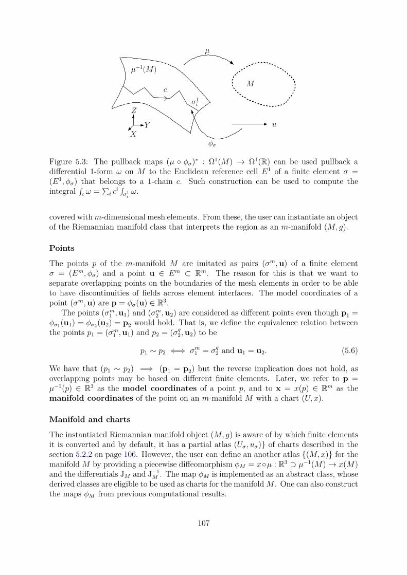
µ

u

M

µ−1(M)

c

φσ

σ1

i

Z

YX

Figure 5.3: The pullback maps (µ φσ)∗ : Ω1(M) → Ω1(R) can be used pullback adifferential 1-form ω on M to the Euclidean reference cell E1 of a finite element σ =(E1, φσ) that belongs to a 1-chain c. Such construction can be used to compute theintegral

∫

c ω =∑

i ci∫

σ1iω.

covered withm-dimensional mesh elements. From these, the user can instantiate an objectof the Riemannian manifold class that interprets the region as an m-manifold (M, g).

Points

The points p of the m-manifold M are imitated as pairs (σm,u) of a finite elementσ = (Em, φσ) and a point u ∈ Em ⊂ R

m. The reason for this is that we want toseparate overlapping points on the boundaries of the mesh elements in order to be ableto have discontinuities of fields across element interfaces. The model coordinates of apoint (σm,u) are p = φσ(u) ∈ R

3.The points (σm

1 ,u1) and (σm2 ,u2) are considered as different points even though p1 =

φσ1(u1) = φσ2

(u2) = p2 would hold. That is, we define the equivalence relation betweenthe points p1 = (σm

1 ,u1) and p2 = (σq2,u2) to be

p1 ∼ p2 ⇐⇒ σm1 = σq

2 and u1 = u2. (5.6)

We have that (p1 ∼ p2) =⇒ (p1 = p2) but the reverse implication does not hold, asoverlapping points may be based on different finite elements. Later, we refer to p =µ−1(p) ∈ R

3 as the model coordinates of a point p, and to x = x(p) ∈ Rm as the

manifold coordinates of the point on an m-manifold M with a chart (U, x).

Manifold and charts

The instantiated Riemannian manifold object (M, g) is aware of by which finite elementsit is converted and by default, it has a partial atlas (Uσ, uσ) of charts described in thesection 5.2.2 on page 106. However, the user can define an another atlas (M,x) for themanifold M by providing a piecewise diffeomorphism φM = xµ : R3 ⊃ µ−1(M)→ x(M)and the differentials JM and J−1

M . The map φM is implemented as an abstract class, whosederived classes are eligible to be used as charts for the manifold M . One can also constructthe maps φM from previous computational results.

107

The class representing φM provides methods to obtain representation x of a pointp ∈ M on a chart of M and the representation p in the model coordinates, as well asthe differentials JM(p) and J−1

M (x) at a given point p. From the differentials, one canconstruct pullbacks and pushforwards for the various tensors on M , as will be describedin a later section.

The model coordinates of a point p = (σm,u) ∈ M are µ−1(p) = p = φσ(u) and themanifold coordinates are x(p) = x = φM(p) = φM(φσ(u)). Given a point p ∈ R

3 inthe model coordinates, it can be turned into point p ∈ M using a two step algorithm:First, find all finite elements near that point in R

3 using an octree search [46]. Second,if a found finite element σm belongs to M , we have p = (σm, φ−1

σ (p)). The result is notunique since there can be other finite elements near p that belong to M .

Maps between manifolds

Let Q be a q-manifold based on an q-region of a preprocessor model, and let µ : R3 →Mand κ : R3 → Q be the corresponding maps from the model coordinates to the manifolds.If their preprocessor representations overlap, i.e. if µ−1(M) ∩ κ−1(Q) 6= ∅ holds, we canconstruct a map κ µ−1 : M → Q, its differential and possibly its inverse map and thedifferential of its inverse. Such map is needed for example if one wanted to compute atrace of a differential form on M to a submanifold Q ⊂ ∂M . We have the following twopossibilities.

1. The mesh element σm of p = (σm,u) ∈ M also belongs to the manifold Q. Thensimply (κ µ−1)(p) = p = (σm,u). In this case, m = q must hold. The differentialis JQ(κ−1(p))J−1

M (x(p)).

2. The mesh element σm of p = (σm,u) ∈ M does not belong to Q. Then, we mapp = φσ(u) ∈ R

3 and find all mesh elements near1 that point in R3 using an octree

search [46]. If a found mesh element σq belongs to Q, we map p′ = (κ µ−1)(p) =(σq, φ−1

σq (p)). The differential is JQ(κ−1(p′))J−1M (x(p)).

In the latter case, the two manifolds M and Q may be based on entirely different prepro-cessor models, i.e. they may have different, but overlapping finite element meshes in R

3.The relation between their points is established via the equivalence of 3-tuples p of R3.

5.3 Imitation of tensorial objects

Tensorial objects are coordinate-free in a sense that although their representations de-pend on the used coordinate system, any coordinate system can be used to perform thecomputations. Since tensors are linear maps, their coordinate transformations must belinear maps as well to conform to the above property. Furthermore, tensors are either co-variant, contravariant, or mixture of both properties depending whether their argumentsare k-covectors or k-vectors or both.

In this section, we present how the most usual contravariant and covariant tensors arerepresented and implemented in the Riemannian manifold interface. Namely, k-covectors,the metric tensor, and k-vectors.

1To a tolerance that stems from the floating-point number inaccuracy.

108

5.3.1 Representation and transformations of tensors on the man-

ifold

On a local coordinate chart (U, x) of the m-manifold M , tangent vectors vp ∈ TpMand covectors ωp ∈ T ∗

pM have coefficient representations v = [v1, . . . ,vm]T and ω =[ω1, . . . ,ωm]T in R

m with respect to the coordinate basis ∂/∂x1, . . . , ∂/∂xm and thecoordinate cobasis dx1, . . . , dxm of (U, x). That is, with the representation ω, we haveωp =

∑mi=1 ωidxi.

While the representation ω depends on the coordinate patch, the linear combinationsωp =

∑mi=1 ωidxi is a coordinate-free object, since the “differentials” dxi can be naturally

expanded by the chain rule of elementary calculus to conform with a different coordinatechart.

Recall from section 2.2.3 on page 31 that if v′ and v are the representations of atangent vector vp on overlapping charts (U ′, x′) and (U, x), they are related by v′ = Jv,where J is the differential of the map x′ x−1. Let ω′ and ω similarly represent a tangentcovector ωp. It was required that ω′T v′ = ω′T Jv = (JTω′)T v = ωT v hold. Therefore,the matrix JT performs the transformation for the tangent covectors. Similarly, if ϕ isa piecewise differentiable map ϕ : M → N , one can pushforward a tangent vector vp tothe manifold N , denoted ϕ∗vp, and pullback a tangent covector ωp to the manifold M ,denoted ϕ∗ωp.

The exterior and tensor algebras of the tangent vectors and the covectors induce thevector spaces of k-(co)vectors and (k, l)-tensors via the exterior product ∧ and the tensorproduct ⊗, respectively, as discussed in the section 2.1.4 on page 27. We denote the spacesof (k, l)-tensors by

⊗lk(TpM) and of k-covectors by Λk(T ∗

pM) ⊂ ⊗k0(TpM) and k-vectors

Λk(TpM) ⊂ ⊗0k(TpM), respectively. The dimension of the spaces on an m-manifold are

r =(

mk

)

for k-(co)vectors and r = mkml for (k, l)-tensors.The representations of k-(co)vectors can be given in the multi-index notation. For

example, the representation of k-covector is ωp =∑

~I ωIdxI , where dxI = dxi1 ∧ . . . ∧dxik . The pushforward and the pullback together with the exterior product and thetensor product also induce the transformation rules for k-(co)vectors and (k, l)-tensors,see section 2.1.4.

A (k, l)-tensor field on the manifold M is a map M → ⊗lk(TM), where

⊗lk(TM)

denotes the (k, l)-tensor bundle of the manifold M . That is, a tensor field is required toassociate to each point p ∈M a representation of a point-wise tensor.

5.3.2 Metric tensor on the manifold

The metric tensor g is symmetric (0, 2) tensor that has a special meaning on the Rie-mannian manifold (M, g). With the metric tensor one can compute inner products ofother tensors and transform (k, l) tensors to (k − 1, l + 1) and (k + 1, l − 1) tensors.Especially, it can be used to to compute the Hodge operator and flat and sharp operatorsof k-(co)vectors.

The metric tensor g : M →⊗20(TpM) of the Riemannian m-manifold (M, g) is point-

wise represented by a symmetric m×m-matrix G. The metric tensor at p ∈M is a mapgp : TpM × TpM → R. Thus, the coefficients with respect to the coordinate basis areGij = gp(∂/∂xi, ∂/∂xj). The representations G and G′ of g on charts (U, x) and (U ′, x′)

109

are related by G′ = JT GJ.There’s a variety of methods one can define the metric tensor on M . Most commonly,

one can pullback the Euclidean metric from the preprocessor coordinates to M using thedifferential of the map µ. One can also provide its coefficients as an analytical expressionson the model coordinates or on the chart coordinates of M , or define a result of a previousnumerical computation to provide the coefficients. Lastly, one can define an another, highdimensional auxiliary Riemannian manifold (N, h) and use the pullback metric tensorg = ϕ∗h on M . Again, h can be either the Euclidean metric tensor or its coefficients canbe defined via analytical expressions or by previous numerical computations.

5.3.3 Implementation details

The k-(co)vectors, metric tensors and general (k, l)-tensors and tensor fields are han-dled as coordinate-independent objects that live on the manifold M . That is, the usermanipulates the coordinate-free mathematical objects, rather than their real number rep-resentations. Under the hood, the real number representations of the objects are alwaysaccompanied with the information about the manifold and chart on which they apply.The user needs to pay attention to the representations only when inputting or outputtingdata. Currently, the real number representations are with respect to the coordinate basisof the chart.

Tensors and tensor fields

The implementation of the tensor class in the interface depends heavily on C++ templates.C++ programming language supports so-called non-type template arguments. For example,a template argument can be a specific integer or a member in an enumeration, ratherthan an integer or enumeration type. In the implementation, the tensor class headerreads:

template <int n, int k, int l, TensorSymmetry s> class Tensor

Here TensorSymmetry is an enumeration type for various symmetries a tensor mightposses, for example skewsymmetry. Integers n, k, and l are the dimension of the mani-fold, and contravariant and covariant indices of the tensor, respectively. With this imple-mentation, the specific type of the tensor is known at the compile time. An alternativeimplementation would be to store the type information as member variables of the class.Then, the type of the tensor would be only known at run time. The static (compile time)type information has several advantages:

1. The number of coefficients that represent the tensor on a chart of a manifold isknown at compile time. Therefore, static data structures can be used to store thecoefficients. This increases the performance in computations.

2. The specific algorithm to perform some tensor operation is chosen at compile timeby the compiler. This removes a performance overhead when the algorithm is chosenat run time. For example, the algorithm to perform the inner product of k-covectorsdepends on the manifold dimension and the covariant index k.

110

3. When performing operations on tensors, in addition to computing the coefficients,the type of the resulting tensor also needs to be computed. Our template implemen-tation performs the type computation at compile time. This is again a performancegain.

4. The C++ compiler static type checking guarantees that the performed operationsof tensors are legitimate. That is, some programming errors are caught at compiletime rather than at run time.

5. Compiler optimizations are more efficient with static type information.

However, the static type information has one considerable disadvantage. If the programto be written is such that the types of the tensors are only known at run time, exten-sive conditional constructs must be written in some places of the program to select theappropriate tensor type.

The field class in this interface is templated by the tensor type, for example k-(co)vectors or symmetric (0, 2)-tensors. It is an abstract class whose derived classesare either discrete or analytic. A discrete field stores the representations of tensors ateach vertex of each mesh element σ in the mesh, and interpolates the element at otherpoints using Whitney 0-forms. Discrete fields can be constructed during computations.An analytic field evaluates a user-defined expression at a given point. In addition, theuser can derive a class whose behaviors he has a complete command and responsibility.The abstract base class provides the interface to use it within the Riemannian manifoldlibrary.

Operations on tensors and tensor fields

The interface hides the coefficient vector computations of the operation on tensors byproviding functions whose inputs and outputs are objects rather than real number repre-sentations. Point-wise, i.e. algebraic operations on tensor fields can be performed usingthe representations of various tensor at the given points.

In contrast, the analytic operations on a tensor field need some information aroundits behavior in a neighborhood, and therefore cannot be performed for tensor fields onthe manifold N , since the map ϕ : M → N is only required to be piecewise differentiable.However, one can pullback covariant tensor fields on the manifold N to the manifold Mand perform analysis for the pullback fields.

Gmsh API provides the finite element σ shape functions λi of any order and theirpartial derivatives ∂λi

∂uj on the reference m-cell Em, the maps φσ : Em → φσ(E) ⊂ R3

and their differentials Jσ, and Gauss integration data. Therefore, the exterior derivative,integration, and trace of differential k-forms ω on the manifold M are implemented viathe pullback (φM φσ)∗ω on the reference cell Em.

The exterior derivative dω [24] of a differential k-form can be computed element-wise using the partial derivatives of the shape functions λi, once given the k-covectorsωσ

i =∑

J ωiJduJ on each vertex i of an element σ on the element-wise chart (Uσ, uσ). Let

dλi =∑m

j=1∂λi

∂uj duj hold, then dω =∑

i(dλi ∧ ωσi ) holds.

A differential k-form ω on the m-manifold M can be integrated over k-dimensionalfinite elements σk = (Ek, φσ) in a finite element environment. The integral can be

111

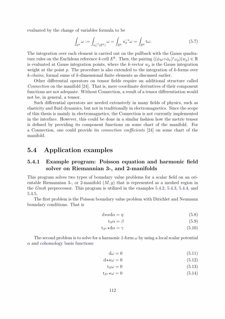
evaluated by the change of variables formula to be∫

σkω :=

∫

u−1σ (Ek)

ω =∫

Eku−∗

σ ω =∫

Ektω. (5.7)

The integration over each element is carried out on the pullback with the Gauss quadra-ture rules on the Euclidean reference k-cell Ek. Then, the pairing ((φM φσ)∗ωp)(wp) ∈ R

is evaluated at Gauss integration points, where the k-vector wp is the Gauss integrationweight at the point p. The procedure is also extended to the integration of k-forms overk-chains, formal sums of k-dimensional finite elements as discussed earlier.

Other differential operators on tensor fields require an additional structure calledConnection on the manifold [24]. That is, mere coordinate derivatives of their componentfunctions are not adequate. Without Connection, a result of a tensor differentiation wouldnot be, in general, a tensor.

Such differential operators are needed extensively in many fields of physics, such aselasticity and fluid dynamics, but not in traditionally in electromagnetics. Since the scopeof this thesis is mainly in electromagnetics, the Connection is not currently implementedin the interface. However, this could be done in a similar fashion how the metric tensoris defined by providing its component functions on some chart of the manifold. Fora Connection, one could provide its connection coefficients [24] on some chart of themanifold.

5.4 Application examples

5.4.1 Example program: Poisson equation and harmonic field

solver on Riemannian 3-, and 2-manifolds

This program solves two types of boundary value problems for a scalar field on an ori-entable Riemannian 3-, or 2-manifold (M, g) that is represented as a meshed region inthe Gmsh preprocessor. This program is utilized in the examples 5.4.2, 5.4.3, 5.4.4, and5.4.5.

The first problem is the Poisson boundary value problem with Dirichlet and Neumannboundary conditions. That is

d⋆κdα = η (5.8)

tSα = β (5.9)

tS∗⋆dα = γ (5.10)

The second problem is to solve for a harmonic 1-form ω by using a local scalar potentialα and cohomology basis functions:

dω = 0 (5.11)

d⋆κω = 0 (5.12)

tSω = 0 (5.13)

tS∗⋆ω = 0 (5.14)

112

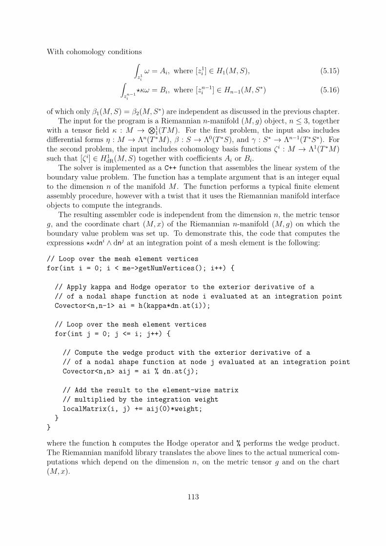
With cohomology conditions∫

z1i

ω = Ai, where [z1i ] ∈ H1(M,S), (5.15)

∫

zn−1

i

⋆κω = Bi, where [zn−1i ] ∈ Hn−1(M,S∗) (5.16)

of which only β1(M,S) = β2(M,S∗) are independent as discussed in the previous chapter.The input for the program is a Riemannian n-manifold (M, g) object, n ≤ 3, together

with a tensor field κ : M → ⊗11(TM). For the first problem, the input also includes

differential forms η : M → Λn(T ∗M), β : S → Λ0(T ∗S), and γ : S∗ → Λn−1(T ∗S∗). Forthe second problem, the input includes cohomology basis functions ζ i : M → Λ1(T ∗M)such that [ζ i] ∈ H1

dR(M,S) together with coefficients Ai or Bi.The solver is implemented as a C++ function that assembles the linear system of the

boundary value problem. The function has a template argument that is an integer equalto the dimension n of the manifold M . The function performs a typical finite elementassembly procedure, however with a twist that it uses the Riemannian manifold interfaceobjects to compute the integrands.

The resulting assembler code is independent from the dimension n, the metric tensorg, and the coordinate chart (M,x) of the Riemannian n-manifold (M, g) on which theboundary value problem was set up. To demonstrate this, the code that computes theexpressions ⋆κdn

i ∧ dnj at an integration point of a mesh element is the following:

// Loop over the mesh element vertices

for(int i = 0; i < me->getNumVertices(); i++)

// Apply kappa and Hodge operator to the exterior derivative of a

// of a nodal shape function at node i evaluated at an integration point

Covector<n,n-1> ai = h(kappa*dn.at(i));

// Loop over the mesh element vertices

for(int j = 0; j <= i; j++)

// Compute the wedge product with the exterior derivative of a

// of a nodal shape function at node j evaluated at an integration point

Covector<n,n> aij = ai % dn.at(j);

// Add the result to the element-wise matrix

// multiplied by the integration weight

localMatrix(i, j) += aij(0)*weight;

where the function h computes the Hodge operator and % performs the wedge product.The Riemannian manifold library translates the above lines to the actual numerical com-putations which depend on the dimension n, on the metric tensor g and on the chart(M,x).

113

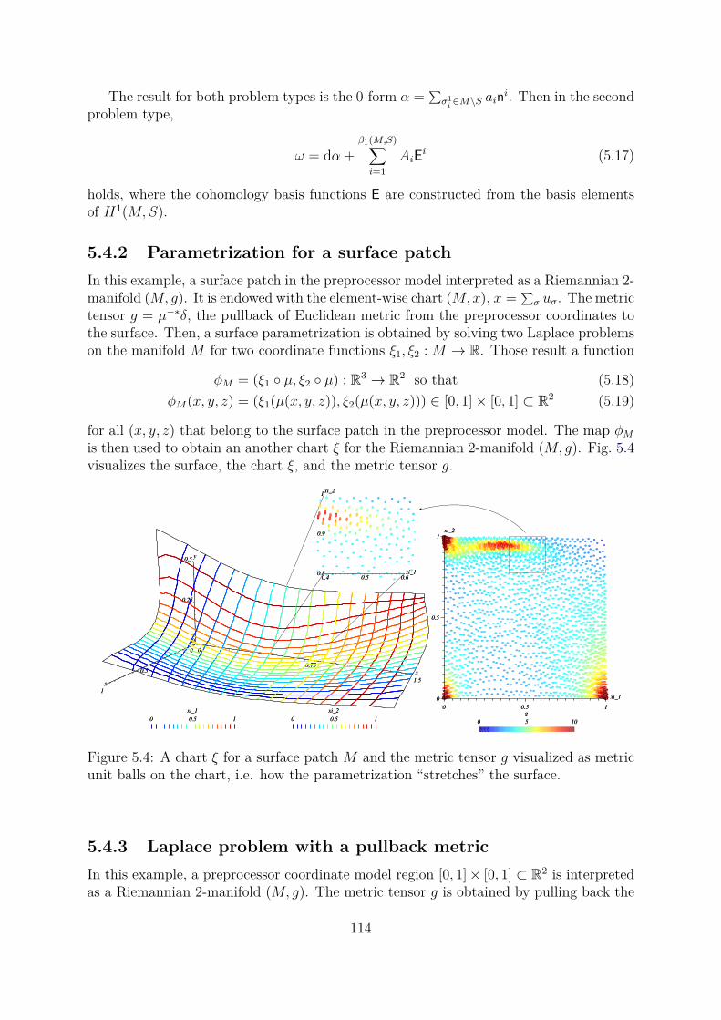
The result for both problem types is the 0-form α =∑

σ1i∈M\S ain

i. Then in the secondproblem type,

ω = dα+β1(M,S)

∑

i=1

AiEi (5.17)

holds, where the cohomology basis functions E are constructed from the basis elementsof H1(M,S).

5.4.2 Parametrization for a surface patch

In this example, a surface patch in the preprocessor model interpreted as a Riemannian 2-manifold (M, g). It is endowed with the element-wise chart (M,x), x =

∑

σ uσ. The metrictensor g = µ−∗δ, the pullback of Euclidean metric from the preprocessor coordinates tothe surface. Then, a surface parametrization is obtained by solving two Laplace problemson the manifold M for two coordinate functions ξ1, ξ2 : M → R. Those result a function

φM = (ξ1 µ, ξ2 µ) : R3 → R2 so that (5.18)

φM(x, y, z) = (ξ1(µ(x, y, z)), ξ2(µ(x, y, z))) ∈ [0, 1]× [0, 1] ⊂ R2 (5.19)

for all (x, y, z) that belong to the surface patch in the preprocessor model. The map φM

is then used to obtain an another chart ξ for the Riemannian 2-manifold (M, g). Fig. 5.4visualizes the surface, the chart ξ, and the metric tensor g.

00

0000

0.250.25

0.50.5yy

0.750.750.50.5

0 0.5 1

xi_1

0 0.5 1

xi_2

0 0.5 1

xi_1

0 0.5 1

xi_2

1.51.5

xx

11

zz

xi_1

0 0.5 1

xi_2

0

0.5

1

xi_1

0 0.5 1

xi_2

0

0.5

1

0 5 10

g

0 5 10

g

0.4 0.5 0.60.8

0.9

1

0.4 0.50.8

1

xi_1

xi_2

xi_1

xi_2

0.9

0.6

Figure 5.4: A chart ξ for a surface patch M and the metric tensor g visualized as metricunit balls on the chart, i.e. how the parametrization “stretches” the surface.

5.4.3 Laplace problem with a pullback metric

In this example, a preprocessor coordinate model region [0, 1]× [0, 1] ⊂ R2 is interpreted

as a Riemannian 2-manifold (M, g). The metric tensor g is obtained by pulling back the

114

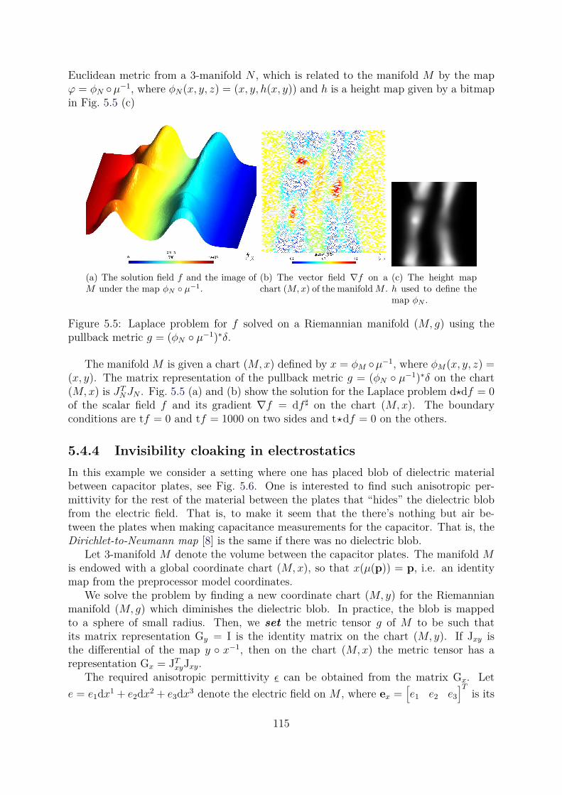
Euclidean metric from a 3-manifold N , which is related to the manifold M by the mapϕ = φN µ−1, where φN(x, y, z) = (x, y, h(x, y)) and h is a height map given by a bitmapin Fig. 5.5 (c)

(a) The solution field f and the image ofM under the map φN µ−1.

(b) The vector field ∇f on achart (M, x) of the manifold M .

(c) The height maph used to define themap φN .

Figure 5.5: Laplace problem for f solved on a Riemannian manifold (M, g) using thepullback metric g = (φN µ−1)∗δ.

The manifold M is given a chart (M,x) defined by x = φM µ−1, where φM(x, y, z) =(x, y). The matrix representation of the pullback metric g = (φN µ−1)∗δ on the chart(M,x) is JT

NJN . Fig. 5.5 (a) and (b) show the solution for the Laplace problem d⋆df = 0of the scalar field f and its gradient ∇f = df ♯ on the chart (M,x). The boundaryconditions are tf = 0 and tf = 1000 on two sides and t⋆df = 0 on the others.

5.4.4 Invisibility cloaking in electrostatics

In this example we consider a setting where one has placed blob of dielectric materialbetween capacitor plates, see Fig. 5.6. One is interested to find such anisotropic per-mittivity for the rest of the material between the plates that “hides” the dielectric blobfrom the electric field. That is, to make it seem that the there’s nothing but air be-tween the plates when making capacitance measurements for the capacitor. That is, theDirichlet-to-Neumann map [8] is the same if there was no dielectric blob.

Let 3-manifold M denote the volume between the capacitor plates. The manifold Mis endowed with a global coordinate chart (M,x), so that x(µ(p)) = p, i.e. an identitymap from the preprocessor model coordinates.

We solve the problem by finding a new coordinate chart (M, y) for the Riemannianmanifold (M, g) which diminishes the dielectric blob. In practice, the blob is mappedto a sphere of small radius. Then, we set the metric tensor g of M to be such thatits matrix representation Gy = I is the identity matrix on the chart (M, y). If Jxy isthe differential of the map y x−1, then on the chart (M,x) the metric tensor has arepresentation Gx = JT

xyJxy.The required anisotropic permittivity ǫ can be obtained from the matrix Gx. Let

e = e1dx1 + e2dx2 + e3dx3 denote the electric field on M , where ex =[

e1 e2 e3

]Tis its

115

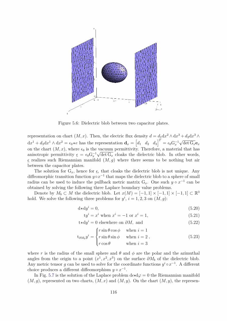
Figure 5.6: Dielectric blob between two capacitor plates.

representation on chart (M,x). Then, the electric flux density d = d1dx2 ∧ dx3 + d2dx3 ∧dx1 + d3dx1 ∧ dx2 = ǫ0⋆e has the representation dx =

[

d1 d2 d3

]T= ǫ0G−1

x

√det Gxex

on the chart (M,x), where ǫ0 is the vacuum permittivity. Therefore, a material that hasanisotropic permittivity ǫ = ǫ0G−1

x

√det Gx cloaks the dielectric blob. In other words,

ǫ realizes such Riemannian manifold (M, g) where there seems to be nothing but airbetween the capacitor plates.

The solution for Gx, hence for ǫ, that cloaks the dielectric blob is not unique. Anydiffeomorphic transition function yx−1 that maps the dielectric blob to a sphere of smallradius can be used to induce the pullback metric matrix Gx. One such y x−1 can beobtained by solving the following three Laplace boundary value problems.

Denote by Mb ⊂ M the dielectric blob. Let x(M) = [−1, 1] × [−1, 1] × [−1, 1] ⊂ R3

hold. We solve the following three problems for yi, i = 1, 2, 3 on (M, g):

d⋆dyi = 0, (5.20)

tyi = xi when xi = −1 or xi = 1, (5.21)

t⋆dyi = 0 elsewhere on ∂M, and (5.22)

t∂Mbyi =

r sin θ cosφ when i = 1

r sin θ sinφ when i = 2

r cos θ when i = 3

, (5.23)

where r is the radius of the small sphere and θ and φ are the polar and the azimuthalangles from the origin to a point (x1, x2, x3) on the surface ∂Mb of the dielectric blob.Any metric tensor g can be used to solve for the coordinate functions yi x−1. A differentchoice produces a different diffeomorphism y x−1.

In Fig. 5.7 is the solution of the Laplace problem dǫ⋆dϕ = 0 the Riemannian manifold(M, g), represented on two charts, (M,x) and (M, y). On the chart (M, y), the represen-

116

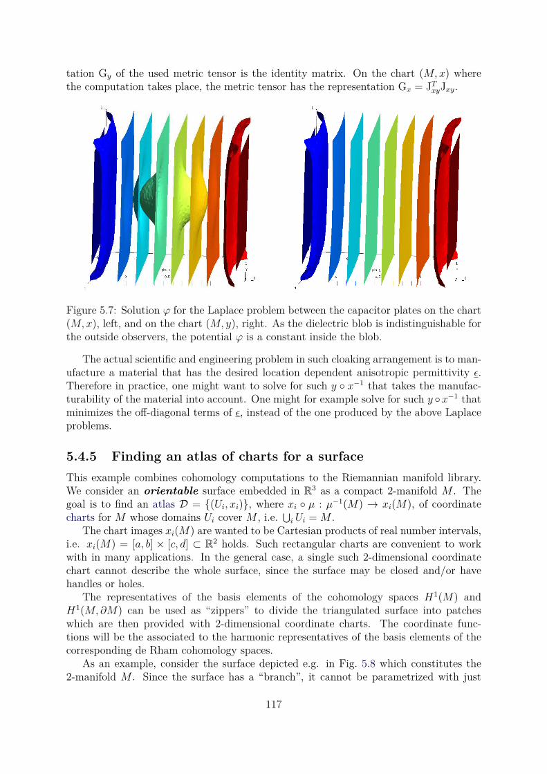
tation Gy of the used metric tensor is the identity matrix. On the chart (M,x) wherethe computation takes place, the metric tensor has the representation Gx = JT

xyJxy.

Figure 5.7: Solution ϕ for the Laplace problem between the capacitor plates on the chart(M,x), left, and on the chart (M, y), right. As the dielectric blob is indistinguishable forthe outside observers, the potential ϕ is a constant inside the blob.

The actual scientific and engineering problem in such cloaking arrangement is to man-ufacture a material that has the desired location dependent anisotropic permittivity ǫ.Therefore in practice, one might want to solve for such y x−1 that takes the manufac-turability of the material into account. One might for example solve for such y x−1 thatminimizes the off-diagonal terms of ǫ, instead of the one produced by the above Laplaceproblems.

5.4.5 Finding an atlas of charts for a surface

This example combines cohomology computations to the Riemannian manifold library.We consider an orientable surface embedded in R

3 as a compact 2-manifold M . Thegoal is to find an atlas D = (Ui, xi), where xi µ : µ−1(M) → xi(M), of coordinatecharts for M whose domains Ui cover M , i.e.

⋃

i Ui = M .The chart images xi(M) are wanted to be Cartesian products of real number intervals,

i.e. xi(M) = [a, b] × [c, d] ⊂ R2 holds. Such rectangular charts are convenient to work

with in many applications. In the general case, a single such 2-dimensional coordinatechart cannot describe the whole surface, since the surface may be closed and/or havehandles or holes.

The representatives of the basis elements of the cohomology spaces H1(M) andH1(M,∂M) can be used as “zippers” to divide the triangulated surface into patcheswhich are then provided with 2-dimensional coordinate charts. The coordinate func-tions will be the associated to the harmonic representatives of the basis elements of thecorresponding de Rham cohomology spaces.

As an example, consider the surface depicted e.g. in Fig. 5.8 which constitutes the2-manifold M . Since the surface has a “branch”, it cannot be parametrized with just

117

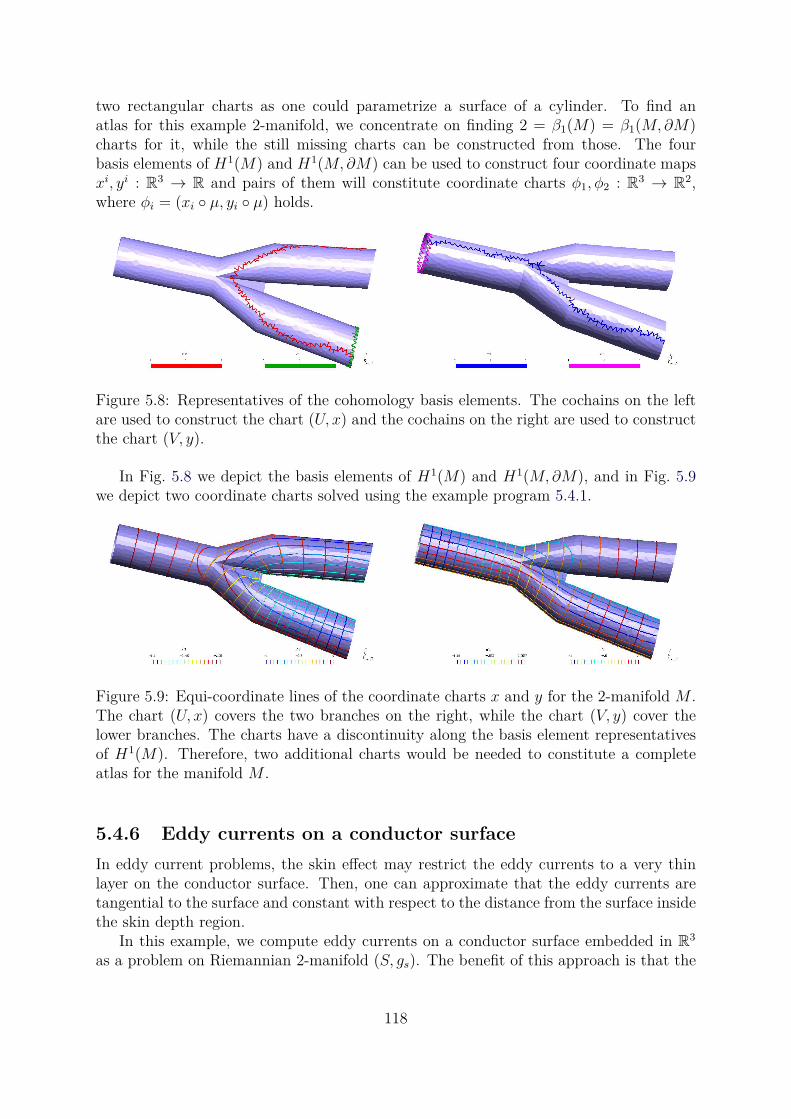
two rectangular charts as one could parametrize a surface of a cylinder. To find anatlas for this example 2-manifold, we concentrate on finding 2 = β1(M) = β1(M,∂M)charts for it, while the still missing charts can be constructed from those. The fourbasis elements of H1(M) and H1(M,∂M) can be used to construct four coordinate mapsxi, yi : R3 → R and pairs of them will constitute coordinate charts φ1, φ2 : R3 → R

2,where φi = (xi µ, yi µ) holds.

Figure 5.8: Representatives of the cohomology basis elements. The cochains on the leftare used to construct the chart (U, x) and the cochains on the right are used to constructthe chart (V, y).

In Fig. 5.8 we depict the basis elements of H1(M) and H1(M,∂M), and in Fig. 5.9we depict two coordinate charts solved using the example program 5.4.1.

Figure 5.9: Equi-coordinate lines of the coordinate charts x and y for the 2-manifold M .The chart (U, x) covers the two branches on the right, while the chart (V, y) cover thelower branches. The charts have a discontinuity along the basis element representativesof H1(M). Therefore, two additional charts would be needed to constitute a completeatlas for the manifold M .

5.4.6 Eddy currents on a conductor surface

In eddy current problems, the skin effect may restrict the eddy currents to a very thinlayer on the conductor surface. Then, one can approximate that the eddy currents aretangential to the surface and constant with respect to the distance from the surface insidethe skin depth region.

In this example, we compute eddy currents on a conductor surface embedded in R3

as a problem on Riemannian 2-manifold (S, gs). The benefit of this approach is that the

118

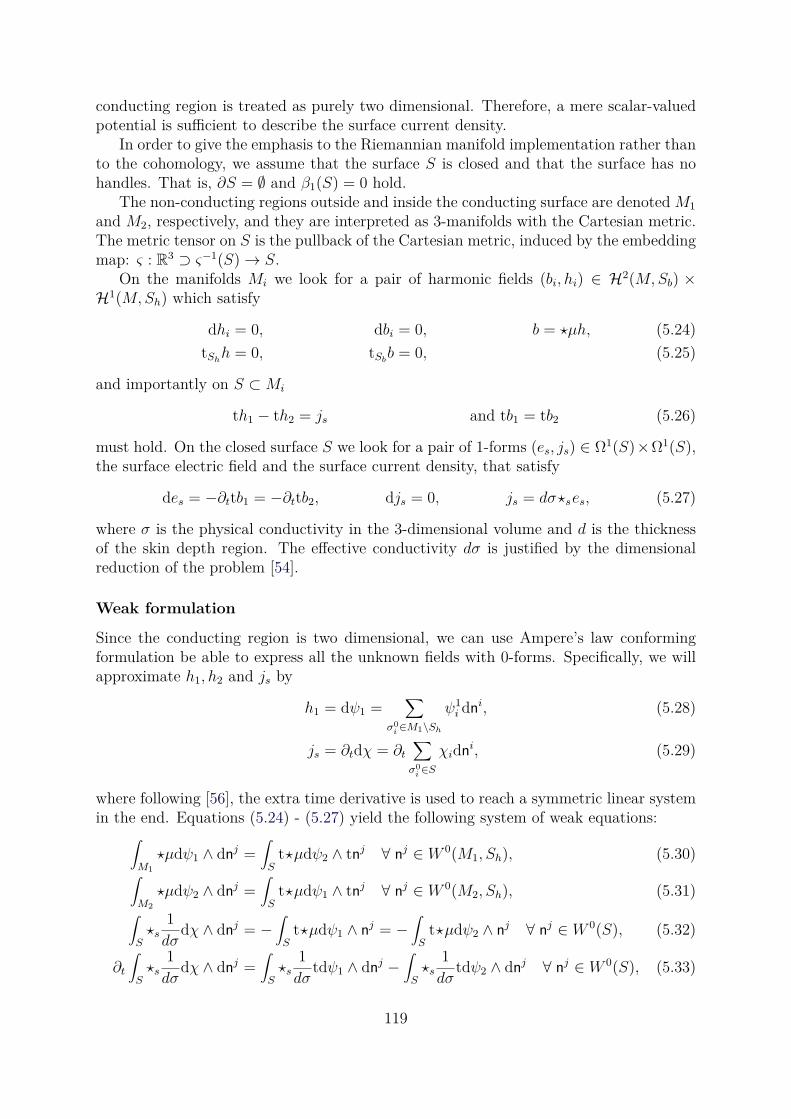
conducting region is treated as purely two dimensional. Therefore, a mere scalar-valuedpotential is sufficient to describe the surface current density.

In order to give the emphasis to the Riemannian manifold implementation rather thanto the cohomology, we assume that the surface S is closed and that the surface has nohandles. That is, ∂S = ∅ and β1(S) = 0 hold.

The non-conducting regions outside and inside the conducting surface are denoted M1

and M2, respectively, and they are interpreted as 3-manifolds with the Cartesian metric.The metric tensor on S is the pullback of the Cartesian metric, induced by the embeddingmap: ς : R3 ⊃ ς−1(S)→ S.

On the manifolds Mi we look for a pair of harmonic fields (bi, hi) ∈ H2(M,Sb) ×H1(M,Sh) which satisfy

dhi = 0, dbi = 0, b = ⋆µh, (5.24)

tShh = 0, tSb

b = 0, (5.25)

and importantly on S ⊂Mi

th1 − th2 = js and tb1 = tb2 (5.26)

must hold. On the closed surface S we look for a pair of 1-forms (es, js) ∈ Ω1(S)×Ω1(S),the surface electric field and the surface current density, that satisfy

des = −∂ttb1 = −∂ttb2, djs = 0, js = dσ⋆ses, (5.27)

where σ is the physical conductivity in the 3-dimensional volume and d is the thicknessof the skin depth region. The effective conductivity dσ is justified by the dimensionalreduction of the problem [54].

Weak formulation

Since the conducting region is two dimensional, we can use Ampere’s law conformingformulation be able to express all the unknown fields with 0-forms. Specifically, we willapproximate h1, h2 and js by

h1 = dψ1 =∑

σ0i∈M1\Sh

ψ1i dn

i, (5.28)

js = ∂tdχ = ∂t

∑

σ0i∈S

χidni, (5.29)

where following [56], the extra time derivative is used to reach a symmetric linear systemin the end. Equations (5.24) - (5.27) yield the following system of weak equations:

∫

M1

⋆µdψ1 ∧ dnj =

∫

St⋆µdψ2 ∧ tnj ∀ n

j ∈ W 0(M1, Sh), (5.30)∫

M2

⋆µdψ2 ∧ dnj =

∫

St⋆µdψ1 ∧ tnj ∀ n

j ∈ W 0(M2, Sh), (5.31)∫

S⋆s

1dσ

dχ ∧ dnj = −

∫

St⋆µdψ1 ∧ n

j = −∫

St⋆µdψ2 ∧ n

j ∀ nj ∈ W 0(S), (5.32)

∂t

∫

S⋆s

1dσ

dχ ∧ dnj =

∫

S⋆s

1dσ

tdψ1 ∧ dnj −

∫

S⋆s

1dσ

tdψ2 ∧ dnj ∀ n

j ∈W 0(S), (5.33)

119

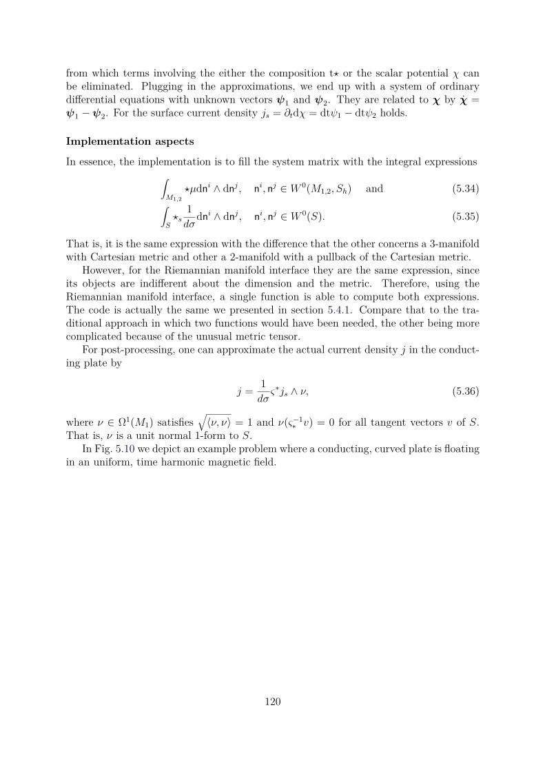
from which terms involving the either the composition t⋆ or the scalar potential χ canbe eliminated. Plugging in the approximations, we end up with a system of ordinarydifferential equations with unknown vectors ψ1 and ψ2. They are related to χ by χ =ψ1 −ψ2. For the surface current density js = ∂tdχ = dtψ1 − dtψ2 holds.

Implementation aspects

In essence, the implementation is to fill the system matrix with the integral expressions∫

M1,2

⋆µdni ∧ dn

j, ni, nj ∈W 0(M1,2, Sh) and (5.34)

∫

S⋆s

1dσ

dni ∧ dn

j, ni, nj ∈W 0(S). (5.35)

That is, it is the same expression with the difference that the other concerns a 3-manifoldwith Cartesian metric and other a 2-manifold with a pullback of the Cartesian metric.

However, for the Riemannian manifold interface they are the same expression, sinceits objects are indifferent about the dimension and the metric. Therefore, using theRiemannian manifold interface, a single function is able to compute both expressions.The code is actually the same we presented in section 5.4.1. Compare that to the tra-ditional approach in which two functions would have been needed, the other being morecomplicated because of the unusual metric tensor.

For post-processing, one can approximate the actual current density j in the conduct-ing plate by

j =1dσς∗js ∧ ν, (5.36)

where ν ∈ Ω1(M1) satisfies√

〈ν, ν〉 = 1 and ν(ς−1∗ v) = 0 for all tangent vectors v of S.

That is, ν is a unit normal 1-form to S.In Fig. 5.10 we depict an example problem where a conducting, curved plate is floating

in an uniform, time harmonic magnetic field.

120

Figure 5.10: The approximate current density j = 1/(dσ)ς∗js ∧ ν = jr + iji. The realpart jr is on the left and the imaginary part ji is on the right.

121

Chapter 6

Conclusion

This study focused on the implementation of computational methods in the finite elementmethod that exploit modern mathematical structures. In particular, we implementedhomology and cohomology solver and a programming interface that separates the metricand the coordinates, and mimics coordinate-free objects on a Riemannian manifold. Theformer tool can be interfaced with finite element mesh generators and solvers, while thelatter can be used to implement finite element pre- and post-processors and user interfacesfor them.

We also showed that these kind of tools and the mathematical structures behindthem are needed to bring computational electromagnetics to a firmer ground. They helpto distinguish the general concepts and to avoid suffocating oneself with all the detailsinvolved.

6.1 Homology and cohomology solver

In the mathematical theory of boundary value problems on Riemannian manifolds, ho-mology of the domain and cohomology class of the unknown field are intimately linked.Together they play a role in the existence and uniqueness of the solution to a boundaryvalue problem. Therefore, they also need to be taken into account in the formulation andimplementation of the numerical methods for boundary value problems. In this thesis wehave shown that explicit computation of homology and cohomology is both practical andbeneficial in the finite element modeling.

While our examples were mainly from the field of electromagnetics, the same principlesapply also on other fields of physics and engineering, creating potential for future possibil-ities. Acknowledging this, the implemented homology and cohomology solver strives forefficient general, possibly relative, homology and cohomology computation. In contrast,for the 1-cohomology computation even more efficient methods might be developed withthe loss of generality.

6.2 Riemannian manifold interface

The language of differential geometry is nowadays prominent in physics. However, engi-neering software tools still interface with the classical vector and tensor analysis which,

122

as we have argued, has some impractical traits. To demonstrate that a different approachmight be viable, we have implemented a programming interface which mimics the frame-work of the differential geometry and the Riemannian manifold. The interface is designedto handle software engineering complexities arising from the free choice of the metric andthe coordinate chart.

Such free choices unify many finite element modeling techniques, such as mesh defor-mation and “transformation techniques” used to model movement and infinite domains,for example. Furthermore, the properties of metamaterials that bend the paths of lightrays, for example [53], can be modeled as the change of metric within the domain.

However, the freedom of choice of the metric and the coordinate chart increases thecomplexity of a computational software, as these choices need to be taken into accountin the actual numerical computations. The solution is to use the metric and coordinatechart agnostic language of differential geometry as an interface, and underneath thatinterface the expressions are automatically translated to the metric and coordinate chartdependent computations. At the programming interface, the choice of the metric and thecoordinate chart is controlled at one place.

6.3 Future developments

In the conclusions of [61] it was envisioned that homology computation should be broughtcloser to the engineering practice. The homology and cohomology solver presented in thisthesis is a definite step towards that direction. We now have easy-to-use and efficienttool at our hands, and we have provided examples of its usage in engineering. In fu-ture, we hope homology and cohomology computation would be used by genuine workingengineers.

The Riemannian manifold imitation presented in this thesis is an programming in-terface, not an user interface. Today, finite element modeling tools use classical vectoranalysis as their user interface. However in future, there might grow a demand for userinterfaces where differential geometry plays the prominent part. If one used a Riemannianmanifold programming interface similar to our implementation underneath, a Rieman-nian manifold user interface can be build on top of it with a minimal effort. Also, thethe classical vector analysis approach is difficult in multiphysics environments due tofield specific practices and tradition. As a new player on the field, differential geometrycould be used as an unifying language. Therefore, one might construct classical fieldspecific user interfaces that support engineer’s intuition and experience, and couple thosevia a Riemannian manifold programming interface to build a maintainable multiphysicsenvironment.

123

Bibliography

[1] P. R. Amestoy, I. S. Duff, J. Koster, and J.-Y. L’Excellent. A fully asynchronousmultifrontal solver using distributed dynamic scheduling. SIAM Journal on MatrixAnalysis and Applications, 23(1):15–41, 2001.

[2] D. N. Arnold, R. S. Falk, and R. Winther. Finite element exterior calcu-lus, homological techniques, and applications. Acta Numer., 15:1–155, 2006.doi:10.1017/S0962492906210018.

[3] D. N. Arnold, R. S. Falk, and R. Winther. Finite element exterior calculus: fromhodge theory to numerical stability. Bull. Amer. Math. Soc. (N.S.), 47:281–354,2010. doi:10.1090/S0273-0979-10-01278-4.

[4] N. Bell and A. N. Hirani. Pydec: A Python library for Discrete Exterior Calculus.http://code.google.com/p/pydec/, 2008.

[5] N. Bell and A. N. Hirani. Pydec: Software and algorithms for discretization ofexterior calculus. ACM Transactions on Mathematical Software, 2012. (to appear).

[6] A. Bossavit. Magnetostatic problems in multiply connected regions: Some prop-erties of the curl operator. Physical Science, Measurement and Instrumentation,Management and Education - Reviews, IEE Proceedings A, 135(3):179–187, 1988.doi:10.1049/ip-a-1:19880028.

[7] A. Bossavit. Solving maxwell equations in a closed cavity, and the question of‘spurious modes’. Magnetics, IEEE Transactions on, 26(2):702–705, Mar 1990.doi:10.1109/20.106414.

[8] A. Bossavit. Computational Electromagnetism. Academic Press, 1998.

[9] A. Bossavit. How weak is the "weak solution" in finite element methods? Magnetics,IEEE Transactions on, 34(5):2429 –2432, sep 1998. doi:10.1109/20.717558.

[10] A. Bossavit. Computational electromagnetism and geometry. (5): The ’galerkinhodge’. Journal of the Japan Society of Applied Electromagnetics, 8(2):203 –209,2000.

[11] G Carlsson. Bull. Amer. Math. Soc., 46:255–308, 2009.doi:10.1090/S0273-0979-09-01249-X.

[12] CHomP Group. CHomP. http://chomp.rutgers.edu/software/, 2012.

124

[13] J. C. Crager and P.R. Kotiuga. Cuts for the magnetic scalar potential in knot-ted geometries and force-free magnetic fields. Magnetics, IEEE Transactions on,38(2):1309–1312, Mar 2002. doi:10.1109/TMAG.2002.996334.

[14] G. F. D. Duff. Differential forms in manifolds with boundary. Annals of Mathematics,56(1):pp. 115–127, 1952.

[15] P. Dular, F. Henrotte, F. Robert, A. Genon, and W. Legros. A generalized sourcemagnetic field calculation method for inductors of any shape. Magnetics, IEEETransactions on, 33(2):1398–1401, 1997. doi:10.1109/20.582518.

[16] P. Dular, P. Kuo-Peng, C. Geuzaine, N. Sadowski, and J.P.A. Bastos. Dualmagnetodynamic formulations and their source fields associated with massive andstranded inductors. Magnetics, IEEE Transactions on, 36(4):1293 –1299, jul 2000.doi:10.1109/20.877677.

[17] P. Dular, W. Legros, and A. Nicolet. Coupling of local and global quantities in variousfinite element formulations and its application to electrostatics, magnetostatics andmagnetodynamics. Magnetics, IEEE Transactions on, 34(5):3078 –3081, sep 1998.doi:10.1109/20.717720.

[18] P. Dłotko and R. Specogna. Efficient cohomology computation for electromagneticmodeling. CMES: Computer Modeling in Engineering & Sciences, 60(3):247–278,2010. doi:doi:10.3970/cmes.2010.060.247.

[19] P. Dłotko and R Specogna. Cohomology in 3d magneto-quasistaticsmodeling. Communications in Computational Physics, 14(1):48–76, 2013.doi:doi:10.4208/cicp.151111.180712a.

[20] P. Dłotko and R. Specogna. A novel technique for cohomology computations inengineering practice. Computer Methods in Applied Mechanics and Engineering,253(0):530 – 542, 2013. doi:10.1016/j.cma.2012.08.009.

[21] P. Dłotko, R. Specogna, and F. Trevisan. Automatic generation of cuts onlarge-sized meshes for the t − ω geometric eddy-current formulation. ComputerMethods in Applied Mechanics and Engineering, 198(47–48):3765 – 3781, 2009.doi:10.1016/j.cma.2009.08.007.

[22] P. Dłotko, R. Specogna, and F. Trevisan. Voltage and current sources for massiveconductors suitable with the geometric eddy-current formulation. Magnetics, IEEETransactions on, 46(8):3069–3072, 2010. doi:10.1109/TMAG.2010.2043510.

[23] H. Flanders. Differential Forms with Applications to the Physical Sciences. DoverPublications, 1963.

[24] T. Frankel. The Geometry of Physics. Cambridge University Press, 1997.

[25] R. Geroch. Mathematical Physics. University of Chicago Press, 1985.

125

[26] C. Geuzaine and J.-F. Remacle. Gmsh: a Three-dimensional Finite Element MeshGenerator with Built-in Pre- and Post-processing Facilities. International Journal forNumerical Methods in Engineering, 79:1309–1331, 11 2009. doi:10.1002/nme.2579.

[27] V. Gol’dshtein, I. Mitrea, and M. Mitrea. Hodge decompositions withmixed boundary conditions and applications to partial differential equationson lipschitz manifolds. Journal of Mathematical Sciences, 172:347–400, 2011.doi:10.1007/s10958-010-0200-y.

[28] P. W. Gross and P. R. Kotiuga. Electromagnetic Theory and Computation. Cam-bridge University Press, 2004.

[29] V. Guillemin and A. Pollack. Differential Topology. AMS Chelsea Publishing Series.AMS Chelsea Pub., 2010.

[30] H. Si. Tetgen a Quality Tetrahedral Mesh Generator and Three-dimensional Delau-nay Triangulator. http://wias-berlin.de/software/tetgen/, 2011.

[31] A. Hatcher. Algebraic Topology. Cambridge University Press, 2002.

[32] H. Helmholtz. Über integrale der hydrodynamischen gleichungen, welcher der wirbel-bewegungen entsprechen. Journal für die reine und angewandte Mathematik, 55:25–55, 1858.

[33] F. Henrotte and K. Hameyer. An algorithm to construct the discrete co-homology basis functions required for magnetic scalar potential formulationswithout cuts. Magnetics, IEEE Transactions on, 39(3):1167–1170, 2003.doi:10.1109/TMAG.2003.810404.

[34] F. Henrotte, B. Meys, H. Hedia, P. Dular, and W. Legros. Finite element modellingwith transformation techniques. IEEE Transactions on Magnetics, 35(3):1434–1437,1999.

[35] M. Holst. Adaptive Numerical Treatment of Elliptic Systems on Manifolds. Advancesin Computational Mathematics, 15:139–191, 2001.

[36] B. D. Saunders J.-G. Dumas, F. Heckenbach and V. Welker. In algebra, geometryand software systems. pages 177–206, March 2003.

[37] J.-G. Dumas, F. Heckenbach, B. D. Saunders and V. Welker. GAP Homology.http://www.eecis.udel.edu/~dumas/Homology/, 2011.

[38] T. Kaczynski, K. Mischaikow, and M. Mrozek. Computational Homology. Springer-Verlag New York Inc., 2004.

[39] T. Kaczynski, M. Mrozek, and M. Ślusarek. Homology Computation by Reductionof Chain Complexes. Computers Math. Applic., 35(4):59 – 70, 1998.

[40] L. Kettunen. Fields and circuits in computational electromagnetism. Magnetics,IEEE Transactions on, 37(5):3393–3396, 2001. doi:10.1109/20.952621.

126

[41] L. Kettunen, K. Forsman, and A. Bossavit. Formulation ofthe Eddy Current Problem in Multiply Connected Regions inTerms of h. Int. J. Numer. Meth. Engng., 41:935 – 954, 1998.doi:10.1002/(SICI)1097-0207(19980315)41:5<935::AID-NME321>3.0.CO;2-F.

[42] P. R. Kotiuga. Hodge Decompositions and Computational Electromagnetics. PhDthesis, Dept. Elect. Eng., McGill Univ., Montreal, Canada, 1984.

[43] P. R. Kotiuga. On making cuts for magnetic scalar potentials in multiply connectedregions. Journal of Applied Physics, 61(8):3916–3918, 1987. doi:10.1063/1.338583.

[44] P. R. Kotiuga. Toward an algorithm to make cuts for magnetic scalar poten-tials in finite element meshes. Journal of Applied Physics, 63(8):3357–3359, 1988.doi:10.1063/1.340781.

[45] P. R. Kotiuga. An algorithm to make cuts for magnetic scalar potentials in tetrahe-dral meshes based on the finite element method. Magnetics, IEEE Transactions on,25(5):4129–4131, 1989. doi:10.1109/20.42544.

[46] Rensselaer Polytechnic Institute. Image Processing Laboratory and D.J.R. Meagher.Octree Encoding: a New Technique for the Representation, Manipulation and Displayof Arbitrary 3-D Objects by Computer. 1980.

[47] M. Mrozek and B. Batko. Coreduction homology algorithm. Discrete & Computa-tional Geometry, 41:96–118, 2009. doi:10.1007/s00454-008-9073-y.

[48] J. R. Munkres. Elements of Algebraic Topology. Perseus Books, 1984.

[49] M. Pellikka, S. Suuriniemi, and L. Kettunen. Homology in electromagneticboundary value problems. Boundary Value Problems, 2010(1):381953, 2010.doi:10.1155/2010/381953.

[50] M. Pellikka, S. Suuriniemi, and L. Kettunen. Powerful heuristics and basis selec-tion bring computational homology to engineers. Magnetics, IEEE Transactions on,47(5):1226 –1229, may 2011. doi:10.1109/TMAG.2010.2091109.

[51] M. Pellikka, S. Suuriniemi, L. Kettunen, and C. Geuzaine. Homology and cohomol-ogy computation in finite element modeling. SIAM Journal on Scientific Computing,35(5):B1195–B1214, 2013. doi:10.1137/130906556.

[52] M. Pellikka, T. Tarhasaari, S. Suuriniemi, and L. Kettunen. A program-ming interface to the riemannian manifold in a finite element environment.Journal of Computational and Applied Mathematics, 246(0):225 – 233, 2013.doi:10.1016/j.cam.2012.10.022.

[53] J. B. Pendry, D. Schurig, and D. R. Smith. Controlling electromagnetic fields. Sci-ence, 312:1780–178, 2006. doi:10.1126/science.1125907.

[54] P. Raumonen. Mathematical Structures for Dimensional Reduction and EquivalenceClassification of Electromagnetic Boundary Value Problems. PhD thesis, Dept. Elect.Eng., Tampere Univ. Technology, Tampere, Finland, 2009.

127

[55] Z. Ren. t−ω -formulation for eddy-current problems in multiply connected regions.Magnetics, IEEE Transactions on, 38(2):557 –560, mar 2002. doi:10.1109/20.996146.

[56] D. Rodger and N. Atkinson. Finite element method for 3d eddy current flow in thinconducting sheets. Physical Science, Measurement and Instrumentation, Manage-ment and Education - Reviews, IEE Proceedings A, 135(6):369–374, 1988.

[57] G. Schwarz. Hodge Decomposition: a Method for Solving Boundary Value Problems.Lecture notes in mathematics. Springer, 1995.

[58] J. Schöberl. Netgen, an Advancing Front 2d/3d-mesh Generator Based on AbstractRules. Comput. Visual. Sci., 1:41–52, 1997.

[59] H. J. S. Smith. Philosophical Transactions of the Royal Society of London, 151:293–326, 1861. doi:10.1098/rstl.1861.0016.

[60] R. Specogna. Complementary geometric formulations for electrostatics. InternationalJournal for Numerical Methods in Engineering, 86(8):1041–1068, 2011.

[61] S. Suuriniemi. Homological Computations in Electromagnetic Modeling. PhD thesis,Dept. Elect. Eng., Tampere Univ. Technology, Tampere, Finland, 2004.

[62] A. Tausz, M. Vejdemo-Johansson, and H. Adams. Javaplex: A research softwarepackage for persistent (co)homology. http://code.google.com/javaplex, 2011.

[63] H. Whitney. Geometric Integration Theory. Princeton University Press, 1957.

[64] C. K. Yap. Fundamental Problems of Algorithmic Algebra. Oxford University Press,2000.

128

Index

C0-manifold, 31Ck-manifold, 31PDIFF -manifold, 31PL-manifold, 31k-boundary, 21k-chain, 39k-coboundary, 24k-cochains, 23k-cocycle, 24k-collapse, 58, 76k-combine, 59k-cotangent bundle, 43k-covector, 28k-cycle, 21k-vector, 28k:th cohomology group, 24k:th homology group, 21q-reduction pair, 55

abelian group, 18affine space, 30alternating, 27

basis, 25basis of a free abelian group, 19boundary ∂M of a manifold, 32boundary homomorphism, 21boundary point, 32

cell basis, 39cell complex, 36cell decomposition, 35cell subcomplex, 36chain complex, 21chain equivalence, 22chain homotopic, 22chain homotopy, 22chain map, 22change of variables formula, 45chart, 31

closed k-form, 44coboundary homomorphism, 23cochain complex, 24codifferential, 48Cohomology basis function, 83cohomology cobasis, 71coordinate basis, 33coordinate cobasis, 33coordinate maps, 32Coreduction, 62coset, 20cotangent bundle, 43cotangent space, 33coupled field-circuit problem, 90cut, 12

de Rham’s theorem, 46differentiable n-manifold, 31differentiable n-manifold-with-boundary, 32differentiable atlas, 31differential, 44dimension, 25dual space, 26

equivalent atlases, 31Euclidean n-ball, 30Euclidean reference k-cell, 37Euclidean space, 30exact k-form, 44exterior product, 28

face, 36finite element, 37finitely generated abelian group, 19flat, 26formal sum, 19free abelian group, 19functor, 23

generalized Stokes’ theorem, 45

129

generating set, 18geometric realization, 35global chart, 31group homomorphism, 18group isomorphism, 18

half-space, 30harmonic differential k-forms, 47Hodge decomposition, 48Hodge operator, 29Hodge’s theorem, 48homologous, 21homotopic, 41homotopy, 41homotopy equivalence, 41

image, 18incidence relation, 36inner oriented k-cell, 35inner product space L2Ωk(M), 47integration by parts, 45

kernel, 18Knot, 76Kronecker delta for multi-indices, 28

Lefschetz duality, 42Leibniz product rule, 44linear map, 25linearly independent, 25

manifold coordinates, 107maximal atlas, 31Mayer-Vietoris sequence, 42metric, 30metric tensor, 34model coordinates, 107multi-index, 28

negative orientation, 30node, 37nonorientable manifold, 34

Omit-collapse, 60orientable manifold, 34orientations of k-cells agree, 36oriented differentiable n-manifold, 34orthonormal, 26

Poincarè duality, 42positive orientation, 30pullback, 26

quotient group, 20

rank of a free abelian group, 19real coordinate space, 30reduced chain complex, 55regular CW-complex, 35relative k-chains, 39relative chain group, 23relative cochain complex, 24relative cohomology groups, 24relative homology groups, 23Riemannian n-manifold, 34

sharp, 26short exact sequence, 21simplicial complex, 37Smith normal form, 64smooth, 32Smooth manifold, 31Sobolev spaces of differential k-forms, 47span, 25splitting short exact sequence, 72standard k-simplex, 37subgroup, 18symplectic manifold, 34

tangent bundle, 43tangent space, 33tangent vector, 32The long exact homology sequence, 42torsion coefficient, 20torsion element, 20torsion subgroup, 20torus knot, 76trace, 44transition map, 31

unimodular matrix, 64

vector space, 25vertex, 37

weak exterior derivative, 47Whitney k-forms, 49

130

Whitney complex, 50Whitney map, 49

131