Computational Photography

Matthias ZwickerUniversity of BernUniversity of Bern

Fall 2010

TodayImage restoration

• Modeling image degradation: degradation function and additive noise

• Restoration under noise only

• Estimating the degradation function

• Deconvolution

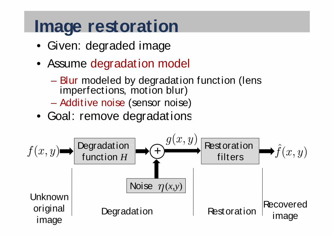
Image restoration• Given: degraded image• Assume degradation model• Assume degradation model

– Blur modeled by degradation function (lens imperfections motion blur)imperfections, motion blur)

– Additive noise (sensor noise)• Goal: remove degradations• Goal: remove degradations

Degradation Restoration ˆg(x, y)

Degradation function H

Restoration filters+f(x, y) f̂(x, y)

g( y)

Noise (x,y)ηUnknown

Degradation RestorationRecovered

image

Unknownoriginalimage

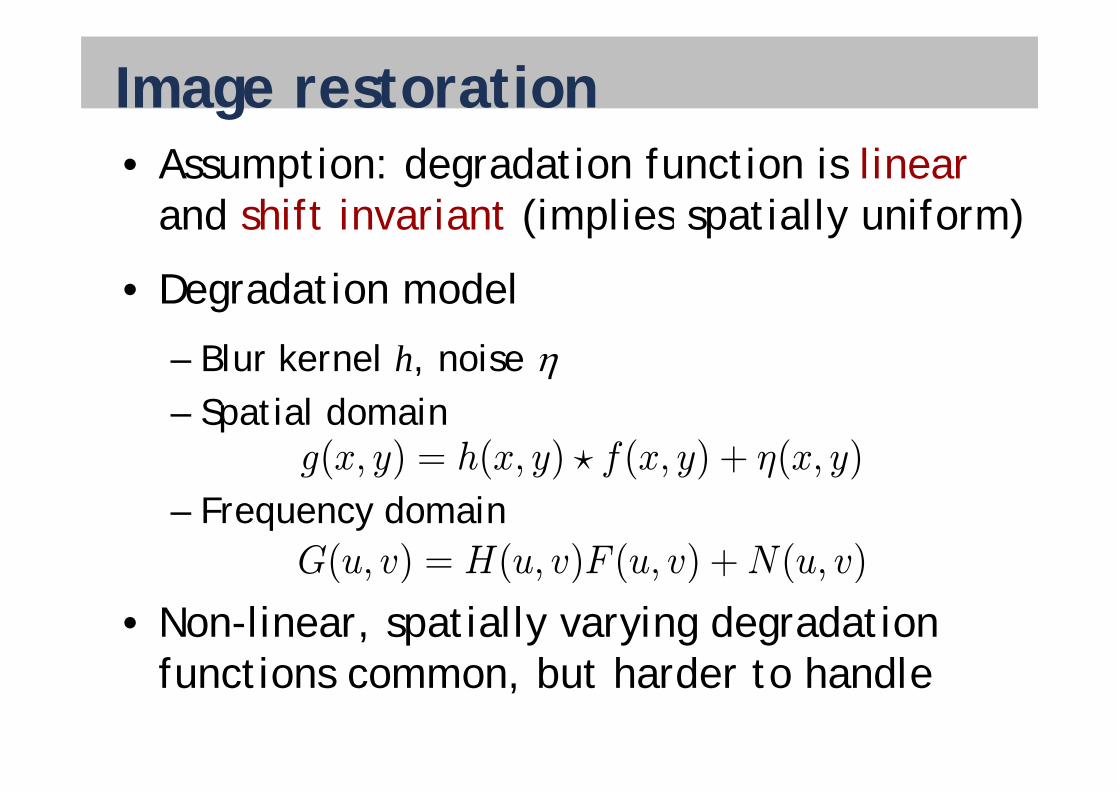
Image restoration• Assumption: degradation function is linear

and shift invariant (implies spatially uniform)and shift invariant (implies spatially uniform)

• Degradation modelg

– Blur kernel h, noise – Spatial domain

g(x, y) = h(x, y) ? f(x, y) + η(x, y)

– Frequency domainG(u, v) = H(u, v)F (u, v) +N(u, v)

• Non-linear, spatially varying degradation f ti b t h d t h dl

( , ) ( , ) ( , ) + ( , )

functions common, but harder to handle

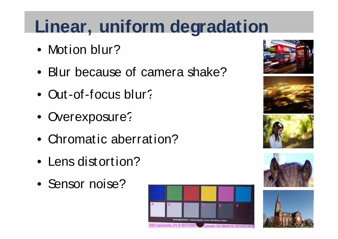
Linear, uniform degradation• Motion blur?

• Blur because of camera shake?

Out of focus blur?• Out-of-focus blur?

• Overexposure?Overexposure?

• Chromatic aberration?

• Lens distortion?

• Sensor noise?

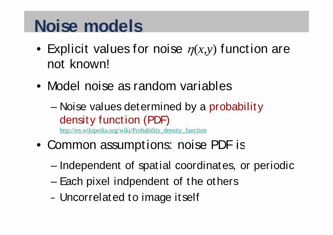
Noise models• Explicit values for noise (x,y) function are

not known!not known!

• Model noise as random variables

– Noise values determined by a probability d it f ti (PDF)density function (PDF)http://en.wikipedia.org/wiki/Probability_density_function

• Common assumptions: noise PDF is• Common assumptions: noise PDF is

– Independent of spatial coordinates, or periodicp p , p– Each pixel indpendent of the others– Uncorrelated to image itself– Uncorrelated to image itself

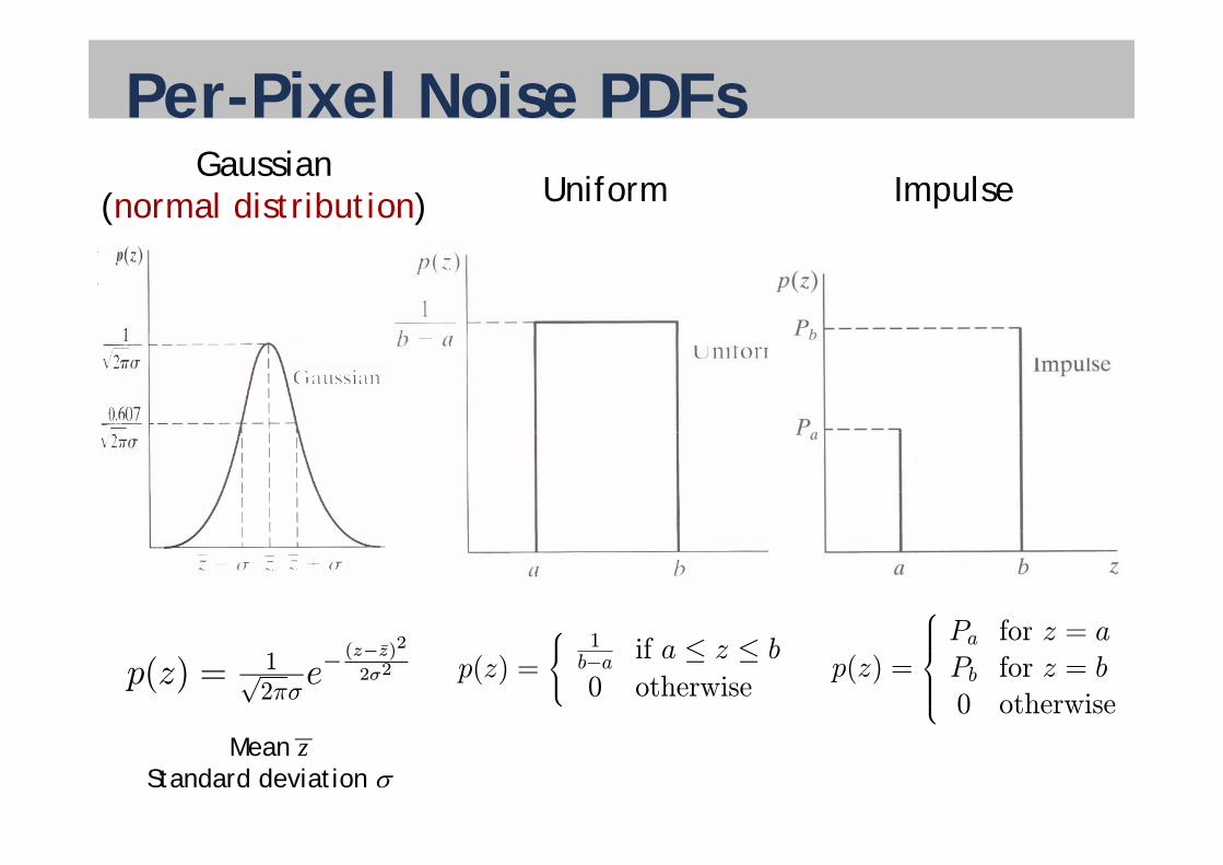
Per-Pixel Noise PDFsGaussian

(normal distribution) Uniform Impulse

⎧P for z a

p(z) = 1√2πσe−

(z−z̄)22σ2 p(z) =

⎧⎨⎩1b−a if a ≤ z ≤ b0 otherwise

p(z) =

⎧⎪⎪⎪⎨⎪⎪⎪⎩Pa for z = aPb for z = b0 otherwise

Mean zStandard deviation

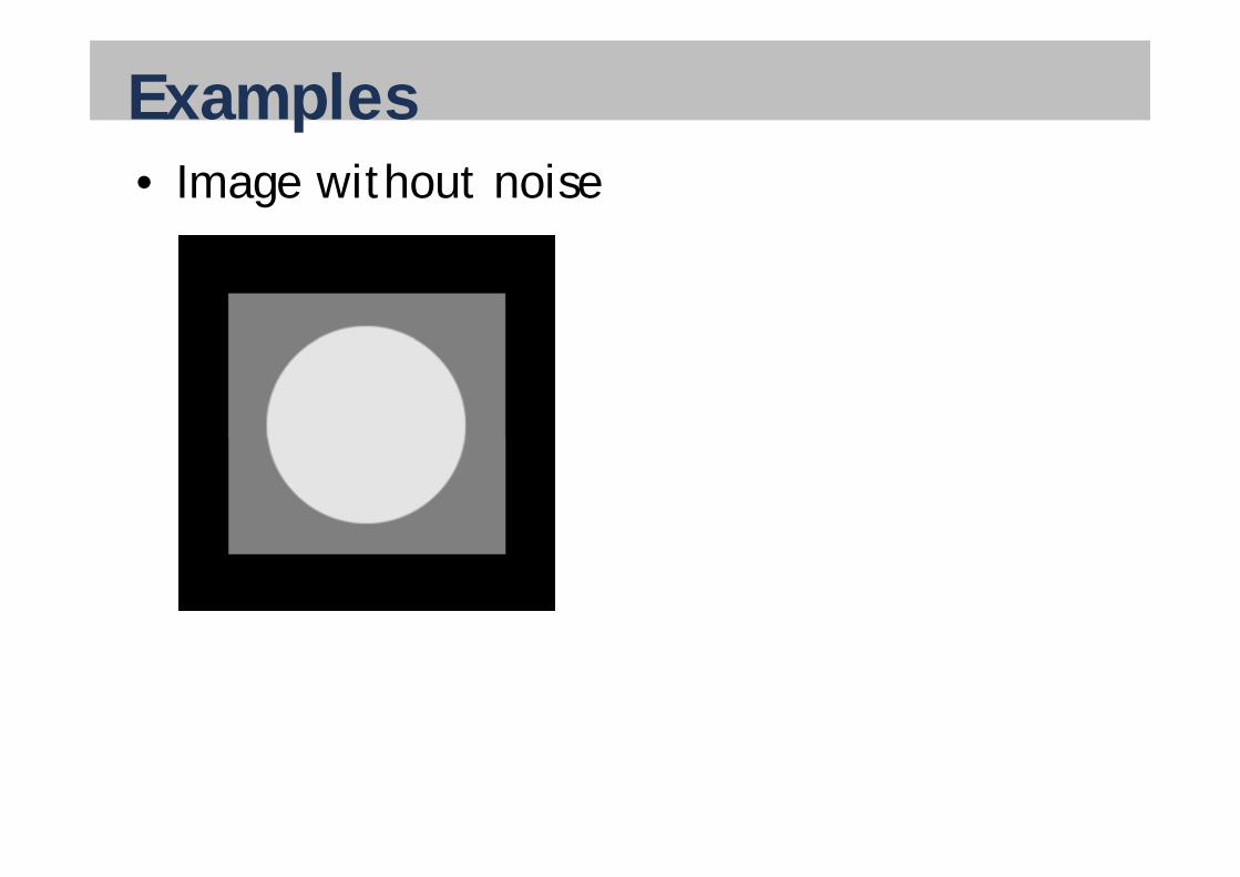
Examples• Image without noise

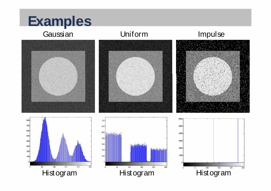
ExamplesGaussian Uniform Impulse

Histogram Histogram Histogram

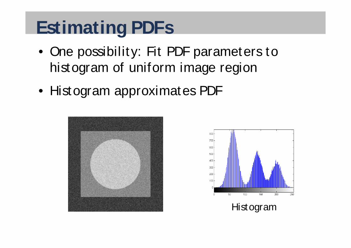
Estimating PDFs• One possibility: Fit PDF parameters to

histogram of uniform image regionhistogram of uniform image region

• Histogram approximates PDFg pp

HistogramHistogram

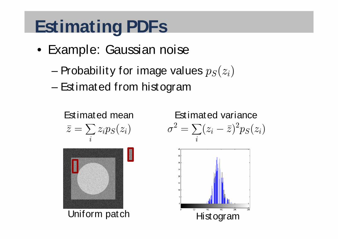
Estimating PDFs• Example: Gaussian noise

– Probability for image values– Estimated from histogram

pS(zi)

g

Estimated mean Estimated variancez̄ =

Xi

zipS(zi) σ2 =Xi

(zi − z̄)2pS(zi)

Uniform patch Histogram

TodayImage restoration

• Modeling image degradation: degradation function and additive noise

• Restoration under noise only

• Estimating the degradation function

• Deconvolution

Restoration under noise only• „Denoising“

• Could use linear smoothing (low-pass) filters

– General idea: replace each pixel with somet f l l g f i l lsort of local average of pixel values

– Problem: sharp edges are blurred

• Many sophisticated, non-linear edge preserving smoothing filters existpreserving smoothing filters exist

• Today: some simple examples, more later

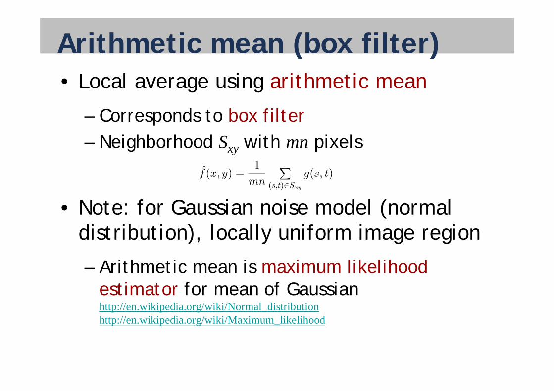
Arithmetic mean (box filter)• Local average using arithmetic mean

– Corresponds to box filter– Neighborhood Sxy with mn pixelsg xy p

f̂(x, y) =1

mn

X(s,t)∈Sxy

g(s, t)

• Note: for Gaussian noise model (normal distribution), locally uniform image region), y g g

– Arithmetic mean is maximum likelihoodti t f f G iestimator for mean of Gaussian

http://en.wikipedia.org/wiki/Normal_distributionhttp://en.wikipedia.org/wiki/Maximum_likelihood

Estimating parameters of normal distribution

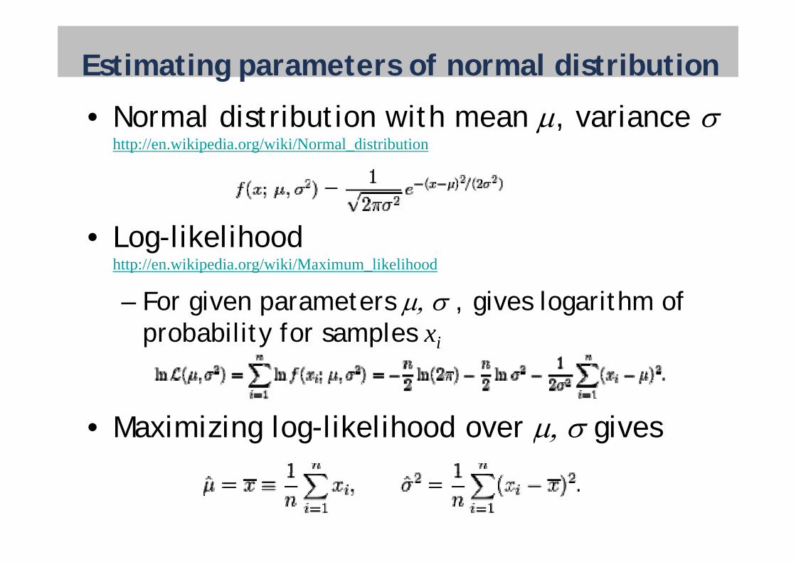
• Normal distribution with mean , variance http://en.wikipedia.org/wiki/Normal_distribution

• Log-likelihoodhttp://en.wikipedia.org/wiki/Maximum_likelihood

– For given parameters , gives logarithm ofprobability for samples xip y p i

• Maximizing log-likelihood over gives

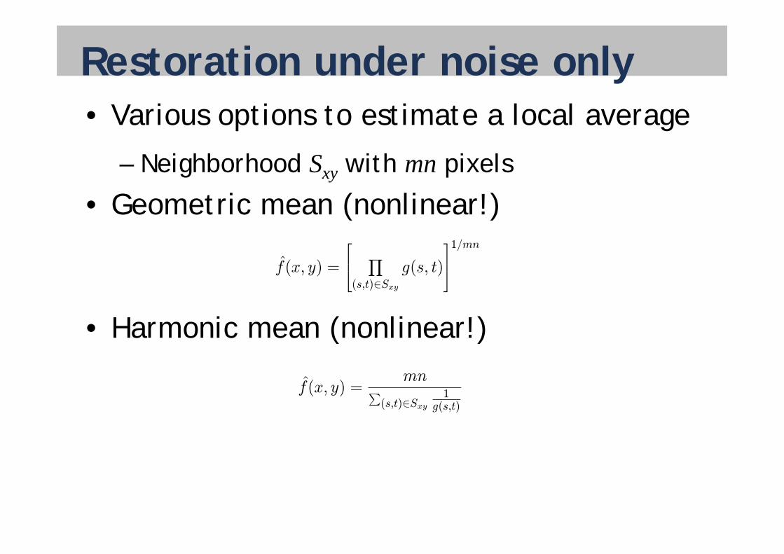
Restoration under noise only• Various options to estimate a local average

– Neighborhood Sxy with mn pixels

• Geometric mean (nonlinear!)Geometric mean (nonlinear!)

f̂(x, y) =

⎡⎢⎣ Yg(s, t)

⎤⎥⎦1/mn

• Harmonic mean (nonlinear!)

⎣(s,t)∈Sxy

⎦

( )

f̂(x, y) =mnP

(s t)∈S1( t)

P(s,t)∈Sxy g(s,t)

Filtering using order statistics• Idea

Order pixels in a neighborhood according to their – Order pixels in a neighborhood according to their values

– Replace central pixel by certain value found from Replace central pixel by certain value found from the ordered list

• Examples for order statistics filters• Examples for order statistics filters– Minimum

M i– Maximum– Median: „value in the middle of ordered list“,

50th percentile 50% of values are smaller 50% 50th percentile, 50% of values are smaller, 50% larger

• Filters are nonlinear!• Filters are nonlinear!

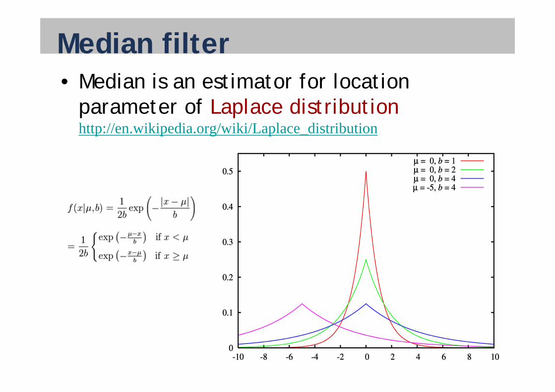
Median filter• Median is an estimator for location

parameter of Laplace distributionparameter of Laplace distributionhttp://en.wikipedia.org/wiki/Laplace_distribution

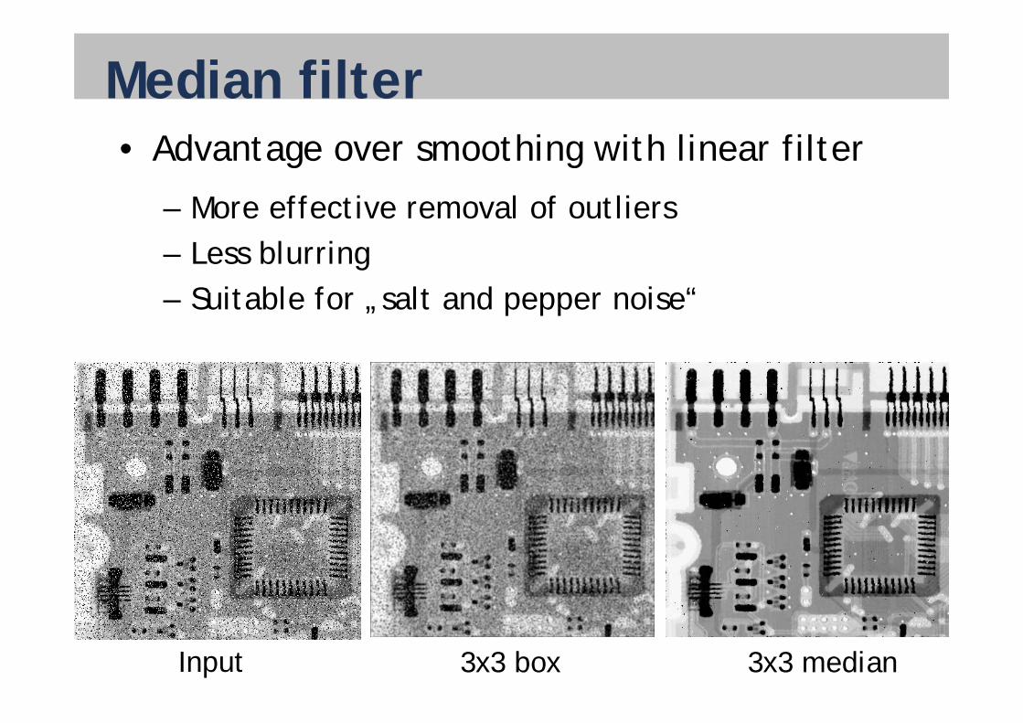
Median filter• Advantage over smoothing with linear filter

M ff ti l f tli– More effective removal of outliers– Less blurring– Suitable for „salt and pepper noise“

Input 3x3 box 3x3 median

TodayImage restoration

• Modeling image degradation: degradation function and additive noise

• Restoration under noise only

• Estimating the degradation function

• Deconvolution

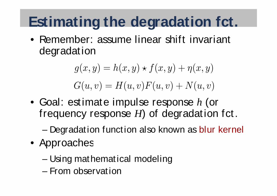
Estimating the degradation fct.• Remember: assume linear shift invariant

degradationdegradation

g(x, y) = h(x, y) ? f(x, y) + η(x, y)

G l i i l (

G(u, v) = H(u, v)F (u, v) +N(u, v)

• Goal: estimate impulse response h (or frequency response H) of degradation fct.– Degradation function also known as blur kernel

• Approaches• Approaches– Using mathematical modeling– From observation

Using mathematical modeling• Use knowledge about capturing process

• Example: camera moves relative to scene at known speed, known exposure timep , p

– Degradation function for motion blur can be d i d f thi i f tiderived from this information

• Disadvantage: applicable only for specific cases where capturing process is precisely knownknown

– Rarely the case in consumer photography

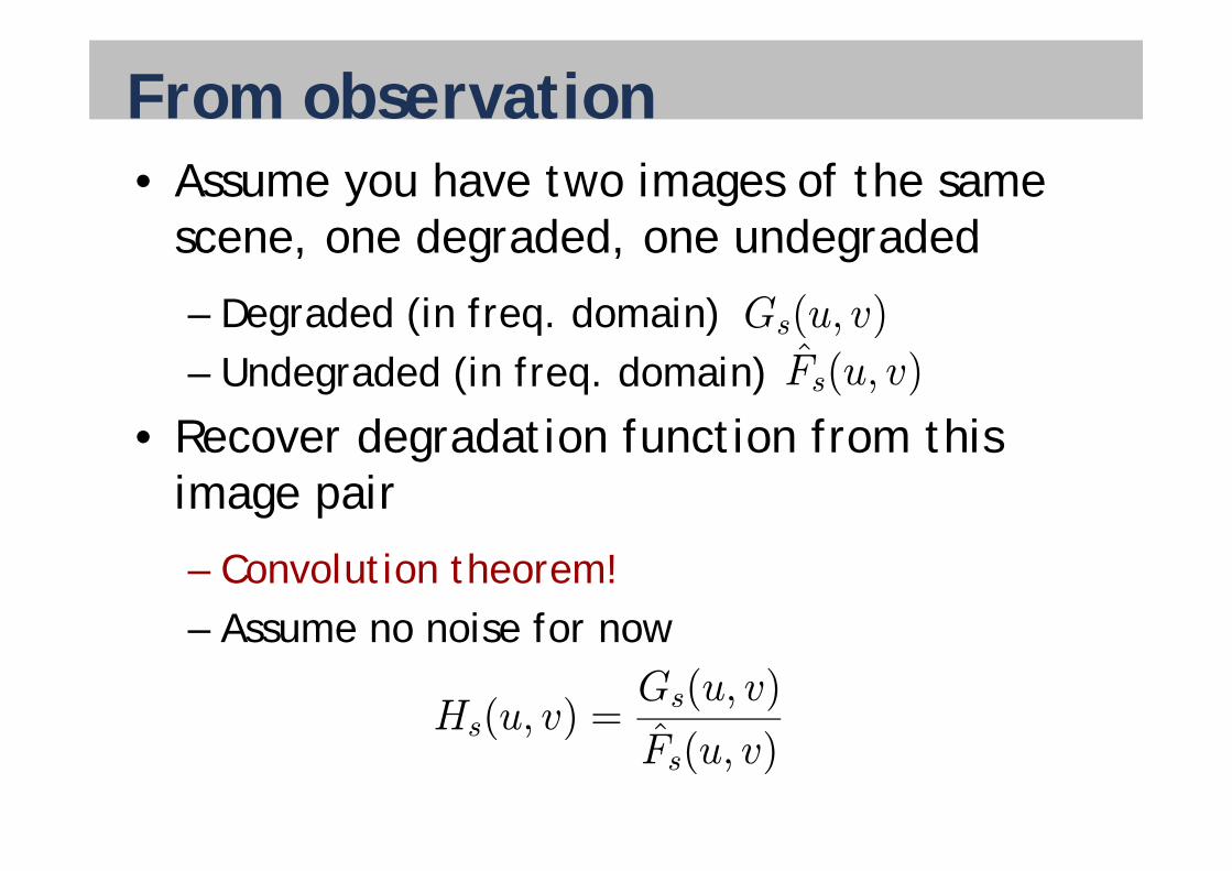
From observation• Assume you have two images of the same

scene one degraded one undegradedscene, one degraded, one undegraded

– Degraded (in freq. domain) Gs(u, v)– Undegraded (in freq. domain)

• Recover degradation function from this

( )

F̂s(u, v)

• Recover degradation function from this image pair

– Convolution theorem!– Assume no noise for nowAssume no noise for now

Hs(u, v) =Gs(u, v)ˆ ( )

s( , )Fs(u, v)

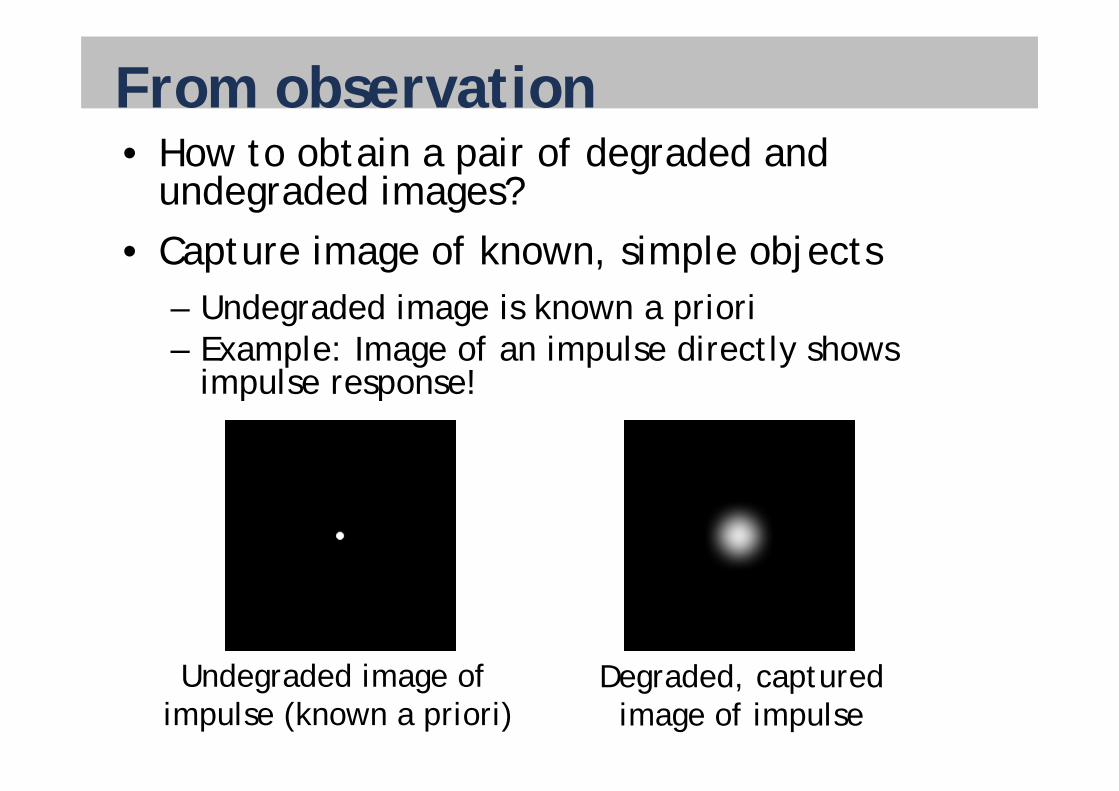
From observation• How to obtain a pair of degraded and

undegraded images?• Capture image of known, simple objects

Undegraded image is known a priori– Undegraded image is known a priori– Example: Image of an impulse directly shows

impulse response!p p

U d d d i f D d d dUndegraded image of impulse (known a priori)

Degraded, capturedimage of impulse

Practical problems• Often impossible to capture pair of

degraded/undegraded imagedegraded/undegraded image

• Example: blur due to camera shake of h d h ld hand-held camera– Shaking is different for every shotShaking is different for every shot

• Solution: use other known properties of captured image and degradation functioncaptured image and degradation function– E.g., „most edges in images are sharp,

d d i f i i h i i l degradation function is smooth, statistical properties of image“A i h – Active research area

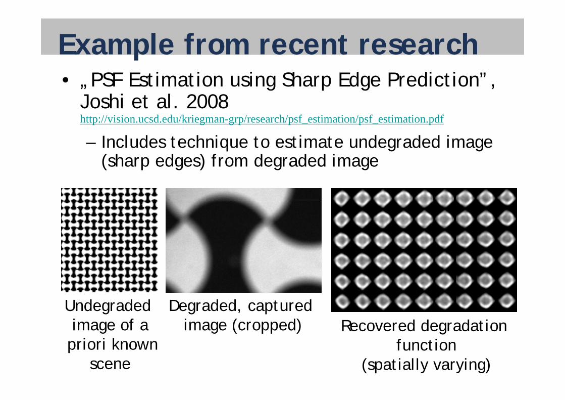
Example from recent research• „PSF Estimation using Sharp Edge Prediction”,

Joshi et al. 2008http://vision.ucsd.edu/kriegman-grp/research/psf_estimation/psf_estimation.pdf

– Includes technique to estimate undegraded image ( h d ) f d d d i(sharp edges) from degraded image

Undegraded image of a Recovered degradation

Degraded, captured image (cropped)

priori knownscene

function(spatially varying)

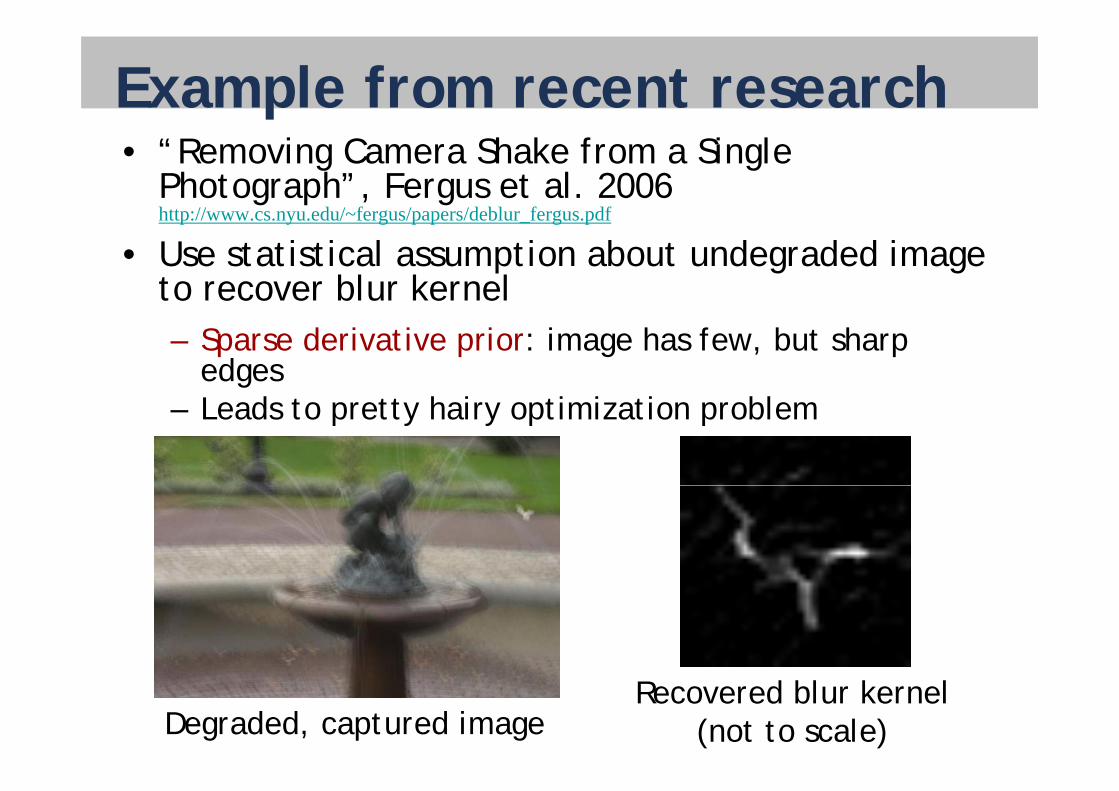
Example from recent research• “Removing Camera Shake from a Single

Photograph”, Fergus et al. 2006http://www cs nyu edu/~fergus/papers/deblur fergus pdfhttp://www.cs.nyu.edu/~fergus/papers/deblur_fergus.pdf

• Use statistical assumption about undegraded image to recover blur kernel– Sparse derivative prior: image has few, but sharp

edges– Leads to pretty hairy optimization problem

Degraded, captured imageRecovered blur kernel

(not to scale)

TodayImage restoration

• Modeling image degradation: degradation function and additive noise

• Restoration under noise only

• Estimating the degradation function

• Deconvolution

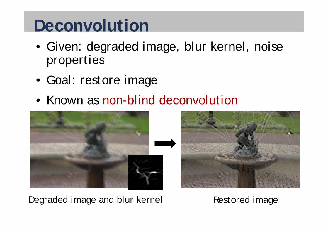
Deconvolution• Given: degraded image, blur kernel, noise

propertiesproperties

• Goal: restore image

• Known as non-blind deconvolution

Degraded image and blur kernel Restored image

Deconvolution• Today

– Inverse filtering– Wiener filteringg– Constrained least square filtering– Richardson-Lucy deconvolution– Richardson-Lucy deconvolution

• Not covered

– Blind deconvolution: recover blur kernel and restore image simultaneouslyrestore image simultaneously

Inverse filtering• Degradation model (frequency domain)

G(u v) = H(u v)F (u v) +N(u v)

• Restored image using inverse filtering

G(u, v) = H(u, v)F (u, v) +N(u, v)

Restored image using inverse filtering– Assuming degradation function H known

F̂ (u, v) =G(u, v)

H(u, v)= F (u, v) +

N(u, v)

H(u, v)• Problems

Noise N(u v) is never known

( , ) ( , )

– Noise N(u,v) is never known– Cannot restore F(u,v) exactly

Oft H( ) h ( ) ll l – Often H(u,v) has (some) very small values, therefore noise dominates restored image!

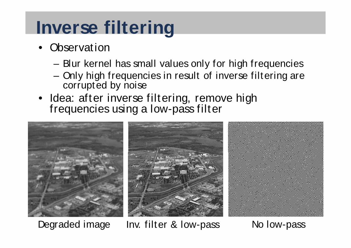
Inverse filtering• Observation

– Blur kernel has small values only for high frequenciesy g q– Only high frequencies in result of inverse filtering are

corrupted by noiseIdea: after inverse filtering remove high • Idea: after inverse filtering, remove high frequencies using a low-pass filter

Degraded image No low-passInv. filter & low-pass

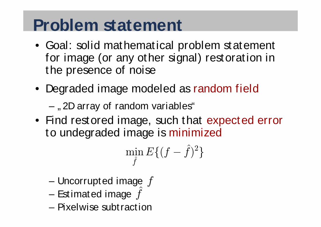
Problem statement• Goal: solid mathematical problem statement

for image (or any other signal) restoration in g ( y g )the presence of noise

• Degraded image modeled as random field• Degraded image modeled as random field– „2D array of random variables“

• Find restored image, such that expected error to undegraded image is minimized

minf̂E{(f − f̂)2}

– Uncorrupted imageE ti t d i

f

ff̂– Estimated image

– Pixelwise subtractionf

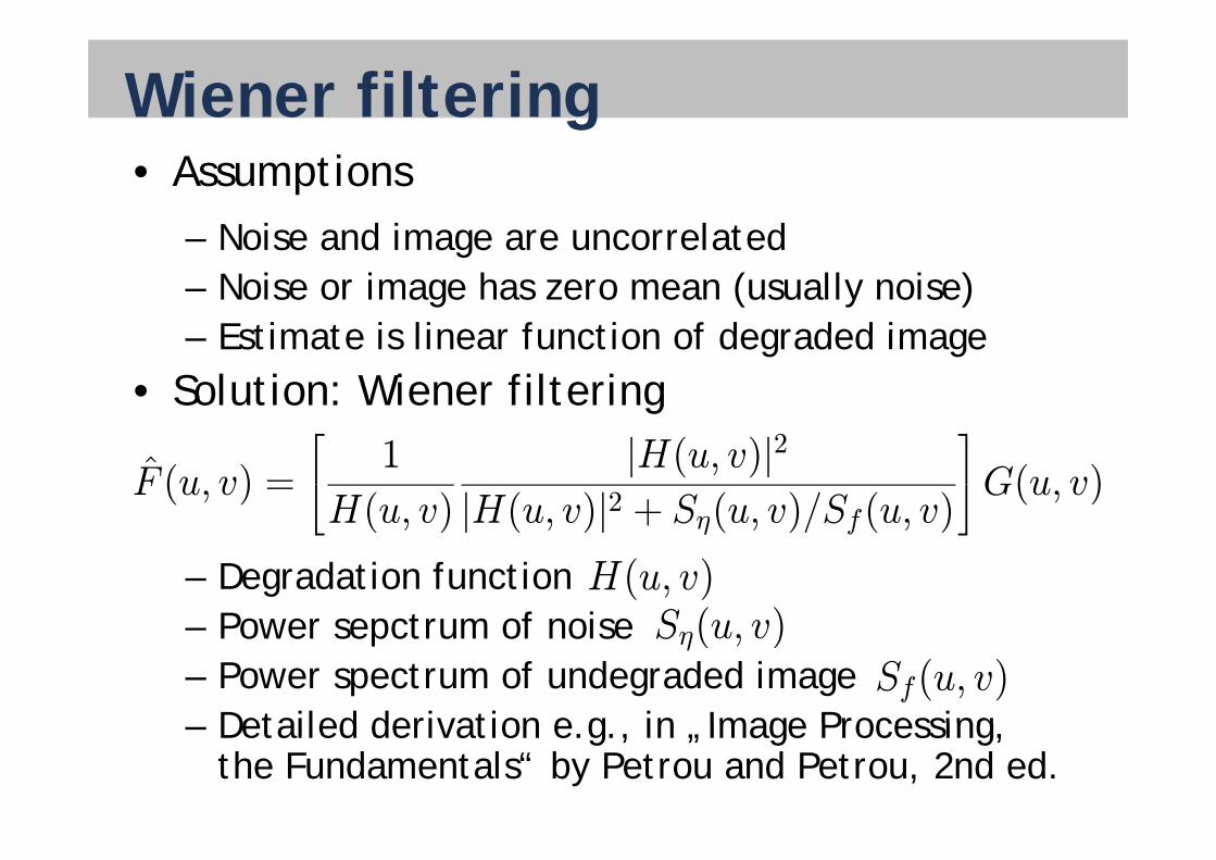
Wiener filtering• Assumptions

Noise and image are uncorrelated– Noise and image are uncorrelated– Noise or image has zero mean (usually noise)

Estimate is linear function of degraded image– Estimate is linear function of degraded image• Solution: Wiener filtering

F̂ (u, v) =

⎡⎣ 1

H(u, v)

|H(u, v)|2|H(u, v)|2 + Sη(u, v)/Sf(u, v)

⎤⎦G(u, v)– Degradation function

Power sepctrum of noise

⎣( , ) | ( , )| η( , )/ f( , )

⎦

S (u v)H(u, v)

– Power sepctrum of noise– Power spectrum of undegraded image

Detailed derivation e g in Image Processing Sf(u, v)

Sη(u, v)

– Detailed derivation e.g., in „Image Processing, the Fundamentals“ by Petrou and Petrou, 2nd ed.

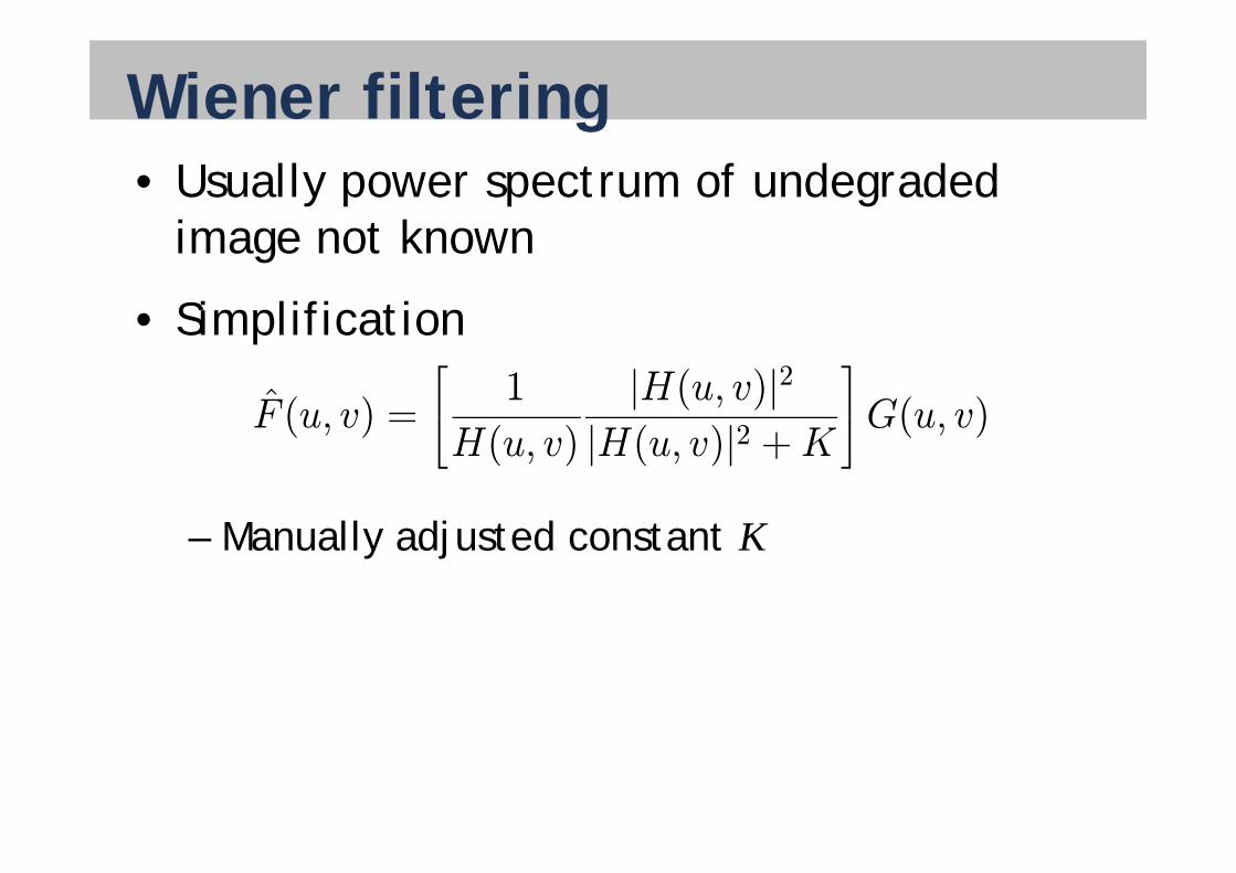
Wiener filtering• Usually power spectrum of undegraded

image not knownimage not known

• Simplificationp

F̂ (u, v) =

⎡⎣ 1

H( )

|H(u, v)|2|H( )|2 +K

⎤⎦G(u, v)Manually adjusted constant K

( ) ⎣H(u, v) |H(u, v)|2 +K

⎦ ( )

– Manually adjusted constant K

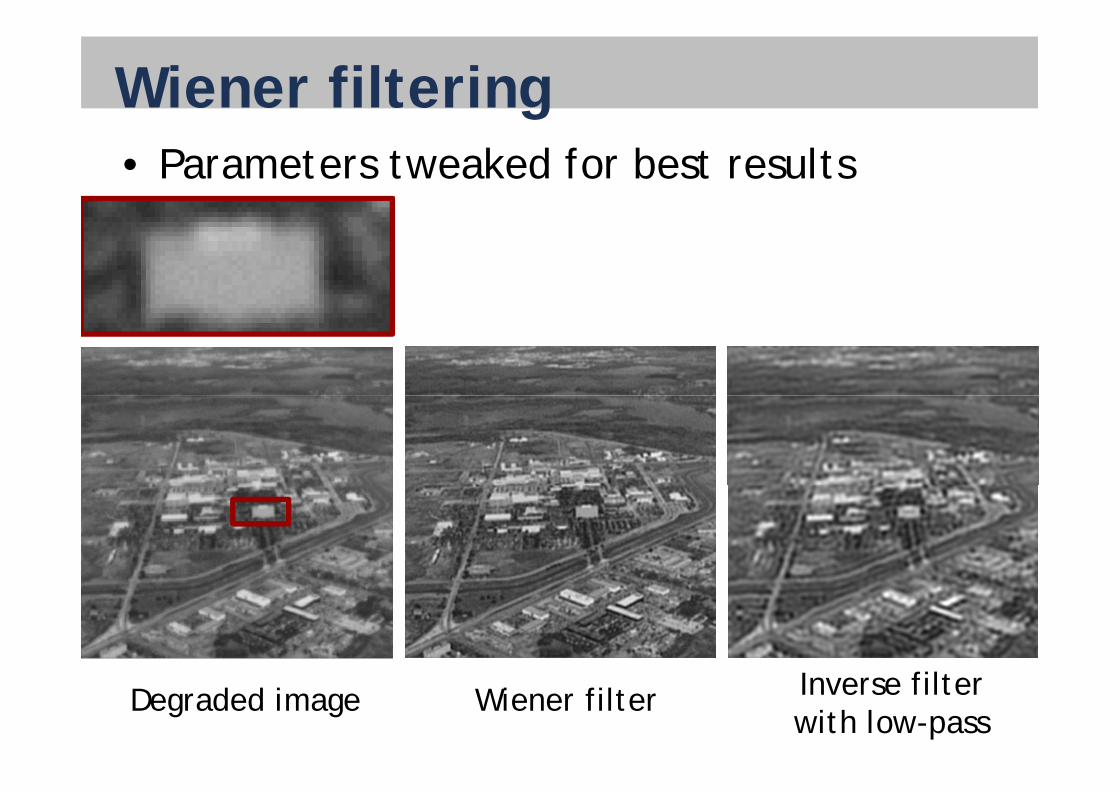
Wiener filtering• Parameters tweaked for best results

Degraded image Inverse filterwith low-pass

Wiener filter

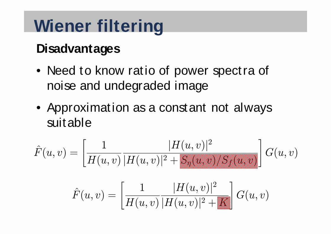
Wiener filteringDisadvantages

• Need to know ratio of power spectra of noise and undegraded imageg g

• Approximation as a constant not always suitable ⎡

1 |H(u v)|2⎤

F̂ (u, v) =

⎡⎣ 1

H(u, v)

|H(u, v)|2|H(u, v)|2 + Sη(u, v)/Sf(u, v)

⎤⎦G(u, v)

F̂ (u v) =

⎡⎣ 1 |H(u, v)|2⎤⎦G(u v)F (u, v) = ⎣

H(u, v) |H(u, v)|2 +K⎦G(u, v)

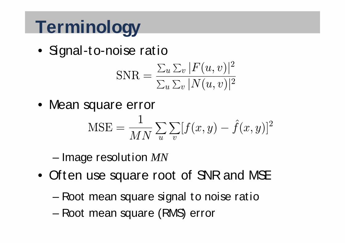
Terminology• Signal-to-noise ratioP P |F (u v)|2

SNR =

PuPv |F (u, v)|2P

uPv |N(u, v)|2

• Mean square error1 ˆ 2MSE =1

MN

Xu

Xv[f(x, y)− f(x, y)]2

– Image resolution MN• Often use square root of SNR and MSE• Often use square root of SNR and MSE

– Root mean square signal to noise ratio– Root mean square (RMS) error

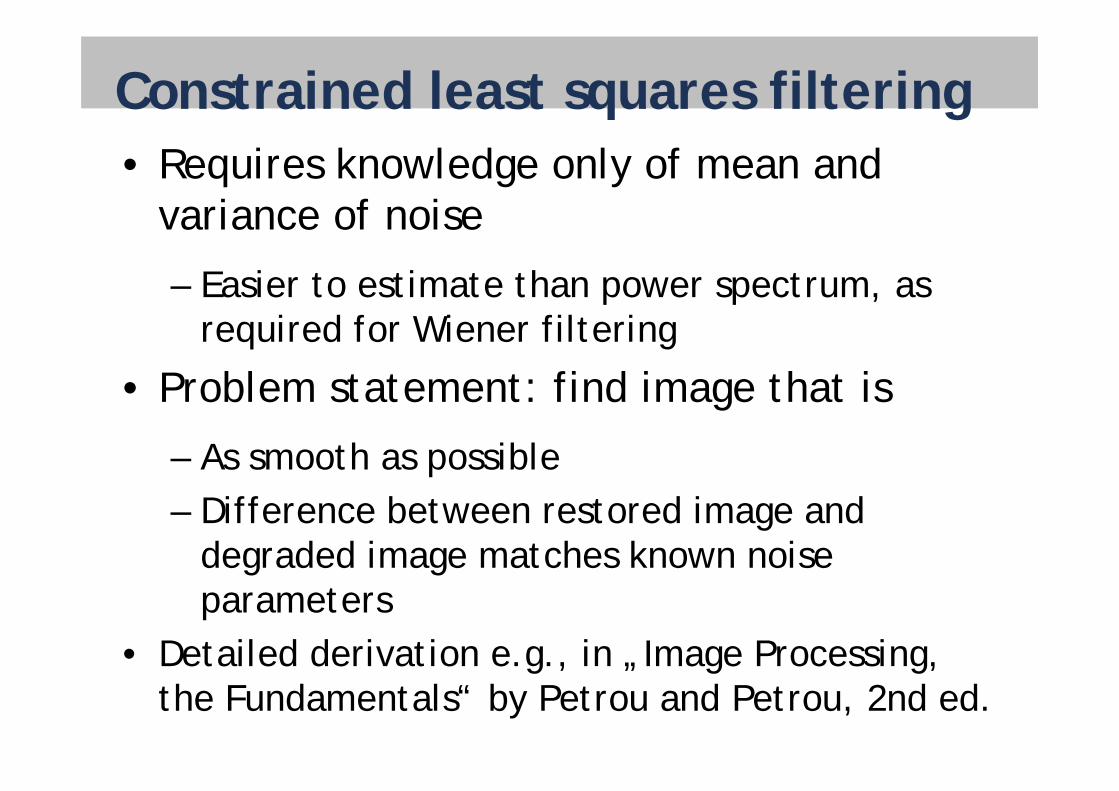
Constrained least squares filtering• Requires knowledge only of mean and

variance of noisevariance of noise

– Easier to estimate than power spectrum, as required for Wiener filtering

• Problem statement: find image that is • Problem statement: find image that is

– As smooth as possible– Difference between restored image and

degraded image matches known noiseg gparameters

• Detailed derivation e.g., in „Image Processing, Detailed derivation e.g., in „Image Processing, the Fundamentals“ by Petrou and Petrou, 2nd ed.

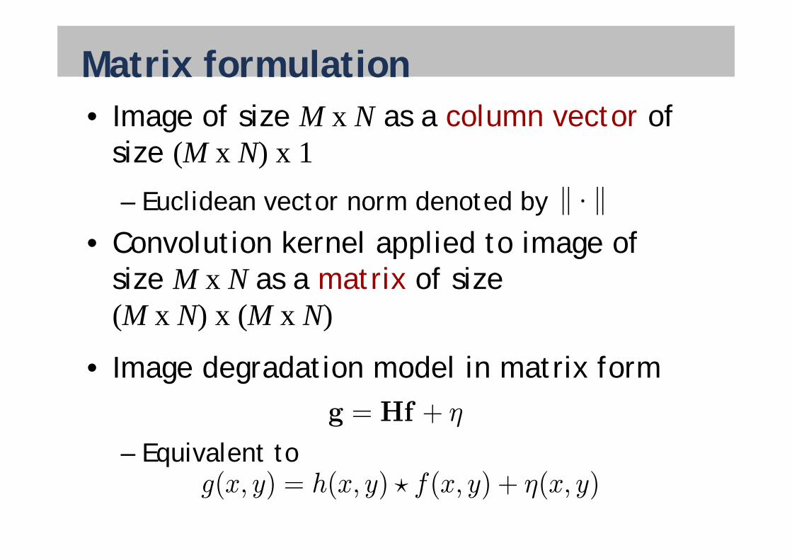
Matrix formulation• Image of size M x N as a column vector of

size (M x N) x 1size (M x N) x 1– Euclidean vector norm denoted by k · k

• Convolution kernel applied to image of size M x N as a matrix of size size M x N as a matrix of size (M x N) x (M x N)

• Image degradation model in matrix formHf +

– Equivalent to

g = Hf + η

g(x, y) = h(x, y) ? f(x, y) + η(x, y)

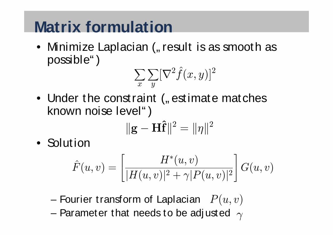
Matrix formulation• Minimize Laplacian („result is as smooth as

possible“)p ) Xx

Xy[∇2f̂(x, y)]2

• Under the constraint („estimate matches known noise level“)

• Solutionkg −Hf̂k2 = kηk2

• Solution

F̂ (u, v) =

⎡⎣ H∗(u, v)

|H( )|2 |P ( )|2⎤⎦G(u, v)

Fourier transform of Laplacian

( , ) ⎣|H(u, v)|2 + γ|P (u, v)|2

⎦G( , )P ( )– Fourier transform of Laplacian

– Parameter that needs to be adjustedP (u, v)

γ

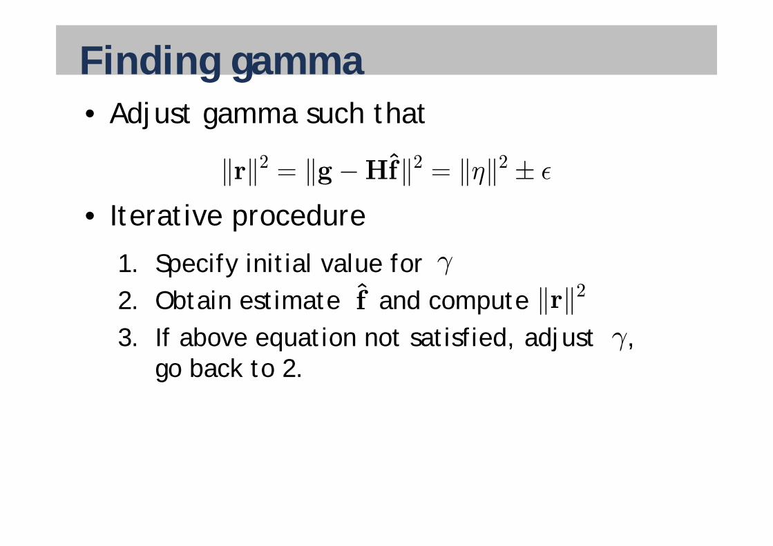
Finding gamma• Adjust gamma such that

Iterative procedure

krk2 = kg −Hf̂k2 = kηk2 ± ²• Iterative procedure

1. Specify initial value for γp y2. Obtain estimate and compute3 If above equation not satisfied adjust

γ

f̂ krk2γ3. If above equation not satisfied, adjust ,

go back to 2.γ

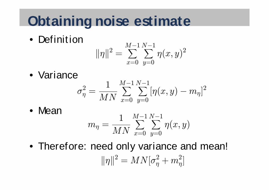
Obtaining noise estimate• Definition

k k2M−1X N−1X

( )2

Variance

kηk2 = Xx=0

Xy=0

η(x, y)2

• Variance

σ2η =1

MN

M−1X N−1X[η(x, y)−mη]

2

• Mean

η MN

Xx=0

Xy=0[η( , y) η]

1 M−1 N−1mη =

1

MN

M−1Xx=0

N−1Xy=0

η(x, y)

• Therefore: need only variance and mean!kηk2 MN [σ2 +m2]kηk =MN [ση +mη]

Summary• Wiener and constrained least squares filter

lead to very similar equations and resultslead to very similar equations and results

• Wiener filter designed to optimize g prestoration in statistical sense

• Constrained least squares filter formulated as problem to find optimal restoration of p pone specific input

D il d d i i i I • Detailed derivation, e.g., in „Image Processing: The Fundamentals“, Petrou & Petrou, 2nd ed., Wiley

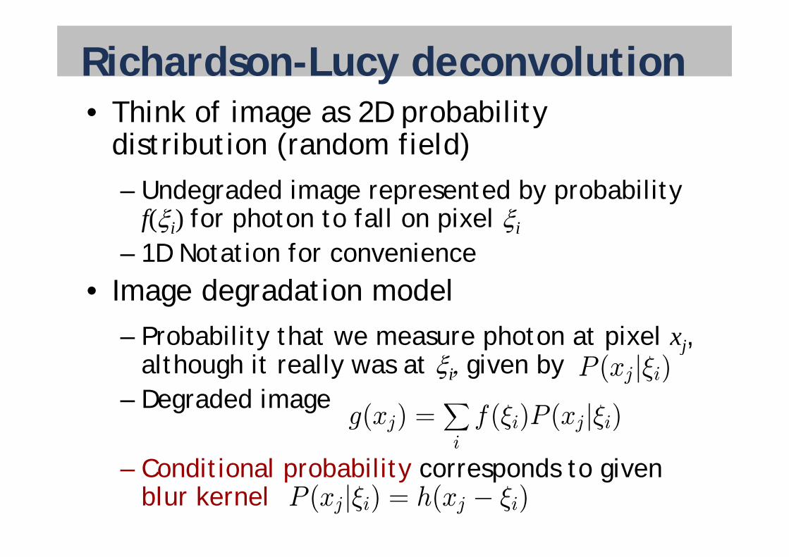
Richardson-Lucy deconvolution• Think of image as 2D probability

distribution (random field)distribution (random field)– Undegraded image represented by probability

f( ) for photon to fall on pixel f(i) for photon to fall on pixel i– 1D Notation for convenience

d d d l• Image degradation model – Probability that we measure photon at pixel xj, Probability that we measure photon at pixel xj,

although it really was at igiven by– Degraded image

( )Xf(ξ ) ( |ξ )

P (xj|ξi)Degraded image

Conditional probability corresponds to given

g(xj) =Xi

f(ξi)P (xj|ξi)– Conditional probability corresponds to given

blur kernel P (xj|ξi) = h(xj − ξi)

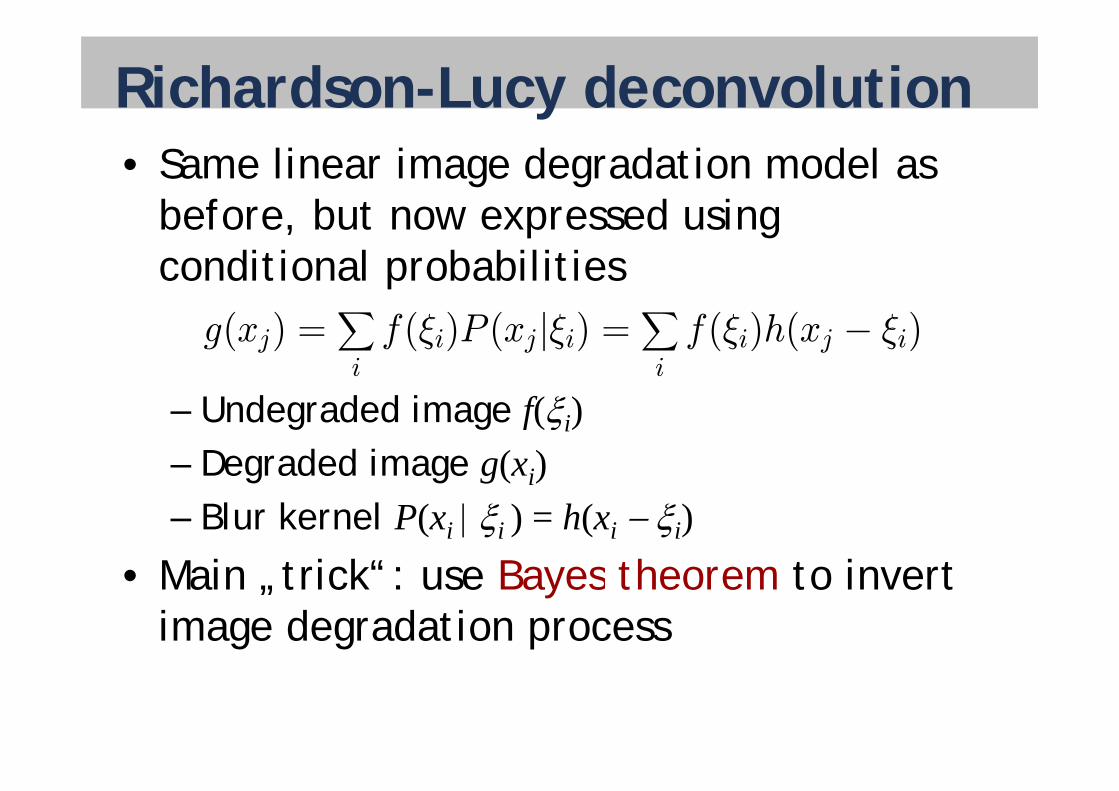
Richardson-Lucy deconvolution• Same linear image degradation model as

before but now expressed usingbefore, but now expressed usingconditional probabilities

U d d d i

g(xj) =Xi

f(ξi)P (xj|ξi) =Xi

f(ξi)h(xj − ξi)

– Undegraded image f(i)– Degraded image g(xi)– Blur kernel P(xi i ) = h(xi i)

• Main trick“: use Bayes theorem to invert• Main „trick : use Bayes theorem to invertimage degradation process

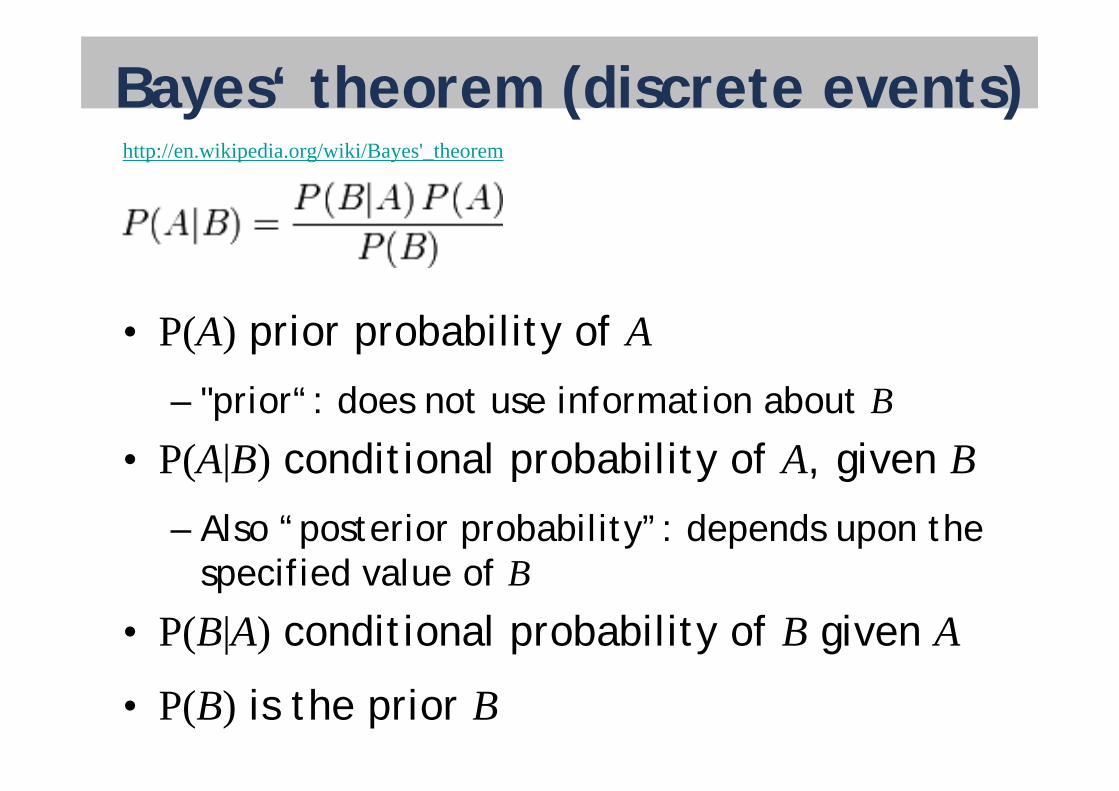
Bayes‘ theorem (discrete events)http://en.wikipedia.org/wiki/Bayes'_theorem

•

• P(A) prior probability of A"prior“: does not use information about B– prior“: does not use information about B

• P(A|B) conditional probability of A, given B– Also “posterior probability”: depends upon the

specified value of Bspecified value of B• P(B|A) conditional probability of B given A

• P(B) is the prior B

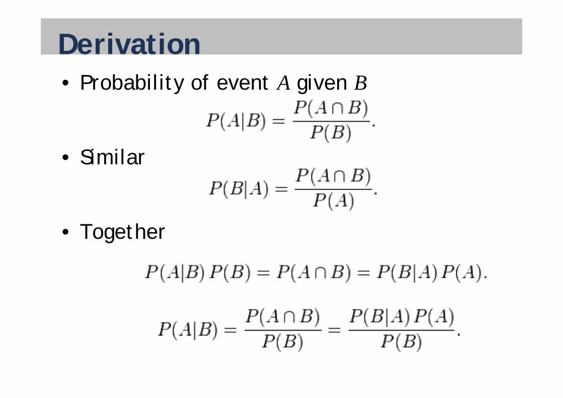
Derivation• Probability of event A given B

Similar• Similar

• Together

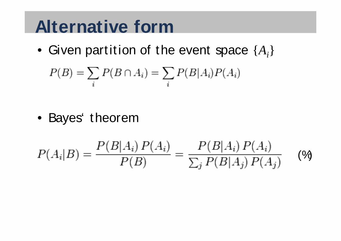
Alternative form• Given partition of the event space {Ai}

• Bayes‘ theoremBayes theorem

(%)

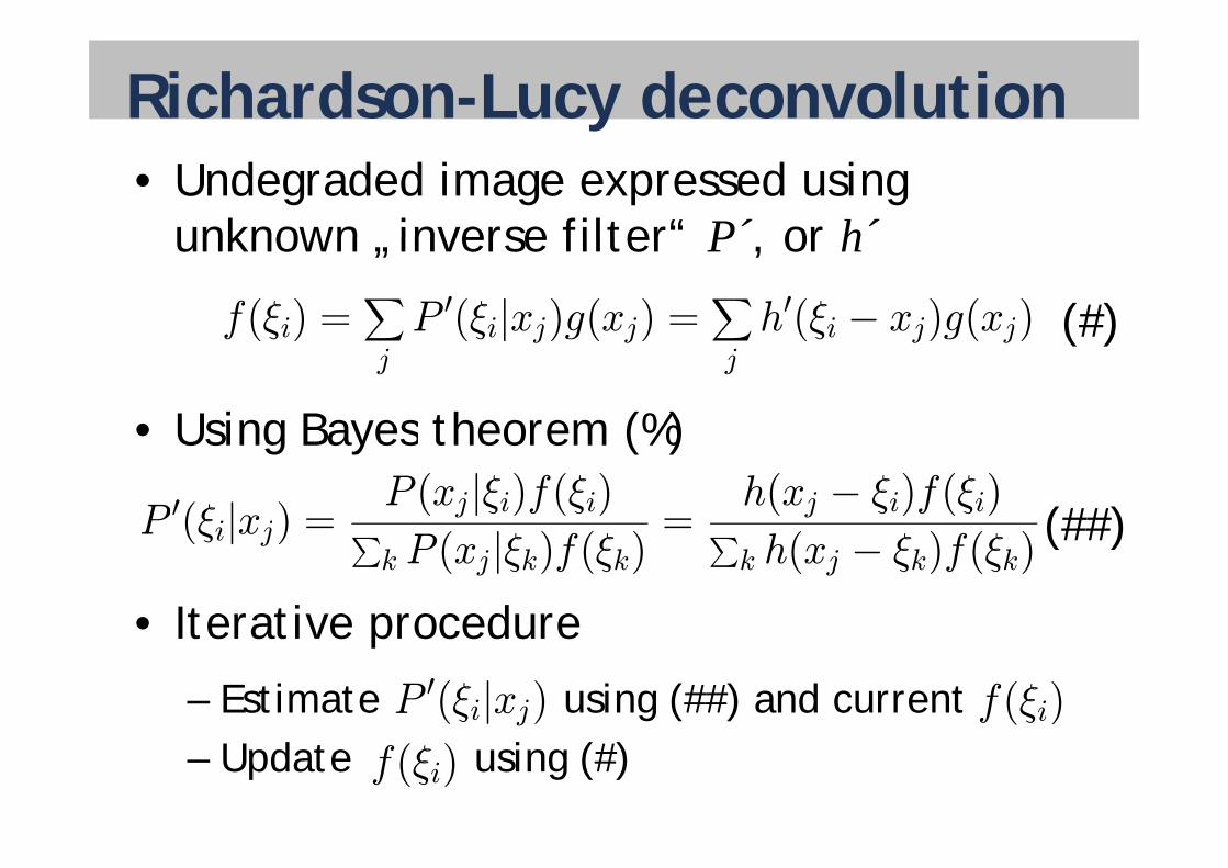
Richardson-Lucy deconvolution• Undegraded image expressed using

unknown inverse filter“ P´ or h´unknown „inverse filter P , or h

f(ξi) =XP 0(ξi|xj)g(xj) =

Xh0(ξi − xj)g(xj) (#)

• Using Bayes theorem (%)

f(ξi)Xj

(ξi| j)g( j)Xj

(ξi j)g( j) (#)

• Using Bayes theorem (%)

P 0(ξi|xj) =P (xj|ξi)f(ξi)( | ) ( )

=h(xj − ξi)f(ξi)

( ) ( )(##)

• Iterative procedure

P (ξi|xj) Pk P (xj|ξk)f(ξk) P

k h(xj − ξk)f(ξk)(##)

• Iterative procedure

– Estimate using (##) and currentP 0(ξi|xj) f(ξi)

– Update using (#) f(ξi)

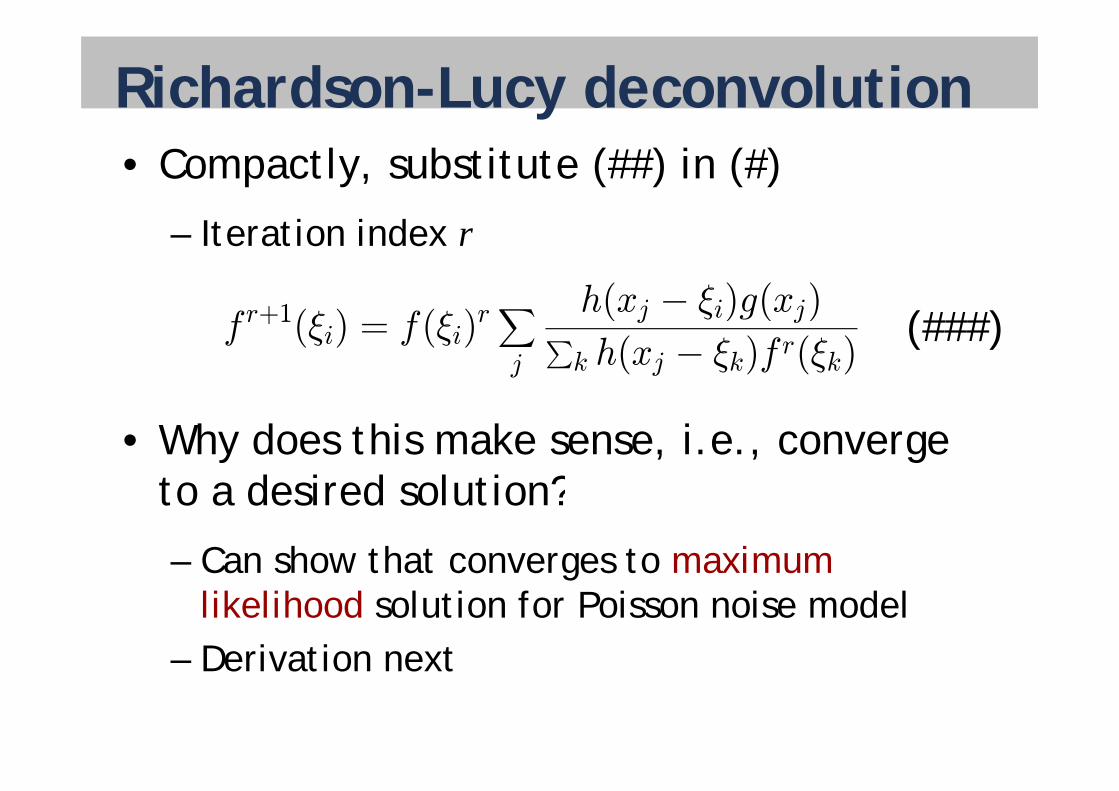
Richardson-Lucy deconvolution• Compactly, substitute (##) in (#)

– Iteration index r

1 h(xj − ξi)g(xj)f r+1(ξi) = f(ξi)

rXj

h(xj ξi)g(xj)Pk h(xj − ξk)f r(ξk)

(###)

• Why does this make sense, i.e., converge to a desired solution?to a desired solution?

– Can show that converges to maximum glikelihood solution for Poisson noise model

– Derivation nextDerivation next

Maximum likelihoodhttp://en.wikipedia.org/wiki/Maximum_likelihood

• Given: probability distribution with a set of Given: probability distribution with a set of parameters

ik lih d f i i b i ll • Likelihood function: given observation, tells us for each parameter setting how likely it is that these parameters lead to observation

• Maximum likelihood solution: given • Maximum likelihood solution: given observation, the one parameter setting that maximizes the likelihood functionmaximizes the likelihood function

– Unknown parameters that most likely generated p y gthe observation

In our context• Assumption

– Photons, i.e. pixels, are independent– Measurement error (noise) of pixels obeys ( ) p y

Poisson distribution

• Likelihood function• Likelihood function

– Product of Poisson distributions– As a function of undegraded pixel values

• Maximum likelhood• Maximum likelhood

– Most likely undegraded pixel values that led to observed image

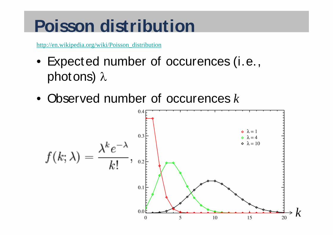
Poisson distributionhttp://en.wikipedia.org/wiki/Poisson_distribution

• Expected number of occurences (i.e., Expected number of occurences (i.e., photons)

• Observed number of occurences k

k

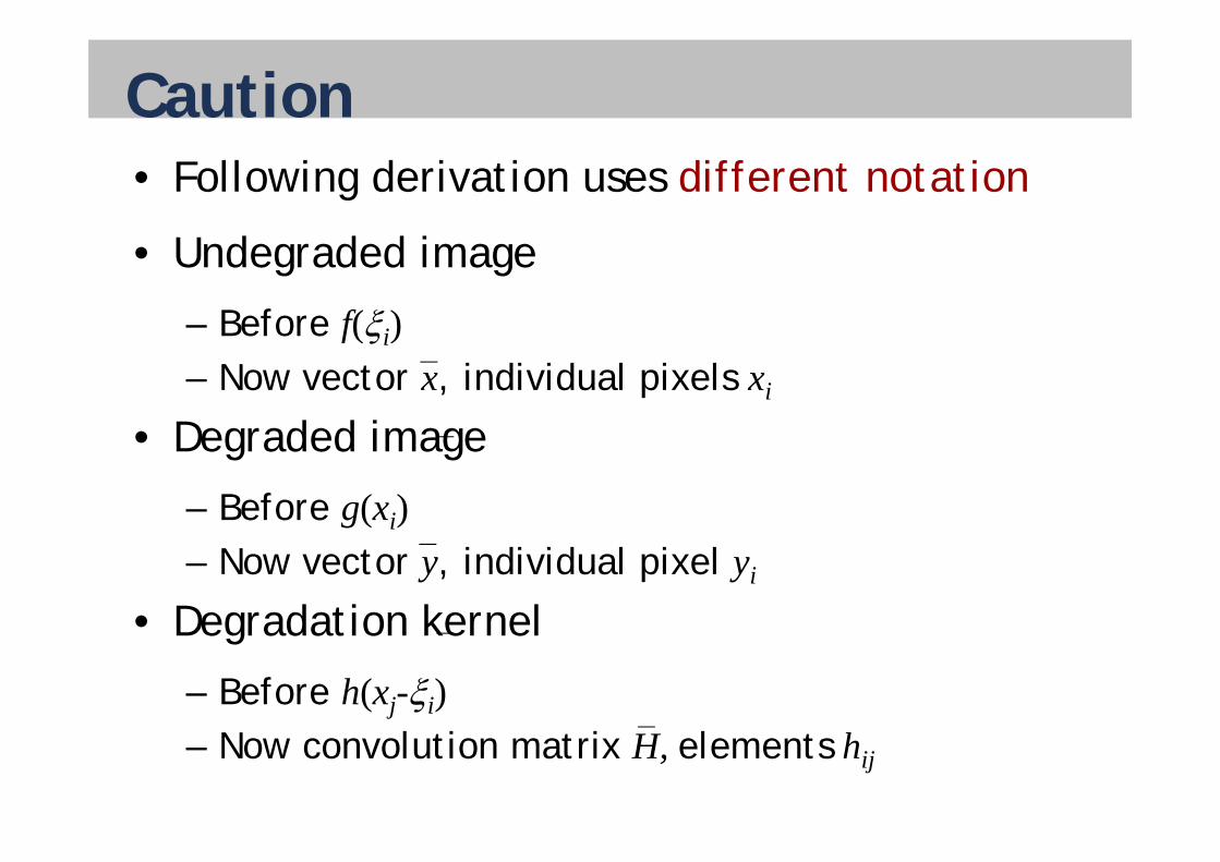
Caution• Following derivation uses different notation

d d d• Undegraded image

– Before f(i)Before f(i)– Now vector x, individual pixels xi

Degraded image• Degraded image

– Before g(xi)i– Now vector y, individual pixel yi

• Degradation kernel• Degradation kernel

– Before h(xj-i)– Now convolution matrix H, elements hij

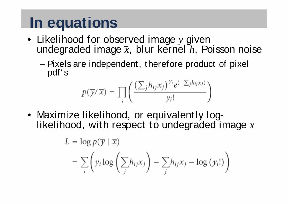
In equations• Likelihood for observed image y given

undegraded image x, blur kernel h, Poisson noise– Pixels are independent, therefore product of pixel

pdf‘s

• Maximize likelihood, or equivalently log-likelihood with respect to undegraded image xlikelihood, with respect to undegraded image x

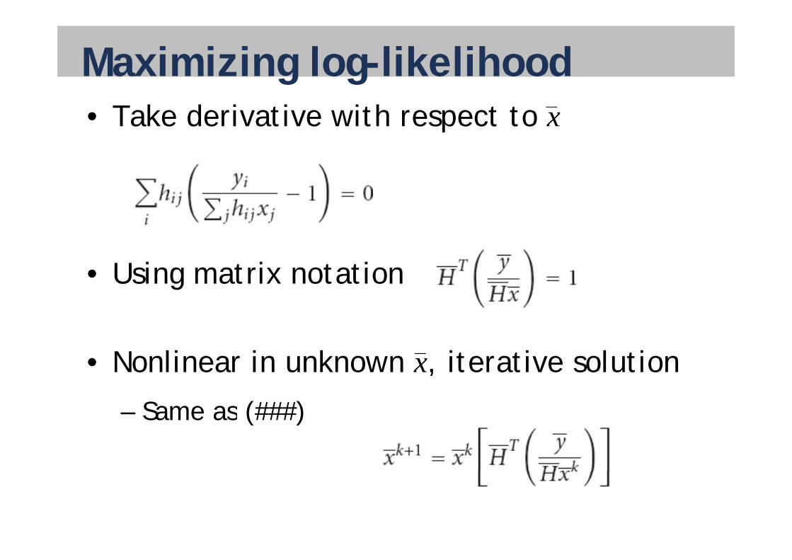
Maximizing log-likelihood• Take derivative with respect to x

• Using matrix notationUsing matrix notation

• Nonlinear in unknown x, iterative solution

Same as (###) – Same as (###)

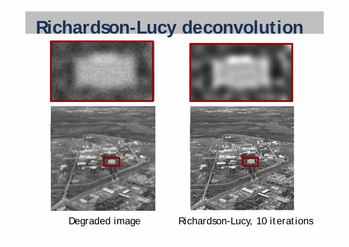
Richardson-Lucy deconvolution

Degraded image Richardson-Lucy, 10 iterations

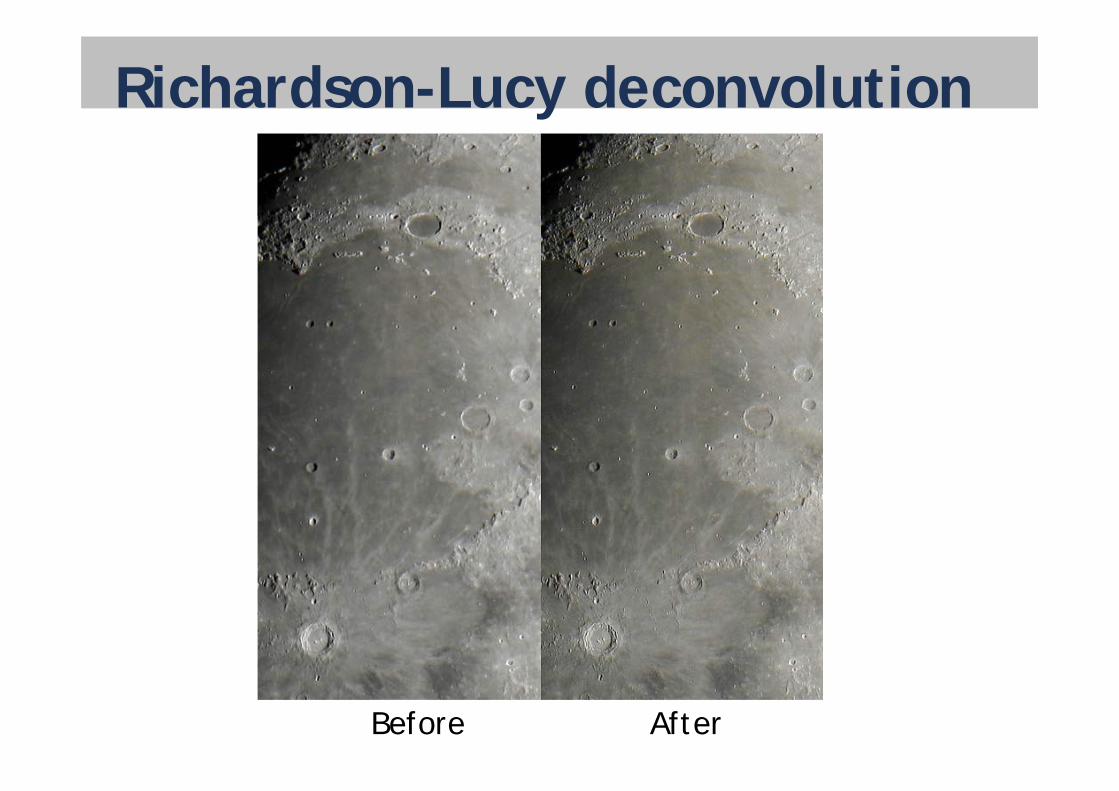
Richardson-Lucy deconvolution

Before After

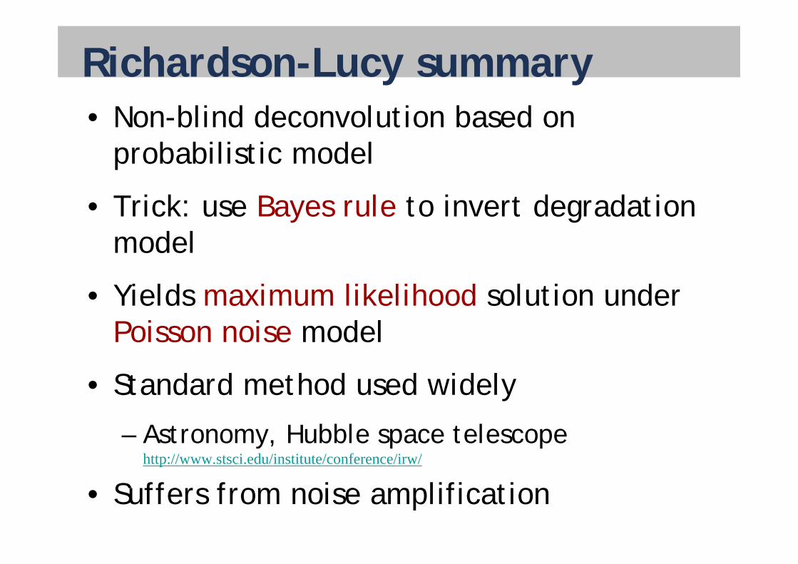
Richardson-Lucy summary• Non-blind deconvolution based on

probabilistic modelprobabilistic model

• Trick: use Bayes rule to invert degradationy gmodel

• Yields maximum likelihood solution under Poisson noise model

• Standard method used widely

– Astronomy, Hubble space telescopehttp://www.stsci.edu/institute/conference/irw/

• Suffers from noise amplification

Literature• Original papers

“B i B d It ti M th d f I g – “Bayesian-Based Iterative Method of Image Restoration”, Richardson, 1972http://www.opticsinfobase.org/abstract.cfm?URI=josa-62-1-55http://www.opticsinfobase.org/abstract.cfm?URI josa 62 1 55

– “An iterative technique for the rectification of observed distributions”, Lucy, 1974, y,http://articles.adsabs.harvard.edu/full/1974AJ.....79..745L

• Adaptive method, derived by maximizing likelihood using Poisson noise model– “An adaptively accelerated Lucy-Richardson An adaptively accelerated Lucy-Richardson

method for image deblurring”, Singh et al. 2008 2008 http://portal.acm.org/citation.cfm?id=1387867

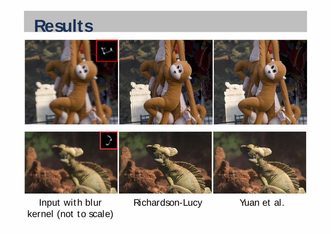
Recent advances• Progressive Inter-scale and Intra-scale Non-

blind Image Deconvolution Yuan et al blind Image Deconvolution, Yuan et al., SIGGRAPH 2008 http://research microsoft com/en-us/um/people/jiansun/papers/ImageDeconv Siggraph08 pdfhttp://research.microsoft.com/en-us/um/people/jiansun/papers/ImageDeconv_Siggraph08.pdf

• Extension of Richardson-Lucy

– Edge preserving filter– Multiresolution approachMultiresolution approach

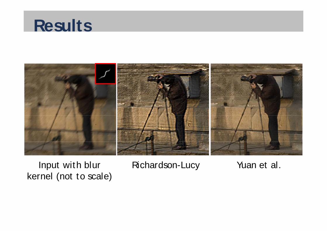
Results

Input with blur Richardson-Lucy Yuan et al.Input with blurkernel (not to scale)

Richardson Lucy Yuan et al.

Results

Input with blurkernel (not to scale)

Richardson-Lucy Yuan et al.

Next time• Gradient based image manipulation