Embed Size (px)
Citation preview
arX
iv:0
812.
4408
v1 [
hep-
th]
23
Dec
200
8
A solution manual for Polchinski’s String Theory
Matthew Headrick
Martin Fisher School of Physics
Brandeis University
Abstract
We present detailed solutions to 81 of the 202 problems in J. Polchinski’s two-volume text-
book String Theory.
BRX-TH-604
CONTENTS 1
Contents
0 Preface 4
1 Chapter 1 5
1.1 Problem 1.1 . . . . . . . . . . . . . . . . . . . . . . . . . . . . . . . . . . . . . . . . . 5
1.2 Problem 1.3 . . . . . . . . . . . . . . . . . . . . . . . . . . . . . . . . . . . . . . . . . 6
1.3 Problem 1.5 . . . . . . . . . . . . . . . . . . . . . . . . . . . . . . . . . . . . . . . . . 7
1.4 Problem 1.7 . . . . . . . . . . . . . . . . . . . . . . . . . . . . . . . . . . . . . . . . . 7
1.5 Problem 1.9 . . . . . . . . . . . . . . . . . . . . . . . . . . . . . . . . . . . . . . . . . 9
2 Chapter 2 11
2.1 Problem 2.1 . . . . . . . . . . . . . . . . . . . . . . . . . . . . . . . . . . . . . . . . . 11
2.2 Problem 2.3 . . . . . . . . . . . . . . . . . . . . . . . . . . . . . . . . . . . . . . . . . 12
2.3 Problem 2.5 . . . . . . . . . . . . . . . . . . . . . . . . . . . . . . . . . . . . . . . . . 13
2.4 Problem 2.7 . . . . . . . . . . . . . . . . . . . . . . . . . . . . . . . . . . . . . . . . . 14
2.5 Problem 2.9 . . . . . . . . . . . . . . . . . . . . . . . . . . . . . . . . . . . . . . . . . 16
2.6 Problem 2.11 . . . . . . . . . . . . . . . . . . . . . . . . . . . . . . . . . . . . . . . . 17
2.7 Problem 2.13 . . . . . . . . . . . . . . . . . . . . . . . . . . . . . . . . . . . . . . . . 18
2.8 Problem 2.15 . . . . . . . . . . . . . . . . . . . . . . . . . . . . . . . . . . . . . . . . 19
2.9 Problem 2.17 . . . . . . . . . . . . . . . . . . . . . . . . . . . . . . . . . . . . . . . . 20
3 Chapter 3 21
3.1 Problem 3.1 . . . . . . . . . . . . . . . . . . . . . . . . . . . . . . . . . . . . . . . . . 21
3.2 Problem 3.2 . . . . . . . . . . . . . . . . . . . . . . . . . . . . . . . . . . . . . . . . . 21
3.3 Problem 3.3 . . . . . . . . . . . . . . . . . . . . . . . . . . . . . . . . . . . . . . . . . 22
3.4 Problem 3.4 . . . . . . . . . . . . . . . . . . . . . . . . . . . . . . . . . . . . . . . . . 24
3.5 Problem 3.5 . . . . . . . . . . . . . . . . . . . . . . . . . . . . . . . . . . . . . . . . . 25
3.6 Problem 3.7 . . . . . . . . . . . . . . . . . . . . . . . . . . . . . . . . . . . . . . . . . 26
3.7 Problem 3.9 . . . . . . . . . . . . . . . . . . . . . . . . . . . . . . . . . . . . . . . . . 28
3.8 Problem 3.11 . . . . . . . . . . . . . . . . . . . . . . . . . . . . . . . . . . . . . . . . 30
3.9 Problem 3.13 . . . . . . . . . . . . . . . . . . . . . . . . . . . . . . . . . . . . . . . . 32
4 Chapter 4 33
4.1 Problem 4.1 . . . . . . . . . . . . . . . . . . . . . . . . . . . . . . . . . . . . . . . . . 33
5 Chapter 5 35
5.1 Problem 5.1 . . . . . . . . . . . . . . . . . . . . . . . . . . . . . . . . . . . . . . . . . 35
CONTENTS 2
6 Chapter 6 40
6.1 Problem 6.1 . . . . . . . . . . . . . . . . . . . . . . . . . . . . . . . . . . . . . . . . . 40
6.2 Problem 6.3 . . . . . . . . . . . . . . . . . . . . . . . . . . . . . . . . . . . . . . . . . 40
6.3 Problem 6.5 . . . . . . . . . . . . . . . . . . . . . . . . . . . . . . . . . . . . . . . . . 40
6.4 Problem 6.7 . . . . . . . . . . . . . . . . . . . . . . . . . . . . . . . . . . . . . . . . . 42
6.5 Problem 6.9 . . . . . . . . . . . . . . . . . . . . . . . . . . . . . . . . . . . . . . . . . 45
6.6 Problem 6.11 . . . . . . . . . . . . . . . . . . . . . . . . . . . . . . . . . . . . . . . . 48
6.7 Problem 6.12 . . . . . . . . . . . . . . . . . . . . . . . . . . . . . . . . . . . . . . . . 51
7 Chapter 7 52
7.1 Problem 7.1 . . . . . . . . . . . . . . . . . . . . . . . . . . . . . . . . . . . . . . . . . 52
7.2 Problem 7.3 . . . . . . . . . . . . . . . . . . . . . . . . . . . . . . . . . . . . . . . . . 54
7.3 Problem 7.5 . . . . . . . . . . . . . . . . . . . . . . . . . . . . . . . . . . . . . . . . . 56
7.4 Problem 7.7 . . . . . . . . . . . . . . . . . . . . . . . . . . . . . . . . . . . . . . . . . 58
7.5 Problem 7.8 . . . . . . . . . . . . . . . . . . . . . . . . . . . . . . . . . . . . . . . . . 59
7.6 Problem 7.9 . . . . . . . . . . . . . . . . . . . . . . . . . . . . . . . . . . . . . . . . . 61
7.7 Problem 7.10 . . . . . . . . . . . . . . . . . . . . . . . . . . . . . . . . . . . . . . . . 62
7.8 Problem 7.11 . . . . . . . . . . . . . . . . . . . . . . . . . . . . . . . . . . . . . . . . 62
7.9 Problem 7.13 . . . . . . . . . . . . . . . . . . . . . . . . . . . . . . . . . . . . . . . . 64
7.10 Problem 7.15 . . . . . . . . . . . . . . . . . . . . . . . . . . . . . . . . . . . . . . . . 66
8 Chapter 8 69
8.1 Problem 8.1 . . . . . . . . . . . . . . . . . . . . . . . . . . . . . . . . . . . . . . . . . 69
8.2 Problem 8.3 . . . . . . . . . . . . . . . . . . . . . . . . . . . . . . . . . . . . . . . . . 70
8.3 Problem 8.4 . . . . . . . . . . . . . . . . . . . . . . . . . . . . . . . . . . . . . . . . . 71
8.4 Problem 8.5 . . . . . . . . . . . . . . . . . . . . . . . . . . . . . . . . . . . . . . . . . 72
8.5 Problem 8.6 . . . . . . . . . . . . . . . . . . . . . . . . . . . . . . . . . . . . . . . . . 72
8.6 Problem 8.7 . . . . . . . . . . . . . . . . . . . . . . . . . . . . . . . . . . . . . . . . . 73
8.7 Problem 8.9 . . . . . . . . . . . . . . . . . . . . . . . . . . . . . . . . . . . . . . . . . 75
8.8 Problem 8.11 . . . . . . . . . . . . . . . . . . . . . . . . . . . . . . . . . . . . . . . . 75
9 Appendix A 78
9.1 Problem A.1 . . . . . . . . . . . . . . . . . . . . . . . . . . . . . . . . . . . . . . . . 78
9.2 Problem A.3 . . . . . . . . . . . . . . . . . . . . . . . . . . . . . . . . . . . . . . . . 80
9.3 Problem A.5 . . . . . . . . . . . . . . . . . . . . . . . . . . . . . . . . . . . . . . . . 80
10 Chapter 10 83
10.1 Problem 10.1 . . . . . . . . . . . . . . . . . . . . . . . . . . . . . . . . . . . . . . . . 83
10.2 Problem 10.2 . . . . . . . . . . . . . . . . . . . . . . . . . . . . . . . . . . . . . . . . 83
CONTENTS 3
10.3 Problem 10.3 . . . . . . . . . . . . . . . . . . . . . . . . . . . . . . . . . . . . . . . . 84
10.4 Problem 10.4 . . . . . . . . . . . . . . . . . . . . . . . . . . . . . . . . . . . . . . . . 84
10.5 Problem 10.5 . . . . . . . . . . . . . . . . . . . . . . . . . . . . . . . . . . . . . . . . 85
10.6 Problem 10.7 . . . . . . . . . . . . . . . . . . . . . . . . . . . . . . . . . . . . . . . . 85
10.7 Problem 10.10 . . . . . . . . . . . . . . . . . . . . . . . . . . . . . . . . . . . . . . . . 86
10.8 Problem 10.11 . . . . . . . . . . . . . . . . . . . . . . . . . . . . . . . . . . . . . . . . 86
10.9 Problem 10.14 . . . . . . . . . . . . . . . . . . . . . . . . . . . . . . . . . . . . . . . . 87
11 Chapter 11 88
11.1 Problem 11.1 . . . . . . . . . . . . . . . . . . . . . . . . . . . . . . . . . . . . . . . . 88
11.2 Problem 11.3 . . . . . . . . . . . . . . . . . . . . . . . . . . . . . . . . . . . . . . . . 88
11.3 Problem 11.4 . . . . . . . . . . . . . . . . . . . . . . . . . . . . . . . . . . . . . . . . 88
11.4 Problem 11.7 . . . . . . . . . . . . . . . . . . . . . . . . . . . . . . . . . . . . . . . . 90
11.5 Problem 11.8 . . . . . . . . . . . . . . . . . . . . . . . . . . . . . . . . . . . . . . . . 91
11.6 Problem 11.9 . . . . . . . . . . . . . . . . . . . . . . . . . . . . . . . . . . . . . . . . 92
11.7 Problem 11.12 . . . . . . . . . . . . . . . . . . . . . . . . . . . . . . . . . . . . . . . . 92
12 Chapter 13 94
12.1 Problem 13.2 . . . . . . . . . . . . . . . . . . . . . . . . . . . . . . . . . . . . . . . . 94
12.2 Problem 13.3 . . . . . . . . . . . . . . . . . . . . . . . . . . . . . . . . . . . . . . . . 95
12.3 Problem 13.4 . . . . . . . . . . . . . . . . . . . . . . . . . . . . . . . . . . . . . . . . 96
12.4 Problem 13.12 . . . . . . . . . . . . . . . . . . . . . . . . . . . . . . . . . . . . . . . . 99
13 Chapter 14 103
13.1 Problem 14.1 . . . . . . . . . . . . . . . . . . . . . . . . . . . . . . . . . . . . . . . . 103
13.2 Problem 14.2 . . . . . . . . . . . . . . . . . . . . . . . . . . . . . . . . . . . . . . . . 103
13.3 Problem 14.6 . . . . . . . . . . . . . . . . . . . . . . . . . . . . . . . . . . . . . . . . 105
14 Chapter 15 108
14.1 Problem 15.1 . . . . . . . . . . . . . . . . . . . . . . . . . . . . . . . . . . . . . . . . 108
14.2 Problem 15.3 . . . . . . . . . . . . . . . . . . . . . . . . . . . . . . . . . . . . . . . . 108
15 Appendix B 110
15.1 Problem B.1 . . . . . . . . . . . . . . . . . . . . . . . . . . . . . . . . . . . . . . . . . 110
15.2 Problem B.3 . . . . . . . . . . . . . . . . . . . . . . . . . . . . . . . . . . . . . . . . . 112
15.3 Problem B.5 . . . . . . . . . . . . . . . . . . . . . . . . . . . . . . . . . . . . . . . . . 113

0 PREFACE 4
0 Preface
The following pages contain detailed solutions to 81 of the 202 problems in J. Polchinski’s two-
volume textbook String Theory [1, 2]. I originally wrote up these solutions while teaching myself
the subject, and then later decided that they may be of some use to others doing the same. These
solutions are the work of myself alone, and carry no endorsement from Polchinski.
I would like to thank R. Britto, S. Minwalla, D. Podolsky, and M. Spradlin for help on these
problems. This work was done while I was a graduate student at Harvard University, and was
supported by an NSF Graduate Research Fellowship.
1 CHAPTER 1 5
1 Chapter 1
1.1 Problem 1.1
(a) We work in the gauge where τ = X0. Non-relativistic motion means Xi ≡ vi ≪ 1. Then
Spp = −m∫
dτ
√
−XµXµ
= −m∫
dt√
1 − v2
≈∫
dt (1
2mv2 −m). (1)
(b) Again, we work in the gauge τ = X0, and assume Xi ≡ vi ≪ 1. Defining ui ≡ ∂σXi, the
induced metric hab = ∂aXµ∂bXµ becomes:
hab =
(
−1 + v2 u · vu · v u2
)
. (2)
Using the fact that the transverse velocity of the string is
vT = v − u · vu
u, (3)
the Nambu-Goto Lagrangian can be written:
L = − 1
2πα′
∫
dσ (− dethab)1/2
= − 1
2πα′
∫
dσ(
u2(1 − v2) + (u · v)2)1/2
≈ − 1
2πα′
∫
dσ |u|(
1 − 1
2v2 +
u · v2
2u2
)
=
∫
dσ |u|12ρv2
T − LsT, (4)
where
ρ =1
2πα′ (5)
is the mass per unit length of the string,
Ls =
∫
dσ |u| (6)
is its physical length, and
T =1
2πα′ = ρ (7)
is its tension.
1 CHAPTER 1 6
1.2 Problem 1.3
It is well known that χ, the Euler characteristic of the surface, is a topological invariant, i.e. does
not depend on the metric. We will prove by explicit computation that, in particular, χ is invariant
under Weyl transformations,
γ′ab = e2ω(σ,τ)γab. (8)
For this we will need the transformation law for the connection coefficients,
Γ′abc = Γabc + ∂bωδ
ac + ∂cωδ
ab − ∂dωγ
adγbc, (9)
and for the curvature scalar,
R′ = e−2ω(R − 2∇a∂aω). (10)
Since the tangent and normal vectors at the boundary are normalized, they transform as
t′a = e−ωta, (11)
n′a = eωna. (12)
The curvature of the boundary thus transforms as follows:
k′ = ±t′an′b(∂at′b + Γ′bact
′c)
= e−ω(k ∓ tatanb∂d), (13)
where we have used (9), (11), (12), and the fact that n and t are orthogonal. If the boundary is
timelike then tata = −1 and we must use the upper sign, whereas if it is spacelike then tata = 1
and we must use the lower sign. Hence
k′ = e−ω(k + na∂aω). (14)
Finally, since ds = (−γττ )1/2dτ for a timelike boundary and ds = γ1/2σσ dσ for a spacelike bounday,
ds′ = ds eω. (15)
Putting all of this together, and applying Stokes theorem, which says that for any vector va,∫
Mdτ dσ (−γ)1/2∇av
a =
∫
∂Mds nava, (16)
we find the transformation law for χ:
χ′ =1
4π
∫
Mdτ dσ (−γ′)1/2R′ +
1
2π
∫
∂Mds′ k′
=1
4π
∫
Mdτ dσ (−γ)1/2(R − 2∇a∂
aω) +1
2π
∫
∂Mds (k + na∂aω)
= χ. (17)
1 CHAPTER 1 7
1.3 Problem 1.5
For simplicity, let us define a ≡ (π/2p+α′l)1/2. Then we wish to evaluate
∞∑
n=1
(n− θ) exp[−(n− θ)ǫa]
= − d
d(ǫa)
∞∑
n=1
exp[−(n− θ)ǫa]
= − d
d(ǫa)
eθǫa
eǫa − 1
= − d
d(ǫa)
(
1
ǫa+ θ − 1
2+
(
1
12− θ
2+θ2
2
)
ǫa+ O(ǫa)2)
=1
(ǫa)2− 1
2
(
1
6− θ + θ2
)
+ O(ǫa). (18)
As expected, the cutoff dependent term is independent of θ; the finite result is
− 1
2
(
1
6− θ + θ2
)
. (19)
1.4 Problem 1.7
The mode expansion satisfying the boundary conditions is
X25(τ, σ) =√
2α′∑
n
1
nα25n exp
[
− iπncτl
]
sinπnσ
l, (20)
where the sum runs over the half-odd-integers, n = 1/2,−1/2, 3/2,−3/2, . . . . Note that there is no
p25. Again, Hermiticity of X25 implies α25−n = (α25
n )†. Using (1.3.18),
Π25(τ, σ) = − i√2α′l
∑
n
α25n exp
[
− iπncτl
]
sinπnσ
l. (21)
We will now determine the commutation relations among the α25n from the equal time com-
mutation relations (1.3.24b). Not surprisingly, they will come out the same as for the free string
(1.3.25b). We have:
iδ(σ − σ′) = [X25(τ, σ),Π25(τ, σ)] (22)
= − il
∑
n,n′
1
n[α25n , α
25n′ ] exp
[
− iπ(n+ n′)cτl
]
sinπnσ
lsin
πn′σ′
l.
Since the LHS does not depend on τ , the coefficient of exp[−iπmcτ/l] on the RHS must vanish for
m 6= 0:1
l
∑
n
1
n[α25n , α
25m−n] sin
πnσ
lsin
π(n−m)σ′
l= δ(σ − σ′)δm,0. (23)
1 CHAPTER 1 8
Multiplying both sides by sin[πn′σ/l] and integrating over σ now yields,
1
2n
(
[α25n , α
25m−n] sin
π(n−m)σ′
l+ [α25
n+m, α25−n] sin
π(n+m)σ′
l
)
(24)
= sinπnσ′
lδm,0,
or,
[α25n , α
25m−n] = nδm,0, (25)
as advertised.
The part of the Hamiltonian (1.3.19) contributed by the X25 oscillators is
l
4πα′p+
∫ l
0dσ
(
2πα′ (Π25)2
+1
2πα′(
∂σX25)2)
=1
4α′p+l
∑
n,n′
α25n α
25n′ exp
[
− iπ(n + n′)cτl
]
×∫ l
0dσ
(
− sinπnσ
lsin
πn′σl
+ cosπnσ
lcos
πn′σl
)
=1
4α′p+
∑
n
α25n α
25−n
=1
4α′p+
∞∑
n=1/2
(
α25n α
25−n + α25
−nα25n
)
=1
2α′p+
∞∑
n=1/2
(
α25−nα
25n +
n
2
)
=1
2α′p+
∞∑
n=1/2
α25−nα
25n +
1
48
, (26)
where we have used (19) and (25). Thus the mass spectrum (1.3.36) becomes
m2 = 2p+H − pipi (i = 2, . . . , 24)
=1
α′
(
N − 15
16
)
, (27)
where the level spectrum is given in terms of the occupation numbers by
N =24∑
i=2
∞∑
n=1
nNin +∞∑
n=1/2
nN25,n. (28)
The ground state is still a tachyon,
m2 = − 15
16α′ . (29)
1 CHAPTER 1 9
The first excited state has the lowest X25 oscillator excited (N25,1/2 = 1), and is also tachyonic:
m2 = − 7
16α′ . (30)
There are no massless states, as the second excited state is already massive:
m2 =1
16α′ . (31)
This state is 24-fold degenerate, as it can be reached either by Ni,1 = 1 or by N25,1/2 = 2. Thus it
is a massive vector with respect to the SO(24,1) Lorentz symmetry preserved by the D-brane. The
third excited state, with
m2 =9
16α′ , (32)
is 25-fold degenerate and corresponds to a vector plus a scalar on the D-brane—it can be reached
by N25,1/2 = 1, by N25,1/2 = 3, or by Ni,1 = 1, N25,1/2 = 1.
1.5 Problem 1.9
The mode expansion for X25 respecting the boundary conditions is essentially the same as the
mode expansion (1.4.4), the only differences being that the first two terms are no longer allowed,
and the oscillator label n, rather than running over the non-zero integers, must now run over the
half-odd-integers as it did in Problem 1.7:
X25(τ, σ) = (33)
i
√
α′
2
∑
n
(
α25n
nexp
[
−2πin(σ + cτ)
l
]
+α25n
nexp
[
2πin(σ − cτ)
l
])
.
The canonical commutators are the same as for the untwisted closed string, (1.4.6c) and (1.4.6d),
[α25m , α
25n ] = mδm,−n, (34)
[α25m , α
25n ] = mδm,−n, (35)
as are the mass formula (1.4.8),
m2 =2
α′ (N + N +A+ A), (36)
the generator of σ-translations (1.4.10),
P = −2π
l(N − N), (37)
and (therefore) the level-matching condition (1.4.11),
N = N . (38)
1 CHAPTER 1 10
However, the level operator N is now slightly different,
N =24∑
i=2
∞∑
n=1
αi−nαin +
∞∑
n=1/2
α25−nα
25n ; (39)
in fact, it is the same as the level operator for the open string on a D24-brane of Problem 1.7.
The left-moving level spectrum is therefore given by (28), and similarly for the right-moving level
operator N . The zero-point constants are also the same as in Problem 1.7:
A = A =1
2
24∑
i=2
∞∑
n=1
n+∞∑
n=1/2
n
= −15
16. (40)
At a given level N = N , the occupation numbers Nin and Nin may be chosen independently, so
long as both sets satisfy (28). Therefore the spectrum at that level will consist of the product of
two copies of the D-brane open string spectrum, and the mass-squared of that level (36) will be 4
times the open string mass-squared (27). We will have tachyons at levels N = 0 and N = 1/2, with
m2 = − 15
4α′ (41)
and
m2 = − 7
4α′ , (42)
respectively. The lowest non-tachyonic states will again be at level N = 1: a second rank SO(24)
tensor with
m2 =1
4α′ , (43)
which can be decomposed into a scalar, an antisymmetric tensor, and a traceless symmetric tensor.
2 CHAPTER 2 11
2 Chapter 2
2.1 Problem 2.1
(a) For holomorphic test functions f(z),
∫
Rd2z ∂∂ ln |z|2f(z) =
∫
Rd2z ∂
1
zf(z)
= −i∮
∂Rdz
1
zf(z)
= 2πf(0). (1)
For antiholomorphic test functions f(z),
∫
Rd2z ∂∂ ln |z|2f(z) =
∫
Rd2z ∂
1
zf(z)
= i
∮
∂Rdz
1
zf(z)
= 2πf(0). (2)
(b) We regulate ln |z|2 by replacing it with ln(|z|2 + ǫ). This lead to regularizations also of 1/z
and 1/z:
∂∂ ln(|z|2 + ǫ) = ∂z
|z|2 + ǫ= ∂
z
|z|2 + ǫ=
ǫ
(|z|2 + ǫ)2. (3)
Working in polar coordinates, consider a general test function f(r, θ), and define g(r2) ≡∫
dθ f(r, θ).
Then, assuming that g is sufficiently well behaved at zero and infinity,
∫
d2zǫ
(|z|2 + ǫ)2f(z, z)
=
∫ ∞
0du
ǫ
(u+ ǫ)2g(u)
=
(
− ǫ
u+ ǫg(u) + ǫ ln(u+ ǫ)g′(u)
)∞
0
−∫ ∞
0du ǫ ln(u+ ǫ)g′′(u).
= g(0)
= 2πf(0). (4)
2 CHAPTER 2 12
2.2 Problem 2.3
(a) The leading behavior of the expectation value as z1 → z2 is
⟨
n∏
i=1
: eiki·X(zi,zi) :
⟩
= iCX(2π)DδD
(
n∑
i=1
ki
)
n∏
i,j=1
|zij |α′ki·kj
= |z12|α′k1·k2iCX(2π)DδD(k1 + k2 +
n∑
i=3
ki)
×n∏
i=3
(
|z1i|α′k1·ki |z2i|α
′k2·ki
)
n∏
i,j=3
|zij |α′ki·kj
≈ |z12|α′k1·k2iCX(2π)DδD(k1 + k2 +
n∑
i=3
ki)
n∏
i=3
|z2i|α′(k1+k2)·ki
n∏
i,j=3
|zij |α′ki·kj
= |z12|α′k1·k2
⟨
: ei(k1+k2)·X(z2,z2) :
n∏
i=3
: eiki·X(zi,zi) :
⟩
, (5)
in agreement with (2.2.14).
(b) The zi-dependence of the expectation value is given by
|z23|α′k2·k3|z12|α
′k1·k2|z13|α′k1·k3
= |z23|α′k2·k3|z12|α
′k1·k2 |z23|α′k1·k3
∣
∣
∣
∣
1 +z12z23
∣
∣
∣
∣
α′k1·k3(6)
= |z23|α′(k1+k2)·k3 |z12|α
′k1·k2
( ∞∑
k=0
Γ(12α
′k1 · k3 + 1)
k! Γ(12α
′k1 · k3 − k + 1)
(
z12z23
)k)
×( ∞∑
k=0
Γ(12α
′k1 · k3 + 1)
k! Γ(12α
′k1 · k3 − k + 1)
(
z12z23
)k)
.
The radius of convergence of a power series is given by the limit as k → ∞ of |ak/ak+1|, where the
ak are the coefficients of the series. In this case, for both of the above power series,
R = limk→∞
∣
∣
∣
∣
∣
(k + 1)! Γ(12α
′k1 · k3 − k)
k! Γ(12α
′k1 · k3 − k + 1)z23
∣
∣
∣
∣
∣
= |z23|. (7)
(c) Consider the interior of the dashed line in figure 2.1, that is, the set of points z1 satisfying
|z12| < |z23|. (8)
2 CHAPTER 2 13
By equation (2.1.23), the expectation value
〈: Xµ(z1, z1)Xν(z2, z2) : A(z3, z3)B(z4, z4)〉 (9)
is a harmonic function of z1 within this region. It can therefore be written as the sum of a
holomorphic and an antiholomorphic function (this statement is true in any simply connected
region). The Taylor expansion of a function that is holomorphic on an open disk (about the center
of the disk), converges on the disk; similarly for an antiholomorphic function. Hence the two Taylor
series on the RHS of (2.2.4) must converge on the disk.
2.3 Problem 2.5
Under the variation of the fields φα(σ) → φα(σ) + δφα(σ), the variation of the Lagrangian is
δL =∂L∂φα
δφα +∂L
∂(∂aφα)∂aδφα. (10)
The Lagrangian equations of motion (Euler-Lagrange equations) are derived by assuming that the
action is stationary under an arbitrary variation δφα(σ) that vanishes at infinity:
0 = δS
=
∫
ddσ δL
=
∫
ddσ
(
∂L∂φα
δφα +∂L
∂(∂aφα)∂aδφα
)
=
∫
ddσ
(
∂L∂φα
− ∂a∂L
∂(∂aφα)
)
δφα (11)
implies∂L∂φα
− ∂a∂L
∂(∂aφα)= 0. (12)
Instead of assuming that δφα vanishes at infinity, let us assume that it is a symmetry. In this case,
the variation of the Lagrangian (10) must be a total derivative to insure that the action on bounded
regions varies only by a surface term, thereby not affecting the equations of motion:
δL = ǫ∂aKa; (13)
Ka is assumed to be a local function of the fields and their derivatives, although it is not obvious
how to prove that this can always be arranged. Using (10), (12), and (13),
∂aja = 2πi∂a
(
∂L∂(∂aφα)
ǫ−1δφα −Ka
)
=2πi
ǫ
(
∂L∂φα
δφα +∂L
∂(∂aφα)∂aδφα − δL
)
= 0. (14)
2 CHAPTER 2 14
If we now vary the fields by ρ(σ)δφα(σ), where δφα is a symmetry as before but ρ is an arbitrary
function, then the variation of the action will be
δL =∂L
∂(∂aφα)∂a(δφαρ) +
∂L∂φα
δφαρ
=
(
∂L∂(∂aφα)
∂aδφα +∂L∂φα
δφα
)
ρ+∂L
∂(∂aφα)δφα∂aρ. (15)
Equation (13) must be satisfied in the case ρ(σ) is identically 1, so the factor in parentheses must
equal ǫ∂aKa:
δS =
∫
ddσ
(
ǫ∂aKaρ+∂L
∂(∂aφα)δφα∂aρ
)
=
∫
ddσ
(
−ǫKa +∂L
∂(∂aφα)δφα
)
∂aρ
=ǫ
2πi
∫
ddσ ja∂aρ, (16)
where we have integrated by parts, assuming that ρ falls off at infinity. Since δ exp(−S) =
− exp(−S)δS, this agrees with (2.3.4) for the case of flat space, ignoring the transformation of
the measure.
2.4 Problem 2.7
(a) Xµ:
T (z)Xµ(0, 0) = − 1
α′ : ∂Xν(z)∂Xν(z) : Xµ(0, 0) ∼ 1
z∂Xµ(z) ∼ 1
z∂Xµ(0)
T (z)Xµ(0, 0) = − 1
α′ : ∂Xν(z)∂Xν(z) : Xµ(0, 0) ∼ 1
z∂Xµ(z) ∼ 1
z∂Xµ(0) (17)
∂Xµ:
T (z)∂Xµ(0) ∼ 1
z2∂Xµ(z) ∼ 1
z2∂Xµ(0) +
1
z∂2Xµ(0)
T (z)∂Xµ(0) ∼ 0 (18)
∂Xµ:
T (z)∂Xµ(0) ∼ 0
T (z)∂Xµ(0) ∼ 1
z2∂Xµ(z) ∼ 1
z2∂Xµ(0) +
1
z∂2Xµ(0) (19)
∂2Xµ:
T (z)∂2Xµ(0) ∼ 2
z3∂Xµ(z) ∼ 2
z3∂Xµ(0) +
2
z2∂2Xµ(0) +
1
z∂3Xµ(0)
T (z)∂2Xµ(0) ∼ 0 (20)
2 CHAPTER 2 15
: eik·X ::
T (z) : eik·X(0,0) : ∼ α′k2
4z2: eik·X(0,0) : +
1
zikµ : ∂Xµ(z)eik·X(0,0) :
∼ α′k2
4z2: eik·X(0,0) : +
1
zikµ : ∂Xµ(0)eik·X(0,0) :
T (z) : eik·X(0,0) : ∼ α′k2
4z2: eik·X(0,0) : +
1
zikµ : ∂Xµ(z)eik·X(0,0) :
∼ α′k2
4z2: eik·X(0,0) : +
1
zikµ : ∂Xµ(0)eik·X(0,0) : (21)
(b) In the linear dilaton theory, the energy-momentum tensor is
T = − 1
α′ : ∂Xµ∂Xµ : +Vµ∂2Xµ,
T = − 1
α′ : ∂Xµ∂Xµ : +Vµ∂2Xµ, (22)
so it suffices to calculate the OPEs of the various operators with the terms Vµ∂2Xµ and Vµ∂
2Xµ
and add them to the results found in part (a).
Xµ:
Vν∂2Xν(z)Xµ(0, 0) ∼ α′V µ
2z2
Vν ∂2Xν(z)Xµ(0, 0) ∼ α′V µ
2z2(23)
Not only is Xµ is not a tensor anymore, but it does not even have well-defined weights, because it
is not an eigenstate of rigid transformations.
∂Xµ:
Vν∂2Xν(z)∂Xµ(0) ∼ α′V µ
z3
Vν ∂2Xν(z)∂Xµ(0) ∼ 0 (24)
So ∂Xµ still has weights (1,0), but it is no longer a tensor operator.
∂Xµ:
Vν∂2Xν(z)∂Xµ(0) ∼ 0
Vν ∂2Xν(z)∂Xµ(0) ∼ α′V µ
z3(25)
Similarly, ∂Xµ still has weights (0,1), but is no longer a tensor.
∂2Xµ:
Vν∂2Xν(z)∂2Xµ(0) ∼ 3α′V µ
z4
Vν ∂2Xν(z)∂2Xµ(0) ∼ 0 (26)
2 CHAPTER 2 16
Nothing changes from the scalar theory: the weights are still (2,0), and ∂2Xµ is still not a tensor.
: eik·X ::
Vν∂2Xν(z) : eik·X(0,0) :∼ iα′V · k
2z2: eik·X(0,0) :
Vν ∂2Xν(z) : eik·X(0,0) :∼ iα′V · k
2z2: eik·X(0,0) : (27)
Thus : eik·X : is still a tensor, but, curiously, its weights are now complex:
(
α′
4(k2 + 2iV · k), α
′
4(k2 + 2iV · k)
)
. (28)
2.5 Problem 2.9
Since we are interested in finding the central charges of these theories, it is only necessary to
calculate the 1/z4 terms in the TT OPEs, the rest of the OPE being determined by general
considerations as in equation (2.4.25). In the following, we will therefore drop all terms less singular
than 1/z4. For the linear dilaton CFT,
T (z)T (0) =1
α′2 : ∂Xµ(z)∂Xµ(z) :: ∂Xν(0)∂Xν(0) :
− 2Vνα′ : ∂Xµ(z)∂Xµ(z) : ∂2Xν(0)
− 2Vµα′ ∂
2Xµ(z) : ∂Xν(0)∂Xν(0) : +VµVν∂2Xµ(z)∂2Xν(0)
∼ D
2z4+
3α′V 2
z4+ O
(
1
z2
)
, (29)
so
c = D + 6α′V 2. (30)
Similarly,
T (z)T (0) =1
α′2 : ∂Xµ(z)∂Xµ(z) :: ∂Xν(0)∂Xν(0) :
− 2Vνα′ : ∂Xµ(z)∂Xµ(z) : ∂2Xν(0)
− 2Vµα′ ∂
2Xµ(z) : ∂Xν(0)∂Xν(0) : +VµVν ∂2Xµ(z)∂2Xν(0)
∼ D
2z4+
3α′V 2
z4+ O
(
1
z2
)
, (31)
so
c = D + 6α′V 2. (32)
2 CHAPTER 2 17
For the bc system,
T (z)T (0) = (1 − λ)2 : ∂b(z)c(z) :: ∂b(0)c(0) :
− λ(1 − λ) : ∂b(z)c(z) :: b(0)∂c(0) :
− λ(1 − λ) : b(z)∂c(z) :: ∂b(0)c(0) :
+ λ2 : b(z)∂c(z) :: b(0)∂c(0) :
∼ −6λ2 + 6λ− 1
z4+ O
(
1
z2
)
, (33)
so
c = −12λ2 + 12λ− 2. (34)
Of course T (z)T (0) = 0, so c = 0.
The βγ system has the same energy-momentum tensor and almost the same OPEs as the bc
system. While γ(z)β(0) ∼ 1/z as in the bc system, now β(z)γ(0) ∼ −1/z. Each term in (33)
involved one b(z)c(0) contraction and one c(z)b(0) contraction, so the central charge of the βγ
system is minus that of the bc system:
c = 12λ2 − 12λ+ 2. (35)
Of course c = 0 still.
2.6 Problem 2.11
Assume without loss of generality that m > 1; for m = 0 and m = ±1 the central charge term in
(2.6.19) vanishes, while m < −1 is equivalent to m > 1. Then Lm annihilates |0; 0〉, as do all but
m− 1 of the terms in the mode expansion (2.7.6) of L−m:
L−m|0; 0〉 =1
2
m−1∑
n=1
αµn−mαµ(−n)|0; 0〉. (36)
Hence the LHS of (2.6.19), when applied to |0; 0〉, yields,
[Lm, L−m]|0; 0〉= LmL−m|0; 0〉 − L−mLm|0; 0〉
=1
4
∞∑
n′=−∞
m−1∑
n=1
ανm−n′ανn′αµn−mαµ(−n)|0; 0〉
=1
4
m−1∑
n=1
∞∑
n′=−∞
(
(m− n′)n′ηνµηνµδn′n + (m− n′)n′δνµδµν δm−n′,n
)
|0; 0〉
=D
2
m−1∑
n=1
n(m− n)|0; 0〉
=D
12m(m2 − 1)|0; 0〉. (37)
2 CHAPTER 2 18
Meanwhile, the RHS of (2.6.19) applied to the same state yields,(
2mL0 +c
12(m3 −m)
)
|0; 0〉 =c
12(m3 −m)|0; 0〉, (38)
so
c = D. (39)
2.7 Problem 2.13
(a) Using (2.7.16) and (2.7.17),
b(z)c(z′) =
∞∑
m,m′=−∞
bmcm′
zm+λz′m′+1−λ
=
∞∑
m,m′=−∞
bmcm′
zm+λz′m′+1−λ −∞∑
m=0
1
zm+λz′−m+1−λ
= b(z)c(z′) −( z
z′
)1−λ 1
z − z′. (40)
With (2.5.7),
: b(z)c(z′) : −b(z)c(z′) =
1
z − z′
(
( z
z′
)1−λ− 1
)
. (41)
(b) By taking the limit of (41) as z′ → z, we find,
: b(z)c(z) : −b(z)c(z) =
1 − λ
z. (42)
Using (2.8.14) we have,
Ng = Qg − λ+1
2
=1
2πi
∮
dz jz − λ+1
2
= − 1
2πi
∮
dz : b(z)c(z) : −λ+1
2
= − 1
2πi
∮
dz b(z)c(z) − 1
2. (43)
(c) If we re-write the expansion (2.7.16) of b(z) in the w-frame using the tensor transformation
law (2.4.15), we find,
b(w) = (∂zw)−λb(z)
= (−iz)λ∞∑
m=−∞
bmzm+λ
= e−πiλ/2∞∑
m=−∞eimwbm. (44)
2 CHAPTER 2 19
Similarly,
c(w) = e−πi(1−λ)/2∞∑
m=−∞eimwcm. (45)
Hence, ignoring ordering,
jw(w) = −b(w)c(w)
= i
∞∑
m,m′=−∞ei(m+m′)wbmcm′ , (46)
and
Ng = − 1
2πi
∫ 2π
0dw jw
= −∞∑
m=−∞bmc−m
= −∞∑
m=−∞
bmc−m
−∞∑
m=0
1. (47)
The ordering constant is thus determined by the value of the second infinite sum. If we write,
more generally,∑∞
m=0 a, then we must regulate the sum in such a way that the divergent part is
independent of a. For instance,
∞∑
m=0
ae−ǫa =a
1 − e−ǫa
=1
ǫ+a
2+ O(ǫ); (48)
the ǫ-independent part is a/2, so the ordering constant in (47) equals −1/2.
2.8 Problem 2.15
To apply the doubling trick to the field Xµ(z, z), define for ℑz < 0,
Xµ(z, z) ≡ Xµ(z∗, z∗). (49)
Then
∂mXµ(z) = ∂mXµ(z∗), (50)
so that in particular for z on the real line,
∂mXµ(z) = ∂mXµ(z), (51)
2 CHAPTER 2 20
as can also be seen from the mode expansion (2.7.26). The modes αµm are defined as integrals over
a semi-circle of ∂Xµ(z) + ∂Xµ(z), but with the doubling trick the integral can be extended to the
full circle:
αµm =
√
2
α′
∮
dz
2πzm∂Xµ(z) = −
√
2
α′
∮
dz
2πzm∂Xµ(z). (52)
At this point the derivation proceeds in exactly the same manner as for the closed string treated
in the text. With no operator at the origin, the fields are holomorphic inside the contour, so with
m positive, the contour integrals (52) vanish, and the state corresponding to the unit operator
“inserted” at the origin must be the ground state |0; 0〉:
1(0, 0) ∼= |0; 0〉. (53)
The state αµ−m|0; 0〉 (m positive) is given by evaluating the integrals (52), with the fields holomorphic
inside the contours:
αµ−m|0; 0〉 ∼=(
2
α′
)1/2 i
(m− 1)!∂mXµ(0) =
(
2
α′
)1/2 i
(m− 1)!∂mXµ(0). (54)
Similarly, using the mode expansion (2.7.26), we see that Xµ(0, 0)|0; 0〉 = xµ|0; 0〉, so
xµ|0; 0〉 ∼= Xµ(0, 0). (55)
As in the closed string case, the same correspondence applies when these operators act on states
other than the ground state, as long as we normal order the resulting local operator. The result
is therefore exactly the same as (2.8.7a) and (2.8.8) in the text; for example, (2.8.9) continues to
hold.
2.9 Problem 2.17
Take the matrix element of (2.6.19) between 〈1| and |1〉, with n = −m and m > 1. The LHS yields,
〈1|[Lm, L−m]|1〉 = 〈1|L†−mL−m|1〉
= ‖L−m|1〉‖2, (56)
using (2.9.9). Also by (2.9.9), L0|1〉 = 0, so on the RHS we are left with the term
c
12(m3 −m)〈1|1〉. (57)
Hence
c =12
m3 −m
‖L−m|1〉‖2
〈1|1〉 ≥ 0. (58)
3 CHAPTER 3 21
3 Chapter 3
3.1 Problem 3.1
(a) The definition of the geodesic curvature k of a boundary given in Problem 1.3 is
k = −nbta∇atb, (1)
where ta is the unit tangent vector to the boundary and nb is the outward directed unit normal. For
a flat unit disk, R vanishes, while the geodesic curvature of the boundary is 1 (since ta∇atb = −nb).
Hence
χ =1
2π
∫ 2π
0dθ = 1. (2)
For the unit hemisphere, on the other hand, the boundary is a geodesic, while R = 2. Hence
χ =1
4π
∫
d2σ g1/22 = 1, (3)
in agreement with (2).
(b) If we cut a surface along a closed curve, the two new boundaries will have oppositely directed
normals, so their contributions to the Euler number of the surface will cancel, leaving it unchanged.
The Euler number of the unit sphere is
χ =1
4π
∫
d2σ g1/22 = 2. (4)
If we cut the sphere along b small circles, we will be left with b disks and a sphere with b holes.
The Euler number of the disks is b (from part (a)), so the Euler number of the sphere with b holes
is
χ = 2 − b. (5)
(c) A finite cylinder has Euler number 0, since we can put on it a globally flat metric for which
the boundaries are geodesics. If we remove from a sphere b+ 2g holes, and then join to 2g of the
holes g cylinders, the result will be a sphere with b holes and g handles; its Euler number will be
χ = 2 − b− 2g. (6)
3.2 Problem 3.2
(a) This is easiest to show in complex coordinates, where gzz = gzz = 0. Contracting two indices
of a symmetric tensor with lower indices by gab will pick out the components where one of the
indices is z and the other z. If the tensor is traceless then all such components must vanish. The
only non-vanishing components are therefore the one with all z indices and the one with all z
indices.
3 CHAPTER 3 22
(b) Let va1···an be a traceless symmetric tensor. Define Pn by
(Pnv)a1···an+1≡ ∇(a1va2···an+1) −
n
n+ 1g(a1a2∇|b|v
ba3···an+1). (7)
This tensor is symmetric by construction, and it is easy to see that it is also traceless. Indeed,
contracting with ga1a2 , the first term becomes
ga1a2∇(a1va2···an+1) =2
n+ 1∇bv
ba3···an+1
, (8)
where we have used the symmetry and tracelessness of v, and the second cancels the first:
ga1a2g(a1a2∇|b|vba3···an+1)
=2
n(n+ 1)ga1a2ga1a2∇bv
ba3···an+1
+2(n − 1)
n(n+ 1)ga1a2ga1a3∇bv
ba2a4···an+1
=2
n∇bv
ba3···an+1
. (9)
(c) For ua1···an+1a traceless symmetric tensor, define P Tn by
(P Tn u)a1···an ≡ −∇buba1···an
. (10)
This inherits the symmetry and tracelessness of u.
(d)
(u, Pnv) =
∫
d2σ g1/2ua1···an+1(Pnv)a1···an+1
=
∫
d2σ g1/2ua1···an+1
(
∇a1va2···an+1− n
n+ 1ga1a2∇bv
ba3···an+1
)
= −∫
d2σ g1/2∇a1ua1···an+1va2···an+1
=
∫
d2σ g1/2(P Tn u)a2···an+1va2···an+1
= (P Tn u, v) (11)
3.3 Problem 3.3
(a) The conformal gauge metric in complex coordinates is gzz = gzz = e2ω/2, gzz = gzz = 0.
Connection coefficients are quickly calculated:
Γzzz =1
2gzz(∂zgzz + ∂zgzz − ∂zgzz)
= 2∂ω, (12)
Γzzz = 2∂ω, (13)
3 CHAPTER 3 23
all other coefficients vanishing.
This leads to the following simplification in the formula for the covariant derivative:
∇zTa1···am
b1···bn = ∂zTa1···am
b1···bn +
m∑
i=1
ΓaizcT
a1···c···am
b1···bn −n∑
j=1
ΓczbjTa1···am
b1···c···bn
=
∂ + 2∂ω
m∑
i=1
δaiz − 2∂ω
n∑
j=1
δzbj
T a1···am
b1···bn ; (14)
in other words, it counts the difference between the number of upper z indices and lower z indices,
while z indices do not enter. Similarly,
∇zTa1···am
b1···bn =
∂ + 2∂ω
m∑
i=1
δaiz − 2∂ω
n∑
j=1
δzbj
T a1···am
b1···bn . (15)
In particular, the covariant derivative with respect to z of a tensor with only z indices is equal to
its regular derivative, and vice versa:
∇zTz···zz···z = ∂T z···zz···z ,
∇zTz···zz···z = ∂T z···zz···z . (16)
(b) As shown in problem 3.2(a), the only non-vanishing components of a traceless symmetric
tensor with lowered indices have all them z or all of them z. If v is an n-index traceless symmetric
tensor, then Pnv will be an (n + 1)-index traceless symmetric tensor, and will therefore have only
two non-zero components:
(Pnv)z···z = ∇zvz···z
=
(
1
2e2ω)n
∇zvz···z
=
(
1
2e2ω)n
∂vz···z
= (∂ − 2n∂ω)vz···z; (17)
(Pnv)z···z = (∂ − 2n∂ω)vz···z. (18)
Similarly, if u is an (n+ 1)-index traceless symmetric tensor, then P Tn u will be an n-index traceless
symmetric tensor, and will have only two non-zero components:
(P Tn u)z···z = −∇bubz···z
= −2e−2ω∇zuzz···z − 2e−2ω∇zuzz···z
= −(
1
2e2ω)n−1
∂u z···zz − 2e−2ω ∂uz···z
= −2e−2ω∂uz···z; (19)
(P Tn u)z···z = −2e−2ω∂uz···z. (20)
3 CHAPTER 3 24
3.4 Problem 3.4
The Faddeev-Popov determinant is defined by,
∆FP(φ) ≡(∫
[dζ] δ(
FA(φζ))
)−1
. (21)
By the gauge invariance of the measure [dζ] on the gauge group, this is a gauge-invariant function.
It can be used to re-express the gauge-invariant formulation of the path integral, with arbitrary
gauge-invariant insertions f(φ), in a gauge-fixed way:
1
V
∫
[dφ] e−S1(φ)f(φ) =1
V
∫
[dφ] e−S1(φ)∆FP(φ)
∫
[dζ] δ(
FA(φζ))
f(φ)
=1
V
∫
[dζ dφζ ] e−S1(φζ)∆FP(φζ)δ(
FA(φζ))
f(φζ)
=
∫
[dφ] e−S1(φ)∆FP(φ)δ(
FA(φ))
f(φ). (22)
In the second equality we used the gauge invariance of [dφ] e−S1(φ) and f(φ), and in the third line
we renamed the variable of integration, φζ → φ.
In the last line of (22), ∆FP is evaluated only for φ on the gauge slice, so it suffices to find an
expression for it that is valid there. Let φ be on the gauge slice (so FA(φ) = 0), parametrize the
gauge group near the identity by coordinates ǫB , and define
δBFA(φ) ≡ ∂FA(φζ)
∂ǫB
∣
∣
∣
∣
∣
ǫ=0
=∂FA
∂φi
∂φζi∂ǫB
∣
∣
∣
∣
∣
ǫ=0
. (23)
If the FA are properly behaved (i.e. if they have non-zero and linearly independent gradients at
φ), and if there are no gauge transformations that leave φ fixed, then δBFA will be a non-singular
square matrix. If we choose the coordinates ǫB such that [dζ] = [dǫB ] locally, then the Faddeev-
Popov determinant is precisely the determinant of δBFA, and can be represented as a path integral
over ghost fields:
∆FP(φ) =
(∫
[dǫB ] δ(
FA(φζ))
)−1
=
(∫
[dǫB ] δ(
δBFA(φ)ǫB
)
)−1
= det(
δBFA(φ)
)
=
∫
[dbA dcB ] e−bAδBF
A(φ)cB . (24)
Finally, we can express the delta function appearing in the gauge-fixed path integral (22) as a path
integral itself:
δ(
FA(φ))
=
∫
[dBA]eiBAFA(φ). (25)
3 CHAPTER 3 25
Putting it all together, we obtain (4.2.3):
∫
[dφ dbA dcB dBA] e−S1(φ)−bAδBFA(φ)cB+iBAF
A(φ)f(φ). (26)
3.5 Problem 3.5
For each field configuration φ, there is a unique gauge-equivalent configuration φF in the gauge
slice defined by the FA, and a unique gauge transformation ζF (φ) that takes φF to φ:
φ = φζF (φ)F . (27)
For φ near φF , ζF (φ) will be near the identity and can be parametrized by ǫBF (φ), the same
coordinates used in the previous problem. For such φ we have
FA(φ) = δBFA(φF )ǫBF (φ), (28)
and we can write the factor ∆FFP(φ)δ(FA(φ)) appearing in the gauge-fixed path integral (22) in
terms of ǫBF (φ):
∆FFP(φ)δ
(
FA(φ))
= ∆FFP(φF )δ
(
FA(φ))
= det(
δBFA(φF )
)
δ(
δBFA(φF )ǫBF (φ)
)
= δ(
ǫBF (φ))
. (29)
Defining ζG(φ) in the same way, we have,
ζG
(
φζ−1
G ζF (φ))
= ζF (φ) . (30)
Defining
φ′ ≡ φζ−1
G ζF (φ), (31)
it follows from (29) that
∆FFP(φ)δ
(
FA(φ))
= ∆GFP(φ′)δ
(
GA(φ′))
. (32)
It is now straightforward to prove that the gauge-fixed path integral is independent of the choice
of gauge:∫
[dφ] e−S(φ)∆FFP(φ)δ
(
FA(φ))
f(φ) =
∫
[dφ′]e−S(φ′)∆GFP(φ′)δ
(
GA(φ′))
f(φ′)
=
∫
[dφ] e−S(φ)∆GFP(φ)δ
(
GA(φ))
f(φ).
(33)
In the first line we simultaneously used (32) and the gauge invariance of the measure [dφ]e−S(φ)
and the insertion f(φ); in the second line we renamed the variable of integration from φ′ to φ.
3 CHAPTER 3 26
3.6 Problem 3.7
Let us begin by expressing (3.4.19) in momentum space, to know what we’re aiming for. The Ricci
scalar, to lowest order in the metric perturbation hab = gab − δab, is
R ≈ (∂a∂b − δab∂2)hab. (34)
In momentum space, the Green’s function defined by (3.4.20) is
G(p) ≈ − 1
p2(35)
(again to lowest order in hab), so the exponent of (3.4.19) is
− a1
8π
∫
d2p
(2π)2hab(p)hcd(−p)
(
papbpcpdp2
− 2δabpcpd + δabδcdp2
)
. (36)
To first order in hab, the Polyakov action (3.2.3a) is
SX =1
2
∫
d2σ
(
∂aX∂aX + (1
2hδab − hab)∂aX∂bX
)
, (37)
where h ≡ haa (we have set 2πα′ to 1). We will use dimensional regularization, which breaks
conformal invariance because the graviton trace couples to X when d 6= 2. The traceless part of hab
in d dimensions is h′ab = hab − h/d. This leaves a coupling between h and ∂aX∂aX with coefficient
1/2 − 1/d. The momentum-space vertex for h′ab is
h′ab(p)ka(kb + pb), (38)
while that for h is
− d− 2
2dh(p)k · (k + p). (39)
There are three one-loop diagrams with two external gravitons, depending on whether the gravitons
are traceless or trace.
We begin by dispensing with the hh diagram. In dimensional regularization, divergences in loop
integrals show up as poles in the d plane. Arising as they do in the form of a gamma function,
these are always simple poles. But the diagram is multiplied by two factors of d− 2 from the two
h vertices, so it vanishes when we take d to 2.
The hh′ab diagram is multiplied by only one factor of d−2, so part of it (the divergent part that
would normally be subtracted off) might survive. It is equal to
− d− 2
4d
∫
ddp
(2π)dh′ab(p)h(−p)
∫
ddk
(2π)dka(kb + pb)k · (k + p)
k2(k + p)2. (40)
The k integral can be evaluated by the usual tricks:∫ 1
0dx
∫
ddk
(2π)dka(kb + pb)k · (k + p)
(k2 + 2xp · k + xp2)2(41)
=
∫ 1
0dx
∫
ddq
(2π)d(qa − xpa)(qb + (1 − x)pb)(q − xp) · (q + (1 − x)p)
(q2 + x(1 − x)p2)2.
3 CHAPTER 3 27
Discarding terms that vanish due to the tracelessness of h′ab or that are finite in the limit d → 2
yields
papb
∫ 1
0dx (
1
2− 3x− 3x2)
∫
ddq
(2π)dq2
(q2 + x(1 − x)p2)2. (42)
The divergent part of the q integral is independent of x, and the x integral vanishes, so this diagram
vanishes as well.
We are left with just the h′abh′cd diagram, which (including a symmetry factor of 4 for the
identical vertices and identical propagators) equals
1
4
∫
ddp
(2π)dh′ab(p)h
′cd(−p)
∫
ddk
(2π)dka(kb + pb)kc(kd + pd)
k2(k + p)2. (43)
The usual tricks, plus the symmetry and tracelessness of h′ab, allow us to write the k integral in the
following way:
∫ 1
0dx
∫
ddq
(2π)d
2d(d+2)δacδbdq
4 + 1d(1 − 2x)2δacpbpdq
2 + x2(1 − x)2papbpcpd
(q2 + x(1 − x)p2)2. (44)
The q4 and q2 terms in the numerator give rise to divergent integrals. Integrating these terms over
q yields
1
8π
∫ 1
0dxΓ(1 − d
2)
(
x(1 − x)p2
4π
)d/2−1
(45)
×[
−2
dx(1 − x)δacδbdp
2 + (1 − 2x)2δacpbpd
]
.
The divergent part of this isδacδbdp
2 − 2δacpbpd24π(d − 2)
. (46)
However, it is a fact that the symmetric part of the product of two symmetric, traceless, 2 × 2
matrices is proportional to the identity matrix, so the two terms in the numerator are actually equal
after multiplying by h′ab(p)h′cd(−p)—we see that dimensional regularization has already discarded
the divergence for us. The finite part of (45) is (using this trick a second time)
δacδbdp2
8π
∫ 1
0dx
[(
−γ − ln
(
x(1 − x)p2
4π
))
(1
2− 3x+ 3x2) − x(1 − x)
]
. (47)
Amazingly, this also vanishes upon performing the x integral. It remains only to perform the
integral for the last term in the numerator of (44), which is convergent at d = 2:
∫ 1
0dx
∫
d2q
(2π)2x2(1 − x)2papbpcpd(q2 + x(1 − x)p2)2
=papbpcpd
4πp2
∫ 1
0dxx(1 − x) =
papbpcpd24πp2
. (48)
Plugging this back into (43), we find for the 2-graviton contribution to the vacuum amplitude,
1
96π
∫
d2p
(2π)2hab(p)hcd(−p)
(
papbpcpdp2
− δabpcpd +1
4δabδcdp
2
)
. (49)
3 CHAPTER 3 28
This result does not agree with (36), and is furthermore quite peculiar. It is Weyl invariant (since
the trace h decoupled), but not diff invariant. It therefore appears that, instead of a Weyl anomaly,
we have discovered a gravitational anomaly. However, just because dimensional regularization
has (rather amazingly) thrown away the divergent parts of the loop integrals for us, does not
mean that renormalization becomes unnecessary. We must still choose renormalization conditions,
and introduce counterterms to satisfy them. In this case, we will impose diff invariance, which
is more important than Weyl invariance—without it, it would be impossible to couple this CFT
consistently to gravity. Locality in real space demands that the counterterms be of the same form
as the last two terms in the parentheses in (49). We are therefore free to adjust the coefficients
of these two terms in order to achieve diff invariance. Since (36) is manifestly diff invariant, it
is clearly the desired expression, with a1 taking the value −1/12. (It is worth pointing out that
there is no local counterterm quadratic in hab that one could add that is diff invariant by itself,
and that would therefore have to be fixed by some additional renormalization condition. This is
because diff-invariant quantities are constructed out of the Ricci scalar, and∫
d2σR2 has the wrong
dimension.)
3.7 Problem 3.9
Fix coordinates such that the boundary lies at σ2 = 0. Following the prescription of problem 2.10
for normal ordering operators in the presence of a boundary, we include in the contraction the
image term:
∆b(σ, σ′) = ∆(σ, σ′) + ∆(σ, σ′∗), (50)
where σ∗1 = σ1, σ∗2 = −σ2. If σ and σ′ both lie on the boundary, then the contraction is effectively
doubled:
∆b(σ1, σ′1) = 2∆
(
(σ1, σ2 = 0), (σ′1, σ′2 = 0)
)
. (51)
If F is a boundary operator, then the σ2 and σ′2 integrations in the definition (3.6.5) of [F ]r can be
done trivially:
[F ]r = exp
(
1
2
∫
dσ1dσ′1 ∆b(σ1, σ
′1)
δ
δXν(σ1, σ2 = 0)
δ
δXν(σ′1, σ
′2 = 0)
)
F . (52)
Equation (3.6.7) becomes
δW[F ]r = [δWF ]r +1
2
∫
dσ1dσ′1 δW∆b(σ1, σ
′1)
δ
δXν(σ1)
δ
δXν(σ′1)
[F ]r. (53)
The tachyon vertex operator (3.6.25) is
V0 = go
∫
σ2=0dσ1 g
1/211 (σ1)[e
ik·X(σ1)]r, (54)
3 CHAPTER 3 29
and its Weyl variation (53) is
δWV0 = go
∫
dσ1 g1/211 (σ1) (δω(σ1) + δW) [eik·X(σ1)]r
= go
∫
dσ1 g1/211 (σ1)
(
δω(σ1) −k2
2δW∆b(σ1, σ1)
)
[eik·X(σ1)]r
= (1 − α′k2)go
∫
dσ1 g1/211 (σ1)δω(σ1)[e
ik·X(σ1)]r, (55)
where we have used (3.6.11) in the last equality:
δW∆b(σ1, σ1) = 2δW∆(σ1, σ′1) = 2α′δω(σ1). (56)
Weyl invariance thus requires
k2 =1
α′ . (57)
The photon vertex operator (3.6.26) is
V1 = −i go√2α′ eµ
∫
σ2=0dσ1 [∂1X
µ(σ1)eik·X(σ1)]r. (58)
The spacetime gauge equivalence,
V1(k, e) = V1(k, e + λk), (59)
is clear from the fact that kµ∂1Xµeik·X is a total derivative. The expression (58) has no explicit
metric dependence, so the variation of V1 comes entirely from the variation of the renormalization
contraction:
δW[∂1Xµ(σ1)e
ik·X(σ1)]r
=1
2
∫
dσ′1dσ′′1 δW∆b(σ
′1, σ
′′1 )
δ
δXν(σ′1)δ
δXν(σ′′1 )
[∂1Xµ(σ1)e
ik·X(σ1)]r
= ikµ ∂1δW∆b(σ1, σ′′1 )∣
∣
σ′′1=σ1
[eik·X(σ1)]r
− k2
2δW∆b(σ1, σ1)[∂1X
µ(σ1)eik·X(σ1)]r
= iα′kµ∂1δω(σ1)[eik·X(σ1)]r − α′k2δω(σ1)[∂1X
µ(σ1)eik·X(σ1)]r, (60)
where in the last equality we have used (56) and (3.6.15a):
∂1δW∆b(σ1, σ′1)∣
∣
σ′1=σ1
= 2 ∂1δW∆(σ1, σ′1)∣
∣
σ′1=σ1
= α′∂1δω(σ1). (61)
Integration by parts yields
δWV1 = −i√
α′
2go(e · kkµ − k2eµ)
∫
dσ1 δω(σ1)[∂1Xµ(σ1)e
ik·X(σ1)]r. (62)
For this quantity to vanish for arbitrary δω(σ1) requires the vector e · kk− k2e to vanish. This will
happen if e and k are collinear, but by (59) V1 vanishes in this case. The other possibility is
k2 = 0, e · k = 0. (63)
3 CHAPTER 3 30
3.8 Problem 3.11
Since we are interested in the H2 term, let us assume Gµν to be constant, Φ to vanish, and Bµν to
be linear in X, implying that
Hωµν = 3∂[ωBµν] (64)
is constant. With these simplifications, the sigma model action becomes
Sσ =1
4πα′
∫
d2σ g1/2(
Gµνgab∂aX
µ∂bXν + i∂ωBµνǫ
abXω∂aXµ∂bX
ν)
=1
4πα′
∫
d2σ g1/2
(
Gµνgab∂aX
µ∂bXν +
i
3Hωµνǫ
abXω∂aXµ∂bX
ν
)
.
(65)
In the second line we have used the fact that ǫabXω∂aXµ∂bX
ν is totally antisymmetric in ω, µ, ν
(up to integration by parts) to antisymmetrize ∂ωBµν .
Working in conformal gauge on the worldsheet and transforming to complex coordinates,
g1/2gab∂aXµ∂bX
ν = 4∂X(µ∂Xν), (66)
g1/2ǫab∂aXµ∂bX
ν = −4i∂X [µ∂Xν], (67)
d2σ =1
2d2z, (68)
the action becomes
Sσ = Sf + Si, (69)
Sf =1
2πα′Gµν
∫
d2z ∂Xµ∂Xν , (70)
Si =1
6πα′Hωµν
∫
d2z Xω∂Xµ∂Xν , (71)
where we have split it into the action for a free CFT and an interaction term. The path integral is
now
〈. . . 〉σ = 〈e−Si . . . 〉f= 〈. . . 〉f − 〈Si . . . 〉f +
1
2〈S2
i . . . 〉f + · · · , (72)
where 〈 〉f is the path integral calculated using only the free action (70). The Weyl variation of the
first term gives rise to the D− 26 Weyl anomaly calculated in section 3.4, while that of the second
gives rise to the term in βBµν that is linear in H (3.7.13b). It is the Weyl variation of the third term,
quadratic in H, that we are interested in, and in particular the part proportional to
∫
d2z 〈: ∂Xµ∂Xν : . . . 〉f , (73)
3 CHAPTER 3 31
whose coefficient gives the H2 term in βGµν . This third term is
1
2〈S2
i . . . 〉f =1
2(6πα′)2HωµνHω′µ′ν′ (74)
×∫
d2zd2z′ 〈: Xω(z, z)∂Xµ(z)∂Xν(z) :: Xω′
(z′, z′)∂′Xµ′(z′)∂′Xν′(z′) : . . . 〉f ,
where we have normal-ordered the interaction vertices. The Weyl variation of this integral will come
from the singular part of the OPE when z and z′ approach each other. Terms in the OPE containing
exactly two X fields (which will yield (73) after the z′ integration is performed) are obtained by
performing two cross-contractions. There are 18 different pairs of cross-contractions one can apply
to the integrand of (74), but, since they can all be obtained from each other by integration by parts
and permuting the indices ω, µ, ν, they all give the same result. The contraction derived from the
free action (70) is
Xµ(z, z)Xν(z′, z′) =: Xµ(z, z)Xν(z′, z′) : −α′
2Gµν ln |z − z′|2, (75)
so, picking a representative pair of cross-contractions, the part of (74) we are interested in is
18
2(6πα′)2HωµνHω′µ′ν′
×∫
d2zd2z′(
−α′
2
)
Gωµ′
∂′ ln |z − z′|2(
−α′
2
)
Gνω′
∂ ln |z − z′|2
×〈: ∂Xµ(z)∂′Xν′(z′) : . . . 〉f= − 1
16π2HµλωHν
λω
∫
d2zd2z′1
|z′ − z|2 〈: ∂Xµ(z)∂′Xν(z′) : . . . 〉f . (76)
The Weyl variation of this term comes from cutting off the logarithmically divergent integral of
|z′ − z|−2 near z′ = z, so we can drop the less singular terms coming from the Taylor expansion of
∂′Xν(z′):
− 1
16π2HµλωHν
λω
∫
d2z 〈: ∂Xµ(z)∂Xν(z) : . . . 〉f∫
d2z′1
|z′ − z|2 . (77)
The diff-invariant distance between z′ and z is (for short distances) eω(z)|z′ − z|, so a diff-invariant
cutoff would be at |z′ − z| = ǫe−ω(z). The Weyl-dependent part of the second integral of (77) is
then∫
d2z′1
|z′ − z|2 ∼ −2π ln(ǫe−ω(z)) = −2π ln ǫ+ 2πω(z), (78)
and the Weyl variation of (76) is
− 1
8πHµλωHν
λω
∫
d2z δω(z)〈: ∂Xµ(z)∂Xν(z) : . . . 〉f . (79)
Using (66) and (68), and the fact that the difference between 〈 〉σ and 〈 〉f involves higher powers
of H (see (72)) which we can neglect, we can write this as
− 1
16πHµλωHν
λω
∫
d2σ g1/2δωgab〈: ∂aXµ∂bXν : . . . 〉σ. (80)
3 CHAPTER 3 32
This is of the form of (3.4.6), with
T ′aa =
1
8HµλωHν
λωgab∂aXµ∂bX
ν (81)
being the contribution of this term to the stress tensor. According to (3.7.12), T ′aa in turn con-
tributes the following term to βGµν :
− α′
4HµλωHν
λω. (82)
3.9 Problem 3.13
If the dilaton Φ is constant and D = d+3, then the equations of motion (3.7.15) become, to leading
order in α′,
Rµν −1
4HµλωHν
λω = 0, (83)
∇ωHωµν = 0, (84)
d− 23
α′ − 1
4HµνλH
µνλ = 0. (85)
Letting i, j, k be indices on the 3-sphere and α, β, γ be indices on the flat d-dimensional spacetime,
we apply the ansatz
Hijk = hǫijk, (86)
where h is a constant and ǫ is the volume form on the sphere, with all other components vanishing.
(Note that this form for H cannot be obtained as the exterior derivative of a non-singular gauge
field B; B must have a Dirac-type singularity somewhere on the sphere.) Equation (84) is then
immediately satisfied, because the volume form is always covariantly constant on a manifold, so
∇iHijk = 0, and all other components vanish trivially. Since ǫijkǫijk = 6, equation (85) fixes h in
terms of d:
h2 =2(d− 23)
3α′ , (87)
implying that there are solutions only for d > 23. The Ricci tensor on a 3-sphere of radius r is
given by
Rij =2
r2Gij . (88)
Similarly,
ǫiklǫjkl = 2Gij . (89)
Most components of equation (83) vanish trivially, but those for which both indices are on the
sphere fix r in terms of h:
r2 =4
h2=
6α′
d− 23. (90)
4 CHAPTER 4 33
4 Chapter 4
4.1 Problem 4.1
To begin, let us recall the spectrum of the open string at level N = 2 in light-cone quantization.
In representations of SO(D − 2), we had a symmetric rank 2 tensor,
fijαi−1α
j−1|0; k〉, (1)
and a vector,
eiαi−2|0; k〉. (2)
Together, they make up the traceless symmetric rank 2 tensor representation of SO(D− 1), whose
dimension is D(D − 1)/2 − 1. This is what we expect to find.
In the OCQ, the general state at level 2 is
|f, e; k〉 =(
fµναµ−1α
ν−1 + eµα
µ−2
)
|0; k〉, (3)
a total of D(D + 1)/2 +D states. Its norm is
〈e, f ; k|e, f ; k′〉 = 〈0; k|(
f∗ρσαρ1α
σ1 + e∗ρα
ρ2
) (
fµναµ−1α
ν−1 + eµα
µ−2
)
|0; k′〉= 2
(
f∗µνfµν + e∗µe
µ)
〈0; k|0; k′〉. (4)
The terms in the mode expansion of the Virasoro generator relevant here are as follows:
L0 = α′p2 + α−1 · α1 + α−2 · α2 + · · · (5)
L1 =√
2α′p · α1 + α−1 · α2 + · · · (6)
L2 =√
2α′p · α2 +1
2α1 · α1 + · · · (7)
L−1 =√
2α′p · α−1 + α−2 · α1 + · · · (8)
L−2 =√
2α′p · α−2 +1
2α−1 · α−1 + · · · . (9)
As in the cases of the tachyon and photon, the L0 condition yields the mass-shell condition:
0 = (L0 − 1)|f, e; k〉= (α′k2 + 1)|f, e; k〉, (10)
or m2 = 1/α′, the same as in the light-cone quantization. Since the particle is massive, we can
go to its rest frame for simplicity: k0 = 1/√α′, ki = 0. The L1 condition fixes e in terms of f ,
removing D degrees of freedom:
0 = L1|f, e; k〉= 2
(√2α′fµνk
ν + eµ
)
αµ−1|0; k〉, (11)
4 CHAPTER 4 34
implying
eµ =√
2f0µ. (12)
The L2 condition adds one more constraint:
0 = L2|f, e; k〉=(
2√
2α′kµeµ + fµµ
)
|0; k〉. (13)
Using (12), this implies
fii = 5f00, (14)
where fii is the trace on the spacelike part of f .
There are D + 1 independent spurious states at this level:
|g, γ; k〉 =(
L−1gµαµ−1 + L−2γ
)
|0; k〉 (15)
=(√
2α′g(µkν) +γ
2ηµν
)
αµ−1αν−1|0; k〉 +
(
gµ +√
2α′γkµ)
αµ−2|0; k〉.
These states are physical and therefore null for g0 = γ = 0. Removing these D − 1 states from the
spectrum leaves D(D− 1)/2 states, the extra one with respect to the light-cone quantization being
the SO(D − 1) scalar,
fij = fδij , f00 =D − 1
5f, e0 =
√2(D − 1)
5f, (16)
with all other components zero. (States with vanishing f00 must be traceless by (14), and this is
the unique state satisfying (12) and (14) that is orthogonal to all of these.) The norm of this state
is proportional to
f∗µνfµν + e∗µe
µ =(D − 1)(26 −D)f2
25, (17)
positive for D < 26 and negative for D > 26. In the case D = 26, this state is spurious, corre-
sponding to (15) with γ = 2f , g0 = 3√
2f . Removing it from the spectrum leaves us with the
states fij, fii = 0, e = 0—precisely the traceless symmetric rank 2 tensor of SO(25) we found in
the light-cone quantization.
5 CHAPTER 5 35
5 Chapter 5
5.1 Problem 5.1
(a) Our starting point is the following formal expression for the path integral:
Z(X0,X1) =
∫
X(0)=X0
X(1)=X1
[dXde]
Vdiffexp (−Sm[X, e]) , (1)
where the action for the “matter” fields Xµ is
Sm[X, e] =1
2
∫ 1
0dτ e
(
e−1∂Xµe−1∂Xµ +m2)
(2)
(where ∂ ≡ d/dτ). We have fixed the coordinate range for τ to be [0,1]. Coordinate diffeomorphisms
ζ : [0, 1] → [0, 1], under which the Xµ are scalars,
Xµζ(τ ζ) = Xµ(τ), (3)
and the einbein e is a “co-vector,”
eζ(τ ζ) = e(τ)dτ
dτ ζ, (4)
leave the action (2) invariant. Vdiff is the volume of this group of diffeomorphisms. The e integral
in (1) runs over positive functions on [0,1], and the integral
l ≡∫ 1
0dτ e (5)
is diffeomorphism invariant and therefore a modulus; the moduli space is (0,∞).
In order to make sense of the functional integrals in (1) we will need to define an inner product
on the space of functions on [0,1], which will induce measures on the relevant function spaces. This
inner product will depend on the einbein e in a way that is uniquely determined by the following
two constraints: (1) the inner product must be diffeomorphism invariant; (2) it must depend on
e(τ) only locally, in other words, it must be of the form
(f, g)e =
∫ 1
0dτ h(e(τ))f(τ)g(τ), (6)
for some function h. As we will see, these conditions will be necessary to allow us to regularize
the infinite products that will arise in carrying out the functional integrals in (1), and then to
renormalize them by introducing a counter-term action, in a way that respects the symmetries of
the action (2). For f and g scalars, the inner product satisfying these two conditions is
(f, g)e ≡∫ 1
0dτ efg. (7)
5 CHAPTER 5 36
We can express the matter action (2) using this inner product:
Sm[X, e] =1
2(e−1∂Xµ, e−1∂Xµ)e +
lm2
2. (8)
We now wish to express the path integral (1) in a slightly less formal way by choosing a fiducial
einbein el for each point l in the moduli space, and replacing the integral over einbeins by an
integral over the moduli space times a Faddeev-Popov determinant ∆FP[el]. Defining ∆FP by
1 = ∆FP[e]
∫ ∞
0dl
∫
[dζ] δ[e − eζl ], (9)
we indeed have, by the usual sequence of formal manipulations,
Z(X0,X1) =
∫ ∞
0dl
∫
X(0)=X0
X(1)=X1
[dX]∆FP[el] exp (−Sm[X, el]) . (10)
To calculate the Faddeev-Popov determinant (9) at the point e = el, we expand e about el for small
diffeomorphisms ζ and small changes in the modulus:
el − eζl+δl = ∂γ − deldlδl, (11)
where γ is a scalar function parametrizing small diffeomorphisms: τ ζ = τ + e−1γ; to respect the
fixed coordinate range, γ must vanish at 0 and 1. Since the change (11) is, like e, a co-vector, we
will for simplicity multiply it by e−1l in order to have a scalar, and then bring into play our inner
product (7) in order to express the delta functional in (9) as an integral over scalar functions β:
∆−1FP[el] =
∫
dδl[dγdβ] exp
(
2πi(β, e−1l ∂γ − e−1
l
deldlδl)el
)
(12)
The integral is inverted by replacing the bosonic variables δl, γ, and β by Grassman variables ξ, c,
and b:
∆FP[el] =
∫
dξ[dcdb] exp
(
1
4π(b, e−1
l ∂c− e−1l
deldlξ)el
)
=
∫
[dcdb]1
4π(b, e−1
l
deldl
)elexp
(
1
4π(b, e−1
l ∂c)el
)
. (13)
We can now write the path integral (10) in a more explicit form:
Z(X0,X1) =
∫ ∞
0dl
∫
X(0)=X0
X(1)=X1
[dX]
∫
c(0)=c(1)=0[dcdb]
1
4π(b, e−1
l
deldl
)el(14)
× exp (−Sg[b, c, el] − Sm[X, el]) ,
where
Sg[b, c, el] = − 1
4π(b, e−1
l ∂c)el. (15)
5 CHAPTER 5 37
(b) At this point it becomes convenient to work in a specific gauge, the simplest being
el(τ) = l. (16)
Then the inner product (7) becomes simply
(f, g)l = l
∫ 1
0dτ fg. (17)
In order to evaluate the Faddeev-Popov determinant (13), let us decompose b and c into nor-
malized eigenfunctions of the operator
∆ = −(e−1l ∂)2 = −l−2∂2 : (18)
b(τ) =b0√l+
√
2
l
∞∑
j=1
bj cos(πjτ), (19)
c(τ) =
√
2
l
∞∑
j=1
cj sin(πjτ), (20)
with eigenvalues
νj =π2j2
l2. (21)
The ghost action (15) becomes
Sg(bj, cj , l) = − 1
4l
∞∑
j=1
jbjcj . (22)
The zero mode b0 does not enter into the action, but it is singled out by the insertion appearing in
front of the exponential in (13):1
4π(b, e−1
l
deldl
)el=
b0
4π√l. (23)
The Faddeev-Popov determinant is, finally,
∆FP(l) =
∫ ∞∏
j=0
dbj
∞∏
j=1
dcjb0
4π√lexp
1
4l
∞∑
j=1
jbjcj
=1
4π√l
∞∏
j=1
j
4l
=1
4π√ldet′
(
∆
16π2
)1/2
, (24)
the prime on the determinant denoting omission of the zero eigenvalue.
5 CHAPTER 5 38
(c) Let us decompose Xµ(τ) into a part which obeys the classical equations of motion,
Xµcl(τ) = X0 + (X1 −X0)τ, (25)
plus quantum fluctuations; the fluctuations vanish at 0 and 1, and can therefore be decomposed
into the same normalized eigenfunctions of ∆ as c was (20):
Xµ(τ) = Xµcl(τ) +
√
2
l
∞∑
j=1
xµj sin(πjτ). (26)
The matter action (8) becomes
Sm(X0,X1, xj) =(X1 −X0)
2
2l+π2
l2
∞∑
j=1
j2x2j +
lm2
2, (27)
and the matter part of the path integral (10)
∫
X(0)=X0
X(1)=X1
[dX] exp (−Sm[X, el])
= exp
(
−(X1 −X0)2
2l− lm2
2
)∫ D∏
µ=1
∞∏
j=1
dxµj exp
−π2
l2
∞∑
j=1
j2x2j
= exp
(
−(X1 −X0)2
2l− lm2
2
)
det′(
∆
π
)−D/2, (28)
where we have conveniently chosen to work in a Euclidean spacetime in order to make all of the
Gaussian integrals convergent.
(d) Putting together the results (10), (24), and (28), and dropping the irrelevant constant factors
multiplying the operator ∆ in the infinite-dimensional determinants, we have:
Z(X0,X1) =
∫ ∞
0dl
1
4π√lexp
(
−(X1 −X0)2
2l− lm2
2
)
(
det′∆)(1−D)/2
. (29)
We will regularize the determinant of ∆ in the same way as it is done in Appendix A.1, by dividing
by the determinant of the operator ∆ + Ω2:
det′∆
det′(∆ + Ω2)=
∞∏
j=1
π2j2
π2j2 + Ω2l2
=Ωl
sinhΩl∼ 2Ωl exp (−Ωl) , (30)
5 CHAPTER 5 39
where the last line is the asymptotic expansion for large Ω. The path integral (29) becomes
Z(X0,X1) (31)
=1
4π(2Ω)(D−1)/2
∫ ∞
0dl l−D/2 exp
(
−(X1 −X0)2
2l− l(m2 − (D − 1)Ω)
2
)
.
The inverse divergence due to the factor of Ω(1−D)/2 in front of the integral can be dealt with by a
field renormalization, but since we will not concern ourselves with the overall normalization of the
path integral we will simply drop all of the factors that appear in front. The divergence coming
from the Ω term in the exponent can be cancelled by a (diffeomorphism invariant) counterterm in
the action,
Sct =
∫ 1
0dτ eA = lA (32)
The mass m is renormalized by what is left over after the cancellation of infinities,
m2phys = m2 − (D − 1)Ω − 2A, (33)
but for simplicity we will assume that a renormalization condition has been chosen that sets mphys =
m.
We can now proceed to the integration over moduli space:
Z(X0,X1) =
∫ ∞
0dl l−D/2 exp
(
−(X1 −X0)2
2l− lm2
2
)
. (34)
The integral is most easily done after passing to momentum space:
Z(k) ≡∫
dDX exp (ik ·X)Z(0,X)
=
∫ ∞
0dl l−D/2 exp
(
− lm2
2
)∫
dDX exp
(
ik ·X − X2
2l
)
=(π
2
)D/2∫ ∞
0dl exp
(
− l(k2 +m2)
2
)
=(π
2
)D/2 2
k2 +m2; (35)
neglecting the constant factors, this is precisely the momentum space scalar propagator.
6 CHAPTER 6 40
6 Chapter 6
6.1 Problem 6.1
In terms of u = 1/z, (6.2.31) is
δd(∑
ki)∏
i<j
∣
∣
∣
∣
1
ui− 1
uj
∣
∣
∣
∣
α′ki·kj
= δd(∑
ki)∏
i<j
(
|uij |α′ki·kj |uiuj |−α
′ki·kj
)
= δd(∑
ki)∏
i<j
|uij |α′ki·kj
∏
i
|ui|α′k2
i . (1)
Since this is an expectation value of closed-string tachyon vertex operators, α′k2i = 4 and the
expectation value is smooth at ui = 0.
6.2 Problem 6.3
For any n ≥ 2 numbers zi, we have
n∑
i=1
(−1)i∏
j<kj,k 6=i
zjk =
∣
∣
∣
∣
∣
∣
∣
∣
∣
∣
1 1 z1 z21 · · · zn−2
1
1 1 z2 z22 · · · zn−2
2...
......
.... . .
...
1 1 zn z2n · · · zn−2
n
∣
∣
∣
∣
∣
∣
∣
∣
∣
∣
= 0. (2)
The minor of the matrix with respect to the first entry in the ith row is a Vandermonde matrix for
the other zj , so its determinant provides the ith term in the sum. Specializing to the case n = 5,
relabeling z5 by z′1, and dividing by z11′z21′z31′z41′ yields
− z23z24z34z11′
+z13z14z34z21′
− z12z14z24z31′
+z12z13z23z41′
=z12z13z14z23z24z34z11′z21′z31′z41′
, (3)
which is what we are required to prove.
6.3 Problem 6.5
(a) We have
I(s, t) =Γ(−1 − α′s)Γ(−1 − α′t)
Γ(−2 − α′s− α′t), (4)
so the pole at α′s = J − 1 arises from the first gamma function in the numerator. The residue of
Γ(z) at z a non-positive integer is (−1)z/Γ(1 − z), so the residue of I(s, t) is
(−1)JΓ(−1 − α′t)Γ(J + 1)Γ(−1 − J − α′t)
=1
J !(2 + α′t)(3 + α′t) · · · (J + 1 + α′t), (5)
a polynomial of degree J in t. Using
s+ t+ u = − 4
α′ , (6)
6 CHAPTER 6 41
once s is fixed at (J − 1)/α′, t can be expressed in terms of t− u:
t =t− u
2− J + 3
2α′ , (7)
so (5) is also a polynomial of degree J in t− u.
(b) The momentum of the intermediate state in the s channel is k1 + k2 = −(k3 + k4), so in its
rest frame we have
ki1 = −ki2, ki3 = −ki4, k01 = k0
2 = −k03 = −k0
4 =
√s
2. (8)
Specializing to the case where all the external particles are tachyons (k2 = 1/α′) and the interme-
diate state is at level 2 (s = 1/α′), we further have
ki1ki1 = ki2k
i2 = ki3k
i3 = ki4k
i4 =
5
4α′ . (9)
It also determines t in terms of ki1ki3:
t = −(k1 + k3)2
= − 5
2α′ − 2ki1ki3. (10)
Using (5), the residue of the pole in I(s, t) at α′s = 1 is
1
2(2 + α′t)(3 + α′t) = −1
8+ 2α′2(ki1k
i3)
2. (11)
The operator that projects matrices onto multiples of the identity matrix in D− 1 dimensional
space is
P 0ij,kl = δij
1
D − 1δkl, (12)
while the one that projects them onto traceless symmetric matrices is
P 2ij,kl =
1
2(δikδjl + δilδjk) − P 0
ij,kl. (13)
Inserting the linear combination β0P0 + β2P
2 between the matrices ki1kj1 and kk3k
l3 yields
(β0 − β2)ki1k
i1kj3kj3
D − 1+ β2(k
i1ki3)
2 = (β0 − β2)25
16α′2(D − 1)+ β2(k
i1ki3)
2. (14)
Comparison with (11) reveals
β0 =2α′2(26 −D)
25, β2 = 2α′, (15)
so that, as promised, β0 is positive, zero, or negative depending on whether D is less than, equal
to, or greater than 26.
6 CHAPTER 6 42
What does all this have to do with the open string spectrum at level 2? The amplitude I has
a pole in s wherever s equals the mass-squared of an open string state, allowing the intermediate
state in the s channel to go on shell. The residue of this pole can be written schematically as
〈f |S(
∑
o
|o〉〈o|〈o|o〉
)
S|i〉, (16)
where the sum is taken over open string states at level J = α′s+ 1 with momentum equal to that
of the initial and final states; we have not assumed that the intermediate states are normalized, to
allow for the possibility that some of them might have negative norm. More specifically,
|i〉 = |0; k1〉|0; k2〉, 〈f | = 〈0;−k3|〈0;−k4|. (17)
The open string spectrum at level 2 was worked out as a function of D in problem 4.1. For any D
it includes D(D − 1)/2 − 1 positive-norm states transforming in the spin 2 representation of the
little group SO(D − 1). Working in the rest frame of such a state, the S-matrix elements involved
in (16) are fixed by SO(D − 1) invariance and (anti-)linearity in the polarization matrix a:
〈a|S|0; k1〉|0; k2〉 ∝ a∗ijki1kj2, 〈0;−k3|〈0;−k4|S|a〉 ∝ aklk
k3k
l4. (18)
Summing over an orthonormal basis in the space of symmetric traceless matrices yields the contri-
bution of these states to (16):
∑
a
a∗ijki1kj2aklk
k3k
l4 = ki1k
j1P
2ij,klk
k3k
l3. (19)
This explains the positive value of β2 found in (15).
For D 6= 26, there is another state |b〉 in the spectrum whose norm is positive for D < 26 and
negative for D > 26. Since this state is an SO(D − 1) scalar, the S-matrix elements connecting it
to the initial and final states are given by:
〈b|S|0; k1〉|0; k2〉 ∝ δijki1kj2, 〈0;−k3|〈0;−k4|S|b〉 ∝ δklk
k3k
l4. (20)
Its contribution to (16) is therefore clearly a positive multiple of
ki1kj1P
0ij,klk
k3k
l3 (21)
if D < 26, and a negative multiple if D > 26.
6.4 Problem 6.7
(a) The X path integral (6.5.11) follows immediately from (6.2.36), where
vµ(y1) = −2iα′(
kµ2y12
− kµ3y13
)
(22)
6 CHAPTER 6 43
(we leave out the contraction between Xµ(y1) and eik1·X(y1) because their product is already renor-
malized in the path integral). Momentum conservation, k1 + k2 + k3 = 0, and the mass shell
conditions imply
0 = k21 = (k2 + k3)
2 =2
α′ + 2k2 · k3, (23)
1
α′ = k23 = (k1 + k2)
2 =1
α′ + 2k1 · k2, (24)
1
α′ = k22 = (k1 + k3)
2 =1
α′ + 2k1 · k3, (25)
so that 2α′k2 · k3 = −2, while 2α′k1 · k2 = 2α′k1 · k3 = 0. Equation (6.5.11) therefore simplifies to
⟨
⋆⋆Xµeik1·X(y1)
⋆⋆
⋆⋆eik2·X(y2)
⋆⋆
⋆⋆eik3·X(y3)
⋆⋆
⟩
D2
(26)
= 2α′CXD2(2π)26δ26(k1 + k2 + k3)
1
y223
(
kµ2y12
+kµ3y13
)
.
The ghost path integral is given by (6.3.2):
〈c(y1)c(y2)c(y3)〉D2= Cg
D2y12y13y23. (27)
Putting these together with (6.5.10) and using (6.4.14),
α′g2oe
−λCXD2CgD2
= 1, (28)
yields
SD2(k1, a1, e1; k2, a2; k3, a3) (29)
= −2ig′o(2π)26δ26(k1 + k2 + k3)y13e · k2 + y12e · k3
y23Tr(λa1λa2λa3) + (2 ↔ 3).
Momentum conservation and the physical state condition e1 · k1 = 0 imply
e1 · k2 = −e1 · k3 =1
2e1 · k23, (30)
so
SD2(k1, a1, e1; k2, a2; k3, a3) (31)
= −ig′0(2π)26δ26(k1 + k2 + k3)e1 · k23Tr(λa1 [λa2 , λa3 ]),
in agreement with (6.5.12).
6 CHAPTER 6 44
(b) Using equations (6.4.17), (6.4.20), and (6.5.6), we see that the four-tachyon amplitude near
s = 0 is given by
SD2(k1, a1; k2, a2; k3, a3; k4, a4)
=ig2
o
α′ (2π)26δ26(∑
i
ki)
×Tr(λa1λa2λa4λa3 + λa1λa3λa4λa2 − λa1λa2λa3λa4 − λa1λa4λa3λa2)u− t
2s
= − ig2o
2α′ (2π)26δ26(∑
i
ki)Tr([λa1 , λa2 ][λa3 , λa4 ])u− t
s. (32)
We can calculate the same quantity using unitarity. By analogy with equation (6.4.13), the
4-tachyon amplitude near the pole at s = 0 has the form
SD2(k1, a1; k2, a2; k3, a3; k4, a4)
= i
∫
d26k
(2π)26
∑
a,e
SD2(−k, a, e; k1, a1; k2, a2)SD2
(k, a, e; k3, a3; k4, a4)
−k2 + iǫ
= i
∫
d26k
(2π)26
∑
a,e
1
−k2 + iǫ(−i)g′0(2π)26δ26(k1 + k2 − k)e · k12Tr(λa[λa1 , λa2 ])
×(−i)g′0(2π)26δ26(k + k3 + k4)e · k34Tr(λa[λa3 , λa4 ])
= −ig′2o (2π)26δ26(∑
i
ki)∑
a
Tr(λa[λa1 , λa2 ])Tr(λa[λa3 , λa4 ])
∑
e e · k12e · k34
s+ iǫ
= −ig′2o (2π)26δ26(∑
i
ki)Tr([λa1 , λa2 ][λa3 , λa4 ])u− t
s + iǫ. (33)
In the second equality we have substituted equation (31) (or (6.5.12)). The polarization vector e
is summed over an orthonormal basis of (spacelike) vectors obeying the physical state condition
e·k = 0, which after the integration over k in the third equality becomes e·(k1+k2) = e·(k3+k4) = 0.
If we choose one of the vectors in this basis to be e′ = k12/|k12|, then none of the others will
contribute to the sum in the second to last line, which becomes,
∑
e
e · k12e · k34 = k12 · k34 = u− t. (34)
In the last equality of (33) we have also applied equation (6.5.9). Comparing (32) and (33), we see
that
g′o =go√2α′ , (35)
in agreement with (6.5.14).
This result confirms the normalization of the photon vertex operator as written in equation
(3.6.26). The state-operator mapping gives the same normalization: in problem 2.9, we saw that
6 CHAPTER 6 45
the photon vertex operator was
eµαµ−1|0; 0〉 ∼= i
√
2
α′ eµ⋆⋆∂Xµeik·X⋆
⋆ = i
√
2
α′ eµ⋆⋆ ∂Xµeik·X⋆
⋆ . (36)
Since the boundary is along the σ1-axis, the derivative can be written using (2.1.3):
X = ∂1X = (∂ + ∂)X = 2∂X. (37)
Hence the vertex operator isi√2α′ eµ
⋆⋆Xµeik·X⋆
⋆ , (38)
which, after multiplying by the factor −go and integrating over the position on the boundary, agrees
with (3.6.26).
6.5 Problem 6.9
(a) There are six cyclic orderings of the four vertex operators on the boundary of the disk,
illustrated in figure 6.2. Consider first the ordering (3, 4, 1, 2) shown in figure 6.2(a). If we fix the
positions of the vertex operators for gauge bosons 1, 2, and 3, with
−∞ < y3 < y1 < y2 <∞, (39)
then we must integrate the position of the fourth gauge boson vertex operator from y3 to y1. The
contribution this ordering makes to the amplitude is
e−λg4o(2α
′)−2Tr(λa3λa4λa1λa2)e1µ1e2µ2
e3µ3e4µ4
×∫ y1
y3
dy4
⟨
⋆⋆c1Xµ3eik3·X(y3)
⋆⋆
⋆⋆Xµ4eik4·X(y4)
⋆⋆
× ⋆⋆c1Xµ1eik1·X(y1)
⋆⋆
⋆⋆c1Xµ2eik2·X(y2)
⋆⋆
⟩
(40)
= e−λg4o(2α
′)−2Tr(λa3λa4λa1λa2)e1µ1e2µ2
e3µ3e4µ4
iCXD2CgD2
(2π)26δ26(∑
i
ki)
×|y12|2α′k1·k2+1|y13|2α
′k1·k3+1|y23|2α′k2·k3+1
×∫ y1
y3
dy4 |y14|2α′k1·k4 |y24|2α
′k2·k4|y34|2α′k3·k4
×〈[vµ3(y3) + qµ3(y3)][vµ4(y4) + qµ4(y4)]
× [vµ1(y1) + qµ1(y1)][vµ2(y2) + qµ2(y2)]〉 .
The vµ that appear in the path integral in the last two lines are linear in the momenta; for instance
vµ(y3) = −2iα′(kµ1 y−131 + kµ2 y
−132 + kµ4 y
−134 ). (41)
They therefore contribute terms in which the polarization vectors ei are dotted with the momenta.
Since we are looking only for terms in which the ei appear in the particular combination e1 ·e2 e3 ·e4,
6 CHAPTER 6 46
we can neglect the vµ. The terms we are looking for arise from the contraction of the qµ with each
other. Specifically, the singular part of the OPE of qµ(y) with qν(y′) is
− 2α′(y − y′)−2ηµν , (42)
so the combination e1 · e2 e3 · e4 arises from the contractions of qµ1(y1) with qµ2(y2) and qµ3(y3)
with qµ4(y4):
ig2oα
′−1Tr(λa3λa4λa1λa2)e1 · e2 e3 · e4(2π)26δ26(∑
i
ki)
×|y12|2α′k1·k2−1|y13|2α
′k1·k3+1|y23|2α′k2·k3+1
×∫ y1
y3
dy4 |y14|2α′k1·k4|y24|2α
′k2·k4|y34|2α′k3·k4−2. (43)
We can choose y1, y2, and y3 as we like, so long as we obey (39), and the above expression simplifies
if we take the limit y2 → ∞ while keeping y1 and y3 fixed. Then |y12| ∼ |y23| ∼ y2 and (since
y3 < y4 < y1) |y24| ∼ y2 as well. Making these substitutions above, y2 appears with a total power
of
2α′k1 · k2 − 1 + 2α′k2 · k3 + 1 + 2α′k2 · k4 = 2α′(k1 + k3 + k4) · k2
= −2α′k22
= 0. (44)
We can simplify further by setting y3 = 0 and y1 = 1. Since s = −2k3 · k4 and u = −2k1 · k4, the
integral above reduces to:
∫ 1
0dy4 (1 − y4)
−α′uy−α′s−2
4 = B(−α′u+ 1,−α′s− 1). (45)
If we now consider a different cyclic ordering of the vertex operators, we can still fix y1, y2,
and y3 while integrating over y4. Equation (43) will remain the same, with two exceptions: the
order of the λa matrices appearing in the trace, and the limits of integration on y4, will change
to reflect the new order. The limits of integration will be whatever positions immediately precede
and succede y4, while the position that is opposite y4 will be taken to infinity. It can easily be seen
that the trick that allowed us to take y2 to infinity (equation (44)) works equally well for y1 or y3.
The lower and upper limits of integration can be fixed at 0 and 1 respectively as before, and the
resulting integral over y4 will once again give a beta function. However, since different factors in
the integrand of (43) survive for different orderings, the beta function will have different arguments
in each case. Putting together the results from the six cyclic orderings, we find that the part of the
6 CHAPTER 6 47
four gauge boson amplitude proportional to e1 · e2 e3 · e4 is
ig2o
α′ e1 · e2 e3 · e4(2π)26δ26(∑
i
ki) (46)
×[
Tr(λa1λa2λa4λa3 + λa1λa3λa4λa2)B(−α′t+ 1,−α′s− 1)
+Tr(λa1λa3λa2λa4 + λa1λa4λa2λa3)B(−α′t+ 1,−α′u+ 1)
+Tr(λa1λa2λa3λa4 + λa1λa4λa3λa2)B(−α′u+ 1,−α′s− 1)]
.
(b) There are four tree-level diagrams that contribute to four-boson scattering in Yang-Mills
theory: the s-channel, the t-channel, the u-channel, and the four-point vertex. The four-point
vertex diagram (which is independent of momenta) includes the following term proportional to
e1 · e2 e3 · e4:
− ig′2o e1 · e2 e3 · e4(2π)26δ26(∑
i
ki)∑
e
(fa1a3efa2a4e + fa1a4efa2a3e) (47)
(see Peskin and Schroeder, equation A.12). The Yang-Mills coupling is
g′o = (2α′)−1/2go (48)
(6.5.14), and the fabc are the gauge group structure constants:
fabc = Tr(
[λa, λb]λc)
. (49)
We can therefore re-write (47) in the following form:
− ig2o
α′ e1 · e2 e3 · e4(2π)26δ26(∑
i
ki)Tr
(
λa1λa3λa2λa4 + λa1λa4λa2λa3 (50)
−1
2(λa1λa2λa4λa3 + λa1λa3λa4λa2 + λa1λa2λa3λa4 + λa1λa4λa3λa2)
)
.
Of the three diagrams that contain three-point vertices, only the s-channel diagram contains a term
proportional to e1 · e2 e3 · e4. It is
−ig′2o e1 · e2 e3 · e4(2π)26δ26(∑
i
ki)u− t
s
∑
e
fa1a2efa3a4e
= − ig2o
α′ e1 · e2 e3 · e4(2π)26δ26(∑
i
ki)t− u
2s(51)
×Tr (λa1λa2λa3λa4 + λa1λa4λa3λa2 − λa1λa2λa4λa3 − λa1λa3λa4λa2) .
Combining (50) and (51) and using
s+ t+ u = 0, (52)
6 CHAPTER 6 48
we obtain, for the part of the four-boson amplitude proportional to e1 · e2 e3 · e4, at tree level,
− ig2o
α′ e1 · e2 e3 · e4(2π)26δ26(∑
i
ki) (53)
×[
Tr(λa1λa2λa4λa3 + λa1λa3λa4λa2)
(
−1 − t
s
)
+Tr(λa1λa3λa2λa4 + λa1λa4λa2λa3)
+Tr(λa1λa2λa3λa4 + λa1λa4λa3λa2)(
−1 − u
s
)
]
.
This is intentionally written in a form suggestively similar to equation (46). It is clear that (46)
reduces to (53) (up to an overall sign) if we take the limit α′ → 0 with s, t, and u fixed, since in
that limit
B(−α′t+ 1,−α′s− 1) ≈ −1 − t
s,
B(−α′t+ 1,−α′u+ 1) ≈ 1, (54)
B(−α′u+ 1,−α′s− 1) ≈ −1 − u
s.
Thus this single string theory diagram reproduces, at momenta small compared to the string scale,
the sum of the field theory Feynman diagrams.
6.6 Problem 6.11
(a) The X path integral is given by (6.2.19):
⟨
: ∂Xµ∂Xνeik1·X(z1, z1) :: eik2·X(z2, z2) :: eik3·X(z3, z3) :⟩
S2
= −iCXS2
α′2
4(2π)26δ26(k1 + k2 + k3) (55)
×|z12|α′k1·k2|z13|α
′k1·k3|z23|α′k2·k3
(
kµ2z12
+kµ3z13
)(
kν2z12
+kν3z13
)
.
The ghost path integral is given by (6.3.4):
〈: c(z1)c(z1) :: c(z2)c(z2) :: c(z3)c(z3) :〉S2= Cg
S2|z12|2|z13|2|z23|2. (56)
The momentum-conserving delta function and the mass shell conditions k21 = 0, k2
2 = k23 = 4/α′
imply
k1 · k2 = k1 · k3 = 0, k2 · k3 = −4/α′. (57)
Using (57), the transversality of the polarization tensor,
e1µνkµ1 = 0, (58)
6 CHAPTER 6 49
and the result (6.6.8),
CS2≡ e−2λCXS2
CgS2
=8π
α′g2c
, (59)
we can put together the full amplitude for two closed-string tachyons and one massless closed string
on the sphere:
SS2(k1, e1; k2; k3)
= g2cg
′ce
−2λe1µν
×⟨
: cc∂Xµ∂Xνeik1·X(z1, z1) :: cceik2·X(z2, z3) :: cceik2·X(z2, z3) :⟩
S2
= −iCS2g2cg
′c
α′2
4(2π)26δ26(k1 + k2 + k3)
×e1µν|z12|2|z13|2
|z23|2(
kµ2z12
+kµ3z13
)(
kν2z12
+kν3z13
)
= −i2πα′g′c(2π)26δ26(k1 + k2 + k3)
×e1µν|z12|2|z13|2
|z23|2(
kµ232z12
− kµ232z13
)(
kν232z12
− kν232z13
)
= −iπα′
2g′c(2π)26δ26(k1 + k2 + k3)e1µνk
µ23k
ν23. (60)
(b) Let us calculate the amplitude for massless closed string exchange between closed string
tachyons (this is a tree-level field theory calculation but for the vertices we will use the amplitude
calculated above in string theory). We will restrict ourselves to the s-channel diagram, because we
are interested in comparing the result with the pole at s = 0 in the Virasoro-Shapiro amplitude.
Here the propagator for the massless intermediate string provides the pole at s = 0:
− i(2π)26δ26(∑
ki)π2α′2g′2c
4s
∑
e
eµνkµ12k
ν12eµ′ν′k
µ′
34kν′
34. (61)
Here e is summed over an orthonormal basis of symmetric polarization tensors obeying the condition
eµν(kµ1 + kµ2 ) = 0. We could choose as one element of that basis the tensor
eµν =k12µk12ν
k212
, (62)
which obeys the transversality condition by virtue of the fact that k21 = k2
2. With this choice, none
of the other elements of the basis would contribute to the sum, which reduces to
(k12 · k34)2 = (u− t)2. (63)
The amplitude (61) is thus
− i(2π)26δ26(∑
ki)π2α′2g′2c
4
(u− t)2
s. (64)
6 CHAPTER 6 50
Now, the Virasoro-Shapiro amplitude is
i(2π)26δ26(∑
ki)16π2g2
c
α′Γ(a)Γ(b)Γ(c)
Γ(a+ b)Γ(a+ c)Γ(b+ c), (65)
where
a = −1 − α′s4, b = −1 − α′t
4, c = −1 − α′u
4. (66)
The pole at s = 0 arises from the factor of Γ(a), which is, to lowest order in s,
Γ(a) ≈ 4
α′s. (67)
To lowest order in s the other gamma functions simplify to
Γ(b)Γ(c)
Γ(a+ b)Γ(a+ c)Γ(b+ c)≈ Γ(b)Γ(c)
Γ(b− 1)Γ(c − 1)Γ(2)
= (b− 1)(c− 1)
= −α′2
64(u− t)2. (68)
Thus the part of the amplitude we are interested in is
− i(2π)26δ26(∑
ki)π2g2
c
(u− t)2
s. (69)
Comparison with (64) shows that
gc =α′g′c2. (70)
(c) In Einstein frame the tachyon kinetic term decouples from the dilaton, as the tachyon action
(6.6.16) becomes
ST = −1
2
∫
d26x (−G)1/2(
Gµν∂µT∂νT − 4
α′ eΦ/6T 2
)
. (71)
If we write a metric perturbation in the following form,
Gµν = ηµν + 2κeµνf, (72)
where eµνeµν = 1, then the kinetic term for f will be canonically normalized. To lowest order in f
and T , the interaction Lagrangian is
Lint = κeµνf∂µT∂νT + κeµµf
(
2
α′T2 − 1
2∂µT∂µT
)
(73)
(from now on all indices are raised and lowered with ηµν). The second term, proportional to the
trace of e, makes a vanishing contribution to the amplitude on-shell:
− iκeµµ
(
4
α′ + k2 · k3
)
(2π)26δ26(k1 + k2 + k3) = 0. (74)
6 CHAPTER 6 51
(The trace of the massless closed string polarization tensor e used in the string calculations of parts
(a) and (b) above represents the dilaton, not the trace of the (Einstein frame) graviton, which can
always be gauged away.) The amplitude from the first term of (73) is
2iκeµνkµ2 k
ν3 (2π)26δ26(k1 + k2 + k3) = −iκ
2eµνk
µ23k
ν23(2π)26δ26(k1 + k2 + k3), (75)
where we have used the transversality of the graviton polarization eµνkµ1 = 0. Comparison with
the amplitude (6.6.14) shows that
κ = πα′g′c. (76)
6.7 Problem 6.12
We can use the three CKVs of the upper half-plane to fix the position z of the closed-string vertex
operator and the position y1 of one of the upper-string vertex operators. We integrate over the
position y2 of the unfixed open-string vertex operator:
SD2(k1, k2, k3)
= gcg2oe
−λ∫
dy2
⟨
: cceik1·X(z, z) : ⋆⋆c1eik2·X(y1)
⋆⋆
⋆⋆eik3·X(y2)
⋆⋆
⟩
D1
= gcg2oe
−λCgD2
|z − y1||z − y1||z − z|iCXD2
(2π)26δ26(k1 + k2 + k3)
×|z − z|α′k21/2|z − y1|2α
′k1·k2∫
dy2 |z − y2|2α′k1·k3|y1 − y2|2α
′k2·k3
= iCD2gcg
2o(2π)26δ26(k1 + k2 + k3)
×|z − y1|−2|z − z|3∫
dy2 |z − y2|−4|y1 − y2|2. (77)
The very last line is equal to 4π, independent of z and y1 (as it should be), as can be calculated
by contour integration in the complex plane. Taking into account (6.4.14), the result is
4πigcα′ (2π)26δ26(k1 + k2 + k3). (78)
7 CHAPTER 7 52
7 Chapter 7
7.1 Problem 7.1
Equation (6.2.13) applied to the case of the torus tells us
⟨
n∏
i=1
: eiki·X(wi,wi) :
⟩
T2
=
iCXT 2(τ)(2π)dδd(∑
ki) exp
−∑
i<j
ki · kjG′(wi, wj) −1
2
∑
i
k2iG
′r(wi, wi)
. (1)
G′ is the Green’s function (7.2.3),
G′(wi, wj) = −α′
2ln∣
∣
∣ϑ1
(wij2π
|τ)∣
∣
∣
2+ α′ (Imwij)
2
4πτ2+ k(τ), (2)
while G′r is the renormalized Green’s function, defined by (6.2.15),
G′r(wi, wj) = G′(wi, wj) +
α′
2ln |wij|2, (3)
designed to be finite in the limit wj → wi:
limwj→wi
G′r(wi, wj) = −α
′
2ln
∣
∣
∣
∣
∣
limwij→0
ϑ1
(wij
2π |τ)
wij
∣
∣
∣
∣
∣
2
+ k(τ)
= −α′
2ln
∣
∣
∣
∣
∂νϑ1(ν = 0|τ)2π
∣
∣
∣
∣
2
+ k(τ). (4)
The argument of the exponential in (1) is thus
−∑
i<j
ki · kjG′(wi, wj) −1
2
∑
i
k2iG
′r(wi, wi)
=∑
i<j
α′ki · kj(
ln∣
∣
∣ϑ1
(wij2π
|τ)∣
∣
∣− (Imwij)
2
4πτ2
)
+α′
2ln
∣
∣
∣
∣
∂νϑ1(0|τ)2π
∣
∣
∣
∣
∑
i
k2i
− 1
2k(τ)
∑
i,j
ki · kj
=∑
i<j
α′ki · kj(
ln
∣
∣
∣
∣
2π
∂νϑ1(0|τ)ϑ1
(wij2π
|τ)
∣
∣
∣
∣
− (Imwij)2
4πτ2
)
, (5)
where in the second equality we have used the overall momentum-conserving delta function, which
implies∑
i,j ki · kj = 0. Plugging this into (1) yields (7.2.4).
Under the modular transformation τ → τ ′ = −1/τ the coordinate w is mapped to w′ = w/τ .
The weights of the vertex operator : exp(iki ·X(wi, wi)) : are (2.4.17)
h = h =α′k2
i
4(6)
7 CHAPTER 7 53
so, according to (2.4.13), the product of vertex operators on the LHS of (1) transforms to
⟨
n∏
i=1
: eiki·X(w′i,w
′i) :
⟩
T 2
= |τ |P
i α′k2
i /2
⟨
n∏
i=1
: eiki·X(wi,wi) :
⟩
T 2
. (7)
On the RHS of (1), the vacuum amplitude
CXT 2 = (4πα′τ2)−d/2|η(τ)|−2d (8)
is invariant, since
τ ′2 =τ2|τ |2 , (9)
and (7.2.4b)
η(τ ′) = (−iτ)1/2η(τ). (10)
According to (7.2.40d),
ϑ1
(
w′ij
2π|τ ′)
= −i(−iτ)1/2 exp
(
iw2ij
4πτ
)
ϑ1
(wij2π
|τ)
(11)
and
∂νϑ1(0|τ ′) = (−iτ)3/2∂νϑ1(0|τ), (12)
so
ln
∣
∣
∣
∣
2π
∂νϑ1(0|τ ′)ϑ1
(
w′ij
2π|τ ′)∣
∣
∣
∣
= ln
∣
∣
∣
∣
2π
τ∂νϑ1(0|τ)ϑ1
(wij2π
|τ)
∣
∣
∣
∣
− Im
(
w2ij
4πτ
)
. (13)
The second term on the right is equal to
Im
(
w2ij
4πτ
)
=1
4π|τ |2(
2τ1 Imwij Rewij − τ2(Rewij)2 + τ2(Imwij)
2)
, (14)
and it cancels the change in the last term on the RHS of (5):
(Imw′ij)
2
4πτ ′2=
1
4πτ2|τ |2(
−2τ1τ2 Imwij Rewij + τ22 (Rewij)
2 + τ21 (Imwij)
2)
. (15)
The only change, then, is the new factor of |τ |−1 in the logarithm on the RHS of (13), which gets
taken to the power∑
i<j
α′ki · kj = −1
2
∑
i
α′k2i ; (16)
we finally arrive, as expected, at the transformation law (7).
7 CHAPTER 7 54
7.2 Problem 7.3
As usual it is convenient to solve Poisson’s equation (6.2.8) in momentum space. Because the torus
is compact, the momentum space is a lattice, generated by the complex numbers ka = 1 − iτ1/τ2
and kb = i/τ2. The Laplacian in momentum space is
− |k|2 = −|naka + nbkb|2 = −|nb − naτ |2τ22
≡ −ω2nanb
. (17)
In terms of the normalized Fourier components
Xnanb(w) =
1
2πτ1/22
ei(naka+nbkb)·w (18)
(where the dot product means, as usual, A · B ≡ ReAB∗), the Green’s function in real space is
(6.2.7)
G′(w,w′) =∑
(na,nb)6=(0,0)
2πα′
ω2nanb
Xnanb(w)∗Xnanb
(w′). (19)
Rather than show that (19) is equal to (7.2.3) (or (2)) directly, we will show that (7.2.3) has the
correct Fourier coefficients, that is,
∫
T 2
d2wX00(w)G′(w,w′) = 0, (20)
∫
T 2
d2wXnanb(w)G′(w,w′) =
2πα′
ω2nanb
Xnanb(w′), (na, nb) 6= (0, 0). (21)
The w-independent part of the Green’s function is left as the unspecified constant k(τ) in (7.2.3),
which is adjusted (as a function of τ) to satisfy equation (20). To prove (21), we first divide both
sides by Xnanb(w′), and use the fact that G′ depends only on the difference w − w′ to shift the
variable of integration:∫
T 2
d2w ei(naka+nbkb)·wG′(w, 0) =2πα′
ω2nanb
. (22)
To evaluate the LHS, let us use coordinates x and y on the torus defined by w = 2π(x+ yτ). The
Jacobian for this change of coordinates is (2π)2τ2, so we have
(2π)2τ2
∫ 1
0dy
∫ 1
0dx e2πi(nax+nby)
[
−α′
2ln |ϑ1(x+ yτ |τ)|2 + α′πy2τ2
]
. (23)
Using the infinite-product representation of the theta function (7.2.38d), we can write,
lnϑ1(x+ yτ |τ) = K(τ) − iπ(x+ yτ)
+∞∑
m=0
ln(
1 − e2πi(x+(y+m)τ))
+∞∑
m=1
ln(
1 − e−2πi(x+(y−m)τ))
, (24)
7 CHAPTER 7 55
where we’ve collected the terms that are independent of x and y into the function K(τ), which
drops out of the integral. Expression (23) thus becomes
− 2π2α′τ2
∫ 1
0dy
∫ 1
0dx e2πi(nax+nby)
[
2πτ2y(1 − y)
+∞∑
m=0
ln∣
∣
∣1 − e2πi(x+(y+m)τ)
∣
∣
∣
2+
∞∑
m=1
ln∣
∣
∣1 − e−2πi(x+(y−m)τ)
∣
∣
∣
2]
. (25)
The integration of the first term in the brackets is straightforward:
∫ 1
0dx
∫ 1
0dy e2πi(nax+nby)2πτ2y(1 − y) =
− τ2πn2
b
, na = 0
0, na 6= 0. (26)
To integrate the logarithms, we first convert the infinite sums into infinite regions of integration in
y (using the periodicity of the first factor under y → y + 1):
∫ 1
0dy e2πi(nax+nby)
×[ ∞∑
m=0
ln∣
∣
∣1 − e2πi(x+(y+m)τ)∣
∣
∣
2+
∞∑
m=1
ln∣
∣
∣1 − e−2πi(x+(y−m)τ)∣
∣
∣
2]
=
∫ ∞
0dy e2πi(nax+nby) ln
∣
∣
∣1 − e2πi(x+yτ)
∣
∣
∣
2
+
∫ 0
−∞dy e2πi(nax+nby) ln
∣
∣
∣1 − e−2πi(x+yτ)∣
∣
∣
2. (27)
The x integral can now be performed by separating the logarithms into their holomorphic and
anti-holomorphic pieces and Taylor expanding. For example,
∫ 1
0dx e2πi(nax+nby) ln
(
1 − e2πi(x+yτ))
= −∞∑
n=1
1
n
∫ 1
0dx e2πi((na+n)x+(nb+nτ)y)
=
1nae2πi(nb−naτ)y, na < 0
0, na ≥ 0. (28)
The y integral is now straightforward:
∫ ∞
0dy
1
nae2πi(nb−naτ)y = − 1
2πina(nb − naτ). (29)
7 CHAPTER 7 56
Similarly,
∫ ∞
0dy
∫ 1
0dx e2πi(nax+nby) ln
(
1 − e−2πi(x+yτ ))
=
12πina(nb−naτ)
, na > 0
0, na ≤ 0, (30)
∫ 0
−∞dy
∫ 1
0dx e2πi(nax+nby) ln
(
1 − e−2πi(x+yτ))
=
− 12πina(nb−naτ)
, na > 0
0, na ≤ 0, (31)
∫ 0
−∞dy
∫ 1
0dx e2πi(nax+nby) ln
(
1 − e2πi(x+yτ ))
=
12πina(nb−naτ)
, na < 0
0, na ≥ 0. (32)
Expressions (26) and (29)–(32) can be added up to give a single expression valid for any sign of na:
− τ2π|nb − naτ |2
; (33)
multiplying by the prefactor −2π2α′τ2 in front of the integral in (25) indeed yields precisely the
RHS of (22), which is what we were trying to prove.
7.3 Problem 7.5
In each case we hold ν fixed while taking τ to its appropriate limit.
(a) When Im τ → ∞, q ≡ exp(2πiτ) → 0, and it is clear from either the infinite sum expressions
(7.2.37) or the infinite product expressions (7.2.38) that in this limit
ϑ00(ν, τ) → 1, (34)
ϑ10(ν, τ) → 1, (35)
ϑ01(ν, τ) → 0, (36)
ϑ11(ν, τ) → 0. (37)
Note that all of these limits are independent of ν.
(b) Inverting the modular transformation (7.2.40a), we have
ϑ00(ν, τ) = (−iτ)−1/2e−πiν2/τϑ00(ν/τ,−1/τ)
= (−iτ)−1/2∞∑
n=−∞e−πi(ν−n)2/τ . (38)
When we take τ to 0 along the imaginary axis, each term in the series will go either to 0 (if
Re(ν − n)2 > 0) or to infinity (if Re(ν − n)2 ≤ 0). Since different terms in the series cannot cancel
for arbitrary τ , the theta function can go to 0 only if every term in the series does so:
∀n ∈ Z, Re(ν − n)2 > 0; (39)
7 CHAPTER 7 57
otherwise it will diverge. For |Re ν| ≤ 1/2, condition (39) is equivalent to
| Im ν| < |Re ν|; (40)
in general, for |Re ν − n| ≤ 1/2, the theta function goes to 0 if
| Im ν| < |Re ν − n|. (41)
Since ϑ01(ν, τ) = ϑ00(ν + 1/2, τ), the region in which it goes to 0 in the limit τ → 0 is simply
shifted by 1/2 compared to the case treated above.
For ϑ10, the story is the same as for ϑ00, since
ϑ10(ν, τ) = (−iτ)−1/2e−πiν2/τϑ01(ν/τ,−1/τ)
= (−iτ)−1/2∞∑
n=−∞(−1)ne−πi(ν−n)2/τ ; (42)
the sum will again go to 0 where (39) is obeyed, and infinity elsewhere.
Finally, ϑ11 goes to 0 in the same region as ϑ01, since the sum is the same as (42) except over
the half-odd-integers,
ϑ11(ν, τ) = i(−iτ)−1/2e−πiν2/τϑ11(ν/τ,−1/τ)
= (−iτ)−1/2∞∑
n=−∞(−1)ne−πi(ν−n+1/2)2/τ , (43)
so the region (39) is shifted by 1/2.
(c) According to (7.2.39) and (7.2.40), under the modular transformations
τ ′ = τ + 1, (44)
τ ′ = −1
τ, (45)
the theta functions are exchanged with each other and multiplied by factors that are finite as long
as ν and τ are finite. Also, under (45) ν is transformed to
ν ′ =ν
τ. (46)
We are considering limits where τ approaches some non-zero real value τ0 along a path parallel
to the imaginary axis, in other words, we set τ = τ0 + iǫ and take ǫ → 0+. The property of
approaching the real axis along a path parallel to the imaginary axis is preserved by the modular
transformations (to first order in ǫ):
τ ′ = τ0 + 1 + iǫ, (47)
τ ′ = − 1
τ0+ i
ǫ
τ20
+ O(ǫ2), (48)
7 CHAPTER 7 58
under (44) and (45) respectively. By a sequence of transformations (44) and (45) one can reach
any rational limit point τ0 starting with τ0 = 0, the case considered in part (b) above. During
these transformations (which always begin with (44)), the region (39), in which ϑ00 goes to 0, will
repeatedly be shifted by 1/2 and rescaled by τ0 (under (46)). (Note that the limiting value, being
either 0 or infinity, is insensitive to the finite prefactors involved in the transformations (7.2.39) and
(7.2.40).) It is easy to see that this cumulative sequence of rescalings will telescope into a single
rescaling by a factor q, where p/q is the final value of τ0 in reduced form.
As for the case when τ0 is irrational, I can only conjecture that the theta functions diverge
(almost) everywhere on the ν plane in that limit.
7.4 Problem 7.7
The expectation value for fixed open string tachyon vertex operators on the boundary of the cylinder
is very similar to the corresponding formula (7.2.4) for closed string tachyon vertex operators on
the torus. The major difference comes from the fact that the Green’s function is doubled. The
method of images gives the Green’s function for the cylinder in terms of that for the torus (7.2.3):
G′C2
(w,w′) = G′T 2(w,w
′) +G′T 2(w,−w′). (49)
However, since the boundary of C2 is given by those points that are invariant under the involution
w → −w, the two terms on the RHS above are equal if either w or w′ is on the boundary. The
renormalized self-contractions are also doubled, so we have
⟨
n∏
i=1
⋆⋆eiki·X(wi,wi)⋆
⋆
⟩
C2
=
iCXC2(t)(2π)26δ26(
∑
i
ki)∏
i<j
∣
∣
∣
∣
η(it)−3ϑ1
(wij2π
|it)
exp
[
−(Imwij)2
4πt
]∣
∣
∣
∣
2α′ki·kj
. (50)
The boundary of the cylinder breaks into two connected components, and the vertex operator
positions wi must be integrated over both components. If there are Chan-Paton factors, then the
integrand will include two traces, one for each component of the boundary, and the order of the
factors in each trace will be the order of the operators on the corresponding component. We will
denote the product of these two traces T (w1, . . . , wn), and of course it will also depend implicitly
on the Chan-Paton factors themselves λai . Borrowing from the cylinder vacuum amplitude given
7 CHAPTER 7 59
in (7.4.1), we can write the n-tachyon amplitude as
SC2(k1, a1; . . . ; kn, an) =
i(2π)26δ26(∑
i
ki)gno
∫ ∞
0
dt
2t(8π2α′t)−13η(it)−24
n∏
i=1
(∫
∂C2
dwi
)
× T (w1, . . . , wn)∏
i<j
∣
∣
∣
∣
η(it)−3ϑ1
(wij2π
|it)
exp
[
−(Imwij)2
4πt
]∣
∣
∣
∣
2α′ki·kj
. (51)
7.5 Problem 7.8
In this problem we consider the part of the amplitude (51) in which the first m ≥ 2 vertex operators
are on one of the cylinder’s boundaries, and the other n − m ≥ 2 are on the other one. For
concreteness let us put the first set on the boundary at Rew = 0 and the second set on the
boundary at Rew = π, and then double the amplitude (51). Since we will be focusing on the
region of the moduli space where t is very small, it is convenient to scale the vertex operator
positions with t, so
wi =
2πixit, i = 1, . . . ,m
π + 2πixit, i = m+ 1, . . . , n. (52)
The xi run from 0 to 1 independent of t, allowing us to change of the order of integration in (51).
Using (16) and the mass shell condition α′k2i = 1 we can write the part of the amplitude we’re
interested in as follows:
S′(k1, a1; . . . ; kn, an) = i(2π)26δ26(∑
i
ki)gno 2−13(2π)n−26α′−13
×∏
i
(∫ 1
0dxi
)
T1(x1, . . . , xm)T2(xm+1, . . . , xn)
×∫ ∞
0dt tn−14η(it)3n−24
∏
i<j
∣
∣ϑ1,2(ixijt|it) exp(−πx2ijt)∣
∣
2α′ki·kj . (53)
In the last product the type of theta function to use depends on whether the vertex operators
i and j are on the same boundary (in which case ϑ1) or on opposite boundaries (in which case
ϑ2(ixijt|it) = −ϑ1(ixijt − 1/2|it)). Concentrating now on the last line of (53), let us apply the
modular transformations (7.2.40b), (7.2.40d), and (7.2.44b), and change the variable of integration
to u = 1/t:∫ ∞
0du η(iu)3n−24
∏
i<j
|ϑ1,4(xij |iu)|2α′ki·kj . (54)
For large u, each of the factors in the integrand of (54) can be written as a fractional power
of q ≡ e−2πu times a power series in q (with coefficients that may depend on the xij; see (7.2.37),
7 CHAPTER 7 60
(7.2.38), and (7.2.43)):
η(iu) = q1/24(1 − q + . . . ); (55)
ϑ1(x|iu) = 2q1/8 sin(πx) (1 − (1 + 2 cos(2πx))q + . . . ) ; (56)
ϑ4(x|iu) =
∞∑
k=−∞(−1)kqk
2/2e2πikx = 1 − 2 cos(2πx)q1/2 + . . . . (57)
For η and ϑ1 this power series involves only integer powers of q, whereas for ϑ4 it mixes integer
and half-integer powers. Substituting (55)-(57) into (54) yields
∏
i<ji≃j
|2 sin πxij |2α′ki·kj
∫ ∞
0du q
n/8−1+α′P
i<ji≃j
ki·kj/4
(1 + . . . )
=∏
i<ji≃j
|2 sin πxij|2α′ki·kj
∫ ∞
0du q−1−α′s/4(1 + . . . ) (58)
The symbol i ≃ j means that the sum or product is only over pairs of vertex operators on the same
boundary of the cylinder. We obtain the second line from the first by using
∑
i<ji≃j
ki · kj =∑
i<j
ki · kj −m∑
i=1
n∑
j=m+1
ki · kj
= −1
2
n∑
i=1
k2i −
(
m∑
i=1
ki
)
·
n∑
j=m+1
kj
= − n
2α′ − s, (59)
where s = −(∑n
i=1 ki)2 is the mass squared of the intermediate state propagating along the long
cylinder. (The two n’s we have cancelled against each other in (58) both come from α′∑i k
2i , so
in fact we could have done without the mass shell condition in the derivation.) Each power of q
appearing in the power series (1 + . . . ) in (58) will produce, upon performing the u integration, a
pole in s:∫ ∞
0du q−1−α′s/4+k =
2
π(4k − 4 − α′s). (60)
Since every (non-negative) integer power k appears in the expansion of (54), we have the entire
sequence of closed string masses at s = 4(k − 1)/α′.
What about the half-integer powers of q that appear in the expansion of ϑ4, (57)? The poles
from these terms in fact vanish, but only after integrating over the vertex operator positions. To
see this, consider the effect of uniformly translating all the vertex operator positions on just one of
the boundaries by an amount y: xi → xi + y, i = 1, . . . ,m. This translation changes the relative
7 CHAPTER 7 61
position xij only if the vertex operators i and j are on opposite boundaries; it thus leaves the
Chan-Paton factors T1 and T2 in (53) invariant, as well as all the factors in the integrand of (54)
except those involving ϑ4; those becomem∏
i=1
n∏
j=m+1
|ϑ4(xij + y|iu)|2α′ki·kj . (61)
Expanding this out using (57), each term will be of the form
cqP
l k2l/2e2πiy
P
l kl , (62)
where the kl are integers and the coefficient c depends on the xi and the momenta ki. Since y is
effectively integrated over when one integrates over the vertex operator positions, only the terms
for which∑
l kl = 0 will survive. This condition implies that∑
l k2l must be even, so only integer
powers of q produce poles in the amplitude.
7.6 Problem 7.9
We wish to consider the result of the previous problem in the simplest case, when n = 4, m = 2,
and there are no Chan-Paton indices. We are interested in particular in the first pole, at s =
−4/α′, where the intermediate closed string goes on shell as a tachyon. Neglecting the “. . . ” and
approximating the exponents 2α′k1 · k2 = 2α′k3 · k4 = −α′s− 2 by 2, (58) becomes
− sin2(πx12) sin2(πx34)32
π(α′s+ 4). (63)
After integrating over the positions xi, the amplitude (53) is
S′(k1, . . . , k4) = −i(2π)26δ26(∑
i
ki)g4o2−9(2π)−23α′−14 1
s+ 4/α′ . (64)
In Problem 6.12, we calculated the three-point vertex for two open-string tachyons to go to a
closed-string tachyon:4πigcα′ (2π)26δ26(k1 + k2 + k3). (65)
We can reproduce the s-channel pole of (64) by simply writing down the Feynman diagram using
this vertex and the closed-string tachyon propagator, i/(s + 4/α′):
− i(2π)26δ26(∑
i
ki)g2c4(2π)2α′−2 1
s+ 4/α′ . (66)
We can now compare the residues of the poles in (64) and (66) to obtain the following relation
between gc and go (note that, since the vertex (65) is valid only on-shell, it is only appropriate to
compare the residues of the poles at s = −4/α′ in (64) and (66), not the detailed dependence on s
away from the pole):g2o
gc= 211/2(2π)25/2α′6. (67)
This is in agreement with (8.7.28).
7 CHAPTER 7 62
7.7 Problem 7.10
When the gauge group is a product of U(ni) factors, the generators are block diagonal. A tree-level
diagram is proportional to Tr(λa1 · · ·λal), and vanishes unless all the Chan-Paton factors are in the
same block. Unitarity requires
Tr(λa1 · · ·λaiλai+1 · · ·λal) = Tr(λa1 · · · λaiλe)Tr(λeλai+1 · · ·λal), (68)
which is an identity for any product of U(ni)s. (The LHS vanishes if all the λa are not in the same
block, and equals the usual U(n) value if the are. The RHS has the same property, because the
λe must be in the same block both with the first group of λas and with the second group for a
non-zero result.)
Now consider the cylinder with two vertex operators on each boundary, with Chan-Paton fac-
tors λa and λb on one boundary and λc and λd on the other. This amplitude is proportional to
Tr(λaλb)Tr(λcλd), i.e. we only need the two Chan-Paton factors in each pair to be in the same
block. However, if we make a unitary cut in the open string channel, then the cylinder becomes
a disk with an open string propagator connecting two points on the boundary. If on the inter-
mediate state we sum only over block-diagonal generators, then this amplitude will vanish unless
λa, λb, λc, λd are all in the same block. For this to be consistent there can only be one block, i.e.
the gauge group must be simple.
7.8 Problem 7.11
We will be using the expression (7.3.9) for the point-particle vacuum amplitude to obtain a gen-
eralized version of the cylinder vacuum amplitude (7.4.1). Since (7.3.9) is an integral over the
circle modulus l, whereas (7.4.1) is an integral over the cylinder modulus t, we need to know the
relationship between these quantities. The modulus l is defined with respect to the point-particle
action (5.1.1), which (after choosing the analog of unit gauge for the einbein e) is
1
2
∫ l
0dτ(
(∂τx)2 +m2
)
. (69)
The Polyakov action in unit gauge (2.1.1), on a cylinder with modulus t, is
1
4πα′
∫ π
0dw1
∫ 2πt
0dw2
(
(∂1X)2 + (∂2X)2)
. (70)
Decomposing X(w1, w2) into its center-of-mass motion x(w2) and its internal state y(w1, w2) (with∫
dw1 y = 0), the Polyakov action becomes
1
4α′
∫ 2πt
0dw2
(
(∂2x)2 +
1
π
∫ π
0dw1
(
(∂1y)2 + (∂2y)
2)
)
. (71)
7 CHAPTER 7 63
We can equate (69) and (71) by making the identifications τ = 2α′w2, l = 4πα′t, and
m2 =1
4πα′2
∫ π
0dw1
(
(∂1y)2 + (∂2y)
2)
. (72)
Using the relation l = 4πα′t to translate between the circle and the cylinder moduli, we can
now sum the circle vacuum amplitude (7.3.9) over the open string spectrum, obtaining the second
line of (7.4.1):
ZC2= iVD
∫ ∞
0
dt
2t(8π2α′t)−D/2
∑
i∈H⊥o
e−2πtα′m2i . (73)
Taking a spectrum with D′ net sets of oscillators and a ground state at m2 = −1/α′, the sum is
evaluated in the usual way (with q = e−2πt):
∑
i∈H⊥o
qα′m2
i =
D′∏
i=1
∞∏
n=1
∞∑
Nin=0
q−1+P∞
n=1nNin
= q−1D′∏
i=1
∞∏
n=1
∞∑
Nin=0
qnNin
= q−1D′∏
i=1
∞∏
n=1
1
1 − qn
= qD′/24−1η(it)−D
′
. (74)
As in Problem 7.8 above, we are interested in studying the propagation of closed string modes
along long, thin cylinders, which corresponds to the region t≪ 1. So let us change the variable of
integration to u = 1/t,
ZC2=
iVD
2(8π2α′)D/2
∫ ∞
0dt t−D/2−1e−2πt(D′/24−1)η(it)−D
′
=iVD
2(8π2α′)D/2
∫ ∞
0duu(D−D′−2)/2e−2π(D′/24−1)/uη(iu)−D
′
, (75)
and add a factor of e−πuα′k2/2 to the integrand, where k is the momentum flowing along the cylinder:
∫ ∞
0duu(D−D′−2)/2e−2π(D′/24−1)/u−πuα′k2/2η(iu)−D
′
. (76)
Now we can expand the eta-function for large u using the product representation (7.2.43). Each
term will be of the form∫ ∞
0duu(D−D′−2)/2e−2π(D′/24−1)/u−2πu(α′k2/4+m−D′24), (77)
where m is a non-negative integer.
7 CHAPTER 7 64
In the case D = 26, D′ = 24, (77) reveals the expected series of closed-string poles, as found in
Problem 7.8. If D′ 6= 24, the integral yields a modified Bessel function,
∫ ∞
0duuc−1e−a/u−b/u = 2b−c/2ac/2Kc
(
2√ab)
, (78)
which has a branch cut along the negative real axis, hence the constraint D′ = 24. When D′ = 24,
(77) simplifies to
∫ ∞
0duu(D−26)/2e−2πu(α′k2/4+m−1) =
Γ(
D−242
)
(2π(α′k2/4 +m− 1))(D−24)/2. (79)
For D odd there is a branch cut. For D even but less than 26, the gamma function is infinite;
even if one employs a “minimal subtraction” scheme to remove the infinity, the remainder has a
logarithmic branch cut in k2. For even D ≥ 26 there is indeed a pole, but this pole is simple (as
one expects for a particle propagator) only for D = 26.
7.9 Problem 7.13
We follow the same steps in calculating the vacuum Klein bottle amplitude as Polchinski does in
calculating the vacuum torus amplitude, starting with finding the scalar partition function:
ZX(t) = 〈1〉X,K2
= Tr(Ωe−2πtH)
= q−13/6 Tr(ΩqL0+L0). (80)
The operator Ω implements the orientation-reversing boundary condition in the Euclidean time
(σ2) direction of the Klein bottle. Since Ω switches left-movers and right-movers, it is convenient
to work with states and operators that have definite properties under orientation reversal. We
therefore define the raising and lowering operators α±m = (αm ± αm)/
√2, so that α+
m commutes
with Ω, while α−m anti-commutes with it (we have suppressed the spacetime index µ). These are
normalized to have the usual commutation relations, and can be used to build up the spectrum of
the closed string in the usual way. The ground states |0; k〉 of the closed string are invariant under
orientation reversal. The ΩqL0+L0 eigenvalue of a ground state is qα′k2/2; each raising operator α+
−mmultiplies that eigenvalue by qm, while each raising operator α−
−m multiplies it by −qm. Summing
over all combinations of such operators, the partition function is
ZX(t) = q−13/6V26
∫
d26k
(2π)26qα
′k2/2∞∏
m=1
(1 − qm)−1(1 + qm)−1
= iV26(4π2α′t)−13η(2it)−26. (81)
7 CHAPTER 7 65
For bc path integrals on the Klein bottle, it is again convenient to introduce raising and lowering
operators with definite properties under orientation reversal: b±m = (bm ± bm)/√
2, c±m = (cm ±cm)/
√2. The particular path integral we will be interested in is
⟨
c±mb+0
⟩
K2= q13/6 Tr
(
(−1)FΩc±mb+0 q
L0+L0
)
. (82)
Build up the bc spectrum by starting with a ground state | ↓↓〉 that is annihilated by b±m for m ≥ 0
and c±m for m > 0, and acting on it with the raising operators b±m (m < 0) and c±m (m ≤ 0).
The operator (−1)FΩqL0+L0 is diagonal in this basis, whereas the operator c±mb+0 takes basis states
to other basis states (if it does not annihilate them). Therefore the trace (81) vanishes. The
only exception is the case of the operator c+0 b+0 , which is diagonal in this basis; it projects onto
the subspace of states that are built up from c+0 | ↓↓〉. This state has eigenvalue −q−2 under
(−1)FΩc+0 b+0 q
L0+L0 . Acting with c−0 does not change this eigenvalue; acting with b+−m or c+−m(m > 0) multiplies it by −qm, and with b−−m or c−−m by qm. We thus have
⟨
c+0 b+0
⟩
K2= 2q1/6
∞∏
m=1
(1 − qm)2(1 + qm)2 = 2η(2it)2. (83)
(We have taken the absolute value of the result.)
The Klein bottle has only one CKV, which translates in the σ2 direction. Let us temporarily
include an arbitrary number of vertex operators in the path integral, and fix the σ2 coordinate of
the first one V1. According to (5.3.9), the amplitude is
S =
∫ ∞
0
dt
4
⟨
∫
dσ11 c
2V1(σ11 , σ
21)
1
4π(b, ∂tg)
n∏
i=2
∫
d2wi2
Vi(wi, wi)⟩
K2
. (84)
The overall factor of 1/4 is from the discrete symmetries of the Klein bottle, with 1/2 from w → w
and 1/2 from w → −w.
To evaluate the b insertion, let us temporarily fix the coordinate region at that for t = t0 and
let the metric vary with t:
g(t) =
(
1 0
0 t2/t20
)
. (85)
Then
∂tg(t0) =
(
0 0
0 2/t0
)
(86)
and
1
4π(b, ∂tg) =
1
4π
∫
dσ1dσ2 2
tb22
= −∫
dσ1(bww + bww)
= 2π(b0 + b0)
= 2√
2πb+0 . (87)
7 CHAPTER 7 66
If we expand the c insertion in the path integral in terms of the cm and cm,
c2(σ1, σ2) =1
2
(
c(z)
z+c(z)
z
)
=1
2
∑
m
(
cmzm
+cmzm
)
, (88)
then, as we saw above, only the m = 0 term, which is c+0 /√
2, will contribute to the ghost path
integral. This allows us to factor the c ghost out of the integal over the first vertex operator position
in (83), and put all the vertex operators on the same footing:
S =
∫ ∞
0
dt
4t
⟨
c+0 b+0
n∏
i=1
∫
d2wi2
Vi(wi, wi)⟩
K2
. (89)
We can now extrapolate to the case where there are no vertex operators simply by setting n = 0
above. Using (80) and (82), this gives
ZK2= iV26
∫ ∞
0
dt
2t(4π2α′t)−13η(2it)−24. (90)
This is off from Polchinski’s result (7.4.15) by a factor of 2.
7.10 Problem 7.15
(a) If the σ2 coordinate is periodically identified (with period 2π), then a cross-cap at σ1 = 0
implies the identification
(σ1, σ2) ∼= (−σ1, σ2 + π). (91)
This means the following boundary conditions on the scalar and ghost fields:
∂1Xµ(0, σ2) = −∂1X
µ(0, σ2 + π), ∂2Xµ(0, σ2) = ∂2X
µ(0, σ2 + π), (92)
c1(0, σ2) = −c1(0, σ2 + π), c2(0, σ2) = c2(0, σ2 + π), (93)
b12(0, σ2) = −b12(0, σ2 + π), b11(0, σ
2) = b11(0, σ2 + π). (94)
These imply the following conditions on the modes at σ1 = 0:
αµn + (−1)nαµ−n = cn + (−1)nc−n = bn − (−1)nb−n = 0 (95)
(for all n). The state corresponding to the cross-cap is then
|C〉 ∝ exp
[
−∞∑
n=1
(−1)n(
1
nα−n · α−n + b−nc−n + b−nc−n
)
]
(c0 + c0)|0; 0; ↓↓〉. (96)
7 CHAPTER 7 67
(b) The Klein bottle vacuum amplitude is∫ ∞
0ds 〈C|c0b0e−s(L0+L0)|C〉. (97)
Since the raising and lowering operators for different oscillators commute with each other (or, in
the case of the ghost oscillators, commute in pairs), we can factorize the integrand into a separate
amplitude for each oscillator:
e2s〈↓↓ |(b0 + b0)c0b0(c0 + c0)| ↓↓〉〈0|e−sα′p2/2|0〉
×∞∏
n=1
(
〈0|e−(−1)ncnbne−sn(b−ncn+c−nbn)e−(−1)nb−nc−n |0〉
× 〈0|e−(−1)n cnbne−sn(b−ncn+c−nbn)e−(−1)n b−nc−n |0〉
×25∏
µ=0
〈0|e−(−1)nαµnαnµ/ne−s(α
µ−nαnµ+αµ
−nαnµ)e−(−1)nαµ−nα−nµ/n|0〉
(98)
(no summation over µ in the last line). We have used the expressions (4.3.17) for the adjoints of
the raising and lowering operators. The zero-mode amplitudes are independent of s, so we won’t
bother with them. The exponentials of the ghost raising operators truncate after the second term:
e−(−1)nb−nc−n |0〉 = |0〉 − (−1)nb−nc−n|0〉, (99)
〈0|e−(−1)ncnbn = 〈0| − (−1)n〈0|cnbn. (100)
Both terms in (99) are eigenstates of b−ncn + c−nbn, with eigenvalues of 0 and 2 respectively. The
first ghost amplitude is thus:(
〈0| − (−1)n〈0|cnbn)(
|0〉 − e−2sn(−1)nb−nc−n|0〉)
= 1 − e−2sn. (101)
The second ghost amplitude gives the same result. To evaluate the scalar amplitudes, we must
expand out the |C〉 exponential:
e−(−1)nαµ−nαnµ/n|0〉 =
∞∑
m=0
1
m!nm(−1)(n+1)m(αµ−nαnµ)
m|0〉. (102)
Each term in the series is an eigenstate of αµ−nαnµ + αµ−nαnµ, with eigenvalue 2nm, and each term
has unit norm, so the amplitude is
∞∑
m=0
e−2snm =1
1 − e−2sn. (103)
Finally, we find that the total amplitude (98) is proportional to
e2s∞∏
n=1
(1 − e−2sn)−24 = η(is/π)−24. (104)
7 CHAPTER 7 68
This is the s-dependent part of the Klein bottle vacuum amplitude, and agrees with the integrand
of (7.4.19).
The vacuum amplitude for the Mobius strip is
∫ ∞
0ds〈B|c0b0e−s(L0+L0)|C〉. (105)
The only difference from the above analysis is the absence of the factor (−1)n multiplying the bras.
Thus the ghost amplitude (101) becomes instead
(
〈0| − 〈0|cnbn)(
|0〉 − e−2sn(−1)nb−nc−n|0〉)
= 1 − (−1)ne−2sn, (106)
while the scalar amplitude (103) becomes
∞∑
m=0
(−1)nme−2snm =1
1 − (−1)ne−2sn. (107)
The total amplitude is then
e2s∞∏
n=1
(
1 − (−1)ne−2sn)−24
= e2s∞∏
n=1
(
1 + e−4s(n−1/2))−24
∞∏
n=1
(
1 − e−4sn)−24
= ϑ00(0, 2is/π)−12η(2is/π)−12, (108)
in agreement with the integrand of (7.4.23).
8 CHAPTER 8 69
8 Chapter 8
8.1 Problem 8.1
(a) The spatial world-sheet coordinate σ1 should be chosen in the range −π < σ1 < π for (8.2.21)
to work. In other words, define σ1 = − Im ln z (with the branch cut for the logarithm on the
negative real axis). The only non-zero commutators involved are
[xL, pL] = i, [αm, αn] = mδm,−n. (1)
Hence
[XL(z1),XL(z2)]
= − iα′
2ln z2 [xL, pL] − i
α′
2ln z1 [pL, xL] − α′
2
∑
m,n 6=0
[αm, αn]
mnzm1 zn2
=α′
2
ln z2 − ln z1 −∑
n 6=0
1
n
(
z1z2
)n
=α′
2
(
ln z2 − ln z1 + ln
(
1 − z1z2
)
− ln
(
1 − z2z1
))
=α′
2
(
ln z2 − ln z1 + ln
(
1 − z1z2
1 − z2z1
))
=α′
2
(
ln z2 − ln z1 + ln
(
−z1z2
))
=iα′
2
(
σ11 − σ1
2 + (σ12 − σ1
1 ± π))
. (2)
Because of where we have chosen to put the branch cut for the logarithm, the quantity in the inner
parentheses must be between −π and π. The upper sign is therefore chosen if σ11 > σ1
2, and the
lower otherwise. (Note that the fourth equality is legitimate because the arguments of both 1− z1z2
and 1 − z2z1
are in the range (−π/2, π/2).)
(b) Inspection of the above derivation shows that
[XR(z1),XR(z2)] = −πiα′
2sign(σ1
1 − σ12). (3)
The CBH formula tells us that, for two operators A and B whose commutator is a scalar,
eAeB = e[A,B]eBeA. (4)
In passing VkLkR(z, z) through Vk′
Lk′
R(z′, z′), (4) will give signs from several sources. The factors
from the cocyles commuting past the operators eikLxL+ikRxR and eik′LxL+ik′RxR are given in (8.2.23).
This is cancelled by the factor from commuting the normal ordered exponentials past each other:
e−(kLk′L−kRk
′R)πiα′ sign(σ1−σ1′)/2 = (−1)nw
′+n′w. (5)
8 CHAPTER 8 70
8.2 Problem 8.3
(a) In the sigma-model action, we can separate X25 from the other scalars, which we call Xµ:
Sσ =1
4πα′
∫
Md2σ g1/2
((
gabGµν + iǫabBµν
)
∂aXµ∂bX
ν
+2(
gabG25µ + iǫabB25µ
)
∂aX25∂bX
µ + gabG25,25∂aX25∂bX
25)
. (6)
(Since we won’t calculate the shift in the dilaton, we’re setting aside the relevant term in the
action.)
(b) We can gauge the X25 translational symmetry by introducing a worldsheet gauge field Aa:
S′σ =
1
4πα′
∫
Md2σ g1/2
((
gabGµν + iǫabBµν
)
∂aXµ∂bX
ν
+ 2(
gabG25µ + iǫabB25µ
)
(∂aX25 +Aa)∂bX
µ
+ gabG25,25(∂aX25 +Aa)(∂bX
25 +Ab))
. (7)
This action is invariant under X25 → X25 + λ, Aa → Aa − ∂aλ. In fact, it’s consistent to allow the
gauge parameter λ(σ) to be periodic with the same periodicity as X25 (making the gauge group a
compact U(1)). This periodicity will be necessary later, to allow us to unwind the string.
(c) We now add a Lagrange multiplier term to the action,
S′′σ =
1
4πα′
∫
Md2σ g1/2
((
gabGµν + iǫabBµν
)
∂aXµ∂bX
ν
+ 2(
gabG25µ + iǫabB25µ
)
(∂aX25 +Aa)∂bX
µ
+ gabG25,25(∂aX25 +Aa)(∂bX
25 +Ab) + iφǫab(∂aAb − ∂bAa))
. (8)
Integrating over φ forces ǫab∂aAb to vanish, which on a topologically trivial worldsheet means that
Aa is gauge-equivalent to 0, bringing us back to the action (6). Of course, there’s not much point
in making X25 periodic on a topologically trivial worldsheet, and on a non-trivial worldsheet the
gauge field may have non-zero holonomies around closed loops. In order for these to be multiples
of 2πR (and therefore removable by a gauge transformation), φ must also be periodic (with period
2π/R). For details, see Rocek and Verlinde (1992).
(d) Any X25 configuration is gauge equivalent to X25 = 0, this condition leaving no additional
gauge degrees of freedom. The action, after performing an integration by parts (and ignoring the
8 CHAPTER 8 71
holonomy issue) is
S′′′σ =
1
4πα′
∫
Md2σ g1/2
((
gabGµν + iǫabBµν
)
∂aXµ∂bX
ν +G25,25gabAaAb
+ 2(
G25µgab∂bX
µ + iB25µǫab∂bX
µ + iǫab∂bφ)
Aa
)
. (9)
We can complete the square on Aa,
S′′′σ =
1
4πα′
∫
Md2σ g1/2
((
gabGµν + iǫabBµν
)
∂aXµ∂bX
ν
+G25,25gab(Aa +G−1
25,25Ba)(Ab +G−125,25Bb) −G−1
25,25gabBaBb
)
, (10)
where Ba = G25µgab∂bX
µ + iB25µǫab∂bX
µ + iǫab∂bφ. Integrating over Aa, and ignoring the result,
and using the fact that in two dimensions gacǫabǫcd = gbd, we have
Sσ =1
4πα′
∫
Md2σ g1/2
((
gabG′µν + iǫabB′
µν
)
∂aXµ∂bX
ν
+2(
gabG′25µ + iǫabB′
25µ
)
∂aφ∂bXµ + gabG′
25,25∂aφ∂bφ)
, (11)
where
G′µν = Gµν −G−1
25,25G25µG25ν +G−125,25B25µB25ν ,
B′µν = Bµν −G−1
25,25G25µB25ν +G−125,25B25µG25ν ,
G′25µ = G−1
25,25B25µ,
B′25µ = G−1
25,25G25µ,
G′25,25 = G−1
25,25. (12)
Two features are clearly what we expect to occur upon T-duality: the inversion of G25,25, and the
exchange of B25µ with G25µ, reflecting the fact that winding states, which couple to the former,
are exchanged with compact momentum states, which couple to the latter.
8.3 Problem 8.4
The generalization to k dimensions of the Poisson resummation formula (8.2.10) is∑
n∈Zk
exp (−πamnnmnn + 2πibnnn) = (det amn)1/2
∑
m∈Zk
exp (−πamn(mm − bm)(mn − bn)) , (13)
where amn is a symmetric matrix and amn is its inverse. This can be proven by induction using
(8.2.10). The Virasoro generators for the compactified Xs are
L0 =1
4α′ v2L +
∞∑
n=1
α−n · αn, (14)
L0 =1
4α′ v2R +
∞∑
n=1
α−n · αn, (15)
8 CHAPTER 8 72
where products of vectors are taken with the metric Gmn. The partition function is
(qq)−1/24 Tr(
qL0 qL0
)
= |η(τ)|−2k∑
n,w1∈Zk
exp[
−πτ2α′ (v2 +R2w2
1) + 2πiτ1n · w1
]
. (16)
Using (13) we now get
VkZX(τ)k∑
w1,w2∈Zk
exp
[
−πR2
α′τ2|w2 − τw1|2 − 2πibmnw
n1w
m2
]
. (17)
This includes the expected phase factor (8.2.12)—but unfortunately with the wrong sign! The
volume factor Vk = Rk(detGmn)1/2 comes from the integral over the zero-mode.
8.4 Problem 8.5
(a) With l ≡ (n/r +mr/2, n/r −mr/2), we have
l l′ = nm′ + n′m. (18)
Evenness of the lattice is obvious. The dual lattice is generated by the vectors (n,m) = (1, 0) and
(0, 1), which also generate the original lattice; hence it is self-dual.
(b) With
l ≡ 1√2α′ (v +wR, v − wR), (19)
one can easily calculate
l l′ = n · w′ + n′ · w (20)
(in particular, Bmn drops out). Again, at this point it is more or less obvious that the lattice is
even and self-dual.
8.5 Problem 8.6
The metric (8.4.37) can be written
Gmn =α′ρ2
R2Mmn(τ), M(τ) =
1
τ2
(
1 τ1
τ1 |τ |2
)
. (21)
Thus
Gmn∂µGnp = ρ−12 ∂µρ2δ
mp + (M−1∂µM)mp. (22)
The decoupling between τ and ρ is due to the fact that the determinant of M is constant (in fact
it’s 1), so that M−1∂µM is traceless:
GmnGpq∂µGmp∂µGnq =
2∂µρ2∂µρ2
ρ22
+ Tr(M−1∂µM)2. (23)
8 CHAPTER 8 73
With a little algebra the second term can be shown to equal 2∂µτ∂µτ /τ2
2 . Meanwhile, the antisym-
metry of B implies that GmnGpq∂µBmp∂µBnq essentially calculates the determinant of the inverse
metric detGmn = (R2/α′ρ2)2, multiplying it by 2∂µB24,25∂
µB24,25 = 2(α′/R2)2∂µρ1∂µρ1. Adding
this to (23) we arrive at (twice) (8.4.39).
If τ and ρ are both imaginary, then B = 0 and the torus is rectangular with proper radii
R24 =√
G24,24R =
√
α′ρ2
τ2, (24)
R25 =√
G25,25R =√
α′ρ2τ2. (25)
Clearly switching ρ and τ is a T-duality on X24, while ρ → −1/ρ is T-duality on both X24 and
X25 combined with X24 ↔ X25.
8.6 Problem 8.7
(a) Since we have already done this problem for the case p = 25 in problem 6.9(a), we can simply
adapt the result from that problem (equation (46) in the solutions to chapter 6) to general p. (In
this case, the Chan-Paton factors are trivial, and we must include contributions from all three
combinations of polarizations.) The open string coupling go,p depends on p, and we can compute
it either by T-duality or by comparing to the low-energy action (8.7.2).
Due to the Dirichlet boundary conditions, there is no zero mode in the path integral and
therefore no momentum-conserving delta function in those directions. Except for this fact, the
three-tachyon and Veneziano amplitudes calculated in section 6.4 go through unchanged, so we
have
CD2,p =1
α′g2o,p
. (26)
The four-ripple amplitude is
S =2ig2
o,p
α′ (2π)p+1δp+1(∑
i
ki)
× (e1 · e2e3 · e4F (t, u) + e1 · e3e2 · e4F (s, u) + e1 · e4e2 · e3F (s, t)) , (27)
where
F (x, y) ≡B(−α′x+ 1, α′x+ α′y − 1) +B(−α′y + 1, α′x+ α′y − 1) +B(−α′x+ 1,−α′y + 1). (28)
If we had instead obtained this amplitude by T-dualizing the answer to problem 6.9(a), using
the fact that κ, and therefore g2o,25, transform according to (8.3.30), we would have found the same
result with g2o,p replaced with g2
o,25/(2π√α′)25−p, so we find
go,p =go,25
(2π√α′)(25−p)/2
. (29)
8 CHAPTER 8 74
(b) To examine the Regge limit, let us re-write the amplitude (27) in the following way:
S =2ig2
o,p
α′ (2π)p+1δp+1(∑
i
ki)
(
1 − cos πα′t+ tanπα′s
2sinπα′t
)
×(
e1 · e2e3 · e4Γ(α′s+ α′t+ 1)Γ(−α′t+ 1)
Γ(α′s+ 2)+ e1 · e3e2 · e4
Γ(α′s+ α′t+ 1)Γ(−α′t− 1)
Γ(α′s)
+ e1 · e4e2 · e3Γ(α′s+ α′t− 1)Γ(−α′t+ 1)
Γ(α′s)
)
. (30)
The factor with the sines and cosines gives a pole wherever α′s is an odd integer, while the last
factor gives the overall behavior in the limit s→ ∞. In that limit the coefficients of e1 ·e2e3 ·e4 and
e1 · e4e2 · e3 go like sα′t−1Γ(−α′t+1), while the coefficient of e1 · e3e2 · e4 goes like sα
′t+1Γ(−α′t−1),
and therefore dominates (unless e1 · e3 or e2 · e4 vanishes). We thus have Regge behavior.
For hard scattering, the amplitude (27) has the same exponential falloff (6.4.19) as the Veneziano
amplitude, since the only differences are shifts of 2 in the arguments of some of the gamma functions,
which will not affect their asymptotic behavior.
(c) Expanding F (x, y) for small α′, fixing x and y, we find (with some assistance from Mathe-
matica) that the leading term is quadratic:
F (x, y) = −π2α′2
2xy +O(α′3). (31)
Hence the low energy limit of the amplitude (27) is
S ≈ −iπ2α′g2o,p(2π)p+1δp+1(
∑
i
ki) (e1 · e2e3 · e4tu+ e1 · e3e2 · e4su+ e1 · e4e2 · e3st) . (32)
The D-brane is embedded in a flat spacetime, Gµν = ηµν , with vanishing B and F fields and
constant dilaton. We use a coordinate system on the brane ξa = Xa, a = 0, . . . , p, so the induced
metric is
Gab = ηab + ∂aXm∂bX
m, (33)
where the fields Xm, m = p+1, . . . , 25, are the fluctuations in the transverse position of the brane,
whose scattering amplitude we wish to find. Expanding the action (8.7.2) to quartic order in the
fluctuations, we can use the formula
det(I +A) = 1 + TrA+1
2(TrA)2 − 1
2TrA2 +O(A3), (34)
to find
Sp = −τp∫
dp+1ξ
(
1 +1
2ηab∂aX
m∂bXm +
1
8(ηabηcd − 2ηacηbd)∂aX
m∂bXm∂cX
n∂dXn
)
. (35)
8 CHAPTER 8 75
The fields Xm are not canonically normalized, and the coupling constant is in fact
1
8τp=π2α′g2
o,p
4(36)
where we have used (6.6.18), (8.7.26), and (8.7.28), and (24). All the ways of contracting four Xms
with the interaction term yield
e1 · e2e3 · e4(8k1 · k2k3 · k4 − 8k1 · k3k2 · k4 − 8k1 · k4k2 · k3) = 4e1 · e2e3 · e4tu (37)
plus similar terms for e1 · e3e2 · e4 and e1 · e4e2 · e3. Multiplying this by the coupling constant (30),
and a factor −i(2π)p+1δp+1(∑
i ki), yields precisely the amplitude (32), showing that the two ways
of calculating go,p agree.
8.7 Problem 8.9
(a) There are two principal changes in the case of Dirichlet boundary conditions from the deriva-
tion of the disk expectation value (6.2.33): First, there is no zero mode, so there is no momentum-
space delta function (this corresponds to the fact that the D-brane breaks translation invariance in
the transverse directions and therefore does not conserve momentum). Second, the image charge
in the Green’s function has the opposite sign:
G′D(σ1, σ2) = −α
′
2ln |z1 − z2|2 +
α′
2ln |z1 − z2|2. (38)
Denoting the parts of the momenta parallel and perpendicular to the D-brane by k and q respec-
tively, the expectation value becomes
⟨
n∏
i=1
: ei(ki+qi)·X(zi,zi) :
⟩
D2,p
=
iCXD2,p(2π)p+1δp+1(∑
i
ki)n∏
i=1
|zi − zi|α′(k2
i −q2i )/2∏
i<j
|zi − zj |α′(ki·kj+qi·qj)|zi − zj |α
′(ki·kj−qi·qj). (39)
(b) For expectation values including operators ∂aXM in the interior, one performs the usual
contractions, but using the Green’s function (38) rather than (6.2.32) for the Dirichlet directions.
8.8 Problem 8.11
(a) The disk admits three real CKVs. Fixing the position of one of the closed-string vertex oper-
ators eliminates two of these, leaving the one which generates rotations about the fixed operator.
We can eliminate this last CKV by integrating the second vertex operator along a line connecting
the fixed vertex operator to the edge of the disk. The simplest way to implement this on the
8 CHAPTER 8 76
upper half-plane is by fixing z2 on the positive imaginary axis and integrating z1 from 0 to z2. The
amplitude is
S = g2ce
−λ∫ z2
0dz1
⟨
: c1ei(k1+q1)·X(z1, z1) :: ccei(k2+q2)·X(z2, z2) :⟩
D2,p, (40)
where, as in problem 8.9, k and q represent the momenta parallel and perpendicular to the D-brane
respectively. The ghost path integral is⟨
1
2(c(z1) + c(z1))c(z2)c(z2)
⟩
D2
=CgD2
2((z1 − z2)(z1 − z2) + (z1 − z2)(z1 − z2)) (z2 − z2)
= 2CgD2
(z1 − z2)(z1 + z2)z2. (41)
To evaluate the X path integral we use the result of problem 8.9(a):⟨
: ei(k1+q1)·X(z1,z1) :: ei(k2+q2)·X(z2,z2) :⟩
D2,p
= iCXD2,p(2π)p+1δp+1(k1 + k2)
× |z1 − z1|α′(k2
1−q2
1)/2|z2 − z2|α
′(k22−q2
2)/2|z1 − z2|α
′(k1·k2+q1·q2)|z1 − z2|α′(k1·k2−q1·q2)
= iCXD2,p(2π)p+1δp+1(k1 + k2)
× 22α′k2−4|z1|α′k2−2|z2|α
′k2−2|z1 − z2|−α′s/2−4|z1 + z2|α
′s/2−2k2+4. (42)
We have used the kinematic relations k1 + k2 = 0 and (k1 + q1)2 = (k2 + q2)
2 = 4/α′, and defined
the parameters
k2 ≡ k21 = k2
2 = 4 − q21 = 4 − q22,
s ≡ −(q1 + q2)2. (43)
So we have
S = −g2cCD2,p(2π)p+1δp+1(k1 + k2)
× 22α′k2−3|z2|α′k2−1
∫ z2
0dz1|z1|α
′k2−2|z1 − z2|−α′s/2−3|z1 + z2|α
′s/2−2k2+5
= −ig2cCD2,p(2π)p+1δp+1(k1 + k2)2
2α′k2−3
∫ 1
0dxxα
′k2−2(1 − x)−α′s/2−3(1 + x)α
′s/2−2k2+5
= −iπ3/2(2π
√α′)11−pgc
32(2π)p+1δp+1(k1 + k2)B(α′k2 − 1,−α′s/4 − 1). (44)
In the last line we have used (26), (29), and (8.7.28) to calculate g2cCD2,p.
(b) In the Regge limit we increase the scattering energy, k2 → −∞, while holding fixed the
momentum transfer s. As usual, the beta function in the amplitude give us Regge behavior:
S ∼ (−k2)α′s/4+1Γ(−α′s/4 − 1). (45)
In the hard scattering limit we again take k2 → −∞, but this time fixing k2/s. As in the Veneziano
amplitude, the beta function gives exponential behavior in this limit.
8 CHAPTER 8 77
(c) The beta function in the amplitude has poles at α′k2 = 1, 0,−1, . . . , representing on-shell
intermediate open strings on the D-brane: the closed string is absorbed and then later re-emitted
by the D-brane. These poles come from the region of the integral in (44) where z1 approaches the
boundary.
Note that there are also poles at s = 0 and s = −4 (the poles at positive s are kinematically
forbidden), representing an on-shell intermediate closed string: the tachyon “decays” into another
tachyon and either a massless or a tachyonic closed string, and the latter is then absorbed (com-
pletely, without producing open strings) by the D-brane. These poles come from the region of the
integral in (44) where z1 approaches z2.
9 APPENDIX A 78
9 Appendix A
9.1 Problem A.1
(a) We proceed by the same method as in the example on pages 339-341. Our orthonormal basis
for the periodic functions on [0, U ] will be:
f0(u) =1√U,
fj(u) =
√
2
Ucos
2πju
U, (1)
gj(u) =
√
2
Usin
2πju
U,
where j runs over the positive integers. These are eigenfunctions of ∆ = −∂2u+ω2 with eigenvalues
λj =
(
2πj
U
)2
+ ω2. (2)
Hence (neglecting the counter-term action)
Tr exp(−HU) =
∫
[dq]P exp(−SE)
=
(
det P∆
2π
)−1/2
=
√
2π
λ0
∞∏
j=1
2π
λj
=
√2π
ω
∞∏
j=1
2πU2
4π2j2 + ω2U2. (3)
This infinite product vanishes, so we regulate it by dividing by the same determinant with ω → Ω:
Ω
ω
∞∏
j=1
1 +(
ΩU2πj
)2
1 +(
ωU2πj
)2 =sinh 1
2ΩU
sinh 12ωU
. (4)
For large Ω this becomeseΩU/2
2 sinh 12ωU
; (5)
the divergence can easily be cancelled with a counter-term Lagrangian Lct = Ω/2, giving
Tr exp(−HU) =1
2 sinh 12ωU
. (6)
The eigenvalues of H are simply
Ei = (i+1
2)ω, (7)
9 APPENDIX A 79
for non-negative integer i, so using (A.1.32) gives
Tr exp(−HU) =
∞∑
i=0
exp(−EiU)
= e−ωU/2∞∑
i=0
e−iωU
=1
2 sinh 12ωU
. (8)
To be honest, the overall normalization of (6) must be obtained by comparison with this result.
(b) Our basis for the anti-periodic functions on [0, U ] consists of the eigenfunctions of ∆,
fj(u) =
√
2
Ucos
2π(j + 12)u
U, (9)
gj(u) =
√
2
Usin
2π(j + 12)u
U,
where the j are non-negative integers, with eigenvalues
λj =
(
2π(j + 12 )
U
)2
+ ω2. (10)
Before including the counter-term and regulating, we have
Tr[
exp(−HU)R]
=
∞∏
j=0
2πU2
(2π(j + 12))2 + (ωU)2
. (11)
After including the counter-term action and dividing by the regulator, this becomes
e−LctU∞∏
j=0
1 +(
ΩU2π(j+ 1
2)
)2
1 +(
ωU2π(j+ 1
2)
)2 = e−LctUcosh 1
2ΩU
cosh 12ωU
∼ e(Ω/2−Lct)U
2 cosh 12ωU
, (12)
so the answer is
Tr[
exp(−HU)R]
=1
2 cosh 12ωU
. (13)
This result can easily be reproduced by summing over eigenstates of H with weight (−1)R, since
the even i eigenstates are also even under reflection, and odd i eigenstates odd under reflection:
Tr[
exp(−HU)R]
=
∞∑
i=0
(−1)ie−(j+1/2)ωU
=1
2 cosh 12ωU
. (14)
9 APPENDIX A 80
9.2 Problem A.3
The action can be written
S =1
4πα′
∫
d2σX(−∂21 − ∂2
2 +m2)X
=1
2
∫
d2σX∆X, (15)
∆ =1
2πα′ (−∂21 − ∂2
2 +m2). (16)
The periodic eigenfunctions of ∆ can be given in a basis of products of periodic eigenfunction of
−∂21 on σ1 with periodic eigenfunctions of −∂2
2 on σ2:
Fjk(σ1, σ2) = fj(σ1)gk(σ2), (17)
f0(σ1) =1√2π,
fj(σ1) =1√π
sin
cos
jσ1, j = 1, 2, . . . ,
g0(σ2) =1√T,
gk(σ2) =1√2T
sin
cos
kσ2, k = 1, 2, . . . .
The eigenvalues are
λjk =1
2πα′
(
j2 +
(
2πk
T
)2
+m2
)
, (18)
with multiplicity njnk, where n0 = 1 and ni = 2 (i = 1, 2, . . . ). The path integral is
(
det P∆
2π
)−1/2
=∞∏
j,k=0
(
2π
λjk
)njnk/2
=∞∏
j=0
( ∞∏
k=0
(
2π
λjk
)nk/2)nj
=
∞∏
j=0
(
1
2 sinh 12
√
j2 +m2T
)nj
, (19)
where in the last step we have used the result of problem A.1. The infinite product vanishes; it
would have to be regulated and a counter-term introduced to extract the finite part.
9.3 Problem A.5
We assume that the Hamiltonian for this system is
H = mχψ. (20)
9 APPENDIX A 81
The periodic trace is
Tr[
(−1)F exp(−HU)]
=
∫
dψ〈ψ,U |ψ, 0〉E
=
∫
[dχdψ] exp
[∫ U
0du(−χ∂uψ −H)
]
=
∫
[dχdψ] exp
[∫ U
0duχ∆ψ
]
, (21)
where
∆ = −∂u −m. (22)
The periodic eigenfunctions of ∆ on [0, U ] are
fj(u) =1√Ue2πiju/U , (23)
while the eigenfunctions of ∆T = ∂u −m are
gj(u) =1√Ue−2πiju/U , (24)
with j running over the integers. Their eigenvalues are
λj = −(
2πij
U−m
)
, (25)
so the trace becomes
∫
[dχdψ] exp
[∫ U
0duχ∆ψ
]
=∞∏
j=−∞λj
=
∞∏
j=−∞−(
2πij
U+m
)
= −m∞∏
j=1
(
(
2πj
U
)2
+m2
)
. (26)
This is essentially the inverse of the infinite product that was considered in problem A.1(a) (eq.
(3)). Regulating and renormalizing in the same manner as in that problem yields:
Tr[
(−1)F exp(−HU)]
= 2 sinh1
2mU. (27)
This answer can very easily be checked by explicit calculation of the LHS. The Hamiltonian operator
can be obtained from the classical Hamiltonian by first antisymmetrizing on χ and ψ:
H = mχψ =1
2m(χψ − ψχ) (28)
9 APPENDIX A 82
−→ H =1
2m(χψ − ψχ). (29)
Now
H| ↑〉 =1
2| ↑〉, (30)
H| ↓〉 = −1
2| ↓〉,
so, using A.2.22,
Tr[
(−1)F exp(−HU)]
= emU/2 − e−mU/2, (31)
in agreement with (27).
The anti-periodic trace is calculated in the same way, the only difference being that the index
j runs over the half-integers rather than the integers in order to make the eigenfunctions (23) and
(24) anti-periodic. Eq. (26) becomes
∫
[dχdψ] exp
[∫ U
0duχ∆ψ
]
=
∞∏
j=1/2,3/2,...
(
(
2πj
U
)2
+m2
)
. (32)
When we regulate the product, it becomes
∏
j
(
2πjU
)2+m2
(
2πjU
)2+M2
=
∏
j
(
1 +(
mU2πj
)2)
∏
j
(
1 +(
MU2πj
)2)
=cosh 1
2mU
cosh 12MU
. (33)
With the same counter-term Lagrangian as before to cancel the divergence in the denominator as
M → ∞, we are simply left with
Tr exp(−HU) = 2 cosh1
2mU, (34)
the same as would be found using (30).
10 CHAPTER 10 83
10 Chapter 10
10.1 Problem 10.1
(a) The OPEs are:
TF (z)Xµ(0) ∼ −i√
α′
2
ψµ(0)
z, TF (z)ψµ(0) ∼ i
√
α′
2
∂Xµ(0)
z. (1)
(b) The result follows trivially from (2.3.11) and the above OPEs.
10.2 Problem 10.2
(a) We have
δη1δη2X = δη1(η2ψ + η∗2ψ) = −η2η1∂X − η∗2η∗1 ∂X, (2)
so, using the anti-commutativity of the ηi,
[δη1 , δη2 ]X = 2η1η2∂X + 2η∗1η∗2 ∂X = δvX (3)
(see (2.4.7)). For ψ we must apply the equation of motion ∂ψ = 0:
δη1δη2ψ = δη1(−η2∂X) = −η2∂(η1ψ + η∗1ψ) = −η2η1∂ψ − η2∂η1ψ, (4)
so
[δη1 , δη2 ]ψ = −v∂ψ − 1
2∂v ψ = δvψ, (5)
the second term correctly reproducing the weight of ψ. The ψ transformation works out similarly.
(b) For X:
δηδvX = −vη∂ψ − v∂η ψ − v∗η∗∂ψ − v∗(∂η)∗ ψ, (6)
δvδηX = −vη∂ψ − 1
2η∂vψ − v∗η∗∂ψ − 1
2η∗(∂v)∗ψ, (7)
so
[δη , δv ]X = δη′X, (8)
where
η′ = −v∂η +1
2∂v η. (9)
For ψ,
δηδvψ = v∂η∂X + vη∂2X +1
2η∂v∂X, (10)
δvδηψ = ηv∂2X + η∂v∂X, (11)
so
[δη, δv ]ψ = δη′ψ, (12)
and similarly for ψ.
10 CHAPTER 10 84
10.3 Problem 10.3
(a) Since the OPE of TXB = −(1/α′)∂Xµ∂Xµ and TψB = −(1/2)ψµ∂ψµ is non-singular,
TB(z)TB(0) ∼ TXB (z)TXB (0) + TψB (z)TψB (z), (13)
which does indeed reproduce (10.1.13a). We then have
TB(z)TF (0)
i√
2/α′ ∼ 1
z2∂Xµ(z)ψµ(0) +
1
2z∂µ(z)∂ψµ(z)∂Xµ(0) +
1
2z2ψµ(z)∂Xµ(0)
∼ 3
2z2ψµ∂Xµ(0) + ψµ∂2Xµ(0) +
1
z∂ψµ∂Xµ(0),
TF (z)TF (0) ∼ D
z3− 2
α′z∂Xµ(z)∂X
µ(0) +1
z2ψµ(z)ψµ(0).
(14)
(b) Again, there is no need to check the TBTB OPE, since that is simply the sum of the X part
and the ψ part. The new terms in TB and TF add two singular terms to their OPE, namely
Vµ∂2Xµ(z)i
√
2
α′ψν∂Xν(0) +
1
2ψµ∂ψµ(z)i
√2α′Vν∂ψ
ν(0)
∼ i√
2α′
z3Vµψ
µ(0) − i
√
2
α
1
z2Vµ∂ψ
µ(z) − i√
2α
z3Vµψ
µ(z)
∼ −3i
√
α′
2
1
z2Vµ∂ψ
µ(0) − i√
2α′
zVµ∂
2ψµ(0),
(15)
which are precisely the extra terms we expect on the right hand side of (10.1.1b). The new terms
in the TFTF OPE are
2ψµ∂Xµ(z)Vν∂ψν(0) + 2Vµ∂ψ
µ(z)ψν∂Xν(0) − 2α′Vµ∂ψµ(z)Vν∂ψ
ν(0)
∼ 2
z2Vµ∂X
µ(z) − 2
z2Vµ∂X
µ(0) +4α′V 2
z3
∼ 2
zVµ∂
2Xµ(0) +4α′V 2
z3.
(16)
10.4 Problem 10.4
The [Lm, Ln] commutator (10.2.11a) is as in the bosonic case. The current associated with the
charge Gr, Gs is, according to (2.6.14),
Resz1→z2 zr+1/21 TF (z1)z
s+1/22 TF (z2) = Resz12→0 z
r+s+12
(
1 +z12z2
)r+1/2( 2c
3z312
+2
z12TB(z2)
)
=(4r2 − 1)c
12zr+s−12 + 2zr+s+1
2 TB(z2).
(17)
10 CHAPTER 10 85
Gr, Gs is in turn the residue of this expression in z2, which is easily seen to equal the RHS of
(10.2.11b). Similarly, for [Lm, Gr] we have
Resz1→z2 zm+11 TB(z1)z
r+1/22 TF (z2)
= Resz12→0 zr+m+3/22
(
1 +z12z2
)m+1( 3
2z212
TF (z2) +1
z12∂TF (z2)
)
=3(m+ 1)
2zr+m+1/22 TF (z2) + z
r+m+3/22 ∂TF (z2).
(18)
The residue in z2 of this is
3(m+ 1)
2Gr+m −
(
r +m+3
2
)
Gr+m, (19)
in agreement with (10.2.11c).
10.5 Problem 10.5
Let us denote by cB the central charge appearing in the TBTB OPE, and by cF that appearing in
the TFTF OPE. One of the Jacobi identies for the superconformal generators is, using (10.2.11),
0 = [Lm, Gr, Gs] + Gr, [Gs, Lm] − Gs, [Lm, Gr]
=1
6
(
cB(m3 −m) +cF4
(
(2s−m)(4r2 − 1) + (2r −m)(4s2 − 1))
)
δm+r+s,0
=1
6(cB − cF )(m3 −m)δm+r+s,0.
(20)
Hence cB = cF .
10.6 Problem 10.7
Taking (for example) z1 to infinity while holding the other zi fixed at finite values, the expectation
value (10.3.7) goes like z−11 . Since eiǫ1H(z1) is a tensor of weight 1/2, transforming to the u = 1/z1
frame this expectation value becomes constant, O(1), in the limit u → 0. This is the correct
behavior—the only poles and zeroes of the expectation value should be at the positions of the other
operators. If we now consider some other function, with exactly the same poles and zeroes and
behavior as z1 → ∞, the ratio between this function and the one given in (10.3.7) would have to
be an entire function which approaches a constant as z1 → ∞. But the only such function is a
constant, so (applying the same argument to the dependence on all the zi) the expression in (10.3.7)
is unique up to a constant.
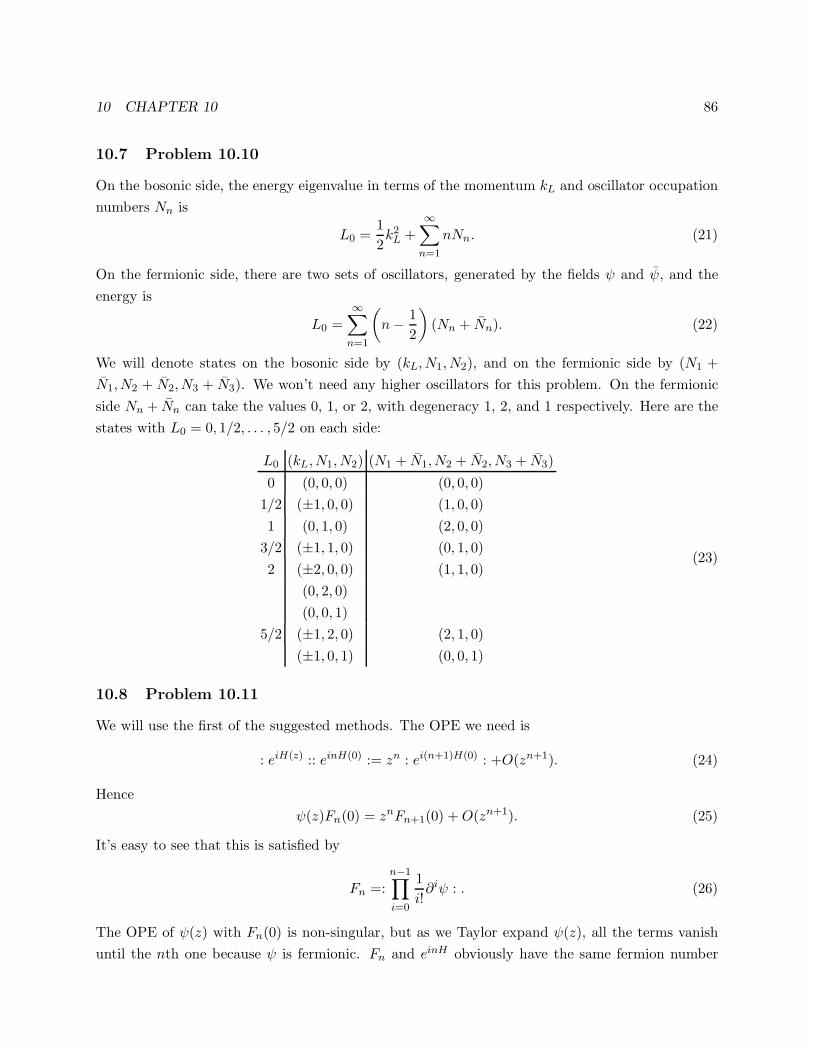
10 CHAPTER 10 86
10.7 Problem 10.10
On the bosonic side, the energy eigenvalue in terms of the momentum kL and oscillator occupation
numbers Nn is
L0 =1
2k2L +
∞∑
n=1
nNn. (21)
On the fermionic side, there are two sets of oscillators, generated by the fields ψ and ψ, and the
energy is
L0 =∞∑
n=1
(
n− 1
2
)
(Nn + Nn). (22)
We will denote states on the bosonic side by (kL, N1, N2), and on the fermionic side by (N1 +
N1, N2 + N2, N3 + N3). We won’t need any higher oscillators for this problem. On the fermionic
side Nn + Nn can take the values 0, 1, or 2, with degeneracy 1, 2, and 1 respectively. Here are the
states with L0 = 0, 1/2, . . . , 5/2 on each side:
L0 (kL, N1, N2) (N1 + N1, N2 + N2, N3 + N3)
0 (0, 0, 0) (0, 0, 0)
1/2 (±1, 0, 0) (1, 0, 0)
1 (0, 1, 0) (2, 0, 0)
3/2 (±1, 1, 0) (0, 1, 0)
2 (±2, 0, 0) (1, 1, 0)
(0, 2, 0)
(0, 0, 1)
5/2 (±1, 2, 0) (2, 1, 0)
(±1, 0, 1) (0, 0, 1)
(23)
10.8 Problem 10.11
We will use the first of the suggested methods. The OPE we need is
: eiH(z) :: einH(0) := zn : ei(n+1)H(0) : +O(zn+1). (24)
Hence
ψ(z)Fn(0) = znFn+1(0) +O(zn+1). (25)
It’s easy to see that this is satisfied by
Fn =:n−1∏
i=0
1
i!∂iψ : . (26)
The OPE of ψ(z) with Fn(0) is non-singular, but as we Taylor expand ψ(z), all the terms vanish
until the nth one because ψ is fermionic. Fn and einH obviously have the same fermion number
10 CHAPTER 10 87
n. Their dimensions work out nicely: for einH we have n2/2; for Fn we have n ψs and n(n − 1)/2
derivatives, for a total of n/2 + n(n− 1)/2 = n2/2.
For e−inH we obviously just replace ψ with ψ.
10.9 Problem 10.14
We start with the NS sector. The most general massless state is
|ψ〉 = (e · ψ−1/2 + fβ−1/2 + gγ−1/2)|0; k〉NS, (27)
where k2 = 0 (by the L0 condition) and |0; k〉NS is annihilated by b0. The BRST charge acting on
|ψ〉 is
QB|ψ〉 = (c0L0 + γ−1/2Gm1/2 + γ1/2G
m−1/2)|ψ〉
=√
2α′(e · kγ−1/2 + fk · ψ−1/2)|0; k〉NS. (28)
The L0 term of course vanishes, along with many others we have not indicated. For |ψ〉 to be
closed requires e · k = f = 0. Furthermore exactness of (28) implies g ∼= g +√
2α′e′ · k for any e′
(so we might as well set g = 0), while e ∼= e+√
2α′f ′k for any f ′. We are left with the 8 transverse
polarizations of a massless vector.
The R case is even easier: all of the work is done by the constraint (10.5.26), and none by the
BRST operator. The general massless state is
|ψ〉 = |u; k〉R, (29)
where u is a 10-dimensional Dirac spinor, and k2 = 0. |ψ〉 is defined to be annihilated by b0 and
β0, which implies that it is annihilated by Gg0. According to (10.5.26), this in turn implies that it
is annihilated by Gm0 , which is exactly the OCQ condition. The only thing left to check is that all
the states satisfying these conditions are BRST closed, which follows more or less trivially from all
the above conditions. Finally, since they are all closed, none of them can be exact.
11 CHAPTER 11 88
11 Chapter 11
11.1 Problem 11.1
In order to establish the normalizations, we first calculate the T+F T
−F OPE:
e+i√
3H(z)e−i√
3H(0) ∼ 1
z3+i√
3∂H(0)
z2− 3∂H(0)∂H(0)
2z+i2√
3∂2H(0)
z. (1)
Since the third term is supposed to be 2TB(0)/z, where
TB = −1
2∂H∂H, (2)
we need
T±F =
√
2
3e±i
√3H . (3)
It follows from the first term that c = 1 (as we already knew), and from the second that
j =i√3∂H. (4)
It is now straightforward to verify each of the OPEs in turn. The TBT±F and TBj OPEs are
from Chapter 2, and show that T±F and j have weight 3
2 and 1 respectively. The fact that the T±F T
±F
OPE is non-singular was also shown in Chapter 2. For the jT±F OPE we have
j(z)T±F (0) = ±
√
2
3
e±i√
3H(0)
z. (5)
Finally,
j(z)j(0) =1
3z2. (6)
11.2 Problem 11.3
See the last paragraph of section 11.2.
11.3 Problem 11.4
(a) Dividing the 32 left-moving fermions into two groups of 16, the untwisted theory contains 8
sectors:
(+ + +), (− − +), (+ −−), (− + −) × (NS,NS,NS), (R,R,R), (7)
where the first symbol in each triplet corresponds to the first 16 left-moving fermions, the second
to the second 16, and the third to the 8 right-moving fermions. If we now twist by exp(πiF1), we
project out (− − +) and (− + −), but project in the twisted sectors (R,NS,NS) and (NS,R,R).
We again have 8 sectors:
(+ + +), (+ −−) × (NS,NS,NS), (R,R,R), (R,NS,NS), (NS,R,R), (8)
11 CHAPTER 11 89
Let us find the massless spacetime bosons first, to establish the gauge group. These will have right-
movers in the NS+ sector, so there are two possibilities, (NS+,NS+,NS+) and (R+,NS+,NS+),
and the states are easily enumerated (primes refer to the second set of left-moving fermions):
αi−1ψj−1/2|0NS, 0NS, 0NS〉 graviton, dilaton, antisymmetric tensor;
λA′
−1/2λB′
−1/2ψi−1/2|0NS, 0NS, 0NS〉 adjoint of SO(16)′;
λA−1/2λB−1/2ψ
i−1/2|0NS, 0NS, 0NS〉 adjoint of SO(16);
ψi−1/2|uR, 0NS, 0NS〉 128 of SO(16). (9)
The last two sets combine to form an adjoint of E8, so the gauge group is E8 × SO(16). There are
similarly two sectors containing massless spacetime fermions, (NS+,R+,R+) and (NS+,R−,R−)
(the (R,R,R) states are all massive due to the positive normal-ordering constant for the left-moving
R fermions); these will give respectively (8,1,128) and (8′,1,128′) of SO(16)spin × E8 × SO(16).
Finally, the tachyon must be in (NS+,NS−,NS−); the only states are λA′
−1/2|0NS, 0NS, 0NS〉, which
transform as (1,1,8v).
(b) Dividing the left-moving fermions into four groups of 8, if we twist the above theory by the
total fermion number of the first and third groups, we get a total of 32 sectors:
(+ + + + +), (− −−− +), (+ + + −−), (− −− + −)×(NS,NS,NS,NS,NS), (NS,R,R,NS,NS), (R,NS,R,NS,NS), (R,R,NS,NS,NS),
(NS,NS,R,R,R), (NS,R,NS,R,R), (R,NS,NS,R,R), (R,R,R,R,R). (10)
Again we begin by listing the massless spacetime bosons, together with their SO(8)spin ×SO(8)1 ×SO(8)2 × SO(8)3 × SO(8)4 quantum numbers:
(NS+,NS+,NS+,NS+,NS+) :
αi−1ψj−1/2
|0NS, 0NS, 0NS, 0NS, 0NS〉 (1 ⊕ 28⊕ 35,1,1,1,1)
λA4
−1/2λB4
−1/2ψi−1/2|0NS, 0NS, 0NS, 0NS, 0NS〉 (8v,1,1,1,28)
λA1
−1/2λB1
−1/2ψi−1/2|0NS, 0NS, 0NS, 0NS, 0NS〉 (8v,28,1,1,1)
λA2
−1/2λB2
−1/2ψi−1/2|0NS, 0NS, 0NS, 0NS, 0NS〉 (8v,1,28,1,1)
λA3
−1/2λB3
−1/2ψi−1/2|0NS, 0NS, 0NS, 0NS, 0NS〉 (8v,1,1,28,1)
(NS+,R+,R+,NS+,NS+) : ψi−1/2|0NS, uR, vR, 0NS, 0NS〉 (8v,1,8,8,1)
(R+,NS+,R+,NS+,NS+) : ψi−1/2|uR, 0NS, vR, 0NS, 0NS〉 (8v,8,1,8,1)
(R+,R+,NS+,NS+,NS+) : ψi−1/2|uR, vR, 0NS, 0NS, 0NS〉 (8v,8,8,1,1). (11)
11 CHAPTER 11 90
The first set of states gives the dilaton, antisymmetric tensor, and graviton. The next set gives the
SO(8)4 gauge bosons. The rest combine to give gauge bosons of SO(24), once we perform triality
rotations on SO(8)1,2,3 to turn the bispinors into bivectors.
The massless spacetime fermions are:
(R+,NS+,NS+,R+,R+) : |uR, 0NS, 0NS, vR, wR〉 (8,8,1,1,8)
(NS+,R+,NS+,R+,R+) : |0NS, uR, 0NS, vR, wR〉 (8,1,8,1,8)
(NS+,NS+,R+,R+,R+) : |0NS, 0NS, uR, vR, wR〉 (8,1,1,8,8). (12)
The triality rotation again turns the SO(8)1,2,3 spinors into vectors, which combine into an SO(24)
vector.
Finally, the tachyon is an SO(8)4 vector but is neutral under SO(24):
(NS+,NS+,NS+,NS−,NS−) : λA4
−1/2|0NS, 0NS, 0NS, 0NS〉 (1,1,1,1,8v). (13)
11.4 Problem 11.7
We wish to show that the state ja−1ja−1|0〉 corresponds to the operator : jj(0) :. Since ja−1|0〉 clearly
corresponds to ja(0), and ja−1 =∮
dz/(2πi)ja(z)/z, we have
: jj(0) :=
∮
dz
2πi
ja(z)ja(0)
z, (14)
where the contour goes around the origin. The contour integral picks out the z0 term in the Laurent
expansion of ja(z)ja(0), which is precisely (11.5.18).
We will now use this to prove the first line of (11.5.20), with z1 = 0 and z3 = z. Using the
Laurent expansion (11.5.2) we have
: jj(0) : jc(z) ∼=∞∑
m=−∞
1
zm+1jcmj
a−1j
a−1|0〉. (15)
Only three terms in this sum are potentially interesting; the rest are either non-singular (for m < 0)
or zero (for m > 2, since the total level of the state would be negative). In fact, the term with
m = 2 must also vanish, since (being at level 0) it can only be proportional to the ground state |0〉,leaving no room for the free Lie algebra index on (15); this can also be checked explicitly. For the
other two terms we have:
jc0ja−1j
a−1|0〉 = if cab(ja−1j
b−1 + jb−1j
a−1)|0〉 = 0, (16)
jc1ja−1j
a−1|0〉 = (kδca + if cabjb0 + ja−1j
c1)j
a−1|0〉
= (2kjc−1 − f cabf badjd−1)|0〉= (k + h(g))ψ2jc−1|0〉. (17)
11 CHAPTER 11 91
The RHS of (17) clearly corresponds to the RHS of (11.5.20).
To check the TT OPE (11.5.24), we employ the same strategy, using the Laurent coefficients
(11.5.26). The OPE will be the operator corresponding to
1
(k + h(g))ψ2
(
1
z4L2 +
1
z3L1 +
1
z2L0 +
1
zL−1
)
ja−1ja−1|0〉; (18)
terms with Lm are non-singular for m < −1 and vanish for m > 2. Life is made much easier by the
fact that jbmja−1j
a−1|0〉 = 0 for m = 0 and m > 1, and the value for m = 1 is given by (17) above.
Thus:
L2ja−1j
a−1|0〉 =
1
(k + h(g))ψ2jb1j
b1ja−1j
a−1|0〉 = jb1j
b−1|0〉 = kdim(g)|0〉,
L1ja−1j
a−1|0〉 = 0,
L0ja−1j
a−1|0〉 =
2
(k + h(g))ψ2jb−1j
b1ja−1j
a−1|0〉 = 2jb−1j
b−1|0〉,
L−1ja−1j
a−1|0〉 =
2
(k + h(g))ψ2jb−2j
b1ja−1j
a−1|0〉 = 2jb−2j
b−1|0〉. (19)
All of these states are easily translated back into operators, the only slightly non-trivial one being
the last. From the Laurent expansion we see that the state corresponding to ∂T sB(0) is indeed
L−3|0〉 = 2/((k + h(g))ψ2)jb−2jb−1|0〉. Thus we have precisely the OPE (11.5.24).
11.5 Problem 11.8
The operator : jj(0) : is defined to be the z0 term in the Laurent expansion of ja(z)ja(0). First let
us calculate the contribution from a single current iλAλB (A 6= B):
iλA(z)λB(z)iλA(0)λB(0) = λA(z)λA(0)λB(z)λB(0) (no sum)
= : λA(z)λA(0)λB(z)λB(0) : +1
z: λA(z)λA(0) : +
1
z: λB(z)λB(0) : +
1
z2. (20)
Clearly the order z0 term is : ∂λAλA : + : ∂λBλB :. Summing over all A and B with B 6= A double
counts the currents, so we divide by 2:
: jj : = (n− 1) : ∂λAλA : (sum). (21)
Finally, we have k = 1, h(SO(n)) = n− 2, and ψ2 = 2, so
T sB =
1
2: ∂λAλA : (sum). (22)
11 CHAPTER 11 92
11.6 Problem 11.9
In the notation of (11.6.5) and (11.6.6), the lattice Γ is Γ22,6, i.e. the set of points of the form
(n1, . . . , n28) or (n1 +1
2, . . . , n28 +
1
2),
∑
i
ni ∈ 2Z (23)
for any integers ni. It will be convenient to divide Γ into two sublattices, Γ = Γ1 ∪ Γ2 where
Γ1 = (n1, . . . , n28) :∑
ni ∈ 2Z,
Γ2 = Γ1 + l0, l0 ≡ (1
2, . . . ,
1
2). (24)
Evenness of l ∈ Γ1 follows from the fact that the number of odd ni must be even, implying
l l =
22∑
i=1
n2i −
28∑
i=23
n2i ∈ 2Z. (25)
Evenness of l + l0 ∈ Γ2 follows from the same fact:
(l + l0) (l + l0) = l l + 2l0 l + l0 l0 = l l +22∑
i=1
ni −28∑
i=23
ni + 4 ∈ 2Z. (26)
Evenness implies integrality, so Γ ⊂ Γ∗. It’s easy to see that the dual lattice to Γ1 is Γ∗1 =
Z28 ∪ (Z28 + l0) ⊃ Γ. But to be dual for example to l0 requires a vector to have an even number
of odd nis, so Γ∗ = Γ.
To find the gauge bosons we need to find the lattice vectors satisfying (11.6.15). But these
are obviously the root vectors of SO(44). In addition there are the 22 gauge bosons with vertex
operators ∂Xmψµ, providing the Cartan generators to fill out the adjoint representation of SO(44),
and the 6 gauge bosons with vertex operators ∂Xµψm, generating U(1)6.
11.7 Problem 11.12
It seems to me that both the statement of the problem and the derivation of the Hagedorn tem-
perature for the bosonic string (Vol. I, pp. 320-21) are misleading. Equation (7.3.20) is not the
correct one to use to find the asymptotic density of states of a string theory, since it does not take
into account the level matching constraint in the physical spectrum. It’s essentially a matter of
luck that Polchinski ends up with the right Hagedorn temperature, (9.8.13).
Taking into account level matching we have n(m) = nL(m)nR(m). To find nL and nR we
treat the left-moving and right-moving CFTs separately, and include only the physical parts of the
spectrum, that is, neglect the ghosts and the timelike and longitudinal oscillators. Then we have,
as in (9.8.11),∑
m2
nL(m)e−πα′m2l/2 ∼ eπc/(12l), (27)

11 CHAPTER 11 93
implying
nL(m) ∼ eπm√α′c/6. (28)
Similarly for the right-movers, giving
n(m) ∼ eπm√α′/6(
√c+
√c). (29)
The Hagedorn temperature is then given by
T−1H = π
√α′
(
√
c
6+
√
c
6
)
. (30)
For the type I and II strings, this gives
TH =1
2π√
2α′ , (31)
while for the heterotic theories we have
TH =1
π√α′ (1 − 1√
2). (32)
The Hagedorn temperature for an open type I string is the same, (31), as for the closed string,
since nopen(m) = nL(2m).
There is an interesting point that we glossed over above. The RHS of (27) is obtained by doing
a modular transformation l → 1/l on the torus partition function with τ = il. Then for small l
only the lowest-lying state in the theory contributes. We implicitly took the lowest-lying state to
be the vacuum, corresponding to the unit operator. However, that state is projected out by the
GSO projection in all of the above theories, else it would give rise to a tachyon. So should we
really consider it? To see that we should, let us derive (27) more carefully, for example in the case
of the left-movers of the type II string. The GSO projection there is (−1)F = −1, where F is the
worldsheet fermion number of the transverse fermions (not including the ghosts). The partition
function from which we will extract nL(m), the number of projected-in states, is
Z(il) =∑
i∈R,NS
qhi−c/24 1
2(1 − (−1)Fi) =
∑
m2
nL(m)e−πα′m2l/2. (33)
This partition function corresponds to a path integral on the torus in which we sum over all four
spin structures, with minus signs when the fermions are periodic in the σ2 (“time”) direction. Upon
doing the modular integral, this minus sign corresponds to giving a minus sign to R sector states.
But the sum on R and NS sectors in (33) means that we now project onto states with (−1)F = 1:
Z(il) =∑
i∈R,NS
e−2π/l(hi−c/24)(−1)αi1
2(1 + (−1)Fi) ∼ eπc/(12l). (34)
We see that the ground state, with h = 0, is indeed projected in, and therefore dominates in the
limit l → 0.
12 CHAPTER 13 94
12 Chapter 13
12.1 Problem 13.2
An open string with ends attached to Dp-branes is T-dual to an open type I string. An open string
with both ends attached to the same Dp-brane and zero winding number is T-dual to an open type
I string with zero momentum in the 9 − p dualized directions, and Chan-Paton factor of the form
ta =1√2
[
0 i
−i 0
]
⊗ diag(1, 0, . . . , 0). (1)
Four open strings attached to the same Dp-brane are T-dual to four open type I strings with zero
momentum in the 9 − p dualized directions and the same Chan-Paton factor (1). The scattering
amplitude for four gauge boson open string states was calculated in section 12.4. Using
Tr(ta)4 =1
2, (2)
the result (12.4.22) becomes in this case
S(ki, ei) = (3)
−8ig2YMα
′2(2π)10δ10(∑
i
ki)K(ki, ei)
(
Γ(−α′s)Γ(−α′u)Γ(1 − α′s− α′u)
+ 2 permutations
)
.
The kinematic factor K is written in three different ways in (12.4.25) and (12.4.26), and we won’t
bother to reproduce it here. Since the momenta ki all have vanishing components in the 9 − p
dualized directions, the amplitude becomes,
−8ig2(p+1),YMα
′2V 29−p(2π)p+1δp+1(
∑
i
ki) (4)
×K(ki, ei)
(
Γ(−α′s)Γ(−α′u)Γ(1 − α′s− α′u)
+ 2 permutations
)
,
where V9−p is the volume of the transverse space, and we have used (13.3.29). But in order to
get the proper (p+ 1)-dimensional scattering amplitude, we must renormalize the wave function of
each string (which is spread out uniformly in the transverse space) by a factor of√
V9−p:
S′(ki, ei) = −8ig2(p+1),YMα
′2(2π)p+1δp+1(∑
i
ki) (5)
×K(ki, ei)
(
Γ(−α′s)Γ(−α′u)Γ(1 − α′s− α′u)
+ 2 permutations
)
.
Finally, using (13.3.30) and (13.3.28), we can write the dimensionally reduced type I Yang-Mills
coupling g(p+1),YM, in terms of the coupling gDp on the brane:
g2(p+1),YM = g2
Dp,SO(32) = 2g2Dp, (6)
12 CHAPTER 13 95
so
S′(ki, ei) = −16ig2Dpα
′2(2π)p+1δp+1(∑
i
ki) (7)
×K(ki, ei)
(
Γ(−α′s)Γ(−α′u)Γ(1 − α′s− α′u)
+ 2 permutations
)
.
(One can also use (13.3.25) to write gDp in terms of the string coupling g.)
12.2 Problem 13.3
(a) By equations (B.1.8) and (B.1.10),
Γ2aΓ2a+1 = −2iSa, (8)
where a = 1, 2, 3, 4, so
β2aβ2a+1 = 2iSa. (9)
If we define
β ≡ β1β2β3, (10)
and label the D4-branes extended in the (6,7,8,9), (4,5,8,9), and (4,5,6,7) directions by the subscripts
2, 3, and 4 respectively, then
β⊥2 = β1β2β3β4β5 = 2iS2β (11)
and similarly
β⊥3 = 2iS3β, β⊥4 = 2iS4β. (12)
The supersymmetries preserved by brane a (a = 2, 3, 4) are
Qs + (β⊥a Q)s = Qs + 2isa(βQ)s, (13)
so for a supersymmetry to be unbroken by all three branes simply requires s2 = s3 = s4. Taking
into account the chirality condition Γ = +1 on Qs, there are four unbroken supersymmetries:
Q(+++++) + i(βQ)(+++++),
Q(−−+++) + i(βQ)(−−+++),
Q(+−−−−) − i(βQ)(+−−−−),
Q(−+−−−) − i(βQ)(−+−−−). (14)
12 CHAPTER 13 96
(b) For the D0-brane,
β⊥D0 = β1β2β3β4β5β6β7β8β9 = −8iS2S3S4β, (15)
so the unbroken supersymmetries are of the form,
Qs + (β⊥D0Q)s = Qs − 8is2s3s4(βQ)s. (16)
The signs in all four previously unbroken supersymmetries (14) are just wrong to remain unbroken
by the D0-brane, so that this configuration preserves no supersymmetry.
(c) Let us make a brane scan of the original configuration:
1 2 3 4 5 6 7 8 9
D42 D D D D D N N N N
D43 D D D N N D D N N
D44 D D D N N N N D D
D0 D D D D D D D D DThere are nine distinct T-dualities that can be performed in the 4, 5, 6, 7, 8, and 9 directions, up
to the symmetries 4 ↔ 5, 6 ↔ 7, 8 ↔ 9, and (45) ↔ (67) ↔ (89). They result in the following
brane content:T-dualized directions (p1, p2, p3, p4)
4 (5, 3, 3, 1)
4, 5 (6, 2, 2, 2)
4, 6 (4, 4, 2, 2)
4, 5, 6 (5, 3, 1, 3)
4, 5, 6, 7 (4, 4, 0, 4)
4, 6, 8 (3, 3, 3, 3)
4, 5, 6, 8 (4, 2, 2, 4)
4, 5, 6, 7, 8 (3, 3, 1, 5)
4, 5, 6, 7, 8, 9 (2, 2, 2, 6)Further T-duality in one, two, or all three of the 1, 2, and 3 directions will turn any of these
configurations into (p1 + 1, p2 + 1, p3 + 1, p4 + 1), (p1 + 2, p2 + 2, p3 + 2, p4 + 2), and (p1 + 3, p2 +
3, p3 + 3, p4 + 3) respectively.
T-dualizing at general angles to the coordinate axes will result in combinations of the above
configurations for the directions involved, with the smaller-dimensional brane in each column being
replaced by a magnetic field on the larger-dimensional brane.
12.3 Problem 13.4
(a) Let the D2-brane be extended in the 8 and 9 directions, and let it be separated from the
D0-brane in the 1 direction by a distance y. T-dualizing this configuration in the 2, 4, 6, and 8
12 CHAPTER 13 97
directions yields 2 D4-branes, the first (from the D2-brane) extended in the 2, 4, 6, and 9 directions,
and the second (from the D0-brane) in the 2, 4, 6, and 8 directions. This is in the class of D4-brane
configurations studied in section 13.4; in our case the angles defined there take the values
φ1 = φ2 = φ3 = 0, φ4 =π
2, (17)
and therefore (according to (13.4.22)),
φ′1 = φ′4 =π
4, φ′2 = φ′3 = −π
4. (18)
For the three directions in which the D4-branes are parallel, we must make the substitution (13.4.25)
(without the exponential factor, since we have chosen the separation between the D0- and D2-branes
to vanish in those directions, but with a factor −i, to make the potential real and attractive). The
result is
V (y) = −∫ ∞
0
dt
t(8π2α′t)−1/2 exp
(
− ty2
2πα′
)
iϑ411(it/4, it)
ϑ11(it/2, it)η9(it). (19)
Alternatively, using the modular transformations (7.4.44b) and (13.4.18b),
V (y) = − 1√8π2α′
∫ ∞
0dt t3/2 exp
(
− ty2
2πα′
)
ϑ411(1/4, i/t)
ϑ11(1/2, i/t)η9(i/t). (20)
(b) For the field theory calculation we lean heavily on the similar calculation done in section 8.7,
adapting it to D = 10. Polchinski employs the shifted dilaton
Φ = Φ − Φ0, (21)
whose expectation value vanishes, and the Einstein metric
G = e−Φ/2G; (22)
their propagators are given in (8.7.23):
〈ΦΦ(k)〉 = −2iκ2
k2, (23)
〈hµνhσρ(k)〉 = −2iκ2
k2
(
ηµσηνρ + ηµρηνσ −1
4ηµνησρ
)
, (24)
where h = G− η. The D-brane action (13.3.14) expanded for small values of Φ and h is
Sp = −τp∫
dp+1ξ
(
p− 3
4Φ +
1
2ha
a
)
, (25)
where the trace on h is taken over directions tangent to the brane. From the point of view of the
supergravity, the D-brane is thus a source for Φ,
JΦ,p(X) =3 − p
4τpδ
9−p(X⊥ −X ′⊥), (26)
12 CHAPTER 13 98
and for h,
Jµνh,p(X) = −1
2τpe
µνp δ9−p(X⊥ −X ′
⊥), (27)
where X ′⊥ is the position of the brane in the transverse coordinates, and eµνp is ηµν in the directions
parallel to the brane and 0 otherwise. In momentum space the sources are
JΦ,p(k) =3 − p
4τp(2π)p+1δp+1(k‖)e
ik⊥·X′⊥ , (28)
Jµνh,p(k) = −1
2τpe
µνp (2π)p+1δp+1(k‖)e
ik⊥·X′⊥ . (29)
Between the D0-brane, located at the origin of space, and the D2-brane, extended in the 8 and 9
directions and located in the other directions at the point
(X ′1,X
′2,X
′3,X
′4,X
′5,X
′6,X
′7) = (y, 0, 0, 0, 0, 0, 0), (30)
the amplitude for dilaton exchange is
AΦ = −∫
d10k
(2π)10JΦ,0(k)〈ΦΦ(k)〉JΦ,2(−k)
= i3
8τ0τ2κ
2
∫
d10k
(2π)102πδ(k0)
1
k2(2π)3δ3(k0, k8, k9)e
ik1y
= iT3
8τ0τ2κ
2
∫
d7k
(2π)7eiky
k2
= iT3
8τ0τ2κ
2G7(y), (31)
where G7 is the 7-dimensional massless scalar Green function. We divide the amplitude by −iT to
obtain the static potential due to dilaton exchange:
VΦ(y) = −3
8τ0τ2κ
2G7(y). (32)
The calculation for the graviton exchange is similar, the only difference being that the numerical
factor (1/4)2(3/4) is replaced by
1
2eµν0 2
(
ηµσηνρ + ηµρηνσ −1
4ηµνησρ
)
1
2eσρ2 =
5
8. (33)
The total potential between the D0-brane and D2-brane is therefore
V (y) = τ0τ2κ2G7(y) = −π(4π2α′)2G7(y), (34)
where we have applied (13.3.4). As expected, gravitation and dilaton exchange are both attractive
forces.
In the large-y limit of (20), the integrand becomes very small except where t is very small. The
ratio of modular functions involved in the integrand is in fact finite in the limit t→ 0,
limt→0
ϑ411(1/4, i/t)
ϑ11(1/2, i/t)η9(i/t)= 2, (35)
12 CHAPTER 13 99
(according to Mathematica), so that the first term in the asymptotic expansion of the potential in
1/y is
V (r) ≈ − 1√2π2α′
∫ ∞
0dt t3/2 exp
(
− ty2
2πα′
)
= −π−1/2(2πα′)2Γ(5
2)y−5
= −π(4π2α′)2G7(y), (36)
in agreement with (34).
12.4 Problem 13.12
The tension of the (pi, qi)-string is (13.6.3)
τ(pi,qi) =
√
p2i + q2i /g
2
2πα′ . (37)
Let the three strings sit in the (X1,X2) plane. If the angle string i makes with the X1 axis is θi,
then the force it exerts on the junction point is
(F 1i , F
2i ) =
1
2πα′ (cos θi
√
p2i + q2i /g
2, sin θi
√
p2i + q2i /g
2). (38)
If we orient each string at the angle
cos θi =pi
√
p2i + q2i /g
2, sin θi =
qi/g√
p2i + q2i /g
2, (39)
then the total force exerted on the junction point is
1
2πα′
3∑
i=1
(pi, qi/g), (40)
which vanishes if∑
pi =∑
qi = 0. This is the unique stable configuration, up to rotations and
reflections.
The supersymmetry algebra for a static (p, q) string extended in the Xi direction is (13.6.1)
1
2L
[
Qα
Qα
]
,[
Q†β Q
†β
]
= τ(p,q)δαβ
[
1 0
0 1
]
+(Γ0Γi)αβ
2πα′
[
p q/g
q/g −p
]
. (41)
Defining
u ≡ p√
p2 + q2/g2, U ≡ 1√
2
[ √1 + u
√1 − u
−√
1 − u√
1 + u
]
, (42)
12 CHAPTER 13 100
we can use U to diagonalize the matrix on the RHS of (41):
1
2Lτ(p,q)
U
[
Qα
Qα
]
,[
Q†β Qβ
†]
UT
=
[
(I16 + Γ0Γi)αβ 0
0 (I16 − Γ0Γi)αβ
]
. (43)
The top row of this 2 × 2 matrix equation tells us that, in a basis in spinor space in which Γ0Γi is
diagonal, the supersymmetry generator
√1 + uQα +
√1 − uQα (44)
annihilates this state if (I16 + Γ0Γi)αα = 0. We can use (I16 − Γ0Γi) to project onto this eight-
dimensional subspace, yielding eight supersymmetries that leave this state invariant:
[
(I16 − Γ0Γi)(√
1 + uQ+√
1 − uQ)]
α. (45)
The other eight unbroken supersymmetries are given by the bottom row of (43), after projecting
onto the subspace annihilated by (I16 − Γ0Γi):
[
(I16 + Γ0Γi)(−√
1 − uQ+√
1 + uQ)]
α. (46)
Now let us suppose that the string is aligned in the direction (39), which depends on p and q.
We will show that eight of the sixteen unbroken supersymmetries do not depend on p or q, and
therefore any configuration of (p, q) strings that all obey (39) will leave these eight unbroken. If
the string is aligned in the direction (39), then
Γi =p
√
p2 + q2/g2Γ1 +
q/g√
p2 + q2/g2Γ2 = uΓ1 +
√
1 − u2Γ2. (47)
Our first set of unbroken supersymmetries (45) becomes
[
(I16 − uΓ0Γ1 −√
1 − u2Γ0Γ2)(√
1 + uQ+√
1 − uQ)]
α. (48)
We work in a basis of eigenspinors of the operators Sa defined in (B.1.10). In this basis Γ0Γ1 = 2S0,
while
Γ0Γ2 =
[
0 1
−1 0
]
⊗[
0 −1
1 0
]
⊗ I2 ⊗ I2 ⊗ I2. (49)
We can divide the sixteen values of the spinor index α into four groups of four according to the
12 CHAPTER 13 101
eigenvalues of S0 and S1:
[
(I16 − uΓ0Γ1 −√
1 − u2Γ0Γ2)(√
1 + uQ+√
1 − uQ)]
(++s2s3s4)(50)
= (1 − u)(√
1 + uQ+√
1 − uQ)(++s2s3s4)
+√
1 − u2(√
1 + uQ+√
1 − uQ)(−−s2s3s4),[
(I16 − uΓ0Γ1 −√
1 − u2Γ0Γ2)(√
1 + uQ+√
1 − uQ)]
(++s2s3s4)(51)
= (1 + u)(√
1 + uQ+√
1 − uQ)(−−s2s3s4)
+√
1 − u2(√
1 + uQ+√
1 − uQ)(++s2s3s4),[
(I16 − uΓ0Γ1 −√
1 − u2Γ0Γ2)(√
1 + uQ+√
1 − uQ)]
(+−s2s3s4)(52)
= (1 − u)(√
1 + uQ+√
1 − uQ)(+−s2s3s4)
−√
1 − u2(√
1 + uQ+√
1 − uQ)(−+s2s3s4),[
(I16 − uΓ0Γ1 −√
1 − u2Γ0Γ2)(√
1 + uQ+√
1 − uQ)]
(−+s2s3s4)(53)
= (1 + u)(√
1 + uQ+√
1 − uQ)(−+s2s3s4)
−√
1 − u2(√
1 + uQ+√
1 − uQ)(+−s2s3s4).
(The indexing by s2, s3, s4 is somewhat redundant, since the chirality condition on both Q and Q
implies the restriction 8s2s3s4 = 1 in the case of (50) and (51), and 8s2s3s4 = −1 in the case of
(52) and (53).) It easy to see that (50) and (51) differ only by a factor of√
(1 − u)/(1 + u), and
(52) and (53) similarly by a factor of −√
(1 − u)/(1 + u), so (50) and (52) alone are sufficient to
describe the eight independent supersymmetry generators in this sector. In the other sector, given
by (46), there is a similar repetition of generators, and the eight independent generators are
[
(I16 + uΓ0Γ1 +√
1 − u2Γ0Γ2)(−√
1 − uQ+√
1 + uQ)]
(++s2s3s4)(54)
= (1 + u)(−√
1 − uQ+√
1 + uQ)(++s2s3s4)
−√
1 − u2(−√
1 − uQ+√
1 + uQ)(−−s2s3s4),[
(I16 + uΓ0Γ1 +√
1 − u2Γ0Γ2)(−√
1 − uQ+√
1 + uQ)]
(+−s2s3s4)(55)
= (1 + u)(−√
1 − uQ+√
1 + uQ)(+−s2s3s4)
+√
1 − u2(−√
1 − uQ+√
1 + uQ)(−+s2s3s4).
Are there linear combinations of the generators (50), (52), (54), and (55) that are independent of u,
and therefore unbroken no matter what the values of p and q? Indeed, by dividing (50) by 2√
1 − u
and (54) by 2√
1 + u and adding them, we come up with four such generators:
Q(++s2s3s4) +Q(−−s2s3s4). (56)
12 CHAPTER 13 102
Four more are found by dividing (52) by 2√
1 − u and (55) by√
1 + u:
Q(+−s2s3s4) −Q(−+s2s3s4). (57)
As promised, one quarter of the original supersymmetries leave the entire configuration described
in the first paragraph of this solution invariant.
13 CHAPTER 14 103
13 Chapter 14
13.1 Problem 14.1
The excitation on the F-string will carry some energy (per unit length) p0, and momentum (per unit
length) in the 1-direction p1. Since the string excitations move at the speed of light, left-moving
excitation have p0 = −p1, while right-moving excitations have p0 = p1. The supersymmetry algebra
(13.2.9) for this string is similar to (13.6.1), with additional terms for the excitation:
1
2L
[
Qα
Qα
]
,[
Q†β Q
†β
]
(1)
=1
2πα′
[
(δ + Γ0Γ1)αβ 0
0 (δ − Γ0Γ1)αβ
]
+(
p0δαβ + p1(Γ0Γ1)αβ
)
[
1 0
0 1
]
.
The first term on the RHS vanishes for those supersymmetries preserved by the unexcited F-string,
namely Qs for which Γ0Γ1 = −1 and Qs for which Γ0Γ1 = 1. The second term thus also vanishes
(making the state BPS) for the Qs if the excitation is left-moving, and for the Qs if the excitation
is right-moving.
For the D-string the story is almost the same, except that the first term above is different:
1
2L
[
Qα
Qα
]
,[
Q†β Q
†β
]
(2)
=1
2πα′g
[
δαβ (Γ0Γ1)αβ
(Γ0Γ1)αβ δαβ
]
+(
p0δαβ + p1(Γ0Γ1)αβ
)
[
1 0
0 1
]
.
When diagonalized, the first term yields the usual preserved supersymmetries, of the form Qα +
(β⊥Q)α. When 1 − (Γ0Γ1)αα = 0 this supersymmetry is also preserved by the second term if the
excitation is left-moving; when 1 + (Γ0Γ1)αα = 0 it is preserved if the excitation is right-moving.
Either way, the state is BPS.
13.2 Problem 14.2
The supergravity solution for two static parallel NS5-branes is given in (14.1.15) and (14.1.17):
e2Φ = g2 +Q1
2π2(xm − xm1 )2+
Q2
2π2(xm − xm2 )2,
Gmn = g−1e2Φδmn, Gµν = gηµν ,
Hmnp = −ǫmnpq∂qΦ, (3)
where µ, ν = 0, . . . , 5 and m,n = 6, . . . , 9 are the parallel and transverse directions respectively, and
the branes are located in the transverse space at xm1 and xm2 . (We have altered (14.1.15a) slightly
in order to make (3) S-dual to the D-brane solution (14.8.1).) A D-string stretched between the
13 CHAPTER 14 104
two branes at any given excitation level is a point particle with respect to the 5+1 dimensional
Poincare symmetry of the parallel dimensions. In other words, if we make an ansatz for the solution
of the form
Xµ = Xµ(τ), Xm = Xm(σ), (4)
then, after performing the integral over σ in the D-string action, we should obtain the point-particle
action (1.2.2) in 5+1 dimensions,
Spp = −m∫
dτ√
−∂τXµ∂τXµ, (5)
where m is the mass of the solution Xm(σ) with respect to the 5+1 dimensional Poincare symmetry.
Assuming that the gauge field is not excited, with this ansatz the D-string action (13.3.14)
factorizes:
SD1 = − 1
2πα′
∫
dτdσ e−Φ√
− det(Gab +Bab)
= − 1
2πα′
∫
dτdσ e−Φ
×
√
√
√
√−∣
∣
∣
∣
∣
Gµν∂τXµ∂τX
ν (Gµn +Bµn)∂τXµ∂σX
n
(Gmν +Bmν)∂σXm∂τX
ν Gmn∂σXm∂σX
n
∣
∣
∣
∣
∣
= − 1
2πα′
∫
dσ e−Φ√
∂σXm∂σXm
∫
dτ√
−∂τXµ∂τXµ. (6)
In the last equality we have used the fact that neither the metric nor the two-form potential in the
solution (3) have mixed µn components. Comparison with (5) shows that
m =g−1/2
2πα′
∫
dσ |∂σXm|, (7)
where the integrand is the coordinate (not the proper) line element in this coordinate system. The
ground state is therefore a straight line connecting the two branes:
m =g−1/2|xm2 − xm1 |
2πα′ . (8)
As explained above, this mass is defined with respect the geometry of the parallel directions,
and it is only in string frame that the parallel metric Gµν is independent of the transverse position.
We can nonetheless define an Einstein-frame mass mE with respect to Gµν at |xm| = ∞, and it
is this mass that transforms simply under S-duality. (Here we are using the definition (14.1.7) of
the Einstein frame, GE = e−Φ/2G, which is slightly different from the one used in volume I and in
Problem 14.6 below, where GE = e−Φ/2G.) From the definition (5) of the mass,
mE = g1/4m, (9)
13 CHAPTER 14 105
so (7) becomes
mE =g−1/4
2πα′
∫
dσ |∂σXm|. (10)
We can calculate the mass of an F-string stretched between two D5-branes in two different
pictures: we can use the black 5-brane supergravity solution (14.8.1) and do a calculation similar
to the one above, or we can consider the F-string to be stretched between two elementary D5-branes
embedded in flat spacetime. In the first calculation, the S-duality is manifest at every step, since
the NS5-brane and the black 5-brane solutions are related by S-duality, as are the D-string and F-
string actions. The second calculation yields the same answer, and is much easier: since the tension
of the F-string is 1/2πα′, and in flat spacetime (Gµν = ηµν) its proper length and coordinate length
are the same, its total energy is
m =1
2πα′
∫
dσ |∂σXm|. (11)
Its Einstein-frame mass is then
mE =g1/4
2πα′
∫
dσ |∂σXm|, (12)
which indeed agrees with (10) under g → 1/g.
13.3 Problem 14.6
To find the expectation values of the dilaton and graviton in the low energy field theory, we add to
the action a source term
S′ =
∫
d10X(
KΦΦ +Kµνh hµν
)
, (13)
and take functional derivatives of the partition function Z[KΦ,Kh] with respect to KΦ and Kh.
For the D-brane, which is a real, physical source for the fields, we also include the sources JΦ and
Jh, calculated in problem 13.4(b) (see (26) and (27) of that solution):
JΦ(X) =3 − p
4τpδ
9−p(X⊥), (14)
Jµνh (X) = −1
2τpe
µνp δ9−p(X⊥). (15)
Recall that h is the perturbation in the Einstein-frame metric, G = η + h, and that eµν equals
ηµν for µ, ν parallel to the brane and zero otherwise. (We have put the brane at the origin, so
that X ′⊥ = 0.) Since the dilaton decouples from the Einstein-frame graviton, we can calculate the
partition functions Z[KΦ] and Z[Kh] separately. Using the propagator (23),
Z[KΦ] = −Z[0]
∫
d10k
(2π)10JΦ(−k)〈ΦΦ(k)〉KΦ(k)
= Z[0]3 − p
2iκ2τp
∫
d9−pk⊥(2π)9−p
1
k2⊥KΦ(k⊥, k‖ = 0)
= Z[0]3 − p
2iκ2τp
∫
d9−pX⊥G9−p(X⊥)
∫
dp+1X‖KΦ(X), (16)
13 CHAPTER 14 106
so that
〈Φ(X)〉 =1
iZ[0]
δZ[KΦ]
δKΦ(X)
=3 − p
2κ2τpG9−p(X⊥). (17)
Using (13.3.22), (13.3.23), and the position-space expression for Gd, this becomes
〈Φ(X)〉 =3 − p
4(4π)(5−p)/2Γ(
7 − p
2)gα′(7−p)/2rp−7
=3 − p
4
ρ7−p
r7−p, (18)
where ρ7−p is as defined in (14.8.2b) with Q = 1. Hence
e2〈Φ〉 ≈ g2(1 + 2〈Φ〉)
≈ g2
(
1 +ρ7−p
r7−p
)(3−p)/2, (19)
in agreement with (14.8.1b) (corrected by a factor of g2).
The graviton calculation is very similar. Using the propagator (24),
Z[Kh] = −Z[0]
∫
d10X
(2π)10Jµνh (−k)〈hµνhρσ(k)〉Kρσ
h (k)
= Z[0]
(
p+ 1
8ηµν − eµν
)
2iκ2τp
∫
d9−pk⊥(2π)10
1
k2⊥Kµνh (k⊥, k‖ = 0)
= Z[0]
(
p+ 1
8ηµν − eµν
)
2iκ2τp (20)
×∫
d9−pX⊥G9−p(X⊥)
∫
dp+1X‖Kµνh (X),
so
〈hµν(X)〉 =
(
p+ 1
8ηµν − eµν
)
2κ2τpG9−p(X⊥)
=
(
p+ 1
8ηµν − eµν
)
ρ7−p
r7−p. (21)
Hence for µ, ν aligned along the brane,
〈Gµν〉 ≈(
1 +ρ7−p
r7−p
)(p−7)/8
ηµν , (22)
while for m,n transverse to the brane,
〈Gmn〉 ≈(
1 +ρ7−p
r7−p
)(p+1)/8
δmn. (23)
13 CHAPTER 14 107
The string frame metric, G = eΦ/2G, is therefore
〈Gµν〉 ≈(
1 +ρ7−p
r7−p
)−1/2
ηµν , (24)
〈Gmn〉 ≈(
1 +ρ7−p
r7−p
)1/2
δmn, (25)
in agreement with (14.8.1).
14 CHAPTER 15 108
14 Chapter 15
14.1 Problem 15.1
The matrix of inner products is
M3 = 〈h|
L31
L1L2
L3
[
L3−1 L−2L−1 L−3
]
|h〉 (1)
=
24h(h + 1)(2h + 1) 12h(3h + 1) 24h
12h(3h + 1) h(8h + 8 + c) 10h
24h 10h 6h+ 2c
. (2)
This matches the Kac formula, with
K3 = 2304. (3)
14.2 Problem 15.3
Let’s begin by recording some useful symmetry relations of the operator product coefficient with
lower indices, derived from the definition (6.7.13) and (6.7.14),
cijk =⟨
A′i(∞,∞)Aj(1, 1)Ak(0, 0)
⟩
S2. (4)
The following relations then hold, with the sign of the coefficient depending on the statistics of the
operators:
cijk = ±(−1)hj+hjckji if Aj is primary (5)
cijk = ±(−1)hi+hj+hk+hi+hj+hkcikj if Ai is primary (6)
cijk = ±(−1)hk+hkcjik if Ai,Aj ,Ak are primary. (7)
Actually, in the above “primary” may be weakened to “quasi-primary” (meaning annihilated by
L1, rather than Ln for all n > 0, and therefore transforming as a tensor under PSL(2, C) rather
than general local conformal transformations), but Polchinski does not seem to find the notion of
quasi-primary operator interesting or useful.
Armed with these symmetries (and in particular relation (5)), but glibly ignoring phase factors
as Polchinski does, we would like to claim that the correct form for (15.2.7) should be as follows
(we haven’t bothered to raise the index):
cik,k,mn = limzn→∞zm→1
z2hnn z2hn
n L−kL−k 〈On(zn, zn)Om(zm, zm)Oi(0, 0)〉S2. (8)
We would also like to claim that the LHS of (15.2.9) should read
⟨
O′l(∞,∞)Oj(1, 1)Om(z, z)On(0, 0)
⟩
S2. (9)
14 CHAPTER 15 109
We are now ready to solve the problem. The case N = 0 is trivial, since by the definition
(15.2.8),
βimn = 1, (10)
so the coefficient of z−hm−hn+hi in F jlmn(i|z) is 1. For N = 1 there is again only one operator,
L−1 · Oi. We have
βi1mn =1
2hi(hi + hm − hn). (11)
Thus the coefficient of z−hm−hn+hi+1 is
1
2hi(hi + hm − hn)(hi + hj − hl). (12)
15 APPENDIX B 110
15 Appendix B
15.1 Problem B.1
Under a change of spinor representation basis, Γµ → UΓµU−1, B1, B2, and C, all transform the
same way:
B1 → U∗B1U−1, B2 → U∗B2U
−1, C → U∗CU−1. (1)
The invariance of the following equations under this change of basis is more or less trivial:
(B.1.17) (the definition of B1 and B2):
U∗B1U−1UΓµU−1(U∗B1U
−1)−1 = U∗B1ΓµB−1
1 UT
= (−1)kU∗Γµ∗UT
= (−1)k(UΓµU−1)∗, (2)
U∗B2U−1UΓµU−1(U∗B2U
−1)−1 = U∗B2ΓµB−1
2 UT
= (−1)k+1U∗Γµ∗UT
= (−1)k+1(UΓµU−1)∗. (3)
(B.1.18), using the fact that Σµν transforms the same way as Γµ:
U∗BU−1UΣµνU−1UB−1UT = U∗BΣµνB−1UT
= −U∗Σµν∗UT
= −(UΣµνU−1)∗. (4)
The invariance of (B.1.19) is the same as that of (B.1.17).
(B.1.21):
UB∗1U
TU∗B1U−1 = UB∗
1B1U−1 = (−1)k(k+1)/2UU−1 = (−1)k(k+1)/2, (5)
UB∗2U
TU∗B2U−1 = UB∗
2B2U−1 = (−1)k(k−1)/2UU−1 = (−1)k(k−1)/2. (6)
(B.1.24) (the definition of C):
U∗CU−1UΓµU−1UC−1UT = U∗CΓµC−1UT
= −U∗ΓµTUT
= −(UΓµU−1)T . (7)
(B.1.25): all three sides clearly transform by multiplying on the left by U and on the right by
U−1.
(B.1.27):
U∗BU−1UΓ0U−1 = U∗BΓ0U−1 = U∗CU−1. (8)
15 APPENDIX B 111
We will determine the relation between B and BT in the ζ(s) basis, where (for d = 2k + 2) B1
and B2 are defined by equation (B.1.16):
B1 = Γ3Γ5 · · ·Γd−1, B2 = ΓB1. (9)
Since all of the Γ’s that enter into this product are antisymmetric in this basis (since they are
Hermitian and imaginary), we have
BT1 = (Γ3Γ5 · · ·Γd−1)T
= (−1)kΓd−1Γd−3 · · ·Γ3
= (−1)k(k+1)/2Γ3Γ5 · · ·Γd−1
= (−1)k(k+1)/2B1. (10)
Using (10), the fact that Γ is real and symmetric in this basis, and (B.1.19), we find
BT2 = (ΓB1)
T
= BT1 ΓT
= (−1)k(k+1)/2B1Γ
= (−1)k(k+1)/2+kΓ∗B1
= (−1)k(k−1)/2B2. (11)
Since B1 is used when k = 0, 3 (mod 4), and B2 is used when k = 0, 1 (mod 4), so in any dimension
in which one can impose a Majorana condition we have
BT = B. (12)
When k is even, C = B1Γ0, so, using the fact that in this basis Γ0 is real and antisymmetric,
and (B.1.17), we find
CT = Γ0TBT1
= (−1)k(k+1)/2+1Γ0∗B1
= (−1)k/2+1B1Γ0
= (−1)k/2+1C. (13)
On the other hand, if k is odd, then C = B2Γ0, and
CT = Γ0TBT2
= (−1)k(k−1)/2+1Γ0∗B2
= (−1)(k+1)/2B2Γ0
= (−1)(k+1)/2C. (14)
That all of these relations are invariant under change of basis follows directly from the trans-
formation law (1), since BT and CT transform the same way as B and C.
15 APPENDIX B 112
15.2 Problem B.3
The decomposition of SO(1,3) spinor representations under the subgroup SO(1,1)×SO(2) is de-
scribed most simply in terms of Weyl representations: one positive chirality spinor, ζ++, transforms
as a positive chirality Weyl spinor under both SO(1,1) and SO(2), while the other, ζ−−, transforms
as a negative chirality Weyl spinor under both (see (B.1.44a)). Let us therefore use the Weyl-spinor
description of the 4 real supercharges of d = 4, N = 1 supersymmetry. The supersymmetry algebra
is (B.2.1a):
Q++, Q†++ = 2(P 0 − P 1),
Q−−, Q†−− = 2(P 0 + P 1), (15)
Q++, Q†−− = 2(P 2 + iP 3).
We must now decompose these Weyl spinors into Majorana-Weyl spinors. Define
Q1L =
1
2(Q++ +Q†
++), Q2L =
1
2i(Q++ −Q†
++), (16)
Q1R =
1
2(Q−− +Q†
−−), Q2R =
1
2i(Q−− −Q†
−−). (17)
(The subscripts L and R signify that the respective supercharges have positive and negative SO(1,1)
chirality.) Hence, for instance,
Q1L, Q
1L =
1
4
(
Q++, Q++ + Q†++, Q
†++ + 2Q++, Q
†++
)
. (18)
The last term is given by the algebra (14), but what do we do with the first two terms? The d = 4
algebra has a U(1) R-symmetry under which Q++ and Q−− are both multiplied by the same phase.
In order for the d = 2 algebra to inherit that symmetry, we must assume that
Q2++ = Q2
−− = Q++, Q−− = 0. (19)
The d = 2 algebra is then
QAL , QBL = δAB(P 0 − P 1), (20)
QAR, QBR = δAB(P 0 + P 1), (21)
QAL , QBR = ZAB, (22)
where
Z =
[
P 2 −P 3
P 3 P 2
]
. (23)
The central charges are thus the Kaluza-Klein momenta associated with the reduced dimensions.
If these momenta are 0 (as in dimensional reduction in the strict sense), then the algebra possesses
a further R-symmetry, namely the SO(2) of rotations in the 2-3 plane. We saw at the beginning
that Q++ is positively charged and Q−− negatively charged under this symmetry. This symmetry
and the original U(1) R-symmetry of the d = 4 algebra can be recombined into two independent
SO(2) R-symmetry groups of the QAL and QAR pairs of supercharges.
15 APPENDIX B 113
15.3 Problem B.5
Unfortunately, it appears that some kind of fudge will be necessary to get this to work out correctly.
There may be an error lurking in the book. The candidate fudges are: (1) The vector multiplet is
8v + 8′, not 8v + 8 (this is suggested by the second sentence of Section B.6). (2) The supercharges
of the N = 1 theory are in the 16′, not 16, of SO(9,1). (3) The frame is one in which k0 = k1, not
k0 = k1 as purportedly used in the book. We will arbitrarily choose fudge #1, although it’s hard
to see how this can fit into the analysis of the type I spectrum in Chapter 10.
The 8v states have helicities (±1, 0, 0, 0), (0,±1, 0, 0), (0, 0,±1, 0), and (0, 0, 0,±1). The 8′ states
have helicities ±(−12 ,+
12 ,+
12 ,+
12 ), ±(+1
2 ,−12 ,+
12 ,+
12), ±(+1
2 ,+12 ,−1
2 ,+12), and ±(+1
2 ,+12 ,+
12 ,−1
2 ).
In a frame in which k0 = k1, the supersymmetry algebra is
Qα, Q†β = 2Pµ(Γ
µΓ0)αβ = −2k0(1 + 2S0)αβ , (24)
so that supercharges with s0 = −12 annihilate all states. The supercharges with s0 = +1
2 form
an 8 representation of the SO(8) little group. Since the operator B switches the sign of all
the helicities s1, . . . , s4, the Majorana condition pairs these eight supercharges into four indepen-
dent sets of fermionic raising and lowering operators. Let Q(+ 1
2,+ 1
2,+ 1
2,+ 1
2,+ 1
2), Q(+ 1
2,+ 1
2,+ 1
2,− 1
2,− 1
2),
Q(+ 1
2,+ 1
2,− 1
2,+ 1
2,− 1
2), and Q(+ 1
2,+ 1
2,− 1
2,− 1
2,+ 1
2) be the raising operators. We can obtain all sixteen of
the states in 8v + 8′ by starting with the state (−1, 0, 0, 0) and acting on it with all possible com-
binations of these four operators. The four states in the 8′ with s1 = −12 are obtained by acting
with a single operator. Acting with a second operator yields the six states in the 8v with s1 = 0. A
third operator gives s1 = +12 , the other four states of the 8′. Finally, acting with all four operators
yields the last state of the 8v, (+1, 0, 0, 0).
REFERENCES 114
References
[1] J. Polchinski, String Theory, Vol. 1: Introduction to the Bosonic String. Cambridge
University Press, 1998.
[2] J. Polchinski, String Theory, Vol. 2: Superstring Theory and Beyond. Cambridge University
Press, 1998.