JHEP02(2014)071

Published for SISSA by Springer

Received: December 9, 2013

Revised: January 9, 2014

Accepted: January 27, 2014

Published: February 18, 2014

Resummation of scalar correlator in higher spin black

hole background

Matteo Beccaria and Guido Macorini

Dipartimento di Matematica e Fisica “Ennio De Giorgi”,

Universita del Salento & INFN, Via Arnesano, 73100 Lecce, Italy

E-mail: matteo.beccaria@le.infn.it, guido.macorini@le.infn.it

Abstract: We consider the proposal that predicts holographic duality between certain

2D minimal models at large central charge and Vasiliev 3D higher spin gravity with a

single complex field. We compute the scalar correlator in the background of a higher spin

black hole at order O(α5) in the chemical potential α associated with the spin-3 charge.

The calculation is performed at generic values of the symmetry algebra hs[λ] parameter λ

and for the scalar in three different representations. We then study the perturbative data

in the Bergshoeff-Blencowe-Stelle limit where λ is taken large and discover remarkable

regularities. This leads to formulate a conjectured closed formula for the resummation of

the various subleading terms at large λ up to the order O(αnλ2n−3).

Keywords: Gauge-gravity correspondence, Black Holes in String Theory, AdS-CFT Cor-

respondence

ArXiv ePrint: 1311.5450

Open Access, c© The Authors.

Article funded by SCOAP3.doi:10.1007/JHEP02(2014)071

JHEP02(2014)071

Contents

1 Introduction 1

2 Higher spin black hole in hs[λ]⊕ hs[λ] Chern-Simons gravity 3

3 Scalar correlator in higher spin gravity 4

4 Structure of the scalar correlator in the black hole background 5

5 Calculation of O(α5) correlators 5

6 Consistency checks 6

6.1 Representation constraints 6

6.2 Zero temperature limit 7

7 Resummation conjectures in the Bergshoeff-Blencowe-Stelle limit 8

7.1 Leading order 8

7.2 Next-to-leading order 9

7.3 Next-next-to-leading order 9

7.4 Higher orders 10

7.5 Resummation structure in the zero temperature limit 10

8 Conclusions 11

A The infinite dimensional algebra hs[λ] 12

B Non-zero polynomials p(n)m,k(λ) for n ≤ 4 12

B.1 Fundamental representation 12

B.2 2-Antisymmetric representation 15

B.3 3-Antisymmetric representation 17

C Zero temperature limit for the 2-antisymmetric representation 19

D Eigenvalue of V 30 on the K-antisymmetric representation 20

E The resummation functions fN3LO 20

1 Introduction

In the striking paper [1], Vasiliev higher spin theory on AdS3 coupled to a complex scalar [2,

3] has been shown to be holographically dual to the conformal 2D coset conformal minimal

models WN at large N . The precise limit that is considered has a large central charge

– 1 –

JHEP02(2014)071

and is parametrised by a single constant λ whose gravity meaning is that of labelling

a family of AdS3 vacua. The symmetry content of the two sides of the correspondence

matches. In particular, the asymptotic symmetry algebra of the higher spin gravity theory

is W∞[λ] [4–7] which is also the classical symmetry of the dual CFT [1, 4].

The bulk theory admits higher spin generalisations of the BTZ black hole [8, 9] as

reviewed in [10]. The thermodynamical properties of these very interesting objects are

in agreement with the proposed duality [11, 12]. However, these tests do not probe the

dynamics of the higher spin gravity complex scalar that plays no role in matching the

black-hole entropy. Indeed, black holes in AdS3 are universal and explore the CFT ther-

modynamics at high temperature, which in two dimensions is only determined by the chiral

algebra and is insensitive to the microscopic features of the conformal theory.

The quantum fluctuations of the complex scalar have been studied in [13]

by computing the bulk-to-boundary scalar propagator in the background of the 3D

higher spin black hole analysed in [11], at least to first order in the spin-3 charge chemical

potential α and for a special value of the λ parameter. Later, the authors of [14], extended

the calculation in several directions. They pushed the calculation to order O(α2), extended

it to all λ, and also considered the two-box antisymmetric representation. Remarkably, they

demonstrated explicitly the agreement with a CFT calculation.

In this paper, we considered again the correlator for the scalar field transforming in

three different representations of the higher spin algebra. To be precise, this means that

one assigns a higher representation Λ+ of the symmetry algebra to the scalar dual CFT

primary. In the bulk, the Vasiliev master field C obeys the equation dC + AC − C A = 0

where the higher spin gauge connections A, A are in the representation Λ+. This implies

that, in the bulk, the master field C actually corresponds to an infinite tower of fields

with different masses. The details of the spectrum can be worked out by decomposing Λ+

into irreducible representations of sl(2) as discussed in [15]. In each case, we computed

the propagator at order O(α5), by applying the powerful methods introduced in [13, 14].

The reason for such a brute-force calculation is the idea that some regularity could be

observable once we have enough perturbative data to inspect.

In particular, we looked for special features of the large λ regime in the spirit of the

analysis in [16]. The large λ limit of the algebra hs[λ] has been considered in the literature

in [17] and is the algebra of area-preserving diffeomorphisms of a 2d hyperboloid. In the

following, we shall denote this limit as the Bergshoeff-Blencowe-Stelle limit after the names

of the authors of [17]. The mathematical reason why this limit is potentially interesting is

that for λ = −N , a negative integer, the pure higher spin sector of Vasiliev theory reduced

to that of a sl(N )⊕ sl(N ) Chern-Simons 3D gravity theory (the full theory, including the

scalar, is of course more complicated). Taking N to be large could lead to some simplifica-

tions in the structure of the perturbative corrections. This attitude proved to be successful

in the analysis of the black hole partition function [16] leading to novel exact results. From

the physical point of view, the Bergshoeff-Blencowe-Stelle limit is not necessarily relevant.

However, it can lead to technical simplified structures that can be helpful in at least two

ways. First, as a check of a fully fledged calculation. Second, as a possible controlled

approximation order by order to the extent that one can control the 1/λ corrections.

– 2 –

JHEP02(2014)071

Anyway, although optimistic, this simple attitude turns out to be correct, even beyond

the leading order. For the three considered representations of the scalar, we show that all

corrections of the order O(αnλ2n−p) with p = 0, 1, 2, 3, i.e. at N3LO, can be resummed in

closed form consistently with the available perturbative data. Also, the extension of the

results to a generic K-antisymmetric representation (�⊗K)A appears to be straightforward,

once one recognises that the representation dependent feature of the resummation formula

is encoded in the spin-3 zero mode eigenvalue of the highest weight of (�⊗K)A. Clearly,

our resummation expressions stand as open conjectures unless a full analytical proof of

exponentiation will be available in the Bergshoeff-Blencowe-Stelle limit.

The plan of the paper is the following. In section (2), we review the formulation

of higher spin black holes in hs[λ] ⊕ hs[λ] Chern-Simons 3D gravity. In section (3), we

summarise the methods that allow to evaluate the scalar correlator. In section (4), we

present the general structure of the correlator in perturbation theory and in section (5) we

give some details of the actual O(α5) calculation. The results are non trivially checked in

section (6). Finally, section (7) is devoted to our proposed resummation formulae.

2 Higher spin black hole in hs[λ]⊕ hs[λ] Chern-Simons gravity

The gauge fields of hs[λ]⊕ hs[λ] Chern-Simons gravity in AdS3 are A and A, and obey the

equation of motion

dA+A ∧ ?A = 0, (2.1)

as well as its conjugate. The generators of hs[λ] are usually denoted V sm with |m| < s.

Space-time is described by a radial coordinate ρ and Euclidean torus coordinates (z, z)

with periodic identification

(z, z) ∼ (z + 2π, z + 2π) ∼ (z + 2π τ, z + 2π τ). (2.2)

As shown in [18], it is possible to choose a gauge where the black hole solution can be

written in the form

A(ρ, z, z) = b−1 a b+ b−1 db, A(ρ, z, z) = b a b−1 + b db−1, (2.3)

where b = eρ V20 and a, a are constant connections without radial components aρ = aρ = 0.

The black hole solution with higher spin charges found in [11] has the following explicit

expression of the holomorphic connection

az = V 21 −

2πLk

V 2−1 −

πW2 k

V 3−2 +

∞∑n=4

Jn V n−n+1, (2.4)

az = −ατaz ? az − trace. (2.5)

Here, ? is the lone star product [19], (L,W) are the stress tensor and spin-3 charges, while

Jn are higher spin charges. Finally, k is the Chern-Simons level. The explicit expansion of

– 3 –

JHEP02(2014)071

the charges in powers of the chemical potential α associated with the spin-3 charge have

been derived in [11, 16]. At order O(α5), we shall need the following expressions,

L = − k

8 (πτ2)+α2k

(λ2 − 4

)24πτ6

−α4(k(λ2 − 7

) (λ2 − 4

))24 (πτ10)

+O(α6), (2.6)

W = − αk

3 (πτ5)+

10α3k(λ2 − 7

)27πτ9

−α5(k(5λ4 − 85λ2 + 377

))9 (πτ13)

+O(α7), (2.7)

J4 =7α2

36τ8−

7α4(2λ2 − 21

)36τ12

+O(α6), (2.8)

J5 =5α3

18τ11−α5(44λ2 − 635

)54τ15

+O(α7), (2.9)

J6 =143α4

324τ14+O

(α6), (2.10)

J7 =182α5

243τ17+O

(α7). (2.11)

From the explicit form of the charges, one can derive the thermal partition function and

the black hole entropy [20, 21].

3 Scalar correlator in higher spin gravity

Let us briefly summarise how to compute the scalar bulk-boundary propagator in 3D higher

spin gravity, see for instance [13, 15, 22–24]. Our presentation closely follows [14] whose

notation we adopt. Assuming the gauge choice (2.3), we define

Λ0 = aµ xµ, Λρ = b−1 ? Λ0 ? b, (3.1)

Λ0 = aµ xµ, Λρ = b ? Λ0 ? b

−1. (3.2)

Then, for a bulk scalar with mass m2 = ∆ (∆−2) transforming in a representation of hs[λ],

the bulk-boundary propagator reads

Φ(z, z, ρ; 0) = e∆ ρ Tr

[e−Λρ ? c ? eΛρ

], (3.3)

where c is a highest weight of hs[λ], i.e. an eigenstate of V 20 under star product annihilated

by positive modes. The boundary two-point correlator between two dual fields at positive

infinity can be extracted by taking the ρ→ +∞ limit giving from AdS/CFT duality

Φ(z, z, ρ; 0) ∼ e−∆ ρ 〈ϕ(z, z)ϕ(0, 0)〉, (3.4)

where the r.h.s. is computed in the holographic dual CFT with W∞[λ] symmetry and ϕ

is a scalar primary of conformal dimension ∆ living in the same representation of hs[λ] as

the bulk scalar field [15]. In the following, we shall consider the defining representation of

hs[λ] and its antisymmetric powers. Then, c is the projector onto the highest weight state

c = |hw〉〈hw| that can be built explicitly from the infinite-dimensional matrix realisation

of hs[λ] (see appendix A). Thus,

Φ(z, z, ρ; 0) = e∆ ρ 〈hw|eΛρ e−Λρ |hw〉, (3.5)

– 4 –

JHEP02(2014)071

and in the large ρ limit we find (| − hw〉 is the lowest weight state)

〈ϕ(z, z)ϕ(0, 0)〉 = 〈−hw|e−Λ0 |hw〉 〈hw|eΛ0 | − hw〉. (3.6)

Due to the above factorisation, we shall consider the purely left-moving part without losing

any information. In particular, this means that az will play no role in the following.

4 Structure of the scalar correlator in the black hole background

For a scalar in a generic representation of hs[λ], we have [13, 14]1

〈ϕ(z, z)ϕ(0, 0)〉 =

(4 τ τ sin

z

2 τsin

z

2 τ

)−∆

R(z, z), (4.1)

R(z, z) = 1 +∞∑n=1

αn

τ2nR(n)(z, z). (4.2)

The corrections R(1) and R(2) have been computed in [14] for the fundamental and

representations. The calculation is done in the bulk and it is matched on the CFT side

where the relevant dual quantity is the torus two-point function of a scalar primary in the

presence of a deformation of the conformal theory by a holomorphic spin-3 operator.

Here, we perform an order O(α5) calculation including also the representation. In

all cases, the general structure of R(n) turns out to be the following:

R(n)(z, z) =1

sin2n(Z

2

) n∑m=0

(Z − Z)mn∑k=0

p(n)m,k(λ)

{sin(kZ), n+m odd

cos(kZ), n+m even, (4.3)

where p(n)m,k(λ) are degree 2n polynomials and the variables Z, Z are

Z =z

τ, Z =

z

τ. (4.4)

5 Calculation of O(α5) correlators

The extension of the results obtained in [14] is fully straightforward. Here, we just point

out a few details that can be useful in order to increase the efficiency of the calculation.

First, one assumes that the functions p(n)m,k(λ) are polynomials. Then, the corrections R(n)

are evaluated at λ = −N for N = 3, 4, . . . up to a point where p(n)m,k(λ) can be consistently

fixed. We always pushed the calculation some order further in order to confirm that p(n)m,k(λ)

are actually polynomials.

At λ = −N , we use the finite-dimensional matrix representation of the generators

V sm. The matrix element 〈−hw|e−Λ0 |hw〉 is evaluated for the scalar transforming in the

K−antisymmetric representation (�⊗K)A using

|hwK〉 =1√K!|1〉 ⊗ |2〉 ⊗ · · · ⊗ |K〉+ signed permutations, (5.1)

1The sum over images required to impose periodicity (z, z)→ (z + 2π, z + 2π) is left implicit.

– 5 –

JHEP02(2014)071

and computing

〈−hwK |e−Λ0 |hwK〉 =∑〈N |e−Λ0 |1〉 〈N − 1|e−Λ0 |2〉 · · · 〈N − k + 1|e−Λ0 |k〉, (5.2)

where the sum is over the signed permutations of the labels {1, . . . , k} in the kets.

The most time consuming part of the calculation is the construction of the exponential

e−Λ0 . We expand −Λ0 =∑∞

n=0 αnXn and write the expansion of the exponential as

E(t) = et∑∞n=0 α

nXn =

∞∑n=0

αnEn(t). (5.3)

From

E′(t) = −Λ0E(t), (5.4)

we obtain

E0(t) = etX0 , (5.5)

En(t) =

∫ t

0E0(t− s)

n∑m=1

XmEn−m(s) ds, n ≥ 1. (5.6)

Finally, the desired exponential is recovered by setting t = 1. The building block E0(t) is

efficiently computed by noting that X0 is diagonalised exploiting the relation

e−i

4τV 2−1 e2 i τ V 2

1

(V 2

1 +1

4τ2V 2−1

)e−2 i τ V 2

1 ei

4τV 2−1 =

i

τV 2

0 , (5.7)

This change of basis can be done at the beginning and undone before taking matrix ele-

ments.

We have computed the polynomials p(n)m,k(λ) for n ≤ 5 for the three representations

, , . The results for n ≤ 4 are listed in appendix B.2

6 Consistency checks

6.1 Representation constraints

Let us denote by R the ratio R with the replacement α → −α. For simplicity, we can set

Z = 0, since that variable is always paired with Z according to (4.3). We have

N = −1 : R� = 1, (6.1)

N = −2 : R� = R = 1, (6.2)

N = −3 : R = 1, R� = R , (6.3)

N = −4 : R� = R , (6.4)

N = −5 : R = R . (6.5)

These properties are simply understood in terms of equivalences of representations of sl(N )

at the above special values of N .

2The explicit polynomials for n = 5 are available upon request to the authors.

– 6 –

JHEP02(2014)071

6.2 Zero temperature limit

An interesting regime is the zero-temperature limit where µ = α/τ is fixed and τ, τ →∞. This is the chiral deformation background discussed in [13, 24]. The constant flat

connection reads in this limit

a = V 21 dz − µV 3

2 dz, a = V 2−1 dz. (6.6)

In [14], it has been proved that

limτ,τ→∞fixed µ

R� =∞∑n=0

(µ z

z2

)n Γ(2n+ 1 + λ)

n! Γ(1 + λ). (6.7)

In appendix C, we prove with a similar calculation that

limτ,τ→∞fixed µ

R =

∞∑n=0

(µ z

z2

)n n∑m=0

(1 + λ)+2m (1 + λ)+

2 (n−m)

m! (n−m)!

λ+ n+ 1 + 2 (n− 2m)2

λ+ 1, (6.8)

where (a)+n = a(a + 1) · · · (a + n − 1) is the ascending Pochammer symbol. The explicit

first terms are

limτ,τ→∞fixed µ

R = 1 +2(λ+ 2)(λ+ 4)µz

z2+

2(λ+ 2)(λ+ 3)(λ2 + 9λ+ 23

)µ2z2

z4

+4(λ+ 2)(λ+ 3)(λ+ 4)(λ+ 6)

(λ2 + 9λ+ 29

)µ3z3

3z6(6.9)

+2(λ+ 2)(λ+ 3)(λ+ 4)(λ+ 5)

(λ4 + 22λ3 + 197λ2 + 872λ+ 1641

)µ4z4

3z8+ · · · .

We have checked that our explicit expression for R obeys this limit at order O(µ5). We

remark that the zeroes appearing in the above expression are not explained in terms of a

representation theoretic argument. Indeed, they appear also in the case of the fundamental

representation and come from the Γ function ratios in (C.3). They express the fact that,

when λ = −N , a negative integer, the matrix elements in (C.3) require N to be large

enough in order to be non zero. This is because expressions of the form (V+)q(V−)q|hw〉,where V± are ladder operators, are trivially zero when q is so large that |hw〉 is annihilated

by the lowering operator. In particular, as a general pattern, the expansion in (6.9) stops

at order (µz/z2)N−2 with the term (µz/z2)N−3 always vanishing for even N .3 The fact

that the linear (cubic) term in (6.9) vanishes at λ = 4 (λ = 6) is a special case of this rule.

3Technically, this follows from the fact that for n = N − 3 and −λ = N even, exactly one of the three

factors

(1 + λ)+2m, (1 + λ)+2 (n−m), λ+ n+ 1 + 2 (n− 2m)2, (6.10)

appearing in (6.8), does vanish for each 0 ≤ m ≤ n. In particular, the third factor vanishes form = N2−1 and

m = N2− 2 while the other two factors vanish before and after these two consecutive integers, respectively.

– 7 –

JHEP02(2014)071

7 Resummation conjectures in the Bergshoeff-Blencowe-Stelle limit

As we mentioned in the Introduction, an interesting regime where the scalar correlator

can be considered is the Bergshoeff-Blencowe-Stelle limit λ→∞ where hs[λ] becomes the

algebra of area-preserving diffeomorphisms of a 2d hyperboloid [17]. This regime has been

recently explored in [16] in the case of the higher spin black hole partition function. One

finds that, with a suitable normalisation of hs[λ] generators, the large λ limit is smooth

and non trivial. Indeed, all higher spin charges are turned on and contribute. Here, we

shall also find that the correlators have a sensible large λ limit. The truncation at λ = −Nsuggest a possible treatment of this regime. The considered observables have a polynomial

dependence on λ, at least at each order of perturbation theory in α. This means that the

large λ limit in hs[λ] is the same as the large N limit in the sl(N )⊕ sl(N ) Chern-Simons

gravity. One expects that considering sl(∞) could lead to some special properties.

In the present case of the scalar correlator, we have investigated the large λ limit and

found a remarkable pattern of regularities order by order in the expansion in powers of the

spin-3 chemical potential. As a preliminary remark, let us notice that we can set Z = 0

since this variable can be inserted back by noting that Z always accompany Z in the

combination Z − Z outside trigonometric functions, see (4.3). The explicit expression of

the ratio Rr, where r = , , , admits the exact expansion

Rr = 1 +∞∑n=1

2n∑m=0

ρn,m(Z)1

λm(λ2 α)n

τ2n. (7.1)

Thus, the index n labels the order in α, while the index m labels the various subleading

terms at large λ apart from the factor λ2 accompanying each factor α. By a proposed

resummation of (7.1), we mean a formula that is able to capture many contributions in

terms of a few Z-dependent coefficients. Of course, we have a limited set of perturbative

data (up to n = 5) and we can only suggest a possible resummation formula as a conjecture.

7.1 Leading order

A leading order resummation is a formula that is able to capture all the terms in (7.1) with

m = 0. Let us introduce the following coefficient associated with the K-antisymmetric

representation

cr=(�⊗K)A =K

6(λ+K)(λ+ 2K). (7.2)

We find that

Rrλ→∞

= exp

(fLO

sin2 Z2

cr α

τ2

)+O(αn λ2n−1), (7.3)

where

fLO = −Z +3 sinZ

2− 1

2Z cosZ. (7.4)

Notice that a single coefficient function fLO is enough to capture all available terms ρn,0in (7.1). The function fLO can be identified with the associated term in the O(α) contri-

bution to Rr. From the CFT calculation of the O(α) contribution to R, we identify the

– 8 –

JHEP02(2014)071

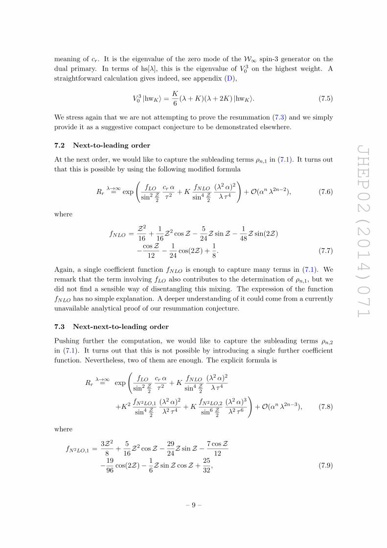
meaning of cr. It is the eigenvalue of the zero mode of the W∞ spin-3 generator on the

dual primary. In terms of hs[λ], this is the eigenvalue of V 30 on the highest weight. A

straightforward calculation gives indeed, see appendix (D),

V 30 |hwK〉 =

K

6(λ+K)(λ+ 2K) |hwK〉. (7.5)

We stress again that we are not attempting to prove the resummation (7.3) and we simply

provide it as a suggestive compact conjecture to be demonstrated elsewhere.

7.2 Next-to-leading order

At the next order, we would like to capture the subleading terms ρn,1 in (7.1). It turns out

that this is possible by using the following modified formula

Rrλ→∞

= exp

(fLO

sin2 Z2

cr α

τ2+K

fNLO

sin4 Z2

(λ2 α)2

λ τ4

)+O(αn λ2n−2), (7.6)

where

fNLO =Z2

16+

1

16Z2 cosZ − 5

24Z sinZ − 1

48Z sin(2Z)

−cosZ12− 1

24cos(2Z) +

1

8. (7.7)

Again, a single coefficient function fNLO is enough to capture many terms in (7.1). We

remark that the term involving fLO also contributes to the determination of ρn,1, but we

did not find a sensible way of disentangling this mixing. The expression of the function

fNLO has no simple explanation. A deeper understanding of it could come from a currently

unavailable analytical proof of our resummation conjecture.

7.3 Next-next-to-leading order

Pushing further the computation, we would like to capture the subleading terms ρn,2in (7.1). It turns out that this is not possible by introducing a single further coefficient

function. Nevertheless, two of them are enough. The explicit formula is

Rrλ→∞

= exp

(fLO

sin2 Z2

cr α

τ2+K

fNLO

sin4 Z2

(λ2 α)2

λ τ4

+K2 fN2LO,1

sin4 Z2

(λ2 α)2

λ2 τ4+K

fN2LO,2

sin6 Z2

(λ2 α)3

λ2 τ6

)+O(αn λ2n−3), (7.8)

where

fN2LO,1 =3Z2

8+

5

16Z2 cosZ − 29

24Z sinZ − 7 cosZ

12

−19

96cos(2Z)− 1

6Z sinZ cosZ +

25

32, (7.9)

– 9 –

JHEP02(2014)071

fN2LO,2 = −3Z3

64− 5

96Z3 cosZ − 1

192Z3 cos(2Z) +

19

96Z2 sinZ +

11

96Z2 sinZ cosZ

−17Z96

+5 sinZ

32− 1

16sin(2Z)− 1

96sin(3Z)

+7

192Z cosZ +

13

96Z cos(2Z) +

1

192Z cos(3Z). (7.10)

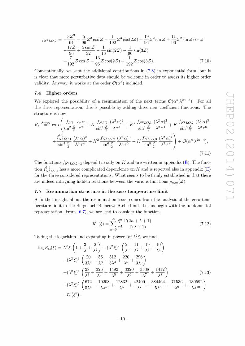
Conventionally, we kept the additional contributions in (7.8) in exponential form, but it

is clear that more perturbative data should be welcome in order to assess its higher order

validity. Anyway, it works at the order O(α5) included.

7.4 Higher orders

We explored the possibility of a resummation of the next terms O(αn λ2n−3). For all

the three representation, this is possible by adding three new coefficient functions. The

structure is now

Rrλ→∞

= exp

(fLO

sin2 Z2

cr α

τ2+K

fNLO

sin4 Z2

(λ2 α)2

λ τ4+K2 fN2LO,1

sin4 Z2

(λ2 α)2

λ2 τ4+K

fN2LO,2

sin6 Z2

(λ2 α)3

λ2 τ6

+f

(r)N3LO,1

sin4 Z2

(λ2 α)2

λ3 τ4+K2 fN3LO,2

sin6 Z2

(λ2 α)3

λ3 τ6+K

fN3LO,3

sin8 Z2

(λ2 α)4

λ3 τ8

+O(αn λ2n−4),

(7.11)

The functions fN3LO,2−3 depend trivially on K and are written in appendix (E). The func-

tion f(r)N3LO,1

has a more complicated dependence on K and is reported also in appendix (E)

for the three considered representations. What seems to be firmly established is that there

are indeed intriguing hidden relations between the various functions ρn,m(Z).

7.5 Resummation structure in the zero temperature limit

A further insight about the resummation issue comes from the analysis of the zero tem-

perature limit in the Bergshoeff-Blencowe-Stelle limit. Let us begin with the fundamental

representation. From (6.7), we are lead to consider the function

R (ξ) =

∞∑n=0

ξn

n!

Γ(2n+ λ+ 1)

Γ(λ+ 1). (7.12)

Taking the logarithm and expanding in powers of λ2ξ, we find

logR (ξ) = λ2 ξ

(1 +

3

λ+

2

λ2

)+ (λ2 ξ)2

(2

λ+

11

λ2+

19

λ3+

10

λ4

)+(λ2 ξ)3

(20

3λ2+

56

λ3+

512

3λ4+

220

λ5+

296

3λ6

)+(λ2 ξ)4

(28

λ3+

326

λ4+

1492

λ5+

3320

λ6+

3538

λ7+

1412

λ8

)(7.13)

+(λ2 ξ)5

(672

5λ4+

10208

5λ5+

12832

λ6+

42400

λ7+

384464

5λ8+

71536

λ9+

130592

5λ10

)+O

(ξ6).

– 10 –

JHEP02(2014)071

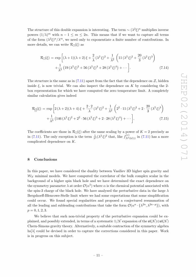
The structure of this double expansion is interesting. The term ∼ (λ2ξ)n multiplies inverse

powers (1/λ)m with n − 1 ≤ m ≤ 2n. This means that if we want to capture all terms

of the form (λ2ξ)n/λm, we need only to exponentiate a finite number of contributions. In

more details, we can write R (ξ) as

R (ξ) = exp

[(λ+ 1)(λ+ 2) ξ +

2

λ(λ2 ξ)2 +

1

λ2

(11 (λ2 ξ)2 +

20

3(λ2 ξ)3

)+

1

λ3

(19 (λ2 ξ)2 + 56 (λ2 ξ)3 + 28 (λ2 ξ)4

)+ · · ·

]. (7.14)

The structure is the same as in (7.11) apart from the fact that the dependence on Z, hidden

inside ξ, is now trivial. We can also inspect the dependence on K by considering the 2-

box representation for which we have computed the zero temperature limit. A completely

similar calculation gives indeed

R (ξ) = exp

[2 (λ+ 2)(λ+ 4) ξ +

2 · 2λ

(λ2 ξ)2 +1

λ2

(22 · 11 (λ2 ξ)2 + 2 · 20

3(λ2 ξ)3

)+

1

λ3

(146 (λ2 ξ)2 + 22 · 56 (λ2 ξ)3 + 2 · 28 (λ2 ξ)4

)+ · · ·

]. (7.15)

The coefficients are those in R (ξ) after the same scaling by a power of K = 2 precisely as

in (7.11). The only exception is the term 1λ3 (λ2 ξ)2 that, like f

(r)N3LO,1

in (7.11) has a more

complicated dependence on K.

8 Conclusions

In this paper, we have considered the duality between Vasiliev 3D higher spin gravity and

WN minimal models. We have computed the correlator of the bulk complex scalar in the

background of a higher spin black hole and we have determined the exact dependence on

the symmetry parameter λ at order O(α5) where α is the chemical potential associated with

the spin-3 charge of the black hole. We have analysed the perturbative data in the large λ

Bergshoeff-Blencowe-Stelle limit where we had some expectations that some simplification

could occur. We found special regularities and proposed a conjectured resummation of

all the leading and subleading contributions that take the form O(αn · {λ2n, λ2n−p}), with

p = 0, 1, 2, 3.

We believe that such non-trivial property of the perturbative expansion could be ex-

plained, and possibly extended, in terms of a systematic 1/N expansion of the sl(N )⊕sl(N )

Chern-Simons gravity theory. Alternatively, a suitable contraction of the symmetry algebra

hs[λ] could be devised in order to capture the corrections considered in this paper. Work

is in progress on this subject.

– 11 –

JHEP02(2014)071

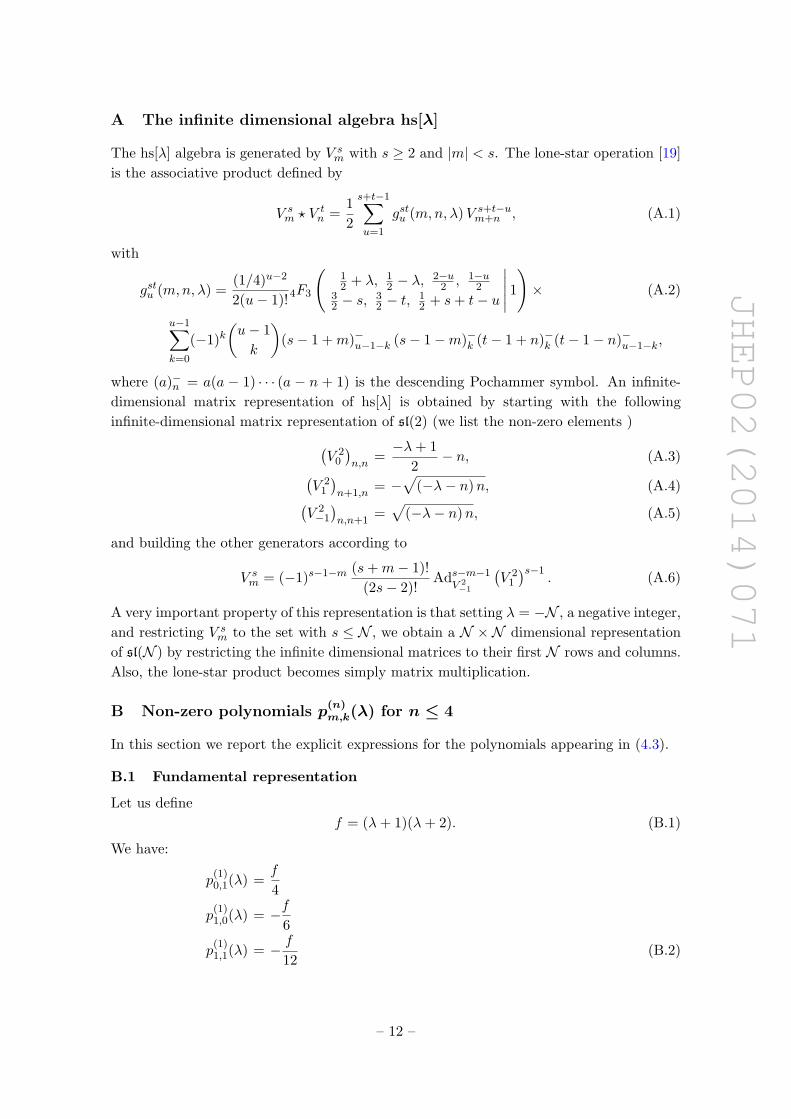
A The infinite dimensional algebra hs[λ]

The hs[λ] algebra is generated by V sm with s ≥ 2 and |m| < s. The lone-star operation [19]

is the associative product defined by

V sm ? V t

n =1

2

s+t−1∑u=1

gstu (m,n, λ)V s+t−um+n , (A.1)

with

gstu (m,n, λ) =(1/4)u−2

2(u− 1)!4F3

(12 + λ, 1

2 − λ,2−u

2 , 1−u2

32 − s,

32 − t,

12 + s+ t− u

∣∣∣∣∣ 1)× (A.2)

u−1∑k=0

(−1)k(u− 1

k

)(s− 1 +m)−u−1−k (s− 1−m)−k (t− 1 + n)−k (t− 1− n)−u−1−k,

where (a)−n = a(a − 1) · · · (a − n + 1) is the descending Pochammer symbol. An infinite-

dimensional matrix representation of hs[λ] is obtained by starting with the following

infinite-dimensional matrix representation of sl(2) (we list the non-zero elements )(V 2

0

)n,n

=−λ+ 1

2− n, (A.3)(

V 21

)n+1,n

= −√

(−λ− n)n, (A.4)(V 2−1

)n,n+1

=√

(−λ− n)n, (A.5)

and building the other generators according to

V sm = (−1)s−1−m (s+m− 1)!

(2s− 2)!Ads−m−1

V 2−1

(V 2

1

)s−1. (A.6)

A very important property of this representation is that setting λ = −N , a negative integer,

and restricting V sm to the set with s ≤ N , we obtain a N ×N dimensional representation

of sl(N ) by restricting the infinite dimensional matrices to their first N rows and columns.

Also, the lone-star product becomes simply matrix multiplication.

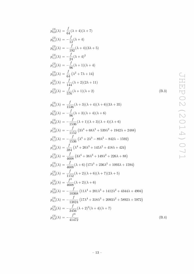
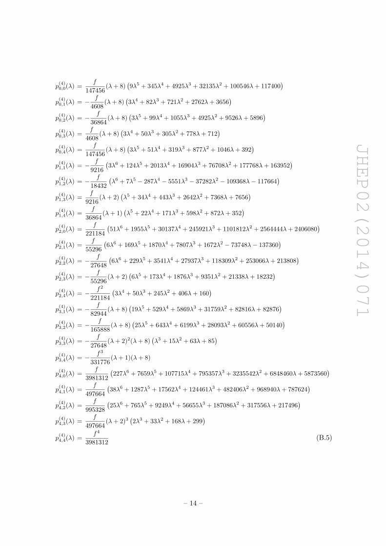
B Non-zero polynomials p(n)m,k(λ) for n ≤ 4

In this section we report the explicit expressions for the polynomials appearing in (4.3).

B.1 Fundamental representation

Let us define

f = (λ+ 1)(λ+ 2). (B.1)

We have:

p(1)0,1(λ) =

f

4

p(1)1,0(λ) = − f

6

p(1)1,1(λ) = − f

12(B.2)

– 12 –

JHEP02(2014)071

p(2)0,0(λ) =

f

64(λ+ 4)(λ+ 7)

p(2)0,1(λ) = − f

12(λ+ 4)

p(2)0,2(λ) = − f

192(λ+ 4)(3λ+ 5)

p(2)1,1(λ) = − f

24(λ+ 4)2

p(2)1,2(λ) = − f

96(λ+ 1)(λ+ 4)

p(2)2,0(λ) =

f

64

(λ2 + 7λ+ 14

)p

(2)2,1(λ) =

f

144(λ+ 2)(2λ+ 11)

p(2)2,2(λ) =

f

576(λ+ 1)(λ+ 2) (B.3)

p(3)0,1(λ) =

f

1536(λ+ 3)(λ+ 4)(λ+ 6)(3λ+ 35)

p(3)0,2(λ) = − f

96(λ+ 3)(λ+ 4)(λ+ 6)

p(3)0,3(λ) = − f

1536(λ+ 1)(λ+ 3)(λ+ 4)(λ+ 6)

p(3)1,0(λ) = − f

1152

(3λ4 + 68λ3 + 539λ2 + 1942λ+ 2488

)p

(3)1,1(λ) = − f

1536

(λ4 + 2λ3 − 89λ2 − 842λ− 1592

)p

(3)1,2(λ) =

f

384

(λ4 + 20λ3 + 145λ2 + 418λ+ 424

)p

(3)1,3(λ) =

f

4608

(3λ4 + 38λ3 + 149λ2 + 226λ+ 88

)p

(3)2,1(λ) =

f

4608(λ+ 6)

(17λ3 + 236λ2 + 1093λ+ 1594

)p

(3)2,2(λ) =

f

1152(λ+ 2)(λ+ 6)(λ+ 7)(2λ+ 5)

p(3)2,3(λ) =

f 2

4608(λ+ 2)(λ+ 6)

p(3)3,0(λ) = − f

10368

(11λ4 + 201λ3 + 1412λ2 + 4344λ+ 4904

)p

(3)3,1(λ) = − f

13824

(17λ4 + 318λ3 + 2093λ2 + 5892λ+ 5972

)p

(3)3,2(λ) = − f

3456(λ+ 2)2(λ+ 4)(λ+ 7)

p(3)3,3(λ) = − f 3

41472(B.4)

– 13 –

JHEP02(2014)071

p(4)0,0(λ) =

f

147456(λ+ 8)

(9λ5 + 345λ4 + 4925λ3 + 32135λ2 + 100546λ+ 117400

)p(4)0,1(λ) = − f

4608(λ+ 8)

(3λ4 + 82λ3 + 721λ2 + 2762λ+ 3656

)p(4)0,2(λ) = − f

36864(λ+ 8)

(3λ5 + 99λ4 + 1055λ3 + 4925λ2 + 9526λ+ 5896

)p(4)0,3(λ) =

f

4608(λ+ 8)

(3λ4 + 50λ3 + 305λ2 + 778λ+ 712

)p(4)0,4(λ) =

f

147456(λ+ 8)

(3λ5 + 51λ4 + 319λ3 + 877λ2 + 1046λ+ 392

)p(4)1,1(λ) = − f

9216

(3λ6 + 124λ5 + 2013λ4 + 16904λ3 + 76708λ2 + 177768λ+ 163952

)p(4)1,2(λ) = − f

18432

(λ6 + 7λ5 − 287λ4 − 5551λ3 − 37282λ2 − 109368λ− 117664

)p(4)1,3(λ) =

f

9216(λ+ 2)

(λ5 + 34λ4 + 443λ3 + 2642λ2 + 7368λ+ 7656

)p(4)1,4(λ) =

f

36864(λ+ 1)

(λ5 + 22λ4 + 171λ3 + 598λ2 + 872λ+ 352

)p(4)2,0(λ) =

f

221184

(51λ6 + 1955λ5 + 30137λ4 + 245921λ3 + 1101812λ2 + 2564444λ+ 2406080

)p(4)2,1(λ) =

f

55296

(6λ6 + 169λ5 + 1870λ4 + 7807λ3 + 1672λ2 − 73748λ− 137360

)p(4)2,2(λ) = − f

27648

(6λ6 + 229λ5 + 3541λ4 + 27937λ3 + 118309λ2 + 253066λ+ 213808

)p(4)2,3(λ) = − f

55296(λ+ 2)

(6λ5 + 173λ4 + 1876λ3 + 9351λ2 + 21338λ+ 18232

)p(4)2,4(λ) = − f 2

221184

(3λ4 + 50λ3 + 245λ2 + 406λ+ 160

)p(4)3,1(λ) = − f

82944(λ+ 8)

(19λ5 + 529λ4 + 5869λ3 + 31759λ2 + 82816λ+ 82876

)p(4)3,2(λ) = − f

165888(λ+ 8)

(25λ5 + 643λ4 + 6199λ3 + 28093λ2 + 60556λ+ 50140

)p(4)3,3(λ) = − f

27648(λ+ 2)2(λ+ 8)

(λ3 + 15λ2 + 63λ+ 85

)p(4)3,4(λ) = − f 3

331776(λ+ 1)(λ+ 8)

p(4)4,0(λ) =

f

3981312

(227λ6 + 7659λ5 + 107715λ4 + 795357λ3 + 3235542λ2 + 6848460λ+ 5873560

)p(4)4,1(λ) =

f

497664

(38λ6 + 1287λ5 + 17562λ4 + 124461λ3 + 482406λ2 + 968940λ+ 787624

)p(4)4,2(λ) =

f

995328

(25λ6 + 765λ5 + 9249λ4 + 56655λ3 + 187086λ2 + 317556λ+ 217496

)p(4)4,3(λ) =

f

497664(λ+ 2)3

(2λ3 + 33λ2 + 168λ+ 299

)p(4)4,4(λ) =

f 4

3981312(B.5)

– 14 –

JHEP02(2014)071

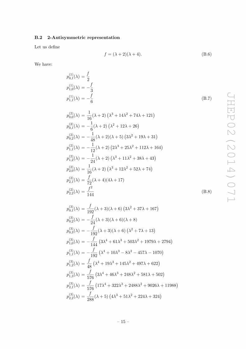
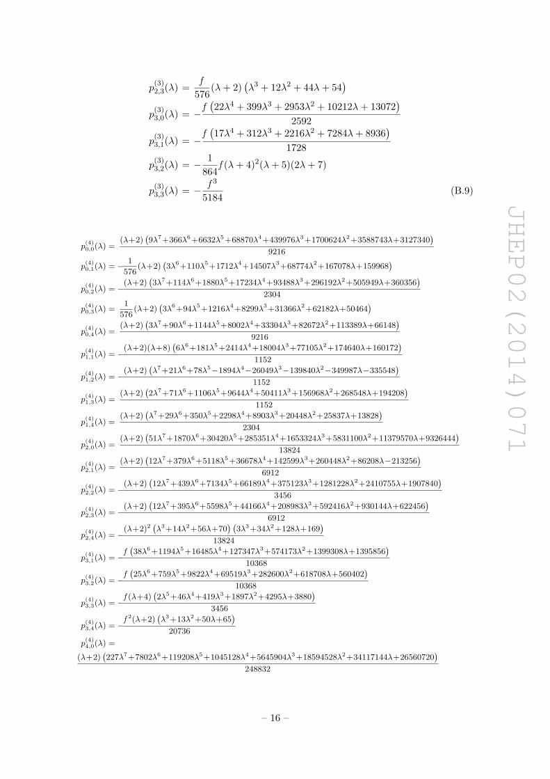
B.2 2-Antisymmetric representation

Let us define

f = (λ+ 2)(λ+ 4). (B.6)

We have:

p(1)0,1(λ) =

f

2

p(1)1,0(λ) = − f

3

p(1)1,1(λ) = − f

6(B.7)

p(2)0,0(λ) =

1

16(λ+ 2)

(λ3 + 14λ2 + 74λ+ 121

)p

(2)0,1(λ) = −1

6(λ+ 2)

(λ2 + 12λ+ 26

)p

(2)0,2(λ) = − 1

48(λ+ 2)(λ+ 5)

(3λ2 + 19λ+ 31

)p

(2)1,1(λ) = − 1

12(λ+ 2)

(2λ3 + 25λ2 + 112λ+ 164

)p

(2)1,2(λ) = − 1

24(λ+ 2)

(λ3 + 11λ2 + 38λ+ 43

)p

(2)2,0(λ) =

1

16(λ+ 2)

(λ3 + 12λ2 + 52λ+ 74

)p

(2)2,1(λ) =

f

72(λ+ 4)(4λ+ 17)

p(2)2,2(λ) =

f 2

144(B.8)

p(3)0,1(λ) =

f

192(λ+ 3)(λ+ 6)

(3λ2 + 37λ+ 167

)p

(3)0,2(λ) = − f

24(λ+ 3)(λ+ 6)(λ+ 8)

p(3)0,3(λ) = − f

192(λ+ 3)(λ+ 6)

(λ2 + 7λ+ 13

)p

(3)1,0(λ) = − f

144

(3λ4 + 61λ3 + 503λ2 + 1979λ+ 2794

)p

(3)1,1(λ) = − f

192

(λ4 + 10λ3 − 8λ2 − 457λ− 1070

)p

(3)1,2(λ) =

f

48

(λ4 + 19λ3 + 145λ2 + 497λ+ 622

)p

(3)1,3(λ) =

f

576

(3λ4 + 46λ3 + 248λ2 + 581λ+ 502

)p

(3)2,1(λ) =

f

576

(17λ4 + 322λ3 + 2488λ2 + 9026λ+ 11988

)p

(3)2,2(λ) =

f

288(λ+ 5)

(4λ3 + 51λ2 + 224λ+ 324

)

– 15 –

JHEP02(2014)071

p(3)2,3(λ) =

f

576(λ+ 2)

(λ3 + 12λ2 + 44λ+ 54

)p

(3)3,0(λ) = −

f(22λ4 + 399λ3 + 2953λ2 + 10212λ+ 13072

)2592

p(3)3,1(λ) = −

f(17λ4 + 312λ3 + 2216λ2 + 7284λ+ 8936

)1728

p(3)3,2(λ) = − 1

864f (λ+ 4)2(λ+ 5)(2λ+ 7)

p(3)3,3(λ) = − f 3

5184(B.9)

p(4)0,0(λ) =

(λ+2)(9λ7+366λ6+6632λ5+68870λ4+439976λ3+1700624λ2+3588743λ+3127340

)9216

p(4)0,1(λ) = −

1

576(λ+2)

(3λ6+110λ5+1712λ4+14507λ3+68774λ2+167078λ+159968

)p

(4)0,2(λ) = −

(λ+2)(3λ7+114λ6+1880λ5+17234λ4+93488λ3+296192λ2+505949λ+360356

)2304

p(4)0,3(λ) =

1

576(λ+2)

(3λ6+94λ5+1216λ4+8299λ3+31366λ2+62182λ+50464

)p

(4)0,4(λ) =

(λ+2)(3λ7+90λ6+1144λ5+8002λ4+33304λ3+82672λ2+113389λ+66148

)9216

p(4)1,1(λ) = −

(λ+2)(λ+8)(6λ6+181λ5+2414λ4+18004λ3+77105λ2+174640λ+160172

)1152

p(4)1,2(λ) = −

(λ+2)(λ7+21λ6+78λ5−1894λ4−26049λ3−139840λ2−349987λ−335548

)1152

p(4)1,3(λ) =

(λ+2)(2λ7+71λ6+1106λ5+9644λ4+50411λ3+156968λ2+268548λ+194208

)1152

p(4)1,4(λ) =

(λ+2)(λ7+29λ6+350λ5+2298λ4+8903λ3+20448λ2+25837λ+13828

)2304

p(4)2,0(λ) =

(λ+2)(51λ7+1870λ6+30420λ5+285351λ4+1653324λ3+5831100λ2+11379570λ+9326444

)13824

p(4)2,1(λ) =

(λ+2)(12λ7+379λ6+5118λ5+36678λ4+142599λ3+260448λ2+86208λ−213256

)6912

p(4)2,2(λ) = −

(λ+2)(12λ7+439λ6+7134λ5+66189λ4+375123λ3+1281228λ2+2410755λ+1907840

)3456

p(4)2,3(λ) = −

(λ+2)(12λ7+395λ6+5598λ5+44166λ4+208983λ3+592416λ2+930144λ+622456

)6912

p(4)2,4(λ) = −

(λ+2)2(λ3+14λ2+56λ+70

) (3λ3+34λ2+128λ+169

)13824

p(4)3,1(λ) = −

f(38λ6+1194λ5+16485λ4+127347λ3+574173λ2+1399308λ+1395856

)10368

p(4)3,2(λ) = −

f(25λ6+759λ5+9822λ4+69519λ3+282600λ2+618708λ+560402

)10368

p(4)3,3(λ) = −

f (λ+4)(2λ5+46λ4+419λ3+1897λ2+4295λ+3880

)3456

p(4)3,4(λ) = −

f 2(λ+2)(λ3+13λ2+50λ+65

)20736

p(4)4,0(λ) =

(λ+2)(227λ7+7802λ6+119208λ5+1045128λ4+5645904λ3+18594528λ2+34117144λ+26560720

)248832

– 16 –

JHEP02(2014)071

p(4)4,1(λ) =

(λ+2)(152λ7+5234λ6+78852λ5+676263λ4+3558120λ3+11403312λ2+20392768λ+15518560

)124416

p(4)4,2(λ) =

(λ+2)(25λ7+820λ6+11607λ5+92220λ4+444648λ3+1298208λ2+2115848λ+1476692

)62208

p(4)4,3(λ) =

f (λ+4)3(8λ3+102λ2+420λ+577

)124416

p(4)4,4(λ) =

f 4

248832(B.10)

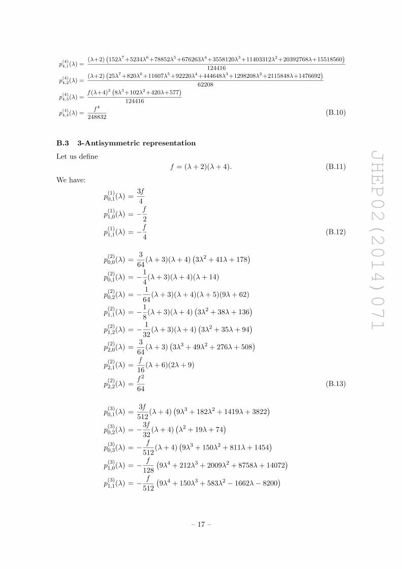
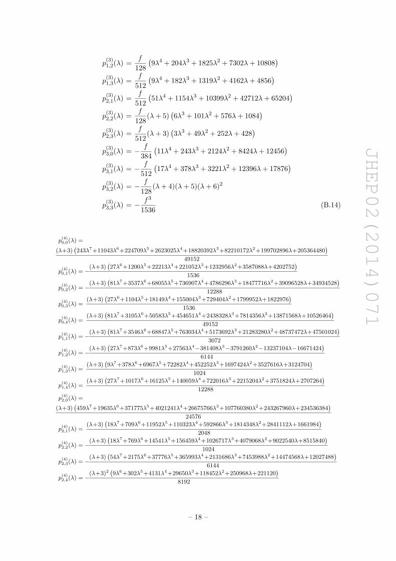
B.3 3-Antisymmetric representation

Let us define

f = (λ+ 2)(λ+ 4). (B.11)

We have:

p(1)0,1(λ) =

3f

4

p(1)1,0(λ) = − f

2

p(1)1,1(λ) = − f

4(B.12)

p(2)0,0(λ) =

3

64(λ+ 3)(λ+ 4)

(3λ2 + 41λ+ 178

)p

(2)0,1(λ) = −1

4(λ+ 3)(λ+ 4)(λ+ 14)

p(2)0,2(λ) = − 1

64(λ+ 3)(λ+ 4)(λ+ 5)(9λ+ 62)

p(2)1,1(λ) = −1

8(λ+ 3)(λ+ 4)

(3λ2 + 38λ+ 136

)p

(2)1,2(λ) = − 1

32(λ+ 3)(λ+ 4)

(3λ2 + 35λ+ 94

)p

(2)2,0(λ) =

3

64(λ+ 3)

(3λ3 + 49λ2 + 276λ+ 508

)p

(2)2,1(λ) =

f

16(λ+ 6)(2λ+ 9)

p(2)2,2(λ) =

f 2

64(B.13)

p(3)0,1(λ) =

3f

512(λ+ 4)

(9λ3 + 182λ2 + 1419λ+ 3822

)p

(3)0,2(λ) = −3f

32(λ+ 4)

(λ2 + 19λ+ 74

)p

(3)0,3(λ) = − f

512(λ+ 4)

(9λ3 + 150λ2 + 811λ+ 1454

)p

(3)1,0(λ) = − f

128

(9λ4 + 212λ3 + 2009λ2 + 8758λ+ 14072

)p

(3)1,1(λ) = − f

512

(9λ4 + 150λ3 + 583λ2 − 1662λ− 8200

)

– 17 –

JHEP02(2014)071

p(3)1,2(λ) =

f

128

(9λ4 + 204λ3 + 1825λ2 + 7302λ+ 10808

)p

(3)1,3(λ) =

f

512

(9λ4 + 182λ3 + 1319λ2 + 4162λ+ 4856

)p

(3)2,1(λ) =

f

512

(51λ4 + 1154λ3 + 10399λ2 + 42712λ+ 65204

)p

(3)2,2(λ) =

f

128(λ+ 5)

(6λ3 + 101λ2 + 576λ+ 1084

)p

(3)2,3(λ) =

f

512(λ+ 3)

(3λ3 + 49λ2 + 252λ+ 428

)p

(3)3,0(λ) = − f

384

(11λ4 + 243λ3 + 2124λ2 + 8424λ+ 12456

)p

(3)3,1(λ) = − f

512

(17λ4 + 378λ3 + 3221λ2 + 12396λ+ 17876

)p

(3)3,2(λ) = − f

128(λ+ 4)(λ+ 5)(λ+ 6)2

p(3)3,3(λ) = − f 3

1536(B.14)

p(4)0,0(λ) =

(λ+3)(243λ7+11043λ6+224709λ5+2623025λ4+18820392λ3+82210172λ2+199702896λ+205364480

)49152

p(4)0,1(λ) = −

(λ+3)(27λ6+1200λ5+22213λ4+221052λ3+1232956λ2+3587088λ+4202752

)1536

p(4)0,2(λ) = −

(λ+3)(81λ7+3537λ6+68055λ5+736907λ4+4786296λ3+18477716λ2+39096528λ+34934528

)12288

p(4)0,3(λ) =

(λ+3)(27λ6+1104λ5+18149λ4+155004λ3+729404λ2+1799952λ+1822976

)1536

p(4)0,4(λ) =

(λ+3)(81λ7+3105λ6+50583λ5+454651λ4+2438328λ3+7814356λ2+13871568λ+10526464

)49152

p(4)1,1(λ) = −

(λ+3)(81λ7+3546λ6+68847λ5+763034λ4+5173692λ3+21283280λ2+48737472λ+47501024

)3072

p(4)1,2(λ) = −

(λ+3)(27λ7+873λ6+9981λ5+27563λ4−381408λ3−3791260λ2−13237104λ−16671424

)6144

p(4)1,3(λ) =

(λ+3)(9λ7+378λ6+6967λ5+72282λ4+452252λ3+1697424λ2+3527616λ+3124704

)1024

p(4)1,4(λ) =

(λ+3)(27λ7+1017λ6+16125λ5+140059λ4+722016λ3+2215204λ2+3751824λ+2707264

)12288

p(4)2,0(λ) =

(λ+3)(459λ7+19635λ6+371775λ5+4021241λ4+26675766λ3+107760380λ2+243267960λ+234536384

)24576

p(4)2,1(λ) =

(λ+3)(18λ7+709λ6+11952λ5+110323λ4+592866λ3+1814348λ2+2841112λ+1661984

)2048

p(4)2,2(λ) = −

(λ+3)(18λ7+769λ6+14541λ5+156459λ4+1026717λ3+4079068λ2+9022540λ+8515840

)1024

p(4)2,3(λ) = −

(λ+3)(54λ7+2175λ6+37776λ5+365993λ4+2131686λ3+7453988λ2+14474568λ+12027488

)6144

p(4)2,4(λ) = −

(λ+3)2(9λ6+302λ5+4131λ4+29650λ3+118452λ2+250968λ+221120

)8192

– 18 –

JHEP02(2014)071

p(4)3,1(λ) = −

(λ+3)(19λ7+797λ6+14783λ5+156299λ4+1011478λ3+3981140λ2+8760984λ+8252288

)1024

p(4)3,2(λ) = −

(λ+3)(25λ7+1031λ6+18493λ5+186753λ4+1144046λ3+4240252λ2+8776344λ+7795072

)2048

p(4)3,3(λ) = −

f (λ+6)(3λ5+81λ4+871λ3+4667λ2+12470λ+13280

)1024

p(4)3,4(λ) = −

f 2(λ+3)(λ3+17λ2+90λ+160

)4096

p(4)4,0(λ) =

(λ+3)(227λ7+9363λ6+169953λ5+1752177λ4+11034384λ3+42243432λ2+90519984λ+83227920

)49152

p(4)4,1(λ) =

(λ+3)(38λ7+1569λ6+28248λ5+287283λ4+1778880λ3+6687912λ2+14078592λ+12733680

)6144

p(4)4,2(λ) =

(λ+3)(25λ7+1005λ6+17427λ5+169035λ4+990348λ3+3502032λ2+6910848λ+5858448

)12288

p(4)4,3(λ) =

f (λ+6)3(2λ3+27λ2+120λ+177

)6144

p(4)4,4(λ) =

f 4

49152(B.15)

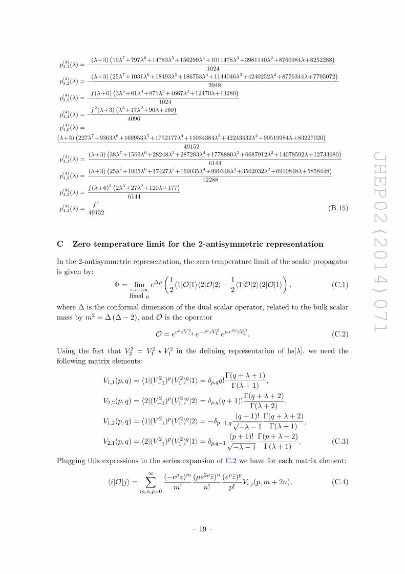
C Zero temperature limit for the 2-antisymmetric representation

In the 2-antisymmetric representation, the zero temperature limit of the scalar propagator

is given by:

Φ = limτ,τ→∞fixed µ

e∆ρ

(1

2〈1|O|1〉〈2|O|2〉 − 1

2〈1|O|2〉〈2|O|1〉

), (C.1)

where ∆ is the conformal dimension of the dual scalar operator, related to the bulk scalar

mass by m2 = ∆ (∆− 2), and O is the operator

O = eeρzV 2−1 e−e

ρzV 21 eµ e

2ρzV 32 . (C.2)

Using the fact that V 32 = V 2

1 ? V 21 in the defining representation of hs[λ], we need the

following matrix elements:

V1,1(p, q) = 〈1|(V 2−1)p(V 2

1 )q|1〉 = δp,qq!Γ(q + λ+ 1)

Γ(λ+ 1),

V2,2(p, q) = 〈2|(V 2−1)p(V 2

1 )q|2〉 = δp,q(q + 1)!Γ(q + λ+ 2)

Γ(λ+ 2),

V1,2(p, q) = 〈1|(V 2−1)p(V 2

1 )q|2〉 = −δp−1,q(q + 1)!√−λ− 1

Γ(q + λ+ 2)

Γ(λ+ 1),

V2,1(p, q) = 〈2|(V 2−1)p(V 2

1 )q|1〉 = δp,q−1(p+ 1)!√−λ− 1

Γ(p+ λ+ 2)

Γ(λ+ 1). (C.3)

Plugging this expressions in the series expansion of C.2 we have for each matrix element:

〈i|O|j〉 =

∞∑m,n,p=0

(−eρz)m

m!

(µe2ρz)n

n!

(eρz)p

p!Vi,j(p,m+ 2n), (C.4)

– 19 –

JHEP02(2014)071

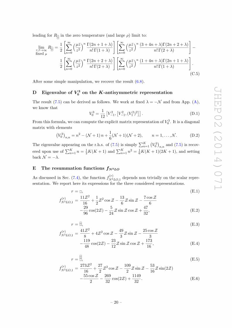
leading for R in the zero temperature (and large ρ) limit to:

limτ,τ→∞fixed µ

R =1

2

[ ∞∑n=0

(µzz2

)n Γ(2n+ 1 + λ)

n! Γ(1 + λ)

][ ∞∑n=0

(µzz2

)n (3 + 4n+ λ)Γ(2n+ 2 + λ)

n! Γ(2 + λ)

]−

1

2

[ ∞∑n=0

(µzz2

)n Γ(2n+ 2 + λ)

n! Γ(2 + λ)

][ ∞∑n=0

(µzz2

)n (1 + 4n+ λ)Γ(2n+ 1 + λ)

n! Γ(1 + λ)

].

(C.5)

After some simple manipulation, we recover the result (6.8).

D Eigenvalue of V 30 on the K-antisymmetric representation

The result (7.5) can be derived as follows. We work at fixed λ = −N and from App. (A),

we know that

V 30 =

1

12

[V 2−1,[V 2−1, (V

21 )2]]. (D.1)

From this formula, we can compute the explicit matrix representation of V 30 . It is a diagonal

matrix with elements(V 3

0

)n,n

= n2 − (N + 1)n+1

6(N + 1)(N + 2), n = 1, . . . ,N . (D.2)

The eigenvalue appearing on the r.h.s. of (7.5) is simply∑K

n=1

(V 3

0

)n,n

and (7.5) is recov-

ered upon use of∑K

n=1 n = 12K(K + 1) and

∑Kn=1 n

2 = 16K(K + 1)(2K + 1), and setting

back N = −λ.

E The resummation functions fN3LO

As discussed in Sec. (7.4), the function f(r)N3LO,1

depends non trivially on the scalar repre-

sentation. We report here its expressions for the three considered representations.

r = , (E.1)

f(r)N3LO,1

=11Z2

16+

1

2Z2 cosZ − 13

6Z sinZ − 7 cosZ

6

−29

96cos(2Z)− 5

24Z sinZ cosZ +

47

32, (E.2)

r = , (E.3)

f(r)N3LO,1

=41Z2

8+ 4Z2 cosZ − 49

3Z sinZ − 25 cosZ

3

−119

48cos(2Z)− 23

12Z sinZ cosZ +

173

16, (E.4)

r = , (E.5)

f(r)N3LO,1

=273Z2

16+

27

2Z2 cosZ − 109

2Z sinZ − 53

16Z sin(2Z)

−55 cosZ2

− 269

32cos(2Z) +

1149

32. (E.6)

– 20 –

JHEP02(2014)071

The functions fN3LO,2−3 are instead universal and read

fN3LO,2 =−79Z3

192− 41

96Z3 cosZ− 7

192Z3 cos(2Z)+

57

32Z2 sinZ+

27

64Z2 sin(2Z)− 55Z

32+

271 sinZ192

−29

48sin(2Z)− 13

192sin(3Z)+

19

32Z cosZ+

35

32Z cos(2Z)+

1

32Z cos(3Z), (E.7)

fN3LO,3 =17Z4

384+

167Z4 cosZ3072

+1

96Z4 cos(2Z)+

Z4 cos(3Z)

3072− 29

128Z3 sinZ− 19

96Z3 sinZ cosZ

− 5

384Z3 sinZ cos(2Z)+

77Z2

288+

5

384Z2 cosZ− 23

96Z2 cos(2Z)− 47Z2 cos(3Z)

1152

−109

288Z sinZ− 31 cosZ

288− 41

576cos(2Z)+

11

288cos(3Z)+

7 cos(4Z)

2304+

7

32Z sinZ cosZ

+5

32Z sinZ cos(2Z)+

1

288Z sinZ cos(3Z)+

317

2304. (E.8)

Open Access. This article is distributed under the terms of the Creative Commons

Attribution License (CC-BY 4.0), which permits any use, distribution and reproduction in

any medium, provided the original author(s) and source are credited.

References

[1] M.R. Gaberdiel and R. Gopakumar, An AdS3 Dual for Minimal Model CFTs, Phys. Rev. D

83 (2011) 066007 [arXiv:1011.2986] [INSPIRE].

[2] M.A. Vasiliev, Higher spin gauge theories in four-dimensions, three-dimensions and

two-dimensions, Int. J. Mod. Phys. D 5 (1996) 763 [hep-th/9611024] [INSPIRE].

[3] M.A. Vasiliev, Higher spin matter interactions in (2+1)-dimensions, hep-th/9607135

[INSPIRE].

[4] M.R. Gaberdiel and R. Gopakumar, Triality in Minimal Model Holography, JHEP 07 (2012)

127 [arXiv:1205.2472] [INSPIRE].

[5] M. Henneaux and S.-J. Rey, Nonlinear W∞ as Asymptotic Symmetry of Three-Dimensional

Higher Spin Anti-de Sitter Gravity, JHEP 12 (2010) 007 [arXiv:1008.4579] [INSPIRE].

[6] A. Campoleoni, S. Fredenhagen, S. Pfenninger and S. Theisen, Asymptotic symmetries of

three-dimensional gravity coupled to higher-spin fields, JHEP 11 (2010) 007

[arXiv:1008.4744] [INSPIRE].

[7] M.R. Gaberdiel and T. Hartman, Symmetries of Holographic Minimal Models, JHEP 05

(2011) 031 [arXiv:1101.2910] [INSPIRE].

[8] M. Banados, C. Teitelboim and J. Zanelli, The Black hole in three-dimensional space-time,

Phys. Rev. Lett. 69 (1992) 1849 [hep-th/9204099] [INSPIRE].

[9] M. Banados, M. Henneaux, C. Teitelboim and J. Zanelli, Geometry of the (2+1) black hole,

Phys. Rev. D 48 (1993) 1506 [gr-qc/9302012] [INSPIRE].

[10] M. Ammon, M. Gutperle, P. Kraus and E. Perlmutter, Black holes in three dimensional

higher spin gravity: A review, J. Phys. A 46 (2013) 214001 [arXiv:1208.5182] [INSPIRE].

[11] P. Kraus and E. Perlmutter, Partition functions of higher spin black holes and their CFT

duals, JHEP 11 (2011) 061 [arXiv:1108.2567] [INSPIRE].

– 21 –

JHEP02(2014)071

[12] M.R. Gaberdiel, T. Hartman and K. Jin, Higher Spin Black Holes from CFT, JHEP 04

(2012) 103 [arXiv:1203.0015] [INSPIRE].

[13] P. Kraus and E. Perlmutter, Probing higher spin black holes, JHEP 02 (2013) 096

[arXiv:1209.4937] [INSPIRE].

[14] M.R. Gaberdiel, K. Jin and E. Perlmutter, Probing higher spin black holes from CFT, JHEP

10 (2013) 045 [arXiv:1307.2221] [INSPIRE].

[15] E. Hijano, P. Kraus and E. Perlmutter, Matching four-point functions in higher spin

AdS3/CFT2, JHEP 05 (2013) 163 [arXiv:1302.6113] [INSPIRE].

[16] M. Beccaria and G. Macorini, On the partition functions of higher spin black holes, JHEP 12

(2013) 027 [arXiv:1310.4410] [INSPIRE].

[17] E. Bergshoeff, M. Blencowe and K. Stelle, Area Preserving Diffeomorphisms and Higher Spin

Algebra, Commun. Math. Phys. 128 (1990) 213.

[18] O. Coussaert, M. Henneaux and P. van Driel, The Asymptotic dynamics of three-dimensional

Einstein gravity with a negative cosmological constant, Class. Quant. Grav. 12 (1995) 2961

[gr-qc/9506019] [INSPIRE].

[19] C. Pope, L. Romans and X. Shen, W∞ and the Racah-wigner Algebra, Nucl. Phys. B 339

(1990) 191 [INSPIRE].

[20] J. de Boer and J.I. Jottar, Thermodynamics of higher spin black holes in AdS3, JHEP 01

(2014) 023 [arXiv:1302.0816] [INSPIRE].

[21] P. Kraus and T. Ugajin, An Entropy Formula for Higher Spin Black Holes via Conical

Singularities, JHEP 05 (2013) 160 [arXiv:1302.1583] [INSPIRE].

[22] M.A. Vasiliev, Unfolded representation for relativistic equations in (2+1) anti-de Sitter

space, Class. Quant. Grav. 11 (1994) 649 [INSPIRE].

[23] C.-M. Chang and X. Yin, Higher Spin Gravity with Matter in AdS3 and Its CFT Dual,

JHEP 10 (2012) 024 [arXiv:1106.2580] [INSPIRE].

[24] M. Ammon, P. Kraus and E. Perlmutter, Scalar fields and three-point functions in D = 3

higher spin gravity, JHEP 07 (2012) 113 [arXiv:1111.3926] [INSPIRE].

– 22 –