Matt Birch Robert Rosenman

1

Product Differentiation in a Hotelling City with Elastic Demand*

Matt Birch

Graduate Student

Washington State University

Robert Rosenman

Professor

Washington State University

Abstract In the many variations and expansions on Hotelling’s original work on product differentiation, the most common assumption is that demand is perfectly inelastic. A common finding for goods with multiple characteristics is that duopolies will maximally differentiate along one dimension and minimally differentiate along all others. We analyze a “Hotelling square” (2-dimensional product characteristics) with elastic demand. We show that with elastic demand there will never be maximal or minimal differentiation. Partial differentiation will exist in at least one dimension, and possibly in both dimensions. We show the conditions under which different degrees and dimensionalities of differentiation occur.

* This paper is very preliminary and incomplete. It is not for attribution or quotation. Most of the proofs are only sketched or outlined.

JEL codes: L1, M3, R3

Birch and Rosenman – preliminary, not for attribution

2

1. Introduction

For the better part of a century, spatial arguments have been utilized to explain product

differentiation as an equilibrium behavior. Depending on the assumptions made, results have differed

widely, including everything from minimal differentiation in all dimensions to maximal differentiation,

partial differentiations and every other combination.

To become acquainted with the literature stemming from Hotelling’s 1929 paper, “Stability in

Competition,” is to read through a labyrinth of arguments concerning the structure of product

differentiation. Hotelling concluded that firms competing in prices and products will offer the roughly

the same product by locating as close to each other as possible (Hotelling, 1929), which is generally

referred to as minimal differentiation. In 1979, Hotelling’s analysis was shown to be unsound because

no equilibrium actually existed when firms were too close together (d'Aspremont, Gabszewiez, & Thisse,

1979). When the transportation costs are quadratic, rather than linear, maximal differentiation is the

equilibrium outcome (d'Aspremont, Gabszewiez, & Thisse, 1979).1

Subsequent papers has explored product differentiation along multiple dimensions. In a three-

dimension Hotelling “cube,” for example, 2 firms competed with max-min-min differentiation in which

firms differentiated only in the most salient dimension (Ansari, Economides, & Steckel, 1998). Irmen and

Thisse extended this analysis to an n-dimensional hypercube. Their robust, but equivalent result is that

firms engaged in max-min-…-min differentiation (Irmen & Thisse, 1998), from which they claimed that

Hotelling was “almost” right. The hypercube concept was later expanded to fit into an evolutionary

framework in which both evolutionary stability and stochastic stability suggested that differentiation

was minimal on all dimensions (Hehenkamp & Wambach, 2010).

1 Economides (1986) analyzed the convexity of the transaction costs and found that while minimum differentiation never happened, maximum differentiation could occur if costs were convex enough, but otherwise would not.


3

Each of these studies relies on the assumptions that there are two firms, consumers have

perfectly inelastic demand uniformly distributed across the market space, and consumers benefit from

buying a good at any location differs only by the individual distance from the location. Different studies

have relaxed these assumptions and gotten starkly different results. If consumers prefer quality as one

of the product characteristics in a two-dimensional market, but quality is costly, there is max-min

differentiation when quality costs are low or max-max differentiation when quality costs are high (Lauga

& Ofek, 2011). If consumers are distributed non-uniformly, there can be partial differentiation in one

dimension instead of max-min-..-min (Liu & Shuai, 2012). When there are more than two firms in the

market, the result of maximal differentiation in one dimension and minimal in all others breaks down

(Tabuchi, 2012). In a three firm, cube market, max-min-min does not hold. Instead there is partial

differentiation along two dimensions and minimal along the third (Feldin, 2012).

Our work is most closely related to Economides (1984) in which the assumption of perfectly

inelastic demand was removed. His model has two firms on a “line,” and when demand is low enough,

local monopolies form and Nash equilibrium exists for a larger set of locations than when demand is

perfectly inelastic. Our analysis expands on the existing literature by incorporating both elastic demand

and multiple dimensions for product charateristics. In our model two firms compete in a Hotelling

“square” with elastic demand. When demand is elastic, we surmise that there will never be maximal or

minimal differentiation in either dimension and that there is partial differentiation in at least one and

possibly both dimensions. We analyze the conditions on demand that lead to these different outcomes.

When S is sufficiently low, differentiation can occur on either or both dimensions. When S is higher,

there will be differentiation in the dominant dimension and may be differentiation on the other

dimension. When S is sufficiently high, there will be differentiation on both dimensions, with a higher

degree of differentiation on the dominant dimension.


4

The rest of this paper is as follows. Section 2 introduces the geometry and the market

framework. Section 3 sets up the firm maximization problem. Section 4 discusses equilibrium conditions.

Section 5 concludes the paper.

2. The Model

There are two profit-maximizing firms, referred to as A and B, competing on a Hotelling square.

We assume that each firm faces a constant marginal cost, which we normalize to zero.2 Firms

simultaneously choose location and prices to maximize profits. Our equilibrium concept is Nash

equilibrium.

Consumers are distributed 𝑔(𝑥), which we assume to be uniformly distributed over the

interval [0,1] × [0,1], and the population is normalized to 1. Consumer x located at (𝑥1, 𝑥2) who buys

from firm A located at (𝑎1, 𝑎2) at a price 𝑝𝐴 receives utility according to equation 1.

𝑈𝐴 = 𝑆 − 𝑡1(𝑥1 − 𝑎1)2 − 𝑡2(𝑥2 − 𝑎2)

2 − 𝑝𝐴 (1)

An equivalent statement holds for buying from firm B at (𝑏1, 𝑏2). The terms 𝑡1 and 𝑡2 are salience

coefficients, which permit heterogeneity in mismatch costs between the two attributes. Intuitively, this

allows for the different attributes to be weighted differently by the consumer. For simplicity and without

loss of generality we assume that 𝑡2 ≥ 𝑡1. Demand at firm A, which we denote as 𝐷𝐴 is given by

equation 2.

𝐷𝐴 = ∫ 𝑔(𝑥)𝑑𝑥

𝑈𝐴≥𝑈𝐵,0

(2)

The marginal consumer who buys from firms A must have a reservation utility of zero. Setting

equation 1 equal to zero gives 𝑡1(𝑥1 − 𝑎1)2 + 𝑡2(𝑥2 − 𝑎2)

2 = 𝑆 − 𝑝𝐴, which defines an ellipse3

2 Assuming zero cost helps us to focus on the competition strategies pertaining to location and price when demand is elastic, which has not been done in a multi-dimensional setting. It is a usual and convenient assumption in models of this sort. With this assumption, the firm’s profit is simply its demand. 3 If 𝑡1 = 𝑡2 then demand forms a circle rather than an ellipse.


5

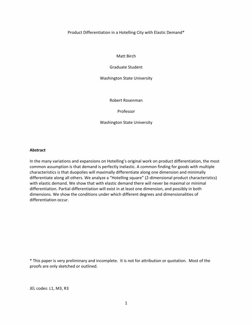
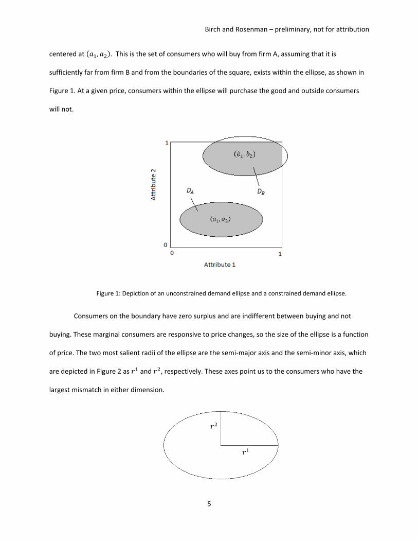
centered at (𝑎1, 𝑎2). This is the set of consumers who will buy from firm A, assuming that it is

sufficiently far from firm B and from the boundaries of the square, exists within the ellipse, as shown in

Figure 1. At a given price, consumers within the ellipse will purchase the good and outside consumers

will not.

Figure 1: Depiction of an unconstrained demand ellipse and a constrained demand ellipse.

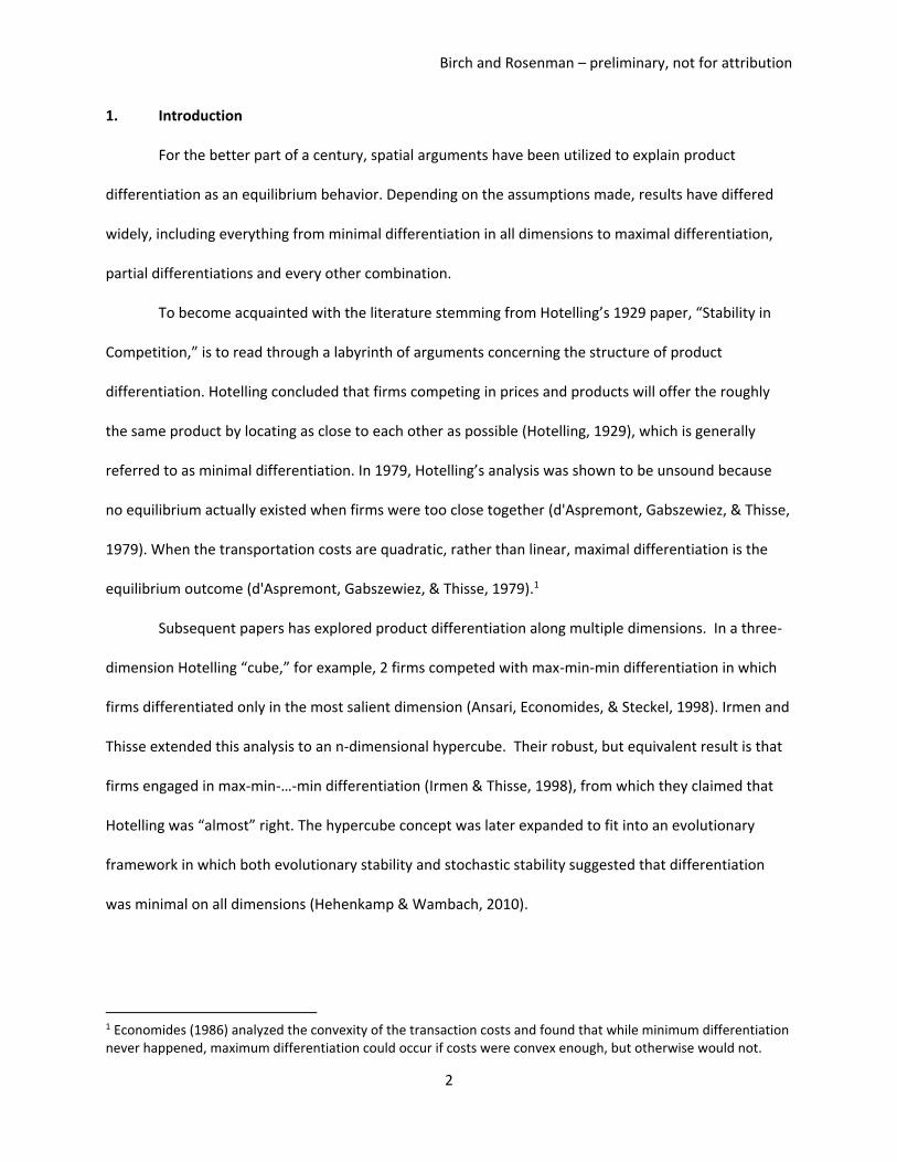
Consumers on the boundary have zero surplus and are indifferent between buying and not

buying. These marginal consumers are responsive to price changes, so the size of the ellipse is a function

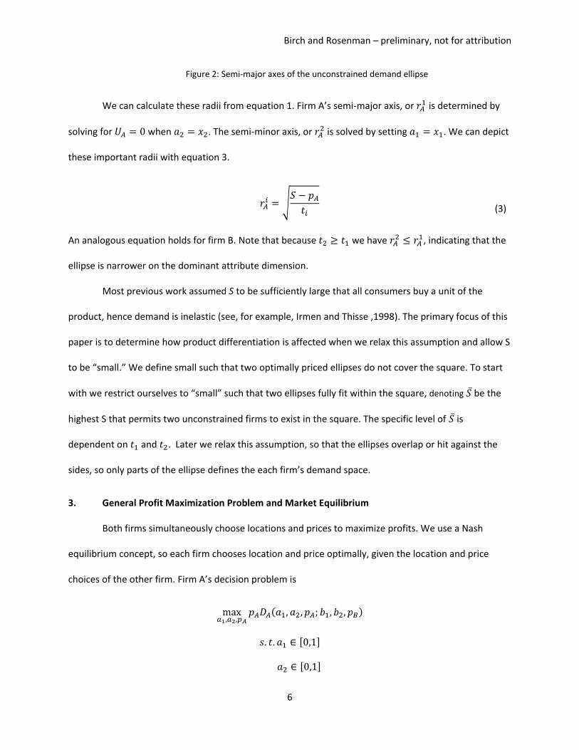
of price. The two most salient radii of the ellipse are the semi-major axis and the semi-minor axis, which

are depicted in Figure 2 as 𝑟1 and 𝑟2, respectively. These axes point us to the consumers who have the

largest mismatch in either dimension.


6

Figure 2: Semi-major axes of the unconstrained demand ellipse

We can calculate these radii from equation 1. Firm A’s semi-major axis, or 𝑟𝐴1 is determined by

solving for 𝑈𝐴 = 0 when 𝑎2 = 𝑥2. The semi-minor axis, or 𝑟𝐴2 is solved by setting 𝑎1 = 𝑥1. We can depict

these important radii with equation 3.

𝑟𝐴𝑖 = √

𝑆 − 𝑝𝐴

𝑡𝑖

(3)

An analogous equation holds for firm B. Note that because 𝑡2 ≥ 𝑡1 we have 𝑟𝐴2 ≤ 𝑟𝐴

1, indicating that the

ellipse is narrower on the dominant attribute dimension.

Most previous work assumed S to be sufficiently large that all consumers buy a unit of the

product, hence demand is inelastic (see, for example, Irmen and Thisse ,1998). The primary focus of this

paper is to determine how product differentiation is affected when we relax this assumption and allow S

to be “small.” We define small such that two optimally priced ellipses do not cover the square. To start

with we restrict ourselves to “small” such that two ellipses fully fit within the square, denoting 𝑆̅ be the

highest S that permits two unconstrained firms to exist in the square. The specific level of 𝑆̅ is

dependent on 𝑡1 and 𝑡2. Later we relax this assumption, so that the ellipses overlap or hit against the

sides, so only parts of the ellipse defines the each firm’s demand space.

3. General Profit Maximization Problem and Market Equilibrium

Both firms simultaneously choose locations and prices to maximize profits. We use a Nash

equilibrium concept, so each firm chooses location and price optimally, given the location and price

choices of the other firm. Firm A’s decision problem is

max𝑎1,𝑎2,𝑝𝐴

𝑝𝐴𝐷𝐴(𝑎1, 𝑎2, 𝑝𝐴; 𝑏1, 𝑏2, 𝑝𝐵)

𝑠. 𝑡. 𝑎1 ∈ [0,1]

𝑎2 ∈ [0,1]


7

We write the firm A Lagrangian as

𝐿𝐴 = 𝑝𝐴𝐷𝐴(𝑎1, 𝑎2, 𝑝𝐴; 𝑏1, 𝑏2, 𝑝𝐵) + 𝜆𝐴1𝑎1 + 𝜆𝐴

2𝑎2 + 𝜇𝐴1(1 − 𝑎1) + 𝜇𝐴

2(1 − 𝑎2)

Where the 𝜆𝐴𝑖 and 𝜇𝐴

𝑖 terms are the Lagrange multipliers associated with the location constraints. Firm A

chooses location and price, by solving the system of Kuhn-Tucker conditions.

𝑝𝐴

𝜕𝐷𝐴

𝜕𝑎1+ 𝜆𝐴

1 − 𝜇𝐴1 = 0 (4)

𝑝𝐴

𝜕𝐷𝐴

𝜕𝑎2+ 𝜆𝐴

2 − 𝜇𝐴2 = 0 (5)

𝑝𝐴

𝜕𝐷𝐴

𝜕𝑝𝐴+ 𝐷𝐴 = 0

(6)

𝜆𝐴1𝑎1 = 𝜆𝐴

2𝑎2 = 𝜇𝐴1(1 − 𝑎1) = 𝜇𝐴

2(1 − 𝑎2) = 0

Proposition 1: Assume that 𝑆 ≤ 𝑆̅. Then none of the location constraints bind and the firms locate on the

interior of the square, i.e. 𝜆𝐴𝑖 = 𝜇𝐴

𝑖 = 𝜆𝐵𝑖 = 𝜇𝐵

𝑖 = 0 and 𝑎𝑖 , 𝑏𝑖 ∈ (0,1).

Proof sketched in the Appendix.

Proposition 1 is a simple but novel result. It says that there will never be maximal differentiation

in any dimension in equilibrium, which is in stark contrast to the majority of the existing literature.

Because demand is low, both firms can choose a location at which profit is maximized and

unconstrained. They will never choose, in Nash equilibrium, to locate on the “edge” or in the “corner” of

the square, or to overlap with the other firm. By doing so the firm would be unnecessarily losing part of

demand, hence profit. From Proposition 1, we can rewrite the KT conditions as the FOCs in equations 7-

9:

𝑝𝐴

𝜕𝐷𝐴

𝜕𝑎1= 0 (7)

𝑝𝐴

𝜕𝐷𝐴

𝜕𝑎2= 0 (8)

𝑝𝐴

𝜕𝐷𝐴

𝜕𝑝𝐴+ 𝐷𝐴 = 0 (9)


8

From equations 7 and 8 we get equation 10, which tells us that we choose location such that for

any given price level and Firm B choice set, the area of the ellipse within the product space is maximized.

Intuitively, the firm chooses location so that at any given price demand is maximized, given the location

and price of the other firm.

𝜕𝐷𝐴(𝑎1, 𝑎2, 𝑝𝐴; 𝑏1, 𝑏2, 𝑝𝐵)

𝜕𝑎1=

𝜕𝐷𝐴(𝑎1, 𝑎2, 𝑝𝐴; 𝑏1, 𝑏2, 𝑝𝐵)

𝜕𝑎2= 0 (10)

Equation 9 is marginal revenue. Hence we see that the firm will expand its radius (i.e. lower

price) until marginal revenue is zero.4 When both firms simultaneously solve their respective FOCs,

taking each other’s actions into account, the economy is in equilibrium. The central focus of this paper is

in analyzing how these equilibrium conditions change when S us below and then increases above 𝑆̅.

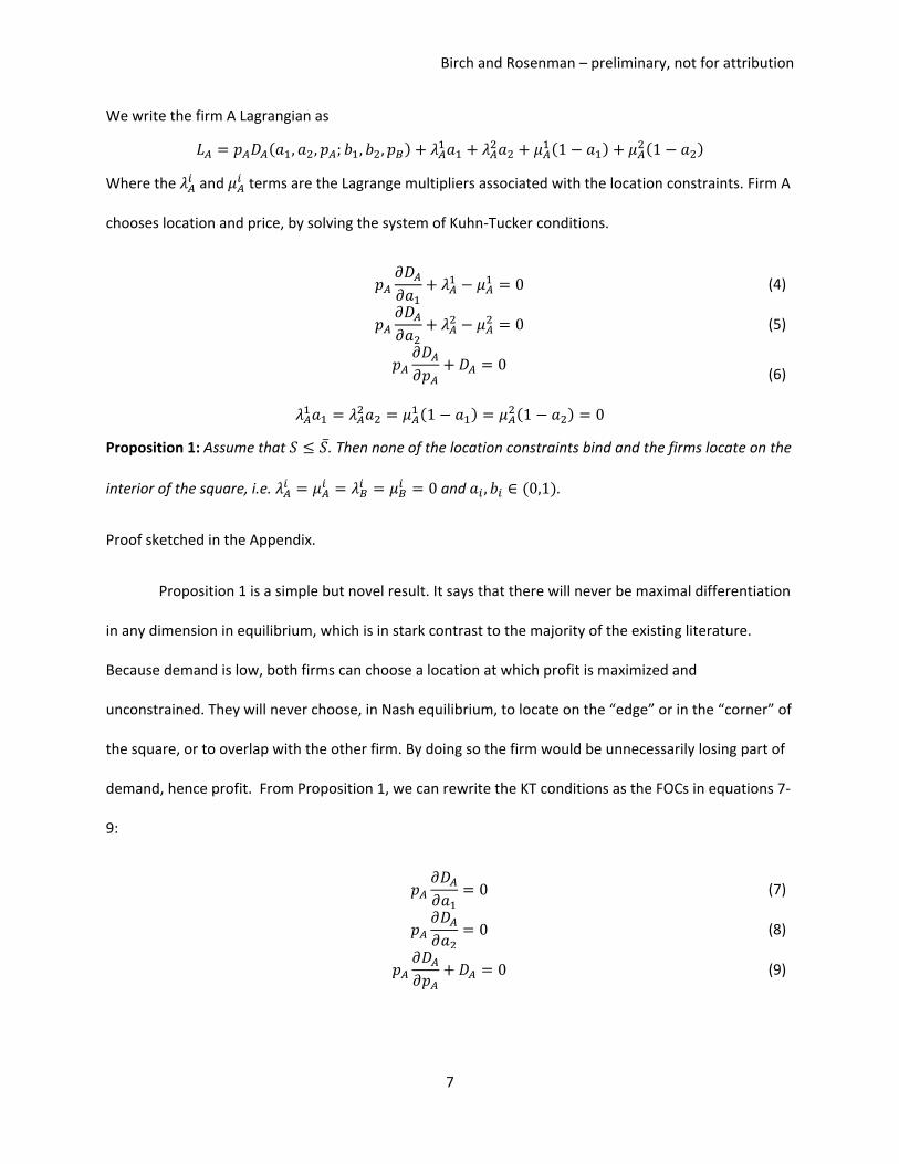
4. Equilibrium and S

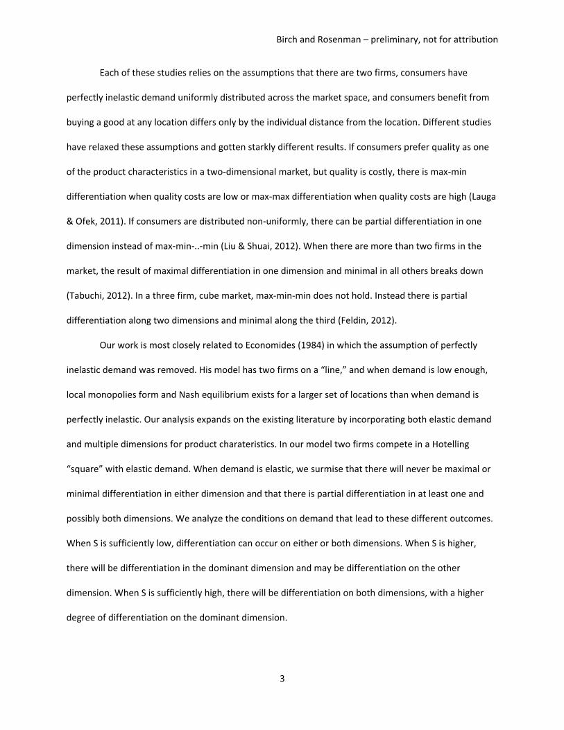
When S is small the demand ellipses are also small. We refer to S as being “small” if both firms

can maximize profits by locating and pricing such that the demand discs are unconstrained within the

square, i.e., when 𝑆 ≤ 𝑆̅. In Figure 3, the market is depicted with 𝑆 < 𝑆̅.

Figure 3: Depiction of Low Demand Market with “small” S

When S is sufficiently small, demand is maximized when the firms do not overlap and locate

away from the edges of the square. The Euclidean distance between the two firms is given as

4 It also means that the price elasticity of demand is unity, which is the expected result given zero marginal cost.


9

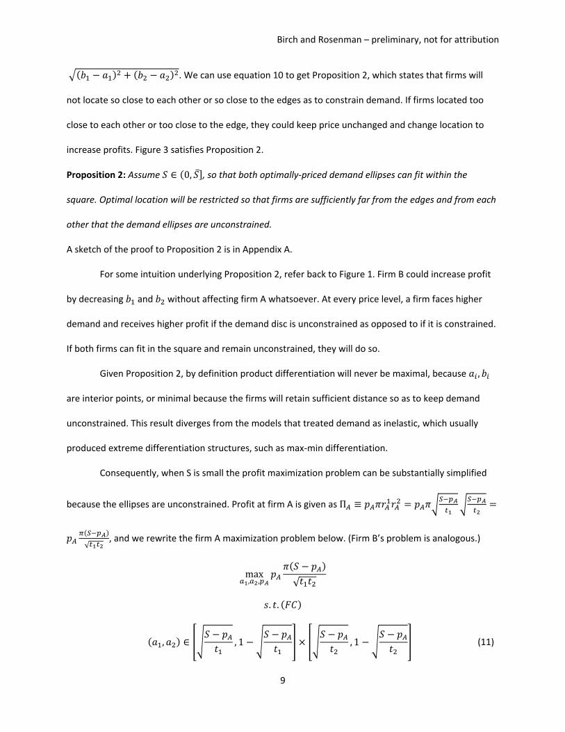
√(𝑏1 − 𝑎1)2 + (𝑏2 − 𝑎2)

2. We can use equation 10 to get Proposition 2, which states that firms will

not locate so close to each other or so close to the edges as to constrain demand. If firms located too

close to each other or too close to the edge, they could keep price unchanged and change location to

increase profits. Figure 3 satisfies Proposition 2.

Proposition 2: Assume 𝑆 ∈ (0, 𝑆̅], so that both optimally-priced demand ellipses can fit within the

square. Optimal location will be restricted so that firms are sufficiently far from the edges and from each

other that the demand ellipses are unconstrained.

A sketch of the proof to Proposition 2 is in Appendix A.

For some intuition underlying Proposition 2, refer back to Figure 1. Firm B could increase profit

by decreasing 𝑏1 and 𝑏2 without affecting firm A whatsoever. At every price level, a firm faces higher

demand and receives higher profit if the demand disc is unconstrained as opposed to if it is constrained.

If both firms can fit in the square and remain unconstrained, they will do so.

Given Proposition 2, by definition product differentiation will never be maximal, because 𝑎𝑖 , 𝑏𝑖

are interior points, or minimal because the firms will retain sufficient distance so as to keep demand

unconstrained. This result diverges from the models that treated demand as inelastic, which usually

produced extreme differentiation structures, such as max-min differentiation.

Consequently, when S is small the profit maximization problem can be substantially simplified

because the ellipses are unconstrained. Profit at firm A is given as Π𝐴 ≡ 𝑝𝐴𝜋𝑟𝐴1𝑟𝐴

2 = 𝑝𝐴𝜋√𝑆−𝑝𝐴

𝑡1√

𝑆−𝑝𝐴

𝑡2=

𝑝𝐴𝜋(𝑆−𝑝𝐴)

√𝑡1𝑡2, and we rewrite the firm A maximization problem below. (Firm B’s problem is analogous.)

max𝑎1,𝑎2,𝑝𝐴

𝑝𝐴

𝜋(𝑆 − 𝑝𝐴)

√𝑡1𝑡2

𝑠. 𝑡. (𝐹𝐶)

(𝑎1, 𝑎2) ∈ [√𝑆 − 𝑝𝐴

𝑡1, 1 − √

𝑆 − 𝑝𝐴

𝑡1] × [√

𝑆 − 𝑝𝐴

𝑡2, 1 − √

𝑆 − 𝑝𝐴

𝑡2] (11)


10

The generic constraint (FC) is purely geometric in nature, and states that the firms must be far

enough apart that the demand ellipses do not overlap in accordance with Proposition 2. Equation 11 is

the “no-boundary-overlap” constraint that keeps firms from getting too close to the edge of the square,

and utilizes 𝑟𝐴1 and 𝑟𝐴

2. In the proof to Proposition 2, it is referred to generically as (NB). Because the

discs are unconstrained 𝑝𝐴 is independent of 𝑎1, 𝑎2, 𝑏1, 𝑏2, 𝑝𝐵. Hence we can solve for price without

having an explicit form on (FC). The price FOC on the profit function is in equation 12.

𝜋(𝑆 − 𝑝𝐴)

√𝑡1𝑡2−

𝜋𝑝𝐴

√𝑡1𝑡2= 0

(12)

Equation 12 implies that optimal pricing in a low S market satisfies 13.

𝑝𝐴 =

𝑆

2 (13)

Thus, when 𝑆 < 𝑆̅ price is dependent only on the consumer valuation of the good and not on locations

or even salience coefficients. By substituting optimal price into the profit function, we get equilibrium

profits. Each firm has 𝑝𝐴 = 𝑝𝐵 =𝑆

2, which gives profit Π𝐴 = Π𝐵 =

𝜋𝑆2

4√𝑡1𝑡2. Both firms earn the same profit

in equilibrium, which is increasing in the demand parameter S and decreasing in the salience

coefficients 𝑡1 and 𝑡2. As it becomes costlier for consumers to buy from the firm in either dimension,

demand decreases and profits also fall.

Now we can also derive (FC) and characterize the low-demand equilibrium. FC is given as

equation 14. The derivation of equation 14 is somewhat tedious, and is included in the Appendix. The

meaning of 14 is simple. It is that the firms are far enough apart that the demand ellipses do not

overlap. Equation 14 applies to both firms.

√2𝑆((|𝑏2 − 𝑎2|)2 + 1)

√𝑡2(|𝑏2 − 𝑎2|)2 + 𝑡1

≤ √(𝑏1 − 𝑎1)2 + (𝑏2 − 𝑎2)

2 (14)


11

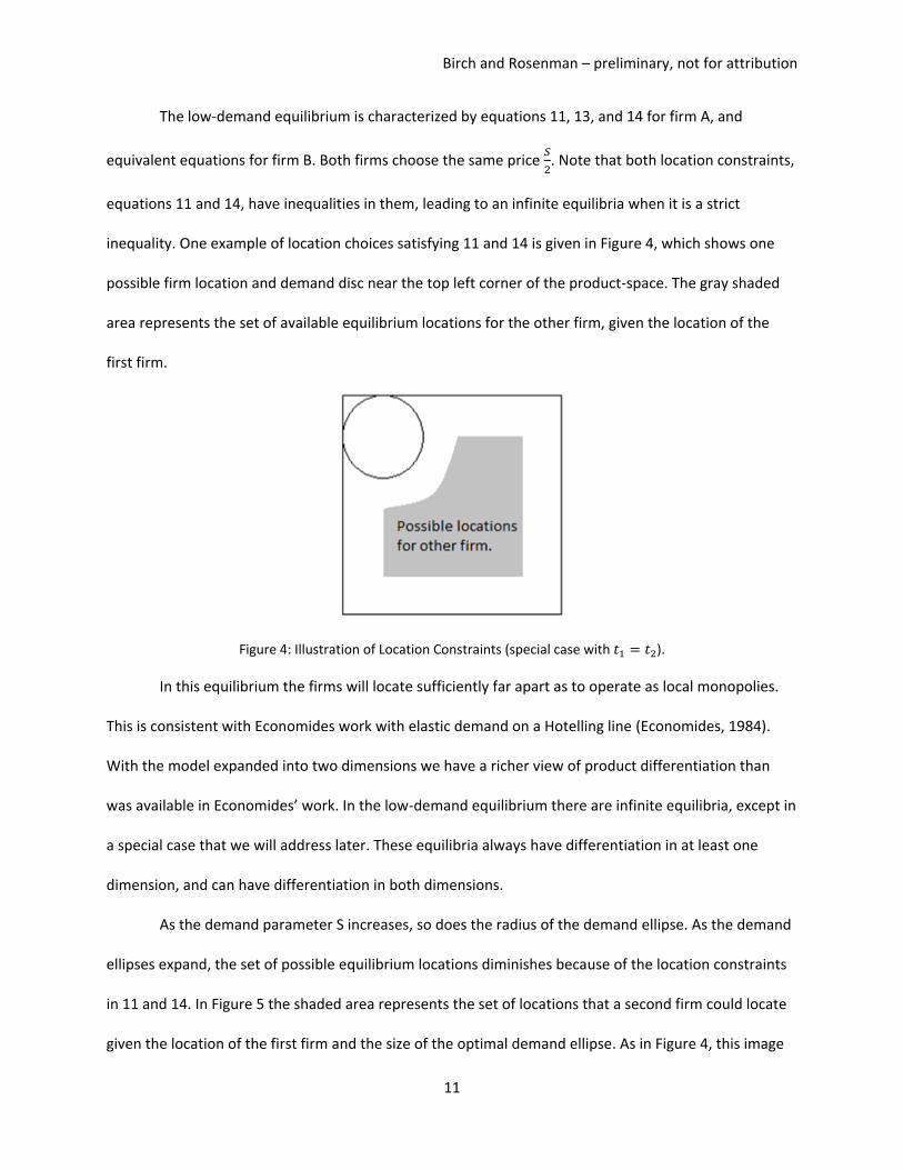
The low-demand equilibrium is characterized by equations 11, 13, and 14 for firm A, and

equivalent equations for firm B. Both firms choose the same price 𝑆

2. Note that both location constraints,

equations 11 and 14, have inequalities in them, leading to an infinite equilibria when it is a strict

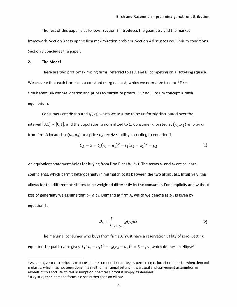
inequality. One example of location choices satisfying 11 and 14 is given in Figure 4, which shows one

possible firm location and demand disc near the top left corner of the product-space. The gray shaded

area represents the set of available equilibrium locations for the other firm, given the location of the

first firm.

Figure 4: Illustration of Location Constraints (special case with 𝑡1 = 𝑡2).

In this equilibrium the firms will locate sufficiently far apart as to operate as local monopolies.

This is consistent with Economides work with elastic demand on a Hotelling line (Economides, 1984).

With the model expanded into two dimensions we have a richer view of product differentiation than

was available in Economides’ work. In the low-demand equilibrium there are infinite equilibria, except in

a special case that we will address later. These equilibria always have differentiation in at least one

dimension, and can have differentiation in both dimensions.

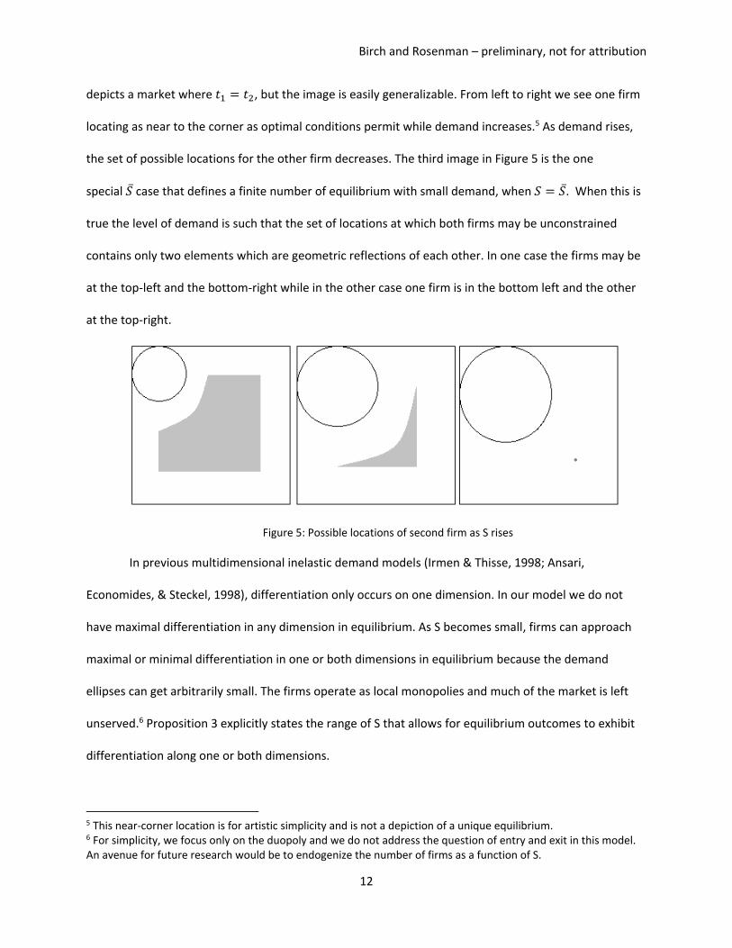
As the demand parameter S increases, so does the radius of the demand ellipse. As the demand

ellipses expand, the set of possible equilibrium locations diminishes because of the location constraints

in 11 and 14. In Figure 5 the shaded area represents the set of locations that a second firm could locate

given the location of the first firm and the size of the optimal demand ellipse. As in Figure 4, this image


12

depicts a market where 𝑡1 = 𝑡2, but the image is easily generalizable. From left to right we see one firm

locating as near to the corner as optimal conditions permit while demand increases.5 As demand rises,

the set of possible locations for the other firm decreases. The third image in Figure 5 is the one

special 𝑆̅ case that defines a finite number of equilibrium with small demand, when 𝑆 = 𝑆̅. When this is

true the level of demand is such that the set of locations at which both firms may be unconstrained

contains only two elements which are geometric reflections of each other. In one case the firms may be

at the top-left and the bottom-right while in the other case one firm is in the bottom left and the other

at the top-right.

Figure 5: Possible locations of second firm as S rises

In previous multidimensional inelastic demand models (Irmen & Thisse, 1998; Ansari,

Economides, & Steckel, 1998), differentiation only occurs on one dimension. In our model we do not

have maximal differentiation in any dimension in equilibrium. As S becomes small, firms can approach

maximal or minimal differentiation in one or both dimensions in equilibrium because the demand

ellipses can get arbitrarily small. The firms operate as local monopolies and much of the market is left

unserved.6 Proposition 3 explicitly states the range of S that allows for equilibrium outcomes to exhibit

differentiation along one or both dimensions.

5 This near-corner location is for artistic simplicity and is not a depiction of a unique equilibrium. 6 For simplicity, we focus only on the duopoly and we do not address the question of entry and exit in this model. An avenue for future research would be to endogenize the number of firms as a function of S.


13

Proposition 3: Let 𝑡2 ≥ 𝑡1 𝑎𝑛𝑑 𝑆 ≤ 𝑆̅, meaning that demand is low enough for interior ellipses and that

attribute 2 is the dominant product-trait. Then

i) For 𝑆 ∈ (0,𝑡1

8] the firms may differentiate on either or both dimensions, but never on none.

ii) For 𝑆 ∈ (𝑡1

8,𝑡2

8] the firms will differentiate along the dominant dimension and may also

differentiate along the other dimension.

iii) For 𝑆 ∈ (𝑡2

8, 𝑆̅] the firms differentiate on both dimensions.

A sketch of the Proof of Proposition 3 is included in the Appendix.

From Proposition 3 we learn that when demand is sufficiently small firms have great freedom

with product differentiation. As S rises, the degree to which product differentiation is possible lessens as

firms locate nearer to the center in order to maintain local monopoly power; the demand discs expand

and firm location becomes more restricted. In the intermediate case ii) the firms must differentiate

along the dominant dimension and may or may not differentiate along the dominated dimension. This is

somewhat reminiscent of the general literature finding that firms differentiate along the dominant

dimension and not in other dimensions, although our findings are more flexible and less extreme due to

the relaxed demand assumption. In case iii) we find that for some levels of demand, there will

undoubtedly be differentiation on both dimensions in equilibrium. In the Hotelling literature, this finding

is novel to our elastic demand model.

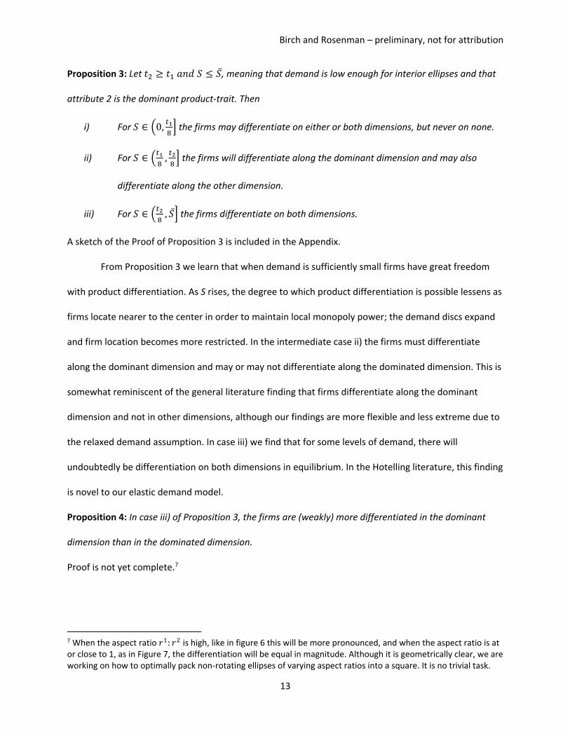
Proposition 4: In case iii) of Proposition 3, the firms are (weakly) more differentiated in the dominant

dimension than in the dominated dimension.

Proof is not yet complete.7

7 When the aspect ratio 𝑟1: 𝑟2 is high, like in figure 6 this will be more pronounced, and when the aspect ratio is at or close to 1, as in Figure 7, the differentiation will be equal in magnitude. Although it is geometrically clear, we are working on how to optimally pack non-rotating ellipses of varying aspect ratios into a square. It is no trivial task.


14

For illustrative purposes, we include Figure 6 to help explain Proposition 4. We show the case in

which 𝑆 = 𝑆̅, but the idea translates to any 𝑆 ∈ (𝑡2

8, 𝑆̅]. Figure 6 shows that when 𝑡2 > 𝑡1, and S is in this

relevant range, that |𝑎2 − 𝑏2| > |𝑎1 − 𝑏1|.

Figure 6: More Differentiation in Dominant Dimension

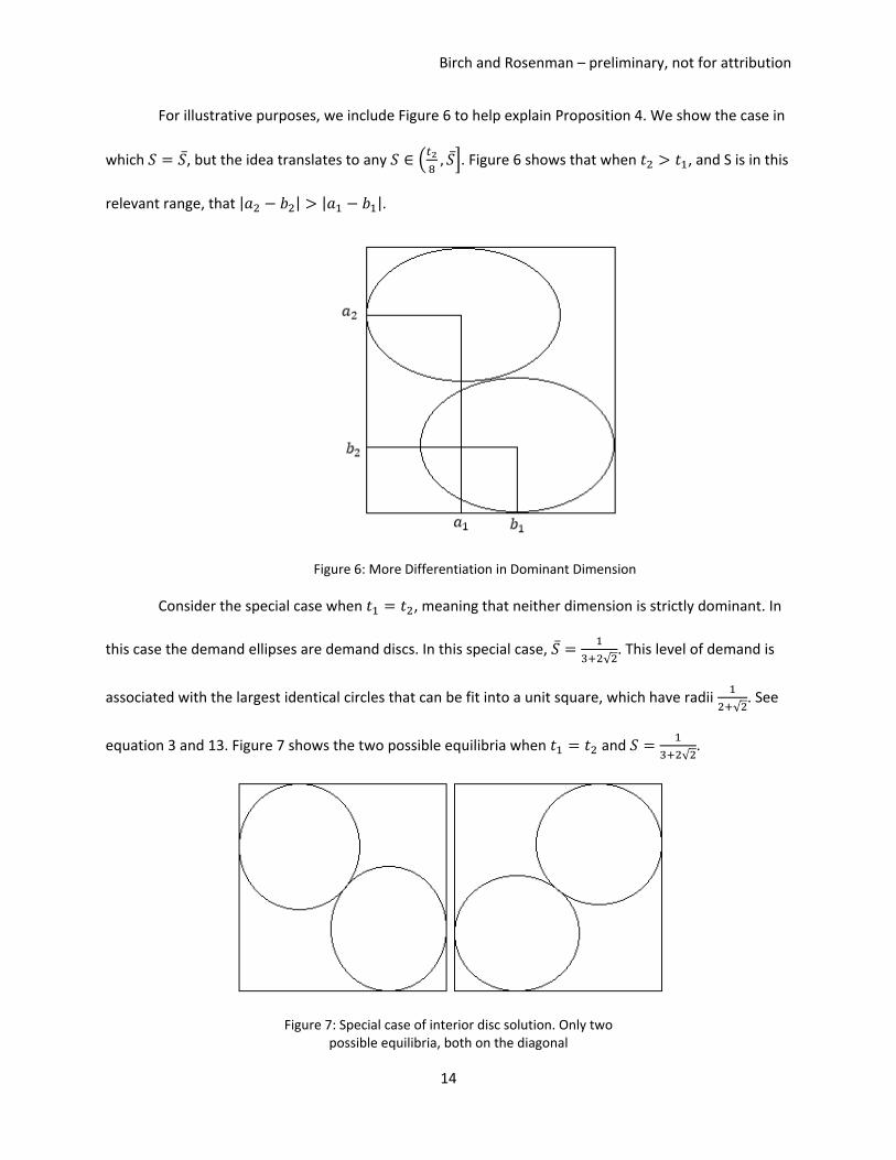
Consider the special case when 𝑡1 = 𝑡2, meaning that neither dimension is strictly dominant. In

this case the demand ellipses are demand discs. In this special case, 𝑆̅ =1

3+2√2. This level of demand is

associated with the largest identical circles that can be fit into a unit square, which have radii 1

2+√2. See

equation 3 and 13. Figure 7 shows the two possible equilibria when 𝑡1 = 𝑡2 and 𝑆 =1

3+2√2.

Figure 7: Special case of interior disc solution. Only two possible equilibria, both on the diagonal


15

In this case, the firms must align on the diagonals of the square. They locate at (𝑎1, 𝑎2) =

(1+√2

2+√2,

1

2+√2) and (𝑏1, 𝑏2) = (

1

2+√2,1+√2

2+√2) or at at (𝑎1, 𝑎2) = (

1

2+√2,

1

2+√2) and (𝑏1, 𝑏2) = (

1+√2

2+√2,1+√2

2+√2).

Differentiation is still partial-partial, but it is now restricted such that differentiation is equal in

magnitude in both dimensions. This is unique to 𝑡1 = 𝑡2.

5. Concluding Remarks

Almost all of the literature extending from Hotelling’s initial model of product differentiation

(1929) has relied on the “knife edge” simplification of assuming perfectly inelastic demand.8 Ours is the

first to incorporate elastic demand in a multi-dimensional market. Our duopoly model includes

uniformly distributed consumers with the same valuation of the good and no preference for product

quality.

We find that there is never maximal or minimal differentiation on any dimension, which is a

novel finding in stark contrast with the bulk of the extant literature. We find product differentiation to

be only limitedly restricted when demand is low, on either or both dimensions. In an intermediate case

with higher demand, firms will differentiate on the dominant dimension but may or may not

differentiate on the dominated dimension. When demand is higher still, the firms will differentiate on

both dimensions. In this case differentiation is stronger in the dominant dimension.

There are still many avenues for future research as the elastic demand concept is still relatively

unapproached. One could increase S beyond 𝑆̅ so that the ellipses are constrained and track

differentiation as S increases towards inelastic demand. One could introduce different distributions of

consumers, quality measures on the goods, or increase the dimensions of the model. It would be

especially useful with the low demand cases to endogenize the number of firms in the model. Our model

8 The only exception known to the authors is (Economides, 1984).


16

is just a starting point. It is the first to include elastic demand in a multi-dimensional Hotelling-type

model. The results are both novel and intuitive and indicate that when demand is elastic, common

findings in the literature are not accurate.


17

References Ansari, A., Economides, N., & Steckel, J. (1998). The Max-Min-Min Principle of Product Differentiation.

Journal of Regional Science.

d'Aspremont, C., Gabszewiez, J. J., & Thisse, J.-F. (1979). On Hotelling's "Stability in Competition".

Econometrica, 47(5), 1145-1150.

Economides, N. (1984). The Principle of Minimum Differentiation Revisited. European Economic Review,

24, 345-368.

Economides, N. (1986). Minimal and Maximal Product Differentiation in Hotelling's Duopoly. Economics

Letters, 21, 67-71.

Feldin, A. (2012). Three Firms on a Unit Disc Market: Intermediate Product Differentiation. Economic and

Business Review, 14(4), 321-345.

Hehenkamp, B., & Wambach, A. (2010). Survival at the center - The stability of minimum differentiation.

Journal of Economic Behavior & Organization, 76, 853-858.

Hotelling, H. (1929). Stability in Competition. The Economic Journal, 39(153), 41-57.

Irmen, A., & Thisse, J.-F. (1998). Competition in Multi-characteristics Spaces: Hotelling Was Almost Right.

Journal of Economic Theory, 78, 76-102.

Lauga, D. O., & Ofek, E. (2011). Product Positioning in a Two-Dimensional Vertical Differentiation Model:

The Role of Quality Costs. Marketing Science, 30(5), 903-923.

Liu, Q., & Shuai, J. (2012). Multi-Dimensional Product Differentiation. Working Paper.

Tabuchi, T. (2012). Multiproduct Firms in Hotellings Spatial Competition. Journal of Economics and

Management Strategy, 21, 445-467.


18

Appendix

These proofs are not yet complete. I seek to depict enough of the logic underlying them to walk

the reader through them.

Sketch of proof for Proposition 1

In Nash equilibrium, both firms have to be choosing optimally, given the actions of the other

firm. If 𝑆 ≤ 𝑆̅ we will never have corner solutions, and hence, never have maximal differentiation.

If both firms are located on the edges, it does not matter if they are near each other or not, both

firms could improve profit, given the location of the other firm.

If one firm is on the edge and the other firm is located on the interior of the square and they are

not overlapping, the first firm can move and improve its profit.

If one firm is on the edge and the other firm is interior, but the demand ellipses are overlapping,

the interior firm can increase profits by moving away from the edge firm.

Thus, we will never have a case where one firm or both firms choose edge solutions under the

conditions of Nash equilibrium.

Sketch of proof for Proposition 2

This proposition claims that if S is low, the firms will locate far enough from each other (firm constraint

called FC) and far enough from the edges (no-border constraint called BC) that the ellipses will be

unconstrained. We can only have a few variations of constraint violations. Either the firms are so close

to each other that they overlap, or they overlap with 1 or 2 product space boundaries, or some

combination of the above. We utilize a series of figures to show that when S is sufficiently low, equation

10 is only satisfied under the conditions of proposition 2.

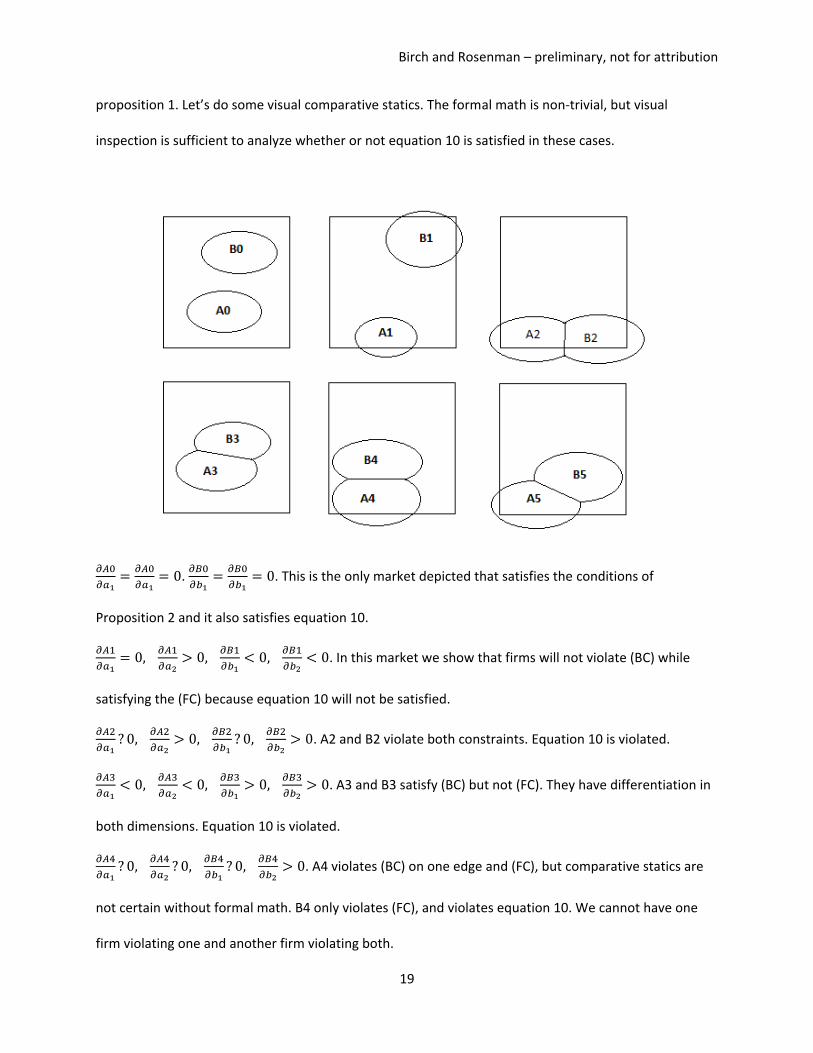
In the following images, Demand ellipses A0, B0, A3, B3, B4, and B5 satisfy the no-boundary-

overlap constraint, or (BC). Demand ellipses A0, B0, A1, and B1, satisfy the no-firm-overlap constraint, or

(FC). These images represent each combination of violation and non-violation of the 2 constraints in


19

proposition 1. Let’s do some visual comparative statics. The formal math is non-trivial, but visual

inspection is sufficient to analyze whether or not equation 10 is satisfied in these cases.

𝜕𝐴0

𝜕𝑎1=

𝜕𝐴0

𝜕𝑎1= 0.

𝜕𝐵0

𝜕𝑏1=

𝜕𝐵0

𝜕𝑏1= 0. This is the only market depicted that satisfies the conditions of

Proposition 2 and it also satisfies equation 10.

𝜕𝐴1

𝜕𝑎1= 0,

𝜕𝐴1

𝜕𝑎2> 0,

𝜕𝐵1

𝜕𝑏1< 0,

𝜕𝐵1

𝜕𝑏2< 0. In this market we show that firms will not violate (BC) while

satisfying the (FC) because equation 10 will not be satisfied.

𝜕𝐴2

𝜕𝑎1? 0,

𝜕𝐴2

𝜕𝑎2> 0,

𝜕𝐵2

𝜕𝑏1? 0,

𝜕𝐵2

𝜕𝑏2> 0. A2 and B2 violate both constraints. Equation 10 is violated.

𝜕𝐴3

𝜕𝑎1< 0,

𝜕𝐴3

𝜕𝑎2< 0,

𝜕𝐵3

𝜕𝑏1> 0,

𝜕𝐵3

𝜕𝑏2> 0. A3 and B3 satisfy (BC) but not (FC). They have differentiation in

both dimensions. Equation 10 is violated.

𝜕𝐴4

𝜕𝑎1? 0,

𝜕𝐴4

𝜕𝑎2? 0,

𝜕𝐵4

𝜕𝑏1? 0,

𝜕𝐵4

𝜕𝑏2> 0. A4 violates (BC) on one edge and (FC), but comparative statics are

not certain without formal math. B4 only violates (FC), and violates equation 10. We cannot have one

firm violating one and another firm violating both.


20

𝜕𝐴5

𝜕𝑎1? 0,

𝜕𝐴5

𝜕𝑎2? 0,

𝜕𝐵5

𝜕𝑏1? 0,

𝜕𝐵5

𝜕𝑏2> 0. A5 violates (BC) on two edges and (FC). While some of the

comparative statics are not certain without formal math, we know that B4 violates (FC) and violates

equation 10. We cannot have one firm violating one and another firm violating both.

There is no combination of violations of (BC) and (FC) in Proposition 1 that satisfy the first order

conditions. When the conditions of Proposition 2 hold, the first order conditions are satisfied. Thus, for

small S, Proposition 2 is uniquely true. QED.

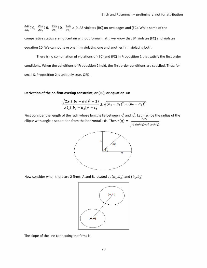
Derivation of the no-firm-overlap constraint, or (FC), or equation 14:

√𝟐𝑺((|𝒃𝟐 − 𝒂𝟐|)

𝟐 + 𝟏)

√𝒕𝟐(|𝒃𝟐 − 𝒂𝟐|)𝟐 + 𝒕𝟏

≤ √(𝒃𝟏 − 𝒂𝟏)𝟐 + (𝒃𝟐 − 𝒂𝟐)

𝟐

First consider the length of the radii whose lengths lie between 𝑟𝐴1 and 𝑟𝐴

2. Let 𝑟(𝑞) be the radius of the

ellipse with angle q separation from the horizontal axis. Then 𝑟(𝑞) =𝑟1𝑟2

√𝑟12 sin2(𝑞)+𝑟2

2 cos2(𝑞).

Now consider when there are 2 firms, A and B, located at (𝑎1, 𝑎2) and (𝑏1, 𝑏2).

The slope of the line connecting the firms is


21

𝑚 =𝑏2 − 𝑎2

𝑏1 − 𝑎1

The angle q then for firm A is given by

𝑞𝐴 = tan−1(𝑚) = tan−1 (𝑏2 − 𝑎2

𝑏1 − 𝑎1)

The angle q for firm B

𝑞𝐵 = tan−1(−𝑚) = tan−1(𝑚) ⇒ tan−1 (𝑏2 − 𝑎2

𝑏1 − 𝑎1) = tan−1 (

|𝑏2 − 𝑎2|

|𝑏1 − 𝑎1|)

So we have 𝑞𝐴 = 𝑞𝐵.

Then the intermediate radii lying on the line connecting the firms are

𝑟𝐴(𝑞𝐴) =𝑟𝐴1𝑟𝐴

2

√(𝑟𝐴1)2 sin2(𝑞𝐴) + (𝑟𝐴

2)2 cos2(𝑞𝐴)

=√

𝑆 − 𝑝𝐴𝑡1

√𝑆 − 𝑝𝐴

𝑡2

√𝑆 − 𝑝𝐴

𝑡1sin2 (tan−1 (

|𝑏2 − 𝑎2||𝑏1 − 𝑎1|

)) +𝑆 − 𝑝𝐴

𝑡2cos2 (tan−1 (

|𝑏2 − 𝑎2||𝑏1 − 𝑎1|

))

=

=√

(𝑆 − 𝑝𝐴)𝑡1𝑡2

√1𝑡1

sin2 (tan−1 (|𝑏2 − 𝑎2||𝑏1 − 𝑎1|

)) +1𝑡2

cos2 (tan−1 (|𝑏2 − 𝑎2||𝑏1 − 𝑎1|

))

=

=√

(𝑆 − 𝑝𝐴)𝑡1𝑡2

√𝑡2

𝑡1𝑡2[ (

|𝑏2 − 𝑎2||𝑏1 − 𝑎1|

)2

(|𝑏2 − 𝑎2||𝑏1 − 𝑎1|

)2

+ 1]

+𝑡1

𝑡1𝑡2[

1

(|𝑏2 − 𝑎2||𝑏1 − 𝑎1|

)2

+ 1]

=√𝑆 − 𝑝𝐴

√

[ 𝑡2 (

|𝑏2 − 𝑎2||𝑏1 − 𝑎1|

)2

+ 𝑡1 (1

|𝑏1 − 𝑎1|)2

(|𝑏2 − 𝑎2||𝑏1 − 𝑎1|

)2

+ (1

|𝑏1 − 𝑎1|)2

]

=√𝑆 − 𝑝𝐴

√[𝑡2(|𝑏2 − 𝑎2|)

2 + 𝑡1(|𝑏2 − 𝑎2|)

2 + 1]

=√(𝑆 − 𝑝𝐴)((|𝑏2 − 𝑎2|)

2 + 1)

√𝑡2(|𝑏2 − 𝑎2|)2 + 𝑡1


22

𝑟𝐵(𝑞𝐵) =𝑟𝐵1𝑟𝐵

2

√(𝑟𝐵1)2 sin2(𝑞𝐵) + (𝑟𝐵

2)2 cos2(𝑞𝐵)

=√

𝑆 − 𝑝𝐵𝑡1

√𝑆 − 𝑝𝐵

𝑡2

√𝑆 − 𝑝𝐵

𝑡1sin2 (tan−1 (

|𝑏2 − 𝑎2||𝑏1 − 𝑎1|

)) +𝑆 − 𝐵

𝑡2cos2 (tan−1 (

|𝑏2 − 𝑎2||𝑏1 − 𝑎1|

))

= ⋯

=√(𝑆 − 𝑝𝐵)((|𝑏2 − 𝑎2|)

2 + 1)

√𝑡2(|𝑏2 − 𝑎2|)2 + 𝑡1

And by substituting in optimal price 𝑝𝐴 = 𝑝𝐵 =𝑆

2 we get

𝑟𝐴(𝑞𝐴) =√𝑆((|𝑏2 − 𝑎2|)

2 + 1)

√2(𝑡2(|𝑏2 − 𝑎2|)2 + 𝑡1)

𝑟𝐵(𝑞𝐵) =√𝑆((|𝑏2 − 𝑎2|)

2 + 1)

√2(𝑡2(|𝑏2 − 𝑎2|)2 + 𝑡1)

The minimum distance the 2 firms can be from each other without overlapping is

𝑟𝐴(𝑞𝐴) + 𝑟𝐵(𝑞𝐵) = 2√𝑆((|𝑏2 − 𝑎2|)

2 + 1)

√2(𝑡2(|𝑏2 − 𝑎2|)2 + 𝑡1)

=√2𝑆((|𝑏2 − 𝑎2|)

2 + 1)

√𝑡2(|𝑏2 − 𝑎2|)2 + 𝑡1

We are now prepared for the no-firm-overlap constraint:

√2𝑆((|𝑏2 − 𝑎2|)2 + 1)

√𝑡2(|𝑏2 − 𝑎2|)2 + 𝑡1

≤ √(𝑏1 − 𝑎1)2 + (𝑏2 − 𝑎2)

2.

Sketch of proof of Proposition 3

Case i:

I rely on the results of Proposition 2 which require that the firms locate so that demand is unconstrained

in equilibrium. From equations 3 and 13 we have 𝑆 ≤𝑡1

8⇒ 𝑟𝐴

1 = 𝑟𝐵1 = √

𝑆

2𝑡1≤ √

1

16=

1

4.

We also know that 𝑟𝐴2 = 𝑟𝐵

2 ≤ 𝑟𝐴1 = 𝑟𝐵

1 because 𝑡1 ≤ 𝑡2.


23

Thus, each ellipse is less than or equal to half of the square’s length on both dimensions. Then we can

differentiation in only one dimension, by having 𝑎1 = 𝑏1 or 𝑎2 = 𝑏2 and still have unconstrained

ellipses, or differentiation in both dimensions 𝑎1 ≠ 𝑏1 and 𝑎2 ≠ 𝑏2 and still have unconstrained ellipses.

Case ii:

From equations 3 and 13 we know that when 𝑆 ∈ (𝑡1

8,𝑡2

8] we have 𝑟𝐴

1 = 𝑟𝐵1 >

1

4 and 𝑟𝐴

2 = 𝑟𝐵2 ≤

1

4. This

means that we can have 𝑎1 = 𝑏1 if 𝑎2 and 𝑏2 are sufficiently differentiated, but never 𝑎2 = 𝑏2 because

Proposition 2 and equation 10 would be violated. Of course we can still have 𝑎1 ≠ 𝑏1 and 𝑎2 ≠ 𝑏2 and

have both firms fit within the square. Thus we will certainly have differentiation in the dominant

dimension, and we may or may not have differentiation in the other dimension.

Case iii:

For 𝑆 ∈ (𝑡2

8, 𝑆̅], we know by equations 3 and 13 that 𝑟𝐴

1 = 𝑟𝐵1 ≥ 𝑟𝐴

2 = 𝑟𝐵2 >

1

4. This means that we cannot

have 𝑎1 = 𝑏1 or 𝑎2 = 𝑏2 because in both cases the ellipses (which are each wider than 1/2 on both

dimensions) are then constrained. Hence we have to have 𝑎1 ≠ 𝑏1 and 𝑎2 ≠ 𝑏2, which is differentiation

in both dimensions.

Proof for Proposition 4:

I have not yet proved this. I know it will have to do with the aspect ratio. The “wider” the ellipse is,

relatively, the more differentiated the good will be in attribute 2, relative to attribute 1. But this is tricky

business.

Documents

Matt Birch Robert Rosenman