Matrix Profile V: A Generic Technique to Incorporate

Matrix Profile V: A Generic Technique to Incorporate Domain Knowledge into Motif Discovery

Hoang Anh Dau Eamonn Keogh University of California, Riverside

USA {hdau001, eamonn}@ucr.edu

ABSTRACT

Time series motif discovery has emerged as perhaps the most used primitive for time series data mining, and has seen applications to domains as diverse as robotics, medicine and climatology. There has been recent significant progress on the scalability of motif discovery. However, we believe that the current definitions of motif discovery are limited, and can create a mismatch between the user’s intent/expectations, and the motif discovery search outcomes. In this work, we explain the reasons behind these issues, and introduce a novel and general framework to address them. Our ideas can be used with current state-of-the-art algorithms with virtually no time or space overhead, and are fast enough to allow real-time interaction and hypotheses testing on massive datasets. We demonstrate the utility of our ideas on domains as diverse as seismology and epileptic seizure monitoring.

KEYWORDS Time series; matrix profile; motif discovery; interactive data mining

1 INTRODUCTION The last decade has seen time series motif discovery become a prominent primitive for time series data mining. It has been applied to diverse domains such as climatology, robotics [11], medicine [23] and seismology [24]. Recently there has been significant progress on the scalability of motif discovery, and

datasets with lengths in the tens of millions can be routinely searched on conventional hardware [24]. Paradoxically, the ease with which we can now perform motif discovery has revealed some weaknesses in the traditional definition of motifs; there are many situations in which the results of motif search do not align with the user’s intent. Below we discuss several examples to help develop the reader’s intuitions for this fact. This section is unusually long for a paper’s “Introduction”, but is warranted by the fact that we are introducing unfamiliar and unintuitive issues.

1.1 Stop-Word Motif Bias In some datasets, the most interesting repeated patterns may be rare, and “swamped” by more frequent patterns. By analogy with text, we can ask what is the most common “motif” (i.e. word) in Poe’s famous poem, The Raven? One might imagine that it is the eponymous bird; however that is only the 13th most common word, with 13 occurrences. The most frequent words with their number of occurrences are “the” (56), “and” (38), “I” (32)…

In retrospect, this finding is not surprising, and we recall that stop-words are removed before any text analytics are performed. A similar problem occurs in time series. Consider the snippet of ECG data shown in Figure 1. Note that the signal begins with a slightly noisy saw-toothed wave (called the calibration signal), which is how the ECG apparatus indicates that it is switched-on, but not detecting a biological signal. Unsurprisingly, the saw-tooth “stop-word” is the best motif in this dataset.

Figure 1: blue/fine: A snippet of ECG data from the LTAF-71 Database [13]. The top motifs come from regions of the calibration signal because they are much more similar than the motifs discovered if we search only data that contains true ECGs.

One might imagine that this issue only affects the beginning of signals, and thus could be easily addressed by manual inspection and truncation. Unfortunately, this is not the case. It is

1000 2000 30000

Calibration Signal True ECG Signal

Top-1 Motif (all data) Top-1 Motif, if we ignore the first 1,000 data points

____________________________________________________ Permission to make digital or hard copies of all or part of this work for personal or classroom use is granted without fee provided that copies are not made or distributed for profit or commercial advantage and that copies bear this notice and the full citation on the first page. Copyrights for components of this work owned by others than ACM must be honored. Abstracting with credit is permitted. To copy otherwise, or republish, to post on servers or to redistribute to lists, requires prior specific permission and/or a fee. Request permissions from [email protected]. KDD '17, August 13-17, 2017, Halifax, NS, Canada © 2017 Association for Computing Machinery. ACM ISBN 978-1-4503-4887-4/17/08…$15.00 http://dx.doi.org/10.1145/3097983.3097993

mailto:[email protected]

http://dx.doi.org/10.1145/3097983.3097993

KDD’17, August 2017, Canada Dau et al.

2

very common for sensors to temporarily lose the signal due to poor contact or patient motion, and this issue shows up dozens of times in this 25-hour trace. It is important to note that the issue of stop-word motifs is not limited to machine artifacts from the recording process. The issue shows up even within “pure” data sources. Again, by analogy, note that a set of text stop-words is context dependent. For example, in a general text search the word “computer” is not a stop-word, but for a search within the ACM portal, it is a stop-word. The exact same situation occurs with time series. Consider the snippet of ECG data shown in Figure 2. The eye is drawn to the repeated ventricular contractions highlighted in red, but the best motifs by the classic definitions are a pair of normal heartbeats.

Figure 2: A snippet of ECG data from BIDMC Congestive Heart Failure Database (chf02). The top motif pair are the two highlighted normal heartbeats. However, a cardiologist’s eye is drawn here to the two repeated ventricular contractions [13].

Even if the rare motifs are more strongly conserved than the background motifs, we should still expect the background motifs to be discovered first. The reason is essentially a real-valued version of the birthday paradox. Consider again the pair of ventricular contractions shown in Figure 2. They are better conserved (under the Euclidean distance) than most pairs of normal beats. However, there are fourteen normal beats, therefore there are 91 pairwise combinations that could match. With so many possibilities, it is unsurprising that the closest pair will be reported as the best motif.

The toy problem in Figure 2 can be solved by visual inspection, but with time series motif discovery now scaling to datasets of length one-hundred million [24], a more general and automatic solution is required. Finally, we note that this problem is not confined to ECGs or other periodic data. For example, in industrial data the top-K motifs may all correspond to patterns caused by calibration runs or shift changes. These known/uninteresting patterns may obscure a much rarer and unexpected repeated pattern.

1.2 Simplicity Bias in Motif Search Imagine that we have {C1,C2}, a pair of subsequences that are “complicated” (informally for now, this means having many peaks and valleys [1]), and {S1,S2}, a pair subsequences that are “simple”. Further imagine that, to your eyes, each pair itself is equally similar. In spite of this imagined subjective equality of similarity,

1 We note that many of the issues we address were reported to us over the last decade by users of motif discovery tools from academia and industry.

it is almost certain that D(C1,C2) is greater than D(S1,S2) under Euclidean distance, Dynamic Time Warping or any other effective distance measure [1]. The practical upshot of this is that it will be difficult to find such complicated motifs, as the top-K will be swamped by many simple motifs. To see this, consider the top motif discovered in the EEG snippet shown in Figure 3.

Figure 3: A snippet of an EEG time series in which two motion artifacts were deliberately introduced by the attending physician [16]. Surprisingly, the top-motif does not correspond to the motion artifacts, but to simple regions of “drift”.

The result is visually jarring. The two motion artifacts are visually similar and do have a small Euclidean Distance, yet they are not discovered as the top motif. Instead, two regions of vaguely rising trends are the top motif. The reason for this mismatch between our expectation and the results is understood, but not in this context. In [1], it was demonstrated that the Euclidean Distance has a bias toward simple shapes. Quoting [1], “pairs of complex objects, even those which subjectively may seem very similar to the human eye, tend to be further apart under (Euclidean) distance measures than pairs of simple objects.”

This issue is perhaps the most reported complaint of users of motif discovery tools1. Almost all large time series datasets have low complexity regions, which are often uninteresting to the analyst, yet it is virtually certain that all the top-K motifs will come from there.

1.3 Actionability Bias In many cases a domain expert wants to find not simply the best motif (as defined as the subsequence pair that minimizes their mutual distance), but regularities in the data which are exploitable or actionable in some domain specific ways. Such constraints have been explained to us by various domain experts1 with statements such as “I want to find motifs in this web-click data, preferably occurring on or close to the weekend”, or “I want to find motifs in this oil pressure data, but they would be more useful if they end with a rising trend”, or “I want to find motifs in this PPG time series data, but it would be better if they happened about five to ten minutes after the accompanying RR time series data was relatively high”.

There is currently no way to support such arbitrary constraints/preferences in motif search. Note that by their very nature, many of these constraints will need to be adjusted in real-time interactive sessions. For example, the user with a preference for a motif that happens near a weekend may be inspired by the quality of the results and wish to sharpen her focus to “strictly on

500 1000 1500 2000 25000

Top-1 Motif Top-1 MotifVentricular Contractions

4000 80001

Motion Artifact Contaminated EEG Data

Motion Artifact

Motion Artifact Top-1 Motif

Top-1 Motif


KDD’17, August 2017, Canada

3

a weekend”, or she may have been disappointed by the sparse results and reluctantly weaken her constraint to “preferably not on a Tuesday or Wednesday”. As we will show, we can support this need interactively with almost no overheard of time or space.

1.4 Summary and Outline We have seen several reasons why classic motif discovery can

fail to produce the expected or desired results. The contribution of this work is to produce a single, real-time, intuitive framework that can handle all the above, and many other domain specific constraints that have yet to occur to us. The basic idea behind our approach is to produce a vector that is “parallel” to the original time series and annotates it with the user’s constraint(s). As the motif discovery algorithm finds candidate motifs, this annotation vector (AV) is used to re-rank them, allowing the motifs that best balance the fidelity of conservation with the user’s constraints to rise to the top.

This only leaves the question of how do we create such annotation vectors? We introduce a generic framework that allows a user to create such vectors, typically with just a few lines of code in a scripting language. For concreteness, we explicitly show the annotation functions that allow us to address all the examples above, and illustrate their utility with detailed case studies. Furthermore, our framework is simple and flexible enough to support domains and constraints that have yet to be explored. Despite the flexibility and expressiveness of our system, we will show that it requires an inconsequential overhead of time and space complexity, relative to the state-of-the-art motif discovery [23][24].

The rest of the paper is organized as follows. In Section 2, we review the related work and introduce necessary notations. In Section 3 we discuss our proposed framework together with several case studies. Section 4 includes a comprehensive quantitative comparison with other motif discovery algorithms in the literature. Finally, we arrive at conclusions and future research in Section 5.

2 RELATED WORK AND NOTATION We begin with a brief review of related work before introducing the notations needed to understand our proposed framework.

2.1 Related Work The literature on general time series motif search is large and growing. We refer the reader to [2][7][23] and references therein.

This section is brief. While there are many papers on exploiting motifs, and scaling up motif search, to the best of our knowledge there are no research efforts that even explicitly note the issues we tackle, much less address them.

Saria and colleagues noted a limitation of the standard motif definition in that it may not readily discover motifs that have significant temporal warping [14]. Similarly, Yankov et al. noted that in some domains we may need to allow uniform scaling to enable meaningful motif discovery [22]. However, both of these issues are largely orthogonal to the issues at hand. In any case,

Mueen has argued that these issues are mostly an artifact of searching small datasets, and as we search larger datasets, these issues simply go away (see Section 4.3.2 of [12]). We do note that in the context of text information retrieval, there is significant work in query-biased (or user-directed) summaries [18]. Such work is in the same spirit as our work, directing the results of a query toward an arbitrary informational need or away from an undesired outcome [10].

2.2 Notation We begin by defining the data type of interest, time series:

Definition 1: A time series 𝑇 ∈ ℝ𝑛 is a sequence of real-valued numbers 𝑡𝑖 ∈ ℝ ∶ 𝑇 = [𝑡1, 𝑡2, . . . , 𝑡𝑛] where 𝑛 is the length of 𝑇.

We are typically not interested in the global properties of a time series, but in the local regions known as subsequences:

Definition 2: A subsequence 𝑇𝑖,𝑚 ∈ ℝ𝑚 of a time series 𝑇 is a continuous subset of the values from 𝑇 of length 𝑚 starting from position 𝑖. Formally, 𝑇𝑖,𝑚 = [𝑡𝑖 , 𝑡𝑖+1, … , 𝑡𝑖+m−1].

The particular local property we are interested in in this work is time series motifs:

Definition 3: A time series motif is the most similar subsequence pair of a time series. Formally, 𝑇𝑎,𝑚 and 𝑇𝑏,𝑚is the

motif pair iff 𝑑𝑖𝑠𝑡(𝑇𝑎,𝑚, 𝑇𝑏,𝑚) ≤ 𝑑𝑖𝑠𝑡(𝑇𝑖,𝑚, 𝑇𝑗,𝑚) ∀ 𝑖, 𝑗 ∈

[1, 2, … , 𝑛 − 𝑚 + 1] where 𝑎 ≠ 𝑏 and 𝑖 ≠ 𝑗 , and 𝑑𝑖𝑠𝑡 is a function that computes the z-normalized Euclidean distance between the input subsequences [2][5][12][22][23][24].

We store the distance between a subsequence of a time series with all the other subsequences from the same time series in an ordered array called distance profile.

Definition 4: A distance profile 𝐷 ∈ ℝ𝑛−𝑚+1 of a time series 𝑇 and a subsequence 𝑇𝑖,𝑚 is a vector stores 𝑑𝑖𝑠𝑡(𝑇𝑖,𝑚, 𝑇𝑗,𝑚) ∀ 𝑗 ∈

[1, 2, … , 𝑛 − 𝑚 + 1], where 𝑖 ≠ 𝑗. One of the most efficient ways to locate exact time series motifs is to compute the matrix profile [23].

Definition 5: A matrix profile 𝑃 ∈ ℝ𝑛−𝑚+1 of a time series 𝑇 is a meta time series that stores the z-normalized Euclidean distance between each subsequence and its nearest neighbor where 𝑛 is the length of 𝑇 and 𝑚 is the given subsequence length. The time series motif can be found by simply locating the two lowest values in 𝑃 (they will have tying values).

Figure 4 illustrates a matrix profile on a small toy dataset.

Figure 4: A time series T and its self-join matrix profile P.

600

P, a matrix profile |P| = |T| - |m | + 1

1

m

Top motif location

T, a random walk time series with two sine waves embedded


4

To avoid trivial matches [12] in which a pattern is matched to

itself, or a pattern that largely overlaps with itself, the matrix profile incorporates an “exclusion-zone” concept, which is a region before and after the location of a given query that should be ignored. The exclusion zone is heuristically set to 𝑚/2.

The time complexity to compute a matrix profile 𝑃 is 𝑂(𝑛2). This may seem untenable for time series data mining, but several factors mitigate this concern. First, note that the time complexity is independent of m, the length of the subsequences. Secondly, the matrix profile can be computed with an anytime algorithm, and in most domains, in just 𝑂(𝑛𝑐) steps the algorithm converges to what would be the final solution [23] (c is a small constant). Finally, the matrix profile can be computed with GPUs, cloud computing and other HPC environments that make scaling to at least tens of millions of data points trivial [23]. Even using standard hardware, all the examples in this paper can be computed much faster than real-time. For example, 30 minutes of ECG sampled at 60Hz takes about four minutes to exactly compute the full matrix profile using STOMP [23]. If that was not fast enough, STAMP can produce a very high quality approximation in under five seconds [23]. 2.1.1 Summary of this section. Before moving on, we wish to restate the reason for our detailed explanation of the matrix profile. As explained in greater detail in [23], once the matrix profile has been computed, all the top-K motifs are available “for free”. For example, the locations of the top-1 motif is simply the (tied) lowest points in the matrix profile. Moreover, all other definitions of motifs (range motifs, top-K motifs etc.) can also be trivially extracted. Thus, we see the computational aspects of motif search largely solved, our contributions are limited to “nudging” the results to be more useful.

3 GUIDED MOTIF SEARCH The basic idea behind guided motif search is to produce a vector that is “parallel” to the original time series (and to the matrix profile) that encodes the user’s domain-dependent bias(es). This vector is then used to modify the matrix profile, changing its shape such that the undesirable solutions are more expensive, and no longer show up in the top-K motifs. We begin by explaining the general domain independent part of our solution in the next section, before showing several examples of how to create domain dependent bias functions.

3.1 The Annotation Vector Framework The Annotation Vector (AV) plays the role of manipulating the motif search. Recall the notation of matrix profile (MP) elucidated in Section 2.2. The MP is the current state-of-the-art for motif discovery [23][24]. Our main idea is to leverage this MP to discover more meaningful motifs. We achieve this goal by combining the matrix profile with the annotation vector to produce a new matrix profile. We will refer to this as the “Corrected” MP (CMP), as it correctly incorporates the contextual bias for the problem at hand.

The annotation vector AV is a time series consisting of real-valued numbers between [0 - 1]. A low value indicates the subsequence starting at that index is not a desirable motif, and therefore should be biased against. Conversely, higher values mean the subsequence at that location should be favored for the potential motif pool. Note that the AV has the same length as the matrix profile MP. In Figure 5 we show the annotation vector that encodes the bias: “I want to find motifs in this traffic data, preferably occurring on or close to the weekend”. There may be some scenarios in which the annotation vector AV consists of just 0s and 1s. For example, this would be the case when the desired motifs are strictly limited to within a certain period, such as, activities between 8am-10am daily, or at a longer time scale, activities that happen only during an Olympic year. For such scenarios, we would assign 0 for AV data points in the untargeted period, and 1 for targeted ones. However, as shown in Figure 5, we allow arbitrary real-number values in the AV, so long as they are in the unit interval.

Figure 5: top) Seventeen days from the Dodger Loop dataset. bottom) The AV that encodes a preference for motifs occurring on or near the weekend.

Having defined the AV, we can now explain how we use it to correct the undesirable results explained above. To do this, we simply produce a Corrected Matrix Profile (CMP) by combining the annotation vector AV and the original matrix profile MP:

𝐶𝑀𝑃𝑖 = 𝑀𝑃𝑖 + (1 − 𝐴𝑉𝑖) ∗ max (𝑀𝑃)

In the above equation, 𝐶𝑀𝑃𝑖 , 𝑀𝑃𝑖 and 𝐴𝑉𝑖 denote the corrected MP value, the original MP value and the AV value respectively. The max (𝑀𝑃) term denotes the maximum value of the original MP. The resulting corrected MP can be interpreted as follow: if a region of the time series potentially contains the meaningful motifs, its MP values are left untouched. Otherwise, its MP values are “pushed” higher (increased) to reduce the possibility of any motif in that region appears in the top-K motif list.

In many cases, the annotation vectors can be created by just a few lines of code. Moreover, they can be created in a simple environment such as MS Excel or a scripting language such as Matlab or Python. This is important, since many of the end-users of motif discovery are biologists, medical doctors, seismologists [23] etc., not computer/data scientists.

For example, to produce one week of the AV shown in Figure 5, assuming that the data is sampled once a minute and starts at midnight Sunday, we can use a single line of Matlab:

AV = [(1440:-1:1)/1440 zeros(1,1440*3) (1:1440)/1440 ones(1,1440*2)] Which we can interpret as: AV = [MonRampDown TueWedThuConstantLow FriRampUp WeekendConstantHigh]

Dodgers Loop data (subset)

m t w t f s su m t w t f s su m t w

Annotation vector0 5000



5

In the following subsections, we will show how the annotation vector is used in action to guide motif search with several motivating case studies.

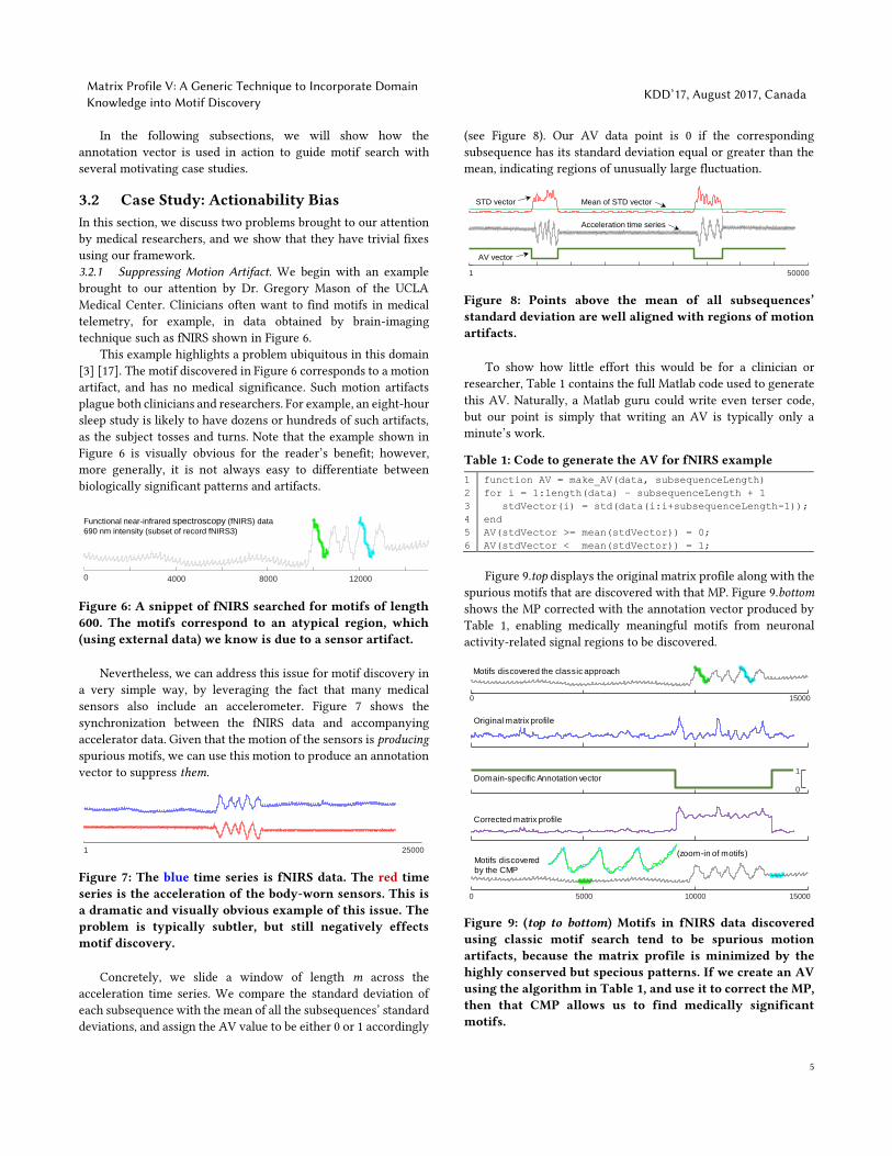
3.2 Case Study: Actionability Bias In this section, we discuss two problems brought to our attention by medical researchers, and we show that they have trivial fixes using our framework. 3.2.1 Suppressing Motion Artifact. We begin with an example brought to our attention by Dr. Gregory Mason of the UCLA Medical Center. Clinicians often want to find motifs in medical telemetry, for example, in data obtained by brain-imaging technique such as fNIRS shown in Figure 6. This example highlights a problem ubiquitous in this domain [3] [17]. The motif discovered in Figure 6 corresponds to a motion artifact, and has no medical significance. Such motion artifacts plague both clinicians and researchers. For example, an eight-hour sleep study is likely to have dozens or hundreds of such artifacts, as the subject tosses and turns. Note that the example shown in Figure 6 is visually obvious for the reader’s benefit; however, more generally, it is not always easy to differentiate between biologically significant patterns and artifacts.

Figure 6: A snippet of fNIRS searched for motifs of length 600. The motifs correspond to an atypical region, which (using external data) we know is due to a sensor artifact.

Nevertheless, we can address this issue for motif discovery in a very simple way, by leveraging the fact that many medical sensors also include an accelerometer. Figure 7 shows the synchronization between the fNIRS data and accompanying accelerator data. Given that the motion of the sensors is producing spurious motifs, we can use this motion to produce an annotation vector to suppress them.

Figure 7: The blue time series is fNIRS data. The red time series is the acceleration of the body-worn sensors. This is a dramatic and visually obvious example of this issue. The problem is typically subtler, but still negatively effects motif discovery.

Concretely, we slide a window of length m across the acceleration time series. We compare the standard deviation of each subsequence with the mean of all the subsequences’ standard deviations, and assign the AV value to be either 0 or 1 accordingly

(see Figure 8). Our AV data point is 0 if the corresponding subsequence has its standard deviation equal or greater than the mean, indicating regions of unusually large fluctuation.

Figure 8: Points above the mean of all subsequences’ standard deviation are well aligned with regions of motion artifacts.

To show how little effort this would be for a clinician or researcher, Table 1 contains the full Matlab code used to generate this AV. Naturally, a Matlab guru could write even terser code, but our point is simply that writing an AV is typically only a minute’s work.

Table 1: Code to generate the AV for fNIRS example

1

2

3

4

5

6

function AV = make_AV(data, subsequenceLength)

for i = 1:length(data) – subsequenceLength + 1

stdVector(i) = std(data(i:i+subsequenceLength-1));

end

AV(stdVector >= mean(stdVector)) = 0;

AV(stdVector < mean(stdVector)) = 1;

Figure 9.top displays the original matrix profile along with the spurious motifs that are discovered with that MP. Figure 9.bottom shows the MP corrected with the annotation vector produced by Table 1, enabling medically meaningful motifs from neuronal activity-related signal regions to be discovered.

Figure 9: (top to bottom) Motifs in fNIRS data discovered using classic motif search tend to be spurious motion artifacts, because the matrix profile is minimized by the highly conserved but specious patterns. If we create an AV using the algorithm in Table 1, and use it to correct the MP, then that CMP allows us to find medically significant motifs.

4000 8000 120000

Functional near-infrared spectroscopy (fNIRS) data

690 nm intensity (subset of record fNIRS3)

1 25000

1 50000

STD vector

AV vector

Mean of STD vector

Acceleration time series

0 15000

0 5000 10000 15000

Motifs discovered the classic approach

Original matrix profile

Corrected matrix profile

Motifs discovered by the CMP

Domain-specific Annotation vector

(zoom-in of motifs)

0

1


6

Note that here we created a Boolean AV, which strictly prohibits finding motifs during sensor movement. However, we could also have created a real-valued AV, which simply bias the motif search away from regions where movement was noted, in proportion to the magnitude of the motion. As it happens, in this case, the Boolean AV was sufficient to solve the problem. In the next section we will show an example of an issue that does require a real-valued AV. 3.2.2 Suppressing Hard-Limited Artifacts. Here we consider another example of a commonly encountered issue that may prevent us from finding meaningful motifs in medical and industrial datasets. In Figure 10.bottom we see that the motif discovered in this Electrooculogram (EOG) has a perfectly flat plateau. This is not reflective of medical reality, but is simply a region where the physical process exceeds the 8-bit precision available to record it [21].

Figure 10: top) A snippet of a left-eye EOG sampled at 50 Hz, from an individual with sleep disorder. bottom) The top motif may be spurious, as it features a region where the time series indicates only the maximum value possible. However this snippet does have a true motif, with medical significance.

In the many datasets that have this limited precision flaw, we can be guaranteed that most or all of the top motifs will feature some of these constant regions, as the flat regions produce little cost in the Euclidean distance calculation2 that defines motifs. However, as shown in Figure 10.bottom.right, the data may be replete with more medically meaningful motifs. It is important to note that we do not wish to completely exclude the possibility of returning motifs with some amount of constant regions. It is just that we want to mitigate the strong bias to finding them exclusively.

Figure 11: The upper and lower bound of the EOG data indicates the regions where the physical process exceeds the 8-bit precision available to record it.

As the reader will now appreciate after having seen our previous examples, we can easily build an AV to suppress these spurious matches. We begin by recording the maximum and the minimum values of the time series, the constant values touching

2 Note, we say little cost, not zero cost, because when the subsequences are z-normalized, the constant regions may have slightly different heights.

the red bars shown in Figure 11. We slide a window across the time series to extract subsequences, counting the number of constant values (from being hard-limited above or below) in each sequence. This number over the subsequence length is used as the bias function. A higher value hints that the motifs that include this subsequence may be spurious, as the overflow/underflow regions act like a “don’t-care” in the motif distance.

Figure 12 illustrates the results of applying this AV to the problematic example shown in Figure 10. Here again the annotation vector helps to bias away from spurious motifs, by leveraging the original matrix profile with domain specific insights.

Figure 12: (top to bottom) Motifs in the EOG domain that are discovered using classic motif search tend to include hard-limited data, because the matrix profile is minimized by having long constant regions. By creating an AV using the algorithm in Table 2 to correct the MP, we can find true motifs corresponding to ponto-geniculo-occipital waves [6].

Once again, for concreteness, in Table 2 we show the full Matlab code used to make the annotation vector discussed above. As before, this simple fix requires only a minute of coding effort.

Table 2: Code to generate the AV for EOG example

1

2

3

4

5

6

7

8


for i = 1: length(data) – subsequenceLength + 1

s = data(i:i+subsequenceLength - 1);

AV(i) = length(s(s == max(data) | s == min(data)));

end

AV = AV - min(AV); % zero one normalization

AV = AV / max(AV); % zero one normalization

AV = 1 – AV; % AV property conformation

3.3 Case Study: Stop-Word Motif Bias We return to the ECG example presented in Figure 1. Recall that the top motifs of this time series do not come from a true medical

4000 80001

200 4000 200 4000

True value exceeds

the 8-bit precisionTrue motif,

suggestive of

REM sleep

1000 5000 9000

Limit of 8-bit precision

1000 5000 9000

Motifs discovered the classic approach

Motifs discovered

by the CMP

Original matrix profile

Domain-specific Annotation vector

Corrected matrix profile

0

1

Zoom-in of motifs



7

signal, but regions of the electrode’s calibration signal. These signals are much more similar than the “genuine” medically significant motifs, and swamp the top-K motif set.

Leveraging similar ideas in text processing, we propose to treat these spurious patterns as a “stop-word” motifs. Our goal is to design an AV that is capable of discounting such motifs. We can make no assumptions about the locations of the stop-word motif, given that they can show up anywhere in the signal.

We assume only that the stop-word motif(s) will be known to the users of our framework, as the stop-words are domain specific. In Figure 13.top, we show an example of a stop-word motif that we are targeting. Figure 13.bottom displays the annotation vector that can bias the motif discovery away from that stop-word.

Figure 13: top) We annotated a single stop-word from the LTAF-71 Database [13]. middle) The stop-words distance profile to the entire dataset was thresholded to create an exclusion zone, which was used to create a AV (bottom).

To create the AV here, we measure the similarity between the stop-word subsequence to all subsequences in T, by sliding a window of the subsequence length across the time series. This gives a distance profile (see Section 2.2 Definition 4). We normalize this distance profile to be in range [0 - 1], as shown in Figure 13.middle. To convert the normalized distance profile into our final AV vector, we employ a threshold parameter. The threshold chosen indicates how similar the corresponding subsequences are in comparison to the stop-word motif. If we set the threshold to be 0.1, we retrieve the location of subsequences that are 90% stop-word-like. Having a threshold is generally undesirable, but recall that our framework has completely divorced the computationally trivial AV adjustment from the expensive computation of the matrix profile. Thus, if the threshold is too aggressive or too lax, the user can update it and refresh the results in under a second, even for datasets as large as one million data points.

To generate the final AV vector, we set the stop-word motif location, and all the data up to 3m points before and after them to 0, retaining the original values of other data points. This 3m “padded” exclusion zone is simply to compensate for the “spikey” valleys of the distance profile.

Figure 14: By correcting the MP to bias away from stop-word motifs, we can discover medically meaningful motifs.

Figure 14.top shows the original MP (left) and the top-1 motif that would have been found using that MP (right, highlighted in green and cyan). Figure 14.bottom shows the corrected MP and the corresponding top-1 motif.

3.4 Case Study: Simplicity Bias The issue of simplicity bias has been reported to us by a dozen research groups in the last decade, although not under that name, which we coined for this paper. The problem can be very subtle, but in Figure 15 below we show a strikingly obvious example.

Figure 15: A short snippet of a time series of the flexion of a subject’s little finger [9]. Subjectively, most people would expect that two occurrences of consecutive multiple flexions to be the top motif (inset). Instead we find the simple “ramp-up” pattern to be the top motif.

The reason why motif discovery fails to match our expectation here was discussed in Section 1.2, and at length in [1] (in a very different context). Given our guided motif framework, the problem is trivial to solve. We just need to create an AV that penalizes for simplicity.

Figure 16: A visual intuition of the complexity estimation of three time series subsequences of different complexity levels.

To do this, we employ the complexity estimation proposed in [1], which will be referred as CE. The authors of [1] originally embedded CE in a complexity correction factor for the Euclidean distance, making this distance measure complexity-invariant. This complexity estimation is simple (one line of code), parameter-free and has a natural interpretation. Intuitively, time

0

0.5

0 1000 2000 3000

Annotation vector

0

1

Extended exclusion zone for

each data point below threshold

0 3000

Distance profile

Stop-word motif

Threshold

1 3000 1 3000

Original MP

Corrected MP 1 150

10000 60000

0 3500

Time series Complexity estimation


8

series can be imagined as “chains” or “ropes”, and have their complexity measured by “stretching” them and measuring the length of the resulting taut lines, as illustrated in Figure 16. The more complex the time series is, the longer its corresponding line will be.

We slide a window across the time series, measuring the complexity of each subsequence and store them in a complexity vector, as shown by the magenta (bold) line of Figure 17. We simply normalize this complexity vector to be in range [0 - 1] to obtain the final AV.

Figure 17: The complexity measure (bold) show in parallel to the raw data (fine).

Table 3 contains the Matlab code used to generate the AV.

Table 3: Code to generate AV for ECoG signal

1

2

3

4

5

6

7


for i = 1: length(data) – subsequenceLength + 1

subsequence = data(i:i+subsequenceLength - 1);

AV(i) = sqrt(sum(diff(subsequence).^2));;

end

AV = AV - min(AV); % zero one normalization

AV = AV / max(AV); % zero one normalization

Figure 18 shows how the real motifs are uncovered, as

opposed to the “ramp-up” patterns that would have dominated if we rely on the classic matrix profile.

Figure 18: By correcting the matrix profile with an AV using the algorithm in Table 3, we discover the true motifs of finger flexion pattern.

To show the ubiquity of this issue, and the generality of our solution, we searched seismology telemetry [24]. Figure 19 illustrates how guided motif search correctly discovers two earthquakes from the same fault, occurring thirteen years apart, in Sonoma Country, CA. The result is impressive given that classic motif search ranks 852 other motifs above this true motif; these higher-ranked motifs are all sensor artifacts [8] that our AV suppresses.

Figure 19: The top motif returned by the classic approach is not an earthquake, but a sensor artifact. Using guided motif search framework, we can avoid such various misleading sensor artifacts, which swamp this 17,279,800 data-points earthquake dataset. The time series shown was edited for visual clarity.

4 EMPIRICAL EVALUATION To ensure that our experiments are reproducible, we have built a website which contains all data/code/raw spreadsheets for the results, in addition to many experiments that are omitted here for brevity [15]. This commitment to reproducibility extends to all the examples the previous sections. We note that we do not need to compare to rival algorithms, but a rival definition, the classic motif definition used in several hundred research efforts over the last decade [2][12][23][24].

4.1 Preliminary Tests We begin with an experiment that is designed to closely model the issue shown in Figure 3, but at a scale that will allow statistically significant results. We produced 1,000 datasets as follows. We created a random walk of length 20,000, then embedded into it two randomly chosen instances from the eight-class MALLAT dataset from the UCR Archive [4]. Figure 20 shows that these synthetic datasets are, at least visually, a good proxy for the real motion artifact contamination data.

Figure 20: A snippet of real motion artifact contamination data (see also Figure 3) and a snippet of our synthetic proxy for it.

For each dataset, we run motif discovery, and count as a success, any answer in which the top-1 returned motifs overlap with any part of the embedded motifs.

1 60000

10000 60000

Motifs discovered

the classic approach

Motifs discovered

by the CMP

Original MP

Motif discovered the classic approach,

a sensor artifact

Corrected MP

Motif discovered by the CMP,

two occurrences of an earthquake

1 40000

1 8000

4000 80001

Motion Artifact Contaminated EEG Data

Motion

Artifact

Motion

Artifact

Top-1 Motif

Top-1 Motif



9

We test the performance of three alternatives: • Classic motif search, to reflect what is currently done in the

literature (Classic) [23]. • Guided Motif Search: In which the AV is created using

complexity bias, as discussed in Section 3.3 (AVcomplexity). • Guided Motif Search: In which the AV is created using the

number of zeros-crossings (AVZeroCrossings) in the subsequences.

We consider two variants of the AV, in order to test the following informal claim: Once a practitioner understands the issue producing poor motifs, there will almost certainly be many simple fixes possible. Table 4 summarizes the results.

A practitioner that exploited the number of zero-crossings would have seen her hit-rate more than double, yet noted there is still room for improvement. Perhaps she would have noticed that random walk data can sometimes have high zero-crossings by chance, and would have turned to a more robust zero-crossings extractor [20]. On the other hand, a more sophisticated practitioner that was aware of complexity bias [1], would have seen essentially perfect results from the first time. In both cases we see that the simple correction offered by an annotation vector can dramatically improve the utility of motif search. We note in passing these results that they support our claim that the time overhead for guided motif search is inconsequential.

Table 4: Comparison between classic motif search and guided motif search over 1000 datasets of length 20,000. Both two variants of guided motif search outperform classic motif search in terms of accuracy, with extra time overhead of just 0.09 second per run, less than a half of a percent.

Approach Average success rate Time per run

Classic 16.3% 22.40 seconds

AVcomplexity 99.9% 22.46 seconds

AVZeroCrossings 38.7% 22.49 seconds

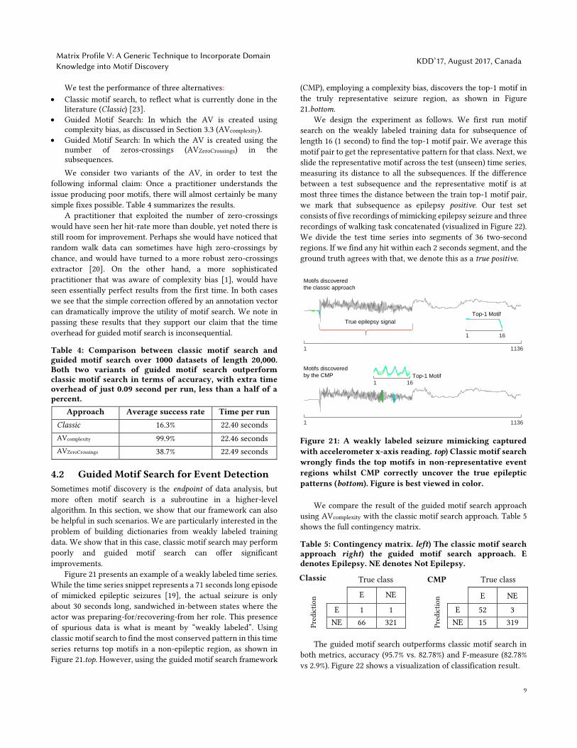
4.2 Guided Motif Search for Event Detection Sometimes motif discovery is the endpoint of data analysis, but more often motif search is a subroutine in a higher-level algorithm. In this section, we show that our framework can also be helpful in such scenarios. We are particularly interested in the problem of building dictionaries from weakly labeled training data. We show that in this case, classic motif search may perform poorly and guided motif search can offer significant improvements.

Figure 21 presents an example of a weakly labeled time series. While the time series snippet represents a 71 seconds long episode of mimicked epileptic seizures [19], the actual seizure is only about 30 seconds long, sandwiched in-between states where the actor was preparing-for/recovering-from her role. This presence of spurious data is what is meant by “weakly labeled”. Using classic motif search to find the most conserved pattern in this time series returns top motifs in a non-epileptic region, as shown in Figure 21.top. However, using the guided motif search framework

(CMP), employing a complexity bias, discovers the top-1 motif in the truly representative seizure region, as shown in Figure 21.bottom.

We design the experiment as follows. We first run motif search on the weakly labeled training data for subsequence of length 16 (1 second) to find the top-1 motif pair. We average this motif pair to get the representative pattern for that class. Next, we slide the representative motif across the test (unseen) time series, measuring its distance to all the subsequences. If the difference between a test subsequence and the representative motif is at most three times the distance between the train top-1 motif pair, we mark that subsequence as epilepsy positive. Our test set consists of five recordings of mimicking epilepsy seizure and three recordings of walking task concatenated (visualized in Figure 22). We divide the test time series into segments of 36 two-second regions. If we find any hit within each 2 seconds segment, and the ground truth agrees with that, we denote this as a true positive.

Figure 21: A weakly labeled seizure mimicking captured with accelerometer x-axis reading. top) Classic motif search wrongly finds the top motifs in non-representative event regions whilst CMP correctly uncover the true epileptic patterns (bottom). Figure is best viewed in color.

We compare the result of the guided motif search approach using AVcomplexity with the classic motif search approach. Table 5 shows the full contingency matrix.

Table 5: Contingency matrix. left) The classic motif search approach right) the guided motif search approach. E denotes Epilepsy. NE denotes Not Epilepsy.

Classic True class

CMP True class

Pred

icti

on E NE

Pred

icti

on E NE

E 1 1 E 52 3

NE 66 321 NE 15 319

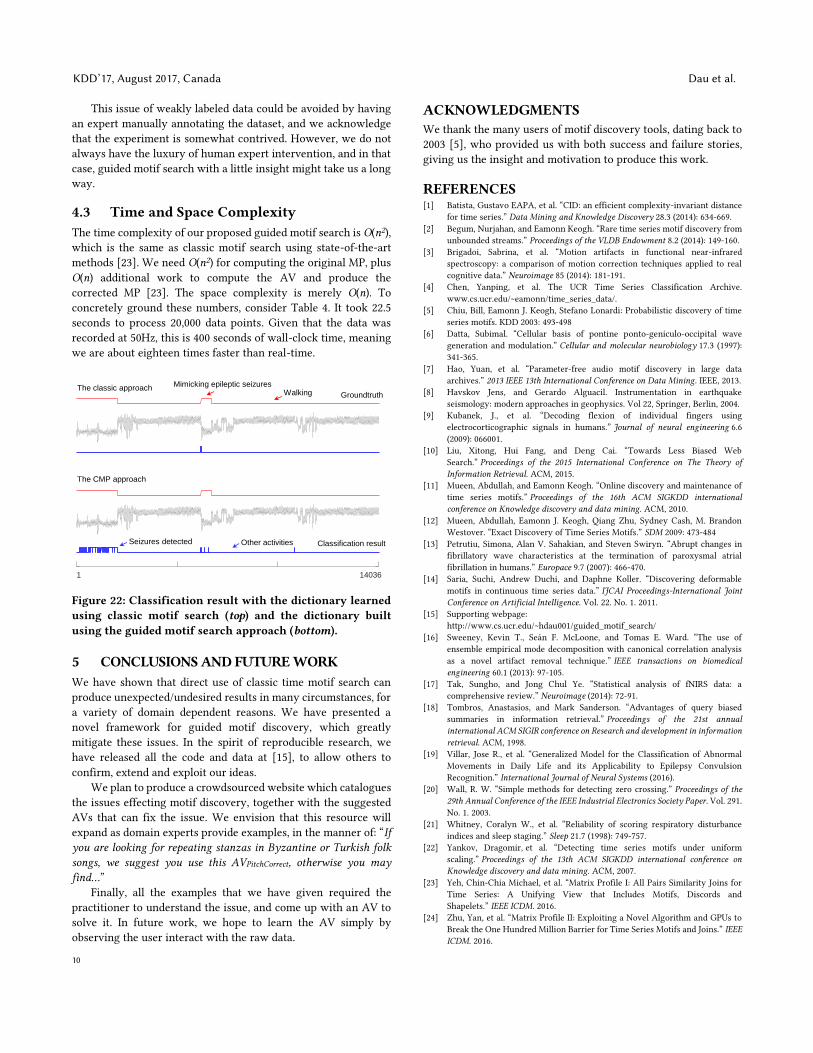
The guided motif search outperforms classic motif search in both metrics, accuracy (95.7% vs. 82.78%) and F-measure (82.78% vs 2.9%). Figure 22 shows a visualization of classification result.

1 1136

Top-1 Motif

1 16

Motifs discovered

the classic approach

1 16

True epilepsy signal

1 1136

Top-1 Motif

Motifs discovered

by the CMP


10

This issue of weakly labeled data could be avoided by having an expert manually annotating the dataset, and we acknowledge that the experiment is somewhat contrived. However, we do not always have the luxury of human expert intervention, and in that case, guided motif search with a little insight might take us a long way.

4.3 Time and Space Complexity The time complexity of our proposed guided motif search is O(n2), which is the same as classic motif search using state-of-the-art methods [23]. We need O(n2) for computing the original MP, plus O(n) additional work to compute the AV and produce the corrected MP [23]. The space complexity is merely O(n). To concretely ground these numbers, consider Table 4. It took 22.5 seconds to process 20,000 data points. Given that the data was recorded at 50Hz, this is 400 seconds of wall-clock time, meaning we are about eighteen times faster than real-time.

Figure 22: Classification result with the dictionary learned using classic motif search (top) and the dictionary built using the guided motif search approach (bottom).

5 CONCLUSIONS AND FUTURE WORK We have shown that direct use of classic time motif search can produce unexpected/undesired results in many circumstances, for a variety of domain dependent reasons. We have presented a novel framework for guided motif discovery, which greatly mitigate these issues. In the spirit of reproducible research, we have released all the code and data at [15], to allow others to confirm, extend and exploit our ideas.

We plan to produce a crowdsourced website which catalogues the issues effecting motif discovery, together with the suggested AVs that can fix the issue. We envision that this resource will expand as domain experts provide examples, in the manner of: “If you are looking for repeating stanzas in Byzantine or Turkish folk songs, we suggest you use this AVPitchCorrect, otherwise you may find…”

Finally, all the examples that we have given required the practitioner to understand the issue, and come up with an AV to solve it. In future work, we hope to learn the AV simply by observing the user interact with the raw data.

ACKNOWLEDGMENTS We thank the many users of motif discovery tools, dating back to 2003 [5], who provided us with both success and failure stories, giving us the insight and motivation to produce this work.

REFERENCES [1] Batista, Gustavo EAPA, et al. “CID: an efficient complexity-invariant distance

for time series.” Data Mining and Knowledge Discovery 28.3 (2014): 634-669. [2] Begum, Nurjahan, and Eamonn Keogh. “Rare time series motif discovery from

unbounded streams.” Proceedings of the VLDB Endowment 8.2 (2014): 149-160. [3] Brigadoi, Sabrina, et al. “Motion artifacts in functional near-infrared

spectroscopy: a comparison of motion correction techniques applied to real cognitive data.” Neuroimage 85 (2014): 181-191.

[4] Chen, Yanping, et al. The UCR Time Series Classification Archive. www.cs.ucr.edu/~eamonn/time_series_data/.

[5] Chiu, Bill, Eamonn J. Keogh, Stefano Lonardi: Probabilistic discovery of time series motifs. KDD 2003: 493-498

[6] Datta, Subimal. “Cellular basis of pontine ponto-geniculo-occipital wave generation and modulation.” Cellular and molecular neurobiology 17.3 (1997): 341-365.

[7] Hao, Yuan, et al. “Parameter-free audio motif discovery in large data archives.” 2013 IEEE 13th International Conference on Data Mining. IEEE, 2013.

[8] Havskov Jens, and Gerardo Alguacil. Instrumentation in earthquake seismology: modern approaches in geophysics. Vol 22, Springer, Berlin, 2004.

[9] Kubanek, J., et al. “Decoding flexion of individual fingers using electrocorticographic signals in humans.” Journal of neural engineering 6.6 (2009): 066001.

[10] Liu, Xitong, Hui Fang, and Deng Cai. “Towards Less Biased Web Search.” Proceedings of the 2015 International Conference on The Theory of Information Retrieval. ACM, 2015.

[11] Mueen, Abdullah, and Eamonn Keogh. “Online discovery and maintenance of time series motifs.” Proceedings of the 16th ACM SIGKDD international conference on Knowledge discovery and data mining. ACM, 2010.

[12] Mueen, Abdullah, Eamonn J. Keogh, Qiang Zhu, Sydney Cash, M. Brandon Westover. “Exact Discovery of Time Series Motifs.” SDM 2009: 473-484

[13] Petrutiu, Simona, Alan V. Sahakian, and Steven Swiryn. “Abrupt changes in fibrillatory wave characteristics at the termination of paroxysmal atrial fibrillation in humans.” Europace 9.7 (2007): 466-470.

[14] Saria, Suchi, Andrew Duchi, and Daphne Koller. “Discovering deformable motifs in continuous time series data.” IJCAI Proceedings-International Joint Conference on Artificial Intelligence. Vol. 22. No. 1. 2011.

[15] Supporting webpage: http://www.cs.ucr.edu/~hdau001/guided_motif_search/

[16] Sweeney, Kevin T., Seán F. McLoone, and Tomas E. Ward. “The use of ensemble empirical mode decomposition with canonical correlation analysis as a novel artifact removal technique.” IEEE transactions on biomedical engineering 60.1 (2013): 97-105.

[17] Tak, Sungho, and Jong Chul Ye. “Statistical analysis of fNIRS data: a comprehensive review.” Neuroimage (2014): 72-91.

[18] Tombros, Anastasios, and Mark Sanderson. “Advantages of query biased summaries in information retrieval.” Proceedings of the 21st annual international ACM SIGIR conference on Research and development in information retrieval. ACM, 1998.

[19] Villar, Jose R., et al. “Generalized Model for the Classification of Abnormal Movements in Daily Life and its Applicability to Epilepsy Convulsion Recognition.” International Journal of Neural Systems (2016).

[20] Wall, R. W. “Simple methods for detecting zero crossing.” Proceedings of the 29th Annual Conference of the IEEE Industrial Electronics Society Paper. Vol. 291. No. 1. 2003.

[21] Whitney, Coralyn W., et al. “Reliability of scoring respiratory disturbance indices and sleep staging.” Sleep 21.7 (1998): 749-757.

[22] Yankov, Dragomir, et al. “Detecting time series motifs under uniform scaling.” Proceedings of the 13th ACM SIGKDD international conference on Knowledge discovery and data mining. ACM, 2007.

[23] Yeh, Chin-Chia Michael, et al. “Matrix Profile I: All Pairs Similarity Joins for Time Series: A Unifying View that Includes Motifs, Discords and Shapelets.” IEEE ICDM. 2016.

[24] Zhu, Yan, et al. “Matrix Profile II: Exploiting a Novel Algorithm and GPUs to Break the One Hundred Million Barrier for Time Series Motifs and Joins.” IEEE ICDM. 2016.

The classic approach

1 14036

The CMP approach

Other activities

Groundtruth

Classification result

Mimicking epileptic seizuresWalking

Seizures detected

Documents

Matrix Profile V: A Generic Technique to Incorporate